Lucchi, R.G., St. John, K.E.K., Ronge, T.A., and the Expedition 403 Scientists
Proceedings of the International Ocean Discovery Program Volume 403
publications.iodp.org
https://doi.org/10.14379/iodp.proc.403.103.2026
Site U16181
![]() R.G. Lucchi,
R.G. Lucchi,
![]() K.E.K. St. John,
K.E.K. St. John,
![]() T.A. Ronge,
T.A. Ronge,
![]() M.A. Barcena,
M.A. Barcena,
![]() S. De Schepper,
S. De Schepper,
![]() L.C. Duxbury,
L.C. Duxbury,
![]() A.C. Gebhardt,
A.C. Gebhardt,
![]() A. Gonzalez-Lanchas,
A. Gonzalez-Lanchas,
![]() G. Goss,
G. Goss,
![]() N.M. Greco,
N.M. Greco,
![]() J. Gruetzner,
J. Gruetzner,
![]() L. Haygood,
L. Haygood,
![]() K. Husum,
K. Husum,
![]() M. Iizuka,
M. Iizuka,
![]() A.K.I.U. Kapuge,
A.K.I.U. Kapuge,
![]() A.R. Lam,
A.R. Lam,
![]() O. Libman-Roshal,
O. Libman-Roshal,
![]() Y. Liu,
Y. Liu,
![]() L.R. Monito,
L.R. Monito,
![]() B.T. Reilly,
B.T. Reilly,
![]() Y. Rosenthal,
Y. Rosenthal,
![]() Y. Sakai,
Y. Sakai,
![]() A.V. Sijinkumar,
A.V. Sijinkumar,
![]() Y. Suganuma, and
Y. Suganuma, and
![]() Y. Zhong2
Y. Zhong2
1 Lucchi, R.G., St. John, K.E.K., Ronge, T.A., Barcena, M.A., De Schepper, S., Duxbury, L.C., Gebhardt, A.C., Gonzalez-Lanchas, A., Goss, G., Greco, N.M., Gruetzner, J., Haygood, L., Husum, K., Iizuka, M., Kapuge, A.K.I.U., Lam, A.R., Libman-Roshal, O., Liu, Y., Monito, L.R., Reilly, B.T., Rosenthal, Y., Sakai, Y., Sijinkumar, A.V., Suganuma, Y., and Zhong, Y., 2026. Site U1618. In Lucchi, R.G., St. John, K.E.K., Ronge, T.A., and the Expedition 403 Scientists, Eastern Fram Strait Paleo-Archive. Proceedings of the International Ocean Discovery Program, 403: College Station, TX (International Ocean Discovery Program). https://doi.org/10.14379/iodp.proc.403.103.2026
2 Expedition 403 Scientists' affiliations.
1. Background and objectives
The Vestnesa Ridge is a roughly east–west oriented prominent bathymetric feature situated in the Fram Strait on the western continental margin of Svalbard (Figure F1). Its evolution is linked to the tectonic, sedimentary, and climatic history of the region, making it a focal point for multidisciplinary scientific research. The 100 km long ridge is a sediment drift generated by persistent bottom currents associated with the West Spitsbergen Current (WSC) (Eiken and Hinz, 1993) that developed over oceanic crust since the Fram Strait opening (17–10 Ma) (Jakobsson et al., 2007; Engen et al., 2008; Ehlers and Jokat, 2013). Although the chronology of the Vestnesa Ridge sediment record deposited since the last glacial is well established (e.g., Rasmussen and Nielsen, 2024, and references therein) and regionally correlatable (Lucchi et al., 2023), the chronology prior to approximately Marine Isotope Stage (MIS) 5 is limited to extrapolation from seismic data from previously drilled sites on the Yermak Plateau (Ocean Drilling Program [ODP] Site 912) and south of the Molloy Transform Fault (ODP Site 909) (Eiken and Hinz, 1993; Knies et al., 2014; Mattingsdal et al., 2014). Seismic Reflectors R1–R8 were drilling targets for Site U1618 (Figure F2), with a total depth target of 738 meters below seafloor (mbsf).
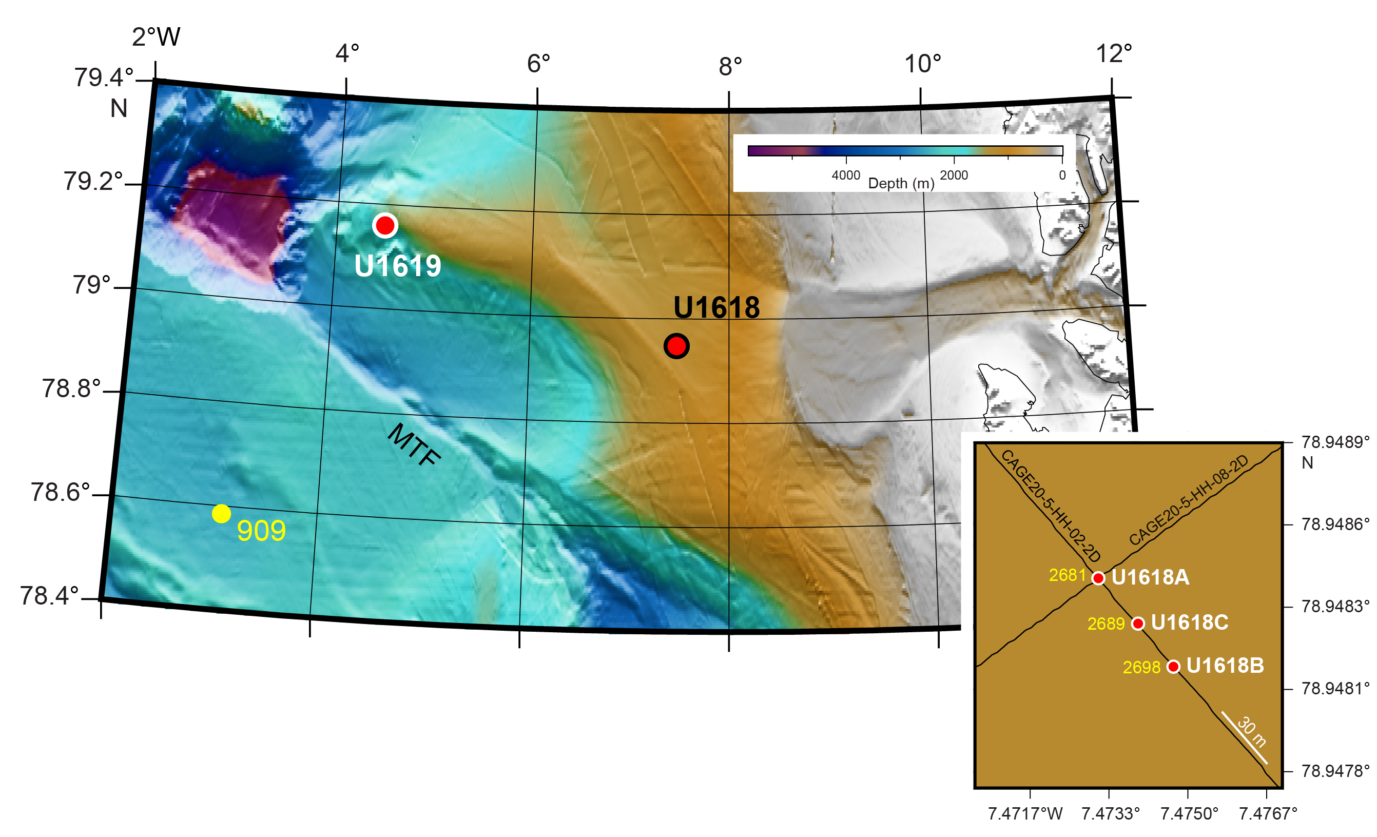
Figure F1. Bathymetric map.
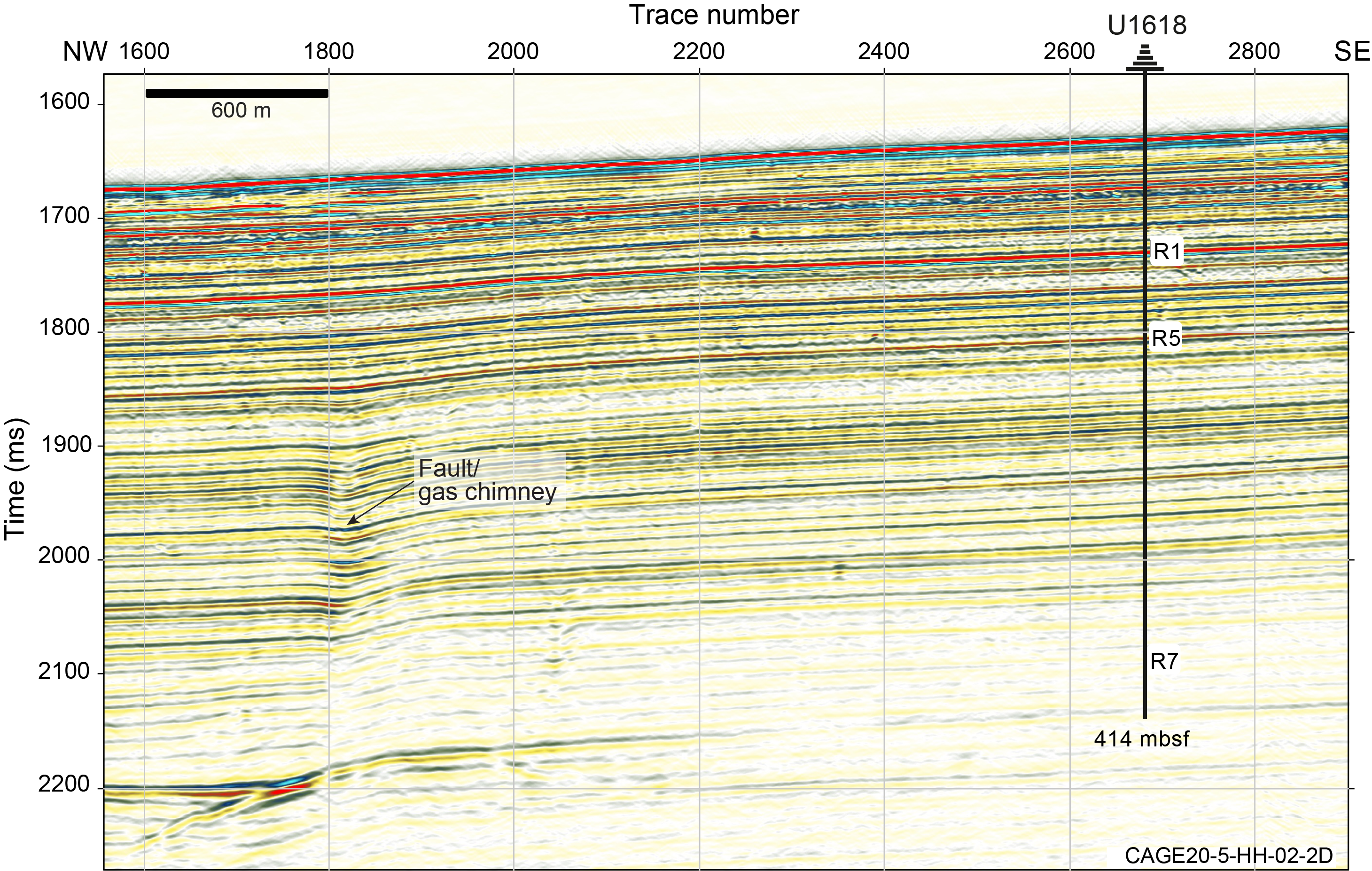
Figure F2. Seismic profile.
The sedimentation and geologic development in this area has been heavily influenced by Pliocene–Pleistocene glaciations, with ice sheet extent over Svalbard and the Barents Sea, and Arctic Ocean sea ice (Jakobsson et al., 2014). Depositional facies representing a range of glaciogenic and bottom current depositional processes, including ice rafting events, dense glacial debris flows, and subglacial meltwater plumes, are well documented in the recent sedimentary record along the western Svalbard continental margin (e.g., Lucchi et al., 2013, 2015; Caricchi et al., 2019) and the Vestnesa Ridge (Schneider et al., 2018; Sztybor and Rasmussen, 2017; Plaza-Faverola et al., 2023; Rasmussen and Nielsen, 2024). The presence of gas hydrates and associated fluid migration are additional controls on the sedimentary record of the Vestnesa Ridge.
Bathymetric and seismic surveys have revealed numerous pockmarks and fluid escape features along the Vestnesa Ridge, indicating active seepage of methane and other hydrocarbons (Hustoft et al., 2009; Bünz et al., 2012; Smith et al., 2014). Seismic surveys also reveal a regional gas hydrate–related bottom-simulating reflector (BSR) and thus the presence of gas hydrate and free gas at depth. Previous studies indicate that the hydrate stability zone is several hundred meters thick and can extend to the seafloor (Himmler et al., 2019; Pape et al., 2020; Rasmussen and Nielsen, 2024; Plaza-Faverola et al., 2023).
Spatial changes in seafloor morphology, faults, and seepage characteristics led to the distinction of two main areas along the Vestnesa Ridge (Plaza-Faverola et al., 2015; Schneider et al., 2018; Sztybor and Rasmussen, 2017): (1) the East Vestnesa Ridge, characterized by a narrow crest (~3 km wide) and large pockmarks connected with chimneys with ongoing seepage activity, and (2) the West Vestnesa Ridge, characterized by a larger crest (>10 km wide) and small, apparently inactive pockmarks, although multidisciplinary investigations point to the presence of methane in the subseafloor (e.g., Consolaro et al., 2015; Plaza-Faverola et al., 2015; Sultan et al., 2020).
Site U1618 (Figure F1), located on the Vestnesa Ridge East termination, was chosen for its proximity to the continental margin and outer reaches of the former paleo-Svalbard–Barents Sea Ice Sheet, which make this site ideal to reconstruct the ice sheet dynamics in the northern area. For safety and to maximize recovery toward the primary science objectives, Site U1618 was positioned away from the regional BSR, and Hole U1618A was located on Seismic Line CAGE20-5-HH-02-2D at 3.8 km from a gas chimney and 1.1 km from a fault that was supposed to act as a conduit for fluid migration (Figure F2). Holes U1618B and U1618C were located 50 and 25 m northeast from Hole U1618A, respectively, along the same seismic line (Figure F1). Water depths at all three holes were between 1195 and 1196 m. The deepest penetration (Hole U1618B) reached 414 mbsf, and the maximum recovery (Hole U1618C) was 110%.
The research objectives for Site U1618 include the following:
- Reconstruction of a high-resolution sediment stratigraphy since the Late Miocene–Early Pliocene transition;
- Study of ocean-cryosphere interactions and forcing mechanisms on the paleo–ice sheet dynamics;
- Definition of the effect of glacial and tectonic stresses on subseafloor sediment deformation and carbon transport; and
- Investigation of the influence of the WSC variability, ice coverage, and climate on the microbial populations through time and to what extent this is still affecting contemporary geochemical fluxes.
Additionally, this location offers the opportunity to explore possible relationships (including feedbacks and tipping points) among paleo–ice sheets, gas hydrate stability, and tectonic stress.
2. Operations
We started our 1677 nmi voyage across the North Atlantic to Fram Strait Site U1618 at 0800 h local time on 4 June 2024 in Amsterdam, The Netherlands. Throughout the transit, all groups familiarized themselves with their respective laboratories and worked on writing their methods sections. The COVID-19 mitigation protocol was followed until 11 June, when it ended at 1815 h after no one tested positive. We completed the transit on 14 June at an average speed of 9.9 kt.
In total, we spent 9.18 days at Site U1618 and penetrated a maximum depth of 414.3 mbsf with a combined penetration of 1104.3 m. The cored interval of 1102.3 m resulted in a recovered length of 1078.45 m. Site U1618 consists of three holes over a 50 m interval (25 m between holes) along Seismic Line CAGE20-5-HH-02-2D. We took 152 cores in total: 26.3% with the advanced piston corer (APC) system (40 cores), 11.2% with the half-length APC (HLAPC) system (17 cores), and 62.5% with the extended core barrel (XCB) system (95 cores). To minimize magnetic overprinting on the cored sediment, nonmagnetic collars and core barrels were used for all APC and HLAPC coring. All three holes had intervals where the sediments significantly expanded due to the presence of gas, resulting in recoveries often exceeding 100% (Table T1). To mitigate the impact of expansion and the potential for core disturbance and to release the pressure, holes were drilled into the liner by the drill crew on the rig floor and the technical staff on the core receiving platform (i.e., catwalk).
To more easily communicate shipboard results, core depth below seafloor, Method A (CSF-A), depths in this chapter are reported as mbsf unless otherwise noted.
2.1. Hole U1618A
The vessel arrived on site on 14 June 2024 with thrusters down and the vessel in full automatic dynamic positioning (DP) mode at 0919 h, beginning operations at the site. A positioning beacon was deployed as a backup to GPS. A depth reading was taken using the precision depth recorder (PDR), estimating the seafloor at 1191.8 meters below sea level (mbsl). The crew assembled the APC bottom-hole assembly (BHA), and prior to beginning coring operations, approximately 1000 m of core winch line were slipped from the drum due to excessive corrosion on the line. The line was reheaded, and a core barrel was deployed. The bit was spaced to 1186.8 mbsl, 5 m above the PDR seafloor depth, and a mudline core was attempted. The first recovered core barrel came back empty; thus, the bit was lowered 5 m to 1191.8 mbsl, and a second core barrel was deployed. Hole U1618A was spudded at 2225 h on 14 June, and the seafloor depth was calculated to be 1196.0 mbsl based on the core recovery from Core 1H. Coring continued with the APC system to 94.0 mbsf. Cores 7H–11H were partial strokes and were advanced by recovery. The HLAPC system was then deployed to extend the hole to 150.8 mbsf (Cores 12F–24F), with partial strokes on Cores 21F, 22F, and 24F. The XCB coring system was used for Cores 25X–32X to 228.3 mbsf by 0000 h on 16 June. Coring continued to 276.9 mbsf. C1/C2 gas headspace ratios were monitored and were in the anomalous zone at 276.9 mbsf. Hole U1618A was terminated, and the gas, temperature, and core data were sent to shore for feedback from the Environmental Protection and Safety Panel (EPSP) to determine whether coring any deeper at the site could be done in a safe manner. The top drive was set back, and the bit was pulled out of the hole, clearing the seafloor at 1043 h on 16 June.
A total of 37 cores were taken from Hole U1618A (Table T1) over a 276.9 m interval with 252.62 m of recovery (91%). The APC system was used for 11 cores over a 94.0 m interval with 90.07 m recovered (96%), the HLAPC system was deployed for 13 cores over a 56.8 m interval with 60.18 m recovered (106%), and the XCB system was deployed for 13 cores over a 126.1 m interval with 102.37 m recovered (81.2%). All APC and HLAPC cores were taken using nonmagnetic core barrels. Temperature measurements were taken on Cores 4H, 7H, 10H, and 13F using the third-generation advanced piston corer temperature (APCT-3) tool. A fifth temperature measurement was taken using the Sediment Temperature 2 (SET2) probe after Core 34X at 249.0 mbsf. In total, we spent 48.50 h (2.1 days) at Hole U1618A.
2.2. Hole U1618B
After clearing Hole U1618A, the vessel was offset 50 m at 139° along Seismic Line CAGE20-5-HH-02-2D to begin operations at Hole U1618B. After careful deliberation, this offset was chosen to move even farther away from a known BSR in the area that was previously identified by IODP's EPSP. A depth reading was taken using the PDR, estimating the seafloor at 1190 mbsl. The top drive was picked up, and the bit was placed at 1189 mbsl for the mudline core. Hole U1618B was spudded at 1245 h on 16 June 2024. The seafloor was calculated to be 1195.2 mbsl based on recovery from Core 1H. Cores 1H–13H were cored with the APC system to 112.8 mbsf. Partial strokes were recorded for Cores 6H, 8H, and 13H. A shattered liner on Core 7H required that the core be pumped out of the core barrel. The HLAPC was deployed for Core 14F from 112.8 to 117.5 mbsf. The decision was made to revert to the APC system for Core 15H. This core was a partial stroke and only advanced from 117.5 to 117.7 mbsf, signaling APC refusal had been reached. Permission was received from EPSP to deepen Hole U1618B past the total depth of Hole U1618A (276.9 mbsf) as long as the headspace C1/C2 ratios in this hole remained normal. The hole was advanced with the XCB coring system for Cores 16X–54X, deepening the hole from 117.5 mbsf to the total depth of 414.3 mbsf. At this depth, the C1/C2 ratio jumped sharply into the anomalous zone, outside our safety envelope, causing coring to be terminated at 1300 h on 19 June. It was decided to attempt downhole wireline logging in Hole U1618B instead of Hole U1618C (see below) because Hole U1618A had to be terminated prematurely for anomalous C1/C2 ratios and higher hydrocarbons. Hence, the future of a potential Hole U1618C was uncertain.
A total of 54 cores were taken from Hole U1618B (Table T1) over a 414.3 m interval with 375.24 m recovered (90.57%). The APC system was used for 14 cores over a 113.0 m interval with 112.48 m recovered, the HLAPC system was deployed for 1 core over a 4.7 m interval with 1.63 m recovered (35%), and the XCB system was deployed for 39 cores over a 296.6 m interval with 261.13 m recovered (88%).
All cores collected with the APC and HLAPC systems were taken using nonmagnetic core barrels. Two temperature measurements were attempted using the SET2 temperature probe. The first, after Core 403-U1618B-40X, returned with no data. The second attempt, after Core 41X, returned a good temperature reading from 325.0 mbsf.
2.3. Hole U1618C
The vessel was offset 25 m northwest at a bearing of 319° from Hole U1618B, halfway back toward Hole U1618A, and the bit was lowered to 1194 mbsl. An APC core barrel was deployed, and Hole U1618C was spudded at 1012 h on 20 June 2024. The seafloor was calculated to be 1195.8 mbsl based on recovery from Core 1H. Cores 1H–12H were APC cored to 91.7 mbsf, with partial strokes recorded on Cores 4H, 5H, and 8H–12H. The APC and HLAPC systems were deployed from 91.7 to 125.6 mbsf (Cores 13F–19H), with one drilled interval (161) from 107.9 to 109.9 mbsf. Partial strokes were recorded on Cores 14H and 19H. The XCB coring system was deployed to extend the hole from 125.6 mbsf to the total depth of 392.1 mbsf (Cores 20X–59X) at 0000 h on 23 June. Advances of 7.0–7.5 m were used on the majority of the XCB cores to allow for gas expansion within the core liner. Cores 60X–62X were retrieved from 392.1 to 413.1 mbsf, the final depth for the hole. Some of the XCB cores expanded upon recovery. The decision to advance by 7–7.5 m to allow for core expansion was kept in place. The C1/C2 ratios for Cores 61X and 62X plotted significantly outside of our safety envelope; thus, the decision was made to end the hole. Although a few cores higher in the hole had an anomalous C1/C2 ratio, Cores 61X and 62X had an additional presence of higher hydrocarbons. Hole U1618C reached a maximum penetration of 413.1 mbsf with a cored interval of 411.1 m and a recovery of 450.59 m (109.61% recovery). The pipe was pulled from the hole, and the bit cleared the rig floor at 1120 h. While pulling the pipe, the beacon was recovered at 0945 h. The rig floor was secured for transit, the vessel switched from DP mode to cruise mode, and the vessel was underway to Site U1619 at 1151 h on June 23.
A total of 61 cores were taken from Hole U1618C (Table T1) over a 411.1 m interval with 450.59 m recovered (109.61%). The APC system was used for 14 cores over a 113.0 m interval with 112.48 m recovered, the HLAPC system was deployed for 3 cores over a 14.1 m interval with 13.71 m recovered (97.3%), and the XCB coring system was deployed for 43 cores over a 287.5 m interval with 337.18 m recovered (114.82%).
2.4. Downhole logging
After concluding coring operations in Hole U1618B, the bit was pulled to 68.6 mbsf and the Schlumberger wireline was rigged up. The triple combo logging tool string was made up and deployed at 1645 h on 19 June 2024, reaching 373.3 mbsf on the first pass and 368.3 mbsf on the second. The tools were recovered, and the Formation MicroScanner (FMS)-sonic logging tool string was made up and deployed at 0300 h on 20 June. The tools reached 358.8 mbsf on the first pass and 342.8 mbsf on the second. The tools were recovered, and the Versatile Seismic Imager (VSI) tool string was made up and deployed at 0445 h on 20 June. While deploying the tool, it was noticed that the Z-axis was not transmitting data. The tools were recovered, and the backup VSI tool was made up and deployed. While powering up the backup tool, a power surge caused a failure in the electronics. With both VSI tool strings inoperable, it was decided to end logging operations for the hole. The Schlumberger equipment was rigged down, and the rig floor was cleared. The bit was pulled out of the hole, clearing the seafloor at 0740 h on 20 June and ending Hole U1618B. In total we spent 93.0 h (3.9 days) at Hole U1618B.
3. Lithostratigraphy
The recovered sequence at Site U1618 consists of 152 cores and 1078.4 m of sediment that exhibits increasing lithification with depth. The sediments throughout all cores from Holes U1618A–U1618C are primarily siliciclastic, mainly composed of dark gray to greenish black silty clay, with interbedded coarser intervals, such as clayey silt, and rarely sandy mud, gravel, and diamicton intervals (Figure F3A, F3B, F3F). These lithologies contain varying amounts of detrital clasts and/or authigenic mineral precipitants. Small (<2 cm) to large (>2 cm) clasts are identified throughout the cores from visual descriptions and X-radiograph observations, when available (Figure F3C–F3E). When present, clast abundance ranges from dispersed (observed on <1% of the split core surface) to common (1%–5%) to abundant (5%–30%). When the sediment is poorly sorted, with clast abundance between 1% and 30% and large clasts (>2 cm) present, the lithology is designated as a diamicton (Figure F3F). Authigenic mineral precipitants range in size from micrometer-scale to 2–3 cm diameter concretions (Figure F4A, F4B). Although sometimes not visible on the split core surfaces (i.e., described as structureless), primary (e.g., laminations and bioturbation) and secondary (e.g., bioturbated infilling by authigenic dense minerals) sedimentary structures are more commonly visible in the X-radiographs available from Hole U1618B and the deeper part of Hole U1618C (Figures F4C, F5, F6). Clasts of varying sizes, interpreted to be ice-rafted debris (IRD), are observed throughout all lithostratigraphic units, with lesser abundance in Lithostratigraphic Unit II. The majority of these clasts are angular to subangular and smaller than 1–2 cm in size, but larger (>2 cm) clasts are also occasionally observed. Most of the clasts consist of siltstones, mudstones, and igneous rocks, but metamorphic rocks are also evident.
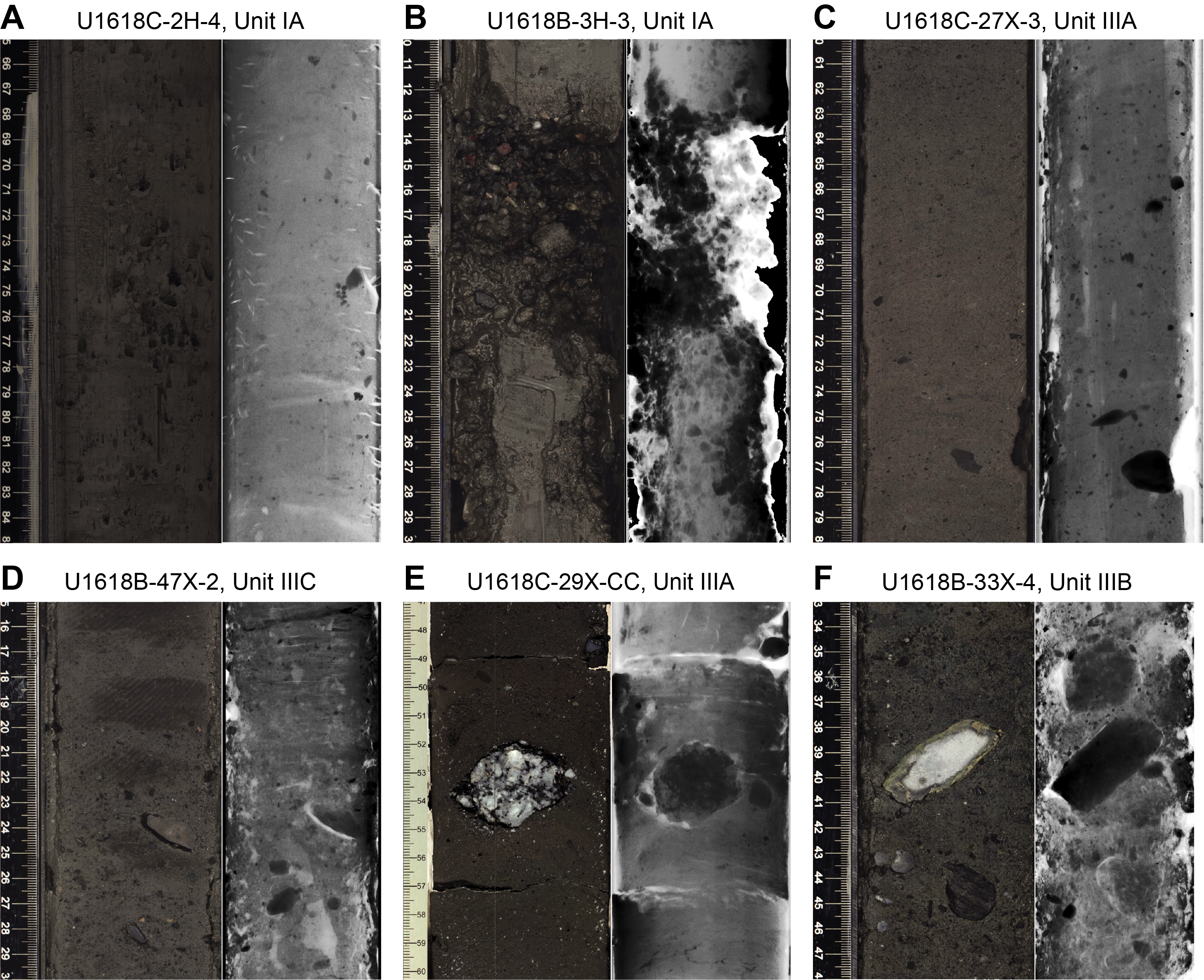
Figure F3. Typical lithologies.
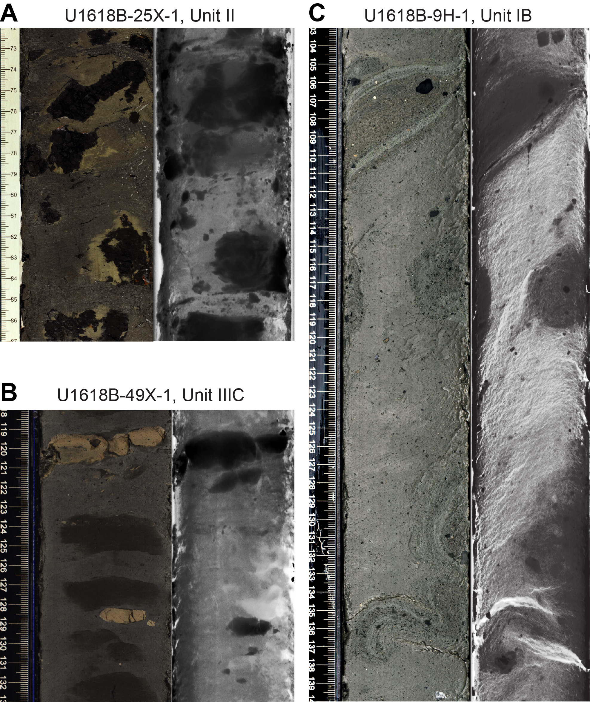
Figure F4. Sedimentologic features.
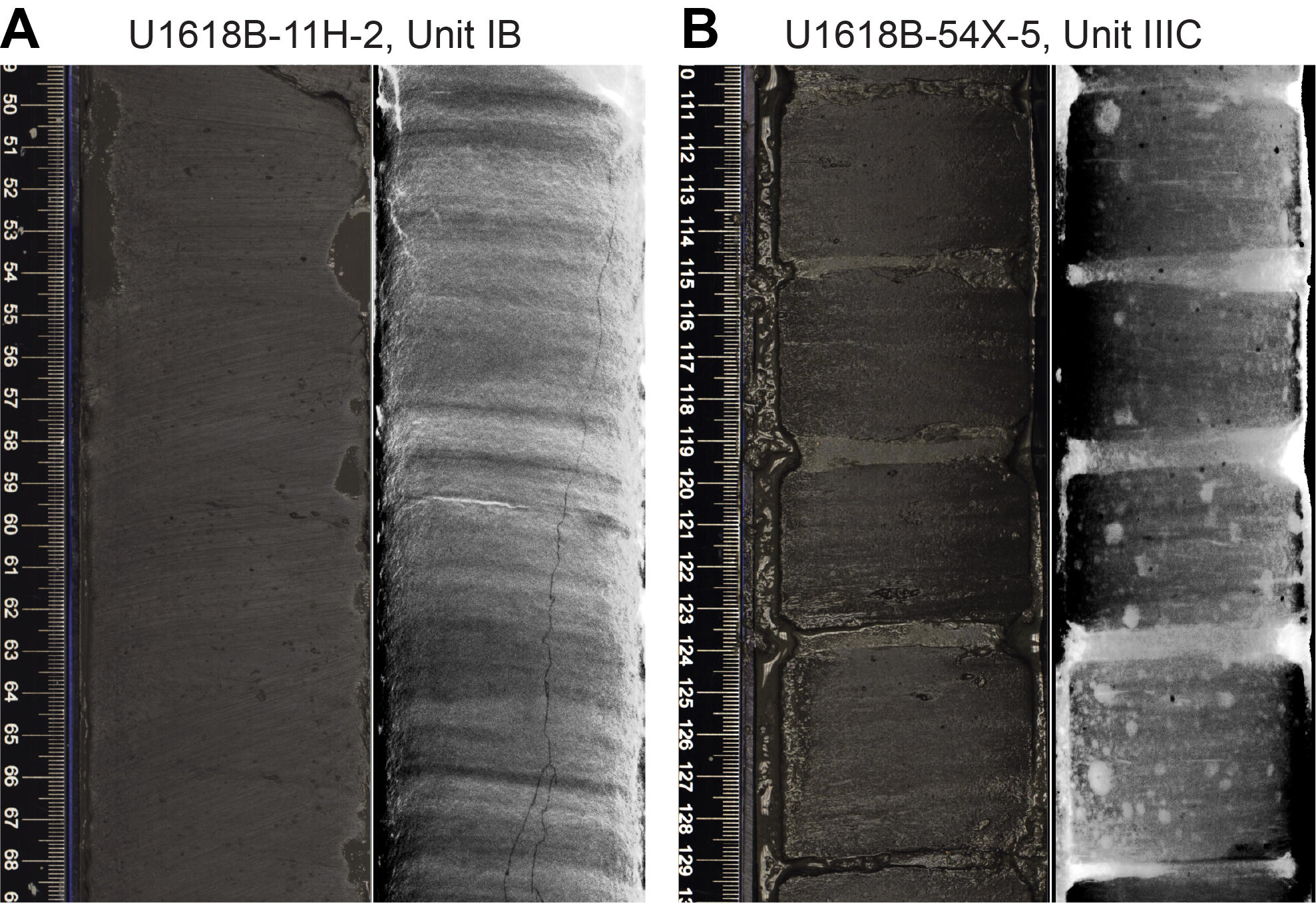
Figure F5. Laminations.
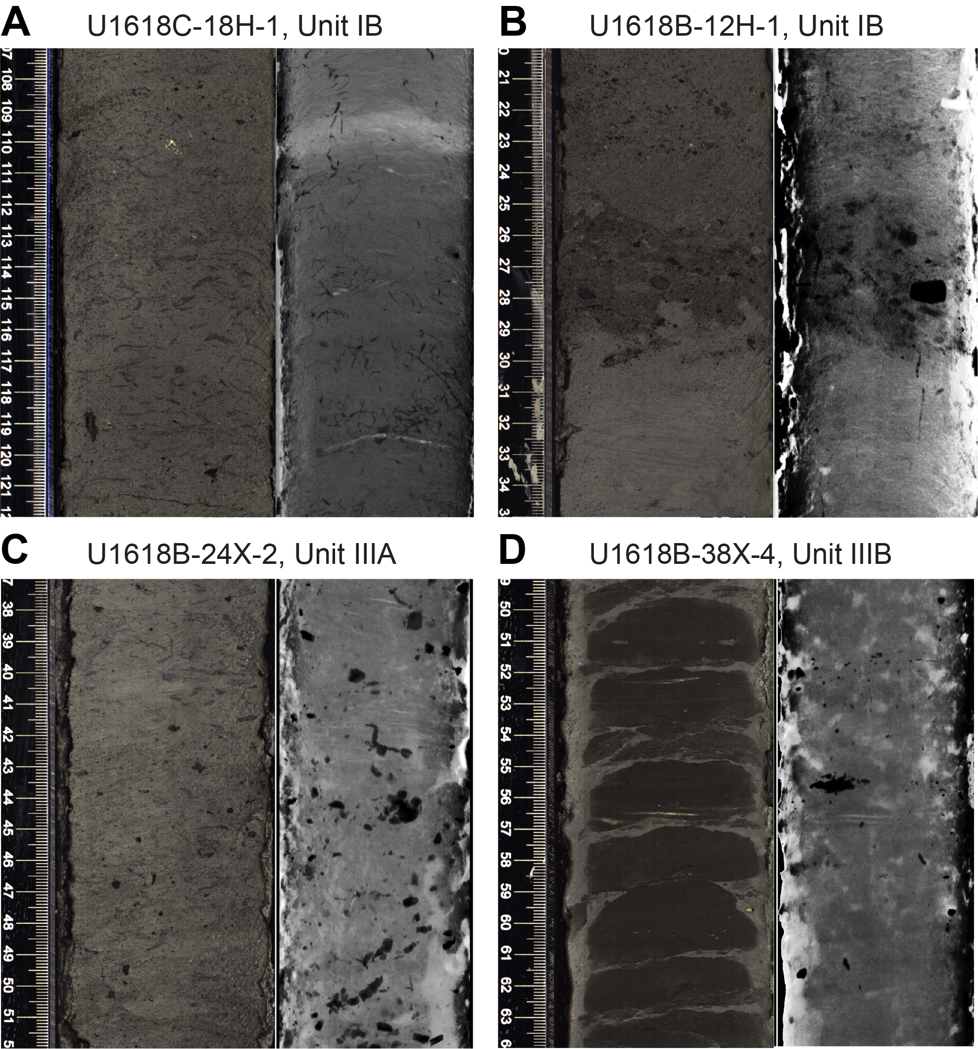
Figure F6. Bioturbation.
Based on these characteristics, the sediments recovered from Site U1618 are divided into three primary lithostratigraphic units and additional subunits (Table T2). The relatively continuous Hole U1618C is used as the primary record to define the lithostratigraphic unit and subunit boundaries. The stratigraphic boundaries in Hole U1618C are subsequently transferred to Holes U1618A and U1618B based on stratigraphic correlation on the mbsf (equivalent to CSF-A) scale (see Stratigraphic correlation) (Figure F7).
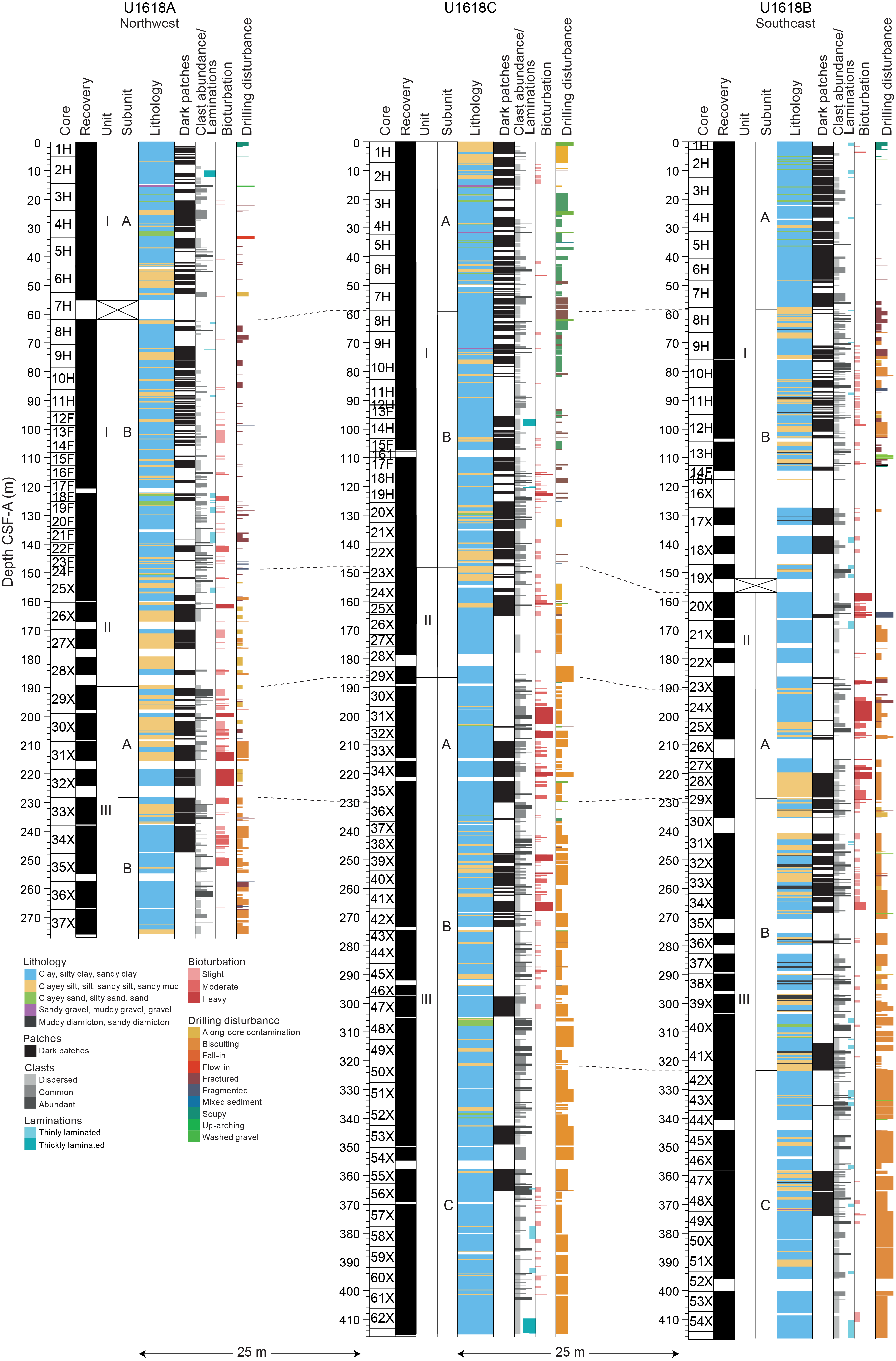
Figure F7. Lithostratigraphic correlation.
The degree of core recovery, coring disturbance, and gas expansion varies with the depth of the cores and the type of coring method employed. APC cores from Holes U1618A–U1618C exhibit minimal disturbance, although low recovery or fracturing is observed beginning around 50–60 mbsf in all holes, with decreased recovery below this depth. Soupy intervals are noted in the upper sections of the first two to three cores from each hole and often result in mixed sediments. Most XCB cores from all holes are moderately to heavily disturbed, primarily by biscuiting, which mainly affects silty clay intervals. Coarser grained intervals appear to be more resistant to disturbance, preventing them from becoming severely biscuited.
The sediments from Site U1618 exhibit similarities to those from the nearest ODP site location (Site 912; Shipboard Scientific Party, 1995). However, lithologic analysis of X-radiographs, coupled with the physical property and geochemical data, revealed new notable information in sediment characteristics.
3.1. Lithostratigraphic unit descriptions
3.1.1. Unit I
- Intervals: 403-U1618A-1H-1 through 23F-CC; 403-U1618B-1H-1 through 19X-CC; 403-U1618C-1H-1 through 23X-1
- Depths: Hole U1618A = 0–148.87 mbsf; Hole U1618B = 0–152.20 mbsf; Hole U1618C = 0–148.05 mbsf
- Age: Pleistocene to Holocene
The sediment in Lithostratigraphic Unit I is predominantly soft to firm dark gray (2.5Y 4/1) to very dark gray (N 3/) silty clay with frequent intervals of coarser clayey silt/sandy mud, occasional greenish gray (e.g., 10GY 5/1) and dark reddish gray (10R 3/1) intervals, and gravels that mostly occur in the upper part of the unit. The lower contacts of the sandy mud intervals are sometimes irregular with grading, suggesting turbidite-type gravitational flow deposition. Based on visual observations of the split core surface and examination of X-radiographs, the presence of gravel- to pebble-sized clasts is highly consistent. There is an abundance of small clasts (<1–2 cm) ranging from dispersed to abundant throughout the unit. In the lower part of the unit, the sediment displays the occasional occurrence of diamicton and laminated intervals, with slight to moderate bioturbation (Figures F5A, F6A, F6B). Debrite-type sediments are visible on both the split core surface and the X-radiographs (Figure F4C).
The most common minerals observed in smear slides are quartz and clay, accompanied by a considerable number of rock fragments and a relatively low concentration of heavy minerals, feldspar, and other minerals (Figure F8). Glauconite is also occasionally recognized. The biogenic component of the sediment is typically less than 2%, except in a few intervals that are dominated by calcareous nannofossils.
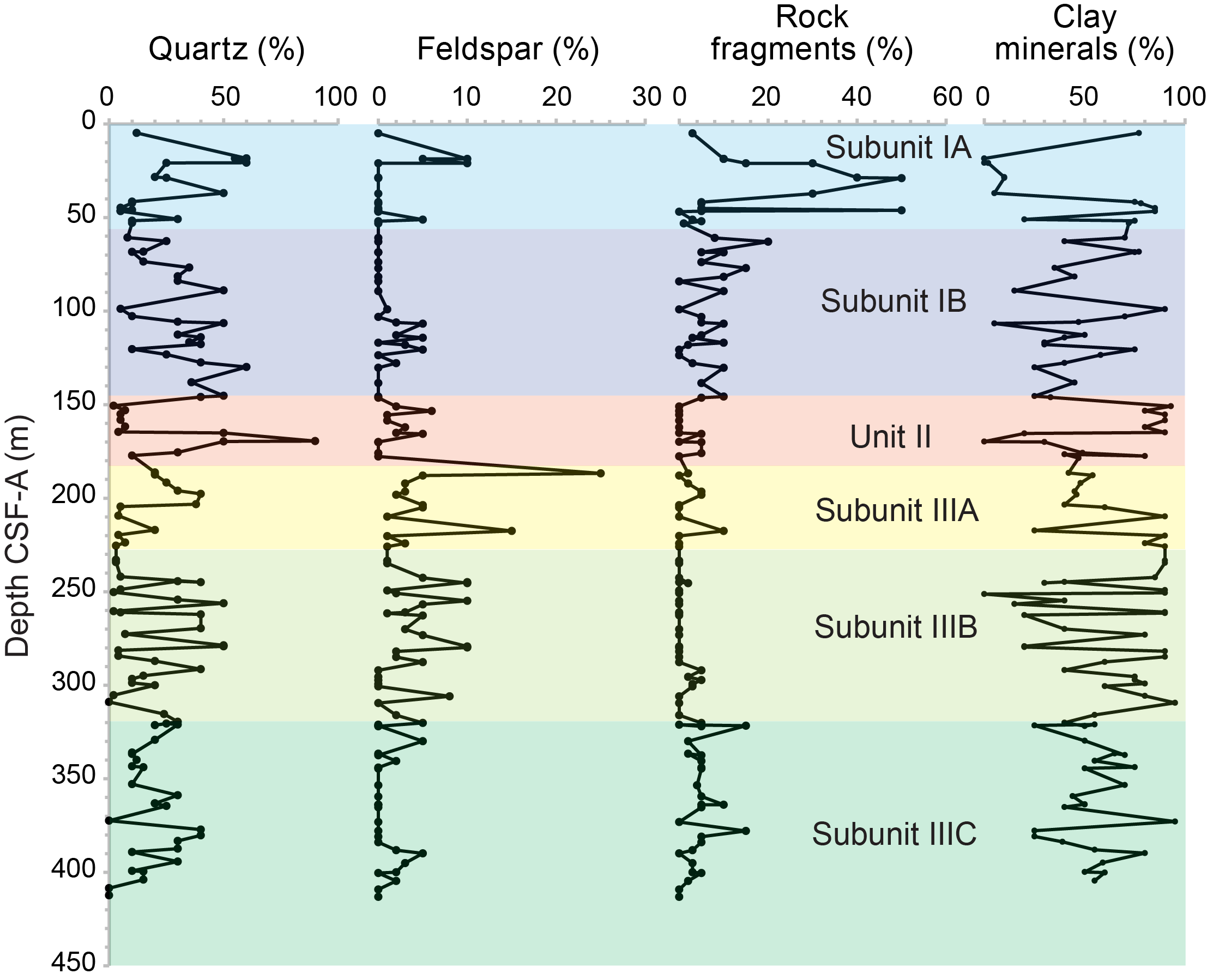
Figure F8. Downhole mineralogy.
Unit I can be divided into two subunits (IA and IB) based on the different occurrence of diamicton and intense lamination in the lower part of the sediment sequence, in addition to the presence of bioturbation, variations in color, and physical properties. This subunit boundary is located at the bottom of Core 403-U1618A-7H (55.10 mbsf); in Section 403-U1618B-8H-1, 81 cm (58.51 mbsf); and at the bottom of Core 403-U1618C-7H (59.19 mbsf) (Table T2).
3.1.1.1. Subunit IA
- Intervals: 403-U1618A-1H-1 through 7H-CC; 403-U1618B-1H-1 through 8H-1, 81 cm; 403-U1618C-1H-1 through 7H-CC
- Depths: Hole U1618A = 0–55.10 mbsf; Hole U1618B = 0–58.51 mbsf; Hole U1618C = 0–59.19 mbsf
Lithostratigraphic Subunit IA is the youngest in the stratigraphic sequence and is characterized by relatively soft and soupy sediments compared to Subunit IB, especially in the uppermost cores, and is less bioturbated overall. The first few cores of this subunit have higher a* and b* color index values compared to the other subunits (Figures F9, F10, F11). Subunit IA has a greater percentage of sand (e.g., sandy mud) (Figure F12) and more recurrent intervals with abundant clasts. Biogenic material generally comprises <2% of the composition, with several intervals exceeding 10%, and there is no visual evidence of diagenesis. Laminations occasionally occur. Subunit IA is also characterized by a general increase in natural gamma radiation (NGR) values toward the bottom, which is possibly associated with increased clast abundance as observed at the bottom of the subunit in Holes U1618B and U1618C.
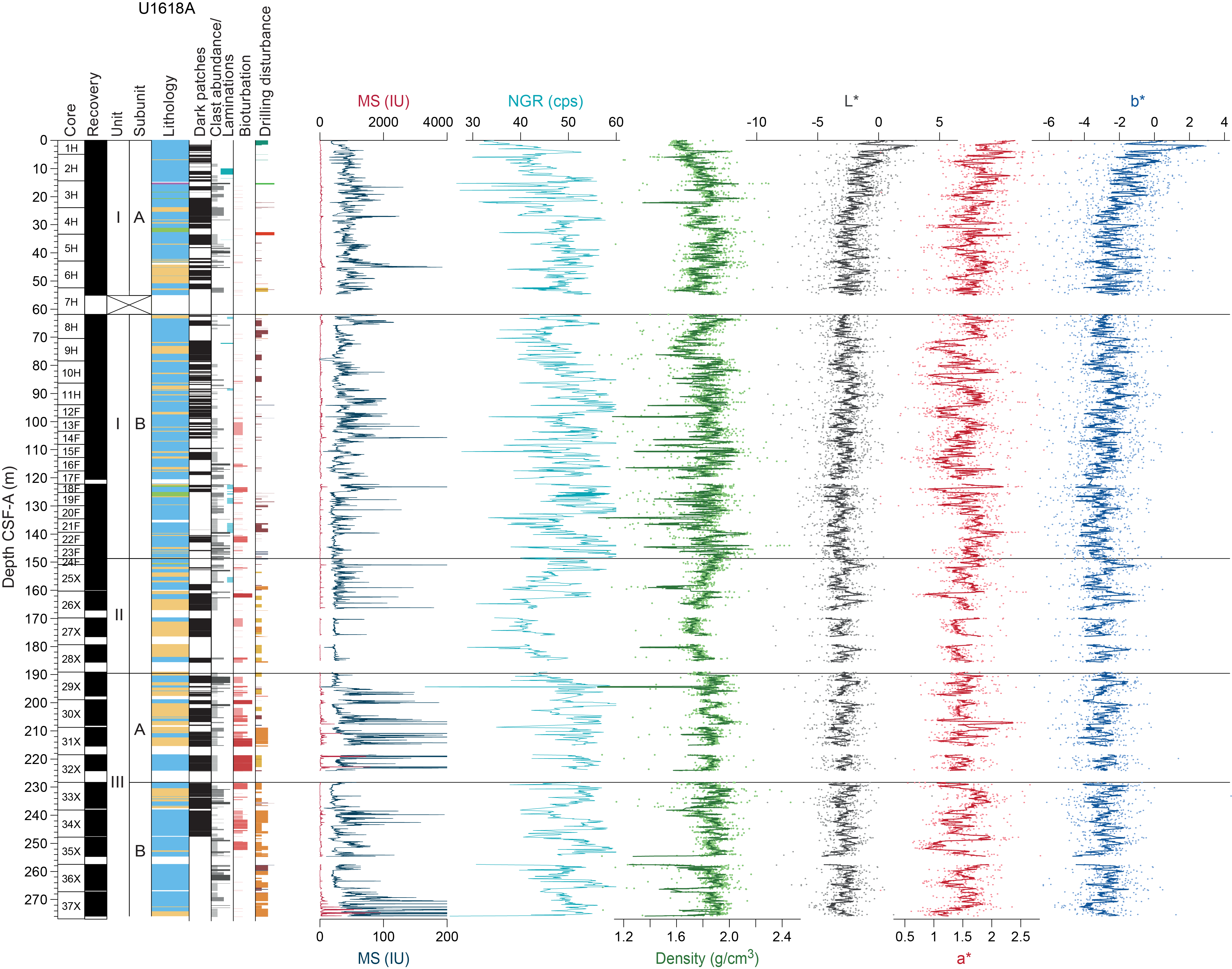
Figure F9. Physical properties, Hole U1618A.
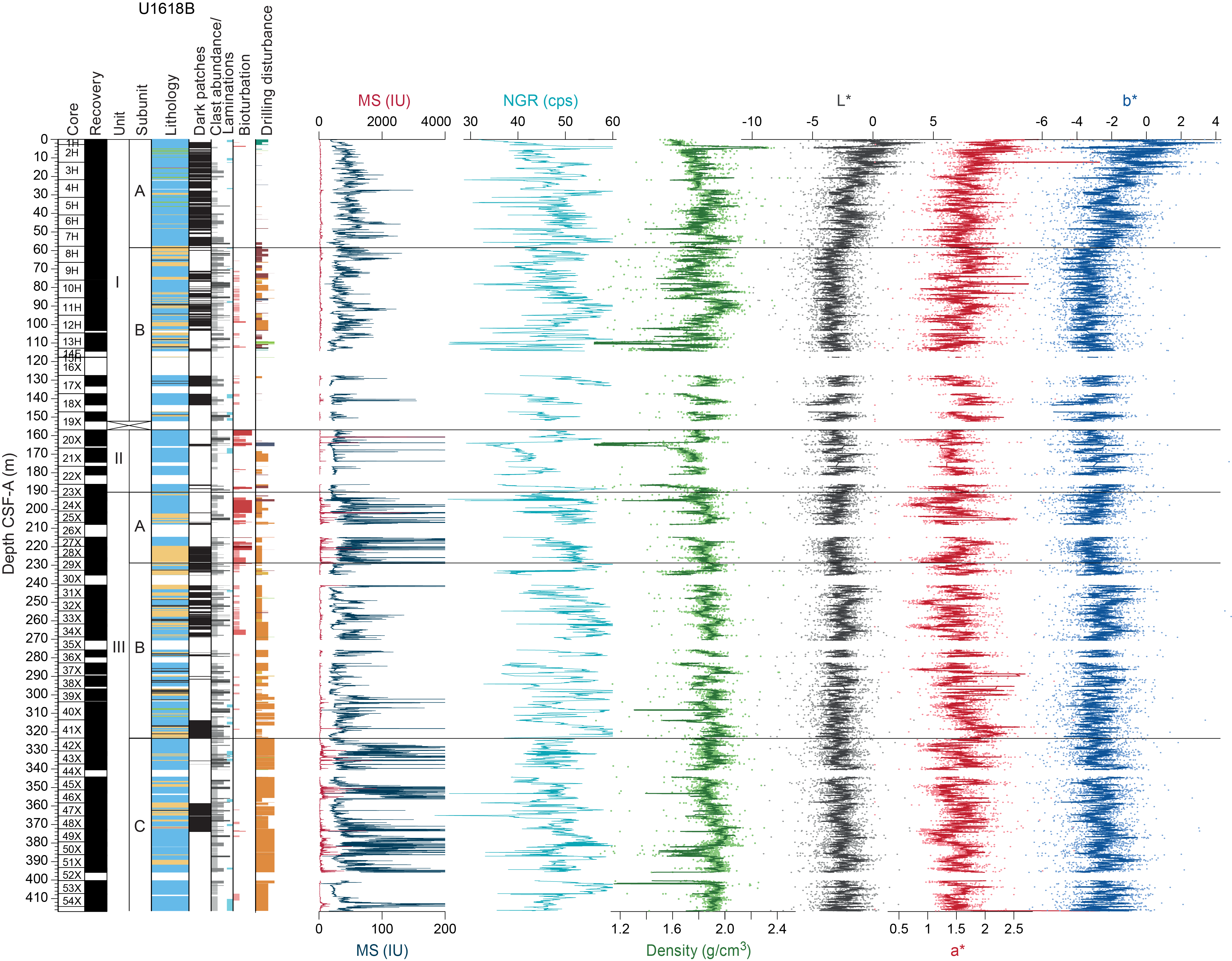
Figure F10. Physical properties, Hole U1618B.
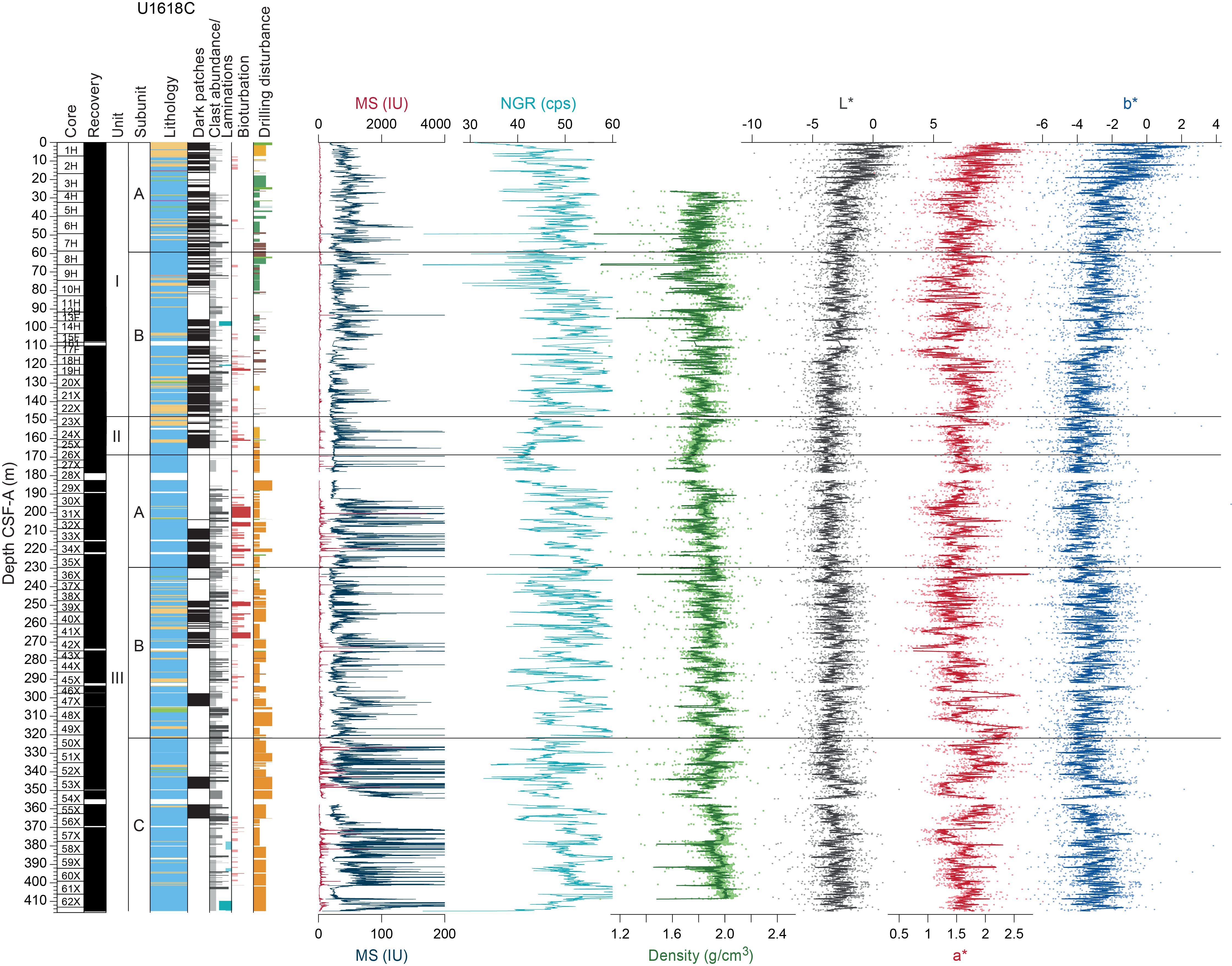
Figure F11. Physical properties, Hole U1618C.
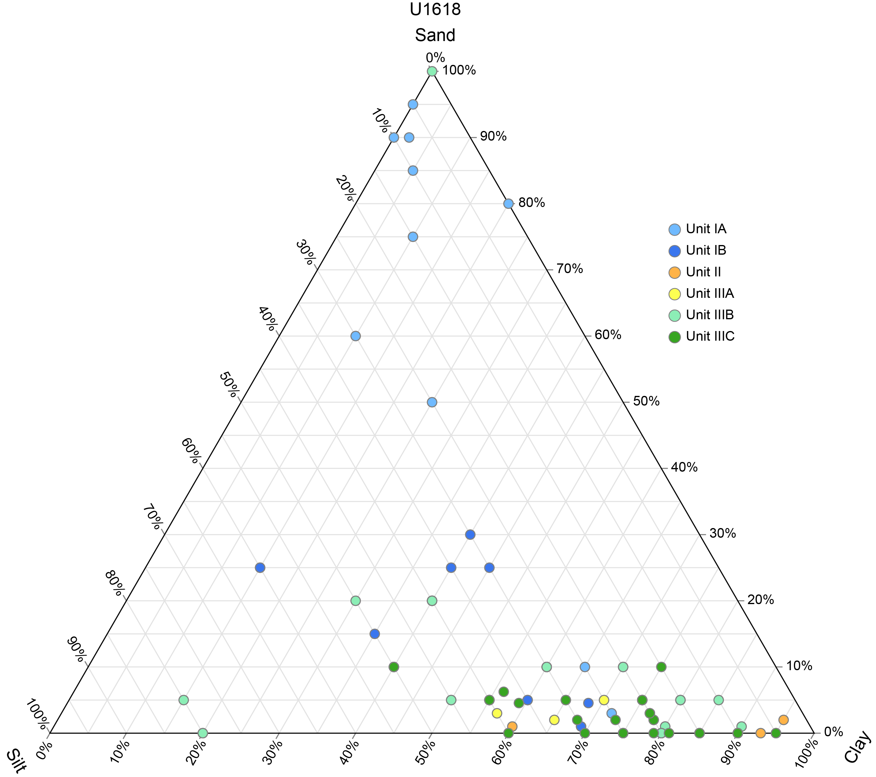
Figure F12. Sand, silt, and clay percentages.
3.1.1.2. Subunit IB
- Intervals: 403-U1618A-8H-1 through 23F-CC; 403-U1618B-8H-1, 81 cm, through 19X-CC; 403-U1618C-8H-1 through 23X-1
- Depths: Hole U1618A = 61.90–148.87 mbsf; Hole U1618B = 58.51–152.20 mbsf; Hole U1618C = 59.19–148.05 mbsf
Lithostratigraphic Subunit IB is slightly more consolidated than Subunit IA, slightly to moderately bioturbated in many cores, and shows lower a* and b* values than Subunit IA. In addition, this subunit is more fractured, with many void intervals, likely related to sediment degassing. Diamicton and laminated intervals are observed. Formation of large authigenic calcite grains is evident in the lowermost part of the subunit.
3.1.2. Unit II
- Intervals: 403-U1618A-24F-1 to 29X-1, 46 cm; 403-U1618B-20X-1 to 23X-4, 78 cm; 403-U1618C-23X-2 through 29X-3
- Depths: Hole U1618A = 148.87–189.56 mbsf; Hole U1618B = 156.95–190.60 mbsf; Hole U1618C = 148.05–186.65 mbsf
- Age: Pleistocene
Lithostratigraphic Unit II is also predominantly dark gray (N 3/) to greenish black (10Y 2.5/1) silty clay and is characterized by relatively firmer induration. Intervals of clayey silt and sandy mud are less common than in Unit I. Based on visual core observations and X-radiographs, the presence of small to large clasts is evident, but their occurrence is less frequent than in Unit I. Diamicton is not observed. This unit is also characterized by frequent occurrence of voids and fractures, which is likely related to sediment degassing.
The most common minerals observed in smear slides are quartz and clay. In addition, occurrences of rock fragments, heavy minerals, opaque minerals, and glauconite are observed. Unit II is typified by limited bioturbation. The biogenic component of the sediment is 0%–1%. In addition to the authigenic carbonate, authigenic iron sulfide minerals are observed in this unit (as inferred from smear slide observations on the split core surface and X-radiographs) (Figure F4A).
Unit II has increased variability in magnetic susceptibility (MS), which most likely corresponds to authigenic iron sulfide minerals. This unit has generally lower NGR and lower gamma ray attenuation (GRA) density (especially Hole U1618A; Figure F9) than the other units. The upper boundary of Unit II is likely to be consistent with Seismic Reflector R5.
3.1.3. Unit III
- Intervals: 403-U1618A-29X-1, 46 cm, to the bottom of the hole; 403-U1618B-23X-4, 78 cm, to the bottom of the hole; 403-U1618C-29X-4 to the bottom of the hole
- Depths: Hole U1618A = 189.56–276.9 mbsf; Hole U1618B = 190.60–414.3 mbsf; Hole U1618C = 186.65–413.1 mbsf
- Age: Pliocene to Pleistocene
The sediment in Lithostratigraphic Unit III is predominantly firm dark gray (5Y 4/1) to greenish black (5GY 2.5/2) silty clay with frequent clayey silt/sandy mud intervals and occasional diamicton intervals. The lower contacts of these coarser intervals are sometimes sharp or erosional, suggesting gravitational flow deposition. There is a slight increase in quartz, feldspar, mica, and opaque minerals as observed in smear slides compared to Units I and II and an increase in smectite toward the bottom of the record (Figure F13) based on X-ray diffraction (XRD). The biogenic component of the sediment is generally low (<3%), although there are several intervals exceeding 5%. The upper boundary of Unit III is marked by a significant increase in authigenic iron sulfide minerals compared to Unit II.
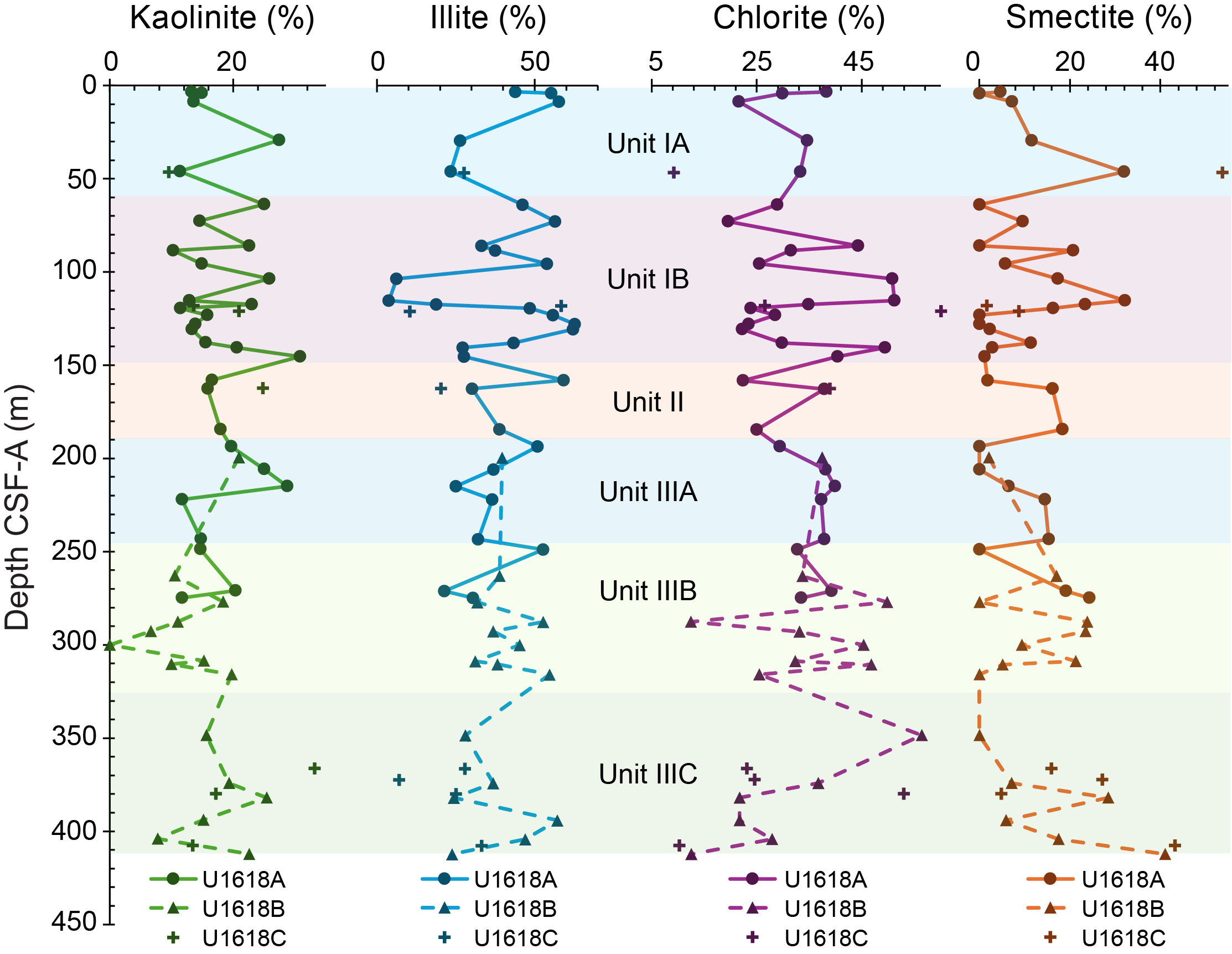
Figure F13. XRD results.
The occurrence of diamicton and lamination and the degree of bioturbation, in addition to variations in the abundance of iron sulfide minerals, allows for the division of Unit III into three subunits (IIIA–IIIC). The boundary between Subunits IIIA and IIIB likely corresponds to Seismic Reflector R6.
3.1.3.1. Subunit IIIA
- Intervals: 403-U1618A-29X-1, 46 cm, through 32X-CC; 403-U1618B-23X-4, 78 cm, through 29X-3, 15 cm; 403-U1618C-29X-4 through 35X-CC
- Depths: Hole U1618A = 189.56–224.21 mbsf; Hole U1618B = 190.60–228.81 mbsf; Hole U1618C = 186.65–230.07 mbsf
Lithostratigraphic Subunit IIIA has a higher contribution of clayey silt compared to Subunits IIIB and IIIC in Holes U1618A and U1618B, but this is not observed in Hole U1618C (Figure F7). This subunit is also characterized by ranging degrees of bioturbation generally from slight to heavy (Figure F6C). The biogenic fraction is absent to low (3%) throughout. The occurrence of larger clasts (>2 cm) is also more common in Subunit IIIA (and Subunit IIIB) compared to Subunit IIIC and includes a variety of rock types. Subunit IIIA is characterized by significant authigenic iron sulfide minerals based on observations of the split core surface, X-radiographs, smear slides, bulk XRD mineralogy, and extreme peaks in MS (e.g., Figures F9, F10, F11).
3.1.3.2. Subunit IIIB
- Intervals: 403-U1618A-33X-1 to the bottom of the hole; 403-U1618B-29X-3, 15 cm, through 41X-CC; 403-U1618C-36X-1 through 49X-CC
- Depths: Hole U1618A = 224.21 mbsf to the bottom of the hole; Hole U1618B = 228.81–323.19 mbsf; Hole U1618C = 230.07–321.56 mbsf
Predominantly a silty clay to clayey silt, Lithostratigraphic Subunit IIIB is characterized by the additional occurrence of diamicton and laminated sediments and a reduced abundance of authigenic iron sulfide minerals, which corresponds well to the observed reduction in the number of extreme MS values. Bioturbation is slight to heavy in the upper part of the subunit (Figure F6D) and decreases in the lower part. Biogenic components are low throughout much of Subunit IIIB, with few intervals having more than 5% biogenics. The occurrence of clasts is similar to the other Unit III subunits.
3.1.3.3. Subunit IIIC
- Intervals: 403-U1618B-42X-1 to the bottom of the hole; 403-U1618C-50X-1 to the bottom of the hole
- Depths: Hole U1618B = 323.19 mbsf to the bottom of the hole; Hole U1618C = 321.56 mbsf to the bottom of the hole
Like Lithostratigraphic Subunit IIIA, Subunit IIIC is predominantly a silty clay to clayey silt. Based on X-radiographic inspection, Subunit IIIC contains diamicton intervals near the top (e.g., Core 403-U1618B-43X), and laminations are common, especially toward the bottom (Figure F5B). This subunit is characterized by significant authigenic iron sulfide minerals that are visible as abundant dark concretions and significant peaks in MS, similar to Subunit IIIA. Authigenic carbonate is present (Figure F4B). Based on X-radiograph observation, bioturbation is generally absent to slight.
3.2. X-ray diffraction
XRD analyses were used to characterize the clay mineral assemblage made of kaolinite, illite, smectite, and chlorite (Figure F13). The relative abundance of kaolinite ranges between 10% and 41% (standard deviation [SD] = 7.21), with higher but fluctuating values observed within Lithostratigraphic Unit I and Subunit IIIC and lower values from the top of Unit II to the base of Subunit IIIB. Illite varies from 4% to 63% (SD = 15.04; 1σ), showing minimal variation throughout the units, except for a significant reduction in Subunit IB at ~110 mbsf. Smectite varies from 0% to 54% (SD = 12.52) and shows an increase toward the base of Subunit IIIC. Chlorite varies from 9% to 60% (SD = 11.54), exhibiting high variability in Subunit IB and a gradual decrease in relative abundance toward the base of Subunit IIIC.
Additionally, bulk XRD analysis of select powdered samples confirms that clay minerals and quartz comprise the primary composition of the representative silty clay lithologies (Table T3). It also confirms the compositions of the suspected authigenic mineralogic components such as iron sulfides and iron carbonate (e.g., greigite, pyrite, and siderite) in Sample 403-U1618B-25X-1, 83–84 cm, and calcium carbonate (CaCO3) in Sample 403-U1618A-11H-6, 0–1 cm.
3.3. Preliminary interpretation
The occurrence of diamicton intervals and laminated sediments in Lithostratigraphic Unit III suggests an early glacial influence and a proximal location of an ice sheet or glacier to the drilled site during the Late Pliocene/Early Pleistocene. In addition, rhythmic changes in color and/or texture observed over the drilled sequences are likely to be related to climatic changes such as orbitally driven glacial–interglacial cycles. The absence of diamicton and fewer terrigenous clasts in Unit II may indicate an extended period of distal depositional conditions of the drilled site with respect to the glacial terminus. Unit I sediments comprise repeated sequences of bioturbated silty clay intervals that alternate with intervals of dispersed to abundant (1%–30%) clasts, which are preliminarily interpreted as IRD. The IRD-rich intervals are often alternating with thin laminations (<0.3 cm) and intervals of diamicton occurring in Subunit IB. The lithostratigraphic sequence suggests dynamic shifts between proximal to distal positions relative to the ice sheet associated with the alternation of Late Pleistocene glacial and interglacial periods. The composition of clasts (sandstone, mudstone, etc.) indicates that the IRD may have been predominantly delivered from Fennoscandia, including Svalbard and the Barents Sea shelf.
4. Biostratigraphy and paleoenvironment
Site U1618 sediments were examined for calcareous nannofossils, planktonic foraminifers, diatoms, and dinoflagellate cysts (dinocysts). None of these microfossil groups are consistently present throughout the sediment column, and several levels are barren (Figure F14).
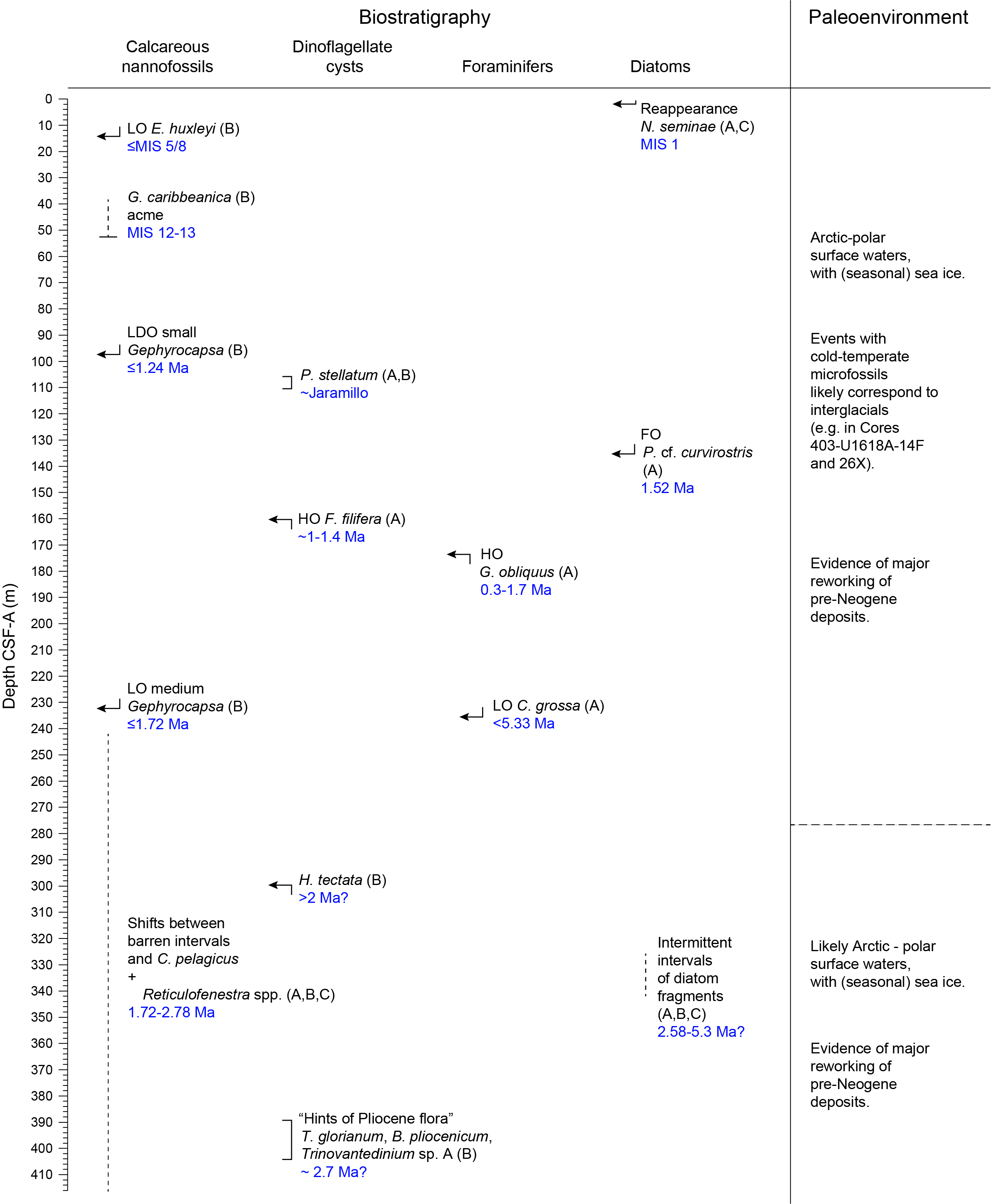
Figure F14. Biostratigraphic summary.
Diatoms are present at the very top and only sporadically downcore. Planktonic foraminifers are present in the upper part but disappear downcore. Calcareous nannofossils are also generally present, but toward the base of the hole the record is mainly barren. Dinocysts are present throughout the sediment column but are absent occasionally. All groups combined, especially with calcareous nannofossils and dinocysts, contribute to a first biostratigraphic and paleoenvironmental assessment and an age-depth model for Site U1618 (Figure F15; Table T4).
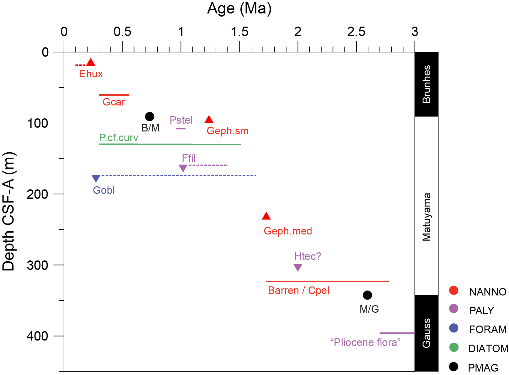
Figure F15. Age-depth model.
The age model for Site U1618 is based on a combination of biostratigraphical and paleomagnetic data. A total of three calibrated calcareous nannofossil events were identified across the three holes at Site U1618: the lowest occurrence (LO) of Emiliania huxleyi, the lowest dominant occurrence (LDO) of the small Gephyrocapsa group, and the LO of medium Gephyrocapsa. The acme of Gephyrocapsa caribbeanica indicates a Late Pleistocene age for the upper part of the site. Two dinocyst events, which suggest an age around 1 Ma, were observed: the restricted presence of Protoperidinium stellatum and the highest occurrence (HO) of Filisphaera filifera. The discontinuous presence of Coccolithus pelagicus, together with a rare content of medium Reticulofenestra and the tentative HO of the dinocyst Habibacysta tectata, suggest an Early Pleistocene age for the lower part of the site. Traces of Late Pliocene flora, such as a few specimens of the dinocysts Barssidinium pliocenicum and Trinovantedinium variabile, appear near the base of the core and are tentatively interpreted as Late Pliocene. Additionally, the HO of Globigerinoides obliquus, the presence of the diatom Proboscia cf. curvirostris, and the record of the benthic foraminifer Cibicides grossa were used to constrain the age-depth model for Site U1618 (Figure F15).
The microfossil assemblages generally indicate Arctic–polar surface waters and seasonal sea ice conditions throughout the Quaternary. Polar surface waters are colder and slightly less saline than Arctic water masses, which are defined as a mixture of Polar and Atlantic water masses following definitions of water masses in the Fram Strait today (e.g., Hopkins, 1991). Exceptions are the cold-temperate conditions and Atlantic water incursion during the middle Pleistocene and occasional incursions of temperate waters in the Early Pleistocene. It is likely that there are more warm intervals (interglacials), given our rather low sampling resolution. Little to substantial reworking of pre-Neogene deposits is evident in all microfossil groups.
4.1. Calcareous nannofossils
The biostratigraphy of calcareous nannofossils at Site U1618 is based on the study of 59 core catchers and 268 split core samples taken from Holes U1618A–U1618C. All core catchers from Hole U1618A were examined for calcareous nannofossils (Figure F16). Core catchers from Holes U1618B and U1618C were analyzed only for those depths extending beyond the maximum depth in Hole U1618A (Figures F17, F18). Split core samples were routinary selected in all cores from Holes U1618A–U1618C based on the visual examination of sediments and physical properties (i.e., changes in color and MS).
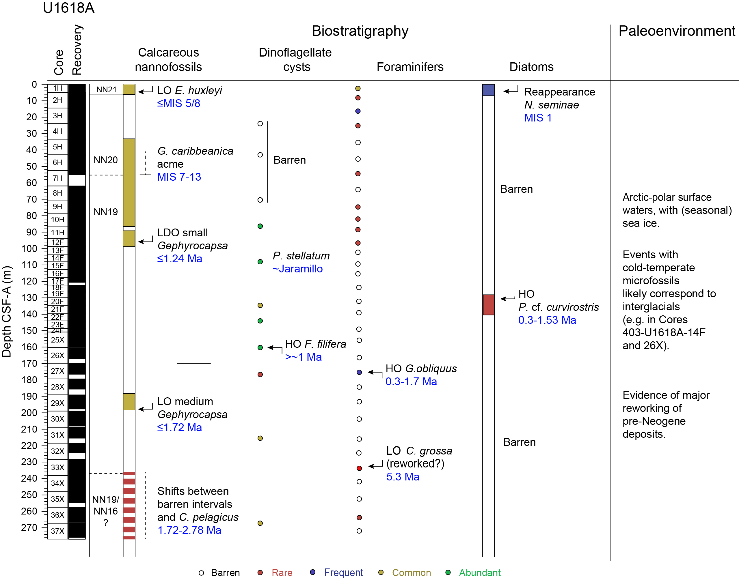
Figure F16. Biostratigraphy and paleoenvironment, Hole U1618A.
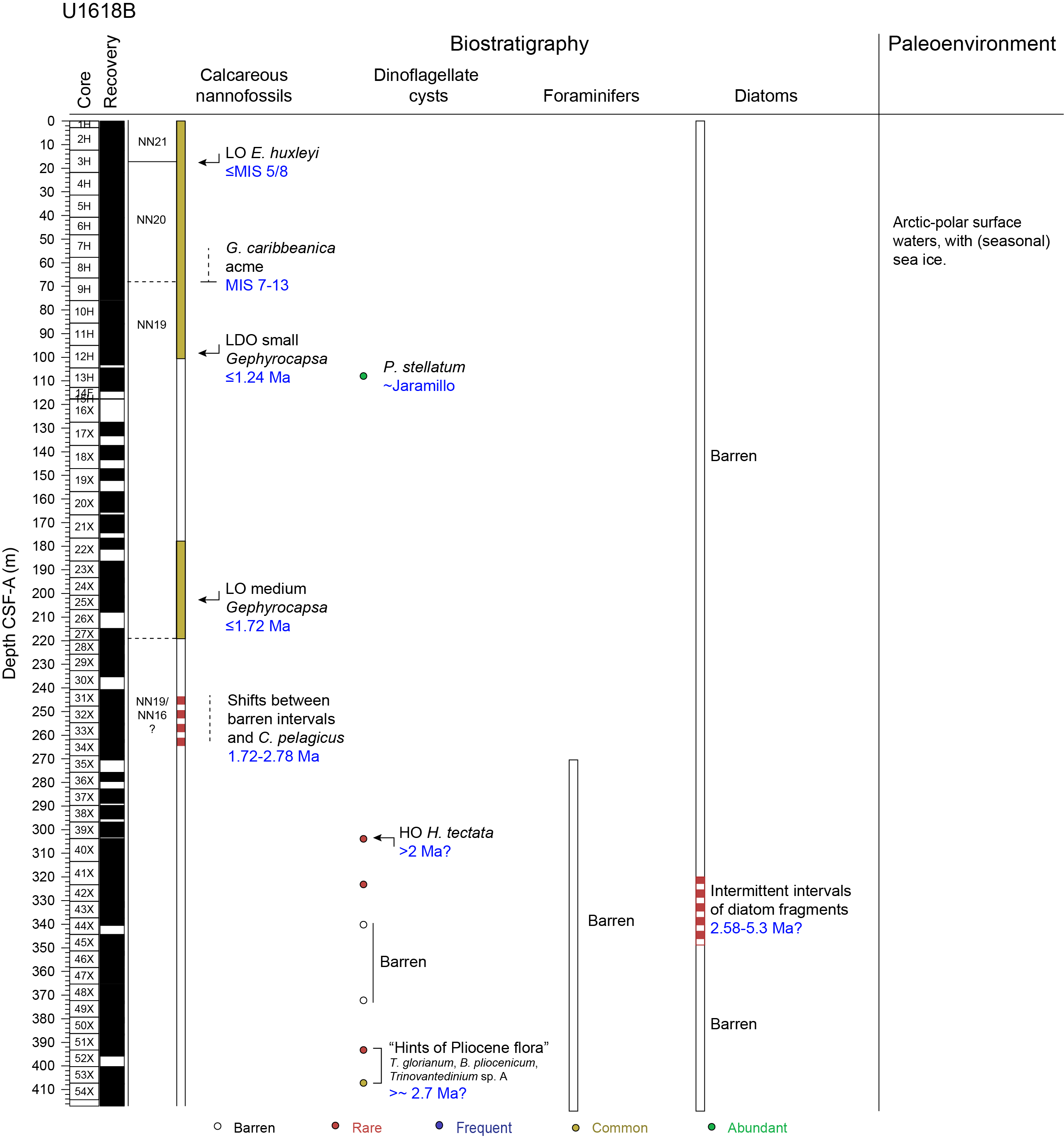
Figure F17. Biostratigraphy and paleoenvironment, Hole U1618B.
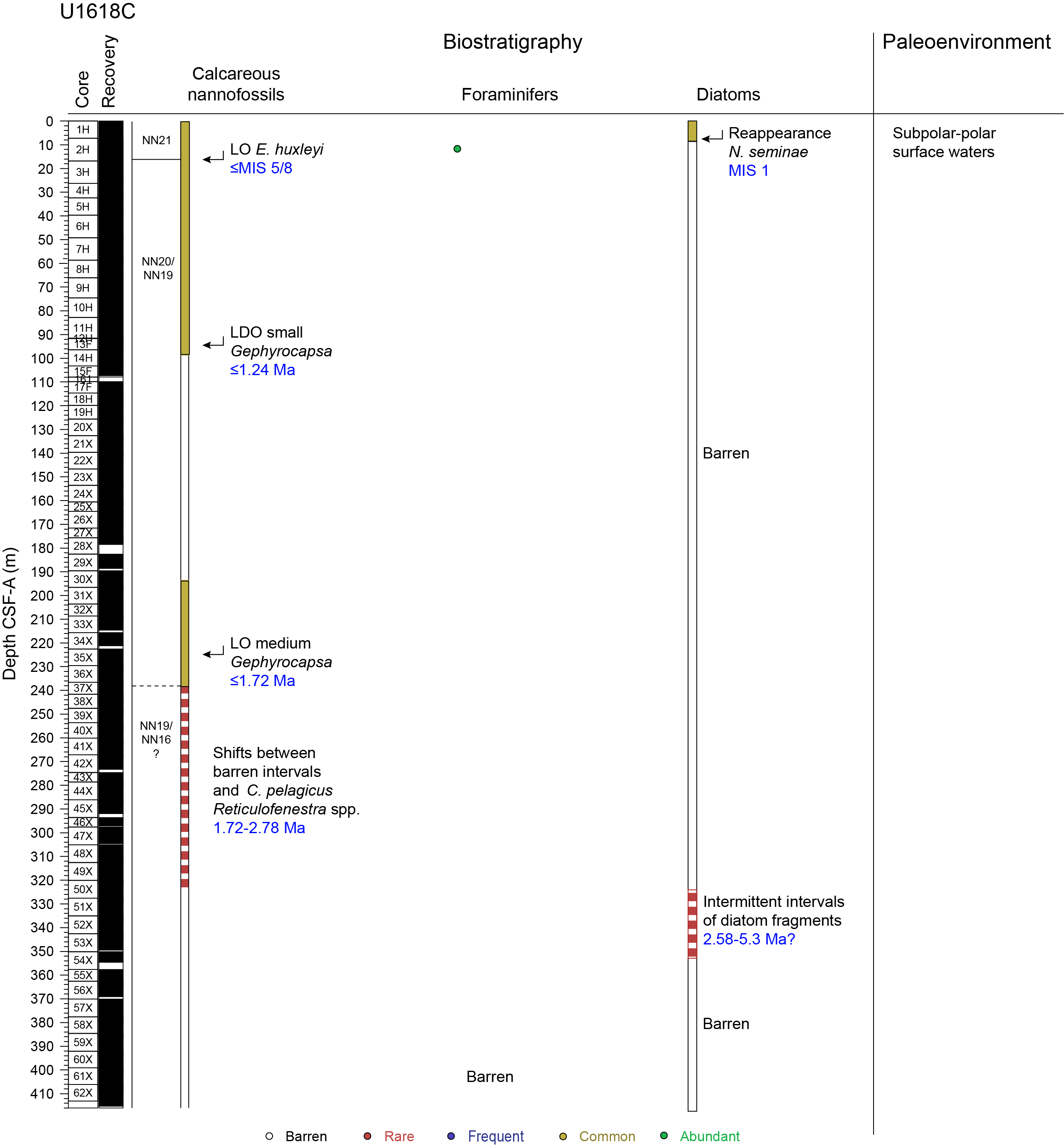
Figure F18. Biostratigraphy and paleoenvironment, Hole U1618C.
Calcareous nannofossils at Site U1618 evidence a discontinuous representation along the studied sequence. The calcareous nannofossil abundance in samples from Holes U1618A–U1618C show a high range of variability between rare and common. Species diversity is generally low, and the state of preservation varies between moderate and good. The nannofossil assemblages in samples from Site U1618 comprise nine groups/taxa, including E. huxleyi, small Gephyrocapsa, G. caribbeanica, medium Gephyrocapsa, medium Reticulofenestra, C. pelagicus, Calcidiscus leptoporus, Helicosphaera carteri, and Syracosphaera spp. Reworked nannofossils from older stratigraphic levels (mostly Cretaceous) are regularly present in samples, with an overall content that ranges between rare and frequent.
A total of three calibrated calcareous nannofossil events were identified across the three holes at Site U1618, allowing the site to be assigned an age range following the global zonation by Martini (1971). A good correspondence between the events in the three holes and nearby ODP Site 911 (Leg 151) is also observed, together with other regional and global records. Adaptation of calibrations for the North Atlantic, Fram Strait, and/or Arctic basin zonations are included when available. All this information assigns an accurate age range for Site U1618.
The LO of E. huxleyi is an indicator of Zone NN21 of Martini (1971), with a global calibration for equatorial to subpolar settings of 291 ka at MIS 8 (Thierstein et al., 1977; Rio et al., 1990; Raffi et al., 2006). In the central Arctic Ocean, the LO of E. huxleyi has been detailed to be time transgressive (i.e., diachronous), with a LO placed around MIS 5 (see Razmjooei et al., 2023, and references therein). At Site U1618, the LO of E. huxleyi is identified for the three holes in Samples 403-U1618A-1H-CC, 403-U1618B-3H-4, 114 cm, and 403-U1618C-3H-2, 140 cm. Combined, this suggests a lower age boundary that could span between MISs 8 and 5 and the assignment to the uppermost part of the Site U1618 sequence to Zone NN21 (Martini, 1971) (Figure F14).
For Hole U1618A, samples between Samples 6H-3, 54 cm, and 7H-CC are characterized by a common content of G. caribbeanica. Among these samples, the representation of this taxa is abundant and nearly monospecific in Sample 7H-1, 50 cm. This structure in nannofossil assemblages could be identifiable with the so-called acme of G. caribbeanica, globally defined between MISs 13 and 7 (Flores et al., 2012) and recognizable from tropical to subpolar settings of the North Atlantic (Maiorano et al., 2015; González-Lanchas et al., 2023) and the Arctic Ocean (Razmjooei et al., 2023). For Hole U1618A, the absence of Pseudoemiliania lacunosa in Sample 7H-1, 50 cm, suggests an age younger than or equal to 430 ka (MIS 12), according to the global calibration for the LO of P. lacunosa, or younger than or equal to MIS 13, according to the revision of this boundary for Arctic environments (Razmjooei et al., 2023) (Figures F14, F16). The recognition of this acme event allows the assignment of this part of the Site U1618 sedimentary sequence to Zone NN20 of the Middle to Late Pleistocene (Figure F14).
The small Gephyrocapsa group is a characteristic dominant component of worldwide calcareous nannofossil assemblages since the Early Pleistocene. The LDO of this group has a calibrated age of 1.24 Ma (Lourens et al., 2004). In the sediments from Site U1618, the LDO of small Gephyrocapsa is consistently identified for the three holes in Samples 403-U1618A-12F-2, 60 cm, 403-U1618B-12H-1, 110 cm, and 403-U1618C-13F-3, 19 cm (Figures F16, F17, F18). In the absence of a regional calibration for this boundary in subpolar and Arctic environments, the standard calibration is adopted, placing the age of these sediments from the three holes as younger or equivalent to 1.24 Ma (Figure F14). The identification of this boundary characterizes this part of the sequence at Site U1618 in the Early Pleistocene, belonging to Zone NN19 (Martini, 1971).
The LO of the medium Gephyrocapsa group has a calibrated age of 1.71/1.73 Ma during the Early Pleistocene (Raffi, 2002; Raffi et al., 2006; Sato et al., 1991; Sato et al., 1999). Adopting the practice for nearby ODP Leg 151, the calibration of 1.72 Ma is considered (Sato and Kameo, 1996). The LO of medium Gephyrocapsa at Site U1618 is observed in Samples 403-U1618A-29X-CC, 403-U1618B-24X-5, 127 cm, and 403-U1618C-36X-2, 33 cm; hence, this Site U1618 sequence is assigned to Zone NN19 in the Early Pleistocene (Figures F16, F17, F18).
Calcareous nannofossils are scarce in samples below the LO of medium Gephyrocapsa and to the bottom of each hole at Site U1618. This interval is mainly barren, but toward the lower part of the sequence, intermittent levels with C. pelagicus occur in sediments from the three holes (Figure F14). A similar distribution of C. pelagicus was observed at ODP Site 911 (Leg 151) between 1.72 and 2.78 Ma (Sato and Kameo, 1996). The 2.78 Ma boundary determines the transition to Zone NN16 (Martini, 1971) and is globally defined by the LO of Discoaster tamalis in low- to mid-latitude records (Curry et al., 1995; Lourens et al., 2004). Because of environmental limitation on this variety in the high latitudes, the 2.78 Ma boundary is established as correspondent to the increase in representation of Reticulofenestra specimens over C. pelagicus in the Late Pliocene sediments at ODP Site 911 (Sato and Kameo, 1996). A rare occurrence of medium Reticulofenestra in Sample 403-U1618C-50X-3, 71 cm, could be considered as a hint of the proximity of this Pliocene boundary (i.e., 2.78 Ma) in the lowermost part of the sequence at Site U1618 (Figures F14, F18). This observation allows the potential assignment of this lower part of the sequence (i.e., from the LO of medium Gephyrocapsa to the bottom) to comprise the Early Pleistocene to Pliocene transition, ranging between Zones NN19 and NN16 (Martini, 1971).
4.2. Diatoms and silicoflagellates
The diatom investigation at Site U1618 included the examination of core catcher samples and additional samples from split core sections. Most of the samples are barren of diatoms, except Samples 403-U1618A-1H-1, 0 cm, and 403-U1618C-1H-1, 0 cm, in which a well-preserved diatom assemblage is found (Figures F16, F18). The most abundant taxa are Chaetoceros in resting spore stage, Fragilariopsis oceanica (Cleve) Hasle, Thalassionema nitzschioides var. nitzschioides (Grunow) Van Heurck, Rhizosolenia borealis (Sundström), and Neodenticula seminae (Simonsen and Kanaya) Akiba and Yanagisawa.
The species N. seminae accounts for more than 40% of the diatom assemblage in the subarctic North Pacific and its high-latitude marginal seas in the modern assemblage (Reid et al., 2007). In the high-latitude North Atlantic and in the Nordic Seas, the species occurred from the Middle Pleistocene (1.26 Ma) to the Early mid-Pleistocene transition at 0.84 Ma (Koç and Scherer, 1996). Its disappearance has been related with a severe cooling and the closure of the Arctic connection between the Atlantic and Pacific Oceans (Reid et al., 2007). Nevertheless, several studies indicated that N. seminae reenters the North Atlantic via the Arctic. It has been documented in plankton samples (Reid et al., 2007), surface sediment samples (Miettinen et al., 2013), and Holocene sediments of the Fram Strait (Matul and Kazarina, 2020).
Across all three holes at Site U1618, some intervals contain fragments of diatoms, but these were not useful for biostratigraphy. For Hole U1618A, an interval with diatom fragments and sponge spicules is observed from 129.93 to 130.27 mbsf (Samples 19F-CC, 28 cm, 20F-1, 3 cm, and 20F-1, 10 cm). For Hole U1618B, another interval is found from 329 to 339.37 mbsf (Samples 42X-4, 130 cm, to 44X-2, 61 cm) (Figure F17). For Hole U1618C, the interval appears from 342.24 to 350.29 mbsf (Samples 52X-6, 69 cm, to 54X-1, 19 cm). Only in Sample 403-U1618A-20F-1, 3 cm, is a fragment of P. cf. curvirostris (Jousé) found, indicating a Pleistocene age (P. curvirostris Biozone) (Koç and Scherer, 1996). The most significant and identifiable diatom fragment is of Paralia sulcata (Ehrenberg) Cleve, which indicates transport from coastal shallow waters into the hemipelagic realm.
No silicoflagellates are observed.
4.3. Dinoflagellate cysts
Dinocysts were analyzed in a total of 18 samples from Holes U1618A–U1618C, and they are dominated by round brown cysts (RBCs) and Brigantedinium. Bitectatodinium tepikiense and Islandinium species are frequently recorded. Assemblages are well preserved, showing no influence of oxidation, and are low in diversity. Key stratigraphic species are present in low abundance.
Samples 403-U1618A-3H-CC, 5H-CC, and 8H-CC are dominated by reworked terrestrial and marine palynomorphs, and only a few in situ dinocysts are found. The in situ assemblage is represented by a few specimens of RBCs, Brigantedinium simplex, Islandinium, and B. tepikiense. The same species are more abundantly present in Sample 10H-CC (Figure F16).
Samples 403-U1618A-14F-CC and 403-U1618B-13H-4, 4–5 cm, contain a diverse assemblage (>10 species). Species encountered include Brigantedinium, RBCs, Spiniferites, B. tepikiense, Protoceratium reticulatum (indicative of Atlantic water), and cysts of P. stellatum. Such a diverse assemblage with abundant P. reticulatum is indicative of interglacial conditions (e.g., Matthiessen et al., 2018). The species P. stellatum is reported by Matthiessen and Brenner (1996) from around the Jaramillo Subchron at nearby ODP Site 911 on the Yermak Plateau (Sample 911A-11H-4, 72–78 cm). F. filifera is recorded in several samples from Hole U1618A (25X-CC, 31X-CC, 36X-CC, and 41X-CC). The HO of F. filifera is not a well-defined stratigraphic event. In the North Atlantic and Nordic Seas in the upper Matuyama Chron, its HO is between 1 and 1.4 Ma, but well-preserved specimens also occur in the Bruhnes Chron (Matthiessen et al., 2018). The range top of F. filifera in Sample 25X-CC would conservatively suggest an age older than ~1 Ma for deposits below this level but possibly older than 1.3–1.4 Ma. The better constrained top of the F. filifera acme (Matthiessen et al., 2018), which corresponds to the top of the Olduvai Subchron, is not identified in Hole U1618A. Only two specimens of H. tectata are recorded: one each in Samples 403-U1618B-39X-CC and 41X-CC (Figure F17). It is very tentative to base a stratigraphic interpretation on so few specimens, but if the record in Sample 39X-CC corresponds to the range top of the species, then this likely indicates an age older than 2 Ma for deposits below Sample 39X-CC. Near the base of Hole U1618B, traces of Late Pliocene flora are found. In Sample 51X-CC, T. variabile and Trinovantedinium sp. A are encountered (Figure F17). The latter species is thus far only found in the Late Pliocene (~2.7 Ma) of the Integrated Ocean Drilling Program Bering Sea Site U1341 (S. De Schepper, unpubl. data, 2024). In Sample 53X-CC, several specimens of Trinovantedinium glorianum and T. variabile and parts of the cyst B. pliocenicum are found. B. pliocenicum was reported from ODP Site 987 to have its HO just below Seismic Reflector R6 (Smelror, 1999). It ranges up into the Early Pleistocene (Head, 1993) but is mainly found in the Pliocene of the North Atlantic and Nordic Seas (De Schepper and Head, 2009; De Schepper et al., 2017).
Almost all investigated samples contain a substantial amount of reworked pollen and spores, degraded plant debris, and also pre-Neogene dinocysts. This reflects the considerable input of pre-Neogene sediments to the site. The in situ dinocyst assemblage is therefore sometimes hard to identify, and several samples are (nearly) barren. Where dinocysts are present, assemblages are mainly low in diversity and dominated by heterotrophic taxa (RBC and Brigantedinium). Islandinium is present in nearly all samples, and together with Brigantedinium it would suggest Arctic–polar water masses with sea ice for most of the studied interval. Exceptions are Samples 403-U1618A-14-CC and 403-U1618B-13H-4, 4–5 cm, which were taken in an interglacial during or near the Jaramillo Subchron (Figure F14). Here, the dinocyst assemblage is diverse and indicates (cold–)temperate conditions as indicated by the presence of heterotrophic species, abundant P. reticulatum, B. tepikiense, and the acritarch Nannobarbophora walldalei. P. reticulatum is a good indicator for cold–temperate conditions and Atlantic water in the Fram Strait region (e.g., Matthiessen and Knies, 2001). B. tepikiense is a subpolar–temperate species, which today occurs mostly at mid-latitudes of the North Atlantic (de Vernal et al., 2020), and the acritarch N. walldalei is linked with warm–temperate conditions and interglacials (Head, 2003).
4.4. Foraminifers
A total of 54 samples from Holes U1618A–U1618C were analyzed for planktonic foraminifers. Planktonic foraminifers are very sparse in Hole U1618A. They are generally present in the uppermost ~99 m (Cores 1H–12H), with abundances from rare to common (Figure F16). They show a moderate to high degree of dissolution or encrustation. Generally, only Neogloboquadrina pachyderma is present, except in Sample 403-U1618A-12H-CC where Globigerinoides bulloides also appear. N. pachyderma is the dominant planktonic foraminiferal species in polar regions (e.g., Bé and Tolderlund, 1971). It is found today in the Fram Strait within Arctic and polar water masses in areas both with and without seasonal sea ice (e.g., Husum and Hald, 2012; Pados and Spielhagen, 2014). Below this level, samples are barren of planktonic foraminifers, except Sample 27X-CC. This sample holds a well-preserved diverse fauna consisting of G. bulloides, Globigerinoides conglobatus, G. obliquus, Globigerinoides ruber, Globorotalita woodi, Neogloboquadrina incompta, Orbulina universa, and Trilobatus sacculifer. These species first appear in the Oligocene and Miocene, and most are extant. Some of the species (e.g., G. ruber) were also observed at ODP Sites 910 and 911 at the nearby Yermak Plateau in upper Pliocene sediments (Spiegler, 1996). G. obliquus and G. woodi have their last appearances in the Early Pleistocene, but recent work by Lam et al. (2022) demonstrated diachronous datums of these species in the Pacific. Their last appearance is at 293 and 427 ka, respectively, in the Northwest Pacific (Lam et al., 2022). Hence, we speculate that the last appearance of these species is also diachronous in the Atlantic but within the Middle Pleistocene (Figure F14). Furthermore, the observed species within Sample 27X-CC are characteristic of temperate–subtropical environments (e.g., Lam et al., 2022) (Figure F16).
During analysis, we also noted whether benthic foraminifers are present. Overall, only potential biostratigraphic marker species were identified to species level, and further taxonomic analysis of benthic foraminifers will be carried out postexpedition. Sample 403-U1618A-27X-CC contains the benthic foraminifer C. grossa (Figure F14). Sample 32X-CC also contains rare specimens of C. grossa, which may suggest a Pliocene age (e.g., Feyling-Hanssen et al., 1983; King, 1983); however, the HO of C. grossa is diachronous, and this event is younger (Pleistocene) than previously defined (Anthonissen, 2008). Other investigations have also reported a Late–Middle Miocene age for the first appearance of C. grossa (Voorthuysen, 1950; Eidvin and Rundberg, 2001).
For Hole U1618B, Samples 35X-CC to 54X-CC were analyzed for planktonic foraminifers. All samples are barren (Figure F17).
One sample from Hole U1618C at 18.17 mbsf that was assumed to be MIS 5 was analyzed (Figure F18). Planktonic foraminifers are very abundant, with very abundant N. pachyderma and rare abundance of N. incompta and G. bulloides. This is a typical subpolar–polar planktonic foraminiferal fauna (e.g., Schiebel and Hemleben, 2017). This targeted sample was also analyzed for benthic foraminiferal fauna. Benthic foraminifers are common, mainly consisting of Islandiella helenae and Epistominella exigua. Melonis barleeanus and Stainforthia fusiformis also occur to some degree (rare abundance). Single specimens of both Cassidulina reniforme and Cassidulina neoteretis in addition to Triloculina tricarinata are also observed. All these species may be found together in high-latitude environments (e.g., Sejrup et al., 2004). Additionally, the composition of this benthic foraminiferal fauna is similar to what has previously been reported from MIS 5 in a sediment core from 500 m water depth at the southern Yermak Plateau (Chauhan et al., 2014), thus tentatively supporting the assumed age (MIS 5). Additionally, the three deepest core catcher samples from Hole U1618C (60X-CC to 62X-CC) were analyzed because they go below the range of Hole U1618B. They are all barren (Figure F14).
5. Paleomagnetism
Paleomagnetic investigation of Site U1618 focused on measurements of the natural remanent magnetization (NRM) before and after alternating field (AF) demagnetization of archive-half sections and vertically oriented discrete cube samples. All archive-half sections were measured except a few that had significant visible coring disturbance. Some archive-half sections with high MS (greater than ~750 IU) were too strong for the NRM to be measured on the superconducting rock magnetometer (SRM) and caused flux jumps even when the track speed was slowed by 10×, thus compromising our ability to collect quality data in these intervals. However, the intensity often was reduced after AF demagnetization, and measurements could then be made. APC and HLAPC archive-half sections were measured before and after 10 and 15 mT peak AF demagnetization. Because XCB cores do not use nonmagnetic core barrels and are more susceptible to the viscous isothermal remanent magnetization (VIRM) drill string overprint (Richter et al., 2007), XCB archive-half sections required higher AF demagnetization steps to remove this overprint and were measured before and after 15 and 30 mT peak AF demagnetization. The NRMs of the oriented discrete cube samples were stepwise demagnetized to higher fields up to either 50 mT if analyzed on the SRM using the in-line AF demagnetizing system or 100 mT if analyzed on the AGICO JR6 spinner magnetometer using the DTECH D-2000 static AF demagnetizer. These measurements were supplemented by measurements of MS and anhysteretic remanent magnetization (ARM) on samples from all holes. Isothermal remanent magnetizations (IRMs) at various direct current fields (100, 300, and 1000 mT and a backfield of −300 mT) were imparted and measured on Hole U1618A samples. Two unoriented iron sulfide nodules were also sampled and subject to MS, ARM, and IRM analyses.
5.1. Sediment magnetic properties
Site U1618 sediments have a wide range of magnetic properties that likely reflect contribution from detrital and authigenic sources. Although sediments are mostly lithogenic in origin (see Lithostratigraphy) and magnetic characterization of samples from the uppermost two cores is consistent with (titano)magnetite, authigenic iron sulfides are visible on the split core surface, sometimes occurring as nodules up to a few centimeters in diameter and sometimes associated with the highest observed MS at Site U1618 (up to ~3000 IU measured on the Whole-Round Multisensor Logger [WRMSL]). MS values greater than 500 IU become common below about 190 mbsf (Figures F25, F26), and these intervals are often associated with high-density objects in X-ray images and black to gray nodules on the split core surface. One of these nodules (from Core 403-U1618B-25X; 201.64 mbsf) with strong MS and a ~2–3 cm diameter was subsampled and studied for its magnetic properties and mineralogy (Figure F19; Table T5). Bulk XRD analysis found the nodule to mostly be composed of greigite (92%; Fe3S4) and associated with iron monosulfide (<1%; FeS) and siderite (7.5%; FeCO3) (Figure F19E). Future work could explore the mineral associations of these iron sulfide nodules to determine formation pathways. Greigite association with siderite has previously been described, and further information on the timing of formation might help determine the age of the greigite-hosted chemical remanent magnetization (CRM) relative to the age of the sediment (Roberts and Weaver, 2005). Magnetic measurements confirmed the strong magnetization of this nodule, with MS, ARM, and IRM intensities almost two orders of magnitude stronger than any other discrete cube sediment sample measured from Site U1618. The nodule has no frequency dependence of MS and an S-ratio (IRM after a 300 mT backfield normalized by a saturating IRM at 1000 mT) (Stober and Thompson, 1979) of 1, indicating that the mineral's remanence fully saturates in a 300 mT field, consistent with previously reported magnetic properties for sedimentary greigite (Roberts et al., 2011; Horng, 2018). Despite having an S-ratio of 1, the nodule has higher coercivity than might be expected for typical detrital (titano)-magnetite assemblages, with 58% of its remanence gained during IRM acquisition between 100 and 300 mT (Table T5). The nodule is also quite resistant to AF demagnetization, with 91% of its ARM remaining after a 30 mT peak AF demagnetization (Figure F19D). A second iron sulfide nodule was sampled from Core 403-U1618B-30X and subject to the same measurements. This sample was found to be weakly magnetic relative to the oriented sediment cube samples from Site U1618 but had a high frequency dependence of MS (~7%), indicating the presence of superparamagnetic material (Table T5). XRD results from this nodule found the composition was 65.7% pyrite, 17.5% quartz, and 16.8% marcasite, which is consistent with there being only trace amounts of material with ferrimagnetic properties present in this sample.
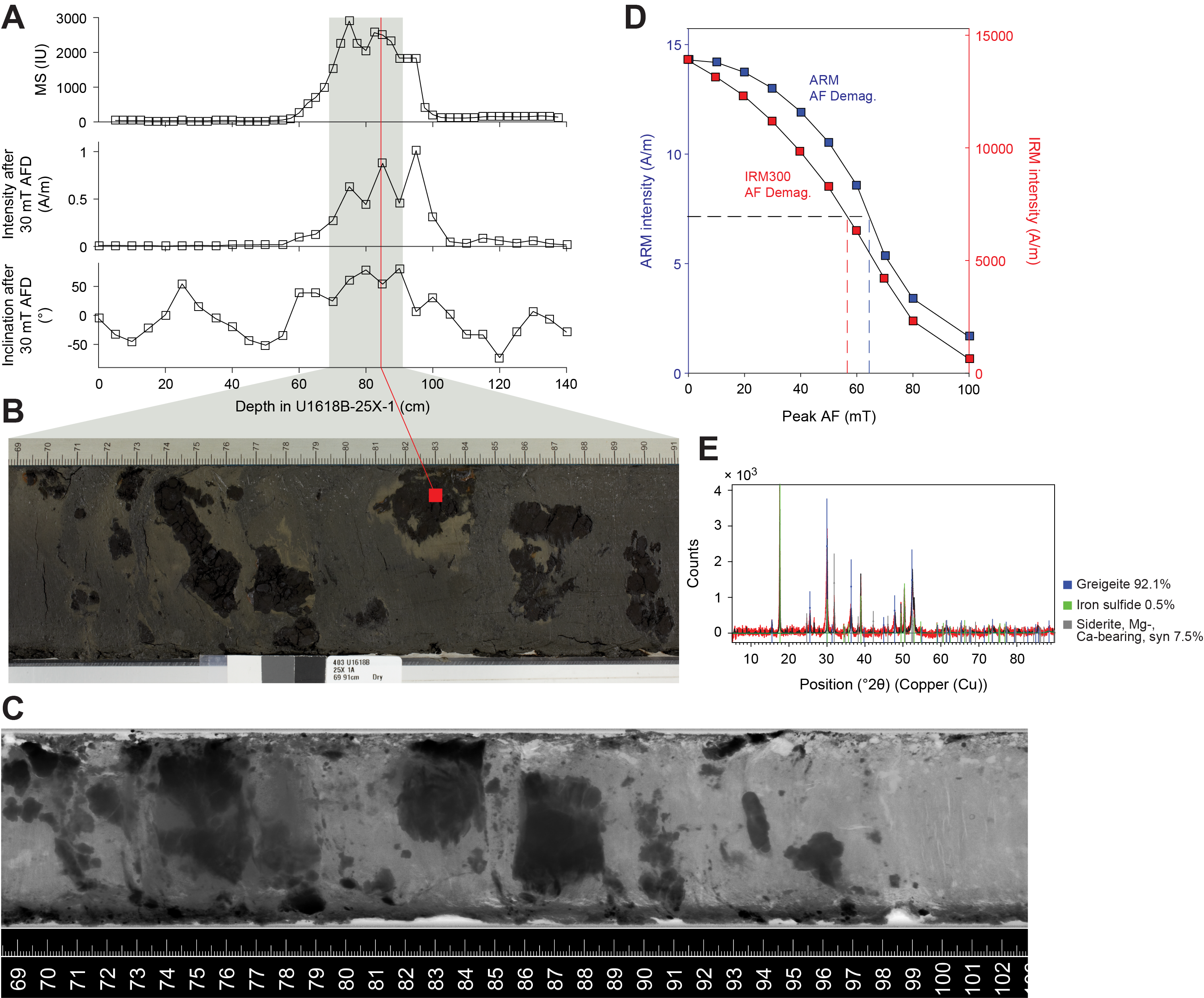
Figure F19. Greigite nodules.
The magnetic properties of 127 oriented sediment cube samples were used to provide insight to the magnetic mineralogy that hosts the NRM. The coarse resolution of the samples (~1 sample per 5 m) is too low to capture downcore trends; however, the variability of the samples likely reflects the range of magnetic minerals present in Site U1618 sediments (Figure F20). ARM coercivity, tracked by the ratio of the ARM after 30 mT peak AF demagnetization to the initial ARM (ARM30mT/ARM), has a wide range of values (0.30–0.94) and a bimodal distribution with modes centered on 0.52 and 0.67. Previous work has demonstrated that both greigite and magnetite can have wide ranges of ARM coercivities, but greigite values are typically much greater (Peters and Thompson, 1998). These previous observations, along with our direct characterization of a Site U1618 greigite nodule (ARM30mT/ARM = 0.91) and samples from the uppermost 20 m in Hole U1618A, which are above the depths where interstitial water (IW) sulfate is depleted (average ARM30mT/ARM = 0.43; n = 4) (Figure F42), suggest that this wide range of ARM coercivities most likely reflects varying contribution of greigite (high ARM30mT/ARM) and detrital magnetic minerals (lower ARM30mT/ARM). This parameter shows a clear mixing relationship between the magnetic mineralogy typical of the uppermost samples (likely [titano]magnetite) and the greigite nodule when comparing multiple rock magnetic parameters like the IRM coercivity (tracked by the 300 mT IRM after 30 mT peak AF demagnetization over the initial IRM at 300 mT; IRM30030mT/IRM300) and the IRM300/ARM ratio (Figure F20). Downhole variations indicate that greigite concentration is variable and there are many samples with magnetic signatures such as low ARM coercivity that are likely dominated by detrital sources. These samples may be more suitable paleomagnetic recorders. Additional magnetic minerals beyond greigite and (titano)magnetite are present in varying concentrations, as indicated by S-ratio values that range 0.67–1 (50% of values are greater than 0.97; 90% of values are greater than 0.80). These variations in the S-ratio indicate the presence of magnetic minerals whose IRM saturates above 300 mT, such as hematite or pyrrhotite. Future rock magnetic work can identify the magnetic minerals present at Site U1618 and their implications for interpreting the paleomagnetic record.
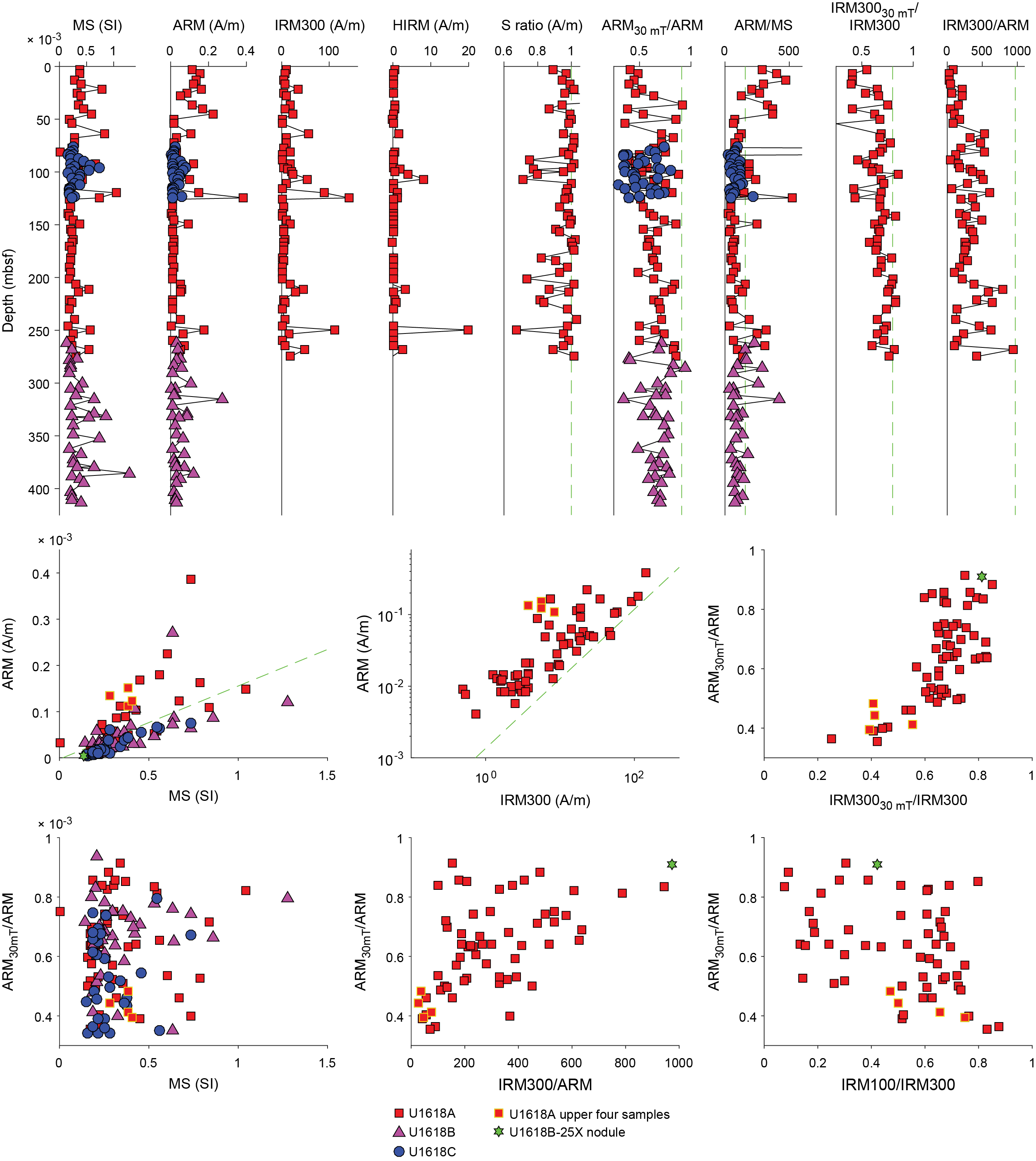
Figure F20. Rock magnetic data.
5.2. Natural remanent magnetization
Of NRM intensities at Site U1618, 95% were between 1.1 × 10⁻³ and 3.8 × 10⁻¹ A/m, with APC/HLAPC sections between 4.0 × 10⁻⁴ and 5.9 × 10⁻² A/m after 15 mT peak AF demagnetization and XCB sections between 5.0 × 10⁻⁴ and 2.0 × 10⁻¹ A/m after 30 mT peak AF demagnetization. Following the 15 mT AF demagnetization step, the distributions of measured inclinations from APC/HLAPC cores have a strong peak slightly less than the expected normal geocentric axial dipole (GAD) prediction for the latitude of Site U1618 (84.4°) in all three holes, reflecting that the majority of APC/HLAPC cored intervals were likely deposited during Chron C1n (Brunhes) (Figure F21). The inclination distributions for XCB-cored intervals after the 30 mT AF demagnetization step are much less pronounced and do not show distributions expected from a geomagnetic field that approximates a GAD on average. This is likely due in part to the differences between coring methods. The APC/HLAPC method is able to recover less disturbed core with less VIRM drill string overprint but also likely reflects some complications in the NRMs themselves, as described below.
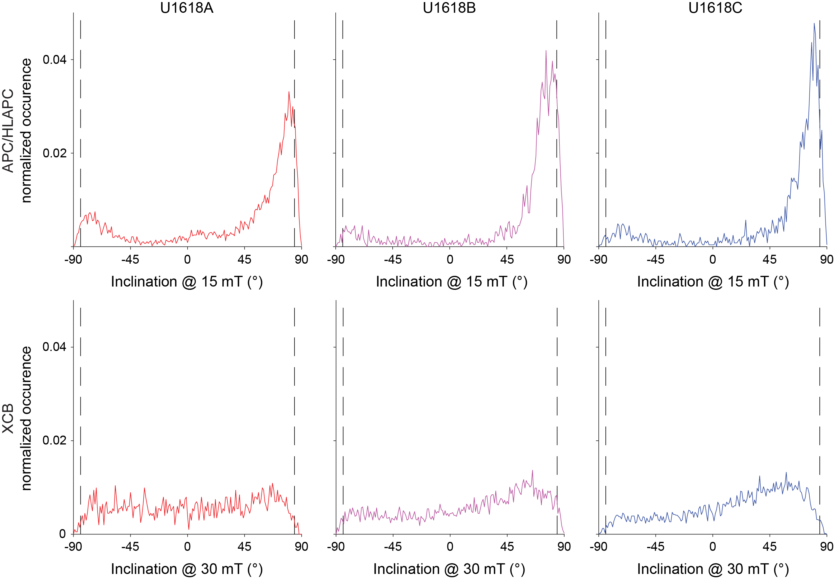
Figure F21. Inclinations.
The uppermost ~90 m at each site have directions that are consistent with normal polarity at this latitude (steep and positive inclinations), outside of some cored intervals that experienced coring deformation or other disturbance. Between 90 and 91 mbsf in each hole, we observe the first reverse directions and note that these first reverse directions correlate to similar MS features (Figure F22). However, below this horizon we observe frequent changes between inclinations consistent with reverse and normal polarity occurring on the scale of <1 to around ~7 m. In the context of biostratigraphy observations at Site U1618 (see Biostratigraphy and paleoenvironment), this pattern contains many more magnetic reversals and polarity zones than the normal 80 ky long Subchron C1r.1n (Jaramillo) or 35 ky long Subchron C1r.2n (Cobb Mountain) expected in the 2020 geologic timescale (GTS2020; Gradstein et al., 2020) or the handful of brief geomagnetic excursions documented in late Chron C1r (Matuyama) (Channell et al., 2020). Thus, the (1) unequivocal evidence for the presence of authigenic greigite at Site U1618 (discussed above), (2) well-defined thick normal polarity zone in the uppermost 90 m, and (3) frequent reversals between normal and reverse GAD consistent directions below the first reverse direction (~90 m) suggest that many intervals in the Site U1618 stratigraphy are potentially remagnetized by a late-forming CRM. These data are consistent with deep (>10s m) formation of authigenic greigite, which would acquire a CRM that is younger than the detrital remanent magnetization of the surrounding sediment. For example, layers of sediment deposited in the reverse Chron C1r.1r (latest Matuyama) may host a CRM acquired during the normal Chron C1n (Brunhes).
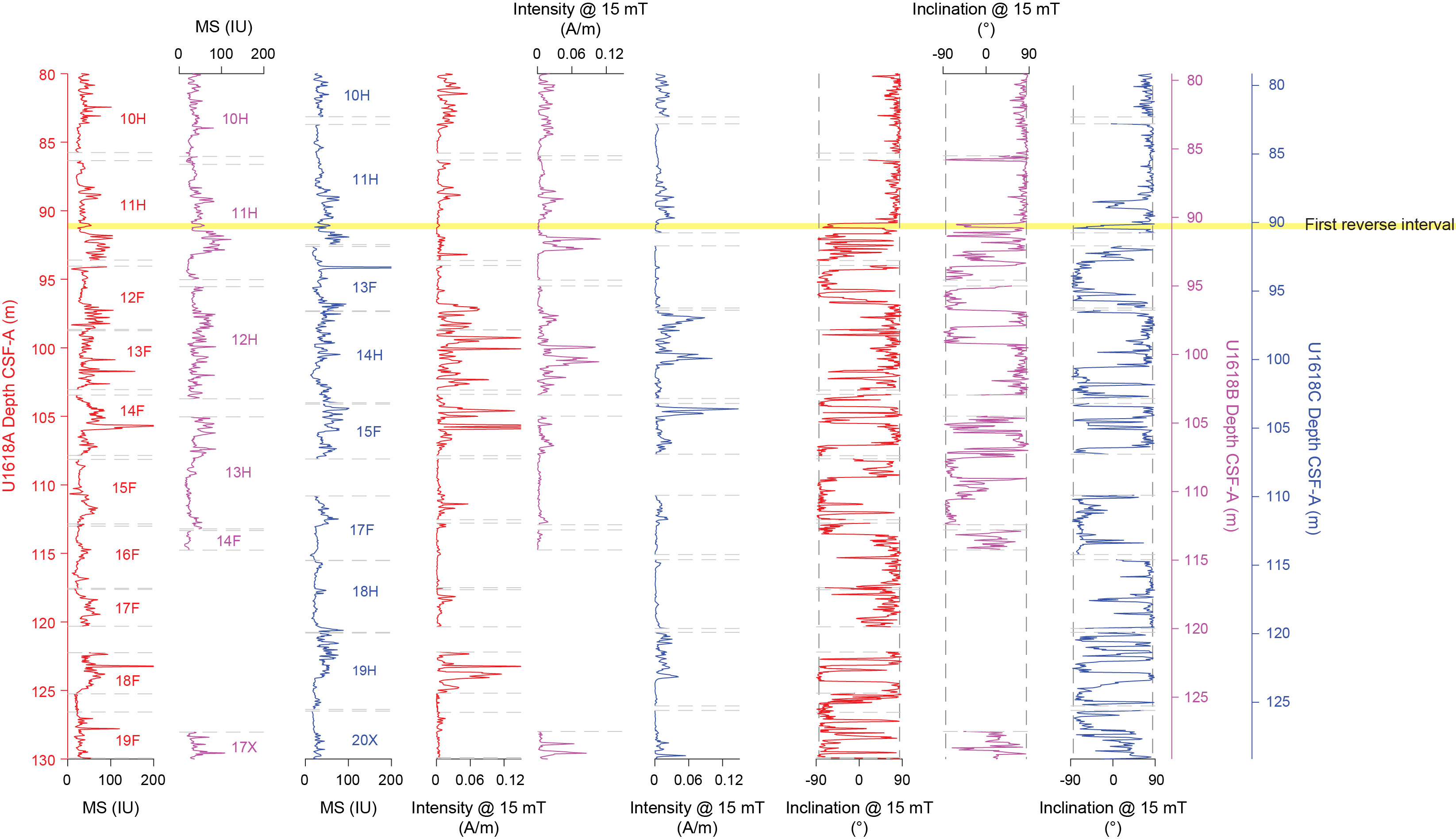
Figure F22. Paleomagnetic measurements around and below interpreted Chron C1n.
To further explore the NRMs of Site U1618 sediment, we examined the AF demagnetization behavior of the discrete cube samples. Orthogonal projection plots show a variety of behaviors, ranging from higher quality samples in which a characteristic remanent magnetization (ChRM) can be defined to samples for which no ChRM can be determined (Figure F23). Some samples gained intensity at higher demagnetization steps, which may be explained as a gyroremanent magnetization or as a result of a nonzero field near the AF coils. Samples with high ARM coercivity that likely contain abundant greigite were often characterized by strong and stable NRMs with well-defined ChRMs. It was difficult to recognize the VIRM drill string overprint in samples with normal magnetizations because the drill string VIRM manifests as a steep and positive inclination, like the ambient normal magnetic field. In samples with reverse magnetization, the effect of the drill string overprint was apparent, with XCB cores often requiring a peak AF of 30 mT or more to fully remove the VIRM. Polarity could be determined for all but eight samples, and ChRMs could typically be defined using a range of AF steps between 15 and 60 mT that varied from sample to sample. The quality of the ChRM could be assessed with the maximum angular deviation parameter (Kirschvink, 1980) and could be used to filter magnetizations that were poorly defined, noisy, VIRM overprinted, or had complex AF demagnetization behavior. The remanence carrier could be inferred from the ARM30mT/ARM ratio to assess whether the magnetization was hosted by greigite. This approach assumes that higher ARM coercivity ratios (up to ~0.90) are dominated by authigenic greigite like the greigite nodule we studied, whereas lower ratios (as low as ~0.4) are dominated by detrital minerals like the samples from the uppermost ~20 m. Although there is much to learn about the formation timing and pathways of greigite at Site U1618, samples dominated by greigite have the potential to host a later forming CRM that may be younger than the age of the surrounding sediment.
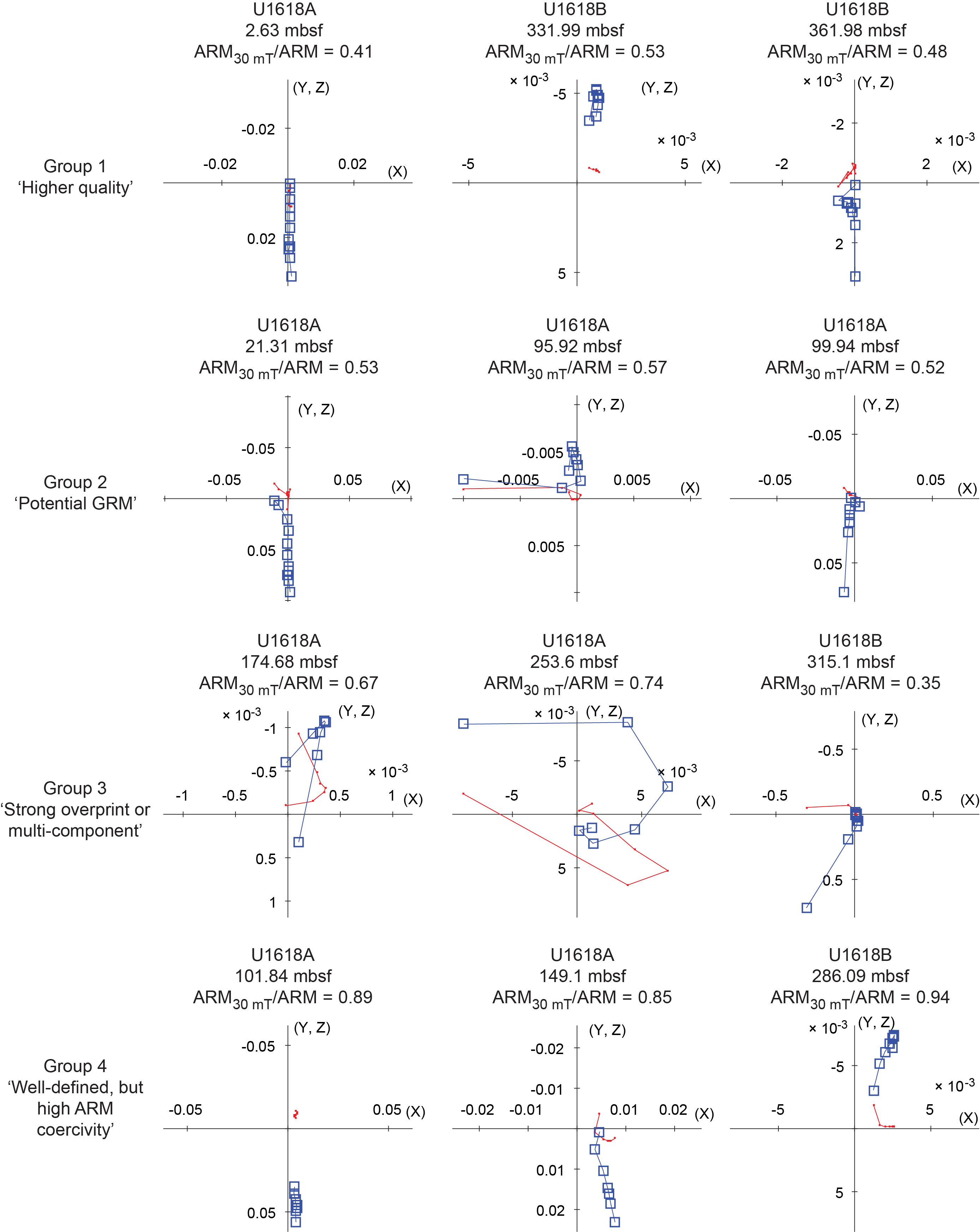
Figure F23. AF demagnetization behavior.
5.3. Magnetic stratigraphy
As previously discussed, determination of polarity zones was complicated by the potential for CRMs hosted by the authigenic mineral greigite. However, we can still confidently identify three major polarity zones that we interpret to reflect Chrons C1n (Brunhes; 0–773 ka), C1r–C2r (Matuyama; 773–2595 ka), and C2An (Gauss; 2595–3596 ka) (Figure F24; Table T6). Our interpretation of the normal polarity zone at the base of Holes U1618B and U1618C as Chron C2An (Gauss) was informed through conversation with the shipboard micropaleontologists and not derived entirely independently. However, this normal polarity zone indicates that the base of recovered sediments at Site U1618 are Late Pliocene in age (younger than 3.6 Ma).
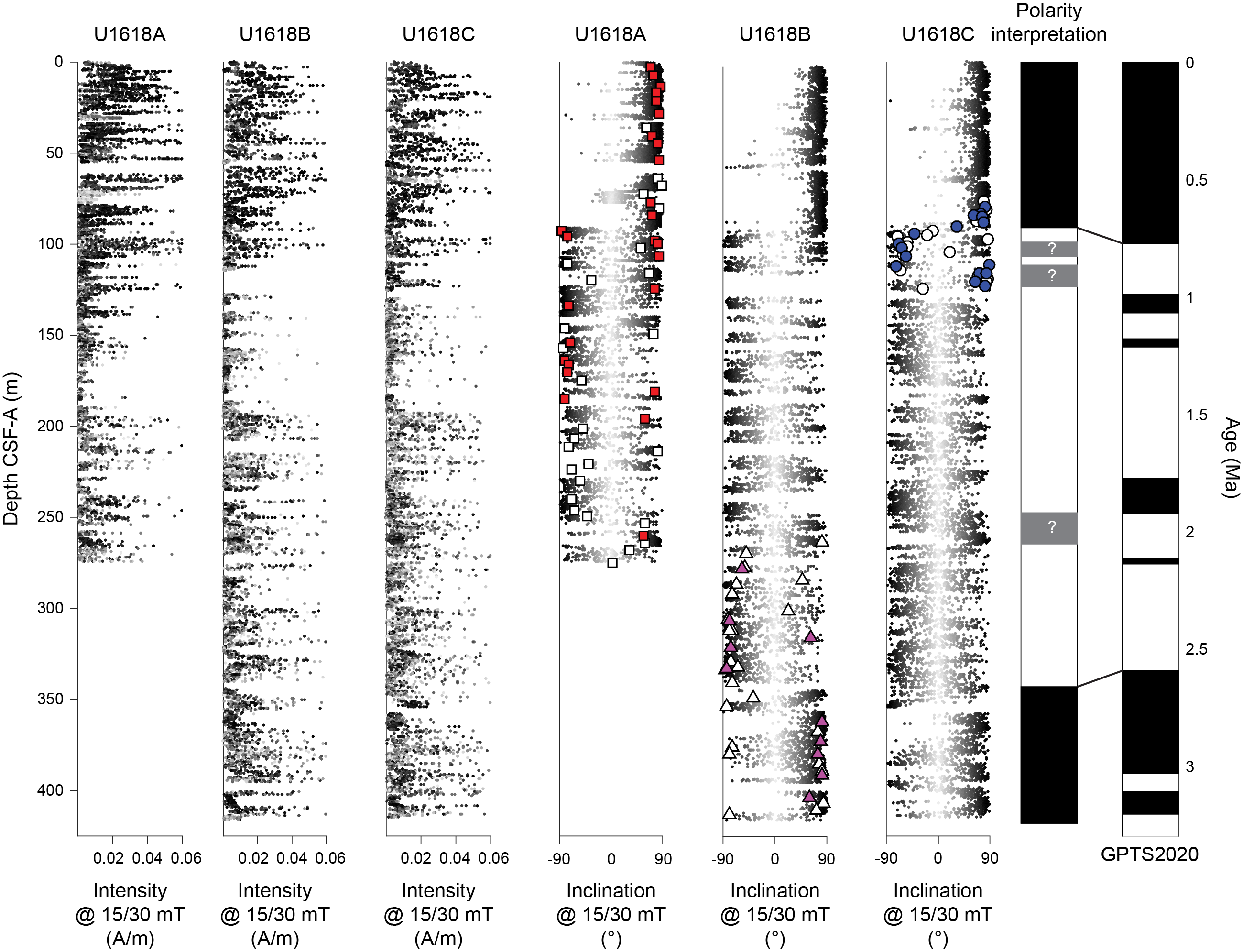
Figure F24. Archive-half and discrete sample paleomagnetic measurements.
The onset of Chron C1n (Matuyama/Brunhes boundary; 773 ka) was determined as the downcore transition to the first reverse polarity interval that could be traced to a correlative MS feature in all three holes (Figure F22). This depth was within 1 m on each hole's CSF-A depth scale: 90.915 mbsf in Hole U1618A, 90.45 mbsf in Hole U1618B, and 90.21 mbsf in Hole U1618C (depths are the midpoint of the transition; the full depth range is reported in Table T6). It is still uncertain if this transition is recorded by a primary detrital remanent magnetization and reflects the actual reversal at 773 ka in MIS 19. However, at a minimum, it must reflect a maximum limiting depth of the reversal because it would be unlikely to have a reverse remagnetization during normal Chron C1n (Brunhes). Detailed work on discrete cube samples, considering only samples that we assume to have a lower influence of greigite with ARM30mT/ARM ratios less than 0.65, supports this placement of the onset of Chron C1n (Brunhes). Cube samples bracket the transition in Hole U1618A at 84.1 mbsf (normal) and 92.69 mbsf (reverse) and in Hole U1618C at 87.65 mbsf (normal) and 94.08 mbsf (reverse) (Figure F24).
The top of Chron C2An (Gauss/Matuyama boundary; 2595 ka) is best defined in Hole U1618B where archive-half measurements can be directly compared to cube samples. Cube samples with ARM30mT/ARM ratios less than 0.65 define a transition between 332 mbsf (reverse) and 362 mbsf (normal), with several well-defined and lower ARM30mT/ARM with normal directions between 362 and 403.5 mbsf (Figure F24). Using archive-half data, we interpret that this range could be narrowed to between 340.1 mbsf (reverse) and 344.8 mbsf (normal) with a midpoint at 342.45 mbsf; however, this could likely be confirmed and refined in postcruise research (Table T6). It is possible that Subchrons C2An.1r (Kaena) and/or C2An.2r (Mammoth) are recorded in brief intervals with reverse archive-half directions in Holes U1618B and U1618C, including clusters around 352 mbsf (Holes U1618B and U1618C) and 384 and 397 mbsf (Hole U1618C). However, all cube samples with reverse magnetization below 362 mbsf in Hole U1618B have ARM30mT/ARM values between 0.68 and 0.76 and likely contain significant amounts of greigite (Figure F24).
There is great potential to further refine the magnetic stratigraphy at Site U1618 with higher resolution and detailed paleomagnetic investigation that characterizes the NRM and magnetic mineral assemblages. Although greigite-hosted CRMs that postdate the primary detrital remanent magnetizations are present, initial rock magnetic characterization indicates that samples through the entire recovered interval contain a wide range of magnetic properties, with many samples having properties consistent with limited influence from greigite. Future work can better characterize how easy-to-measure magnetic parameters, such as ARM30mT/ARM, correlate to the exact mineralogy with additional thermal, in-field magnetization, scanning electron microscope/energy dispersive spectrometry, and mineralogical studies. This may be helpful to better define depths of the Chron C1n (Matuyama/Brunhes boundary) onset and Chron C2An (Gauss/Matuyama boundary) termination and identify shorter polarity intervals, such as Subchrons C1r.1n (Jaramillo), C1r.2n (Cobb Mountain), C2n (Olduvai), C2An.1r (Kaena), and C2An.2r (Mammoth). Of note, clusters of normal directions defined by cube samples with lower ARM30mT/ARM ratios between 97.87 and 106.6 mbsf in Hole U1618A and 115.6 and 123.2 mbsf in Hole U1618C may be good candidates for Subchrons C1r.1n (Jaramillo) and/or C1r.2n (Cobb Mountain) (Figure F24). However, there is not good agreement between the two holes, and this interval deserves closer attention and a more rigorous assessment of the magnetic minerals present. Similarly, a broad cluster of normal directions between around 246 and 266 mbsf in all three holes with a well defined normal direction in a cube sample from 259.9 mbsf in Hole U1618A may be a good candidate for Subchron C2n (Olduvai) and also deserves closer attention (Figure F24).
6. Physical properties
The physical properties measured shipboard for Site U1618 included nondestructive whole-round measurements using the Special Task Multisensor Logger (STMSL), WRMSL, and Natural Gamma Radiation Logger (NGRL), as well as thermal conductivity and discrete P-wave velocity measurements on working-half sections after cores were split. GRA bulk density and MS were measured on the STMSL immediately after recovery and then on the WRMSL after thermally equilibrating for a minimum of 4 h. Cores 403-U1618C-1H through 3H and 62X were excluded from GRA bulk density measurements due to their selection for sedimentary ancient DNA (sedaDNA) sampling and the need to avoid exposure to the radioactive cesium source. Physical property data from the STMSL were used for initial hole-to-hole stratigraphic correlation and splicing (see Stratigraphic correlation) to aid in near-real-time drilling and sampling decisions (e.g., sedaDNA sampling), but they are not further evaluated and reported here. Further use of STMSL data is discouraged because WRMSL and Section Half Multisensor Logger (SHMSL) data, collected after allowing for thermal equilibration, are available in the Laboratory Information Management System (LIMS) database. Aside from three 10 cm intervals that were sampled for anelastic strain recovery (ASR) analysis, P-wave velocity was measured on the WRMSL for all core sections. Results from whole-round scans are compiled in Figure F25. Discrete P-wave measurements were made on at least one section per core for the uppermost cores from Holes U1618A and U1618C using the Section Half Measurement Gantry (SHMG). However, below ~50 mbsf, SHMG measurements ceased due to poor data quality in deeper sediments, likely related to higher gas content and coarser material. Thermal conductivity measurements were made for all cores from Hole U1618A and deeper cores from Holes U1618B and U1618C using a puck probe on the split face of working-half sections. Whole-round physical property data were used for the final hole-to-hole stratigraphic correlation and splicing (see Stratigraphic correlation).
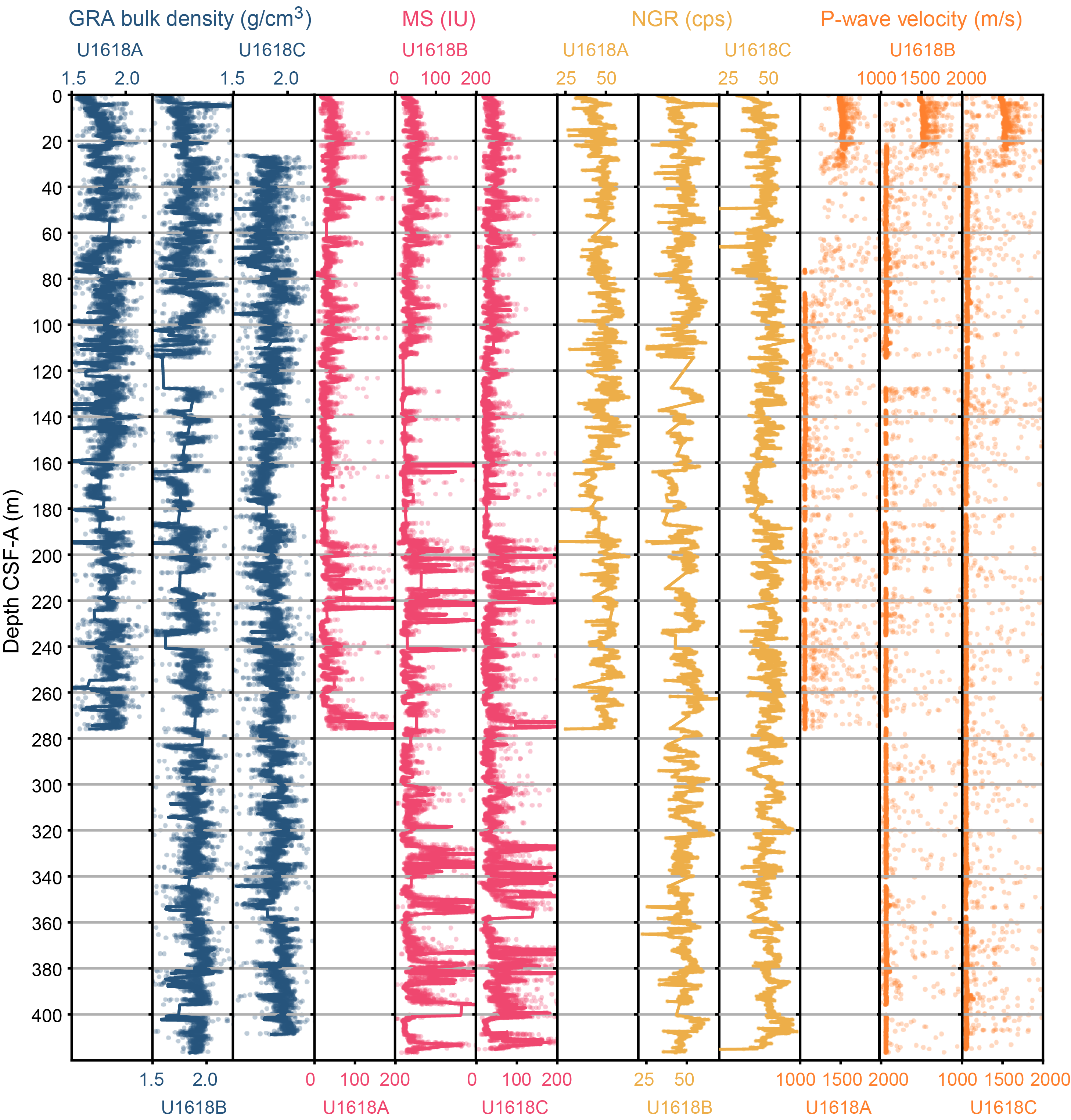
Figure F25. Physical properties, Site U1618.
Working-half sections of all cores from Hole U1618A and deeper cores from Holes U1618B and U1618C were sampled for moisture and density (MAD) analyses. Representative lithostratigraphic units with minimal coring disturbances were targeted. Archive halves were measured with the SHMSL for point MS (MSP) and color reflectance and X-ray scanned using the X-Ray Linescan Logger (XSCAN) (see Lithostratigraphy). Three 10 cm interval whole-round samples from Holes U1618B and U1618C were taken for ASR analysis.
6.1. Magnetic susceptibility
MS was measured both on whole-round sections using a pass-through loop sensor on the WRMSL track and on split archive-half sections using a point-source sensor on the SHMSL track. Sections were measured at 2.5 cm increments on the WRMSL. The resolution for the SHMSL measurements was 2.5 cm and occasionally switched to 5 cm in the interest of time for Holes U1618B and U1618C. WRMSL and SHMSL MS measurements yielded similar values and downhole variability (Figure F26). MS values range 0.7–4186 IU for measured whole-round sections and 0.1 to ~12,000 IU for point measurements on the archive-half section surfaces. Overall, the average MS value for both WRMSL and SHMSL data is ~47–50 IU across Holes U1618A–U1618C (see Physical properties in the Expedition 403 methods chapter [Lucchi et al., 2026] for details on instrument units).
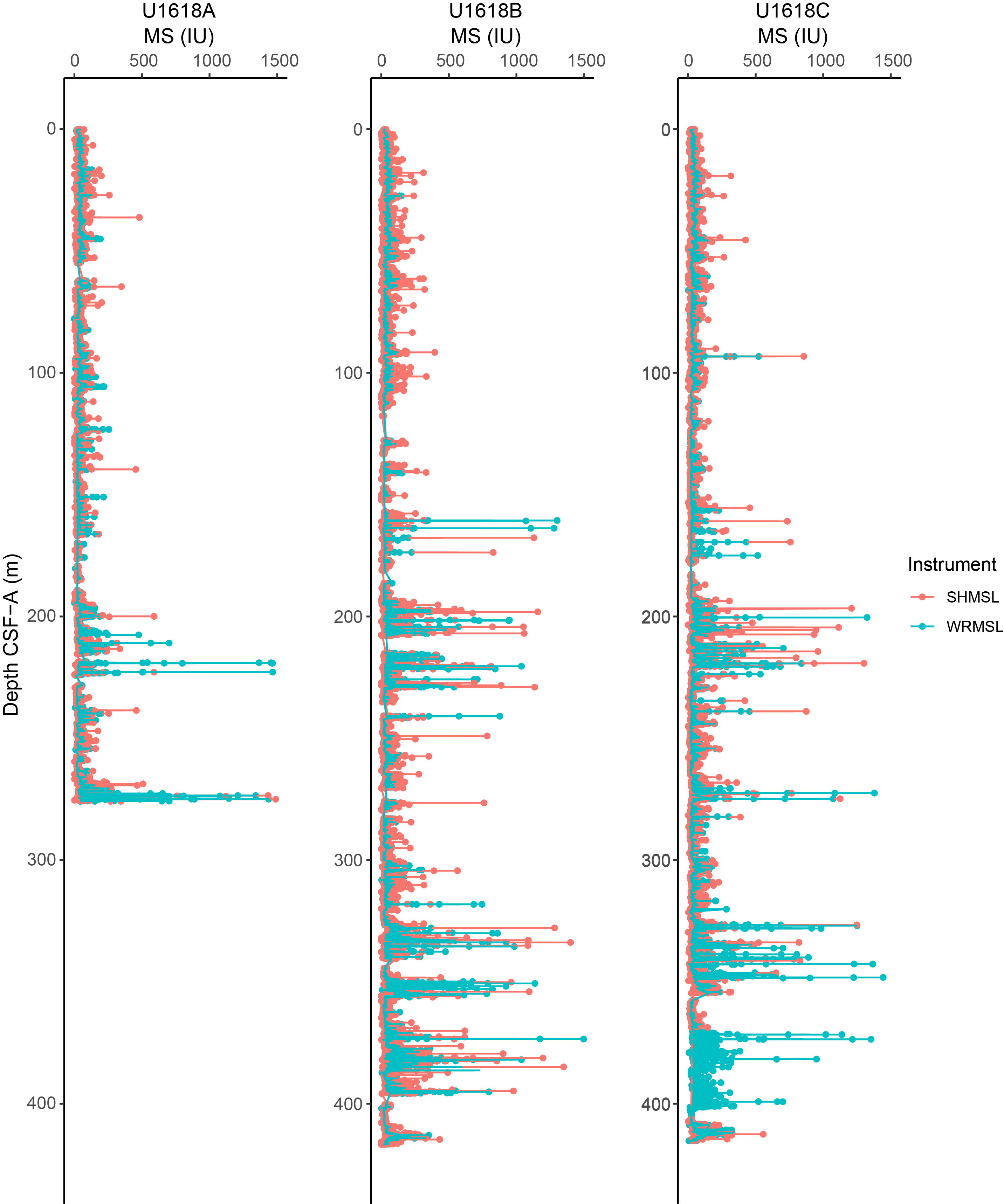
Figure F26. MS.
From the seafloor to ~150 mbsf, MS values vary between ~2–5 and ~150 IU and MS co-varies with NGR and GRA bulk density. However, below ~150 mbsf, there is no obvious association of MS with other downcore physical properties. From ~150 mbsf to the base of the hole, irregularly spaced, large peaks in MS become prevalent, with maximum WRMSL-derived MS values between ~300 and ~5000 IU. These maxima are orders of magnitude higher than the background, which is represented by MS modes of 24.69, 24.49, and 24.27 IU for Holes U1618A, U1618B, and U1618C, respectively. MS peaks are often associated with the occurrence of authigenic iron sulfide minerals (e.g., greigite identified in rock magnetic and XRD analyses) (see Lithostratigraphy, Geochemistry, and Paleomagnetism). The large peaks in MS generally do not correspond to peaks in NGR or GRA bulk density (Figure F27). The changes in physical properties observed at ~150 mbsf correlate to the boundary between Lithostratigraphic Units I and II (see Lithostratigraphy).
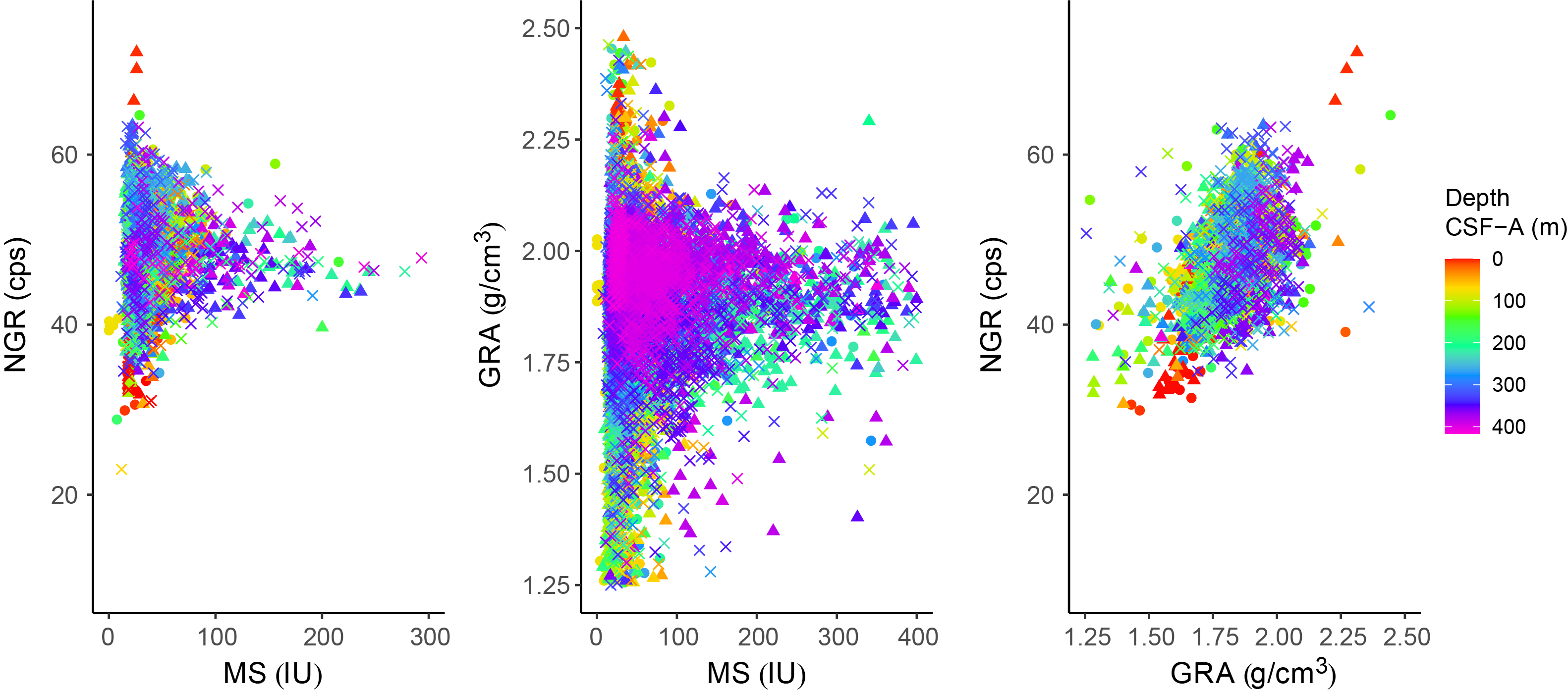
Figure F27. NGR, GRA bulk density, and MS.
6.2. Gamma ray attenuation bulk density
Except for the cores that were sampled for sedaDNA, every whole-round section was measured at 2.5 cm intervals with the GRA densitometer on the WRMSL. Excluding outliers related to voids or coring disturbances, measured GRA bulk density values range ~1.6 to ~2.0 g/cm3, with a strong mode at ~1.8–1.9 g/cm3 and no correlation with MS (Figure F27). The GRA bulk density recorded downcore shows a rapid increase from the seafloor (~1.6 g/cm3) to ~25 mbsf (1.8–1.9 g/cm3) that is likely related to increased compaction with depth. Several large peaks in bulk density, reaching ~2.4 g/cm3, occur in intervals ~25–150 and ~250–375 mbsf. These may be associated with clast-rich lithologies (e.g., diamicton). Observed bulk density lows at ~150–200 mbsf are associated with Unit II (see Lithostratigraphy). From ~170 mbsf to the base of the hole, GRA bulk density is less variable, which may be associated with the transition to XCB cores below ~120 mbsf.
6.3. Natural gamma radiation
NGR was measured on all whole-round core sections at 10 cm intervals. Measured NGR values range 18–74 counts/s (average = ~49 counts/s). From the seafloor to ~80 mbsf, NGR values average ~47 counts/s. From ~80 to 150 mbsf, NGR values increase to an average of ~50 counts/s and show more variability, ranging ~27–65 counts/s. An interval with a relatively low average NGR of ~45 counts/s and a tighter distribution of NGR values at ~150–190 mbsf corresponds to Lithostratigraphic Unit II (see Lithostratigraphy). From ~190 mbsf to the base of the hole, NGR values increase to an average of ~50.5 counts/s and demonstrate a more sawtooth variability. Generally, NGR mirrors GRA bulk density trends downcore, such as at 80–100, 160–180, and 300–350 mbsf, but correlations are less apparent below 360 mbsf (Figure F27).
6.4. P-wave velocity
Whole-round sections were measured for compressional P-wave velocity on the WRMSL at a resolution of 2.5 cm for all core sections from Site U1618. Values range from ~1350 m/s at the seafloor to ~1560 m/s at 25 mbsf. Below ~25 mbsf, the signal becomes dominated by noise with values out of the range expected for marine sediments, reaching outlier values of ~15,000 m/s and above. No downcore signal was detectable. We encountered persistent issues with void spaces and gas expansion, which we suspect contributed to anomalous values. The use of these data for interpretation is discouraged.
Discrete P-wave velocity measurements were made using the SHMG (see Physical properties in the Expedition 403 methods chapter [Lucchi et al., 2026]) in intervals that excluded excessive coring disturbances, voids, cracks, or large clasts. One section per core was measured for Cores 403-U1618A-1H through 6H and 403-U1618C-1H through 9H using the x-caliper and y- and z-bayonets. Because of noise in the signal, P-wave velocity waveforms were manually selected. Values range from ~1500 m/s at the seafloor to ~1600 m/s at ~50 mbsf, generally increasing downcore, as expected with sediment compaction at depth. Below ~50 mbsf, however, P-wave measurements on the SHMG were abandoned due to increasing noise and eventual lack of a detectable signal. We suspect the abundance of large clasts and authigenic mineral formations (e.g., greigite nodules and authigenic carbonates), as well as free gas trapped in isolated pore spaces of the deeper, more consolidated sediments, contributes to signal depletion below ~50 mbsf.
6.5. Moisture and density
MAD analyses were conducted using 107 discrete samples collected from the working section halves of Cores 403-U1618A-1H through 37X, 403-U1618B-34X through 54X, and 403-U1618C-56X through 62X (see Physical properties in the Expedition 403 methods chapter [Lucchi et al., 2026]). Several parameters, including porosity, water content, and bulk density, were calculated using the wet mass, dry mass, and volume measurements of samples. MAD bulk density increases sharply from ~1.5 g/cm3 at the sediment surface to ~2.0 g/cm3 at ~50 m downcore, corresponding to sharply decreasing porosity and water content from 67% to 54% and 43% to 32%, respectively. This change in porosity and water content closely corresponds to the increase in sediment induration that is a defining characteristic of the Lithostratigraphic Subunit IA/IB boundary (see Lithostratigraphy). From 50 mbsf to the termination of Hole U1618B, MAD bulk density ranges ~1.7 to ~2 g/cm3 (average = ~1.9 g/cm3). There is greater variability in MAD bulk density to ~200 mbsf, below which depth values are generally stable around ~1.8 g/cm3. Overall, MAD bulk density values correspond well to GRA bulk density trends downcore (Figure F28). The highest MAD bulk density values are found at ~140 mbsf (~2.1 g/cm3) near the transition from Unit I to II (see Lithostratigraphy) and from APC/HLAPC to XCB recovery at ~285 mbsf (~2.1 g/cm3) and between ~360 and 370 mbsf (~2.0 g/cm3). Additional parameters calculated from MAD analyses include water content, porosity, and void ratio. These properties co-vary downcore, and water content, void ratio, and porosity are anticorrelated with MAD bulk density (Figure F29). After an initial sharp decrease from the seafloor to ~50 mbsf, water content generally ranges ~22%–27% downcore, and porosity ranges ~46%–51%.
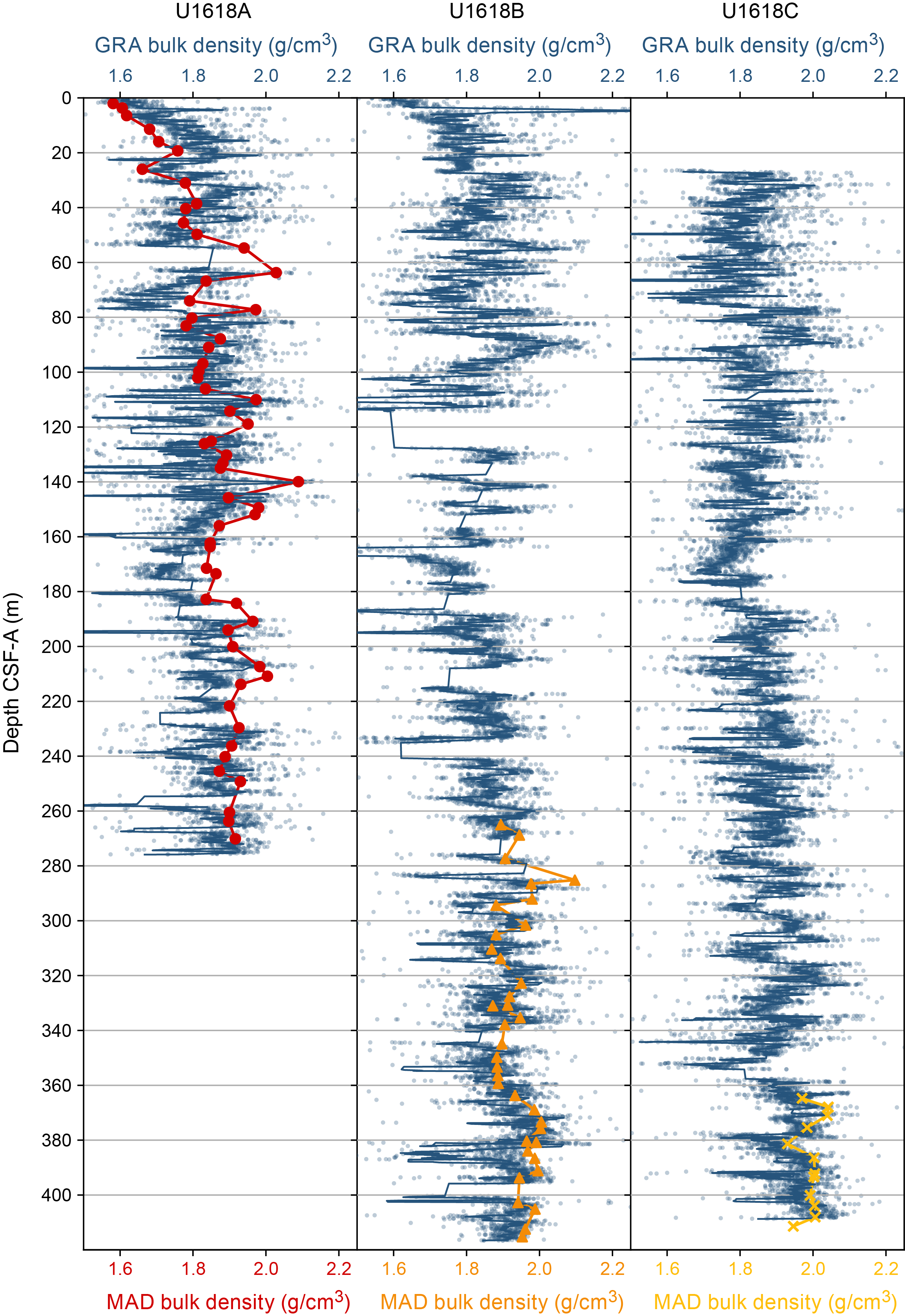
Figure F28. GRA bulk density and MAD.
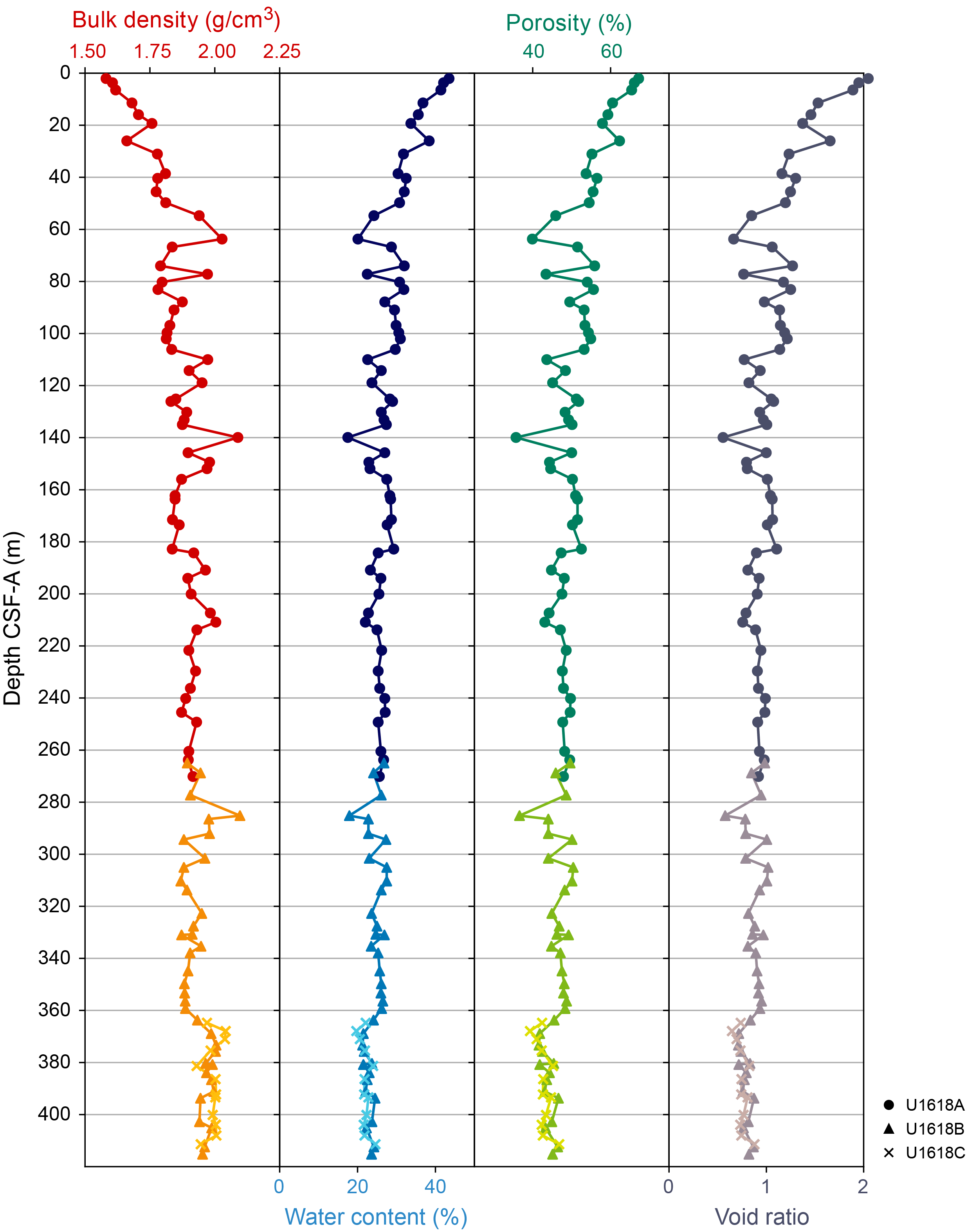
Figure F29. MAD parameters.
6.6. Thermal conductivity
To calculate heat flow and interpolate temperature data, thermal conductivity measurements were made using the TK04 system for one working section half per core for Cores 403-U1618A-15H through 37X; 403-U1618B-34X through 54X; and 403-U1618C-1H-29X, 40X, 41X, and 56X–62X. A puck contact probe was placed on the split face of working section halves. To ensure good contact with the probe, a small amount of deionized water was added and/or the face was swept with a spatula. Homogeneous intervals lacking large clasts, voids, cracks, and sediment disturbances were targeted. Three measurements were made on the same interval, but we encountered a few failed measurements from the TK04 meter. Some cores did not have suitable intervals for thermal conductivity, especially XCB cores, which often had biscuiting, large clasts, and cracks on the surface of split core halves. Therefore, thermal conductivity results were not possible for all cores and may be responsible for some of the scatter in measurements downcore. Overall, thermal conductivity values at Site U1618 increase slightly with depth from ~1.1 W/(m·K) at the seafloor to ~1.3 W/(m·K) at ~415 mbsf, likely corresponding to a downcore increase in dry bulk density and a decrease in porosity from compaction (Figure F30). Results from thermal conductivity taken from split cores agree with the downhole temperature gradient (see Downhole logging).
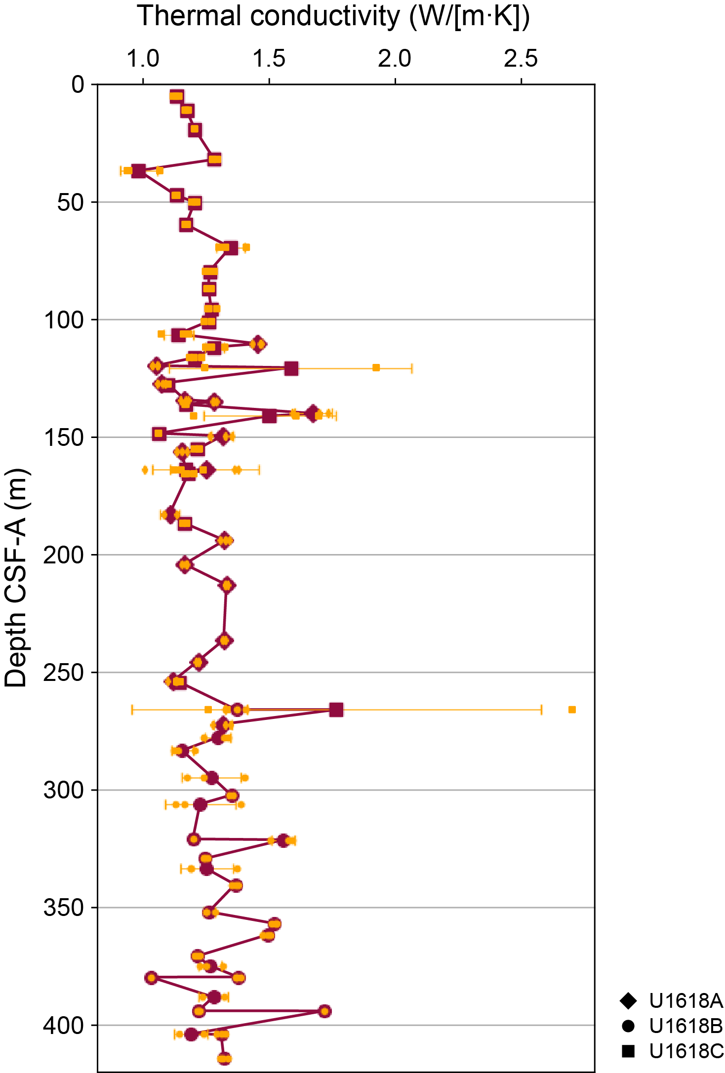
Figure F30. Thermal conductivity.
6.7. Anelastic strain recovery
ASR experiments were conducted using three whole-round samples, each 10 cm long, selected from the top of Sections 403-U1618B-40X-4 and 54X-2 and the bottom of Section 403-U1618C-6H-9. After STMSL and NGR scanning, the whole-round core liners were cut on the core receiving platform, and samples were removed from the core liners. To attach 16 strain gauges, soft materials (i.e., drilling mud) surrounding the core samples were removed and the surfaces were flattened with a spatula and/or sandpaper. Gauges were glued onto the surfaces, and the samples were wrapped with plastic bags and put into a thermostatic water bath. All strain gauges were then electrically connected to a data logger to collect 3D strain recovery. All sample preparation procedures were completed within 3.5–4.5 h after core recovery from the subseafloor. Average strain values of 11 ASR measurements were collected every 10 min from each of the 18 strain gauges. Temperatures and dummy channel data were also measured to ensure that the water temperature was stable and that the data logger was operating correctly. Gauges remained connected to the samples to monitor strain value for ~14 days to fully record the recovery. Preliminary results show that after temperature equilibrium, strain released logarithmically but that some strain gauges showed shrinking (Figures F31, F32, F33). Postexpedition, inversion analysis will be conducted to convert the raw strain data set to 3D strain that will be combined with azimuths of core samples by paleomagnetism to determine actual principal stress azimuths.
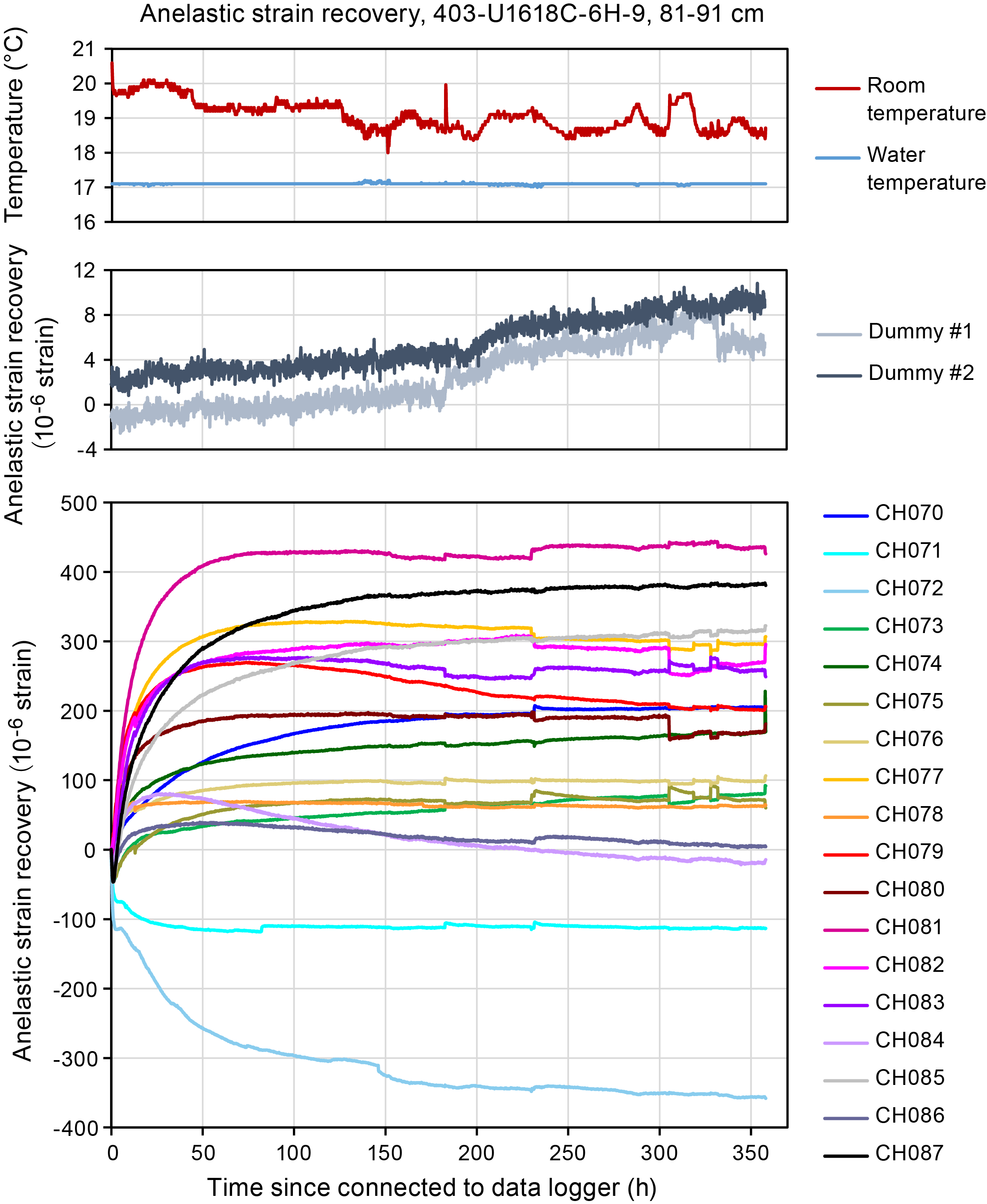
Figure F31. ASR initial results, Sample 403-U1618B-6H-9, 81–91 cm.
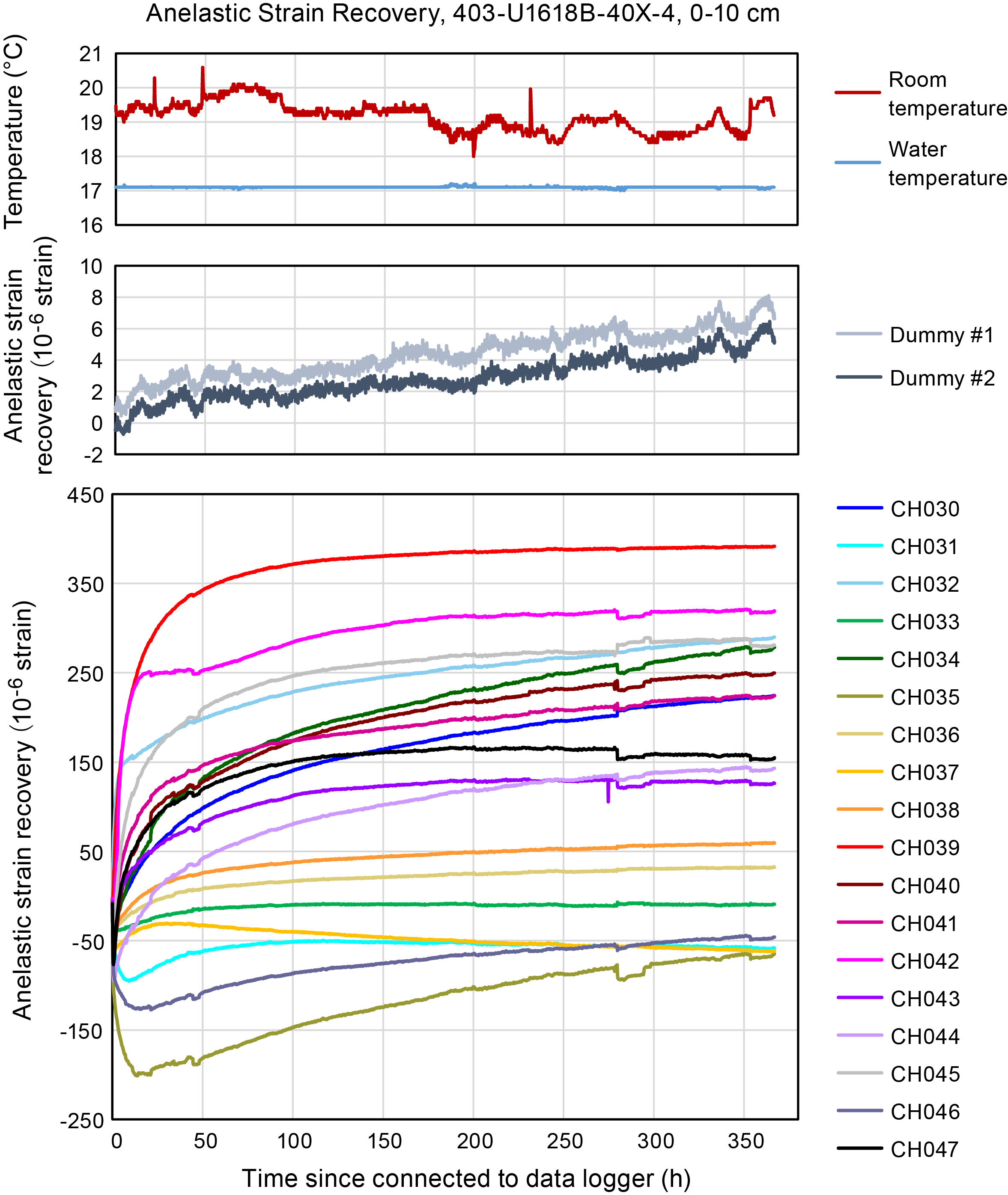
Figure F32. ASR initial results, Sample 403-U1618A-40X-4, 0–10 cm.
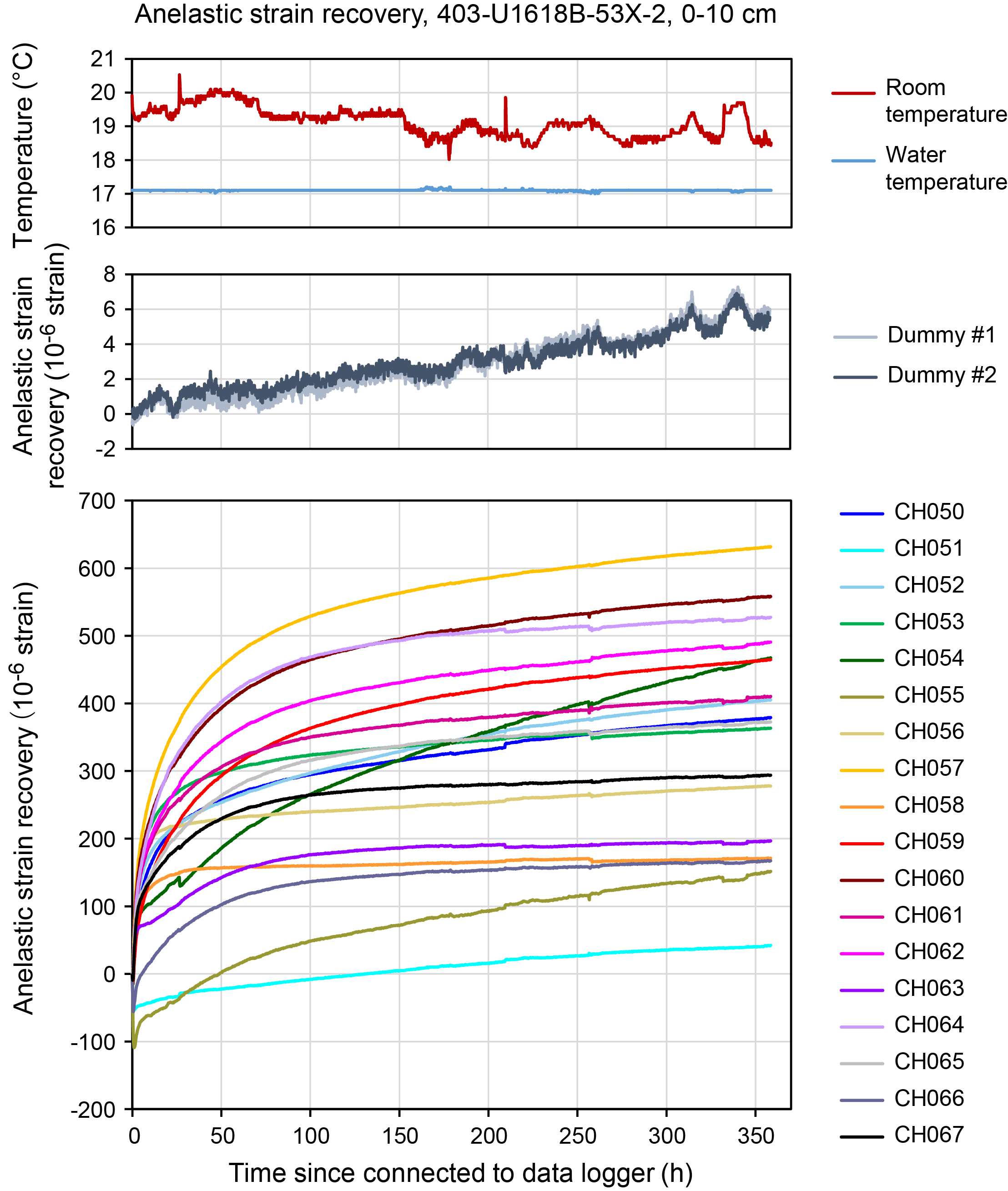
Figure F33. ASR initial results, Sample 403-U1618B-53X-2, 0–10 cm.
6.8. Physical properties summary
There is generally good correspondence between data collected at higher resolution on the MS loop sensor and data collected at lower resolution on the MSP sensor, with the MSP measurements picking up additional peaks in MS that were missed during the averaging in WRMSL measurements. There is also good correspondence between GRA bulk density and discrete MAD sample measurements. Because of issues with gas, as discussed above, P-wave velocity data are not considered reliable, and there is no detectable signal in discrete nor logger data below ~25–50 mbsf. Thermal conductivity data generally show a downcore increase, with a few outliers likely associated with measurements that did not have proper contact with the probe (see Downhole logging).
GRA bulk density and NGR show a positive linear correlation, consistent with NGR counts tracking fine-grained clay. All correlations are stronger in shallower cores less than ~150 m deep (Lithostratigraphic Unit I/II boundary). The NGR signal is a marker of lithologic change (Figure F34) with lowest counts in Unit II and higher counts in Subunit IIIA. NGR is important for identifying the relationship between physical properties and lithostratigraphy, especially because the MS signal was influenced by postdepositional alteration and GRA measurements were omitted in cores sampled for sedaDNA analyses.
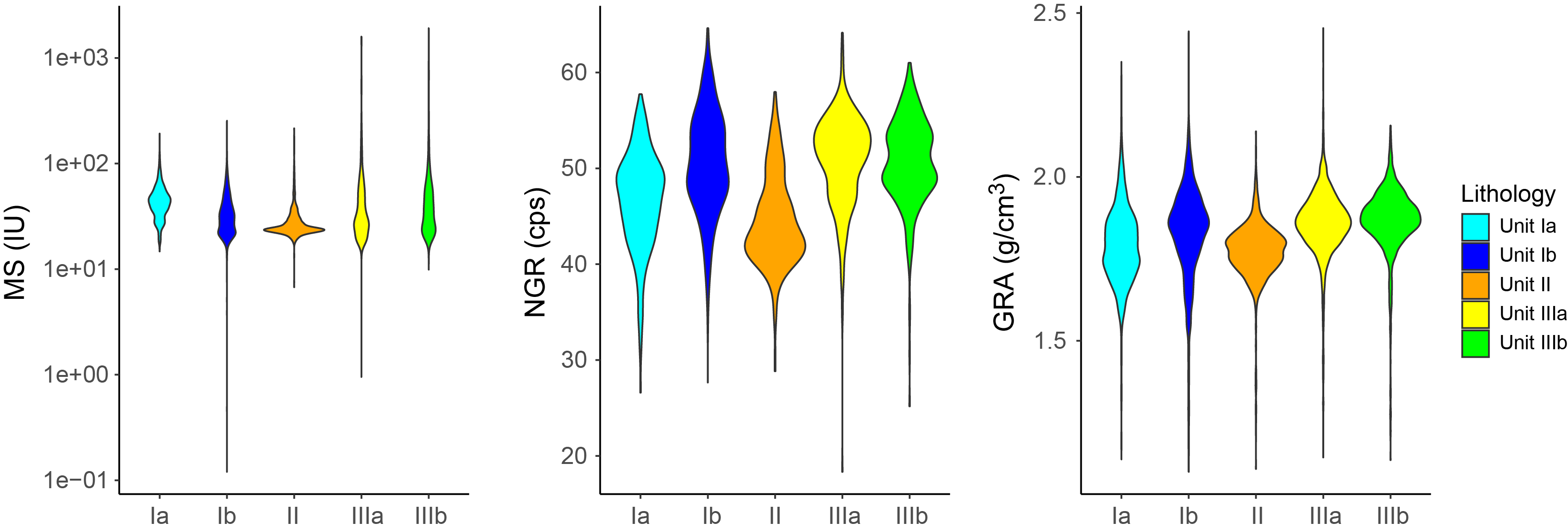
Figure F34. Physical property associations with preliminary lithostratigraphic units/subunits.
A notable feature at Site U1618 is the prevalence of peaks with MS values that are orders of magnitude higher than the background. The outsized MS maxima below 150 mbsf are likely associated with authigenic iron sulfide nodules (see Paleomagnetism) and can indicate diagenetic alteration. GRA bulk density has a strong mode at ~1.8–1.9 g/cm3, which does not co-vary with MS (Figure F27), indicating that magnetically strong constituents are not limited to a specific material or degree of compaction.
Overall, physical properties at Site U1618 appear to be influenced by glaciogenic deposition and postdepositional processes that complicate interpretations of depositional lithofacies. Glaciogenic deposition, including dense glacial diamicts and debris flows, is consistent with the location of the eastern Vestnesa Ridge close to the Kongsfjorden Trough Mouth Fan on the western margin of Svalbard, and postdepositional processes are consistent with findings of authigenic concretions in an active methane hydrate seepage area. Further studies onshore are necessary to interpret the relationship between physical properties measured on board, depositional lithofacies, and postdepositional alteration.
7. Stratigraphic correlation
Correlations between holes at Site U1618 were accomplished using Correlator software (version 4.5.4). In the upper part of the holes (above 125 mbsf), tie points were primarily established with WRMSL MS and GRA bulk density data. Below this depth, gas caused substantial expansion of the sediments and in some cases extrusion out of the top and bottom of the core liner and onto the rig floor; expansion also resulted in many gaps in the cores. In some cases, expansion caused shattering of the liners and made it difficult to extract them from the core barrel. These factors resulted in relatively high growth factors, disturbed sediment (especially in some of the first sections of XCB cores in Holes U1618A and U1618B), and voids, which affected the physical properties (e.g., density) and resulted in stratigraphic inconsistencies among holes. In the deeper sections (below 125 mbsf), the occurrence of authigenic iron sulfide minerals, as well as diagenetic overprint, added uncertainty to the correlation (Table T7) and splice (Table T8). WRMSL GRA bulk density and NGR data were helpful but were not used in making the correlations. Although we relied on MS data (Figure F35), we note that the NGR data are less noisy than other data sets (Figure F36) and may be useful in comparing with climate records (e.g., coarse sediments delivered by ice sheet versus clay-rich sediments mostly delivered by bottom currents). We constructed two spliced intervals, one from 0 to 294.2 m core composite depth below seafloor (CCSF) based on correlations among the three holes and another from 294.2 to 474.15 m CCSF based on a correlation between Holes U1618B and U1618C. For this deeper interval, expansion of the cores made it difficult to correlate, and at several gaps we appended the cores based on an average growth factor of ~1.1 of the previous cores (Figure F35; Table T8). Thus, parts of the sedimentary sequence were difficult to correlate between holes, and postcruise work will be required to verify some of the tentative tie points used to construct the splice.
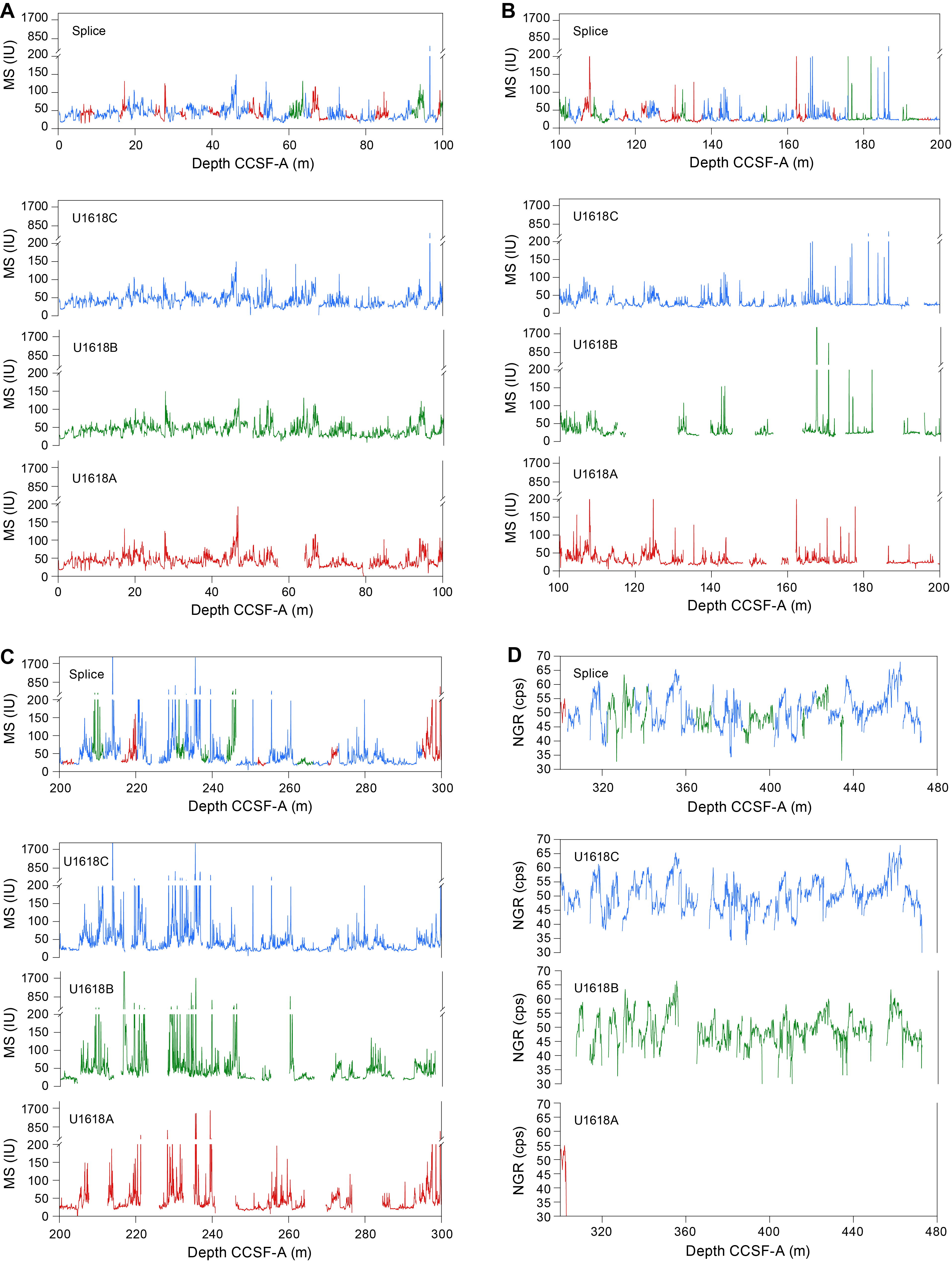
Figure F35. WRMSL MS.
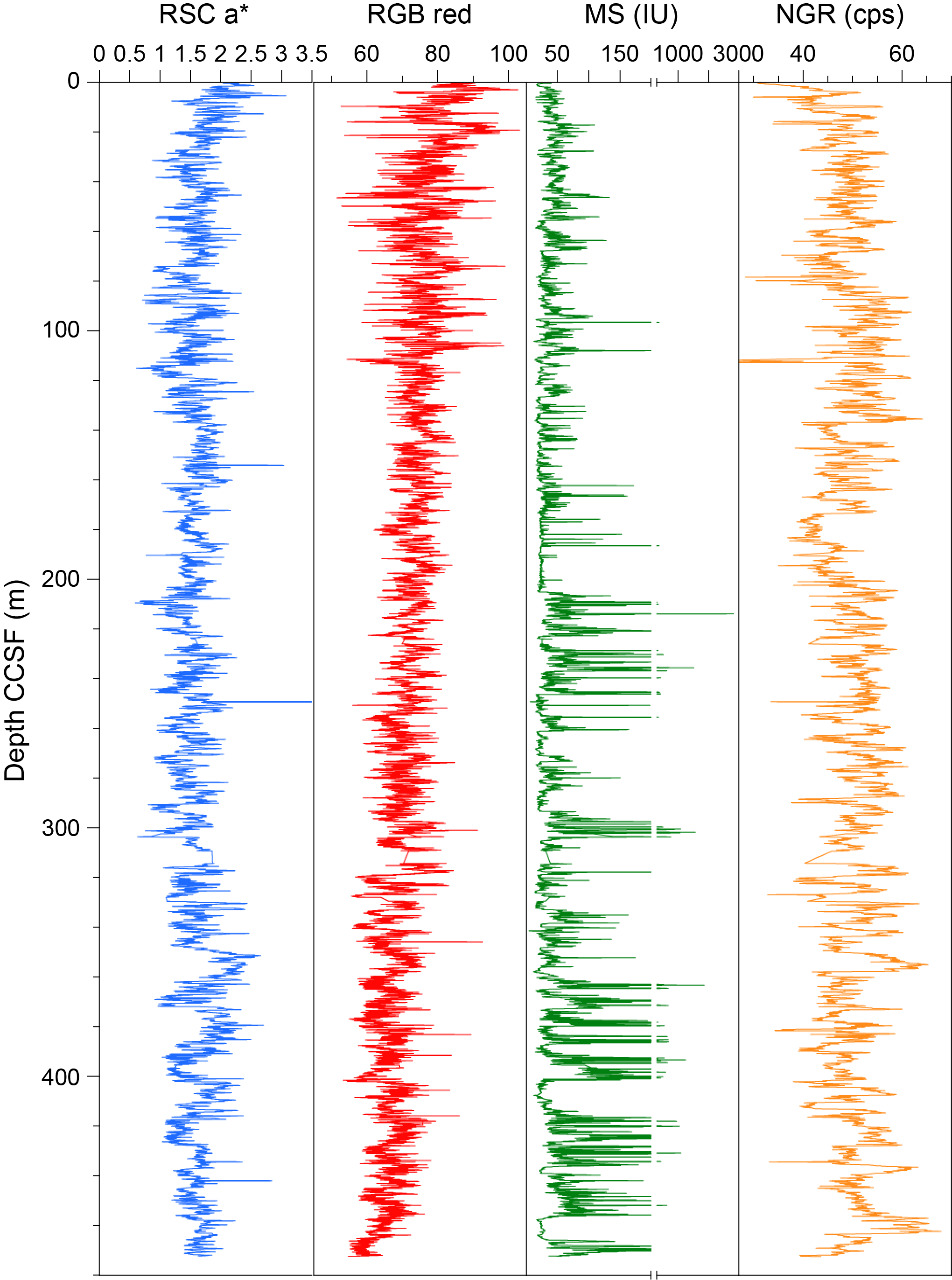
Figure F36. Spliced composite records.
The CCSF scale is anchored to the mudline of Core 403-U1618C-1H, which is assigned the depth of 0 m CCSF. From this anchor, we worked downhole using Correlator to establish a composite stratigraphy on a core-by-core basis. The match between holes is relatively well constrained within the spliced intervals, although there are gaps throughout the splice. Between 0 and ~200 m CCSF, the splice is secured except to a few tentative tie points (Table T8). Below this depth, incomplete recovery and sediment expansion resulted in more gaps, especially in Holes U1618A and U1618B, that were not fully covered by Hole U1618C and need to be confirmed or secured with additional analyses (e.g., X-ray fluorescence data). We approached the construction of the splice by mainly using the best recovered stratigraphy of Hole U1618C as the backbone, where possible, and using primarily Hole U1618A to fill the core gaps down to 294 mbsf (Figure F35A–F35C), where coring in Hole U1618A was terminated. Below this depth, we used Hole U1618B to fill the gaps in Hole U1618C (Figure F35D). We have provided the exact position of the tie points we used to determine the offsets for cores that were not used in the splice (Table T7); this information will make it easier for studies that utilize samples from intervals that are outside the splice to compare data to records from the splice.
The cumulative offset between the mbsf and CCSF depth scales is nearly linear (Figure F37A), but close inspection of the cumulative offset as a function of depth (mbsf) (Figure F37B) reveals that in the upper section (0 to ~140 mbsf), cores from all three sites consistently show minimal growth factor because of low expansion associated with the release of overburden combined with methane gas expansion. The growth factors below ~140 mbsf are strongly affected by making hole-to-hole correlations, and expansion and the loss of some sediment is also affecting the core offsets. In a few intervals, we have small floating sections that were difficult to correlate. Because of the expansion and incomplete recovery in all three holes, we had to include offsets between cores based on an average growth factor in the preceding cores. This uncertainty was large in Hole U1618B, resulting in decreasing cumulative offsets in some cores (Figure F37B), which obviously is incorrect, and we avoided using these parts of the records in the splice. In summary, we are very confident about the splice between 0 and 140 mbsf. Below this depth, the splice may be inaccurate, but we used mainly sections from Hole U1618C, which is more reliable than Holes U1618A and U1618B. Calculation of mass accumulation rates based on the CCSF scale should account for the expansion by dividing apparent depth intervals by the appropriate growth factor.
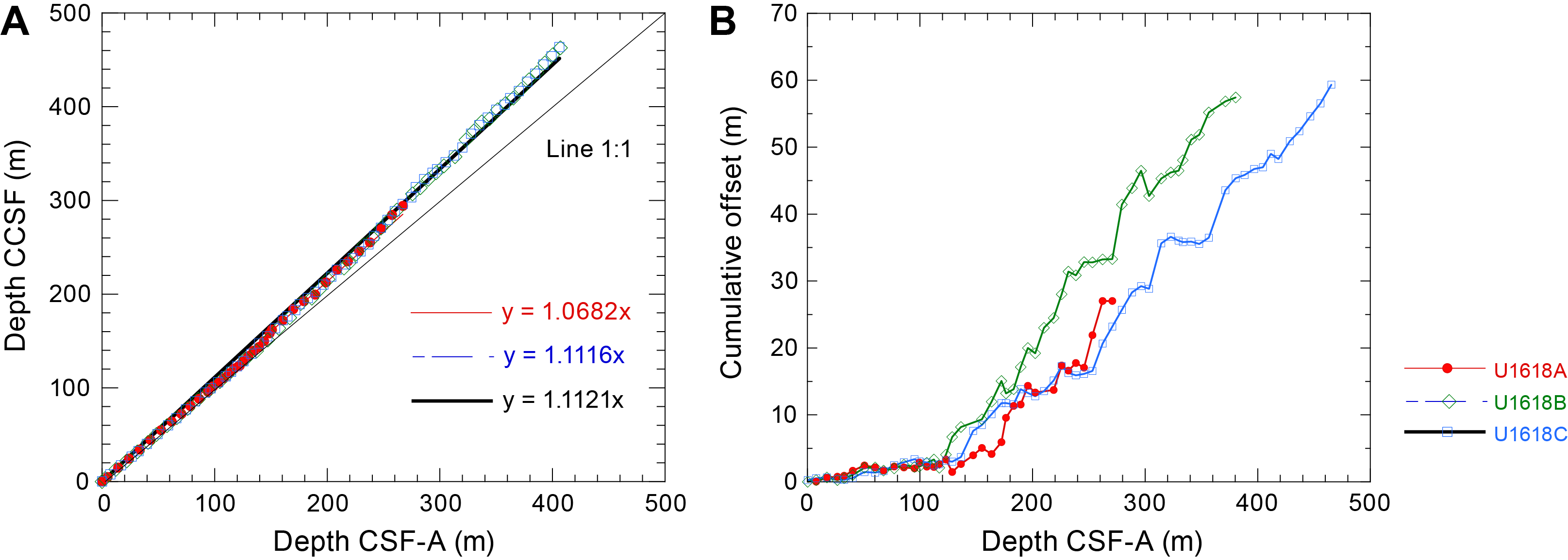
Figure F37. Depth scale offset.
8. Geochemistry
Samples for IW chemistry, bulk sediment geochemistry, and headspace gas were analyzed at Site U1618. The main findings from IW analysis suggest anaerobic conditions below approximately 20 mbsf and possible fluid migration in the sediments resulting in diachronous authigenic iron sulfide mineral formation and authigenic carbonate formation. Elemental analysis of solid material revealed carbon and nitrogen content across most intervals that is typical of the Arctic region (Stein and Stax, 1996). Headspace hydrocarbon gas measurements showed low concentrations in the uppermost 16.50 m and a sharp peak in methane below this depth, indicative of biogenic methanogenesis.
Although Site U1618 is not located near a known gas hydrate–related bottom-simulating seismic reflector, the headspace gas, IW geochemistry, and bulk sediment geochemistry indicate the presence and influence of gas hydrate and free gas at depth.
8.1. Interstitial water chemistry
A total of 46 IW samples were squeezed from 5 or 10 cm whole-round samples. Typical samples yielded 10 cm3 of water for subsequent analysis. A suite of major and trace elements (Table T9) were measured via ion chromatography (IC) and inductively coupled plasma (ICP) spectroscopy, respectively.
8.1.1. pH, chloride, sodium, and salinity
The measured pH of the IWs varied between 7.7 and 8.2 at Site U1618, with no discernible trends. The concentrations of chloride (Cl), sodium (Na), and salinity are conservative tracers used to investigate gas hydrate formation and dissociation in sediments (e.g., Ussler and Paull, 2001; Kastner et al., 2008). Gas hydrate dissociation involves breaking down hydrates in the sediments, which results in the freshening of IWs, whereas gas hydrate formation results in an increased salinity profile of IWs. The Cl concentrations at Site U1618 show a linear decrease from 559 mM at 12.30 mbsf to 377 mM at 406.26 mbsf. This linear decrease of Cl suggests diffusion of fluids deeper than 406.26 mbsf, which may indicate that gas hydrate dissociation occurred deeper than core recovery. The Na concentration (measured via IC) also tends to decrease with depth from 477 mM at 12.30 mbsf to 338 mM at 406.26 mbsf. Salinity linearly decreases downcore from 34 to a minimum of 22 at 406.26 mbsf. The salinity of 34 is comparable to established average seawater values, and the linear decrease down to 22 is indicative of the freshening of the IWs, which may be due to gas hydrate dissociation throughout Hole U1618A. Chloride, Na, and salinity concentration-depth profiles are shown in Figure F38.
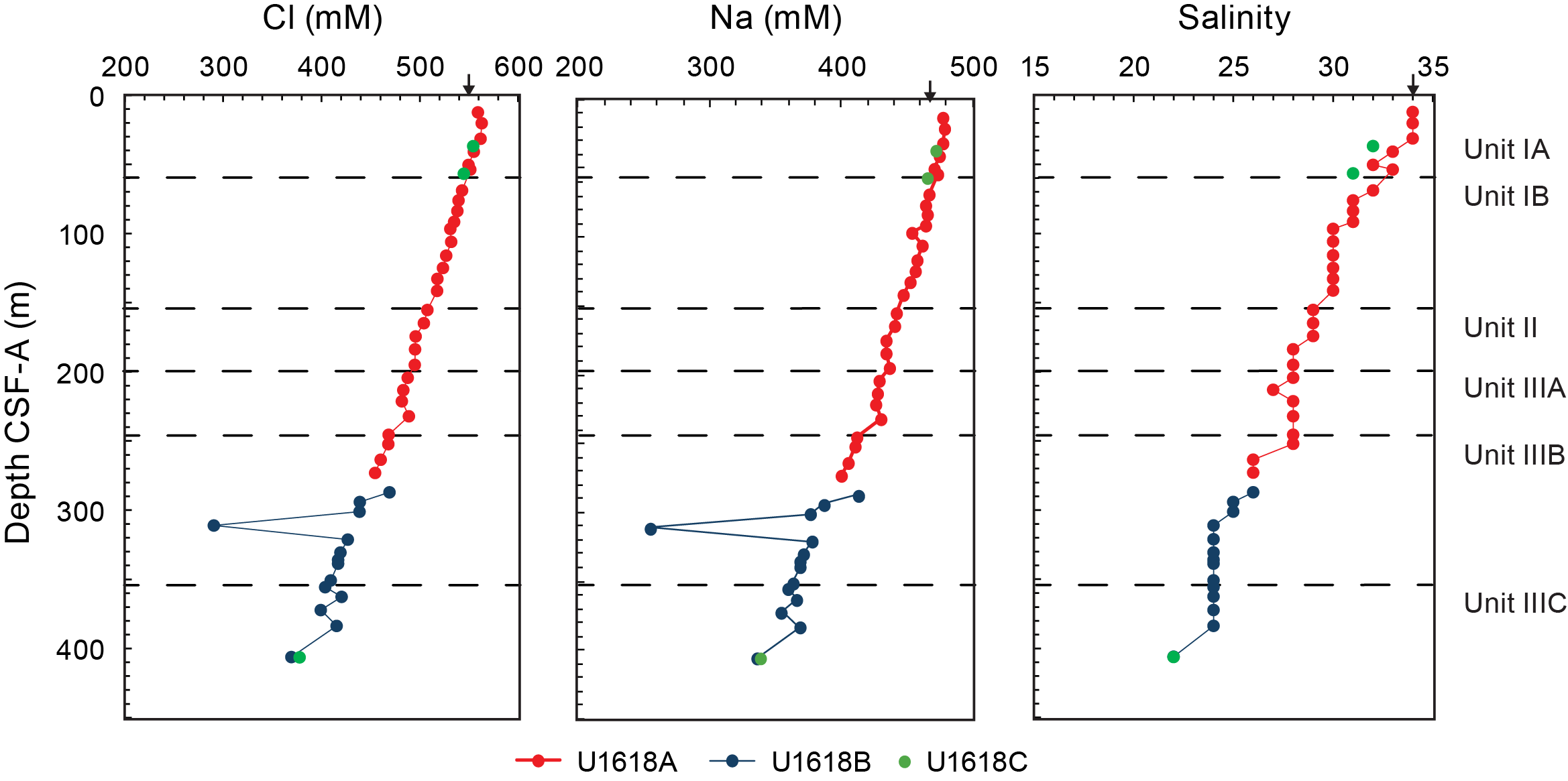
Figure F38. IW chloride, sodium, and salinity.
8.1.2. Sulfate, alkalinity, iron, and manganese
The sulfate–methane transition zone (SMTZ) is characterized by sulfate depletion and methane increase. The depth of the SMTZ can vary and is generally near the sediment/water interface in locations of high methane supply (Borowski et al., 1996; Graves et al., 2017). Sulfate at Site U1618 is rapidly depleted from 9 mM at 12.30 mbsf (well below the established average seawater value of 28 mM; e.g., Bruland and Lohan, 2006) to ~0.8 mM at 20.31 mbsf, where it remains at values ≤ 1 mM. The rapid depletion of sulfate in the IWs corresponds to an increase in methane concentrations in the headspace samples (described below). This suggests the SMTZ at Site U1618 is shallow, likely somewhere between 12.30 m and 20.31 mbsf. A shallow SMTZ is also supported by the measured alkalinity data. Alkalinity values increase from 14 mM at 12.30 mbsf to a maximum of 19 mM at 20.31 mbsf. This increase is consistent with the production of bicarbonate that occurs at the SMTZ due to the anaerobic oxidation of methane (AOM), as follows:
There are trace amounts of sulfate at 53.81, 200–250, and 350–400 mbsf ranging ~3–5 mM; the cause behind this slight increase is unknown.
Iron decreases from 33 to ~1 µM concentrations from 12.30 to 20.31 mbsf, suggesting Fe reduction above the SMTZ. Iron concentrations slightly increase to ~3 µM between 40 and 50 mbsf, where Fe concentrations then remain at values ≤ 1 µM, except for an increase to ~16 µM at 287.03 mbsf. The formation of authigenic iron sulfide minerals in Lithostratigraphic Unit II and Subunits IIIA and IIIC may explain the low Fe concentrations in the IWs. Manganese (Mn) decreases from 6 µM to near 3 µM concentrations from 12.30 to 20.31 mbsf, also suggesting Mn reduction above the SMTZ. Below the SMTZ, Mn concentrations tend to fluctuate between near 0 to ~2 µM in the IWs. In general, the decrease of Fe and Mn in the IWs is assumed to be due to incorporation into diagenetic mineral phases. Sulfate, alkalinity, Fe, and Mn concentration-depth profiles are shown in Figure F39.
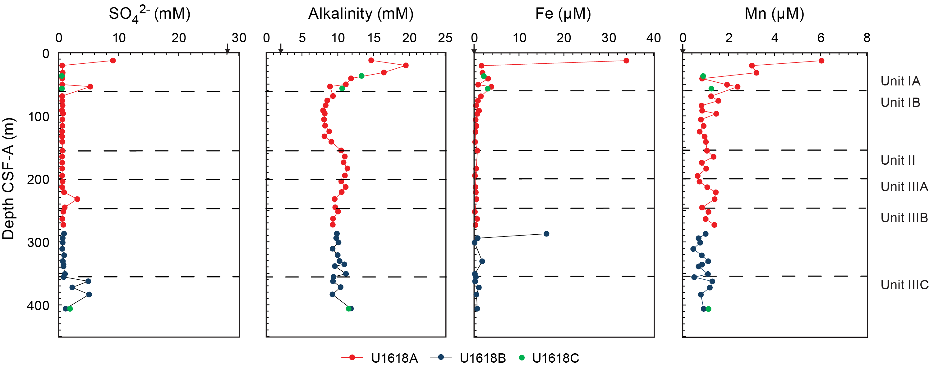
Figure F39. IW sulfate, alkalinity, iron, and manganese.
8.1.3. Calcium, magnesium, strontium, silicon, barium, lithium, boron, bromide, and potassium
The calcium (Ca) and magnesium (Mg) trends in the IWs are typical of those observed within the SMTZ, as well as within the methanogenic zone, and may also include processes of silicate weathering and authigenic mineral formation. Calcium decreases from 6 mM at 12.30 mbsf to 3 mM at 40.87 mbsf, where Ca begins to increase and continues to increase downcore. The decrease of Ca in the IWs between 12.30 and 40.87 mbsf corresponds to authigenic carbonate mineral precipitation (see Lithostratigraphy). The formation of authigenic carbonates at this depth is also consistent with the typical reaction to form carbonate during AOM, where bicarbonate produced during AOM reacts with the Ca in IWs to form carbonate (Graves et al., 2017). The continuous increase of Ca in the IWs with depth may be attributed to the formation of siderite, where Fe would partially replace the Ca in the carbonate minerals; this may explain the release of Ca and the decrease of Fe, while also supporting carbonate mineral formation observed throughout the cores. Similar to Ca, Mg between 12.30 and 40.87 mbsf decreases from 43 to 33 mM and strontium (Sr) decreases from 78 to 72 µM, which suggests Mg and Sr may also be incorporated into authigenic carbonate minerals. Additionally, dolomite formation below the SMTZ cannot be completely excluded, given that the concentration of Mg continues to decrease with depth, suggesting removal from the IWs. Silicon (Si) concentrations fluctuate with depth. The increases of Si concentration in IWs in Lithostratigraphic Unit II and Subunits IB and IIIB (lower) are consistent with Si release due to the alteration of silicates in methanogenic sediments. It is possible that the Si trend is also reflecting Si from diatoms dissolved in the alkaline pore water. Diatoms, which are phytoplankton that build their frustules from Si dissolved in seawater, were not found in the sedimentary sequence below the uppermost sample. There is likely marine barite formation and dissolution within Unit I, given that changes in dissolved barium (Ba) occur within this cored interval. The dissolved Ba shows barite formation above the SMTZ at 12.30 mbsf. The subsequent increase in dissolved Ba within and below the SMTZ (20.31–68.84 mbsf) is a result of marine barite dissolution in the sulfate-depleted pore water. Lithium (Li) in the IW is unique, increasing with depth to ~242 µM (Hole U1618C) at 406.26 mbsf. Specifically, the increase in Li concentration within Subunits IIIB and IIIC (~300–406.26 mbsf) suggests diffusion from a Li-rich fluid that is deeper than core recovery. It is likely the Li-rich fluids are related to hydrothermal circulation (Zhang et al., 1998) and fluid flow, which has been observed at the Vestnesa Ridge (Bünz et al., 2012). The Ca, Mg, Sr, Si, Ba, and Li concentration-depth profiles are shown in Figure F40. Potassium (K) (measured via IC) decreases from 11.4 mM (above average seawater values; e.g., Bruland and Lohan, 2006) to 4 mM with depth, well below average seawater values (10.2 mM), consistent with incorporation into authigenic mineral phases within methanogenic sediments. Boron (B) concentrations are higher than average seawater (416 µM, e.g., Bruland and Lohan, 2006) to 115.91 mbsf, where concentrations subsequently decrease with depth to near 200 µM. The K and B trends (Figure F41) are consistent with authigenic mineral (e.g., carbonate) formation. Bromide concentrations linearly increase with depth to >2 mM, with the exception of a slight decrease to 1.5 mM.
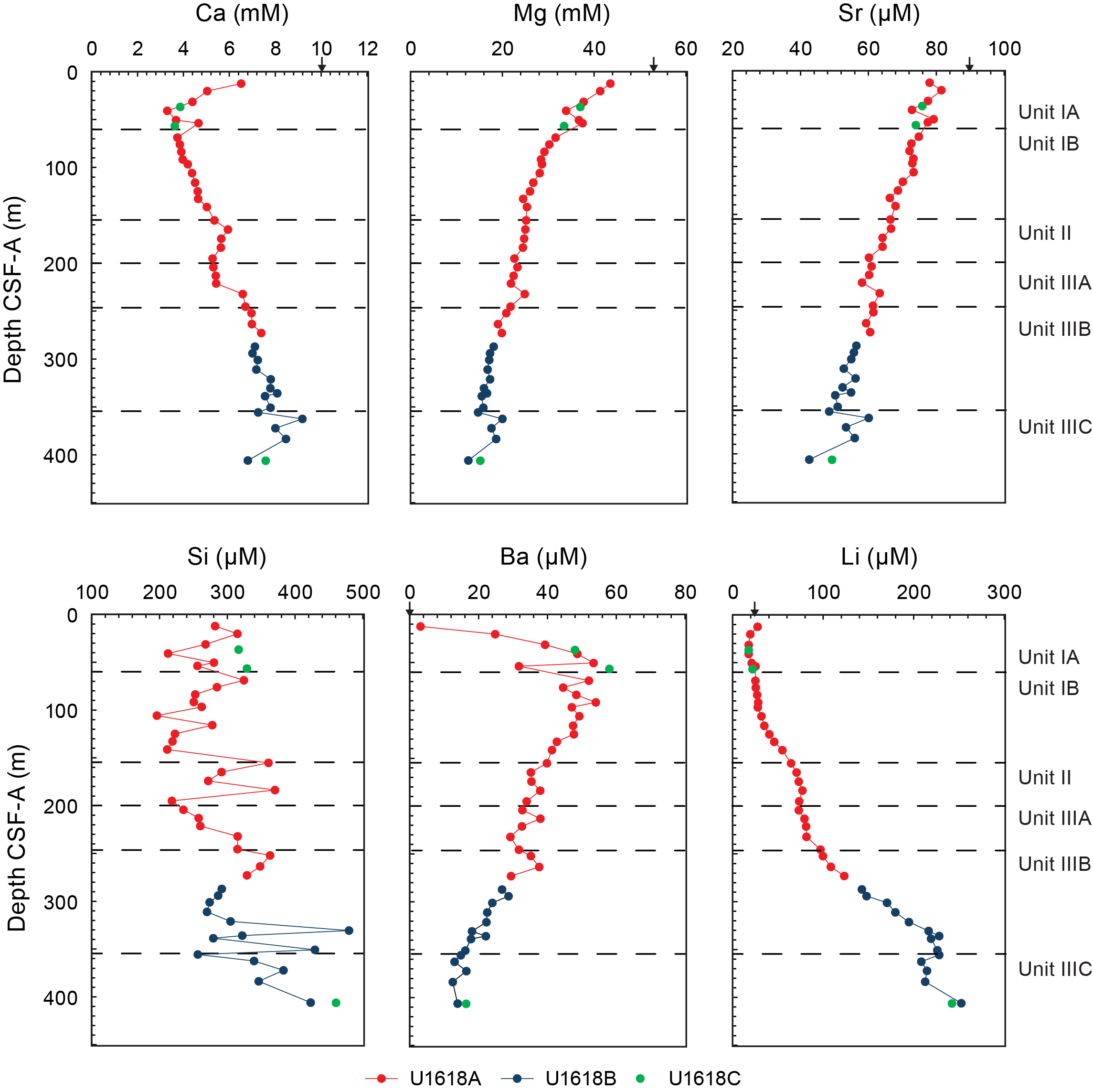
Figure F40. IW calcium, magnesium, strontium, silicon, barium, and lithium.
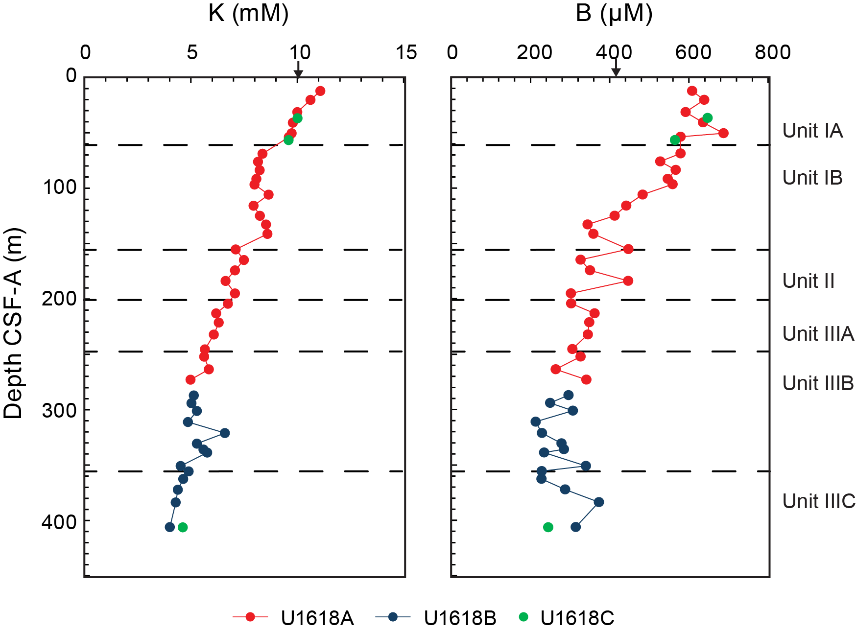
Figure F41. IW potassium and boron.
8.1.4. Phosphate and ammonium
The phosphate concentration increases from 20 µM at 12.30 mbsf to 72 µM at 20.31 mbsf, followed by a constant decrease to ~6 µM at 406.26 mbsf. The relatively higher phosphate concentrations in the upper meters at Site U1618 are most likely due to organic matter remineralization, which is a diagenetic process driven by photosynthetic activity. The ammonium concentrations increase from ~1 mM at 12.30 mbsf to ~3 mM at 406.26 mbsf, with the highest ammonium concentration (~4 mM) observed at 232.14 mbsf. The increase with depth of ammonium in the pore water is also indicative of organic matter diagenesis and supports the interpretation of the measured phosphate data. The phosphate and ammonium concentration-depth profiles are shown in Figure F42.
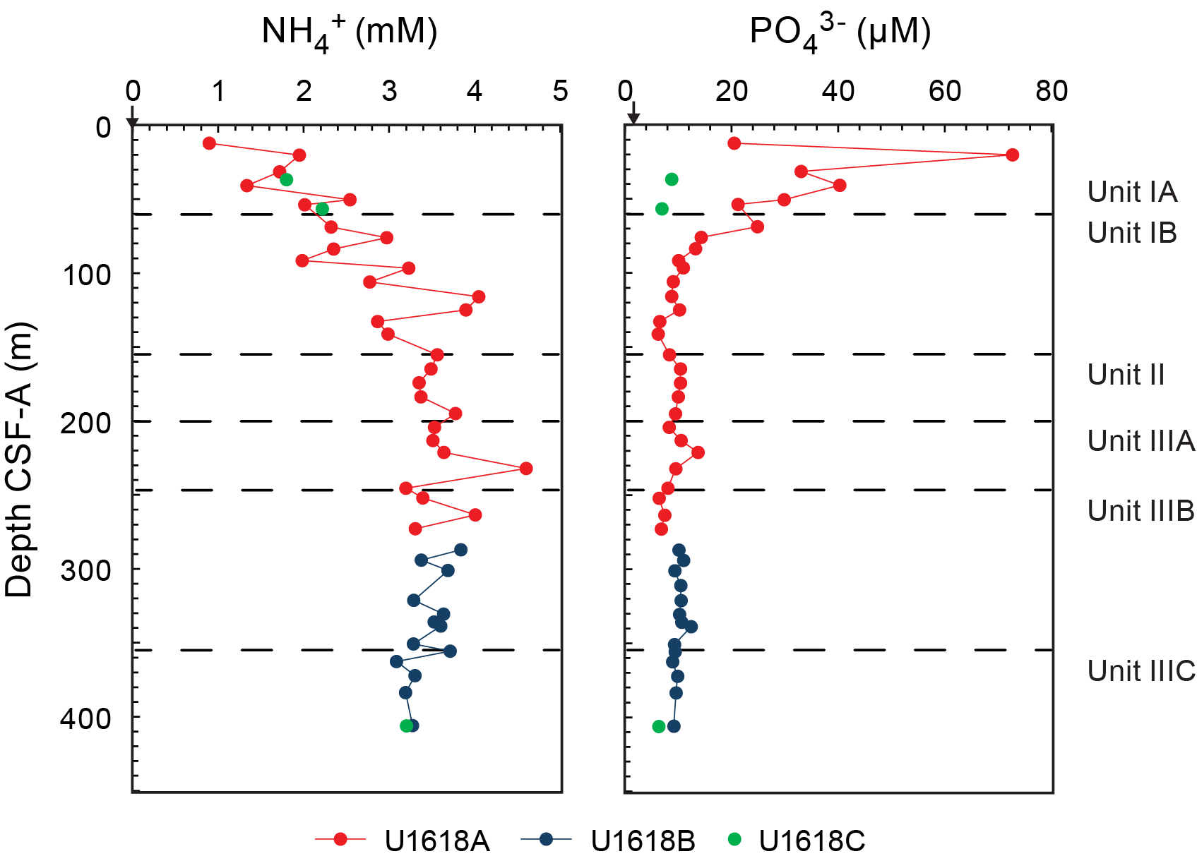
Figure F42. IW ammonium and phosphate.
8.2. Sedimentary organic geochemistry
Shipboard solid-phase analysis at Site U1618 involved measurements of total inorganic carbon (TIC; i.e., CaCO3), total nitrogen (TN), total carbon (TC), total organic carbon (TOC; calculated as TC − TIC), and total sulfur (TS) (Table T10) using shipboard plastic cylinder sampling (sample type CARB). The sedimentology team identified intervals for CARB samples from Holes U1618A–U1618C, resulting in a total of 43 samples taken. These samples are not systematically spaced, and they include representation of both major and minor lithologies.
The TC content in the sedimentary sequences of Holes U1618A–U1618C is generally high, with most values exceeding 0.5 wt%. Specifically, there are peaks of about 4 wt% at 80.92 mbsf in Hole U1618A, of about 4 wt% at 263.28 mbsf Hole U1618B, and of approximately 6 wt% at 372.35 mbsf in Hole U1618C. CaCO3 content varies with depth, ranging 0–40 wt%, with peaks corresponding closely to TC peaks in each hole. This suggests that the authigenic carbonate minerals contribute significantly to the TC variations because biogenic carbonates (e.g., foraminifers and nannofossils) are generally in low abundance (see Biostratigraphy and paleoenvironment) and authigenic mineral was observed at Site U1618 (see Lithostratigraphy).
The TOC content in Holes U1618A–U1618C ranges 0–2 wt%. Generally, TOC content is lower in the upper layers (approximately above 30 mbsf) and increases downhole to 80.92 mbsf. Below this depth, a decreasing trend is observed in Hole U1618A, whereas no distinct trends are noted in Holes U1618B and U1618C. The TN content in Holes U1618A–U1618C ranges 0–0.15 wt%, typically lower in the upper sediment layers and gradually increasing with depth and showing fluctuations. The ratio of TOC/TN (C/N), which is commonly used to identify sources of sedimentary organic matter (e.g., Meyers, 1997), varies from 7 to 23 at Site U1618. C/N ratios ranging between 4 and 10 suggest a marine origin, primarily from marine algae; C/N ratios of 20 or higher indicate a terrestrial origin (e.g., Meyers, 1994, 1997). The C/N ratios at this site vary within 5 to 25, suggesting organic matter is sourced from both continental (e.g., ice sheet derived) and marine origins. The sediment grain size affects C/N ratios, with fine-grained sediments generally having lower C/N ratios compared to coarse-grained sediments (e.g., Meyers, 1997). The higher C/N ratios correlate well with coarse-grained sediments (see Lithostratigraphy), supporting a terrestrial origin. The TS content in Holes U1618A–U1618C ranges between 0 and 1 wt% down to 383.03 mbsf, where there is an increase of TS content to ~3 wt%, and correlates with the observed sulfide minerals at depth within the cores. Figure F43 illustrates the downcore profiles of CaCO3, TOC, and TN contents (in weight percent) and C/N ratios at Site U1618, and Figure F44 illustrates the downcore profile of TS content (in weight percent) at Site U1618.
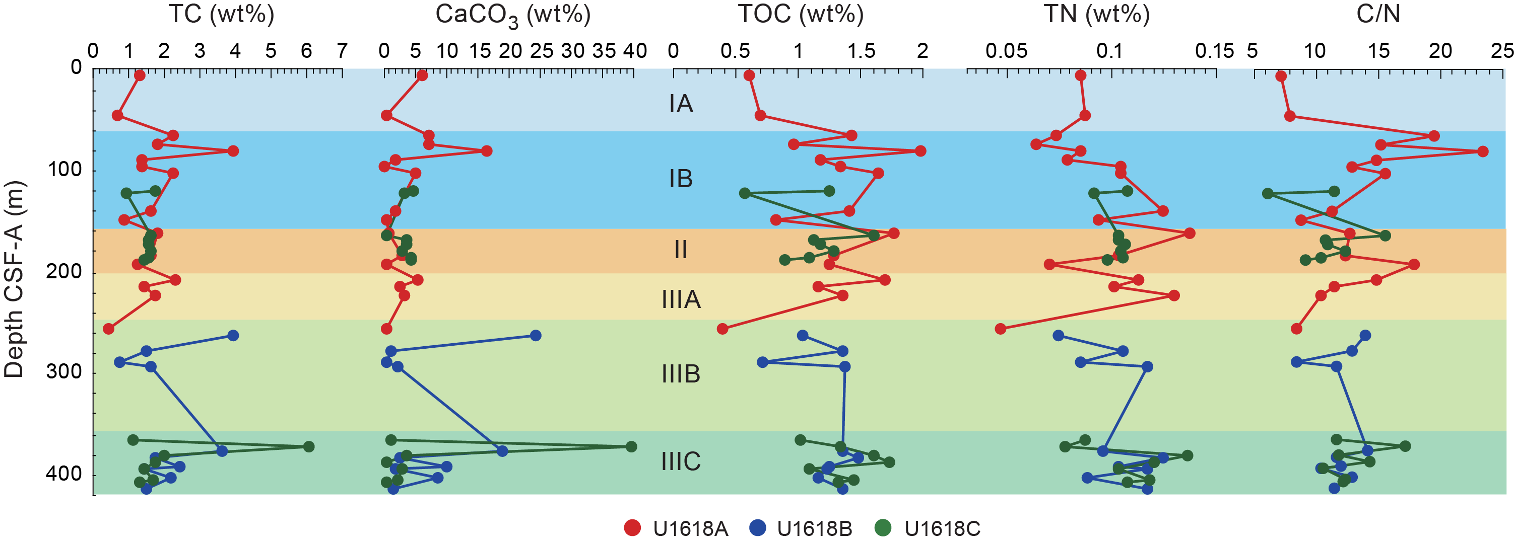
Figure F43. Bulk sediment contents of CaCO3, TC, TOC, TN, and C/N ratio.
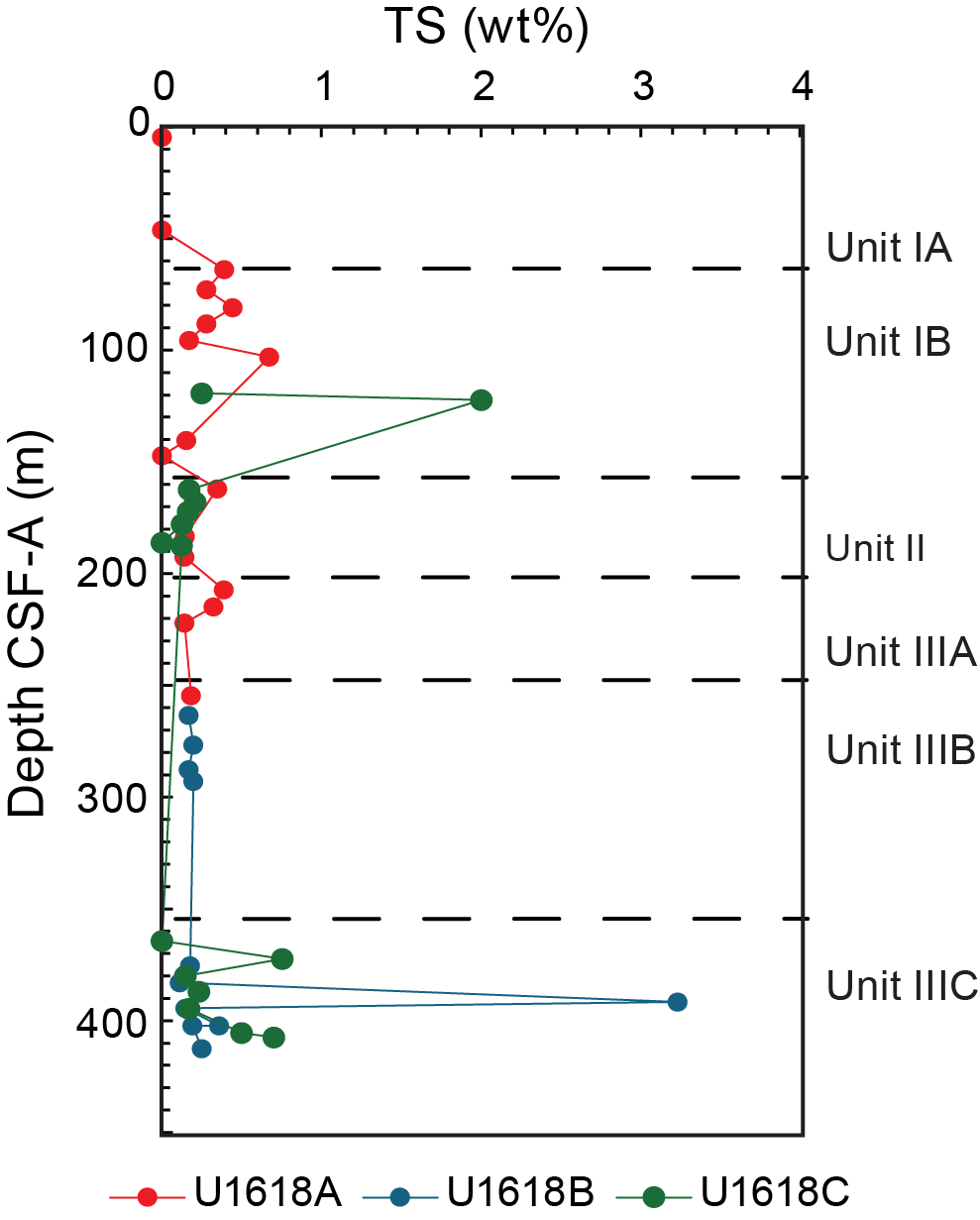
Figure F44. Bulk sediment contents of TS.
8.3. Headspace gas geochemistry
As part of routine environmental protection and safety monitoring, headspace hydrocarbons were analyzed at Site U1618 (Figure F45; Table T11). Samples for headspace gas analysis were taken at a resolution of one sample per core. For Hole U1618B, samples were taken at a deeper depth than for Holes U1618A and U1618C. A total of 122 samples were analyzed for headspace hydrocarbons. For safety considerations, the ratio of methane (C1) to ethane (C2) is generally used to obtain quick information about the origin of the hydrocarbons (i.e., to distinguish between biogenic gas and gas migrated from a deeper source of thermogenic hydrocarbons).

Figure F45. Methane and ethane concentrations and methane/ethane ratios.
Methane concentrations were low in the uppermost 16.50 m, and ethane was not detected in this interval, indicating a biogenic source of gas (Figure F45). At approximately 40–90 mbsf, methane concentrations sharply increased by about three orders of magnitude, reaching 51,970 ppmv at 45.86 mbsf. At 31.48 mbsf, the first amounts of ethane (3.78 ppmv) were detected, with a methane/ethane (C1/C2) ratio of 4866 (Figure F45). Ethane gradually increased to about 350 mbsf, after which a decreasing trend downcore appeared, with a sharp increase below approximately 406 mbsf. Propane was first detected below 96.65 mbsf in Hole U1618B, whereas iso-butane and n-butane first appeared below 204.30 mbsf. Traces of n-pentane, iso-hexane, and n-hexane were found below 263.63 mbsf in Hole U1618A, below 406.14 mbsf in Hole U1618B, and below 403.36 mbsf in Hole U1618C. In these intervals, C1/C2 ratios less than 100 were observed, suggesting a thermogenic source of hydrocarbons.
Additionally, six void gas samples (VACs) were analyzed from Hole U1618A where voids were observed through the core liner on the core receiving platform. The VAC samples had methane and ethane concentrations that were two to three orders of magnitude higher than the headspace samples. The respective maximum values for methane and ethane were 1,011,937 and 251 ppmv at 106.07 and 132.85 mbsf, respectively.
Gas hydrates are ice-like structures found in the subseafloor in deep marine and continental shelf environments. They form when water freezes around methane gas or other higher molecular weight hydrocarbons (e.g., ethane or propane) under cold temperatures and high-pressure conditions (Sloan, 1998). Gas hydrate stability zones in marine sedimentary sequences can be estimated from pressure and downhole temperature data (Brooks et al., 1983). Site U1618 had a water depth of 1196 m, and Hole U1618A had a measured geothermal gradient of 75°C/km (see Downhole measurements). Thus, the gas hydrate stability zone was calculated to extend to approximately 214 mbsf. Downhole temperature was also measured on three lower depths in Hole U1618B, revealing a lower geothermal gradient of 72°C/km in this hole, either suggesting a change in the rate of temperature increase with depth or a deeper gas hydrate stability zone in this hole. The occurrence of gas voids in the core liner and very high gas concentration of the VACs may possibly be related to the presence of hydrates that disassociated at depth and/or when exposed to lower pressure environments as the cores were brought up to sea level.
Authigenic carbonates precipitate at the upper and lower depths where gas hydrates exist, affecting the chemical composition of the IW and altering alkalinity (Rodriguez et al., 2000). The high peaks of CaCO3 content at Site U1618 might be due to authigenic carbonate appearing in the upper and lower sections of intervals believed to contain gas hydrates. Additionally, slight changes in alkalinity and other major elements (i.e., Ca and Mg) occur in these intervals. These changes in major elements and alkalinity, along with carbonate precipitation, support the presence of gas hydrates. Although Site U1618 did not show clear signs of gas hydrates in seismic data, we detected geochemical signatures associated with gas hydrates, including an increase in alkalinity around 130–230 mbsf.
9. Microbiology
9.1. Site U1618
SedaDNA samples were taken in contamination-controlled conditions at low resolution in Hole U1618B to examine the entire record and at a higher resolution in Hole U1618C to examine the time interval from the MIS 6/5e glacial–interglacial transition to the recent past. In total, 126 sedaDNA samples were taken across the two holes (Table T12); these samples will be analyzed postcruise. The drill fluid contains seawater, which is a potential source of biological contamination, and therefore the drill fluid was infused with perfluorodecalin (PFD) tracers to assess whether sedaDNA samples had been contaminated. A total of 147 PFD samples were analyzed at this site shipboard on an Agilent 6890 gas chromatograph with Micro-electron capture detector (Table T12). Results from the shipboard analyses of the control samples are discussed below.
9.1.1. Hole U1618B
Hole U1618B was sampled at low resolution (one sample per core) for the full 414 m record (Figure F46; Table T13). In total, 48 sedaDNA samples were taken on the core receiving platform. Preliminary shipboard chronological work suggests this sedaDNA record will span from the recent past to the Pliocene. Drill fluid in this hole was infused with 0.6 ng/L of PFD so that positive and negative PFD controls could be taken. The positive control was taken from a sample of drill fluid at the top of the sampled core and the negative control from directly adjacent to the sedaDNA sample. All positive drill fluid controls contained levels of PFD above background levels of 0.007 ppb (defined by the highest background levels of PFD in blank samples), indicating PFD was dispensed successfully into the drill fluid throughout coring in Hole U1618B (Table T14). Overall, the results from the negative controls showed drill fluid contamination was likely in 44% of sedaDNA samples from Hole U1618B. Coring with the APC/HLAPC system resulted in lower drill fluid contamination of sedaDNA control samples (15%) compared to coring with the XCB system (57%) (Figure F46). This contamination difference is likely due to the increased core disturbance (e.g., fracturing and biscuiting) produced by the XCB system. Nevertheless, these findings also indicate that it is possible to obtain uncontaminated sedaDNA samples with both types of coring approaches, extending the potential for sedaDNA studies in a wider range of drilling conditions than previously documented in marine sediments.
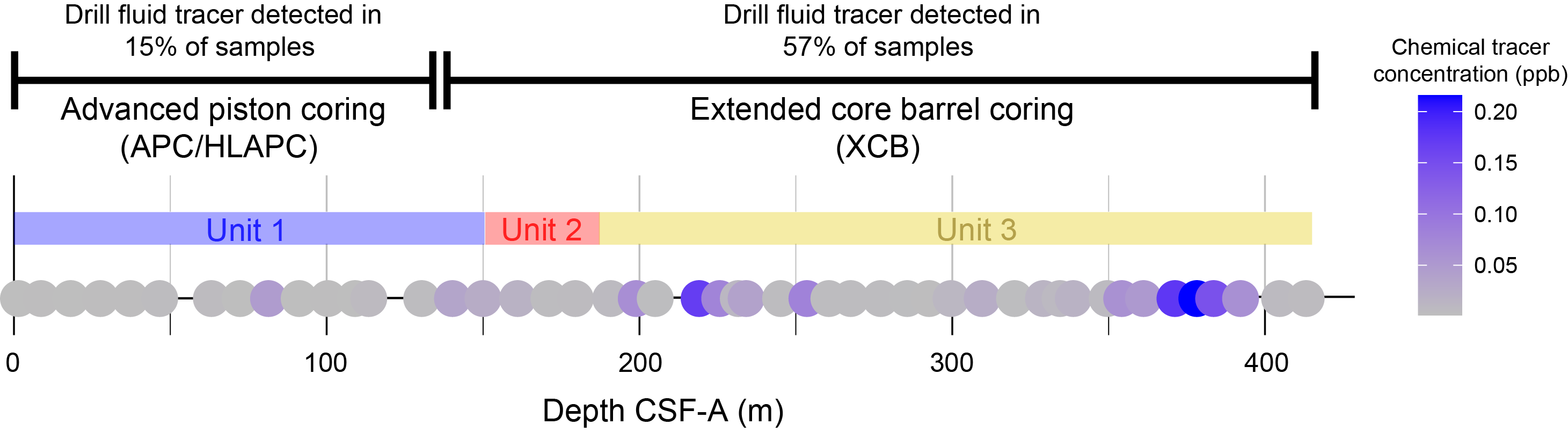
Figure F46. Low-resolution sedaDNA sampling.
9.1.2. Hole U1618C
9.1.2.1. High-resolution record of the recent past to the lead up to the last interglacial
Hole U1618C was selected for high-resolution sampling of split core sections of the target interval spanning the MIS 6/5e transition to the present. In total, 78 sedaDNA samples were taken across the first three cores, which extend to ~26 mbsf (Table T13). These cores were obtained using the APC system. Analysis of PFD concentrations in the controls indicated PFD was correctly dispensed and 90% of the sedaDNA control samples were free from drill fluid contamination.
The precise sampling strategy for the target stratigraphic interval was developed dynamically and in collaboration with other shipboard scientists (Figure F47). A preliminary estimate of MIS 5e was determined after correlating MS data with well-dated regional records (Jessen et al., 2010) and comparing with the biostratigraphic events (i.e., nannofossils and diatoms biostratigraphy). In collaboration with the stratigraphic correlators, we used MS data to determine the possible position of MIS 5e and sampled across it to capture the transitions into (MIS 6 glacial termination) and out (MIS 4 glaciation) of this period of warmth. We further sampled across meltwater events to assess the paleoecological shifts associated with them. The location of Meltwater Pulse 1A (Deschamps et al., 2012) was identified based on well-established regional glaciomarine facies (Lucchi et al., 2013, 2015) observed on the split core surface.
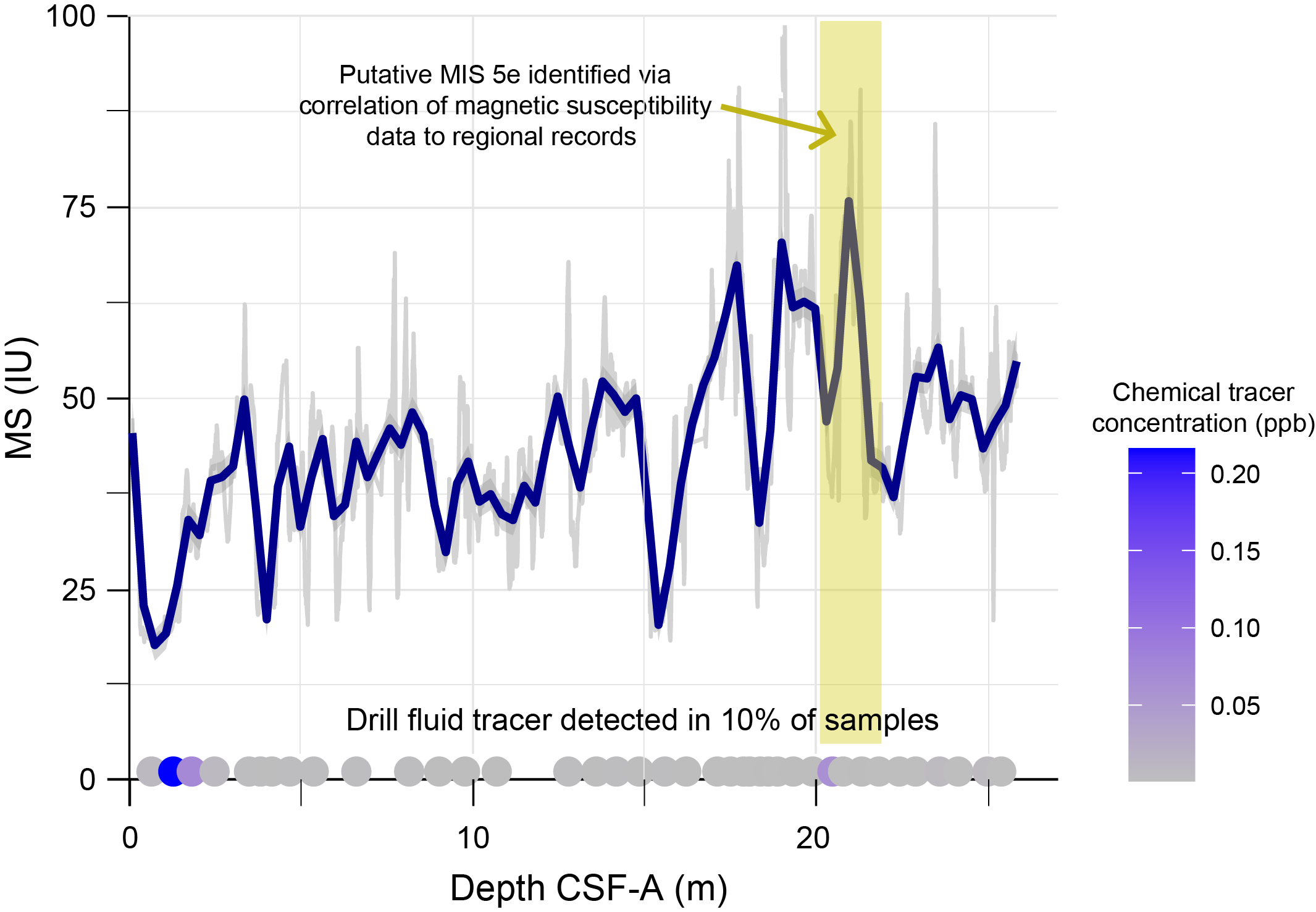
Figure F47. High-resolution sedaDNA targeted sampling.
9.1.2.2. Oldest preservation of sedaDNA
One sample was also taken from the middle of Section 2 of the last core (403-U1618C-62X) to test for the oldest preservation of sedaDNA at Site U1618. The preliminary chronology from this site (see Biostratigraphy and paleoenvironment and Paleomagnetism) suggests the bottom of the core may have crossed into the Pliocene, which would make any ancient DNA extracted from the sediment older than the 2 My old DNA recovered in Arctic permafrost, the oldest ancient DNA sequenced to date (Kjær et al., 2022).
For the best possible chance of an uncontaminated sample, the sample was taken from the interior of a biscuit, where the stratigraphic sequence is better preserved than in the unconsolidated gravy that is an artifact of XCB drilling. The PFD negative control from immediately adjacent to the sedaDNA sample showed no detectable PFD. However, this result needs to be interpreted with caution because all the positive PFD controls were also negative, suggesting there was a problem with the tracer in the drill fluid.
10. Downhole measurements
10.1. Formation temperature
During APC coring in Hole U1618A, in situ formation temperature was measured every third core (4H, 7H, 10H, and 13H) using the APCT-3 tool. After switching to XCB coring, in situ formation temperature was measured prior to Cores 35X, 403-U1618B-42X, and 53X using the SET2 probe. Temperature increased almost linearly with depth, and the slope of linear regression provides a typical geothermal gradient (78.8°C/km) for oceanic sediments compared with the statistical data set (Kolawole and Evenick, 2023) (Figure F48). The heat flow in the sediments and the temperature at the seafloor were calculated from the measured thermal conductivity in Cores 403-U1618A-15F through 37X, 403-U1618B-36X through 54X, and 403-U1618C-1H through 15F and the formation temperature measurements. Assuming a linear relationship between thermal conductivity and depth, the heat flow in the sediments and the temperature at the seafloor are approximately 98.5 mW/m2 and −0.814°C, respectively.
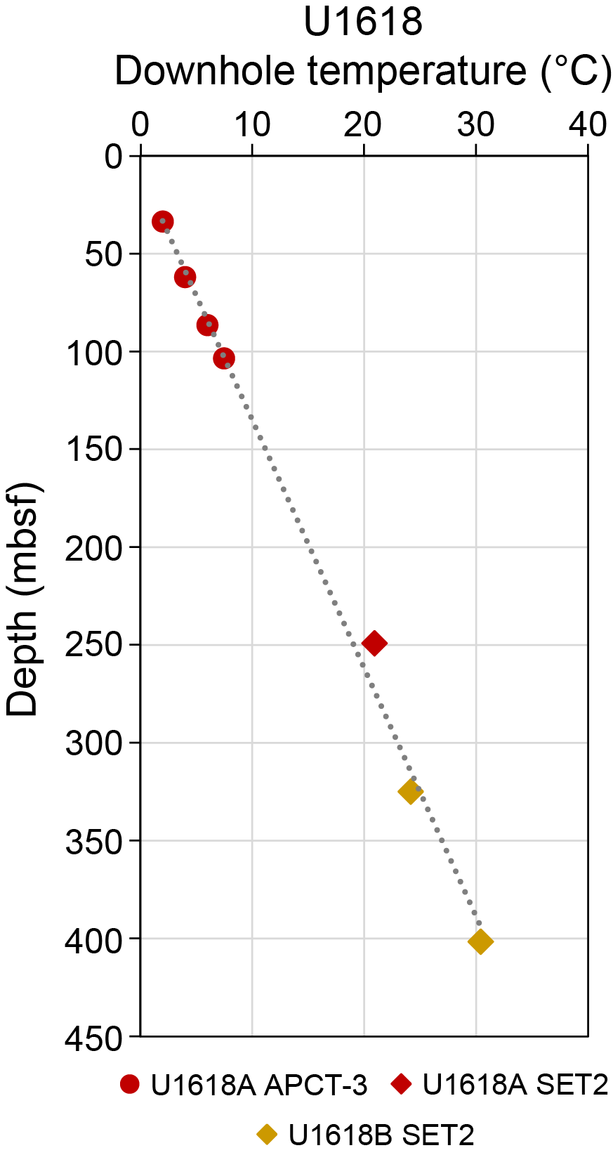
Figure F48. Formation temperature.
10.2. Downhole logging
In Hole U1618B, downhole logging was conducted using the triple combo and FMS-sonic tool strings to obtain multiple in situ property measurements. Logging operations for these tools are illustrated in Figure F49. After the BHA was set at 79.6 m wireline log matched depth below seafloor (WMSF), the string was first lowered to 369.4 m WMSF for downlog while the caliper closed. A downlog of the Hostile Environment Litho-Density Sonde (HLDS) was not obtained. Subsequently, the tool string was pulled up for the first uplog from 379.2 to 288.8 m WMSF. To increase data recovery, the strings were lowered again to 370.1 m WMSF and pulled up to 0 m WMSF for the second uplog. After the triple combo tool string, the FMS-sonic string was lowered to 356.6 m WMSF. For the first image uplog, the FMS-sonic string was pulled up from 359.7 to 122.8 m WMSF. To increase data recovery, the tools were lowered again to 342.9 m WMSF and pulled up to 0 m WMSF for the second image uplog. The average peak-to-peak heave was estimated at 0.5 m, and the heave compensator was utilized during the logging operation.
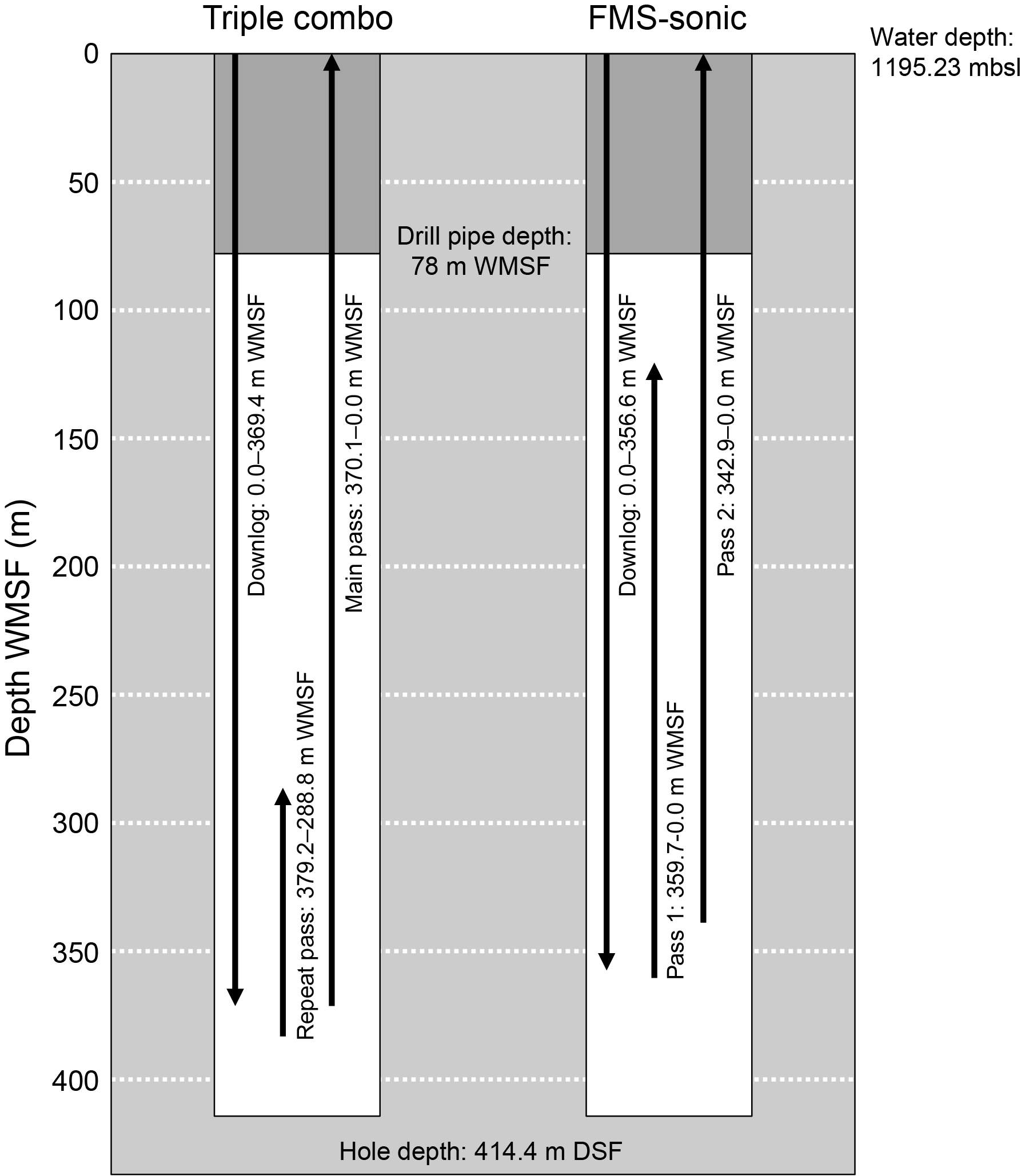
Figure F49. Downhole operations.
Logging data were sent for processing to the Lamont-Doherty Earth Observatory (LDEO; Columbia University, USA) (Figure F50; Table T15). The data provide important information for core-log integration to understand the actual depth and thickness of each lithostratigraphic unit because most cores at this site suffered from gas expansion. Seismic imaging using the VSI was canceled because the z-axis accelerometer to correct the vertical position of data was out of order.
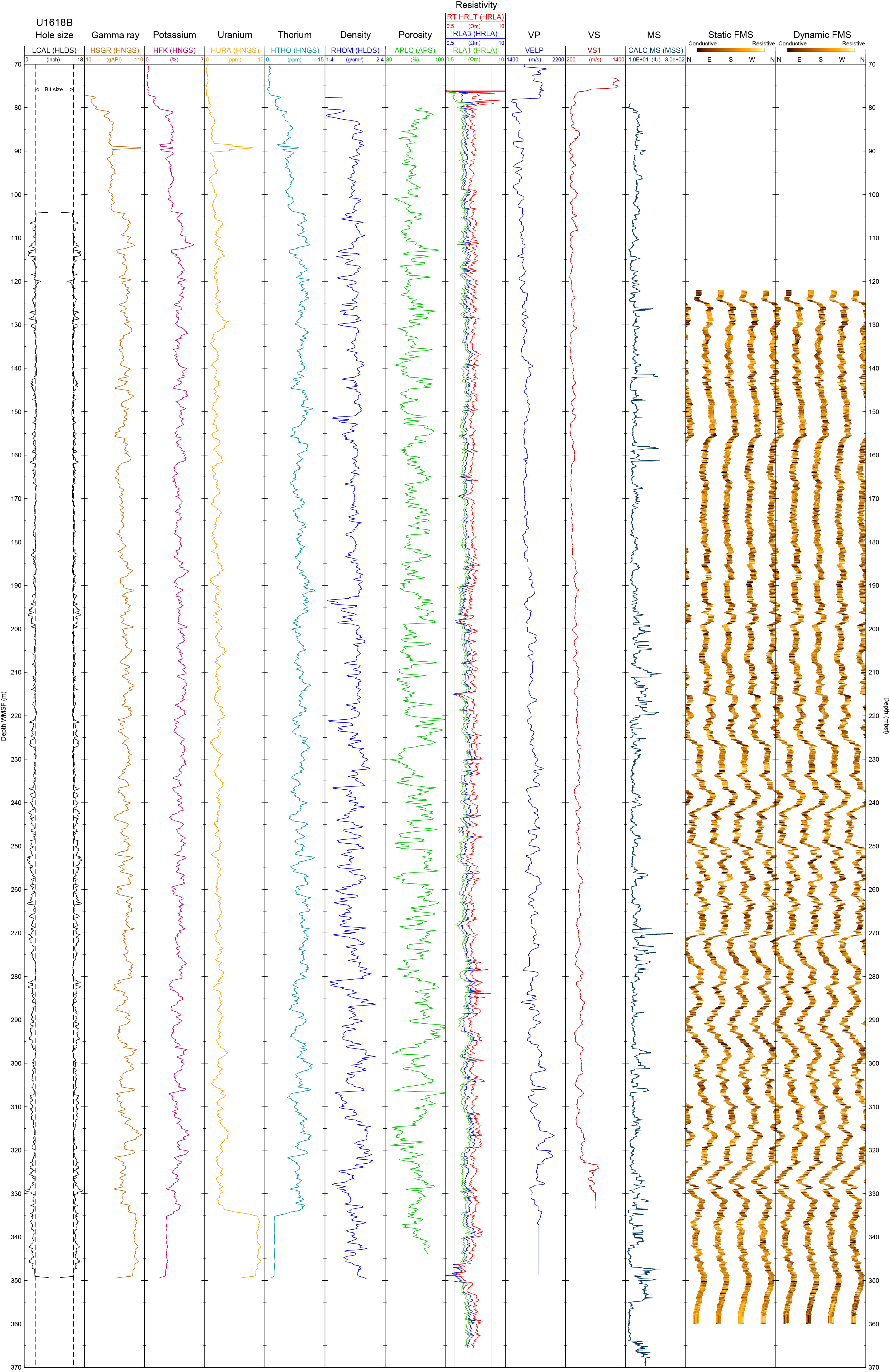
Figure F50. Downhole logging data.
10.2.1. Triple combination
Overall, the triple combo successfully acquired borehole diameter, density, natural gamma ray, MS, and electrical resistivity. For several depth levels, however, the data should be interpreted with caution because the irregularly enlarged borehole affects eccentralization and/or good contact of tools with the borehole wall (Figure F50).
Logging data were collected for variations in the borehole diameter, which were measured using a hydraulic caliper on the HLDS during each uplog. Based on these caliper measurements, the borehole diameter was enlarged at almost all depths, indicating that washouts occurred while drilling mud circulated in Hole U1618B. Given the characteristics of sondes and methodologies, borehole diameter variation may affect the logging of MS and porosity. On a specific thin layer at ~120 m WMSF, we observed a rapid reduction of borehole diameter from ~11 to ~8.5 inches. Given the correspondence to the core description of Holes U1618A and U1618C (see Lithostratigraphy), this might be a mud cake that adhered to the borehole wall as water from the drilling mud moved into a permeable sand layer. Unfortunately, cores were not recovered from the same depth in Hole U1618B.
Natural gamma ray, density, and MS show almost the same trends as the shipboard scanning data. HLDS density log measurements from 82 to 350 m WMSF (below the drill pipe) are on average 1.88 g/cm3 and do not show a significant downhole trend. Cyclic changes with increasing amplitude downhole were observed. Absolute values of the HLDS density measurements are very similar to densities derived from GRA bulk density core logging and discrete MAD measurements (Figure F51A).
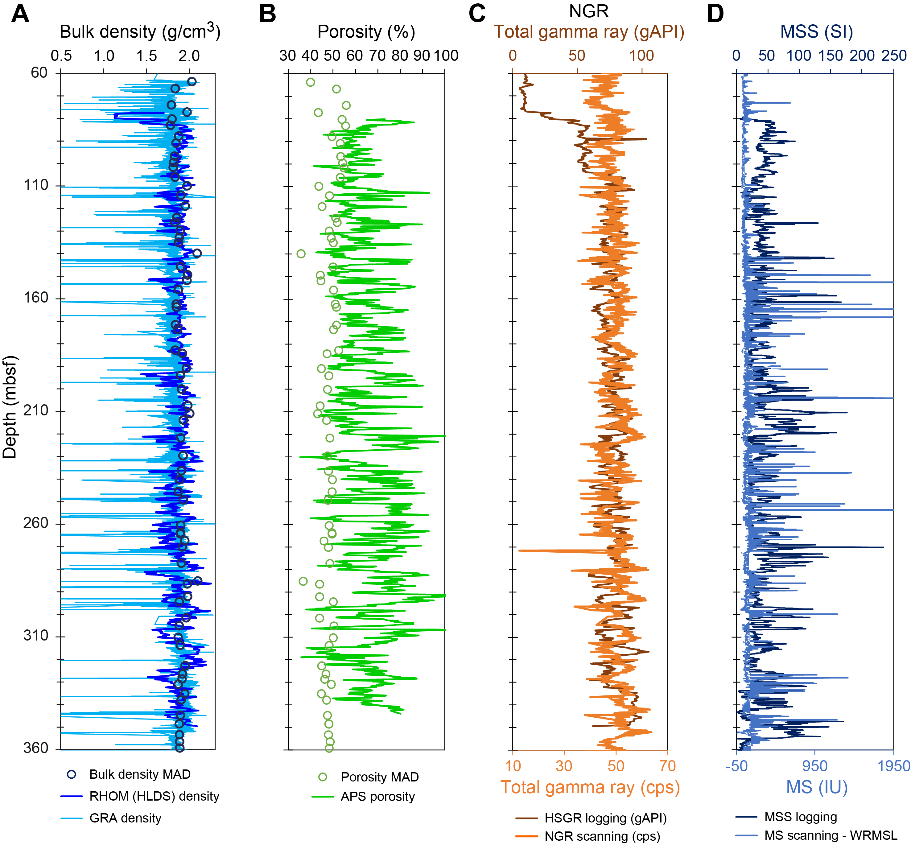
Figure F51. Core-log comparison.
Because of poor borehole conditions, the Accelerator Porosity Sonde (APS) likely did not obtain accurate porosity data (Figure F50), but relative cyclic changes show correlation with density and electrical resistivity at several depths (Figure F51B). In addition, the gradual increase in amplitude of cyclical changes is similar to other parameters, such as natural gamma ray or density.
Downhole natural gamma ray was reported as total spectral gamma ray (HSGR) data and potassium (K), uranium (U), and thorium (Th) contents. Each K, U, and Th component was derived from the spectrum of total natural gamma ray counts and 256-window spectroscopy. For the total natural gamma ray measurements not influenced by the drill pipe (>104 m WMSF), the average value is 78 American Petroleum Institute gamma radiation units (gAPI). Cyclic amplitude fluctuations around this value were observed. The amplitude of these cyclic variations is higher in the lower part (>280 m WMSF) of the measurements. An interval of lower HSGR values occurs around 160–180 m WMSF. Potassium and uranium showed similar trend and fluctuation to HSGR, whereas thorium indicates relatively lower amplitudes. The HSGR data showed great similarity to natural gamma ray measured on cores with the natural gamma ray logger (Figure F51C), indicating that core and log depth scales can be readily correlated. The differences of the depth scales can be assumed to be less than 1 m. Absolute values of the HSGR in the upper 100 m are much lower because measurements were made through the drill pipe.
The Magnetic Susceptibility Sonde (MSS) provided data that range 0.91–234.19 SI and correspond well to core measurements using the WRMSL (Figure F51D). MSS showed some peaks much higher than background that can be associated with the existence of authigenic iron sulfides (see Physical properties).
For electrical resistivity, laterologging using the High-Resolution Laterolog Array (HRLA) tool recorded multiple logs depending on the travel paths of electrical current: apparent resistivity from shallow to deep, as well as true resistivity. Resistivity ranged 1–3 Ω·m across most depths. At ~190–200 m WMSF, low resistivity that corresponds to logging of low density and high porosity was observed. Because electrical resistivity of formation is highly dependent on water content, unless lithology changes, it suggests the presence of large pore spaces and high-water content, which is consistent with low density and high porosity in the same interval. The same trend of resistivity was found around 350 m WMSF.
10.2.2. FMS-sonic
The FMS-sonic string successfully logged natural gamma ray, acoustic velocity, and borehole resistivity images (Figure F50).
Because of hydrate-bearing sediments or free gas, automatic detection of the correct arrival time of the acoustic wave pulse was difficult for the raw data from the Dipole Sonic Imager (DSI). This is similar to failed P-wave measurements in the core laboratory on the ship. The raw velocities are likely to be a signal of wave conducted through slow sediments (i.e., soft sediments released from compression by drilling and washing) or fluid in the borehole, which may be a mixture of drilling mud and seawater. The data reprocessing provided us with meaningful P-wave velocity data (Figure F50). The reprocessed data show increasing values with depth. The calculated linear trend is 0.98 m/s. The trend is overlain by cyclic changes that mimic changes seen in the density. Maximum velocities of 2026 m/s were measured at 321 m WMSF.
Because of the capacity of the FMS calipers, borehole resistivity images have 25% recovery of all around the borehole walls at every depth. The images indicate no significant signal of borehole breakouts nor drilling-induced tensile fractures.
References
Anthonissen, E.D., 2008. Late Pliocene and Pleistocene biostratigraphy of the Nordic Atlantic region. Newsletters on Stratigraphy, 43(1):33–48. https://doi.org/10.1127/0078-0421/2008/0043-0033
Bé, A.W.H., and Tolderlund, D.S., 1971. Distribution and ecology of living planktonic foraminifera in surface waters of the Atlantic and Indian Oceans. In Funnel, B.M. and Riedel, W.R., The Micropaleontology of Oceans. Cambridge, United Kingdom (Cambridge University Press), 105–150.
Borowski, W.S., Paull, C.K., and Ussler, W., III, 1996. Marine pore-water sulfate profiles indicate in situ methane flux from underlying gas hydrate. Geology, 24(7):655–658. https://doi.org/10.1130/0091-7613(1996)024<0655:MPWSPI>2.3.CO;2
Brooks, J.M., Barnard, L.A., Weisenburg, D.A., Kennicutt, M.C., II, and Kvenvolden, K.A., 1983. Molecular and isotopic compositions of hydrocarbons at Site 533, Deep Sea Drilling Project Leg 76. In Sheridan, R.E., Gradstein, F.M., et al., Initial Reports of the Deep Sea Drilling Project, 76: Washington, DC (U.S. Government Printing Office), 377–384. https://doi.org/10.2973/dsdp.proc.76.108.1983
Bruland, K.W., and Lohan, M.C., 2006. Controls of trace metals in seawater. In Elderfield, H., Treatise on Geochemistry (Volume 6): the Oceans and Marine Geochemistry. Amsterdam (Elsevier), 23–47. https://doi.org/10.1016/B0-08-043751-6/06105-3
Bünz, S., Polyanov, S., Vadakkepuliyambatta, S., Consolaro, C., and Mienert, J., 2012. Active gas venting through hydrate-bearing sediments on the Vestnesa Ridge, offshore W-Svalbard. Marine Geology, 332–334:189–197. https://doi.org/10.1016/j.margeo.2012.09.012
Cande, S.C., and Kent, D.V., 1995. Revised calibration of the geomagnetic polarity timescale for the Late Cretaceous and Cenozoic. Journal of Geophysical Research: Solid Earth, 100:6093–6095. https://doi.org/10.1029/94JB03098
Caricchi, C., Lucchi, R.G., Sagnotti, L., Macrì, P., Di Roberto, A., Del Carlo, P., Husum, K., Laberg, J.S., and Morigi, C., 2019. A high-resolution geomagnetic relative paleointensity record from the Arctic Ocean deep-water gateway deposits during the last 60 kyr. Geochemistry, Geophysics, Geosystems, 20(5):2355–2377. https://doi.org/10.1029/2018GC007955
Channell, J.E.T., Singer, B.S., and Jicha, B.R., 2020. Timing of Quaternary geomagnetic reversals and excursions in volcanic and sedimentary archives. Quaternary Science Reviews, 228:106114. https://doi.org/10.1016/j.quascirev.2019.106114
Chauhan, T., Rasmussen, T.L., Noormets, R., Jakobsson, M., and Hogan, K.A., 2014. Glacial history and paleoceanography of the southern Yermak Plateau since 132 ka BP. Quaternary Science Reviews, 92:155–169. https://doi.org/10.1016/j.quascirev.2013.10.023
Consolaro, C., Rasmussen, T.L., Panieri, G., Mienert, J., Bünz, S., and Sztybor, K., 2015. Carbon isotope (δ13C) excursions suggest times of major methane release during the last 14 kyr in Fram Strait, the deep-water gateway to the Arctic. Climate of the Past, 11(4):669–685. https://doi.org/10.5194/cp-11-669-2015
Curry, W.B., Shackleton, N.J., Richter, C, et al., 1995. Proceedings of the Ocean Drilling Program, Initial Reports, 154: College Station, TX (Ocean Drilling Program). https://doi.org/10.2973/odp.proc.ir.154.1995
De Schepper, S., Beck, K.M., and Mangerud, G., 2017. Late Neogene dinoflagellate cyst and acritarch biostratigraphy for Ocean Drilling Program Hole 642B, Norwegian Sea. Review of Palaeobotany and Palynology, 236:12–32. https://doi.org/10.1016/j.revpalbo.2016.08.005
De Schepper, S., and Head, M.J., 2009. Pliocene and Pleistocene dinoflagellate cyst and acritarch zonation of DSDP Hole 610A, eastern North Atlantic. Palynology, 33(1):179–218. https://doi.org/10.2113/gspalynol.33.1.179
de Vernal, A., Radi, T., Zaragosi, S., Van Nieuwenhove, N., Rochon, A., Allan, E., De Schepper, S., Eynaud, F., Head, M.J., Limoges, A., Londeix, L., Marret, F., Matthiessen, J., Penaud, A., Pospelova, V., Price, A., and Richerol, T., 2020. Distribution of common modern dinoflagellate cyst taxa in surface sediments of the Northern Hemisphere in relation to environmental parameters: The new n=1968 database. Marine Micropaleontology, 159:101796. https://doi.org/10.1016/j.marmicro.2019.101796
Deschamps, P., Durand, N., Bard, E., Hamelin, B., Camoin, G., Thomas, A.L., Henderson, G.M., Okuno, J.i., and Yokoyama, Y., 2012. Ice-sheet collapse and sea-level rise at the Bolling warming 14,600 years ago. Nature, 483(7391):559–564. https://doi.org/10.1038/nature10902
Ehlers, B.-M., and Jokat, W., 2013. Paleo-bathymetry of the northern North Atlantic and consequences for the opening of the Fram Strait. Marine Geophysical Research, 34(1):25–43. https://doi.org/10.1007/s11001-013-9165-9
Eidvin, T., and Rundberg, Y., 2001. Late Cainozoic stratigraphy of the Tampen area (Snorre and Yisund fields) in the northern North Sea, with emphasis on the chronology of early Neogene sands. Norwegian Journal of Geology, 81(2):119–160. https://njg.geologi.no/images/NJG_articles/NGT_81_2_119-160.pdf
Eiken, O., and Hinz, K., 1993. Contourites in the Fram Strait. Sedimentary Geology, 82(1–4):15–32. https://doi.org/10.1016/0037-0738(93)90110-Q
Engen, Ø., Faleide, J.I., and Dyreng, T.K., 2008. Opening of the Fram Strait gateway: a review of plate tectonic constraints. Tectonophysics, 450(1–4):51–69. https://doi.org/10.1016/j.tecto.2008.01.002
Feyling-Hanssen, R.W., Funder, S., and Petersen, K.S., 1983. The Lodin Elv Formation; a Plio-Pleistocene occurrence in Greenland. Bulletin of the Geological Society of Denmark, 31:81–106. https://2dgf.dk/xpdf/bull31-03-04-81-106.pdf
Flores, J.A., Filippelli, G.M., Sierro, F.J., and Latimer, J.C., 2012. The "White Ocean" Hypothesis: A Late Pleistocene Southern Ocean Governed by Coccolithophores and Driven by Phosphorus. Frontiers in Microbiology, 3. https://doi.org/10.3389/fmicb.2012.00233
González-Lanchas, A., Rickaby, R.E.M., Sierro, F.J., Rigual-Hernández, A.S., Alonso-García, M., and Flores, J.A., 2023. Globally enhanced calcification across the coccolithophore Gephyrocapsa complex during the mid-Brunhes interval. Quaternary Science Reviews, 321:108375. https://doi.org/10.1016/j.quascirev.2023.108375
Gradstein, F.M., Ogg, J.G., Schmitz, M.D., and Ogg, G.M. (Eds.), 2020. Geologic Time Scale 2020: Amsterdam (Elsevier BV). https://doi.org/10.1016/C2020-1-02369-3
Graves, C.A., James, R.H., Sapart, C.J., Stott, A.W., Wright, I.C., Berndt, C., Westbrook, G.K., and Connelly, D.P., 2017. Methane in shallow subsurface sediments at the landward limit of the gas hydrate stability zone offshore western Svalbard. Geochimica et Cosmochimica Acta, 198:419–438. https://doi.org/10.1016/j.gca.2016.11.015
Head, M.J., 1993. Dinoflagellates, sporomorphs, and other palynomorphs from the upper Pliocene St. Erth beds of Cornwall, southwestern England. Memoir (The Paleontological Society), 31. https://doi.org/10.1017/S0022336000061126
Head, M.J., 2003. Neogene occurrences of the marine acritarch genus Nannobarbophora Habib and Knapp, 1982 emend., and the new species N. Gedlii. Journal of Paleontology, 77(2):382–385. https://doi.org/10.1666/0022-3360(2003)077<0382:NOOTMA>2.0.CO;2
Himmler, T., Sahy, D., Martma, T., Bohrmann, G., Plaza-Faverola, A., Bünz, S., Condon, D.J., Knies, J., and Lepland, A., 2019. A 160,000-year-old history of tectonically controlled methane seepage in the Arctic. Science Advances, 5(8):eaaw1450. https://doi.org/10.1126/sciadv.aaw1450
Hopkins, T.S., 1991. The GIN Sea—a synthesis of its physical oceanography and literature review 1972–1985. Earth-Science Reviews, 30(3):175–318. https://doi.org/10.1016/0012-8252(91)90001-V
Horng, C.-S., 2018. Unusual Magnetic Properties of Sedimentary Pyrrhotite in Methane Seepage Sediments: Comparison With Metamorphic Pyrrhotite and Sedimentary Greigite. Journal of Geophysical Research: Solid Earth, 123(6):4601–4617. https://doi.org/10.1002/2017JB015262
Hustoft, S., Bünz, S., Mienert, J., and Chand, S., 2009. Gas hydrate reservoir and active methane-venting province in sediments on <20 Ma young oceanic crust in the Fram Strait, offshore NW-Svalbard. Earth and Planetary Science Letters, 284(1–2):12–24. https://doi.org/10.1016/j.epsl.2009.03.038
Husum, K., and Hald, M., 2012. Arctic planktic foraminiferal assemblages: Implications for subsurface temperature reconstructions. Marine Micropaleontology, 96-97:38–47. https://doi.org/10.1016/j.marmicro.2012.07.001
Jakobsson, M., Backman, J., Rudels, B., Nycander, J., Frank, M., Mayer, L., Jokat, W., Sangiorgi, F., O'Regan, M., Brinkhuis, H., King, J., and Moran, K., 2007. The Early Miocene onset of ventilated circulation regime in the Arctic Ocean. Nature, 447(7147):986–990. https://doi.org/10.1038/nature05924
Jakobsson, M., Ingólfsson, Ó., Long, A.J., and Spielhagen, R.F., 2014. The dynamic Arctic. Quaternary Science Reviews, 92:1–8. https://doi.org/10.1016/j.quascirev.2014.03.022
Jessen, S.P., Rasmussen, T.L., Nielsen, T., and Solheim, A., 2010. A new late Weichselian and Holocene marine chronology for the western Svalbard slope 30,000–0 cal years BP. Quaternary Science Reviews, 29(9–10):1301–1312. https://doi.org/10.1016/j.quascirev.2010.02.020
Kastner, M., Claypool, G., and Robertson, G., 2008. Geochemical constraints on the origin of the pore fluids and gas hydrate distribution at Atwater Valley and Keathley Canyon, northern Gulf of Mexico. Marine and Petroleum Geology, 25(9):860–872. https://doi.org/10.1016/j.marpetgeo.2008.01.022
King, C., 1983. Cainozoic micropalaeontological biostratigraphy of the North Sea. Report of the Institute of Geological Sciences, 82/7:1–40. https://pubs.bgs.ac.uk/publications.html?pubID=B01222
Kirschvink, J.L., 1980. The least-squares line and plane and the analysis of palaeomagnetic data. Geophysical Journal International, 62(3):699–718. https://doi.org/10.1111/j.1365-246X.1980.tb02601.x
Kjær, K.H., Winther Pedersen, M., De Sanctis, B., De Cahsan, B., Korneliussen, T.S., Michelsen, C.S., Sand, K.K., Jelavić, S., Ruter, A.H., Schmidt, A.M.A., Kjeldsen, K.K., Tesakov, A.S., Snowball, I., Gosse, J.C., Alsos, I.G., Wang, Y., Dockter, C., Rasmussen, M., Jørgensen, M.E., Skadhauge, B., Prohaska, A., Kristensen, J.Å., Bjerager, M., Allentoft, M.E., Coissac, E., Alsos, I.G., Coissac, E., Rouillard, A., Simakova, A., Fernandez-Guerra, A., Bowler, C., Macias-Fauria, M., Vinner, L., Welch, J.J., Hidy, A.J., Sikora, M., Collins, M.J., Durbin, R., Larsen, N.K., Willerslev, E., and PhyloNorway, C., 2022. A 2-million-year-old ecosystem in Greenland uncovered by environmental DNA. Nature, 612(7939):283–291. https://doi.org/10.1038/s41586-022-05453-y
Knies, J., Mattingsdal, R., Fabian, K., Grøsfjeld, K., Baranwal, S., Husum, K., De Schepper, S., Vogt, C., Andersen, N., Matthiessen, J., Andreassen, K., Jokat, W., Nam, S.-I., and Gaina, C., 2014. Effect of early Pliocene uplift on Late Pliocene cooling in the Arctic–Atlantic gateway. Earth and Planetary Science Letters, 387:132–144. https://doi.org/10.1016/j.epsl.2013.11.007
Koç, N., and Scherer, R.P., 1996. Neogene diatom biostratigraphy of the Iceland Sea Site 907. In Thiede, J., Myhre, A.M., Firth, J.V., Johnson, G.L., and Ruddiman, W.F. (Eds.), Proceedings of the Ocean Drilling Program, Scientific Results, 151: College Station, TX (Ocean Drilling Program), 61–74. https://doi.org/10.2973/odp.proc.sr.151.108.1996
Kolawole, F., and Evenick, J.C., 2023. Global distribution of geothermal gradients in sedimentary basins. Geoscience Frontiers, 14(6):101685. https://doi.org/10.1016/j.gsf.2023.101685
Lam, A.R., Crundwell, M.P., Leckie, R.M., Albanese, J., and Uzel, J.P., 2022. Diachroneity rules the mid-latitudes: a test case using Late Neogene planktic foraminifera across the Western Pacific. Geosciences, 12(5):190. https://doi.org/10.3390/geosciences12050190
Lourens, L., Hilgen, F., Shackleton, N.J., Laskar, J., and Wilson, D., 2004. The Neogene period. In Smith, A.G., Gradstein, F.M. and Ogg, J.G., A Geologic Time Scale 2004. Cambridge, UK (Cambridge University Press), 409–440. https://doi.org/10.1017/CBO9780511536045.022
Lucchi, R.G., Camerlenghi, A., Rebesco, M., Colmenero-Hidalgo, E., Sierro, F.J., Sagnotti, L., Urgeles, R., Melis, R., Morigi, C., Bárcena, M.A., Giorgetti, G., Villa, G., Persico, D., Flores, J.A., Rigual-Hernández, A.S., Pedrosa, M.T., Macri, P., and Caburlotto, A., 2013. Postglacial sedimentary processes on the Storfjorden and Kveithola trough mouth fans: significance of extreme glacimarine sedimentation. Global and Planetary Change, 111:309–326. https://doi.org/10.1016/j.gloplacha.2013.10.008
Lucchi, R.G., Sagnotti, L., Camerlenghi, A., Macrì, P., Rebesco, M., Pedrosa, M.T., and Giorgetti, G., 2015. Marine sedimentary record of Meltwater Pulse 1a along the NW Barents Sea continental margin. arktos, 1(1):7. https://doi.org/10.1007/s41063-015-0008-6
Lucchi, R.G., St. John, K., and Ronge, T.A., 2023. Expedition 403 Scientific Prospectus: Eastern Fram Strait Paleo-Archive (FRAME). International Ocean Discovery Program. https://doi.org/10.14379/iodp.sp.403.2023
Lucchi, R.G., St. John, K.E.K., Ronge, T.A., Barcena, M.A., De Schepper, S., Duxbury, L.C., Gebhardt, A.C., Gonzalez-Lanchas, A., Goss, G., Greco, N.M., Gruetzner, J., Haygood, L., Husum, K., Iizuka, M., Kapuge, A.K.I.U., Lam, A.R., Libman-Roshal, O., Liu, Y., Monito, L.R., Reilly, B.T., Rosenthal, Y., Sakai, Y., Sijinkumar, A.V., Suganuma, Y., and Zhong, Y., 2026. Expedition 403 methods. In Lucchi, R.G., St. John, K.E.K., Ronge, T.A., and the Expedition 403 Scientists, Eastern Fram Strait Paleo-Archive. Proceedings of the International Ocean Discovery Program, 403: College Station, TX (International Ocean Discovery Program). https://doi.org/10.14379/iodp.proc.403.102.2026
Maiorano, P., Marino, M., Balestra, B., Flores, J.A., Hodell, D.A., and Rodrigues, T., 2015. Coccolithophore variability from the Shackleton Site (IODP Site U1385) through MIS 16-10. Global and Planetary Change, 133:35–48. https://doi.org/10.1016/j.gloplacha.2015.07.009
Martini, E., 1971. Standard Tertiary and Quaternary calcareous nannoplankton zonation. Proceedings of the Second Planktonic Conference, Roma, 1970:739–785.
Matthiessen, J., and Brenner, W., 1996. Dinoflagellate cyst ecostratigraphy of Pliocene-Pleistocene sediments from the Yermak Plateau (Arctic Ocean, Hole 911A). In Thiede, J., Myhre, A.M., Firth, J.V., Johnson, G.L., and Ruddiman, W.F. (Eds.), Proceedings of the Ocean Drilling Program, Scientific Results, 151: 243–253. https://doi.org/10.2973/odp.proc.sr.151.109.1996
Matthiessen, J., and Knies, J., 2001. Dinoflagellate cyst evidence for warm interglacial conditions at the northern Barents Sea margin during marine oxygen isotope stage 5. Journal of Quaternary Science, 16(7):727–737. https://doi.org/10.1002/jqs.656
Matthiessen, J., Schreck, M., De Schepper, S., Zorzi, C., and de Vernal, A., 2018. Quaternary dinoflagellate cysts in the Arctic Ocean: potential and limitations for stratigraphy and paleoenvironmental reconstructions. Quaternary Science Reviews, 192:1–26. https://doi.org/10.1016/j.quascirev.2017.12.020
Mattingsdal, R., Knies, J., Andreassen, K., Fabian, K., Husum, K., Grøsfjeld, K., and De Schepper, S., 2014. A new 6 Myr stratigraphic framework for the Atlantic–Arctic gateway. Quaternary Science Reviews, 92:170–178. https://doi.org/10.1016/j.quascirev.2013.08.022
Matul, A., and Kazarina, G.K., 2020. The North Pacific Diatom Species Neodenticula seminae in the Modern and Holocene Sediments of the North Atlantic and Arctic. Geosciences, 10(5). https://doi.org/10.3390/geosciences10050173
Meyers, P.A., 1994. Preservation of elemental and isotopic source identification of sedimentary organic matter. Chemical Geology, 114(3–4):289–302. https://doi.org/10.1016/0009-2541(94)90059-0
Meyers, P.A., 1997. Organic geochemical proxies of paleoceanographic, paleolimnologic, and paleoclimatic processes. Organic Geochemistry, 27(5–6):213–250. https://doi.org/10.1016/S0146-6380(97)00049-1
Miettinen, A., Koç, N., and Husum, K., 2013. Appearance of the Pacific diatom Neodenticula seminae in the northern Nordic Seas — An indication of changes in Arctic sea ice and ocean circulation. Marine Micropaleontology, 99:2–7. https://doi.org/10.1016/j.marmicro.2012.06.002
Pados, T., and Spielhagen, R.F., 2014. Species distribution and depth habitat of recent planktic foraminifera in Fram Strait, Arctic Ocean. Polar Research, 33. https://doi.org/10.3402/polar.v33.22483
Pape, T., Bünz, S., Hong, W.-L., Torres, M.E., Riedel, M., Panieri, G., Lepland, A., Hsu, C.-W., Wintersteller, P., Wallmann, K., Schmidt, C., Yao, H., and Bohrmann, G., 2020. Origin and transformation of light hydrocarbons ascending at an active pockmark on Vestnesa Ridge, Arctic Ocean. Journal of Geophysical Research: Solid Earth, 125(1):e2018JB016679. https://doi.org/10.1029/2018JB016679
Peters, C., and Thompson, R., 1998. Magnetic identification of selected natural iron oxides and sulphides. Journal of Magnetism and Magnetic Materials, 183(3):365–374. https://doi.org/10.1016/S0304-8853(97)01097-4
Plaza-Faverola, A., Bünz, S., Johnson, J.E., Chand, S., Knies, J., Mienert, J., and Franek, P., 2015. Role of tectonic stress in seepage evolution along the gas hydrate-charged Vestnesa Ridge, Fram Strait. Geophysical Research Letters, 42(3):733–742. https://doi.org/10.1002/2014GL062474
Plaza-Faverola, A., Sultan, N., Lucchi, R.G., El bani Altuna, N., Ramachandran, H., Singhroha, S., Cooke, F., Vadakkepuliyambatta, S., Ezat, M.M., and Rasmussen, T.L., 2023. Spatial changes in gas transport and sediment stiffness influenced by regional stress: observations from piezometer data along Vestnesa Ridge, eastern Fram Strait. Journal of Geophysical Research: Solid Earth, 128(5):e2022JB025868. https://doi.org/10.1029/2022JB025868
Raffi, I., 2002. Revision of the Early-Middle Pleistocene calcareous nannofossil biochronology (1.75–0.85 Ma). Marine Micropaleontology, 45(1):25–55. https://doi.org/10.1016/S0377-8398(01)00044-5
Raffi, I., Backman, J., Fornaciari, E., Pälike, H., Rio, D., Lourens, L., and Hilgen, F., 2006. A review of calcareous nannofossil astrobiochronology encompassing the past 25 million years. Quaternary Science Reviews, 25(23):3113–3137. https://doi.org/10.1016/j.quascirev.2006.07.007
Rasmussen, T.L., and Nielsen, T., 2024. Glacial-interglacial sedimentation control on gas seepage exemplified by Vestnesa Ridge off NW Svalbard margin. Frontiers in Earth Science, 12:1356341. https://doi.org/10.3389/feart.2024.1356341
Razmjooei, M.J., Henderiks, J., Coxall, H.K., Baumann, K.-H., Vermassen, F., Jakobsson, M., Niessen, F., and O'Regan, M., 2023. Revision of the Quaternary calcareous nannofossil biochronology of Arctic Ocean sediments. Quaternary Science Reviews, 321:108382. https://doi.org/10.1016/j.quascirev.2023.108382
Reid, P.C., Johns, D.G., Edwards, M., Starr, M., Poulin, M., and Snoeijs, P., 2007. A biological consequence of reducing Arctic ice cover: arrival of the Pacific diatom Neodenticula seminae in the North Atlantic for the first time in 800,000 years. Global Change Biology, 13(9):1910–1921. https://doi.org/10.1111/j.1365-2486.2007.01413.x
Richter, C., Acton, G., Endris, C., and Radsted, M., 2007. Technical Note 34: Handbook for shipboard paleomagnetists. Ocean Drilling Program. https://doi.org/10.2973/odp.tn.34.2007
Rio, D., Fornaciari, E., and Raffi, I., 1990. Late Oligocene through early Pleistocene calcareous nannofossils from western equatorial Indian Ocean (Leg 115). In Duncan, R.A., Backman, J., Peterson, L. C, et al., Proceedings of the Ocean Drilling Program, Scientific Results, 115: College Station, TX (Ocean Drilling Program), 175–235. https://doi.org/10.2973/odp.proc.sr.115.152.1990
Roberts, A.P., Chang, L., Rowan, C.J., Horng, C.-S., and Florindo, F., 2011. Magnetic properties of sedimentary greigite (Fe3S4): an update. Reviews of Geophysics, 49(1):RG1002. https://doi.org/10.1029/2010RG000336
Roberts, A.P., and Weaver, R., 2005. Multiple mechanisms of remagnetization involving sedimentary greigite (Fe3S4). Earth and Planetary Science Letters, 231(3):263–277. https://doi.org/10.1016/j.epsl.2004.11.024
Rodriguez, N.M., Paull, C.K., and Borowski, W.S., 2000. Zonation of authigenic carbonates within gas hydrate-bearing sedimentary sections on the Blake Ridge: offshore southeastern North America. In Paull, C.K., Matsumoto, R., Wallace, P.J., and Dillon, W.P. (Eds.), Proceedings of the Ocean Drilling Program, Scientific Results, 164: College Station, TX (Ocean Drilling Program), 301–312. https://doi.org/10.2973/odp.proc.sr.164.227.2000
Sato, T., and Kameo, K., 1996. Pliocene to Quaternary calcareous nannofossil biostratigraphy of the Arctic Ocean, with reference to late Pliocene glaciation. In Thiede, J., Myhre, A.M., Firth, J.V., Johnson, G.L., and Ruddiman, W.F. (Eds.), Proceedings of the Ocean Drilling Program, Scientific Results, 151: College Station, TX (Ocean Drilling Program), 39–59. https://doi.org/10.2973/odp.proc.sr.151.112.1996
Sato, T., Kameo, K., and Mita, I., 1999. Validity of the latest Cenozoic calcareous nannofossil datums and its application to the tephrochronology. Earth Science (Chikyu Kagaku), 53(4):265–274. https://doi.org/10.15080/agcjchikyukagaku.53.4_265
Sato, T., Kameo, K., and Takayama, T., 1991. Coccolith biostratigraphy of the Arabian Sea. In Prell, W.L., Niitsuma, N., et al., Proceedings of the Ocean Drilling Program, Scientific Results, 117: College Station, TX (Ocean Drilling Program), 37–54. https://doi.org/10.2973/odp.proc.sr.117.133.1991
Schiebel, R., and Hemleben, C., 2017. Planktic Foraminifers in the Modern Ocean: Berlin (Springer). https://doi.org/10.1007/978-3-662-50297-6
Schneider, A., Panieri, G., Lepland, A., Consolaro, C., Crémière, A., Forwick, M., Johnson, J.E., Plaza-Faverola, A., Sauer, S., and Knies, J., 2018. Methane seepage at Vestnesa Ridge (NW Svalbard) since the Last Glacial Maximum. Quaternary Science Reviews, 193:98–117. https://doi.org/10.1016/j.quascirev.2018.06.006
Sejrup, H.P., Birks, H.J.B., Klitgaard Kristensen, D., and Madsen, H., 2004. Benthonic foraminiferal distributions and quantitative transfer functions for the northwest European continental margin. Marine Micropaleontology, 53(1):197–226. https://doi.org/10.1016/j.marmicro.2004.05.009
Shipboard Scientific Party, 1995. Site 912. In Myhre, A.M., Thiede, J., Firth, J.V., et al., Proceedings of the Ocean Drilling Program, Initial Reports, 151: College Station, TX (Ocean Drilling Program), 319–343. https://doi.org/10.2973/odp.proc.ir.151.110.1995
Sloan, E.D., 1998. Gas Hydrates: Review of Physical/Chemical Properties. Energy & Fuels, 12(2):191-196. https://doi.org/10.1021/ef970164+
Smelror, M., 1999. Pliocene-Pleistocene and redeposited dinoflagellate cysts from the western Svalbard margin (Site 986); biostratigraphy, paleoenvironments, and sediment provenance. In Raymo, M.E., Jansen, E., Blum, P., and Herbert, T.D. (Eds.), Proceedings of the Ocean Drilling Program, Scientific Results, 162: College Station, TX (Ocean Drilling Program), 83–97. https://doi.org/10.2973/odp.proc.sr.162.011.1999
Smith, A.J., Mienert, J., Bünz, S., and Greinert, J., 2014. Thermogenic methane injection via bubble transport into the upper Arctic Ocean from the hydrate-charged Vestnesa Ridge, Svalbard. Geochemistry, Geophysics, Geosystems, 15(5):1945–1959. https://doi.org/10.1002/2013GC005179
Spiegler, D., 1996. Planktonic foraminifer Cenozoic biostratigraphy of the Arctic Ocean, Fram Strait (Sites 908–909), Yermak Plateau (Sites 910-912), and East Greenland Margin (Site 913). In Thiede, J., Myhre, A.M., Firth, J.V., Johnson, G.L., and Ruddiman, W.F. (Eds.), Proceedings of the Ocean Drilling Program, Scientific Results, 151: College Station, TX (Ocean Drilling Program), 153–167. https://doi.org/10.2973/odp.proc.sr.151.104.1996
Stein, R., and Stax, R., 1996. Organic carbon and n-alkane distribution in late Cenozoic sediments of Arctic gateways Sites 909 and 911 and their paleoenvironmental implications: preliminary results. In Thiede, J., Myhre, A.M., Firth, J.V., Johnson, G.L., and Ruddiman, W.F. (Eds.), Proceedings of the Ocean Drilling Program, Scientific Results, 151: College Station, TX (Ocean Drilling Program), 391–405. https://doi.org/10.2973/odp.proc.sr.151.143.1996
Stober, J.C., and Thompson, R., 1979. An investigation into the source of magnetic minerals in some Finnish lake sediments. Earth and Planetary Science Letters, 45(2):464–474. https://doi.org/10.1016/0012-821X(79)90145-6
Sultan, N., Plaza-Faverola, A., Vadakkepuliyambatta, S., Buenz, S., and Knies, J., 2020. Impact of tides and sea-level on deep-sea Arctic methane emissions. Nature Communications, 11(1):5087. https://doi.org/10.1038/s41467-020-18899-3
Sztybor, K., and Rasmussen, T., 2017. Late glacial and deglacial palaeoceanographic changes at Vestnesa Ridge, Fram Strait: methane seep versus non-seep environments. Palaeogeography, Palaeoclimatology, Palaeoecology, 476:77–89. https://doi.org/10.1016/j.palaeo.2017.04.001
Thierstein, H.R., Geitzenauer, K.R., Molfino, B., and Shackleton, N.J., 1977. Global synchroneity of late Quaternary coccolith datum levels validation by oxygen isotopes. Geology, 5(7):400–404. https://doi.org/10.1130/0091-7613(1977)5<400:GSOLQC>2.0.CO;2
Ussler, W., III, and Paull, C.K., 2001. Ion Exclusion Associated with Marine Gas Hydrate Deposits. In Natural Gas Hydrates: Occurrence, Distribution, and Detection. 41–51. https://doi.org/10.1029/GM124p0041
Voorthuysen, J.H., 1950. The quantitative distribution of the Pleistocene, Pliocene and Miocene Foraminifera of boring Zaandam (Netherlands). Mededelingen Geologische Stichting, Nieuwe, 4:51–72.
Zhang, L., Chan, L.-H., and Gieskes, J.M., 1998. Lithium isotope geochemistry of pore waters from Ocean Drilling Program Sites 918 and 919, Irminger Basin. Geochimica et Cosmochimica Acta, 62(14):2437–2450. https://doi.org/10.1016/S0016-7037(98)00178-1