| IODP Proceedings Volume contents Search | |||||||||||||||||

|
|||||||||||||||||
| Expedition reports Research results Supplementary material Drilling maps Expedition bibliography | |||||||||||||||||
|
doi:10.2204/iodp.proc.308.102.2006 Physical propertiesShipboard measurements of physical properties quantify and contribute to characterizing variations in the sediment records caused by environmental changes, depositional and erosional events, and other geological phenomena. They further help to correlate core lithology, downhole geophysical logs, and seismic data. Wet bulk density, compressional wave velocity, magnetic susceptibility, and electrical resistivity were measured on whole-core sections on the MST. Thermal conductivity measurements using the needle probe method were performed at discrete intervals in whole-round sections. Measurements made in undisturbed sections of split cores included compressional wave velocity in three directions, vane shear strength, and moisture and density (MAD) measurements, used to define bulk density, water content, grain density, dry bulk density, porosity, and void ratio. These laboratory methods were performed according to ODP laboratory practices (Blum, 1997). The undrained peak shear strength was also measured with a handheld penetrometer. Most measurements were performed at regularly spaced intervals, although some were taken in thin lithologic units that would have been missed by the regular sampling patterns. The flowchart of the analyses in the laboratory is shown in Figure F8. Multisensor TrackThe MST incorporates the gamma ray attenuation (GRA) densitometer, P-wave logger (PWL), magnetic susceptibility logger (MSL), and noncontact resistivity (NCR) detector. All MST measurements depend on core diameter and/or volume and therefore are most reliable in APC cores and undisturbed XCB cores. XCB cores often show drilling disturbance, have irregular variations in core diameter, and contain voids; corrections must be applied when these data are analyzed. At the drilling sites, drillover after APC refusal and XCB coring were used. All sections, excluding core catchers and those with deformed core liners, were run through the MST and the data were stored in the Janus database. Core sections were run through the MST after they had warmed to at least 17°C (measured at the top of the section). All cores were processed through the MST before splitting. For Sites U1319 and U1320, NCR and magnetic susceptibility measurements were taken at 2 cm intervals. PWL and GRA measurements were taken at 4 cm intervals. At Site U1324 from Core 308-U1324B-5H and beyond and for all cores at Site U1322, all MST measurements were taken at 6 cm intervals because of the high core recovery rate. Gamma ray attenuation bulk densityGRA bulk density is determined by comparing the attenuation of gamma rays through the cores with their attenuation through aluminum and distilled water standards. Recalibration was required approximately every 24 h. GRA bulk densities were calculated by means of shipboard software using calibration coefficients from the aluminum standard runs. Aluminum has a Compton mass attenuation coefficient of 0.10 cm2/g, which is also valid for most common minerals. GRA bulk densities were not corrected for the presence of water, which has an attenuation coefficient of 0.11 cm2/g. GRA bulk density provides a high-resolution data set used to fill trends between the MAD measurements and to compare with log-derived bulk density. P-wave loggerThe PWL transmits a 500 kHz compressional pulse wave through the core and core liner. Transmitting and receiving transducers are aligned perpendicular to the long axis of the core. A pair of displacement transducers monitors the separation between the compressional wave transducers; variations in the outside diameter of the liner, therefore, do not degrade the accuracy of velocities. Water was sprayed on the outer surface of the core liner to enhance contact between transducers and liner. Poor contact between liner and sediment significantly degrades data. Magnetic susceptibility loggerMagnetic susceptibility was measured on all sections using the 1.0 range on the Bartington Instruments magnetic susceptibility meter (model MS2) with an 80 mm diameter loop. Magnetic susceptibility, in addition to assisting with correlation between holes, aids in the detection of fine variations in magnetic intensity associated with magnetic reversals and lithologic changes. The quality of these results is degraded if the core liner is not completely filled and/or the core is disturbed. However, general downhole trends may still be used for core to well-log correlation. Noncontact resistivityThe NCR technique operates by inducing a high-frequency magnetic field in the core from a transmitter coil, which induces electrical currents in the core that are inversely proportional to the resistivity. A receiver coil measures very small magnetic fields that are regenerated by the electrical current. To measure these very small magnetic fields accurately, a differential technique has been developed to compare the readings generated from the measuring coils with the readings from an identical set of coils operating in air. This technique provides the accuracy and stability required. The measurements are sensitive to core temperature and should be obtained in a stable temperature environment for best results. Calibration was achieved by filling short lengths (~25 cm each) of core liner with water containing known concentrations of NaCl. This provides a series of calibration samples with known resistivities that are then placed on the MST and logged. Resistivity is determined using the following equation;
where
NCR data are used for correlation with log-derived resistivity and as complementary data for interpretation of porosity and lithology. Thermal conductivityThermal conductivity measurements on whole-round samples were made using the TK04 (Teka Bolin) system described by Blum (1997). Measurements were made once per core. Cores were allowed to equilibrate to ambient temperature before measurement. The measurement system employs a single needle probe (Von Herzen and Maxwell, 1959) heated continuously in full-space configuration. The needle probe contains a heater wire and a calibrated thermistor. At the beginning of each measurement, temperatures in the samples were monitored automatically, without applying a heater current, until the background thermal drift was <0.04°C/min. Once the samples were equilibrated, the heater circuit was closed and the temperature rise in the probe was recorded. The probe is assumed to be a perfect conductor because of its high conductance relative to the core sediments. Thus, during heating, temperature in the probe shows a linear relationship with the natural logarithm of time:
where
Thermal conductivity (k) was determined using Equation 2 by fitting the temperatures measured during the first 150 s of each heating experiment (see Kristiansen, 1982; Blum, 1997). The reported thermal conductivity value for each sample is the average of three repeated measurements. Data are reported in watts per meters degree Kelvin (W/[m·K]), with measurement errors of 5%–10% in high-quality cores. Corrections were not attempted for in situ temperature or pressure effects. Compressional wave velocityP-wave velocity measurements on split cores were carried out on the working-half core station along the x-, y-, and z-axis (Fig. F9). One measurement every two sections was performed. The locations for the P-wave measurements were generally next to the discrete MAD samples. When measuring PWS1, along the z-axis, and PWS2, along the y-axis, transducer pairs were inserted into the soft semiconsolidated sediment so that the measurement does not involve the core liner. PWS3 is designed to measure the P-wave velocity along the x-axis through the core liner. The P-wave measurements were carried out in the order PWS3, PWS1, and PWS2 to minimize the disturbance by the transducer in the working half. When gas expansion prevented accurate measurements of P-wave velocity using PWS3; PWS2 and PWS1 were not used. P-wave velocity is calculated by measuring the traveltime between transducers that are separated by a known distance. The distance is regularly measured with calipers and then assumed to be constant. The distance between the probe surfaces does not exactly correspond to the distance between the transducers. In addition, there is some electrical delay. The total delay was determined by inserting the probes into distilled water of known temperature and therefore of known acoustic velocity. This calibration was only performed after repeated use of the tool, which could have resulted in a change in distance between the probes. The temperature within the cores was measured for correction of the measured P-wave velocity. The presented data are uncorrected for in situ temperature and pressure. These corrections can be made using the relationships outlined in Wyllie et al. (1956), Wilson (1960), and Mackenzie (1981). For measurements with the PWS3 contact probe, the instrument is equipped with a digital scale unit that allows precise determination of sample thickness. A Tectronix signal generator, differential amplifier, and oscilloscope are used to transmit and receive signals from all three transducer pairs and to digitize analog waveform data. The anisotropy of P-wave velocity (or acoustic anisotropy, measured in percent) is defined here, following Carlson and Christensen (1977), as the difference between velocities in the horizontal and vertical directions expressed as a percentage of the mean velocity:
where
In clay-rich marine sediments, positive transverse anisotropy will vary from 0% near the surface (isotropic) to >12% at depths of several hundred meters (Brückman et al., 1997). Sources for P-wave anisotropy include (but are not limited to) (1) compactional anisotropy (preferential alignment of pores and particles parallel to bedding because of gravitational compaction under increasing overburden) and (2) presence of microstructures such as microfractures and microcracks. Moisture and densityMAD parameters including bulk density, grain density, and porosity were determined from wet mass, dry mass, and dry volume measurements of split core sediments after method C of Blum (1997). For each core section, at least one sample of ~10 cm3 was taken and placed in a 10 mL glass beaker. Care was taken to sample undisturbed parts of the core and to avoid sampling drilling fluid. The wet weight of the samples was measured, and then the samples were dried for at least 24 h in an oven at 105°C. The samples cooled in a desiccator to room temperature. Dry weight was measured, after which volume was determined using a pycnometer. Sample mass was determined to a precision of 0.01 g using two Scientech 202 electronic balances and a computer averaging system to compensate for ship motion. The reference mass was always set to be within a 5 g margin of the actual sample weight. Sample volumes were determined using two helium-displacement penta-pycnometers with a precision of 0.02 cm3. Volume measurements were repeated three times, until the last two measurements exhibited <0.1% standard deviation. A reference volume was used to calibrate the pycnometers and to check for instrument drift and systematic error. Moisture content, grain density, bulk density, and porosity were calculated from the measured wet mass, dry mass, and dry volume as described by Blum (1997). The presented data are corrected for the mass and volume of evaporated seawater assuming a seawater salinity of 35 ppt. This results in a fluid density of 1.024 g/cm3 assuming a salt density of 2.20 g/cm3. Shear strengthUndrained shear strength was measured using the automatic vane shear (AVS) and a pocket penetrometer. The measurements were not performed at in situ stress conditions and thereby underestimate the true undrained peak shear strength in situ. All shear strength measurements were performed in the y–z plane (see Fig. F9). Automatic vane shear systemUndrained shear strength (τfu) was measured in fine-grained, plastic sediment using the AVS system following the procedures of Boyce (1977). The vane rotation rate was set to 90°/min. Measurements were made only in fine-grained sediment. Peak undrained shear strength was measured typically at every second section. The instrument measures the torque and strain at the vane shaft using a torque transducer and potentiometer. The peak shear strength was determined from the torque versus strain plot. The experiment was set up to run for 6 min, which equals 1.5 vane laps. The residual shear strength was taken to be the lowest measured shear strength after reaching the peak value during the test cycle. All shear strengths were measured with the rotation axis parallel to the bedding plane. PenetrometerA pocket penetrometer (Geotester STCL-5) was used to obtain additional undrained shear strength measurements. The penetrometer is a flat-footed, cylindrical probe that is pushed 6.4 mm into the split-core surface. The penetrometer is calibrated as an unconfined compression test, which (for an ideal clay) measures twice the undrained shear strength, or 2τfu (Holtz and Kovacs, 1981). The scale on the dial is converted into shear strength (in kilopascals) using the following equation:
where
The maximum shear strength that can be measured with the pocket penetrometer is 220 kPa. Penetrometers are designed for use in soft sediment, and readings were discarded if the sediment cracked during measurement. Measurements using the penetrometer were typically performed every second section. Presentation of undrained shear strengthFor every site, the undrained shear strength is presented in plots with the undrained peak and the residual shear strength from the AVS system, a comparsion between the undrained peak shear strength measured by the AVS system and the penetrometer, the sensitivity, and a plot of the undrained peak strength versus the hydrostatic vertical effective stress. The peak undrained shear strength measured with the AVS system is defined as the peak value during the shearing procedure, and the residual undrained shear strength is defined as the lowest measured undrained shear strength during the shearing period (1.5 laps). If a negative value was achieved during the test, the residual shear strength was set to 0 kPa. The penetrometer only measured the undrained peak shear strength. Sensitivity (Sn) is here defined as the ratio between the peak and residual undrained shear strength from the AVS system.
Sensitivity allows estimation of the loss in strength of a sediment sample when the undrained shear stress exceeds the corresponding undrained peak shear strength. The total vertical stress (σv) and vertical hydrostatic effective stress (σvh′) are estimated using bulk density data and hydrostatic stress conditions (Equations 6 and 7);
where
|
|||||||||||||||||

 .
. and
and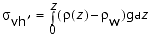 ,
,