Previous   |    Next

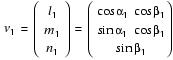
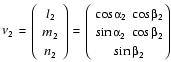
doi:10.2204/iodp.proc.334.102.2012

Structural geology

Our methods for documenting the structural geology of Expedition 334 cores largely followed those given by the Expeditions 315 and 316 structural geologists (Expedition 315 Scientists, 2009; Expedition 316 Scientists, 2009). We documented the deformation observed in the split cores by classifying structures, determining the depth extent, measuring orientation data, and recording kinematic information. The collected data were logged manually onto a printed form at the core table and then typed into both a spreadsheet and the DESClogik database. Where possible, the orientation data were also corrected for rotation related to drilling on the basis of paleomagnetic declination and inclination information.

Structural data acquisition and orientation measurements

Each structure was recorded manually on a description table sheet modified from that used during Expedition 316 (Fig. F4). Core measurements followed those made during Expeditions 315 and 316, which in turn were based on previous Ocean Drilling Program (ODP) procedures developed at the Nankai accretionary margin (i.e., ODP Legs 131 and 190). We used a plastic protractor for orientation measurements (Fig. F5). Using the working half of the split core provided greater flexibility in removing—and cutting, if necessary—pieces of the core for measurements.

Orientations of planar and linear features in cored materials were determined relative to the core axis, which represents the vertical axis in the core reference frame, and the “double line” marked on the working half of the split core liner, which represents 0° (and 360°) in the plane perpendicular to the core axis (Fig. F6). To determine the orientation of a planar structural element, two apparent dips of this element were measured in the core reference frame and converted to a plane represented by dip angle and either a strike or dip direction (Fig. F7). One apparent dip is usually represented by the intersection of the planar feature with the split face of the core and it is quantified by measuring the dip direction and angle in the core reference frame (in β₁; Fig. F8). Typical apparent dip measurements have a trend of 90° or 270° and range in plunge from 0° to 90°. The second apparent dip is usually represented by the intersection of the planar feature and a cut or fractured surface at a high angle to the split face of the core. In most cases, this was a surface either parallel or perpendicular to the core axis. In the former cases, the apparent dip lineation trended 000° or 180° and plunged from 0° to 90°; in the latter cases, the trend ranged from 000° to 360° and plunged 0°. Linear features observed in the cores were always associated with planar structures (e.g., striations on faults), and their orientations were determined by measuring either the rake (or pitch) on the associated plane or the trend and plunge in the core reference frame. During Expedition 334, we measured rake for striations on fault surface and azimuth and plunge for other lineation (e.g., fold axes). All data were recorded on the log sheet with appropriate depths and descriptive information.

Paleomagnetic correction

Paleomagnetic data were used during Expedition 334 to restore the structural data with respect to the geographic reference system (Fig. F7). Especially in the XCB and RCB intervals at Sites U1378–U1380, drilling-induced biscuiting of the cores and individual rotation of each core biscuit requires paleomagnetic reorientation to make the structural data usable. Given the cores taken by the APC are continuous, we can use the orientation data from discrete paleomagnetic samples or from the orientation tool attached to the APC to restore all structural data collected from the same core. In the XCB and RCB intervals, we have to take discrete samples for paleomagnetic correction because of rotation of each biscuit. We therefore recorded “coherent intervals for paleomagnetic correction” (i.e., intact and undisturbed intervals without internal biscuiting) when we identified structures. We collected paleomagnetic measurement samples from the same coherent core piece in which structures were measured. After the paleomagnetic measurements, we reoriented the structural data using the declination of the characteristic remanence of magnetization (see “Paleomagnetism”).

Description and classification of structures

We made a structural geology template for DESClogik and described and classified the structures observed. For clarity, we defined the terminology used to describe fault-related rocks, as well as the basis for differentiating natural structures from drilling-induced features.

Faults were classified into several categories based on the sense of fault slip and their structural characteristics. The sense of the fault slip was identified using offsets of markers (e.g., bedding and older faults) across the fault plane and predominantly by slickensteps. A fault with cohesiveness across the fault was described as a healed fault. Zones of dense fracture distribution and intense deformation were termed “brecciated zones” and “fractured zones.” Here, fractured zones are moderately deformed zones with decimeter-size fragments; brecciated zones are intensively deformed zones with centimeter-size and smaller fragments, containing a few larger fragments.

In basement rocks, igneous rocks and tectonic mélanges were expected corresponding to the onshore geological map of Osa Peninsula. Whereas lithology and mineralogy of the vein minerals were described by the petrologists, orientations of the veins, foliations, and other structural features in the igneous rocks were measured by the structural geologists.

Natural structures can be strongly disturbed by drilling-induced disturbances such as flow-in structures in APC cores and biscuiting, fracturing, faulting, and rotation of fragments in XCB and RCB cores. If structures were disturbed by flow-in >60% of the cross section of the core, we excluded measurements because of the intense disturbance (bending, rotation, etc.) of these structures. To correct for the possible rotations of the fault orientation caused by coring, we used paleomagnetic data. Helicoidal striated surfaces or polished surfaces showing striations that diverge outward most likely indicated drilling-induced faults/fractures resulting from the torque exerted by the bit on the drilled material. In contrast, faults that display more planar geometry, parallel striations, and orientations compatible with multiple faults nearby (i.e., defining a system) are likely to be natural. When multiple orientation measurements were plotted in stereographic projection, natural faults were expected to display preferred orientations (i.e., strike and dip) that may be related to coherent tectonic stress orientations, whereas drilling-induced faults/fractures were expected to yield random orientation distributions.

Calculation of plane orientation

For planar structures (e.g., bedding or faults), two apparent dips on two different surfaces (e.g., one being the split core surface, which is east–west vertical, and the other being the horizontal or north–south vertical surface) were measured in the core reference frame as azimuths (measured clockwise from north, looking down) and plunges (Figs. F6, F7, F8). A coordinate system was defined in such a way that the positive x-, y-, and z-directions coincide with north, east, and vertical downward, respectively. If the azimuths and plunges of the two apparent dips are given as (α₁, β₁) and (α₂, β₂), respectively, as in Figure F8, then the unit vectors representing these two lines, v₁ and v₂, are

and

.

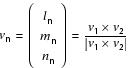
The unit vector normal to the plane, v_n (Fig. F8), is then defined as

,

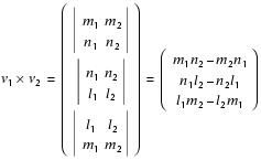
where

.

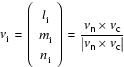
The azimuth, α_n, and plunge, β_n, of v_n are given by

.

The dip direction, α_d, and dip angle, β, of this plane are α_n and 90° + β_n, respectively, when β_n < 0° (Fig. F9A). They are α_n ± 180° and 90° – β_n, respectively, when β_n ≥ 0° (Fig. F9B). The right-hand rule strike of this plane, α_s, is then given by α_d – 90°.

Calculation of slickenline rake

For a fault with striations, the apparent rake angle of the striation, ϕ_a, was measured on the fault surface from either the 90° or 270° direction of the split-core surface trace (Figs. F7, F10). Fault orientation was measured as described above. Provided that v_n and v_c are unit vectors normal to the fault and split core surfaces, respectively, the unit vector of the intersection line, vi, is perpendicular to both v_n and v_c (Fig. F10) and is therefore defined as

,

where

and

.

Knowing the right-hand rule strike of the fault plane, αs, the unit vector, vs, toward this direction is then

.

The rake angle of the intersection line, ϕ_i, measured from the strike direction is given by

because

The rake angle of the striation, ϕ, from the strike direction is ϕ_i ± ϕ_a, depending on which direction the apparent rake was measured from and which direction the fault plane dips toward. ϕ_a should be subtracted from ϕ_i when the fault plane dips toward west and ϕ_a was measured from either the top or 90° direction (Fig. F11A) or when the fault plane dips toward east and ϕ_a was measured from either the bottom or 90° direction (Fig. F11B). On the other hand, ϕ_a should be added to ϕ_i when the fault plane dips toward east and ϕ_a was measured from either the top or 270° direction (Fig. F11C) or when the fault plane dips toward west and ϕ_a was measured from either the bottom or 270° direction (Fig. F11D).

Azimuth correction using paleomagnetic data

Provided that a core is vertical, its magnetization is primary, and its bedding is horizontal, its paleomagnetic declination (α_p) indicates magnetic north when inclination (β_p) ≥ 0° (Figs. F7, F12A), whereas α_p indicates magnetic south when β_p < 0° (Fig. F12B). The dip direction and strike of a plane in the geographic reference frame, α_d* and α_s*, are therefore

and

when

and are

and

when

If the core was complete and continuous, one paleomagnetism sample per section (1.5 m) was deemed sufficient. If the core was discontinuous, then each part of the core that was continuous and structurally important had to contain a paleomagnetism sample. The paleomagnetism samples were taken as cubic or cylindrical samples close to the measured structures (usually within 5 cm) and from a coherent interval that included the structure. Core fragments which were so small that a spin around an axis significantly deviating from the core axis were avoided (e.g., brecciated fragments).

DESClogik structural database

The DESClogik database represents a program to store a visual (macroscopic and/or microscopic) description of core structures at a given section index. During this expedition, only the locations of structural features, raw data collected from cores, calculated orientations in the core coordinate, and restored orientation based on the paleomagnetic data were input into DESClogik, and orientation data management and planar and linear fabric analysis were done with a spreadsheet as mentioned above.

Top of page   |    Previous   |    Next