Clemens, S.C., Kuhnt, W., LeVay, L.J., and the Expedition 353 Scientists
Proceedings of the International Ocean Discovery Program Volume 353
publications.iodp.org
doi:10.14379/iodp.proc.353.108.2016

Site U14481
S.C. Clemens, W. Kuhnt, L.J. LeVay, P. Anand, T. Ando, M. Bartol, C.T. Bolton, X. Ding, K. Gariboldi, L. Giosan, E.C. Hathorne, Y. Huang, P. Jaiswal, S. Kim, J.B. Kirkpatrick, K. Littler, G. Marino, P. Martinez, D. Naik, A. Peketi, S.C. Phillips, M.M. Robinson, O.E. Romero, N. Sagar, K.B. Taladay, S.N. Taylor, K. Thirumalai, G. Uramoto, Y. Usui, J. Wang, M. Yamamoto, and L. Zhou2
Keywords: International Ocean Discovery Program, IODP, Expedition 353, JOIDES Resolution, Site U1448, Indian monsoon, monsoon, Bay of Bengal, Andaman Sea, paleoclimate, paleoceanography, Miocene, Pliocene, Pleistocene, Holocene, Ninetyeast Ridge, Indian Ocean, salinity, orbital, millennial, centennial, abrupt climate change
MS 353-108: Published 29 July 2016
Background and objectives
The Andaman Sea is situated between the Andaman Islands and the Malay Peninsula (Figure F1). The Andaman-Sumatra island arc system results from the oblique subduction of the Indo-Australian plate beneath the Eurasian plate (Singh et al., 2013). Stretching and rifting of the overriding plate during the early Miocene (~25 Ma) resulted in two distinct plates (Sunda and Burma) separated by an active spreading center (Curray, 1991, 2005) located in the deepest portion of the Andaman Sea. An accretionary wedge complex scraped off the subducting slab lies west of the spreading center, forming a series of shallower basins associated with backthrust faulting within the accreted sediments (Figure F2). The Andaman Sea drilling sites are within the Nicobar-Andaman Basin, bounded on either side by the Diligent and Eastern margin faults.
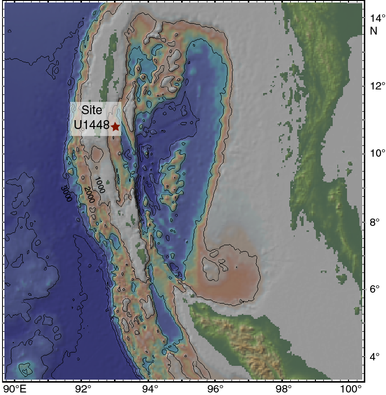
Figure F1. Andaman Sea map with location of Site U1448.
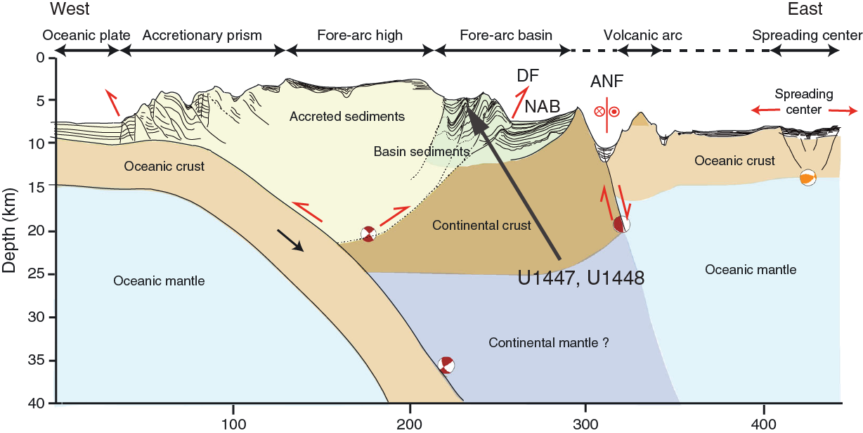
Figure F2. Summary sketch showing the subduction zone through the back-arc basin to ~40 km depth.
Runoff into the Andaman Sea is dominated by the Irrawaddy and Salween Rivers (Varkey et al., 1996), supplying a combined 30.8 × 10¹⁰ m3 of water during June, July, and August. Comparison with the winter (December, January, and February) discharge of 2.8 × 10¹⁰ m3 indicates strong seasonality with a dominance of summer (92%) over winter (8%) runoff. Terrigenous sediment supply to the Andaman Sea is dominantly from the Irrawaddy and Salween Rivers (Colin et al., 1999, 2006) with contributions from the Indo-Burman-Arakan mountain ranges as well as the Andaman Islands (Awasthi et al., 2014). However, by virtue of proximity, Little Andaman Island is likely a dominant source of terrigenous materials to International Ocean Discovery Program (IODP) Site U1448. Analysis of Andaman Sea surface sediments indicates that foraminifers are abundant and well preserved shallower than ~1800 meters below sea level (mbsl) (>100,000 individuals/g) and decrease to <100 individuals/g deeper than 3000 mbsl (Frerichs, 1971).
Site U1448 is located at 1091 mbsl, ~44 km offshore Little Andaman Island on a rise separating north-south–oriented basins associated with the Eastern margin and Diligent fault zones. Seismic sections (Figure F3) indicate ~420 m of sediments overlying an accretionary wedge complex. Sedimentation rates at Site NGHP-01-17 (Collett et al., 2008; Flores et al., 2014) suggest that this site should reach the late Miocene. Unlike IODP Site U1447, the elevated location of Site U1448 helps shield the site from turbidite deposition.

Figure F3. Seismic lines showing location of Site U1448.
The objective at this site is to recover Miocene to Holocene sediments from multiple holes in order to reconstruct changes in surface water salinity and runoff associated with summer monsoon rainfall at tectonic to suborbital timescales. Sites U1448 and U1447 constitute the middle (10°N) portion of a meridional salinity transect that includes sites on the northeast Indian margin (19°N) and is anchored by IODP Site U1443 at 5°N.
Operations
Site U1448 consisted of three holes (Table T1), ranging in depth from 34.3 to 421.0 m drilling depth below seafloor (DSF). Overall, 121 cores were recorded for the site. A total of 427.52 m of core over a 416.2 m cored interval was recovered using the advanced piston corer (APC) system (103% recovery). The cored interval with the half-length advanced piston corer (HLAPC) system was 318.6 m with a core recovery of 333.24 m (105%). The cored interval with the extended core barrel (XCB) system was 77.6 m with 78.21 m of core recovered (101%). The overall recovery percentage for Site U1448 was 103%. The total time spent on Site U1448 was 3.9 days.
Table T1. Site U1448 core summary. Download table in .csv format. View PDF table.
Transit to Site U1448
The 9.4 nmi transit from Site U1447 to U1448 was completed in dynamic positioning mode with much of the transit being completed while the drill pipe was being pulled. The vessel arrived at Site U1448 at 1845 h (UTC + 8 h) on 21 January 2015. A positioning beacon was deployed at 1916 h, and the vessel settled over the site coordinates.
Hole U1448A
Hole U1448A was spudded at 0010 h on 22 January 2015. Core 353-U1448A-1H was used to estimate the seafloor depth at 1098.3 mbsl. The APC system was used for Cores 1H through 23H. Core 23H had no core recovery and was reshot from the same depth. The HLAPC was deployed for Cores 24F through 52F. Cores 53X through 60X were cut with the XCB system. Downhole temperature measurements were attempted using the advanced piston corer temperature tool (APCT-3) shoe, but when it was deployed for Core 4H, the reading was bad. The Icefield MI-5 tool was used to obtain orientation data for Cores 3H through 23H. At the end of coring operations, the drill pipe was pulled from the hole and cleared the seafloor at 1830 h on 23 January.
A total of 23 APC cores were taken over a 204.2 m interval with a total core recovery of 210.99 m (103% core recovery). The HLAPC system was used for 29 cores over a cored interval of 139.2 m with 145.62 m recovered (105%). A total of 8 XCB cores were cut over a 77.6 m interval with 78.21 m of core recovered (101%). Total core recovery for Hole U1448A was 103%.
Hole U1448B
The vessel was offset 20 m south of Hole U1448A, and Hole U1448B was spudded at 2010 h on 23 January 2015. Cores 353-U1448B-1H through 19H were recovered using the APC system. Before switching to the HLAPC system, the hole was advanced 1.5 m without coring. The HLAPC was used for Cores 21F through 58F. Temperature measurements using the APCT-3 were taken on Cores 4H, 7H, 10H, and 15H. Cores 3H through 19H were oriented using the Icefield MI-5 tool. The drill string was then pulled from the hole and the bit cleared the seafloor at 0630 h on 25 January, ending Hole U1448B.
A total of 19 APC cores were taken over a 177.7 m interval with a total core recovery of 181.76 m (102% core recovery). The HLAPC system was used for 38 cores that were taken over a 179.4 m interval with 187.62 m of core recovered (105%). One drilled interval of 1.5 m (353-U1448B-201) was recorded for the hole. Total core recovery for Hole U1448B was 103%.
Hole U1448C
The vessel was offset 20 m west of Hole U1448B, and Hole U1448C was spudded at 0750 h on 25 January 2015. Cores 353-U1448C-1H through 4H were cored with the APC system to a total depth of 34.3 m DSF. The drill string was then pulled from the hole with the bit clearing the seafloor at 1000 h, and the rig was secured for transit to Singapore.
A total of four APC cores were taken over a 34.3 m cored interval with a total core recovery of 34.77 m (101% core recovery).
Transit to Loyang, Singapore
The vessel began transit to Singapore at 1542 h on 25 January 2015. The vessel arrived at the Singapore pilot station at 0811 h on 29 January 2015, after a 904 nmi transit, where Expedition 353 officially ended.
Lithostratigraphy
Sediments recovered from Holes U1448A–U1448C are principally composed of Late Pleistocene to middle Miocene hemipelagic sediments with a significant clay and biogenic component, comprising four distinct lithostratigraphic units (I–IV) (Figure F4). The observed lithologic differences between units are primarily the result of varying abundances of bioclastics (nannofossils, foraminifers, diatoms, and sponge spicules), clay, and glauconite (Figure F5). Unit I is 180 m thick and composed of Late to early Pleistocene greenish gray clay with varying proportions of nannofossils and foraminifers, as well as clayey nannofossil ooze. Unit II is 160 m thick and composed of early Pleistocene to late Miocene greenish clay with varying proportions of nannofossils and foraminifers and is characterized by low biosilica content (≤1%). Unit III is 40 m thick and composed of late Miocene greenish dark to light gray nannofossil-rich clay and clay with nannofossils, characterized by increased abundance of glauconite (up to 7%) and siliceous sponge spicules (up to 4%). A hiatus representing ~8 My occurs at the base of Unit III at 379.11 m core depth below seafloor, Method A (CSF-A), where there is an abrupt change in lithology that defines the top of Unit IV. Unit IV is composed of middle to early Miocene greenish gray to light greenish gray biosiliceous ooze with varying proportions of clay and nannofossils. Lithologic descriptions are based primarily on sediments recovered from Hole U1448A, supplemented with observations from Hole U1448B.
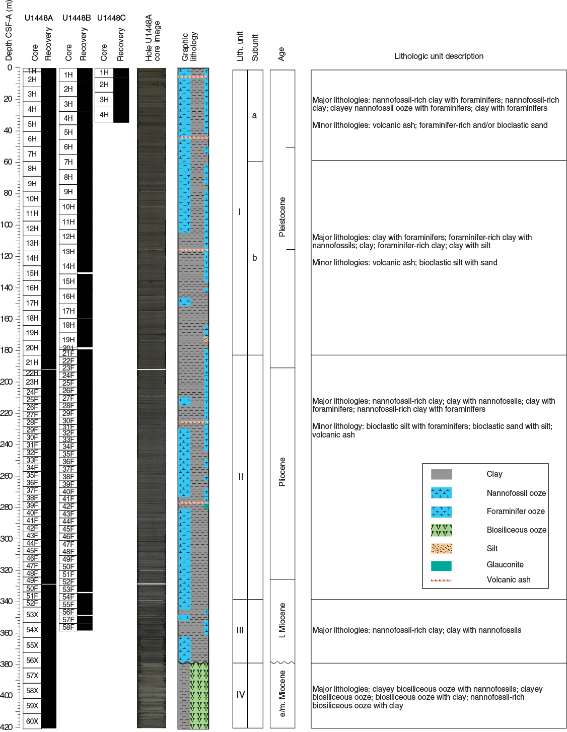
Figure F4. Lithostratigraphic summary, Site U1448.
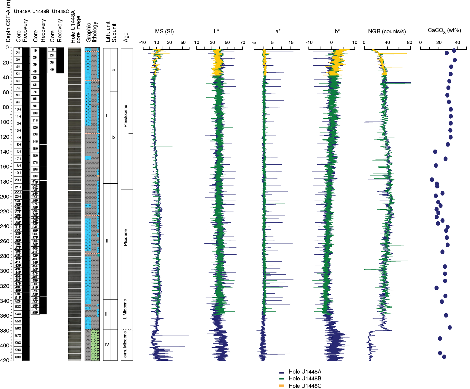
Figure F5. Lithostratigraphic summary with selected physical property and geochemical data from Holes U1448A–U1448C.
Unit I
- Intervals: 353-U1448A-1H-1, 0 cm, through 20H-CC, 29 cm; 353-U1448B-1H-1, 0 cm, through 21F-CC, 29 cm; 353-U1448C-1H-1, 0 cm, through 4H-CC, 17 cm
- Depths: Hole U1448A = 0–183.11 m CSF-A; Hole U1448B = 0–184.28 m CSF-A; Hole U1448C = 0–34.71 m CSF-A
- Age: early Pleistocene to Late Pleistocene
- Lithology: nannofossil-rich clay, clayey nannofossil ooze, foraminifer-rich clay, and clay
Unit I is a ~180 m thick succession of dark greenish gray to greenish gray (GLEY 1 4/10Y–6/10Y, GLEY 1 5GY series, and GLEY 1 10GY series) clay with varying proportions of nannofossils and foraminifers, as well as clayey nannofossil ooze (Figures F4, F6, F7, F8). Clay composes ~40%–60% of the sediment followed by calcareous nannofossils (20%–40%), foraminifers (10%–30%), and siliceous sponge spicules (up to 5%) (Figure F6). The proportion of clay increases downhole, reflected in the increasing natural gamma radiation (NGR) values (Figure F5) (see Physical properties). Turbidites and ash layers are rarely observed. The Unit I/II boundary is defined by changes in the proportion of nannofossils and biosilica (Figure F6). Unit I is divided into two subunits. Subunit Ib is distinguished from Subunit Ia by a decrease in nannofossils and increase in siliceous sponge spicules.
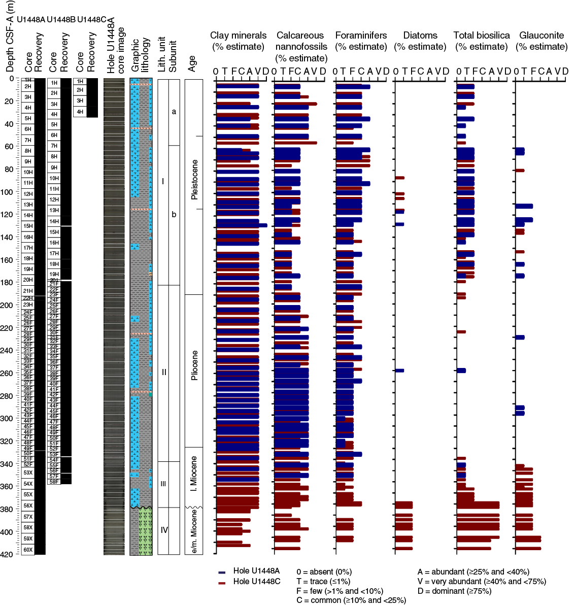
Figure F6. Smear slide data, Holes U1448A and U1448C.

Figure F7. Main lithologies, Site U1448. A. Nannofossil-rich clay with foraminifers. B. Foraminifer-rich clay. C. Nannofossil-rich clay with foraminifers. D. Clay with nannofossils. E. Clayey biosiliceous ooze.
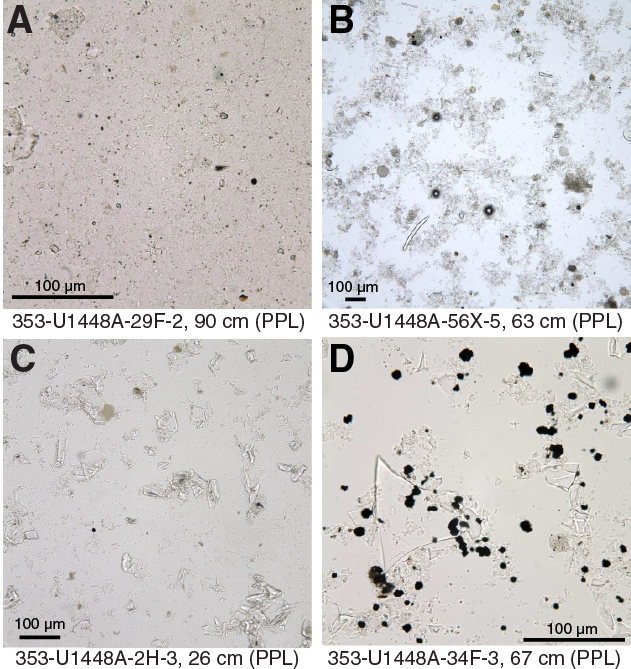
Figure F8. Lithologic types, Site U1448. A. Nannofossil-rich clay. B. Clayey biosiliceous ooze. C. Volcanic ash. D. Volcanic ash including iron sulfides.
Subunit Ia
- Intervals: 353-U1448A-1H-1, 0 cm, through 7H-CC, 25 cm; 353-U1448B-1H-1, 0 cm, through 7H-4, 147 cm; 353-U1448C-1H-1, 0 cm, through 4H-CC, 17 cm
- Depths: Hole U1448A = 0–59.78 m CSF-A; Hole U1448B = 0–60.99 m CSF-A; Hole U1448C = 0–34.71 m CSF-A
- Age: Late Pleistocene
- Major lithology: nannofossil-rich clay with foraminifers, nannofossil-rich clay, clayey nannofossil ooze with foraminifers, and clay with foraminifers
- Minor lithology: volcanic ash and foraminifer-rich and/or bioclastic sand
Subunit Ia is a ~60 m thick succession of light greenish gray (GLEY 1 5/10Y) nannofossil-rich clay with foraminifers, nannofossil-rich clay, clayey nannofossil ooze with foraminifers, and clay with foraminifers (Figures F4, F6, F7). Clays make up ~40%–60% of the sediment in Subunit Ia, followed by calcareous nannofossils (20%–40%), and foraminifers (~10%–20%) (Figure F6). Turbiditic beds composed of 2–7 cm thick bioclastic sands with normal grading are rarely observed. Two thick vitric ash layers are present in sediments from Subunit Ia (Figure F8). A light gray ash at 5.85–6.09 m CSF-A in Hole U1448A, 5.53–6.09 m CSF-A in Hole U1448B, and 5.71–5.83 m CSF-A in Hole U1448C is likely associated with the Toba eruption during the Late Pleistocene (Figures F8C, F9A). Some dark gray blebs and nodules of iron sulfides are observed. Drilling disturbance is minor with occasional horizontal cracks, fall-in, and soupy textures.
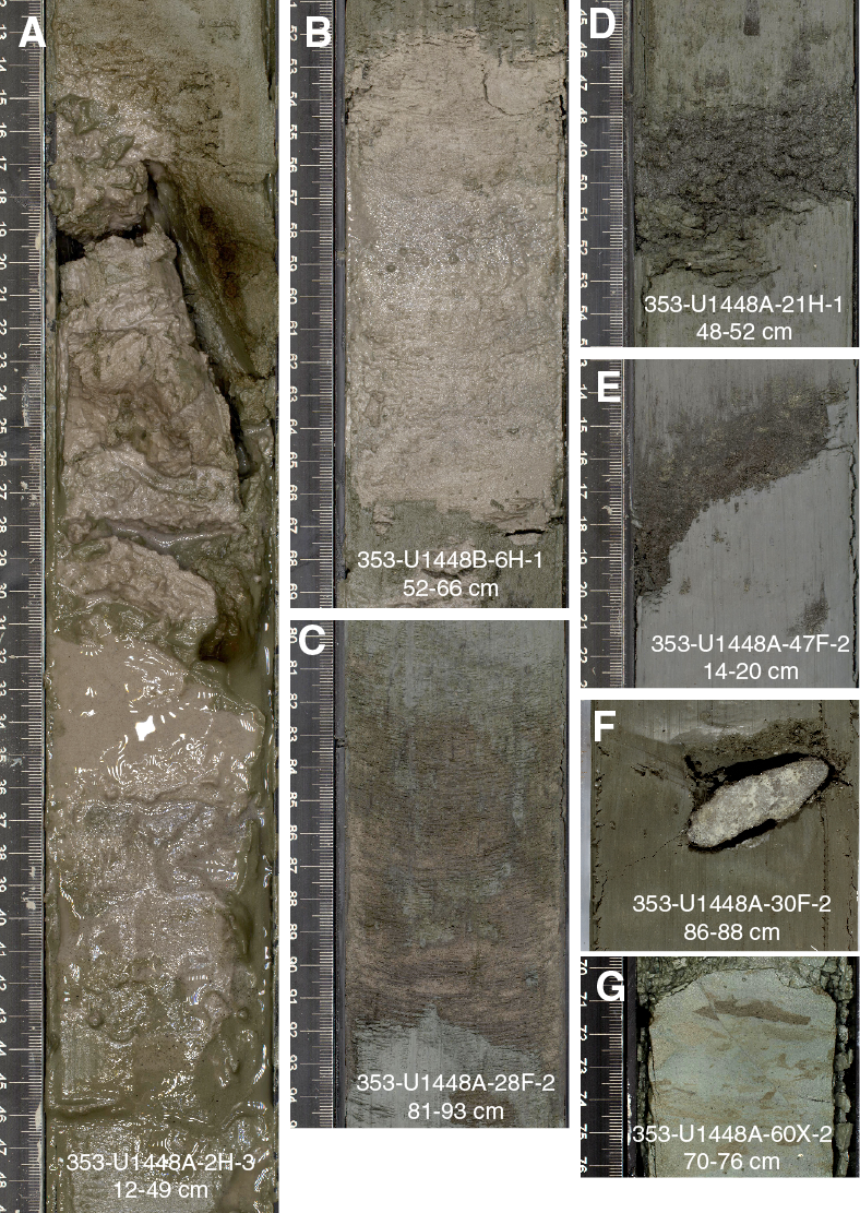
Figure F9. Minor lithologies, Site U1448. A. Volcanic ash. B. Light gray volcanic ash, Subunit Ia. C. Pinkish gray volcanic ash. D. Thin turbidite. E. Very thin turbidite. F. Pyrite nodule. G. Microfault.
Subunit Ib
- Intervals: 353-U1448A-8H-1, 0 cm, through 20H-CC, 29 cm; 353-U1448B-7H-5, 0 cm, through 21F-CC, 29 cm
- Depths: Hole U1448A = 59.78–183.11 m CSF-A; Hole U1448B = 60.99–184.28 m CSF-A
- Age: early Pleistocene to Middle Pleistocene
- Major lithology: clay with foraminifers, foraminifer-rich clay with nannofossils, clay, foraminifer-rich clay, and clay with silt
- Minor lithology: volcanic ash and bioclastic silt with sand
Subunit Ib is a ~120 m thick succession of dark greenish gray to greenish gray (GLEY 1 4/10Y–6/10Y, GLEY 1 5GY series, and GLEY 1 10GY series) nannofossil-rich clay with foraminifers, nannofossil-rich clay, clayey nannofossil ooze with foraminifers, and clay with foraminifers (Figures F4, F5, F6, F7). Clays compose ~40%–60% of Subunit Ib, followed by calcareous nannofossils (20%–40%), foraminifers (~10%–20%), and siliceous sponge spicules (up to 5%). Proportions of foraminifers show a gradual decrease from ~30% to ~10% through this unit, with calcareous nannofossils showing a similar decline (Figure F6). A 0.5 cm thick turbidite and a 3 cm thick ash layer are observed, as well as some dark gray blebs and nodules of iron sulfides. Punctures caused by a deformed liner are the only minor drilling disturbance.
Unit II
- Intervals: 353-U1448A-21H-1, 0 cm, through 51F-CC, 21 cm; 353-U1448B-22F-1, 0 cm, through 55F-CC, 23 cm
- Depths: Hole U1448A = 183.11–338.60 m CSF-A; Hole U1448B = 184.28–344.55 m CSF-A
- Age: late Miocene to late Pliocene
- Major lithology: nannofossil-rich clay, clay with nannofossils, clay with foraminifers, and nannofossil-rich clay with foraminifers
- Minor lithology: bioclastic silt with foraminifers, bioclastic sand with silt, and volcanic ash
Unit II is a ~160 m thick succession of greenish gray (GLEY 1 4/10Y–6/10Y, GLEY 1 5GY series, and GLEY 1 10GY series) nannofossil-rich clay, clay with nannofossils, clay with foraminifers, and nannofossil-rich clay with foraminifers (Figures F7, F8). Clay composes ~50%–70% of the sediment followed by calcareous nannofossils (10%–30%) and foraminifers (up to 18%) (Figure F6). The sediments are low in biosilica (≤1%) and are dominated by diatoms (Figure F6). Proportions of nannofossils show a gradual increase downcore from ~10% to ~30% in the upper 100 m interval of this unit. Beds of bioclastic silt, 1.5–6 cm thick, with normal grading are rarely observed and are likely turbidites. Ash layers are rare, but a ~12 cm thick pinkish gray (7.5YR 7/2) ash is observed at 225.71–225.83 m CSF-A in Hole U1448A and 228.00–228.125 m CSF-A in Hole U1448B. Centimeter-scale pyrite nodules and pyritized wood fragments are observed. The Unit II/III boundary is defined by changes in color and biosilica content. Drilling disturbance is minor with occasional horizontal cracks, fragmented textures, and fall-in within Unit II.
Unit III
- Intervals: 353-U1448A-52F-1, 0 cm, through 56X-5, 60 cm; 353-U1448B-56F-1, 0 cm, through 58F-CC, 8 cm
- Depths: Hole U1448A = 338.60–379.11 m CSF-A; Hole U1448B = 344.55–358.22 m CSF-A
- Age: late Miocene
- Major lithology: nannofossil-rich clay and clay with nannofossils
Unit III is a ~40 m thick succession of dark to light greenish gray (GLEY 1 4/10Y–7/10Y, GLEY 1 5GY series, and GLEY 1 10GY series) nannofossil-rich clay and clay with nannofossils (Figure F7). Clay makes up ~50%–70% of the sediment followed by calcareous nannofossils (10%–30%) (Figure F6). Increases in the proportions of glauconite (up to 7%) and siliceous sponge spicules (up to 4%) are observed. Bioturbation as indicated by burrows and mottled patches are observed throughout Unit III. Turbidites and ash layers are not present. Millimeter-scale dark greenish gray clasts are observed in the lower part of this unit (376.15–378.97 m CSF-A) (Figure F10A–F10B). At of the bottom of Unit III (378.97–379.11 m CSF-A) (Figure F10C), dark greenish gray pyrite and glauconite nodules ranging from millimeter to centimeter scale are present. The bottom of this unit is marked by a ~8 My hiatus during the Miocene (see Biostratigraphy). The Unit III/IV boundary is defined by changes in color and lithology and is characterized by a sharp and inclined contact (Figure F10C). This lithostratigraphic boundary is also clearly visible in physical property data, illustrated by a subtle rise in magnetic susceptibility (MS) values, a sharp fall in NGR values (Figure F5), and concurrent changes in the gamma ray attenuation (GRA) and moisture and density (MAD) trends (see Physical properties). The hiatus boundary is characterized by bioturbation with smear slide and thin section observations showing burrows in Unit IV filled with nannofossil-rich clay from Unit III. Slight drilling disturbance is present in Unit III as biscuiting.
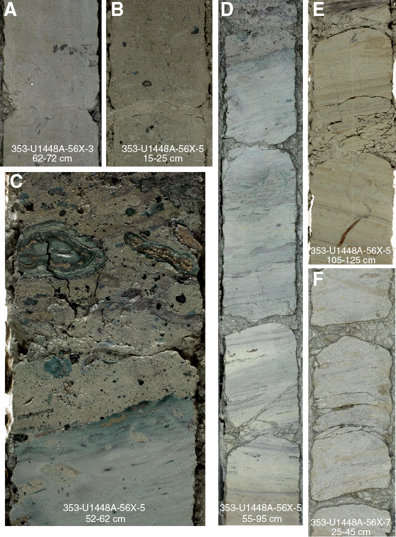
Figure F10. Miocene hiatus interval near the Unit III/IV boundary, Hole U1448A. A. Nannofossil-rich clay. B. Clay with nannofossils. C. Inclined boundary between Unit III and Unit IV. D. Clayey biosiliceous ooze. E. Nannofossil-rich biosiliceous ooze. F. Clayey biosiliceous ooze with nannofossils.
Unit IV
- Interval: 353-U1448A-56X-5, 60 cm, through 60X-CC, 41 cm
- Depth: Hole U1448A = 379.11–420.60 m CSF-A
- Age: early to middle Miocene
- Major lithology: clayey biosiliceous ooze with nannofossils, clayey biosiliceous ooze, biosiliceous ooze with clay, and nannofossil-rich biosiliceous ooze with clay
Unit IV is a ~40 m thick succession of greenish gray to light greenish gray (GLEY 1 6/10Y–7/10GY and GLEY 1 5GY series) clayey biosiliceous ooze with nannofossils, clayey biosiliceous ooze, biosiliceous ooze with clay, and nannofossil-rich biosiliceous ooze with clay (Figures F7, F8). Smear slide observations indicate a substantial increase in biosilica and concurrent decrease in lithogenic grains relative to Unit III (Figure F6). Biosilica, dominated by diatoms, makes up ~40%–60% of the sediment, followed by clay (20%–40%), calcareous nannofossils (10%–30%), and glauconite (up to 15%) (Figure F6). Turbidites and ash layers are not present in Unit IV. The lithology of the uppermost ~30 cm interval of this unit (379.11–379.43 m CSF-A) shows light greenish gray (5G 7/1) clayey biosiliceous ooze and is characterized by abundant laminations (Figure F10D). In the underlying interval, the lithology gradationally changes to greenish gray (GLEY 1 6/10Y) biosiliceous ooze with varying proportions of clay and nannofossils. Bioturbation is present as indicated by burrows and mottled patches. Occasional laminations are visible and offset by microfaults (Figures F9G, F10E–F10F). Drilling disturbance is present as moderate to severe biscuiting.
Biostratigraphy
Calcareous nannofossils are abundant (50%–90% of sediment particles) throughout Hole U1448A, and their preservation is very good in the Pleistocene, Pliocene, and latest Miocene sediment sections (0–379.1 m CSF-A). A hiatus was observed at 379.11 m CSF‑A, below which nannofossils are still abundant and moderately well preserved. The composition of assemblages allowed sediments between the hiatus and the bottom of Hole U1448A (420.6 m CSF‑A) to be assigned a middle Miocene age. Foraminifers are well preserved in all core catcher samples from Hole U1448A. Foraminifers are dominant in the upper 340 m CSF-A. Abundance decreases to common just above the hiatus and drops to few to common below the hiatus. Diatoms are rarely present in the uppermost 379.04 m of Hole U1448A. They are abundant just below the hiatus, and their preservation varies from moderate to good.
The age model for Site U1448 was established by combining calcareous nannofossil, planktonic foraminifer, and diatom datums (the latter below the hiatus only). The oldest calcareous nannofossil sample studied above the hiatus (Sample 353-U1448A-56X-5W, 59 cm) contained both Discoaster quinqueramus and Reticulofenestra rotaria, suggesting an age between 5.94 and 6.91 Ma. The core catcher sample immediately below the hiatus (Sample 56X-CC) was older than 14.91 Ma based on calcareous nannofossils. Planktonic foraminifer datums suggest that the age of the oldest core catcher sample above the hiatus (Sample 55X-CC) is between 5.92 and 8.58 Ma and the age of the youngest core catcher sample below the hiatus (56X-CC) is older than 14.53 Ma. The oldest planktonic foraminifer datum encountered is the last occurrence (LO) of Praeorbulina glomerosa (14.78 Ma) in Sample 59X-CC. P. glomerosa is found in the deepest sample (60X-CC), defining the basal age of Hole U1448A as 14.78 to 16.27 Ma. The co-occurrence of the diatom species Rhaphidodiscus marylandicus and Annellus californicus in the lowermost part of Hole U1448A suggests that the bottom of Hole U1448A is older than 16.7 Ma (LO of R. marylandicus) and younger than 17.3 Ma (first occurrence [FO] of A. californicus).
Calcareous nannofossils
Calcareous nannofossils were examined in all core catcher samples from Hole U1448A. Additional split core samples from Hole U1448A were examined to refine the depth of biostratigraphic datums once they were defined between two core catcher samples. Semiquantitative species abundance estimates for all core catcher samples are shown in Table T2. Pleistocene to late Miocene nannofossil assemblages are typical of tropical/subtropical paleoenvironments and include common to abundant Florisphaera profunda, Gephyrocapsa spp., Reticulofenestra spp., Sphenolithus spp., Discoaster spp., Helicosphaera spp., Calcidiscus spp., and Umbilicosphaera spp. in Samples 353-U1448A-1H-CC through 56X-5W, 59 cm. Samples between 56X-5W, 61 cm, and 60X-CC contain common to abundant Helicosphaera spp., Sphenolithus heteromorphus, Discoaster spp., Coccolithus spp., and Umbilicosphaera spp. and few to common Cyclicargolithus floridanus. We were therefore able to construct a relatively high-resolution stratigraphy using nannofossils (Table T3; Figure F11). Reworked nannofossil specimens are few to rare (Table T2).
Table T2. Semiquantitative calcareous nannofossils abundance counts from core catcher samples, Hole U1448A. Download table in .csv format.
Table T3. Calcareous nannofossil datums, Hole U1448A. Download table in .csv format.
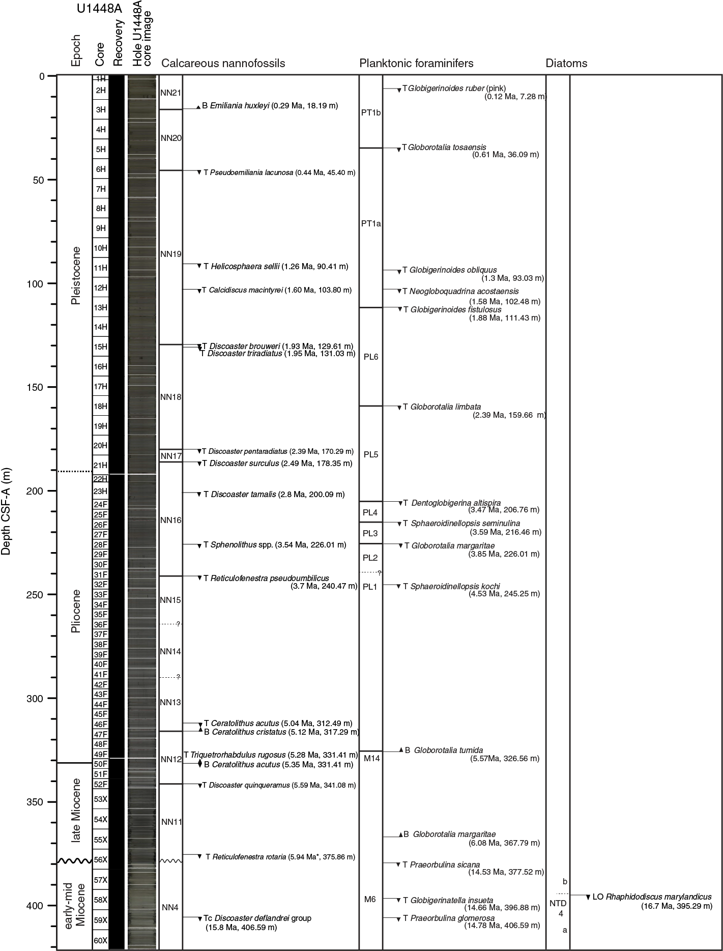
Figure F11. Summary of biostratigraphic events identified in Hole U1448A.
Pliocene–Pleistocene
Well to very well preserved calcareous nannofossils are present throughout the Pleistocene (0 to ~190 m CSF-A) and Pliocene (~190–330 m CSF-A) sedimentary section of Hole U1448A. All Pleistocene marker species defined by Martini (1971) and Okada and Bukry (1980) were found (Table T3) (see Biostratigraphy in the Expedition 353 methods chapter [Clemens et al., 2016a] for zonal schemes used; all ages cited in the text and figures are those of Gradstein et al., 2012). Emiliania huxleyi, which delineates the base of Zone NN21 (0.29 Ma), is present in Sample 353-U1448A-3H-2W, 140 cm (14.8 m CSF-A), and all shallower samples studied based on shipboard scanning electron microscope work. The onset of dominance of E. huxleyi among the Noelaerhabdaceae could not be reliably determined because of the presence of various different small Noelaerhabdaceae species in the Late Pleistocene.
The LO of Pseudoemiliania lacunosa, dated at 0.44 Ma, occurs between Samples 353-U1448A-5H-CC and 6H-CC (midpoint depth = 45.40 m CSF-A). Reticulofenestra asanoi is present only in Sample 7H-CC. Large Gephyrocapsa (>5.5 µm) were of no biostratigraphic value at Site U1448 because of their rare and sporadic occurrences. Well-defined Pleistocene events at Site U1448 are the FOs of Helicosphaera sellii, Calcidiscus macintyrei, Discoaster brouweri, Discoaster triradiatus, Discoaster pentaradiatus, and Discoaster surculus (Table T3; Figure F11). We note that in Hole U1448A, D. triradiatus is rare where present; therefore, limited confidence can be placed in the exact depth of its LO at 1.95 Ma.
The Pliocene/Pleistocene boundary (2.59 Ma) is placed below the LO of D. pentaradiatus (2.39 Ma) between Samples 353-U1448A-19H-3W, 5 cm, and 19H-CC (midpoint depth = 170.29 m CSF-A) and above the LO of Discoaster tamalis (2.8 Ma) between Samples 22H-CC and 23H-CC. The LO of Sphenolithus species (3.54 Ma) occurs between Samples 27F-CC and 28F-CC (midpoint depth = 226.01 m CSF-A). Reticulofenestra pseudoumbilicus (>7 µm) was found in Sample 31F-CC (242.845 m CSF-A) and deeper. Discoaster asymmetricus was almost entirely absent from the Site U1448 assemblage. The LO of Ceratolithus acutus (5.04 Ma) occurs between Samples 45F-CC and 46F-CC (midpoint depth = 312.49 m CSF-A), whereas the FO of Ceratolithus cristatus (5.12 Ma, named Ceratolithus rugosus in Gradstein et al., 2012) occurs between Samples 46F-CC and 47F-CC (midpoint depth = 317.29 m CSF-A).
Miocene
The Miocene/Pliocene boundary (5.33 Ma) occurs between Samples 353-U1448A-50F-CC and 51F-CC (324.245 and 338.58 m CSF-A) based on the LO of Triquetrorhabdulus rugosus (5.28 Ma) and the FO of C. acutus (5.35 Ma) in this interval. The LO of D. quinqueramus (5.59 Ma) occurs between Samples 51F-CC and 52F-CC. A hiatus comprising the early late and late middle Miocene was observed in Sample 56X-5W, 60 cm, at 379.11 m CSF-A. R. rotaria, which occurs in Subzone CN9c/NN11c (Bown, 1998; 5.94–6.91 Ma based on the calibrated ages of Gradstein et al., 2012), was very rare in Sample 56X-3W, 50 cm, and rare in Sample 56X-5W, 59 cm (immediately above the hiatus); therefore, its LO can be placed just above the hiatus. This allows the oldest sediments recovered above the hiatus to be assigned to an interval between 5.94 and 6.91 Ma. Below the hiatus, all samples studied contained marker species S. heteromorphus (13.53–17.71 Ma) and Helicosphaera ampliaperta (>14.91 Ma). Discoaster deflandrei increased in abundance downcore from few to common between Samples 58X-CC and 59X-CC, and this likely represents the top common (Tc) D. deflandrei group event (15.8 Ma). No Discoaster signus (LO at 15.85 Ma) were unambiguously identified. Thus, we are able to constrain the age range of this middle–late Miocene section to 14.91–17.71 Ma based on nannofossils.
Planktonic foraminifers
Planktonic foraminifer biostratigraphy of the Pleistocene to Miocene section at Site U1448 was based on the shipboard study of core catcher samples from Hole U1448A with the addition of a single sample from Section 353-U1448A-13H-7, where a core catcher was not available. The distribution of planktonic foraminifers in Hole U1448A is shown in Table T4. The absolute ages assigned to biostratigraphic datums listed in Table T5 follow the references given in Table T2 in the Expedition 353 methods chapter (Clemens et al., 2016a).
Table T4. Semiquantitative planktonic foraminifer abundance counts from core catcher samples, Hole U1448A. Download table in .csv format.
Table T5. Planktonic foraminifer datums, Hole U1448A. Download table in .csv format.
Planktonic foraminifer percentages are consistently high (mean = 93.9%) in the Pliocene–Pleistocene with total foraminifers averaging >17,000 per 10 cm3 of raw sediment. Planktonic foraminifer percentages are more variable in the Miocene, with the lowest value immediately above the hiatus. Total foraminifer numbers decrease dramatically beneath the hiatus. The planktonic/benthic ratio, reported as percentage planktonic foraminifers of the total foraminifer population, and the number of benthic foraminifers and total foraminifers found in a 10 cm3 sample are based on examination of the >150 µm size fraction of core catcher samples.
Pleistocene
Pleistocene planktonic foraminifer assemblages were recovered from Samples 353-U1448A-1H-CC through 23H-CC (2.43–204.30 m CSF-A). Foraminifers are dominant and very well preserved in all Pleistocene samples. Planktonic assemblages are dominated by the tropical to warm subtropical species Globigerinoides ruber, Neogloboquadrina dutertrei, Globigerinoides sacculifer, Pulleniatina obliquiloculata, and Globigerinoides trilobus. Neogloboquadrina pachyderma (dextral), Orbulina universa, Globigerinita glutinata, and Globigerina bulloides are significant and consistent contributors to the assemblage.
The LO of G. ruber (pink) in Sample 353-U1448A-2H-CC (12.12 m CSF-A) places these sediments in Zone PT1b. The top of Zone PT1a is located at the LO of Globorotalia tosaensis in Sample 5H-CC (40.75 m CSF-A). The LOs of Globigerinoides obliquus in Sample 11H-CC (97.75 m CSF-A), Neogloboquadrina acostaensis in Sample 12H-CC (107.22 m CSF-A), and Globigerinoides fistulosus in Sample 13H-7 (115.64 m CSF-A) define Zone PT1a. The LO of Globorotalia limbata in Sample 18H-CC (164.37 m CSF-A) is located in Zone PL5.
Pliocene
Pliocene planktonic foraminifer assemblages were recovered from Samples 353-U1448A-24H-CC through 48F-CC (209.23–324.58 m CSF-A). Foraminifers are dominant and well preserved in all Pliocene samples. G. sacculifer, Globigerinoides extremus, Dentoglobigerina altispira, G. obliquus, G. trilobus, and N. dutertrei dominate Pliocene samples. G. ruber does not appear in any sample deeper than 240 m CSF-A.
The LO of D. altispira in Sample 353-U1448A-24F-CC (208.23 m CSF-A) defines the upper boundary of Zone PL4. The LO of Sphaeroidinellopsis seminulina in Sample 26F-CC (218.84 m CSF‑A) marks top of Zone PL3. The upper boundary of Zone PL2 is marked by the LO of Globorotalia margaritae in Sample 28F-CC (228.39 m CSF-A), and the LO of Sphaeroidinellopsis kochi in Sample 32F-CC (247.66 m CSF-A) marks the top of Zone PL1.
Miocene
Samples 353-U1448A-49F-CC through 60X-CC (328.54–420.58 m CSF-A) contain Miocene sediments. A hiatus exists between Samples 55X-CC and 56X-CC that may represent up to 8.6 My. Foraminifer abundance decreases with depth to common or few below the hiatus. Preservation is good throughout the Miocene. The planktonic foraminifer assemblage is dominated by G. extremus, G. trilobus, D. altispira, and G. obliquus above the hiatus, with consistent contributions from G. sacculifer and Globoturborotalita woodi, and contributions by Globigerinoides subquadratus, Globigerinoides immaturus, and Praeorbulina sicana below the hiatus.
The FO of Globorotalia tumida in Sample 353-U1448A-48F-CC (324.58 m CSF-A) identifies the top of Zone M14. The FO of G. margaritae in Sample 54X-CC (362.96 m CSF-A) identifies the samples immediately above the hiatus as falling within Zone M14. Below the hiatus, the LOs of P. sicana and Globigerinatella insueta in Samples 56X-CC (382.22 m CSF-A) and 58X-CC (401.79 m CSF-A), respectively, place these sediments in Zone M6. Zones M7–M13 are missing from the sedimentary record. P. glomerosa is found in Sample 60X-CC, suggesting that the basal age of Hole U1448A is between 14.78 and 16.27 Ma.
Diatoms
In order to define the sediment age and paleoenvironmental conditions, core catcher samples and samples from selected split core sections from Hole U1448A were investigated (Table T6). The sampling resolution deeper than Sample 353-U1448A-55X-CC was high, with the number of samples varying from 7 to 9 per core.
Table T6. Semiquantitative diatom abundance counts from core catcher and split core samples, Site U1448. Download table in .csv format.
Diatom distribution in Hole U1448A is shown in Table T6. The absolute ages assigned to biostratigraphic datums listed in Table T7 follow the references given in Table T3 in the Expedition 353 methods chapter (Clemens et al., 2016a). Figure F12 shows the age/depth of Site U1448 (also shown are nannofossils and foraminifer datums).
Table T7. Diatom datums, Site U1448. Download table in .csv format.
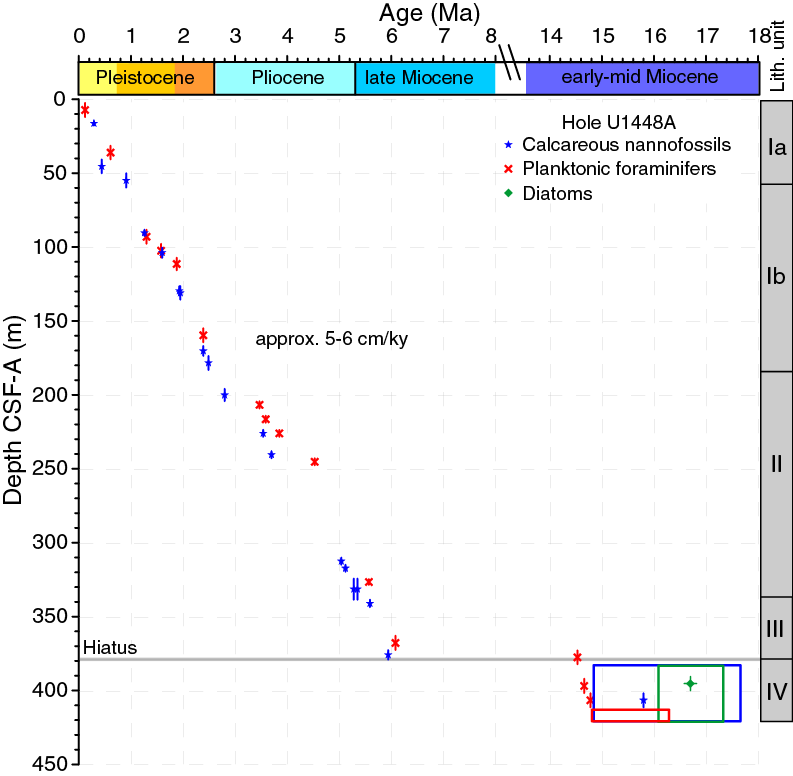
Figure F12. Biostratigraphic- and magnetostratigraphic-based age-depth plot, Hole U1448A.
Diatom biostratigraphy
The prehiatus interval is characterized by many diatom species of common occurrence during the middle Miocene (Coscinodiscus lewisianus, Cestodiscus pulchellus, Cestodiscus pulchellus var. maculatus, Cestodiscus robustus, Nitzschia maleinterpretaria, Thalassiosira fraga, A. californicus, Rossiella paleacea, Cestodiscus peplum, and R. marylandicus). Among early and middle Miocene diatom bioevents (see Figure F4B in the Expedition 353 methods chapter [Clemens et al., 2016a]), only the LO of R. marylandicus (16.7 Ma) was well defined between Samples 353-U1448A-58X-5W, 81 cm, and 57X-CC. The presence of T. fraga at Sample 56X-CC suggests that the sediments below the hiatus are older than 16.1 Ma. Based on the occurrence of A. californicus at Sample 353-U1448A-58X-5W, 81 cm, the lowermost part of the Hole U1448A sediment column is younger than 17.3 Ma (see Figure F4B in the Expedition 353 methods chapter [Clemens et al., 2016a]).
Sedimentation rates and age model
Age-depth relationships for Hole U1448A based on biostratigraphy for the three fossil groups studied (calcareous nannofossils, planktonic foraminifers, and diatoms) show good agreement (Figure F12). The ages of nannofossil and planktonic foraminifer biostratigraphic events above and below the Miocene hiatus indicate a hiatus lasting ~8 My between 5.94–6.91 and 14.91–16.38 Ma (Figure F13).
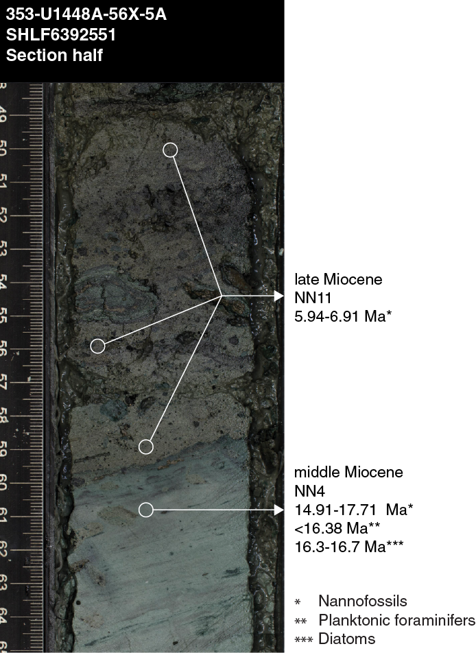
Figure F13. Biostratigraphic ages of several horizons above and below the hiatus at 379.11 m CSF-A, Hole U1448A.
Based on a linear fit including all data, sedimentation rates in Hole U1448A are around 5–6 cm/ky in the Pleistocene to late Miocene. A number of minor sedimentation rate changes can be identified in Figure F12; however, these changes cannot be reliably resolved until an orbital-resolution isotope stratigraphy has been generated. Below the hiatus, sedimentation rates in the early to middle Miocene sedimentary unit cannot be meaningfully resolved with the available biostratigraphic information from the three fossil groups at this time.
Geochemistry
The geochemistry of Site U1448 mainly reflects the anaerobic processes of sulfate reduction and methanogenesis associated with microbial degradation of organic matter. The organic carbon content ranges from 0.2 to 1.4 wt% and clearly shows two zones: one with a mean value of ~1 wt% and another with ~0.4 wt%. The transition in organic carbon content occurs at ~200 m CSF-A (lithostratigraphic Subunit Ib/Unit II boundary). Headspace methane concentration increases immediately below the sulfate depletion zone and continues downcore with the highest values between 200 and 250 m CSF-A. The overall concentrations, however, are quite low (<30 parts per million [ppm]) compared to nearby Site U1447. Pore water sulfate decreases from 28 mM at the sediment/water interface to nearly zero at approximately 40 m CSF-A. Alkalinity has a broad peak, significantly lower than at Site U1447, from 40 to 150 m CSF-A before gradually decreasing, consistent with the production of bicarbonate during sulfate reduction. A monotonic increase in dissolved Ba concentration with depth suggests ongoing barite dissolution. Changes in the concentration of other elements and ions (Fe, Mn, Ca, B, ammonia, and Sr) in interstitial water can be readily explained by microbially mediated chemical reactions and their effects on pH, alkalinity, and mineral dissolution and precipitation. Sedimentary carbonate content varies significantly between 12 and 37 wt%.
Sediment gas sampling and analysis
Headspace gas samples were taken at a frequency of one sample per core in Hole U1448A as part of the routine environmental protection and safety-monitoring program (Table T8). Methane concentration increases from 2 ppm between 0 and 49 m CSF-A to values of 13–28 ppm in three peaks at 97, 203, and 237 m CSF-A, before decreasing to <5 ppm from 290 m CSF-A until the bottom of the hole (Figure F14). Heavier hydrocarbons such as ethane and propane were not detected.
Table T8. Headspace methane concentrations, Hole U1448A. Download table in .csv format.
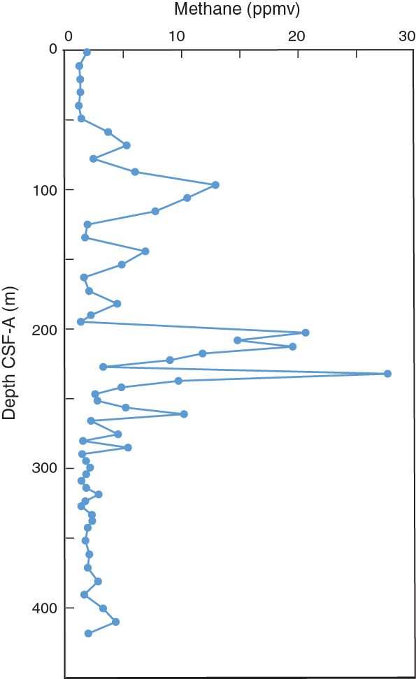
Figure F14. Headspace methane concentrations, Hole U1448A.
Bulk sediment geochemistry
Calcium carbonate, inorganic carbon, and total organic carbon (TOC) contents were determined on sediment samples from Hole U1448A (Table T9; Figure F15). CaCO3 content ranges between 12 and 37 wt% and is generally lower in the lower part of Subunit Ib and upper part of Unit II. TOC ranges between 0.2 and 1.4 wt% and clearly shows two zones: one with mean value of ~1% and another with ~0.4%. The transition between these TOC content zones occurs at ~200 m CSF-A (the lithostratigraphic Subunit Ib/Unit II boundary).
Table T9. Calcium carbonate and carbon contents, Hole U1448A. Download table in .csv format.
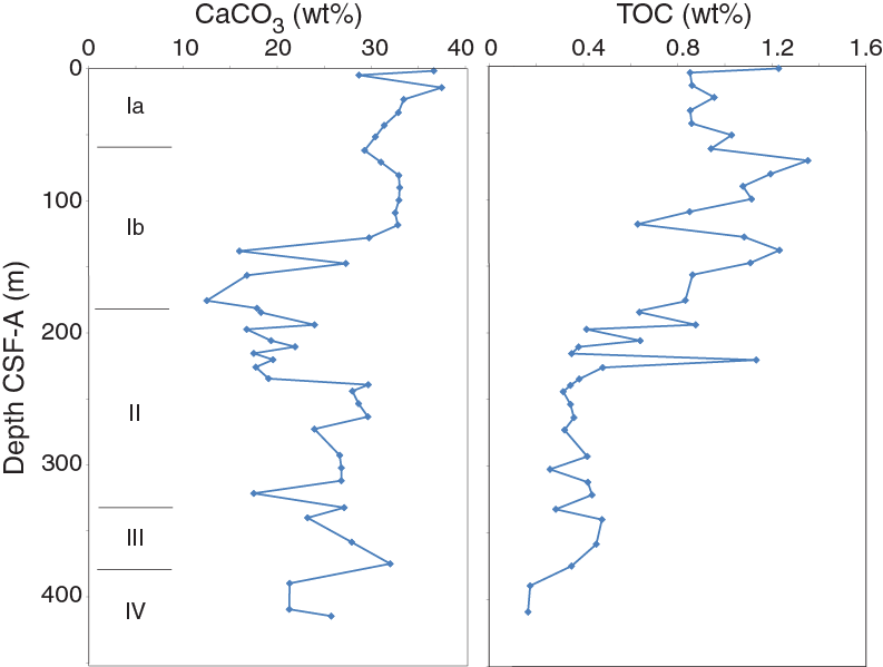
Figure F15. Calcium carbonate and TOC contents, Hole U1448A.
Interstitial water sampling and chemistry
Hole U1448A was sampled for pore water chemistry at a relatively coarse resolution of one sample per core for the uppermost section, switching to every other core for HLAPC and XCB cores. The whole-round samples for pore water squeezing were kept under N2 during extraction of interstitial waters.
Concomitant with a sharp drawdown of sulfate in the uppermost 40 m, an increase in alkalinity is observed (Figure F16; Table T10). Although sulfate is below detection from ~40 m CSF-A to the base of the hole, Ba increases sharply from a few micromolar at ~11 m CSF-A to ~72 µM at ~49 m CSF-A. Alkalinity peaks at ~15 mM at 40 m CSF-A and has a broad peak to 150 m CSF-A before gradually decreasing to ~9.7 mM at 241 m CSF-A, consistent with the production of bicarbonate during sulfate reduction. Alkalinity is lower than at Site U1447. Ammonium increases from 0.2 mM in the top of Hole U1448A to 3.5 mM at 135 m CSF-A in Hole U1448A, before decreasing gradually downhole to values of ~1.5 mM.
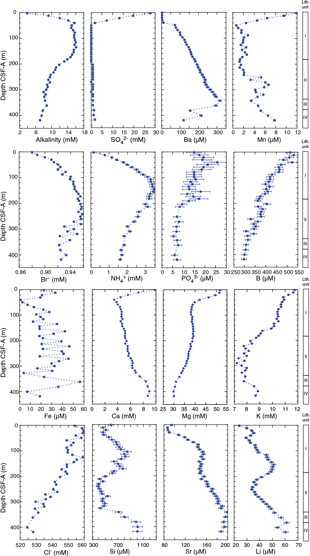
Figure F16. Interstitial water chemistry profiles, Hole U1448A.
Table T10. Interstitial water chemistry, Hole U1448A. Download table in .csv format.
Calcium concentration decreases from around 10 mM near the sediment/water interface to ~3.4 mM at ~40 m CSF-A then increases gradually with depth (Figure F16). The drop in Ca concentration in the top 40 m CSF-A is probably related to production of bicarbonate with sulfate reduction. Magnesium concentration is highest at the sediment/water interface, gradually decreases to a minimum of ~38 mM around 125 m CSF-A, and remains more or less constant until 222 m CSF-A. Deeper than 222 m CSF-A, Mg again decreases gradually to around 29 mM until the bottom of the hole. Lithium, Si, and Sr all show similar downhole concentration patterns with peaks around 140 m CSF-A, followed by a trough and increase to a peak deeper than 380 m CSF-A. The minimum and maximum concentrations of Li, Sr, and Si are 24, 94, and 464 and 60, 187, and 1009 µM, respectively (Figure F16; Table T10).
Dissolved Mn concentration decreases rapidly from 12 to 0.67 µM in the uppermost 49 m, consistent with microbial reduction of Mn oxides in the uppermost sediments. (Figure F16; Table T10). Dissolved Fe concentration decreases from 33 to ~0.96 µM within the top 40 m CSF-A of the sediment column, possibly associated with sulfate reduction and the production of hydrogen sulfide scavenging soluble Fe. Below this minimum, dissolved Fe varies between ~2 and 57 µM in the remaining sediment column, probably reflecting variable amounts and dissolution of residual iron oxides in sediments. Boron concentration decreases in a stepwise manner from around 514 µM at 0 m CSF-A to 298 µM at the bottom of the sedimentary section.
Paleomagnetism
Paleomagnetic measurements were conducted on archive-half sections for all three holes at Site U1448 (Figures F17, F18). To accommodate the core flow, only APC and HLAPC cores from Hole U1448A were demagnetized by an alternating field (AF) up to 10 mT. XCB cores from Hole U1448A and APC cores from Holes U1448B and U1448C were measured predominantly for natural remanent magnetization (NRM), with a few exceptions. HLAPC cores from Hole U1448B were not measured because of time constraints. Discrete samples taken from the working-half sections of Hole U1448A (N = 90) were also analyzed, with stepwise AF demagnetization typically up to 80 mT. Generally, the determination of characteristic remanence was difficult (Table T11). The stability of NRM appears to be higher just below the hiatus at 379.11 m CSF-A, with possible polarity transitions recorded. Anhysteretic remanent magnetization (ARM) was acquired and measured on a selection of discrete samples from Hole U1448A for preliminary insight into depth variations in Site U1448 sediment bulk magnetic properties.
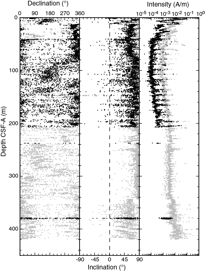
Figure F17. Downhole variations in declination, inclination, and intensity, Hole U1448A.
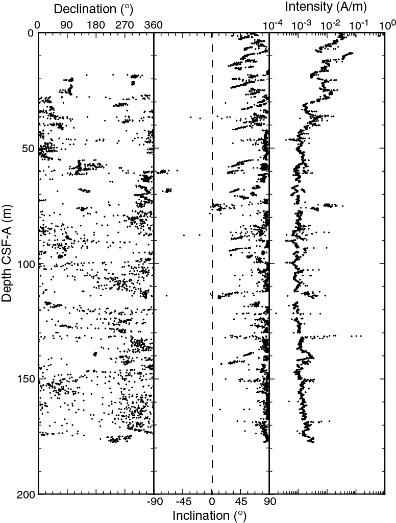
Figure F18. Downhole variations in declination, inclination, and intensity, Hole U1448B.
Table T11. Summary of discrete sample measurements, Hole U1448A. Download table in .csv format.
Magnetostratigraphy
Cores 353-U1448A-3H through 23H and 353-U1448B-3H through 19H were oriented using the Icefield MI-5 tool. Therefore, we have obtained “true” declinations between 3.30 and 260.20 for Hole U1448A and between 18.40 and 133.45 m CSF-A for Hole U1448B (Figures F17, F18; Table T12). The true declinations generally concentrate around 0 (360°) or 180° downhole to ~200 m CSF-A for both holes. Inclinations of both NRM and NRM after 10 mT demagnetization were steep downward (near 90°), indicating severe drilling-related overprint. Discrete samples also revealed severe drilling-related overprint, except for samples shallower than 2.1 m CSF-A.
Table T12. Magnetic toolface values obtained from the Icefield MI-5 tool/FlexIT tool, Site U1448. Download table in .csv format.
The true declinations from archive halves suggest that both Hole U1448A and U1448B sediments downhole to ~200 m CSF-A can be largely divided into three magnetozones (Figure F19). The biostratigraphic results (see Biostratigraphy) indicate that the Pliocene/Pleistocene boundary (2.58 Ma) corresponds to ~170 m CSF‑A. On this basis, we speculate that the three magnetozones correspond to Brunhes (C1n), Matuyama (C1r), and Gauss (C2An) Chrons. However, scatter in the declination data prevents further refinement of magnetostratigraphy.
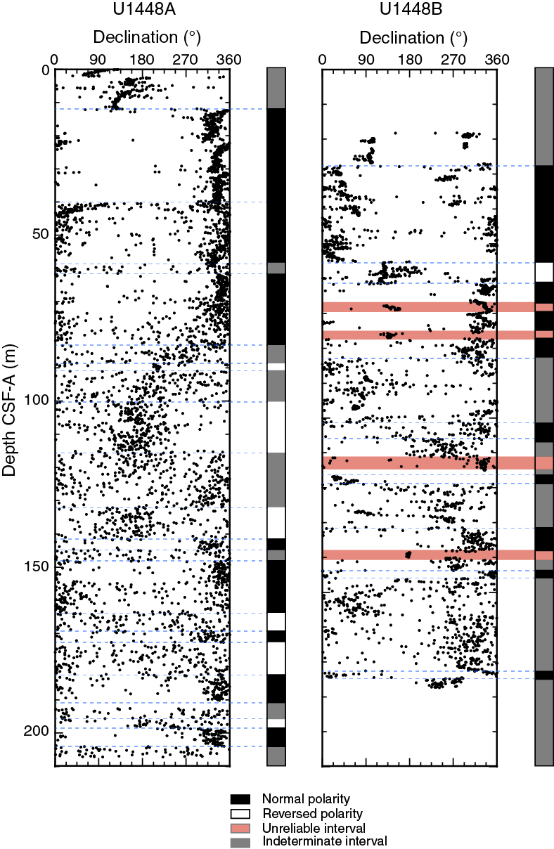
Figure F19. Speculative magnetostratigraphy, Holes U1448A and U1448B.
Bulk magnetic properties
ARM (0.05 mT direct current field, 80 mT AF field) was acquired on a selection of discrete samples taken from the working halves of Hole U1448A. ARM broadly measures relative changes in the concentration of ferrimagnetic minerals, where increases in the concentration of finer grained particles will increase ARM values much greater than an equivalent change in coarser grained particles. A significant decrease in ARM values for Hole U1448A at 10 m CSF-A (Figure F20) suggests either a decrease in the input, or the removal, of fine-grained ferrimagnetic minerals. This is likely a response to early diagenesis (see Geochemistry). The decrease at this depth (10 m CSF-A) is similar to what we see at IODP Site U1445 in the Mahanadi basin (see Paleomagnetism in the Site U1445 chapter [Clemens et al., 2016b]) and at Site U1447 in the Andaman Sea (see Paleomagnetism in the Site U1447 chapter [Clemens et al., 2016c]). Outside of the noticeable low in ARM observed between 205 and 215 m CSF-A, there is a steady increase in ARM with depth. In addition, ARM increases significantly below the hiatus at ~379 m CSF-A. Interpretations for these variations are currently unknown and further rock magnetic measurements in parallel with other proxies are required.
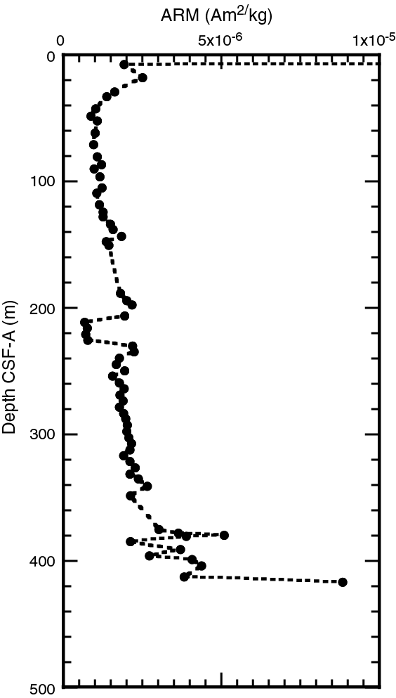
Figure F20. Downhole variations in mass-normalized ARM acquired on Hole U1448A discrete samples.
Magnetic signal around hiatus
Discrete Sample 353-U1448A-56X-5W, 118–120 cm (379.7 m CSF-A), shows a much higher stability of NRM against AF demagnetization than other discrete samples measured near the hiatus in Hole U1448A (Figure F21). This sample comes from ~60 cm below the inferred hiatus (see Lithostratigraphy). To investigate the spatial distribution of this anomalous signal, Section 56X-5A was measured at a 2 cm resolution with demagnetization steps of 5 and 10 mT. NRM intensity shows a clear peak at 19–29 cm offset of this section. Interestingly, this peak disappeared upon AF demagnetization, and the ratio of NRM intensity after 10 mT demagnetization to the NRM intensity shows two peaks at 105 and 127 cm offset (Figure F22). In addition, when plotting directional changes, the measurements around the shallower peak suggest a negative inclination similar to discrete Sample 56X-5W, 118–120 cm, whereas measurements around the deeper peak show endpoint directions antiparallel to that. We speculate that these signals indicate polarity transitions across these two peaks.
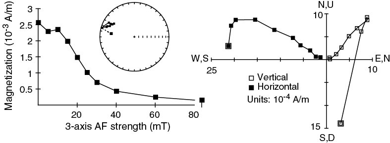
Figure F21. Stepwise demagnetization results for discrete Sample 353-U1448A-56X-5W, 118–120 cm.
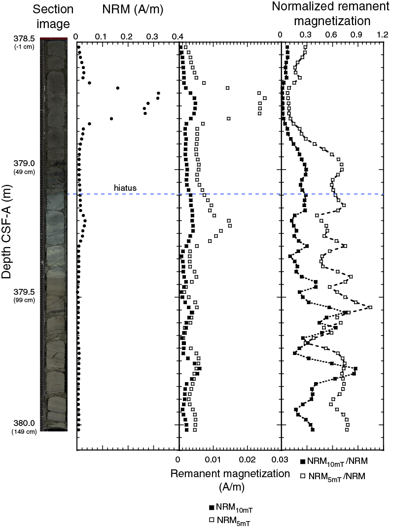
Figure F22. High-resolution section measurements across the hiatus, showing NRM, NRM after 5 and 10 mT AF demagnetization, and NRM after demagnetization normalized by the original NRM.
Physical properties
Standard physical property measurements were collected in Holes U1448A–U1448C. For Hole U1448A (0–440.6 m CSF-A), we defined six physical property (PP) units based on significant changes within the physical property measurements (Table T13): Units 1 (0–30.9 m CSF-A), 2 (30.9–107.2 m CSF-A), and 3 (107.2–182.9 m CSF-A) are independent of the lithostratigraphic units, and Units 4 (182.9–338.6 m CSF-A), 5 (338.6–379.1 m CSF-A), and 6 (379.1–440.6 m CSF-A) correspond to lithostratigraphic Units II, III, and IV, respectively (see Lithostratigraphy). Hole U1448B (0–358.22 m CSF-A) is generally in good agreement with Hole U1448A. This report predominantly discusses Hole U1448A. Hole U1448C was a geochemistry hole and therefore is not being discussed here.
Table T13. Physical property units, Site U1448. Download table in .csv format.
GRA, MS, P-wave velocity (VP), and NGR measurements were acquired on all whole-round sections using the Special Task Multisensor Logger (STMSL), the Whole-Round Multisensor Logger (WRMSL), and the Natural Gamma Radiation Logger (NGRL). Whole-round sections from Hole U1448A were logged on the STMSL and then the WRMSL at a 10 cm sampling resolution before being taken to the core rack for thermal equilibration to ~18°C. The WRMSL was used to provide measurements for stratigraphic correlation purposes, and all sections from Holes U1448B and U1448C were logged for GRA and MS data using the WRMSL only at a 10–15 cm sampling interval. Following thermal equilibration, sections were logged on the NGRL. Sediment samples were collected from the working halves of Sections 2, 4, and 6 for MAD analyses. The archive-half sections were used to collect color reflectance and point MS data on the Section Half Multisensor Logger (SHMSL) and red, green, and blue (RGB) data on the Section Half Imaging Logger (SHIL). The data plots presented here (Figures F23, F24, F25, F26, F27, F28, F29, F30, F31, F32) were filtered to remove outliers from endcaps, voids, and foam spacers. We present the minimum, maximum, and mean values of all measured parameters for downhole and hole-to-hole comparison (Table T14). No infrared thermal anomalies were detected at this site.
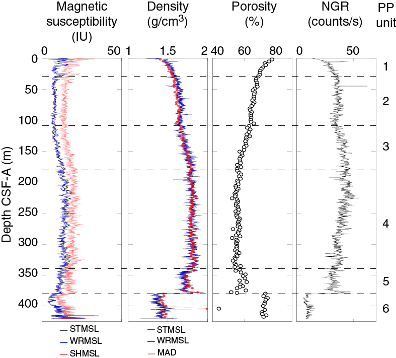
Figure F23. Physical properties showing downhole variability in magnetic susceptibility, density, porosity, and NGR, Hole U1448A.

Figure F24. Physical properties showing downhole variability in magnetic susceptibility, density, and NGR, Hole U1448B.
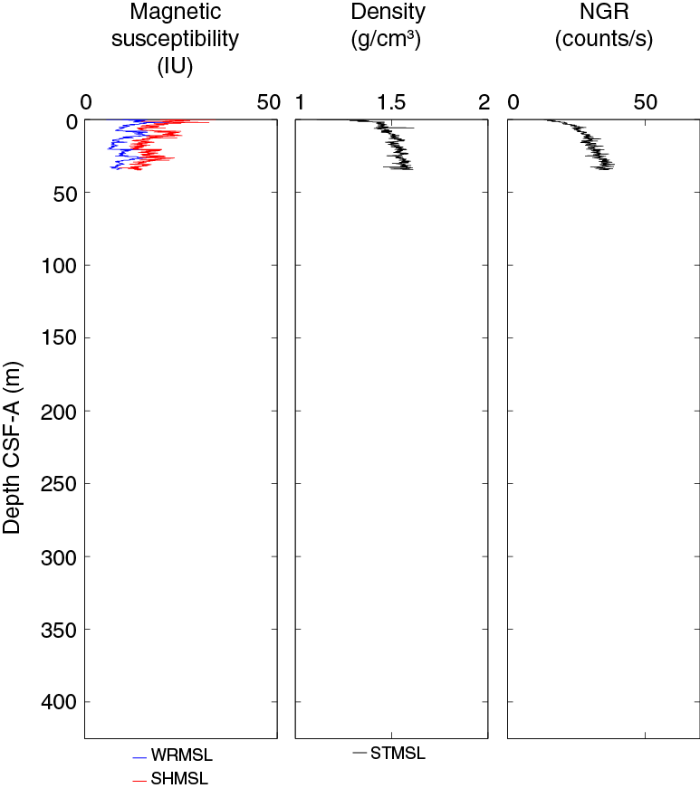
Figure F25. Physical properties showing downhole variability in magnetic susceptibility, density, and NGR, Hole U1448C.
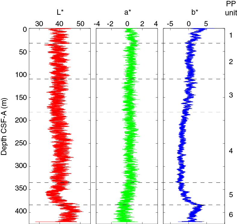
Figure F26. L*, a*, and b* data, Hole U1448A.
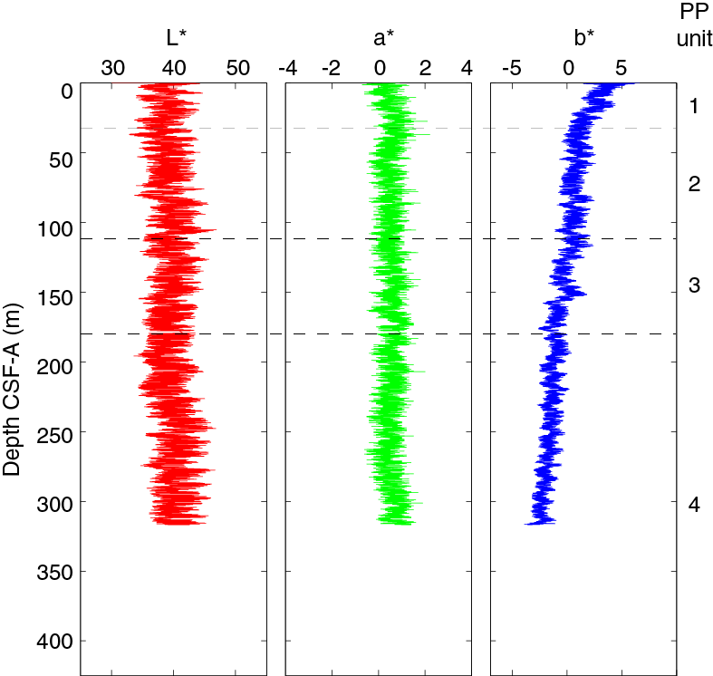
Figure F27. L*, a*, and b* data, Hole U1448B.
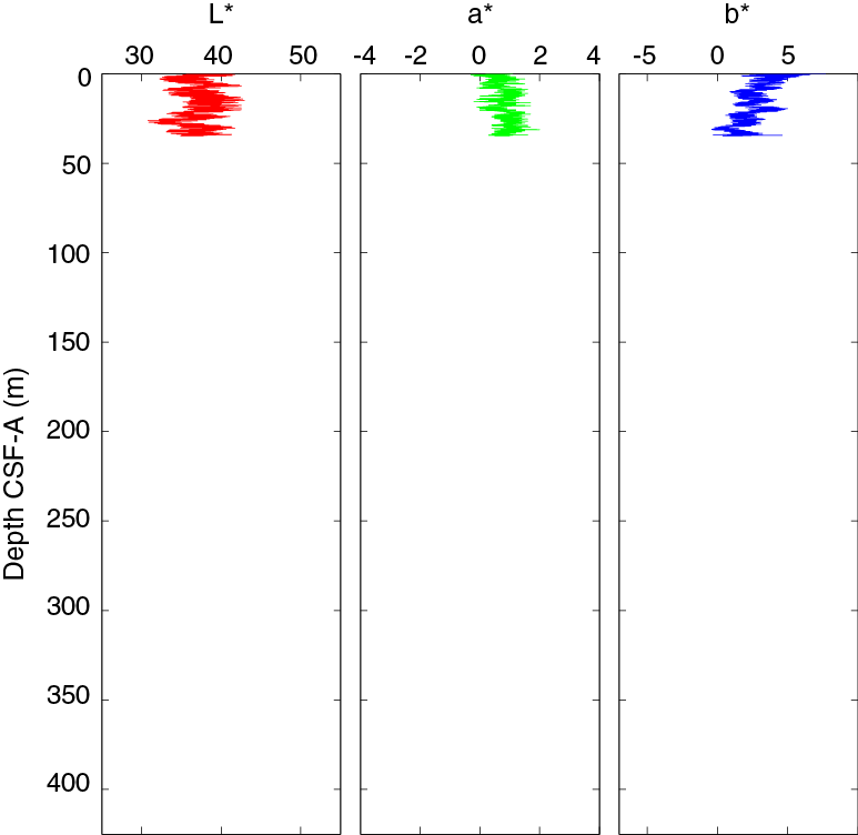
Figure F28. L*, a*, and b* data, Hole U1448C.
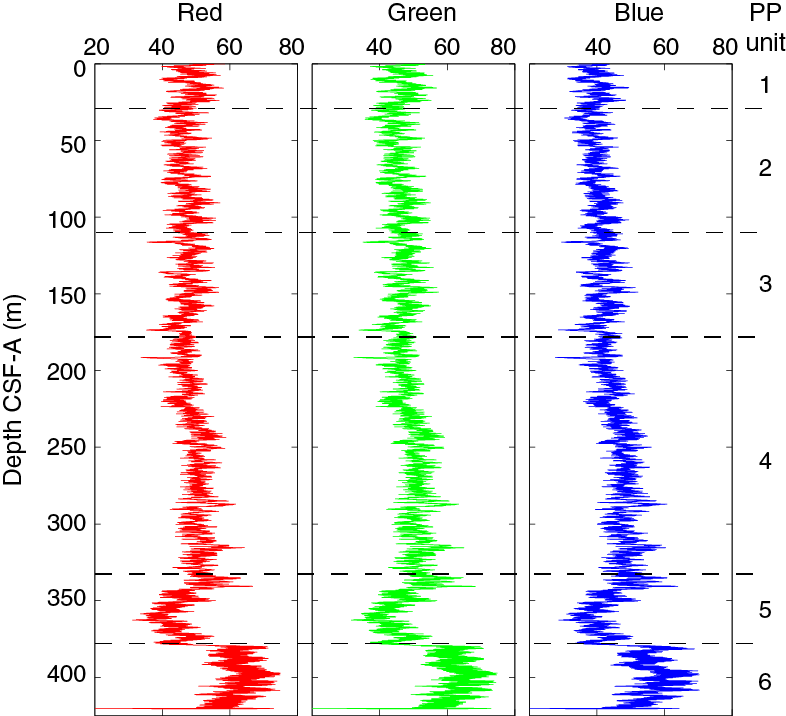
Figure F29. SHIL RGB color data, Hole U1448A.

Figure F30. SHIL RGB color data, Hole U1448B.
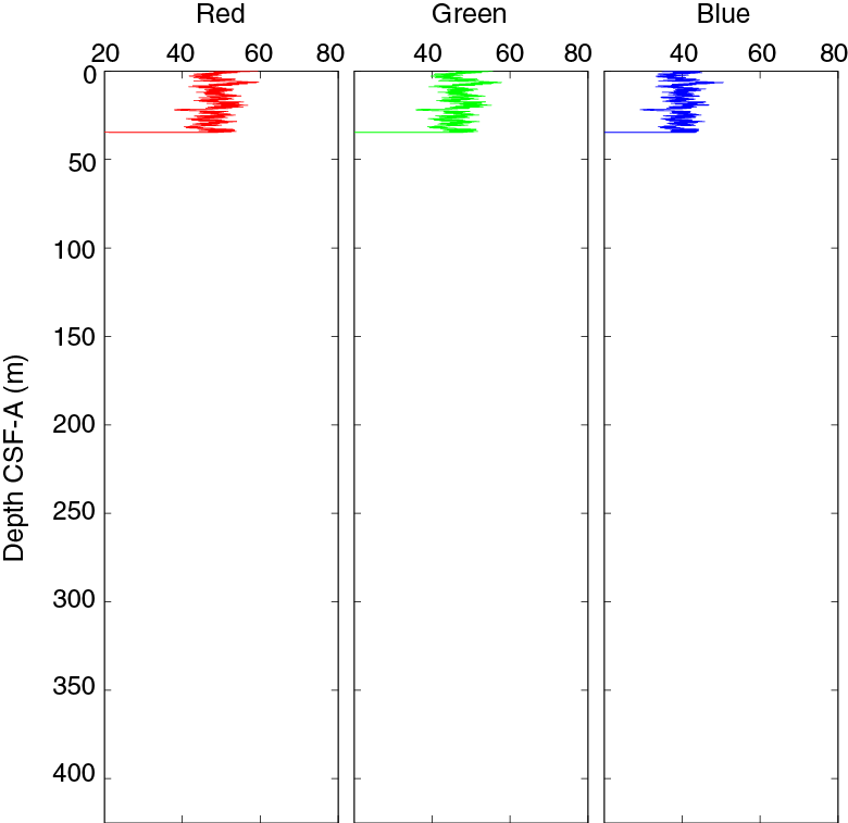
Figure F31. SHIL RGB color data, Hole U1448C.
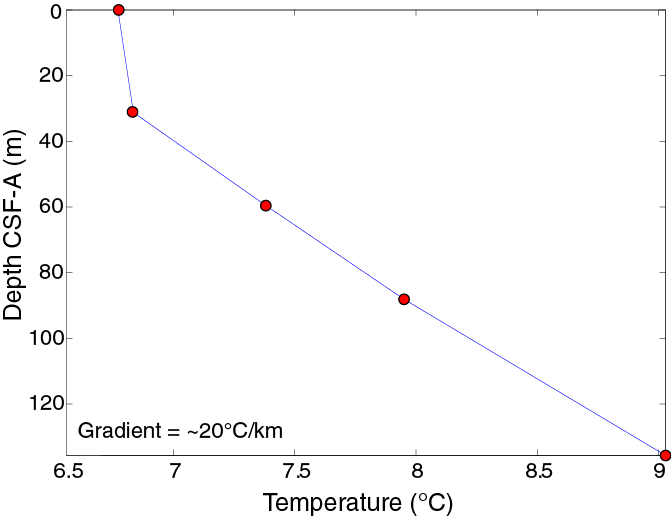
Figure F32. Downhole temperature data, Hole U1448B.
Table T14. Minimum, maximum, and mean statistics of measured physical property data, Holes U1448A–U1448C. Download table in .csv format.
Magnetic susceptibility
The STMSL and WRMSL MS values recorded for Hole U1448A show minor variability overall, with values between 1.28 and 37.61 instrument units (IU) (Figure F23). PP Unit 1 is characterized by higher average MS values with high variability possibly related to the unconsolidated nature of these upper sediments. PP Unit 2 remains relatively constant with an average value of 7.69 IU. PP Unit 3 is characterized by little variability but a steady increase from ~7.66 to 12.26 IU downhole to PP Unit 4. There is more variability in PP Unit 4 than in PP Units 2 or 3 with values ranging between 2 and 21.79 IU. PP Unit 5 has little variability with an average value of 10.9 IU, and there is a sharp drop in MS between PP Units 5 and 6 that was determined to be an ~8 Ma hiatus (see Biostratigraphy) (Figure F23). The STMSL and WRMSL track measurements agree nicely with the SHMSL point measurements trends; however, there is a constant offset between the whole-round and point measurements. It is likely that the slight increase in MS values downhole is related to compaction, whereas the generally low variability suggests no significant changes to the lithogenic flux or dilution to the lithogenic fraction from an increase in carbonate content on long-term geologic timescales between PP Units 1 and 5. PP Unit 6, however, does show a dramatic drop in MS, GRA, and NGR measurements following the hiatus.
Natural gamma radiation
NGR counts in Hole U1448A range between 3.93 and 62.76 counts/s. There is low variability with an increasing trend downhole in PP Unit 1 from ~13.87 to 45.06 counts/s. PP Unit 2 counts steady out with an average of 35.2 counts/s. PP Unit 3 counts show and increasing trend relative to PP Unit 2 with an average of 40.57 counts/s. There is a slight jump to higher NGR counts at the PP Unit 3/4 boundary. PP Unit 4 shows high variability (22.62–55.45 counts/s) with an overall decreasing trend following the initial jump to higher counts. PP Unit 4 averages 39.62 counts/s. PP Unit 5 is generally steady at ~30.8 counts/s. There is a dramatic drop in NGR counts at the PP Unit 5/6 hiatus, indicating less clay content in PP Unit 6, with an average of 9.63 counts/s (Figure F23). The long-term trends in NGR counts between PP Units 1 and 5 show cyclicity that is possibly related to variations in the input of terrigenous sediments.
GRA and MAD bulk density
The bulk density at Site U1448 was measured using (1) the GRA method using the WRMSL and STMSL for estimates from whole-round sections and (2) MAD measurements on discrete samples that provide a second, independent measure of bulk density and the dry density, grain density, water content, and porosity (Figures F23, F24, F25). The MAD and GRA data show excellent agreement. The GRA data between Holes U1448A and U1448B are also in excellent agreement; therefore, we discuss the data from the WRMSL and MAD measurements taken in Hole U1448A only.
Although the density data generally follow a linear increase with depth because of compaction, we still divide the data into the same six physical property units as the MS and NGR unit depths. The GRA bulk density values range from ~0.991 to 1.94 g/cm3. Comparably, MAD bulk density ranges between 1.395 and 1.991 g/cm3 with mean density values of 1.705 g/cm3 (bulk) and 2.740 g/cm3 (grain). The minimum and maximum dry density is 0.611 and 1.539 g/cm3, respectively. Porosity decreases with depth in PP Units 1, 2, and 3 and levels off to an average of ~56% in PP Unit 6. PP Unit 5 is characterized by an anomalous porosity increase up to 61.5% possibly from an increase in biosiliceous material (sponge spicules), and then there is an intense porosity increase below the hiatus in PP Unit 6. PP Unit 6 has an average porosity of 72.5%. The overall porosity ranges between 44.1% and 77.3%, whereas the volume of the pore water per 10 cm3 sample is between 1.885 and 8.162 cm3 with a mean value of 5.531 cm3 (Figure F23).
The average bulk density from GRA measurements for PP Units 1–5 are 1.49, 1.61, 1.69, 1.73, 1.62, and 1.39 cm3, respectively. Downcore, the minimum GRA bulk density is 0.901 cm3 and the maximum is 1.950 cm3 with an overall average of 1.682 cm3. A dramatic decrease in density with a corresponding dramatic increase in porosity occurs below the hiatus that demarks the PP Unit 5/6 boundary.
Diffuse reflectance spectroscopy and digital color image
Spectral reflectance was measured on all archive section halves using the SHMSL. There are slight color variations downhole with the most noticeable change related to a general lowering of the b* trend downcore until Hole U1448A PP Unit 6. There is little variation in a* and moderate to high variations in L*. PP Unit 1 shows high variation in all SHMSL values.
In Hole U1448A, L* ranges between 28.1 and 51.6 (average = 39.72) and reflectance a* and b* range between −1.9 and 1.7 (average = 0.34) and −3.7 and 7.2 (average = −0.49), respectively (Table T14; Figure F26). There is a stepwise change to lower L* values at the PP Unit 4/5 boundary and an increase in L* at the PP Unit 5/6 boundary. The PP Unit 1/2 boundary is not as distinct but rather is the beginning of a gradual downcore transition to lower b* values until the PP Unit 5/6 boundary. Downhole variability in L*, a*, and b* from Holes U1448B and U1448C are shown in Figures F27 and F28.
SHIL data (RGB) were measured from the surface of the split archive halves prior to drying. In Hole U1448A, R ranges between 9.4 and 74.9 (average = 49.19), G ranges between 8.8 and 74.8 (average = 48.76), and B ranges between 8.6 and 70.3 (average = 44.28) (Table T14). A marked increase in R, G, and B counts occur at the PP Unit 5/6 boundary below the hiatus. (Figure F29). Between PP Units 1 and 5, the color data show cyclicity on short- and long-term timescales. Downcore variability in RGB is also shown for Holes U1448B and U1448C (Figures F30, F31).
Downhole temperature
Downhole temperature measurements were made on Cores 353-U1448B-4H, 7H, 10H, and 15H using the APCT-3 (Table T15). The geothermal gradient was calculated to be ~20°C/km (Figure F32).
Table T15. Downhole temperature data from the APCT-3, Hole U1448B. Download table in .csv format.
Summary
We identified six physical property units in Hole U1448A. The data between Holes U1448A and U1448B correlate well. Many of the changes in physical property characteristics of Hole U1448A were gradual shifts to increasing or decreasing values. The NGR data were the only data to show long-term cyclicity, possibly related to cycles in terrigenous input. PP Unit 1 (0–30.9 m CSF-A) shows high variability in most measurements, likely related to the unconsolidated nature of the upper sediment column. PP Unit 2 (30.9–107.2 m CSF-A) shows little MS variability, increasing density, decreasing porosity, and relatively steady NGR counts. PP Unit 3 is characterized by an increase in MS, increase in density, increase in NGR counts, decrease in porosity, and lower b* values, indicating more terrigenous material and clay relative to carbonate or siliceous fractions. PP Unit 4 (182.9–338.6 m CSF-A) corresponds to lithostratigraphic Unit II. It has steady high MS values, steady high density, a continued decrease in porosity, variable NGR counts, and the lowest b* values that transitions to a smaller PP Unit 5 (338.6–379.1 m CSF‑A) where MS values decrease, density decreases, porosity increases, NGR counts decrease, and b* begins to increase. The physical properties of PP Unit 5 likely indicate an increase in abundance of more biosilica-rich clay (see Lithostratigraphy). Most noticeably, all physical property measurements showed a very dramatic change at 379.1 m CSF-A, which was determined to mark a ~8 Ma hiatus (see Biostratigraphy).
Stratigraphic correlation
A composite scale (CCSF-A) and a splice (CCSF-D) were constructed for Site U1448 using Holes U1448A–U1448C (as defined in Stratigraphic correlation in the Expedition 353 methods chapter [Clemens et al., 2016a]). Splicing among these holes enabled us to construct a continuous stratigraphic sequence to ~ 203 m CCSF-D (Tables T16, T17; Figure F33). Following a set gap, a floating composite scale was constructed between ~205 and ~260 m CCSF-A using Holes U1448A and U1448B (Table T16).
Table T16. Vertical offsets applied to cores in order to align structure in adjacent holes, Site U1448. Download table in .csv format.
Table T17. Splice intervals, Site U1448. Download table in .csv format.
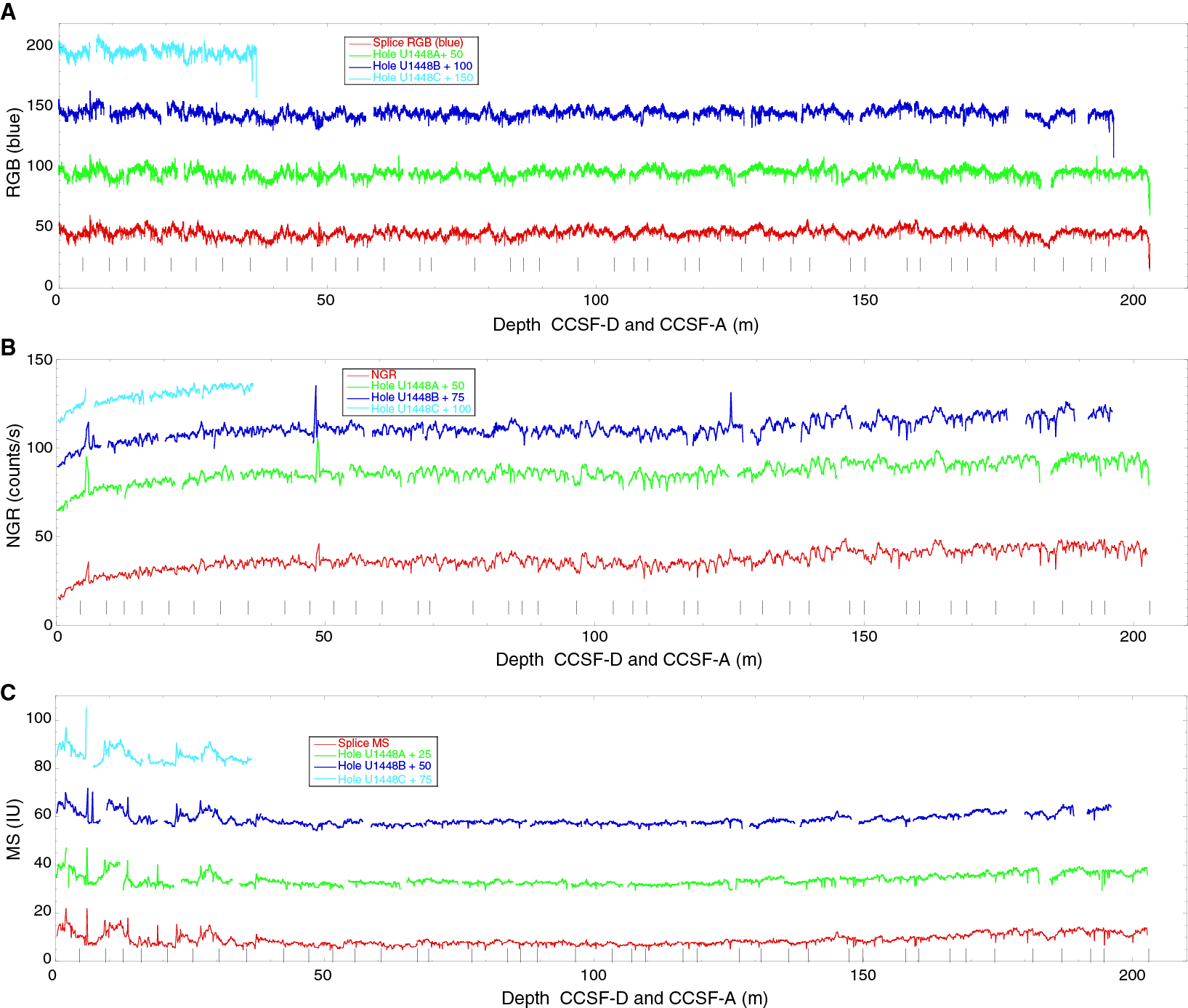
Figure F33. Core alignment shown using (A) RGB blue, (B) NGR, and (C) MS profiles, Holes U1448A–U1448C.
Construction of CCSF-A scale
We selected the core with the best mudline recovery (Core 353-U1448C-1H) to anchor the composite depth scale and defined the top as 0 m CCSF-A. The CCSF-A scale for Site U1448 (see Table T16) is based on correlation of RGB color and secondarily on MS data. RGB green was utilized for correlations in Site U1448. MS was measured on whole-round sections, whereas green was measured on archive-half sections (see Physical properties for details). The R, G, and B components of the RGB triplet are highly correlated to each other because, on the first order, all are measures of the reflectivity of the sediment. The small differences between R, G, and B can be expressed as ratios such as red/green, red/blue, or green/blue. However, ratios were not employed in our correlation due to lack of time (see the Expedition 353 methods chapter [Clemens et al., 2016a]). Reflectance spectroscopy data (i.e., L*, a*, and b*), which can produce information similar to RGB ratios, were not used for correlation due to inconsistent variability from hole to hole resulting from low-quality wavelength spectra collected by the Ocean Optics USB4000 spectrophotometer on the monotonously dark sediments of Site U1448.
Construction of CCSF-D scale
A combination of Holes U1448A–U1448C cover the stratigraphic section to ~203 m CCSF-D. When constructing the splice, we tried to minimize inclusion of disturbed intervals and avoid whole-round sampling intervals (notably from Hole U1448A) as much as possible. Selected splice intervals are listed in Table T17. Postcruise, the splice interval tables were modified using the Splice-File-Fixer program to ensure that each depth has been assigned the correct sample ID. Both the affine and the corrected splice interval tables were uploaded into the Laboratory Information Management System (LIMS) during the first postcruise meeting in June 2015. The core top depths in the affine tables were not corrected and hence may be slightly incorrect in a range of <2 cm. However, the offsets are correct.
Reliance on RGB, which sometimes has fuzzy character due to cracks and defects of the split core surface, precluded, in places, the definition of a unique correlation. Features and general trends were used instead, reducing the accuracy of the splice to the decimeter range. As a result, correlation should be viewed with caution deeper than ~115 m CCSF-A, notably if high-resolution sampling is planned. Onshore X-ray fluorescence scanning, color reflectance rescanning, and bulk δ18O should provide better means of correlation.
References
Awasthi, N., Ray, J.S., Singh, A.K., Band, S.T., and Rai, V.K., 2014. Provenance of the late Quaternary sediments in the Andaman Sea: implications for monsoon variability and ocean circulation. Geochemistry, Geophysics, Geosystems, 15(10):3890–3906. http://dx.doi.org/10.1002/2014GC005462
Barron, J.A., 1985. Miocene to Holocene planktic diatoms. In Bolli, H.M., Saunders, J.B., and Perch-Nielsen, K. (Eds.), Plankton Stratigraphy: Cambridge, United Kingdom (Cambridge University Press), 763–809.
Bown, P.R. (Ed.), 1998. Calcareous Nannofossil Biostratigraphy: Dordrecht, The Netherlands (Kluwer Academic Publishing).
Clemens, S.C., Kuhnt, W., LeVay, L.J., Anand, P., Ando, T., Bartol, M., Bolton, C.T., Ding, X., Gariboldi, K., Giosan, L., Hathorne, E.C., Huang, Y., Jaiswal, P., Kim, S., Kirkpatrick, J.B., Littler, K., Marino, G., Martinez, P., Naik, D., Peketi, A., Phillips, S.C., Robinson, M.M., Romero, O.E., Sagar, N., Taladay, K.B., Taylor, S.N., Thirumalai, K., Uramoto, G., Usui, Y., Wang, J., Yamamoto, M., and Zhou, L., 2016a. Expedition 353 methods. In Clemens, S.C., Kuhnt, W., LeVay, L.J., and the Expedition 353 Scientists, Indian Monsoon Rainfall. Proceedings of the International Ocean Discovery Program, 353: College Station, TX (International Ocean Discovery Program). http://dx.doi.org/10.14379/iodp.proc.353.102.2016
Clemens, S.C., Kuhnt, W., LeVay, L.J., Anand, P., Ando, T., Bartol, M., Bolton, C.T., Ding, X., Gariboldi, K., Giosan, L., Hathorne, E.C., Huang, Y., Jaiswal, P., Kim, S., Kirkpatrick, J.B., Littler, K., Marino, G., Martinez, P., Naik, D., Peketi, A., Phillips, S.C., Robinson, M.M., Romero, O.E., Sagar, N., Taladay, K.B., Taylor, S.N., Thirumalai, K., Uramoto, G., Usui, Y., Wang, J., Yamamoto, M., and Zhou, L., 2016b. Site U1445. In Clemens, S.C., Kuhnt, W., LeVay, L.J., and the Expedition 353 Scientists, Indian Monsoon Rainfall. Proceedings of the International Ocean Discovery Program, 353: College Station, TX (International Ocean Discovery Program). http://dx.doi.org/10.14379/iodp.proc.353.105.2016
Clemens, S.C., Kuhnt, W., LeVay, L.J., Anand, P., Ando, T., Bartol, M., Bolton, C.T., Ding, X., Gariboldi, K., Giosan, L., Hathorne, E.C., Huang, Y., Jaiswal, P., Kim, S., Kirkpatrick, J.B., Littler, K., Marino, G., Martinez, P., Naik, D., Peketi, A., Phillips, S.C., Robinson, M.M., Romero, O.E., Sagar, N., Taladay, K.B., Taylor, S.N., Thirumalai, K., Uramoto, G., Usui, Y., Wang, J., Yamamoto, M., and Zhou, L., 2016c. Site U1447. In Clemens, S.C., Kuhnt, W., LeVay, L.J., and the Expedition 353 Scientists, Indian Monsoon Rainfall. Proceedings of the International Ocean Discovery Program, 353: College Station, TX (International Ocean Discovery Program). http://dx.doi.org/10.14379/iodp.proc.353.107.2016
Colin, C., Turpin, L., Bertaux, J., Desprairies, A., and Kissel, C., 1999. Erosional history of the Himalayan and Burman ranges during the last two glacial–interglacial cycles. Earth and Planetary Science Letters, 171(4):647–660. http://dx.doi.org/10.1016/S0012-821X(99)00184-3
Colin, C., Turpin, L., Blamart, D., Frank, N., Kissel, C., and Duchamp, S., 2006. Evolution of weathering patterns in the Indo-Burman Ranges over the last 280 kyr: effects of sediment provenance on 87Sr/86Sr ratios tracer. Geochemistry, Geophysics, Geosystems, 7(3):Q03007. http://dx.doi.org/10.1029/2005GC000962
Collett, T.S., Riedel, M., Cochran, J., Boswell, R., Presley, J., Kumar, P., Sathe, A.V., Sethi, A., Lall, M., Sibal, V., and the NGHP Expedition 01 Scientists, 2008. Indian National Gas Hydrate Program (NGHP) Expedition 01, Initial Report: Noida, India (DGH, Ministry of Petroleum and Natural Gas).
Curray, J.R., 1991. Possible greenschist metamorphism at the base of a 22-km sedimentary section, Bay of Bengal. Geology, 19(11):1097–1100. http://dx.doi.org/10.1130/0091-7613(1991)019<1097:PGMATB>2.3.CO;2
Curray, J.R., 2005. Tectonics and history of the Andaman Sea region. Journal of Asian Earth Sciences, 25(1):187–232. http://dx.doi.org/10.1016/j.jseaes.2004.09.001
Flores, J.A., Johnson, J.E., Mejía-Molina, A.E., Álverez, M.C., Sierro, F.J., Singh, S.D., Mahanti, S., and Giosan, L., 2014. Sedimentation rates from calcareous nannofossil and planktonic foraminifera biostratigraphy in the Andaman Sea, northern Bay of Bengal, and eastern Arabian Sea. Marine and Petroleum Geology, 58(Part A):425–437. http://dx.doi.org/10.1016/j.marpetgeo.2014.08.011
Frerichs, W.E., 1971. Planktonic foraminifera in the sediments of the Andaman Sea. Journal of Foraminiferal Research, 1(1):1–14. http://dx.doi.org/10.2113/gsjfr.1.1.1
Gradstein, F.M., Ogg, J.G., Schmitz, M.D., and Ogg, G.M. (Eds.), 2012. The Geological Time Scale 2012: Amsterdam (Elsevier).
Martini, E., 1971. Standard Tertiary and Quaternary calcareous nannoplankton zonation. In Farinacci, A. (Ed.), Proceedings of the Second Planktonic Conference, Roma 1970: Rome (Edizioni Tecnoscienza), 2:739–785.
Okada, H., and Bukry, D., 1980. Supplementary modification and introduction of code numbers to the low-latitude coccolith biostratigraphic zonation (Bukry, 1973; 1975). Marine Micropaleontology, 5:321–325. http://dx.doi.org/10.1016/0377-8398(80)90016-X
Singh, S.C., Moeremans, R., McArdle, J., and Johansen, K., 2013. Seismic images of the sliver strike-slip fault and back thrust in the Andaman-Nicobar region. Journal of Geophysical Research: Solid Earth, 118(10):5208–5224. http://dx.doi.org/10.1002/jgrb.50378
Varkey, M.J., Murty, V.S.N., and Suryanarayana, A., 1996. Physical oceanography of the Bay of Bengal and Andaman Sea. Oceanography and Marine Biology, 34:1–70. http://drs.nio.org/drs/handle/2264/2276
1Clemens, S.C., Kuhnt, W., LeVay, L.J., Anand, P., Ando, T., Bartol, M., Bolton, C.T., Ding, X., Gariboldi, K., Giosan, L., Hathorne, E.C., Huang, Y., Jaiswal, P., Kim, S., Kirkpatrick, J.B., Littler, K., Marino, G., Martinez, P., Naik, D., Peketi, A., Phillips, S.C., Robinson, M.M., Romero, O.E., Sagar, N., Taladay, K.B., Taylor, S.N., Thirumalai, K., Uramoto, G., Usui, Y., Wang, J., Yamamoto, M., and Zhou, L., 2016.Site U1448. In Clemens, S.C., Kuhnt, W., LeVay, L.J., and the Expedition 353 Scientists, Indian Monsoon Rainfall. Proceedings of the International Ocean Discovery Program, 353: College Station, TX (International Ocean Discovery Program). http://dx.doi.org/10.14379/iodp.proc.353.108.2016
- F1. Andaman Sea map with location of Site U1448.
- F2. Summary sketch showing the subduction zone through the back-arc basin to ~40 km depth.
- F3. Seismic lines showing location of Site U1448.
- F4. Lithostratigraphic summary, Site U1448.
- F5. Lithostratigraphic summary with selected physical property and geochemical data from Holes U1448A–U1448C.
- F6. Smear slide data, Holes U1448A and U1448C.
- F7. Main lithologies, Site U1448. A. Nannofossil-rich clay with foraminifers. B. Foraminifer-rich clay. C. Nannofossil-rich clay with foraminifers. D. Clay with nannofossils. E. Clayey biosiliceous ooze.
- F8. Lithologic types, Site U1448. A. Nannofossil-rich clay. B. Clayey biosiliceous ooze. C. Volcanic ash. D. Volcanic ash including iron sulfides.
- F9. Minor lithologies, Site U1448. A. Volcanic ash. B. Light gray volcanic ash, Subunit Ia. C. Pinkish gray volcanic ash. D. Thin turbidite. E. Very thin turbidite. F. Pyrite nodule. G. Microfault.
- F10. Miocene hiatus interval near the Unit III/IV boundary, Hole U1448A. A. Nannofossil-rich clay. B. Clay with nannofossils. C. Inclined boundary between Unit III and Unit IV. D. Clayey biosiliceous ooze. E. Nannofossil-rich biosiliceous ooze. F. Clayey biosiliceous ooze with nannofossils.
- F11. Summary of biostratigraphic events identified in Hole U1448A.
- F12. Biostratigraphic- and magnetostratigraphic-based age-depth plot, Hole U1448A.
- F13. Biostratigraphic ages of several horizons above and below the hiatus at 379.11 m CSF-A, Hole U1448A.
- F14. Headspace methane concentrations, Hole U1448A.
- F15. Calcium carbonate and TOC contents, Hole U1448A.
- F16. Interstitial water chemistry profiles, Hole U1448A.
- F17. Downhole variations in declination, inclination, and intensity, Hole U1448A.
- F18. Downhole variations in declination, inclination, and intensity, Hole U1448B.
- F19. Speculative magnetostratigraphy, Holes U1448A and U1448B.
- F20. Downhole variations in mass-normalized ARM acquired on Hole U1448A discrete samples.
- F21. Stepwise demagnetization results for discrete Sample 353-U1448A-56X-5W, 118–120 cm.
- F22. High-resolution section measurements across the hiatus, showing NRM, NRM after 5 and 10 mT AF demagnetization, and NRM after demagnetization normalized by the original NRM.
- F23. Physical properties showing downhole variability in magnetic susceptibility, density, porosity, and NGR, Hole U1448A.
- F24. Physical properties showing downhole variability in magnetic susceptibility, density, and NGR, Hole U1448B.
- F25. Physical properties showing downhole variability in magnetic susceptibility, density, and NGR, Hole U1448C.
- F26. L*, a*, and b* data, Hole U1448A.
- F27. L*, a*, and b* data, Hole U1448B.
- F28. L*, a*, and b* data, Hole U1448C.
- F29. SHIL RGB color data, Hole U1448A.
- F30. SHIL RGB color data, Hole U1448B.
- F31. SHIL RGB color data, Hole U1448C.
- F32. Downhole temperature data, Hole U1448B.
- F33. Core alignment shown using (A) RGB blue, (B) NGR, and (C) MS profiles, Holes U1448A–U1448C.
- T1. Site U1448 core summary.
- T2. Semiquantitative calcareous nannofossils abundance counts from core catcher samples, Hole U1448A.
- T3. Calcareous nannofossil datums, Hole U1448A.
- T4. Semiquantitative planktonic foraminifer abundance counts from core catcher samples, Hole U1448A.
- T5. Planktonic foraminifer datums, Hole U1448A.
- T6. Semiquantitative diatom abundance counts from core catcher and split core samples, Site U1448.
- T7. Diatom datums, Site U1448.
- T8. Headspace methane concentrations, Hole U1448A.
- T9. Calcium carbonate and carbon contents, Hole U1448A.
- T10. Interstitial water chemistry, Hole U1448A.
- T11. Summary of discrete sample measurements, Hole U1448A.
- T12. Magnetic toolface values obtained from the Icefield MI-5 tool/FlexIT tool, Site U1448.
- T13. Physical property units, Site U1448.
- T14. Minimum, maximum, and mean statistics of measured physical property data, Holes U1448A–U1448C.
- T15. Downhole temperature data from the APCT-3, Hole U1448B.
- T16. Vertical offsets applied to cores in order to align structure in adjacent holes, Site U1448.
- T17. Splice intervals, Site U1448.