France-Lanord, C., Spiess, V., Klaus, A., Schwenk, T., and the Expedition 354 Scientists
Proceedings of the International Ocean Discovery Program Volume 354
publications.iodp.org
doi:10.14379/iodp.proc.354.102.2016

Expedition 354 methods1
C. France-Lanord, V. Spiess, A. Klaus, R.R. Adhikari, S.K. Adhikari, J.-J. Bahk, A.T. Baxter, J.W. Cruz, S.K. Das, P. Dekens, W. Duleba, L.R. Fox, A. Galy, V. Galy, J. Ge, J.D. Gleason, B.R. Gyawali, P. Huyghe, G. Jia, H. Lantzsch, M.C. Manoj, Y. Martos Martin, L. Meynadier, Y.M.R. Najman, A. Nakajima, C. Ponton, B.T. Reilly, K.G. Rogers, J.F. Savian, T. Schwenk, P.A. Selkin, M.E. Weber, T. Williams, and K. Yoshida2
Keywords: International Ocean Discovery Program, IODP, Expedition 354, JOIDES Resolution, Site U1449, Site U1450, Site U1451, Site U1452, Site U1453, Site U1454, Site U1455, Bengal Fan
Introduction, background, and operations
This chapter documents the procedures and methods employed in the various shipboard laboratories on the R/V JOIDES Resolution during International Ocean Discovery Program (IODP) Expedition 354. This information applies only to shipboard work described in the Expedition Reports section of the Expedition 354 Proceedings of the International Ocean Discovery Program volume. Methods used by investigators for shore-based analyses of Expedition 354 data will be described in separate individual publications. This introductory section provides an overview of operations, curatorial conventions, depth scale terminology, and general core handling and analyses.
Site locations
GPS coordinates from precruise site surveys were used to position the vessel at all Expedition 354 sites. A SyQuest Bathy 2010 compressed high-intensity radar pulse (CHIRP) subbottom profiler was used to monitor seafloor depth on the approach to each site to confirm the depth profiles from precruise surveys. Once the vessel was positioned at a site, the thrusters were lowered, and at deeper penetration sites, a positioning beacon was dropped to the seafloor. Dynamic positioning control of the vessel used navigational input from the GPS system and triangulation to the seafloor beacon, weighted by the estimated positional accuracy. The final hole position was the mean position calculated from the GPS data collected over a significant time interval.
Coring and drilling operations
All four standard coring systems, the advanced piston corer (APC), half-length APC (HLAPC), extended core barrel (XCB), and rotary core barrel (RCB) systems, were used during Expedition 354. The APC system was used in the upper portion of each hole to obtain high-quality core. The APC system cuts soft-sediment cores with minimal coring disturbance relative to other IODP coring systems. After the APC core barrel is lowered through the drill pipe and lands near the bit, the drill pipe is pressured up until the two shear pins that hold the inner barrel attached to the outer barrel fail. The inner barrel then advances into the formation and cuts the core. The driller can detect a successful cut, or “full stroke,” from the pressure gauge on the rig floor.
APC refusal is conventionally defined in two ways: (1) the piston fails to achieve a complete stroke (as determined from the pump pressure reading) because the formation is too hard, or (2) excessive force (>60 klb; ~267 kN) is required to pull the core barrel out of the formation. When a full stroke cannot be achieved, additional attempts are typically made, and after each attempt, the bit is advanced by the length of core recovered. The number of additional attempts is generally dictated by the length of recovery of the partial stroke core and the time available to advance the hole by piston coring. Note that this results in a nominal recovery of ~100% based on the assumption that the barrel penetrates the formation by the equivalent of the length of core recovered. When it can be “drilled over,” meaning after the inner core barrel is successfully shot into the formation, the drill bit is advanced to total depth to free the APC barrel.
The standard (full) APC system contains a 9.5 m long core barrel. The newly engineered HLAPC coring system uses a 4.7 m long core barrel. In most instances, the HLAPC system is deployed after the APC reaches refusal. During use of the HLAPC system, the same criteria were applied in terms of refusal as for the APC system. Use of this new technology allowed for significantly greater continuous APC sampling depths to be attained than would have otherwise been possible. During Expedition 354, the full-length APC system could not adequately penetrate the formation, resulting in poor recovery and ruptured core liners that severely damaged the core that was recovered. As result, we mostly used the HLAPC system.
Nonmagnetic core barrels were used during all conventional APC and HLAPC coring to a pull force of ~40,000 lb (note that nonmagnetic core barrels were used for all coring systems except where noted). APC cores were oriented using either the MI-5 Multishot magnetic inclinometer (Icefield MI-5) or FlexIT tools (see Paleomagnetism). Formation temperature measurements were made with the advanced piston corer temperature (APCT-3) tool to obtain temperature gradients and heat flow estimates (see Downhole measurements) for all APC cores.
The XCB system is used to advance the hole when APC refusal occurs before the target depth is reached or when the formation becomes either too stiff for APC coring or hard substrate is encountered. The XCB system is a rotary system with a small cutting shoe (bit) that extends below the large APC/XCB bit. The smaller bit can cut a semi-indurated core with less torque and fluid circulation than the main bit, optimizing recovery. The XCB cutting shoe extends ~30.5 cm ahead of the main bit in soft sediment but retracts into the main bit when hard formations are encountered. The XCB system could not adequately recover the poorly consolidated and coarse lithologies penetrated during Expedition 354.
The bottom-hole assembly (BHA) is the lowermost part of the drill string. The exact configuration of the BHA is reported in the Operations section of each site chapter. A typical APC/XCB BHA consists of a drill bit (outer diameter = 11⁷⁄₁₆ inch), a bit sub, a seal bore drill collar, a landing saver sub, a modified top sub, a modified head sub, a nonmagnetic drill collar (for APC/XCB), a number of 8¼ inch drill collars, a tapered drill collar, six joints (two stands) of 5½ inch (~13.97 cm) drill pipe, and one crossover sub. A lockable float valve was used when downhole logging was planned so that downhole logs could be collected through the bit.
The RCB system is deployed when deeper penetration in consolidated rocks is expected. The RCB system requires a dedicated RCB BHA and a dedicated RCB drilling bit. The BHA used for RCB coring included a 9⅞ inch RCB drill bit, a mechanical bit release (to allow for wireline logging; not always deployed because of concerns of premature release), a modified head sub, an outer core barrel, a modified top sub, a modified head sub, and from 7 to 10 control-length drill collars followed by a tapered drill collar to the two stands of 5½ inch drill pipe. Most cored intervals are ~9.7 m long, which is the length of a standard rotary core and approximately the length of a joint of drill pipe. In some cases, the drill string is drilled or “washed” ahead without recovering sediment to advance the drill bit to a target depth to resume core recovery. Such intervals are typically drilled using a center bit installed within the RCB bit.
Core handling and analysis
Recovered cores were extracted from the core barrel in 67 mm diameter plastic liners. These liners were carried from the rig floor to the core processing area on the catwalk outside the Core Laboratory, where they were split into ~1.5 m sections. Liner caps (blue = top, colorless = bottom, and yellow = whole-round sample taken) were glued with acetone onto liner sections on the catwalk by the Core Technicians. The length of each section was entered into the database as “created length” using the Sample Master application. This length measurement was used to calculate core recovery. Cores with loose sands, most often partially filling the core liner, were cut into sections that were placed vertically on the core receiving platform to allow the sand to settle to the bottom. The water was drained off, and the sections were then curated as normal core sections. The core sections subjected to this procedure were noted in the database and are reported in tables in the Lithostratigraphy section of each site chapter.
As soon as cores arrived on deck, headspace samples were taken either using a syringe in soft formations or taking chips of harder material for immediate hydrocarbon analysis as part of the shipboard safety and pollution prevention program. Core catcher samples were taken for biostratigraphic analysis. Whole-round samples were taken from some core sections for shipboard and postexpedition interstitial water analyses. In some shallower sections, Rhizon interstitial water samples were taken from selected intervals in core sections later in the laboratory (see Geochemistry and microbiology). In addition, whole-round and syringe samples were immediately taken from the ends of some cut sections for shore-based microbiological analysis. Because preserving all silt and sand recovered in the core was a primary cruise objective, plastic buckets were used to catch any sediment that flowed out of the core as it was being processed on the core receiving platform. This practice was followed at the top of the core and between each section as it was cut. Sediment collected from multiple locations in any single core was consolidated into a single bucket, allowed to settle so the water could be poured off, and then archived as a sample associated with the entire core. Sediment recovered in this method was not included in the documented overall recovery for the core.
Core sections were then placed in core racks in the laboratory. Selected sections were then subjected to Rhizon interstitial water sampling. When the cores reached equilibrium with laboratory temperature (typically after ~4 h), whole-round core sections were run through the Whole-Round Multisensor Logger (WRMSL; measuring P-wave velocity, density, and magnetic susceptibility) and the Natural Gamma Radiation Logger (NGRL). Thermal conductivity measurements were typically taken at a rate of approximately one per core (see Physical properties). The core sections were then split lengthwise from bottom to top into working and archive halves. Investigators should note that older material may have been transported upward on the split face of each section during splitting. For lithified rocks, core sections were was split with a diamond-impregnated saw.
The working half of each sedimentary core was sampled for shipboard biostratigraphic, physical property, paleomagnetic, and geochemical analyses. The archive half of all cores was scanned on the Section Half Imaging Logger (SHIL) and measured for color reflectance and magnetic susceptibility on the Section Half Multisensor Logger (SHMSL). At the same time, the archive halves were described visually and by means of smear slides and thin sections. All observations were recorded in the Laboratory Information Management System (LIMS) database using DESClogik, a descriptive data capture application. After visual description, the archive halves were run through the cryogenic magnetometer. Discrete samples were taken from working section halves for shipboard physical property, paleomagnetic, paleontologic, and geochemical analyses, as well as selected personal samples for postexpedition analyses.
Both halves of the core were put into labeled plastic tubes that were sealed and transferred to cold storage space aboard the ship. At the end of the expedition, the cores were transported from the ship to permanent cold storage at the Kochi Core Center at Kochi University (Japan).
Drilling disturbance
Cores may be significantly disturbed as a result of the drilling process and may contain extraneous material as a result of the coring and core handling processes. In formations with loose sand layers, sand from intervals higher in the hole may be washed down by drilling circulation, accumulate at the bottom of the hole, and be sampled with the next core. The uppermost 10–50 cm of each core must therefore be examined critically during description for potential “fall-in” or other coring deformation. Common coring-induced deformation includes the concave-downward appearance of originally horizontal bedding. Piston action may result in fluidization (flow-in) of unlithified sediment, often at the bottom of APC cores, but also can occur anywhere in a core. Retrieval from depth to the surface may result in elastic rebound. Gas that is in solution at depth may become free and drive core segments within the liner apart. Both elastic rebound and gas pressure can result in a total length for each core that is longer than the interval that was cored and thus a calculated recovery of >100%. If gas expansion or other coring disturbance results in a void in any particular core section, the void can be closed by moving material if very large, stabilized by a foam insert if moderately large, or left as is. When gas content is high, pressure must be relieved for safety reasons before the cores are cut into segments. This is accomplished by drilling holes into the liner, which forces some sediment as well as gas out of the liner. These disturbances are described in the Lithostratigraphy sections in each site chapter and are graphically indicated on the core summary graphic reports (visual core descriptions [VCDs]). In extreme instances, core material can be ejected from the core barrel, sometimes violently, onto the rig floor by high pressure in the core or other coring problems. This core material was replaced in the plastic core liner by hand and should not be considered to be in stratigraphic order. Core sections so affected are marked by a yellow label marked “disturbed,” and the nature of the disturbance is noted in the coring log.
Curatorial procedures
Numbering of sites, holes, cores, and samples follows standard IODP procedure. Drilling sites are numbered consecutively from the first site drilled by the D/V Glomar Challenger in 1968. Integrated Ocean Drilling Program Expedition 301 began using the prefix “U” to designate sites occupied by the JOIDES Resolution. For all IODP drill sites, a letter suffix distinguishes each hole drilled at the same site. The first hole drilled is assigned the site number modified by the suffix “A,” the second hole the site number and the suffix “B,” and so on.
Cores taken from a hole are numbered sequentially from the top of the hole downward (Figure F1). When an interval is drilled down, this interval is also numbered sequentially and the drill down designated by a “1” instead of a letter that designates the coring method used (e.g., 354-U1449A-11 vs. 354-U1449A-1H). Cores taken with the APC system are designated with “H” (full length) or “F” (half-length), “X” designates XCB cores, and “R” designates RCB cores. “G” designates “ghost” cores that are collected while washing down through a previously drilled portion of a hole with a core barrel in place. The core barrel is then retrieved prior to coring the next interval. Core numbers and their associated cored intervals are unique in a given hole. Generally, maximum recovery for a single core is 9.5 m of sediment (APC; 4.7 m for HLAPC) or 9.7 m of rock or sediment (XCB/RCB) contained in a plastic liner (6.6 cm internal diameter) plus an additional ~0.2 m in the core catcher, which is a device at the bottom of the core barrel that prevents the core from sliding out when the barrel is retrieved from the hole. In certain situations, recovery may exceed the 9.5 or 9.7 m maximum. In soft sediment, this is normally caused by core expansion resulting from depressurization or gas-induced expansion. In lithified sediment cores, this typically occurs when a pedestal of rock fails to break off and is grabbed by the core barrel of the subsequent core. High heave, tidal changes, and overdrilling can also result in an advance that differs from the planned 9.5/9.7 m.
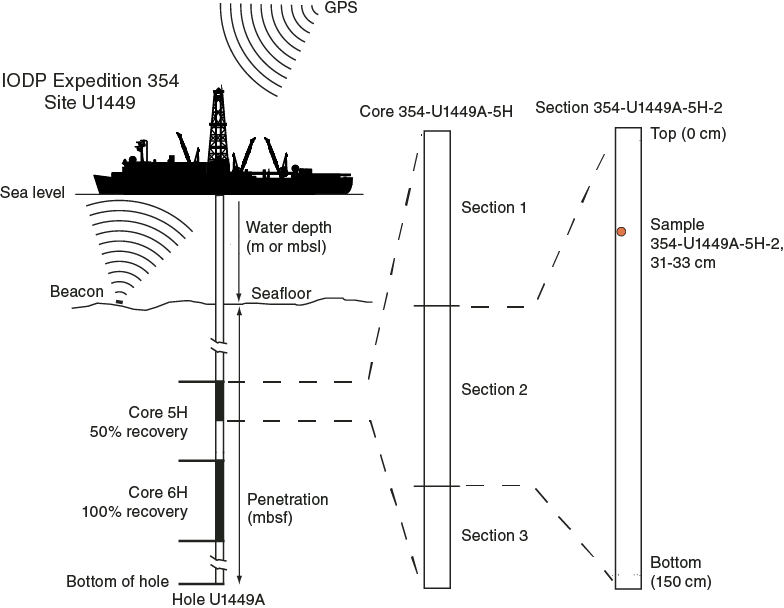
Figure F1. IODP conventions for naming sites, holes, cores, and samples.
Recovered cores are divided into 1.5 m sections that are numbered serially from the top downcore. When full recovery is obtained, the sections are numbered 1–7, with the last section usually being <1.5 m. Rarely, an unusually long core may require more than seven sections. When the recovered core is shorter than the cored interval, by convention the top of the core is deemed to be located at the top of the cored interval for the purpose of calculating (consistent) depths. Samples and descriptions of cores are designated by distance measured in centimeters from the top of the section to the top and bottom of each sample or interval. In sedimentary cores, the core catcher section is treated as a separate section (CC). When the only recovered material is in the core catcher, it is placed at the top of the cored interval.
A full curatorial sample identifier consists of the following information: expedition, site, hole, core number, core type, section number, and interval in centimeters measured from the top of the core section. For example, a sample identification of “354-U1449A-2H-5, 80–85 cm,” represents a sample taken from the interval between 80 and 85 cm below the top of Section 5 of Core 2 (collected using the APC system) of the first hole (Hole A) of Site U1449 during Expedition 354.
Sample depth calculations
For a complete description of depths, see IODP Depth Scales Terminology, v.2, at http://www.iodp.org/policies-and-guidelines. The primary depth scale types are based on the measurement of the drill string length deployed beneath the rig floor (drilling depth below rig floor [DRF] and drilling depth below seafloor [DSF]), the length of each core recovered (core depth below seafloor [CSF] and core composite depth below seafloor [CCSF]), and the length of the logging wireline deployed (wireline log depth below rig floor [WRF], wireline log depth below seafloor [WSF], and wireline log matched depth below seafloor [WMSF]). All units are in meters. Depths of samples and measurements are calculated at the applicable depth scale either by fixed protocol (e.g., CSF) or by combinations of protocols with user-defined correlations (e.g., CCSF). The definition of these depth scale types and the distinction in nomenclature should keep the user aware that a nominal depth value at two different depth scale types might not refer to exactly the same stratigraphic interval in a hole.
Depths of cored intervals are measured from the drill floor based on the length of drill pipe deployed beneath the rig floor (DRF scale). The depth of the cored interval is referenced to the seafloor (DSF scale) by subtracting the seafloor depth at the time of the first hole from the DRF depth of the interval. In most cases, the seafloor depth is the length of pipe deployed minus the length of the mudline core recovered. However, some seafloor depths can be determined in other manners (e.g., by offset from a previous known measurement of depth, or by observing the bit tag the seafloor with the camera system).
Standard depths of cores in meters below the seafloor (CSF-A scale) are determined based on the assumption that (1) the top depth of a recovered core corresponds to the top depth of its cored interval (DSF scale), and (2) the recovered material is a contiguous section even if core segments are separated by voids when recovered. When possible, voids in the core are closed by pushing core segments together on the catwalk during core handling. This convention is also applied if a core has incomplete recovery, in which case the true position of the core within the cored interval is unknown and should be considered a sample depth uncertainty, up to the length of the core barrel used, when analyzing data associated with the core material. Standard depths of samples and associated measurements (CSF-A scale) are calculated by adding the offset of the sample or measurement from the top of its section and the lengths of all higher sections in the core to the top depth of the cored interval.
A soft to semisoft sediment core from less than a few hundred meters below seafloor expands upon recovery (typically a few percent to as much as 15%), so the length of the recovered core often exceeds that of the cored interval. Therefore, a stratigraphic interval may not have the same nominal depth at the DSF and CSF scales in the same hole. When core recovery (the ratio of recovered core to cored interval times 100%) is >100%, the CSF depth of a sample taken from the bottom of a core will be deeper than that of a sample from the top of the subsequent core (i.e., the data associated with the two core intervals overlap at the CSF-A scale).
Cored intervals are defined by the core top depth in DSF and the distance the driller advanced the bit and/or core barrel in meters. The length of the core is defined by the sum of lengths of the core sections. The CSF depth of a sample is calculated by adding the offset of the sample below the section top and the lengths of all higher sections in the core to the core top depth measured with the drill string (DSF). During Expedition 354, all core depths below seafloor were calculated according to the core depth below seafloor Method A (CSF-A) depth scale.
Lithostratigraphy
This section outlines the methods used to describe sedimentary successions recovered during Expedition 354, including core description and smear slide description. Only general procedures are outlined, except where they depart significantly from IODP conventions.
Preparation for core description
The standard method of splitting a core by pulling a wire lengthwise through its center tends to smear the cut surface and obscure fine details of lithology and sedimentary structure. When necessary during Expedition 354, the archive halves of cores were gently scraped across (not along) the core section using a stainless steel scraper to prepare the surface for unobscured sedimentological examination and digital imaging. Scraping parallel to bedding with a freshly cleaned tool prevented cross-stratigraphic contamination. In (semi)lithified sediments, wire splitting generates uneven and wavy cut surfaces. Therefore, these sediments were cut by saw, the cut surface gently rinsed to clear saw cuttings, and were not scraped.
Sediment classification
Sediments recovered during Expedition 354 have siliciclastic, biogenic, and volcaniclastic components. They were described using a classification scheme derived from methods used during Ocean Drilling Program (ODP) Leg 155 (Flood, Piper, Klaus, et al., 1995) and Integrated Ocean Drilling Program Expedition 339 (Stow, Hernandez-Molina, Alvarez-Zarikian, and the Expedition 339 Scientists, 2013), as well as those defined by Shepard (1954). The siliciclastic component consists of mineral and rock fragments derived from sedimentary, igneous, and metamorphic rocks. Volcaniclastic refers to all clastic sediments composed mainly of particles of volcanic origin (glass shards, pumice, crystals, and rock fragments), regardless of how the sediment formed. The biogenic component consists of the skeletal debris of marine calcareous and siliceous plankton and macrofossil shell fragments. The relative proportion of these three components is used to define the major classes of sediments in this scheme (Figure F2). For Expedition 354, siliciclastic sediments are those that contain >50% siliciclastic grains and <50% biogenic and volcaniclastic grains. Biogenic sediments are those that contain >50% biogenic grains and <50% siliciclastic and volcaniclastic grains. Sediments containing >50% silt- and sand-sized volcanic grains are classified as ash layers.
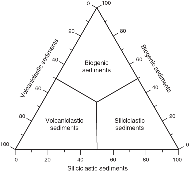
Figure F2. Ternary diagram showing lithologic classification of sediments.
Lithologies for siliciclastic components are based on the relative proportions of sand-, silt-, and clay-sized particles (Figure F3). The principal name is based on the textural characteristic of the dominant component (i.e., sand, silt, or clay). The second most abundant component defines the prefix (e.g., clayey sand or sandy silt), and other additional components are mentioned as a suffix after the main descriptors (e.g., silty sand with mica). However, distinguishing between some of these categories can be difficult (e.g., silty clay versus clayey silt) without accurate measurements of grain size abundances. Unless specified, the term “clay” is used to describe particle size and is applied to both clay minerals and all other grains <4 µm in diameter.
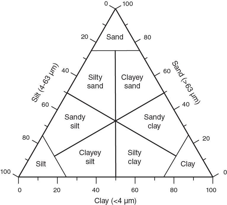
Figure F3. Ternary diagram showing lithologic classification for siliciclastic terrigenous sediments according to their granular texture.
If sediment contains a mixture of clay-sized siliciclastic particles and calcareous components (i.e., carbonate contents between 10% and 75%), the principal name is calcareous clay or calcareous claystone (Figure F4). The principal name of sediment that appears to contain >75% carbonate is calcareous ooze or limestone, preceded by the second most abundant component (e.g., nannofossil-rich calcareous ooze). Other additional components are mentioned as a suffix after the main descriptors (e.g., nannofossil-rich calcareous ooze with foraminifers). The principal name of sediment that appears to contain <10% carbonate is clay or claystone. This nomenclature was adopted to describe the continuum of sediments recovered from almost pure claystone to almost pure limestone.
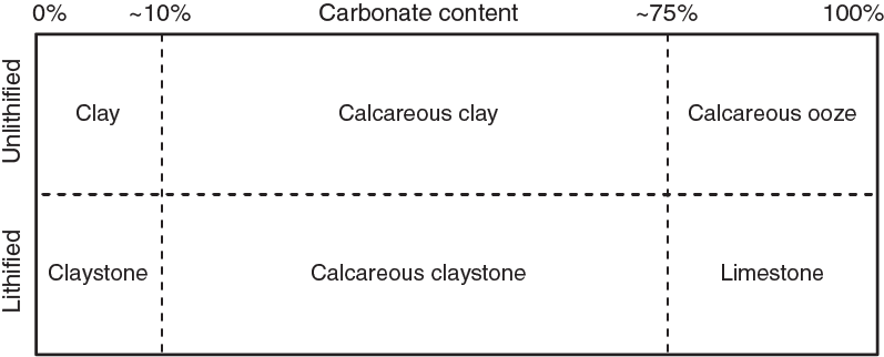
Figure F4. Sediment nomenclature for clay-sized siliciclastic material and carbonate.
The following terms describe lithification depending on the dominant composition. If the sediment cannot be deformed easily with a finger, the suffix “stone” is appended to the name (e.g., claystone or sandstone). Indurated calcareous and biosiliceous oozes are replaced by the terms “limestone” and “chert,” respectively. An indurated volcanic ash is called “tuff.”
Primary lithologies and major modifiers of siliciclastic lithologies are indicated in the graphic lithology chart (Figure F5).
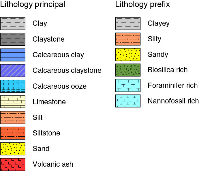
Figure F5. Graphic lithology patterns.
Stratification and sedimentary structures
Bedding features and other sedimentary structures, such as mottling, mud clasts, color banding, and graded bedding intervals were described from the split core surfaces. Symbols representing these features are shown in Figure F6.

Figure F6. Symbols for sedimentary descriptions.
For Expedition 354, the following terminology (based on Stow, 2005) was used to describe the scale of stratification:
- Lamination = <1 cm thick.
- Very thin bed = 1–3 cm thick.
- Thin bed = 3–10 cm thick.
- Medium bed = 10–30 cm thick.
- Thick bed = 30–100 cm thick.
- Very thick bed = >100 cm thick.
Lithologic accessories
Lithologic, diagenetic, and paleontologic accessories such as plant fragments, concretions, pyrite, and shells are accounted for in the core descriptions. The designated symbols for these features are shown in Figure F6.
Sediment disturbance
The intensity of drilling-related sediment disturbance is described as slight or high. The style of drilling disturbance is described for soft and lithified sediments using the following terms:
- Fall-in: heavily fractured and deformed pieces from the borehole wall and/or cuttings that fell into the top of the core.
- Up-arching: material retains its coherency, with material closest to core liner bent downward. Most apparent when horizontal features are distorted.
- Flow-in: results in significant contortion of layers due to fluidization of unlithified sediment.
- Soupy: intervals are water saturated and do not show any sign of their original bedding.
- Void: empty space within the cored material (e.g., due to gas exsolution/expansion during core retrieval). Voids may also be related to partial strokes during the coring process, although these voids are curated on the catwalk and do not appear in any core description.
- Fractured: firm sediments are pervasively broken and may be displaced or rotated.
- Biscuit: intervals of the core pieces are broken into pieces and rotated relative to each other. Soupy slurry fills the space between these pieces. Typical sediment deformation for XCB and RCB coring.
- Gas expansion: sediment does not entirely fill the core liner, and soupy textures occur. Stratification is commonly destroyed, and bed thickness is artificially increased.
Symbols for sediment disturbance are shown in Figure F6. Representative images are provided in Figure F7.
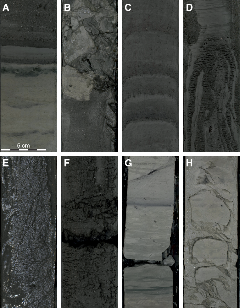
Figure F7. Representative examples of drilling disturbances. A. Undisturbed sediment beds. B. Fall-in. C. Up-arching. D. Flow-in. E. Soupy. F. Void. G. Fracture. H. Biscuit..
Smear slides
Typically, 1 to 11 smear slides were made per core. These were taken from the archive halves during core description. Tables summarizing relative abundance of sedimentary components from the smear slides were generated.
For each smear slide, a small amount of sediment was removed using a toothpick and placed directly on a 25 mm × 75 mm glass slide. A drop of deionized water was added, and the sediment was evenly spread across the glass slide using a toothpick and dried on a hot plate at a low setting (50°C). A drop of optical adhesive (Norland optical adhesive Number 61) was added to mount a 22 mm × 30 mm coverslip to the glass slide. The slide and mounted cover were then placed in an ultraviolet light box for about 10 min. Once the mounts were fixed, each slide was scanned at 5×, 10×, 20×, 50×, and 63× with a transmitted light petrographic microscope using an eyepiece micrometer to assess grain-size distributions of clay (<4 µm), silt (4–63 µm), and sand (>63 µm) fractions. Several fields were examined at 5×, 10×, 20×, 50×, and 63× for mineralogical and microfossil identification. Standard petrographic techniques were employed to identify commonly occurring minerals and biogenic groups, as well as important accessory minerals and microfossils. Relative abundances of identified components such as mineral grains, microfossils, and biogenic fragments were described on a semiquantitative basis by percentage estimation.
It should be noted that, on occasion, the lithologic name assigned from the smear slide does not match the name in the macroscopic lithology description because the smear slide data refers to a smaller area sampled, which may not be representative of the entire described interval. In addition, very fine and coarse grains are difficult to observe in smear slide, and their relative proportions in the sediment can be affected during slide preparation.
Maximum grain size was determined at approximately 10 m intervals (1 or 2 per core). In each case, the coarsest fraction in the individual core (generally from the base of the coarsest turbidite) was chosen for smear slide analysis. The five largest detrital (hard) grains were measured using the calibrated eyepiece grid scale on the microscope. The mean value was reported as the maximum grain size.
Thin sections
Slices of rocks were taken and trimmed to even thickness with a thin wire or cut with a saw. Samples were freeze-dried for about 12 h to avoid excessive cracking, although thin microcracks still penetrated much of the freeze-dried sediment. The dried samples were impregnated with Epo-Tek resin under vacuum and then grinded/polished until standard thin sections were generated.
Clay extraction and X-ray diffraction analysis
Samples analyzed for clay mineralogy were first treated with 10% acetic acid to remove carbonate before classic separation. Excess acid was removed by repeated centrifuging followed by homogenization. The <2 µm fraction was separated by centrifuge and used to make oriented aggregates on glass slides. When required, lithified samples were dispersed with Calgon solution. All samples were air-dried and glycolated (12 h under vacuum in ethylene glycol at 60°–70°C). Semiquantitative estimation of clay-mineralogic content is based on the heights and areas of basal reflections on XRD diagrams, assuming that these weighted amounts add up to 100%.
Samples for X-ray diffraction (XRD) analyses were selected from the working half, generally at the same depth as sampling for solid-phase geochemistry and smear slide analyses. Approximately one 5 cm3 sample was taken of a representative lithology per core, typically in Section 2. Samples taken for XRD analysis were also analyzed for sedimentary inorganic (i.e., carbonate analysis) and organic (i.e., carbon-hydrogen-nitrogen-sulfur analysis) carbon in the Geochemistry Laboratory (see Geochemistry and microbiology). Samples analyzed for bulk mineralogy were freeze-dried and homogenized by grinding in the metal ball mill. Prepared samples were top-mounted onto a sample holder and analyzed using a Bruker D-4 Endeavor diffractometer mounted with a Vantec-1 detector, using nickel-filtered CuKα radiation. The standard locked coupled scan was as follows:
- Voltage = 37 kV.
- Current = 40 mA.
- Goniometer scan = 4°–70°.
- Step size = 0.0166°.
- Scan speed = 1 s/step.
- Divergence slit = 0.3 mm.
Shipboard results yielded only qualitative results of the presence and relative abundances of the most common mineralogical components.
Diffractograms of bulk samples were evaluated with the aid of the EVA software package, which allowed for mineral identification and basic peak characterization (e.g., baseline removal and maximum peak intensity). Files were created that contained d-spacing values, diffraction angles, and peak intensities with and without the background removed. These files were scanned by the EVA software to find d-spacing values characteristic of a limited range of minerals.
Visual core description sheets
Visual core description sheets provide a summary of the data obtained during shipboard analysis of each sediment core. Detailed observations of each section were entered into the DESClogik software, which provides compatible data for the Strater software to generate a simplified, annotated graphical description (VCD) for each core. Site, hole, and depth (CSF-A, in meters) are given at the top of the VCD, with the corresponding depths of core sections along the left margin. Columns on the VCD include Lithologic unit, Core image, Graphic lithology, Coring disturbances, Sedimentary structures, Lithologic accessories, Shipboard samples, and Age. Profiles of magnetic susceptibility, natural gamma radiation (NGR), and reflectance are also included (see Physical properties).
Lithologies of the described core are represented on the VCDs by graphic patterns illustrated in Figure F5. Lithologies that constitute <10% of the core are generally not shown but are listed in the description. However, some distinctive secondary lithologies, such as ash layers, are included graphically. The relative abundances of lithologies represented in the VCDs are useful for general characterization of the sediment but do not constitute a precise quantitative observation.
Sand collection
APC and HLAPC coring in turbiditic formations returned some intervals with large quantities of loose sand—sometimes with large amounts of water. The term soupy sand has been used to describe this state where no primary sedimentary structures have been preserved because of the coring process and/or core handling and processing. Although the exact position of the sand in the cored interval is questionable because it may be partly sucked in while pulling the piston core out of the formation, this sand originates from the vicinity of the cored interval and is a valuable sample of this formation. Large sample sizes (>2 kg) are required for heavy and rare mineral separation to acquire a statistically significant quantity (i.e., n = ~100) of individual detrital grains for geochronological analyses (e.g., Gehrels et al., 2008). Because this sand is in suspension in the core liner, we had to adapt the recovery from the core liner using two methods. One method used for Site U1449 and Hole U1450A involves using buckets to capture loose sand “fall out” when cores are divided into sections on the catwalk. Clean empty buckets are held beneath core liners as they are split, catching wet sands as they fall from between section divisions. In most cases, a single bucket sample contains sands collected from numerous intervals within a single 4.5 or 9 m core (i.e., a single bucket sample may contain an amalgamation of sands from different depth intervals). Likewise, sands collected from cores at adjacent depth intervals may be combined to increase the overall size of individual samples. Buckets with sand are then left to settle and dewater for several hours. Excess water is poured off, and remaining sand is transferred to a gallon Ziploc bag, weighed, and labeled.
Starting with Hole U1451A, we applied a second method where core sections containing soupy sand were stored vertically on the catwalk to allow all of the sediment contained in the core liner to settle. When a core contains large intervals of wet sand, core liners up to 3 m long are securely capped on one end (typically the top) and placed vertically upright to settle on the catwalk for up to several hours. Excess water is poured off, and the core liner is cut off to the top of the settled sediment, capped, and then normally processed as a core section. This method increases retention of the core material (including fine fractions) and reduces potential contamination that may be introduced via catwalk processing or within buckets. Samples may then be collected directly from settled sections after they have been described and processed for shipboard analyses or from the bucket samples. This settling process may have induced grain-size variations (e.g., grading, layering, etc.) that may have been captured on whole-round and split core measurements and observations (physical properties, core images, etc.). Any structures in the sections that were subjected to this settling must not be interpreted as primary structures of the sediment. Each site where this technique has been applied includes a table listing the sections that were subjected to this type of core handling.
Biostratigraphy
Calcareous nannofossils and benthic and planktonic foraminifers in core catcher samples were studied at all sites. Samples from core sections were also examined when a more refined age determination was necessary and when time permitted. Biostratigraphic events, mainly the first occurrence (FO) and last occurrence (LO) of diagnostic species, are tied to the geologic timescale of Gradstein et al. (2012).
Calcareous nannofossils
Calcareous nannofossil zonal scheme
The standard nannofossil zonations of Martini (1971), Bukry (1973), and Okada and Bukry (1980) were utilized during the expedition to evaluate nannofossil age datums (Table T1). These zonal schemes were correlated to the Gradstein et al. (2012) geological timescale. The program Nannoware and the website Nannotax (http://ina.tmsoc.org/Nannotax3) were consulted to identify nannofossil species.
Table T1. Calcareous nannofossil biomarker species and ages. Download table in .csv format.
Methods
Calcareous nannofossil assemblages were examined and described from smear slides made from core catcher and core section samples. To process a sample, a small portion of sediment was placed directly on a glass coverslip (22 mm × 50 mm × 1 mm). A drop of distilled water was added, and the sediment was evenly spread across the coverslip using a flat-sided toothpick. The coarser grained fraction was removed during this process. The coverslip was then dried on a hot plate. After drying, it was mounted onto a glass microscope slide with Norland optical adhesive (Number 61) and placed under a UV light bulb until the adhesive hardened. Samples were examined using a Zeiss Axiophot or AxioScope light microscope with oil immersion lenses (40×, 63×, and 100×). Phase contrast, brightfield, and cross-polarized light were employed. When possible, relative abundances of nannofossils were counted using BugWin software (http://www.bugware.com/BugWin.html). Photomicrographs were taken using a Spot RTS system with image capture software.
Determinations on the degree of preservation and group and species abundances were recorded in DESClogik and uploaded to the LIMS database. Group and species relative abundances of calcareous nannofossils were determined from 20 fields of view (FOV) at 1000× magnification. Two additional traverses were undertaken to find less abundant nannofossils, and when found they were assigned a value of “rare.”
Group and species relative abundances of calcareous nannofossils were determined using the criteria defined below:
- V = very abundant (>100 specimens per FOV at 1000× magnification).
- A = abundant (10–100 specimens per FOV at 1000× magnification).
- C = common (1–10 specimens per FOV at 1000× magnification).
- F = few (1–10 specimens per 2–10 FOV at 1000× magnification).
- VF = very few (1 specimen per 2–10 FOV at 1000× magnification).
- R = rare (1 specimen per >10 FOV at 1000× magnification).
- B = barren (no nannofossils per FOV).
- * = reworked (reworked occurrence).
The following basic criteria were used to qualitatively provide a measure of preservation of the nannofossil assemblage:
- E = excellent (no dissolution is seen; all specimens can be identified).
- G = good (little dissolution and/or overgrowth is observed; diagnostic characteristics are preserved, and all specimens can be identified).
- M = moderate (dissolution and/or overgrowth are evident; a significant proportion [up to 25%] of the specimens cannot be identified to species level with absolute certainty).
- P = poor (severe dissolution, fragmentation, and/or overgrowth has occurred; most primary features have been destroyed, and many specimens cannot be identified at the species level).
Foraminifers
Planktonic foraminifer zonal scheme and taxonomy
The planktonic foraminiferal zonation schemes of Blow (1969, 1979) and Berggren et al. (1995), as modified by Wade et al. (2011), were used in this study. Calibrated ages for biomarkers are from Gradstein et al. (2012) (Table T2).
Table T2. Foraminiferal biomarker species and ages. Download table in .csv format.
Taxonomic concepts for Neogene and Paleogene taxa mainly follow those of Kennett and Srinivasan (1983) and Bolli and Saunders (1985).
Methods for foraminifers
Core catcher samples (plus one sample per section as needed) were washed in deionized water and washed over a 63 µm mesh sieve. Indurated samples were soaked in 200 mL water with 50 mL of 30% hydrogen peroxide solution prior to washing. Lithified material was broken into ~2 cm3 pieces and soaked in kerosene for 12 h. The kerosene was then poured off, and hot water was added. The samples were sieved ~12 h later. All samples were dried on filter paper in a 45°C oven. To minimize contamination of foraminifers, the sieves were placed into a sonicator for several minutes, cleaned with pressurized air, and thoroughly checked between samples. The dried samples were sieved over a 150 µm sieve, retaining the <150 µm size fraction for additional observation when necessary. The >150 µm size fraction specimens were examined under a light microscope for species identification, and the 63–150 µm size fraction was scanned for distinctive taxa. Selected specimens were mounted on scanning electron microscope (SEM) stubs and examined on a TM3000 tabletop SEM in order to distinguish different wall textures and the degree of crystallization. Thin sections were made of lithified sediments and examined using a petrographic microscope for biostratigraphic analysis. Planktonic foraminifer species distribution and range charts are presented in each site chapter. Relative percentages of benthic to planktonic tests were determined by counting specimens in four adjacent quadrants in three different locations on the picking tray.
The following abundance categories were estimated from visual examination of the dried >63 µm residue. The total abundance of planktonic foraminifers was defined as follows:
- A = abundant (>25% specimens in total residue).
- C = common (11%−25% specimens in total residue).
- F = few (6%−10% specimens in total residue).
- R = rare (<5% specimens in total residue).
- VR = very rare (<0.1% specimens in total residue).
- B = barren (no specimens in total residue).
Individual planktonic foraminifers were recorded in qualitative terms based on an assessment of forms observed in a random sample of ~150 specimens from the >150 µm size fraction. In samples where fewer than 150 specimens were present, all specimens were counted. Relative abundances were reported using the following categories:
- A = abundant (>25% of the assemblage).
- C = common (11%−25% of the assemblage).
- F = few (6%−10% of the assemblage).
- R = rare (<5% of the assemblage).
- B = barren (none present).
The preservation status of planktonic and benthic foraminifers was estimated as follows:
- VG = very good (no evidence of overgrowth, dissolution, or abrasion).
- G = good (little evidence of overgrowth, dissolution, or abrasion).
- M = moderate (calcite overgrowth, dissolution, or abrasion are common but minor).
- P = poor (substantial overgrowth, dissolution, or abrasion).
The fragmentation of the planktonic foraminifers was visually estimated and categorized as follows:
- N = none (no fragmentation observed).
- L = light (0%–10% fragmentation observed).
- M = moderate (10%–25% fragmentation observed).
- S = severe (25%–50% fragmentation observed).
- VS = very severe (>50% fragmentation observed).
Biozone and midpoint calculations
Midpoint depths are used to represent the depth at which nannofossil and foraminifer biomarkers occur. They are calculated by halving the distance between the depth of the biomarkers’ FO or LO and the nonbarren sample above (or below) that did not contain the biomarker. The error is half of the interval between the two samples. These midpoints are used in the Stratigraphic synthesis figures in each site chapter, and the values and calculations can be found in Biostratigraphy in each site chapter.
Paleomagnetism
Paleomagnetic measurements
Paleomagnetic investigations during Expedition 354 focused primarily on determining natural remanent magnetization (NRM) vectors, both before and after alternating field (AF) demagnetization, for the purposes of matching magnetic polarity intervals to a geomagnetic polarity timescale (Gradstein et al., 2012), correlating data between sites, and assessing the feasibility of shore-based studies (e.g., relative paleointensity and environmental magnetism). Although much of our interest is in the oriented APC cores, we also measured the magnetization of XCB and RCB cores. The nonmagnetic drill collar was included in the BHA for all holes where APC coring was conducted to aid in core orientation. Only APC, half-length APC, and RCB cores were collected using nonmagnetic core barrels.
Split core measurements
All remanence measurements on archive section halves were made using a 2G Enterprises 760R superconducting rock magnetometer (SRM) using direct current (DC) superconducting quantum interference devices (SQUIDs) and an in-line, automated three-axis degaussing system capable of maximum peak fields of 80 mT. Both the SRM and the degaussing system are controlled through the SRM Section software interface. The background noise level of the SRM is ~2 × 10⁻⁹ Am2 (2 × 10⁻⁵ A/m for a ~100 cm3 split core). Practically speaking, however, reliable split core measurements are typically ~10–4 A/m or higher (Richter et al., 2007). The spatial resolution of the SRM is limited by the SQUID response functions, which are ~10 cm wide at half height (Parker and Gee, 2002).
We measured archive section halves from split core sections in the SRM. All cores were wrapped in plastic wrap before measuring to limit contamination of the SRM. Measurements were taken at 1, 2.5, or 5 cm intervals in APC sections and at a 2.5 or 5 cm interval in XCB and RCB sections. To account for gaps in the core due to poor recovery, disturbance, water, or geochemical sampling, we manually noted these features in a log notebook and omitted these intervals in postprocessing. We also measured 15 cm before the core entered the magnetometer’s sensing region (header) and 15 cm after the core left the sensing region (trailer) to allow for deconvolution of SQUID signals after the expedition and monitor for background noise and drift. The NRM of archive section halves was typically measured after 0, 10, 15 and 20 mT (peak field) AF demagnetization to evaluate the effectiveness of demagnetization at removing drilling and viscous overprints. The 10 and/or 15 mT demagnetization steps were omitted for some cores when the slow speed of paleomagnetic measurements was restricting core flow. For some cores, only NRM was measured to further speed core flow and/or to preserve NRM for later demagnetization (at sites with multiple holes). Sections from certain high-recovery cores planned for high-resolution study (e.g., Core 354-U1452A-1H) were not demagnetized on board to allow for future shore-based paleomagnetic work. To reduce background noise, we cleaned and degaussed the sample tray (at 80 mT peak field) once per day. Tray and background measurements have been subtracted from all results reported here. Peak AFs higher than 20 mT were not used on archive section halves so that cores could be preserved for future shore-based study.
The previous expedition (353) experienced numerous residual flux counts in the Y-axis SQUID (see figure F2 of Richter et al., 2007, for coordinates), and this was monitored carefully during Expedition 354. Several residual flux counts on the Y-SQUID were observed during Expedition 354, often resulting in measurements that appeared to have low noise but anomalous directions. We speculate that flux jumps may affect measurements on carbonate ooze more than other lithologies; one residual flux count superimposed on the weak magnetization of ooze produces a much larger directional change than a residual flux count against the much stronger magnetization of terrigenous sediments. When we identified section-half measurements affected by residual flux counts, we remeasured the section half. Anecdotal information from Expedition 353 indicated that a strip of thin packing foam placed between the section half and the SRM core tray reduced the frequency of flux jumps. We followed this suggestion starting at Site U1453 but found it to have little effect.
In some instances, we also observed a position error that resulted in shifts of identifiable features in inclination, declination, and/or intensity by as much as 20 cm between repeat measurements (Figure F8). Typically, measurements would be offset in one direction between an initial AF demagnetization step and the following step and then shifted in the opposite direction in the next pair of AF demagnetization steps. This sometimes resulted in important information (e.g., reversal boundaries) being offset into the header or trailer records. This issue is related to the position-sensing mechanism of the SRM’s automatic core movement system. IODP staff corrected this issue in the SRM Section software as of 19 March 2015. Sections for which position offset was thought to be a problem were demagnetized a second time at 20 mT (to remove any viscous overprint acquired during storage) and remeasured. Remeasured data (remanent magnetization measurements after 20 mT demagnetization) were uploaded to the LIMS database. Depths of reversals specified in the site chapters are based on measurements that we believe to be free of position error.
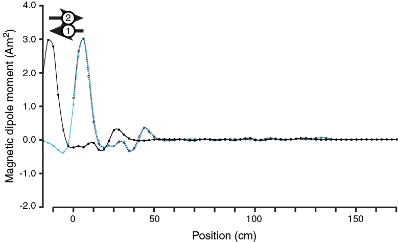
Figure F8. Magnetic dipole moment measured three times using the SRM, illustrating position error. Y component is plotted here; similar errors were observed in X and Z components.
To minimize contamination of paleomagnetic data due to coring deformation or lithologies unlikely to hold a stable remanence, we identified remanence measurements from all intervals described as being “highly disturbed,” “soupy,” or “flow-in,” as well as having a “sandy principal lithology” (see Lithostratigraphy in the Site U1450 chapter [France-Lanord et al., 2016]), which we cross-checked with our own observations. These intervals, as well as remanent magnetization vectors from the top 20 cm of each core and the top and bottom 10 cm of each section, were not used in our final magnetostratigraphic interpretations.
Discrete sample measurements
To supplement split-core measurements, we measured the progressive demagnetization of discrete samples from select APC, XCB, and RCB cores. Discrete samples for shipboard measurement were generally collected from three or four intervals in each APC core, with sampling focused on undeformed, finer grained (muddy) intervals. Samples were not collected in some intervals with rare lithologies or features considered worth protecting for postexpedition sampling. Fewer samples were collected in XCB and RCB cores and in APC cores that were highly deformed, sandy, or short. Most discrete samples were progressively demagnetized along three axes (z, y, and x, in that order) in peak AFs of 0, 10, 15, 20, 25, 30, 40, 50, and 60 mT using a DTECH D2000 AF demagnetizer and measured in an AGICO JR-6A dual-speed spinner magnetometer. Early in the expedition, one set of samples was demagnetized in the 2G-600 AF demagnetizer and measured in the SRM using a tray designed to fit sample cubes. These samples acquired a gyroremanent magnetization (GRM) or anhysteretic remanent magnetization (ARM; see below), so the remaining samples were demagnetized in the DTECH D2000, which allowed more flexibility in the AF treatment procedure. Some discrete samples, particularly calcareous oozes, were too weak to measure in the JR-6A at some of the higher AF steps (40–60 mT), so stepwise demagnetization was stopped before 60 mT. A limited number of samples were demagnetized at additional steps (80 and 100 mT) to evaluate the decay of NRM at low and high fields. In all cases, principal component characteristic remanent magnetization (ChRM) vectors were fit to subsets of the demagnetization data using principal component analysis (PCA; Kirschvink, 1980).
Paleomagnetists on Expedition 353 determined that some samples acquired a GRM at fields above 60 mT (Clemens et al., 2015). GRM affected Expedition 353 remanence data from peak AF steps >40 mT and was easily identified by a remanent magnetization intensity that increased (in the Y direction) with progressive demagnetization. If we noticed that discrete samples were acquiring a GRM or ARM, we used the demagnetization scheme of Dankers and Zijderveld (1981) on AF steps above 40 mT in the D2000 and on measured samples in the JR-6A. The modified Dankers-Zijderveld scheme involved the following steps:
- AF demagnetize sample along z-, y-, and x-axes and measure (normal procedure).
- AF demagnetize sample along –z-axis and measure.
- AF demagnetize sample along –y-axis and measure.
- AF demagnetize sample along –x-axis and measure.
- Take average (Fisher mean) of all measurements.
In some cases, it is difficult to distinguish between GRM and ARM acquired during AF demagnetization. To determine whether an ARM was being acquired, a subset of samples were inserted in the degausser in a reverse direction (–z-, –y-, and –x-axes) at the 15, 25, and 35 mT AF steps before measurement. A jagged demagnetization diagram and a high median angular deviation angle resulted when samples acquired appreciable ARMs during the demagnetization process. This was evident even at relatively low AF treatments (<20 mT). However, because the ARM acquired was along alternating positive and negative axes, its effect was minimal on the sample ChRM directions determined by PCA.
Orientation
The low latitude of the Middle Bengal Fan coring sites made orientation information necessary for any useful paleomagnetic information. Orientation information was obtained in two ways: during core collection (for APC cores) and after core collection (for lithified RCB cores). APC cores were collected using a nonmagnetic core barrel. In many cases, full-length APC cores were oriented using the Icefield MI-5 or FlexIT orientation tools. HLAPC, XCB, and RCB cores were unoriented. We report all results of oriented cores in geographic coordinates derived using Icefield MI-5 or FlexIT measurements and local International Geomagnetic Reference Field (IGRF12) magnetic declination. Split-section measurements on archive section halves used the standard right-handed IODP coordinate system (see figure F2 of Richter et al., 2007). Discrete samples were collected from the working section halves by pushing Natsuhara-Giken sampling cubes (7 cm3 sample volume) into the sediment with the cube’s up arrow pointing toward the top of the core.
Rotary coring (XCB and RCB) presents an additional orientation problem: individual pieces of a core (“biscuits”) are rotated independently about the vertical drill string axis. In some RCB cores, we observed sedimentary beds that appeared to be tilted. We measured apparent dips of bedding planes on the cut faces of archive section halves and used those data in combination with magnetic declination measurements to simultaneously calculate a best-fit true dip and to evaluate magnetic polarity as follows.
The relationship between a plane’s true dip, δ, and its apparent dip, δ′, depends on the angle α between the plane’s strike and the cut face where the apparent dip is measured:
(1)Sign conventions for all variables are illustrated in Figure F9. For RCB cores, δ′ was measured and δ was unknown but assumed to be constant within a core. The value of α depends on the strike S (angle between north and the line of strike) and the ChRM vector declination Dec (angle between coordinate system +x-axis and north):
(2)Note that both S and Dec in our usage are relative to magnetic north. The declination of remanent magnetization after 20 mT AF was used to approximate Dec. The value of S was unknown but assumed to be constant within a core. For convenience, we defined
(3)and
(4)such that
(5)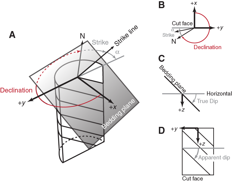
Figure F9. Summary of apparent dip reorientation technique.
We used the Nelder-Mead SIMPLEX algorithm as implemented in Matlab’s “fminsearch” function (Lagarias et al., 1998) to calculate best-fit parameters R and D that minimized the misfit between the calculated apparent dips and the measured apparent dips for all measurements i within a hole:
(6)The termination tolerance was set to 1 × 10⁻⁴ units (degrees for R, tan(radians) for S, and tan(radians) for misfit). Minimum misfit values greater than ~0.1 indicate a poor fit between the model parameters and the observed apparent dips, possibly because of horizontal-axis rotations of core pieces during drilling, measurement of apparent dips of nonbedding-parallel features (e.g., burrows, soft-sediment deformation features, or cross-beds mistaken for bedding), drilling-induced magnetization, or paleomagnetic secular variation. In some cases, poorly constrained models gave low minimum misfit values. This was particularly true in cores where a very small number of apparent dips were measured, where all measured apparent dips were within ~1° of horizontal, or where there was a small amount of variation in δ′-Dec space.
The best-fit values of D and R in Equation 5 allow us to estimate the orientation of two planes (with strike S and dip ±δ) that fit the apparent dip and declination data. We then compare individual measurements of tan δ′ and Dec to the calculated values from the two sine functions that correspond to the two planes. We interpret changes in the sign of δ within a core in terms of changes in magnetic polarity rather than reversals in dip direction. Where δ′ – Dec data are a poor match to one of the best-fit dipping planes or where the apparent dips are close to 0°, we consider the polarity undetermined.
We tested the computational technique using a data set of 100 simulated apparent dip–magnetic declination pairs derived from Fisher-distributed model magnetic vectors (Figure F10; κ = 10; mean declination/inclination: 000/00°), model bedding planes (pole to bedding κ = 100; mean declination/inclination: 096/82°), and cut core faces (uniformly distributed in azimuth, corresponding to uniformly distributed rotations). We determined the apparent dips of the model bedding planes using Equation 1. The pole to the best-fit bedding plane was oriented 095/83° with a minimum misfit of 0.1898, suggesting that even best-fit planes with high degrees of misfit may still recover useful directional information.
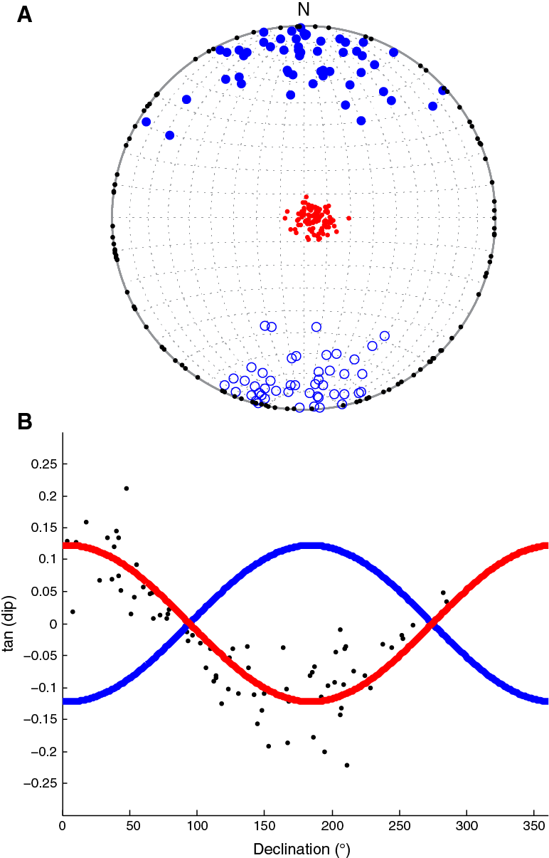
Figure F10. Test of apparent dip reorientation technique using simulated magnetic declination/apparent dip pairs.
In addition to magnetic polarity information, this method can be used to find best-fit orientation estimates for bedding planes. When applied to individual cores (rather than to all data from a hole), the method allows us to identify downhole variations in strike and dip, possibly due to tectonic deformation.
Rock magnetism and anisotropy
In addition to demagnetizing NRM, we also imparted ARM and isothermal remanent magnetization (IRM) to selected samples using the DTECH D2000 and ACS Scientific IM-20 impulse magnetizer, respectively, to characterize the rock magnetic properties of the sediment. ARM was imparted using a bias field of 50 µT in a peak AF of 100 mT and demagnetized in peak AFs of 20 and 40 mT; IRM was imparted at 100, 300, and 1000 mT. All remanence acquisition and demagnetization steps were measured in the JR-6A.
Typically, anisotropy of magnetic susceptibility (AMS) is measured on discrete samples using an AGICO KLY-4S Kappabridge. The Kappabridge was unavailable for Expedition 354, so AMS will be measured on shore.
We use bulk magnetic susceptibility data to normalize our split-section NRM measurements as a way to identify sections of interest for shore-based relative paleointensity measurements. Bulk magnetic susceptibility was measured on whole-round sections using a modified Bartington MS2C loop sensor on the WRMSL and on archive section halves using a Bartington MS2E point sensor on the SHMSL (see Lithostratigraphy and Physical properties). Both are attached to Bartington MS2 susceptometers with a resolution of 1 × 10⁻⁵ SI units. The MS2C loop on the WRMSL has an internal diameter of 80 mm (loop of 88 mm) and an operating frequency of 0.565 kHz. To convert to SI volume susceptibilities for the 80 mm loop, raw instrument measurements (stored in the LIMS database) are multiplied by 0.576 × 10⁻⁵ (1/κrel, where κrel = 3.45(d/D)3; d = 70 mm, D = 88 mm). The MS2E sensor operates at a frequency of 2 kHz and has a response function with approximate dimensions (FWHM) 3.8 mm parallel to the sensor track, 10.5 mm across the track, and 1 mm deep in the core. Point susceptibility data stored in the LIMS database are in 10–5 SI units.
Geochemistry and microbiology
The shipboard geochemistry program for Expedition 354 included measurements for
- Interstitial water composition;
- Headspace gas content; and
- Sediment geochemistry, including TIC, TC, TN, and major and trace element content.
These analyses were carried out to satisfy routine shipboard safety and pollution prevention requirements, characterize interstitial water, sediment, and rock geochemistry for shipboard interpretation, and provide a basis for sampling for shore-based research.
Interstitial water sampling and chemistry
Sample collection
Interstitial water samples were obtained by both squeezing whole-round samples and Rhizon samplers. Rhizon samples allowed interstitial water samples to be obtained without having to take a whole-round core sample and permitted more closely spaced sampling. The exact method of obtaining interstitial water samples (Rhizon or whole-round core) and frequency of sampling is described in each site chapter. Rhizon sampling for interstitial water lasted for ~2–4 h to obtain ~20 mL water samples for shipboard and shore-based analyses. As soon as Rhizon sampling was not capable of delivering ~20 mL of water, standard whole-round samples 5 cm long were employed. As water content decreased downhole, the size of the whole-round samples was increased to 15 cm to enable extraction of the ~20 mL of water needed for shipboard and shore-based analyses. Whole-round samples were cut and capped as quickly as possible after the core arrived on deck and immediately moved to the chemistry laboratory for squeezing. All samples were processed under normal atmospheric conditions. Whole-round samples were collected at a frequency of approximately one sample per core unless interstitial water extraction required a >15 cm whole-round section, whereupon the frequency of sampling was decreased or sampling discontinued. The exterior of the whole-round sample was carefully cleaned in the laboratory with a spatula to remove potential contamination from drilling fluid. For XCB cores, the intruded drilling mud between biscuits was also removed to eliminate contamination from drilling fluid. The cleaned sediment was placed into a 9 cm diameter titanium squeezer that was then placed in a Carver hydraulic press (Manheim and Sayles, 1974) and squeezed at pressures no higher than 25,000 lb (~17 MPa) to prevent the release of interlayer water from clay minerals during squeezing. The squeezed interstitial water was collected into a 60 mL deionized water–washed (18 MΩ/cm) high-density polyethylene syringe attached to the squeezing assembly and subsequently filtered through a 0.45 μm polyethersulfone membrane filter into various precleaned vials for subsampling.
Sample allocation was determined based on the pore fluid volume obtained and analytical priorities based on expedition objectives. Aliquots for shore-based analysis by inductively coupled plasma–atomic emission spectroscopy (ICP-AES) were acidified by adding ~10 μL of trace metal–grade concentrated HNO3 and placed in 5 mL cryovials, with a subset in 22 mL Teflon beakers. Aliquots for shipboard titration and ion chromatography analyses were put into 10 mL high-density polyethylene vials. Aliquots for shore-based isotopic analysis of dissolved inorganic carbon (DIC) and isotopic analyses of oxygen and hydrogen were placed in zero-headspace 2 mL septum screw-lid glass vials. Aliquots for shore-based dissolved Sr isotopic composition were also placed in 5 mL cryovials. The samples were stored at 4°C after collection. We then transferred 2 mL aliquots into 7 mL glass vials under nitrogen atmosphere for shore-based characterization of the dissolved organic matter (DOM) pool and another 2 mL in a separate glass vial under nitrogen atmosphere for the stable carbon isotopic composition of volatile fatty acids (VFA), all stored at –20°C.
Alkalinity, pH, and salinity were analyzed within 12 h after interstitial water was obtained. Other shipboard analyses were carried out in batches. Dissolved sodium, calcium, magnesium, potassium, chloride, bromide, and sulfate were analyzed by ion chromatography. Ammonium, dissolved silica, and phosphate were analyzed by spectrophotometry.
After interstitial water extraction was complete, sediment squeeze cakes were divided and sealed in plastic bags for shore-based analyses and curation at the IODP core repository (Kochi, Japan). Squeeze-cake samples for shore-based organic analysis were stored at –80°C. All other squeeze-cake samples were refrigerated at 4°C.
Shipboard analysis
Interstitial water samples were analyzed on board following the protocols described in Gieskes et al. (1991) and the IODP user manuals for shipboard instrumentation.
Alkalinity and pH
Alkalinity and pH were measured immediately after sampling, following the procedures described in Gieskes et al. (1991). pH was measured with a combined glass electrode, and alkalinity was determined by Gran titration with an autotitrator (Metrohm 794 basic Titrino) using 0.1 M HCl at 25°C. International Association for the Physical Sciences of the Oceans (IAPSO) standard seawater was used for calibration and was analyzed at the beginning of a set of samples and after every 10 samples. Alkalinity titrations had a precision better than 2% based on repeated analysis of IAPSO standard seawater. For sample volumes of ≤14 mL, alkalinity and pH were not measured because each alkalinity and pH analysis requires 3 mL of interstitial water.
Chloride by titration and salinity
High-precision chloride concentrations were acquired using a Metrohm 785 DMP autotitrator and silver nitrate (AgNO3) solution calibrated against repeated titrations of an IAPSO standard. A 0.5 mL aliquot of sample was diluted with 30 mL of an 80 mM HNO3 solution and titrated with 0.1 M AgNO3. Repeated analyses of an IAPSO standard yielded a precision better than ±0.05%; however, the chloride concentration yielded by the titration technique includes not only dissolved chloride but also all of the other halide elements and bisulfide. The JOIDES Resolution is equipped with a Metrohm 850 Professional ion chromatograph (IC) that can analyze anions and cations simultaneously. The chloride concentration was analyzed by both titration and ion chromatography for Expedition 353 Site U1444, Site U1449, and the upper section of Hole U1450A. Chloride concentrations analyzed by ion chromatography were not greater than those analyzed by titration (Figure F11), indicating that ion chromatography provides reliable chloride data. As a result, chloride concentration was analyzed only by ion chromatography for the remaining sites during Expedition 354.
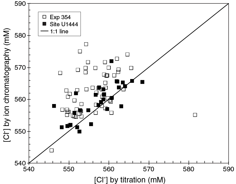
Figure F11. Relationship between interstitial water chloride concentrations measured by titration and by ion chromatography.
Salinity was calculated based on the chloride concentration and assumes a chemistry of the interstitial water close to normal seawater chemistry. The observed deviation from seawater chemistry in the concentration of all the dissolved interstitial water species besides sodium and chloride implies a maximum inaccuracy of the calculated salinity of ±0.7.
Sulfate, chloride, bromide, calcium, potassium, magnesium, and sodium
Sulfate, chloride, bromide, calcium, potassium, magnesium, and sodium concentrations were analyzed by ion chromatography (Metrohm 850 Professional IC) using aliquots of 100 μL that were diluted 1:100 with deionized water (18 MΩ/cm). At the beginning of each run, different dilutions of IAPSO standard seawater were used to determine a calibration curve, and IAPSO standard seawater was also analyzed along with the samples as an unknown for quality control and to determine accuracy and precision. Based on 17 measurements of IAPSO standard seawater, the only significant drift detected was for the bromide measurement. An offline linear correction was applied for this element, and corrected values are reported in the database. This resulted in analytical precision (2σ) and accuracy of, respectively, 1.2% and 0.4% for chloride, 1.7% and 0.1% for bromide, 1.8% and 0.8% for sulfate, 5.8% and 3.4% for calcium, 1.2% and 0.3% for potassium, 2.8% and 1.6% for magnesium, and 1.1% and 0.5% for sodium.
Ammonium, dissolved silica, and phosphate
Ammonium, dissolved silica, and phosphate concentrations were determined using an Agilent Technologies Cary Series 100 UV-Vis spectrophotometer with a sipper sample introduction system following the protocol described in Gieskes et al. (1991). For ammonium concentration analysis, a 0.1 mL sample aliquot was diluted with 1 mL reagent water, to which 0.5 mL phenol ethanol, 0.5 mL sodium nitroprusside, and 1 mL oxidizing solution (trisodium citrate and sodium hydroxide) were added in a 5 mL capped glass vial (Gieskes et al., 1991). The solution was kept at room temperature for ~6.5 h to develop color. Ammonium concentrations were determined at an absorbance of 640 nm. Precision of the ammonium analyses was ±3% (2σ).
For dissolved silica, a 0.2 mL aliquot was mixed with 2 mL molybdate solution added to the vial and allowed to react for exactly 15 min. Then 3 mL of reducing solution (mix of Metol sulfite and oxalic acid solution) was added to the vial (Gieskes et al., 1991), which was capped and kept at room temperature for at least 3 h to develop color. Repeat reruns after 24 h demonstrated the stability of the complex. The silica concentration was determined at an absorbance wavelength of 812 nm. Precision and accuracy of the silica analyses were better than 1% and 0.6%, respectively.
For phosphate analysis, a 0.3 mL sample was diluted with 1 mL deionized water (18 MΩ/cm) in a 4 mL glass vial. Then 2 mL of mixed reagent (ammonium molybdate, sulfuric acid, ascorbic acid, and potassium antimonyl tartrate) was added to the vial (Gieskes et al., 1991), which was capped and kept at room temperature for at least several minutes to develop color. The phosphate concentration was determined at an absorbance wavelength of 885 nm ~30 min after adding the mixed reagent solution. Precision and accuracy of the phosphate analyses were better than 2.5% and 1%, respectively.
Headspace gas geochemistry
Two sediment samples from each core (approximately 5 cm3 each, one for shipboard and the other for shore-based analyses), collected immediately after retrieval on deck, were placed in a 20 cm3 glass vial and sealed with a septum and a crimped metal cap. When consolidated or lithified samples were encountered, chips of material were placed in the vial and sealed, whereas fluidized sand was sampled with a scoop. If an interstitial water sample was obtained, the headspace sample was taken from the top of the section immediately next to the interstitial water sample whenever possible. Otherwise, the headspace sample was taken from the top of the third section. The vial was labeled with the core, section, and interval from which the sample was taken and then placed in an oven at 70°C for 30 min. A 5 cm3 aliquot of gas extracted through the septum was then injected with a gas-tight glass syringe into a gas chromatograph (GC).
An Agilent 6890 GC equipped with a flame ionization detector (FID) was used to measure the concentrations of methane (C1), ethane (C2), ethylene (C2=), propane (C3), and propylene (C3=). A 2.4 m × 2.0 mm stainless steel column packed with 80/100 mesh HayeSep “R” was installed in the GC oven. The injector consists of a ¹⁄₁₆ inch Valco union with a 7 μm screen connected to a Valco-to-Luer lock syringe adaptor. This injector connects to a 10-port Valco valve that is switched pneumatically by a digital valve interface. The injector temperature was set at 120°C throughout each run. Samples were introduced into the GC through a 0.25 cm3 sample loop connected to the Valco valve. The valve can be switched automatically to backflush the column. The oven temperature was programmed to start at 80°C for 8.25 min and then increase to 150°C at a rate of 40°C/min and hold for 5 min. Helium was used as the carrier gas. Initial helium flow in the column was 30 mL/min. Flow was then ramped up to 60 mL/min after 8.25 min to accelerate elution of C3 and C3=. The run time was 15 min. The GC was also equipped with an electronic pressure control module to control the overall gas flow. The FID was set at 250°C. No accurate measurement of the sediment mass was carried out. As such, measured concentrations are only semiquantitative (likely carrying a ±25% relative uncertainty, mainly reflecting variations in the sediment mass around the target mass), and are only indicative for safety monitoring. However, gas ratios (e.g., C1/C2) are not affected by the uncertainty on the sediment mass.
Both headspace gas vials were stored for future onshore investigations, one to be used for isotopic characterization of hydrocarbon gases (addition of 5 mL of 1 M NaOH and storage at –20°C) and the other to be used for measurement of CO2 concentration (replacement of headspace with saturated NaCl solution and storage at +4°C).
Sediment geochemistry
Sediment inorganic and organic carbon content
On average, two samples were collected from each core. Sediment samples were taken from intervals of distinct lithology. Samples were freeze-dried for ~24 h, crushed using an agate pestle and mortar, and then analyzed for total carbon (TC), total inorganic carbon (TIC), and total nitrogen (TN).
TC and TN of the sediment samples were determined with a ThermoElectron Corporation FlashEA 1112 CHNS elemental analyzer equipped with a ThermoElectron packed column CHNS/NCS GC and a thermal conductivity detector (TCD). Approximately 20–25 mg of dry sediment was weighed into a tin cup and then combusted at 950°C in a stream of oxygen. The reaction gases were passed through a reduction chamber to reduce nitrogen oxides to N2 and then were separated by the GC column before detection by the TCD. All measurements were calibrated to a set of reference standards covering the range in expected TC and TN values (Soil Reference Material [SRM] PDWR 3472541, SRM PWDR 5968501, and SRM PDWR 3472541 mixed 1/9 with powdered quartz combusted at 1025°C for 4 h), which was run every five samples. Peak areas from the TCD were calculated to determine the TC and TN of the samples. Blank levels were determined by analyzing empty tin cups and were subtracted from each measurement. Blank contribution for C is on the order of 1 µg. Given the typical sample mass used (20 mg on average) and using a signal/blank threshold of 10, this translates into a detection limit of ~0.04 wt%. For N, blanks were also estimated from the intercept of the calibration curve, which gave results similar to direct blank determination (i.e., empty tin cup blank). Blank contribution for N is on the order of 12 µg, unsurprisingly high considering the use of a sampler open to the atmosphere. This translates into a detection limit of ~0.06 wt%. Assuming a total organic carbon (TOC)/TN ratio of ~10 (typical of detritic material found in the Bengal Fan), this implies that sediments with TOC < 0.6 wt% have TN values below detection limit. Given that >85% of the samples analyzed fall in that category, we opted to not report TN concentrations. Accuracy of TC determination was estimated using repeated measurements of reference material and was found to be better than 5% of the TC value (i.e., <0.05 wt% for the vast majority of samples analyzed). Precision of TC determination was estimated from limited duplicate measurements and was systematically within estimated accuracy.
TIC was determined using a Coulometrics 5015 CO2 coulometer. Approximately 50 mg (10 mg for lithologies dominated by carbonates) of sediment was weighed into a glass vial and acidified with 2 M HCl. The liberated CO2 was titrated, and the corresponding change in light transmittance in the coulometric cell was monitored using a photodetection cell. The weight percent of calcium carbonate was calculated from the inorganic carbon content using the following equation:
(7)Blank levels were determined by analyzing empty reactors as well as aliquots of powdered quartz combusted at 1025°C for 4 h. Blank levels were found to vary between 3 and 7 µg C and were subtracted from each measurement. Repeated measurements of pure CaCO3 (several times at the beginning and end of each run) were used to estimate accuracy, which was <2% of the TIC. TOC content was calculated by subtraction of TIC from TC.
Elemental analysis of bulk sediment/sedimentary rock by ICP-AES
Elemental composition of bulk sediment (a subset of the samples studied for TC, TIC, and TN) was determined using a Leeman ICP-AES. Our analytical approach followed the general procedure outlined by Murray et al. (2000) and the constraints indicated by Quintin et al. (2002). Analytical blanks were prepared using 400 mg of lithium metaborate (LiBO2) flux to ensure matrix matching. Samples analyzed by ICP-AES were ignited prior to dissolution by heating 3–5 g of finely ground sediment at 1025°C in a furnace for 5 h to determine weight loss on ignition (LOI), release volatile phases (H2O, CO2, and S), and fully oxidize all iron to ferric iron. Reference standards LKSD2, STSD2, JG1a, JG2, JG3, AGV1, SCo-1, SO-3, and SGR-1, defining a range of LOI from 0.37% to 41.74%, were processed in an identical manner to the samples and provided a way to define a LOI blank correction (on average 32 mg of adsorbed moisture on the powder applied to every sample) and to estimate the LOI accuracy to better than 4.8%.
Aliquots of 100 mg of ignited sediment sample and standards were mixed with 400 mg of LiBO2 flux. Subsequently, 10 µL of a wetting agent, 0.172 mM lithium bromide (LiBr), was added to the samples, standards, and blanks. This mixture was fused at 1050°C for 5 min in a Bead Sampler NT-4100 prior to dissolution in 50 mL of 10% HNO3. For complete dissolution, 1 h of shaking with a Burrell wrist-action shaker was required. Aliquots of 5 mL of the resulting solutions were filtered (0.45 µm) and diluted with 35 mL of 10% HNO3, resulting in a 4000× dilution of the original sediment.
A range of standards was selected to cover the entire range of expected sediment compositions, with their suitability monitored during the expedition. These standards were: LKSD2, JG1a, JG2, JG3, AGV1, SCo-1, SO-3, and SGR-1. LKSD2 and SCo-1 are lake sediment and shale with a chemical composition expected to be in the range of sediment and rock analyzed during Expedition 354 and were, therefore, selected as the drift and consistency standards, respectively. A range of major and trace elements was analyzed. Major elements included Si, Al, Fe, Mg, Ca, Na, K, Ti, Mn, and P, and trace elements included Ba, Co, Cr, Ge, Rb, Sc, Sr, V, Zn, and Zr. Major elements were expressed as weight percent oxide and trace elements as parts per million.
Standard rock powders and full procedural blanks were included with unknowns in each ICP-AES run (note that among the elements analyzed, contamination from the tungsten carbide mills is negligible; Quintin et al., 2002). All samples and standards were weighed on a microbalance with weighing errors estimated to be ±0.05 mg under relatively smooth sea-surface conditions.
Major and trace element concentrations of standards and samples were determined with a Leeman ICP-AES instrument. The plasma was ignited at least 30 min before each run of samples to allow the instrument to warm up and stabilize.
The ICP-AES data presented in the Geochemistry and microbiology section of each site chapter were acquired using the Gaussian mode of the Prodigy software. This mode fits a curve to points across a peak and integrates the area under the curve for each element measured. Each sample was analyzed four times from the same dilute solution (i.e., in quadruplicate) within a given sample run. For elements measured at more than one wavelength, we either used the wavelength giving the best calibration line in a given run or, if the calibration lines for more than one wavelength were of similar quality, used the data from all wavelengths and reported the average concentration.
- Certified rock standards (including JG1a, JG2, JG3, AGV1, SCo-1, SO-3, and SGR-1) analyzed twice during each run;
- Samples (unknowns) analyzed in quadruplicate;
- A drift-correcting standard (LKSD2) analyzed in every fourth sample position and at the beginning and end of each run;
- A blank solution analyzed near the beginning;
- A “check” standard (mainly SCo-1, but LKSD2 was also used for some batches) run as unknowns, each also analyzed in quadruplicate; and
- A 10% HNO3 wash solution run for 60 s between each analysis.
Following each run of the instrument, the measured raw intensity values were transferred to a data file, corrected for instrument drift, and then corrected for the procedural blank. Drift correction was applied to each element by linear interpolation between the drift-monitoring solutions run in every eighth sample position.
After drift correction and blank subtraction, a calibration line for each element was calculated using the results for the certified rock standards corrected for their respective LOI. Element concentrations in the samples were then calculated from the relevant calibration lines.
Individual analyses of both standards and samples produced total volatile-free major element weight percentages that vary from 100 wt% by as much as several percent. Possible causes include some combination of errors in weighing the sample (particularly in rougher seas) and/or flux powders, variability in the dilutions (which were done volumetrically), and the duration and relatively low temperature of fusion. To facilitate comparison of Expedition 354 results with each other and with data from the literature, the measured major and trace element values were renormalized considering the total volatile-free major element weight percentages as accurate (mean of all the standards is 99.14% ± 0.33%) and included the LOI. Precisions (2σ) estimated on the check standard for Sites U1449–U1451 were better than 5% for Si, Al, Fe, Mg, Ca, K, Ti, and Cr, as well as Zr when measured. The precisions for Mn, Na, P, Sc, Sr, and V are better than 10% (2σ), elements such as Ba and Zn have a precision better than 20% when reported, and Co, Ge, and Rb concentrations are only indicative. The mean values of the check standards can be used for estimation of accuracy and suggest that except for Mn, Co, and Rb (inaccurate by 10%, 22%, and 38%, respectively), all other measured elements are accurate within 5%.
Elemental analysis of bulk sediment/sedimentary rock by XRF
In situ elemental composition of bulk sediment was determined using the Thermo Scientific Niton XL3 Series X-ray fluorescence (XRF) analyzer on selected cores. Selected working section halves were laid horizontally, and the handset of the Niton instrument was attached to radiation-protected support above the section and connected to a computer. Spot analysis with the Niton consists of a half-sphere of rock or sediment ~2 cm3 irradiated by an X-ray source. The specific fluorescence of the major elements Fe, Mn, Ca, K, and Ti and trace elements As, Co, Cr, Cu, Mo, Ni, Pb, Rb, S, Sc, Se, Sr, Th, U, V, Zn, and Zr are detected and their intensity quantified. The system check and calibration of the detector were processed for each section, and the running operation corresponded to a 120 s integration time under the Soils mode of the Niton. Concentration data are reported in parts per million (ppm) for all elements measured. Average, median, minimum, and maximum values of the associated errors are given in tables in each site chapter. No solid standards were used to calibrate the XRF data, and given the variability in the bulk density and water content of the different lithologies studied here, the results are considered to be only semiquantitative. Nevertheless, particular attention was paid to the Ca content as a proxy for carbonate content, and 10 intervals analyzed by XRF were subsequently sampled and analyzed for carbonate content by coulometry. The resulting calibration curve based on a range of carbonate content from 2 to 87 wt% is best described by an exponential relationship (Figure F12), accounting for the change in dry density and water content and allowing for the estimation of carbonate content by XRF analysis. The accuracy of the method, estimated by the average relative deviation of the 10 intervals used for the calibration is better than 3% (relative).
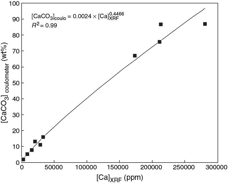
Figure F12. Relationship between uncalibrated XRF calcium content data obtained in Soils mode and carbonate content measured by coulometry on the same intervals.
Microbiology
Two types of samples were taken for microbiology: (1) when possible (e.g., Hole U1449B), a dedicated mudline APC core to allow high-resolution prokaryotic cell count, spores quantification, and enzymatic activity studies and (2) deeper samples for further microbiological investigations like phylogenetic studies, enzymatic activity measurements, and incubation experiments.
Whole-round cores of 5 cm were taken directly on the catwalk and split in the chemistry laboratory for subsampling. Sediments of 2 cm3 were subsampled using 2.5 cm3 syringes for prokaryotic cell enumeration. Microbial cells were fixed immediately by plunging sediment into 8 mL 2.5% (w/v) NaCl and 2% (v/v) formalin solution in 15 mL Falcon tubes. The fixed samples were stored at 4°C for shore-based processing. From the same whole-round core, two 10 cm3 minicores were taken using 10 cm3 syringes each for microbial spores quantification and hydrogenase enzyme activity measurement. The samples were vacuum packed, heat sealed, and stored at –80°C for analyses at home laboratories. For the identification and characterization of the microbial community in Bengal Fan sediments, samples for DNA analysis were taken using 10 cm3 sterile syringes, vacuum packed, heat sealed, and stored at –80°C. To characterize carbon turnover processes, postexpedition incubation experiments are planned. All microbiology samples were taken carefully to minimize contamination by using sterile tools and discarding the outermost layers of the whole-round cores, which were potentially contaminated.
Physical properties
Physical property measurements were made during Expedition 354 to obtain high-resolution insight into various lithologic and structural aspects of the cores. This work will also be the basis of further investigation of sediment composition, grain size distribution, and lithology assignation. On board, the data are used to tie into core descriptions, downhole data, and seismic profiles. In particular, physical property data provide the basis for hole-to-hole and site-to-site comparison, lithologic correlation, detection of discontinuities, information about differences in the composition and texture of sediment, identification of major seismic reflectors, and construction of synthetic seismic profiles. A variety of techniques and methods were used to characterize Expedition 354 cores on whole-round, split section-half, and discrete samples.
Sedimentary cores
Whole-round sections were first allowed to equilibrate to ambient room temperature (~20°C) and pressure for at least 1 h. After thermally equilibrating, core sections were run through the WRMSL for measurement of density by gamma ray attenuation (GRA), magnetic susceptibility, and compressional wave velocity on the P-wave logger (PWL). Cores recovered with the RCB system are slightly smaller in diameter than those cored with the APC system. As a result, sections cored with the RCB system typically have gaps between the liner and the core, so GRA density measured with WRMSL underestimates in situ values and PWL velocity cannot be measured because of the air gap. Sections were then measured with the spectral NGRL. Thermal conductivity was the last property measured on whole-round cores, usually in one section per core. We used a needle probe inserted through a small hole drilled through the plastic core liner close to the center of a section for softer, nonlithified material. For lithified material, however, we used the small puck in the working section half. Once the cores were split longitudinally, with one half surface-smoothed and designated as archive half and one as working half for sampling and analysis, the archive half of the core was passed through the SHMSL for measurement of point magnetic susceptibility and color reflectance (RSC). P-wave velocity measurements on split cores were made on working halves that were sampled for moisture and density (MAD), employing the caliper transducers oriented in the x-axis direction. Discrete samples were collected from working halves (at least two samples per core to capture the maximum and minimum sand content or the variability in lithofacies) to measure wet bulk density, dry bulk density, water content, porosity, and grain density with MAD procedures. Interstitial water was extracted before physical property measurements by Rhizon samplers every 5, 10, or 20 cm in the second core in the 0–60 m CSF-A interval and in the first core in the 60–200 m CSF-A interval depending on the site; GRA wet bulk density values are reduced in these zones because of the missing mass of water.
Whole-Round Multisensor Logger measurements
GRA-derived bulk density, PWL-derived P-wave velocity, and magnetic susceptibility were measured nondestructively with the WRMSL at 2.5 cm resolution (Figure F13). To optimize the measurement process, sampling intervals and measurement integration times were the same for all sensors, except for specific cores of interest, which were run at 1 cm resolution. These sampling intervals are common denominators of the distances between the sensors installed on the WRMSL (30 cm), which allows sequential and simultaneous measurements. After every core, quality control and quality assurance (QA/QC) were monitored by passing a single core liner filled with deionized water through the WRMSL. PWL values in the standard were measured at ~1490 m/s (depending on ambient temperature), and GRA densities were around 1 g/cm3, with correlation coefficients in excess of 0.99.
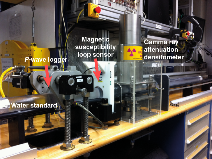
Figure F13. WRMSL on board the JOIDES Resolution. PWL, magnetic susceptibility sensor, and wet bulk density (GRA).
Gamma ray attenuation bulk density
Bulk density can be used to estimate the pore volume in sediment and evaluate the consolidation state of sediment. GRA density is an estimate of the water-saturated bulk density of core material based on the attenuation of a gamma ray beam. The beam is produced by a 137Cs gamma ray source at a radiation level of 370 MBq within a lead shield with a 5 mm collimator, which is directed downward through the whole-round core. The gamma ray detector on the opposite side of the core from the source includes a scintillator and an integral photomultiplier tube to record the gamma radiation that passes through the core. The attenuation of gamma rays occurs primarily by Compton scattering, in which gamma rays are scattered by electrons in the formation (e.g., Evans, 1965); the degree of scattering is related to the material bulk density. Therefore, for a known thickness of sample, the density (ρ) is proportional to the intensity of the attenuated gamma rays and can be expressed as
(8)where
- I = the measured intensity of gamma rays passing through the sample,
- I0 = gamma ray source intensity,
- μ = Compton attenuation coefficient, and
- d = sample diameter.
The μ and I0 are treated as constants so that ρ can be calculated from I.
In general, WRMSL measurements are most accurate when taken on a completely filled core liner with minimal drilling disturbance; otherwise, measurements tend to underestimate true values. By default, the instrument reports measurements using the internal diameter of the core liner (66 mm) as the assumed sample diameter. This assumption is suitable for most sediment cores obtained by the APC and XCB systems; however, for sediment and/or hard rock cored by the RCB system, core diameter is usually about 58 mm or less. Following Jarrard and Kerneklian (2007), the density measurements of cores obtained by the RCB system were corrected by multiplying the density values by 66/58 = 1.138 to account for this bias. However, comparison of different measurement methods on both whole-round and split cores carried out during Expedition 354 shows that this simple correction does not account adequately for the missing volume of RCB coring (Figure F14). RCB-drilled Core 354-U1451B-47R was first measured in the WRMSL. Average values were 1.89 g/cm3, which translated to 2.15 g/cm3. However, measurements on the split core scored below both the original measurements, even when the core thickness profile generated by the SHMSL is taken into account to correct for variable thicknesses. We should note that there is also a difference in thickness between the working and archive halves. The WRMSL and STMSL GRA instruments are also slightly different from each other in terms of independent calibration and age of source.

Figure F14. Comparison of wet bulk densities obtained by different core logging techniques using both whole-round and split cores on the WRMSL and the SHMSL.
The spatial resolution of the GRA densitometer is less than ±1 cm. The gamma ray detector is calibrated with sealed calibration cores (one standard core liner filled with distilled water and aluminum cylinders of various diameters). To establish the calibration curves, gamma ray counts were taken through each aluminum cylinder for 60 s. Each aluminum cylinder has a density of 2.7 g/cm3, and d is 1, 2, 3, 4, 5, or 6 cm. The relationship between I and µd is
(9)where A, B, and C are coefficients determined from the calibration.
Recalibration was performed as needed when the deionized water QA/QC standard deviated significantly (more than a few percent) from 1 g/cm3.
The fact that water has up to 10% higher GRA than most rock-forming minerals will have to be taken into account for postexpedition work to correct wet bulk densities, porosities, and water content obtained through GRA measurements using the iteration method described in Weber et al. (1997). This method should improve the overall quality of acoustic impedance parameters downhole and thus their correlation to seismic records.
Magnetic susceptibility
Magnetic susceptibility (χ) is a dimensionless measure of the degree to which material can be magnetized by an external magnetic field:
(10)where M is the magnetization induced in the material by an external field of strength H. Magnetic susceptibility is primarily sensitive to the concentration of ferrimagnetic minerals (e.g., magnetite and maghemite). It is also sensitive to magnetic mineralogy and can be related to the origin of the materials in the core and their subsequent diagenesis. For example, ash typically has magnetic susceptibility an order of magnitude greater than the surrounding calcareous clays.
The measurements were made using a Bartington MS2C loop sensor with a 9 cm diameter. An oscillator circuit in the sensor, which operates at a frequency of 0.565 kHz and an AF of ~140 A/m, produces a low-intensity, nonsaturating alternating magnetic field. Sediment or hard rock core sections going through the influence of this field cause a change in oscillator frequency. Frequency information returned in pulse form to the susceptometer is converted into magnetic susceptibility. The loop sensor has a field of influence of ~8 cm (Blum, 1997) and is accurate to within 2%.
P-wave velocity
P-wave velocities were measured to evaluate porosity and cementation and to relate these data sets to lithology, seismic records, and stratigraphy. From P-wave velocity and wet bulk density measurements, acoustic impedance is determined, and this will be used to calculate synthetic seismograms. P-wave velocity (VP) is defined by the time required for a compressional wave to travel a specific distance (e.g., Hamilton, 1970):
(11)where d is the path length of the wave across the core and tcore is the traveltime through the core.
The PWL measures the traveltime of 500 kHz ultrasonic waves horizontally across the core at 2.5 cm intervals while it remains in the core liner. Waves are transmitted to the core by plastic transducer contacts connected to linear actuators. Pressure is applied to the actuators to ensure coupling between the transducers and the core liner. P-wave velocity transducers measure total traveltime of the compressional wave between transducers. The wave travels horizontally across the whole core and core liner. The total observed traveltime tcore is composed of
- tdelay = time delay related to transducer faces and electronic circuitry,
- tpulse = delay related to the peak detection procedure,
- tliner = transit time through the core liner, and
- tcore = traveltime through the sediment.
The system is calibrated using a core liner filled with distilled water, which provides control for tdelay, tpulse, and tliner. From these calibrations, VP can be calculated for the whole-round specimens in core liners as
(12)where
- dcl = measured diameter of core and liner,
- dliner = liner wall thickness, and
- to = measured total traveltime.
Equation 12 assumes that the core completely fills the core liner. The WRMSL PWL was turned off for the majority of cores recovered with the RCB system, which do not fill the core liner entirely.
Natural Gamma Radiation Logger measurements
Gamma radiation is emitted from the decay series of 238-uranium (238U), 232-thorium (232Th), and 40-potassium (40K). NGR (Figure F15) measures this natural emission on whole-round cores using a system designed and built by the IODP JOIDES Resolution Science Operator (JRSO) (Texas A&M University, USA) (Vasiliev et al., 2011; Dunlea et al., 2013). When 238U, 232Th, and 40K radioisotopes decay, they and their daughter isotopes emit gamma radiation at specific energy levels unique to each isotope. NGR spectroscopy measures a wide energy spectrum that can be used to estimate the abundance of each isotope based on the strength of the signal at characteristic energies (Blum et al., 1997). Spectral data were collected and used for postcruise processing for U, Th, and K abundance but were not processed on board. Total counts were used on board, with high counts usually identifying fine-grained deposits containing K-rich clay minerals and their absorbed U and Th isotopes. NGR data thus reveal stratigraphic details that aid in core-to-core correlations. The main NGR detector unit consists of 8 sodium iodide (NaI) detectors arranged along the core measurement axis at 20 cm intervals surrounding the lower half of the section. The detector array has passive (layers of lead) and active (plastic scintillators) shielding to reduce the background environmental and cosmic radiation. The overlying plastic scintillators detect incoming high-energy gamma and muon cosmic radiation and cancel this signal from the total counted by the NaI detectors.
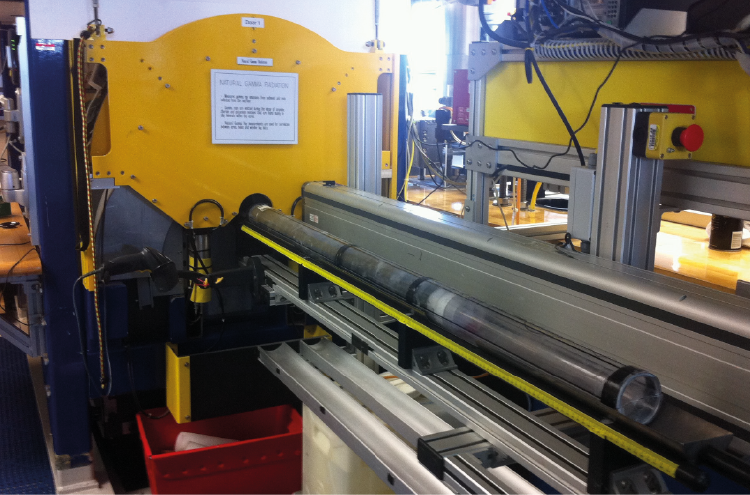
Figure F15. NGR system logger.
A measurement run consisted of two sample positions, 10 cm apart, for a total of 16 measurements per 150 cm section. The quality of the energy spectrum measured in a core depends on the concentration of radionuclides in the sample but also on the counting time, with higher times yielding better and more reliable spectra. Counting times were chosen as 5 min per position, or ~10 min per core, yielding statistically significant energy spectra (Vasiliev et al., 2011).
Thermal conductivity measurements
After NGR measurements were completed, thermal conductivity was measured with the TK04 (Teka Bolin) system (Figure F16) using a needle probe method in full-space configuration for whole-round sediment cores (Von Herzen and Maxwell, 1959) or a contact probe method (small puck) in half-space configuration on split cores for lithified core sections. The probes contain a heater wire and calibrated thermistor.
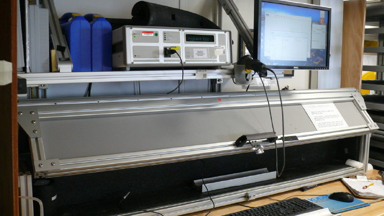
Figure F16. Thermal conductivity TK04 (Teka Bolin) system.
For soft sediment, the needle probe was inserted into a 2 mm diameter hole drilled through the liner along one of the lines that later guided core splitting and possibly in the center of the section. To avoid interference from air flow in the laboratory, the core was placed into an enclosed box outfitted with foam. For lithified rock cores, samples were selected from the working half and returned unaltered to the core liner upon completion of the tests. The contact probe embedded in the surface of an epoxy block with a low thermal conductivity (Vacquier, 1985) was placed flush on the smooth split-core surface and kept in contact using rubber bands.
The calibrated heat source of the probe was then turned on and the increase in temperature was recorded over 80 s (60 s for the small puck). A heating power of 2 W/m was typically used in soft sediment and 0.8 W/m was used for lithified material. The solution to the heat conduction equation with a line source of heat was then fit to the temperature measurements to obtain the thermal conductivity. Because the probe is much more conductive than sediment or hard rock, the probe is assumed to be a perfect conductor. Under this assumption, the temperature of the very conductive probe has a linear relationship with the natural logarithm of the time after the initiation of the heat,
(13)where
- T = temperature (K),
- q = heat input per unit length per unit time (J/m/s),
- k = thermal conductivity (W/[m·K]),
- t = time after the initiation of the heat (s), and
- C = instrumental constant.
In most cases, five measuring cycles were performed to calculate average conductivity. A self-test, which included a drift study, was conducted at the beginning of each measurement cycle. Once the probe temperature stabilized, the heater circuit was closed and the temperature rise in the probe was recorded. Thermal conductivity was calculated from the rate of temperature rise while the heater current was flowing. Temperatures measured during the first 80 or 60 s (depending on the type of the material) of the heating cycle were fitted to an approximate solution of a constantly heated line source (for details, see Kristiansen, 1982; Blum, 1997). Thermal conductivity measurements were routinely taken in one section per core.
Section Half Multisensor Logger measurements
We measured color reflectance and magnetic susceptibility on archive section halves using the SHMSL (Figure F17). The archive half of the split core was placed on the core logger, above which an electronic platform moves along a track, recording the height of the split-core surface with a laser sensor. The laser establishes the location of the bottom of the section, and then the platform reverses the direction of movement, moving from bottom to top making measurements of point magnetic susceptibility and color reflectance. All foam inserts were removed from the section-half cores before measurement, so the measured range of values represents that of the core material only. During Expedition 354, point magnetic susceptibility and color reflectance data were routinely collected at 1 cm increments. Specific high-resolution measurements were conducted at 0.1–0.5 cm increments. These measurements have higher resolution for comparison with the results obtained from the WRMSL magnetic susceptibility loop.
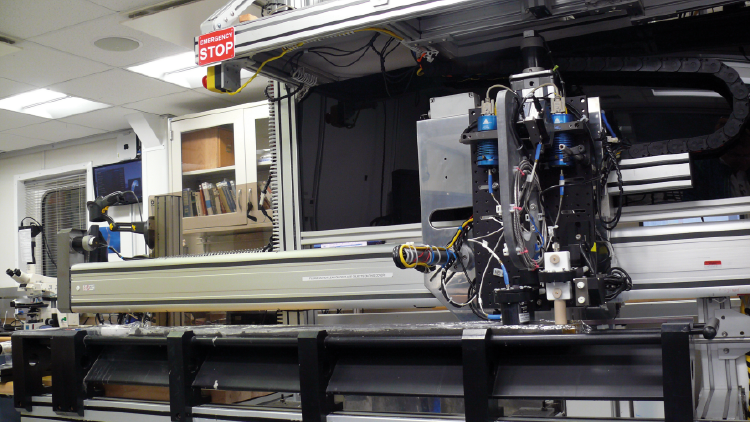
Figure F17. SHMSL for measurements of color reflectance and point magnetic susceptibility on archive section halves.
Color reflectance spectrometry
L*a*b* color reflectance measurements describe coordinates in a spherical system with 16.8 million possible variations (for details, see Blum 1997; Weber, 1998). The L* axis measures the black–white color component, known as lightness or gray value. The a* axis is redness (positive) versus greenness (negative), and the b* axis is yellowness (positive) versus blueness (negative). The color reflectance spectrometer used during Expedition 354 is an Ocean Optics 30 mm integrating sphere and both halogen and LED light source, which covers wavelengths from ultraviolet through visible to near infrared. The measurements were taken from 400 to 850 nm wavelengths at 2 nm intervals. The approximate 3 s data acquisition offset was applied for the entire scan of the archive section half. The color reflectance spectrometer calibrates on two spectra, pure white (reference) and pure black (dark). Color calibration was conducted approximately once every 6 h.
Point magnetic susceptibility
Point magnetic susceptibility was measured with a Bartington MS-2 meter and an MS2K contact probe with a flat 15 mm diameter round sensor with a field of influence of 25 mm and an operation frequency of 930 Hz. The instrument averages three measurements from the sensor for each offset, leading to an accuracy of ~5%. The spatial resolution of the point magnetic susceptibility instrument is ~3.8 mm, higher than that of the whole-round magnetic susceptibility for sections containing broken pieces <4 cm in length (the spatial resolution of whole-round magnetic susceptibility). As with whole-round measurements, the output displayed by the point magnetic susceptibility sensor is 10–5 SI. The probe is zeroed in air before each measurement location to avoid influence from the metal track. The point magnetic susceptibility meter was calibrated by the manufacturer before installation on the ship and is quality checked every ~6 h at the same time as color reflectance sensor calibration.
Digital color imaging
The archive half of each core was placed in the SHIL to obtain high-resolution digital color images (Figure F18). The SHIL collects digital images with three line-scan charge-coupled device arrays (2048 pixels each) behind an interference filter to create three channels (red, green, and blue).
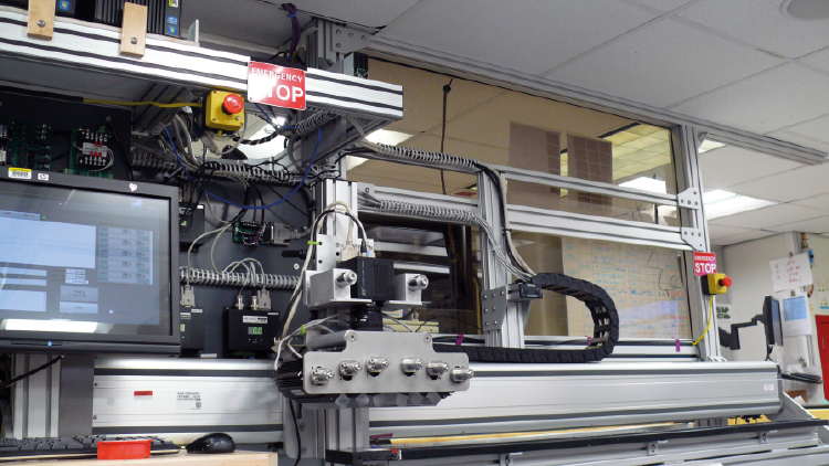
Figure F18. SHIL to obtain high-resolution digital color images and pixel-based RGB data.
The image resolution was fixed at approximately 200 lines per centimeter down the length of the section and approximately the same across, depending on changes in distance to the surface of the section. All images were taken at a fixed aperture setting of f/16. A QPCard 101 grayscale standard was imaged with each section and used as an internal control check.
Image correction involved the following three stages:
- The camera’s internal settings were used to correct for nonuniform pixel response and lens vignetting. The image response across the 0–255 range was white balanced using a combination of exposure and gain for the desired acquisition rate.
- An uncorrected image of the Macbeth ColorChecker color rendition chart was used, and then a polynomial correction to the acquired RGB values against the Macbeth published sRGB values for the grayscale color chips was fitted. A correction lookup table for each RGB channel was then generated and applied to TIFF images during acquisition.
- Applied only to the JPEG images that included the previous corrections, this correction used brightness, contrast, and gamma to create a visually appealing image.
On a regular basis, the photographer imaged the Macbeth ColorChecker color rendition chart and checked the grayscale values against the published values.
A microscanner was used to identify samples, and the software-generated digital label was appended to the image. For each section, scanned output from the SHIL included an ROI file of the original data with links to the TIFF file and an enhanced, uncropped JPEG file. A manually cropped JPEG image was generated to assist in visual core description.
As has been determined postcruise, there is an offset of all RGB values extracted from the line-scan camera. In each full section, the measurement starts ~4.5–5.5 cm inside the image and extends an equivalent length past the section end.
Section-half measurement gantry measurements
For soft-sediment cores, P-wave velocity measurements were performed on the working half of split cores before any samples were taken. P-wave velocity measurements used the x-axis caliper transducers (Figure F19) on the section-half measurement gantry, with several analyses per core. Different positions with respect to lithology were chosen to generate viable data. For RCB-drilled cores, we increased the number of caliper measurements because PWL measurements were not useful anymore. Also, for more lithified material, P-wave velocity was measured by caliper.

Figure F19. Caliper measurements of P-wave velocity.
P-wave velocity
The P-wave velocity system uses Panametrics-NDT Microscan delay line transducers, which transmit at 0.5 MHz. The signal received through the section half or the discrete sample was recorded by the computer attached to the system, with the peak (P-wave arrival) usually chosen by autopicking software. In the case of a weak signal, the first arrival was manually picked. During Expedition 354, we usually used the automatically picked points that fell along the ascending curve. Sometimes, however, we manually picked the beginning of the ascending curve of the first arrival peak. The distance between transducers was measured with a built-in linear voltage displacement transformer. Calibration was performed with a series of acrylic cylinders of differing thicknesses and a known P-wave velocity of 2750 ± 20 m/s. The determined system time delay from calibration was subtracted from the picked arrival time to give a traveltime of the P-wave through the sample. The thickness of the sample (calculated by the linear voltage displacement transformer, in meters) was divided by the traveltime (in seconds) to calculate P-wave velocity in meters per second.
Discrete sample measurements of moisture and density
Discrete samples were collected from the working halves to determine wet and dry bulk density, grain density, water content, and porosity. In sediment, ~10 cm3 samples were collected with a plastic syringe or spatula to fit that of the preweighed glass vials. We measured samples to capture the maximum and minimum sand or carbonate content and to correct for WRMSL GRA measurements by taking, on average, three samples per core, depending on lithologic variability and available time.
Sample preparation
Sediment samples were placed in numbered, preweighed ~16 mL Wheaton glass vials for wet and dry sediment weighing, drying, and dry volume measurements. After measurement of wet mass, samples were dried in a convection oven for at least 24 h at 105° ± 5°C. Dried samples were then cooled in a desiccator for at least 60 min before the dry mass and volume were measured.
Dual balance mass measurement
The weights of wet and dry sample masses were determined to a precision of 0.005 g using two Mettler Toledo electronic balances, with one acting as a reference. A standard weight of comparable value to the sample was placed on the reference balance to increase accuracy. A computer averaging system was used to compensate for the ship’s motion. The default setting of the balances is 300 measurements (taking ~1.5 min).
Pycnometer volume measurement
Dry sample volume was determined using a hexapycnometer system of a six-celled, custom-configured Micrometrics AccuPyc 1330TC helium-displacement pycnometer (Figure F20). The precision of each cell is 1% of the full-scale volume. Volume measurement was preceded by three purges of the sample chamber with helium warmed to ~24°C. Three measurement cycles were run for each sample. A reference volume (set of two calibration spheres) was placed sequentially in one of the chambers to check for instrument drift and systematic error. The volumes occupied by the numbered Wheaton vials were calculated before the expedition by multiplying each vial’s weight against the average density of the vial glass. The procedures for the determination of these physical properties comply with the American Society for Testing and Materials (ASTM) designation (D) 2216 (ASTM International, 1990). The fundamental relation and assumptions for the calculations of all physical property parameters are discussed by Blum (1997) and summarized below.
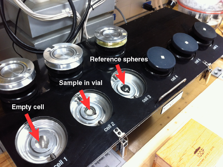
Figure F20. Pycnometer cells for moisture and density measurements.
Mass and volume calculation
Calculations given below are used as an IODP standard in accordance with Blum (1997). We measured wet mass (Mwet), dry mass (Mdry), and dry volume (Vdry). The ratio of mass (rm) is a computational constant of 0.965 (i.e., 0.965 g of freshwater per 1 g of seawater). Salt precipitated in sediment pores during the drying process is included in the Mdry and Vdry values. The mass of the evaporated water (Mwater) and salt (Msalt) in the sample are given by
(14)and
(15)where s is the assumed saltwater salinity (0.035%) corresponding to a pore water density (ρpw) of 1.024 g/cm3 and a salt density (ρsalt) of 2.22 g/cm3. The corrected mass of pore water (Mpw), volume of pore water (Vpw), mass of solids excluding salt (Msolid), volume of salt (Vsalt), volume of solids excluding salt (Vsolid), and wet volume (Vwet) are
(16) (17) (18) (19) (20) (21)and
(22)Calculation of bulk properties
For all sediment samples, water content (w) is expressed as the ratio of mass of pore water to wet sediment (total) mass:
(23)Wet bulk density (ρwet), dry bulk density (ρdry), sediment grain density (ρsolid), porosity (φ), and void ratio (VR) are calculated as:
(24) (25) (26) (27)and
(28)MAD properties reported and plotted in the Physical properties section of each site chapter were calculated with the MADMax shipboard program set with the “method C” calculation process.
Grain densities determined by MAD procedures might be too high. Average grain densities range from 2.79 to 2.84 g/cm3. These values are 0.1–0.2 g/cm3 above the values usually observed for sediment-forming minerals, which, in the case of Bengal Fan deposits, mainly reflect the specific weight of quartz (2.64 g/cm3). We recalculated results obtained by the equations mentioned above and compared them with those given in Weber et al. (1997) and found an exact match of the results. Therefore, the mismatch cannot be associated with erroneous calculations. When powdering a set of samples, there was a decrease in grain density that could account for up to half of the mismatch, although only sandy lithologies showed a clear trend. The remaining difference could be due to a higher fraction of heavy minerals or erroneous determination of the void. Postexpedition work will focus on measuring some of the samples with a pycnometer to solve this issue.
Lithology assignation to physical properties
Using a forecast algorithm within Microsoft Excel, we assigned the principal lithology to each depth where physical property measurements were made. This enabled us to (1) study the relationship between physical properties and the different lithologies and (2) retrieve complete thicknesses for all lithologies cored at a site. We calculated the total core length of each principal lithology from the DESC Excel core description table provided by the lithostratigraphers and summed these lengths to give the total length of described core. For this exercise, we removed any overlap between cores caused by sediment expansion, which sometimes resulted in slight differences between our calculated core length and the core lengths and recoveries given in the LIMS summary tables. The results are displayed as tables in each site chapter.
Downhole measurements
Downhole logs are used to determine physical, chemical, and structural properties of the formation penetrated by a borehole. The data are rapidly collected, continuous with depth, and measured in situ; they can be interpreted in terms of the stratigraphy, lithology, mineralogy, and geochemical composition of the penetrated formation. Where core recovery is incomplete or disturbed, log data may provide the only way to characterize the borehole section. Where core recovery is good, log and core data complement one another and may be interpreted jointly.
Downhole logs measure formation properties on a scale that is intermediate between those obtained from laboratory measurements on core samples and those from geophysical surveys. They are useful in calibrating the interpretation of geophysical survey data (e.g., through the use of synthetic seismograms) and provide a necessary link for the integrated understanding of physical properties on all scales.
Wireline logging
During wireline logging operations, the logs are recorded with Schlumberger logging tools combined into tool strings, which are lowered into the hole after completion of coring operations. Two tool strings were used during Expedition 354: the triple combination (triple combo), which measures NGR, density, and resistivity, and the Formation MicroScanner (FMS)-sonic, which provides FMS resistivity images of the borehole wall and sonic velocities (Figure F21; Table T3). The Versatile Seismic Imager (VSI) for making vertical seismic profiles was planned as a possibility, but it was not run because of unstable holes and time constraints. Each tool string also contains a telemetry cartridge for communicating through the wireline to the Schlumberger data acquisition system (MAXIS unit) on the drillship.

Figure F21. Wireline tool strings.
Table T3. Downhole measurements made by wireline tool strings. Download table in .csv format.
In preparation for logging, the boreholes were flushed of debris by circulating a high-viscosity mud (sepiolite) sweep and then filled with heavy mud (attapulgite weighted with barite, up to a density of about 12 lb/gal) to help stabilize the borehole walls. The BHA was pulled up to about 80 m WSF to cover the unstable upper part of the hole. The tool strings were then lowered downhole on a seven-conductor wireline cable before being pulled up at constant speed, typically 275 or 550 m/h, to provide continuous measurements of several properties simultaneously. A wireline heave compensator (WHC) was used to minimize the effect of ship’s heave on the tool position in the borehole (see below) except when ship heave was minimal. During each logging run, incoming data were recorded and monitored in real time on the Schlumberger MCM MAXIS logging computer.
Logged sediment properties and tool measurement principles
The logged properties and the principles used in the tools to measure them are briefly described in this section. The main logs are listed in Table T4. More detailed information on individual tools and their geological applications may be found in Serra (1984, 1986, 1989), Schlumberger (1989, 1994), Rider (1996), Goldberg (1997), Lovell et al. (1998), and Ellis and Singer (2007). A complete online list of acronyms for Schlumberger tools and measurement curves is at http://iodp.tamu.edu/tools/logging/index.html.
Table T4. Acronyms and units used for downhole wireline tools and measurements. Download table in .csv format.
Natural gamma radiation
The Hostile Environment Natural Gamma Ray Sonde (HNGS) was used on the triple combo tool string to measure and classify NGR in the formation. It has two bismuth germanate scintillation detectors, and concentrations of K, U, and Th are determined from the characteristic gamma ray energy spectra of isotopes in the 40K, 232Th, and 238U radioactive decay series.
An additional NGR sensor is housed in the Enhanced Digital Telemetry Cartridge (EDTC), run on all tool strings. Its sodium iodide scintillation detector measures the total NGR emission of the formation with no spectral information. The inclusion of a NGR sonde in every tool string allows use of NGR data for depth correlation between logging strings and passes and for core-log integration.
Density and phototelectric factor
Formation density was measured with the Hostile Environment Litho-Density Sonde (HLDS). The sonde contains a radioactive cesium (137Cs) gamma ray source (622 keV) and far and near gamma ray detectors mounted on a shielded skid, which is pressed against the borehole wall by a hydraulically activated decentralizing arm. Gamma rays emitted by the source undergo Compton scattering, in which gamma rays are scattered by electrons in the formation. The number of scattered gamma rays that reach the detectors is proportional to the density of electrons in the formation, which is in turn related to bulk density. Porosity may also be derived from this bulk density if the matrix (grain) density is known.
The HLDS also measures photoelectric absorption as the photoelectric factor (PEF). Photoelectric absorption of gamma rays occurs when their energy falls below 150 keV as a result of being repeatedly scattered by electrons in the formation. Because PEF is higher for elements with a higher atomic number, it also varies according to mineral composition and can be used to identify some minerals. For example, the PEF of calcite is 5.08 b/e–, illite is 3.03 b/e–, quartz is 1.81 b/e–, and kaolinite is 1.49 b/e–. Good contact between the tool and borehole wall is essential for good HLDS logs; poor contact results in underestimation of density values. When unstable hole conditions were anticipated because of fluidized sands and difficult drilling, the radioactive source was left out and the HLDS functioned solely as a caliper tool to measure the borehole diameter. The Accelerator Porosity Sonde (APS) was also left out of the triple combo tool string for this expedition because of the risk of unstable hole conditions.
Electrical resistivity
The High-Resolution Laterolog Array (HRLA) provides six resistivity measurements with different depths of investigation (including borehole mud resistivity and five measurements of formation resistivity with increasing penetration into the formation). The tool sends a focused current into the formation and measures the intensity necessary to maintain a constant drop in voltage across a fixed interval, providing direct resistivity measurements. The tool has one central (source) electrode and six electrodes above and below it, which serve alternatively as focusing and returning current electrodes. By rapidly changing the role of these electrodes, a simultaneous resistivity measurement at six penetration depths is achieved. The tool is designed to ensure that all signals are measured at exactly the same time and tool position and to reduce the sensitivity to “shoulder bed” effects when crossing sharp beds thinner than the electrode spacing. The design of the HRLA tool, which eliminates the need for a surface reference electrode, improves formation resistivity evaluation compared to the traditional dual induction tool. The HRLA tool needs to be run centralized in the borehole for optimal results, so bowspring centralizers were used to keep the HRLA in the center of the borehole, and knuckle joints allowed the density tool to be eccentralized and maintain good contact with the borehole wall (Figure F21).
Calcite, silica, and hydrocarbons are electrical insulators, whereas ionic solutions like interstitial water are conductors. Electrical resistivity can therefore be used to evaluate porosity for a given salinity and resistivity of the interstitial water. Clay surface conduction also contributes to the resistivity values, but at high porosities this is a relatively minor effect.
Acoustic velocity
The Dipole Shear Sonic Imager (DSI) measures the transit times between sonic transmitters and an array of eight receivers. It combines replicate measurements, thus providing a direct measurement of sound velocity through formations that is relatively free from the effects of formation damage and an enlarged borehole (Schlumberger, 1989). Along with the monopole transmitters found on most sonic tools, it also has two crossed-dipole transmitters, which allow the measurement of shear wave velocity in addition to compressional wave velocity. Dipole measurements are necessary to measure shear velocities in slow formations whose shear velocity is less than the velocity of sound in the borehole fluid. Such slow formations are typically encountered in deep-ocean drilling.
Formation MicroScanner
The FMS provides high-resolution electrical resistivity–based images of borehole walls. The tool has four orthogonal arms and pads, each containing 16 button electrodes that are pressed against the borehole wall during logging. The electrodes are arranged in two diagonally offset rows of eight electrodes each. A focused current is emitted from the button electrodes into the formation, with a return electrode near the top of the tool. Resistivity of the formation at the button electrodes is derived from the intensity of current passing through the button electrodes. Tool orientation and motion is tracked by three-axis magnetometer and a three-axis accelerometer in the General Purpose Inclinometry Tool (GPIT), part of the FMS-sonic tool string. Processing transforms these measurements into oriented high-resolution images that reveal the geologic structures of the borehole wall.
The development of the FMS tool added a new dimension to wireline logging (Luthi, 1990; Salimullah and Stow, 1992; Lovell et al., 1998). Features such as bedding, stratification, fracturing, slump folding, and bioturbation can be observed. Because the images are oriented to magnetic north, further analysis can be carried out to provide measurement of the dip and direction (azimuth) of planar features in the formation. In addition, when the corresponding planar features can be identified in the recovered core samples, individual core pieces can be reoriented with respect to true north.
The maximum extension of the caliper arms is 40.6 cm (16 inches). In holes with a diameter greater than this maximum (relatively common during Expedition 354), the pad contact at the end of the caliper arms is inconsistent, and the FMS images may appear out of focus and too conductive. Irregular (rough) borehole walls also adversely affect the images if contact with the wall is poor. Standard procedure is to make two full passes up the borehole with the FMS to maximize the chance of getting full borehole coverage with the pads.
Log data quality
The main influence on log data quality is the condition of the borehole wall. Where the borehole diameter varies over short intervals because of washouts (wide borehole) or ledges made of layers of harder material, the logs from tools that require good contact with the borehole wall (i.e., the FMS, density, and porosity tools) may be degraded. Deep investigation measurements such as NGR, resistivity, and sonic velocity, which do not require contact with the borehole wall, are generally less sensitive to borehole conditions. Very narrow (“bridged”) sections will also cause irregular log results. The quality of the borehole is improved by minimizing the circulation of drilling fluid while drilling, flushing the borehole to remove debris, and logging as soon as possible after drilling and hole conditioning are completed. During the expedition, circulation of drilling fluid, necessary to cool the bit and clear the hole of cuttings, washed out (widened) the borehole in places, particularly in less consolidated sediments.
The quality of the wireline depth determination depends on several factors. The depth of the logging measurements is determined from the length of the cable played out from the winch on the ship. The seafloor is identified on the NGR log by the abrupt reduction in gamma ray count at the water/sediment boundary (mudline). Discrepancies between the drilling depth and the wireline log depth occur. In the case of drilling depth, discrepancies are because of core expansion, incomplete core recovery, or incomplete heave compensation. In the case of log depth, discrepancies between successive runs occur because of incomplete heave compensation, incomplete correction for cable stretch, and cable slip. Tidal changes in sea level affect both drilling and logging depths. To minimize the wireline tool motion caused by ship heave, a hydraulic WHC was used to adjust the wireline length to compensate vertical rig motion during wireline logging operations.
Wireline heave compensator
The WHC system is designed to compensate for the vertical motion of the ship and maintain a steady motion of the logging tools. It uses vertical acceleration measurements made by a motion reference unit (MRU) located under the rig floor near the center of gravity of the ship to calculate the vertical motion of the ship. It then adjusts the length of the wireline by varying the distance between two sets of pulleys through which the cable passes. Real-time measurements of uphole (surface) and downhole acceleration are made simultaneously by the MRU and the EDTC, respectively.
Logging data flow and log depth scales
Data for each wireline logging run were monitored in real time and recorded using the Schlumberger MAXIS 500 system. The initial logging data were referenced to the rig floor (m WRF). After logging was completed, the data were shifted to a seafloor reference (m WSF) based on the step in gamma radiation at the sediment/water interface.
The data were transferred on shore to the Borehole Research Group at the Lamont-Doherty Earth Observatory (Columbia University, USA), where standardized data reduction took place. The main correction is depth matching to remove depth offsets between data from different logging runs, which results in a new depth scale, wireline log matched depth below seafloor (WMSF). Also, corrections are made to certain tools and logs (e.g., FMS imagery is corrected for tool acceleration, including “stick and slip” motion), documentation for the logs (with an assessment of log quality) is prepared, and the data are converted to ASCII for the conventional logs and GIF for the FMS images. Schlumberger Geo-Quest’s GeoFrame software package is used for most of the wireline log data processing. The data were transferred back to the ship within a few days of logging, and this processed data set was made available to the science party (in ASCII format and in JPG/GIF format for the image logs).
In situ temperature measurements
During Expedition 354, in situ temperature measurements were made at each site with the advanced piston corer temperature tool (APCT-3). The APCT-3 fits directly into the coring shoe of the APC and consists of a battery pack, data logger, and platinum resistance-temperature device calibrated over a temperature range of 0°–30°C. Before entering the borehole, the tool is first stopped at the mudline for 5 min to thermally equilibrate with bottom water. After the APC system penetrated the sediment, it was held in place for about 10 min as the APCT-3 recorded the temperature of the cutting shoe every second (a longer equilibration time is preferable). When the APC system is plunged into the formation, there is an instantaneous temperature rise from frictional heating. This heat gradually dissipates into the surrounding sediments as the temperature at the APCT-3 equilibrates toward the temperature of the sediments.
The equilibrium temperature of the sediments was estimated by applying a mathematical heat-conduction model to the temperature decay record (Horai and Von Herzen, 1985). The synthetic thermal decay curve for the APCT-3 is a function of the geometry and thermal properties of the probe and the sediments (Bullard, 1954; Horai and Von Herzen, 1985). The equilibrium temperature must be estimated by applying a fitting procedure (Pribnow et al., 2000). However, where the APC system has not achieved a full stroke or where ship heave pulls the APC system up from full penetration, the temperature equilibration curve will be disturbed and temperature determination is more difficult. The nominal accuracy of the APCT-3 temperature measurements is ±0.05°C.
APCT-3 temperature data were combined with measurements of thermal conductivity (see Physical properties) obtained from whole-core samples to obtain heat flow values. Heat flow was calculated according to the Bullard method to be consistent with the synthesis of ODP heat flow data by Pribnow et al. (2000).
References
ASTM International, 1990. Standard method for laboratory determination of water (moisture) content of soil and rock (Standard D2216–90). In Annual Book of ASTM Standards for Soil and Rock (Volume 04.08): Philadelphia (American Society for Testing Materials). [revision of D2216-63, D2216-80]
Berggren, W.A., Kent, D.V., Swisher, C.C., III, and Aubry, M.-P., 1995. A revised Cenozoic geochronology and chronostratigraphy. In Berggren, W.A., Kent, D.V., Aubry, M.-P., and Hardenbol, J. (Eds.), Geochronology, Time Scales and Global Stratigraphic Correlation. Special Publication - SEPM (Society for Sedimentary Geology), 54:129–212. http://dx.doi.org/10.2110/pec.95.04.0129
Blow, W.H., 1969. Late middle Eocene to recent planktonic foraminiferal biostratigraphy. Proceedings of the International Conference on Planktonic Microfossils, 1:199–422.
Blow, W.H., 1979. The Cainozoic Globigerinida: A Study of the Morphology, Taxonomy, Evolutionary Relationships and the Stratigraphical Distribution of Some Globigerinida (mainly Globigerinacea): Leiden, The Netherlands (E.J. Brill).
Blum, P., 1997. Technical Note 26: Physical Properties Handbook—A guide to the Shipboard Measurement of Physical Properties of Seep-sea Cores. Ocean Drilling Program. http://dx.doi.org/10.2973/odp.tn.26.1997
Bolli, H.M., and Saunders, J.B., 1985. Oligocene to Holocene low latitude planktic foraminifera. In Bolli, H.M., Saunders, J.B., and Perch-Nielsen, K. (Eds.), Plankton Stratigraphy (Volume 1): Planktic Foraminifera, Calcareous Nannofossils and Calpionellids: Cambridge, United Kingdom (Cambridge University Press), 155–262.
Bukry, D., 1973. Low-latitude coccolith biostratigraphic zonation. In Edgar, N.T., Saunders, J.B., et al., Initial Reports of the Deep Sea Drilling Project, 15: Washington, DC (U.S. Government Printing Office), 685–703. http://dx.doi.org/10.2973/dsdp.proc.15.116.1973
Bullard, E.C., 1954. The flow of heat through the floor of the Atlantic Ocean. Proceedings of the Royal Society of London, Series A: Mathematical, Physical and Engineering Sciences, 222(1150):408–429. http://dx.doi.org/10.1098/rspa.1954.0085
Clemens, S.C., Kuhnt, W., LeVay, L.J., Anand, P., Ando, T., Bartol, M., Bolton, C.T., Ding, X., Gariboldi, K., Giosan, L., Hathorne, E.C., Huang, Y., Jaiswal, P., Kim, S., Kirkpatrick, J.B., Littler, K., Marino, G., Martinez, P., Naik, D., Peketi, A., Phillips, S.C., Robinson, M.M., Romero, O.E., Sagar, N., Taladay, K.B., Taylor, S.N., Thirumalai, K., Uramoto, G., Usui, Y., Wang, J., Yamamoto, M., and Zhou, L., 2016. Expedition 353 methods. In Clemens, S.C., Kuhnt, W., LeVay, L.J., and the Expedition 353 Scientists, Indian Monsoon Rainfall. Proceedings of the International Ocean Discovery Program, 353: College Station, TX (International Ocean Discovery Program). http://dx.doi.org/10.14379/iodp.proc.353.102.2016
Dankers, P.H.M., and Zijderveld, J.D.A., 1981. Alternating field demagnetization of rocks, and the problem of gyromagnetic remanence. Earth and Planetary Science Letters, 53(1):89–92. http://dx.doi.org/10.1016/0012-821X(81)90029-7
Dunlea, A.G., Murray, R.W., Harris, R.N., Vasiliev, M.A., Evans, H., Spivack, A.J., and D’Hondt, S., 2013. Assessment and use of NGR instrumentation on the JOIDES Resolution to quantify U, Th, and K concentrations in marine sediment. Scientific Drilling, 15:57–63. http://dx.doi.org/10.2204/iodp.sd.15.05.2013
Ellis, D.V., and Singer, J.M., 2007. Well Logging for Earth Scientists (2nd edition): New York (Elsevier).
Evans, H.B., 1965. GRAPE—a device for continuous determination of material density and porosity. Transactions of the SPWLA Annual Logging Symposium: 6(2):B1–B25. https://www.spwla.org/SymposiumTransactions/grape-device-continuous-determination-material-density-and-porosity
Flood, R.D., Piper, D.J.W., Klaus, A., et al., 1995. Proceedings of the Ocean Drilling Program, Initial Reports, 155: College Station, TX (Ocean Drilling Program). http://dx.doi.org/10.2973/odp.proc.ir.155.1995
France-Lanord, C., Spiess, V., Klaus, A., Adhikari, R.R., Adhikari, S.K., Bahk, J.-J., Baxter, A.T., Cruz, J.W., Das, S.K., Dekens, P., Duleba, W., Fox, L.R., Galy, A., Galy, V., Ge, J., Gleason, J.D., Gyawali, B.R., Huyghe, P., Jia, G., Lantzsch, H., Manoj, M.C., Martos Martin, Y., Meynadier, L., Najman, Y.M.R., Nakajima, A., Ponton, C., Reilly, B.T., Rogers, K.G., Savian, J.F., Schwenk, T., Selkin, P.A., Weber, M.E., Williams, T., and Yoshida, K., 2016. Site U1450. In France-Lanord, C., Spiess, V., Klaus, A., Schwenk, T., and the Expedition 354 Scientists, Bengal Fan. Proceedings of the International Ocean Discovery Program, 354: College Station, TX (International Ocean Discovery Program). http://dx.doi.org/10.14379/iodp.proc.354.104.2016
Gehrels, G.E., Valencia, V.A., and Ruiz, J., 2008. Enhanced precision, accuracy, efficiency, and spatial resolution of U-Pb ages by laser ablation–multicollector–inductively coupled plasma–mass spectrometry. Geochemistry, Geophysics, Geosystems, 9(3):Q03017. http://dx.doi.org/10.1029/2007GC001805
Gieskes, J.M., Gamo, T., and Brumsack, H., 1991. Technical Note 15: Chemical Methods for Interstitial Water Analysis Aboard JOIDES Resolution. Ocean Drilling Program. http://dx.doi.org/10.2973/odp.tn.15.1991
Goldberg, D., 1997. The role of downhole measurements in marine geology and geophysics. Reviews of Geophysics, 35(3):315–342. http://dx.doi.org/10.1029/97RG00221
Gradstein, F.M., Ogg, J.G., Schmitz, M.D., and Ogg, G.M. (Eds.), 2012. The Geological Time Scale 2012: Amsterdam (Elsevier).
Hamilton, E.L., 1970. Sound velocity and related properties of marine sediments, North Pacific. Journal of Geophysical Research, 75):4423–4446. http://dx.doi.org/10.1029/JB075i023p04423
Horai, K., and Von Herzen, R.P., 1985. Measurement of heat flow on Leg 86 of the Deep Sea Drilling Project. In Heath, G.R., Burckle, L.H., et al., Initial Reports of the Deep Sea Drilling Project, 86: Washington, DC (U.S. Government Printing Office), 759–777. http://dx.doi.org/10.2973/dsdp.proc.86.135.1985
Jarrard, R.D., and Kerneklian, M.J., 2007. Data report: physical properties of the upper oceanic crust of ODP Site 1256: multisensor track and moisture and density measurements. In Teagle, D.A.H., Wilson, D.S., Acton, G.D., and Vanko, D.A. (Eds.), Proceedings of the Ocean Drilling Program, Scientific Results, 206: College Station, TX (Ocean Drilling Program), 1–11. http://dx.doi.org/10.2973/odp.proc.sr.206.011.2007
Kennett, J.P., and Srinivasan, M.S., 1983. Neogene Planktonic Foraminifera: A Phylogenetic Atlas: Stroudsburg, PA (Hutchinson Ross).
Kirschvink, J.L., 1980. The least-squares line and plane and the analysis of palaeomagnetic data. Geophysical Journal of the Royal Astronomical Society, 62(3):699–718. http://dx.doi.org/10.1111/j.1365-246X.1980.tb02601.x
Kristiansen, J.I., 1982. The transient cylindrical probe method for determination of thermal parameters of earth materials [Ph.D. dissertation]. Åarhus University, Åarhus, Denmark.
Lagarias, J.C., Reeds, J.A., Wright, M.H., and Wright, P.E., 1988. Convergence properties of the Nelder–Mead simplex method in low dimensions. SIAM Journal on Optimization, 9(1): 112–147. http://dx.doi.org/10.1137/S1052623496303470
Lovell, M.A., Harvey, P.K., Brewer, T.S., Williams, C., Jackson, P.D., and Williamson, G., 1998. Application of FMS images in the Ocean Drilling Program: an overview. In Cramp, A., MacLeod, C.J., Lee, S.V., and Jones, E.J.W. (Eds.), Geological Evolution of Ocean Basins: Results from the Ocean Drilling Program. Geological Society Special Publication, 131(1):287–303. http://dx.doi.org/10.1144/GSL.SP.1998.131.01.18
Luthi, S.M., 1990. Sedimentary structures of clastic rocks identified from electrical borehole images. In Hurst, A., Lovell, M.A., and Morton, A.C. (Eds.), Geological Applications of Wireline Logs. Geological Society Special Publication, 48:3–10. http://dx.doi.org/10.1144/GSL.SP.1990.048.01.02
Manheim, F.T., and Sayles, F.L., 1974. Composition and origin of interstitial waters of marine sediments, based on deep sea drill cores. In Goldberg, E.D. (Ed.), The Sea (Volume 5): Marine Chemistry: The Sedimentary Cycle: New York (Wiley), 527–568.
Martini, E., 1971. Standard Tertiary and Quaternary calcareous nannoplankton zonation. In Farinacci, A. (Ed.), Proceedings of the Second Planktonic Conference, Roma 1970: Rome (Edizioni Tecnoscienza), 2:739–785.
Murray, R.W., Miller, D.J., and Kryc, K.A., 2000. Technical Note 29: Analysis of Major and Trace Elements in Rocks, Sediments, and Interstitial Waters by Inductively Coupled Plasma–Atomic Emission Spectrometry (ICP-AES). Ocean Drilling Program. http://dx.doi.org/10.2973/odp.tn.29.2000
Okada, H., and Bukry, D., 1980. Supplementary modification and introduction of code numbers to the low-latitude coccolith biostratigraphic zonation (Bukry, 1973; 1975). Marine Micropaleontology, 5:321–325. http://dx.doi.org/10.1016/0377-8398(80)90016-X
Parker, R.L., and Gee, J.S., 2002. Calibration of the pass-through magnetometer—II. Application. Geophysical Journal International, 150:140–152. http://dx.doi.org/10.1046/j.1365-246X.2002.01692.x
Pribnow, D., Kinoshita, M., and Stein, C., 2000. Thermal Data Collection and Heat Flow Recalculations for Ocean Drilling Program Legs 101–180: Hanover, Germany (Institute for Joint Geoscientific Research, Institut für Geowissenschaftliche Gemeinschaftsaufgaben [GGA]). http://www-odp.tamu.edu/publications/heatflow/ODPReprt.pdf
Quintin, L.L., Faul, K.L., Lear, C., Graham, D., Peng, C., Murray, R.W., and Shipboard Scientific Party, 2002. Geochemical analysis of bulk marine sediment by inductively coupled plasma–atomic emission spectroscopy on board the JOIDES Resolution. In Lyle, M., Wilson, P.A., Janecek, T.R., et al., Proceedings of the Ocean Drilling Program, Initial Reports, 199: College Station, TX (Ocean Drilling Program), 1–14. http://dx.doi.org/10.2973/odp.proc.ir.199.107.2002
Raffi, I., and Flores, J.-A., 1995. Pleistocene through Miocene calcareous nannofossils from eastern equatorial Pacific Ocean (Leg 138). In Pisias, N.G., Mayer, L.A., Janecek, T.R., Palmer-Julson, A., and van Andel, T.H. (Eds.), Proceedings of the Ocean Drilling Program, Scientific Results, 138: College Station, TX (Ocean Drilling Program), 233–286. http://dx.doi.org/10.2973/odp.proc.sr.138.112.1995
Richter, C., Acton, G., Endris, C., and Radsted, M., 2007. Technical Note 34: Handbook for Shipboard Paleomagnetists. Ocean Drilling Program. http://dx.doi.org/10.2973/odp.tn.34.2007
Rider, M.H., 1996. The Geological Interpretation of Well Logs (2nd edition): Caithness, Scotland (Whittles Publishing).
Salimullah, A.R.M., and Stow, D.A.V., 1992. Application of FMS images in poorly recovered coring intervals: examples from ODP Leg 129. In Hurst, A., Griffiths, C.M., and Worthington, P.F. (Eds.), Geological Application of Wireline Logs II. Geological Society Special Publication, 65(1):71–86. http://dx.doi.org/10.1144/GSL.SP.1992.065.01.06
Schlumberger, 1989. Log Interpretation Principles/Applications: Houston (Schlumberger Education Services), SMP–7017.
Schlumberger, 1994. IPL Integrated Porosity Lithology: Houston (Schlumberger Wireline Testing), SMP-9270.
Serra, O., 1984. Fundamentals of Well-Log Interpretation (Volume 1): The Acquisition of Logging Data: Amsterdam (Elsevier).
Serra, O., 1986. Fundamentals of Well-Log Interpretation (Volume 2): The Interpretation of Logging Data: Amsterdam (Elsevier).
Serra, O., 1989. Formation MicroScanner Image Interpretation: Houston (Schlumberger Education Services), SMP-7028.
Shepard, F.P., 1954. Nomenclature based on sand-silt-clay ratios. Journal of Sedimentary Research, 24(3):151–158. http://dx.doi.org/10.1306/D4269774-2B26-11D7-8648000102C1865D
Stow, D.A.V., 2005. Sedimentary Rocks in the Field: A Colour Guide: London (Manson Publishing)
Stow, D.A.V., Hernández-Molina, F.J., Alvarez Zarikian, C.A., and the Expedition 339 Scientists, 2013. Proceedings of the Integrated Ocean Drilling Program, 339: Tokyo (Integrated Ocean Drilling Program Management International, Inc.). http://dx.doi.org/10.2204/iodp.proc.339.2013
Vacquier, V., 1985. The measurement of thermal conductivity of solids with a transient linear heat source on the plane surface of a poorly conducting body. Earth and Planetary Science Letters, 74(2–3):275–279. http://dx.doi.org/10.1016/0012-821X(85)90027-5
Vasiliev, M.A., Blum, P., Chubarian, G., Olsen, R., Bennight, C., Cobine, T., Fackler, D., Hastedt, M., Houpt, D., Mateo, Z., and Vasilieva, Y.B., 2011. A new natural gamma radiation measurement system for marine sediment and rock analysis. Journal of Applied Geophysics, 75:455–463. http://dx.doi.org/10.1016/j.jappgeo.2011.08.008
Von Herzen, R., and Maxwell, A.E., 1959. The measurement of thermal conductivity of deep-sea sediments by a needle-probe method. Journal of Geophysical Research, 64(10):1557–1563. http://dx.doi.org/10.1029/JZ064i010p01557
Wade, B.S., Pearson, P.N., Berggren, W.A., and Pälike, H., 2011. Review and revision of Cenozoic tropical planktonic foraminiferal biostratigraphy and calibration to the geomagnetic polarity and astronomical time scale. Earth-Science Reviews, 104(1–3):111–142. http://dx.doi.org/10.1016/j.earscirev.2010.09.003
Weber, M.E., 1998. Estimation of biogenic carbonate and opal by continuous non-destructive measurements in deep-sea sediments: application to the eastern equatorial Pacific. Deep-Sea Research, Part I, 45(11):1955–1975. http://dx.doi.org/10.1016/S0967-0637(98)00028-4
Weber, M.E., Niessen, F., Kuhn, G., and Wiedicke, M., 1997. Calibration and application of marine sedimentary physical properties using a multi-sensor core logger. Marine Geology, 136(3–4):151–172. http://dx.doi.org/10.1016/S0025-3227(96)00071-0
1France-Lanord, C., Spiess, V., Klaus, A., Adhikari, R.R., Adhikari, S.K., Bahk, J.-J., Baxter, A.T., Cruz, J.W., Das, S.K., Dekens, P., Duleba, W., Fox, L.R., Galy, A., Galy, V., Ge, J., Gleason, J.D., Gyawali, B.R., Huyghe, P., Jia, G., Lantzsch, H., Manoj, M.C., Martos Martin, Y., Meynadier, L., Najman, Y.M.R., Nakajima, A., Ponton, C., Reilly, B.T., Rogers, K.G., Savian, J.F., Schwenk, T., Selkin, P.A., Weber, M.E., Williams, T., and Yoshida, K., 2016. Expedition 354 methods. In France-Lanord, C., Spiess, V., Klaus, A., Schwenk, T., and the Expedition 354 Scientists, Bengal Fan. Proceedings of the International Ocean Discovery Program, 354: College Station, TX (International Ocean Discovery Program). http://dx.doi.org/10.14379/iodp.proc.354.102.2016