Pecher, I.A., Barnes, P.M., LeVay, L.J., and the Expedition 372A Scientists
Proceedings of the International Ocean Discovery Program Volume 372A
publications.iodp.org

https://doi.org/10.14379/iodp.proc.372A.102.2019

Expedition 372A methods¹

I.A. Pecher, P.M. Barnes, L.J. LeVay, S.M. Bourlange, M.M.Y. Brunet, S. Cardona, M.B. Clennell, A.E. Cook, M.P. Crundwell, B. Dugan, J. Elger, D. Gamboa, A. Georgiopoulou, A. Greve, S. Han, K.U. Heeschen, G. Hu, G.Y. Kim, H. Kitajima, H. Koge, X. Li, K.S. Machado, D.D. McNamara, G.F. Moore, J.J. Mountjoy, M.A. Nole, S. Owari, M. Paganoni, K.E. Petronotis, P.S. Rose, E.J. Screaton, U. Shankar, C.L. Shepherd, M.E. Torres, M.B. Underwood, X. Wang, A.D. Woodhouse, and H.-Y. Wu²

Keywords: International Ocean Discovery Program, IODP, JOIDES Resolution, Expedition 372, Site U1517, Hikurangi margin, Tuaheni Landslide Complex, Tuaheni Basin, New Zealand, gas hydrates, slope stability, fluid flow, mass transport deposits, logging while drilling

MS 372A-102: Published 5 May 2019

Introduction

This chapter documents the procedures and methods employed in the various shipboard laboratories of the R/V JOIDES Resolution during International Ocean Discovery Program (IODP) Expedition 372. This information applies only to shipboard work described in the Expedition reports section of the Expedition 372A Proceedings of the International Ocean Discovery Program volume. Methods used by investigators for shore-based analyses of Expedition 372 data will be described in separate, individual publications. This introductory section provides an overview of operations, curatorial conventions, depth scale terminology, and general core handling and analyses.

Authorship of the site chapters

All shipboard scientists contributed to this volume. However, certain sections were written and edited by discipline-based groups of scientists as listed alphabetically below:

Background and objectives: Barnes, Pecher
Operations: Grigar, LeVay
Lithostratigraphy: Brunet, Cardona, Georgiopoulou, Mountjoy, Underwood
Biostratigraphy: Crundwell, Shepherd, Woodhouse
Paleomagnetism: Greve, Li, Petronotis
Geochemistry: Heeschen, Machado, Owari, Rose, Torres
Physical properties: Bourlange, Hu, Kitajima, Nole, Screaton
Downhole measurements: Dugan
Logging while drilling: Clennell, Cook, Dugan, Elger, Gamboa, Han, Kim, Koge, McNamara, Moore, Paganoni, Shankar, Wang, Wu
Core-log integration: Brunet, Cardona, Han, Nole, Paganoni, Screaton
Log-seismic integration: Elger, Gamboa, Han, Moore

Site location

GPS coordinates from precruise site surveys were used to position the vessel at Site U1517. A Syquest Bathy 2010 CHIRP subbottom profiler was used to monitor the seafloor depth on the approach to the site to reconfirm the depth profile from precruise surveys. Once the vessel was positioned at the site, the thrusters were lowered and a positioning beacon was dropped to the seafloor. The dynamic positioning control of the vessel used navigational input from the GPS system and triangulation to the seafloor beacon weighted by the estimated positional accuracy. The final position for each hole at Site U1517 was the mean position calculated from the GPS data collected over a significant portion of the time the hole was occupied.

Coring and drilling operations

The advanced piston corer (APC) and half-length APC (HLAPC) systems were used during Expedition 372.

The APC and HLAPC systems cut soft-sediment cores with minimal coring disturbance relative to other IODP coring systems. After the APC core barrel is lowered through the drill pipe and lands near the bit, the drill pipe is pressured up until two shear pins that hold the inner barrel attached to the outer barrel fail (Figure F1). The inner barrel then advances into the formation and cuts the core. The driller can detect a successful cut, or “full stroke,” from the pressure gauge on the rig floor.

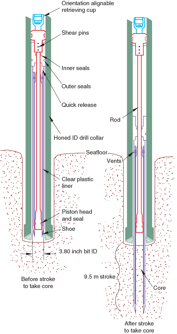
Figure F1. APC system.

The depth limit of the APC system, often referred to as APC refusal, is indicated in two ways: (1) the piston consistently fails to achieve a complete stroke (as determined from the pump pressure reading) because the formation is too hard and limited core recovery is achieved, or (2) excessive force (>60,000 lb; ~267 kN) is required to pull the core barrel out of the formation. When a full stroke could not be achieved, one or more additional attempts are typically made, and each time the bit is advanced by the length of recovered core. This process results in a nominal recovery of ~100% based on the assumption that the barrel penetrated the formation by the length of core recovered. When a full or partial stroke is achieved but excessive force cannot retrieve the barrel, the core barrel is sometimes “drilled over,” meaning after the inner core barrel was successfully shot into the formation, the drill bit is advanced to total depth to free the APC barrel.

The standard APC system contains a 9.5 m long core barrel, and the HLAPC system uses a 4.7 m long core barrel. In most instances, the HLAPC system is deployed after the standard APC system reaches refusal. During use of the HLAPC system, the same criteria as for the full-length APC system are applied in terms of refusal. The HLAPC system allows significantly greater APC sampling depths to be attained than would otherwise be possible without this system.

Nonmagnetic core barrels were used for all deployments of the APC and HLAPC systems. Orientation was applied to standard APC cores using the Icefield MI-5 core orientation tool and the FlexIT tool (see Downhole measurements). Formation temperature measurements were made to obtain temperature gradients and heat flow estimates using the advanced piston corer temperature tool (APCT-3). In situ formation pressure and temperature were measured using the temperature dual pressure probe (T2P) and the sediment temperature pressure tool (SETP) (see Downhole measurements).

The bottom-hole assembly (BHA) is the lowermost part of the drill string. A typical APC BHA consists of a drill bit (outside diameter [OD] = 11⁷⁄₁₆ inches [~29 cm]), a bit sub, a seal bore drill collar, a landing saver sub, a modified top sub, a modified head sub, a nonmagnetic drill collar (for APC), a number of 8¼ inch (~20.32 cm) drill collars, a tapered drill collar, six joints (two stands) of 5½ inch (~13.97 cm) drill pipe, and one crossover sub. A lockable flapper valve is used to collect downhole logs without dropping the bit when APC coring.

The logging-while-drilling (LWD)/measurement-while-drilling (MWD) BHA used during Expedition 372 consisted of an 8½ inch tungsten carbide insert tricone bit, an 8¼ inch near bit stabilizer/bit sub, various LWD/MWD tools, an 8¼ inch string stabilizer, a 6¾ inch (~17 cm) float sub, a crossover sub, twelve 6¾ inch drill collars, a 6½ inch (16.51 cm) drilling jar, three 6¾ inch drill collars, and a crossover to 5 inch (12.7 cm) drill pipe.

Drilling disturbance

Cores may be significantly disturbed as a result of the drilling process and may contain extraneous material as a result of the coring and core handling process. The uppermost 10–50 cm of each core must therefore be examined critically during description for potential “cave-in” and other disturbances (e.g., fluidization related to drill string heave in poor weather conditions). Common coring-induced deformation includes the concave-downward appearance of originally horizontal bedding. Piston action may result in fluidization (flow-in) at the bottom of APC cores. Retrieval from depth to the surface may result in elastic rebound. Gas that is in solution at depth may become free and drive core segments in the liner apart. When gas content is high, pressure must be relieved for safety reasons before the cores are cut into segments. This is accomplished by drilling holes into the liner, which forces some sediment, as well as gas, out of the liner. Drilling disturbances are described in Lithostratigraphy in the Site U1517 chapter (Barnes et al., 2019) and are graphically indicated on the visual core description (VCD) graphic reports (see Core descriptions).

Core handling and curatorial procedures

Special core handling procedures were implemented for gas hydrate identification and sampling. Cores recovered during Expedition 372 were extracted from the core barrel in plastic liners. These liners were carried from the rig floor to the core processing area on the catwalk outside the core laboratory. After wiping down the core liner, each core was immediately scanned with an infrared (IR) thermal imaging camera to identify gas hydrate layers, which appeared cold relative to the rest of the sediment core. Thermal images were collected and cataloged for each core in its entirety, regardless of whether it contained gas hydrates. If gas hydrate was observed with the IR camera, it was immediately marked on the core liner and sampled for interstitial water (IW) chemistry or post-expedition research. The gas hydrate samples collected for post-expedition research were cut out of the core in 5–14 cm long whole rounds, photographed, wrapped in aluminum foil, bagged, and placed in a dewar of liquid nitrogen. For some cores where gas expansion was happening quickly, holes were drilled into the core liner immediately to relieve the pressure. Once the core was sampled for gas hydrate, the cores were cut into sections. Sections are typically 1.5 m in length; however, because of whole-round sampling and gas expansion, these sections were often shorter. The exact section length was noted and later entered into the database as “created length” using the SampleMaster application. This length was used to calculate recovery. Whole-round samples were taken for IW chemistry at regular intervals. Headspace samples were taken from selected section ends (typically 2–4 per core) using a syringe for immediate hydrocarbon analysis as part of the shipboard safety and pollution prevention program. (See Geochemistry for more information on chemical sampling.) Core catcher samples were taken for biostratigraphic analysis during and after IODP Expedition 375. When catwalk sampling was complete, liner caps (blue = top; colorless = bottom; yellow = bottom where whole-round was removed) were glued onto liner sections with acetone, and sections were placed in core racks in the laboratory for analysis. Whole rounds for personal research were cut from the core sections after being processed through the physical properties whole-round loggers and after thermal conductivity measurements.

Numbering of sites, holes, cores, and samples followed standard IODP procedure. A full curatorial sample identifier consists of the following information: expedition, site, hole, core number, core type, section number, section half, and offset in centimeters measured from the top of a given section. For example, a sample identification of “372-U1517C-1H-2W, 10–12 cm,” represents a sample taken from the interval between 10 and 12 cm below the top of Section 2 (“W” indicates the working half of the section) of Core 1 (“H” designates that this core was taken with the APC system) of Hole C at Site U1517 during Expedition 372. The “U” preceding the hole number indicates that the hole was drilled by the JOIDES Resolution. Cores taken with the HLAPC system are designated as “F.”

Shipboard core analysis

Core sections were allowed to reach equilibrium with laboratory temperature (after ~4 h) prior to running through the Whole-Round Multisensor Logger (WRMSL) and Natural Gamma Radiation Logger (NGRL). Thermal conductivity was run on each whole-round core section. Based on the results of these physical properties measurements, whole-round samples for post-expedition research were cut from the sections. Each section was split lengthwise from bottom to top into working (“W”) and archive (“A”) halves. Investigators should note that older material might have been transported upward on the split face of each section during splitting. The working half of each section was sampled for shipboard analysis (physical properties, geochemistry, and bulk X-ray diffraction [XRD] mineralogy) and post-expedition research. The archive half of each section for each core was scanned on the Section Half Imaging Logger (SHIL) and measured for color reflectance and magnetic susceptibility on the Section Half Multisensor Logger (SHMSL). At the same time, the archive halves were described macroscopically, as well as microscopically by means of smear slides. Both halves of the core were then put into labeled plastic tubes that were sealed and transferred to cold storage space aboard the ship. The core sections remained aboard the ship through IODP Expeditions 374 and 375. During Expedition 375, the archive halves were run on the superconducting rock magnetometer (SRM).

All archive and working halves were transported at the end of Expedition 375 from the ship to the Gulf Coast Repository in College Station, Texas (USA), where they will be kept in permanent cold storage.

Sample depth calculations

The primary depth scale types are based on the measurement of the drill string length deployed beneath the rig floor (drilling depth below rig floor [DRF] and drilling depth below seafloor [DSF]) and the length of each core recovered (core depth below seafloor [CSF]). All depths are in meters. Depths of samples and measurements are calculated on the applicable depth scale by fixed protocol (e.g., CSF). The definition of these depth scale types and the distinction in nomenclature should keep the user aware that a nominal depth value on two different depth scale types usually does not refer to exactly the same stratigraphic interval in a hole.

Depths of cored intervals are measured from the drill floor based on the length of drill pipe deployed beneath the rig floor (DRF scale). The depth of the cored interval is referenced to the seafloor (DSF scale) by subtracting the seafloor depth at the time of the first hole from the DRF depth of the interval. In most cases, the seafloor depth is the length of pipe deployed minus the length of the mudline core recovered.

Standard depths of cores in meters below seafloor (CSF-A scale) are determined based on the assumptions that (1) the top depth of a recovered core corresponds to the top depth of its cored interval (DSF scale) and (2) the recovered material is a contiguous section even if core segments are separated by voids when recovered. Voids in the core are closed by pushing core segments together, if possible, during core handling. This convention is also applied if a core has incomplete recovery, in which case the true position of the core within the cored interval is unknown and should be considered a sample depth uncertainty (as much as the length of the core barrel used) when analyzing data associated with the core material. Standard depths of samples and associated measurements (CSF-A scale) are calculated by adding the offset of the sample or the measurement from the top of its section and the lengths of all higher sections in the core to the top depth of the cored interval.

A soft- to semisoft-sediment core from less than a few hundred meters below seafloor expands upon recovery (typically a few percent to as much as 15%), so the length of the recovered core exceeds that of the cored interval. Therefore, a stratigraphic interval may not have the same nominal depth on the DSF and CSF scales in the same hole. When core recovery (the ratio of recovered core to cored interval times 100%) is >100%, the CSF depth of a sample taken from the bottom of a core will be deeper than that of a sample from the top of the subsequent core (i.e., the data associated with the two core intervals overlap on the CSF-A scale). The core depth below seafloor, Method B (CSF-B), depth scale is a solution to the overlap problem. This method scales the recovered core length back into the interval cored, from >100% to exactly 100% recovery.

Wireline logging and in this instance LWD and MWD are measured on the LWD depth below seafloor (LSF) scale. LWD data are measured by time and are subsequently depth corrected.

It should be noted that all depths in this volume are given in meters below seafloor (mbsf) unless otherwise noted.

Lithostratigraphy

This section outlines the procedures used to document the composition, texture, and sedimentary structures of the sediment recovered during Expedition 372. The procedures include visual core description, digital color imaging, color spectrophotometry, smear slide analysis, and XRD analysis of bulk powders.

Core preparation for description

Archive halves were used for sedimentological and petrographic observations. Sections were dominated by unlithified sediment and split using a thin wire held in high tension. The split surface of the archive half was then scraped with a glass slide. Scraping parallel to bedding with a freshly cleaned tool prevents up- or downcore contamination. The archive half was then imaged by the SHIL and analyzed for color reflectance and magnetic susceptibility using the SHMSL (see Physical properties). We aimed to run the SHIL as soon as possible after core splitting to limit oxidation of the sediment surface obscuring sedimentary structures. The archive half was reimaged if required to improve the visibility of sedimentary structures and fabrics following treatment of the split-core surface. Following imaging, the archive halves of the sediment cores were macroscopically described for lithologic and sedimentary features aided by use of a 20× wide-field hand lens and binocular microscope.

Visual core descriptions

Visual inspection of sediment yielded information on lithologic variation, color, sedimentary structures, structural features, and drilling disturbance. Continuous or repeated bedded units were described as one interval rather than selecting a bed thickness cutoff for description. If an unusual bed occurred in an otherwise monotonous sequence, it was described separately. Smear slide analysis was used to identify sedimentary constituents, including microfossils. All of the descriptive data were entered into the DESClogik spreadsheet customized for Expedition 372 (see DESC_WKB in Supplementary material). All descriptions and sample locations were recorded using curated depths and documented on the VCDs (Figure F2). Graphic reports were assessed for quality control and consistency using the SHIL images and were adjusted and expanded where appropriate. Once core description was completed, Lithostratigraphic Units I–V were defined and included on the VCDs.

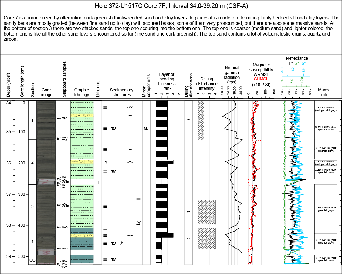
Figure F2. VCD sheet.

Graphic lithology

Lithologies in the core intervals are represented on the VCDs by graphic patterns in the Graphic lithology column (Figure F3). Other sedimentary features of the core, including sedimentary structures and sediment components, are represented by symbols. Bedding thickness for intervals described in packages are plotted as a rank. All grain size designations followed the conventional Wentworth (1922) scheme. Color was determined qualitatively for core intervals using Munsell color charts.

Figure F3. Graphic patterns and symbols.

Lithologic features

The locations and types of stratification and sedimentary structures visible on the split-core surfaces were entered into DESClogik with their respective location and depth and shown in the Sedimentary structures column on the VCDs.

For Expedition 372, we used the following terminology (based on Stow, 2005) to describe the scale of stratification:

Lamination = <1 cm thick.
Very thin bed = 1–3 cm thick.
Thin bed = >3–10 cm thick.
Medium bed = >10–30 cm thick.
Thick bed = >30–100 cm thick.
Very thick bed = >100 cm thick.

We used these terms to define a scale for bedding thickness from 1 (lamination) to 5 (thick bed). We defined the following terms for sedimentary structures. Cross-bedding describes a bed that contains thin horizontal or inclined laminations with inclined internal foresets. Structureless beds were not specifically entered, but beds that are homogeneous in lithology and color and exhibit no bedding, cross-bedding, grading, bioturbation, or bed disturbance are described as massive in the core description. Sediment grading is described as ungraded, normally graded (fining upward), and inversely graded (coarsening upward). Contacts are either gradational, sharp, wavy, bioturbated, or irregular and are represented by symbols. A range of deformation structures were recognized and reported in a separate column on the VCDs. Bioturbation intensity was recorded with symbols as slight, moderate, and heavy. Any distinctive features not captured by symbols are listed in the section summary.

Drilling disturbance

Drilling-related sediment disturbance and intensity (slight, moderate, severe, and destroyed) are recorded in the Drilling disturbance column on the VCDs. Assessment of core disturbance by drilling and core processing was primarily based on the degree to which observed textures and fabrics depart from expected natural occurring features. In tectonically deformed sediment and landslide deposits, however, the distinction between natural and induced fabrics can be particularly ambiguous.

The type of drilling disturbance was described using the following terms:

Flow-in (midcore or basal), coring/drilling slurry, or along-core gravel/sand contamination: soft-sediment stretching and/or compressional shearing structures are severe and are attributed to coring/drilling.
Gas expansion: sediment is cracked horizontally, forcing apart parallel to bedding planes due to gas coming out of solution. Cores are typically pushed back together using a wooden plunger tool.
Mingling and distortion of different beds: out-of-place material at the top of a core has fallen downhole onto the cored surface.
Soupy: intervals are water saturated and have lost all aspects of original bedding.
Upward-arching bed contacts: material retains its coherency, with material closest to the core liner bent downward. These contacts are most apparent when horizontal features are distorted.
Void: open horizontal fractures most likely related to gas expansion are forcing core apart. These voids are recorded in comments only but indicated in core with labeled foam insert.

Smear slides

Smear slides were prepared according to IODP standard practice, and descriptions were recorded in data tables. These tables include information about the sample location, a description of where the smear slide was taken, the estimated percentages of texture (i.e., sand, silt, and clay), and the estimated percentages of composition (i.e., ash, siliciclastic, detrital carbonate, biogenic carbonate, and biogenic silica). Relative abundances of identified components such as mineral grains, microfossils, and biogenic fragments were assigned on a semiquantitative basis using the following abbreviations:

D = dominant (>50% of the field of view).
A = abundant (>20%–50% of the field of view).
C = common (>5%–20% of the field of view).
P = present (>1%–5% of the field of view).
R = rare (0.1%–1% of the field of view).
T = trace (<0.1% of the field of view).

X-ray diffraction

Samples for XRD analyses were selected from the working half at the same depth as sampling for solid-phase geochemistry and physical properties. Bulk powder samples were analyzed during Expedition 372, and the raw data files were processed on shore using MacDiff software. Diagnostic peaks for total clay minerals, quartz, feldspar, and calcite are listed in Table T1. Regression equations for computing relative mineral abundances are listed in Table T2. For additional details including sample preparation, instrument settings, and error analysis, see Wallace et al. (2019).

Biostratigraphy

The primary objectives of shipboard biostratigraphic analysis were to provide biostratigraphic ages and develop an integrated biostratigraphy for Site U1517. Preliminary age assignments were based on biostratigraphic analyses using calcareous nannofossils and planktonic foraminifers from 5 cm (176 cm³) core catcher samples. Additional 24 cm³ split-core samples were analyzed to locate the base of the Holocene more accurately. Benthic foraminifers were examined to provide data on paleowater depths and downslope reworking. In addition to the abundance and preservation of the major microfossil groups, the presence of other microfossil groups, including shell fragments, micromollusks, ostracods, otoliths, bryozoan fragments, echinoid spines and plates, fish teeth and remains, radiolarians, diatoms, and sponge spicules, was monitored.

The 2012 geologic timescale (GTS2012; Gradstein et al., 2012) was used during Expedition 372 in conjunction with the New Zealand geological timescale (Raine et al., 2015) to facilitate integration of Expedition 372 data with regional geological and seismic data (Figure F4).

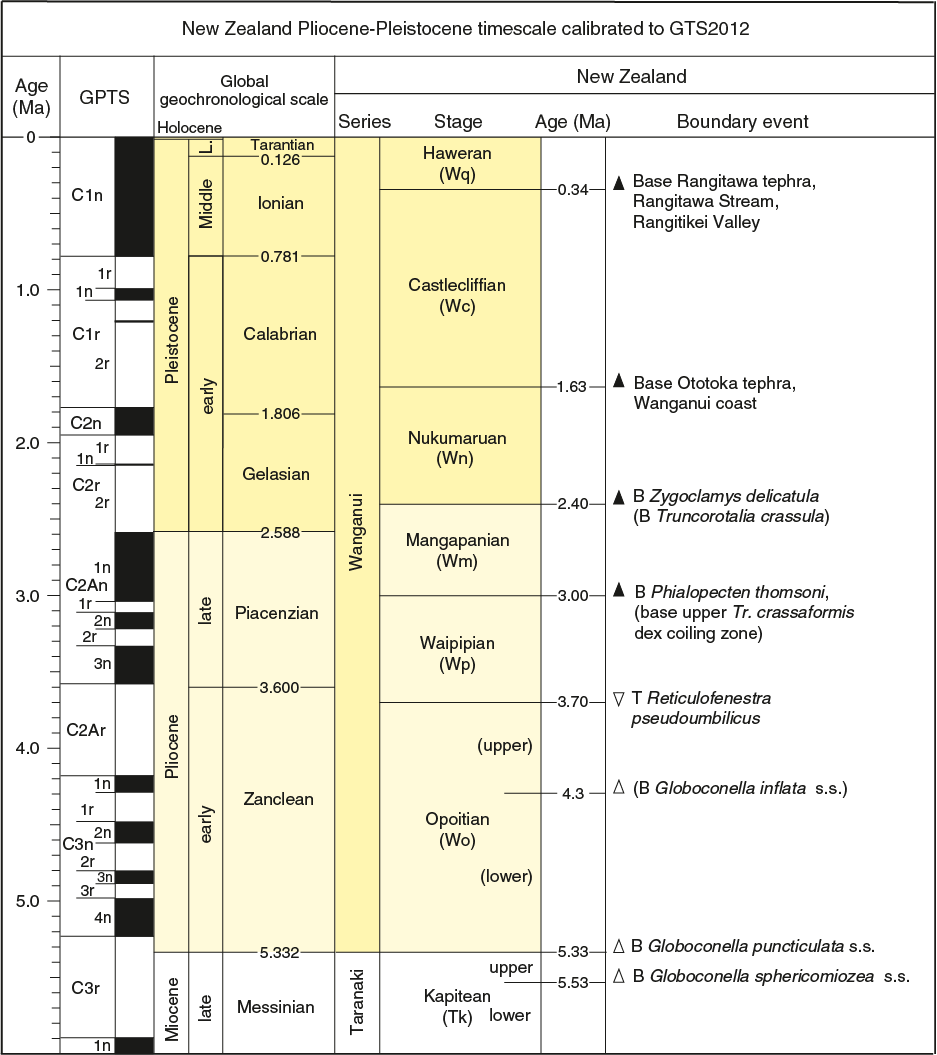
Figure F4. New Zealand Pliocene–Pleistocene timescale.

Calcareous nannofossils

Calcareous nannofossil zones are based on the scheme of Martini (1971) (NN) with ages calibrated to GTS2012 (Gradstein et al., 2012) (Table T3).

Considerable variation in the size and morphological features of species in the genus Gephyrocapsa, which are commonly used as Pleistocene biostratigraphic markers, often causes problems in identification (e.g., Samtleben, 1980; Su, 1996; Bollmann, 1997). This study utilized size-defined morphological groups of this genus as event markers (Young, 1998; Maiorano and Marino, 2004; Lourens et al., 2004; Raffi et al., 2006), including small Gephyrocapsa spp. (<3.5 µm), medium Gephyrocapsa spp. (≥4 µm), and large Gephyrocapsa spp. (≥5.5 µm).

Species differentiation in and between “species” of Reticulofenestra that are used as Cenozoic biostratigraphic markers is often problematic (e.g., Backman, 1980; Su, 1996; Young, 1998). This study adopts the definition of Reticulofenestra pseudoumbilicus by Young (1998) as having a maximum coccolith length >7 µm, with smaller forms recorded as R. pseudoumbilicus 5–7 µm.

Taxonomic concepts for other species follow those of Perch-Nielsen (1985), Bown (1998, 2005), Dunkley Jones et al. (2009), and Shamrock and Watkins (2012), as compiled in the online Nannotax3 database (http://www.mikrotax.org/Nannotax3).

Methods

Calcareous nannofossil smear slides were prepared from core catcher samples using standard techniques. In some instances, strewn slides were prepared by mixing a small amount of sediment in a buffered solution (pH = ~8.5), which was left for 10–15 s to allow larger particles to settle before the suspended sediment was transferred with a pipette to a coverslip and placed on a warming plate to dry. Once dry, the coverslip was affixed to a glass microscope slide using Norland optical adhesive Number 61 and cured under ultraviolet light.

Slides were analyzed using an Olympus BX53 microscope at 400× to 1250× magnification in plane-transmitted light, cross-polarized light, and phase-contrast light.

Nannofossil preservation was noted as follows:

G = good (little or no evidence of dissolution and/or overgrowth was observed, primary morphological features are slightly altered, and specimens were identifiable to the species level).
M = moderate (specimens exhibit some dissolution and/or overgrowth, primary morphological features are somewhat altered, but most specimens were identifiable to the species level).
P = poor (severe dissolution, fragmentation, and/or overgrowth was observed, primary morphological features have largely been destroyed, and most specimens could not be identified at the species and/or generic level).

Intermediate categories (e.g., G/M or M/P) were used in some cases to better describe the state of preservation of calcareous nannofossil assemblages.

Total nannofossil abundance in the sediment was visually estimated at 1000× magnification and reported using the following categories:

D = dominant (>90% of sediment particles).
A = abundant (>50%–90% of sediment particles).
C = common (>10%–50% of sediment particles).
F = few (1%–10% of sediment particles).
R = rare (<1% of sediment particles).
B = barren (no calcareous nannofossils).

The relative abundance of individual calcareous nannofossil species or taxa groups was estimated at 1000× magnification and noted as follows:

D = dominant (>100 specimens per field of view).
A = abundant (>10–100 specimens per field of view).
C = common (>1–10 specimens per field of view).
F = few (1 specimen per 1–10 fields of view).
R = rare (<1 specimen per 10 fields of view).
* = reworked (presence of species interpreted to be reworked).
? = questionable (questionable specimen of that taxon).

Foraminifers

Locally calibrated ages were used for all Neogene and Quaternary planktonic foraminifer datums based on Cooper (2004), Crundwell (2004), and Crundwell and Nelson (2007) (Table T4). Foraminifer criteria for the adopted marine paleoenvironmental classification, modified after Hayward et al. (1999), are shown in Figure F5.

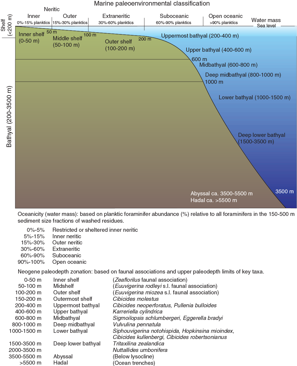
Figure F5. Marine paleoenvironmental classification.

The taxonomy of planktonic foraminifers follows a modified version of the phylogenetic classification of Kennett and Srinivasan (1983). Abbreviations for common genera are given in Table T5. Species concepts are primarily based on Hornibrook (1981, 1982), Hornibrook et al. (1989), Scott et al. (1990), Hornibrook and Jenkins (1994), Crundwell and Nelson (2007), and Crundwell (2015a, 2015b).

Qualifiers for taxa identified in this study are as follows:

cf. = confer (compare with).
sp. = unidentified species assigned to the genus.
spp. = more than one unidentified species assigned to the genus.
? = identification uncertain.

Methods

Samples (5 cm whole rounds and 24 cm³ split-core samples) were prepared by manually breaking the core into small pieces and soaking them in hot water with a few drops of detergent. After ~5–10 min, samples were disaggregated and sieved to 125 µm to remove all mud and very fine sand. The washed residue retained on the sieve was then dried at 120°–150°C in an oven and divided with a microsplitter into equal aliquots for examination. As a precaution against cross-contamination, sieves were cleaned with jetted water and rinsed with methylene blue solution between successive samples.

The percentage of planktonic foraminifers relative to total foraminifers was determined quantitatively from random counts of 100 foraminifers in the 500–150 µm grain size fractions of the washed residues to determine oceanicity. Age and depth markers were then picked from successive 500–300, 300–212, and 212–150 µm grain size fractions and mounted onto 60-division faunal slides coated with gum tragacanth. As time allowed, other species and microfossils were also picked and mounted on the same slides. In most cases, the 500–212 µm grain size fraction was examined, and in samples where age diagnostic species were difficult to find, the 212–150 µm and 150–125 µm size fractions were also examined.

During the examination of microfossil samples, the abundance of foraminifers and other fossil groups in the 150–500 µm grain size fractions of washed samples was determined visually and categorized as follows:

D = dominant (foraminifers compose >50% of the washed microfossil residue).
A = abundant (foraminifers compose >20%–50% of the washed microfossil residue).
C = common (foraminifers compose >5%–20% of the washed microfossil residue).
F = few (foraminifers compose 1%–5% of the washed microfossil residue).
R = rare (foraminifers compose <1% of the washed microfossil residue).
X = present (present in sample; abundance undetermined).

In addition, the preservation of foraminifers was categorized as follows:

VG = very good (specimens were mostly whole, very well preserved ornamentation and surface ultrastructure, and no visible modification of the test wall).
G = good (specimens were often whole, ornamentation and surface ultrastructure were preserved but sometimes abraded or overgrown, and visible evidence of modification of the test wall).
M = moderate (specimens were often etched or broken, the ornamentation and surface ultrastructure were modified, and the majority of specimens were identifiable to species level).
P = poor (most specimens were crushed or broken, recrystallized, diagenetically overgrown, or infilled with crystalline calcite; most specimens were difficult to identify to species level).

Planktonic foraminifers

Planktonic foraminifer dating was used in conjunction with calcareous nannofossil dating to determine biostratigraphic ages. Planktonic foraminifers were also used to identify changes in marine climate. To achieve these goals, planktonic foraminifers that are useful for biostratigraphic dating and warm-water taxa denoting inflows of subtropical water were preferentially picked during the examination of samples. As time allowed, representatives of other planktonic species were also picked.

Benthic foraminifers

Benthic foraminifers were the primary paleontological tool used for estimating paleowater depths (Figure F5). In some instances, they were also used as secondary markers for biostratigraphic dating. Paleowater depths were estimated on the basis of the deepest calibrated depth marker contained in each sample using the markers given in Figure F5. Displaced shallow-water species (e.g., Hayward et al., 1999) that had been reworked downslope were also noted to identify redeposited sediment.

Paleomagnetism

Paleomagnetic investigations on Site U1517 cores were conducted by shipboard scientists and technicians during Expedition 375. Because of time constraints, analyses were limited to natural remanent magnetization (NRM) measurement of archive halves prior to and following partial alternating field (AF) demagnetization. All measurements were conducted using a triaxial SRM (2G Enterprises, model 760R-4K) coupled with a 2G sample degaussing system that allows automated AF demagnetization by up to 100 mT. The system was designed for the continuous measurement of sections as long as 1.5 m and thus has a chamber with an 8.2 cm wide entrance. The response curves for each of the superconducting quantum interference device sensors have a total width of ~8 cm (H. Oda and C. Xuan, unpubl. data). Automated and continuous demagnetization is controlled using the in-house IMS-SRM v.9.2 software (SRM User Guide v.371 available on the JOIDES Resolution). Prior to leaving port, a profile of the background field across the measurement chamber was constructed using a fluxgate magnetometer (Applied Physics, type 520), showing that the field in the x-, y ‑, and z-directions does not exceed 0.008 nT. To minimize noise caused by dirt trapped in the measurement chamber, the sample tray was demagnetized twice per day using an AF of 40 mT followed by measurement of the tray only. This background field usually yields magnetic moments in the range of 3 × 10⁻⁹ A/m² in the x- and y-directions and 4 × 10⁻¹² A/m² along the z-axis. Core sections were measured at a spacing of 2.5 cm. On each end of a section, an additional 10 cm was measured as a “header” and “trailer” to allow for deconvolution during future analysis. All data reported in the Laboratory Information Management System (LIMS) database are presented both in raw format and corrected for background field and magnetic drift of the sensors.

NRM measurements usually yield anomalous components of magnetization along core due to a viscous remanent magnetization acquired during the drilling process. All cores were thus subjected to stepwise AF demagnetization using 4–5 steps up to a peak field of 30 mT (Cores 372-U1517C-1H through 10F), 20 mT (Cores 11F–18H), or less, and NRM was measured following each demagnetization step. Calculated inclination, declination, and intensity were visually inspected using the IMS-SRM v.9.2 software and, where necessary, carefully analyzed using vector component diagrams (Zijderveld, 1967) to verify whether the remanence directions and/or magnetic polarities determined were of primary origin. Subsequently, variations in declination, inclination, and intensity records and interpreted polarity sequences with respect to depth below seafloor were displayed using MATLAB.

Coordinate convention and core reorientation

The magnetic data sets presented are displayed relative to the standard IODP coordinate system (Figure F6) with +z pointing downcore and +x pointing toward the double lines at the bottom of the working half and thus out of the archive half. The SRM coordinate system is inverted with respect to IODP coordinates (+z_IODP = −z_SRM). Conversion from SRM to IODP coordinates is thus required prior to data display, which occurs prior to data upload into the LIMS database. All paleomagnetic data (declination and inclination) discussed here refer to this convention.

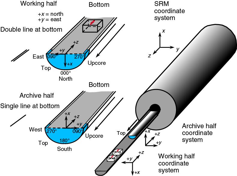
Figure F6. IODP coordinate systems.

Cores 372-U1517C-1H and 2H were independently oriented using the FlexIT tool, and Cores 15H–18H were oriented using the Icefield MI-5 core orientation tool. The latter uses three orthogonally oriented fluxgate magnetometers to record the azimuthal orientation of the double lines (x-axis in IODP convention) with respect to magnetic north and thus provides an angular correction from core to geographic reference frameworks for each deployment (Arculus et al., 2015). Assuming that the borehole is vertical, declination data sets can be related to a geographic reference frame using

$D_{T r u e} = D_{o b s e r v e d} = {A z}_{F l e x I T} + D_{l o c a l},$

where

D_True = corrected and desired declination value,
D_observed = data measured and described in IODP coordinate system,
Az_FlexIT = angle between magnetic north and the double lines on the core liner, and
D_local = local compass declination.

Experience from previous expeditions suggests that the accuracy of reorientation falls between 20° and 30° (McNeill et al., 2017). The local declination of the 12th generation International Geomagnetic Reference Field (IGRF) (Thébault et al., 2015) at the drill site in December 2017 was 21.23° (calculated using https://www.ngdc.noaa. gov/geomag-web).

Geochemistry

The Expedition 372 coring program was designed to establish the mechanisms responsible for the creeping behavior of the Tuaheni Landslide Complex (TLC). The three main objectives of the geochemistry program for Site U1517 were to (1) determine gas hydrate presence and its potential link to the style of deformation observed at the TLC, (2) establish distribution and cycling of methane, and (3) provide information on transient events that may result from recent mass transport deposition, gas hydrate dynamics, fluid migration, and changes in upward methane flux. In addition, the geochemical data will be useful for evaluating biogeochemical processes, particularly element cycling in response to ash alteration processes in methanic sediment.

Pore fluid sampling protocol

Samples were collected on the catwalk at a frequency of four samples per core in the upper 15.2 m (Cores 372-U1517C-1H through 2H) and two samples per core from 15.2 to 112.4 mbsf (Cores 3F–19F). Deeper than 112.4 mbsf, care was taken to select samples where the IR camera scans suggested the potential for gas hydrate occurrence, as well as in sections away from IR anomalies (background samples), resulting in a sampling frequency of as many as six samples per HLAPC core (see Geochemistry in the Site U1517 chapter [Barnes et al., 2019]).

For headspace analyses of gas concentrations, three sediment plugs of 3 mL each were routinely collected; one plug was used for standard hydrocarbon concentration monitoring on board, and the other two were used for stable isotope measurements at onshore laboratories. Headspace samples were collected adjacent to most IW samples when they were taken, resulting in 1–5 samples per core. In cases where not enough core was recovered for IW sampling or the presence of sand layers prevented collection of IW samples, headspace samples were taken at a minimum resolution of one sample per half core for safety monitoring purposes. When gas voids were present, they were sampled at a frequency of 1–4 samples per HLAPC core.

Pore fluid collection

Whole-round (WR) core samples were cut on the catwalk, capped, and taken to the laboratory for processing. During high-resolution sampling, when there were too many IW samples to process immediately, capped WR core samples were stored under a nitrogen atmosphere at 4°C until they were squeezed, which occurred no later than 30 h after core retrieval.

After extrusion from the core liner, the surface of each WR IW sample was carefully scraped with a spatula to remove potential contamination from seawater and from sediment smearing in the borehole. The remaining sediment (~150–300 cm³) was placed in a titanium squeezer modified after the stainless steel squeezer of Manheim and Sayles (1974). Samples were squeezed at gauge forces of as much as 30,000 lb. The squeezed pore fluids were filtered through a prewashed Whatman Number 1 filter placed in the squeezers above a titanium screen. The squeezed pore fluids were collected in precleaned, plastic syringes attached to the squeezing assembly and subsequently filtered through a 0.2 µm Gelman polysulfone disposable filter.

Sample allocation was determined based on the pore fluid volume recovered and on analytical priorities based on the expedition objectives. The shipboard analytical protocols are summarized in the following section.

Gas hydrate samples

For some of the intervals in which the IR camera records suggest the potential for gas hydrate occurrence, whole rounds were collected at the catwalk and immediately immersed in a Dewar filled with liquid nitrogen for storage and shipping to onshore laboratories.

Shipboard pore fluid analyses

Pore fluid samples were analyzed on board following the protocols in Gieskes et al. (1991) and the online IODP user manuals.

Salinity, alkalinity, and pH

Salinity, alkalinity, and pH were measured immediately after squeezing. Salinity was measured using a Fisher temperature-compensated handheld refractometer, pH was measured with a combination glass electrode, and alkalinity was determined by Gran titration with an autotitrator (Metrohm 794 basic Titrino) using 0.1 M HCl at 20°C. International Association for the Physical Sciences of the Oceans (IAPSO) standard seawater was analyzed at the beginning and end of each set of samples and after approximately every 10 samples.

Chloride, sulfate, and bromide

High-precision chloride concentrations were acquired using a Metrohm 785 DMP autotitrator and silver nitrate (AgNO₃) solutions that were calibrated against repeated titrations of an IAPSO standard. A 0.1 mL aliquot of sample was diluted with 10 mL of 90 ± 2 mM HNO₃ and titrated with 0. 014 M AgNO₃. Repeated analyses of an IAPSO standard yielded a precision better than 0.5%.

Sulfate (SO₄²⁻), chloride (Cl⁻), and bromide (Br⁻) concentrations were analyzed using 100 µL aliquots diluted 1:100 with deionized water (18 MΩ·cm). Measurements were conducted using a Metrohm 850 Professional ion chromatograph (IC) with eluent solutions of 3.2 mM Na₂CO₃ and 1.0 mM NaHCO₃. Concentrations were determined using peak areas. The analytical protocol was to run a standard after five samples for six cycles, after which three extra standards were analyzed. The standards used were based on IAPSO dilutions of 50×, 80×, 150×, 250×, 500×, 750×, 1000×, 1200×, 1500×, and 2000×. Sample replicates (N = 5) were analyzed during each run for reproducibility. Reproducibility was also checked based on the interspersed standard samples run throughout the expedition. Analytical precision was better than 2% for these anions. Sulfate concentrations below ~0.85 mM are below the detection limit with the calibration curve used. Chloride analyses by both titration and IC agree within 2%; for Expedition 372 we report both values but plot only the titration data.

Ammonium, phosphate, and silica

Ammonium, phosphate, and silica concentrations were determined by spectrophotometry using an Agilent Technologies Cary Series 100 UV-Vis spectrophotometer with a sipper sample introduction system following the protocol in Gieskes et al. (1991). Phosphate was measured using the ammonium molybdate method described in Gieskes et al. (1991) with appropriate dilutions. Orthophosphate reacts with Mo(VI) and Sb(III) in an acidic solution to form an antimony-phosphomolybdate complex. Ascorbic acid reduces this complex to form a blue color, and absorbance is measured spectrophotometrically at 885 nm.

The ammonium method is based on diazotization of phenol and subsequent oxidation of the diazo compound by Clorox to yield a blue color measured spectrophotometrically at 640 nm. Samples were diluted prior to color development so that the highest concentration was <1000 µM.

Silica was also measured spectrophotometrically using the method based on the production of a yellow silicomolybdate complex. The complex is reduced by ascorbic acid to form molybdenum blue and measured at 812 nm.

Major and minor elements by ICP-AES

Dissolved major (Na, K, Ca, SO₄, and Mg) and minor (Li, Sr, B, Si, Mn, Fe, and Ba) elements were determined by an Agilent 5110 inductively coupled plasma–atomic emission spectrometer (ICP-AES) with an SPS4 autosampler. This instrument was newly installed at the start of IODP Expedition 371 (July 2017), and new analytical procedures were developed during IODP Expeditions 371 and 369.

For shipboard ICP-AES analyses of IW samples collected during Expedition 372, we adopted a procedure that incorporates aspects of the methods previously developed for this instrument with the goal of establishing a procedure that (1) takes advantage of the new capabilities of the Agilent 5110 to measure major and minor ions in the same run using both the radial and axial configurations, (2) is simple enough for routine use, and (3) generates good quality data. Each acidified IW sample was diluted 1:10 using 2% HNO₃ and spiked with 100 µL of a 10 ppm Y solution as an internal standard. For calibration, serial dilutions of IAPSO standard seawater (10%, 30%, 50%, 70%, 90%, 110%, and 200%) were prepared to cover IW concentrations smaller than or equal to normal seawater. Additional calibration solutions for major and minor element concentrations exceeding seawater (Ca, B, Ba, Fe, Li, Mn, P, Si, and Sr) were prepared with 3.5% NaCl as a matrix. Calibration solutions were made up from certified stock solutions for minor elements (B, Ba, Fe, Li, Mn, P, Si, and Sr) and spiked in the same way as the IW samples.

During each ICP-AES run, a complete set of all in-house and IAPSO dilutions were analyzed at the beginning and end of each batch. Furthermore, solutions of 100% concentration in-house and IAPSO standards were run every 8–10 samples to monitor instrumental drift. The elemental concentrations reported for each sample were average values from three replicate integrations from each sample measured consecutively via continuous flow, as set by instrumental parameters. The standard error in the average was also calculated by the instrument software.

Following each ICP run, the measured concentrations were recalculated after setting background correction parameters and adjusting peak centers using software that accompanies the ICP. Precision was determined by the instrument from triplicate runs of each sample.

Major elements by ion chromatography

The shipboard IC (Metrohm 850 Professional IC) also yields major cation (Ca, Mg, Na, and K) concentration data. Samples analyzed on the IC were diluted 100 times with Milli-Q water. The eluent solutions used for cation measurements were 3.2 mM Na₂CO₃ and 1.7 mM pyridine-2,6-dicarboxylic acid (PDCA), supplied by Metrohm (CAS#499-83-2). Concentrations were determined using peak areas. The analytical protocol was to run a standard after five samples for six cycles, after which three extra standards were analyzed. The standards used were based on IAPSO dilutions of 50×, 80×, 150×, 250×, 500×, 750×, 1000×, 1200×, 1500×, and 2000×. Sample replicates (N = 5) were analyzed during each run for reproducibility. Reproducibility was also checked based on the interspersed standard samples run throughout the expedition. Analytical precision was 0.3% for Na and K, 0.6% for Mg, and 1.0% for Ca.

Preference for multiple data sets

Often, more than one data set was produced for the concentration of a dissolved species. For example, Ca, Mg, K, Na, Sr, Si, B, Ba, Fe, and Mn were measured using two or more wavelengths by ICP-AES, and the adoption of each wavelength was based on data quality details. In addition, Ca, Mg, K, and Na were measured by IC, and Si was measured by spectrophotometry. Cl⁻ concentrations were analyzed by titration and IC. The data plotted reflect the chosen method of analyses, which is listed in Table T6. This table also includes the chosen ICP-AES wavelength and the estimated precision of each analysis.

Fluid organic geochemistry

Routine analysis of hydrocarbon gases in sediment cores is a part of the standard IODP shipboard monitoring program to ensure that the sediments being drilled do not contain greater than the expected amounts of higher hydrocarbons (Pimmel and Claypool, 2001). The most common method of hydrocarbon monitoring used during IODP expeditions is the analysis of gas samples obtained from sediment samples (headspace analysis) following the procedures described by Kvenvolden and McDonald (1986).

For headspace analyses, three 3 cm³ bulk sediment samples were collected from the freshly exposed top end of a core section and next to the IW sample immediately after core retrieval using a 3 mL plastic syringe with the top cut off. The sediment plug designated for shipboard analysis was sealed with an aluminum crimp cap and silicon septa. The vial was then heated to 70°C for ~30 min to evolve hydrocarbon gases from the sediment plug. A 5 cm³ volume of headspace gas was extracted from the sealed sample vial using a standard gas-tight syringe and was analyzed by gas chromatography.

The remaining two sediment plugs were collected to measure the stable carbon and hydrogen isotopic composition of hydrocarbons at onshore laboratories. The sampling method is the same as that used for the safety analysis, except that the sediment plug is extruded into a 20 cm³ headspace glass vial filled with 10 cm³ of a 1 M potassium chloride (KCl) solution and sealed with an aluminum crimp cap and Teflon/butyl septum. The vial was then vigorously shaken to help dissociate the sediment. Potassium chloride is toxic and was used to stop all microbial activity in the sediment. The vials were flushed with N₂ and capped within 1 h prior to sampling to remove air from the headspace and ensure the sample was preserved anaerobically.

When gas pockets occurred in the expanding cores, the free gas was drawn from the sediment void using a syringe attached to a hollow stainless steel tool used to puncture the core liner. The gas was then injected into a presealed 20 mL vial filled with 2 M NaCl solution. The gas injected into the vial replaced the brine. This way, contact with air was minimized. The void gases were initially collected for onboard measurements of the gas composition and stable isotope measurements of carbon and hydrogen of the hydrocarbons on shore. Because of difficulties with the calibration of the natural gas analyzer (NGA) gas chromatographic setup, all measurements will be done on shore.

The composition of headspace samples was measured using one of the two shipboard gas chromatographs (GCs), designated as GC3 and NGA. During Expedition 372, the GC3 system was the only one used. Calibrations of the NGA for higher hydrocarbons and particularly nonhydrocarbon gases turned out to be insufficient to allow for onboard measurements.

The GC3 is an Agilent 7890 gas chromatograph with a flame ionization detector (FID) used to determine concentrations of light hydrocarbon gases C₁–C₃ (alkanes and alkenes). It is equipped with a 25 µL sample loop, a 10 port VALCO valve, an 80/100 mesh 8 ft HayeSep R packed column (2.0 mm inside diameter [ID] × ⅛ inch OD), and an FID set at 250°C. The GC3 oven temperature was programmed to hold for 8.25 min at 80°C, ramp at 40°C/min to 150°C, hold for 5 min, and return to 100°C postrun for a total of 15 min. Helium was used as the carrier gas. Precision and accuracy are ±2% for concentrations as high as 10,000 ppm and ±1% for higher values.

Chromatographic response is calibrated using nine preanalyzed standards with methane concentrations ranging from 15 to 900,000 parts per million by volume (ppmv). The standards with high methane concentrations are likely to contain small amounts of ethane not used for calibration. The gas concentrations for the required safety analyses are expressed as component parts per million by volume relative to the analyzed gas. Data were collected using the Hewlett Packard 3365 Chemstation data processing program.

Sediment geochemistry

For the shipboard sediment geochemistry analyses, 5 cm³ of sediment was freeze-dried for ~24 h, crushed to a fine powder using an agate pestle and mortar, and sampled to analyze inorganic carbon, total carbon (TC), and total nitrogen (TN).

The TC and TN of sediment samples were determined with a ThermoElectron Corporation FlashEA 1112 carbon-hydrogen-nitrogen-sulfur (CHNS) elemental analyzer equipped with a ThermoElectron CHNS/nitrogen-carbon-sulfur (NCS) packed column and a thermal conductivity detector (TCD). Approximately 10–15 mg of freeze-dried, ground sediment was weighed and sealed in a tin capsule, and the sample was combusted at 900°C in a stream of oxygen. The reaction gases were passed through a reduction chamber to reduce nitrogen oxides to nitrogen and were then separated by gas chromatography before detection by TCD. All measurements were calibrated to a standard sediment reference material (National Institute of Standards and Technology [NIST] 2704 Buffalo River Sediment) for carbon and nitrogen detection, which was run every six samples as a verification. The detection limit was 0.001% for TN (instrument limit) and 0.002% for TC (procedural blank; measured as an empty tin cup). Sample replicates (N = 10 for each of five samples) yielded precisions of <10% for TN and <7% for TC.

Total inorganic carbon (TIC) concentrations were determined using a UIC 5011 CO₂ coulometer. Between 10 and 15 mg of freeze-dried, ground sediment was weighed and reacted with 2 M HCl. The liberated CO₂ was titrated, and the end point was determined by a photodetector. Calcium carbonate content expressed as weight percent was calculated from the TIC content assuming that all evolved CO₂ was derived from dissolution of CaCO₃:

${C a C O}_{3} (w t %) = T I C \times 8.33 (w t %) .$

No correction was made for the presence of other carbonate minerals. Accuracy during individual batches of analyses was determined by running a carbonate standard (100 wt% CaCO₃) every 10 samples. Typical precision, assessed using replicate analyses of carbonate samples (N = 10 for each of 5 samples), was 2%. The detection limit for CaCO₃, defined here as 3× the standard deviation of the blank (2 M HCl), was 0.1%. Total organic carbon (TOC) content was calculated as the difference between TC (measured on the elemental analyzer) and inorganic carbon (measured by coulometry):

$T O C = T C - i n o r g a n i c c a r b o n .$

Physical properties

Physical properties measurements provide fundamental information required to characterize lithostratigraphic units and allow for correlation of cored materials with logging data. A comprehensive discussion of methodologies and calculations used in the JOIDES Resolution physical properties laboratory is presented in Blum (1997).

After sectioning (see Core handling and curatorial procedures), core sections were moved into the laboratory to equilibrate to room temperature for ~4 h. After thermally equilibrating, core sections longer than 30 cm were run through the WRMSL for measurement of gamma ray attenuation (GRA) bulk density, magnetic susceptibility, and compressional wave (P-wave) velocity (P-wave logger [PWL]). Sections longer than 50 cm were measured with the spectral NGRL.

Thermal conductivity measurements were carried out on two whole-round core sections per full core (APC) or one section per half core (HLAPC) using the needle probe technique. After cores were split into archive and working halves, the archive half was passed through the SHIL for digital image scanning on the cut surface and the SHMSL for measurement of point magnetic susceptibility (MSP) and color spectrophotometry (see also Lithostratigraphy).

Discrete samples for moisture and density (MAD) measurements were taken from the working half at a frequency of approximately one per section. In sections where whole-round core samples were removed for interstitial water or other testing, MAD samples were located close to these samples to help characterize the tested interval. MAD measurements yielded wet bulk density, dry bulk density, grain density, water content, void ratio, and porosity. P-wave velocity was measured on the working half, and strength was measured using the automated vane shear (AVS) apparatus and penetrometers. P-wave velocity and strength measurements were conducted once per section where core conditions allowed.

Whole-Round Multisensor Logger measurements

GRA bulk density, P-wave velocity, and magnetic susceptibility were measured nondestructively with the WRMSL. To optimize WRMSL performance, sampling intervals and measurement integration times were the same for all sensors. The sampling interval was set at 1 cm with an integration time of 3 s for each measurement. GRA performance was monitored by passing a single core liner filled with deionized water through the WRMSL after every core.

In general, measurements are most effective with a completely filled core liner with minimal drilling disturbance. For APC sediment cores, the 66 mm core liner width is generally filled. Sections consisting of discontinuous fragments were not measured with the WRMSL sensors. Sections were run through the WRMSL only if they were longer than 30 cm.

Gamma ray attenuation bulk density

GRA bulk density is an estimate of bulk density based on the attenuation of a gamma ray beam. The beam is produced by a ¹³⁷Cs gamma ray source at a radiation level of 370 MBq in a lead shield with a 5 mm collimator, which is directed through the whole-round core. The gamma ray detector on the opposite side of the core from the source includes a scintillation detector and an integral photomultiplier tube to record the gamma radiation that passes through the core. The attenuation of gamma rays occurs primarily by Compton scattering, in which gamma rays are scattered by electrons in the formation; the degree of scattering is related to the material bulk density. Bulk density (ρ) determined with this method can be expressed as

$ρ = 1 / (μ d) \times l n (I_{0} / I),$

where

µ = Compton attenuation coefficient,
d = sample diameter,
I₀ = gamma ray source intensity, and
I = measured intensity of gamma rays passing through the sample.

The attenuation coefficient and gamma ray source intensity are treated as constants such that ρ can be calculated from I. The gamma ray detector was calibrated with a set of aligned aluminum cylinders of various diameters surrounded by distilled water in a sealed core liner that is the same as that used during coring operations. The relationship between I and the product of µ and d can be expressed as

$l n I = B (μ d) + C,$

where B and C are coefficients determined during calibration. Gamma ray counts through each cylinder were determined for a period of 60 s, and the natural log of resulting intensity values was plotted as a function of µd. Here, the density of each aluminum cylinder is 2.7 g/cm³ and d is 1, 2, 3, 4, 5, or 6 cm. The WRMSL provided the values of I and µ, and ρ was calculated with the above equation. Recalibration was performed as needed if the deionized water standard after every core deviated significantly (more than a few percent) from 1 g/cm³. The spatial resolution of the GRA densiometer is <1 cm.

Magnetic susceptibility

Magnetic susceptibility (k) is a dimensionless measure of the degree to which a material can be magnetized by an external magnetic field:

$k = M / H,$

where M is the magnetization induced in the material by an external field strength H. Magnetic susceptibility responds to variations in the magnetic composition of the sediment that commonly can be related to mineralogical composition (e.g., terrigenous versus biogenic materials) and diagenetic overprinting. Materials such as clay generally have a magnetic susceptibility several orders of magnitude lower than magnetite and some other iron oxides that are common constituents of igneous material. Water and plastics (core liner) have a slightly negative magnetic susceptibility.

The WRMSL incorporates a Bartington Instruments MS2 meter coupled to a MS2C sensor coil with a 90 mm diameter and operates at a frequency of 452 Hz. A correction factor of 1.174 was provided by Bartington for this diameter and frequency and was applied to magnetic susceptibility measurements. Data shown here and in the database are not corrected for volume effects because of varying sample bulk density values. The instrument was calibrated with a homogeneous mixture of magnetite and epoxy in a 40 cm long piece of core liner to an accuracy of ±5%. Information from Bartington indicates that the MS2C loop has 2.0 cm spatial resolution. Tests reported by Blum (1997) using synthetic cores suggested a full-width half-maximum response of 4.0 to 4.4 cm.

Compressional wave velocity

The PWL measures the ultrasonic P-wave velocity of the whole-round sample residing in the core liner. The PWL transmits a 500 kHz P-wave pulse across the core section at a specified repetition rate. This signal is coupled to the sample by the plastic pole contacts of the transducers clamped to the sides of the core by the linear actuator. Water is used for each measurement to improve coupling between the transducers and the liner. The plastic pole contacts and the pressure applied by the actuator were generally sufficient for reliable P-wave measurement. The transmitting and receiving ultrasonic transducers were aligned so that wave propagation is perpendicular to the long axis of the core section.

The basic relationship for sonic velocity (V) is

$V = d / t,$

where d is the path length of the wave through the core and t is the traveltime. Besides the traveltime through the sample, the total traveltime between the transducers includes three additional components:

t_delay = time delay related to transducer faces and electronic circuitry,
t_pulse = delay related to the peak detection procedure, and
t_liner = transit time through the core liner.

For routine measurement on whole-round cores inside core liners, the corrected core velocity (V_core) can be expressed by

$V_{c o r e} = ({d'}_{c o r e} - {2 d}_{l i n e r}) / (t_{0} - t_{p u l s e} - t_{d e l a y} - {2 t}_{l i n e r}),$

where

dʹ_core = measured diameter of core and liner,
d_liner = liner wall thickness, and
t₀ = measured total traveltime.

The system was calibrated using a core liner filled with deionized water and an aluminum block with known velocity (6295 m/s) and length (76.2 mm).

Traveltime was determined by signal processing software that automatically detects the first arrival of the P-wave signal. Because high background noise makes it challenging for an automated routine to pick the first arrival of a potentially weak signal, the search method skips the first positive amplitude and finds the second positive amplitude using a detection threshold limit typically set to 30% of the maximum amplitude of the signal. The program then finds the preceding zero crossing and subtracts one wave period to determine the first arrival. To avoid extremely weak signals, a minimum signal strength can be set (typically 0.02 V) and weaker signals are ignored. To avoid signal interference at the beginning of the record from the receiver, a delay (typically 0.01 ms) can be set to force the amplitude search to begin in the quiet interval preceding the first arrival. In addition, a trigger (typically 4 V) is selected to initiate the arrival search process, and the number of waveforms to be stacked (typically 50) can also be set. A laser measures the separation of the transducer to derive a signal path length (i.e., core diameter). After corrections for system propagation delay, liner thickness, and liner material velocity, the ultrasonic P-wave velocity is calculated. The software removes any extremely unrealistic velocity values (<900 m/s or >6000 m/s).

Natural Gamma Radiation Logger

The NGRL measures gamma radiation emitted from whole-round core sections that arises primarily from the decay of ²³⁸U, ²³²Th, and ⁴⁰K isotopes. The main natural gamma radiation (NGR) detector unit consists of 8 sodium iodide (NaI) scintillator detectors. The NaI detectors are covered by 8 cm of lead shielding. In addition, lead separators (~7 cm of low-background lead) are positioned between the NaI detectors. Half of the lead shielding closest to the NaI detectors is composed of low-background lead, whereas the outer half is composed of regular (virgin) lead. In addition to passive lead shielding, the NGRL employs plastic scintillators to suppress the high-energy gamma and muon components of cosmic radiation by producing a canceling signal when these charged particles pass through the plastic scintillators.

A measurement run consisted of eight simultaneous measurements offset by 20 cm each. The quality of the energy spectrum measured in a core depends on the concentration of radionuclides in the sample but also on the counting time, with higher times yielding better spectra. Counting times were 300 s in each of two positions for a total of 10 min. For presentation purposes, the counts are summed over the range of 100–3000 keV. The spatial resolution of the NGR measurements is 18–20 cm (Vasiliev et al., 2011). Sections were run through the NGRL only when the retrieved interval was longer than 50 cm.

The NGRL was calibrated using a source consisting of ¹³⁷Cs and ⁶⁰Co and identifying the peaks at 662 (¹³⁷Cs) and 1330 keV (⁶⁰Co). Calibration materials were provided by Eckert & Ziegler Isotope Products, Valencia, California (USA). Background measurements of an empty core liner counted for 40,000 s (~10 h) at each measurement position were made upon arrival at the site. Over the 100–3000 keV integration range, background counts averaged 4–5 counts/s.

Section Half Multisensor Logger measurements

The SHMSL measures magnetic susceptibility and spectral reflectance on archive halves. The archive half is placed on the system’s core track. An electronic platform moves along a track above the core section, recording the sample height with a laser sensor. The laser establishes the location of the bottom of the section, and the platform reverses the direction of movement, moving from bottom to top taking MSP and spectral reflectance measurements at 1 cm intervals.

Color reflectance spectrometry

The color reflectance spectrometer uses an Ocean Optics 30 mm integrating sphere and both halogen and LED light sources, which cover wavelengths from ultraviolet through visible to near infrared. Measurements were taken from 380 to 900 nm wavelengths at 2 nm intervals. The approximate 3 s data acquisition offset was applied for the entire scan of the archive half. The data are reported using the red-green-blue and L*a*b* color systems, in which L* is lightness, a* is redness (positive) versus greenness (negative), and b* is yellowness (positive) versus blueness (negative) of the rock. The color reflectance spectrometer calibrates on two spectra, pure white (reference) and pure black (dark). Color calibration was conducted automatically approximately once every 6 h (twice per shift).

Point magnetic susceptibility

MSP was measured with a Bartington MS2K contact probe with a flat, 15 mm diameter, round sensor with a field of influence of 25 mm and an operation frequency of 930 Hz. The instrument averages three measurements from the sensor for each offset, leading to an accuracy of ~5%. As with whole-round measurements, the output displayed by the point magnetic susceptibility sensor must be converted to dimensionless SI units by multiplying by 10⁻⁵. The probe is zeroed in air before each measurement location to avoid influence from the metal track. The MSP meter was calibrated by the manufacturer before installation on the ship and was quality checked every ~6 h at the same time as color reflectance sensor calibration.

Thermal conductivity

Thermal conductivity is a measure of the ease at which heat flows through a material and is dependent on composition, porosity, and structure. Thermal conductivity was measured on unconsolidated sediment using the TeKa TK04 unit needle probe (Blum, 1997; Von Herzen and Maxwell, 1959). To insert this probe, a hole was made in the core liner of a whole-round core section at a position based on visual inspection of the core to avoid disturbed regions.

All measurements were made after cores equilibrated to ambient laboratory temperature. After the background thermal drift was determined to be stable, the heater circuit was closed and the increase in the probe temperature was recorded. Temperature-time series were acquired over ~80 s. Thermal conductivity values are based on the observed rise in temperature for a given flux of heat. Three measurements were taken with a cooling time of 10 min between measurements.

Temperature influences thermal conductivity of porous rocks in two competing ways. The thermal conductivity of the rock matrix is inversely related to temperature (Zoth and Haenel, 1988), whereas the thermal conductivity of water increases with temperature (Keenan et al., 1978). Reported thermal conductivity values are at laboratory temperatures and have not been corrected to in situ temperature.

Moisture and density

Several basic quantities of interest (water content, bulk density, dry density, porosity, and void ratio) are most accurately determined through mass and volume determinations on discrete samples. MAD samples were taken from the working half at a frequency of approximately one per section during Expedition 372. In unconsolidated sediments, samples were taken from the core using syringes. Sediment samples were carefully placed in vials that had previously been weighed and had their volume determined. Care was taken to avoid disturbed core material, fill the vial as completely as possible, remove excess material from the outside of the vial, and collect samples as rapidly as possible after core splitting. Immediately after sediment samples were collected, the vials were capped until weighing to prevent moisture loss. As soon as possible after collection, wet sediment mass (M_wet) was measured. Dry sediment mass (M_dry) and volume (V_dry) were measured after drying the samples in a convection oven for >24 h at a temperature of 105° ± 5°C and then cooling in a desiccator for >1 h. A dual-balance system was used to measure both wet and dry masses. Two Mettler-Toledo XS204 balances were used to compensate for ship motion, with one acting as a reference and the other for measurement of the unknown. A standard weight of similar value to the sample was placed upon the reference balance to increase accuracy. The default setting of the balances was 300 measurements (taking ~1.5 min).

Dry volume was measured using a helium-displacement pycnometer with a nominal precision of ±0.04 cm³. The pycnometer system measures dry sample volume using six pressurized, helium-filled chambers. Individual volume measurements were preceded by three purges of the sample chambers with research-grade (99.995% or better) helium heated to 28°C followed by three data acquisition cycles. Each reported value consists of an average of the three measurements.

At the start of the expedition and whenever the helium gas tank was changed, shipboard technicians performed a calibration using stainless steel spheres of known volume. Each pycnometer chamber was tested at least once every 30 samples by running two spheres of known volume in one of the chambers during each use (e.g., as many as 5 sediment samples were tested, and the remaining cell contained the spheres with known volume). The pycnometer chamber was recalibrated if the measured volume was not within 1% of the known volume.

For calculation of sediment bulk density, dry density, grain density, porosity, and void ratio, the traditional Ocean Drilling Program method was used (Method C; Blum, 1997). Water content, porosity, and void ratio are defined by the mass or volume of extracted water before and after removal of interstitial pore water through the drying process. Standard seawater density (1.024 g/cm³) is used for the density of pore water.

Water content (W_c) was determined following the methods of the American Society for Testing and Materials (ASTM) Designation D2216 (ASTM International, 1990). Corrections are required for salt when measuring the water content of marine samples. In addition to the recommended water content calculation in ASTM D2216 (i.e., the ratio of pore fluid mass to dry sediment mass [percent dry weight]), we also calculated the ratio of pore fluid mass to total sample mass (percent wet weight). The equations for water content are

$W_{c} (% dry wt) = (M_{w e t} - M_{d r y}) / (M_{d r y} - r M_{w e t}), and$

$W_{c} (% wet wt) = (M_{w e t} - M_{d r y}) / [(1 - r) \times M_{w e t}],$

where

M_wet = total mass of the saturated sample,
M_dry = mass of the dried sample, and
r = salinity.

Bulk density (ρ) is the density of the saturated samples, where ρ = M_wet/V_wet. The mass (M_wet) was measured using the balance, and V_wet was determined from the pycnometer measurements of dry volume (V_dry) and the calculated volumes of the pore fluid (V_f) and salt (V_salt):

(V_wet = V_dry + V_f − V_salt).

Porosity (ϕ) was calculated using

ϕ = (W_c × ρ)/[(1 + W_c) × ρ_w],

where

ρ = calculated bulk density,
ρ_w = density of the pore fluid, and
W_c = water content expressed as a decimal ratio of percent dry weight.

Grain density (ρ_grain) was determined from measurements of dry mass and dry volume made in the balance and in the pycnometer, respectively. Mass and volume were corrected for salt using

ρ_grain = (M_d − s)/[V_d − (s/ρ_salt)],

where s is the salt content (in grams) and ρ_salt is the density of salt (2.257 g/cm³).

Discrete compressional wave velocity

Discrete P-wave velocity measurements were obtained on the working halves of sediment cores at a frequency of one per section where conditions allowed. The frequency of the transducers is 500 kHz. y- and z-axis measurements were acquired using two pairs of bayonet probes inserted perpendicular and parallel to the axis of the working half, respectively. x-axis measurements were acquired with a caliper-type contact probe with one plastic transducer contact on the face of the working half and the other contact against the core liner. For x-axis measurements, the distance between the transducers was measured by laser (in meters) and velocity values were corrected for liner thickness and velocity.

The signal received through the sample was recorded by the computer attached to the system, and the first arrival was chosen with autopicking software, as described in Compressional wave velocity. The caliper-type contact probe was calibrated each day before measurements with an aluminum block of known velocity. Water was used to calibrate the bayonet probes.

Shear strength

Measurements using the AVS device and a pocket penetrometer provide a profile of variations in strength. The measurements were not performed at in situ stress conditions and thereby underestimate the true undrained peak shear strength in situ. Measurements were made with the vane rotation axis and penetrometer penetration direction perpendicular to the split surface (i.e., parallel to any sedimentary horizontal lamination of bedding present).

Undrained shear strength was measured in fine-grained unconsolidated sediment using the AVS system following the procedures of Boyce (1977). The vane rotation rate was set to 90°/min. Peak undrained shear strength was measured typically once per section. The instrument measures the torque and strain at the vane shaft using a torque transducer and potentiometer. Vane shear strength (S_u(v)) (kilopascal) is calculated as

$S_{u (v)} = T / K_{v},$

where T is the torque required to cause the material to fail (newton meters) and K_v is the constant depending on vane dimensions (cubic meters) (Blum, 1997).

All AVS measurements reported were obtained using a vane with a height and diameter of 12.7 mm. Failure torque was determined by measuring the degrees of rotation of one of four torsional springs and a manufacturer-specified linear calibration equation relating the rotation angle to torque for the particular spring being used. Selection of the appropriate spring was based on the anticipated shear strength of the material. Vane shear results were generally considered reliable for shear strength values less than ~150–200 kPa, above which excessive cracking and separation of the core material occurred.

A pocket penetrometer was used to measure compressive strength. Penetration measurements were all conducted on the split-core face. As with the vane shear, this means that results were measured parallel to any horizontal bedding or lamination. The Geotester STCL-5 pocket penetrometer is a spring-operated device used to measure compressive strength by pushing a 0.25 inch (6.4 mm) diameter probe 0.25 inches (6.4 mm) deep (to the red marker) below the split-core surface. The mechanical scale of compressive strength (Δσ_f) is in units of kilograms per square centimeter, which are converted into units of kilopascals for reporting as follows:

${∆ σ}_{f} (k P a) = 98.1 \times {∆ σ}_{f} (k g / {c m}^{2}) .$

Unconfined shear strength (S_u(penet)) is approximately related to compressive strength by the following equation (Blum, 1997):

$S_{u (p e n e t)} = {∆ σ}_{f} / 2 .$

A 1 inch (25.4 mm) diameter adapter foot was used for measuring in very soft sediment. It provided a 16× increase in area. Results in the database are corrected for the larger area by dividing by 0.0625. The maximum compressive strength that can be measured with the pocket penetrometer is 220 kPa. Measurements using the penetrometer are typically performed once per section.

Downhole measurements

In situ pressure and temperature measurements

Measurements of formation temperature and pore pressure were made at discrete depths at Site U1517 to assess the in situ temperature and pore pressure in the TLC. The APCT-3 was used to collect temperature data at discrete depths during APC operations in Hole U1517C. The T2P and SETP were used to collect temperature and pressure measurements at discrete depths in Hole U1517D. Temperature measurements were used to estimate the geothermal gradient, which was combined with thermal conductivity measurements made on core samples (see Physical properties) to provide an estimate of the local vertical, conductive heat flow. Pore pressure measurements provided a means to estimate the in situ pressure gradient that will be used with post-expedition permeability measurements to estimate vertical fluid flow.

Advanced piston corer temperature tool

The APCT-3 fits into a modified APC coring shoe (Figure F7A). The APCT-3 consists of a battery pack, a data logger, and a platinum resistance-temperature device calibrated over a temperature range from 0° to 30°C. For APCT-3 measurements, the core barrel with the APCT-3 coring shoe is stopped at the seafloor for 5 min to thermally equilibrate with bottom water before collecting the core. At the bottom of the hole, the APC core is shot. Shooting the APC into the formation generates an instantaneous temperature rise from frictional heating. As heat dissipates into the surrounding sediment, the temperature at the APCT-3 equilibrates toward the formation temperature. To measure this temperature dissipation, the APC is held in place for ~10 min as the APCT-3 records the temperature of the cutting shoe. Temperature data are sampled at 1 Hz. The formation temperature is estimated from the recorded data by fitting model curves that are specific to the sensor and the tool geometry (Heesemann et al., 2006).

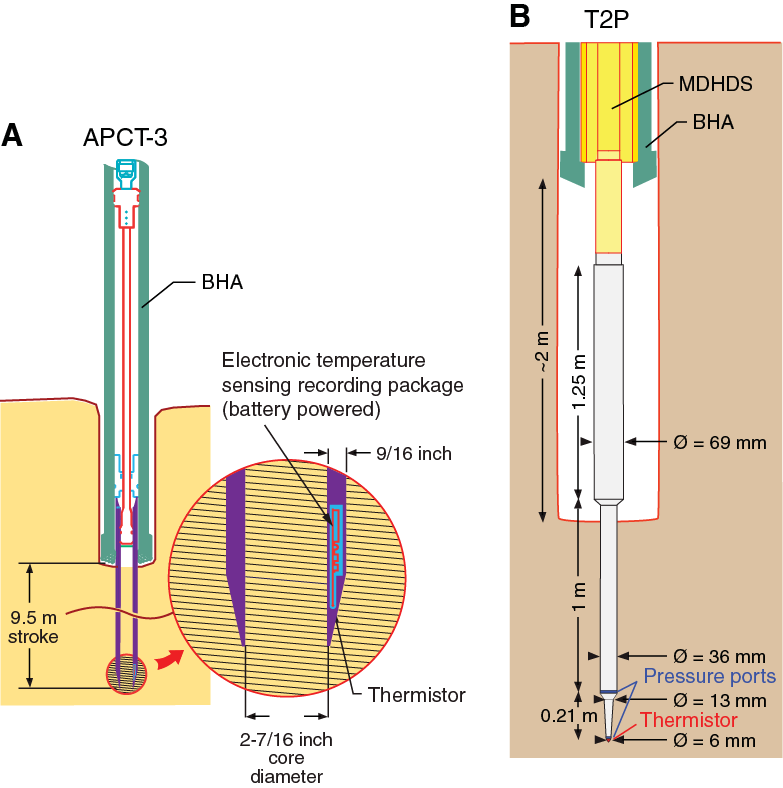
Figure F7. APCT-3 and T2P deployed with MDHDS.

Temperature dual pressure probe

The T2P is a narrow-diameter penetrometer developed by the University of Texas at Austin (USA) to evaluate in situ pore pressure, hydraulic conductivity, and temperature in low-permeability sediment (Flemings et al., 2008). The T2P measures pressure and temperature at the tool tip and pressure 21 cm upprobe from the tip (Figure F7B). The slim design of the T2P facilitates rapid, high-quality measurements of in situ conditions in low-permeability, fine-grained sediment by minimizing formation pressure increase and frictional heat generated during penetration. The two pressure sensors have different dissipation rates because they are at locations on the tool with different diameters (Flemings et al., 2008). Analysis of the two dissipation curves allows in situ pore pressure to be interpreted from a shorter dissipation period than if only one sensor was used.

Each T2P deployment required a dedicated wireline run. Deployment was controlled by using the Motion Decoupled Hydraulic Delivery System (MDHDS) (Figure F8) (Flemings et al., 2013) to decouple the probe from the drill string, minimize heave effects, and improve measurement reliability. The Electronic Release System (ERS) delivers and retrieves the MDHDS-T2P assembly in the drill pipe (Figure F9). The ERS is composed of an electronics section and a motor section that contains the latching mechanism that allows releasing and retrieving of the MDHDS.

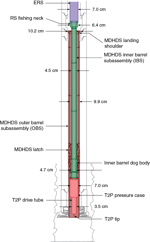
Figure F8. ERS-MDHDS-T2P tool string assembly.

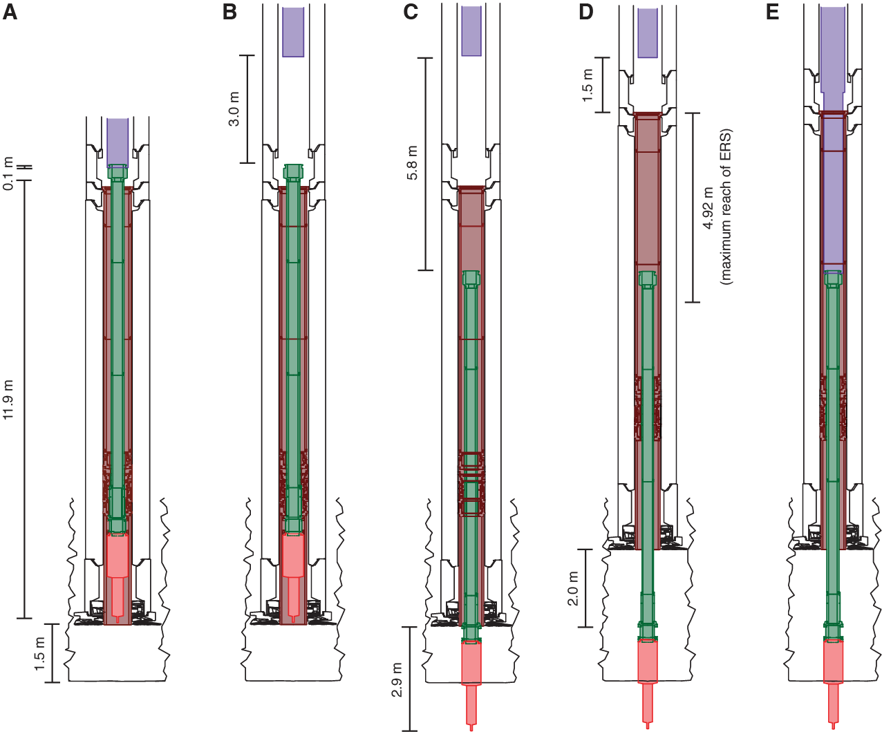
Figure F9. Deployment procedures for T2P with ERS and MDHDS.

The MDHDS is composed of an inner barrel subassembly (IBS) that is latched to the T2P and an outer barrel subassembly (OBS) (Figure F8). Prior to lowering the tool string downhole, the MDHDS is placed in its latched position and fixed in place with shear pins. The ERS-MDHDS-T2P assembly is then lowered downhole on the wireline until it lands in the BHA. While lowering the tool string downhole, hydrostatic references are taken for typically ~2 min near the seafloor and just above the bottom of the hole. The ERS releases the MDHDS and is raised above the MDHDS (Figure F9). The drill string pressure is raised to shear the shear screws and activate the MDHDS latch. The standpipe pressure is then bled down to move the MDHDS to the unlatched position. This frees the IBS from the OBS, and the IBS and T2P may fall because of their weight. The drill string pressure is then raised, and the T2P is pumped into the formation. After the piston head seal passes through the flapper guide, tube circulation is reestablished, and the BHA is raised 2 m. Raising the BHA allows ±3.0 m of vertical motion. Circulation is then terminated, and the tool is left in place for ~30 min to record pressure and temperature dissipation.

To extract the T2P, the ERS is lowered until it latches with the RS fishing neck of the IBS (Figure F9E). After latching is confirmed, the IBS and T2P are pulled from the formation into the OBS, and the entire ERS-MDHDS-T2P tool string is recovered to the rig floor via the wireline. The T2P is detached from the IBS and moved into the downhole tools laboratory. In the laboratory, the temperature and pressure data are downloaded from the tool. In situ temperature is determined from the temperature dissipation data, and in situ pore pressure is estimated from the pressure dissipation data from both pressure sensors (Flemings et al., 2008).

Sediment temperature pressure tool

The SETP (Figure F10) is a penetrometer-based tool designed to allow in situ measurement of formation pressure and temperature in semiconsolidated sediment.

Figure F10. SETP.

The SETP incorporates a single thermistor in an oil-filled tip and ports that allow hydraulic transmission of formation pressure to an internal pressure gauge. A standard data logger records the pressure and temperature data. The temperature sensor in the SETP operates over a range of 0°–85°C with a resolution of 0.001°C. The pressure sensor has a sensitivity of 70 Pa over a range of 0–70 MPa. All pressures and temperatures are recorded at 1 Hz. The SETP also includes a three-component accelerometer. All accelerometer data are recorded at 10 Hz.

A typical SETP deployment consists of connecting the SETP to the colleted delivery system (CDS), lowering the tool string by wireline, and taking hydrostatic calibration measurements on the trip to the bottom of the hole. The CDS allows decoupling of the tool with the drill string to minimize heave effects on the in situ measurements. When the drill bit is 2 m off the bottom of the hole, the tool string is lowered until the CDS engages in the BHA, with the tip of the tool extending 1.1 m below the drill bit. The SETP is pushed into the sediment by lowering the drill bit to the bottom of the hole. Pressure and temperature are recorded for >30 min. No fluids are circulated during data collection at the calibration points or when the tool is in the sediment. The tool string is then recovered via wireline.

Logging while drilling

LWD well log data were collected at Site U1517 to (1) monitor for gas entering the borehole or fluid overpressures; (2) help identify targets for in situ pressure/temperature measurements; (3) facilitate lithologic interpretation; (4) guide interpretation of faults, fractures, and sediment deformation structures; (5) estimate hydrate saturation; and (6) help constrain elastic moduli for integration with seismic data.

LWD tools are instrumented drill collars in the BHA. The LWD and MWD tools are attached behind the bit and measure in situ formation properties. The MWD tool (TeleScope) provides electrical power and transmits data from other tools up the borehole. The TeleScope transmits limited LWD data channels, referred to as real-time data, using mud-pulse telemetry during drilling. The complete LWD data set is recorded in each tool and downloaded from memory after the tool is recovered on the rig floor; this is referred to as recorded-mode data. The term “LWD” is often used to refer to both LWD- and MWD-type measurements and tools, and we use that convention here.

LWD tools are powered by batteries or by pumping drilling fluid through a turbine. Each LWD tool has a memory chip to store recorded-mode data. The tools take measurements at regular time intervals. Drilling depth is measured using a geolograph, which is a spooled wire depth encoder attached to the top drive. Following drilling and the return of the tools to the drill floor, the recorded-mode data are downloaded and the data timestamps are synced with the geolograph depth file.

For the TLC site (U1517), the LWD BHA comprised five LWD tools assembled in the following order behind the 8½ inch (~21.5 cm) drill bit: geoVISION, SonicScope, NeoScope, TeleScope, and proVISION (Figure F11; Table T7). All tools were 6¾ inch (~17 cm) drill collars in the Schlumberger 675 series.

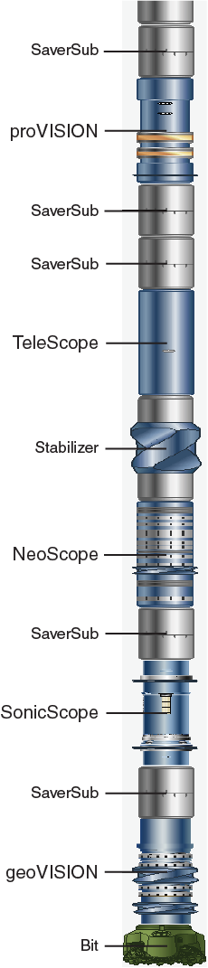
Figure F11. LWD BHA.

LWD tools

geoVISION

The geoVISION tool is a battery-operated hybrid resistivity device that collects 1-D laterolog-type resistivity measurements, 360° azimuthal resistivity (resistivity images), and natural gamma ray images of the borehole wall. The geoVISION tool was placed directly behind the bit (Figure F11).

The resistivity measurements are performed by two transmitter electrodes that send signals to a series of receiver electrodes, providing three sets of information:

Bit resistivity is measured using the lower portion of the geoVISION tool and the drill bit as the measurement electrode. Alternating current flows through the lower transmitter, the collar, and the drill bit and down into the formation before returning to the drill collar. Resistivity is derived from the axial current passing through the formation at a given induced voltage. The vertical resolution of the bit resistivity measurements ranges from ~30 to 60 cm with a depth of investigation of ~30 cm (Table T7).
Ring resistivity is measured using the radial flow of current out of the collar. Current is approximately perpendicular to the tool, depending on the homogeneity of the formation. Resistivity is determined by measuring the current flowing out the tool at the 4 cm thick integral cylindrical electrode, located 90 cm from the bottom of the tool. Ring resistivity is a focused lateral resistivity measurement with a vertical resolution of ~5–8 cm and a depth of investigation of ~18 cm (Table T7).
Button resistivity is measured by three longitudinally spaced, azimuthally focused, 2.5 cm thick button electrodes stacked in the upper portion of the tool that provide resistivity data at various depths of investigation. Measurements acquired from these buttons during tool rotation in the borehole provide data for generating 360° resistivity images of the borehole wall. The vertical resolution of the button resistivity measurements is ~5–8 cm, and the depth of investigation is of ~2.5, ~7.5, and ~13 cm for shallow, medium, and deep resistivity measurements, respectively (Table T7).

Gamma ray measurements are obtained with a scintillation gamma ray detector that has a vertical resolution of ~4 cm and records measurements in American Petroleum Institute gamma radiation units (gAPI), a standard for natural gamma ray measurements in a borehole (Table T7). Similar to button resistivity, azimuthal gamma measurements are recorded during tool rotation allowing data for generating a 360° gamma ray image log.

During Expedition 372, all geoVISION data were sampled every 5 s, resulting in data points every 0.042 m as long as the rate of penetration (ROP) remained below 30 m/h (Table T8).

SonicScope

The SonicScope (second LWD tool behind the bit) is a multipole source tool that measures compressional and shear wave data and records full waveforms. We present results as velocity in meters per second. These measurements enable a more complete characterization of the elastic moduli of the formation. For Site U1517, the SonicScope was the second LWD tool behind the bit (Figure F11).

The SonicScope can work in a monopole or quadrupole mode. The monopole source generates a dilatational wave that travels out from the tool. The quadrupole source generates simultaneous dilation and compression in directions 90° apart. The transmitter has a frequency of 1–20 kHz. The arrival times of the compressional and shear waves are measured at the receiver station, which includes 48 digital sensors distributed among four 1.12 m axial arrays that are each aligned with one of the transmitter quadrants. Expedition 372 targeted shallow, unconsolidated sediments with low shear velocity; thus, the quadrupole mode was crucial to provide shear wave data.

The SonicScope has a vertical resolution of 10 cm (Table T7). The tool was configured to store waveform data at 10 s intervals, resulting in measurements every 0.083 m as long as the ROP remained below 30 m/h (Table T8). Waveform data recorded from the SonicScope were sent to Schlumberger for the Leaky P and Leaky Q processing needed for the low-velocity sediments logged during Expedition 372.

NeoScope

The NeoScope tool (third tool behind the bit) collects measurements of azimuthal natural gamma ray, a suite of electromagnetic wave propagation resistivities, neutron porosity, neutron-gamma bulk density, ultrasonic caliper, annular pressure, and annular temperature (Figure F11). Expedition 372 was the first time the NeoScope tool was used on the JOIDES Resolution; however, similar tools (EcoScope, adnVISION, and arcVISION) were used during Integrated Ocean Drilling Program Expeditions 308, 311, 314, 332, 334, 338, and 343 (Expedition 308 Scientists, 2006; Expedition 311 Scientists, 2006; Expedition 314 Scientists, 2009; Expedition 332 Scientists, 2011; Expedition 334 Scientists, 2012; Strasser et al., 2014; Expedition 343/343T Scientists, 2013).

Electromagnetic waves are attenuated and phase shifted when they propagate through a formation of finite conductivity, and the degree of attenuation and phase shift depends on the resistivity of the formation (Bonner et al., 1995). Propagation resistivity measurements on the NeoScope tool include attenuation resistivity and phase-shift resistivity at two frequencies (2 MHz and 400 kHz) and five transmitter receiver spacings (16, 22, 28, 34, and 40 inches; ~0.41, 0.56, 0.71, 0.86, and 1.02 m). The vertical resolution of these measurements is 0.5–1.5 m, which is significantly larger than most geoVISION resistivity measurements (Table T7). Phase-shift resistivity is more sensitive to vertical features (e.g., vertical fractures and borehole breakouts) and has a shallower depth of investigation (~0.3–0.8 m), whereas attenuation resistivity is more sensitive to horizontal features (e.g., bedding and shallow dipping fractures) and has a deeper depth of investigation (0.5–1.0 m) (Table T7).

The NeoScope uses a high-energy, pulsed neutron generator and a variety of receivers to determine neutron porosity. Neutron porosity is determined by the amount of hydrogen in the formation (fluid and sediment), which is measured by accounting for the amount of scattered and slowed neutrons. Sediments with porosity >30% and high clay content usually lead to disproportionately high neutron porosity values, and readings of over 50% should probably be disregarded (Ellis and Singer, 2007).

The secondary gamma rays produced in the formation from the neutron flux produced by the NeoScope source provide a measurement of formation density. This measurement, known as sourceless neutron-gamma density or RHON (as opposed to a live gamma ray source that is usually used to measure in situ bulk density), is also degraded when the formation water content is high. Caution should be used when using RHON as a bulk density measurement because the accuracy of these measurements in high-porosity sediments in near-seafloor environments has not been evaluated.

The NeoScope also measures azimuthal gamma ray using a scintillation gamma ray detector in the same manner as the geoVISION tool. Annular pressure is measured by a Wheatstone bridge strain gauge in the tool that has an accuracy of ±25 psi (0.172 MPa). Annular temperature is measured by a platinum resistor in the tool that has an accuracy of ±1°C. Annular pressure and temperature data were used for safety monitoring during drilling and for environmental corrections.

The NeoScope tool has a measurement rate of every 2 s for the electromagnetic wave propagation resistivity measurements and 4 s for all other measurements (Table T8). This resulted in a sampling every 0.0167 m for the propagation resistivity and every 0.033 m for all other measurements as long as the ROP did not exceed 30 m/h.

TeleScope

The TeleScope tool (fourth tool behind the bit) collects MWD data and transmits selected data channels from LWD tools to the ship. The TeleScope uses mud-pulse telemetry to transmit data uphole through the fluid in the drill pipe. A modulator in the tool generates a continuous pressure wave in the drilling fluid and changes the phase of this signal to transmit various measurements made by the MWD tool or by LWD tools in the BHA. The mud-pulsed pressure wave is read at two locations along the standpipe, which allows real-time monitoring of borehole conditions and LWD data and facilitates preliminary geological interpretation.

proVISION Plus

The proVISION Plus tool (fifth and final LWD tool behind the bit) is a nuclear magnetic resonance (NMR) tool that provides formation information based on the relaxation time of the magnetically induced precession of polarized protons (hydrogen nuclei) in the pore and bound fluids (Ellis and Singer, 2007). Polarization of the nuclear spins in pore fluid is achieved by permanent magnets in the tool that produce a toroidal static magnetic field that is approximately parallel to the borehole wall and extends several tens of centimeters above and below the zone of measurement. Coils in the central region of the tool produce a magnetic field that, when energized at the resonant frequency, tips the spins through 90° and causes them to precess. Receiver antennas tuned to slightly different frequencies detect the signal radiating from the tipped spins in concentric annular shells a few millimeters thick in a sensitive zone approximately 76 cm in diameter around the tool axis that extends for 10 cm vertically.

A series of calibrated, very short magnetic pulses radiated from the tool antennas stimulate pore and bound fluids to generate a train of as many as several thousand spin echoes of decreasing magnitude. The time taken for the transverse magnetization to decay (T₂ relaxation time) corresponds to the size of the pore space in which the fluid resides. When used in enhanced precision mode, a series of short, medium, and long pulse trains are combined, enabling the tool to measure the fluids in large- and medium-sized pores and the fast-relaxing spins in water bound to clay minerals. Thus, the total fluid-filled porosity of the formation is measured, and the distribution of relaxation times provides an indication of the pore size distribution and clay content. Secondary porosity, such as fractures and vugs, appear in the T₂ distribution as very long relaxation times.

If proton spins decay too quickly to lie in the measurement range of the tool, then this part of the signal will not be detected. This applies to protons in solids, such as those found in hydroxyl groups in clay minerals, that are detected by the neutron porosity tool but not by NMR. Gas hydrate also contains protons in the solid state that are detected by the neutron tool but are completely invisible to downhole NMR; thus, the difference between the different porosity measurements can be used to estimate gas hydrate saturation.

proVISION measurements have a vertical resolution of 25–51 cm (depending on the ROP) and a depth of penetration of 7 cm (Table T7). proVISION measurements were collected every 30 s for a data sampling rate of 0.125 m at an ROP of 15 m/h (Table T8).

After the data were collected, postprocessing and quality control were conducted onshore by Schlumberger. This processing produced total NMR porosity, bound water volume, logarithmic mean value of the relaxation time, and an estimate of permeability, although the latter is applicable only to sand and silt and typically requires some laboratory calibration.

Tool activation

The geoVISION and SonicScope tools are battery powered, whereas the NeoScope, Telescope, and proVISION are activated by achieving a pump rate that turns on the tools via a turbine (Table T7). Pump rates used to collect measurements from the turbine-powered tools are dependent on water depth, although the lowest rate of tool activation was 360 gal/min. A pump rate below tool activation was maintained from 0 to 17 mbsf to preserve hole size and to collect high quality, battery-powered data in recorded mode. Detailed spud-in procedures can be found in Operations in the Site U1517 chapter (Barnes et al., 2019).

Safety monitoring

The LWD BHA allows real-time monitoring of multiple sensors for safety monitoring. In particular, the annular pressure while drilling (APWD) measurement can document free gas in the borehole because the pressure decreases when seawater is replaced with less dense gas. The annular pressure measurement can also measure fluid pressure increases that result from formation overpressures. A summary of safety monitoring operations for Hole U1517 can be found in Logging while drilling in the Site U1517 chapter (Barnes et al., 2019).

Additional LWD measurements that may help detect the presence of gas are P-wave velocity (decreases with free gas) and resistivity (increases with gas hydrate or free gas). The gamma ray log is also valuable for monitoring because it provides constraints on lithology that affects the ability of fluids to flow (lower gamma ray indicates coarser grained formations). The caliper measurement can be used for monitoring borehole integrity, which influences the quality of the logs and may explain some pressure changes due to borehole wall material caving into the borehole. Using these logs, we employed a system to evaluate potential risks (Table T9).

Pressure monitoring

To implement safe drilling, the borehole pressure must be monitored and a threshold pressure anomaly must be defined. The primary measurement used for safety (gas and/or overpressure) monitoring was APWD. Simple calculations (e.g., static column or fixed mass of free gas per unit volume) at any depth can be used to predict the pressure drop for a given gas saturation in the borehole annulus. For example, a gas saturation of ~20% in the annulus yields a pressure drop of 50 psi (0.34 MPa) at 200 mbsf (A. Malinverno, unpubl. data). For a pressure increase, the threshold is defined by the increase in pressure that can be supplied by weighted mud without fracturing the formation assuming a static column. For example, a 10.5 lb/gal mud provides 67 psi (0.46 MPa) of overpressure (pressure in excess of hydrostatic) at 200 mbsf.

Given these baseline calculations, dynamic effects, the measurement response time, and the time required to displace a hole, we employed a safety protocol based on a pressure decrease or increase >50 psi (0.34 MPa) relative to the equivalent circulating density (ECD) reference (Figure F12). The ECD reference is influenced by the hydrostatic pressure, pumping rate, borehole diameter, and cuttings in the annulus. We determined the ECD reference by careful and continuous monitoring of the annular pressure in relation to the hydrostatic pressure and the static column for 10.5 lb/gal mud. We established that if a >50 psi pressure decrease or increase was observed, drilling advancement would cease and relevant personnel (Driller, Co-Chief Scientists, Expedition Project Manager, Operations Superintendent, and Offshore Installation Manager) would be notified. Seawater would then be circulated in the hole, and the APWD response would be monitored to obtain the baseline pressure. The duration of monitoring would depend on downhole conditions and would be informed by shipboard personnel experience, but it would not be less than the time it took to displace three borehole volumes. If the pressure was maintained within 75 psi of the ECD reference, then drilling would advance at a reduced ROP. Weighted mud would be used as necessary to maintain pressure within 75 psi of the ECD reference. The ability to continue advancing the hole using weighted mud would depend on mud availability. If pressure could not be controlled to within 75 psi of the ECD reference, the hole would be plugged and abandoned (Figure F12). No pressure excursions exceeding the 50 psi threshold were observed during Expedition 372.

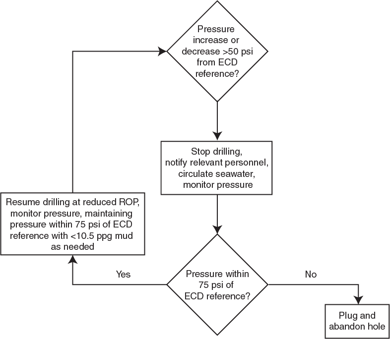
Figure F12. Safety decision tree for LWD/MWD pressure monitoring.

Analysis

Annular pressure analysis

APWD was continually measured during LWD operations for safety monitoring because the annular pressure can indicate gas entering the borehole or the presence of permeable, overpressured horizon. We also analyzed the APWD to show whether annular conditions are below (negative APWD) or above (positive APWD) hydrostatic pressure. For comparison to driller’s mud weight and riserless drilling conditions, we relate the APWD to the ECD relative to the seafloor (ECD_rsf) (in pounds per gallon or parts per gallon):

${E C D}_{r s f} = (P_{A P W D} - P_{w s f}) / [0.0519 (D_{A P W D} - D_{w} - R K B)],$

where

P_APWD = APWD sensor reading (in pounds per square inch),
P_wsf = hydrostatic pressure at seafloor (in pounds per square inch),
D_APWD = true vertical depth of the APWD sensor referenced to the rig floor (in feet),
D_w = water depth (in feet),
RKB = distance from the sea level to the rig floor (in feet), and
0.0519 = conversion factor.

Hydrostatic pressure at the seafloor (P_wsf) can be calculated by the ECD of seawater (ECD_sw) and the water depth:

$P_{w s f} = 0.0519 \times {E C D}_{s w} \times D_{w},$

where we assume an ECD_sw of 8.54 lb/gal based on an average seawater density of 1024 kg/m³.

Image analysis

Processing of geoVISION resistivity images included orientation of the image to magnetic north, accounting for the magnetic declination at each well site, and static and dynamic (window size = 2 m) normalizations. Quality control assessment of the image logs was performed on acquisition parameters including tool movement (revolutions per minute), stick and slide, tool orientation, magnetometer readings, and image artifacts where present.

Each image provided from the geoVISION tool was adjusted for orientation and depth of investigation (electrical penetration) parameters. Orientation for each image was set to north, and the orientation value was set to −3.21. This value is related to the fact that the first of the 56 circumferential bins that compose the geoVISION images are centered on the reference direction, and thus the edge of the first sector needs to be oriented a half sector counterclockwise to the reference direction (−[360/56]/2 = −3.21).

The geoVISION tool orients images using a magnetometer inside of the tool. The image is oriented by assigning one of the acquisition bins, Bin 21, to magnetic north and assigning Bin 0 as the Pad 1 North (P1NO), which is 225° from Bin 21. To correct for magnetic declination in vertical wells, the angle of declination must be added or subtracted (depending on global position) to the P1NO value (Figure F13). This correction is often already done by Schlumberger and should be checked prior to any attempt to correct for declination. If the P1NO values read anything other than 225°, it has already been adjusted.

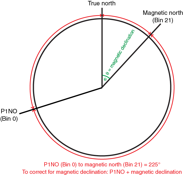
Figure F13. Image orientation to true north.

The final step to be able to accurately measure borehole feature data from geoVISION images is to assign the images with a value for the electrical penetration (referred to as depth of investigation in the Schlumberger Techlog software). Each button (shallow, medium, and deep) has a fixed electrical penetration despite having different depths of investigation. The local response of the electrical signal is the part of the signal that is used to generate the resistivity images. This response is dependent on the size of the button and the standoff, which are similar for all three buttons on the geoVISION. The electrical penetration is 1.5 inches (3.81 cm) for the geoVISION tool, which corresponds to a percentage of the integrated geometrical radial response needed to resolve a resistivity contrast on the image. See Faivre and Catala (1995) for more detail.

A brief descriptive feature classification scheme for image logs acquired during Expedition 372 was chosen to allow multiple subsequent interpretations and analyses (Trice, 1999). The image log–based classification included lithologic, structural, and stress-induced features (Figure F14; Table T10). The geometric and morphological interpretation of observed natural and stress-induced image log features can provide information on the lithology, stratigraphy, structure, and in situ stress character (Conin et al., 2014; Zoback, 2010; Massiot et al., 2015; Heidbach et al., 2016). Additionally, because gas hydrates are resistive, image logs also aid the interpretation of hydrate-bearing sediments in terms of vertical hydrate distribution, morphology with respect to the host sediments, and saturation (e.g., Cook et al., 2008; Riedel et al., 2009; Collett et al., 2012; Kim et al., 2013; Kumar et al., 2014).

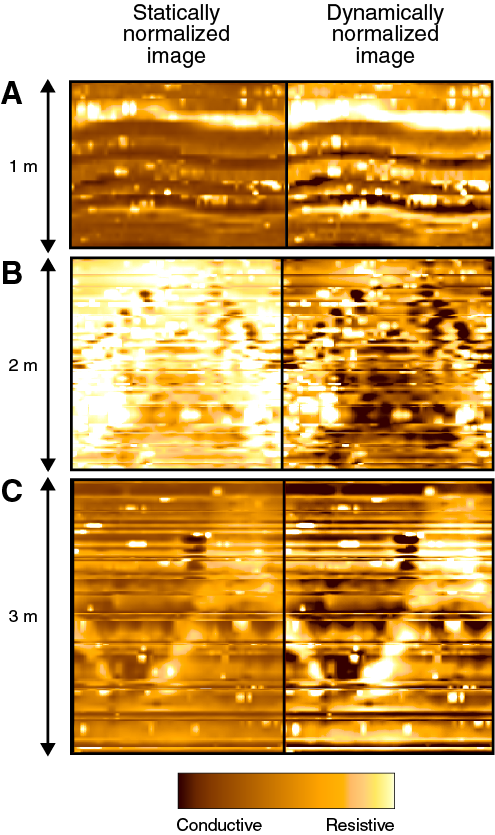
Figure F14. Resistivity images.

Gas hydrate saturation

Gas hydrate–bearing sediments have higher electrical resistivity than water-saturated sediment, meaning that downhole resistivity logs can be used to identify and assess the amount of gas hydrate present in a sedimentary section (e.g., Pearson et al., 1983; Collett and Ladd, 2000; Goldberg et al., 2010). Note that this technique is only applicable when gas hydrate occurs in the primary pore space of sand or silt.

In formations characterized by nonconductive sediment grains, it has been empirically shown that the resistivity of water-saturated sediment is proportional to the resistivity of its pore fluid (Archie, 1942):

$R_{0} = F \times R_{w},$

where

R₀ = resistivity of a water-saturated sediment,
R_w = resistivity of pore water, and
F = factor of proportionality known as the formation factor.

The formation factor is not constant and has been shown to relate to porosity through a power law relationship:

$F = ϕ^{- m},$

where ϕ is the formation porosity and m, known as the cementation exponent, is related to the tortuosity, connectivity, and the converging/diverging nature of the formation pore network. This formulation is often used to estimate water saturation:

$R_{t} = R_{0} {S_{w}}_{}^{- n},$

where

R_t = measured resistivity,
S_w = water saturation, and
n = empirical saturation exponent.

In pores containing only gas hydrate and water, the hydrate saturation (S_h) is equal to 1 − S_w. Thus, hydrate saturation can be estimated (Collett and Ladd, 2000):

S_h = 1 − [(aR_w)/(ϕ^−mR_t)]^1/n,

where a is a fitting parameter. To estimate the cementation exponent (m) from well-log data, formation resistivity data were divided by pore water resistivity and then fit as a power law function of porosity measurements. This requires a clean, water-saturated interval with nonconducting sediment grains. We assumed n over a range of 1.5–2.5, which is in line with pore-filling models (Spangenberg, 2001) and field results (Malinverno et al., 2008).

Core-log integration

At Site U1517, LWD and piston coring using the APC and HLAPC systems were undertaken to better characterize the lithologic properties and the potential occurrence and morphology of gas hydrate in the extensional region of the TLC. LWD data provide a suite of in situ measurements at high resolution but are often at lower resolution than core measurements. Therefore, comparing LWD data with measured physical properties from retrieved cores can help calibrate LWD data sets and refine measurement interpretations. Our integration of core and log data sets was divided into two main sections: physical properties and hydrate saturation estimations. Complementary measurements were compiled in Schlumberger’s Techlog.

Physical properties measurements

The following physical properties measurements were taken:

Core measurements and LWD data of NGR were compared for consistency and calibration purposes.
MAD measurements on core samples were used to check the consistency and accuracy of LWD neutron porosity and NMR porosity data.
MAD bulk density data were compared with bulk density measurements derived from neutron porosity and NMR data sets.
Limited P-wave velocity data from core samples were compared with LWD P-wave velocity data.
All data sets were compared with lithostratigraphy as interpreted from retrieved cores.

Gas hydrate saturation estimation

The following gas hydrate saturation estimates were made:

Diagnostic information from IR thermal scanning of retrieved core was used to determine spot core intervals where pore water geochemistry was analyzed for hydrate presence.
Two independent estimations of gas hydrate saturation, one derived from LWD data and one derived from core geochemistry, were compared for consistency in (1) predicted intervals of hydrate occurrence and (2) the magnitude of predicted hydrate saturation. The data sets that derived the LWD estimate (neutron porosity and ring resistivity) and the core geochemistry estimate (pore water chlorinity) are shown for comparison (see Logging while drilling; see also Geochemistry in the Site U1517 chapter [Barnes et al., 2019]).
P-wave velocity and waveform attenuation can be indicative of gas hydrate. These LWD data sets were also compared with hydrate saturation estimations.
Any discrepancies between log and core data were also compared against drilling parameters that may have affected LWD data acquisition or core recovery.

Log-seismic integration

During Expedition 372, we used information from several of the LWD data sets to establish accurate ties to the network of 2-D and 3-D multichannel seismic (MCS) reflection data (e.g., Multiwave, unpubl. data; Mountjoy et al., 2014b; Böttner et al., 2018; Gross et al., 2018).

At Site U1517, LWD data were acquired from 0 to 205 mbsf. The LWD BHA included the geoVISION, SonicScope, NeoScope, TeleScope, and proVISION tools. For details regarding techniques, refer to Logging while drilling, Lithostratigraphy, and Physical properties.

Seismic reflection data

Data acquisition along the Expedition 372 drilling transect consisted of multiple cruises that collected 2-D seismic reflection data and one that collected 3-D P-cable data. The Tuaheni site (U1517) is within the P-cable 3-D cube (Mountjoy et al., 2014a; Gross et al., 2018; Böttner et al., 2018). The 3-D seismic cube was collected during Cruise TAN1404 using a P-cable system with 15 streamers spaced at ~12.5 m. Each streamer had eight channels. The sound source was a 0.7 L (45 inch³) generator-injector (GI) gun. The 3-D data were binned onto a 3.125 m common midpoint grid, bandpass filtered (40/70–350/500 Hz), stacked and migrated with a 3-D poststack Kirchhoff time migration with a constant velocity of 1500 m/s, and corrected for spherical divergence. The resulting seismic volume is ~13.5 km long and ~5.9 km wide.

Synthetic seismograms

We constructed synthetic seismograms by convolving a source wavelet determined from seismic data with reflection coefficient models based on LWD and core measurements (see Logging while drilling and Physical properties in the Site U1517 chapter [Barnes et al., 2019]). A source wavelet is determined from the seafloor reflection along the flat region of seafloor. Seafloor reflections from five adjacent traces are stacked to yield a high signal-to-noise ratio.

Modeling of acoustic impedance and reflection coefficient is conducted using two different approaches with information from core and LWD data. In the first approach, we calculated acoustic impedance and reflection coefficients using the neutron-gamma density log from the NeoScope and the detailed velocity log from the SonicScope tool. Poor quality density and V_P values caused by borehole washout were edited. Because log measurements have high sampling rates compared with the resolution of seismic data, log data were then blocked into intervals corresponding to the frequency range of seismic data. The second approach used the interpretation of LWD and core measurements to build a log-lithostratigraphic model that highlighted major acoustic impedance at unit boundaries.

Conversion from time to depth is generally required during synthetic seismogram construction to allow for correlating the depth-based LWD logs with the traveltime-based seismic. However, for Site U1517, we constructed the synthetic seismograms in the depth domain using a MATLAB script. The wavelets were then convolved with a reflectivity series (R) expressed as the following:

$R = (v_{1} ρ_{1} - v_{2} ρ_{2}) / (v_{1} ρ_{1} + v_{2} ρ_{2}),$

where v₁ and v₂ and ρ₁ and ρ₂ are the P-wave velocity and density in the upper layer and lower layer, respectively.

A direct comparison was then made between all the available LWD and MCS reflection data using MATLAB, Paradigm’s SeisEarth, and Schlumberger’s Petrel software. This comparison enabled an overall assessment and integration of the unit boundaries and internal features determined during the analysis of each independent data set.

References

Archie, G.E., 1942. The electrical resistivity log as an aid in determining some reservoir characteristics. Transactions of the AIME, 146(1):54–62. https://doi.org/10.2118/942054-G

Arculus, R.J., Ishizuka, O., Bogus, K., Aljahdali, M.H., Bandini-Maeder, A.N., Barth, A.P., Brandl, P.A., do Monte Guerra, R., Drab, L., Gurnis, M.C., Hamada, M., Hickey-Vargas, R.L., Jiang, F., Kanayama, K., Kender, S., Kusano, Y., Li, H., Loudin, L.C., Maffione, M., Marsaglia, K.M., McCarthy, A., Meffre, S., Morris, A., Neuhaus, M., Savov, I.P., Sena Da Silva, C.A., Tepley, F.J., III, van der Land, C., Yogodzinski, G.M., and Zhang, Z., 2015. Expedition 351 methods. In Arculus, R.J., Ishizuka, O., Bogus, K., and the Expedition 351 Scientists, Izu-Bonin-Mariana Arc Origins. Proceedings of the International Ocean Discovery Program, 351: College Station, TX (International Ocean Discovery Program). https://doi.org/10.14379/iodp.proc.351.102.2015

ASTM International, 1990. Standard method for laboratory determination of water (moisture) content of soil and rock (Standard D2216–90). In Annual Book of ASTM Standards for Soil and Rock (Volume 04.08): Philadelphia (American Society for Testing Materials). [revision of D2216-63, D2216-80]

Backman, J., 1980. Miocene–Pliocene nannofossils and sedimentation rates in the Hatton-Rockall Basin, NE Atlantic Ocean. Acta Universitatis Stockholmiensis: Stockholm Contributions in Geology, 36(1):1–91.

Barnes, P.M., Pecher, I.A., LeVay, L.J., Bourlange, S.M., Brunet, M.M.Y., Cardona, S., Clennell, M.B., Cook, A.E., Crundwell, M.P., Dugan, B., Elger, J., Gamboa, D., Georgiopoulou, A., Greve, A., Han, S., Heeschen, K.U., Hu, G., Kim, G.Y., Kitajima, H., Koge, H., Li, X., Machado, K.S., McNamara, D.D., Moore, G.F., Mountjoy, J.J., Nole, M.A., Owari, S., Paganoni, M., Petronotis, K.E., Rose, P.S., Screaton, E.J., Shankar, U., Shepherd, C.L., Torres, M.E., Underwood, M.B., Wang, X., Woodhouse, A.D., and Wu, H.-Y., 2019. Site U1517. In Pecher, I.A., Barnes, P.M., LeVay, L.J., and the Expedition 372A Scientists, Creeping Gas Hydrate Slides. Proceedings of the International Ocean Discovery Program, 372A: College Station, TX (International Ocean Discovery Program). https://doi.org/10.14379/iodp.proc.372A.103.2019

Blum, P., 1997. Technical Note 26: Physical Properties Handbook—A Guide to the Shipboard Measurement of Physical Properties of Deep-Sea Cores. Ocean Drilling Program. https://doi.org/10.2973/odp.tn.26.1997

Bollmann, J., 1997. Morphology and biogeography of Gephyrocapsa coccoliths in Holocene sediments. Marine Micropaleontology, 29(3–4):319–350. https://doi.org/10.1016/S0377-8398(96)00028-X

Bonner, S.D., Tabanou, J.R., Wu, P.T., Seydoux, J.P., Moriarty, K.A., Seal, B.K., Kwok, E.Y., and Kuchenbecker, M.W., 1995. New 2-MHz multiarray borehole-compensated resistivity tool developed for MWD in slim holes [paper presented at SPE Annual Technical Conference and Exhibition, Dallas, Texas, 22–25 October 1995]. (Abstract SPE-30547-MS) https://doi.org/10.2118/30547-MS

Böttner, C., Gross, F., Geersen, J., Crutchley, G.J., Mountjoy, J.J., and Krastel, S., 2018. Marine forearc extension in the Hikurangi margin: new insights from high-resolution 3-D seismic data. Tectonics, 37(5):1472–1491. https://doi.org/10.1029/2017TC004906

Bown, P.R. (Ed.), 1998. Calcareous Nannofossil Biostratigraphy: Dordrecht, The Netherlands (Kluwer Academic Publishing).

Bown, P.R., 2005. Palaeogene calcareous microfossils from the Kilwa and Lindi areas of coastal Tanzania (Tanzania Drilling Project 2003–4). Journal of Nannoplankton Research, 27(1):21–95. http://ina.tmsoc.org/JNR/online/27/Bown 2005_ JNR27-1_TDP.pdf

Boyce, R.E., 1977. Deep Sea Drilling Project procedures for shear strength measurement of clayey sediment using modified Wykeham Farrance laboratory vane apparatus. In Barker, P.F., Dalziel, I.W.D., et al., Initial Reports of the Deep Sea Drilling Project, 36: Washington, DC (U.S. Government Printing Office), 1059–1068. https://doi.org/10.2973/dsdp.proc.36.1977

Collett, T.S., and Ladd, J., 2000. Detection of gas hydrate with downhole logs and assessment of gas hydrate concentrations (saturations) and gas volumes on the Blake Ridge with electrical resistivity log data. In Paull, C.K., Matsumoto, R., Wallace, P.J., and Dillon, W.P. (Eds.), Proceedings of the Ocean Drilling Program, Scientific Results, 164: College Station, TX (Ocean Drilling Program), 179–191. https://doi.org/10.2973/odp.proc.sr.164.219.2000

Collett, T.S., Lee, M.W., Zyrianova, M.V., Mrozewski, S.A., Guerin, G., Cook, A.E., and Goldberg, D.S., 2012. Gulf of Mexico Gas Hydrate Joint Industry Project Leg II logging-while-drilling data acquisition and analysis. Marine and Petroleum Geology, 34(1):41–61. https://doi.org/10.1016/j.marpetgeo.2011.08.003

Conin, M., Bourlange, S., Henry, P., Boiselet, A., and Gaillot, P., 2014. Distribution of resistive and conductive structures in Nankai accretionary wedge reveals contrasting stress paths. Tectonophysics, 611:181–191. https://doi.org/10.1016/j.tecto.2013.11.025

Cook, A.E., Goldberg, D., and Kleinberg, R.L., 2008. Fracture-controlled gas hydrate systems in the northern Gulf of Mexico. Marine and Petroleum Geology, 25(9):932–941. https://doi.org/10.1016/j.marpetgeo.2008.01.013

Cooper, R.A. (Ed.), 2004. The New Zealand Geological Timescale. Institute of Geological and Nuclear Sciences Monograph, 22.

Crundwell, M.P., 2004. New Zealand late Miocene biostratigraphy and biochronology: studies of planktic foraminifers and bolboforms at oceanic Sites 593 and 1123 and selected onland sections [Ph.D. thesis]. University of Waikato, New Zealand. http://odp.georef.org/vufind/Record/2009082475/Details

Crundwell, M.P., 2015a. Revised Pliocene and early Pleistocene planktonic foraminiferal biostratigraphy, DSDP Site 284, Challenger Plateau, New Zealand. GNS Science Internal Report, 2015\22.

Crundwell, M.P., 2015b. Pliocene and early Pleistocene planktic foraminifera: important taxa and bioevents in ODP Hole 1123B, Chatham Rise, New Zealand. GNS Science Report, 2015/51.

Crundwell, M.P., and Nelson, C.S., 2007. A magnetostratigraphically constrained chronology for late Miocene bolboformids and planktic foraminifers in the temperate Southwest Pacific. Stratigraphy, 4(1):1–34. http://www.micropress.org/microaccess/check/1502

Crundwell, M.P., Scott, G.H., and Thrasher, G.P., 1994. Calibration of paleobathymetry indicators by integrated seismic and paleontological analysis of forest sequences, Taranaki Basin, New Zealand. In The Post Maui Challenge: Investment and Development Opportunities. New Zealand Petroleum Conference Proceedings, 169–178.

Dunkley Jones, T., Bown, P.R., and Pearson, P.N., 2009. Exceptionally well preserved upper Eocene to lower Oligocene calcareous nannofossils (Prymnesiophycidae) from the Pande Formation (Kilwa Group), Tanzania. Journal of Systematic Palaeontology, 7(4):359–411. https://doi.org/10.1017/S1477201909990010

Ellis, D.V., and Singer, J.M., 2007. Well Logging for Earth Scientists (2nd edition): New York (Elsevier). https://doi.org/10.1007/978-1-4020-4602-5

Expedition 308 Scientists, 2006. Methods. In Flemings, P.B., Behrmann, J.H., John, C.M., and the Expedition 308 Scientists, Proceedings of the Integrated Ocean Drilling Program, 308: College Station, TX (Integrated Ocean Drilling Program Management International, Inc.). https://doi.org/10.2204/iodp.proc.308.102.2006

Expedition 311 Scientists, 2006. Methods. In Riedel, M., Collett, T.S., Malone, M.J., and the Expedition 311 Scientists, Proceedings of the Integrated Ocean Drilling Program, 311: Washington, DC (Integrated Ocean Drilling Program Management International, Inc.). https://doi.org/10.2204/iodp.proc.311.102.2006

Expedition 314 Scientists, 2009. Expedition 314 methods. In Kinoshita, M., Tobin, H., Ashi, J., Kimura, G., Lallemant, S., Screaton, E.J., Curewitz, D., Masago, H., Moe, K.T., and the Expedition 314/315/316 Scientists, Proceedings of the Integrated Ocean Drilling Program, 314/315/316: Washington, DC (Integrated Ocean Drilling Program Management International, Inc.). https://doi.org/10.2204/iodp.proc.314315316.112.2009

Expedition 332 Scientists, 2011. Methods. In Kopf, A., Araki, E., Toczko, S., and the Expedition 332 Scientists, Proceedings of the Integrated Ocean Drilling Program, 332: Tokyo (Integrated Ocean Drilling Program Management International, Inc.). https://doi.org/10.2204/iodp.proc.332.102.2011

Expedition 334 Scientists, 2012. Methods. In Vannucchi, P., Ujiie, K., Stroncik, N., Malinverno, A., and the Expedition 334 Scientists, Proceedings of the Integrated Ocean Drilling Program, 334: Tokyo (Integrated Ocean Drilling Program Management International, Inc.). https://doi.org/10.2204/iodp.proc.334.102.2012

Expedition 343/343T Scientists, 2013. Methods. In Chester, F.M., Mori, J., Eguchi, N., Toczko, S., and the Expedition 343/343T Scientists, Proceedings of the Integrated Ocean Drilling Program, 343/343T: Tokyo (Integrated Ocean Drilling Program Management International, Inc.). https://doi.org/10.2204/iodp.proc.343343T.102.2013

Faivre, O., and Catala, G., 1995. Dip estimation from azimuthal laterolog tools [paper presented at the SPWLA 36th Annual Logging Symposium, Paris, France, 26–29 June 1995]. (Abstract SPWLA-1995-CC) https://www.onepetro.org/download/conference-paper/SPWLA-1995-CC?id=conference-paper%2FSPWLA-1995-CC

Flemings, P. B., Long, H., Dugan, B., Germaine, J., John, C.M., Behrmann, J.H., Sawyer, D., and the IODP Expedition 308 Scientists, 2008. Erratum to “Pore pressure penetrometers document high overpressure near the seafloor where multiple submarine landslides have occurred on the continental slope, offshore Louisiana, Gulf of Mexico” [Earth and Planetary Science Letters 269/3–4 (2008) 309–32]. Earth and Planetary Science Letters, 274(1–2):269–283. https://doi.org/10.1016/j.epsl.2008.06.027

Flemings, P.B., Polito, P.J., Pettigrew, T.L., Iturrino, G.J., Meissner, E., Aduddell, R., Brooks, D.L., Hetmaniak, C., Huey, D., Germaine, J.T., and the IODP Expedition 342 Scientists, 2013. The Motion Decoupled Delivery System: a new deployment system for downhole tools is tested at the New Jersey Margin. Scientific Drilling, 15:51–56. https://doi.org/10.2204/iodp.sd.15.07.2013

Gieskes, J.M., Gamo, T., and Brumsack, H., 1991. Technical Note 15: Chemical Methods for Interstitial Water Analysis Aboard JOIDES Resolution. Ocean Drilling Program. https://doi.org/10.2973/odp.tn.15.1991

Goldberg, D.S., Kleinberg, R.L. Weinberger, J.L. Malinverno, A., McLellan, P.J., and Collett, T.S., 2010. Evaluation of natural gas-hydrate systems using borehole logs. In Riedel, M., Willoughby, E.C., and Chopra, S. (Eds.), Geophysical Characterization of Gas Hydrates: Tulsa, OK (Society of Exploration Geophysicists), 239–261. https://doi.org/10.1190/1.9781560802197.ch16

Gradstein, F.M., Ogg, J.G., Schmitz, M.D., and Ogg, G.M. (Eds.), 2012. The Geological Time Scale 2012: Amsterdam (Elsevier). https://doi.org/10.1016/C2011-1-08249-8

Gross, F., Mountjoy, J.J., Crutchley, G.J., Böttner, C., Koch, S., Bialas, J., Pecher, I., et al., 2018. Free gas distribution and basal shear zone development in a subaqueous landslide—insight from 3D seismic imaging of the Tuaheni Landslide Complex, New Zealand. Earth and Planetary Science Letters, 502:231–243. https://doi.org/10.1016/j.epsl.2018.09.002

Hayward, B.W., Grenfell, H.R., Reid, C.M., and Hayward, K.A., 1999. Recent New Zealand shallow-water benthic foraminifera: taxonomy, ecologic distribution, biogeography, and use in paleoenvironmental assessment. New Zealand Geological Survey Bulletin, 75.

Hayward, B.W., Grenfell, H.R., Sabaa, A.T., Neil, H.L., and Buzas, M.A., 2010. Recent New Zealand Deep-Water Benthic Foraminifera: Taxonomy, Ecologic Distribution, Biogeography, and Use in Paleoenvironmental Assessment. GNS Science Monograph, 26.

Heesemann, M., Villinger, H., Fisher, A.T., Tréhu, A.M., and White, S., 2006. Data report: testing and deployment of the new APCT-3 tool to determine in situ temperatures while piston coring. In Riedel, M., Collett, T.S., Malone, M.J., and the Expedition 311 Scientists. Proceedings of the Integrated Ocean Drilling Program, 311: Washington, DC (Integrated Ocean Drilling Program Management International, Inc.). https://doi.org/10.2204/iodp.proc.311.108.2006

Heidbach, O. (Ed.), 2016. Scientific Technical Report 16-01: WSM Quality Ranking Scheme, Database and Analysis Guidelines for Stress Indicators. With contributions by A. Barth, B. Müller, J. Reinecker, O. Stephansson, M., Tingay, and A. Zhang. WSM World Stress Map. http://www.world-stress-map.org/fileadmin/wsm/pdfs/WSM_STR_16_01.pdf

Hornibrook, N.d.B., 1981. Globorotalia (planktic Foraminiferida) in the late Pliocene and early Pleistocene of New Zealand. New Zealand Journal of Geology and Geophysics, 24(2):263–292. https://doi.org/10.1080/00288306.1981.10422717

Hornibrook, N.d.B., 1982. Late Miocene to Pleistocene Globorotalia (Foraminiferida) from DSDP Leg 29, Site 284, southwest Pacific. New Zealand Journal of Geology and Geophysics, 25(1):83–99. https://doi.org/10.1080/00288306.1982.10422507

Hornibrook, N.d.B., Brazier, R.C., and Strong, C.P., 1989. Manual of New Zealand Permian to Pleistocene foraminiferal biostratigraphy. New Zealand Geological Survey Paleontological Bulletin, 56.

Hornibrook, N.d.B., and Jenkins, D.G., 1994. DSDP 594, Chatham Rise, New Zealand—late Neogene planktonic foraminiferal biostratigraphy revisited. Journal of Micropalaeontology, 13(2):93–101. https://doi.org/10.1144/jm.13.2.93

Keenan, J.H., Keyes, F.G., Hill, P.G., and Moore, J.G., 1978. Steam Tables: Thermodynamic Properties of Water Including Vapor, Liquid, and Solid Phases: New York (John Wiley & Sons).

Kennett, J.P., and Srinivasan, M.S., 1983. Neogene Planktonic Foraminifera: A Phylogenetic Atlas: Stroudsburg, PA (Hutchinson Ross).

Kim, G.Y., Narantsetseg, B., Ryu, B.-J., Yoo, D.-G., Lee, J.Y., Kim, H.S., and Riedel, M., 2013. Fracture orientation and induced anisotropy of gas hydrate-bearing sediments in seismic chimney-like-structures of the Ulleung Basin, East Sea. Marine and Petroleum Geology, 47:182–194. https://doi.org/10.1016/j.marpetgeo.2013.06.001

Kumar, P., Collett, T.S., Boswell, R., Cochran, J.R., Lall, M., Mazumdar, A., Ramana, M.V., et al., 2014. Geologic implications of gas hydrates in the offshore of India: Krishna–Godavari Basin, Mahanadi Basin, Andaman Sea, Kerala–Konkan Basin. Marine and Petroleum Geology, 58:29–98. https://doi.org/10.1016/j.marpetgeo.2014.07.031

Kvenvolden, K.A., and McDonald, T.J., 1986. Technical Note, 6: Organic Geochemistry on the JOIDES Resolution—An Assay. Ocean Drilling Program. https://doi.org/10.2973/odp.tn.6.1986

Lourens, L., Hilgen, F., Shackleton, N.J., Laskar, J., and Wilson, D., 2004. The Neogene period. In Gradstein, F.M., Ogg, J.G., and Smith, A. (Eds.), A Geologic Time Scale 2004: Cambridge, United Kingdom (Cambridge University Press), 409–440. https://doi.org/10.1017/CBO9780511536045.022

Maiorano, P., and Marino, M., 2004. Calcareous nannofossil bioevents and environmental control on temporal and spatial patterns at the early–middle Pleistocene. Marine Micropaleontology, 53(3–4):405–422. https://doi.org/10.1016/j.marmicro.2004.08.003

Malinverno, A., Kastner, M., Torres, M.E., and Wortmann, U.G., 2008. Gas hydrate occurrence from pore water chlorinity and downhole logs in a transect across the northern Cascadia margin (Integrated Ocean Drilling Program Expedition 311). Journal of Geophysical Research: Solid Earth, 113(B8):B08103. https://doi.org/10.1029/2008JB005702

Manheim, F.T., and Sayles, F.L., 1974. Composition and origin of interstitial waters of marine sediments, based on deep sea drill cores. In Goldberg, E.D. (Ed.), The Sea (Volume 5): Marine Chemistry: The Sedimentary Cycle: New York (Wiley), 527–568.

Martini, E., 1971. Standard Tertiary and Quaternary calcareous nannoplankton zonation. In Farinacci, A. (Ed.), Proceedings of the Second Planktonic Conference, Roma 1970: Rome (Edizioni Tecnoscienza), 2:739–785.

Massiot, C., McNamara, D.D., and Lewis, B., 2015. Processing and analysis of high temperature geothermal acoustic borehole image logs in the Taupo Volcanic Zone, New Zealand. Geothermics, 53:190–201. https://doi.org/10.1016/j.geothermics.2014.05.010

McNeill, L.C., Dugan, B., Petronotis, K.E., Backman, J., Bourlange, S., Chemale, F., Chen, W., Colson, T.A., Frederik, M.C.G., Guèrin, G., Hamahashi, M., Henstock, T., House, B.M., Hüpers, A., Jeppson, T.N., Kachovich, S., Kenigsberg, A.R., Kuranaga, M., Kutterolf, S., Milliken, K.L., Mitchison, F.L., Mukoyoshi, H., Nair, N., Owari, S., Pickering, K.T., Pouderoux, H.F.A., Yehua, S., Song, I., Torres, M.E., Vannucchi, P., Vrolijk, P.J., Yang, T., and Zhao, X., 2017. Expedition 362 methods. In McNeill, L.C., Dugan, B., Petronotis, K.E., and the Expedition 362 Scientists, Sumatra Subduction Zone. Proceedings of the International Ocean Discovery Program, 362: College Station, TX (International Ocean Discovery Program). https://doi.org/10.14379/iodp.proc.362.102.2017

Mountjoy, J., Krastel, S., Crutchley, G., Dannonski, A., Graw, M., Koch, S., Micallef, A., Quinn, W., and Woelz, S., 2014a. NIWA Voyage Report TAN1404: SCHLIP-3D: submarine clathrate hydrate landslide imaging project: Auckland, New Zealand (National Institute of Water and Atmospheric Research).

Mountjoy, J.J., Pecher, I., Henrys, S., Crutchley, G., Barnes, P.M., and Plaza-Faverola, A., 2014b. Shallow methane hydrate system controls ongoing, downslope sediment transport in a low-velocity active submarine landslide complex, Hikurangi Margin, New Zealand. Geochemistry, Geophysics, Geosystems, 15(11):4137–4156. https://doi.org/10.1002/2014GC005379

Okada, H., and Bukry, D., 1980. Supplementary modification and introduction of code numbers to the low-latitude coccolith biostratigraphic zonation (Bukry, 1973; 1975). Marine Micropaleontology, 5:321–325. https://doi.org/10.1016/0377-8398(80)90016-X

Pearson, C.F., Halleck, P.M., McGuire, P.L., Hermes, R., and Mathews, M., 1983. Natural gas hydrate deposits: a review of in situ properties. Journal of Physical Chemistry, 87(21):4180–4185. https://doi.org/10.1021/j100244a041

Pecher, I.A., Barnes, P.M., LeVay, L.J., and the Expedition 372A Scientists, 2019. Supplementary material, https://doi.org/10.14379/iodp.proc.372Asupp.2019. Supplement to Pecher, I.A., Barnes, P.M., LeVay, L.J., and the Expedition 372A Scientists, Creeping Gas Hydrate Slides. Proceedings of the International Ocean Discovery Program, 372A: College Station, TX (International Ocean Discovery Program). https://doi.org/10.14379/iodp.proc.372A.2019

Perch-Nielsen, K., 1985. Cenozoic calcareous nannofossils. In Bolli, H.M., Saunders, J.B., and Perch-Nielsen, K. (Eds.), Plankton Stratigraphy: Cambridge, United Kingdom (Cambridge University Press), 427–554.

Pimmel, A., and Claypool, G., 2001. Technical Note 30: Introduction to Shipboard Organic Geochemistry on the JOIDES Resolution. Ocean Drilling Program. https://doi.org/10.2973/odp.tn.30.2001

Raffi, I., Backman, J., Fornaciari, E., Pälike, H., Rio, D., Lourens, L., and Hilgen, F., 2006. A review of calcareous nannofossil astrobiochronology encompassing the past 25 million years. Quaternary Science Reviews, 25(23–24):3113–3137. https://doi.org/10.1016/j.quascirev.2006.07.007

Raine, J.I., Beu, A.G., Boyes, A., Campbell, H.J., Cooper, R.A., Crampton, J.S., Crundwell, M.P., Hollis, C.J., and Morgans, H.E., 2015. A revised calibration of the New Zealand Geological Timescale: NZGT2015 [paper presented at International Conference and Exhibition, Melbourne, Australia, 13–16 September 2015]. https://doi.org/10.1190/ice2015-2211449

Riedel, M., Collett, T., Malone, M.J., and IODP Expedition 311 Scientists, 2009. Gas hydrate drilling transect across northern Cascadia margin—IODP Expedition 311. Geological Society Special Publication, 319:11–19. https://doi.org/10.1144/SP319.2

Samtleben, C., 1980. Die Evolution der Coccolithophoriden-Gattung Gephyrocapsa nach Befunden im Atlantik. Paläontologische Zeitschrift, 54(1–2):91–127. https://doi.org/10.1007/BF02985885

Scott, G.H., Bishop, S., and Burt, B.J., 1990. Guide to some Neogene Globotalids (Foraminiferida) from New Zealand. New Zealand Geological Survey Paleontological Bulletin, 61:1–135.

Shamrock, J.L., and Watkins, D.K., 2012. Eocene calcareous nannofossil biostratigraphy and community structure from Exmouth Plateau, Eastern Indian Ocean (ODP Site 762). Stratigraphy, 9(1):1–54. http://www.micropress.org/microaccess/stratigraphy/issue-292/article-1783

Spangenberg, E., 2001. Modeling of the influence of gas hydrate content on the electrical properties of porous sediments. Journal of Geophysical Research: Solid Earth, 106(B4):6535–6548. https://doi.org/10.1029/2000JB900434

Stow, D.A.V., 2005. Sedimentary Rocks in the Field: A Colour Guide: London (Manson Publishing)

Strasser, M., Dugan, B., Kanagawa, K., Moore, G.F., Toczko, S., Maeda, L., Kido, Y., Moe, K.T., Sanada, Y., Esteban, L., Fabbri, O., Geersen, J., Hammerschmidt, S., Hayashi, H., Heirman, K., Hüpers, A., Jurado Rodriguez, M.J., Kameo, K., Kanamatsu, T., Kitajima, H., Masuda, H., Milliken, K., Mishra, R., Motoyama, I., Olcott, K., Oohashi, K., Pickering, K.T., Ramirez, S.G., Rashid, H., Sawyer, D., Schleicher, A., Shan, Y., Skarbek, R., Song, I., Takeshita, T., Toki, T., Tudge, J., Webb, S., Wilson, D.J., Wu, H.-Y., and Yamaguchi, A., 2014. Methods. In Strasser, M., Dugan, B., Kanagawa, K., Moore, G.F., Toczko, S., Maeda, L., and the Expedition 338 Scientists, Proceedings of the Integrated Ocean Drilling Program, 338: Yokohama, Japan (Integrated Ocean Drilling Program). https://doi.org/10.2204/iodp.proc.338.102.2014

Su, X., 1996. Development of late Tertiary and Quaternary coccolith assemblages in the northeast Atlantic. GEOMAR Report, 48. https://doi.org/10.3289/GEOMAR_Report_48_1996

Thébault, E., Finlay, C.C., Beggan, C.D., Alken, P., Aubert, J., Barrois, O., Bertrand, F., et al., 2015. International Geomagnetic Reference Field: the 12th generation. Earth, Planets and Space, 67:79. https://doi.org/10.1186/s40623-015-0228-9

Trice, R., 1999. A methodology for applying a non unique, morphological classification to sine wave events picked from borehole image log data. In Lovell, M., Williamson, G., and Harvey, P. (Eds.), Borehole Imaging: Applications and Case Histories. Geological Society Special Publication, 159:77–90. https://doi.org/10.1144/GSL.SP.1999.159.01.04

Vasiliev, M.A., Blum, P., Chubarian, G., Olsen, R., Bennight, C., Cobine, T., Fackler, D., Hastedt, M., Houpt, D., Mateo, Z., and Vasilieva, Y.B., 2011. A new natural gamma radiation measurement system for marine sediment and rock analysis. Journal of Applied Geophysics, 75:455–463. https://doi.org/10.1016/j.jappgeo.2011.08.008

Von Herzen, R., and Maxwell, A.E., 1959. The measurement of thermal conductivity of deep-sea sediments by a needle-probe method. Journal of Geophysical Research, 64(10):1557–1563. https://doi.org/10.1029/JZ064i010p01557

Wallace, L.M., Saffer, D.M., Barnes, P.M., Pecher, I.A., Petronotis, K.E., LeVay, L.J., Bell, R.E., Crundwell, M.P., Engelmann de Oliveira, C.H., Fagereng, A., Fulton, P.M., Greve, A., Harris, R.N., Hashimoto, Y., Hüpers, A., Ikari, M.J., Ito, Y., Kitajima, H., Kutterolf, S., Lee, H., Li, X., Luo, M., Malie, P.R., Meneghini, F., Morgan, J.K., Noda, A., Rabinowitz, H.S., Savage, H.M., Shepherd, C.L., Shreedharan, S., Solomon, E.A., Underwood, M.B., Wang, M., Woodhouse, A.D., Bourlange, S.M., Brunet, M.M.Y., Cardona, S., Clennell, M.B., Cook, A.E., Dugan, B., Elger, J., Gamboa, D., Georgiopoulou, A., Han, S., Heeschen, K.U., Hu, G., Kim, G.Y., Koge, H., Machado, K.S., McNamara, D.D., Moore, G.F., Mountjoy, J.J., Nole, M.A., Owari, S., Paganoni, M., Rose, P.S., Screaton, E.J., Shankar, U., Torres, M.E., Wang, X., and Wu, H.-Y., 2019. Expedition 372B/375 methods. In Wallace, L.M., Saffer, D.M., Barnes, P.M., Pecher, I.A., Petronotis, K.E., LeVay, L.J., and the Expedition 372/375 Scientists, Hikurangi Subduction Margin Coring, Logging, and Observatories. Proceedings of the International Ocean Discovery Program, 372B/375: College Station, TX (International Ocean Discovery Program). https://doi.org/10.14379/iodp.proc.372B375.102.2019

Wentworth, C.K., 1922. A scale of grade and class terms for clastic sediments. Journal of Geology, 30(5):377–392. https://doi.org/10.1086/622910

Young, J.R., 1998. Neogene. In Bown, P.R. (Ed.), Calcareous Nannofossil Biostratigraphy: Dordrecht, The Netherlands (Kluwer Academic Publishing), 225–265.

Zijderveld, J.D.A., 1967. AC demagnetization of rocks: analysis of results. In Collinson, D.W., Creer, K.M., and Runcorn, S.K. (Eds.), Developments in Solid Earth Geophysics (Volume 3): Methods in Palaeomagnetism: Amsterdam (Elsevier), 254–286. https://doi.org/10.1016/B978-1-4832-2894-5.50049-5

Zoback, M.D., 2010. Reservoir Geomechanics: Cambridge, United Kingdom (Cambridge University Press).

Zoth, G., and Haenel, R., 1988. Appendix. In Haenel, R., Rybach, L., and Stegena, L. (Eds.), Solid Earth Sciences Library (Volume 4): Handbook of Terrestrial Heat-Flow Density Determination: Dordrecht, The Netherlands (Kluwer Academic Publishers), 449–468. https://doi.org/10.1007/978-94-009-2847-3_10

¹Pecher, I.A., Barnes, P.M., LeVay, L.J., Bourlange, S.M., Brunet, M.M.Y., Cardona, S., Clennell, M.B., Cook, A.E., Crundwell, M.P., Dugan, B., Elger, J., Gamboa, D., Georgiopoulou, A., Greve, A., Han, S., Heeschen, K.U., Hu, G., Kim, G.Y., Kitajima, H., Koge, H., Li, X., Machado, K.S., McNamara, D.D., Moore, G.F., Mountjoy, J.J., Nole, M.A., Owari, S., Paganoni, M., Petronotis, K.E., Rose, P.S., Screaton, E.J., Shankar, U., Shepherd, C.L., Torres, M.E., Underwood, M.B., Wang, X., Woodhouse, A.D., and Wu, H.-Y., 2019. Expedition 372A methods. In Pecher, I.A., Barnes, P.M., LeVay, L.J., and the Expedition 372A Scientists, Creeping Gas Hydrate Slides. Proceedings of the International Ocean Discovery Program, 372A: College Station, TX (International Ocean Discovery Program). https://doi.org/10.14379/iodp.proc.372A.102.2019

²Expedition 372A Scientists’ affiliations.

This work is distributed under the Creative Commons Attribution 4.0 International (CC BY 4.0) license.

PDF Download figures Download tables Cited by

Figures

Tables

Expedition 372A methods1

Introduction

Authorship of the site chapters

Site location

Coring and drilling operations

Drilling disturbance

Core handling and curatorial procedures

Shipboard core analysis

Sample depth calculations

Lithostratigraphy

Core preparation for description

Visual core descriptions

Graphic lithology

Lithologic features

Drilling disturbance

Smear slides

X-ray diffraction

Biostratigraphy

Calcareous nannofossils

Methods

Foraminifers

Methods

Planktonic foraminifers

Benthic foraminifers

Paleomagnetism

Coordinate convention and core reorientation

Geochemistry

Pore fluid sampling protocol

Pore fluid collection

Gas hydrate samples

Shipboard pore fluid analyses

Salinity, alkalinity, and pH

Chloride, sulfate, and bromide

Ammonium, phosphate, and silica

Major and minor elements by ICP-AES

Major elements by ion chromatography

Preference for multiple data sets

Fluid organic geochemistry

Sediment geochemistry

Physical properties

Whole-Round Multisensor Logger measurements

Gamma ray attenuation bulk density

Magnetic susceptibility

Compressional wave velocity

Natural Gamma Radiation Logger

Section Half Multisensor Logger measurements

Color reflectance spectrometry

Point magnetic susceptibility

Thermal conductivity

Moisture and density

Discrete compressional wave velocity

Shear strength

Downhole measurements

In situ pressure and temperature measurements

Advanced piston corer temperature tool

Temperature dual pressure probe

Sediment temperature pressure tool

Logging while drilling

LWD tools

geoVISION

SonicScope

NeoScope

TeleScope

proVISION Plus

Tool activation

Safety monitoring

Pressure monitoring

Analysis

Annular pressure analysis

Image analysis

Gas hydrate saturation

Core-log integration

Physical properties measurements

Gas hydrate saturation estimation

Log-seismic integration

Seismic reflection data

Synthetic seismograms

References

Expedition 372A methods¹