Pecher, I.A., Barnes, P.M., LeVay, L.J., and the Expedition 372A Scientists
Proceedings of the International Ocean Discovery Program Volume 372A
publications.iodp.org

https://doi.org/10.14379/iodp.proc.372A.103.2019
Site U15171
P.M. Barnes, I.A. Pecher, L.J. LeVay, S.M. Bourlange, M.M.Y. Brunet, S. Cardona, M.B. Clennell, A.E. Cook, M.P. Crundwell, B. Dugan, J. Elger, D. Gamboa, A. Georgiopoulou, A. Greve, S. Han, K.U. Heeschen, G. Hu, G.Y. Kim, H. Kitajima, H. Koge, X. Li, K.S. Machado, D.D. McNamara, G.F. Moore, J.J. Mountjoy, M.A. Nole, S. Owari, M. Paganoni, K.E. Petronotis, P.S. Rose, E.J. Screaton, U. Shankar, C.L. Shepherd, M.E. Torres, M.B. Underwood, X. Wang, A.D. Woodhouse, and H.-Y. Wu2
Keywords: International Ocean Discovery Program, IODP, JOIDES Resolution, Expedition 372, Site U1517, Hikurangi margin, Tuaheni Landslide Complex, Tuaheni Basin, New Zealand, gas hydrates, slope stability, fluid flow, mass transport deposits, logging while drilling
MS 372A-103: Published 5 May 2019
Background and objectives
International Ocean Discovery Program (IODP) Site U1517 (proposed Site TLC-04B) is located at 38°49.772′S, 178°28.557′E in the extensional, creeping part of the Tuaheni Landslide Complex (TLC) (Figure F1; see Figure F2 in the Expedition 372A summary chapter [Barnes et al., 2019a]) (Mountjoy et al., 2014b). Hole U1517A was drilled in a water depth of 725 meters below sea level (mbsl); Holes U1517B and U1517C lie at 720 mbsl. The primary drilling objective was to log and sample through the landslide mass and the gas hydrate stability zone to understand the mechanisms behind creeping. Therefore, we planned to log the sediment column to 205 meters below seafloor (mbsf) using logging-while-drilling (LWD) tools, followed by advanced piston corer (APC) coring, pressure coring, and temperature dual pressure probe (T2P) deployments.
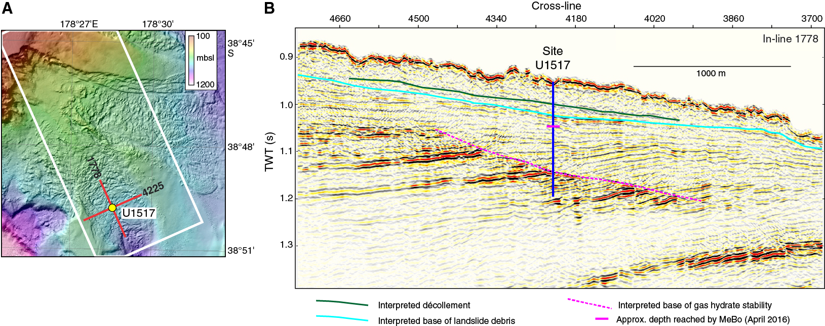
Figure F1. Bathymetry and IL1778 seismic section.
Predrilling interpretation was based largely on high-resolution 3-D seismic site survey data collected in 2014 (Mountjoy et al., 2014a) (Figure F1). These data show that, in general, the transition from a compressional to an extensional (creeping) regime coincides with the predicted landward edge of the gas hydrate stability zone. The 3-D seismic cube also provided detailed images of the structure of the TLC, particularly a horizon in the debris mass that is interpreted to mark the décollement for the slowly deforming part of the TLC.
The 3-D seismic volume was acquired with streamers that were too short for seismic velocity analysis; therefore, velocity values were constrained from multichannel seismic Line 05CM-02 across the northeastern part of the 3-D cube and from sparsely spaced ocean-bottom seismometers (MacMahon, 2016; Wild, 2016). A subseafloor velocity of 1700 m/s was determined for converting two-way traveltime (TWT) to depth. Prior to drilling, we interpreted the following at Site U1517 (Figures F1, F2) (see Gross et al., 2018):
- A possible décollement for creeping at 0.043 s TWT (37 mbsf),
- The base of the debris mass at 0.069 s TWT (59 mbsf), and
- The base of gas hydrate stability (BGHS) at 0.190 s TWT (162 mbsf).
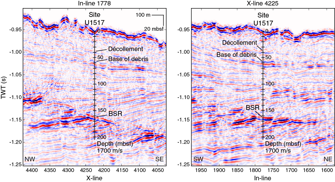
Figure F2. Seismic in-lines and cross-lines.
The BGHS is mostly defined by the termination of high-amplitude reflections, although bottom-simulating reflectors (BSRs) appear in patches along this level (Figure F2).
Site U1517 was previously drilled to 80 mbsf with the Meeresboden-Bohrgerät 200 (MeBo) system during R/V Sonne Voyage SO-247 (Site GeoB20831) (Huhn, 2016). Clayey silt landslide debris was recovered between 0 and 28 mbsf. Recovery was poor between 28 and 60 mbsf, yielding disturbed very fine sandy coarse silt in sections as long as 1.5 m (per 3.5 m stroke length). In this interval, the cores were highly disturbed by the drilling process and mixed with seawater, which precluded any inferences on the presence of gas hydrate that may aid in elucidating its role in the creeping behavior of the TLC. Stiff clayey silt was sampled from 60 to 78.8 mbsf in the bedded sedimentary sequence underlying the landslide complex with good core recovery.
Site-specific objectives included the following:
- Obtaining lithologic information in the creeping slides, particularly material across the interpreted creeping décollement and the lower part of the landslide debris.
- Collecting samples for shore-based laboratory studies. Potential laboratory studies include long-term deformation tests on gas hydrate–bearing sediments and geotechnical investigations of hydrate-bearing and hydrate-free sediments.
- Constraining in situ gas hydrate saturation and composition to better understand the local gas hydrate system and to calibrate seismic data. This study includes the identification of possible fluid sources and chemical disequilibria.
- Obtaining pore pressure and temperature profiles to investigate possible overpressure and search for evidence of nonsteady-state fluid and heat flux.
- Identifying fractures and determining whether fracture patterns change across the BGHS or in the slide mass.
- Calibrating seismic data. Beyond stratigraphic tie-ins, calibration of both 3-D and long-offset 2-D seismic data will improve constraints for extending profiles of gas hydrate saturation and pore pressure away from the borehole.
Refer to the Expedition 372A summary chapter (Barnes et al., 2019a) for more details on the scientific background and objectives for drilling the TLC.
Operations
Fremantle port call
Expedition 372 began at 0742 h (UTC + 8 h) on 26 November 2017 with the first line ashore at Victoria Quay in Fremantle, Australia. To comply with the New Zealand ship biofouling regulations, the ship scheduled a 2 day hull cleaning operation at anchorage outside of Fremantle. The vessel departed Victoria Quay on 1 December. After a 10 nmi transit, the ship arrived at the ORAN1 anchorage near Garden Island. Hull cleaning concluded on 3 December, and the vessel began the sea passage to Site U1517 at 1830 h.
Transit to Site U1517
After a 3419 nmi transit, the ship arrived at Site U1517 at 0200 h (UTC + 13 h) on 16 December 2017. The voyage took ~12 days (291.9 h) at an average of 11.7 kt.
Site U1517
Site U1517 consisted of four holes ranging in depth from 9.4 to 205.0 mbsf (Table T1). Operations at Site U1517 included LWD, piston coring, and formation pressure and temperature measurements. In total, 37 cores were recovered at Site U1517.
LWD operations with continuous safety monitoring advanced to 205 mbsf in Hole U1517A. A total of 186.84 m of core over a 197.9 m interval was recovered from Holes U1517B and U1517C using the APC and half-length APC (HLAPC) systems (94% core recovery). Hole U1517D was drilled to 168.7 mbsf with probe deployments at four locations. The total time spent on site was 5.1 days.
Hole U1517A
Once the vessel arrived on site, the thrusters were lowered, and the ship moved to the site coordinates at 0247 h on 16 December 2017. The APC/extended core barrel (XCB) bottom-hole assembly (BHA) was put together in preparation for coring in Hole U1517B. The LWD BHA was assembled and contained the geoVISION, SonicScope, NeoScope, TeleScope, and proVISION tools. For more information on the Schlumberger logging tools, see Logging while drilling in the Expedition 372A methods chapter (Pecher et al., 2019a).
The precision depth recorder placed the seafloor at 722.5 mbsl, and the BHA was lowered to 672 mbsl for flow and pressure testing of the LWD tools to determine the flow rates at which the tools activate; all turbine-powered tools activated during the pump test. The subsea video camera was deployed to observe the drill bit tag the seafloor, which occurred at 1755 h. The seafloor depth for Hole U1517A was 725.4 mbsl. The camera system was retrieved, and drilling in Hole U1517A commenced at 1935 h on 16 December. The bit advanced at an average rate of 20 m/h. LWD in Hole U1517A continued through 17 December, reaching the total depth of 205 mbsf at 1115 h. After a 30 bbl mud sweep, the drill pipe and LWD BHA were pulled from the hole while the logging tools continued to record sonic measurements. The bit cleared the seafloor at 1245 h and the rotary table at 1840 h on 17 December, ending Hole U1517A.
Hole U1517B
The vessel was offset 20 m southeast (heading of 155°) for coring operations in Hole U1517B. The assembled APC/XCB BHA was run to 704 mbsl. The bit was spaced out, and the first core was shot at 720 mbsl. Hole U1517B was spudded at 0130 h on 18 December 2017, and Core 372-U1517B-1H recovered 9.4 m of sediment. The mudline in this core could not be identified with certainty, and the decision was made to abandon Hole U1517B and attempt to recover a mudline core at the same hole location.
Hole U1517C
The bit was raised 4 m, and coring in Hole U1517C began at 0210 h on 18 December 2017. APC Cores 372-U1517C-1H and 2H were drilled to 15.2 mbsf before switching to the HLAPC system to recover a silt-rich interval. Cores 3F–14F (15.2–71.6 mbsf) were taken before switching back to the APC system for Cores 15H–18H (71.6–108.3 mbsf), all of which had partial strokes and were advanced by recovery. The HLAPC system was redeployed for Cores 19F–36F (108.3–188.5 mbsf). Of these, Cores 19F, 20F, 22F, 23F, 25F–28F, and 30F–36F recorded partial strokes and were advanced by recovery, except for Cores 34F–36F, which were advanced by 4.7 m. All of the APC cores were oriented using either the FlexIT tool (Cores 1H and 2H) or the Icefield MI-5 core orientation tool (Cores 15H–18H). The advanced piston corer temperature tool (APCT-3) was run on Cores 15H, 17H, 20F, 23F, 26F, 29F, and 34F. A total of 177.44 m of core was recovered from the 188.5 m interval (94% recovery). Six APC cores were taken over a 51.9 m interval with 52.66 m recovered (101% recovery). Thirty HLAPC cores were taken over a total interval of 136.6 m with 124.78 m recovered (91% recovery).
After reaching the total depth of 188.5 mbsf, the drill pipe was pulled out of the hole. The bit cleared the seafloor at 1015 h on 19 December and the rotary table at 1220 h, ending Hole U1517C. The ship was secured for the 20 nmi transit to Site U1518 (Saffer et al., 2019) at 1310 h on 19 December.
Hole U1517D
The vessel returned to Site U1517 at 2300 h on 31 December 2017 following a 32 nmi transit from Site U1520 (Barnes et al., 2019b). The BHA was made up, and the drill string was assembled in preparation for formation temperature and pressure measurements. Hole U1517D was spudded at 0720 h on 1 January 2018 and was drilled to 80 mbsf. The center bit was retrieved, and the Motion Decoupled Hydraulic Delivery System and T2P were deployed to measure in situ formation pressure and temperature. The shear pins failed to shear on the first attempt, and a second attempt was made ~1 h later. This time, the shear pins sheared and the T2P was inserted into the sediment. The tool could not be recovered using the Electronic Release System (ERS) on the Schlumberger wireline and had to be picked up using the coring winch. Upon retrieval, it was noted that the T2P tip was damaged, having lost the thermistor in the tip; however, it did record a good pressure measurement. The center bit was installed, and the hole was drilled to 120 mbsf. After the center bit was retrieved, a second T2P was deployed. After sitting in the formation for ~45 min, the ERS again could not retrieve the tool, and the core winch was used. Upon recovery to the rig floor, it was noted that the second T2P was also damaged; this time, the T2P was missing the entire tapered probe tip and the electronics had been flooded. This damage likely occurred during tool recovery. The hole was drilled to 130 mbsf, and the sediment temperature pressure tool (SETP) was deployed using the colleted delivery system. The hole was drilled to a total depth of 168.7 mbsf, and a final SETP measurement was made. The drill string was pulled from the hole, and the bit cleared the seafloor at 1030 h and the rotary table at 1315 h. The ship was secured for transit, and Site U1517 ended at 1536 h on 2 January when the ship began the transit to Lyttelton, New Zealand.
Transit to Lyttelton
The 404 nmi transit to Lyttelton, New Zealand, began at 1536 h (UTC + 13 h) on 2 January 2018 after completing operations in Hole U1517D. The vessel reached the pilot station at 0600 h on 4 January 2018, and Expedition 372 ended with the first line ashore at 0706 h in Lyttelton.
Lithostratigraphy
The dominant sediment from Hole U1517C is clayey silt to silty clay with sandy interbeds (Figure F3). It is primarily a bedded sequence comprising alternating graded beds and structureless clayey silt. Magnetic susceptibility background values are <200 × 10−5 SI, and peak values correlate well with the presence of relatively coarser grained (fine sand) material (Figures F4, F5). Magnetic susceptibility varies downsection but averages ~14 × 10−5 SI. We see an inverse correlation with red-green-blue (RGB) color, where low RGB indicates darker sand layers that have a higher magnetic signature.
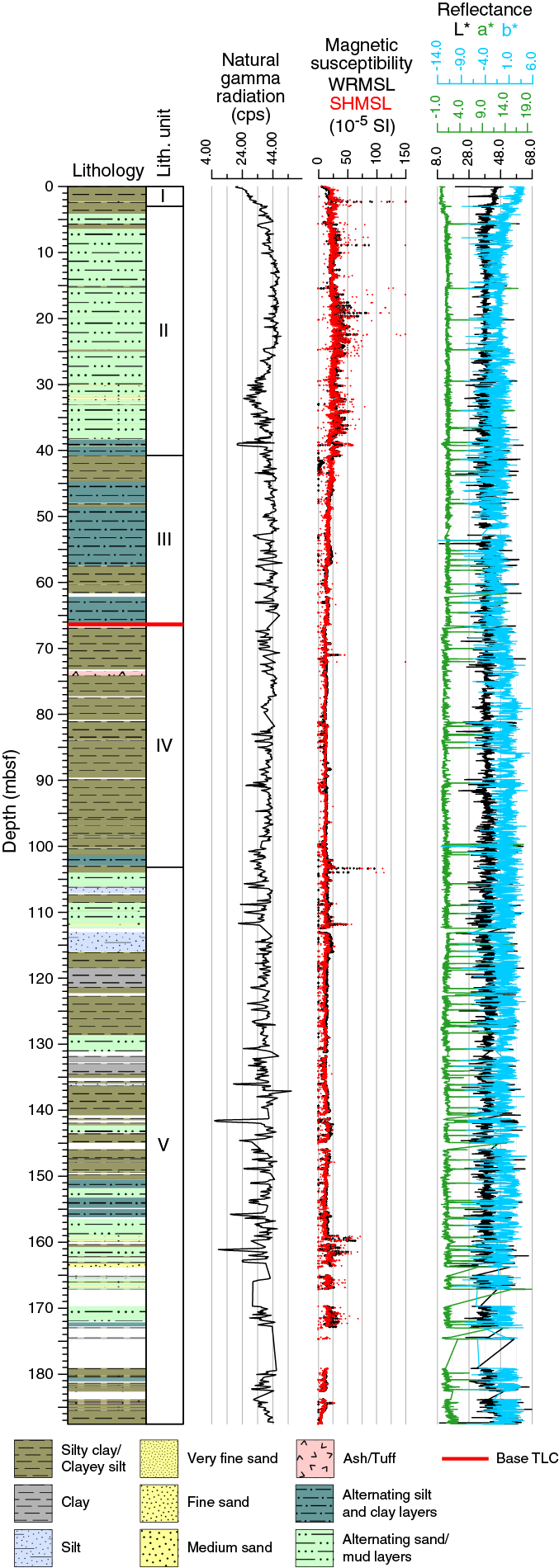
Figure F3. Composite lithology log.

Figure F4. RGB and point magnetic susceptibility.
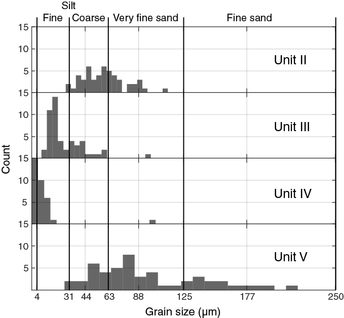
Figure F5. Grain size distribution.
We recognize five lithostratigraphic units in Hole U1517C (Table T2; Figure F3). Definition of these units is based on visual core descriptions and smear slide analysis, as well as RGB color and magnetic susceptibility logs. The unit boundaries and their primary characteristics are listed in Table T2. Visual estimates from smear slides show an overall decrease in grain size from Unit I to Unit IV, whereas Unit V includes a broad distribution of material size. Textural averages for Units II–V plot in distinctly different regions on a ternary diagram of grain size (Figure F6).
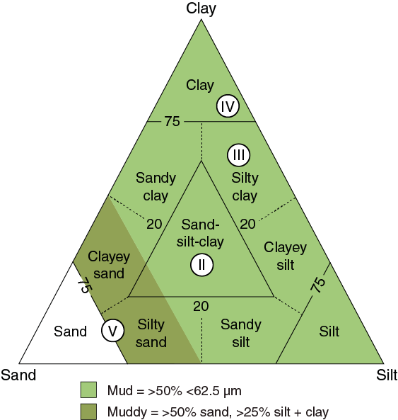
Figure F6. Visual estimates of average grain size.
The coring process occasionally affected material recovered from this hole in several ways that are important to recognize before deciphering sediment structure information (Figure F7). Most beds experienced “bed drag” (referred to as “upward-arching bed contacts” in DESClogik) resulting from liner friction overcoming the strength of the sediment and deforming bedding as it penetrates the sediment. Figure F7A shows one of the few examples of undeformed beds from Hole U1517C, and Figure F7B shows bed deformation dragging contacts as far as 4 cm downcore. From Core 372-U1517C-5F downhole (~25 mbsf), core fracturing occurred on the catwalk, likely caused by gas depressurization that forced the sediment apart in the liner. Fractures as long as 5 cm (“disking”) developed during degassing; the location where this deformation occurred and the magnitude of expansion were not recorded. Material was then pushed together with a wooden plunger to recreate a continuous sediment core, which often resulted in a void in the core that does not necessarily indicate lost material (Figure F7C). The disking from gas expansion can significantly disrupt sediment structures. The uppermost 20–50 cm of the first section from each core can be highly deformed, and little useful information can be gained from some of these intervals because the lithology and sedimentary structures are mixed beyond recognition (Figure F7D). Fluidization of sand may result in sand from above the coring interval flowing into the base of the hole (Figure F7E). Some midcore deformation at the base of cores resulted in apparent vertical sedimentary structures and lithologic mixing (Figure F7F, F7G).
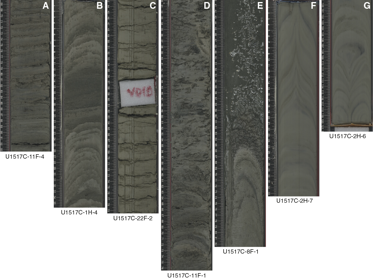
Figure F7. Drilling-related disturbance.
Lithostratigraphic Unit I
Unit I is a 3 m thick sequence that comprises greenish gray (GLEY 1 5/10Y) silty clay with no primary sedimentary structures (Figure F8). The unit is devoid of bioturbation and contains some scattered shell fragments. The magnetic susceptibility log shows low values with one peak (194 × 10−5 SI) that correlates with volcaniclastic fine sand in interval 372-U1517C-1H-1, 72 cm. The base of the unit is defined at the top of a sandy bed that marks the transition into sandier graded beds below (Figure F8).
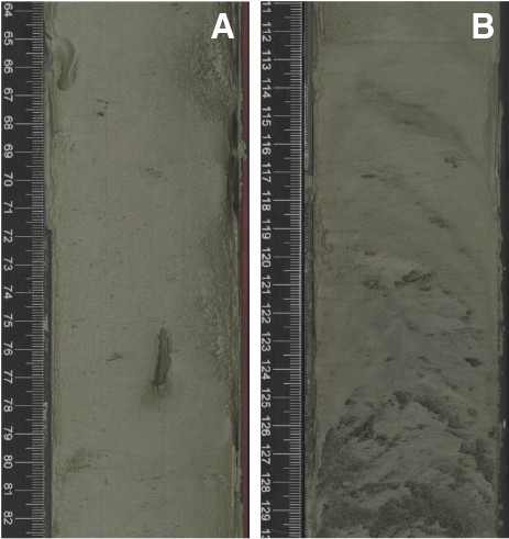
Figure F8. Lithostratigraphic Unit I.
Foraminifers indicate Unit I is Holocene in age (see Biostratigraphy).
Lithostratigraphic Unit II
The major lithologies in Unit II are alternating mud (clayey silt to silty clay) and very fine greenish gray sand (GLEY 1 5/10Y). Subtle grain size variations may be present. The strata are very thinly to thinly bedded with scattered medium-thickness sand beds (as thick as 29 cm). No primary sedimentary structures were observed in the clayey silt apart from color banding. The most common evidence of bioturbation is diffuse, millimeter-scale dark sulfide mottling and color banding that disappeared soon after splitting, leaving grains with a rusty hue around them. No distinct ichnofossils were observed. Unit II is characterized by strong variations in magnetic susceptibility values that reflect the alternating sand/mud layers (Figure F3).
Representative smear slide observations from a sandy interval in Unit II are illustrated by photomicrographs in Figure F9, where we estimate the grain size proportion to be 35% sand, 35% silt, and 30% clay. The very fine sand– to silt-sized portion is dominated by monocrystalline and polycrystalline detrital quartz grains, lithic fragments, and nonskeletal carbonate grains. Quartz grains are subrounded to rounded, whereas carbonate grains are angular to very angular. Foraminifer tests and glauconite grains are minor components.

Figure F9. Representative photomicrographs, Unit II.
Drilling-induced disturbances, such as fall-in and flow textures, were observed near the top portion of several cores. Despite these disturbances, the original bedding and characteristics are mostly preserved. The basal contacts of the sand beds are sharp and vary from irregular to very irregular. The thin-bedded sands appear graded, whereas the medium-bedded sands appear massive but grade upward into clayey silt over a 1–2 cm interval. Some of the sand beds also show sharp top contacts or grain size breaks before they grade into the clayey silt. The top contacts, both sharp and graded, are also irregular in places (Figures F10B, F11). Most beds show upward-arching contacts due to drilling disturbance, but the bases of the sand beds ≥2 cm thick tend to remain horizontal to subhorizontal with no arching (Figure F7B).
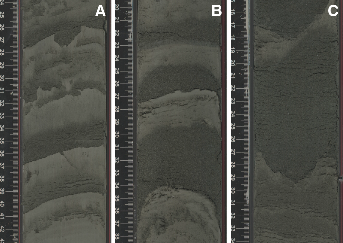
Figure F10. Lithostratigraphic Unit II.
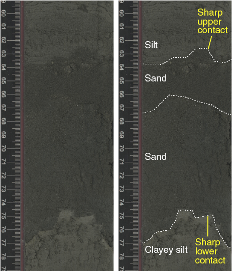
Figure F11. Amalgamated sand beds.
Thinner sand beds in Unit II are commonly truncated or broken into segments (Figure F10A). A few sand-filled subvertical fractures were observed, particularly in Core 372-U1517C-2H. Small-scale subvertical microfaults and contorted beds are present at several depth intervals and record syn- or postdepositional instability of the sedimentary sequence. The distribution of these features is summarized in Table T3.
Foraminifers indicate Unit II is Late Pleistocene in age (see Biostratigraphy).
Preliminary interpretation
Unit II is interpreted to be a succession of stacked turbidites. Highly irregular basal contacts are not unusual for turbidite beds and could represent erosion of the underlying substrate during emplacement. However, many of the irregular basal contacts appear unusually rugged and angular and in some cases have a “staircase” geometry. This geometry may reflect postemplacement deformation related to landslide processes or earthquakes. The sharp top contacts and grain size breaks could be attributed to bottom current thieving of the turbidity current tail; however, they appear highly irregular in places (Figure F11), even where graded (Figure F10C). In contrast, we did not see inverse grading or erosional top contacts that might have indicated parts of the sequence were inverted and incorporated into a debris flow. Bulk density is unexpectedly high and porosity is unusually low for a sedimentary sequence at shallow burial depths (see Physical properties). On the basis of the above evidence, two hypotheses are considered: Unit II is either part of the TLC deposits or an in situ but locally deformed sequence.
Lithostratigraphic Unit III
The major lithologies in Unit III are massive clayey silt to silty clay and alternating layers of dark greenish gray silt and clay (GLEY 1 4/5GY) (Figure F12). The most striking differences from Unit II are bed thickness and grain size. Unit III comprises thick beds of clayey silt with blebs of sand and ash and laminated stacked couplets of silt and clay. The sequence contains very little sand. Black sulfide mottling is also present throughout the unit, and color banding is associated only with the laminated intervals. No distinct ichnofossils were observed. Representative smear slide photomicrographs are shown in Figure F13, and visual analysis indicates an average composition of 10% sand, 30% silt, and 60% clay (Figure F6). The clay-sized fraction is dominated by chloritic clumps or authigenic glauconite. Authigenic micronodules of biogenic origin were identified. The silt-sized fraction comprises detrital quartz and volcanic fragments with minor detrital carbonate input.
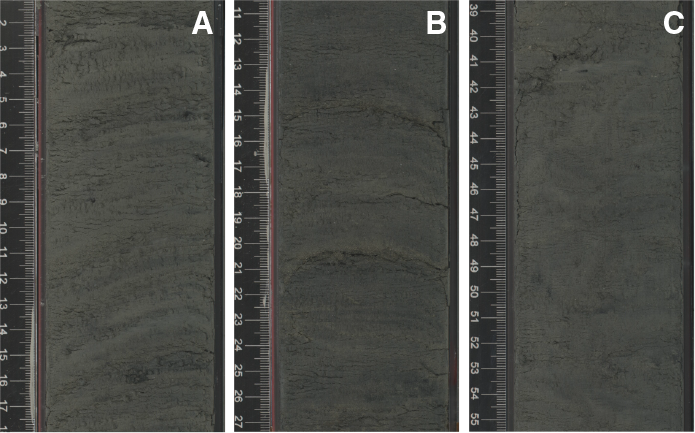
Figure F12. Lithostratigraphic Unit III.

Figure F13. Representative photomicrographs, Unit III.
Convolute bedding was observed in the clayey silt beds but never in association with the laminated units, which appear horizontal or slightly inclined (Figure F12). Upward arching due to drilling disturbance affected all the laminated layers in a slight to moderate degree but still allowed for recognition of primary characteristics. The bases of the silt beds are sharp and slightly irregular and grade upward into clay or clayey silt.
Clasts with irregular edges were identified in some of the clayey silt beds (Sections 372-U1517C-8F-2, 9F-1, 12F-2, and 12F-4). Only two microfaults were observed in Sections 9F-2, 80–87 cm (45.49–45.56 mbsf), and 11F-4, 9–14 cm (56.05–56.01 mbsf). Unit III has a relatively uniform magnetic susceptibility of ~18 × 10−5 SI, and its base is marked by a decrease in magnetic susceptibility.
Foraminifers indicate Unit III is Late Pleistocene in age (see Biostratigraphy).
Preliminary interpretation
The clayey silt intervals with clasts and convolute bedding can be interpreted to be plastically deformed, matrix-supported mass transport deposits (MTDs). These intervals are interbedded with finely laminated silt and clay that might suggest fine-grained turbidites. Their repetitive nature points to a rhythmic style of deposition. The base of Unit III is marked by a sharp change in porosity and bulk density to strata that are much less consolidated; we interpret the unit boundary to be the base of the TLC.
Lithostratigraphic Unit IV
The major lithology of Unit IV is massive greenish gray to dark greenish gray clayey silt with variable amounts of clay characterized by Munsell colors GLEY 1 5/10Y, 4/10Y, and 4/5GY (Figure F14). Although the unit locally appears bedded based on color changes, it is mostly massive with light-colored ash blebs and shell fragments scattered throughout. The silty bedded intervals have sharp bases and gradational top contacts. Convolute bedding was observed in two intervals at 76.06–77.24 mbsf (interval 372-U1517C-15H-5, 0–118 cm) and 82.45–82.59 mbsf (interval 16H-2, 63–75 cm). Black sulfide mottling and low and uniform magnetic susceptibility (~13 × 10−5 SI) is seen throughout the sequence. No indication of bioturbation is present. Representative smear slide photomicrographs (Figure F15) indicate an average clay fraction >75% that is dominated by calcareous nannofossils (coccoliths) and siliceous (opaline) sponge spicules. Authigenic minerals from alteration of volcaniclastic material (e.g., phillipsite) were also identified. The base of the unit is placed at the top of the first significant sand bed encountered.
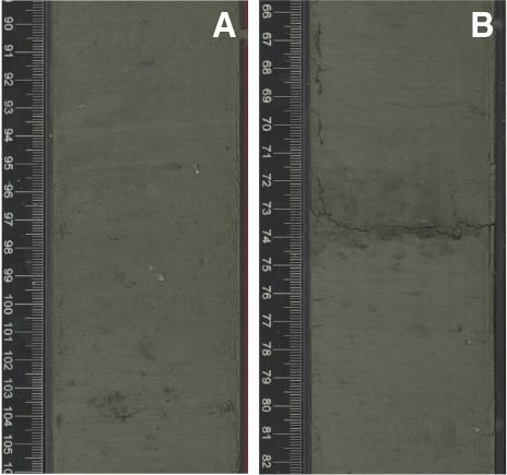
Figure F14. Lithostratigraphic Unit IV.
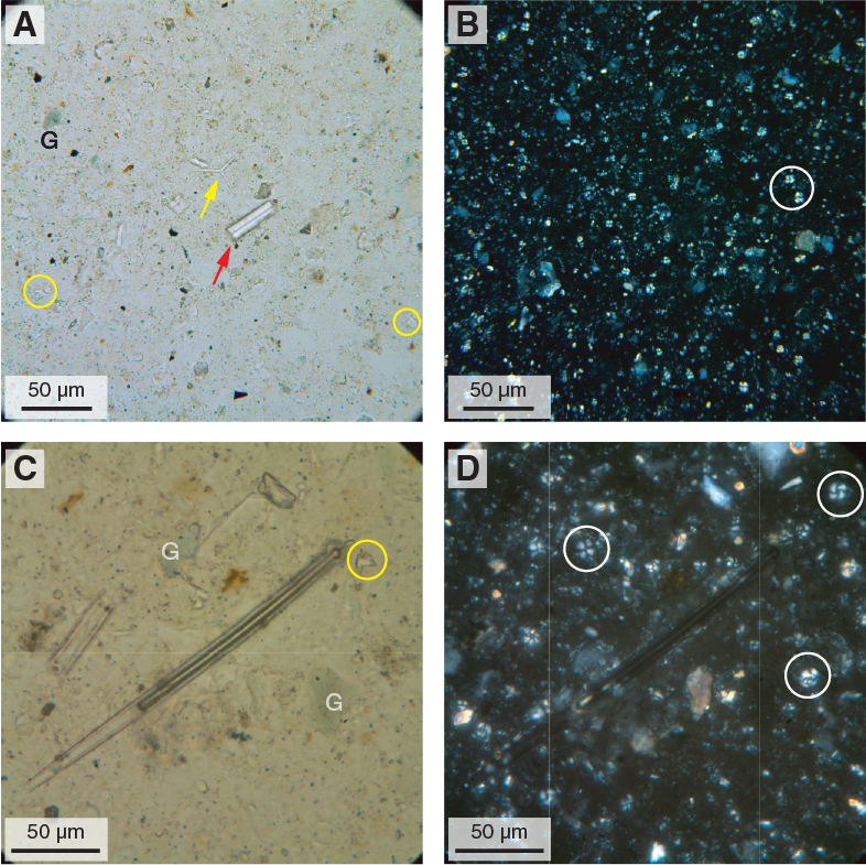
Figure F15. Representative photomicrographs, Unit IV.
Foraminifers indicate Unit IV is Late Pleistocene in age (see Biostratigraphy).
Preliminary interpretation
Unit IV is interpreted to be a hemipelagic sequence punctuated by scattered silty turbidites and MTDs. Bulk density and porosity measurements suggest the sequence is poorly consolidated (see Physical properties).
Lithostratigraphic Unit V
- Interval: 372-U1517C-18H-2, 3 cm, to 36F-CC, 15 cm
- Depth: 103.16–187.53 mbsf (bottom of hole)
- Age: Middle Pleistocene
Unit V is highly variable and includes characteristics similar to those of Units II and IV but with more complex heterogeneity (Figure F3). This unit is composed of alternating sand and mud and intervals of massive clayey silt or silty clay. Near the bottom of the hole are several decimeter-scale ash/tuff layers (Figure F16). Unit V contains the coarsest sand beds recovered from Hole U1517C; some reach medium-sand size. These sand beds exhibit sharp irregular bases and are graded and locally laminated. Sandy beds increase in frequency below 150 mbsf, and medium-thickness (15–20 cm) sand beds occur from 158 to 170 mbsf. Some intervals show convolute bedding or chaotic character with an abundance of whole and broken bivalve shells (Section 372-U1517C-18H-7). One normal microfault was observed in Section 24F-1 (11–24 cm). Black sulfide mottling is seen throughout the core. Color banding is present and predominantly associated with the massive layers. Bulk density and porosity show high variability associated with different lithologies (see Physical properties and Logging while drilling).
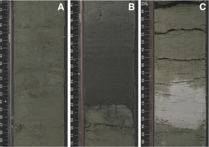
Figure F16. Lithostratigraphic Unit V.
Based on representative smear slide photomicrographs (Figure F17), we estimate the grain size proportion to be 70% sand, 20% silt, and 10% clay (Figure F6). The very fine– to fine-sized fraction is dominated by well-rounded grains of calcareous debris, probably biogenic in origin, an interpretation supported by their shape. The very fine– to silt-sized fraction is composed mainly of detrital quartz, altered volcanic fragments, and glass shards. Glauconite and mica (biotite and muscovite) are present as minor components.
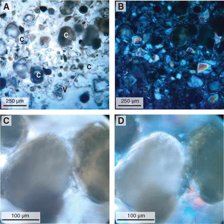
Figure F17. Representative photomicrographs, Unit V.
Foraminifers and nannofossils indicate Unit V is Middle Pleistocene in age (see Biostratigraphy).
Preliminary interpretation
Unit V is interpreted to be a mixed slope sedimentary succession that includes hemipelagic sediment (massive clay to clayey silt beds) alternating with turbidites (graded sandy beds), MTDs (convoluted and chaotic intervals), and ash layers.
X-ray diffraction
The results of bulk powder X-ray diffraction (XRD) analyses are summarized in Figure F18 and Table T4. Most of the analyzed samples are representative of the background lithology (silty clay to clayey silt), so compositional variations are relatively small. Representative diffractograms are shown in Figure F19. Decreases in total clay mineral abundance are matched by increases in quartz and feldspar; we attribute this trend to grain size effects. The computed relative percentages of calcite are typically greater (by 1%–2%) than CaCO3 values from coulometric analyses. These discrepancies increase slightly when the XRD results are normalized to 100% (Table T4).
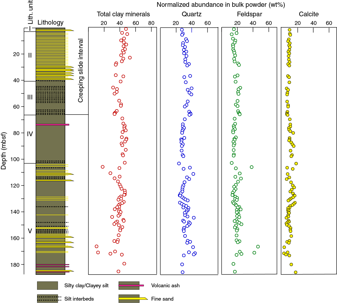
Figure F18. Bulk powder XRD results.
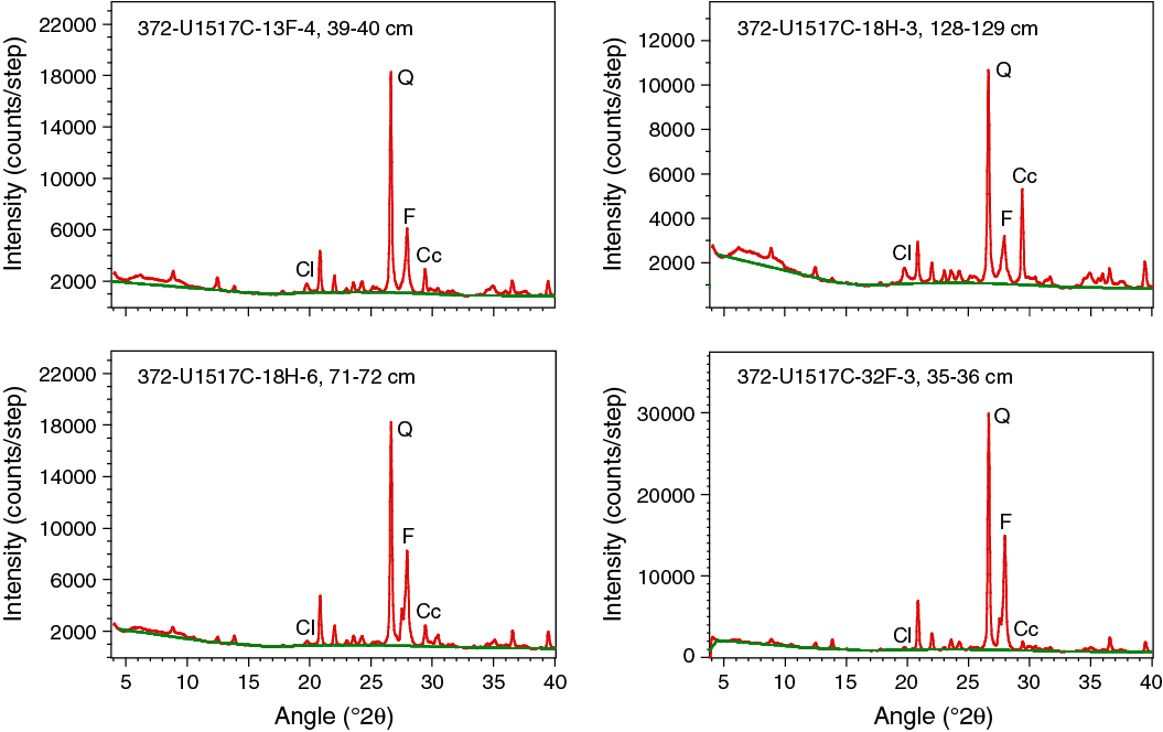
Figure F19. X-ray diffractograms.
Compositional differences among the lithostratigraphic units are small. The one sample analyzed from Unit I contains 47.7 wt% total clay minerals, 27.2 wt% quartz, 15.4 wt% feldspar, and 9.6 wt% calcite. Average values for Unit II are total clay minerals = 42.7 wt%, quartz = 31.6 wt%, feldspar = 16.7 wt%, and calcite = 9.0 wt%. Average values for Unit III are total clay minerals = 36.2 wt%, quartz = 35.9 wt%, feldspar = 20.8 wt%, and calcite = 7.1 wt%. In Unit IV, the average values are total clay minerals = 45.0 wt%, quartz = 28.0 wt%, feldspar = 15.6 wt%, and calcite = 11.5 wt%. Averages for Unit V are total clay minerals = 37.4 wt%, quartz = 32.4 wt%, feldspar = 20.4 wt%, and calcite = 9.8 wt%.
Biostratigraphy
Calcareous nannofossils and planktonic foraminifers were examined from core catcher samples and additional split-core samples to develop a shipboard biostratigraphic framework for Site U1517. Benthic foraminifers were also examined to provide data on paleowater depths and downslope reworking.
A Holocene to Middle Pleistocene sedimentary sequence was recovered at Site U1517. The base of the Holocene is placed between Samples 372-U1517C-1H-3, 29–34 cm, and 1H-4, 42–47 cm (3.29–4.92 mbsf), at the level of a lithologic change from relatively soft (featureless) bioturbated silty clay to a compacted thin-bedded silty clay sequence and at an abrupt shift in physical properties (see Physical properties). The underlying section (Samples 1H-4, 42–47 cm, through 17H-CC, 44–49 cm [4.92–99.55 mbsf]) is Late Pleistocene (11–120 ka), and the lowermost section (Samples 18H-CC, 0–5 cm, through 36F-CC, 15–20 cm [108.25–187.53 mbsf]) is Middle Pleistocene (126–530 ka or younger).
From biostratigraphic dating, the average sedimentation rate for Site U1517 is estimated to be ~0.8 m/ky.
Calcareous nannofossils
Calcareous nannofossils were examined in core catcher samples from Hole U1517C. Nannofossils are common throughout the cored sequence, with poor to moderate preservation. Reworking of older, poorly preserved material is common in most samples. Biostratigraphic datums are given in Table T5, and the distribution of calcareous nannofossil taxa is given in Table T6.
The recognition of key datums is problematic at Site U1517 because of substantial reworking of Pliocene–Cretaceous taxa throughout the sequence. Emiliania huxleyi (first appearance datum [FAD] = 0.29 Ma) was not observed under light microscopy, and further sampling for scanning electron microscope analysis is required to determine the presence or absence of this taxa. Medium Gephyrocapsa spp. (4–5.5 µm) are recorded throughout the cored sequence (Samples 372-U1517C-1H-CC, 28–33 cm, through 36F-CC, 15–20 cm [5.65–187.53 mbsf]); therefore, the base of the sequence is interpreted to be early Pleistocene or younger based on the FAD of medium Gephyrocapsa spp. (1.73 Ma or younger; in Zone NN19).
Assemblages in the Pleistocene sequence are characterized by common to abundant small Gephyrocapsa spp. (<3.5 µm) and Reticulofenestra minuta, with rare to common specimens of Calcidiscus leptoporus, Coccolithus pelagicus, Helicosphaera carteri, Reticulofenestra haqii, Reticulofenestra minutula, Reticulofenestra perplexa, Reticulofenestra producta, and Syracosphaera pulchra. Less common taxa include Braarudosphaera bigelowii, Calcidiscus tropicus, Calciosolenia brasiliensis, Ceratolithus cristatus, Helicosphaera hyalina, Helicosphaera sellii, Pontosphaera discopora, Pontosphaera japonica, Pontosphaera multipora, Pseudoemiliania lacunosa, Pseudoemiliania ovata, Rhabdosphaera clavigera, Umbilicosphaera rotula, and Umbilicosphaera sibogae.
Foraminifers
The foraminifer biostratigraphy at Site U1517 was based on the examination of core catcher samples from Hole U1517C. Additional split-core samples from Core 372-U1517C-1H were examined to locate the base of the Holocene. Ages assigned to planktonic biostratigraphic datums follow those listed in Table T4 in the Expedition 372A methods chapter (Pecher et al., 2019a). Biostratigraphic datums are given in Table T5, the distribution of foraminifers and other fossil material is given in Table T7, and planktonic abundances and indications of oceanicity, paleowater depths, and downslope reworking are given in Table T8.
Microfossil residues (>125 µm) from washed samples are characterized by common to abundant well-preserved foraminifers. Most samples are dominated by planktonic foraminifers, but abundances range from neritic (37%) to open oceanic (95%) values. Planktonic age markers are present in sufficient numbers to date most samples reliably. Tephra and clastic grains, minor plant material, pyrite, and other fossil material, including shell (mostly bivalve and gastropod) fragments, echinoid spines and plate fragments, radiolarians, ostracods, otoliths, and fish teeth, are also present in variable amounts. Small numbers of reworked Pliocene and Miocene taxa are also noted in some Pleistocene samples but not in Holocene samples.
Planktonic foraminifer biostratigraphy
Truncorotalia truncatulinoides is common through the cored sedimentary sequence at Site U1517. The presence of this age marker and the persistence of sinistral coiled populations indicates that the age is Middle Pleistocene or younger (younger than 530 ka) (Table T5). Higher biostratigraphic precision was achieved by correlating short-lived influxes of Hirsutella hirsuta at Site U1517 with similar events in the isotopically tuned and calibrated biostratigraphic record at Ocean Drilling Program (ODP) Site 1123 (Crundwell et al., 2008). The youngest influx of Hr. hirsuta, in Samples 372-U1517C-1H-1, 20–25 cm, through 1H-3, 29–34 cm (0.20–3.29 mbsf), where specimens are common, is correlated with Marine Isotope Stage (MIS) 1 (0–11 ka). The base of the Holocene is placed immediately below the influx of Hr. hirsuta between Samples 1H-3, 29–34 cm, and 1H-4, 42–47 cm (3.29–4.92 mbsf). The other influx of common Hr. hirsuta occurs in Sample 17H-CC, 44–49 cm (99.55 mbsf), and is correlated with MIS 5 (95–120 ka). The last appearance datum of Truncorotalia crassacarina (50 ka) occurs in Sample 14F-CC, 37–42 cm (71.55 mbsf), between the acmes of Hr. hirsuta.
Holocene foraminifers and paleoenvironment
Foraminifer assemblages from the Holocene section in Hole U1517C are generally well preserved, although a small proportion of specimens (<10%) are broken or have partially dissolved shell walls. Holocene planktonic abundances range from 53% to 78%, indicating deposition under outer neritic or suboceanic conditions. The presence of common midbathyal markers Eggerella bradyi and Sigmoilopsis schlumbergeri in Sample 372-U1517C-1H-2, 106–111 cm (2.56 mbsf), is consistent with the present-day water depth of Site U1517 (~720 m). Rare specimens of lower bathyal markers Planulina wuellerstorfi and Bulimina truncanella in Sample 1H-2, 106–111 cm (2.56 mbsf), suggest water depths were possibly deeper earlier in the Holocene. Holocene assemblages show no evidence of downslope reworking other than rare specimens of the shelf species Nonionella flemingi and no evidence of reworking from older sedimentary rocks.
Late Pleistocene foraminifers and paleoenvironment
Late Pleistocene assemblages in Samples 372-U1517C-1H-4, 42–47 cm, through 17H-CC, 44–49 cm (4.92–99.55 mbsf), are moderately diverse and contain few to abundant well-preserved foraminifers. Moderately preserved foraminifers that were reworked from older sedimentary rocks are also present in some samples, primarily 6F-CC, 21–26 cm, through 12F-CC, 26–31 cm (33.93–61.65 mbsf). Planktonic abundances vary between extraneritic (37%) and open oceanic (94%) values. The lower planktonic values generally coincide with samples that have common reworked foraminifers (e.g., Sample 1H-4, 42–47 cm [4.92 mbsf]). Small numbers of bathyal taxa (Pullenia bulloides, Melonis barleeanum, and elongate nodosarids) that are diagnostic of upper bathyal or deeper water depths >200 m are present in the upper part of the Late Pleistocene section (Samples 1H-4, 42–47 cm, through 5F-CC, 24–29 cm [4.92–29.25 mbsf]). The underlying interval (Samples 6F-CC, 21–26 cm, through 11F-CC, 26–31 cm [33.93–57.42 mbsf]) lacks bathyal markers and has assemblages that are characteristic of shelf water depths (<200 m). The absence of bathyal markers contrasts with the deep-water assemblages in the underlying interval (Samples 12F-CC, 26–31 cm, through 17H-CC, 44–49 cm [61.65–99.55 mbsf]) that have common mid- and lower bathyal markers (e.g., E. bradyi, S. schlumbergeri, B. truncanella, and P. wuellerstorfi). The juxtaposition of the shallow-water and deep-water faunas occurs between Samples 11F-CC, 26–31 cm, and 12F-CC, 26–31 cm (57.42–61.65 mbsf). This well-defined change in benthic fauna coincides with the compacted base of the TLC (see Logging while drilling) and has a biostratigraphic age younger than 50 ka. Shallow-water foraminifers that were transported downslope from shelf water depths <200 m are also present in other assemblages, but they are less common in the lower part of the Late Pleistocene section (Samples 12F-CC, 26–31 cm, through 17H-CC, 44–49 cm [61.65–99.55 mbsf]).
Middle Pleistocene foraminifers and paleoenvironment
Middle Pleistocene assemblages in Samples 372-U1517C-18H-CC, 0–5 cm, through 36F-CC, 15–20 cm (108.25–187.53 mbsf), are moderately diverse and contain very rare to abundant well-preserved foraminifers. Foraminifer abundances are lowest in samples that have high proportions of tephra or sand. The presence of common midbathyal markers ( E. bradyi and S. schlumbergeri) and sporadic occurrences of lower bathyal markers (B. truncanella and P. wuellerstorfi) indicate deposition in lower bathyal water depths >1000 m. Shallow-water taxa that are diagnostic of shelf water depths <200 m, including Zeaflorilus parri, N. flemingi, Haynesina depressula, Elphidium charlottensis, and Notorotalia finlayi, are also present and indicate downslope reworking and sediment redeposition.
Paleomagnetism and rock magnetism
Figure F20 displays the paleomagnetic inclination, declination, and intensity records of natural remanent magnetization (NRM) prior to and following alternating field demagnetization to a peak field of 20 mT with the lithostratigraphic unit classification (see Lithostratigraphy) and half-core magnetic susceptibility measured using the Section Half Multisensor Logger (SHMSL) (see Physical properties). In Lithostratigraphic Units I–IV, core recovery was high and all sections were largely undisturbed, so depositional remanences were adequately preserved. However, a slight deformation along the core liners (or bed drag) often resulted in a slight concave curvature of the bedding that may have affected the remanence directions recorded.
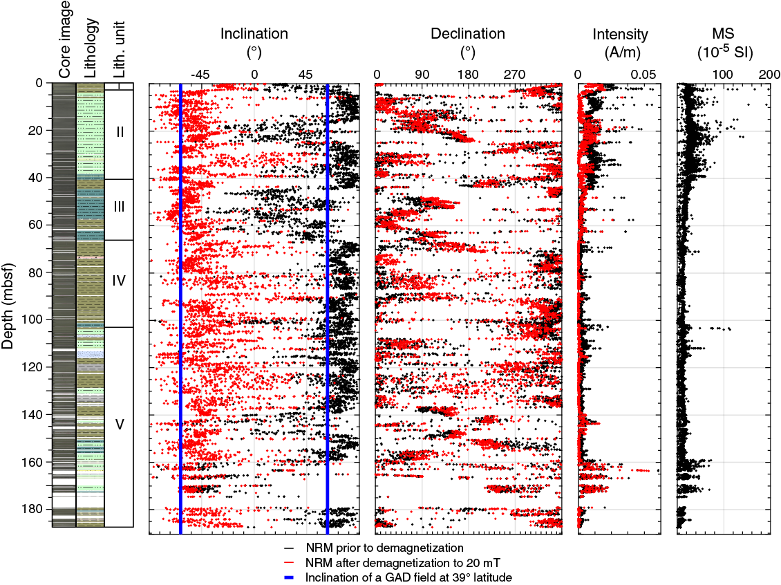
Figure F20. Inclination, declination, intensity, and point magnetic susceptibility.
NRM intensity prior to demagnetization ranges from 4 × 10⁻³ to 0.1 A/m. Peak values coincide with sand-bearing units encountered in Lithostratigraphic Units I and V and are coherent with the higher magnetic susceptibility values measured in these intervals. Measured NRM inclination shows a pervasive overprint along core that manifests in steeply dipping and downward facing inclinations and most likely represents a viscous remanent magnetization acquired during the drilling process. Visual inspection of individual archive-half demagnetizations in vector component diagrams shows that this overprint was successfully removed at the 10 or 20 mT demagnetization level, after which NRM intensity decays linearly toward the origin. Figure F21 shows typical demagnetization behavior from units that are considered to preserve depositional remanences (i.e., fine-grained, undisturbed sediment). Following the removal of strong drilling-induced overprints, magnetic remanence usually decays linearly toward the origin. The median destructive fields are usually ≥15 mT, and in many cases as much as 70% of the initial remanence intensity remains following demagnetization to 30 mT. A few segments demagnetize more rapidly and yield median destructive fields as low as 5 mT. We suggest that these differences may be caused by contributions to the sediments from sources with differing rock magnetic properties and/or grain size. Post-expedition research may unravel such contributions by measuring magnetic properties as a proxy for provenance, environmental conditions during emplacement, and subsequent mineral diagenesis (Liu et al., 2012).
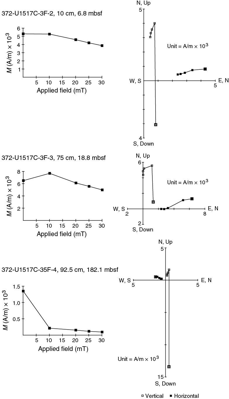
Figure F21. Vector component and NRM intensity vs. demagnetization.
The entire sequence recovered at Site U1517 yields NRM directions with upward facing (negative) inclinations following demagnetization to 20 mT. Preliminary biostratigraphic datums suggest that the material at this site is no older than 0.53 Ma, and we thus infer that the depositional remanences measured were acquired during the Brunhes Normal Chron (C1n) (Gradstein et al., 2012).
Geochemistry
Fluid geochemistry
The main objectives of the fluid (water and gas) geochemistry program at Site U1517 were to document variations in chemical and isotopic compositions that can be used to (1) determine gas hydrate presence and its potential link to the style of deformation observed at the TLC, (2) establish the methane distribution and sources, and (3) provide information on transient events that may result from recent mass transport deposition, gas hydrate dynamics, fluid migration, and/or changes in upward methane flux. In addition, the geochemical data will be useful for evaluating biogeochemical processes, particularly element cycling in response to ash alteration processes in methanic sediment.
Interstitial water sampling
We collected 2 whole-round (WR) samples (5 cm long) from Hole U1517B (APC cores) and 78 WR samples (5–14 cm long) from Hole U1517C (18 from APC cores and 60 from HLAPC cores). Three of these samples were discarded because of the poor quality of the recovered material. Five of the WR samples were separated into two subsamples to determine the host lithology for gas hydrate accumulation, as was previously done during other expeditions where gas hydrate was targeted (e.g., Integrated Ocean Drilling Program Expedition 311 [Expedition 311 Scientists, 2006]).
Samples were collected on the catwalk at a frequency of four samples per core in the upper 15.2 m (Cores 372-U1517C-1H through 2H) and two samples per core from 15.2 to 112.4 mbsf (Cores 3F–19F). Deeper than 112.4 mbsf, care was taken to select samples where scans using the IR thermal imaging camera suggested the potential for gas hydrate occurrence, resulting in a sampling frequency of as many as six samples per HLAPC core deeper than 113 mbsf (Cores 20F–36F). In many cases, IR camera scans identified gas hydrate either in the uppermost sediment of a core (which commonly extruded from the liner because of methane release) or in its core catcher. These samples are not appropriate for a full characterization of the pore fluid composition because of the high risk of contamination and are normally not processed as part of the interstitial water (IW) program of an expedition. However, because one of the main objectives at this site was to document the gas hydrate distribution, samples were collected to address this expedition goal even when they were of less than optimal quality. For these samples, we only report results for dissolved chloride and sulfate concentrations; however, in the lowermost sections of the hole where gas hydrate was present, sampling was not always optimal, which is reflected in the high degree of scatter in the data for the deepest samples.
All samples from WRs were thoroughly cleaned in an effort to remove drilling fluid contamination. All cleaned samples were placed in titanium squeezers and squeezed at gauge forces of as much as 30,000 pounds. The volume of pore fluid recovered varied with lithology and depth and ranged from 20 to 60 mL in APC cores and from 4 to 50 mL in HLAPC cores.
Below the sulfate–methane transition (SMT), sulfate is depleted in the pore fluids and any sulfate present in a sample is a result of contamination with surface seawater used as drilling fluid during Site U1517 operations. Contamination was especially problematic in coarse-grained samples. Based on the sulfate concentration of each IW sample, we used the chemical composition of the surface seawater to correct each analyte for contamination using the following equations:
- fSW = fraction of a pore fluid sample that is contaminated with surface seawater,
- fPW = fraction of uncontaminated pore water in a sample,
- [X]corr = corrected value of a solute (e.g., Cl, Ca, Sr, etc.),
- [X]meas = measured concentration of that solute, and
- [X]SW = concentration of the solute in surface seawater.
The raw data for the organic metabolites and major element concentrations are listed in Table T9, and Table T10 lists the sulfate-corrected concentration data. Similarly, Tables T11 and T12 list the uncorrected and corrected minor element concentrations, respectively. Only the sulfate-corrected data are illustrated in Figures F22, F23, F24, and F25.
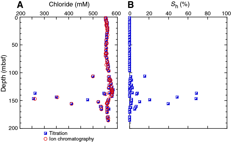
Figure F22. Chloride profiles and Sh values.
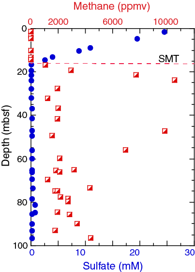
Figure F23. Sulfate and methane profiles, upper 100 m.
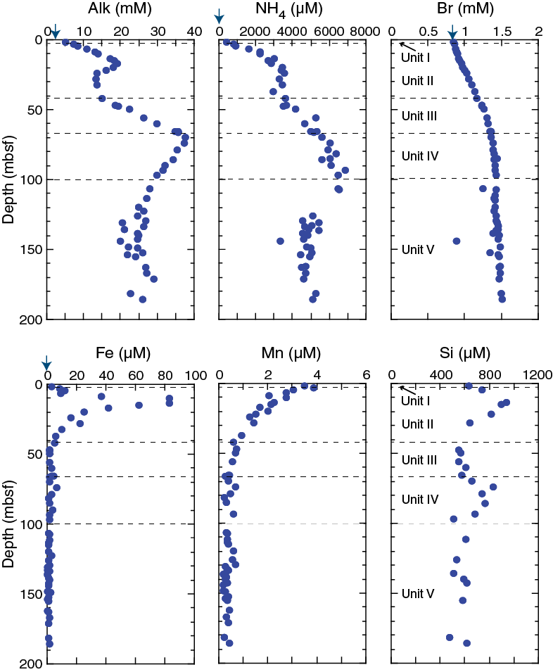
Figure F24. Alkalinity, ammonium, bromide, iron, manganese, and silica.
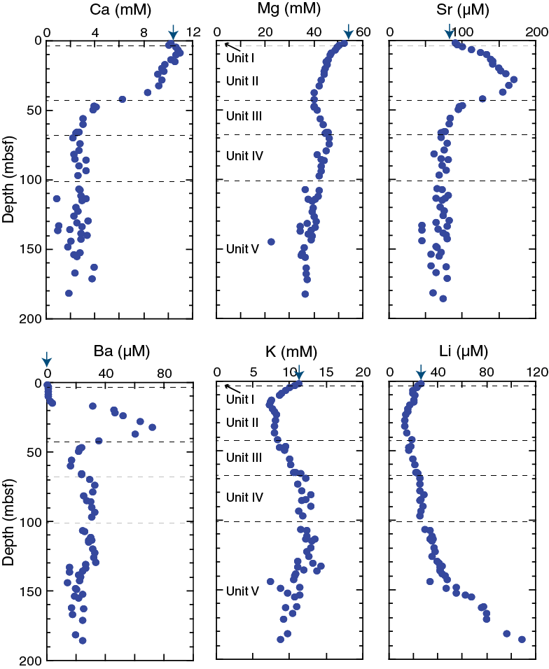
Figure F25. Calcium, magnesium, strontium, barium, potassium, and lithium.
Chloride concentration and gas hydrate occurrence
Because one of the main objectives of the expedition was to establish the occurrence, abundance, and distribution of gas hydrate and its role on the behavior of the TLC, pore water sampling was guided by cold temperature anomalies in IR scans. These anomalies were used as indicators for gas hydrate presence (see Core-log integration). We took care to obtain at least one sample from each core at a distance away from IR temperature anomalies. These WRs were intended as background samples and were used to characterize horizons without gas hydrate so as to constrain the in situ background chloride concentration. The dissolved chloride at Site U1517 was measured by titration and ion chromatography (IC) (see Geochemistry in the Expedition 372A methods chapter [Pecher et al., 2019a]) with good agreement between the two data sets (Figure F22).
The overall trend in downhole dissolved chloride shows a broad peak between 81 and 179 mbsf with values as high as 582 mM. Superimposed on this overall trend, we observe discrete excursions to lower chloride values in the gas hydrate stability zone, similar to those previously observed in pore waters recovered from gas hydrate–bearing sediment (Shipboard Scientific Party, 2003; Expedition 311 Scientists, 2006). Estimates of gas hydrate abundance are commonly based on the magnitude of discrete excursions from in situ chloride to anomalously low chloride values that represent the degree of gas hydrate dissociation during core retrieval (e.g., Paull and Ussler, 2001). We used an empirical approach in which the in situ background chloride concentration is defined as the envelope of measurements around the discrete chloride anomalies (e.g., Torres et al., 2008). These discrete, sulfate-corrected chloride anomalies were used to estimate a gas hydrate saturation (Sh) value:
- Cb = in situ background pore water salinity,
- C = chloride concentration measured in the core sample after gas hydrate dissociation, and
- α = dimensionless constant that quantifies the density change due to gas hydrate dissociation and equals 1.257 (Malinverno et al., 2008).
Malinverno et al. (2008) show that by propagating the uncertainties associated with parameters in this equation, the typical uncertainty in estimating Sh from chloride concentration data is ±1.5%. At Site U1517, the chloride data indicate the presence of discrete gas hydrate occurrences between ~135 and 165 mbsf with Sh values ranging from 2% to 68% (Figure F22; Table T13). This distribution is consistent with inferences on gas hydrate saturation based on resistivity data obtained by LWD (Figure F42). When it was possible to isolate thin, dark, coarse silt layers from the background fine clay matrix, we analyzed each lithology separately. Table T13 lists the gas hydrate saturation for samples with Sh higher than 1.5% and includes the paired samples where Sh was estimated from both the coarse- and fine-grained samples in the same whole round. Gas hydrate in the fine clay sediment layers that were immediately in contact with the gas hydrate–bearing, coarse-grained layers ranged from nondetectable to 1.7%, illustrating the preferential occurrence of gas hydrate in the coarse-grained material. For those samples in which the coarse-grained material could not be isolated, the gas hydrate saturations listed in Table T13 should be considered minimum values. By selecting samples based on IR anomalies, we introduced a bias toward high gas hydrate saturation; thus, the data in Table T13 are not suited for obtaining a robust average saturation value over the gas hydrate occurrence zone.
Early diagenetic reactions
The pore fluid profiles of sulfate, alkalinity, and ammonium concentrations in the uppermost ~100 m have characteristic organic matter remineralization concentration-depth profiles (Figures F23, F24). Sulfate concentration decreases from 25 mM at the seafloor to 0 mM at 17 mbsf; the SMT is well defined and corresponds to an increase in methane concentration (Figure F23). Alkalinity increases from seawater value at the seafloor to a maximum value of 19 mM at 17 mbsf, gradually decreases with depth between 19 and 41 mbsf, and increases again between 41 and 69 mbsf to an overall maximum of 37.5 mM at 69 mbsf.
Organic matter diagenesis in the upper sediment section is also reflected in the Site U1517 ammonium concentration-depth profile, where ammonium values increase with depth to a maximum value of ~6500 µM at 107 mbsf. Dissolved iron and manganese in the upper sediments have high concentrations relative to seawater. Manganese has values as high as 3.8 and 3.5 µM in the uppermost samples from Holes U1517B and U1517C, respectively; iron reaches a maximum of 83 µM at 10 mbsf. These distributions point to the role of iron and manganese as electron acceptors in the typical redox ladder that characterizes the microbially mediated pathways of organic matter oxidation in marine sediment (Froelich et al., 1979). Both iron and manganese decrease to very low concentrations at depth, indicative of their removal into diagenetic mineral phases.
Phosphate concentration is low in the upper 40 m (4.2–30.5 µM) relative to what would be expected from organic matter degradation and increases deeper than 50 mbsf, but the data show a very high degree of scatter throughout the core (Table T10). The reasons for the scatter and the observed distributions are not clear.
Calcium, magnesium, strontium, barium, and potassium concentrations are shown in Figure F25. Calcium concentration shows a slight increase in the uppermost 9 m to 10.9 mM, followed by a decrease to 6.2 mM in sediment in Lithostratigraphic Unit II (see Lithostratigraphy). Values as low as 2.2 mM are reached at the Unit III/IV boundary and correspond to the depth range of the second alkalinity maxima (Figure F24). These low calcium concentrations reflect precipitation of authigenic carbonates, which is consistent with observations of authigenic calcite grains in these sediments (see Lithostratigraphy). Strontium concentration increases rapidly below the seafloor, reaching a maximum of 170 µM at 27 mbsf, followed by a rapid decrease to values that are typically lower than its seawater concentration of 87 µM in the pore water of sediment in Units IV and V. The high strontium data are indicative of ash alteration reactions, and the low strontium concentrations that correspond to low calcium values may reflect incorporation of strontium into authigenic carbonate minerals.
Magnesium concentration decreases from seawater value at the seafloor to 40.1 mM at 37 mbsf. In contrast with the observed decrease in calcium, the dissolved Mg in sediments deeper than 41 mbsf shows a slight increase to 46.6 mM, indicating a diagenetic source for this ion. Dissolved barium shows a marked increase in concentration below the SMT in Lithostratigraphic Unit II (Figure F25), reaching values as high as 71 µM at 32 mbsf. This distribution results from release of barium via either ash alteration reactions or the dissolution of marine barite in sulfate-depleted pore fluids (e.g., Torres et al., 1996) and sequestration into barite above the SMT. Barium concentration remains relatively constant in Unit III and shows a slight increase with depth deeper than 65 mbsf in Units IV and V (see Lithostratigraphy). The silica profile shows two maxima: one at 13 mbsf and another one with a less well-defined peak at ~65 mbsf (Figure F24), consistent with alteration of ash and/or silicate minerals. Potassium decreases from its seawater value to 7.7 mM, reflecting incorporation of this element in authigenic minerals during alteration of silica phases (e.g., volcanic ash) at low temperatures (Figure F25). Potassium remains low in Unit II and shows an increase with depth toward higher values in pore waters in Unit IV, where concentrations are above 12 mM. Bromide shows a smooth increase with depth from its seawater value of 0.86 mM to values higher than 1.35 mM in Units IV and V (Figure F24).
Collectively, the increases in Si, Mg, Ba, and K in the pore fluids of Lithostratigraphic Unit II are consistent with a release from alteration of reactive silica phases in methanogenic sediment. The removal of calcium and strontium and to a lesser degree the lower values of K and Mg deeper than 150 mbsf are consistent with the formation of authigenic phases driven by silicate weathering (Wallmann et al., 2008; Solomon et al., 2014; Kim et al., 2016), which is in agreement with chalcedony and medium-sized calcite grains observed in smear slides from Unit IV (see Lithostratigraphy).
It is worth noting that both the alkalinity and ammonium profiles show two distinct peaks: one at ~16 mbsf and another one deeper in the sediment in Lithostratigraphic Unit IV (see Lithostratigraphy). Given the location of Site U1517 on the TLC, the pore water profiles in Units IV and V do not necessarily reflect a continuous diagenetic sequence with the data above but may instead record reactions that occurred in the sediment before emplacement of the MTDs. In this scenario, the pore water profiles would be indicative of a diffusional smoothing beneath and above the MTDs. Thus, the observed alkalinity peak at 65 mbsf may be a remnant from a previous SMT, where alkalinity was generated by methane oxidation in the past, and may or may not be related to silicate weathering reactions. The break in the alkalinity and ammonium profiles, with relative constant values between ~20 and 40 mbsf, is also consistent with successive slump depositional events on the TLC.
It is likely that the observed profiles are the result of a combination of the various depositional and diagenetic signals developed over the evolution of the sediment stratigraphy at Site U1517. Post-expedition strontium isotopic analyses will determine the silicate weathering contribution. Carbon isotopes will identify the different organic matter degradation pathways, and the water isotopic composition can aid in differentiating among diagenetic reactions. The isotopic measurements, combined with additional information such as dating the sediment packages that comprise the MTD and modeling the pore fluid data, will help to unravel the different scenarios discussed above.
Lithium is consumed in Lithostratigraphic Unit II, similar to K and suggestive of alteration of silicate minerals at low temperature (Figure F25). The lithium distribution, however, is unique in that it shows a marked increase with depth with a high value of 108.8 µM measured in the deepest sample analyzed (186 mbsf). The lithium profile in Unit V indicates diffusion from a fluid with high lithium concentration below the cored section (Figure F25).
Gas analyses
Headspace samples were taken from each sediment core to monitor for the presence and abundance of C1–C3 hydrocarbons as part of the standard safety protocol during drilling (Pimmel and Claypool, 2001). These samples are commonly collected from sediment next to the WR samples taken for measurements of background IW concentrations, and additional samples were collected in support of the gas hydrate objectives of the expedition. A total of 67 headspace samples were analyzed by gas chromatography (GC) (see Geochemistry in the Expedition 372A methods chapter [Pecher et al., 2019a]). In Core 372-U1517C-5F (29 mbsf) and deeper, increasingly large pressurized voids occur frequently to 181 mbsf (Section 35F-3). No voids are present in the deepest core (36F), which is sand and tephra rich (see Lithostratigraphy). When possible, 2–3 voids were sampled per core using the IODP void sampler. Out of the 67 gas samples collected, 18 samples were analyzed on board using both the GC3 and the natural gas analyzer (NGA) gas chromatographic systems (see Geochemistry in the Expedition 372A methods chapter [Pecher et al., 2019a]). Measurements using the NGA system gave erroneous values for C2–C6, O2, and N2 and were therefore discarded. A second sample taken from the headspace vials was injected into the GC3. These samples suffered from air contamination due to underpressure in the sample vials after the extraction of 5 mL for the first measurement. The data will be evaluated once the other gas samples are measured onshore because C1/C2 ratios might not be affected. Ethane concentrations need to be confirmed because small ethane peaks occurred in unison with higher methane concentrations during calibration, which is likely due to the presence of ethane in the standard gases. The hydrocarbon concentrations are presented in parts per million by volume (ppmv), which represents the volume of the respective hydrocarbon in the serum vial headspace. The results from Hole U1517C are shown in Table T14 and Figure F26.
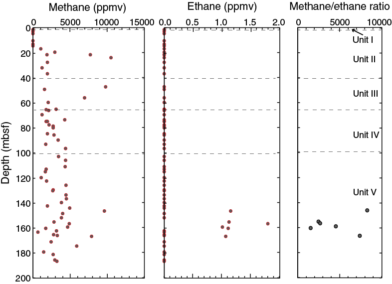
Figure F26. Methane, ethane, and methane/ethane ratio.
Between 0 and 15 mbsf, methane concentrations of 2 ppmv are indistinguishable from the instrumental blanks. Deeper than 15 mbsf, which is ~2 m shallower than the SMT estimated from sulfate and alkalinity data, the concentration rapidly increases to as much as 10,000 ppmv at 24 mbsf, indicating ongoing methanogenesis. Deeper than 16 mbsf, methane concentration in the headspace samples remains between 1200 and 9000 ppmv. All of these values are commonly above pore water saturation at ambient conditions but below equilibrium gas saturation values for methane in seawater (~0.1 mol/kg at water depths of 700–900 m and in situ temperatures) (Duan and Mao, 2006). Measured concentrations are lower than the estimated in situ saturation by at least one order of magnitude (compared with ~140,000 ppmv). The measured concentrations reflect a qualitative estimate of the amount of gas remaining in the sediment after recovery and handling of the core. Concentrations in the headspace samples are strongly affected by pore water degassing, gas expansion, and/or gas hydrate decomposition. True in situ methane concentrations are only obtained by pressure coring.
Ethane was not detected in the headspace samples shallower than 146 mbsf, but it was repeatedly measured at very low concentrations of 1–2 ppm between 146 and 166 mbsf. Because these samples were not injected into the GC sequentially and represented the only samples with reoccurring ethane peaks, we conclude that ethane was indeed present in this part of Hole U1517C. The depth range of ethane occurrences coincides with anomalous depletions in chlorinity relative to background values and the inferred presence of gas hydrate. Shore-based Raman spectroscopic measurements will be carried out to determine if ethane is a guest molecule in these gas hydrates. The absence of ethane throughout most of the core and the high methane/ethane ratios indicate a microbial source for the hydrocarbons (Claypool and Kvenvolden, 1983), which is consistent with earlier findings (Greinert et al., 2010; Coffin et al., 2014). Onshore measurements of stable carbon and hydrogen isotopes will be used to verify the methane source. No further ethane occurrences were encountered deeper than 166 mbsf.
Bulk sediment analysis
A total of 99 samples were taken for elemental analysis to determine total carbon (TC) and total nitrogen (TN) concentrations and for coulometric measurements of inorganic C content. Calcium carbonate (CaCO3) and TC values in Lithostratigraphic Units I–III (see Lithostratigraphy) are relatively similar, with CaCO3 values ranging between 4.63 and 8.99 wt% (mean = 6.52 ± 1.13 wt%) and TC ranging between 0.96 and 1.97 wt% (mean = 1.26 ± 0.22 wt%) (Table T15). Values in Units IV and V are slightly higher (mean is 7.43 ± 2.39 wt% for CaCO3 and 1.42 ± 0.31 wt% for TC) with peaks in CaCO3 around 100–130 mbsf, similar to TC (Figure F27).
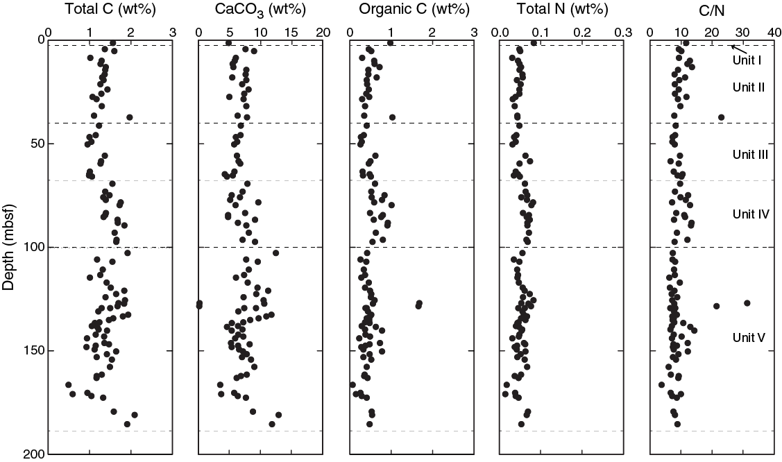
Figure F27. TC, CaCO3, organic C, TN, and C/N ratio.
Organic C (OC), calculated as the difference between TC and inorganic carbon content (see Geochemistry in the Expedition 372A methods chapter [Pecher et al., 2019a]), shows elevated values in Lithostratigraphic Unit IV (mean = 0.71 ± 0.16 wt%), although peaks that reached 1.68 wt% were localized in Unit V (100–188 mbsf) (Figure F27).
TN values are relatively constant in all lithostratigraphic units (0–187.6 mbsf) and range from 0.03 to 0.08 wt% (mean = 0.05 ± 0.01 wt%), although slightly higher values may be found in Unit IV.
The ratio of OC and TN (C/N) can provide information on organic material provenance because terrestrial organic matter typically has a C/N ratio of ~20, whereas marine organic matter, which is more proteinaceous, is characterized by a C/N ratio of ~5–8 (Pimmel and Claypool, 2001). The observed percentage of OC to percentage of TN ranges from 3.78 to 31.34 (mean = 9.46 ± 3.52). Localized peaks occur in the C/N ratios in Lithostratigraphic Units II and V, suggesting increasing heterogeneity of the organic matter.
Gas hydrate sampling
Thirteen whole rounds were collected based on the observation of cold spots in the IR images and were preserved in liquid nitrogen for post-expedition analyses of gas hydrate. The samples were shipped to laboratories at the British Geological Survey (UK), GeoForschungsZentrum Potsdam (Germany), and the Qingdao Institute of Marine Geology (China) (Table T16).
Physical properties
Physical properties were characterized through a set of measurements on whole cores, split cores, and discrete samples (see Physical properties in the Expedition 372A methods chapter [Pecher et al., 2019a]). Results from Hole U1517C are described below. Cores from Hole U1517B were run through the WR tracks but are not described because of unknown depths below seafloor. Physical properties are impacted by lithologic variations (see Lithostratigraphy) and the compaction and deformation history of the sediments (Figure F28). In general, Lithostratigraphic Unit I (0–3 mbsf) is marked by relatively high porosity values, consistent with its description as recent slope drape. Porosity values decrease sharply at the upper boundary of Unit II (3–40.74 mbsf), a bedded sand and mud sequence. The upper boundary of Unit III (40.74–66.38 mbsf), a sequence of laminated clay and silt, is marked by a reduction in variability in magnetic susceptibility. Other physical properties do not change significantly at the Unit II/III boundary. An increase in porosity (decrease in bulk density), an increase in RGB values, and a decrease in reflectance a* and b* values mark the transition from Unit III to Unit IV (66.38–103.16 mbsf), the latter of which consists of massive silty clay. Relative to Unit IV, Unit V (103.16–187.53 mbsf) shows greater variability in magnetic susceptibility, porosity/bulk density, RGB, and thermal conductivity. The variability in Unit V is consistent with its composition of variably bedded sand, silt, clay, and volcanic ash.

Figure F28. Physical properties.
Density and porosity
Bulk density values in Hole U1517C were determined from both gamma ray attenuation (GRA) measurements on whole-round cores and mass/volume measurements on discrete samples from working halves (see Physical properties in the Expedition 372A methods chapter [Pecher et al., 2019a]). The whole-round measurements show some lower, scattered values because of voids caused by gas expansion (Figure F29). Grain density values from the discrete samples average 2.69 g/cm3 with no clear variations or trends. In the upper 66 m, porosity values average 0.44, corresponding to an average bulk density of 1.97 g/cm3. Porosity values in Units II and III are lower than typically expected for shallowly buried sediments. Porosity values vary from 0.68 at 1.37 mbsf to 0.39 at 65.36 mbsf. Deeper than 66 mbsf, porosity values shift higher, averaging 0.48 and corresponding to an average bulk density of 1.89 g/cm3.
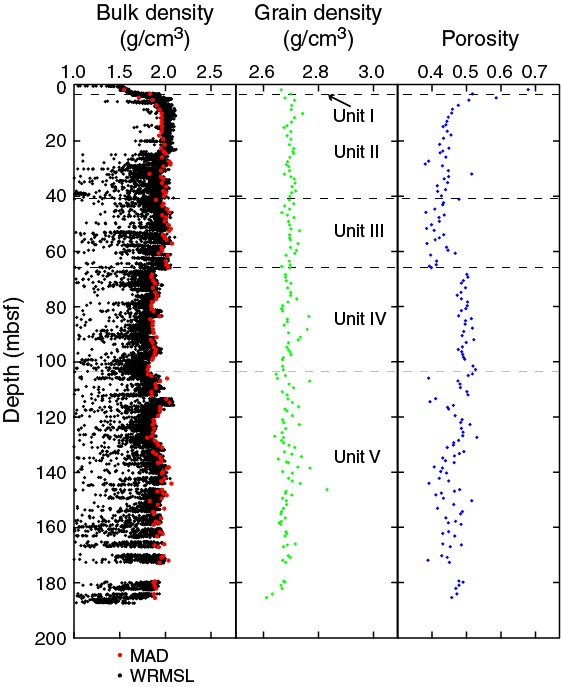
Figure F29. Density and porosity.
Magnetic susceptibility
Volumetric magnetic susceptibility values were measured using the Whole-Round Multisensor Logger (WRMSL), and point measurements were made on the SHMSL (Figure F30). Magnetic susceptibility values measured by these two methods match each other well. Magnetic susceptibility values average 17 × 10−5 SI. In the upper 40 mbsf, magnetic susceptibility values average 28 × 10−5 SI. Deeper than 40 mbsf, magnetic susceptibility values were lower, averaging 14 × 10−5 SI.
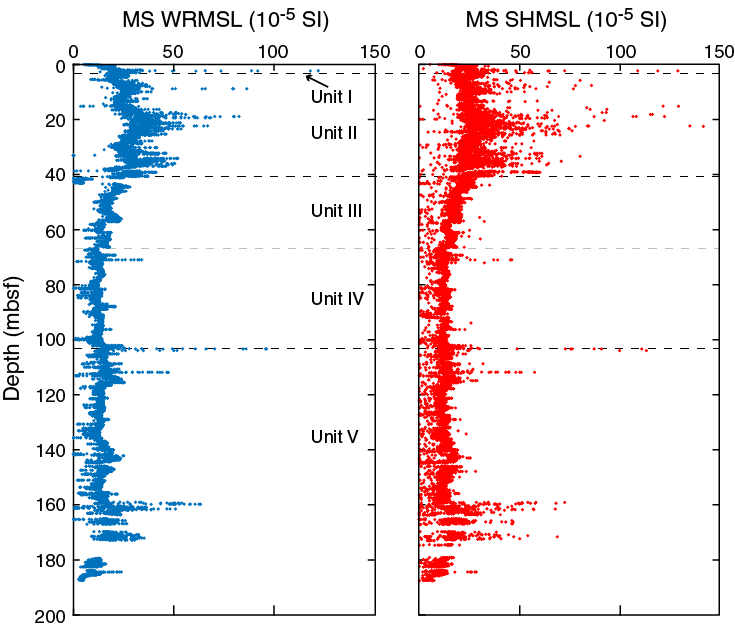
Figure F30. Magnetic susceptibility.
Natural gamma radiation
Natural gamma radiation (NGR) values increase linearly from 20 to 43 counts/s in the upper 5 mbsf (Figure F31). From 5 to 24 mbsf, NGR values average 44 counts/s. Values drop to 24.9 counts/s at 32.1 mbsf and then rise back to 42.8 counts/s at 40.0 mbsf. Deeper than 40 mbsf, NGR values show small fluctuations and average 39.2 counts/s.
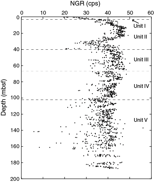
Figure F31. WRMSL NGR.
Thermal conductivity
Because sediment grains have higher thermal conductivity than water, bulk thermal conductivity values are inversely related to porosity. Units II and III show similar thermal conductivity values, averaging 1.32 W/(m·K) (Figure F32). Values are lower in Units IV and V, ranging from 0.86 to 1.50 W/(m·K) and averaging 1.19 W/(m·K).

Figure F32. Thermal conductivity.
P-wave velocity and sediment strength
P-wave velocity values and sediment strength measurements were greatly compromised by pervasive fracturing because of gas expansion deeper than 20 mbsf (Figure F28). Both P-wave velocity values and measured strength increase rapidly in the upper 20 mbsf. P-wave measurements were not possible in the gas-affected zones because of the lack of a transmitted signal. Penetrometer data are extremely noisy because of the disturbance, and measurements were discontinued deeper than 110 mbsf.
Reflectance spectrophotometry and colorimetry
Color reflectance data collected from archive halves are presented in both the L*a*b* and RGB color spaces (Figure F28). Reflectance a* and b* profiles show a transition around 66 mbsf that corresponds to the Unit II/III boundary. A shift in RGB values also occurs at this depth. Color reflectance values generally show more fluctuations in Lithostratigraphic Unit V than in Unit IV, consistent with the variability in sediment type described in Unit V (see Lithostratigraphy).
Downhole measurements
Formation temperature and heat flow
The APCT-3 was deployed seven times in Hole U1517C (Table T17), and four deployments provided reliable formation temperature estimates. The T2P was deployed twice in Hole U1517D (Tables T18, T19, T20). These deployments did not provide any reliable temperature data (Table T18). The SETP was deployed at two depths in Hole U1517D; unfortunately, no reliable temperature data were acquired (Tables T18, T21, T22).
The APCT-3 deployment at 81.1 mbsf (Core 372-U1517C-15H) had a temperature spike upon insertion followed by a smooth temperature decay (Figure F33A). From the temperature-time data, the estimated formation temperature was 8.55°C (Table T17; Figures F33A, F34).
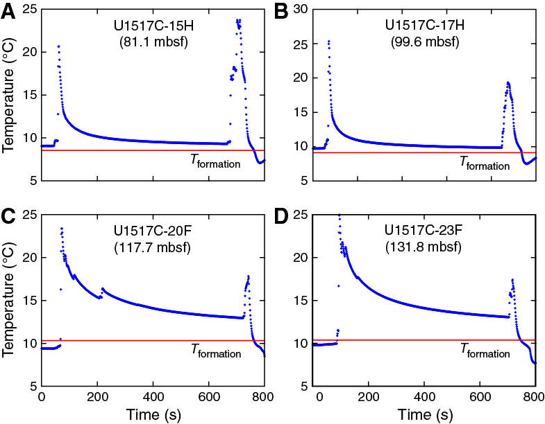
Figure F33. APCT-3 temperature-time data.
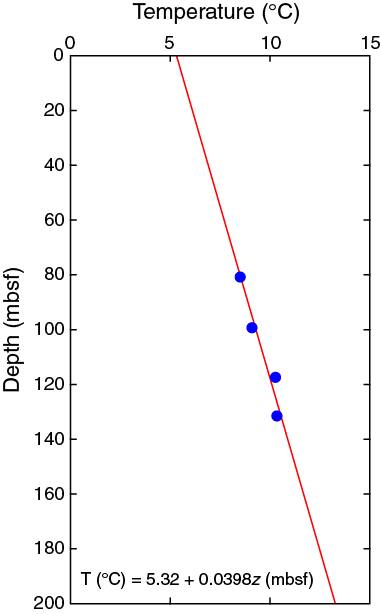
Figure F34. Temperature-depth data.
The APCT-3 deployment at 99.6 mbsf (Core 372-U1517C-17H) had a temperature spike upon insertion followed by a smooth temperature decay (Figure F33B). From the temperature-time data, the estimated formation temperature was 9.14°C (Table T17; Figures F33B, F34).
The APCT-3 deployment at 117.7 mbsf (Core 372-U1517C-20F) had a temperature spike upon insertion but did not have a smooth decay; three small temperature increases were observed during the temperature decay (Figure F33C). The small temperature increases along the decay were likely from movements in the cutting shoe while it was in the formation. From the longest portion of the smooth temperature decay, the estimated formation temperature was 10.32°C (Table T17; Figures F33C, F34).
The APCT-3 deployment at 131.8 mbsf (Core 372-U1517C-23F) had a temperature spike upon insertion followed by three small temperature increases during the temperature decay (Figure F33D). The small temperature increases during the decay were likely from movements in the cutting shoe while it was in the formation. From the longest portion of the smooth temperature decay, the estimated formation temperature was 10.39°C (Table T17; Figures F33D, F34).
The APCT-3 deployments at 145.9, 159.3, and 179.1 mbsf (Cores 372-U1517C-26F, 29F, and 34F) did not provide reliable temperature spikes upon insertion or temperature decay curves, so they did not provide reliable formation temperature estimates.
The T2P deployment at 80 mbsf measured temperature during the deployment; however, the data do not provide reliable formation data. During probe insertion, the temperature dropped significantly (Figure F35), and no temperature decay data exist. Upon recovery of the tool, the tip that houses the thermistor was missing (Tables T18, T19). It is possible the thermistor was damaged during insertion, impeding reliable temperature measurements in the formation. All field-processed temperature data are available in DOWNHOLE in Supplementary material.
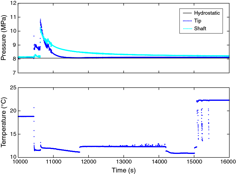
Figure F35. T2P pressure and temperature data.
We were unable to recover the data from the T2P after the deployment at 120 mbsf (Tables T18, T20). Upon recovery of the tool to the rig floor, the tapered probe was missing, the drive tube was flooded, and there was some water in the data housing, which could have damaged the memory card. Efforts to recover data from the memory card after the expedition failed.
The SETP deployments at 130 and 168.7 mbsf did not provide any temperature data (Tables T18, T21, T22). The data from the first SETP deployment were lost during data transfer on the tool. The data from the second SETP deployment were recovered from the tool, but the conversion to ASCII created a corrupted file. Efforts to produce a valid ASCII file for analysis after the expedition were unsuccessful.
The four reliable APCT-3 temperature estimates define a linear temperature profile. A least-squares linear fit to the temperature-depth data defines a gradient of 39.8°C/km (Figure F34). From the linear temperature gradient (dT/dz) and an estimate of thermal conductivity (K), we can estimate the vertical conductive heat flow (q):
The average thermal conductivity of the shallow sedimentary section is 1.22 W/(m·K) (Figure F32), which provides an average heat flow of 49 mW/m2. It should be noted that the average thermal conductivity is based on laboratory measurements that have not been corrected for in situ conditions, so it is likely lower than the in situ thermal conductivity. This simple estimate of conductive, vertical heat flow is consistent with regional values estimated based on BSRs (~45–50 mW/m2) (Henrys et al., 2003; Townend, 1997) but is notably higher than local estimates based on shallow heat flow probe measurements (<20 mW/m2; Huhn, 2016).
Formation pressure
The T2P deployment at 80 mbsf (Tables T18, T19) was successful at collecting pressure data at the tip and shaft of the probe (Figure F35). The tip and shaft showed sharp pressure spikes during probe insertion into the formation, with the tip reaching a slightly higher pressure than the shaft. After insertion, there was some noise in the initial decay curves that may have been related to pressure fluctuations in the standpipe while pumping the tool into the formation (Table T19). After this initial noise, both the tip and shaft pressures show smooth decay curves. Initial analyses of the pressure curves suggest that the formation pressure is near hydrostatic (Figure F35). Post-expedition processing and modeling of the decay curves are required to finalize the interpretation of the formation pressure. All field-processed pressure data are available in DOWNHOLE in Supplementary material.
We were unable to recover the data from the T2P after the deployment at 120 mbsf (Tables T18, T20). Upon recovery of the tool to the rig floor, the tapered probe was missing, the drive tube was flooded, and some water was in the data housing, which could have damaged the memory card. Efforts to recover data from the memory card after the expedition were unsuccessful.
The SETP deployments at 130 and 168.7 mbsf did not provide any pressure data (Tables T18, T21, T22). The data from the first SETP deployment were lost during data transfer on the tool. The data from the second SETP deployment were recovered from the tool, but the conversion to ASCII created a corrupted file. Post-expedition efforts to produce a valid ASCII file for analysis were unsuccessful.
Logging while drilling
The LWD data for Hole U1517A were collected with a BHA composed of five LWD tools attached in the following order behind the 8½ inch bit: geoVISION, SonicScope, NeoScope, TeleScope, and proVISION. These tools provide a wide array of measurements, including gamma ray (geoVISION and NeoScope), resistivity (geoVISION and NeoScope), porosity (NeoScope and proVISION), and compressional and shear wave velocity (SonicScope), as described in Logging while drilling in the Expedition 372A methods chapter (Pecher et al., 2019a).
Drilling parameters
In the composite plot of drilling parameters (Figure F36), data are sorted according to the LWD operations period starting on 15 December 2017 at 1230 h ship local time and terminating on 17 December at 0540 h ship local time. The target rate of penetration (ROP) was 20 m/h to acquire high quality data, and ROP remained around this value during drilling. The drilling pipe rotation rate was maintained close to 50 rpm. Weight on bit (WOB) values ranged between −10 and 25 klb. For most of the hole, WOB values are negative because almost no weight was on the bit. An increase in WOB values was observed below 164 mbsf. Annular pressure increased progressively with depth. The equivalent circulating density started at 2.4 g/cm3 at the top of the hole and decreased to 1.2 g/cm3 at the bottom of the borehole. At the seafloor, the annular temperature was measured at ~6°C. During drilling, the measured annular temperature was ~11°C.
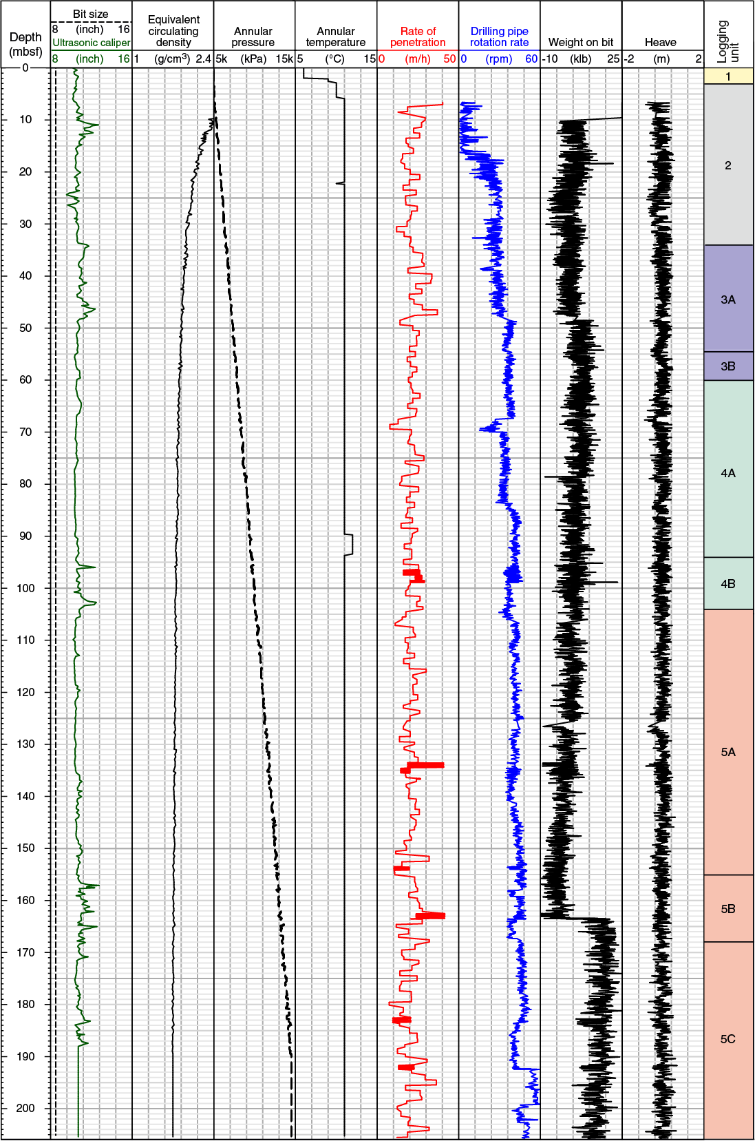
Figure F36. Drilling parameters.
Data quality
Borehole conditions were assessed by the ultrasonic caliper measurement of the borehole diameter (Figures F36, F37). The ultrasonic caliper, however, can incorrectly identify intervals with extreme borehole enlargement (>5 cm) as depth intervals with caliper values near bit size; therefore, porosity and resistivity measurements were also used to identify enlarged or washout depth intervals. Enlarged boreholes, or washouts, are characterized by anomalously low resistivity readings (~0.3–0.9 Ωm) and high porosity (~0.7–1.0), both of which imply that the borehole is enlarged and the measurements are detecting more seawater than formation. Degraded borehole conditions are more likely in intervals with noncohesive sediment such as sand and silt with little clay. In finer grained clay-rich intervals, the borehole is closer to bit size. In general, the highest quality logging measurements are collected when the hole is close to bit size.

Figure F37. LWD measurements.
The resistivity image logs of the borehole wall are poor quality throughout Hole U1517A (Figure F38). Data loss is high at 0–20.5, 26–27, 35.5–44, and 64–66 mbsf because of a combination of slow drilling pipe rotation rate and several washout intervals. Horizontal imaging artifacts are common throughout the imaged interval and are likely related to stick and slide of the resistivity buttons as they rotate around the borehole, possibly smearing the muddy sediments being drilled through.
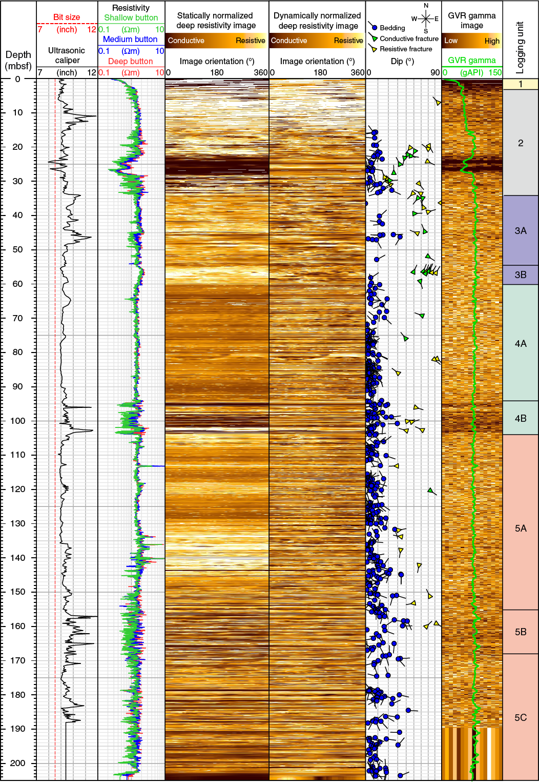
Figure F38. Resistivity image log data.
The nuclear magnetic resonance (NMR) data are of reasonable quality, but the transverse relaxation time (T2) distribution is truncated to values between 1 and 1000 ms (Figure F37). Therefore, not all of the clay-bound water (which ranges typically from 0.3 to 3 ms) is recorded. Additionally, the largest pores in coarse sediments and washouts are recorded as a long T2 peak between 50 and 500 ms, which are probably too low because a T2 of 3000 ms is bulk water; therefore, they should be near 1000 ms, the highest recordable value.
Logging units
The integration and interpretation of the LWD measurements led us to define five well-log units (Figure F37; Table T23) that correspond approximately to the lithostratigraphic units defined for Hole U1517C (Figure F3). Logging units were determined with an accuracy of about ±0.3 m.
Logging Unit 1 (0–3.0 mbsf)
Logging Unit 1 is the recent drape sediments from the seafloor to the top of the landslide in the sediment cores. It is poorly defined in the LWD data because of enlargement of the shallow section of the hole.
Logging Unit 2 (3.0–34.0 mbsf)
Logging Unit 2 is the upper part of the MTD on the TLC (see Log-seismic integration) and is characterized by variable gamma ray, porosity, and resistivity values and NMR T2 distributions. Two washout zones are observed at 10.5–13.5 and 21.5–28 mbsf. The upper washout zone has an NMR porosity close to 1, a caliper log indicative of enlarged borehole conditions, and a bimodal NMR T2 distribution. The deeper washout zone is characterized by low gamma ray and resistivity values, compressional velocity (P-wave) close to seawater values (~1500 m/s), porosity close to 1, and a bimodal NMR T2 distribution. Outside of washed out intervals, resistivity is higher than average for sediments this close to the seafloor, which is typically 1 Ωm or less. This higher resistivity implies porosity is lower than normal in this interval (see Physical properties); porosity measured by neutron porosity is higher than porosity measured on cores, whereas NMR porosity is more accurate and similar to physical properties measurements (see Core-log integration).
Logging Unit 3 (34.0–60.0 mbsf)
Logging Unit 3 is divided into two subunits that compose the bottom of the MTD (see Log-seismic integration). Subunit 3A (34.0–54.6 mbsf) has a more uniform LWD response with in-gauge borehole conditions and fairly constant gamma ray responses and porosity (0.52 for neutron porosity and 0.39 for NMR porosity). LWD measurements in Subunit 3B (54.6–60.0 mbsf) show a consistently higher resistivity (around 2 Ωm) and P-wave velocity (as high as 1740 m/s) and lower porosity (0.45 for neutron porosity and 0.36 for NMR porosity) than the overlying and underlying units, indicating this subunit is more compacted; this compaction was also observed in the cores (see Physical properties). The high resistivity of Subunit 3B is also clearly observed in the statically normalized resistivity image as a lighter color (Figure F38).
Logging Unit 4 (60.0–104.0 mbsf)
Logging Unit 4 (60.0–104.0 mbsf) displays relatively constant gamma ray (near 50 gAPI), porosity (0.57 for neutron porosity and 0.46 for NMR porosity), resistivity (1.3–1.4 Ωm), and P-wave velocity (~1650 m/s) through Subunit 4A (60.0–94.0 mbsf), but all resistivity, P-wave velocity, and gamma ray measurements decrease and porosity increases where washout occurs in Subunit 4B (94.0–104.0 mbsf). Subunit 4A appears in gauge along most of the interval. The NMR T2 distribution is mostly unimodal with all values <33 ms, suggesting only small pore sizes in Subunit 4A. Subunit 4B is washed out, and accordingly resistivity and density decrease and porosity increases, implying this interval is coarser grained sediment than that above. We note that in Hole U1517C cores, the lower part of Unit 4 does not show distinct lithologic changes or physical properties contrasts compared with the upper part (see Lithostratigraphy).
Logging Unit 5 (104.0–205.0 mbsf)
Logging Unit 5 contains three subunits that are mostly fine grained with some coarse-grained thin layers that contain gas hydrate. The upper part of Unit 5 (Subunit 5A; 104.0–155.0 mbsf) is uniform and has a gamma ray response similar to that of Subunit 4A but with slightly lower porosity (0.55 for neutron porosity and 0.45 for NMR porosity) and higher background resistivity (1.5 Ωm). Subunit 5A contains several thin, centimeter- to meter-thick intervals with high resistivity values of ~10 Ωm compared with background values of ~1.5 Ωm and elevated P-wave velocity as high as 1800 m/s compared with background values of around 1700 m/s. Overall, three separate intervals are identified with high resistivity and P-wave velocity, which are related to gas hydrate in the pore space of the sediments.
Subunit 5B (155.0–168.0 mbsf) is characterized by an increase in larger T2 relaxation times and a reduction in gamma ray to ~50 gAPI that indicates an increase in coarser grained thin layers. The borehole size and rugosity increase at 155 mbsf, and borehole quality is poor for the remainder of the hole. The propagation resistivity measurements are less affected by washouts and display background resistivity values of approximately 1.4 Ωm. Porosity values measured in this interval are high compared with Subunit 5A, also reflecting the washout borehole conditions.
Subunit 5C (168.0–205.0 mbsf) is characterized by consistent propagation resistivity measurements of 2 Ωm. Button resistivity measurements also show a closer agreement (although they still vary between 1 and 3 Ωm), and gamma ray indicates slightly more fine grained sediments than Subunit 5B. The P-wave velocity data show great variability, expressed in the LWD data as numerous high-value (as high as 1940 m/s) and low-value (1516 m/s) spikes. Many measurements only cover part of Subunit 5C because of the higher position of tools on the LWD BHA (see Logging while drilling in the Expedition 372A methods chapter [Pecher et al., 2019a]).
Image analysis
Bedding features were identified throughout the imaged interval (Figure F38). In general, we assign a low confidence to most of these features because of horizontal imaging artifacts that obscure bedding and fracture sinusoids. Bedding is mostly shallowly dipping (<10°) with no consistent dip direction. Bright, resistive spots can be observed in the imaged interval, particularly at 51–55, 60–98, and 106–150 mbsf.
A number of fractures were observed, most with a high resistivity in relation to the surrounding material. At ~55 mbsf, a cluster of fractures dipping north-northeast were identified coinciding with the top of an interval of denser, lower porosity material inferred to represent the décollement of the landslide. From 82 to 160 mbsf, a number of resistive fractures were noted, with two very clearly defined at ~82 mbsf and another defined at ~113 mbsf. The resistive fracture at ~113 mbsf could be a layer because it has a lower angle dip.
No stress-induced features such as borehole breakouts and drilling-induced fractures were observed on these resistivity image logs.
Gas hydrate observations on LWD
The first hydrate interval (113 mbsf) is ~30 cm thick and has a resistivity spike of 11.3 Ωm (deep button resistivity) and a spike in P-wave velocity (to 1750 m/s). A small divergence between the neutron and the NMR porosity is observed in this thin interval, with the latter measurement decreasing to 0.39 from background values of ~0.43–0.44.
The second hydrate interval (117.5–121 mbsf) displays scattered, moderately high resistivity as high as 2.6 Ωm (deep button resistivity). This interval has a broadened bimodal NMR T2 distribution and an increased P-wave velocity (1740 m/s).
The third hydrate interval (128–145.5 mbsf) has a slightly higher overall resistivity of 2 Ωm above the background. Superimposed on the region of overall higher resistivity, at least five separate high-resistivity spikes (>3 Ωm) are identified in the central part of this zone (133.5–134, 136–136.2, 136.8–137.5, 139.8–140.4, and 140.9–141.3 mbsf), with a peak resistivity value of 15.7 Ωm (140.2 mbsf; deep button resistivity). The NMR T2 distribution in this interval is variable and displays a bimodal distribution. There is good correlation between the highest peaks in resistivity and the zones with low NMR T2 distributions. NMR porosity diverges from neutron porosity at several of the highest resistivity spikes like it does at 113 mbsf. P-wave velocity is higher compared with background values and displays multiple peaks (as high as 1885 m/s at 139.3 mbsf). Finally, waveforms from the high- and low-frequency monopole sources are highly attenuated in this interval compared with the surroundings (Figure F37).
Gas hydrate saturation
Indication for the presence of gas hydrate was found in both the logging data and cores; therefore, we calibrated Archie parameters and calculated hydrate saturation as described in Logging while drilling in the Expedition 372A methods chapter (Pecher et al., 2019a).
For Hole U1517A, the lithology was found to include very fine grained silt and clay, so determining a clay-free, water-saturated interval for calibrating Archie exponents was nontrivial. Using two different porosity estimations from the NMR porosity log and the thermal neutron porosity log, we determined that a relatively clean interval with a distinct relationship between resistivity and porosity occurred between 50 and 70 mbsf. NMR porosity and neutron porosity logs consistently yielded different porosity measurements at a given depth, so they correspondingly also provide different estimates of the formation factor (Figure F39).
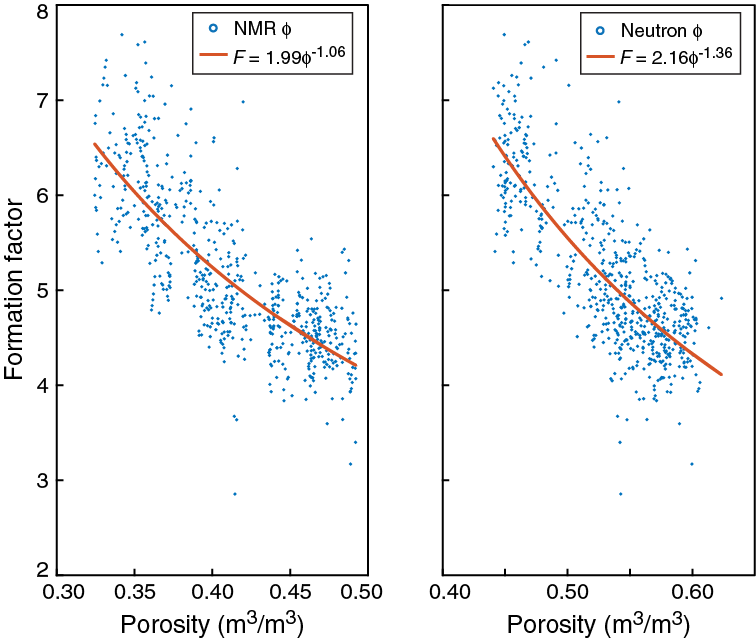
Figure F39. Archie exponent analysis.
Porosity derived from NMR measurements is likely a more accurate estimate of true formation porosity than neutron porosity measurements (see Core-log integration) (Figure F39). However, because gas hydrate in the pore space is a solid phase, protons locked in hydrate lattices relax extremely rapidly, and therefore the NMR log only sees fluid-filled porosity. Because the total formation porosity is required when estimating hydrate saturation using Archie’s equation, we elected to use a formation factor trend derived from neutron porosity. Hydrate saturation is estimated to be proportional to any deviations from the expected formation factor, so this estimate should be valid because models for formation factor and hydrate saturation are self-consistent.
Estimates of hydrate saturation derived from resistivity are summarized in Figure F40. Results from pore water geochemistry and stratigraphy from coring data suggest that hydrate is concentrated in thin intervals (~1–10 cm coarse-grained beds; see Core-log integration), but the vertical resolution of button resistivity, thermal neutron porosity, and NMR porosity measurements are 5–8, 40, and 10 cm, respectively. Therefore, estimating hydrate saturation from this set of well logs using a modified Archie equation averages over a running window of a few tens of centimeters containing discontinuous vertical accumulations of hydrate.
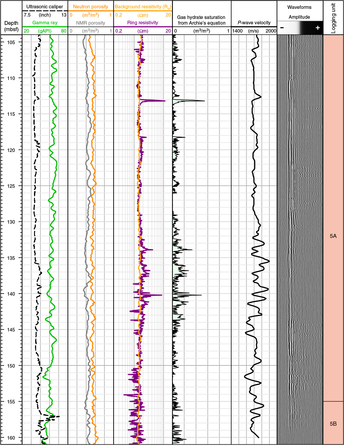
Figure F40. Gas hydrate saturation, Logging Subunit 5A.
As illustrated in Figure F40, two significant hydrate-bearing intervals are indicated by the resistivity and porosity measurements in Logging Unit 5: one thin region from 112 to 114 mbsf with high hydrate saturation (60% of the pore volume) and another, thicker region from approximately 130 to 145 mbsf characterized by lower hydrate saturation (10%–20% of the pore volume). These intervals are likely not continuous accumulations of hydrate but rather average values across high hydrate saturations and water saturated layers.
Safety monitoring
Continuous safety monitoring (see Logging while drilling in the Expedition 372A methods chapter [Pecher et al., 2019a]) was carried out during LWD operations at Site U1517 to monitor for the presence of abnormal pressure or free gas and to ensure safe drilling conditions. Real-time monitoring in Hole U1517A started at 17.2 mbsf and continued to 204.9 mbsf. Observed overpressure generally increased downhole, and the maximum observed overpressure was 0.159 MPa (23 psi). No pressure kicks were observed during drilling.
Core-log integration
LWD data provide a suite of in situ measurements at high resolution but are often at a lower resolution than core measurements. Data from core samples and pore fluids can be used to calibrate LWD measurements and refine their interpretation. By integrating LWD data from Hole U1517A and cores retrieved from Hole U1517C, we compared lithologic indicators (NGR, sonic P-wave velocity, porosity, and bulk density) and independent estimates of gas hydrate accumulation (pore water geochemistry and resistivity-porosity relationships).
Natural gamma ray, porosity, and P-wave velocity
Holes U1517A (LWD) and U1517C (cored) are located 20 m apart. In Hole U1517A, the subsea video camera was used to tag the seafloor at 725.4 mbsl, whereas in Hole U1517C, the mudline measured the seafloor depth at 720.9 mbsl (see Operations). Depending on geological layer dip orientation, lateral variations in differential compaction, deformation, or other lateral lithologic variations, this ~5 m difference in seafloor depth between the two boreholes could impart a ~5 m offset in core data from Hole U1517C relative to LWD data acquired in Hole U1517A.
NGR measurements are typically indicative of lithology, with lower gamma ray readings associated with sandy sediments and higher readings indicating clay-rich sediments. NGR data sets can be used to tie well-log measurements from Hole U1517A to core measurements from Hole U1517C. In the LWD data, gamma ray values decrease to a low value near 20 gAPI between 25 and 28 mbsf, whereas NGR values from the core logger show a low value of about 30 counts/s at 33 mbsf, implying a depth offset between the data sets of 5–8 m (Figure F41).
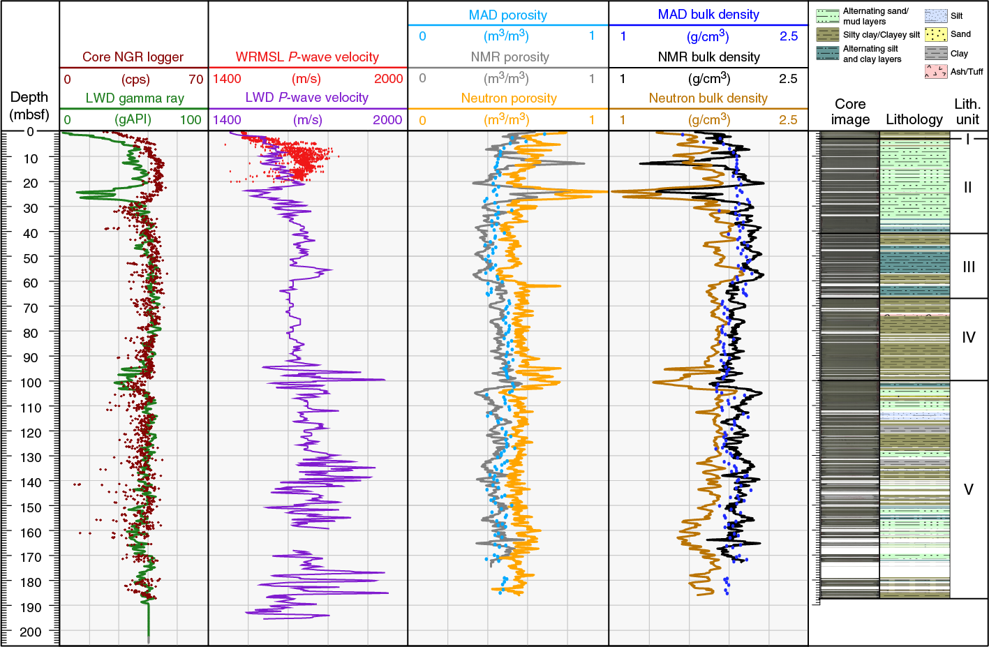
Figure F41. LWD and core NGR, P-wave velocity, porosity, and bulk density.
Porosity measurements show a similar depth discrepancy between LWD and downcore profiles. LWD measurements show a shift toward higher porosity values and lower bulk density values starting at about 59 mbsf, but a similar trend is not seen in core porosity and bulk density measurements until about 66 mbsf, suggesting a 7 m depth offset.
This apparent offset between LWD and core data is not as distinct below ~70 mbsf, which could be due to less significant changes in lithology. The gamma ray values from both LWD data and core NGR measurements correlate well from 40 to 120 mbsf. The range in NGR core measurements increases below 120 mbsf, whereas LWD gamma ray values below 120 mbsf vary less, likely because of the presence of thin, coarse grained beds that are below the measurement resolution of the LWD gamma ray.
Of the three independent measurements of formation porosity, two were obtained from LWD data (NMR and neutron porosity) and one was obtained from core samples (moisture and density [MAD] porosity). As shown in Figure F41, the NMR porosity log most closely matches the measured MAD porosity. The neutron porosity measurements are consistently higher than both the NMR and MAD porosity measurements. Thus, it appears that the NMR log is a closer match to the core-based porosity measurement than the neutron porosity log at this site.
P-wave velocity measurements on core samples were only obtainable for the first 20 m of core because of significant gas expansion effects in deeper intervals. Between 5 and 20 mbsf, P-wave velocity values obtained on core measurements are generally higher than their LWD counterparts. It is likely that borehole washouts affected the LWD P-wave velocity measurements in this interval, and core-based P-wave velocity measurements are probably more accurate.
Gas hydrate saturation estimation
Integration between LWD measurements and core data highlights possible gas hydrate–bearing zones at Site U1517. Highly resistive intervals may be suggestive of mineralization, compaction, hydrocarbon presence, or gas hydrate occurrence. Based on LWD resistivity data in Hole U1517A, we interpret intervals potentially containing gas hydrate accumulations at 113.0–113.3, 117.5–121.0, and 128.0–145.5 mbsf (see Logging while drilling). In these sections, we identify several ~10–100 cm thick, high-resistivity spikes that we interpret to be thin, coarser intervals with high hydrate saturation exceeding 20% pore volume (Figure F42). The increase in resistivity in these hydrate-bearing zones is generally accompanied by an increase in P-wave velocity. Hydrate saturation has been estimated with an Archie approach using ring resistivity and neutron porosity measurements (see Logging while drilling in the Expedition 372A methods chapter [Pecher et al., 2019a]). The results are considered reliable only between 104.0 and 170.0 mbsf because of significant fine-scale heterogeneities and the presence of clay-rich sediments throughout the well.

Figure F42. Neutron porosity and resistivity and IR imaging.
IR thermal imagery was taken on all cores at the time of retrieval as a diagnostic tool to indicate hydrate presence. Endothermic hydrate dissociation tends to cool the immediate area surrounding a dissociating hydrate mass. Sections of retrieved core in which hydrate has dissociated could potentially be anomalously cold relative to core intervals that do not contain hydrate. Therefore, IR thermal imaging was performed on cores immediately after they were recovered to guide sampling and pore water chlorinity measurements (Figure F42). Chlorinity measurements from Hole U1517C detected significant pore water freshening in some samples between 135 and 165 mbsf, with corresponding peak hydrate saturations ranging from 2% to 68% (see Geochemistry).
Core and LWD estimates of hydrate saturation and the most probable intervals of gas hydrate accumulation are comparable, although their predictions of actual hydrate saturation in these intervals somewhat disagree, which is not surprising given the 5–8 m depth offset observed between the holes. Moreover, there were challenges associated with determining a resistivity baseline for resistivity-derived hydrate estimates related to formation heterogeneity and clay content (see Logging while drilling).
Log-seismic integration
LWD data from Hole U1517A reflect the geophysical characteristics of the sedimentary sequence, and cores recovered from Hole U1517C provide detailed lithologic information for the sedimentary sequence from 0 to 187.53 mbsf. The Tuaheni 3-D seismic volume (Mountjoy et al., 2014) ties to Site U1517 at the intersection of In-Line (IL) 1778 and Cross-Line 4225. Here we use a version of IL1778 that was converted from time to depth using a constant velocity of 1700 m/s below the seafloor.
Figure F43 presents an overview of the seismic units in this region. We endeavored to use the same unit designations as defined by the lithostratigraphy and LWD groups (see Lithostratigraphy and Logging while drilling). Seismic unit depths are identical to the logging units defined in Logging while drilling.

Figure F43. Interpreted seismic units on IL1778.
To tie the LWD data to the seismic data, we generated two synthetic seismic traces for Site U1517. One is calculated from partly edited neutron density and sonic VP logs. The second is based on interpretations of the core and downhole log data and uses a log-lithologic model of the main lithostratigraphic units and physical properties. Figure F44 shows the correlation between the LWD and seismic data near Site U1517. Because the seismic line was converted from time to depth using a constant velocity, the depths shown are only approximate. Thus, in the following discussion, the depths presented are determined from the LWD data. Seismic reflections are the result of changes in physical properties caused by changing lithology or the material in the pore space (i.e., seawater, natural gas, or gas hydrate). The seafloor is represented by the high-amplitude, positive reflection with an irregular morphology and offsets as high as 20 m.
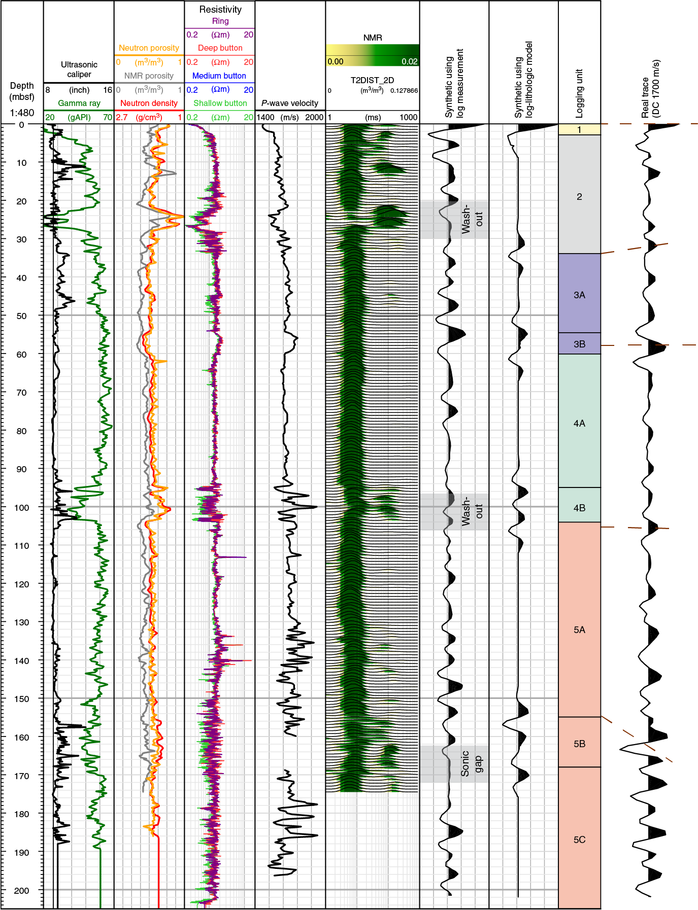
Figure F44. Log-seismic integration.
Seismic Unit 1 (0–3 mbsf)
Seismic Unit 1 (corresponding to Logging Unit 1) is documented by cores in the uppermost 3.0 m of Hole U1517C and cannot be resolved in the seismic data because of the small thickness.
Seismic Unit 2 (3–34 mbsf)
In the seismic data, the base of Seismic Unit 2 is marked by a reflection at about 34.0 mbsf with good lateral continuity throughout the seismic profile. Seismic Unit 2 is interpreted to consist of bedded sand and mud sequences and is characterized on the seismic profile by chaotic reflections of moderate amplitude, with rare high-amplitude segments in the seismic data; this unit is in the upper section of the TLC MTD. The logs exhibit a general increasing trend in gamma ray, resistivity, and P-wave velocity, although the gamma ray curve displays a jagged pattern that may reflect the alternating sand and mud beds described in the lithostratigraphic units.
The seismic data and the synthetic seismogram markers show good correlation, evidencing the main reflections at the seafloor and the lithologic change in the TLC.
Seismic Unit 3 (34–60.0 mbsf)
Seismic Unit 3 consists of clay and silt sequences that make up the lower half of the MTD. Both the top and the base of the unit are delimited by a mostly laterally continuous horizon trackable throughout the seismic data set. The unit gradually thins seaward (Figure F43). At the base of Seismic Unit 3 from 54.6 to 60.0 mbsf (Logging Subunit 3B), P-wave velocity, neutron density, and resistivity increase, indicating a geological control on the physical properties associated with compaction along the detachment interval of the TLC MTD. The increase in both density and velocity at 54.6 mbsf correlates well with the seismic character of Seismic Unit 3, showing the highest amplitude reflections at the base of the unit and matching well with the synthetic seismograms.
Seismic Unit 4 (60–104 mbsf)
Seismic Unit 4 (60.0–104.0 mbsf) underlies the submarine landslide, has a seaward-thinning wedge geometry, and is formed of massive, uniform silty clays characterized by uniform physical properties in the LWD and core log data. The internal reflections in Unit 4 have moderate amplitudes and are generally continuous along the seismic profile. The LWD data from the lower part of Seismic Unit 4 (Subunit 4B; 94.0–104.0 mbsf) show characteristics of increasingly coarser sediments (washouts and opposite-trending bell-shaped curves of the gamma ray and caliper logs), and cores recovered sandy layers from Hole U1517C. The seismic data image this change in physical properties with an increasing reflection amplitude near the base of Seismic Unit 4.
Seismic Unit 5 (104–205 mbsf)
The transition to Seismic Unit 5 is marked by a reflection at ~110 mbsf in the seismic data that commonly onlaps the underlying unit east of the drill site. The onlapping geometry and the irregular morphology suggest that the Seismic Unit 4–5 transition corresponds to an erosional unconformity. Synthetic seismogram curves calculated from the LWD data produce waveforms directly comparable to the reflection pattern in the seismic data, with generally moderate to low amplitudes throughout Seismic Unit 4 and an amplitude increase at its base.
Seismic Unit 5 is characterized by reflections with a clear and constant dip toward the west, although the angle tends to decrease seaward. Resistivity peaks in the LWD data (see Logging while drilling) and information from Hole U1517C cores show indications of gas hydrates (e.g., ~136 mbsf) in the upper part of Seismic Unit 5 (Logging Subunit 5A, 104.0–155.0 mbsf). At 155.0–168.0 mbsf (Logging Subunit 5B), the decrease in P-wave velocity may suggest the presence of gas.
At Site U1517, the seismic data show a continuous high-amplitude BSR that is subparallel to the seafloor, dipping east and crosscutting the regional stratigraphic trends. The BSR that intersects the borehole at ~160 mbsf is an indication of the base of the gas hydrate stability zone because it images the free gas present below it. The synthetic wavelets do not match the BSR depth in the seismic data perfectly, indicating that the velocity model used for the depth conversion is not completely accurate.
Below Logging Subunit 5B, the LWD data and drilled core data from Hole U1517C show an overall decrease in gas but a few thin intervals with increased gas content, a pattern that is supported by the observation of high-amplitude reflections in Seismic Unit 5 (Figure F43).
References
Barnes, P.M., Pecher, I.A., LeVay, L.J., Bourlange, S.M., Brunet, M.M.Y., Cardona, S., Clennell, M.B., Cook, A.E., Crundwell, M.P., Dugan, B., Elger, J., Gamboa, D., Georgiopoulou, A., Greve, A., Han, S., Heeschen, K.U., Hu, G., Kim, G.Y., Kitajima, H., Koge, H., Li, X., Machado, K.S., McNamara, D.D., Moore, G.F., Mountjoy, J.J., Nole, M.A., Owari, S., Paganoni, M., Petronotis, K.E., Rose, P.S., Screaton, E.J., Shankar, U., Shepherd, C.L., Torres, M.E., Underwood, M.B., Wang, X., Woodhouse, A.D., and Wu, H.-Y., 2019a. Expedition 372A summary. In Pecher, I.A., Barnes, P.M., LeVay, L.J., and the Expedition 372A Scientists, Creeping Gas Hydrate Slides. Proceedings of the International Ocean Discovery Program, 372A: College Station, TX (International Ocean Discovery Program). https://doi.org/10.14379/iodp.proc.372A.101.2019
Barnes, P.M., Wallace, L.M., Saffer, D.M., Pecher, I.A., Petronotis, K.E., LeVay, L.J., Bell, R.E., Crundwell, M.P., Engelmann de Oliveira, C.H., Fagereng, A., Fulton, P.M., Greve, A., Harris, R.N., Hashimoto, Y., Hüpers, A., Ikari, M.J., Ito, Y., Kitajima, H., Kutterolf, S., Lee, H., Li, X., Luo, M., Malie, P.R., Meneghini, F., Morgan, J.K., Noda, A., Rabinowitz, H.S., Savage, H.M., Shepherd, C.L., Shreedharan, S., Solomon, E.A., Underwood, M.B., Wang, M., Woodhouse, A.D., Bourlange, S.M., Brunet, M.M.Y., Cardona, S., Clennell, M.B., Cook, A.E., Dugan, B., Elger, J., Gamboa, D., Georgiopoulou, A., Han, S., Heeschen, K.U., Hu, G., Kim, G.Y., Koge, H., Machado, K.S., McNamara, D.D., Moore, G.F., Mountjoy, J.J., Nole, M.A., Owari, S., Paganoni, M., Rose, P.S., Screaton, E.J., Shankar, U., Torres, M.E., Wang, X., and Wu, H.-Y., 2019b. Site U1520. In Wallace, L.M., Saffer, D.M., Barnes, P.M., Pecher, I.A., Petronotis, K.E., LeVay, L.J., and the Expedition 372/375 Scientists, Hikurangi Subduction Margin Coring, Logging, and Observatories. Proceedings of the International Ocean Discovery Program, 372B/375: College Station, TX (International Ocean Discovery Program). https://doi.org/10.14379/iodp.proc.372B375.105.2019
Claypool, G.E., and Kvenvolden, K.A., 1983. Methane and other hydrocarbon gases in marine sediment. Annual Review of Earth and Planetary Sciences, 11(1):299–327. https://doi.org/10.1146/annurev.ea.11.050183.001503
Coffin, R.B., Hamdan, L.J., Smith, J.P., Rose, P.S., Plummer, R.E., Yoza, B., Pecher, I., and Montgomery, M.T., 2014. Contribution of vertical methane flux to shallow sediment carbon pools across Porangahau Ridge, New Zealand. Energies, 7(8):5332–5356. https://doi.org/10.3390/en7085332
Crundwell, M., Scott, G., Naish, T., and Carter, L., 2008. Glacial–interglacial ocean climate variability from planktonic foraminifera during the Mid-Pleistocene transition in the temperate Southwest Pacific, ODP Site 1123. Palaeogeography, Palaeoclimatology, Palaeoecology, 260(1-2): 202–229. https://doi.org/10.1016/j.palaeo.2007.08.023
Duan, Z., and Mao, S., 2006. A thermodynamic model for calculating methane solubility, density and gas phase composition of methane-bearing aqueous fluids from 273 to 523 K and from 1 to 2000 bar. Geochimica et Cosmochimica Acta, 70(13):3369–3386. https://doi.org/10.1016/j.gca.2006.03.018
Expedition 311 Scientists, 2006. Expedition 311 summary. In Riedel, M., Collett, T.S., Malone, M.J., and the Expedition 311 Scientists, Proceedings of the Integrated Ocean Drilling Program, 311: Washington, DC (Integrated Ocean Drilling Program Management International, Inc.). https://doi.org/10.2204/iodp.proc.311.101.2006
Froelich, P.N., Klinkhammer, G.P., Bender, M.L., Luedtke, N.A., Heath, G.R., Cullen, D., Dauphin, P., Hammond, D., Hartman, B., and Maynard, V., 1979. Early oxidation of organic matter in pelagic sediments of the eastern equatorial Atlantic: suboxic diagenesis. Geochimica et Cosmochimica Acta, 43(7):1075–1090. https://doi.org/10.1016/0016-7037(79)90095-4
Gradstein, F.M., Ogg, J.G., Schmitz, M.D., and Ogg, G.M. (Eds.), 2012. The Geological Time Scale 2012: Amsterdam (Elsevier). https://doi.org/10.1016/C2011-1-08249-8
Greinert, J., Lewis, K.B., Bialas, J., Pecher, I.A., Rowden, A., Bowden, D.A., De Batist, M., and Linke, P., 2010. Methane seepage along the Hikurangi margin, New Zealand: overview of studies in 2006 and 2007 and new evidence from visual, bathymetric and hydroacoustic investigations. Marine Geology, 272(1–4):6–25. https://doi.org/10.1016/j.margeo.2010.01.017
Gross, F., Mountjoy, J.J., Crutchley, G.J., Böttner, C., Koch, S., Bialas, J., Pecher, I., et al., 2018. Free gas distribution and basal shear zone development in a subaqueous landslide—insight from 3D seismic imaging of the Tuaheni Landslide Complex, New Zealand. Earth and Planetary Science Letters, 502:231–243. https://doi.org/10.1016/j.epsl.2018.09.002
Henrys, S.A., Ellis, S., and Uruski, C., 2003. Conductive heat flow variations from bottom-simulating reflectors on the Hikurangi margin, New Zealand. Geophysical Research Letters, 30(2):1065. https://doi.org/10.1029/2002GL015772
Huhn, K., 2016. DSRV Sonne SO247 Cruise Report—SlamZ: slide activity on the Hikurangi margin, New Zealand, Wellington–Auckland, 27 March–27 April 2016. Bundesministerium für Bildung und Forschung. https://www.portal-forschungsschiffe.de/lw_resource/datapool/_items/item_183/fahrtbericht_so247.pdf
Kim, J.-H., Torres, M.E., Haley, B.A., Ryu, J.-S., Park, M.-H., Hong, W.-L., and Choi, J., 2016. Marine silicate weathering in the anoxic sediment of the Ulleung Basin: evidence and consequences. Geochemistry, Geophysics, Geosystems, 17(8):3437–3453. https://doi.org/10.1002/2016GC006356
Liu, Q., Roberts, A.P., Larrasoaña, J.C., Banerjee, S.K., Guyodo, Y., Tauxe, L., and Oldfield, F., 2012. Environmental magnetism: principles and applications. Reviews of Geophysics, 50(4):RG4002. https://doi.org/10.1029/2012RG000393
MacMahon, J., 2016. High-resolution velocity analysis of seismic data to identify gas hydrates in the Tuaheni Landslide Complex on the Hikurangi margin, New Zealand [M.S. thesis]. University of Auckland, New Zealand. http://hdl.handle.net/2292/28209
Malinverno, A., Kastner, M., Torres, M.E., and Wortmann, U.G., 2008. Gas hydrate occurrence from pore water chlorinity and downhole logs in a transect across the northern Cascadia margin (Integrated Ocean Drilling Program Expedition 311). Journal of Geophysical Research: Solid Earth, 113(B8):B08103. https://doi.org/10.1029/2008JB005702
Martini, E., 1971. Standard Tertiary and Quaternary calcareous nannoplankton zonation. In Farinacci, A. (Ed.), Proceedings of the Second Planktonic Conference, Roma 1970: Rome (Edizioni Tecnoscienza), 2:739–785.
Mountjoy, J., Krastel, S., Crutchley, G., Dannonski, A., Graw, M., Koch, S., Micallef, A., Quinn, W., and Woelz, S., 2014a. NIWA Voyage Report TAN1404: SCHLIP-3D: submarine clathrate hydrate landslide imaging project: Auckland, New Zealand (National Institute of Water and Atmospheric Research).
Mountjoy, J.J., Pecher, I., Henrys, S., Crutchley, G., Barnes, P.M., and Plaza-Faverola, A., 2014b. Shallow methane hydrate system controls ongoing, downslope sediment transport in a low-velocity active submarine landslide complex, Hikurangi margin, New Zealand. Geochemistry, Geophysics, Geosystems, 15(11):4137–4156. https://doi.org/10.1002/2014GC005379
Paull, C.K., and Ussler, W., III, 2001. History and significance of gas sampling during DSDP and ODP drilling associated with gas hydrates. In Paull, C.K., and Dillon, W.P. (Eds.), Natural Gas Hydrates: Occurrence, Distribution, and Detection. Geophysical Monograph, 124:53–66. https://doi.org/10.1029/GM124p0053
Pecher, I.A., Barnes, P.M., LeVay, L.J., Bourlange, S.M., Brunet, M.M.Y., Cardona, S., Clennell, M.B., Cook, A.E., Crundwell, M.P., Dugan, B., Elger, J., Gamboa, D., Georgiopoulou, A., Greve, A., Han, S., Heeschen, K.U., Hu, G., Kim, G.Y., Kitajima, H., Koge, H., Li, X., Machado, K.S., McNamara, D.D., Moore, G.F., Mountjoy, J.J., Nole, M.A., Owari, S., Paganoni, M., Petronotis, K.E., Rose, P.S., Screaton, E.J., Shankar, U., Shepherd, C.L., Torres, M.E., Underwood, M.B., Wang, X., Woodhouse, A.D., and Wu, H.-Y., 2019a. Expedition 372A methods. In Pecher, I.A., Barnes, P.M., LeVay, L.J., and the Expedition 372A Scientists, Creeping Gas Hydrate Slides. Proceedings of the International Ocean Discovery Program, 372A: College Station, TX (International Ocean Discovery Program). https://doi.org/10.14379/iodp.proc.372A.102.2019
Pecher, I.A., Barnes, P.M., LeVay, L.J., and the Expedition 372A Scientists, 2019b. Supplementary material, https://doi.org/10.14379/iodp.proc.372Asupp.2019. Supplement to Pecher, I.A., Barnes, P.M., LeVay, L.J., and the Expedition 372A Scientists, Creeping Gas Hydrate Slides. Proceedings of the International Ocean Discovery Program, 372A: College Station, TX (International Ocean Discovery Program). https://doi.org/10.14379/iodp.proc.372A.2019
Pimmel, A., and Claypool, G., 2001. Technical Note 30: Introduction to Shipboard Organic Geochemistry on the JOIDES Resolution. Ocean Drilling Program. https://doi.org/10.2973/odp.tn.30.2001
Saffer, D.M., Wallace, L.M., Barnes, P.M., Pecher, I.A., Petronotis, K.E., LeVay, L.J., Bell, R.E., Crundwell, M.P., Engelmann de Oliveira, C.H., Fagereng, A., Fulton, P.M., Greve, A., Harris, R.N., Hashimoto, Y., Hüpers, A., Ikari, M.J., Ito, Y., Kitajima, H., Kutterolf, S., Lee, H., Li, X., Luo, M., Malie, P.R., Meneghini, F., Morgan, J.K., Noda, A., Rabinowitz, H.S., Savage, H.M., Shepherd, C.L., Shreedharan, S., Solomon, E.A., Underwood, M.B., Wang, M., Woodhouse, A.D., Bourlange, S.M., Brunet, M.M.Y., Cardona, S., Clennell, M.B., Cook, A.E., Dugan, B., Elger, J., Gamboa, D., Georgiopoulou, A., Han, S., Heeschen, K.U., Hu, G., Kim, G.Y., Koge, H., Machado, K.S., McNamara, D.D., Moore, G.F., Mountjoy, J.J., Nole, M.A., Owari, S., Paganoni, M., Rose, P.S., Screaton, E.J., Shankar, U., Torres, M.E., Wang, X., and Wu, H.-Y., 2019. Site U1518. In Wallace, L.M., Saffer, D.M., Barnes, P.M., Pecher, I.A., Petronotis, K.E., LeVay, L.J., and the Expedition 372/375 Scientists, Hikurangi Subduction Margin Coring, Logging, and Observatories. Proceedings of the International Ocean Discovery Program, 372B/375: College Station, TX (International Ocean Discovery Program). https://doi.org/10.14379/iodp.proc.372B375.103.2019
Shipboard Scientific Party, 2003. Leg 204 summary. In Tréhu, A.M, Bohrmann, G., Rack, F.R., Torres, M.E., et al., Proceedings of the Ocean Drilling Program, Initial Reports, 204: College Station, TX (Ocean Drilling Program), 1–75. https://doi.org/10.2973/odp.proc.ir.204.101.2003
Solomon, E.A., Spivack, A.J., Kastner, M., Torres, M.E., and Robertson, G., 2014. Gas hydrate distribution and carbon sequestration through coupled microbial methanogenesis and silicate weathering in the Krishna–Godavari Basin, offshore India. Marine and Petroleum Geology, 58(A):233–253. https://doi.org/10.1016/j.marpetgeo.2014.08.020
Torres, M.E., Brumsack, H.-J., Bohrmann, G., and Emeis, K.C., 1996. Barite fronts in continental margin sediments: a new look at barium remobilization in the zone of sulfate reduction and formation of heavy barites in diagenetic fronts. Chemical Geology, 127(1–3):125–139. https://doi.org/10.1016/0009-2541(95)00090-9
Torres, M.E., Tréhu, A.M., Cespedes, N., Kastner, M., Wortmann, U.G., Kim, J.-H., Long, P., Malinverno, A., Pohlman, J.W., Riedel, M., and Collett, T., 2008. Methane hydrate formation in turbidite sediments of northern Cascadia, IODP Expedition 311. Earth and Planetary Science Letters, 271(1–4):170–180. https://doi.org/10.1016/j.epsl.2008.03.061
Townend, J., 1997. Estimates of conductive heat flow through bottom-simulating reflectors on the Hikurangi and southwest Fiordland continental margins, New Zealand. Marine Geology, 141(1–4):209–220. https://doi.org/10.1016/S0025-3227(97)00073-X
Wallmann, K., Aloisi, G., Haeckel, M., Tishchenko, P., Pavlova, G., Greinert, J., Kutterolf, S., and Eisenhauer, A., 2008. Silicate weathering in anoxic marine sediments. Geochimica et Cosmochimica Acta, 72(12):2895–2918. https://doi.org/10.1016/j.gca.2008.03.026
Wild, J.J., 2016. Seismic velocities beneath creeping gas hydrates slides: analysis of ocean bottom seismometer data in the Tuaheni Landslide Complex on the Hikurangi margin, New Zealand [M.S. thesis]. University of Auckland, New Zealand. http://hdl.handle.net/2292/30188
1 Barnes, P.M., Pecher, I.A., LeVay, L.J., Bourlange, S.M., Brunet, M.M.Y., Cardona, S., Clennell, M.B., Cook, A.E., Crundwell, M.P., Dugan, B., Elger, J., Gamboa, D., Georgiopoulou, A., Greve, A., Han, S., Heeschen, K.U., Hu, G., Kim, G.Y., Kitajima, H., Koge, H., Li, X., Machado, K.S., McNamara, D.D., Moore, G.F., Mountjoy, J.J., Nole, M.A., Owari, S., Paganoni, M., Petronotis, K.E., Rose, P.S., Screaton, E.J., Shankar, U., Shepherd, C.L., Torres, M.E., Underwood, M.B., Wang, X., Woodhouse, A.D., and Wu, H.-Y., 2019. Site U1517. In Pecher, I.A., Barnes, P.M., LeVay, L.J., and the Expedition 372A Scientists, Creeping Gas Hydrate Slides. Proceedings of the International Ocean Discovery Program, 372A: College Station, TX (International Ocean Discovery Program). https://doi.org/10.14379/iodp.proc.372A.103.2019
2 Expedition 372A Scientists’ affiliations.
This work is distributed under the Creative Commons Attribution 4.0 International (CC BY 4.0) license. 