de Ronde, C.E.J., Humphris, S.E., Höfig, T.W., and the Expedition 376 Scientists
Proceedings of the International Ocean Discovery Program Volume 376
publications.iodp.org

https://doi.org/10.14379/iodp.proc.376.102.2019
Expedition 376 methods1
C.E.J. de Ronde, S.E. Humphris, T.W. Höfig, P.A. Brandl, L. Cai, Y. Cai, F. Caratori Tontini, J.R. Deans, A. Farough, J.W. Jamieson, K.P. Kolandaivelu, A. Kutovaya, J.M. Labonté, A.J. Martin, C. Massiot, J.M. McDermott, I.M. McIntosh, T. Nozaki, V.H. Pellizari, A.G. Reyes, S. Roberts, O. Rouxel, L.E.M. Schlicht, J.H. Seo, S.M. Straub, K. Strehlow, K. Takai, D. Tanner, F.J. Tepley III, and C. Zhang2
Keywords: International Ocean Discovery Program, IODP, JOIDES Resolution, Expedition 376, Brothers Arc Flux, Brothers volcano, Site U1527, Site U1528, Site U1529, Site U1530, Site U1531, Kermadec arc, submarine arc volcano, hydrothermal systems, volcaniclastics, dacite lava, hydrothermal alteration, borehole fluids, hypersaline brine, fluid inclusions, acidic fluids, alteration mineral assemblages, Upper Cone, Lower Cone, NW Caldera
MS 376-102: Published 5 July 2019
Introduction
This chapter documents the procedures and methods employed in the various shipboard laboratories on the R/V JOIDES Resolution during International Ocean Discovery Program (IODP) Expedition 376. This information applies only to shipboard work described in the Expedition reports section of the Expedition 376 Proceedings of the International Ocean Discovery Program volume, which used the shipboard sample registry, imaging and analytical instruments, core description tools, and Laboratory Information Management System (LIMS) database. Methods for shore-based analysis of Expedition 376 samples and data will be described in the individual peer-reviewed scientific contributions to be published in the Expedition research results section of this volume and in international scientific journals and books.
All shipboard scientists contributed in various ways to this volume with the following primary responsibilities (authors are listed in alphabetical order; see Expedition 376 scientists for contact information):
- Summary chapter: Expedition 376 Scientists
- Methods and site chapters:
- Background and objectives: de Ronde and Humphris
- Introduction/Operations: de Ronde, Höfig, Humphris, and Operations Superintendent Midgley
- Igneous petrology and volcanology: Brandl, Seo, Straub, Strehlow, Tanner, and Tepley
- Alteration: Y. Cai, Jamieson, Martin, Nozaki, Reyes, Roberts, Schlicht, and Zhang
- Geochemistry: Kutovaya, McDermott, Rouxel, and Straub
- Structural geology: Deans
- Petrophysics (core and downhole): Farough, Kolandaivelu, Massiot, McIntosh, and Reyes
- Paleomagnetism: Caratori Tontini
- Microbiology: L. Cai, Labonté, Pellizari, and Takai
This introductory section covers methods and procedures that apply to most or all of the shipboard laboratory groups. Subsequent sections describe detailed methods used by each laboratory group.
Sites and holes
GPS coordinates from precruise site surveys were used for the general position of the vessel at Expedition 376 sites. Markers were deployed previously by remotely operated vehicles on the seafloor at the three primary sites and three of the four alternate sites at Brothers volcano. A SyQwest Bathy 2010 CHIRP subbottom profiler was used to monitor the seafloor depth during the approach to the site to reconfirm the depth profiles from precruise surveys. Once the vessel was positioned at the site, a camera survey was conducted to locate the marker, to ensure no proximal animal communities were present, and to confirm suitable locations for spudding several holes, should they be needed (Table T1). A positioning beacon was deployed on the seafloor only at Site U1527. While on site, ship location over the hole was maintained using the Neutronics 5002 dynamic positioning (DP) system on the JOIDES Resolution. DP control of the vessel used navigational input from the GPS (and triangulation to the seafloor beacon at Site U1527). The final hole position was the mean position calculated from the GPS data collected over a significant portion of the time the hole was occupied.
The site was numbered according to the series that began with the first site drilled by the Deep Sea Drilling Project D/V Glomar Challenger in 1968. Starting with Integrated Ocean Drilling Program Expedition 301, the prefix “U” designates sites occupied by the JOIDES Resolution. For all IODP drill sites, a letter suffix distinguishes each hole drilled at the same site. The first hole drilled is assigned the site number modified by the suffix “A,” the second hole takes the site number and the suffix “B,” and so forth. During Expedition 376, five sites were drilled: Site U1527 (Holes U1527A–U1527C), Site U1528 (Holes U1528A–U1528D), Site U1529 (Holes U1529A and U1529B), Site U1530 (Hole U1530A), and Site U1531 (Holes U1531A–U1531E).
Drilling and coring operations
The drilling strategy for Expedition 376 was to drill, core, and log three primary sites: one situated on the northwest rim of the caldera at Brothers volcano, another on the floor of the caldera near the western caldera wall, and a third at the summit of the Upper Cone. Operations at each site began with attempts to drill a pilot hole to ascertain conditions for casing. Except at Site U1530, these attempts were followed by the deployment of casing of different lengths (depending on the site conditions) and an attached reentry funnel drilled-in using a mud motor and underreamer. We used the rotary core barrel (RCB) system for all of the drilling and coring except for two brief tests of a prototype turbine-driven coring system (TDCS) brought on board by Center for Deep Earth Exploration (CDEX) engineers. The RCB system is the most conventional rotary coring system and is suitable for lithified rock. It cuts a core as long as 9.5 m with a nominal diameter of 5.87 cm. RCB coring can be conducted with or without core liners. Liners are sometimes omitted with the RCB system in an attempt to prevent core pieces from getting caught at the edge of the liner, which could lead to a jam and lack of recovery. During Expedition 376, plastic liners were used for all of the cores. Nonmagnetic core barrels were used throughout.
The bottom-hole assembly (BHA) is the lowermost part of the drill string and is configured to provide appropriate strength and tension in the drill string. A typical RCB BHA consists of a 9⅞ inch (~25.1 cm) drill bit, a bit sub, an outer core barrel, a top sub, a head sub, ten stands of 8¼ inch (~21.0 cm) drill collars, a tapered drill collar, two stands of standard 5.5 inch (~14.0 cm) drill pipe, and a crossover sub to the regular 5 inch (~12.7 cm) drill pipe.
During most IODP expeditions, cored intervals are 9.6–9.8 m long, which is the length of a core barrel. The length of the recovered core varies based on a number of factors. In igneous rock, the length of the recovered core is typically less than the cored interval. A common cause of poor recovery is core jamming in the bit or in the throat of the core barrel, which prevents additional core from entering the core barrel. This problem can be partly mitigated by extracting cores at shorter coring intervals; half cores were collected during Expedition 376 in all holes after two or three full-length cores were extracted following initial spud-in of the holes.
Cored intervals may not be contiguous if separated by intervals drilled but not cored. Drilling ahead without coring may be necessary or desired because certain intervals are hard or impossible to recover or need to be reamed to the diameter required for coring or because the cored interval is set to target a specific stratigraphic interval. For example, during Expedition 376, we drilled ahead without coring using a tricone bit for a 22 m interval from the seafloor in Hole U1528C (see Operations in the Site U1528 chapter [de Ronde et al., 2019a]). Holes thus consist of a sequence of cored and drilled intervals, or advancements. These advancements are numbered sequentially from the top of the hole downward. Numbers assigned to physical cores recovered correspond to advancements and may not be consecutive.
Recovery rates for each core were calculated based on the total length of a core recovered divided by the length of the cored interval (see Core curatorial procedures and sampling). In igneous rocks, recovery rates are typically <100%.
Core curatorial procedures and sampling
Whole-round section preparation
To minimize contamination of the core with platinum group elements and gold, all personnel handling and describing the cores or other sample material removed jewelry and wore nitrile gloves.
Cores recovered in core liners were extracted from the core barrel by rig personnel and carried to the catwalk by JOIDES Resolution Science Operator (JRSO) technicians. Technicians cut the liner and the core, if necessary, into ~1.5 m long sections. The sections were temporarily secured with blue and colorless liner end caps to denote top and bottom, respectively, a convention that was used throughout the curation process. The sections were transferred to the core splitting room, where the core liners were emptied and the pieces were transferred into split core liners for processing.
In cases where core recovery was minimal (i.e., a few small fragments), JRSO technicians waited with a 1.5 m long presplit core liner at the end of the catwalk. Once the core barrel was lowered horizontally, each rock piece was removed from the core barrel one by one and placed in consecutive order in the split plastic liner (Figure F1). If a core catcher sample was present, it was taken to the splitting area separately and added to the bottom section of the recovered core. Once all core material was removed from the core barrel, the split liner sections were transferred to the core splitting area, where the pieces were transferred into split core liners, this time from top to bottom for processing.
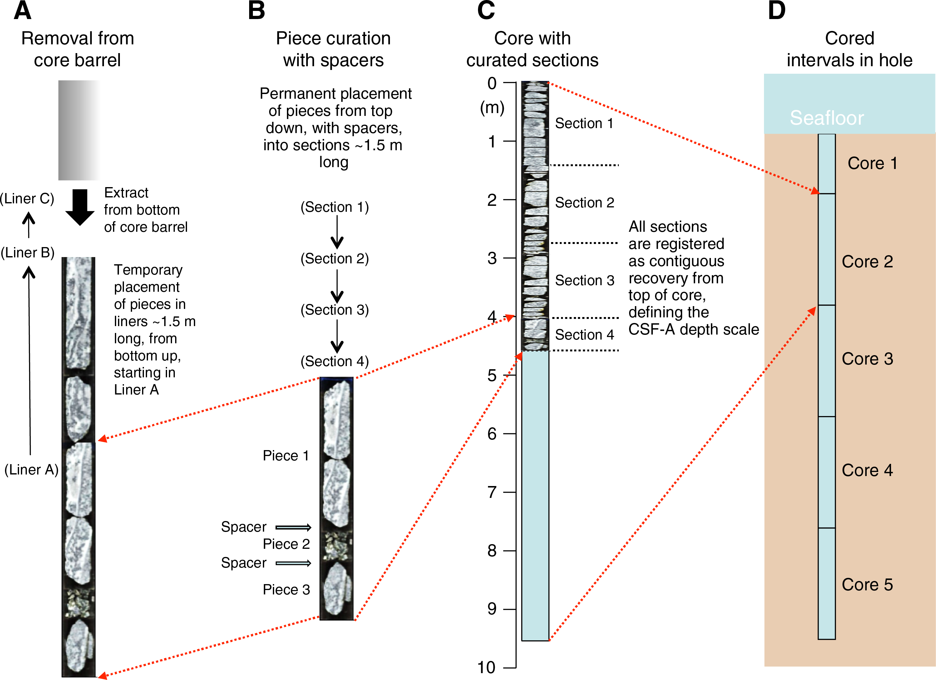
Figure F1. Core handling.
The total length of all rock material in each section was measured and entered into the SampleMaster application as recovered length. The sum of all recovered lengths in a core was used to compute core recovery as a percentage of the cored interval.
Microbiology samples were taken from selected pieces according to the expedition sampling plan under supervision of the assigned Sample Allocation Committee (SAC) representative. Only the necessary 4–5 people wearing face masks and nitrile gloves were in the room for microbiology sampling to minimize contamination, and the samples were immediately transferred to the microbiology preparation laboratory (see Microbiology for information on microbiology sample handling and preparation).
Plastic dividers made from core liner caps were then inserted between core pieces to keep them in place for curation. The spacers may represent substantial intervals of no recovery, to the point of creating a curated core that is longer than the cored interval (see Depth computations). Adjacent core pieces that could be fitted together along fractures, or where other continuous features were observed (e.g., volcanic clast or fabric), were curated as single pieces. JRSO personnel marked the bottom of all oriented pieces (i.e., pieces with a greater length than diameter; approximately >5 cm). Core pieces that appeared susceptible to crumbling were encased in shrink-wrap.
At least one designated scientist (usually the structural geologist) then checked and approved the binning and reconstruction of fractured pieces. The scientist marked a splitting line on each piece with a wax pencil so that the piece could be split into representative working and archive halves, ideally maximizing the expression of dipping structures on the cut face of the core while maintaining representative features in both archive and working halves. To ensure a consistent protocol for whole-core imaging, the splitting line was drawn so that the working half was on the right side of the line looking in the upcore direction. The working half of each piece was marked with a “W” to the right of the splitting line (Figure F2). Where magmatic/volcanic fabrics or crystal-plastic fabrics (CPFs) were present, cores were marked for splitting with the fabric dipping east (090°) or west (270°) in the IODP core reference frame (CRF) (see Core reference frame for sample orientation) (Figure F2). This protocol was sometimes overridden by the presence of specific features (e.g., mineralized areas, filled vugs, or veins) that were divided between the archive and working halves to ensure preservation and/or allow shipboard or postcruise sampling.
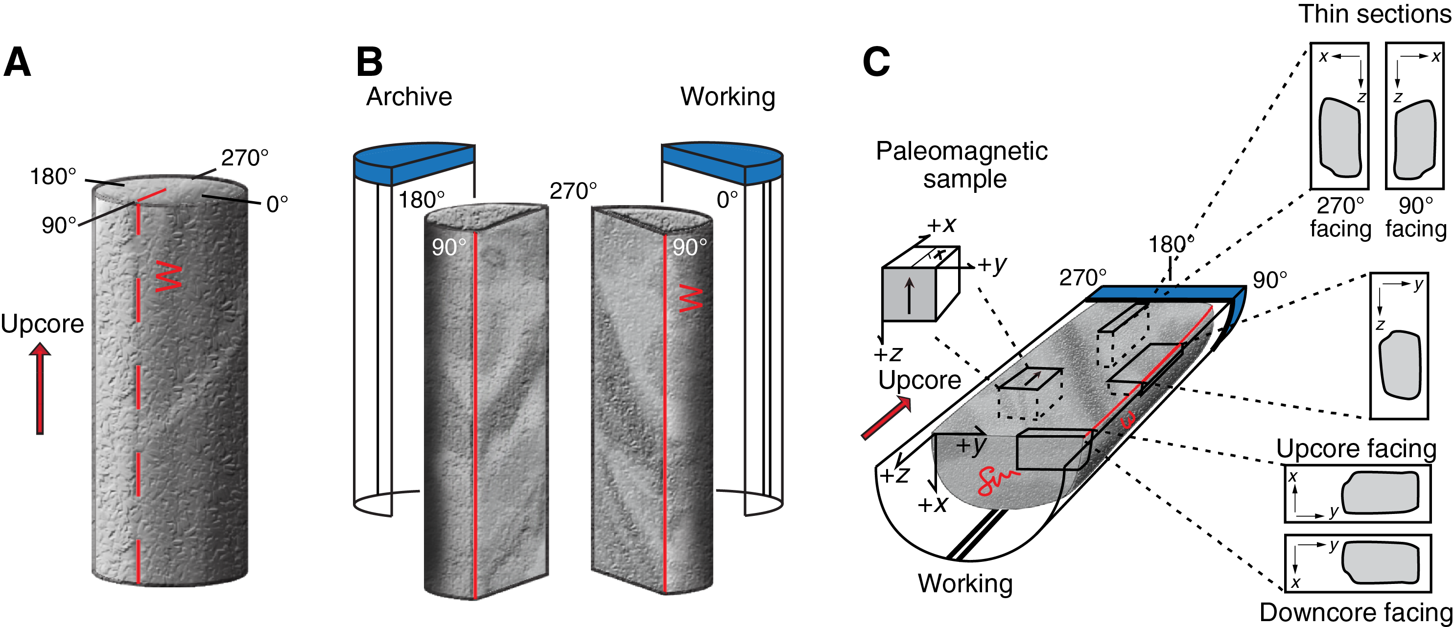
Figure F2. CRF for structural and paleomagnetic orientation measurements.
Once the split line was drawn, JRSO technical personnel secured the plastic spacers permanently with acetone between individual pieces into matching working and archive half split-core liners. Spacers were mounted into the liners with the angle brace facing uphole. This spacing ensured that the top of each piece had the same depth as the top of the curated interval for each bin. The top and bottom offsets of each bin were entered into SampleMaster. Based on the calculated bin lengths, the cumulative length of all bins, including spacers, was computed as the curated length of the section (Figure F1). The empty split liner with spacers glued in was then placed over the split liner containing the pieces, and the two halves were taped together in a few places for temporary storage until core pieces were dry and equilibrated to laboratory conditions (usually ~2 h after arrival from the catwalk).
Whole-round section measurements
Once the core sections were deemed thermally equilibrated, the following whole-round measurements were taken:
- Whole-round surface imaging (i.e., four surface quarter image scans orthogonal to angles of 000°, 090°, 180°, and 270° relative to the CRF) using the Section Half Imaging Logger (SHIL) configured for whole-round sections;
- Logging using the Whole-Round Multisensor Logger (WRMSL) with the magnetic susceptibility loop (MSL) sensor, the gamma ray attenuation (GRA) detector, and the P-wave velocity logger (PWL); and
- Natural gamma radiation (NGR) logging using the Natural Gamma Radiation Logger (NGRL) when the length of an individual section was >40 cm.
P-wave velocity measurements using the P-wave caliper (PWC) were also made on discrete whole-round pieces of fractured hard rock cores (that could not be measured using the PWL), which were then returned to the whole-round core prior to splitting. See Physical properties for further discussion of these measurements.
Section-half preparation
After the completion of whole-round measurements, each piece of core was split into archive and working halves with the positions of plastic spacers between pieces maintained in both halves. Piece halves were labeled sequentially from the top of each section, beginning with number 1 (Figure F1). Pieces were labeled only on the outer cylindrical surfaces of the core with a plastic label sealed with epoxy.
Archive-half measurements
The following archive-half measurements were taken:
- Imaging of the dry faces of archive halves using the SHIL;
- Automated compilation of a core composite image in which all sections of a core are displayed next to each other in a one-page layout;
- Logging using the Section Half Multisensor Logger (SHMSL) with reflectance spectroscopy and colorimetry (RSC) and the point magnetic susceptibility (MSP) contact probe (see Physical properties);
- Macroscopic core description using the DESClogik data capture program (see Igneous petrology and volcanology, Alteration, and Structural geology);
- Remanent magnetization logging using the superconducting rock magnetometer (SRM) (see Paleomagnetism);
- Close-up images of particular features for illustrations in the summary of each site, as requested by individual scientists; and
- Handheld portable X-ray fluorescence (pXRF) measurements on some core pieces and on crushed rock powders (see Igneous petrology and volcanology and Geochemistry).
Working-half sampling and measurements
The following working-half samples and measurements were taken:
- Dry faces of working halves were imaged using the SHIL and also logged using the SHMSL for RSC and MSP.
- Thin section billets (TSBs) were cut to prepare thin sections for microscopic observations (see Igneous petrology and volcanology, Alteration, and Structural geology).
- Cube samples (~8 cm3) were taken and shared for paleomagnetism measurements, moisture and density (MAD) tests, and P-wave velocity measurements using the PWC mounted on the Section Half Measurement Gantry (SHMG) (see Paleomagnetism and Physical properties).
- Slabs or chips were taken and powdered for inductively coupled plasma–atomic emission spectroscopy (ICP-AES), total carbon-nitrogen-sulfur (CNS) elemental analyzer (EA) tests, carbonate-associated carbon contents, loss on ignition (LOI), and pXRF measurements (see Geochemistry and Igneous petrology and volcanology).
- Fragments were scraped off or chips were taken and powdered for X-ray diffraction (XRD) analyses (see Igneous petrology and volcanology and Alteration).
Samples for shore-based research
Samples for postcruise analyses were taken from the working halves for individual investigators based on requests approved by the SAC. Four sampling parties were held for (1) Sites U1527 and U1529, (2) Site U1528, (3) Site U1530, and (4) Site U1531. For each sampling party, all cores from the designated sites were laid out across the entire core deck and sampled. Scientists viewed the cores, flagged sampling locations, and submitted detailed lists of requested samples. The SAC reviewed the flagged samples and resolved any conflicts as needed. Shipboard staff cut, registered, and packed the samples. A total of 2377 samples was taken for shore-based analyses in addition to the 1563 samples taken for shipboard analysis.
Rock samples were sealed in plastic vials or bags and labeled, and fluid and microbial samples were preserved in suitable sampling vessels (see Geochemistry and Microbiology). Each sample cut from the working half was logged into the LIMS database using SampleMaster, including the sample type and either the shipboard analysis (test) conducted on the sample or the name of the investigator receiving the sample for postcruise analysis. Records of all samples taken from the cores are accessible online in the LIMS database at Sample report under Curation and samples (http://web.iodp.tamu.edu/LORE).
Final sample storage
Following shipboard initial scientific observations, measurements, and sampling, both core halves were shrink-wrapped in plastic to prevent rock pieces from moving out of sequence during transit. Working and archive halves were then put into labeled plastic tubes, sealed, and transferred to cold-storage space aboard the drilling vessel. At the end of Expedition 376, cores were transferred from the ship to the Kochi Core Center (Japan) for permanent storage.
Sample identification
Sample names are computer-generated constructs of multiple pieces of information registered in the LIMS database during the course of the various sampling and curation processes that follow specific rules. Understanding the three concepts (text ID, label ID, and printed labels) in use may help users enter the correct information into SampleMaster to find samples of interest using the available filters in the LIMS Reports applications.
Text ID
Samples taken on the JOIDES Resolution are uniquely identified for use by software applications using the text ID, which combines two elements:
- The sample type designation (e.g., SHLF for section half) and
- A unique sequential number for any sample and sample type added to the sample type code (e.g., SHLF30495837).
The text ID is not particularly helpful to most users. For a more process-oriented comprehensible sample naming convention, the label ID links a number of parameters, according to specific rules.
Label ID
The label ID is used throughout JOIDES Resolution workflows as a convenient, comprehensible sample identification and nomenclature. The label ID is made up of two parts: primary sample identifier and sample name. Label IDs are not necessarily unique.
Primary sample identifier
The primary sample identifier is composed of the following parameters, per decades-long convention:
- Expedition during which the core was taken (e.g., 376);
- Site at which one or more holes were drilled (e.g., U1527);
- Hole at the designated site (e.g., A);
- Core number and type retrieved in one wireline run (e.g., 3R [R = RCB]);
- Section cut from the core (e.g., 2);
- Section half after splitting, working or archive (W or A, respectively); and
- Sample top and bottom offset, relative to the parent sample (e.g., 35/37); also see the label ID offset rules below.
The complete label for the primary sample thus has 2–5 dash-delimited terms followed by the space-delimited offset/offset element (e.g., 376-U1527A-3R-2-W 35/37).
Specific rules were set for printing the offset/offset at the end of the primary sample identifier:
- For samples taken from the hole, core, or section, offset/offset is not added to the label ID. This rule has implications for the common process of taking samples from the core catcher, which technically is a section (for microbiology and paleontology samples).
- For samples taken from the section half, offset/offset is always added to the label ID. The rule is triggered when an update to the sample name, offset, or length occurs.
- Offsets are always rounded to the nearest centimeter before insertion into the label ID (even though the database stores higher precisions and reports offsets to millimeter precision).
Sample name
The sample name is a free-text parameter for subsamples taken from a primary sample or from subsamples thereof. It is always added to the primary sample identifier following a hyphen (-NAME) and populated from one of the following prioritized user entries in SampleMaster:
- Entering a sample type (-TYPE) is mandatory (same sample type code used as part of the text ID; see above). By default, -NAME = -TYPE (examples include SHLF, CUBE, CYL, PWDR, etc.).
- If the user selects a test code (-TEST), the test code replaces the sample type and -NAME = -TEST. The test code indicates the purpose of taking the sample, which does not guarantee that the test was actually completed on the sample (examples include TSB, ICP, PMAG, MAD, etc.).
- If the user selects a requester code (-REQ), it replaces -TYPE or -TEST, and -NAME = -REQ. The requester code represents the initials of the requester of the sample who will conduct postcruise analysis (examples include CDR, SEH, etc.).
- If the user types a value (-VALUE) in the -NAME field, perhaps to add critical sample information for postcruise handling, the value replaces -TYPE, -TEST, or -REQ, and -NAME = -VALUE (examples include TAK-80deg, CARA-40mT, etc.).
In summary, and given the examples above, the same subsample may have the following label IDs based on the priority rule -VALUE > -REQ > -TEST > -TYPE:
- 376-U1528D-3R-1-W 35/37-CYL,
- 376-U1528D-3R-1-W 35/37-PMAG,
- 376-U1528D-3R-1-W 35/37-CARA, and
- 376-U1528D-3R-1-W 35/37-CARA-40mT.
When subsamples are taken out of subsamples, the -NAME of the first subsample becomes part of the parent sample ID and another -NAME is added to that parent sample label ID:
For example, a TSB taken from the working half at a 40–42 cm offset from the section top resulted in the label ID 376-U1528D-3R-1-W 40/42-TSB. After the thin section was prepared (~48 h later), the technician entered it as a subsample of the billet (because additional thin sections could be prepared from the same billet) and entered the value TS08 (because it was the eighth thin section made during the expedition). The resulting thin section label ID was 376-U1528D-3R-1-W 40/42-TSB-TS_8.
Printed labels
The requirements for printed labels have no relationship to the rules applied to create the label ID. A printed label may look like it carries a label ID, and the label ID is encoded in the barcode field, but the rules for what is printed on the label are subject to the label format definition, which emphasizes requester and routing information.
Depth computations
The bit depths in a hole during deployment of a reentry system or drilling and coring are based on the length of drill pipe added at and deployed beneath the rig floor (to the nearest 0.1 m). These depths are reported on the drilling depth below rig floor (DRF) scale (in meters) (Figure F3). When applicable, these depths are converted to the drilling depth below seafloor (DSF) scale by subtracting the seafloor depth determined by tagging the seafloor (or some other method) from the current bit depths (both on the DRF scale). The bit depths (on the DRF and DSF scales) at which a coring advance begins and ends define the cored interval.
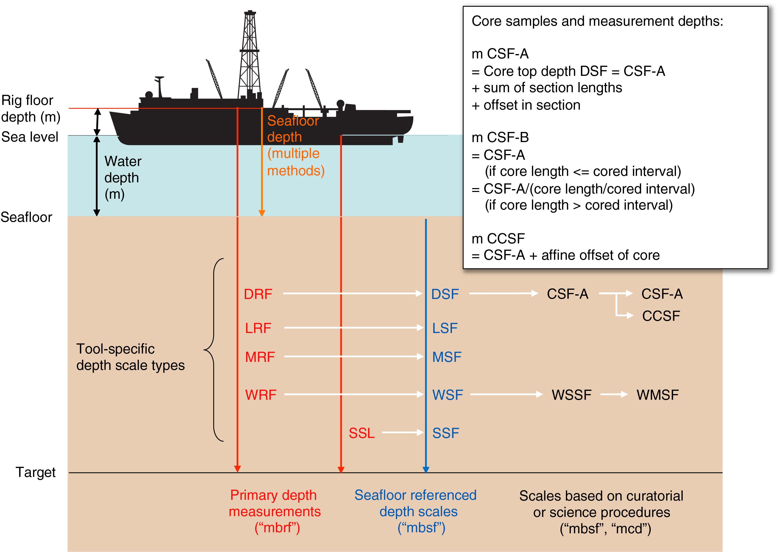
Figure F3. Depth scale types.
Once the recovered core is subjected to curatorial procedures (see Core curatorial procedures and sampling) (Figure F1), the core depth below seafloor, method A (CSF-A), depth scale is used for assigning depths to samples and measurements. The top depth of a core on the CSF-A scale is equal to the top of the cored interval on the DSF scale. However, the bottom depth of the core on the CSF-A scale and the depths of samples and measurements in the core are based on the curatorial procedures and rules applied on the catwalk and in the shipboard laboratory and have no defined relation to the bottom depth of the cored interval on the DSF scale. Depths of samples and associated measurements on the CSF-A scale were calculated by adding the offset of the sample or measurement from the top of its section and the lengths of all higher sections in the core to the top depth of the cored interval. This computation assumes that the recovered material represents a contiguous interval, starting at the top depth of the cored interval, even if core pieces are separated by nonrecovered stratigraphic intervals. If a core is shorter than the full barrel length and/or consists of more than one piece, the true depth of a sample or measurement in the core is unknown and a sample depth uncertainty should be considered when analyzing data associated with the core material.
If cores must be depth-shifted to create a modified depth scale that better represents the stratigraphy at a site or simply to remove artificial overlaps between cores related to natural, drilling, or curatorial processes, a core composite depth below seafloor (CCSF) scale is constructed. A simple, single depth offset is defined for each core, and the transform from the CSF-A scale to the CCSF scale for all cores in a hole is given by the affine table. All site reports and figures, except those relating to logging, use the CSF-A depth scale (see the LIMS database for offset values used during Expedition 376).
Additional depth scales are defined for downhole logging operations because those measurements are based on the length of the logging cable deployed beneath the rig floor with specific sources of uncertainly and correction procedures.
In summary, the depth scales used (Figure F3) (IODP Depth Scales Terminology version 2; http://www.iodp.org/top-resources/program-documents/policies-and-guidelines/142-iodp-depth-scales-terminology-april-2011/file) and the corresponding pre-IODP references are as follows:
- Drilling and coring depth scales:
- DRF = meters below rig floor (mbrf).
- DSF = meters below seafloor (mbsf).
- CSF-A = mbsf.
- CCSF = meters composite depth (mcd).
- Logging depth scales:
Core reference frame for sample orientation
Each core piece that has a length exceeding that of the core liner diameter is associated with its own CRF (i.e., oriented; Figure F2). The primary reference is the axial orientation (i.e., the top and bottom of the piece) determined by piece orientation when extracted from the core barrel. The core axis defines the z-direction, where positive is downcore. The secondary reference, the cut line, is an arbitrarily marked axis-parallel line on the whole-round surface of a piece that marks the plane through the cut line and the core axis where the piece will be split. The cut line was selected to maximize the dip angle of planar features on the split surface, which facilitates accurate structural measurements. The x-axis of the CRF is defined orthogonally to the cut plane, positive (000°) into the working half and negative (180°) into the archive half. The y-axis is orthogonal to the x-z plane and, using the right-hand cork-screw rule, is positive (090°) to the right and negative (270°) to the left when looking upcore at the working half (Figure F2).
Cube samples taken from the working half were marked with an arrow pointing in the −z-direction (upcore) on the working half surface (y-z plane), which defines the cube’s orientation unequivocally in the CRF. TSBs and thin sections made from billets were also marked with an upcore arrow in the most common case where the thin section was cut from the y-z plane of the working half. If thin sections were cut in the x-y or x-z plane, these directions were marked on the thin sections (Figure F2).
Section graphic summary (visual core descriptions)
For each core section, the most pertinent instrument measurement parameters and core description observables were plotted on a section graphic summary (traditionally referred to as a visual core description form [VCD]). An existing template was reviewed by the science party, and JRSO personnel implemented modifications as needed during the course of the expedition to arrive at the final template (Figure F4). JRSO personnel plotted all graphic summaries using the final template and data retrieved from the LIMS database or directly from DESClogik, including symbols, patterns, and line plots with depth, using the commercial plotting program Strater (Figure F5). A key to symbols used on the graphic summaries is given in Figure F6.
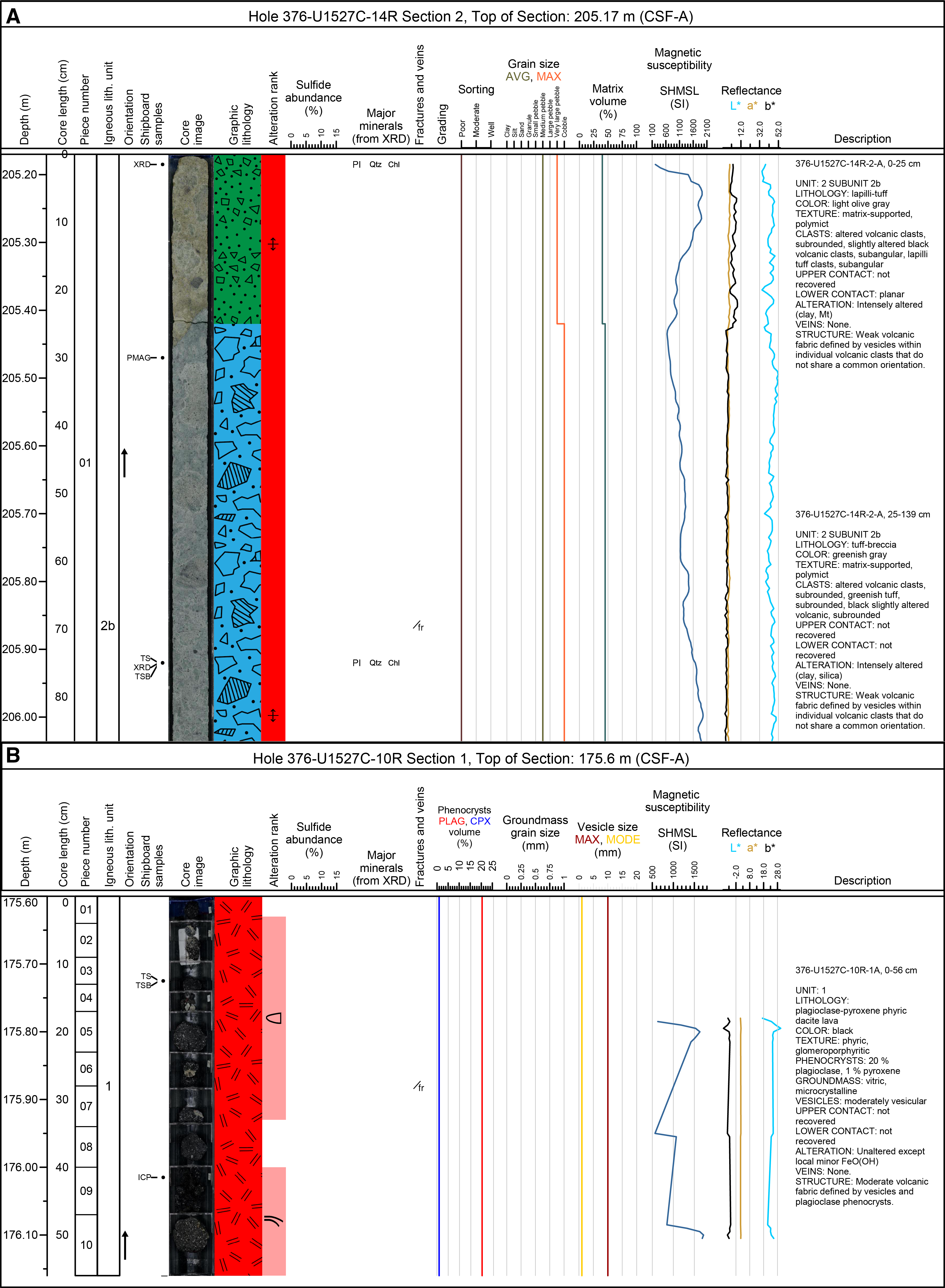
Figure F4. VCD.
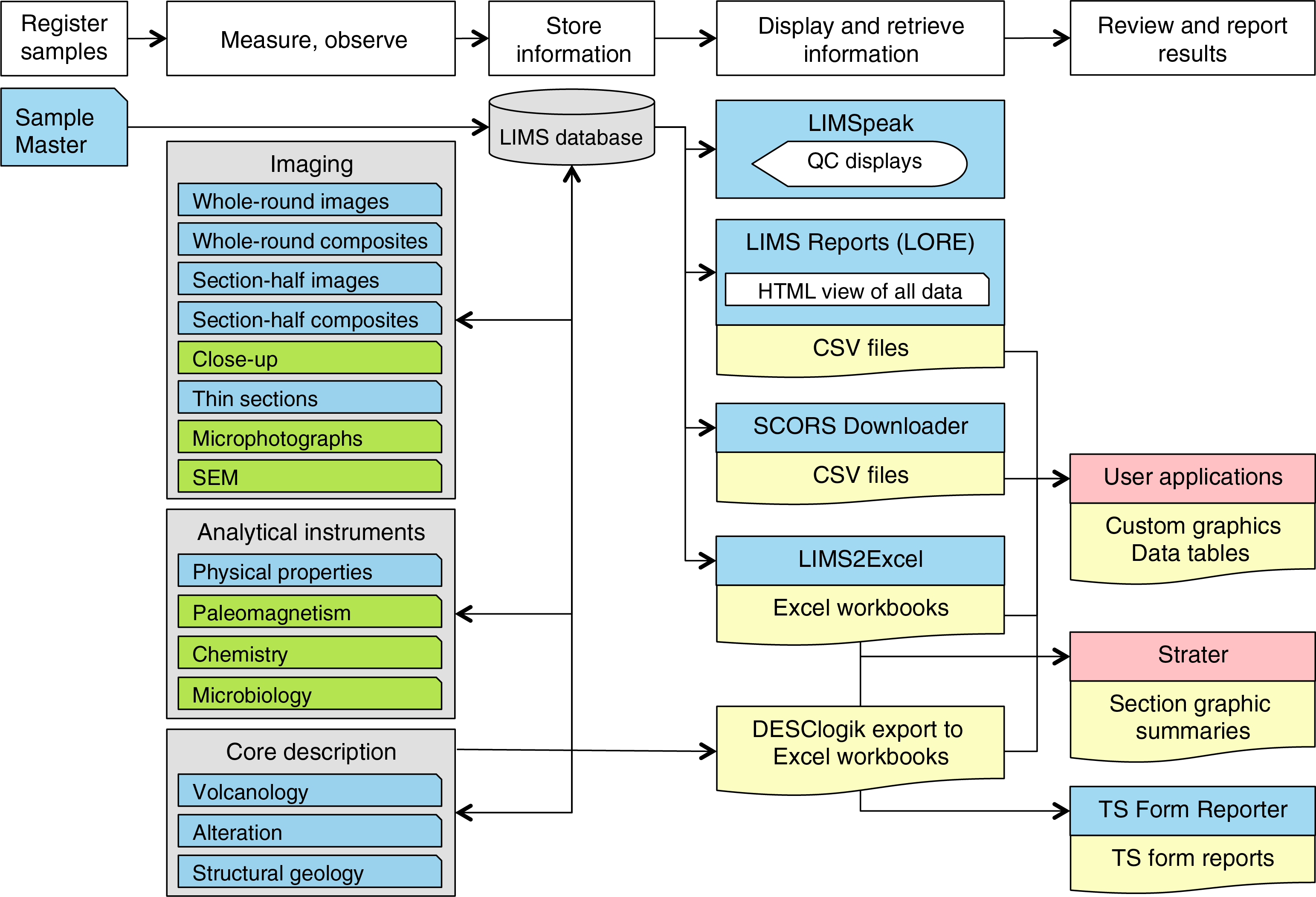
Figure F5. General data flow and software tools.
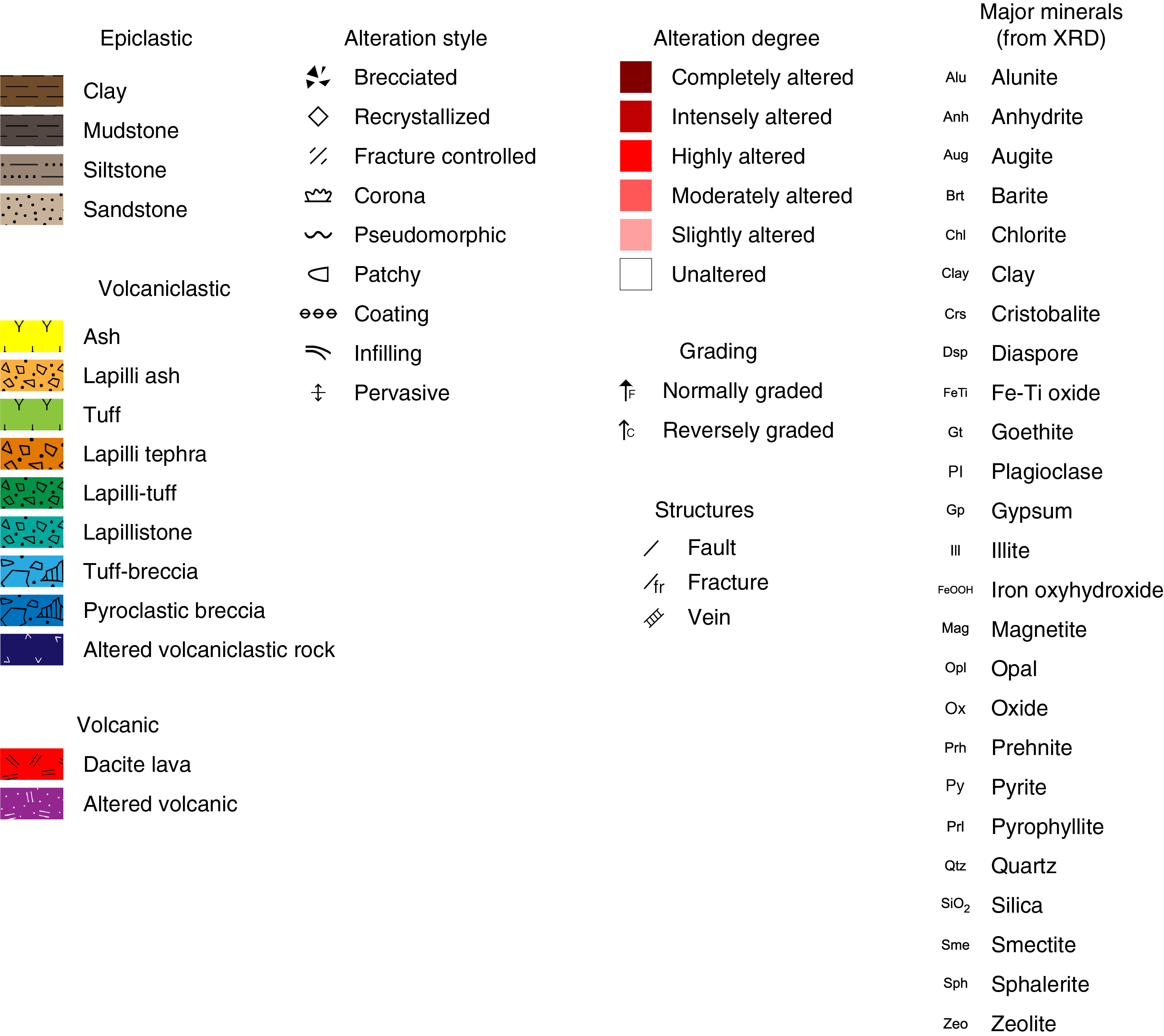
Figure F6. VCD legend.
The VCDs summarize the shipboard observations for the section, starting with a summary from each description team (igneous petrology and volcanology, alteration, and structural geology) across the top. All other information is plotted by depth in the main report area, starting with an image of the archive half and followed by the identification of pieces recovered; the lithologic units defined; the shipboard samples analyzed; the most significant observed igneous, alteration, and structural parameters; magnetic susceptibility (MS) measurements; and reflectance (Figure F4).
Thin section reports were created to summarize the most significant information for each thin section, which is extracted with a program from the extensive observation workbooks exported from DESClogik in a single-page PDF (Figure F7). JRSO personnel created the report definition in the report builder custom tool, updated the definition with input from scientists during the course of the expedition, and generated batches of PDF reports on request using the report writer tool.
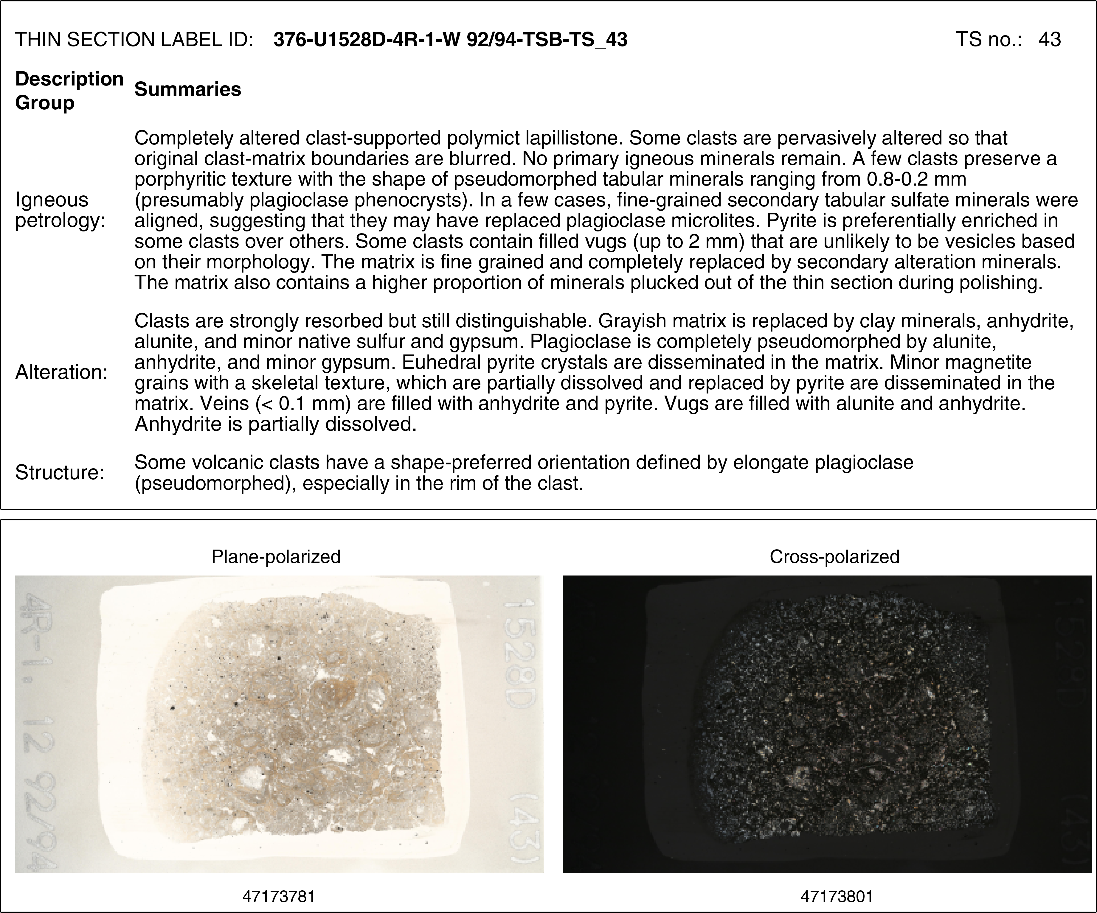
Figure F7. Thin section summary.
Software tools and databases
LIMS database
The JRSO LIMS database is an infrastructure to store all operational, sample, and analytical data produced during a drilling expedition (Figure F5). The LIMS database consists of an Oracle database and a custom-built asset management system, along with numerous web services to exchange data with information capture and reporting applications.
Sample registry tool
All samples collected during Expedition 376 were registered in the LIMS database using SampleMaster. The program has workflow-specific interfaces to meet the needs of different users. Sample registration begins with the driller entering information about the hole and the cores retrieved from the hole. IODP personnel enter additional core information, sections, pieces, and any other subsamples taken from these cores, such as cubes or TSBs. One interface is designed for scientists to autonomously enter subsample information according to the sampling plan.
Imaging systems
The following highly integrated and workflow-customized imaging systems were used during Expedition 376:
- The SHIL captured section-half surface images; it also captured whole-round section surface (360°) images using a special configuration that images four swaths at 90° angles to cover ~90% of the surface.
- A manual compositing process for the whole-round section images produced a quasi-360° presentation of features on the core surface.
- An automated compositing process for all section-half images of a core produced a virtual core table view.
- Close-up images were taken to meet special imaging needs, typically requested by shipboard scientists, not covered with routine linescan images.
- A custom-built imaging system captured whole-area high-resolution thin section images.
- Commercial cameras mounted on all microscopes took photomicrographs.
- The scanning electron microscope (SEM) captured high-resolution images.
All images were uploaded to the LIMS database immediately after capture and were accessible via browser-based reports. Images were provided in at least one generally usable format (JPG, TIFF, or PDF) and in multiple formats if appropriate.
Core description
Descriptive and interpretive information was entered and stored using DESClogik, and all information was stored in the LIMS database. The main DESClogik interface is a spreadsheet with extensive data entry and data validation support. The columns (observables), worksheets (sets of observables logged in context), and workbooks (sets of worksheets used in conjunction with each other) are entirely configurable by JRSO personnel based on experience from past expeditions and specific requirements defined by Expedition 376 scientists.
Teams were formed for each 12 h shift to describe volcanology, rock alteration, and structural geology for all core sections and thin sections prepared on board (see Igneous petrology and volcanology, Alteration, and Structural geology). This approach ensured that interdisciplinary teams worked collaboratively on all recovered material. Consistency in descriptions between teams was monitored during shift changes when time was available to jointly look at recovered material and exchange information.
At the beginning of the expedition, each group reviewed existing workbook templates for fresh and altered volcanic rocks and specified expedition-specific modifications that were implemented in the DESClogik application by JRSO personnel. Observable parameters were of three types: controlled values, free text, and numbers. For the controlled-value columns, subject matter experts defined specific value lists that were configured in DESClogik as drop-down lists to facilitate consistent data entry. These values are defined in each description team’s section of this chapter. Free text fields had no constraints and were used for comments and summaries.
Instrumented measurement systems
Physical property, paleomagnetic, and geochemistry analytical systems in the shipboard laboratories were used to capture instrumental data, as described in the corresponding sections below, using dozens of commercial and custom-built software applications. In cases where no user interaction was required after data capture, data upload to the LIMS database was triggered automatically. In cases where quality control or data processing was needed before upload, the user triggered the upload to the LIMS database when the data were ready.
Data retrieval
All data used for analysis, interpretation, and report preparation were downloaded using the latest version of LIMS Reports (Figure F5), where the user selects the type of desired information from ~50 available reports, selects a hole (and optionally cores, sections, or samples), and uses additional report-specific filters, if desired, to view a report online or download information in a standard comma-separated value (CSV) file.
Alternatively, data could also be retrieved using applications built for more specific purposes with various filtering and configuration options:
- LIMS2Excel, a highly configurable Java-based data extractor in which users can save a specific configuration for any combination of data parameters and export it into a Microsoft Excel workbook, and
- SCORS Downloader, which is designed to download certain data sets iteratively for stratigraphic analysis programs and can be used for any data and purpose.
Many data sets could also be viewed in LIVE, a browser-based application that plots cores, sections, and samples along with a user-selected data set, including images, against depth. The application is particularly useful for monitoring core logging data acquisition, performing real-time quality control, and browsing images.
Igneous petrology and volcanology
Lithology
Igneous and volcaniclastic rocks were the common primary lithologies encountered during Expedition 376. Most igneous and volcaniclastic rock description procedures used were adapted from Integrated Ocean Drilling Program Expeditions 330 and 344 (Expedition 330 Scientists, 2012; Harris et al., 2013) and IODP Expeditions 349, 350, 351, and 352 (Li et al., 2015; Tamura et al., 2015; Arculus et al., 2015; Reagan et al., 2015). Data for the macroscopic and microscopic descriptions of recovered cores were entered into the LIMS database using DESClogik.
Our shipboard studies sought to systematically describe the physical appearance, petrology, and alteration of the cored rocks. First, phenocryst abundance and appearance, lithologic components (for volcaniclastic sediments), and characteristic igneous textures and vesicle distribution were described at a macroscopic level and investigated in more detail by thin section and SEM imaging. Second, the recovered and described material was divided into coherent units. Igneous and volcaniclastic lithologic unit boundaries were defined using complementary information including petrography, volcanic and sedimentary structure/textures, chemical composition, and physical properties such as MS.
Core description workflow
The procedures used to document the composition, texture, and structures of rocks recovered during Expedition 376 included visual core description [VCD only refers to the form, not the process (see dictionary)], petrographic thin section analysis, digital color imaging, SEM imaging, color spectrophotometry, pXRF (see Geochemistry), XRD, and ICP-AES. (Note that data produced on the Agilent 5110 inductively coupled plasma–optical emission spectrometer [ICP-OES] were collected in AES mode and are referred to as “ICP-AES” in the online LIMS/LIMS Reports [LORE] database. Thus, in this volume, “ICP-AES” is used to refer to these data.) Before the core was split into working and archive halves, nondestructive measurements of physical properties were implemented (see Physical properties). Whole-round images of >10 cm long pieces of core were generated by stitching together images taken at four distinct angles (0°, 90°, 180°, and 270°). All cores were processed following the established shipboard procedure for hard rocks. Prior to splitting, fragmented pieces of hard rock were oriented (if possible) and put into bins separated by plastic spacers. Hard rock pieces and/or coherent sections were then split by means of a diamond-impregnated saw along lines chosen by a structural geologist and an igneous petrologist/alteration mineralogist so that important compositional and structural features were preserved in both the archive and working halves. If the retrieved core barrel contained loose sediment such as gravel, it was homogenized and split equally into working and archive halves, either manually when gravel only partially filled the core liner or by pulling a wire lengthwise through the center of the core. Once the core was split, the hard rock pieces in both the working and the archive halves were labeled individually with unique piece/subpiece numbers from the top of each section to the bottom (e.g., 1A, 1B, 2A, 2B, etc.). If the orientation of a piece of rock could be determined, an arrow was added to the label to indicate the uphole direction. The working and archive halves were imaged in this order using the SHIL, which also recorded red, green, and blue spectral colors along the centerline of the core. After imaging, the archive halves were analyzed for color reflectance and MS at 2.0 cm intervals using the SHMSL (see Physical properties). The working halves were sampled for destructive shipboard analyses such as physical property measurements, paleomagnetic measurements, thin section production, XRD, pXRF, and geochemical analysis by ICP-AES. Most cores sampled for shipboard ICP-AES and XRD analysis had complementary pXRF measurements performed utilizing powders produced for these methods. Because precious metals were expected in samples recovered during this expedition, no jewelry was allowed near the core and gloves were used for handling at all times.
Each section of core was first macroscopically examined and described for petrologic, alteration, and sedimentary characteristics (aided by use of a 10× magnification field hand lens and a binocular microscope) by a team with diverse expertise including igneous petrology, volcanology, sedimentology, alteration, and sulfide mineralogy. Lithologic descriptions and most structural observations (see Structural geology) were made on the archive halves. For both macroscopic and microscopic observations, DESClogik was used to record the primary igneous characteristics (e.g., groundmass and phenocryst mineralogy, as well as vesicle abundance), sedimentary features (e.g., lithologic components and textures), alteration (e.g., color, vesicle filling, secondary minerals, and vein/fracture fillings; see Alteration), and lithologic unit division.
Macroscopic features observed in the cores are summarized and presented in the VCDs. They display the following entries in terms of igneous, volcaniclastic, alteration, structural, and physical property features for each core section (from left to right in Figure F4; see Figure F6 for VCD legend):
- CSF-A depth scale in meters (equivalent to mbsf),
- Core length scale from 0 to 150 cm,
- Number of hard rock pieces,
- Igneous unit/subunit,
- Orientation of hard rock pieces,
- Interval and type of shipboard samples,
- Scanned digital image of the archive half,
- Graphic representation of lithology,
- Column with variable patterns depicting alteration intensity,
- Sulfide abundance (vol%),
- Major minerals (from XRD data), and
- Fractures and veins.
Volcaniclastic VCDs (Figure F4A) include the following:
Igneous VCDs (Figure F4B) include the following:
- Phenocryst abundance (vol%) for plagioclase (PLAG; red line) and clinopyroxene (CPX; blue line),
- Crystal size of modal groundmass (in mm),
- Vesicle size (MAX and MODE [mm]),
- Plot showing SHMSL MSP measurements,
- Diagram displaying color reflectance parameters luminescence (L*), red-green (a*), and blue-yellow (b*), and
- Section unit summary of each lithologic unit identified in the corresponding section (see below for details).
The section unit summary (presented on the right side of the VCD; Figure F4) for each igneous lithologic unit contains the following:
- Expedition, site, hole, core, section number, interval, and core type (archive [A] or working half [W]);
- Igneous lithologic unit/subunit number(s);
- Lithology;
- Simplified standard Munsell color determined on the dry rock surface;
- Texture based on texture of volcaniclastic material (volcaniclastics) or total percentage of phenocrysts (igneous);
- Description and type of clasts (volcaniclastics) or phenocryst type and percentage and groundmass texture or mineralogy based on minerals identifiable by the unaided eye, hand lens, or microscope (igneous);
- Abundance and general shape of vesicles (igneous only);
- Upper and lower unit contact relations and boundaries based on physical changes observed in retrieved core material (e.g., presence of chilled margins, changes in vesicularity, and alteration), including information regarding their position in the section; the term “not recovered” was entered where no direct contact was recovered (Expedition 349 Scientists, 2014);
- Alteration intensity;
- Vein mineralogy;
- Structure; and
- Comment, if applicable.
Drilling disturbance
Cores may be significantly disturbed and contain extraneous material as a result of the coring and core handling process (Jutzeler et al., 2014). Each core was therefore examined critically during description for potential “fall-in” material, and any disturbance was recorded in DESClogik.
Lithologic unit classifications
Lithologic units and subunits are classified based on VCDs and complementary information (geochemical analysis, physical properties, etc.). Igneous rock unit boundaries are generally chosen to reflect different volcanic cooling and/or eruptive units. The definition of an igneous lithologic unit is usually based on the presence of lava flow contacts that are typically marked by chilled or glassy margins on the upper and lower contact or by the presence of intercalated volcaniclastic or sedimentary horizons. If no such boundaries were recovered (e.g., because of low recovery), we defined the igneous lithologic unit boundaries according to changes in the primary mineral assemblage (based on abundances of visible phenocryst and groundmass mineral phases), grain size, color, structure or texture, or physical properties (MS, NGR data, etc.). Boundaries between volcaniclastic lithologic units were chosen to reflect changes in composition and/or emplacement and transport processes and were based on characteristics such as lithologic components, grain size, and texture (e.g., bedding, grading, or sorting). A volcaniclastic unit can therefore reflect an entire eruption, one particular phase of an eruption marked by changes in the mode of transport (e.g., fall vs. flow deposit), or different post-eruptive erosive and displacement phases. In practice, these changing boundary characteristics were difficult to discern because of the degree of alteration of the primary lithology.
Igneous lithologic units are given consecutive Arabic numerals downhole (e.g., Units 1, 2, 3, etc.) irrespective of whether they are lava flows, volcaniclastic deposits, or igneous intrusions. Igneous lithologic subunits were used in cases where the mineralogy/composition remains similar but frequent changes in texture were observed (e.g., Subunits 1a, 1b, 1c, etc.).
Because of the effects of overprinting hydrothermal activity, we commonly encountered rocks altered to such a degree that proper identification was no longer possible. When this occurred, the principal lithologic name “altered volcanic rock” or “altered volcaniclastic rock” was chosen, and any further specification can be found under Alteration.
Volcaniclastic classification
Volcaniclastic sediments were the typical sediments encountered during Expedition 376. The sedimentary classification scheme employed emphasizes important descriptors for sediments, which were quantified and recorded in DESClogik (Macroscopic template, Volcaniclastic_sedimentary tab). A schematic of the description parameters and classification scheme is shown in Figures F8 and F9 and Table T2. The classification scheme for volcaniclastic rocks is based on standard sedimentological practice and the sedimentary descriptive scheme typically used by IODP (as applied during Expedition 351; Arculus et al., 2015).
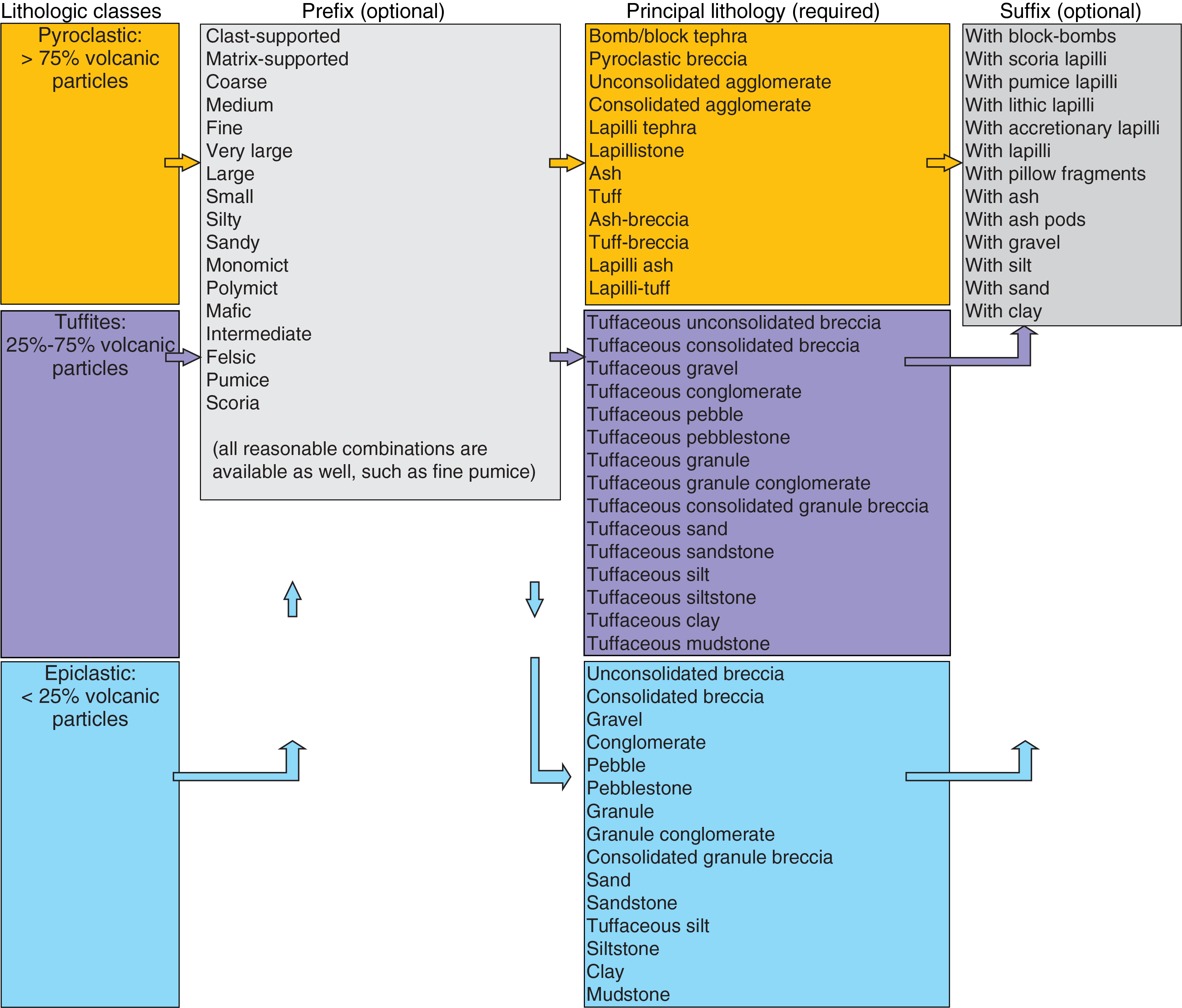
Figure F8. Classification scheme for clastic sediments.
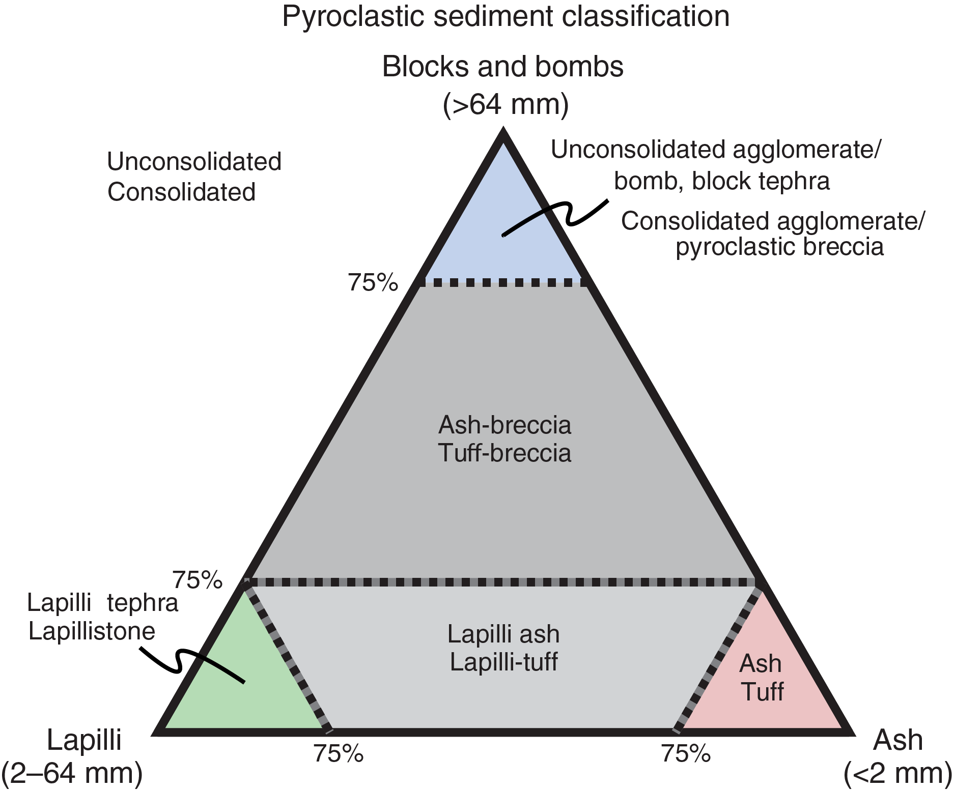
Figure F9. Classification scheme for pyroclastic rocks.
Volcaniclastic and siliciclastic sediments are divided into three lithologic classes based on their components (types of particles) following Fisher and Schmincke (1984) (Figure F8):
- Pyroclastic sediments containing >75% volcanic particles,
- Tuffites containing 25%–75% volcanic particles, and
- Epiclastic sediments containing <25% volcanic particles.
Within each class, the principal lithology name is based on particle size and consolidation. In addition, appropriate prefixes provide further classifying information, and suffixes indicate minor components within a principal lithology type (see below).
Principal lithology names
The principal lithology name is first derived from the volcanic content that determines the lithologic class (see above). Within each of these classes, both a consolidated and an unconsolidated term exists for each grain size class, and they are mutually exclusive (e.g., mud or mudstone; ash or tuff). The classification scheme for volcaniclastic sediments (Table T2; Figure F9) is based on terms defined by Fisher and Schmincke (1984), Wentworth (1922), and Bates and Jackson (1987), with some minor adaptations to ensure consistency between volcanic and nonvolcanic terms. Some additional clarifying definitions follow:
- Block/Bomb: a volcanic fragment larger than 64 mm. Bombs are juvenile clasts that are ejected when still (partially) molten and therefore show fluidal textures.
- Agglomerate: a welded aggregate mainly containing bombs.
- Lapilli: a volcanic fragment between 2 and 64 mm in diameter (fine, medium, or coarse lapilli).
- Ash: volcanic fragments smaller than 2 mm (fine, medium, or coarse ash).
- Tuffaceous: indicates a tuffite.
- Breccia: composed of mainly subangular to angular clasts larger than 64 mm.
- Conglomerate: consolidated sediment composed mainly of subrounded to rounded clasts larger than 64 mm.
- Ash-breccia, lapilli ash: pyroclastic sediments containing a mix of ash, lapilli, and bombs/blocks, as defined in Figure F9.
- Tuff-breccia, lapilli-tuff: consolidated equivalents of ash-breccia and lapilli ash, respectively.
Irrespective of the sediment or rock lithologic class, the average and maximum grain sizes reported in the VCDs follow Wentworth (1922) with minor adaptations (Table T2). For example, a coarse ash would be described as having sand-sized particles.
If observations allowed an interpretation regarding the mode of transport and/or fragmentation and/or emplacement mechanism, a note was made in the comments. Some examples are given below; definitions are from Bates and Jackson (1987) and Fisher and Schmincke (1984):
- Block and ash flow: formed by a pyroclastic flow of lava debris (due to dome collapse); contains mostly volcanic blocks and ash.
- Ignimbrite: formed by a pyroclastic flow of pumice and ash (due to column collapse); contains ash and a wide range of lapilli- to block-sized clasts.
- Hyaloclastite: formed by the intrusion of lava or magma into water, ice, or water-saturated sediment and its consequent granulation or shattering into small angular fragments.
- Autoclastite: a rock with a brecciated structure that was formed in the place where it is found as a result of crushing, shattering, or other mechanical forces.
Prefixes
Prefixes were chosen to provide additional classification information where possible, such as an estimated composition, further specification of grain sizes, or textural information. Where appropriate, combinations of prefixes were adopted. Prefixes include
- Compositional information: description of volcanic material as felsic, intermediate, or mafic with an additional distinction between monomict (clast compositions of a single type) and polymict (clast compositions of multiple types).
- Textural information: matrix-supported (smaller particles visibly envelop each of the larger particles) versus clast-supported (clasts form the sediment framework).
- Specification of grain sizes: fine, medium, or coarse, as well as silty and sandy (e.g., for “medium lapilli” or “sandy silt”).
- Description of volcanic clasts: categorization of volcanic clasts as pumice or scoria.
Suffixes
A suffix was used for a subordinate but important component (i.e., abundance 5%–25%) that deserves to be highlighted. For example, if an ash layer contains some accretionary lapilli, it would be named “ash with accretionary lapilli.” Suffixes are restricted to a single phrase to maintain a short and effective lithology name containing the most important information only.
Other parameters
Several additional parameters were recorded in macroscopic core descriptions to further delineate volcaniclastic units. These parameters include color (using Munsell color charts; Munsell Color Company, Inc., 2009a, 2009b), average and maximum particle sizes, description of boundaries and contacts between units, sorting (Figure F10), grading, layer/bedding thickness, and sedimentary structures such as wavy bedding or cross-lamination. Where available, we also described the matrix in terms of lithology and sorting and the three most dominant clasts >2 mm in terms of lithology and roundness (Figure F10). That is, we distinguish between lithic clasts, vitric/volcanic clasts, and crystals. For consolidated sediments, we also distinguish types of lithification between welded or cemented, where applicable.
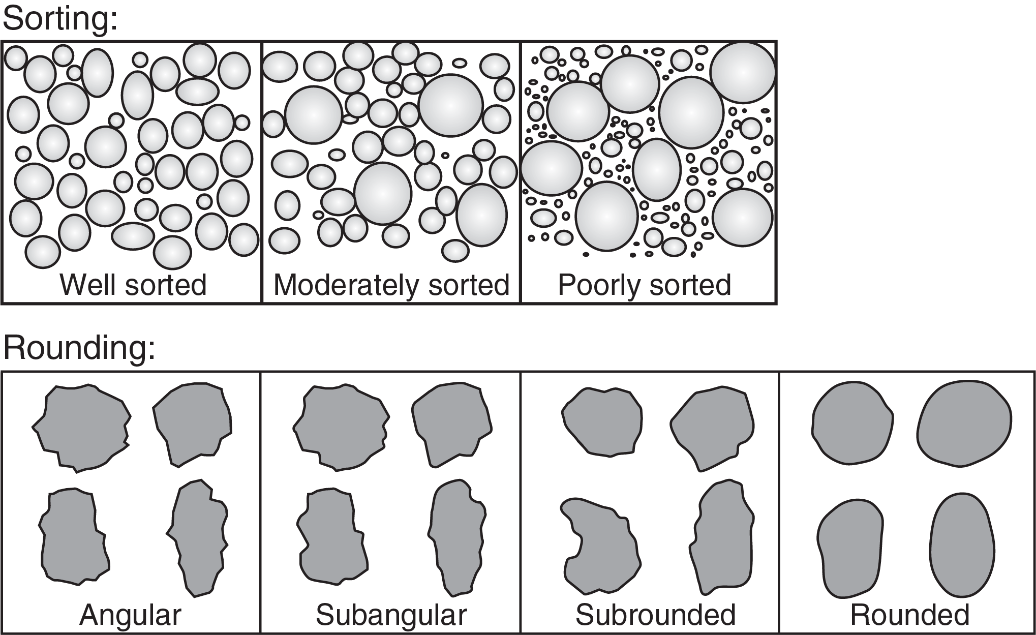
Figure F10. Terms used to describe sorting and rounding of clasts.
When a boundary between two adjacent lithologies was observed, it was classified using the terms presented in Table T3. Where the geometry of a contact could be directly observed, we classified the lower boundary as planar, curviplanar, or irregular. The lower boundary was further classified as sharp, scoured, wavy, or gradational. The dip of the boundary was described as inclined, subhorizontal, horizontal, subvertical, or vertical (see Structural geology for detailed methodology).
Microscopic description of volcaniclastic rocks
To complement macroscopic descriptions, we analyzed smear slides of sufficiently fine grained, unconsolidated material and thin sections of consolidated sediments and large-enough individual clasts from unconsolidated material. Thin sections were initially described using a template for handwritten description, and the data were subsequently entered into the Smear_slide tab and the Sediment_ts tab, respectively, in the Microscopic template in DESClogik. Data include the abundance of different grain sizes in the sample, as well as the lithologic components (i.e., the respective abundance of volcanic [juvenile] clasts, lithic/epiclastic clasts, and different crystals). For each clast type, we recorded the respective grain size and roundness. Additionally, vesicularity and likely composition of volcanic particles were recorded, if possible. Sedimentary textures such as sorting, bedding thickness, or lamination, as well as the composition and grain size of the matrix (if present), were analyzed in thin sections. Many clasts in recovered volcaniclastic rocks were large and unaltered enough that their igneous features were recognizable. In those cases, microscopic features as outlined in the next section regarding (sub)volcanic classifications were also recorded, including vesicularity, groundmass textures, and phenocryst assemblages. If necessary, two domains were used in the Sediment_ts tab of DESClogik to record information for clasts and matrix separately for the same sample. However, the microscopic distinction of individual clasts versus matrix was often challenging to impossible because of the similarity in composition and/or alteration. In that case, the sample was described in one domain. Alteration minerals were exclusively described in the Alteration tab of DESClogik, but all (or traces of) primary igneous or sedimentary features, such as pseudomorphs of phenocrysts, were recorded in the Sediment_ts tab.
Figure F11 includes the template used to record microscopic description. For each thin section, a summary of observations regarding sedimentary/volcanic, alteration, and structural features used for the DESClogik output was written (Figure F7).
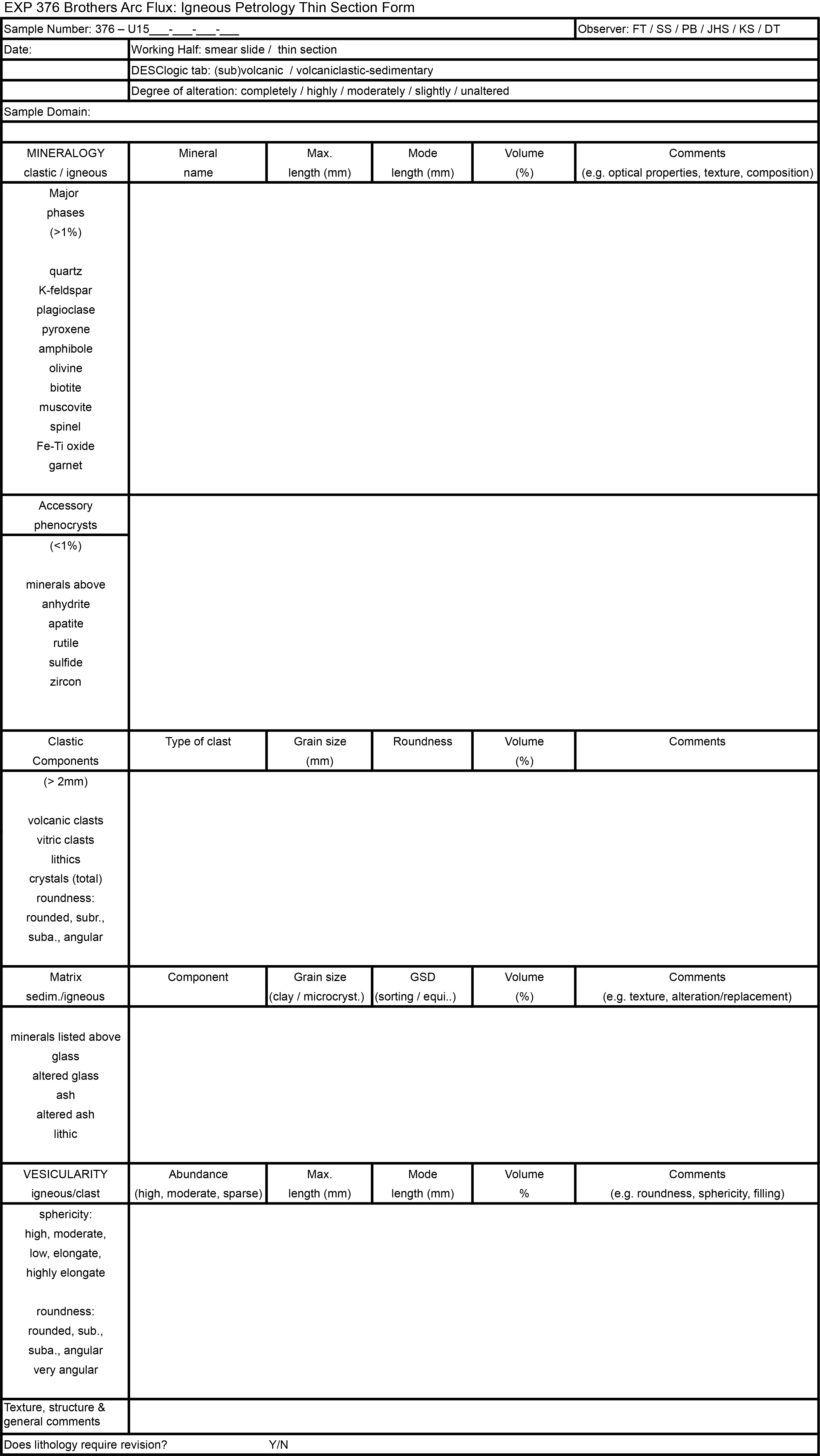
Figure F11. Template used for microscopic description of volcaniclastic units.
(Sub)volcanic classifications
Volcanic and hypabyssal (subvolcanic) rocks were described as follows:
- Grain size classification and distribution, texture, and rock color;
- Description of primary mineral phases and groundmass;
- Definition of principal lithology including prefixes and optional suffixes; and
- Lava flow types and contacts.
Grain size classification and distribution, texture, and color
Groundmass
The term “groundmass” describes the crystalline and/or glassy matrix between phenocrysts (see definition below) in an extrusive or hypabyssal rock. For VCDs, the grain size of the groundmass is estimated using the terms “coarse grained,” “medium grained,” and “fine grained” (Neuendorf et al., 2005); the grain size of the groundmass is quantified using thin section microscopy:
- Coarse grained (crystal diameters = 5–30 mm),
- Medium grained (crystal diameters = 1–5 mm), and
- Fine grained (crystal diameters = 0.2–1 mm).
For reports and description summaries, we have simplified these values to fine-grained or coarse-grained groundmass. The distribution of the groundmass crystals was classified into bimodal, equigranular, inequigranular, granular, poikilitic, or seriate. The texture of groundmass was described using the terms defined in Table T4.
Volcanic glass
We noted whether or not glass was present, documenting the proportion of glass, fresh glass, spherulites, and altered glass, and elaborated on glass preservation in optional comments as needed.
Vesicles
Macroscopic observations of vesicles included visual estimates of vesicle abundance, maximum and average vesicle size, roundness, sphericity, and vesicle filling supplemented by optional comments as appropriate.
Vesicle abundance was classified using the criteria of Reagan et al. (2015):
- Nonvesicular = 0% vesicles.
- Sparsely vesicular = <5% vesicles.
- Moderately vesicular = 5%–20% vesicles.
- Highly vesicular = >20% vesicles.
The sphericity and roundness of vesicles was described according to the terms presented in Figure F12. Vesicle fillings were recorded as being present or absent, with more detailed observation of the type of filling made in Alteration.
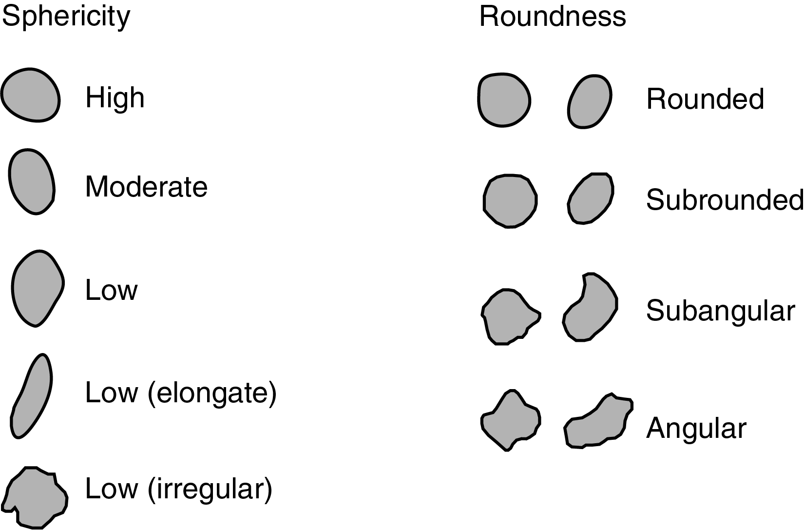
Figure F12. Terms used to describe sphericity and roundness of vesicles.
Igneous textures
The principal distinguishable textures of subvolcanic and volcanic rock were described (Table T5).
Color
Rock color was determined on a dry, cut surface of the archive half using Munsell color charts (Munsell Color Company, Inc., 2009a; 2009b).
Primary mineral phases
The following primary mineral phases were described:
- Shapes, which include euhedral, subhedral, anhedral, and interstitial;
- Aspect ratios to describe the euhedral to subhedral habit of a crystal, adapted from ODP Leg 209 (Shipboard Scientific Party, 2004): equant, subequant, tabular, elongate, and acicular; and
- Habits for plagioclase and clinopyroxene adapted from ODP Legs 148 and 206 (Alt et al., 1993; Shipboard Scientific Party, 2004).
Phenocrysts
Porphyritic volcanic rocks were named according to major phenocryst phase(s) when the total abundance of phenocrysts was >1% (see Lithology prefix). The term “phenocryst” is used to describe any crystal significantly larger (typically five times larger) than the average size of groundmass and >1 mm in diameter, irrespective of the potential ante- or xenocrystic origin. The term “microphenocryst” is used for crystals larger than the modal groundmass grain size but <1 mm. “Glomerocryst” is used to describe clusters of phenocrysts of the normal phenocryst assemblage. Macroscopically, as many as three different types of the most abundant phenocrysts (e.g., garnet, biotite, Fe-Ti oxide, amphibole, muscovite, olivine, plagioclase, pyroxene, quartz, spinel, and K-feldspar) were described in more detail. Observations include percentage, maximum size, modal size, and shape (anhedral, subhedral, or euhedral) of phenocryst, elaborated by optional comments as required. In addition, the total phenocryst abundance was recorded.
Accessory mineral phases
Any macroscopically identifiable mineral phase with a very scarce total abundance (usually <1%) was recorded as an accessory mineral (e.g., biotite, anhydrite, apatite, amphibole, Fe-Ti oxide, garnet, muscovite, olivine, plagioclase, pyroxene, quartz, rutile, spinel, sulfide, and zircon). As many as two phases were recorded, supplemented by optional comments.
Rock types/lithology
A lithologic name is composed of a principal lithology name and an optional prefix and suffix. Volcanic rocks and their principal lithology names are classified according to the International Union of Geological Sciences (IUGS) classification scheme of Le Maitre et al. (2002) based on the nature of the phenocrysts and their relative proportions (Figure F13). However, because detailed petrography and/or chemical analyses are usually not available when the core is initially logged, we modified the initial rock classification if necessary when chemical data or detailed petrography became available.
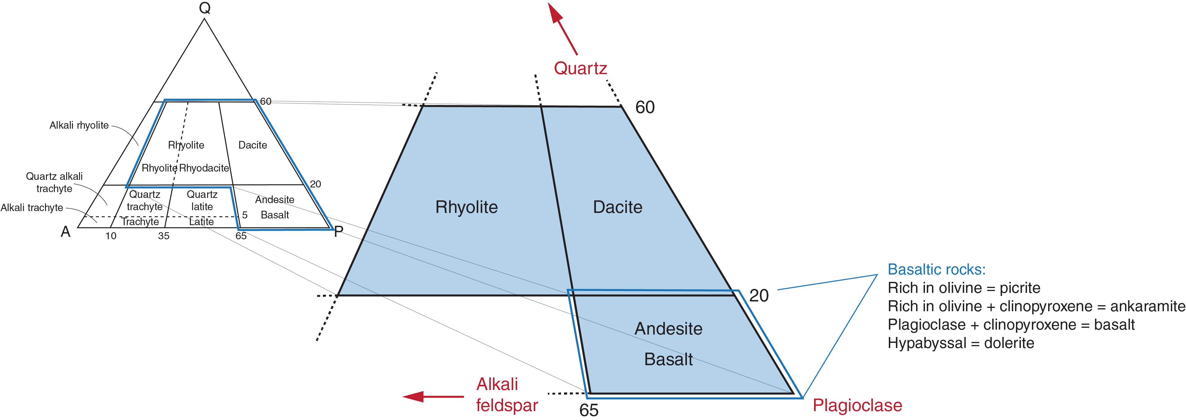
Figure F13. IUGS classification scheme.
Principal lithology
Nine principal lithology categories (in order of increasing SiO2 content) were defined in DESClogik (Tables T5, T6):
- Picrite: basaltic rock visibly enriched in olivine crystals, often as phenocrysts (Gill, 2010).
- Basalt: rock containing plagioclase and pyroxene (Reagan et al., 2015).
- Ankaramite: basaltic rock rich in olivine and clinopyroxene phenocrysts (Gill, 2010).
- Dolerite: medium-grained igneous rock consisting essentially of pyroxene and plagioclase. Generally, a hypabyssal, intrusive equivalent of basalt.
- Andesite: rock containing pyroxene and/or feldspar and/or amphibole, typically devoid of olivine and quartz (Reagan et al., 2015).
- Dacite: typically plagioclase-phyric rock, sometimes containing pyroxene ± quartz ± hornblende (Reagan et al., 2015). Note that at Brothers volcano, dacites are unusually dark gray to black in color.
- Rhyolite: plagioclase-phyric rock, sometimes containing quartz ± hornblende (Reagan et al., 2015).
- Altered volcanic rock: general term for (formerly) primary volcanic rock that has been altered so that the primary rock type (apart from its texture indicating a volcanic origin) cannot be determined with certainty.
- Peperite: breccia-like volcanic rock enclosed by marine sedimentary rock. Interpreted by some to be a mixture of lava with sediment and by others as shallow intrusions of magma into wet sediment (Bates and Jackson, 1987).
Lithology prefix
A prefix was chosen to indicate one of the following: (1) content and type of common volcanic phenocrysts present, (2) additional lithologic qualifier of composition and texture, or (3) the presence of accessory minerals. Prefixes include
- Aphyric (for nonporphyritic rocks) or -phyric (as a suffix for porphyritic minerals) was used with the principal phenocrysts olivine, plagioclase, pyroxene, amphibole, quartz, and biotite and their combinations. In the case of multiple phenocryst occurrences (e.g., plagioclase-pyroxene), the first mineral name is the most abundant in the sample.
- Other lithologic prefixes used are brecciated (if the rock is coherent enough not to be called pyroclastic), andesitic, basaltic, dacitic, doleritic, or rhyolitic.
Lithology suffix
A suffix was chosen to indicate the mode of emplacement if direct volcanic or subvolcanic features could be determined, including pillow lava, lava flow (general term for massive lava independent from type of lava flow), dike (intrusive with a dominantly vertical orientation), and sill (intrusive with a dominantly horizontal orientation). The following distinguishing criteria were used:
- Pillow lavas:
- Curvilinear chilled to glassy margins,
- Concentric banding of vesicles,
- Internally radiating vesicle chains, and
- Internally radiating joint patterns.
- Lava flows:
- Dikes and sills:
Any subvertical hypabyssal igneous rocks were classified as dikes. Other subhorizontal hypabyssal igneous rocks were classified as sills.
Contact types
Because of limited recovery in most cores, contacts between two lithologies (which are typically the boundaries of descriptive intervals) were commonly absent. When a boundary between two adjacent lithologies was observed, it was classified using the terms presented in Table T3. Where the geometry of a contact could be directly observed, we classified the lower boundary as planar, curviplanar, or irregular. The lower boundary was further classified as sharp, scoured, wavy, or gradational. The dip of the boundary was described as inclined, subhorizontal, horizontal, subvertical, and vertical (see Structural geology for detailed methodology).
Microscopic description of (sub)volcanic rocks
To complement macroscopic descriptions, we analyzed representative thin sections of volcanic, hypabyssal, and plutonic rocks. Thin sections were initially described using a template for handwritten description, and the data were subsequently entered in the microscopic template in DESClogik in the (Sub)volcanic and Plutonic tabs, respectively, where appropriate. The description followed the macroscopic description of these rock types closely but was supplemented by specific microscopic observations such as crystal habit (equant, subequant, tabular, or elongate), crystal zoning (continuous, discontinuous, patchy, or oscillatory zoning) and zoning extent (none, scarce, abundant, or very abundant), and possible crystal exsolution (bleb or lamellae). For accessory crystals, only type and abundance were recorded, and for groundmass crystals, abundance, size, type, and shape were described. If vesicles were present, they were described by volume (vol%); the proportion empty and/or filled (%); minimum, maximum, and mode size; roundness; and sphericity, again closely following the procedure for macroscopic descriptions. Figure F14 shows the template used to record microscopic descriptions. For each thin section, a summary of observations regarding igneous, alteration, and structural features was written and used for the DESClogik output (Figure F7).
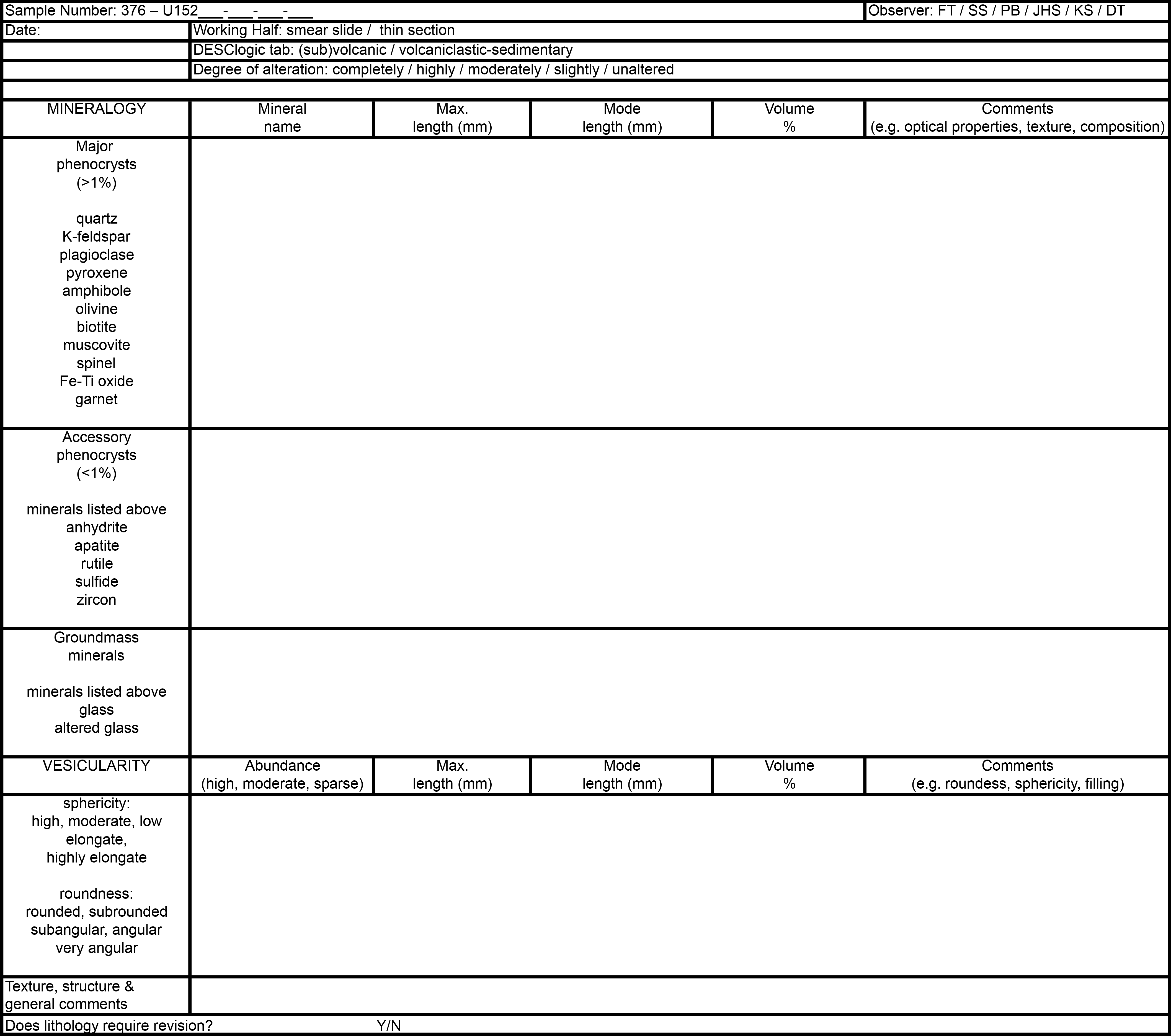
Figure F14. Template used for microscopic description of igneous units.
Alteration
Procedures developed specifically to aid in visual description of hydrothermal mineralization and alteration encountered during Expedition 376 are detailed in the following sections.
Visual description of hydrothermally altered material
Significant detail was incorporated into DESClogik, which enabled a comprehensive report of the predominant style of hydrothermal mineralization and alteration of specific intervals of the recovered core material.
Degree of alteration
An initial estimate of the degree of alteration was reported for every defined alteration interval. Degree of alteration is reported based on the modal percentage of secondary alteration minerals and assigned an alteration ranking from 0 (unaltered) to 5 (completely altered) (Table T7). This alteration ranking was used to plot alteration intensity on the visual core logs. The proportions of alteration minerals are estimated primarily based on visual observations (including observation under binocular stereoscope). In most cases, a comparison between macroscopic and microscopic estimates of alteration mineral proportions indicate that macroscopic estimates are consistently overestimated. As a result, thin section descriptions and the relative intensities of XRD peaks, when available, were used to validate or adjust visual estimates for degree of alteration.
Alteration color
The color of alteration was determined visually using Munsell Color Charts (Munsell Color Company, Inc., 2009b).
Alteration texture
The alteration texture was determined visually using descriptive terms established in the hydrothermal literature (Table T8).
Alteration mineralogy
The modal abundances of the main alteration products were determined macroscopically. The initial mineral identification and degree of alteration estimates were later refined by incorporating the results from thin section descriptions (using both transmitted and reflected light modes), XRD, and pXRF analyses.
Secondary sulfide minerals
The texture of sulfide minerals that were precipitated by secondary processes (i.e., through hydrothermal fluid–rock interaction) were described separately from the alteration textures ascribed to the host rock (see Table T9).
Alteration of clasts and matrix
Evidence of brecciation was reported according to the shape of both coherent and noncoherent clasts, clast size, whether the clast is matrix supported, and the degree of clast angularity using the criteria summarized in Table T10 and Figure F15. The dominant alteration mineralogy of both clasts and matrix was reported.
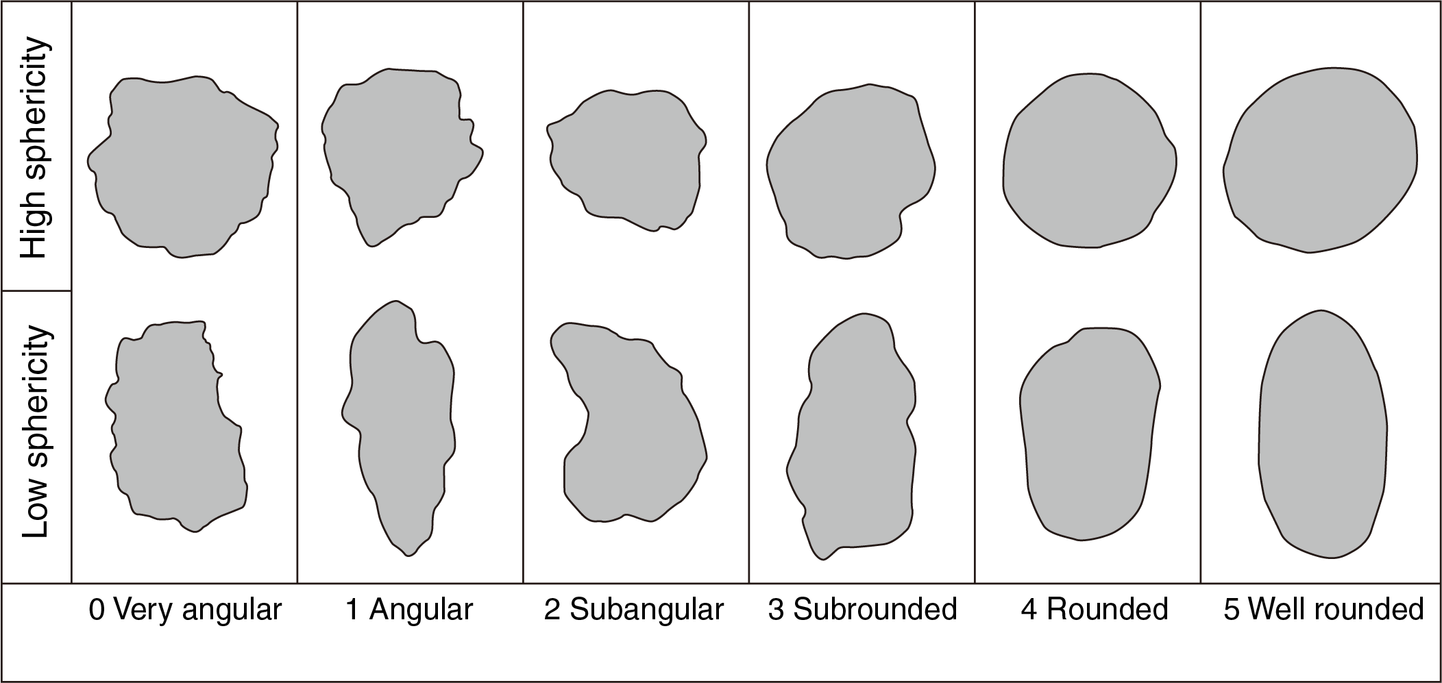
Figure F15. Visual guide for estimating clast angularity.
Vesicle, vug, and vein filling
Vesicles in the volcanic rocks and vugs developed during alteration of the sample were reported as visual estimates of the percent of the overall sample volume. They were further characterized based on fill mineralogy and average percent fill.
The term “vein” was applied to any later crosscutting feature that precipitated from hydrothermal fluids. Veins were described based on visual estimation of spatial density (defined as percent of sample interval composed of vein-fill material), vein geometry (using criteria outlined in Table T11), description of the vein margin (e.g., sharp, diffusive, or irregular), maximum vein width, and vein fill texture (Table T12). If distinct vein sets defined based on compositional or morphological characteristics were present, crosscutting relationships were used to define vein generations, and each generation was described separately (see Structural geology).
Other observations
Other evidence of water–rock interaction, such as evidence of anhydrite dissolution, was also reported.
Common alteration assemblages
Specific alteration mineral assemblages are described based on their modal composition and the presence or absence of key indicator minerals. These assemblages are often used as a proxy for the physicochemical conditions of a hydrothermal fluid (e.g., pH, temperature) during alteration and subsequent mineralization for a variety of hydrothermal ore systems. For example, in magmatic-dominated hydrothermal ore deposits, advanced argillic, argillic, and propylitic alteration styles are commonly composed of distinct mineral assemblages (Tables T13, T14). When describing the broad style of mineralization encountered in the recovered core, reference was made to these characteristic alteration assemblages. However, it should be noted that the mineral assemblages described above are synonymous with mineralization formed through the interaction of hydrothermal fluids with meteoric water. In contrast, seawater is the dominant fluid in submarine hydrothermal systems. Thus, the alteration assemblage may differ from that described for subaerial deposits, especially where related to the low-temperature limits of hydrothermal activity and/or in zones of obvious mixing with seawater. For example, low-temperature mineral assemblages are likely to be dominated by zeolites, Na-Ca smectite, celadonite, and opal (Reyes, 2003; de Ronde et al., 2005).
Analytical techniques
Binocular microscope
Rock samples from archive halves were studied under a Zeiss SteREO Discovery V8 binocular microscope equipped with a camera system to identify alteration minerals. Magnification ranged from 1.0× to 8× and was suitable for observing small hydrothermal minerals on sample surfaces, such as zeolite infilling lava vesicles.
Polished thin sections
Polished thin sections were prepared as 30 µm thick slices of working halves. The standard size of a TSB cut from the core was 2 cm × 3 cm × 0.8 cm. Polished thin sections were observed under both transmitted and reflected light using an Axio or Axioplan polarizing microscope (Carl Zeiss) equipped with a SPOT Flex (Diagnostic Instruments, Inc.) digital camera.
X-ray diffraction analysis
Samples for XRD analysis were crushed using an agate mortar and pestle. Diffraction data were generated on the shipboard Bruker D4 Endeavor X-ray diffractometer, which is equipped with a Cu source and uses a generator voltage of 35 kV and current of 40 mA. Depending on the rate of core recovery and scientific objectives, the XRD operated under two different protocols. For routine analyses to aid core description and deliver essentially qualitative analyses, the operating conditions were set to step scans from 4° to 75°2θ for 3750 steps at a rate of 1 s/step (the typical setting used on board during previous expeditions). For high-precision XRD analyses capable of quantitative analysis via Rietveld-based full pattern fitting techniques using small amounts of sample, acquisition occurred at step scans from 4° to 120°2θ for 5800 steps at a rate of 2 s/step. Diffraction results were evaluated against powder diffraction files and the International Centre for Diffraction Data database for minerals using the Search/Match component of Bruker’s EVA Diffraction Evaluation software (full pattern).
Selected residues of shipboard samples were subject to shore-based XRD analysis postcruise. These diffraction data were generated on Panalytical X’pert3 Powder and Rigaku D/Max IIIa diffractometers (each equipped with a Cu source) at the School of Earth Sciences and Engineering, Nanjing University (China). The former was operated using a generator voltage of 45kV and current of 40 mA, and the latter used a voltage of 37.5 kV and current of 25 mA. The XRD shore-based measurements for all samples were carried out using two protocols. For high-precision XRD analyses capable of quantitative analysis via Rietveld-based full pattern fitting techniques using small amounts of sample, acquisition occurred at step scans from 3° to 120°2θ for 5850 steps at a rate of 2 s/step. The specimens were prepared with a side-packing method to reduce the orientation of the grains. For clay minerals, the XRD data were generated using Rigaku D/max-IIIa operated at a step scan from 3° to 35°2θ for 1600 steps at a rate of 2 s/step. Specimen powders (<2 µm) dispersed in distilled water were dropped on a glass slide, air-dried, and subsequently saturated in vapor of ethylene glycolated by heating in sealed containers at 70°C for 24 h. Both air-dried and ethylene-glycolated oriented slides were then analyzed to differentiate clay minerals and verify their compositions.
Fluid inclusions
Fluid inclusions (FIs) are microscopic vacuoles in crystals that contain fluids (gas, aqueous, and hydrocarbon solutions) that have been trapped at specific temperatures and pressures. Solids in FIs may form from the trapped fluids or may be trapped particles. At the most basic level, the homogenization and freezing point depression temperatures of an individual FI or a fluid inclusion assemblage can be measured using a heating/freezing stage mounted on a petrographic microscope. The temperature at which the fluids in an inclusion homogenize to a single phase gives information about the temperature at which an FI was formed. In addition, the freezing point depression temperature (i.e., the point when ice in the FI disappears below 0°C) is related to the salinity of the aqueous solutions (Roedder, 1984).
A significant amount of literature addresses the pressure correction of homogenization temperatures for the true trapping temperatures of FIs, especially in ore deposits and hydrocarbon systems (e.g., Roedder, 1971). However, under hydrostatic conditions at Brothers volcano, homogenization temperatures are essentially the same as trapping temperatures in active hydrothermal systems and are often ±20°C or less of measured fluid temperatures in geothermal wells (Reyes et al., 1993, 2003).
It is necessary to distinguish between primary and secondary FIs and assess whether secondary FIs can be used to determine original pressure, temperature, and chemical conditions. In active hydrothermal systems, fracturing and changes in hydrological flow periodically occur within a short period of time of usually <10,000 y (Henley and Ellis, 1983), and therefore both primary and secondary FIs should be analyzed because they record hydrological, fluid composition, pressure, fluid phase, and thermal changes with time, as well as any perturbations in the crust, especially localized ones such as hydrothermal fracturing. Hydrological changes recorded in both primary and secondary FIs, for example, vary from the renewed incursion of colder meteoric water or seawater or the influx of magmatic-hydrothermal fluids.
In most active, arc-type hydrothermal systems such as Brothers volcano, determining the salinity of aqueous solutions in FIs is often not straightforward, if not impossible, because of the presence of dissolved gas. Dissolved gas, dominated by CO2 in hydrothermal systems (e.g., Giggenbach, 1995), tends to form clathrates. Some of these clathrates may appear to homogenize at <0°C, leading to overestimations of fluid salinity (Hedenquist and Henley, 1985). Experimental data and best-fit equations (Bozzo et al., 1973) are used to calculate the salinity of fluids in the presence of CO2 clathrates, and Darling (1991) extends the equation of Chen (1972) to cover the range of clathrate melting from −10° to 10°C (Equation E1).
Estimating salinity and pressures
In all aspects of FI studies in active hydrothermal systems, a detailed petrological study of the FIs, their associated secondary mineral assemblage, and fracturing events is necessary to interpret FI measurements appropriately.
Some of the first observations to note in FIs before any measurements are taken using the heating/freezing stage are (1) occurrence of leakage or “necking,” which indicates homogenization temperatures will be unreliable; (2) sizes, morphologies, and types of occurrence (i.e., solitary or aligned along microfractures); (3) sequence of entrapment in a crystal (i.e., from center to rim or crosscutting microfractures); and (4) fluid phases with a general note on the size of the vapor bubble, if present, and the occurrence of solids.
In the presence of CO2 clathrates (NaCl-H2O-CO2), salinity (S) is calculated (Darling, 1991) as follows:
(1)where t is the final clathrate melting point (°C).
Assuming that the trapped fluids lie within the NaCl-H2O binary system but clathrates are absent, the salinity of the FIs can be estimated using the equations detailed below.
Based on the freezing point depression temperatures measured in a heating/freezing stage (Sterner et al., 1988; Bodnar, 1993), salinity (NaCl in wt%) can be estimated as follows:
(2)where x is the freezing point depression temperature (°C). Salinity can also be estimated as a function of halite dissolution (Sterner et al., 1988):
(3)Under critical conditions, the temperature can be estimated from the salinity (Equation E4), whereas the critical pressure (Equation E5) can be estimated from the critical temperature (Knight and Bodnar, 1989):
(4) (5)Fluid inclusion apparatus
The Fluid Incorporated United States Geological Survey (USGS) gas flow heating/freezing stage consists of a heating/freezing stage with an electric gas heating element, a Doric Trendicator, a foot pedal to pause the temperature reading on the trendicator, and a liquid N2 dewar. The heating/freezing stage is set on a petrographic microscope with an x-y stage. This setup was brought on board the JOIDES Resolution as a third-party instrument from GNS Science (New Zealand).
Before analyzing samples, the heating/freezing stage was first calibrated using two standards: (1) 75 mole% H2O + 25 mole% CO2, which has a calibration temperature of −56.6°C and a safe temperature range of −198° to +30°C, and (2) pure water with calibration temperatures of 0.0°C (triple point of H2O) and 374.1°C (the critical point of H2O). Refer to the Fluid Incorporated manual Temperature calibration standards by Syn Flinc for the calibration procedures (Fluid Incorporated, 1992).
Crystals smaller than 10 mm were mounted on cover slip shards with a high-temperature silicone gasket (e.g., Loctite SI 5920 that is stable to 316°C based on the manufacturer’s specifications but can be stable to 400°C according to experiments using the heating stage). The silicone gasket was cured for at least 10 min before heating.
Experiments set up specifically for Expedition 376
Because of concerns regarding (1) the efficacy and durability of the temperature logging tools, the Kuster Flow Through Sampler (Kuster FTS) for sampling fluids, and the cables that hold the logging tools and (2) the lack of an efficient way to detect fluid acidity during well drilling and any fluid phase changes with depth, two experimental methods were specifically designed and prepared for the expedition: synthesizing FIs in preprepared quartz, calcite, and anhydrite crystals and fashioning thermometers using temperature-sensitive materials.
Synthetic fluid inclusions in introduced crystals
Quartz and calcite crystals with synthetically induced fractures have been used as temperature probes and fluid samplers in very high temperature active subaerial hydrothermal systems in Japan (Ikeuchi et al., 1998). For example, in the WD-1 well in Kakkonda, Japan, the induced crystal cracks in quartz and calcite healed at temperatures consistent with the equilibrated borehole temperatures of 200°–271°C (Sawaki et al., 1997).
In experiments conducted before Expedition 376, artificial fractures in natural calcite, anhydrite, and Brazilian quartz were created and any earlier FIs were decrepitated by immediately pouring liquid nitrogen on crystals that had been heated in the furnace at 450°C for 10 min. The procedure was repeated as many as five times on doubly polished ≤1 mm thick quartz so that fractures formed. However, because of the prominent fractures in calcite and anhydrite, too many repetitions of thermal shocking tend to shatter the crystals into finer material. Thus, anhydrite and calcite were not double-polished. Instead, individual crystals with minimum or no FIs were selected. For the shipboard work, at least 80 crystals each of quartz, calcite, and anhydrite were prepared and photographed at the GNS Science laboratory. Unlike the Japanese experiments on synthesizing FIs, no extraneous fluids (cf. Sawaki et al., 1997) were added to the crystals used during the expedition because of the high salinity of seawater.
Quartz and anhydrite are the main crystals from Brothers volcano that trapped fluids for FI homogenization and salinity measurements. Apart from being used as “vessels” that trap fluids for FI homogenization and freezing point depression temperature measurements, calcite crystals were used as an acid fluid indicator based on any dissolution pits in the crystals. For shipboard measurements, the crystals were wrapped in gold or copper foil secured with copper or nichrome wire.
The crystals were inserted into one of two recesses in the drill bit (Figure F16). The crystals attached to the drill bit were exposed to a range of temperatures and fluid compositions during drilling and were downhole for as long as 1.6 days (cf. the drill bit can be deployed for as long as 40 h of actual drilling time).
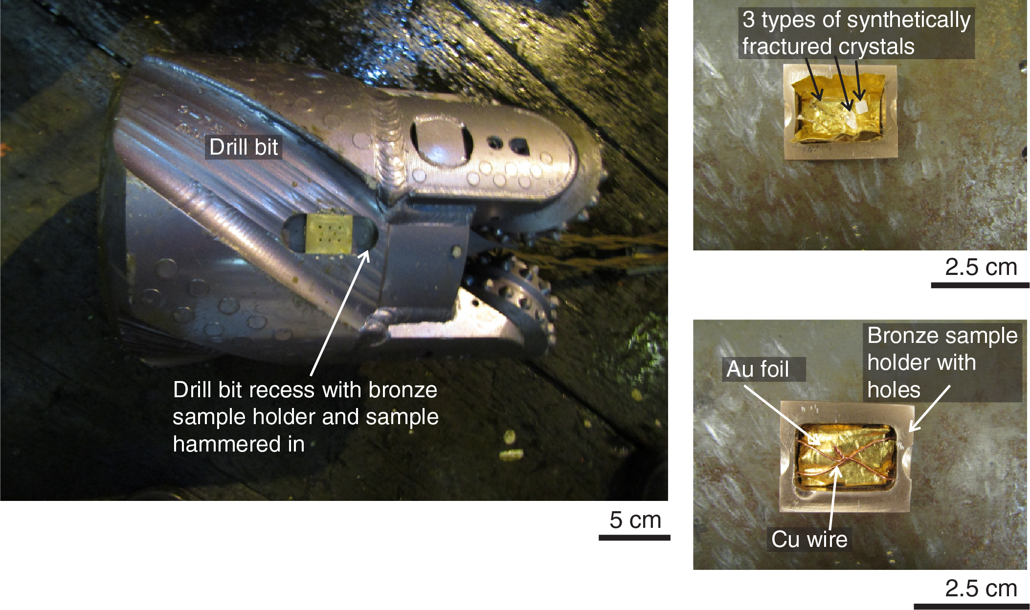
Figure F16. Experimental setup.
Glass capillary thermometers
Temperature-indicating strips were used to monitor maximum downhole temperatures during drilling. Laboratory experiments using temperature sensitive Tempilaq lacquers and temperature-indicating strips have shown that these products become ineffective when wetted by any type of fluid. The strips also react to contact pressure, giving erroneous results. Given this vulnerability to water and pressure, glass capillary thermometers were devised that cover a range of temperatures from 70° to 630°C.
The melting point temperatures of selected solids were 80°, 115°, 232°, 328°, 420°, 450°, 501°, 564°, and 630°C. Also included were two Tempilaq lacquers that change color at 204° and 399°C, respectively. These thermometers always record maximum temperatures.
The Tempilaq lacquers were mixed with silica powder before a few milligrams were inserted into the soda-lime glass capillary tubes. The capillary tubes were then filled with silica powder, heat-sealed, and checked for any air pockets. Solids with specific melting points were ground into a powder, if possible, before a few milligrams were similarly inserted into the tubes. The tubes were again filled with silica powder and checked for air-tightness after sealing.
To increase the probability of getting any information from the melting of solids, the capillary tubes were cut in half to decrease the surface area exposed to high pressures in the borehole. Each tube was wrapped in 15 µm thick aluminum foil with fine holes to increase the probability of preserving any information from the melting of solids, even if the glass capillary tubes shattered. Three to five of these thermometers of various temperatures were inserted into a 4.5 cm long × 16 mm outer diameter (OD) stainless steel tube with ends packed by steel wool. These steel tubes, with temperature-indicating strips included, were then inserted into external recesses in the thermowell section of the Kuster FTS tool, the housing on top of the core barrel, and the chamber in the Schlumberger logging tool strings (Figure F17).
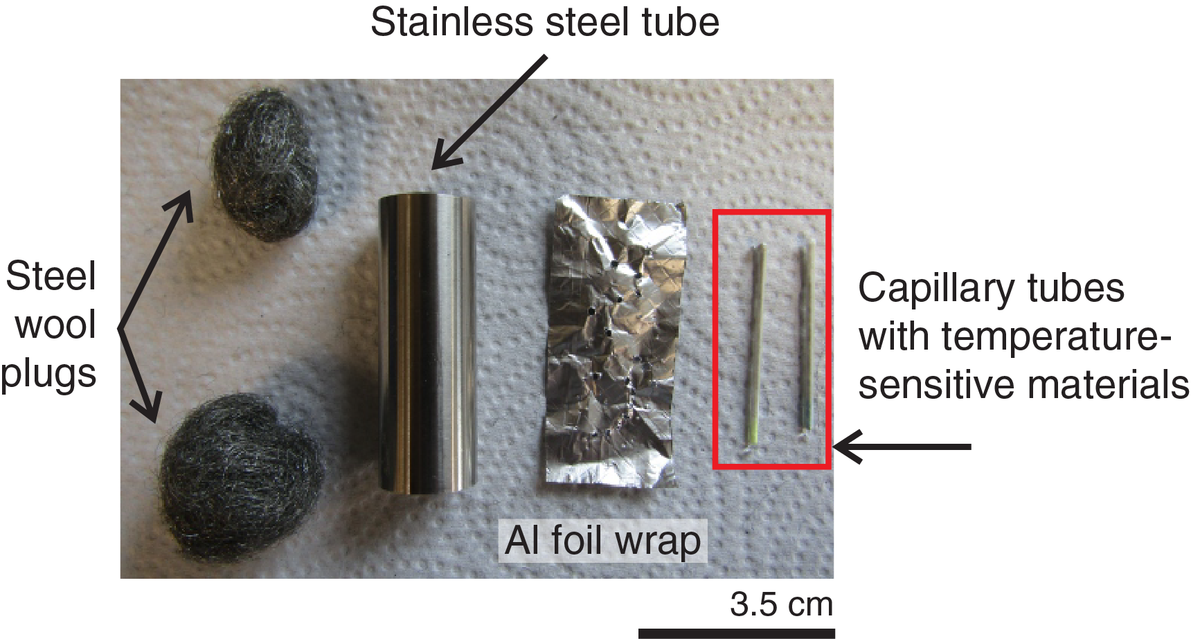
Figure F17. Setup for the deployment of capillary tube thermometers.
Thin section preparation for fluid inclusion analysis
For thin section preparation, the rock sample was crushed using a mortar and pestle, dried in the oven if wet, and then attached to a glass slide with a thin layer of fast-setting cyanoacrylate (superglue). Upon drying, the section was ground using 100 µm Al2O3 on a whetstone and then further ground using wetted 240 to 400 grit sandpaper. When the thickness was acceptable, the section was covered with clear nail polish. Otherwise, the sample was further polished for reflected light analysis via progressive polishing using 9 µm Al2O3 powder followed by 6 µm and then 1 µm diamond suspensions.
Structural geology
Brothers volcano is an arc caldera volcano with several active hydrothermal systems. These rocks are expected to retain a record of volcanic eruption, caldera floor collapse, intraarc extension, and superposed or coincident alteration events. The methods described here are organized from structures formed at high to low temperatures. Many features such as volcanic, alteration, and sedimentary contacts and structural features like alteration veins were measured in coordination with other core description groups.
Conventions for structural studies established during previous “hard rock” drilling projects (e.g., Ocean Drilling Program [ODP] Legs 118, 131, 140, 147, 153, 176, 179, 206, and 209; Integrated Ocean Drilling Program Expeditions 304/305, 309/312, 335, and 345; and IODP Expedition 360 [Shipboard Scientific Party, 1989, 1991, 1992a, 1992b, 1992c, 1993a, 1993b, 1995, 1999, 2003, 2004; Expedition 304/305 Scientists, 2006; Expedition 309/312 Scientists, 2006; Expedition 335 Scientists, 2012; Gillis et al., 2014; MacLeod et al., 2017]) were generally followed during Expedition 376. Definitions of structural measurements and descriptive parameters were further refined during Expeditions 335, 345, 352, and 360 to configure DESClogik for hard rock descriptions. DESClogik was used to enter and upload the information into the LIMS database (see Introduction).
Structural measurements
Orientation measurements were made only on core pieces that had an established upcore direction, which is determined for pieces longer than ~5 cm (piece lengths ≥5 cm ensure that a piece cannot rotate around a horizontal axis resulting in an uncertain upcore orientation). Structural features categorized as magmatic/volcanic, crystal-plastic, or brittle, together with alteration, igneous, and sedimentary contacts, were logged by intervals in centimeters from the top of each section. Depth intervals of structures were recorded as the distance from the top of the section (0 cm) to the top and bottom of the feature where the feature intersects the center of the section half surface (Figure F18). If the structure does not intersect the core center line, the depth to the center portion of the structure was recorded. Structures were measured on the archive half relative to the standard IODP CRF. The CRF is defined by the plane normal to the axis of the borehole and is referred to as the horizontal plane. On this plane, a 360° net is used with pseudosouth (180°; −x-direction) pointing into the archive half and pseudonorth (000°; x-direction) pointing from the split surface out of the archive half (Figure F1). The cut surface of the section half, therefore, is a vertical plane striking 090°–270°.
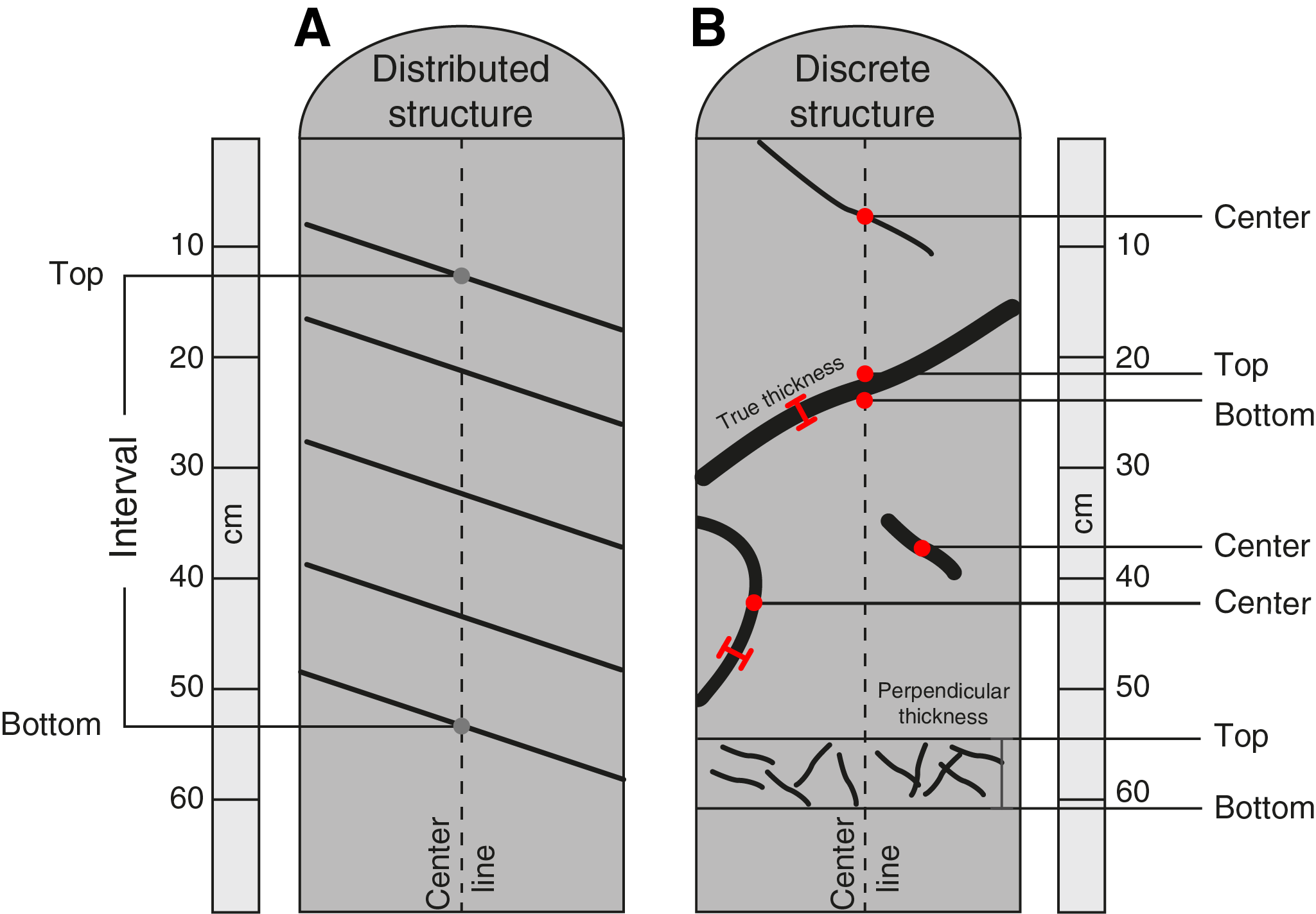
Figure F18. Method for logging structures.
Orientation of structural features is usually determined by making two apparent dip measurements. One apparent dip angle of planar features was measured on the split face of the core with an azimuth of either 090° or 270° (Figure F19A). To obtain a true dip value, a second apparent dip was measured in a section perpendicular to the split face with a dip azimuth of either 000° or 180° (Figure F19B). The two apparent dips and dip azimuths were used to calculate the true dip (0°–90°) and dip azimuth (0°–360°) (i.e., the bearing of maximum dip in the CRF). If the feature intersected the upper or lower surface of the core piece, measurements of the strike could be made directly in the CRF and recorded as the trend of a line with zero dip angle (Figure F19C). When combined with an apparent dip measurement made on the cut surface of the core, calculation of the true dip and dip azimuth in the CRF could be made. If a feature was exposed on the surface of the core (i.e., a fracture or vein defining the top or bottom of a piece), the true dip and dip azimuth were measured directly on the feature with no need for another measurement or calculation. True dip and dip azimuth in the CRF were calculated using a macro in Microsoft Excel written by Dr. Michael Cheadle for ODP Leg 209 or the Stereonet 10 program developed by Allmendinger et al. (2011) and Cardozo and Allmendinger (2013) and imported into the various structure worksheets in the Macroscopic workbook in DESClogik. All structural measurements made on the core were reported in DESClogik and are separated based on whether the orientation was calculated from two apparent dips or measured directly. Where linear structural elements were observed (e.g., slickenlines on a fault or elongate vesicles), the trend and plunge or the rake of the lineations were measured directly, relative to the CRF. The sense of shear on fault surfaces was determined by structures such as groove marks or steps in slickensides. Senses of shear for CPFs were determined using the asymmetry of rotated crystals, porphyroclast-tail systems, or foliation deflection morphologies (e.g., Ramsay and Huber, 1987).
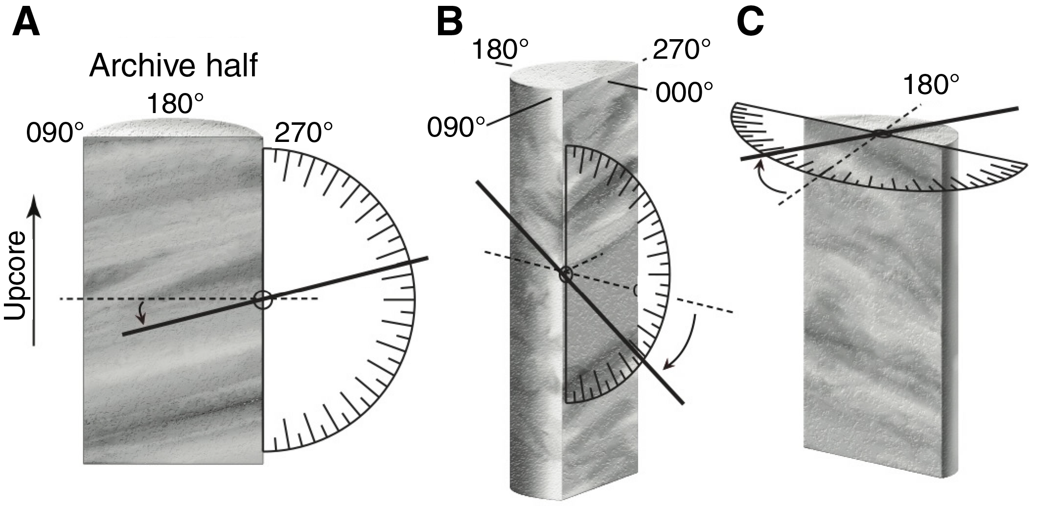
Figure F19. CRF and method for measuring the orientation of planar features.
Statistical analysis of true-dip vein and fracture data
Statistical analysis of true dip of discrete planar features with small lengths compared with the width of the borehole (e.g., veins and fractures) requires an understanding of two geometrical effects:
- The length-scale or spherical effect, which leads to over-representation of steeply dipping planar structures; and
- The so-called borehole effect, which leads to preferential sampling of shallow-dipping planar structures compared with more steeply dipping structures.
Length-scale or spherical effect
A purely random distribution of planes represented by poles in any given area on a unit hemisphere will, on average, contain the same number of poles, irrespective of the position on the unit sphere (Martel, 1999). In any given dip interval, the number of poles is a function of the number of poles intercepting the corresponding arc on the unit sphere. By integration, it can be shown that the number of planes (N) with a given dip (α) is obtained by
(6)where C is a constant. The resultant distribution for a theoretical random data set is shown in Figure F20. The dip data are biased such that there is an over-representation of steeper dips as a result of the spherical geometry effect on the true dip data.
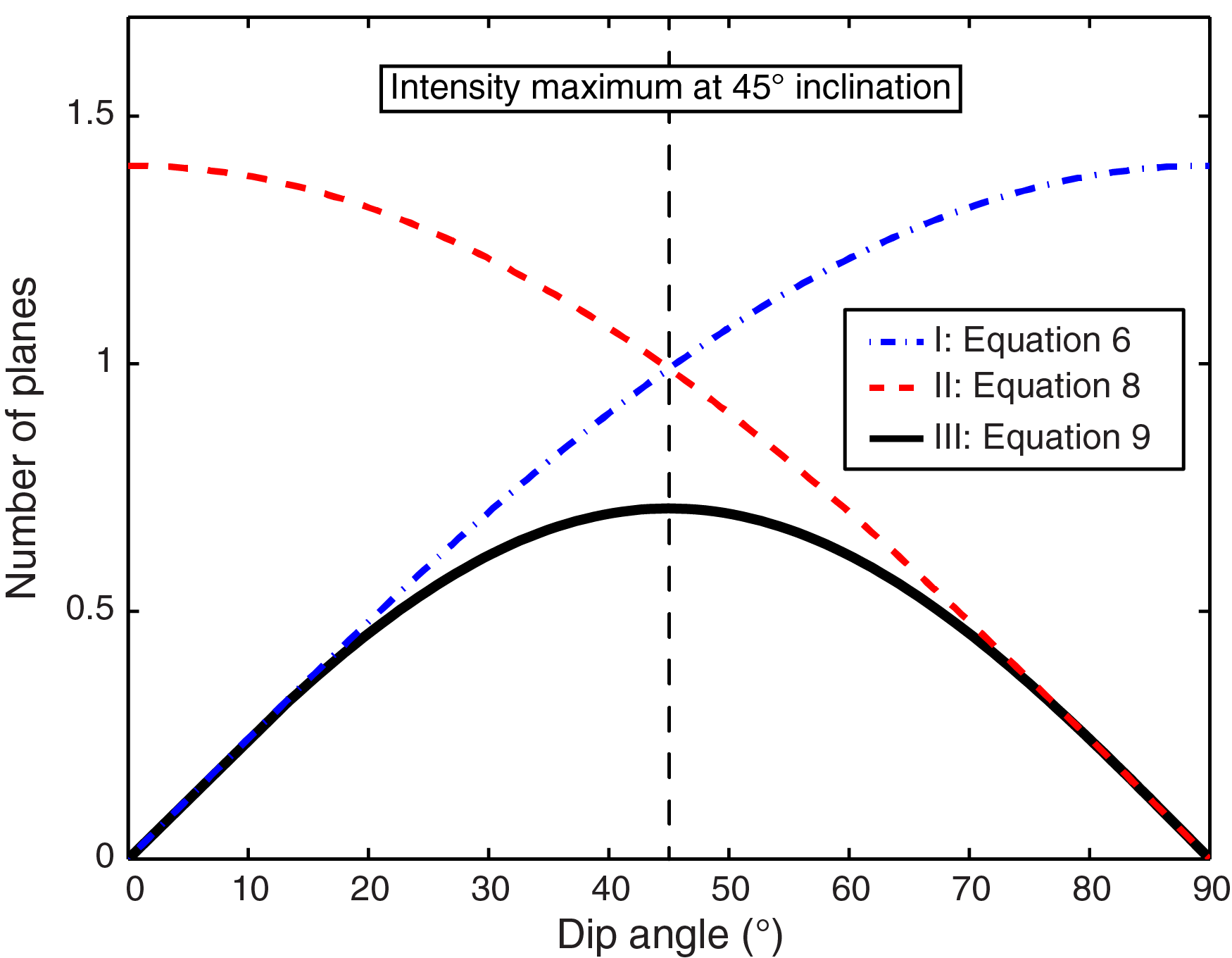
Figure F20. Predicted distribution of a random set of planar features.
Borehole effect
A further consideration is the effect of sampling bias introduced by the vertical nature of a borehole (see Terzaghi, 1965; Newmark et al., 1985). If we consider an equally spaced set of horizontal planes, then the number (N) encountered in a unit borehole length (l) is given by
(7)where s is the spacing of the planes. For vertical planes, either 1 or 0 planes are encountered in the borehole. Thus, for the general case of dipping planes,
(8)Thus, this effect tends to bias the data in favor of shallow dips (Figure F20).
Combining the two aforementioned effects (i.e., Equations E6 and E8) results in the following relationship:
(9)where K is a constant (i.e., scaling factor) and the distribution derived from Equation E9 results in a frequency maximum at 45° inclination (i.e., dip) (Figure F20). Consequently, we present a random distribution curve derived from Equation E9 on all appropriate frequency distribution plots for fracture and vein dips to help assess whether dip distributions are random or nonrandom.
If the length scale of structures such as magmatic contacts, layering, or CPFs considerably exceeds the width of the borehole, then the length scale or spherical effect does not apply. However, these features are still subject to the borehole effect, so steeply dipping features will be undersampled relative to gently dipping features. For a more in-depth discussion, the reader is referred to Martel (1999).
Macroscopic core description and terminology
Workflow organization
Whole-round pieces were oriented for splitting prior to curation by a member of the structural geology and the igneous petrology and volcanology teams. Cores were marked and split to maximize the dip of planar structures so that the dominant structure dips toward 090° or 270° in the CRF (Figure F19). This convention was adopted primarily for ease of structural feature measurement. Where no obvious structures were present, cores were marked to maximize contiguity and/or to ensure that representative material is present in both the working and archive halves of the core. During Expedition 376, the structural geologist was assisted by a member of the igneous petrology and volcanology team who worked on the opposite shift. Each shift was responsible for making all possible observations and measurements throughout the expedition. All descriptions and structural measurements during Expedition 376 were made on the archive halves.
Each core section was described and logged with detailed structural information. This information was then entered into the DESClogik framework. The DESClogik worksheets listed below contain data on the interval, type of structure, intensity, orientation, and comments:
- (Sub)volcanic worksheet: contact characterization in conjunction with the igneous petrology and volcanology team, including contact type, geometry, and orientation.
- Volcaniclastic_sedimentary worksheet: contact characterization in conjunction with the igneous petrology and volcanology team, including contact type, geometry, and orientation.
- Alteration worksheet: contact characterization in conjunction with the alteration team, including contact type, geometry, and orientation.
- Vein worksheet: alteration vein characterization in conjunction with the alteration team, including vein fill, geometry, width, generation, and orientation.
- Vein and fracture density worksheet: number of veins or fractures per 10 cm.
- Structure worksheet: fault rock type and intensity, apparent fault offset, sense of shear, fracture morphology, CPF intensity, magmatic/volcanic fabric intensity, and orientation.
The most representative and/or prominent structural features in the Expedition 376 cores are plotted on the VCD macroscopic graphic reports: the presence of faults, fractures, or veins. Structural descriptions include the main vein fill mineral(s) for that interval along with a description of major structural features like volcanic fabric, fault, slickenline, or igneous, volcaniclastic, or sedimentary contact.
Short explanations for terms and abbreviations used in the respective structural categories, given below, are based on definitions in Ramsay and Huber (1987), Twiss and Moores (1992), Passchier and Trouw (2005), and Davis et al. (2011).
Volcanic/magmatic structures
Volcanic, intrusive, and structural contacts were measured and described in accordance with the igneous petrology and volcanology worksheets ([Sub]volcanic and Plutonic) (see Igneous petrology and volcanology):
- Bottom contact or boundary: curviplanar, planar, and irregular.
- Bottom contact or boundary definition: wavy, sharp, scoured, and gradational.
- Bottom contact or boundary attitude: subvertical, inclined, subhorizonal, vertical, and horizontal.
- Orientation: dip and dip azimuth in the CRF.
Volcaniclastic and sedimentary structures were measured and described in accordance with the igneous petrology and volcanology worksheet (Volcaniclastic_sedimentary):
- Bottom contact or boundary: curviplanar, planar, and irregular.
- Bottom contact or boundary definition: wavy, sharp, scoured, and gradational.
- Bottom contact or boundary attitude: subvertical, inclined, subhorizontal, vertical, and horizontal.
- Sedimentary structure and volcaniclastic structure.
- Orientation: dip and dip azimuth in the CRF.
Volcanic fabrics were defined by the presence and intensity of any shape-preferred orientation of volcanic phases or features (e.g., phenocrysts or vesicles). A magmatic and/or volcanic fabric intensity of 0 was attributed to intervals characterized by isotropic texture and/or where no igneous textures are preserved because of crystal-plastic or alteration overprint. Descriptions of magmatic and/or volcanic fabrics were captured in the Structure worksheet in the Macroscopic workbook and include the following:
- Magmatic/volcanic fabric intensity and associated intensity rank (Figure F21):
- Orientation of the magmatic fabric: dip and dip azimuth, as well as trend and plunge or rake of lineation, where measurable in the CRF.
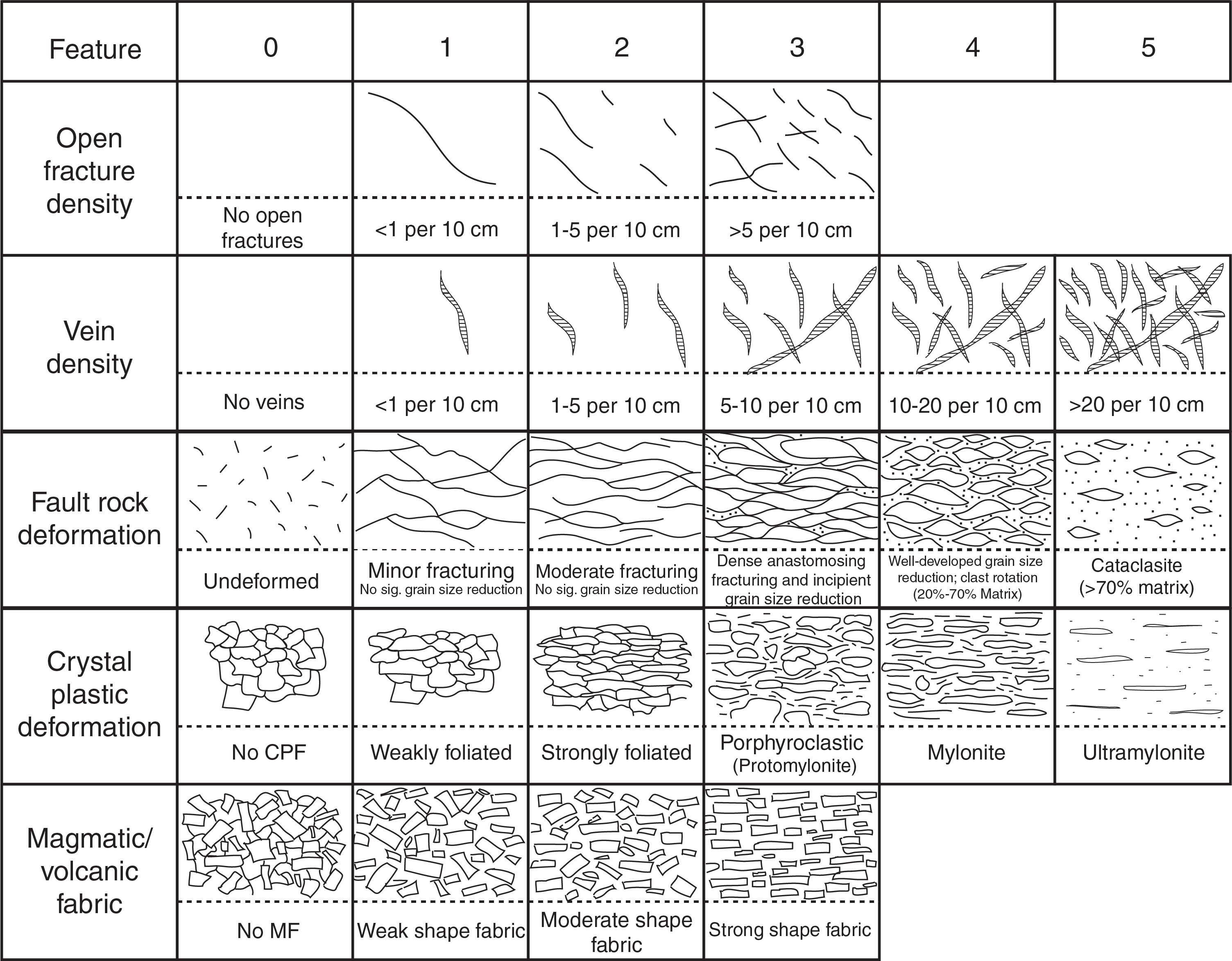
Figure F21. Intensity ranks used to describe macroscopic and microscopic observations.
The final characterization of magmatic/volcanic fabrics were performed after petrographic inspection, when possible.
Crystal-plastic fabrics
CPFs include planar or linear fabrics defined by crystals exhibiting plastic strain. Descriptions for CPFs were captured in the Structure worksheet of the Macroscopic workbook and include the following:
- CPF intensity and associated intensity rank (Figure F21):
- 0 = no fabric.
- 1 = weakly foliated.
- 2 = strongly foliated.
- 3 = porphyroclastic-protomylonite.
- 4 = mylonite.
- 5 = ultramylonite.
- Orientation of the CPF (dip and dip azimuth, where measurable in the CRF; in practice, almost exclusively foliation planes).
The final characterization of CPFs was performed after petrographic inspection, when possible.
Alteration veins
Alteration vein descriptions were captured in the Vein worksheet in the Macroscopic workbook. The descriptions include characterization of the vein margin, structure of the vein fill, and vein generation and other structures, together with orientation. The nature of the alteration vein fill material was identified in consultation with the alteration team. Descriptions of veins include the following:
- Vein morphology: planar, en echelon, anastomosing, stringer, reticulated, or dendritic (Table T11).
- Vein texture: laminated, massive, vuggy, comb, coarse, or fibrous (Table T12).
- Sense of shear: normal (n), reversed (r), dextral (d), sinistral (s), a combination of these (nd, ns, rd, or rs), or unknown.
- Mean vein perpendicular thickness (in centimeters).
- Vein offset (in millimeters), if present and where measurable.
- Orientation of the vein given by dip and dip azimuth and trend and plunge of associated lineation in the CRF, where measureable.
- Vein density (Figure F21). In practice, discrete and network veins were considered. The highest density coincides with the presence of network veins.
Density of veins was recorded in the Vein_fracture_density worksheet of the Macroscopic workbook.
Brittle deformation
Brittle fabrics described during Expedition 376 include breccias, faults (defined as fractures with shear displacement), and fractures. Drilling-induced fractures, defined by subhorizontal fractures with rounded edges and fresh breaks, were not measured or recorded. However, drilling disturbance was recorded by the igneous petrology and volcanology team. Brittle deformation descriptions were captured in the Structure worksheet of the Macroscopic workbook and include the following:
- Fault rock type: fault gouge, fault breccia, cataclasite, hydrothermal breccia, or pseudotachylite.
- Fault rock cohesion:
- Apparent fault offset (in centimeters), where measurable.
- Sense of shear: normal (n), reversed (r), dextral (d), sinistral (s), a combination of these (nd, ns, rd, or rs), or unknown.
- Deformation intensity for brittle fabrics, based on the percentage of matrix present in each fault rock (Figure F21); thin section descriptions, where available, aided this categorization. In practice, minor fracturing was assigned if veins or fractures were present, indicating minimal brittle deformation:
- 0 = undeformed.
- 1 = minor fracturing, no significant grain size reduction.
- 2 = moderate fracturing, no significant grain size reduction.
- 3 = dense anastomosing fracturing, incipient grain size reduction.
- 4 = well-developed grain size reduction, clast rotation, 20%–70% matrix.
- 5 = cataclasite, >70% matrix.
- Clast/matrix ratio in fault rock (in percent).
- Average size of clast in fault rock (in millimeters).
- Clast morphology: angular or rounded.
- Fracture morphology: planar, curved, or irregular (Figure F22).
- Fracture perpendicular thickness (in centimeters), where measureable.
- Orientation given by dip and dip azimuth of fracture and trend and plunge of associated lineation (e.g., slickensides/slickenlines/slickenfibers).
- Fracture density (Figure F21):
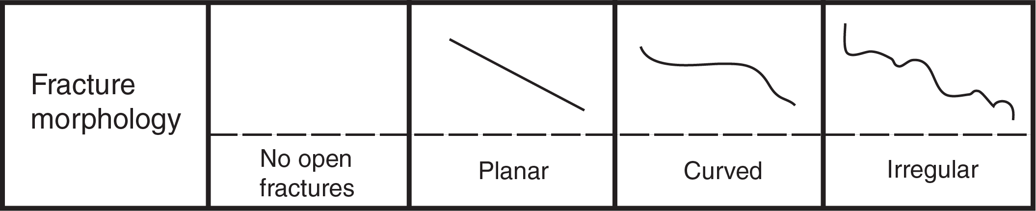
Figure F22. Classification of fracture morphology.
Density of fractures was recorded in the Vein_fracture_density worksheet of the Macroscopic workbook.
Microstructure description and terminology
Workflow organization
To better characterize different types of deformation, microstructural features of interesting and/or prominent mesoscopic structures were studied. Thin sections were examined to
Shipboard thin sections were systematically oriented relative to the CRF if in an oriented piece, as marked on each thin section (Figure F2). Marking two directions is necessary to achieve unambiguous orientation of the thin sections cut parallel to the cut surface of the core. If oriented, each thin section was marked with a half arrow pointing in the upcore direction and the half arrow side of the symbol in the +y-direction (toward 090° in the working half). Because all thin sections were cut parallel to the cut face of the core, this was the only marking required. Macroscopic observations were refined by the microscopic description. Digital photomicrographs were taken to document microstructures that best illustrate different deformation styles, crosscutting relationships, and intensity recorded in the LIMS database. Microstructural notes were entered into the TS_structures worksheet in the Thin section workbook.
Microstructure terminology
Expedition 376 followed the terminology used during ODP Legs 153, 176, and 209; Integrated Ocean Drilling Program Expeditions 304/305 (Expedition 304/305 Scientists, 2006), 345 (Gillis et al., 2014); and IODP Expedition 360 (MacLeod et al., 2017), which broadly follows the terminology of Passchier and Trouw (2005). In the TS_structures worksheet of the Thin section workbook, we described the following microscopic features for each thin section:
- Type of microstructure: magmatic, volcanic, crystal-plastic, brittle, semibrittle, fold, or contact.
- Intensity of static recrystallization: absent, partial, strong, or complete.
- Intensity of magmatic/volcanic fabric and rank (Figure F21):
- Intensity of overall CPF with intensity rank (Figure F21):
- 0 = no fabric.
- 1 = weakly foliated/lineated.
- 2 = strongly foliated/lineated.
- 3 = porphyroclastic/protomylonite.
- 4 = mylonite.
- 5 = ultramylonite.
- Fault rock clast and/or matrix ratio percent of cataclasite and/or brittle fracture.
- Size (in centimeters) of clasts in cataclasite and/or brittle fracture.
- Fault rock intensity and rank (Figure F21):
- 0 = undeformed.
- 1 = minor fracturing, no significant grain size reduction.
- 2 = moderate fracturing, no significant grain size reduction.
- 3 = dense fracturing, incipient grain size reduction.
- 4 = well-developed grain size reduction, clast rotation, 20%–70% matrix.
- 5 = cataclasite, >70% matrix.
- Sense of shear: normal (n), reversed (r), dextral (d), sinistral (s), a combination of these (nd, ns, rd, or rs), or unknown.
- Comments: any details of microstructures.
Geochemistry
Headspace gas analysis
Headspace analysis of hydrocarbon gases
One sample per core was collected, if possible, for headspace hydrocarbon gas analysis as part of the standard shipboard safety monitoring procedure, as described in Kvenvolden and McDonald (1986) and Pimmel and Claypool (2001), to ensure that drilled materials did not contain amounts of hydrocarbons above prescribed safety levels.
A ~5 cm3 sample of small, crushed rock pieces was taken from the core immediately after it was brought on deck and sectioned. The sample was placed in a 20 cm3 glass vial and sealed with a polytetrafluoroethylene (PTFE)/silicon septum and a crimped aluminum cap. During Expedition 376, headspace samples were, in most cases, taken at the bottom of Section 1 of each core. Each vial containing the headspace sample was placed in an oven at 80°C for 30 min. A 5 cm3 aliquot of any released hydrocarbon gases was withdrawn from the headspace vial with a standard gas syringe and manually injected into an Agilent/Hewlett Packard 6890 Series II gas chromatograph (GC) equipped with a flame ionization detector set at 250°C. The column (2 mm inner diameter [ID]; 6.3 mm OD) was packed with 80/100 mesh HayeSep (Restek). The GC oven program was set to remain at 80°C for 8.25 min with a subsequent rise to 150°C at 40°C/min. Each analysis required 15 min.
The results were processed using the Hewlett Packard 3365 ChemStation data software package. The chromatographic response was calibrated using nine different gas standards and checked daily. Concentrations of hydrocarbon gases are reported in millimoles per kilogram of pore water as well as parts per million by volume (ppmv). Pore water hydrocarbon abundance was calculated using the weight, density, and porosity of the rock sample. Reported data are normalized to total pore water volume.
Headspace analysis of H2, CO, ΣCO2, and acid-volatile sulfide
Two separate headspace samples, each composed of 1.5 cm3 of small crushed rock pieces, were taken from the core immediately after it was brought on deck and sectioned. Each sample was then placed in a 20 cm3 glass vial containing either 3 mL of distilled water plus a small amount of HgCl2 to prevent microbial activity or 3 mL of 1 mol/L HCl solution to extract ΣCO2 and acid-volatile sulfide (AVS) from the pore fluid of the rock material. AVS is defined as those materials which release ΣH2S if treated with HCl (Rickard and Morse, 2005). Such materials can include dissolved and volatile reduced S(−II) species (e.g., H2S, HS−, FeHS+, FeS clusters, and iron sulfide nanoparticles) and solid phase minerals such as mackinawite (FeS). Pyrite (FeS2) is not usually considered to contribute to AVS because HCl-leach methods allegedly do not dissolve pyrite.
The vial was sealed with a PTFE-coated butyl rubber septum and a crimped aluminum cap. The vial for H2 and CO analysis (with HgCl2) was then placed in the oven at 80°C for 30 min. A 0.5 cm3 aliquot of the headspace was withdrawn from the vial with a standard gas syringe and manually injected into a GL Science GC4000 GC equipped with a helium ionization detector (HID) set at 160°C for quantification of H2 and CO. The column (2 mm ID; 6.3 mm OD) was packed with molesieve 5Å (Agilent/Hewlett Packard). The GC oven program was set at 80°C isothermal. For the second sample (with HCl), a 0.1 cm3 aliquot of gas was withdrawn from the headspace with a standard gas syringe and manually injected into a GL Science GC4000 GC equipped with a HID set at 240°C for quantification of CO2. The column (2 mm ID; 6.3 mm OD) was packed with Porapack Q (Agilent/Hewlett Packard). The GC oven program was set at 40°C isothermal. In addition, a 1 cm3 aliquot of solution was extracted from the acidified headspace vial with a disposable syringe. This aliquot was measured by an electrochemical ΣH2S probe (H2S-40N, Unisense, Denmark). The ΣH2S concentration was calibrated with seawater containing 0.05, 0.5, and 5 mmol/L Na2S and acidified using 1 mol/L HCl at a temperature matching that of measured conditions.
The chromatographic response was calibrated using two different concentrations of gas standards and checked daily. The concentrations of the analyzed H2, CO, CH4, ΣCO2, and AVS were reported in micromoles or millimoles per kilogram of pore water calculated using the weight, density, and porosity of the rock sample and normalized to total pore water volume, as for hydrocarbons.
Borehole fluid geochemistry
Sampling
After the final drilling depth was achieved, borehole fluids were collected at selected depths from within the drill string using the mechanical clock-activated Kuster FTS tool attached to the core line. Timing of the clock was set such that the FTS remained at the target depth for 15 min after the closing time to accommodate potential uncertainty in the clock function at elevated temperatures. The design and deployment of the Kuster FTS are detailed in Downhole logging operations.
Shipboard processing
Volatile-rich aqueous borehole fluids were extracted from the 600 mL Kuster FTS tool and processed aboard the ship immediately upon recovery of the tool. The transfer head assembly was outfitted with a 25 MPa (250 bar) pressure gauge and a gas-tight extraction line (Figure F23) for shipboard analysis of volatile species (H2 and ΣH2S [ΣH2S = H2S + HS− + S2−]), dissolved inorganic constituents (salinity, pH, alkalinity, Al, Ba, Br, Ca, Cl, Co, Cr, Cu, Fe, K, Mg, Mn, Na, Ni, Si, ΣSO4 [ΣSO4 = SO42− + HSO4− + H2SO4], Sr, Ti, V, and Zn), and particles (Al, Ba, Co, Cr, Cu, Fe, Mn, Ni, Ti, V, Zn, total S, total C, and total N). Headspace gases were sampled from the top valve via the extraction line with the 600 mL Kuster FTS tool in a horizontal position. The sample was homogenized by rotating the tool twice, and the fluids were expelled out the top valve by applying gentle backpressure to the open bottom valve using a portable glove bag filled with N2. Sample allocation was determined based on the borehole fluid volume recovered and analytical priorities based on the expedition objectives. The borehole fluids collected from the 600 mL Kuster FTS tool were divided into aliquots for the following shipboard analyses:
- 3 mL for salinity measurement with a refractometer, pH, and alkalinity;
- 100 μL for ion chromatographic (IC) analysis of major anions and cations;
- 100 μL for analysis of major, minor, and trace elements by ICP-AES;
- 9 mL for H2 analysis by gas chromatography; and
- 30 mL for ΣH2S analysis by gravimetry.
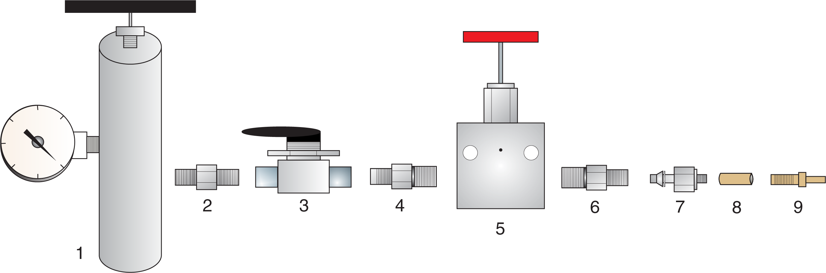
Figure F23. Gas-tight valve components.
During sample processing, aliquots were extracted in priority order for immediate analysis of pH (25°C; 1 bar), H2, and dissolved ΣH2S. Aliquots for shipboard analysis of dissolved inorganic species were then collected in acid-washed, high-density polyethylene (HDPE) bottles. An aliquot of the unacidified dissolved inorganic sample was diluted 100-fold (v/v) and analyzed for dissolved Si via ICP-AES. Aliquots for shipboard dissolved transition metal analyses were filtered immediately through 0.22 μm polyethersulfone filters using acid-washed syringes; aliquots for total and total dissolvable metals were left unfiltered. Aliquots for total metals were prepared after complete digestion of an aliquot of unfiltered fluid fraction with concentrated trace-metal grade HNO3 on a hot plate for 3 h. The sample was then diluted with 10% concentrated Optima HNO3. All other transition metal aliquots, including the dissolved and total dissolvable aliquots, were acidified to 1 wt% with concentrated Optima HNO3. A separate fluid aliquot was collected for ΣSO4 and sparged with ultra–high purity Ar (~30 min) to remove volatile S species such as ΣH2S and SO2 that may otherwise oxidize and result in artificial elevation of measured ΣSO4 abundances.
Hydrothermal fluid samples often contain transition metal–rich precipitates that can form during the time period between sampling and extraction from the sampler. In addition, at high-acidity, high-temperature conditions in the borehole, the steel drill pipe and the Kuster FTS itself can contribute particle-forming metals and other possible species to the fluids. After the complete removal of the borehole fluid sample from the 600 mL Kuster FTS tool, the dregs fraction, which is composed of precipitates that formed in the sampler either before or after valve closure, was collected on 0.22 μm Millipore Durapore filters by rinsing the interior of the Kuster FTS with reagent-grade acetone and nanopure water, followed by vacuum filtration. A fraction of each solid dregs aliquot was digested in concentrated trace metal–grade HNO3 in PTFE beakers at 80°C until near-dryness. Digested dregs were then dissolved in 10 wt% HNO3 and analyzed via ICP-AES following the same methods as for aqueous determination (see below).
Shipboard analyses
Borehole fluids were analyzed following protocols similar to those used for interstitial water (IW), as described in Gieskes et al. (1991), Murray et al. (2000), and the IODP user manuals for shipboard instrumentation, in addition to methods modified after those described in McDermott et al. (2018). Precision and accuracy were tested using International Association for the Physical Sciences of the Oceans (IAPSO) standard seawater with the following composition: 2.35 mmol/L alkalinity, 10.53 mmol/L Ca, 54.11 mmol/L Mg, 10.46 mmol/L K, 90.62 μmol/L Sr, 28.93 mmol/L SO4, 559.8 mmol/L Cl, 478.7 mmol/L Na, and 426.0 μmol/L B. Borehole fluid components reported here that have low abundances in seawater (e.g., Fe, Mn, Al, Ba, Co, Cr, Cu, Ni, Zn, and Si) are based on calibrations using certified stock solutions (Gieskes et al., 1991).
Dissolved aliquots for trace metal analysis (filtered immediately as samples were drawn) were diluted and analyzed directly via ICP-AES. Total dissolvable trace metal aliquots (unfiltered as samples were drawn) were filtered ~12 h after sample collection and acidification to 1 wt% with Optima-grade HNO3, and the aqueous fraction was diluted and analyzed via ICP-AES. The digested total metals sample was then dissolved in 10 wt% HNO3 and analyzed via ICP-AES.
Salinity, alkalinity, and pH
Salinity, alkalinity, and pH were measured immediately after borehole fluid extraction following the procedures in Gieskes et al. (1991). Salinity was measured using a Fisher temperature-compensated handheld refractometer (Fisher Model S66366). The valve system was used to transfer two drops of borehole fluid to the salinity refractometer, and the corresponding salinity was recorded. Fluid pH was measured with a combination glass electrode standardized with pH 1, 4, and 7 buffers (±0.02 at 25°C; National Institute of Standards and Technology [NIST] traceable) for low-pH samples and with pH 4, 7, and 10 buffers for near-neutral pH samples. Alkalinity was determined by Gran titration with an autotitrator (Metrohm 794 Basic Titrino) using 0.1 mol/L HCl at 20°C. Certified Reference Material 104 was used to calibrate the acid. IAPSO standard seawater was used for calibration and was analyzed at the beginning and end of the sample set for each site. Repeated measurements of IAPSO standard seawater alkalinity yielded a precision of <0.8%.
Ion chromatography
Anion (Cl, ΣSO4, and Br) and cation (Na, Mg, K, and Ca) elemental abundances were analyzed using a Metrohm 850 ion chromatograph equipped with a Metrohm 858 Professional Sample Processor as an autosampler. The sample solutions used were diluted 1:100 or 1:200, depending on anticipated species abundances, with nanopure water using specifically designated pipettes. A seawater standard calibration curve was generated using IAPSO dilutions of 67×, 80×, 100×, 150×, 200×, and 350× the pure seawater composition. Reproducibility (expressed as the percent of one relative standard deviation [RSD]) for 100× IAPSO analyses interspersed with the unknowns were: 0.7% Br, 0.5% Cl, 0.7% ΣSO4, 2.6% Ca, 1.3% Mg, 0.6% K, and 0.5% Na (N = 22).
Inductively coupled plasma–atomic emission spectrometry
Major and minor elements were analyzed on borehole fluids by ICP-AES with an Agilent 5110 ICP-OES spectrometer. The general method for shipboard ICP-AES analysis of samples is described in ODP Technical Note 29 (Murray et al., 2000) and the shipboard user guide for ICP-AES, with modifications as indicated in the Expedition 369 methods chapter (Huber et al., 2019).
Samples and standards were diluted 1:50 using 2 wt% HNO3 for metal and trace element (Al, Ba, Co, Cr, Cu, Fe, Mn, Ni, Sr, Ti, V, and Zn) and major constituent (Na, Mg, Si, S, K, and Ca) analyses. Each batch of samples run on the ICP-AES includes blanks and standard solutions of known concentrations. Each sample or standard aspirated was counted three times from the same dilute solution in a given sample run. Following each instrument run, the measured raw intensity values were transferred to a data file and corrected for instrument drift and blank. If necessary, a drift correction was applied to each element by linear interpolation between the drift-monitoring solutions and by using internal standards (Be, In, Sc, and Sb). Standardization of major cations was achieved by successive dilution of IAPSO to 20×, 40×, 100×, and 1000×. Replicate analyses of 40× IAPSO were run as unknowns throughout each batch of analyses to yield estimates for precision and accuracy. Reproducibility for 40× IAPSO interspersed with the unknowns was between 1% and 3% (N = 12). Because of the high concentration of matrix salts in the borehole fluid samples at 1:50 dilution, matrix matching the calibration standards for minor elements was necessary to achieve accurate results by ICP-AES. A matrix solution that approximated seawater Na and Cl concentrations was prepared by adding trace metal clean NaCl to a stock standard solution prepared from ultrapure primary standards (Science Plasma-CAL) in 2% HNO3 solution. The stock solution was then serially diluted in the same 2 wt% HNO3 solution and was spiked with the same internal standard suite as the samples just prior to analysis. For calibrated trace elements, the reproducibility of duplicate measurements was between 1% and 3%.
Dissolved gases (H2 and ΣH2S)
Dissolved H2 was analyzed via gas chromatography in accordance with methods described in McDermott et al. (2018) and IODP user manuals for shipboard instrumentation. Dissolved H2 was analyzed by gas chromatography with thermal conductivity detection (TCD) and Ar carrier gas (Agilent 6890) after headspace extraction using a gas-tight glass syringe (McDermott et al., 2018). Samples and standards were injected into a 0.5 mL calibrated loop. Gas components were then separated by a 30 m × 0.53 mm × 40 μm HP-PLOT Q capillary column followed in series by a 30 m × 0.53 mm × 50 μm HP-PLOT molesieve capillary column, after which H2 was detected via TCD. Valve and Ar blanks were monitored, as were N2 and O2, to ensure that injections entrained minimal ambient air. Samples were bracketed with injections of calibrated H2 gases daily (100, 1000, and 10000 ppmv of H2 into a sample loop of precisely known volume). Dissolved ΣH2S was precipitated as Ag2S in 5 wt% AgNO3 and recovered on a 0.22 μm pore size filter via vacuum filtration in accordance with methods described in McDermott et al. (2018). Concentrations were then gravimetrically determined.
Contamination assessment
Between samples and before each deployment on the core line, the sample chamber of the 600 mL Kuster FTS tool was cleaned with analytical-grade acetone, scrubbed with a stainless steel brush, swabbed with a laboratory tissue, and rinsed with nanopure water. O-rings were checked for mechanical damage and embrittlement, replaced as needed, and lubricated. The sampler is made up of 17-4 PH stainless steel (15–17.5% chromium, 3–5% nickel, and 3–5% copper) and Monel, a nickel-copper alloy (as much as 67% Ni) that contains minor amounts of iron, manganese, carbon, and silicon. Silicone- and MoS2-based greases were used to lubricate O-rings. All of these constituents may contribute to contamination of the sampled borehole fluids. They are likely to be chemically reactive under the acidic borehole conditions encountered (measured pH down to 1.8; see Principal results in the Site U1528 chapter [de Ronde et al., 2019]). Therefore, a series of contamination assessments was performed by setting up the sampler in the deployment configuration and filling it with the following solutions, closing the valves, and waiting 12 h at 20°C before proceeding with processing and analysis of aqueous samples for major ions and metals (Table T15):
- 18.2 MΩ/cm Barnstead nanopure water and
- Seawater from the JOIDES Resolution drilling fluid reservoir, untreated.
The sampler was cleaned fully, and the O-rings were lubricated between each contamination test. Contamination tests were run before the first samples were taken.
Pre- and posttest deionized water and drilling seawater were analyzed via ion chromatography for major anion and cation elements and via ICP-AES for minor and trace elements. Shipboard results indicate that the 600 mL Kuster FTS tool does not contaminate for anions or cations that are present in major concentrations in the fluid. However, metals including Co, Cr, Cu, Fe, Mn, and especially Ni were contributed during these room temperature tests. Thus, the sampler most likely reacts to an even greater degree under the acidic, high-temperature borehole conditions encountered (measured pH down to 1.8; see Principal results in the Site U1528 chapter [de Ronde et al., 2019]).
Interstitial water geochemistry
Whole-round core samples of unconsolidated materials, generally 10–20 cm long, were partitioned immediately after the core was brought on deck, capped, and taken to the laboratory for pore fluid processing. After extrusion from the core liner, contamination from seawater and sediment smearing was removed by scraping the core surface with a spatula. The TDCS core samples had ~0.5 cm of material from the OD, and the top and bottom faces were removed. IW samples from RCB coring were not scraped because they were collected from cores composed of relatively loose sand and coarser grained (~0.1–0.5 cm diameter) volcanic pebbles. The core was placed into a titanium squeezer (modified after Manheim and Sayles, 1974) and compressed using a laboratory hydraulic press. The squeezed pore fluids were filtered through a prewashed Whatman No. 1 filter placed in the squeezers above a titanium mesh screen. Approximately 2–12 mL of pore fluid was collected in precleaned plastic syringes attached to the squeezing assembly and subsequently filtered through a 0.45 μm Gelman polysulfone disposable filter. In some sections, fluid recovery was as low as 2 mL after squeezing the sediment for as long as ~2 h.
After the fluids were extracted, the squeezer parts were cleaned with shipboard water and rinsed with deionized water. Parts were dried thoroughly prior to reuse.
Sample allocation was determined based on the pore fluid volume recovered and on analytical priorities based on the expedition objectives. The IW extracted from the compressed sediment sample was divided into aliquots (in priority order) for the following analyses:
- 100 μL for IC analysis of major anions and cations;
- 100 μL for ICP-AES analysis of major, minor, and trace elements; and
- 3 mL for pH and alkalinity.
Shipboard analytical protocols were identical to the methods described for borehole fluid analyses.
Hard rock geochemistry
Sample preparation
Unconsolidated samples were taken from the interiors of cores with 10 cm3 cubes and then oven-dried for ~24 h to remove water. In some cases, residues of samples processed for IW, including squeeze cakes and rock chips, were also prepared for shipboard analysis. Hard rock samples were prepared from 5–10 cm3 of rock. Solid rock samples were cut from the cores using a diamond-blade rock saw. Outer surfaces of rock samples were ground using a diamond-impregnated grinding wheel to remove saw marks and any drilling-induced alteration on the exterior.
Each cleaned solid rock sample was placed in a beaker containing isopropanol and agitated in an ultrasonic bath for 15 min. The isopropanol was decanted, and the samples were then agitated twice in an ultrasonic bath in nanopure deionized water (18 MΩ/cm) for 10 min. The cleaned pieces were then dried for 10–12 h at 110°C. After drying, the rock samples were crushed to <1 cm between two Delrin plastic disks in a hydraulic press.
Considering the high concentration of anhydrite (CaSO4) encountered in many altered volcaniclastic rocks and lavas recovered during Expedition 376, additional tests were performed to evaluate the effect of rock powder preparation (e.g., water cleaning) on anhydrite and the potential dissolution of other water-soluble minerals. A test was performed on a relatively anhydrite rich sample (376-U1530A-9R-1, 8–10 cm) in which the first and second water rinses of the ICP-AES wedge were analyzed via ICP-AES for dissolved Ca, S, and other species to determine the extent of water-soluble element loss during powder preparation. For comparison, a ground powder from the same sample was leached in nanopure water (250 mg powder; 15 mL water) for 12 h to determine the total amount of anhydrite present in the sample (as water-soluble Ca and S). Results for total anhydrite dissolution yielded 1.39 wt% Caanhydrite and 1.10 wt% Sanhydrite in the initial sample. In the rinse solutions, Ca and S were released in a Ca/S molar ratio of 1.01, indicating that some anhydrite was solubilized. The amount of dissolved Ca and S released in combined water rinses of the wedge accounted for only ~3.3% of the total anhydrite present in the rock, suggesting minor anhydrite loss during rock powder preparation. Other species (e.g., K and Al) were below detection for ICP-AES in the water rinses.
Crushed chips of rock were ground to a fine powder using a SPEX 8515 Shatterbox powdering system with a tungsten carbide mill. A check on contamination from grinding in tungsten carbide mills was performed during ODP Leg 206 (Shipboard Scientific Party, 2003) and found to be negligible for major elements and most of the trace elements measured on board (Sc, V, Cr, Ni, Sr, Y, Zr, and Ba). However, a systematic analysis of the shipboard powders from Integrated Ocean Drilling Program Expedition 304/305 indicated possible Co contamination during powdering (Godard et al., 2009).
For most samples, the prepared powder was divided into two parts: one portion was processed for XRD and pXRF analysis, and the other portion was processed for ICP-AES and volatile measurements.
Volatile measurements
Volatile concentrations of rocks were measured on powdered splits of ICP-AES samples.
Carbonates
The carbonate-associated carbon content of the samples (also referred to as total inorganic carbon [TIC]) was determined by acidifying ~40 to 100 mg of powder with 5 mL of 2 mol/L HCl at 50°C and measuring the amount of CO2 generated using a UIC 5011 CO2 coulometer. The gas volume was determined by trapping the CO2 with ethanolamine and titrating coulometrically with hydroxyethyl carbamic acid. The end point of the titration was determined by a photodetector; the change in light transmittance is proportional to the inorganic carbon content of the sample.
All CO2 was assumed to derive from dissolution of CaCO3. No corrections were made for other carbonate minerals. Results are reported as TIC in micrograms per gram (µg/g). The detection limit of this technique was generally between 30 and 50 µg/g. Several standards with low TIC concentrations and ignited unaltered dacitic samples were analyzed to improve both the internal precision of the measurement and assessment of the detection limit.
Total carbon, total nitrogen, and total sulfur
Total carbon (TC), total sulfur, and total nitrogen (TN) contents were determined from an aliquot of the ICP-AES sample powder by combustion at >900°C in a Thermo Electron FlashEA 1112 EA equipped with a Thermo Electron packed column carbon-hydrogen-nitrogen-sulfur (CHNS)/nitrogen-carbon-sulfur (NCS) analyzer and a TCD for TC, total S, and TN. Between 10 and 40 mg of powder was weighed into a tin cup and subsequently combusted in an oxygen gas stream at 900°C. The reaction gases were passed through a reduction chamber to reduce nitrogen oxides to N2, and the mixture of CO2, SO2, and N2 was separated by GC and detected by the TCD. Calibration was based on the NIST 2704 (Buffalo River sediment) reference material standard, which contains 3.35 wt% TC, 0.18 wt% TN, and 0.40 wt% TS. A set of in-house synthetic samples was also used for calibrating total sulfur measurements of S-enriched samples (see Calibration, blanks, and standards).
Aliquots of powder (typically ~20 mg for igneous rocks) were weighed on a Cahn C-29 microbalance, with weighing errors conservatively estimated to be ±0.2 mg. Powders were packed into tin containers (Universal Tin Container “light”; Thermo Electron P/N 240-06400) and mixed with a spatula full of vanadium pentoxide (V2O5) estimated at 10 ± 3 mg. The samples were placed in a revolving autosampler with 31 spaces and dropped into a 900°C resistance furnace, where they were combusted in a reactor. The tin capsule creates a violent flash combustion (Sn has a melting point of only 230°C), and the V2O5 generates an oxygen-enriched atmosphere. The oxidized and liberated volatiles were then entrained by a constant helium gas flow through a commercial glass column (Costech P/N 061110) packed with an oxidation catalyst of tungsten trioxide (WO3) and a copper reducer. The gases were then separated by a packed GC column (Costech P/N 0581080) and a water trap. During the measuring time of 1000 s, the millivoltage at the thermal conductivity detector was continuously recorded, with peaks for N2, CO2, and SO2 at approximately 60, 98, and 770 s, respectively.
Loss on ignition
After powdering, an aliquot between 2.00 and 5.00 ± 0.05 g of the sample powder was weighed on a Mettler Toledo balance and ignited for 4 h at 1025°C for igneous rocks to determine weight LOI with an estimated precision of 0.02 g (0.4%).
In comparing the GC volatile analyses with the LOI results, it is important to note that Fe2+ will change to Fe3+ (as well as S0 and S2− to oxidized S6+) during ignition of the sample in ambient atmosphere. This can result in a weight gain of as much as 11.1% of the proportion of ferrous Fe in the sample (e.g., a sample with 10% Fe2+ could increase in weight by >1 wt%). Also, ignition at or above 1000°C can result in the loss of K and Na because these elements have vapor points below 1000°C (759°C for K and 883°C for Na) (Lide, 2000). These two issues can lead to discrepancies between LOI analyses and volatile concentrations determined by GC analysis.
Total organic carbon
Total organic carbon was calculated by subtracting the weight percent of inorganic carbon from TC obtained with the CHNS analyzer. Repeated measurements of pure CaCO3 and BHVO-2 (several times at the beginning and end of each run) were used to estimate accuracy, which was <5% of the TIC. The BHVO-2 standard was chosen for calibration of TIC because of its low TIC concentrations, which are close to those expected during Expedition 376.
Calibration, blanks, and standards
Analytical runs typically began with a blank consisting of a tin capsule with ~10 mg of V2O5 and five variably sized aliquots of the SRM 2704 standard, which contains 3.35 wt% C and 0.172–0.18 wt% N. This standard was chosen for calibration of every run for C and N.
To assess the effect of a Ba-rich matrix on S recovery and obtain a good calibration curve for high-sulfur samples, various sulfur compounds were added to ashed powders to create in-house EA standards that matched the matrix and S content of Brothers volcano samples. These standards were gravimetrically calibrated using a Cahn C-31 microbalance. Pure MgSO4 and AgS2 compounds were mixed with ashed rock powder (Sample 376-U1527A-5R-1, 13–15 cm) to get a 2.5 wt% concentration of TS. Pure BaSO4 and native sulfur were also added to ashed rock powders in proportion to create 8, 4, and 2 wt% and 10, 5, and 2.5 wt% S standards, respectively. These in-house standards were run for EA measurements prior to every run as a quality control of the measurement and for data analysis. The calibration curve for the CHNS analyzer from in-house standards is shown in Figure F24. In contrast to in-house standards with MgSO4, AgS2, and native sulfur, BaSO4 standards reported lower reproducibility for those with higher BaSO4 concentrations (i.e., >2.5 wt%).
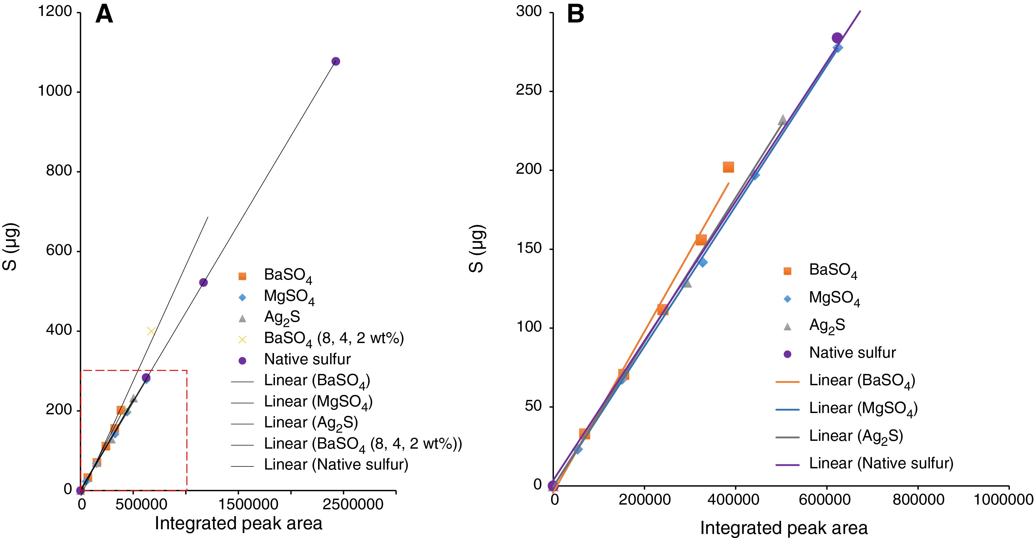
Figure F24. Total S calibration curves.
ICP-AES
The standard shipboard procedure for digestion of rocks and subsequent ICP-AES analysis is described in Murray et al. (2000) and the shipboard user guide for ICP-AES, with modifications as indicated in the Expedition 369 methods chapter (Huber et al., 2019). The following protocol is a synopsis of this procedure with minor changes and additions.
Digestion procedure
Each sample and standard was weighed on a Cahn C-31 microbalance to 100.0 ± 0.5 mg; weighing errors are estimated to be ±0.2 mg under relatively smooth sea-surface conditions. Aliquots of ignited whole-rock powders were mixed with 400.0 ± 0.5 mg of LiBO2 flux (preweighed on shore). Aqueous LiBr solution (10 µL of 0.172 mmol/L) was added to the flux and rock powder mixture as a nonwetting agent prior to sample fusion to prevent the fused bead from sticking to the crucible during cooling. Samples were fused individually in Pt-Au (95:5) crucibles for ~12 min at a maximum temperature of 1050°C in an internally rotating induction furnace (Bead Sampler NT-2100).
The beads were then transferred into 50 mL HDPE bottles and dissolved in a 50 mL solution containing 10 wt% HNO3 (prepared from Optima-grade concentrated HNO3). The solution bottle was placed in a Burrell wrist-action shaker for 1 to 2 h at 7°C to aid dissolution, and then 0.5 mL was pipetted into a polyethylene centrifuge tube and diluted with 4.4 mL of 10 wt% HNO3 and 0.1 mL of internal standard solution containing Be, In (100 µg/g), and Sb (200 µg/g). The final solution-to-sample dilution factor was 4000×; this solution was analyzed for both major and trace elements.
A different digestion procedure was used for trace element analysis of chalcophile elements (e.g., As, Se, Sb, Cd, and Pb), which are prone to significant contamination (e.g., Pb) or are potentially volatile during fusion (e.g., Cd and Se). About 100 mg of rock powder was digested in an acid-clean low thermal expansion borosilicate glass beaker on a hot plate (120°–150°C) with concentrated trace metal–grade HNO3. Because this procedure dissolves sulfide minerals but only partly dissolves clay minerals and other silicates, trace metals and metalloids analyzed with this procedure are referred to as acid-soluble elements.
To determine the abundance of H2O-soluble S relative to total S in rocks from Holes U1528A, U1528C, and U1528D, a portion of the powdered rock prepared for ICP-AES analysis was leached with nanopure water, and H2O-soluble components were analyzed via ICP-AES. First, a 250 mg portion of the sample was weighed into an acid-cleaned 50 mL polyethylene centrifuge tube, and 15 mL of nanopure water (18.2 MΩ) was added. The samples were agitated and placed in a shaker for 12 h at 7°C. Samples were then centrifuged, and the supernatant liquid was filtered. Aliquots were acidified to 1 wt% with HNO3, and the concentrations of Ca, S, and Sr were determined via ICP-AES. Abundances of H2O-soluble Ca, S, and Sr were then determined for the bulk rock and taken to represent species derived from anhydrite. The difference between each species (e.g., total S from elemental analysis and anhydrite-derived S) was calculated and taken to represent the H2O-insoluble fraction of that element in the rock.
Analysis
Major and trace element concentrations of standards and samples were determined using an Agilent 5110 ICP-OES instrument in AES mode. The analyzed elements and the wavelengths used for sample analysis are provided in Table T16. Certified international rock reference materials, calibration and drift solutions, and chemical procedure blanks were included with the unknown samples for each sample run (Table T17). Detection limits were calculated as three times the standard deviation of the mean for blank solution measurements (Table T18).
The ICP-AES plasma was ignited at least 20 min before each sample run to allow the instrument to warm up and stabilize. The ICP-AES data presented in the rock geochemistry sections for each Expedition 376 site were acquired using Agilent’s ICP Expert software. The intensity curve for each element is defined by 20 measurements within the designated wavelength window. The Expert software integrates the area delineated by the baseline and the intensity curve. Each sample was analyzed three times from the same dilute solution in a given sample run. For several elements, measurements were made at two or more wavelengths in axial/radial mode (Table T16). For each run, the wavelength yielding the best calibration line was identified and used to determine concentrations.
Estimates of accuracy and precision of major and trace element analyses were based on replicate analyses of international standards (Table T18). During Expedition 376, run-to-run RSD by ICP-AES was typically ±1% for major elements and ±5% to 10% for trace elements. A drift-correction sample (basalt BHVO-2) and procedural blank solutions were analyzed in every fifth sample position and at the beginning and end of each run. Procedural blank solutions were run near the beginning and end of each run. As many as 60 unknown samples were analyzed during a single run. A 10% HNO3 wash solution was run for 90 s between each sample analysis. Check standards were used to test analytical accuracy and the reproducibility of the final data, and blank measurements were used to determine detection limits.
Data reduction
All analyses were corrected first for drift. A drift correction was applied to each element based on linear interpolation between drift-monitoring solutions run every fourth analysis. After drift correction and subtraction of the procedural blank, a calibration line for each element was calculated using the results for the certified rock standards. Concentrations used for the calibrations were compiled values from the literature; they were recalculated on a volatile-free basis for those samples having LOI values >2%. Total Fe oxide concentrations were reported as Fe2O3t. The compiled values were from Govindaraju (1994) and the GeoRem website (http://georem.mpch-mainz.gwdg.de) (Jochum et al., 2005) (Table T17). Element concentrations in the samples were then calculated from the relevant calibration lines (Table T16).
A set of eight certified rock standards, analyzed at least twice per run, were chosen for their wide range in composition to calibrate the analyses (Table T17): basalts BIR-1, BHVO-2, and BCR-2; gabbro MRG-1; andesites JA-1 and AGV-1; and rhyolites JR-1 and RGM-1 for igneous rocks and SRM 2704 and SO-1 for sediments. Results are presented in Table T18. Acid-soluble trace elements (As, Se, Sb, Cd, and Pb) were analyzed using a set of synthetic standards prepared from mono-elemental standard solutions.
Portable X-ray fluorescence measurements
A pXRF instrument (Olympus Delta) was available for rapid, in situ chemical analysis of solid rock samples (such as surfaces of archive-half sections and TSB) and aliquots of fresh rock powders prepared for XRD and/or ICP-AES analysis. The pXRF has been demonstrated on previous expeditions to be a valuable tool for initial assessments of the composition of igneous rock and hydrothermal alteration products, for determining unit boundaries in conjunction with petrographic observations, and for refining sample selection for postcruise research (IODP Expeditions 352 [Ryan et al., 2017]; 366 [Johnston et al., 2018]; and 367/368 [Jian et al., 2018]).
Analytical protocol
Instrument setup includes two modes (“geochem” and “soils”) that have different scanning parameters for preferentially analyzing some elements over others as they apply different correction protocols depending on sample type and geometry. We applied the geochem mode, which uses two sequential beams of different energy to determine a wide range of elements. The Olympus Delta pXRF instrument cannot determine elements lighter than Mg (atomic weight = ~24) and does not perform well with the relatively light elements Mg, Al (atomic weight = ~27), and Si (atomic weight = ~28).
For quantitative analysis, it is important to mount the sample with its surface parallel to and in direct contact with the measurement window of the instrument analyzer so that atmospheric absorption effects and losses related to variations in the geometry between sample and analyzer are minimized. Two different holders were used depending on the type of sample. Long archive-half section pieces (>5 cm) were analyzed directly in the core liner using a specially made holder with leaded shielding that holds the pXRF instrument vertically downward and resting in direct contact with the flat core section surface. To ensure contact with the sample surface, the rock surface was raised by inserting a sheet of cling-wrapped modeling clay between the rock and liner. For smaller rock pieces (<5 cm), the pXRF instrument was supported in a stand, pointing vertically upward, with a special shielded chamber attached to the front of the instrument. This allowed samples to be placed directly against the instrument’s measurement window. Calibration and rock powders were measured in the same stand after mounting on plastic powder mount assemblies provided with the instrument. A short length of thin, transparent film for X-ray fluorescence applications (Ultralene or an equivalent product) was stretched across one end of the mount base, covered with 1–2 g of rock powder, and held in place with a plastic ring cap, producing a smooth, transparent surface that was placed against the measurement window of the instrument. Plastic foam spacers (similar to those used to fill gaps left by sampling working halves) were cut to size to hold the sample in place in the holder during measurements.
Each measurement took 120 s (60 s for each beam), and typically three measurements were made on each sample point and averaged for an individual analysis following the protocol of Ryan et al. (2017). The pXRF instrument is internally calibrated on a daily basis, which ensures comparable raw data output in element parts per million (ppm) for all elements measured. However, although internal calibration ensures instrument stability, the accuracy of the data is far less stringent than is common in geosciences. Therefore, to ensure sufficient accuracy and comparability with published data, the raw output should be recalibrated whenever possible (e.g., Johnston et al., 2018).
Secondary calibrations were made on powders of standard materials for Si, Ti, Al, Fe, Mn, Mg, Ca, K, P, Cr, Ni, Cu, Zn, Rb, Sr, Y, Zr, Nb, and Pb using powder mounts of seven international standard reference materials (BIR-1, JB-2, BHVO-2, BCR-2, JA-2, JA-1, and AGV-1). The accepted values for these standards were compiled for shipboard analyses by JRSO staff (Table T19). All data were processed in Microsoft Excel.
The parameters of the calibration curves for 19 elements are given in Table T20. The quality of the calibration curves varies. The correlation coefficients (R2 > 0.99) are best for Ti, Fe, Ca, K, Ni, Cu, Zn, Rb, Sr, Zr, and Pb. A second group with elements Mn, Mg, P, and Y have correlation coefficients of R2 > 0.97. The correlation curves are poor for Si, Nb, and Cr. The latter was below the detection limits in almost all samples and is not further considered. Despite low correlation coefficients, the Si (R2 = 0.89) and Nb (R2 = 0.67) calibration curves are stable, producing repeatable and within-limits reasonable abundance data. Therefore, the SiO2 and Nb data were collected. No linear correlation curve could be obtained for Al, presumably due to the influence of matrix effects, so the Al2O3 data were disregarded. The addition of rhyolite standards JR-1 and RGM-1 to the calibration line improved the calibration parameters. However, the accuracy of the data deteriorated, in particular for SiO2. Therefore, the poorer yet stable calibration curves were accepted.
As recommended by Johnston et al. (2018), the calibration line was established in the first weeks of the expedition and then continuously monitored. A basalt and a dacite powder of reference materials (BHVO-2 and JA-1; the latter chosen for its resemblance to typical Brothers volcanic rocks) were analyzed during each run to monitor data quality and instrument performance. In addition, a fresh dacite powder (Sample 376-U1527A-6R-1, 25–27 cm) was rerun to monitor instrument stability (Tables T21, T22, T23). Reproducibility (expressed as a percent of 1 RSD) over the course of the expedition was 1%–2% RSD for most of the calibrated major elements, with the exception of MgO (7%–12% RSD) and P2O5 (3%–8% RSD). For calibrated trace elements, reproducibility was between 1% and 3%, except for Pb (12% RSD at 4 ppm).
S, Co, Hg, V, As, Se, Bi, Th, U, Mo, Ag, Cd, Sn, Sb, W, and LREE (sum of light rare earth elements, as per manufacturer) were not recalibrated either because no reference concentration and/or standards were available or because calibration curves were very poor. Because several of these elements (e.g., S, Hg, As, Se, and U) were of particular interest for Expedition 376, the raw data were observed by first-order means of monitoring. Sulfur is measurable, as shown by a test on sulfur-bearing standard JGB-1 (gabbro; S = 1950 ppm); a good overall correlation with sulfur data obtained by ICP-AES on aliquot powders (y = 0.76 × + 0.61; R2 = 0.94) suggests that pXRF is capable of monitoring and/or measuring sulfur abundances in sulfur-rich rock powders with some degree of accuracy. The other uncalibrated elements (e.g., Hg, As, Se, B, and U) produced signals on some of the Expedition 376 core material (e.g., upper Hole U1530A) that were clearly above background. These cases were noted and referred to ICP-AES work for further assessment.
Rock-surface analysis
Previous studies showed that calibrations made on rock powders are usable for measurements on solid core material (e.g., Ryan et al., 2017). However, the rocks recovered during Expedition 376 were not amenable to rock-surface analyses. Fresh Expedition 376 volcanic rocks were vesicular, and thus some air came into contact with the analyzer window during analysis, resulting in generally lower abundance levels. This effect is most noticeable in the most abundant major elements (e.g., SiO2). In contrast, abundances of elements with lower abundances in the Brothers volcano rocks could be approximated reasonably well. It was possible to obtain indirect information on the SiO2 concentration of the lavas by using the observed linear correlations of SiO2 with CaO, Fe2O3, Y, and so on from previously published Kermadec arc and Brothers volcano magmas (see GeoROC database at http://georoc.mpch-mainz.gwdg.de/georoc) (Figure F25). For example, CaO of 4.21 ± 0.03 wt% was determined for a powder of rock Sample 376-U1527A-6R-1, 25–27 cm. Based on published data, this suggests a bulk rock SiO2 of ~66 wt%. The pXRF measurement of the least vesicular hard rock gave a lower CaO of ~3.5 wt%, which is still sufficiently close (in conjunction with other elements) to confirm the dacitic composition of the host rock.
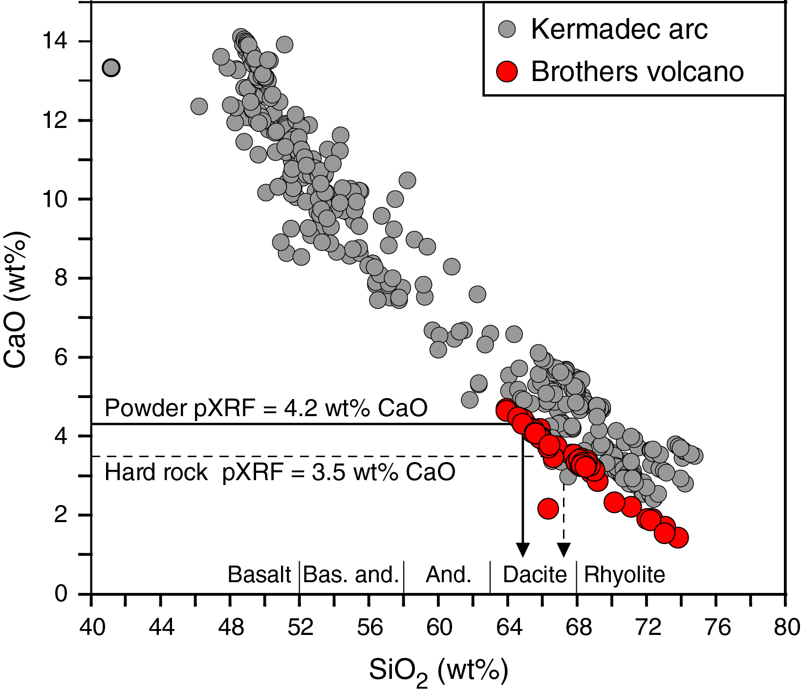
Figure F25. CaO (wt%) vs. SiO2 (wt%).
Similar problems were encountered when analyzing the rock surfaces of hydrothermally altered rocks (predominant Expedition 376 rock lithology), which are often finely porous. The resultant major element abundances were too low, with no means to reestablish them indirectly. In addition, rock-surface analyses also produced ghost signals for elements (e.g., for sulfur) that were below detection limit when measured in an aliquot rock powder. Therefore, during Expedition 376, pXRF rock-surface measurements were used mainly for fast assessment purposes but were generally discontinued in favor of pXRF measurements of rock powders.
Rock powder analysis
pXRF data on rock powders were obtained for all five Expedition 376 Sites (U1527–U1531) from splits of powders obtained for XRD and/or ICP-AES analyses. Many samples measured by pXRF were also selected for onboard ICP-AES analyses, allowing for direct comparison of the data for Si, Ti, Fe, Mn, Mg, Ca, K, P, Ni, Cu, Zn, Sr, Y, and Zr. As noted previously, the data obtained compare generally well (e.g., Johnston et al., 2018) and are best for Fe, K, Sr, Y, Cu, and Zn. The others compare less favorably for one or more possible following causes:
- Matrix effects: pXRF data are obtained from undiluted rock material, whereas ICP-AES samples are diluted by a factor of 4000. Consequently, pXRF analyses are much more likely to be subjected to matrix effects.
- pXRF instrument background: The pXRF calibration lines for some elements (e.g., Mg, Ca, and Cr) do not intercept at or near the origin, suggesting background signals influence the analyses. This leads to deviations at low abundance levels.
Despite these shortcomings, the calibrated pXRF abundances were still a useful, rapid first-order assessment of rock compositions during the expedition and a helpful aid for postcruise research.
Paleomagnetism
Shipboard paleomagnetic experiments were carried out during Expedition 376 on fresh and altered cores recovered from Sites U1527, U1528, U1530, and U1531. Nonmagnetic core barrels were used throughout Expedition 376 to reduce the severity of drilling-induced overprint (Tamura et al., 2015; Lund et al., 2003). Natural remanent magnetization (NRM) was measured on archive halves and discrete cube samples from working halves. NRM was also measured before and after alternating field (AF) stepwise demagnetization for all archive halves to remove any overprinting magnetization and to isolate the primary magnetization. Discrete samples were extracted from working halves and subjected to anisotropy of magnetic susceptibility (AMS) measurements and more detailed AF stepwise demagnetization or thermal demagnetization (TD) to further constrain primary magnetic minerals. Isothermal remanent magnetization (IRM) experiments were also carried out after the demagnetization experiments. The magnetic directions are relative to the sample core coordinate system (Figures F26, F27) because the azimuthal orientations of the core are not determined. The Brothers volcano drill sites are located at a latitude of ~34°S. At this latitude, the geomagnetic axial dipole is characterized by an inclination of approximately −55°, which makes it possible to identify magnetostratigraphic chrons (Cande and Kent, 1995) using inclination data alone. Moreover, the location of these drill sites in the southern hemisphere results in positive inclinations to indicate reversed polarities.
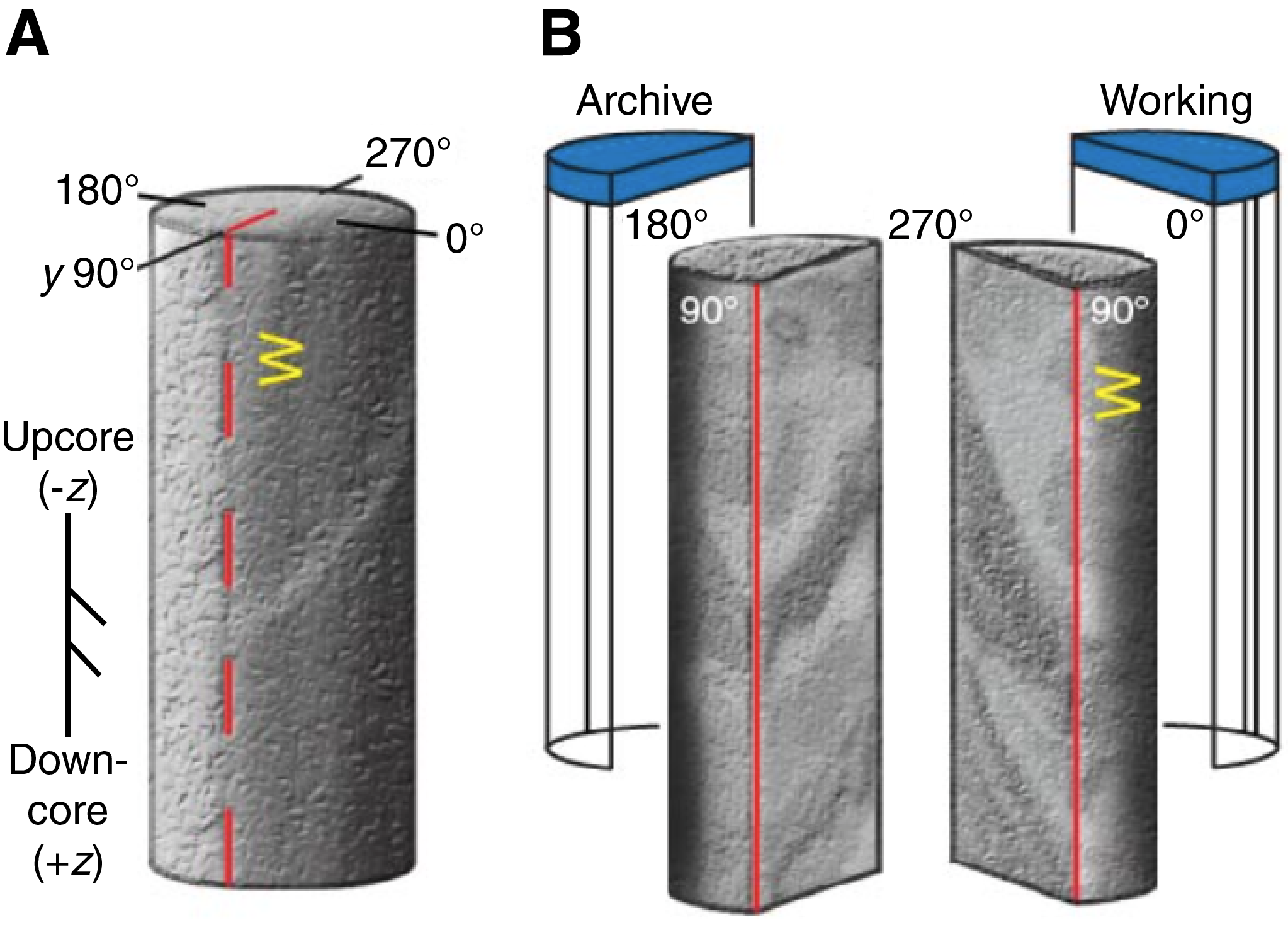
Figure F26. Orientation of the archive- and working-half sections.
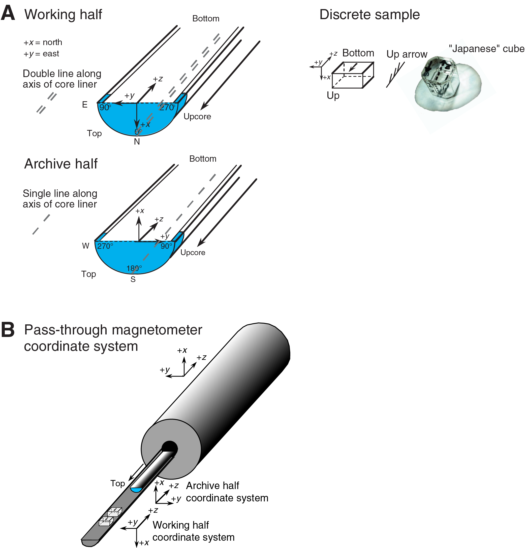
Figure F27. Orientation of paleomagnetic sampling.
Archive-half sections
Because of low recovery from the volcanic rock cores, the largest oriented archive-half pieces were measured to obtain maximum magnetic information. Measurements of NRM and stepwise AF demagnetization on archive halves were performed using a helium-free superconducting cryogenic rock magnetometer (SRM; 2G model 760R-4K) with an integrated, in-line AF demagnetizer with peak fields as high as 80 mT. The magnetometer is controlled by a customized version of Labview software IMS-SRM v. 9.2 (see the Expedition 371 SRM User Guide). For each of the SQUID sensors, the response curve has a width of approximately 8 cm, which means that data collected within ~4 cm of gaps or section boundaries are significantly affected by edge effects and do not provide meaningful results (Reagan et al., 2015). For this reason, the irregular shape of some of the rock pieces measured with the SRM affected the measured magnetization, and the raw data uploaded to the LIMS database must be used with caution. However, archive-half measurements were very important for optimizing discrete sampling of paleomagnetic cubes and analysis of the working halves. The sample tray of the SRM was demagnetized every day using an AF of 30 mT to minimize noise effects, with tray magnetic background values then subtracted from the core measurements. Core sections were measured at a spacing of 2.5 cm and were subject to stepwise AF demagnetization up to a peak field of 70 mT to remove magnetic overprints resulting from the acquisition of viscous remanent magnetization derived from drilling, coring, and sample preparation (Richter et al., 2007). AF demagnetization experiment results for archive halves were plotted using PuffinPlot v. 1.0.3 (Lurcock and Wilson, 2012).
Discrete samples
Discrete samples from working halves were cut into 8 cm3 cubes. These same samples were then shared with the physical property group for additional analyses (see Physical properties). We used the Agico Kappa Bridge (model KLY 4) to measure the AMS of discrete samples. Mean MS, degree of anisotropy, degree of magnetic lineation, and foliation were measured and plotted using Agico’s Anisoft v. 5.0 software. After these measurements, NRM of discrete samples was measured using the Agico JR-6A spinner magnetometer (sensitivity = ~20 × 10−6 A/m). Stepwise AF demagnetization of some discrete samples was achieved using a DTech D-2000 AF demagnetizer at 10 mT intervals up to 100 mT. In some cases, demagnetization increments and maximum AF intensities were adjusted in real time to analyze the coercivity of each sample in detail; the AF experiments were completed when a primary magnetization direction could be clearly identified or after a significant decrease of the NRM intensity. Some discrete samples were thermally demagnetized using ASC Scientific’s model TD-48SC thermal demagnetizer to temperatures >600°C. The internal field inside the demagnetizer tube is less than 50 mT, and samples were widely spaced inside the sample boat to reduce interaction with each other. The samples were then held at a specified temperature (see below) for 30 min, cooled, and then measured with the Agico JR-6A spinner magnetometer. The general temperature increments were ~50°C for temperatures >200°C and smaller intervals of 20°C around 575°C (i.e., the Curie temperature of pure magnetite), although in some specific cases temperature increments and ranges were adjusted in real time to optimize measurements of the specific blocking temperature of each sample by looking at preliminary demagnetization plots. Similar to AF experiments, in some cases the thermal experiments were completed when a primary magnetization direction was clearly identified or after a significant decrease in NRM intensity. To facilitate sample sharing, some thermal experiments were conducted on physical property samples already subjected to MAD measurements, in which samples are water saturated and then dried at 105°C for 24 h in a magnetically noisy environment, acquiring a laboratory-induced magnetic overprint. For these samples, we measured NRM at room temperature before the MAD experiments and then with TD at 110°C after the MAD experiment before continuing with additional TD steps. Results from demagnetization experiments for the discrete samples were plotted using Remasoft 3.1 software provided by Agico, and primary magnetization directions were calculated by principal component analysis (Kirschvink, 1980) in vector component diagrams (Zijderveld, 1967) using PuffinPlot v. 1.0.3 (Lurcock and Wilson, 2012). Following the demagnetization experiments, IRM experiments were carried out to measure sample coercivity. Impulse fields were imparted at variable steps in the range of 0–1.2 T along the sample positive z-axis using the ASC Scientific impulse magnetizer (model IM-10) and subsequently measuring the corresponding IRM with the JR-6A spinner magnetometer at each step.
Physical properties
Shipboard measurements of physical properties were undertaken to provide a quantitative characterization of recovered core material. These data are used to link the geological observations made on the core to the results of downhole measurements and regional geophysical surveys.
Laboratory core flow
Cores were measured in the following sequence (work flow):
- Core temperatures were measured using the forward-looking infrared (FLIR) thermal imaging camera as soon as they were brought in from the core-receiving deck.
- Cores were left to equilibrate to ambient room temperature (~30–60 min).
- Whole-round 360° image scanning was conducted.
- Representative pieces of the whole-round core were used for P-wave measurements in the x- and y-directions using the P-wave Gantry system.
- Whole-round cores were run on the WRMSL, which includes a GRA bulk densitometer, a magnetic susceptibility pass-through loop (MSL) system, and a PWL. The default sampling interval was set to 2 cm. For hard rock cores that did not fill the core liner, the PWL was turned off.
- Whole-round cores were also run on the NGRL when the length of an individual section was >50 cm.
- Cores were split, after which both the archive and working halves of the core were imaged.
- The archive half of the core was run on the SHMSL for MSP and RSC.
- Representative samples ≥6 cm long were taken from the working half and saturated in seawater prior to thermal conductivity measurements.
- P-wave velocity measurements were made along the working half in its core liner using the P-wave gantry system. Porous hard rock samples may require saturation for a clear signal; seawater-saturated thermal conductivity samples were used in this case.
- Discrete samples for shipboard measurements were collected from each section of the working half. Oriented cube samples (8 cm3) were shared between paleomagnetic, MAD, and P-wave velocity anisotropy measurements.
- Additional MAD measurements were also made on nonoriented rough pieces and sediment samples.
- Sediment samples were collected in the splitting room to preserve the original moisture content of saturated samples.
- Paleomagnetic measurements of discrete cubes were made first using either AF demagnetization or TD. For TD samples, only a room temperature measurement of NRM was made at this point.
- Cubes and rough pieces were saturated in seawater under vacuum conditions for ~2 h at ambient temperature to remove air from any pore spaces.
- The wet mass of samples was obtained for MAD measurements.
- P-wave velocity was measured on wet cube samples in the x-, y-, and z-directions.
- Samples were dried in a 105°C oven for 22–24 h and then cooled to room temperature in a desiccator for 1 h, after which their dry mass was obtained for MAD measurements.
- Sample volume was obtained using Helium pycnometry. Bulk density, dry density, grain density, and porosity were then calculated from wet mass, dry mass, and dry volume measurements using IODP Method C (Blum, 1997).
- Discrete cubes used for TD were then returned to the Paleomagnetism group.
During Expedition 376, all raw data were uploaded to the LIMS database. A comprehensive discussion of all methodologies and calculations used aboard the JOIDES Resolution in the physical property laboratory is found in Blum (1997).
Core temperature measurement
Core temperature was initially measured as soon as the cores were brought to the core-receiving deck using the FLIR E8 thermal imaging camera. The FLIR analyzes the 7.5–13 µm spectral range using an infrared lens to obtain temperature readings. FLIR data can be either read off the instrument directly or downloaded by connecting to a computer installed with the FLIR Tools software and exported as a PDF file. FLIR measurement locations were selected based on noticeable lithologic variations. The same locations were remeasured prior to WRMSL analyses to confirm that cores had equilibrated to room temperature. Arrival temperatures of cores were monitored because of the likelihood of drilling hot formations; however, all cores were found to have equilibrated with surface sea temperatures during core barrel retrieval. From Site U1530 onward, arrival temperatures were no longer obtained.
Whole-Round Multisensor Logger measurements
The WRMSL was used to measure GRA bulk density, MS (on the MSL), and P-wave velocity (on the PWL) of cores nondestructively. The default sampling interval was set at 2 cm. For hard rock cores that did not fill the core liner, the PWL was turned off. Calibration was verified after each core measurement by running a freshwater-filled calibration core through the WRMSL. Calibrations were accepted if they were within 2% of the standard values for each measurement type.
GRA bulk density
The bulk density of sediments and rocks can be estimated from GRA. These data indicate changes in lithology and porosity and are particularly useful for core-to-core correlation. The GRA densitometer on the WRMSL operates by passing gamma rays from a 137Cs source through a whole-round core and into a 75 mm3 NaI detector located directly below the core. The input gamma ray peak has a principal energy of 0.662 MeV and is attenuated by Compton scattering as it passes through the core. The attenuation is a function of the electron density, which is related to the bulk density by
(10)- ρb = bulk density,
- ρe = electron density,
- w = molecular weight, and
- N = atomic number of elements in the material
For the majority of elements and for anhydrous rock-forming minerals, attenuation is ~1, whereas for hydrogen it is 1.9841. For a known sample thickness (i.e., the core diameter), the gamma ray count is therefore proportional to the bulk density. The quality of GRA data is significantly affected by voids or incomplete filling of the core liner. In such cases, the density estimate will be too low. For cores in this category, the highest density values are therefore the most reliable. However, it is possible to correct the data from cores with variable thickness using a thickness log obtained from core photographs according to
(11)- ρ = output density,
- d = assumed thickness (core diameter),
- ρ1 = actual density, and
- d1 = actual thickness.
Acquisition time for each measurement is 3 s. Calibration of the GRA densitometer was performed using a core liner filled with freshwater and aluminum density standards. Recalibration was performed if the measured density of the freshwater standard was not 1.00 ± 0.02 g/cm3. Bulk density was also acquired for discrete samples during MAD measurements (see below).
Magnetic susceptibility
MS is a volume-specific measure of the degree to which a material can be magnetized by an external magnetic field:
(12)where κ is MS and M is the magnetization induced in the material by an external field with strength H (using a very low field strength of ≤0.5 mT).
The MS of rocks varies in response to the magnetic properties of their constituents, making it a useful indicator of mineralogical variations. MS measurements are also an important method for making core-to-core and downhole measurement correlations. Materials such as clay generally have an MS several orders of magnitude lower than iron oxides, such as magnetite, that are common components of igneous rocks. Water and plastics (such as the core liner) have a low MS of slightly negative value.
The WRMSL measures volume MS using a Bartington Instruments MS2 meter coupled to a MS2C sensor coil (88 mm diameter) and operates at an AF of 250 µT and a frequency of 0.565 kHz (Bartington Instruments, Ltd., 2019). MS is reported in instrument units. To convert results into dimensionless SI units, it is necessary to multiply the data by a correction factor that is a function of the probe type, core diameter, and loop size. The size of small rock pieces in incomplete cores varies, so application of a single correction factor is not justified and therefore no correction is applied to the WRMSL data. This conversion factor does not change the order of magnitude of the measured susceptibility values, so the results are comparable with the susceptibility measured by the paleomagnetic group with the same physical units (SI).
Results are the average of three measurements made at each interval. The along-core response curve of the MSC2 coil has a full width at half maximum of ~4 cm (Blum, 1997). Measurements on core pieces <8 cm long will thus significantly underestimate MS by >10%. MS data recorded on the WRMSL must therefore be interpreted with reference to breaks and variable diameters of fragmented cores; this information can be obtained from the 360° photo imaging record. Note that higher spatial resolution MSP data are also collected on section halves by the SHMSL (see below), and bulk MS data are collected for discrete cubes during AMS analyses (see Paleomagnetism).
P-wave velocity
P-wave velocity is the distance traveled by a compressional P-wave through a medium per unit of time, expressed in meters per second (m/s). P-wave velocity is dependent on the composition, porosity, bulk density, fabric, and temperature of the material, which in turn are functions of consolidation and lithification, state of stress, and fracturing. Along with bulk density data, P-wave velocity data can be used to calculate acoustic impedances and reflection coefficients that are needed to estimate the depth of specific seismic horizons.
The PWL system on the WRMSL transmits a 500 kHz P-wave pulse across the core liner at a repetition rate of 1 kHz. Pulser and receiver are mounted on a caliper-type device and are aligned to ensure that wave propagation is perpendicular to the section’s long axis. A linear variable differential transducer measures the P-wave travel distance between the pulse source and the receiver. Good coupling between transducers and the core liner is facilitated by water dripping onto the contact from a peristaltic water pump system. Signal processing software picks the first arrival of the wave at the receiver, and the processing routine also corrects for the thickness of the liner.
A series of acrylic cylinders of varying thicknesses are used to calibrate the PWL system. The regression of traveltime versus travel distance yields the P-wave velocity of the standard material, which should be 2750 ± 20 m/s. The thickness of the calibration samples, corrected for liner thickness, is divided by the traveltime to calculate P-wave velocity in meters per second. The calibration is confirmed by measuring a core liner filled with pure water, and the calibration passes if the measured velocity is within ± 20 m/s of the expected value for water at room temperature (i.e., 1485 m/s).
Natural gamma radiation measurements
NGR is emitted from rocks as a result of the radioactive decay of 238U, 232Th, and 40K isotopes. Measurement of NGR from the recovered whole-round cores provides an indication of these element concentrations and can provide insight into many important lithologic characteristics and geologic processes. For example, in hard rocks, NGR measurements can yield information about the alteration and heat production of rocks (Dunlea et al., 2013) that is useful when correlating core measurements with downhole measurements of NGR (e.g., Révillon et al., 2002). The NGRL installed on the JOIDES Resolution was designed and built at IODP (Texas A&M University, USA) (Vasiliev et al., 2011). The main NGR detector unit consists of 8 sodium iodide (NaI) scintillator detectors (~1270 cm3 each), 7 plastic scintillation detectors, 22 photomultipliers, and passive lead shielding. The eight NaI detectors are spaced every 20 cm in the detector; the detectors themselves are semicylindrical annuli around the lower half of the core (each crystal is ~13 cm wide along the core). The detectors are shielded by lead to reduce external gamma radiation measurement, and the seven plastic scintillation detectors also detect and actively suppress the effect of high-energy gamma and muon components of cosmic radiation.
A single measurement run with the NGRL provides a total of 16 measurements at 10 cm intervals over a 150 cm section of core. To achieve a 10 cm interval using the NGRL’s eight sensors spaced every 20 cm, the NGRL records two sets of measurements offset by 10 cm. Total counts are routinely summed over the range of 100–3000 keV and depend on the concentration of radionuclides in the sample and the counting time, with longer counting times providing better counting statistics. The default measurement time was set to 5 min. However, occasional additional measurements with counting times of 18 h were conducted to qualitatively identify relative abundances of different radioactive isotopes from relative peak heights in collected spectra.
Section Half Multisensor Logger measurements
The SHMSL includes a platform moving above the section half that records the sample height using a laser sensor. The laser profile establishes the location of the bottom of the core section and the distribution of rock to measure by locating gaps and cracks between pieces based on a laser distance exceeding a set value. After identifying the section length, the SHMSL then measures reflectance spectrophotometry and colorimetry and MSP at regular intervals along the section. Measurements were made at 2 cm intervals along the core.
Reflectance spectrophotometry and colorimetry
An Ocean Optics, Inc., system for UV through visible to near-infrared light (171–1100 nm wavelength at 2 nm increments) mounted on the SHMSL was used to measure spectral reflectance. Each full-band measurement takes ~5 s to acquire. Spectral data are routinely reduced to the L*a*b* (CIELAB) color space for output and presentation, in which L* is luminescence, a* is the red–green value, and b* is the blue–yellow value. The color reflectance spectrometer calibrates on two spectra: pure white (reference) and pure black (dark).
Point magnetic susceptibility
MSP is measured on the SHMSL using a Bartington MS2E contact probe with a flat 15 mm diameter sensor operating at a frequency of 0.580 kHz. The sensor takes and averages three measurements made at 1 s intervals to an accuracy of 5%. The area of response of the MS2E sensor is 3.8 mm × 10.5 mm, with a depth response of 50% at 1 mm and 10% at 3.5 mm (Bartington Instruments, Ltd., 2011). The MSP measured on the SHMSL on section halves therefore has a higher spatial resolution than MS measured by WRMSL on whole-round cores. The probe is zeroed in air before each measurement point, and a background magnetic field is measured and removed from the data. Measurements are output in instrument units but reported in SI (see Magnetic susceptibility).
Thermal conductivity
Thermal conductivity (k) is the coefficient of proportionality relating conductive heat flow to a thermal gradient. It reflects the rate at which heat is conducted through a material and is dependent on saturating fluid types, porosity, bulk density, water content, temperature, composition and texture of the mineral phases, and so on. At steady state, thermal conductivity is the coefficient of heat transfer (q) across a steady-state temperature difference (ΔT) over a distance (Δx):
(13)Thermal conductivity was measured on pieces from the working half (samples ≥6 cm) under ambient conditions using the TeKa TK04 system described in Blum (1997). Because almost all of the cores recovered were hard rock, half-space determinations of thermal conductivity were made using standard half-space (HLQ) needle probe pucks (numbers H11040 and H11038) and mini HLQ needle probe pucks (numbers H51037 and H51018). These pucks, which are recommended for planar surfaces, consist of a Plexiglas block (k = 0.184 W/[m·K]) with a half-space needle probe embedded in its base. Heat is assumed to be transferred through the sample, and the TK04 documentation indicates that heat flow through the Plexiglas block itself is only significant for samples with thermal conductivities <1 W/(m·K). On one occasion (Hole U1528C) when unconsolidated soft material was recovered, a full-space (VLQ) standard needle probe (number V11064) was used, and the needle was inserted into the whole-round core perpendicular to the long axis. All measurements were made at room temperature and pressure, and they were not corrected for in situ conditions. This system measures thermal conductivity by transient heating of the sample with a known heating power and geometry. Changes in temperature with time during heating are recorded and used to calculate thermal conductivity. Heating power can be adjusted for each sample depending on the type of HLQ puck being used; heating power can be varied from 1 to 1.6 W/m for a standard puck and from 0.5 to 1.2 W/m for a mini puck. For most samples, a heating power of 1.2 W/m for a standard puck and 0.8 W/m for a mini puck was used. For the VLQ needle probe, a heating power of 1.2 W/m was used. The temperature of the superconductive needle probe has a quasilinear relationship with the natural logarithm of the time after the initiation of heating (Blum, 1997). The TeKa TK04 device uses a special approximation method to calculate conductivity and to assess the fit of the heating curve. This method fits discrete windows to the theoretical function of temperature (T) with time (t) for a constantly heated line source (Kristiansen, 1982):
(14)where A1−4 are constants that are calculated by linear regression. A1, A3, and A4 are related to the sample geometry and the material properties surrounding the needle probe, and A2 is related to the heating power and thermal conductivity. Having determined these constants (and how well they fit the data), the apparent conductivity (ka) for the fitted curve is time dependent:
(15)where Q is the input heat flux. The maximum value of ka and the time (tmax) at which it occurs on the fitted curve are used to assess the validity of that time window for calculating the thermal conductivity. The best solutions are those where tmax is greatest, and these solutions are selected for use. Data are considered good if ka has a maximum value, tmax is large, and the standard deviation of the least-squares fit is low. For each heating cycle, several output values can be used to assess the quality of the data, including the natural logarithm of extreme time, which should be large; the number of solutions (N), which should also be large; and the contact value, which assesses contact resistance between the probe and the sample and should be small and uniform for repeated measurements.
The measurement apparatus was evaluated frequently by measuring the thermal conductivity of a certified MACOR ceramic standard (k = 1.626 W/[m·K]). For measurement of the ceramic standard, the half-space standard puck or mini puck was coated in silicone thermal contact gel and then placed on the standard; if the measured thermal conductivity was within 2% of the known value, then the puck was used for sample measurements. After the standard and prior to sample measurement, the silicone gel was thoroughly removed from the puck to avoid potential geochemical contamination of core material.
Prior to analysis, hard rock pieces were left to equilibrate to room temperature in a seawater vacuum saturator for ~2–12 h depending on the porosity of the samples, and then the sample piece and sensor needle were kept equilibrated at room temperature in seawater (k = ~0.6 W/[m·K]) in an isolated bath (Coleman-brand cooler) for at least 5 min prior to measurement (Figure F28). Seawater was used to improve the needle/sample contact; silicone thermal contact gel was not used when measuring core samples to avoid potential contamination of the core. Isolation of the sample piece and sensor needle in the cooler eliminated the effect of small but rapid temperature changes introduced by air currents in the laboratory. To further reduce the effects of air currents, a foam board was used to cover the sample inside the cooler. The instrument internally measures temperature drift and does not begin a heating run until sufficient thermal equilibrium is attained. Each reported measurement represents the averaged results of as many as four successive heating cycles.

Figure F28. Apparatus for hard rock thermal conductivity measurements.
Discrete measurements
P-wave velocity
Discrete measurements of P-wave velocity were made using the P-wave gantry system. The PWC records arrivals, and the peak of the first arrival is identified automatically by the IMS 10 Velocity software. Typically, the first arrival was then picked following manual adjustment. Both the automatic and manual first arrival pick and original waveform are saved. System calibration runs with standards were conducted periodically to ensure that system and transducer delay time settings were current.
Whole-round measurements
The P-wave gantry system software was modified during Expedition 376 to support P-wave velocity measurements of oriented pieces of the whole-round core in the x- and y-directions. These additional measurements were made to rapidly acquire P-wave velocity data for hard rock lithologies (which cannot be run on the WRMSL PWL system). These data enabled timely interpretation of seismic images relative to depths of ongoing drilling. Measurements were made using the PWC system. To ensure stability of the whole-round piece while lowering the transducer, the sample was placed in a piece of half liner to prevent it from rolling. A hole was cut in the base of this liner to accommodate contact between the bottom transducer and the sample. When saving the measurement to the LIMS database, the sample offset from the top of the core was input manually.
Discrete cube measurements
P-wave velocity measurements in the x-, y-, and z-directions were performed on the same 8 cm3 discrete cube samples that were used for MAD and paleomagnetic determinations. The cubes were oriented following standard IODP conventions and placed on the PWC gantry.
Anisotropy of P-wave velocity
P-wave anisotropy was calculated for whole-round core and discrete cube samples based on the method used during IODP Expedition 352 (Reagan et al., 2015). Anisotropy between the average horizontal and vertical velocities (Anis(xy)z; for discrete cubes) and horizontal anisotropy (Anisxy; calculated for both whole-round core pieces and discrete cubes) were calculated according to
(16) (17)- x, y, and z = standard core coordinate axes;
- Vx and Vy = transverse core velocities; and
- Vz = longitudinal core velocity.
Section half measurements
P-wave velocity was also measured at regular intervals on section halves resting in their plastic core liners using the PWC and calculated by applying a correction in the IMS 10 Velocity software to account for the thickness of the core liner. For hard rock cores, for which WRMSL measurements generally do not use the PWL system, these measurements offer the potential to obtain P-wave velocity data along the section to supplement the analyses of whole-round core pieces and discrete cubes. In addition, if downhole measurement of P-wave velocity by the Dipole Sonic Imager (DSI) is not possible because of temperature limitations (see Downhole logging operations), these section-half measurements may provide the most continuous record of P-wave velocity variation with depth. Successful analyses require good contact between the transducers and the rock and core liner surfaces, which is enhanced by wetting the transducers with deionized water. For vesicular samples, successful analysis may require saturated samples. In such cases, measurements were made on seawater-saturated samples used for thermal conductivity measurements.
Moisture and density measurements
For hard rock samples, MAD measurements were made on rough pieces, sediments, and discrete 8 cm3 sample cubes that were also used for paleomagnetic and P-wave velocity measurements. Mass and volume measurements were made to determine bulk density, dry density, grain density, and porosity. The shipboard MAD facility consists of a dual-balance system and a hexapycnometer.
Dual-balance system
A dual-balance system was used to measure both wet and dry masses. Two analytical balances (Mettler-Toledo XS204) compensate for ship motion; one acts as a reference, and the other measures the sample relative to the reference. A standard mass of similar value to that of the sample mass was placed on the reference balance to increase accuracy. An accuracy of 0.005 g was readily attainable by using a reference mass within 10% of the sample mass. Samples were saturated in seawater under vacuum conditions for ~2 h and then weighed to obtain their wet mass. Samples were placed in an oven at 105 ± 5° C for 22–24 h and then allowed to cool in a desiccator for 1 h prior to dry mass measurement.
Hexapycnometer system
The hexapycnometer is an IODP custom-built system that uses six MicroMetrics cell units, electronics, and control programs. The system measures dry sample volume using pressurized He-filled chambers with a precision of 0.02 cm3. Shipboard technicians performed a calibration using stainless steel spheres of known volume at the start of the expedition and whenever the helium gas tank was changed. For each measurement, five cells containing samples and one cell containing two calibration spheres (3 and 7 cm3) with a total volume of 10 cm3 were run. Calibration spheres were cycled through the cells to identify any systematic error and/or instrument drift. Spheres were assumed to be known to within 1% of their total volume. If the volumes of the calibration spheres deviated by >1% from their known volumes, then that pycnometer cell was recalibrated.
Moisture and density calculations
MAD calculations were performed according to Method C in the IODP Physical Properties Handbook (Blum, 1997). For density calculations, both mass and volume are first corrected for the salt content of the pore fluid:
(18)- Msalt = mass of salt,
- S = pore water salinity (seawater with salinity 35 psu or 0.035 g/cm3),
- Mw = wet mass of the sample, and
- Md = dry mass of the sample.
Grain density (ρg) is determined from the dry mass (Md) and dry volume (Vd) measurements:
(19)where ρsalt is the density of salt (2.20 g/cm3).
The salt-corrected mass of pore water (Mpw) is calculated as
(20)Then the volume of pore water (Vpw) is
(21)where we assume the density of the pore fluid (ρpw) = 1.024 g/cm3 (seawater with salinity of 35 psu).
To calculate sample bulk density (ρb) of the wet sample, bulk volume (Vb) of the wet sample is first computed:
(22) (23)Connected porosity (φ) is calculated from the two volume parameters obtained from the MAD measurements and resulting bulk and pore water volume calculations:
(24)Downhole logging operations
Downhole logging data are rapidly and continuously collected in situ at sampling intervals ranging from 2.5 mm to 15 cm. These data are used to determine the physical, chemical, and structural properties of the formation penetrated by a borehole. They can aid the interpretation of the rock stratigraphy, lithology, mineralogy, and geochemical composition, as well as the formation fluid conditions. Downhole logs also provide information about the status and size of a borehole, which can include information about formation stress or deformation induced by drilling. In the event of incomplete core recovery, the continuous nature of this data set may provide the only means of characterizing the geological formation structure and lithostratigraphy and fluid conditions penetrated by the drill hole. Downhole logs are intermediate in scale between laboratory measurements of core samples and volcano-scale geophysical surveys and are therefore particularly useful in calibrating and groundtruthing the interpretation of these geophysical survey data. In short, logs are an essential link in understanding physical properties across a range of scales. Due to incomplete core recovery, logging data proved particularly valuable during Expedition 376 and will be important in postcruise studies.
During Expedition 376, we drilled into a hydrothermal environment that required monitoring of in situ temperatures using the Elevated Temperature Borehole Sensor tool (ETBS) before running other wireline logs because most wireline logging tools are limited to operational temperatures of either ≤175° or ≤260°C. We also used a new tool, the Petrospec thermocouple memory tool (TCMT), for monitoring rebounded borehole temperatures, and we collected borehole fluids with a Kuster FTS. All tool acronyms are listed in Tables T24 and T25.
We adhered to standard wireline logging techniques during Expedition 376. After the temperature was deemed sufficiently low for logging by the ETBS, the logging tools were combined and stacked together, lowered downhole, and pulled up at a constant speed. Recording by the various tools (see below) occurred on both downhole and uphole passes to increase data recovery. For wireline tools with real-time reading, the downhole pass meant that the temperature ratings of the tools could be monitored closely so that operational limits were not exceeded. In Hole U1528D, the temperature measured by the ETBS, combined with the low pH and presence of H2S, required deployment of a modified flasked tool string capable of operating in temperatures as high as 260°C.
Memory tools
Elevated Temperature Borehole Sensor tool
The ETBS tool is a slim-hole probe run on the coring line (Table T24) that was modified and upgraded from the Ultra High Temperature Multisensor Memory Tool (UHT-MSM) used during ODP Legs 169 and 193 (Shipboard Scientific Party, 1998, 2000) (Figure F29). The tool was originally developed for the University of Miami (USA) by Geophysical Research Corporation (GRC, 1994a, 1994b, 1996). The ETBS contains internal and ultrahigh external temperature measuring devices, a pressure gauge, a multisensor memory unit, and a dewar flask that acts as an insulator to maintain a stable temperature and cooldown rate for the tool (Figure F29). The heat shield is aircraft-grade aluminum bound at both ends by brass heat sinks. The dewar flask can maintain an internal temperature suitable for tool operation for 4–5 h at an external temperature of 400°C. Operations are possible for as long as 10 h if the average temperature does not exceed 232°C.
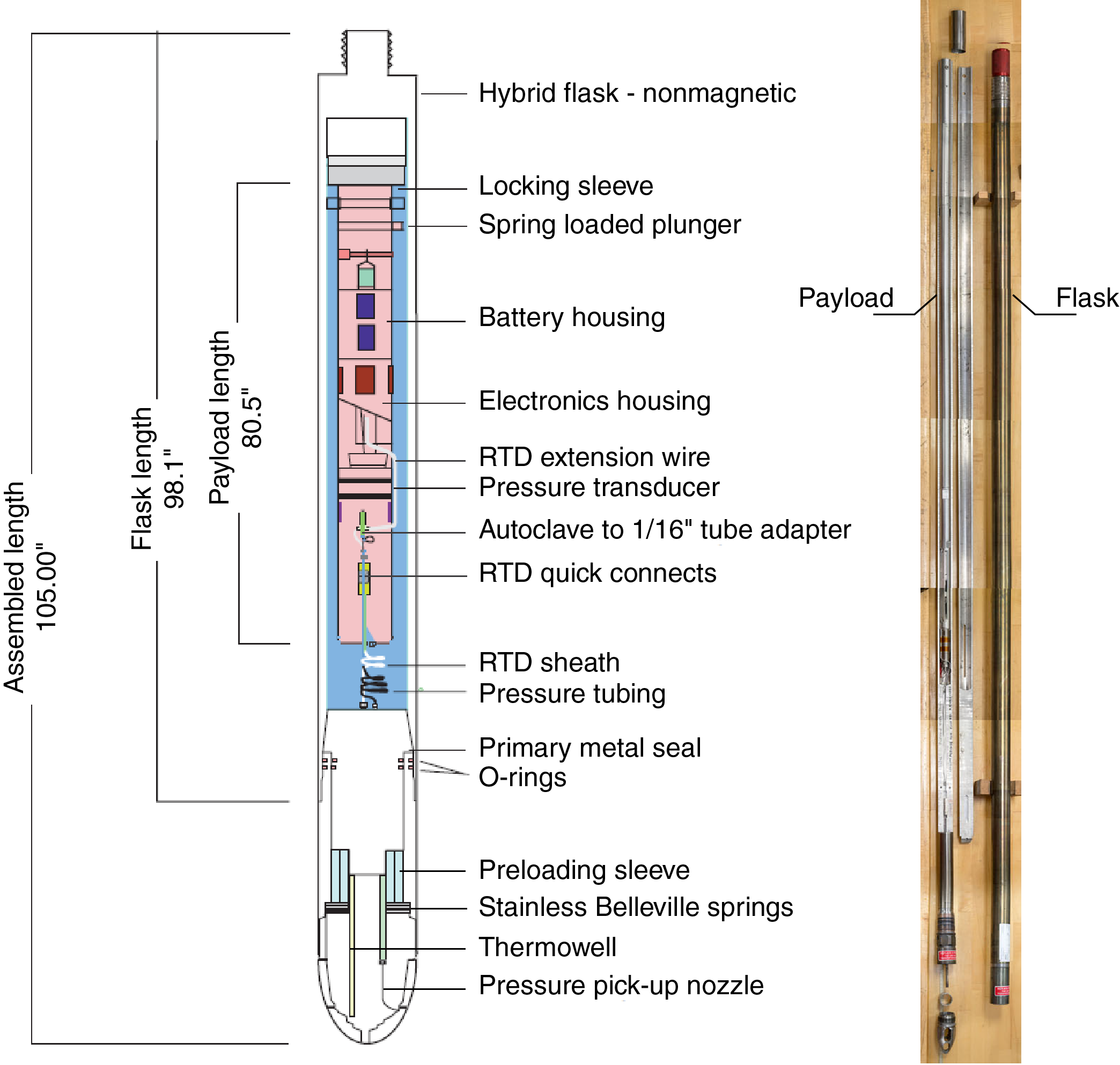
Figure F29. ETBS.
The ETBS tool was connected to the core line via a new attachment designed on board to be compatible with the Kuster FTS tool. This attachment allows deployment through the throat of the RCB system bit. This procedure minimizes the time that the drill string spends without circulation of seawater in the hole, when risk of borehole collapse is highest. The ETBS was fitted with Chemraz seals and Kalrez O-rings.
The ETBS has a longer response time than the logging equipment head-mud temperature tool (LEH-MT) on the Schlumberger High-Temperature Triple Combo (HTTC), triple combo, and Formation MicroScanner (FMS)-sonic tool strings (see Wireline tools). The ETBS also reaches higher speeds of acquisition (60–70 m/min in Hole U1528D and 20–40 m/min in Hole U1530A) compared with the LEH-MT (8–10 m/min), indicating that the ETBS underestimates temperatures in zones of rapidly increasing temperature with depth and the converse.
Petrospec thermocouple memory tool
The spool-in Petrospec TCMT was developed by Petrospec for Expedition 376 (Figure F30). It is designed to measure high hydrothermal fluid temperatures that exceed the ETBS rating, particularly after rebound of downhole temperatures from drilling-induced disturbance. Because it is deployed on the coring line within the drill string, it is engineered to operate in highly corrosive fluids. The Petrospec TCMT is composed of a 9 m long thermocouple cable rated to 600°C, two discrete temperature-sensing junctions at the terminal end of the cable, and a memory tool carrier assembly rated to 40°C that is capable of measuring temperature at regular intervals (e.g., 1 s, 10 s, or 1 min). The memory tool carrier is kept within the drill string in circulating cold seawater, whereas the thermocouple cable hangs below the bottom of the drill string with the sensors in the open hole, weighted by a sinker bar.
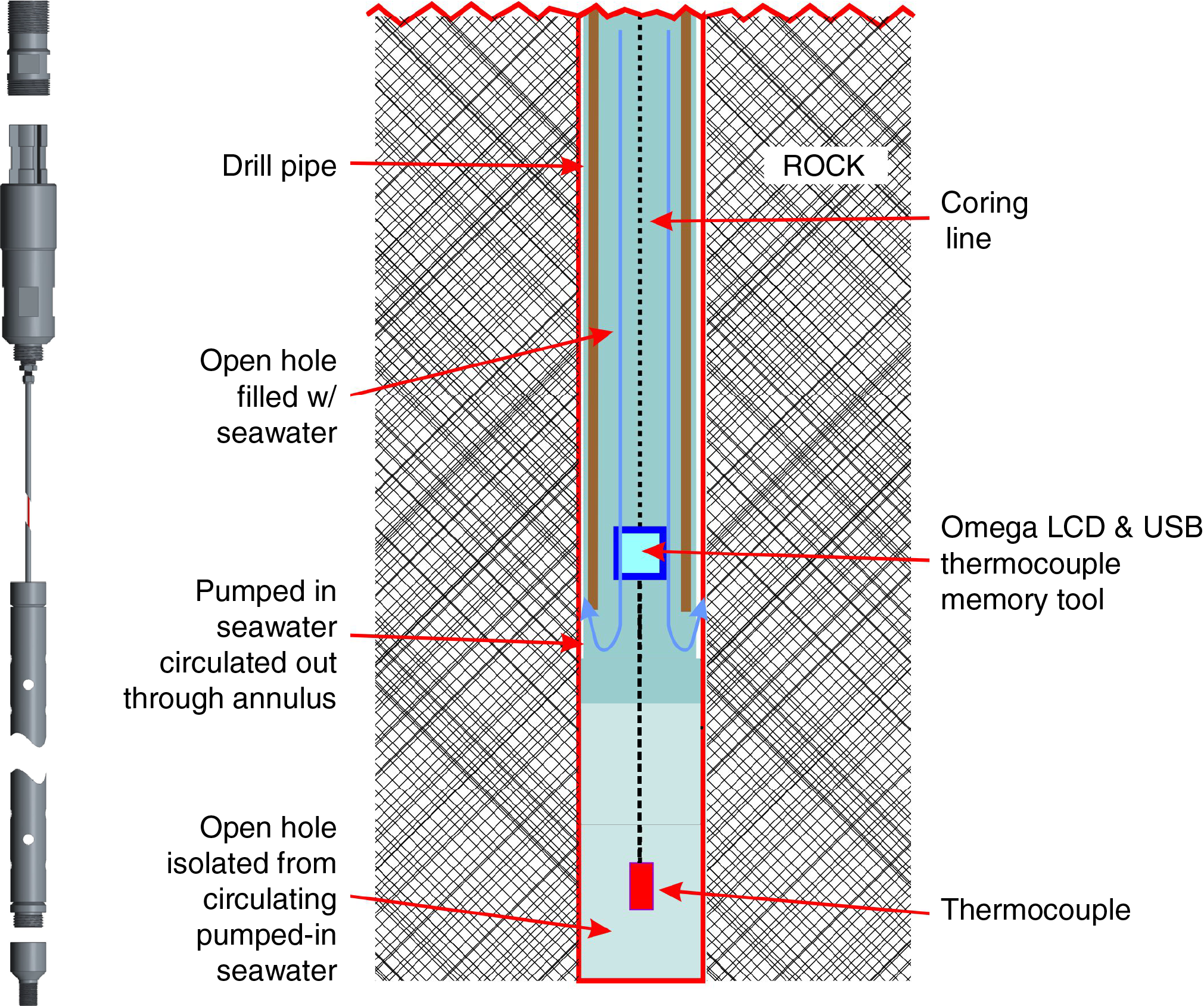
Figure F30. Petrospec TCMT.
Kuster Flow Through Sampler
Borehole fluid sampling was accomplished using a Kuster FTS. The Kuster FTS is rated to 10,000 psi (690 bar) and 232.2°C, although it has been successfully run as high as 260°C (M. Watkins, pers. comm., 2018). The Kuster FTS tool with a 1000 mL sample chamber was initially fitted with a Kalrez 7075 O-ring, but the entire assembly was lost in the hole. Hence, all sampling during Expedition 376 was conducted using a backup 600 mL Monel steel Kuster FTS tool (Probe product reference 11700-100) deployed on the core line (Figure F31) with standard O-rings provided by MB Century. The tool was run directly after temperature logging with the ETBS to identify depths where hydrothermal fluids were most likely flowing into the borehole. Procedures for downhole survey operation were followed in accordance with manufacturer guidelines (MB Century, unpubl. data. Available from Info-NZ@mbcentury.com.).
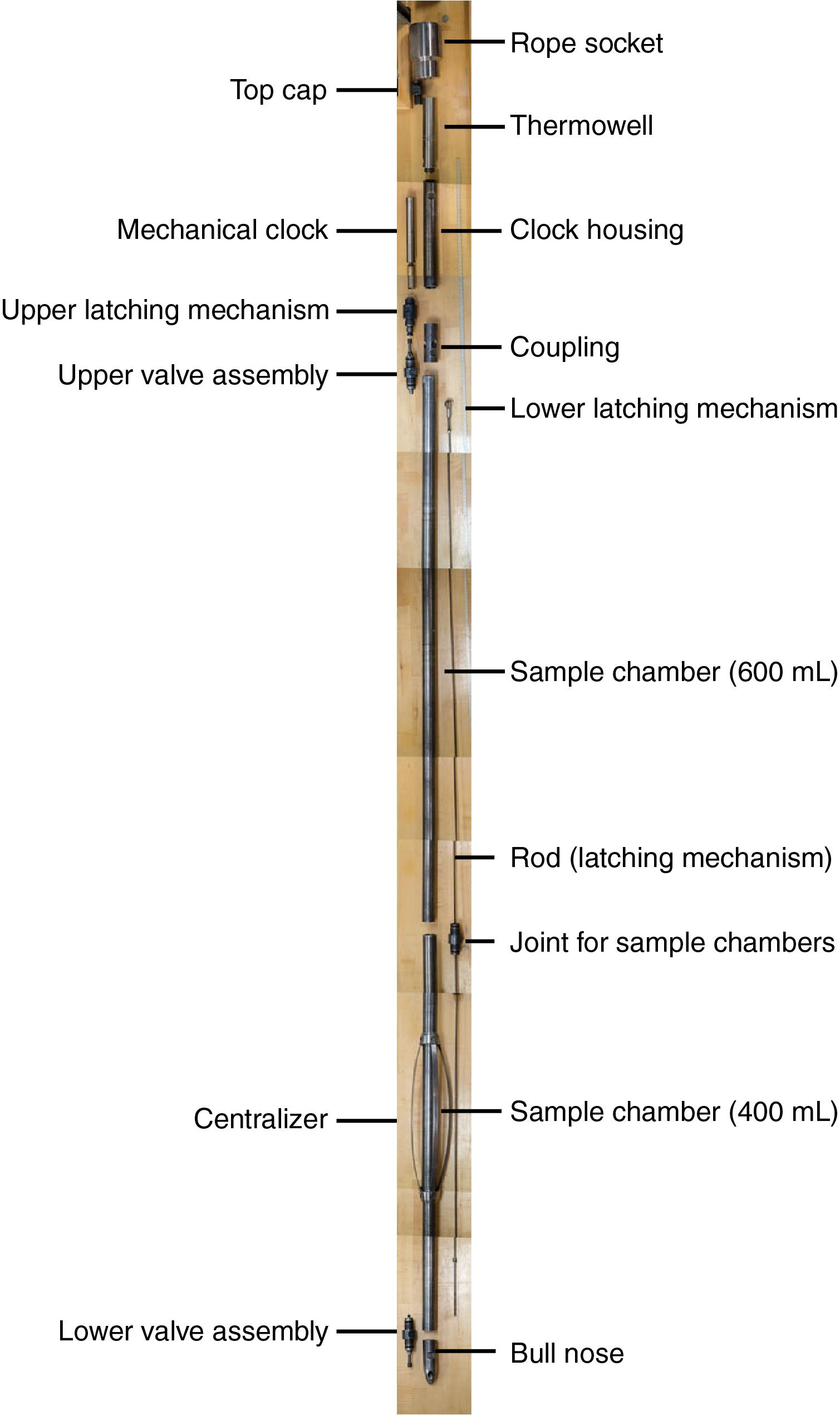
Figure F31. Kuster FTS.
The tool consists of a 600 mL capacity fluid sample chamber, which can be connected to an additional 400 mL capacity tube with a spring-loaded valve on each end of the sample chamber. The lower end has a removable bull nose with ports to allow the fluid to enter. At the top is a rope socket for attaching the wireline. A latching mechanism connects the valves together and holds them open during deployment. A programmable mechanical clock is attached above the chamber, with either 1 or 3 h clocks for trigger times <50 min and >50 min, respectively. This clock is preset at the surface to define the closing time, at which point a ball-operated tripping mechanism releases the valves, trapping the fluid in the sampler and maintaining the pressure of the sampling depth until the tool is recovered and the fluids are retrieved through a transfer head assembly (see Borehole fluid geochemistry). Operationally, 10 min were allowed to elapse following the estimated valve closure time before the Kuster FTS was recovered at an ascent rate of 70 m/min. Although the fluid sampling locations cannot be definitively confirmed because of the clock-triggered closing mechanism, the 10 min buffer maximizes the likelihood that the sample was trapped at the deepest depth reached on each run.
Between samples, the Kuster FTS was cleaned with ACS reagent grade acetone, rinsed with deionized water, and serviced following manufacturer guidelines (MB Century, unpubl. data). Likewise, it was ensured that the transfer head assembly was free of contaminants by washing with acetone and distilled water and testing that the valves would easily open or shut. After recovery of the sampler, the valves, the O-rings, and any stuck particles on the O-rings were checked for mechanical wear and embrittlement and replaced as necessary prior to the next run. Because of the downhole exposure to high-temperature (>246°C) and low-pH (1.8) fluids, the tool runs in Hole U1528D required more extensive servicing because the tool returned with a green-black coating and degraded O-rings. Cleaning the tool required using the onboard heat transfer system for the main chamber and an ultrasonic bath followed by a wire wheel for the smaller parts, with a full servicing of every part of the tool.
Temperature-indicating strips
Temperature-indicating strips were positioned in a housing on top of the core barrel, in the Thermowell part of the Kuster FTS, and in the data logger carrier of the Petrospec TCMT. These self-adhesive labels consist of a series of temperature-sensitive purified organic chemicals sealed between heat-resistant substrate with transparent windows. Each element changes color distinctly (white to black) as its rated temperature is exceeded (Figure F32). Strips manufactured by OMEGA record temperature from 40° to 260°C, and strips from Tempil record temperatures from 37° to 290°C (Table T26). This simple method provides an estimate of the highest temperature encountered by the strip during that deployment. Note that the steel housing is too thick to fully equilibrate quickly enough with mud temperature. The strips need to be isolated from fluids to ensure reliable measurements (Figure F32B).
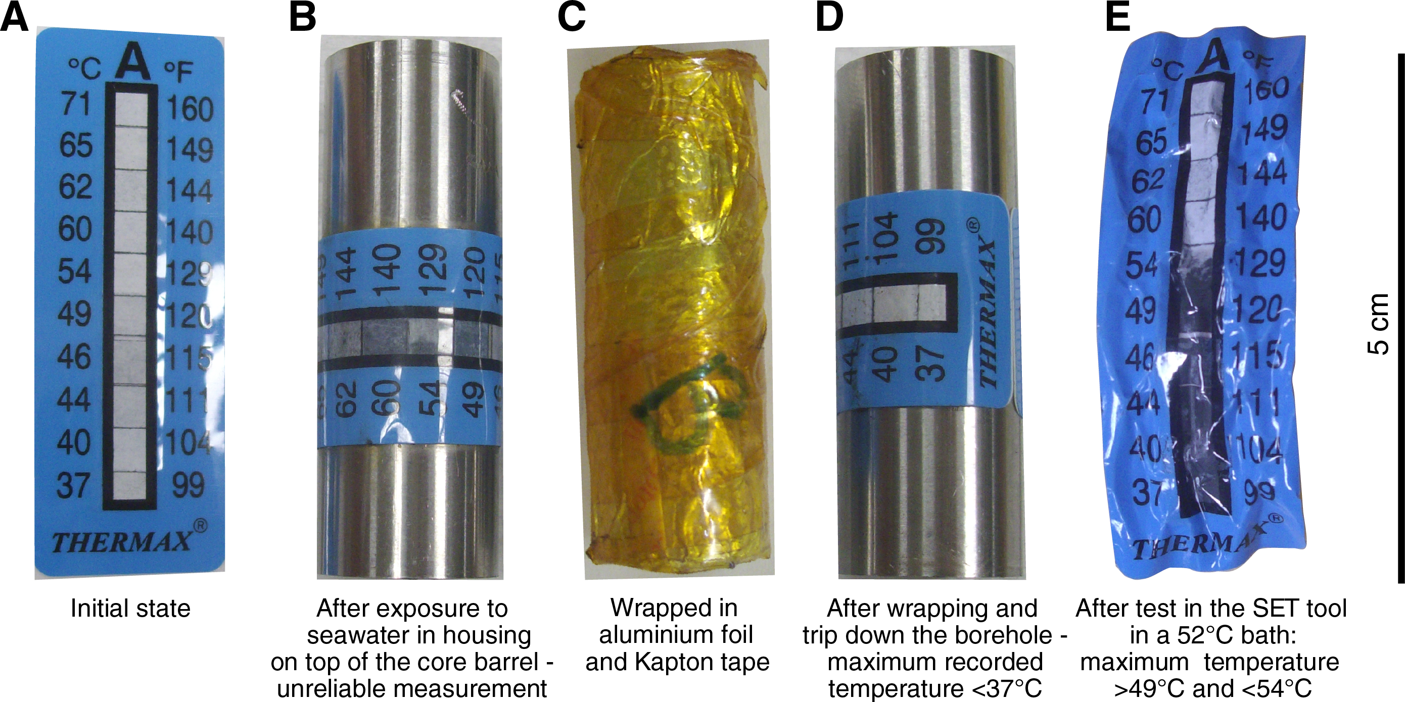
Figure F32. Temperature indicating strips.
Wireline tools
Downhole measurements with real-time surface read-out (wireline) data were acquired using a variety of logging tools (manufactured by Schlumberger and the Lamont-Doherty Earth Observatory) that were combined into tool strings (Tables T24, T25) and run downhole on a wireline cable after coring operations were completed in Holes U1528D and U1530A. During Expedition 376, three tool strings were used (Figure F33):
- A HTTC tool string in Hole U1528D recorded bulk density and photoelectric effect (PEF; Hostile Environment Litho-Density Sonde [HLDS]), spectral (Hostile Environment Natural Gamma Ray Sonde [HNGS]) and total count (Enhanced Digital Telemetry Cartridge [EDTC]) natural gamma ray, and fluid temperature (LEH-MT).
- A standard triple combo tool string in Hole U1530A recorded bulk density and PEF (HLDS), porosity (Accelerator Porosity Sonde [APS]), spectral (HNGS) and total count (EDTC) natural gamma ray, resistivity (High-Resolution Laterolog Array [HRLA] tool), and fluid temperature (LEH-MT).
- A FMS-sonic tool string in Hole U1530A recorded sonic velocities (DSI), resistivity image (FMS), and spectral (HNGS) and total count (EDTC) natural gamma ray.
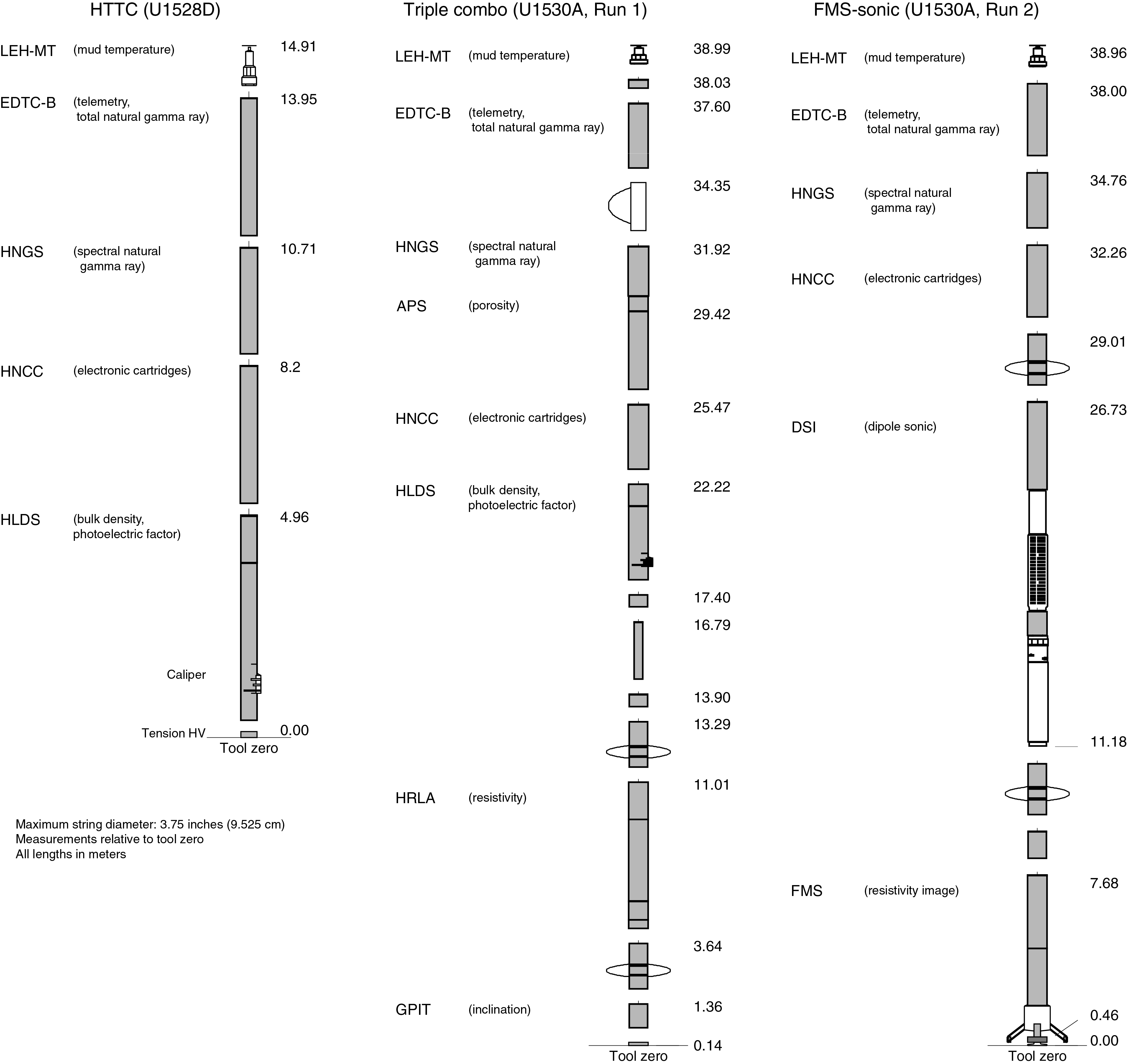
Figure F33. Wireline tool strings.
Each of these tool strings also included a telemetry cartridge in the EDTC that transmitted the data in real time from the tools to the Schlumberger data acquisition system (MAXIS unit) on the ship through the wireline cable. The tools in the high-temperature tool string were vacuum-flasked to increase their temperature rating. The wireline cable, which powers the tools and transmits the data to the surface in real time, is rated to 232°C, thereby limiting operations with the HTTC tool string. In addition, the 7-Conductor wireline sheathed in armor-wire Galvanized Improved Plow Steel is rated to fluids with H2S <0.05 psi (345 Pa) partial pressure and CO2 <32 psi (0.2 MPa) partial pressure. Exceeding these conditions would cause embrittlement of the wireline. Thus, the wireline cable was inspected after each logging run, and any affected sections were cut out as deemed necessary.
At Site U1528, the bit was changed to a logging bit before tool string deployment, whereas at Site U1530, a mechanical bit release was used to drop the RCB bit in the hole ahead of logging. The drill string was then pulled inside the casing, and the tool strings were deployed through the drill string on a 7-Conductor wireline cable in sequential runs. Owing to the absence of a reentry system at Site U1530 (i.e., there was no casing), the drill pipe was raised to ~70 mbsf, and the logging tools were deployed through the drill string. Logging data were recorded in the open-hole section below this depth. At both sites, each tool string was pulled up at a constant speed, typically ~9 m/min, to provide a continuous set of measurements in each logging run. To minimize the effect of the ship’s heave on the position of the tool string in the borehole, a wireline heave compensator (WHC) was employed as required (see below). During each logging run, real-time incoming data were recorded and monitored on the MCM MAXIS logging computer.
The Schlumberger logging equipment head (or cablehead) measures tension at the very top of the wireline tool string. These measurements detect and can diagnose difficulties in running the tool string up or down the borehole when exiting or entering the drill string or casing. The EDTC includes an accelerometer whose data are used to evaluate the efficiency of the WHC (see below). The EDTC also includes a scintillation gamma ray detector to aid correlation between log runs and detects when the tool passes the seafloor. A clearer indication of the seafloor is provided by the HNGS.
Because the tool strings combine tools of different generations and various designs, they include several adapters and joints between individual tools to allow communication, provide isolation, avoid interferences (mechanical or acoustic), terminate wirings, or position the tool properly in the borehole. Knuckle joints in particular were used to allow some of the tools, such as the HRLA resistivity tool, to remain centralized in the borehole while the overlying HLDS was pressed against the borehole wall. All of these additions contribute to the total length of the tool strings (Figure F33).
At the end of the Hole U1528D logging session, which encountered high-temperature, low-pH, and H2S-bearing fluids, the tools were washed on the rig floor. The resultant black-green coating on the tools had to be subsequently cleaned with sandpaper and a wire wheel.
Logged formation properties and tool measurement principles
The properties of the formations logged and the methods by which they were measured are described below. The main logs recorded during Expedition 376 are listed in Table T25. Further information regarding individual tools and their applications is widely available (e.g., Ellis and Singer, 2007; Goldberg, 1997; Lovell et al., 1998; Rider and Kennedy, 2011; Schlumberger, 1989; Serra, 1984, 1986, 1989). In addition, a complete list of acronyms for Schlumberger tools and logs is available at http://www.glossary.oil- field.slb.com.
Natural gamma radiation
Total and spectral gamma ray measurements were acquired using the HNGS. This tool utilizes two bismuth germanate scintillation detectors and five-window spectroscopy to determine concentrations of 40K, 232Th, and 238U in the formation. Sensitivity to any additives in the drilling fluid (notably sepiolite-based drilling mud clay) is eliminated because the HNGS filters out gamma ray energies <500 keV, thus improving measurement accuracy. The inclusion of HNGS in all tool strings allows the use of gamma ray data for depth correlation between consecutive tool string runs and individual tool string passes (up and down).
Density
The HLDS measures formation density utilizing a cesium (137Cs) gamma ray source and far and near gamma ray detectors mounted on a shielded skid. This skid is pressed against the borehole wall using a hydraulically activated eccentering arm. The gamma particles emitted from the source are attenuated through the process of Compton scattering, which involves a partial energy loss resulting from elastic collision with electrons in the formation. The quantity of gamma radiation that reaches the detectors is directly related to the density of electrons in the formation, which in turn is related to the bulk density. Good tool/borehole contact is essential for effective HLDS measurements, whereas poor contact results in an underestimation of formation density values.
Photoelectric effect
The HLDS also measures photoelectric absorption as the PEF. After repeated Compton scattering, as a result of collision with formation electrons, gamma radiation reaches an energy that is low enough (<150 keV) to be photoelectrically absorbed. The PEF is dependent on the atomic number of the elements in the formation and therefore varies according to the mineralogical composition of the lithologies encountered. As such, the PEF can be used to identify the presence of some minerals. Bartetzko et al. (2003), for example, interpret values >6 barns/e− as a general indicator for sulfide or oxide mineralization.
Porosity
A porosity measurement can be derived from the HLDS density measurement using average grain density, for example from MAD measurements on core samples (see Physical properties) and fluid density.
Formation porosity was measured with the APS in Hole U1530A. The sonde includes a minitron neutron generator that produces fast neutrons and five detectors positioned at different spacings from the minitron. The tool’s detectors count neutrons that arrive after being scattered and slowed by collisions with atomic nuclei in the formation. The highest energy loss occurs when neutrons collide with hydrogen nuclei, which have essentially the same mass as the neutron. Therefore, the tool provides a measure of hydrogen content, which is most commonly found in water in the pore fluid and can be directly related to porosity. However, hydrogen may be present in sedimentary, igneous, and alteration minerals, including clay minerals, which can result in an overestimation of actual porosity.
Upon reaching thermal energies (0.025 eV), the neutrons are captured by the nuclei of Cl, Si, B, and other elements, resulting in gamma ray emission. This neutron capture cross section (Σf) is also measured by the tool and can be used to identify these elements (Broglia and Ellis, 1990; Brewer et al., 1996).
Electrical resistivity
Six resistivity measurements with different depths of investigation (including one borehole fluid measurement and five formation measurements) were acquired with the HRLA. The array provides direct resistivity measurements by emitting a focused current into the formation and measuring the intensity necessary to maintain a constant drop in voltage across a fixed interval. The HRLA has one central (source) electrode and six electrodes above and below it that alternate as transmitting and receiving current electrodes. Simultaneous resistivity measurements at six penetration depths are possible because of the rapid alternation in roles of these electrodes. Typically, sulfide and oxide minerals and ionic solutions like pore fluid are electrical conductors, whereas silicates found in crustal rocks are electrical insulators. As a result, electrical conduction in most rocks will occur primarily by ion transport through pore fluids and conductive minerals such as phyllosilicates (Bartetzko et al., 2003). Thus, the resistivity measurement is largely dependent on porosity from fractures and matrix.
Acoustic velocity
The DSI measures the transit time of acoustic pulses between sonic transmitters and an array of eight receivers. The resulting waveforms are used to calculate the sonic velocity of the formation. High-frequency (5–15 kHz) pulses emitted by an omnidirectional monopole transmitter are used to extract the compressional velocity (VP) of the formation. It is possible to extract the shear wave velocity (VS) from these data in the event that it is faster than the acoustic velocity in the borehole fluid. The monopole transmitter can also be fired in sequence at a lower frequency (0.5–1.0 kHz) to generate Stoneley waves, which are sensitive to fractures and variations in formation permeability. The DSI has two cross-dipole transmitters that facilitate the acquisition of shear wave velocity data in slow formations where the formation VS is less than that of the borehole fluid. In fast formations, VS measurements from the monopole waveforms are possible and have sharper arrivals and more accurate VS estimates than the equivalent cross-dipole data. However, the cross-dipole-derived shear velocities can be useful in identifying any sonic anisotropy associated with the local stress regime.
Microresistivity images
High-resolution electrical resistivity images of the borehole walls were provided by the FMS. The tool has four orthogonal arms with pads, and each pad has 16 button electrodes that are pressed against the borehole wall during recording. The electrodes are arranged in two diagonally offset rows with eight electrodes in each row. A focused current is emitted from these electrodes into the formation, with a return electrode near the top of the tool. Formation resistivity is derived from the intensity of the current passing through the button electrodes. Processing these data in combination with azimuthal data from the General Purpose Inclinometry Tool (GPIT; see below) transforms the measurements into geographically oriented, high-resolution (millimeter to centimeter scale) images that can reveal the geologic features exposed in the borehole wall. Features such as vesicles, veins, fractures, and volcaniclastic textures may be resolved, and fabric analysis can be undertaken, in addition to quantitative analyses of the nature and orientation of structural and stratigraphic features.
The FMS microresistivity images do not provide full coverage of the borehole wall with a single pass (~37% coverage in an 8.5 inch hole). To increase this coverage, it is standard practice to undertake two passes of the borehole in the hope that the tool will be oriented differently on the second pass.
Accelerometry and magnetic field measurement
The GPIT undertakes three-component acceleration and magnetic field measurements. The primary purpose of this tool is to determine the acceleration and geographic orientation of the tool string in which it is deployed. The resulting data can be used to facilitate corrections for irregular tool motion and to provide geographically oriented image data from the FMS tool. GPIT data are also used to provide real-time evaluation of the WHC (see Wireline heave compensator).
Log data quality
The condition of a borehole is the principal factor contributing to log data quality. The ideal conditions for logging include a consistent borehole diameter of the size of the bit with no washouts (enlarged borehole) or bridges (narrowed borehole). Oversized borehole diameters can have a significant impact on measurements, especially those that require tool eccentering (e.g., HLDS) or tool centralization (e.g., FMS). The measurement principles of the eccentered tools and the centralized FMS mean that direct contact with the formation is essential for acquisition of high-quality data sets. Borehole wall contact is lost beyond a 20 inch (50.80 cm) borehole diameter for the HLDS and a 15 inch (38.10 cm) borehole diameter for the FMS. Certain measurements (notably, spectral gamma ray [HNGS], resistivity [HRLA], and acoustic velocity [DSI]) taken during Expedition 376 are still representative of the formation in larger borehole diameters. Consequently, these measurements are less affected by borehole conditions, although data are optimized in boreholes where the tools can be centralized (as large as ~20 inch diameter). High temperatures can also limit data quality because of the faster logging speeds required for tool preservation.
If the borehole diameter changes over short intervals as a consequence of washouts or ledges, logging results may be irregular. Bridged sections will also cause irregular log results. The quality of the borehole can be improved by minimizing the circulation of drilling fluid, flushing the borehole to remove debris prior to logging, performing a full wiper trip, and starting logging as soon as possible after drilling and hole conditioning.
The length of wireline cable payed out is used to determine the depth of the logging measurements. The quality of this logging depth determination is dependent on a number of factors, including the ship’s heave, cable stretch, cable slip, and tidal changes. To minimize the effect of the ship’s heave on logging depth, a hydraulic WHC is used to adjust the wireline length for rig motion during logging operations (see Wireline heave compensator). An important reference datum in wireline logging is the seafloor/mudline, which is determined from the gamma ray logs acquired in each logging run. Discrepancies between the drilling core depth and the wireline logging depth occur because of incomplete core recovery, core expansion, incomplete heave compensation, and drill pipe stretch. Reconciling the differences between the two data sets is possible through comparison of the common data sets acquired in situ and on the core (e.g., NGR and MS).
Wireline heave compensator
The WHC, first used during Integrated Ocean Drilling Program Expedition 320T in 2009, is designed to compensate for the ship’s vertical motion to help maintain the steady movement of the logging tools in the borehole (Iturrino et al., 2013). Vertical acceleration measurements made by the motion reference unit, located under the rig floor near the ship’s center of gravity, are used to calculate the vertical motion of the ship. The WHC then adjusts the length of the wireline by varying the distance between two sets of pulleys through which the cable passes. Simultaneous real-time measurements of surface and downhole acceleration are made by the EDTC and GPIT tools (see Accelerometry and magnetic field measurement), respectively. These data are then analyzed and compared in real time using a software package developed by Lamont-Doherty Earth Observatory. The actual motion of the tool string is displayed, enabling evaluation of the compensator’s efficiency.
The WHC was used during logging operations at Sites U1528 and U1530 with favorable sea conditions (<1 m peak-to-peak heave).
Logging data flow and depth scales
Downhole data for each logging run were monitored in real time and recorded by the Schlumberger MAXIS 500 system. Initially, the logging data were referenced to the rig floor. After completion of logging operations, the data were shifted to a seafloor reference using the step in gamma ray data (acquired in all logging runs) at the sediment/water interface.
Downhole logging data were also transferred onshore to Lamont-Doherty Earth Observatory for standardized data processing. Processing primarily involves depth matching to provide consistency in the depth scale between the different logging runs. Similar to the depth shift to the seafloor datum, this depth matching was undertaken primarily by utilizing the gamma ray data. In addition, corrections were made to certain tools and logs (e.g., speed and voltage corrections to microresistivity images), documentation for the logs (including an assessment of log data quality) was prepared, and the data were converted to ASCII for the conventional logs and GIF for the images. The data were transferred back to the ship within a few days of logging and were made available (in ASCII and DLIS formats) through the shipboard IODP logging database.
Microbiology
Microbial community development patterns associated with the two different types of hydrothermal activity at Brothers volcano have been explored using limited samples collected from the seafloor (Stott et al., 2008; Takai et al., 2009). Microbial community compositions collected from chimneys at the Type I NW Caldera site are characterized by an abundance of slightly thermophilic and hyperthermophilic chemolithoautotrophs (Takai et al., 2009), as observed in typical high-temperature hydrothermal vent environments of mid-ocean ridges and back-arc basin systems (Nakamura and Takai, 2014). When the temperature is below 150°C, aerobic to facultatively anaerobic, acidophilic sulfur– and iron-oxidizing chemolithotrophs and accompanying heterotrophs may be present.
The collective overarching objectives for microbiological study focus on the biomass, activity, and community structure of subsurface microbial and viral communities using an array of microbiological applications. Relatively few shipboard analyses were performed because most measurements require postcruise studies in shore-based laboratories. Consequently, the majority of our effort was dedicated to collecting and preserving an adequate number of samples for subsequent shore-based molecular biological studies.
Shore-based analyses will use a number of techniques to achieve the overall science objectives. DNA analyses of small-subunit (SSU) ribosomal gene amplicon sequencing will be conducted to address community structure. Metagenomics analysis will be conducted to reconstruct the metabolic potential and identify entire genomes from microbial populations in the samples. RNA determination using metatranscriptomics will help to establish potential community activity (i.e., the genes that are highly expressed in a given microbial environment). Genetic potential determined through metagenomics and single-cell genomics will provide detailed information about the possible metabolic characteristics of microbes, link those potentials to cellular identity, and provide clues related to the best environment to cultivate cells from recovered samples. Metabolic activity measurements of microbial communities using stable isotope– or radioactive isotope–labeled tracers will identify what kinds of major energy and carbon metabolisms are potentially present and their rates in the subseafloor habitats. Enrichment of specific groups of microorganisms will identify the unique physiological properties of the organisms. A considerable amount of time during the expedition was dedicated to collecting samples for quality assurance and quality control to constrain the microbiological quality of the samples.
The microbiologists plan to correlate these molecular microbiological and cultivation results with variations in IW geochemistry to interpret the metabolic potential of the microbial communities. Our goal for these comparisons will be to test specific hypotheses regarding the consequences of magma degassing for metal transport to the seafloor and its effect on the functioning of microbial communities. The metal-rich and acidic nature of the Brothers volcano hydrothermal system may also unleash discoveries related to the origin of microbial life on Earth.
Sampling
Microbiological sampling depends on careful sample handling techniques and the use of tracers to assess potential contamination. Microorganisms collected from beneath the seafloor are expected to be sensitive to chemical and physical changes they encounter when brought to the surface. Changes in oxygen concentration and temperature are two important factors to be considered when bringing cells from likely hot, anoxic conditions to the surface. Therefore, the following procedures were followed to minimize harm to subsurface microbes without compromising other expedition objectives.
For microbiological studies, whole-round core samples are required to have enough material to work with while avoiding contamination introduced by sample handling before and during the core splitting process. Whole rounds were sampled in the splitting room after the core was brought in from the catwalk. Technicians wore gloves and face masks and shook the core into a split core liner sprayed with ethanol to minimize the chances of contamination. The microbiologist then selected a whole-round section for sampling with the Co-Chief Scientist on shift or the Staff Scientist. An ideal sample was one that consisted largely of sediments (epiclastic or volcaniclastic deposits) and/or that had some indication of hydrothermal fracturing (such as visible veins) but that had not split apart during the dislocation and did not have a unique lithology that would be critical to the core description team. Both the microbiologists and the geologists taking part in sample selection wore gloves sprayed with ethanol and a face mask to limit possible contamination of the sample from human contact. The microbiologists wore closed-sleeve laboratory coats. The whole-round rock sample chosen for dedicated microbiology investigation was then transferred into a sterile Whirl-Pak bag and transported to the microbiology laboratory for processing.
Once in the microbiology laboratory, the whole-round sample was rinsed four times in sterile water (changing the Whirl-Pak bag once after the second rinse) to reduce contamination from drilling fluid. The sample was then transferred to an ethanol-sterilized metal rock box placed under aseptic conditions using a table KOACH (a super-clean zone creator) (KOKEN T-500, Tokyo, Japan) with a HEPA air filter, which greatly reduced the number of air particles (Figure F34). The outside of each core was sprayed with 70% ethanol at least twice and then sprayed one final time with ethanol and left to air dry (~5 min). At all stages of the process, samples were handled as little as possible and with gloved hands only. Masks, gloves, and a laboratory coat were worn by those handling the samples during whole-round cleaning and all subsequent steps.
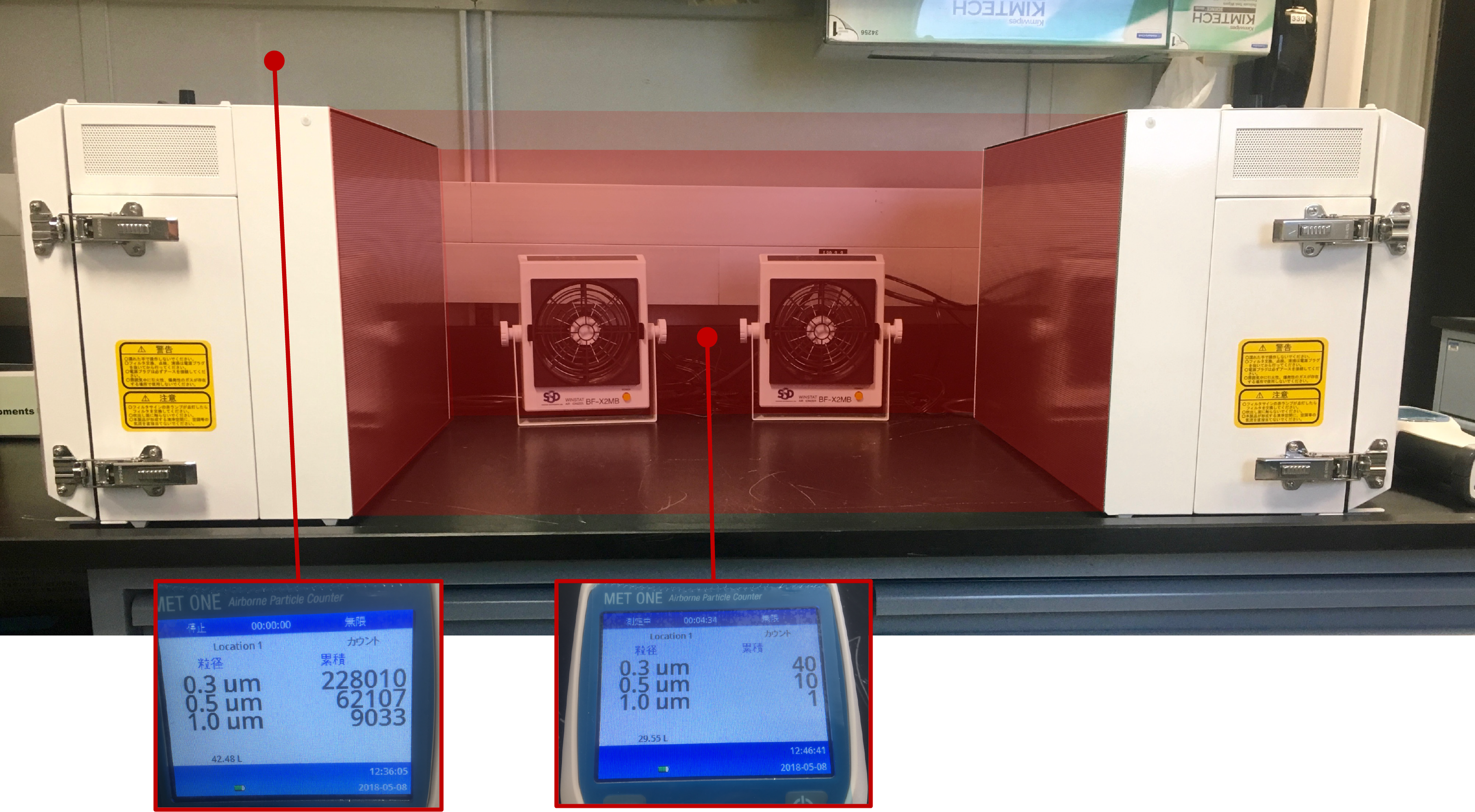
Figure F34. Clean area designed for microbiology sampling.
Prior work has shown that the interior of rock cores is generally free from contamination (Lever et al., 2006). Therefore, efforts were taken to sample only the interior of the cores. Sections that displayed soft material or showed some sign of alteration or fluid flow conduits were specifically chosen because these are the most likely locations for microbial life.
On average, microbiology samples were ~10–12 cm long. Sample material was divided into subsamples for a variety of tests (Figure F35). All inclusive, these tests include shore-based cell and viral particle counts, molecular biology (DNA and RNA), viral and prokaryotic activity measurements, initiation of fungal and prokaryotic enrichment cultures, shipboard initiation of nutrient addition bioassays, and adenosine triphosphate (ATP) quantification. Subsamples were collected for cell and viral particle counts, DNA and RNA analyses, nutrient enrichment incubations and ATP quantification, and activity measurements, depending on material available.
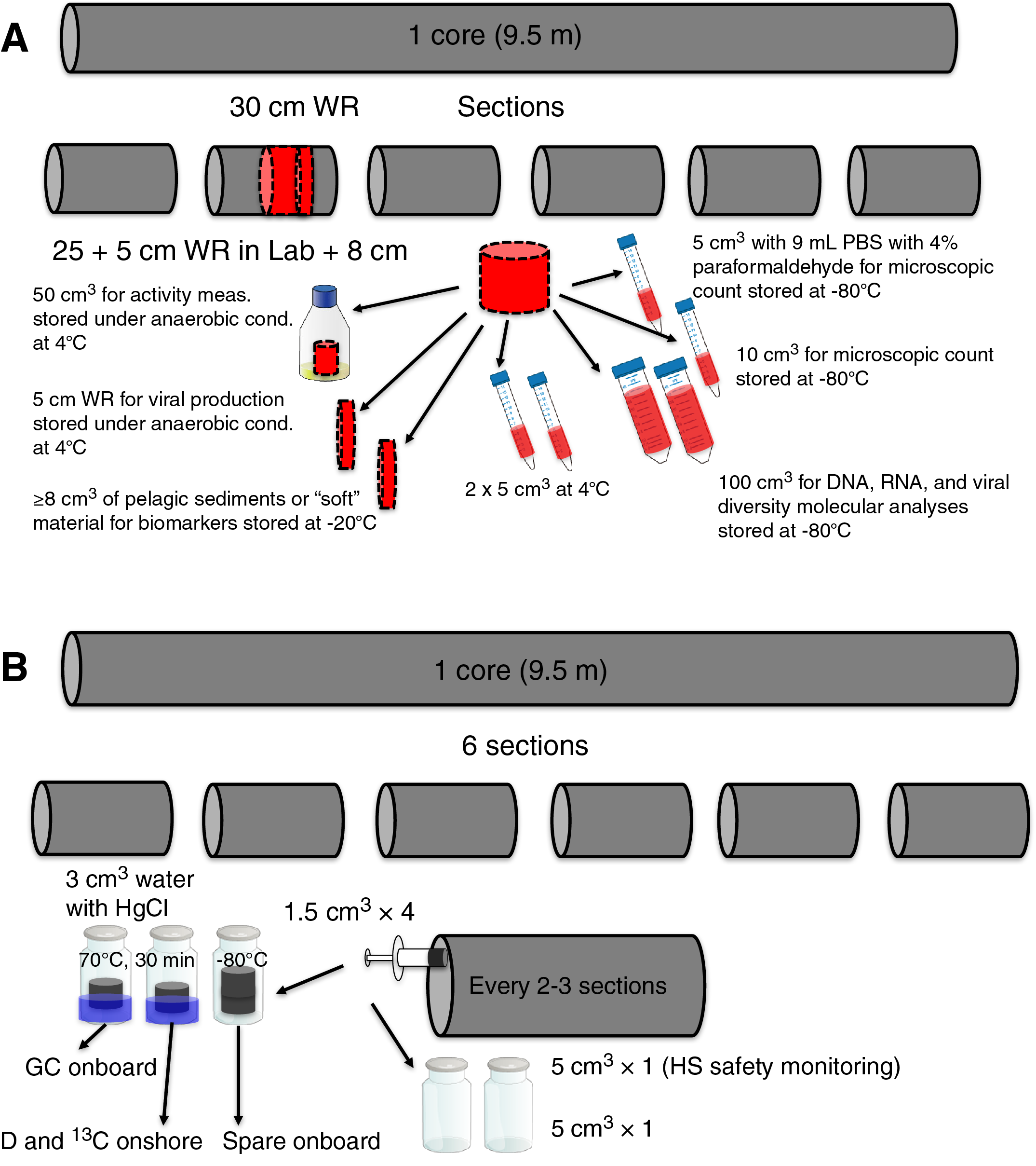
Figure F35. Microbiology sample plan.
After cleaning the exterior of whole-round core samples, the rock was split with a sterile chisel and core interiors were subsampled for the above-mentioned tests. Ethanol-sterilized stainless steel spatula and tweezers were used to separate the core exterior from the interior of large pieces. Samples for RNA analysis were taken first and immediately frozen at −80°C (in RNAlater solution [Invitrogen Ref. AM7021]). Whenever pieces of the whole-round core remained after collection of material for analysis, they were returned to the curator to be placed back into the working and archive halves, along with the outer portions of the core that had to be removed for sampling. Following completion of sample processing, all tools and the rock box were cleaned with deionized water. They were then brought back into the sampling enclosure and sprayed with 75% ethanol, wiped with Kimwipes, sprayed with 75% ethanol again, and allowed to air dry. The bench top was also sprayed with 75% ethanol, wiped with Kimwipes, sprayed once more, and allowed to air dry.
Contamination testing of drilling fluid
As part of the drilling process, a huge amount of surface seawater is injected into the borehole as drilling fluid. This is the major potential source of microorganism contamination of the cores. As a check for infiltration of drilling fluid into the core samples, the microbial composition of drilling fluid will be assessed onshore via DNA sequencing approaches. We collected samples of the drilling fluid for microbial community SSU ribosomal RNA gene diversity analysis at the start of drilling during Expedition 376 and then periodically thereafter. These samples were collected directly from the injection pipe on the rig floor into sterile bottles with screw caps and handled using sterile equipment. Organisms found to be present in both the drilling fluid and rock samples will be considered a sign of contamination. Although it is possible that some taxa found in surface seawater may also survive in the deep subsurface biosphere, these organisms will be conservatively interpreted to be contaminants, not subsurface residents. Thus, any samples where all of the organisms detected during postcruise analyses are also detected in the drilling fluid will be excluded from further analysis. Consistent with a recent study of deep subsurface sediments (Inagaki et al., 2015), we consider that a conservative approach is most appropriate. Our 1 L samples of drilling fluid were filtered onto 45 mm 0.20 μm pore-size Millipore Express Plus polycarbonate filters and frozen at −80°C for shore-based DNA extraction and analysis. Samples of drilling mud (i.e., sepiolite) were also collected on the rig floor prior to injection into the drill pipe into two sterile 50 mL polypropylene centrifuge tubes and frozen at −80°C for shore-based DNA extraction.
Perfluoromethyl decaline (PFMD) was added to the drilling fluid as a tracer at a rate of ~0.55 mL/min (1% of the mud pump rate; equivalent to between 0.4 and 0.6 mL/min). Because the concentration of PFMD in the samples was very low, the rate was increased by ten times at Site U1531. Samples were taken only for the cores that were tested for contamination. For contamination tests of whole-round samples, a fragment of the exterior of each core sample prior to cleaning was transferred to a 20 mL headspace glass vial with metal caps and Teflon seals for detection of PFMD. This sample provided a baseline for the level of contamination present prior to cleaning. This process ensured that the rock samples measured for PFMD were completely exposed to the PFMD, whereas, when sampling from the whole round, one inevitably includes portions of the rock interior just behind the outside wall that were not exposed. Sampling of the exterior of the whole round was also conducted following cleaning of the core sample exterior and then again for an interior sample.
Cell counts
A subsample of ~5 cm3 was placed into a 15 mL plastic tube, and then 5 mL (or enough to cover the sample) of paraformaldehyde (4% solution in 100 mM phosphate-buffered saline) was added. Preserved samples were stored at −80°C for onshore analysis using a density gradient separation of cells from rocks prior to cell counting.
Activity measurements
Samples (50 cm3) for activity measurements were collected and stored in 100 mL glass bottles with 1 mL of 5% (weight/volume) sodium sulfide (Na2S) solution and a butyl rubber stopper under N2 atmosphere at 4°C for onshore analysis.
Virus assessment and quantification
Samples (10 cm3) were collected and stored at −80°C for onshore virus counting. Additionally, 5 cm long whole rounds were anaerobically stored at 4°C for viral production analysis. Finally, samples (10 cm3) were collected and stored at −80°C for onshore viral diversity studies based on polymerase chain reaction amplification.
Cultivation experiments (nutrient addition experiments)
Little is known about limiting factors for growth in subseafloor volcanic basement because of the difficulty of sampling this environment and the typically low biomass. We used a nutrient addition bioassay approach to assess whether added inorganic nutrients and/or organic carbon can stimulate growth of in situ microbial communities. Microcosm experiments in 20 mL serum vials were used for this purpose, with anaerobic seawater (seawater collected from the ship during sampling was filtered and autoclaved) as the basal media for all enrichments. Depending on availability, ~5 cm3 samples were pulverized using a sterile chisel and hammer in Whirl-Pak bags to contain the fragments in sterile conditions. Four conditions were tested: (1) no addition of nutrients (control), (2) addition of 750 μM NH4Cl, (3) addition of 750 μM NH4Cl and 50 μM K2HPO4, and (4) addition of 200 μM each of acetate, formate, and lactate. To initiate enrichments, 1–3 cm3 of crushed rock chips, depending on sample availability, were transferred to 20 mL serum vials and submerged in anaerobic sterile seawater to a level equivalent to 18 mL total volume (crushed rock plus media). After the appropriate additions were made to the vials, they were sealed with butyl stoppers and gassed with nitrogen. Enrichments were stored at 40°C for the remainder of the expedition and will be analyzed 6 months or more postcruise to allow for sufficient growth.
Adenosine triphosphate quantification
For quantification of ATP in rock samples, we collected 0.1 cm3 of pulverized rock in a 1.5 mL centrifuge tube. Samples were stored at 4°C for as long as 4 days before performing the ATP assay because samples were run in batches to preserve and optimize the assay reagent, which requires a standard curve. Previous experiments showed no difference in quantification for samples read immediately after sampling or after storage (MacLeod et al., 2017). We added 200 μL of autoclaved Milli-Q water to the 0.1 cm3 powdered rock, vortexed it for 60 s, and then spun the tube at 2000 rotations/min for 1 min in a benchtop microcentrifuge. The commercial ATP Determination Kit (Invitrogen, Carlsbad, CA [USA]) was used for quantification in a Turner TD20/20 Luminometer (available in the microbiology laboratory). Acid-cleaned (10% HCl) glass vials were used for measurement. As per the manufacturer’s suggestions, 0.1 mL of ATP assay mix was added to the glass vials and allowed to sit for 3 min prior to adding the sample to hydrolyze any ATP present in the vial. After 3 min, 0.1 mL of the supernatant from the 1.5 mL centrifuge tube was added to the assay vial, and then the vial was swirled briefly and immediately (luminescence fades quickly) placed in the luminometer. Raw luminescence was converted to picograms per milliliter (pg/mL) ATP by running 0, 1, and 10 pg/mL standards, diluted from the ATP standard included in the kit, with each batch of samples.
Molecular biology
DNA
For DNA analyses, we collected 15–50 cm3 samples and froze them at −80°C. These samples will be analyzed during postcruise research.
RNA
Samples (rock chips) were placed in sterile 50 mL Falcon tubes, covered in RNAlater, and immediately stored at −80°C. RNAlater protects the viability of microbial cells while keeping them in stasis, allowing for efficient DNA and RNA extractions from samples collected in the field. These samples will be analyzed during postcruise research.
References
Allmendinger, R.W., Cardozo, N., and Fisher, D.M., 2011. Structural Geology Algorithms: Vectors and Tensors: Cambridge, United Kingdom (Cambridge University Press). https://doi.org/10.1017/CBO9780511920202
Alt, J.C., Kinoshita, H., Stokking, L.B., et al., 1993. Proceedings of the Ocean Drilling Program, Initial Reports, 148: College Station, TX (Ocean Drilling Program). https://doi.org/10.2973/odp.proc.ir.148.1993
Arculus, R.J., Ishizuka, O., Bogus, K., Aljahdali, M.H., Bandini-Maeder, A.N., Barth, A.P., Brandl, P.A., do Monte Guerra, R., Drab, L., Gurnis, M.C., Hamada, M., Hickey-Vargas, R.L., Jiang, F., Kanayama, K., Kender, S., Kusano, Y., Li, H., Loudin, L.C., Maffione, M., Marsaglia, K.M., McCarthy, A., Meffre, S., Morris, A., Neuhaus, M., Savov, I.P., Sena Da Silva, C.A., Tepley, F.J., III, van der Land, C., Yogodzinski, G.M., and Zhang, Z., 2015. Expedition 351 methods. In Arculus, R.J., Ishizuka, O., Bogus, K., and the Expedition 351 Scientists, Izu-Bonin-Mariana Arc Origins. Proceedings of the International Ocean Discovery Program, 351: College Station, TX (International Ocean Discovery Program). https://doi.org/10.14379/iodp.proc.351.102.2015
Bartetzko, A., Paulick, H., Iturrino, G., and Arnold, J., 2003. Facies reconstruction of a hydrothermally altered dacite extrusive sequence: evidence from geophysical downhole logging data (ODP Leg 193). Geochemistry, Geophysics, Geosystems, 4(10):1087. https://doi.org/10.1029/2003GC000575
Bartington Instruments, Ltd., 2011. Operation Manual for MS2 Magnetic Susceptibility System: Oxford, United Kingdom (Bartington Instruments, Ltd.). https://www.gmw.com/magnetic_properties/pdf/BI-MAN-MS2-OM0408.pdf
Bartington Instruments, Ltd., 2019. MS2/MS3 Magnetic Susceptibility System: Oxford, UK (Bartington Instruments, Ltd.). http://www.bartington.com/Literaturepdf/Datasheets/MS2_MS3_DS0020.pdf
Bates, R.L., and Jackson, J.A. (Eds.), 1987. Glossary of Geology (3rd edition): Alexandria, VA (American Geological Institute).
Blum, P., 1997. Technical Note 26: Physical Properties Handbook—A Guide to the Shipboard Measurement of Physical Properties of Deep-Sea Cores. Ocean Drilling Program. https://doi.org/10.2973/odp.tn.26.1997
Bodnar, R.J., 1993. Revised equation and table for determining the freezing point depression of H2O-NaCl solutions. Geochimica et Cosmochimica Acta, 57(3):683–684. https://doi.org/10.1016/0016-7037(93)90378-A
Bozzo, A.T., Chen, H.-S., Kass, J.R., and Barduhn, A.J., 1973. The properties of the hydrates of chlorine and carbon dioxide. In Delyannis, A., and Delyannis, E. (Eds.), Proceedings of the Fourth International Symposium on Fresh Water from the Sea (Volume 3): Ion Exchange, Desalination Membranes, Electrodialyses, Other Ionic Processes, Freezing Processes, Hydrate Processes: Athens (European Federation of Chemical Engineering), 437–451.
Brewer, T.S., Harvey, P.K., Locke, J., and Lovell, M.A., 1996. Neutron absorption cross section (Σ) of basaltic basement samples from Hole 896A, Costa Rica rift. In Alt, J.C., Kinoshita, H., Stokking, L.B., and Michael, P.J. (Eds.), Proceedings of the Ocean Drilling Program, Scientific Results, 148: College Station, TX (Ocean Drilling Program), 389–394. https://doi.org/10.2973/odp.proc.sr.148.154.1996
Broglia, C., and Ellis, D., 1990. Effect of alteration, formation absorption, and standoff on the response of the thermal neutron porosity log in gabbros and basalts: examples from Deep Sea Drilling Project-Ocean Drilling Program sites. Journal of Geophysical Research: Solid Earth, 95(B6):9171–9188. https://doi.org/10.1029/JB095iB06p09171
Cande, S.C., and Kent, D.V., 1995. Revised calibration of the geomagnetic polarity timescale for the Late Cretaceous and Cenozoic. Journal of Geophysical Research: Solid Earth, 100(B4):6093–6095. https://doi.org/10.1029/94JB03098
Cardozo, N., and Allmendinger, R.W., 2013. Spherical projections with OSXStereonet. Computers & Geosciences, 51:193–205. https://doi.org/10.1016/j.cageo.2012.07.021
Chen H.S., 1972. The Properties of Carbon Dioxide Hydrate. Office of Saline Water, Research and Development Progress Report, 830.
Darling, R.S., 1991. An extended equation to calculate NaCl contents from final clathrate melting temperatures in H2O-CO2-NaCl fluid inclusions: Implications for P-T isochore location. Geochimica et Cosmochimica Acta, 55(12):3869–3871. https://doi.org/10.1016/0016-7037(91)90079-K
Davis, G.H., Reynolds, S.J., and Kluth, C., 2011. Structural Geology of Rocks and Regions (3rd edition): New York (John Wiley & Sons).
de Ronde, C.E.J., Hannington, M.D., Stoffers, P., Wright, I.C., Ditchburn, R.G., Reyes, A.G., Baker, E.T., et al., 2005. Evolution of a submarine magmatic-hydrothermal system: Brothers Volcano, southern Kermadec arc, New Zealand. Economic Geology, 100(6):1097–1133. https://doi.org/10.2113/gsecongeo.100.6.1097
de Ronde, C.E.J., Humphris, S.E., Höfig, T.W., Brandl, P.A., Cai, L., Cai, Y., Caratori Tontini, F., Deans, J.R., Farough, A., Jamieson, J.W., Kolandaivelu, K.P., Kutovaya, A., Labonté, J.M., Martin, A.J., Massiot, C., McDermott, J.M., McIntosh, I.M., Nozaki, T., Pellizari, V.H., Reyes, A.G., Roberts, S., Rouxel, O., Schlicht, L.E.M., Seo, J.H., Straub, S.M., Strehlow, K., Takai, K., Tanner, D., Tepley, F.J., III, and Zhang, C., 2019. Site U1528. In de Ronde, C.E.J., Humphris, S.E., Höfig, T.W., and the Expedition 376 Scientists, Brothers Arc Flux. Proceedings of the International Ocean Discovery Program, 376: College Station, TX (International Ocean Discovery Program). https://doi.org/10.14379/iodp.proc.376.104.2019
Dunlea, A.G., Murray, R.W., Harris, R.N., Vasiliev, M.A., Evans, H., Spivack, A.J., and D’Hondt, S., 2013. Assessment and use of NGR instrumentation on the JOIDES Resolution to quantify U, Th, and K concentrations in marine sediment. Scientific Drilling, 15:57–63. https://doi.org/10.2204/iodp.sd.15.05.2013
Ellis, D.V., and Singer, J.M., 2007. Well Logging for Earth Scientists (2nd edition): New York (Elsevier).
Expedition 304/305 Scientists, 2006. Methods. In Blackman, D.K., Ildefonse, B., John, B.E., Ohara, Y., Miller, D.J., MacLeod, C.J., and the Expedition 304/305 Scientists, Proceedings of the Integrated Ocean Drilling Program, 304/305: College Station, TX (Integrated Ocean Drilling Program Management International, Inc.). https://doi.org/10.2204/iodp.proc.304305.102.2006
Expedition 309/312 Scientists, 2006. Methods. In Teagle, D.A.H., Alt, J.C., Umino, S., Miyashita, S., Banerjee, N.R., Wilson, D.S., and the Expedition 309/312 Scientists. Proceedings of the Integrated Ocean Drilling Program, 309/312: Washington, DC (Integrated Ocean Drilling Program Management International, Inc.). https://doi.org/10.2204/iodp.proc.309312.102.2006
Expedition 330 Scientists, 2012. Methods. In Koppers, A.A.P., Yamazaki, T., Geldmacher, J., and the Expedition 330 Scientists, Proceedings of the Integrated Ocean Drilling Program, 330: Tokyo (Integrated Ocean Drilling Program Management International, Inc.). https://doi.org/10.2204/iodp.proc.330.102.2012
Expedition 335 Scientists, 2012. Methods. In Teagle, D.A.H., Ildefonse, B., Blum, P., and the Expedition 335 Scientists, Proceedings of the Integrated Ocean Drilling Program, 335: Tokyo (Integrated Ocean Drilling Program Management International, Inc.). https://doi.org/10.2204/iodp.proc.335.102.2012
Expedition 349 Scientists, 2014. Expedition 349 Preliminary Report: South China Sea Tectonics. Integrated Ocean Drilling Program. https://doi.org/10.14379/iodp.pr.349.2014
Fisher, R.V., and Schmincke, H.-U., 1984. Pyroclastic Rocks: Berlin (Springer-Verlag). https://doi.org/10.1007/978-3-642-74864-6
Fluid Incorporated, 1992. Temperature Calibration Standards by Syn Flinc: Denver (Fluid Incorporated).
Folk, R.L., 1965. Some aspects of recrystallization in ancient limestones. In Pray, L.C., and Murray, R.C. (Eds.), Dolomitization and Limestone Diagenesis. Special Publication - SEPM (Society for Sedimentary Geology), 13:13–48. https://doi.org/10.2110/pec.65.07.0014
Gaidies, F., Milke, R., Heinrich, W., and Abart, R., 2017. Metamorphic mineral reactions: porphyroblast, corona and symplectite growth. In Heinrich, W., and Abart, R. (Eds.), Mineral Reaction Kinetics: Microstructures, Textures, Chemical and Isotopic Signatures. European Mineralogical Union Notes in Mineralogy, 16:469–540. https://doi.org/10.1180/EMU-notes.16.14
Gieskes, J.M., Gamo, T., and Brumsack, H., 1991. Technical Note 15: Chemical Methods for Interstitial Water Analysis Aboard JOIDES Resolution. Ocean Drilling Program. https://doi.org/10.2973/odp.tn.15.1991
Gifkins, C.C., and Allen, R.L., 2001. Textural and chemical characteristics of diagenetic and hydrothermal alteration in glassy volcanic rocks: examples from the Mount Read Volcanics, Tasmania. Economic Geology, 96(5):973–1002. https://doi.org/10.2113/gsecongeo.96.5.973
Gifkins, C.C., Herrmann, W., and Large, R.R., 2005. Altered Volcanic Rocks: A Guide to Description and Interpretation: Hobart, Australia (Centre for Ore Deposit Research, University of Tasmania). https://eprints.utas.edu.au/296/
Giggenbach, W.F., 1995. Variations in the chemical and isotopic composition of fluids discharged from the Taupo Volcanic Zone, New Zealand. Journal of Volcanology and Geothermal Research, 68(1–3):89–116. https://doi.org/10.1016/0377-0273(95)00009-J
Gill, R., 2010. Igneous Rocks and Processes: A Practical Guide: Chichester, United Kingdom (Wiley-Blackwell).
Gillis, K.M., Snow, J.E., Klaus, A., Guerin, G., Abe, N., Akizawa, N., Ceuleneer, G., Cheadle, M.J., Adrião, Á., Faak, K., Falloon, T.J., Friedman, S.A., Godard, M.M., Harigane, Y., Horst, A.J., Hoshide, T., Ildefonse, B., Jean, M.M., John, B.E., Koepke, J.H., Machi, S., Maeda, J., Marks, N.E., McCaig, A.M., Meyer, R., Morris, A., Nozaka, T., Python, M., Saha, A., and Wintsch, R.P., 2014. Methods. In Gillis, K.M., Snow, J.E., Klaus, A., and the Expedition 345 Scientists, Proceedings of the Integrated Ocean Drilling Program, 345: College Station, TX (Integrated Ocean Drilling Program). https://doi.org/10.2204/iodp.proc.345.102.2014
Godard, M., Awaji, S., Hansen, H., Hellebrand, E., Brunelli, D., Johnson, K., Yamasaki, T., et al., 2009. Geochemistry of a long in-situ section of intrusive slow-spread oceanic lithosphere: results from IODP Site U1309 (Atlantis Massif, 30°N Mid-Atlantic-Ridge). Earth and Planetary Science Letters, 279(1–2):110–122. https://doi.org/10.1016/j.epsl.2008.12.034
Goldberg, D., 1997. The role of downhole measurements in marine geology and geophysics. Reviews of Geophysics, 35(3):315–342. https://doi.org/10.1029/97RG00221
Govindaraju, K., 1994. 1994 compilation of working values and sample description for 383 geostandards. Geostandards Newsletter, 18(1). https://doi.org/10.1111/j.1751-908X.1994.tb00502.x
GRC, 1994a. Multi-Sensor Memory Module Operation Manual, Document #006-0112-00: Tulsa, OK (Geophysical Research Corporation).
GRC, 1994b. University of Miami UHT-MSM Operations Manual, Document #006-0122-00: Tulsa, OK (Geophysical Research Corporation).
GRC, 1996. MSM/MIAMI Operation Software (Revision 0) User’s Guide, Document #006-0128-00: Tulsa, OK (Geophysical Research Corporation).
Hallsworth, C.R., and Knox, R.W.O’B., 1999. BGS Rock Classification Scheme (Volume 3): Classification of Sediments and Sedimentary Rocks. British Geological Survey Research Report, RR 99–03. https://www.bgs.ac.uk/downloads/start.cfm?id=9
Harris, R.N., Sakaguchi, A., Petronotis, K., Baxter, A.T., Berg, R., Burkett, A., Charpentier, D., Choi, J., Diz Ferreiro, P., Hamahashi, M., Hashimoto, Y., Heydolph, K., Jovane, L., Kastner, M., Kurz, W., Kutterolf, S.O., Li, Y., Malinverno, A., Martin, K.M., Millan, C., Nascimento, D.B., Saito, S., Sandoval Gutierrez, M.I., Screaton, E.J., Smith-Duque, C.E., Solomon, E.A., Straub, S.M., Tanikawa, W., Torres, M.E., Uchimura, H., Vannucchi, P., Yamamoto, Y., Yan, Q., and Zhao, X., 2013. Methods. In Harris, R.N., Sakaguchi, A., Petronotis, K., and the Expedition 344 Scientists, Proceedings of the Integrated Ocean Drilling Program, 344: College Station, TX (Integrated Ocean Drilling Program). https://doi.org/10.2204/iodp.proc.344.102.2013
Hedenquist, J.W., and Henley, R.W., 1985. The importance of CO2 on freezing point measurements of fluid inclusions: evidence from active geothermal systems and implications for epithermal ore deposition. Economic Geology, 80(5):1379–1406. https://doi.org/10.2113/gsecongeo.80.5.1379
Henley, R.W., and Ellis, A.J., 1983. Geothermal systems ancient and modern: a geochemical review. Earth-Science Reviews, 19(1):1–50. https://doi.org/10.1016/0012-8252(83)90075-2
Huber, B.T., Hobbs, R.W., Bogus, K.A., Batenburg, S.J., Brumsack, H.-J., do Monte Guerra, R., Edgar, K.M., Edvardsen, T., Garcia Tejada, M.L., Harry, D.L., Hasegawa, T., Haynes, S.J., Jiang, T., Jones, M.M., Kuroda, J., Lee, E.Y., Li, Y.-X., MacLeod, K.G., Maritati, A., Martinez, M., O’Connor, L.K., Petrizzo, M.R., Quan, T.M., Richter, C., Riquier, L., Tagliaro, G.T., Wainman, C.C., Watkins, D.K., White, L.T., Wolfgring, E., and Xu, Z., 2019. Expedition 369 methods. In Hobbs, R.W., Huber, B.T., Bogus, K.A., and the Expedition 369 Scientists, Australia Cretaceous Climate and Tectonics. Proceedings of the International Ocean Discovery Program, 369: College Station, TX (International Ocean Discovery Program). https://doi.org/10.14379/iodp.proc.369.102.2019
Ikeuchi, K., Doi, N., Sakagawa, Y., Kamenosono, H., and Uchida, T., 1998. High-temperature measurements in well WD-1A and the thermal structure of the kakkonda geothermal system, Japan. Geothermics, 27(5–6):591–607. https://doi.org/10.1016/S0375-6505(98)00035-2
Inagaki, F., Hinrichs, K.-U., Kubo, Y., Bowles, M.W., Heuer, V.B., Long, W.-L., Hoshino, T., et al., 2015. Exploring deep microbial life in coal-bearing sediment down to ~2.5 km below the ocean floor. Science, 349(6246):420–424. https://doi.org/10.1126/science.aaa6882
Iturrino, G., Liu, T., Goldberg, D., Anderson, L., Evans, H., Fehr, A., Guerin, G., et al., 2013. Performance of the wireline heave compensation system onboard D/V JOIDES Resolution. Scientific Drilling, 15:46–50. https://doi.org/10.2204/iodp.sd.15.08.2013
Jébrak, M., 1997. Hydrothermal breccias in vein-type ore deposits: a review of mechanisms, morphology and size distribution. Ore Geology Reviews, 12(3):111–134. https://doi.org/10.1016/S0169-1368(97)00009-7
Jian, Z., Larsen, H.C., Alvarez Zarikian, C.A., and the Expedition 368 Scientists, 2018. Expedition 368 Preliminary Report: South China Sea Rifted Margin. International Ocean Discovery Program. https://doi.org/10.14379/iodp.pr.368.2018
Jochum, K.P., Nohl, U., Herwig, K., Lammel, E., Stoll, B., and Hofmann, A.W., 2005. GeoRem: a new geochemical database for reference materials and isotopic standards. Geostandards and Geoanalytical Research, 29(3):333–338. https://doi.org/10.1111/j.1751-908X.2005.tb00904.x
Johnston, R.M., Ryan, J.G., and the Expedition 366 Scientists, 2018. pXRF and ICP-AES characterization of shipboard rocks and sediments: protocols and strategies. In Fryer, P., Wheat, C.G., Williams, T., and the Expedition 366 Scientists, Mariana Convergent Margin and South Chamorro Seamount. Proceedings of the International Ocean Discovery Program, 366: College Station, TX (International Ocean Discovery Program). https://doi.org/10.14379/iodp.proc.366.110.2018
Jutzeler, M., White, J.D.L., Talling, P.J., McCanta, M., Morgan, S., Le Friant, A., and Ishizuka, O., 2014. Coring disturbances in IODP piston cores with implications for offshore record of volcanic events and the Missoula megafloods. Geochemistry, Geophysics, Geosystems, 15(9):3572–3590. https://doi.org/10.1002/2014GC005447
Kirschvink, J.L., 1980. The least-squares line and plane and the analysis of palaeomagnetic data. Geophysical Journal of the Royal Astronomical Society, 62(3):699–718. https://doi.org/10.1111/j.1365-246X.1980.tb02601.x
Knight, C.L., and Bodnar, R.J., 1989. Synthetic fluid inclusions: IX. Critical PVTX properties of NaCl-H2O solutions. Geochimica et Cosmochimica Acta, 53(1):3–8. https://doi.org/10.1016/0016-7037(89)90267-6
Kristiansen, J.I., 1982. The transient cylindrical probe method for determination of thermal parameters of earth materials [Ph.D. dissertation]. Åarhus University, Åarhus, Denmark.
Kvenvolden, K.A., and McDonald, T.J., 1986. Technical Note, 6: Organic Geochemistry on the JOIDES Resolution—An Assay. Ocean Drilling Program. https://doi.org/10.2973/odp.tn.6.1986
Le Maitre, R.W. (Ed.), Streckeisen, A., Zanettin, B., Le Bas, M.J., Bonin, B., Bateman, P., Bellieni, G., Dudek, A., et al., 2002. Igneous Rocks: A Classification and Glossary of Terms (2nd edition)—Recommendations of the International Union of Geological Sciences Subcommission on the Systematics of Igneous Rocks: Cambridge, United Kingdom (Cambridge University Press). https://doi.org/10.1017/CBO9780511535581
Lever, M.A., Alperin, M., Engelen, B., Inagaki, F., Nakagawa, S., Steinsbu, B.O., Teske A., and IODP Expedition 301 Scientists, 2006. Trends in basalt and sediment core contamination during IODP Expedition 301. Geomicrobiology Journal, 23(7):517–530. https://doi.org/10.1080/01490450600897245
Li, C.-F., Lin, J., Kulhanek, D.K., Williams, T., Bao, R., Briais, A., Brown, E.A., Chen, Y., Clift, P.D., Colwell, F.S., Dadd, K.A., Ding, W., Hernández-Almeida, I., Huang, X.-L., Hyun, S., Jiang, T., Koppers, A.A.P., Li, Q., Liu, C., Liu, Q., Liu, Z., Nagai, R.H., Peleo-Alampay, A., Su, X., Sun, Z., Tejada, M.L.G., Trinh, H.S., Yeh, Y.-C., Zhang, C., Zhang, F., Zhang, G.-L., and Zhao, X., 2015. Methods. In Li, C.-F., Lin, J., Kulhanek, D.K., and the Expedition 349 Scientists, South China Sea Tectonics. Proceedings of the International Ocean Discovery Program, 349: College Station, TX (International Ocean Discovery Program). https://doi.org/10.14379/iodp.proc.349.102.2015
Lide, D.R. (Ed.), 2000. Handbook of Chemistry and Physics (81st edition): Boca Raton, FL (Chemical Rubber Publishing Company).
Lovell, M.A., Harvey, P.K., Brewer, T.S., Williams, C., Jackson, P.D., and Williamson, G., 1998. Application of FMS images in the Ocean Drilling Program: an overview. In Cramp, A., MacLeod, C.J., Lee, S.V., and Jones, E.J.W. (Eds.), Geological Evolution of Ocean Basins: Results from the Ocean Drilling Program. Geological Society Special Publication, 131(1):287–303. https://doi.org/10.1144/GSL.SP.1998.131.01.18
Lund, S.P., Stoner, J.S., Mix., A.C., Tiedemann, R., Blum, P., and the Leg 202 Shipboard Scientific Party, 2003. Appendix: observations on the effect of a nonmagnetic core barrel on shipboard paleomagnetic data: results from ODP Leg 202. In Mix, A.C., Tiedemann, R., Blum, P., et al., Proceedings of the Ocean Drilling Program, Initial Reports, 202: College Station, TX (Ocean Drilling Program), 1–10. https://doi.org/10.2973/odp.proc.ir.202.114.2003
Lurcock, P.C., and Wilson, G.S., 2012. PuffinPlot: a versatile, user-friendly program for paleomagnetic analysis. Geochemistry, Geophysics, Geosystems, 13(6):Q06Z45. https://doi.org/10.1029/2012GC004098
MacLeod, C.J., Dick, H.J.B., Blum, P., Abe, N., Blackman, D.K., Bowles, J.A., Cheadle, M.J., Cho, K., Ciążela, J., Deans, J.R., Edgcomb, V.P., Ferrando, C., France, L., Ghosh, B., Ildefonse, B.M., Kendrick, M.A., Koepke, J.H., Leong, J.A.M., Liu, C., Ma, Q., Morishita, T., Morris, A., Natland, J.H., Nozaka, T., Pluemper, O., Sanfilippo, A., Sylvan, J.B., Tivey, M.A., Tribuzio, R., and Viegas, L.G.F., 2017. Expedition 360 methods. In MacLeod, C.J., Dick, H.J.B., Blum, P., and the Expedition 360 Scientists, Southwest Indian Ridge Lower Crust and Moho. Proceedings of the International Ocean Discovery Program, 360: College Station, TX (International Ocean Discovery Program). https://doi.org/10.14379/iodp.proc.360.102.2017
Manheim, F.T., and Sayles, F.L., 1974. Composition and origin of interstitial waters of marine sediments, based on deep sea drill cores. In Goldberg, E.D. (Ed.), The Sea (Volume 5): Marine Chemistry: The Sedimentary Cycle: New York (Wiley), 527–568.
Martel, S.J., 1999. Analysis of fracture orientation data from boreholes. Environmental & Engineering Geoscience, 5(2):213–233. https://doi.org/10.2113/gseegeosci.V.2.213
McDermott, J.M., Sylva, S.P., Ono, S., German, C.R., and Seewald, J.S., 2018. Geochemistry of fluids from Earth’s deepest ridge-crest hot-springs: Piccard hydrothermal field, Mid-Cayman Rise. Geochimica et Cosmochimica Acta, 228:95–118. https://doi.org/10.1016/j.gca.2018.01.021
Munsell Color Company, Inc., 2009a. Munsell Rock Color Book: Grand Rapids, MI (Munsell Color Co., Inc.).
Munsell Color Company, Inc., 2009b. Munsell Soil Color Chart: Grand Rapids, MI (Munsell Color Co., Inc.).
Murray, R.W., Miller, D.J., and Kryc, K.A., 2000. Technical Note 29: Analysis of Major and Trace Elements in Rocks, Sediments, and Interstitial Waters by Inductively Coupled Plasma–Atomic Emission Spectrometry (ICP-AES). Ocean Drilling Program. https://doi.org/10.2973/odp.tn.29.2000
Nakamura, K., and Takai, K., 2014. Theoretical constraints of physical and chemical properties of hydrothermal fluids on variations in chemolithotrophic microbial communities in seafloor hydrothermal systems. Progress in Earth and Planetary Science, 1(1):5. https://doi.org/10.1186/2197-4284-1-5
Neuendorf, K.K.E., Mehl, J.P., Jr., and Jackson, J.A., 2005. Glossary of Geology (5th edition, revised): Alexandria, VA (American Geological Institute).
Newmark, R.L., Anderson, R.N., Moos, D., and Zoback, M.D., 1985. Sonic and ultrasonic logging of Hole 504B and its implications for the structure, porosity, and stress regime of the upper 1 km of the oceanic crust. In Anderson, R.N., Honnorez, J., Becker, K., et al., Initial Reports of the Deep Sea Drilling Project, 83: Washington, DC (U.S. Government Printing Office), 479–510. https://doi.org/10.2973/dsdp.proc.83.127.1985
Passchier, C.W., and Trouw, R.A.J., 2005. Microtectonics (2nd edition): Berlin (Springer). https://doi.org/10.1007/3-540-29359-0
Pimmel, A., and Claypool, G., 2001. Technical Note 30: Introduction to Shipboard Organic Geochemistry on the JOIDES Resolution. Ocean Drilling Program. https://doi.org/10.2973/odp.tn.30.2001
Putnis, A., 2002. Mineral replacement reactions: from macroscopic observations to microscopic mechanisms. Mineralogical Magazine, 66(5):689–708. https://doi.org/10.1180/0026461026650056
Ramsay, J.G., and Huber, M.I., 1987. The Techniques of Modern Structural Geology (Volume 2): Folds and Fractures: New York (Academic Press).
Reagan, M.K., Pearce, J.A., Petronotis, K., Almeev, R., Avery, A.A., Carvallo, C., Chapman, T., Christeson, G.L., Ferré, E.C., Godard, M., Heaton, D.E., Kirchenbaur, M., Kurz, W., Kutterolf, S., Li, H.Y., Li, Y., Michibayashi, K., Morgan, S., Nelson, W.R., Prytulak, J., Python, M., Robertson, A.H.F., Ryan, J.G., Sager, W.W., Sakuyama, T., Shervais, J.W., Shimizu, K., and Whattam, S.A., 2015. Expedition 352 methods. In Reagan, M.K., Pearce, J.A., Petronotis, K., and the Expedition 352 Scientists, Izu-Bonin-Mariana Fore Arc. Proceedings of the International Ocean Discovery Program, 352: College Station, TX (International Ocean Discovery Program). https://doi.org/10.14379/iodp.proc.352.102.2015
Révillon, S., Barr, S.R., Brewer, T.S., Harvey, P.K., and Tarney, J., 2002. An alternative approach using integrated gamma-ray and geochemical data to estimate the inputs to subduction zones from ODP Leg 185, Site 801. Geochemistry, Geophysics, Geosystems, 3(12):8902. https://doi.org10.1029/2002GC000344
Reyes, A.G., 2003. Petrographic evaluation of dredged samples from the Brothers, Macauley and Giggenbach submarine volcanoes, Kermadec Arc. Institute of Geological and Nuclear Sciences Science Report, 2003/29.
Reyes, A.G., Giggenbach, W.F., Saleras, J.R.M., Salonga, N.D., and Vergara, M.C., 1993. Petrology and geochemistry of Alto Peak, a vapor-cored hydrothermal system, Leyte Province, Philippines. Geothermics, 22(5–6):479–520. https://doi.org/10.1016/0375-6505(93)90033-J
Richter, C., Acton, G., Endris, C., and Radsted, M., 2007. Technical Note 34: Handbook for Shipboard Paleomagnetists. Ocean Drilling Program. https://doi.org/10.2973/odp.tn.34.2007
Rickard, D., and Morse, J.W., 2005. Acid volatile sulfide (AVS). Marine Chemistry, 97(3–4):141–197. https://doi.org/10.1016/j.marchem.2005.08.004
Rider, M.H., and Kennedy, M., 2011. The Geological Interpretation of Well Logs (3rd edition): Sutherland, United Kingdom (Rider-French Consulting Limited).
Roedder, E., 1971. Fluid inclusion studies on the porphyry-type ore deposits at Bingham, Utah, Butte, Montana, and Climax, Colorado. Economic Geology, 66(1):98–120. https://doi.org/10.2113/gsecongeo.66.1.98
Roedder, E., 1984. Fluid inclusions. In Ribbe P.H. (Series Ed.), Reviews in Mineralogy (Volume 12): Washington, DC (Mineralogical Society of America). https://doi.org/10.1515/9781501508271
Ryan, J.G., Shervais, J.W., Li, Y., Reagan, M.K., Li, H.Y., Heaton, D., Godard, M., et al., 2017. Application of a handheld X-ray fluorescence spectrometer for real-time, high-density quantitative analysis of drilled igneous rocks and sediments during IODP Expedition 352. Chemical Geology, 451:55–66. https://doi.org/10.1016/j.chemgeo.2017.01.007
Salvatore, M.R., Mustard, J.F., Head, J.W., Cooper, R.F., Marchant, D.R., and Wyatt, M.B., 2013. Development of alteration rinds by oxidative weathering processes in Beacon Valley, Antarctica, and implications for Mars. Geochimica et Cosmochimica Acta, 115:137–161. https://doi.org/10.1016/j.gca.2013.04.002
Sawaki, T., Sasada, M., Sasaki, M., Tsukimura, K., Hyodo, M., Okabe, T., Uchida, T., and Yag, M., 1997. Synthetic fluid inclusion logging to measure temperatures and sample fluids in the Kakkonda geothermal field, Japan. Geothermics, 26(3):281–303. https://doi.org/10.1016/S0375-6505(96)00044-2
Schlumberger, 1989. Log Interpretation Principles/Applications: Houston (Schlumberger Education Services), SMP–7017.
Serra, O., 1984. Fundamentals of Well-Log Interpretation (Volume 1): The Acquisition of Logging Data: Amsterdam (Elsevier).
Serra, O., 1986. Fundamentals of Well-Log Interpretation (Volume 2): The Interpretation of Logging Data: Amsterdam (Elsevier).
Serra, O., 1989. Formation MicroScanner Image Interpretation: Houston (Schlumberger Education Services), SMP-7028.
Shipboard Scientific Party, 1989. Introduction and explanatory notes. In Robinson, P.T., Von Herzen, R., et al., Proceedings of the Ocean Drilling Program, Initial Reports, 118: College Station, TX (Ocean Drilling Program), 3–23. https://doi.org/10.2973/odp.proc.ir.118.101.1989
Shipboard Scientific Party, 1991. Explanatory notes. In Taira, A., Hill, I., Firth, J.V., et al., Proceedings of the Ocean Drilling Program, Initial Reports, 131: College Station, TX (Ocean Drilling Program), 25–60. https://doi.org/10.2973/odp.proc.ir.131.104.1991
Shipboard Scientific Party, 1992a. Explanatory notes. In Dick, H.J.B., Erzinger, J., Stokking, L.B., et al., Proceedings of the Ocean Drilling Program, Initial Reports, 140: College Station, TX (Ocean Drilling Program), 5–33. https://doi.org/10.2973/odp.proc.ir.140.101.1992
Shipboard Scientific Party, 1992b. Explanatory notes. In Parson, L., Hawkins, J., Allan, J., et al., Proceedings of the Ocean Drilling Program, Initial Reports, 135: College Station, TX (Ocean Drilling Program), 49–79. https://doi.org/10.2973/odp.proc.ir.135.102.1992
Shipboard Scientific Party, 1992c. Site 504. In Dick, H.J.B., Erzinger, J., Stokking, L.B., et al., Proceedings of the Ocean Drilling Program, Initial Reports, 140: College Station, TX (Ocean Drilling Program), 37–200. https://doi.org/10.2973/odp.proc.ir.140.102.1992
Shipboard Scientific Party, 1993a. Explanatory notes. In Alt, J.C., Kinoshita, H., Stokking, L.B., et al., Proceedings of the Ocean Drilling Program, Initial Reports, 148: College Station, TX (Ocean Drilling Program), 5–24. https://doi.org/10.2973/odp.proc.ir.148.101.1993
Shipboard Scientific Party, 1993b. Explanatory notes. In Gillis, K., Mével, C, Allan, J., et al., Proceedings of the Ocean Drilling Program, Initial Reports, 147: College Station, TX (Ocean Drilling Program), 15–42. https://doi.org/10.2973/odp.proc.ir.147.102.1993
Shipboard Scientific Party, 1995. Explanatory notes. In Cannat, M., Karson, J.A., Miller, D.J., et al., Proceedings of the Ocean Drilling Program, Initial Reports, 153: College Station, TX (Ocean Drilling Program), 15–42. https://doi.org/10.2973/odp.proc.ir.153.10X.1995
Shipboard Scientific Party, 1998. Explanatory notes. In Fouquet, Y., Zierenberg, R.A., Miller, D.J., et al., Proceedings of the Ocean Drilling Program, Initial Reports, 169: College Station, TX (Ocean Drilling Program), 17–32. https://doi.org/10.2973/odp.proc.ir.169.102.1998
Shipboard Scientific Party, 1999. Explanatory notes. In Dick, H.J.B., Natland, J.H., Miller, D.J., et al., Proceedings of the Ocean Drilling Program, Initial Reports, 176: College Station, TX (Ocean Drilling Program), 1–42. https://doi.org/10.2973/odp.proc.ir.176.102.1999
Shipboard Scientific Party, 2000. Explanatory notes. In Binns, R.A., Barriga, F.J.A.S., Miller, D.J., et al., Proceedings of the Ocean Drilling Program, Initial Reports, 193: College Station, TX (Ocean Drilling Program), 1–72. https://doi.org/10.2973/odp.proc.ir.193.102.2002
Shipboard Scientific Party, 2002. Site 1188. In Binns, R.A., Barriga, F.J.A.S., Miller, D.J., et al., Proceedings of the Ocean Drilling Program, Initial Reports, 193: College Station, TX (Ocean Drilling Program), 1–305. https://doi.org/10.2973/odp.proc.ir.193.103.2002
Shipboard Scientific Party, 2003. Explanatory notes. In Wilson, D.S., Teagle, D.A.H., Acton, G.D. et al., Proceedings of the Ocean Drilling Program, Initial Reports, 206: College Station, TX (Ocean Drilling Program), 1–94. https://doi.org/10.2973/odp.proc.ir.206.102.2003
Shipboard Scientific Party, 2004. Explanatory notes. In Kelemen, P.B., Kikawa, E., Miller, D.J., et al., Proceedings of the Ocean Drilling Program, Initial Reports, 209: College Station, TX (Ocean Drilling Program), 1–75. https://doi.org/10.2973/odp.proc.ir.209.102.2004
Sterner, S.M., Hall, D.L., and Bodnar, R.J., 1988. Synthetic fluid inclusions. V. Solubility relations in the system NaCl-KCl-H2O under vapor-saturated conditions. Geochimica et Cosmochimica Acta, 52(5):989–1005. https://doi.org/10.1016/0016-7037(88)90254-2
Stott, M.B., Saito, J.A., Crowe, M.A., Dunfield, P.F., Hou, S., Nakasone, E., Daughney, C.J., et al., 2008. Culture-independent characterization of a novel microbial community at a hydrothermal vent at Brothers Volcano, Kermadec arc, New Zealand. Journal of Geophysical Research: Solid Earth, 113(B8):B08S06. https://doi.org/10.1029/2007JB005477
Takai, K., Mottl, M.J., Nielsen, S.H., and the Expedition 331 Scientists, 2011. Proceedings of the Integrated Ocean Drilling Program, 331: Tokyo (Integrated Ocean Drilling Program Management International, Inc.). https://doi.org/10.2204/iodp.proc.331.2011
Takai, K., Nunoura, T., Horikoshi, K., Shibuya, T., Nakamura, K., Suzuki, Y., Stott, M., et al., 2009. Variability in microbial communities in black smoker chimneys at the NW caldera vent field, Brothers Volcano, Kermadec arc. Geomicrobiology Journal, 26(8):552–569. https://doi.org/10.1080/01490450903304949
Tamura, Y., Busby, C.J., Blum, P., Guèrin, G., Andrews, G.D.M., Barker, A.K., Berger, J.L.R., Bongiolo, E.M., Bordiga, M., DeBari, S.M., Gill, J.B., Hamelin, C., Jia, J., John, E.H., Jonas, A.-S., Jutzeler, M., Kars, M.A.C., Kita, Z.A., Konrad, K., Mahony, S.H., Martini, M., Miyazaki, T., Musgrave, R.J., Nascimento, D.B., Nichols, A.R.L., Ribeiro, J.M., Sato, T., Schindlbeck, J.C., Schmitt, A.K., Straub, S.M., Vautravers, M.J., and Yang, Y., 2015. Expedition 350 methods. In Tamura, Y., Busby, C.J., Blum, P., and the Expedition 350 Scientists, Izu-Bonin-Mariana Rear Arc. Proceedings of the International Ocean Discovery Program, 350: College Station, TX (International Ocean Discovery Program). https://doi.org/10.14379/iodp.proc.350.102.2015
Terzaghi, R.D., 1965. Sources of error in joint surveys. Geotechnique, 15(3):287–304. https://doi.org/10.1680/geot.1965.15.3.287
Tomkeieff, S.I., Walton, E.K., Randall, B.A.O., Battey, M.H., and Tomkeieff, O. (Eds.), 1983. Dictionary of Petrology: Chichester, United Kingdom (John Wiley & Sons).
Twiss, R.J., and Moores, E.M., 1992. Structural Geology: New York (Freeman).
Vasiliev, M.A., Blum, P., Chubarian, G., Olsen, R., Bennight, C., Cobine, T., Fackler, D., et al., 2011. A new natural gamma radiation measurement system for marine sediment and rock analysis. Journal of Applied Geophysics, 75:455–463. https://doi.org/10.1016/j.jappgeo.2011.08.008
Wentworth, C.K., 1922. A scale of grade and class terms for clastic sediments. Journal of Geology, 30(5):377–392. https://doi.org/10.1086/622910
Zijderveld, J.D.A., 1967. AC demagnetization of rocks: analysis of results. In Collinson, D.W., Creer, K.M., and Runcorn, S.K. (Eds.), Developments in Solid Earth Geophysics (Volume 3): Methods in Palaeomagnetism: Amsterdam (Elsevier), 254–286. https://doi.org/10.1016/B978-1-4832-2894-5.50049-5
1 de Ronde, C.E.J., Humphris, S.E., Höfig, T.W., Brandl, P.A., Cai, L., Cai, Y., Caratori Tontini, F., Deans, J.R., Farough, A., Jamieson, J.W., Kolandaivelu, K.P., Kutovaya, A., Labonté, J.M., Martin, A.J., Massiot, C., McDermott, J.M., McIntosh, I.M., Nozaki, T., Pellizari, V.H., Reyes, A.G., Roberts, S., Rouxel, O., Schlicht, L.E.M., Seo, J.H., Straub, S.M., Strehlow, K., Takai, K., Tanner, D., Tepley, F.J., III, and Zhang, C., 2019. Expedition 376 methods. In de Ronde, C.E.J., Humphris, S.E., Höfig, T.W., and the Expedition 376 Scientists, Brothers Arc Flux. Proceedings of the International Ocean Discovery Program, 376: College Station, TX (International Ocean Discovery Program). https://doi.org/10.14379/iodp.proc.376.102.2019
2 Expedition 376 Scientists’ affiliations.
This work is distributed under the Creative Commons Attribution 4.0 International (CC BY 4.0) license. 
- F1. Core handling.
- F2. CRF for structural and paleomagnetic orientation measurements.
- F3. Depth scale types.
- F4. VCD.
- F5. General data flow and software tools.
- F6. VCD legend.
- F7. Thin section summary.
- F8. Classification scheme for clastic sediments.
- F9. Classification scheme for pyroclastic rocks.
- F10. Terms used to describe sorting and rounding of clasts.
- F11. Template used for microscopic description of volcaniclastic units.
- F12. Terms used to describe sphericity and roundness of vesicles.
- F13. IUGS classification scheme.
- F14. Template used for microscopic description of igneous units.
- F15. Visual guide for estimating clast angularity.
- F16. Experimental setup.
- F17. Setup for the deployment of capillary tube thermometers.
- F18. Method for logging structures.
- F19. CRF and method for measuring the orientation of planar features.
- F20. Predicted distribution of a random set of planar features.
- F21. Intensity ranks used to describe macroscopic and microscopic observations.
- F22. Classification of fracture morphology.
- F23. Gas-tight valve components.
- F24. Total S calibration curves.
- F25. CaO (wt%) vs. SiO2 (wt%).
- F26. Orientation of the archive- and working-half sections.
- F27. Orientation of paleomagnetic sampling.
- F28. Apparatus for hard rock thermal conductivity measurements.
- F29. ETBS.
- F30. Petrospec TCMT.
- F31. Kuster FTS.
- F32. Temperature indicating strips.
- F33. Wireline tool strings.
- F34. Clean area designed for microbiology sampling.
- F35. Microbiology sample plan.
- T1. General shipboard workflow.
- T2. Classification scheme for volcaniclastic sediments.
- T3. Contact types.
- T4. Groundmass descriptors.
- T5. Igneous textures.
- T6. Essential and type minerals.
- T7. Alteration rank.
- T8. Alteration texture.
- T9. Sulfide mineral textures.
- T10. Clast angularity.
- T11. Vein geometry.
- T12. Vein fill textures.
- T13. Mineralogy associated with common alteration assemblages.
- T14. Sulfide minerals associated with common alteration assemblages.
- T15. KTS contamination test results.
- T16. Wavelengths measured in axial and radial modes.
- T17. Preferred values for rock standards.
- T18. Analyses of international rock reference materials.
- T19. Concentration of rock reference materials.
- T20. Calibration curve parameters.
- T21. JA1 reference rock material.
- T22. BHV02 reference rock material.
- T23. Interval 376-U1527A-6R-1, 25–27 cm.
- T24. Logging tool strings and properties measured.
- T25. Acronyms for wireline logging tools.
- T26. Temperature range.