Röhl, U., Thomas, D.J., Childress, L.B., and the Expedition 378 Scientists
Proceedings of the International Ocean Discovery Program Volume 378
publications.iodp.org
https://doi.org/10.14379/iodp.proc.378.102.2022
Expedition 378 methods1
![]() U. Röhl,
D.J. Thomas,
U. Röhl,
D.J. Thomas,
![]() L.B. Childress,
L.B. Childress,
![]() E. Anagnostou,
E. Anagnostou,
![]() B. Ausín,
B. Ausín,
![]() B. Borba Dias,
B. Borba Dias,
![]() F. Boscolo-Galazzo,
F. Boscolo-Galazzo,
![]() S. Brzelinski,
S. Brzelinski,
![]() A.G. Dunlea,
A.G. Dunlea,
![]() S.C. George,
S.C. George,
![]() L.L. Haynes,
L.L. Haynes,
![]() I.L. Hendy,
I.L. Hendy,
![]() H.L. Jones,
H.L. Jones,
![]() S.S. Khanolkar,
S.S. Khanolkar,
![]() G.D. Kitch,
G.D. Kitch,
![]() H. Lee,
H. Lee,
![]() I. Raffi,
I. Raffi,
![]() A.J. Reis,
A.J. Reis,
![]() R.M. Sheward,
R.M. Sheward,
![]() E. Sibert,
E. Sibert,
![]() E. Tanaka,
E. Tanaka,
![]() R.H. Wilkens,
R.H. Wilkens,
![]() K. Yasukawa,
K. Yasukawa,
![]() W. Yuan,
W. Yuan,
![]() Q. Zhang,
Q. Zhang,
![]() Y. Zhang,
Y. Zhang,
![]() A.J. Drury,
A.J. Drury,
![]() E.M. Crouch,
E.M. Crouch,
![]() C.J. Hollis2
C.J. Hollis2
1 Röhl, U., Thomas, D.J., Childress, L.B., Anagnostou, E., Ausín, B., Borba Dias, B., Boscolo-Galazzo, F., Brzelinski, S., Dunlea, A.G., George, S.C., Haynes, L.L., Hendy, I.L., Jones, H.L., Khanolkar, S.S., Kitch, G.D., Lee, H., Raffi, I., Reis, A.J., Sheward, R.M., Sibert, E., Tanaka, E., Wilkens, R., Yasukawa, K., Yuan, W., Zhang, Q., Zhang, Y., Drury, A.J., Crouch, E.M., and Hollis, C.J., 2022. Expedition 378 methods. In Röhl, U., Thomas, D.J., Childress, L.B., and the Expedition 378 Scientists, South Pacific Paleogene Climate. Proceedings of the International Ocean Discovery Program, 378: College Station, TX (International Ocean Discovery Program). https://doi.org/10.14379/iodp.proc.378.102.2022
2 Expedition 378 Scientists’ affiliations.
1. Introduction
The procedures and tools employed in coring operations and in the various shipboard laboratories of the research vessel (R/V) JOIDES Resolution, including measurements made at the Gulf Coast Repository (GCR) (e.g., X-ray fluorescence [XRF] core scanning) and additional biostratigraphic investigations included in the shipboard data set, are documented here for International Ocean Discovery Program (IODP) Expedition 378. This information applies only to shipboard (and the above mentioned GCR and biostratigraphic) work described in the Expedition reports section of the Expedition 378 Proceedings of the International Ocean Discovery Program volume. Methods for postcruise analyses of Expedition 378 samples and data will be described in separate individual publications. This introductory section of the methods chapter describes procedures and equipment used for drilling, coring, core handling, and sample registration; computation of depth for samples and measurements; and the sequence of shipboard analyses. Subsequent methods sections describe laboratory procedures and instruments in more detail.
Unless otherwise noted, all depths in this volume refer to the meters below seafloor (mbsf) scale.
1.1. Operations
1.1.1. Site location and holes
GPS coordinates from Deep Sea Drilling Project (DSDP) Site 277 were used to position the vessel at Expedition 378 Site U1553. A SyQwest Bathy 2010 CHIRP subbottom profiler was used to monitor the seafloor depth on the approach to the site and confirm the depth previously recorded. Once the vessel was positioned at the site, the thrusters were lowered. A positioning beacon was not deployed. Dynamic positioning control of the vessel used navigational input from the GPS weighted by the estimated positional accuracy. The final hole position was the mean position calculated from GPS data collected over a significant portion of the time the hole was occupied.
Drill sites are numbered according to the series that began with the first site drilled by the Glomar Challenger in 1968. Starting with Integrated Ocean Drilling Program (ODP) Expedition 301, the prefix “U” designates sites occupied by JOIDES Resolution.
When multiple holes are drilled at a site, hole locations are typically offset from each other by ~20 m. A letter suffix distinguishes each hole drilled at the same site. The first hole drilled is assigned the site number modified by the suffix “A,” the second hole takes the site number and the suffix “B,” and so forth. During Expedition 378, five holes were drilled at Site U1553.
1.1.2. Coring and drilling strategy
The primary coring strategy for Expedition 378 was to core multiple holes at the site to achieve high-resolution paleoceanographic objectives, and the secondary goal was to penetrate as deeply as required to possibly recover critical boundary objectives, including recovery of the uppermost Cretaceous. For the planned redrill of DSDP Site 277 (a single, partially spot and rotary cored hole), the plan specified two holes to be cored with the advanced piston corer (APC) and half-length APC (HLAPC) systems to refusal and two additional holes to be drilled to APC/HLAPC refusal depth and then cored using the extended core barrel (XCB) and rotary core barrel (RCB) systems with recovery to 670 mbsf, followed by logging of the entire sequence. To recover the best possible record at this single site, the operational plan was updated to include an additional hole to be cored with the APC/HLAPC system to refusal. Although all five planned holes at Site U1553 were cored, the deepest holes (U1553C and U1553D) were both terminated before reaching 670 mbsf (Figure F1). Hole U1553C was terminated at 567.5 mbsf when anomalously low C1/C2 hydrocarbon ratios were detected. Hole U1553D was terminated at 584.3 mbsf, above the approved maximum depth, to allow sufficient time to drill the third hole (U1553E) with the APC and XCB systems prior to ending operations and beginning the final transit to Papeete, Tahiti. These same time considerations also precluded logging in Hole U1553D.
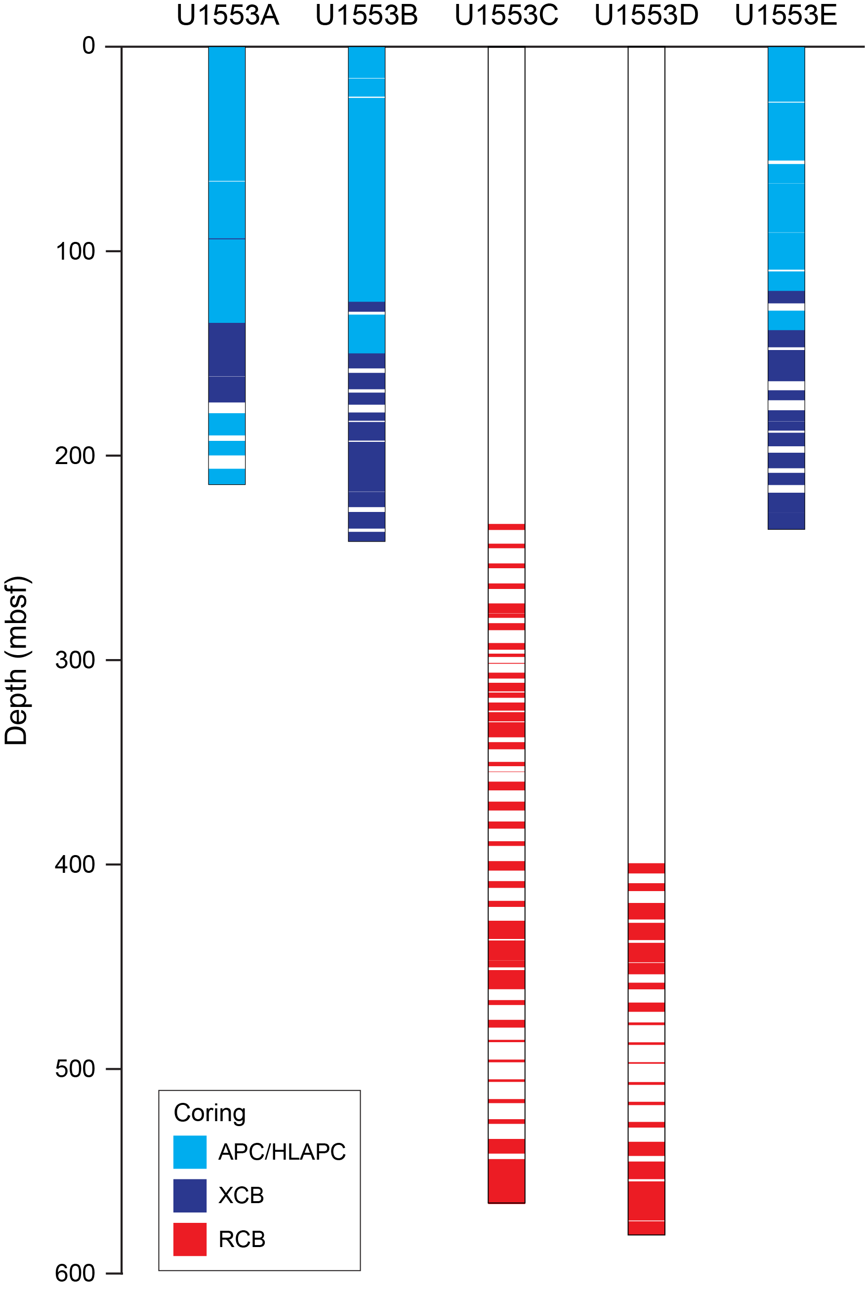
Figure F1. Coring systems.
1.1.3. JOIDES Resolution standard coring systems
The APC and HLAPC coring systems cut soft-sediment cores with minimal coring disturbance relative to the other coring systems and typically are ideal for the upper portion of each hole. After the APC core barrel is lowered through the drill pipe and lands near the bit, the inside of the drill pipe is pressurized until failure of the two shear pins holding the inner barrel to the piston rod. The inner barrel then advances into the formation at high speed and cuts a core with a diameter of 66 mm (2.6 inches). The driller can detect a successful cut, or “full stroke,” from the pressure gauge on the rig floor. The assumption is that the barrel penetrated the formation by the length of core recovered (nominal recovery of ~100%), so the bit is advanced by that length before cutting the next core. The maximum subbottom depth that can be achieved with the APC system (often referred to as “APC refusal”) is limited by the formation stiffness or cohesion and is indicated in two ways: (1) the piston fails to achieve a complete stroke (as determined from the pump pressure reading) because the formation is too hard or (2) excessive force (>100,000 lb; ~267 kN) is required to pull the core barrel out of the formation. Typically, several attempts are made when a full stroke is not achieved. When a full or partial stroke is achieved but excessive force cannot retrieve the barrel, the core barrel is “drilled over,” meaning that after the inner core barrel is successfully shot into the formation, the drill bit is advanced by the length of the APC barrel (~9.6 m).
Nonmagnetic core barrels and the downhole orientation tool (typically deployed except when refusal appears imminent) were employed for Holes U1553A and U1553B. We obtained three formation temperature measurements with the advanced piston corer temperature (APCT-3) tool embedded in the APC coring shoe while coring Hole U1553A (Cores 4H, 7H, and 10H). These measurements are applied to calculations of the downhole temperature gradient and heat flow estimates.
The XCB rotary system has a small cutting shoe (bit) that extends below the large rotary APC/XCB bit. The XCB bit is able to cut a semi-indurated core with less torque and fluid circulation than the larger main bit, optimizing recovery. The XCB cutting shoe extends ~30.5 cm ahead of the main bit in soft sediment but retracts into the main bit when hard formations are encountered. The resulting cores have a nominal diameter of 5.87 cm (2.312 inches), which is slightly less than the 6.6 cm diameter of APC cores. XCB cores are often broken (torqued) into “biscuits,” which are disc-shaped pieces a few to several centimeters long with remolded sediment (including some drilling slurry) interlayering the discs in a horizontal direction and packing the space between the discs and the core liner in a vertical direction. This type of drilling disturbance may give the impression that the XCB cores have the same thickness (66 mm) as the APC cores. Although both XCB and RCB core recovery (below) generally lead to drilling disturbance in similar sedimentary material, switching from an APC/XCB bottom-hole assembly (BHA) to an RCB BHA requires a pipe trip and adds significant time to the coring operations on site. Thus, we opted to attempt recovery with the XCB coring system as deeply as possible prior to terminating operations in Holes U1553A, U1553B, and U1553E (the three shallow holes).
The RCB system is a conventional rotary coring system suitable for lithified rock material. We opted to use the RCB system exclusively for the two deep holes (U1553C and U1553D) after exploring the efficacy of the XCB coring system in Holes U1553A and U1553B. Increasingly poor recovery with the XCB coring system toward the bottom of Holes U1553A and U1553B precluded deployment for the deeper goals of Holes U1553C and U1553D. Like the XCB system, the RCB system cuts a core with a nominal diameter of 5.87 cm. RCB coring can be done with or without the core liners used routinely with the APC/XCB soft-sediment systems. Coring without liners is sometimes done when core pieces seem to get caught at the edge of the liner, leading to jamming and reduced recovery. During Expedition 378, most RCB cores were drilled with a core liner in place. However, 11 RCB cores were drilled without a liner after recovery became extremely low with a liner in the core barrel.
The BHA is the lowermost part of the drill string. It is typically ~130–170 m long, depending on the coring system used and total drill string length. A typical APC/XCB BHA consists of a drill bit (outside diameter = 11⁷⁄₁₆ inches), a bit sub, a seal bore drill collar, a landing saver sub, a modified top sub, a modified head sub, a nonmagnetic drill collar (for APC/XCB coring), a number of 8¼ inch (~20.32 cm) drill collars, a tapered drill collar, 6 joints (two stands) of 5½ inch (~13.97 cm) drill pipe, and 1 crossover sub. A typical RCB BHA consists of a drill bit, a bit sub, a head sub, an outer core barrel, a top sub, a head sub, 8 joints of 8¼ inch drill collars, a tapered drill collar, 2 stands of standard 5½ inch drill pipe, and a crossover sub to the regular 5 inch drill pipe.
Cored intervals may not be contiguous if separated by intervals that were drilled but not cored. We drilled ahead without coring using a center bit with the RCB system to accelerate penetration because an interval had already been cored in an adjacent hole (234.0 m in Hole U1553C; 399.4 m in Hole U1553D). Holes thus consist of a sequence of cored and drilled intervals, or “advancements.” These advancements are numbered sequentially from the top of the hole downward. Numbers assigned to physical cores correspond to advancements and may not be consecutive.
1.1.4. Drilling disturbance
Cores may be significantly disturbed by the drilling process or contain extraneous material as a result of the coring and core handling process. In formations with loose granular layers (sand, ash, foraminifer ooze, chert fragments, shell hash, etc.), drilling circulation may allow granular material from intervals higher in the hole to settle and accumulate in the bottom of the hole. Such material could be sampled by the next core. Therefore, the uppermost 10–50 cm of each core must be assessed for potential “fall-in.”
Common coring-induced deformation includes the concave-downward appearance of originally horizontal bedding. Piston action may result in fluidization (“flow-in”) at the bottom of, or sometimes in, APC cores. Retrieval of unconsolidated (APC) cores to the surface typically results to some degree in elastic rebound, and gas that is in solution at depth may become free and drive core segments in the liner apart. When gas content is high, pressure must be relieved for safety reasons before the cores are cut into segments. Holes are drilled into the liner, which forces some sediment and gas out of the liner. As noted above, XCB coring typically results in biscuits mixed with drilling slurry. RCB coring typically homogenizes unlithified core material and often fractures lithified core material.
Drilling disturbances are described in Lithostratigraphy in the Site U1553 chapter (Röhl et al., 2022a) and are indicated on graphic core summary reports, also referred to as visual core descriptions (VCDs) (see Core descriptions).
1.1.5. Seawater sampling strategy
Samples for phytoplankton and seawater analysis were collected from international waters during the transit from Site U1553 to Papeete (between 38°37.841′S and 25°36′S) to assess seawater geochemistry and the abundance of coccolithophores, foraminifers, and microplastics across a South Pacific Ocean transect. Filtered seawater samples were stored for shore-based geochemical analysis and for analysis of shipboard pH, alkalinity, major ions, nutrients, and major elements.
Seawater samples (~20 L) were collected approximately every 12 h at ~0600 and 1830 h (shipboard time) using a plastic bucket with a nylon rope over the side of the ship. The sampling depth approximately represents a mixed upper 10 m of surface water. Latitude and longitude coordinates and the time and date of each collection (in UTC) were recorded. Seawater was stored in a plastic 20 L carboy during filtering. Upon arrival in the laboratory, seawater temperature was measured.
For postcruise coccolithophore assemblage characterization, 1–3 L of seawater was decanted from the 20 L carboy and filtered under gentle pressure through a 47 mm diameter cellulose nitrate filter (0.45 µm pore size). The exact volume of water filtered was recorded to enable species abundance per unit seawater to be calculated at a later date. The filtered seawater was then discarded. The filters were dried for 2–4 h at 45°C and stored at room temperature in petri dishes until the end of the expedition. Coccolithophore assemblages will be examined using transmitted light microscopy and scanning electron microscopy (SEM).
For analysis of seawater chemistry, the glass filtration equipment was first rinsed three times with the seawater sample. Then, 1 L of seawater was filtered through a 47 mm, 0.45 µm pore size cellulose ester filter. The volume of water filtered was measured using a graduated cylinder and recorded. From this first liter of filtered seawater, samples for shore-based geochemical analysis of δ44Ca, δ17O, iodine speciation, and trace element composition were taken. A split for shipboard analysis of pH and alkalinity as well as ion chromatography measurement of major ions was taken and analyzed (see Geochemistry). For future analysis, samples of minor elements, iodine, and δ44Ca were stored in acid-washed high-density polyethylene bottles.
After sample bottles for geochemistry were filled, another 1 L of water was passed through the first filter. Subsequently, we completed a second filtration of 2 L of water through a new filter. In each case, the volume of water filtered was measured using a graduated cylinder and recorded. The seawater from both of these steps was discarded. After filtering, filters were removed with tweezers, placed in petri dishes, and left to dry for ~2–4 h in a low-temperature oven (45°C).
1.2. Core and section handling
1.2.1. Whole-core handling
All APC, XCB, and RCB cores recovered during Expedition 378 were extracted from the core barrel in plastic liners, with the exception of 11 RCB cores from Holes U1553C and U1553D that were collected in split liners on the rig floor. These split liners were carried from the rig floor to the core processing area on the catwalk outside the core laboratory and then closed with the other half of the liner and taped. All cores were then cut into ~1.5 m sections. The exact section length was noted and entered into the database as “created length” using the Sample Master application. This number was used to calculate recovery. Subsequent processing differed for soft-sediment and lithified material.
1.2.2. Sediment section handling
Headspace samples were taken from selected section ends (one per core) using a syringe for immediate hydrocarbon analysis as part of the shipboard safety and pollution prevention program. Whole-round samples for interstitial water (IW) analysis were also taken immediately after the core was sectioned. Microbiological sections were taken from the working-half side of the fresh cutting surface (from the top of the adjacent section). Core catcher samples (PALs) were taken for biostratigraphic analysis. When catwalk sampling was complete, liner caps (blue = top, colorless = bottom, and yellow = top of a whole-round sample removed from the section) were glued with acetone onto liner sections and sections were placed in core racks for analysis.
For sediment cores, the curated length was set equal to the created length and was updated very rarely (e.g., in cases of errors or when section length kept expanding by more than ~2 cm). Depths in hole calculations are based on the curated section length (see Depth calculations).
After completion of whole-round section analyses (see Shipboard core analysis), the sections were split lengthwise from bottom to top into working and archive halves. The softer cores were split with a wire, and harder cores were split with a diamond saw. It is important to be aware that older material can be transported upward on the split face of a section during splitting.
1.3. Sample naming
1.3.1. Editorial practice
Sample naming in this volume follows standard IODP procedure. A full sample identifier consists of the following information: expedition, site, hole, core number, core type, section number, section half, and offset in centimeters measured from the top of the core section. For example, a sample identification of “378-U1553A-1H-2W, 10–12 cm” represents a sample taken from the interval between 10 and 12 cm below the top of the working half of Section 2 of Core 1 of Hole U1553A during Expedition 378. “H” designates that this core was taken with the full-length APC system, “F” that it was taken with a half-length APC system, “X” that it was taken with an extended core barrel, and “R” that it was rotary drilled.
When working with data downloaded from the Laboratory Information Management System (LIMS) database or physical samples that were labeled on the ship, three additional sample naming concepts may be encountered: text ID, label ID, and printed labels.
1.3.2. Text ID
Samples taken on board JOIDES Resolution are uniquely identified for use by software applications using the text ID, which combines two elements:
- Sample type designation (e.g., SHLF for section half) and
- A unique sequential number for any sample and sample type added to the sample type code (e.g., SHLF30495837).
The text ID is not particularly helpful to most users but is critical for machine reading and troubleshooting.
1.3.3. Label ID
The label ID is used throughout the JOIDES Resolution workflows as a convenient, human-readable sample identity. However, a label ID is not necessarily unique. The label ID is made up of two parts: primary sample identifier and sample name.
1.3.3.1. Primary sample identifier
The primary sample identifier is very similar to the editorial sample name described above, with two notable exceptions:
- Section halves always carry the appropriate identifier (378-U1553A-35R-2-A and 378-U1553A-35R-2-W for archive and working half, respectively).
- Sample top and bottom offsets, relative to the parent section, are indicated as “35/37” rather than “35–37 cm.”
Specific rules were set for printing the top offset/bottom offset at the end of the primary sample identifier:
- For samples taken out of the hole, core, or section, top offset/bottom offset is not added to the label ID. This has implications for the common process of taking samples out of the core catcher (CC), which technically is a section (relevant primarily for microbiology and paleontology samples).
- For samples taken out of the section half, top offset/bottom offset is always added to the label ID. The rule is triggered when an update to the sample name, offset, or length occurs.
- The offsets are always rounded to the nearest centimeter before insertion into the label ID (even though the database stores higher precisions and reports offsets to millimeter precision).
1.3.3.2. Sample name
The sample name is a free text parameter for subsamples taken from a primary sample or from subsamples thereof. It is always added to the primary sample identifier following a hyphen (-NAME) and populated from one of the following prioritized user entries in the Sample Master application:
- Entering a sample type (-TYPE) is mandatory (same sample type code used as part of the text ID; see Text ID). By default, -NAME = -TYPE (examples include SHLF, CUBE, CYL, and PWDR).
- If the user selects a test code (-TEST), it replaces the sample type and -NAME = -TEST. The test code indicates the purpose of taking the sample but does not guarantee that the test was actually completed on the sample (examples include PAL, TSB, ICP, PMAG, and MAD).
- If the user selects a requester code (-REQ), it replaces -TYPE or -TEST and -NAME = -REQ. The requester code represents the name of the requester of the sample who will conduct postcruise analysis.
- If the user types any kind of value (-VALUE) in the -NAME field, perhaps to add critical sample information for postcruise handling, the value replaces -TYPE, -TEST, or -REQ and -NAME = -VALUE (examples include SYL-80deg and DAL-40mT).
In summary, and given the examples above, the same subsample may have the following label IDs based on the priority rule -VALUE > -REQ > -TEST > -TYPE:
- 378-U1553A-35R-2-W 35/37-CYL,
- 378-U1553A-35R-2-W 35/37-PMAG,
- 378-U1553A-35R-2-W 35/37-DAL, or
- 378-U1553A-35R-2-W 35/37-DAL-40mT.
When subsamples are taken out of subsamples, the -NAME of the first subsample becomes part of the parent sample ID, and another -NAME is added to that parent sample label ID:
For example, a thin section billet (sample type = TSB) taken from the working half at 40–42 cm offset from the section top might result in a label ID of 378-U1553A-38R-4-W 40/42-TSB. After the thin section was prepared (~48 h later), a subsample of the billet might receive an additional designation of TS05, which would be the fifth thin section made during the expedition. A resulting thin section label ID might therefore be 378-U1553A-38R-4-W 40/42-TSB-TS_5.
1.4. Depth calculations
Sample and measurement depth calculations were based on the methods described in IODP Depth Scales Terminology v.2 (https://www.iodp.org/policies-and-guidelines/142-iodp-depth-scales-terminology-april-2011/file) (Table T1). The definition of multiple depth scale types and their distinction in nomenclature should keep the user aware that a nominal depth value at two different depth scale types (and even two different depth scales of the same type) generally does not refer to exactly the same stratigraphic interval in a hole (Figure F2). The SI unit for all depth scales is meter (m).

Figure F2. Depth scales.
Depths of cored intervals were measured from the drill floor based on the length of drill pipe deployed beneath the rig floor and are referred to as drilling depth below rig floor (DRF), which is traditionally referred to with custom units of meters below rig floor (mbrf). The depth of each cored interval, measured on the DRF scale, can be referenced to the seafloor by subtracting the seafloor depth measurement (in DRF) from the cored interval (in DRF). This seafloor-referenced depth of the cored interval is referred to as the drilling depth below seafloor (DSF), with a traditionally used custom unit designation of mbsf. In the case of APC coring, the seafloor depth was the length of pipe deployed minus the length of the mudline core recovered. In the case of RCB coring, the seafloor depth was adopted from a previous hole drilled at the site or by tagging the seafloor.
Depths of samples and measurements in each core were computed based on a set of rules that result in a depth scale type referred to as core depth below seafloor, Method A (CSF-A). The two fundamental rules are that (1) the top depth of a recovered core corresponds to the top depth of its cored interval (top DSF = top CSF-A) regardless of the type of material recovered or drilling disturbance observed and (2) the recovered material is a contiguous stratigraphic representation even when core segments are separated by voids when recovered, when the core is shorter than the cored interval, or when it is unknown how much material is missing between core pieces. When voids were present in the core on the catwalk, they were closed by pushing core segments together whenever possible. The length of missing core should be considered a depth uncertainty when analyzing data associated with core material.
When core sections were given their curated lengths, they were also given a top and a bottom depth based on the core top depth and the section length. Depths of samples and measurements on the CSF-A scale were calculated by adding the offset of the sample (or measurement from the top of its section) to the top depth of the section.
Per IODP policy established after the introduction of the IODP Depth Scales Terminology v.2, sample and measurement depths on the CSF-A depth scale type are commonly referred to with the custom unit mbsf, just like depths on the DSF scale type. The reader should be aware, however, that the use of mbsf for different depth scales can cause confusion in specific cases because different “mbsf depths” may be assigned to the same stratigraphic interval. A core composite depth below seafloor (CCSF-A) scale can be constructed to mitigate inadequacies of the CSF-A scale for scientific analysis and data presentation. The most common application is the construction of a CCSF-A scale from multiple holes drilled at a site using depth shifting of correlative features across holes. This method not only eliminates the CSF-A core overlap problem but also allows splicing of core intervals such that gaps in core recovery, which are inevitable in coring a single hole, are essentially eliminated and a continuous stratigraphic representation is established. This depth scale was used at Site U1553 (see Stratigraphic correlation and composite section).
A CCSF-A scale and stratigraphic splice are accomplished by downloading correlation data from the expedition (LIMS) database using the Correlation Downloader application, correlating stratigraphic features across holes using Correlator or any other application and depth-shifting cores to create an “affine table” with an offset for each core relative to the CSF-A scale and a “splice interval table” that defines which core intervals from the participating holes make up the stratigraphic splice. Affine and splice interval tables were uploaded to the LIMS database, where internal computations created a CCSF depth scale. The CCSF depth can then be added to all subsequent data downloads from the LIMS database, and data can be downloaded for a splice.
1.5. Shipboard core analysis
Whole-round core sections were immediately run through the Whole-Round Multisensor Logger (WRMSL), which measures P-wave velocity, density, and magnetic susceptibility (MS), and the Natural Gamma Radiation Logger (NGRL). For some holes, whole-round core sections were scanned on the X-Ray Multisensor Logger (XMSL) while the cores thermally equilibrated. After the cores thermally equilibrated for at least 4 h, thermal conductivity measurements were also taken before the cores were split lengthwise into working and archive halves. The working half of each core was sampled for shipboard analysis, routinely for paleomagnetism and physical properties and more irregularly for geochemistry and biostratigraphy. The archive half of each core was scanned on the Section Half Imaging Logger (SHIL). Archive halves were also measured for color reflectance and MS on the Section Half Multisensor Logger (SHMSL). Archive halves were described macroscopically and microscopically in smear slides. Finally, archive halves were run through the cryogenic magnetometer. Both halves of the core were then put into labeled plastic tubes that were sealed and transferred to cold storage space aboard the ship.
A total of 1962 samples were taken for shipboard analysis. At the end of Expedition 378, all core sections and thin sections were shipped to the GCR in preparation for XRF core scanning to prepare a spliced composition section, followed by a shore-based sampling party. The sections and samples will be permanently stored in the GCR.
2. Lithostratigraphy
The lithology of sediment recovered during Expedition 378 was primarily determined using observations based on visual (macroscopic) core description, smear slides, and thin sections. Digital core imaging, color reflectance spectrophotometry, MS analysis, and in some cases X-ray diffraction (XRD), XRF, SEM, and carbonate content measurements (see Geochemistry) provided complementary descriptive information. The methods employed during this expedition were similar to those used during Integrated Ocean Drilling Program Expedition 346 (Tada et al., 2015) and IODP Expedition 379 (Gohl et al., 2021). We used the DESClogik application (version 16.2.0.0) to record and upload visual descriptive data into the LIMS database (see the DESClogik user guide at http://iodp.tamu.edu/labs/index.html; select User guides and laboratory manuals (Confluence) and then select Core Description). Spreadsheet templates were set up in DESClogik and customized for Expedition 378 before the first core on deck. The templates were used to record VCDs as well as microscopic data from smear slides and thin sections, which were also used to quantify the texture and relative abundance of biogenic and nonbiogenic components. The locations of all smear slide and thin section samples taken from each core were recorded in the Sample Master application.
The standard method of splitting cores into working and archive halves (using either a piano wire or a saw) can affect the appearance of the split core surface and obscure fine details of lithology and sedimentary structure. Prior to visual description and imaging of sediments, the archive halves of soft-sediment cores were gently scraped across, rather than along, the core section using a stainless steel or glass scraper to prepare the surface for unobscured sedimentologic examination and description, digital imaging, point MS (MSP), and color measurements. Scraping parallel to bedding with a freshly cleaned tool prevented cross-stratigraphic contamination. Cleaned archive halves were imaged as soon as possible after splitting using the SHIL. Thereafter, archive halves were visually described and analyzed using the SHMSL.
2.1. Visual core descriptions
VCDs of the archive halves of the split cores provide a visual overview of the descriptive lithostratigraphic, biostratigraphic, and physical properties data obtained during shipboard analyses (Figure F3). All associated data are uploaded to the LIMS database.
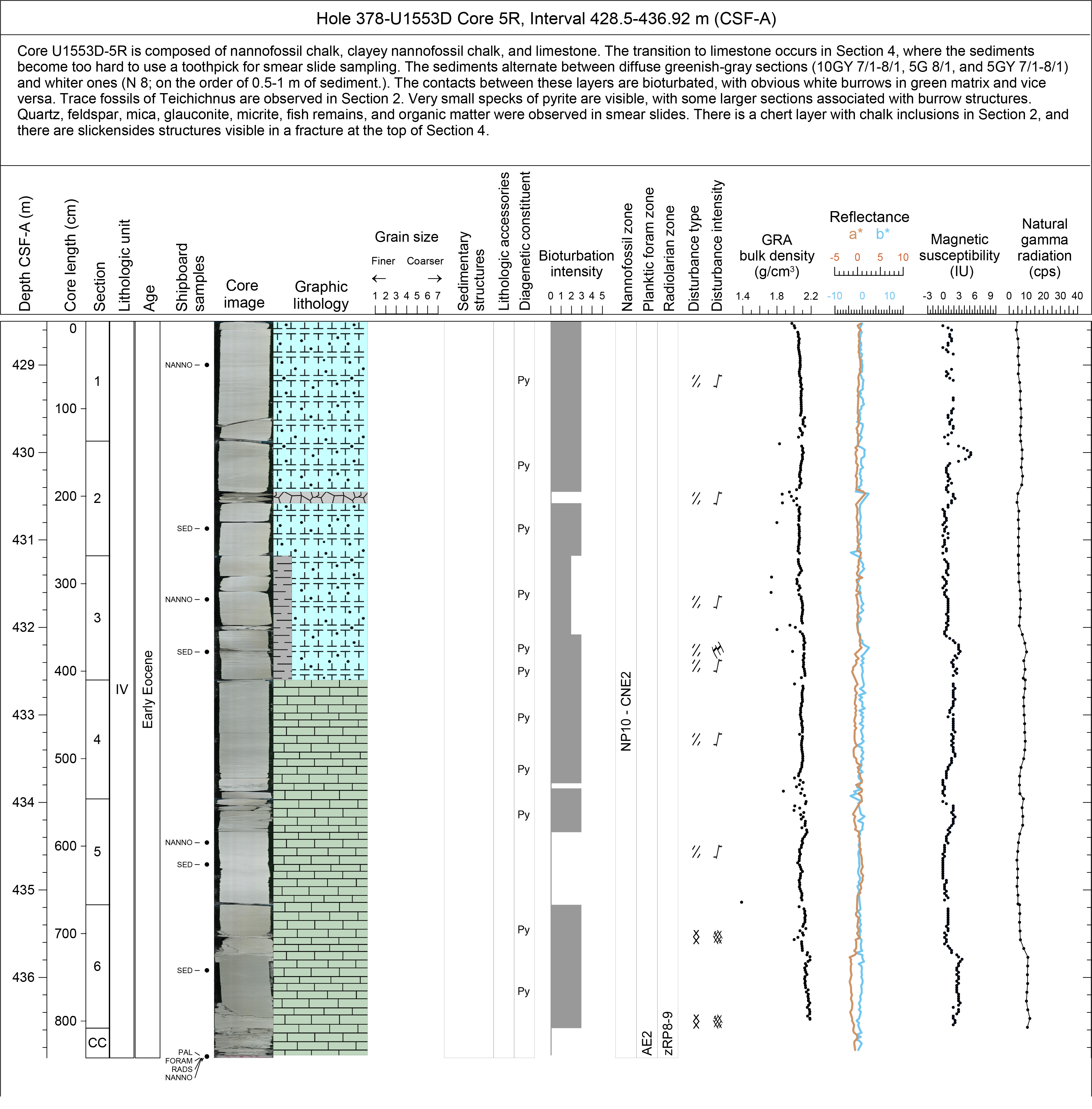
Figure F3. Example visual core description.
Site, hole, and core depth below seafloor, calculated using Method A (CSF-A), are shown at the top of each VCD. Core depths are reported in mbsf, and the depth of core sections is indicated along the left margin. Physical core descriptions correspond to entries in DESClogik, including bioturbation intensity, macrofossils, sedimentary structures, diagenetic constituents, and drilling disturbance. Symbols used in the VCDs are shown in Figure F4. Additionally, sedimentary VCDs display bulk density, MS, natural gamma radiation (NGR), color reflectance, and the locations of samples taken for shipboard measurements. VCDs for Holes U1553C and U1553D also show visual grain size classifications. The written description for each core contains a succinct overview of major and minor lithologies, the Munsell colors, and notable features such as sedimentary structures and major disturbances resulting from the coring process.
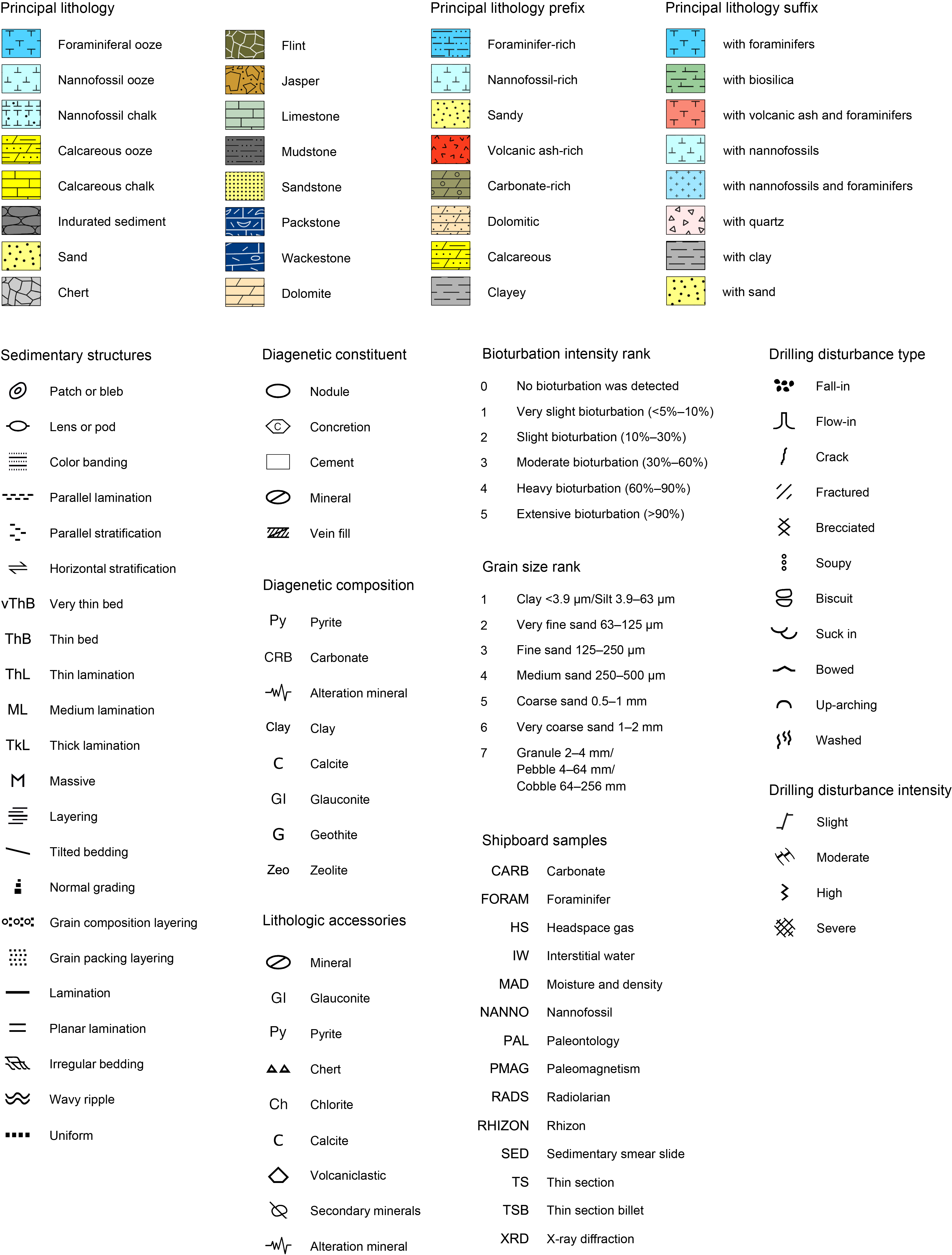
Figure F4. Symbols used for visual core descriptions.
2.1.1. Section summary
A brief overview of major and minor lithologies present in this section, along with notable features (e.g., sedimentary structures), is presented in the section summary text field at the top of the VCD. The summary includes sediment color determined qualitatively using Munsell soil color charts. Because sediment color may evolve during drying and subsequent oxidation, color was described shortly after the cores were split and imaged. However, cores from deeper than Cores 378-U1553C-35R and 378-U1553D-10R only revealed distinct lithologic color changes and detailed sedimentary features after many hours of drying (see Lithostratigraphy in the Site U1553 chapter [Röhl et al., 2022a]). Accordingly, sediment color was obtained only after the archive-half surfaces had fully dried. For these cores, the section-half images and red-green-blue (RGB) color data that were obtained both initially (commented as “regular” in LIMS) and after the surface was fully dry (commented as “dried” in LIMS) are accessible through the LIMS database.
2.1.2. Section-half image
After the water used during cutting had dried, the flat faces of the archive halves were scanned with the SHIL as soon as possible after splitting (and scraping, if necessary) to minimize color changes caused by sediment oxidation and/or drying. Exceptions are the cores from deeper than Cores 378-U1553C-35R and 378-U1553D-10R, which revealed previously unobservable sedimentary features and structures upon drying (see above). The SHIL uses three pairs of advanced illumination high-current-focused LED line lights to illuminate large cracks and blocks in the core surface. Each LED pair has a color temperature of 6,500 K and emits 90,000 lx at 3 inches. A line-scan camera imaged 10 lines per millimeter to create a high-resolution TIFF file. The camera height was adjusted so that each pixel imaged a 0.1 mm2 section of the core. However, actual core width per pixel varied because of differences in section-half surface height. High- and low-resolution JPEG files were subsequently created from the high-resolution TIFF file. All image files include a gray scale and ruler. Section-half depths were recorded so that these images could be used for core description and analysis.
2.1.3. Graphic lithology
Lithologies of the core intervals recovered are represented on the VCDs by graphic patterns in the Graphic lithology column (Figure F4) to scale for all beds that are at least 2 cm thick. Modifiers of primary lithologies are shown in narrow columns to the left (major = prefix) and right (minor = suffix) using the same lithology patterns. Lithologic abundances are recorded in DESClogik and are rounded to the nearest 5%. In the interest of VCD readability, secondary lithologies are not shown, but they are accessible using the LIMS database. Relative abundances of lithologies reported in this way are useful for general characterization of the sediment but do not constitute precise quantitative observations.
2.1.4. Sedimentary structures
The locations and types of stratification and sedimentary structures visible on the prepared surfaces of the split cores are shown in the Sedimentary structures column of the VCD sheet. Symbols in this column indicate the locations and scales of interstratification as well as the locations of individual bedding features and any other sedimentary features such as stratification, lamination, and color banding (Figure F4). Relative abundance of commonly observed green millimeter- to centimeter-scale layers was also regularly noted in the Minor lithology description in DESClogik (see Principal names and modifiers). For Expedition 378, the following terminology (based on Stow, 2005) was used to describe the scale of stratification:
- Thin lamination = <0.3 cm thick.
- Medium lamination = 0.3–0.6 cm thick.
- Thick lamination = 0.6–1 cm thick.
- Very thin bed = 1–3 cm thick.
- Thin bed = 3–10 cm thick.
- Medium bed = 10–30 cm thick.
- Thick bed = 30–100 cm thick.
- Very thick bed = >100 cm thick.
Descriptive terms for bed boundaries, such as sharp, erosive, gradual, undulating/wavy, and bioturbated, are noted in DESClogik.
2.1.5. Lithologic accessories
Lithologic, diagenetic, and paleontologic accessories such as nodules, sulfides, and shells are indicated on the VCDs. The symbols used to designate these features are shown in Figure F4.
Features interpreted to be diagenetic, including minerals, nodules, concretions, halos, and layering, were noted in DESClogik.
2.1.6. Bioturbation intensity
Six levels of bioturbation are recognized using a scheme similar to that of Droser and Bottjer (1986). These levels are illustrated with a numeric scale in the Bioturbation intensity column on the VCDs. Any identifiable trace fossils (ichnofossils) are identified in the bioturbation comments or the general interval comment in the core description.
- 0 = no bioturbation was detected, or level could not be determined.
- 1 = very slight bioturbation (<5%–10%).
- 2 = slight bioturbation (10%–30%).
- 3 = moderate bioturbation (30%–60%).
- 4 = heavy bioturbation (60%–90%).
- 5 = extensive bioturbation (>90%).
2.1.7. Sediment disturbance
Drilling-related sediment disturbance is recorded in the Disturbance column of the VCDs using the symbols shown in Figure F4. The style of drilling disturbance is described for soft and firm sediments using the following terms:
- Fall-in: part of the formation at the top of a hole has fallen onto the subsequently cored surface.
- Bowed: bedding contacts are slightly to moderately deformed but subhorizontal and continuous.
- Flow-in: significant soft-sediment stretching and/or compressional shearing structures are present and attributed to the coring/drilling process.
- Soupy: intervals are water saturated and have lost all aspects of original bedding.
- Biscuiting: sediments of intermediate stiffness show vertical variations in the degree of disturbance. Softer intervals are washed and/or soupy, whereas firmer intervals (biscuits) are relatively undisturbed.
- Cracked or fractured: firm sediments are broken but not displaced or rotated significantly.
- Fragmented or brecciated: firm sediments are pervasively broken and may be displaced or rotated.
The degree of fracturing within indurated sediments is described using the following categories:
- Slightly fractured: core pieces are in place but broken.
- Moderately fractured: core pieces are in place or partly displaced, but original orientation is preserved or recognizable.
- Highly fractured: core pieces are probably in correct stratigraphic sequence, but original orientation is lost.
- Drilling breccia: core is crushed and broken into many small and angular pieces, and original orientation and stratigraphic position are lost.
2.1.8. Age
The subepoch that defines the age of the sediments was provided by the shipboard biostratigraphers (see Biostratigraphy and paleoenvironment) and is listed in the Age column of the VCDs.
2.1.9. Samples
The exact positions of samples used for microscopic descriptions (i.e., smear slides and thin sections), biochronological determinations, and shipboard analysis of chemical and physical properties of the sediments are recorded in the Shipboard samples column of the VCDs.
2.2. Sediment classification
Lithologic descriptions were based on the classification schemes used during ODP Leg 178 (Shipboard Scientific Party, 1999); the Antarctic Drilling Project (Naish et al., 2006); Integrated Ocean Drilling Program Expeditions 318 (Expedition 318 Scientists, 2011) and 341 (Jaeger et al., 2014); and IODP Expeditions 371 (Sutherland et al., 2019), 374 (McKay et al., 2019), and 379 (Gohl et al., 2021).
2.2.1. Principal names and modifiers
The principal lithologic name was purely descriptive, assigned only based on the relative abundances of siliciclastic and biogenic grains (Figure F5). For each principal name, both a consolidated (i.e., semilithified to lithified) and a nonconsolidated term exist, and they are mutually exclusive.

Figure F5. Siliciclastic sediments/rocks without gravel.
The principal name of a sediment/rock with >50% siliciclastic grains is based on an estimate of the grain sizes present (Figure F5B). The Wentworth (1922) scale was used to define size classes of clay, silt, sand, and gravel and was related to numeric values for the purpose of plotting on the VCD sheet (Figure F3):
- Cobble: 64–256 mm; 7.
- Pebble: 4–64 mm; 7.
- Granule: 2–4 mm; 7.
- Very coarse sand: 1–2 mm; 6.
- Coarse sand: 0.5–1 mm; 5.
- Medium sand: 250–500 µm; 4.
- Fine sand: 125–250 µm; 3.
- Very fine sand: 63–125 µm; 2.
- Silt: 3.9–63 µm; 1.
- Clay: <3.9 µm; 1.
Grain size was plotted on VCDs only for holes where a major siliciclastic unit was present (Holes U1553C and U1553D; Lithologic Unit V).
If no gravel was present, the principal sediment/rock name was determined based on the relative abundances of sand, silt, and clay (e.g., silt, sandy silt, silty sand, etc.) (Naish et al., 2006, after Shepard, 1954, and Mazzullo et al., 1988) (Figure F5B). For example, if any one of these components exceeds 80%, then the lithology is defined by the primary grain size class (e.g., sand). The term “mud” is used to define sediments containing a mixture of silt and clay (these are difficult to separate using visual macroscopic inspection) in which neither component exceeds 80%. Furthermore, no reliable separation could be made between fine and coarse silt during core macroscopic observation. Sandy mud to muddy sand describes sediment composed of a mixture of at least 20% each of sand, silt, and clay (Figure F5B). For sediment consisting of two grain size fractions that each exceed 20% (e.g., clay and silt or sand and mud), the prefix was determined by the fraction with the lower percentage (Figure F5B). The principal name of sediment with >50% biogenic grains is “ooze” modified by the most abundant specific biogenic grain type. For example, if diatoms exceed 50%, then the sediment is called “diatom ooze.” However, if the sediment is composed of 40% diatoms and 15% sponge spicules, then the sediment is termed “biosiliceous ooze.” The same principle applies to calcareous microfossils. For example, if foraminifers exceed 50%, then the sediment is called “foraminifer ooze,” whereas a mixture of 40% foraminifers and 15% calcareous nannofossils is termed “calcareous ooze.” The lithologic name “chert” is used to describe biosiliceous rocks where the main biogenic component is not identifiable. Lithified biosiliceous sediment that has a more glassy texture and conchoidal fracture than chert is termed “flint.” The lithologic name “carbonate” is used for consolidated and nonconsolidated sediments consisting predominantly of calcareous material that do not allow identification of calcareous microfossils. Following Dunham and Ham’s (1962) classification modified by Embry and Klovan (1972), the lithologic name “packstone” is used for sediments containing sand-sized grains <2 mm that have grain-supported textures with mud between the sand grains.
For all lithologies, major and minor modifiers were applied to the principal sediment/rock names with the following modified scheme from Expeditions 318 (Expedition 318 Scientists, 2011), 371 (Sutherland et al., 2019), and 379 (Gohl et al., 2021):
- Major biogenic modifiers are those components that comprise 25%–50% of the grains and are indicated by the suffix “-rich” (e.g., clay-rich or diatom-rich).
- Major siliciclastic modifiers are those components with abundances of 25%–50% and are indicated by the suffix “-y” (e.g., silty, muddy, or sandy).
- Minor modifiers are those components with abundances of 10%–25% and are indicated after a “with” (e.g., with clay or with diatoms).
For intervals in which two lithologies are interbedded or interlaminated (where individual beds or laminated intervals are <15 cm thick and alternate between one lithology and another), the term “layering” is recorded in the Sedimentary structures column in the macroscopic DESClogik template. Secondary features (e.g., pervasive green layers) were assigned a second color and given a percentage abundance as a minor lithology relative to the major lithology. However, multiple (faint/pale green) layers in the carbonate sequence were described in the general interval comment only. This terminology is for ease of data entry and graphic log display purposes for VCDs (Figures F3, F4). When beds are distributed throughout a different lithology (e.g., centimeter- to decimeter-thick sand beds within a mud bed), they sometimes were logged individually and the associated bed thickness and grain size ranges were described.
The following terms describe lithification that varies depending on the dominant composition:
- Sediment composed predominantly of calcareous microfossils (e.g., calcareous nannofossils and foraminifers): the lithification terms “ooze” and “chalk” reflect whether the sediment can be easily deformed (ooze) or is slightly lithified (chalk). The transition from ooze to chalk was preliminarily noted based on the required use of the saw instead of piano wire to split the cores. If a toothpick could no longer be easily used to take a smear slide sample, the lithification term “limestone” was used. Locations of these transitions in lithification were ultimately identified via the use of physical properties data, which led to the definition of major lithologic units within the carbonate facies.
- Sediments composed predominantly of siliciclastic material: if the sediment can be easily deformed, no lithification term is added and the sediment is named for the dominant grain size (i.e., sand, silt, or clay). For more consolidated material, the lithification suffix “-stone” is appended to the dominant size classification (e.g., claystone).
2.3. Spectrophotometry
Reflectance of visible light from the archive halves of sediment cores was measured using an Ocean Optics USB4000 spectrophotometer mounted on the automated SHMSL. Freshly split cores were covered with clear plastic wrap and placed on the SHMSL. Measurements were taken at 2.0 cm spacing to provide a high-resolution stratigraphic record of color variations for visible wavelengths. Each measurement was recorded in 2 nm wide spectral bands from 390 to 730 nm. Reflectance parameters of L*, a*, and b* were recorded (Balsam et al., 1997). The SHMSL takes measurements in empty intervals and over intervals where the core surface is well below the level of the core liner, but it cannot recognize relatively small cracks, disturbed areas of core, or plastic section dividers. Additional detailed information about measurement and interpretation of spectral data can be found in Balsam et al. (1997, 1998) and Balsam and Damuth (2000).
2.4. Natural gamma radiation
Data generated from the NGRL (see Physical properties) are used to augment geologic interpretations and are plotted in the VCDs.
2.5. Magnetic susceptibility
MS was measured using a Bartington Instruments MS2K point sensor (high-resolution surface-scanning sensor) on the SHMSL. Because the SHMSL demands flush contact between the MS point sensor and the split core, measurements were made on the archive halves of split cores, which were covered with clear plastic wrap. Measurements were taken at 2.0 cm spacing. Measurement resolution was 1.0 SI, and each measurement integrated a volume of 10.5 mm × 3.8 mm × 4 mm, where 10.5 mm is the length perpendicular to the core axis, 3.8 mm is the width along the core axis, and 4 mm is the depth into the core. The full width at half maximum response was 25.4 mm diameter. The depth of response was 50% 3 mm into the core and 10% 8 mm into the core. Only one measurement was taken at each measurement position.
2.6. Smear slide observation
Two or more smear slide samples of the main lithologies were collected from the archive half of each core. Additional samples were collected from specific areas of interest (e.g., laminations, ash layers, and nodules). A small amount of sediment was taken with a flat, wooden toothpick and put on a 2.5 cm × 7.5 cm glass slide. A metal spatula was used when the sediment was too stiff to sample with a wooden toothpick. The sediment sample was homogenized with a drop of deionized water and evenly spread across the slide to create a very thin (about <50 µm) uniform layer of sediment grains for quantification. The dispersed sample was dried on a hot plate. A drop of Norland Optical Adhesive 61 was added as a mounting medium to a coverslip, which was carefully placed on the dried sample to prevent air bubbles from being trapped in the adhesive. The smear slide was then fixed in an ultraviolet light box for ~10 min.
Smear slides were examined and imaged with a transmitted- and reflected-light petrographic microscope (Zeiss AXIO Scope.A1) equipped with a standard eyepiece micrometer. Several fields of view were examined at 50×, 100×, 200×, 400×, and 630× to assess the identity and abundance of detrital, biogenic, and authigenic components. The relative abundance of the sedimentary constituents was visually estimated (Rothwell, 1989). The texture of siliciclastic grains (relative abundance of sand-, silt-, and clay-sized grains) and the proportions and presence of biogenic and mineral components were recorded and entered into a smear slide tab in the DESClogik microscopic template. Biogenic and mineral components were identified using Marsaglia et al. (2013, 2015). For Expedition 378, the following categories (based on Expedition 342; Norris et al., 2014) were used to describe the abundance of each component:
- 0 = absent (0%).
- P = present (<1%).
- F = few (1%–10%).
- C = common (>10%–25%).
- A = abundant (>25%–50%).
- VA = very abundant (>50%).
The mineralogy of clay-sized grains could not be determined from smear slides. Note that smear slide analyses tend to underestimate the amount of sand-sized and larger grains because these grains are difficult to incorporate onto the slide.
2.7. Thin section observation
Descriptions of consolidated sediments were complemented by shipboard thin section analyses. Standard thin section billets (30 mm × 20 mm) were cut or sawed from selected intervals in core section intervals that were undisturbed by drilling. One large thin section (50 mm × 40 mm) was also made. Samples were initially sprayed with isopropyl alcohol and left to dry for 10 min before being placed in Epo-Tek 301 epoxy for 12 h under vacuum. For some samples, this epoxy was stained with Petroproxy 154 blue dye to show pore space in the thin section. Samples were then placed in molds before being sanded to obtain a flat, smooth surface that was adhered to a glass slide with epoxy. Next, they were cut and then ground to ~30 μm thickness. Subsequently, coverslips were placed on thin sections using immersion oil. In some cases, the nature of the sediment led to plucking of the surface during grinding, so some thin sections were left thicker than 30 μm (~60–100 μm) to avoid further damage.
Some thin sections containing carbonate were stained using potassium ferricyanide and Alizarin Red S (Figure F6). The following colors were used to distinguish the different carbonates (Dickson, 1965):
- Calcite: very pale pink to red.
- Ferroan calcite: purple to mauve.
- Dolomite: no color.
- Ferroan dolomite and ankerite: pale to deep turquoise, depending on ferrous content.
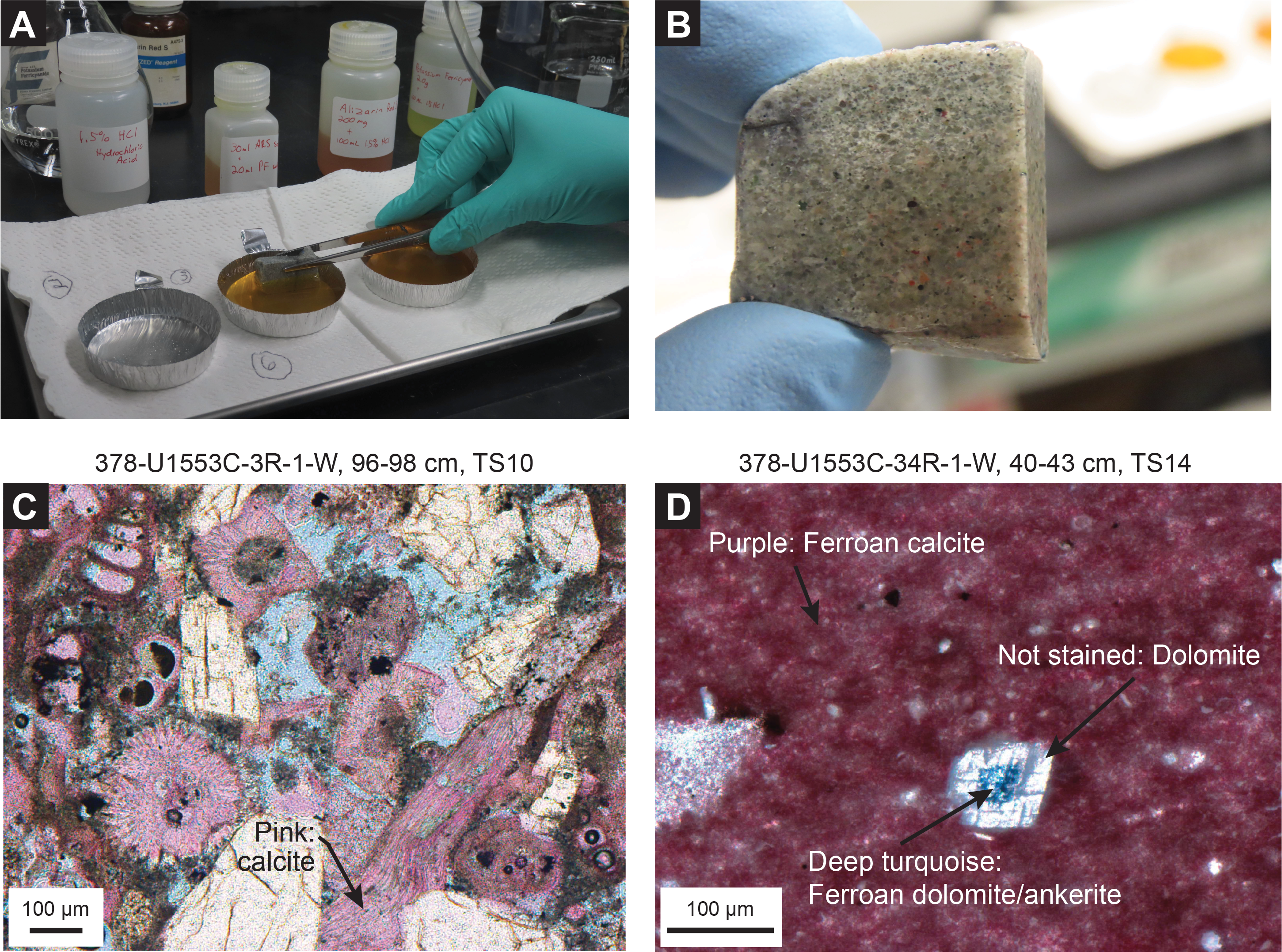
Figure F6. Procedure for staining thin sections.
Thin sections were examined and imaged with a transmitted- and reflected-light petrographic microscope equipped with a standard eyepiece micrometer. Several fields of view were examined at 50×, 100×, 200×, 400×, and 630× to assess the identity and to approximate abundance of detrital, biogenic, and authigenic components as well as textural relationships. Narrative visual descriptions of thin section components were entered into the thin section tab of the DESClogik microscopic template.
2.8. Scanning electron microscope observations
Selected samples were mounted for SEM observations that supplemented smear slide analyses. Observations were made with a Hitachi TM3000 tabletop SEM at 15 kV.
2.9. X-ray diffraction analyses
Samples were prepared for XRD analysis for semiquantitative bulk mineral estimates. The XRD results combined with smear slide estimates, weight percent carbonate, and visual descriptions were used to assist in lithologic classification. In general, two 5 cm3 samples were routinely taken for analysis from each core retrieved using the APC, XCB, and RCB systems, and one sample was taken for every HLAPC core. Sampling for Holes U1553B–U1553E only covered depth intervals not recovered in previous holes. Additional samples were taken and analyzed based on visual core observations (e.g., color variability and visual changes in lithology and texture) and smear slides. In general, the sampling strategy was to colocate the sampling of the working half of the cores with adjacent moisture and density (MAD) samples (see Physical properties), combined XRD/XRF samples, and carbonate content measurement samples (see Geochemistry).
Samples prepared for XRD analysis were freeze-dried and either ground by hand or in an agate ball mill, depending on lithification. To identify the minor constituents from calcite-rich sediments, several samples from Lithostratigraphic Units II and III were decalcified after an initial XRD analysis with 10% acetic acid and the remaining residues were analyzed. None of the 5 cm3 samples yielded sufficient residue for analysis, and only one 10 cm3 sample yielded sufficient material for analysis. Prepared samples were top-mounted onto a sample holder and analyzed using a Bruker D4 Endeavor diffractometer mounted with a Vantec-1 detector using nickel-filtered CuKα radiation. The standard locked coupled scan was as follows:
- Voltage = 40 kV.
- Current = 40 mA.
- Goniometer scan = 4°–70°2θ.
- Step size = 0.0087°2θ.
- Scan speed = 0.2 s/step.
- Divergence slit = 0.6 mm.
Diffractograms of bulk samples were evaluated with the HighScore Plus software package (version 4.8), which allowed for mineral identification and basic peak characterization (e.g., baseline removal and maximum peak intensity). The d-spacing values, diffraction angles, and peak intensities with background removed were scanned by the HighScore Plus software to find d-spacing values characteristic of a limited range of minerals. Occasionally, measurement of the aluminum oxide standard was used to monitor data quality. Peak intensities were reported for each mineral identified to provide a semiquantitative measure of mineral variations downhole and between sites. Muscovite/illite and kaolinite/chlorite have similar diffraction patterns and are usually not differentiated shipboard by XRD. However, 10 samples were processed for silt and clay separation before ethylene glycol and heat treatment to enhance clay identification. The diffraction patterns are available from the LIMS database (http://iodp.tamu.edu/tasapps) as digital files.
2.10. X-ray fluorescence analysis
An Olympus Vanta M series handheld portable XRF (pXRF) spectrometer was used to measure elemental composition on the residue from ground samples used for XRD. Measurements were performed with a 10–50 kV (10–50 μA) Rh X-ray tube and a high-count rate detector with a count time of 60 s. The pXRF was placed securely in a table mount with the measurement beam directed upward into a lead-shielded box where the pelletized samples were placed. The instrument data correction packages solve a series of nonlinear equations for each analyzed element. The Geochem mode was used to examine the relative abundance of major and trace elements. pXRF measurements of standards were performed once per day without standardization to track instrument drift. For onshore XRF core scanning, see Geochemistry.
3. Biostratigraphy and paleoenvironment
Microfossils were examined to provide preliminary shipboard biostratigraphy and paleoenvironmental information for the recovered sediments. Biostratigraphic age assignments are based on analyses of calcareous nannofossils, planktonic and benthic foraminifers, and radiolarians. Paleodepth interpretations are based on benthic foraminifers. Age assignments are based on the 2012 geological timescale of Gradstein et al. (2012) (GTS2012) (Figure F7). Biohorizons taken from other sources (see below) are recalibrated to the GTS2012. Correlation of New Zealand stages with the GTS2012 is based on Raine et al. (2015). Biohorizons are listed in Tables T2 (calcareous nannofossils), T3 (foraminifers), and T4 (radiolarians). Taxonomic lists for key species in these three groups are provided in Tables T5, T6, and T7.
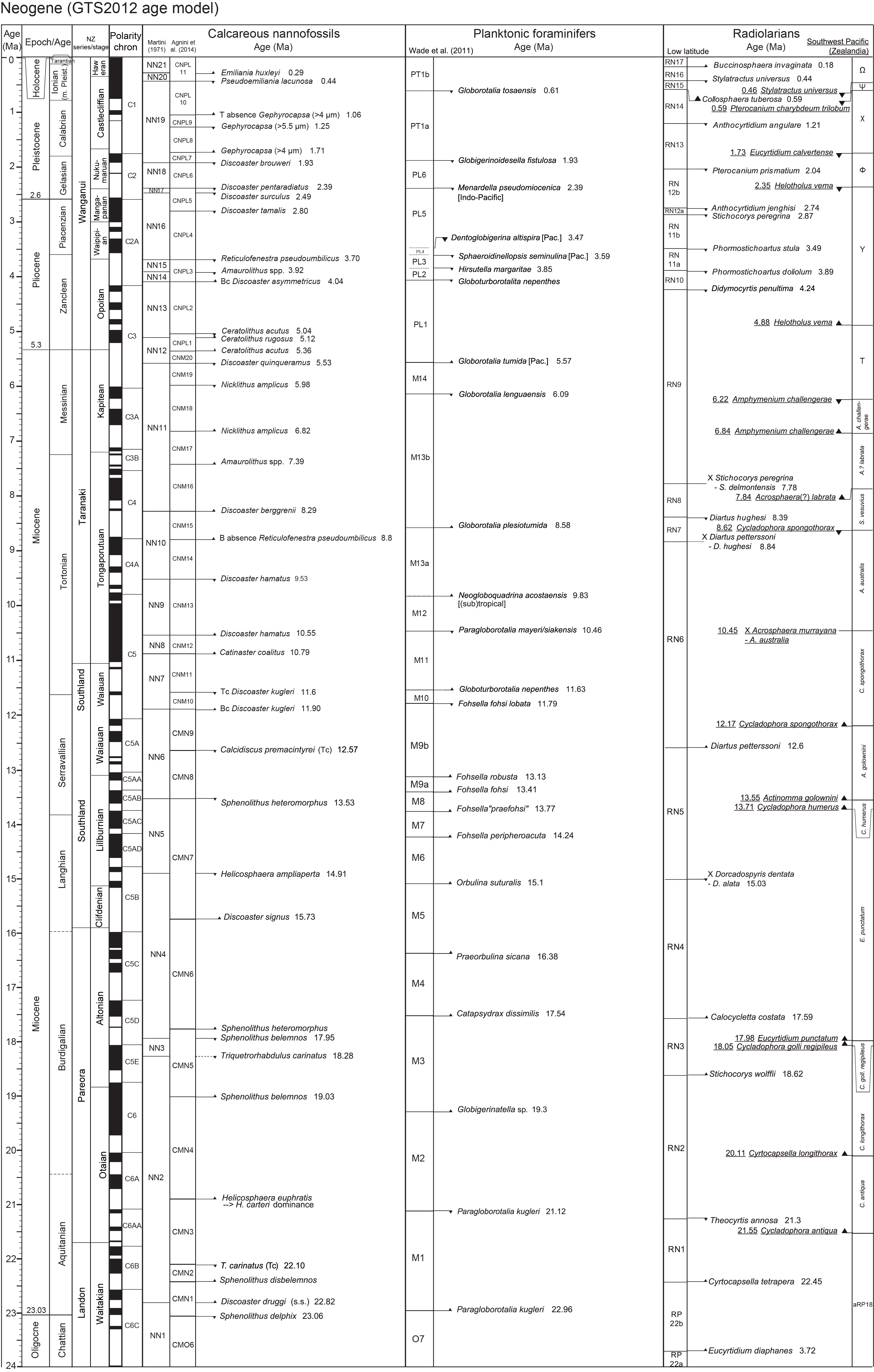
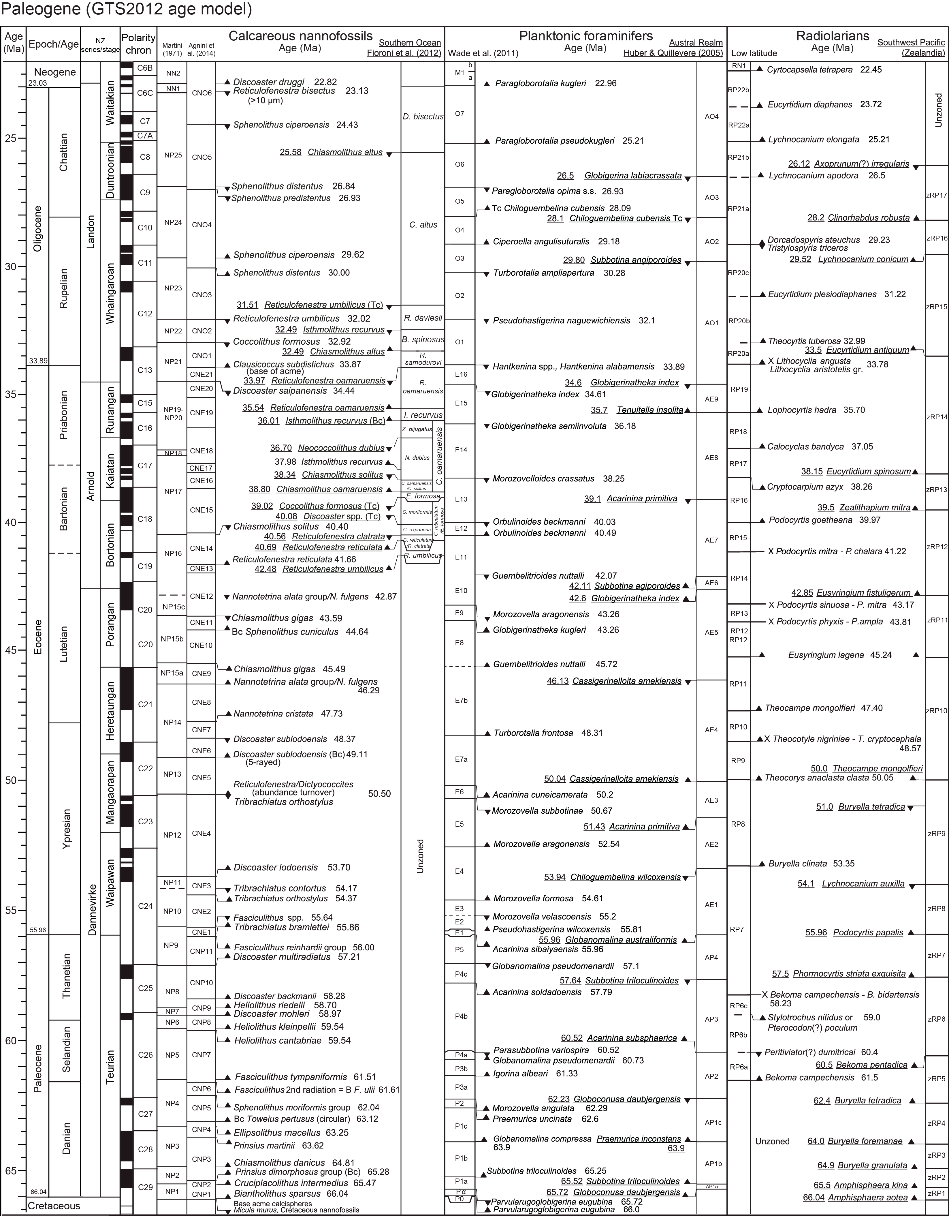
Figure F7. Global and New Zealand chronostratigraphy and datums.
Microfossil samples were collected from almost all core catcher sections, and additional samples, mostly for nannofossil biostratigraphy, were taken from working-half sections to refine age estimates and to initially constrain critical intervals. Where necessary, sample depths are cited as sample intervals. Biohorizon depths are generally cited as the midpoint between the two samples bounding the biohorizon. For the purposes of shipboard age estimation, emphasis was placed on age diagnostic species and total assemblages were not completely described. Information on microfossil group preservation, abundance, taxon identifications, and zonal assignment were uploaded into the LIMS database through DESClogik.
Biostratigraphic analyses were carried out for all holes drilled at Site U1553. Datum tables, microfossil distribution charts, an integrated biozonation figure, and a microfossil group abundance and preservation figure are included in Biostratigraphy and micropaleontology in the Site U1553 chapter (Röhl et al., 2022a).
3.1. Calcareous nannofossils
3.1.1. Taxonomy and biostratigraphy
Nannofossil taxonomy refers to Bown (1998, 2005) and Perch-Nielsen (1985a, 1985b) as compiled in the online Nannotax3 database (http://www.mikrotax.org/Nannotax3). The nannofossil biohorizons used for biostratigraphic classification (Table T2) represent an integration of the zonal scheme of Martini (1971; zonal codes NP and NN) with the Southern Ocean calcareous nannofossil zonal scheme of Fioroni et al. (2012) used for the Oligocene to upper Eocene interval. Additional biohorizons from the Paleogene and Neogene biozonation schemes of Agnini et al. (2014; zonal codes CNP, CNE, and CNO) and Backman et al. (2012; CNM and CNPL) are also included, although they are based predominantly on mid- to low-latitude calcareous nannofossil assemblages. This composite zonation scheme provides a general framework for calcareous nannofossil biostratigraphic classification (Figure F7).
Several biohorizons approximate critical events and chronostratigraphic boundaries:
- Eocene/Oligocene boundary (33.89 Ma): at high-latitude sites, the boundary falls within the Reticulofenestra samodurovi Zone, 0.08 My above the top of Reticulofenestra oamaruensis (33.97 Ma) and close to the base of acme for Reticulofenestra daviesii (33.71 Ma).
- Paleocene/Eocene boundary (55.96 Ma): the boundary is bracketed by the top of Fasciculithus richardii group (base of Zone CNE1; 56 Ma), the base of Rhomboaster spp. (55.96 Ma), and the base of Tribrachiatus bramlettei (base of Zone NP10; 55.86 Ma).
- Cretaceous/Paleogene boundary (66.04 Ma): the boundary is bracketed by the top of Cretaceous nannoflora (top of Zone NC23; base of Zone CNP1; 66.04 Ma) together with the base of Biantholithus sparsus (base of Zone NP1; 66.04 Ma) below and a flood of calcispheres above.
3.1.2. Methods of study, abundance, and preservation estimates
Calcareous nannofossils were examined from standard smear slides (Bown and Young, 1998) and analyzed using standard transmitted light microscope techniques on a Zeiss Axiophot microscope with cross-polarization and phase contrast at 1000× or 1250× magnification. All taxa were assigned qualitative abundance codes.
Total calcareous nannofossil group abundance in the sediment was recorded as follows:
- D = dominant (>90% of sediment particles).
- A = abundant (>50%–90% of sediment particles).
- C = common (>10%–50% of sediment particles).
- F = few (1%–10% of sediment particles).
- R = rare (<1% of sediment particles).
- B = barren (no specimens).
Individual calcareous nannofossil taxon abundance was recorded as follows:
- D = dominant (>100 specimens per field of view).
- A = abundant (>10–100 specimens per field of view).
- C = common (>1–10 specimens per field of view).
- F = few (1 specimen per 1–10 fields of view).
- R = rare (<1 specimen per 10 fields of view).
- VR = very rare (<5 specimens seen while logging slide).
Calcareous nannofossil preservation was recorded as follows:
- G = good (little or no evidence of dissolution or recrystallization, primary morphological characteristics were only slightly altered, and specimens were identifiable at the species level).
- M = moderate (specimens exhibit some etching or recrystallization, primary morphological characteristics were somewhat altered, and most specimens were identifiable at the species level).
- P = poor (specimens were severely etched or overgrown, primary morphological characteristics were largely destroyed, fragmentation has occurred, and specimens often could not be identified at the species or genus level).
Intermediate categories (e.g., G/M or M/P) were used in some cases to better describe the preservation state of calcareous nannofossil assemblages.
All light microscope images were taken using a Spot RTS system with the IODP Image Capture and Spot commercial software. Selected samples were observed using a Hitachi TM3000 SEM to verify the preservation state of calcareous nannofossils.
3.2. Foraminifers
3.2.1. Planktonic foraminiferal taxonomy and biostratigraphy
Planktonic foraminiferal taxonomy follows Huber (1991), Olsson et al. (1999), Pearson et al. (2006), and Wade et al. (2018). A taxonomic list of planktonic foraminiferal index species is given in Table T6. The planktonic:benthic ratio is expressed as the percentage of planktonic foraminifers relative to the total foraminiferal assemblage community.
We used a combination of the tropical zonation for Cenozoic foraminifers (Wade et al. 2011; zonal codes P, E, and O) and the Paleogene Southern Ocean zonation of Huber and Quillévéré (2005; zonal codes AP, AE, and AO) in addition to datum ages for the New Zealand region from Raine et al. (2015). The planktonic foraminiferal zonal scheme used during Expedition 378 is illustrated in Figure F7. Age estimates for foraminiferal datums are listed in Table T3.
Biohorizons approximating critical events and chronostratigraphic boundaries are as follows:
- Eocene/Oligocene boundary (33.89 Ma): the boundary falls in Zone AO1, 0.71 My above the top of Globigerinatheka index (34.6 Ma).
- Paleocene/Eocene Thermal Maximum (Paleocene/Eocene boundary) (55.96 Ma): the boundary coincides with the boundary between Biozones AE1 and AP4 and with the top of Globanomalina australiformis (55.96 Ma).
3.2.2. Benthic foraminiferal taxonomy and paleobathymetry
Taxonomic assignments mainly follow Van Morkhoven et al. (1986), Hornibrook et al. (1989), Jones and Brady (1994), and Kaminski and Gradstein (2005). The taxonomic list of benthic foraminiferal species is in Table T6. Paleodepth estimates are based on Tjalsma and Lohmann (1983), Van Morkhoven et al. (1986), and Hayward (1986) using the following categories:
- Neritic = <200 meters below sea level (mbsl).
- Upper bathyal = 200–600 mbsl.
- Mid-bathyal = 600–1000 mbsl.
- Lower bathyal = 1000–2000 mbsl.
3.2.3. Sample preparation for analysis of all foraminiferal assemblages
The sediments were wet sieved over a 63 μm mesh. The samples were then dried over a filter paper in a low-temperature (<60°C) oven and analyzed using standard optical stereomicroscope techniques on a Zeiss Discovery V8. The sieves were ultrasonicated at regular intervals to avoid contamination of samples. Lithified sediment samples were soaked in a 10%–30% hydrogen peroxide solution for 30–60 min before wet sieving. Strongly lithified samples were digested in cold 80% acetic acid when needed. To aid micropaleontological identification, selected specimens were photographed using a Hitachi TM3000 SEM.
The preservation status of planktonic and benthic foraminifers was estimated as follows:
- VG = very good (no evidence of overgrowth, dissolution, or abrasion).
- G = good (little evidence of overgrowth, dissolution, or abrasion).
- M = moderate (calcite overgrowth, dissolution, or abrasion are common but minor).
- P = poor (substantial overgrowth, dissolution, or fragmentation).
3.2.4. Planktonic foraminiferal abundance estimates
Planktonic foraminiferal abundance relative to total sediment in the >63 μm fraction was estimated from visual examination of the dried residue as follows:
- D = dominant (>30% of sediment particles).
- A = abundant (>10%–30% of sediment particles).
- F = few (>5%–10% of sediment particles).
- R = rare (1%–5% of sediment particles).
- P = present (<1% of sediment particles).
- B = barren.
The relative abundance of planktonic foraminiferal species was categorized as follows:
- A = abundant (>50 specimens on the tray).
- C = common (20–49 specimens on the tray).
- F = few (10–19 specimens on the tray).
- R = rare (2–9 specimens on the tray).
- P = present (<2 specimens on the tray).
- B = barren.
3.2.5. Benthic foraminiferal abundance estimates
Benthic foraminiferal abundance relative to total sediment in the >63 μm fraction was estimated from visual examination of the dried residue as follows:
- D = dominant (>30% of total sediment particles).
- A = abundant (>10%–30% of total sediment particles).
- F = few (>5%–10% of total sediment particles).
- R = rare (1%–5% of total sediment particles).
- P = present (<1% of total sediment particles).
- B = barren.
The relative abundance of benthic foraminiferal species was categorized as follows:
- D = dominant (>30% of benthic assemblage).
- A = abundant (>10%–30% of benthic assemblage).
- F = few (1%–10% of benthic assemblage).
- P = present (<1% of benthic assemblage).
The number of individuals of each benthic morphotype (epifaunal, infaunal, calcareous, and agglutinated) was counted for the samples analyzed and categorized as follows:
- D = dominant (>30% of benthic assemblage).
- A = abundant (>10%–30% of benthic assemblage).
- F = few (1%–10% of benthic assemblage).
- P = present (<1% of benthic assemblage).
- B = barren.
The ichthyoliths (isolated fish teeth and shark scales) found during foraminifer picking were also quantified and assemblages defined according to the morphological scheme of Sibert et al. (2018).
3.3. Radiolarians
3.3.1. Taxonomy and biostratigraphy
Radiolarian assemblages from Site U1553 sediments were anticipated to consist of cosmopolitan taxa with minor proportions of low- and high-latitude taxa. Consequently, we were not able to use the low-latitude zonation (Sanfilippo and Nigrini, 1998; Kamikuri et al., 2012) and instead correlated the Late Cretaceous and Paleogene assemblages to the Southwest Pacific (Zealandian) biozonation of Hollis et al. (2017, 2020) and Sutherland et al. (2019) (Table T4; Figure F7). In the late Eocene and Oligocene, these Southwest Pacific zones are equivalent to the Southern Ocean zones of Takemura and Ling (1997) and Funakawa and Nishi (2005). These Paleogene zones and datums have been calibrated to the GTS2012. Neogene zones and datums follow southern high-latitude zonations established by Abelmann (1990) and Lazarus (1992). The calibration of these datums to the GTS2012 follows McKay et al. (2019).
Radiolarian taxonomic concepts for the Cenozoic primarily follow those of Sanfilippo et al. (1985), Abelmann (1990), Lazarus (1992), Nishimura (1992), Hollis (1997, 2002), Hollis et al. (1997), O’Connor (1999), Sanfilippo (1990), Sanfilippo and Riedel (1992), Sanfilippo and Caulet (1998), Nigrini et al. (2006), Kamikuri et al. (2012), and Pascher et al. (2015). Additional sources are noted in the taxonomic list (Table T7).
3.3.2. Sample preparation
For calcareous lithologies, a ~5 cm3 sediment sample was first leached in 10% hydrochloric acid until the reaction ceased. Samples were then washed through a 63 μm mesh. The residue was cleaned by gently heating it in a solution of 10% hydrogen peroxide. If clay was present, 1–2 g of powdered sodium metaphosphate dispersant was added to the solution. After effervescence subsided, the mixture was washed again through a 63 μm mesh. For weakly calcareous and noncalcareous lithologies, samples were heated in the hydrogen peroxide/sodium metaphosphate solution, followed by hydrochloric acid treatment to ensure all carbonate was removed.
Strewn slides were prepared by pipetting the residue onto a microscope slide that was dried on a hot plate. Norland mounting medium was applied to the glass slide (~10 drops) while it was still warm. A coverslip was then gently placed on the slide. The mounting medium was fixed by placing the slide under a UV lamp for at least 15 min.
All light microscope images were taken using a Spot RTS system with the IODP Image Capture and Spot commercial software.
3.3.3. Preservation
Radiolarian assemblage preservation has been recorded as follows:
- E = excellent (specimens complete; fine structures preserved).
- G = good (most specimens complete; fine structures preserved in many specimens).
- M = moderate (some dissolution, recrystallization, and/or breakage).
- P = poor (common dissolution, recrystallization, and/or breakage).
- VP = very poor (complete recrystallization and loss of ornament).
3.3.4. Abundance
Total radiolarian abundance has been estimated as radiolarians per cubic centimeter of wet sediment as follows:
- A = abundant (>10,000).
- C = common (1,001–10,000).
- F = few (101–1,000).
- R = rare (10–100).
- Tr = trace (<10).
- B = barren.
These values were derived by estimating the volume of sediment disaggregated and the proportion of residue used to prepare slides, and they therefore have a wide error margin. For this reason, we base these categories on order of magnitude differences in abundance.
Where time allowed, the relative abundance of taxa was recorded in a single slide traverse as follows:
Taxa encountered in the sample but not in the slide traverse were recorded as present (P). Where relative abundance was not determined, all taxa present were recorded as present. Uncertain identifications were recorded as a question mark (?).
3.4. Dinoflagellate cysts
Dinoflagellate cysts (dinocysts) were examined in a shore-based study to confirm the age of the lower part of the cored interval (Unit V).
3.4.1. Taxonomy and biostratigraphy
The dinoflagellate cyst (dinocyst) assemblages have been correlated to the New Zealand Paleocene biozonation of Crouch et al. (2014). Dinocyst taxonomy corresponds to that cited in Fensome et al. (2019).
3.4.2. Sample preparation
Thirteen core catcher samples from Hole U1553D, 8R-CC to 20R-CC, were processed using standard palynological techniques. Around 10 cm3 of sediment was crushed and dried, and the carbonate and siliceous components were removed by adding 10% HCl and 50% HF, respectively. Heavy liquid separation (using sodium polytungstate) was completed on selected samples, and all samples were then placed in an ultrasonic bath for 30 s prior to sieving. Samples were sieved over a 6 µm mesh, and well-mixed representative fractions of the >6 µm residue were mounted on glass slides using a glycerine jelly medium.
3.4.3. Sample examination
For each sample, approximately 200 dinocysts were counted and at least one entire slide was scanned for the presence of additional rare taxa. While slides were scanned, spore and pollen taxa were also noted but counts were not completed. Quantitative data are calculated as a percentage of the total dinocyst count and are discussed using the following terms: rare (1%–5%), common (6%–10%), frequent (11%–20%), abundant (21%–40%), and superabundant (>40%).
4. Paleomagnetism
Shipboard paleomagnetic studies were conducted on both the archive-half and working-half sections from Expedition 378 cores. The primary objectives were to determine the directions of natural remanent magnetization (NRM) components, including the magnetic polarity, and downhole variation of magnetic properties. Routine measurements were carried out on archive-half sections with stepwise alternating field (AF) demagnetization. For discrete samples taken from selected working-half sections, stepwise AF and thermal demagnetization were applied. These data were used for core orientation and magnetostratigraphy construction.
Ocean drilling cores generally carry secondary remanence components or overprints, such as natural viscous remanent magnetization and a steep downward-pointing component imparted by the drilling process. Nonmagnetic core barrels were thus adopted for all cores except those recovered with the XCB coring system. To separate these overprints from the characteristic remanent magnetization (ChRM), stepwise AF demagnetization in low fields (≤12 mT) was performed. In addition, the downhole orientation tool (Icefield MI-5 core orientation tool) was deployed for all full-length APC cores in Holes U1553A and U1553B to correct the measured core declinations back to true coordinates. All measurement data were uploaded to the LIMS database. The stepwise demagnetization data of the discrete samples were analyzed using principal component analysis to define the ChRM (Kirschvink, 1980). Data visualization (Zijderveld demagnetization plots [Zijderveld, 1967] and equal-area projections) and principal component analysis were mainly conducted using the PuffinPlot desktop application (version 1.03) (Lurcock and Wilson, 2012) and PmagPy software (Tauxe et al., 2016).
4.1. Magnetic measurements on archive-half sections
The remanent magnetization of archive-half sections was measured using a pass-through, liquidhelium–free superconducting rock magnetometer (SRM; 2G Enterprises model 760-4k) equipped with direct-current superconducting quantum interference devices (SQUIDs) and an in-line, automated AF demagnetizer capable of reaching a peak field of 80 mT. The measurement of archive halves was conducted using the SRM software (IMS-SRM version 10.3), and an assumed sample area of 17.5 cm2 was adopted for conversion to volume-normalized magnetization units (A/m).
The interval between NRM measurement points was typically 2.5–5 cm at a speed of 10 cm/s. The time to measure each point as well as the AF demagnetization process usually requires 3.5–4 min at 5 cm spacing. The response functions of the pickup coils of the SQUID sensors have a full width of 7.25–8.8 cm at half height. Therefore, data collected within ~4 cm of piece boundaries (or voids) are significantly affected by edge effects. Consequently, all data points within 4.5 cm of section boundaries (as documented in the curatorial record) were filtered out prior to further processing. It should be noted that edge effects may also occur in a contiguous core piece if substantial heterogeneity (in intensity or direction) is present. It is more difficult to filter out such artifacts, but calculating the average direction (using Fisher statistics) for each core piece could provide a means of identifying these problems (Expedition 330 Scientists, 2012). In addition, core disturbance, often found in the top part of the first section of each core, leads to a surge in magnetization and scattered demagnetization data. Therefore, caution is needed when interpreting those data.
Successive AF demagnetization was performed using the SRM in-line AF demagnetizer on all split archive halves. The in-line AF demagnetizer applies a field to the x-, y-, and z-axes of the SRM in this fixed order (Figure F8A, F8D). Demagnetization fields no higher than 15 mT were used to demagnetize the sections. For most of the cores, three steps were performed after NRM from 3 to 9 mT. No higher AF steps were employed here because (1) the cored materials were mostly weak in NRMs, (2) the shipboard paleomagnetic laboratory is not in a magnetically shielded room and is easily affected by surrounding environments, and (3) previous reports suggested that higher AF demagnetization fields have produced significant anhysteretic remanent magnetization along the z-axis of the SRM (e.g., Harris et al., 2013). AF demagnetization results were plotted individually as vector plots (Zijderveld, 1967) as well as downhole variations with depth. The plots were visually inspected to determine whether the remanence after demagnetization at the highest AF step reflects the ChRM and geomagnetic polarity sequence.
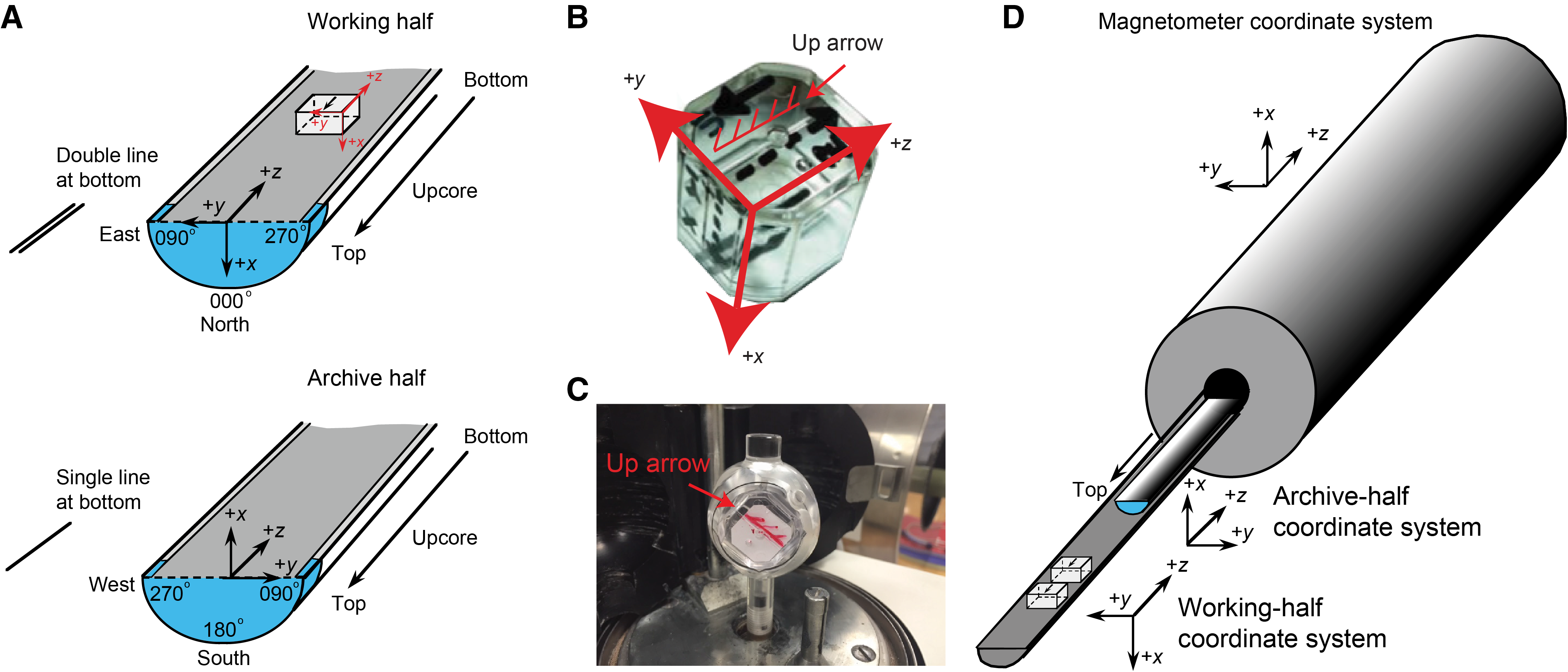
Figure F8. IODP coordinates for paleomagnetic samples.
Low-field MS (κ) measured on whole-round core sections using the WRMSL and on archive halves using the SHMSL (see Physical properties) was used to indicate the concentration of magnetic minerals. Data were compared to discrete cube measurements made with the Agico KLY 4S Kappabridge MS meter. Whole-round records of MS were compared to visual features in the split cores to flag any artifacts or split disturbance.
4.2. Magnetic measurements on discrete samples
Oriented discrete samples were collected from working-half sections, nominally 2–3 discrete samples per core. Discrete sample locations were chosen preferentially in fine-grained intervals where drilling deformation was minimal or not visible. In soft sediment, discrete samples were taken with plastic “Japanese” Natsuhara-Giken sampling cubes (7 cm3 sample volume) (Figure F8B). Cubes were manually pushed into the working half of the core, and the “up” arrow on the cube pointed upsection in the core. In lithified sediments and hard rocks, 2 cm cubes (8 cm3 sample volume) were cut with a parallel saw.
Incremental AF demagnetization was performed with the DTech AF demagnetizer (model D-2000) for the JR-6A spinner magnetometer with up to 9 mT AF demagnetization for most of the samples because higher AF treatments often record a surge in magnetization with demagnetization path trending away from the origin, probably suggesting acquisitions of gyroremanent magnetization (e.g., Snowball, 1997). Several high-coercivity samples underwent higher AF steps up to 50 mT, where the surge of magnetization often occurs at around 20 to 40 mT. Progressive thermal demagnetization was also applied using a thermal specimen demagnetizer (ASC Scientific model TD-48 SC) in 25°C steps up to 175°C. However, thermal treatments appeared to affect the magnetic minerals in some of the sediments, suggested by an obvious color change to much lighter gray. An increase in magnetization was often observed at ~150°C accompanied by an off-origin trend of the demagnetization path.
Anisotropy of magnetic susceptibility (AMS) was measured on an Agico KLY 4S Kappabridge instrument using the AMSSpin LabVIEW program designed by Gee et al. (2008) and adopted for the shipboard KLY 4S. The KLY 4S Kappabridge measures AMS by rotating the sample along three axes, stacking the data, and calculating the best-fit second-order tensor. It also measures the volume-normalized, calibrated bulk susceptibility (χ).
It is worth mentioning that the SRM is not recommended to measure discrete samples because the resultant demagnetization behavior of the discrete samples becomes very noisy at higher AF treatments and difficult for useful magnetic interpretation. Shipboard tests of the reliability of discrete measurements on the 2G SRM showed significant scatter in NRM directions from a standard sample that was measured over hundreds of times. In addition, to avoid contamination by the ambient magnetic field during shipboard measurements, discrete samples were stored in two available cylindrical mu-metal shields (aligned approximately perpendicular to the ambient magnetic field) with low field environments.
4.3. Coordinates
All magnetic data are reported relative to the IODP orientation conventions: +x points into the face of the working half, +y points toward the left side of the face of the working half, and +z points downsection (Figure F8). The relationship of the SRM coordinates (X-, Y-, and Z-axes) to the data coordinates (x-, y-, and z-directions) is as follows: for archive halves, x-direction = X-axis, y-direction = −Y-axis, and z-direction = Z-axis; for working halves, x-direction = −X-axis, y-direction = Y-axis, and z-direction = Z-axis (Figure F8). The coordinate systems for the spinner magnetometer (AGICO model JR-6A) and Natsuhara-Giken sampling cubes are also shown in Figure F8.
4.4. Core orientation
Paleomagnetic study of marine sediment cores is greatly enhanced if the angle between magnetic north and the double line orientation marked on the core liner is established through orientation. Core orientation using the APC system employs a nonmagnetic barrel and the Icefield MI-5 core orientation tool mounted on the core barrel. The Icefield MI-5 tool consists of triaxial magnetometers and accelerometers. The information from the magnetometers and sensors allows measuring the azimuth and dip of the hole as well as the azimuth of the core. This azimuth, combined with the local magnetic declinations, allows us to reorient the measured core declinations back to true geographic coordinates. In the orientation deployment, the tool is connected to the core barrel in such a way that the double lines on the core liner are at a fixed and known angle relative to its sensors. This angle has been assumed to be zero. Previous expeditions have reported that in general, these orientation tools have an accuracy of 20°–30°. However, the corrected declinations of the APC cores in the first two holes (U1553A and U1553B) did not turn out to be useful to the interpretation of the paleomagnetic data. This is probably because of the low abundance of ferromagnetic minerals. Thus, the tool was not deployed in Hole U1553E.
4.5. Magnetostratigraphy construction
The magnetostratigraphy was constructed by correlating observed polarity patterns with the reference geomagnetic polarity timescale (GPTS) constrained by biostratigraphic units. The chosen GPTS for Expedition 378 is the synthesis of astronomical tuning of Cenozoic through the latest Cretaceous polarity zones compiled for the GTS2012. The Cenozoic portion of this GPTS together with microfossil biozones is shown in Figure F7.
A magnetic reversal was defined when a ~180° shift in the declinations as well as significant shallowing of the inclinations were observed in the paleomagnetic data obtained from the pass-through measurements on long, coherent core sections at the 6 mT demagnetization step. This was subsequently verified by the ChRM directions of the discrete samples from the corresponding meter level of the working half. However, polarity reversals occasionally occurring at core section tops were often subject to drilling disturbance and thus were interpreted conservatively.
The naming convention of the polarity patterns follows that of correlative chron and anomaly numbers (e.g., Tauxe et al., 1984; Harland et al., 1990; Cande and Kent, 1992). Normal polarity subchrons are referred to by adding suffixes (n1, n2, etc.) that increase with age. For the younger ages of the timescale (Pliocene–Pleistocene), traditional names are used to refer to the various chrons and subchrons (e.g., Brunhes, Jaramillo, Olduvai).
5. Geochemistry
The shipboard geochemistry program for Expedition 378 conducted a rigorous sampling and analytical program to characterize IW and sediment chemical composition and to constrain the diverse diagenetic and authigenic reactions occurring at Site U1553. Headspace samples were analyzed immediately for routine hydrocarbon monitoring as required for safety and pollution prevention protocol. The geochemistry sampling and analysis plan accounted for one to two geochemists on each 12 h shift.
5.1. Hydrocarbon gas sampling and analyses
One headspace gas sample was collected from each Hole U1553A core, usually from the top of the section adjacent to the deepest IW whole-round sample. Headspace gas samples were also taken from cores from additional holes where depths exceeded those of previously drilled holes or where hydrocarbon concentrations required detailed monitoring. Between 3 and 5 cm3 of sediment was sampled immediately after cores were split into sections on the catwalk using a cork borer in soft sediments (Cores 1H–24X) and a metal spatula for more lithified material (below Core 24X and for all other samples). Samples were subsequently extruded into a glass serum vial, sealed with a septum and metal crimp cap, and lightly swirled. After heating the samples at 70°C for 30 min, approximately 5 cm3 of the evolved gas was sampled from the headspace in the vial with a glass syringe and injected into an Agilent 7890 gas chromatograph (GC) equipped with a flame ionization detector (FID) for rapid estimation of methane (C1), ethane (C2), ethene (C2=), propane (C3), and propene (C3=). Helium was used as the carrier gas. The initial GC oven temperature was 35°C. It was held for 4 min before ramping at 25°C/min to 200°C before a final holding time of 5 min. Data were collected and evaluated with an Agilent Chemstation data-handling program. The chromatographic response was calibrated to three different gas standards containing known variable concentrations of low molecular weight hydrocarbons. Check standards were measured regularly.
5.2. Bulk sediment geochemistry
In 1–2 sections per core, approximately 5 cm3 of sediment was sampled adjacent to MAD and XRD sampling for analyses of carbonate and organic matter content and maturity. Additional samples were taken when interesting lithologic changes were observed. Samples were freeze-dried for 12 h and homogenized using an agate mortar and pestle or a shatter box for lithified material. Samples were stored in glass vials until preparation for chemical analyses.
5.2.1. Calcium carbonate analyses
Calcium carbonate (CaCO3) content was determined using a CM5015 coulometer. About 10 mg of dry sediment was placed into a glass vial, heated in the acidification module (CM5030), and reacted with 5–10 mL of 1 M HCl. The evolved CO2 was back-titrated to a colorimetric end point. Carbonate content, reported as weight percent, was calculated from the inorganic carbon (IC) content based on the assumption that all IC exists as CaCO3:
Analytical reproducibility was determined by replicate measurements of selected samples. A verification external standard (i.e., 100 wt% CaCO3) was run every 10 samples. Analyses would only continue if values were between 99 and 100 wt%. The coulometer cell was replaced after 24 h or 50 measurements.
5.2.2. Total carbon, nitrogen, and sulfur
Total carbon (TC), nitrogen (N), and sulfur (S) content was determined using a Thermo Electron Flash EA 1112 elemental analyzer equipped with a Thermo Electron packed GC column carbon-hydrogen-nitrogen-sulfur (CHNS)/NCS (polytetrafluoroethylene; length = 2 m; diameter = 6 mm × 5 mm) and thermal conductivity detector (TCD). Aliquots of 12–15 mg of freeze-dried ground sediment were weighed into tin cups. Less than ~4 mg of vanadium oxide was added to each sample to act as a catalyst for total sulfur analyses. Capsules were wrapped and combusted at 950°C in the reactor oven of the instrument with a pulse of O2. Nitrogen oxides were reduced to N2, and the mixture of gases produced (N2, CO2, H2O, and SO2) was separated using the GC and measured using the TCD. The GC oven temperature was held at 65°C between runs. All elemental analyzer measurements were calibrated by comparison to a soil reference material (TC = 3.496 wt%; total nitrogen = 0.365 wt%; total sulfur = 0.063 wt%). Analytical reproducibility was determined by 10 replicate measurements of this standard. Associated standard deviation was 0.02, 0.10, and 0.00 for N, C, and S, respectively. The coefficient of variation was 6.3%, 2.0%, and 2.2% for N, C, and S, respectively. External verification standards (i.e., soil reference material) were run every 10 samples as quality control. Total organic carbon (TOC) was determined as the difference between TC and IC measured by coulometry:
Reliable determination of C/N ratios was hampered by the overall low N values. Peak tailing and anomalous values were monitored for combustion column degradation and guided regular cleaning and replacement.
5.2.3. Pyrolysis
Pyrolysis analysis was conducted on 19 bulk sediment samples from Cores 378-U1553C-42R through 44R and 378-U1553D-19R through 20R to investigate the thermal maturation of the organic matter, hydrocarbon sources, and petroleum potential. Approximately 80 mg of freeze-dried, homogenized sediment was weighed into metal crucibles and measured with a Weatherford Instruments source rock analyzer (SRA) equipped with an infrared section and a FID. Weatherford Laboratories SRA Rock Standard 533 was used as the calibration and quality control standard. Each sample was heated at 340°C for 3 min, and the volatile hydrocarbons present in the sample were released and measured as S1 peak (mg HC/g rock). After the temperature was increased to 640°C at 25°C/min, the hydrocarbons produced during thermal cracking of kerogen were measured as the S2 peak (mg HC/g rock). The temperature at which maximum release of hydrocarbons occurs during S2 analysis is reported as Tmax. Each sample was then heated from 340° to 390°C, and the released CO2 (mg C/g rock) was measured as the S3 peak. Additional CO2 produced by oxidizing the pyrolysis residue at 580°C is the S4 peak. S4 is used along with S1 and S2 to estimate TOC (wt%). Other indirect measurements are the carbon-normalized hydrogen index (HI) (mg HC/g C), the oxygen index (OI) (mg CO2/g C), and the production index (PI):
No hydrocarbon potential (S2) was detected in 11 samples, leading to randomized Tmax values and providing unreliable and overestimated values for other indexes.
5.2.4. Major and trace element concentrations
Sediment samples for inductively coupled plasma–atomic emission spectrometry (ICP-AES) analyses were prepared using a flux fusion approach. (Data produced on the Agilent 5110 inductively coupled plasma–optical emissions spectrometer [ICP-OES] was collected in AES mode and is referred to as “ICP-AES” in the LIMS database. In this document, “ICP-AES” is used to refer to this data.) This technique ensures complete dissolution of the sample material, allowing a full elemental analysis. To begin, 100 mg ±1 mg of each sample or a standard (BCR-2, BIR-1, BHVO-2, DNC-1, NBS-1c, PACS-3, W-2, SCo-1, or AGV-1) was weighed on a Cahn C31 microbalance. The 100 mg ±1 mg of sample or standard powder was mixed with 400 mg of lithium metaborate that was preweighed on land and stored in a glass vial covered with Parafilm M. A LiBr solution (10 µL of 0.172 mM) was added to the flux and sediment powder mixture prior to sample fusion to prevent the fused bead from sticking to the crucible during cooling. Samples were fused individually in Pt-Au (95:5) crucibles for 2 min at 700°C, 5 min at 1050°C, and 5 min in agitation at 1050°C (12 min total) in an internally rotating induction furnace (Bead and Fuse Sampler TK-4100). The fused beads were transferred into 125 mL high-density polypropylene bottles and dissolved in a 50 mL solution containing 10% trace metal grade HNO3. Each solution bottle was shaken in a Burrell wrist-action shaker until the bead dissolved. Increments of 20 mL of the solution were passed through a 0.45 µm filter into a clean 60 mL wide-mouth high-density polypropylene bottle. From this filtered solution, 0.5 mL was pipetted into a sample tube and diluted with 4.5 mL of 10% HNO3, 10 ppm Y. Within any analytical run, the dilution factor was kept constant for all samples, blanks, and standards, and the ICP-AES approach is similar to the one for IW samples (see Rhizons). The standard reference material BHVO-2 was run as an unknown between every five samples. The precision of the BHVO-2 concentrations run as unknowns (n = 17) was <1% for Al2O3, CaO, Fe2O3, MgO, MnO, SiO2, Sr, and TiO2 and <2% for Ba, Cr, K2O, Na2O, Sc, V, Y, and Zr. The precision for La was 12%, for P2O5 was 6%, and for Zn was 13.6%. The measured values of BHVO-2 run as unknowns were accurate within precision.
5.2.5. Repository core analysis for shipboard data (XRF core scanning)
XRF elemental records were generated for all core sections with a third-generation Avaatech XRF core scanner and a fourth-generation Avaatech XRF core scanner at the GCR in College Station, Texas. The data presented are available as a shipboard data set in LIMS.
For all the scanned sections of Site U1553, XRF core scanner data were collected every 2 cm downcore over a 1.2 cm2 area with a downcore slit size of 10 mm using generator settings of 10, 30, and 50 kV, a 0.12 mA current for the 10 kV setting, 1.25 mA for the 30 kV setting, a 0.75 mA current for the 50 kV setting, and a sampling time of 6 s directly at the split core surface of the archive half. The 30 kV run was measured using a Pd thick filter, and the 50 kV run was measured using a Cu filter (to lower the background noise).
The split core surface was covered with a 4 μm thin SPEXCerti Prep Ultralene foil to avoid contamination of the XRF measurement unit and desiccation of the sediment. Both of the Avaatech XRF core scanners have similar components and thus provide very similar data. Data were acquired using Brightspec silicon drift detectors (Model SiriusSD-D65133BE-INF with 133 eV X-ray resolution), the TopazX high-resolution digital multichannel analyzer, and water-cooled, 100 W rhodium side-window X-ray tubes. Raw data spectra were processed by the analysis of X-ray spectra using the Iterative Least square software (WIN AXIL) package from Canberra Eurisys.
5.3. Interstitial water
5.3.1. Interstitial water sample collection and preservation
During Expedition 378, a “mudline” sample was collected from within the core liner above the uppermost sediment recovered from the first hole (U1553A), and one sample was collected from between the core liner and sediment at Section 378-U1553B-26X-5, 214.13 mbsf. IW was extracted from sediment cores using two different techniques: squeezing of whole-round intervals and removal using Rhizon samplers. Both techniques were employed to mitigate the disadvantages of each (e.g., Dickens et al., 2007; Schrum et al., 2012; Miller et al., 2014). All whole-round and Rhizon samples were taken at room temperature (and pressure) and subsequently stored in the refrigerator, and we are aware of potential temperature effects on IW chemistry (Sayles and Manheim, 1975; Gieskes, 1975).
5.3.1.1. Whole rounds
Whole-round samples for IW were taken on the catwalk after a core was cut into 1.5 m (nominal) sections. The samples subsequently were trimmed to remove potentially contaminated sediment and water. When there was a backlog, some whole rounds were stored in a cold room in a Ziploc bag flushed with nitrogen gas. Squeezing of samples was completed less than 4.5 h after the core arrived on deck.
Extraction of IW was achieved with a Carver laboratory hydraulic press, which extruded IW through a prewashed (with 18.2 MΩ water) Whatman Number 1 filter fitted above a titanium screen within the squeezer and a 0.45 μm polysulfone disposable filter (Whatman Puradisc PES) and then into a precleaned (10% HCl) 60 mL syringe. After squeezing, the compressed cylinder of sediment (squeeze cake) was removed and the squeezing apparatus was cleaned. The compressed sediment squeeze cake was divided and preserved for additional individual postcruise research.
5.3.1.2. Rhizons
Rhizons are thin tubes of hydrophilic porous polymer. When inserted into a sediment core through a hole in the liner and attached to a collection tube and an evacuated syringe, they permit collection of small volumes (typically <12 mL) of IW through suction filtering. Such IW samples come without removal of whole rounds, thus preserving the sedimentary record. They also enable water sampling at very high depth resolution (<5 cm). For Expedition 378, the chosen samplers were Rhizon CCS 5 cm (flat tip and 2.5 mm outer diameter) from Rhizosphere Research Products (Netherlands), which were prerinsed three times with 18.2 MΩ deionized water.
Rhizon sampling commenced after core sections were run through the Special Task Multisensor Logger (STMSL) and during the time (nominally 3–4 h) when cores equilibrate for NGR measurement (see Physical properties). The extraction of IW from each Rhizon was ended when the syringe was full or after ~2 h, whichever came first, so that Rhizon sampling was kept at the pace of the core recovery and equilibration and did not interrupt core flow.
A sample of fluid from between the core liner and the sediment was collected at the top of Section 378-U1553B-26X-5 and filtered through a Rhizon in the laboratory to determine whether seawater in the edge of the liner (a result of smaller diameter XCB recovery) was biasing or contaminating IW results from XCB cores. Our shipboard measurements suggest seawater was not affecting the major features of chemical profiles in the pore fluids and sediments, and further onshore analyses will test for potential outliers in the data. There was a delay between Rhizon sample collection and subsequent transfer to individual vials for storage and/or analyses of 10 to ~15 h, and samples from Cores 378-U1553B-11H through 14H were left for last. Most samples were kept in either the refrigerator or the cold room in their individual syringes that were capped and stored in Ziploc bags. Therefore, we do not expect any major alteration to their chemical composition.
5.3.2. Interstitial water analytical methods
5.3.2.1. Salinity
Salinity was analyzed with a Fisher Model S66366 portable salinity refractometer. A few drops of sample were applied to the daylight plate assembly with a pipette, and the measurement was read through the eyepiece, with typical measurement precision of ±1‰. Blanks (18.2 MΩ deionized water) and International Association for the Physical Sciences of the Oceans (IAPSO) water (OSIL Environmental Instruments and Systems, Batch P162) were analyzed routinely to check for contamination. Salinity measurements were completed days after collection of the IW. Therefore, for smaller size aliquot samples (<1 mL), artificially high values are likely.
5.3.2.2. Alkalinity and pH
pH and alkalinity were measured within 24 h after squeezing to avoid degradation (Gieskes, 1975). The pH was measured using a combination glass electrode (Brinkman pH electrode), and alkalinity was determined by Gran titration using an autotitrator (Metrohm 794 Titrino). A total of 3 mL of IW was titrated with 0.1 M HCl at 25°C. The electrode was calibrated using a series of buffers with a pH of 4, 7, and 10. IAPSO seawater was analyzed every ~12 h or after a period of no use to check accuracy. Alkalinity was typically within 2% of the expected value for IAPSO (2.325 mM).
5.3.2.3. Ion chromatography
Concentrations of major anions (Cl−, SO42−, and Br−) and major cations (Ca2+, Na+, Mg2+, and K+) were measured on a Metrohm 850 professional ion chromatograph with an 858 professional sample processor. IW was diluted 1:100 with 18.2 MΩ deionized water in preparation for ion chromatography analysis. Diluted IAPSO seawater was analyzed every 10 samples as a consistency standard and to create a six-point calibration curve. Precision was 5% for Ca2+ and Br− and 3% for the other ions.
5.3.2.4. Inductively coupled plasma–atomic emission spectroscopy
Suites of major (S, Ca, Mg, K, and Na) and minor (B, Ba, Fe, Li, Mn, P, Si, and Sr) elements were analyzed with an Agilent Technologies 5110 spectrometer ICP-AES. The shipboard ICP-AES procedure is similar to that of Murray et al. (2000). Samples and standards were diluted using 2% ultrapure HNO3 spiked with 10 ppm Y with dilution ratios of 1:10. Samples were typically run in batches of 35–85 samples. With every batch run for major elements (S, Ca, Mg, K, and Na), a seven-point calibration curve was created using different dilution levels of IAPSO seawater. For minor elements (B, Ba, Fe, Li, Mn, P, Si, and Sr), an eight-point calibration curve was created using synthetic seawater spiked with minor elements to varying degrees. This was then used to convert background-corrected intensities to concentrations. Additionally, the calibration curves included four extra standards that were spiked with the trace elements and had IAPSO as a base rather than synthetic seawater to ensure that no matrix effects were imposed by the synthetic seawater. The IAPSO dilutions for the major element calibration curve were also included in the trace element calibration curve for the trace elements with detectable concentrations. All of these standards were analyzed at the beginning of the run to construct a calibration curve using the Agilent software, and they were also analyzed a second time as unknowns at the end of the run to check accuracy and drift. An IAPSO standard spiked with trace elements was run every five to seven samples to further monitor drift and precision of each element throughout the run. Three blanks were run with every batch to check for contamination, to allow for blank subtractions, and to calculate the detection limits of each element. Additionally, four samples that span the range of concentrations (selected after the first run) were also analyzed in each subsequent run to check for interrun precision of the samples.
The intrarun precision was calculated as the standard deviation of the spiked IAPSO standards (run as unknowns between every five to seven samples) divided by their average. The first and third run had <1% intrarun precision, and the second run had ~3% intrarun precision for every element except Fe. For Fe concentrations, many of the samples were below the detection limit (0.2 μM), and the triplicate measurements of samples within a few micrometers above had a standard deviation of ±0.2 μM and must therefore be interpreted with caution. Higher concentrations of Fe had a precision of <1%, similar to the other elements. The standards measured as unknowns were accurate within the precision of the known concentrations of the spiked IAPSO standard. The interrun precision was <3%, calculated as the standard deviation of a sample run in each of the three runs divided by the average of the concentrations generated in each of the three runs.
5.3.2.5. Spectrophotometry
Dissolved ammonium (NH4+) and phosphate (PO43−) were determined spectrophotometrically using an Agilent Cary 100 ultraviolet-visible light spectrophotometer according to the method of Solórzano (1969) for ammonium concentrations with a 2% precision (13% for concentrations below 200 μM). Phosphate concentrations were measured according to the method described by Strickland and Parsons (1968) as modified by Presley (1971). The precision was 3 μM for phosphate concentrations up to 10 μM.
5.4. Microbiology sampling
A 5 cm3 syringe sample and a ~2 cm3 syringe sample were obtained for shore-based microbiology DNA analysis and cell counting, respectively. For Cores 378-U1553A-1H through 5H, the pairs of microbiology samples were taken on every other section and adjacent to the whole-round IW sample taken on the catwalk. Samples were collected from the anticipated future working-half section based on predrawn core splitting lines. For cores deeper than Core 5H, one set of the two microbiology syringe samples was taken every other core until the sediments became too stiff to sample with the syringes.
5.4.1. Sampling for cell counting
A set of sterilized 2.5 cm3 syringes with the tapered tips removed was provided to the geochemistry laboratory before departure. These syringes were used to collect samples for cell counting. After a core was sectioned on the catwalk and a whole-round IW sample was sliced off with an ethanol-sterilized spatula, a syringe was plunged into the working-half section of the exposed core. While the plunger was held, about 2.0 cm3 of sediment was ejected from the syringe into a tube containing 10% filtered formalin solution. The tubes were labeled and stored in a refrigerator at 4°C within 20 min after arrival on the catwalk.
5.4.2. Sampling for DNA/RNA analysis
Samples for DNA/RNA were also collected on the catwalk from the cut core section adjacent to the 2.5 cm3 syringe sample for cell counting on the future working-half sections. Sterilized 10 mL syringes with the tapered tips removed were used to extract 5–10 cm3 of sediment. Each syringe that contained sediment was placed in a heat-sealed clear plastic bag. This bag was placed in a clear plastic bag and heat sealed again. Samples were processed and stored in a −80°C freezer within 15 min after arrival on the catwalk.
6. Physical properties
High-resolution physical property measurements were made during Expedition 378 to aid lithostratigraphic characterization and to contribute to hole-to-hole stratigraphic correlation, detection of hiatuses, and identification of differences in the composition and texture of sediment. A variety of techniques and methods were used on whole-round sections, section halves, and discrete samples to characterize the Site U1553 cores.
6.1. General sampling and measurement sequence
6.1.1. Whole-round core measurements
All whole-round sections were equilibrated to ambient room temperature (~20°C) and pressure for ~4 h. After equilibration, core sections were run through the WRMSL at a 2.5 cm sampling resolution to generate measurements of density by gamma ray attenuation (GRA), MS, and compressional P-wave velocity (on the P-wave logger [PWL]). P-wave velocity was not measured on XCB cores from Holes U1553A, U1553B, or U1553E or on any cores from Holes U1553C or U1553D because of insufficient contact of the sediments with the core liner. All core sections were measured with the spectral NGRL. In addition to the standard suite of physical properties measurements, all whole-round core sections were imaged using the X-Ray Imager (XRI) prior to splitting.
Core sections from Holes U1553B–U1553E were run through the STMSL to measure GRA bulk density and MS at a lower sampling resolution (5 cm) prior to equilibration to help with rapid stratigraphic correlation to inform drilling decisions. Three cores from Hole U1553C (31R–33R) were run through the STMSL in an attempt to identify a potentially critical stratigraphic interval. All of these fast-tracked sections were remeasured using the WRMSL at a 2.5 cm sampling resolution following the standard 4 h thermal equilibration period because some of the physical properties measurements are particularly sensitive to temperature. Each core section was then run through the NGRL at a 10 cm resolution.
Thermal conductivity was measured on one whole-round section per sediment core (typically Section 3). Thermal conductivity measurements were taken by inserting a needle probe into a small hole drilled through the plastic core liner close to the middle of the core section. They were taken only on cores soft enough to insert and maintain sufficient contact with the needle probe.
After splitting, the archive half of each section was passed through the SHMSL for measurement of MSP and color reflectance. Compressional P-wave velocity measurements were made on the x-axis of the working halves (usually two sections per core). Additional P-wave measurements were made during intervals where there was a clear lithostratigraphic change. Z-axis P-wave measurements were attempted on the first three cores of Hole U1553A using the P-wave bayonet system inserted into the working half. Because of insufficient contact between the sediment and the sensors, these measurements were highly inaccurate. Because z-axis P-wave measurements are destructive to the working halves and there was poor data quality, it was decided to forgo the measurement on the remaining cores.
Discrete MAD samples were collected from the working halves to calculate wet bulk density, dry bulk density, water content, porosity, and grain density. Generally, two MAD samples were taken per core from Sections 2 and 5 or in the same sections where the discrete P-wave measurements were taken, and samples were carefully selected to cover the representative lithology of each core. Care also was taken to avoid locations of obvious drilling disturbance and regions of significant stratigraphic interest. These ~10 cm3 samples were measured for wet mass, dry mass, and dry volume, and using these measurements, porosity, salt volume, bulk density, and grain density were calculated. A summary of the physical properties sampling strategy for Expedition 378 is shown in Table T8.
6.1.2. Downhole temperature measurements
During APC coring operations in Hole U1553A, formation temperature measurements were taken in three cores (4H, 7H, and 10H) using the APCT-3 tool, which replaces the normal coring shoe. One in situ temperature measurement was also taken using the Sediment Temperature 2 (SET2) tool in the Hole U1553D drilled interval (during drill down) at 181 mbsf.
6.2. Whole-Round Multisensor Logger measurements
GRA bulk density, P-wave velocity, and MS were measured nondestructively using the WRMSL (Figure F9). To optimize the measurement process, sampling intervals and measurement integration times were the same for all sensors. Sampling intervals were set at 2.5 cm with an integration time of 3 s for each measurement on the WRMSL and at 5 cm with an integration time of ~1 s for each measurement on the STMSL when data were required immediately for stratigraphic correlation. These sampling intervals are common denominators of the distances between the sensors installed on the STMSL and WRMSL (30–50 cm), which allows sequential and simultaneous measurements. After every core, quality was monitored by passing a single core liner filled with deionized water through the STMSL or WRMSL.

Figure F9. WRMSL.
6.2.1. Gamma ray attenuation bulk density
Bulk density can be used to estimate the pore volume in sediment and evaluate the consolidation state of sediment. GRA bulk density is an estimate of bulk density based on the attenuation of a gamma ray beam. The beam is produced by a 137Cs gamma ray source at a radiation level of 370 MBq within a lead shield with a 5 mm collimator and then directed through the whole-round core at a spatial resolution of <1 cm. The gamma ray detector on the opposite side of the core from the source includes a scintillator and an integral photomultiplier tube to record the gamma radiation that passes through the core. The attenuation of gamma rays occurs primarily by Compton scattering, in which gamma rays are scattered by electrons in the formation; the degree of scattering is related to the material bulk density. Therefore, for a known sample thickness, the density (ρ) is proportional to the intensity of the attenuated gamma rays and can be expressed as
- I = the measured intensity of gamma rays passing through the sample,
- I0 = gamma ray source intensity,
- µ = Compton attenuation coefficient, and
- d = sample diameter.
µ and I0 are treated as constants such that ρ can be calculated from I.
In general, WRMSL measurements are only accurate when taken on a completely filled core liner with minimal drilling disturbance. Otherwise, measurements tend to underestimate true values. The gamma ray detector is calibrated with sealed calibration cores (one standard core liner filled with distilled water and aluminum cylinders of various diameters). To establish the calibration curves, gamma ray counts were taken through each aluminum cylinder for 60 s. Each aluminum cylinder has a density of 2.7 g/cm3, and the diameter (d) is 1, 2, 3, 4, 5, or 6 cm. The relationship between I and µd is
where A, B, and C are coefficients determined from the calibration.
Recalibration was performed as needed when the deionized water QA/QC standard deviated significantly (more than a few percent) from 1 g/cm3.
There is a systematic offset in GRA bulk density and MAD bulk density in data from Holes U1553C and U1553D, where rotary coring yielded cores of smaller diameter, compared to the GRA and MAD measurements in Holes U1553A, U1553B, and U1553E (piston cored), leading to an underestimation of GRA bulk density by the WRMSL instrument. This systematic underestimation can be corrected to compare with the measured MAD values by multiplying by a correction factor of 1.10. This was determined by linear regression (R2 = 0.997; ρ < 0.0001), which we have applied in analyses that rely on GRA bulk density. Throughout this volume, we have presented the raw (uncorrected) GRA bulk density values in the figures.
6.2.2. Magnetic susceptibility
MS (χ) is a measure of the degree to which a material can be magnetized by an external magnetic field:
where M is the magnetization induced in the material by an external field of strength H. MS is primarily sensitive to the concentration of ferromagnetic minerals (e.g., magnetite and maghemite) and thus can commonly be related to mineralogical composition (e.g., terrigenous versus biogenic materials) or the diagenesis of magnetic minerals. Ferromagnetic minerals have a specific MS several orders of magnitude higher than clay, which has paramagnetic properties. Carbonate layers, opal, water, and plastic (core liner) have small negative MS values. Calcareous and biogenic deposits with very small amounts of clays and iron-bearing mineral debris thus have values approaching the detection limit of MS meters.
Measurements were made using a Bartington MS2C loop sensor with a 9 cm diameter. An oscillator circuit in the sensor operates at a frequency of 0.565 kHz and an AF of ~140 A/m to produce a low-intensity, nonsaturating alternating magnetic field. Sediment or hard rock core sections going through the influence of this field cause a change in oscillator frequency. Frequency information returned in pulse form to the susceptometer is converted into MS. The loop sensor has a spatial resolution of 23–27 mm and is accurate to within 2%.
6.2.3. P-wave velocity
P-wave velocity data can be used to evaluate the material’s porosity, cementation, bulk density, and lithology as well as state of stress, temperature, and fabric or degree of fracturing. Compressional P-wave velocity (VP) is defined by the time required for a compressional wave to travel a specific distance:
where d is the path length of the wave across the core and tcore is the traveltime through the core.
The PWL measures the traveltime of 500 kHz ultrasonic waves horizontally across the core at 2.5 cm intervals while it remains in the core liner. Waves are transmitted to the core by plastic transducer contacts connected to linear actuators. Pressure is applied to the actuators to ensure coupling between the transducers and the core liner. P-wave velocity transducers measure total traveltime of the compressional wave between transducers. The wave travels horizontally across the whole-round core and core liner. The total observed traveltime tcore is composed of
- tdelay = time delay related to transducer faces and electronic circuitry,
- tpulse = delay related to the peak detection procedure,
- tliner = transit time through the core liner, and
- tcore = traveltime through the sediment.
The system is calibrated using a core liner filled with distilled water, which provides control for tdelay, tpulse, and tliner. From these calibrations, VP can be calculated for the whole-round specimens in core liners as
- dcl = measured diameter of core and liner,
- dliner = liner wall thickness, and
- to = measured total traveltime.
The above equation assumes that the core completely fills the core liner. Therefore, data collection from the WRMSL’s PWL was disabled for most of the cores recovered with the XCB system and all of the cores recovered with the RCB system because they often did not fill the core liner and thus produced poor quality data.
6.3. Natural Gamma Radiation Logger measurements
Gamma radiation is emitted from the decay of mineral-hosted 238U, 232Th, and 40K. The NGRL (Figure F10) measures this natural emission on whole-round cores using a system designed and built at Texas A&M University (USA) (Vasiliev et al., 2011; Dunlea et al., 2013). When 238U, 232Th, and 40K radioisotopes decay, they and their daughter products emit gamma radiation at specific energy levels unique to each isotope. NGR spectroscopy measures a wide energy spectrum that can be used to estimate the abundance of each isotope based on the strength of the signal at characteristic energies (Blum, 1997; Gilmore, 2008). In sediments and sedimentary rocks, Th and K are usually associated with particular clay minerals, whereas U is often encountered in either clay minerals or organic-rich material. Because minor changes in the abundance of clay minerals produce a relatively large variation in gamma radiation, NGR data are useful as a lithologic indicator. These spectral data were processed to estimate U, Th, and K abundance using the corrected GRA bulk density measurements (e.g., De Vleeschouwer et al., 2017). High counts usually identify fine-grained deposits containing K-rich clay minerals and their absorbed U and Th isotopes. NGR data thus reveal stratigraphic details that aid in hole-to-hole correlations.
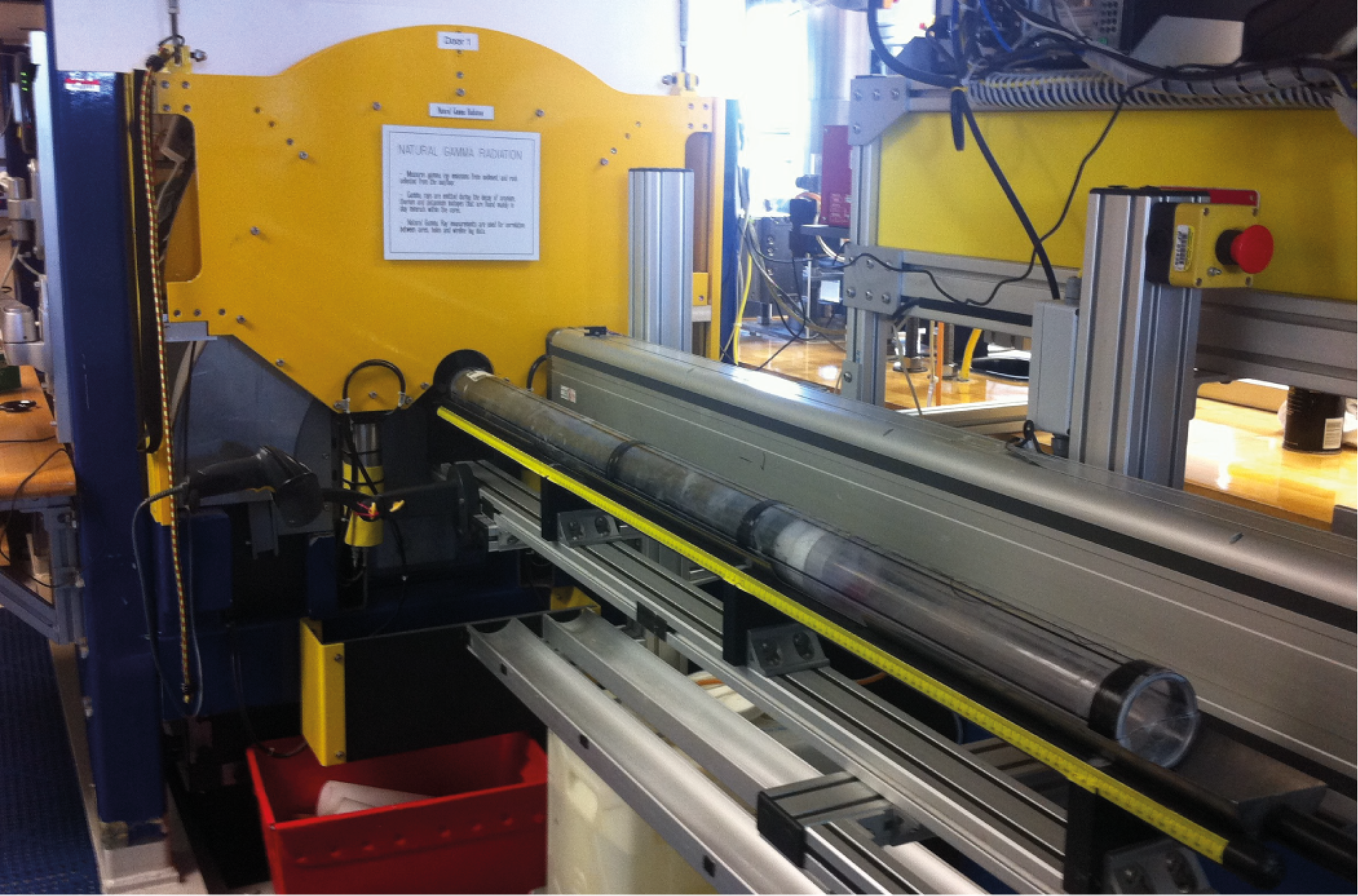
Figure F10. NGRL.
The main NGR detector unit consists of eight sodium iodide (NaI) detectors arranged along the core measurement axis at 20 cm intervals surrounding the lower half of the section (Figure F11) (Vasiliev et al., 2011). The detector array has passive (layers of lead) and active (plastic scintillators) shielding to reduce the background environmental and cosmic radiation. The overlying plastic scintillators detect incoming high-energy gamma and muon cosmic radiation and cancel this signal from the total counted by the NaI detectors.
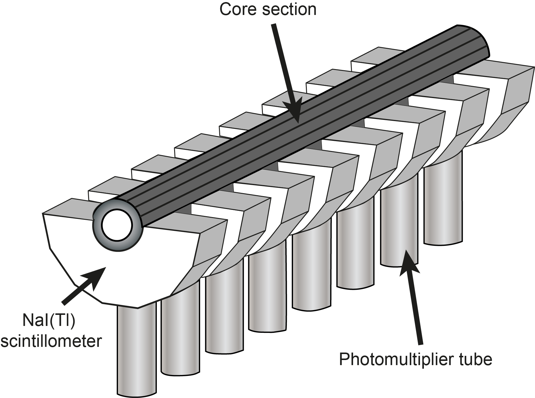
Figure F11. Main components of the NGRL.
Each measurement run consisted of two sample positions 10 cm apart for a total of 16 measurements per 150 cm section. The quality of the energy spectrum measured in a core depends on the concentration of radionuclides in the sample but also on the counting time, and higher times yield better spectra. Counting times were chosen as 5 min per position or ~10 min per section, yielding statistically significant energy spectra (Vasiliev et al., 2011).
During Expedition 378, a software error resulted in overwrite of the calibration file. As a result, all core sections measured used an incomplete calibration file, and the NGR calibration files in the LIMS database are missing the slope and intercept for channel to energy conversion. Although missing energy conversion information does not affect data reduction and reported counts/s, threshold channel number picks can affect the data reduction on reported counts/s in the LIMS database. Core sections were run with threshold channel numbers either one higher or the same as would have been picked by hand using a complete calibration, and even though picks of neighboring channels have a statistically insignificant impact on the overall data, concentration studies require a complete set of calibrations. A complete calibration file set is available in NGR_CALIBRATION in Supplementary material.
6.4. Thermal conductivity measurements
Thermal conductivity is an intrinsic material property for which values depend on the chemical composition, porosity, density, structure, and fabric of the material. After NGR measurements were completed, thermal conductivity was measured with the Teka Bolin TK04 system using a needle probe method in full-space configuration for whole-round sediment cores (Von Herzen and Maxwell, 1959). The probes contain a heater wire and calibrated thermistor.
The needle probe was inserted into a 2 mm diameter hole drilled through the liner along one of the lines that later guided core splitting. To avoid interference from air flow in the laboratory, the core was placed into an enclosed box outfitted with foam (Figure F12). The calibrated heat source of the probe was then turned on, and the increase in temperature was recorded over 80 s. A heating power of 2 to 2.5 W/m was typically used. The solution to the heat conduction equation with a line source of heat was then fit to the temperature measurements to obtain the thermal conductivity. Because the probe is much more conductive than sediment, it is assumed to be a perfect conductor. Under this assumption, the temperature of the superconductive probe has a linear relationship with the natural logarithm of the time after the initiation of the heat:
- T = temperature (K),
- q = heat input per unit length per unit time (J/m/s),
- k = thermal conductivity (W/[m·K]),
- t = time after the initiation of the heat (s), and
- C = instrumental constant.
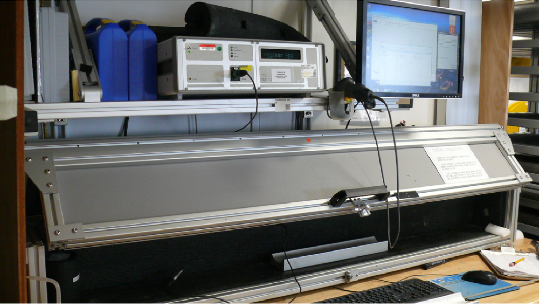
Figure F12. Thermal conductivity TK04 case.
Three measuring cycles were automatically performed to calculate average conductivity. A self-test, which included a drift study, was conducted at the beginning of each measurement cycle. Once the probe temperature stabilized, the heater circuit was closed and the temperature rise in the probe was recorded. Thermal conductivity was calculated from the rate of temperature rise while the heater current was flowing. Temperatures measured during the first 80 s of the heating cycle were fitted to an approximate solution of a constantly heated line source (Kristiansen, 1982; Blum, 1997). For Site U1553, thermal conductivity profiles of sediment and rock sections were used along with in situ temperature measurements to determine heat flow using methods described in Pribnow et al. (2000).
Measurement errors were 5%–10%. Thermal conductivity measurements were routinely taken in one section per core (typically Section 3 or 4) for Hole U1553A and Cores 378-U1553B-27X through 29X, which extend past the bottom of Hole U1553A. Thermal conductivity measurements were not taken on cores from Holes U1553C and U1553D because cracks in the cores due to rotary coring and lithified sediments caused poor coupling of the needle probe to the sediment. No measurements were taken on cores from Hole U1553E because it spanned the same depths as Holes U1553A and U1553B.
6.5. X-ray imaging
X-ray images of all cores were produced to evaluate bioturbation intensity, drilling disturbance, sedimentary structures, and clast abundance. Images were obtained on all whole-round core sections prior to splitting and often during the 4 h thermal equilibrium period because X-ray imaging is not temperature sensitive. The onboard XRI is composed of a Teledyne ICM CP120B X-ray generator and a detector unit. The generator works with a maximum voltage of 120 kV and a tube current of 1 A, and it has a 0.8 mm × 0.5 mm focal spot. The generator produces a directional cone at a beam angle of 50° × 50°. The detector unit is located 65 cm from the source and consists of a Go-Scan 1510 H system composed of an array of complementary metal oxide semiconductor (CMOS) sensors arranged to offer an active area of 102 mm × 153 mm and a resolution of 99 µm. Core sections were run through the imaging area at 12 cm intervals, providing images of 15 cm onto the detector and allowing an overlap of 3 cm.
Tests were conducted on whole-round sections to obtain the best image resolution for determining the internal structure of cores. The XRI settings were then changed to adjust to the varying lithologies of the cores. The number of images stacked was 20, taken at exposure times of 300 s, and the current was kept at 0.7 mA. The voltage ranged between 70 and 90 kV; higher voltages were used for denser lithologies.
The raw images were collected as 16-bit images and were processed with the IODP in-house processing utility in the Integrated Measurement System software (version 1.3). The software applies corrections for the detector (gain and offset corrections), compensates for core shape and thickness, and adjusts the image contrast. The Savitzky-Golay FIR filter was chosen to smooth images. The resulting processed images include a masked background, the depth scale of the section, and the acquisition parameters. The software applies different processing to APC or HLAPC cores than to RCB cores. Some sections where the processing utility did not give good results were reprocessed, first with the LeVay processing software and later with the processing utility (images are available upon request from the IODP Data Librarian: database@iodp.tamu.edu).
6.6. Section Half Multisensor Logger measurements
We measured color reflectance and MS on archive halves using the SHMSL (Figure F13). The archive half was placed on the core track, above which an electronic platform moves along a track recording the height of the split surface with a laser sensor. The laser establishes the location of the bottom of the section, and then the platform reverses the direction of movement, moving from bottom to top making measurements of MSP and color reflectance. During Expedition 378, MSP and color reflectance data were collected at a 2.5 cm resolution. These measurements have a sufficient resolution for comparison with the results obtained from the MS loop on the WRMSL.

Figure F13. SHMSL.
6.6.1. Color reflectance spectrometry
The color reflectance spectrometer uses an Ocean Optics 30 mm integrating sphere and both a halogen and LED light source, which cover wavelengths from ultraviolet through visible to near infrared. The measurements were taken from 380 to 900 nm wavelengths at 2 nm intervals. The approximately 3 s data acquisition offset was applied for the entire scan of the archive half. The data are reported using the L*a*b* color system, in which L* is lightness, a* is redness (positive) versus greenness (negative), and b* is yellowness (positive) versus blueness (negative). The color reflectance spectrometer calibrates on two spectra, pure white (reference) and pure black (dark). Color calibration was conducted approximately once every 6 h (twice per shift).
6.6.2. Point magnetic susceptibility
MSP was measured at a 2.5 cm resolution using a Bartington MS2 meter and an MS2K contact probe with a flat 15 mm diameter round sensor with a field of influence of 25 mm and an operation frequency of 930 Hz. The instrument averages three measurements from the sensor for each offset, giving an accuracy of ~5%. The spatial resolution of the MSP instrument is ~3.8 mm, higher than that of the whole-round MS. This measurement is therefore better suited for sections containing broken pieces <4 cm in length (the spatial resolution of whole-round MS). As with whole-round measurements, the output displayed by the MSP sensor can be converted to dimensionless SI units by multiplying by 10−5. The probe is zeroed in air before each measurement location to avoid influence from the metal track. The MSP meter was calibrated by the manufacturer before installation on the ship and is quality checked every ~6 h at the same time as color reflectance sensor calibration.
6.7. Section Half Measurement Gantry measurements
P-wave velocity measurements were performed on working halves before samples were taken. P-wave velocity measurements were made using the x-axis caliper contact probe transducers on the Section Half Measurement Gantry (SHMG) (Figure F14) for two analyses per core, generally in Sections 2 and 5. Additional measurements were taken where there was a change in lithology. Measurements were usually taken at ~75 cm in the section and as close as possible to where the MAD sample was taken. However, if this interval provided poor sediment/transducer coupling (e.g., had significant cracking), exhibited drilling disturbance, was in between biscuits of core, or was not representative of the core section, different positions were selected to ensure viable data.
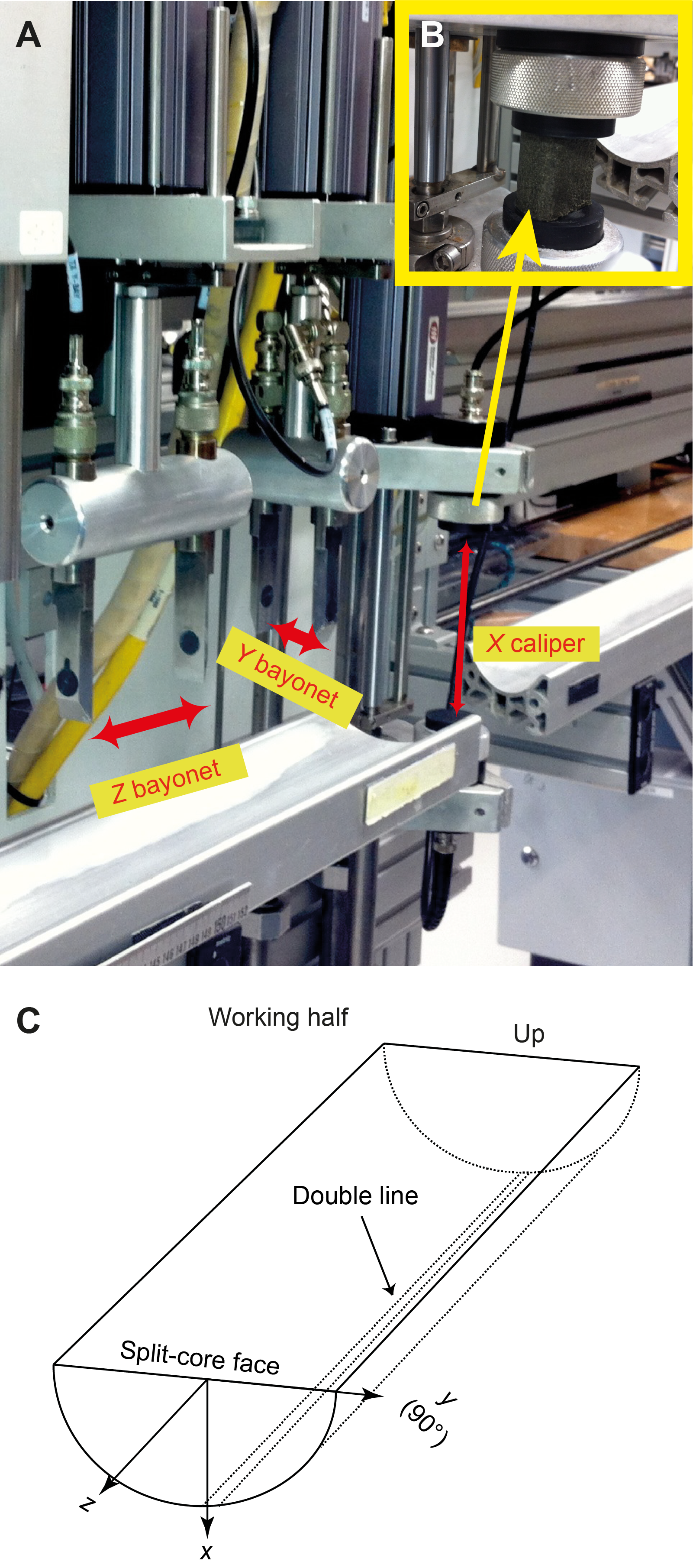
Figure F14. Section Half Measurement Gantry and axes.
The P-wave velocity system uses Panametrics-NDT Microscan delay line transducers, which transmit at 0.5 MHz. The signal received through the section half or the discrete sample was recorded by the computer attached to the system. The first P-wave arrival was selected by the autopicking software and confirmed by a manual check. The distance between transducers was measured with a built-in linear voltage displacement transformer. Calibration was performed with a series of acrylic cylinders of differing thicknesses and a known P-wave velocity of 2750 ± 20 m/s. The determined system time delay from calibration was subtracted from the picked arrival time to give a traveltime of the P-wave through the sample. The thickness of the sample (calculated by the linear voltage displacement transformer, in meters) was divided by the traveltime (in seconds) to calculate P-wave velocity in meters per second.
6.8. Shear and compressional strength measurements
Shear strength is the resistance of a material to failure in shear. Shear stress in unconsolidated materials is resisted only by the network of solid particles. Shear strength (τf) can be expressed as a function of the effective normal stress at failure (σ′), the effective cohesion (c′), and the friction angle (φ′):
where c′ and φ′ are the shear strength parameters that define a linear relationship between τf and φ′, according to the Mohr-Coulomb failure criterion.
Shear strength parameters can be determined by multiple laboratory tests. The c′ and φ′ are relevant in situations where field drainage conditions correspond to test conditions. The shear strength of a soil under undrained conditions (IW drainage does not occur during failure) is different from that under drained conditions (IW drainage occurs).
Undrained shear strength (Su) can be expressed in terms of total stress in the case of fully saturated materials of low permeability (e.g., clays). The most common strength tests in shipboard laboratories are the vane shear and penetrometer tests, which provide measurements of undrained shear strength (Blum, 1997).
During Expedition 378, Su was measured in undisturbed soft sediment using a handheld Torvane shear device on working halves because the commonly employed automated vane shear device was broken. Using the Torvane device, undrained shear strength was determined by inserting a vane into the split core and rotating it while maintaining a constant vertical pressure at a constant rate such that failure occurred in 5–10 s. Measurements were made with the vane rotation axis perpendicular to the split surface. The maximum shear value was then read off the Torvane dial in kilograms per square centimeter (kg/cm2). The 1.0 and 2.5 adapters were used, depending on the stiffness of the sediment. The mechanical scale is in units of kilograms per square centimeter, and the data were uploaded to the LIMS database in this form.
A pocket penetrometer was used to measure the unconfined compressive strength of the unconsolidated sediments. The penetrometer is a flat-footed, spring-operated device used to measure compressive strength by pushing a 0.25 inch (6.4 mm) diameter probe 0.25 inches (6.4 mm) deep (to the red marker) below the split surface (test spots with a smooth surface were selected). The mechanical scale is in kilograms per square centimeter, and the data were uploaded to the LIMS database in this form.
The compressive strength was read directly off the pocket penetrometer. The force in kilograms per square centimeter can be converted to kilopascals (kPa) using the following formula:
The maximum shear strength that can be measured with the pocket penetrometer is 4.5 kg/cm2.
Torvane and penetrometer measurements were taken in two sections per core (usually Sections 2 and 5) for Hole U1553A only until the sediment became too firm for instrument penetration (below Core 20H; ~165 mbsf).
6.9. Discrete sample measurements of moisture and density
Discrete samples were collected from the working halves as close as possible to where the P-wave velocity, shear strength, and compressional strength measurements were taken to determine wet and dry bulk density, grain density, water content, and porosity. Generally, MAD samples were taken from two sections per core for Holes U1553A and U1553C (generally Sections 2 and 5), and additional samples were taken near the base of Holes U1553B and U1553D, where the depth of the holes exceeded that of Holes U1553A and U1553C, respectively. Most MAD samples were taken adjacent to or near the XRD and carbonate content samples. For each sample, ~10 cm3 of sediment was extracted from the working half and placed in numbered, preweighed ~16 mL Wheaton glass vials for wet and dry sediment weighing, drying, and dry volume measurements. For softer sediments, MAD samples were taken using a plastic syringe, and for stiffer, lithified sediments, already broken pieces of sediment were extracted using a spatula or rock saw. The volumes of the numbered Wheaton vials were calculated before the expedition by multiplying each vial’s weight against the average density of the vial glass.
After wet sediment analysis, samples were dried in a convection oven for at least 24 h at 105°C ± 5°C. Dried samples were then cooled to room temperature in a desiccator for ~4 h before the dry mass and volume were measured. The weights of wet and dry sample masses were determined to a precision of 0.005 g using paired Mettler Toledo electronic balances, with one acting as a reference to compensate for the ship’s motion. A standard weight of similar value to the sample was placed upon the reference balance to increase accuracy. A computer averaging system was used to compensate for the ship’s motion and calculate a more accurate mass. The default setting of the balances is 300 measurements (taking ~1.5 min), and the balances were tared approximately every 12 h at the beginning of a shift.
Dry sample volume was determined using a hexapycnometer system of a six-celled, custom-configured Micrometrics AccuPyc 1330TC helium-displacement pycnometer (Figure F15). The precision of each cell is 1% of the full-scale volume. Volume measurement was preceded by three purges of the sample chamber with helium warmed to ~28°C. Three measurement cycles were run for each sample. A reference volume (set of two calibration spheres) was placed sequentially in each of the chambers to check for instrument drift and systematic error. The procedures for the determination of these physical properties comply with the American Society for Testing and Materials (ASTM) designation (D) 2216 (ASTM International, 1990). The fundamental relation and assumptions for the calculations of all physical property parameters are discussed by Blum (1997) and summarized below.
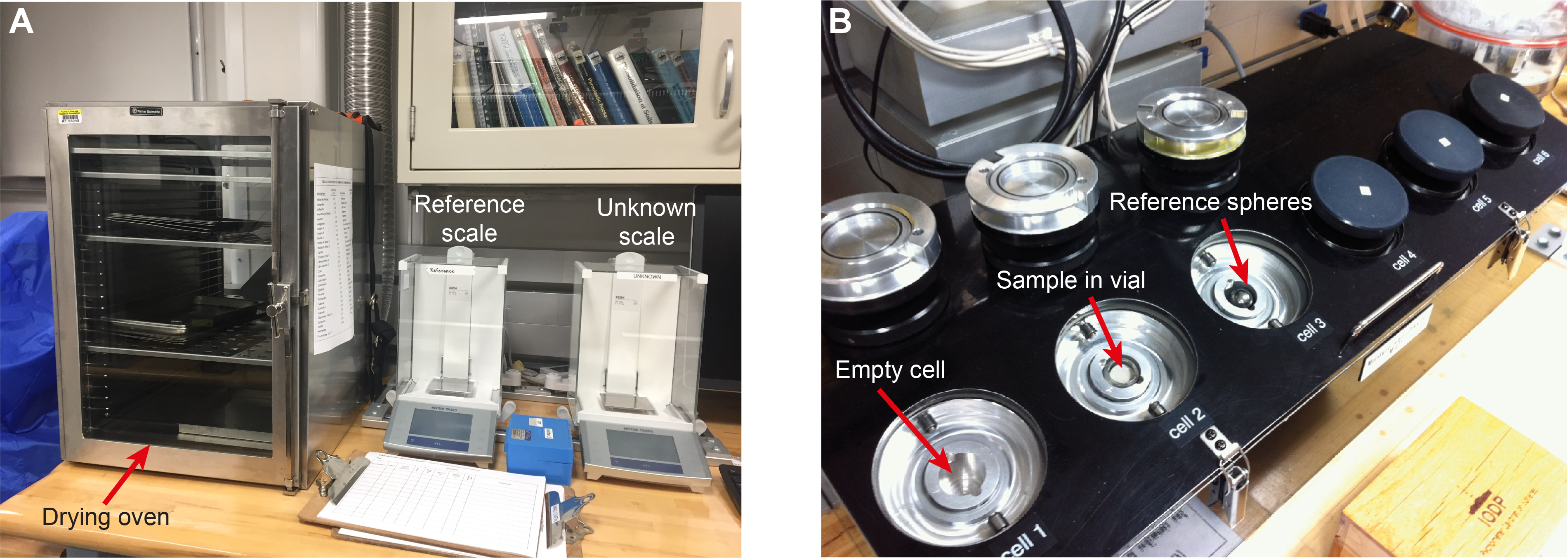
Figure F15. Drying oven, balances, and pycnometer.
6.9.1. Mass and volume calculation
Wet mass (Mwet), dry mass (Mdry), and dry volume (Vdry) were measured on MAD samples. The ratio of mass (rm) is a computational constant of 0.965 (i.e., 0.965 g of freshwater per 1 g of seawater). Salt precipitated in sediment pores during the drying process is included in the Mdry and Vdry values. The masses of the evaporated water (Mwater) and salt (Msalt) in the sample are given by
where s is the assumed saltwater salinity (0.035) corresponding to a pore water density (ρpw) of 1.024 g/cm3 and a salt density (ρsalt) of 2.22 g/cm3. The corrected mass of pore water (Mpw), volume of pore water (Vpw), mass of solids excluding salt (Msolid), volume of salt (Vsalt), volume of solids excluding salt (Vsolid), and wet volume (Vwet) are
6.9.1.1. Calculation of bulk properties
For all sediment samples, water content (w) is expressed as the ratio of pore water mass to wet sediment (total) mass:
Wet bulk density (ρwet), dry bulk density (ρdry), sediment grain density (ρsolid), porosity (), and void ratio (VR) are calculated as
MAD properties reported and plotted in Physical properties in the Site U1553 chapter (Röhl et al., 2022a) were calculated with the MADMax shipboard program’s Method C calculation process.
6.10. In situ temperature measurements
In situ temperature measurements were made with the APCT-3 tool in Cores 378-U1553A-4H, 7H, and 10H and with the SET2 tool during the drill down in Hole U1553D at 181 mbsf.
The APCT-3 tool fits directly into the coring shoe of the APC system and consists of a battery pack, a data logger, and a platinum resistance-temperature device calibrated over a temperature range of 0°–30°C. Before entering the borehole, the tool is first stopped at the mudline for 5 min to thermally equilibrate with bottom water. However, the lowest temperature recorded during the run was occasionally used instead of the average temperature at the mudline as an estimate of the bottom water temperature because it was more repeatable and the bottom water is expected to have the lowest temperature in the profile. When the APC system is plunged into the formation, there is an instantaneous temperature rise from frictional heating. This heat gradually dissipates into the surrounding sediment as the temperature at the APCT-3 tool equilibrates toward the temperature of the sediment. After the APC system penetrated the sediment, it was held in place for up to 10 min while the APCT-3 tool recorded the temperature of the cutting shoe every second.
The SET2 tool is designed to take temperature measurements in sediments that are too consolidated to use the APCT-3 tool. The SET2 tool is lowered into the hole using the motion decoupled hydraulic delivery system (MDHDS) and released electronically using the Electric RS (ERS) Overshot/MDHDS tools. The smooth tapered probe tip is designed to create a seal against the sediments as it is pushed in so that in situ temperature measurements can be recorded. The temperature measurement is taken at the tip of the thermistor string using a thermistor. Typical recording time for the tool in sediment is 20 min. After temperature measurements are recorded, the tool is retrieved using the ERS/MDHDS and the SET2 tool is moved to the laboratory for data download.
The equilibrium temperature of the sediment was estimated by applying a mathematical heat-conduction model to the temperature decay record (Horai and Von Herzen, 1985). The synthetic thermal decay curve for the APCT-3 tool is a function of the geometry and thermal properties of the probe and the sediment (Bullard, 1954; Horai and Von Herzen, 1985). Equilibrium temperature was estimated by applying a fitting procedure (Pribnow et al., 2000). The nominal accuracy of APCT-3 temperature measurements is ±0.05°C.
APCT-3 temperature data were combined with measurements of thermal conductivity obtained from whole-round core sections to obtain heat flow values. Heat flow was calculated according to the Bullard method to be consistent with the synthesis of ODP heat flow data by Pribnow et al. (2000) and using the average approach because there was no distinct trend in the thermal conductivity with depth.
7. Stratigraphic correlation and composite section
Assembly and verification of a complete composite stratigraphic section require construction of a composite depth scale. It has been demonstrated that a continuous section is never recovered from a single borehole because of core recovery gaps between successive APC and XCB cores even with nominal recovery of 100% or more (e.g., Ruddiman et al., 1987; Hagelberg et al., 1992). Construction of a complete stratigraphic section, referred to as a composite splice, requires combining stratigraphic intervals from two or more holes cored at the same site. To achieve overlapping core recovery in successive holes, the driller targets a different depth of penetration (i.e., different mudline depth) for the first core of each hole. This practice ensures that most between-core intervals missing for a given hole are recovered in at least one of the adjacent holes. Our composite section and splice construction methodology follows one that has been successfully employed during a number of previous ODP legs and Integrated Ocean Drilling Program and IODP expeditions.
Once a composite depth scale has been completed, a stratigraphically continuous and complete composite splice can be created from representative intervals from the multiple holes. Ideally, both core recovery gaps and intervals with coring deformation are absent in the spliced section. The continuity and completeness of the spliced section are dependent on avoiding coeval core recovery gaps in multiple holes, which is addressed through adjustments to the depths at which a core is collected during drilling operations.
Site U1553 drilling operations began with two holes cored using the APC and XCB systems, followed by two holes cored using the RCB system and a third APC/XCB hole. The scientific objectives of Expedition 378 required the recovery of a complete upper stratigraphic section at Site U1553 from Holes U1553A, U1553B, and U1553E. Incomplete recovery of core from the RCB-cored Holes U1553C and U1553D made correlation challenging, except for good recovery of and correlation within the interval that includes the Paleocene/Eocene Thermal Maximum.
7.1. Core composite depth scale
The goal of constructing a composite depth scale is to place coeval, laterally continuous stratigraphic features into a common frame of reference by depth shifting the mbsf depth scales of individual cores to maximize correlation between holes. In the composite depth scale used by IODP, referred to as core composite depth below seafloor (CCSF), the depths of individual cores can only be shifted by a constant amount without permitting expansion or contraction of the relative depth scale within any core. Ultimately, this provides good first-order correlation between cores from different holes and avoids more subjective, and potentially erroneous, interpretations. The CCSF scale, once established, provides a basis upon which higher order depth composite scales can be built.
In essence, the CCSF scale overcomes many of the inadequacies of the mbsf depth scale, which is based on drill pipe measurements and is unique to each hole. The mbsf depth scale is based on the length that the drill string is advanced on a core-by-core basis and is often inaccurate because of ship heave (which is not compensated for in APC coring), tidal variations in sea level, and other sources of error. In contrast, the CCSF scale is built by anchoring the composite depth scale to the longest first core that captures the mudline because this is typically the only core for which the mbsf and CCSF depths are equivalent. From this anchor, physical property core logging data (e.g., bulk density and MS) are correlated among holes downsection. For each core, a depth offset (a constant) that best aligns the physical property variations to the equivalent cores in adjacent holes is added to the mbsf depth in sequence downhole. Depth offsets are often chosen to optimize correlation of specific features that define splice levels in cores from adjacent holes.
For Site U1553, shipboard scanning data collected during operations did not exhibit sufficient variation to confidently correlate sequences and construct a splice. The final offsets and splice, therefore, were determined through analysis of postcruise XRF scanning, which was performed at the GCR in College Station, Texas (USA). Splice construction was done by the correlation team at their respective home institutions.
The initial (shipboard) CCSF scale was based on the stratigraphic correlation of data from the STMSL, WRMSL, SHMSL, NGRL, and SHIL. STMSL data were only used for real-time continuity assessment and are not presented in this volume. NGRL data were collected at 10 cm intervals, STMSL data at 5 cm intervals, and WRMSL and SHMSL at 2.5 cm intervals. The SHIL scans have a depth resolution of approximately 30 µm. XRF data were collected at ~2 cm intervals. The raw stratigraphic data were imported into Correlator version 3.1 and culled as necessary to avoid incorporating anomalous data influenced by edge effects at section boundaries and by coring disturbance. Additionally, correlators employed the Code for Ocean Drilling Data (CODD), an Igor Pro–based system designed to integrate ocean drilling data of all types with depth-scaled core images (https://www.CODD-Home.net).
Because depth intervals within cores are not compressed or expanded by Correlator, it is not possible to align all correlative features with the same offset. Expansion or compression between cores from different holes may reflect small-scale differences in sedimentation and/or distortion caused by the coring and archiving processes. The tops of APC cores are generally expanded, and the bottoms are compressed, although this effect is lithology dependent. In addition, sediment (especially unconsolidated mud, ash, sand, and gravel) occasionally falls from higher levels in the borehole onto the tops of cores as they are recovered, and as a result the uppermost 0–100 cm of many cores are not part of the stratigraphically continuous section.
Correlations among cores from adjacent holes are evaluated visually and statistically by cross-correlation within a 2 m depth interval, which can be adjusted in length when appropriate. Depth-shifted data are denoted by CCSF. See Table T16 in the Site U1553 chapter (Röhl et al., 2022a) for the depth offsets for each core. These tables are necessary for converting the scale from mbsf to CCSF. The CCSF depth for any point in a core equals the mbsf depth plus the cumulative offset. Correlation at finer resolution is not possible with Correlator because a single adjustment is applied to entire cores; no adjustments, such as squeezing and stretching, are made within cores.
The stratigraphic correlator group for Expedition 378 was unique, consisting of one shipboard correlator (with assistance from a Co-Chief Scientist experienced in correlation) and one shore-based member of the science party. Our shore-based stratigraphic correlator used the data and images sent from the ship to verify and correct our initial hole-to-hole correlation and assist in the construction of a provisional CCSF scale for Site U1553 that was improved by utilizing the onshore XRF core scanning data (see Geochemistry).
References
Abelmann, A., 1990. Oligocene to middle Miocene radiolarian stratigraphy of southern high latitudes from Leg 113, Sites 689 and 690, Maud Rise. In Baker, P.F., Kennett, J.P., et al., Proceedings of the Ocean Drilling Program, Initial Reports, 113: College Station, TX (Ocean Drilling Program), 675–708. https://doi.org/
Agnini, C., Fornaciari, E., Raffi, I., Catanzariti, R., Pälike, H., Backman, J., and Rio, D., 2014. Biozonation and biochronology of Paleogene calcareous nannofossils from low and middle latitudes. Newsletters on Stratigraphy, 47(2):131–181. https://doi.org/
Agnini, C., Fornaciari, E., Raffi, I., Rio, D., Röhl, U., and Westerhold, T., 2007. High-resolution nannofossil biochronology of middle Paleocene to early Eocene at ODP Site 1262; implications for calcareous nannoplankton evolution. Marine Micropaleontology, 64(3):215–248. https://doi.org/
Agnini, C., Muttoni, G., Kent, D.V., and Rio, D., 2006. Eocene biostratigraphy and magnetic stratigraphy from Possagno, Italy: the calcareous nannofossil response to climate variability. Earth and Planetary Science Letters, 241(3–4):815–830. https://doi.org/
Agnini, C., Spofforth, D.J.A., Dickens, G.R., Rio, D., Pälike, H., Backman, J., Muttoni, G., and Dallanave, E., 2016. Stable isotope and calcareous nannofossil assemblage record of the late Paleocene and early Eocene (Cicogna section). Climate of the Past, 12(4):883–909. https://doi.org/
ASTM International, 1990. Standard method for laboratory determination of water (moisture) content of soil and rock (Standard D2216–90). In Annual Book of ASTM Standards for Soil and Rock: Philadelphia (American Society for Testing Materials).
Backman, J., Raffi, I., Rio, D., Fornaciari, E., and Pälike, H., 2012. Biozonation and biochronology of Miocene through Pleistocene calcareous nannofossils from low and middle latitudes. Newsletters on Stratigraphy, 45(3):221–244. https://doi.org/
Balsam, W.L., and Damuth, J.E., 2000. Further investigations of shipboard vs. shore-based spectral data: implications for interpreting Leg 164 sediment composition. In Paull, C.K., Matsumoto, R., Wallace, P.J., and Dillon, W.P. (Eds.), Proceedings of the Ocean Drilling Program, Scientific Results, 164: College Station, TX (Ocean Drilling Program), 313–324. https://doi.org/
Balsam, W.L., Damuth, J.E., and Schneider, R.R., 1997. Comparison of shipboard vs. shore-based spectral data from Amazon Fan cores: implications for interpreting sediment composition. In Flood, R.D., Piper, D.J.W., Klaus, A., and Peterson, L.C. (Eds.), Proceedings of the Ocean Drilling Program, Scientific Results. 155: College Station, TX (Ocean Drilling Program), 193–215. https://doi.org/
Balsam, W.L., Deaton, B.C., and Damuth, J.E., 1998. The effects of water content on diffuse reflectance spectrophotometry studies of deep-sea sediment cores. Marine Geology, 149(1):177–189. https://doi.org/
Berggren, W.A., Kent, D.V., Swisher, C.C., III, Aubry, M.-P., Berggren, W.A., Kent, D.V., Aubry, M.-P., and Hardenbol, J., 1995. A revised Cenozoic geochronology and chronostratigraphy. In Berggren, W.A., Kent, D.V., Aubry, M.-P., and Hardenbol, J. (Eds.), SEPM Special Publication (Volume 54): Geochronology, Time Scales and Global Stratigraphic Correlation: Tulsa, OK (SEPM Society for Sedimentary Geology). https://doi.org/
Blaj, T., Backman, J., and Raffi, I., 2009. Late Eocene to Oligocene preservation history and biochronology of calcareous nannofossils from paleo-equatorial Pacific Ocean sediments. Rivista Italiana di Paleontologia e Stratigrafia, 1:67–85. http://urn.kb.se/
Blum, P., 1997. Physical properties handbook: a guide to the shipboard measurement of physical properties of deep-sea cores. Ocean Drilling Program Technical Note, 26. https://doi.org/
Bown, P., 2005. Palaeogene calcareous nannofossils from the Kilwa and Lindi areas of coastal Tanzania (Tanzania Drilling Project Sites 1 to 10, 2003–4). Journal of Nannoplankton Research, 27(1):21–95.
Bown, P.R., 1998. Calcareous Nannofossil Biostratigraphy: Dordrect, Netherlands (Kluwer Academic Publishing).
Bown, P.R., and Young, J.R., 1998. Techniques. In Bown, P.R. (Ed.), Calcareous Nannofossil Biostratigraphy: Dordrect, Netherlands (Kluwer Academic Publishing), 16–28.
Bullard, E.C., 1954. The flow of heat through the floor of the Atlantic Ocean. Proceedings of the Royal Society of London, Series A: Mathematical and Physical Sciences, 222(1150):408–429. https://doi.org/
Cande, S.C., and Kent, D.V., 1992. A new geomagnetic polarity time scale for the Late Cretaceous and Cenozoic. Journal of Geophysical Research: Solid Earth, 97(B10):13917–13951. https://doi.org/
Crouch, E.M., Willumsen, P.S., Kulhanek, D.K., and Gibbs, S.J., 2014. A revised Paleocene (Teurian) dinoflagellate cyst zonation from eastern New Zealand. Review of Palaeobotany and Palynology, 202:47–79. https://doi.org/
Crundwell, M.P., Morgans, H.E.G., and Hollis, C.J., 2016. Micropaleontological report on dredge samples collected during the 2015 VESPA (Volcanic Evolution of South Pacific Arcs) expedition. GNS Science Internal Report, 22:83.
Dallanave, E., Agnini, C., Bachtadse, V., Muttoni, G., Crampton, J.S., Strong, C.P., Hines, B.R., Hollis, C.J., and Slotnick, B.S., 2015. Early to middle Eocene magneto-biochronology of the southwest Pacific Ocean and climate influence on sedimentation: insights from the Mead Stream section, New Zealand. Geological Society of America Bulletin, 127(5–6):643–660 https://doi.org/
De Vleeschouwer, D., Dunlea, A.G., Auer, G., Anderson, C.H., Brumsack, H., de Loach, A., Gurnis, M., et al., 2017. Quantifying K, U, and Th contents of marine sediments using shipboard natural gamma radiation spectra measured on DV JOIDES Resolution. Geochemistry, Geophysics, Geosystems, 18(3):1053–1064. https://doi.org/
Dickens, G.R., Koelling, M., Smith, D.C., Schnieders, L., and the IODP Expedition 302 Scientists, 2007. Rhizon sampling of pore waters on scientific drilling expeditions: an example from the IODP Expedition 302, Arctic Coring Expedition (ACEX). Scientific Drilling, 4:22–25. https://doi.org/
Dickson, J.A.D., 1965. A modified staining technique for carbonates in thin section. Nature, 205(4971):587. https://doi.org/
Droser, M.L., and Bottjer, D.J., 1986. A semiquantitative field classification of ichnofabric. Journal of Sedimentary Research, 56(4):558–559. https://doi.org/
Dunham, R.J., and Ham, W.E., 1962. Classification of carbonate rocks according to depositional texture. AAPG Memoir, 1.
Dunlea, A.G., Murray, R.W., Harris, R.N., Vasiliev, M.A., Evans, H., Spivack, A.J., and D’Hondt, S., 2013. Assessment and use of NGR instrumentation on the JOIDES Resolution to quantify U, Th, and K concentrations in marine sediment. Scientific Drilling, 15:57–63. https://doi.org
Embry, A.F., and Klovan, J.E., 1972. Absolute water depth limits of late Devonian paleoecological zones. Geologische Rundschau, 61(2):672–686. https://doi.org/
Expedition 318 Scientists, 2011. Methods. In Escutia, C., Brinkhuis, H., Klaus, A., and the Expedition 318 Scientists, Proceedings of the Integrated Ocean Drilling Program, 318: Tokyo (Integrated Ocean Drilling Program Management International, Inc.). https://doi.org/
Expedition 330 Scientists, 2012. Methods. In Koppers, A.A.P., Yamazaki, T., Geldmacher, J., and the Expedition 330 Scientists, Proceedings of the Integrated Ocean Drilling Program, 330: Tokyo (Integrated Ocean Drilling Program Management International, Inc.). https://doi.org/
Fensome, R.A., Williams, G.L., and MacRae, R.A., 2019. The Lentin and Williams Index of Fossil Dinoflagellates 2019 Edition. American Association of Stratigraphic Palynologists Contributions Series, 50.
Fioroni, C., Villa, G., Persico, D., Wise, S.W., and Pea, L., 2012. Revised middle Eocene-upper Oligocene calcareous nannofossil biozonation for the Southern Ocean. Revue de Micropaléontologie, 55(2):53–70. https://doi.org/
Funakawa, S., and Nishi, H., 2005. Late middle Eocene to late Oligocene radiolarian biostratigraphy in the Southern Ocean (Maud Rise, ODP Leg 113, Site 689). Marine Micropaleontology, 54(3–4):213–247. https://doi.org/
Gee, J.S., Tauxe, L., and Constable, C., 2008. AMSSpin: a LabVIEW program for measuring the anisotropy of magnetic susceptibility with the Kappabridge KLY-4S. Geochemistry, Geophysics, Geosystems, 9(8):Q08Y02. https://doi.org/
Gieskes, J.M., 1975. Chemistry of interstitial waters of marine sediments. Annual Review of Earth and Planetary Sciences, 3:433–453. https://doi.org/
Gilmore, G.R., 2008. Practical Gamma-Ray Spectrometry, 2nd Edition: New York (Wiley). https://doi.org/
Gohl, K., Wellner, J.S., Klaus, A., Bauersachs, T., Bohaty, S.M., Courtillat, M., Cowan, E.A., De Lira Mota, M.A., Esteves, M.S.R., Fegyveresi, J.M., Frederichs, T., Gao, L., Halberstadt, A.R., Hillenbrand, C.-D., Horikawa, K., Iwai, M., Kim, J.-H., King, T.M., Klages, J.P., Passchier, S., Penkrot, M.L., Prebble, J.G., Rahaman, W., Reinardy, B.T.I., Renaudie, J., Robinson, D.E., Scherer, R.P., Siddoway, C.S., Wu, L., and Yamane, M., 2021. Expedition 379 methods. In Gohl, K., Wellner, J.S., Klaus, A., and the Expedition 379 Scientists, Amundsen Sea West Antarctic Ice Sheet History. Proceedings of the International Ocean Discovery Program, 379: College Station, TX (International Ocean Discovery Program). https://doi.org/
Gradstein, F.M., Ogg, J.G., Schmitz, M.D., and Ogg, G.M. (Eds.), 2012. The Geological Time Scale 2012: Amsterdam (Elsevier). https://doi.org/
Hagelberg, T., Shackleton, N., Pisias, N., and the Shipboard Scientific Party, 1992. Development of composite depth sections for Sites 844 through 854. In Mayer, L., Pisias, N., Janecek, T., et al., Proceedings of the Ocean Drilling Program, Initial Reports, 138: College Station, TX (Ocean Drilling Program), 79–85. https://doi.org/
Harland, W.B., Armstrong, R.L., Cox, A.V., Craig, L.E., Smith, A.G., and Smith, D.G., 1990. A Geologic Time Scale 1989: Cambridge, UK (Cambridge University Press).
Harris, R.N., Sakaguchi, A., Petronotis, K., Baxter, A.T., Berg, R., Burkett, A., Charpentier, D., Choi, J., Diz Ferreiro, P., Hamahashi, M., Hashimoto, Y., Heydolph, K., Jovane, L., Kastner, M., Kurz, W., Kutterolf, S.O., Li, Y., Malinverno, A., Martin, K.M., Millan, C., Nascimento, D.B., Saito, S., Sandoval Gutierrez, M.I., Screaton, E.J., Smith-Duque, C.E., Solomon, E.A., Straub, S.M., Tanikawa, W., Torres, M.E., Uchimura, H., Vannucchi, P., Yamamoto, Y., Yan, Q., and Xhao, X., 2013. Methods. In Harris, R.N., Sakaguchi, A., Petronotis, K., and the Expedition 344 Scientists, Proceedings of the Integrated Ocean Drilling Program, 344: College Station, TX (Integrated Ocean Drilling Program). https://doi.org/
Hayward, B.W., 1986. A Guide to Paleoenvironmental Assessment Using New Zealand Cenozoic Foraminiferal Faunas: Lower Hutt, New Zealand (New Zealand Geological Survey).
Hollis, C.J., 1997. Cretaceous-Paleocene Radiolaria from Eastern Marlborough, New Zealand: Lower Hutt, New Zealand (Institute of Geological & Nuclear Sciences).
Hollis, C.J., 2002. Biostratigraphy and paleoceanographic significance of Paleocene radiolarians from offshore eastern New Zealand. Marine Micropaleontology, 46(3–4):265–316. https://doi.org/
Hollis, C.J., Pascher, K.M., Kamikuri, S.-I., Nishimura, A., Suzuki, N., and Sanfilippo, A., 2017. Towards an integrated cross-latitude event stratigraphy for Paleogene radiolarians. Newsletter of the International Association of Radiolarists, 15:288–289.
Hollis, C.J., Pascher, K.M., Sanfilippo, A., Nishimura, A., Kamikuri, S., and Shepherd, C.L., 2020. An Austral radiolarian biozonation for the Paleogene. Stratigraphy, 17(4):213–278.
Hollis, C.J., Waghorn, D.B., Strong, C.P., and Crouch, E.M., 1997. Integrated Paleogene Biostratigraphy of DSDP Site 277 (Leg 29): Foraminifera, Calcareous Nannofossils, Radiolaria, and Palynomorphs, Report 97/7: Lower Hutt, New Zealand (Institute of Geological & Nuclear Sciences Limited).
Horai, K., and Von Herzen, R.P., 1985. Measurement of heat flow on Leg 86 of the Deep Sea Drilling Project. In Heath, G.R., Burckle, L. H., et al., Initial Reports of the Deep Sea Drilling Project, 86: Washington, DC (US Government Printing Office), 759–777. https://doi.org/
Hornibrook, N.B., Brazier, R.C., and Strong, C.P., 1989. Manual of New Zealand Permian to Pleistocene foraminiferal biostratigraphy. New Zealand Geological Survey Paleontological Bulletin, 56.
Huber, B., 1991. Paleogene and early Neogene planktonic foraminifer biostratigraphy of Sites 738 and 744, Kerguelen Plateau (southern Indian Ocean). In Barron, J., Larsen, B., et al., Proceedings of the Ocean Drilling Program, Scientific Results, 119: College Station, TX (Ocean Drilling Program), 427–451. https://doi.org/
Huber, B.T., and Quillévéré, F., 2005. Revised Paleogene planktonic foraminiferal biozonation for the austral realm. Journal of Foraminiferal Research, 35(4):299–314. https://doi.org/
Jaeger, J.M., Gulick, S.P.S., LeVay, L.J., Asahi, H., Bahlburg, H., Belanger, C.L., Berbel, G.B.B., Childress, L.B., Cowan, E.A., Drab, L., Forwick, M., Fukumura, A., Ge, S., Gupta, S.M., Kioka, A., Konno, S., März, C.E., Matsuzaki, K.M., McClymont, E.L., Mix, A.C., Moy, C.M., Müller, J., Nakamura, A., Ojima, T., Ridgway, K.D., Rodrigues Ribeiro, F., Romero, O.E., Slagle, A.L., Stoner, J.S., St-Onge, G., Suto, I., Walczak, M.H., and Worthington, L.L., 2014. Methods. In Jaeger, J.M., Gulick, S.P.S., LeVay, L.J., and the Expedition 341 Scientists, Proceedings of the Integrated Ocean Drilling Program, 341: College Station, TX (Integrated Ocean Drilling Program). https://doi.org/
Jones, R.W., and Brady, H.B., 1994. The Challenger Foraminifera: Oxford, UK (Oxford University Press).
Kamikuri, S., Moore, T.C., Ogane, K., Suzuki, N., Pälike, H., and Nishi, H., 2012. Early Eocene to early Miocene radiolarian biostratigraphy for the low-latitude Pacific Ocean. Stratigraphy, 9(1):77–108. https://www.micropress.org/
Kaminski, M., and Gradstein, F., 2005. Atlas of Paleogene Cosmopolitan Deep-Water Agglutinated Foraminifera: New York (Grzybowski Foundation). https://foraminifera.eu/
Kirschvink, J.L., 1980. The least-squares line and plane and the analysis of palaeomagnetic data. Geophysical Journal International, 62(3):699–718. https://doi.org/
Kristiansen, J.I., 1982. The transient cylindrical probe method for determination of thermal parameters of Earth materials [Ph.D. dissertation]. Åarhus University, Denmark. http://digitallib.oit.edu/
Lazarus, D.B., 1992. Antarctic Neogene radiolarians from the Kerguelen Plateau, Legs 119 and 120. In Wise, S.W., Jr., Schlich, R., et al., Proceedings of the Ocean Drilling Program, Scientific Results, 120: College Station, TX (Ocean Drilling Program), 785–809. https://doi.org/
Lourens, L., Hilgen, F., Shackleton, N.J., Laskar, J., and Wilson, D., 2005. The Neogene period. In Smith, A.G., Gradstein, F.M. and Ogg, J.G. (Eds.), A Geologic Time Scale 2004: Cambridge, UK (Cambridge University Press), 409–440. https://doi.org/
Lurcock, P.C., and Wilson, G.S., 2012. PuffinPlot: a versatile, user-friendly program for paleomagnetic analysis. Geochemistry, Geophysics, Geosystems, 13(6):Q06Z45. https://doi.org/
Marsaglia, K., Milliken, K., and Doran, L., 2013. IODP digital reference for smear slide analysis of marine mud, Part 1: Methodology and atlas of siliciclastic and volcanogenic components. Integrated Ocean Drilling Program Technical Note, 1. https://doi.org/
Marsaglia, K., Milliken, K., Leckie, R., Tentori, D., and Doran, L., 2015. IODP smear slide digital reference for sediment analysis of marine mud, Part 2: Methodology and atlas of biogenic components. Integrated Ocean Drilling Program Technical Note, 2. https://doi.org/
Martini, E., 1971. Standard Tertiary and Quaternary calcareous nannoplankton zonation. Proceedings of the Second Planktonic Conference, Roma, 1970, 739–785.
Mazzullo, J., Meyer, A., and Kidd, R., 1988. Appendix I: New sediment classification scheme for the Ocean Drilling Program. In Mazzullo, J., and Graham, A.G. (Eds.), Handbook for shipboard sedimentologists. Ocean Drilling Program Technical Note, 8:44–67. https://doi.org/
McKay, R.M., De Santis, L., Kulhanek, D.K., Ash, J.L., Beny, F., Browne, I.M., Cortese, G., Cordeiro de Sousa, I.M., Dodd, J.P., Esper, O.M., Gales, J.A., Harwood, D.M., Ishino, S., Keisling, B.A., Kim, S., Kim, S., Laberg, J.S., Leckie, R.M., Müller, J., Patterson, M.O., Romans, B.W., Romero, O.E., Sangiorgi, F., Seki, O., Shevenell, A.E., Singh, S.M., Sugisaki, S.T., van de Flierdt, T., van Peer, T.E., Xiao, W., and Xiong, Z., 2019. Expedition 374 methods. In McKay, R.M., De Santis, L., Kulhanek, D.K., and the Expedition 374 Scientists, Ross Sea West Antarctic Ice Sheet History. Proceedings of the International Ocean Discovery Program, 374: College Station, TX (International Ocean Discovery Program). https://doi.org/
Miller, M.D., Adkins, J.F., and Hodell, D.A., 2014. Rhizon sampler alteration of deep ocean sediment interstitial water samples, as indicated by chloride concentration and oxygen and hydrogen isotopes. Geochemistry, Geophysics, Geosystems, 15(6):2401–2413. https://doi.org/
Moore, T.C., Kamikuri, S.-I., Erhardt, A.M., Baldauf, J., Coxall, H.K., and Westerhold, T., 2015. Radiolarian stratigraphy near the Eocene–Oligocene boundary. Marine Micropaleontology, 116:50–62. https://doi.org/
Murray, R.W., Miller, D.J., and Kryc, K.A., 2000. Analysis of major and trace elements in rocks, sediments, and interstitial waters by inductively coupled plasma–atomic emission spectrometry (ICP-AES). Ocean Drilling Program Technical Note, 29. https://doi.org/
Naish, T.R., Levy, R.H., and Powell, R.D., 2006. Scientific Logistics Implementation Plan for the ANDRILL McMurdo Ice Shelf Project.
Nigrini, C.A., Sanfilippo, A., and Moore, T.J., Jr., 2006. Cenozoic radiolarian biostratigraphy: a magnetobiostratigraphic chronology of Cenozoic sequences from ODP Sites 1218, 1219, and 1220, equatorial Pacific. In Wilson, P.A., Lyle, M., and Firth, J.V. (Eds.), Proceedings of the Ocean Drilling Program, Scientific Results, 199: College Station, TX (Ocean Drilling Program). https://doi.org/
Nishimura, A., 1992. Paleocene radiolarian biostratigraphy in the northwest Atlantic at Site 384, Leg 43, of the Deep Sea Drilling Project. Micropaleontology, 38(4):317–362. https://doi.org/
Norris, R.D., Wilson, P.A., Blum, P., Fehr, A., Agnini, C., Bornemann, A., Boulila, S., Bown, P.R., Cournede, C., Friedrich, O., Ghosh, A.K., Hollis, C.J., Hull, P.M., Jo, K., Junium, C.K., Kaneko, M., Liebrand, D., Lippert, P.C., Li, Z., Matsui, H., Moriya, K., Nishi, H., Opdyke, B.N., Penman, D., Romans, B., Scher, H.D., Sexton, P., Takagi, H., Turner, S.K., Whiteside, J.H., Yamaguchi, T., and Yamamoto, Y., 2014. Methods. In Norris, R.D., Wilson, P.A., Blum, P., and the Expedition 342 Scientists, Proceedings of the Integrated Ocean Drilling Program, 342: College Station, TX (Integrated Ocean Drilling Program). https://doi.org/
O’Connor, B., 1999. Radiolaria from the late Eocene Oamaru diatomite, South Island, New Zealand. Micropaleontology, 45(1):1–55.
Olsson, R.K., Berggren, W.A., Hemleben, C., and Huber, B.T., 1999. Atlas of Paleocene Planktonic Foraminifera: Washington, DC (Smithsonian Institution Press). https://doi.org/
Pascher, K.M., Hollis, C.J., Bohaty, S.M., Cortese, G., McKay, R.M., Seebeck, H., Suzuki, N., and Chiba, K., 2015. Expansion and diversification of high-latitude radiolarian assemblages in the late Eocene linked to a cooling event in the southwest Pacific. Climate of the Past, 11(12):1599–1620. https://doi.org/
Pearson, P.N., Olsson, R.K., Huber, B.T., Hemleben, C., and Berggren, W.A., 2006. Atlas of Eocene planktonic foraminifera. Special Publication - Cushman Foundation for Foraminiferal Research, 41.
Perch-Nielsen, K., 1985a. Cenozoic calcareous nannofossils. In Bolli, H.M., Saunders, J.B. and Perch-Nielsen, K. (Eds.), Plankton Stratigraphy (Volume 1): Cambridge, UK (Cambridge University Press), 427–554.
Perch-Nielsen, K., 1985b. Mesozoic calcareous nannofossils. In Bolli, H.M., Saunders, J.B., and Perch-Nielsen, K. (Eds.), Plankton Stratigraphy (Volume 1): Cambridge, UK (Cambridge University Press), 329–426.
Presley, B.J., 1971. Appendix: techniques for analyzing interstitial water samples, Part 1: Determination of selected minor and major inorganic constituents. In Winterer, E.L., et al., Initial Reports of the Deep Sea Drilling Project, 7: Washington, DC (US Government Printing Office), 1749–1755. https://doi.org/
Pribnow, D.F.C., Kinoshita, M., and Stein, C.A., 2000. Thermal data collection and heat flow recalculations for ODP Legs 101–180: Hannover, Germany (Institut für Geowissenschaftliche Gemeinschaftsaufgaben). http://www-odp.tamu.edu/
Raffi, I., Backman, J., Fornaciari, E., Pälike, H., Rio, D., Lourens, L., and Hilgen, F., 2006. A review of calcareous nannofossil astrobiochronology encompassing the past 25 million years. Quaternary Science Reviews, 25(23):3113–3137. https://doi.org/
Raine, J.I., Beu, A.G., Boyes, A.F., Campbell, H.J., Cooper, R.A., Crampton, J.S., Crundwell, M.P., Hollis, C.J., Morgans, H.E.G., and Mortimer, N., 2015. New Zealand Geological Timescale NZGT 2015/1. New Zealand Journal of Geology and Geophysics, 58(4):398–403. https://doi.org/
Richter, C., Acton, G., Endris, C., and Radsted, M., 2007. Handbook for shipboard paleomagnetists. Ocean Drilling Program Technical Note, 34. https://doi.org/
Röhl, U., Thomas, D.J., Childress, L.B., Anagnostou, E., Ausín, B., Borba Dias, B., Boscolo-Galazzo, F., Brzelinski, S., Dunlea, A.G., George, S.C., Haynes, L.L., Hendy, I.L., Jones, H.L., Khanolkar, S.S., Kitch, G.D., Lee, H., Raffi, I., Reis, A.J., Sheward, R.M., Sibert, E., Tanaka, E., Wilkens, R., Yasukawa, K., Yuan, W., Zhang, Q., Zhang, Y., Drury, A.J., Crouch, E.M., and Hollis, C.J., 2022a. Site U1553. In Röhl, U., Thomas, D.J., Childress, L.B., and the Expedition 378 Scientists, South Pacific Paleogene Climate. Proceedings of the International Ocean Discovery Program, 378: College Station, TX (International Ocean Discovery Program). https://doi.org/
Röhl, U., Thomas, D.J., Childress, L.B., and the Expedition 378 Scientists, 2022b. Supplementary material, https://doi.org/
Rothwell, R.G., 1989. Minerals and Mineraloids in Marine Sediments: An Optical Identification Guide: London (Elsevier). https://doi.org/
Ruddiman, W.F., Cameron, D., and Clement, B.M., 1987. Sediment disturbance and correlation of offset holes drilled with the hydraulic piston corer - Leg 94. In Ruddiman, W.F., Kidd, R. B., Thomas, E., et al., Initial Reports of the Deep Sea Drilling Project, 94: Washington, DC (US Government Printing Office), 615–634. https://doi.org/
Sanfilippo, A., 1990. Origin of the subgenra Cyclampterium, Paralampterium and Sciadiopeplus from Lophocyrtis (Lophocyrtis) (Radiolaria, Theoperidae). Marine Micropaleontology, 15(3-4):287–312.
https://doi.org/
Sanfilippo, A., and Caulet, J.-P., 1998. Taxonomy and evolution of Paleogene Antarctic and tropical Lophocyrtid radiolarians. Micropaleontology, 44(1):1–43. https://doi.org/
Sanfilippo, A., and Nigrini, C., 1998. Code numbers for Cenozoic low latitude radiolarian biostratigraphic zones and GPTS conversion tables. Marine Micropaleontology, 33(1):109–156. https://doi.org/
Sanfilippo, A., and Riedel, W.R., 1992. The origin and evolution of Pterocorythidae (Radiolaria): a Cenozoic phylogenetic study. Micropaleontology, 38(1):1–36. https://doi.org/
Sanfilippo, A., Westberg-Smith, M.J., and Riedel, W.R., 1985. Cenozoic radiolaria. In Bolli, H.M., Saunders, J.B., and Perch-Nielsen, K. (Eds.), Plankton Stratigraphy (Volume 2): Cambridge, UK (Cambridge University Press), 631–712.
Sayles, F.L., and Manheim, F.T., 1975. Interstitial solutions and diagenesis in deeply buried marine sediments: results from the Deep Sea Drilling Project. Geochimica et Cosmochimica Acta, 39(2):103–127. https://doi.org/
Schrum, H., Murray, R., and Gribsholt, B., 2012. Comparison of rhizon sampling and whole round squeezing for marine sediment porewater. Scientific Drilling, 13:47–50. https://doi.org/
Shepard, F.P., 1954. Nomenclature based on sand-silt-clay ratios. Journal of Sedimentary Research, 24(3):151–158. https://doi.org/
Shipboard Scientific Party, 1999. Leg 178 summary. In Barker, P.F., Camerlenghi, A., Acton, G.D., et al., Proceedings of the Ocean Drilling Program, Initial Reports, 178: College Station, TX (Ocean Drilling Program), 1–60. https://doi.org/
Sibert, E., Friedman, M., Hull, P., Hunt, G., and Norris, R., 2018. Two pulses of morphological diversification in Pacific pelagic fishes following the Cretaceous–Palaeogene mass extinction. Proceedings of the Royal Society of London, Series B: Biological Sciences, 285(1888):20181194. https://doi.org/
Snowball, I.F., 1997. Gyroremanent magnetization and the magnetic properties of greigite-bearing clays in southern Sweden. Geophysical Journal International, 129(3):624–636. https://doi.org/
Solórzano, L., 1969. Determination of ammonia in natural waters by phenolhypochlorite method. Limnology and Oceanography, 14(5):799–801. https://doi.org/
Stow, D.A.V., 2005. Sedimentary Rocks in the Field. A Colour Guide: London (Manson Publishing).
Strickland, J.D.H., and Parsons, T.R., 1968. A Practical Handbook of Seawater Analysis: Ottawa, Canada (Fisheries Research Board of Canada).
Sutherland, R., Dickens, G.R., Blum, P., Agini, C., Alegret, L., Asatryan, G., Bhattacharya, J., Bordenave, A., Chang, L., Collot, J., Cramwinckel, M.J., Dallanave, E., Drake, M.K., Etienne, S.J.G., Giorgioni, M., Gurnis, M., Harper, D.T., Huang, H.-H.M., Keller, A.L., Lam, A.R., Matsui, H., Newsam, C., Park, Y.-H., Pascher, K.M., Pekar, S.F., Penman, D.E., Saito, S., Stratford, W.R., Westerhold., T., and Zhou, X., 2019. Methods. In Sutherland, R., Dickens., G.R., Blum, P., and the Expedition 371 Scientists, Tasman Frontier Subduction Initiation and Paleogene Climate. Proceedings of the International Ocean Discovery Program, 371: College Station, TX (International Ocean Discovery Program). https://doi.org/
Tada, R., Murray, R.W., Alvarez Zarikian, C., Anderson, W.T., Jr., Bassetti, M.-A., Brace, B.J., Clemens, S.C., da Costa Gurgel, M.H., Dickens, G.R., Dunlea, A.G., Gallagher, S.J., Giosan, L., Henderson, A.C.G., Holbourn, A.E., Ikehara, K., Irino, T., Itaki, T., Karasuda, A., Kinsley, C.W., Kubota, Y., Lee, G.S., Lee, K.E., Lofi, J., Lopes, C.I.C.D., Peterson, L.C., Saavedra-Pellitero, M., Sagawa, T., Singh, R.K., Sugisaki, S., Toucanne, S., Wan, S., Xuan, C., Zheng, H., and Ziegler, M., 2015. Methods. In Tada, R., Murray, R.W., Alvarez Zarikian, C.A., and the Expedition 346 Scientists, Proceedings of the Integrated Ocean Drilling Program, 346: College Station, TX (Integrated Ocean Drilling Program). https://doi.org/
Takemura, A., and Ling, H.Y., 1997. Eocene and Oligocene radiolarian biostratigraphy from the Southern Ocean: correlation of ODP Legs 114 (Atlantic Ocean) and 120 (Indian Ocean). Marine Micropaleontology, 30(1–3):97–116. https://doi.org/
Tauxe, L., Shaar, R., Jonestrask, L., Swanson-Hysell, N.L., Minnett, R., Koppers, A.A.P., Constable, C.G., Jarboe, N., Gaastra, K., and Fairchild, L., 2016. PmagPy: software package for paleomagnetic data analysis and a bridge to the Magnetics Information Consortium (MagIC) Database. Geochemistry, Geophysics, Geosystems, 17(6):2450–2463. https://doi.org/
Tauxe, L., Tucker, P., Petersen, N.P., and LaBrecque, J.L., 1984. Magnetostratigraphy of Leg 73 sediments. In Hsü, K.J., and LaBrecque, J. L., et al., Initial Reports of the Deep Sea Drilling Project, 73: Washington, DC (US Government Printing Office), 609–621. https://doi.org/
Tjalsma, R.C., and Lohmann, G.P., 1983. Paleocene-Eocene Bathyal and Abyssal Benthic Foraminifera from the Atlantic Ocean: Flushing, NY (Micropaleontology Press).
Van Morkhoven, F.M., Berggren, W.A., and Edwards, A.S., 1986. Cenozoic cosmopolitan deep-water benthic foraminifera. Bulletin des Centres de Recherches Exploration-Production Elf-Aquitaine, 11.
Vasiliev, M.A., Blum, P., Chubarian, G., Olsen, R., Bennight, C., Cobine, T., Fackler, D., et al., 2011. A new natural gamma radiation measurement system for marine sediment and rock analysis. Journal of Applied Geophysics, 75(3):455–463. https://doi.org/
Villa, G., Fioroni, C., Pea, L., Bohaty, S., and Persico, D., 2008. Middle Eocene–late Oligocene climate variability: calcareous nannofossil response at Kerguelen Plateau, Site 748. Marine Micropaleontology, 69(2):173–192. https://doi.org/
Von Herzen, R., and Maxwell, A.E., 1959. The measurement of thermal conductivity of deep-sea sediments by a needle-probe method. Journal of Geophysical Research, 64(10):1557–1563. https://doi.org/
Wade, B.S., Olsson, R.K., Pearson, P.N., Huber, B.T., and Berggren, W.A., 2018. Atlas of Oligocene Planktonic Foraminifera. Special Publication - Cushman Foundation for Foraminiferal Research, 46.
Wade, B.S., Pearson, P.N., Berggren, W.A., and Pälike, H., 2011. Review and revision of Cenozoic tropical planktonic foraminiferal biostratigraphy and calibration to the geomagnetic polarity and astronomical time scale. Earth-Science Reviews, 104(1–3):111–142. https://doi.org/
Wentworth, C.K., 1922. A scale of grade and class terms for clastic sediments. The Journal of Geology, 30(5):377–392. https://doi.org/
Zijderveld, J.D.A., 1967. AC demagnetization of rocks: analysis of results. In Runcorn, S.K.C., Creer, K.M., and Collinson, D.W. (Eds.), Methods in Palaeomagnetism: Amsterdam (Elsevier), 254–286.