Röhl, U., Thomas, D.J., Childress, L.B., and the Expedition 378 Scientists
Proceedings of the International Ocean Discovery Program Volume 378
https://doi.org/10.14379/iodp.proc.378.103.2022
Site U15531
![]() U. Röhl,
D.J. Thomas,
U. Röhl,
D.J. Thomas,
![]() L.B. Childress,
L.B. Childress,
![]() E. Anagnostou,
E. Anagnostou,
![]() B. Ausín,
B. Ausín,
![]() B. Borba Dias,
B. Borba Dias,
![]() F. Boscolo-Galazzo,
F. Boscolo-Galazzo,
![]() S. Brzelinski,
S. Brzelinski,
![]() A.G. Dunlea,
A.G. Dunlea,
![]() S.C. George,
S.C. George,
![]() L.L. Haynes,
L.L. Haynes,
![]() I.L. Hendy,
I.L. Hendy,
![]() H.L. Jones,
H.L. Jones,
![]() S.S. Khanolkar,
S.S. Khanolkar,
![]() G.D. Kitch,
G.D. Kitch,
![]() H. Lee,
H. Lee,
![]() I. Raffi,
I. Raffi,
![]() A.J. Reis,
A.J. Reis,
![]() R.M. Sheward,
R.M. Sheward,
![]() E. Sibert,
E. Sibert,
![]() E. Tanaka,
E. Tanaka,
![]() R.H. Wilkens,
R.H. Wilkens,
![]() K. Yasukawa,
K. Yasukawa,
![]() W. Yuan,
W. Yuan,
![]() Q. Zhang,
Q. Zhang,
![]() Y. Zhang,
Y. Zhang,
![]() A.J. Drury,
A.J. Drury,
![]() E.M. Crouch,
E.M. Crouch,
![]() C.J. Hollis2
C.J. Hollis2
1 Röhl, U., Thomas, D.J., Childress, L.B., Anagnostou, E., Ausín, B., Borba Dias, B., Boscolo-Galazzo, F., Brzelinski, S., Dunlea, A.G., George, S.C., Haynes, L.L., Hendy, I.L., Jones, H.L., Khanolkar, S.S., Kitch, G.D., Lee, H., Raffi, I., Reis, A.J., Sheward, R.M., Sibert, E., Tanaka, E., Wilkens, R., Yasukawa, K., Yuan, W., Zhang, Q., Zhang, Y., Drury, A.J., Crouch, E.M., and Hollis, C.J., 2022. Site U1553. In Röhl, U., Thomas, D.J., Childress, L.B., and the Expedition 378 Scientists, South Pacific Paleogene Climate. Proceedings of the International Ocean Discovery Program, 378: College Station, TX (International Ocean Discovery Program). https://doi.org/10.14379/iodp.proc.378.103.2022
2 Expedition 378 Scientists’ affiliations
1. Background and objectives
1.1. Reconstruction of environmental conditions and physical processes in the Paleogene oceans
Ocean floor sediments have the potential to record many dimensions of past environmental conditions such as the major features of ocean circulation and the temperature and chemical composition of the water masses. From sedimentary records, we can infer water mass distributions and regions of steep gradients in temperature, salinity, and biologic productivity. For example, in the modern ocean surface water, provinces are identified by their salinity and temperature. Distinct assemblages of planktonic organisms are associated with these provinces; thus, microfossil assemblages of these organisms can be used to define the geographic extent of water masses in premodern sediments. Divergence of near-surface water usually supports higher organic productivity, which leaves a diagnostic geochemical and micropaleontological fingerprint in the underlying sediments. Steep gradients in the surface ocean are preserved in the records of planktonic microfossil assemblages and mark regions of vigorous near-surface transport such as wind-driven open-ocean and boundary currents. Winds that drive these currents may be reconstructed through the geochemical composition of the dust from upwind continental areas and the grain size of that dust once the contributions of volcanic ash have been characterized.
Reconstruction of the physical processes in the ocean provides substantial insight into past climate dynamics, particularly oceanic heat transport and its role in sustaining overall warm climates. In the present climate system, heat transport to the poles is divided approximately equally between the atmospheres and the oceans. Wind-driven currents achieve about half of the ocean heat transport, whereas the balance of oceanic heat transport is driven by the overturning circulation. Obviously, all aspects of heat transport must be defined as well as possible in our effort to better understand ocean circulation and the role it plays in times of extremely warm climates.
1.2. Sea-surface temperatures
The early Paleogene (66–34 Ma) was the most recent geologic interval during which atmospheric pCO2 levels were likely above ~1000 ppm (e.g., Pearson et al., 2009; Pagani et al., 2011; Hönisch et al., 2012; Anagnostou et al., 2016, 2020; Gutjahr et al., 2017; Harper et al., 2020). Theory and models indicate that elevated atmospheric greenhouse gas inventories would have produced higher sea-surface temperatures (SSTs). These results are confirmed by multiproxy reconstructions of SSTs (Hollis et al., 2019) and indicate that tropical SSTs ranged from ~34° to 38°C at ~50 Ma (Pearson et al., 2007; Huber, 2008), SSTs in the high-latitude South Pacific (~55°S) and in the low-latitude Atlantic ranged from 20° to 35°C (Bijl et al., 2009; Hollis et al., 2012; Pross et al., 2012; Cramwinckel et al., 2018), and SST estimates from Seymour Island were ~15°C (Ivany et al., 2011). These SST estimates produce early Paleogene equator-to-pole thermal gradients significantly lower than those of the modern ocean (e.g., Hollis et al., 2009; Lunt et al., 2012). Fully coupled model simulations using strong greenhouse gas radiative forcing yield seasonal thermal gradients generally consistent with the available proxy data (Huber and Caballero, 2011; Hollis et al., 2012; Lunt et al., 2012) but tend to produce meridional temperature gradients that remain somewhat too strong and typically underestimate high-latitude precipitation (Carmichael et al., 2016).
1.3. Ocean circulation
Oceanic meridional overturning circulation (MOC) is a crucial component of the climate system that impacts heat transport, nutrient transport, and global carbon cycling. The operating mode of the MOC was significantly different during the Late Cretaceous and early Paleogene (e.g., Thomas et al., 2014; Hutchinson et al., 2018). In the modern oceans, Antarctica is surrounded by the world’s strongest ocean current, the Antarctic Circumpolar Current (ACC), which flows around Antarctica and reaches from the surface to abyssal depths. The current is sufficiently strong to cause erosion and sediment transport near its axis at 50°–55°S (e.g., Goodell et al., 1971; Watkins and Kennett, 1977; Hollister and Nowell, 1991; Barker and Thomas, 2004). In the early Paleogene, the Southern Ocean was divided into Pacific and Atlantic-Indian sectors because Australia and South America were joined to Antarctica. Each Southern Ocean sector developed a unique subpolar gyre; the Pacific sector gyre is known as the proto-Ross Gyre (Huber et al., 2004; Stickley et al., 2004).
An increasing catalog of water mass proxy data combined with state-of-the-art numerical simulations provides a reconstruction of MOC characterized by convection in the South Pacific and the North Pacific during the latest Cretaceous through early Paleogene. Nd isotope data also suggest that MOC in the Pacific Ocean was distinct and separate from that in the Atlantic Ocean (Thomas et al., 2014). This reconstruction is supported by fully coupled Global Circulation Model simulations that indicate the “age” of deep water in the Pacific Ocean increased from high to low latitudes in both the South and North Pacific (Hague et al., 2012).
Modern Antarctic circulation developed when deepwater passages were formed south of Australia (the Tasman Gateway) and through the Scotia arc (Drake Passage). Interestingly, abyssal hiatuses along the thermohaline flow path at the base of the Campbell Plateau developed at the time of the Eocene/Oligocene boundary, but shallow-water hiatuses developed perhaps 3 My later. Furthermore, data along the ACC flow path suggest that the ACC developed in the late Oligocene or at the Oligocene/Miocene boundary (Pfuhl and McCave, 2005; Lyle et al., 2007).
Data from Ocean Drilling Program (ODP) Leg 189 (Stickley et al., 2004; Bijl et al., 2013) suggest the earliest throughflow of a westbound ACC began at ~49–50 Ma through a southern opening of the Tasman Gateway in conjunction with the simultaneous onset of regional surface water and continental cooling (2°–4°C). The timing of subsequent deepening of the Tasman Gateway and Drake Passage is still not well constrained, and estimates range from the middle Eocene to the early Miocene for the development of circum-Antarctic deepwater passages and the formation of the full ACC (Lawver and Gahagan, 1998, 2003; Barker, 2001; Pfuhl and McCave, 2005; Scher and Martin, 2006). The impact of ACC formation on regional and global climate is still debated. The proposed sites in the pelagic southwestern Pacific will help constrain when the ACC formed and how it impacted climate evolution.
1.4. Water formation and hydrologic cycling
Deep and bottom water likely formed south of the Polar Front (e.g., van de Flierdt et al., 2004; Thomas et al., 2014), and the character of this deeper water can be assessed by measuring geochemical signals preserved in benthic foraminifers, fossil fish teeth and bones, and Fe-Mn oxide minerals at the proposed drill sites. Data from Site U1553 will enable us to assess existing models for the evolving mode of intermediate water formation through the Paleogene.
Proxy estimates of atmospheric CO2, SSTs, and terrigenous organic matter inputs will contribute significantly to the understanding of Paleogene prevailing winds and hydrologic cycling. For example, published model simulations and existing proxy data suggest that overall hydrologic cycling was more intense during the early Paleogene, resulting in higher precipitation in temperate and high latitudes (e.g., Pagani et al., 2006). Higher precipitation/humidity would have produced temperate- and high-latitude continental regions with greater vegetative cover than in drier periods. Lower aridity in these dust source regions would result in diminished dust transport to the ocean basins. Conversely, an enhanced hydrological cycle implies a drying of the arid-to-semiarid regions (Held and Soden, 2006) that may have enhanced the size of the subtropical dust source regions.
Only a few dust accumulation and provenance records exist for the Late Cretaceous and early Paleogene (e.g., Janecek and Rea, 1983; Hovan and Rea, 1992; Zhou and Kyte, 1992). In general, the compilation of long-term data indicates higher dust accumulation in the North Pacific (Deep Sea Drilling Project [DSDP] Site 576; piston Core LL44-GPC3) than the southern Indian Ocean (ODP Sites 756 and 757) during the Late Cretaceous and early Paleogene. Late Paleocene high-resolution data from Indian Ocean DSDP Site 215 show a transient increase in dust fluxes at ~59 Ma, but fluxes prior to and after the pulse seem to be consistent with the few other Southern Hemisphere locations (Hovan and Rea, 1992). Northern Hemisphere dust fluxes increased throughout the Neogene; however, the Indian Ocean sites record a slight decrease in flux throughout the Cenozoic. Site U1553 provides an opportunity to contribute to the record of dust deposition and provenance in the southwestern Pacific, and statistical analysis of bulk sediment elemental data will enable us to determine the accumulation rate of and distinguish between eolian dust and disseminated ash (e.g., Dunlea et al., 2015).
1.5. Chronostratigraphy
High-quality, multiple-hole Cenozoic sedimentary successions from the Atlantic (ODP Legs 171B, 207, and 208 and Integrated Ocean Drilling Program Expedition 342) and Pacific (ODP Legs 198 and 199 and Integrated Ocean Drilling Program Expeditions 320 and 321) drill sites yielded high-resolution geochemical records that also led to the development of astronomically calibrated age models (e.g., Röhl et al., 2007; Westerhold et al., 2011, 2018, 2020; Littler et al., 2014; Lauretano et al., 2016; Barnet et al., 2019). Expedition 378 will contribute a unique section that includes crucial time intervals for the South Pacific area and will be integrated into the global chronostratigraphy.
1.6. Previous drilling
The best-known Paleogene paleoceanographic site in the entire region is DSDP Site 277, which was drilled during Leg 29 in 1973. This site is located south of New Zealand, and the current water depth is ~1215 m. At that time, Leg 29 drilling recovered upper Oligocene to upper Paleocene carbonates by only rotary coring in a single hole; however, the Eocene portion of this hole was spot cored with low recovery (Kennett et al., 1975). The sediment sequence consists of ~10 m of Pliocene–Pleistocene carbonate ooze that is disconformably separated from an expanded middle Paleocene to upper Oligocene sequence with sedimentation rates of 19–22 m/My. The sediments spanning the upper Eocene to upper Oligocene are stiff carbonate oozes, and the ooze–chalk transition is nominally placed at 246 meters below seafloor (mbsf). Middle Paleocene to upper Eocene sediments are variably indurated but typically consist of chalks with low to moderate amounts of lithification (Kennett et al., 1975). Materials from this site provided most of the samples for two classic oxygen isotope curves that first defined the unusually warm early Eocene period (Shackleton and Kennett, 1975; Savin, 1977).
Improvements in advanced piston corer (APC) and half-length APC (HLAPC) technologies and better core-log integration have vastly improved the ability to develop triple-core stratigraphic splices and to correlate seismic reflection data. This capacity will allow us unprecedented insight into the details and timing of the major events preserved in the sedimentary record on the Campbell Plateau (Hollis et al., 2015).
1.7. Revised scientific objectives for Site U1553
Expedition 378, as laid out in International Ocean Discovery Program (IODP) Proposal 567-Full4, sought to elucidate the temperate to subpolar climate and oceanography of the very warm Eocene, as well as the late Paleogene and late Cenozoic, in the far southern Pacific Ocean. Drill sites are positioned along Anomaly 25 (56 Ma) between 56° and 70°S paleolatitudes (using the Ocean Drilling Stratigraphic Network web page backtrack scheme; https://www.odsn.de).
Revised drilling operations for Expedition 378 eliminated all the abyssal sites listed in the Scientific Prospectus and prompted a significant revision of the scientific objectives of the expedition. Much of the transit from Lautoka, Fiji, to Site U1553 was devoted to revisiting laboratory groups and individual science plans to ensure that each member of the science party had the ability to contribute to postcruise science. All of the science plans were crafted to exploit the new continuously cored, multiple-hole sediment section to achieve the following revised objectives:
- To reconstruct the surface and deepwater temperatures, as well as vertical temperature gradients, through the Paleogene and Late Cretaceous, with particular emphasis on the major events that punctuate this long-term record (Eocene–Oligocene transition [EOT], Middle Eocene Climatic Optimum, Paleocene/Eocene Thermal Maximum [PETM], and Cretaceous/Paleogene [K/Pg] boundary);
- To develop a common chronostratigraphic framework for Paleogene Southern Ocean magnetostratigraphy, biostratigraphy, and cyclostratigraphy;
- To refine our understanding of the evolution of seawater chemistry;
- To evaluate Paleogene biological productivity and determine nutrient exchange and mixing of surface and subsurface waters;
- To track the development and variability of South Pacific intermediate-water composition and its role in overturning circulation during the Paleogene and Late Cretaceous, with emphasis on refining the timing and development of the ACC;
- To determine, if possible, Paleogene and Neogene development of ice rafting from Antarctica;
- To better determine Paleogene Pacific plate motion; and
- To reconstruct the evolution of the Paleogene wind field.
1.8. Seismic studies and site survey data
The original siting for DSDP Site 277 was based solely on drilling vessel Glomar Challenger shipboard subbottom depth profiling (3.5 kHz) (Shipboard Scientific Party, 1975) (Figure F1); no modern seismic surveys exist in the immediate vicinity of Site U1553.
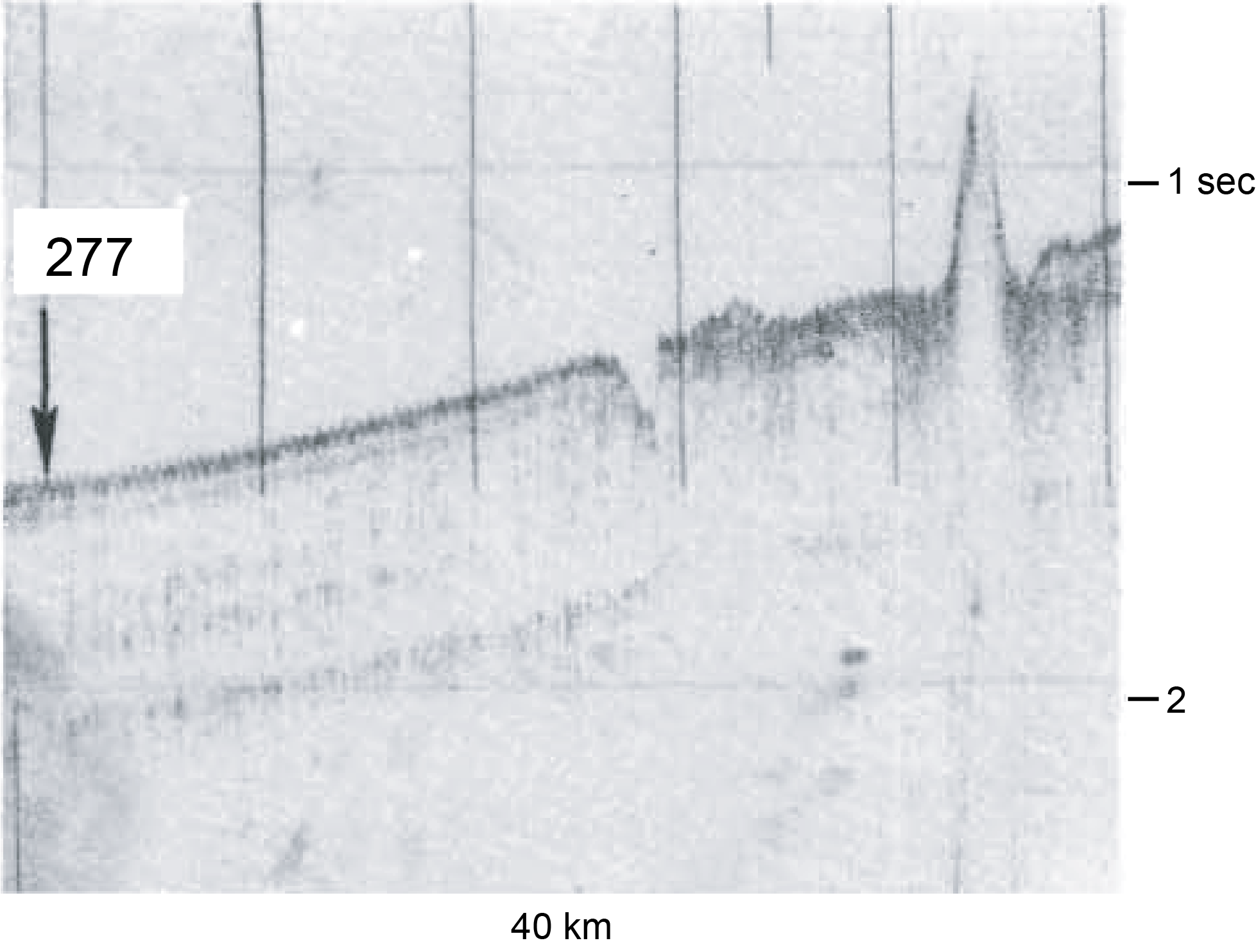
Figure F1. Shallow subbottom profiler record.
2. Operations
2.1. Port call
IODP Expedition 378 began in Lautoka, Fiji, at Queen’s Wharf at 0800 h on 3 January 2020. The vessel had been tied up at Queen’s Wharf for a maintenance period and to complete intermediate repairs on the piperacker skate and derrick. The Co-Chief Scientists, Expedition Project Manager (EPM), and JOIDES Resolution Science Operator (JRSO) technical staff boarded the vessel and began port call activities, including IODP JRSO crew change and crossover and Co-Chief Scientist orientations. The science party boarded the vessel on 4 January and began expedition preparations, including orientations on life at sea and safety. The science party continued safety training and received introductions in the laboratories during the rest of the port call.
During the 3 day port call, the ship crew change was completed, and some derrick repairs continued through 5 January. The welded areas of the derrick were inspected and painted, and rigdown of equipment was completed on 5 January. Two trucks of fresh produce were also loaded aboard the vessel.
The vessel was readied for departure, and the pilot came on board at 0656 h on 6 January. The last line was released at 0720 h to start the transit to Site U1553 (DSDP Site 277). The first fire and lifeboat safety drill was held for everyone on board. The Co-Chief Scientists and EPM met with each laboratory team to discuss requirements, tasks, and issues, and the teams began to prepare for their work.
2.2. Site U1553
Site U1553 was the only site occupied during Expedition 378. The research vessel JOIDES Resolution completed the 2249 nmi transit from Fiji to Site U1553 in 221.5 h (9.2 d). The vessel arrived on site at 1148 h on 15 January 2020. The thrusters were lowered, and the dynamic positioning system was engaged. At 1210 h, operations began for Site U1553.
Hole location, water depth, and the number of cores recovered are listed in Table T1. All times below are local ship time (UTC + 13 h) unless otherwise noted.
2.2.1. Hole U1553A
The APC/extended core barrel (XCB) bottom-hole assembly (BHA) was made up and deployed to 1187 meters below sea level (mbsl), and the top drive was picked up. Two “pigs” (pipe cleaning devices) were pumped through the drill string to remove some of the rust. Based on the precision depth recorder reading, the bit was spaced out to 1215 mbsl. The sinker bars and the core orientation tool were installed, and Hole U1553A was spudded at 2105 h on 15 January 2020. Mudline Core 1H arrived on deck at 2120 h, recovering 3.08 m. This established a seafloor depth of 1221.2 mbsl.
Coring continued with the APC system until a partial stroke was recorded on Core 15H at 127.5 mbsf. The XCB system was deployed for a single core (16X) to penetrate a 1.3 m hard interval. APC coring then continued until refusal at Core 20H, where a drillover and 100,000 lb of overpull were required to free the core barrel. The HLAPC system was then deployed until refusal at Core 22F, when a drillover and 100,000 lb of overpull were again required to free the core barrel.
The XCB was then deployed, reaching a total depth of 216.4 mbsf with Core 27X. This had been determined to be the final core for the hole prior to deploying the barrel. However, while cutting the core, the driller noticed an increase in top drive torque, and the hole was terminated prior to coring the full length. After recovering Core 27X, it was determined that the increase in torque was caused by a malfunction in the top drive shaft brake actuator. The brake had partially closed and overheated. The drill string was pulled to 1187 mbsl to allow the crew to replace the top drive brake. The bit cleared the seafloor at 2215 h on 16 January, ending Hole U1553A. The vessel was then offset 20 m east to prepare for Hole U1553B.
A total of 27 cores were taken from Hole U1553A over a 216.4 m interval with 98.9% recovery. Temperature measurements using the advanced piston corer temperature (APCT-3) tool were taken on Cores 4H, 7H, and 10H, and all full-length APC cores were oriented using the Icefield MI-5 core orientation tool. Total time on Hole U1553A was 34.00 h (1.4 days).
2.2.2. Hole U1553B
The top drive brake was repaired, and operations resumed at 0915 h on 17 January 2020. The top drive was picked up, and Hole U1553B was spudded at 1105 h on 17 January. The seafloor depth was calculated at 1221.7 mbsl based on recovery of the mudline in Core 378-U1553B-1H. Core 3H encountered a gravel layer and was a partial stroke. After a full 9.5 m advance, APC coring continued through Core 14H to 124.8 mbsf. The XCB system was then deployed for one core based on the hard interval encountered in Hole U1553A. Core 378-U1553B-15X advanced 6.2 m, and APC coring resumed through Core 17H to 150.0 mbsf.
To avoid stuck core barrels, which were encountered in Hole U1553A, the XCB system was deployed from 150.0 mbsf to the termination of coring at a total depth of 243.0 mbsf. The bit was then recovered, clearing the seafloor at 1350 h and the rig floor at 1645 h on 18 January and ending Hole U1553B. The vessel was then offset 20 m south for Hole U1553C.
A total of 29 cores were taken over a 243.0 m interval with 95.4% recovery. All full-length APC cores were oriented using the Icefield MI-5 core orientation tool. Total time on Hole U1553B was 42.50 h (1.8 days), with 10 h spent repairing the top drive.
2.2.3. Hole U1553C
With inclement weather systems moving in, the third APC/XCB hole was deferred in favor of an attempt to reach the deeper objectives with the rotary core barrel (RCB) system. A four-stand RCB BHA was made up and deployed to 1193 mbsl. Hole U1553C was spudded at 0010 h on 19 January 2020 and drilled ahead without core recovery to 234.0 mbsf. The center bit was pulled, and RCB coring began.
Half advances (~5 m) were used on Cores 378-U1553C-6R, 7R, 9R–16R, 19R, and 20R as a strategy to maximize recovery. Half advances also were used on Cores 29R–32R to optimize recovery of the PETM. Cores 40R–43R were cored without liners in the core barrel in an effort to improve recovery. An anomalously low C1/C2 hydrocarbon ratio in Core 43R caused Core 44R to be pulled after a 2.7 m advance to verify the values. With anomalously low C1/C2 ratios in consecutive cores, the decision was made to terminate coring at 567.5 mbsf. The bit was recovered to the surface and cleared the seafloor at 0105 h on 22 January, ending Hole U1553C. The vessel was offset 20 m west for Hole U1553D.
A total of 43 cores were taken over a 334.6 m interval with 47.4% recovery. Total depth for Hole U1553C was 567.5 mbsf, and total time was 82.75 h (3.4 days).
2.2.4. Hole U1553D
A new bit was installed on the RCB BHA, and it was deployed to 1193 mbsl to begin Hole U1553D. Hole U1553D was spudded at 0845 h on 22 January and drilled ahead to 178.3 mbsf. The center bit was pulled, and the Sediment Temperature 2 (SET2) tool was lowered to obtain a fourth temperature measurement with the goal of refining the thermal gradient at Site U1553.
After recovering the SET2 tool, the center bit was again deployed and the hole was drilled to 399.4 mbsf. The center bit was pulled, and the RCB system was deployed. Cores 378-U1553D-11R through 17R were cored without using liners to improve recovery.
During coring operations, clearance was provided by the Environmental Protection and Safety Panel to advance Hole U1553D deeper than Hole U1553C. This clearance was conditional and based on the need to wait for the results of headspace gas analysis prior to taking the next core. Coring was paused after Core 378-U1553D-19R to allow time for headspace gas analysis before proceeding. Coring was terminated at the Co-Chief Scientists’ request after Core 20R at 584.3 mbsf to allow sufficient time for a fifth hole to provide triplicate recovery of the APC/XCB section recovered in Holes U1553A and U1553B. The bit was recovered and cleared the seafloor at 2355 h on 24 January and the rotary table at 0255 h on 25 January, ending Hole U1553D. The vessel was offset 20 m west for Hole U1553E.
2.2.5. Hole U1553E
An APC/XCB BHA was made up and deployed to 1187 mbsl, and Hole U1553E was spudded at 0845 h on 25 January 2020. Based on recovery from Core 378-U1553E-1H, the seafloor was calculated at 1221.3 mbsl.
Coring continued with the APC system through Core 14H at 119.4 mbsf. One XCB core was taken from 119.4 to 129.1 mbsf to capture a hard interval encountered in Holes U1553A and U1553B. The APC system was then deployed for Core 378-U1553E-16H to 138.6 mbsf. The XCB was deployed from 138.6 to 237.6 mbsf, ending with Core 27X. Half advances were used on Cores 21X and 22X (177.8–188.8 mbsf) to improve recovery.
The drill string was recovered to the rig floor, and the bit cleared the seafloor at 0830 h on 26 January. The rig floor was secured for transit at 1215 h, and the vessel was switched from dynamic positioning mode at 1242 h, ending Hole U1553E and Site U1553.
A total of 27 cores were taken over a 237.6 m interval with 88.3% recovery. Total depth for Hole U1553E was 237.6 mbsf, and total time was 33.25 h (1.4 days). The total time spent at Site U1553 was 11.02 days, which includes 10 h lost because of breakdown.
The vessel then began the 531 nmi transit to Timaru, New Zealand, to pick up fuel filters before continuing to Papeete, Tahiti (French Polynesia). After the fuel filter transfer (tug Hinewai) at 1318 h on 28 January, the vessel began the 2564 nmi transit to Papeete. The detour to Timaru added ~13 h to the originally planned transit to Papeete. Expedition 378 officially ended with the first line ashore at 1312 h on 6 February local time (UTC − 10 h).
3. Lithostratigraphy
Coring at Site U1553 reached a maximum depth of 584.3 mbsf and recovered a 581.16 m long sedimentary succession of deep-sea sediment of Pleistocene and Oligocene to early Paleocene age from the Campbell Plateau. Five lithostratigraphic units were defined in the recovered sections on the basis of visual core description, smear slide and thin section analyses, and physical properties data (Figure F2). An interval of ~4 m of Pleistocene foraminifer-rich nannofossil ooze and foraminifer ooze (Unit I) overlies an expanded sequence (~200 m thick) of late Oligocene through early Oligocene nannofossil ooze with foraminifers (Unit II). The nannofossil ooze of Unit II gradually transitions into the nannofossil chalk of Unit III from ~175 to 225 mbsf. Lithification of carbonates increases downcore with chalk transitioning to limestone, defining Unit IV. Finally, the bottom ~100 m of the recovered sediment column contains siliciclastic Unit V, which is characterized by mudstone to dolomitic mudstone that is occasionally sandy. X-ray diffraction (XRD) analysis of samples from Holes U1553A–U1553D confirms the dominance of calcite at this site in the upper 470 m, followed by the dominance of quartz-bearing facies to the bottom of the hole.

Figure F2. Lithologic summary.
3.1. Unit I
- Intervals: 378-U1553A-1H-1, 0 cm, to 2H-1, 100 cm; 378-U1553B-1H-1, 0 cm, to 1H-3, 67 cm; 378-U1553E-1H-1, 0 cm, to 1H-3, 60 cm
- Depths: Hole U1553A = 0–4.00 mbsf; Hole U1553B = 0–3.68 mbsf; Hole U1553E = 0–3.61 mbsf
- Age: Pleistocene
- Lithology: foraminifer-rich nannofossil ooze and nannofossil-rich foraminifer ooze
The top of Lithostratigraphic Unit I is defined by alternating white (and light greenish gray) foraminifer-rich nannofossil ooze and nannofossil-rich foraminifer ooze. A sharp color change from light greenish gray to white occurs in Section 378-U1553A-1H-1, 103 cm (Figure F3). In Section 1H-2, 30 cm, the sediment color begins to change from white and gray to (light) grayish olive, light olive-gray, and pale greenish yellow (Figure F3). This sediment color change is not associated with a change in lithology; we infer that it likely reflects sedimentary redox conditions. Unit I is slightly bioturbated in some intervals. Smear slide observations found silt- to coarse sand–sized foraminifers and nannofossils (Figure F4A), the ratios of which fluctuated markedly with depth. XRD analysis of a bulk sediment sample (1H-2, 77–78 cm) reveals the presence of calcite and minor quartz and clay minerals (Figure F5A). In Holes U1553B and U1553E, Unit I is more disturbed (soupy) than in Hole U1553A and has fewer visible, sharp contacts between sediment color changes. The sharp, undulating boundary with Unit II is marked by a change in core color, which suggests an unconformity. This inference is supported by nannofossil species abundance, which indicates an abrupt transition from Pleistocene to Oligocene sediments at approximately 4 mbsf (see Biostratigraphy and micropaleontology).
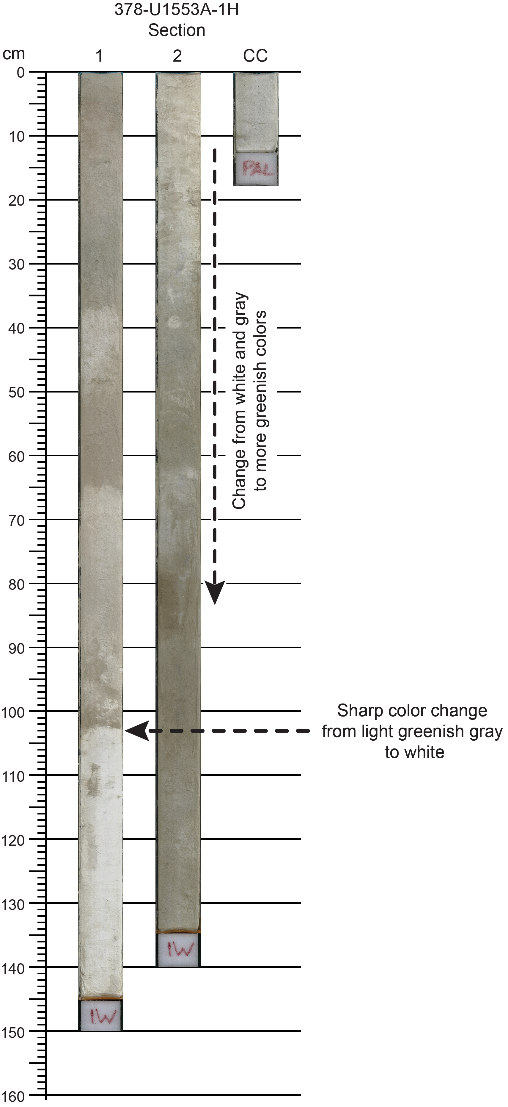
Figure F3. Characteristic lithology of Unit I.
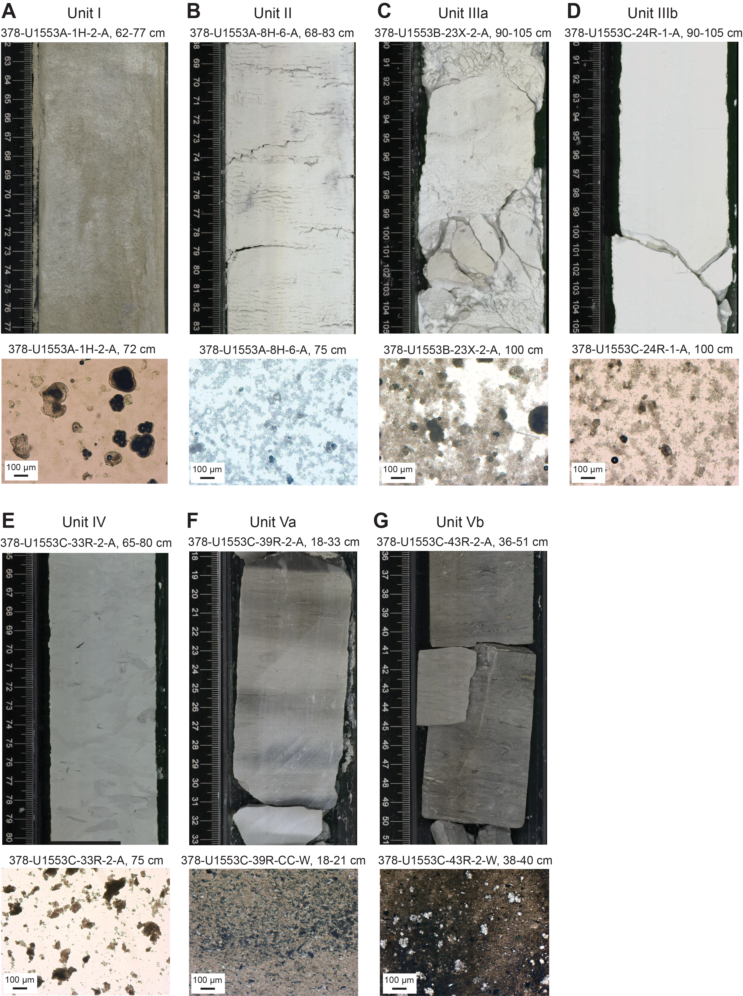
Figure F4. Representative lithologies.

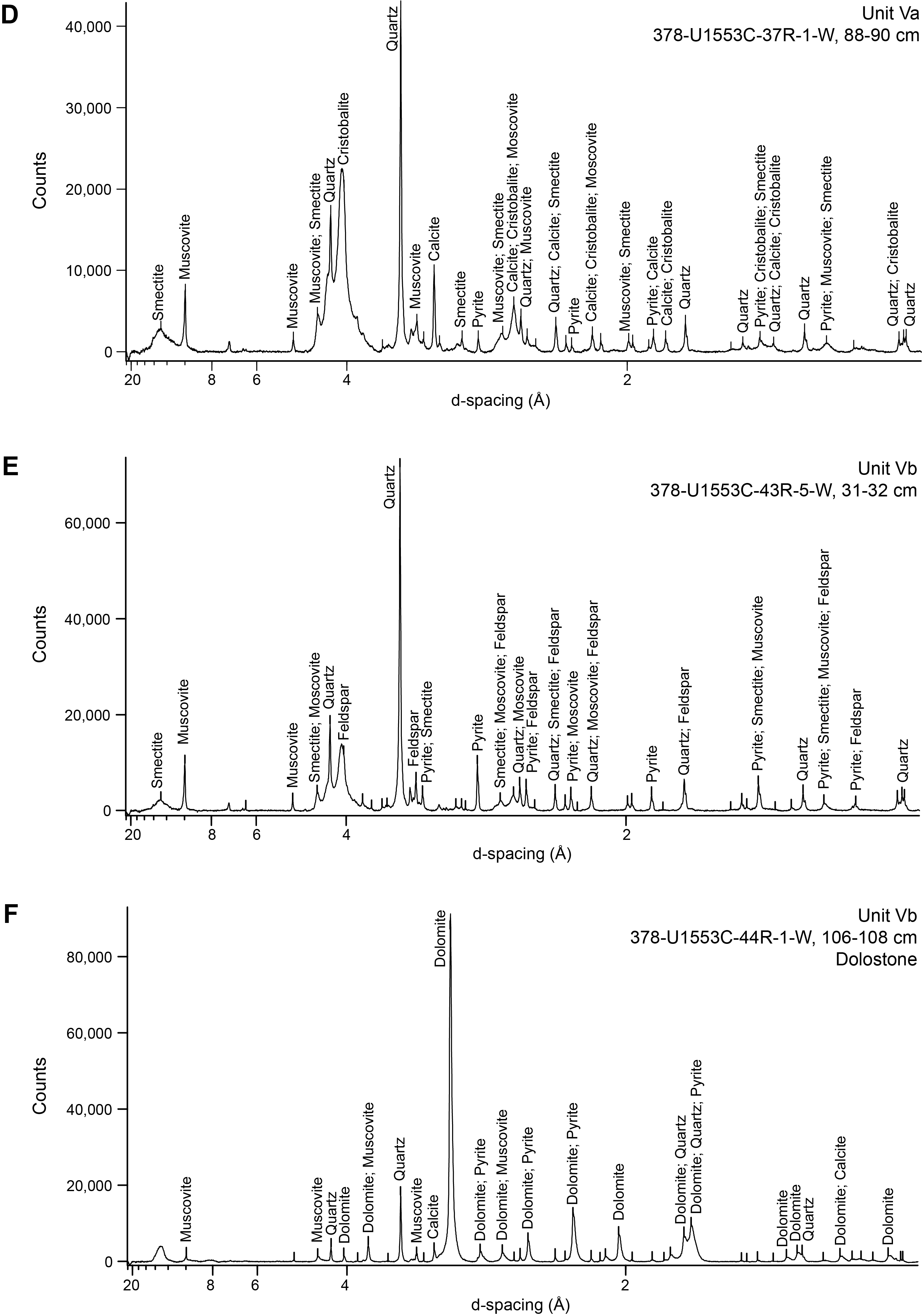
Figure F5. X-ray diffraction results.
3.2. Unit II
- Intervals: 378-U1553A-2H-1, 100 cm, to 24X-1, 58 cm; 378-U1553B-1H-3, 67 cm, to 22X-1, 150 cm; 378-U1553E-1H-3, 60 cm, to 20X-CC, 38 cm
- Depths: Hole U1553A = 4.00–179.98 mbsf; Hole U1553B = 3.68–185.10 mbsf; Hole U1553E = 3.61–172.85 mbsf
- Age: late Oligocene to early Oligocene (younger than 32.92 Ma)
- Lithology: nannofossil ooze with varying abundances of foraminifers and radiolarians along with interbedded packstone/calcareous sandstone
Lithostratigraphic Unit II is a ~180 m thick succession of alternating nannofossil ooze, foraminifer-rich nannofossil ooze, and nannofossil ooze with foraminifers (Figures F4B, F6). The dominating colors in Unit II are light olive-gray, (light) greenish gray, and white. The most distinct features of Unit II are diffuse to well-defined millimeter- to centimeter-scale laminated and/or layered green beds that also display diagenetic alteration, which is manifested as colored halos (Figure F6). In Core 378-U1553E-3H, a transition occurs where yellow bands grade to the green color seen throughout the rest of the hole (Figure F7). This feature is not present in Holes U1553A and U1553B. Smear slide observations found varying abundances of diatoms, calcareous and siliceous sponge spicules, radiolarians, and fish remains (Figure F8) and confirm that black spots and patches observable at the macroscopic scale can be attributed to the presence of pyrite framboids and possibly other sulfide minerals (Figure F9). Volcanic glass and rock fragments are found in smear slide analysis of Sample 378-U1553A-9H-1, 2 cm. From the top of Core 10H to the base of the unit, pyritized worm burrows and bioturbation are present. XRD analysis of bulk sediment samples from Unit II indicates that calcite dominates the minerals present. To increase the resolution of the secondary mineral assemblage present in this unit, a representative sample (378-U1553B-18X-CC, 15–17 cm) from a green layer was decalcified and analyzed using XRD (Figure F5B). Results indicate that the insoluble mineral fraction of the fine green layers includes quartz, barite, glauconite, and other clay minerals.
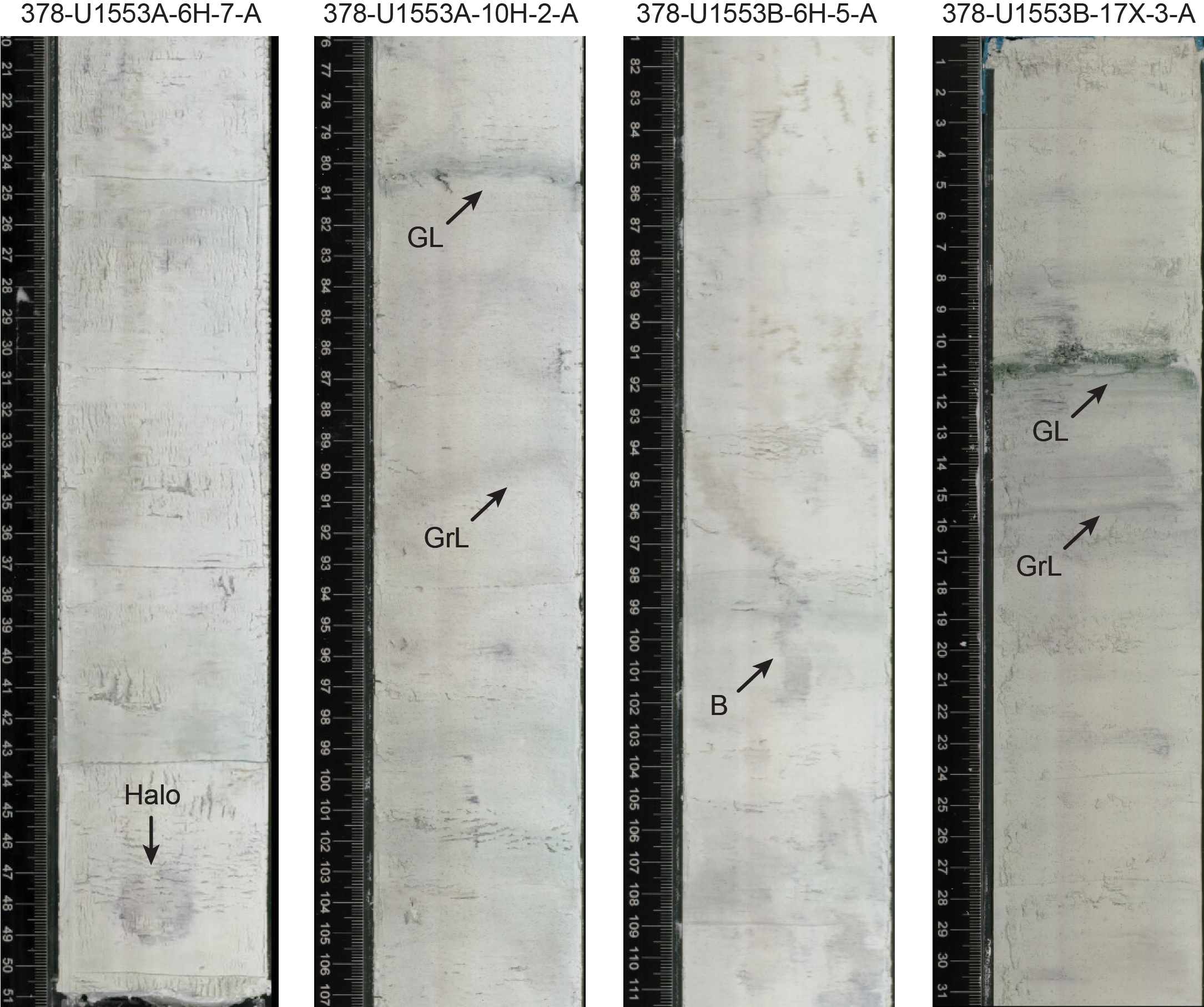
Figure F6. Characteristic lithologies in Unit II, Holes U1553A and U1553B.
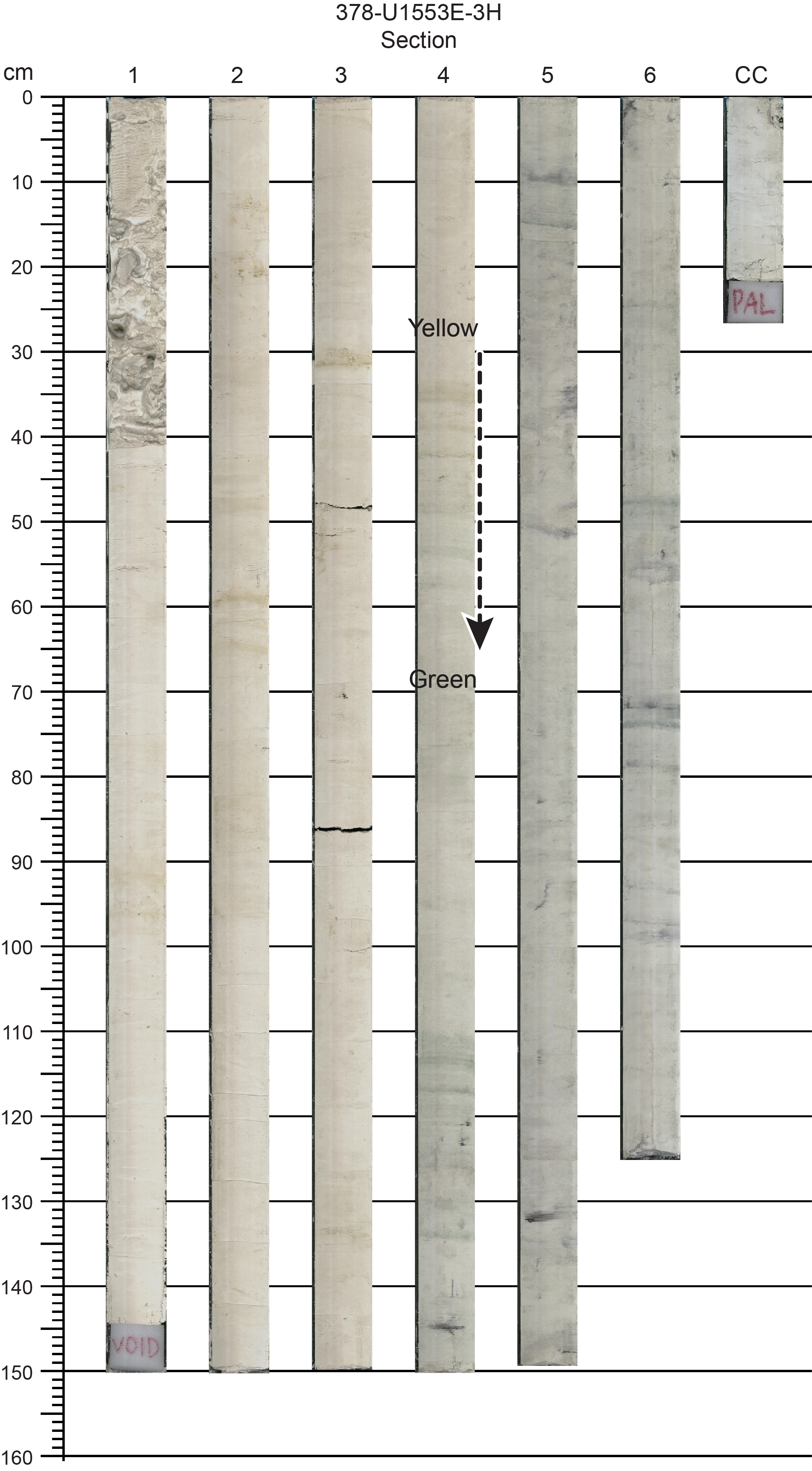
Figure F7. Sediment color change.
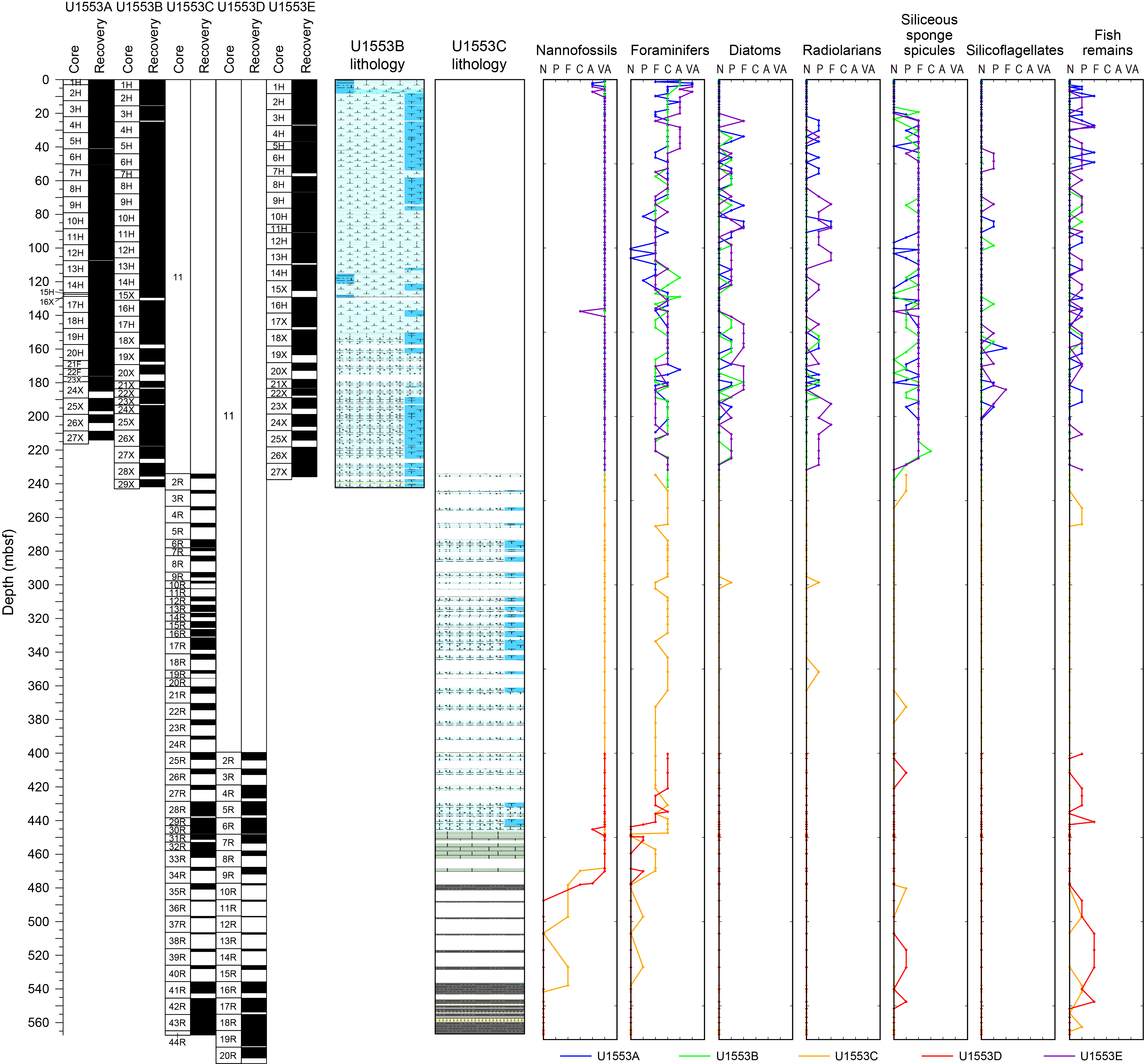
Figure F8. Abundance.
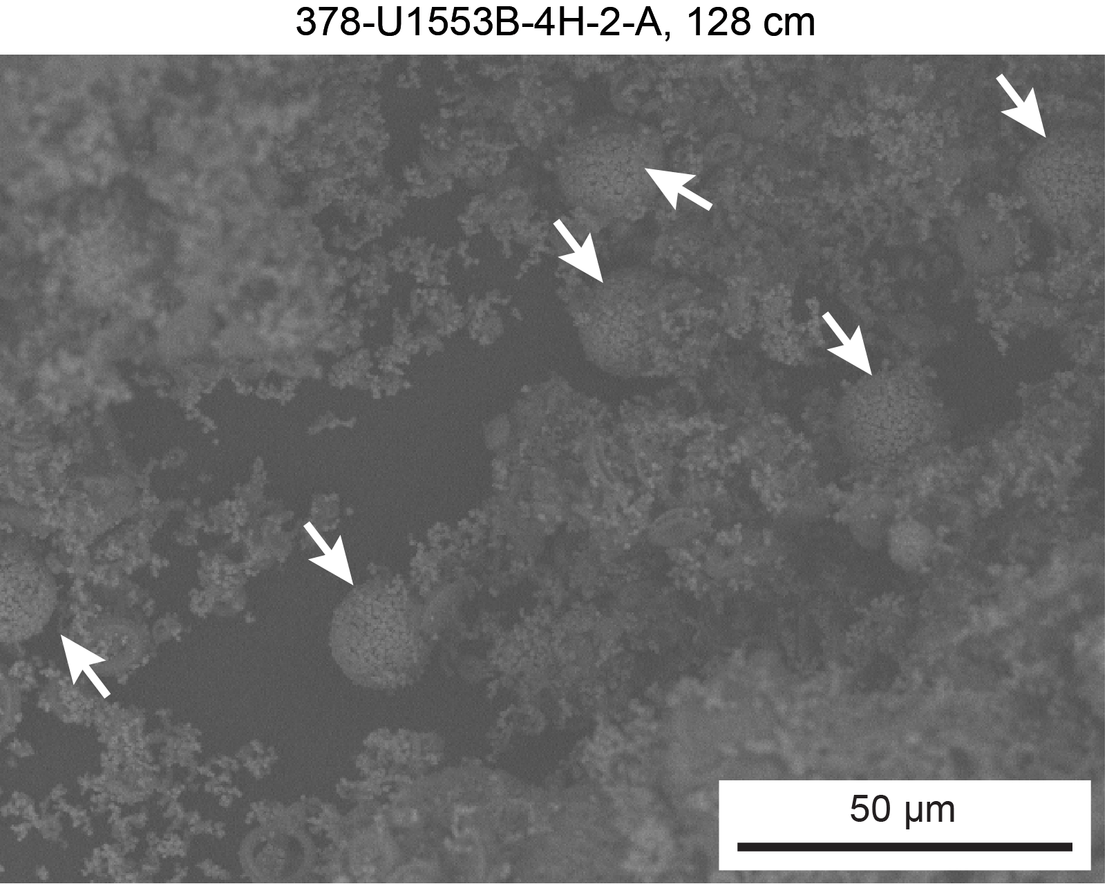
Figure F9. Framboidal pyrites.
In Unit II, a 10 cm bed of packstone and/or sandstone overlies a 5 cm bed of unlithified bluish gray medium sand between 128.97 and 129.02 mbsf in Hole U1553B (Core 15X) and between 124.00 and 124.16 mbsf in Hole U1553E (Core 15X) (Figure F10A–F10C). This early Oligocene (planktonic foraminifer Zone AO1) facies can be correlated between holes but was only partially recovered in Section 378-U1553A-16X-CC. The maximum magnetic susceptibility (MS) response is highest in medium sand (Figure F10D). The sand bed is composed of quartz, pyroxene, plagioclase, and rock fragments and is interpreted to be at least partially volcanic in origin. Thin section analysis of this facies in Section 16X-CC (127.52–127.76 mbsf) shows that this facies is packstone/sandstone. There is a gradational pattern between closely packed, rounded to subrounded sand-sized quartz grains (sandstone fabric) and a microfossil-rich packstone fabric across the three thin sections (127.50–127.73 mbsf). Foraminifer shells are abundant and are often filled with glauconite or pyrite/metal sulfide. Rounded glauconite grains are also visible in this facies. In thin sections from Sample 378-U1553B-15X-3, 110–112 cm (128.91–128.93 mbsf), a calcareous sandstone composed of mainly large, well-sorted, and rounded quartz grains (60%) superimposed on a fine matrix of unidentified calcareous fossils and clays is present (Figure F10E). Other framework grains include feldspar (mainly microcline) that is partially replaced by clay minerals and carbonate, zeolites as infilling of pore spaces, and minor quantities of muscovite.
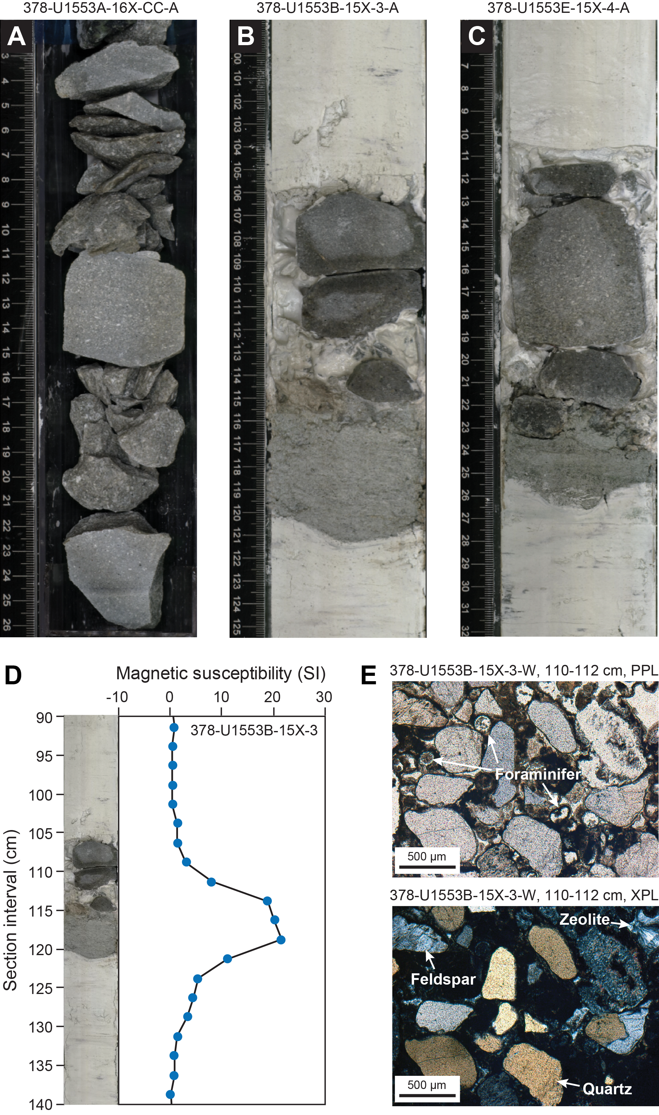
Figure F10. Indurated rocks.
3.3. Unit III
- Intervals: 378-U1553A-24X-1, 58 cm, to 27X-CC, 38 cm (bottom of hole [BOH]); 378-U1553B-22X-2, 0 cm, to 29X-CC, 34 cm (BOH); 378-U1553C-2R-1, 0 cm, to 27R-1, 46 cm; 378-U1553D-2R-1, 0 cm, to 4R-3, 82 cm; 378-U1553E-21X-1, 0 cm, to 27X-CC, 32 cm (BOH)
- Depths: Hole U1553A = 179.98–214.18 mbsf; Hole U1553B = 185.10–241.99 mbsf; Hole U1553C = 234.00–419.26 mbsf (0–234 mbsf = drilled interval); Hole U1553D = 399.4–423.16 mbsf (0–399.4 mbsf = drilled interval); Hole U1553E = 177.80–236.00 mbsf
- Age: late Eocene to early Eocene (~34 to ~52 Ma)
- Lithology: nannofossil chalk with foraminifers along with interbedded wackestone/packstone/sandstone
Lithostratigraphic Unit III is defined as the transition from ooze to chalk, which occurs in foraminiferal Zone AO1 in the early Oligocene (see Biostratigraphy and micropaleontology). The exact boundary between Units II and III is based on physical properties (Figure F2). Reflectance data (a decrease in lightness [L*] and red-green-blue [RGB] color space values) were employed alongside P-wave velocity and natural gamma radiation (NGR) counts to define this boundary. This unit is divided into Subunits IIIa and IIIb at the top of Section 378-U1553C-17X-1. In Hole U1553D, Subunit IIIb was encountered in Section 2R-1.
3.3.1. Subunit IIIa
- Intervals: 378-U1553A-24X-1, 58 cm, to 27X-CC, 38 cm (BOH); 378-U1553B-22X-2, 0 cm, to 29X-CC, 34 cm (BOH); 378-U1553C-2R-1, 0 cm, to 16R-CC, 19 cm; 378-U1553E-21X-1, 0 cm, to 27X-CC, 37 cm (BOH)
- Depths: Hole U1553A = 179.98–214.18 mbsf; Hole U1553B = 183.6–241.99 mbsf; Hole U1553C = 234.00–330.76 mbsf; Hole U1553E = 177.80–236.05 mbsf
- Age: late Eocene to middle Eocene (~34 to ~42 Ma)
- Lithology: nannofossil chalk with foraminifers as well as interbedded wackestone/packstone/sandstone
The stiffness of Lithostratigraphic Subunit IIIa varies, ranging from soft and disturbed (drilling biscuits interbedded with softer disturbed sediment; Figure F4C) to a stiff fabric that required core splitting with a saw. Drilling disturbance increases downcore in Subunit IIIa and includes slight to severe fracturing and biscuiting of soft, brecciated material between harder sections of sediment (Figure F11A–F11D). Biscuiting is particularly severe in Hole U1553E. Lithification increases downcore throughout Unit III and is associated with secondary calcite growth (see Biostratigraphy and micropaleontology) and the appearance of calcium silicate hydrate in XRD analysis (Figure F5C). Noncalcareous biogenic sediment containing siliceous sponge spicules, diatoms, silicoflagellates, and radiolarians was observed in low abundance in smear slides (1%–10%) throughout this subunit (Figure F8). Ichnofossil burrows (including Teichichnus type) are clearly visible in the lower portion of this subunit, indicating the degree of bioturbation (Figure F11B). Fine, millimeter-scale green laminations are also characteristic of this subunit, and they sometimes crosscut lateral ichnofossils (Figure F12A); other vertical burrows crosscut the laminations (Figure F12B). In addition, black to gray diagenetic halos and millimeter-sized specks of pyrite and other metal sulfides are visible throughout Subunit IIIa (Figure F11B). Gray to brown chert nodules and layers appear sporadically throughout this subunit (Figure F11C). The extent of silicification is variable, ranging from pale brown to gray, in which trace fossils are still visible (e.g., interval 378-U1553C-5R-2, 46–106 cm; 264.94–265.54 mbsf), to dark olive-gray, glassy flint (e.g., interval 9R-2, 73–76 cm; 294.63–294.66 mbsf).
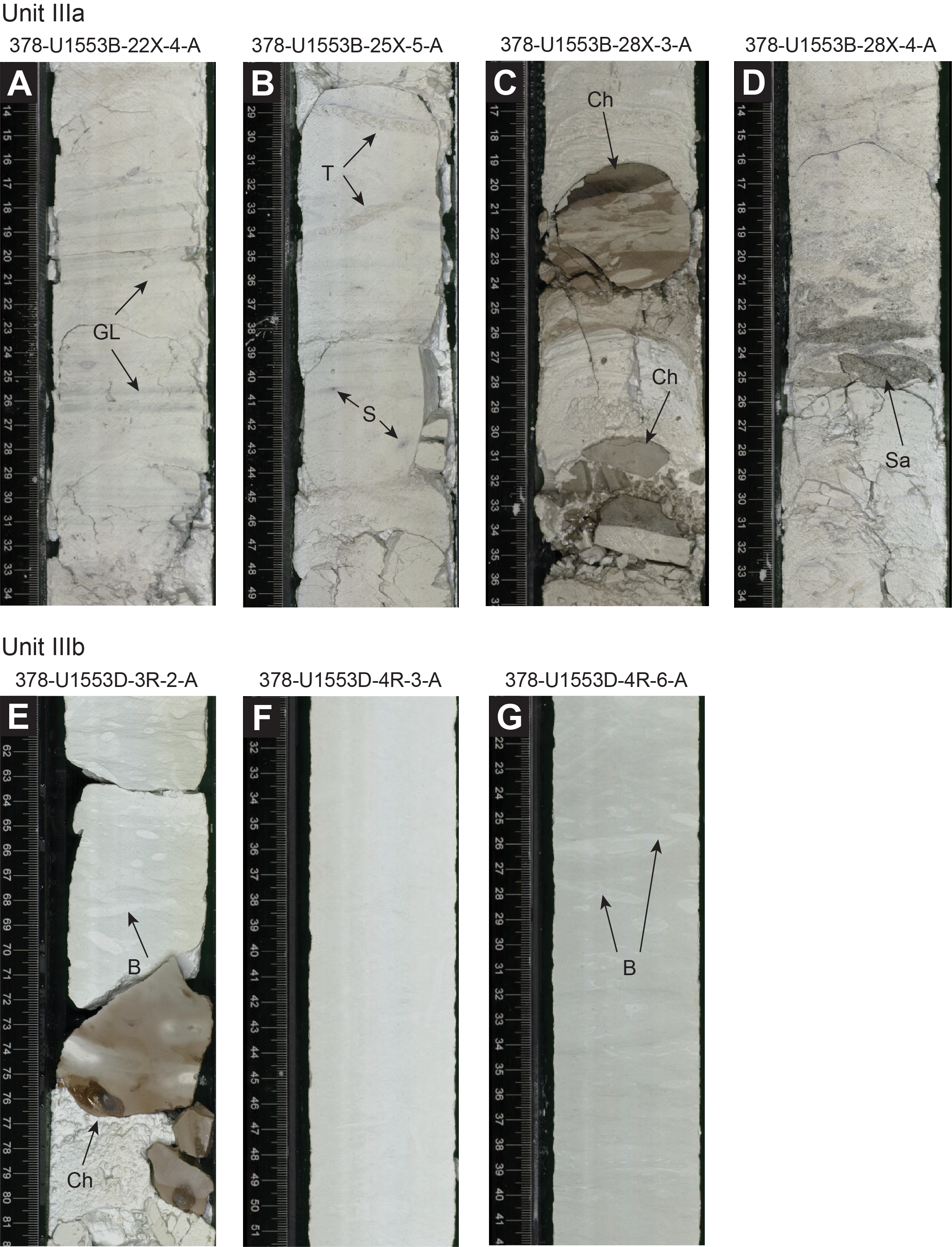
Figure F11. Characteristic lithologies in Unit III, Holes U1553B and U1553D.
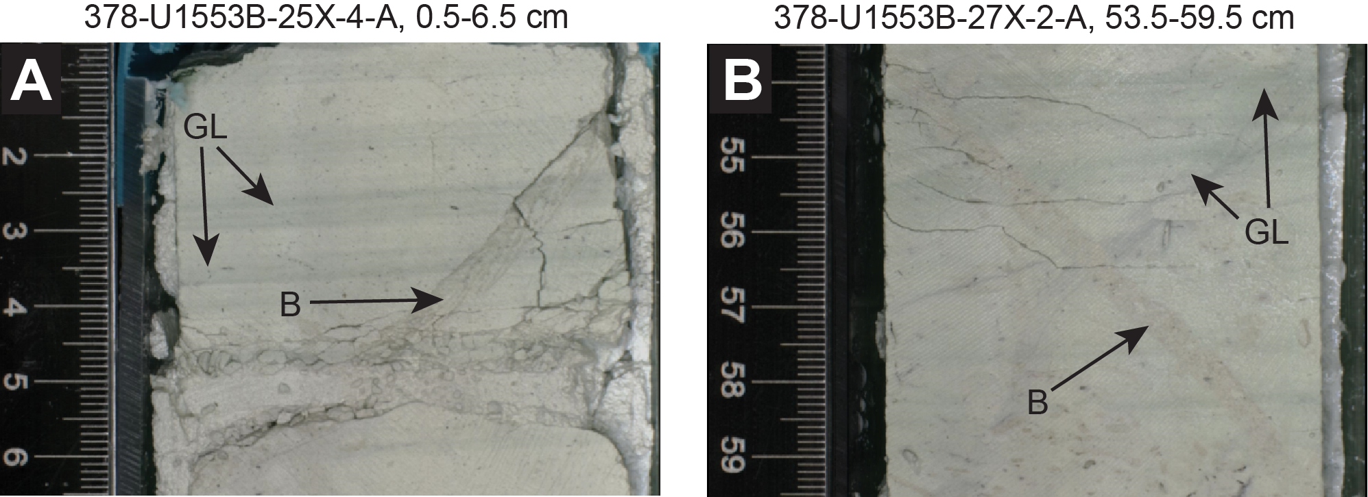
Figure F12. Trace fossil burrows.
Coarse-grained siliciclastics are interbedded in chalk in Holes U1553B and U1553C between ~230 and 255 mbsf (e.g., Figure F11D). A 3 cm thin section at the base of Hole U1553B in a thick layer of gray, fine-grained rock identified as wackestone (Sample 29X-CC, 31–34 cm; 241.96–241.99 mbsf) is dominantly carbonate bioclasts and jagged, angular quartz grains in a brownish matrix of micritic carbonate (Figure F13). In Hole U1553C, three packstone or sandstone intervals are present (Sections 3R-1, 3R-2, and 4R-1). In interval 3R-1, 75–108 cm (244.45–244.78 mbsf), a 14 cm thick packstone overlies a 19 cm thick carbonate-rich sandstone, and both are slightly bedded (Figure F14A). The packstone is very poorly sorted and contains carbonate bioclasts and quartz, plagioclase, chert, and glauconite. Some of the quartz grains are large (650 µm) and typically well rounded, but much of the matrix is highly angular. The medium-grained sandstone (Figure F14A) contains well-rounded and highly fractured and altered quartz, feldspar, chert, and carbonate bioclasts with a 1–3 µm micritic matrix (Figure F14B–F14E). An analogous 13 cm thick carbonate-rich sandstone is present in interval 3R-2, 36–49 cm (245.14–245.27 mbsf),and a comparable 18 cm thick packstone is present in interval 4R-1, 3–21 cm (253.43–253.61 mbsf).
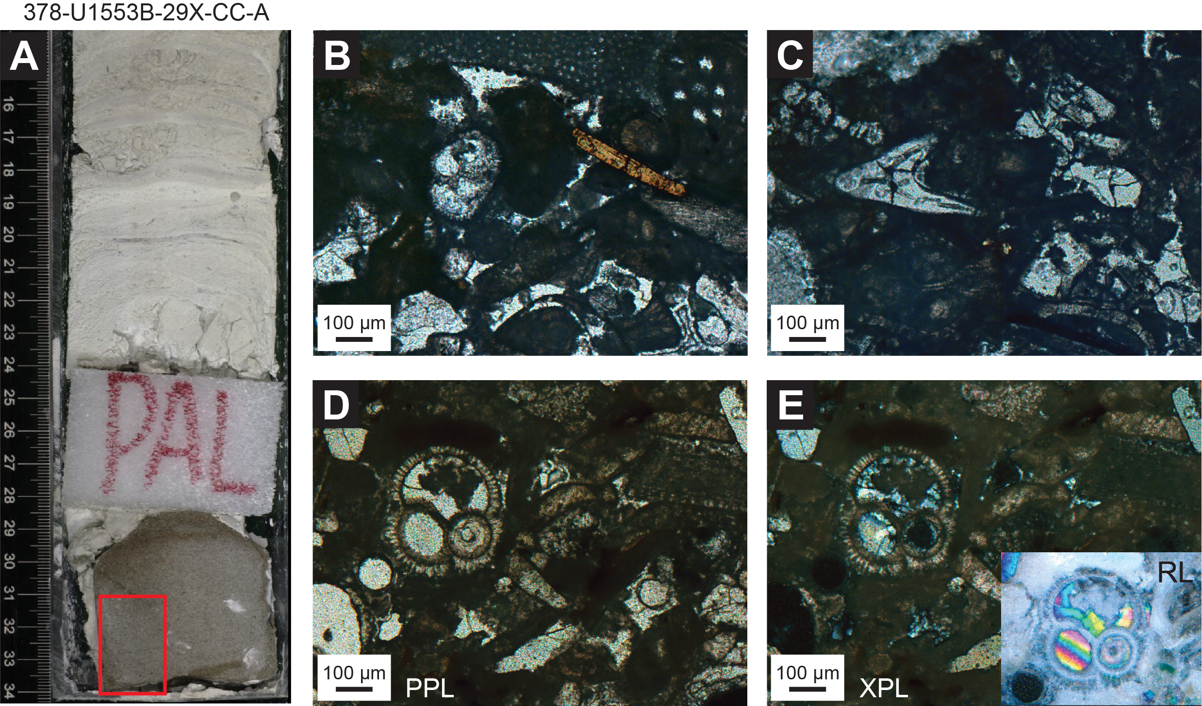
Figure F13. Wackestone.
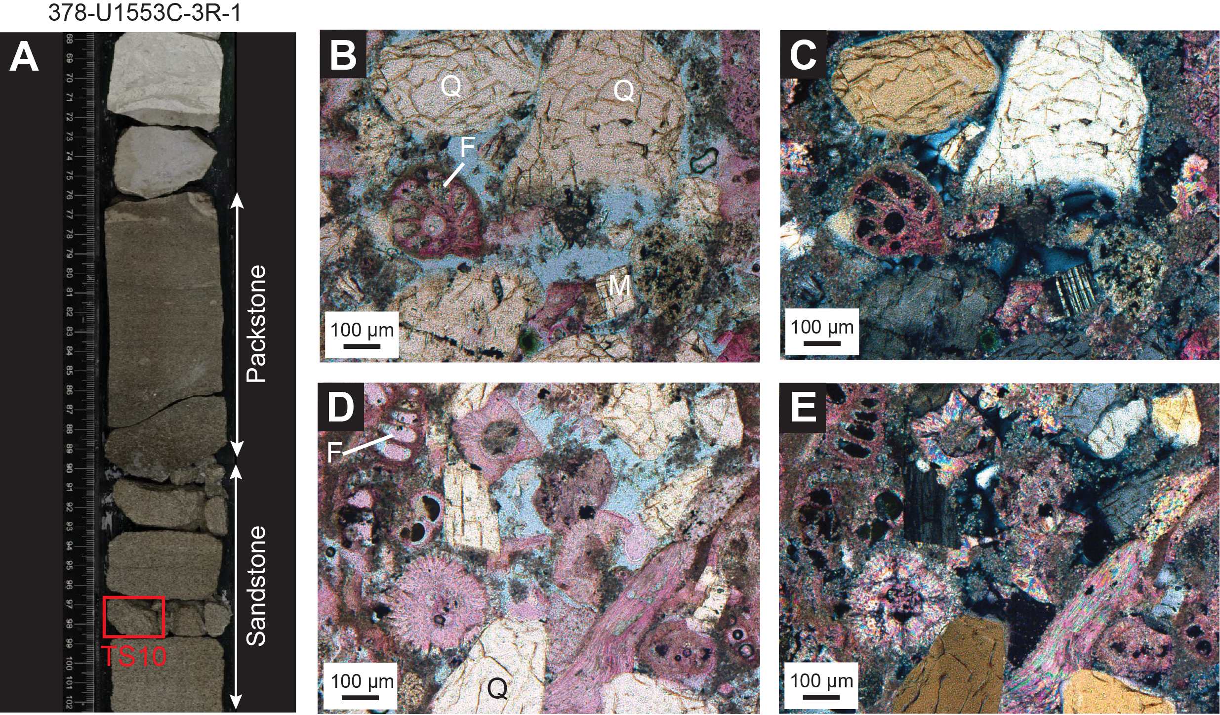
Figure F14. Sandstone.
3.3.2. Subunit IIIb
- Intervals: 378-U1553C-17R-1, 0 cm, to 27R-1, 46 cm; 378-U1553D-2R-1, 0 cm, to 4R-3, 82 cm
- Depths: Hole U1553C = 331.30–419.26 mbsf; Hole U1553D = 399.4–422.48 mbsf
- Age: late Eocene to early Eocene (~42 to ~52 Ma)
- Lithology: nannofossil chalk with foraminifers
Lithostratigraphic Subunit IIIb is distinguished by a reduction in green laminated intervals and an increase in intervals of bright white homogeneous sediments (Figure F11F). This increase in sediment lightness was visible using the Munsell color system and in RGB and L* values beginning at the top of Core 378-U1553C-17X (Figure F2). These white sediments are interrupted by periodic decimeter-scale beds of a slightly darker light greenish gray color. Bioturbation is visible in periodic contacts between white and slightly darker beds (Figure F11G). Tan to gray chert nodules are also present in this subunit (Figure F11E). Smear slide analyses do not indicate any clear changes in sedimentary composition in this subunit compared to Subunit IIIa (Figures F4, F8). However, X-ray fluorescence (XRF) analysis found an increase in Ca from 41.8% to 43.6% and minimum CaCO3 weight percent (wt%) increases from Subunit IIIa (88 wt%) to Subunit IIIb (93 wt%) (see Geochemistry). XRD analysis of Unit III sediments validates the continued dominance of calcite. However, minor contributions from Fe-sulfides associated with other metals such as Cu (bornite) appear in XRD analyses (Figure F5C) in addition to glauconite and glaucophane.
3.4. Unit IV
- Intervals: 378-U1553C-27R-1, 46 cm, to 34R-CC, 29 cm; 378-U1553D-4R-3, 82 cm, to 10R-1, 16 cm
- Depths: Hole U1553C = 419.26–469.86 mbsf; Hole U1553D = 422.48–477.36 mbsf
- Age: early Eocene to late Paleocene (~52–62 Ma)
- Lithology: limestone
Lithostratigraphic Unit IV is distinguished from Unit III by increased lithification of the limestone facies (Figure F2). Sediments are white to pale grayish green (Figure F4E) and tend to alternate in decimeter-scale beds. Boundary contacts range from sharp to gradational. A characteristic feature of this unit is the highly variable degree of bioturbation (slight to heavy; Figure F15). In Sections 378-U1553C-29R-2 and 378-U1553D-6R-4, sediments darken to a blue-gray hue and are increasingly lithified (Figure F15). Smear slide analyses from this interval show the presence of common to abundant micrite and nannofossils as well as quartz, micas, and ferromagnesian minerals (Figure F8). Throughout Unit IV, CaCO3 values decrease from 90 to 63 wt% as the facies’ color darkens (Figure F15) (see Geochemistry). XRD analysis also indicates an increase in quartz and other siliciclastic inputs, such as clays, toward the base of the unit, although calcite remains the dominant mineral. A thin section from a limestone in Section 378-U1553C-34R-1 stained with potassium ferricyanide and Alizarin Red S shows that the matrix is composed of ferroan calcite and that most of the microfossils are composed of dolomite (Figure F16). There are some small (20–50 µm) secondary dolomite rhombs in the matrix, a few of which have a little blue color in their core from the carbonate stain, which indicates the presence of ferroan dolomite or ankerite (Figure F16E).
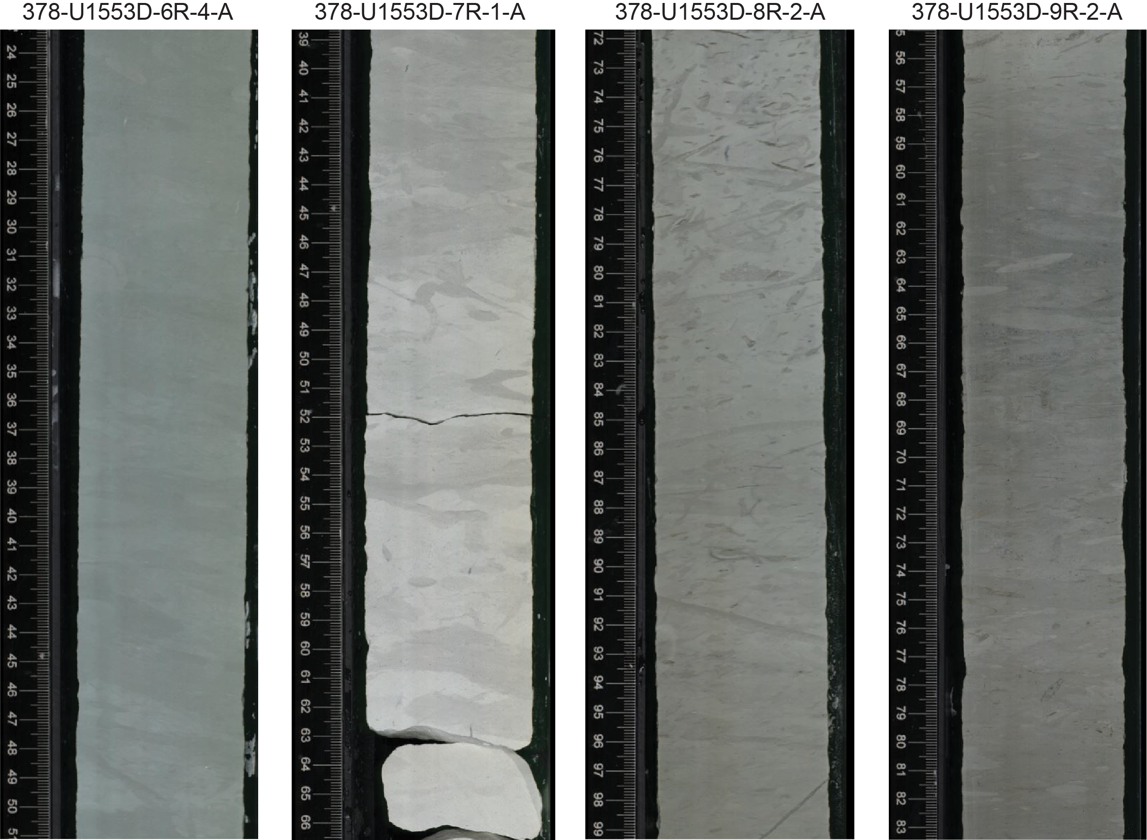
Figure F15. Characteristic lithologies in Unit IV.
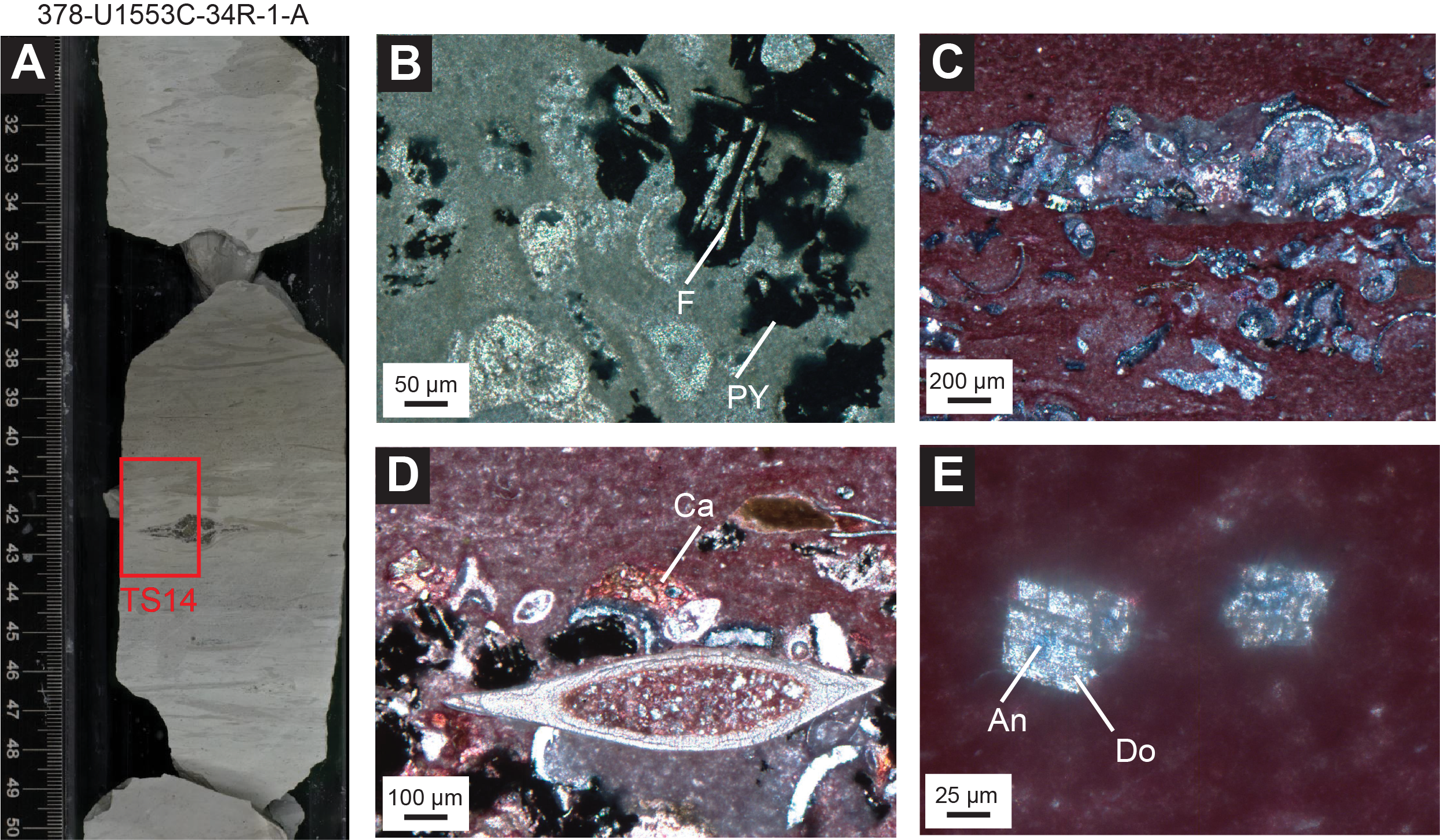
Figure F16. Limestone.
The onset of the PETM occurs in Unit IV in Cores 378-U1553C-31R and 378-U1553D-7R at approximately 449.5 mbsf. The PETM is tentatively related to the sharp boundary between a white, nonbioturbated interval and a darker green interval with white burrows (Figure F17).
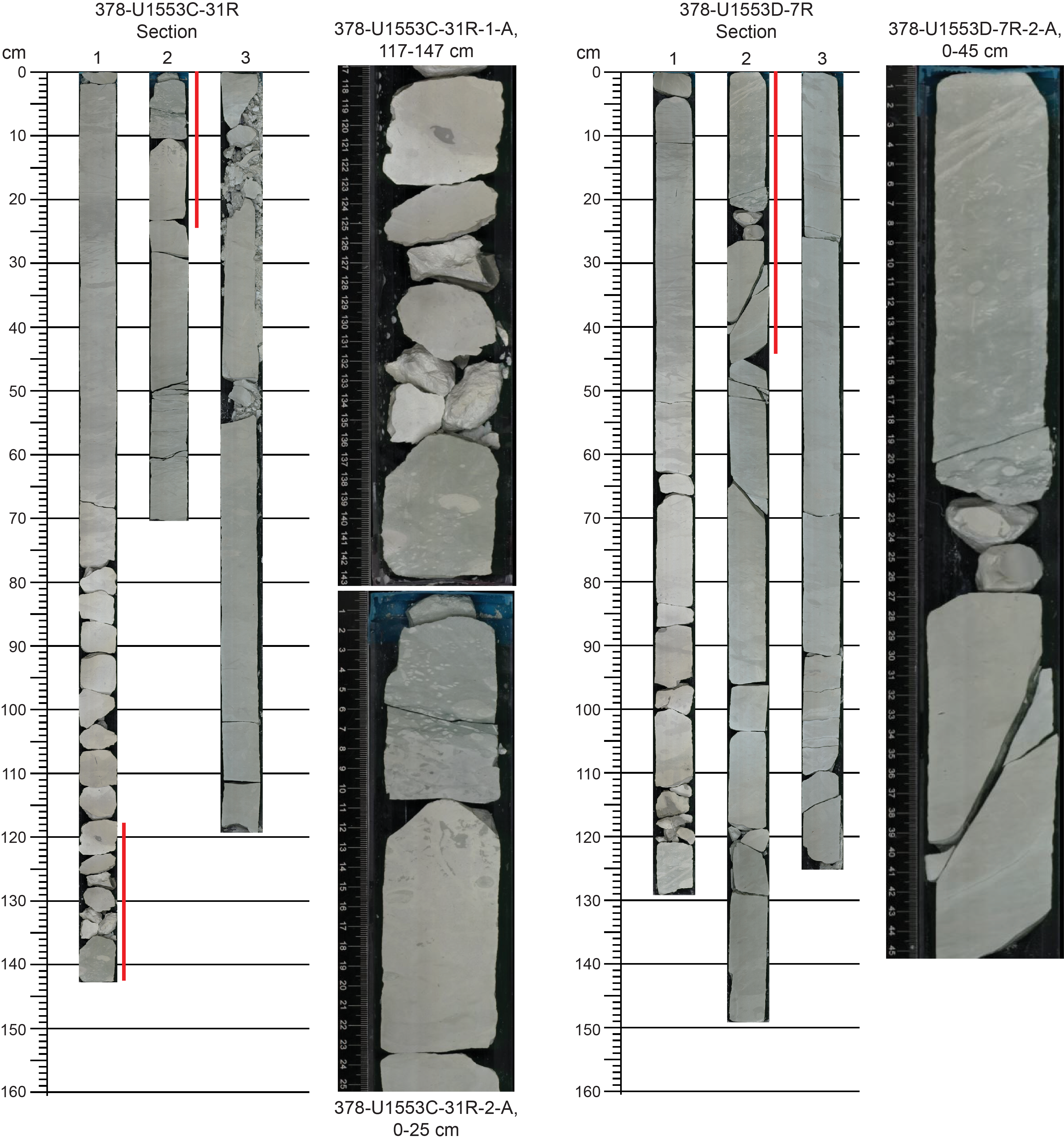
Figure F17. PETM interval.
3.5. Unit V
- Intervals: 378-U1553C-35R-1, 0 cm, to 44R-CC, 5 cm (BOH); 378-U1553D-10R-1, 16 cm, to 20R-CC, 5 cm (BOH)
- Depths: Hole U1553C = 477.20–566.03 mbsf; Hole U1553D = 477.36–581.16 mbsf
- Age: Paleocene (older than 62 Ma)
- Lithology: mudstone to dolomitic mudstone, occasionally sandy
Splitting cores from Lithostratigraphic Unit V in Holes U1553C and U1553D resulted in a detectable hydrocarbon odor, which generally became more pronounced in the deeper cores. Directly after splitting Section 378-U1553D-20R-1 and before washing the split-core surfaces, an ultraviolet light revealed a bright purple fluorescence on the split-core surfaces (Figure F18).
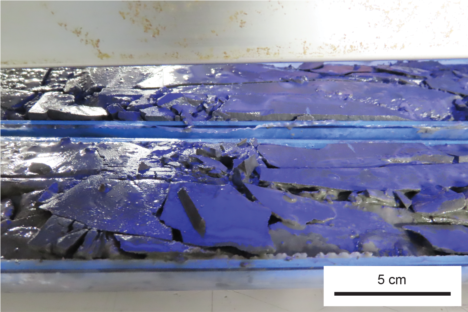
Figure F18. UV light illumination.
The standard procedure for imaging archive section halves is to do so immediately after splitting once the surface water from the saw has dried (generally about 30 min) (see Lithostratigraphy in the Expedition 378 methods chapter [Röhl et al., 2022]). This procedure was followed for all Unit V cores, resulting in an initial set of very dark core images. It was noticed during core description that progressive drying of section halves from Unit V resulted in substantial color changes over a span of >24 h. The initially very dark core gradually became more reflective and variable in color, revealing more observable sedimentological features. Each section was consequently reimaged after drying for ~24 h (see Lithostratigraphy in the Expedition 378 methods chapter [Röhl et al., 2022]).
Unit V is a dominantly siliciclastic unit. Macroscopic determination of lithology for this unit is challenging, and shipboard assessment benefited from XRD and XRF analyses and thin section petrography. XRD analysis demonstrated a change in dominant mineral composition from calcite in Unit IV to quartz with associated clays and muscovite (Figure F5) that also was observable in smear slides and thin sections (Figure F4F, F4G). In accordance with the change in sediment color from the upper carbonate units, CaCO3 abundance is low and varies from below the detection limit to 8.7 wt% with an average of 1.8 wt% (see Geochemistry). Microcrystalline pyrite is abundant throughout this unit and often forms on/in fracture surfaces, as confirmed by XRD analysis (Figure F19). Thin section analysis indicates a high heterogeneity of sediment fabrics and components in this unit. Unit V is generally characterized by a brownish silt to clay-sized matrix that supports varying numbers of pyrite crystals, quartz and other siliciclastics, glauconite, and siliceous and calcareous microfossils (Figure F5D–F5F). Clastic components range from silt to very fine sand sized. Dolomite crystals 50–200 µm in size are abundant (Figures F19A, F20E) and often appear as sand-sized grains in hand sample. Varying degrees of pink staining from potassium ferricyanide and Alizarin Red S indicate the presence of a varying but low abundance of calcite in the matrix, probably as micrite. Therefore, the dominant classification given to this unit is mudstone to dolomitic mudstone. Significant differences in bioturbation fabrics and the presence of large (centimeter-sized), diagenetically modified areas have motivated the distinction of Lithostratigraphic Subunits Va and Vb (Figure F21).
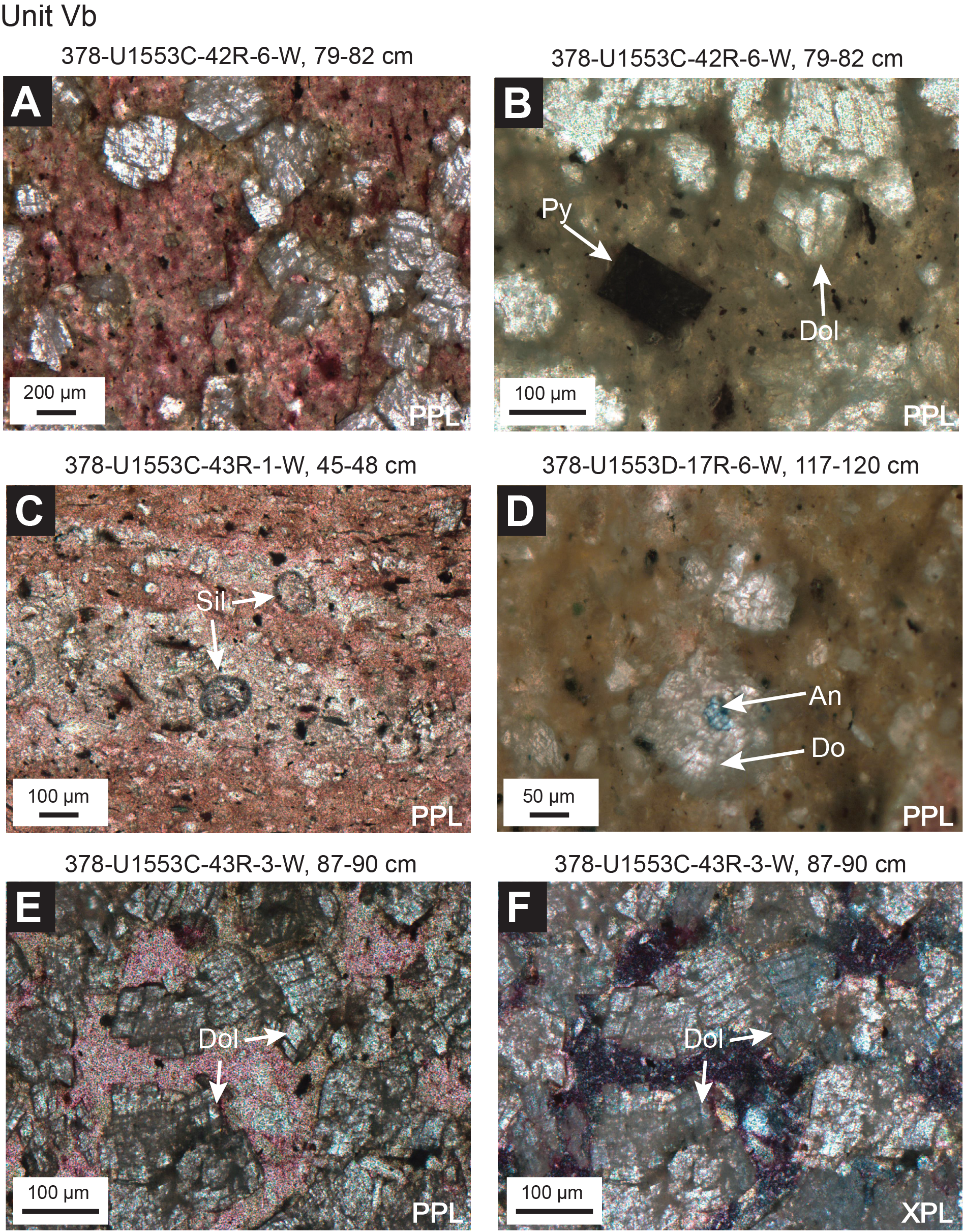
Figure F19. Thin section microphotographs from Subunit Vb.
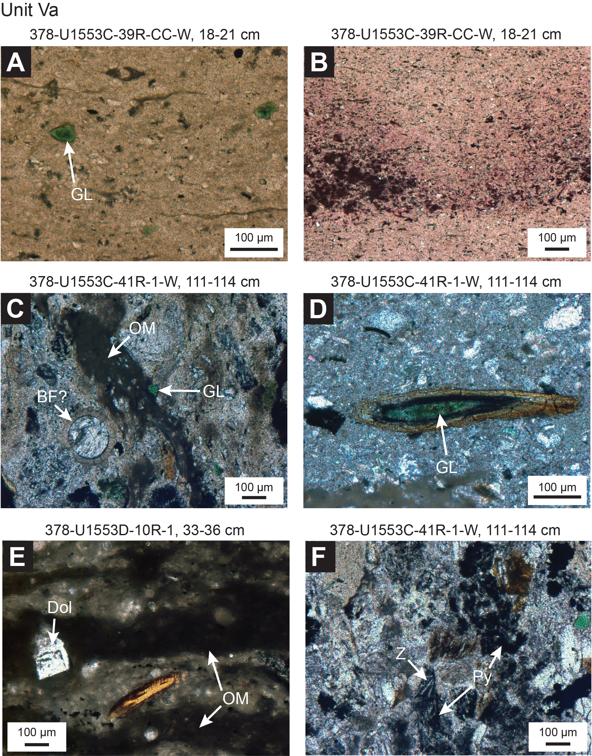
Figure F20. Thin section microphotographs from Subunit Va.
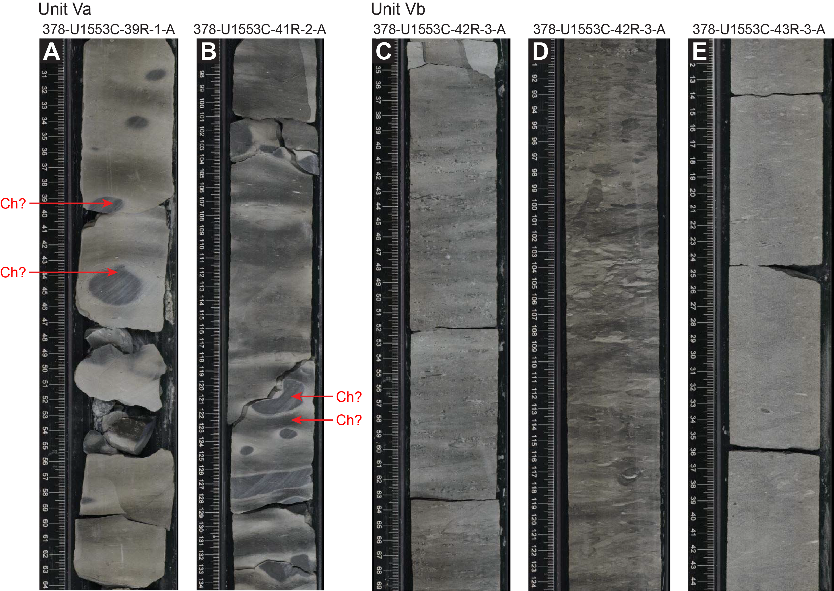
Figure F21. Characteristic lithologies in Unit V.
3.5.1. Subunit Va
- Intervals: 378-U1553C-35R-1, 0 cm, to 41R-CC, 15 cm; 378-U1553D-10R-1, 16 cm, to 16R-CC, 16 cm
- Depths: Hole U1553C = 477.20–542.7 mbsf; Hole U1553D = 477.36–542.5 mbsf
- Age: Paleocene (older than 62 Ma)
- Lithology: mudstone to dolomitic mudstone, occasionally sandy
Lithostratigraphic Subunit Va is characterized as mudstone that is sometimes carbonate rich, with some fine to medium sandy intervals. After drying, the dominant color is medium gray to light gray (Figure F21A–F21B). Throughout this subunit, there are darker gray, centimeter-sized diagenetically modified areas against the lighter gray matrix. These are attributed to chert nodules. This was not confirmed by thin section microscopy, but it is supported by the XRD observation of amorphous SiO2 (cristobalite) associated with opal-C (Figure F5D). Bioturbation is generally categorized as slight to moderate in Subunit Va. The CaCO3 content averages 3.9 wt% for Subunit Va (see Geochemistry). This is supported by XRF (Ca = 2.0%) and XRD analyses, which identified a minor contribution from calcite (Figure F5D). The presence of Bathysiphon foraminifers indicates an upper bathyal depositional environment (see Biostratigraphy and micropaleontology). Foraminifers are common and can be concentrated in millimeter-scale beds, which is interpreted to indicate deposition by currents.
Thin section microscopy of three samples from Subunit Va indicates that the matrix of the mudstones is pale yellow brown (Figure F20) and mainly composed of clays, a calcitic micrite, and organic matter. Staining with potassium ferricyanide and Alizarin Red S produced a pale pink color in the matrix that is consistent with the presence of calcite (Figure F20B). Glauconite is usually present as distinct, isolated grains (Figure F20A) and has an abundance of <1%. In one location, a probable glauconite pellet (200 µm long) is surrounded by very clear black and orange alteration zones (Figure F20D). Small clusters of a pale, fibrous mineral that has low birefringence is present in Sections 378-U1553C-41R-1 and 378-U1553D-10R-1 and is tentatively identified as zeolite (Figure F20F). A thin interval in this subunit also contains small amounts (about 5%) of secondary dolomite crystals (interval 10R-1, 33–36 cm) (Figure F20E).
3.5.2. Subunit Vb
- Intervals: 378-U1553C-42R-1, 0 cm, to 44R-CC, 5 cm (BOH); 378-U1553D-17R-1, 0 cm, to 20R-CC, 5 cm (BOH)
- Depths: Hole U1553C = 545.40–566.03 mbsf; Hole U1553D = 545.30–581.16 mbsf
- Age: unknown
- Lithology: mudstone to dolomitic mudstone, occasionally sandy
Lithostratigraphic Subunit Vb is delineated by an increase in bioturbation as well as a sometimes high abundance of secondary dolomite crystals (Figure F21C–F21E). Bioturbation is ubiquitous, and many different types of ichnofossils are visible, tentatively including Chondrites, Zoophycos, Phycosiphon, and Teichichnus. Beds with mudstone containing large (average = 200 µm) dolomite crystals have a distinct dark gray color and medium-grained texture and are often interlayered with mudstone units. XRF, XRD, and coulometric analysis indicate a decrease in calcite in this subunit. Calcium concentration decreases from 2.0% in Subunit Va to 0.43% in Subunit Vb according to XRF analyses, and calcite can no longer be detected by XRD in Subunit Vb (Figure F5E). The CaCO3 content from the coulometer averages 0.85 wt% for Subunit Vb (see Geochemistry). Iron increases in this subunit to a maximum of 7.2%, as measured by XRF. Bathysiphon foraminifers are also present in small layers to lenses throughout this subunit.
A ≥19 cm thick calcareous dolostone concretion with 85 wt% CaCO3 and 0.44 wt% total organic carbon (TOC) is present at the bottom of Section 378-U1553C-44R-1 (565.79–565.98 mbsf) (see Geochemistry). XRD analysis indicates the concretion is dominantly composed of dolomite (Figure F5F) with a minor contribution from calcite in addition to pyrite and muscovite. XRF analysis reveals a fourfold increase in Mg (7.5%) and an order of magnitude increase in Mn concentration (1877 ppm). An analogous 19 cm thick calcareous dolostone concretion is present in Section 378-U1553D-18R-4 (559.35–559.54 mbsf).
Thin section analysis of 13 samples from Subunit Vb shows that dolomite varies substantially in abundance throughout the cores and sometimes within a single thin section. For example, a thin section from Section 378-U1553C-42R-6 contains about 30% dolomite (Figure F19A). Dolomite can be easily distinguished from the pink-stained matrix of the mudstone, which is interpreted to be a mixture of clays and micritic calcite, although we note that CaCO3 wt% indicates a low calcite contribution in this unit. However, other mudstones contain significantly less dolomite. One interval (43R-3, 87–96 cm; 558.39–558.48 mbsf) is mainly composed of an interlocking matrix of dolomite crystals cemented by calcite (Figure F19E–F19F) and is termed calcareous dolostone. The extent of dolostone in Subunit Vb could not be determined by macroscopic observation because it looks similar to the mudstone. In one thin section (Sample 378-U1553D-17R-6, 117–120 cm), a small amount of ferroan dolomite or ankerite that stained a turquoise color was detected in the center of a dolomite crystal (Figures F19D, F21E), but the vast majority of the dolomite in the thin section does not contain iron. Some biogenic silica is present (Figure F19E). Pyrite is sometimes present in cubic form, sometimes as clumps or in small lenses (Figure F19B).
4. Biostratigraphy and micropaleontology
The five holes drilled at Site U1553 recovered a 580 m thick succession of nannofossil ooze, chalk, limestone, and muddy sandstone to silty mudstone. Biostratigraphic results indicate that, apart from a thin veneer of Pleistocene sediments, the succession spans the early late Oligocene to early Paleocene and includes an expanded ~250 m thick Oligocene–late Eocene interval with good preservation of calcareous nannofossils, foraminifers, and radiolarians. Diatoms, silicoflagellates, and sponge spicules are also common and well preserved throughout this interval. The Eocene and Paleocene intervals are less expanded and have more variable microfossil abundance and preservation, but biostratigraphic and lithologic evidence indicates that both the EOT and Paleocene/Eocene (P/E) boundary are intact. Low calcareous and siliceous microfossil abundance and generally poor preservation in the basal muddy sandstone unit (Lithostratigraphic Unit V) meant that we could not date this unit all the way down to the total depth of Holes U1553C and U1553D. Postcruise study of dinoflagellate assemblages has confirmed that the base of the cored interval is of early Paleocene age. A summary of abundance and preservation for calcareous nannofossils, foraminifers, and radiolarians for Site U1553 is shown in Figure F22.
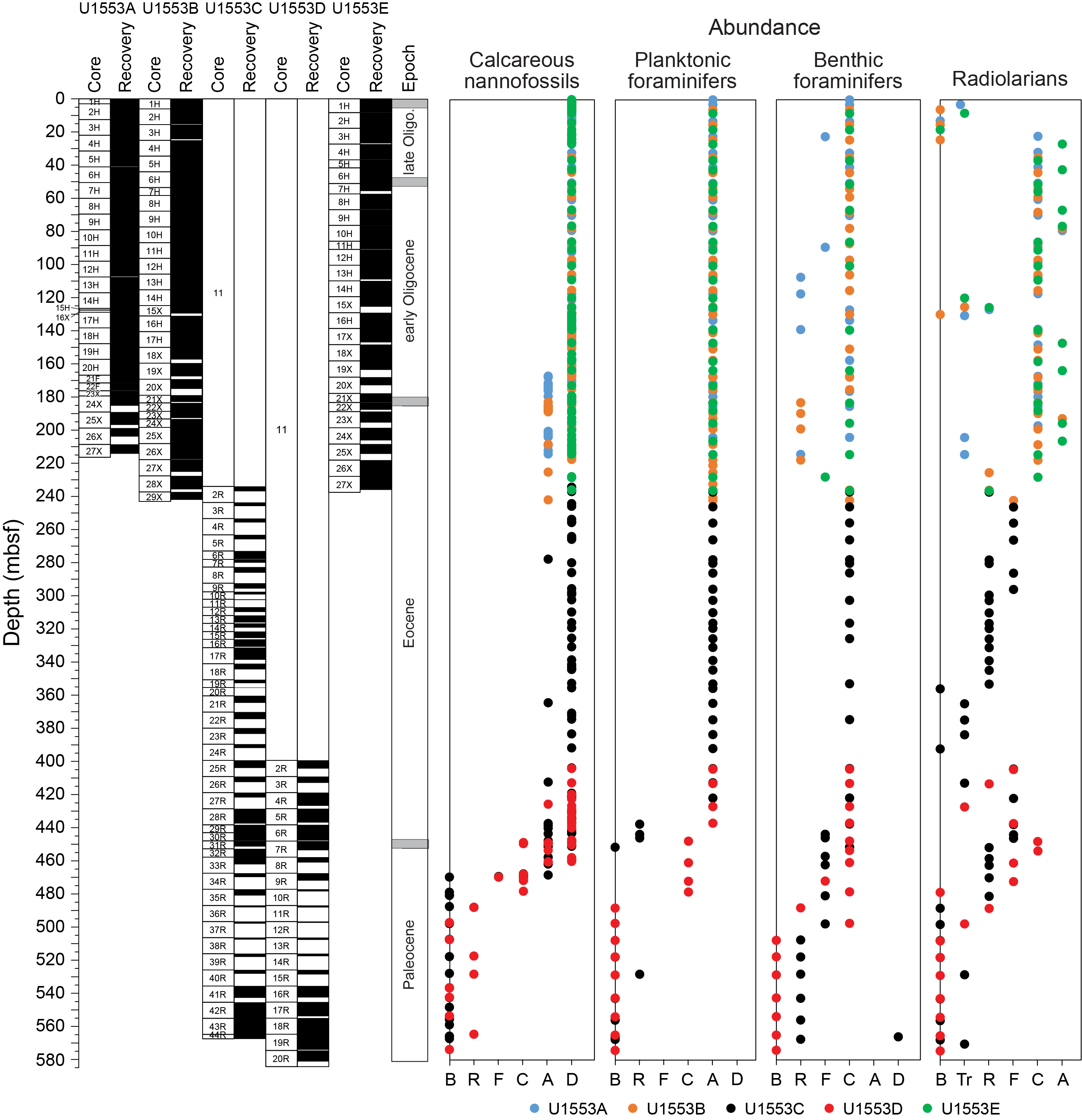
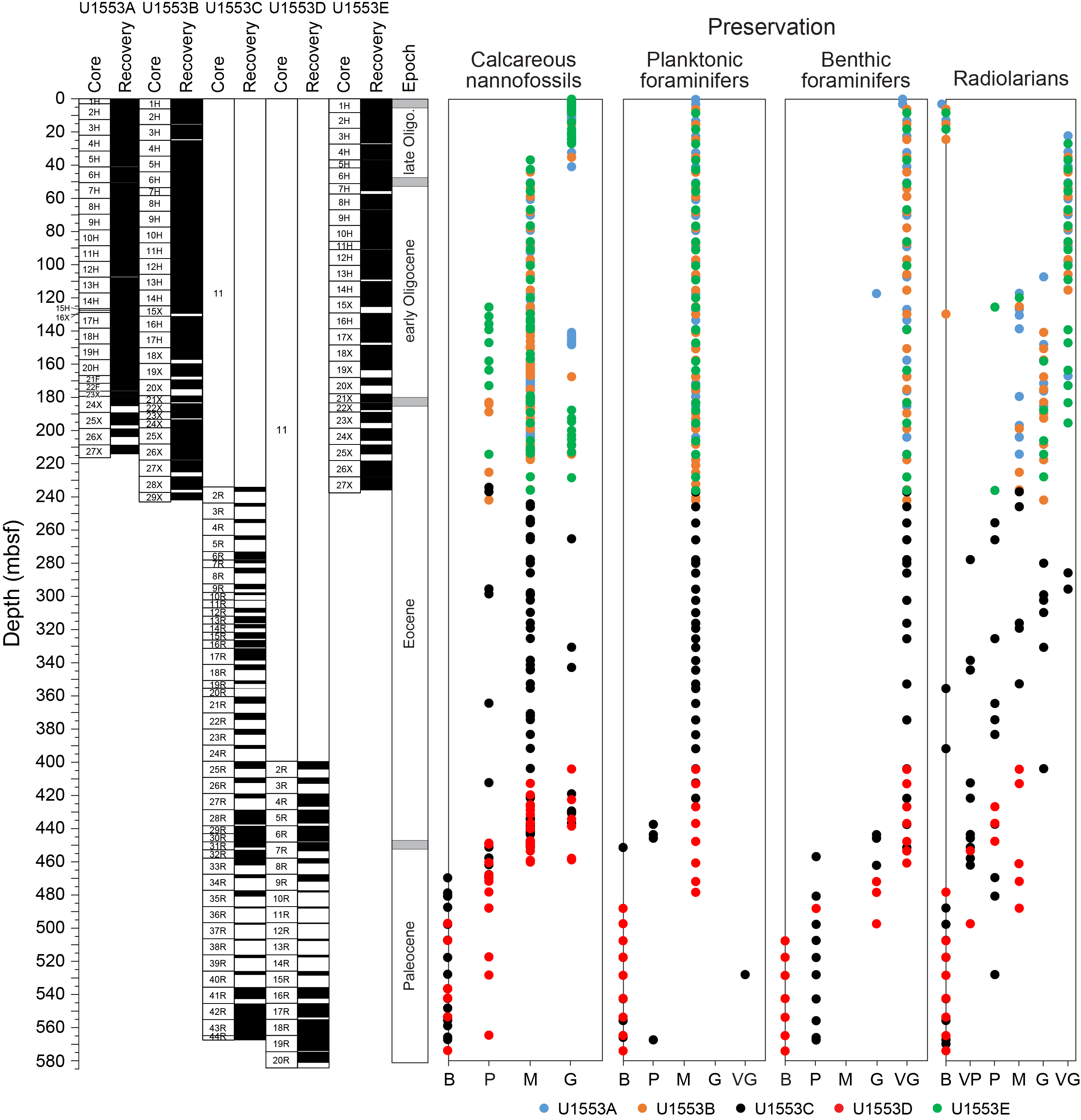
Figure F22. Microfossil abundance and preservation.
All planktonic microfossil groups lack most of the low-latitude species that form the basis of standard zonation schemes. For this reason, correlation and age assignments are based primarily on Southern Ocean and Southwest Pacific zonations, as noted below. An integrated biozonation for the five holes shows overall good agreement between the observed bioevents in different microfossil groups (Figures F23, F24). Tables T2, T3, and T4 list the datums that underpin the biozonations and are used, together with some paleomagnetic data, to develop the age-depth model for Site U1553 (see Age-depth model and mass accumulation rates).
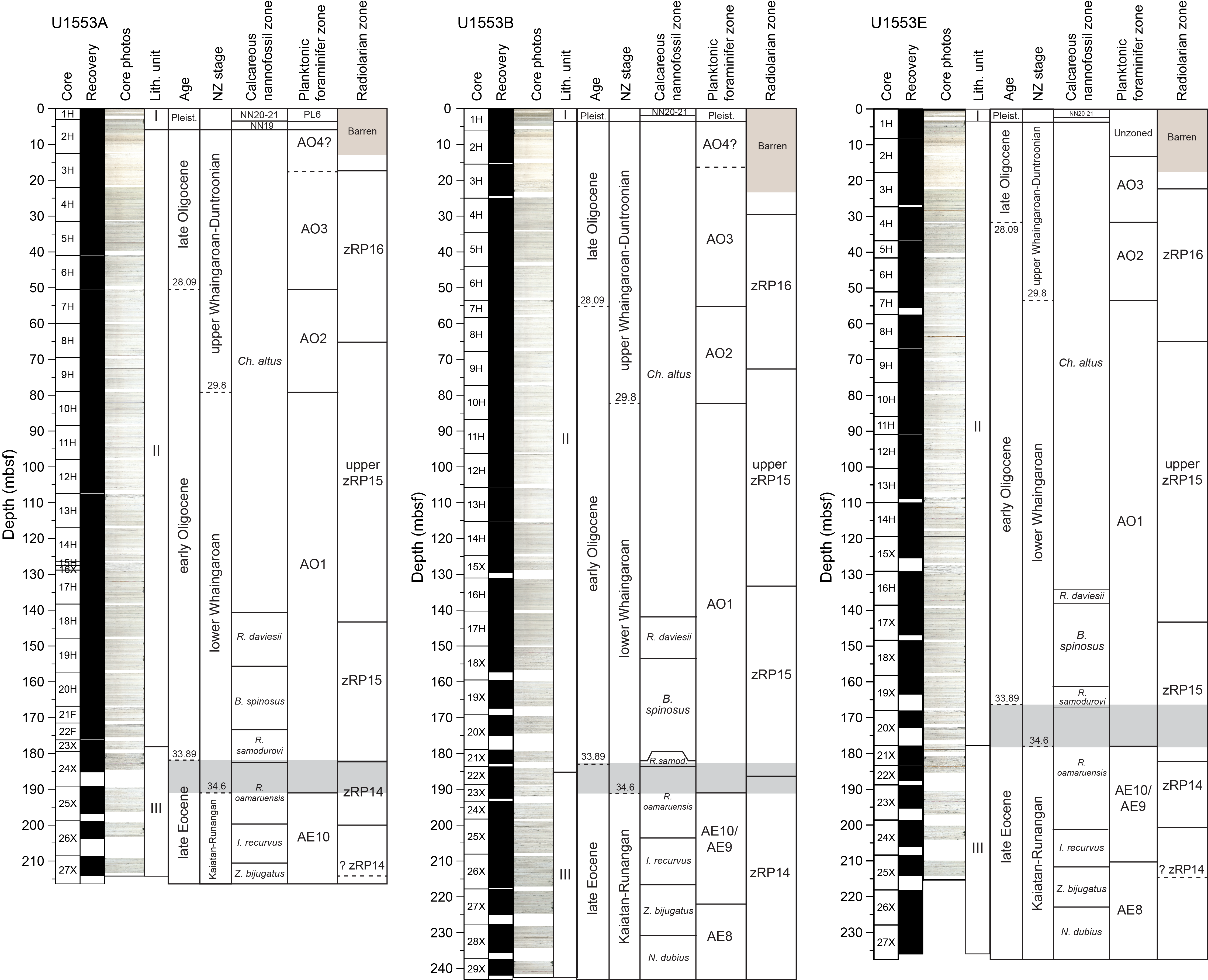
Figure F23. Biostratigraphic zones and datum events, Holes U1553A, U1553B, and U1553E.
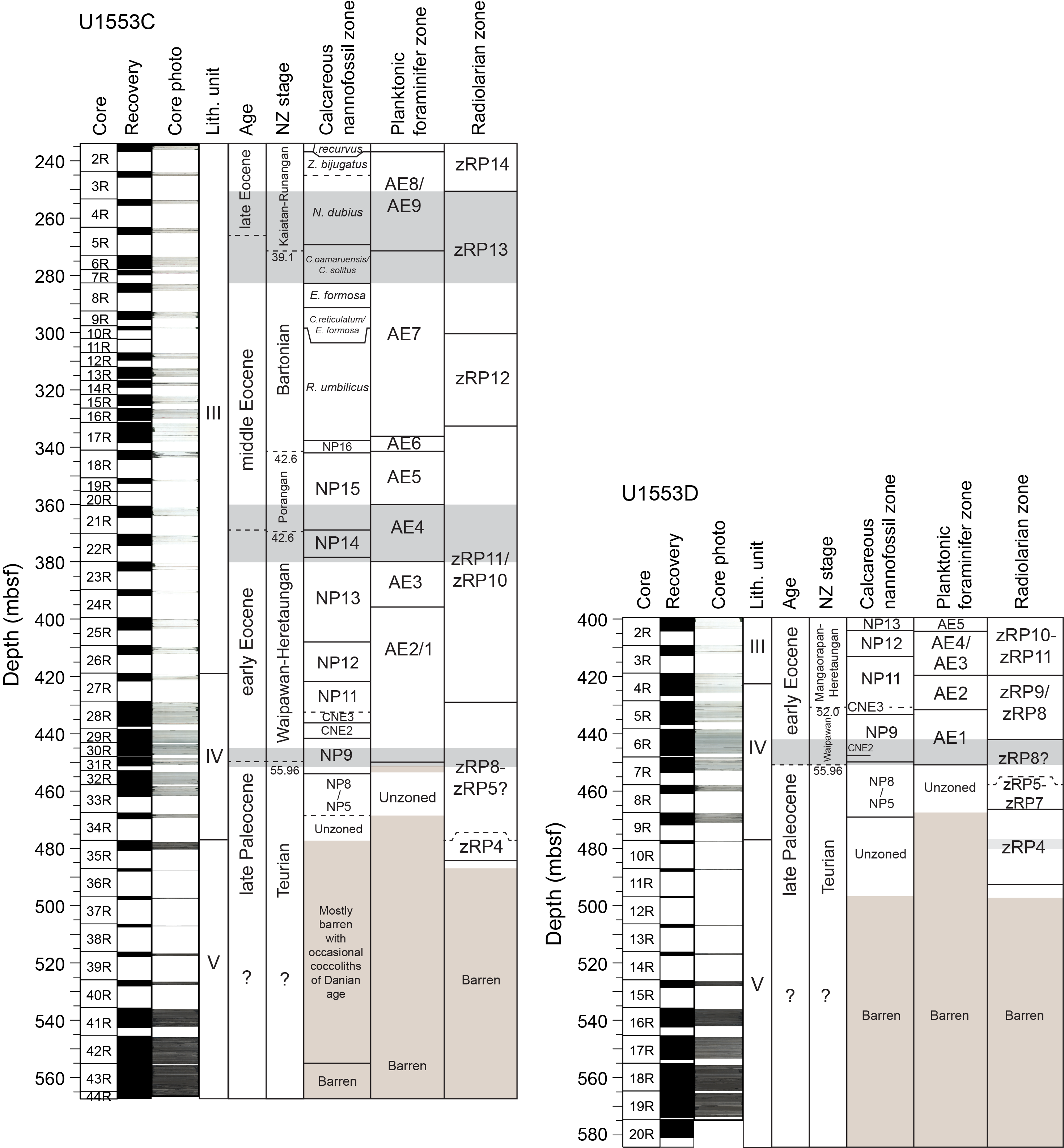
Figure F24. Biostratigraphic zones and datum events, Holes U1553C and U1553D.
4.1. Calcareous nannofossils
Shipboard calcareous nannofossil biostratigraphy focused primarily on age diagnostic species (Figure F25) in core catcher and additional working-half samples and therefore is not representative of complete assemblages. Table T2 shows depth positions and age estimates of calcareous nannofossil biostratigraphic marker events identified at Site U1553. Calcareous nannofossil occurrence data are shown in Table T5. Calcareous nannofossils are abundant in the majority of samples from Holes U1553A, U1553B, and U1553E and are abundant to barren in Holes U1553C and U1553D (Figure F22). Abundance of calcareous nannofossils is related to lithology; abundance is high in Lithostratigraphic Unit I (foraminiferal ooze with calcareous nannofossils) and Unit II (nannofossil ooze with foraminifers) and decreases in Unit III (limestone). Abundance is very low or nannofossils are absent in Unit IV (muddy sandstone); carbonate content varies from 5% to 90% in the upper part of Unit IV, where only rare/sporadic nannofossils were recorded. Nannofossils are generally absent in the underlying interval, although rare occurrences of single specimens are noted. Preservation ranges from good to poor and is generally good to moderate in the entire succession of Holes U1553A, U1553B, and U1553E, corresponding to the very high carbonate content of Units I–III. Preservation generally starts to deteriorate around the Eocene/Oligocene (E/O) boundary, where nannofossils show signs of overgrowth or etching. Sediments of late Eocene to late Paleocene age generally have moderate to poor preservation due to calcite overgrowth, which sometimes obscures morphological features of the diagnostic taxa. This is especially problematic for the genus Chiasmolithus and can hinder confident species-level identification.
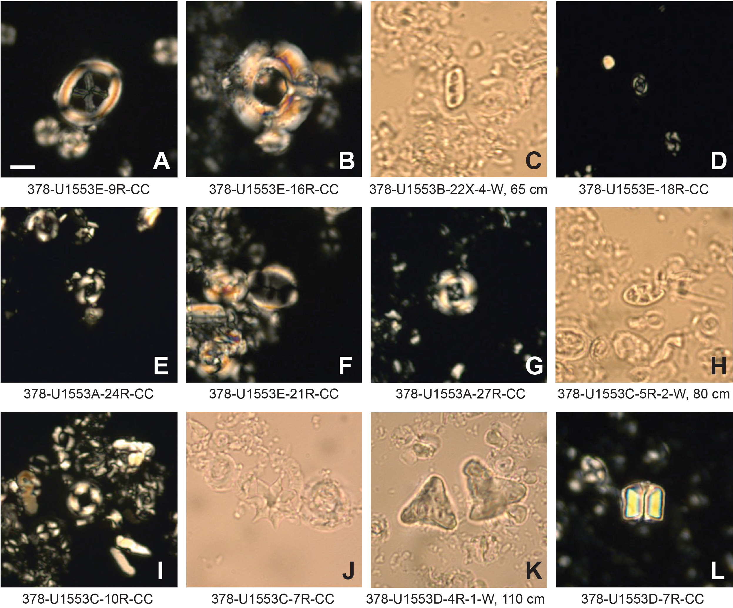
Figure F25. Selected calcareous nannofossil index species.
Calcareous nannofossil assemblages at Site U1553 are dominated throughout by typical high-latitude/cool-affinity genera (e.g., Reticulofenestra and Chiasmolithus) and are lower in diversity than lower latitude assemblages. Warm- and temperate-water Sphenolithus and Discoaster species are generally absent or very rare and scattered in Oligocene and late Eocene sediments at Site U1553. We therefore utilize the Southern Ocean biozonation scheme of Fioroni et al. (2012) for the calcareous nannofossil biostratigraphy of the middle Eocene–upper Oligocene sediments in Holes U1553A, U1553B, and U1553E. The high-latitude character is also reflected in the nannofossil assemblages observed in middle Eocene to lower Paleocene sediments, in which most of the markers from low- to mid-latitude biozonations are missing or sporadically occur. In this interval, however, the scheme of Martini (1971), with some integrations of the biohorizons indicated above, has been applied successfully.
4.1.1. Pleistocene
The uppermost sediment at Site U1553 contains abundant nannofossils of Pleistocene Biozones NN20–NN21, as indicated by the presence of abundant Gephyrocapsa spp. and the presence of Pseudoemiliania lacunosa in Samples 378-U1553A-1H-CC; 378-U1553B-1H-2, 100 cm; and 378-U1553E-1H-3, 50 cm. A major hiatus is inferred between Sample 378-U1553A-1H-CC, which contains upper Pleistocene taxa including P. lacunosa, and Sample 2H-1, 110 cm, which can be placed in the upper Oligocene Chiasmolithus altus Zone (which corresponds to Biozone NP25). This hiatus is observed in Hole U1553B between Samples 1H-3, 50 cm, and 1H-3, 100 cm, and in Hole U1553E between Samples 1H-3, 50 cm, and 1H-3, 100 cm. The hiatus indicated by the calcareous nannofossil biostratigraphy corresponds to the sharp lithologic transition at 4.0 mbsf in Hole U1553A, 3.68 mbsf in Hole U1553B, and 3.61 mbsf in Hole U1553C. The position of the top of P. lacunosa (0.44 Ma), precisely recorded in Hole U1553B at 2.25 mbsf, is consistent with the paleomagnetic data that place the Brunhes/Matuyama reversal at 2.2 mbsf in Hole U1553A. The assemblage composition of the samples immediately below the hiatus shows evidence of mixing/reworking; there are specimens of, for example, late Eocene Chiasmolithus expansus, Discoaster saipanensis, Neococcolithes dubius, and Reticulofenestra oamaruensis within samples of late Oligocene age in Cores 378-U1553A-2H, 378-U1553B-1H, and 378-U1553E-1H.
4.1.2. Oligocene
Cores 378-U1553A-2H through 23H, 378-U1553B-1H through 21H, and 378-U1553E-1H through 19X are Oligocene in age. Application of the zonation scheme of Fioroni et al. (2012) enables differentiation of biozones only in the lower part of the early Oligocene, owing to the very low biostratigraphic resolution that characterizes the overlying Oligocene interval. This interval is correlated to the late–early Oligocene C. altus Zone. The underlying interval extends 140.82–182.45 mbsf in Hole U1553A, 141.91–186.95 mbsf in Hole U1553B, and 134.89–167.81 mbsf in Hole U1553E (Figure F23). The top common occurrence of Reticulofenestra umbilicus (between Samples 378-U1553A-18H-1, 100 cm, and 18H-2, 100 cm [140.06 mbsf]; 378-U1553B-16H-CC and 17H-2, 110 cm [141.91 mbsf]; and 378-U1553E-16H-4, 50 cm, and 16H-5, 50 cm [134.89 mbsf]) marks the base of the C. altus Zone (early Oligocene). The top of Isthmolithus recurvus (between Samples 378-U1553A-19H-5, 80 cm, and 19H-6, 80 cm [155.36 mbsf]; 378-U1553B-17H-CC and 18X-5, 72 cm [153.64 mbsf]; and 378-U1553E-16X-6, 50 cm, and 16X-7, 50 cm [137.90 mbsf]) marks the base of the Reticulofenestra daviesii Zone. Oligocene assemblages have common to abundant Reticulofenestra spp., Chiasmolithus spp., Cyclicargolithus spp., and Coccolithus pelagicus and few Zygrhablithus bijugatus, Sphenolithus moriformis, and I. recurvus. Discoaster spp. are generally very rare and occur sporadically in samples throughout the early Oligocene to late Eocene. The base of C. altus (between Samples 378-U1553A-22F-2, 100 cm, and 22F-3, 100 cm [174.76 mbsf]; 378-U1553B-21X-3, 42 cm, and 21X-CC [182.63 mbsf]; 378-U1553E-18X-CC and 19X-CC [160.79 mbsf]) marks the base of the Blackites spinosus Subzone. An interval characterized by an increase in the abundance of Clausicoccus subdistichus is observed in Cores 378-U1553A-20H and 21F and between Samples 378-U1553B-19H-CC and 20H-CC. This event (base common occurrence) may indicate proximity to the E/O boundary, as observed at low- and mid-latitude sites where it has been calibrated to 33.88 Ma (Agnini et al., 2014). The E/O boundary is approximated by the top of R. oamaruensis (Wei and Thierstein, 1991) near the top of Chron C13r, as calibrated at other Southern Ocean sites (Fioroni et al., 2012). This biohorizon occurs between Samples 378-U1553A-24X-2, 80 cm, and 24X-3, 80 cm (182.45 mbsf); 378-U1553B-21X-CC and 22X-1, 48 cm (183.51 mbsf); and 378-U1553E-19X-CC and 20X-CC (167.81 mbsf) and marks the base of the Reticulofenestra samodurovi Zone. The top of R. oamaruensis is widely used in high-latitude sequences as an alternative biohorizon to the highest occurrence of rosette-shaped discoasterids (top of D. saipanensis; base of Biozone NP21; 34.44 Ma) and occurs just before the E/O boundary at lower latitudes (Fioroni et al., 2012).
4.1.3. Eocene
In the late Eocene, nannofossil assemblages largely resemble early Oligocene assemblages, including taxa such as Reticulofenestra spp. (common to abundant), Cyclicargolithus spp., Chiasmolithus spp., and C. pelagicus. In the late Eocene, the interval characterized by the presence of R. oamaruensis was recovered in Hole U1553A from 182.45 to 199.75 mbsf, in Hole U1553B from 183.51 to 203.52 mbsf, and in Hole U1553E from 167.81 to 201.38 mbsf. It corresponds to the latest Eocene R. oamaruensis Zone (Figure F23). The underlying upper Eocene biozones are defined by the following biohorizons: the base of common and continuous I. recurvus (between Samples 378-U1553A-27X-1, 46 cm, and 27X-3, 54 cm, [210.60 mbsf]; 378-U1553B-26X-6, 20 cm, and 26X-7, 20 cm [216.35 mbsf]; and 378-U1553E-25X- 3, 67 cm, and 25X-4, 10 cm [212.15 mbsf]), which marks the base of the I. recurvus Zone, and the top of Reticulofenestra reticulata, an additional biohorizon occurring between Samples 378-U1553A-26X-CC and 27X-1, 46 cm (206.47 mbsf); 378-U1553B-26X-6, 20 cm, and 26X-7, 20 cm (216.35 mbsf); and 378-U1553E-25X-2, 67 cm, and 25X-3, 67 cm (211.32 mbsf). The top of Neococcolithus dubius in Samples 378-U1553B-27X-CC and 28X-CC places the bottom of Hole U1553B (Core 28X) in the Chiasmolithus oamaruensis Zone, which straddles the middle–late Eocene time interval. This biohorizon was not identified in Holes U1553A and U1553E, presumably because these holes were shallower than Hole U1553B.
Holes U1553C and U1553D recovered sediments Eocene to early Paleocene in age (Figure F24). The biohorizon top of R. reticulata and base of common I. recurvus are recorded at the top of the Hole U1553C succession in Section 2R, confirming a late Eocene age (I. recurvus Zone). This interval overlaps with the sediments in Core 378-U1553A-27X, the upper part of Core 378-U1553B-27X, and the lower part of Core 378-U1553E-24X. The presence of N. dubius in Core 378-U1553C-3R-CC indicates the late–middle Eocene N. dubius Subzone of the C. oamaruensis Zone. The overlying Z. bijugatus Subzone seems restricted to the very top of Core 2R-CC. Below the N. dubius Subzone, the C. oamaruensis/Chiasmolithus solitus Subzone (the lowermost subzone of the C. oamaruensis Zone) is recognized in the interval between the top of C. solitus (273.41 mbsf) and the base of C. oamaruensis (282.92 mbsf). It has been identified despite calcite overgrowth that obscured the diagnostic morphologic features of the central area of many Chiasmolithus spp. specimens throughout this interval. The interval spanning the middle Eocene between 282.92 and 298.61 mbsf in Hole U1553C corresponds to the Ericsonia formosa Zone, the Chiasmolithus reticulatum/E. formosa Zone, and the R. umbilicus Zone. The biohorizons recorded are the top of common occurrence of Coccolithus formosus (= E. formosa) between Samples 8R-CC and 9R-CC (290.72 mbsf); the base of R. reticulata between Samples 10R-1, 30 cm, and 10R-1, 100 cm (298.26 mbsf); and the base of R. umbilicus between Samples 17R-5, 60 cm, and 17R-CC (338.21 mbsf). This datum has an age of 42.48 Ma (Fioroni et al., 2012).
For the early middle Eocene and Paleocene, the zonation scheme of Martini (1971) was applied because no higher latitude schemes have been devised for the Paleocene to early Eocene time period. Although we see a general shift toward an increased but irregular presence of warm water Discoaster specimens with increasing age downcore, warm water taxa are persistently sparse throughout the recovered intervals of Holes U1553C and U1553D, except for occasional samples in which nannofossil assemblages show greater abundances of taxa typical of low-latitude assemblages. Additionally, some biostratigraphically meaningful taxa in the lower Eocene and upper Paleocene sediments, such as Tribrachiatus spp., are generally rare, and Rhomboaster spp. are not observed at all. Because the majority of early Eocene and late Paleocene biohorizons are based on these three genera, it is challenging to define biohorizons with complete confidence based purely on shipboard observation. However, we identify the top of Tribrachiatus orthostylus between Samples 378-U1553C-25R-CC and 26R-CC (408.20 mbsf) and 378-U1553D-2R-CC and 3R-CC (408.58 mbsf) (Figure F26). This datum defines the base of lower Eocene Biozone NP13 and has an age of 50.5 Ma. Overgrown specimens of Tribrachiatus contortus and Tribrachiatus bramlettei are observed, rare and scattered, in Cores 378-U1553C-28R through 30R and 378-U1553D-5R and 6R, but their identification should be considered tentative (e.g., the presence of overgrown specimens of T. bramlettei recorded in Sample 378-U1553C-30R-1, 41 cm). The other bioevents that typically approximate the P/E boundary, the base of Rhomboaster spp. and the top of the Fasciculithus richardii group, could not be defined because specimens of these taxa were not observed. The absence of Rhomboaster spp. and Tribrachiatus spp. has been reported at onshore New Zealand sites of the same age (Kulhanek et al., 2015). The P/E boundary was therefore determined to be approximately within Sections 378-U1553C-31R-1 and 31R-2 and Section 378-U1553D-7R-1 in Biozone CNE1 (Agnini et al., 2014). The top of Fasciculithus tympaniformis (between Samples 378-U1553C-29R-2, 52 cm, and 29R-3, 42 cm [440.99 mbsf], and 378-U1553D-6R-7, 45 cm, and 6R-CC [447.64 mbsf]) and the presence of common to abundant Discoaster multiradiatus (between Samples 378-U1553C-31R-2, 49 cm, and 31R-CC [449.93 and 451 mbsf] and Samples 378-U1553D-7R-1, 101 cm, and 7R-1, 128 cm [449.11 and 449.38 mbsf]) were used to constrain the P/E boundary. The nannofossil assemblage observed in this interval shows the characteristics of assemblages of the P/E transition interval already observed at the high-latitude reference section of ODP Site 690 (Bralower, 2002).
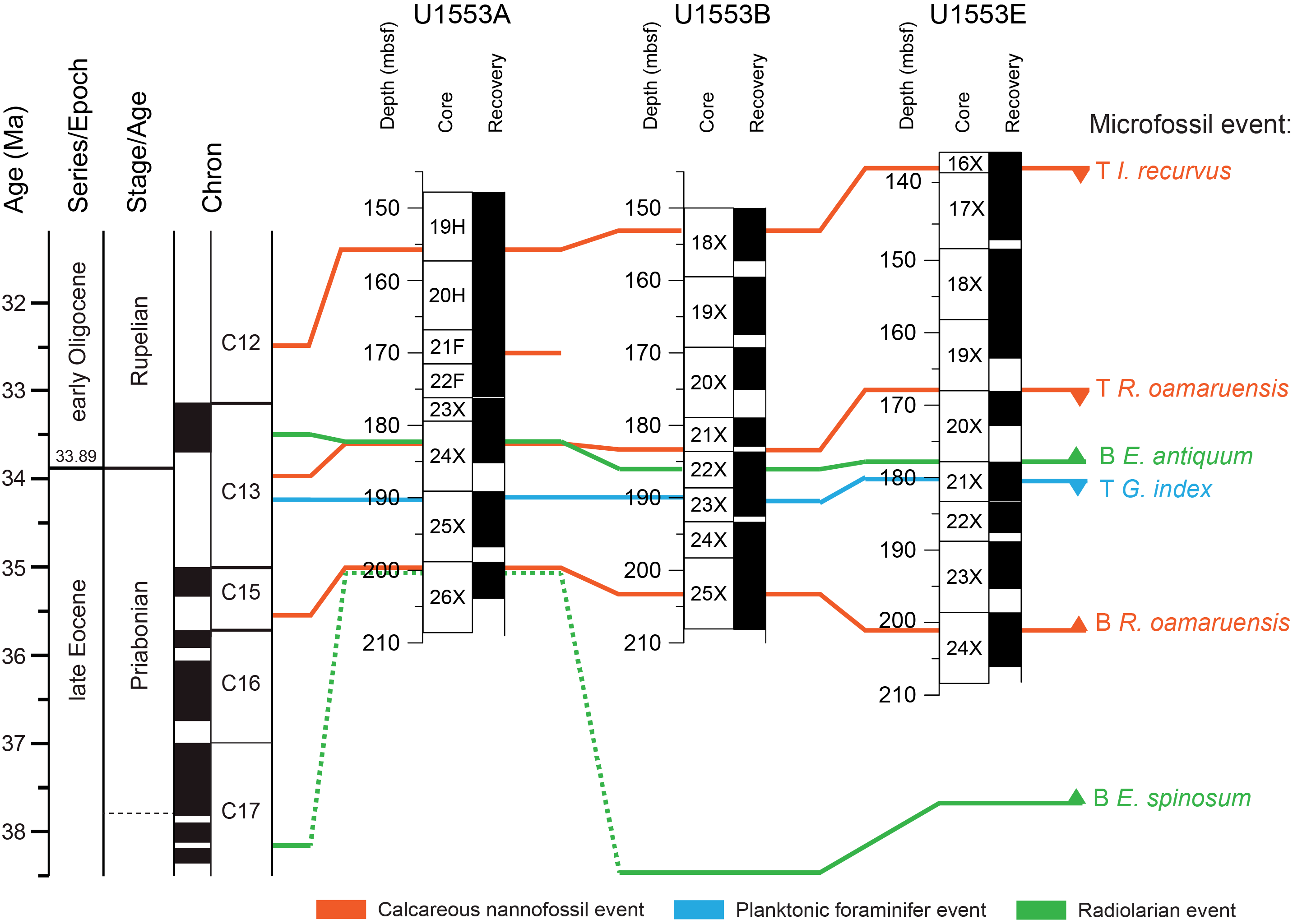
Figure F26. Eocene–Oligocene transition.
4.1.4. Paleocene
Nannofossil-bearing Paleocene sediments were recovered from 450 to ~470 mbsf in Hole U1553C (Cores 31R–34R) and from ~450 to ~470 mbsf in Hole U1553D (Cores 8R–10R). Nannofossil assemblages are generally poorly preserved (severe overgrowth and fragmentation) and scarce. The scattered presence or absence of most of the typical Paleocene marker species, such as the species belonging to Discoaster and Heliolithus, prevents a detailed biostratigraphic classification of the sediments (Figure F24). For example, the sporadic presence of D. multiradiatus in many samples in its range hampered the location of its first occurrence; therefore, the biohorizon base of D. multiradiatus (between Samples 378-U1553C-31R-CC and 32R-CC [454.61 mbsf] and 378-U1553D-7R-2, 27 cm, and 7R-2, 104 cm [450.06 mbsf]) should be considered to be poorly constrained at Site U1553. Nevertheless, the sediments between 450 and 470 mbsf in Holes U1553C and U1553D were assigned to a late and middle Paleocene age based on the presence of specimens of Paleocene species Toweius, the sporadic but sometimes common occurrence of F. tympaniformis, and the absence of Heliolithus spp. The presence of F. tympaniformis below the base of D. multiradiatus (base of Biozone NP9) implies a correlation to Biozones NP5–NP8 in the interval between ~450 and ~468 mbsf in Holes U1553C and U1553D, but these biozones cannot be differentiated because of the above-mentioned absence of any marker species of Heliolithus. Below 470 mbsf in Holes U1553C and U1553D, calcareous nannofossil abundance is very sparse, corresponding to a lithologic transition at ~480 mbsf from limestone (Unit IV) to muddy sandstone (Unit V) with low carbonate content (average = 2.2%). Fasciculithus spp. are present in Sample 378-U1553D-8R-CC, which implies a zonation of NP4 or younger, but they are absent in Sample 9R-CC, implying a correlation with lower NP4 or earlier biozones. The limited thickness (~20 m) of the recovered sediments from between 450 and 470 mbsf, which should correspond to Biozones NP8/9–NP5, relative to the estimated sedimentation rates of this interval (Figure F60), suggests the presence of a hiatus in the sedimentation at Site U1553 between the middle–late Paleocene Biozones NP8 and NP5. This is in agreement with the hiatus representing Biozones NP7 and NP8 proposed in Hollis et al. (2015) that resulted from detailed calcareous nannofossil investigation of DSDP Site 277 sediments. Deeper than 480 mbsf in Hole U1553C, in the dark grayish black siliciclastic Unit V (see Lithostratigraphy), single nannofossil specimens were occasionally observed, as at 548.57 mbsf (Sample 42R-3, 33 cm), where early Paleocene Zeugrhabdotus sigmoides, Chiasmolithus danicus, Futyania petalosa, and small Prinsius spp. occur. Two individual specimens of Cretaceous Watznaueria spp. were observed in Samples 36R-CC and 42R-3, 33 cm. The rareness of lower Paleocene and Cretaceous specimens suggests that these presences result from reworking within the siliciclastic Unit V. It is therefore not possible to constrain the stratigraphic position of Cores 378-U1553C-35R through 44R and 378-U1553D-12R through 20R and their proximity to the K/Pg boundary.
4.2. Planktonic foraminifers
At Site U1553, planktonic foraminifers are abundant and have moderate to good preservation in Holes U1553A, U1553B, and U1553E (Figure F22), whereas they are abundant in the upper part of Holes U1553C and U1553D and absent from both holes below ~460 mbsf, apart from an isolated occurrence in Sample 378-U1553C-40R-CC (see below). Test preservation is moderate in the upper part of Holes U1553C and U1553D and becomes poorer downhole starting at around 400 mbsf (Figure F22). Several biozones spanning the middle Oligocene to the late Paleocene were recognized at Site U1553 based on planktonic foraminifers (Figures F23, F24). Overall, planktonic foraminifers display low diversity assemblages and species compositions typical of high-latitude areas in the Oligocene to late Eocene, with notably small test sizes in some intervals in the Oligocene. In the middle to early Eocene, assemblages are more diverse and contain common muricate forms. Muricate planktonic foraminifers, such as Acarinina and Morozovella, are typical of tropical to subtropical latitudes but extend southward to the paleolocation of Site U1553 in the middle to early Eocene. The average planktonic:benthic (P:B) ratio is approximately 98%. In spite of the high P:B ratio, benthic foraminifers are relatively common at Site U1553 and have good preservation. Most of the species identified are epifaunal calcareous taxa, but there is an increased contribution of agglutinated taxa below 428 mbsf. The benthic foraminiferal species identified are useful for constraining the paleobathymetry at the site.
4.2.1. Overview of planktonic foraminifer biostratigraphy
We analyzed planktonic foraminifer assemblages for biostratigraphy in each core catcher sample from Site U1553, the deepest of which was from 581 mbsf (Sample 378-U1553D-20R-CC) (Figures F23, F24). Planktonic foraminifer marker species for the tropical zonation (Wade et al., 2011) are absent throughout. Thus, ages assigned to the investigated samples used the Austral zonation scheme of Huber and Quillévéré (2005). Four biozones were identified at the midpoint depths in Hole U1553A: middle Oligocene Biozones AO3 (44.59 ± 4.83 mbsf) and AO2 (84.05 ± 4.95 mbsf), early Oligocene Biozone AO1 (190.99 ± 5.8 mbsf), and late Eocene Biozone AE10 (below 196.79 mbsf to the bottom of Hole A) (Figure F23). Sample 1H-CC contains species ranging from the late Pliocene to the Pliocene/Pleistocene boundary, such as Truncorotalia crassula, and forms that are transitional between Globoconella puncticulata and Globoconella inflata and were assigned to Biozone PL6. In Sample 2H-CC, reworked Pliocene–Pleistocene planktonic foraminifers are common and can be distinguished from the Oligocene assemblage by differences in preservation. Five biozones were identified at the midpoint depths in Hole U1553B: middle and early Oligocene Biozones AO3 (56.27 ± 2.46 mbsf), AO2 (82.27 ± 4.65 mbsf), and AO1 (191 ± 1.54 mbsf) and late Eocene Biozones AE10/AE9 (214.13 ± 21.56 mbsf) and AE8 (below 235.69 mbsf to the bottom of Hole B). Hole U1553E spans Biozones AO3 to AE8 considering the midpoint depths: middle and early Oligocene Biozones AO3 (31.74 ± 4.94 mbsf), AO2 (53.32 ± 2.27 mbsf), AO1 (117.97 ± 5.17 mbsf), and AE10/9 (210.18 ± 4.07 mbsf) and late Eocene Biozone AE8 (below 214.25 mbsf to the bottom of Hole E). The uppermost occurrence of Globigerinatheka index is recorded in Samples 378-U1553A-25X-CC, 378-U1553B-23X-CC, and 378-U1553E-21X-CC, indicating a latest Eocene age (top of AE10), and it is used to locate the E/O boundary in these holes. Thus, the E/O boundary occurs between Cores 378-U1553A-24X and 25X (185.19–196.79 mbsf), 378-U1553B-22X and 23X (189.45–192.54 mbsf), and 378-U1553E-20X and 21X (172.80–183.14 mbsf) (Figure F26), and it is poorly constrained based on only core catcher samples. Further sampling at higher resolution is required to pinpoint the E/O boundary in these holes. Holes U1553C and U1553D recovered sediments spanning the late Eocene to early Paleocene (Figure F24). Considering the midpoint depths, six biozones were recovered in Hole U1553C: middle Eocene Biozones AE8 (271.11 ± 5.97 mbsf), AE7 (334.63 ± 3.92 mbsf), AE6 (341.46 ± 2.91 mbsf), and AE5 (360.03 ± 4.51 mbsf); middle to early Eocene Biozone AE4 (378.85 ± 4.45 mbsf); and early Eocene Biozone AE3 (429.58 ± 7.88 mbsf). Four biozones were recovered in Hole U1553D (Figure F24): middle to early Eocene Biozone AE4/AE3 (419.83 ± 6.95 mbsf), early Eocene Biozones AE2 (431.84 ± 5.06 mbsf) and AE1 (450.61 ± 2.85 mbsf), and late Paleocene Biozone AP4 (below 453.46 mbsf). Samples 378-U1553C-30R-CC, 31R-CC, 378-U1553D-6R-CC, and 7R-CC span the P/E boundary at Site U1553 (Figure F27). Samples 378-U1553C-30R-CC and 31R-CC are heavily affected by dissolution, and the P/E boundary could not be located based on planktonic foraminifer biostratigraphy. We confirm the occurrence of the P/E boundary between Samples 378-U1553D-6R-CC and 7R-CC (447.76–453.46 mbsf) based on the base of Globanomalina australiformis (55.96 Ma) in Sample 6R-CC, which defines the top of the Paleocene in the Austral zonation of Huber and Quillévéré (2005).
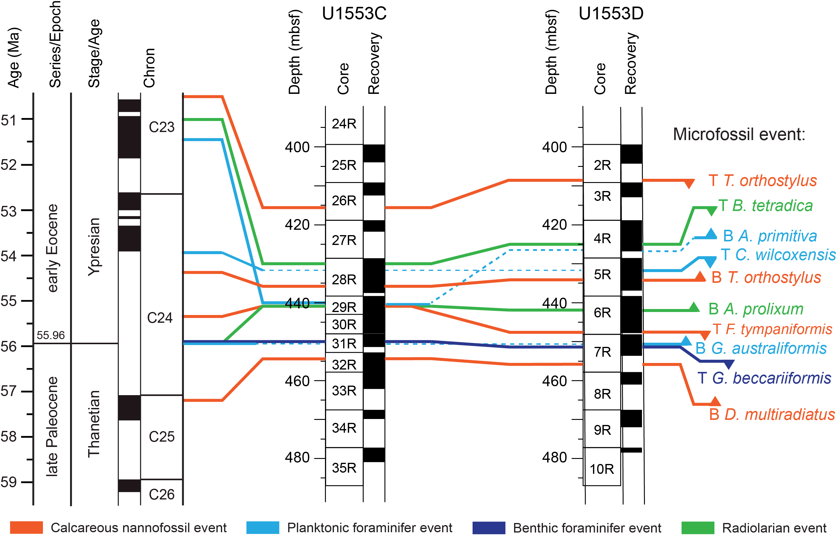
Figure F27. Paleocene–Eocene transition.
4.2.2. Oligocene
The uppermost interval of Site U1553 comprises sediments of late Oligocene or younger age based on the absence of Globoturborotalita labiacrassata, the top of which defines the base of late Oligocene Biozone AO4. This datum lies between Samples 378-U1553A-3H-CC (22.24–22.29 mbsf) and 378-U1553B-2H-CC (15.18–15.23 mbsf) (Figure F28; Table T6). At Site U1553, common species in Biozone AO3 include Subbotina eocaena, Subbotina corpulenta, Globoturborotalita paracancellata, Globoturborotalita eolabiacrassata, G. labiacrassata, Paragloborotalia nana, Paragloborotalia opima, Paragloborotalia pseudocontinuosa, and Globigerinella obesa.
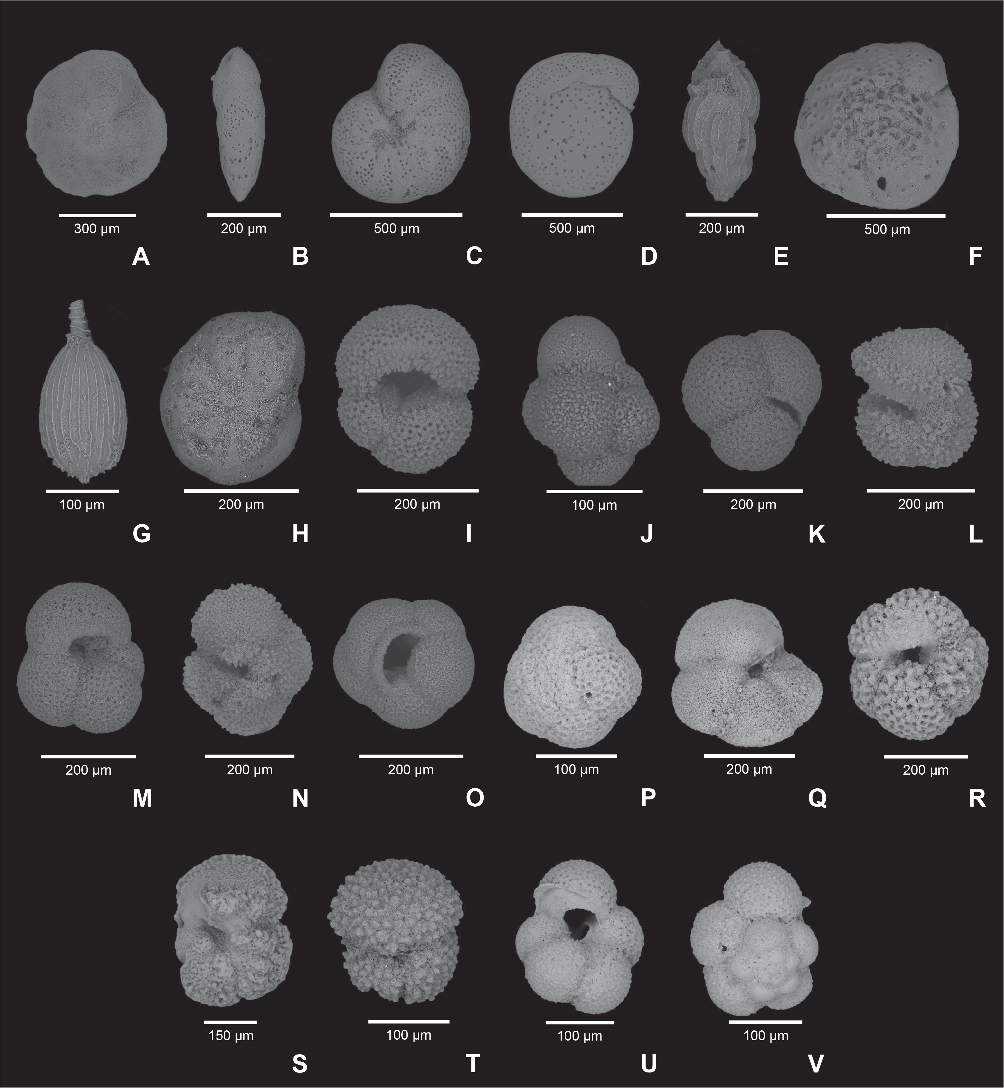
Figure F28. Foraminifer species.
Chiloguembelina cubensis is a species commonly observed in high-latitude areas in the early to middle Oligocene, and its highest common (top common [Tc]) occurrence marks the base of Biozone AO3 (28.1 Ma). The Tc of C. cubensis is identified in Samples 378-U1553A-6H, 378-U1553B-7H, and 378-U1553E-4H (50.42–50.47, 58.72–58.77, and 36.68–36.73 mbsf, respectively). Planktonic foraminifer species observed in this interval include P. nana, S. eocaena, Subbotina utilisindex, and G. labiacrassata. Below this datum, the highest occurrence (top) of Subbotina angiporoides in Samples 378-U1553A-11H-CC, 378-U1553B-10H-CC, and 378-U1553E-7R-CC defines the base of Biozone AO2 (29.8 Ma). In this biozone, we observe common S. utilisindex, G. labiacrassata, Globigerinella archaeobulloides, and Parasubbotina varianta. In Biozone AO1, species diversity tends to decrease downhole, possibly linked to the stratigraphic and temporal proximity of the E/O boundary. Several samples in Biozone AO1 have planktonic foraminifer assemblages dominated by small planktonic taxa such as C. cubensis, Tenuitella spp., and Pseudohastigerina spp. This may indicate the presence of blooms linked to upwelling or shifts of the subPolar Front resulting in more nutrient-rich surface waters and higher productivity. See Table T3 for the list of Oligocene planktonic foraminifer datums used in this study.
4.2.3. Eocene
The top of Hantkenina alabamensis (33.89 Ma) is the planktonic foraminifer datum that most closely approximates the E/O boundary. However, H. alabamensis does not occur in the investigated core catcher samples, likely because this species was restricted to lower latitudes in the Eocene. Shipboard biostratigraphy using only core catcher samples has a relatively coarse resolution, however, and subsequent higher resolution studies might reveal the occurrence of H. alabamensis, allowing a more precise definition of the E/O boundary. Following the Austral zonation scheme of Huber and Quillévéré (2005), we use the top of G. index (34.60 Ma) between Samples 378-U1553A-24H-CC and 25H-CC, 378-U1553B-22H-CC and 23X-CC, and 378-U1553E-20R-CC and 21R-CC to provide an estimate of the stratigraphic position of the E/O boundary (Figures F26, F28I). The top of G. index marks the boundary between Biozones AO1 and AE10. Biozone AE10 has a short duration, and it was not possible to detect the base of this biozone, which is marked by the top of Tenuitella insolita. We therefore could not distinguish the boundary between Biozones AE10 and AE9. Common species observed in this interval are G. index, S. angiporoides, Subbotina linaperta, Turborotalia ampliapertura, Catapsydrax unicavus, and Pseudohastigerina wilcoxensis. We estimated the base of late Eocene Biozone AE9 based on the top of Globigerinatheka barri in Samples 378-U1553B-28X-CC, 378-U1553E-25X-CC, and 378-U1553C-5R-CC. This species and the majority of Globigerinatheka species (other than G. index) are reported to range up to the upper part of Biozone AE8 (Pearson et al., 2006). Common planktonic foraminifers in underlying Biozone AE8 include G. index, Subbotina gortanii, S. linaperta, S. eocaena, and S. angiporoides.
The uppermost part of Hole U1553C (265.8–255.56 mbsf) consists of late Eocene samples, which were assigned to Biozone AE8 (see above). The top of Acarinina primitiva (39.1 Ma) marks the boundary between Biozones AE8 and AE7 between Samples 5R-CC and 6R-CC. Biozone AE7 spans the mid-Bartonian to early Lutetian (39.1–42.11 Ma), defining the transition from the late to the middle Eocene at Site U1553. It is characterized by a distinct increase in species diversity and test size compared to the sediments spanning the late Eocene to early Oligocene. Large Globigerinatheka typical of middle Eocene tropical to subtropical assemblages—G. index, G. barri, and Globigerinatheka subconglobata—are common in this biozone, together with A. primitiva and Acarinina collactea and subbotinids such as S. angiporoides, S. linaperta, S. eocaena, and large Turborotalia frontosa. A similar assemblage characterizes Biozones AE6 and AE5. AE6 is a short duration biozone that extends from the base of S. angiporoides in Sample 17R-CC to the base of G. index in Sample 18R-CC. The base of Biozone AE5 is defined by the top of Cassigerinelloita amekiensis in Samples 378-U1553C-21R-CC and 378-U1553D-2R-CC. This extremely small species (Figure F28J) was reported as a distinctive and common stratigraphic marker in middle Eocene planktonic foraminifer assemblages on the Kerguelen Plateau in the Indian sector of the Southern Ocean (Huber and Quillévéré, 2005). Because of its small size, we performed a dedicated search for this species in Hole U1553A. This allowed us to report it for the first time in the ocean region offshore New Zealand, confirming its stratigraphic utility for the southern subpolar region. Biozone AE4 marks the transition to the upper Ypresian and is characterized by the uppermost occurrence of the genus Morozovella at Site U1553. In particular, the top of Morozovella crater is recorded in Samples 378-U1553C-22R-CC and 378-U1553D-3R-CC. Magneotobiochronology in the mid-Waipara section (New Zealand) indicates an age of 45.7 Ma for this datum (Raine et al., 2015; Dallanave et al., 2016). However, its uppermost occurrence at Site U1553 (within the core catcher samples) appears to be no younger than 46.13 Ma and not older than 50.04 Ma based on planktonic foraminifer datum events in adjacent cores. Between Samples 378-U1553C-22R-CC and 23R-CC, we identify the base of C. amekiensis, which marks the boundary between Biozones AE4 and AE3. Species commonly observed in Biozone AE3 are A. primitiva, A. collactea, Subbotina lineaperta, Subbotina rosnaesensis, S. eocaena, Subbotina senni, Subbotina crociapertura, S. corpulenta, and G. australiformis. We identified the boundary between Biozones AE3 and AE2 between Samples 378-U1553C-27R-CC and 28R-CC and 378-U1553D-3R-CC and 4R-CC where we place the biohorizon base A. primitiva. This species (Figure F28T) evolved from Acarinina coalingensis (Figure F28L) in the early Eocene, and the two species coexisted for roughly 2 My and exhibit strong morphological intergradation. Our identification of the base of A. primitiva in the above intervals is based on the occurrence of the lowermost convincing specimens of A. primitiva in Samples 378-U1553C-27R-CC and 378-U1553D-3R-CC and the occurrence of the uppermost definitive specimens of A. coalingensis in Samples 378-U1553C-28R-CC and 378-U1553D-4R-CC. Other species common in this interval are Acarinina esnehensis, Acarinina pseudotopilensis, A. collactea, P. wilcoxensis, S. linaperta, S. eocaena, Chiloguembelina wilcoxensis, and G. australiformis. Species belonging to the genus Morozovella commonly occur between Samples 378-U1553C-22R-CC and 26R-CC and 378-U1553D-2R-CC and 4R-CC, confirming previous studies that indicate this genus, generally reported as confined to tropical to subtropical latitudes (Pearson et al., 2006), extends its range poleward to subpolar latitudes during the acme of the Cenozoic warmth (Jenkins, 1975; Hollis et al., 1997). Morozovella species commonly observed within this interval in Holes U1553C and U1553D are M. crater, Morozovella gracilis, Morozovella subbotinae, and Morozovella lensiformis. Rare Morozovella aragonensis were also observed.
Between 46 and 52 Ma, planktonic foraminifer preservation decreases substantially. Between Samples 378-U1553C-27R-CC and 30R-CC and 378-U1553D-5R-CC and 7R-CC, there are clear signs of dissolution. Planktonic foraminifer assemblages are dominated by subbotinids, and dissolution-prone muricate forms decrease in abundance and diversity. The upper part of this interval, around 400 mbsf, coincides with a decrease in bulk sediment CaCO3 wt% in Holes U1553C and U1553D. We cannot assign a biozone to Samples 378-U1553C-29R-CC to 32R-CC because of the scarcity of specimens and their poor preservation. The decrease in preservation in Hole U1553D starts about 15 m deeper than in Hole U1553C, and we tentatively place the Biozone AE2/AE1 boundary between Samples 378-U1553D-4R-CC and 378-U1553C-5R-CC. This is based on the disappearance of C. wilcoxensis, which occurs in the samples immediately above that biozone and which may represent biohorizon top C. wilcoxensis (53.94 Ma). A higher resolution study will be required to confirm the presence of the Biozone AE2/AE1 boundary at Site U1553.
See Table T3 for the list of Eocene planktonic foraminifer datums used in this study.
4.2.4. Paleocene
Calcareous nannofossil and benthic foraminifer data indicate the occurrence of the P/E boundary between Cores 378-U1553C-30R and 31R and Samples 378-U1553D-6R-CC and 7R-CC. Planktonic foraminifers are rare and poorly preserved in Samples 378-U1553C-30R-CC and 31R-CC, and Sample 32R-CC is barren of planktonic foraminifers. We therefore could not confirm this interpretation using planktonic foraminifers. We assigned a late Paleocene age to Sample 378-U1553D-7R-CC based on the absence of G. australiformis. The top of G. australiformis marks the boundary between Biozones AE1 and AP4 and is calibrated at 55.96 Ma. This species consistently occurs in the Eocene samples from Hole U1553D despite the decrease in preservation. We therefore consider the disappearance of G. australiformis a reliable datum in Hole U1553D and confirm the occurrence of the P/E boundary between Samples 6R-CC and 7R-CC (447.76–453.46 mbsf) (Figure F26). We observed an increase in species diversity along with an improvement of planktonic foraminifer preservation in Sample 8R-CC. This sample is characterized by a Paleocene assemblage with common Acarinina nitida, A. coalingensis, A. collactea, Acarinina subglobosa, Igorina pusilla, Subbotina velascoensis, Subbotina triangularis, Parasubbotina variospira, and P. wilcoxensis, and we assign it to Biozone AP4. In this sample, we also observed a decrease in the P:B ratio to 77%. This points to a decrease in paleodepth rather than an increase in dissolution because preservation improves in this sample and planktonic foraminifers are more abundant than in the previous, poorly preserved samples. Also, this decrease is consistent with a benthic foraminifer assemblage indicative of a shallower paleodepth than overlies in, for example, middle bathyal (see below). Sample 8R-CC may indicate the transition to a time interval characterized by a paleodepth remarkably shallower in this area because core catcher samples are barren in planktonic foraminifers to the bottom of Hole U1553D. This transition also coincides with the abrupt change in lithology from chalk to mudstone observed at the same depth (Figure F24; see Lithostratigraphy). In the dark grayish black siliciclastic Unit V, which starts at about 477 mbsf in Holes U1553C and U1553D, the only sample containing planktonic foraminifers is Sample 378-U1553C-40R-CC at 528.11 mbsf. This sample contains few specimens of well-preserved planktonic foraminifers, two specimens of unidentified microperforate form (Figure F28U, F28V), and six specimens that resemble Neogloboquadrina pachyderma (Figure F28O, F28P). The presence of N. pachyderma, whose first or lowest occurrence is in the late Miocene, possibly indicates downhole contamination within this unit.
4.3. Benthic foraminifers
Benthic foraminifer abundance and preservation were qualitatively analyzed for Site U1553 (Figure F22). The abundance ranges from few to rare; only in Sample 378-U1553C-44R-CC were they abundant. Benthic foraminifers are barren below 500 mbsf in Hole U1553D. Preservation is very good in the Pleistocene, Oligocene, and Eocene and ranges from very good to poor in the Paleocene. Samples are mostly dominated by calcareous taxa (Table T7; Figure F28). Although few agglutinated taxa, such as Bathysiphon, Gaudryina, and Siphotextularia, are recorded in the latest Paleocene, agglutinated taxa are an important component of assemblages in the earlier Paleocene.
During the Pleistocene, Oligocene, and Eocene, epifaunal taxa are dominant, and the assemblages include Anomalinoides sp., Cibicides sp., Gyroidinoides sp., Hanzawaia scopus, and Nuttallides sp. Although epifaunal dominance indicates a highly oxygenated environment, the constant presence of infaunal taxa (such as bolivinids, buliminids, Globocassidulina sp., Lagena sulcata, Lenticulina sp., nodosariids, Oridorsalis umbonatus, Pullenia sp., Trifarina sp., and Uvigerina sp.) suggests relatively high productivity.
The assemblages in Samples 378-U1553C-31R-CC and 378-U1553D-7R-CC are also dominated by epifaunal taxa and have greater relative abundances of infaunal species such as Bathysiphon spp. and Loxostomoides sp. The last appearance of Gavelinella beccariiformis occurs in these two samples, indicating that the P/E boundary lies in Cores 378-U1553C-31R and 378-U1553D-7R. Underlying Paleocene assemblages are dominated by infaunal taxa and agglutinated species (such as Bathysiphon spp. and Spiroplectammina sp.), the presence of which may suggest deposition in low oxygen conditions and a mesotrophic paleoenvironment.
The continuous presence of Laticarina pauperata in the Oligocene interval and the abundance of Gyroidinoides neosoldanii, Pullenia bulloides, Anomalinoides aotea, and O. umbonatus during the Eocene confirms sediment deposition at lower bathyal depths (Hollis et al., 1997; Hayward et al., 2010). In the Paleocene interval (Samples 378-U1553C-31R-CC to 44R-CC and 378-U1553D-7R-CC to 12R-CC), a mid–lower bathyal paleodepth is inferred by the occurrence of Bathysiphon spp., G. beccariiformis, and Nuttallides truempyi (Tjalsma and Lohmann 1983; Hornibrook et al., 1989; Alegret and Thomas, 2013). Redeposition of Paleocene or older sediments is suggested by the frequent presence of large, broken specimens of the genus Lenticulina, which is inferred to have been derived from shelf environments (e.g., in Samples 378-U1553C-35R-CC and 378-U1553D-9R-CC to 12R-CC). A similar occurrence of this genus in deepwater settings was reported by Sutherland et al. (2019) for IODP Expedition 371 sediments. The presence of bryozoan fragments in Samples 378-U1553C-35R-CC and 378-U1553D-11R-CC also suggests downslope redeposition of shelf sediments.
4.4. Radiolarians
Radiolarians are abundant and very well preserved in the Oligocene and late Eocene at Site U1553. They are rare but still well preserved in the middle Eocene. In the early Eocene and Paleocene, radiolarian occurrence is sporadic, many samples are barren, and preservation is poor. In some early Eocene samples, however, radiolarians are very abundant but very poorly preserved. Trends in radiolarian abundance and preservation in Holes U1553A and U1553B are shown in Figure F22. In several samples in the lower Oligocene and upper Eocene, black overgrowths are present on some radiolarian tests and sponge spicules and are inferred to be pyrite (Figure F29O).
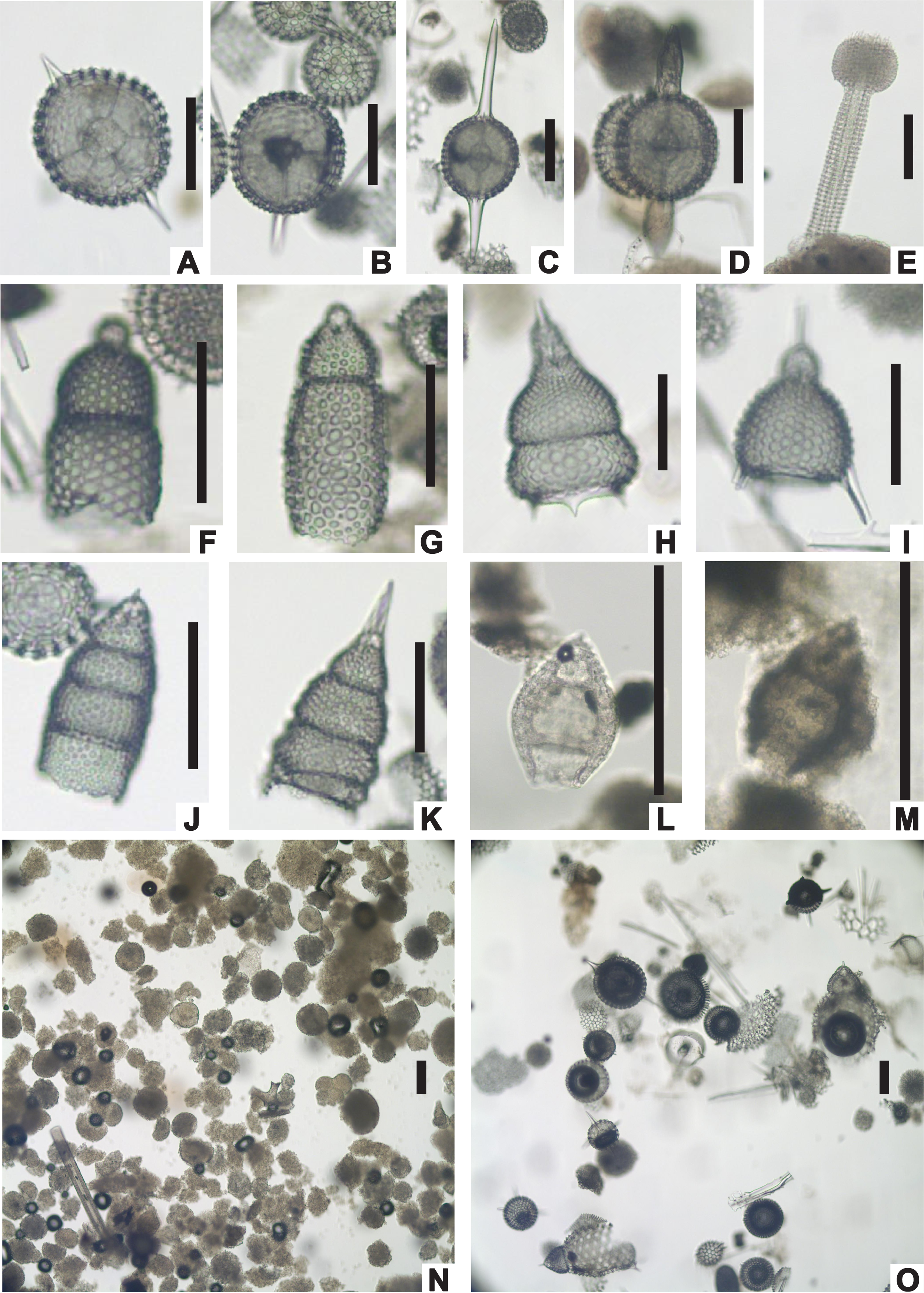
Figure F29. Selected radiolarian index species and assemblages.
Because low-latitude index species are absent or very rare, radiolarian assemblages have been correlated to the Southwest Pacific zonation, which has been recently revised (Hollis et al., 2017; C.J. Hollis, unpubl. data; Sutherland et al., 2019). This zonation incorporates the Oligocene–late Eocene Southern Ocean zonation of Funakawa and Nishi (2005). The radiolarian succession has been correlated to Biozones zRP16–zRP3 (early late Oligocene to early Paleocene) (Table T4). The following description of the downhole biostratigraphy is based on preliminary assessment of core catcher samples in all five holes at Site U1553. The radiolarian occurrence tables for each hole (Table T8) and database information should not be considered to be a full census of species present because shipboard analysis focused on identifying key species (Figure F29A–F29N).
4.4.1. Neogene
The uppermost cores from Holes U1553A, U1553B, and U1553E are barren of radiolarians (i.e., Cores 378-U1553A-1H and 2H, 378-U1553B-1H through 3H, and 378-U1553E-1H and 2H) (Table T4).
4.4.2. Oligocene
Very well preserved and abundant Oligocene radiolarians occur in the upper part of Holes U1553A, U1553B, and U1553E from ~20 to ~125 mbsf (Cores 378-U1553A-3H through 13H, 378-U1553B-4H through 13H, and 378-U1553E-3H through 13H). Diatoms and sponge spicules are also abundant in this interval, and silicoflagellates are noted in most samples. Between ~120 and 130 mbsf (Cores 14H and 15H in Holes U1553A, U1553B, and U1553E), radiolarians and diatoms are very rare or absent. In the underlying Oligocene interval (~130 to ~180 mbsf), radiolarians are common and well preserved, but diatoms are relatively rare.
In Cores 378-U1553A-3H through 7H, the co-occurrence of Lychnocanium aff. conicum (Lychnocanoma conica in the sense of Abelmann, 1990) and Axoprunum? irregularis indicates a correlation with early late Oligocene Biozone zRP16 (Table T4). It is possible that the index species for Biozone zRP17, Clinorhabdus robusta, occurs in this interval, but it has yet to be confidently identified. Assemblages in this biozone include numerous reworked radiolarians of middle Eocene age, including Artobotrys auriculaleporis, Eusyringium fistuligerum, Periphaena decora, and Theocampe mongolfieri. It is notable that although the first three species are common in the middle Eocene at this site, T. mongolfieri has yet to be discovered in situ in the middle Eocene assemblages. Two Cretaceous–Paleocene species were also encountered in this biozone: Amphipyndax stocki and Amphipternis alamedaensis. All reworked specimens are well preserved and, without knowledge of their upper range limits, cannot currently be differentiated from in situ Oligocene species.
For underlying Biozone zRP15, we use the lowest occurrence (base) of A? irregularis in Sample 378-U1553A-17H-CC to divide the biozone into upper and lower parts. The highest occurrences (tops) of Aphetocyrtis rossi and Eucyrtidium spinosum are coincident and slightly below this datum, respectively (Table T4). Another useful datum identified in this study is the base of Lamprocyclas matakohe, which occurs within the upper part of Biozone zRP15. This datum is not calibrated beyond the New Zealand region, but the age-depth model for DSDP Site 277 indicates an age of ~30 Ma (Hollis et al., 1997, 2017; C.J. Hollis, unpubl. data). The base of Biozone zRP15 is identified by the base of Eucyrtidium antiquum in Core 378-U1553A-23X. The event was previously found to occur at the Runangan/Whaingaroan local stage boundary at Site 277 (Hollis et al., 1997), which coincides with the base of nannofossil Biozone NP21 in the latest Eocene. Here, we use the datum to identify the approximate position of the E/O boundary at ~180 mbsf.
An equivalent downhole succession of Oligocene radiolarian datums is observed in Cores 378-U1553B-4H through 23X and 378-U1553E-3H through 20H (Table T4).
4.4.3. Eocene
Radiolarian-bearing Eocene sediments are present in all five holes at Site U1553. Radiolarians are common and well preserved in the late Eocene, rare but still relatively well preserved in the middle Eocene, and generally rare and poorly preserved in the early Eocene. Sponge spicules remain common in the Eocene, but diatoms are rare and silicoflagellates are seldom observed.
In Holes U1553A, U1553B, and U1553E, the top of the Eocene is placed at the base of E. antiquum, which corresponds to the top of Biozone zRP14 at ~180 mbsf. The base of Biozone zRP14 is identified by the base of E. spinosum in Core 378-U1553A-25X. This marker species was not encountered in the depauperate and poorly preserved assemblages in the underlying two cores in Hole U1553A. The samples are assigned to the Biozone zRP12–zRP14 interval based on the presence of Lophocyrtis longiventer, a species with a poorly defined base in the lower part of middle Eocene Biozone zRP12.
In Hole U1553B, the interval from Core 22X to the bottom of the hole in Core 29X is correlated with Biozone zRP14 based on the presence of E. spinosum and absence of E. antiquum. The observation that Biozone zRP14 extends to 241.92 mbsf in Hole U1553B suggests that the absence of E. spinosum in the lowest two samples in Hole U1553A is an artifact of the poor preservation and low abundance of radiolarians.
In Hole U1553E, Biozone zRP14 extends from Core 21X through Core 26X. As with Hole U1553A, a poorly preserved assemblage in basal Core 27X contains L. longiventer and is therefore provisionally assigned to Biozones zRP12–zRP14.
Radiolarians are relatively rare but well preserved in the middle Eocene in Hole U1553C (Cores 4R–16R). Middle Eocene Biozones zRP13 and zRP12 are identified by their primary datums: the base of Zealithapium mitra in Core 11R and the base of E. fistuligerum in Core 16R. Below this level, radiolarians are generally rare and poorly preserved, and early Eocene biozones are poorly constrained. The interval from the base of E. fistuligerum to the top of Buryella tetradica is correlated to Biozones zRP10 and zRP11 (Cores 17R–27R). The top of B. tetradica defines the top of Biozone zRP9. The primary marker for Biozone zRP11, Eusyringium lagena, was not found at Site U1553, nor was it recorded in DSDP Site 277 assemblages (Hollis et al., 1997; C.J. Hollis unpubl. data). Cores 28R–30R contain abundant, very poorly preserved spumellarians (Figure F29N), which are a feature of earliest Eocene assemblages of PETM sections in New Zealand (Mead Stream) (Hollis, 2006) and the northwest Atlantic (IODP Expedition 342) (Norris et al., 2014). We tentatively correlate these assemblages with earliest Eocene Biozone zRP8. A primary datum for the base of the biozone, the base of Amphicraspedum prolixum s.s., occurs in the uppermost core in this interval (Core 28R).
Hole U1553D contains an early Eocene radiolarian succession equivalent to that described for Hole U1553C. Sparse and relatively poorly preserved assemblages in the upper two cores (378-U1553D-2R and 3R) are correlated with Biozones zRP10 and zRP11 based on the absence of both B. tetradica and E. fistuligerum. The underlying two cores (4R and 5R) are correlated with Biozones zRP8 and zRP9 based on the co-occurrence of A. prolixum s.s. and B. tetradica. The next two underlying cores (6R and 7R) are tentatively correlated with Biozone zRP8 based on the abundance of poorly preserved spumellarians. Therefore, the P/E boundary is tentatively placed at the base of Core 7R.
4.4.4. Paleocene
Radiolarians are rare and relatively poorly preserved in the Paleocene in Holes U1553C and U1553D. Below the interval of abundant spumellarians in Hole U1553C, we tentatively correlate four cores (31R–34R) that contain poorly preserved assemblages with late Paleocene Biozones zRP5–zRP7 based on the low spumellarian abundance and the absence of early Paleocene marker species. Despite poor preservation, the assemblage in the lowest radiolarian-bearing core in Hole U1553C (35R) can be assigned to Biozone zRP4 based on the presence of the primary index species, Buryella foremanae, and the absence of the index species for the overlying biozone, B. tetradica.
Hole U1553D contains an equivalent Paleocene succession. Core 8R is correlated with Biozones zRP5–zRP7 based on the presence of B. tetradica and absence of early Paleocene index species. Cores 378-U1553D-9R through 11R are correlated with early Paleocene Biozone zRP4 based on the presence of the primary index species, B. foremanae, and the absence of B. tetradica. Because of the sparse and poorly preserved assemblages in this interval, we are unable to confirm the presence or absence of the late Paleocene unconformity identified by Hollis et al. (2014, 2015).
4.5. Ichthyoliths
Ichthyoliths (isolated fish teeth and shark scales) were found in low abundance throughout the sedimentary sequence at Site U1553. Specific occurrences were noted in the following foraminifer core catcher samples: 378-U1553A-4H-CC; 378-U1553B-3H-CC, 17H-CC, and 20X-CC; 378-U1553C-2R-CC, 3R-CC, 5R-CC, 19R-CC, 21R-CC, 22R-CC, 25R-CC, and 40R-CC; 378-U1553D-5R-CC, 6R-CC, and 9R-CC; and 378-U1553E-8H-CC, 19X-CC, 23X-CC, 25X-CC, and 27X-CC. These occurrences are likely to underestimate the frequency of ichthyolith occurrence because they are incidental findings in samples that were not processed specifically for ichthyoliths. Several large (>5 mm) ichthyoliths were found during core description upon inspection of archive half sections in Lithostratigraphic Units II and III.
Although ichthyoliths are relatively rare throughout the sequence, there is a concentrated horizon of ichthyoliths in Sample 378-U1553D-9R-CC. This sample is barren of planktonic foraminifers, but ichthyoliths are more abundant than anywhere else observed in the overlying units. This assemblage can be differentiated according to the morphological scheme of Sibert et al. (2018) into four age-diagnostic morphotypes:
- Large long curved bladed cone (Late Cretaceous to ~60 Ma);
- Pointy flare bottom, wide (Late Cretaceous to ~62 Ma);
- Clear, concave tooth, ¼ root, a rare morphotype that ranges from Early to Late Cretaceous (some evidence suggests that it ranges into the early Paleocene); and
- Bladed cone, curved, a morphotype restricted to the early Paleocene (~62 to ~60 Ma).
This assemblage is devoid of any morphotypes restricted to the Late Cretaceous, and the combination of age ranges converges on an age estimate of ~62 Ma, which is in broad agreement with radiolarian biostratigraphy for Hole U1553D, which places Sample 378-U1553D-9R-CC in the upper part of Biozone zRP4 (64–62.4 Ma; Table T4).
4.6. Dinoflagellate cysts
A shore-based study of dinoflagellate cysts (dinocysts) was undertaken to improve the age control of Paleocene Lithostratigraphic Unit V and, specifically, to determine if the unit spanned the K/Pg boundary. Thirteen core catcher samples from Site U1553D (8R-CC to 20R-CC) were examined. All samples contain relatively abundant dinocyst assemblages. Preservation is moderately good, although palynomorphs are pale and fragmented in some samples. The dinocyst succession examined from Site U1553D has been correlated to Biozones NZDP1 and NZDP2 to NZDP6 and NZDP7 (early to early late Paleocene) within the New Zealand zonation of Crouch et al. (2014).
4.6.1. Paleocene
Sample 378-U1553D-8R-CC (460.74–460.77 mbsf) is correlated with Biozones NZDP6 and NZDP7 based on the common presence of the Eisenackia reticulata group and the absence of key dinocyst taxa that are present in the underlying sample (9R-CC) that indicate Biozone NZDP5. This sample contains more abundant representatives of genera that indicate an open ocean, or more distal, setting, such as Impagidinium, Cerebrocysta, and Spiniferites (e.g., Sluijs et al., 2005), than samples stratigraphically below it (particularly from Sample 10R-CC and lower samples).
Samples 378-U1553D-9R-CC to 14R-CC (471.91–471.94 to 517.59–517.62 mbsf) are correlated with early Paleocene Biozones NZDP4 and NZDP5. The presence of Deflandrea foveolata, Isabelidinium cingulatum, and Alterbidinium pentaradiatum in Sample 9R-CC suggests Biozone NZDP5. The primary marker for the base of Biozone NZDP5, D. foveolata, is only recognized in Sample 9R-CC, making it difficult to confidently identify the NZDP4/NZDP5 biozone boundary. A secondary datum that occurs close to the NZDP4/NZDP5 zonal boundary is the top of Palaeoperidinium pyrophorum; this datum is recorded in Sample 11R-CC (488.11–488.14 mbsf), which provides a tentative correlation for the base of Biozone NZDP5. The base of I. cingulatum is recorded in Sample 13R-CC (507.66–507.69 mbsf), indicating lower Biozone NZDP4, and A. pentaradiatum is present through the interval correlated to Biozones NZDP4 and NZDP5 (Samples 9R-CC to 14R-CC). Through most of this interval, the dinocyst assemblage contains common to frequent occurrences of taxa more indicative of coastal to neritic settings, such as Areoligera and Glaphyrocysta spp. A peak in the abundance of the peridinioid genus Spinidinium is observed in Samples 12R-CC and 13R-CC (497.40–497.43 and 507.66–507.69 mbsf, respectively).
Samples 378-U1553D-15R-CC to 17R-CC (528.57–528.62 to 553.79–553.84 mbsf) are correlated with Biozone NZDP3 based on the presence of Senoniasphaera inornata, common to abundant occurrence of P. pyrophorum, and the top of Vozzhennikovia angulata in Sample 16R-CC. The top of S. inornata, the primary marker for the NZDP3/NZDP4 zonal boundary, is seen in Sample 15R-CC. Taxa indicative of coastal to neritic settings, Areoligera and Cordosphaeridium spp., are common to frequent, and peridinioid taxa are abundant in this interval.
The lowermost samples examined from Site U1553D (18R-CC to 20R-CC; 564.90–581.16 mbsf), appear to be early Paleocene, and this interval is correlated with Biozones NZDP1 and NZDP2. Sample 18R-CC contains well-preserved specimens of Trithyrodinium evittii, a species with its lowest occurrence in the earliest Paleocene in New Zealand (Willumsen, 2011; Taylor et al., 2018). The base of A. pentaradiatum is also observed in Sample 18R-CC, which occurs within Biozone NZDP2. Samples 19R-CC and 20R-CC contain rare and poorly preserved specimens of S. inornata; the lowest occurrence of this species is directly above the K/Pg boundary (Willumsen, 2011; Taylor et al., 2018). A poorly preserved and pale specimen of T. evittii was tentatively identified in the lowermost sample (20R-CC). Supporting evidence that Site U1553 did not penetrate Late Cretaceous strata are the occurrence of abundant P. pyrophorum, which is rare in the latest Cretaceous (Willumsen, 2011), and an absence of any distinctive Late Cretaceous taxa (e.g., Chatangiella campbellensis, Manumiella druggii, Xenikoon australis). Peridinioid dinocysts are abundant in this lowermost interval.
4.7. Integrated stratigraphy
The zonation charts (Figures F23, F24) indicate good overall agreement in age control of Site U1553 for calcareous nannofossils, planktonic foraminifers, and radiolarians. An expanded Oligocene interval spans most of the upper 180 m of the sedimentary succession. Foraminifer biostratigraphy indicates that the early/late Oligocene boundary (28.1 Ma), which coincides with the base of Biozone AO3 (top of Globigerina labiacrassata), occurs at ~40 mbsf (40.8–50.4 mbsf in Hole U1553A; 53.8–58.7 mbsf in Hole U1553B; 26.8–36.7 mbsf in U1553E). This is consistent with correlation of this interval with the nannofossil C. altus zone, which spans the early–late Oligocene transition. Radiolarians suggest that the entire Oligocene succession is within the early Oligocene, but this is likely an artifact of difficulties with confident identification of C. robusta. The lowest occurrence of this species marks the base of Biozone zRP17 in the latest early Oligocene (28.2 Ma).
There is good agreement between all fossil groups for the E/O boundary (33.89 Ma), placing it at ~180 mbsf in Holes U1553A, U1553B, and U1553E (Figure F26). The boundary is bracketed by two nannofossil datums (the base of C. altus and the top of R. oamaruensis; 33.31 and 33.97 Ma, respectively), and it lies directly above the top of foraminifer Biozone AE8 (top of G. index; 34.6 Ma) and directly below the base of radiolarian Biozone zRP15 (base of E. antiquum; 33.5 Ma). These datums allow us to place the E/O boundary between 169.3 and 183.2 mbsf in Hole U1553A, between 182.9 and 187.2 mbsf in Hole U1553B, and between 160.7 and 167.8 mbsf in Hole U1553E.
The middle/late Eocene (Bartonian/Priabonian; 37.8 Ma) boundary was identified only in Hole U1553C (Figure F24). It is bracketed by two nannofossil datums (the top of N. dubius [36.70 Ma; 234.31–236.88 mbsf] and the top of C. solitus [38.34 Ma; 265.85–273.41 mbsf]). A location at ~255 mbsf is consistent with latest middle Eocene foraminiferal and radiolarian datums. The base of foraminiferal Zone AE8 (top of A. primitiva; 39.1 Ma) is identified at 265.8–277.74 mbsf, and the base of radiolarian Zone RP14 (base of E. spinosum; 38.15 Ma) is identified at 245.85–255.58 mbsf. The top of A. primitiva also defines the base of the New Zealand Kaiatan Stage (Raine et al. 2015). The early/middle Eocene boundary is also recorded only in Hole U1553C (Figure F24) and is provisionally placed at the base of nannofossil Zone NP14 (49.11 Ma), which is marked by the base of common Discoaster sublodoensis (5-rayed) at 374.40–383.33 mbsf. This location is consistent with foraminifer and radiolarian biostratigraphy, being within Biozone AE4 and Biozones zRP10 and zRP11, which span the early/middle Eocene boundary.
The Paleocene–Eocene transition was recovered in Holes U1553C and U1553D. The P/E boundary is well constrained by the top of the range of the benthic foraminifer species G. beccariiformis, which is one of the species known to go extinct at the P/E boundary. The datum is identified in Samples 378-U1553C-31R-CC and 378-U1553D-7R-CC and constrains the boundary to between 445.79 and 451.36 mbsf in Hole U1553C and between 447.8 and 453.5 mbsf in Hole U1553D. The precise location of the P/E boundary in this interval has yet to be determined, but a location within Core 378-U1553D-7R is supported by the lowest occurrence of planktonic foraminifer species G. australiformis, which marks the base of Biozone AE1, in Sample 6R-CC. The base of radiolarian species A. prolixum, which marks the base of earliest Eocene radiolarian Zone zRP8, also occurs in this sample, but in Hole U1553C the datum is higher in the hole (Sample 29R-CC). Similarly, the earliest Eocene calcareous nannofossil datum, the top of F. tympaniformis (base of Biozone CNE2), and the characteristic of the observed nannofossil assemblage help to constrain the P/E boundary within Section 378-U1553D-7R-2 and within the upper part of Core 378-U1553C-31R (between the base of Section 31R-1 and the base of Core 29R). A further complication is that the radiolarian assemblage in Sample 31R-CC consists of abundant poorly preserved spumellarians, which is a feature found in PETM intervals in New Zealand and Northwest Atlantic IODP Expedition 342 sites, suggesting an earliest Eocene age for this sample.
Given the shipboard biostratigraphy sample resolution, there is currently some uncertainty in the detailed early/late Paleocene stratigraphic succession in Hole U1553D regarding poor nannofossil assemblages. Other groups are too sparse in Hole U1553D and all groups are too sparse in Hole U1553C to evaluate this interval in more detail on board. Identification of early Paleocene radiolarians at ~480 mbsf in Holes U1553C and U1553D suggests that the K/Pg boundary may be near the base of the cored interval at Site U1553 (~580 mbsf) or possibly below the cored interval. Trace occurrences of early Paleocene nannofossils were noted to ~550 mbsf in Hole U1553C. Dinoflagellate cysts in core catcher samples from Paleocene Lithostratigraphic Unit V in Hole U1553D confirmed that the base of the cored interval is within the early Paleocene.
4.7.1. Correlation with New Zealand stages
The sedimentary sequence at Site U1553 can be correlated with New Zealand stages based on the following foraminifer and dinocyst datums:
- The top of S. angiporoides (base of Biozone AO2) = the base of the upper Whaingaroan–Duntroonian stage (29.8 Ma).
- The top of G. index (base of Biozone AO1) = the base of the lower Whaingaroan stage (34.6 Ma).
- The top of A. primitiva (base of Biozone AE8) = the base of the Kaiatan–Runangan stage (39.1 Ma).
- The base of G. index (base of Biozone AE6) = the base of the Bortonian stage (42.6 Ma).
- The top of M. crater = the base of the Porangan stage (45.7 Ma).
- The base of M. crater = the base of the Mangaorapan–Heretaungan stage (52 Ma).
- The top of G. beccariiformis = the base of the Waipawan stage (55.96 Ma).
- The base of S. inornata (Dinocyst Zone NZDP1) = the base of the Teurian stage (66.04 Ma).
5. Paleomagnetism
5.1. Shipboard measurements
Shipboard paleomagnetic studies of Site U1553 consisted of in-line alternating field (AF) demagnetization and measurement of archive-half sections using the pass-through 2G Enterprises superconducting rock magnetometer (SRM) as well as AF demagnetization of oriented discrete samples (see Paleomagnetism in the Expedition 378 methods chapter (Röhl et al., 2022) measured on the spinner magnetometer (AGICO JR-6A). Representative discrete samples (117 total) were collected approximately every other core section (~3 m) except for those sections that were severely disturbed or had special research interests, like critical boundaries.
In spite of good core recovery and the use of nonmagnetic core barrels (on APC, HLAPC, and RCB cores) and the Icefield MI-5 core orientation tool (Holes U1553A and U1553B; APC cores), because of carbonate-rich lithologies (see Lithostratigraphy and Demagnetization behavior) with less magnetic carriers, the sediment magnetization was not strong (10−8 A/m2 to 10−9 A/m2) and was close to the background noise and drift level (10−9 A/m2) after low AF treatments (3 and/or 6 mT). Additional AF treatments were not considered so as not to further demagnetize the cores, allowing more detailed treatments and measurements in home laboratories. Thus, only low-temperature thermal treatments (up to 175°C) and low-field AF treatments were employed shipboard. Most of the discrete samples were measured using AF treatments, and four were selected from different lithologies (nannofossil ooze, nannofossil chalk, limestone, and muddy sandstone/mudstone, respectively; see Lithostratigraphy for detailed rock unit descriptions) and underwent stepwise thermal treatments (100°, 125°, 150°, and 175°C) (see Demagnetization behavior).
Ten magnetic reversals were determined based on the paleomagnetic data of the upper ~125 m of Hole U1553A (see Magnetostratigraphy). The rest turned out to be very challenging for a reliable magnetostratigraphic reconstruction, most likely because of the very low abundance of magnetic carriers in carbonate-rich sediment.
Anisotropy of magnetic susceptibility (AMS) of all discrete samples, except those that were too broken or crumbly to fit the instrument, was also measured. The results imply a possible change in the bottom water dynamic at ~440 mbsf, above which bottom water velocity increased (see Anisotropy of magnetic susceptibility).
5.2. Demagnetization behavior
The recovered Site U1553 sediments are mostly composed of nannofossil ooze/chalk or limestone in Lithostratigraphic Units I–IV (0 to ~475 mbsf) (see Lithostratigraphy), and magnetic minerals such as magnetite are not abundant. This results in a weak natural remanent magnetization. Muddy sandstone/mudstone is the primary lithology below ~475 mbsf in Holes U1553C and U1553D (Lithostratigraphic Unit V), and this unit contains relatively more magnetite than the carbonate-rich sediments above. Except for Unit I, the lithostratigraphic units are characterized by demagnetization measurements indistinguishable from the background level and likely only represent noise. Consequently, polarity interpretation and magnetostratigraphy construction are challenging. This is probably due to the overall lack of magnetic carriers and, to some degree, diagenetic processes such as dissolution of magnetite to form glauconite and/or pyrite/greigite, as suggested by Ohneiser and Tapia (2020) for DSDP Site 277 sediments.
Variations in magnetic remanence with depth can reflect changes in lithology or drilling disturbance. For example, the higher values of magnetic intensity recorded at ~129 mbsf in Section 378-U1553B-15X-3 correlate with an ash layer (Figure F30). The ~9.5 cm cyclicity in the magnetic intensity data is actually an artifact from drilling disturbance (mechanical force, as discussed in Yang et al., 2019). In addition, higher magnetic intensity values for the first section of each core are often caused by soupy intervals from drilling disturbance that possibly contain fall-in pyrite nodules (see Lithostratigraphy). The drilling-induced remanence was removed in most core sections by AF treatment of 3–6 mT (Figure F31D).
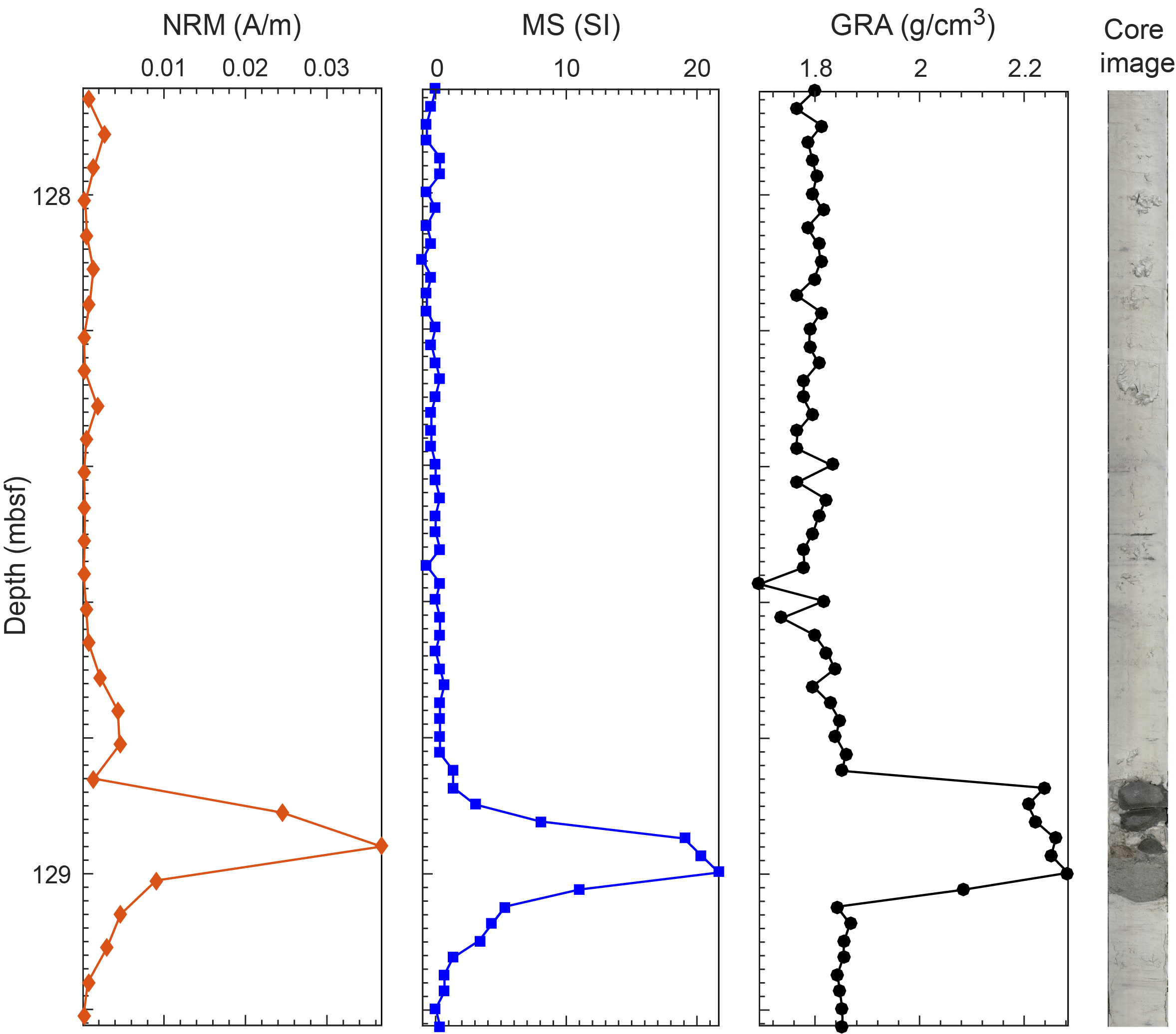
Figure F30. Magnetic intensity data.
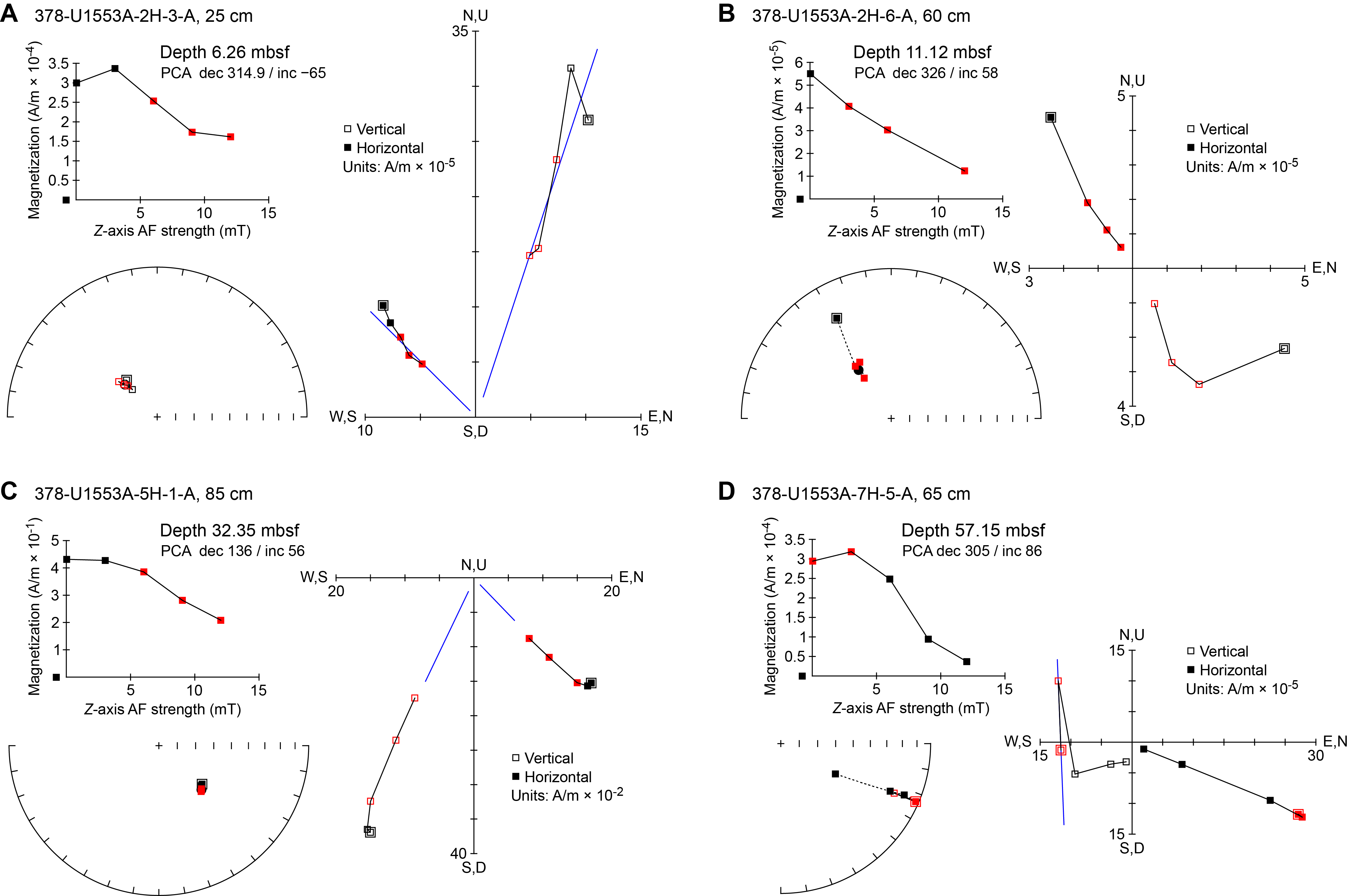
Figure F31. Demagnetization plots, archive halves.
The intensity of the field strength of in-line AF demagnetization was limited because of our limited ability to measure weak magnetizations in the nonmagnetically shielded shipboard environment and the destructive nature of such treatments preventing high-quality measurements in our home laboratories. Typical examples of normal and reversed polarity interpretations of Hole U1553A archive-half section data are illustrated in Figure F31A–F31D. The modern geocentric axial dipole (GAD) inclination at Site U1553 is about 68.8°, calculated using PmagPy software (Tauxe et al., 2016) (dashed blue lines in the inclination column in Figures F32, F33, F34, F35, F36, and F37). The Eocene GAD inclination of this location, which was farther south according to paleogeography reconstructions (e.g., Torsvik et al., 2012), is about 70° as proven in DSDP Site 277 records (Ohneiser and Tapia, 2020). Although we do not have enough data to quantitatively solve characteristic remanent magnetization (ChRM), the demagnetization paths and/or trends of low AF treatment steps (6–9 mT) were usually sufficient to estimate a normal or reversed polarity from the inclinations. For example, the measurement point in Section 378-U1553A-5H-1, 85 cm (57.15 mbsf), is interpreted to be reversed because the demagnetization first removes a drilling-induced steep-down component (inclination = 86°) at 3 mT and then removes the present-day overprint at 6 mT to reveal the Eocene component (Figure F31D). Only the last step, 12 mT, seems to reach the expected ChRM before the magnetization gets too close to background noise and drift level. Data resulting from measurements on section halves at measurement points in Sections 378-U1553A-2H-6, 60 cm (11.12 mbsf), and 378-U1553A-7H-5, 65 cm (32.35 mbsf) (Figure F31B–F31C), are classified as representing good reversed polarity, gradually removing overprints and trending toward the origin. The ChRM inclinations are a bit shallower compared to the Eocene GAD inclination, likely due to sediment compaction and consequent inclination flattening (e.g., Tauxe, 2005). The measurement from Section 378-U1553A-2H-3, 25 cm (6.26 mbsf) (Figure F31A), likely records a robust normal polarity because no reversal trend was observed during the demagnetization.
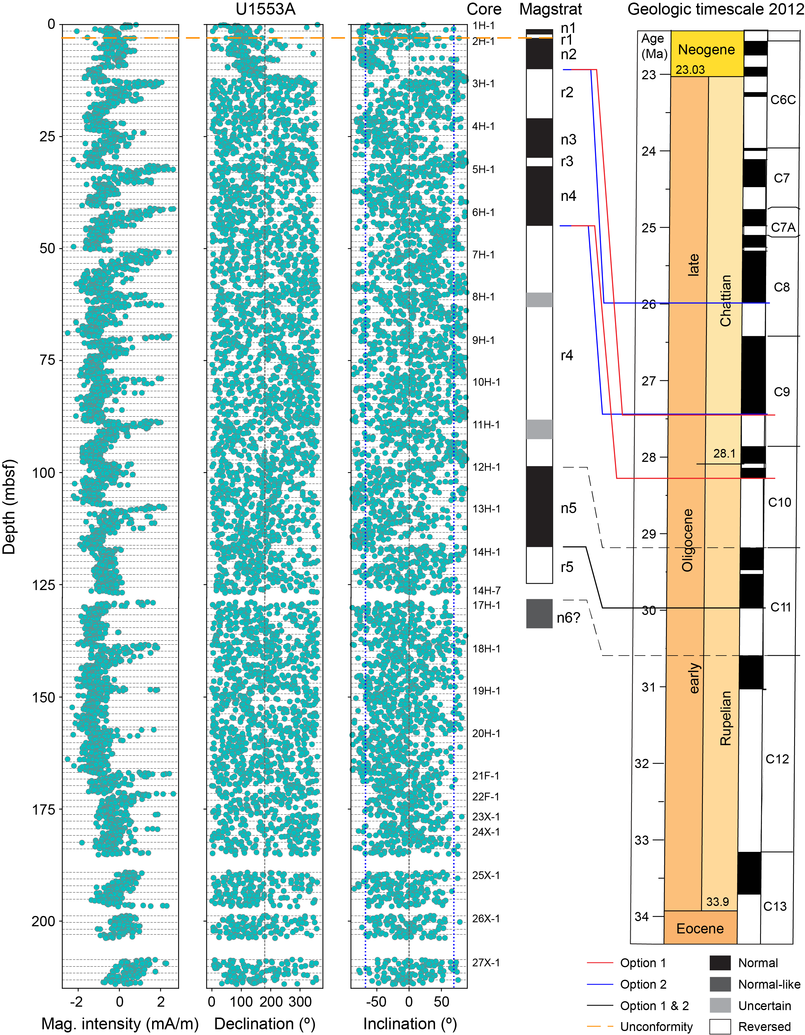
Figure F32. Magnetic measurements.

Figure F33. Paleomagnetic data, Hole U1553B.
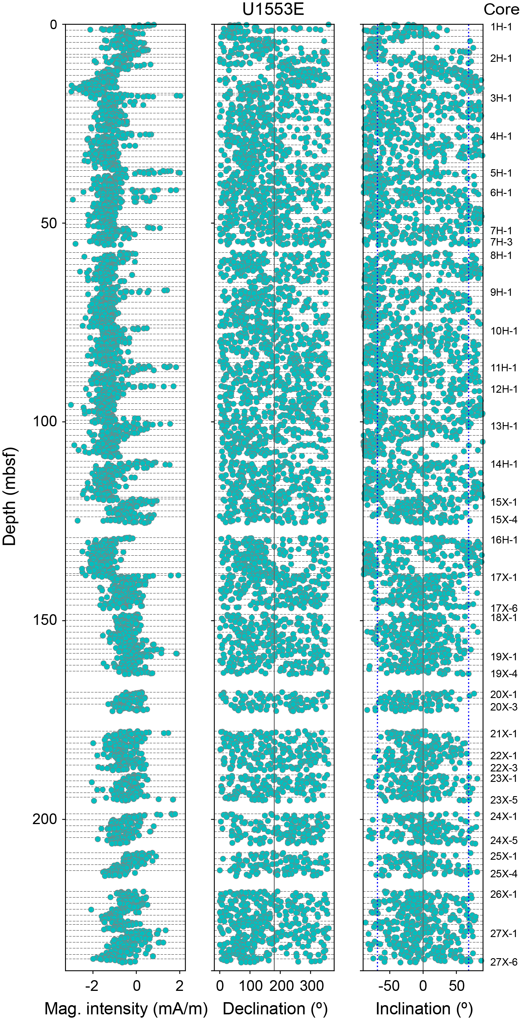
Figure F34. Paleomagnetic data, Hole U1553E.
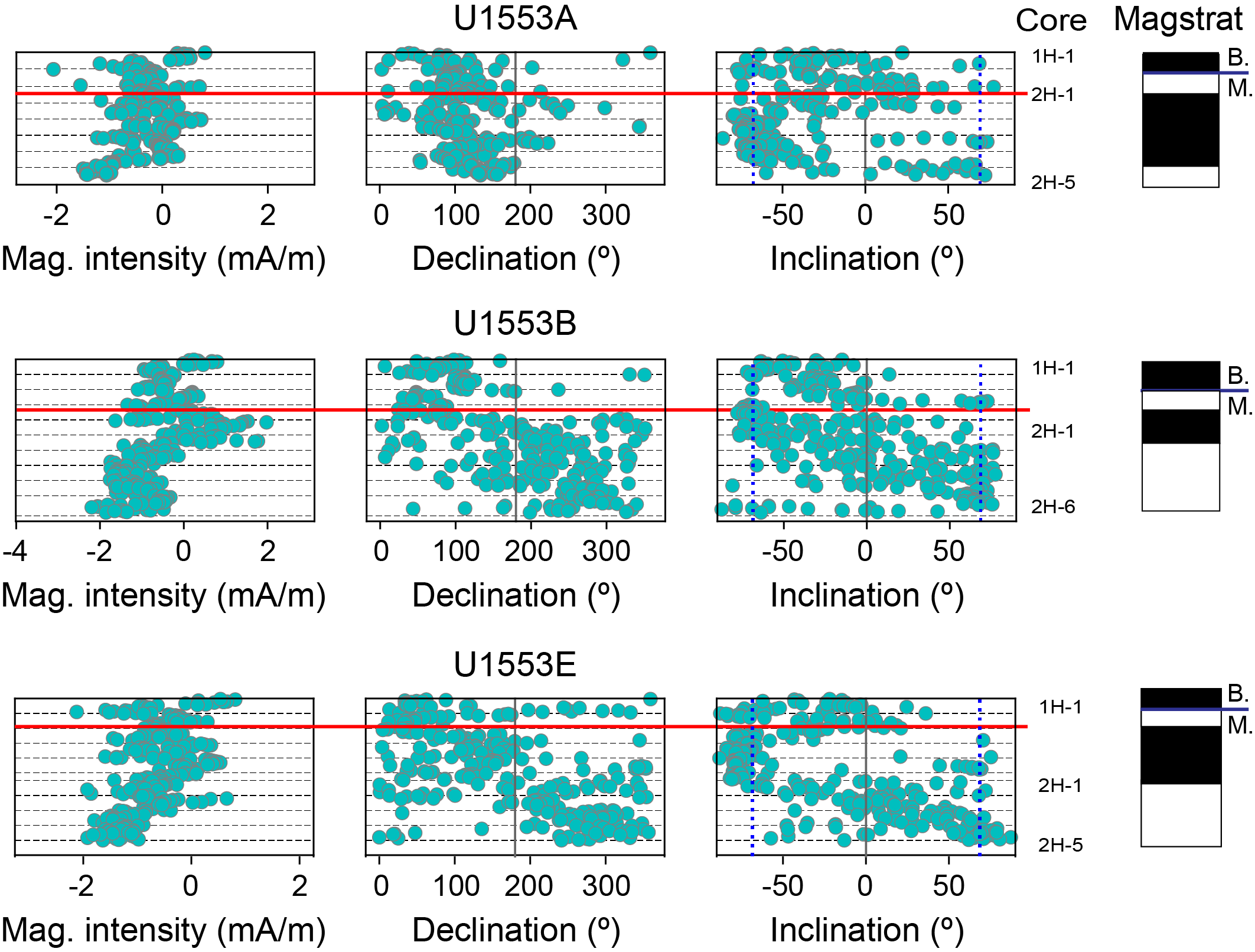
Figure F35. Paleomagnetic data, Holes U1553A, U1553B, and U1553E.
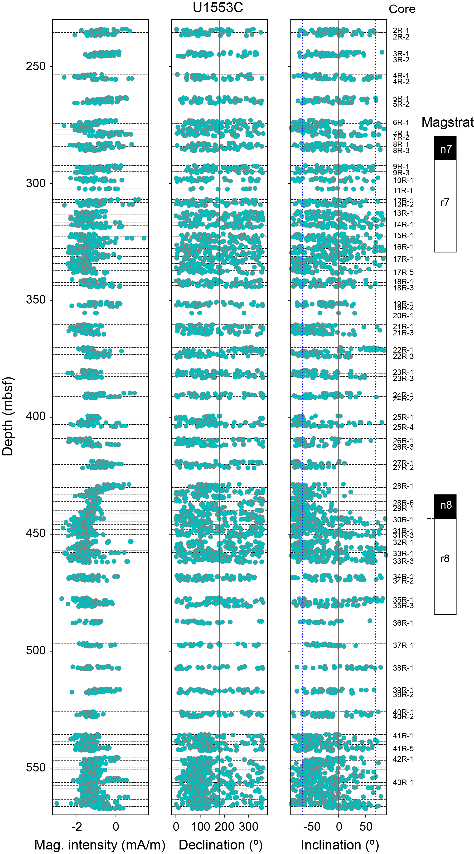
Figure F36. Paleomagnetic data, Hole U1553C.
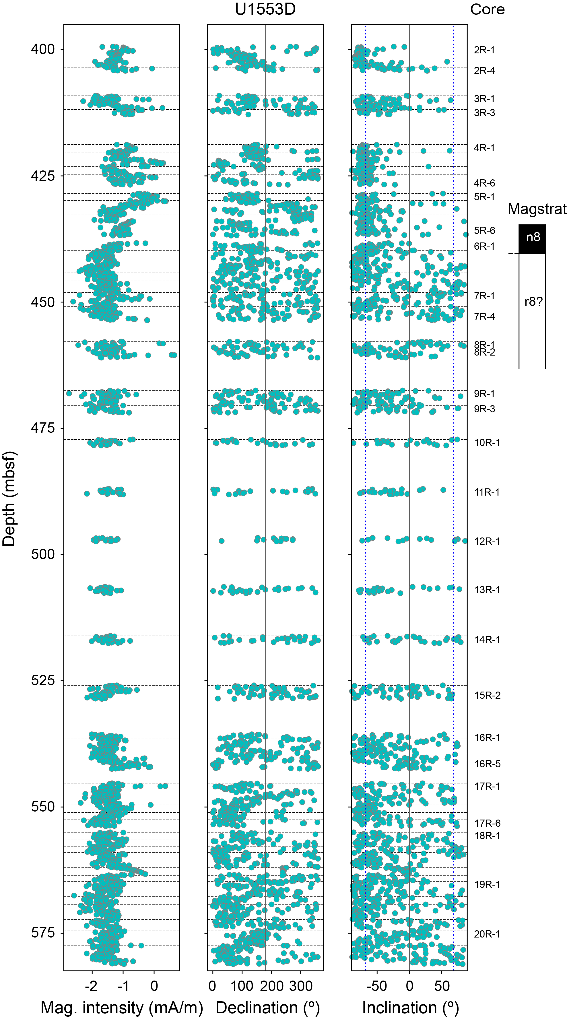
Figure F37. Paleomagnetic data, Hole U1553D.
The typical magnetic behaviors of discrete samples from Holes U1553A and U1553C are shown in Figure F38. Regarding AF treatments, most samples show an initial increase in intensity at 3–6 mT followed by a gradual decrease before increasing again at 20–40 mT (at 8 mT in Sample 378-U1553A-10H-2, 46–48 cm) (Figure F38D), trending away from the origin on the orthogonal vector plot. We suspect that the initial intensity increase is caused by removing an opposite-directed drilling-induced magnetization component similar to the archive-half analyses. The second increase suggests a higher coercivity magnetic mineral composition that could not be demagnetized using low AF treatments, a result associated with the presence of greigite (e.g., Rowan and Roberts, 2006). Further shore-based AF/thermal demagnetization tests will refine our understanding of these properties. Sample 378-U1553C-43R-6, 57–59 cm (Figure F38E), did not exhibit an intensity increase but instead gradually trended toward the origin. The ChRM inclination is calculated to be −72°, which is slightly steeper than the estimated Eocene GAD inclination. Regarding thermal treatments (Figure F38F), an intensity drop of 50% is often observed at 100°C and followed by an increase at 150°C while trending away from the origin. This is probably caused by the formation of magnetite by the oxidation of pyrite/greigite.
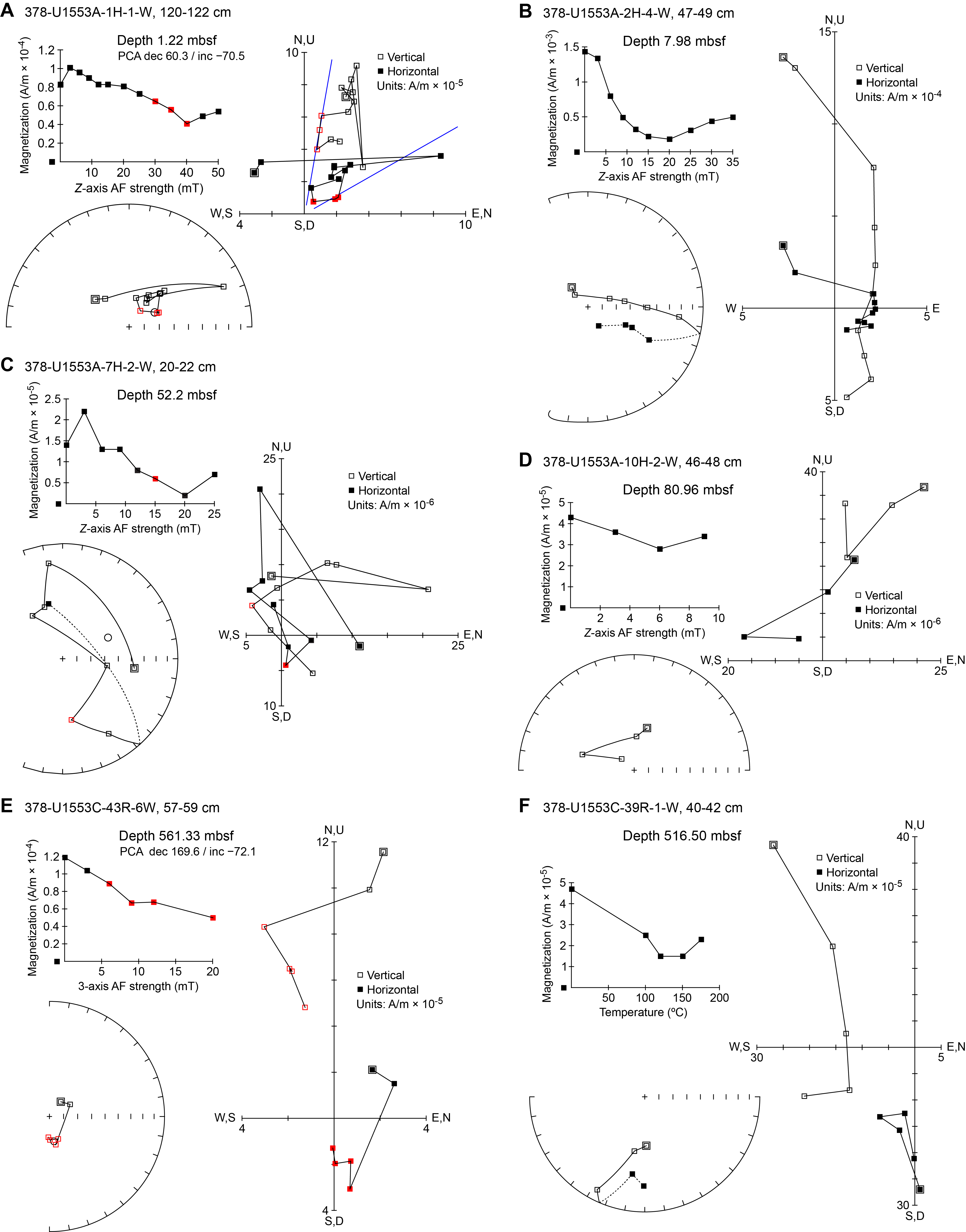
Figure F38. Demagnetization plots, discrete samples.
According to preliminary shipboard observations, glauconite is present in the pale green layers of the pale chalk unit (Lithostratigraphic Unit III) and the presence of pyrites and cherts/flints increases with depth below seafloor (see Lithostratigraphy and Geochemistry). The abundance of glauconite has been reported in marine sediments in New Zealand land sections (e.g., Lurcock and Wilson, 2013), which could dilute the amount of magnetite and weaken the overall remanence magnetization. Pyrite/greigite is often associated with the dissolution of magnetite through sulfate reduction, which complicates the demagnetization behaviors (e.g., Roberts, 2015; Roberts et al., 2013; Rowan and Roberts, 2006). Postcruise research efforts will be required to better understand why the sediments are weakly magnetized with poor demagnetization behaviors.
5.3. Magnetostratigraphy
Declinations of the APC cores from Holes U1553A and U1553B were corrected using the Icefield MI-5 core orientation tool. However, the corrected declinations did not help resolve magnetic polarity, probably because of the extremely weak remanence magnetization, and therefore were not used. Based on inclinations at 6 mT and the demagnetization paths of specimens from archive halves, we constructed a preliminary magnetostratigraphy of the upper ~125 m of Hole U1553A (Figure F32). Below ~125 mbsf, no polarity interpretation was attempted. Data from Holes U1553B and U1553E seem to indicate strong overprints and are not as clear as those from Hole U1553A. Therefore, only the raw data for Holes U1553B and U1553E are shown in Figures F33 and F34.
This ~125 m preliminary magnetostratigraphy of Hole U1553A is composed of five pairs of normal and reverse polarity patterns (n1/r1 to n5/r5 downsection). Core 378-U1553A-1H is Pleistocene in age and lies unconformably above Core 2H, which is Oligocene in age, based on shipboard microfossil ages (see Biostratigraphy and micropaleontology). This boundary approximately aligns with the base of r1. Comparison to the 2012 geologic timescale (GTS2012) (Gradstein et al., 2012) suggests that n1 and r1 correlate to the Brunhes and Matuyama polarity chrons, respectively. We thus propose that the unconformity should be placed at the base of r1 in Sections 378-U1553A-2H-1, 40 cm (3.4 mbsf), 378-U1553B-1H-4, 8 cm (4.6 mbsf), and 378-U1553E-1H-3, 19 cm (3.2 mbsf) (Figure F35). Because the ~125 m magnetostratigraphy of Hole U1553A is normal-polarity dominated, we correlate it with the middle–late Oligocene geomagnetic polarity timescale of GTS2012 (Figure F32) (Gradstein et al., 2012). The position of each reversal is listed in Table T9. Two options are provided here regarding the polarity reversals n2/r2, n3/r3, and n4/r4. Option 1 (red solid lines in Figure F32) correlates the base of n4 with the base of C10n.2n, the base of r2 with the base of C9r, and the base of n2 with the base of C9n of GTS2012 (Gradstein et al., 2012). This option results in an average sediment depositional rate of ~4 cm/ky for the upper ~100 m. Option 2 (blue solid lines in Figure F32) instead correlates the base of n4 with the base of C9n, the base r2 with the base of C8r, and the base of n2 with the base of C8n. This option results in a slower sediment depositional rate of ~2.5 cm/ky. When compared to the shipboard biostratigraphic age model, Option 1 appears to be more consistent, although further shore-based work is required to verify both paleomagnetic and biostratigraphic age models.
The recovery gaps in Holes U1553C and U1553D make it more challenging to build a polarity pattern and to correlate with the standard geomagnetic timescale. Further work will be conducted postcruise with the goal to better establish a magnetostratigraphy below ~125 mbsf. However, two reversals were identified in Hole U1553C: at ~290 mbsf between the recovery gap of Cores 8R and 9R and at 442.8 mbsf in Section 29R-4, 7 cm (n7/r7 and n8/r8 in Figure F36). The deepest reversal observed in Hole U1553C may also be present in Hole U1553D in Section 6R-2, 24 cm (440 mbsf) (Figure F37). Given that these successions are Paleocene to Eocene in age, we attempted to correlate the first reversal (n7/r7) with the base of Chron C18n.2n and the second reversal (n8/r8) with the base of Chron C24n.3n, which agrees with the shipboard biostratigraphic age model (see Biostratigraphy and micropaleontology and Age-depth model and mass accumulation rates). However, these two reversals need further verification, as noted in Table T9.
5.4. Anisotropy of magnetic susceptibility
We measured the AMS of all discrete samples except those that were too broken or crumbly to fit into the Agico KLY 4S Kappabridge instrument. The AMS fabric is described by a symmetrical second rank tensor (Hrouda, 1982), which can be described by a triaxial ellipsoid with the principal eigenvectors Kmax > Kint > Kmin representing the maximum, intermediate, and minimum susceptibility axes, respectively (Figure F39B). These eigenvectors could reflect the depositional plane of sediments (e.g., Lowrie and Hirt, 1987) and are associated with bottom water dynamic conditions. Usually, the Kmax axis aligns parallel with water currents, and the tilting direction of the Kmin axis can be used to infer the absolute water current direction (e.g., Piper et al., 1996; Liu et al., 2001). The AMS data (Figure F39A) clearly show a transition from steep Kmin inclinations to much shallower and wildly distributed patterns around Section 378-U1553C-29R-2, 19 cm (~440 mbsf). This is also illustrated in the equal-area projection plots (Figure F39D), which show a change in Kmin distributions from semiclustering in the steep area to scattering around the entire area. We interpreted this AMS orientation change as reflecting an increase in bottom water velocity from a low–moderate velocity below ~440 mbsf to a relatively faster velocity above (Figure F39C).
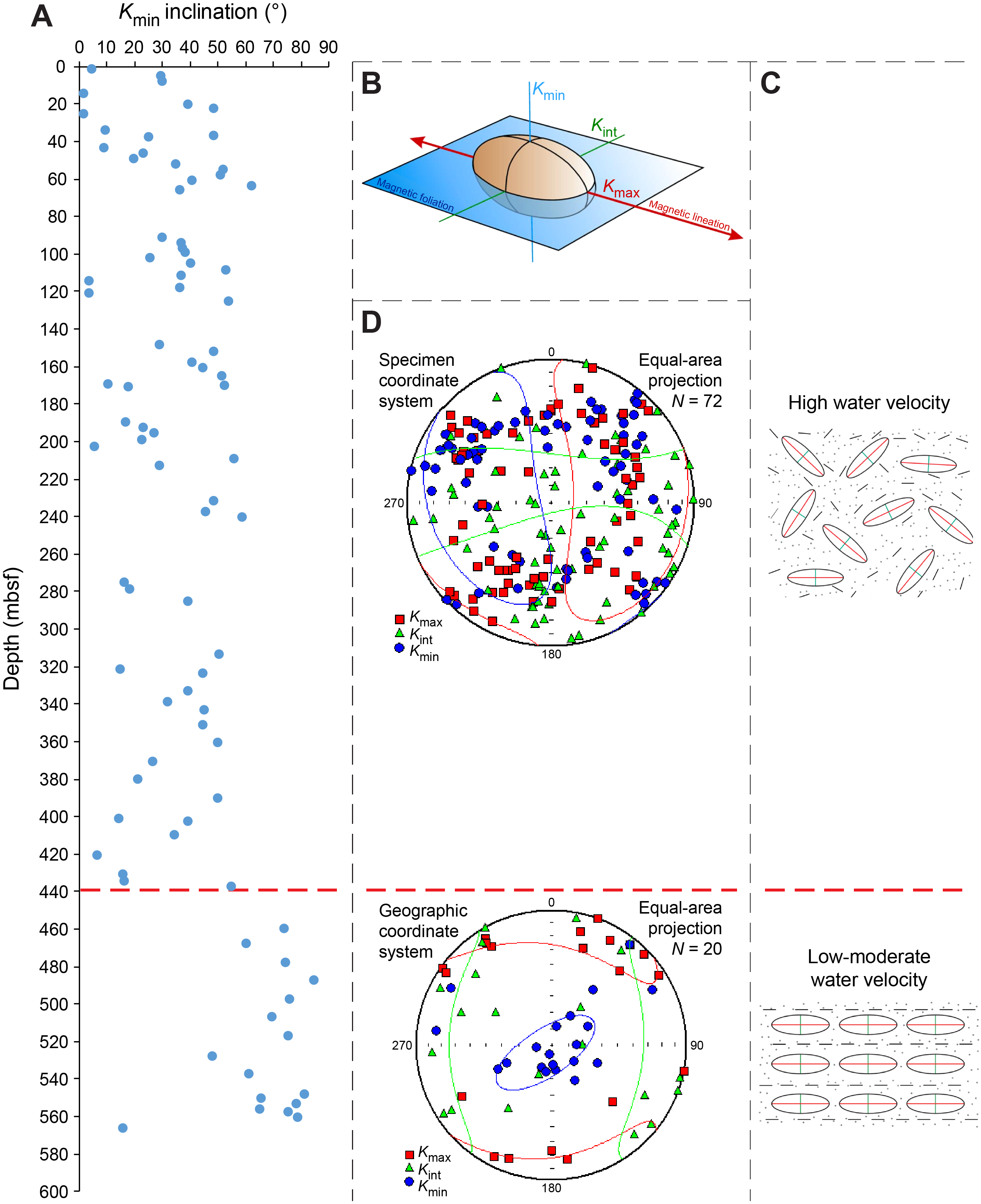
Figure F39. Anisotropy of magnetic susceptibility.
6. Geochemistry
The geochemical composition of the sediment and water samples from Site U1553 reflects the lithostratigraphic descriptions of the sediment (see Lithostratigraphy). The presence of abundant calcite and occasional glauconite, manganese nodules, pyrite, and chert suggests possible subseafloor changes in the aluminosilicates and siliceous and carbonaceous components of the sediment. At Site U1553, sufficiently resolved interstitial water (IW) profiles and solid-phase analyses were obtained to characterize the diagenetic impact on the sedimentary record that may affect paleoceanographic proxies.
6.1. Headspace gas monitoring
For the uppermost 480 m of Site U1553 (above Sample 378-U1553C-35R-2, 133–134 cm), methane is close to the 1:1 signal-to-noise ratio and ethane, propane, butane, and other heavier hydrocarbons are below the detection limit, suggesting a lack of biogenic and/or thermogenic gas production or their upward migration. A sudden increase in methane concentration occurs at 490 mbsf (Figure F40; Table T10), coincident with a strong hydrocarbon gas smell and a drastic change from white to gray core material that corresponds to the transition from Lithostratigraphic Unit IV to Unit V (see Lithostratigraphy). The methane increase is accompanied by the detection of thermogenic hydrocarbons (C2, C3, and C4) beginning at 542 mbsf, suggesting in situ methane production, possibly by microbial activity, and thermogenic gas upward migration. The low porosity of the core material at the top of Unit V (see Physical properties) may have acted as a physical barrier for upward gas migration. Hydrocarbons reach a local maximum at ~555 mbsf (Sample 378-U1553C-42R-8, 149–150 cm), where methane values reached 5180 ppmv. Gradually decreasing C1/C2 ratios with depth led to the termination of drilling operations in Hole U1553C at 568 mbsf (Table T10). Reevaluation of the chromatographic response with known standards determined an underestimation of methane concentrations of 15% and a subsequent underestimation of C1/C2 ratios. Recalculation of C1/C2 ratios and an additional temperature measurement (15.63°C) at 181 mbsf in Hole U1553D provided a better constraint for the deeper drilling in Hole U1553D (Figure F41).
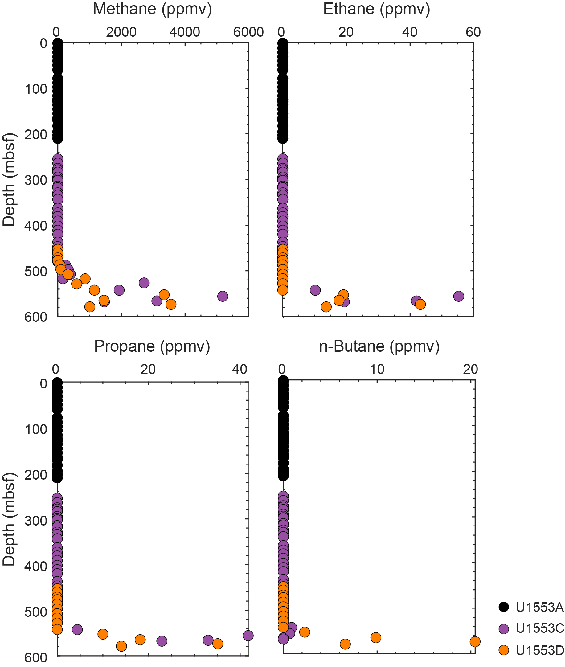
Figure F40. Hydrocarbon gas concentrations.
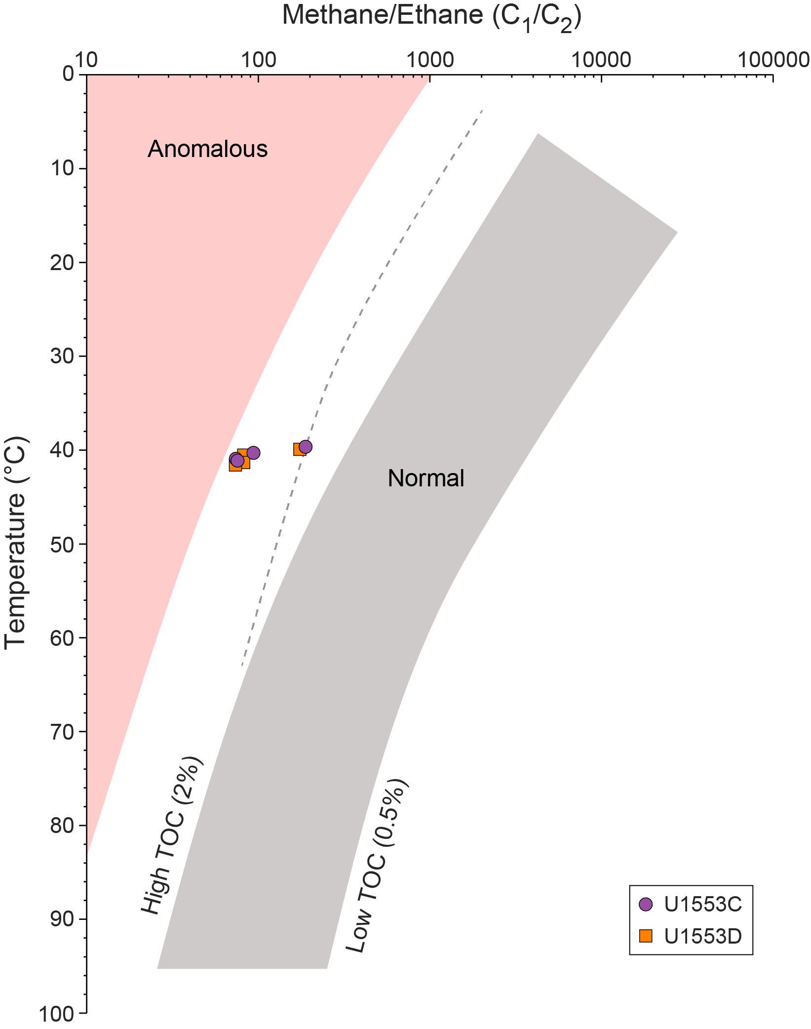
Figure F41. Methane/ethane ratios.
6.2. Interstitial water results
For analysis of water chemistry, 77 IW samples were taken from whole-round squeezing of sediment intervals in Holes U1553A, U1553B, and U1553C (61, 3, and 13 samples, respectively). Additional samples collected included one mudline sample (Section 378-U1553A-1H-1) and one core liner water sample (Section 378-U1553B-23X-5), which were filtered with Rhizon samplers. In Hole U1553B, 99 Rhizon samples were taken for additional IW analyses. Ion chromatography (IC) was used to measure major ions, and inductively coupled plasma–atomic emission spectrometry (ICP-AES) was used to analyze samples for major and trace elements. All IC and ICP-AES measurements were converted to molar concentrations using both in-house standards and the International Association for the Physical Sciences of the Oceans (IAPSO) seawater. Ammonia and phosphate concentrations were determined with spectrophotometry, and salinity was estimated with the refractometer. For XCB cores, some Rhizon sample data suggest that water carried into the core liner through drilling disturbance was sampled, rather than in situ pore fluids.
6.2.1. Alkalinity and pH
Total alkalinity increases from 2.5 mM at the seafloor to 3.6 mM at ~200 mbsf (Sections 378-U1553A-23X-1 through 27X-1). Alkalinity continues to increase with depth in Holes U1553B and U1553C. The rate of increase is highest in the upper 5 m and below 120 mbsf, likely as a result of carbonate dissolution. pH mirrors the alkalinity trend and increases from 7.6 to ~7.8. The highest pH is found between 130 and 170 mbsf, most likely due to dissolution of carbonates (Figure F42).
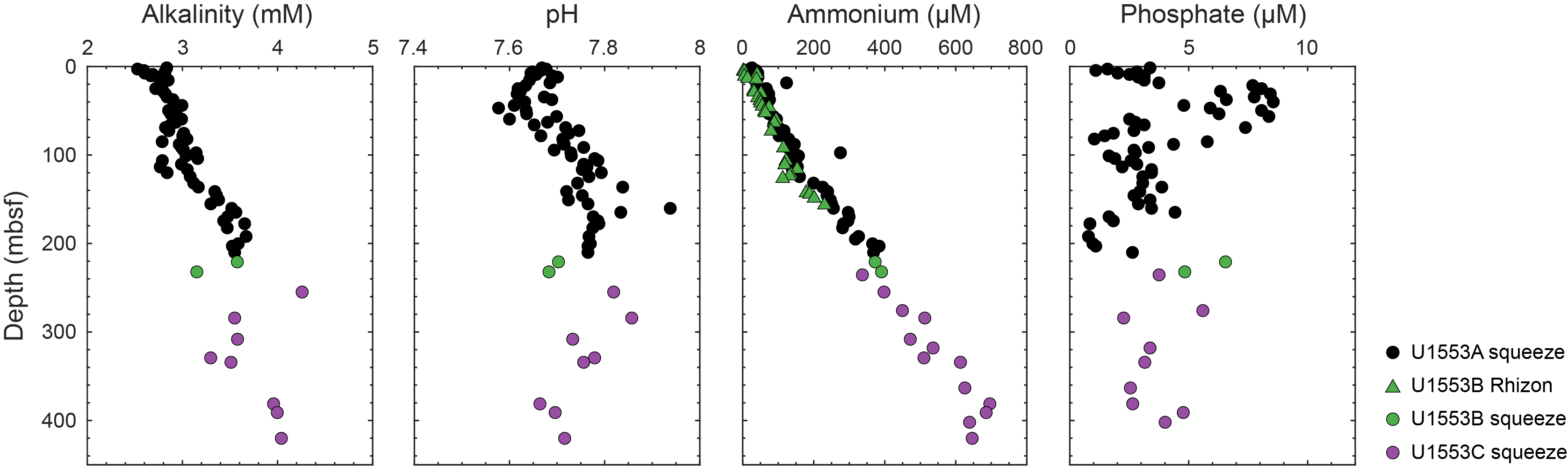
Figure F42. Alkalinity, pH, ammonium, and phosphate.
6.2.2. Ammonium and phosphate
Despite the overall low organic carbon content, ammonium increases from ~20 µM at the seafloor to 650–700 µM below 390 mbsf (Sections 378-U1553C-23R-1 through 27R-1) (Figure F42), suggesting either a contribution of ammonium from organic matter degradation or from mixing with a deeper, potentially microbial, source. Precision for ammonia standards varied from 13% for ≤200 µM concentrations to 2% for higher concentrations up to 1000 µM. Phosphate is less than 5 µM at the seafloor and reaches a maximum value of ~9 µM at 40 mbsf (Sample 378-U1553A-5H-6, 99–104 cm) (Figure F42), most likely as the result of degradation of organic matter. Deeper than 80 mbsf, phosphate concentrations decrease, some below the precision level (3 µM), and are therefore unreliable. Rhizon sampling resulted in a noisy phosphate profile for Hole U1553B and thus was not used further.
6.2.3. Calcium, strontium, and barium
Calcium concentrations in the IW samples increase from 10.4 mM at the mudline (similar to the average seawater concentration) to ~13.5 mM at 200 mbsf in Holes U1553A–U1553C. The rate of increase changes slightly at ~100 mbsf (Figure F43). From 200 to 400 mbsf, the concentration of Ca remains constant between 12.5 and 14 mM. The trend is reflected in both the squeezed samples and the Rhizon samples, and it is reproduced by both inductively coupled plasma spectroscopy and IC analyses. Sr concentrations increase from 89.6 µM at the mudline to ~200 µM at 124 mbsf (Sample 378-U1553A-14H-5, 145–150 cm). Between 129 and 132 mbsf, concentrations abruptly increase from ~200 to ~234 µM. Deeper than 136 mbsf, Sr concentrations continue to increase and average 470 µM at 334–420 mbsf (Sections 378-U1553C-17R-2 through 27R-1). Carbonate dissolution could explain the increase in calcium and strontium with depth. The abrupt change in Ca and likely also in Sr from 124 to 136 mbsf corresponds to a sandstone layer encountered in all holes. This step change in the IW Ca and Sr profile may also represent a coring disturbance or poor recovery near a hard layer of sediment. Ba concentrations derived from squeezed samples are noisier than the trends observed in the Rhizon samples. This is considered an artifact related to the squeeze process, and many of the squeezed samples at or near the detection limit (all Hole U1553A samples) were discarded. The uppermost 160 m of Site U1553 are characterized by <0.2 µM Ba concentrations. Below 200 mbsf, Ba concentrations increase to 2.5 µM. Although these Ba concentrations are still very low, the trends in the profile possibly suggest low amounts of sulfate reduction that dissolves barite (BaSO4), releasing Ba into the IW.
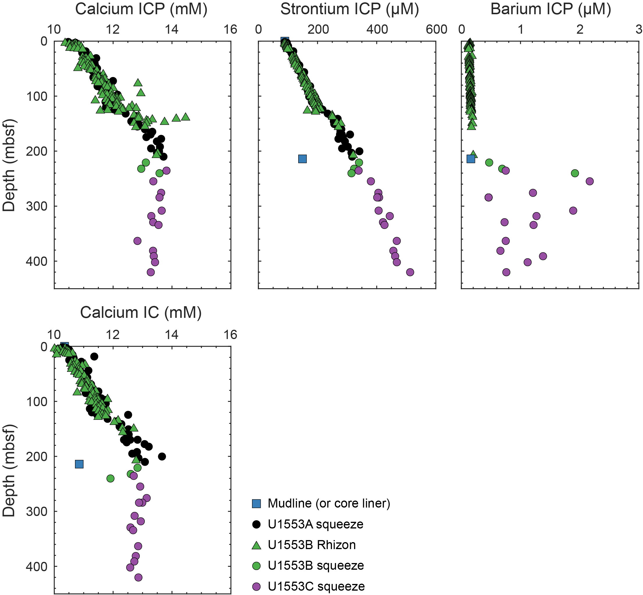
Figure F43. Calcium, strontium, and barium.
6.2.4. Magnesium, potassium, lithium, silicon, and boron
Dissolved Mg concentrations are 53 mM in the mudline water sample and decrease to ~33 mM at 420 mbsf (Sample 378-U1553C-27R-1, 138–143 cm) (Figure F44), possibly due to uptake into recrystallizing carbonates or authigenic clays forming within the seafloor. Alternatively, there may be a sink of Mg deeper in the sediment (e.g., dolomite), and the Mg profile reflects diffusion between seawater and the hypothesized deeper sink. K concentrations decrease downcore from 10.5 mM at the mudline to ~6 mM at 420 mbsf, reflecting alteration and uptake into clays formed within the seafloor (e.g., glauconite). Li concentrations are ~28 µM at the mudline and decrease to ~18 µM around 170 mbsf in Holes U1553A and U1553B. Below 170 mbsf, Li concentrations increase to ~34 µM at 420 mbsf. Si concentrations at the mudline are 55 µM but increase progressively to ~800 µM at 100 mbsf (Holes U1553A and U1553B). From 100 to 128 mbsf, Si concentrations decrease to ~580 µM. Si concentrations increase to 1030 µM, the maximum value measured at this site, at 170 mbsf. Below 170 mbsf, Si concentrations decrease and remain between 490 and 620 µM from 232 to 400 mbsf. The concave shape of the Si profile would suggest that Si is being supplied to the pore waters from the seafloor to 170 mbsf, except near 128 mbsf where there is a net removal of Si from the pore waters. Si concentrations deeper than 232 mbsf do not vary, perhaps because of the more lithified nature of the sediment. B concentrations increase from ~417 µM at the mudline to 760 µM at 420 mbsf (Sample 378-U1553C-27R-1, 138–143 cm), possibly because of the dissolution of biogenic carbonates and reprecipitation in B-depleted inorganic carbonates.
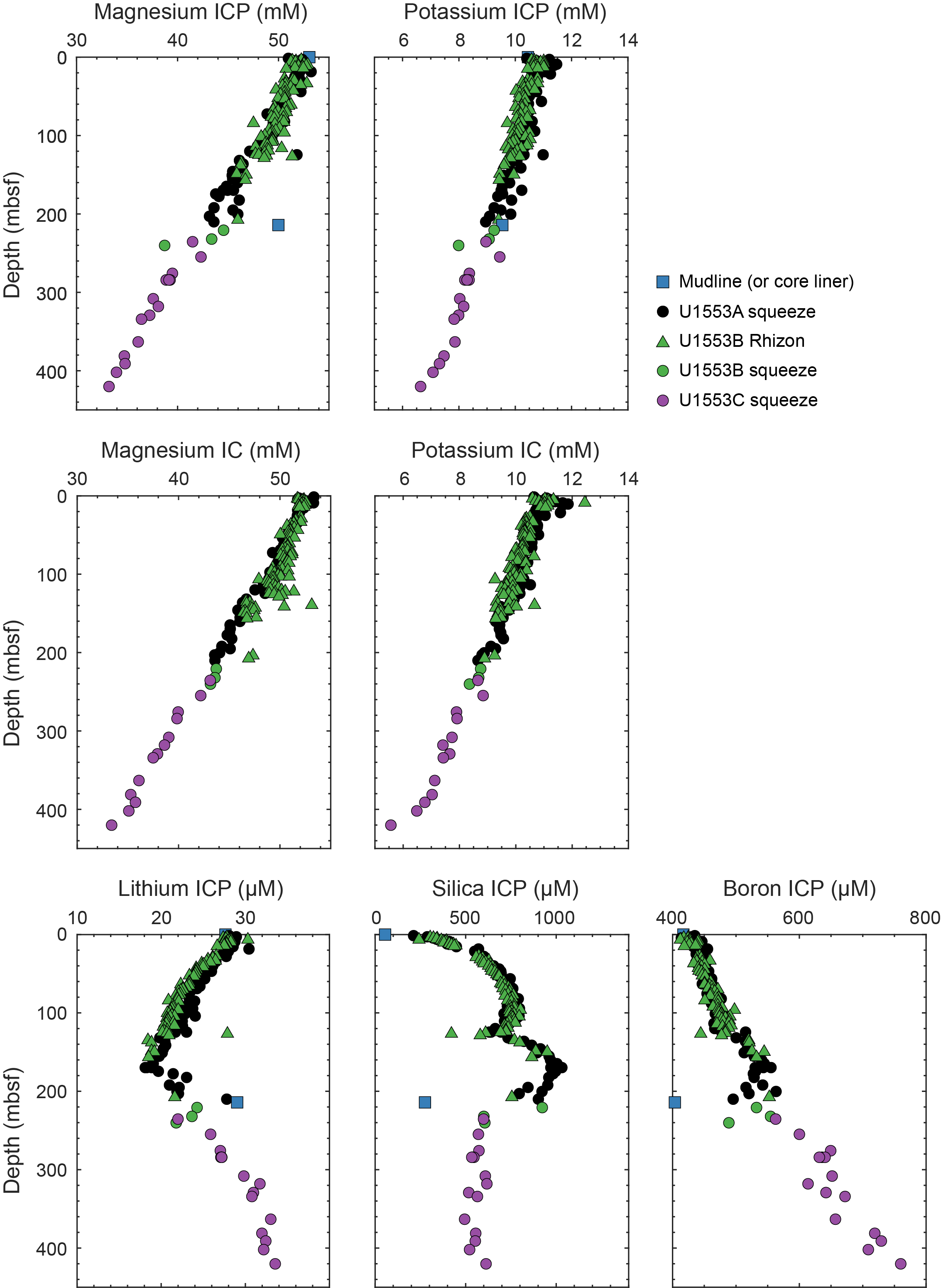
Figure F44. Magnesium, potassium, lithium, silica, and boron.
6.2.5. Sodium, chloride, bromide, and salinity
IW Na, Cl, and Br profiles reveal trends that may be linked to changes in freshwater and organic matter supply (e.g., Shishkina, 1978). Rhizon and squeeze samples indicate mostly uniform concentrations with depth for Na and Cl and show a ratio similar to seawater, suggesting a dominant seawater origin (Figure F45). Na concentrations show no significant downcore trend, although values are scattered between 430 and 550 mM. Cl concentrations measured from squeezers and Rhizon samplers show scatter between ~545 and 565 mM. Br concentrations vary within the lower range expected from seawater, possibly because of low organic carbon input to the seafloor during deposition (Leri et al., 2010). Although Rhizon sample analyses generated for Hole U1553B show larger variations than the squeeze samples derived from the overlapping depth range in Hole U1553A, they follow similar trends, with the exception of Br. The magnitude of Br variability derived from Rhizon samples was not commensurate with the values derived from squeezed samples (Table T11) and were therefore not included in the profile. Br concentration decreases gradually from 0.85 mM at the seafloor to 0.8 mM at 130–210 mbsf (Sections 378-U1553A-17H-2 through 27X-1) and remains largely constant through the deepest samples squeezed (all Hole U1553C samples). Salinity measurements with the refractometer resulted in higher values than estimated from Cl alone (assuming a salinity of 35 is equivalent to a Cl concentration of 558 mM). Because salinity was measured on the archive solution several days after collection and because remaining volumes were ≤1 mL for several samples, evaporation could have affected the analysis. Therefore, salinity estimates >37 (beyond the range predicted from Cl concentrations) are not included in Table T11. This is demonstrated by comparing the salinity measurements from Holes U1553A and U1553B (Figure F45).
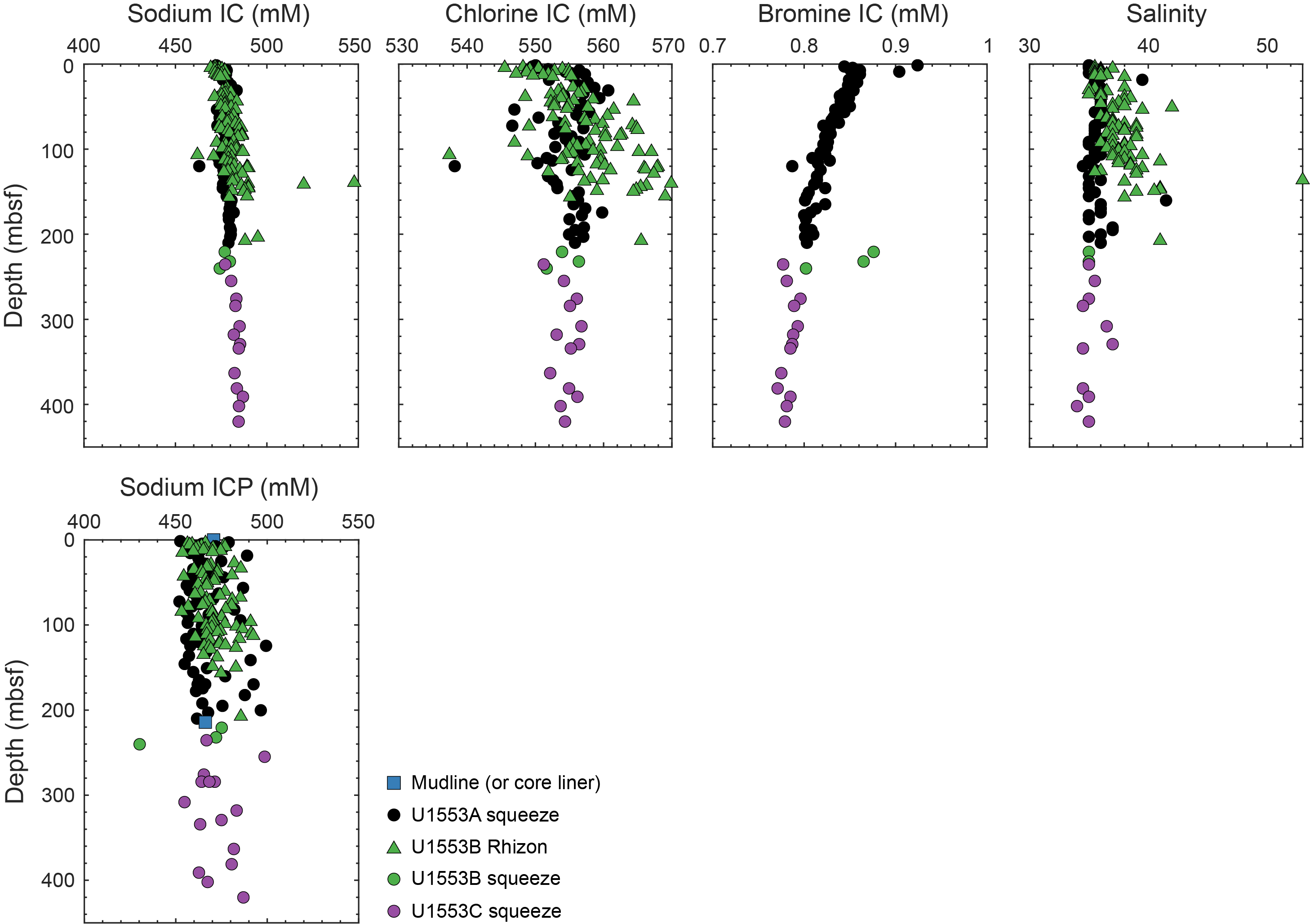
Figure F45. Sodium, chloride, bromide, and salinity.
6.2.6. Manganese, sulfate, and iron
Mn concentrations in the IW samples are between 0.7 and 1 µM in the uppermost 20 m (Figure F46). From 20 to 27 mbsf, Mn concentrations decrease rapidly to ~0.2 µM. Below 27 mbsf, Mn concentrations gradually increase with depth to 0.5 µM at 300–363 mbsf and then increase more rapidly to 0.9 µM at 420 mbsf (Sample 378-U1553C-27R-1, 138–143 cm). The higher Mn concentrations near the seafloor suggest Mn oxides are reduced during the oxidation of organic matter. Analyses of the samples below 363 mbsf (Sections 23R-1 through 27R-1) may reflect anaerobic oxidation of methane, which results in Mn reduction and dissolution of Mn oxides and is consistent with XRF measurements (see Lithostratigraphy). Sulfate decreases from ~29 mM in the mudline sample to 14 mM at 420 mbsf (Sample 27R-1, 138–143 cm) (Figure F46). The smell of sulfide gas was noticeable in Core 34R (~470 mbsf), but the sediment was too lithified to recover any IW and no sulfide measurements were performed. However, the sulfide odor in Core 34R suggests that the sulfate–methane transition zone is ~470 mbsf, where the reduction of sulfate oxidizes methane and produces sulfide. Instead, hydrogen sulfide (HS−) concentrations (Figure F46) estimated by the difference between dissolved inorganic carbon (DIC) and total alkalinity indicate a potential small peak below 140 mbsf. DIC values used to estimate HS− were derived from alkalinity and pH measurements using the CO2sys.exe software (Pierrot et al., 2006). Fe concentrations decline from ~2 µM at 5 mbsf (Holes U1553A and U1553B) to 1 µM at ~20 mbsf. Fe concentrations increase to >3 µM between 20 and 120 mbsf (Hole U1553B), which may represent Fe oxides being reduced during the oxidation of organic matter. Below 135 mbsf, the majority of samples were below the detection limit, although a few samples had Fe concentrations of 0.5–1 µM below 270 mbsf. Deeper than 135 mbsf, Ba concentrations increase coincident with low Fe concentrations in the pore water, suggesting barite dissolution due to sulfate reduction in the pore waters. This implies Fe was reacting to form an iron sulfide mineral such as pyrite, which was observed in Lithostratigraphic Units II and III (see Lithostratigraphy).
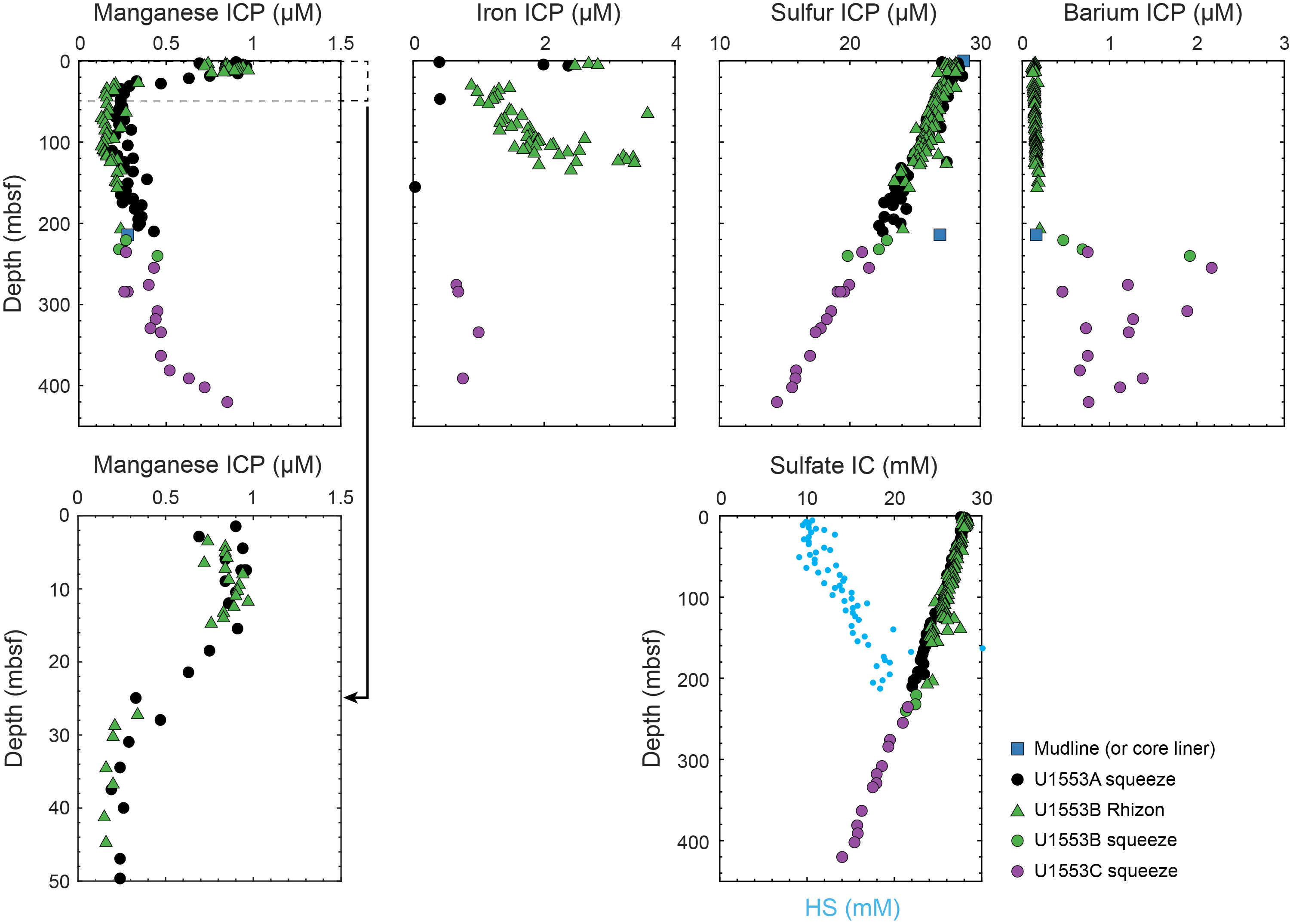
Figure F46. Manganese, iron, sulfur and sulfate, and barium.
6.3. Bulk sediment geochemistry
6.3.1. Carbon content
A total of 96 discrete freeze-dried bulk-sediment samples were measured for calcium carbonate, organic carbon, total nitrogen, and total sulfur. Drastic changes and strong geochemical gradients in carbonate content occur in parallel with the main lithostratigraphic changes. Assuming that all measured inorganic carbon is in the form of calcium carbonate, sediments predominantly consist of carbonate (90% on average) for the uppermost 420 m of Site U1553, ranging from 78% to 99% ± 0.5% (Figure F47). A drastic decrease to 9% carbonate between 420 and 480 mbsf corresponds to marlstone and coincides with a lithostratigraphic transition from limestone to muddy sandstone (see Lithostratigraphy). From 480 mbsf (Sample 378-U1553C-38R-1, 35–37 cm) to 580 mbsf (Sample 378-U1553D-20R-5, 28–29 cm), average carbonate content is 2.2%. One exception occurs at 566 mbsf in Sample 378-U1553C-44R-1, 107–108 cm, which contains 85% carbonate and is related to a dolomite-calcite concretion.

Figure F47. Elemental composition of the solid phase.
Total carbon content shows a similar trend to that of calcium carbonate downhole (Figure F47), indicating that most of the carbon is inorganic. Overall, organic carbon content, calculated from total carbon and inorganic carbon, is generally <0.4% ± 0.06% (Figure F47). Relatively low organic carbon prevails for the uppermost 200 m (0.14% on average), increasing gradually to 330 mbsf and averaging 0.33% from 330 to 580 mbsf. This observation is in line with a transition from an oligotrophic system to a mesotrophic system, which corresponds with observations from benthic foraminiferal assemblages (see Biostratigraphy and micropaleontology). Organic matter degradation and diagenesis are apparent from the geochemical profiles from IW samples (Figures F42, F43, F44, F45, F46). Total nitrogen content is low (<0.13%) or below the detection limit at Site U1553, which hampers confident estimation of C/N ratios. Total sulfur is only present in the lowermost part of Site U1553 (479–565 mbsf). Average values are <1% and may derive from pyrite minerals, which increase in abundance over this depth range (Table T12).
6.3.2. Organic matter source analysis
Headspace gas measurements with low C1/C2 ratios prompted the investigation of a possible proximal source of thermogenic gas. Pyrolysis was conducted with the source rock analyzer (SRA) on a set of 19 discrete bulk sediment samples from 295 to 580 mbsf to explore the thermal maturity of Lithostratigraphic Unit V. If no hydrocarbon potential (S2) is detected, values for Tmax and other indexes are randomized. This is the case for 11 samples. The presence of hydrocarbons and low petroleum potential are observed in Unit V at Site U1553 from S1 and S2 parameters, respectively, for 8 samples (Table T13). Tmax values below 335°C and low production index values indicate organic matter is immature. Hydrogen index and oxygen index parameters indicate that the material is primarily of terrestrial origin and is kerogen Type III (Tissot and Welte, 1984). Overall, TOC values are low (<1%). However, linear correlation of TOC values estimated from the difference between total carbon measured on the elemental analyzer and those from IC by coulometry is low (R2 = 0.39) (Figure F48). Large and variable magnitudes of the offsets between values derived from both methods were observed, similar to the TOC values measured using the SRA being higher than those from elemental analyzer coulometry, as has been previously observed and discussed in great detail (e.g., Expedition 317 Scientists, 2011).
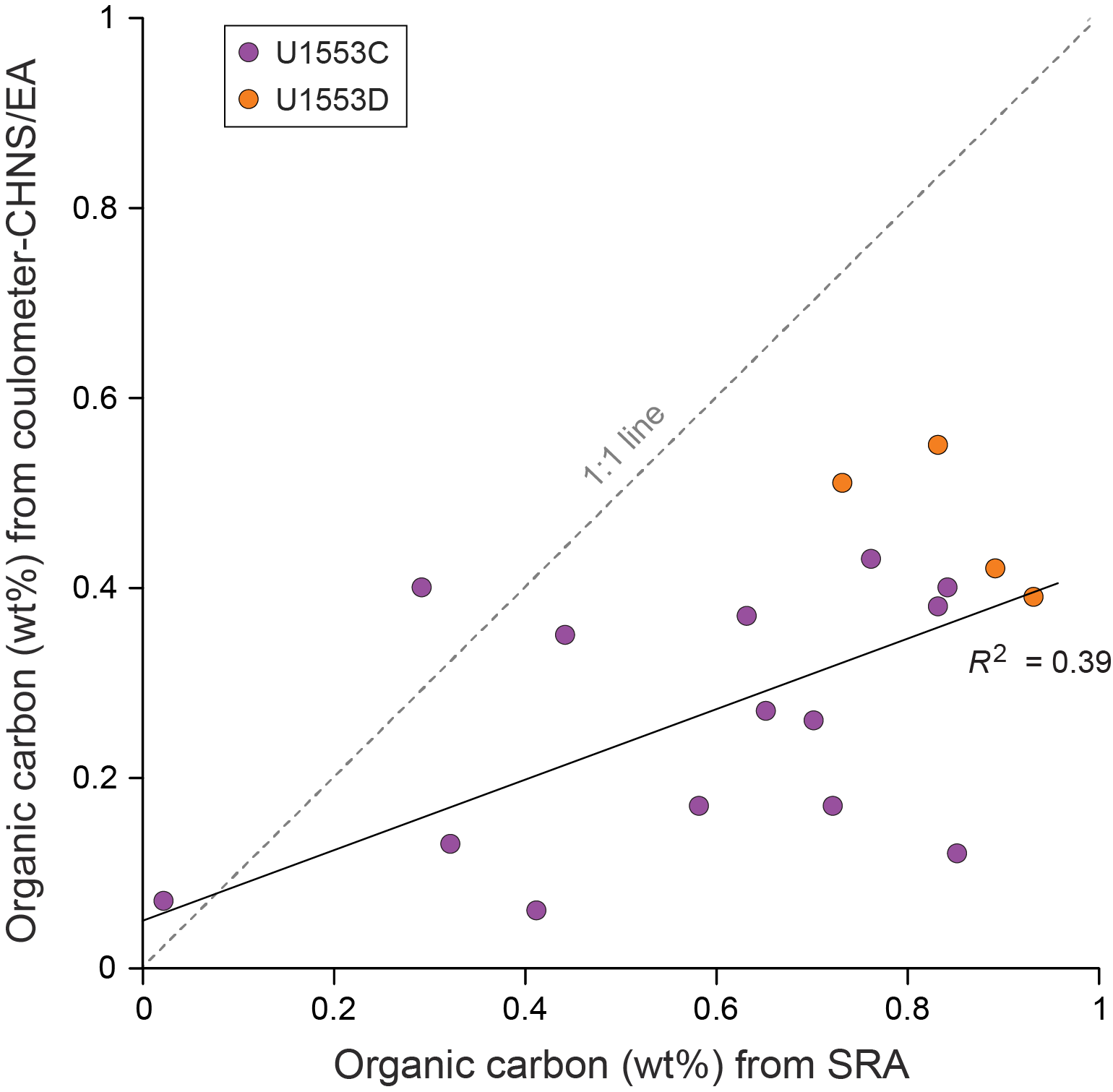
Figure F48. Total organic carbon results.
6.3.3. Major and trace element concentrations
The major and trace element concentrations (Figure F49; Table T14) reflect the major change in lithologies at the boundary between Lithostratigraphic Units I–IV and Unit V (see Lithostratigraphy). Elements commonly associated with aluminosilicate phases in the sediment are low in Units I–IV. In Units I–IV, concentrations range from 0.8 to 10.3 wt% for SiO2, from 0.3 to 1.64 wt% for Al2O3, from below detection limit to 0.05 wt% for TiO2, from 0.07 to 0.8 wt% for Fe2O3, from 0.03 to 0.3 wt% for K2O, from 0.2 to 0.6 wt% for MgO, from below detection limit to 35 ppm for Cr, from 0.9 to 2.9 ppm for Sc, and from 10.27 to 35 ppm for V (a few are below detection limit). Zn remains below 53 ppm, and Zr concentrations above the detection limit are ≤16.35 ppm. These elements increase in Unit V and reach maxima of 83 wt% for SiO2, 8.5 wt% for Al2O3, 0.45 wt% for TiO2, 4.9 wt% for Fe2O3, 1.7 wt% for K2O, 1.6 wt% for MgO, 71 ppm for Cr, 7 ppm for Sc, 61 ppm for V, 193 ppm for Zn, and 199 ppm for Zr. Elements enriched in carbonates have high concentrations in Units I–IV, such as 55.6 wt% for CaO and 1721 ppm for Sr. In Unit V, CaO decreases to as low as 0.15 wt% and Sr decreases to as low as 82 ppm. MnO and Ba are consistently lower than 0.023 wt% and 1070 ppm, respectively, throughout the samples analyzed, except those from between 285 mbsf (Sample 378-U1553C-8R-2, 70 cm) and 480 mbsf (Sample 35R-2, 133 cm), in which concentrations are higher, reaching maxima of 0.06 wt% and 3120 ppm, respectively. Concentrations of Na2O decrease from ~1 wt% at the seafloor to ~0.5 wt% at ~470 mbsf (Sample 34R-1, 13 cm) and then increase to 0.9–1.3 wt% from 480 to 580 mbsf (Sections 378-U1553C-35R-2 through 378-U1553D-20R-5). Concentrations of P2O5 range from 0.04 to 0.24 wt% and do not show a significant change with depth. One sample is from the dolomite concretion at 565 mbsf (Sample 378-U1553C-44R-1, 107–108 cm) and has anomalously high MgO (14.3 wt%), CaO (27.6 wt%), and MnO (0.24 wt%) compared to samples from similar depths.
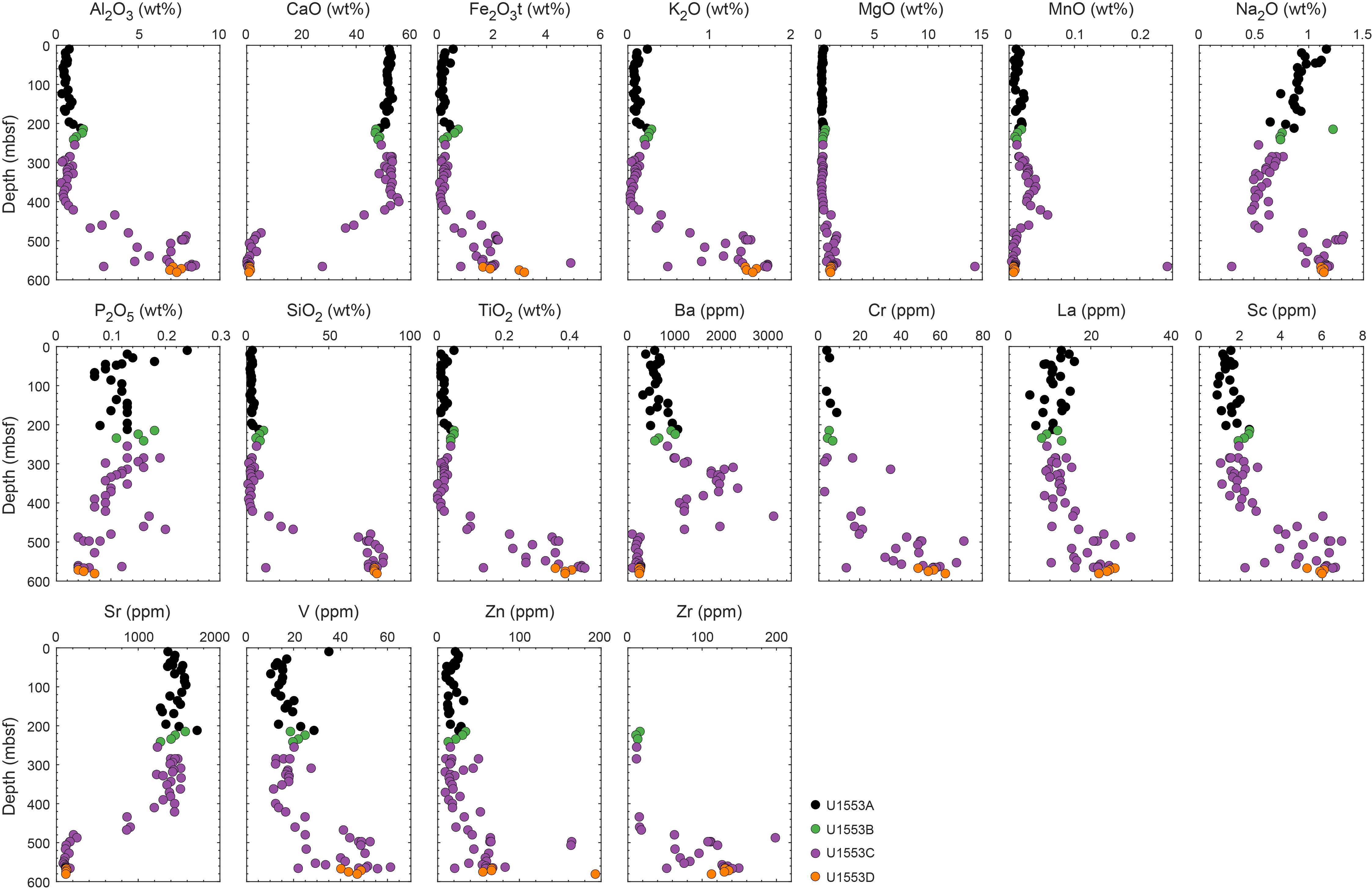
Figure F49. Major and trace elements.
6.3.4. X-ray fluorescence scanning of Site U1553 cores
Semiquantitative elemental results from XRF scanning of sediment cores were collected from Site U1553. XRF elemental data were collected every 2 cm (see Major and trace element concentrations) from all core sections drilled at Site U1553. We acquired raw elemental intensities (total counts) at suborbital resolution for, for example, Al, Si, K, Ca, Ti, Fe, Br, Sr, Zr, and Ba and identify covariation patterns that have been crucial for compiling the spliced composite record that was not accurately possible with shipboard core logging data (see Stratigraphic correlation). Our XRF scanning of Site U1553 sediments was conducted to aid in core correlation of the mainly high-carbonate sediments, is consistent with lithofacies variations, and will facilitate detailed interpretation of sedimentation and more detailed paleoceanographic studies at this location.
The XRF scanning data provide a high-resolution record of the geochemistry of the sediments analyzed at Site U1553. Based on shipboard estimated sedimentation rates of 0.5–4 cm/ky for the interval analyzed (see Age-depth model and mass accumulation rates), the 2 cm measurement interval yields a temporal spacing of 0.5–4 ky between data points.
7. Physical properties
7.1. Physical properties
Gamma ray attenuation (GRA) bulk density, MS, P-wave velocity, NGR, moisture and density (MAD), thermal conductivity, color, reflectance, shear strength, and compressive strength were measured on cores from Site U1553 (for sampling strategy, see Physical properties in the Expedition 378 methods chapter [Röhl et al., 2022]). Whole-round P-wave velocity, thermal conductivity, discrete shear strength, and compressive strength measurements were not made on RCB cores (Holes U1553C and U1553D). Downhole temperature measurements were taken in Holes U1553A and U1553D.
Variations in physical properties data correspond to transitions between major lithologic units, and in some cases these variations were used to define unit boundaries (see Lithostratigraphy). A slight increase in bulk density and NGR at 180 mbsf was used to define the transition between Lithostratigraphic Units II and III. A significant increase in P-wave velocity and bulk density at ~423 mbsf marks the top of Lithostratigraphic Unit IV. A large increase in NGR counts, decrease in P-wave velocity and bulk density, and change in color at 477 mbsf correspond to the higher silica and clay content of Lithostratigraphic Unit V.
7.2. Gamma ray attenuation bulk density
GRA bulk density was measured on the Whole-Round Multisensor Logger (WRMSL). Variations in GRA bulk density may reflect variations in lithology, consolidation, cementation, and porosity. There is a systematic offset between GRA-measured bulk density and MAD-calculated bulk density in Holes U1553C and U1553D, where RCB coring yielded cores of smaller diameter leading to an underestimation of GRA bulk density by the WRMSL. This systematic underestimation can be corrected to compare with the measured MAD values by multiplying by a correction factor of 1.10. The correction factor was determined by linear regression (R2 = 0.997; p < 0.0001). Figure F50 shows the uncorrected raw data to enhance potential quality and accuracy of GRA bulk density data, which strongly depend on the calibration parameters and coring method. From 0 to ~225 mbsf, GRA bulk density increases slowly with depth from an average of 1.6 to 1.7 g/cm3, which is consistent with the relatively homogeneous calcareous nannofossil ooze lithology of Lithostratigraphic Unit II and compaction downhole (Figure F50). GRA bulk density values below 1.5 g/cm3, such as those in Cores 378-U1553B-3H and 378-U1553A-15H, are associated with poor core recovery and drilling disturbance. Bulk density declines in the uppermost 40 m of Lithostratigraphic Unit III before stabilizing throughout the remainder of the unit (~225–425 mbsf) with uncorrected GRA bulk density values around 1.7–1.8 g/cm3. These measurements are consistent with the dominant lithology of compacted chalk. The boundary between Units II and III is more clearly observed when the GRA bulk density offset correction is applied because Unit II has a lower average bulk density (~1.7 g/cm3) than Unit III (~1.9 g/cm3). At 425 mbsf, the uncorrected GRA bulk density increases from 1.7 to 1.9 g/cm3 (from 1.9 to 2.1 g/cm3 in the corrected data), which coincides with the boundary between Lithostratigraphic Units III and IV. GRA bulk density values then remain high and stable to 477 mbsf, where there is a decrease to ~1.5 g/cm3 (uncorrected) or ~1.7 g/cm3 (corrected) that corresponds to the boundary between Lithostratigraphic Units IV and V. Variable GRA bulk density values in Lithostratigraphic Unit V may be caused by the lithologic heterogeneity that is pervasive throughout the unit (see Lithostratigraphy). Below 520 mbsf in Cores 378-U1553C-41R through 43R and 378-U1553D-16R, there are intervals of extremely low GRA bulk density (~0.5–0.7 g/cm3) that are associated with darker sections of rubble in Lithostratigraphic Unit V.
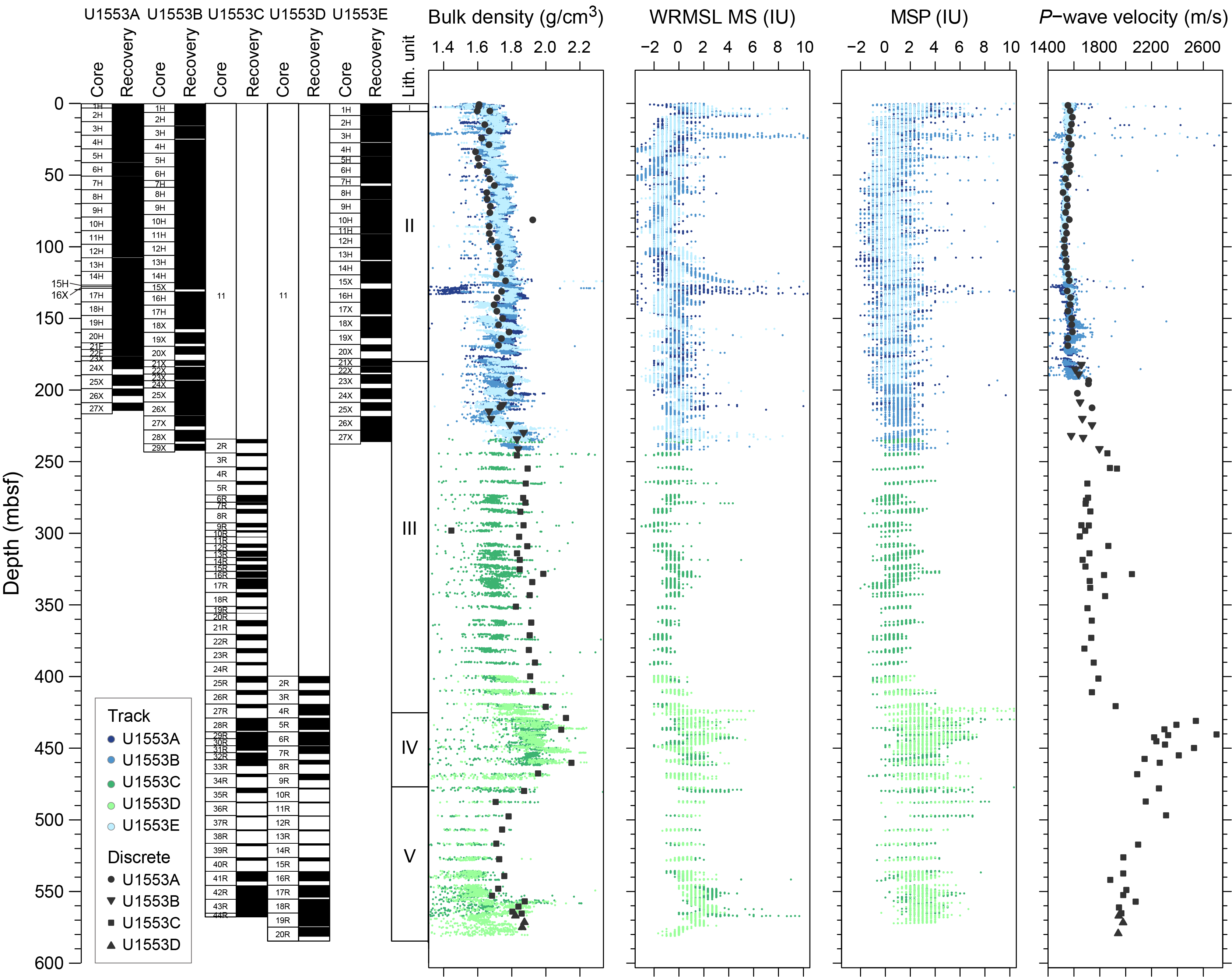
Figure F50. Physical properties measurements.
7.2.1. Magnetic susceptibility
MS was measured on the WRMSL with a loop and on the Section-Half Multisensor Logger (SHMSL) with a point sensor, increasing resolution and accuracy. MS ranges from −2 to 10 instrument units (IU). Values higher than ~4 IU correspond to the tops and bottoms of cores and core sections where sediments are most likely to be disturbed or poorly measured on the logger tracks (Figure F50). Throughout the upper 425 m of Site U1553, MS remains near zero (ranging from −2 to 2 IU), which is consistent with the predominantly carbonate lithology, except for drilling disturbances in Cores 378-U1553A-15H and 378-U1553B-3H where suck-in occurred. MS slightly increases to ~3–4 IU throughout Lithostratigraphic Unit IV (425–477 mbsf). In Lithostratigraphic Unit V (477–577 mbsf), MS is elevated compared to the upper units but is still relatively low, ranging from 0 to 4 IU.
7.2.2. P-wave velocity
Between 0 and ~175 mbsf, P-wave velocities remain constant at ~1600 m/s. The high P-wave values of ~4400 m/s at ~130 mbsf derived from the packstone layer recovered in Core 378-U1553A-16X. Whole-round P-wave measurements from the WRMSL are consistent with discrete P-wave caliper measurements made on selected section halves and discrete MAD cubes. Below 175 mbsf, P-wave velocities were measured using only the Section Half Measurement Gantry (SHMG) (see Physical properties in the Expedition 378 methods chapter [Röhl et al., 2022]). Between 175 and 425 mbsf, P-wave velocities gradually increase to ~2000 m/s. In this interval, some discrete measurements were also taken on the interbedded chert layers, which recorded higher P-wave velocities (3000–4200 m/s) than the majority of Lithostratigraphic Unit III. A sharp increase in P-wave velocity from ~2000 to 2600 m/s occurs at 425 mbsf, which coincides with the boundary between Lithostratigraphic Units III and IV. P-wave values gradually decrease throughout Lithostratigraphic Unit IV (425–477 mbsf) to approximately 2100 m/s. In Lithostratigraphic Unit V, P-wave velocities remain at ~1900–2000 m/s.
7.2.3. Natural gamma radiation
NGR was measured on whole-round sections with the Natural Gamma Radiation Logger (NGRL) (Figure F51). NGR measurements at Site U1553 ranged from 0 to 40 counts/s. Consistent with other physical properties measurements, NGR and the constituent elemental concentrations remain low and constant between ~0 and 180 mbsf, which corresponds to the homogeneous carbonate lithology of Lithostratigraphic Unit II. Between 180 and 240 mbsf, there is a transient increase in NGR values to ~10 counts/s (~225 mbsf) followed by a decrease to ~5 counts/s. NGR then remains constant to 425 mbsf, where an increase in the average value (from ~5 to 15 counts/s) coincides with the transition from Lithostratigraphic Unit III to Unit IV. NGR values remain elevated but variable throughout Lithostratigraphic Unit IV (425–477 mbsf). At 477 mbsf, there is a sharp increase in NGR counts associated with the boundary between Lithostratigraphic Units IV and V. Although data are sparse between ~477 and 540 mbsf because of poor core recovery, NGR counts in Lithostratigraphic Unit V are variable (10–40 counts/s). Similar to GRA bulk density measurements, this is likely a result of the heterogeneous lithology, and NGR counts remain greater than values observed in the overlying carbonate units. The NGR spectra were also deconvolved into approximated uranium, thorium, and potassium concentrations using the interpolated MAD-derived bulk density values and methods described by De Vleeschouwer et al. (2017). U, Th, and K concentrations covary throughout most of the hole. The U/Th ratio increases at the Lithostratigraphic Unit IV/V boundary, coinciding with the increased clay content of the sediments.
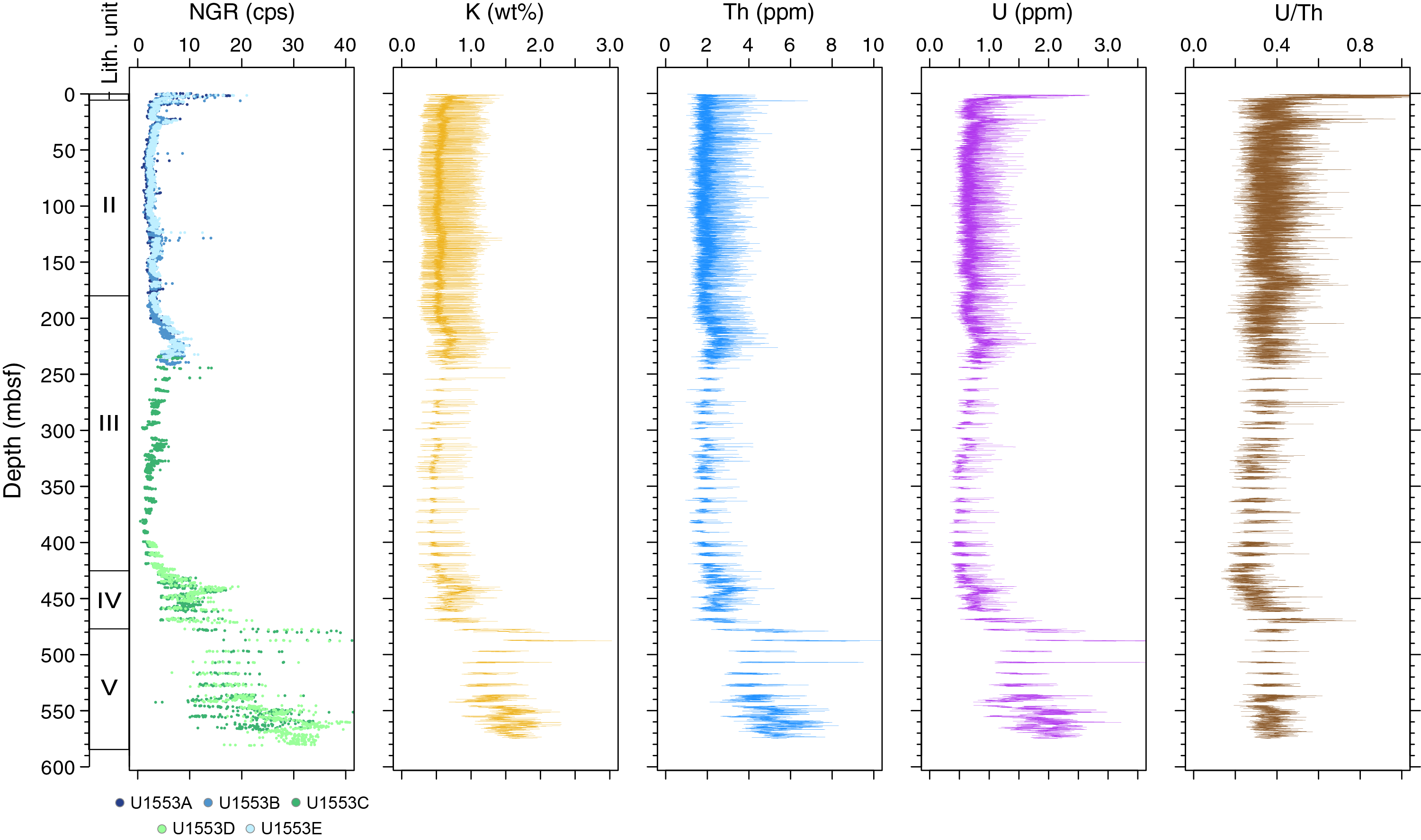
Figure F51. Whole-round NGR data.
7.2.4. Moisture and density
To achieve a continuous downhole record, two carefully selected samples were taken from each Hole U1553A core and from Cores 378-U1553B-26X through 29X, 378-U1553C-3R through 44R, and 378-U1553D-19R and 20R for MAD analysis. Care was taken to cover representative lithologies and to avoid intervals of obvious drilling disturbance, and special caution was taken to exclude intervals with potentially critical boundaries. The ~10 cm3 samples were measured for wet mass, dry mass, and dry volume. Using these measurements, bulk density, grain density, porosity, and salt volume were calculated. Throughout Lithostratigraphic Units I–III (0–425 mbsf), bulk density gradually increases downhole from 1.6 to 1.9 g/cm3. This is followed by a transient decrease in bulk density to 1.6 g/cm3 at 220 mbsf alongside a decrease in porosity from 65% to 45% (Figure F52). Grain density remains near constant at 2.7 g/cm3 to 450 mbsf. This is consistent with a near-pure carbonate lithology undergoing increasing compaction downhole (Figure F53). Coincident declines in salt volume and porosity, alongside an increase in NGR counts/s between 170 and 225 mbsf, mark the gradual transition between the carbonate ooze of Lithostratigraphic Unit II and the chalk that is characteristic of Lithostratigraphic Unit III. At 425 mbsf, porosity declines to 35% and bulk density increases to 2.1 g/cm3, marking the transition to the limestone of Lithostratigraphic Unit IV. Throughout Lithostratigraphic Unit V (below 477 mbsf), decreased but variable grain density ranges from 2.1 to 2.6 g/cm3. Bulk density is also lower in Lithostratigraphic Unit V, averaging around 1.7 g/cm3 and increasing slightly at the base of the hole to 1.85 g/cm3. The observed variability in bulk density, porosity, and grain density is consistent with the heterogeneous lithology observed throughout the unit (Figure F53).
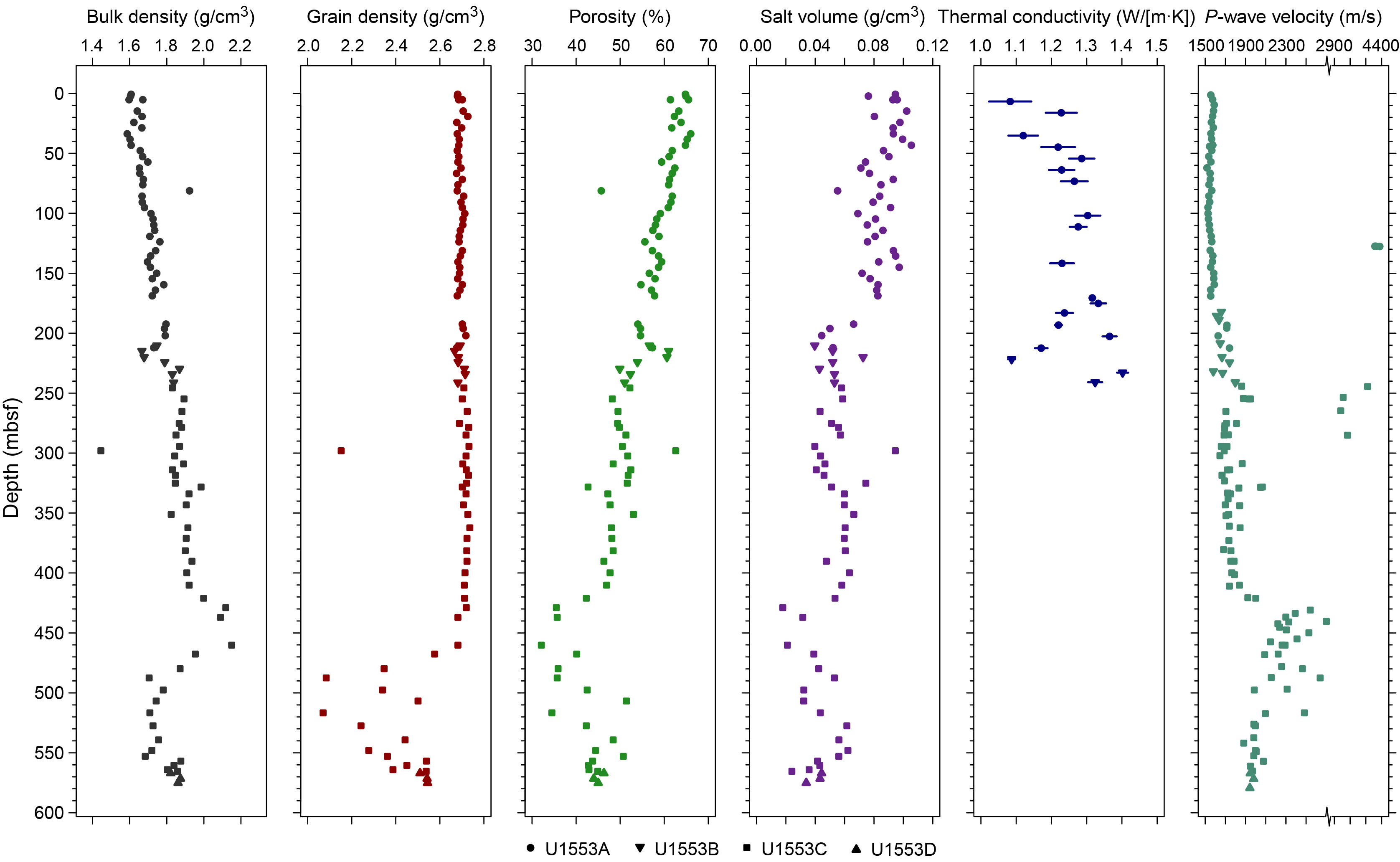
Figure F52. Physical properties measurements, Holes U1553A–U1553D.
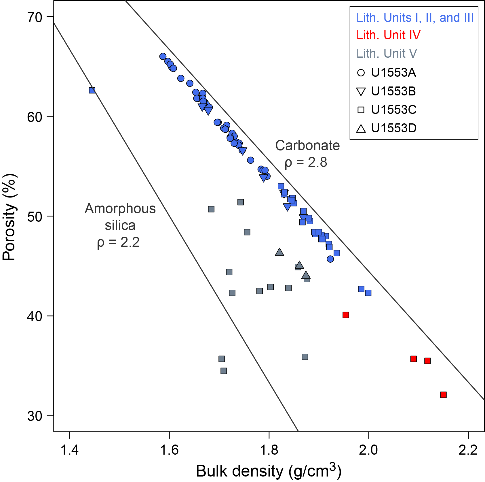
Figure F53. Bulk density and calculated porosity.
7.2.5. Thermal conductivity, temperature, and heat flow
Thermal conductivity was measured on cores with good recovery and softer lithologies that are conducive for measurements. Measurements were generally collected in the third section of each core. Because of lithification, measurements were only collected to 241 mbsf. Thermal conductivity measurements ranged from 1.1 to 1.4 W/m2, did not vary significantly with depth, and were often compromised because of poor contact between the needle probe and the sediment.
Downhole temperature measurements were collected from Cores 378-U1553A-4H, 7H, and 10H (31.5, 60, and 88.5 mbsf, respectively) using the APCT-3 tool and from 181 mbsf in the drilled interval of Hole U1553D (Section 1-1) using the SET2 tool (Table T15). Temperatures ranged from 5.83°C at 31.5 mbsf in Hole U1553A to 15.63°C at 181 mbsf in Hole U1553D. Calculations of heat flow at Site U1553 resulted in a value of 80 mW/m2 following the methods outlined in Pribnow et al. (2000) and using an average approach. However, this value should be considered with care because there was no systematic downhole trend in the calculated thermal conductivity.
7.2.6. Reflectance spectrophotometry and colorimetry
Reflectance spectroscopy colorimetry (RSC) and RGB color space data were measured on the surface of archive-half sections at a 2.5 cm resolution for L*, a*, and b* and at a 1 cm resolution for RGB (Figure F54). From 0 to ~425 mbsf, high RGB values of ~220 reflect the light color of the cores, which is typical of Lithostratigraphic Units II and III. The high reflectance of this core interval is also indicated by a high L* value of about 80. From 0 to 20 mbsf, the b* values increase from 0 to 10, indicating more yellow colors. From ~25 to ~425 mbsf, L*, a*, and b* values vary only slightly. Changes in the RSC and RGB data correspond to the Lithostratigraphic Unit III/IV boundary. Throughout Lithostratigraphic Unit IV, from 425 to 477 mbsf, sediments become darker and L* values decrease from 80 to 50. RGB channels decrease from 220 to 100 to the base of the unit (~477 mbsf). At ~445 mbsf, a* values reach a minimum value of −4, indicating the presence of an enhanced green interval. Below 477 mbsf, relatively low L* values (~30) and RGB values (~100–150) reflect the darker sediments of Lithostratigraphic Unit V.

Figure F54. Color reflectance and color channels.
7.2.7. Shear and compressional strength
Sediment shear strength and compressional strength were measured on two section halves per core in Hole U1553A using the handheld Torvane and penetrometer, respectively (Figure F55). Compressional and shear strength were not measured below Section 21F-2 because of increased lithification of the sediments that exceeded instrument measurement limits and the potential presence of critical boundaries. Shear strength varies from ~0.1 to 0.3 kg/cm2 between 1 and ~100 mbsf, followed by increased variability from 0.15 to 1.25 kg/cm2 between ~114 and 173 mbsf. Compressional strength is relatively constant at approximately 2.0 kg/cm2 for the uppermost 110 m and increases to 3.5–4.5 kg/cm2 downsection.
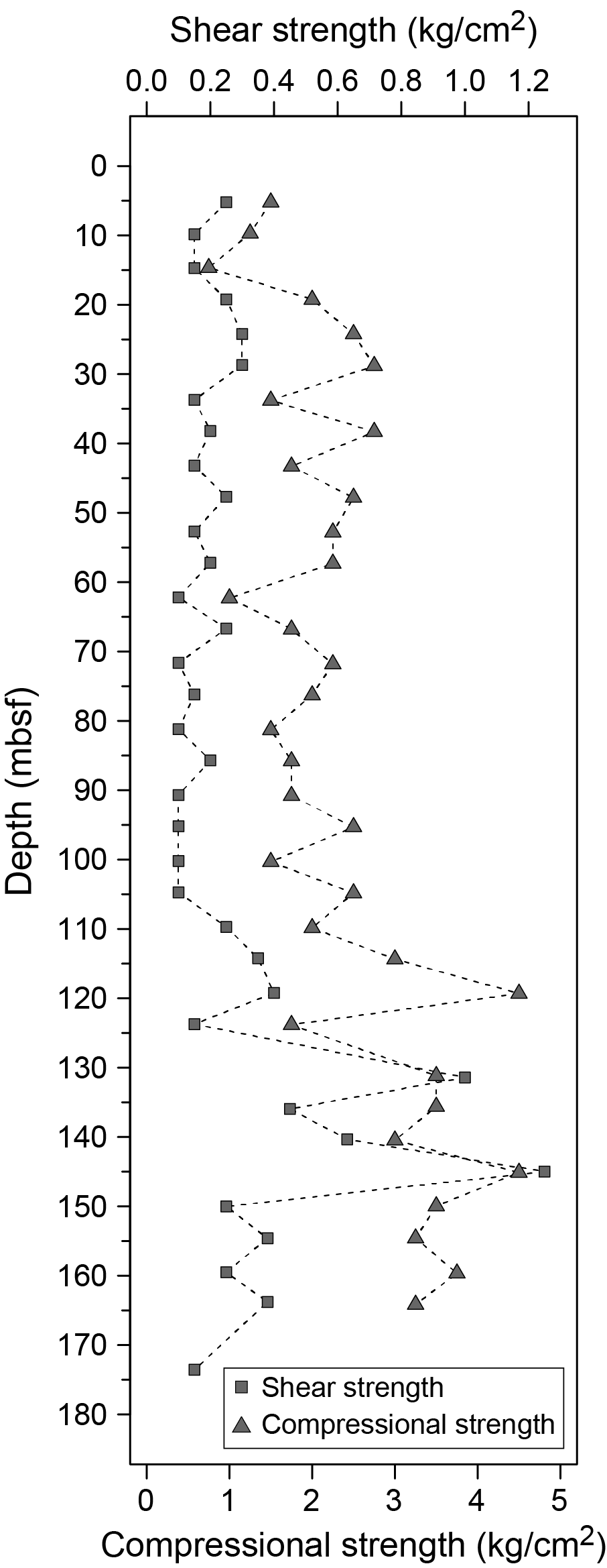
Figure F55. Sediment compressional and shear strength.
8. Stratigraphic correlation
Final core offsets and a splice for Site U1553 were not completed until ~7 months postcruise following XRF scanning at the Gulf Coast Repository in College Station, Texas (USA). Cores recovered using the APC and XCB coring systems in Holes U1553A, U1553B, and U1553E, which seem to be in good condition and have reasonable recovery rates, were difficult to correlate on board JOIDES Resolution. The combined effects of the carbonate-rich lithology, the age of the sediments, their postdepositional history, and occasional drilling disturbance, mostly at the top of the cores (i.e., the first section), made it difficult to identify precise tie points between holes using the scanning data collected on board the ship. GRA density scans, usually reliable for piston-cored sediments, at times exhibited variability within cores that was not recognizable in cores from adjacent holes at similar depths (mbsf scale). Natural gamma ray and MS traces were invariant for most of the cored intervals, although natural gamma ray did play a vital role in tying together Cores 378-U1553A-1H through 3H, 378-U1553B-1H through 3H, and 378-U1553E-1H through 3H at the top of the holes, as well as Cores 378-U1553C-28R through 32R and 378-U1553D-4R through 7R, which span the late Paleocene to early Eocene, including a possible PETM sequence and, deeper, the early Paleocene. Parameter a* (RSC) was the only useful color-related data. The RGB color space profiles have 1.5 m section-related cycles, and scans of core sections are slightly darker at the top than at the bottom. This artifact was only noticeable because of the extremely limited range of colors in the recovered core. Core images, usually helpful in tying holes to one another, did not show enough variability to be useful in most instances. XRF scans overcame many of the problems encountered in the shipboard data and were used as the primary source for setting offsets and splices in Holes U1553A, U1553B, and U1553E. Cumulative offsets for all five holes at Site U1553 are provided in Table T16, and splice intervals are given in Table T17.
In the following discussion, we will address separately the holes cored using the APC and XCB tools (Holes U1553A, U1553B, and U1553E) and those cored using the RCB system (Holes U1553C and U1553D). A core image splice is presented in Figure F56. Although there are a few possible gaps in the APC/XCB splice, recovery was much better than for the RCB system. The deepest APC/XCB core, 378-U1553B-29X, overlaps in mbsf depth with the first rotary core (378-U1553C-2R; the first core after a drilled interval). However, calcareous nannofossil biostratigraphy (Table T2) indicates that Core 378-U1553C-2R may overlap with the shallow holes approximately 20 m higher in the section (e.g., Cores 378-U1553A-25X, 378-U1553B-26X, and 378-U1553E-25X). Such a large difference in mbsf depth seems unjustified, especially because barium-strontium ratio values (Figure F57) in Core 378-U1553C-2R are roughly half the values in Cores 378-U1553A-25X, 378-U1553B-26X, and 378-U1553E-25X. Poor recovery from the top of Hole U1553C (the first three cores from Hole U1553C have a total recovery of 7.5 m) calls into question whether the recovered cores span overlapping depths. Because scan data do not suggest a tie between the two cores and a 20 m adjustment to mbsf depth seems overly large, we decided to offset the data from the rotary cores such that the top of Core 378-U1553C-2R is below Core 378-U1553B-29X rather than imply correlation where none can be found. Fortunately, any future revision of the overlap between Holes U1553B and U1553C will not have any effect on the relative spacing of samples between Holes U1553C and U1553D lower in the section.
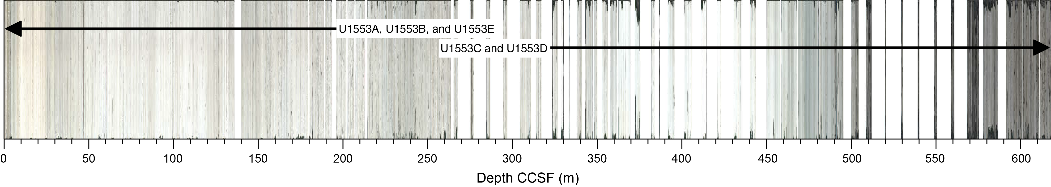
Figure F56. Spliced core image.
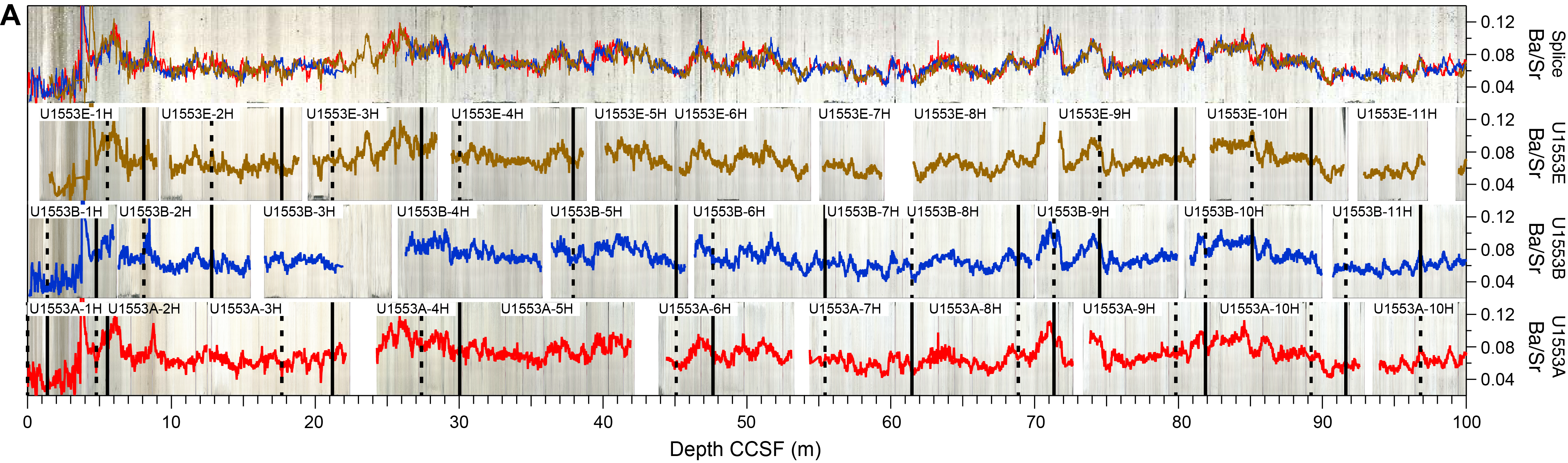

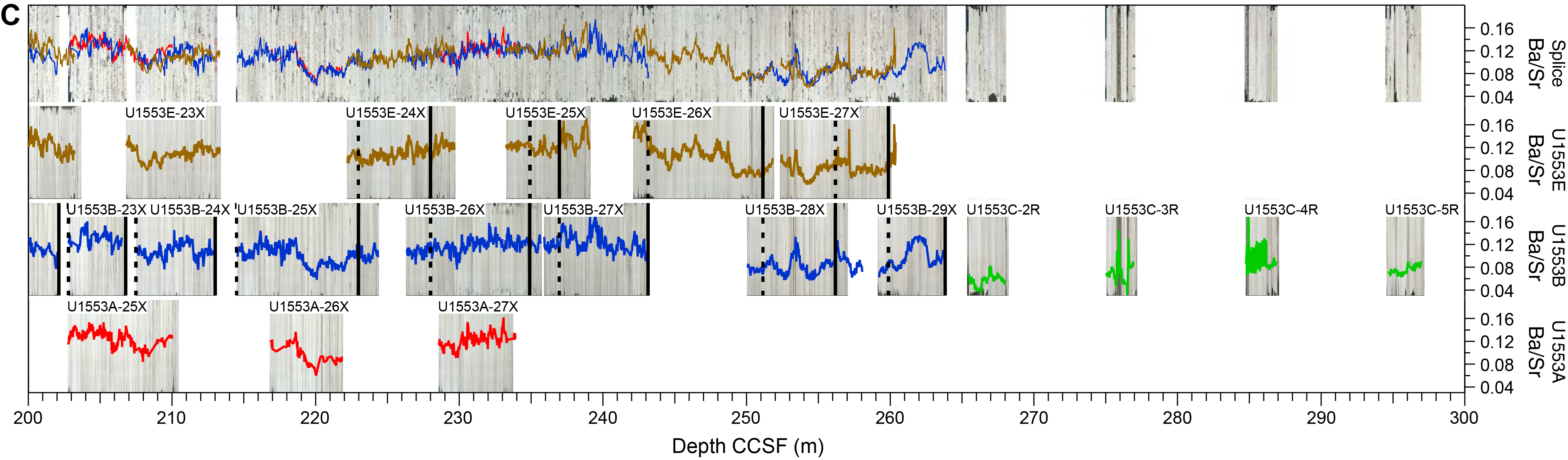
Figure F57. Ba/Sr data, CCSF scale.
8.1. Holes U1553A, U1553B, and U1553E
The barium-strontium ratio (Ba/Sr) derived from XRF scans is plotted on top of core images in Figure F57. The data from individual holes are plotted against a single axis at the top of the figure. A spliced core image is also included under the single-axis Ba/Sr data. Cores are labeled, and splice sections are indicated by vertical lines at the tops and bottoms of splice intervals. Disturbed core has been removed from the core images so that in some cases labels or data seem to extend beyond the core image boundaries. This is a reminder not to use those bits of data for correlation or analysis.
Between the seafloor and 100 m core composite depth below seafloor (CCSF) (Figure F57A), we have pieced together a robust continuous record. A gap that is spanned by only a single record occurs at 23 m CCSF, but reasonable fits between data from Holes U1553A and U1553E above and below this interval suggest that recovery is complete there. Note also that there appear to be intervals of misfit evident in the plot of Ba/Sr on the single axis. This is the result of the often unequal thickness of correlatable events in the data. For instance, if a feature observed near the top of two cores is aligned, there may be features deeper in the core that do not share the same alignment. An example can be seen at 86 m CCSF. This misfit may only be remedied by expanding and compressing data within cores, which is beyond the scope of this report.
The quality of the splice is high to approximately 134 m CCSF (Figure F57B), where cherts were encountered, resulting in poor recovery. Chert (or at least some chert) was the only sediment recovered from Core 378-U1553A-16A, but Holes U1553B and U1553E recovered intercalated sediment with the chert. Nevertheless, there is a good possibility of missing 1 m or so of section here.
The splice becomes tenuous from 180 to 214 m CCSF. Core 378-U1553A-21F is appended to the bottom of Core 20H. Disturbance at the top of Core 21F creates a gap in the splice, and it is important to remember that in any instance where a core is appended to a core above, there is most likely a missing section between them. Between 190 and 223 m CCSF, a combination of half cores and modest recovery created a major splicing challenge. We decided to carry the splice through a series of appends of Cores 378-U1553B-20X through 25X. Cores from Holes U1553A and U1553E were aligned as best possible, but no firm splices were identified. This is a critical area spanning the EOT. Isotope studies of cores in this interval from all three APC holes should help further refine our understanding of the sedimentary progression. Below 215 m CCSF, variability in the data and somewhat better recovery allow construction of a continuous record (Figure F57C).
Holes U1553C and U1553D penetrate into the sedimentary succession from the base of Hole U1553B at 263 m CCSF to a total depth of 618 m CCSF in Hole U1553D. Much of the cored interval in Holes U1553C and U1553D was poorly recovered (Figure F56), and coring in Hole U1553D only began at 430 mbsf. The probable PETM, however, was well captured by Cores 378-U1553C-28R through 32R and 378-U1553D-4R through 7R and is illustrated in a plot of natural gamma ray data superimposed on core images (Figure F58). The PETM occurs just below the pale interval between 481 and 482 m CCSF. Sedimentation rates calculated for these cores (Figure F63) suggest that coring captured matter from approximately 0.5 My prior to the possible PETM and extending almost continuously to approximately 1 My after, with a good chance of more in overlying cores of Hole U1553D.
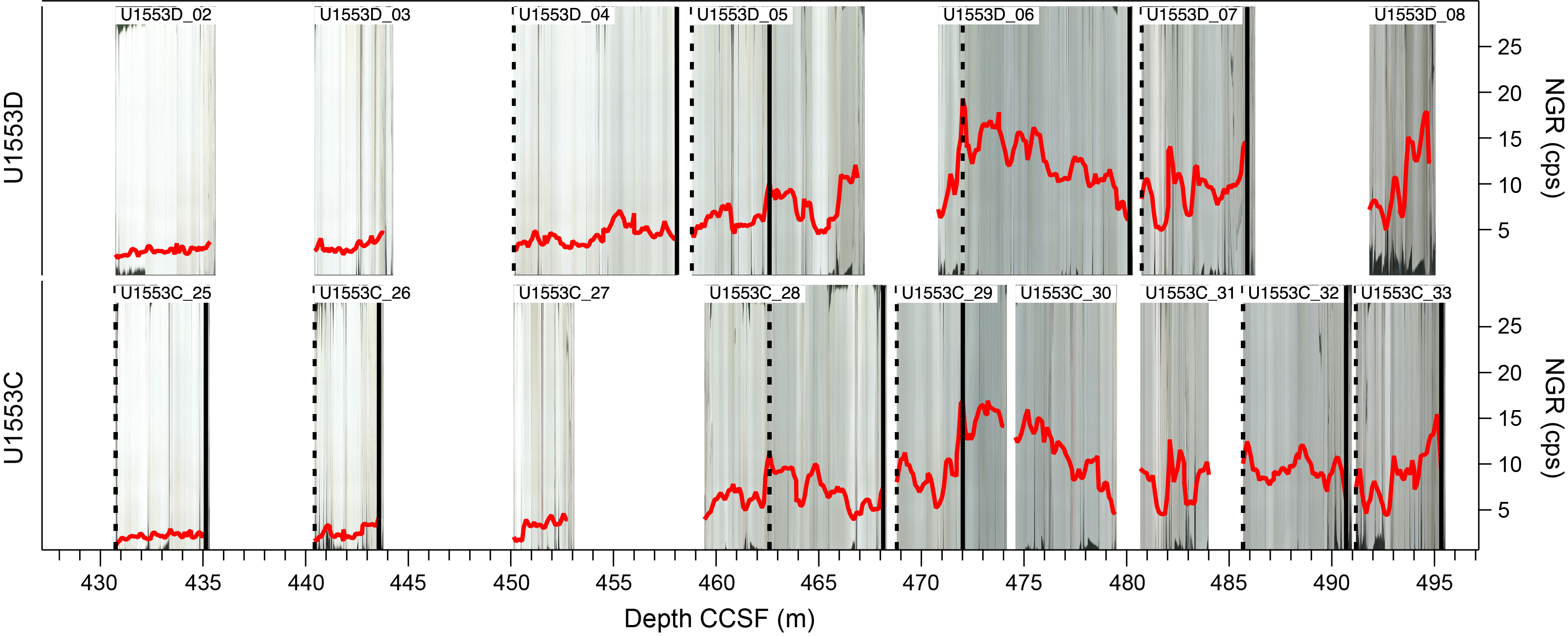
Figure F58. NGR data, CCSF scale.
Comparison of mbsf depth with CCSF depth (Figure F59) indicates that CCSF is approximately 9% greater than mbsf in Holes U1553A, U1553B, and U1553E based on the slope of the best fit to the data. Note that Holes U1553C and U1553D are not included because they have an almost constant offset, and no shifting was done to cores from those holes other than some small adjustments in the late Paleocene to early Eocene and deeper down in the hole in early Paleocene cores.
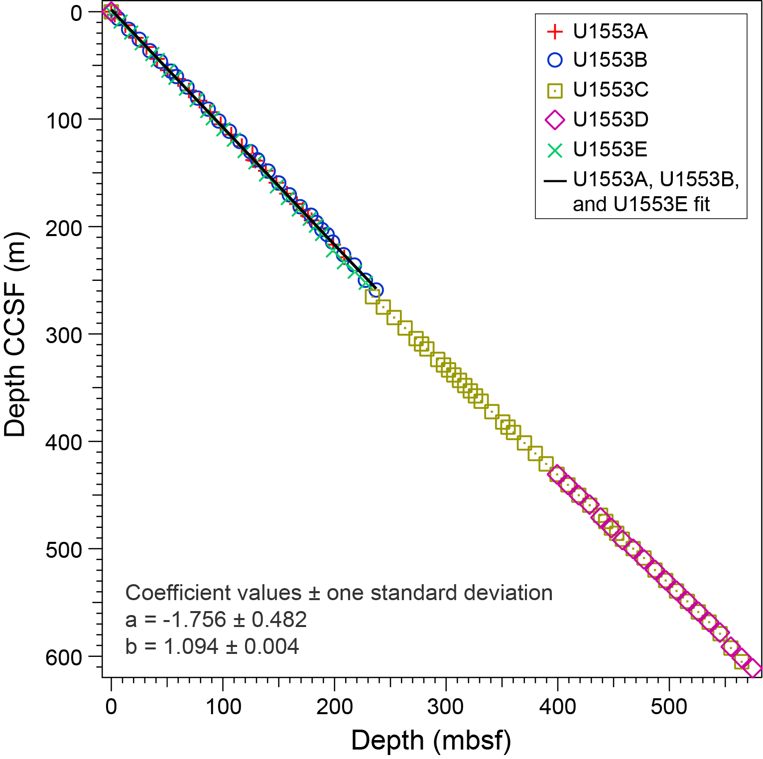
Figure F59. CCSF depths versus original mbsf depths.
9. Age-depth model and mass accumulation rates
The age-depth model developed for Site U1553 is based on an integrated sequence of datums derived from shipboard biostratigraphy and magnetostratigraphy (Table T18). The micropaleontologists examined all five holes in similar detail, whereas the paleomagnetists focused on Holes U1553A and U1553C. Because of difficulties in establishing a spliced composite record with shipboard data and providing the age-depth information for all the cored holes, the current model is based on depth measured as meters below seafloor for all five holes (Figures F60, F61). Core composite depth below seafloor depths that resulted from preliminary correlation of physical properties track data from parallel holes (see Stratigraphic correlation) are also listed in Table T18. Datums are placed at midpoints for biostratigraphy and between inflection points in the inclination data for magnetochron boundaries. All datum ages are based on the geologic timescale of Gradstein et al. (2012). See Biostratigraphy and micropaleontology for more detailed descriptions of datums and biozones and Paleomagnetism for a more detailed description of the basis for magnetochron delineation.
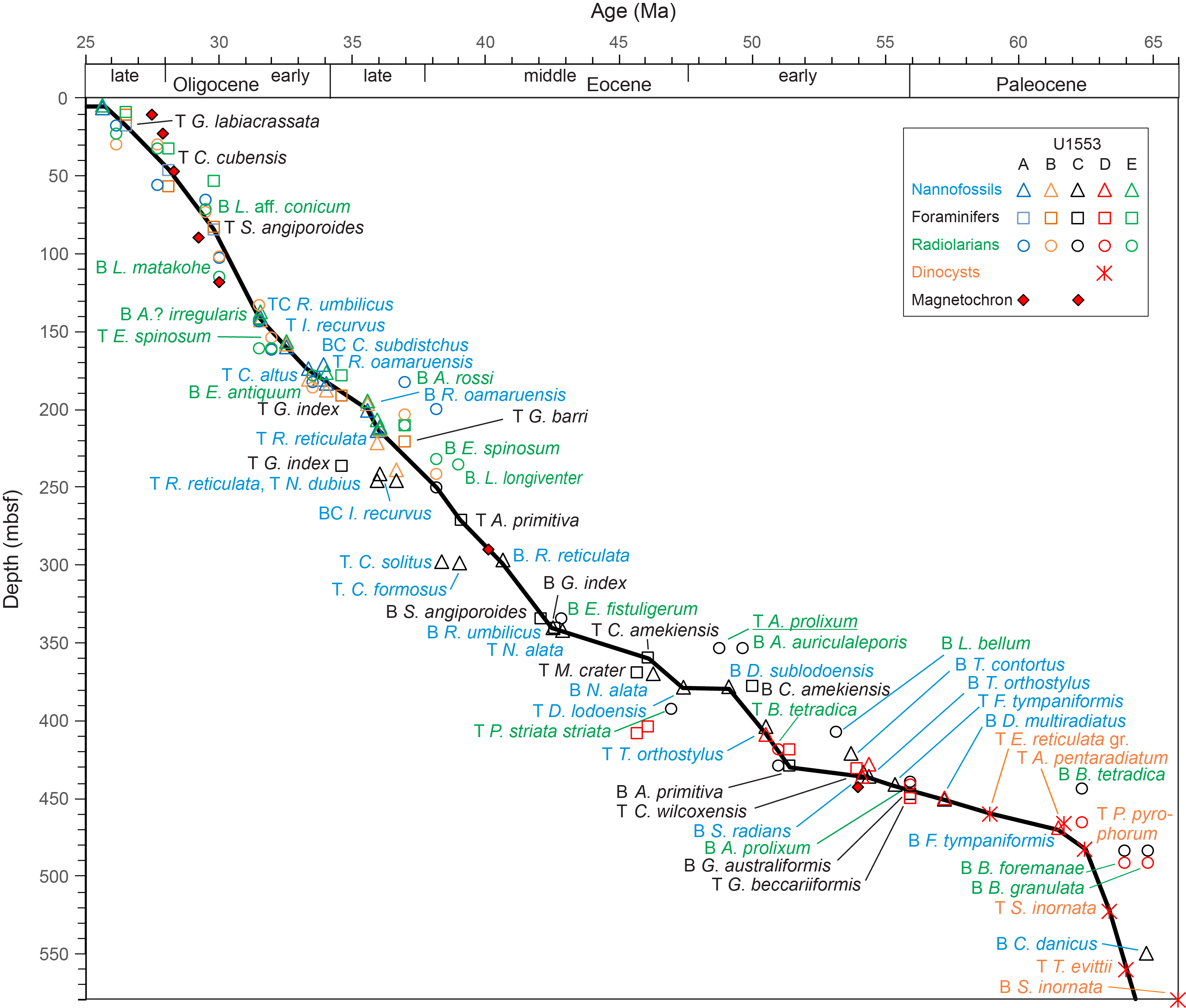
Figure F60. Age-depth plot, 25–66 Ma.
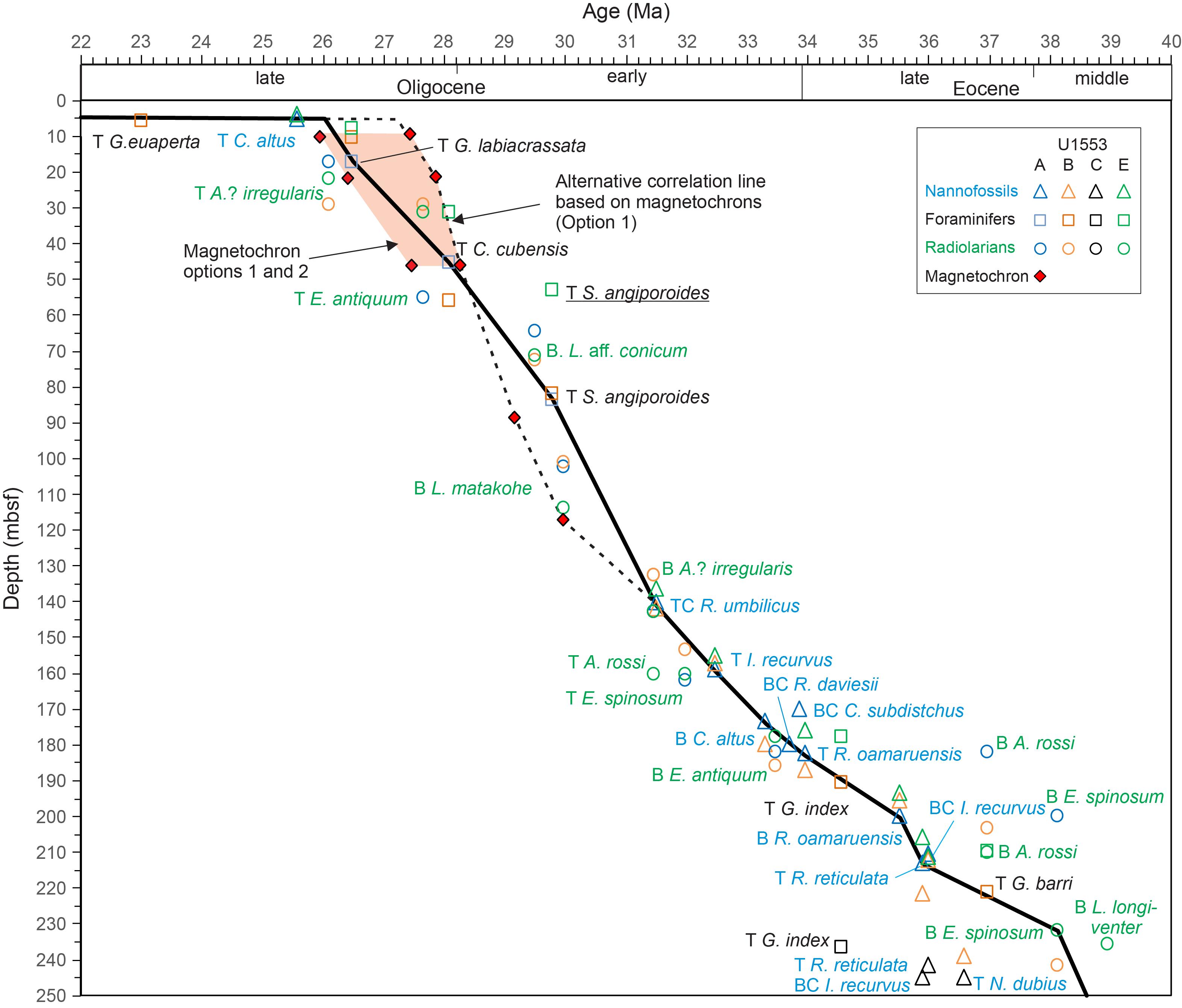
Figure F61. Age-depth plot, 22–40 Ma.
9.1. Age-depth model
The age-depth model is based mainly on datums from Holes U1553A, U1553C, and U1553D. Although general agreement exists among holes, there are significant offsets between datums from Holes U1553A, U1553B, and U1553E in some intervals. We hope these offsets will be reconciled once higher resolution onshore biostratigraphic data and a refined composite record are established. The shipboard datums were primarily identified with a ~10 m resolution for foraminifers and radiolarians and a ~1.5 m resolution for calcareous nannofossils. The line of correlation is constructed by connecting primary datums where possible (Table T19). Where there is a conflict between datums, the line is drawn to ensure most of the datum bases are above the line and most of the datum tops are below the line. Datum bases below the line and datum tops above the line are referred to as age reversals. A datum top above the line of correlation implies the marker species ranges higher than its established range. Similarly, a datum base below the line of correlation implies that the marker species ranges lower than its established range. Such range extensions are unlikely for well-known species and are considered to signify a problem with the age model or with the datum range.
In broad terms, the age-depth plot for all datums identified at Site U1553 shows general agreement between biostratigraphic and magnetostratigraphic datums and within the microfossil groups (Figure F60). However, it was not possible to reconcile detailed biostratigraphy and magnetostratigraphy in the upper part of the Oligocene (Figure F61). Neither of the two options for magnetostratigraphic interpretation (Table T9) in the upper 50 m of Hole U1553A can be reconciled with foraminifer datums in this interval. Option 1 results in an age reversal for S. angiporoides, whereas Option 2 results in age reversals for C. cubensis and S. angiporoides. We show a possible line of correlation based on Option 1 (dashed line in Figure F61), but the preferred line of correlation is based on biostratigraphic datums because it is consistent with both foraminifer and radiolarian datums in this interval and avoids age reversals. In the entire sequence, only one age reversal is noted. The top of early Eocene index species A. prolixum is found to occur in the middle Eocene (Figure F60). The upper range limit of this species is not well established; therefore, this may represent a true range extension for the species.
Several other datums are not age reversals, but they do represent last occurrences earlier than the established datum age or first occurrences later than the established datum age. This is likely an artifact of a preliminary study based on widely spaced core catcher samples. With further study of samples, it is anticipated that a closer fit with the correlation line will emerge.
9.2. Comparison with Site 277
Many of the biostratigraphic datums identified at Site U1553 were also found at the single hole, spot cored DSDP Site 277 (Hollis et al., 1997, 2014, 2015). A depth-depth plot of datums for the two sites (Figure F62) shows very good correspondence in the upper part (<200 mbsf) but more divergence in the lower part where spot-coring at Site 277 is likely a contributing factor for sporadic identification of marker species. In studies of Site 277 (Hollis et al., 1997, 2014, 2015), unconformities were identified in the middle Eocene (~45 Ma), early Eocene (~54 Ma), and late Paleocene (~59.60 Ma). Further study may also reveal uncertainties in some intervals of low sedimentation rate in the lowermost 340 m of Site U1553. Overall, there is a good linear correlation between the two sites.
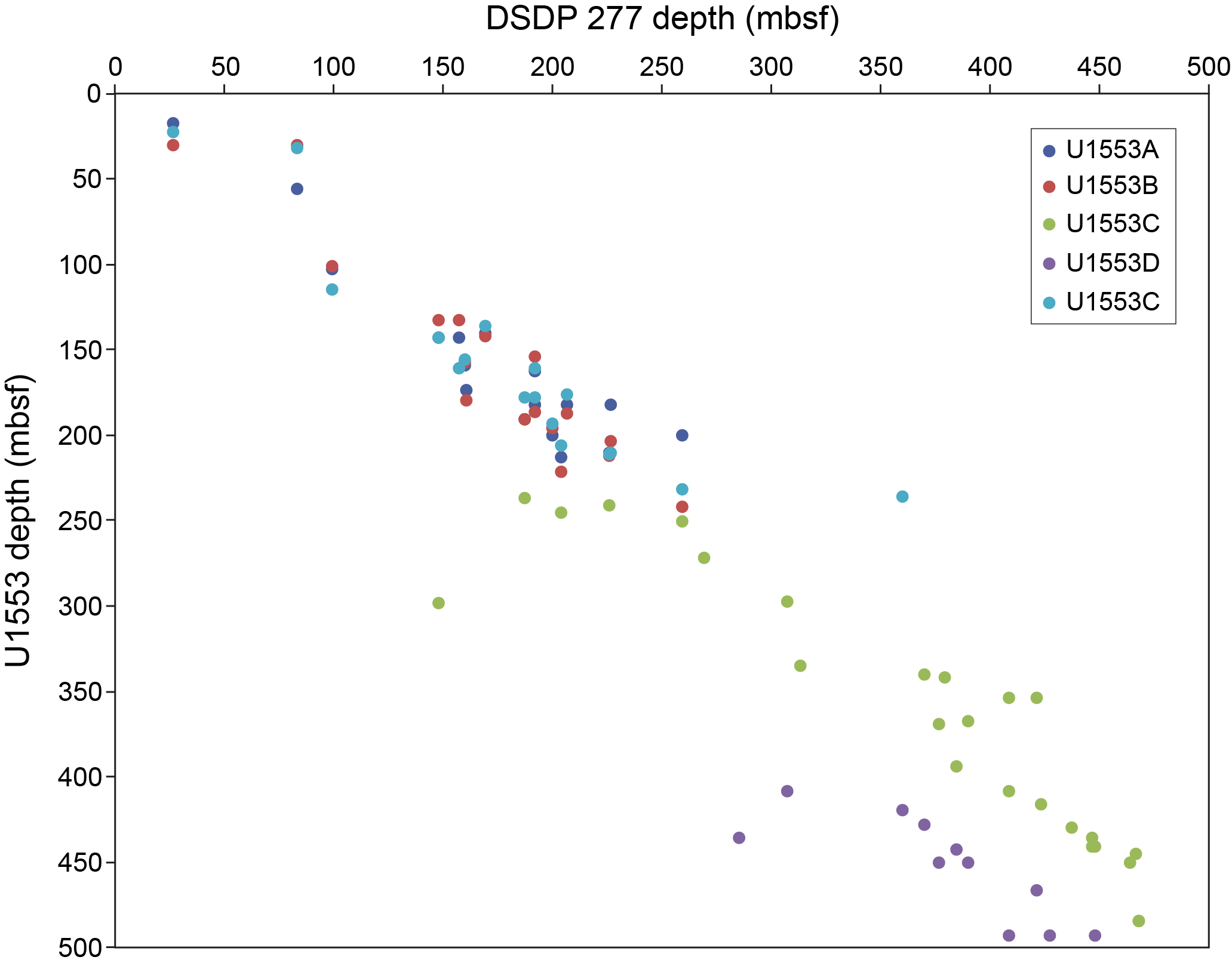
Figure F62. Biostratigraphic datum depths.
9.3. Linear sedimentation rates
Major changes in linear sedimentation rates (LSRs) were calculated (Table T19) and are illustrated as line segments in the age-depth plot (Figure F60). They are plotted versus depth and age in Figure F63.
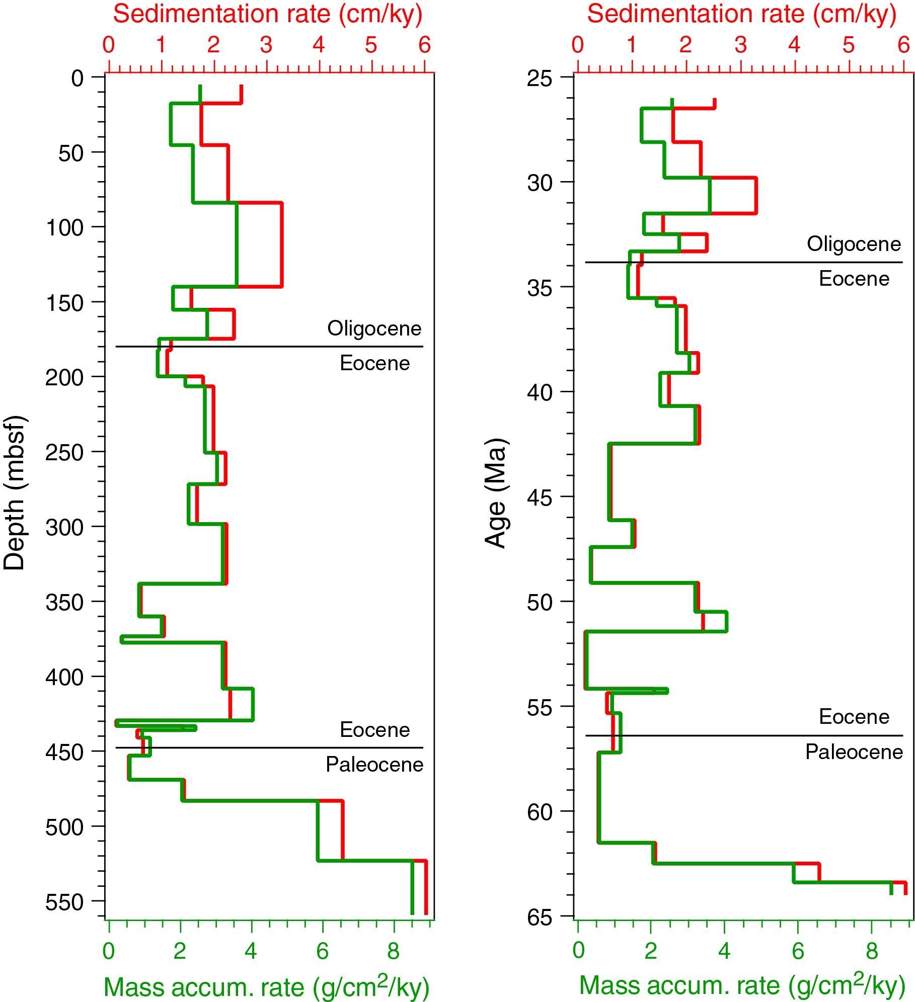
Figure F63. LSR and MAR.
9.4 Mass accumulation rates
Mass accumulation rates (MARs) are listed for the LSR intervals in Table T19. They are plotted versus depth (mbsf scale) and age in Figure F63 alongside the LSRs. MARs were calculated from the LSR interval values and the average of dry bulk density (ρ G) measurements (see Physical properties) within the intervals using the formula:
The calculation excluded the upper 3–5 m (depending on the hole) above the Pleistocene–Oligocene unconformity. The MAR is primarily a function of the sedimentation rate in these relatively uniform carbonate sediments because ρ G varies little (see Physical properties).
References
Abelmann, A., 1990. Oligocene to middle Miocene radiolarian stratigraphy of southern high latitudes from Leg 113, Sites 689 and 690, Maud Rise. In Baker, P.F., Kennett, J.P., et al., Proceedings of the Ocean Drilling Program, Initial Reports, 113: College Station, TX (Ocean Drilling Program), 675–708. https://doi.org/
Agnini, C., Fornaciari, E., Raffi, I., Catanzariti, R., Palike, H., Backman, J., and Rio, D., 2014. Biozonation and biochronology of Paleogene calcareous nannofossils from low and middle latitudes. Newsletters on Stratigraphy, 47(2):131–181. https://doi.org/
Alegret, L., and Thomas, E., 2013. Benthic foraminifera across the Cretaceous/Paleogene boundary in the Southern Ocean (ODP Site 690): diversity, food and carbonate saturation. Marine Micropaleontology, 105:40–51. https://doi.org/
Anagnostou, E., John, E.H., Babila, T.L., Sexton, P.F., Ridgwell, A., Lunt, D.J., Pearson, P.N., Chalk, T.B., Pancost, R.D., and Foster, G.L., 2020. Proxy evidence for state-dependence of climate sensitivity in the Eocene greenhouse. Nature Communications, 11(1):4436. https://doi.org/
Anagnostou, E., John, E.H., Edgar, K.M., Foster, G.L., Ridgwell, A., Inglis, G.N., Pancost, R.D., Lunt, D.J., and Pearson, P.N., 2016. Changing atmospheric CO2 concentration was the primary driver of early Cenozoic climate. Nature, 533(7603):380–384. https://doi.org/
Barker, P.F., 2001. Scotia Sea regional tectonic evolution: implications for mantle flow and palaeocirculation. Earth-Science Reviews, 55(1):1–39. https://doi.org/
Barker, P.F., and Thomas, E., 2004. Origin, signature and palaeoclimatic influence of the Antarctic Circumpolar Current. Earth-Science Reviews, 66(1–2):143–162. https://doi.org/
Barnet, J.S.K., Littler, K., Westerhold, T., Kroon, D., Leng, M.J., Bailey, I., Röhl, U., and Zachos, J.C., 2019. A high-fidelity benthic stable isotope record of Late Cretaceous-early Eocene climate change and carbon-cycling. Paleoceanography and Paleoclimatology, 34(4):672–691. https://doi.org/
Bijl, P.K., Bendle, J.A.P., Bohaty, S.M., Pross, J., Schouten, S., Tauxe, L., Stickley, C.E., et al., 2013. Eocene cooling linked to early flow across the Tasmanian Gateway. Proceedings of the National Academy of Sciences of the United States of America, 110(24):9645–9650. https://doi.org/
Bijl, P.K., Schouten, S., Sluijs, A., Reichart, G.-J., Zachos, J.C., and Brinkhuis, H., 2009. Early Palaeogene temperature evolution of the southwest Pacific Ocean. Nature, 461(7265):776–779. https://doi.org/
Bralower, T.J., 2002. Evidence of surface water oligotrophy during the Paleocene-Eocene Thermal Maximum: nannofossil assemblage data from Ocean Drilling Program Site 690, Maud Rise, Weddell Sea. Paleoceanography and Paleoclimatology, 17(2):13-11–13-12. https://doi.org/
Carmichael, M.J., Lunt, D.J., Huber, M., Heinemann, M., Kiehl, J., LeGrande, A., Loptson, C.A., et al., 2016. A model–model and data–model comparison for the early Eocene hydrological cycle. Climate of the Past, 12(2):455–481. https://doi.org/
Cramwinckel, M.J., Huber, M., Kocken, I.J., Agnini, C., Bijl, P.K., Bohaty, S.M., Frieling, J., et al., 2018. Synchronous tropical and polar temperature evolution in the Eocene. Nature, 559(7714):382–386. https://doi.org/
Crouch, E.M., Willumsen, P.S., Kulhanek, D.K., and Gibbs, S.J., 2014. A revised Paleocene (Teurian) dinoflagellate cyst zonation from eastern New Zealand. Review of Palaeobotany and Palynology, 202:47–79. https://doi.org/
Dallanave, E., Bachtadse, V., Crouch, E.M., Tauxe, L., Shepherd, C.L., Morgans, H.E.G., Hollis, C.J., Hines, B.R., and Sugisaki, S., 2016. Constraining early to middle Eocene climate evolution of the Southwest Pacific and Southern Ocean. Earth and Planetary Science Letters, 433:380–392. https://doi.org/
De Vleeschouwer, D., Dunlea, A.G., Auer, G., Anderson, C.H., Brumsack, H., de Loach, A., Gurnis, M., et al., 2017. Quantifying K, U, and Th contents of marine sediments using shipboard natural gamma radiation spectra measured on DV JOIDES Resolution. Geochemistry, Geophysics, Geosystems, 18(3):1053–1064. https://doi.org/
Dunlea, A.G., Murray, R.W., Sauvage, J., Spivack, A.J., Harris, R.N., and D’Hondt, S., 2015. Dust, volcanic ash, and the evolution of the South Pacific Gyre through the Cenozoic. Paleoceanography and Paleoclimatology, 30(8):1078–1099. https://doi.org/
Expedition 317 Scientists, 2011. Methods. In Fulthorpe, C.S., Hoyanagi, K., Blum, P., and the Expedition 317 Scientists, Proceedings of the Integrated Ocean Drilling Program, 317: Tokyo (Integrated Ocean Drilling Program Management International, Inc.). https://doi.org/
Fioroni, C., Villa, G., Persico, D., Wise, S.W., and Pea, L., 2012. Revised middle Eocene-upper Oligocene calcareous nannofossil biozonation for the Southern Ocean. Revue de Micropaléontologie, 55(2):53–70. https://doi.org/
Funakawa, S., and Nishi, H., 2005. Late middle Eocene to late Oligocene radiolarian biostratigraphy in the Southern Ocean (Maud Rise, ODP Leg 113, Site 689). Marine Micropaleontology, 54(3):213–247. https://doi.org/
Goodell, H.G., Meylan, M.A., and Grant, B., 1971. Ferromanganese deposits of the South Pacific Ocean, Drake Passage, and Scotia Sea. In Reid, J.L. (Ed.), Antarctic Research Series (Volume 15):Antarctic Oceanology I: Washington, DC (American Geophysical Union), 27–92. https://doi.org/
Gradstein, F.M., Ogg, J.G., Schmitz, M.D., and Ogg, G.M. (Eds.), 2012. The Geological Time Scale 2012: Amsterdam (Elsevier). https://doi.org/
Gutjahr, M., Ridgwell, A., Sexton, P.F., Anagnostou, E., Pearson, P.N., Palike, H., Norris, R.D., Thomas, E., and Foster, G.L., 2017. Very large release of mostly volcanic carbon during the Palaeocene-Eocene Thermal Maximum. Nature, 548(7669):573–577. https://doi.org/
Hague, A.M., Thomas, D.J., Huber, M., Korty, R., Woodard, S.C., and Jones, L.B., 2012. Convection of North Pacific Deep Water during the early Cenozoic. Geology, 40(6):527–530. https://doi.org/
Harper, D.T., Hönisch, B., Zeebe, R.E., Shaffer, G., Haynes, L.L., Thomas, E., and Zachos, J.C., 2020. The magnitude of surface ocean acidification and carbon release during Eocene Thermal Maximum 2 (ETM-2) and the Paleocene-Eocene Thermal Maximum (PETM). Paleoceanography and Paleoclimatology, 35(2):e2019PA003699. https://doi.org/
Hayward, B.W., Grenfell, H.R., Sabaa, A., Neil, H.L., and Buzas, M.A., 2010. Recent New Zealand deep-water benthic foraminifera: taxonomy, ecologic distribution, biogeography, and use in paleoenvironmental assessment. GNS Science Monograph, 26.
Held, I.M., and Soden, B.J., 2006. Robust responses of the hydrological cycle to global warming. Journal of Climate, 19(21):5686–5699. https://doi.org/
Hollis, C.J., 2006. Radiolarian faunal turnover through the Paleocene-Eocene transition, Mead Stream, New Zealand. Eclogae Geologicae Helvetiae, 99(1):S79–S99. https://doi.org/
Hollis, C.J., Dunkley Jones, T., Anagnostou, E., Bijl, P.K., Cramwinckel, M.J., Cui, Y., Dickens, G.R., et al., 2019. The DeepMIP contribution to PMIP4: methodologies for selection, compilation and analysis of latest Paleocene and early Eocene climate proxy data, incorporating version 0.1 of the DeepMIP database. Geoscientific Model Development, 12(7):3149–3206. https://doi.org/
Hollis, C.J., Handley, L., Crouch, E.M., Morgans, H.E.G., Baker, J.A., Creech, J., Collins, K.S., et al., 2009. Tropical sea temperatures in the high-latitude South Pacific during the Eocene. Geology, 37(2):99–102. https://doi.org/
Hollis, C.J., Hines, B.R., Littler, K., Villasante-Marcos, V., Kulhanek, D.K., Strong, C.P., Zachos, J.C., Eggins, S.M., Northcote, L., and Phillips, A., 2015. The Paleocene-Eocene Thermal Maximum at DSDP Site 277, Campbell Plateau, southern Pacific Ocean. Climate of the Past, 11(7):1009–1025. https://doi.org/
Hollis, C.J., Pascher, K.M., Kamikuri, S.-I., Nishimura, A., Suzuki, N., and Sanfilippo, A., 2017. Towards an integrated cross-latitude event stratigraphy for Paleogene radiolarians. Newsletter of the International Association of Radiolarists, 15:288–289.
Hollis, C.J., Tayler, M.J.S., Andrew, B., Taylor, K.W., Lurcock, P., Bijl, P.K., Kulhanek, D.K., et al., 2014. Organic-rich sedimentation in the South Pacific Ocean associated with late Paleocene climatic cooling. Earth-Science Reviews, 134:81–97. https://doi.org/
Hollis, C.J., Taylor, K.W.R., Handley, L., Pancost, R.D., Huber, M., Creech, J.B., Hines, B.R., et al., 2012. Early Paleogene temperature history of the southwest Pacific Ocean: reconciling proxies and models. Earth and Planetary Science Letters, 349–350:53–66. https://doi.org/
Hollis, C.J., Waghorn, D.B., Strong, C.P., and Crouch, E.M., 1997. Integrated Paleogene Biostratigraphy of DSDP Site 277 (Leg 29): Foraminifera, Calcareous Nannofossils, Radiolaria, and Palynomorphs, Report 97/7: Lower Hutt, New Zealand (Institute of Geological & Nuclear Sciences Limited).
Hollister, C.D., and Nowell, A.R.M., 1991. HEBBLE epilogue. Marine Geology, 99(3):445–460. https://doi.org/
Hönisch, B., Ridgwell, A., Schmidt, D.N., Thomas, E., Gibbs, S.J., Sluijs, A., Zeebe, R., et al., 2012. The geological record of ocean acidification. Science, 335(6072):1058–1063. https://doi.org/
Hornibrook, N.B., Brazier, R.C., and Strong, C.P., 1989. Manual of New Zealand Permian to Pleistocene foraminiferal biostratigraphy. New Zealand Geological Survey Paleontological Bulletin, 56.
Hovan, S.A., and Rea, D.K., 1992. Paleocene/Eocene boundary changes in atmospheric and oceanic circulation: a Southern Hemisphere record. Geology, 20(1):15–18. https://doi.org/
Hrouda, F., 1982. Magnetic anisotropy of rocks and its application in geology and geophysics. Geophysical surveys, 5(1):37–82. https://doi.org/
Huber, B.T., and Quillévéré, F., 2005. Revised Paleogene planktonic foraminiferal biozonation for the austral realm. Journal of Foraminiferal Research, 35(4):299–314. https://doi.org/
Huber, M., 2008. A hotter greenhouse? Science, 321(5887):353–354. https://doi.org/
Huber, M., Brinkhuis, H., Stickley, C.E., Doos, K., Sluijs, A., Warnaar, J., Schellenberg, S.A., and Williams, G.L., 2004. Eocene circulation of the Southern Ocean: was Antarctica kept warm by subtropical waters? Paleoceanography and Paleoclimatology, 19(4):PA4026. https://doi.org/
Huber, M., and Caballero, R., 2011. The early Eocene equable climate problem revisited. Climate of the Past, 7(2):603–633. https://doi.org/
Hutchinson, D.K., de Boer, A.M., Coxall, H.K., Caballero, R., Nilsson, J., and Baatsen, M., 2018. Climate sensitivity and meridional overturning circulation in the late Eocene using GFDL CM2.1. Climate of the Past, 14(6):789–810. https://doi.org/
Ivany, L.C., Brey, T., Huber, M., Buick, D.P., and Schöne, B.R., 2011. El Niño in the Eocene greenhouse recorded by fossil bivalves and wood from Antarctica. Geophysical Research Letters, 38(16):L16709. https://doi.org/
Janecek, T.R., and Rea, D.K., 1983. Eolian deposition in the northeast Pacific Ocean: Cenozoic history of atmospheric circulation. Geological Society of America Bulletin, 94(6):730–738. https://doi.org/
Jenkins, D.G., 1975. Cenozoic planktonic foraminiferal biostratigraphy of the southwestern Pacific and Tasman Sea—DSDP Leg 29. In Kennett, J.P., Houtz, R. E., et al., Initial Reports of the Deep Sea Drilling Project, 29: Washington, DC (US Government Printing Office), 449–467. https://doi.org/
Kennett, J.P., Houtz, R.E., Andrews, P.B., Edwards, A.R., Gostin, V.A., Hajos, M., Hampton, M., Jenkins, D.G., Margolis, S.V., Ovenshine, A.T., and Perch-Nielsen, K., 1975. Introduction and explanatory notes. In Kennett, J.P., Houtz, R. E., et al., Initial Reports of the Deep Sea Drilling Project, 29: Washington, DC (US Government Printing Office), 3–16. https://doi.org/
Kulhanek, D.K., Crouch, E.M., Tayler, M.J.S., and Hollis, C.J., 2015. Paleocene calcareous nannofossils from East Coast, New Zealand: biostratigraphy and palaeoecology. Journal of Nannoplankton Research, 35(2):155–176.
Lauretano, V., Hilgen, F.J., Zachos, J.C., and Lourens, L.J., 2016. Astronomically tuned age model for the early Eocene carbon isotope events: a new high-resolution benthic δ13C benthic record of ODP Site 1263 between ~49 and ~54 Ma. Newsletters on Stratigraphy, 49(2):383–400. https://doi.org/
Lawver, L.A., and Gahagan, L.M., 1998. Opening of Drake Passage and its impact on the Cenozoic Ocean. In Crowley, T.J., and Burke, K.C. (Eds.), Tectonic Boundary Conditions for Climate Reconstructions: Oxford (Oxford University Press), 212–223.
Lawver, L.A., and Gahagan, L.M., 2003. Evolution of Cenozoic seaways in the circum-Antarctic region. Palaeogeography, Palaeoclimatology, Palaeoecology, 198(1):11–37. https://doi.org/
Leri, A.C., Hakala, J.A., Marcus, M.A., Lanzirotti, A., Reddy, C.M., and Myneni, S.C.B., 2010. Natural organobromine in marine sediments: new evidence of biogeochemical Br cycling. Global Biogeochemical Cycles, 24(4):GB4017. https://doi.org/
Littler, K., Röhl, U., Westerhold, T., and Zachos, J.C., 2014. A high-resolution benthic stable-isotope record for the South Atlantic; implications for orbital-scale changes in late Paleocene-early Eocene climate and carbon cycling. Earth and Planetary Science Letters, 401:18–30. https://doi.org/
Liu, B., Saito, Y., Yamazaki, T., Abdeldayem, A., Oda, H., Hori, K., and Zhao, Q., 2001. Paleocurrent analysis for the late Pleistocene–Holocene incised-valley fill of the Yangtze delta, China by using anisotropy of magnetic susceptibility data. Marine Geology, 176(1):175–189. https://doi.org/
Lowrie, W., and Hirt, A.M., 1987. Anisotropy of magnetic susceptibility in the Scaglia Rossa pelagic limestone. Earth and Planetary Science Letters, 82(3):349–356. https://doi.org/
Lunt, D.J., Jones, T.D., Heinemann, M., Huber, M., Legrande, A., Winguth, A., Loptson, C., et al., 2012. A mode-data comparison for a multi-model ensemble of early Eocene atmosphere ocean simulations: EoMIP. Climate of the Past, 8:1717–1736. https://doi.org/
Lurcock, P.C., and Wilson, G.S., 2013. The palaeomagnetism of glauconitic sediments. Global and Planetary Change, 110(C):278–288. https://doi.org/
Lyle, M., Gibbs, S., Moore, T.C., and Rea, D.K., 2007. Late Oligocene initiation of the Antarctic Circumpolar Current: evidence from the South Pacific. Geology, 35(8):691–694. https://doi.org/
Martini, E., 1971. Standard Tertiary and Quaternary calcareous nannoplankton zonation. Proceedings of the Second Planktonic Conference, Roma, 1970, 2:739–785.
Norris, R.D., Wilson, P.A, Blum, P., and the Expedition 342 Scientists, 2014. Proceedings of the Integrated Ocean Drilling Program, 342: College Station, TX (Integrated Ocean Drilling Program). https://doi.org/
Ohneiser, C., and Tapia, C., 2020. Diagenesis of magnetic minerals at the Southwest Pacific DSDP Site 277. New Zealand Journal of Geology and Geophysics, 63(2):250–261. https://doi.org/
Pagani, M., Huber, M., Liu, Z., Bohaty, S.M., Henderiks, J., Sijp, W., Krishnan, S., and DeConto, R.M., 2011. The role of carbon dioxide during the onset of Antarctic glaciation. Science, 334(6060):1261–1264. https://doi.org/
Pagani, M., Pedentchouk, N., Huber, M., Sluijs, A., Schouten, S., Brinkhuis, H., Sinninghe Damsté, J.S., et al., 2006. Arctic hydrology during global warming at the Palaeocene/Eocene Thermal Maximum. Nature, 442(7103):671–675. https://doi.org/
Pearson, P.N., Foster, G.L., and Wade, B.S., 2009. Atmospheric carbon dioxide through the Eocene–Oligocene climate transition. Nature, 461(7267):1110–1113. https://doi.org/
Pearson, P.N., Olsson, R.K., Huber, B.T., Hemleben, C., and Berggren, W.A., 2006. Atlas of Eocene planktonic foraminifera. Special Publication - Cushman Foundation for Foraminiferal Research, 41.
Pearson, P.N., van Dongen, B.E., Nicholas, C.J., Pancost, R.D., Schouten, S., Singano, J.M., and Wade, B.S., 2007. Stable warm tropical climate through the Eocene Epoch. Geology, 35(3):211–214. https://doi.org/
Pfuhl, H.A., and McCave, I.N., 2005. Evidence for late Oligocene establishment of the Antarctic Circumpolar Current. Earth and Planetary Science Letters, 235(3):715–728. https://doi.org/
Pierrot, D.E., Lewis, E., and Wallace, D.W.R., 2006. MS Excel program developed for CO 2 system calculations: Oak Ridge, TN (Carbon Dioxide Information Analysis Center, Oak Ridge National Laboratory, US Department of Energy).
Pimmel, A., and Claypool, G., 2001. Introduction to shipboard organic geochemistry on the JOIDES Resolution. Ocean Drilling Program Technical Note, 30. https://doi.org/
Piper, J.D.A., Elliot, M.T., and Kneller, B.C., 1996. Anisotropy of magnetic susceptibility in a Palaeozoic flysch basin: the Windermere Supergroup, northern England. Sedimentary Geology, 106(3–4):235–258. https://doi.org/
Pribnow, D.F.C., Kinoshita, M., and Stein, C.A., 2000. Thermal Data Collection and Heat Flow Recalculations for ODP Legs 101–180: Hannover, Germany (Institut für Geowissenschaftliche Gemeinschaftsaufgaben). http://www-odp.tamu.edu/
Pross, J., Contreras, L., Bijl, P.K., Greenwood, D.R., Bohaty, S.M., Schouten, S., Bendle, J.A., et al., 2012. Persistent near-tropical warmth on the Antarctic continent during the early Eocene epoch. Nature, 488(7409):73–77. https://doi.org/
Raine, J.I., Beu, A.G., Boyes, A.F., Campbell, H.J., Cooper, R.A., Crampton, J.S., Crundwell, M.P., Hollis, C.J., Morgans, H.E.G., and Mortimer, N., 2015. New Zealand Geological Timescale NZGT 2015/1. New Zealand Journal of Geology and Geophysics, 58(4):398–403. https://doi.org/
Roberts, A.P., 2015. Magnetic mineral diagenesis. Earth-Science Reviews, 151:1–47. https://doi.org/
Roberts, A.P., Florindo, F., Chang, L., Heslop, D., Jovane, L., and Larrasoaña, J.C., 2013. Magnetic properties of pelagic marine carbonates. Earth-Science Reviews, 127:111–139. https://doi.org/
Röhl, U., Thomas, D.J., Childress, L.B., Anagnostou, E., Ausín, B., Borba Dias, B., Boscolo-Galazzo, F., Brzelinski, S., Dunlea, A.G., George, S.C., Haynes, L.L., Hendy, I.L., Jones, H.L., Khanolkar, S.S., Kitch, G.D., Lee, H., Raffi, I., Reis, A.J., Sheward, R.M., Sibert, E., Tanaka, E., Wilkens, R., Yasukawa, K., Yuan, W., Zhang, Q., Zhang, Y., Drury, A.J., Crouch, E.M., and Hollis, C.J., 2022. Expedition 378 methods. In Röhl, U., Thomas, D.J., Childress, L.B., and the Expedition 378 Scientists, South Pacific Paleogene Climate. Proceedings of the International Ocean Discovery Program, 378: College Station, TX (International Ocean Discovery Program). https://doi.org/
Röhl, U., Westerhold, T., Bralower, T.J., and Zachos, J.C., 2007. On the duration of the Paleocene-Eocene Thermal Maximum (PETM). Geochemistry, Geophysics, Geosystems, 8(12):Q12002. https://doi.org/
Rowan, C.J., and Roberts, A.P., 2006. Magnetite dissolution, diachronous greigite formation, and secondary magnetizations from pyrite oxidation: unravelling complex magnetizations in Neogene marine sediments from New Zealand. Earth and Planetary Science Letters, 241(1):119–137. https://doi.org/
Savin, S.M., 1977. The history of the Earth’s surface temperature during the past 100 million years. Annual Review of Earth and Planetary Sciences, 5(1):319–355. https://doi.org/
Scher, H.D., and Martin, E.E., 2006. Timing and climatic consequences of the opening of Drake Passage. Science, 312(5772):428–430. https://doi.org/
Shackleton, N.J., and Kennett, J.P., 1975. Paleotemperature history of the Cenozoic and the initiation of Antarctic glaciation: oxygen and carbon isotope analyses in DSDP Sites 277, 279, and 281. In Kennett, J.P., Houtz, R. E., et al., Initial Reports of the Deep Sea Drilling Project, 29: Washington, DC (US Government Printing Office), 743–755. https://doi.org/
Shipboard Scientific Party, 1975. Site 277. In Kennett, J.P., Houtz, R.E., et al., Initial Reports of the Deep Sea Drilling Project, 29: Washington, DC (US Government Printing Office), 45–120. https://doi.org/
Shishkina, O.V., 1978. Distribution of bromine, Cl/Br relationships, and iodine in interstitial water of the Black Sea, based on DSDP Leg 42B. In Ross, D.A., Neprochnov, Y. P., et al., Initial Reports of the Deep Sea Drilling Project, 42, Part 2: Washington, DC (US Government Printing Office), 631–635. https://doi.org/
Sibert, E., Friedman, M., Hull, P., Hunt, G., and Norris, R., 2018. Two pulses of morphological diversification in Pacific pelagic fishes following the Cretaceous–Palaeogene mass extinction. Proceedings of the Royal Society, B: Biological Sciences, 285(1888):20181194. https://doi.org/
Sluijs, A., Pross, J., and Brinkhuis, H., 2005. From greenhouse to icehouse; organic-walled dinoflagellate cysts as paleoenvironmental indicators in the Paleogene. Earth-Science Reviews, 68(3):281–315.https://doi.org/
Stickley, C.E., Brinkhuis, H., Schellenberg, S.A., Sluijs, A., Röhl, U., Fuller, M., Grauert, M., Huber, M., Warnaar, J., and Williams, G.L., 2004. Timing and nature of the deepening of the Tasmanian Gateway. Paleoceanography and Paleoclimatology, 19(4):PA4027. https://doi.org/
Sutherland, R., Dickens, G.R., Blum, P., and the Expedition 371 Scientists, 2019. Tasman Frontier Subduction Initiation and Paleogene Climate. Proceedings of the International Ocean Discovery Program, 371: College Station, TX (International Ocean Discovery Program). https://doi.org/
Tauxe, L., 2005. Inclination flattening and the geocentric axial dipole hypothesis. Earth and Planetary Science Letters, 233(3–4):247–261. https://doi.org/
Tauxe, L., Shaar, R., Jonestrask, L., Swanson-Hysell, N.L., Minnett, R., Koppers, A.A.P., Constable, C.G., Jarboe, N., Gaastra, K., and Fairchild, L., 2016. PmagPy: software package for paleomagnetic data analysis and a bridge to the Magnetics Information Consortium (MagIC) Database. Geochemistry, Geophysics, Geosystems, 17(6):2450–2463. https://doi.org/
Taylor, K.W.R., Willumsen, P.S., Hollis, C.J., and Pancost, R.D., 2018. South Pacific evidence for the long-term climate impact of the Cretaceous/Paleogene boundary event. Earth-Science Reviews, 179:287–302. https://doi.org/
Thomas, D.J., Korty, R., Huber, M., Schubert, J.A., and Haines, B., 2014. Nd isotopic structure of the Pacific Ocean 70–30 Ma and numerical evidence for vigorous ocean circulation and ocean heat transport in a greenhouse world. Paleoceanography and Paleoclimatology, 29(5):454–469. https://doi.org/
Tissot, B.P., and Welte, D.H., 1984. Petroleum Formation and Occurrence : New York (Springer-Verlag). https://www.osti.gov/
Tjalsma, R.C., and Lohmann, G.P., 1983. Paleocene-Eocene Bathyal and Abyssal Benthic Foraminifera from the Atlantic Ocean: Flushing, NY (Micropaleontology Press).
Torsvik, T.H., Van der Voo, R., Preeden, U., Mac Niocaill, C., Steinberger, B., Doubrovine, P.V., van Hinsbergen, D.J.J., et al., 2012. Phanerozoic polar wander, palaeogeography and dynamics. Earth-Science Reviews, 114(3–4):325–368. https://doi.org/
van de Flierdt, T., Frank, M., Halliday, A.N., Hein, J.R., Hattendorf, B., Günther, D., and Kubik, P.W., 2004. Deep and bottom water export from the Southern Ocean to the Pacific over the past 38 million years. Paleoceanography and Paleoclimatology, 19(1):PA1020. https://doi.org/
Wade, B.S., Pearson, P.N., Berggren, W.A., and Pälike, H., 2011. Review and revision of Cenozoic tropical planktonic foraminiferal biostratigraphy and calibration to the geomagnetic polarity and astronomical time scale. Earth-Science Reviews, 104(1–3):111–142. https://doi.org/
Watkins, N.D., and Kennett, J.P., 1977. Erosion of deep-sea sediments in the Southern Ocean between longitudes 70°E and 190°E and contrasts in manganese nodule development. In Heezen, B.C. (Ed.), Developments in Sedimentology (Volume 23): Influence of Abbysal Circulation on Sedimentary Accumulations in Space and Time: New York (Elsevier), 103–111. https://doi.org/
Wei, W., and Thierstein, H.R., 1991. Upper Cretaceous and Cenozoic calcareous nannofossils of the Kerguelen Plateau (southern Indian Ocean) and Prydz Bay (East Antarctica). In Barron, J., Larsen, B., et al., Proceedings of the Ocean Drilling Program, Scientific Results, 119: College Station, TX (Ocean Drilling Program), 467–493. https://doi.org/
Westerhold, T., Marwan, N., Drury, A.J., Liebrand, D., Agnini, C., Anagnostou, E., Barnet, J.S.K., et al., 2020. An astronomically dated record of Earth’s climate and its predictability over the last 66 million years. Science, 369(6509):1383–1387. https://doi.org/
Westerhold, T., Röhl, U., Donner, B., McCarren, H.K., and Zachos, J.C., 2011. A complete high-resolution Paleocene benthic stable isotope record for the central Pacific (ODP Site 1209). Paleoceanography and Paleoclimatology, 26(2):PA2216. https://doi.org/
Westerhold, T., Röhl, U., Donner, B., and Zachos, J.C., 2018. Global extent of early Eocene hyperthermal events: a new Pacific benthic foraminiferal isotope record from Shatsky Rise (ODP Site 1209). Paleoceanography and Paleoclimatology, 33(6):626–642. https://doi.org/
Willumsen, P.S., 2011. Maastrichtian to Paleocene dinocysts from the Clarence Valley, South Island, New Zealand. Alcheringa: An Australasian Journal of Palaeontology, 35(2):199–240. https://doi.org/
Yang, T., Zhao, X., Petronotis, K., Dekkers, M.J., and Xu, H., 2019. Anisotropy of magnetic susceptibility (AMS) of sediments from Holes U1480E and U1480H, IODP Expedition 362: sedimentary or artificial origin and implications for paleomagnetic studies. Geochemistry, Geophysics, Geosystems, 20(11):5192–5215. https://doi.org/
Zhou, L., and Kyte, F.T., 1992. Sedimentation history of the South Pacific pelagic clay province over the last 85 million years inferred from the geochemistry of Deep Sea Drilling Project Hole 596. Paleoceanography, 7(4):441–465. https://doi.org/
Zijderveld, J.D.A., 1967. AC demagnetization of rocks: analysis of results. In Runcorn, S.K.C., Creer, K.M., and Collinson, D.W. (Ed.), Methods in Palaeomagnetism: Amsterdam (Elsevier), 254–286.