Gohl, K., Wellner, J.S., Klaus, A., and the Expedition 379 Scientists
Proceedings of the International Ocean Discovery Program Volume 379
publications.iodp.org

https://doi.org/10.14379/iodp.proc.379.102.2021
Expedition 379 methods1
K. Gohl, J.S. Wellner, A. Klaus, T. Bauersachs, S.M. Bohaty, M. Courtillat, E.A. Cowan, M.A. De Lira Mota, M.S.R. Esteves, J.M. Fegyveresi, T. Frederichs, L. Gao, A.R. Halberstadt, C.-D. Hillenbrand, K. Horikawa, M. Iwai, J.-H. Kim, T.M. King, J.P. Klages, S. Passchier, M.L. Penkrot, J.G. Prebble, W. Rahaman, B.T.I. Reinardy, J. Renaudie, D.E. Robinson, R.P. Scherer, C.S. Siddoway, L. Wu, and M. Yamane2
Keywords: International Ocean Discovery Program, IODP, JOIDES Resolution, Expedition 379, Amundsen Sea West Antarctic Ice Sheet History, Site U1532, Site U1533, Amundsen Sea Embayment, Pine Island Glacier, Thwaites Glacier, Marie Byrd Land, paleoclimate, paleo–ice sheet, marine ice sheet, continental rise, deep-sea sediments, sediment drift, contourite, ocean-bottom current, seismic stratigraphy, ice-rafted debris, glacial–interglacial cyclicity, core X-ray, headspace gas, contamination tracer
MS 379-102: Published 23 February 2021
Introduction
This introduction provides an overview of operations, depth conventions, core handling, curatorial procedures, and analyses performed on board the R/V JOIDES Resolution during International Ocean Discovery Program (IODP) Expedition 379. The information applies to shipboard work described in the Expedition Reports section of the Expedition 379 Proceedings of the International Ocean Discovery Program volume. Methods used by investigators for shore-based analyses of Expedition 379 data will be described in separate individual postcruise research publications.
Site locations
GPS coordinates (WGS84 datum) from precruise site surveys were used to position the vessel at Expedition 379 sites. A SyQwest Bathy 2010 CHIRP subbottom profiler was used to monitor seafloor depth on the approach to each site to confirm the seafloor depth once on site. Once the vessel was positioned at a site, the thrusters were lowered and a seafloor positioning beacon was prepared for deployment in case it was needed. Dynamic positioning control of the vessel primarily used navigational input from the GPS (Figure F1); we did not deploy seafloor beacons during this expedition. The final hole position was the mean position calculated from the GPS data collected over a significant portion of the time during which the hole was occupied.
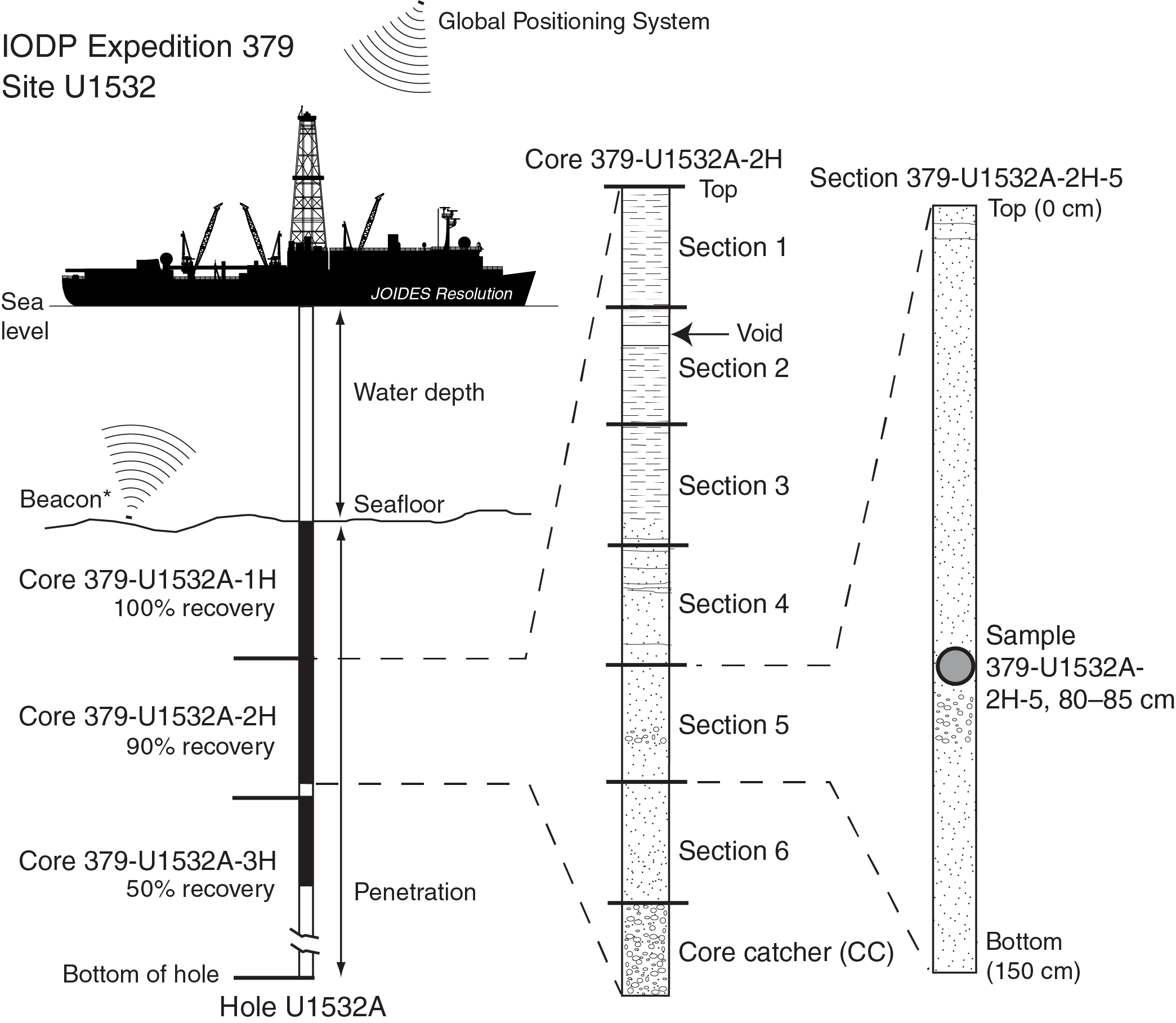
Figure F1. IODP naming convention.
Drilling operations
The advanced piston corer (APC), half-length APC (HLAPC), extended core barrel (XCB), and rotary core barrel (RCB) systems were available during Expedition 379 (Figures F2, F3, F4). These tools and other drilling technology are documented in Graber et al. (2002).
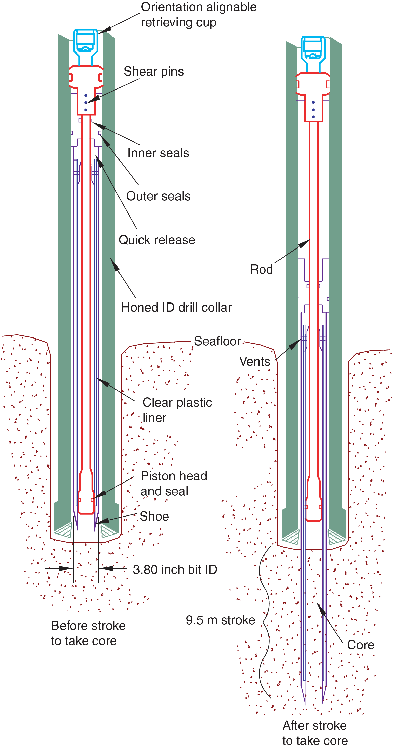
Figure F2. APC/HLAPC system.

Figure F3. XCB system.
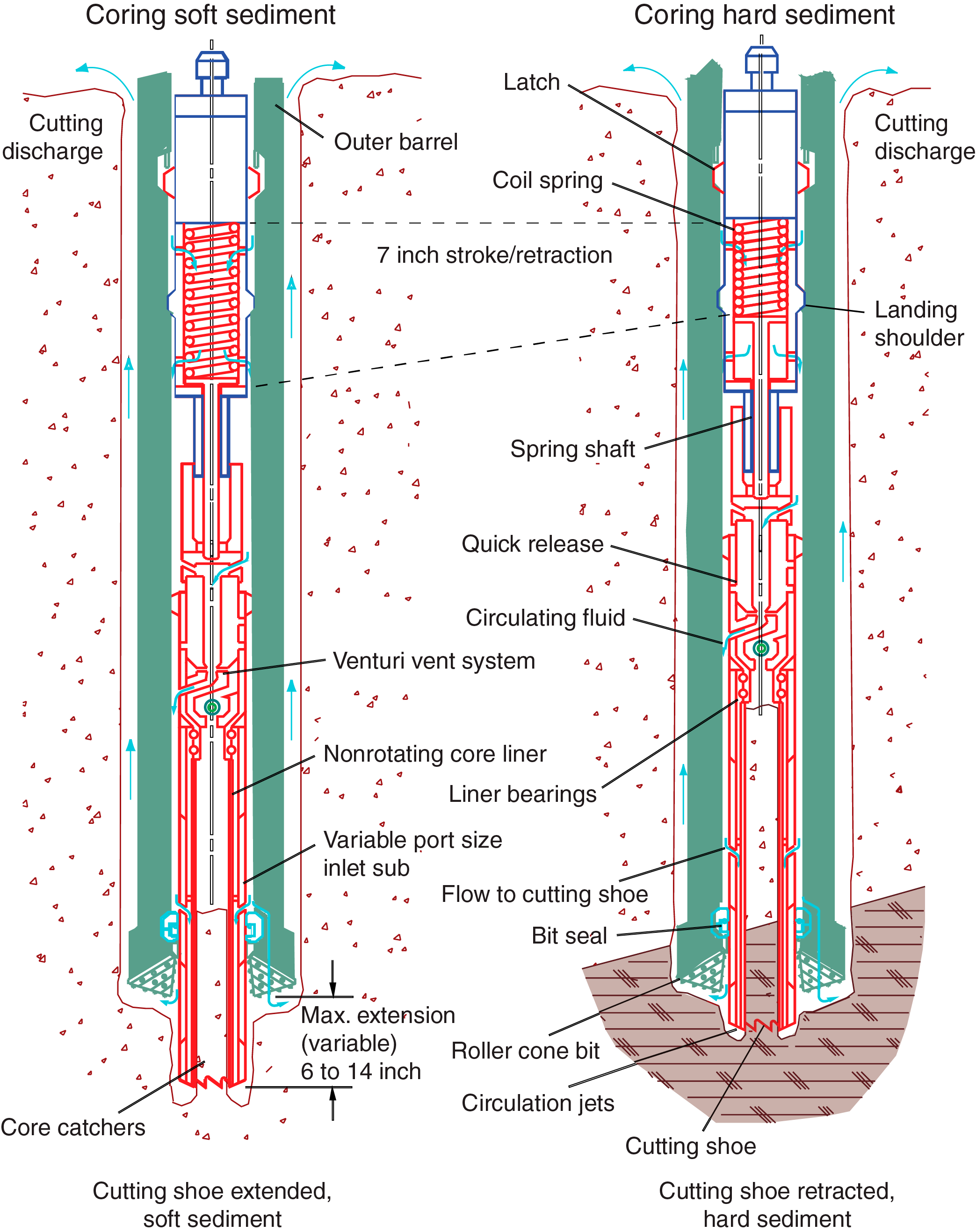
Figure F4. RCB system.
The APC and HLAPC systems cut soft-sediment cores with minimal coring disturbance relative to other IODP coring systems. After the APC/HLAPC core barrel is lowered through the drill pipe and lands above the bit, the drill pipe is pressured up until the two shear pins that hold the inner barrel attached to the outer barrel fail. The inner barrel then advances into the formation and cuts the core (Figure F2). The driller can detect a successful cut, or “full stroke,” by observing the pressure gauge on the rig floor because the excess pressure accumulated prior to the stroke drops rapidly.
APC refusal is conventionally defined in one of two ways: (1) the piston fails to achieve a complete stroke (as determined from the pump pressure and recovery reading) because the formation is too hard or (2) excessive force (>60,000 lb) is required to pull the core barrel out of the formation. For APC cores that do not achieve a full stroke, the next core can be taken after advancing to a depth determined by the recovery of the previous core (advance by recovery) or to the depth of a full APC core (typically 9.5 m). When a full stroke could not be achieved, one or more additional attempts were typically made, and each time the bit was advanced by the length of the core recovered (note that for these cores, this results in a nominal recovery of ~100%). When a full or partial stroke is achieved but excessive force is not able to retrieve the barrel, the core barrel can be “drilled over,” meaning that after the inner core barrel was successfully shot into the formation, the drill bit was advanced to total depth to free the APC barrel.
The standard APC system uses a 9.5 m long core barrel, whereas the HLAPC system uses a 4.7 m long core barrel. In most instances, the HLAPC was deployed after the standard APC had repeated partial strokes and the core liners were damaged. During use of the HLAPC system, the same criteria were applied in terms of refusal as for the APC system. Use of the HLAPC system allowed for significantly greater APC sampling depths to be attained than would have otherwise been possible.
The XCB system is typically used when the APC/HLAPC system has difficulty penetrating the formation and/or damages the core liner and/or core. The XCB system can also either be used to initiate holes where the seafloor is not suitable for APC coring or be interchanged with the APC/HLAPC system when dictated by changing formation conditions. The XCB system was used to advance the hole when HLAPC refusal occurred before the target depth was reached or when drilling conditions required it. The XCB is a rotary system with a small cutting shoe that extends below the large rotary APC/XCB bit (Figure F3). The smaller bit can cut a semi-indurated core with less torque and fluid circulation than the main bit, potentially improving recovery. The XCB cutting shoe typically extends ~30.5 cm ahead of the main bit in soft sediments, but a spring allows it to retract into the main bit when hard formations are encountered. Shorter XCB cutting shoes can also be used.
The bottom-hole assembly (BHA) used for APC and XCB coring is typically composed of an 11⁷⁄₁₆ inch (~29.05 cm) drill bit, a bit sub, a seal bore drill collar, a landing saver sub, a modified top sub, a modified head sub, 8¼ inch control length drill collars, a tapered drill collar, two stands of 5½ inch transition drill pipe, and a crossover sub to the drill pipe that extends to the surface. A different APC/XCB bit, a 9⅞ inch APC/XCB polycrystalline diamond compact (PDC) bit, was used at Site U1533 so that it could pass through 10¾ inch casing.
The RCB system is a rotary system designed to recover firm to hard sediments and basement rocks. The BHA, including the bit and outer core barrel, is rotated with the drill string while bearings allow the inner core barrel to remain stationary (Figure F4).
A typical RCB BHA includes a 9⅞ inch drill bit, a bit sub, an outer core barrel, a modified top sub, a modified head sub, a variable number of 8¼ inch control length drill collars, a tapered drill collar, two stands of 5½ inch drill pipe, and a crossover sub to the drill pipe that extends to the surface.
Nonmagnetic core barrels were used for all APC, HLAPC, and RCB coring. APC cores were oriented with the Icefield MI-5 core orientation tool when coring conditions allowed. Formation temperature measurements were taken with the advanced piston corer temperature tool (APCT-3; see Downhole formation temperature measurements). Information on recovered cores, drilled intervals, downhole tool deployments, and related information are provided in the Operations, Paleomagnetism, and Physical properties sections of each site chapter.
IODP depth conventions
The primary depth scales used during Expedition 379 are based on the length of the drill string deployed (e.g., drilling depth below rig floor [DRF] and drilling depth below seafloor [DSF]) or the length of core recovered (e.g., core depth below seafloor [CSF]) (see IODP Depth Scales Terminology at http://www.iodp.org/top-resources/program-documents/policies-and-guidelines). All units are in meters. The relationship between scales is defined either by protocol, such as the rules for computation of CSF from DSF, or by user-defined correlations, such as core-to-core or core-to-log correlation. The distinction in nomenclature should keep the reader aware that a nominal depth value in different depth scales usually does not refer to the exact same stratigraphic interval.
Depths of cored intervals are measured from the drill floor based on the length of drill pipe deployed beneath the rig floor (DRF scale). The depth of the cored interval is referenced to the seafloor (DSF scale) by subtracting the seafloor depth of the hole from the DRF depth of the interval. Standard depths of cores in meters below the seafloor (CSF, Method A [CSF-A] scale) are determined based on the assumption that the top depth of a recovered core corresponds to the top depth of its cored interval (at the DSF scale). Standard depths of samples and associated measurements (CSF-A scale) are calculated by adding the offset of the sample or measurement from the top of its section and the lengths of all higher sections in the core to the top depth of the core.
If a core has <100% recovery, for curation purposes all cored material is assumed to originate from the top of the cored interval as a continuous section. In addition, voids in the core are closed by pushing core segments together, if possible, during core handling. If the core pieces cannot be pushed together to get rid of the voids, then foam spacers are inserted and clearly labeled “void.” Therefore, the true depth interval within the cored interval is only partially constrained. This should be considered a sampling uncertainty in age-depth analysis or correlation of core data with downhole logging data.
When core recovery is >100% (i.e., the length of the recovered core exceeds that of the cored interval), the CSF-A depth of a sample or measurement taken from the bottom of a core will be deeper than that of a sample or measurement taken from the top of the subsequent core (i.e., the data associated with the two core intervals overlap at the CSF-A scale). This can happen when a soft to semisoft sediment core recovered from a few hundred meters below the seafloor expands upon recovery (typically by a few percent to as much as 15%). Therefore, a stratigraphic interval may not have the same nominal depth at the DSF and CSF scales in the same hole.
During Expedition 379, all core depths below seafloor were initially calculated according to the CSF-A depth scale. Unless otherwise noted, all depths presented are core depths below seafloor calculated as CSF-A and are reported as “m.”
Curatorial procedures and sample depth calculations
Numbering of sites, holes, cores, and samples followed standard IODP procedures (Figure F1). A full curatorial identifier for a sample consists of the following information: expedition, site, hole, core number, core type, section number, section half, piece number (hard rocks only), and interval in centimeters measured from the top of the core section. For example, a sample identification of “379-U1532A-2H-5W, 80–85 cm,” indicates a 5 cm sample removed from the interval between 80 and 85 cm below the top of Section 5 (working half) of Core 2 (“H” designates that this core was taken with the APC system) of Hole A at Site U1532 during Expedition 379 (Figure F1). The “U” preceding the hole number indicates the hole was drilled by the US IODP platform, JOIDES Resolution. The drilling system used to obtain a core is designated in the sample identifiers as follows: H = APC, F = HLAPC, R = RCB, and X = XCB. Integers are used to denote the “core” type of drilled intervals (e.g., a drilled interval between Cores 2H and 4H would be denoted by Core 31).
Core handling and analysis
The overall flow of cores, sections, analyses, and sampling implemented during Expedition 379 is shown in Figure F5.
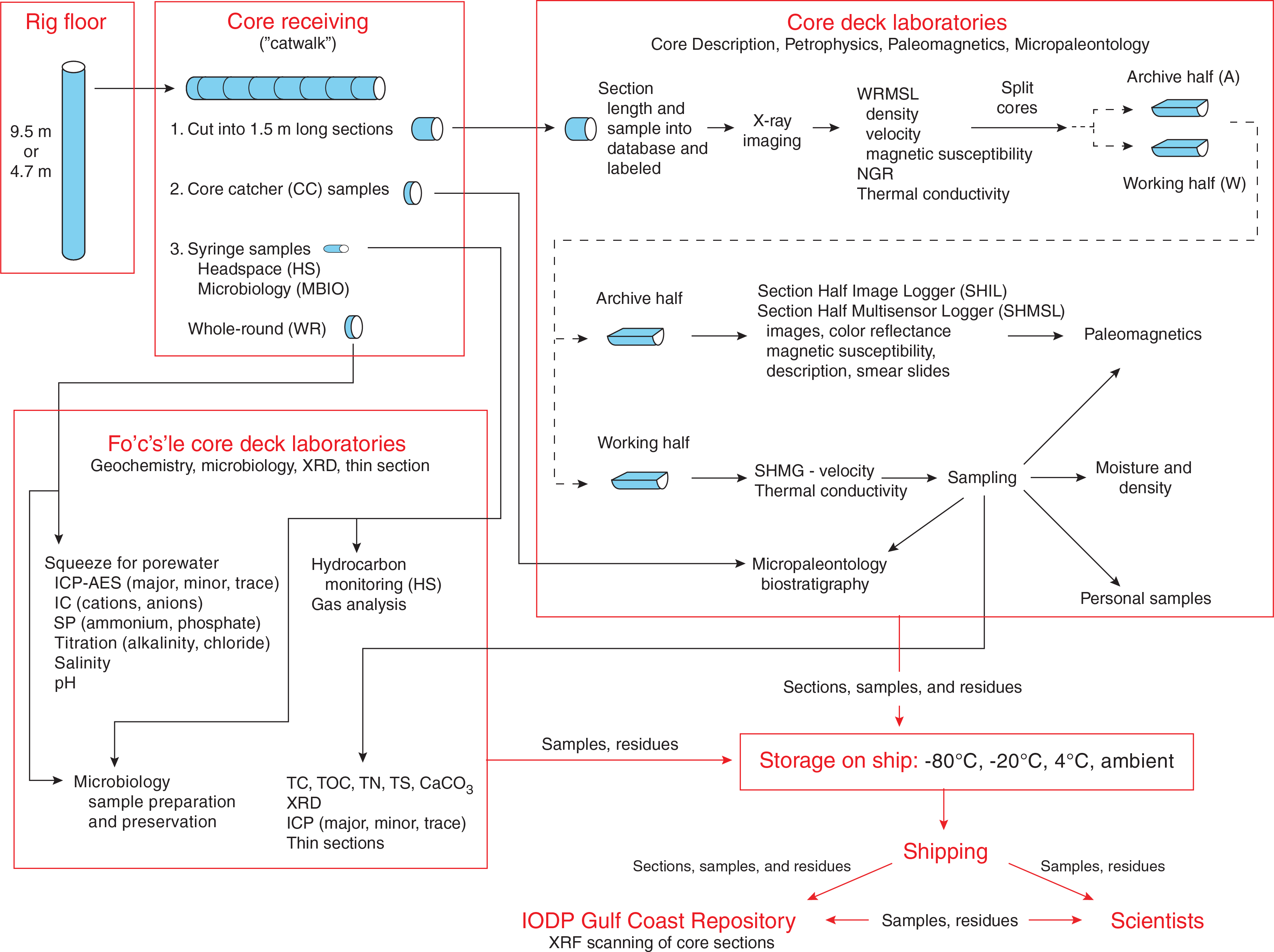
Figure F5. Core collection, sampling, and analyses.
When the core barrel reached the rig floor, the core catcher from the bottom of the core was removed and taken to the core-receiving platform (“catwalk”), and a sample was extracted for paleontological (PAL) analysis. Next, the sediment core was extracted from the core barrel in its plastic liner. The liner was carried from the rig floor to the core processing area on the catwalk outside the core laboratory, where it was split into ~1.5 m sections. Blue (uphole direction) and clear (downhole direction) liner caps were glued with acetone onto the cut liner sections. Laboratory gloves were worn by all core handlers.
Once the core was cut into sections, whole-round samples were taken for interstitial water (IW) chemical analyses. When a whole-round sample was removed, a yellow cap was used to indicate a whole-round sample had been taken. Syringe samples were taken for gas analyses according to the IODP hydrocarbon safety monitoring protocol. Syringe and whole-round samples were taken for microbiology contamination testing and postcruise analyses. Toothpick samples for smear slides were taken from some of the section ends for additional paleontological analysis.
The core sections were placed in a core rack in the laboratory. After the core information was entered into the database and the sections were labeled, X-ray imaging of all core sections was conducted. When the core sections reached equilibrium with laboratory temperature (typically after 4 h), they were run through the Whole-Round Multisensor Logger (WRMSL) for P-wave velocity (P-wave logger [PWL]), magnetic susceptibility (MS), and gamma ray attenuation (GRA) bulk density (see Physical properties). The core sections were also run through the Natural Gamma Radiation Logger (NGRL), and thermal conductivity measurements were taken once per core when the material was suitable.
Core sections were then split lengthwise from bottom to top into working and archive halves. Investigators should note that older material can be transported upward on the split face of each section during splitting. Sediment sections or intervals too indurated to be cut with wire, including hard rock clasts and concretions, were split with a diamond saw.
Discrete samples were then taken for moisture and density (MAD) and paleomagnetic (PMAG) analyses and for remaining shipboard analyses such as X-ray diffraction (XRD) and carbonate (CARB) from the working-half sections. Samples were not collected when the lithology was a high-priority interval for expedition or postcruise research, the core material was unsuitable, or the core was severely deformed. During the expedition, the only samples taken for personal postcruise research were those concerning ephemeral properties (e.g., IW, organic geochemistry, and microbiology) or for analyses required to plan for sensible postcruise sampling. Following shipboard sampling, oriented P-wave velocity measurements were performed using the Section Half Measurement Gantry (SHMG).
The archive half of each core was scanned on the Section Half Imaging Logger (SHIL) to provide line-scan images and then measured for point magnetic susceptibility (MSP) and reflectance spectroscopy and colorimetry on the Section Half Multisensor Logger (SHMSL). Labeled foam pieces were used to denote missing whole-round intervals in the SHIL images. The archive-half sections were then described visually and by means of smear slides for sedimentology. Occasionally, additional toothpick samples were extracted from key intervals for micropaleontologic smear slides from either the working or archive halves. Finally, the magnetization of archive-half sections and working-half discrete pieces was measured with the cryogenic magnetometer and spinner magnetometer. Certain critical intervals were approved for shipboard sampling for clast, geochemical, or paleontologic analysis from the working half.
When all steps were completed, cores were wrapped, sealed in plastic tubes, and transferred to cold storage space aboard the ship. At the end of the expedition, the cores were sent to the IODP Gulf Coast Repository (GCR; Texas A&M University, College Station, Texas, USA). After the cores arrived at the GCR, X-ray fluorescence (XRF) data were collected at the JOIDES Resolution Science Operator XRF facility. These data are included as part of the initial datasets along with other shipboard data. Later, samples for individual scientists' postcruise research were taken.
Drilling and handling core disturbance
Occasionally, cores may be significantly disturbed and contain extraneous material as a result of the coring and core handling process (Jutzeler et al., 2014). For example, in formations with loose sand layers, sand from intervals higher in the hole may be washed down by drilling circulation, accumulate at the bottom of the hole, and be sampled with the next core. The uppermost 10–50 cm of each core must therefore be critically examined during description for potential “fall-in.” Common coring-induced deformation includes the concave-downward appearance of originally horizontal bedding. Piston action can result in fluidization (“flow-in”) at the bottom of APC cores. Extending APC or HLAPC coring into deeper, firmer formation can also induce significant core deformation. The rotation of the drilling and coring hardware (drill string, bit, core barrel) during XCB and RCB coring can transfer rotary torque to the core, causing core pieces to rotate relative to each other as they enter the core barrel. The resulting deformation is called “biscuiting.” The seawater circulated during XCB and RCB coring combined with the rotational biscuiting of core pieces can also introduce fluids into the core and/or cause fluidization and remobilization of poorly consolidated/cemented sediments. This often creates short intervals of coherent core pieces that alternate with intervals of a completely fluidized sediment-fluid mix (slurry). Retrieval from depth to the surface can result in elastic rebound. Gas that is in solution at depth may become free and drive apart core segments in the liner. When gas content is high, pressure must be relieved for safety reasons before the cores are cut into segments. This is accomplished by drilling holes into the liner, which forces some sediment as well as gas out of the liner. These disturbances are described in each site chapter and graphically indicated on the visual core descriptions (VCDs).
Lithostratigraphy
Sediments and rocks recovered during Expedition 379 were described macroscopically from archive-half sections and microscopically from smear slides and thin sections. Observations were recorded in separate macroscopic and microscopic DESClogik templates (version x.16.1.0.19; see the DESClogik user guide at http://iodp.tamu.edu/labs/documentation). While the cores were equilibrating to room temperature prior to whole-core WRMSL and NGRL scanning, each whole-core section was X-rayed. These methods along with color spectrophotometry and MSP data are described in detail in Physical properties. Percent carbonate and percent organic matter (carbon-hydrogen-nitrogen-sulfur analyzer [CHNS]) measurements on shipboard sediment and sedimentary rock samples are described in Geochemistry and microbiology.
Core preparation
The technique used for splitting cores into working and archive halves (using either a piano wire or a saw and splitting from the bottom to the top; see Lithostratigraphy in the Site U1532 chapter and Lithostratigraphy in the Site U1533 chapter [Wellner et al., 2021a, 2021b] for the depth at which the change was made in each core) affects the appearance of the split-core surface. Prior to core description and high-resolution digital color imaging, the quality of the split-core surface of the archive half of each core was assessed, and the split-core surface was scraped lightly with a glass microscope slide or stainless steel plate to even the surface when necessary (e.g., the surface was irregular or smeared).
Section-half images
After cleaning the core surface, the archive half was imaged with the SHIL as soon as possible to avoid sediment color changes caused by oxidation and drying. In cases of watery or soupy sediment, the surface was dried sufficiently to avoid light reflection prior to scanning. The SHIL uses three pairs of Advanced Illumination high-current focused LED line lights to illuminate the features of the core. Each of the LED pairs has a color temperature of 6,500 K and emits 200,000 lux at 3 inches. Digital images were taken by a JAI line-scan camera at an interval of 10 lines/mm to create a high-resolution TIFF file. The camera height was set so that each pixel imaged a 0.1 mm2 section of the core surface; however, actual core width per pixel can vary because of slight differences in the section-half surface height. A high-resolution JPEG with grayscale and depth ruler and a low-resolution cropped JPEG showing only the core section surface were created from the high-resolution TIFF files.
Visual core description
Macroscopic descriptions of each section (nominally 0–150 cm long) were recorded on handwritten VCD forms generated from the SHIL (Figure F6). All handwritten sheets were digitally preserved as PDF files (see LITH in Supplementary material). Standard sedimentological observations of lithology, boundaries, primary and secondary (i.e., syn- and postsedimentary deformation) sedimentary structures (including bioturbation intensity), drilling disturbance, pebble abundance (number of grains with a long axis >4 mm per 10 cm core interval), and shipboard sample types and depths were recorded in individual columns. Shape and petrology characteristics of coarse pebbles (>2 cm) and macroscopic biogenic remains (i.e., shell fragments, shells, etc.) were recorded as comments. Color was also recorded for each interval, aided by Munsell soil color charts (Munsell Color Company, Inc., 2010).
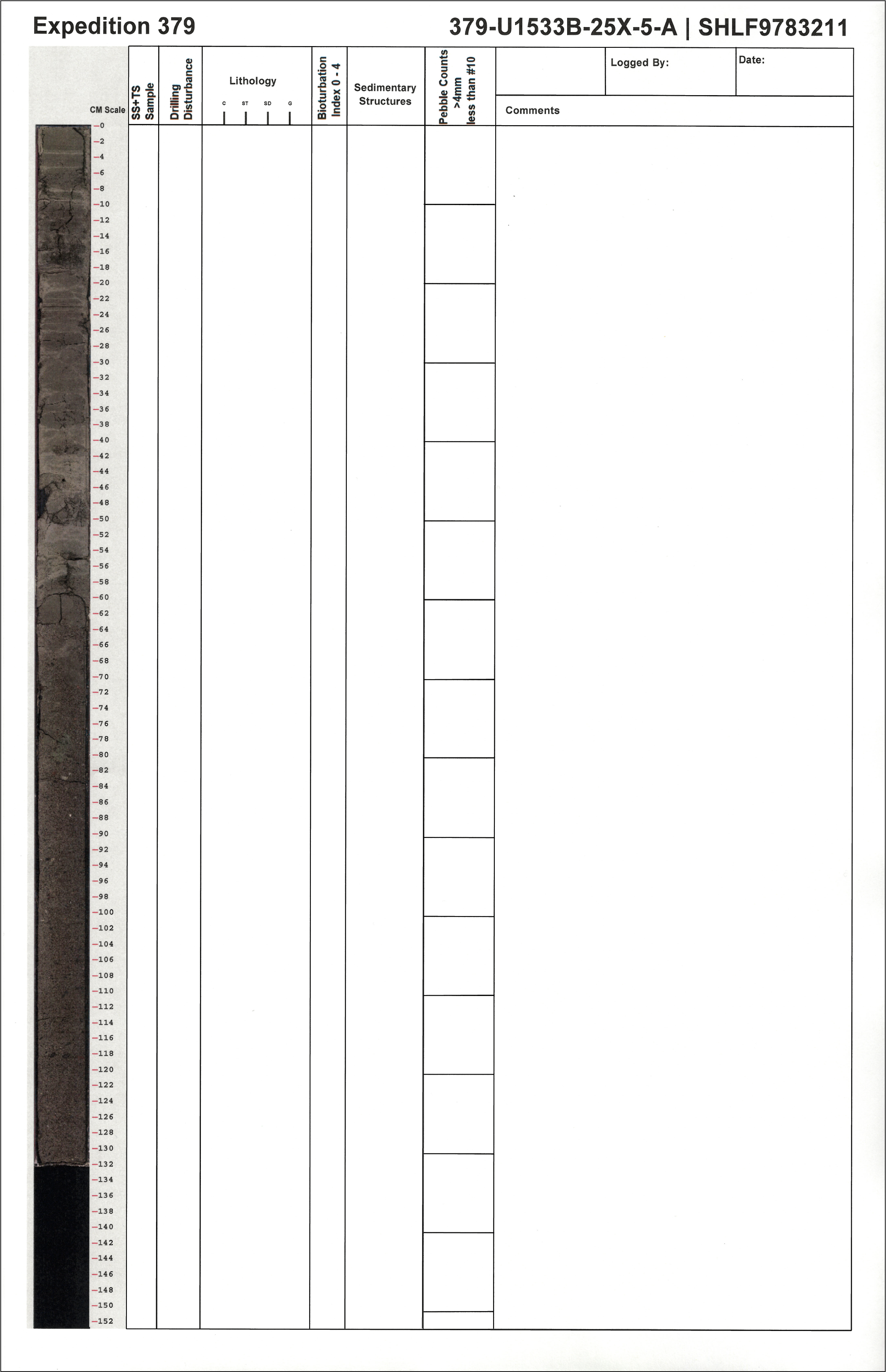
Figure F6. Handwritten VCD template.
DESClogik data capture software
Data from the handwritten core description sheets were compiled and entered into the IODP Laboratory Information Management System (LIMS) database using the DESClogik software. A macroscopic spreadsheet template with the following five tabs was constructed and customized for Expedition 379:
- Drilling disturbance (type and intensity),
- General (major lithology, degree of consolidation, color, bioturbation intensity, diagenetic constituents/composition, macroscopic biogenic material, etc.),
- Sedimentary structures,
- Clasts (number of pebbles >4 mm counted at 10 cm intervals and characteristics of coarse pebbles >2 cm), and
- Core summary (written description of major lithologic findings by core).
A microscopic template with two tabs to capture texture and relative abundance of biogenic/mineralogic components was configured and used to record smear slide and thin section data, respectively. Data entered into DESClogik were then uploaded to the LIMS database and used to produce VCD standard graphical reports.
Standard graphical report
A one-page VCD of each core was generated using the Strater software package (Golden Software) (Figure F7). Hole, core, and interval are included at the top of each VCD, along with a summary core description. VCDs display the core depth below seafloor (CSF-A; in meters), core length (in centimeters), sections, location of shipboard samples, and the SHIL digital color image to the left of the graphic lithology column. Columns to the right of graphic lithology include type and intensity of drilling disturbance, bioturbation intensity, biogenic material (Holes U1532A and U1532B only), diagenetic constituents (Holes U1532C–U1532G and U1533A–U1533D), sedimentary structures, type of lower boundary, pebble abundance (when appropriate for a given site), and physical property data (magnetic susceptibility and GRA bulk density collected by the WRMSL and NGR) (see Physical properties) (Figure F7). Graphic lithologies, sedimentary structures, and other visual observations shown on the VCDs by graphic patterns and symbols are explained in Figure F8.
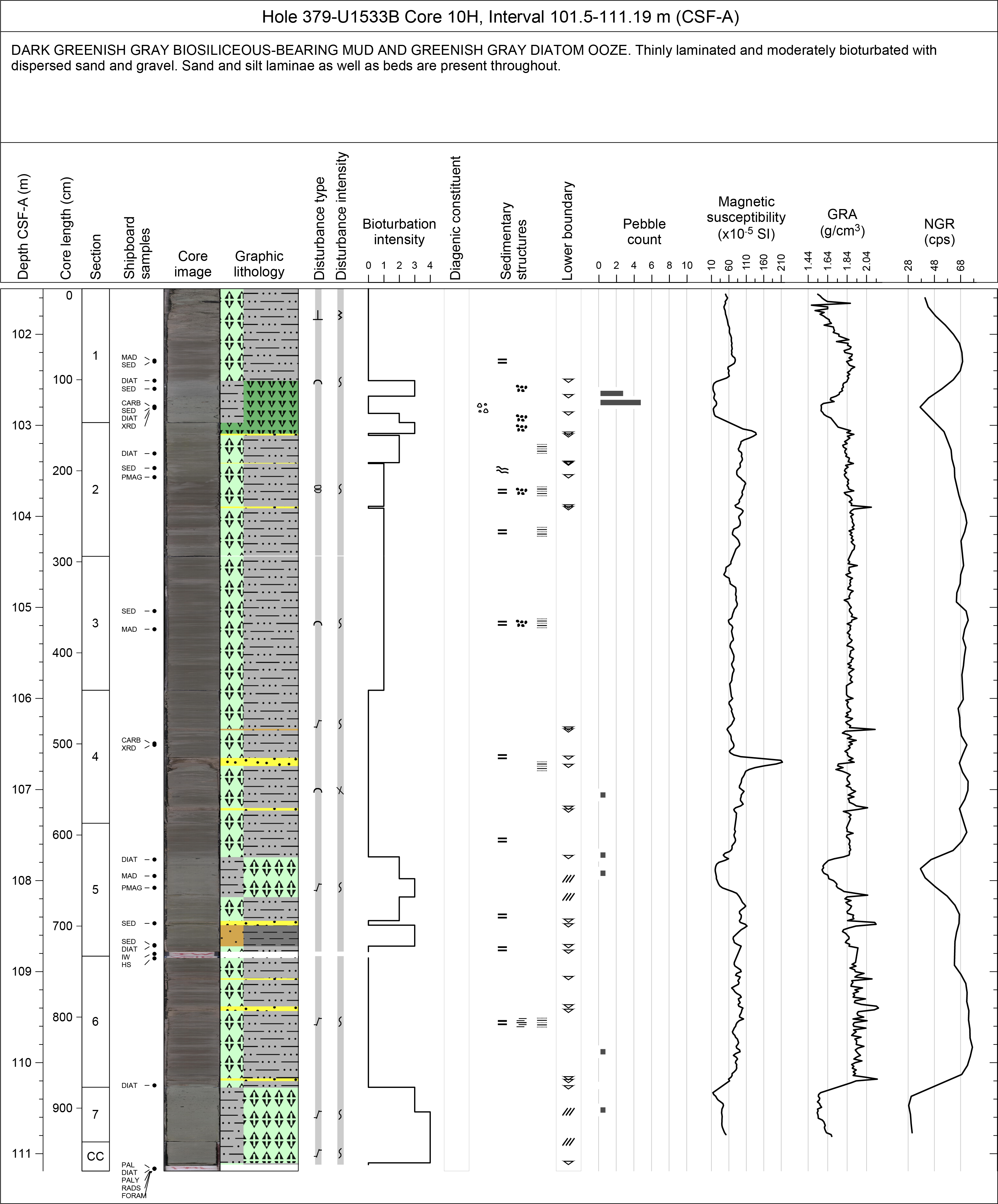
Figure F7. VCD.
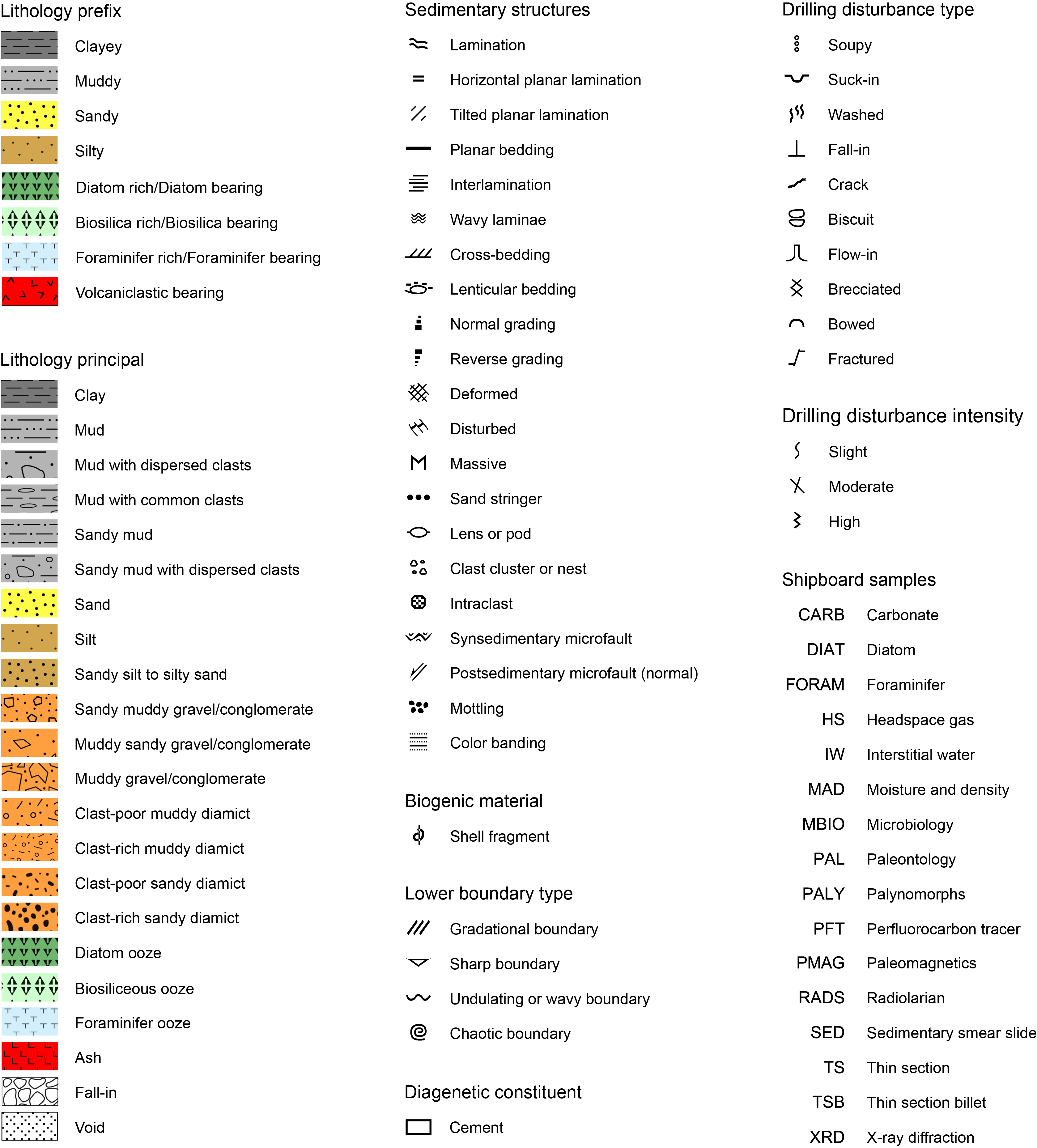
Figure F8. Symbols used for VCDs.
Lithologic classification scheme
Lithologic descriptions were based on the classification schemes used during Ocean Drilling Program (ODP) Leg 178 (Shipboard Scientific Party, 1999), the Cape Roberts Project (CRP; Hambrey et al., 1997), the Antarctic Drilling Project (ANDRILL; Naish et al., 2006), Integrated Ocean Drilling Program Expeditions 318 (Expedition 318 Scientists, 2011) and 341 (Jaeger et al., 2014), and IODP Expedition 374 (McKay et al., 2019).
Principal names and modifiers
The principal lithologic name was assigned based on the relative abundances of siliciclastic and biogenic grains (Figure F9). The principal name is purely descriptive and does not include interpretive classifications relating to fragmentation, transport, deposition, or alteration processes. Only the principal name for a nonconsolidated lithology was entered in DESClogik, and an entry in an additional column clarifies whether the sediment is consolidated or unconsolidated.
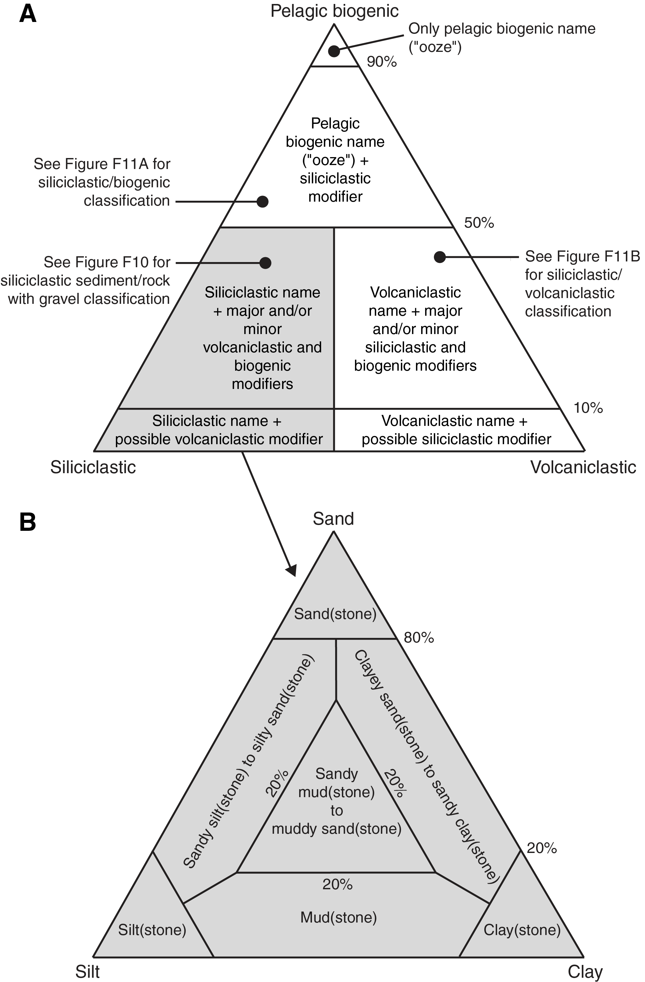
Figure F9. Classification scheme for siliciclastic sediment/rock without gravel.
The principal name of a sediment/rock with >50% siliciclastic grains is based on an estimate of the grain sizes present (Figure F9A). The Wentworth (1922) scale was used to define size classes of clay, silt, sand, and gravel. If no gravel was present, the principal sediment/rock name was determined based on the relative abundances of sand, silt, and clay (e.g., silt, sandy silt, silty sand, etc.; Naish et al., 2006, after Shepard, 1954, and Mazzullo et al., 1988) (Figure F9B). For example, if any one of these components exceeds 80%, then the lithology is defined by the primary grain size class (e.g., sand). The term “mud” is used to define sediments containing a mixture of silt and clay (these are difficult to separate using visual macroscopic inspection) in which neither component exceeds 80%. Sandy mud to muddy sand describes sediment composed of a mixture of at least 20% each of sand, silt, and clay (Figure F9B). For sediment consisting of two grain size fractions that each exceed 20% (e.g., clay and silt or sand and mud), the prefix was determined by the fraction with the lower percentage (Figure F9B).
If the sediment/rock contains siliciclastic gravel, then the principal name was determined from the relative abundance of gravel (>2 mm) and the sand/mud ratio of the clastic matrix, following the textural classifications of Moncrieff (1989) (Figure F10), and gravel percent was estimated using the comparison chart of Terry and Chilingar (1955). The term “diamict” is used as a nongenetic term for unsorted to poorly sorted terrigenous sediment that contains a wide range of particle sizes. Accordingly, a clast-poor muddy diamict includes 1%–5% gravel (>2 mm) and 25%–50% sand in matrix, whereas a clast-rich muddy diamict includes 5%–30% gravel and 25%–50% sand in matrix. A clast-poor sandy diamict has 1%–5% gravel and 50%–75% sand in matrix. For a clast-rich sandy diamict, gravel content is 5%–30%, sand content is 50%–75%, and the remainder is mud. The terms “gravel,” “conglomerate,” and “breccia” are used when the matrix includes >30% gravel. “Conglomerate” describes a sediment with dominantly rounded to well-rounded gravel grains, and “breccia” describes a sediment with dominantly angular to very-angular gravel grains (Figure F10).
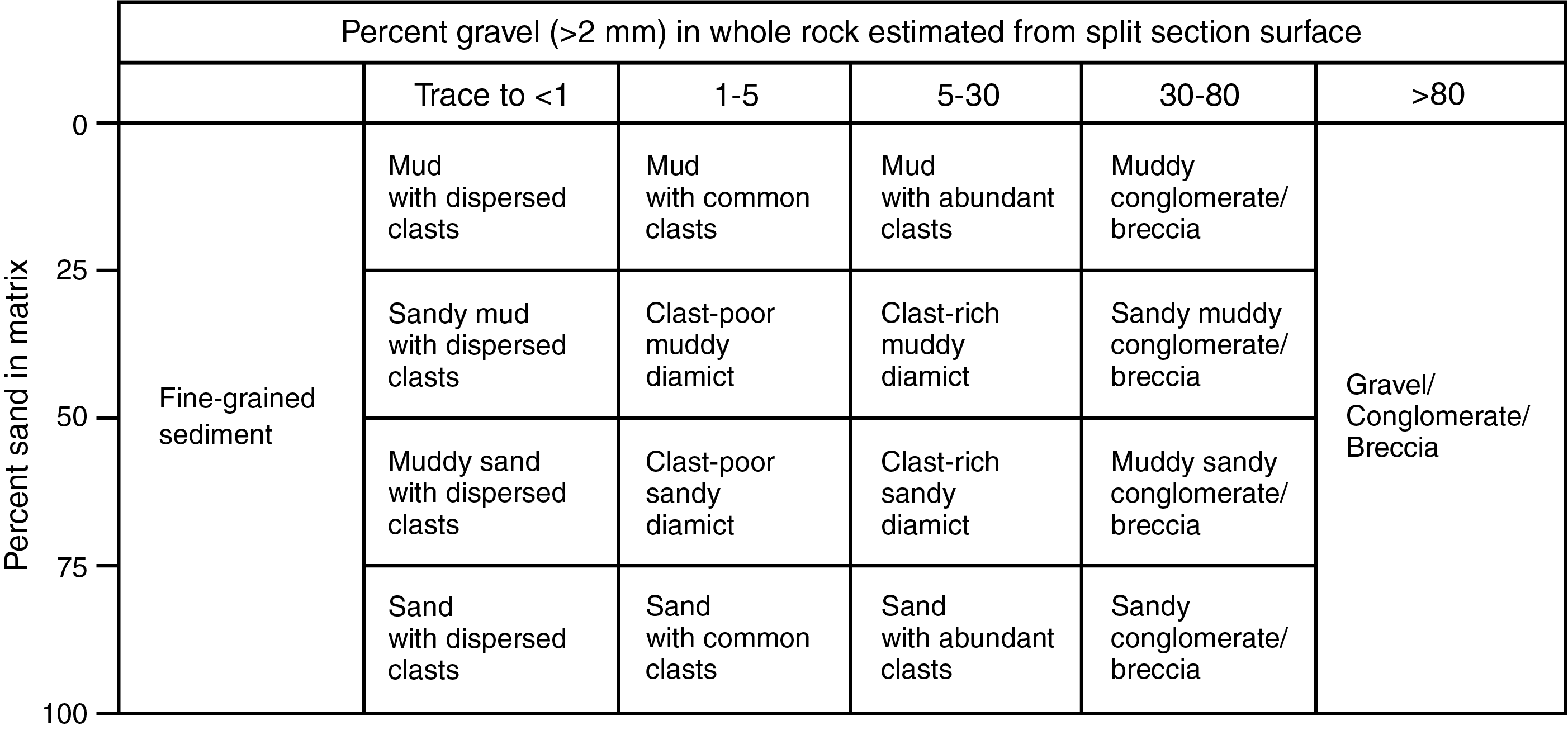
Figure F10. Classification scheme for siliciclastic sediment/rock with gravel.
The principal name of sediment with >50% biogenic grains is “ooze” modified by the most abundant specific biogenic grain type (Figure F11A). For example, if diatoms exceed 50%, then the sediment is called “diatom ooze.” However, if the sediment is composed of 40% diatoms and 15% sponge spicules, then the sediment is termed “biosiliceous ooze.” The same principle applies to calcareous microfossils. For example, if foraminifers exceed 50%, then the sediment is called “foraminifer ooze,” whereas a mixture of 40% foraminifers and 15% calcareous nannofossils is termed “calcareous ooze.” The lithologic name “chert” is used to describe biosiliceous rocks recovered from below the opal-CT transition, where the main biogenic component is not identifiable. The lithologic name “carbonate” is used for consolidated and nonconsolidated sediments consisting predominantly of calcareous material that do not allow identification of calcareous microfossils. Voids within a core section were captured under Principal lithology.

Figure F11. Classification scheme for mixed sediments.
For all lithologies, major and minor modifiers were applied to the principal sediment/rock names with the following modified scheme from Expedition 318 (Expedition 318 Scientists, 2011) (Figure F11A):
- Major biogenic modifiers are those components that comprise 25%–50% of the grains and are indicated by the suffix “-rich” (e.g., diatom-rich).
- Minor biogenic modifiers are those components with abundances of 10%–25% and are indicated by the suffix “-bearing” (e.g., diatom-bearing).
- Siliciclastic modifiers in biogenic oozes are those components with abundances of 10%–50% and are indicated by the suffix “-y” (e.g., silty, muddy, or sandy).
Modifiers for sediments containing mixtures of siliciclastic components and volcanic grains were determined according to Figure F11B.
For intervals in which two lithologies are interbedded or interlaminated (individual beds or laminated intervals are <15 cm thick and alternate between one lithology and another), the term “interbedded” or “interlaminated” is recorded in the General tab under Comments in the macroscopic DESClogik template and noted as a sedimentary structure in the Sedimentary structures tab. This terminology is for ease of data entry and graphic log display purposes for VCDs (Figures F7, F8). When beds are distributed throughout a different lithology (e.g., centimeter- to decimeter-thick sand beds within a mud bed), they are logged individually and the associated bed thickness and grain size ranges are described.
Lithostratigraphic units
At each site, units were assigned to highlight major lithologic changes downhole. Lithostratigraphic units were established based on prominent changes in principal lithology, sedimentary structures, biogenic components, or pebble counts. Units are numbered from the top of the stratigraphic succession using Roman numerals. When more subtle significant changes were observed, units were divided into subunits. Subunits are distinguished from the main lithostratigraphic units by adding a letter to the unit number (e.g., IA would indicate Subunit A of Unit I).
Sedimentary structures
The locations and types of sedimentary structures visible on the prepared surfaces of the archive halves were entered in the Sedimentary structures tab in the macroscopic DESClogik template. Basal boundaries between different lithologies are classified as sharp, gradational, inclined, contorted, undulating/wavy, or chaotic. The following bedding and lamination definitions are from Mazzullo et al. (1988):
- Thinly laminated (≤3 mm thick),
- Laminated (3 mm to 1 cm),
- Very thinly bedded (1–3 cm),
- Thinly bedded (3–10 cm),
- Medium bedded (10–30 cm),
- Thickly bedded (30–100 cm), and
- Very thickly bedded (>100 cm).
The presence of graded beds was also noted. “Normal grading” corresponds to layers with an upward decrease in grain size, whereas “reverse grading” corresponds to layers with an upward increase in grain size.
Deformation of the core identified as unrelated to drilling was also recorded in the Sedimentary structures tab of the macroscopic DESClogik template and the VCDs (Figures F7, F8), including both synsedimentary structures and postdepositional deformation features (e.g., microfaults). When it was possible to determine apparent motion sense for faults with certainty, direction of displacement (i.e., reverse or normal) was recorded; otherwise “fault (general)” was noted. Interval thickness was recorded from the uppermost to the lowermost extent of the described feature. It is also recorded in the comments column of the core description sheet.
Where sediments are diagenetically altered (e.g., mottling or staining or the presence of pyrite, concretions, or cement), the diagenetic constituent was entered in the Diagenetic constituent composition column of the General tab in the macroscopic DESClogik template. We define mottles (millimeter to centimeter scale) as spots or smears where material has a different color than the surrounding sediment.
Bioturbation
Ichnofabric description included the extent of bioturbation and notation of distinctive biogenic structures. To assess the degree of bioturbation semiquantitatively, the Droser and Bottjer (1986) ichnofabric index (0–4) modified by Savrda et al. (2001) was used (Figure F12):
- 0 = no apparent bioturbation (≤10%).
- 1 = slight bioturbation (>10%–30%).
- 2 = moderate bioturbation (>30%–60%).
- 3 = heavy bioturbation (>60%–90%).
- 4 = complete bioturbation (>90%).
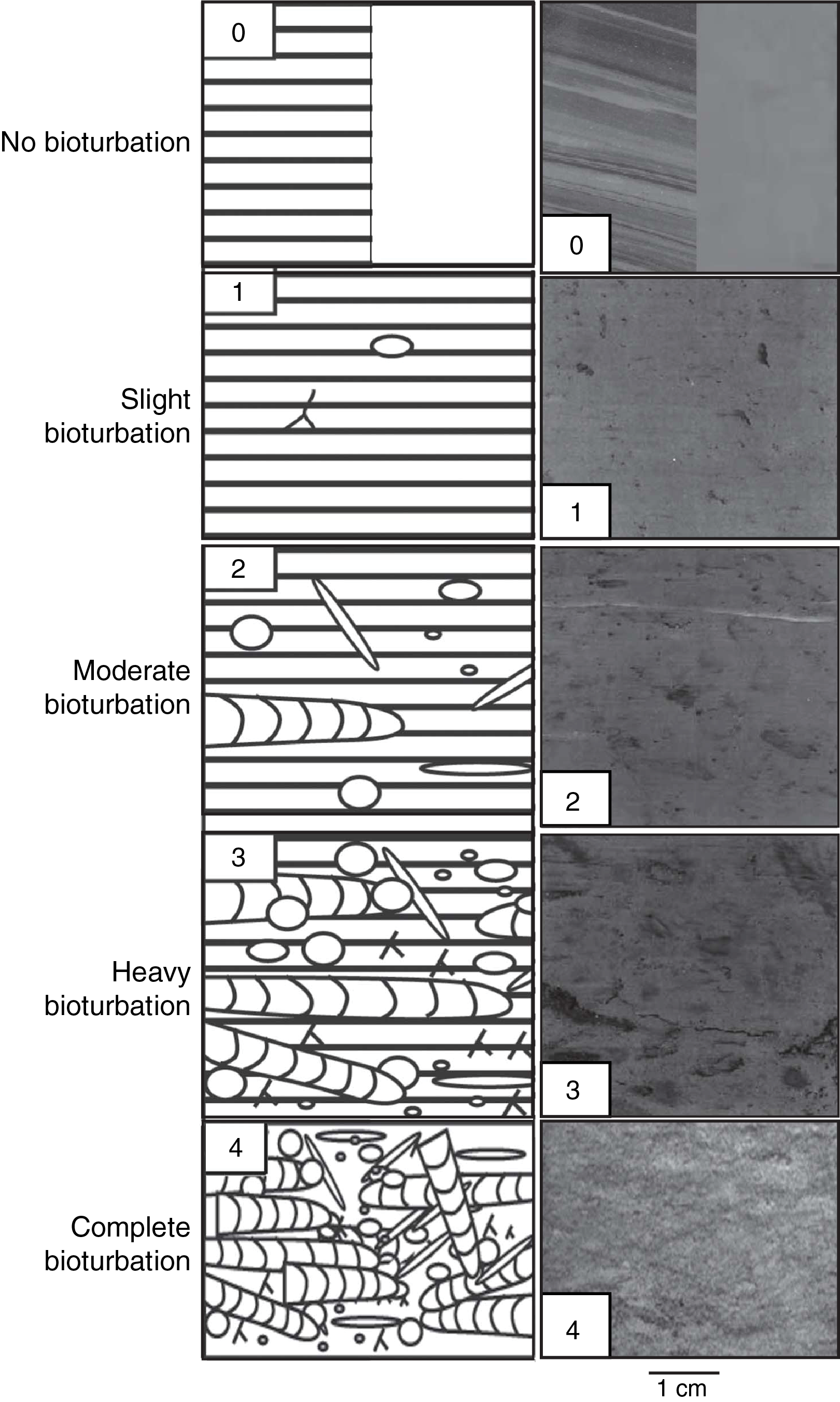
Figure F12. Ichnofabric index legend.
We note that massive muds may be deposited rapidly in glacial environments and record no evidence of bioturbation; they were assigned a value of 0. However, mud may also lack sedimentary structures because of complete bioturbation (e.g., 4 on the ichnofabric index), which may be accompanied by color mottling. This scenario is more likely for deepwater sites than for shallower continental shelf sites. The ichnofabric index was graphed using the numerical scale in the bioturbation column of the VCD. When identifiable, ichnofacies (Ekdale et al., 1984) were noted and logged in the General interval comment column of the General tab of the macroscopic DESClogik template.
Macroscopic biogenic components and diagenetic features
Paleontologic and diagenetic features other than those delineated above were entered in the corresponding columns of the General tab and depicted as symbols in the VCDs (Figures F7, F8). These features include macroscopic biogenic remains (e.g., shells, sponge spicules, etc.) and concretions. When possible, concretions were described by composition.
Pebble abundance and characteristics
Coarse gravel abundance was determined by counting the pebbles visible on the surface of the archive half. Where only holes or depressions caused by lithic or diamict clasts were observed, the working half was also examined to determine pebble abundance. Pebbles (4 mm–6 cm long axis diameter) were counted in 10 cm depth intervals. If between one and nine individual pebbles were counted per 10 cm depth interval, the number of pebbles per interval was entered into DESClogik under the Clasts tab. If 10 or more pebbles were present in a 10 cm interval, the number 10 was entered into DESClogik. Details on lithology, size, shape, and rounding of pebbles with a long axis >2 cm were provided in the core description sheets and the Coarse pebbles (>2 cm) comment column under the Clasts tab.
The coarse components of prominent clast-rich intervals in core sections were closely examined to obtain sedimentary provenance information. For coarse silt to pebble sized grains, the mineral/rock types were determined from direct observation of individual grains using a hand lens and binocular microscope. Grain/pebble types were identified according to mineral and rock type, and the abundances by type were determined by counting grains for selected representative core intervals. Counts were made from cut faces of the archive halves and/or washed, sieved material from core catcher sections that were prepared for micropaleontology. In general, the grain size range of these residues is 0.25 to 2.0 mm. When available, material from “ghost” cores and material removed (scraped) from slightly disturbed surfaces of split cores were used. The mineral/rock type counts were converted to percent and reported in table form and/or ternary plots.
Drilling disturbance
Core disturbance from the drilling process may alter the cores slightly (e.g., bent/bowed bedding contacts) or greatly (e.g., complete disruption of the stratigraphic sequence) (see Jutzeler et al., 2014, for examples). The style of drilling disturbance is described using the following terms:
- Fall-in: out-of-place material at the top of a core has fallen downhole onto the cored surface.
- Bowed: bedding contacts are slightly to moderately deformed but still subhorizontal and continuous.
- Flowage: severe soft-sediment stretching and/or compressional shearing attributed to coring/drilling. The particular type of deformation may also be noted (e.g., flow-in).
- Soupy: intervals that are water saturated and have lost all aspects of original bedding.
- Gas expansion: a part of the core is partitioned into pieces and voids due to expansion of interstitial gas. The particular type of deformation may also be noted (e.g., mousse-like).
- Biscuited: sediments of intermediate stiffness show vertical variations in the degree of disturbance. Softer intervals are washed and/or soupy, whereas firmer intervals are relatively undisturbed.
- Fractured: firm sediments are broken but not displaced or significantly rotated (including cracks).
- Fragmented: firm sediments are broken into pieces and rotated, and their stratigraphic position may not be preserved.
- Brecciated: firm sediments are pervasively broken into small and angular pieces with original orientation and stratigraphic position lost and are often completely mixed with drilling slurry.
- Washed gravel: fine material was probably lost during drilling, and only washed coarse material, commonly gravels or pebbles, remains. Washed gravel often results when coring unsorted or poorly sorted, unconsolidated sediments with considerable coarse-grained content (e.g., diamict).
- None: No obvious drilling disturbance is observed.
The intensity of drilling disturbance was also described in the Drilling disturbance tab of DESClogik and displayed graphically on the VCDs. Intensity of drilling disturbance of unconsolidated and consolidated sediments was classified into the three categories: slight, moderate, and high.
In unconsolidated sediments, the three categories imply the following:
- Slightly disturbed: bedding contacts are slightly bent or bowed in an upward-arching appearance.
- Moderately disturbed: bedding contacts are bent or bowed in an upward-arching appearance but are still visible.
- Highly disturbed: bedding is completely deformed and may show diapiric or flow structures.
In harder sediments (i.e., consolidated by compaction or cementation), the three categories stand for
- Slightly fractured: core pieces are in place and have very little drilling slurry or brecciation.
- Moderately fractured or biscuited: core pieces are from the cored interval and are probably in correct stratigraphic sequence (although the entire section may not be represented). Intact core pieces are broken into rotated discs (or “biscuits”) as a result of the drilling process, and drilling mud has possibly flowed in.
- Highly fractured or brecciated: pieces are from the cored interval but may not occur in correct stratigraphic sequence within the core.
In addition to drilling-related artifacts, disturbance also occurred during core handling. If a core liner shattered during coring, the pieces were brought onto the catwalk and transferred to a new core liner for curation. This process may result in pieces of core that are out of stratigraphic order or inverted relative to their original position. These cores should be considered highly disturbed. Additionally, the split-core surface of lithologies with relatively high porosity was occasionally disturbed after core description and imaging were completed because of excess pressure applied by the MSP instrument.
Microscopic descriptions
Smear slides
To aid in lithologic classification, the size, composition, and abundance of sediment constituents were estimated microscopically using smear slides (Figure F13). Toothpick samples were taken mostly from the primary lithologies at a frequency of at least one sample per section. For each smear slide, a small amount of sediment was removed from the archive half using a wooden toothpick and put on a 22 mm × 30 mm coverglass. A drop of deionized water was added, and the sediment was homogenized and evenly spread across the coverglass. The dispersed sample was dried on a hot plate at a moderate setting (150°C). A couple of drops of Norland optical adhesive Number 61 was added to a glass microscope slide that was then carefully placed on the dried sample to prevent air bubbles from being trapped in the adhesive. The smear slide was then placed in an ultraviolet light box for 15 min to cure the adhesive.
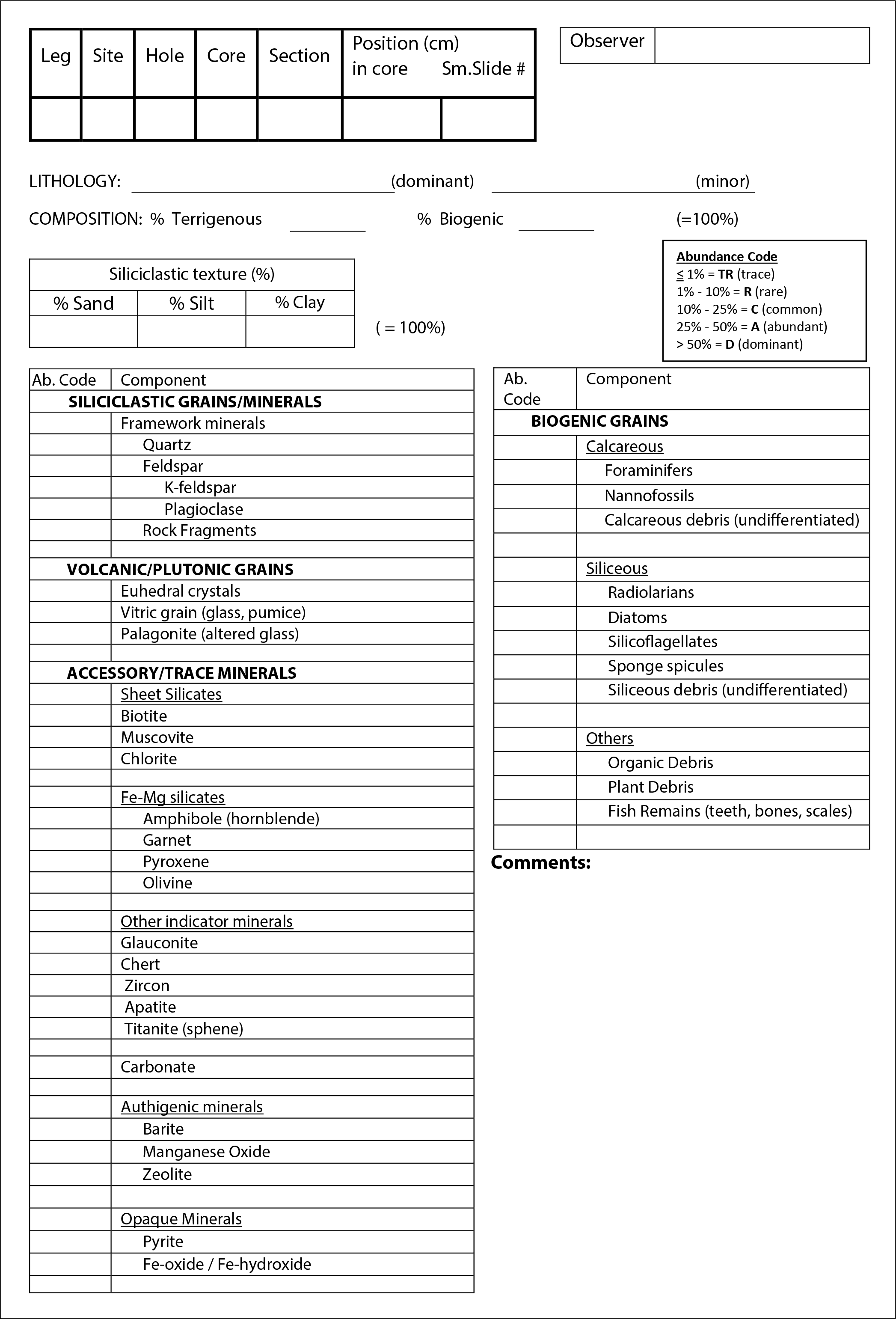
Figure F13. Example smear slide description worksheet.
Smear slides were examined with a transmitted-light petrographic microscope equipped with a standard eyepiece micrometer. Biogenic and mineral components were identified following standard petrographic techniques as stated in Rothwell (1989) and Marsaglia et al. (2013, 2015). Several fields of view were examined at 100×, 200×, 400×, and 500× to assess the abundance of detrital, biogenic, and authigenic components. The relative abundance percentages of the sedimentary constituents were visually estimated using the techniques of Rothwell (1989). The texture of siliciclastic lithologies (e.g., relative abundance of sand-, silt-, and clay-sized grains) and the proportions and presence of biogenic and mineral components were recorded in the smear slide worksheet of the microscopic DESClogik template.
Components observed in smear slides were categorized as follows:
- TR = trace (≤1%).
- R = rare (>1%–10%).
- C = common (>10%–25%).
- A = abundant (>25%–50%).
- D = dominant (>50%).
Smear slides provide only a rough estimate of the relative abundance of sediment constituents. Occasionally, the lithologic name assigned based on smear slide observation does not match the name in the macroscopic lithology description because a small sample may not represent the macroscopic description of a much larger sediment interval. Additionally, very fine and coarse grains are difficult to observe in smear slides, and their relative proportions in the sediment can be affected during slide preparation. Therefore, intervals dominated by sand and larger sized constituents were examined by macroscopic comparison to grain size reference charts. Photomicrographs of some smear slides were taken and uploaded to the LIMS database.
Sample residues obtained from shipboard paleontologists (PAL samples) were also analyzed. Samples were wet-sieved at 45 and 150 µm (see Biostratigraphy) and dried. Biogenic components (radiolarians and foraminifers) were removed, and the sieve residues were systematically analyzed.
Thin sections
Descriptions of both consolidated and unconsolidated sediments were complemented by shipboard thin section analyses. Standard thin section billets (20 mm × 15 mm) were cut or sawed from selected intervals or features as needed from core section intervals that were either undisturbed or slightly disturbed by drilling. Samples were initially sprayed with isopropyl and left to dry for 10 min before being placed in Epo Tek 301 epoxy for 12 h under vacuum. Samples were then placed in molds before being sanded to obtain a flat, smooth surface that was adhered to a glass slide with epoxy. Next, samples were first cut and then ground down to ~150 µm thickness. Coverslips were placed on thin sections using Immersol immersion oil, and initial analysis including collection of thin section images and photomicrographs was completed. This process was repeated for selected thin sections that were further ground down to ~80 µm thickness and to ~30 µm thickness where possible. The process of photographing and examining the thin section at different thicknesses was essential to preserve sedimentary structures in unlithified sediments that could be easily destroyed before reaching the desired sample thickness of 30 µm. Particularly for unconsolidated sediments, it was not always possible to get samples <100 µm thick. Thin sections were examined with a transmitted-light petrographic microscope equipped with a standard eyepiece micrometer. Data were entered into the Thin section tab of the DESClogik microscopic template.
Spectrophotometry and colorimetry
The SHMSL employs multiple sensors to measure bulk physical properties in a motorized and computer-controlled section-half logging instrument. The sensors included in the SHMSL are a spectrophotometer, an MSP sensor, and a laser surface analyzer. The resolution used for the SHMSL during Expedition 379 was 2 cm. Both the MSP sensor and the spectrophotometer require flush contact with the split-core surface, so the archive halves were covered with clear plastic wrap prior to measurement. A built-in laser surface analyzer aids in the recognition of irregularities in the split-core surface (e.g., cracks and voids), and data from this tool were recorded to provide an independent check on SHMSL measurement fidelity. Magnetic susceptibility was measured with a Bartington Instruments MS2 meter and a MS2K contact probe. Instrument details are given in Physical properties. Reflectance spectroscopy (spectrophotometry) was carried out using an Ocean Optics QE Pro detector that measures the reflectance spectra of the split core from the ultraviolet to near-infrared range. Each measurement was recorded in 2 nm spectral bands from 390 to 732 nm. The data were converted to the L*a*b* color space system, which expresses color as a function of lightness (L*; grayscale) and color values a* and b*, where a* reflects the balance between red (positive a*) and green (negative a*) and b* reflects the balance between yellow (positive b*) and blue (negative b*).
X-ray fluorescence analysis
An Olympus Vanta M series handheld portable X-ray fluorescence spectrometer (pXRF) was used to measure elemental composition on selected intervals of split-core sections from Site U1532 and the residual “cakes” resulting from IW measurements for Site U1533. Measurements were performed with a 10–50 kV (10–50 µA) Rh X-ray tube and a high–count rate detector with a count time of 60 s. The instrument data correction packages solve a series of nonlinear equations for each analyzed element. The “Geochem” mode was used to examine the relative abundance of major and trace elements. pXRF measurements of standards were performed once per day to track instrument drift, but standardization using synthetic or natural standards (e.g., Lemière, 2018) was not performed. In some instances, other analyses such as XRD were coordinated with the pXRF measurements. The pXRF measurements were acquired as an aid to core description using pXRF measurement methods suitable for each interval of interest. Observational criteria such as lithologic variability, presence of cement, or color banding aided the identification of intervals of interest. At Site U1532, major and trace elements for selected intervals were measured on the archive halves with the analyst holding the Vanta XRF “gun” vertically with the detector pointed downward (McKay et al., 2019). Two transects were conducted to compare compositional variations between adjacent lithofacies; these entailed single pXRF point measurements systematically spaced at 10 cm intervals. The pXRF analysis served to acquaint shipboard scientists with instrument use, data acquisition, and data quality, a process that led to the development of the pXRF approach used at Site U1533.
At Site U1533, the Vanta XRF gun was placed securely in a table mount with the measurement beam directed upward into a lead-shielded box where homogenized samples of 60 to 100 cm3 were placed. The sample material consisted of the mostly clayey cake residues that remained after the extraction of IW for shipboard geochemical analyses. The measurements were performed at three different points on the flat surface of the IW cake, the results were averaged, and error was determined to be 1σ.
Compared to in situ measurements on the archive halves, the use of high-pressed IW cakes for pXRF analysis presents the following advantages:
- The effect of light element (LE; elements having atomic mass lighter than sodium [Na]) variability, arising from volatile phases (including H2O), on major and trace element abundances is minimized.
- The IW cake material is more texturally homogeneous than stratified sediment that may have a shape-preferred orientation of minerals that affects the pXRF results.
- Multiple points on the same IW cake can be collected quickly by slight repositioning of the samples within the stationary measurement chamber.
- The pXRF gun maintains an extremely stable position in its mount throughout data acquisition, and the surfaces of IW cakes are smooth, resulting in a consistent distance between sample and X-ray source for all measurements.
Although fine-scale lithologic information was lost for the IW cake material, it still could be recovered in part from the X-radiographs taken of the core sections before the IW whole-round sample was selected.
The qualitative pXRF geochemical information, systematically obtained at low spatial resolution to the full depth of continuous core recovery, reveals trends and associations corresponding to bulk sediment chemical variations.
XRD analysis
XRD analysis was carried out on clay separates (<2 µm fraction). On average, one sample (~5 cm3) per core was taken from the working halves for XRD analysis. The samples, chosen to characterize different lithologic intervals and facies, were selected based on visual core observations (e.g., color variability, visual changes in lithology, texture, etc.) and smear slide investigations.
The sample was placed in 10% acetic acid for at least 1 h on an agitator to remove carbonate and then centrifuged for 15 min at 1500 rpm. The acid was decanted, and 25 mL of nanopure water was added to wash out remaining acid and salt before the sample was centrifuged for 15 min at 1500 rpm. This procedure was repeated two more times. The clay plug resulting from the centrifugation was placed in 25 mL of 1% borax solution and disaggregated for 1 min 5 s. Afterward, the sample was centrifuged for 4 min at 750 rpm to remove the >2 µm fraction, and the suspended liquid was decanted into a separate centrifuge tube. The remaining clay fraction was treated again with 25 mL of 1% borax solution, disaggregated once more to separate out any remaining <2 µm clay fraction, and centrifuged again for 4 min at 750 rpm. The suspended fraction was decanted and added to the first <2 µm clay separate. The entire <2 µm fraction was then centrifuged for 15 min at 1500 rpm to remove the borax solution. The borax was decanted and replaced with 25 mL of nanopure water. The sample was then centrifuged for 60 min at 3000 rpm, and the liquid was decanted. Thereafter, each sample was loaded with a pipette onto a zero-background silica disk using isopropyl alcohol. This method was applied to all APC core samples. Samples taken from XCB and RCB cores were freeze-dried for 12 h and placed into 10% acetic acid. The samples were then sonicated for 2 h before being agitated overnight. The preparation then followed the method described above, starting with the first wash step in 25 mL of nanopure water.
After the borax decanting step, 1 mL of 0.4% molybdenite (MoS2) solution was added to all samples from Site U1532 that were taken above Core 379-U1532G-37R. The MoS2 solution was added in an attempt to use the MoS2 peak at 6.15 Å as an internal standard for aligning diffractograms and calculating peak area and height ratios between the MoS2 standard and individual clay minerals. However, the MoS2 solution was not added to samples taken from Cores 37R–47R and from all cores recovered at Site U1533 because the MoS2 peak heights and areas showed considerable variability in the diffractograms of samples spiked in this way. The diffractograms of samples from Cores 37R–47R and from all cores from Site U1533 were aligned using the 3.34 Å peak of quartz.
Following methods described by Moore and Reynolds (1989), a small number of subsamples from Sites U1532 and U1533 were chosen for testing the presence of the clay minerals chlorite and kaolinite, whose peaks overlap in diffractograms. The samples were chosen based on the presence of only a single 3.5 Å peak in diffractograms (in contrast, a characteristic kaolinite-chlorite double peak was observed at 3.5 Å in the high-resolution diffractometer scans of most other samples) and underwent additional treatment.
To test a sample for the (sole) presence of chlorite, an aliquot was placed on a hot plate in 20 mL of 1 N HCl at 300°C; this sample was kept at a boil for 2 h. Additional HCl was added as needed to keep the sample saturated, and a stir bar was used at 60 rpm to keep the sample in solution. Afterward, the sample was washed three times with nanopure water before it was loaded for XRD analysis. If no peak or only a reduced peak at 3.5 Å could be observed afterward, it proved the presence of chlorite in the untreated sample. To test a sample for the presence of kaolinite, the same or another aliquot was placed in a furnace and heated at a controlled rate (1.5°C increase per minute) to 550°C and maintained at this temperature for 1 h before allowing it to cool to room temperature and loading it for XRD analysis. If the residual 3.5 Å peak in the HCl-treated sample vanished or if a reduced and shifted peak in the heated-only sample was observed, it proved the presence of kaolinite in the original sample.
Samples were analyzed on a Bruker D4 Endeavor diffractometer with a Vantec-1 detector using nickel-filtered CuKα radiation (voltage = 40 kV, current = 40 mA, and divergence slit = 0.3 mm). Prior to measuring all samples, a corundum standard was scanned from 20° to 130°2θ. Three separate goniometer scans were performed on each sample. The first scan was performed on air-dried samples from 3.5° to 15.5°2θ at a step size of 0.01658092° per second. The second and third scans were performed after the sample was placed in an ethylene glycol atmosphere for 12 h at 65°C. The second scan was run from 3.5° to 40°2θ at a step size of 0.01658092° per second to measure the main peaks of the major clay mineral groups smectite, illite, chlorite, and kaolinite. The third scan from 24.5° to 26.0°2θ at a step size of 0.00829451° per second was run to resolve the 3.54 Å peak of kaolinite and the 3.58 Å peak of chlorite. At the beginning of the expedition, the third scan was conducted from 24.5° to 26.5°2θ, but it was then realized that a narrower range was sufficient to resolve the kaolinite-chlorite double peak at 3.5 Å, and subsequent goniometer scans were limited to 24.5° to 26.0°2θ. Sample aliquots that had been heated to 550°C or treated with HCl were scanned two additional times. The first scan was performed from 3.5° to 40°2θ at a step size of 0.01658092° per second, and the second scan was run from 12.5° to 26.0°2θ at a step size of 0.01658092° per second and from 24.5° to 26.0°2θ at a step size of 0.00829451° per second.
The diffractograms of the samples were evaluated with the Bruker DIFFRAC.EVA software package (version 4.2.1). The DIFFRAC.EVA manual available on board (and also the manual emailed to the ship by the manufacturer on request during the expedition) was actually for v. 3.0, which has a different user interface. As a consequence, some essential functions in DIFFRAC.EVA, such as baseline correction and peak subtraction, could only be applied insufficiently to the diffractograms. Therefore, clay mineral percentages presented in the site reports (see Lithostratigraphy in the Site U1532 chapter and Lithostratigraphy in the Site U1533 chapter [Wellner et al., 2021a, 2021b]) are preliminary results.
Relative abundances of the major clay mineral groups were established on the basis of quantifying integrated peak areas and maximum peak intensities, preferentially from the analysis of the ethylene glycol–solvated samples. Contents of the clay mineral groups smectite, illite, chlorite, and kaolinite (in percent) were determined semiquantitatively following the methods described in Petschick et al. (1996) using empirically estimated weighting factors (Biscaye, 1964, 1965; Brindley and Brown, 1980). In addition, illite chemistry was evaluated by calculating its 5/10 Å peak intensity ratio (Esquevin, 1969).
X-ray imaging
All of the whole-round cores and a few archive halves were X-rayed for a preliminary assessment of core quality/drilling disturbance, sedimentary structures, and clast occurrence. Specific core sections were also X-rayed to identify depths for taking IW samples without destroying any key sediment intervals. The IODP X-ray system is composed of a 120 kV, 1 mA constant potential X-ray source and a detector unit. The X-ray source is a Teledyne ICM CP120B portable X-ray generator with a 0.8 mm × 0.5 mm focal spot. The beam angle is 50° × 50° and generates a directional cone onto the detector, which is 65 cm from the source. The detector is a Go-Scan 1510 H unit composed of an array of CMOS sensors with an active area of 102 mm × 153 mm and a resolution of 99 μm.
Each of the core sections passed through the imaging area at 12 cm increments with the working-half base facing upward, projecting ~15 cm of core length onto the detector and providing a 3 cm overlap between individual images. The ideal parameters used during Expedition 379 were as follows:
The X-radiograph raw images from Holes U1532A–U1532D were collected using Teledyne Go-Scan Sherlock software as 14 bit and then saved as 16-bit TIFF images, resulting in dark raw images prior to image corrections. The X-radiograph raw images from Hole U1532G and Holes U1533A–U1533D were collected as 16-bit images using the Integrated Measurement System (IMS) software (version 10.2) with LabView (version 17.0). The raw image outputs from both software packages already had the calibration for the detector (gain and offset corrections) applied. Image processing was completed using IODP in-house software that detects the location of the core in the image, compensates for core shape and thickness, and can be used to adjust the image contrast. Images were X-rayed by section, and therefore in most cases each X-radiograph for a specific section has a common grayscale. During Expedition 379, findings from X-radiographs merely assisted visual core description. Because of time constraints, X-ray images could not be routinely examined in detail and therefore observational results were not integrated in the VCDs.
Biostratigraphy
Diatoms, radiolarians, foraminifers, and dinoflagellate cysts (dinocysts) provided preliminary shipboard biostratigraphic and paleoenvironmental information during Expedition 379. Occurrences of other microfossil groups such as calcareous nannofossils, ostracods, miospores, silicoflagellates, ebridians, endoskeletal dinoflagellates, and ichthyoliths were noted and, where possible, used to further refine shipboard biostratigraphic age control and for understanding of key paleoenvironmental or depositional changes. All micropaleontologists shared information regarding observations they made that are potentially important though ancillary to their primary task. For example, sieved residues from the radiolarian and foraminifer specialists’ preparations included other fossil groups plus rock and mineral components of value to geochemists or sedimentary petrologists.
Shipboard biostratigraphic age assignments were based on analyses of microfossils from all mudline and core catcher samples, which were shared among the micropaleontology groups. Where appropriate, additional samples from split-core sections were analyzed, mostly as smear slides, to refine biostratigraphic boundaries, examine critical intervals, or, working with the lithostratigraphy team, investigate significant lithologic transitions or analyze sedimentary clasts. Core catcher samples from all holes were examined, including sites where two or more holes recovered overlapping stratigraphic intervals.
Biostratigraphic methods for each microfossil group are presented individually in the representative sections below. All biostratigraphic events and zonal boundaries were compiled in reference to the Gradstein et al. (2012) geological timescale (GTS2012) and are presented in Figure F14. Diatoms and radiolarians provided the most biostratigraphic control for Miocene to recent intervals cored during Expedition 379. Ages assigned to datum levels for these two groups largely followed the convention used during Expedition 374 (McKay et al., 2019), which utilized age calibrations developed by the composite ordering of events and model age output from constrained optimization (CONOP) analyses of Southern Hemisphere data sets (Cody et al., 2008). These included, among others, results from the ANDRILL AND-1B drill core (Cody et al., 2012), Leg 178 (Iwai et al., 2002; Winter and Iwai, 2002) and Expedition 318 (Tauxe et al., 2012). Elements of the diatom biostratigraphic zonations for the Southern Ocean (Harwood and Maruyama, 1992; Censarek and Gersonde, 2002; Zielinski and Gersonde, 2002) and Antarctic continental shelf (Olney et al., 2007; Winter et al., 2012) were also integrated in Figure F14. The radiolarian biostratigraphic zones follow the middle Miocene to Pleistocene zonation defined and refined by Lazarus (1990, 1992) (Figure F14).
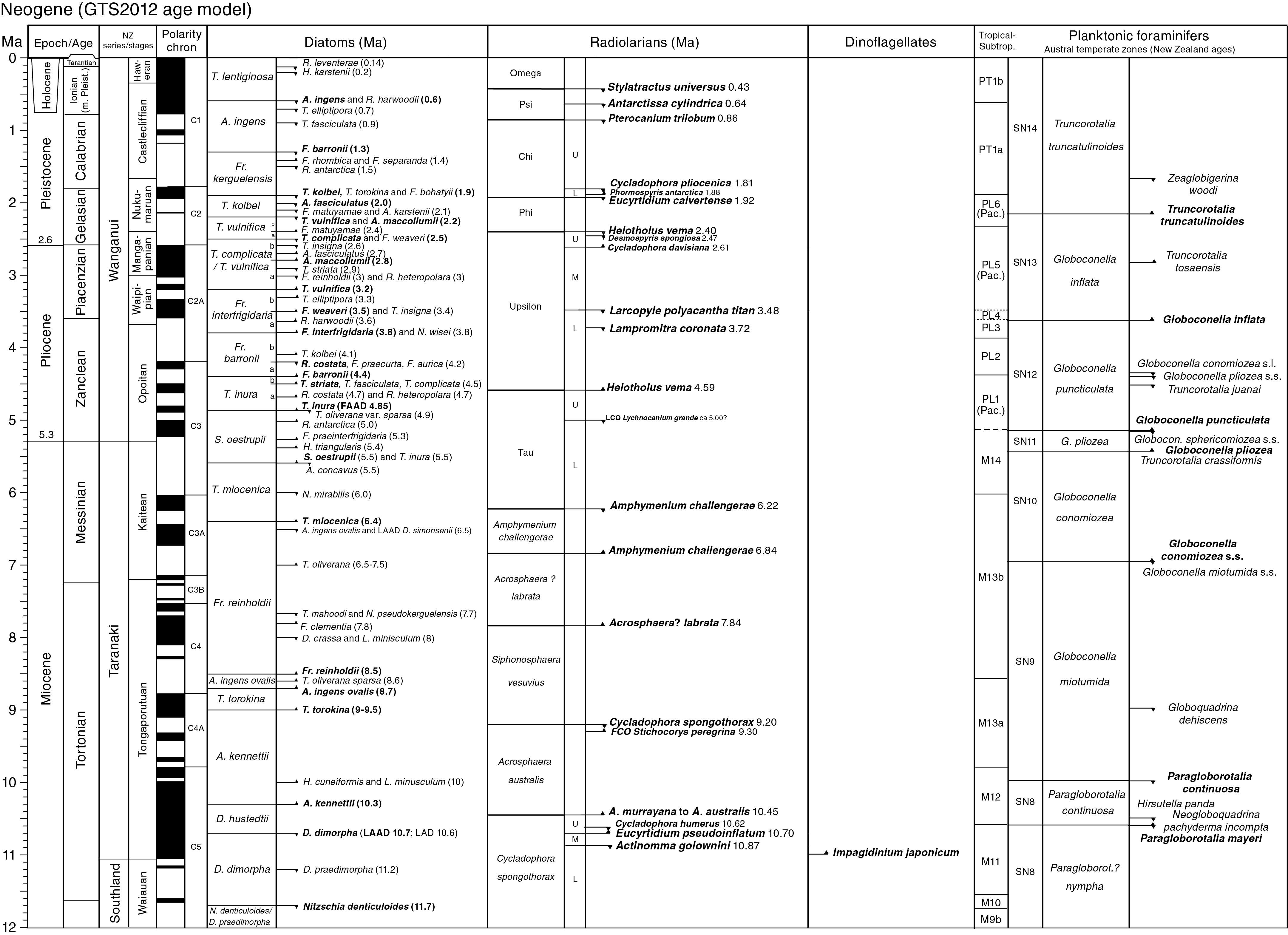
Figure F14. Chronostratigraphic age framework.
An effort to utilize biostratigraphic zones of austral temperate planktonic foraminifers was based on Jenkins (1993) and datum ages derived from the New Zealand Geological Timescale and correlated to New Zealand Series and Stages from Crundwell et al. (2016), but foraminifers were too rare throughout the recovered sequences to apply a foraminifer-based biostratigraphic scheme. Neogene dinoflagellate cyst (dinocyst) biostratigraphy is currently developing, and tentative placement of selected biostratigraphic datums for southern high latitudes is drawn mainly from Bijl et al. (2018) (Figure F14).
Reworking and recycling of older microfossils into younger deposits is a particular problem for age dating in glacial proximal depositional settings. Every effort was made to recognize displaced fossils before depositional age assignments were made because reworked zonal markers may imply an age older than the actual age of deposition. Significant reworking is often obvious (e.g., Paleozoic pollen in Quaternary marine sediment or Oligocene diatoms in Pliocene diamicton), but recycling of, for example, early Pliocene diatoms into late Pliocene sediments can be difficult to recognize. For this reason, we put much heavier weight on first stratigraphic occurrences than last, especially where fossils are relatively rare or poorly preserved. When recognized as such, reworked fossils, especially in glacial sediments, can provide information regarding sediment transport and provenance and can act as important records that document subglacial or otherwise inaccessible sedimentary deposits.
The Biostratigraphy sections in the site chapters present a summary of biostratigraphic information plus limited paleoenvironmental interpretation provided by each microfossil group and information regarding approaches and literature used to guide taxonomic identifications. Data for each microfossil group are presented in abundance and taxonomic distribution charts that record occurrences of key taxa observed in samples from each hole. Relative abundance and preservation data were entered through the DESClogik application into the LIMS database for all identified microfossil taxa and all paleontological data gathered during shipboard investigations. These data are available from the LIMS database. Taxonomic occurrence charts also record suspected upsection reworking or otherwise out-of-place species.
Distribution charts for microfossil groups presented in each site chapter are based exclusively on shipboard analysis. Shipboard biostratigraphic studies focused primarily on the identification of biostratigraphic horizons (biohorizons) in the cores and are biased toward the reporting of age-diagnostic species and identifying intervals and ages of reworking. Events reported include the last appearance datum (LAD) or first appearance datum (FAD) of a taxon’s stratigraphic range, in some cases with modification to identify the last common/abundant appearance datum (LCAD/LAAD) or first common/abundant appearance datum (FCAD/FAAD) to identify an abundance change within a taxon’s range if these are more reliable for correlation. Where possible, identification of a sequence of biohorizons in stratigraphic order was used to define biostratigraphic zones and subzones using standard schemes. A summary table of the main biostratigraphic events identified at each site is presented in each site chapter. The chronostratigraphic compilation provides a framework for estimating sediment accumulation rates, identifying hiatuses, guiding correlation between holes, and assessing recovery as compared with the Scientific Prospectus (Gohl et al., 2017). All age models presented in this volume are preliminary and may be subject to moderate or significant revision following postcruise research updates.
Diatoms
Diatom taxonomy
Taxonomic concepts for Neogene Antarctic diatoms, many of which are endemic to the southern high latitudes, have developed largely through the last nearly 50 y of stratigraphic drilling in the Southern Ocean and Antarctic shelf by the Deep Sea Drilling Project (DSDP), ODP, the Integrated Ocean Drilling Program, and IODP (McCollum, 1975; Gombos, 1976; Schrader, 1976; Ciesielski, 1983; Gersonde, 1990, 1991; Gersonde and Burckle, 1990; Baldauf and Barron, 1991; Fenner, 1991; Harwood and Maruyama, 1992; Mahood and Barron, 1996; Gersonde and Barcena, 1998; Censarek and Gersonde, 2002; Iwai and Winter, 2002; Zielinski and Gersonde, 2002; Arney et al., 2003; Bohaty et al., 2003; Whitehead and Bohaty, 2003). Parallel to the above efforts, ice platform stratigraphic drilling programs on the Antarctic margin recovered neritic diatom floras that serve as useful Antarctic continental shelf taxonomic and biostratigraphic references. These programs include the Dry Valley Drilling Project (DVDP; Brady, 1979), McMurdo Sound Sediment and Tectonic Studies (MSSTS; Harwood, 1986), Cenozoic Investigation in the Western Ross Sea (CIROS; Harwood 1989; Winter and Harwood, 1997), the Cape Roberts Project (Bohaty et al., 1998; Scherer et al., 2000; Olney et al., 2007, 2009) and ANDRILL (Sjunneskog et al., 2012; Winter et al., 2012). Other useful taxonomic references for Neogene and modern Antarctic marine diatoms include Fenner et al. (1976), Akiba (1982), Harwood et al. (1989), Medlin and Priddle (1990), Yanagisawa and Akiba (1990), Cremer et al. (2003), and Scott and Thomas (2005).
Methods for diatom sample preparation and analysis
With a primary focus on core catcher samples, smear slides were examined on a routine basis for diatom stratigraphic markers. For samples in which diatoms were very rare or highly fragmented, additional preparation steps were undertaken. These involved (1) making strewn slides from raw sample material disaggregated in deionized water and/or (2) concentrating larger specimens through sieving at >10 µm with polyester mesh or >20 µm with a stainless steel sieve. Examination of the sieved fractions or differentially settled strewn slides allowed recovery of identifiable diatom specimens in samples characterized by low concentration and high fragmentation of diatoms. We acknowledge that this approach likely increased the presence of larger, more heavily silicified species and removed many potentially biostratigraphically important, smaller diatoms from these slides. However, this approach is deemed essential for providing a sufficient number of specimens to allow rapid age interpretation of core catcher samples. Both smear and strewn slide preparations were mounted on cover glasses and permanently fixed to labeled glass slides using Norland optical adhesive Number 61 (refractive index = 1.56) and cured under an ultraviolet lamp.
Samples prepared for diatom analysis were examined using Zeiss Axioskop transmitted-light microscopes. Photomicrographs were taken using a SPOT Flex 64 Mp digital camera. A Hitachi TM3000 tabletop scanning electron microscope (SEM) was available for higher magnification micrographs of selected specimens when deemed advantageous to taxonomic identification and data production but was not utilized for diatom analysis during Expedition 379 because of the persistent ship movement related to weather and sea state. Qualitative siliceous microfossil group abundances were determined from smear slides using 630× magnification. Care was taken to ensure smear slides were prepared with similar amounts of sediment. For each sample, the following abundances of diatoms were qualitatively estimated by light-microscopic observations with the examination of five random fields of view (FOVs):
- B = barren (no diatom debris).
- T = trace (trace quantities <2%).
- R = rare (2%–5% diatoms).
- F = few (5%–10% diatoms).
- C = common (10%–20% diatoms).
- A = abundant (20%–40% diatoms).
- V = very abundant (40%–60% diatoms).
- M = mass abundance (>60% diatoms).
Trace quantities (<2%) may include very rare, heavily degraded, and unidentifiable fragments, possibly including pyritized, recrystallized, or partially dissolved diatoms that indicate nothing more than the prior occurrence of diatomaceous debris impacted by heavy dissolution or diagenesis. Visual estimates of percentages followed standard guidelines (e.g., Rothwell, 1989).
The following relative abundances of individual taxa were categorized in reference to their occurrence in FOVs or to a traverse across a 40 mm wide coverslip (~100 FOVs at 630× magnification):
- T = trace (<1 specimen per 5 average horizontal transects [40 mm]).
- R = rare (1 specimen within 1–5 transects).
- F = few (1–5 specimens per transect).
- C = common (1–5 specimens per ~5 FOVs).
- A = abundant (2 or more specimens per FOV).
- D = dominant (the taxon represents >50% of all diatoms in diatom-rich samples).
The counting concept of Schrader and Gersonde (1978) was applied for the above. Shipboard observations of diatom species occurrences logged in DESClogik focused on the presence of age-diagnostic species, so the distribution data may not accurately characterize the true nature of the full diatom assemblage, which is typically dominated by non–age diagnostic (e.g., long ranging) taxa.
Preservation of diatoms was qualitatively assessed with regard to both the degree of dissolution and fragmentation. The degree of siliceous microfossil fragmentation often mirrors dissolution, but the two factors are not always directly correlated. Diatoms with well-preserved fine structures can be highly fragmented. Dissolution is a wholly chemical process (Warnock and Scherer, 2015), but fragmentation can be dominantly or entirely due to mechanical processes such as compaction or subglacial shear strain (Scherer et al., 2004). Fragmentation of finely silicified diatoms can occur in sediments as a result of digestion by grazers and deposition in fecal pellets.
The degree of dissolution was qualitatively graded as follows:
- L = low (slight to no apparent dissolution [fine structures generally preserved]).
- M = moderate (moderate dissolution [fine structures generally lost]).
- H = high (severe effects of dissolution, including widened areolae, relatively abundant margins and cingula compared with valves, and notably higher proportions of heavily silicified forms).
The degree of fragmentation was graded as follows:
- L = low (a majority of valves are unbroken).
- M = moderate (>50% of diatom valves are broken, but most are identifiable).
- H = high (valves highly fragmented with very few complete valves present, hampering identification).
Diatom age assignment
Initial shipboard diatom age assignment of individual upper Paleogene and Neogene samples was based on identification of primary and secondary datum events that are well calibrated at Southern Ocean sites. Biostratigraphic zones were also defined where possible using the Neogene zonal schemes derived from Southern Ocean sites by Harwood and Maruyama (1992), Zielinski and Gersonde (2002; Oligocene to recent) and Censarek and Gersonde (2002; Miocene) and for Antarctic continental shelf sites by Winter et al. (2012). A wealth of biostratigraphic information is available from the drill core–based studies listed in Diatom taxonomy and the integrated biochronological syntheses in the associated volumes for each leg/expedition (e.g., Gersonde et al., 1990; Barron et al., 1991; Harwood et al., 1992; Iwai et al., 2002; Tauxe et al., 2012). Ages applied to specific diatom events and zonal boundaries were guided by successive iterations of the diatom biochronology afforded by CONOP (Cody et al., 2008, 2012; Florindo et al., 2013). These ages are in general agreement with ages of appearance and extinction of Southern Ocean endemic diatoms presented in Barron (2003), although some offset of latest Miocene to early Pliocene datums were noted by Iwai et al. (2002) and Tauxe et al. (2012). Age assignments for diatom datum levels used during Expedition 379 are presented in Figure F14 and Table T1. This data set is adapted from the working data set of Expedition 374 in the Ross Sea (McKay et al., 2019). Minor adjustments have been made based on current knowledge and recent observations and calibration. It is important to note that data sets like this, although currently state of the art, are in continual revision as more data and analyses become available, including from this expedition.
Radiolarians
Radiolarian taxonomy
The main taxonomic concepts for the Neogene radiolarians studied here are based primarily on Popofsky (1908), Riedel (1958), Petrushevskaya (1967, 1975), Lombari and Lazarus (1988), Lazarus (1990, 1992), Caulet (1991), Abelmann (1992), Nigrini and Sanfilippo (2001), Vigour and Lazarus (2002), Lazarus et al. (2005), and Renaudie and Lazarus (2012, 2013, 2015, 2016). All radiolarian semiquantitative abundance data produced on board were logged in DESClogik and are available for each site (see DESC_WKB in Supplementary material).
Methods for sample preparation and analysis of radiolarians
To minimize paleontological preparation time, the following protocol was adopted for combined preparation of samples for radiolarians, foraminifers, and ostracods. These preparations also provided residues for the analysis of other fossil groups, as well as rock and mineral fragments. A 5–20 cm3 sediment sample, generally from core catchers but also from other samples as they became available, was placed in a beaker with 50 mL of water (per 5 cm3 of sediment), a 15% solution of hydrogen peroxide, and a small quantity of diluted borax. The beaker was then warmed on a hot plate with a magnetic automatic stirrer. When effervescence was finished (typically approximately between 30 min and 3 h), the solution was washed through two sieves, 150 and 38 µm. The <38 µm fraction was preserved for further exploration for smaller phytoplankton such as diatoms, nannofossils, and so forth and for quality control of the sieving procedure. The 38–150 µm residue and the >150 µm residue were placed in separate bowls. Using a pipette, several drops of each was placed on two 25 mm × 75 mm microscope slides and allowed to dry. Once dried, a few drops of Norland optical adhesive Number 61 were added and covered by a 22 mm × 50 mm coverslip. The microscope slides were then placed under the ultraviolet lamp to cure for 15 min. The rest of the 38–150 and >150 µm fractions were reserved for foraminiferal and other analyses (see Foraminifers).
Microscopy and identification
Radiolarian species were identified and their abundance estimated using a Zeiss Axioplan microscope with bright field illumination at 100×, 200×, and 400× magnification. Photomicrographs were taken using a SPOT Flex 64 Mp digital camera and uploaded to the LIMS database.
For each sample, the total abundance of radiolarians was qualitatively estimated by light-microscopic observations at 100× magnification along one horizontal traverse of the slide and recorded as follows:
- A = abundant (>100 specimens per traverse).
- C = common (51–100 specimens per traverse).
- F = frequent (11–50 specimens per traverse).
- R = rare (1–10 specimens per traverse).
- Tr = trace (1–10 specimens per slide).
- B = barren (absent).
Qualitative estimates of individual species abundances were also recorded by scanning through both slides at 100× magnification as follows:
- A = abundant (≥2 specimens/FOV).
- C = common (1 specimen/FOV).
- F = frequent (1 specimen/2–5 FOV).
- R = rare (1 specimen/5–30 FOV).
- Tr = trace (≤1 specimen per traverse).
Preservation of the radiolarian assemblages was recorded as follows:
- G = good (fine structures preserved).
- M = moderate (minor dissolution and/or breakage).
- P = poor (common dissolution, recrystallization to opal-CT, and/or breakage).
Radiolarian biostratigraphy and age assignment
The Southern Ocean zonation used here was based on Lazarus (1992; for the middle Miocene to Pleistocene). The original age estimates for radiolarian datums for the early Miocene to Pleistocene were based on their calibration to magnetostratigraphy according to Hays and Opdyke (1967), Gersonde et al. (1990), Lazarus (1990), Spieß (1990), Barron et al. (1991), Caulet (1991), Harwood et al. (1992), Lazarus (1992), and Ramsey and Baldauf (1999). Age estimates were recalibrated to the GTS2012 using the Neptune database (http://www.nsb-mfn-berlin.de). Some additional age estimates from Florindo et al. (2013) were added as secondary datums for the Miocene and Pliocene (Table T2) when appropriate and when consistent with the stratigraphic ranges found in Renaudie (2012).
Foraminifers
Planktonic foraminifer taxonomy
Neogene planktonic foraminifer taxonomic concepts follow those of Jenkins (1971, 1978), Kennett (1973), Kennett and Vella (1975), Hornibrook (1982), Kennett and Srinivasan (1983), Leckie and Webb (1985), Cifelli and Scott (1986), Hornibrook et al. (1989), Scott et al. (1990), Berggren (1992), and Majewski (2010).
Benthic foraminifer taxonomy
The taxonomy of modern and Pleistocene benthic foraminifers of the Amundsen Sea continental shelf and slope follows Pflum (1966), Kellogg and Kellogg (1987), Majewski (2013), and Majewski et al. (2017) and is augmented by circum-Antarctic taxonomic work by Fillon (1974), Anderson, (1975), Osterman and Kellogg (1979), Ishman and Domack (1994), Igarashi et al. (2001), and Majewski (2005, 2013). Few occurrences of foraminifers were noted in pre-Pleistocene sediments, and no detailed systematic analysis was performed on these materials during shipboard study. The classification of Loeblich and Tappan (1988) was followed for determinations at the genus level.
Methods for sample preparation and analysis of foraminifers
Most sediment samples (10–20 cm3) were placed in a beaker with 100 mL of water, a 10% solution of hydrogen peroxide, and a small quantity (<5 mL) of diluted borax (depending on the presence of clay). For Site U1533, however, hydrogen peroxide and borax were not used so that the isotope signal of the foraminifers would be preserved. As described for radiolarians, the beakers were warmed on a hot plate with a magnetic stirrer. When effervescence was finished (~30 min), the solution was washed through two sieves: 150 and 38 µm. The <38 µm fraction was preserved for further exploration for smaller phytoplankton. The 38–150 and >150 µm residues were placed in separate bowls and placed in an oven at 45°C until dry (minimum ~2 h).
The dried residues were then weighed and observed under a binocular light microscope. Each of the individual specimens were picked from the sample using a very fine brush and mounted on a gridded cardboard slide coated with a thin layer of water-soluble paste made from gum tragacanth powder. Tephras and ichthyoliths were also picked for postcruise isotopic or radiometric dating. After foraminifer picking, sieved residues that included mineral matter, including sand and larger clasts, were made available to the lithostratigraphy team.
Microscopy and identification
Foraminifer species were identified using a Zeiss Discovery V8 binocular light microscope. Photomicrographs were taken using a SPOT Idea digital camera and uploaded to the LIMS database.
Species identifications were generally made on the >150 μm size fraction. Time permitting, the 38–150 μm size fraction was scanned for small or rare species.
The preservation state of planktonic and benthic foraminifers was estimated as follows:
- E = excellent (totally glassy specimens with no to very little evidence of overgrowth, dissolution, or abrasion).
- VG = very good (some minor evidence of overgrowth, dissolution, or abrasion).
- G = good (little evidence of overgrowth, dissolution, or abrasion).
- M = moderate (common but minor calcite overgrowth, dissolution, or abrasion).
- P = poor (substantial overgrowth, dissolution, or fragmentation).
The planktonic to benthic foraminifer ratio (P/B) was calculated using the relative abundance of each group and then was used as a first approximation of carbonate dissolution.
Foraminifer biostratigraphy and age assignment
Given the southern high-latitude location of Sites U1532 and U1533, the Subantarctic zonal scheme of Berggren (1992; DSDP Leg 120, Kerguelen Plateau) and austral temperate zonal scheme of Jenkins (1993) were utilized with ages updated to the GTS2012, as well as planktonic foraminifer biostratigraphic datums of Crundwell et al. (2016). The scarcity of foraminifers in recovered sediments precluded application of biostratigraphic schemes in the pre-Pleistocene strata. The foraminifer biostratigraphic ages that were used during Expedition 379 are summarized in Table T3.
Palynology
Taxonomy and zonation scheme
A magnetostratigraphically calibrated dinocyst stratigraphy for the Oligocene and early to middle Miocene from Expedition 318 Hole U1356A on the Wilkes Land margin is presented in Bijl et al. (2018). The Oligocene to middle Miocene observations of Bijl et al. (2018) are supplemented by observations from around the Antarctic margin, including Leg 28 (Kemp, 1975; Kulhanek et al., 2019), ODP Leg 188 Site 1165 (Hannah, 2006), CRP drilling (Hannah et al., 2000; Clowes et al., 2016a), and Leg 178 (Harland and Pudsey, 2002). We report FADs and LADs for Neogene dinocyst taxa previously reported in the Southern Hemisphere high latitudes that have been calibrated to the GTS2012 but note that Neogene dinocyst biostratigraphy is developing and placement of selected biostratigraphic datums is tentative. To date, only limited correlation between high southern latitude sites exists (Table T4).
Late Paleogene–Neogene dinocyst taxonomy follows that presented in Hannah et al., (2001), Clowes et al. (2016a), Williams et al. (2017), and Bijl et al. (2018). No complete integrated stratigraphic dinocyst framework currently exists for the younger Neogene of the Southwest Pacific, although the recent (core top) distribution has been documented in southern high latitudes (Esper and Zonneveld, 2007; Prebble et al., 2013). Antarctic miospores (terrestrial pollen and spores) of Neogene age are generally of insufficient diversity and abundance to support biostratigraphic studies (Cantrill and Poole, 2012). Furthermore, biogeographic provincialism is likely to further reduce the utility of extrapolating occurrence datums around the Antarctic margin, for example from the (relatively) better seafloor-documented western Ross Sea (Askin and Raine, 2000; Raine and Askin, 2001; Prebble et al., 2006; Kulhanek et al., 2019).
Methods for palynology study
Approximately 5–10 g of each sediment sample was processed for shipboard palynology analysis (e.g., Prebble et al., 2013). Two sample processing methods were employed. Most samples were processed using a disaggregation/sieving method described in Riding and Kyffin-Hughes (2011). Samples were disaggregated by soaking and agitation in 1% borax solution followed by 10% sodium hexametaphosphate and then sieved through a 10 µm mesh. The light (organic rich) fraction was concentrated by swirling and decanting. Samples were put in an ultrasonic bath for ~30 s when required to further disaggregate and remove clays. For most samples, a variation of the Riding and Kyffin-Hughes (2011) method was used, whereby disaggregation was achieved using only water rather than sodium hexametaphosphate. Samples with high concentrations of biogenic silica were subsequently processed using a second method with hydrofluoric acid (HF) described below.
Samples were digested with 10% HCl and cold 48% HF to dissolve carbonates and silicates followed by 30% HCl to remove silicate gels. Centrifuging and decanting were carried out after each step. Residues were filtered through a 10 μm mesh and sieved through a 250 μm mesh when required. The processing method applied to each sample is recorded in the site chapters. Where duplicate samples were processed, palynological results from the two methods were found to be comparable in these nonindurated sediments. All samples were mounted on glass microscope slides using Norland optical adhesive Number 61 as the mounting medium. Species identification and data collection were carried out with a Zeiss Axio microscope using bright field illumination at 400×, 630× (oil), and 1000× (oil) magnification. Photomicrography was conducted using a SPOT Flex 64 Mp digital camera.
Palynomorph abundance and preservation
Palynomorph abundance and palynofacies schemes applied here followed those reported for the Ross Sea (McKay et al., 2019) to facilitate future comparison. Palynofacies categories are described in Clowes et al. (2016b).
Palynofacies were grouped into the following broad categories:
- In situ marine organic-walled dinocysts,
- Reworked marine organic-walled dinocysts,
- Foraminifer test linings,
- Prasinophytes,
- Acritarchs,
- In situ miospores (pollen and spores),
- Reworked miospores (pollen and spores),
- Black phytoclasts,
- Brown phytoclasts,
- Fungal spores, and
- Amorphous organic matter.
For semiquantitative estimates of the abundance of these palynofacies groups, the following scale was used:
- D = dominant (>90% of palynomorphs).
- A = abundant (>50%–90% of palynomorphs).
- C = common (>10%–50% of palynomorphs).
- F = few (1%–10% of palynomorphs).
- R = rare (<1% of palynomorphs).
- BR = barren to rare (few specimens identified in two slides).
- B = barren (not present).
Dinocysts in each sample were identified at genus or species level. The following qualitative indication of their occurrence is given in the tables of each site chapter:
For biostratigraphic and paleoenvironmental purposes, shipboard analysis of palynomorphs focused primarily on determining the presence of age-diagnostic dinocyst taxa and characterizing the palynological assemblage in terms of paleoenvironment. When possible with given dinocyst yields and time, dinocyst counts were carried out per sample. For each sample, one 22 mm × 10 mm slide was scanned and counted.
Miospores identified during these counts were also quantitatively registered and attributed to the following four broad categories:
Where possible, miospores were identified to genus and species level using Askin and Raine (2000), Raine and Askin (2001), Prebble et al. (2006), Raine et al. (2011), Prebble (2016), and references therein.
Palynomorph preservation was qualitatively classified as one of the following levels:
- G = good (little or no evidence of degradation or oxidation).
- M = moderate (some evidence of degradation or oxidation).
- P = poor (major degradation or oxidation has occurred).
Palynology-based paleoenvironmental analysis
Three palynomorph groups were used to infer aspects of the depositional environment: total palynofacies, dinocyst assemblages, and miospore assemblages. In suitable depositional settings, total palynofacies data can provide relative information about source, transport distance, and reworking of the organic carbon fraction (e.g., Tyson, 1995; Clowes et al., 2016b; Prebble et al., 2018).
The use of dinocysts as paleoenvironmental indicators derives from information on their present-day global distribution, including in southern high latitudes (Esper and Zonneveld, 2007; Prebble et al., 2013; Zonneveld et al., 2013). These studies show dinoflagellate distribution in the modern ocean is strongly influenced by sea-surface temperature and surface productivity. Because many of the modern species were apparently extant during the Neogene and Quaternary, these observations may be used with caution (e.g., De Schepper et al., 2011) to infer past surface ocean conditions. Other aquatic palynomorphs, in particular acritarchs and prasinophytes, were used to infer information on meltwater input/water stratification. Miospore assemblages can provide quantitative and semiquantitative information about terrestrial conditions at the time the source vegetation grew (e.g., Warny et al., 2009; Prebble et al., 2017), again with caveats arising from the appropriateness of the analogs (Jordan et al., 2011).
Other fossil occurrences
Other fossil groups were also noted during Expedition 379. These included rare ostracods encountered during foraminiferal preparation and other fossil groups noted and utilized when possible during smear slide analysis for diatoms, including calcareous nannofossils, silicoflagellates, ebridians, endoskeletal dinoflagellates, chrysophyte cysts, sponge spicules, and ichthyolith fragments. When possible, these fossils, notably silicoflagellates and ebridians, were identified and utilized informally in the biostratigraphic assessment. Calcareous nannofossils were specifically sought as part of routine smear slide analysis by diatom paleontologists.
Paleomagnetism
We conducted paleomagnetic studies primarily to determine directions of remanence components. Routine measurements were completed on almost all archive-half sections with stepwise alternating field (AF) demagnetization. In a very few instances where the intensity of natural remanent magnetization (NRM) exceeded the maximum magnetic flux change that the superconducting rock magnetometer (SRM) is capable of measuring, only NRM was saved and the archive-half sections were not demagnetized. Discrete cube samples were taken from selected working-half sections and measured with stepwise AF demagnetization. These data were used for magnetostratigraphic dating and complemented by rock magnetic measurements. Paleomagnetic data were integrated with biostratigraphic data to develop shipboard age models. Icefield MI-5 core orientation tool data were acquired for all APC cores, but these data were not applied to shipboard interpretation of paleomagnetic data. The orientation data will help to improve postcruise interpretation of paleomagnetic measurements.
Magnetic measurements
Remanent magnetization was measured using a SRM (2G Enterprises model 760R-4K, #121) equipped with direct-current superconducting quantum interference devices (SQUIDs) and an in-line, automated AF demagnetizer capable of reaching a peak field of 80 mT. Ocean drilling cores generally carry secondary remanence components (overprints) that include natural viscous remanence and sometimes a steep downward-pointing component attributed to the drill string. To separate the overprints from the characteristic remanence (ChRM), stepwise demagnetization experiments were performed.
Archive-half sections
Measurements of archive-half sections were conducted using the SRM IMS 10.2 software. The nominal sample-area parameter was 13.4 cm2 for RCB archive-half sections and 17.5 cm2 for HLAPC and XCB archive-half sections. The measurement interval and speed were 2.5 cm and 10 cm/s, respectively. The spatial resolution is determined from the integrated response function (following Acton et al., 2017) with effective lengths of 7.3 cm for the x- and y-axes and 9.0 cm for the z-axis. The practical noise level of the SRM is ~2 × 10⁻⁹ Am2 and is primarily controlled by the magnetization of the core liner and the background magnetization of the measurement tray.
At the beginning of every working shift (approximately every 12 h), we cleaned the sample tray. It was then AF demagnetized with a peak field of 30 mT, and its remanence was measured to monitor any changes to the sample tray during the course of the expedition and to ensure accurate tray correction values.
NRM measurements of archive-half sections were made at 2.5 cm intervals with a 5 cm trailer and leader interval to monitor the background magnetic moment. Previous reports suggest that higher AF demagnetization fields produce significant anhysteretic remanent magnetization (ARM) along the z-axis of the SRM. With this limitation, we measured the initial NRM and the NRM after AF demagnetization with peak fields of 5, 10, 15, and 20 mT using the 2G Enterprises Model 2G600 in-line demagnetizer.
AF demagnetization results were plotted individually as vector plots (Zijderveld, 1967) and as downhole variations with depth. We inspected the plots visually to judge whether the remanence after demagnetization at the highest AF step reflects the ChRM and geomagnetic polarity sequence. Usually, the 20 mT demagnetization step was assumed to represent the ChRM and was therefore used for further interpretation.
Section-half data collected on the pass-through SRM were uploaded to the LIMS database.
Discrete samples
Depending on characteristics such as lithologic changes or to refine the magnetostratigraphy, we typically collected one or two oriented discrete samples per core. These discrete samples were used for measurements of mean (bulk) magnetic susceptibility, anisotropy of magnetic susceptibility (AMS), and NRM and its stepwise AF demagnetization. We collected discrete samples from each site by pushing plastic Natsuhara-Giken (“Japanese”) cubes (with a 2 cm external edge length and an internal volume of ~7 cm3) into working-half sections with the arrow marker on the cube pointing upcore. The sample x-axis is toward the double lines on the working-half sections, and the up arrow marks the negative z-axis (toward core top; Figure F15A, F15C). When the sediment was more indurated, the sediment was extruded onto a clean cutting board and the cube was placed on top. When the sediment (or hard rock) was too lithified to use the extruder, oriented cubes (~8 cm3) were cut and trimmed using a dual-blade saw.

Figure F15. Paleomagnetism coordinate system.
For discrete samples, we performed successive AF demagnetization up to a field of 100 mT with the DTech AF demagnetizer (Model D-2000). Remanence was measured after each demagnetization step on the AGICO JR-6 spinner magnetometer. We analyzed the stepwise demagnetization data of the discrete samples by principal component analysis (PCA) to define the ChRM (Kirschvink, 1980).
AMS and mean (bulk) magnetic susceptibility of the discrete samples were measured on a KLY 4S Kappabridge. To ensure accurate susceptibility values, we calibrated the KLY 4S at least prior to each site using the standard provided by AGICO. The Kappabridge SUFAR software measures AMS by rotating the sample along three axes, stacking the data, and estimating the best-fit second-order tensor. The mean (bulk) magnetic susceptibility is calculated as the average of the magnetic susceptibilities in all three orientations, and we referred to this as mean magnetic susceptibility throughout Expedition 379. We only use the directions and (relative) amplitudes of the three principal axes of the susceptibility tensor, κmax (maximum susceptibility axis), κint (intermediate axis), and κmin (minimum axis), to approximate magnetic fabric (i.e., grain shape and orientation). When sediments are deposited in an undisturbed environment, sedimentary fabrics are oblate and the vertical axis has minimum susceptibility. Disturbance by slumping or other deformation often yields triaxial fabrics. Hence, we use the AMS as an indicator of disturbance to complement the information on drilling disturbance given by the core description.
Discrete data collected on the KLY 4S Kappabridge and on the JR-6 were uploaded to the LIMS database.
Coordinates
All magnetic data are reported relative to IODP orientation conventions: +x points into the face of the working-half core section, +y points toward the left side of the working-half core section when looking downcore, and +z is downcore (Figure F15A). The relationship between the SRM coordinates (X, Y, and Z) and the sample coordinates (x, y, and z) is +X = +x, +Y = +y, and +Z = −z for archive-half sections and +X = −x, +Y = −y, and +Z = −z for working-half sections (Figure F15). Note that the orientation of the SRM axes forms a left-handed coordinate system that is converted to a right-handed system in the SRM software by multiplying the calibration constant for the y-axis by −1. The orientation of discrete samples depends on how the sample is collected. For samples collected by pushing the Japanese cube into the working-half section, the arrow on the sample points upcore along the z-axis and is along the face of the working-half core section as in Figure F15A and F15C. The orientation of sawed cubes and cubes placed on top of extruded sediment follows the orientation of the Japanese cubes. The discrete samples were placed in the AGICO JR-6 spinner magnetometer as shown in Figure F16. We entered values of 0° and 90° for azimuth and dip, respectively, in the JR-6 software. Data for inclination and declination consistent with those from the SRM were saved as geographic coordinates in the JR-6 data files.
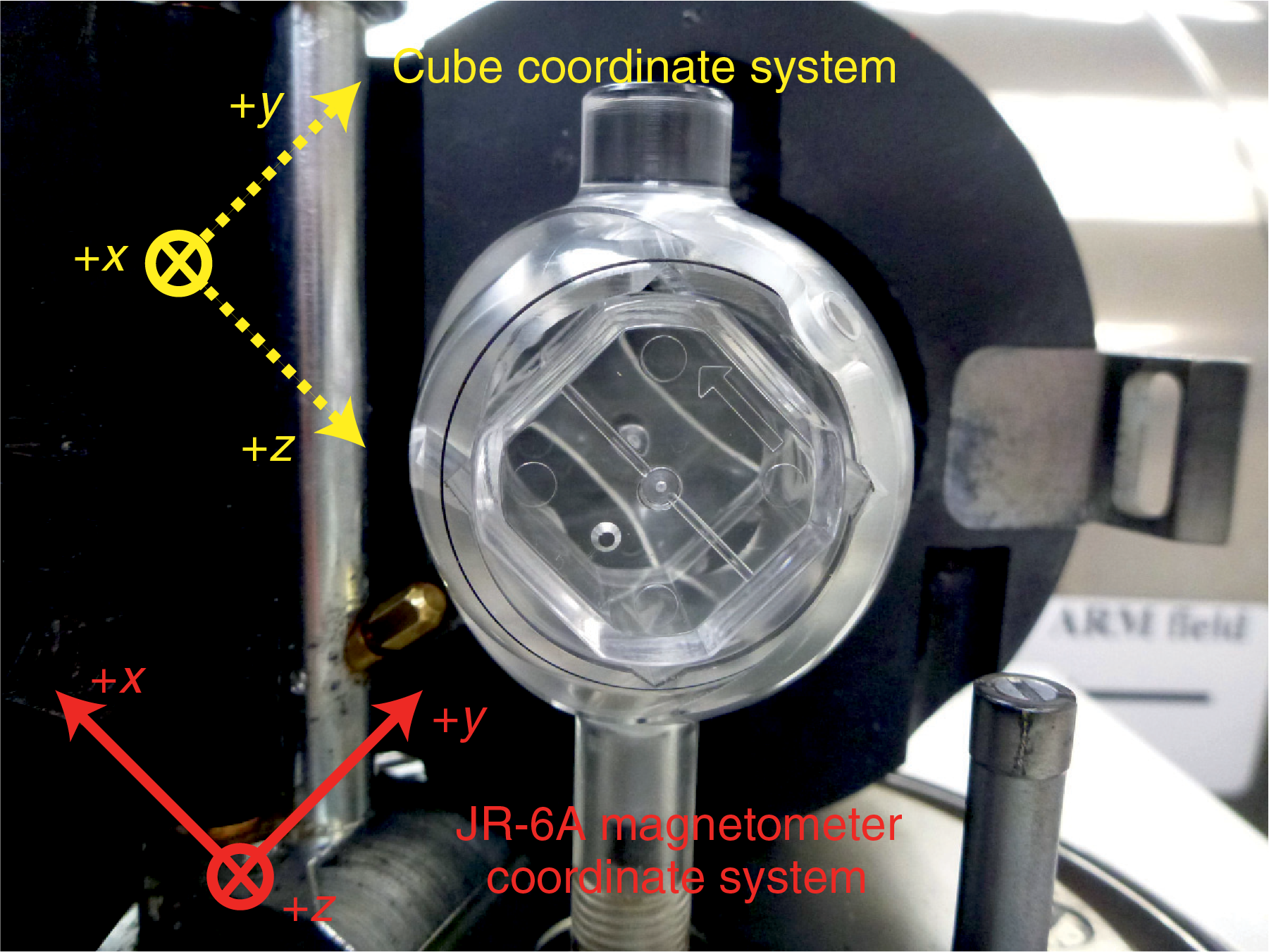
Figure F16. Discrete samples in the JR-6A spinner magnetometer.
Core orientation
Cores were collected using nonmagnetic core barrels for the APC, HLAPC, and RCB coring systems. These nonmagnetic core barrels are weaker than the steel core barrels and cannot be used with the XCB system because its rotation is driven from the top of the barrel. When APC/XCB coring, the BHA included a Monel (nonmagnetic) drill collar. The Monel drill collar is required when the Icefield MI-5 core orientation tool is deployed. When an APC core is taken, the Icefield tool is positioned so that it is within the Monel drill collar so that the tool is not within the more intense magnetic field of the normal drill collars.
The Icefield MI-5 core orientation tool can only be used with APC core barrels. It uses three orthogonally mounted fluxgate magnetometers to record the orientation of the double lines scribed on the core liner with respect to magnetic north. The tool declination, inclination, total magnetic field, and temperature are recorded internally at a regular interval until the tool’s memory capacity is filled. For the measurement interval of 10 s used during Expedition 379, the tool can typically be run for more than a day, although we aimed to switch tools more frequently than that. Prior to firing the APC, the core barrel is held stationary (along with the pipe and BHA) for several minutes. During this time, data are recorded (while the Icefield tool is within the Monel drill collar) to constrain the core orientation. When the APC fires, the core barrel is assumed to maintain the same orientation. An antispiral key keeps the core barrel from rotating as it is fired, but the core may rotate and/or the core liner can twist as it penetrates the sediments.
The Icefield MI-5 core orientation data collected during Expedition 379 are given along with the observed core mean paleomagnetic directions in a table in each site chapter. The mean direction of each core is computed using Fisher statistics from the paleomagnetic archive-half section measurements.
All directions with positive inclinations were inverted to their antipodal position by multiplying the inclination by −1 and adding 180° to the declination. We then computed the mean by using all directions with inclinations between −40° and −90°.
The orientation correction that converts the observed declination (Dobs) to a true declination (Dtrue) is given by
where MTF is the magnetic tool face angle from the Icefield MI-5 core orientation tool and Damb is the ambient geomagnetic field declination obtained from geomagnetic field models. Using 69°S/109°W as mean coordinates, the World Magnetic Model 2015 gives a value of ~45° for the drill sites. Given that the Antarctic plate has not moved significantly over the past 20 My (Torsvik et al., 2012), the expected true declination is roughly 0°.
Neither the core mean directions nor the Icefield MI-5 observations are ideal for use in core orientation but may help to improve the interpretation of the paleomagnetic data at a later stage. The steepness of the paleomagnetic field (with an inclination generally >70°) and the present-day geomagnetic field (inclination ~70°) result in the horizontal component (declination) being only a very small part of the total vector field. For example, when the inclination is 80°, a measurement error of only 20° in angular distance of the geomagnetic field can yield a declination of 0° versus 180°.
Indeed, the corrected declinations cluster around the expected value of 0° but exhibit a bias to westerly directions (see data presented in the respective site chapters). During Expedition 379, we did not use the correction for shipboard interpretation, but we intend to apply it during further postcruise data processing.
Magnetostratigraphy
Magnetic polarity zones were predominantly assigned based on changes in inclination after 20 mT peak AF demagnetization that occur in undisturbed cores recovered by all coring devices. Sediment disturbance caused by coring or geological processes (e.g., slumping or faulting) often leads to distorted and unreliable paleomagnetic directional records and largely altered sediment fabric. We used the classification of drilling disturbance made during the shipboard core description to mark disturbed intervals and avoided using paleomagnetic data from those intervals.
Once a magnetostratigraphy was established for a given hole, we correlated the pattern to the GTS2012 (Table T5). The GTS2012 includes orbitally tuned reversals between Chron C1n and the base of Subchron C5r.2n (0–11.657 Ma) and between the base of Chron C5ABn and Subchron C5Bn.1n (13.608–15.215 Ma). The intervals between Subchron C5r.2n and Chron C5ABn and between Chrons C5Bn and C6Cn (11.657–13.608 and 15.215–23.030 Ma, respectively) are calibrated by spline fitting marine magnetic anomaly profiles following Lourens et al. (2004) and Hilgen et al. (2012). We follow the chron terminology of Gradstein et al. (2012) and list several rarely observed polarity changes that were not formally classified as subchrons in the GTS2012 (Remarks column in Table T5). The shipboard age model for each site, based on paleomagnetic results and biostratigraphic datums, is presented in Chronostratigraphy in the Site U1532 chapter and Chronostratigraphy in the Site U1533 chapter (Wellner et al., 2021a, 2021b).
Geochemistry and microbiology
The shipboard geochemistry program for Expedition 379 included measurements for headspace gases (light hydrocarbons; C1–C3), interstitial water, and bulk sediment geochemical compositions. Samples for geomicrobiological analyses were collected on board and fixed for culture experiments and shore-based measurements of metagenomics, intact polar lipids (IPLs), and cell counts.
Inorganic geochemistry
Sampling protocol
The surface seawater used as drilling fluid was filtered through 0.20 µm polysulfone disposable filters from Whatman and collected in HCl-prewashed 24 mL syringes. It was also distributed in HCl-prewashed plastic or glass bottles for shipboard and postcruise analyses.
The samples for interstitial water geochemistry were obtained according to two general procedures. Interstitial water sampling varied with depth and started with a frequency of approximately three whole-round samples per core between 0 and 10 m, two whole-round samples per core between 10 and 100 m, and one whole-round sample per core below 100 m from cores obtained with the APC, HLAPC, and XCB systems. Where recovery was sufficient, one whole-round sample was taken every three RCB cores to the bottom of each hole; samples were taken at greater spacing when recovery was limited. The whole-round samples started with 5 cm lengths in the shallowest cores and increased with depth depending on interstitial water recovery, shipboard and shore-based sample volume needs, and other expedition priorities.
Interstitial water collection
For interstitial water analyses, whole-round samples were cut on the catwalk, capped, and taken to the laboratory for processing. After extrusion from the core liner and under atmospheric conditions in the laboratory, the surface of each whole-round sample was carefully scraped with a spatula or ceramic knife to remove potential contamination from seawater and sediment smearing along the inside of the core liners. For APC cores, ~0.5 cm of material from the outer diameter, top, and bottom faces was usually removed, whereas in XCB and RCB cores, where borehole contamination may be more substantial, as much as two-thirds of the sediment was removed from each whole-round section. The cleaned sediment (~150–300 cm3) was placed into a 9 cm diameter titanium squeezer that was then placed in a Carver hydraulic press (Manheim and Sayles, 1974) and squeezed at pressures no higher than ~20,000 lb (~10 MPa) to prevent release of interlayer water from clay minerals during squeezing. The squeezed interstitial water was filtered through a prewashed Whatman Number 1 filter placed in the squeezers above a titanium screen. The squeezed fluids were collected in an acid-cleaned, 24 or 60 mL high-density polyethylene syringe attached to the squeezing assembly and subsequently filtered through a 0.2 µm polyethersulfone membrane disposable filter.
Sample distribution was determined based on the recovered interstitial water volume and analytical priorities based on the objectives of the expedition. Priorities for the interstitial water sample distribution and analyses during Expedition 379 were in the following order:
- Salinity and Cl (shipboard),
- Anions and cations (shipboard),
- Major and trace element analyses (shipboard),
- δD/δ18O isotopes (postcruise),
- pH and alkalinity (shipboard),
- Nutrients (shipboard),
- δ13CDIC (postcruise), and
- Unconventional isotopes (87Sr/86Sr, 7Li/6Li, 10B/11B; postcruise).
Data produced on the Agilent 5110 inductively coupled plasma–optical emission spectrometer (ICP-OES) was collected in atomic emission spectroscopy (AES) mode and is referred to as “ICP-AES” in the LIMS/LORE database. Hereafter in this document, ICP-AES is used to refer to this data.
Aliquots for ICP-AES and unconventional isotope analyses were acidified by adding trace metal–grade concentrated HNO3 (~10 µL per 1 mL sample), and samples for δ13CDIC analysis were treated with 30 μL of a saturated HgCl2 solution. Individual interstitial water samples were stored at refrigerator (~4°C) or freezer (−20°C) temperatures. After interstitial water extraction was completed, sediment squeeze cakes were sealed in plastic bags for postcruise analyses.
Shipboard interstitial water analyses
Interstitial water samples were analyzed on board following the protocols in Gieskes et al. (1991), Murray et al. (2000), and the IODP user manuals for shipboard instrumentation (http://iodp.tamu.edu/labs/documentation), which were updated during this expedition.
Salinity, alkalinity, and pH
Salinity, alkalinity, and pH were measured immediately after squeezing and following the procedures in Gieskes et al. (1991). Salinity was measured using a Fisher temperature-compensated handheld refractometer (Model S66366). pH was measured with a combination glass electrode, and alkalinity was determined by Gran titration with a Metrohm 794 basic Titrino autotitrator using 0.1 N HCl at 20°C. The International Association for the Physical Sciences of the Oceans (IAPSO) standard seawater was used for calibration. The IAPSO standard was analyzed at the beginning and end of a set of samples for each site and after every 10 samples.
Chloride by titration
High-precision chloride concentrations were acquired using a Metrohm 785 DMP autotitrator and silver nitrate (AgNO3) solutions that were calibrated against repeated titrations of the IAPSO standard seawater (~559 mM). A 0.1 mL aliquot of sample diluted with 30 mL of 90 ± 2 mM HNO3 and titrated with a 0.0153 N AgNO3 of the IAPSO standard seawater yielded a standard error of <0.2%.
Sulfate, chloride, bromide, sodium, magnesium, potassium, and calcium
Sulfate, chloride, bromide, sodium, magnesium, potassium, and calcium concentrations were analyzed by ion chromatography (Metrohm 850 Professional IC) using aliquots of 100 μL that were diluted 1:100 with deionized water (18 MΩ/cm). For anion (Cl−, SO42−, and Br−) analyses, a Metrosep C6 column (100 mm long; 4 mm inner diameter [ID]) was used with 3.2 mM Na2CO3 and 1.0 mM NaHCO3 solutions used as eluents. For cation analyses (Na+, K+, Mg2+, and Ca2+), a Metrosep A supp 7 column (150 mm long; 4 mm ID) was used with 1.7 mM of HNO3 and pyridine-2,6-dicarboxylic acid (PDCA) solutions as eluents. The standards used were based on IAPSO dilutions of 50×, 67×, 100×, 150×, 200×, and 350×. Reproducibility was checked based on the standard sample (IAPSO) dilution of 100× run after every 10 sample. The reproducibility of chloride, sulfate, sodium, magnesium, and potassium was better than 1%, whereas in the case of bromide and calcium it was better than 3%. All concentrations were calculated based on comparison of peak areas of the analyzed components corresponding to that of the respective standards.
Ammonium and phosphate
Ammonium concentrations were determined by spectrophotometry using an Agilent Technologies Cary Series 100 UV-Vis spectrophotometer with a sipper sample introduction system following the protocol of Gieskes et al. (1991). Samples were diluted prior to color development so that the highest concentration was always below 1000 μM. The solution was kept at room temperature for ~6.5 h to develop color after adding the reagents. Ammonium concentrations were determined at an absorbance wavelength of 640 nm. The reproducibility of the analysis was better than 2.0%.
Phosphate was measured using the ammonium molybdate method described in Gieskes et al. (1991) and appropriate dilutions. The phosphate concentration was determined at an absorbance of 885 nm wavelength ~30 min after adding the mixed reagent solution. The reproducibility was better than 2.0%.
Major and minor elements
Major and minor elements (Na, Ca, Mg, K, S, Li, B, Si, P, Ba, Fe, and Mn) were analyzed by an Agilent 5110 ICP-OES instrument with a SPS4 autosampler. The general method for shipboard ICP-AES analysis of samples is described in ODP Technical Note 29 (Murray et al., 2000) and in the user manuals for shipboard instrumentation with modifications as indicated. Samples and standards were diluted 1:10 in 2% HNO3 and spiked with an internal standard to correct for atomic and ionic interferences. In detail, 100 μL of spike solution containing 100 ppm Be, In, and Sc and 200 ppm Sb was added to 500 μL of interstitial water sample and 4.4 mL of 2% HNO3. Each batch of samples analyzed on the ICP spectrometer contained blanks and solutions of known concentrations. Each item aspirated into the ICP spectrometer was counted three times from the same dilute solution in a given sample run. Following each instrument run, the measured raw-intensity values were transferred to a data file and automatically corrected for instrument drift and blank values by ICP Expert software (version 7.3.0.1.9507).
Standardization of major cations (Na+, K+, Mg2+, and Ca2+) was achieved by successive dilution of IAPSO standard seawater to 200%, 150%, 100%, 75%, 50%, 25%, 10%, 5%, 1%, and 0%. Analytical reproducibility based on repeated analyses of the 100% dilution standard over the two-month expedition was Ca2+ < 2.0%, Mg2+ < 2.5%, Na+ < 2.0%, and K+ < 2.0%. Major cations were also determined by ion chromatography at 1:100 dilutions.
For minor element concentration analyses (Li, B, Si, P, Ba, Fe, Mn, and Sr), matrix matching the standard solution with the interstitial water is necessary to achieve accurate results by ICP-AES. A matrix solution that approximated IAPSO standard seawater major ion concentrations was prepared following the protocol of Murray et al. (2000). A stock standard solution was prepared from ultrapure primary standards (1000 ppm SPEX CertiPrep reference standards) in a 2% nitric acid solution. The stock solution was then diluted in the same 2% ultrapure nitric acid solution to concentrations of 100%, 75%, 50%, 25%, 10%, 5%, and 0%. For consistency, the calibration standards were then diluted using the same method as the samples. The 100% standard was repeatedly analyzed with each batch of samples over the two-month expedition as a check of analytical reproducibility. The average reproducibility of the minor and trace element (Li, B, Ba, Si, P, Fe, Mn, and Sr) analyses was better than 1%.
Organic geochemistry
Headspace gas analysis
Headspace gas analysis was conducted on sediment core material as part of the routine IODP shipboard hydrocarbon monitoring program following the procedures described by Kvenvolden and McDonald (1986). For this analysis, a 5 cm3 bulk sediment sample was collected from the freshly exposed top end of a core section and adjacent to the interstitial water sample immediately after core retrieval using a brass boring tool. Each sediment plug was extruded into a headspace vial, which was sealed with an aluminum crimp cap fitted with a polytetrafluoroethylene septum. The vials were then heated at 70°C for ~30 min to evolve hydrocarbon gases from the sediment plug. When consolidated or lithified samples were encountered, material equal to 5 cm3 were placed in the headspace vial, which was sealed and processed as outlined above.
For the detection and quantification of light hydrocarbons, including methane (C1), ethane (C2), ethylene (C2=), propane (C3), and propylene (C3=), a 5 cm3 volume of headspace gas was extracted from the sealed sample vial using a standard gas-tight syringe and analyzed by an Agilent HP 6890 Series II gas chromatograph equipped with an 8 ft × 2.00 mm ID × ⅛ inch outer diameter (OD) stainless steel column packed with 80/100 mesh HayeSep R and a flame ionization detector (FID). Helium was used as the carrier gas at an initial flow in the column of 30 mL/min. After 8.25 min, the flow was increased to 60 mL/min to accelerate the elution of C3 and C3=. The FID was set to 250°C. The gas chromatograph oven temperature was programmed to hold for 8.25 min at 80°C, ramp at 40°C/min to 150°C, hold for 5 min, and then return to 100°C postrun for a total of 15 min. Concentrations of hydrocarbons are reported in parts per million by volume (ppmv).
Sediment geochemistry
Sediment samples (each 5 cm3) for the required shipboard geochemical analyses were collected from the working-half sections. Each sample was freeze-dried for ~12 h, crushed to a fine powder using a solvent-cleaned agate pestle and mortar, and subsampled to determine total carbon (TC), inorganic carbon (IC), total organic carbon (TOC), total nitrogen (TN), and total sulfur (TS) contents as well as sedimentary TOC/TN ratios.
Elemental analysis
TC, TN, and TS contents of the sediments were determined with a ThermoElectron Corporation FlashEA 1112 CHNS elemental analyzer equipped with a ThermoElectron packed column CHNS/NCS. Approximately 25 mg of freeze-dried, ground sediment was weighed into a tin cup, and the sample was combusted at 950°C in a stream of O2. The reaction gases were passed through a reduction chamber to reduce nitrogen oxides to nitrogen and then separated by gas chromatography before detection by a thermal conductivity detector. All measurements were calibrated to the Buffalo Mountain soil standard, a reference material for TC, TN, and TS detection (Thermo), and calibrations were run every tenth sample for verification. Repeated (N = 43) analyses of the standard yielded a reproducibility of <0.04 wt% for TC, <0.02 wt% for TN, and <0.02 wt% for TS. Sedimentary TOC/TN ratios were calculated on an atomic basis.
Inorganic and organic carbon content
Ion chromatography concentrations were determined using a UIC 5011 CO2 coulometer. Approximately 25 mg of freeze-dried, ground sediment was weighed and reacted with 2 N HCl. The liberated CO2 was titrated, and the end point was determined by a photodetector. Calcium carbonate (CaCO3) content, expressed as weight percent, was calculated from the IC content, assuming that all evolved CO2 was derived from dissolution of CaCO3, by using the following equation:
No correction was made for the presence of other carbonate minerals. Accuracy during individual batches of analyses was determined by running a CaCO3 standard (100 wt% CaCO3) every tenth sample. Reproducibility based on replicate analyses of the carbonate standard was 0.8 wt%. The TOC content was calculated as the difference between TC and IC:
Microbiology
Microbiology sampling
Microbiology sampling was carried out for shore-based IPL and metagenomics analyses, cell counting, and culture experiments. Immediately after APC core retrieval and curation into single sections, samples were collected from the freshly exposed bottom end surfaces of centrally located core sections to minimize the risk of contamination by drilling fluids. For XCB and RCB cores, 5 cm long whole rounds were collected on the core receiving platform and transferred to the chemistry laboratory for subsampling, as outlined above, in a cleanbench. Two 5 cm3 autoclaved cut-off syringes were used to collect sediments for metagenomics and culturing work. The sediment-filled syringes for the former analysis were transferred to sterile sample bags, sealed and immediately stored at −86°C. Sediments for culture experiments were extruded in sterile 15 mL Sarstedt tubes and kept refrigerated at +4°C. An additional autoclaved 5 cm3 cut-off syringe was used to collect a 2 cm3 plug of sediment, which was transferred to a 15 mL Sarstedt tube filled with 7.5 mL of filter-sterilized (0.2 µm) 2% (v/v) formaldehyde in 2.7% sodium chloride solution. The slurry was thoroughly vortexed to ensure complete mixing and then stored at +4°C for optimal preservation of the fixed cells and later onshore cell counting. Samples for IPL analysis (~5–10 cm3) were scooped out of the central part of split core sections or whole-round samples using a sterile spatula, wrapped in precombusted aluminum foil, and immediately stored in silver wine bags at −86°C.
Contamination testing
The assessment of sediment core contamination by fluids (carrying microbial cells) used during drilling operations is critical to confirm the suitability of cored material for microbiological analyses. To monitor the degree of contamination during coring, perfluorocarbon (PFC) tracers were introduced into the stream of drilling fluid following well-established methodologies applied during previous IODP expeditions (Smith et al., 2000; Lever et al., 2006). The PFC tracer used at Site U1532 was perfluoromethylcyclohexane (PMCH), which was injected into the drilling fluid using a high-performance liquid chromatography pump at a constant concentration of 1 mg/mL (the maximum solubility of PMCH in water). PMCH was also used in Holes U1533A, U1533C, and U1533D. No tracers were used during APC coring in Hole U1533B. With the start of HLAPC coring at 187 m in Hole U1533B, PMCH was replaced by perfluoromethyldecalin (PFMD), which was introduced at the same concentration as PMCH and continuously injected into the drilling fluid for the remainder of the coring operations at Site U1533, including both XCB and RCB coring.
To monitor and quantify intrusion of drilling fluids into cores (and thus potential contamination), two 5 cm3 sediment samples were taken using sterile cut-off syringes, one in close proximity to the core liner, where contamination was expected to be highest, and another one in the center of the core. These samples were taken either in the core retrieving area or immediately after the 5 cm whole-round samples were transferred to the chemistry laboratory. They were taken from each core obtained during the first ~30 m of APC coring, which usually shows no or only minor sample contamination, and continuously for every second to third core during XCB and RCB drilling operations. Each time, the tracer samples were collected at the top of the section located closest to the microbiology samples or on the same sediments in the case of whole-round sampling. For quality control, samples of both the drilling fluid and drilling mud amended with tracer were also collected at regular intervals throughout the drilling process. All PFC samples were immediately placed into 20 mL headspace vials containing 5 mL Milli-Q water and stored upside down at +4°C for later analysis on board using an Agilent 6890N gas chromatograph coupled to an electron capture detector. The analytical protocol followed the technical specifications outlined by Smith et al. (2000) but included an additional preincubation step (~2 h at 80°C) of the tracer samples prior to measurement to ensure full PFC recovery from sediments, as was done during other IODP expeditions (Expedition 301 Scientists, 2005; Andrén et al., 2015). PFC tracer analysis was carried out as soon as possible and no later than 3 to 4 days after sample collection. Absolute abundances of tracers were calculated using five-point calibrations of different tracer concentrations.
Physical properties
During Expedition 379, physical property measurements were made to aid lithostratigraphic characterization and to tie core descriptions to borehole data and seismic profiles. Physical property data were crucial for tasks such as correlating hole-to-hole and site-to-site stratigraphy, detecting discontinuities and inhomogeneities, obtaining information about differences in the composition and texture of sediment, identifying major seismic reflectors, and constructing synthetic seismic traces. A variety of techniques and methods were used to characterize Expedition 379 cores on whole-round, section-half, and discrete samples.
General sampling and measurement sequence
Procedures for measuring soft sediments versus harder, more lithified sediments differ slightly and are explained for individual property methods below. Prior to measurement, whole-round core sections were equilibrated to ambient room pressure and temperature (~19°–22°C) for 4 h to ensure thermal and barometric homogeneity to minimize any effects on physical property measurements and to protect sensors from damage.
Prior to splitting, whole-round sections were analyzed with three whole-round physical properties core-logging systems: the WRMSL, the NGRL, and the thermal conductivity logger (for soft sediments). Previous IODP expeditions have also used the Special Task Multisensor Logger (STMSL), but for Expedition 379 this track was replaced with a new onboard whole-round X-ray imaging system (see Lithostratigraphy). The WRMSL incorporates a GRA bulk densitometer, a magnetic susceptibility loop sensor, and a compressional PWL. For the WRMSL, all whole-round sections from all holes were measured at 2 cm resolution. The PWL requires consistent and unbroken contact between sediments and core liner to make accurate measurements. This is generally the case for the APC system; however, cores recovered from the XCB or RCB systems typically consist of a gap between recovered material and the core liner, leading to measurements outside the accepted velocity range (1000–4500 m/s). Thus, the PWL was not utilized for any measurements on cores recovered using the XCB or RCB systems. Following measurements on the WRMSL, all whole-round sections from all holes were run on the NGRL to collect spectral gamma ray data at a 10 cm interval. Following measurements on the NGRL, thermal conductivity was measured on one section per core. For soft sediments, a needle probe was inserted into the section through a small hole drilled along the split line near the center of the section. For lithified sediments, a contact probe was used on the working half (see Thermal conductivity measurements).
After whole-round measurements were completed, core sections were split longitudinally; one half was designated as an archive section and the other as a working section for sampling. Archive halves were measured with the SHMSL at 2 cm resolution using a Bartington probe for magnetic susceptibility and an Ocean Optics spectrophotometer for color reflectance and colorimetry. From the working halves of soft sediments, P-wave velocity measurements were made at a resolution of approximately three x-caliper contact probe measurements per core, along with one measurement from each of the y- and z-axis bayonets per core, on the SHMG. Discrete samples were also taken for MAD measurements (approximately three per core) to quantify wet and dry masses, wet and dry bulk densities, water content, porosity, and grain density using the MADMax software.
Full descriptions of methodologies and calculations can be found in Blum (1997) as well as shipboard user guides available online. An overview of the sampling strategies for Expedition 379 physical properties can be found in Table T6, and any variability in sampling schemes are noted in individual sections below along with detailed methods for each property measurement.
Whole-Round Multisensor Logger measurements
The WRMSL (Figure F17) is a logging system for physical properties that is used for automatically conveying and positioning whole-round cores to record the following distinct measurements in each core section (see also Blum, 1997):
- GRA densitometry,
- Magnetic susceptibility logging (with the magnetic susceptibility loop [MSL]), and
- Compressional P-wave velocity logging (with the PWL).
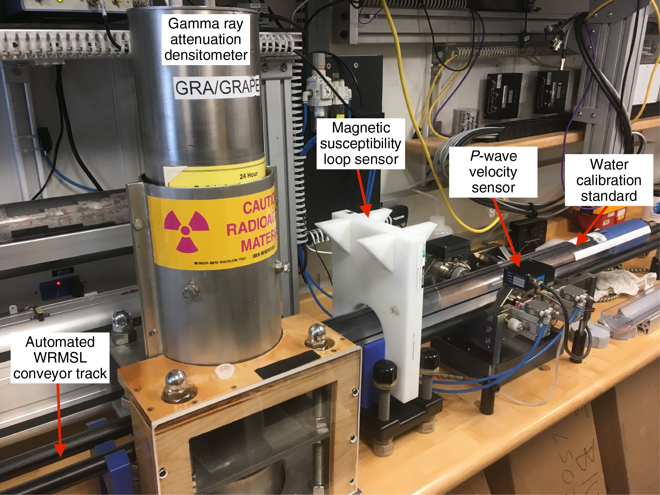
Figure F17. WRMSL.
During Expedition 379, GRA bulk density, magnetic susceptibility, and P-wave velocity were measured nondestructively with the WRMSL for each whole-round section. To optimize and streamline measurement procedures on the WRMSL and to better match other instrument measurement settings within the core processing line, sampling intervals (centimeters) and periods (seconds) were synchronized across all measurement sensors. For optimized sampling, it is critical that parameter settings are such that intervals and periods are multiples of each other. This ensures that the idle time of sensors is minimized and that the data quantity and quality are maximized for a given total core section scan period. When selecting sampling intervals, consideration was also given to the thickness interval that each sensor can resolve. Here, to achieve high-resolution measurements over the longest practical sampling period that would not negatively impact the overall flow of the core processing line, sampling intervals were set at 2.0 cm for each instrument measurement. Following the measurement of each final core section, a deionized water standard was run through the WRMSL to keep the instruments calibrated and to maintain quality assurance and quality control (QA/QC). All instruments were recalibrated if their measured standard values were outside the range of published tolerances (Blum, 1997).
Gamma ray attenuation bulk density
GRA bulk density is an overall measurement of density taken through a whole-round core at discrete intervals and the first measurement made on the WRMSL (Figure F17). This bulk density measurement relates to the physical properties of a formation such as porosity, grain size, consolidation state, mineral composition, and other disturbances or contrast. Here, the GRA instrument estimates bulk density through the measure of attenuation of a directed gamma ray beam through the core. The beam is produced by a 137Cs gamma ray source at radiation and energy levels of 370 MBq and 660 KeV, respectively. The source is mounted within a lead shield with a 5 mm collimator directly above the whole-round core track such that the beam is directed downward through each core section during measurement. A scintillation detector with an integrated photomultiplier tube is mounted underneath the core track (and opposite the 137Cs source) and measures the gamma radiation that passes through the core sections as they advance on the track. The principle behind the measurement of GRA bulk density is that medium-energy gamma rays (0.1–1 MeV) interact with the material of a formation mainly by Compton scattering and that the measured electron density of that scattering can be inverted to a material bulk density. For a known thickness of sample, the density (ρ) is proportional to the intensity of the attenuated gamma rays and can be expressed as
- I = the measured intensity of gamma rays passing through the sample,
- I0 = gamma ray source intensity,
- μ = Compton attenuation coefficient, and
- d = sample diameter.
The μ and I0 are treated as constants, such that ρ can be calculated from I.
GRA bulk density measurements are most accurate when made on a completely filled core liner with minimal drilling disturbance or discontinuities. When cores do not completely fill the core liner or are disturbed, measurements tend to underestimate true values. By default, the GRA instrument reports all measurements assuming that the sample diameter matches the internal diameter of the core liner (66 mm). This assumption is appropriate for most sediment cores obtained by the APC; however, for sediment cored by the XCB or RCB systems, core diameter is usually only 58 mm (or less). No correction for sample diameter has been applied for XCB and RCB core GRA measurements, so GRA bulk densities for these intervals are underestimated compared to true values. The spatial resolution of the GRA densitometer is less than ±1 cm, and it is calibrated with specific sealed calibration cores (one standard core liner filled with distilled water and aluminum cylinders of various diameters; see also Blum, 1997). Recalibration was performed as needed when the deionized water QA/QC standard deviated significantly (>2%) from 1 g/cm3. As previously noted, to maintain synchronized sampling across the WRMSL instruments, the sampling interval for the GRA densiometer was set at 2.0 cm with an integration time of 3 s. All collected GRA bulk density data were postprocessed for edge effects by “clipping” the first and last 4 cm of each section. Single-point outliers caused by drilling artifacts (e.g., voids, cracked core liners, or metal drill fragments) and any values <1 g/cm3 were also removed.
Magnetic susceptibility
Magnetic susceptibility was measured on each whole-round core section using a pass-through loop on the WRMSL immediately following the GRA bulk density measurement (Figure F17). Magnetic susceptibility (χ) is a dimensionless measure of the degree to which a material can be magnetized by an external magnetic field and is generally used as a relative proxy indicator for changes in composition, which can also be linked to paleoclimate-controlled depositional processes. Because magnetic susceptibility is measured at very low magnetic fields generally not exceeding 400 A/m, it is also often referred to as “low-field” susceptibility. If the ratio of the magnetization is expressed per unit volume, volume susceptibility is defined as
where M is the magnetization induced in the material by an external field of strength H. Magnetic susceptibility is most sensitive to formations containing a high concentration of ferromagnetic minerals (e.g., magnetite, hematite, and various other iron oxides). In addition, it is also sensitive to magnetic mineralogy and can be related to the origin of the materials in the core and their subsequent diagenesis. Ferromagnetic minerals typically have magnetic susceptibility values several orders of magnitude greater than their alteration products, such as clay. Diamagnetic minerals such as calcite, halite, or kaolinite, as well as water and plastic (core liner), have small or negative magnetic susceptibility values. Therefore, calcareous and siliceous biogenic deposits with very small amounts of clay and iron-bearing minerals often have values approaching the detection limit of the magnetic susceptibility instrument sensor.
All measurements were made using a Bartington MS2C loop sensor with a 90 mm diameter. On the WRMSL, an oscillator circuit in the sensor operates at a frequency of 565 Hz to avoid any potential interference between instruments (with an automatic software correction factor of 1.174), and a ~140 A/m AF produces a low-intensity, nonsaturating alternating magnetic field. Sediment sections going through the influence of this field cause a change in oscillator frequency. Frequency information is returned in pulse form to the susceptometer and converted into a magnetic susceptibility value. The loop sensor has a spatial resolution of 20 mm and a published accuracy of 2% (see also Blum, 1997). The output of the magnetic susceptibility sensors is set to dimensionless instrument units (IU), which are equivalent to 10−5 SI units. All returned values represent the mean of three discrete measurements. Magnetic susceptibility values reported in the text and figures of site reports will be in 10−5 SI units unless otherwise noted. The magnetic susceptibility instrument was automatically zeroed at the beginning of each run before the core entered the measurement loop. Also, instrument drift can occur during the period of a core section scan, so to correct for this drift, a zero-background measurement was taken at the end of a core section scan. As previously noted, to maintain synchronized sampling across the WRMSL instruments, the sampling interval for magnetic susceptibility was set at 2.0 cm. All collected magnetic susceptibility data were postprocessed for edge effects by “clipping” the first and last 4 cm of each section. Single-point outliers caused by drilling artifacts (e.g., voids, cracked core liners, or metal drill fragments) were also removed.
Compressional P-wave velocity
Compressional P-wave velocity was measured on each whole-round section using the PWL instrument on the WRMSL, immediately following the magnetic susceptibility measurement (Figure F17). P-wave velocity varies with the lithology, porosity, and bulk density of the measured material. In addition, the velocity can also be affected by the state of stress, lithostatic pressure, and/or fabric or degree of fracturing within the material. Velocity values are also controlled by the degree of consolidation and lithification or occurrence and abundance of free gas. Together with measurements of density, a P-wave sonic velocity can be used to calculate acoustic impedance, and with that, reflection coefficients. These calculations can then be used to derive synthetic seismograms to help estimate the depth of reflectors observed in seismic profiles. P-wave velocity (VP) is defined by the time required for a compressional wave to travel a specific distance,
where d is the path length of the wave across the core and tcore is the traveltime through the core.
During measurement by the PWL, the core section travels between two piezoelectric transducers mounted in stainless steel housings (a transmitter and a receiver). Acoustic coupling through an epoxy resin surface is enhanced by a water film supplied by an automated drip system. A 500 kHz pulse (2 μs wave period; 120 V) is produced at a repetition rate of 1 kHz and sent to the transmitter transducer, which then generates an ultrasonic compressional pulse at about 500 kHz (pulse timing is measured with a resolution of 50 ns). Pressure is applied to the actuators to ensure coupling between the transducers and the core liner, and the automated drip system maintains wet contacts on the transducers to ensure a reliable coupling is always established. The compressional P-wave then propagates horizontally through the core, is received by the receiver transducer on the opposite side, and is then amplified by an automatic gain control amplifier to produce the received signal. P-wave velocity transducers measure total traveltime of the compressional wave between transducers. A calibration of the PWL accounts for errors in the total distance (dtotal) and the total traveltime (ttotal). Errors on dtotal were assumed to come from the laser distance. The reported value represents the average of 100 discrete measurements at the set interval.
During measurement, a core liner of assumed thickness (L) surrounded each core section. The traveltime through the liner (tliner) was determined by measuring the total traveltime through a core liner filled with distilled water of known velocity (~1480 m/s). A correction (tdelay; system delay) was measured using the traveltime through a standard block of aluminum with a known thickness and a published velocity of 6295 m/s. Arrival time picks were chosen at the inflection point of the second lobe of the waveform, giving a second correction (tpulse) from the first arrival. During Expedition 379, tpulse and tdelay were combined and represented simply as ttotaldelay. Therefore, the velocity of the core is
- VP = velocity of the core (km/s),
- dtotal = measured diameter of core and liner (mm),
- L = liner wall thickness (mm),
- ttotal = total measured traveltime for pulse to travel through core and liner (µs),
- tliner = traveltime through liner (µs), and
- ttotaldelay = delay related to combined transducer faces, electronic circuitry, and peak detection procedures (µs).
The above equation assumes that the core completely fills the core liner. The WRMSL PWL was turned off for cores recovered with the XCB or RCB systems, which generally do not completely fill the core liner. Any measured P-wave signal can degenerate due to an incompletely filled core liner, any voids that are present, or attenuation caused by microcracks that formed during core recovery. This degeneration is partly reflected by the gain (signal strength) factor applied to the original signal by the automated gain control. However, signal strength also represents the grain size of the sediment, and low-strength signals can therefore not simply be interpreted as proportional to attenuation. As previously noted, to maintain synchronized sampling across the WRMSL instruments, the sampling interval for the PWL was set at 2.0 cm.
Natural Gamma Radiation Logger measurements
The NGRL measures the cumulative radiation emitted during natural decay of three long-lived radioisotopes: 40K, 232Th, and 238U (which have half-lives of 1.3 × 10⁹, 1.4 × 10¹⁰, and 4.4 × 10⁹ y, respectively). These isotopes adsorb to mainly clay minerals and are the primary source of the NGR in sediments or sedimentary rocks measured by the NGRL (Blum, 1997). Thus, high counts generally reflect the presence of fine-grained deposits, and relative changes are indicative of stratigraphic details and aid in core-to-core, core-to-wireline log data, and/or borehole correlations between holes.
The NGRL measures NGR on whole-round cores using a system described by the Integrated Ocean Drilling Program US Implementing Organization (USIO) (Texas A&M University, USA; Vasiliev et al., 2011; Dunlea et al., 2013) (Figure F18). The system consists of eight sodium iodide (NaI) detectors arranged along the core measurement axis at 20 cm intervals surrounding the lower half of the section (Figure F18B). The detector array is fitted with both passive (layers of lead) and active (plastic scintillators) shielding to reduce the background environmental and cosmic radiation. The overlying plastic scintillators detect incoming high-energy gamma and muon cosmic radiation and cancel this signal from the total counted by the NaI detectors.
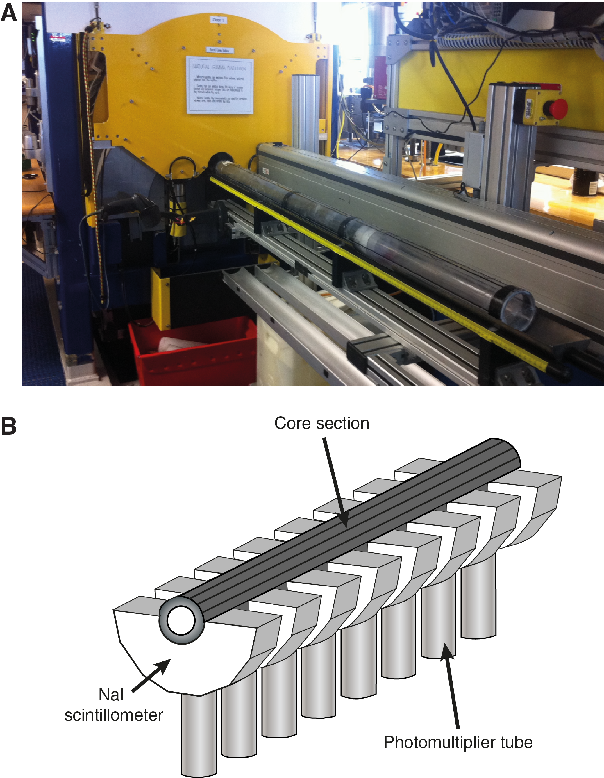
Figure F18. NGRL.
Quality of the measured energy spectrum in a core depends not only on the concentration of radionuclides but also the counting time. For optimization, a measurement run began with two sample positions 10 cm apart and a counting period of 300 s. After 300 s, the position was advanced downcore by 10 cm and counted again for 300 s. A run yielded a total of 16 measurements (10 cm apart) per 150 cm core section. Measurement times were ~5 min per measurement cycle or ~10 min per core section. This measurement scheme yielded statistically significant total counts. All collected NGR data were postprocessed for edge effects by clipping the first and last ~10 cm of each section to remove artifacts caused by the processing software. Single-point outliers caused by drilling artifacts (e.g., voids or cracked core liners) were also removed.
Thermal conductivity measurements
The coefficient of thermal conductivity represents the rate at which heat flows through a material, which is dependent on the chemical composition, porosity, density, structure, and fabric of the material (Blum, 1997). Thermal conductivity profiles of sediment and rock sections, along with in situ temperature measurements, are used to determine geothermal heat flow. Geothermal heat flow is an indicator of type and age of ocean crust, fluid circulation processes from various depths, and young magmatic and tectonic processes of continental crust (Dziadek et al., 2019).
After NGR measurements were completed, thermal conductivity was measured on one section per core with the TK04 (Teka Bolin) system (Table T6). A needle-probe method in full-space configuration for whole-round cores was used for soft sediments (Von Herzen and Maxwell, 1959), and a contact probe method in half-space configuration was used on split cores for harder, more lithified sediments. The probes each contain a heater wire and calibrated thermistor. For soft sediments, the needle probe was inserted into a 2 mm diameter hole drilled through the liner along a split-line. To avoid interference from airflow in the laboratory, the core was placed in an enclosed box outfitted with insulating foam (Figure F19). For harder or lithified sediments, half sections displaying the least amount of fracturing and most homogeneous portions of core were chosen for measurement. The sections were prepared for a puck-style contact probe by applying a small amount of deionized water onto the sediment surface and then gently wiping it with a sponge. This ensured proper contact between sediment and the probe. The puck probe was placed directly on the sediments and secured in place with a strap to ensure proper contact pressure. The entire section half was then placed in the insulated box to stabilize thermal conditions during measurements.
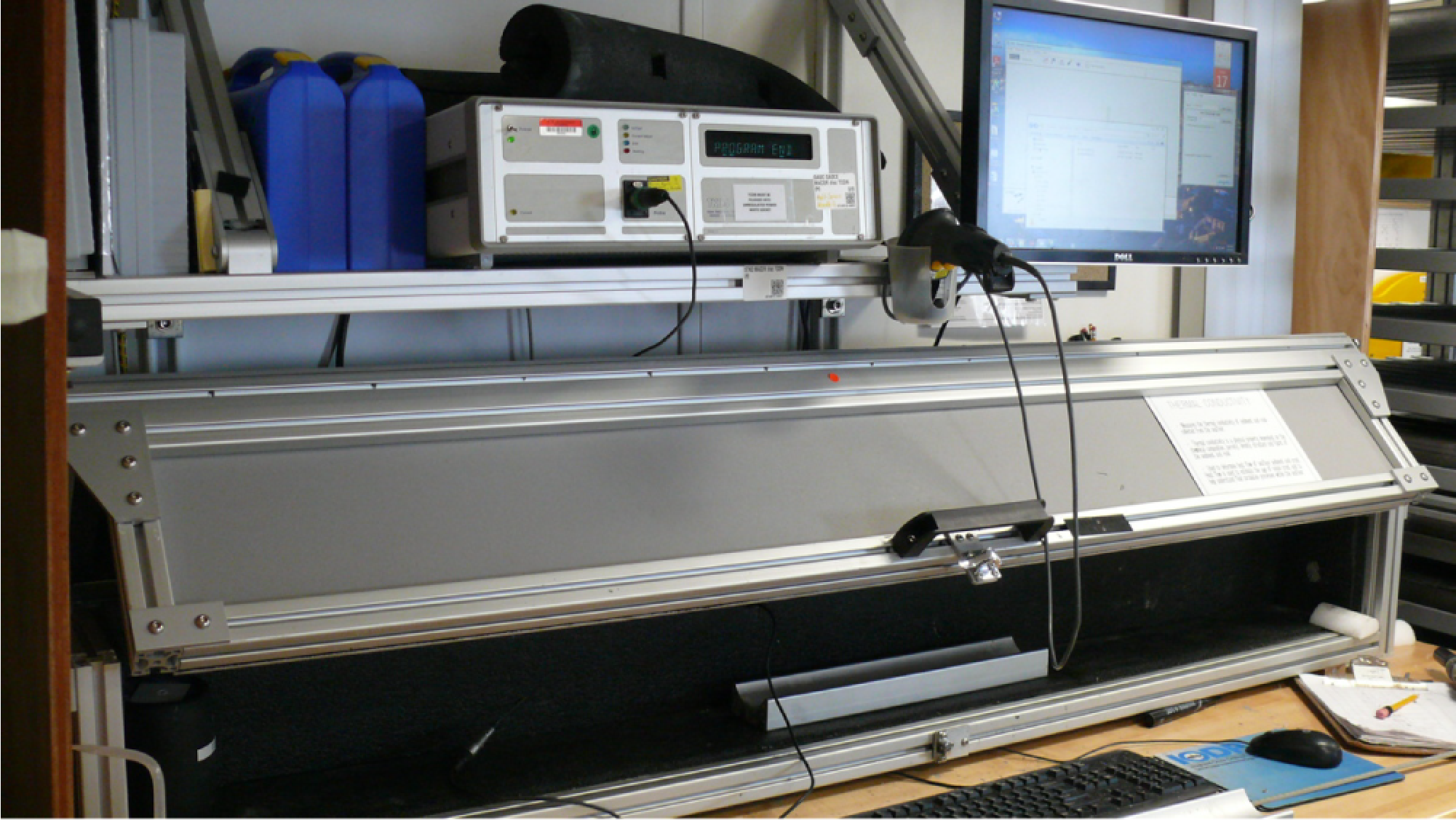
Figure F19. Shipboard station for thermal conductivity measurements.
The calibrated heat source of the probe was then turned on, and the increase in temperature was recorded over 80 s for the needle probe (soft sediments) and 60 s for the contact probe (hard or lithified sediments). A heating power of 0.8–2.5 W/m was typically used in soft sediments, and 0.5–2.5 W/m was used for lithified material. The solution to the heat conduction equation with a line source of heat was then fit to the temperature measurements to obtain the thermal conductivity. Because the probe is much more conductive than sediment or hard rock, the probe is assumed to be a perfect conductor. Under this assumption, the temperature of the superconductive probe has a linear relationship with the natural logarithm of the time after the initiation of the heat:
- T = temperature (K),
- q = heat input per unit length per unit time (J/m/s),
- k = thermal conductivity (W/[m·K]),
- t = time after the initiation of the heat (s), and
- C = instrumental constant.
Three measuring cycles were automatically performed to calculate average conductivity. A self-test, which included a drift study, was conducted at the beginning of each measurement cycle. Once the probe temperature stabilized, the heater circuit was closed and the temperature rise in the probe was recorded. Thermal conductivity was calculated from the rate of temperature rise while the heater current was flowing. Temperatures measured during the first 80 s of the needle probe heating cycle and 60 s of the contact probe heating cycle were fit to an approximate solution of a constantly heated line source (for details, see Kristiansen, 1982; Blum, 1997). Measurement errors were 5%–10%.
Section Half Multisensor Logger measurements
Color reflectance and magnetic susceptibility were measured on the archive-half cores using the SHMSL (Figure F20). Archive-half cores were covered with plastic wrap and placed on the SHMSL core track, above which an electronic platform moves along a track and records the height of the core surface. The laser sensor detects the location of the surface of the archive-half core, and then the instrument progresses along the core making measurements of MSP and color reflectance. During Expedition 379, color reflectance and MSP data were collected at 2 cm spacing.
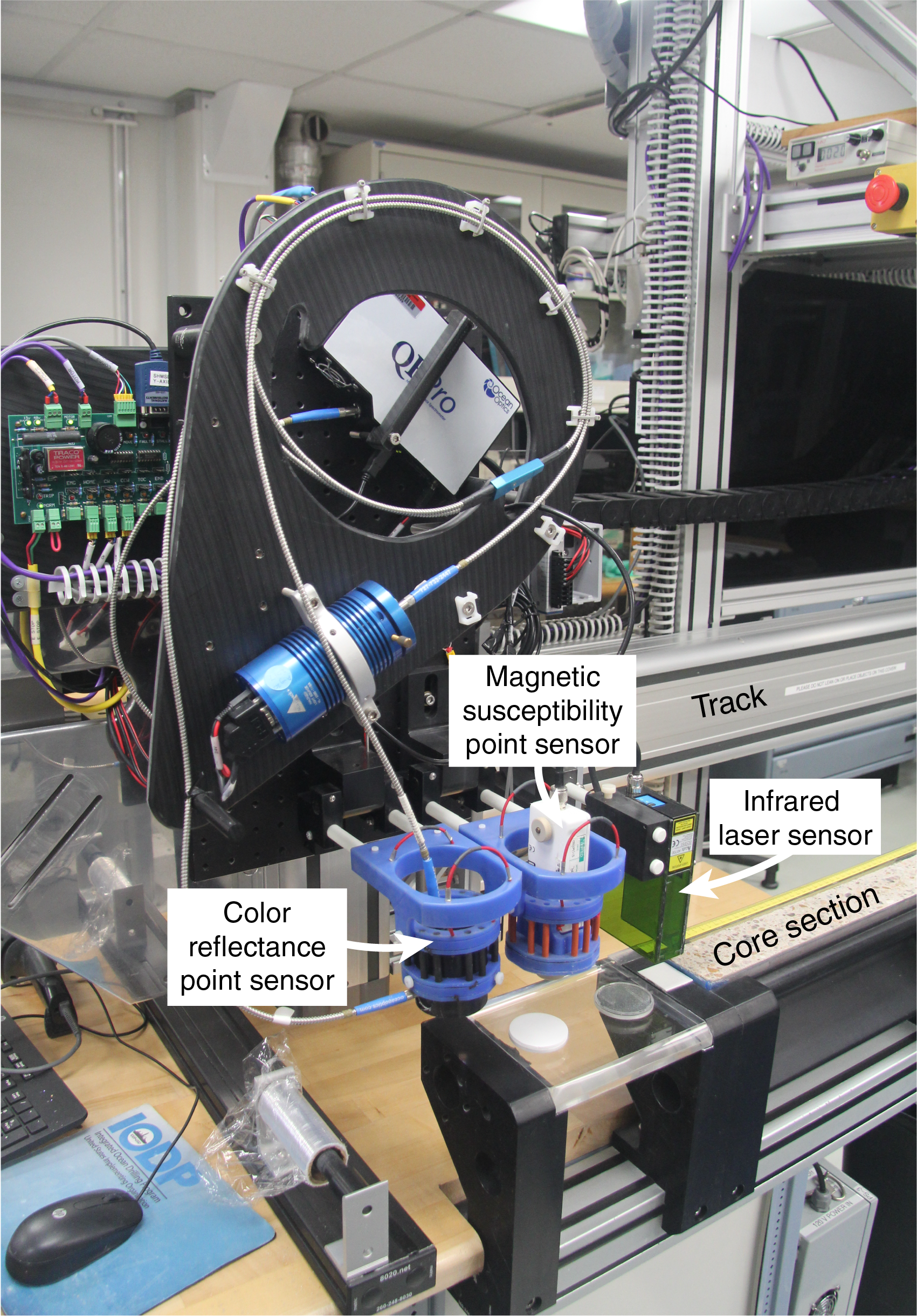
Figure F20. SHMSL.
Color reflectance spectrometry
The color reflectance spectrometry of the archive-half cores was measured using an Ocean Optics QE Pro detector integrating sphere and associated light sources covering wavelengths from UV through visible to near infrared. Each measurement was taken in 2 nm wide spectral bands from 390 to 732 nm. The data are reported using the L*a*b* color system, where L* is lightness, a* is redness (positive) versus greenness (negative), and b* is yellowness (positive) versus blueness (negative). The color reflectance spectrometer calibrates using two spectra, pure white (reference) and pure black (dark). Color calibration was conducted approximately once every 6 h (twice per shift). Additional details regarding measurement and interpretation of spectral data can be found in Balsam et al. (1997), Balsam and Damuth (2000), and Giosan et al. (2002).
Point magnetic susceptibility
MSP was measured with a Bartington MS2 meter and an MS2K contact probe with a flat 15 mm diameter round sensor with a field of influence of 25 mm and an operation frequency of 930 Hz. The instrument averages three measurements from the sensor for each offset with an accuracy of ~5%. The spatial resolution of the MSP sensor is ~3.8 mm, and values are reported in instrument units (which can also be converted to approximate dimensionless SI units by multiplying by 10−5). The MSP meter was calibrated by the manufacturer before installation on JOIDES Resolution and is quality checked every 6 h at the same time as color reflectance sensor calibration.
Section Half Measurement Gantry measurements
P-wave velocity measurements were performed on working-half cores using the SHMG. Measurements were typically made with the x-caliper on every other section of each core. Bayonet measurements in the y and z orientations were taken once per core, typically in Section 6 (Table T6). The bayonet measurements were discontinued when good contact in brittle sediments was no longer possible. X-caliper measurements were increased to once per section for XCB and RCB cores when the PWL on the WRMSL was not able to provide accurate velocity measurements. Measurements were taken at varying section intervals to accommodate lithologic variations, drilling disturbance, fractures, larger clasts, and general core quality.
P-wave velocity
P-wave velocities on working-half cores were measured with the P-wave caliper (PWC) and the P-wave bayonets (PWBs). The PWC measures the P-wave velocity vertically to the sectional plane of the core (x-axis), whereas the PWBs measure the cross-section (y-axis) and the long axis (z-axis) of the core (Figure F21). The system uses Panametrics-NDT Microscan delay line transducers that transmit at 500 KHz. During measurement, the signal transmitted through the core was recorded by the attached computer system, and the peak (P-wave arrival) was chosen via an automated algorithm in the processing software. In cases of a weak signal, the instrument operator manually picked the first arrival. The distance between transducers was measured with a built-in linear voltage displacement transformer (LVDT). Calibration was performed with an aluminum standard with a known thickness and a published velocity of 6295 m/s that matches the compressional P-wave measurements on the WRMSL. The determined system time delay from calibration was subtracted from the picked arrival time to give a traveltime of the P-wave through the sample. The thickness of the sample (calculated by LVDT in meters) was divided by the traveltime (in seconds) to calculate P-wave velocity in meters per second.
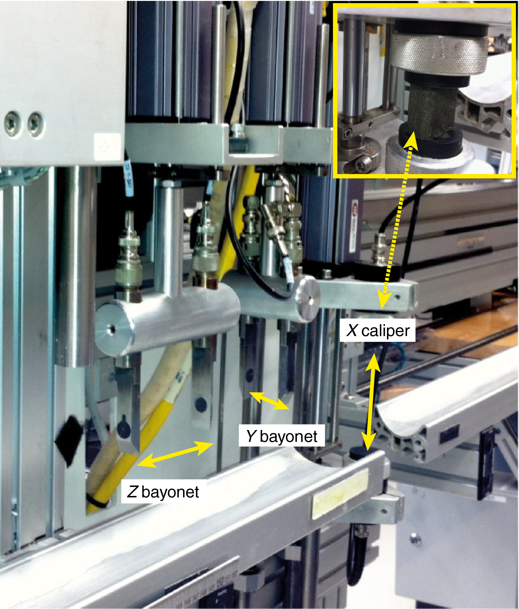
Figure F21. SHMG.
Moisture and density measurements
MAD measurements were collected on discrete samples from working halves to determine wet and dry bulk density, grain density, water content, and porosity. In soft sediments, ~10 cm3 samples were collected with a plastic syringe. Approximately three samples were collected from each core, typically from Sections 1, 3, and 5 at an offset of ~75 cm. In some cases, samples were moved to adjacent sections within cores to avoid disturbed sediments or avoid/target particular features in the core. In more lithified sediments, samples were taken adjacent to the samples that were cut and prepared for paleomagnetic measurements.
Sediment samples were placed in numbered, preweighed ~16 mL Wheaton glass vials for wet and dry sediment weighing, drying, and dry volume measurements. Wet sample mass was first measured on each vial before placing it in a convection oven for approximately 24 h at 105° ± 5°C to dry. Once dried, samples were then cooled in a desiccator for at least 3 h before dry mass and volume were measured. The weights of wet and dry sample masses were determined to a precision of 0.005 g using two Mettler Toledo electronic balances, with one balance acting as a reference (Figure F22A). A standard weight of similar value to the sample was placed upon the reference balance to increase accuracy. A computer averaging algorithm was used to compensate for the motion of the ship. The default measurement setting of the two balances was 300 measurements over an interval of ~1.5 min.
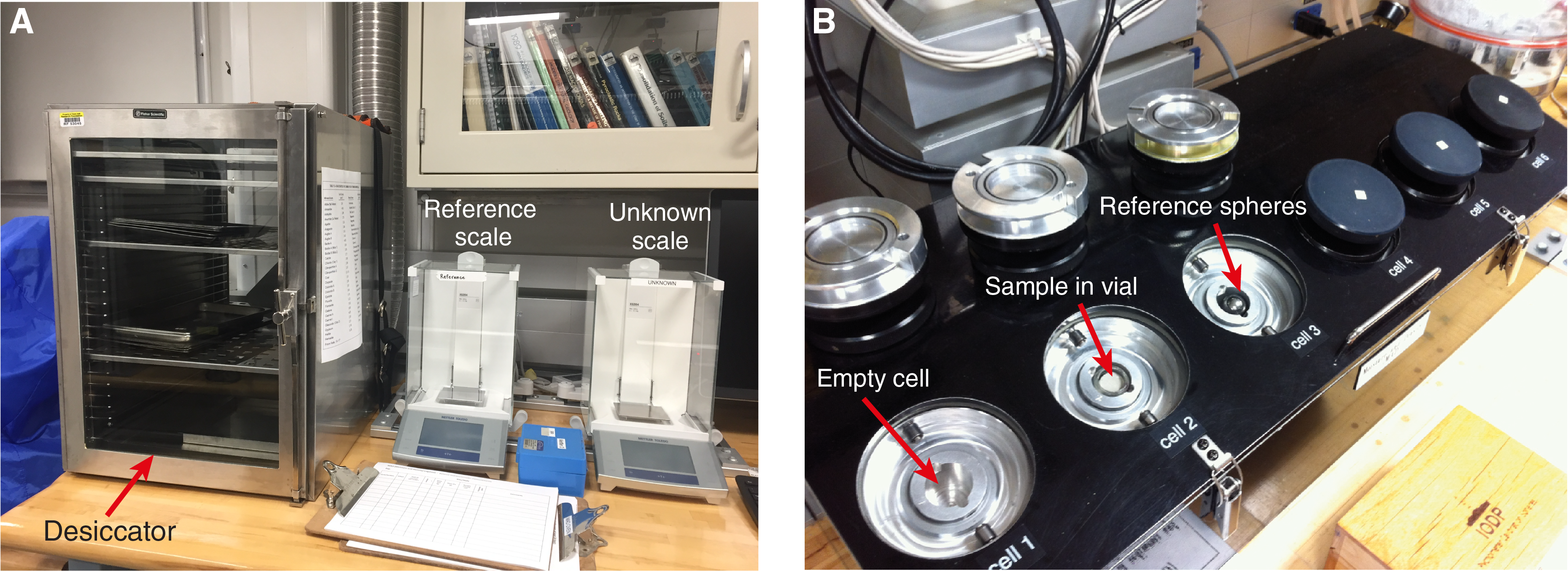
Figure F22. Equipment used for MAD analyses.
Dry sample volume was determined using a six-celled, custom-configured Micrometrics AccuPyc 1330TC helium-displacement pycnometer (hexapycnometer) (Figure F22B). The precision of each cell is 1% of the full-scale volume. Volume measurements are preceded by three purges of the sample chamber with helium warmed to ~28°C. Three measurement cycles were run for each sample. A reference volume (set of two calibration spheres) was periodically placed in each chamber to check for instrument drift and systematic error. The volumes occupied by the numbered Wheaton vials were calculated before the expedition by multiplying the weight of each vial against the average density of the vial glass. The procedures for the determination of these physical properties comply with the American Society for Testing and Materials (ASTM) designation (D) 2216 (ASTM International, 2019). The fundamental relation and assumptions for the calculations of all physical property parameters are discussed by Blum (1997) and summarized below. MAD properties reported and displayed in Physical properties in the Site U1532 chapter and Physical properties in the Site U1533 chapter (Wellner et al., 2021a, 2021b) were calculated using the MADMax software.
Mass and volume calculation
Wet mass (Mwet), dry mass (Mdry), and dry volume (Vdry) were measured in the laboratory. The ratio of mass (rm) is a computational constant of 0.965 (i.e., 0.965 g of freshwater per 1 g of seawater). Salt precipitated in sediment pores during the drying process is included in the Mdry and Vdry values. The mass of the evaporated water (Mwater) and salt (Msalt) in the sample are given by
respectively, where s is the assumed saltwater salinity (0.035%) corresponding to a pore water density (ρpw) of 1.024 g/cm3 (from experimental and empirical relations between salinity and density at laboratory conditions; Blum, 1997) and a salt density (ρsalt) of 2.22 g/cm3. The corrected mass of pore water (Mpw), volume of pore water (Vpw), mass of solids excluding salt (Msolid), volume of salt (Vsalt), volume of solids excluding salt (Vsolid), and wet volume (Vwet) are, respectively,
Wet (or total) volume (Vt), dry mass (Mdry), and dry volume (Vdry) were measured in the laboratory. Total mass, including freshwater in the pores, is calculated using a water density of 1 g/cm3 by
Assuming a pore water density of 1.024 g/cm3, the volume of the pore water is calculated as
Finally, the mass of the pore water is calculated as
Calculation of bulk properties
For all sediment samples, water content (w) is expressed as the ratio of mass of pore water to wet sediment (total) mass:
Wet bulk density (ρwet), dry bulk density (ρdry), sediment grain density (ρsolid), porosity (φ), and void ratio (VR) are calculated as
Downhole formation temperature measurements
In situ temperature measurements were made with the APCT-3 (Heesemann et al., 2006) in Holes U1532A and U1532B. The APCT-3 fits directly into the APC coring shoe and consists of a battery pack, a data logger, and a platinum resistance-temperature device calibrated over a temperature range from 0° to 30°C. Before entering the borehole, the tool is first stopped at the mudline for 5 min to thermally equilibrate with bottom water. When the APCT-3 moves into the formation, frictional heating causes an instantaneous temperature rise. This heat gradually dissipates into the surrounding sediment as the APCT-3 equilibrates to the temperature of the sediment. Thus, after the APCT-3 enters the formation, it is held in place for ~10 min while the APCT-3 records the temperature of the cutting shoe every 1 s.
The equilibrium temperature of the sediment is estimated by applying a mathematical heat-conduction model to the temperature decay record (Horai and Von Herzen, 1985). The synthetic thermal decay curve for the APCT-3 is a function of the geometry and thermal properties of the probe and the sediment (Bullard, 1954; Horai and Von Herzen, 1985). Equilibrium temperature is estimated by applying a fitting procedure (Pribnow et al., 2000). However, if the APC system does not achieve a full stroke or if the ship has pulled the APC up from full penetration, the temperature equilibration curve is disturbed and the temperature determination is less accurate. The nominal accuracy of the APCT-3 temperature measurements is ±0.05°C.
APCT-3 temperature data were combined with measurements of thermal conductivity (see Thermal conductivity measurements) collected from whole-round core sections to obtain heat flow values. Heat flow is calculated according to the Bullard method to be consistent with the synthesis of ODP heat flow data by Pribnow et al. (2000).
References
Acton, G., Morris, A., Musgrave, R., Zhao, X., and IODP SRM Personnel, 2017. Assessment of the New Superconducting Rock Magnetometer (SRM) on the JOIDES Resolution. http://iodp.tamu.edu/publications/JRSO/SRM_Workshop_2017.pdf
Akiba, F., 1982. Late Quaternary diatom biostratigraphy of the Bellingshausen Sea, Antarctic Ocean. Report of the Technology Research Center, Japan National Oil Corporation, 16:31–74.
Anderson, J.B., 1975. Ecology and distribution of foraminifera in the Weddell Sea of Antarctica. Micropaleontology, 21(1):69–96. https://doi.org/10.2307/1485156
Andrén, T., Jørgensen, B.B., Cotterill, C., Green, S., Andrén, E., Ash, J., Bauersachs, T., Cragg, B., Fanget, A.-S., Fehr, A., Granoszewski, W., Groeneveld, J., Hardisty, D., Herrero-Bervera, E., Hyttinen, O., Jensen, J.B., Johnson, S., Kenzler, M., Kotilainen, A., Kotthoff, U., Marshall, I.P.G., Martin, E., Obrochta, S., Passchier, S., Quintana Krupinski, N., Riedinger, N., Slomp, C., Snowball, I., Stepanova, A., Strano, S., Torti, A., Warnock, J., Xiao, N., and Zhang, R., 2015. Methods. In Andrén, T., Jørgensen, B.B., Cotterill, C., Green, S., and the Expedition 347 Scientists, Proceedings of the Integrated Ocean Drilling Program, 347: College Station, TX (Integrated Ocean Drilling Program). https://doi.org/10.2204/iodp.proc.347.102.2015
Arney, J.E., McGonigal, K.L., Ladner, B.C., and Wise, S.W., Jr., 2003. Lower Oligocene to middle Miocene diatom biostratigraphy of ODP Site 1140, Kerguelen Plateau. In Frey, F.A., Coffin, M.F., Wallace, P.J., and Quilty, P.G. (Eds.), Proceedings of the Ocean Drilling Program, Scientific Results, 183: College Station, TX (Ocean Drilling Program), 1–21. https://doi.org/10.2973/odp.proc.sr.183.009.2003
Askin, R.A., and Raine, J.I., 2000. Oligocene and early Miocene terrestrial palynology of the Cape Roberts Drillhole CRP-2/2A, Victoria Land Basin, Antarctica. Terra Antartica, 7(4):493–501. https://epic.awi.de/id/eprint/27369/1/Ask2000a.pdf
ASTM International, 2019. Standard Test Methods for Laboratory Determination of Water (Moisture) Content of Soil and Rock by Mass (Standard D2216-19): West Conshohocken, PA (ASTM International). https://doi.org/10.1520/D2216-19
Baldauf, J.G., and Barron, J.A., 1991. Diatom biostratigraphy: Kerguelen Plateau and Prydz Bay regions of the Southern Ocean. In Barron, J., Larsen, B., et al., Proceedings of the Ocean Drilling Program, Scientific Results, 119: College Station, TX (Ocean Drilling Program), 547–598. https://doi.org/10.2973/odp.proc.sr.119.135.1991
Balsam, W.L., and Damuth, J.E., 2000. Further investigations of shipboard vs. shore-based spectral data: implications for interpreting Leg 164 sediment composition. In Paull, C.K., Matsumoto, R., Wallace, P., and Dillon, W.P. (Eds.), Proceedings of the Ocean Drilling Program, Scientific Results, 164: College Station, TX (Ocean Drilling Program), 313–324. https://doi.org/10.2973/odp.proc.sr.164.222.2000
Balsam, W.L., Damuth, J.E., and Schneider, R.R., 1997. Comparison of shipboard vs. shore-based spectral data from Amazon Fan cores: implications for interpreting sediment composition. In Flood, R.D., Piper, D.J.W., Klaus, A., and Peterson, L.C. (Eds.), Proceedings of the Ocean Drilling Program, Scientific Results, 155: College Station, TX (Ocean Drilling Program), 193–215. https://doi.org/10.2973/odp.proc.sr.155.210.1997
Barron, J.A., 2003. Planktonic marine diatom record of the past 18 m.y.: appearances and extinctions in the Pacific and Southern Oceans. Diatom Research, 18(2):203–224. https://doi.org/10.1080/0269249X.2003.9705588
Barron, J.A., Baldauf, J.G., Barrera, E., Caulet, J.-P., Huber, B.T., Keating, B.H., Lazarus, D., Sakai, H., Thierstein, H.R., and Wei, W., 1991. Biochronologic and magnetochronologic synthesis of Leg 119 sediments from the Kerguelen Plateau and Prydz Bay, Antarctica. In Barron, J., Larsen, B., et al., Proceedings of the Ocean Drilling Program, Scientific Results, 119: College Station, TX (Ocean Drilling Program), 813–847. https://doi.org/10.2973/odp.proc.sr.119.188.1991
Berggren, W.A., 1992. Neogene planktonic foraminifer magnetobiostratigraphy of the southern Kerguelen Plateau (Sites 747, 748, and 751). In Wise, S.W., Jr., Schlich, R., et al., Proceedings of the Ocean Drilling Program, Scientific Results, 120: College Station, TX (Ocean Drilling Program), 631–647. https://doi.org/10.2973.odp.proc.sr.120.153.1992
Bijl, P.K., Houben, A.J.P., Bruls, A., Pross, J., and Sangiorgi, F., 2018. Stratigraphic calibration of Oligocene–Miocene organic-walled dinoflagellate cysts from offshore Wilkes Land, East Antarctica, and a zonation proposal. Journal of Micropaleontology, 37(1):105–138. https://doi.org/10.5194/jm-37-105-2018
Biscaye, P.E., 1964. Distinction between kaolinite and chlorite in recent sediments by X-ray diffraction. American Mineralogist, 49:1281–1289. http://www.minsocam.org/ammin/AM49/AM49_1281.pdf
Biscaye, P.E., 1965. Mineralogy and sedimentation of recent deep-sea clay in the Atlantic Ocean and adjacent seas and oceans. Geological Society of America Bulletin, 76(7):803–831. https://doi.org/10.1130/0016-7606(1965)76[803:MASORD]2.0.CO;2
Blum, P., 1997. Technical Note 26: Physical Properties Handbook—A Guide to the Shipboard Measurement of Physical Properties of Deep-Sea Cores. Ocean Drilling Program. https://doi.org/10.2973/odp.tn.26.1997
Bohaty, S.M., Scherer, R.P., and Harwood, D.M., 1998. Quaternary diatom biostratigraphy and palaeoenvironments of the CRP-1 drillcore, Ross Sea, Antarctica. Terra Antartica, 5(3):431–453. http://epic.awi.de/27451/1/Boh1998a.pdf
Bohaty, S.M., Wise, S.W., Jr., Duncan, R.A., Moore, C.L., and Wallace, P.J., 2003. Neogene diatom biostratigraphy, tephra stratigraphy, and chronology of ODP Hole 1138A, Kerguelen Plateau. In Frey, F.A., Coffin, M.F., Wallace, P.J., and Quilty, P.G. (Eds.), Proceedings of the Ocean Drilling Program, Scientific Results, 183: College Station, TX (Ocean Drilling Program), 1–53. https://doi.org/10.2973/odp.proc.sr.183.016.2003
Brady, H.T., 1979. The extraction and interpretation of diatom zones in Dry Valley Drilling Project Holes 10 and 11, Taylor Valley, South Victoria Land, Antarctica. Memoirs of National Institute of Polar Research, 13:150–163.
Brindley, G.W., and Brown, G. (Eds.), 1980. Crystal Structures of Clay Minerals and Their X-ray Identification. Mineralogical Society Monograph, 5. https://doi.org/10.1180/mono-5
Bullard, E.C., 1954. The flow of heat through the floor of the Atlantic Ocean. Proceedings of the Royal Society of London, Series A: Mathematical, Physical and Engineering Sciences, 222(1150):408–429. https://doi.org/10.1098/rspa.1954.0085
Cantrill, D.J., and Poole, I., 2012. The Vegetation of Antarctica through Geological Time: Cambridge, United Kingdom (Cambridge University Press). https://doi.org/10.1017/CBO9781139024990
Caulet, J.-P., 1991. Radiolarians from the Kerguelen Plateau, Leg 119. In Barron, J., Larsen, B., et al., Proceedings of the Ocean Drilling Program, Scientific Results, 119: College Station, TX (Ocean Drilling Program), 513–546. https://doi.org/10.2973/odp.proc.sr.119.137.1991
Censarek, B., and Gersonde, R., 2002. Miocene diatom biostratigraphy at ODP Sites 689, 690, 1088, 1092 (Atlantic sector of the Southern Ocean). Marine Micropaleontology, 45(3–4):309–356. https://doi.org/10.1016/S0377-8398(02)00034-8
Ciesielski, P.F., 1983. The Neogene and Quaternary diatom biostratigraphy of subantarctic sediments, Deep Sea Drilling Project Leg 71. In Ludwig, W.J., Krasheninnikov, V.A., et al., Initial Reports of the Deep Sea Drilling Project, 71: Washington, DC (U.S. Government Printing Office), 635–666. https://doi.org/10.2973/dsdp.proc.71.125.1983
Cifelli, R., and Scott, G., 1986. Stratigraphic record of the Neogene Globorotaliid radiation (planktonic Foraminiferida). Smithsonian Contributions to Paleobiology, 58. https://repository.si.edu/bitstream/handle/10088/1980/SCtP-0058-Lo_res.pdf
Clowes, C.D., Hannah, M.J., Wilson, G.J., and Wrenn, J.H., 2016a. Marine palynostratigraphy and new species from the Cape Roberts drill-holes, Victoria Land Basin, Antarctica. Marine Micropaleontology, 126:65–84. https://doi.org/10.1016/j.marmicro.2016.06.003
Clowes, C.D., Prebble, J.G., Crouch, E.M., and Roncaglia, L., 2016b. Development and multi-operator calibration of a standardised palynofacies analysis technique. GNS Science Report, 2016/19. https://doi.org/10.21420/G2SG6B
Cody, R., Levy, R., Crampton, J., Naish, T., Wilson, G., and Harwood, D., 2012. Selection and stability of quantitative stratigraphic age models: Plio–Pleistocene glaciomarine sediments in the ANDRILL 1B drillcore, McMurdo Ice Shelf. Global and Planetary Change, 96–97:143–156. https://doi.org/10.1016/j.gloplacha.2012.05.017
Cody, R.D., Levy, R.H., Harwood, D.M., and Sadler, P.M., 2008. Thinking outside the zone: high-resolution quantitative diatom biochronology for the Antarctic Neogene. Palaeogeography, Palaeoclimatology, Palaeoecology, 260(1–2):92–121. https://doi.org/10.1016/j.palaeo.2007.08.020
Cremer, H., Roberts, D., McMinn, A., Gore, D., and Melles, M., 2003. The Holocene diatom flora of Marine Bays in the Windmill Islands, East Antarctica. Botanica Marina, 46(1):82–106. https://doi.org/10.1515/BOT.2003.010
Crundwell, M.P., Morgans, H.E.G., and Hollis, C.J., 2016. Micropaleontological report on dredge samples collected during the 2015 VESPA (Volcanic Evolution of South Pacific Arcs) expedition. GNS Science Internal Report.
De Schepper, S., Fischer, E.I., Groeneveld, J., Head, M.J., and Matthiessen, J., 2011. Deciphering the palaeoecology of late Pliocene and early Pleistocene dinoflagellate cysts. Palaeogeography, Palaeoclimatology, Palaeoecology, 309(1–2):17–32. https://doi.org/10.1016/j.palaeo.2011.04.020
Droser, M.L., and Bottjer, D.J., 1986. A semiquantitative field classification of ichnofabric. Journal of Sedimentary Research, 56(4):558–559. https://doi.org/10.1306/212F89C2-2B24-11D7-8648000102C1865D
Dunlea, A.G., Murray, R.W., Harris, R.N., Vasiliev, M.A., Evans, H., Spivack, A.J., and D’Hondt, S., 2013. Assessment and use of NGR instrumentation on the JOIDES Resolution to quantify U, Th, and K concentrations in marine sediment. Scientific Drilling, 15:57–63. https://doi.org/10.2204/iodp.sd.15.05.2013
Dziadek, R., Gohl, K., Kaul, N. and the Science Team of Expedition PS104, 2019. Elevated geothermal surface heat flow in the Amundsen Sea Embayment, West Antarctica. Earth and Planetary Science Letters, 506:530–539. https://doi.org/10.1016/j.epsl.2018.11.003
Ekdale, A.A., Bromley, R.G., and Pemberton, S.G. (Eds.), 1984. Ichnology: The Use of Trace Fossils in Sedimentology and Stratigraphy. SEPM Short Course, 15. https://doi.org/10.2110/scn.84.15
Esper, O., and Zonneveld, K.A.F., 2007. The potential of organic-walled dinoflagellate cysts for the reconstruction of past sea-surface conditions in the Southern Ocean. Marine Micropaleontology, 65(3–4):185–212. https://doi.org/10.1016/j.marmicro.2007.07.002
Esquevin, J., 1969. Influence de la composition chimique des illites sur le cristallinité. Bulletin du Centre de recherches de Pau, 3:147–154.
Expedition 301 Scientists, 2005. Methods. In Fisher, A.T., Urabe, T., Klaus, A., and the Expedition 301 Scientists, Proceedings of the Integrated Ocean Drilling Program, 301: College Station, TX (Integrated Ocean Drilling Program Management International, Inc.). https://doi.org/10.2204/iodp.proc.301.105.2005
Expedition 318 Scientists, 2011. Methods. In Escutia, C., Brinkhuis, H., Klaus, A., and the Expedition 318 Scientists, Proceedings of the Integrated Ocean Drilling Program, 318: Tokyo (Integrated Ocean Drilling Program Management International, Inc.). https://doi.org/10.2204/iodp.proc.318.102.2011
Fenner, J., Schrader, H.-J., and Wienigk, H., 1976. Diatom phytoplankton studies in the southern Pacific Ocean: composition and correlation to the Antarctic Convergence and its paleoecological significance. In Hollister, C.D., Craddock, C., et al., Initial Reports of the Deep Sea Drilling Project, 35: Washington, DC (U.S. Government Printing Office), 757–813. https://doi.org/10.2973/dsdp.proc.35.app3.1976
Fenner, J.M., 1991. Late Pliocene–Quaternary quantitative diatom stratigraphy in the Atlantic sector of the Southern Ocean. In Ciesielski, P.F., Kristoffersen, Y., et al., Proceedings of the Ocean Drilling Program, Scientific Results, 114: College Station, TX (Ocean Drilling Program), 97–120. https://doi.org/10.2973/odp.proc.sr.114.133.1991
Fillon, R.H., 1974. Late Cenozoic foraminiferal paleoecology of the Ross Sea, Antarctica. Micropaleontology, 20(2):129–151. https://doi.org/10.2307/1485056
Florindo, F., Farmer, R.K., Harwood, D.M., Cody, R.D., Levy, R., Bohaty, S.M., Carter, L., and Winkler, A., 2013. Paleomagnetism and biostratigraphy of sediments from Southern Ocean ODP Site 744 (southern Kerguelen Plateau): implications for early-to-middle Miocene climate in Antarctica. Global and Planetary Change, 110(C):434–454. https://doi.org/10.1016/j.gloplacha.2013.05.004
Gersonde, R., 1990. Taxonomy and morphostructure of Neogene diatoms from the Southern Ocean, ODP Leg 113. In Barker, P.F., Kennett, J.P., et al., Proceedings of the Ocean Drilling Program, Scientific Results, 113: College Station, TX (Ocean Drilling Program), 791–802. https://doi.org/10.2973/odp.proc.sr.113.128.1990
Gersonde, R., 1991. Taxonomy and morphostructure of late Neogene diatoms from the Maude Rise (Antarctic Ocean). Polarforschung, 59(3):141–171. http://epic.awi.de/28264/1/Polarforsch1989_3_4.pdf
Gersonde, R., Abelmann, A., Burckle, L.H., Hamilton, N., Lazarus, D., McCartney, K., O’Brien, P., Spieß, V., and Wise, S.W., Jr., 1990. Biostratigraphic synthesis of Neogene siliceous microfossils from the Antarctic Ocean, ODP Leg 113 (Weddell Sea). In Barker, P.F., Kennett, J.P., et al., Proceedings of the Ocean Drilling Program, Scientific Results, 113: College Station, TX (Ocean Drilling Program), 915–936. https://doi.org/10.2973/odp.proc.sr.113.209.1990
Gersonde, R., and Bárcena, M.A., 1998. Revision of the upper Pliocene: Pleistocene diatom biostratigraphy for the northern belt of the Southern Ocean. Micropaleontology, 44(1):84–98. https://doi.org/10.2307/1486086
Gersonde, R., and Burckle, L.H., 1990. Neogene diatom biostratigraphy of ODP Leg 113, Weddell Sea (Antarctic Ocean). In Barker, P.F., Kennett, J.P., et al., Proceedings of the Ocean Drilling Program, Scientific Results, 113: College Station, TX (Ocean Drilling Program), 761–789. https://doi.org/10.2973/odp.proc.sr.113.126.1990
Gieskes, J.M., Gamo, T., and Brumsack, H., 1991. Technical Note 15: Chemical Methods for Interstitial Water Analysis Aboard JOIDES Resolution. Ocean Drilling Program. https://doi.org/10.2973/odp.tn.15.1991
Giosan, L., Flood, R.D., and Aller, R.C., 2002. Paleoceanographic significance of sediment color on western North Atlantic drifts: I. Origin of color. Marine Geology, 189(1–2):25–41. https://doi.org/10.1016/S0025-3227(02)00321-3
Gohl, K., Wellner, J.S., and Klaus, A., 2017. Expedition 379 Scientific Prospectus: Amundsen Sea West Antarctic Ice Sheet History. International Ocean Discovery Program. https://doi.org/10.14379/iodp.sp.379.2017
Gohl, K., Wellner, J.S., Klaus, A., and the Expedition 379 Scientists, 2021. Supplementary material, https://doi.org/10.14379/iodp.proc.379supp.2021. Supplement to Gohl, K., Wellner, J.S., Klaus, A., and the Expedition 379 Scientists, Amundsen Sea West Antarctic Ice Sheet History. Proceedings of the International Ocean Discovery Program, 379: College Station, TX (International Ocean Discovery Program). https://doi.org/10.14379/iodp.proc.379.2021
Gombos, A.M., Jr., 1976. Paleogene and Neogene diatoms from the Falkland Plateau and Malvinas Outer Basin: Leg 36, Deep Sea Drilling Project. In Barker, P.F., Dalziel, I.W.D. et al., Initial Reports of the Deep Sea Drilling Project, 36: Washington, DC (U.S. Government Printing Office), 575–687. https://doi.org/10.2973/dsdp.proc.36.111.1977
Graber, K.K., Pollard, E., Jonasson, B., and Schulte, E. (Eds.), 2002. Technical Note 31: Overview of Ocean Drilling Program engineering tools and hardware. Ocean Drilling Program. https://doi.org/10.2973/odp.tn.31.2002
Gradstein, F.M., Ogg, J.G., Schmitz, M.D., and Ogg, G.M. (Eds.), 2012. The Geological Time Scale 2012: Amsterdam (Elsevier). https://doi.org/10.1016/C2011-1-08249-8
Hambrey, M., and Victoria University of Wellington Antarctic Research Centre, 1997. Cape Roberts Project Core Logging Manual: Coring for Antarctic Tectonic and Climatic History: Wellington, New Zealand (Antarctic Research Centre, Research School of Earth Sciences, Victoria University of Wellington). https://trove.nla.gov.au/version/8486761
Hannah, M.J., 2006. The palynology of ODP Site 1165, Prydz Bay, East Antarctica: a record of Miocene glacial advance and retreat. Palaeogeography, Palaeoclimatology, Palaeoecology, 231(1–2):120–133. https://doi.org/10.1016/j.palaeo.2005.07.029
Hannah, M.J., Wilson, G.J., and Wrenn, J.H., 2000. Oligocene and Miocene marine palynomorphs from CRP-2/2A, Victorialand Basin, Antarctica. Terra Antarctica, 7(4):503–511. http://epic.awi.de/27368/1/Han2000f.pdf
Harland, R., and Pudsey, C.J., 2002. Protoperidiniacean dinoflagellate cyst taxa from the upper Miocene of ODP Leg 178, Antarctic Peninsula. Review of Palaeobotany and Palynology, 120(3–4):263–284. https://doi.org/10.1016/S0034-6667(02)00080-5
Harwood, D.M., 1986. Diatoms. In Barrett, P.J. (Ed.), Antarctic Cenozoic History from the MSSTS-1 Drillhole, McMurdo Sound. DSIR Bulletin (New Zealand), 237:69–107.
Harwood, D.M., 1989. Siliceous microfossils. In Barrett, P.J. (Ed.), Antarctic Cenozoic History from the CIROS-1 Drillhole, McMurdo Sound. DSIR Bulletin (New Zealand), 245:67–97.
Harwood, D.M., Lazarus, D.B., Abelmann, A., Aubry, M.-P., Berggren, W.A., Heider, F., Inokuchi, H., Maruyama, T., McCartney, K., Wei, W., and Wise, S.W., Jr., 1992. Neogene integrated magnetobiostratigraphy of the central Kerguelen Plateau, Leg 120. In Wise, S.W., Jr., Schlich, R., et al., Proceedings of the Ocean Drilling Program, Scientific Results, 120: College Station, TX (Ocean Drilling Program), 1031–1052. https://doi.org/10.2973/odp.proc.sr.120.185.1992
Harwood, D.M., and Maruyama, T., 1992. Middle Eocene to Pleistocene diatom biostratigraphy of Southern Ocean sediments from the Kerguelen Plateau, Leg 120. In Wise, S.W., Jr., Schlich, R., et al., Proceedings of the Ocean Drilling Program, Scientific Results, 120: College Station, TX (Ocean Drilling Program), 683–733. https://doi.org/10.2973/odp.proc.sr.120.160.1992
Harwood, D.M., Scherer, R.P., and Webb, P.-N., 1989. Multiple Miocene marine productivity events in West Antarctica as recorded in upper Miocene sediments beneath the Ross Ice Shelf (Site J-9). Marine Micropaleontology, 15(1–2):91–115. https://doi.org/10.1016/0377-8398(89)90006-6
Hays, J.D., and Opdyke, N.D., 1967. Antarctic radiolaria, magnetic reversals, and climate change. Science, 158(3804):1001–1011. https://www.jstor.org/stable/172295
Heesemann, M., Villinger, H., Fisher, A.T., Tréhu, A.M., and White, S., 2006. Data report: testing and deployment of the new APCT-3 tool to determine in situ temperatures while piston coring. In Riedel, M., Collett, T.S., Malone, M.J., and the Expedition 311 Scientists. Proceedings of the Integrated Ocean Drilling Program, 311: Washington, DC (Integrated Ocean Drilling Program Management International, Inc.). https://doi.org/10.2204/iodp.proc.311.108.2006
Hilgen, F.J., Lourens, L.J., and Van Dam, J.A., 2012. The Neogene period. With contributions by A.G. Beu, A.F. Boyes, R.A. Cooper, W. Krijgsman, J.G. Ogg, W.E. Piller, and D.S. Wilson. In Gradstein, F.M., Ogg, J.G., Schmitz, M.D., and Ogg, G.M. (Eds.), The Geologic Time Scale: Oxford, United Kingdom (Elsevier), 923–978. https://doi.org/10.1016/B978-0-444-59425-9.00029-9
Horai, K., and Von Herzen, R.P., 1985. Measurement of heat flow on Leg 86 of the Deep Sea Drilling Project. In Heath, G.R., Burckle, L.H., et al., Initial Reports of the Deep Sea Drilling Project, 86: Washington, DC (U.S. Government Printing Office), 759–777. https://doi.org/10.2973/dsdp.proc.86.135.1985
Hornibrook, N.d.B., 1982. Late Miocene to Pleistocene Globorotalia (Foraminiferida) from DSDP Leg 29, Site 284, southwest Pacific. New Zealand Journal of Geology and Geophysics, 25(1):83–99. https://doi.org/10.1080/00288306.1982.10422507
Hornibrook, N.d.B., Brazier, R.C., and Strong, C.P., 1989. Manual of New Zealand Permian to Pleistocene foraminiferal biostratigraphy. New Zealand Geological Survey Paleontological Bulletin, 56.
Igarashi, A., Numanami, H., Tsuchiya, Y., and Fukuchi, M., 2001. Bathymetric distribution of fossil foraminifera within marine sediment cores from the eastern part of Lützow-Holm Bay, East Antarctica, and its paleoceanographic implications. Marine Micropaleontology, 42(3–4):125–162. https://doi.org/10.1016/S0377-8398(01)00004-4
Ishman, S.E., and Domack, E.W., 1994. Oceanographic controls on benthic foraminifers from the Bellingshausen margin of the Antarctic Peninsula. Marine Micropaleontology, 24(2):119–155. https://doi.org/10.1016/0377-8398(94)90019-1
Iwai, M., Acton, G.D., Lazarus, D., Osterman, L.E., and Williams, T., 2002. Magnetobiochronologic synthesis of ODP Leg 178 rise sediments from the Pacific sector of the Southern Ocean: Sites 1095, 1096, and 1101. In Barker, P.F., Camerlenghi, A., Acton, G.D., and Ramsay, A.T.S. (Eds.), Proceedings of the Ocean Drilling Program, Scientific Results, 178: College Station, TX (Ocean Drilling Program), 1–40. https://doi.org/10.2973/odp.proc.sr.178.236.2002
Iwai, M., and Winter, D., 2002. Data report: taxonomic notes of Neogene diatoms from the western Antarctic peninsula: Ocean Drilling Program Leg 178. In Barker, P.F., Camerlenghi, A., Acton, G.D., and Ramsay, A.T.S. (Eds.), Proceedings of the Ocean Drilling Program, Scientific Results, 178: College Station, TX (Ocean Drilling Program), 1–57. https://doi.org/10.2973/odp.proc.sr.178.239.2002
Jaeger, J.M., Gulick, S.P.S., LeVay, L.J., Asahi, H., Bahlburg, H., Belanger, C.L., Berbel, G.B.B., Childress, L.B., Cowan, E.A., Drab, L., Forwick, M., Fukumura, A., Ge, S., Gupta, S.M., Kioka, A., Konno, S., März, C.E., Matsuzaki, K.M., McClymont, E.L., Mix, A.C., Moy, C.M., Müller, J., Nakamura, A., Ojima, T., Ridgway, K.D., Rodrigues Ribeiro, F., Romero, O.E., Slagle, A.L., Stoner, J.S., St-Onge, G., Suto, I., Walczak, M.H., and Worthington, L.L., 2014. Methods. In Jaeger, J.M., Gulick, S.P.S., LeVay, L.J., and the Expedition 341 Scientists, Proceedings of the Integrated Ocean Drilling Program, 341: College Station, TX (Integrated Ocean Drilling Program). https://doi.org/10.2204/iodp.proc.341.102.2014
Jenkins, D.G., 1971. New Zealand Cenozoic planktonic foraminifera. New Zealand Geological Survey Paleontological Bulletin, 42.
Jenkins, D.G., 1978. Neogene planktonic foraminifers from DSDP Leg 40 Sites 360 and 362 in the southeastern Atlantic. In Bolli, H.M., Ryan, W.B.F., et al., Initial Reports of the Deep Sea Drilling Project, 40: Washington, DC (U.S. Govt. Printing Office), 723–738. https://doi.org/10.2973/dsdp.proc.40.116.1978
Jenkins, D.G., 1993. Cenozoic southern mid- and high-latitude biostratigraphy and chronostratigraphy based on planktonic foraminifera. In Kennett, J.P., and Warnke, D.A. (Eds.), The Antarctic Paleoenvironment: A Perspective on Global Change: Part Two. Antarctic Research Series, 60:125–144. https://agupubs.onlinelibrary.wiley.com/doi/abs/10.1002/9781118668061.ch7
Jordan, G.J., Carpenter, R.J., Bannister, J.M., Lee, D.E., Mildenhall, D.C., and Hill, R.S., 2011. High conifer diversity in Oligo–Miocene New Zealand. Australian Systematic Botany, 24(2):121–36. https://doi.org/10.1071/SB11004
Jutzeler, M., White, J.D.L., Talling, P.J., McCanta, M., Morgan, S., Le Friant, A., and Ishizuka, O., 2014. Coring disturbances in IODP piston cores with implications for offshore record of volcanic events and the Missoula megafloods. Geochemistry, Geophysics, Geosystems, 15(9):3572–3590. https://doi.org/10.1002/2014GC005447
Kellogg, D.E., and Kellogg, T.B., 1987. Microfossil distributions in modern Amundsen Sea sediments. Marine Micropaleontology, 12:203–222. https://doi.org/10.1016/0377-8398(87)90021-1
Kemp, E.M., 1975. Palynology of Leg 28 drill sites, Deep Sea Drilling Project. In Hayes, D.E., Frakes, L.A., et al., Initial Reports of the Deep Sea Drilling Project, 28: Washington, DC (U.S. Government Printing Office), 599–623. https://doi.org/10.2973/dsdp.proc.28.116.1975
Kennett, J.P., 1973. Middle and late Cenozoic planktonic foraminiferal biostratigraphy of the southwest Pacific—DSDP Leg 21. In Burns, R.E., Andrews, J.E., et al., Initial Reports of the Deep Sea Drilling Project, 21: Washington, DC (U.S. Government Printing Office), 575–639. https://doi.org/10.2973/dsdp.proc.21.117.1973
Kennett, J.P., and Srinivasan, M.S., 1983. Neogene Planktonic Foraminifera: A Phylogenetic Atlas: Stroudsburg, PA (Hutchinson Ross).
Kennett, J.P., and Vella, P., 1975. Late Cenozoic planktonic foraminifera and paleoceanography at DSDP Site 284 in the cool subtropical South Pacific. In Kennett, J.P., Houtz, R.E., et al., Initial Reports of the Deep Sea Drilling Project, 29: Washington, DC (U.S. Government Printing Office), 769–799. https://doi.org/10.2973/dsdp.proc.29.119.1975
Kirschvink, J.L., 1980. The least-squares line and plane and the analysis of palaeomagnetic data. Geophysical Journal of the Royal Astronomical Society, 62(3):699–718. https://doi.org/10.1111/j.1365-246X.1980.tb02601.x
Kristiansen, J.I., 1982. The transient cylindrical probe method for determination of thermal parameters of earth materials [Ph.D. dissertation]. Åarhus University, Åarhus, Denmark.
Kulhanek, D.K., Levy, R.H., Clowes, C.D., Prebble, J.G., Rodelli, D., Jovane, L., Morgans, H.E.G., et al., 2019. Revised chronostratigraphy of DSDP Site 270 and late Oligocene to early Miocene paleoecology of the Ross Sea sector of Antarctica. Global and Planetary Change, 178:46–64. https://doi.org/10.1016/j.gloplacha.2019.04.002
Kvenvolden, K.A., and McDonald, T.J., 1986. Technical Note 6: Organic Geochemistry on the JOIDES Resolution—An Assay. Ocean Drilling Program. https://doi.org/10.2973/odp.tn.6.1986
Lazarus, D., 1990. Middle Miocene to Recent radiolarians from the Weddell Sea, Antarctica, ODP Leg 113. In Barker, P.F., Kennett, J.P., et al., Proceedings of the Ocean Drilling Program, Scientific Results, 113: College Station, TX (Ocean Drilling Program), 709–727. https://doi.org/10.2973/odp.proc.sr.113.132.1990
Lazarus, D., 1992. Antarctic Neogene radiolarians from the Kerguelen Plateau, Legs 119 and 120. In Wise, S.W., Jr., Schlich, R., et al., Proceedings of the Ocean Drilling Program, Scientific Results, 120: College Station, TX (Ocean Drilling Program), 785–809. https://doi.org/10.2973/odp.proc.sr.120.192.1992
Lazarus, D., Faust, K., and Popova-Goll, I., 2005. New species of prunoid radiolarians from the Antarctic Neogene. Journal of Micropaleontology, 24(2):97–121. https://doi.org/10.1144/jm.24.2.97
Leckie, R.M., and Webb, P.-N., 1985. Candeina antarctica, n.sp., and the phylogenetic history and distribution of Candeina spp. in the Paleogene–early Neogene of the Southern Ocean. Journal of Foraminiferal Research, 15(2):65–78. https://doi.org/10.2113/gsjfr.15.2.65
Lemière, B., 2018. A review of pXRF (field portable X-ray fluorescence) applications for applied geochemistry. Journal of Geochemical Exploration, 188:350–363. https://doi.org/10.1016/j.gexplo.2018.02.006
Lever, M.A., Alperin, M., Engelen, B., Inagaki, F., Nakagawa, S., Steinsbu, B.O., Teske A., and IODP Expedition 301 Scientists, 2006. Trends in basalt and sediment core contamination during IODP Expedition 301. Geomicrobiology Journal, 23(7):517–530. https://doi.org/10.1080/01490450600897245
Loeblich, A.R., Jr., and Tappan, H., 1988. Foraminiferal Genera and Their Classification: New York (Van Nostrand Reinhold).
Lombari, G., and Lazarus, D.B., 1988. Neogene cycladophorid radiolarians from North Atlantic, Antarctic, and North Pacific deep-sea sediments. Micropaleontology, 34(2):97–135. https://doi.org/10.2307/1485657
Lourens, L., Hilgen, F., Shackleton, N.J., Laskar, J., and Wilson, D., 2004. The Neogene period. In Gradstein, F.M., Ogg, J.G., and Smith, A. (Eds.), A Geologic Time Scale 2004: Cambridge, United Kingdom (Cambridge University Press), 409–440. https://doi.org/10.1017/CBO9780511536045.022
Mahood, A.D., and Barron, J.A., 1996. Late Pliocene diatoms in a diatomite from Prydz Bay, East Antarctica. Micropaleontology, 42(3):285–302. https://doi.org/10.2307/1485876
Majewski, W., 2005. Benthic foraminiferal communities: distribution and ecology in Admiralty Bay, King George Island, West Antarctica. Polish Polar Research, 26(3):159–214. http://www.paleo.pan.pl/people/Majewski/Publications/Majewski%202005.pdf
Majewski, W., 2010. Planktonic foraminiferal response to middle Miocene cooling in the Southern Ocean (ODP Site 747, Kerguelen Plateau). Acta Palaeontologica Polonica, 55(3):541–560. https://doi.org/10.4202/app.2009.0088
Majewski, W., 2013. Benthic foraminifera from Pine Island and Ferrero Bays, Amundsen Sea. Polish Polar Research, 34 (2):169–200.
Majewski, W., Tatur, A., Witkowski, J., and Gaździcki, A., 2017. Rich shallow-water benthic ecosystem in late Miocene East Antarctica (Fisher Bench Fm, Prince Charles Mountains). Marine Micropaleontology, 133:40–49. https://doi.org/10.1016/j.marmicro.2017.06.002
Manheim, F.T., and Sayles, F.L., 1974. Composition and origin of interstitial waters of marine sediments, based on deep sea drill cores. In Goldberg, E.D. (Ed.), The Sea (Volume 5): Marine Chemistry: The Sedimentary Cycle: New York (Wiley), 527–568.
Marsaglia, K., Milliken, K., and Doran, L., 2013. Technical Note 1: IODP digital reference for smear slide analysis of marine mud—Part 1: Methodology and atlas of siliciclastic and volcanogenic components. Integrated Ocean Drilling Program. https://doi.org/10.2204/iodp.tn.1.2013
Marsaglia, K., Milliken, K., Leckie, R.M., Tentori, D., and Doran, L., 2015. Technical Note 2: IODP smear slide digital reference for sediment analysis of marine mud, Part 2: Methodology and atlas of biogenic components. International Ocean Discovery Program. https://doi.org/10.2204/iodp.tn.2.2015
Mazzullo, J.M., Meyer, A., and Kidd, R.B., 1988. New sediment classification scheme for the Ocean Drilling Program. In Mazzullo, J., and Graham, A.G. (Eds.), Technical Note 8: Handbook for Shipboard Sedimentologists. Ocean Drilling Program, 44–67. https://doi.org/10.2973/odp.tn.8.1988
McCollum, D.W., 1975. Diatom stratigraphy of the Southern Ocean. In Hayes, D.E., Frakes, L.A., et al., Initial Reports of the Deep Sea Drilling Project, 28: Washington, DC (U.S. Government Printing Office), 515–571. https://doi.org/10.2973/dsdp.proc.28.112.1975
McKay, R.M., De Santis, L., Kulhanek, D.K., Ash, J.L., Beny, F., Browne, I.M., Cortese, G., Cordeiro de Sousa, I.M., Dodd, J.P., Esper, O.M., Gales, J.A., Harwood, D.M., Ishino, S., Keisling, B.A., Kim, S., Kim, S., Laberg, J.S., Leckie, R.M., Müller, J., Patterson, M.O., Romans, B.W., Romero, O.E., Sangiorgi, F., Seki, O., Shevenell, A.E., Singh, S.M., Sugisaki, S.T., van de Flierdt, T., van Peer, T.E., Xiao, W., and Xiong, Z., 2019. Expedition 374 methods. In McKay, R.M., De Santis, L., Kulhanek, D.K., and the Expedition 374 Scientists, Ross Sea West Antarctic Ice Sheet History. Proceedings of the International Ocean Discovery Program, 374: College Station, TX (International Ocean Discovery Program). https://doi.org/10.14379/iodp.proc.374.102.2019
Medlin, L.K., and Priddle, J. (Eds.), 1990. Polar Marine Diatoms: Cambridge, United Kingdom (British Antarctic Survey).
Moncrieff, A.C.M., 1989. Classification of poorly-sorted sedimentary rocks. Sedimentary Geology, 65(1–2):191–194. https://doi.org/10.1016/0037-0738(89)90015-8
Moore, D.M., and Reynolds, R.C., Jr., 1989. Quantitative analysis. In Moore, D.M., and Reynolds, R.C., Jr. (Eds.), X-Ray Diffraction and the Identification and Analysis of Clay Minerals: New York (Oxford University Press USA), 272–309.
Munsell Color Company, Inc., 2010. Munsell Soil Color Chart: with genuine Munsell color chips: Grand Rapids, MI (Munsell Color Company, Inc.).
Murray, R.W., Miller, D.J., and Kryc, K.A., 2000. Technical Note 29: Analysis of Major and Trace Elements in Rocks, Sediments, and Interstitial Waters by Inductively Coupled Plasma–Atomic Emission Spectrometry (ICP-AES). Ocean Drilling Program. https://doi.org/10.2973/odp.tn.29.2000
Naish, T.R., Levy, R.H., Powell, R.D., and MIS Science and Operations Team Members, 2006. Scientific Logistics Implementation Plan for the ANDRILL McMurdo Ice Shelf Project, ANDRILL Contribution 7: Lincoln, NE (University of Nebraska, Lincoln). https://digitalcommons.unl.edu/andrillinfo/5/
Nigrini, C., and Sanfilippo, A., 2001. Technical Note 27: Cenozoic radiolarian stratigraphy for low and middle latitudes with descriptions of biomarkers and stratigraphically useful species. Ocean Drilling Program. https://doi.org/10.2973/odp.tn.27.2001
Olney, M.P., Bohaty, S.M., Harwood, D.M., and Scherer, R.P., 2009. Creania lacyae gen. nov. et sp. nov. and Synedropsis cheethamii sp. nov., fossil indicators of Antarctic sea ice? Diatom Research, 24(2):357–375. https://doi.org/10.1080/0269249X.2009.9705807
Olney, M.P., Scherer, R.P., Harwood, D.M., and Bohaty, S.M., 2007. Oligocene–early Miocene Antarctic nearshore diatom biostratigraphy. Deep Sea Research, Part II: Topical Studies in Oceanography, 54(21–22):2325–2349. https://doi.org/10.1016/j.dsr2.2007.07.020
Osterman, L.E., and Kellogg, T.B., 1979. Recent benthic foraminiferal distributions from the Ross Sea, Antarctica: relation to ecologic and oceanographic conditions. Journal of Foraminiferal Research, 9(3):250–269. https://doi.org/10.2113/gsjfr.9.3.250
Petrushevskaya, M.G., 1967. Radiolarians of orders Spumellaria and Nassellaria of the Antarctic region. Biological Reports of the Soviet Antarctic Expedition (1955–1958), 3(12):5–186.
Petrushevskaya, M.G., 1975. Cenozoic radiolarians of the Antarctic, Leg 29, DSDP. In Kennett, J.P., Houtz, R.E., et al., Initial Reports of the Deep Sea Drilling Project, 29: Washington, DC (U.S. Government Printing Office), 541–675. https://doi.org/10.2973/dsdp.proc.29.114.1975
Petschick, R., Kuhn, G., and Gingele, F., 1996. Clay mineral distribution in surface sediments of the South Atlantic: sources, transport, and relation to oceanography. Marine Geology, 130(3–4):203–229. http://dx.doi.org/10.1016/0025-3227(95)00148-4
Pflum, C.E., 1966. The distribution of foraminifera in the eastern Ross Sea, Amundsen Sea, and Bellingshausen Sea, Antarctica. Bulletins of American Paleontology, 50(226):151–209.
Popofsky, A., 1908. Die Radiolarien der Antarktis (mit Ausnahme der Tripyleen) (Radiolaria from the Antarctic [Tripylida excepted]). Deutsche Sudpolar Expedition 1901–1903, Zoologie II, 10:183–306.
Prebble, J.G., 2016. Descriptions and occurrences of pollen and spores from New Zealand Cenozoic sediments. GNS Science Internal Report, 2016/09.
Prebble, J.G., Crouch, E.M., Carter, L., Cortese, G., Bostock, H., and Neil, H., 2013. An expanded modern dinoflagellate cyst dataset for the Southwest Pacific and Southern Hemisphere with environmental associations. Marine Micropaleontology, 101:33–48. https://doi.org/10.1016/j.marmicro.2013.04.004
Prebble, J.G., Hinojosa, J.L., and Moy, C.M., 2018. Palynofacies assemblages reflect sources of organic matter in New Zealand fjords. Continental Shelf Research, 154:19–25. https://doi.org/10.1016/j.csr.2017.12.009
Prebble, J.G., Raine, J.I., Barrett, P.J., and Hannah, M.J., 2006. Vegetation and climate from two Oligocene glacioeustatic sedimentary cycles (31 and 24 Ma) cored by the Cape Roberts Project, Victoria Land Basin, Antarctica. Palaeogeography, Palaeoclimatology, Palaeoecology, 31(1–2):41–57. https://doi.org/10.1016/j.palaeo.2005.07.025
Prebble, J.G., Reichgelt, T., Mildenhall, D.C., Greenwood, D.R., Raine, J.I., Kennedy, E.M., and Seebeck, H.C., 2017. Terrestrial climate evolution in the Southwest Pacific over the past 30 million years. Earth and Planetary Science Letters, 459:136–144. https://doi.org/10.1016/j.epsl.2016.11.006
Pribnow, D., Kinoshita, M., and Stein, C., 2000. Thermal Data Collection and Heat Flow Recalculations for Ocean Drilling Program Legs 101–180: Hanover, Germany (Institute for Joint Geoscientific Research, Institut für Geowissenschaftliche Gemeinschaftsaufgaben [GGA]). http://www-odp.tamu.edu/publications/heatflow/ODPReprt.pdf
Raine, J.I., and Askin, R.A., 2001. Terrestrial palynology of Cape Roberts Project drillhole CRP-3, Victoria Land Basin, Antarctica. Terra Antarctica, 8(4):389–400. https://epic.awi.de/id/eprint/27346/
Raine, J.I., Mildenhall, D.C., and Kennedy, E.M., 2011. New Zealand fossil spores and pollen: an illustrated catalogue (4th edition). GNS Science Miscellaneous Series, 4. http://data.gns.cri.nz/sporepollen/index.html
Ramsay, A.T.S., and Baldauf, J.G., 1999. A reassessment of the Southern Ocean biochronology. Memoir - Geological Society of America, 18:1–122.
Renaudie, J., 2012. A synthesis of Antarctic Neogene radiolarians: taxonomy, macroevolution and biostratigraphy [Ph.D. thesis]. Humboldt University of Berlin. https://doi.org/10.18452/16985
Renaudie, J., and Lazarus, D.B., 2012. New species of Neogene radiolarians from the Southern Ocean. Journal of Micropaleontology, 31(1):29–52. https://doi.org/10.1144/0262-821X10-026
Renaudie, J., and Lazarus, D.B., 2013. New species of Neogene radiolarians from the Southern Ocean–Part II. Journal of Micropaleontology, 32(1):59–86. https://doi.org/10.1144/jmpaleo2011-025
Renaudie, J., and Lazarus, D.B., 2015. New species of Neogene radiolarians from the Southern Ocean–Part III. Journal of Micropaleontology, 34(2):181–209. https://doi.org/10.1144/jmpaleo2013-034
Renaudie, J., and Lazarus, D.B., 2016. New species of Neogene radiolarians from the Southern Ocean–Part IV. Journal of Micropaleontology, 35(1):26–53. https://doi.org/10.1144/jmpaleo2014-026
Riding, J.B., and Kyffin-Hughes, J.E., 2011. A direct comparison of three palynological preparation techniques. Review of Palaeobotany and Palynology, 167(3–4):212–2218. https://doi.org/10.1016/j.revpalbo.2011.07.008
Riedel, W.R., 1958. Radiolaria in Antarctic sediments. Reports of BANZ Antarctic Research Expedition, 1979–1931, Series B, 6:247–255.
Rothwell, R.G., 1989. Minerals and Mineraloids in Marine Sediments: An Optical Identification Guide: London (Elsevier). https://doi.org/10.1007/978-94-009-1133-8
Savrda, C.E., Krawinkel, H., McCarthy, F.M.G., McHugh, C.M.G., Olson, H.C., and Mountain, G., 2001. Ichnofabrics of a Pleistocene slope succession, New Jersey margin: relations to climate and sea-level dynamics. Palaeogeography, Palaeoclimatology, Palaeoecology, 171(1–2):41–61. https://doi.org/10.1016/S0031-0182(01)00266-8
Scherer, R.P., Bohaty, S.M., and Harwood, D.M., 2000. Oligocene and lower Miocene siliceous microfossil biostratigraphy of Cape Roberts Project core CRP-2/2A, Victoria Land Basin, Antarctica. Terra Antartica, 7(4):417–442. http://epic.awi.de/27353/1/Sch2000w.pdf
Scherer, R.P., Sjunneskog, C.M., Iverson, N.R., and Hoover, T.S., 2004. Assessing subglacial processes from diatom fragmentation patterns. Geology, 32(7):557–560. https://doi.org/10.1130/G20423.1
Schrader, H.-J., 1976. Cenozoic planktonic diatom biostratigraphy of the Southern Pacific Ocean. In Hollister, C.D., Craddock, C., et al., Initial Reports of the Deep Sea Drilling Project, 35: Washington, DC (U.S. Government Printing Office), 605–671. https://doi.org/10.2973/dsdp.proc.35.136.1976
Schrader, H.J., and Gersonde, R., 1978. Diatoms and silicoflagellates. In Zachariasse, W.J., et al. (Eds.), Micropaleontological Counting Methods and Techniques: An Exercise of an Eight Metres Section of the Lower Pliocene of Cap Rossello, Sicily. Utrecht Micropaleontology Bulletin, 17:129–176.
Scott, F.J., and Thomas, D.P., 2005. Diatoms. In Scott, F.J., and Marchant, H.J. (Eds.), Antarctic Marine Protists: Canberra, ACT (Australian Biological Resources Study/Australian Antarctic Division), 13–201.
Scott, G.H., Bishop, S., and Burt, B.J., 1990. Guide to some Neogene Globotalids (Foraminiferida) from New Zealand. New Zealand Geological Survey Paleontological Bulletin, 61:1–135.
Shipboard Scientific Party, 1999. Explanatory notes. In Barker, P.F., Camerlenghi, A., Acton, G.D., et al., Proceedings of the Ocean Drilling Program, Initial Reports, 178: College Station, TX (Ocean Drilling Program), 1–66. https://doi.org/10.2973/odp.proc.ir.178.104.1999
Shepard, F.P., 1954. Nomenclature based on sand-silt-clay ratios. Journal of Sedimentary Research, 24(3):151–158. https://doi.org/10.1306/D4269774-2B26-11D7-8648000102C1865D
Sjunneskog, C., Riesselman, C., Winter, D., and Scherer, R., 2012. Fragilariopsis diatom evolution in Pliocene and Pleistocene Antarctic shelf sediments. Micropaleontology, 58(3):273–289. http://www.micropress.org/microaccess/micropaleontology/issue-291/article-1781
Smith, D.C., Spivack, A.J., Fisk, M.R., Haveman, S.A., Staudigel, H., and the Leg 185 Shipboard Scientific Party, 2000. Technical Note 28: Methods for Quantifying Potential Microbial Contamination during Deep Ocean Coring. Ocean Drilling Program. https://doi.org/10.2973/odp.tn.28.2000
Spieß, V., 1990. Cenozoic magnetostratigraphy of Leg 113 drill sites, Maud Rise, Weddell Sea, Antarctica. In Barker, P.F., Kennett, J.P., et al., Proceedings of the Ocean Drilling Program, Scientific Results, 113: College Station, TX (Ocean Drilling Program), 261–315. https://doi.org/10.2973/odp.proc.sr.113.182.1990
Tauxe, L., Stickley, C.E., Sugisaki, S., Bijl, P.K., Bohaty, S.M., Brinkhuis, H., Escutia, C., et al., 2012. Chronostratigraphic framework for the IODP Expedition 318 cores from the Wilkes Land Margin: constraints for paleoceanographic reconstruction. Paleoceanography and Paleoclimatology, 27(2):PA2214. https://doi.org/10.1029/2012PA002308
Terry, R.D., and Chilingar, G.V., 1955. Summary of “Concerning some additional aids in studying sedimentary formations,” by M. S. Shvetsov. Journal of Sedimentary Research, 25(3):229–234. https://doi.org/10.1306/74D70466-2B21-11D7-8648000102C1865D
Torsvik, T.H., Van der Voo, R., Preeden, U., Mac Niocaill, C., Steinberger, B., Doubrovine, P.V., van Hinsbergen, D.J.J., et al., 2012. Phanerozoic polar wander, palaeogeography and dynamics. Earth-Science Reviews, 114(3–4):325–368. https://doi.org/10.1016/j.earscirev.2012.06.007
Tyson, R.V., 1995. Sedimentary Organic Matter: Organic Facies and Palynofacies: London (Chapman and Hall).
Vasiliev, M.A., Blum, P., Chubarian, G., Olsen, R., Bennight, C., Cobine, T., Fackler, D., Hastedt, M., Houpt, D., Mateo, Z., and Vasilieva, Y.B., 2011. A new natural gamma radiation measurement system for marine sediment and rock analysis. Journal of Applied Geophysics, 75:455–463. https://doi.org/10.1016/j.jappgeo.2011.08.008
Vigour, R., and Lazarus, D., 2002. Biostratigraphy of late Miocene–early Pliocene radiolarians from ODP Leg 183 Site 1138. In Frey, F.A., Coffin, M.F., Wallace, P.J., and Quilty, P.G. (Eds.), Proceedings of the Ocean Drilling Program, Scientific Results, 183: College Station, TX (Ocean Drilling Program), 1–17. https://doi.org/10.2973/odp.proc.sr.183.007.2002
Von Herzen, R., and Maxwell, A.E., 1959. The measurement of thermal conductivity of deep-sea sediments by a needle-probe method. Journal of Geophysical Research, 64(10):1557–1563. https://doi.org/10.1029/JZ064i010p01557
Warnock, J.P., and Scherer, R.P., 2015. Diatom species abundance and morphologically-based dissolution proxies in coastal Southern Ocean assemblages. Continental Shelf Research, 102:1–8. https://doi.org/10.1016/j.csr.2015.04.012
Warny, S., Askin, R.A., Hannah, M.J., Mohr, B.A.R., Raine, J.I., Harwood, D.M., Florindo, F., and the SMS Science Team, 2009. Palynomorphs from a sediment core reveal a sudden remarkably warm Antarctica during the middle Miocene. Geology, 37(10):955–958. https://doi.org/10.1130/G30139A.1
Wellner, J.S., Gohl, K., Klaus, A., Bauersachs, T., Bohaty, S.M., Courtillat, M., Cowan, E.A., Esteves, M.S.R., De Lira Mota, M.A., Fegyveresi, J.M., Frederichs, T., Gao, L., Halberstadt, A.R., Hillenbrand, C.-D., Horikawa, K., Iwai, M., Kim, J.-H., King, T.M., Klages, J.P., Passchier, S., Penkrot, M.L., Prebble, J.G., Rahaman, W., Reinardy, B.T.I., Renaudie, J., Robinson, D.E., Scherer, R.P., Siddoway, C.S., Wu, L., and Yamane, M., 2021a. Site U1532. In Gohl, K., Wellner, J.S., Klaus, A., and the Expedition 379 Scientists, Amundsen Sea West Antarctic Ice Sheet History. Proceedings of the International Ocean Discovery Program, 379: College Station, TX (International Ocean Discovery Program). https://doi.org/10.14379/iodp.proc.379.103.2021
Wellner, J.S., Gohl, K., Klaus, A., Bauersachs, T., Bohaty, S.M., Courtillat, M., Cowan, E.A., Esteves, M.S.R., De Lira Mota, M.A., Fegyveresi, J.M., Frederichs, T., Gao, L., Halberstadt, A.R., Hillenbrand, C.-D., Horikawa, K., Iwai, M., Kim, J.-H., King, T.M., Klages, J.P., Passchier, S., Penkrot, M.L., Prebble, J.G., Rahaman, W., Reinardy, B.T.I., Renaudie, J., Robinson, D.E., Scherer, R.P., Siddoway, C.S., Wu, L., and Yamane, M., 2021b. Site U1533. In Gohl, K., Wellner, J.S., Klaus, A., and the Expedition 379 Scientists, Amundsen Sea West Antarctic Ice Sheet History. Proceedings of the International Ocean Discovery Program, 379: College Station, TX (International Ocean Discovery Program). https://doi.org/10.14379/iodp.proc.379.104.2021
Wentworth, C.K., 1922. A scale of grade and class terms for clastic sediments. Journal of Geology, 30(5):377–392. https://doi.org/10.1086/622910
Whitehead, J.M., and Bohaty, S.M., 2003. Data report: Quaternary–Pliocene diatom biostratigraphy of ODP Sites 1165 and 1166, Cooperation Sea and Prydz Bay. In Cooper, A.K., O'Brien, P.E., and Richter, C. (Eds.), Proceedings of the Ocean Drilling Program, Scientific Results, 188: College Station, TX (Ocean Drilling Program), 1–25. https://doi.org/10.2973/odp.proc.sr.188.008.2003
Williams, G.L., Fensome, R.A., and MacRae, R.A., 2017. The Lentin and Williams index of fossil dinoflagellates (2017 edition). AASP Contributions Series, 48. https://palynology.org/wp-content/uploads/2017/01/AASP-Contribution-Series-No.48.pdf
Winter, D., and Iwai, M., 2002. Data report: neogene diatom biostratigraphy, Antarctic Peninsula Pacific margin, ODP Leg 178 rise sites. In Barker, P.F., Camerlenghi, A., Acton, G.D., and Ramsay, A.T.S. (Eds.), Proceedings of the Ocean Drilling Program, Scientific Results, 178: College Station, TX (Ocean Drilling Program), 1–25. https://doi.org/10.2973/odp.proc.sr.178.230.2002
Winter, D., Sjunneskog, C., Scherer, R., Maffioli, P., and Harwood, D., 2012. Pliocene–Pleistocene diatom biostratigraphy of nearshore Antarctica from the AND-1B drillcore, McMurdo Sound. Global and Planetary Change, 96-97:59–74. https://doi.org/10.1016/j.gloplacha.2010.04.004
Winter, D.M., and Harwood, D.M., 1997. Integrated diatom biostratigraphy of late Neogene drillholes in Southern Victoria Land and correlation to Southern Ocean records. In Ricci, C.A. (Ed.), The Antarctic Region: Geological Evolution and Processes. Terra Antartica Publication, 985–992.
Yanagisawa, T., and Akiba, F., 1990. Taxonomy and phylogeny of the three marine diatom genera, Crucidenticula, Denticulopsis, and Neodenticula. Bulletin of the Geological Survey of Japan, 41(5):197–301. https://www.gsj.jp/data/bull-gsj/41-05_01.pdf
Zielinski, U., and Gersonde, R., 2002. Plio–Pleistocene diatom biostratigraphy from ODP Leg 177, Atlantic sector of the Southern Ocean. Marine Micropaleontology, 45(3–4):225–268. https://doi.org/10.1016/S0377-8398(02)00031-2
Zijderveld, J.D.A., 1967. AC demagnetization of rocks: analysis of results. In Collinson, D.W., Creer, K.M., and Runcorn, S.K. (Eds.), Developments in Solid Earth Geophysics (Volume 3): Methods in Palaeomagnetism: Amsterdam (Elsevier), 254–286. https://doi.org/10.1016/B978-1-4832-2894-5.50049-5
Zonneveld, K.A.F., Marret, F., Versteegh, G.J.M., Bogus, K., Bonnet, S., Bouimetarhan, I., Crouch, E., et al., 2013. Atlas of modern dinoflagellate cyst distribution based on 2405 data points. Review of Palaeobotany and Palynology, 191. https://doi.org/10.1016/j.revpalbo.2012.08.003
1 Gohl, K., Wellner, J.S., Klaus, A., Bauersachs, T., Bohaty, S.M., Courtillat, M., Cowan, E.A., De Lira Mota, M.A., Esteves, M.S.R., Fegyveresi, J.M., Frederichs, T., Gao, L., Halberstadt, A.R., Hillenbrand, C.-D., Horikawa, K., Iwai, M., Kim, J.-H., King, T.M., Klages, J.P., Passchier, S., Penkrot, M.L., Prebble, J.G., Rahaman, W., Reinardy, B.T.I., Renaudie, J., Robinson, D.E., Scherer, R.P., Siddoway, C.S., Wu, L., and Yamane, M., 2021. Expedition 379 methods. In Gohl, K., Wellner, J.S., Klaus, A., and the Expedition 379 Scientists, Amundsen Sea West Antarctic Ice Sheet History. Proceedings of the International Ocean Discovery Program, 379: College Station, TX (International Ocean Discovery Program). https://doi.org/10.14379/iodp.proc.379.102.2021
2 Expedition 379 Scientists’ affiliations.
This work is distributed under the Creative Commons Attribution 4.0 International (CC BY 4.0) license. 