McNeill, L.C., Shillington, D.J., Carter, G.D.O., and the Expedition 381 Participants
Proceedings of the International Ocean Discovery Program Volume 381
publications.iodp.org

https://doi.org/10.14379/iodp.proc.381.106.2019
Site M00801
L.C. McNeill, D.J. Shillington, G.D.O. Carter, J.D. Everest, E. Le Ber, R.E.Ll. Collier, A. Cvetkoska, G. De Gelder, P. Diz, M.-L. Doan, M. Ford, R.L. Gawthorpe, M. Geraga, J. Gillespie, R. Hemelsdaël, E. Herrero-Bervera, M. Ismaiel, L. Janikian, K. Kouli, S. Li, M.L. Machlus, M. Maffione, C. Mahoney, G. Michas, C. Miller, C.W. Nixon, S.A. Oflaz, A.P. Omale, K. Panagiotopoulos, S. Pechlivanidou, M.P. Phillips, S. Sauer, J. Seguin, S. Sergiou, and N.V. Zakharova2
Keywords: International Ocean Discovery Program, IODP, D/V Fugro Synergy, mission-specific platform, Expedition 381, Site M0080, Corinth rift, Gulf of Corinth, Alkyonides Gulf, Eastern Mediterranean Sea, Aegean Sea, continental rifting, extension, active rift, normal fault, earthquake, horst, fault growth, rift development, synrift stratigraphy, drainage evolution, surface processes, basin paleoenvironment, glacio-eustatic cycles, sea level, semi-isolated basin, marine basin, lacustrine, sediment flux, Quaternary, Pliocene, Miocene, carbon cycling, nutrient preservation, marine isotope stage
MS 381-106: Published 28 February 2019
Operations
During International Ocean Discovery Program (IODP) Expedition 381, cores were recovered from one hole at Site M0080 (Figures F1, F2).
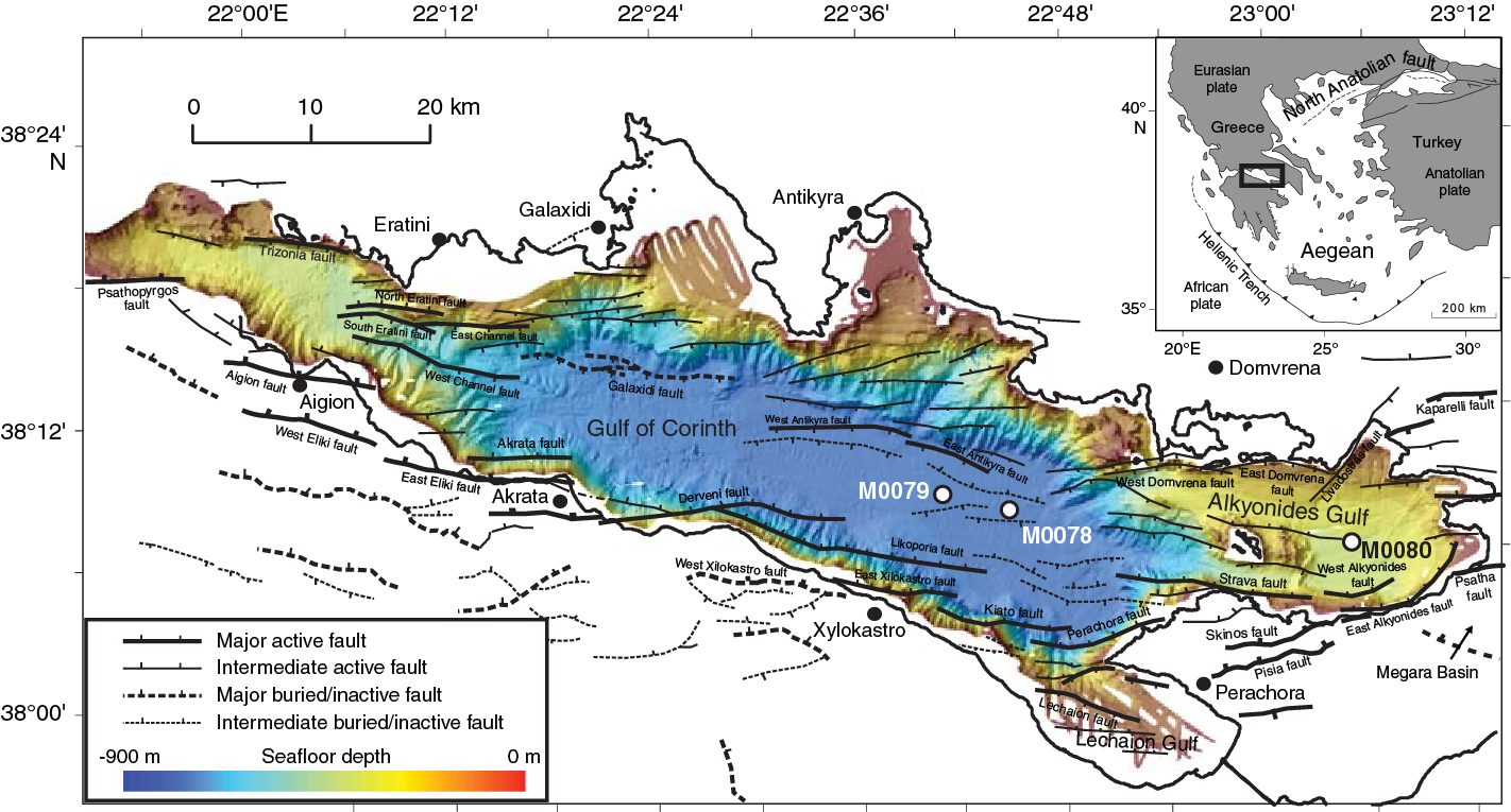
Figure F1. Corinth rift.
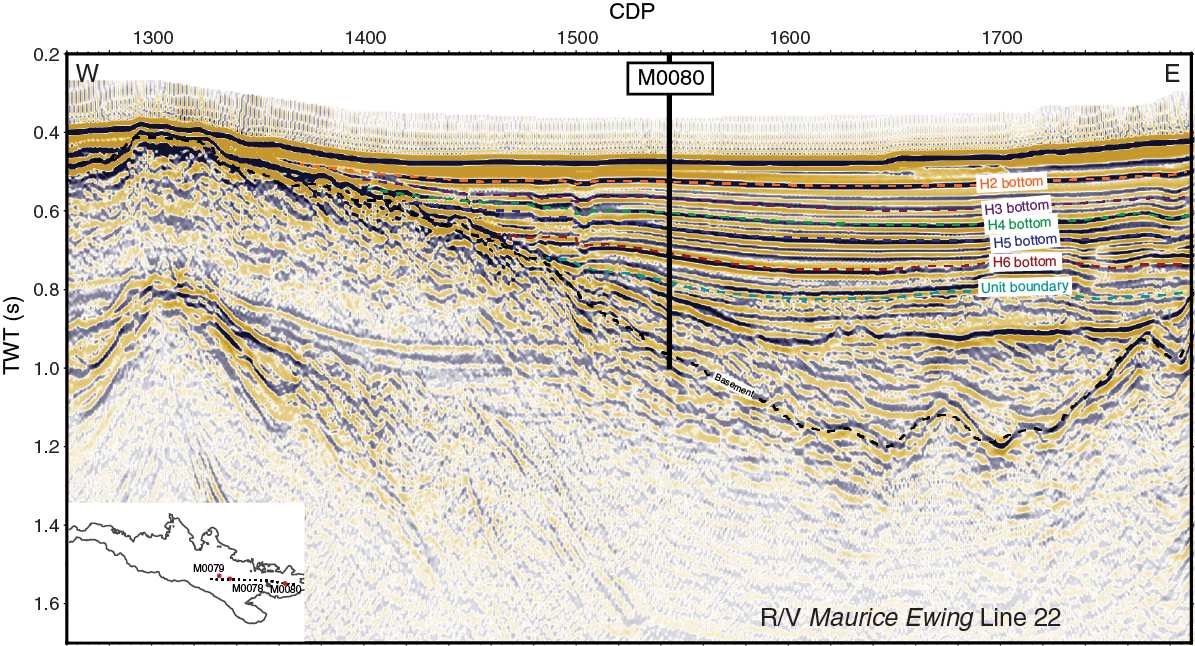
Figure F2. R/V Maurice Ewing Line 22.
Drilling and coring in Hole M0080A was completed to 534.1 meters below seafloor (mbsf) in 13 days, achieving an average core recovery of 84% (see Table T1 for details). The Fugro Corer in both push and percussive modes was used to collect the upper 141 m of sediment. The Fugro Extended Marine Core Barrel (FXMCB) was used to complete the lower 393 m of the borehole. Wireline logging operations were then conducted over 2 days.
Transit to Site M0080
Transit to Site M0080 began in the early hours of 2 December 2017. While in transit, four surface seawater samples were collected.
Coring operations
During the positioning process for Hole M0080A on 2 December 2017, a water depth of 348.8 m was established following a sound velocity profile and then the seabed frame (SBF) and pipe were lowered to within 50 m of the seafloor. After positioning was complete, the SBF and pipe were lowered to the seafloor and coring commenced using the Fugro Corer in push mode. A seabed/water interface sample was collected. The corer was dropped through the drill string in free fall and penetrated 1.5 m with a recovery of 1.4 m of sediment. Coring continued uninterrupted for the rest of 2 December and throughout 3 December, with exceptional progress made at a rate of >100 m/day. A switch to the percussive mode of the Fugro Corer occurred at 84 mbsf. The ability to alternate between push and percussive coring modes enabled nonrotary coring to greater depths than would have otherwise been possible. A temperature cone penetration test (CPT) measurement was made close to 100 mbsf to acquire in situ temperature and friction/strength information of the formation. The change to the FXMCB was made on the evening of 3 December at 141 mbsf when the efficacy of the Fugro Corer had dropped and the sediments were deemed firm enough to withstand the effects of rotary coring. A second temperature CPT measurement was taken around 210 mbsf. Coring continued at a very high rate until the morning of 5 December. At that time, the ground conditions became considerably more challenging, encountering alternating beds of sands and gravels, which resulted in a slowing of the rate of advance to 29.6 m/day. These slow rates continued and worsened until 12 December, with the lowest advance of 20.0 m/day in Hole M0080A on 9 December. Coring continued uninterrupted during this period.
The rate of advance improved significantly throughout 12 and 13 December to 85.4 m of advance because of favorable ground conditions. The drilling rate slowed again on 14 December as conditions became more challenging.
The final core from Hole M0080A was recovered at 0330 h (Eastern European Time [EET]) on 15 December, achieving a final depth of 534.1 mbsf. Despite a small number of discrete intervals where recovery was low, in general good recovery (84%) was achieved in Hole M0080A. The borehole was cored 65 m deeper than anticipated because the scientific goal for this borehole (basement) was deeper than the initial estimated target depth. Basement sensu stricto was not reached; however, the deepest cores recovered very coarse grained conglomerates thought to immediately overlie basement.
In general, seawater was used as the drilling medium; however, bentonite was used for core Runs 64–103 and 127–146.
Logging operations
In preparation for logging, Hole M0080A was stabilized by displacement with weighted bentonite mud (8.8 lb/gal). Standalone logging tools were used (because of the loss of stacked tools during Site M0078 operations), and they were systematically run with a sinker bar fitted above each tool to help its descent. Logging the hole started through the pipe with the spectral gamma ray (ASGR512) tool and then continued in three depth stages where the following tools were planned to be deployed in the open hole: magnetic susceptibility and conductivity (EM51), sonic (2PSA-1000), dual induction (DIL45), and ASGR512.
All tools were run with the primary winch (GV550). Hole M0080A logging started on 15 December 2017 at 0330 h with the drill bit pulled up to 533.1 m drilling depth below seafloor (DSF) (just above the base of the hole) to log through the pipe. The ASGR512 tool did not encounter any difficulty going down through the bentonite mud and in the pipe; it passed the drill bit to reach the bottom of the hole, and logging up commenced. After recovery of the ASGR512 tool, the drill bit was pulled up to 365 m DSF to log in the open hole for the first depth stage (365–533 m DSF). Bentonite mud (8.8 lb/gal) was circulated to stabilize the hole. The EM51 tool was deployed and passed the drill bit, but difficulties were encountered in the open hole from 410 to 425 m wireline log depth below seafloor (WSF), with several losses of tension. After borehole conditions prevented the tool from passing beyond ~425 m WSF, EM51 data were collected from this depth to the drill bit, and the tool was recovered on deck to perform a wiper trip downhole. The drill string was lowered to the bottom of the hole and then pulled up to 430 m WSF to avoid the interval where losses of tension were observed during the previous run. The EM51 and 2PSA-1000 tools were run successfully, reaching a maximum depth of ~530 m WSF and collecting data from this depth to the drill bit at 430 m WSF. However, when deploying the ASGR512 tool, losses of tension were observed ~10 m below the drill bit. The decision was made to move to the next depth stage, and the drill bit was lowered to 460 m DSF to clean the borehole walls and then pulled to 230 m DSF for the second depth stage. In this depth interval, the EM51 tool was run down the hole but could not pass beyond ~430 m WSF. Data were therefore collected with the EM51 tool from 430 to 230 m WSF. The 2PSA-1000 tool was deployed but could not pass beyond ~370 m WSF; therefore, data were collected up from this depth to the drill bit at 230 m DSF. After recovery of the 2PSA-1000 tool, the DIL45 tool and then the ASGR512 tool were deployed successfully in a similar depth range to the 2PSA-1000 tool, collecting data from 370 to 230 m WSF. The third and final depth stage was logged after the drill bit had been pulled up to 50 m DSF, and the bentonite present in the borehole was displaced with seawater. This change in fluid was intended to improve borehole stability for the expected lithologies in this shallow interval. Once deployed, the first tool (EM51) could not pass beyond ~220 m WSF downhole. The EM51, 2PSA-1000, DIL45, and ASGR512 tools were all deployed with data acquisition from ~220 to 50 m WSF. Logging operations were completed at 1235 h on 17 December.
Demobilization
Following the completion of logging operations in Hole M0080A, the European Consortium for Ocean Research Drilling (ECORD) Science Operator (ESO) team continued demobilizing the containerized laboratories and offices. All operations ceased at 1235 h on 17 December 2017, and the remaining pipe was tripped out of the hole. Transit to Corinth, Greece, took place overnight, with the D/V Fugro Synergy arriving dockside at 0600 h on 18 December.
Lithostratigraphy
Site M0080 is divided into four lithostratigraphic units based on a combination of observed facies associations (FA; see the Expedition 381 facies associations chapter [McNeill et al., 2019a]; Table T2), micropaleontology, seismic facies, and physical properties. In the following sections, we describe the units and subunits at Site M0080 (Table T3).
Unit and subunit description
Site M0080 was drilled in the Alkyonides Gulf to investigate the rift stratigraphy and evolutionary history in the eastern part of the Corinth rift (Figure F1). The succession encountered in Hole M0080A is divided into four main lithostratigraphic units (Figure F3). Unit 1 has similar characteristics to those of Unit 1 at Sites M0078 and M0079 and is divided into 11 subunits based on alternations between dominantly bioturbated homogeneous and bedded greenish gray and gray mud (FA1 and FA6) and bedded and laminated mud (FA2, FA3, FA4, and FA5). Unit 2 is divided into five subunits; the upper three subunits are dominated by light gray bioturbated mud (FA12), and the lower two units have greater variability of facies and grain size, including ophiolitic-rich conglomerates, paleosols, and highly bioturbated mudstone with shallow-water foraminifer assemblages. Unit 2 is probably partly time-equivalent to the lower part of Unit 1 at Sites M0078 and M0079. Two main facies associations dominate Unit 3. The upper half has a high proportion of red-brown coarse clastic sediment (FA7) that passes downhole into distinctive red-brown mud and silt (FA8). The base of Unit 3 comprises a range of facies associations, including shelly, bioturbated mudstone (FA17). Unit 4 is dominated by shelly laminated to bedded carbonates (FA15 and FA16), with the lowermost two cores consisting of pebble–cobble conglomerates with abundant limestone clasts.

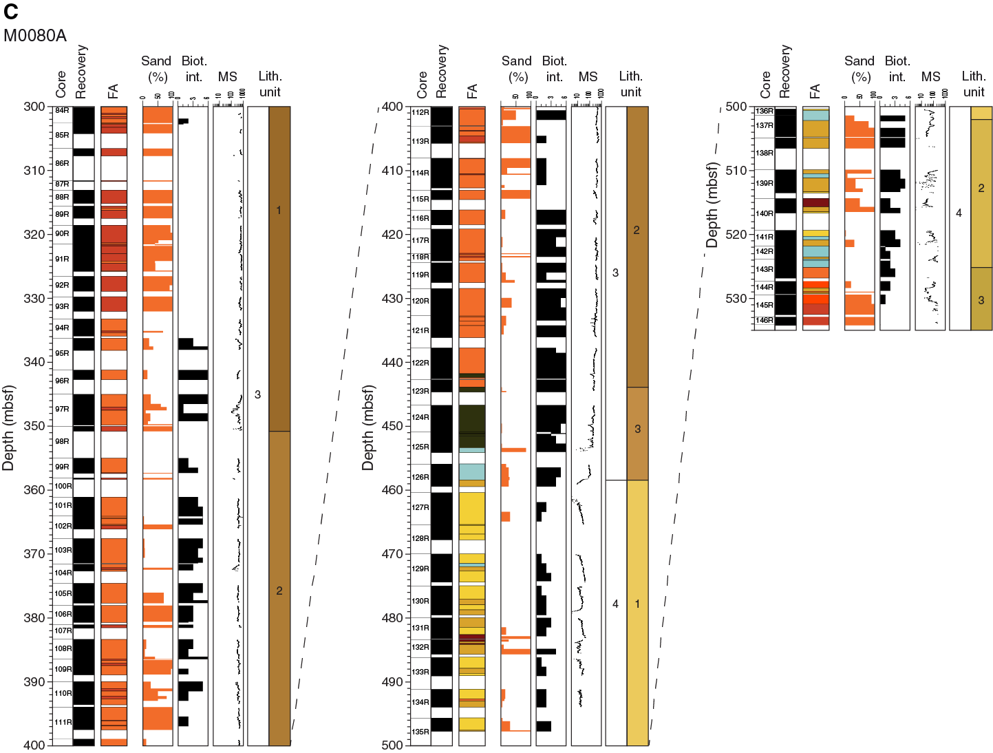
Figure F3. Composite stratigraphic log.
Composition information was deduced from X-ray diffraction (XRD) analysis and smear slide observations. Units 1 and 2 are dominated by moderately sorted, silt- to clay-grade carbonate minerals including low- and high-Mg calcite and dolomite with occasional intervals dominated by aragonite (Figure F4). Minor terrigenous components include quartz, mica, and feldspar mineral grains. Ophiolite-related serpentinite minerals, biogenic components, and framboidal pyrite are present throughout the units. Units 3 and 4 include ophiolitic-derived material in all grain size fractions but most obviously in the coarser grain size range (sand to pebble grade). Serpentine minerals (represented mainly by chrysotile) dominate the fine grain size fraction in the upper half of Unit 3 and decrease below this interval. Heavy minerals, including zeolites and amphiboles, are sparsely present. Carbonate minerals are less abundant but maintain a relatively constant proportion with respect to quartz and mica. In Unit 3, clast compositions in conglomerates and pebbly sandstone are dominated by mafic/ultramafic lithologies with minor micritic limestone and red chert (from Section 381-M0080A-68R-2 to Section 98R-2CC; 256.2–350.7 mbsf). The very fine sand to mud fraction commonly contains abundant clay-sized Fe oxides that may be responsible for the sediment’s reddish brown to pale yellow color. Unit 4 is dominated by shelly and silty limestone, and the base of the hole has conglomerates in which limestone clasts dominate (90%–95% of the clasts), with minor amounts of red chert and mafic/ultramafic clasts.
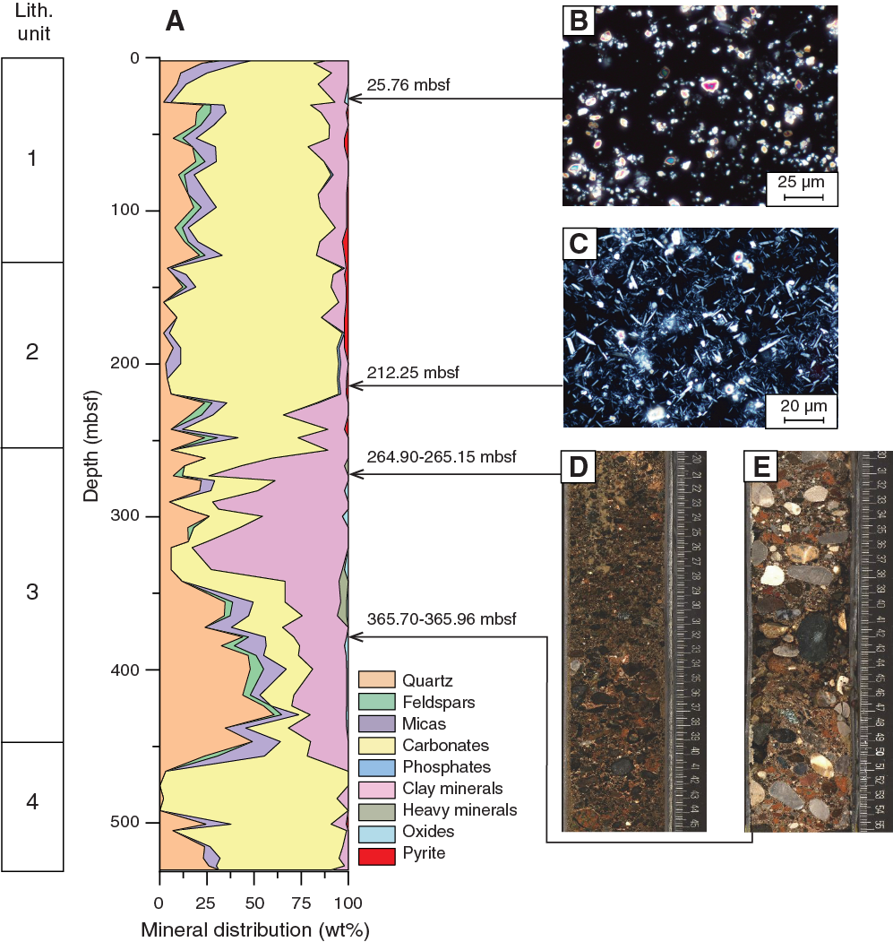
Figure F4. A. Downhole major mineral distribution.
Tephra and cryptotephra intervals were found in Site M0080 cores. These intervals were identified by a combination of visual inspection and physical properties. An increase in the Multi-Sensor Core Logger (MSCL) natural gamma radiation (NGR) intensity was usually observed in association with both visible tephra layers and with cryptotephra intervals, and this relationship was used as the primary method for targeting further investigation. Distinct and visible tephra layers (e.g., Section 381-M0080A-56R-1, 131.0–133.5 cm; 210.310–210.335 mbsf) were usually a different color from the surrounding sediment, with highly reflective character resulting from high concentrations of bubble wall shards in these layers. Distinct tephra layers were composed of very well sorted silt size grains and commonly preserved an increase in grain size toward a coarser (very fine sand size) basal layer. The majority of the tephra identified in the cores were cryptic tephra intervals and were identifiable only through methodical sampling of NGR intensity peaks and subsequent visual examination of sampled material using optical microscopy. Cryptotephra were also identified incidentally during routine micropaleontological work by observation of glass shards.
Unit 1
Subunit 1-1
- Interval: 381-M0080A-1P-1, 0 cm, to 3P-2, 24 cm
- Depth: 0–6.24 mbsf (6.24 m thick including 0.26 m of missing core)
The top boundary of Subunit 1-1 is at the seafloor, and the lower boundary is marked by a transition in a 5 cm interval between FA1 and FA5 and a downhole change in magnetic susceptibility from relatively constant to more fluctuating values.
Subunit 1-1 consists entirely of FA1 homogeneous mud of olive gray color and a high degree of bioturbation (bioturbation intensity [BI] = 4–6). The subunit contains sparse organic layers and millimeter- to centimeter-scale organic fragments, as well as a few shell fragments from Section 381-M0080A-3P-1 downhole. Only one interval has a silt to very fine sand grain size (Section 2P-2, 105–107 cm; 4.05–4.07 mbsf). Close to the basal boundary, around the transition from FA1 to FA5, are distinct Teichichnus burrows.
Subunit 1-2
- Interval: 381-M0080A-3P-2, 24 cm, to 7P-2, 13 cm
- Depth: 6.24–22.83 mbsf (16.59 m thick including 0.62 m of missing core)
The top of Subunit 1-2 is marked by a change from FA1 (above) to FA5 (below) and a corresponding downhole decrease in NGR and increase in the variability of magnetic susceptibility values (Figure F3). The lower boundary occurs at a sharp change from FA3 (above) to FA1 (below) (Figure F5). One sand–homogeneous mud couplet >10 cm thick occurs in Subunit 1-2.
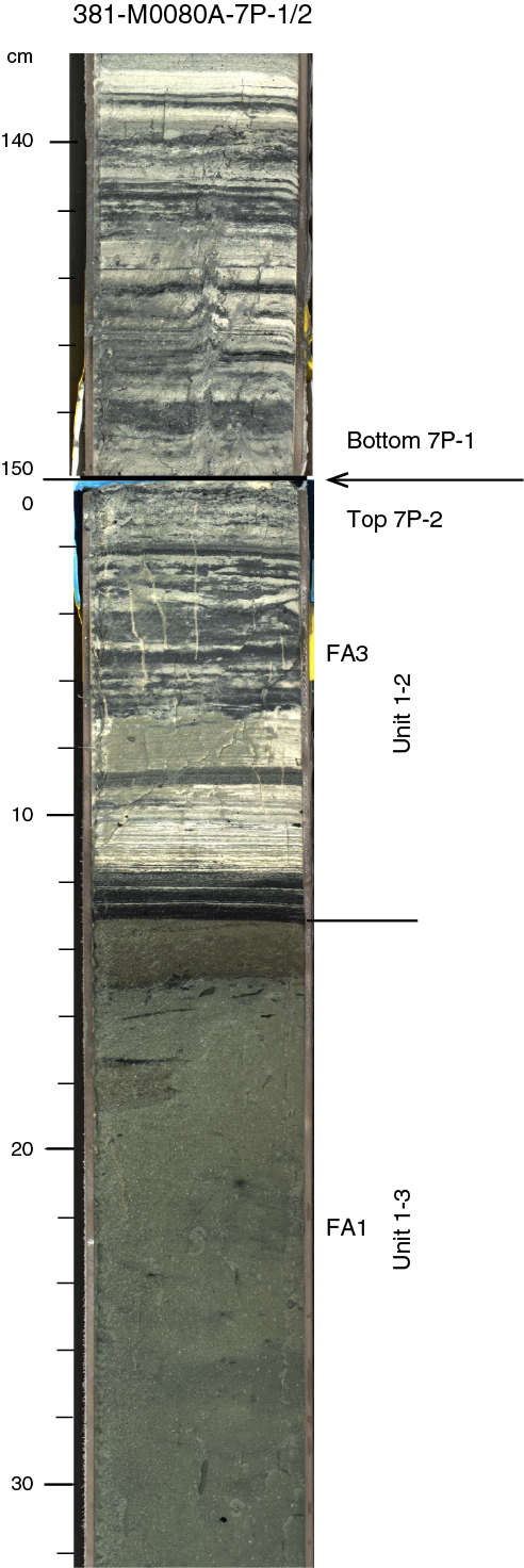
Figure F5. Boundary between Subunits 1-2 and 1-3.
Subunit 1-2 is characterized by alternations of greenish gray bedded mud (FA5) (~50%) and greenish gray mud with dark gray to black silty beds (FA2) (~45%), with the greenish gray bedded mud with centimeter-thick silt (FA11) occurring in Section 381-M0080A-6P-3, 46–126 cm (19.96–20.76 mbsf). A thin interval of laminated mud with whitish laminations occurs in the lowest part of the subunit, just above the lower subunit boundary, in Section 7P-2, 0–13 cm (21.20–21.33 mbsf).
Subunit 1-3
- Interval: 381-M0080A-7P-2, 13 cm, to 12P-1, 50 cm
- Depth: 22.83–35.80 mbsf (12.97 m thick with 0.2 m of missing core)
The top of Subunit 1-3 is marked by a sharp change from finely laminated FA3 (above) to green bioturbated FA1 mud (below) (Figure F5). The bottom of the subunit is marked by a change from FA1 to FA4 with a diffuse zone of increasing bedding definition.
Subunit 1-3 is divided into three parts with boundaries in Sections 381-M0080A-8P-1, 4 cm (25.94 mbsf), and 8P-3, 109 cm (29.99 mbsf). The upper part is composed of greenish gray homogeneous mud (FA1) with rare shell fragments. The middle part is composed of bedded mud (FA5) above creamy white laminated mud (FA3) with some thin silt beds. The lower part is composed of homogeneous mud (FA1) with common shell fragments and rare discrete burrows, as well as some faintly bedded greenish mud (FA6). The homogeneous parts of the subunit are completely bioturbated, whereas the middle part is sparsely bioturbated.
Subunit 1-4
- Interval: 381-M0080A-12P-1, 50 cm, to 17P-2, 100 cm
- Depth: 35.80–55.70 mbsf (19.90 m thick including 0.63 m of missing core)
The top of Subunit 1-4 is characterized by a transition from homogeneous mud (FA1; above) to bedded and laminated mud (FA5). The bottom boundary is set at the base of a short interval (12 cm thick) of laminated sediment (FA3) that lies above FA1 mud in Subunit 1-5.
Subunit 1-4 contains three parts. The upper part (Sections 381-M0080A-12P-1, 50 cm, to 13P-3, 24 cm; 35.80–43.16 mbsf) is composed of greenish gray to gray (GLEY 1 6/5GY–6/N) bedded and laminated mud intervals that correspond to FA5. The sediment includes occasional black organic-rich silty laminations and is sparsely bioturbated. The sporadic presence of shell debris is also noted. The middle part is a transition to FA2 sediment that continues to Section 16P-1, 37 cm (52.07 mbsf). This middle part consists of mud and centimeter-thick fining-upward silt with organic-rich layers and is also marked by bioclasts and mottled pyritized features. The lower part is composed of slightly bioturbated alternating greenish gray to light greenish gray (GLEY 1 6/5GY to 7/10Y) FA11 and FA5 sediment with generally higher sand proportions (as much as 20%). The basal sedimentary interval of this subunit (below Section 17P-2, 88 cm; 55.58 mbsf) consists of a thin interval of well-laminated FA3 sediment, including millimeter-scale pale gray or white laminations, which are interbedded with moderately bioturbated mud beds with common discrete burrows.
Subunit 1-5
- Interval: 381-M0080A-17P-2, 100 cm, to 19P-3, 56 cm
- Depth: 55.70–66.16 mbsf (10.46 m thick including 0.09 m of missing core)
The top of Subunit 1-5 is marked by a sharp transition from FA3 white thin laminations (above) to FA1 green bioturbated mud (below) and is characterized by the appearance of marine microfossils and shell fragments (see Micropaleontology). The base of this subunit is strongly bioturbated, and the boundary with Subunit 1-6 is marked by a transition from FA1 bioturbated mud (above) to FA4 laminated mud (below).
The upper part, from the upper boundary to Section 381-M0080A-17P-3, 26 cm (56.46 mbsf), consists of FA1 homogeneous mud that is pervasively bioturbated but also shows discrete burrows. Below Section 17P-3, 26 cm, is a distinct interval of FA5 mud overlying FA3 light gray/white laminated mud that extends to Section 17P-3, 105 cm (57.25 mbsf). Greenish gray FA1 homogeneous mud reappears and continues to Section 18P-1, 40 cm (58.30 mbsf).
Below this FA1 homogeneous mud, FA5 greenish gray mud (GLEY 1 7/10Y to 6/10Y) with homogeneous centimeter-thick gray mud beds extends to Section 19P-1, 29 cm (62.89 mbsf), and the lowest 25 cm of this interval tends toward light gray to whitish laminated mud (GLEY 1 7/N). Thalassinoides branched burrows extend down from the overlying FA1 mud into the FA5 bedded mud interval that otherwise shows only rare millimeter-scale burrows that are typically restricted to the upper parts of centimeter-scale mud beds. Thin (millimeter-scale) silt to very fine sand beds, often exhibiting normal grading, also occur in the FA5 succession.
Below Section 19P-1, 29 cm (62.89 mbsf), homogeneous mud (FA1) extends to the base of the subunit. The homogeneous mud is highly to completely bioturbated (BI = 4–6) and contains scattered shell fragments.
Subunit 1-6
- Interval: 381-M0080A-19P-3, 56 cm, to 25P-2, 61 cm
- Depth: 66.16–83.11 mbsf (16.95 m thick including 1.64 m of missing core)
The top of Subunit 1-6 represents a change from homogeneous mud (FA1; above) to laminated mud (FA4; below) and is marked by the corresponding appearance of diffuse mud laminations that are initially intensely bioturbated. The lower boundary of the subunit is marked by a change from bedded mud and very fine sand (FA11; above) to homogeneous mud (FA1; below).
The upper part of Subunit 1-6 is composed of poorly laminated and bedded (centimeter-scale) light gray to greenish gray mud of FA4 and FA5 in Sections 381-M0080A-19P-3, 56 cm, to 20P-2, 78 cm (66.16–69.44 mbsf). The mud is intensely bioturbated near the top boundary of the subunit, and pyrite is scattered throughout. The middle of the subunit consists of gray to greenish gray mud (FA5) with centimeter- to decimeter-scale bedding in Sections 20P-2, 78 cm, to 24P-2, 90 cm (69.44–78.70 mbsf). Pyrite particles are scattered through this middle section.
The lower part includes an interval of light gray to buff weakly laminated mud with abundant bioturbation (FA12) (5Y 7/1 to GLEY 1 7/10Y) in Sections 381-M0080A-24P-2, 90 cm, to 24P-3, 87 cm (77.20–80.18 mbsf). The mud includes individual gastropods and other shell fragments, together with discrete burrows superimposed on background burrow mottling. Below this interval, centimeter-scale silt to very fine sand beds interbedded in the greenish gray mud of FA5, FA2, and FA11 occur. Numerous black (organic-rich) laminations and beds were observed in the lower part of the subunit, as well as abundant shell fragments, pyrite, and discrete burrowing.
Subunit 1-7
- Interval: 381-M0080A-25P-2, 61 cm, to 28V-1, 70 cm
- Depth: 83.11–89.20 mbsf (6.09 m thick including 0.10 m of missing core)
The top boundary of Subunit 1-7 is marked by a transition from FA11 (above) to FA1 (below). The base of the subunit is marked by a relatively sharp color change in a bioturbated contact between darker FA1 greenish gray mud (above) and FA12 light gray mud (below).
Subunit 1-7 consists entirely of FA1 homogeneous mud that is greenish gray and almost completely bioturbated (BI = 6). The only interval with faint bedding (BI = 2–4) is in Section 381-M0080A-27V-3 (87.52–88.42 mbsf). Shell fragments, including gastropods, are common throughout, as are discrete millimeter- to centimeter-scale burrows and feeding traces including Thalassinoides, Nereites(?), and Teichichnus.
Subunit 1-8
- Interval: 381-M0080A-28V-1, 70 cm, to 31V-1, 140 cm
- Depth: 89.20–103.10 mbsf (13.9 m thick including 0.42 m of missing core)
The top of Subunit 1-8 appears sharp and is marked by a change from FA1 (above) to FA12 (below) and a corresponding decrease in NGR. The lower boundary occurs at a sharp change from FA2 (above) to FA6 (below) and is marked by a downhole increase in bioturbation and a decrease in magnetic susceptibility.
Subunit 1-8 is composed of FA12 mud to Section 381-M0080A-30V-2, 92 cm (99.42 mbsf). This interval is characterized by thick light gray to buff homogeneous to weakly stratified mud with moderate to intense bioturbation (BI = 3–5; low to moderate diversity, including Teichichnus and Planolites) (Figure F6A). The lower part of the subunit shows a downhole increase in bedding and then lamination definition with greenish gray mud with homogeneous centimeter-thick mud beds (FA5) with moderate levels of bioturbation to more organic-rich greenish gray laminated mud (FA2). The latter exhibits relatively sparse levels of bioturbation.
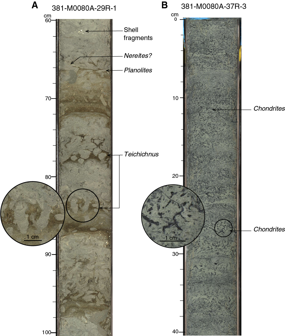
Figure F6. A. FA12 in Subunits 1-8 and Subunit 1-10.
Subunit 1-9
- Interval: 381-M0080A-31V-1, 140 cm, to 34V-1, 0 cm
- Depth: 103.10–110.40 mbsf (7.3 m thick with 0.3 m of missing core)
The top of the subunit is marked by a change from FA2 to FA6, with the uppermost 38 cm composed of centimeter-scale bedded mud with uncommon bioturbation. The base is marked by a change from FA1 to FA12 between cores.
Subunit 1-9 is composed of homogeneous bioturbated mud, which is completely bioturbated (FA1) beneath the upper 38 cm, with common to abundant scattered shell fragments and pyrite. Discrete bioturbation includes vertical, inclined, and horizontal burrows. Macrofossils include intact gastropods and oyster fragments.
Subunit 1-10
- Interval: 381-M0080A-34V-1, 0 cm, to 38V-2, 112 cm
- Depth: 110.40–130.92 mbsf (20.52 m thick including 0.39 m of missing core)
The upper boundary of this subunit marks a change from FA1 mud (above) to FA12 homogeneous to weakly stratified mud (below). The bottom boundary marks a change from FA12 mud containing decimeter-thick fining-upward sand to mud beds to greenish gray FA6 mud of the underlying subunit.
Subunit 1-10 is composed of FA12 homogeneous to weakly stratified mud with variations in color. Colors range from pale greenish gray (typically between GLEY 1 7/10Y and 6/5GY) to more buff. Bioturbation is pervasive with extensive mottling, but superimposed on these features are discrete ichnofabrics including 0.5–1.0 cm diameter vertical, inclined, and horizontal burrows of Teichichnus, Palaeophycus, and a Chondrites-like fabric (Figure F6B). Plant and woody fragments also occur. Pyrite is scattered throughout.
Subunit 1-11
- Interval: 381-M0080A-38V-2, 112 cm, to 40V-1, 26 cm
- Depth: 130.92–136.96 mbsf (6.04 m thick including 0.06 m of missing core)
The top of Subunit 1-11 is marked by a shell-rich bed and a change from FA12 mud (above) to FA6 mud (below). The lower boundary with Unit 2 is marked by an irregular, probably erosive contact between FA1 bioclastic greenish gray mud (above) and FA12 light greenish gray mud (below) (Figure F7).
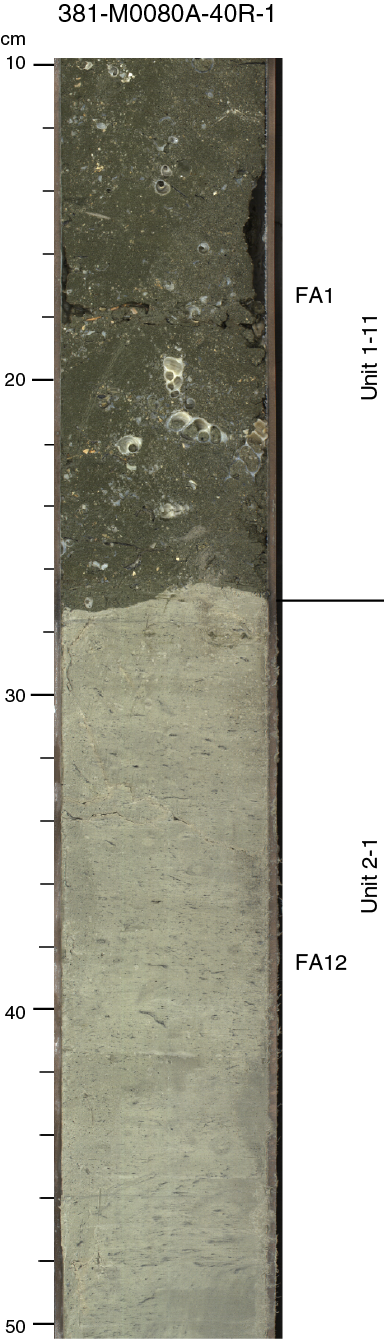
Figure F7. Erosive boundary between Units 1 and 2.
Subunit 1-11 consists mainly of FA1 greenish gray homogeneous mud. The majority of the succession is completely bioturbated (BI = 6) and is characterized by abundant scattered shells such as gastropods and oysters that are occasionally preserved intact but also as fragments (<1 cm). Centimeter-thick shell-rich beds are found in the homogeneous mud (e.g., Sections 381-M0080A-38V-3, 90 cm; 39V-1, 120 cm; 39V-1, 132 cm; and 39V-2, 108 cm [132.2, 134.20, 134.32, and 135.58 mbsf, respectively]). In general, pervasive bioturbation results in a mottled texture, with relatively few discrete burrow forms seen. Recognized discrete burrows include subvertical burrows and irregular feeding trace patches.
Unit 2
Subunit 2-1
- Interval: 381-M0080A-40V-1, 26 cm, to 47R-1, 5 cm
- Depth: 136.96–164.05 mbsf (27.09 m thick including 0.71 m of missing core)
The top of Subunit 2-1 is marked by a sharp erosive surface separating FA1 bioclastic greenish gray mud (above) from FA12 light greenish gray faintly bedded mud (below) (Figure F7). The lower boundary of this subunit is marked by the appearance of abundant shell fragments and shallow-marine foraminifers in underlying Subunit 2-2, although the general facies continues to be FA12.
Subunit 2-1 comprises light greenish gray homogeneous to decimeter-scale bedded mud (FA12) that is highly to completely bioturbated. Scattered bioclasts and shell fragments occur in this subunit, including ostracods in Sections 381-M0080A-40V-1 and 46R-1 (136.96 and 159.00 mbsf, respectively), bivalves in Section 42R-3 (143.52 mbsf), and gastropods in Sections 42R-3, 43R-1, and 44R-1 (143.52, 144.00, and 149.00 mbsf, respectively). Although the subunit is generally mottled by burrowing, discrete burrows are also common, becoming more abundant toward the bottom of the subunit, with Planolites and possible local horizons of Teichichnus.
Subunit 2-2
- Interval: 381-M0080A-47R-1, 5 cm, to 48R-1, 13 cm
- Depth: 164.05–169.13 mbsf (5.08 m thick including 1.35 m of missing core)
The top of Subunit 2-2 is associated with a slight color change (gray to greenish gray) in FA12 mud and the occurrence of shell beds and a shallow-marine foraminifer assemblage (see Micropaleontology). The lower boundary also occurs at a gradual color change (from greenish gray to gray) in FA12 mud and is marked by sharp-based fine sand containing shell fragments.
Subunit 2-2 is composed entirely of light gray to buff homogeneous to weakly stratified mud (FA12). It is highly bioturbated (BI = 5–6) and has a moderately diverse trace fossil assemblage including Teichichnus, Planolites, and Palaeophycus. Shell fragments and pyrite are scattered in small amounts throughout the unit.
Subunit 2-3
- Interval: 381-M0080A-48R-1, 13 cm, to 58R-1, 72 cm
- Depth: 169.13–218.22 mbsf (49.91 m thick including 7.01 m of missing core)
The top of Subunit 2-3 coincides with the base of a shelly, very fine sand in FA12. The lower boundary corresponds to a sharp color and facies change between FA3 light greenish gray mud (above) and FA5 dark greenish gray mud (below).
Subunit 2-3 is dominated by FA12 and is divided into three different parts. The top part (169.13–200.63 mbsf) consists almost completely of FA12, with the exception of a short FA5 interval (195.95–197.00 mbsf) that contains abundant to completely bioturbated light gray to greenish gray mud with discrete traces of Chondrites, Skolithos, Teichichnus, and Nereites(?). Sparse scattered shell fragments including gastropods also occur in this part of the subunit. Visible scattered pyrite occurs between 174.00 and 178.6 mbsf.
The middle part of the subunit (200.63–206.03 mbsf) contains whitish finely laminated mud (FA3) at its top and base, whereas the central section is characterized by alternation of FA4, FA5, and FA11, with very fine to medium sand and scattered shell fragments. The bottom part of the subunit (209.00–218.22 mbsf) is composed of highly to completely bioturbated buff-colored mud (FA12). A short interval of brownish silt (210.31–210.335 mbsf) contains abundant tephra glass shards. At the base of the subunit is 15 cm of FA3 whitish laminated mud above a change to FA5 bedded greenish mud in underlying Subunit 2-4.
Subunit 2-4
- Interval: 381-M0080A-58R-1, 72 cm, to 63R-3, 121 cm
- Depth: 218.22–241.41 mbsf (23.17 m thick including 1.46 m of missing core)
The top boundary of Subunit 2-4 is sharp and is marked by a change from FA3 (above) to FA5 (below). The lower boundary occurs at a sharp change from FA15 (above) to greenish gray shelly mud and fine sand of FA12 (below).
More than half of Subunit 2-4 consists of FA11 and FA5, and the remainder of the subunit comprises FA10 and FA12. This subunit is divided into two main parts with a boundary at the top of Section 381-M0080A-61R-2 (229.18 mbsf). The upper part is characterized by greenish gray mud with homogeneous centimeter-thick mud beds (FA5) alternating with bedded mud/silt and centimeter- to decimeter-thick sand beds (FA10 and FA11) and light gray to buff homogeneous to weakly stratified mud (FA12). The lower part is characterized by bedded mud, silt, and centimeter- to decimeter-thick sand and conglomerate beds (FA10/FA11) interbedded with light gray to buff homogeneous to weakly stratified mud (FA12). The dark bioturbated mud at the base of the subunit contains a shallow-marine foraminifer assemblage.
Subunit 2-5
- Interval: 381-M0080A-63R-3, 121 cm, to 68R-2, 65 cm
- Depth: 241.41–256.85 mbsf (15.44 m thick including 0.92 m of missing core)
The top boundary of Subunit 2-4 is sharp and marked by a change from FA15 (above) to FA12 (below). The lower boundary is also sharp and marked by a facies change from FA15 beige/greenish laminated silt (above) to FA7 conglomerates in Unit 3 (below) (Figure F8).
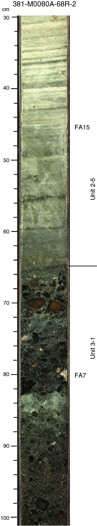
Figure F8. Unit 2/3 boundary.
FA14 and FA8 contribute more than 50% of Subunit 2-5, together with lesser, approximately equal amounts of FA12, FA10, and FA7. The upper part of the subunit is characterized by light gray to buff homogeneous to weakly stratified mud (FA12) that overlies interbedded mud/silt and decimeter-thick sand beds (FA10). Below the top of Core 381-M0080A-65R (246.70 mbsf), the subunit is dominated by greenish gray pebbly silt and clast-supported fining-upward conglomerates rich in ophiolite-derived clasts (FA7 and FA14) that are intercalated with FA8 gray to brown mud and silt that include mottled textures and rootlets. The lowest part of the subunit comprises clast-supported sandy conglomerates and pebbly sand (FA7) rich in ophiolite clasts that overlie bioturbated to parallel-laminated shelly carbonate silt and sand that are possibly rooted in Section 68R-1.
Unit 3
- Interval: 381-M0080A-68R-2, 65 cm, to 126R-3, 44 cm
- Depth: 256.85–458.40 mbsf
- Age: Pleistocene–?Pliocene
Subunit 3-1
- Interval: 381-M0080A-68R-2, 65 cm, to 98R-2CC, 0.08 cm
- Depth: 256.85–350.79 mbsf (93.94 m thick including 31.12 m of missing core)
The top of Subunit 3-1 is marked by an abrupt grain size change from FA15 beige/greenish laminated silt (above) to FA7 pebble conglomerates (below) (Figure F8). The lower boundary lies in a core gap of more than 4 m with conglomerates (FA7) above and red-brown silt (FA8) below.
Subunit 3-1 consists predominantly of clast-supported poorly to moderately sorted pebble conglomerates (FA7) alternating with minor FA8 poorly stratified sand and silt. The thickness of FA7 conglomerate intervals reaches as thick as 6 m in some places, but this value is likely to be higher because of poor core recovery; around half of the cores are incomplete because of poor core recovery. The lower part of Subunit 3-1 (the last 18 m) is more dominated by FA8 sand and silt than the conglomerates that dominate the upper part of the subunit; only a few tens of centimeter-thick conglomerates are present in this lower part. The lower boundary of Subunit 3-1 corresponds to the last appearance of a submeter-thick FA7 conglomerate bed (350.00–350.79 mbsf). This interval contains some cobbles of limestone.
Subunit 3-2
- Interval: 381-M0080A-98R-2CC, 0.08 cm, to 123R-2, 46 cm
- Depth: 350.79–443.89 mbsf (93.10 m thick including 24.41 m of missing core)
The top of Subunit 3-2 is situated in a zone of no recovery between 350.79 and 355.00 mbsf. Below this gap, red-brown mud, silt, and fine sand (FA8) are predominant for 93.1 m. The lower boundary at 443.89 mbsf corresponds to a sharp change from red-brown mud with calcretes (FA8; above) to green mud (FA1; below).
Subunit 3-2 consists predominantly of FA8 mud, silt, and fine sand with scattered pebbles and granules and small (centimeter diameter) calcrete nodules. This largely homogeneous succession of red-brown mud, silt, and fine sand is punctuated by rare 30 cm thick FA7 conglomerate beds with a mean clast size of fine to medium pebbles. The mud and silt are commonly highly bioturbated with large (millimeter- to centimeter-scale) horizontal, vertical, or subvertical burrows. Rootlets, calcretes, and mottled textures and color variations indicate various degrees of pedogenesis. Some subvertical infilled fissures were also observed in Section 381-M0080A-117R-3, 31 cm (422.00 mbsf). The reddish brown mudstone in the lower part of Subunit 3-2 is interrupted by intervals of homogeneous gray mud containing scattered shell fragments and carbonate nodules.
Subunit 3-3
- Interval: 381-M0080A-123R-2, 46 cm, to 126R-3, 44 cm
- Depth: 443.89–458.40 mbsf (14.51 m thick including 3.84 m of missing core)
The top of Subunit 3-3 comprises a sharp transition from homogeneous red-brown mud with calcretes (FA8; above) to crudely bedded greenish gray mudstone and siltstone (FA1) that are fossiliferous and bioturbated. The sharp bottom boundary separates FA17 green-gray mudstone (above) from FA16 very pale brown siltstone and sandstone (below), associated with a decrease in bioturbation intensity.
Subunit 3-3 is divided into two parts with a boundary at Section 381-M0080A-125R-3, 66 cm (453.39 mbsf). The upper part comprises homogeneous dark greenish gray highly bioturbated mudstone with abundant shell debris throughout and rare millimeter-thick siltstone (FA1). The uppermost 50 cm of the lower part of Subunit 3-3 is characterized by centimeter-thick beds of dark gray mudstone interbedded with centimeter-thick beds of laminated very fine sandstone that fines upward into silty mudstone with millimeter-scale ripples (FA17). In places, these beds are highly bioturbated. The lower part of this subunit consists of dark gray bioturbated fine sandstone and siltstone with abundant bioclasts, limestone nodules (1 cm average diameter), and centimeter- to decimeter-thick graded sandstone beds (FA17).
Unit 4
- Interval: 381-M0080A-126R-3, 44 cm, to 146R-CC, 12 cm
- Depth: 458.40–534.20 mbsf (base of Hole M0080A)
- Age: Pliocene–late Miocene?
Subunit 4-1
- Interval: 381-M0080A-126R-3, 44 cm, to 137R-1, 73 cm
- Depth: 458.40–502.01 mbsf (43.61 m thick with 11.96 m of missing core)
The top of Subunit 4-1 is marked by a decrease in bioturbation intensity and a marked color and facies change from FA17 dark gray (GLEY 1 5/10Y) sandstone and mudstone (above) to FA16 very pale brown (10YR 6/4) very fine sandstone and siltstone (below). The base of the subunit is marked by 1 m of fossiliferous homogeneous bioturbated mudstone and a change from FA17 to FA16.
Subunit 4-1 consists of fully lithified fossiliferous mudstone, siltstone, and sandstone with a distinctive very pale brown color associated with minor intervals of dark gray-green mudstone. This subunit is divided into two main parts with a boundary at Section 381-M0080A-130R-3, 76 cm (478.76 mbsf). The upper part is predominantly composed of centimeter-scale bedded to millimeter-scale laminated very pale brown calcareous siltstone (FA15) with a small amount of centimeter- to decimeter-bedded calcareous siltstone and sandstone (FA16) and some greenish fossiliferous bedded mudstone (FA17). Ostracods and scaphopods are commonly found in this part of the subunit, with some isolated ostracod grainstone beds. Centimeter-thick scaphopod beds also occur throughout.
The lower part of the subunit is composed of both thinly bedded/laminated calcareous siltstone and sandstone (FA15) and centimeter- to decimeter-bedded calcareous siltstone and sandstone (FA16). These two facies associations are present throughout in approximately equal amounts and are interspersed on a meter scale. An interval (~1.5 m) of dark gray brecciated mudstone and siltstone occurs in the upper part of the lower subunit (FA13). This slumped/brecciated interval contains mud intraclasts, abundant shelly fragments, and some limestone granules. The basal ~1.5 m of the unit is characterized by FA17 mudstone, siltstone, and sandstone. Shell fragments are common throughout the lower part of the subunit, most commonly subcentimeter-sized gastropods, bivalves, and some ostracods.
Subunit 4-2
- Interval: 381-M0080A-137R-1, 73 cm, to 143R-1, 134 cm
- Depth: 502.01–525.14 mbsf (23.12 m thick with 7.01 m of missing core)
The top of Subunit 4-2 is marked by a change from FA17 to FA16 with a gradual color change and an increase downhole in fossil content. The base is placed at the appearance of red-brown mottling as the rock changes downhole from FA17 green nodular mudstone (above) to FA8 red-brown mudstone (below).
Subunit 4-2 is composed of disturbed and variably bedded calcareous sandstone and siltstone (FA16) that varies from light brown to dark gray-green. Small intervals of laminated siltstone (FA15) and a 1.3 m interval of contorted calcareous siltstone and sandstone (FA13) also occur. The rapid and chaotic changes in bedding dip suggest that this entire interval may be slumped. Subunit 4-2 is also affected by natural faulting and has a significant drilling-induced deformation (DID) overprint (see Structural geology). In the upper part, the sediment is commonly to abundantly bioturbated (BI = 4–5). The lower part of Subunit 4-2 is characterized by relatively undisturbed FA17 greenish gray homogeneous mudstone with common carbonate concretions (average diameter of approximately 1 cm) and rare bioturbation (BI = 0–2 and occasionally 3). Minor zones of brown faintly bedded siltstone (FA16) also occur. Shell fragments, gastropods, and bivalves are common throughout the subunit.
Subunit 4-3
- Interval: 381-M0080A-143R-1, 134 cm, to base of Hole M0080A
- Depth: 525.14–534.20 mbsf (9.06 m thick including 1.00 m of missing core)
The top of Subunit 4-3 marks a transition from FA17 green nodular mudstone (above) to FA8 red-brown mudstone (below). The bottom boundary corresponds to the base of Hole M0080A and is set in deposits of FA7.
Subunit 4-3 contains three distinct intervals whose boundaries are not well defined because of poor core recovery. The upper part to Section 381-M0080A-144R-1, 0 cm (527.3 mbsf), comprises green to reddish brown mudstone (FA8) that becomes progressively more reddish brown and increasingly mottled downhole. Bioturbation increases downhole, and limestone nodules (calcrete nodules?) also become more numerous and larger, even merging to form a complete carbonate layer in Section 143R-2, 103 cm (526.33 mbsf). Below this layer to Section 145R-1, 144 cm (530.84 mbsf), siltstone to very coarse gray to gray-green pebbly sandstone (FA9) dominate with intervals of pale brown siltstone (FA16). FA9 siltstone and sandstone are homogeneous to poorly bedded, with some centimeter- to decimeter-thick fining-upward beds. No fossils or bioturbation were seen. Finally, the deepest part of Subunit 4-3, below Section 145R-1, 144 cm (530.84 mbsf), comprises well-lithified pebble–cobble conglomerates (FA7) that are clast supported and poorly sorted. Clasts are dominated by subangular to subrounded limestone with highly altered (deep rusty brown) ultrabasic rocks and probable intraclasts of well-lithified coarse-grained pebbly sandstone (Figure F9).
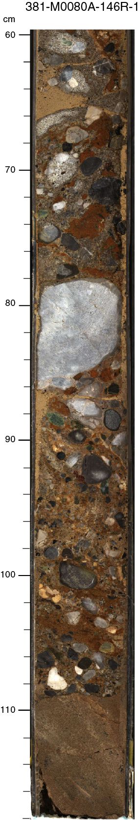
Figure F9. Base of hole (Subunit 4-3).
Interpretation of Hole M0080A
In Hole M0080A, deep-water turbiditic and hemipelagic deposits dominate Unit 1. The character of alternating facies associations in Unit 1 is similar to that observed in Unit 1 at Sites M0078 and M0079 and is interpreted in a similar manner. The alternating subunits are thus provisionally identified as representing marine and isolated/semi-isolated basinal environments with good correlation to micropaleontology results (see Micropaleontology). The upper part of Unit 2 has a similar character to that at Sites M0078 and M0079 in that it is dominated by highly bioturbated mud (FA12) but is likely to be diachronous between the sites, with at least some of the upper part of Unit 2 at Site M0080 being time-equivalent to the lower parts of Unit 1 at Sites M0078 and M0079.
In contrast to the upper part of Hole M0080A (Unit 1 and the upper part of Unit 2), the lower part of Unit 2 (Subunits 2-4 and 2-5) and Units 3 and 4 have markedly different facies associations and composition from those observed at the other sites. Subunits 2-4 and 2-5 contain ophiolitic-rich conglomerates, paleosols, and highly bioturbated mudstone with shallow-water foraminifer assemblages that are interpreted to have been deposited in a nearshore to coastal plain setting subject to repeated progradation and transgression.
Unit 3 is predominantly composed of red-brown siltstone, sandstone, and conglomerates that contain rooted horizons and calcretes, suggesting an overall alluvial–fluvial depositional environment that contrasts markedly with the predominantly subaqueous deposition higher in the hole. This unit displays a coarsening-upward stacking pattern with siltstone in the lower part giving way to sand and conglomerates in the upper section, suggesting progradation of the depositional system. Clast compositions fluctuate in the unit, suggesting a mixed limestone and ophiolite source area. The lowermost part of Unit 3 contains shelly and bioturbated mudstone, siltstone, and sandstone deposited in an overall subaqueous, nearshore setting.
The upper part of Unit 4 in Hole M0080A is carbonate dominated with thinly bedded and laminated shelly carbonates interpreted to be deposited in an overall low-energy, shallow-water environment with limited clastic input. Phases of subaerial exposure and incipient soil formation are indicated by weakly rooted horizons and immature pedogenic calcretes, suggesting seasonally wet and dry conditions. Conglomerate beds and coarser sand represent flood events in nearby alluvial–fluvial depositional system, with thinner sandstone representing distal crevasse and sheet-flood deposits, and organic-rich, lignitic beds forming in coastal marshy areas. The pebble to cobble conglomerates at the very base of the hole reflect a high-energy alluvial fan–fan delta environment with a mixed limestone and ophiolite source area.
Structural geology
In Hole M0080A, DID and tectonic deformation were systematically recorded during core logging. The east–west seismic reflection profile through Site M0080 (Figure F2) shows the hole positioned at the eastern base of a high onto which the upper subhorizontal succession onlaps. The succession below this onlap surface has a moderate apparent dip to the east. No faults are imaged seismically through the drilled section. Four major lithostratigraphic units are defined at this site (see Lithostratigraphy); each unit has distinct rheological properties (see Physical properties) and structural characteristics. Units 1 and 2 are predominantly composed of mud, progressively compacted with depth. The upper part of Unit 3 is dominated by unconsolidated granule to pebble conglomerates with predominantly mafic/ultramafic ophiolitic and limestone clasts, whereas the lower part of Unit 3 and Unit 4 comprise a fully consolidated succession of siltstones and sandstones with some mudstones and conglomerates.
Observed tectonic structures
Bedding attitudes in the core are generally horizontal to subhorizontal. Subhorizontal bedding in cores persists at depth despite a very gentle increase in dip of seismic reflection horizons around Site M0080 (Figure F2).
Small-scale natural faulting is concentrated in specific depth intervals in this hole (Figure F10). Drilling-induced normal faulting was also observed but is not as well developed as at Site M0079 (see below). Natural faults were distinguished relatively easily from drilling-induced faulting using criteria described for Site M0078 (see Structural geology in the Site M0078 chapter [McNeill et al., 2019c]). The shallowest observed natural fault is in Core 381-M0080A-14P (45.30 mbsf).
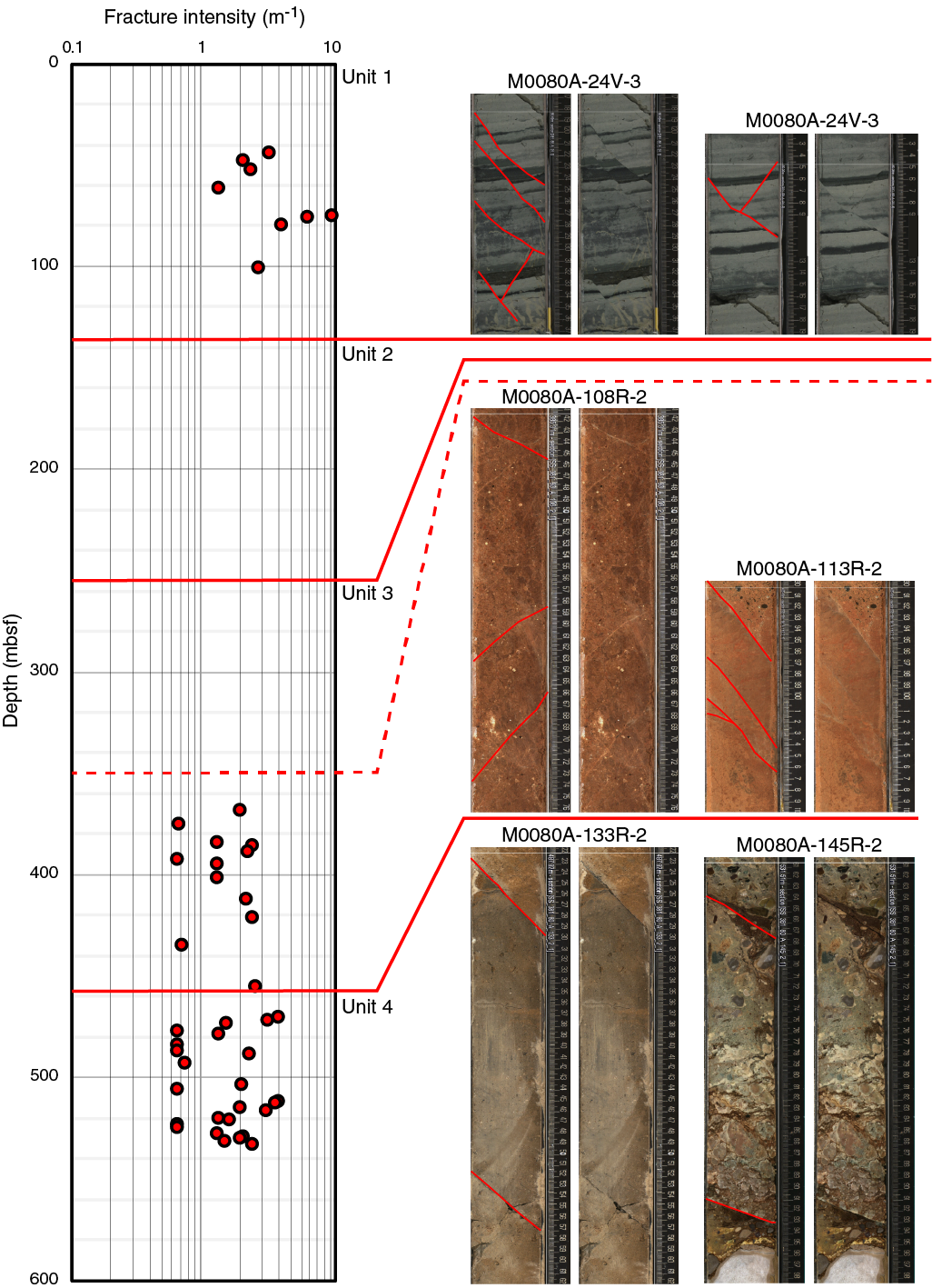
Figure F10. Fracture intensity and fault traces.
The highest range of natural fault intensity values occurs in Unit 1, ranging from 1.4 to 10.5 m−1 (Figure F10). In contrast, no faulting was observed in Unit 2 and Subunit 3-1 (Cores 381-M0080A-31V through 102R; 101.70–367.60 mbsf). This interval is characterized by FA12 (bioturbated homogeneous mud) in Unit 2 and the mainly unconsolidated conglomerates in lithostratigraphic Subunit 3-1 (FA7; see Lithostratigraphy), suggesting a potential lithologic and rheological control on fault and fracture development. In Subunits 3-2 and 3-3 and Unit 4, fracture intensity values range from 0.7 to 4.0 m−1 (Figure F10).
Faults in Unit 1 have apparent normal displacements that commonly range from 2 mm to 3.2 cm. Offsets on faults in Units 3 and 4 could not be measured because of a general absence of bedding traces in the consolidated siltstones, sandstones, and conglomerates (Figure F10). However, many of the faults in Units 3 and 4 are thought to have displacements greater than the length of the fault trace observed in the core. Some have millimeter- to centimeter-thick fault gouges and mineralized surfaces that often show slickenlines (e.g., Figure F11). Slickenline orientations indicate a range of motion senses from dip-slip to oblique-slip to strike-slip (Figures F11, F12). A significant number of faults show strike-slip or oblique displacement.
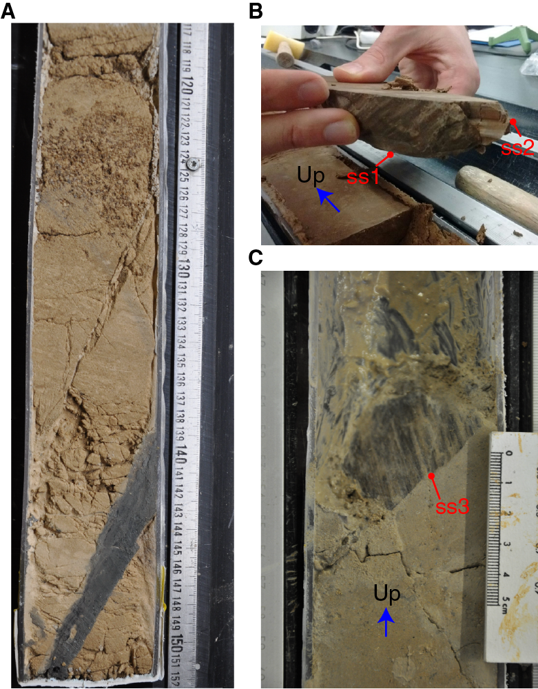
Figure F11. Tectonic faults.
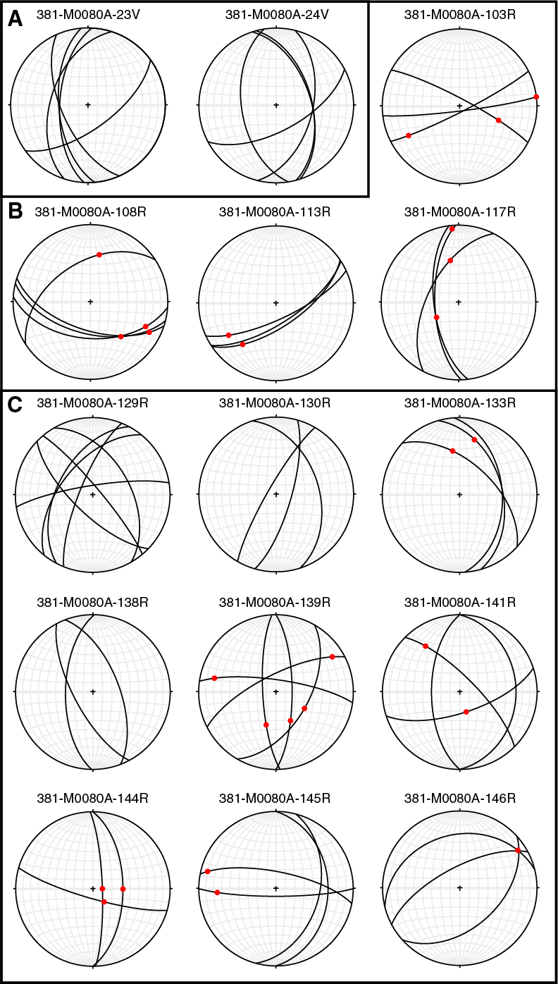
Figure F12. Fault plane and slickenline orientations.
In total, 82 faults were sampled for orientation analysis. The faults in the soft sediment of Unit 1 were measured using the same technique as for Sites M0078 and M0079 (see the Expedition 381 methods chapter [McNeill et al., 2019b]). The normal faults in Unit 1 appear to mainly fall into a conjugate set with an average NNE–SSW strike in the core reference frame, as illustrated by the stereographic projection plots (Figure F12A). As observed at Sites M0078 and M0079, the consistent fault orientations throughout Unit 1 suggest that our sampling is biased, and we mainly detect faults that are trending approximately perpendicular to the split-core surface. We may thus be undersampling faults that strike obliquely or subparallel to the core split face.
Fault orientations were measured in a different way in the consolidated rocks of Units 3 and 4 at Site M0080. Here, the working core tended to break cleanly along fault planes so that blocks of core could be temporarily lifted out, thus exposing the fault surfaces in three dimensions and allowing a more robust orientation analysis of the surface and measurement of any slickenlines (Figure F11B). We were thus able to sample faults even if the core split face is orientated obliquely or subparallel to the fault strikes. The results from these intervals therefore include a more complete and complex fault orientation distribution in Units 3 and 4 that is not biased by orientation relative to the core split face. We note in particular that fault orientations can vary between cores. In Unit 3, sampled faults have similar strikes in the same core and sometimes form conjugate sets of either strike-slip (e.g., Core 381-M0080A-103R) or oblique-slip faults (e.g., Core 108R) (Figure F12). In Unit 4, fault orientations are often more variable within each core, sometimes forming conjugate as well as bimodal fault sets. Fault orientations in Cores 129R, 139R, and 141R are highly variable and complex, probably due to rotation and development of intense biscuiting. Therefore, further filtering of the fault data will be needed before restoring the fault orientations to geographic north using the core paleomagnetic data.
The sampled normal faults show true dips ranging from 28° to 85° but with a clear modal average dip of 50°–60° and a mean dip of 61° (Figure F13). The steeply dipping to subvertical faults are often linked with oblique-slip or strike-slip oriented slickensides and are therefore considered natural (Figure F12). Overall, the abundance and geometry of small normal faults in Unit 1 are consistent with those observed at Sites M0078 and M0079 and in agreement with the overall extensional nature of the rift deformation. However, the range in fault displacements and geometries in the stratigraphically older Units 3 and 4 suggests a more complex history of faulting possibly involving multiple fault generations and/or fault reactivation.
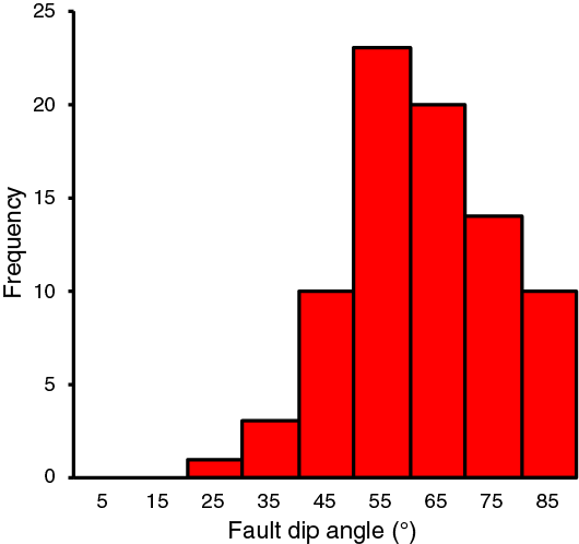
Figure F13. Fault dip frequency.
Observed drilling-induced deformation
A wide range of drilling-induced features was observed at Site M0080. The most common features were arching bedding, biscuiting, sediment flow/smearing along the core liner, voids, and open and shear fractures (Figures F14, F15). Other features that were less commonly observed are listed in Table T1 in the Expedition 381 methods chapter (McNeill et al., 2019b).
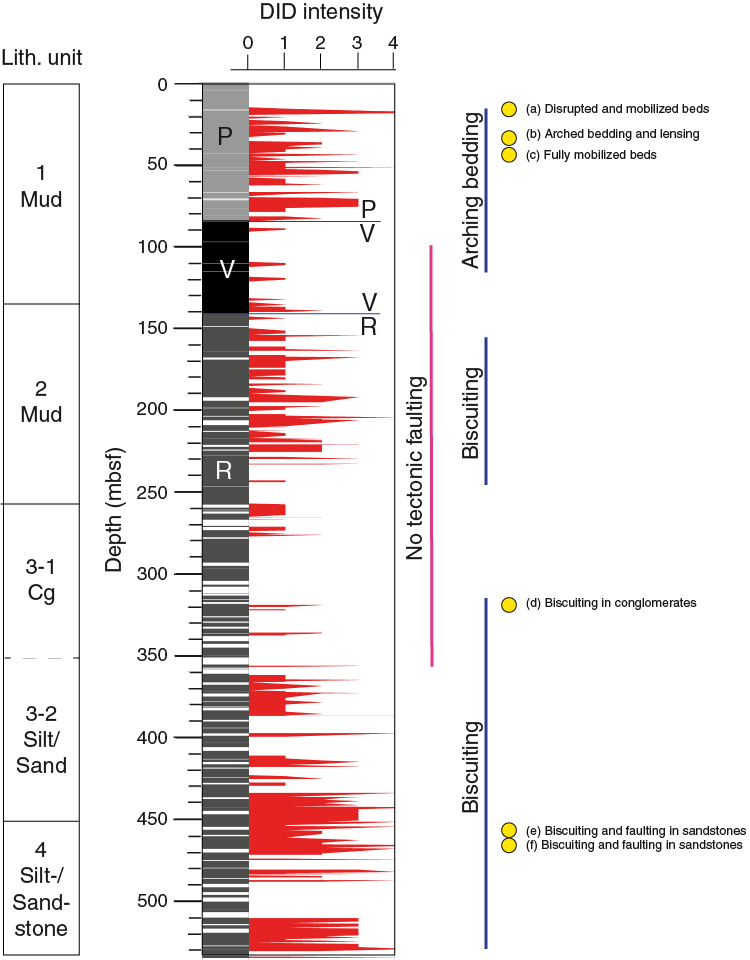
Figure F14. DID intensity.
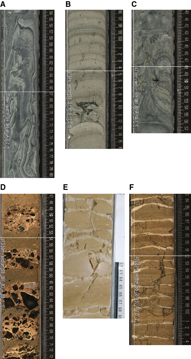
Figure F15. Examples of DID.
Hydraulic piston coring was not used in this borehole; only push (P), percussive (V), and rotary (R) coring were used (Figure F14). Overall, DID intensity is highly variable, with significant lengths of the core having little or no DID. We provisionally relate this variation to a combination of drilling technique and core material strength, with correlations to lithostratigraphic units. In the push cores deeper than 15 mbsf, DID is pervasive (Figure F14). This low- to high-intensity DID in the mud-dominant lithostratigraphic Unit 1 is expressed principally by arching bedding, lensing, flow along the core liner with some local soupy texture, axial flow, brecciation, voids, and open fractures (Figure F15). Sections 381-M0080A-6P-1, 0 cm, through 6P-2, 73 cm (16.5–18.72 mbsf), are notable for complete mobilization and destruction of bedding. DID intensity remains low to absent in percussive cores in the mud-dominant lower lithostratigraphic Unit 1. Rotary coring started at Core 42R (141 mbsf) with a clear change in DID intensity and type. Biscuiting is dominant in Sections 45R-1 through 64R-2 (156–244 mbsf) and Sections 88R-1 through 144R-2 (314–530 mbsf) (Figures F14, F15D) and is associated mainly with some shear fractures and open fractures. DID intensity is low to high through most of the mud-dominant lithostratigraphic Unit 2 and drops to low or absent in the lowest part of Unit 2 and through most of the conglomerate-dominated Subunit 3-1. DID intensity again becomes moderate to high through the finer grained lower Unit 3 and through most of the fully lithified Unit 4, although there are lengths of core with little or no DID (Sections 135R-1 through 139R-1; 497–510 mbsf; Figure F14). In Unit 4, biscuiting and brecciation are dominant with regular occurrences of voids, open fractures, and shear fractures (Figure F15E–F15F). Overall, drilling-induced shear fracturing is less common at Site M0080 than at Site M0079.
Micropaleontology
Hole M0080A is located in the Alkyonides Gulf, east of and connected to the Gulf of Corinth (Figure F1). Hole M0080A is divided into four major units, each of which is divided into different subunits by integration of lithologic and physical properties characteristics (see Lithostratigraphy) and observed microfossil assemblages. Unit 1 is characterized by alternating marine and isolated/semi-isolated intervals, Unit 2 is characterized by dominantly isolated/semi-isolated conditions, Unit 3 is characterized by terrestrial deposits, and Unit 4 is primarily characterized by carbonate-rich sand, silt, and mudstone interpreted to represent a shallow-water to intermittently subaerial environment.
Calcareous nannofossils
Calcareous nannofossils were observed in all Unit 1 marine intervals/subunits to 136.7 mbsf. The calcareous nannofossil assemblages observed in Hole M0080A are similar to those observed in Holes M0078A, M0078B, and M0079A, with the most commonly observed species belonging to Emiliania huxleyi, Gephyrocapsa spp., Helicosphaera carteri, Reticulofenestra spp., and Syracosphaera spp. (Table T4).
In contrast to Sites M0078 and M0079, a significantly higher abundance of a large morphotype of E. huxleyi (>3 µm) was observed, especially in Subunit 1-1. These large morphotypes are thought to be the result of colder surface waters (Young and Westbroek, 1991; Flores et al., 2010).
E. huxleyi is the dominant taxa in the youngest marine interval, Subunit 1-1. The last downhole occurrence (LDO) is noted at the base of Subunit 1-3 in Sample 381-M0080A-12P-1, 15–16 cm (35.45 mbsf). Because of the irregularity of the depositional environment here, this occurrence likely does not represent the true first appearance datum (FAD) that marks 0.29 Ma (Backman et al., 2012) and biostratigraphic application should be conservative.
A crossover in dominance between E. huxleyi and Gephyrocapsa “small” (<4 µm) was observed at Site M0080, as at the other sites. This crossover occurs here in Subunit 1-2 between 8.87 and 21.15 mbsf. Below this depth, starting in Subunit 1-3, Gephyrocapsa spp. is the dominant species. The timing of this crossover in dominance has been documented and discussed by Thierstein et al. (1977), Raffi et al. (2006), and Anthonissen and Ogg (2012), among others. The crossover appears to be time transgressive depending on latitude and is not well calibrated (Thierstein et al., 1977), so one should proceed with caution when applying this datum. Anthonissen and Ogg (2012) document this crossover occurring at 0.07 Ma in the Mediterranean Sea, which corresponds to early marine isotope Stage (MIS) 4 (Lisiecki and Raymo, 2005). If this datum is applied to Hole M0080A in the Alkyonides Gulf, then MIS 4 is represented by the Subunit 1-2 isolated/semi-isolated interval. Unfortunately, this crossover cannot be better characterized here because of the isolation of the Alkyonides Gulf during this period.
In Subunit 1-5, Sample 381-M0080A-17P-4CC, 0–1 cm (57.63 mbsf), contains an assemblage conspicuously similar to Samples 381-M0078A-112R-4CC, 15–26 cm (329.20 mbsf); 381-M0079A-123R-4, 34–35 cm (539.74 mbsf); and 381-M0079A-124R-2, 72–73 cm (542.12 mbsf). This assemblage contains abundant Gephyrocapsa spp., higher counts of H. carteri and Calcidiscus leptoporus, and an increase in reworked microfossils. This assemblage implies warm waters in a nearshore depositional setting influenced by freshening and nutrient enrichment resulting from increased continental runoff (Dimiza et al., 2014, 2016).
In the Subunit 1-7 marine interval (83.87–88.52 mbsf), the calcareous nannofossil assemblage contains a relatively high amount of Reticulofenestra “large” (≥4 µm). This assemblage was not observed at the other two sites, implying variation in the depositional environment relative to Sites M0078 and M0079 in the Gulf of Corinth.
Calcareous nannofossils were not observed in Units 2 or 3, except for specimens that were obviously reworked (e.g., poorly preserved Paleogene or Cretaceous species).
Unit 4 is devoid of calcareous nannofossils, both in situ and reworked, with the exception of Subunit 4-1 where two species were observed in three samples: 381-M0080A-128R-1, 143–150 cm (466.83 mbsf); 128R-3CC, 12–13 cm (467.73 mbsf); and 136R-1, 98–99 cm (501.28 mbsf). The specimens were observed in low quantities and are of moderate preservation, and these samples were otherwise devoid of reworked microfossil material. Given this and what we currently know about the sedimentology in Hole M0080A, these fossils are interpreted to be in situ. The two species, Amaurolithus primus and Isolithus semenenko, have a concurrent range zone of 7.39–4.58 Ma (late Miocene–early Pliocene) based on the FAD and last appearance datum (LAD) of A. primus, both of which are geologic age markers (Backman et al., 2012).
Marine diatoms
Marine diatoms are virtually absent from Site M0080 with the exception of two samples, 381-M0080A-8P-4CC, 25–26 cm (30.58 mbsf), in Subunit 1-3 and 38V-3, 7–8 cm (131.37 mbsf), in Subunit 1-11, where they co-occur with calcareous nannofossils (Table T4). In Subunit 1-3, the observed marine diatoms belong to a single genus, Rhizosolenia. In Subunit 1-11, the dominant species was Paralia sulcata, a brackish/marine species. The significantly lower abundance of marine diatoms at this site relative to the other sites indicates a critical lack of nutrients and/or niche space. At this time, the marine diatom record is only appropriate for making simple interpretations regarding nutrient levels in the surface waters and to contribute to preliminary interpretation of the depositional environment.
Nonmarine diatoms
Nonmarine diatoms were primarily examined in smear slides made from core catcher samples offshore. Further onshore examination of the nonmarine diatom species sought to improve species identification and increase the understanding of ecology (Table T5).
From offshore sample analysis, nonmarine diatoms were observed in Units 1 and 2, and an additional 39 samples from Units 1, 2, and 3 were analyzed onshore to provide preliminary information about the depositional environment at Site M0080 (Tables T4, T6). In both cases, the nonmarine diatom assemblages at this site show better preservation and are composed of a greater abundance and diversity of benthic species, indicating a shallower environment than at the other two sites. A total of 46 taxa (including morphological varieties) were identified, 35 of them with benthic life habitat (Figure F16).
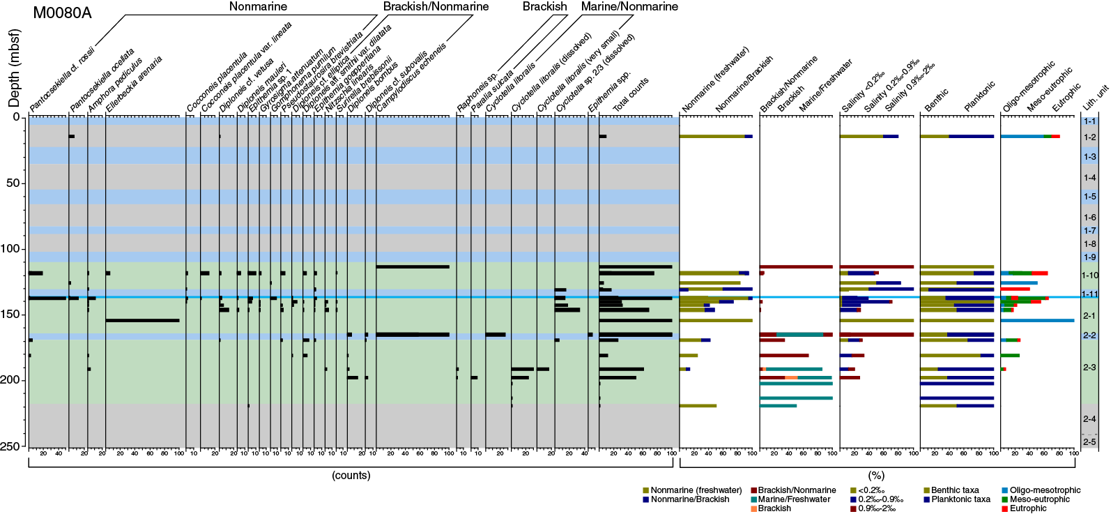
Figure F16. Most common diatom taxa.
The samples from Subunits 1-2 and 1-3 appeared barren or sometimes contained very few broken valves of benthic species that could not be identified to the species level. The only exception was Sample 381-M0080A-5P-1, 81 cm (14.31 mbsf), where a tephra layer was also visually identified. The diatom assemblage here is composed of small (~5 µm) valves of Pantocsekiella ocellata and some benthic nonmarine species like Caloneis lancetula, Campylodiscus cf. hibernicus, and so on. The dominance of small-sized planktonic diatoms associated with tephra deposition has been observed at other sites (Cvetkoska et al., 2012, 2014; Jovanovska et al., 2016) and is related to nutrient enrichment—especially silica (SiO2). In contrast, the poor preservation and/or absence of diatoms in some of the subunits in Unit 1 (without tephra) can be related to the bicarbonate composition of local bedrock.
The assemblages from Subunit 1-10, an isolated/semi-isolated interval, contain diverse benthic diatom communities. Sample 34V-3, 25 cm (113.65 mbsf), is dominated by Campylodiscus echeneis, a benthic taxon primarily related to coastal and brackish environments but also reported from some nonmarine environments (e.g., the Great Lakes, USA [Stoermer et al., 1999]). Subunit 1-10 features a shift between samples dominated by nonmarine (freshwater) taxa that indicate lower nutrient levels (Samples 35V-3, 1 cm, and 37V-2, 6 cm; 118–125.7 mbsf) and an assemblage with increased presence of brackish taxa that are considered as eutrophic indicators (Sample 38V-2, 60 cm; 130.4 mbsf).
The samples analyzed from Subunit 2-1 show a change from nonmarine planktonic-dominated assemblages toward nonmarine assemblages dominated by benthic taxa at the boundary with Subunit 2-2. Pantocsekiella cf. rossii and P. ocellata dominate in Sample 40V-1, 86 cm (137.56 mbsf). The presence and diversity of benthic taxa increase between Samples 41V-1, 66 cm, and 43R-2, 75 cm (140.16–146.26 mbsf). The most common nonmarine benthic taxa in these assemblages are Amphora pediculus, C. lancetula, Diploneis cf. elliptica, Diploneis cf. vetusa, and Pseudostaurosira brevistriata, whereas the most common benthics, which prefer shallow, nonmarine, and/or brackish environments, are Epithemia goeppertiana, Nitzschia linearis, and Surirella brebissonii. The lowermost sample analyzed from this unit (Sample 45R-1, 20 cm; 154.2 mbsf) is dominated by Ellerbeckia arenaria, which along with the great abundance of ostracods found in the same sample indicates that this probably represents an interval of shallow, nonmarine (freshwater), oligotrophic–mesotrophic environment.
The upper part of Subunit 2-2 includes Sample 47R-1, 94 cm (164.94 mbsf), which is characterized by a mixed planktonic–benthic diatom assemblage. Cyclotella litoralis and C. echeneis dominate the assemblage, whereas Diploneis bombus and Diploneis cf. subovalis occur at lower counts. The overall assemblage indicates a brackish depositional paleoenvironment.
The samples analyzed from Subunit 2-3 contain well-preserved diatom assemblages that show a trend of increasing marine influence toward the lower part of this subunit. Samples 48R-1, 20 cm, and 50R-2, 63 cm (169.2 and 181.13 mbsf), contain a higher proportion of benthic taxa than planktonic taxa. These taxa have been primarily reported from nonmarine environments but also from some brackish environments (e.g., Diploneis aff. smithii var. dilatata, D. cf. subovalis, and E. goeppertiana). Samples 52R-2, 78 cm, and 53R-3, 86 cm (191.28 and 197.86 mbsf), show a change toward an increased proportion of planktonic taxa and increased taxa that can tolerate higher salinity levels, like C. litoralis, P. sulcata, D. bombus, and D. cf. subovalis.
Seven samples in total were analyzed from Unit 3 between Samples 95R-1, 35 cm, and 123R-2, 49 cm (336.55–443.92 mbsf), but no diatoms were found. The only exception was Sample 117R-2, 32 cm (420.68 mbsf), where a single valve was observed, but identification was not possible because of its poor preservation.
Overall, the diatom taxa identified in Hole M0080A samples were divided into several categories according to their environmental preferences. In addition to the general environment, here we adopted the salinity classification available from Van Dam et al. (1994) (Table T5). Both approaches seem to reflect the changes described above, leading to a general impression that the major shifts occur between oligotrophic–mesotrophic assemblages with low-salinity preferences and mesotrophic–eutrophic benthic assemblages tolerant to higher salinity. This implies that further detailed diatom analyses from Hole M0080A can provide insights into climate and sea level change driving environment at this site.
Nonmarine diatoms and calcareous nannofossils were not observed together in mixed microfossil assemblages as frequently as they were at the other two sites. At Site M0080, only four samples are currently described as having a mixed microfossil assemblage.
Foraminifers
A total of 183 samples were examined for foraminifer microfossils (145 samples from core catchers taken offshore and 38 additional core samples from split-core sections taken during the onshore phase of the expedition). Foraminifer specimens were observed only in specific intervals in Units 1 and 2 and always showed large variations in their abundances. Foraminifers were absent from Sample 381-M0080A-68R-3, 11–12 cm (257.81 mbsf), at the top of Unit 3 through Sample 144R-2, 46–47 cm (529.26 mbsf), near the base of Unit 4, except for Sample 139R-4, 9–11 cm (513.37 mbsf), which contained only very few specimens of Ammonia tepida (Table T7).
Unit 1 includes seven intervals in which benthic and/or planktonic foraminifers appear in relatively high abundances:
- Samples 1P-1, 139–140 cm, to 3P-2, 13–15 cm (1.39–6.13 mbsf), in Subunit 1-1;
- Samples 7P-1, 20–22 cm, to 7P-4, 19–20 cm (22.9–25.76 mbsf), in the upper part of Subunit 1-3;
- Samples 8P-4, 25–26 cm, to 12P-1, 15–17 cm (30.58–35.45 mbsf), in the lower part of Subunit 1-3;
- Samples 17P-2, 110–112 cm, to 19P-1, 47–49 cm (55.8–63.07 mbsf), in Subunit 1-5;
- Samples 25P-3, 0–3 cm, to 27V-4, 10–11 cm (83.87–88.52 mbsf), in Subunit 1-7;
- Samples 31V-3, 102–103 cm, to 33V-4, 0–1 cm (105.72–109.87 mbsf), in Subunit 1-9; and
- Samples 38V-2, 126–128 cm, to 39V-4, 30–31 cm (131.06–136.7 mbsf), in Subunit 1-11.
In the remaining parts of the hole, foraminifers are rare or absent.
When present, foraminifers are well preserved. Benthic foraminifers are almost always more abundant than planktonic foraminifers. This trend is most obvious in Subunit 1-11, where planktonic foraminifers are absent. The three most commonly abundant species in Subunits 1-1, 1-3, 1-5, and 1-7 are Hyalinea balthica, Cassidulina carinata, Bulimina marginata, and Bulimina aculeata with a relatively minor contribution of Melonis barleeanus (Table T8). Ecological studies relate a high abundance of these species to the presence of high inputs of organic carbon to the seafloor in the form of fresh phytodetritus (Goineau et al., 2015). Assemblages in Subunit 1-9 contain an abundance of the benthic foraminifer species C. carinata, and they also contain a relatively high contribution of species characteristic of nearshore marine environments such as A. tepida and Elphidium excavatum (Debenay, 2000). In intervals where planktonic foraminifers are abundant (in Subunits 1-1, 1-3, 1-5, and 1-9), the planktonic assemblages show relatively low diversities. These assemblages are usually dominated by neogloboquadrinids, suggesting the development of a deep chlorophyll maximum layer, or by Turborotalita quinqueloba, suggesting the prevalence of surficial water of relatively low salinity and low temperature and/or enhanced fertility (Rohling and Gieskes, 1989; Rohling et al., 1993). The only exception is Sample 8P-4, 25–26 cm (30.58 mbsf), where the dominant planktonic species is Globorotalia inflata, which may indicate the development of a cool and deep mixed layer (Pujol and Vergnaud Grazzini, 1995) (Table T9).
Unit 2 includes three intervals in which foraminiferal fauna appear in high abundances:
- Samples 47R-1, 66–68 cm, to 47R-4, 0–1 cm (164.66–167.54 mbsf), in Subunit 2-2;
- Samples 63R-3, 36–38 cm, to 63R-5, 10–11 cm (240.56–242.31 mbsf), in the upper part of Subunit 2-5; and
- Samples 67R-4, 9–10 cm, to 68R-1, 143–150 cm (255.1–256.13 mbsf), in the lower part of Subunit 2-5.
In these intervals, foraminifers are represented only by benthic species and are dominated by A. tepida, a shallow-marine species that represents as much as 90% of the assemblage. Faunal assemblages from 255.1 to 256.13 mbsf are likely influenced by postdepositional processes involving carbonate chemical reactions.
Palynology
A total of 15 core catcher samples from Hole M0080A were analyzed for palynomorphs (Table T10): 3 samples from Unit 1, 5 samples from Unit 2, 4 samples from Unit 3, and 3 samples from Unit 4. All samples examined from Unit 4 were either barren or contained badly preserved palynomorphs that did not allow for further analysis. In Unit 3, only Sample 124R-4, 11 cm (451.19 mbsf), yielded well-preserved palynomorphs and is included in the analyses. In Unit 2, all samples are included in the analyses with the exception of Sample 67R-4, 9 cm (255.1 mbsf), which is barren. In Unit 1, Sample 24P-2, 146 cm (79.26 mbsf), yielded very low concentrations of palynomorphs and is excluded from the analyses.
A total of seven samples yielded good palynomorph preservation and are presented with a mean concentration of corroded pollen grains of 314 grains/g and a maximum of 460 grains/g in Sample 124R-4, 11 cm (451.19 mbsf). The mean concentration of fungal remains is 23 per gram, and the mean concentration of charred microscopic particles is 4027 per gram with a maximum of 7690 per gram in Sample 9P-1, 0 cm (30.6 mbsf). Terrestrial pollen concentrations have a mean value of 6,716 grains/g that is higher than at the other two sites, with a maximum of 14,163 grains/g recorded in Sample 50R-5, 0 cm (184.04 mbsf).
Pollen assemblages are generally dominated by arboreal pollen (Table T10). Maximum tree percentages and concentrations are recorded in Sample 50R-5, 0 cm (184.04 mbsf), with values of 87.9% and 13,577 grains/g, respectively.
Pollen spectra in Hole M0080A are dominated by Quercus pollen; however, the occurrence of Corylus, Acer, Carpinus, and Ulmus suggests the presence of a mixed deciduous forest in the surroundings of the Alkyonides Gulf. Pollen grains of relict species include Cedrus, Zelkova, Carya, Pterocarya, Tsuga, and Tricolpoporopollenites sibiricum (Table T10). Cedrus reaches a maximum of 57.5% in Sample 124R-4, 11 cm (451.19 mbsf), along with low abundances of Carya, Tsuga, Zelkova, and T. sibiricum. Steppic elements reach a maximum value of 14.7% in Sample 57R-3, 124 cm (217.24 mbsf), whereas Mediterranean sclerophyllous vegetation reaches a maximum of 12.6% in Sample 47R-4, 0 cm (167.54 mbsf). High abundances of green algae Botryococcus coenobia are present in Samples 47R-4, 0 cm (167.54 mbsf), and 57R-3, 124 cm (217.24 mbsf).
In contrast to the other two sites, dinoflagellate cysts were encountered in only three samples. Samples 9P-1, 0 cm (30.6 mbsf), and 31V-3, 102 cm (105.72 mbsf), are dominated by multiple species of marine dinoflagellates; Sample 42R-3, 73 cm (144.25 mbsf), is characterized by high abundances of Spiniferites cruciformis.
Biostratigraphy summary
Age control is provided solely by the calcareous nannofossils in Hole M0080A, and it should be applied cautiously given the complexity of the depositional environment (Table T11). Two biohorizons were recognized at Site M0080. The first age datum that is considered here is that of the crossover in dominance between E. huxleyi and Gephyrocapsa “small.” This crossover has been observed in multiple locations (Thierstein et al., 1977; Raffi et al., 2006; Anthonissen and Ogg, 2012), and in the Mediterranean Sea it is calibrated at 0.07 Ma in MIS 4 (Anthonissen and Ogg, 2012). If this datum can be applied accurately in Hole M0080A, then it occurs in Subunit 1-2 between 8.87 and 21.15 mbsf.
The LDO of E. huxleyi was observed in Sample 381-M0080A-12P-1, 15–16 cm (35.45 mbsf), but likely does not represent the true FAD (0.29 Ma) because this species evolved in glacial MIS 8, a time when the Gulf of Corinth was presumably disconnected from the Mediterranean Sea.
In three samples from Subunit 4-1, two calcareous nannofossil species were observed. I. semenenko and A. primus were both observed in Sample 128R-1, 143–150 cm (466.83 mbsf), and only I. semenenko was observed in Samples 128R-3CC, 12–13 cm (467.73 mbsf), and 136R-1, 98–99 cm (501.28 mbsf). I. semenenko first occurs in the Tortonian (11.63–7.25 Ma), and its last occurrence is in the Zanclean (5.33–3.6 Ma); it is not a biostratigraphic marker species. A. primus is a marker species and both its FAD and LAD are biostratigraphic age markers at 7.39 and 4.58 Ma, respectively. These two species, therefore, have a concurrent range zone of 7.39–4.58 Ma (late Miocene–early Pliocene) (Backman et al., 2012; Ogg et al., 2016), and this is the age range that is tentatively applied to this interval. It is important to consider that these species are not abundant and are moderately preserved, but they are currently interpreted to be in situ because no other reworked specimens were observed.
Micropaleontology summary
Micropaleontology at Site M0080 maintains a high level of complexity both in individual microfossil groups and collectively, as it did at Sites M0078 and M0079. Unit 1 alternates primarily between marine and undetermined/barren assemblages but also includes a few mixed and nonmarine assemblages toward the base of the unit. Pollen assemblages examined in this unit suggest the occurrence of a forested landscape in the surroundings of the Alkyonides Gulf. Unit 2 alternates between nonmarine, undetermined/barren, and marine/brackish assemblages. Unit 3 is devoid of microfossils, except palynomorphs, and is almost entirely terrestrial. Unit 4 is nearly devoid of microfossils with the exception of three samples that contain calcareous nannofossils in low concentrations. See Figure F17 for a summary of the microfossil assemblages by subunit, and refer to individual data sets for details.
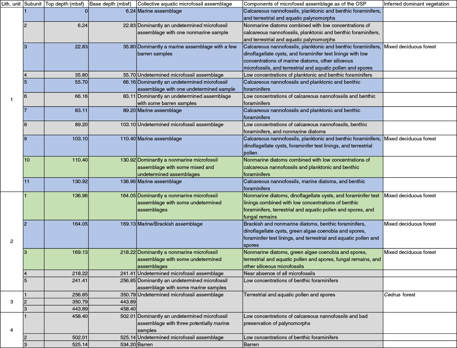
Figure F17. Micropaleontology assemblages.
Geochemistry
Interstitial water
At Site M0080, 62 interstitial water samples were collected from 0.90 to 502.13 mbsf. Rhizon sampling acquired pore water to 20.50 mbsf, and whole-round squeeze cakes were used to sample pore water from 32.05 to 502.13 mbsf. Both methods successfully produced the required water volume to 365.33 mbsf. Subsequently, squeeze cakes only produced limited water, and not all pore water splits could be collected. Additionally, drilling mud fluid samples were taken from discrete depths to evaluate any potential drilling mud fluid contamination (see Geochemistry in the Expedition 381 methods chapter [McNeill et al., 2019b]). Pore water compositions at Site M0080 can be grouped into four distinct geochemical regions that correspond to the four lithostratigraphic units present at the site: Unit 1 (possible alternations between marine and isolated/semi-isolated intervals), Unit 2 (mostly isolated/semi-isolated), Unit 3 (principally terrestrial deposits), and Unit 4 (primarily characterized by carbonate-rich sand, silt, and mudstone; see Lithostratigraphy). The pore water geochemistry of these units is described in detail below.
Salinity variations: salinity, sodium, and chloride
Salinity decreases from approximate modern Gulf of Corinth seawater values (37.47) at the seafloor to 12.38 at 49.45 mbsf. Deeper than 49.45 mbsf, salinity gradually increases to a maximum of 37.82 in the deepest sample at 502.13 mbsf (Figure F18A). Chloride (Cl−) concentrations follow salinity downhole throughout Site M0080 (Figure F18B). Concentrations decrease from 593.11 mM at the sediment/water interface to 199.95 mM at 86.95 mbsf and then increase to 522.46 mM at the base of the hole. Cl− concentrations in pore water samples at 264.63, 291.06, 322.90, and 439.31 mbsf are markedly lower than surrounding samples, suggesting possible contamination with drilling mud (bentonite + freshwater).
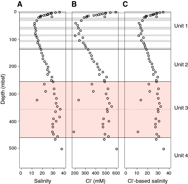
Figure F18. Pore water salinity, chloride, and Cl−-based salinity.
Organic matter degradation: alkalinity, ammonium, boron, bromide, iron, manganese, pH, phosphate, sulfate, and dissolved inorganic carbon
Organic matter degradation in sediments leads to distinct changes in pore water geochemistry, generally revealing redox reactions (Berner, 1980). These shallow redox reactions were observed in the pore water profiles from the upper 14.70 mbsf in Hole M0080A (Figure F19). Comparable to Sites M0078 and M0079, the Mn2+ profile shows elevated concentrations (as high as 31.45 µM) in the upper 7.20 mbsf of Hole M0080A, most likely indicating Mn oxide reduction, and low concentrations deeper in the hole. However, between 400.44 and 421.87 mbsf, pore water Mn2+ concentrations increase again and reach high concentrations of 47.38–63.17 µM. Dissolved Fe2+ concentrations are highest in the uppermost sample (166.74 µM) and then decrease sharply to 0.5 µM at 8.50 mbsf, indicating possible reduction of Fe oxides. A second minor peak (40.19 µM) occurs at 12.90 mbsf, and concentrations remain below this value to the base of the hole.
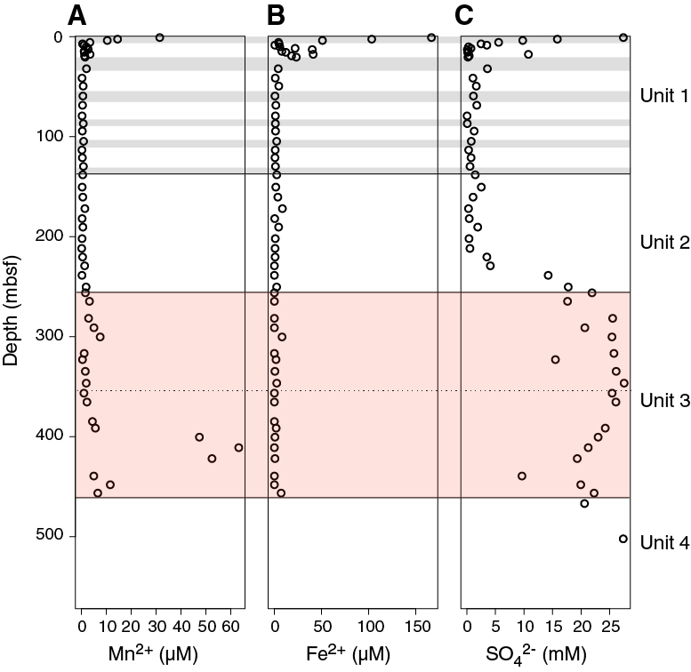
Figure F19. Pore water manganese, iron, and sulfate.
Sulfate (SO42−) concentrations decrease from 27.40 mM near the sediment/water interface to 0.30 mM at 10.20 mbsf (Figure F19C). Deeper than 10.20 mbsf, SO42− concentrations are low until an abrupt increase at 238.64 mbsf (18.2 m above the Unit 2/3 boundary) continuing to the base of the hole (maximum of 27.53 mM at 346.44 mbsf). SO42− concentrations in pore water samples at 264.63, 291.06, 322.90, and 439.31 mbsf (the same depths where contamination is suggested in the Cl− profile; Figure F18B) are markedly lower than in surrounding samples (Figure F19C), also suggesting possible contamination with drilling mud (bentonite + freshwater).
Ammonium (NH4+), phosphate (PO43−), and bicarbonate (HCO3−), an important component of dissolved inorganic carbon (DIC) at this pH range, are common products of microbial organic matter degradation. Each of these parameters have the same downhole increasing trend in the upper 20.50 mbsf at Site M0080 (Figure F20). However, depths of major changes in concentrations are not directly comparable deeper than 20.50 mbsf. NH4+ concentrations increase from seafloor values of 0.2 mM to a maximum of 5.3 mM at 138.15 mbsf. NH4+ concentrations then decrease from 160.44 to 281.63 mbsf (immediately below the Unit 2/3 boundary), where concentrations remain low (less than 0.3 mM) to the base of the hole. In contrast to NH4+, PO43− concentrations reach a maximum (21.82 µM) at a shallower depth and then decrease in a stepwise manner to 0.54 µM at 201.94 mbsf. Further downhole, PO43− concentration remains low to the base of the hole.
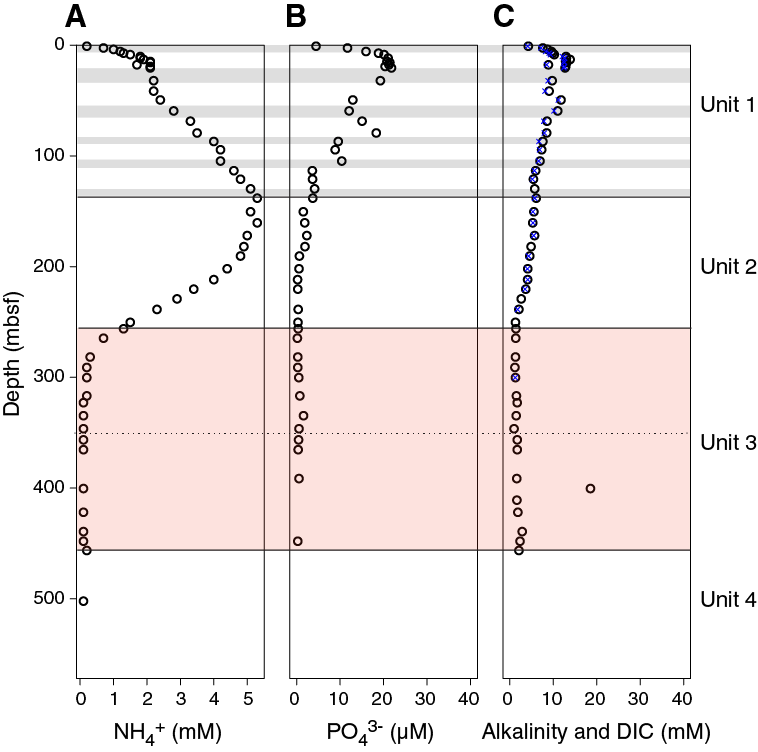
Figure F20. Pore water ammonium, phosphate, and alkalinity and DIC.
Alkalinity, a parameter that measures the sum of all bases (including HCO3−), increases in the top 12.90 m from 4.25 mM to a maximum of 13.87 mM (Figure F20C). Similar to PO43− concentrations, alkalinity then decreases, reaching a zone of much lower concentrations (less than 1.5 mM) from 256.13 mbsf to the base of the hole. Alkalinity values are similar to DIC concentrations, suggesting HCO3− is the dominant fraction of alkalinity. Pore water pH at Site M0080 varies between 7.4 and 8.2 (Figure F21A). pH generally decreases downhole from a maximum at shallow depths (8.2 at 10.20 mbsf) to a minimum of 7.4 at 400.44 mbsf.
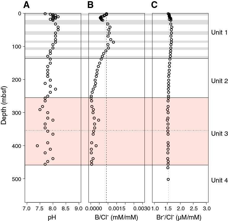
Figure F21. Pore water pH and B/Cl– and Br–/Cl– ratios.
Boron (B) and bromide (Br−) accumulate in organic matter. A common method to determine the relative contributions of seawater and organic carbon oxidation to pore water chemistry is to plot the ratio of B and Br− to Cl− (Figure F21B–F21C). Disparity of B/Cl− and Br−/Cl− from seawater values can indicate production or removal of ions from solution. Both B/Cl− and Br−/Cl− values at Site M0080 broadly follow the PO43− profile with depth, including a shift to lower values around the depth of the Unit 2/3 boundary. Below the Unit 2/3 boundary, alkalinity, DIC, NH4+, Mn2+, and Fe2+ concentrations are much lower. These values are in the same range as concentrations in the drilling mud (Table T12); hence, potential drilling mud contamination, as mentioned above for SO42− and Cl−, would have less effect on the alkalinity, DIC, NH4+, Mn2+, and Fe2+ concentrations.
Mineral reactions
Barium, calcium, magnesium, potassium, sodium, and strontium
Calcium (Ca2+), magnesium (Mg2+), potassium (K+), and sodium (Na+) are all major ions in seawater, and barium (Ba2+) and strontium (Sr2+) are minor components. Their concentrations in pore water may be altered by processes such as ion exchange, mineral weathering, and formation of new minerals. The Na+ and K+ depth profiles (Figure F22) resemble those of salinity and Cl−, indicating that salinity changes govern the overall pattern. The Na+/Cl− ratio stays very close to the seawater value in the uppermost 350 m. Deeper in the hole, a decrease in the Na+/Cl− ratio suggests a removal of Na+. The observed K+/Cl− ratio profile shows that K+ concentrations are influenced by reactions with the sediment because the ratios differ downhole and do not reflect that of modern Gulf of Corinth seawater composition (vertical dashed line, Figure F22E). K+/Cl− values remain lower than in seawater throughout the hole, with the lowest values in Unit 2 and the lower part of Unit 3.

Figure F22. Pore water sodium, potassium, and barium.
Ba2+ and salinity have opposite trends in the shallow sediment. Ba2+ concentration increases from 0.28 to 49.45 µM at 49.45 mbsf and then continues to increase to a maximum of 36.43 µM at the Unit 1/2 boundary at 136.96 mbsf (Figure F22C). This increase suggests a release of Ba2+ at this unit transition. Deeper in the hole, Ba2+ concentrations decrease again and remain below 2.82 µM to the base of the hole. The dissolved Ca2+ and Mg2+ depth profiles largely follow the Cl− and salinity profiles (Figures F18, F23A–F23B). Ca2+ concentration decreases in the top 8.50 m from 8.39 to 1.58 mM, and Mg2+ decreases from 52.16 mM at the sediment/water interface to 16.51 mM at 79.26 mbsf. In Unit 1, both Ca2+ and Mg2+ decrease more significantly than Cl− as indicated by the Ca2+/Cl− and Mg2+/Cl− ratios, which are lower than seawater values in this part of the hole (Figure F23D–F23E). In Unit 2, both the Ca2+/Cl− and Mg2+/Cl− ratios stay close to seawater values, whereas in Unit 3, especially in the lower part, they are considerably higher, suggesting the release of Ca2+ and Mg2+ to pore waters or diffusion of these ions from below.
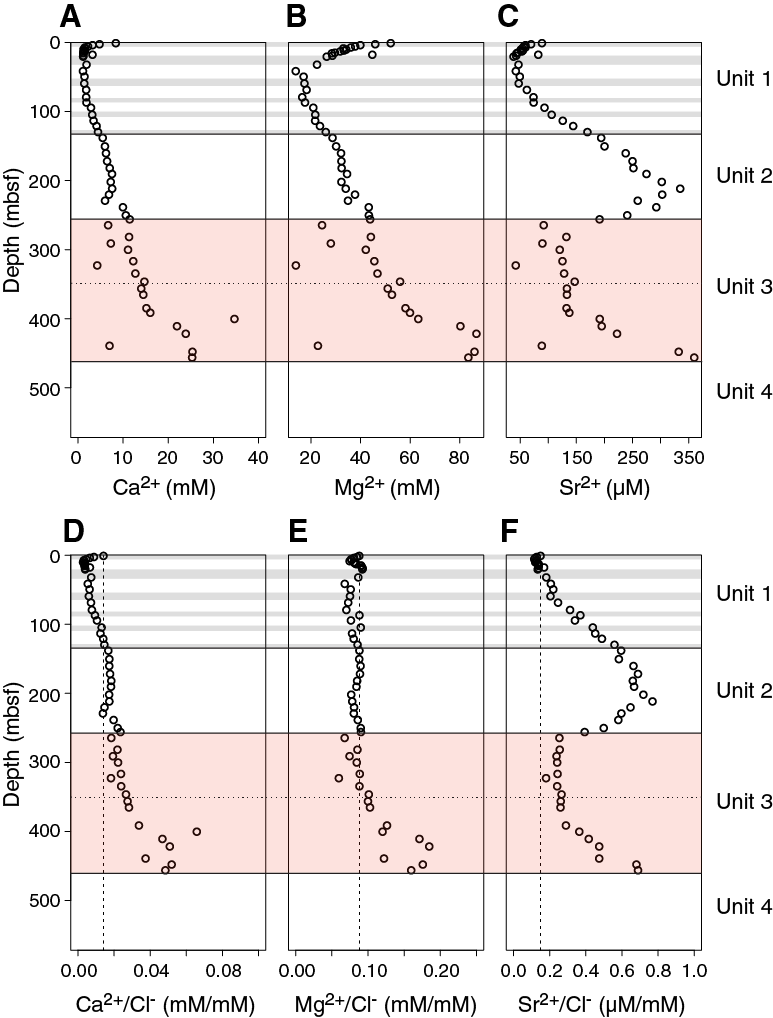
Figure F23. Pore water calcium, magnesium, and strontium.
Although the Sr2+ trends at Sites M0078 and M0079 largely follow the Ca2+ profiles, they differ considerably at Site M0080 (Figure F23C). Sr2+ shows a decrease in the uppermost 10.20 m of Hole M0080A from 88.79 to 51.32 µM, similar to Sites M0078 and M0079, followed by a strong downhole increase to a peak of 334.99 µM at 211.74 mbsf in Unit 2. The interval between 334.63 and 391.44 mbsf (Unit 3) is marked by stable Sr2+ concentrations around 130 µM before increasing again to a maximum of 359.97 µM at the bottom of the hole, suggesting a release of Sr2+ or diffusion from below, as for Mg2+ and Ca2+. Although the Ca2+, Sr2+, and Mg2+ profiles differ throughout the three sites as described above, they all show an increase at the bottom of the hole, suggesting an underlying carbonate source for all sites.
The samples suggesting drilling mud contamination (bentonite + freshwater; see Salinity variations: salinity, sodium, and chloride) in the SO42− and Cl− profiles (at 264.63, 291.06, 322.90, and 439.31 mbsf), show lower Mg2+, Ca2+, and Sr2+ concentrations than surrounding samples. Na+, Mg2+, and Ca2+ (Table T12) are present in much lower concentrations in the drilling mud compared with the pore water samples, supporting the suggestion that drilling mud contamination is responsible for the “outliers” mentioned above.
Silica and lithium
Silica accumulates in sediments as silicate minerals and the remnants of siliceous organisms (predominantly diatoms and radiolarians). Therefore, dissolved silica (H4SiO4) is typically released to pore water through dissolution of these sediment components. Measured Si (referred to as H4SiO4) concentrations increase from 247.07 µM below the seafloor to 583.03 µM at 12.90 mbsf and then generally continue to increase to a maximum of 1134.11 µM at 201.94 mbsf (55 m above the Unit 2/3 boundary) (Figure F24A). Deeper than 201.94 mbsf, H4SiO4 shifts to lower concentrations, ranging from 209.43 to 346.44 µM, and remains in this range throughout Unit 3.
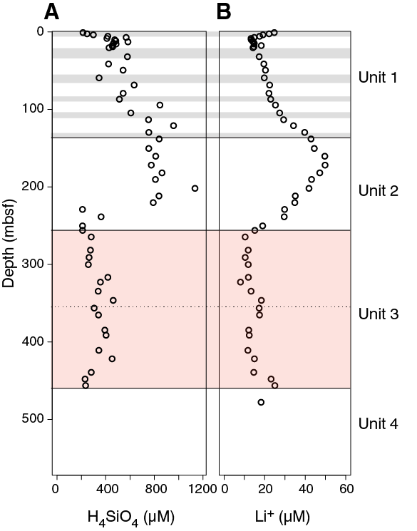
Figure F24. Pore water dissolved silica and lithium.
Lithium (Li+) concentrations in pore waters decrease from 24.76 µM close to the seafloor to 13.28 µM at 8.50 mbsf (Figure F24B). Deeper than 8.50 mbsf, concentrations increase to a maximum of 49.80 µM at 171.94 mbsf (just below Unit 1/2 boundary) and then decrease to 10.3 µM at 264.63 mbsf (the Unit 2/3 boundary). Downhole and throughout Unit 3, Li+ concentrations stay low, between 8.08 and 25.03 µM. Higher Li+ concentrations may suggest chemical weathering of sediment contributing to increased pore water values. Li+ and H4SiO4 concentrations in the drilling mud samples are lower than the concentrations in pore water samples (Table T12). Contrary to other elements mentioned above, no indication of contamination is shown in the Li+ and Si profiles.
Sediment
Carbon content
Total carbon (TC) and total organic carbon (TOC) values were measured and total inorganic carbon (TIC) was calculated (the difference between TC and TOC) for 68 ground samples from Hole M0080A. The results are presented in Table T13 and plotted in Figure F25. TC ranges from 1.00 to 12.72 wt%, with the highest overall values in Unit 2 and 4 (averaging 8.79 and 9.89 wt%, respectively). Low TC values are reported for Unit 3 with an average of 3.09 wt%. These trends are duplicated in TIC because of the dominance of inorganic carbon over organic carbon in all Hole M0080A samples. TIC averages 7.46 wt% (±3.26 standard deviation) over Hole M0080A. The average TOC is 0.24 wt% (±0.19 standard deviation) (lower than TIC). The lowest TOC values are also reported for Unit 3 (average = 0.06 wt%), with generally higher but variable values in Units 1, 2, and 4. Local maxima of TOC (as high as 0.89 wt%) are located at 31.30, 52.74, 120.30, 137.63, 199.72, 242.90, 316.00, and 475.74 mbsf, implying higher organic matter burial at these depths.
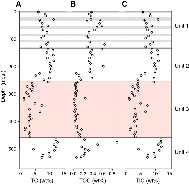
Figure F25. Solid-phase TC, TOC, and TIC.
ED-XRF
Energy dispersive X-ray fluorescence (ED-XRF) was used to quantify 24 elements from the 68 ground solid sediment samples from Hole M0080A. All elements are included in Table T13; however, for some elements, measurements were affected by low yield or interference and could not be accurately quantified (marked with asterisks and daggers, Table T13). The 10 elements (Al, Ca, Fe, K, Mg, Mn, Si, Sr, Zr, and Rb) that could be quantified are plotted with depth in Figures F26, F27, F28, and F29. Final postexpedition processing of all ED-XRF data determined that Ni concentrations have low accuracy because of low concentrations; therefore, the results are not plotted for Site M0080. Most of the elements plotted highlight the compositional differences in the sediments in the four different units at Site M0080 (see Lithostratigraphy).
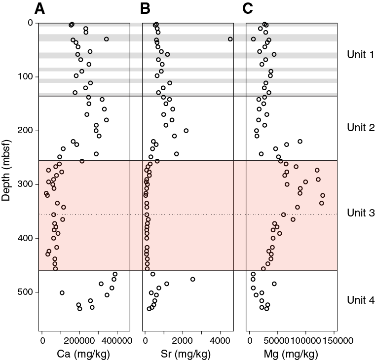
Figure F26. Solid-phase calcium, strontium, and magnesium.
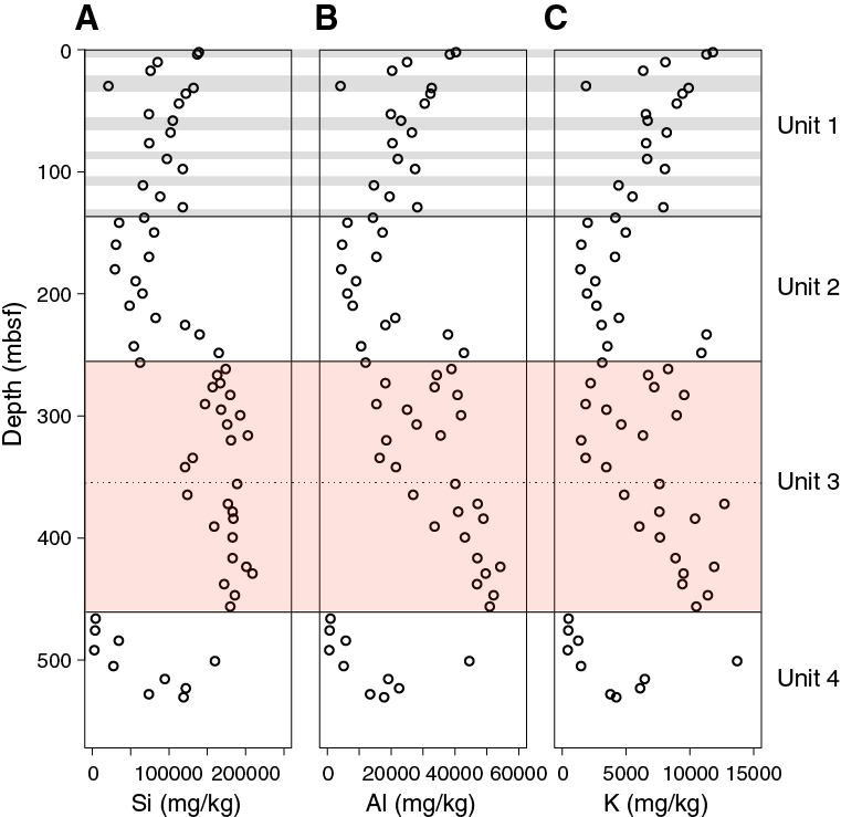
Figure F27. Solid-phase silicon, aluminum, and potassium.
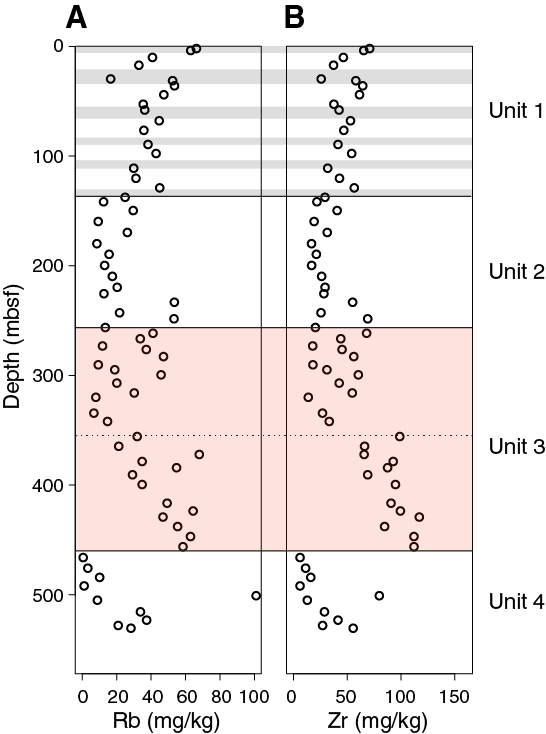
Figure F28. Solid-phase rubidium and zirconium.
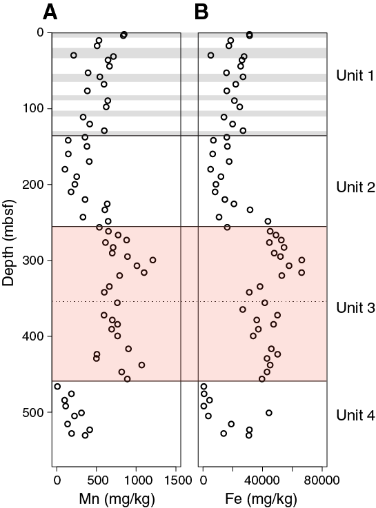
Figure F29. Solid-phase manganese and iron.
As for Sites M0078 and M0079, calcium is the dominant element in the majority of samples, with concentrations ranging from 22.6 to 389 g/kg (Figure F26). The highest Ca concentrations are present between 466.08 and 491.92 mbsf (corresponding to Unit 4) and between 141.70 and 209.69 mbsf (in Unit 2). Silica is the second most common element, with concentrations ranging from 2.5 to 209.69 g/kg (Figure F27A). Ca and Si correlate negatively (r2 = 0.95), so samples with lower Ca have higher Si content. This correlation is evident in samples between 242.90 and 456.20 mbsf, corresponding to Unit 3, where the dominant element switches from Ca to Si. Samples from Unit 3 also contain higher Al, K, Rb, Zr, Mn, and Fe concentrations (Figures F27, F28, F29). All of these elements are typically associated with terrigenous materials. Strontium, often associated with carbonates, follows similar trends with depth to Ca but shows exceptionally low values in Unit 3. (Figure F26). Unlike Sites M0078 and M0079, elements other than Ca do not correlate well with Si, likely due to the more variable lithology at Site M0080.
Physical properties
This section summarizes the physical properties results from Site M0080, where one hole was drilled (Hole M0080A) to 534.20 mbsf. Most data sets were collected at the sampling rates defined in Physical properties in the Expedition 381 methods chapter (McNeill et al., 2019b), except for P-wave velocity, thermal conductivity, and shear strength, where the nature of the sediment limited data acquisition. Overall, the data sets show good correlations with interpreted paleoenvironments and lithologic changes, especially magnetic susceptibility, NGR, density, porosity, and color reflectance. A synthesis of physical properties for Hole M0080A is presented in Figures F30 and F31.
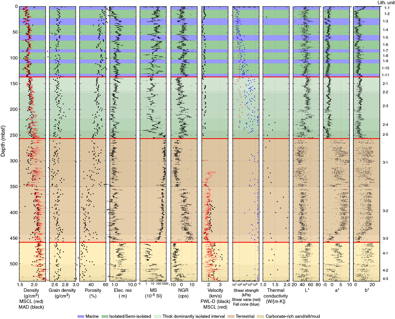
Figure F30. Physical properties with environmental interpretation.
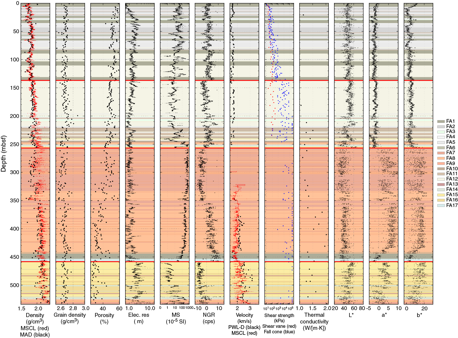
Figure F31. Physical properties with facies associations.
Shear strength
Sediment strength for Hole M0080A was measured offshore using a handheld penetrometer and CPT and onshore using a fall cone and shear vane. Penetrometer and CPT measurements were taken approximately every 20 and 100 m, respectively, whereas fall cone and shear vane measurements were taken one per core section and one per core, respectively.
Strength values for Hole M0080A consistently show an increase with depth (Figure F32). However, strength values obtained using the four different methods differ significantly. In particular, strength data derived from handheld penetrometer measurements offshore are consistently higher than the shear strength from fall cone and shear vane measurements in the upper ~60 mbsf, showing an increase from 150 kPa at ~3 mbsf to 790 kPa at ~64 mbsf. Deeper than ~82 mbsf, handheld penetrometer values approximately coincide with fall cone values, increasing from 630 kPa at ~98 mbsf to 5880 kPa at ~284 mbsf. Deeper than ~284 mbsf, offshore handheld penetrometer measurements were not taken because of the change in lithology (mud to conglomerates) and formation stiffness.
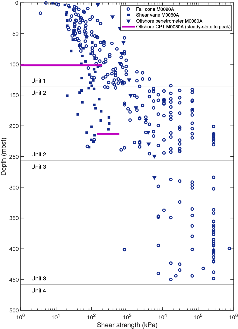
Figure F32. Shear strength.
Fall cone measurements are consistently higher than the shear vane measurements deeper than ~100 mbsf. Fall cone strength values increase from 0 to ~10 mbsf and then remain relatively constant at ~70 kPa to ~55 mbsf. From ~55 to ~245 mbsf, fall cone values increase almost exponentially and reach values >250,000 kPa deeper than ~200 mbsf, where strength values saturate because of the limits of the fall cone apparatus. Although the maximum fall cone values are not considered realistic, they indicate an overall strength increase downhole in Hole M0080A.
Shear vane measurements follow a similar increasing trend with depth. Shear strength increases linearly from ~10 to ~235 mbsf, with strength values ranging between ~20 and ~313 kPa. Shear vane measurements were taken to ~235 mbsf (Section 381-M0080A-62R-2). Deeper than ~235 mbsf, sediment is either too consolidated, exceeding the maximum applied force capacity of the shear vane apparatus, or the lithology is characterized by conglomerates (Unit 3), sand (Units 3 and 4), and carbonates (Unit 4), making shear vane measurements inefficient because (1) the equipment is designed for cohesive soils and could not penetrate the core material without damaging the tool and (2) the sample size tested is too small in these materials with pluricentrimetric heterogeneities.
The two in situ CPT measurements at ~100 and ~213 mbsf indicate a similar shear strength depth increase from 193 to 603 kPa (maximum values), respectively, suggesting increased consolidation with depth (Figure F32).
Overall, the four types of strength measurements indicate shear strength increases with depth for Hole M0080A, suggesting increased consolidation. The increase in fall cone values at ~140 mbsf coincides with the switch from vibrocoring to rotary coring (Section 381-M0080A-42R-1) but also with the lithologic transition from Unit 1 (marine sediment; FA1/FA6) to Unit 2 (thick dominantly isolated/semi-isolated interval; FA12) (Section 40V-1). Deeper than ~257 mbsf, the lithologic transition from Unit 2 (mainly mud) to Unit 3 (conglomerates and silt) limits shear strength measurements, which are designed for soils.
Natural gamma ray
Overall, the low NGR values at Site M0080 indicate that K, Th, and U concentrations are depleted throughout much of the hole but show increases in parts of Unit 3. Gamma ray data acquired by downhole logging (see Downhole measurements) correlate well with trends measured in the same intervals of the hole, suggesting these data faithfully capture NGR trends in the hole. Note that the negative values result from the removal of the background during data processing, which was determined at the beginning of the expedition. Despite these negative values, the overall trend reflects changes in the nature of the sediment recovered.
In interpreted marine subunits in lithostratigraphic Unit 1 (0–136.96 mbsf), NGR values vary from −3.94 to 13.41 counts/s with a mean of 2.78 counts/s (Figures F30, F33). In interpreted isolated/semi-isolated subunits, NGR values vary from −4.78 to 24.05 counts/s with a mean of 0.91 counts/s (lower than marine environments). In Unit 2 (characterized as mostly isolated/semi-isolated), NGR values vary from −5.68 to 14.35 counts/s with a mean of 0.19 counts/s (Figure F33). In Unit 3 (256–458 mbsf; characterized as terrestrial/aquatic), the NGR values exhibit greater variability than in the marine and isolated subunits in Units 1 and 2, averaging 0.54 counts/s with a fluctuating range of −9.21–11.85 counts/s. A significant decrease in NGR occurs at the top of Unit 3 (Figure F30). In the Unit 4 carbonate-rich sand/silt/mud (458–534 mbsf), NGR values vary from −8.91 to 12.01 counts/s with a mean of −4.30 counts/s, significantly lower than any of the other lithostratigraphic units at this site or other sites.
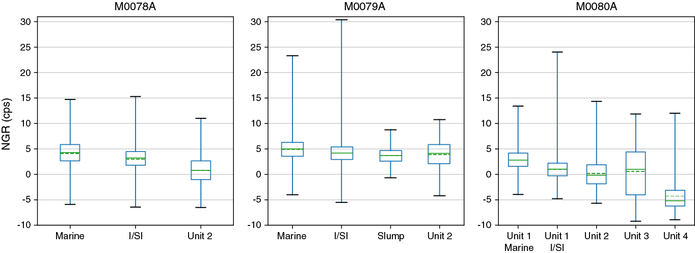
Figure F33. MSCL NGR.
Significant drops in NGR values occur at 136.96 mbsf (Unit 1/2 boundary), 256.85 mbsf (Unit 2/3 boundary), and 458.40 mbsf (Unit 3/4 boundary), and an increase was observed at approximately 350 mbsf (boundary between Subunits 3-1 and 3-2) (Figures F30, F31). NGR values are distinctly higher and exhibit more scatter in Subunit 3-2 than in other units. The distinct downhole decrease in NGR values at 458.40 mbsf is associated with a major facies change from FA17 (greenish to buff laminated fossiliferous mud) to FA15 (greenish to buff laminated siltstone to bedded fine sandstone; may include bioturbation, ostracods, and rootlets). NGR values decrease when the facies association changes from FA1 (homogeneous mud) to FA12 (light gray to buff homogeneous to weakly stratified mud) in the 0–150 mbsf interval (Figure F31).
Magnetic susceptibility
Magnetic susceptibility appears to reflect the changes in lithology associated with variations in the nature of magnetic minerals and/or their sizes at Site M0080 (see Lithostratigraphy; Figures F30, F31). Magnetic susceptibility values range from ~1 × 10⁻⁵ to ~270 × 10−5 SI with a fluctuating signal, averaging 25.60 × 10⁻⁵ SI in the lithostratigraphic Unit 1 marine subunits (Figure F34). In the Unit 1 isolated/semi-isolated subunits, magnetic susceptibility values vary from −0.47 × 10⁻⁵ to 480 × 10−5 SI with a higher mean value of 39.58 × 10⁻⁵ SI. In Unit 2 (characterized as mostly isolated/semi-isolated), magnetic susceptibility values vary from −7.69 × 10⁻⁵ to ~765 × 10−5 SI with a mean of 37.92 × 10⁻⁵ SI, similar to the Unit 1 isolated/semi-isolated subunits. In Unit 3 (256.85–458.40 mbsf; characterized as terrestrial/aquatic), the mean magnetic susceptibility value is much higher than in other units (Figure F34), averaging 346.05 × 10⁻⁵ SI with a clear and relatively flat signal (Figure F30), varying from −5.57 × 10⁻⁵ to ~937 × 10−5 SI. High magnetic susceptibility values from 258 to 442 mbsf are associated with FA7 (clast-supported sandy conglomerates and pebbly reddish brown sand) and FA8 (gray to brown mud and/or silt) (Figure F31). This distinct high and flat signal in the terrestrial/aquatic sections may be due to terrigenous input from ophiolite complex. In Unit 4 (characterized as carbonate-rich sand/silt/mud; 458–534 mbsf), magnetic susceptibility values vary from −9.06 × 10⁻⁵ to ~450 × 10−5 SI with a mean of 26.19 × 10⁻⁵ SI (Figure F34).
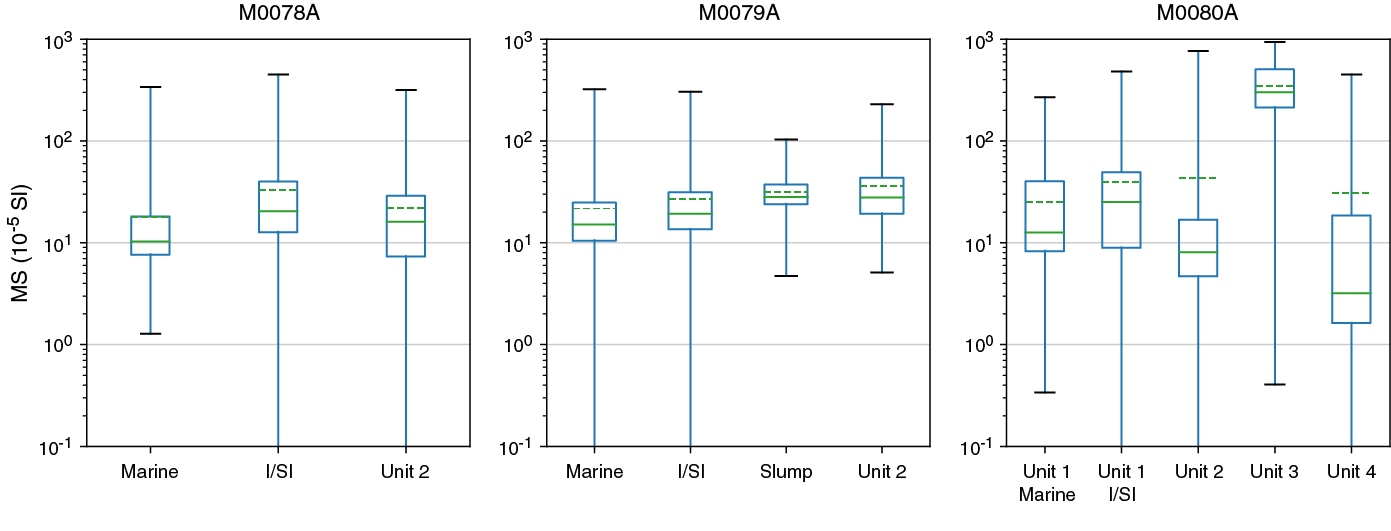
Figure F34. MSCL magnetic susceptibility.
Average values in isolated/semi-isolated intervals are higher than in marine intervals and exhibit slightly more variability. The scattered magnetic susceptibility behavior in interpreted isolated/semi-isolated sections may be due to changes in sedimentary inputs, fluctuations in the quantity of fine detrital particles, diagenetic processes, and/or preservation of original layering. Paleomagnetic studies of the discrete samples from Site M0080 suggest that the variation in the magnetic susceptibility signal is mainly controlled by concentrations of different magnetic minerals/phases (see Paleomagnetism).
Magnetic susceptibility values sometimes drop below 0 SI. These values reflect sensor drift on some sections, and these values are likely closer to 0.
P-wave velocity
P-wave velocity measurements for Hole M0080A were collected offshore using a Geotek MSCL and onshore on split cores using the MSCL track and on discrete samples with a Geotek P-wave logger for discrete samples (PWL-D) (see Physical properties in the Expedition 381 methods chapter [McNeill et al., 2019b]) (Figure F35).
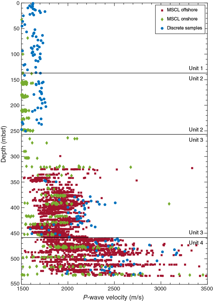
Figure F35. P-wave velocity data.
Offshore MSCL measurements provided good P-wave signals and realistic P-wave velocity values (>1500 m/s) deeper than ~320 mbsf. The MSCL measurement quality in the upper part of Hole M0080A was strongly affected by either the unconsolidated nature of sediment, coring disturbances, and/or variable fill space between the sediment and the core liner. Between ~250 and ~320 mbsf, the lithologic transition to Unit 3 (mainly conglomerates and silt) also affected the MSCL measurement quality. In this depth interval and because of the nature of the sediments in Unit 3, discrete samples for P-wave velocity measurements were not collected. Similar issues regarding the quality of the P-wave velocity measurements emerged during onshore MSCL measurements on split cores. In the upper part of Hole M0080A, P-wave velocity values were particularly low (<1500 m/s), but more realistic velocity values were measured deeper than ~320 mbsf.
P-wave velocity (VP) values, either collected on the MSCL or on discrete samples, show an overall increase with depth (Figure F35). Between 0 and ~250 mbsf (Units 1 and 2), P-wave velocity values from discrete samples are relatively low and range between 1500 and 1763 m/s. Deeper than ~350 mbsf, P-wave velocity values range between 1500 and 3500 m/s, and VP both from MSCL and discrete samples show an overall increase with depth. Lower MSCL velocity values at ~340 mbsf correspond to the bottom of Subunit 3-1 (FA 8). P-wave velocity values increase between ~350 and ~430 mbsf (Subunit 3-2), with values between 1593 and 2509 m/s. The velocity decrease at the bottom of Unit 3 (~450 mbsf) corresponds to a lithologic transition to FA1. Deeper than ~460 mbsf (Unit 4), P-wave velocity values increase for both MSCL and discrete sample measurements, with maximum values of ~3400 m/s. P-wave velocity measured on the MSCL onshore is consistently lower than the velocity collected either on the MSCL offshore or on discrete samples.
The common trend of increasing P-wave velocity values between MSCL, discrete samples, and downhole log sonic velocity data (see Figures F47, F48) in the lower part of the hole indicates the transition to more consolidated sediment with depth (see also Core-log-seismic integration).
Density
Gamma ray attenuation (GRA) bulk density values from the MSCL offshore range from 1.33 to 2.77 g/cm3 with an average of 1.98 g/cm3, a similar average to Holes M0078A and M0079A. Approximately 97% of the bulk density values are greater than 1.7 g/cm3 (2% less than the average for Hole M0079A), and only about 13% are greater than 2.2 g/cm3 (11% higher than Hole M0079A). Bulk density increases with depth with some relatively sharp increases in density compared with Holes M0078A and M0079A (Figure F30; also see Figure F29 in the Site M0078 chapter and Figure F25 in the Site M0079 chapter [McNeill et al., 2019c, 2019d]). Notable changes in bulk density correlate with the four major lithostratigraphic unit boundaries; however, density variations also occur within each lithostratigraphic unit (Figure F30).
In Unit 1, a decrease in density occurs in some interpreted marine intervals (e.g., 22.83–35.80, 83.11–89.20, and 130.92–136.96 mbsf), consistent with observations from Holes M0078A and M0079A (Figure F30; also see Figure F29 in the Site M0078 chapter and Figure F25 in the Site M0079 chapter [McNeill et al., 2019c, 2019d]). An increase in density also occurs at approximately 36 mbsf, near the boundary between Subunits 1-3 and 1-4, marking a change in average bulk density from 1.74 g/cm3 (0–35.80 mbsf) to 1.81 g/cm3 (35.80–136.96 mbsf).
The top of Unit 2 is marked by an increase in bulk density. In this unit, another increase in density occurs at approximately 203 mbsf, marking a change in average bulk density from 1.90 g/cm3 (136.96 to ~203 mbsf) to 2.0 g/cm3 (~203–256.85 mbsf).
An increase in density occurs in Unit 3 at approximately 350 mbsf, correlating with a lithology change from dominantly red-brown conglomerates and silt to dominantly silt with calcretes, marking an increase in average density from 2.03 g/cm3 (256.85–350.79 mbsf) to 2.16 g/cm3 (350–458 mbsf) (see Lithostratigraphy).
Increases in bulk density occur in Unit 4 at 502.01 and 525.14 mbsf. At 525.14 mbsf, the average bulk density increases from 2.19 g/cm3 (458–525 mbsf) to 2.33 g/cm3 (525–535 mbsf), marking the top of the basal conglomerate subunit.
Bulk density from moisture and density (MAD) analysis displays similar values and shows a similar trend to GRA bulk density (Figure F30). The exception to this occurs between 218.22 and 350.79 mbsf, where MAD bulk density values are lower than GRA bulk density, most likely due to the bias created by preferential sampling of matrix rather than clastic material for MAD measurements. MAD bulk density values range from 1.38 to 2.39 g/cm3 with an average of 1.93 g/cm3. Approximately 97% of the MAD bulk density values are greater than 1.7 g/cm3 with only 6% of the values greater than 2.2 g/cm3.
Sediment grain density ranges between 2.2 and 2.9 g/cm3 with an average of 2.66 g/cm3 and 87% of the values between 2.6 and 2.8 g/cm3. These average and percentage values are lower than those measured in Hole M0079A (0.34 g/cm3 and 10%, respectively). Calculated grain density values are mostly between pure sandstone and pure limestone (Kennedy, 2015). Grain density generally increases with increasing bulk density and decreasing porosity as observed at previous sites, except between 218.22 and 350.79 mbsf. This exception may be due to MAD bulk density being underestimated because of the sampling bias described above, and thus may not reflect the many mafic gravel-sized grains in the conglomerates.
Porosity
Porosity ranges from 18% to 79% with an average of 45%. Porosity shows a general decrease with depth in Hole M0080A, punctuated by peaks of higher porosity (Figures F30, F36). The average porosity decreases from 54% to 48% to 40% to 30% from lithostratigraphic Units 1 to 4, respectively (Figure F30), and higher porosity generally correlates with lower density.
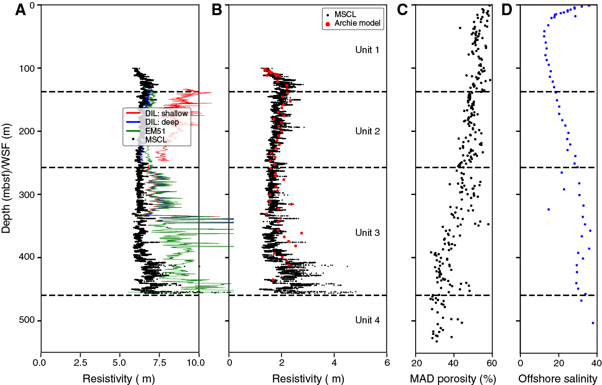
Figure F36. Electrical resistivity and theoretical Archie model.
Resistivity
In Hole M0080A, electrical resistivity was measured offshore with the MSCL and in situ with two induction tools during downhole logging (EM51 and DIL45 tools) (see Downhole measurements; Figure F36).
As at Sites M0078 and M0079, electrical resistivity from the MSCL shows low values ranging from 0.34 to 13.3 Ωm and a median value of 1.23 Ωm (Figure F30). The electrical resistivity predicted by the downhole logs differs in amplitude but is similar in trend (Figure F36). Borehole sonde responses are sensitive to downhole conditions, as visible in their different behaviors in Unit 2 (borehole filled with seawater) and Units 3 and 4 (borehole filled with drilling mud). The MSCL values can be explained by the high porosity of the sediment because it is compatible with the value derived from the Archie equation from MAD porosity and salinity measured from pore water. The following discussion, therefore, focuses on electrical resistivity derived from the MSCL (Figure F30).
In the upper ~25 mbsf of the hole, resistivity increases linearly with depth from 0.5 to 2 Ωm, which corresponds to a decrease in pore fluid salinity (Figure F36). Resistivity then slowly decreases to 1.2 Ωm until ~100 mbsf, which also corresponds to a gradual increase in pore water salinity, and then remains constant to the bottom of Unit 3, although resistivity still has a tendency to increase in each core. It should be noted that these excursions are more limited in Subunit 3-1. Electrical resistivity increases in Unit 4 with a median value of 2 Ωm (Figure F37), and the scatter of electrical resistivity values is diminished. Instead, distinctive low resistivity zones at the top and bottom of Subunit 4-2 and a surge to high resistivity in the deepest subunit of the hole (Subunit 4-3) occur. In the absence of pore water data at a high depth resolution, it is difficult to assess whether the origin of this sharp increase in resistivity measurements is due to a change in fluid conductivity or a change in lithology and/or in the porous network of the rock.
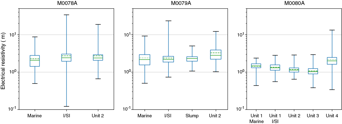
Figure F37. MSCL electrical resistivity.
Thermal conductivity
Similar to Site M0079, with the exception of a few results, data acquisition in the 0–200 mbsf interval was not successful, possibly due to water content, compaction effects, cracks, or small-scale changes in lithology that affected the measurement quality. The measured laboratory thermal conductivity values range from 0.9 to 2.03 W/(m·K) with an average of 1.42 W/(m·K) (Figure F30). Laboratory values were corrected to in situ conditions because thermal conductivity is affected by temperature and pressure. The corrected thermal conductivity values range from 0.9 to 2.09 W/(m·K) with an average of 1.46 W/(m·K) and show a similar trend to the original laboratory measurements (Figures F30, F38). The correction to in situ conditions was undertaken following Hyndman et al. (1974).
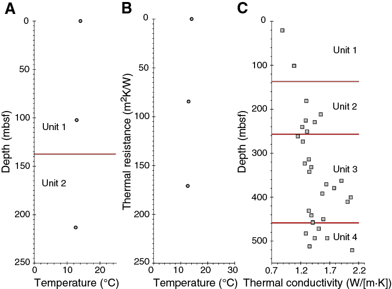
Figure F38. Temperature and thermal conductivity data.
Formation temperature and heat flow
Temperature measurements at three depths (two temperature CPT measurements and one seafloor measurement from a sound velocity profile) were collected offshore and plotted against depth to estimate the geothermal gradient (Figure F38). Temperature decreases with depth, resulting in a negative geothermal gradient. This result is unexpected for a continental setting, particularly in a tectonically active region, and suggests possible errors with the temperature measurements and should be further investigated.
The temperature data are combined with thermal conductivity to estimate heat flow using the Bullard method, which plots thermal resistance against temperature (Figure F38) and calculates heat flow from the slope of the best fitting line (see Physical properties in the Expedition 381 methods chapter [McNeill et al., 2019b]). The resultant derived heat flow is also negative and likewise is probably erroneous.
Color reflectance
The mean values ± standard deviations and minimum/maximum values of all depths in Hole M0080A are 49 ± 6 and 9/71, respectively, for L*, −2.1 ± 0.8 and −9.3/0.6, respectively, for a*, and 3.6 ± 2.7 and −15/15, respectively, for b*. Overall, variations in color reflectance values change with different environments, units, and subunits (Figures F30, F39) and follow the changes in facies associations (Figure F31) with much more pronounced changes compared with Holes M0078A and M0079A.
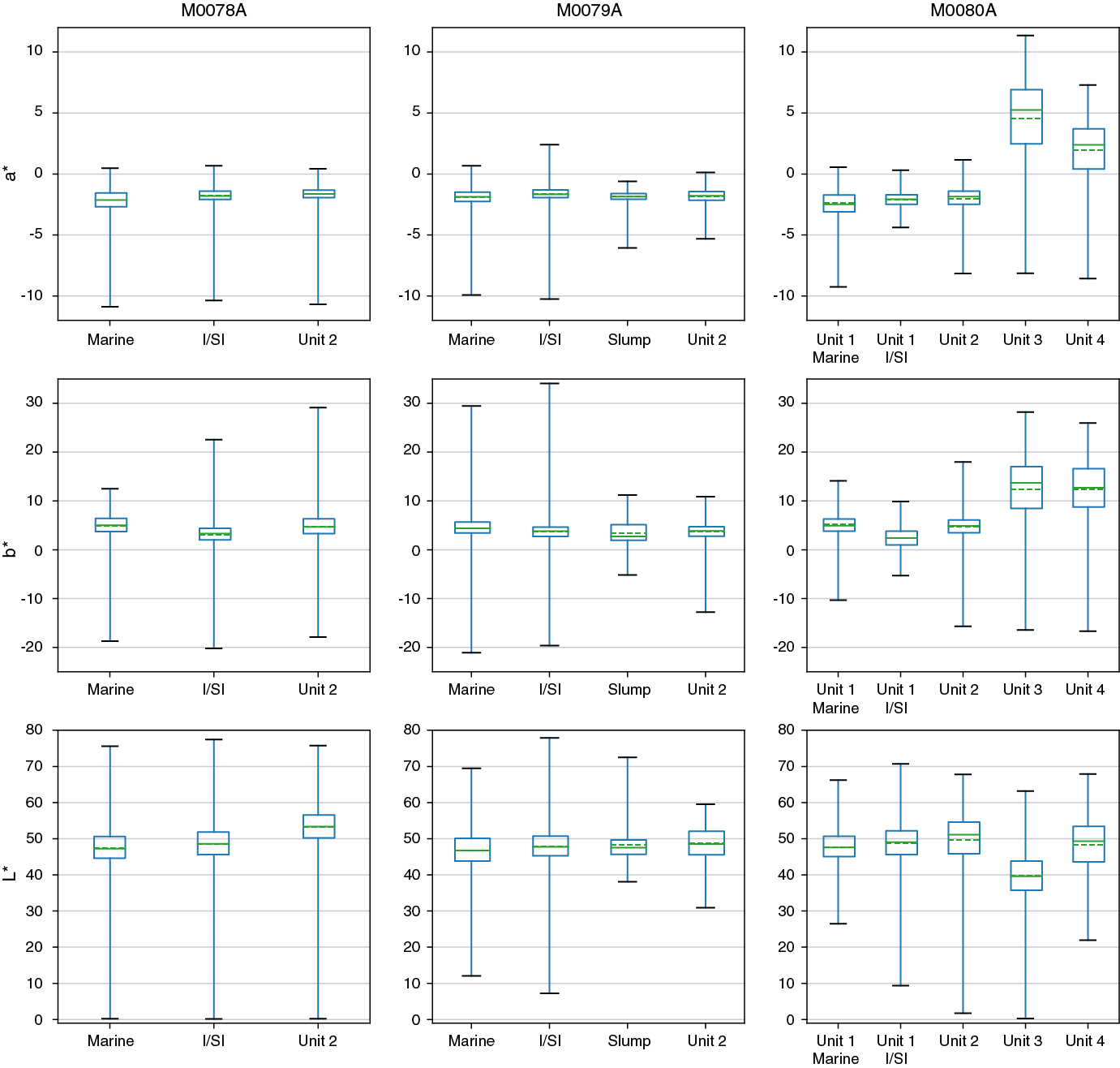
Figure F39. L*a*b* color reflectance.
Color reflectance values change with depth in several intervals (Figure F30). The most notable change is the transition from Unit 2 to Unit 3, where a change was observed in both the mean values and the amount of scatter (Figures F30, F39). The second most notable change was observed between Units 3 and 4, where the mean of L*, a*, and b* values shift (Figure F30). Both major changes follow the differences in color of the dominant facies associations between three intervals: the combined Units 1 and 2, Unit 3, and Unit 4.
In the upper part of Hole M0080A (the top ~5 m in Subunit 1-1), a general decreasing trend in color reflectance values occurs, especially distinct in b* values, similar to the tops of Holes M0078A and M0079A. Minor changes in color reflectance a* and b* values follow alternation between marine and isolated/semi-isolated environments in Unit 1 (marine: Subunits 1-1, 1-3, 1-5, 1-9, and 1-11 with mean a* values of −2.4 and b* values of 5.2 for all these subunits; isolated/semi-isolated: Subunits 1-2, 1-4, 1-6, 1-8, and 1-10 with mean a* values of −2.1 and b* values of 2.5 for all these subunits).
Changes in average values and the intensity of scattering in color reflectance values are also associated with facies changes (see Lithostratigraphy; Figure F31). Scattering of the data is more pronounced in the heterogeneous material of Units 3 and 4 than in the mud-dominated facies associations described in Units 1 and 2. This observation is verified in FA7, FA8, and FA9, especially for a* and b* values, exhibiting more scattering than in the facies encountered in Units 1 and 2.
Paleomagnetism
Magnetic susceptibility
A total of 379 discrete samples were analyzed from Hole M0080A. Frequency distribution diagrams of magnetic susceptibility (k) from discrete samples, together with shipboard MSCL continuous data (2 cm interval) from whole core sections, are shown in Figure F40. Magnetic susceptibility in Hole M0080A shows a unimodal distribution peaking between 0 and 50 × 10−6 SI, with values ranging from negative to positive approximately between −100 × 10−6 and 4000 × 10−6 SI (Figure F41B, F41D). A similar trend is observed from shipboard MSCL susceptibility data, where the unimodal distribution peaks approximately between 100 and 150 × 10−6 SI, and values range between −100 × 10−6 and 3500 × 10−6 SI (Figures F40B, F41E). MSCL and discrete sample magnetic susceptibility data show a good match overall. Downhole distribution of magnetic susceptibility in Hole M0080A (Figure F41) shows a low variability to ~250 mbsf, which is the bottom of lithostratigraphic Unit 2 (see Lithostratigraphy), with values around ~100 × 10−6 SI. Much higher variability and overall higher susceptibility values occur between ~250 and ~460 mbsf (coinciding with lithostratigraphic Unit 3), where susceptibility ranges between ~100 × 10−6 and ~4000 × 10−6 SI. This trend is much clearer when discrete sample and MSCL magnetic susceptibility data are plotted together against depth (Figure F41E). The scatter in susceptibility values between ~250 and ~460 mbsf is likely due to the occurrence of mafic ophiolitic clasts in Unit 3, which are produced by the erosion of a nearby ophiolite exposed at the southeastern margin of the Gulf of Corinth (Sakellariou et al., 2007). The good match between the downhole variation in magnetic susceptibility and natural remanent magnetization (NRM) (Figure F41) suggest that the susceptibility variation is mainly (but perhaps not exclusively) controlled by the change in concentration of the magnetic phases in the sediment. The direct relationship between NRM and susceptibility in Hole M0080A (Figure F42) is linear, suggesting the predominance of one type of magnetic mineral contributing to both NRM and magnetic susceptibility. The downcore increase or decrease in both NRM and susceptibility may therefore just be controlled by the dilution of the magnetic minerals in the sediment.
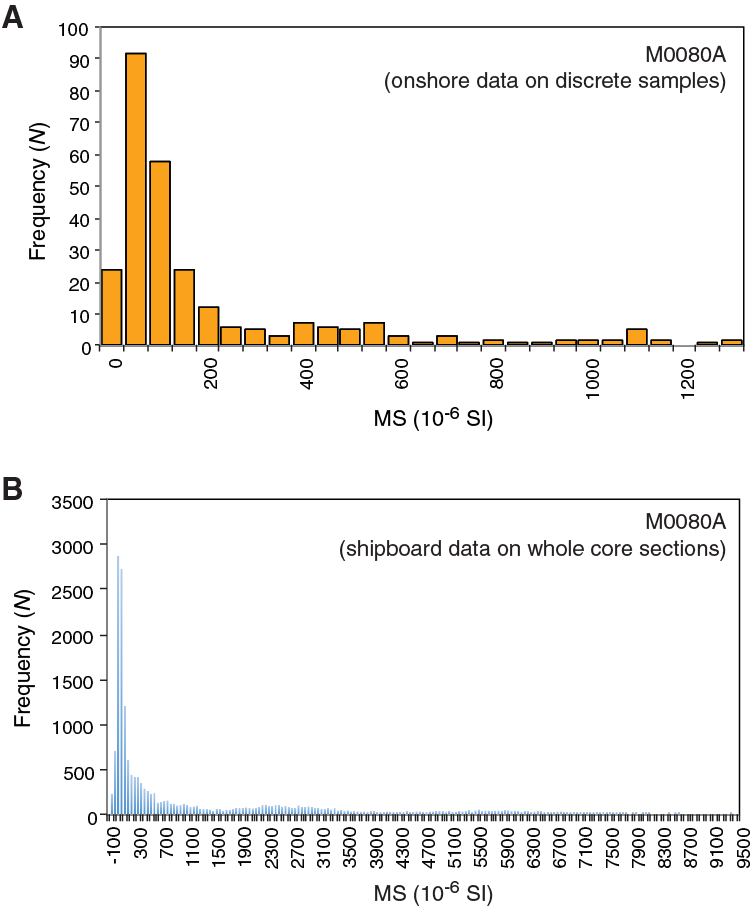
Figure F40. Magnetic susceptibility frequency distribution.
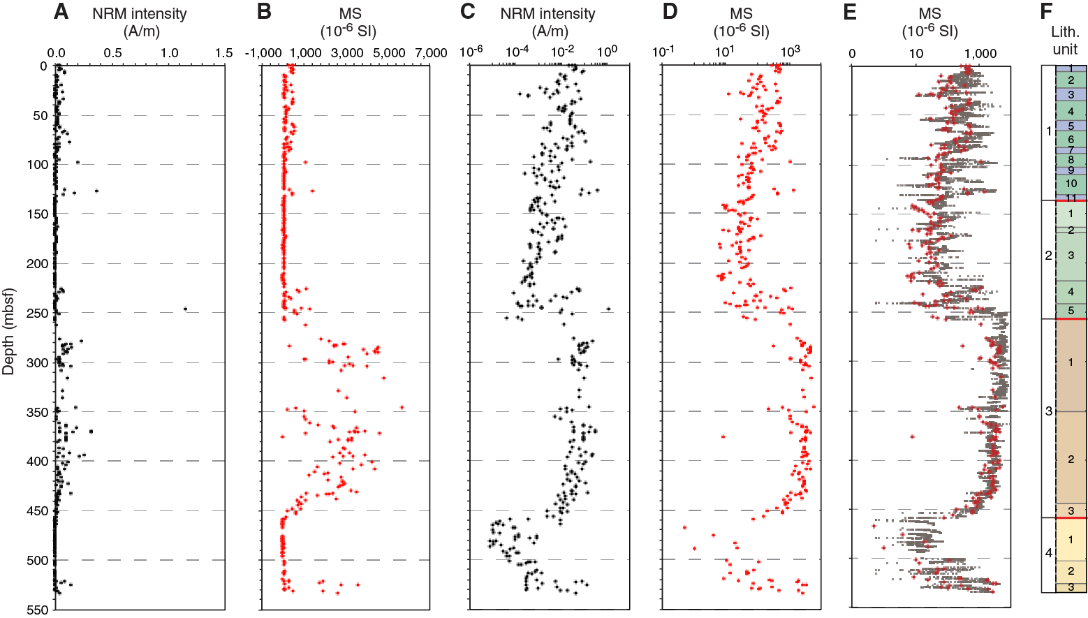
Figure F41. NRM intensity and magnetic susceptibility.
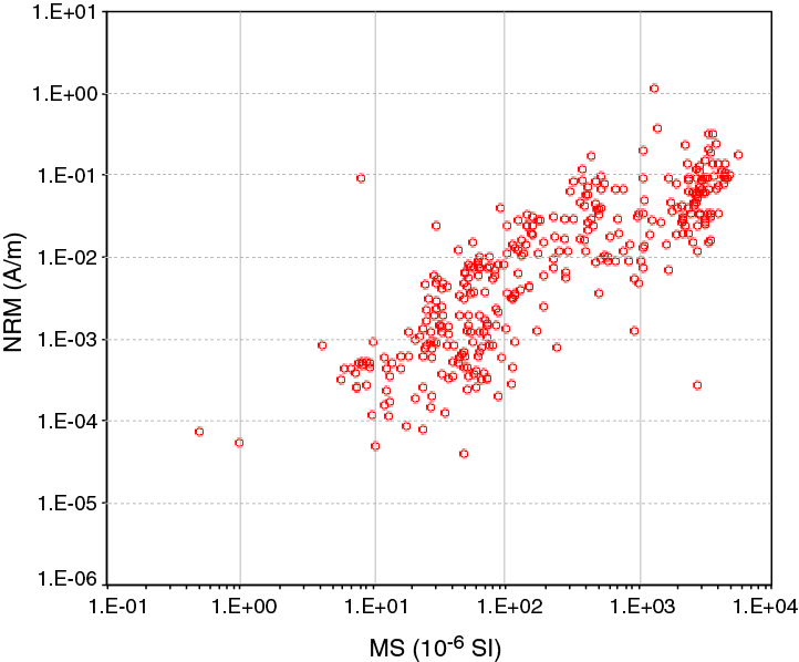
Figure F42. NRM intensity vs. magnetic susceptibility.
Magnetic mineralogy
Thermal variation of the low-field magnetic susceptibility was determined for six representative samples from Hole M0080A prior to the Onshore Science Party (OSP) (see Paleomagnetism in the Expedition 381 methods chapter [McNeill et al., 2019b] for more details). Figure F43 shows the results of the thermomagnetic experiments, revealing a wide range of Curie temperatures ranging between 116° and ~646°C. However, most of the samples show a primary Curie temperature between 116° and 310°C, corresponding to Ti-rich magnetite, and between 502° and 585°C, which is typical of Ti-poor titanomagnetite or stoichiometric magnetite. Other Curie temperatures between 365° and 486°C suggest the occurrence of Ti-rich titanomagnetite. Oxidized (titano)magnetite (i.e., titanomaghemite) may also be present, with Curie temperatures ranging between 580° and 646°C.
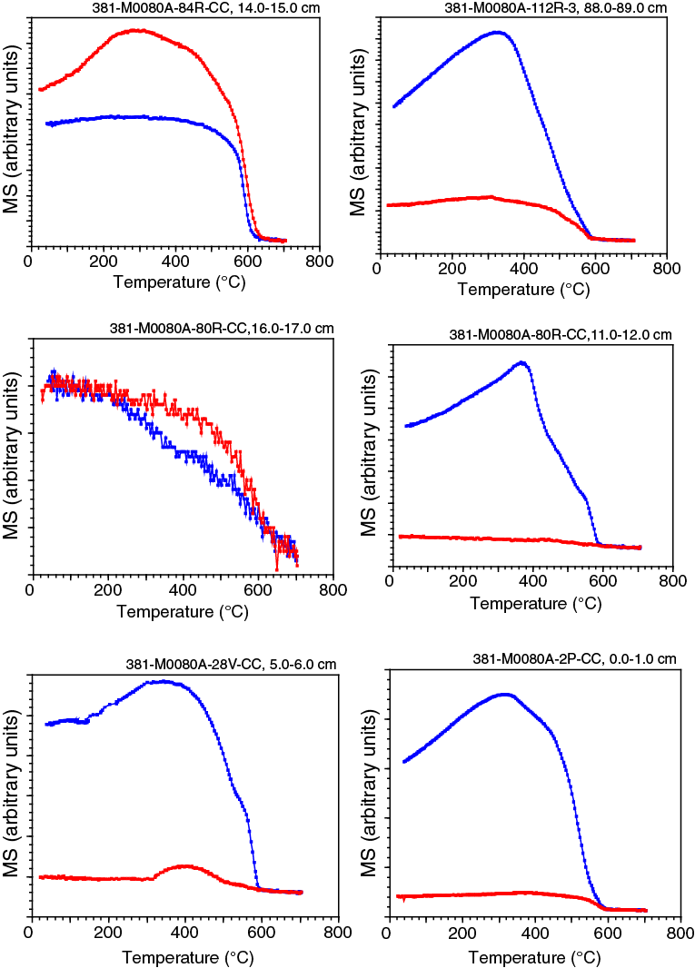
Figure F43. Low-field susceptibility vs. temperature experiment results.
Natural remanent magnetization
NRM direction and intensity of discrete samples were measured using the superconducting rock magnetometer 755–4000 cryogenic magnetometer (2G-Enterprise) at the University of Bremen (Germany). A total of 379 discrete cubic samples were analyzed from Hole M0080A. All samples were stepwise demagnetized by alternating fields (AFs) to determine the stability of the NRM during sequential demagnetization. Magnetization was measured after each demagnetization step, and in most of the samples it decays steadily up to nearly complete removal at the maximum AF step of 100 mT (Figure F44B). This decay indicates the occurrence of low-coercivity magnetic minerals, such as magnetite or titanomagnetite. The shapes of the magnetization decay curves are typical of pseudosingle-domain grains. About ~10% of the samples acquired a gyroremanent magnetization at AFs higher than 60–70 mT (Figure F44A). This spurious magnetization is typically acquired because of the occurrence of greigite (Fe3S4). The magnetization of samples showing this behavior is therefore likely to be carried by a mixture of greigite, magnetite, and titanomagnetite, in agreement with what was inferred from the rock magnetic experiments shown in Figure F43.
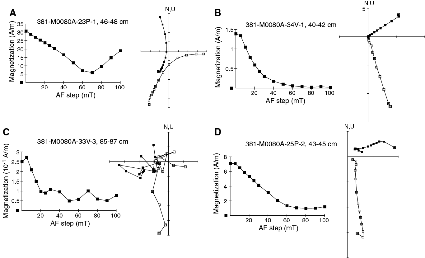
Figure F44. Orthogonal projections and relative decay paths.
Orthogonal demagnetization diagrams (Figure F44) show that demagnetizing fields of 15–20 mT are sufficient to remove the weak viscous remanent magnetization and other secondary components of magnetization. After the application of a 30 mT demagnetizing field, 144 of the 379 samples show an inclination that is higher than the expected inclination (57.5°) for the site latitude (i.e., dots inside red dashed circle, Figure F45). Magnetization of these samples might have either partially or totally been overprinted by a vertical drilling-induced magnetization. The overall scatter in the remanence directions after demagnetization at 30 mT compared with that after 40 mT is reduced, with the concentration parameter (K) being slightly smaller for the 30 mT data set (K = 9.0) than for the 40 mT data set (K = 7.5). For this reason, the inclination data after the 30 mT demagnetizing step were used to build the Hole M0080A magnetostratigraphy.
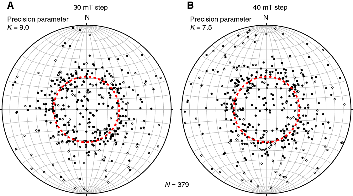
Figure F45. Remanence directions.
Magnetostratigraphy
Figure F46 shows the inclination data at 30 mT AF step (interpreted to be indicative of the characteristic remanent magnetization component) from Hole M0080A, together with a preliminary magnetostratigraphy. This magnetostratigraphy is then tentatively correlated with the geomagnetic instability timescale (GITS) of Singer (2014). Downhole, the polarity is normal to 324.97 mbsf (Sample 91R-3, 50–52 cm) and then is reversed below 328.29 mbsf (Sample 92R-2, 39–41 cm). This transition occurs in the red-brown siltstone, sandstone, and conglomerates of Subunit 3-1 (see Lithostratigraphy) and might correspond to the Brunhes–Matuyama reversal (0.773 Ma; Singer, 2014), although this hypothesis remains speculative because of the paucity of biostratigraphic constraints (see Micropaleontology). Also, considering the predominant continental nature of Subunit 3-1, the occurrence of hiatuses and unconformities in Subunit 3-1 cannot be excluded; hence, the nature and age of the polarity transition occurring at 324.97–328.29 mbsf should be interpreted cautiously.
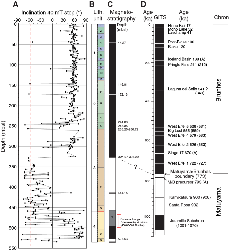
Figure F46. Inclination of the remanence after demagnetization at 30 mT.
In this uppermost normal polarity interval above 324.97 mbsf, several samples with reversed polarity occur, only a few of which reach the expected inclination values of −57.5° and are marked with a white line in the magnetostratigraphic log of Figure F46C. It is possible that these samples recorded some of the excursions of the Brunhes normal chron. Additional rock magnetic experiments and chronostratigraphic constraints, however, will be necessary to establish whether and which one of these reversed polarity samples represent true magnetic field excursions.
Below 328.29 mbsf, the polarity is predominantly reversed to 458.18 mbsf and then frequently variable from normal to reversed to 492.93 mbsf. Data from the interval between 458.18 and 492.93 mbsf need to be interpreted carefully, and for now we prefer not to assign any polarity to this interval (gray shaded area in Figure F46C). Below this interval, samples show a consistent normal polarity to 527.53 mbsf. Under the assumption that the transition at 328.29 mbsf is the Brunhes/Matuyama boundary and the sedimentary sequence is continuous, this normal polarity interval (492.93–527.53 mbsf) might represent the Jaramillo Subchron (1.001–1.076 Ma), although this hypothesis remains highly speculative at the time this report was prepared. A concurrent range (I. semenenko and A. primus; 4.58–7.39 Ma) was identified in Hole M0080A between 466.83 and 501.28 mbsf (Figure F46; see also Micropaleontology). This biostratigraphic constraint, if reliable, excludes the hypothesis that the normal polarity interval at 492.93–527.53 mbsf coincides with the Jaramillo Subchron, and would rather suggest that it corresponds to some older normal polarity chron.
The absence of firm biostratigraphic constraints from the deeper part of Hole M0080A (lithostratigraphic Units 3 and 4) and the possibility of reworking of material prevents us from drawing conclusive correlations between the deeper borehole magnetostratigraphy and the GITS. Further analysis and integration of magnetostratigraphic and biostratigraphic data and other age constraints will be a focus of postexpedition research.
Downhole measurements
A nearly complete set of logging data were collected throughout most of Hole M0080A, including spectral gamma ray through pipe and resistivity, sonic, magnetic susceptibility, conductivity, and spectral gamma ray in the open hole. The deployment of wireline logging tools in Hole M0080A was changed relative to the logging plan because of several factors. The variation in formation downhole, in particular the presence of sand, gravel, and pebbles in the lower half of the borehole, meant that hole instability needed to be considered. In addition, the dominance of mud facies in the upper part of the borehole meant that swelling of the formation was a possibility. Although absolute values of physical properties differ between core and log measurements, the logging data trends compare well with the core data (e.g., compare Figures F47, F30).
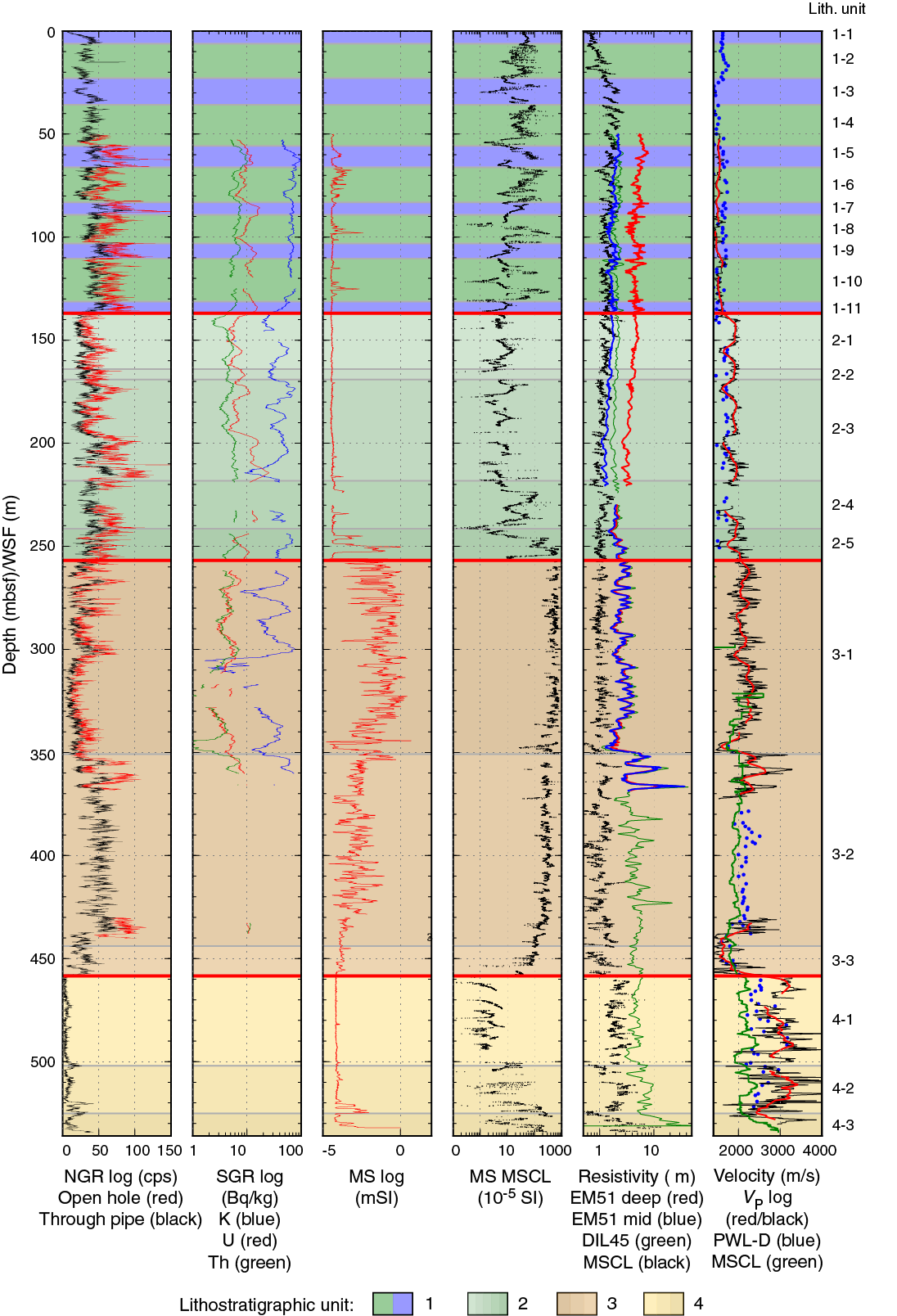
Figure F47. Wireline log data compared with data from cores.
Spectral gamma ray
Spectral gamma ray log data were acquired both through pipe and in the open hole. Open hole logs were acquired in three stages and cover the following depth intervals: 440–430, 370–230, and 220–50 m WSF. Through pipe data acquisition took place from the base of the hole to the seafloor in one run. The two data sets compare well (Figure F47).
The upper ~135 m WSF (lithostratigraphic Unit 1) consists of increasing gamma ray values with depth, starting at <50 counts/s close to the seafloor (through pipe) and reaching 50 counts/s (through pipe) or 70–100 counts/s (open hole) at 135 m WSF (Figures F47, F48). Superimposed on this background trend, the gamma ray log shows local variations, with relatively higher gamma ray values (50–100 counts/s) associated with marine subunits and relatively lower gamma ray values (40–70 counts/s) associated with isolated/semi-isolated subunits. In addition, spectral gamma ray logs indicate a relatively higher uranium and thorium content in the marine subunits (e.g., 55–65, 83–89, and 103–100 m WSF).
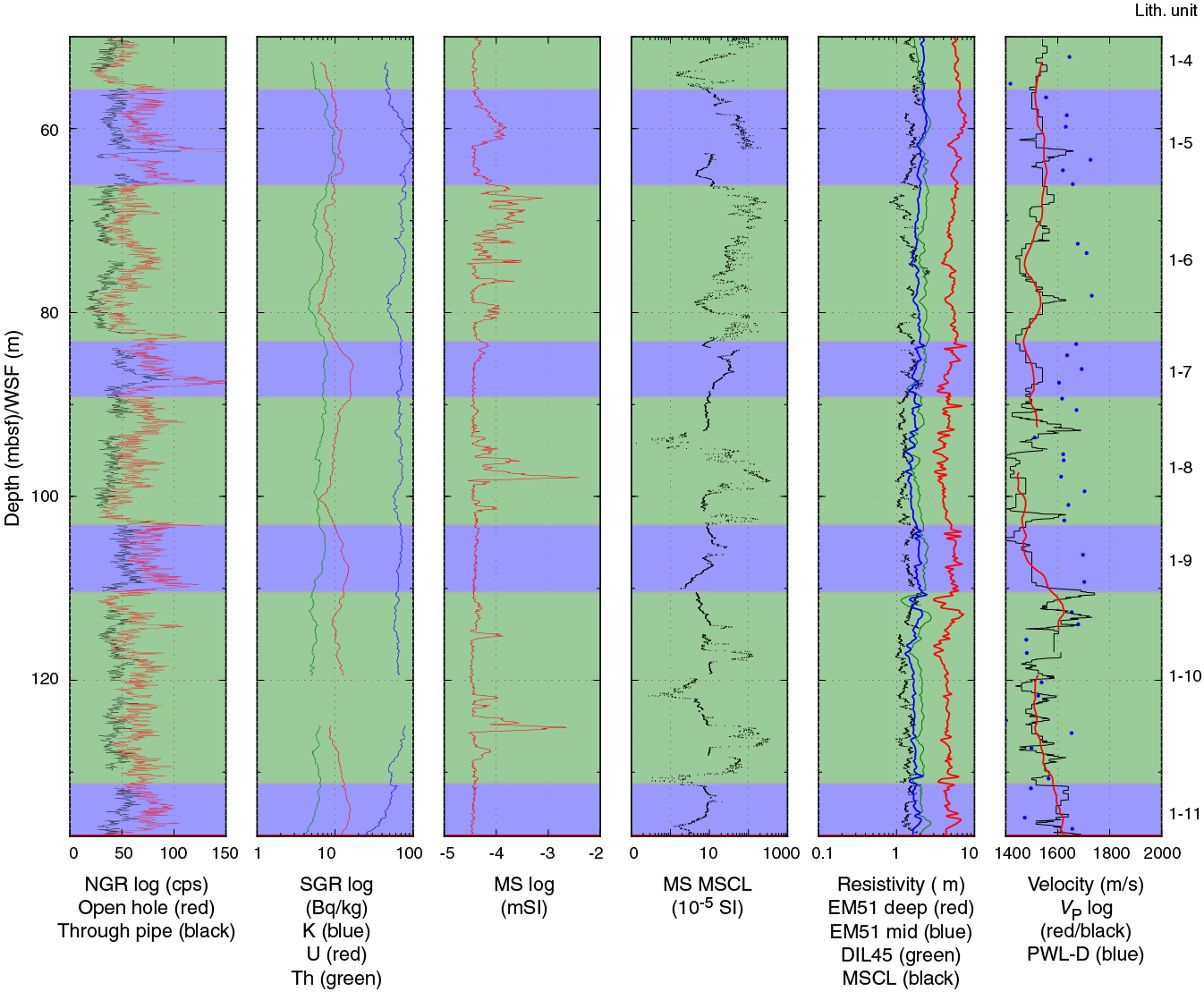
Figure F48. Wireline log data, Unit 1.
Below 135 m WSF in Unit 2, gamma ray values decrease sharply to <50 counts/s and then increase progressively to ~220 m WSF, reaching values >100 counts/s (Figure F47). The overall increase is not steady, and variability in the total count is associated with changes in the potassium and uranium logs. Below 215–220 m WSF, gamma ray values show multiple 20–50 m thick decreasing and increasing trends, fluctuating between <50 and 100 counts/s. At 355 m WSF, gamma ray values sharply increase at the transition to Subunit 3-2. From 355 to 435 m WSF (Subunit 3-2), the signal becomes more stable and remains around 50 counts/s (through pipe data; minimal open hole data collected in this interval) followed by a sharp decrease to <50 counts/s at 435 m WSF, corresponding to the tool measuring through the thick collars of the drill string, attenuating the signal received from the formation. Another decrease (<20 counts/s) occurs at ~460 m WSF and below (Unit 4) and is associated with changes in other logs, reflecting changes in the formation.
Magnetic susceptibility
Values recorded by the magnetic susceptibility tool are questionable because they are <0, but the trends mirror those observed in the core MSCL data (Figure F47). Therefore, when describing this log, only trends are described and no values are given. Comparing the log and core MSCL data, the trends in magnetic susceptibility with depth are similar, but some distinct differences in variability and scatter occur in each lithostratigraphic unit.
The EM51 tool was sent downhole first at each stage and was therefore more likely to collect data with hole conditions at their best. Data were collected in three stages: 532–430, 428–230, and 223–50 m WSF. From 50 to 255 m WSF in Units 1 and 2, the magnetic susceptibility log remains relatively low and flat with local excursions toward higher values at 65–80, 90–102, and 115–130 m WSF (Figure F48). These positive excursions occur in isolated/semi-isolated subunits in Unit 1, whereas intervals with low values and little variation correspond to marine subunits. From 135 to 230 m WSF in Unit 2, the magnetic susceptibility exhibits little variation; however, below 230 m WSF, positive excursions are recorded, trending toward higher values downhole. From 255 to 345 m WSF (in Subunit 3-1), magnetic susceptibility values stay relatively high, exhibiting strong scattering. This scattering is likely associated with formation heterogeneity (see Lithostratigraphy). From 350 to 460 m WSF (lower part of Unit 3; Subunits 3-2 and 3-3), values progressively decrease with a clear reduction in scattering from 430 to 460 m WSF. Below 460 m WSF (Unit 4), the log exhibits almost no variation until 500–520 m WSF, where values start to increase again at the very bottom of the hole.
Resistivity
Resistivity logs were derived from the induction log of the EM51 tool and from the induction logs of the DIL45 tool. Resistivity derived from the EM51 tool covers most of the borehole depth. Deep and shallow resistivity logs derived from the dual induction tool were recorded from 368 to 230 m WSF and from 220 to 50 m WSF. Note that in the upper part of the hole, deep and shallow resistivity values do not overlap (deep resistivity is ~4–5 Ωm higher than shallow resistivity), in contrast to the lower part of the hole. This overlap is due to the use of bentonite to stabilize the hole for the deeper logging Stages 1 and 2 (535–230 m WSF), whereas seawater was used for the shallower Stage 3 (230–50 m WSF). All resistivity logs compare very well (Figure F47). From 50 to 350 m WSF, resistivity values are typically <10 Ωm, with local variability from 50 to ~135 m WSF (typically ±2 Ωm excursions; Unit 1) and little variability from 135 to 250 m WSF (<1 Ωm variations; Unit 2). A clear increase in resistivity occurs below 250 m WSF (into Unit 3), also associated with more variability on a <5 m depth scale until reaching 340 m WSF. This interval (~250–340 m WSF) is also characterized by high and variable magnetic susceptibility measurements. Both data sets may be explained by the heterogeneity of the coarse-grained terrestrial material in this interval (see Lithostratigraphy). At 350 m WSF (boundary between Subunits 3-1 and 3-2), resistivity increases sharply and then increases from 5 to >10 Ωm from 350 m WSF to the bottom of the hole, with local sharp increases >10 Ωm from 350 to 420 m WSF.
Sonic
Sonic data were collected in three stages: 530–430, 372–230, and 220–50 m WSF. Data processing was made challenging by uncertainty in picking the first arrivals, especially in the deeper parts of the borehole (below 230 m WSF; see results from picking compared with semblance analysis, Figure F49). Despite these difficulties, the sonic trend derived from the raw data compares well with MSCL and discrete P-wave data from cores, where collected (see Physical properties; Figure F47). From 50 to 135 m WSF (Unit 1), sonic velocity values are relatively low (1500–1600 m/s). The values increase to 1700–2000 m/s from 135 to 255 m WSF (Unit 2) and reach values >2000 m/s from 255 to 340 m WSF (Subunit 3-1). Just above 350 m WSF, a prominent decrease occurs for ~10 m to 1700 m/s. From 350 to 370 m WSF (below the boundary between Subunits 3-1 and 3-2), velocity values stay above 2000 m/s. From 430 to 460 m WSF, sonic velocity values decrease and increase again from 2500 to 1600 and back to 2500 m/s. Below 460 m WSF (Unit 4), average velocity values are typically >2500 m/s, with pronounced scattering between 2000 and 4000 m/s.
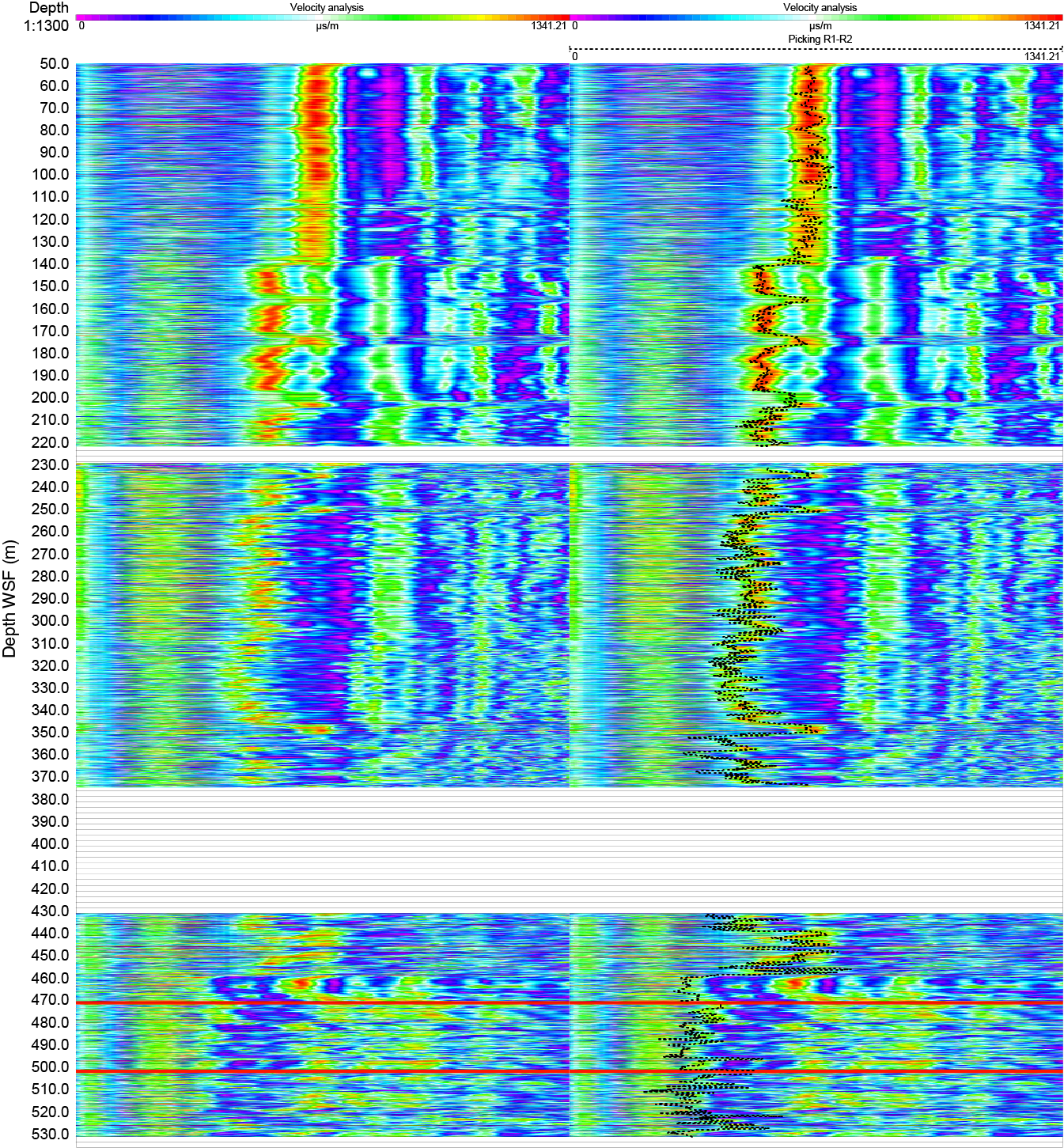
Figure F49. Semblance compared with manual picking.
Note that the trends between sonic and resistivity logs compare well, reflecting relatively good data quality (a notable example is from 350 to 371 m WSF). The local decreases in sonic velocity values at 155 and 175 m WSF are probably real because they match with local, small-scale scattering in the resistivity data from the DIL45 tool.
Comparison with lithostratigraphic units
Borehole logs recorded in Hole M0080A compare well with the lithostratigraphic units and subunits defined from core descriptions (see Lithostratigraphy). Lithostratigraphic Unit 1 (0–136.96 mbsf) is characterized by relatively high gamma ray counts with locally higher counts in marine subunits, locally higher magnetic susceptibility values in isolated/semi-isolated subunits, and local resistivity variations. Sonic velocity values are 1500–1600 m/s in this unit. In Unit 2 (136.96–256.85 mbsf), gamma ray count markedly decreases, magnetic susceptibility and resistivity log data have little variation, and sonic velocity increases to close to 2000 m/s. Subunit 2-5 can be identified in the magnetic susceptibility log, with local positive excursions. Unit 3 (256.85–458.40 mbsf) is distinct in the magnetic susceptibility and resistivity logs, with higher values and more scattering in both data sets. The boundary between Subunits 3-1 and 3-2 can be identified from these same logs, with a clear change in pattern at ~350 m WSF where magnetic susceptibility decreases and resistivity increases sharply. Unit 4 (458.40–534.20 mbsf) is very distinct in the magnetic susceptibility log, with low values exhibiting very little variability, except for the deepest part of the borehole, compared with Unit 3 above. Unit 4 is also characterized by a clear increase in sonic velocity values, typically >2000 m/s. Finally, the gamma ray through pipe log, although attenuated by the drill string collars, shows a sharp decrease at the Unit 3/4 boundary, with low values in Unit 4 thought to reflect the carbonate-rich lithologies.
Core-log-seismic integration
Core-log-seismic integration (CLSI) at Site M0080 utilized MSCL density data and velocity information from downhole logging and MSCL measurements on discrete samples to link core data to coincident seismic data (Figure F2). Out of the three sites drilled during Expedition 381, Site M0080 had the largest amount of information on P-wave velocity, potentially making it possible to establish the most accurate time-depth relationship (TDR) for seismic horizons. However, each of the velocity data sets had quality limitations and thus required significant effort with filtering and quality control.
Velocity data integration
A downhole sonic log was acquired in almost the full depth range of Hole M0080A (50–530 m WSF). However, it exhibits large velocity fluctuations, suggesting poor borehole conditions in some parts of the hole (Figures F50, F51). The sonic log has a 60 m long gap at 370–420 m WSF, and relatively high values (>3000 m/s) occur below 460 m WSF (Figure F51). The overall trend, however, agrees well with core MSCL VP data acquired offshore. VP measured on discrete samples, on average, exceeds downhole values to ~110 mbsf (Figure F50). At greater depths, velocity values acquired on discrete samples onshore mostly fall between the MSCL and downhole log values (Figure F51). After testing multiple approaches to combining and filtering VP data from various methods and testing the sensitivity of synthetics to the input velocity information, the two scenarios described below were selected, which represent two end-member versions of the P-wave velocity profile in the deepest part of the hole (Figure F52).
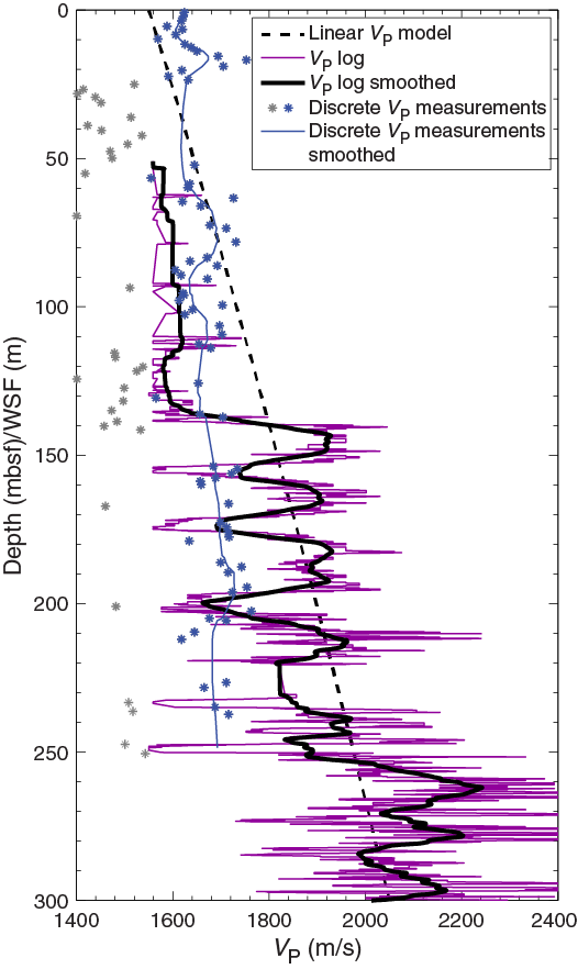
Figure F50. VP data sets available for 0–300 mbsf.
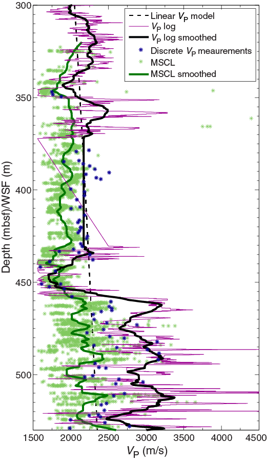
Figure F51. VP data sets available for 300–530 mbsf.
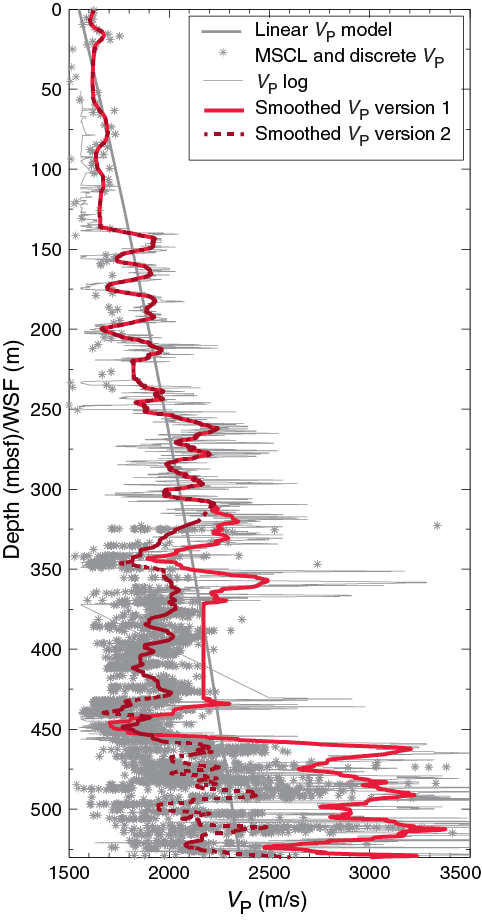
Figure F52. Two versions of composite VP data used for synthetics generation.
Version 1 of input velocity for synthetics represents the high VP end-member scenario. After removing VP values less than 1550 m/s, a 10-point (~15 m) running average of VP measured on discrete samples between 0 and 136 mbsf was combined with a 150-point running average (~7.5 m) of the downhole sonic log below 136 mbsf. For Version 2, which constitutes a low VP end-member, the same approach was used in the upper 320 mbsf, but instead of using the sonic log to the total depth of the borehole, core MSCL data were used below 320 mbsf. The MSCL data were also filtered to remove values under 1550 m/s and then smoothed with a 150-point (~3 m) running average. Figure F52 illustrates the two resulting VP profiles used for synthetics generation (Tables T14, T15). The density profile for synthetics generation was produced from filtered and smoothed MSCL data using the approach developed offshore and depth shifted to sea level (Table T16) (see Core-log-seismic integration in the Expedition 381 methods chapter [McNeill et al., 2019b]).
Impact of input velocity on reflection coefficient series and time-depth conversion
The input VP profile influences two key parameters of synthetics generation: the reflection coefficient series (RC), which determines the appearance (shape and intensity) of reflections in the synthetic seismogram, and the TDR function, which determines how those reflectors are positioned in the time and depth domains. By utilizing different input velocity values, it was possible to assess the robustness of resulting synthetics and TDR functions and their sensitivity to the input parameters. Three input velocity profile versions were tested for Site M0080 for both the impact on the RC and the time-depth conversion: a linear velocity model derived from seismic data before the expedition (see Core-log-seismic integration in the Expedition 381 methods chapter [McNeill et al., 2019b) and the two versions of core- and log-based combinations described above (Versions 1 and 2, Figure F52).
Impact on reflection coefficient series
Three versions of the synthetic seismograms shown in Figure F53 were generated with three different inputs for the RC computation: (1) the original (pre-expedition) linear velocity profile derived from seismic data, (2) a combination of discrete and downhole velocity values (the high VP end-member version described above; Version 1), and (3) a combination of discrete, downhole, and MSCL velocity values (the low VP end-member version described above; Version 2). To facilitate comparison, all three versions were based on the linear velocity profile as a starting point for time-depth conversion, adjusted slightly to tie to seismic data. Using core- and log-based VP for RC computation improves the appearance of synthetic seismograms and the reproducibility of reflections in coincident seismic data compared with the linear velocity model, but the observed difference is surprisingly small. In fact, all three versions reproduce the main reflectors, suggesting that in this geologic setting, the main reflectors in the seismic record can be predicted by density variation (Table T17), increasing our confidence in the CLSI results at Sites M0078 and M0079, where very limited VP data were available.
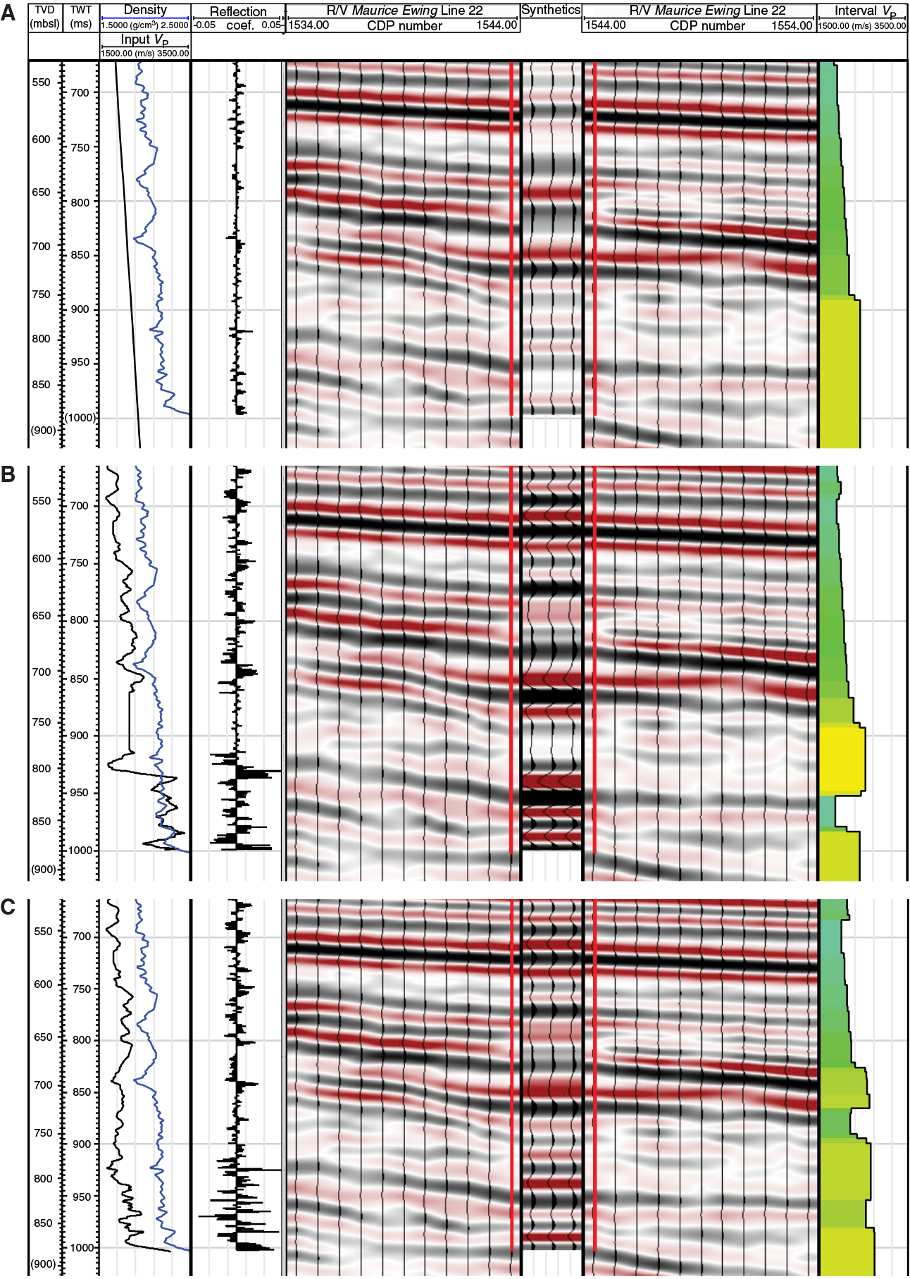
Figure F53. Comparison of synthetic seismograms.
The largest difference in the appearance of synthetic seismograms at Site M0080 occurred in the deepest part of Hole M0080A, where using core- and log-based input velocity values increase the synthetics resolution. Judging by the appearance of the synthetics, the input velocity that is based on MSCL data provides the best fit to seismic data (Figure F53C). The output interval velocity values are slightly different in all three scenarios, but all suggest an increase in VP at around 400 mbsf (~750 meters below sea level [mbsl]).
Impact on time-depth relationship
An important effect of input velocity on core-seismic data integration is its influence on the output interval velocity and time-depth conversion function. Therefore, the next step consists of comparing cases in which both reflection coefficients and time-depth conversions are based on velocity values from discrete samples and logging data and on discrete samples, downhole logging, and core MSCL data (Figures F54, F55). In all of the scenarios, the output interval velocity from tying synthetics to seismic data in Hole M0080A shows similar large-scale features at <450 mbsf. Very low velocity values (1500–1600 m/s) are needed for the tie in the upper 120–130 mbsf, which could be explained by either very high porosity (Figure F30) or by unaccounted hole deviation. No other evidence supports the latter, and therefore, CLSI is performed assuming a vertical hole. Other consistent features in the output interval velocity function include a stepwise increase at 120–130 mbsf, another at ~250 mbsf, and a very sharp increase at ~360–370 mbsf. Slight differences can be seen in the finer details, but overall, output interval velocity and time-depth conversion functions for the upper 450 m of Hole M0080A appear very robust.
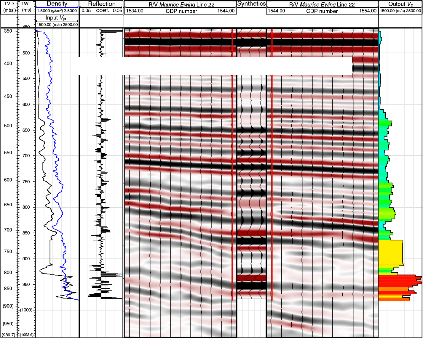
Figure F54. Synthetic seismogram based on Version 1 input velocity profile.
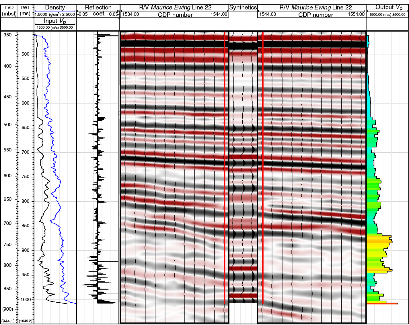
Figure F55. Synthetic seismogram based on Version 2 input velocity profile.
A big difference occurs at the base of the hole, where downhole logging data (used to build the high VP end-member model) suggest velocity values close to 3500 m/s, which strongly compresses the lower portion of the synthetic seismogram and shifts synthetics upward with respect to the seismic data (Figure F54). For the lower VP end-member (with velocity values based on MSCL data; Version 2), a good match between synthetic and seismic data is achieved, but the resulting velocity profile suggests very low values for such depth, ranging from as low as 1700 m/s to about 2600 m/s (Figure F55). The output velocity profile and TDRs are shown in Figure F56 (full data files are available in M0080_TDR1.xlsx and M0080_TDR2.xlsx in CLSI in Supplementary material).
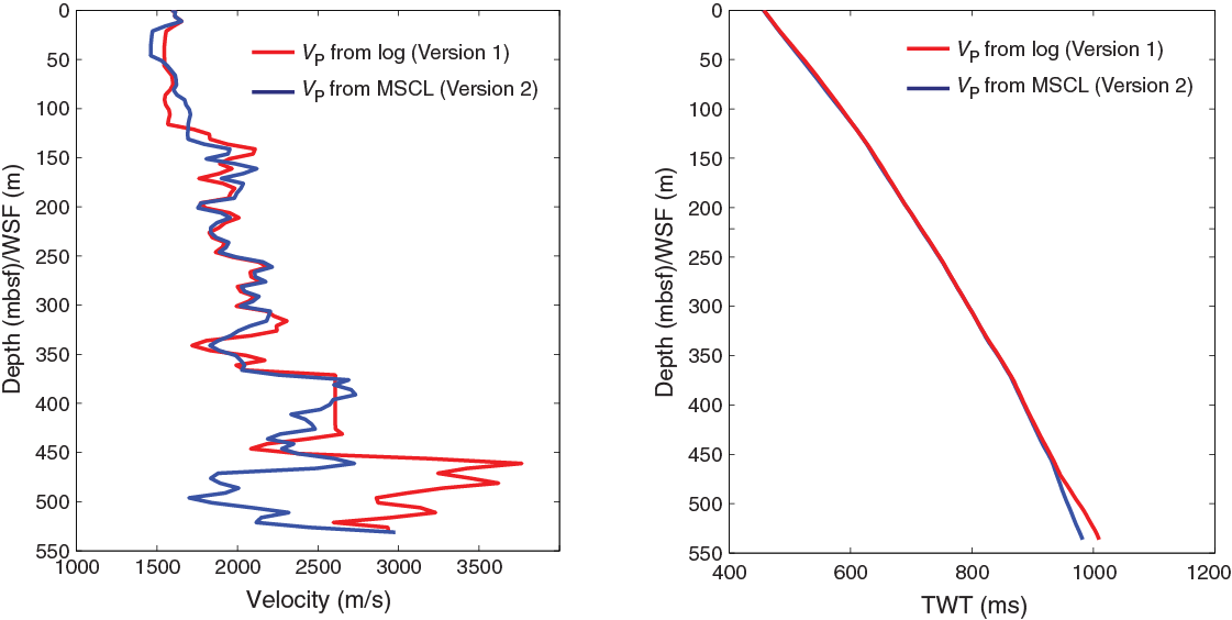
Figure F56. Comparison of final interval velocity and TDRs.
Core-seismic integration
Synthetic seismograms at Site M0080 reproduce the reflectors in the seismic data remarkably well, and the reflectivity pattern is similar for all versions of the input velocity profiles (e.g., Figures F53, F54, F55). The only point of ambiguity occurs in matching the lowermost part of the hole and the transition into basal conglomerates (Figures F54, F55), which is described in greater detail below.
The four lithostratigraphic units identified in the core have visibly different expressions in seismic R/V Maurice Ewing Line 22, crossing the site in the east–west direction (Figures F57, F2). Lithostratigraphic Unit 1, characterized by a succession of relatively thin marine and isolated/semi-isolated intervals, exhibits a series of continuous reflectors with pronounced positive peaks. These reflectors are likely caused by the change to lower density in marine intervals seen in MSCL and MAD data (e.g., Figure F30). The resolution of the seismic data does not make it possible to resolve all of the marine and isolated/semi-isolated subunits, but at least a couple of the subunit boundaries can be reliably traced from core to seismic data (Figure F57). Lithostratigraphic Unit 1 is characterized by very low velocity, likely caused by high porosity in this unit. The lithostratigraphic Unit 1/2 boundary corresponds to an increase in velocity and coincides with a clear change in the seismic reflectivity pattern.
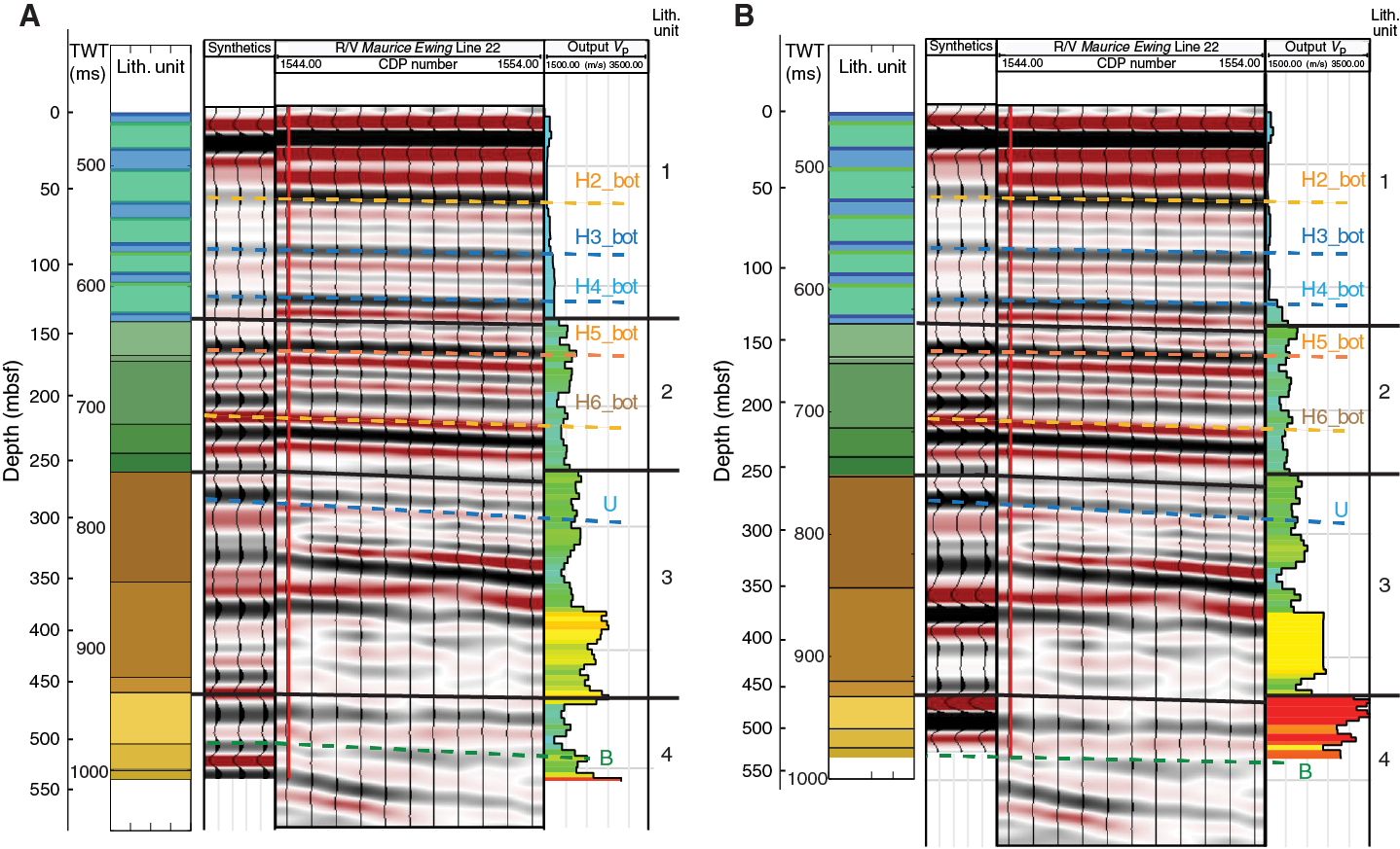
Figure F57. Lithostratigraphic boundaries compared with synthetic seismograms and seismic data.
Lithostratigraphic Unit 2 is also characterized by a series of continuous reflectors in the seismic record, but in contrast to Unit 1, the reflectors have a different character; the positive peaks and negative troughs of the reflectors have similar amplitudes (Figure F57). The reflectors identified as the bases of marine intervals by Nixon et al. (2016) (H5 and H6) correspond to subunit boundaries in this predominantly isolated/semi-isolated unit. The unit is characterized by slightly higher velocity values, with some variability within the unit. Another increase in velocity occurs at the lithostratigraphic Unit 2/3 boundary, which corresponds to a low-amplitude reflector one cycle shallower than previously interpreted by Nixon et al. (2016).
Unit 3 exhibits a more complex reflectivity signature, characterized by less continuous reflectors and some gaps in reflectivity (Figure F57), apparently corresponding to conglomerates in Subunit 3-1. A relatively bright reflection is predicted at the boundary between Subunits 3-1 and 3-2, which appears to have an equivalent in the seismic reflection data. Subunit 3-2 (dominated by silt) is characterized by higher velocity values that decrease again in Subunit 3-3, which corresponds to the transition into gray mud (see Lithostratigraphy).
The link between lithostratigraphic Unit 4 and the seismic data varies depending on the input velocity model (Figure F57). For the case of lower input velocity values derived from MSCL data (Version 2), the top and bottom of Unit 4 are marked by two distinct reflectors, the lower of which was previously attributed to the top basement unconformity by Nixon et al. (2016). This reflector would correspond to the boundary between Subunits 4-1 and 4-2, and the top of basal conglomerates would correspond to a reflection below the originally interpreted “basement” reflection from Nixon et al. (2016).
For the case of higher velocity values derived from the downhole log (Version 1), the entirety of Unit 4 maps onto the top reflector and the subunit boundaries cannot be resolved (Figure F57B). In this case, the reflector interpreted to be the basement boundary would be intersected at the very bottom of Hole M0080A. Unit 4 is dominated by consolidated carbonates and therefore can be expected to have velocity values above 3000 m/s. In addition, the MSCL and discrete sample velocity measurements are conducted ex situ and are likely to underestimate in situ velocity values. The higher velocity interpretation (Version 1) is thus favored. Given the significant difference in the seismic correlation for Unit 4, P-wave velocity values in the base of the hole need to be carefully reevaluated by additional well log processing and confined VP measurements, if possible.
References
Anthonissen, D.E., and Ogg, J.G., 2012. Appendix 3—Cenozoic and Cretaceous biochronology of planktonic foraminifera and calcareous nannofossils. In Gradstein, F.M., Ogg, J.G., Schmitz, M.D., and Ogg, G.M., (Eds.), The Geologic Time Scale 2012: Amsterdam (Elsevier), 1083–1127. https://doi.org/10.1016/B978-0-444-59425-9.15003-6
Backman, J., Raffi, I., Rio, D., Fornaciari, E., and Pälike, H., 2012. Biozonation and biochronology of Miocene through Pleistocene calcareous nannofossils from low and middle latitudes. Newsletters on Stratigraphy, 45(3):221–244. https://doi.org/10.1127/0078-0421/2012/0022
Bell, R.E., McNeill, L.C., Bull, J.M., Henstock, T.J., Collier, R.E.L., and Leeder, M.R., 2009. Fault architecture, basin structure and evolution of the Gulf of Corinth Rift, central Greece. Basin Research, 21(6):824–855. https://doi.org/10.1111/j.1365-2117.2009.00401.x
Berner, R.A., 1980. Early Diagenesis: A Theoretical Approach: Princeton, NJ (Princeton University Press).
Cvetkoska, A., Jovanovska, E., Francke, A., Tofilovska, S., Vogel, H., Levkov, Z., Donders, T.H., Wagner, B., and Wagner-Cremer, F., 2016. Ecosystem regimes and responses in a coupled ancient lake system from MIS 5b to present: the diatom record of lakes Ohrid and Prespa. Biogeosciences, 13(10):3147–3162. https://doi.org/10.5194/bg-13-3147-2016
Cvetkoska, A., Levkov, Z., Reed, J.M., and Wagner, B., 2014. Late Glacial to Holocene climate change and human impact in the Mediterranean: the last ca. 17 ka diatom record of Lake Prespa (Macedonia/Albania/Greece). Palaeogeography, Palaeoclimatology, Palaeoecology, 406:22–32. https://doi.org/10.1016/j.palaeo.2014.04.010
Cvetkoska, A., Reed, J.M., and Levkov, Z., 2012. Diatoms as indicators of environmental change in ancient Lake Ohrid during the last glacial–interglacial cycle (ca. 140 ka). In Witkowski, A. (Ed.), Diatom Monographs: Königstein, Germany (Koeltz Scientific Books).
Debenay, J.-P., 2000. Foraminifers of paralic tropical environments. Micropaleontology, 46:153–160. https://www.jstor.org/stable/1486186
Dimiza, M.D., Triantaphyllou, M.V., and Malinverno, E., 2014. New evidence for the ecology of Helicosphaera carteri in polluted coastal environments (Elefsis Bay, Saronikos Gulf, Greece). Journal of Nannoplankton Research, 34:37–43. http://ina.tmsoc.org/JNR/online/34/Dimiza et al 2014 JNR Crete.pdf
Dimiza, M.D., Triantaphyllou, M.V., Malinverno, E., Psarra, S., Karatsolis, B.-T., Mara, P., Lagaria, A., and Gogou, A., 2016. The composition and distribution of living coccolithophores in the Aegean Sea (NE Mediterranean). Micropaleontology, 61(6):521–540. http://www.micropress.org/microaccess/micropaleontology/issue-321/article-1966
Flores, J.-A., Colmenero-Hidalgo, E., Mejía-Molina, A.E., Baumann, K.-H., Hendericks, J., Larsson, K., Prabhu, C.N., Sierro, F.J., and Rodrigues, T., 2010. Distribution of large Emiliania huxleyi in the central and northeast Atlantic as a tracer of surface ocean dynamics during the last 25,000 years. Marine Micropaleontology, 76(3–4):53–66. https://doi.org/10.1016/j.marmicro.2010.05.001
Ford, M., Rohais, S., Williams, E.A., Bourlange, S., Jousselin, D., Backert, N., and Malartre, F., 2013. Tectono-sedimentary evolution of the western Corinth Rift (central Greece). Basin Research, 25(1):3–25. https://doi.org/10.1111/j.1365-2117.2012.00550.x
Ford, M., Williams, E.A., Malartre, F., and Popescu, S.-M., 2007. Stratigraphic architecture, sedimentology and structure of the Vouraikos Gilbert-type fan delta, Gulf of Corinth, Greece. In Nichols, G., Paola, C., and Williams, E. (Eds.), Sedimentary Processes, Environments and Basins: A Tribute to Peter Friend. Jarvis, I. (Series Ed.). Special Publication of the International Association of Sedimentologists, 38:44–90. https://doi.org/10.1002/9781444304411.ch4
Goineau, A., Fontanier, C., Mojtahid, M., Fanget, A.-S., Bassetti, M.-A., Berné, S., and Jorissen, F., 2015. Live–dead comparison of benthic foraminiferal faunas from the Rhône prodelta (Gulf of Lions, NW Mediterranean): development of a proxy for palaeoenvironmental reconstructions. Marine Micropaleontology, 119:17–33. https://doi.org/10.1016/j.marmicro.2015.07.002
Houk, V., Klee, R., and Tanaka, H., 2010. Atlas of Freshwater Centric Diatoms with a Brief Key and Descriptions: Part 3. Stephanodiscaceae A. Cyclotella, Tertiarius, Discostella: Praha, Czech Republic (Czech Phycological Society).
Hyndman, R.D., Erickson, A.J., and Von Herzen, R.P., 1974. Geothermal measurements on DSDP Leg 26. In Davies, T.A., Luyendyk, B.P., et al., Initial Reports of the Deep Sea Drilling Project, 26: Washington, DC (U.S. Govt. Printing Office), 451–463. https://doi.org/10.2973/dsdp.proc.26.113.1974
Jovanovska, E., Cvetkoska, A., Hauffe, T., Levkov, Z., Wagner, B., Sulpizio, R., Francke, A., Albrecht, C., and Wilke, T., 2016. Differential resilience of ancient sister lakes Ohrid and Prespa to environmental disturbances during the Late Pleistocene. Biogeosciences, 13(4):1149–1161. https://doi.org/10.5194/bg-13-1149-2016
Kennedy, M. (Ed.), 2015. Developments in Petroleum Science (Volume 62): Practical Petrophysics. Cubitt, J. (Series Ed.): Amsterdam (Elsevier). https://www.sciencedirect.com/bookseries/developments-in-petroleum-science/vol/62
Krammer, K., and Lange-Bertalot, H., 1991. Bacillariophyceae, Part 3. Centrales, Fragilariaceae, Eunotiaceae. In Ettl, H., Gerloff, J., Heynig, H., and Mollenhauer, D. (Eds.), Süßwaserflora von Mitteleuropa (Volume 2/3): Stuttgart, Germany (Gustav Fischer Verlag).
Lisiecki, L.E., and Raymo, M.E., 2005. A Pliocene–Pleistocene stack of 57 globally distributed benthic δ18O records. Paleoceanography, 20(1):PA1003. https://doi.org/10.1029/2004PA001071
Martini, E., 1971. Standard Tertiary and Quaternary calcareous nannoplankton zonation. In Farinacci, A. (Ed.), Proceedings of the Second Planktonic Conference, Roma 1970: Rome (Edizioni Tecnoscienza), 2:739–785.
McNeill, L.C., Shillington, D.J., Carter, G.D.O., Everest, J.D., Le Ber, E., Collier, R.E.Ll., Cvetkoska, A., De Gelder, G., Diz, P., Doan, M.-L., Ford, M., Gawthorpe, R.L., Geraga, M., Gillespie, J., Hemelsdaël, R., Herrero-Bervera, E., Ismaiel, M., Janikian, L., Kouli, K., Li, S., Machlus, M.L., Maffione, M., Mahoney, C., Michas, G., Miller, C., Nixon, C.W., Oflaz, S.A., Omale, A.P., Panagiotopoulos, K., Pechlivanidou, S., Phillips, M.P., Sauer, S., Seguin, J., Sergiou, S., and Zakharova, N.V., 2019a. Expedition 381 facies associations. In McNeill, L.C., Shillington, D.J., Carter, G.D.O., and the Expedition 381 Participants, Corinth Active Rift Development. Proceedings of the International Ocean Discovery Program, 381: College Station, TX (International Ocean Discovery Program). https://doi.org/10.14379/iodp.proc.381.103.2019
McNeill, L.C., Shillington, D.J., Carter, G.D.O., Everest, J.D., Le Ber, E., Collier, R.E.Ll., Cvetkoska, A., De Gelder, G., Diz, P., Doan, M.-L., Ford, M., Gawthorpe, R.L., Geraga, M., Gillespie, J., Hemelsdaël, R., Herrero-Bervera, E., Ismaiel, M., Janikian, L., Kouli, K., Li, S., Machlus, M.L., Maffione, M., Mahoney, C., Michas, G., Miller, C., Nixon, C.W., Oflaz, S.A., Omale, A.P., Panagiotopoulos, K., Pechlivanidou, S., Phillips, M.P., Sauer, S., Seguin, J., Sergiou, S., and Zakharova, N.V., 2019b. Expedition 381 methods. In McNeill, L.C., Shillington, D.J., Carter, G.D.O., and the Expedition 381 Participants, Corinth Active Rift Development. Proceedings of the International Ocean Discovery Program, 381: College Station, TX (International Ocean Discovery Program). https://doi.org/10.14379/iodp.proc.381.102.2019
McNeill, L.C., Shillington, D.J., Carter, G.D.O., Everest, J.D., Le Ber, E., Collier, R.E.Ll., Cvetkoska, A., De Gelder, G., Diz, P., Doan, M.-L., Ford, M., Gawthorpe, R.L., Geraga, M., Gillespie, J., Hemelsdaël, R., Herrero-Bervera, E., Ismaiel, M., Janikian, L., Kouli, K., Li, S., Machlus, M.L., Maffione, M., Mahoney, C., Michas, G., Miller, C., Nixon, C.W., Oflaz, S.A., Omale, A.P., Panagiotopoulos, K., Pechlivanidou, S., Phillips, M.P., Sauer, S., Seguin, J., Sergiou, S., and Zakharova, N.V., 2019c. Site M0078. In McNeill, L.C., Shillington, D.J., Carter, G.D.O., and the Expedition 381 Participants, Corinth Active Rift Development. Proceedings of the International Ocean Discovery Program, 381: College Station, TX (International Ocean Discovery Program). https://doi.org/10.14379/iodp.proc.381.104.2019
McNeill, L.C., Shillington, D.J., Carter, G.D.O., Everest, J.D., Le Ber, E., Collier, R.E.Ll., Cvetkoska, A., De Gelder, G., Diz, P., Doan, M.-L., Ford, M., Gawthorpe, R.L., Geraga, M., Gillespie, J., Hemelsdaël, R., Herrero-Bervera, E., Ismaiel, M., Janikian, L., Kouli, K., Li, S., Machlus, M.L., Maffione, M., Mahoney, C., Michas, G., Miller, C., Nixon, C.W., Oflaz, S.A., Omale, A.P., Panagiotopoulos, K., Pechlivanidou, S., Phillips, M.P., Sauer, S., Seguin, J., Sergiou, S., and Zakharova, N.V., 2019d. Site M0079. In McNeill, L.C., Shillington, D.J., Carter, G.D.O., and the Expedition 381 Participants, Corinth Active Rift Development. Proceedings of the International Ocean Discovery Program, 381: College Station, TX (International Ocean Discovery Program). https://doi.org/10.14379/iodp.proc.381.105.2019
Nixon, C.W., McNeill, L.C., Bull, J.M., Bell, R.E., Gawthorpe, R.L., Henstock, T.J., Christodoulou, D., et al., 2016. Rapid spatiotemporal variations in rift structure during development of the Corinth Rift, central Greece. Tectonics, 35(5):1225–1248. https://doi.org/10.1002/2015TC004026
Ogg, J.G., Ogg, G., and Gradstein, F.M., 2016. A Concise Geologic Time Scale 2016: Boston (Elsevier). https://doi.org/10.1016/C2009-0-64442-1
Pujol, C., and Vergnaud Grazzini, C., 1995. Distribution patterns of live planktic foraminifers as related to regional hydrography and productive systems of the Mediterranean Sea. Marine Micropaleontology, 25(2–3):187–217. https://doi.org/10.1016/0377-8398(95)00002-I
Raffi, I., Backman, J., Fornaciari, E., Pälike, H., Rio, D., Lourens, L., and Hilgen, F., 2006. A review of calcareous nannofossil astrobiochronology encompassing the past 25 million years. Quaternary Science Reviews, 25(23–24):3113–3137. https://doi.org/10.1016/j.quascirev.2006.07.007
Reed, J.M., Cvetkoska, A., Levkov, Z., Vogel, H., and Wagner, B., 2010. The last glacial-interglacial cycle in Lake Ohrid (Macedonia/Albania): testing diatom response to climate. Biogeosciences, 7(10):3083–3094. https://doi.org/10.5194/bg-7-3083-2010
Rohling, E.J., and Gieskes, W.W.C., 1989. Late Quaternary changes in Mediterranean intermediate water density and formation rate. Paleoceanography and Paleoclimatology, 4(5):531. https://doi.org/10.1029/PA004i005p00531
Rohling, E.J., Jorissen, F.J., Vergnaud Grazzini, C., and Zachariasse, W.J., 1993. Northern Levantine and Adriatic Quaternary planktic foraminifera; reconstruction of paleoenvironmental gradients. Marine Micropaleontology, 21(1–3):191–218. https://doi.org/10.1016/0377-8398(93)90015-P
Sakellariou, D., Lykousis, V., Alexandri, S., Kaberi, H., Rousakis, G., Nomikou, P., Georgiou, P., and Ballas, D., 2007. Faulting, seismic-stratigraphic architecture and Late Quaternary evolution of the Gulf of Alkyonides Basin–East Gulf of Corinth, Central Greece. Basin Research, 19(2):273–295. https://doi.org/10.1111/j.1365-2117.2007.00322.x
Singer, B.S., 2014. A Quaternary geomagnetic instability time scale. Quaternary Geochronology, 21:29–52. https://doi.org/10.1016/j.quageo.2013.10.003
Skourtsos, E., and Kranis, H., 2009. Structure and evolution of the western Corinth Rift, through new field data from the northern Peloponnesus. In Ring, U., and Wernicke, B. (Eds.), Extending a Continent: Architecture, Rheology and Heat Budget. Geological Society Special Publication, 321(1):119–138. https://doi.org/10.1144/SP321.6
Stoermer, E.F., Kreis, R.G., Jr., and Andresen, N.A., 1999. Checklist of diatoms from the Laurentian Great Lakes, II. Journal of Great Lakes Research, 25(3):515–566. https://doi.org/10.1016/S0380-1330(99)70759-8
Taylor, B., Weiss, J.R., Goodliffe, A.M., Sachpazi, M., Laigle, M., and Hirn, A., 2011. The structures, stratigraphy and evolution of the Gulf of Corinth Rift, Greece. Geophysical Journal International, 185(3):1189–1219. https://doi.org/10.1111/j.1365-246X.2011.05014.x
Thierstein, H.R., Geitzenauer, K.R., Molfino, B., and Shackleton, N.J., 1977. Global synchroneity of late Quaternary coccolith datum levels validation by oxygen isotopes. Geology, 5(7):400–404. https://doi.org/10.1130/0091-7613(1977)5<400:GSOLQC>2.0.CO;2
Van Dam, H., Mertens, A., and Sinkeldam, J., 1994. A coded checklist and ecological indicator values of freshwater diatoms from The Netherlands. Netherland Journal of Aquatic Ecology, 28(1):117–133. https://doi.org/10.1007/BF02334251
Young, J.R., and Westbroek, P., 1991. Genotypic variation in the coccolithophorid species Emiliania huxleyi. Marine Micropaleontology, 18(1–2):5–23. https://doi.org/10.1016/0377-8398(91)90004-P
1 McNeill, L.C., Shillington, D.J., Carter, G.D.O., Everest, J.D., Le Ber, E., Collier, R.E.Ll., Cvetkoska, A., De Gelder, G., Diz, P., Doan, M.-L., Ford, M., Gawthorpe, R.L., Geraga, M., Gillespie, J., Hemelsdaël, R., Herrero-Bervera, E., Ismaiel, M., Janikian, L., Kouli, K., Li, S., Machlus, M.L., Maffione, M., Mahoney, C., Michas, G., Miller, C., Nixon, C.W., Oflaz, S.A., Omale, A.P., Panagiotopoulos, K., Pechlivanidou, S., Phillips, M.P., Sauer, S., Seguin, J., Sergiou, S., Zakharova, N.V., 2019. Site M0080. In McNeill, L.C., Shillington, D.J., Carter, G.D.O., and the Expedition 381 Participants, Corinth Active Rift Development. Proceedings of the International Ocean Discovery Program, 381: College Station, TX (International Ocean Discovery Program). https://doi.org/10.14379/iodp.proc.381.106.2019
2 Expedition 381 Participants’ affiliations.
This work is distributed under the Creative Commons Attribution 4.0 International (CC BY 4.0) license. 