Weber, M.E., Raymo, M.E., Peck, V.L., Williams, T., and the Expedition 382 Scientists
Proceedings of the International Ocean Discovery Program Volume 382
publications.iodp.org

https://doi.org/10.14379/iodp.proc.382.102.2021
Expedition 382 methods1
M.E. Weber, M.E. Raymo, V.L. Peck, T. Williams, L.H. Armbrecht, I. Bailey, S.A. Brachfeld, F.G. Cardillo, Z. Du, G. Fauth, M. García, A. Glüder, M.E. Guitard, M. Gutjahr, S.R. Hemming, I. Hernández-Almeida, F.S. Hoem, J.-H. Hwang, M. Iizuka, Y. Kato, B. Kenlee, Y.M. Martos, S. O'Connell, L.F. Pérez, B.T. Reilly, T.A. Ronge, O. Seki, L. Tauxe, S. Tripathi, J.P. Warnock, and X. Zheng2
Keywords: International Ocean Discovery Program, IODP, JOIDES Resolution, Expedition 382, Iceberg Alley and Subantarctic Ice and Ocean Dynamics, Site U1534, Site U1535, Site U1536, Site U1537, Site U1538, Subantarctic Front, Pirie Basin, Dove Basin
MS 382-102: Published 20 May 2021
Introduction
This section provides an overview of operations, depth conventions, core handling, curatorial procedures, and analyses performed on the R/V JOIDES Resolution during International Ocean Discovery Program (IODP) Expedition 382. This information applies only to shipboard work described in the Expedition reports section of the Expedition 382 Proceedings of the International Ocean Discovery Program volume. Methods used by investigators for shore-based analyses of Expedition 382 data will be described in separate individual postcruise research publications.
Site locations
GPS coordinates (WGS84 datum) from precruise site surveys were used to position the vessel at Expedition 382 sites. A SyQwest Bathy 2010 CHIRP subbottom profiler was used to monitor seafloor depth during the approach to each site and to confirm the seafloor depth once on site. Once the vessel was positioned at a site, the thrusters were lowered and a seafloor positioning beacon was prepared for deployment in case it was needed. Dynamic positioning control of the vessel primarily used navigational input from the GPS (Figure F1); we deployed a seafloor beacon only at Site U1536, which was the deepest penetration site, during this expedition. The final hole position was the mean position calculated from the GPS data collected over a significant portion of the time during which the hole was occupied.
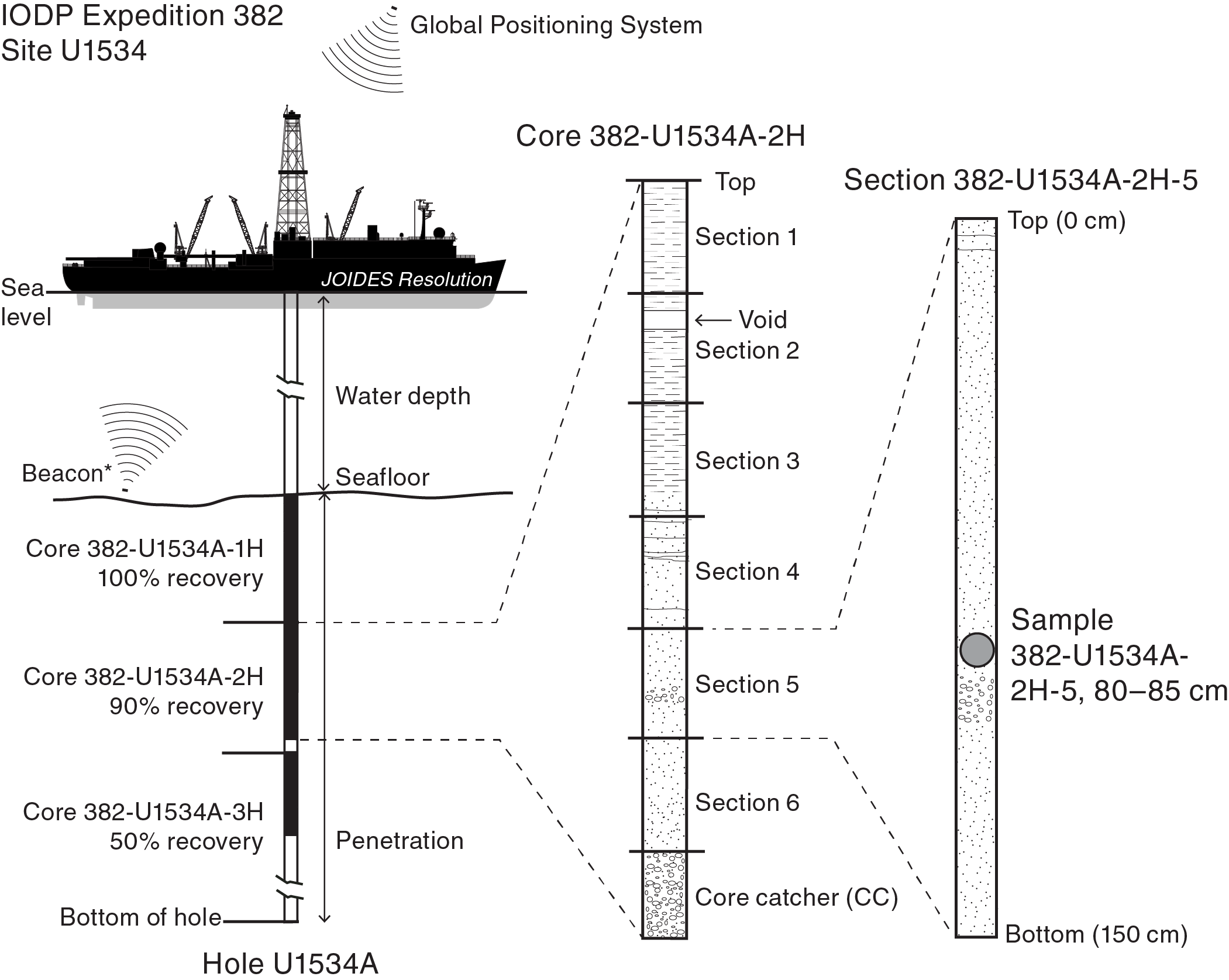
Figure F1. IODP naming convention.
Drilling operations
The advanced piston corer (APC), half-length APC (HLAPC), extended core barrel (XCB), and rotary core barrel (RCB) systems were all used during Expedition 382 (Figures F2, F3, F4). These tools and other drilling technology are documented in Graber et al. (2002).
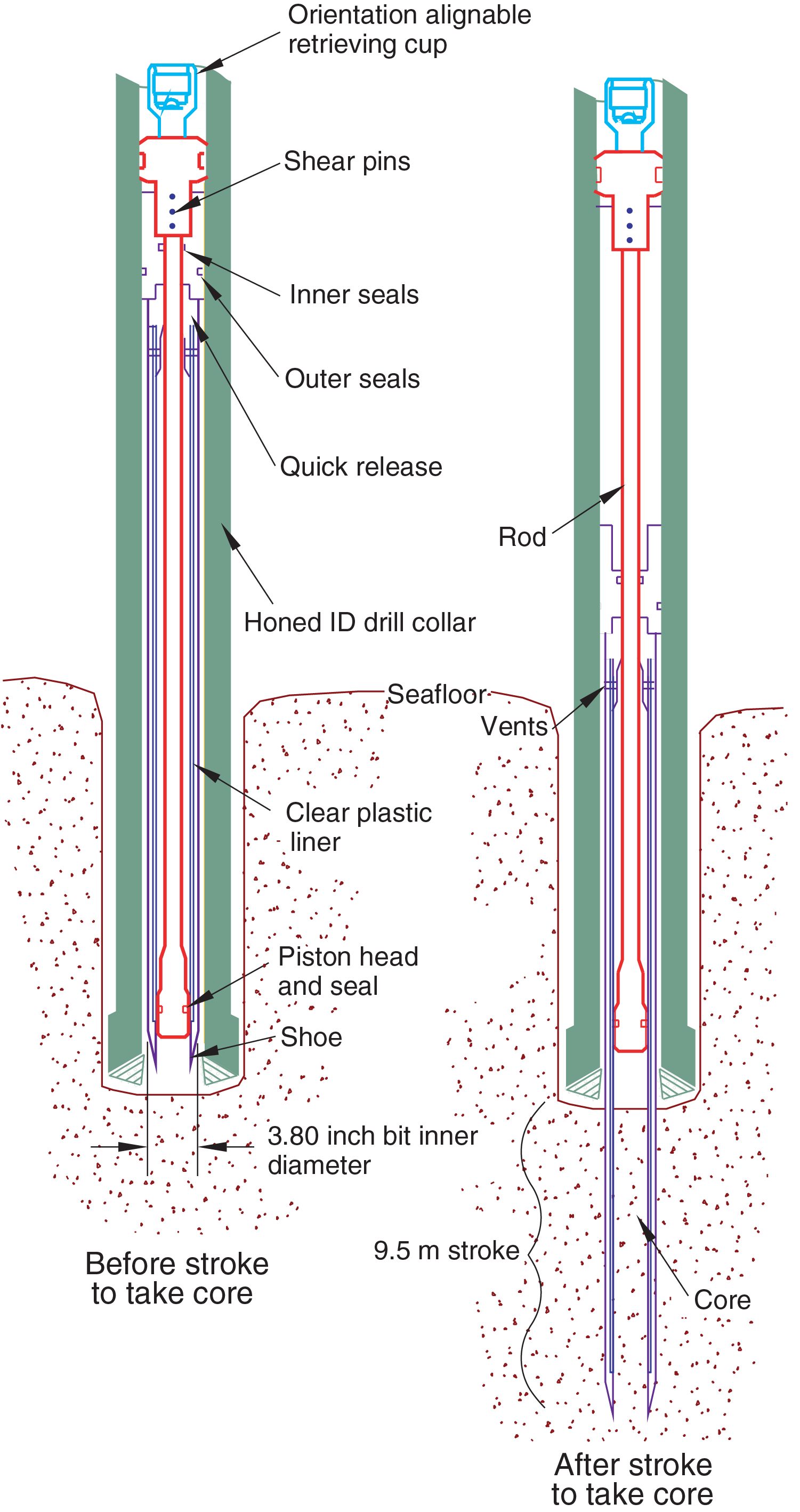
Figure F2. APC system.
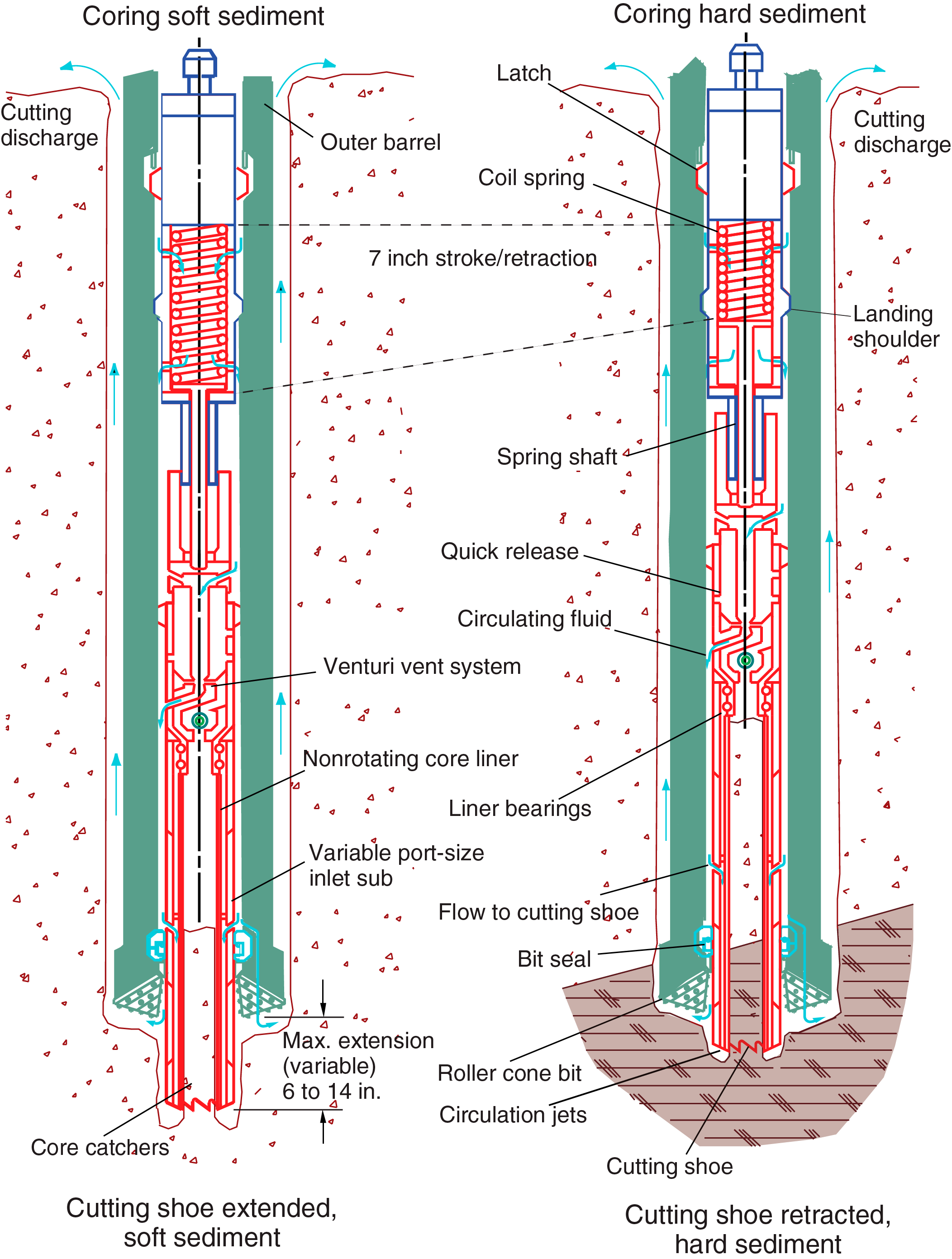
Figure F3. XCB system.
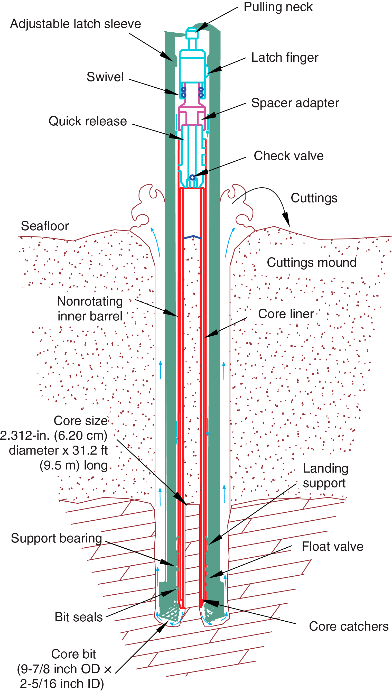
Figure F4. RCB system.
The APC and HLAPC systems cut soft-sediment cores with minimal coring disturbance relative to other IODP coring systems. After the APC/HLAPC core barrel is lowered through the drill pipe and lands above the bit, the drill pipe is pressured up until the two shear pins that hold the inner barrel attached to the outer barrel fail. The inner barrel then advances into the formation and cuts the core (Figure F2). The driller can detect a successful cut, or "full stroke," by observing the pressure gauge on the rig floor because the excess pressure accumulated prior to the stroke drops rapidly.
APC refusal is conventionally defined in one of two ways: (1) the piston fails to achieve a complete stroke (as determined from the pump pressure and recovery reading) because the formation is too hard, or (2) excessive force (>60,000 lb) is required to pull the core barrel out of the formation. For APC cores that do not achieve a full stroke, the next core can be taken after advancing to a depth determined by the recovery of the previous core (advance by recovery) or to the depth of a full APC core (typically 9.5 m). When a full stroke is not achieved, one or more additional attempts are typically made, and each time the bit is advanced by the length of the core recovered (note that for these cores, this results in a nominal recovery of ~100%). When a full or partial stroke is achieved but excessive force is not able to retrieve the barrel, the core barrel can be "drilled over," meaning that after the inner core barrel is successfully shot into the formation, the drill bit is advanced to total depth to free the APC barrel.
The standard APC system uses a 9.5 m long core barrel, whereas the HLAPC system uses a 4.7 m long core barrel. In most instances, the HLAPC system is deployed after the standard APC system has repeated partial strokes and/or the core liners are damaged. During use of the HLAPC system, the same criteria are applied in terms of refusal as for the APC system. Use of the HLAPC system allowed for significantly greater APC sampling depths to be attained than would have otherwise been possible.
The XCB system is typically used when the APC/HLAPC system has difficulty penetrating the formation and/or damages the core liner or core. The XCB system can also be used to either initiate holes where the seafloor is not suitable for APC coring or be interchanged with the APC/HLAPC system when dictated by changing formation conditions. The XCB system is used to advance the hole when HLAPC refusal occurs before the target depth is reached or when drilling conditions require it. The XCB system is a rotary system with a small cutting shoe that extends below the large rotary APC/XCB bit (Figure F3). The smaller bit can cut a semi-indurated core with less torque and fluid circulation than the main bit, potentially improving recovery. The XCB cutting shoe typically extends ~30.5 cm ahead of the main bit in soft sediments, but a spring allows it to retract into the main bit when hard formations are encountered. Shorter XCB cutting shoes can also be used.
The bottom-hole assembly (BHA) used for APC and XCB coring is typically composed of an 11⁷⁄₁₆ inch (~29.05 cm) roller cone drill bit, a bit sub, a seal bore drill collar, a landing saver sub, a modified top sub, a modified head sub, 8¼ inch control length drill collars, a tapered drill collar, two stands of 5½ inch transition drill pipe, and a crossover sub to the drill pipe that extends to the surface.
The RCB system is a rotary system designed to recover firm to hard sediments and basement rocks. The BHA, including the bit and outer core barrel, is rotated with the drill string while bearings allow the inner core barrel to remain stationary (Figure F4).
A typical RCB BHA includes a 9⅞ inch drill bit, a bit sub, an outer core barrel, a modified top sub, a modified head sub, a variable number of 8¼ inch control length drill collars, a tapered drill collar, two stands of 5½ inch drill pipe, and a crossover sub to the drill pipe that extends to the surface.
Nonmagnetic core barrels were used for all APC, HLAPC, and RCB coring. APC cores were oriented with the Icefield MI-5 core orientation tool when coring conditions allowed. Formation temperature measurements were taken with the advanced piston corer temperature tool (APCT-3; see Downhole measurements). Information on recovered cores, drilled intervals, downhole tool deployments, and related information are provided in the Operations, Paleomagnetism, and Downhole measurements sections of each site chapter.
IODP depth conventions
The primary depth scales used by IODP are based on the measurement of the drill string length deployed beneath the rig floor (drilling depth below rig floor [DRF] and drilling depth below seafloor [DSF]), the length of core recovered (core depth below seafloor [CSF] and core composite depth below seafloor [CCSF]), and the length of logging wireline deployed (wireline log depth below rig floor [WRF], wireline log depth below seafloor [WSF], and wireline log matched depth below seafloor [WMSF]). All depths are in meters. The relationship between scales is defined either by protocol, such as the rules for computation of CSF depths from DSF depths, or by combinations of protocols with user-defined correlations (e.g., CCSF scale). The distinction in nomenclature should keep the user aware that a nominal depth value in two different depth scales usually does not refer to exactly the same stratigraphic interval (see Curatorial procedures and sample depth calculations). For more information on depth scales, see IODP Depth Scales Terminology at http://www.iodp.org/policies-and-guidelines. To more easily communicate shipboard results, core depth below seafloor, Method A [CSF-A], depths in this volume are reported as meters below seafloor (mbsf) unless otherwise noted.
Depths of cored intervals are measured from the drill floor based on the length of drill pipe deployed beneath the rig floor (DRF scale; Figure F1). The depth of the cored interval is referenced to the seafloor (DSF scale) by subtracting the seafloor depth of the hole from the DRF depth of the interval. Standard depths of cores in meters below the seafloor (CSF-A scale) are determined based on the assumption that the top depth of a recovered core corresponds to the top depth of its cored interval (DSF scale). Standard depths of samples and associated measurements (CSF-A scale) are calculated by adding the offset of the sample or measurement from the top of its section and the lengths of all higher sections in the core to the top depth of the core.
If a core has <100% recovery, for curation purposes all cored material is assumed to originate from the top of the drilled interval as a continuous section. In addition, voids in the core are closed by pushing core segments together, if possible, during core handling. If the core pieces cannot be pushed together to get rid of the voids, then foam spacers are inserted and clearly labeled "void." Therefore, the true depth interval within the cored interval is only partially constrained. This should be considered a sampling uncertainty in age-depth analysis or correlation of core data with downhole logging data.
When core recovery is >100% (the length of the recovered core exceeds that of the cored interval), the CSF-A depth of a sample or measurement taken from the bottom of a core will be deeper than that of a sample or measurement taken from the top of the subsequent core (i.e., the data associated with the two core intervals overlap at the CSF-A scale). This overlap can happen when a soft to semisoft sediment core recovered from a few hundred meters below the seafloor expands upon recovery (typically by a few percent to as much as 15%). Therefore, a stratigraphic interval may not have the same nominal depth on the DSF and CSF-A scales in the same hole.
During Expedition 382, all core depths below seafloor were initially calculated according to the CSF-A depth scale. CCSF depth scales are constructed for sites with two or more holes to create as continuous a stratigraphic record as possible. It also helps mitigate the CSF-A core overlap problem and the coring gap problem. Using shipboard core logger–based physical property data verified with core photos, core depths in adjacent holes at a site are vertically shifted to correlate between cores recovered in adjacent holes. This process produces the CCSF depth scale. The correlation process results in affine tables that indicate the vertical shift of cores on the CCSF scale relative to the CSF-A scale. Once the CCSF scale is constructed, a splice can be defined that best represents the stratigraphy of a site by utilizing and splicing the best portions of individual sections and cores from each hole. Because of core expansion, the CCSF depths of stratigraphic intervals are typically 10%–15% deeper than their CSF-A depths. CCSF depth scale construction also reveals that coring gaps on the order of 1.0–1.5 m typically occur between two subsequent cores despite the apparent >100% recovery. For more details on the construction of the CCSF depth scale, see Stratigraphic correlation.
Curatorial procedures and sample depth calculations
Numbering of sites, holes, cores, and samples followed standard IODP procedure (Figure F1). A full curatorial identifier for a sample consists of the following information: expedition, site, hole, core number, core type, section number, section half, piece number (hard rocks only), and interval in centimeters measured from the top of the core section. For example, a sample identification of "382-U1534A-2H-5W, 80–85 cm," indicates a 5 cm sample removed from the interval between 80 and 85 cm below the top of Section 5 (working half) of Core 2 ("H" designates that this core was taken with the APC system) of Hole A at Site U1534 during Expedition 382 (Figure F1). The "U" preceding the hole number indicates the hole was drilled by the US IODP platform, JOIDES Resolution. The drilling system used to obtain a core is designated in the sample identifiers as follows: H = APC, F = HLAPC, R = RCB, and X = XCB. Integers are used to denote the "core" type of drilled intervals (e.g., a drilled interval between Cores 2H and 4H would be denoted by Core 31).
Core handling and analysis
The overall flow of cores, sections, analyses, and sampling implemented during Expedition 382 is shown in Figure F5.
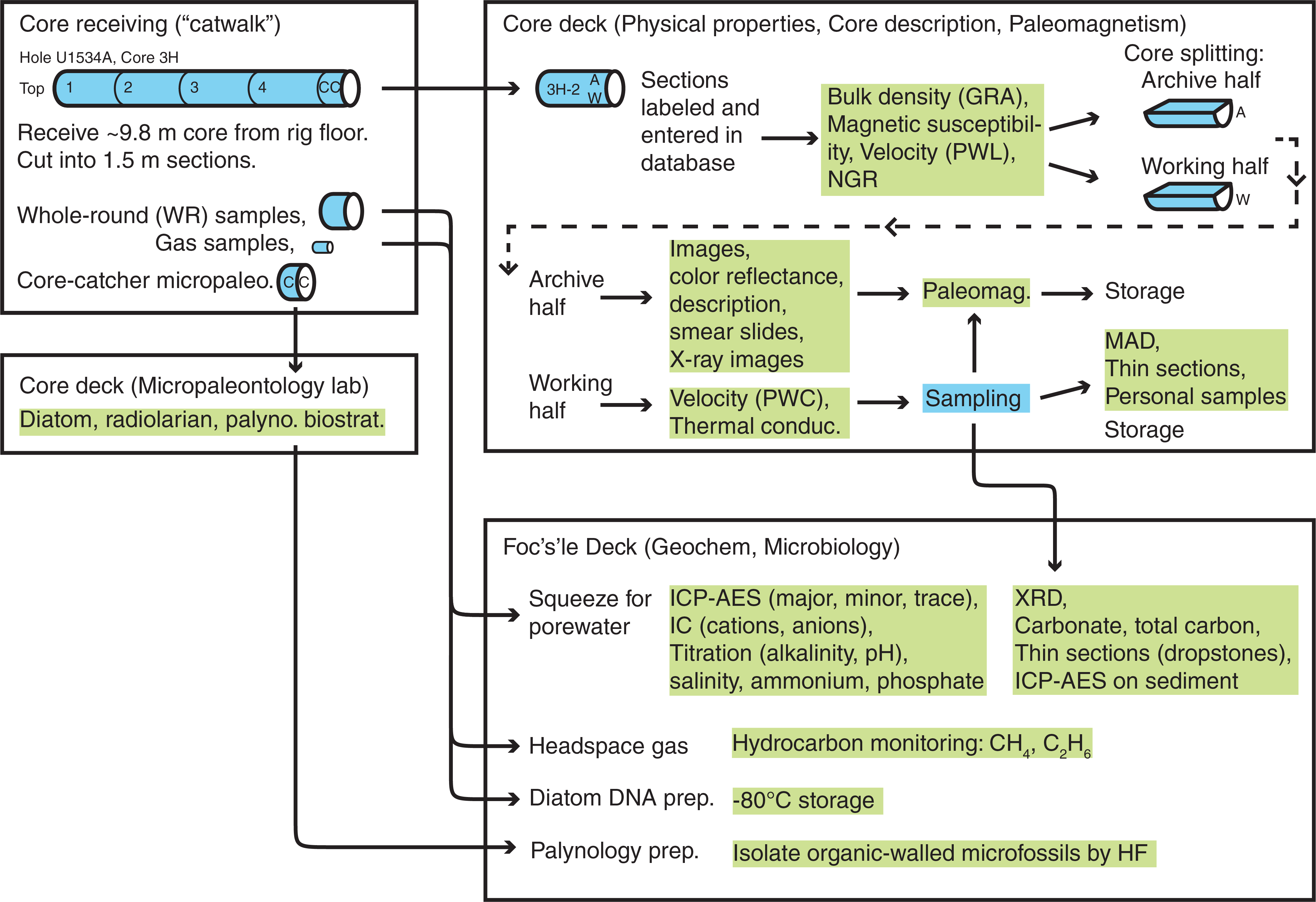
Figure F5. Core, section, analysis, and sampling flow.
Sediment
When the core barrel reached the rig floor, the core catcher from the bottom of the core was removed and taken to the core receiving platform ("catwalk"), and a sample was extracted for paleontological (PAL) analysis. Next, the sediment core was extracted from the core barrel in its plastic liner. The liner was carried from the rig floor to the core processing area on the catwalk outside the core laboratory, where it was split into ~1.5 m sections. Blue (uphole direction) and clear (downhole direction) liner caps were glued with acetone onto the cut liner sections.
Once the core was cut into sections, whole-round samples were taken for interstitial water (IW) chemical analyses. When a whole-round sample was removed, a yellow cap was used to indicate it was taken. Syringe samples were taken for gas analyses according to the IODP hydrocarbon safety monitoring protocol. Syringe and whole-round samples were taken for microbiology contamination testing and postcruise analyses. Toothpick samples for smear slides were taken from some of the section ends for additional paleontological analysis.
The core sections were placed in a core rack in the laboratory, core information was entered into the database, and the sections were labeled. When the core sections reached equilibrium with laboratory temperature (typically after 4 h), they were run through the Whole-Round Multisensor Logger (WRMSL) for P-wave velocity (P-wave logger [PWL]), magnetic susceptibility (MS), and gamma ray attenuation (GRA) bulk density (see Physical properties). The core sections were also run through the Natural Gamma Radiation Logger (NGRL), often prior to temperature equilibration because that does not affect the natural gamma radiation (NGR) data, and thermal conductivity measurements were taken once per core when the material was suitable.
The core sections were then split lengthwise from bottom to top into working and archive halves. Investigators should note that older material can be transported upward on the split face of each section during splitting.
Discrete samples were then taken for moisture and density (MAD) and paleomagnetic (PMAG) analyses and for remaining shipboard analyses such as X-ray diffraction (XRD), carbonate (CARB), and inductively coupled plasma–atomic emission spectroscopy (ICP-AES). Samples were not collected when the lithology was a high-priority interval for expedition or postcruise research, the core material was unsuitable, or the core was severely deformed. During the expedition, samples for personal postcruise research were taken when they concerned ephemeral properties (e.g., IW and ancient DNA [aDNA] sampling). We also took a limited number of personal or shared "pilot" samples for two reasons: (1) to find out whether an analytical method works and yields interpretable results and how much sample is needed to guide postcruise sampling and (2) to generate low spatial resolution pilot data sets that can be incorporated in proposals and potentially increase their chances of being funded.
The archive half of each core was scanned on the Section Half Imaging Logger (SHIL) to provide linescan images and then measured for point magnetic susceptibility (MSP) and reflectance spectroscopy and colorimetry (RSC) on the Section Half Multisensor Logger (SHMSL). All of the archive halves were then X-ray imaged. Labeled foam pieces were used to denote missing whole-round intervals in the SHIL images. The archive halves were then described visually and by means of smear slides for sedimentology. Finally, the magnetization of archive halves and working-half discrete pieces was measured with the cryogenic magnetometer and spinner magnetometer.
When all steps were completed, cores were wrapped, sealed in plastic tubes, and transferred to cold storage space aboard the ship. At the end of the expedition, the working halves of the cores were sent to the IODP Bremen Core Repository (Center for Marine Environmental Sciences [MARUM], Bremen, Germany), where samples for postcruise research were taken in November 2019. The archive halves of the cores were first sent to the IODP Gulf Coast Repository (Texas A&M University, College Station, Texas, USA), where a subset was scanned for X-ray fluorescence (XRF) and U-channel paleomagnetic samples were taken, before being forwarded to the Bremen Core Repository for long-term archive.
Drilling and handling core disturbance
Cores may be significantly disturbed and contain extraneous material as a result of the coring and core handling process (Jutzeler et al., 2014). For example, in formations with loose gravel- or pebble-sized clasts, clasts from intervals higher in the hole may be washed down by drilling circulation, accumulate at the bottom of the hole, and be sampled with the next core. The uppermost 10–50 cm of each core must therefore be examined critically during description for potential "fall-in." Common coring-induced deformation includes the concave-downward appearance of originally horizontal bedding. Piston action can result in fluidization ("flow-in") at the bottom of APC cores. The rotation and fluid circulation used during XCB and RCB coring can also cause core pieces to rotate relative to each other as well as induce fluids into the core and/or cause fluidization and remobilization of poorly consolidated/cemented sediments. In addition, extending APC or HLAPC coring into deeper, firmer formation can also induce core deformation. Retrieval from depth to the surface can result in elastic rebound. Gas that is in solution at depth may become free and drive apart core segments in the liner. When gas content is high, pressure must be relieved for safety reasons before the cores are cut into segments. This is accomplished by drilling holes into the liner, which forces some sediment as well as gas out of the liner. These disturbances are described in each site chapter and graphically indicated on the visual core descriptions.
Lithostratigraphy
This section outlines the procedures for documenting the sedimentology of cores recovered during Expedition 382, including core description, smear slide description, color spectrophotometry, and XRD of clay mineral preparations. Only general procedures are outlined. All observations and data were uploaded directly into the IODP Laboratory Information Management System (LIMS) database using the DESClogik application. DESClogik also includes a graphic display mode for core data (e.g., digital images of section halves and measurement data) that was used for quality control (QC) of the uploaded data sets.
Visual core description and standard graphic report
Information from macroscopic standard sedimentologic observations for each core was recorded directly into the Tabular data capture mode of DESClogik. A template was constructed, and tabs and columns were customized to include relevant descriptive information categories (lithology, sedimentary structures, fossils, bioturbation, diagenesis, drilling disturbance, clast properties, and clast abundance). A summary description was also entered for each core.
A simplified one-page graphical representation of each core (standard graphic report or visual core description [VCD]) (Figure F6) was generated using the LIMS2Excel application and a commercial program (Strater, Golden Software). VCDs are presented with a CSF depth scale, split-core photographs, graphic lithology, and columns for core disturbance, clast abundance, sedimentary structures, fossils, diagenesis, bioturbation, shipboard samples, MS, color reflectance (b*), and GRA density. The graphic lithologies, sedimentary structures, and other visual observations are represented on the VCDs by graphic patterns and symbols (Figure F7). Each VCD also contains the summary description for the core. For the summary figure for each chapter, only the major lithologies are shown.
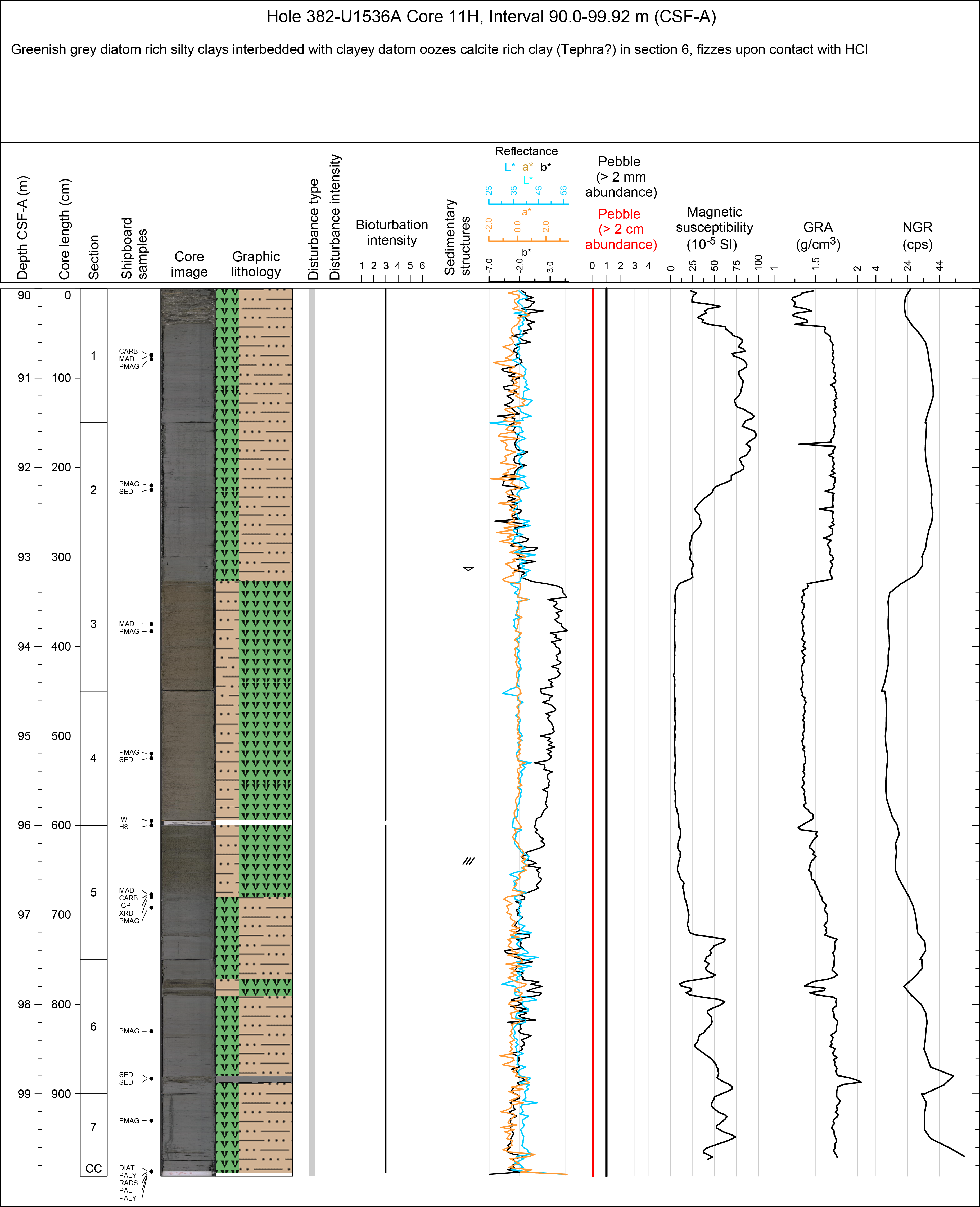
Figure F6. VCD.
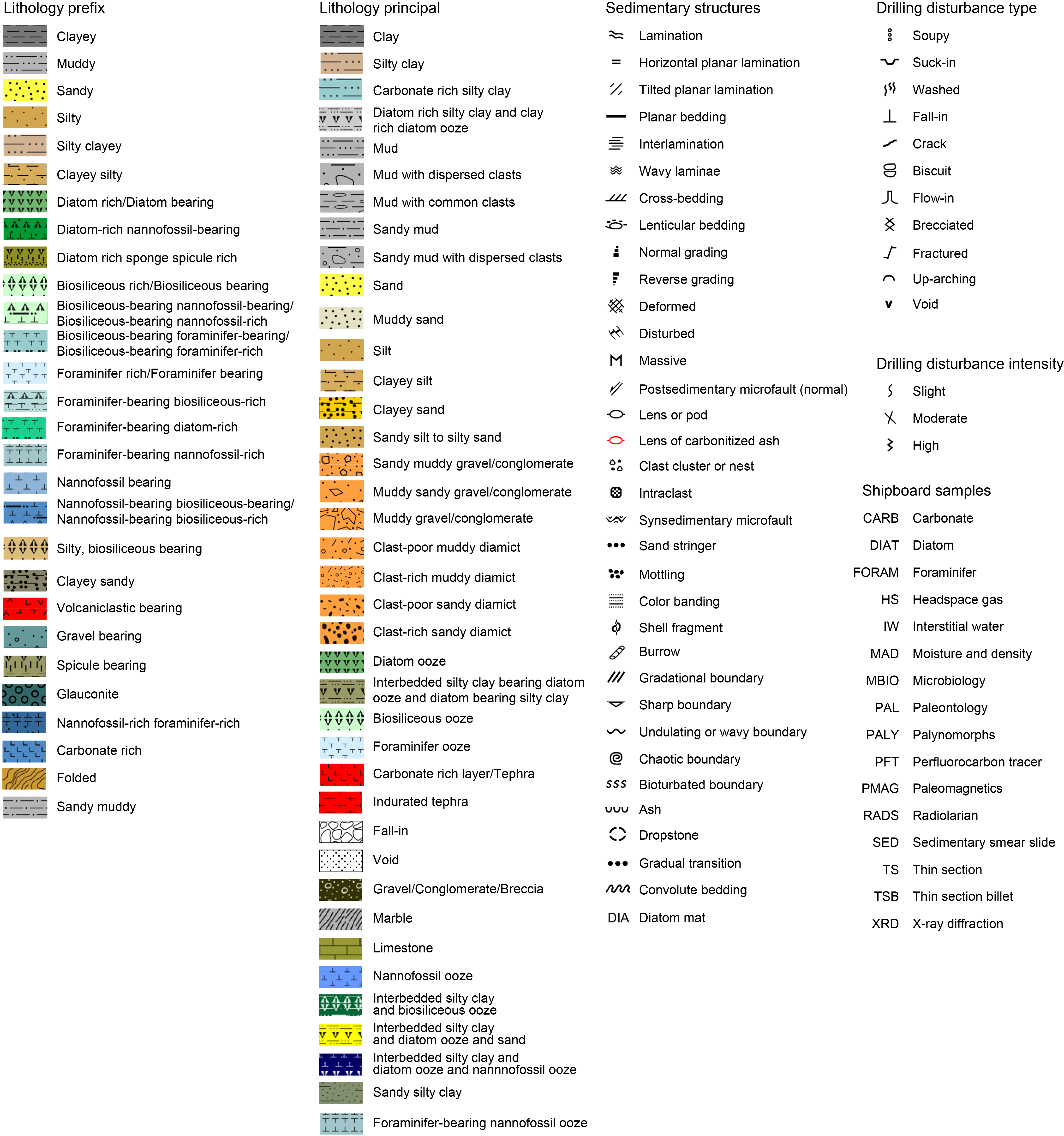
Figure F7. VCD legend.
Smear slides
Smear slide microscopic analysis was used to determine biogenic and terrigenous constituents and abundance to aid in lithologic classification. Toothpick samples were taken in each lithology and at a frequency of at least two samples per core. For these preparations, the sediment was mixed with distilled water on a glass coverslip or glass slide and dried on a hot plate at 50°C. The dried sample was then mounted in Norland optical adhesive Number 61 and fixed in a UV light box. Type and relative abundance of biogenic and terrigenous components were estimated for each smear slide. Data were first entered into the LIMS database using a custom tabular template in DESClogik.
Lithologic classification scheme
Lithologic terminology for granular sediments and rocks was modified from the classification systems used during Integrated Ocean Drilling Program Expedition 318 (Expedition 318 Scientists, 2011) following the Wentworth (1922) scale to define grain size classes.
Principal terminology
The principal lithologic name was assigned on the basis of the relative abundances of biogenic and terrigenous clastic grains.
The principal name of a sediment/rock with <50% biogenic grains was based on the grain size characteristics of the terrigenous clastic fraction:
- If the sediment/rocks contain no gravel or minor amounts of gravel (>2 mm), then the principal name was determined by the relative abundances of sand, silt, and clay (Figure F8; after Mazzullo et al., 1988).
- If the sediment contains siliciclastic gravel, the principal name was based on the relative abundance of gravel and the sand/mud ratio of the clastic matrix.
- Unsorted or poorly sorted terrigenous sediments with a wide range of grain sizes were identified with the nongenetic term "diamict."
- The term "cuttings" was used when the core was interpreted to primarily comprise fall-in or broken rocks clearly created in the drilling process. In this situation, the pieces of rock were counted in the clast counts.
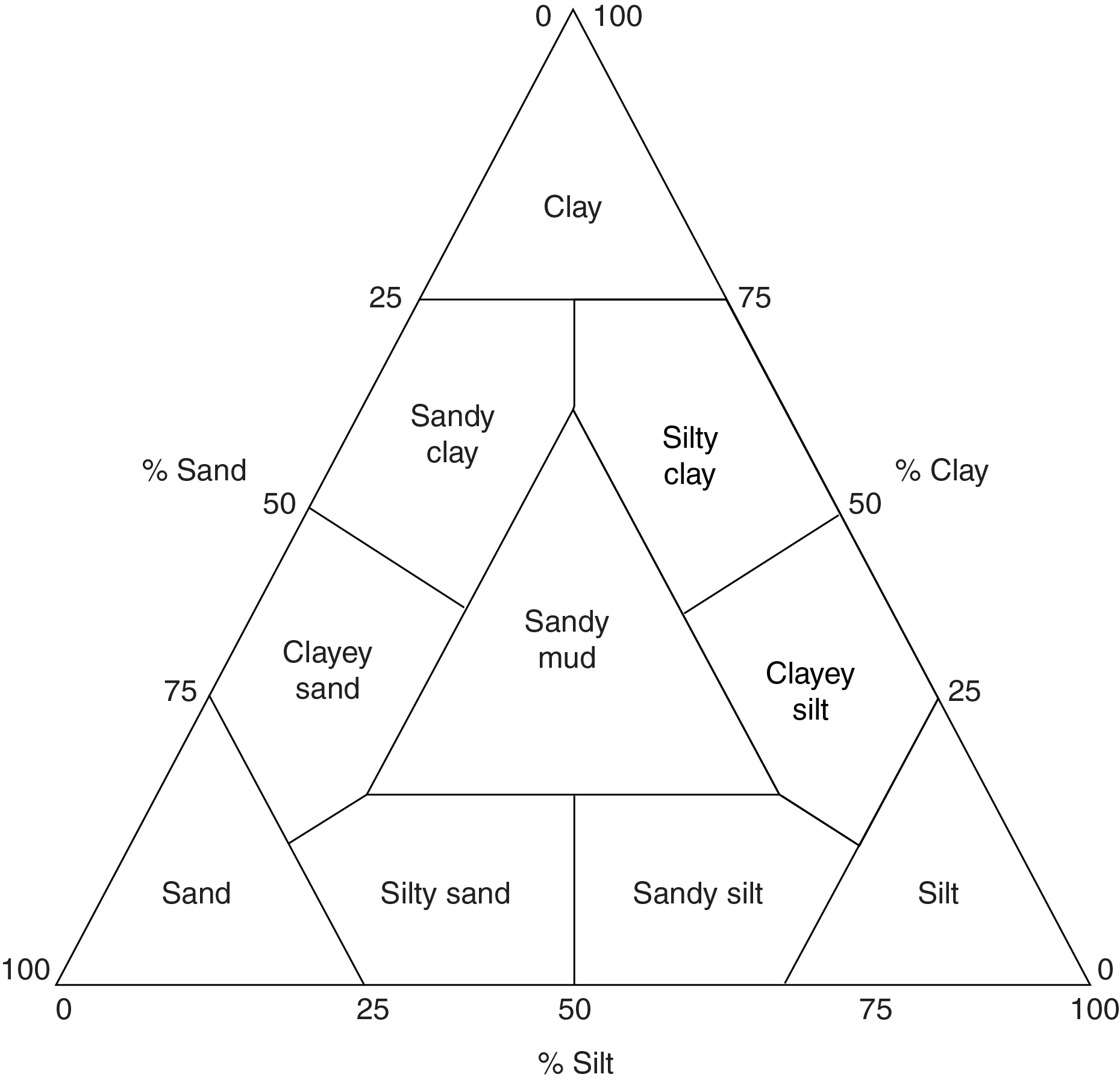
Figure F8. Classification scheme for terrigenous clastic sediments without gravel.
The principal name of a sediment/rock with ≥50% biogenic grains was "ooze," and that name was modified by the most abundant specific biogenic grain type that forms 50% or more of the sediment/rock (e.g., if diatoms exceeded 50%, then the sediment was classified as a "diatom ooze"). Additionally, biogenic components were grouped together to exceed this 50% abundance threshold (e.g., if diatoms are 40% of the sediment and sponge spicules are 20%, then the sediment was termed "biosiliceous ooze") (Figure F9).
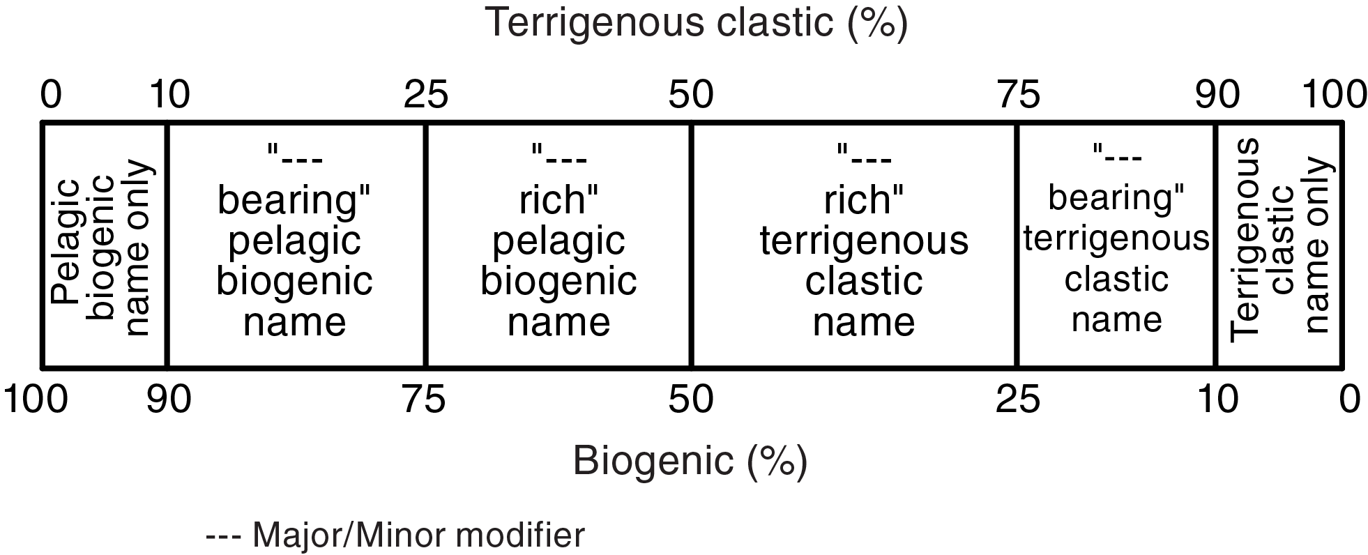
Figure F9. Classification scheme for mixed sediments.
Major and minor modifiers were applied to any of the principal granular sediment/rock names. The use of major and minor modifiers followed the scheme of Expedition 318 (Expedition 318 Scientists, 2011) (Figure F9):
- Minor modifiers are used for components with abundances of 10% to <25%, which are indicated by the suffix "-bearing" (e.g., diatom-bearing).
- Major modifiers are used for components with abundances between 25% and 49%, which are indicated by the suffix "-rich" (e.g., diatom-rich).
- If possible, modifiers were assigned on the basis of the most abundant specific grain type (e.g., diatom-rich versus biosilica-rich).
Clast abundance
For Sites U1534 and U1535, clast counts on the split-core surface were recorded in two categories: the total number of clasts >2 mm and >2 cm in every core section. For Sites U1535–U1538, the abundance of clasts between 2 mm and 2 cm and >2 cm was estimated for each section and assigned a category from 0 to 4:
For Site U1538, in addition to the split-core clast estimates, estimates of clasts >1 mm in the processed X-radiograph images were recorded using the same abundance scale. For centimeter-scale clasts, the lithology, rounding, and surface texture of the clasts were commonly noted separately in DESClogik comments.
Bioturbation
Ichnofabric description analysis included evaluation of the extent of bioturbation and notation of distinctive biogenic structures. To assess the degree of bioturbation semiquantitatively, the ichnofabric index from Droser and O'Connell (1992) (from 1 to 6) was employed (e.g., 1 = bioturbation absent, 3 = moderate bioturbation [10%–40% of the surface], and 6 = total biogenic homogenization of sediment). This index is illustrated using the numerical scale in the Relative bioturbation column of the VCDs. For Site U1538, in addition to the split-core bioturbation estimates, estimates of the percentage of burrows in the processed X-radiograph images were recorded in DESClogik using the same abundance scale.
Core disturbance
Drilling disturbance was classified into four categories:
- None.
- Slightly disturbed: bedding contacts are slightly bowed.
- Moderately disturbed: bedding contacts are extremely bowed.
- Extremely disturbed: bedding is completely deformed and may show diapiric or minor flow structures or be soupy to the degree that the sediments are water saturated and show no traces of original bedding or structure.
When a specific type of drilling disturbance was identified, the nomenclature of Jutzeler et al. (2014) was used to characterize the drilling disturbance:
- Biscuit,
- Bowed,
- Brecciated,
- Crack,
- Fall-in,
- Flow-in,
- Fractured,
- Gas expansion,
- Soupy,
- Uparching,
- Washed, and
- Washed gravel.
Digital color imaging
The SHIL captures continuous high-resolution images of the archive-half surface for analysis and description. The instrument was used shortly after core splitting in an effort to avoid time-dependent color changes resulting from sediment drying and oxidation. The shipboard system uses a commercial linescan camera lens (AF Micro Nikon; 60 mm; 1:2.8 D) with a custom assembly of three pairs of LED strip lights that provide constant illumination over a range of surface elevations. Each pair of lights has a color temperature of 6,500 K and emits 90,000 lux at 3 inches. The resolution of the linescan camera was set at 10 pixels/mm. Users set a crop rectangle around the core section for each image to remove extraneous information. Images were saved as high-resolution TIFF files. Available files include the original high-resolution image with gray scale and ruler as well as reduced JPEG images cropped to show only the section-half surfaces.
Spectrophotometry and colorimetry
The SHMSL employs multiple sensors for the measurement of bulk physical properties, including RSC, MS, and a laser surface analyzer. Reflectance spectroscopy (spectrophotometry) was carried out using an Ocean Optics USB4000 spectrophotometer. This instrument measures the reflectance spectra of the split core from the UV to near-infrared range. Colorimetric information from split cores is also recorded by this instrument in the L*a*b* color space system. The L*a*b* color space expresses color as a function of lightness (L*) and color values a* and b*; a* reflects the balance between red (positive a*) and green (negative a*) and b* reflects the balance between yellow (positive b*) and blue (negative b*). When a* and b* are 0, there is no color and L* determines gray scale.
On the SHMSL, MS was measured with a Bartington MS2 meter and MS2K contact probe. For instrument details, see Physical properties.
Accurate spectrophotometry using the SHMSL demands a flush contact between the instrument sensors and the split core. A built-in laser surface analyzer aids the recognition of irregularities in the split-core surface (e.g., cracks and voids), and data from this tool were recorded to provide an independent check on the fidelity of SHMSL measurements.
X-ray diffraction analysis
Selected samples for XRD analysis were obtained from the working halves of the cores at an average spacing of one or two samples per core. When possible, the samples were taken adjacent to MAD physical property samples. XRD analysis was performed on the clay fraction in most samples. For these preparations, a ~2 g sample was placed in a 50 mL centrifuge tube with 10% acetic acid, sonicated for 15 min, and allowed to stand overnight to remove carbonate material. After centrifuging for 15 min at 1500 rpm, the acetic acid was decanted, 25 mL of distilled water was added, the sample was centrifuged again, and the water was decanted. This washing procedure was repeated two more times to remove both the acid and salts from the sample. After decanting the final wash, 25 mL of 1% sodium metaphosphate solution was added to the sample in a 50 mL beaker. The sample was then placed in an ultrasonic bath for 5 min to suspend the clays using ultrasonic disaggregation and then centrifuged for 5 min at 1000 rpm to settle the >2 µm particles. The clays that remained in suspension were removed from the top ~1 cm of the centrifuge tube and pipetted onto two amorphous quartz sample discs. The sample discs were then left to air dry in a desiccator. After drying, one disc was analyzed and the other was solvated with ethylene glycol for ~8 h at 65°C and reanalyzed to determine the presence of expandable clays.
The prepared samples were mounted onto a sample holder and analyzed by XRD using a Bruker D-4 Endeavor diffractometer mounted with a Vantec-1 detector using nickel-filtered CuKα radiation. The standard locked-coupled scan was as follows:
- Voltage = 35 kV.
- Current = 40 mA.
- Goniometer scan = 3.5°–30°2θ.
- Step size = ~0.0085°.
- Scan speed = 1 s/step.
- Divergence slit = 0.3°.
The diffractograms of single samples were evaluated with the Bruker Diffrac-Plus EVA software package. Relative abundances of the major clay mineral groups were established on the basis of maximum peak intensity, preferentially from the glycolated analysis. Quantification of mineral contents was not possible because the samples were not spiked with a defined amount of a mineral standard for calibration. Therefore, the shipboard results were interpreted qualitatively on the basis of relative occurrences and abundances of the most common clay mineralogical components.
A small number of selected samples were freeze-dried, ground, and mounted on aluminum holders for bulk XRD analysis. Scans of these samples were performed with the same instrument settings as the clay preparations and scanned over a goniometer range of 3.5°–70°2θ.
X-ray imaging
Cores from all sites were X-ray imaged, resulting in a total collection of 24,384 images: 3,677 images from Site U1534, 1,168 images from Site U1535, 8,166 images from Site U1536, 5,429 images from Site U1537, and 5,944 images from Site U1538 (Table T1). For Sites U1534 and U1535, most of the images were taken on whole-round sections and only a few were imaged after splitting when shattered liners impeded the whole-round sections being introduced in the X-ray system. For Sites U1536–U1538, most of the X-ray imaging was performed after SHIL imaging on archive-half sections and only a few images were taken on whole-round sections for testing purposes. X-ray images were used for identification of core quality/drilling disturbance, sedimentary structures, clast occurrence, and bioturbation.
The new IODP X-Ray Imager (XRI) is composed of a Teledyne ICM CP120B X-ray generator and a detector unit (Figure F10). The generator works with a maximum voltage of 120 kV and tube current of 1 mA and has a 0.8 mm × 0.5 mm focal spot. The generator produces a directional cone at a beam angle of 50° × 50°. The detector unit is 65 cm from the source and consists of a Go-Scan 1510 H system composed of an array of CMOS sensors arranged to offer an active area of 102 mm × 153 mm and a resolution of 99 µm. Core sections were run through the imaging area at 12 cm intervals, providing 15 cm images onto the detector and allowing an overlap of 3 cm.
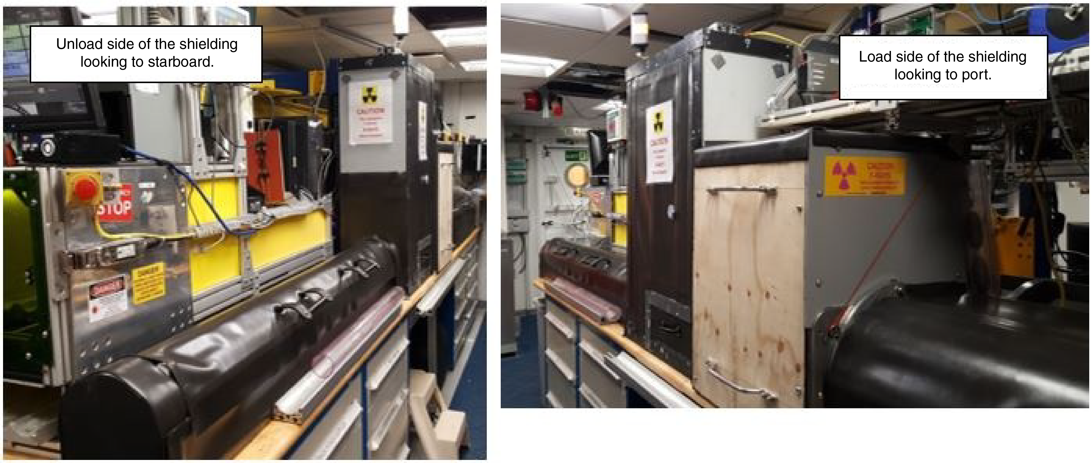
Figure F10. IODP XRI.
During Expedition 382, tests were conducted on both whole-round sections and section halves to obtain the best image resolution for determining the internal structure of cores. The XRI settings were changed to adjust to the varying lithologies of the cores (Table T1). The number of images stacked was 20, taken at exposure times of 300–500 ms. The voltage ranged between 60 and 90 kV, and the current varied from 0.8 to 1 mA.
The raw images were collected as 16-bit images and were processed with the IODP in-house Processing Utility in the Integrated Measurement System (IMS) software v. 10.3. The software applies corrections for the detector (gain and offset corrections), compensates for core shape and thickness, and adjusts the image contrast. The Savitzky-Golay finite impulse response (FIR) filter was chosen to smooth images. The resulting processed images include a masked background, the depth scale in the section, and the acquisition parameters. The software applies a different processing to APC/HLAPC and rotary cores. Some sections for which the Processing Utility did not give good results were reprocessed, first with the LeVay Processing software and later with the Processing Utility.
Biostratigraphy
Diatoms, radiolarians, palynomorphs, foraminifers, and nannofossils were utilized to derive preliminary shipboard biostratigraphic and paleoenvironmental constraints during Expedition 382. Methods for individual fossil groups are presented below. Biostratigraphic models were based primarily on core catcher samples; however, additional samples were analyzed where appropriate, generally where changes in lithology were observed in split cores or to refine the placement of biostratigraphic datums.
Zonations were distinguished primarily based on first occurrence (FO) and last occurrence (LO) datums. Biostratigraphic events and biozone boundaries were expressed relative to the geologic timescale (GTS2012; Gradstein et al., 2012) and are given in Figure F11. Specific ages assigned to each datum follow those of recent IODP expeditions to the Southern Ocean (e.g., Expeditions 374 and 379 [McKay et al., 2019; Gohl et al., 2021]). These references largely follow a constrained optimization (CONOP)-based synthesis of Southern Hemisphere biostratigraphy (Cody et al., 2008). Additional biostratigraphic data for diatoms were taken from Harwood and Maruyama (1992), Censarek and Gersonde (2002), Iwai et al. (2002), Winter and Iwai (2002), Zielinski and Gersonde (2002), Olney et al. (2007), Tauxe et al. (2012), Cody et al. (2012), Winter et al. (2012), and Armbrecht et al. (2018). Radiolarian biostratigraphy for the middle Miocene to Pleistocene additionally follows Lazarus (1990, 1992) and Florindo et al. (2013). Dinoflagellate cyst (dinocyst) biostratigraphy following Bijl et al. (2018) and references therein was also utilized.
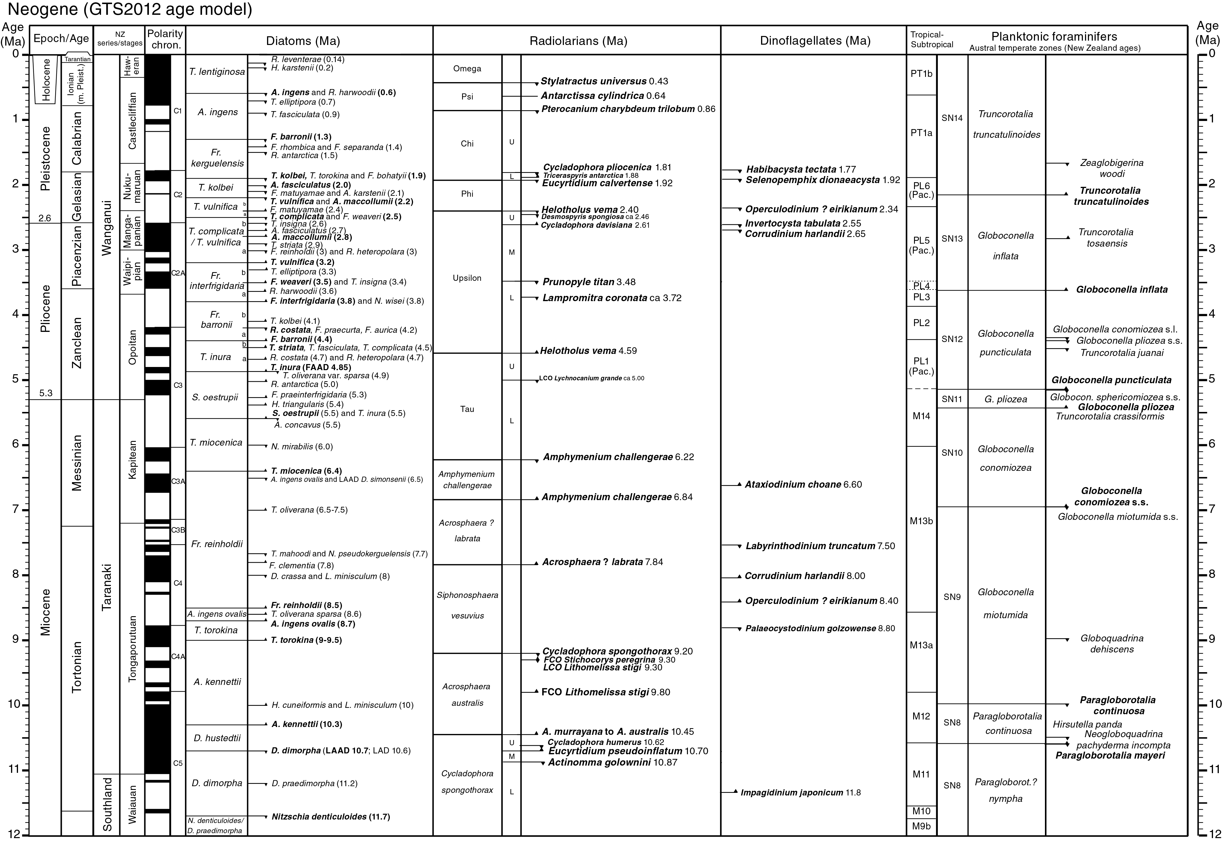
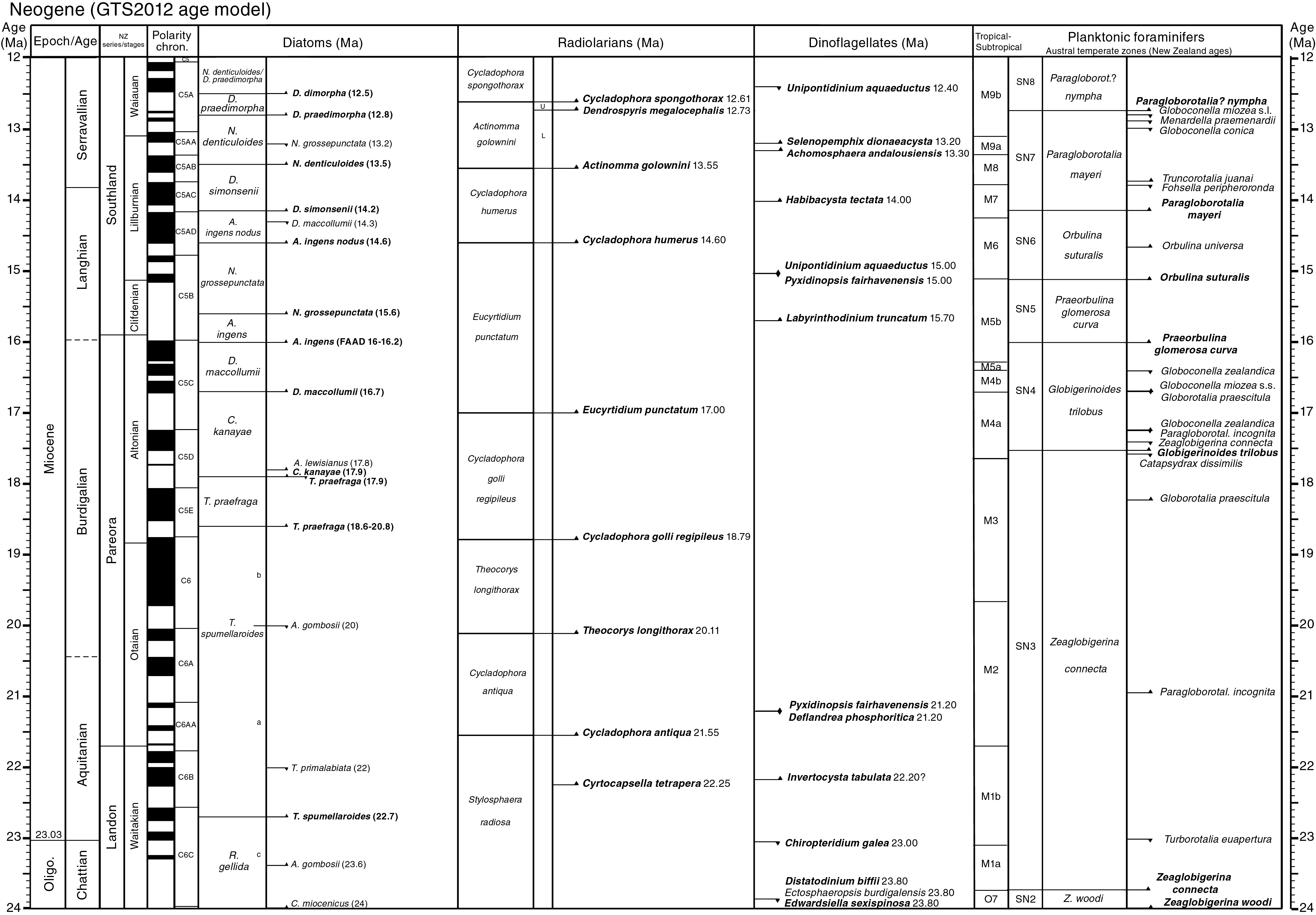
Figure F11. Chronostratigraphic age framework.
Reworking of older fossils is of particular concern in Southern Ocean sediments, especially during glacial periods when ice sheet advance and ice rafting increase the potential for noncontemporary material to be introduced to the sediment column. Reworking complicates data by introducing older species above their respective LOs in the stratigraphic section. Reworking can be recognized by the inclusion of notably anomalous fossils in sediments (e.g., a few Oligocene diatom valves detected in an otherwise Pliocene-typical assemblage). However, less extreme examples of reworking (e.g., late Pliocene diatoms in an early Pleistocene assemblage) are possible and not as easily recognized. As such, less emphasis was placed on LOs than FOs. Site-specific reworking is discussed in the Biostratigraphy section of each site chapter. FOs and LOs were used to identify biohorizons in stratigraphic order that were further used to define biostratigraphic zones and subzones following standard schemes in the GTS2012.
Data generated for each microfossil group are presented on taxonomic distribution charts that record occurrences and as qualitative relative abundances for each sample. Preservation data were also recorded. All micropaleontological data obtained on board were entered into the LIMS database using the DESClogik software. These data are available from the LIMS database in accordance with IODP policy. Taxonomic occurrence charts also indicate instances of suspected reworking of microfossils. These charts are a result of shipboard work only and are biased toward biostratigraphic marker species. A figure in the Biostratigraphy section of each site chapter provides a summary of the biostratigraphy information from each microfossil group. Age-depth plots that note shipboard estimates of sedimentation rate and the locations of unconformities are also provided in each site chapter.
Diatoms
Diatom taxonomy
Diatoms were identified to the species level where possible. Taxonomic concepts for Neogene Antarctic diatoms, many of which are endemic to the southern high latitudes, have developed largely through the last 45 y of stratigraphic drilling in the Southern Ocean and on the Antarctic shelf by the Deep Sea Drilling Project (DSDP), Ocean Drilling Program (ODP), Integrated Ocean Drilling Program, and IODP (McCollum, 1975; Schrader, 1976; Gombos, 1976; Ciesielski, 1983; Gersonde and Burckle, 1990; Gersonde, 1990, 1991; Fenner, 1991; Baldauf and Barron, 1991; Harwood and Maruyama, 1992; Mahood and Barron, 1996; Gersonde and Bárcena, 1998; Censarek and Gersonde, 2002; Iwai and Winter, 2002; Zielinski and Gersonde, 2002; Arney et al., 2003; Bohaty et al., 2003; Whitehead and Bohaty, 2003). In parallel to these efforts, ice platform drilling on the Antarctic margin recovered neritic diatom flora that serve as useful taxonomic references on the Antarctic shelf (Harwood, 1986, 1989; Winter and Harwood, 1997; Bohaty et al., 1998; Harwood et al., 1998; Scherer et al., 2000; Sjunneskog and Scherer, 2005; Olney et al., 2007, 2009; Sjunneskog et al., 2012; Winter et al., 2012). Other useful taxonomic references for Neogene and modern Antarctic marine diatoms include Fenner et al. (1976), Akiba (1982), Johansen et al. (1985), Harwood et al. (1989), Yanagisawa and Akiba (1990), Medlin and Priddle (1990), Cremer et al. (2003), and Scott and Thomas (2005).
Diatom methodology
Smear slides were generated to evaluate diatom floras. A small drop of deionized water was placed on a coverslip. A toothpick sample of sediment from the core catcher or any other interval deemed interesting was then mixed with the water and smeared across the coverslip. In some cases, sieved samples were utilized where deemed necessary. Sediments were washed through a 20 µm sieve, and dilute Borax solution was used to disaggregate clays. For all slide types, the sediment was allowed to dry on the coverslip before being permanently affixed to a slide with Norland optical adhesive Number 61 (refractive index = 1.56), which was cured under UV light.
Strewn slides were also made to improve the visibility of diatom frustules. A toothpick sample of sediment was disaggregated into water via gentle repeated pipetting in a beaker. The resulting sediment slurry was then pipetted onto a coverslip, allowing diatoms to settle out into a single plane with little overlap of valves, and dried. Once dry, the coverslip was affixed to a slide in the same way as smear slides.
Slides were examined using a Zeiss Axioskop or Zeiss Axiophot transmitted-light microscope fitted with phase contrast. Diatoms were generally identified under 630× magnification, but 1000× was used when needed. Photomicrographs were taken using a SPOT Flex 64 Mp digital camera (Diagnostic Instruments, Inc.) and uploaded to the LIMS database. Qualitative abundances, level of fragmentation, and level of dissolution were assessed using 630× magnification. When needed, 1000× magnification was used to assess preservation in greater detail. The relative abundance of diatoms was qualitatively estimated at 630× magnification using the following codes:
- A = abundant (>5 complete valves per field of view [FOV]).
- C = common (2–5 complete valves per FOV).
- F = frequent (1 complete valve in 1–5 FOVs).
- R = rare (1 complete valve in 6–30 FOVs).
- Tr = trace (very rare valves or diatom fragments).
- B = barren (no diatom valves or fragments observed).
Relative abundances of individual diatom taxa were estimated at 630× magnification (one transect = 40 mm) using the following codes:
- D = dominant (>10 valves per FOV).
- A = abundant (>5 and <10 valves per FOV).
- C = common (1–5 valves per FOV).
- F = frequent (1 valve in every 10 FOVs).
- R = rare (<5 valves per transect).
The degree of siliceous microfossil fragmentation often mirrors dissolution, but the two factors are not always directly correlated. Diatoms with well-preserved fine structures can be highly fragmented. Dissolution is a wholly chemical process (Warnock and Scherer, 2015), but fragmentation can be dominantly or entirely due to mechanical processes such as compaction or subglacial processes (Scherer et al., 2004). Preservation of diatoms, therefore, was qualitatively assessed with regard to both the degree of dissolution and fragmentation.
The degree of dissolution was qualitatively graded as follows:
- L = low (slight to no apparent dissolution [fine structures generally preserved]).
- L-M = low to medium (degree of dissolution between L and M).
- M = moderate (moderate dissolution [fine structures may be lost]).
- M-H = moderate to high (degree of dissolution between M and H).
- H = high (severe effects of dissolution, including widened areolae, fusion of neighboring areolae, relatively abundant margins and cingula compared with valves, and notably higher proportions of heavily silicified forms).
The degree of fragmentation was graded as follows:
- L = low (at least 50% of identifiable diatoms are intact).
- L-M = low to medium (degree of fragmentation between L and M).
- M = moderate (more than 50% of diatom valves are broken, but most are identifiable).
- M-H = moderate to high (degree of fragmentation between M and H).
- H = high (valves highly fragmented and very few complete valves present, hampering identification).
Age assignment
Initial shipboard ages of individual Neogene samples were based on identification of primary and secondary datum events. Biostratigraphic zones were also defined where possible utilizing schemes derived from Southern Ocean sites by Harwood and Maruyama (1992; Oligocene–recent), Zielinski and Gersonde (2002; Pliocene–Pleistocene), and Censarek and Gersonde (2002; Miocene), as well as the Antarctic continental shelf site scheme of Winter et al. (2012). A wealth of biostratigraphic information is available from drill core–based studies listed in Diatom taxonomy and the integrated biochronological syntheses in the associated volumes for each leg/expedition (e.g., Gersonde et al., 1990; Barron et al., 1991; Harwood et al., 1992; Iwai et al., 2002; Tauxe et al., 2012).
Ages applied to specific diatom events and zonal boundaries were guided by successive iterations of the diatom biochronology afforded by CONOP (Cody et al., 2008, 2012; Florindo et al., 2013). These ages are in general agreement with ages of appearance and extinction of Southern Ocean endemic diatoms presented in Barron (2003), although some offset of latest Miocene–early Pliocene datums were noted by Iwai et al. (2002) and Tauxe et al. (2012). Age assignments for diatom datum levels used during Expedition 382 are presented in Figure F11 and Table T2. This data set was adapted from the working data set of Expedition 374 in the Ross Sea (McKay et al., 2019). Minor adjustments were made based on current knowledge and recent observations and calibration. It is important to note that data sets like this, although currently state-of-the-art, are in continual revision as more data and analyses come available, including from this expedition.
Radiolarians
Radiolarian taxonomy
Radiolarian biostratigraphy during Expedition 382 was based on the taxonomic concepts for Neogene radiolarians by Popofsky (1908), Riedel (1958), Petrushevskaya (1967, 1975), Lombari and Lazarus (1988), Caulet (1991), Lazarus (1990, 1992), Abelmann (1992), Nigrini and Sanfilippo (2001), Vigour and Lazarus (2002), Lazarus et al. (2005), and Renaudie and Lazarus (2012, 2013, 2015, 2016). Primary datums from the Pleistocene to Miocene are listed in Table T3.
Radiolarian methodology
A ~10 cm3 sediment sample, generally from core catchers, was taken for radiolarian analysis and directly washed through a 63 µm mesh sieve to minimize paleontological preparation time and provide sample residues that could be used for foraminifer analyses. If the sample had substantial clay aggregation or high organic matter content, it was disaggregated prior to sieving in a beaker to which 10 mL of 15% solution of hydrogen peroxide and the same volume of diluted Borax was added. The beaker was then warmed on a hot plate with a magnetic, automatic stirrer for 30 min to 1 h. Using a pipette, a small quantity of the >63 µm residue was placed on two 25 mm × 75 mm microscope slides and allowed to dry. Once dried, a few drops of Norland optical adhesive Number 61 were added, covered by a 22 mm × 50 mm coverslip, and then placed under the UV lamp to cure for 15 min.
Microscopy and identification
Radiolarian species were identified and their abundance was estimated using a Zeiss Axioplan microscope with bright-field illumination at 100×, 200×, and 630× magnification. Photomicrographs were taken using a SPOT Flex 64 Mp digital camera and uploaded to the LIMS database.
For each sample, the total abundance of radiolarians was qualitatively estimated by light-microscopic observations at 100× magnification along one horizontal traverse of the slide using the following codes:
- A = abundant (>100 specimens per traverse).
- C = common (51–100 specimens per traverse).
- F = frequent (11–50 specimens per traverse).
- R = rare (1–10 specimens per traverse).
- Tr = trace (1–10 specimens per slide).
- B = barren (absent).
Qualitative estimates of individual species abundances were also recorded by scanning the slide at 100× magnification according to the following criteria:
- A = abundant (≥2 specimens per FOV).
- C = common (1 specimen per FOV).
- F = frequent (1 specimen per 2–5 FOVs).
- R = rare (1 specimen per 5–30 FOVs).
- Tr = trace (≤1 specimen per traverse).
Preservation of the radiolarian assemblages was recorded as follows:
- G = good (most specimens complete; fine structures preserved).
- M = moderate (minor dissolution and/or breakage).
- P = poor (common dissolution, recrystallization to opal-CT, and/or breakage).
Zonation scheme
The Southern Ocean zonation used here is that of Lazarus (1992; middle Miocene–Pleistocene). The original age estimates for radiolarian datums for the early Miocene–Pleistocene were based on their calibration to magnetostratigraphy according to Hays and Opdyke (1967), Gersonde et al. (1990), Barron et al. (1991), Lazarus (1990, 1992), Spieß (1990), Caulet (1991), Harwood et al. (1992), and Ramsay and Baldauf (1999). Some additional age estimates from Florindo et al. (2013) were added as secondary datums for the Miocene and Pliocene (Table T3) when appropriate and when consistent with the stratigraphic ranges found in Renaudie (2012).
Palynology
Dinocyst taxonomy and age assignments
The most recent magnetostratigraphically calibrated dinocyst stratigraphy for the Neogene, used here, is from Integrated Ocean Drilling Program Expedition 318 Hole U1356A on the Wilkes Land margin (Bijl et al., 2018). Dinocyst taxonomy follows that presented in Williams et al. (2017), Clowes et al. (2016), and Bijl et al. (2018). The observations of Bijl et al. (2018) are supplemented by observations from circum-Antarctic palynological observations from DSDP Leg 28 (Kemp, 1975), ODP Leg 188 Site 1165 (Hannah, 2006), Cape Roberts Project drilling (Hannah et al., 2000), and ODP Leg 178 (Harland and Pudsey, 2002). No complete integrated stratigraphic dinocyst framework exists for the Neogene of the southwest Atlantic. Neogene dinocyst biostratigraphy is currently in development, and placement of selected biostratigraphic datums are tentative. Recent dinoflagellate species distribution has been documented in southern high latitudes from core top samples (Esper and Zonneveld, 2007; Prebble et al., 2013). Antarctic miospores (terrestrial pollen and spores) of Neogene age are generally of insufficient diversity and abundance to support biostratigraphic studies (Cantrill and Poole, 2012).
The FOs and LOs for Neogene dinocyst taxa found in the Southern Hemisphere midlatitudes, Northern Hemisphere midlatitudes, and Northern Hemisphere high latitudes calibrated to the GTS2012 are given in Table T4, as reported in Bijl et al. (2018) and references therein. The dinocyst event data shown in Figure F11 are a selection of those reported in Table T4. The selection was based on species encountered during Expeditions 318 and 374.
Palynology methodology
Two sample processing methods were employed depending on biogenic silica concentrations and whether conditions on the ship were safe enough (e.g., not rough seas) to use hydrofluoric acid (HF). The techniques are labeled as non-HF, both (if HF treatment was carried out on the non-HF residues), and HF. The processing technique applied to each sample is indicated in the relative abundance table in each site chapter.
Non-HF method
Samples were processed using a disaggregation/sieving method described in Riding and Kyffin-Hughes (2011). Sediment samples of 5–10 g were disaggregated by soaking and agitation in 1% Borax solution followed by 10% sodium hexametaphosphate solution and then sieved through a 10 µm mesh. The mesh with sample was put in an ultrasonic bath for ~30 s to further disaggregate and remove clays. The light (organic-rich) fraction was concentrated by placing the sample in a porcelain bowl in the ultrasonic bath, letting the heavy particles sink, and decanting the floating residue into vials. In most cases, the silica content in the sample residue was still too high after the non-HF method. To remove the excess silica, small amounts of HF were added to the sample in 50 mL residue vials following the same procedure described for the HF method. In samples processed using both techniques, the remaining residue could in some samples appear diluted; thus, relative abundance of assemblages might be underestimated. Processing a larger amount of sediment reduces this risk.
HF method
Approximately 5–10 g of dry sediment was processed according to standard palynological laboratory protocols (e.g., Brinkhuis et al., 2003). Samples were digested with cold 48% HF to dissolve carbonates and silicates followed by 30% HCl to remove silicate gels. Centrifuging and decanting was carried out after each step. Residues were sieved with nylon 250 and 10 µm sieves using an ultrasonic bath.
All samples were mounted on glass microscope slides (22 mm × 50 mm or 22 mm × 40 mm) using Norland optical adhesive Number 61 (refractive index = 1.56) as the mounting medium.
Species identification and data collection were carried out with a Zeiss Axiophot microscope using bright-field illumination at 400×, 630× (oil), and 1000× (oil) magnification. Photomicrography was conducted using a SPOT Flex digital camera, and images were uploaded to the LIMS database.
Palynomorph abundance and preservation
Palynofacies were grouped into the following broad categories:
- Marine organic-walled dinocysts in situ,
- Marine organic-walled dinocysts reworked,
- Foraminifer test linings,
- Prasinophytes,
- Acritarchs,
- Sporomorphs (pollen and spores) in situ,
- Sporomorphs (pollen and spores) reworked,
- Black phytoclasts,
- Brown phytoclasts,
- Fungal spores,
- Amorphous organic matter, and
- Pyritized microfossils.
Semiquantitative estimates of the abundance of these palynofacies groups used the following criteria:
- D = dominant (>90% of palynomorphs).
- A = abundant (>50%–90% of palynomorphs).
- C = common (>10%–50% of palynomorphs).
- F = few (1%–10% of palynomorphs).
- R = rare (<1% of palynomorphs).
- BR = barren to rare (few specimens identified on slide).
- B = barren (not present).
Dinocysts in each sample were identified at genus or species level. A qualitative indication of their occurrence is given in the tables of each site chapter:
For biostratigraphic and paleoenvironmental purposes, shipboard analysis of palynomorphs focused primarily on determining the presence of age-diagnostic dinocyst taxa and characterizing the palynological assemblage in terms of paleoenvironment. For each sample, one 22 mm × 40 mm slide was scanned.
Terrestrial sporomorphs identified during these counts were also quantitatively registered, attributing them to four broad categories:
Palynomorph preservation was qualitatively classified as one of the following levels:
- G = good (little or no evidence of degradation or oxidation).
- M = moderate (some evidence of degradation or oxidation).
- P = poor (major degradation or oxidation has occurred).
Palynology-based paleoenvironmental analysis
The use of palynomorphs, in particular dinocysts, as paleoenvironmental indicators derives from information on the present-day global dinocyst distribution published in Zonneveld et al. (2013). Esper and Zonneveld (2007) and Prebble et al. (2013) provided detailed ecological indications for dinocysts in the high southern latitudes. These studies show that dinoflagellate distribution in the modern ocean is strongly influenced by sea-surface temperature and surface productivity. Because many of the modern species were apparently extant during the Neogene and Quaternary, these observations may be used with caution (e.g., De Schepper et al., 2011) to infer surface ocean conditions during the Neogene. Previous investigations of circum-Antarctic Oligocene and Neogene sedimentary sequences (Hannah et al., 2000 Hannah, 2006; Harland and Pudsey, 2002; Warny et al., 2009; Houben et al., 2013; Clowes et al., 2016) predominantly yielded protoperidinioid dinocysts (the likely cyst of heterotrophic dinoflagellates) generally associated with a high-productivity sea ice environment. More recent studies of Oligocene and Miocene sediments from Expedition 318 also revealed the presence of abundant phototrophic dinocysts (Bijl et al., 2018; Sangiorgi et al., 2018). Based on this framework, the differential occurrence of taxa is used to reconstruct environmental parameters, namely surface water productivity, surface water temperature, and the presence of sea ice. Other aquatic palynomorphs, in particular acritarchs and prasinophytes, were used to obtain information on meltwater input/water stratification. Terrestrial miospores can indicate environment and vegetation on adjacent land. Whether the pollen and spores are reworked can be carefully determined by the preservation and color of the miospores. Various factors such as burial depth and geological age contribute to their thermal maturation, and palynomorphs reflect the amount of heating by exine (wall) color changes from light yellow through orange, red-brown, and dark brown to black.
Planktonic and benthic foraminifers
Given our southern high latitude location, the subantarctic zonal scheme of Berggren (1992; ODP Leg 120, Kerguelen Plateau) and austral temperate zonal scheme of Jenkins (1993) were utilized with ages updated to the GTS2012, as well as planktonic foraminifer biostratigraphic datums from Crundwell et al. (2016). Planktonic foraminifer chronology is less applicable at the Scotia Sea sites because of the frequent absence or low abundance of foraminiferal species in the sediments. In addition, high-latitude foraminiferal assemblages typically contain low-diversity and long-ranging species that are of limited biostratigraphic use. Although benthic foraminifers provide limited biostratigraphic age constraints, the occurrence of benthic foraminifers was noted, and most common species were identified.
Planktonic and benthic foraminifer methodology
A 20 cm3 core catcher sample was used for shipboard identification of planktonic and benthic foraminifers. The sediment was soaked in reverse osmosis (RO) water, disaggregated and washed over a 63 µm sieve, and dried in an oven at ~45°C. When necessary, several different methods were used for disaggregation of consolidated sediments, including soaking for as long as 3 h in 15% hydrogen peroxide and dilute Borax solution. Well-indurated samples were subjected to drying and rewetting to break up the sample. The sieves were ultrasonicated and rinsed with RO water between successive samples. Foraminifer species were identified from the >63 µm fraction using a Zeiss Discovery V8 binocular light microscope. Photomicrographs were taken using a SPOT Idea digital camera and uploaded to the LIMS database. The abundance of planktonic foraminifers as a group relative to the total sieved residue was categorized as follows:
- A = abundant (>50%).
- C = common (25%–50%).
- F = frequent (10%–25%).
- R = rare (<5% of the residue).
- B = barren (no specimens in sample).
Benthic foraminifer species abundances were recorded as follows:
- D = dominant (>50% of total assemblage).
- A = abundant (10%–50% of total assemblage).
- C = common (1%–10% of total assemblage).
- F = frequent (0.1%–1% of total assemblage).
- R = rare (<0.1% of total assemblage).
- B = barren (no specimens observed).
Foraminifer dissolution was categorized as follows:
- L = low (dissolution effects are rare).
- M = moderate (dissolution damage is common).
- H = high (a high degree of dissolution).
Foraminifer fragmentation was categorized as follows:
- L = low (fragmentation is observed in a minority of specimens).
- M = moderate (partially broken tests or fragments are common).
- H = high (fragments are more common than whole tests).
Marine sedimentary ancient DNA sampling
The shipboard program for marine sedimentary aDNA sampling included collecting samples and applying chemical tracers to assess potential core contamination. Most sample preparation and analyses will be conducted on shore at the special facilities of the Australian Centre for Ancient DNA (ACAD), Adelaide. The overarching aim of this aDNA research is to characterize marine eukaryotic paleocommunities over time, focusing on the Holocene and providing a biological perspective to the scientific objectives of Expedition 382. This aim will be achieved by applying a metagenomics approach after DNA has been extracted from the collected samples, with bioinformatics pipelines specifically designed to achieve authentic aDNA results through vigorous QC.
Sampling for marine sedimentary aDNA was conducted immediately after core recovery on sediments acquired using piston coring (APC system) at Sites U1534, U1536, U1537, and U1538 (Table T5) to prevent DNA degradation due to sediment exposure to oxygen, elevated temperatures, and/or irradiation. Sampling followed either the catwalk sampling or high-resolution sampling procedures described below.
Catwalk sampling
Throughout aDNA sampling on the catwalk, personal protective equipment (PPE) (lab coat, face mask, head cover [hairnet or beanie], safety goggles, and two pairs of disposable gloves) were worn by the analyst and technicians, and the outer pair of gloves was changed immediately if they were contaminated with any sediment material. Upon arrival of the core on the catwalk, core liners were wiped clean twice with a bleached paper towel (3% bleach) at each cutting point at which aDNA was anticipated to be sampled. The core cutters were cleaned prior to each cut (3% bleach followed by 80% ethanol). The first ~3 mm of surface material from the bottom of each sampled section was removed using clean scrapers prior to sampling (~4 cm wide; bleach and ethanol treated). A cylindrical sample was taken from the center of the core using a sterile (autoclaved) 10 mL cut-tip syringe, providing ~5 cm3 of sediment material. The syringe was placed in a sterile plastic bag (Whirl-Pak) and immediately frozen at −80°C. The mudline (sediment/seawater interface) was transferred from the core liner into a clean (bleached) bucket, and a sample (10 mL in a sterile 15 mL centrifuge tube) was retained and frozen at −80°C. This sample is anticipated to provide an overview about recent communities.
Samples were collected at various depth intervals depending on the site to span the Holocene (according to our preliminary biostratigraphic and physical property age estimates). Additional samples were collected from the bottom section of deeper cores (until the APC system was changed to the XCB system) to investigate the age to which aDNA is preserved in the sediments (Table T5). Three additional samples were collected from Core 382-U1534C-1H to test for the presence of aDNA after the core had been split and exposed to irradiation (X-ray and gamma irradiation from shipboard instruments) (Table T5). Also, Samples 1H-CC through 3H-CC (three samples) were sieved under sterile conditions (under a bleach- and ethanol-cleaned laminar flow hood with bleach- and ethanol-treated tools and wearing the same PPE described above) through 63 and 20 µm sieves (as routinely applied to microfossil analyses). A sample of each fraction (~2 mL), including the flow through, was transferred to a sterile 15 mL centrifuge tube and frozen at −80°C. Microscope slides for each size fraction were prepared to analyze diatoms, radiolarians, and foraminifers. These size-fractioned samples will provide information on the source of aDNA preservation in marine sediments.
High-resolution working-half sampling
Cores selected for high-resolution sampling were sectioned using the same decontamination procedures described above for cores sampled on the catwalk. Prior to slicing, all working surfaces, the core liners, and cutting wires were decontaminated using bleach and ethanol while wearing PPE (gloves, hairnet, lab coat, safety goggles, and face mask) at all times. The sections were split into halves from bottom to top.
Subsampling was undertaken wearing the same PPE with two pairs of gloves, and the outer pair was changed immediately if contaminated with any sediment material. To remove any contamination potentially introduced through the cutting procedure, the surface layer (~3 mm) of the working half was scraped off perpendicular to the length of the core at each anticipated sampling depth using bleach- and ethanol-treated metal scrapers. A plunge sample was taken using a sterile 15 mL centrifugation tube (~3 cm3). The outside of the plunge sample tube was cleaned with a paper towel, and the tube was closed, placed in a sterile plastic bag, and stored at −80°C. In most instances, the top, middle, and bottom of each section were sampled (Table T5).
Contamination control
After sampling for aDNA from each hole, at least one air control was taken on the catwalk or in the core splitting room to test for potential airborne contamination (Table T5). For this control, an empty syringe (catwalk sampling) or opened centrifuge tube (working-half sampling) was held for a few seconds in the sampling area and then transferred into a sterile bag and frozen just like the samples. Additionally, laboratory swabs were collected in the core splitting room to further test for potential contamination from laboratory working surfaces. The controls will be processed and analyzed alongside the sediment samples to account for potential contamination.
Piston coring unavoidably involves pumping seawater (drilling fluid) into the borehole; therefore, seawater is a significant source of sediment core contamination by modern DNA. However, of all the coring systems available, this type of coring is the least susceptible to contamination (House et al., 2003; Lever et al., 2006), which was one of the reasons for limiting our aDNA sampling to cores acquired by the APC system. To assess potential contamination, we added the chemical tracer perfluoromethyl decaline (PFMD) to the drilling fluid at a rate of ~0.55 mL/min for cores collected at Sites U1534 and U1536 (Smith et al., 2000). Because PFMD concentrations were below the detection limit, the infusion rate was doubled prior to aDNA sampling at Sites U1537 and U1538 (to ensure low PFMD concentrations represent low contamination rather than delivery failure of PFMD to the core). PFMD is smaller than our expected aDNA fragments (≥25 base pairs); however, it is currently the best-suited commonly available contamination tracer because others are either extremely volatile (e.g., perfluoromethylcyclohexane [PFMCH]; MacLeod et al., 2017) or much bigger than DNA fragments (e.g., particulate fluorescent microspheres; 0.5–1 mm) and thus either difficult to measure or not informative. The tracer is delivered with the drilling fluid into the borehole and to the core; thus, sampling of sediments at the core periphery compared to the center provides a measure of whether the tracer-infused drilling fluid reached the core pipe and the core center at the tested depth. We tested sediment samples from the periphery of the core by transferring ~3 cm3 of sediment using a disposable, autoclaved 5 mL cut-tip syringe into a 20 mL headspace vial with metal caps and Teflon seals prior to any scraping/cleaning of surface sediments. The sample from the center was collected in the same way after scraping and right next to the location of the aDNA sample to minimize differences between material tested for aDNA and chemical tracers. During catwalk sampling, samples were collected from the same depths at which aDNA was sampled. During high-resolution sampling, PFMD samples were collected in the middle of each section (usually ~69–70 cm unless the section was shorter than 1.5 m).
Samples were analyzed using a Hewlett-Packard (HP) 6890 gas chromatograph (GC) with an electron capture detector (HP G1223A) using an injection volume of 2500 µL, a fill speed of 100 µL/s, a 500 ms pre- and postinjection delay, a 10 s flush time, an incubation and syringe temperature of 70°C, and an incubation time of 10 min (total GC run time = 60 min) (MacLeod et al., 2017). The oven temperature program included a 3 min equilibration, a maximum temperature set to 260°C, an increase from an initial 50°C (6 min) in 15°C steps until reaching a final temperature of 200°C (21.5 min), and then a decrease to 100°C (total run time = 37.5 min). The front inlet was used in "splitless" mode with an initial pressure of 28.1 psi and a total flow of 36.6 mL/min, a gas saver flow of 20.0 mL/min, and a saver time of 2.00 min, using helium. The front detector was set to a constant makeup flow (20 mL/min) using nitrogen as makeup gas type and without applying temperature. A capillary column with the following parameters was used: maximum temperature = 260°C, nominal length = 50.0 m, nominal diameter = 530.00 µm, nominal film thickness = 10.00 µm, constant flow mode, initial flow = 33.8 mL/min, nominal initial pressure = 28.1 psi, average velocity = 142 cm/s, inlet at front, front detector as outlet, and ambient outlet pressure. The GC was calibrated using 5, 10, 15, and 20 ng/µL PFMD (adapted from IODP Expedition 376). The retention time of PFMD was 30 min, and that of other perfluorocarbon tracers (PFTs) (~10% of our PFT mixture) was 21.6 min.
In addition to the sediment samples, we also collected a sample of the tracer-infused drilling fluid by filling a sterile plastic bottle with the fluid directly from the injection pipe on the rig floor (wearing gloves). Approximately 10 mL of the drilling fluid was transferred to a 15 mL centrifuge tube, placed in a sterile plastic bag, and stored at −80°C. The drilling fluid samples will be processed and analyzed in the same way as the sediment samples. Any organisms detected in both sediments and drilling fluid after sequencing and data filtering will be carefully investigated and interpreted and then either removed from our analysis (subtractive filtering) or processed using bioinformatic software designed to differentiate samples and controls based on community structure (Davis et al., 2018).
Calcareous nannofossils
Slides for calcareous nannofossil analysis were generated as needed. Smear slides were made following the procedure for diatoms (above). Identification followed Burns (1975), van Heck (1981), and Wise (1983).
Paleomagnetism
Paleomagnetic investigations during Expedition 382 focused on measuring the natural remanent magnetization (NRM) and alternating field (AF) demagnetization of the NRM on archive-half sections. In general, we used low peak fields (<20 mT) to remove the drill string overprint and identify a direction of the characteristic remanence that can be matched to the magnetic polarity intervals of the geomagnetic polarity timescale (GPTS) (Gradstein et al., 2012). Low AF values were selected to balance the competing goals of timely core processing, identifying/removing any drilling overprints, and preserving the NRM for high-resolution measurements using U-channel samples.
Discrete cube samples (~7 cm3) were taken from most working-half sections recovered from the first hole at each site, avoiding sections and intervals that were visually disturbed. These cubes were supplemented by select intervals from additional holes at each site to complete coverage. All cube samples were measured and subjected to low peak fields (5, 10, 15, and in some cases 20 mT) to remove the drill string overprint. Detailed AF demagnetization of the NRM (up to 50 mT), rock magnetic properties, and magnetic fabric were investigated using a subset of the discrete samples to evaluate the fidelity of the archive-half measurements and assess the feasibility of shore-based studies (e.g., environmental magnetism and relative paleointensity).
Preoperations instrumentation tests
Prior to the start of coring operations, we used test samples to cross-check sample coordinate schemes on the superconducting rock magnetometer (SRM; see Coordinates), AGICO JR-6A spinner magnetometer, and AGICO KLY 4S Kappabridge. This test also allowed us to ensure that both the SRM and JR-6A yielded similar directional and intensity data. To do this, we measured a standard sample used for the JR-6A with a remanence vector directed along the +z-axis and a nominal magnetization of 8.13 A/m on both instruments. The magnetization measured by the SRM was 8.0 A/m with a declination of 11.3° and an inclination of 88.2°, whereas the magnetization measured by the JR-6A (after calibration with another standard with a magnetization of 7.62 A/m) was 7.92 A/m with a declination of 276.6° and an inclination of 88.2°. The angular difference between the two measurements is therefore 2.7°. The difference between intensity values was within 1%. We conclude that the two magnetometers are comparable.
We noted an issue with the discrete sample orientation settings during these initial tests; the direction of the magnetic vector reported following rotations performed for many of the cube orientations by the SRM software did not match the expected magnetic vector of the sample. In collaboration with the shipboard technical staff, we ultimately discovered that this issue was the result of an incorrect calibration constant for the Y superconducting quantum interference device (SQUID) in the SRM software. This error impacted the data collected at Sites U1534 and U1535 but was corrected before starting measurements for Site U1536. Data presented in figures in the Expedition reports section of the Expedition 382 Proceedings of the International Ocean Discovery Program volume and data to be archived in the Magnetics Information Consortium (MagIC) database (http://earthref.org/MagIC) have been corrected for this issue. Data archived in the LIMS database are the primary measurements as reported by the magnetometer. To correct these data, the magnetic moment measured on the Y SQUID should be multiplied by −1.
Two AF demagnetizers were on board: a DTECH D-2000 and the in-line 2G AF demagnetizer. To compare their performance, we used two samples taken from a test core. First we measured the archive half of the test core on the SRM. Then we took discrete samples collected with side-by-side Natsuhara-Giken ("Japanese") cubes using the same depth interval. One of these was collected with the Japanese extruder tube made for use with these cubes, and the other we collected by gently pushing a cube into the split face of the core. Although the up arrows are the same for both, the azimuth of the x-directions are antipodal. To account for that, we affixed a sticker with a hatched arrow on the stratigraphic top of the cube with the arrow pointing in the direction of the double line on the core barrel and the hatches pointing toward +y (see Coordinates). The NRM of the two cubes was then measured on the JR-6A and on the SRM in discrete sample mode (working half; top-away). The remanence vectors of the two cubes were within ~4° of each other, but the data were consistently shallower on the SRM than the JR-6A by a couple of degrees. The NRM of the two test cubes was demagnetized at 5 mT increments up to 80 mT using the SRM in-line AF coils. We observed incremental demagnetization with increasing AF steps and no indication of acquisition of a magnetization at any peak AF, suggesting no bias field related to imperfect shielding near the AF coils (Figure F12A).
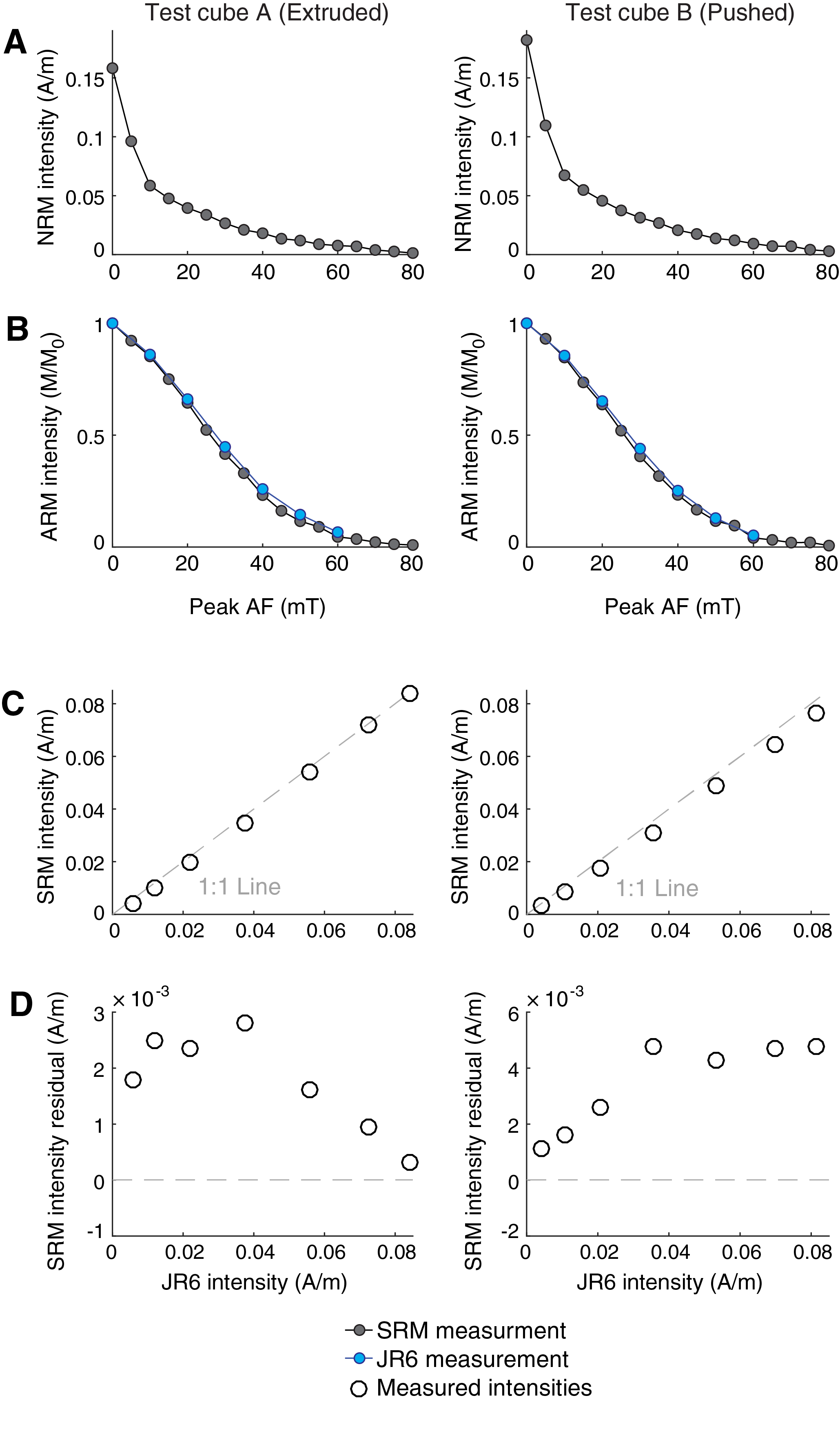
Figure F12. AF demagnetization of two test discrete samples.
Following demagnetization of the NRM, the samples were demagnetized using a 100 mT peak AF. An anhysteretic remanent magnetization (ARM) was then imparted using a 100 mT peak AF and a 50 µT biasing field. We measured the ARM and demagnetized it at 5 mT increments to 80 mT using the SRM. This procedure was repeated using the JR-6A and demagnetizing with the DTECH D-2000 at 10 mT increments to 60 mT. In this test, SRM intensities were lower than equivalent steps measured on the JR-6A although no systematic linear relationship could be determined. The offset could be related to slightly lower peak AFs generated by the SRM in-line AF system relative to the DTECH D-2000 and/or the previously observed lower intensities reported by the SRM (Figure F12B–F12D).
Core collection and orientation
Cores were collected using nonmagnetic core barrels for the APC, HLAPC, and RCB coring systems. These nonmagnetic core barrels are more brittle than standard core barrels and cannot be used in conjunction with the XCB system (see Drilling operations). The BHA included a Monel (nonmagnetic) drill collar that was used for all APC and XCB cores. This collar is required when the Icefield MI-5 core orientation tool is used, but it was used for all APC/XCB holes during Expedition 382 because it can potentially reduce the magnetic field near where the core is cut and in the core barrel.
The Icefield MI-5 tool can only be used with (full-length) APC core barrels. It uses three orthogonally mounted fluxgate magnetometers to record the orientation of the magnetic tool face (MTF), which is colinear with the double line scribed on the core liner with respect to magnetic north. The tool declination, inclination, total magnetic field, and temperature are recorded internally at a regular interval until the tool's memory capacity is filled. For the measurement interval of 10 s used during Expedition 382, the tool can typically be run for more than a day, but we aimed to switch tools more frequently than that. Prior to firing the APC, the core barrel is held stationary (along with the pipe and BHA) for several minutes. During this time, data are recorded to constrain the core orientation. When the APC fires, the core barrel is assumed to maintain the same orientation. An antispiral key keeps the core barrel from rotating as it is fired. However, the core may rotate and/or the core liner can twist as it penetrates the sediments.
The orientation correction that converts the observed declination (Dobs) to a true declination (Dtrue) is given by
where MTF is the magnetic tool face angle from the Icefield MI-5 tool and Damb is the ambient geomagnetic field declination obtained from geomagnetic field models. The 2018 International Geomagnetic Reference Field (IGRF) declination values for the drill sites are given in Table T6.
Although polarity stratigraphy at high-latitude sites can generally be determined using only inclination, which does not require core orientation, core orientation is useful for geomagnetic studies that require the full magnetic vector and for sedimentological studies that utilize magnetic fabric. Additionally, comparing magnetic polarity derived from inclination and magnetic polarity derived from Icefield MI-5 tool–oriented declination can help better understand uncertainties associated with the Icefield MI-5 tool. Assessing this uncertainty is useful for lower latitude IODP expeditions where inclination alone cannot be used for polarity stratigraphy.
The field inclination expected from a geocentric axial dipole (GAD) is quite steep at the latitudes drilled (−74° at the most southerly site), so one would expect the Icefield MI-5 tool (which relies on the horizontal component) to have difficulty orienting the cores. However, because of the so-called "South Atlantic Anomaly," the actual field in this region (according to the 2018 IGRF) is quite a bit shallower, ranging between approximately −50° and −56° at our sites. Thus, collecting the Icefield MI-5 tool data was worth attempting.
Ultimately, even after working with IODP technical staff and communicating with Icefield technical support during Expedition 382, we were unable to derive consistent and meaningful results from the Icefield MI-5 tools. In some cases, we found apparent systematic differences between the different tools. After using the tools to measure controlled fields in the laboratory (see Paleomagnetism), we are confident that the tools themselves are faithfully measuring the magnetic field (G. Messé, unpubl. data). Therefore, we are left with the hypothesis that there must be an anomalous magnetic field present during the coring process that prevents the tools from recording the geomagnetic field at the core site, rendering the tool incapable of core orientation.
Samples and measurements
Archive sections
Remanence measurements on archive halves and discrete samples were made using a 2G Enterprises Model-760R-4K SRM equipped with direct-current SQUIDs (DC-SQUIDs) and an in-line, automated AF demagnetizer capable of peak fields of 80 mT. The spatial resolution for archive-half measurements is a function of the integrated response function (following Acton et al., 2017), with effective lengths of 7.30 cm for the X-axis, 7.30 cm for the Y-axis, and 9.00 cm for the Z-axis. The practical noise level of the SRM is ~2 × 10⁻⁹ Am2 and is primarily controlled by the magnetization of the core liner and the background magnetization of the measurement tray.
We cleaned the sample tray with deionized water at the beginning of every working shift (approximately every 12 h) or more often if deemed necessary. The sample tray was then AF demagnetized with a peak field of 30 mT, and its remanence was measured using the "section background" routine to update the background correction values for the empty sample tray.
NRM measurements of the archive halves were made at 5 cm intervals with a 15 cm trailer and leader to monitor the background magnetic moment. We measured the initial NRM and the remanent magnetization remaining after AF demagnetization steps of 10 and 15 mT peak fields, including extra steps (5 or 20 mT) when time permitted.
Discrete samples
We collected one oriented discrete sample per section from the working half of Hole A at each site and some additional samples from other holes to fill in gaps as required. We sampled from the center of each section away from disturbed sediments near the core liner and at roughly evenly spaced intervals throughout the core, modifying the exact location based on lithologic observations or core disturbance observations. Discrete samples were collected by pushing plastic Japanese cubes (2 cm external edge length and internal volume of ~7 cm3) into working halves with the arrow marker on the cube pointing toward the stratigraphic up direction. When the sediment was more indurated, a hollow metal tube was pushed into the working half and a plunger was used to extrude the sample into the plastic cube. Care was taken to identify each sampling method because they result in different orientations of the specimen +x- and −x-axes relative to the base and lid of the plastic box (see Coordinates). An orange sticker was placed on the stratigraphic top of the cube with a hatched arrow pointing toward the double line on the outside of the working-half core liner. The hatches extend in the +y-direction.
All discrete sample cubes were measured and subjected to demagnetization up to either 15 or 20 mT. To investigate the AF demagnetization behavior of the NRM, a subset of discrete samples were AF demagnetized and measured on the SRM in 5–10 mT increments from 0 to 50 mT, with the maximum peak field dependent on sample behavior or the AF level at which the remanence intensity remaining dropped below 10% of the NRM. Starting at Site U1536, samples were measured three times at each AF demagnetization step, including rotating the cubes to be measured in three perpendicular directions for peak AFs of 10 mT and above (SRM software orientations of top-away, top-right, and away-bottom). Because of the different sampling techniques (pushed or extruded), care was taken to maintain a consistent orientation of the X-axis (toward the core's double line) for these different orientations.
In some cases, the JR-6A and DTECH D-2000 were used for cube measurements and AF demagnetization. The sample measurement protocol for the JR-6A spinner magnetometer (NRM, ARM, and isothermal remanent magnetization [IRM]) was as follows. The instrument was calibrated using the 7.99 A/m cube standard with an 8 cm3 volume. A holder correction was determined by measuring an empty cube inside the rotating specimen holder. Data acquisition settings were as follows:
- Holder = automatic (sample is automatically rotated around 3 mutually perpendicular axes).
- Specimen type = cube.
- Acquisition time = normal.
- Speed of rotation = low (16.7 rev/s) to avoid deforming water-rich sediment.
- Specimen volume = 7 cm3 for Japanese cubes.
- Orientation parameters P1–P4 = 12, 0, 12, and 0, respectively (see Coordinates).
- Azimuth and dip = 0 and 90, respectively (see Coordinates).
The orientation parameters P1–P4, azimuth, and dip allow the AGICO software to convert the declination and inclination measured in the specimen coordinate system to geographic declination and inclination, which are the data reported in this volume.
We initially used the JR-6A to implement a gyroremanent magnetization (GRM) protocol at Site U1534 in intervals where we suspected the presence of iron sulfide greigite. The GRM protocol (after Stephenson, 1993) was applied to a subset of cubes in an attempt to separate the GRM from the primary detrital magnetization. The GRM protocol consisted of the following sequence of steps at each AF step:
- Three-axis AF demagnetization in the +x-, +y-, and −z-directions with the DTECH D-2000 followed by measurement using the JR-6A.
- Single-axis AF demagnetization in the −x-direction with the DTECH D-2000 followed by measurement using the JR-6A.
- Single-axis AF demagnetization in the −y-direction with the DTECH D-2000 followed by measurement using the JR-6A.
The three measurements were then averaged to yield a GRM-free vector. This protocol was later replaced by the three-position measurement scheme on the SRM as described above.
Rock-magnetic analyses
Discrete samples were analyzed for bulk MS and anisotropy of magnetic susceptibility (AMS) using a KLY 4S Kappabridge. AMS characterizes the orientation of the paramagnetic (mainly phyllosilicates) and ferromagnetic minerals in sediments and can be interpreted in terms of depositional processes (e.g., Rees and Woodall, 1975; Ellwood, 1980; Taira, 1989; Schwehr and Tauxe, 2003). Settling of particles produces an oblate magnetic fabric with the minimum susceptibility clustered around the pole of the depositional plane. Ideally, the maximum and intermediate susceptibility axes are uniformly dispersed, defining a planar, near horizontal, gravity-induced settling fabric. The magnetic fabric of sediments deposited by flowing water is typified by current-oriented magnetic foliation that can be either horizontal or tilted (imbricated) and/or by clustering of the maximum susceptibility parallel to the flow direction. Disturbance by slumping or other deformation generally yields triaxial fabrics. We used the Hext (1963) method to assess the degree and type of anisotropy at the specimen level and the bootstrap method to estimate confidence bounds on AMS eigenparameters for multiple specimens (Constable and Tauxe, 1990; Tauxe, 2010).
For AMS measurements, the KLY 4S Kappabridge was calibrated prior to each session using the AGICO cylindrical standard, which has maximum susceptibility along the axis of the cylinder and minimum susceptibility in the transverse direction. Each analysis consists of measuring the specimen in three orientations while it is rotated within the applied field (Figure F13). The final step is a bulk susceptibility measurement.
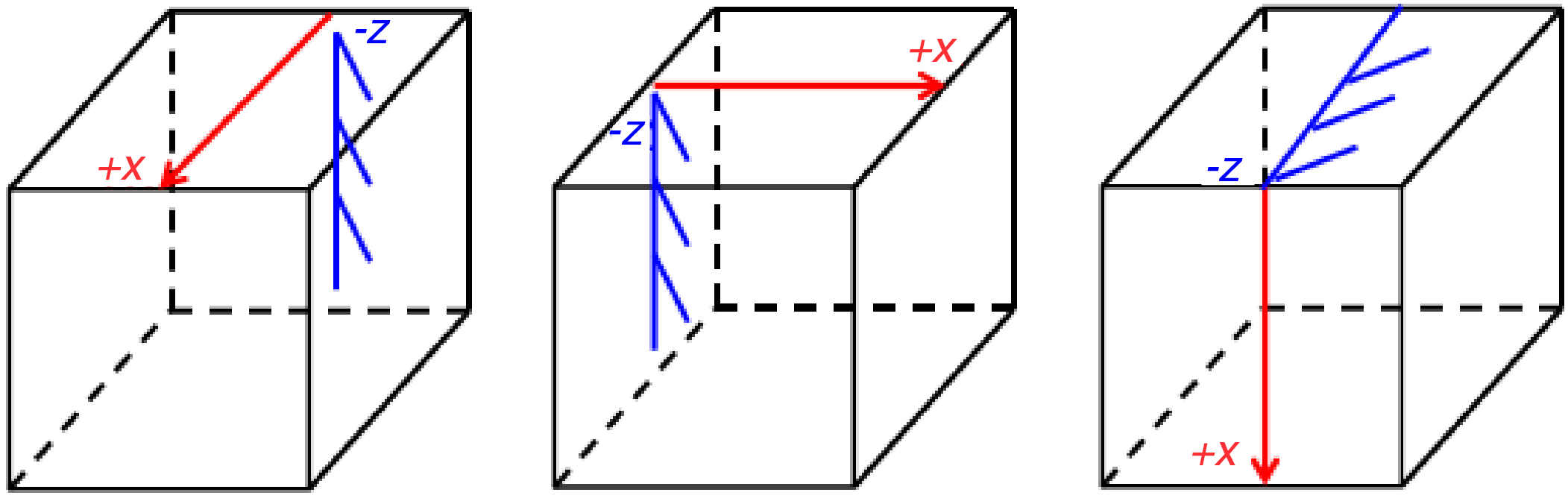
Figure F13. Orientation of discrete cubes in KLY 4S Kappabridge.
Additional rock magnetic investigations were used to characterize the remanence carriers of a subset of samples selected to be representative of a range of recovered lithologies and variations observed during NRM investigation. ARMs were imparted using a peak AF of 100 mT, a decay rate of 0.005 mT/half-cycle, and a direct current (DC) bias field of 0.05 mT along the sample's Y-direction using the DTECH D-2000. ARM samples were oriented using the top-away orientation setting in the SRM software. IRM was imparted using a range of DC fields in an ASC Scientific Model IM-10 impulse magnetizer. IRM was imparted along the sample Y-axis with the orange sticker's arrow positioned on top of the cube and pointing to the right in the instrument. AF demagnetization of these laboratory magnetizations was used to investigate the coercivity of the remanence carriers.
ARM is commonly used to estimate the presence of fine-grained (~0.03–0.1 µm), stable single domain (SSD) magnetite, whereas IRM acquisition at 100 mT is more sensitive to the occurrence of coarse-grained (>0.1 µm) multidomain (MD) magnetite (King et al., 1982; Frederichs et al., 1999). Thus, assuming a consistent magnetic mineralogy, the ARM/IRM100mT ratio traces the grain size variation of magnetite downcore. Contributions of high-coercivity minerals (hematite + goethite) can be investigated by the difference between a "saturating" IRM imparted at 1000 mT and a subsequent "backfield" IRM imparted by a −300 mT field, which should only reflect the contribution of remanence carriers with coercivities >300 mT. This method can be used to track the relative contribution of high-coercivity minerals using the S-ratio (IRM−300mT/IRM1000mT) or the concentration of the high-coercivity minerals as a hard IRM (HIRM) (e.g., Liu et al., 2012):
Coordinates
All magnetic data are reported relative to IODP orientation conventions: +x points into the face of the working half (toward the double line), +y points toward the left side of the working half when looking downcore, and +z is downcore. The relationship between the SRM coordinates (X, Y, and Z) and the sample coordinates (x, y, and z) is +X = +x, +Y = +y, and + Z = −z for archive halves and +X = −x, +Y = −y, and +Z = −z for working halves (Figure F14). Note that the orientation of the SRM axes form a left-handed coordinate system that is converted to a right-handed system in the IMS software by multiplying the calibration constant for the y-axis by −1.
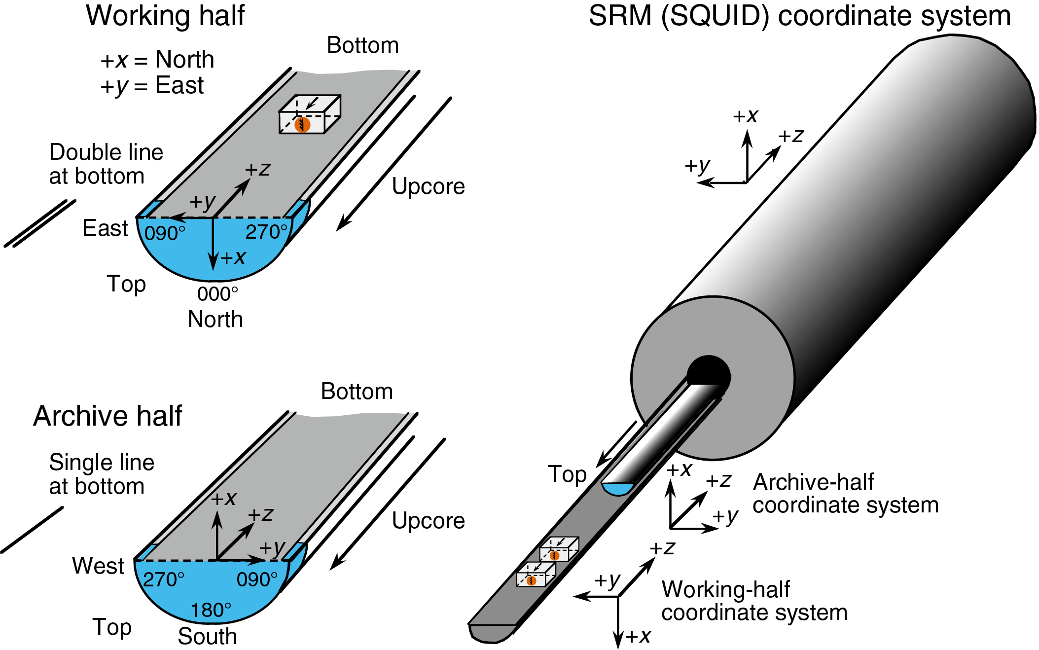
Figure F14. Paleomagnetism coordinate system.
Discrete sample labeling is shown in Figure F15. Positioning in the SRM and the JR-6A spinner magnetometer depends on the collection method used (extruder or push-in) to account for the 180° difference in the x-axis relative to the base and lid of the cube. For the SRM, we used the face = top and arrow = away settings when placing the upcore arrow (−z) pointing away from the SRM entry and the x arrow pointing down (Figure F16). Starting at Site U1536, discrete samples were also measured following peak AF demagnetization at 10 mT and above using the face = top and arrow = right settings and the face = away and arrow = bottom settings and rotating the cube as indicated by the SRM software. For the JR-6A, we used the azimuth = 0, dip = 90, P1 = 12, P2 = 0, P3 = 12, and P4 = 0 settings with the −z arrow pointing to the northwest and the x arrow pointing away from the user (into the holder) (Figure F17).
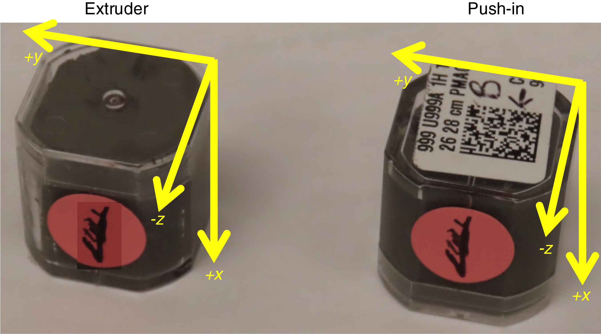
Figure F15. Coordinate system for extruder and push-in samples.
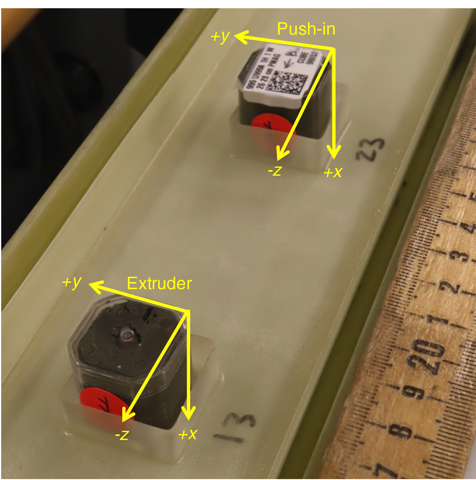
Figure F16. Sample orientations, SRM.
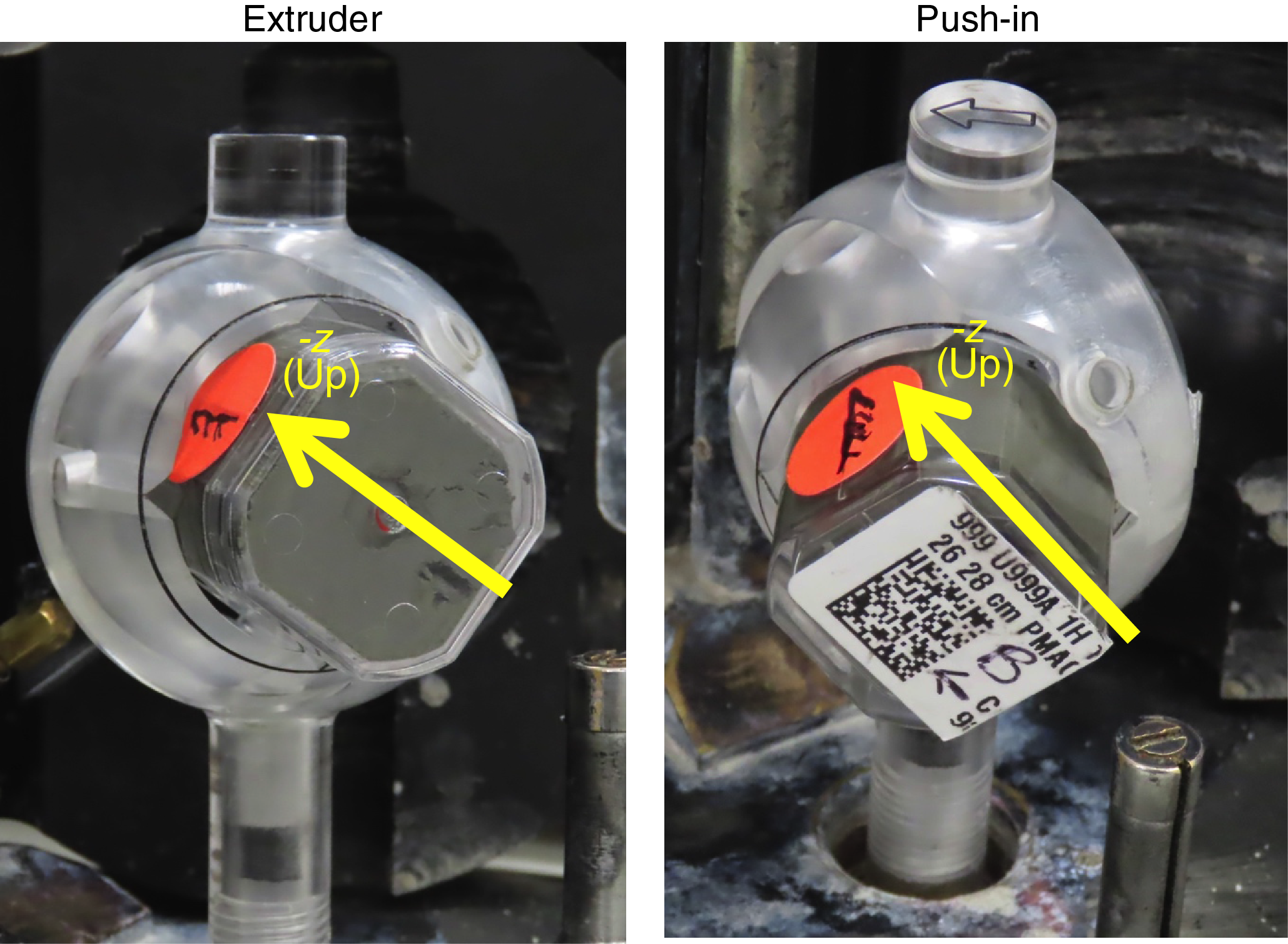
Figure F17. Sample orientations, JR-6A spinner magnetometer.
Editing of archive measurements for coring disturbance
Sediment disturbance due to coring or geological processes (slumping, faulting, etc.) often leads to distorted and unreliable paleomagnetic directional records and largely altered sediment fabric. The paleomagnetic data were therefore filtered to remove these intervals. Editing of the archive-half measurements was automated using Jupyter notebooks. These data were systematically filtered:
- We deleted all measurements within 10 cm of the section ends to remove the edge effect inherent in all pass-through measurement systems such as the SRM.
- We deleted all measurements in the upper 80 cm of Section 1 of all APC and HLAPC cores because they are the most susceptible to the accumulation of fall-in material during coring. Additionally, the strong vertical drilling overprint in these intervals often appeared to be more difficult to remove.
- We deleted all data from intervals that were assigned the "high" drilling disturbance intensity code entered during visual core description (see Lithostratigraphy) to remove data in intervals affected by coring-induced disturbance such as fall-in and flow-in. The site chapters include the DESClogik tables that record these intervals (the tables are also available in DESC_WKB in Supplementary material).
We next inspected core composite photographs and X-radiographs for evidence of coring or sedimentary disturbance. We found the new shipboard XRI to be the most useful tool for identifying cored intervals suitable for magnetostratigraphic interpretation through the assessment of sediment composition, character of the deposit, and coring deformation. Observations of these X-ray images were carefully documented and used to filter the paleomagnetic data.
Core composite photographs were used to remove water-rich "soupy" intervals and intervals in which the core liner is not completely full (Figure F18A). Soupy intervals are also apparent in the X-radiographs as very light gray, structureless intervals with abundant bubbles and high concentrations of gravel and pebbles (Figure F18B). Beginning with Site U1536, X-radiographs for all APC and HLAPC sections were used to identify additional features that might adversely affect the NRM but may not be readily apparent during visual description (e.g., large dropstones beneath the core surface or centimeter-scale deformation of the sediment that would not be considered "highly disturbed" in a macroscopic sense but is sufficient to disrupt the microfabric of the NRM). Such features could lead to false identification of geomagnetic excursions. X-radiographs and paleomagnetic data were collected from the archive halves, so features observed in X-radiographs are directly relevant to paleomagnetic data.
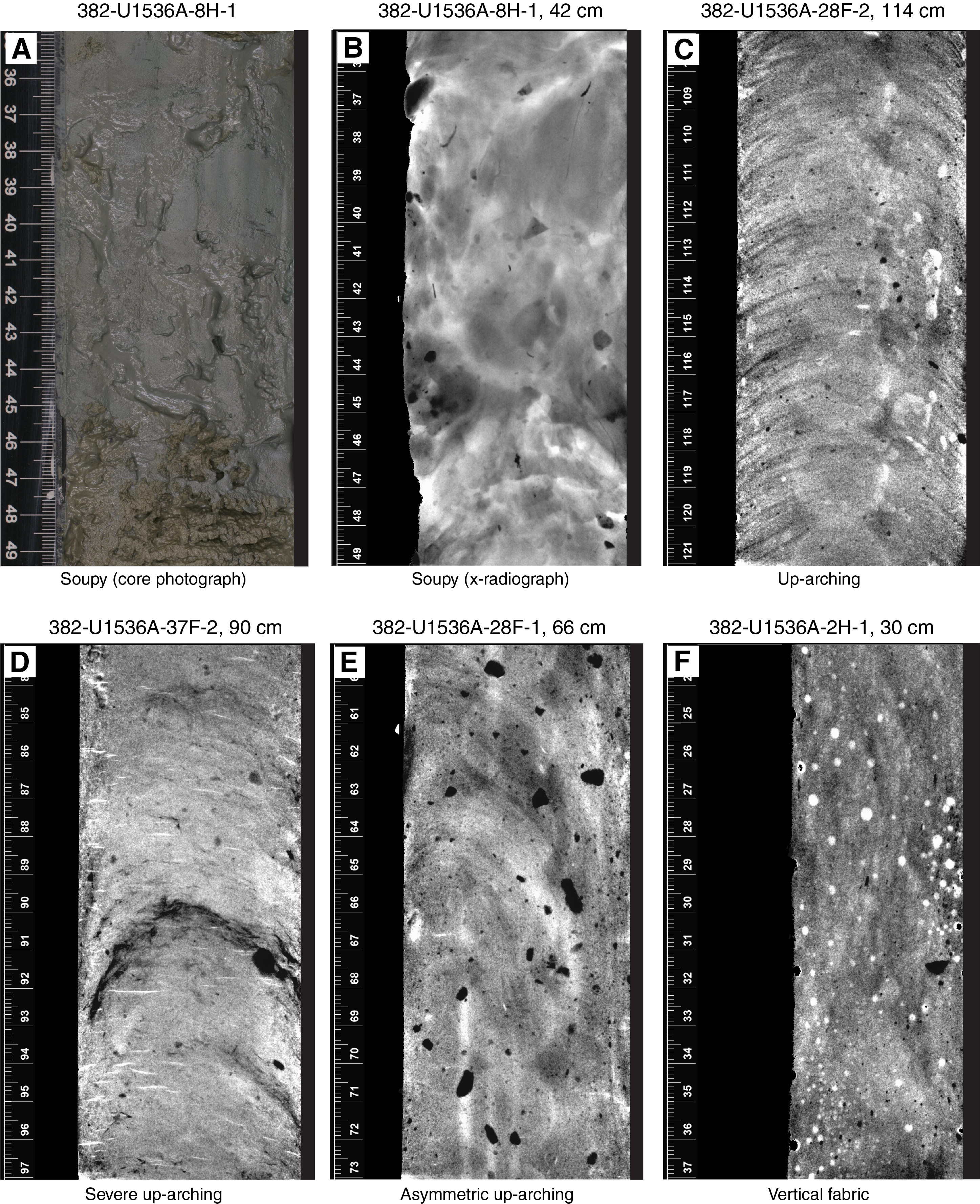
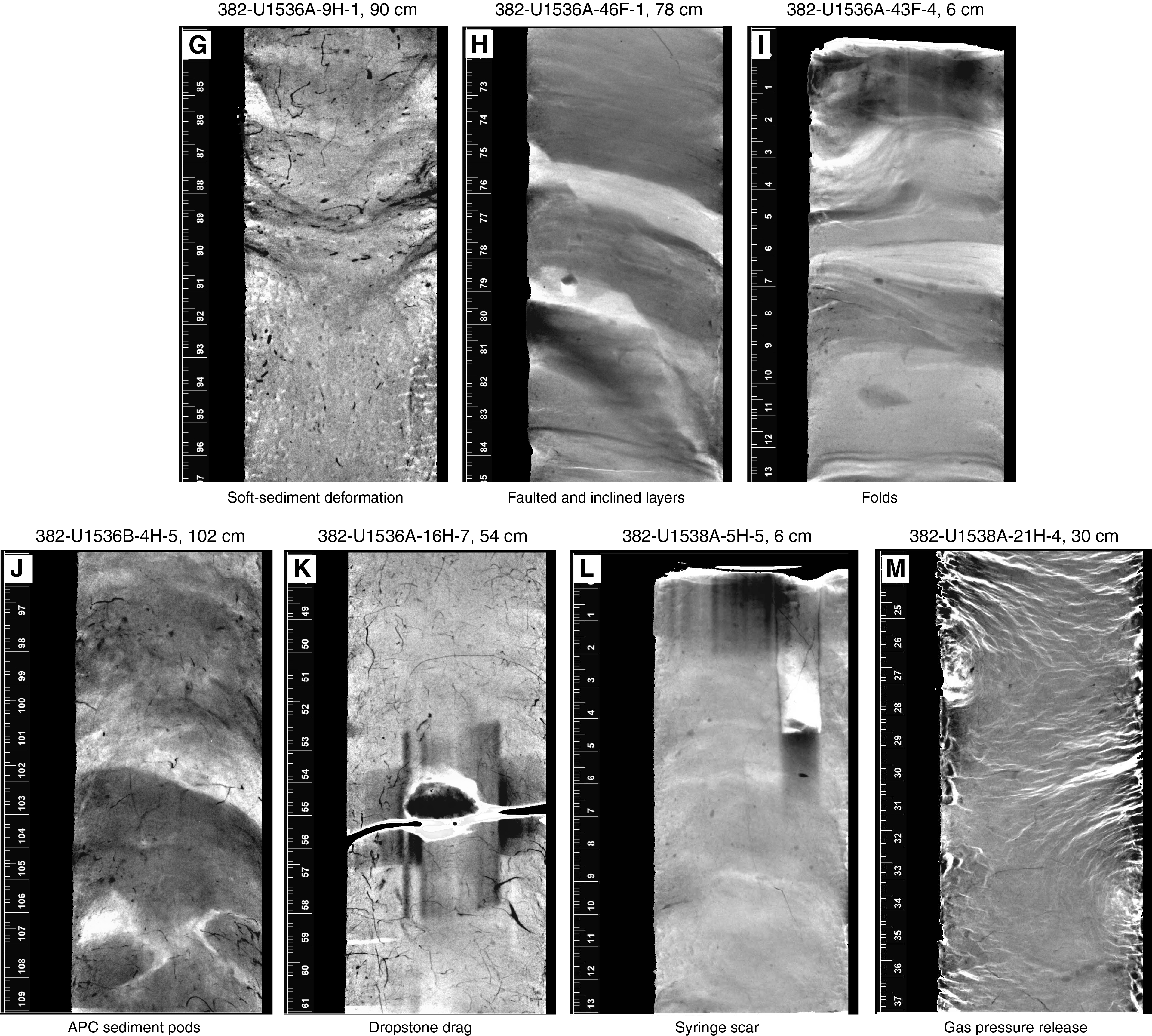
Figure F18. Identified features.
Shipboard processing of X-radiographs rendered high-density discrete objects such as dropstones with low (black) grayscale values and low-density objects such as air bubbles and water pockets with high (light gray to white) values. Negative features such as voids, imprints where large rocks were removed from the sediment or dragged by the cutting wire, and measurement probe and sampling tool scars where sediment is compressed or removed manifest as both high and low grayscale values. We therefore identified and defined disturbances using a combination of grayscale values, feature shape, structural characteristics of the sediment, and overall context of core handling and processing during Expedition 382. Examples of features identified in the core photographs and X-radiographs are shown in Figure F18.
We use the term "uparching" to describe convex-upward layers (after Jutzeler et al., 2014). These structures result from upward suction of originally horizontal layers during piston coring. Figure F18C illustrates minor uparching for which the top of the convex layer is <1 cm above the base of the layer. Intervals with minor uparching were retained in the NRM data because cube sampling from minimally disturbed centers of the working halves allowed us to assess the fidelity of archive-half measurements in such cases (Acton et al., 2002). The light-colored circular features in Figure F18C are the footprints of the MSP sensor on the SHMSL where it comes in contact with the split-core face. The measurement of one archive half both before and after SHMSL analysis indicated that these footprints do not adversely affect the NRM.
Figure F18D illustrates severe uparching in which the tops of the convex layers are stretched 3 cm higher than their bases. Figure F18E illustrates asymmetric uparching in which the peak of convexity is offset from the center line of the core face. Layers on the right-hand side of the image are steeply inclined to near vertical, which distorts and biases both declination and inclination measurements. In both cases, there is no segment of a stratigraphic horizon where a paleomagnetic cube or U-channel could recover undisturbed sediment. Figure F18F illustrates a vertical fabric associated with flow-in in which upward suction and liquefaction is so extreme that the original stratigraphy is completely destroyed (McCoy, 1985; Buckley et al., 1994). Flow-in was logged during visual core description when macroscopic features such as diapirs were clearly present, but it is difficult to detect such features in a homogeneous single lithology that lacks sedimentary structures to monitor (e.g., laminations, Buckley et al., 1994). In these cases, X-radiographs and computed tomography scanning allowed the detection of deformation-related structures that are not easily recognizable from the core face description alone (e.g., Walczak et al., 2017). Intervals of >2 cm uparching, all intervals of asymmetric uparching, and all intervals with vertical fabrics were removed from the NRM data set.
Other types of deformation or interference removed from the NRM data set include the following:
- Soft-sediment deformation (e.g., an upper layer sagging downward into the underlying layer; Figure F18G).
- Faulted sections of sediment (Figure F18H) in which >1 cm of displacement occurs along the fault.
- Folds that resemble anticlines or synclines (Figure F18I), including recumbent folds (horizontal hinge planes) in slumped intervals.
- "APC sediment pods" in which a pod or clot of material is encased in the surrounding matrix (observed when two lithologies were present; e.g., a pod of biosiliceous material encased in a clay-rich matrix; Figure F18J). These features resemble RCB biscuits in X-radiographs.
- Single large dropstones or clusters of dropstones spanning a >1 cm interval that coincided with an NRM measurement position (i.e., offsets of 0, 5, 10 cm, etc.) (Figure F18K).
- Intervals in which a large dropstone was dragged several centimeters by the core splitting wire that manifest in X-radiographs as a vertical feature with boundaries tangential to the dropstone and extending several centimeters to several tens of centimeters above and/or below the dropstone (Figure F18K).
- Cracks and voids spanning a >1 cm interval and coinciding with an NRM measurement position.
- Foreign objects in the sediment (e.g., shear pins, pieces of cutting wire, and core splitting blades). Where possible, these objects were physically removed from the sediment core prior to measurement on the SRM, but processed X-rays typically were not yet available before it was time to measure archive halves on the SRM.
An additional feature observed in X-rays but not filtered from the NRM data set was concentric ring structures around drill holes in the sides of core liners (Figure F18M). Small holes were drilled along the sides of core lines prior to splitting in instances where bulging end caps and liners indicated the buildup of exsolved gases as the cores warmed up to room temperature. Upon splitting the cores, we observed expansion cracks. Concentric ring structures observed in X-rays suggest that sediment moves during the release of gas pressure. However, we chose to retain data in these intervals because we could not distinguish between the effects of the expansion cracks, weakly magnetized lithologies, and drill holes, which often occurred together. In some instances, there appeared to be shallowing of inclinations at the horizon of the drill hole. In other instances, we observed both expansion cracks and concentric ring structures, and inclinations remained consistent with intact sediment in the surrounding horizons and consistent with those expected at our site latitude.
We also note that filtering 10 cm from the ends of each core section also served to remove intervals of sediment disturbed by the insertion of the temperature probe into the top of each section prior to commencing physical property measurements of whole rounds and "syringe scars" where a syringe was inserted into a section end to extract sediment for headspace gas measurements or microbiology/aDNA analysis (Figure F18L). The tables used to edit data based on X-ray images are included in the Paleomagnetism section of the chapters for Sites U1536–U1538. X-ray images were not logged for Sites U1534 and U1535 on the ship but will be completed postcruise.
Magnetostratigraphy
Magnetic polarity zones were assigned based on changes in inclination after 15 mT peak AF demagnetization. After a polarity stratigraphy was established for a given hole, we correlated the pattern with the GPTS of the GTS2012 (Gradstein et al., 2012), summarized in Table T7. Correlation to the GPTS was informed by discussions with the shipboard biostratigraphy team when needed. The GTS2012 includes orbitally tuned reversals between Chron C1n and the base of Subchron C5r.2n (0–11.657 Ma) and between the base of Chron C5ABn and Subchron C5Bn.1n (13.608–15.215 Ma). The intervals between Subchron C5r.2n and Chron C5ABn and between Chrons C5Bn and C6Cn (11.657–13.608 and 15.215–23.030 Ma, respectively) are calibrated by spline fitting of marine magnetic anomaly profiles following Lourens et al. (2004) and Hilgen et al. (2012). We follow the chron terminology of Gradstein et al. (2012) listed in Table T7. Since the development of the GTS2012, improvements have been made to the intercalibration of the GPTS and the Pleistocene benthic δ18O timescale (e.g., Channell et al., 2016) that should be considered for future orbital resolution chronostratigraphic work. Additionally, improved intercalibration of Pliocene–Pleistocene diatom datums and the GPTS should also be considered (Tauxe et al., 2012).
Geochemistry
A multitude of organic and inorganic geochemical parameters, outlined below, were determined on JOIDES Resolution during Expedition 382 following JOIDES Resolution standard procedures, including headspace gas content (hydrocarbons), IW composition, and bulk sediment geochemical parameters. Furthermore, some IW samples will be shipped for further shore-based geochemical analyses.
Volatile hydrocarbons
For safety and pollution prevention, concentrations and distribution of light hydrocarbon gases, mainly methane (C1), ethane (C2), and propane (C3), were monitored upon retrieval of each core as part of the routine IODP shipboard hydrocarbon monitoring program. The standard method used was headspace sampling as described by Kvenvolden and McDonald (1986). On deck, one sediment plug (~5 cm3) was collected from Hole A at each site for headspace gas analyses immediately after retrieval on deck using a brass boring tool. The sample was placed in a 21.5 cm3 glass serum vial that was sealed with an aluminum crimp cap fitted with a Teflon septum. Additional samples were collected from other holes when depths surpassed those previously drilled. Headspace samples were collected from the top of a section from the middle of the core immediately adjacent to the IW sample when possible. Each vial was labeled with the core, section, and interval the sample was taken from. Before gas analyses, the vial was heated to 70°C for ~35 min to evolve hydrocarbon gases from the sediment plug. When consolidated or lithified samples were encountered, chips of rock (equaling 5 cm3) were arranged in the headspace vial, which was sealed and processed as explained above.
To detect and quantify light hydrocarbons, including methane (C1), ethane (C2), ethylene (C2=), propane (C3), and propylene (C3=), samples were extracted from the sealed sample vial using the septum with a gas-tight glass syringe and injected into and analyzed by an Agilent/HP 6890 Series II GC equipped with a 2.4 m × 2.00 mm stainless steel column packed with 80/100 mesh HayeSep "R" and a flame ionization detector set to 250°C. Samples were introduced into the GC through a 0.25 cm3 sample loop connected to the Valco valve. The valve can be switched automatically to back flush the column. The GC oven temperature was programmed to start at 80°C for 8.25 min, increase to 150°C for 5 min at a rate of 40°C/min, and then return to 100°C postrun for a total of 15 min. Helium was used as a gas carrier. Initial helium flow in the column was 30 mL/min. Flow was then ramped to 60 mL/min after 8.25 min to accelerate elution of C3 and C3=. The total run time was 15 min. The GC was also equipped with an electronic pressure control module to monitor the overall flow into the GC. Data were collected and evaluated using the Agilent Chemstation software (2001–2006), and the chromatographic response was calibrated against different preanalyzed gas standards with variable quantities of low–molecular weight hydrocarbons, as stipulated by Scott Specialty Gases (Air Liquide). Concentrations of hydrocarbon gases are reported in parts per million by volume (ppmv).
Interstitial water chemistry
IW samples for shipboard determination of salinity, alkalinity, pH, phosphate, and ammonium, as well as major and trace elemental concentrations, were processed by squeezing 5–10 cm whole-round sections cut from cores immediately after core retrieval. Whole-round samples were usually collected at a frequency of one sample per core (<100 mbsf) or every third core (>120 mbsf) to the bottom of the site, except for Site U1538. For Site U1538, we collected samples at a frequency of one sample per core (<222 mbsf), every two cores (222–300 mbsf), or every third core (<300 mbsf) to the bottom of the site. Sampling frequency was reduced by half when using the HLAPC system or when cutting half cores with rotary coring systems. Sufficient quantities of IW for shipboard and planned shore-based analyses were collected for every targeted site during Expedition 382. Potentially present drilling fluid residues on the exterior of the whole-round sample were carefully removed with a spatula to exclusively target uncontaminated sediments. For two depths at Site U1538, subtle amounts of drilling fluid may have been recovered. Samples are highlighted in the respective chapter. For XCB and RCB cores, the intruded drilling mud between biscuits was also removed to avoid contamination from drilling fluid. After arrival in the geochemistry laboratory, the cleaned sediment was transferred into an 8 cm inner diameter titanium squeezer that was then placed in a thoroughly cleaned Carver hydraulic press (Manheim and Sayles, 1974) and squeezed with slowly increasing pressure to a maximum of 25,000 force pounds (1.112 × 10⁶ N). The first extracted milliliter of solution was discarded to avoid contamination, and the remaining squeezed IW was collected into a 60 mL deionized water–washed (18 MΩ/cm) high-density polyethylene syringe attached to the squeezing assembly.
The priority list for shipboard analyses and shore-based samples from IW (from highest to lowest priority) was as follows:
- Salinity (~100 µL) determined by optical refractometry immediately after squeezing;
- pH and alkalinity (~3 mL) via titration also determined immediately after squeezing;
- Ammonium and phosphate concentrations (~200 µL each) measured by spectrophotometry;
- Selected anions and cations (~100 µL; Na+, K+, Ca2+, Mg2+, Cl−, Br−, and SO42−) measured by ion chromatography;
- Major and trace elemental analyses (~2 mL; B, Ba, Ca, Fe, K, Li, Mg, Mn, Na, S, Si, and Sr) obtained by ICP-AES;
- Shore-based analyses of various trace elements (e.g., rare earth elements [REEs]) that are below the detection limit of the shipboard ICP-AES (~3 mL) to be carried out via inductively coupled plasma–mass spectrometry (ICP-MS) at the Helmholtz Centre for Ocean Research Kiel (Germany);
- Shore-based analyses of boron (δ11B), silicon (δ30Si), strontium (87Sr/86Sr), and barium (δ137Ba) isotopic compositions to be carried out at the Helmholtz Centre for Ocean Research Kiel;
- Shore-based analyses of Li isotopes (δ7Li), Mg isotopes (δ26Mg), and K isotopes (δ41K) (~1 mL) by multicollector ICP-MS (MC-ICP-MS) to be carried out at the Korea Basic Science Institute; and
- Shore-based analyses of δ18O, δD, and δ13CDIC (~2 mL) by elemental analysis–isotope ratio mass spectrometry (EA-IRMS) and/or cavity ring-down spectroscopy (CRDS) to be carried out at the Korea Basic Science Institute.
Prior to all above-mentioned analyses, IW was filtered through a 0.45 µm polysulfone disposable filter (Whatman) into one or two 15 mL centrifuge tubes (depending on the amount of IW). After the assessment of sample volumes available, shore-based samples were transferred into separate acid-cleaned vials, acidified or pretreated as required, and stored for shipping. All other shipboard analyses were carried out in batches if possible/feasible.
Shipboard analysis
IW samples were analyzed on board following the protocols in Gieskes et al. (1991), Murray et al. (2000), and the IODP user manuals for shipboard instrumentation.
Alkalinity, pH, and salinity
IW alkalinity and pH were measured using a Metrohm autotitrator (Model 794 Basic Titrino) equipped with a pH glass electrode and a stirrer (Model 728). pH was obtained from the LabVIEW alkalinity program provided on the ship. Alkalinity was measured by titrating 3 mL of solution with 0.1 M HCl to reach an end point of pH = 4.2. Calibration and standardization for pH and alkalinity measurements were achieved using the International Association for the Physical Sciences of the Oceans (IAPSO) seawater standard, which was analyzed repeatedly throughout the expedition. Salinity was analyzed with a Fisher Model S66366 refractometer calibrated using 18 MΩ Milli-Q grade deionized water to a precision of 0.5. The IAPSO seawater was measured alongside samples for data QC.
Ion chromatography (selected cations and anions)
Aliquots of IW were diluted at 1:100 with deionized water for analysis of Na+, K+, Ca2+, Mg2+, Cl−, Br−, and SO42− using a Metrohm 85 Professional ion chromatograph (IC). The IAPSO seawater standard was used for standardization of measurements. Typical analytical uncertainty based on reproducibility was <5% (2 standard deviation [SD]) for each ion.
Spectrophotometry (ammonium and phosphate)
Ammonium concentrations were determined by spectrophotometry using an Agilent Technologies Cary Series 100 UV-Vis spectrophotometer with a sipper sample introduction system following the protocol of Gieskes et al. (1991). Sufficient standards with a range of ammonium concentrations for calibration purposes were prepared to allow for the accurate measurement of low to highly elevated ammonium concentrations such as those seen at Site U1536 (maximum = 2.78 mM). Because of these high concentrations, subsequent runs at Sites U1537 and U1538 were conducted on more highly diluted samples. Replicate standard concentration measurements carried out at every site confirmed the accuracy of the obtained results. The solution was kept at room temperature for ~6.5 h to develop color after the reagents were added. Ammonium analyses were conducted by phenol diazotization and subsequent oxidization by sodium hypochlorite to yield a blue color measured spectrophotometrically at a wavelength of 640 nm. Ammonium chloride (NH4Cl) was used for calibration and standardization. Analytical uncertainty, assessed via repeated measurements of ammonium chloride standard material, was better than 4.0%.
Phosphate was measured using the ammonium molybdate method described in Gieskes et al. (1991) with appropriate dilutions based on prior experience. Phosphate concentrations were determined at an absorbance of 885 nm wavelength ~30 min after adding the mixed reagent solution. Analytical uncertainty, assessed via repeated measurements of a phosphate standard, was better than 2.0%.
Dissolved silica concentrations were measured at selected sites by reacting samples with ammonium molybdate tetrahydrate solution acidified with hydrochloric acid to form molybdosilicic acid. The complex was reduced by adding ascorbic acid to form molybdenum blue, which was measured at a wavelength of 812 nm. Solutions of sodium silicofluoride (Na2SiF6) at 360 and 480 µM concentrations were used as standards with a reproducibility of better than 3%.
Inductively coupled plasma–atomic emission spectroscopy
Dissolved major (Ca, K, Mg, and Na) and minor (B, Ba, Fe, Li, Mn, S, Si, and Sr) elemental concentrations were determined by an Agilent 5110 inductively coupled plasma–optical emission spectrometer (ICP-OES) with an SPS4 autosampler. Data produced on the Agilent 5110 ICP-OES were collected in AES mode and are referred to as "ICP-AES" in the LIMS/LIMS Reports (LORE) database and in this volume.
IW samples were diluted 1:10 in 2% HNO3 (v/v) and spiked with an internal standard to correct for drift and atomic and ionic interferences. In detail, 100 µL of spike solution containing 100 ppm beryllium (Be), indium (In), and scandium (Sc) and 200 ppm antimony (Sb) was added to 500 µL of IW sample and 4.4 mL of 2% HNO3. For calibration, serial dilutions of IAPSO standard seawater (0%, 1%, 5%, 10%, 25%, 50%, 75%, 100%, and 200%) were prepared to cover IW concentrations smaller than or equal to normal seawater. Additional calibration solutions for major and minor element concentrations exceeding that of seawater were prepared with 3.5% NaCl as a matrix. Calibration solutions for B, Ba, Ca, Fe, K, Li, Mg, Mn, P, Si, and Sr were spiked in the same way as IW samples.
During each ICP-AES batch run, a complete set of in-house and IAPSO dilutions was analyzed at the beginning and the end, bracketing sample analyses. Known solutions of in-house standards were analyzed every 8–10 samples to monitor instrumental drift, and the IAPSO standard was analyzed at a similar frequency to monitor accuracy. The elemental concentrations reported for each sample were average values from three replicate integrations for each sample. Reproducibility was typically better than 5% for all elements and mostly around 1%–3%. A few trace elements such as Co, Ni, or Sc that reproduced less well are only displayed for general information in the respective tables and not discussed in individual chapters.
Comparability between ICP-AES and IC concentrations for IW samples
Reproducibility between the shipboard ICP-AES and IC approaches was assessed for elements run via both approaches (i.e., Ca, Mg, K, Na, and S/SO42−). For most IW samples, the IC data are in good agreement with the ICP-AES results. Reproducibility between the IC and ICP-AES analyses was typically better than 10% for K and Na and better than 15% for Ca and Mg. Total S (ICP-AES) and SO42− (IC) from the IW samples for all sites were also in very good agreement, with reproducibility between the two techniques typically better than 10%. Respective concentrations only differed for samples close to the detection limit, for which only IC concentrations were used after an additional calibration for low-concentration SO42− samples. For consistency, only ICP-AES Ca, Mg, Na, and K concentration data are shown in the figures in the individual site chapters. Exceptions are the chapters for Sites U1537 and U1538, where IC Na and K concentration data are shown in the respective figures.
Sediment major and minor elemental analysis by ICP-AES
Major (Al, Ca, Fe, K, Mg, Mn, Na, Si, and Ti) and several minor (Ba, Sr, and Zr) elemental concentrations were determined by an Agilent 5110 ICP-OES in AES mode with an SPS4 autosampler following the methods outlined in Murray et al. (2000). Because bulk sediment analyses require reliable QC because of the unwanted introduction of sample handling artifacts, five sediment reference materials were included alongside the sedimentary analyses (BCR-2, BHVO-2, BCS-CRM 393, PACS-3, and MESS-4). Results for individual standards are reported in Table T8.
Approximately 100 mg of homogenized ground sediment sample or reference material was weighed (100 ± 0.5 mg) on the Cahn C-31 microbalance and placed in a vial containing 400 mg of preweighed lithium metaborate (LiBO2), aiming for a sample flux ratio of 1:4. Following homogenization of sample and flux powders, the mixture was poured into a Pt-Au crucible and 10 µL of 0.172 M LiBr was added to prevent the cooled bead from sticking to the crucible. Each sample was fused individually at 1050°C for ~12 min in an internal-rotating induction furnace (Bead Sampler NT-2100) and subsequently left to cool to form a bead. At room temperature, the bead was dissolved in 50 mL trace metal grade 10% HNO3 (dilution factor 1:500) in acid-washed high-density polypropylene Nalgene wide-mouth bottles. These bottles were subsequently agitated on a Burrell wrist-action bottle shaker for 1.5 h. Aliquots (500 µL) of the filtered solution were mixed with 4.4 mL 2% HNO3 and 100 µL of a spike solution containing 100 ppm Be, In, and Sc and 200 ppm Sb. Samples were then measured analogously to the IW samples. Sedimentary standards processed in this manner reproduced all elemental concentrations typically better than 5% (2 SD) and mostly around 1%–3%, which was almost as precisely as the IW samples. Reproducibility (1 relative standard deviation [RSD]) for all major and trace elements as determined during 21 repeat measurements on rock standard material MESS-4 is displayed at the bottom of Table T8. Various trace element concentrations falling closer to the detection limit of the ICP-AES (e.g., Co, Cu, and Ni) shown in Table T8 produced less well but are shown for completeness.
Sedimentary inorganic and organic carbon, nitrogen, and carbonate content
Sediment samples (~5 cm3 each) were collected from the working-half cores following identification of major lithologies by sedimentologists for shipboard bulk sediment analyses. Each sample was freeze-dried for ~12 h, crushed to a fine powder using a solvent-cleaned agate pestle and mortar, and sampled for the individual analyses.
Total carbon (TC), total sulfur (TS), and total nitrogen (TN) contents of the sediment samples were determined with a ThermoElectron Corporation FlashEA 1112 CHNS elemental analyzer equipped with a ThermoElectron packed column CHNS/NCS GC and a thermal conductivity detector (TCD). Approximately 15 mg of freeze-dried ground sediment was weighed in a tin cup, and the sample was combusted at 950°C in a stream of O2. Nitrogen oxides were reduced to N2, and the mixture of N2 and CO2 gases were separated by the GC and measured by the TCD. All measurements were calibrated to the National Institute of Standards and Technology (NIST) 2704 Buffalo River Sediment standard material, which was analyzed every 10 samples.
Inorganic and organic carbon contents
Inorganic carbon concentrations were determined using a UIC 5011 CO2 coulometer. Approximately 5 mg of freeze-dried ground sediment was weighed and reacted with 2 M HCl. The liberated CO2 was titrated, and the end point was determined by a photodetector cell. Calcium carbonate content (CaCO3) expressed as weight percent was calculated from the inorganic carbon content, assuming that all evolved CO2 was derived from dissolution of CaCO3, by using the following equation:
Standard CaCO3 (>99.9% CaCO3; Fisher Scientific) was used during individual batches of analyses to confirm accuracy and instrument performance before, during, and after each session (target reproducibility is better than 2%). No correction was made for the presence of other carbonate minerals.
Total organic carbon (TOC) content was calculated as the difference between TC and inorganic carbon:
Rhizon interstitial water
Rhizon IW samples were taken following the IW sampling guidelines from Andrén et al. (2015) and Dickens et al. (2007). The samples were collected at a 20 cm resolution for the uppermost 3 m and at a 50 cm resolution from 3 to 8 mbsf. Around 4 mm wide holes were drilled in the untouched portions of the cores, Rhizon soil moisture samplers (Rhizosphere Research Products, Wageningen, The Netherlands) with 0.15 µm pore size and a porous length of 10 cm were inserted, and IW was collected by creating a vacuum in a connected 12 mL syringe. One aliquot of each IW sample was filled in 5 mL polypropylene (PP) tubes and conditioned with 2% HNO3, acidified with nitric acid to pH <2, and stored at 4°C. Shore-based analyses of δ18O, δD, δ13CDIC, Li isotopes (δ7Li), Mg isotopes (δ26Mg), and K isotopes (δ41K) by MC-ICP-MS (~1 mL) will be carried out at the Korea Basic Science Institute for all collected samples.
Physical properties
During Expedition 382, physical property measurements were made for lithostratigraphic characterization and stratigraphic correlation and to tie core descriptions to downhole data and the main seismic discontinuities. Physical property data were key to generating high-resolution and continuous data sets for hole-to-hole and site-to-site stratigraphic correlation, detecting discontinuities and inhomogeneities, obtaining information about differences in the composition and texture of sediment, identifying major seismic discontinuities, and constructing synthetic seismic profiles. The thermal conductivity of the recovered material was also measured and combined with downhole temperature measurements to estimate geothermal heat flow. Different techniques and methods were used to characterize Expedition 382 cores on whole-round, split section-half, and discrete samples.
General sampling and measurement sequence
Cores measuring ~9.5 m in length were collected and then split into 1.5 m sections (see Drilling operations and Core handling and analysis). A core with ~100% recovery thus yields six 1.5 m sections plus an additional shorter seventh section. The resolution of physical property measurements made during Expedition 382 was site dependent and was established to complete the core analyses without impacting workflow in the different laboratories.
Different measuring procedures were considered for soft sediments versus semilithified and lithified sediments. The methodologies differ slightly and are explained in detail for each instrument/property below. Whole-round core sections were equilibrated to ambient room temperature (~19°–22°C) for at least 4 h to ensure thermal and barometric homogeneity and minimize any effects of changing conditions on the physical property measurements, especially for P-wave velocity, as well as to protect sensors from damage. An exception was made for a few cores, noted in the site chapters, so that their physical properties could be measured before time-sensitive sampling took place.
Prior to splitting, whole-round sections were analyzed with three whole-round physical property core logging systems: the WRMSL, the NGRL, and the thermal conductivity instrument (when possible). Previous IODP expeditions used the Special Task Multisensor Logger (STMSL), but for Expedition 382 this track was replaced by the new shipboard 2-D XRI (see Lithostratigraphy for details). The WRMSL includes a GRA bulk densitometer, a loop magnetic susceptibility (MSL) sensor, and a compressional PWL. All whole-round sections from all holes were measured at a 1 or 2.5 cm resolution on the WRMSL depending on the site and hole. A consistent and unbroken contact between the sediments and core liner is required to make accurate and realistic measurements with the PWL. This contact was generally found to be good when using the APC and HLAPC systems; however, PWL data quality tended to decrease with depth, and good contact was not observed for cores recovered with the XCB and RCB systems. These cores are typically characterized by gaps between recovered material and the core liner because the cored material has a smaller diameter than the APC, leading to unrealistic measurements outside of the expected velocity range (1400–4500 m/s). Therefore, the PWL was not activated for cores collected using the XCB and RCB systems.
All whole-round sections from all holes were also run on the NGRL to collect spectral gamma ray data at a 10 cm resolution. Following NGR measurements, thermal conductivity was measured on at least one whole-round section per core (when possible). A needle probe was inserted into the section through a small hole drilled along the split line of the plastic core liner near the central part of the section. When the needle did not provide measurements or for lithified sediments, the measurements were conducted using a contact probe (see Thermal conductivity measurements).
After all whole-round measurements were completed, core sections were split longitudinally. One half was designated as an archive section; the other half was designated as a working section for sampling and physical property purposes. Archive halves were used for measuring MS, color reflectance, and colorimetry with the SHMSL, a Bartington probe, and an Ocean Optics spectrophotometer, respectively, at a 1, 2, or 2.5 cm resolution depending on the site and hole. Working halves underwent P-wave velocity measurements using the P-wave x-axis caliper on the Section Half Measurement Gantry (SHMG). Measurements were made at a resolution of generally three per core. Discrete samples were also taken for MAD measurements (typically approximately three per core or more) to quantify wet and dry mass, wet and dry bulk density, water content, porosity, and grain density using the MADMax software. The goal of the MAD sampling distribution was to obtain an unbiased representation of all the different lithologies at various depths throughout the entire hole.
When all sediment core descriptions were finalized, the archive halves were taken back to the physical property laboratory, where X-ray imaging was performed to determine the internal structure (such as the presence of iceberg-rafted detritus, bioturbation, slumping, coring disturbance, etc.) of the sediment cores.
Detailed descriptions of methodologies and procedures can be found in Blum (1997) and Weber et al. (1997) as well as shipboard user guides available online. An overview of the sampling strategies for physical properties during Expedition 382 can be found in Table T9. Detailed procedures for each physical property measurement are described below.
Whole-Round Multisensor Logger measurements
The WRMSL (Figure F19) is a logging system for GRA densitometry, MS, and compressional P-wave velocity. The selected sampling intervals in the WRMSL were common denominators of the distances between the participating sensors (30–50 cm) to allow sequential and simultaneous measurements.
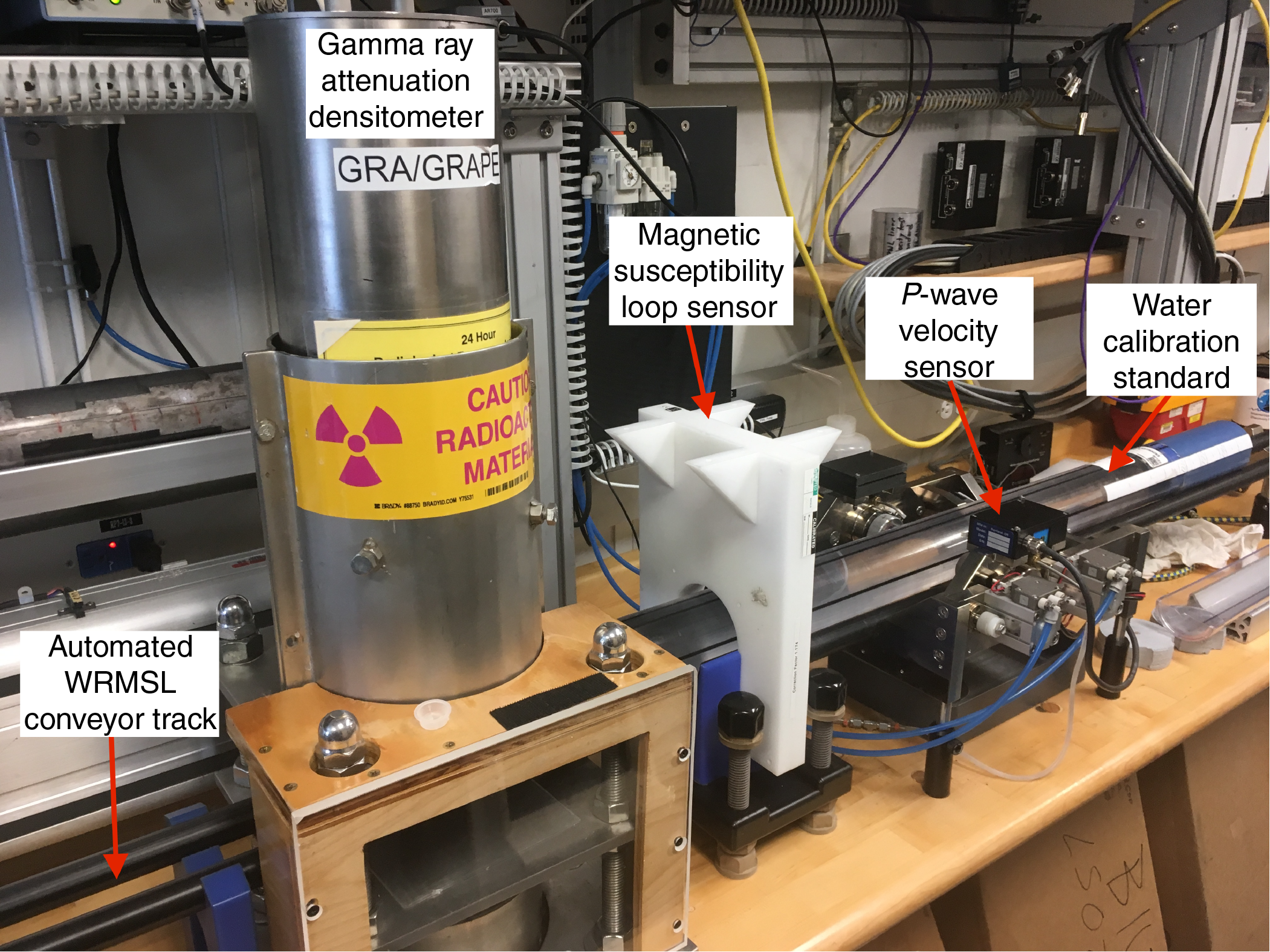
Figure F19. WRMSL.
WRMSL measurements were applied to all whole-round core sections during Expedition 382. Before measuring, the cores were equilibrated at room temperature, except for the first cores that were used for stratigraphic correlation purposes and were run on the WRMSL as soon they entered the laboratory and then measured a second time after temperature equilibration. To optimize the measurement procedure and provide consistency, sampling intervals and measurement times were the same for all sensors on each instrument. In this way, all sensors measured simultaneously and idle periods were avoided. A sampling resolution of 1 and 2.5 cm depending on the site and hole was considered appropriate for stratigraphic correlation and integration with seismic profiles and allowed efficient core flow. After measurements were finalized for the last section of the core, a deionized water standard was run through all instruments to keep the instruments calibrated and to assure quality assurance (QA)/QC. The instruments underwent recalibration if the measured standard values deviated from the range of published tolerances (Blum, 1997).
Gamma ray attenuation bulk density
The GRA bulk density instrument is used to measure a whole-round core at discrete and equidistant intervals to provide an average density value. The GRA instrument measures the attenuation of a directed gamma ray beam through the core. This beam is produced by a 137Cs gamma ray source at 370 MBq radiation and 660 KeV energy levels. The source is mounted directly above the whole-round core track within a lead shield with a 5 mm collimator at the bottom. The beam is directed down toward the core section during measurement. A scintillation detector with an integrated photomultiplier tube is mounted underneath the core track (and opposite the 137Cs source) and measures the gamma radiation that passes through the core sections. The GRA bulk density instrument operates with medium-energy gamma rays (0.1–1 MeV) that interact with the material of a formation by Compton scattering. The measured electron density of the scattering is then used to estimate the bulk density of the material. For a known thickness of sample, the density (ρ) is derived from the attenuation of gamma rays (lower intensity gamma rays reaching the detector mean the sample is denser):
- I0 = gamma ray source intensity,
- I = measured intensity of gamma rays passing through the sample,
- µ = Compton attenuation coefficient, and
- d = sample diameter.
µ and I0 are constants, and ρ is then calculated from I. The bulk density provided by the GRA instrument is related to the porosity, grain size, consolidation state, mineral composition, and any disturbances or contrasts present in a formation.
Generally, GRA bulk density measurements are most accurate when the core liner is completely filled and has minimal drilling disturbance, gaps, or double liners. Otherwise, measurements tend to underestimate true values. The GRA instrument estimates bulk density based on an internal core diameter of 66 mm, which is appropriate for most sediment cores obtained using the APC and HLAPC systems, whereas for material recovered using the XCB or RCB systems, the core diameter is usually lower (≤58 mm) and no correction was applied. The GRA densitometer is calibrated with specific calibration cores (one standard core liner filled with distilled water and aluminum cylinders of various diameters; Blum, 1997). The spatial resolution is less than ±1 cm. The instrument was recalibrated when the deionized water QA/QC standard deviated significantly (>2%) from 1 g/cm3. As mentioned previously, the sampling resolution was set at 1 or 2.5 cm depending on the site with an integration time of 3 s. Additional postprocessing of the GRA bulk density measurements was needed to remove edge effects at the ends of core sections. Single data spikes caused by voids, cracks in the core liner, and metal drill fragments, among other causes, were removed, as well as any values <1 g/cm3.
Magnetic susceptibility
MS was acquired for all whole-round core sections using a pass-through loop on the WRMSL. Magnetic susceptibility (χ) is a dimensionless parameter in the metric system that indicates the degree to which a material can be magnetized by an external magnetic field. χ is an indicator for the concentration of magnetic minerals, in particular magnetite, in the formation, which can also be related to paleoclimate-controlled depositional events or processes. MS is acquired at very low fields generally not exceeding 0.5 mT. The volume susceptibility is defined as
where M is the magnetization induced in the material by the external field of strength H. Accordingly, MS is most sensitive to formations containing high concentrations of ferromagnetic minerals such as magnetite, pyrite, hematite, and various other iron oxides. In addition, χ can also be related to the origin of the materials in the core and their subsequent diagenesis. Ferromagnetic minerals are characterized by MS values several orders of magnitude higher than their alteration products. Other minerals such as paramagnetic and diamagnetic (e.g., calcite, halite, water, and plastic) minerals present very small or even negative values of MS. Therefore, calcareous and siliceous biogenic deposits often have values close to the detection limit of the instrument itself.
All MS measurements on the WRMSL were taken by a Bartington MS2C loop sensor with a 90 mm diameter. An oscillator circuit in the sensor operates at a frequency of 565 Hz to avoid any potential interference between instruments and uses an automatic software correction factor of 1.174 and a ~140 A/m AF. This AF is responsible for a low-intensity, nonsaturating alternating magnetic field. Sediment core sections passing through the influence of this field cause a change in oscillator frequency. Frequency information is returned in pulse form to the susceptometer, and the MS value is estimated. The spatial resolution of the sensor is 20 mm with an accuracy of 2% (Blum, 1997). The output provided by the sensor is in dimensionless instrument units (IU) and is equivalent to 10−5 SI units. The estimated values are computed as the mean of three discrete measurements in the same location. MS values in the text and figures of the site chapters are expressed in instrument units unless otherwise noted. Instrument drift should be taken into account because it can occur during the period of a core section scan. The instrument was automatically zeroed at the beginning of each run, and a zero-background measurement was taken at the end of a core section to correct for this drift. The sampling resolution was set to 1 or 2.5 cm as for the GRA and PWL measurements. All acquired MS data needed postprocessing to remove edge effects and single data spikes caused by voids, cracks in the core liner, and metal drill fragments, among other causes.
Compressional P-wave velocity
Compressional P-wave velocity was acquired for each whole-round core section using the PWL. P-wave velocity depends on the lithology, porosity, and bulk density of the formation as well as the state of stress, lithostatic pressure, temperature, and/or fabric or degree of fracturing within the material. The degree of consolidation and lithification and the occurrence and abundance of free gas also influence the velocity. The acoustic impedance and downhole reflection coefficients are obtained using the P-wave velocity values together with the density values. These parameters can be used to derive synthetic seismograms, which in turn can be used to estimate the depth of the main reflectors observed in seismic profiles. P-wave velocity (VP) is defined by the time required for a compressional wave to travel a specific distance:
where d is the length that the wave crosses (i.e., the section core) and tcore is the traveltime through the core.
For P-wave velocity measurements with the PWL, the core section is placed between two piezoelectric transducers (a transmitter and a receiver) mounted in stainless steel housings. Acoustic coupling is through an epoxy resin surface and is enhanced by a water film supplied by an automated drip system. A 500 kHz pulse (2 µs wave period; 120 V) is produced at a frequency of 1 kHz and sent to the transmitter transducer, which generates an ultrasonic compressional pulse at about 500 kHz (pulse timing is measured with a resolution of 50 ns). Pressure is applied to the actuators to ensure coupling between the transducers and the core liner, and the automated drip system maintains wet contacts on the transducers to ensure a reliable coupling is always established. The compressional P-wave propagates horizontally through the core and is received by the receiver transducer on the opposite side. Velocity is amplified by an automatic gain control amplifier to produce the received signal. P-wave velocity transducers measure total traveltime of the compressional wave between transducers. A calibration of the PWL accounts for errors in the total distance (dtotal) and the total traveltime (ttotal). Errors in dtotal were assumed to be related to the laser distance. The obtained discrete data are the average of 100 discrete measurements at the set interval.
A core liner of assumed thickness (L) covered each core section for all measurements. The traveltime through the core liner (tliner) was determined by measuring the total traveltime through a core liner filled with distilled water with a velocity of ~1480 m/s. A correction (tdelay; system delay) was measured using the traveltime through a standard block of aluminum with a known thickness and a published velocity of 6295 m/s. Arrival time picks were chosen at the inflection point of the second lobe of the waveform, giving a second correction (tpulse) from the first arrival. Then tpulse and tdelay were combined and named ttotal_delay. Therefore, the velocity is computed as
- VP = core velocity (km/s),
- dtotal = measured diameter of the core and the liner (mm),
- L = wall thickness of the liner (mm),
- ttotal = total time for the pulse to travel through the core and liner (µs),
- tliner = traveltime through the liner (µs), and
- ttotal_delay = delay related to the combined transducer faces, electronic circuitry, and peak detection procedures (µs).
The VP equation above assumes that the core completely fills the core liner and gaps or air are not present. P-wave velocity was not measured for cores recovered with the XCB or RCB systems, which generally do not completely fill the core liner and hence do not provide realistic data. Any measured P-wave signal can degenerate because of an incompletely filled core liner, any voids present, or attenuation caused by microcracks that formed during core recovery. This degeneration is partly reflected in the gain (signal strength) factor applied to the original signal by the automated gain control. However, signal strength also represents the grain size of the sediment; therefore, low-strength signals cannot simply be interpreted to be proportional to attenuation. As already mentioned for previous WRMSL instruments, the sampling resolution was also set at 1 or 2.5 cm for the PWL depending on the site.
Natural Gamma Radiation Logger measurements
The NGRL measures NGR on whole-round cores using a system designed and built by the Integrated Ocean Drilling Program (Texas A&M University, USA) (Vasiliev et al., 2011; Dunlea et al., 2013). This instrument measures the cumulative radiation emitted during natural decay of radioisotopes in three long-lived decay series, potassium (40K), thorium (232Th), and uranium (238U), which have half-lives of 1.3 × 10⁹, 1.4 × 10¹⁰, and 4.4 × 10⁹ y, respectively. These isotopes and their daughter products emit gamma radiation at specific energy levels unique to each isotope. NGR can be used to estimate the abundance of each isotope based on the strength of the signal at characteristic energies (Blum, 1997; Gilmore, 2008). In sediments and sedimentary rocks, Th and K are usually associated with particular clay minerals, whereas U is often encountered in either clay minerals or organic-rich material. High counts generally reflect the presence of clay-rich fine-grained deposits, and relative changes are indicative of stratigraphic details that can aid in core-to-core, core-to-wireline log data, and/or borehole correlations between holes.
The NGRL system consists of eight sodium iodide (NaI) detectors arranged along the core measurement axis at 20 cm intervals surrounding the lower half of the section (Figure F20). The detector array is fit with both passive (layers of lead) and active (plastic scintillators) shielding to reduce the background environmental and cosmic radiation. The overlying plastic scintillators detect incoming high-energy gamma and muon cosmic radiation above 3 MeV and cancel this signal from the total counted by the NaI detectors.
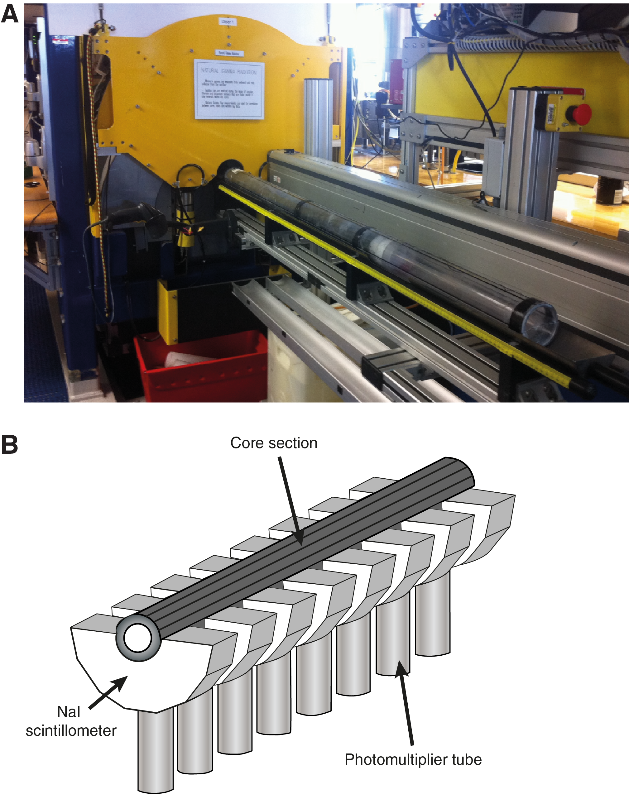
Figure F20. NGRL.
The quality of the core measurements depends on the concentration of radionuclides and the counting time. For Expedition 382, measurements were made at two sample positions 10 cm apart using a counting period of 300 s. After 300 s, the position was advanced downcore by 10 cm and counted again for 300 s. This method yielded a total of 16 measurements (10 cm apart) per 150 cm core section. Total acquisition times were ~5 min per measurement cycle or ~10 min per core section. This measurement procedure yielded statistically significant total counts. The collected data were of very good quality but needed some postprocessing to remove single data spikes due to cracks in the core liner and metal drill fragments among other causes.
Thermal conductivity measurements
Thermal conductivity is an intrinsic property of the core material; hence, it depends on the chemical composition, porosity, density, structure, and fabric composing it (Jumikis, 1966). Thermal conductivity is the capacity of the material to transfer heat by conduction. Measurements of this parameter in sediments and rock sections combined with in situ temperature measurements (see Downhole measurements) are used to estimate local geothermal heat flow. Geothermal heat flow is an indicator of the type and age of oceanic crust, which is in turn influenced by the geodynamics and tectonic processes impacting the region (Martos et al., 2017, 2018, 2019).
Thermal conductivity was measured immediately after NGR analysis in soft sediments (whole rounds) and when reliable measurements were yielded by the probe. A single measurement per core was generally taken in the central section using the TK04 (Teka Bolin) system (Table T9). For whole-round cores, the needle probe method in full-space configuration was used (Von Herzen and Maxwell, 1959). The needle probe was inserted into a 2 mm diameter hole drilled through the core liner along the split line. The core was placed in an enclosed box with insulating foam to avoid interference with airflow in the laboratory (Figure F21).
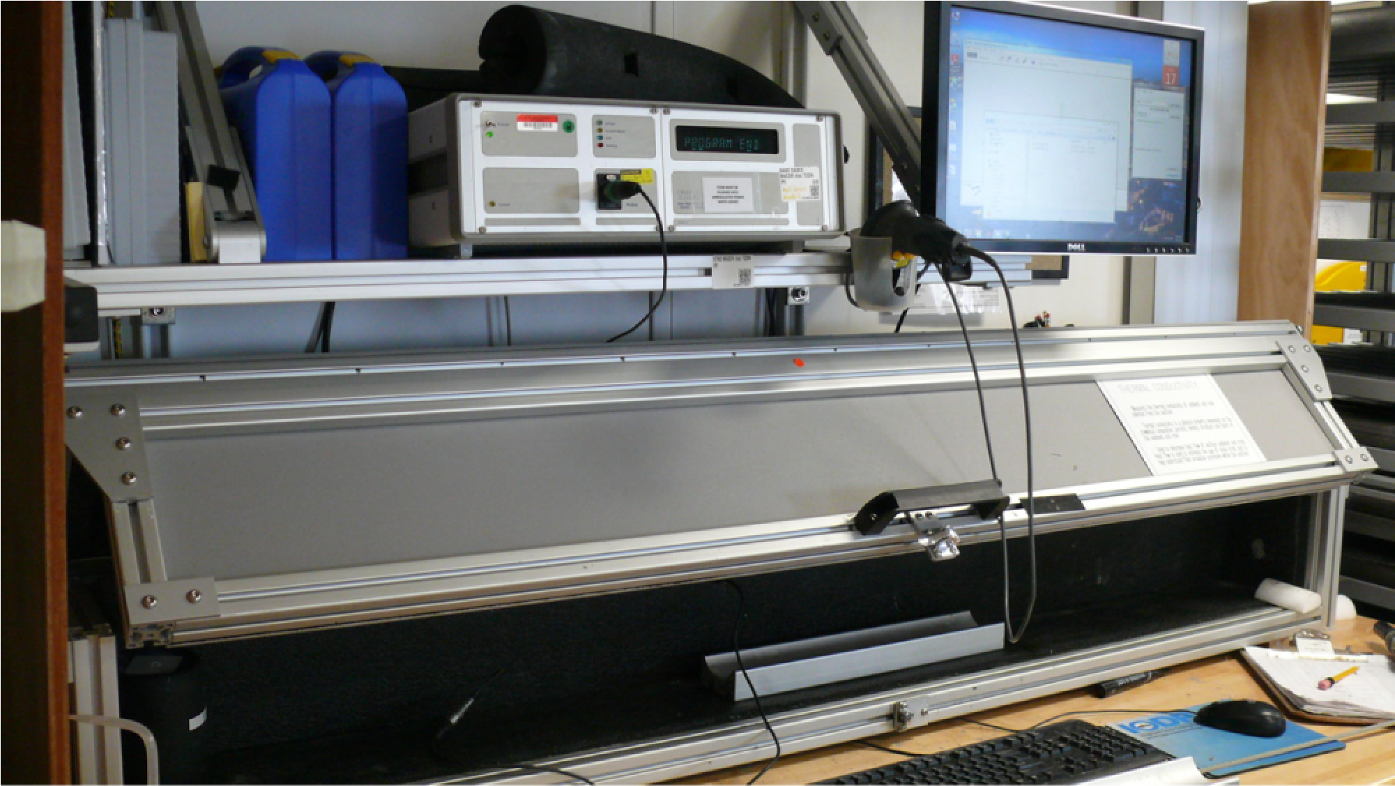
Figure F21. Shipboard station for thermal conductivity measurement.
For lithified sediments or rocks and soft sediments in which the needle probe did not yield reliable results, a contact probe method was used for half-space configurations on split cores. The probes consist of a heater wire and a calibrated thermistor. The measurement locations were chosen based on where the least amount of fracturing and most homogeneous portions of core sections were observed. The sections were prepared for a puck-style contact probe by applying distilled water onto the sediment surface. This procedure was applied to ensure good contact between the sediment and the probe. The puck probe was placed directly on the sediment and secured in place with a rubber strap or wooden tool to ensure proper contact pressure. Then the section half was placed in the insulated box to stabilize thermal conditions during measurements.
After either whole rounds or section halves were prepared for measurements and placed in the insulated box, the calibrated heat source of the probe was turned on and the increase in temperature was recorded over 80 s for the needle probe (soft sediments) and 60 s for the contact probe (hard or lithified sediments). The heating power ranged between 0.8 and 4 W/m for needle measurements and between 0.8 and 3.5 W/m for contact probe measurements. The heat equation solution for a line source of heat was then fit to the temperature measurements to obtain the thermal conductivity. The probe is assumed to be a perfect conductor because it conducts heat more efficiently than sediment or hard rock. Following this assumption, the linear relationship between the superconductive probe temperature and the natural logarithm of the time after initiation of the heat is expressed as
- T = temperature (K),
- q = heat input per unit length per unit time (J/m/s),
- k = thermal conductivity (W/[m·K]),
- t = time after the initiation of the heat (s), and
- C = instrumental constant.
To calculate the average thermal conductivity, three measurement cycles were performed separated by 10 min. A self-test, which included a drift study, was carried out at the beginning of each measurement cycle. The heater circuit was closed after the probe temperature stabilized, and the temperature increase in the probe was recorded. Thermal conductivity was estimated from the temperature increase rate while the heater current was flowing. Temperatures measured during the first 80 s of the needle probe heating cycle and 60 s of the contact probe heating cycle were fit to an approximate solution of a constantly heated line source (Kristiansen, 1982; Blum, 1997). Measurement errors were 5%–10%.
Section Half Multisensor Logger measurements
Color reflectance and MS were measured on archive halves using the SHMSL (Figure F22). Archive halves were covered with plastic wrap and placed on the SHMSL track, above which an electronic platform moves along a track and records the height of the core surface. The laser sensor detects the location of the bottom of the archive half, and then the instrument progresses along core making measurements of MSP and color reflectance. Color reflectance and MSP data were collected at a 1, 2, or 2.5 cm resolution during Expedition 382 depending on the site and hole.
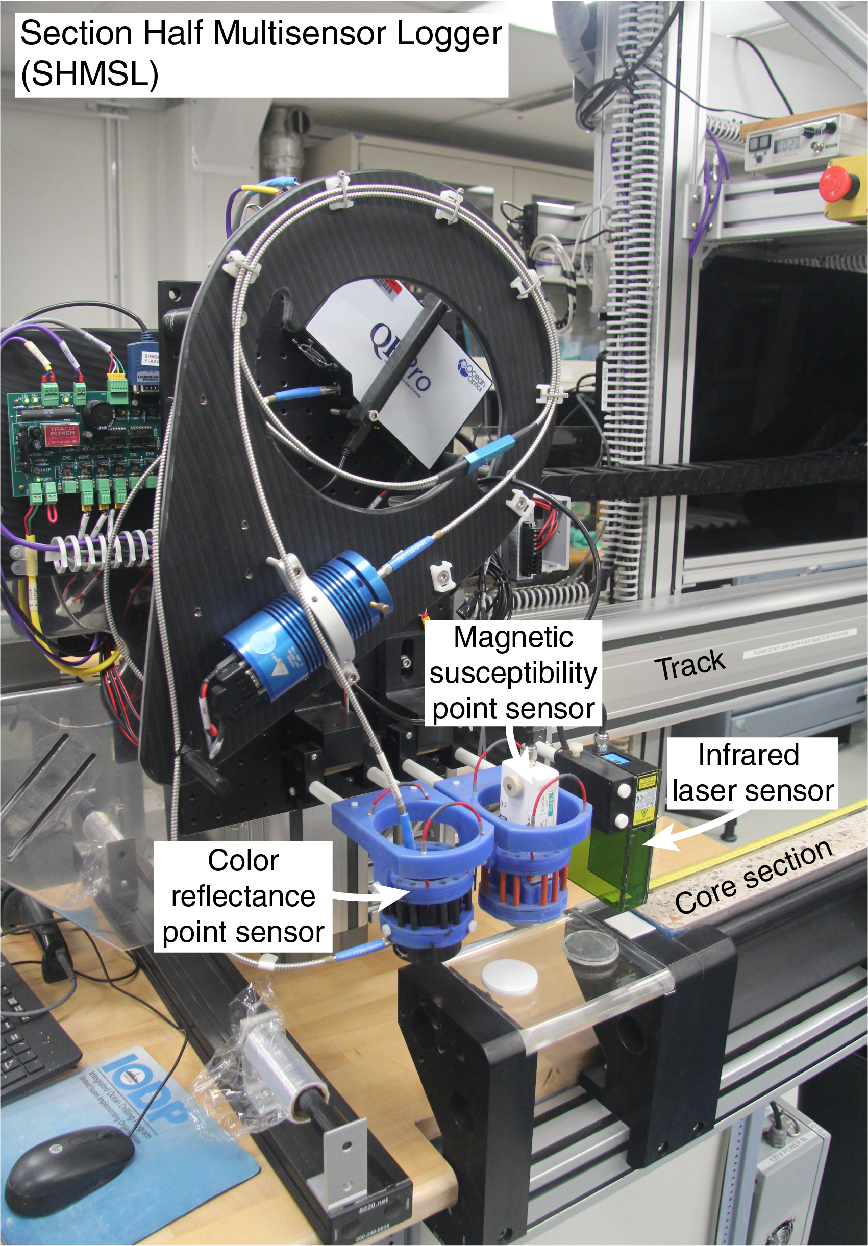
Figure F22. SHMSL.
Color reflectance spectrometry
The color reflectance spectrometry of the archive halves was measured using an Ocean Optics QE Pro detector integrating sphere and associated light sources covering wavelengths from UV through visible to near infrared. Each measurement was taken in 2 nm wide spectral bands from 390 to 732 nm. The data are reported using the L*a*b* color system, where L* is lightness, a* is redness (positive) versus greenness (negative), and b* is yellowness (positive) versus blueness (negative). Two spectra, pure white (reference) and pure black (dark), were used to calibrate the color reflectance spectrometer. Color calibration was conducted approximately once every 6 h (twice per shift). Additional details regarding measurement and interpretation of spectral data can be found in Balsam et al. (1997), Weber (1998), Balsam and Damuth (2000), and Giosan et al. (2002).
Point magnetic susceptibility
MSP was measured with a Bartington MS2 meter and an MS2K contact probe with a flat 15 mm diameter round sensor with a field of influence of 25 mm and an operation frequency of 930 Hz. The instrument averages three measurements from the sensor for each offset with an accuracy of ~5%. The spatial resolution of the MSP sensor is ~3.8 mm, and it reports values in instrument units, which can be converted to dimensionless SI units by multiplying by 10−5. The instrument was calibrated by the manufacturer before installation on JOIDES Resolution and is quality checked every 6 h at the same time as color reflectance sensor calibration.
Digital color imaging
The SHIL captures continuous high-resolution images of the archive-half surface for analysis and description. The instrument was used shortly after core splitting in an effort to avoid time-dependent color changes resulting from sediment drying and oxidation. The shipboard system uses a commercial linescan camera lens (AF Micro Nikon; 60 mm; 1:2.8 D), and illumination is provided by a custom assembly of three pairs of LED strip lights that provide constant illumination over a range of surface elevations. Each pair of lights has a color temperature of 6,500 K and emits 90,000 lux at 3 inches. The resolution of the linescan camera was set at 10 pixels/mm. Users set a crop rectangle for each image to remove extraneous information. Images were saved as high-resolution TIFF files. Available files include the original high-resolution image with gray scale and ruler and reduced JPEG images cropped to show only the section-half surfaces. Red, green, and blue (RGB) data were extracted from SHIL images every 0.5–2 cm depending on the site.
Section Half Measurement Gantry measurements
P-wave velocity measurements were performed on working halves using the SHMG. Measurements were typically made with the x-caliper on every section of each core (Table T9). The number of x-caliper measurements was increased for XCB and RCB cores or when the PWL on the WRMSL was not able to estimate accurate velocity measurements (e.g., because of internal cracks in the cores). Measurements were taken at varying section intervals to accommodate lithologic variations, drilling disturbance, fractures, larger clasts, general core quality, and MAD samples.
P-wave velocity
P-wave velocities were measured on working halves with the P-wave caliper (PWC). The PWC measures the P-wave velocity vertical to the sectional plane of the section (x-axis) (Figure F23). The system uses Panametrics-NDT Microscan delay line transducers that transmit at 500 kHz. During measurement, the signal transmitted through the core was recorded by the attached computer system, which then used an automated algorithm in the processing software to choose the peak (P-wave) arrival. In cases of poor contact or a weak signal, the instrument operator manually picked the first arrival. The distance between transducers was measured with a built-in linear voltage displacement transformer (LDVT). Calibrations were performed with an acrylic standard with a known thickness and a published velocity of 2730 m/s, whereas for the compressional P-wave measurements on the WRMSL, an aluminum standard with a velocity of 6295 m/s was used. The system time delay determined from the calibration was subtracted from the chosen arrival time to calculate a P-wave traveltime through the sample. Sample thickness (calculated by LDVT in meters) was divided by the traveltime (in seconds) to calculate P-wave velocity (in meters/second).
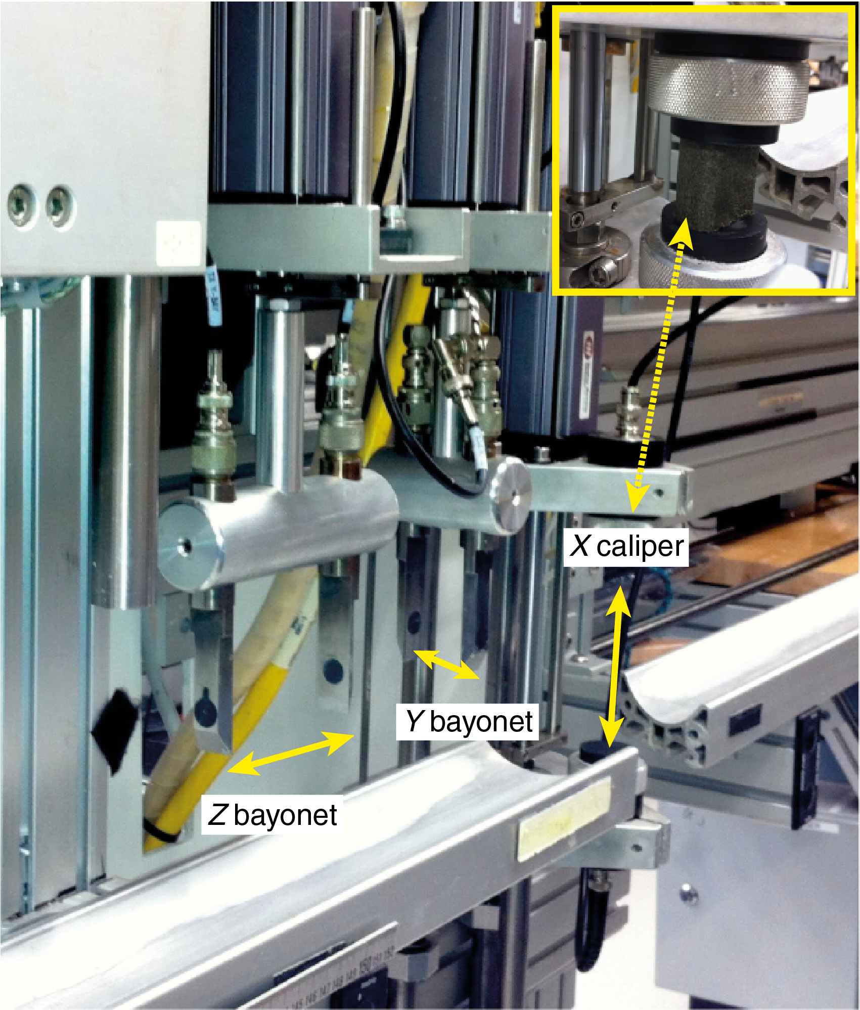
Figure F23. SHMG.
Moisture and density measurements
Discrete samples from working halves were selected to carry out MAD measurements to determine wet and dry bulk density, grain density, water content, and porosity. For soft-sediment cores, ~10 cm3 samples were collected with a plastic syringe. Generally, three samples were collected per core with the aim of representing the complete core lithology. For harder sediments or rocks, samples were taken adjacent to the samples that were cut and prepared for other laboratories, such as paleomagnetism.
Sediment samples were placed in numbered, preweighed ~16 mL Wheaton glass vials to obtain wet and dry sediment mass and dry volume measurements. Wet sample mass was first measured on each vial before placing it in a convection oven for approximately 24 h at 105° ± 5°C to dry. Once samples were dried, they were cooled in a desiccator for at least 3 h before measuring dry mass and volume. Wet and dry sample masses were determined to an accuracy of 0.005 g using two Mettler Toledo electronic balances, with one balance acting as a reference and the other acting as an unknown. A standard mass of similar value to the sample mass was placed on the reference balance to increase the accuracy of the unknown sample measurement (Figure F24). An averaging algorithm in the MADMax software was used to correct for the motion of the ship. The default measurement setting of the two balances was 300 measurements over an interval of ~1.5 min.
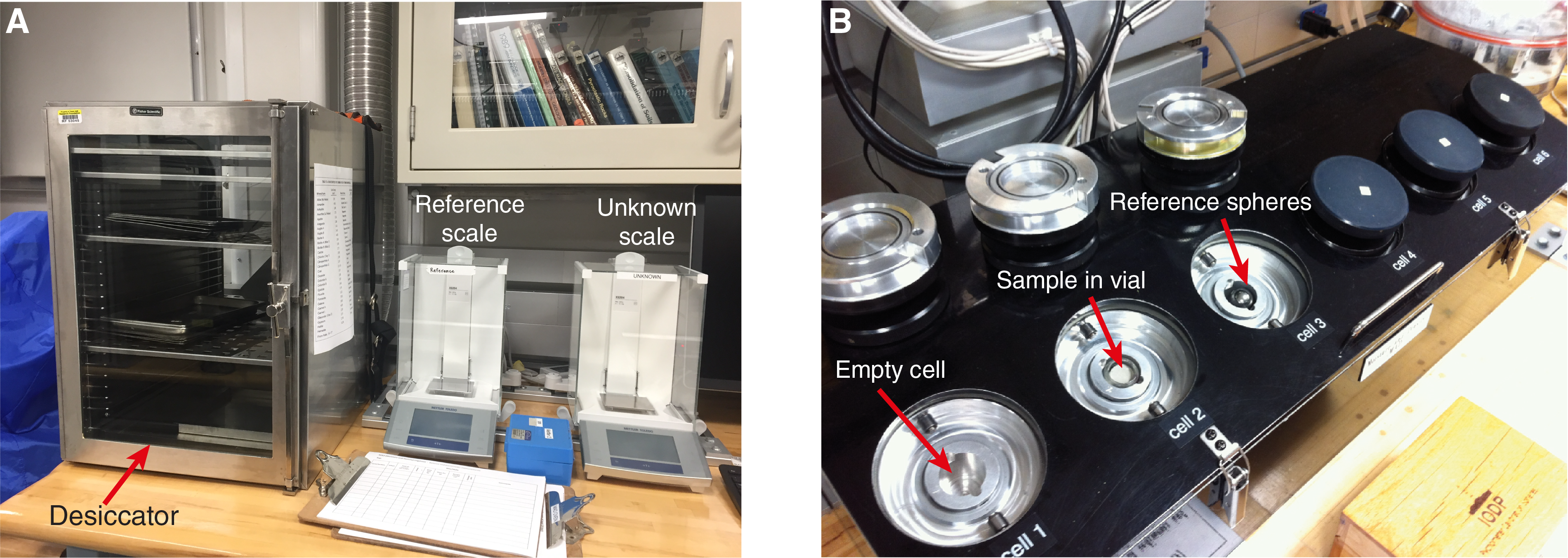
Figure F24. Equipment used for MAD analyses.
Dry sample volume was determined using a six-celled, custom-configured Micrometrics AccuPyc 1330TC helium-displacement pycnometer (Figure F24). The precision of each cell is 1% of the full-scale volume. Volume measurements were preceded by three purges of the sample chamber with helium warmed to ~28°C. Three measurement cycles were run for each sample. A set of two calibration spheres was periodically placed in each chamber to check for instrument drift and systematic error. The volumes occupied by the numbered Wheaton vials were calculated before the expedition by multiplying the weight of each vial against the average density of the vial glass. The procedures for the determination of these physical properties comply with the American Society for Testing and Materials (ASTM) designation 2216 (ASTM International, 1990). The relationships and assumptions for calculations of physical property parameters are discussed in detail in Blum (1997) and Weber et al. (1997) and summarized below. The MADMax shipboard program was used for computing the displayed MAD properties.
Mass and volume calculation
Wet mass (Mwet), dry mass (Mdry), and dry volume (Vdry) were measured in the laboratory as detailed above. The mass ratio (rm) is a computational constant of 0.965 (i.e., 0.965 g of freshwater per 1 g of seawater). Salt precipitated in sediment pores during the drying process is included in the Mdry and Vdry values. The mass of the evaporated water (Mwater) and salt (Msalt) in the sample are given by
where s is the assumed saltwater salinity (0.035%) corresponding to a pore water density (ρpw) of 1.024 g/cm3 (from experimental and empirical relations between salinity and density at laboratory conditions; Blum, 1997) and a salt density (ρsalt) of 2.22 g/cm3. The corrected mass of pore water (Mpw), volume of pore water (Vpw), mass of solids excluding salt (Msolid), volume of salt (Vsalt), volume of solids excluding salt (Vsolid), and wet volume (Vwet) are defined as
Wet (or total) volume (Vt), dry mass (Mdry), and dry volume (Vdry) were measured in the laboratory. Total mass, including the freshwater of the pore water, is calculated using a water density of 1 g/cm3 by
Assuming a pore water density of 1.024 g/cm3, the volume of the pore water is calculated as
Finally, the mass of the pore water is estimated as
Calculation of bulk properties
Water content (w) is expressed as the ratio of the mass of pore water to wet sediment (total) mass:
Wet bulk density (ρwet), dry bulk density (ρdry), sediment grain density (ρsolid), porosity (ϕ), and void ratio (VR) are calculated using the following expressions:
Stratigraphic correlation
The Expedition 382 scientific objectives required the recovery of complete stratigraphic sections to the best extent possible. A continuous sedimentary sequence cannot be recovered from a single borehole because gaps in recovery exist between successive cores even when recovery for individual cores exceeds 100% (Ruddiman et al., 1987; Hagelberg et al., 1995). The magnitude of the gaps cannot be known. A complete (synthetic) stratigraphic section, commonly referred to as a splice, is constructed by combining stratigraphic sections from two or more holes recovered at the same site to produce a composite and continuous record. To maximize the probability of bridging gaps between cores from any given hole (so as to document the magnitude of the gap and to recover "missing" sediment), each hole is correlated with the others using core physical properties. One hole with a clear mudline is used as the depth anchor, and the initially recorded core depths for each hole are offset by amounts required to line the holes up at correlation tie points. At least two holes, and in many cases three or more holes, are needed to generate a complete (primary) splice from cores recovered using the APC system. Typically, four or more holes must be recovered to permit the construction of a complete alternate (e.g., secondary) splice, although the correlation of intervals with the splice may allow some splice duplication.
Our methodology for developing splices attempted to follow a basic strategy that is now common practice during all high-resolution paleoceanographic IODP expeditions within the constraints of competing demands for time as well as weather and icebergs. We used the initial analyses of core petrophysical data run on the WRMSL to develop preliminary composite depths for the purposes of making real-time drilling decisions following the strategy developed by the ODP Leg 202 Shipboard Scientific Party (2003). In most cases, we were not able to change the drilling decisions because of competing pressures, and in some cases, core gaps were subsequently lined up for long intervals.
Our goals for stratigraphic correlation, in priority order, were as follows:
- To establish a composite depth scale,
- To define a sampling splice where possible, and
- To guide drilling in real time where possible to enhance the chances of recovering a complete stratigraphic section.
In meeting these goals, several different depth scales were created (Figure F25). A detailed discussion of the definitions of these depth scales and the processes by which they were created are outlined below.
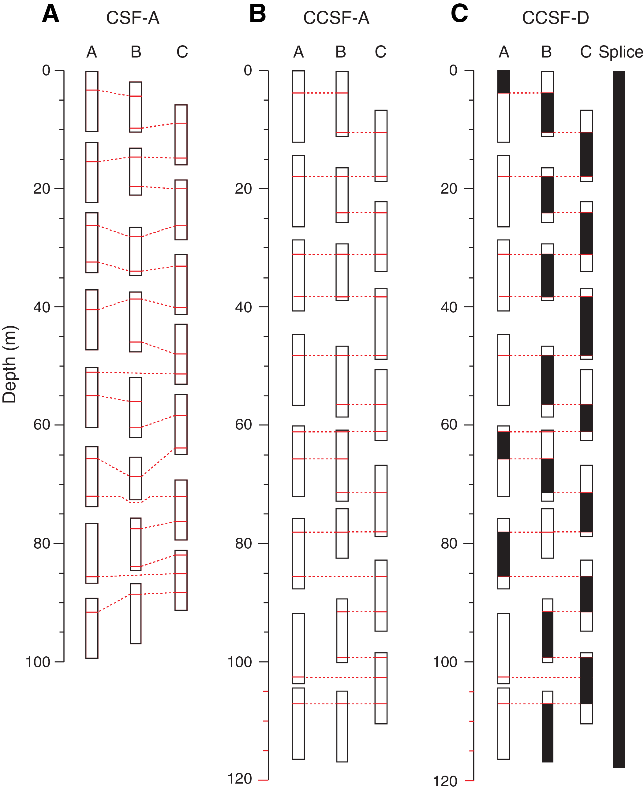
Figure F25. Depth scales used.
Composite depth scale
The initial depth scale produced during IODP coring is the CSF-A scale (Figure F25A). This depth scale is defined as the length the drill string is advanced core by core. The CSF-A scale can be inaccurate because of ship heave (which is beyond that compensated for during APC coring), tidal variations in sea level, core expansion, and other sources of error.
Before a splice can be constructed, cores from multiple holes must be stratigraphically correlated with each other. Such correlation transfers the CSF-A scale into a composite depth scale referred to as core composite depth below seafloor, Method A (CCSF-A) (Figure F25B). The splice that can be generated from a subset of these correlations is built on a scale known as core composite depth below seafloor, Method D (CCSF-D) (Figure F25C). Importantly, differences between these depth scales occur because features may be slightly offset between individual holes on their own CCSF-A scales and the splice on the CCSF-D scale.
The CCSF-A scale is built by assuming the uppermost sediment (commonly referred to as the mudline) in the first core from one of the holes is the sediment/water interface. This selected core becomes the anchor in the composite depth scale. From this anchor, core petrophysical data are correlated among holes starting from the top. Despite the potential for relative stretching or thinning, a single depth offset or "affine" value is chosen for each core to best align the observed physical property feature to the equivalent cores in adjacent holes. The affine values are added to the CSF-A depth in sequence down the holes.
During Expedition 382, affine ties were typically established using 2 or 1 cm resolution MS or GRA density data derived on the WRMSL. These ties were then confirmed using core photographs and other physical property data (most notably NGR intensity data). Specific methods for WRMSL and SHMSL measurements are described in Physical properties, and SHIL measurements are described in Lithostratigraphy. Most WRMSL and SHMSL core logging data were collected at 1 or 2.5 cm intervals depending on time availability and core flow. SHIL data are pixel based and thus at an even higher resolution.
Composite depth scale construction
The core logging data were imported into the specialized shipboard software program Correlator (version 3; Mac). Correlator enables the construction of a composite depth scale for each hole at a given site by depth shifting individual cores to maximize the correlation of reproducible features observed in the core petrophysical data. For hole-to-hole correlations and for plotting results, data were cropped to avoid incorporating anomalous data influenced by edge effects at section boundaries, at core tops, or in voids where no sediment was present. All original data are retained in the LIMS database.
Correlations among cores from adjacent holes are evaluated both visually and statistically (by windowed cross correlation). The depth offsets for each core that are necessary to convert CSF-A depths to the CCSF-A scale are recorded in an affine table for each site. The CCSF-A depth for any point in a core equals the CSF-A depth plus the affine offset. Correlation at a finer resolution between cores is not possible with Correlator because depth adjustments are applied linearly to individual cores. At this stage, no adjustments are made in the length of each core, such as numerically squeezing and stretching within cores. Finer scale adjustments of individual depths within cores relative to splice depths (e.g., Hagelberg et al., 1995; Pälike et al., 2005) or relative to logging data (e.g., Harris et al., 1995) can be done following the development of the splice. Such finer scale adjustments are required to assign accurate CCSF-D values to samples taken from cores that are not part of a site's main splice.
Owing to imperfect core recovery and/or disturbance, not all cores can be tied into the CCSF-A scale. Therefore, the base of the continuous CCSF-A scale does not always correspond to the bottom of the deepest core recovered from the deepest hole. The CSF-A depths of cores that cannot be tied directly into the overlying continuous CCSF-A scale are appended to it. CCSF-A depths for these cores are determined by adding a constant offset to CSF-A, which is usually determined by the average percent growth of the composite section given by the affine values used to establish the continuous CCSF-A for that site up to that point. An exception to this procedure occurs when cores from two or more holes recovered from depths greater than the base of the CCSF-A and CCSF-D splice can be correlated with each other. In this scenario, it is possible to generate a "floating" CCSF-A scale and CCSF-D splice for an interval deeper than the continuous CCSF-A scale.
Splice
The splice is a composite stratigraphic section that represents the complete record at a site or through intervals at a site. It is composed of core sections from adjacent holes such that coring gaps in one hole are filled with core from an adjacent hole. An effort is also made to minimize the inclusion of disturbed sections or intervals of sediment fall-in (typically the top ~10–100 cm of a core) or flow-in. Disturbed sections are identified by examining the cores, their photographs, and X-radiographs. The splice ultimately should guide core sampling for high-resolution studies. Tables and figures in each site chapter summarize the intervals from each hole used to construct the splice if a splice could be constructed. The portion of the CCSF-A depth scale that is used to construct the splice is referred to as the CCSF-D depth scale. Within the splice sections, CCSF-D depths are identical to CCSF-A depths.
In generating a splice, depth intervals within cores are not squeezed or stretched by Correlator. It is therefore not possible to align all the correlative features in each core using affine values. Depth differences between features in different holes on the CCSF-A scale may reflect small-scale differences in sedimentation and/or distortion caused by the coring and archiving processes. For example, the tops of APC cores may be stretched and the bottoms may be compressed, although this depends on lithology and the extent of lithification. Even though all samples have CCSF-A depths, the final composite depth scale (CCSF-D) is only formally defined within the primary splice. Accordingly, affine values should not be used to assign CCSF-D values to samples taken from cores not used to construct the primary (or alternative) splice without further evaluation of stratigraphic correlations (Figure F26).
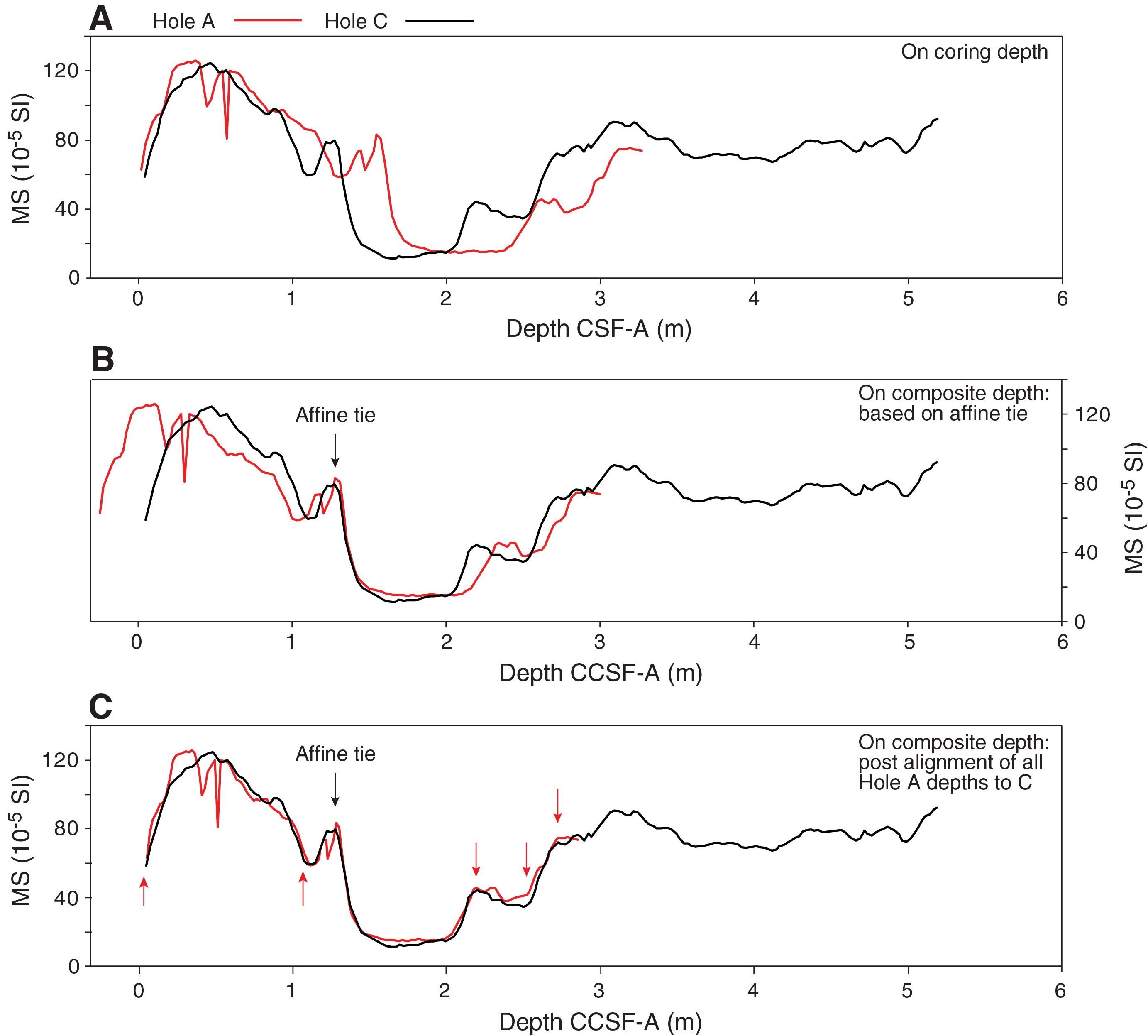
Figure F26. Site U1534 MS data adjusted to CCSF scale.
To minimize subjectivity when generating splice tie points, we followed four rules:
- Tie points were defined, where possible, by a peak or trough in these data. We prefer this approach because it removes the possibility that splice jumps occur during important climate transitions recorded by paleodata subsequently generated from the record.
- Where possible, we avoided using the first and last sections of cores where disturbance due to drilling artifacts (even if not apparent in core logging data) is most likely.
- We attempted to incorporate those parts of the stratigraphic sequence that in our judgment were most representative of the holes recovered and appeared to be the least disturbed.
- To ensure that paleodata generated postcruise but prior to the sampling party for Site U1534 can be robustly tied to the age model developed for the CCSF-D depth scale for a site, we tried to include intervals sampled during the expedition for pilot data in its splice.
Downhole measurements
Downhole logs are used to determine the physical, chemical, and structural properties of the formations penetrated by a borehole. The data are rapidly and continuously collected with depth and measured in situ; they can be interpreted in terms of the stratigraphy, lithology, mineralogy, and geochemical composition of the penetrated formation. Where core recovery is incomplete or disturbed, log data may provide the only characterization of the borehole section. Where core recovery is good, downhole logging data are complementary to core data and may be interpreted jointly. Downhole logs measure formation properties on an intermediate scale between geophysical surveys and laboratory measurements obtained from core samples. They are useful in calibrating the interpretation of geophysical survey data (e.g., downhole velocity values) and provide a necessary link for the integrated understanding of physical properties and seismic information. In addition, formation temperature as a function of depth can be measured using the APCT-3, which is deployed together with the APC coring system for selected depths. The obtained temperature gradient combined with thermal conductivity measurements allows us to estimate the local geothermal heat flux, which is an indicator of the geology and tectonic regime of a region.
Wireline logging
During wireline logging operations, logs are recorded with a variety of Schlumberger logging tools that are combined into several tool strings (Figure F27; Table T10) and lowered into the hole after completion of coring operations. The tool strings are lowered downhole on a seven-conductor wireline cable before being pulled up at a constant speed, typically 250–550 m/h, to provide continuous measurements of several properties simultaneously. One tool string was used during Expedition 382. The modified triple combination (triple combo) included the Hostile Environment Litho-Density Sonde (HLDS), Hostile Environment Natural Gamma Ray Sonde (HNGS), Enhanced Digital Telemetry Cartridge (EDTC-B), High-Resolution Laterolog Array (HRLA), Magnetic Susceptibility Sonde (MSS-B), and Dipole Sonic Imager (DSI). These tools measure gamma radiation, porosity, density, resistivity, MS, and P- and S-wave velocity. Each tool string contains a telemetry cartridge for communicating through the wireline to the Schlumberger data acquisition system (MAXIS unit) on the ship. Total gamma ray is also measured. During Expedition 382, a downhole log was collected in Hole U1536E. We included the DSI tool on the triple combo because collecting downhole velocity data was a high priority together with density.
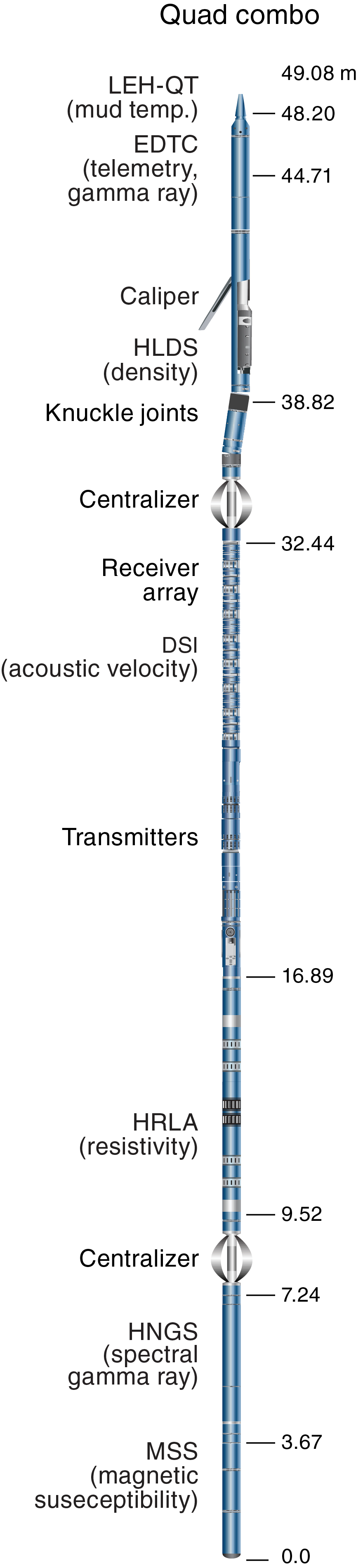
Figure F27. Quad combo downhole logging tool string.
Before logging, the borehole was flushed of debris by circulating viscous drilling fluid and then filled with a seawater-based logging gel (sepiolite mud mixed with seawater and weighted with barite; approximate density = 10.5 lb/gal) to help stabilize the borehole walls. The BHA was pulled up to ~83 m WSF to cover the upper part of the open hole. Although heave was high during logging operations, the wireline heave compensator (WHC) was not used because the software that controls the compensation did not receive correct ship motion data, resulting in a fast drop of the upper pulleys to the lower end stop when it was switched on. During the logging run, incoming data were recorded and monitored in real time on the MCM MAXIS logging computer.
Logged sediment properties and tool measurement principles
The logged properties and the principles used in the tools to measure them are described below. More detailed information on individual tools and their geological applications may be found in Serra (1984, 1986, 1989), Schlumberger (1989, 1994), Rider (1996), Goldberg (1997), Lovell et al. (1998), and Ellis and Singer (2007). A complete online list of acronyms for the Schlumberger tools and measurement curves is at http://www.apps.slb.com/cmd/index.aspx.
Natural gamma radiation
The HNGS uses two bismuth germanate scintillation detectors and five-window spectroscopy to determine concentrations of potassium (in weight percent), thorium, and uranium (both in parts per million) from the characteristic gamma ray energies of isotopes in the 40K, 232Th, and 238U radioactive decay series, which dominate the natural radiation spectrum. The computation of the elemental abundances uses a least-squares method of extracting U, Th, and K elemental concentrations from the spectral measurements. The HNGS filters out gamma ray energies below 500 keV, eliminating sensitivity to bentonite or KCl in the drilling mud and improving measurement accuracy. The HNGS also provides a measure of the total spectral gamma ray (HSGR) emission and uranium-free or computed gamma ray (HCGR), which are both measured in American Petroleum Institute units (gAPI). HNGS data are corrected for borehole diameter variations during acquisition.
The EDTC, which is used primarily to communicate data to the surface, also contains a gamma ray sensor. The sensor includes a sodium iodide scintillation detector that measures the total natural gamma ray emissions of the formation. It is not a spectral tool, but it provides total gamma radiation for each pass. The inclusion of the HNGS in the tool string allowed us to use the gamma ray data for depth-match processing between the logging measurements and core-log integration.
Density and photoelectric factor
Because the borehole was considered stable, formation density was measured with the HLDS. The HLDS contains a cesium (137Cs) gamma ray source (662 keV) and far and near gamma ray detectors mounted on a shielded skid that is pressed against the borehole wall by a hydraulically activated decentralizing arm. Gamma rays emitted by the source undergo Compton scattering, in which gamma rays are scattered by electrons in the formation. The number of scattered gamma rays that reach the detectors is proportional to the density of electrons in the formation, which is in turn related to bulk density. Porosity may also be derived from this bulk density if the matrix (grain) density is known.
The HLDS also computes the photoelectric effect (PEF), a measure of the photoelectric absorption of low-energy gamma radiation. Photoelectric absorption of gamma rays occurs when their energy falls below 150 keV as a result of being repeatedly scattered by electrons in the formation. PEF is determined by comparing the counts from the far detector in the high-energy region, where only Compton scattering occurs, with those in the low-energy region, where count rates depend on both reactions. PEF varies according to the chemical composition of the minerals present and can be used to identify the overall mineral makeup of the formation (Serra, 1984; Schlumberger, 1989).
Good contact between the tool and borehole wall is essential for good HLDS logs; poor contact results in underestimation of density values. The density correction and caliper measurement of the hole are used to check the contact quality. In the deeper parts of the hole, the PEF log should be used with caution, especially in washouts, because barium in the logging mud swamps the signal despite a correction for the influence of mud.
Electrical resistivity
Resistivity can be used to evaluate porosity for a given salinity and resistivity of IW.
The HRLA tool provides six resistivity measurements with different depths of investigation including the borehole (mud) resistivity and five measurements of formation resistivity with increasing penetration into the formation. The tool sends a focused current into the formation and measures the intensity necessary to maintain a constant drop in voltage across a fixed interval, providing direct resistivity measurements. The array has one central (source) electrode and six electrodes above and below it that serve alternatively as focusing and returning current electrodes. By rapidly changing the roles of these electrodes, a simultaneous resistivity measurement at six penetration depths is achieved. The tool is designed to ensure that all signals are measured at exactly the same time and tool position to reduce the sensitivity to "shoulder bed" effects when crossing sharp beds thinner than the electrode spacing. The design of the HRLA, which eliminates the need for a surface reference electrode, improves formation resistivity evaluation compared to traditional dual induction and allows the full range of resistivity to be measured from low (e.g., in high-porosity sediments) to high (e.g., in basalt). The HRLA needs to be run centralized in the borehole for optimal results, so knuckle joints were used to centralize the HRLA while allowing the density and porosity tools to maintain good contact with the borehole wall.
Magnetic susceptibility
The MSS was the only non-Schlumberger wireline tool run during the expedition. It was designed and built by Lamont-Doherty Earth Observatory (LDEO). It measures MS (the ease with which formations are magnetized when subjected to a magnetic field). MS is ultimately related to the concentration and composition (size, shape, and mineralogy) of magnetic minerals (principally magnetite) in the formation. The MSS dual-coil sensor provides ~40 cm vertical resolution measurements with a ~20 cm depth of horizontal investigation. The MSS was run as the lowermost tool in the triple combo tool string using a specially developed data translation cartridge that enables the MSS to be run in combination with the Schlumberger tools.
MS data are plotted as uncalibrated instrument units. The MSS reading responses are affected by temperature and borehole size (higher temperatures lead to higher susceptibility measurements). When the MS signal in sediment is very low, the detection limits of the tool may be reached. For QC and environmental correction, the MSS also measures internal tool temperature, z-axis acceleration, and low-resolution borehole conductivity.
Acoustic velocity
The sound velocity through formations is measured by the DSI, which measures the transit times between sonic transmitters and an array of eight receivers. The direct measurement is a combination of replicate measurements and therefore is relatively free from the effects of formation damage and an enlarged borehole (Schlumberger, 1989). In addition to compressional wave velocity, the DSI has two crossed-dipole transmitters that allow shear wave velocity measurement. Dipole measurements are necessary to measure shear velocity in slow formations with shear velocity values below the sound velocity values in the borehole fluid.
Wireline heave compensator
A WHC system compensates for the vertical motion of the ship (heave) and maintains a steady motion of the logging tools to ensure high-quality logging data acquisition (Liu et al., 2013; Iturrino et al., 2013). The WHC uses a vertical accelerometer (motion reference unit [MRU]) positioned under the rig floor near the ship's center of gravity to calculate the vertical motion of the ship with respect to the seafloor. It then adjusts the length of the wireline by varying the distance between two sets of pulleys through which the cable passes to minimize downhole tool motion. Real-time measurements of uphole (surface) and downhole acceleration are made simultaneously by the MRU and the EDTC, respectively. An LDEO-developed software package allows these data to be analyzed and compared in real time, displaying the actual motion of the logging tool string and enabling monitoring of the efficiency of the compensator. As mentioned previously, the WHC was not used during logging because of issues in the software that controls the compensation, which did not receive correct ship motion data.
Logging data flow, data quality, and log processing
Data for each wireline logging run were monitored in real time and recorded using the Schlumberger MAXIS 500 system. Logging measurement depth is determined from the length of the cable payed out from the winch on the ship and is measured on the WRF depth scale. The seafloor is usually identified on the HSGR log by the abrupt upward reduction in gamma ray count at the water/sediment interface (mudline), and the seafloor depth is subtracted to give the WSF depth. Discrepancies between the DSF and WSF depth scales may occur because of incomplete heave compensation, incomplete correction for cable stretch, and cable slip. For Hole U1536E, the seafloor was difficult to determine by the step in HSGR because it was a low amplitude similar to the noise level because the top ~10 m of the sediment column was very biogenic rich with low contents of radioactive isotopes. Deeper, the correlation among different properties including MSS and HSGR was used to determined the correct seafloor depth.
The most determining factor influencing the log data quality is the condition of the borehole wall and the vertical movement of the ship. Where the borehole diameter varies over short intervals because of washouts of softer material or ledges of harder material, the logs from tools that require good contact with the borehole wall may be degraded. "Bridged" sections, where borehole diameter is significantly narrower than the bit size, also cause irregular log results. The quality of the borehole is improved by minimizing the circulation of drilling fluid while drilling, flushing the borehole to remove debris, and logging as soon as possible after drilling and conditioning are completed.
The downhole log data were transferred on shore to LDEO for standardized data processing. Schlumberger's Techlog software package is used for most of the processing, which mainly includes depth matching that removes depth offsets between different logging runs. The records are referred to the WMSF scale. Additional processing includes corrections to certain tools and logs, log documentation including an assessment of log quality, and data format conversion to ASCII and GIF.
The data were transferred back to the ship within a few days of logging and made available to the science party.
Log-core-seismic integration
A depth-traveltime relationship must be determined at the site to correlate log and core data acquired at depth with seismic reflection profiles in two-way traveltime. A calibrated depth-traveltime relationship allows for correlation of the borehole stratigraphy with seismic reflection features. Logging sonic data from the uphole and downhole runs as well as core data (PWC measurements) were used to convert to seismic traveltime and create synthetic seismograms using the Petrel software package to select the best fit for the time-depth model (see Physical properties and Core-log-seismic integration in the Site U1536 chapter [Weber et al., 2021a]).
Downhole formation temperature measurements
In situ temperature measurements were made with the APCT-3 (Heesemann et al., 2006) at all sites, specifically in Holes U1534A, U1534C, U1535A, U1536A, U1536B, U1537A, U1537D, U1538A, and U1538D. The APCT-3 is composed of a battery pack, data logger, and platinum resistance-temperature device calibrated over a temperature range of 0°–30°C. This instrument perfectly fits into the coring shoe of the APC system. Once the APCT-3 is deployed, it is first stopped to rest at the mudline for 5 min to thermally equilibrate with bottom water before entering the borehole. Frictional heating is created as the APCT-3 moves into the formation and causes instantaneous temperature increases. This heat gradually dissipates into the surrounding sediment as the APCT-3 equilibrates to the temperature of the formation. Then the APCT-3 is held in place for ~10 min while it acquires the temperature of the cutting shoe every 1 s.
The equilibrium temperature of the sediment is estimated by applying a mathematical heat-conduction model to the temperature decay record (Horai and Von Herzen, 1985). The synthetic thermal decay curve for the APCT-3 is a function of the geometry and thermal properties of the probe and the sediment (Bullard, 1954; Horai and Von Herzen, 1985). Equilibrium temperature is estimated by applying a fitting procedure (Pribnow et al., 2000). However, if the APC does not achieve a full stroke or if the ship pulls the APC up from full penetration, the temperature equilibration curve is disturbed and the temperature determination is not accurate. The nominal accuracy of APCT-3 temperature measurements under favorable conditions is ±0.05°C.
APCT-3 downhole temperature data are combined with thermal conductivity measurements (see Physical properties) obtained from the sections. Heat flow is estimated according to the Bullard method to be consistent with the synthesis of ODP heat flow data by Pribnow et al. (2000).
References
Abelmann, A., 1992. Early to middle Miocene radiolarian stratigraphy of the Kerguelen Plateau, Leg 120. In Wise, S.W., Jr., Schlich, R., et al., Proceedings of the Ocean Drilling Program, Scientific Results, 120: College Station, TX (Ocean Drilling Program), 757–783. https://doi.org/10.2973/odp.proc.sr.120.165.1992
Acton, G., Morris, A., Musgrave, R., Zhao, X., and IODP SRM Personnel, 2017. Assessment of the New Superconducting Rock Magnetometer (SRM) on the JOIDES Resolution. http://iodp.tamu.edu/publications/JRSO/SRM_Workshop_2017.pdf
Acton, G.D., Okada, M., Clement, B.M., Lund, S.P., and Williams, T., 2002. Paleomagnetic overprints in ocean sediment cores and their relationship to shear deformation caused by piston coring. Journal of Geophysical Research: Solid Earth, 107(B4):2067–2081. https://doi.org/10.1029/2001JB000518
Akiba, F., 1982. Late Quaternary diatom biostratigraphy of the Bellingshausen Sea, Antarctic Ocean. Report of the Technology Research Center, Japan National Oil Corporation, 16:31–74.
Andrén, T., Jørgensen, B.B., Cotterill, C., Green, S., Andrén, E., Ash, J., Bauersachs, T., Cragg, B., Fanget, A.-S., Fehr, A., Granoszewski, W., Groeneveld, J., Hardisty, D., Herrero-Bervera, E., Hyttinen, O., Jensen, J.B., Johnson, S., Kenzler, M., Kotilainen, A., Kotthoff, U., Marshall, I.P.G., Martin, E., Obrochta, S., Passchier, S., Quintana Krupinski, N., Riedinger, N., Slomp, C., Snowball, I., Stepanova, A., Strano, S., Torti, A., Warnock, J., Xiao, N., and Zhang, R., 2015. Methods. In Andrén, T., Jørgensen, B.B., Cotterill, C., Green, S., and the Expedition 347 Scientists, Proceedings of the Integrated Ocean Drilling Program, 347: College Station, TX (Integrated Ocean Drilling Program). https://doi.org/10.2204/iodp.proc.347.102.2015
Armbrecht, L.H., Lowe, V., Escutia, C., Iwai, M., McKay, R., and Armand, L. 2018. Variability in diatom and silicoflagellate assemblages during mid-Pliocene glacial-interglacial cycles determined in Hole U1361A of IODP Expedition 318, Antarctic Wilkes Land Margin. Marine Micropaleontology, 139:28–41. https://doi.org/10.1016/j.marmicro.2017.10.008
Arney, J.E., McGonigal, K.L., Ladner, B.C., and Wise, S.W., Jr., 2003. Lower Oligocene to middle Miocene diatom biostratigraphy of ODP Site 1140, Kerguelen Plateau. In Frey, F.A., Coffin, M.F., Wallace, P.J., and Quilty, P.G. (Eds.), Proceedings of the Ocean Drilling Program, Scientific Results, 183: College Station, TX (Ocean Drilling Program), 1–21. https://doi.org/10.2973/odp.proc.sr.183.009.2003
ASTM International, 1990. Standard method for laboratory determination of water (moisture) content of soil and rock (Standard D2216–90). In Annual Book of ASTM Standards for Soil and Rock (Volume 04.08): Philadelphia (American Society for Testing Materials). [revision of D2216-63, D2216-80]
Baldauf, J.G., and Barron, J.A., 1991. Diatom biostratigraphy: Kerguelen Plateau and Prydz Bay regions of the Southern Ocean. In Barron, J., Larsen, B., et al., Proceedings of the Ocean Drilling Program, Scientific Results, 119: College Station, TX (Ocean Drilling Program), 547–598. https://doi.org/10.2973/odp.proc.sr.119.135.1991
Balsam, W.L., and Damuth, J.E., 2000. Further investigations of shipboard vs. shore-based spectral data: implications for interpreting Leg 164 sediment composition. In Paull, C.K., Matsumoto, R., Wallace, P., and Dillon, W.P. (Eds.), Proceedings of the Ocean Drilling Program, Scientific Results, 164: College Station, TX (Ocean Drilling Program), 313–324. https://doi.org/10.2973/odp.proc.sr.164.222.2000
Balsam, W.L., Damuth, J.E., and Schneider, R.R., 1997. Comparison of shipboard vs. shore-based spectral data from Amazon Fan cores: implications for interpreting sediment composition. In Flood, R.D., Piper, D.J.W., Klaus, A., and Peterson, L.C. (Eds.), Proceedings of the Ocean Drilling Program, Scientific Results, 155: College Station, TX (Ocean Drilling Program), 193–215. https://doi.org/10.2973/odp.proc.sr.155.210.1997
Barron, J.A., 2003. Planktonic marine diatom record of the past 18 m.y.: appearances and extinctions in the Pacific and Southern Oceans. Diatom Research, 18(2):203–224. https://doi.org/10.1080/0269249X.2003.9705588
Barron, J.A., Baldauf, J.G., Barrera, E., Caulet, J.-P., Huber, B.T., Keating, B.H., Lazarus, D., Sakai, H., Thierstein, H.R., and Wei, W., 1991. Biochronologic and magnetochronologic synthesis of Leg 119 sediments from the Kerguelen Plateau and Prydz Bay, Antarctica. In Barron, J., Larsen, B., et al., Proceedings of the Ocean Drilling Program, Scientific Results, 119: College Station, TX (Ocean Drilling Program), 813–847. https://doi.org/10.2973/odp.proc.sr.119.188.1991
Berggren, W.A., 1992. Neogene planktonic foraminifer magnetobiostratigraphy of the southern Kerguelen Plateau (Sites 747, 748, and 751). In Wise, S.W., Jr., Schlich, R., et al., Proceedings of the Ocean Drilling Program, Scientific Results, 120: College Station, TX (Ocean Drilling Program), 631–647. https://doi.org/10.2973.odp.proc.sr.120.153.1992
Bijl, P.K., Houben, A.J.P., Bruls, A., Pross, J., and Sangiorgi, F., 2018. Stratigraphic calibration of Oligocene–Miocene organic-walled dinoflagellate cysts from offshore Wilkes Land, East Antarctica, and a zonation proposal. Journal of Micropaleontology, 37(1):105–138. https://doi.org/10.5194/jm-37-105-2018
Blum, P., 1997. Technical Note 26: Physical Properties Handbook—A Guide to the Shipboard Measurement of Physical Properties of Deep-Sea Cores. Ocean Drilling Program. https://doi.org/10.2973/odp.tn.26.1997
Bohaty, S.M., Scherer, R.P., and Harwood, D.M., 1998. Quaternary diatom biostratigraphy and palaeoenvironments of the CRP-1 drillcore, Ross Sea, Antarctica. Terra Antartica, 5(3):431–454. https://epic.awi.de/id/eprint/27451/1/Boh1998a.pdf
Bohaty, S.M., Wise, S.W., Jr., Duncan, R.A., Moore, C.L., and Wallace, P.J., 2003. Neogene diatom biostratigraphy, tephra stratigraphy, and chronology of ODP Hole 1138A, Kerguelen Plateau. In Frey, F.A., Coffin, M.F., Wallace, P.J., and Quilty, P.G. (Eds.), Proceedings of the Ocean Drilling Program, Scientific Results, 183: College Station, TX (Ocean Drilling Program), 1–53. https://doi.org/10.2973/odp.proc.sr.183.016.2003
Brinkhuis, H., Munsterman, D.K., Sengers, S., Sluijs, A., Warnaar, J., and Williams, G.L., 2003. Late Eocene–Quaternary dinoflagellate cysts from ODP Site 1168, off western Tasmania. In Exon, N.F., Kennett, J.P., and Malone, M.J. (Eds.), Proceedings of the Ocean Drilling Program, Scientific Results, 189: College Station, TX (Ocean Drilling Program), 1–36. https://doi.org/10.2973/odp.proc.sr.189.105.2003
Buckley, D.E., MacKinnon, W.G., Cranston, R.E., and Christian, H.A., 1994. Problems with piston core sampling: mechanical and geochemical diagnosis. Marine Geology, 117(1–4):95–106. https://doi.org/10.1016/0025-3227(94)90008-6
Bullard, E.C., 1954. The flow of heat through the floor of the Atlantic Ocean. Proceedings of the Royal Society of London, Series A: Mathematical, Physical and Engineering Sciences, 222(1150):408–429. https://doi.org/10.1098/rspa.1954.0085
Burns, D.A., 1975. Distribution, abundance, and preservation of nannofossils in Eocene to recent Antarctic sediments. New Zealand Journal of Geology and Geophysics, 18(4):583–596. https://doi.org/10.1080/00288306.1975.10421558
Cantrill, D.J., and Poole, I., 2012. The Vegetation of Antarctica through Geological Time: Cambridge, United Kingdom (Cambridge University Press). https://doi.org/10.1017/CBO9781139024990
Caulet, J.-P., 1991. Radiolarians from the Kerguelen Plateau, Leg 119. In Barron, J., Larsen, B., et al., Proceedings of the Ocean Drilling Program, Scientific Results, 119: College Station, TX (Ocean Drilling Program), 513–546. https://doi.org/10.2973/odp.proc.sr.119.137.1991
Censarek, B., and Gersonde, R., 2002. Miocene diatom biostratigraphy at ODP Sites 689, 690, 1088, 1092 (Atlantic sector of the Southern Ocean). Marine Micropaleontology, 45(3–4):309–356. https://doi.org/10.1016/S0377-8398(02)00034-8
Channell, J.E.T., Hodell, D.A., and Curtis, J.H., 2016. Relative paleointensity (RPI) and oxygen isotope stratigraphy at IODP Site U1308: North Atlantic RPI stack for 1.2–2.2 Ma (NARPI-2200) and age of the Olduvai Subchron. Quaternary Science Reviews, 131(A):1–19. https://doi.org/10.1016/j.quascirev.2015.10.011
Ciesielski, P.F., 1983. The Neogene and Quaternary diatom biostratigraphy of subantarctic sediments, Deep Sea Drilling Project Leg 71. In Ludwig, W.J., Krasheninnikov, V.A., et al., Initial Reports of the Deep Sea Drilling Project, 71: Washington, DC (U.S. Government Printing Office), 635–666. https://doi.org/10.2973/dsdp.proc.71.125.1983
Clowes, C.D., Hannah, M.J., Wilson, G.J., and Wrenn, J.H., 2016. Marine palynostratigraphy and new species from the Cape Roberts drill-holes, Victoria Land Basin, Antarctica. Marine Micropaleontology, 126:65–84. https://doi.org/10.1016/j.marmicro.2016.06.003
Cody, R., Levy, R., Crampton, J., Naish, T., Wilson, G., and Harwood, D., 2012. Selection and stability of quantitative stratigraphic age models: Plio–Pleistocene glaciomarine sediments in the ANDRILL 1B drillcore, McMurdo Ice Shelf. Global and Planetary Change, 96–97:143–156. https://doi.org/10.1016/j.gloplacha.2012.05.017
Cody, R.D., Levy, R.H., Harwood, D.M., and Sadler, P.M., 2008. Thinking outside the zone: high-resolution quantitative diatom biochronology for the Antarctic Neogene. Palaeogeography, Palaeoclimatology, Palaeoecology, 260(1–2):92–121. https://doi.org/10.1016/j.palaeo.2007.08.020
Constable, C., and Tauxe, L., 1990. The bootstrap for magnetic susceptibility tensors. Journal of Geophysical Research: Solid Earth, 95(B6):8383–8395. https://doi.org/10.1029/JB095iB06p08383
Cremer, H., Roberts, D., McMinn, A., Gore, D., and Melles, M., 2003. The Holocene diatom flora of Marine Bays in the Windmill Islands, East Antarctica. Botanica Marina, 46(1):82–106. https://doi.org/10.1515/BOT.2003.010
Crundwell, M.P., Morgans, H.E.G., and Hollis, C.J., 2016. Micropaleontological report on dredge samples collected during the 2015 VESPA (Volcanic Evolution of South Pacific Arcs) expedition. GNS Science Internal Report.
Davis, N.M, Proctor, D.M., Holmes, S.P., Relman, D.A., and Callahan, B.J., 2018. Simple statistical identification and removal of contaminant sequences in marker-gene and metagenomics data. Microbiome, 6: 226. https://doi.org/10.1186/s40168-018-0605-2
De Schepper, S., Fischer, E.I., Groeneveld, J., Head, M.J., and Matthiessen, J., 2011. Deciphering the palaeoecology of late Pliocene and early Pleistocene dinoflagellate cysts. Palaeogeography, Palaeoclimatology, Palaeoecology, 309(1–2):17–32. https://doi.org/10.1016/j.palaeo.2011.04.020
Dickens, G.R., Koelling, M., Smith, D.C., Schneiders, L., and the IODP Expedition 302 Scientists, 2007. Rhizon sampling of pore waters on scientific drilling expeditions: an example from the IODP Expedition 302, Arctic Coring Expedition (ACEX). Scientific Drilling, 4:22–25. https://doi.org/10.2204/iodp.sd.4.08.2007
Droser, M.L., and O'Connell, S., 1992. Trace fossils and ichnofabric in Triassic sediments from cores recovered on Ocean Drilling Program Leg 122. In von Rad, U., Haq, B.U., et al., Proceedings of the Ocean Drilling Program, Scientific Results, 122: College Station, TX (Ocean Drilling Program), 475–486. https://doi.org/10.2973/odp.proc.sr.122.170.1992
Dunlea, A.G., Murray, R.W., Harris, R.N., Vasiliev, M.A., Evans, H., Spivack, A.J., and D'Hondt, S., 2013. Assessment and use of NGR instrumentation on the JOIDES Resolution to quantify U, Th, and K concentrations in marine sediment. Scientific Drilling, 15:57–63. https://doi.org/10.2204/iodp.sd.15.05.2013
Ellis, D.V., and Singer, J.M., 2007. Well Logging for Earth Scientists (2nd edition): New York (Elsevier). https://doi.org/10.1007/978-1-4020-4602-5
Ellwood, B.B., 1980. Induced and remanent magnetic properties of marine sediments as indicators of depositional processes. Marine Geology, 38(1–3):233–244. https://doi.org/10.1016/0025-3227(80)90061-4
Esper, O., and Zonneveld, K.A.F., 2007. The potential of organic-walled dinoflagellate cysts for the reconstruction of past sea-surface conditions in the Southern Ocean. Marine Micropaleontology, 65(3–4):185–212. https://doi.org/10.1016/j.marmicro.2007.07.002
Expedition 318 Scientists, 2011. Methods. In Escutia, C., Brinkhuis, H., Klaus, A., and the Expedition 318 Scientists, Proceedings of the Integrated Ocean Drilling Program, 318: Tokyo (Integrated Ocean Drilling Program Management International, Inc.). https://doi.org/10.2204/iodp.proc.318.102.2011
Fenner, J., 1991. Late Pliocene–Quaternary diatom stratigraphy in the Atlantic sector of the Southern Ocean. In Ciesielski, P.F., Kristoffersen, Y., et al., Proceedings of the Ocean Drilling Program, Scientific Results, 114: College Station, TX (Ocean Drilling Program), 97–121. https://doi.org/10.2973/odp.proc.sr.114.187.1991
Fenner, J., Schrader, H.-J., and Wienigk, H., 1976. Diatom phytoplankton studies in the southern Pacific Ocean: composition and correlation to the Antarctic Convergence and its paleoecological significance. In Hollister, C.D., Craddock, C., et al., Initial Reports of the Deep Sea Drilling Project, 35: Washington, DC (U.S. Government Printing Office), 757–813. https://doi.org/10.2973/dsdp.proc.35.app3.1976
Florindo, F., Farmer, R.K., Harwood, D.M., Cody, R.D., Levy, R., Bohaty, S.M., Carter, L., and Winkler, A., 2013. Paleomagnetism and biostratigraphy of sediments from Southern Ocean ODP Site 744 (southern Kerguelen Plateau): implications for early-to-middle Miocene climate in Antarctica. Global and Planetary Change, 110(C):434–454. https://doi.org/10.1016/j.gloplacha.2013.05.004
Frederichs, T., Bleil, U., Däumler, K., von Dobeneck, T., and Schmidt, A.M., 1999. The magnetic view on the marine paleoenvironment: parameters, techniques, and potentials of rock magnetic studies as a key to paleoclimatic and paleoceanographic changes. In Fischer, G., and Wefer, G. (Eds.), Use of Proxies in Paleoceanography: Examples from the South Atlantic: Berlin (Springer-Verlag), 575–599. https://doi.org/10.1007/978-3-642-58646-0_24
Gersonde, R., 1990. Taxonomy and morphostructure of Neogene diatoms from the Southern Ocean, ODP Leg 113. In Barker, P.F., Kennett, J.P., et al., Proceedings of the Ocean Drilling Program, Scientific Results, 113: College Station, TX (Ocean Drilling Program), 791–802. https://doi.org/10.2973/odp.proc.sr.113.128.1990
Gersonde, R., 1991. Taxonomy and morphostructure of late Neogene diatoms from the Maude Rise (Antarctic Ocean). Polarforschung, 59(3):141–171. http://epic.awi.de/28264/1/Polarforsch1989_3_4.pdf
Gersonde, R., Abelmann, A., Burckle, L.H., Hamilton, N., Lazarus, D., McCartney, K., O'Brien, P., Spieß, V., and Wise, S.W., Jr., 1990. Biostratigraphic synthesis of Neogene siliceous microfossils from the Antarctic Ocean, ODP Leg 113 (Weddell Sea). In Barker, P.F., Kennett, J.P., et al., Proceedings of the Ocean Drilling Program, Scientific Results, 113: College Station, TX (Ocean Drilling Program), 915–936. https://doi.org/10.2973/odp.proc.sr.113.209.1990
Gersonde, R., and Bárcena, M.A., 1998. Revision of the upper Pliocene: Pleistocene diatom biostratigraphy for the northern belt of the Southern Ocean. Micropaleontology, 44(1):84–98. https://doi.org/10.2307/1486086
Gersonde, R., and Burckle, L.H., 1990. Neogene diatom biostratigraphy of ODP Leg 113, Weddell Sea (Antarctic Ocean). In Barker, P.F., Kennett, J.P., et al., Proceedings of the Ocean Drilling Program, Scientific Results, 113: College Station, TX (Ocean Drilling Program), 761–789. https://doi.org/10.2973/odp.proc.sr.113.126.1990
Gieskes, J.M., Gamo, T., and Brumsack, H., 1991. Technical Note 15: Chemical Methods for Interstitial Water Analysis Aboard JOIDES Resolution. Ocean Drilling Program. https://doi.org/10.2973/odp.tn.15.1991
Gilmore, G.R., 2008. Practical Gamma-ray Spectrometry (2nd edition): Hoboken, NJ (John Wiley & Sons). https://doi.org/10.1002/9780470861981
Giosan, L., Flood, R.D., and Aller, R.C., 2002. Paleoceanographic significance of sediment color on western North Atlantic drifts: I. Origin of color. Marine Geology, 189(1–2):25–41. https://doi.org/10.1016/S0025-3227(02)00321-3
Gohl, K., Wellner, J.S., Klaus, A., Bauersachs, T., Bohaty, S.M., Courtillat, M., Cowan, E.A., Esteves, M.S.R., De Lira Mota, M.A., Fegyveresi, J.M., Frederichs, T., Gao, L., Halberstadt, A.R., Hillenbrand, C.-D., Horikawa, K., Iwai, M., Kim, J.-H., King, T.M., Klages, J.P., Passchier, S., Penkrot, M.L., Prebble, J.G., Rahaman, W., Reinardy, B.T.I., Renaudie, J., Robinson, D.E., Scherer, R.P., Siddoway, C.S., Wu, L., and Yamane, M., 2021. Expedition 379 methods. In Gohl, K., Wellner, J.S., Klaus, A., and the Expedition 379 Scientists, Amundsen Sea West Antarctic Ice Sheet History. Proceedings of the International Ocean Discovery Program, 379: College Station, TX (International Ocean Discovery Program). https://doi.org/10.14379/iodp.proc.379.102.2021
Goldberg, D., 1997. The role of downhole measurements in marine geology and geophysics. Reviews of Geophysics, 35(3):315–342. https://doi.org/10.1029/97RG00221
Gombos, A.M., Jr., 1976. Paleogene and Neogene diatoms from the Falkland Plateau and Malvinas Outer Basin: Leg 36, Deep Sea Drilling Project. In Barker, P.F., Dalziel, I.W.D. et al., Initial Reports of the Deep Sea Drilling Project, 36: Washington, DC (U.S. Government Printing Office), 575–687. https://doi.org/10.2973/dsdp.proc.36.111.1977
Graber, K.K., Pollard, E., Jonasson, B., and Schulte, E. (Eds.), 2002. Technical Note 31: Overview of Ocean Drilling Program engineering tools and hardware. Ocean Drilling Program. https://doi.org/10.2973/odp.tn.31.2002
Gradstein, F.M., Ogg, J.G., Schmitz, M.D., and Ogg, G.M. (Eds.), 2012. The Geological Time Scale 2012: Amsterdam (Elsevier). https://doi.org/10.1016/C2011-1-08249-8
Hagelberg, T.K., Pisias, N.G., Shackleton, N.J., Mix, A.C., and Harris, S., 1995. Refinement of a high-resolution, continuous sedimentary section for studying equatorial Pacific Ocean paleoceanography, Leg 138. In Pisias, N.G., Mayer, L.A., Janecek, T.R., Palmer-Julson, A., and van Andel, T.H. (Eds.), Proceedings of the Ocean Drilling Program, Scientific Results, 138: College Station, TX (Ocean Drilling Program), 31–46. https://doi.org/10.2973/odp.proc.sr.138.103.1995
Hannah, M.J., 2006. The palynology of ODP Site 1165, Prydz Bay, East Antarctica: a record of Miocene glacial advance and retreat. Palaeogeography, Palaeoclimatology, Palaeoecology, 231(1–2):120–133. https://doi.org/10.1016/j.palaeo.2005.07.029
Hannah, M.J., Wilson, G.J., and Wrenn, J.H., 2000. Oligocene and Miocene marine palynomorphs from CRP-2/2A, Victorialand Basin, Antarctica. Terra Antartica, 7(4):503–511. http://epic.awi.de/27368/1/Han2000f.pdf
Harland, R., and Pudsey, C.J., 2002. Protoperidiniacean dinoflagellate cyst taxa from the upper Miocene of ODP Leg 178, Antarctic Peninsula. Review of Palaeobotany and Palynology, 120(3–4):263–284. https://doi.org/10.1016/S0034-6667(02)00080-5
Harris, S., Hagelberg, T., Mix, A., Pisias, N.G., and Shackleton, N.J., 1995. Sediment depths determined by comparisons of GRAPE and logging density data during Leg 138. In Pisias, N.G., Mayer, L.A., Janecek, T.R., Palmer-Julson, A., and van Andel, T.H. (Eds.), Proceedings of the Ocean Drilling Program, Scientific Results, 138: College Station, TX (Ocean Drilling Program), 47–55. https://doi.org/10.2973/odp.proc.sr.138.104.1995
Harwood, D.M., 1986. Diatoms. In Barrett, P.J. (Ed.), Antarctic Cenozoic History from the MSSTS-1 Drillhole, McMurdo Sound. DSIR Bulletin (New Zealand), 237:69–107.
Harwood, D.M., 1989. Siliceous microfossils. In Barrett, P.J. (Ed.), Antarctic Cenozoic History from the CIROS-1 Drillhole, McMurdo Sound. DSIR Bulletin (New Zealand), 245:67–97.
Harwood, D.M., Bohaty, S.M., and Scherer, R.P., 1998. Lower Miocene diatom biostratigraphy of the CRP-1 drillcore, McMurdo Sound, Antarctica. Terra Antartica, 5(3):499–514. https://epic.awi.de/27445/1/Har1998d.pdf
Harwood, D.M., Lazarus, D.B., Abelmann, A., Aubry, M.-P., Berggren, W.A., Heider, F., Inokuchi, H., Maruyama, T., McCartney, K., Wei, W., and Wise, S.W., Jr., 1992. Neogene integrated magnetobiostratigraphy of the central Kerguelen Plateau, Leg 120. In Wise, S.W., Jr., Schlich, R., et al., Proceedings of the Ocean Drilling Program, Scientific Results, 120: College Station, TX (Ocean Drilling Program), 1031–1052. https://doi.org/10.2973/odp.proc.sr.120.185.1992
Harwood, D.M., and Maruyama, T., 1992. Middle Eocene to Pleistocene diatom biostratigraphy of Southern Ocean sediments from the Kerguelen Plateau, Leg 120. In Wise, S.W., Jr., Schlich, R., et al., Proceedings of the Ocean Drilling Program, Scientific Results, 120: College Station, TX (Ocean Drilling Program), 683–733. https://doi.org/10.2973/odp.proc.sr.120.160.1992
Harwood, D.M., Scherer, R.P., and Webb, P.-N., 1989. Multiple Miocene marine productivity events in West Antarctica as recorded in upper Miocene sediments beneath the Ross Ice Shelf (Site J-9). Marine Micropaleontology, 15(1–2):91–115. https://doi.org/10.1016/0377-8398(89)90006-6
Hays, J.D., and Opdyke, N.D., 1967. Antarctic radiolaria, magnetic reversals, and climate change. Science, 158(3804):1001–1011. http://www.jstor.org.lib-ezproxy.tamu.edu:2048/stable/1722956
Heesemann, M., Villinger, H., Fisher, A.T., Tréhu, A.M., and White, S., 2006. Data report: testing and deployment of the new APCT-3 tool to determine in situ temperatures while piston coring. In Riedel, M., Collett, T.S., Malone, M.J., and the Expedition 311 Scientists. Proceedings of the Integrated Ocean Drilling Program, 311: Washington, DC (Integrated Ocean Drilling Program Management International, Inc.). https://doi.org/10.2204/iodp.proc.311.108.2006
Hext, G.R., 1963. The estimation of second-order tensors, with related tests and designs. Biometrika, 50(3–4):353–373. https://doi.org/10.1093/biomet/50.3-4.353
Hilgen, F.J., Lourens, L.J., and Van Dam, J.A., 2012. The Neogene period. With contributions by A.G. Beu, A.F. Boyes, R.A. Cooper, W. Krijgsman, J.G. Ogg, W.E. Piller, and D.S. Wilson. In Gradstein, F.M., Ogg, J.G., Schmitz, M.D., and Ogg, G.M. (Eds.), The Geologic Time Scale: Oxford, United Kingdom (Elsevier), 923–978. https://doi.org/10.1016/B978-0-444-59425-9.00029-9
Horai, K., and Von Herzen, R.P., 1985. Measurement of heat flow on Leg 86 of the Deep Sea Drilling Project. In Heath, G.R., Burckle, L.H., et al., Initial Reports of the Deep Sea Drilling Project, 86: Washington, DC (U.S. Government Printing Office), 759–777. https://doi.org/10.2973/dsdp.proc.86.135.1985
Houben, A.J.P., Bijl, P.K., Pross, J., Bohaty, S.M., Passchier, S., Stickley, C.E., Röhl, U., et al., 2013. Reorganization of Southern Ocean plankton ecosystem at the onset of Antarctic glaciation. Science, 340(6130):341–344. https://doi.org/10.1126/science.1223646
House, C.H., Cragg, B.A., Teske, A., and the Leg 201 Scientific Party, 2003. Drilling contamination tests during ODP Leg 201 using chemical and particulate tracers. In D'Hondt, S.L., Jørgensen, B.B., Miller, D.J., et al., Proceedings of the Ocean Drilling Program, Initial Reports, 201: College Station, TX (Ocean Drilling Program), 1–19. https://doi.org/10.2973/odp.proc.ir.201.102.2003
Iturrino, G., Liu, T., Goldberg, D., Anderson, L., Evans, H., Fehr, A., Guerin, G., et al., 2013. Performance of the wireline heave compensation system onboard D/V JOIDES Resolution. Scientific Drilling, 15:46–50. https://doi.org/10.2204/iodp.sd.15.08.2013
Iwai, M., Acton, G.D., Lazarus, D., Osterman, L.E., and Williams, T., 2002. Magnetobiochronologic synthesis of ODP Leg 178 rise sediments from the Pacific sector of the Southern Ocean: Sites 1095, 1096, and 1101. In Barker, P.F., Camerlenghi, A., Acton, G.D., and Ramsay, A.T.S. (Eds.), Proceedings of the Ocean Drilling Program, Scientific Results, 178: College Station, TX (Ocean Drilling Program), 1–40. https://doi.org/10.2973/odp.proc.sr.178.236.2002
Iwai, M., and Winter, D., 2002. Data report: taxonomic notes of Neogene diatoms from the western Antarctic peninsula: Ocean Drilling Program Leg 178. In Barker, P.F., Camerlenghi, A., Acton, G.D., and Ramsay, A.T.S. (Eds.), Proceedings of the Ocean Drilling Program, Scientific Results, 178: College Station, TX (Ocean Drilling Program), 1–57. https://doi.org/10.2973/odp.proc.sr.178.239.2002
Jaeger, J.M., Gulick, S.P.S., LeVay, L.J., Asahi, H., Bahlburg, H., Belanger, C.L., Berbel, G.B.B., Childress, L.B., Cowan, E.A., Drab, L., Forwick, M., Fukumura, A., Ge, S., Gupta, S.M., Kioka, A., Konno, S., März, C.E., Matsuzaki, K.M., McClymont, E.L., Mix, A.C., Moy, C.M., Müller, J., Nakamura, A., Ojima, T., Ridgway, K.D., Rodrigues Ribeiro, F., Romero, O.E., Slagle, A.L., Stoner, J.S., St-Onge, G., Suto, I., Walczak, M.H., and Worthington, L.L., 2014. Methods. In Jaeger, J.M., Gulick, S.P.S., LeVay, L.J., and the Expedition 341 Scientists, Proceedings of the Integrated Ocean Drilling Program, 341: College Station, TX (Integrated Ocean Drilling Program). https://doi.org/10.2204/iodp.proc.341.102.2014
Jenkins, D.G., 1993. Cenozoic southern mid- and high-latitude biostratigraphy and chronostratigraphy based on planktonic foraminifera. In Kennett, J.P., and Warnke, D.A. (Eds.), The Antarctic Paleoenvironment: A Perspective on Global Change: Part Two. Antarctic Research Series, 60:125–144. https://agupubs.onlinelibrary.wiley.com/doi/abs/10.1002/9781118668061.ch7
Johansen, J.R., Doucette, G.J., and Fryxell, G.A., 1985. The Genus Thalassiosira (Bacillariophyceae): morphology of heterovalvate resting spores of T. scotia. American Journal of Botany, 72:1861–1870. https://doi.org/10.1002/j.1537-2197.1985.tb08460.x
Jumikis, A.R., 1966. Thermal Soil Mechanics: New Brunswick, N.J. (Rutgers University Press).
Jutzeler, M., White, J.D.L., Talling, P.J., McCanta, M., Morgan, S., Le Friant, A., and Ishizuka, O., 2014. Coring disturbances in IODP piston cores with implications for offshore record of volcanic events and the Missoula megafloods. Geochemistry, Geophysics, Geosystems, 15(9):3572–3590. https://doi.org/10.1002/2014GC005447
Kemp, E.M., 1975. Palynology of Leg 28 drill sites, Deep Sea Drilling Project. In Hayes, D.E., Frakes, L.A., et al., Initial Reports of the Deep Sea Drilling Project, 28: Washington, DC (U.S. Government Printing Office), 599–623. https://doi.org/10.2973/dsdp.proc.28.116.1975
King, J., Banerjee, S.K., Marvin, J., and Özdemir, Ö., 1982. A comparison of different magnetic methods for determining the relative grain size of magnetite in natural materials: some results from lake sediments. Earth and Planetary Science Letters, 59(2):404–419. https:/doi.org/10.1016/0012-821X(82)90142-X
Kristiansen, J.I., 1982. The transient cylindrical probe method for determination of thermal parameters of earth materials [Ph.D. dissertation]. Åarhus University, Åarhus, Denmark.
Kvenvolden, K.A., and McDonald, T.J., 1986. Technical Note 6: Organic Geochemistry on the JOIDES Resolution—An Assay. Ocean Drilling Program. https://doi.org/10.2973/odp.tn.6.1986
Lazarus, D., 1990. Middle Miocene to Recent radiolarians from the Weddell Sea, Antarctica, ODP Leg 113. In Barker, P.F., Kennett, J.P., et al., Proceedings of the Ocean Drilling Program, Scientific Results, 113: College Station, TX (Ocean Drilling Program), 709–727. https://doi.org/10.2973/odp.proc.sr.113.132.1990
Lazarus, D., 1992. Antarctic Neogene radiolarians from the Kerguelen Plateau, Legs 119 and 120. In Wise, S.W., Jr., Schlich, R., et al., Proceedings of the Ocean Drilling Program, Scientific Results, 120: College Station, TX (Ocean Drilling Program), 785–809. https://doi.org/10.2973/odp.proc.sr.120.192.1992
Lazarus, D., Faust, K., and Popova-Goll, I., 2005. New species of prunoid radiolarians from the Antarctic Neogene. Journal of Micropaleontology, 24(2):97–121. https://doi.org/10.1144/jm.24.2.97
Lever, M.A., Alperin, M., Engelen, B., Inagaki, F., Nakagawa, S., Steinsbu, B.O., Teske A., and IODP Expedition 301 Scientists, 2006. Trends in basalt and sediment core contamination during IODP Expedition 301. Geomicrobiology Journal, 23(7):517–530. https://doi.org/10.1080/01490450600897245
Lisiecki, L.E., and Raymo, M.E., 2005. A Pliocene–Pleistocene stack of 57 globally distributed benthic δ18O records. Paleoceanography, 20(1):PA1003. https://doi.org/10.1029/2004PA001071
Liu, T., Iturrino, G., Goldberg, D., Meissner, E., Swain, K., Furman, C., Fitzgerald, P., Frisbee, N., Chlimoun, J., Van Hyfte, J., and Beyer, R., 2013. Performance evaluation of active wireline heave compensation systems in marine well logging environments. Geo-Marine Letters, 33(1):83–93. https://doi.org/10.1007/s00367-012-0309-8
Liu, Q., Roberts, A.P., Larrasoaña, J.C., Banerjee, S.K., Guyodo, Y., Tauxe, L., and Oldfield, F., 2012. Environmental magnetism: principles and applications. Reviews of Geophysics, 50(4):RG4002. https://doi.org/10.1029/2012RG000393
Lombari, G., and Lazarus, D.B., 1988. Neogene cycladophorid radiolarians from North Atlantic, Antarctic, and North Pacific deep-sea sediments. Micropaleontology, 34(2):97–135. https://doi.org/10.2307/1485657
Lourens, L.J., Hilgen, F.J., Laskar, J., Shackleton, N.J., and Wilson, D., 2004. The Neogene period. In Gradstein, F.M., Ogg, J., et al. (Eds.), A Geologic Time Scale 2004: Cambridge, United Kingdom (Cambridge University Press), 409–440. https://doi.org/10.1017/CBO9780511536045.022
Lovell, M.A., Harvey, P.K., Brewer, T.S., Williams, C., Jackson, P.D., and Williamson, G., 1998. Application of FMS images in the Ocean Drilling Program: an overview. In Cramp, A., MacLeod, C.J., Lee, S.V., and Jones, E.J.W. (Eds.), Geological Evolution of Ocean Basins: Results from the Ocean Drilling Program. Geological Society Special Publication, 131(1):287–303. https://doi.org/10.1144/GSL.SP.1998.131.01.18
MacLeod, C.J., Dick, H.J.B., Blum, P., Abe, N., Blackman, D.K., Bowles, J.A., Cheadle, M.J., Cho, K., Ciazela, J., Deans, J.R., Edgcomb, V.P., Ferrando, C., France, L., Ghosh, B., Ildefonse, B.M., Kendrick, M.A., Koepke, J.H., Leong, J.A.M., Liu, C., Ma, Q., Morishita, T., Morris, A., Natland, J.H., Nozaka, T., Pluemper, O., Sanfilippo, A., Sylvan, J.B., Tivey, M.A., Tribuzio, R., and Viegas, L.G.F., 2017. Expedition 360 methods. In MacLeod, C.J., Dick, H.J.B., Blum, P., and the Expedition 360 Scientists, Southwest Indian Ridge Lower Crust and Moho. Proceedings of the International Ocean Discovery Program, 360: College Station, TX (International Ocean Discovery Program). https://doi.org/10.14379/iodp.proc.360.102.2017
Mahood, A.D., and Barron, J.A., 1996. Late Pliocene diatoms in a diatomite from Prydz Bay, East Antarctica. Micropaleontology, 42(3):285–302. https://doi.org/10.2307/1485876
Manheim, F.T., and Sayles, F.L., 1974. Composition and origin of interstitial waters of marine sediments, based on deep sea drill cores. In Goldberg, E.D. (Ed.), The Sea (Volume 5): Marine Chemistry: The Sedimentary Cycle: New York (Wiley), 527–568.
Martos, Y.M., Catalán, M., and Galindo-Zaldivar, J., 2019. Curie Depth, heat flux and thermal subsidence reveal the Pacific mantle outflow through the Scotia Sea. Journal of Geophysical Research: Solid Earth, 124(11):10735–10751. https://doi.org/10.1029/2019JB017677
Martos, Y.M., Catalán, M., Jordan, T.A., Golynsky, A., Golynsky, D., Eagles, G., and Vaughan, D.G., 2017. Heat flux distribution of Antarctica unveiled. Geophysical Research Letters, 44(22):11417–11426. https://doi.org/10.1002/2017GL075609
Martos, Y.M., Jordan, T.A., Catalán, M., Jordan, T.M., Bamber, J.L., and Vaughan, D.G., 2018. Geothermal heat flux reveals the Iceland hotspot track underneath Greenland. Geophysical Research Letters, 45(16):8214–8222. https://doi.org/10.1029/2018GL078289
Mazzullo, J.M., Meyer, A., and Kidd, R.B., 1988. New sediment classification scheme for the Ocean Drilling Program. In Mazzullo, J., and Graham, A.G. (Eds.), Technical Note 8: Handbook for Shipboard Sedimentologists. Ocean Drilling Program, 44–67. https://doi.org/10.2973/odp.tn.8.1988
McCollum, D.W., 1975. Diatom stratigraphy of the Southern Ocean. In Hayes, D.E., Frakes, L.A., et al., Initial Reports of the Deep Sea Drilling Project, 28: Washington, DC (U.S. Government Printing Office), 515–571. https://doi.org/10.2973/dsdp.proc.28.112.1975
McCoy, F.W., 1985. Mid-core flow-in; implications for stretched stratigraphic sections in piston cores. Journal of Sedimentary Research, 55(4):608–610. https://doi.org/10.1306/212F8774-2B24-11D7-8648000102C1865D
McKay, R.M., De Santis, L., Kulhanek, D.K., Ash, J.L., Beny, F., Browne, I.M., Cortese, G., Cordeiro de Sousa, I.M., Dodd, J.P., Esper, O.M., Gales, J.A., Harwood, D.M., Ishino, S., Keisling, B.A., Kim, S., Kim, S., Laberg, J.S., Leckie, R.M., Müller, J., Patterson, M.O., Romans, B.W., Romero, O.E., Sangiorgi, F., Seki, O., Shevenell, A.E., Singh, S.M., Sugisaki, S.T., van de Flierdt, T., van Peer, T.E., Xiao, W., and Xiong, Z., 2019. Expedition 374 methods. In McKay, R.M., De Santis, L., Kulhanek, D.K., and the Expedition 374 Scientists, Ross Sea West Antarctic Ice Sheet History. Proceedings of the International Ocean Discovery Program, 374: College Station, TX (International Ocean Discovery Program). https://doi.org/10.14379/iodp.proc.374.102.2019
Medlin, L.K., and Priddle, J. (Eds.), 1990. Polar Marine Diatoms: Cambridge, United Kingdom (British Antarctic Survey).
Murray, R.W., Miller, D.J., and Kryc, K.A., 2000. Technical Note 29: Analysis of Major and Trace Elements in Rocks, Sediments, and Interstitial Waters by Inductively Coupled Plasma–Atomic Emission Spectrometry (ICP-AES). Ocean Drilling Program. https://doi.org/10.2973/odp.tn.29.2000
Nigrini, C., and Sanfilippo, A., 2001. Technical Note 27: Cenozoic radiolarian stratigraphy for low and middle latitudes with descriptions of biomarkers and stratigraphically useful species. Ocean Drilling Program. https://doi.org/10.2973/odp.tn.27.2001
Olney, M.P., Bohaty, S.M., Harwood, D.M., and Scherer, R.P., 2009. Creania lacyae gen. nov. et sp. nov. and Synedropsis cheethamii sp. nov., fossil indicators of Antarctic sea ice? Diatom Research, 24(2):357–375. https://doi.org/10.1080/0269249X.2009.9705807
Olney, M.P., Scherer, R.P., Harwood, D.M., and Bohaty, S.M., 2007. Oligocene–early Miocene Antarctic nearshore diatom biostratigraphy. Deep Sea Research, Part II: Topical Studies in Oceanography, 54(21–22):2325–2349. https://doi.org/10.1016/j.dsr2.2007.07.020
Pälike, H., Moore, T., Backman, J., Raffi, I., Lanci, L., Parés, J.M., and Janecek, T., 2005. Integrated stratigraphic correlation and improved composite depth scales for ODP Sites 1218 and 1219. In Wilson, P.A., Lyle, M., and Firth, J.V. (Eds.), Proceedings of the Ocean Drilling Program, Scientific Results, 199: College Station, TX (Ocean Drilling Program), 1–41. https://doi.org/10.2973/odp.proc.sr.199.213.2005
Petrushevskaya, M.G., 1967. Radiolarians of orders Spumellaria and Nassellaria of the Antarctic region. Biological Reports of the Soviet Antarctic Expedition (1955–1958), 3(12):5–186.
Petrushevskaya, M.G., 1975. Cenozoic radiolarians of the Antarctic, Leg 29, DSDP. In Kennett, J.P., Houtz, R.E., et al., Initial Reports of the Deep Sea Drilling Project, 29: Washington, DC (U.S. Government Printing Office), 541–675. https://doi.org/10.2973/dsdp.proc.29.114.1975
Popofsky, A., 1908. Die Radiolarien der Antarktis (mit Ausnahme der Tripyleen) (Radiolaria from the Antarctic [Tripylida excepted]). Deutsche Sudpolar Expedition 1901–1903, Zoologie II, 10:183–306.
Prebble, J.G., Crouch, E.M., Carter, L., Cortese, G., Bostock, H., and Neil, H., 2013. An expanded modern dinoflagellate cyst dataset for the Southwest Pacific and Southern Hemisphere with environmental associations. Marine Micropaleontology, 101:33–48. https://doi.org/10.1016/j.marmicro.2013.04.004
Pribnow, D., Kinoshita, M., and Stein, C., 2000. Thermal Data Collection and Heat Flow Recalculations for Ocean Drilling Program Legs 101–180: Hanover, Germany (Institute for Joint Geoscientific Research, Institut für Geowissenschaftliche Gemeinschaftsaufgaben [GGA]). http://www-odp.tamu.edu/publications/heatflow/ODPReprt.pdf
Ramsay, A.T.S., and Baldauf, J.G., 1999. A reassessment of the Southern Ocean biochronology. Memoir - Geological Society of America, 18:1–122.
Rees, A.I., and Woodall, W.A., 1975. The magnetic fabric of some laboratory-deposited sediments. Earth and Planetary Science Letters, 25(2):121–130. https://doi.org/10.1016/0012-821X(75)90188-0
Renaudie, J., 2012. A synthesis of Antarctic Neogene radiolarians: taxonomy, macroevolution and biostratigraphy [Ph.D. thesis]. Humboldt University of Berlin. https://doi.org/10.18452/16985
Renaudie, J., and Lazarus, D.B., 2012. New species of Neogene radiolarians from the Southern Ocean. Journal of Micropaleontology, 31(1):29–52. https://doi.org/10.1144/0262-821X10-026
Renaudie, J., and Lazarus, D.B., 2013. New species of Neogene radiolarians from the Southern Ocean–Part II. Journal of Micropaleontology, 32(1):59–86. https://doi.org/10.1144/jmpaleo2011-025
Renaudie, J., and Lazarus, D.B., 2015. New species of Neogene radiolarians from the Southern Ocean–Part III. Journal of Micropaleontology, 34(2):181–209. https://doi.org/10.1144/jmpaleo2013-034
Renaudie, J., and Lazarus, D.B., 2016. New species of Neogene radiolarians from the Southern Ocean–Part IV. Journal of Micropaleontology, 35(1):26–53. https://doi.org/10.1144/jmpaleo2014-026
Rider, M.H., 1996. The Geological Interpretation of Well Logs (2nd edition): Caithness, Scotland (Whittles Publishing).
Riding, J.B., and Kyffin-Hughes, J.E., 2011. A direct comparison of three palynological preparation techniques. Review of Palaeobotany and Palynology, 167(3–4):212–2218. https://doi.org/10.1016/j.revpalbo.2011.07.008
Riedel, W.R., 1958. Radiolaria in Antarctic sediments. Reports of BANZ Antarctic Research Expedition, 1979–1931, Series B, 6:247–255.
Ruddiman, W.F., Cameron, D., and Clement, B.M., 1987. Sediment disturbance and correlation of offset holes drilled with the hydraulic piston corer: Leg 94. In Ruddiman, W.F., Kidd, R.B., Thomas, E., et al., Initial Reports of the Deep Sea Drilling Project, 94: Washington, DC (U.S. Government Printing Office), 615–634. https://doi.org/10.2973/dsdp.proc.94.111.1987
Sangiorgi, F., Bijl, P.K., Passchier, S., Salzmann, U., Schouten, S., McKay, R., Cody, R.D., et al., 2018. Southern Ocean warming and Wilkes Land ice sheet retreat during the mid-Miocene. Nature Communications, 9(1):317. https://doi.org/10.1038/s41467-017-02609-7
Scherer, R.P., Bohaty, S.M., and Harwood, D.M., 2000. Oligocene and lower Miocene siliceous microfossil biostratigraphy of Cape Roberts Project core CRP-2/2A, Victoria Land Basin, Antarctica. Terra Antartica, 7(4):417–442. http://epic.awi.de/27353/1/Sch2000w.pdf
Scherer, R.P., Sjunneskog, C.M., Iverson, N.R., and Hooyer, T.S., 2004. Assessing subglacial processes from diatom fragmentation patterns. Geology, 32(7):557–560. https://doi.org/10.1130/G20423.1
Schlumberger, 1989. Log Interpretation Principles/Applications: Houston (Schlumberger Education Services), SMP–7017.
Schlumberger, 1994. IPL Integrated Porosity Lithology: Houston (Schlumberger Education Services), SMP-9270.
Schrader, H.-J., 1976. Cenozoic planktonic diatom biostratigraphy of the Southern Pacific Ocean. In Hollister, C.D., Craddock, C., et al., Initial Reports of the Deep Sea Drilling Project, 35: Washington, DC (U.S. Government Printing Office), 605–671. https://doi.org/10.2973/dsdp.proc.35.136.1976
Schwehr, K., and Tauxe, L., 2003. Characterization of soft-sediment deformation: detection of cryptoslumps using magnetic methods. Geology, 31(3):203–206. https://doi.org/10.1130/0091-7613(2003)031<0203:COSSDD>2.0.CO;2
Scott, F.J., and Thomas, D.P., 2005. Diatoms. In Scott, F.J., and Marchant, H.J. (Eds.), Antarctic Marine Protists: Canberra, ACT (Australian Biological Resources Study/Australian Antarctic Division), 13–201.
Serra, O., 1984. Fundamentals of Well-Log Interpretation (Volume 1): The Acquisition of Logging Data: Amsterdam (Elsevier).
Serra, O., 1986. Fundamentals of Well-Log Interpretation (Volume 2): The Interpretation of Logging Data: Amsterdam (Elsevier).
Serra, O., 1989. Formation MicroScanner Image Interpretation: Houston (Schlumberger Education Services), SMP-7028.
Shipboard Scientific Party, 2003. Explanatory notes. In Mix, A.C., Tiedemann, R., Blum, P., et al., Proceedings of the Ocean Drilling Program, Initial Reports, 202: College Station, TX (Ocean Drilling Program), 1–76. https://doi.org/10.2973/odp.proc.ir.202.102.2003
Sjunneskog, C., Riesselman, C., Winter, D., and Scherer, R., 2012. Fragilariopsis diatom evolution in Pliocene and Pleistocene Antarctic shelf sediments. Micropaleontology, 58(3):273–289. http://www.micropress.org/microaccess/micropaleontology/issue-291/article-1781
Sjunneskog, C., and Scherer, R.P., 2005. Mixed diatom assemblages in glacigenic sediment from the central Ross Sea, Antarctica. Palaeogeography, Palaeoclimatology, Palaeoecology, 218(3–4):287–300. https://doi.org/10.1016/j.palaeo.2004.12.019
Smith, D.C., Spivack, A.J., Fisk, M.R., Haveman, S.A., and Staudigel, H., 2000. Tracer-based estimates of drilling-induced microbial contamination of deep sea crust. Geomicrobiology Journal, 17(3):207–219. https://doi.org/10.1080/01490450050121170
Spieß, V., 1990. Cenozoic magnetostratigraphy of Leg 113 drill sites, Maud Rise, Weddell Sea, Antarctica. In Barker, P.F., Kennett, J.P., et al., Proceedings of the Ocean Drilling Program, Scientific Results, 113: College Station, TX (Ocean Drilling Program), 261–315. https://doi.org/10.2973/odp.proc.sr.113.182.1990
Stephenson, A., 1993. Three-axis static alternating field demagnetization of rocks and the identification of natural remanent magnetization, gyroremanent magnetization, and anisotropy. Journal of Geophysical Research: Solid Earth, 98(B1):373–381. https://doi.org/10.1029/92JB01849
Taira, A., 1989. Magnetic fabrics and depositional processes. In Taira, A., and Masuda, F. (Eds.), Sedimentary Facies in the Active Plate Margin. Advances in Earth and Planetary Sciences, 43–77.
Tauxe, L., 2010. Essentials of Paleomagnetism. With contributions by R.F. Butler, R. Van der Voo, and S.K. Banerjee: Berkeley, California (University of California Press).
Tauxe, L., Stickley, C.E., Sugisaki, S., Bijl, P.K., Bohaty, S.M., Brinkhuis, H., Escutia, C., et al., 2012. Chronostratigraphic framework for the IODP Expedition 318 cores from the Wilkes Land Margin: constraints for paleoceanographic reconstruction. Paleoceanography, 27(2):PA2214. https://doi.org/10.1029/2012PA002308
van Heck, S. (Ed.), 1981. Bibliography and taxa of calcareous nannoplankton. International Nannoplankton Association Newsletter, 3(1):4–41. http://ina.tmsoc.org/JNR/NINA/INANewsl3(1).pdf
Vasiliev, M.A., Blum, P., Chubarian, G., Olsen, R., Bennight, C., Cobine, T., Fackler, D., Hastedt, M., Houpt, D., Mateo, Z., and Vasilieva, Y.B., 2011. A new natural gamma radiation measurement system for marine sediment and rock analysis. Journal of Applied Geophysics, 75:455–463. https://doi.org/10.1016/j.jappgeo.2011.08.008
Vigour, R., and Lazarus, D., 2002. Biostratigraphy of late Miocene–early Pliocene radiolarians from ODP Leg 183 Site 1138. In Frey, F.A., Coffin, M.F., Wallace, P.J., and Quilty, P.G. (Eds.), Proceedings of the Ocean Drilling Program, Scientific Results, 183: College Station, TX (Ocean Drilling Program), 1–17. https://doi.org/10.2973/odp.proc.sr.183.007.2002
Von Herzen, R., and Maxwell, A.E., 1959. The measurement of thermal conductivity of deep-sea sediments by a needle-probe method. Journal of Geophysical Research, 64(10):1557–1563. https://doi.org/10.1029/JZ064i010p01557
Walczak, M.H., Stoner, J.S., Mix, A.C., Jaeger, J., Rosen, G.P., Channell, J.E.T., Heslop, D., and Xuan, C., 2017. A 17,000 yr paleomagnetic secular variation record from the southeast Alaskan margin: regional and global correlations. Earth and Planetary Science Letters, 473:177–189. https://doi.org/10.1016/j.epsl.2017.05.022
Warnock, J.P., and Scherer, R.P., 2015. Diatom species abundance and morphologically-based dissolution proxies in coastal Southern Ocean assemblages. Continental Shelf Research, 102:1–8. https://doi.org/10.1016/j.csr.2015.04.012
Warny, S., Askin, R.A., Hannah, M.J., Mohr, B.A.R., Raine, J.I., Harwood, D.M., Florindo, F., and the SMS Science Team, 2009. Palynomorphs from a sediment core reveal a sudden remarkably warm Antarctica during the middle Miocene. Geology, 37(10):955–958. https://doi.org/10.1130/G30139A.1
Weber, M.E., 1998. Estimation of biogenic carbonate and opal by continuous non-destructive measurements in deep-sea sediments: application to the eastern equatorial Pacific. Deep-Sea Research, Part I: Oceanographic Research Papers, 45(11):1955–1975. https://doi.org/10.1016/S0967-0637(98)00028-4
Weber, M.E., Niessen, F., Kuhn, G., and Wiedicke, M., 1997. Calibration and application of marine sedimentary physical properties using a multi-sensor core logger. Marine Geology, 136(3–4):151–172. http://dx.doi.org/10.1016/S0025-3227(96)00071-0
Weber, M.E., Raymo, M.E., Peck, V.L., Williams, T., Armbrecht, L.H., Bailey, I., Brachfeld, S.A., Cardillo, F.G., Du, Z., Fauth, G., García, M., Glüder, A., Guitard, M.E., Gutjahr, M., Hemming, S.R., Hernández-Almeida, I., Hoem, F.S., Hwang, J.-H., Iizuka, M., Kato, Y., Kenlee, B., Martos, Y.M., O'Connell, S., Pérez, L.F., Reilly, B.T., Ronge, T.A., Seki, O., Tauxe, L., Tripathi, S., Warnock, J.P., and Zheng, X., 2021a. Site U1536. In Weber, M.E., Raymo, M.E., Peck, V.L., Williams, T., and the Expedition 382 Scientists, Iceberg Alley and Subantarctic Ice and Ocean Dynamics. Proceedings of the International Ocean Discovery Program, 382: College Station, TX (International Ocean Discovery Program). https://doi.org/10.14379/iodp.proc.382.105.2021
Weber, M.E., Raymo, M.E., Peck, V.L., Williams, T., and the Expedition 382 Scientists, 2021b. Supplementary material, https://doi.org/10.14379/iodp.proc.382supp.2021. Supplement to Weber, M.E., Raymo, M.E., Peck, V.L., Williams, T., and the Expedition 382 Scientists, Iceberg Alley and Subantarctic Ice and Ocean Dynamics. Proceedings of the International Ocean Discovery Program, 382: College Station, TX (International Ocean Discovery Program). https://doi.org/10.14379/iodp.proc.382.2021
Wentworth, C.K., 1922. A scale of grade and class terms for clastic sediments. Journal of Geology, 30(5):377–392. https://doi.org/10.1086/622910
Whitehead, J.M., and Bohaty, S.M., 2003. Data report: Quaternary–Pliocene diatom biostratigraphy of ODP Sites 1165 and 1166, Cooperation Sea and Prydz Bay. In Cooper, A.K., O'Brien, P.E., and Richter, C. (Eds.), Proceedings of the Ocean Drilling Program, Scientific Results, 188: College Station, TX (Ocean Drilling Program), 1–25. https://doi.org/10.2973/odp.proc.sr.188.008.2003
Williams, G.L., Fensome, R.A., and MacRae, R.A., 2017. The Lentin and Williams index of fossil dinoflagellates (2017 edition). AASP Contributions Series, 48. https://palynology.org/wp-content/uploads/2017/01/AASP-Contribution-Series-No.48.pdf
Winter, D., and Iwai, M., 2002. Data report: Neogene diatom biostratigraphy, Antarctic Peninsula Pacific margin, ODP Leg 178 rise sites. In Barker, P.F., Camerlenghi, A., Acton, G.D., and Ramsay, A.T.S. (Eds.), Proceedings of the Ocean Drilling Program, Scientific Results, 178: College Station, TX (Ocean Drilling Program), 1–25. https://doi.org/10.2973/odp.proc.sr.178.230.2002
Winter, D., Sjunneskog, C., Scherer, R., Maffioli, P., and Harwood, D., 2012. Pliocene–Pleistocene diatom biostratigraphy of nearshore Antarctica from the AND-1B drillcore, McMurdo Sound. Global and Planetary Change, 96-97:59–74. https://doi.org/10.1016/j.gloplacha.2010.04.004
Winter, D.M., and Harwood, D.M., 1997. Integrated diatom biostratigraphy of late Neogene drillholes in Southern Victoria Land and correlation to Southern Ocean records. In Ricci, C.A. (Ed.), The Antarctic Region: Geological Evolution and Processes. Terra Antartica Publication, 985–992.
Wise, S.W., 1983. Mesozoic and Cenozoic calcareous nannofossils recovered by Deep Sea Drilling Project Leg 71 in the Falkland Plateau region, Southwest Atlantic Ocean. In Ludwig W.J., Krasheninnikov, V.A. et al., Initial Reports of the Deep Sea Drilling Project, 71: Washington (U.S. Government Printing Office), 481–550. https://doi.org/10.2973/dsdp.proc.71.121.1983
Yanagisawa, T., and Akiba, F., 1990. Taxonomy and phylogeny of the three marine diatom genera, Crucidenticula, Denticulopsis, and Neodenticula. Bulletin of the Geological Survey of Japan, 41(5):197–301. https://www.gsj.jp/data/bull-gsj/41-05_01.pdf
Zielinski, U., and Gersonde, R., 2002. Plio–Pleistocene diatom biostratigraphy from ODP Leg 177, Atlantic sector of the Southern Ocean. Marine Micropaleontology, 45(3–4):225–268. https://doi.org/10.1016/S0377-8398(02)00031-2
Zonneveld, K.A.F., Marret, F., Versteegh, G.J.M., Bogus, K., Bonnet, S., Bouimetarhan, I., Crouch, E., et al., 2013. Atlas of modern dinoflagellate cyst distribution based on 2405 data points. Review of Palaeobotany and Palynology, 191. https://doi.org/10.1016/j.revpalbo.2012.08.003
1 Weber, M.E., Raymo, M.E., Peck, V.L., Williams, T., Armbrecht, L.H., Bailey, I., Brachfeld, S.A., Cardillo, F.G., Du, Z., Fauth, G., García, M., Glüder, A., Guitard, M.E., Gutjahr, M., Hemming, S.R., Hernández-Almeida, I., Hoem, F.S., Hwang, J.-H., Iizuka, M., Kato, Y., Kenlee, B., Martos, Y.M., O'Connell, S., Pérez, L.F., Reilly, B.T., Ronge, T.A., Seki, O., Tauxe, L., Tripathi, S., Warnock, J.P., and Zheng, X., 2021. Expedition 382 methods. In Weber, M.E., Raymo, M.E., Peck, V.L., Williams, T., and the Expedition 382 Scientists, Iceberg Alley and Subantarctic Ice and Ocean Dynamics. Proceedings of the International Ocean Discovery Program, 382: College Station, TX (International Ocean Discovery Program). https://doi.org/10.14379/iodp.proc.382.102.2021
2 Expedition 382 Scientists' affiliations.
This work is distributed under the Creative Commons Attribution 4.0 International (CC BY 4.0) license. 