Weber, M.E., Raymo, M.E., Peck, V.L., Williams, T., and the Expedition 382 Scientists
Proceedings of the International Ocean Discovery Program Volume 382
publications.iodp.org

https://doi.org/10.14379/iodp.proc.382.105.2021
Site U15361
M.E. Weber, M.E. Raymo, V.L. Peck, T. Williams, L.H. Armbrecht, I. Bailey, S.A. Brachfeld, F.G. Cardillo, Z. Du, G. Fauth, M. García, A. Glüder, M.E. Guitard, M. Gutjahr, S.R. Hemming, I. Hernández-Almeida, F.S. Hoem, J.-H. Hwang, M. Iizuka, Y. Kato, B. Kenlee, Y.M. Martos, S. O'Connell, L.F. Pérez, B.T. Reilly, T.A. Ronge, O. Seki, L. Tauxe, S. Tripathi, J.P. Warnock, and X. Zheng2
Keywords: International Ocean Discovery Program, IODP, JOIDES Resolution, Expedition 382, Iceberg Alley and Subantarctic Ice and Ocean Dynamics, Site U1536, Dove Basin, Scotia Sea, Weddell Sea, sea ice, Antarctica, Antarctic Ice Sheet, sea level, ice-rafted debris, ice-rafted detritus, iceberg-rafted debris, iceberg, provenance, contourites, Weddell Sea Deep Water, Antarctic Circumpolar Current, Southern Hemisphere westerly winds, paleoceanography, paleoclimatology, mid-Pleistocene transition, Pliocene, interglacial climate, marine isotope stage, MIS 5, MIS 11
MS 382-105: Published 20 May 2021
Background and objectives
International Ocean Discovery Program (IODP) Site U1536 (proposed Site SCO-13) is located 235 km northwest of the South Orkney Islands at 59°26.46′S, 41°3.66′W in 3220 m of water. Site U1536 is the first of two sites drilled in Dove Basin, which is located in the southern Scotia Sea. This site was targeted to recover a complete Neogene record of Antarctic ice and ocean dynamics, examine the character and age of regionally correlative seismic reflectors, and date the acoustic basement to constrain the tectonic origin of Dove Basin.
Previous piston coring at Site MD07-3134 in a small subbasin in the northeastern part of Dove Basin recovered a 58 m long, high accumulation rate sediment record covering the last glacial cycle (Weber et al., 2012). Site U1536 is located 23 km east of that site in the deeper part of a broad basin and on the western flank of a north–south ridge.
Sediments in the southern Scotia Sea are primarily deposited by contourite currents along the pathway of the Antarctic Circumpolar Current. Specifically in Dove Basin, contourite deposition is also assumed to be influenced by Weddell Sea Deep Water (WSDW) flowing from the south through bathymetric gaps around the South Orkney Plateau after exiting the Weddell Sea (Maldonado et al., 2003). The contourites are lens shaped in seismic profiles, as thick as 1 km in the center of small troughs (Maldonado et al., 2006), and thin toward the edges of the troughs.
Three seismic lines indicate a basin-like structure with several small-scale ridges and continuous reflectors in the central to northern part of Dove Basin. Site U1536 is located at Shotpoint 1709 on Multichannel Seismic (MCS) Reflection Profile SCAN 10/04. Five seismic units were identified above acoustic basement (Maldonado et al., 2006), and the seismic reflectors show parallel lamination with occasionally undulating structures likely indicative of minor synsedimentary downslope transport. This downslope movement is a fairly common feature in the basin, and none of the Expedition 382 sites were able to avoid these disturbances completely. Site U1536 provided the best compromise between a relatively thick and undisturbed stratigraphic sequence for climate studies and access to acoustic basement located at a relatively shallow depth of ~900 meters below seafloor (mbsf).
At Site U1536, the main objective was to obtain a complete late Neogene record of ice and ocean dynamics in the center of "Iceberg Alley" in the more southerly of our two drilling areas in the Scotia Sea. Specific objectives include (1) the reconstruction of past variability in Antarctic Ice Sheet mass loss and its related sea level history, (2) a study of the water mass composition of the Drake Passage throughflow and WSDW inflow, and (3) a study of north–south shifts of the frontal systems in response to changing climate conditions, including changes in water mass properties, ocean temperature, and sea ice extent. An additional goal was to reconstruct changes in dust-climate couplings between Patagonia and Antarctica as well as related atmospheric circulation changes throughout the Pliocene–Pleistocene in a more distal location relative to the main dust source, Patagonia. A final science objective at Site U1536 was to drill through the deeper reflectors, specifically the basin-wide Reflector c, to determine the age of this unconformity. This determination would allow us to date the regional change in bottom water flow, which probably led to the formation of the reflector. We were not able to reach acoustic basement at ~900 mbsf to determine its nature and age because of time and hazard constraints.
Operations
We started the voyage across the Southern Ocean to Scotia Sea Site U1536 at 0848 h local time on 3 April 2019. Iceberg conditions in the region of Site U1536 were classified as "ice free" in the daily reports from the US National Ice Center. The first iceberg of the expedition was spotted at 1600 h at 56°20′S, 49°28′W. Midmorning on 5 April, we reduced speed because of icebergs in the general area and reduced visibility due to fog, but we were able to resume normal speed by late morning. The towed magnetometer was deployed during the transit in international waters. The 709 nmi transit to Site U1536 in the Dove Basin study area took 2.8 days at an average speed of 10.5 kt.
During the transit to Site U1536, we observed that the 3.5 kHz subbottom profile contains a series of reflections to about 100 mbsf, a notable level of detail not normally seen in such profiles. Based on this observation, we decided to make two 3.5 kHz survey profiles over the site in a cross shape, each 4 nmi long along the site survey seismic lines. The survey confirmed the water depth and provided details of the shallow reflectors at the site. The thrusters were lowered at 0430 h on 6 April, ending the transit.
The drill string was assembled and lowered to the seafloor at Site U1536. A pig was pumped down to remove rust from the inside of the drill pipe, but it appears that it did not emerge from the end of the drill string because the first attempt to take a mudline core recovered half of the pig. A second attempt also misfired, and despite deploying a barrel with a center bit to try to remove any remaining obstruction, the piston corer misfired a third time. We raised the drill string back to the ship to inspect the bottom-hole assembly (BHA). This process was interrupted from 0815 to 1500 h on 7 April with the bit at 77 meters below rig floor (mbrf) because sea conditions were too rough to safely handle the BHA on the rig floor. Eventually the BHA was inspected, no obstruction was found, and everything appeared to be functioning normally. Rough sea conditions returned at 1800 h, and we waited until 0730 h on 8 April for the weather to improve sufficiently to restart operations. We made up the BHA and tested that the piston corer was landing correctly. The rest of the drill string was assembled and lowered to the seafloor, and the top drive was installed by 1830 h. The first piston core run broke the shear pins mechanically before it could be shot as planned. The second piston corer was run with three shear pins to test that the system pressured up without problems. The third piston core was successful in recovering sediment.
Hole U1536A was started at 0005 h on 9 April. Core 382-U1536A-1F was run with a half-length barrel and recovered 4.5 m (100%) (Table T1). The core was almost full, but it appeared to recover a mudline, giving a water depth for Hole U1536A of 3219.5 m. Cores 1F–53F penetrated from the seafloor to 354.4 mbsf and recovered 364.3 m (103%). All full-length advanced piston corer (APC) cores (2H–23H) were oriented. Formation temperature measurements were made while taking Cores 7H, 10H, 16H, 19H, and 22H. The coring line parted during the Core 13H run, so 50 m of line was cut and the core barrel was fished. Cores 22H and 23H were difficult to pull out of the formation, so we switched to half-length APC (HLAPC) coring for Core 24F.
At 2115 h on 11 April, an iceberg approached within 5.7 nmi (5.5 h) of the ship, so we stopped coring and raised the drill string to ~50 mbsf following the previously established protocol for icebergs entering the "red zone." The red zone is defined as a projected closest point of approach (CPA) of less than 3 nmi and a time to reach that point as less than twice the time required to pull up the drill string to within 50 mbsf (T-time). At 0130 h on 12 April when the iceberg was 1.7 nmi away, we raised the drill string above the seafloor and moved ~1 nmi east-northeast to avoid the path of the iceberg, ending operations in Hole U1536A. By 0320 h, the iceberg had passed and we started to move back to Site U1536 while monitoring a second iceberg and a growler (small iceberg the size of a truck). At 0615 h, the location was free of ice and we started lowering the drill string to the seafloor.
Hole U1536B was started at 0930 h on 12 April. Cores 382-U1536B-1H through 25H penetrated from the seafloor to 226.1 mbsf and recovered 230.7 m (102%). All cores were oriented, and formation temperature measurements were made while taking Cores 5H, 8H, and 13H. At 1130 h on 13 April, we started to raise the drill string because of approaching ice, which consisted of a large iceberg and a flotilla of smaller icebergs that had calved from the main iceberg. At 1325 h, the drill string cleared the seafloor, ending Hole U1536B. At 1340 h, we moved to avoid the small icebergs, and we continued to monitor the large iceberg until it passed us. Rig floor operations resumed at 1800 h.
Hole U1536C was started at 2035 h on 13 April. Cores 382-U1536C-1H through 40F (and drilled intervals 31, 91, 111, 131, 161, and 271, which advanced 144.0 m without recovery) penetrated from the seafloor to 352.0 mbsf and recovered 187.4 m (90% of the cored interval). The aim of Hole U1536C was to spot core the upper section to fill gaps in the stratigraphy recovered from Holes U1536A and U1536B and then core continuously from 224 mbsf down. We encountered hard layers at 225 and 292 mbsf that were thought to be cemented tephra layers. At 2245 h on 15 April, an iceberg entered the red zone. We stopped coring at that point and raised the drill string from 341 to 50 mbsf. By 0700 h on 16 April, the iceberg had passed our location and we started to lower the drill string to resume coring. We were able to advance to 352.0 mbsf; however, at 1400 h, another iceberg entered the red zone, and we decided to end Hole U1536C, pull the drill string out of the hole, move 20 m north, and take another mudline core for high-resolution interstitial water (IW) sampling. Because the drill pipe was above the seafloor, mudline coring and pipe tripping operations were performed safely despite the presence of icebergs in the area.
Hole U1536D started at 1940 h on 16 April. Core 382-U1536D-1H penetrated from the seafloor to 6.9 mbsf. However, the core liner shattered, and the core had to be pumped out of the barrel, so it could not be used for IW sampling. We ended Hole U1536D and raised the drill string to the ship to change to the rotary core barrel (RCB) BHA.
Hole U1536E was started at 2140 h on 17 April. We drilled without recovery to 312 mbsf, and at 0850 h on 18 April we deployed a free-fall funnel (FFF), which would enable reentry into the hole if icebergs forced us to pull out and move aside. We then continued to drill to 340 mbsf, just shallower than the depth reached in Holes U1536A and U1536C. At 1300 h, an iceberg entered the red zone before we could start coring, so we pulled up the drill string to ~50 mbsf and waited for the iceberg to pass. At 1700 h, we resumed operations and lowered the drill string back down the hole. The bottom of the hole contained 3 m of soft fill.
We started coring Hole U1536E at 2000 h on 18 April. Cores 382-U1536E-2R through 33R penetrated from 340.0 to 645.4 mbsf and recovered 113.3 m (36%). Coring was interrupted four times. The first interruption was from 0315 to 0700 h on 19 April after taking Core 7R (397.4 mbsf), when an iceberg entered the red zone and we raised the drill string to 50 mbsf and waited for it to pass. The second interruption was from 2130 to 2315 h on 19 April after taking Core 16R (482.2 mbsf), when weather conditions deteriorated and heave reached as high as 5.8 m, requiring us to raise the drill string a few meters off the bottom of the hole. The third interruption started at 1400 h on 20 April after taking Core 24R (559 mbsf), when an iceberg entered the red zone and we raised the drill string to 50 mbsf. After that iceberg moved past our location, we did not have enough time to resume coring because a second iceberg was approaching and entered the red zone at 2200 h. Icebergs continued to stay close enough to prevent drilling through most of 21 April, with projected CPAs within 3 nmi of the ship. At 2145 h, an iceberg moved within 1.6 nmi of the ship on a trajectory to move closer, so we had to raise the drill string out of the hole and move aside 0.5 nmi west-northwest to let the iceberg pass. By 0730 h on 22 April, the iceberg had moved clear of Site U1536, and we were able to move back to the site. However, sea conditions were rough and vessel heave was as high as 4.3 m, which was too high to safely prepare the subsea camera to guide reentry into Hole U1536E. By 1100 h, the seas had calmed enough, and the subsea camera was deployed at 1245 h. Although the FFF had sunk into the soft seafloor sediment and/or been covered by cuttings, the caved space above the funnel was clearly visible.
We reentered Hole U1536E at 1415 h and washed down to 559 mbsf (current depth of the hole) after removing 22 m of fill. From 2145 to 0000 h, we waited with the drill string near the base of the hole while tracking two icebergs with a projected CPA of less than 5 nmi, but they did not move closer than that, allowing us to resume coring. Cores 382-U1536E-25R through 26R penetrated from 559.0 to 578.2 mbsf and recovered 5.1 m (27%). At 0800 h on 23 April, an iceberg entered the red zone and continued on a path toward the ship, and coring in this hole was interrupted for a fourth time. We raised the drill string clear of the seafloor at 1035 h and moved ~0.5 nmi east.
By 1315 h, the iceberg had moved clear of the site, so we repositioned and reentered Hole U1536E at 1605 h. After clearing 16 m of soft fill and 4 m of hard fill from the bottom of the hole, we resumed coring again at 0010 h on 24 April. Cores 382-U1536E-27R through 33R penetrated from 578.2 to 645.4 mbsf and recovered 10.3 m (15%). At 1715 h after recovering Core 33R, we decided to stop coring and log the hole to fill stratigraphic gaps in core recovery. The weather forecast predicted relatively calm seas until 1200 h on 25 April, and although icebergs were on the radar, they were not close or moving in our direction. This rare combination of conditions would permit a time window long enough for downhole logging.
In preparation for logging, we pumped cuttings out of the hole with a 30 bbl mud sweep, released the bit at the bottom of the hole, filled the hole with barite-weighted mud, and raised the drill pipe to the logging depth of 84 mbsf. The "quad combo" logging tool string was assembled by 0400 h on 25 April. It consisted of tools to measure the magnetic susceptibility (MS), natural gamma radiation (NGR), electrical resistivity, sonic velocity, and density of the formation. We waited until 0630 h for an iceberg to pass the ship; its CPA was ~5 nmi. We then started to lower the logging tool string to the seafloor. At 0830 h, we started logging Hole U1536E while lowering the tool string at 550 m/h, reaching 643 mbsf (~3 m above the bottom of the hole); at 1000 h, we made a second logging pass while raising the tool string, also at 550 m/h. The wireline heave compensator (WHC) would not start correctly, and given the time constraints, we decided to log without using it. Ship heave was ~2.5 m during logging, which was enough to cause depth discrepancies of a similar magnitude in the logging data. The borehole diameter was wider than 17 inches from 84 to 420 mbsf. The logging tools were recovered and disassembled by 1515 h. The drill string was raised to the ship, which completed operations in Hole U1536E.
Lithostratigraphy
The sedimentary sequence at Site U1536 consists of 638.5 m of sediment and sedimentary rock divided into three lithostratigraphic units. The Pleistocene to Pliocene age lithologies are primarily interbedded greenish gray silty clay and diatom ooze with increasing lithification toward the bottom (Figure F1). At depth and into the Miocene interval, diatom-bearing mudstone and mudstone are interbedded with limestone. Rare, thin diagenetic carbonate beds are present in all three units. Small (<1 cm wide) dropstones were observed throughout and identified predominantly in the X-radiographs. Bioturbation was recognized throughout mottling and pyritized and silt-filled burrows, and a few discrete ichnofossils were also observed.
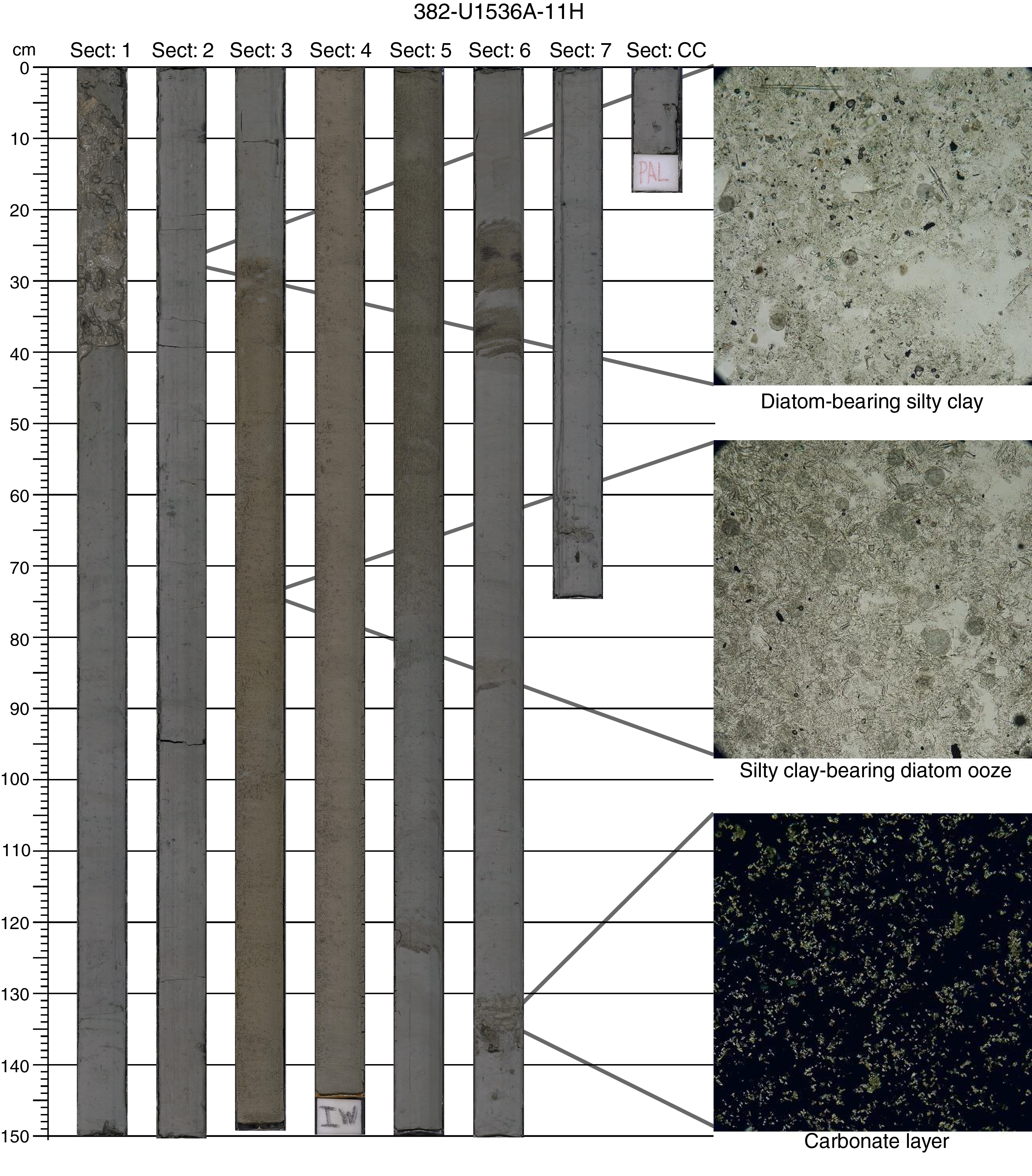
Figure F1. Main lithologies.
Coring disturbance is variable. APC cores from Holes U1536A–U1536C typically exhibit little disturbance, although flow-in and suck-in is common in the upper 60–70 m of Holes U1536A and U1536C. Soupy intervals were also noted in the first sections of multiple cores. Most RCB cores from Hole U1536E are heavily disturbed, primarily by biscuiting and fall-in.
Three lithostratigraphic units were identified based on sediment composition in smear slides and visual core description (Figure F2). Unit I is composed of interbedded diatom oozes and silty clays. Unit II incorporates increasingly more lithified silty clay containing 10%–50% biogenic material (mainly diatoms). Unit III consists of semi- to fully lithified mudstone interbedded with nannofossil-containing limestone.
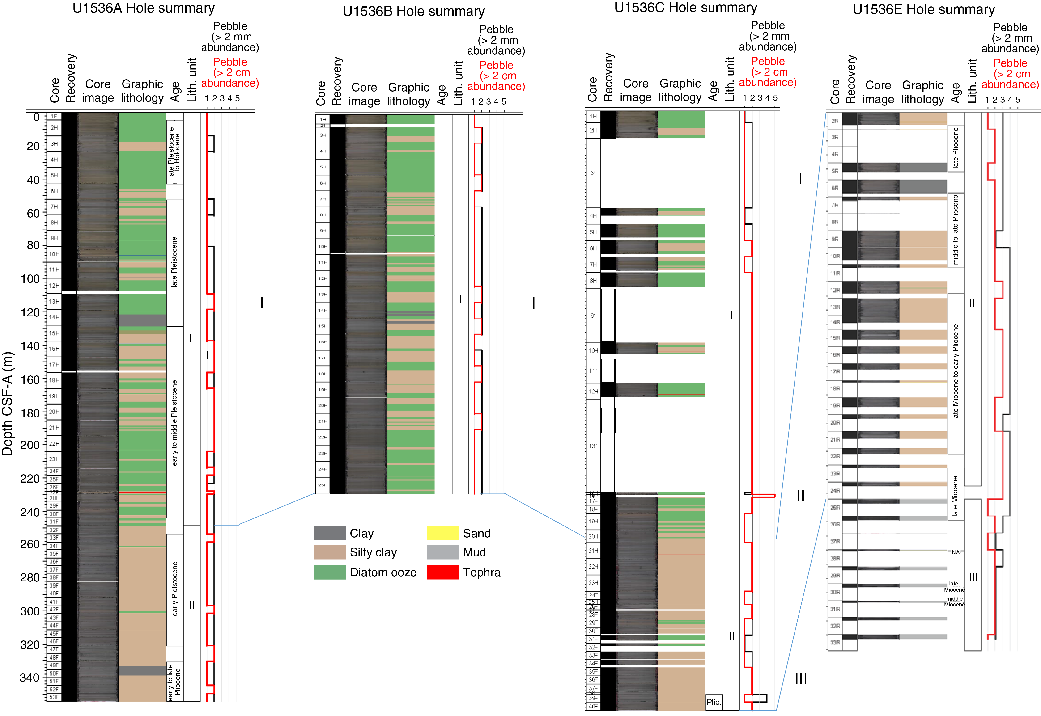
Figure F2. Lithostratigraphic summary.
Discrete carbonate-rich beds were identified in all units (Table T2). Smear slide analyses indicate that this carbonate is not biogenic and in most cases is accompanied by silt-sized rock fragments. Similar layers were previously observed in other ocean basins (Hein et al., 1979), where they have been linked to the presence of ash beds. It is surmised that through bacterial decay of organic matter, carbon is made available to bond with cations (Ca, Mg, Fe, and Mn) sourced from surrounding tephra. Even though no shards were observed in most layers, we tentatively interpret the origin of these layers to be devitrified tephra. No analysis of total organic carbon (TOC) in these layers was performed during shipboard analysis.
Iceberg-rafted debris (IBRD), most commonly angular clasts of subcentimeter size, is present throughout all units and was identified through visual core description and X-radiographs. Additionally, larger IBRD of varying lithologies was recovered at numerous depths throughout cores from Holes U1536A–U1536C (Sections 382-U1536A-13H-4, 13H-CC, 23H-3, 24F-3, 27F-2, 33F-1, and 47F-3; 382-U1536B-13H-3 and 18H-4; and 382-U1536C-6H-1; Figure F3). In Unit I, rare planktonic and trace benthic foraminifers are present in several core catcher samples from Hole U1536A.
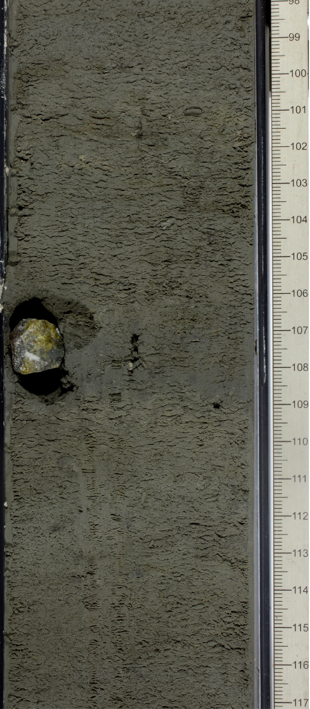
Figure F3. Olivine-bearing dropstone (382-U1536A-23H-3, 106–109 cm).
Unit descriptions
Unit I
- Intervals: 382-U1536A-1F-1 to 31F-4, 72 cm; 382-U1536B-1H-1 to 25H-CC, 27 cm; 382-U1536C-1H-1 to 20H-4, 101 cm; 382-U1536D-1H-1 to 1H-CC, 62 cm
- Depths: Hole U1536A = 0–248.73 mbsf; Hole U1536B = 0–226.58 mbsf (total depth); Hole U1536C = 0–251.43 mbsf; Hole U1536D = 0–6.24 mbsf (total depth)
- Age: early/mid-Pleistocene–Holocene
Unit I is dominated by interbedded diatom oozes and silty clays. The terrigenous component in the oozes is generally less than 25%, and the biogenic component, mainly diatoms, in the silty clays typically exceeds 25% of the sediment. Bedding thickness decreases from very thickly bedded in the upper unit to thinly bedded toward the base of the unit. With the exception of the interval between ~135 and 190 mbsf, where silty clay is more abundant, diatom ooze is the dominant lithology in Unit I.
Diatom oozes and silty clays vary in color from greenish gray (5GY 5/1) to dark greenish gray (10Y 4/1). Some oozes contain green-blue color banding, as seen in interval 382-U1536A-19H-7, 108–124 cm (Figure F4). Based on smear slide analysis, the color appears to be due to the presence of authigenic glauconite. The mineral most commonly observed in smear slides is quartz with rare occurrences of feldspar, as well as accessory and opaque minerals. Diatoms are the dominant biogenic component of Unit I, but rare sponge spicules and radiolarian fragments were also observed. Planktonic foraminifers, including Neogloboquadrina pachyderma sinistral, are rare in half of the Hole U1536A core catcher samples throughout this unit. Rare occurrences of benthic foraminifers are also present.
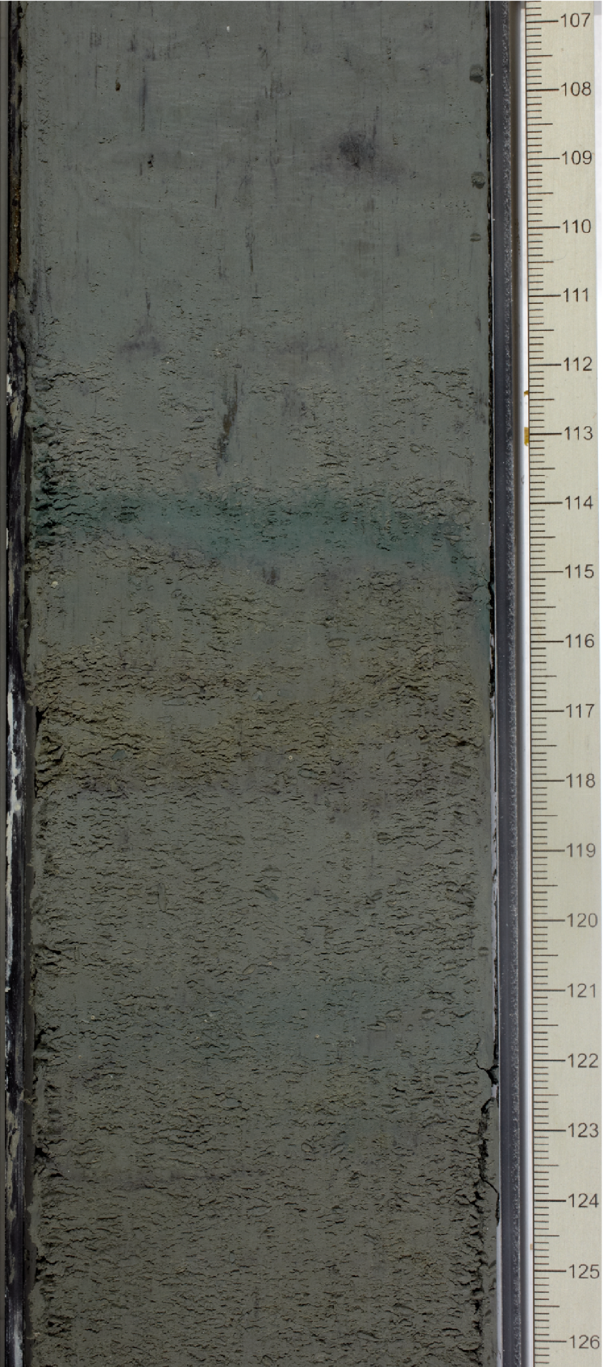
Figure F4. Color banding at diatom ooze–silty clay transition.
Dropstones are visible on the split surface, although many more were observed in the X-radiographs. Slight to moderate bioturbation is visible throughout. The occurrence of pyritized burrows (seen in the visual core descriptions [VCDs] and X-radiographs) increases toward the base of the unit, and the abundance of silty clay increases. Carbonate-rich clay layers are present (Table T2; Figure F5). Smear slide analyses from a similar layer indicate that this carbonate is not biogenic. An example of one of the smear slides is shown in Figure F6 (Sample 382-U1536B-9H-2, 114 cm).
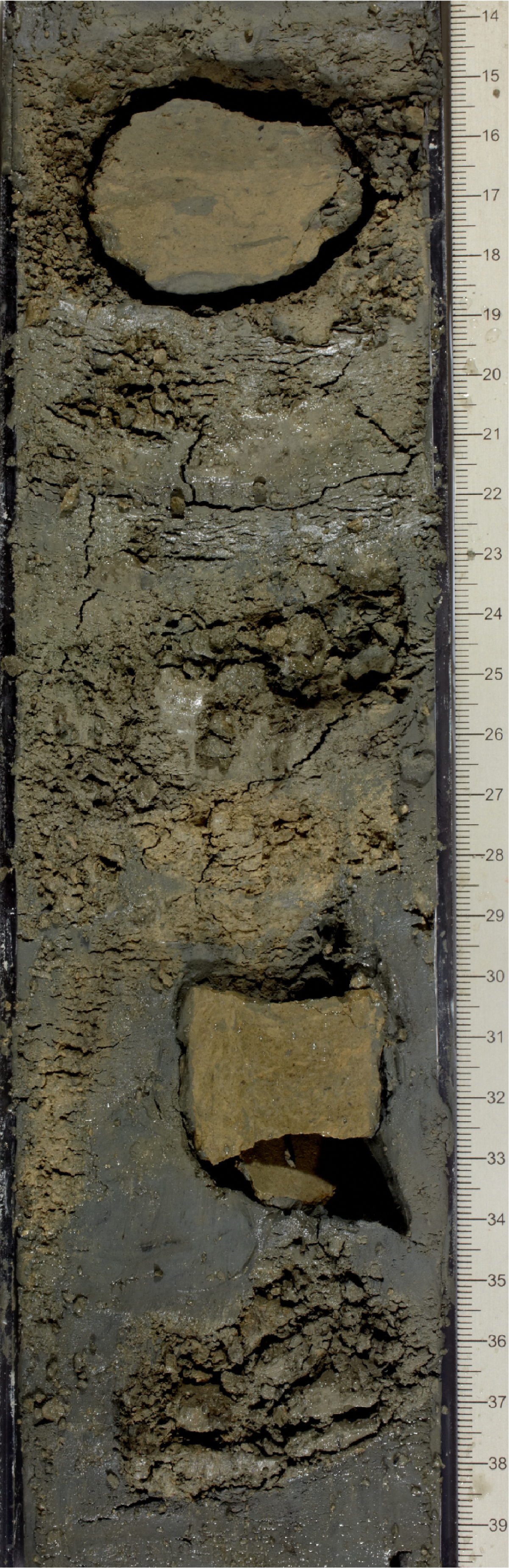
Figure F5. Carbonate-rich layer.
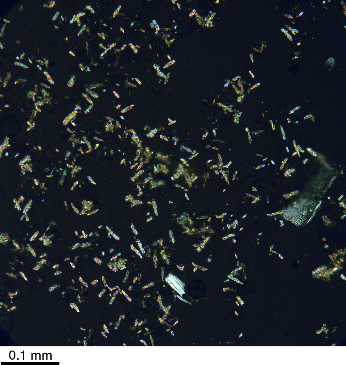
Figure F6. Diagenetic carbonate minerals.
Unit II
- Intervals: 382-U1536A-31F-CC to 53F-CC, 20 cm; 382-U1536C-20H-4, 101 cm, to 40F-CC, 21 cm; 382-U1536E-2R-1 to 24R-CC, 17 cm
- Depths: Hole U1536A = 248.73 to >354.49 mbsf (base of unit not recovered); Hole U1536C = 251.43 to >352.15 mbsf (base of unit not recovered); Hole U1536E = 340.0–551.59 mbsf
- Age: early/late Pliocene to early Pleistocene
The dominant lithology for Unit II is dark greenish gray (5GY 5/1) silty clay with a biogenic content of 10%–49%. Unit II is denser and more lithified than Unit I. Interbedded layers of diatom ooze generally occur in laminations (0.3–1 cm thick) and very thin beds (1–3 cm thick).
The terrigenous fraction is composed of >50% quartz with rare feldspar and accessory and opaque minerals. The biogenic fraction consists predominately (>50%) of diatoms and also contains rare (<10%) to common (10%–25%) radiolarians and sponge spicules. Consistent features of Unit II are intervals occupied by pyritized and silt-filled burrows.
Occasional carbonate-rich intervals are present throughout the unit (Table T2). Dropstones (>1–2 mm) were observed commonly throughout the unit in both the VCDs and X-radiographs. In addition, Unit II contains a slump that is visible as isolated upward-tilting beds in Hole U1536A and is clearly identifiable in Section 382-U1536C-29F-2 (Figure F7).
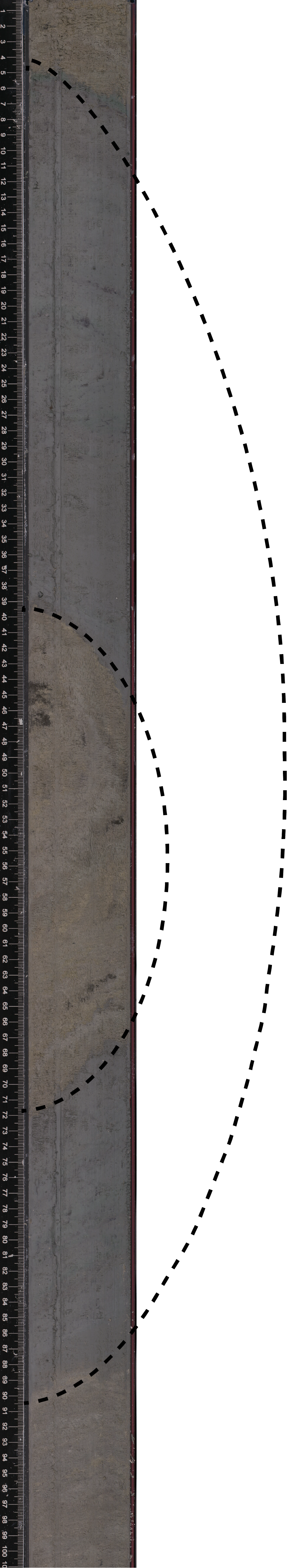
Figure F7. Slump.
In Hole U1536E, Unit II was rotary cored to 559.1 mbsf, resulting in reduced recovery and high core disturbance, predominantly biscuiting. A 34 cm interval of greenish gray, graded, quartz-rich sandstone was observed in Section 382-U1536E-18R-1 (Figures F8, F9). The color is darker in the finer grained rock at the top of the interval. Glauconite is present in the thin section and may be contributing to the green color. This sandstone exhibits the same bedding orientation and color as the surrounding sediments and may be interpreted to be either a pervasive lithified layer in the unit or a large tabular dropstone.
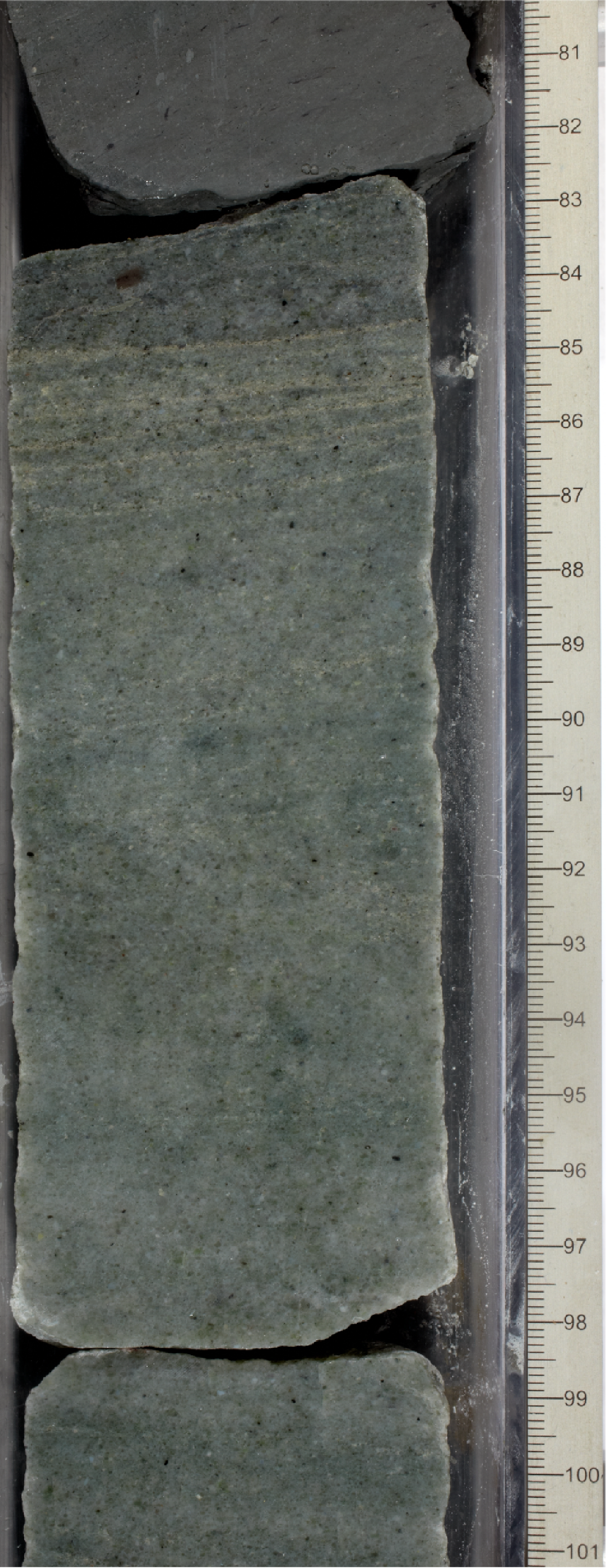
Figure F8. Part of greenish gray, graded glauconite.
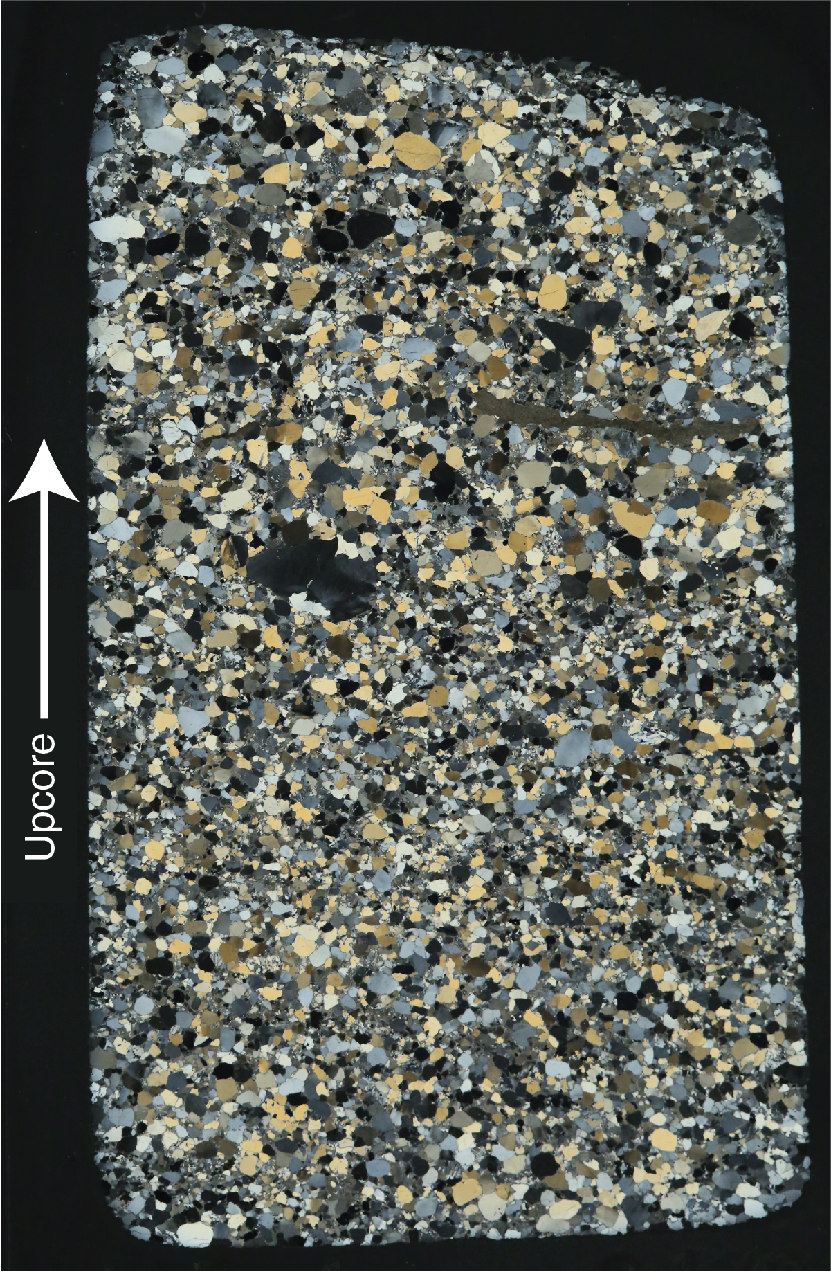
Figure F9. Top of greenish gray, graded glauconite.
Carbonate-rich layers were equally found in this interval (Table T2). Dropstone-rich intervals are also common, and some contain a variety of igneous rocks >2 cm (Figure F10). Below about 340 mbsf, Unit II contains noticeably more IBRD than Unit I above and Unit III below.
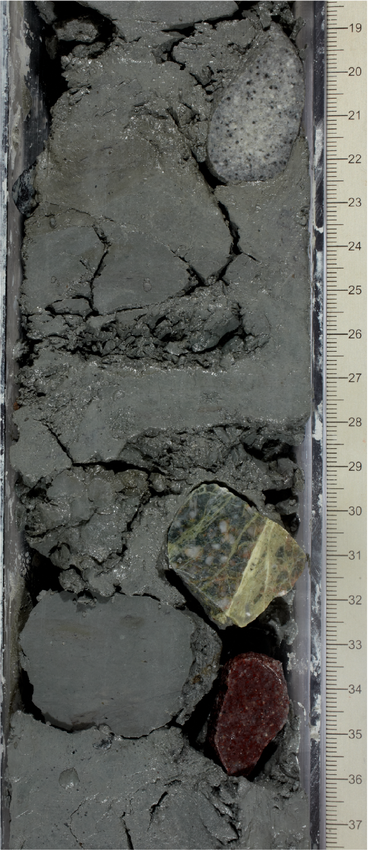
Figure F10. Dropstone-rich interval.
Unit III
- Interval: 382-U1536E-25R-1 to 33R-CC, 26 cm
- Depth: 559.00–638.5 mbsf
- Age: mid-Miocene to late Pliocene
Because of rotary drilling, recovery in Unit III was very low (3%–28%) and the cores are heavily disturbed (biscuited). Unit III consists of semi- to fully lithified mudstone (Figure F11), sometimes with large sand grains (Section 382-U1536E-28R-1; Figures F12, F13) and rare beds of limestone and sometimes classified as nannofossil-bearing to nannofossil-rich and containing foraminifers and radiolarians (Figures F14, F15). Distinct, slight to moderately bioturbated boundaries between the siltstone and mudstone were observed in coherent undisturbed intervals of the core (Section 32R-1, 117–130 cm; Figure F11). Silt-rimmed and filled burrows are common (Section 32R-1; Figure F12). The mudstone color varies through shades of 5Y (olive grays) to 5B (bluish grays) and 5G (greenish grays) and is sometimes defined by sharp boundaries (Section 33R-2, 89–100 cm; Figure F16). The color of the limestone layers is N7 (light gray). Biogenic components in this unit consist of nannofossils, foraminifers, diatoms, and other biosilica. Additionally, three intervals in Section 31R-1 have mudstone biscuits that are biosilica rich (intervals 31R-1, 9–47 cm; 31R-1, 54–64 cm; and 31R-1, 79–85 cm).
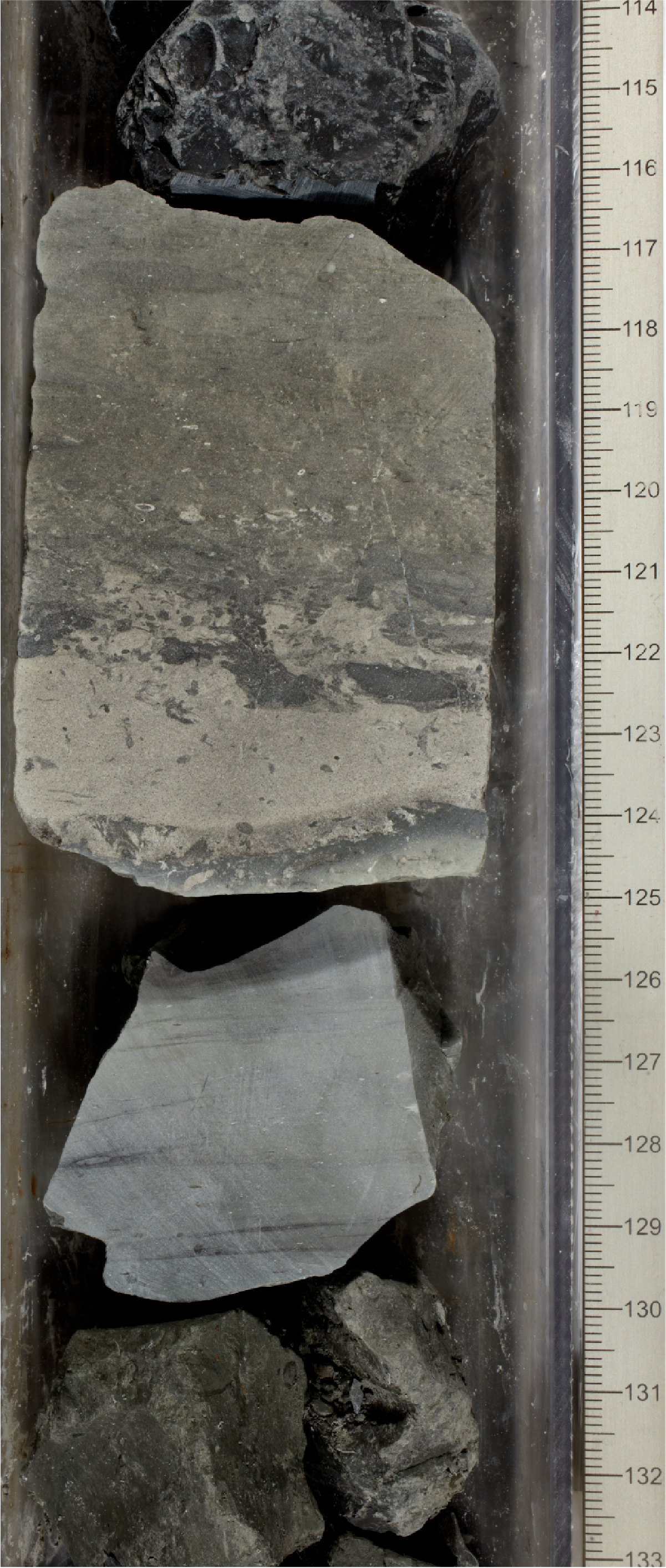
Figure F11. Two drilling biscuits.
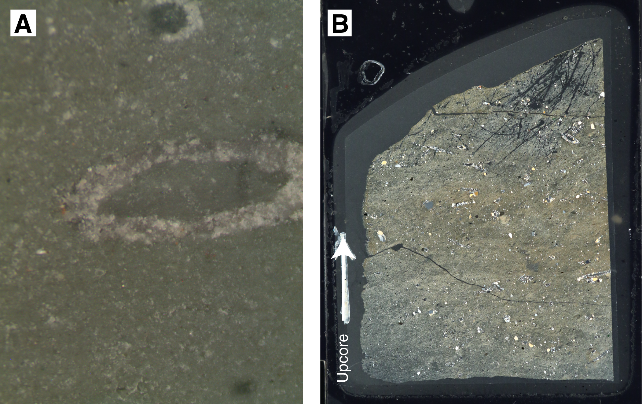
Figure F12. Silt-rimmed and silty clay–filled burrows.
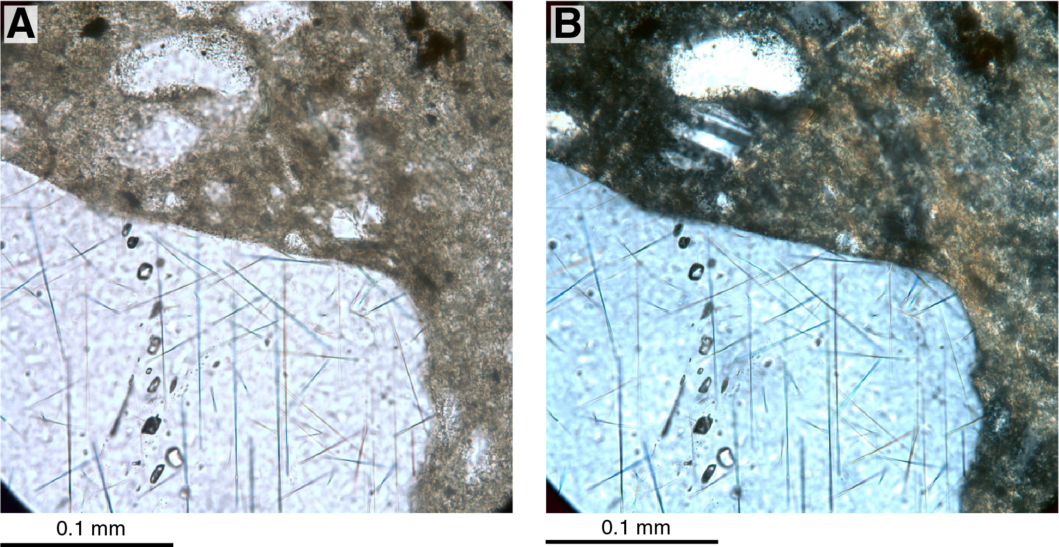
Figure F13. Rutile and apatite in large sand grain.
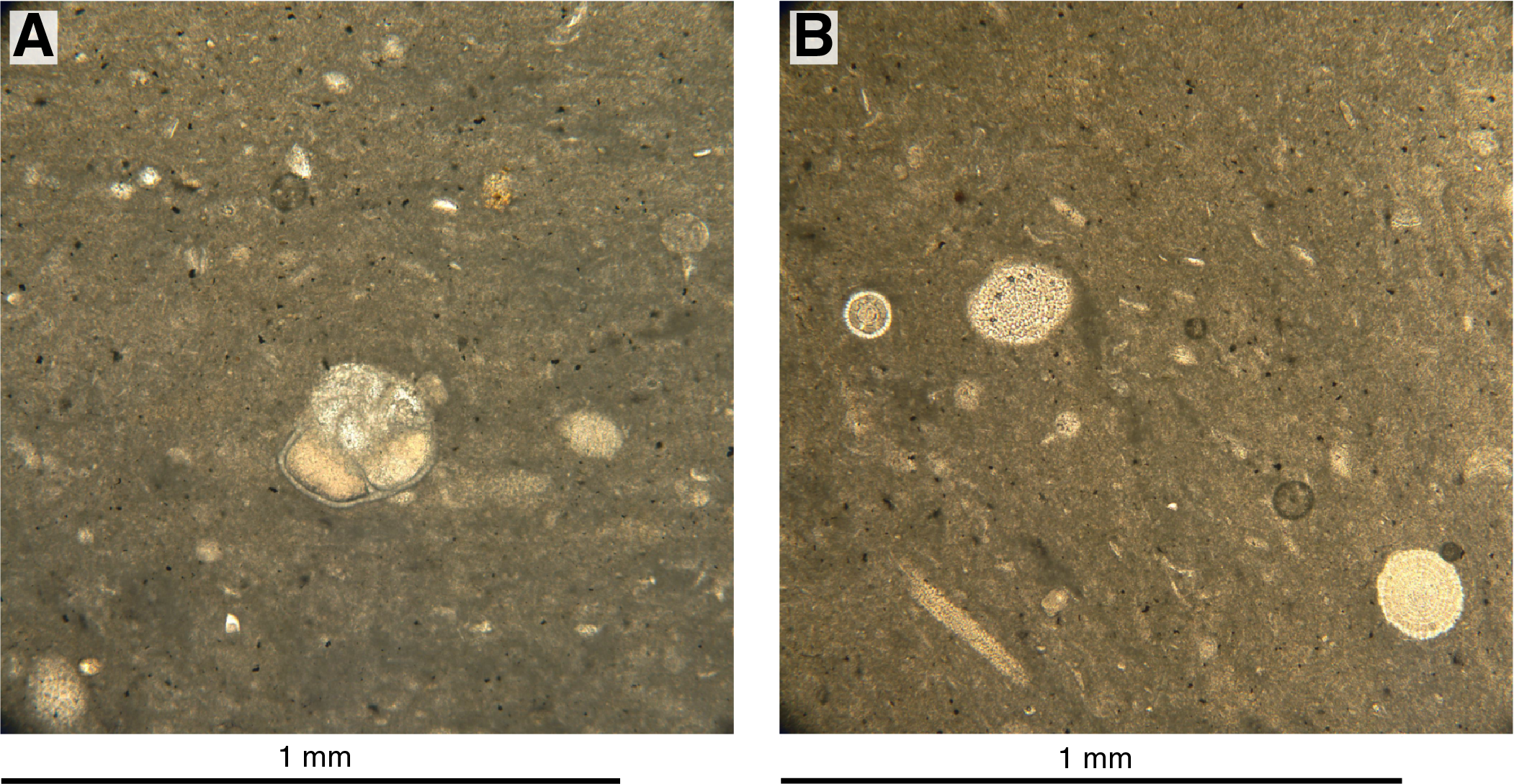
Figure F14. Foraminifer and radiolarians in Miocene limestone.
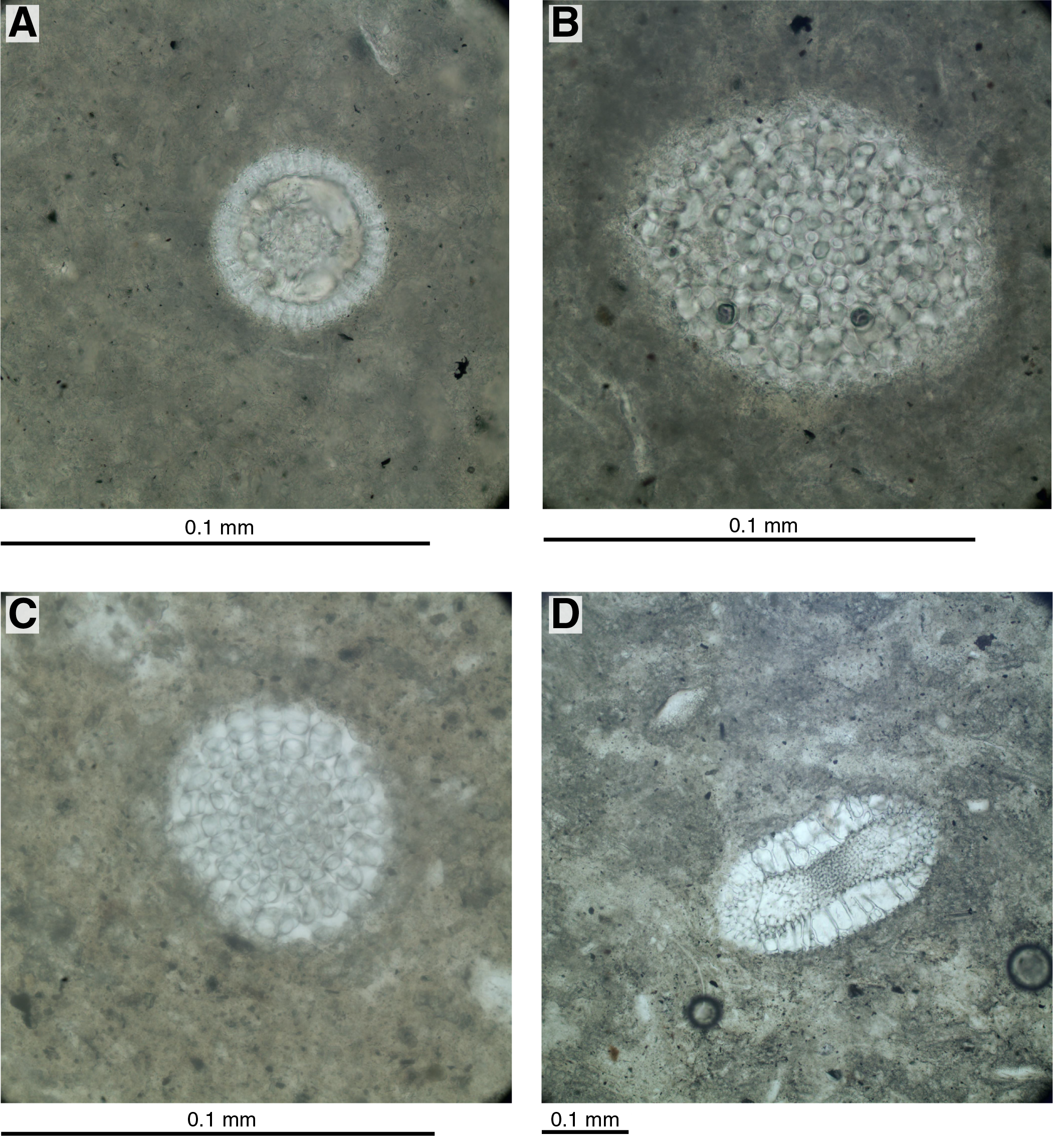
Figure F15. Radiolarians in Miocene limestone.
Figure F16. Sharp lithologic boundary.
X-ray images
For Hole U1536A, X-ray images were taken continuously from sediment cores. Images from APC and HLAPC cores (7879 images) are of good quality and have been visually analyzed to identify and describe their most distinct features. Images from extended core barrel (XCB) cores are of low quality because of high pixel value contrasts.
X-ray images show both gradual and sharp contacts between the two main lithologies identified at the site: diatom ooze and silty clays. X-ray images in diatom ooze intervals are characterized by light to medium pixel values (darkness reflecting denser material) with background texture ranging from spotty to faintly or distinctly banded. Fine (millimeter- to centimeter-scale) laminations are rare at this site. The background exhibits a typical spotty texture (Figure F17A). In contrast, silty clay intervals present a relatively darker, more homogeneous background texture with rare to common darker bands and patches (Figure F17B).
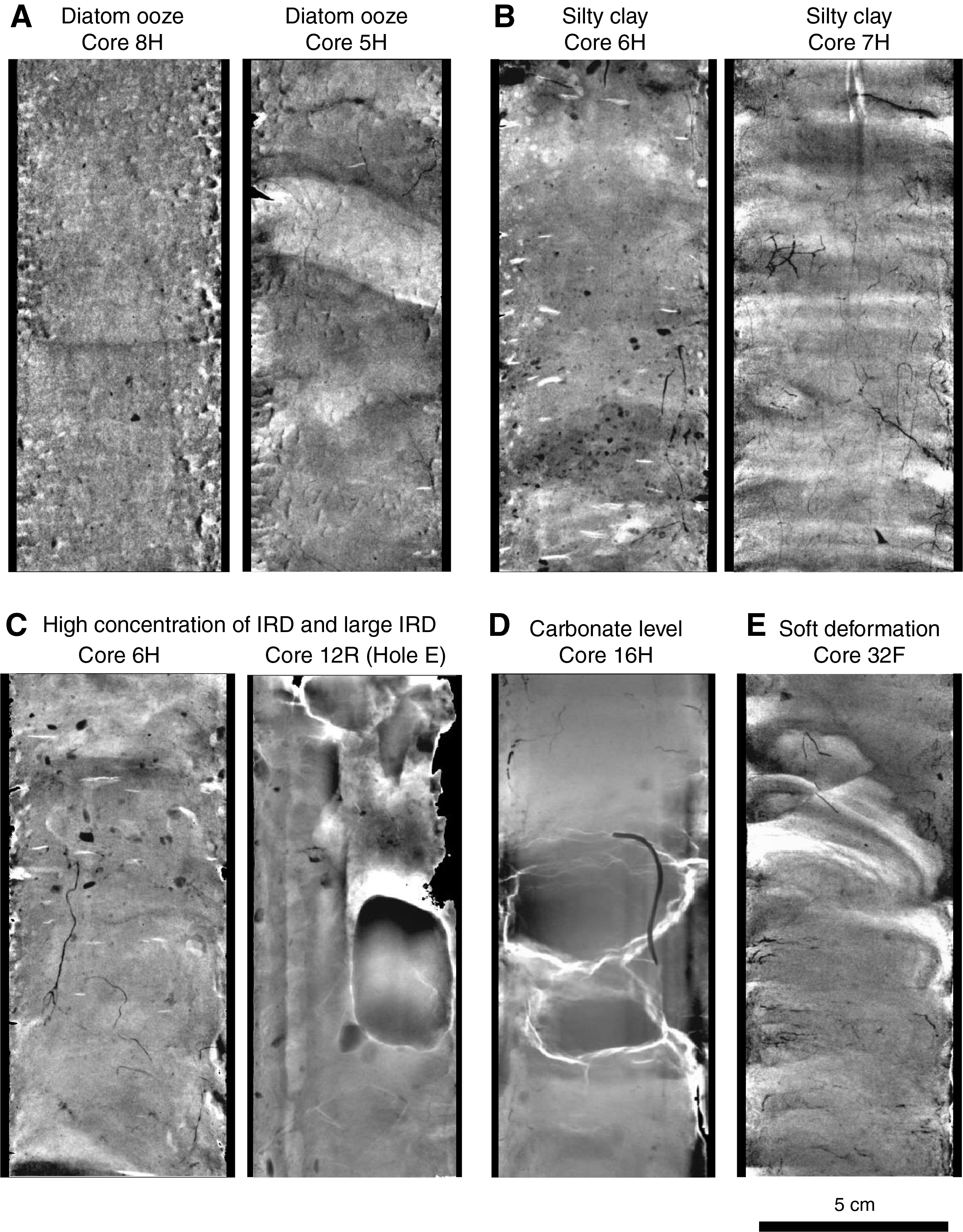
Figure F17. X-ray images.
Millimeter- to centimeter-scale IBRD generally shows contrasting high pixel values in the X-ray images. IBRD does not form layers but is concentrated in distinct intervals when present (Figure F17C). Larger IBRDs are common in the lower part of the sedimentary record.
Carbonate-rich layers display a relatively dark, featureless texture (Figure F17D).
Burrows are visible because of the contrasting density of the postdepositional material infilling the structures generated by organisms. These burrows are primarily distinctly darker features, possibly due to the precipitation of pyrite and more rarely lighter material. Burrows with a wide range of morphologies (linear, curved, and subcircular) are present throughout the sediment column (Figure F17B). They are as wide as 0.5 cm and a few centimeters long and are rarely wider than the core diameter. Burrows are more common and more diverse in the silty clay intervals in Unit I and in Unit II. Generally absent from the rotary cores of Unit III, they are again present in the lower part of Unit III (Cores 382-U1536E-31R through 33R).
Postsedimentary deformation is identified in the X-ray images as folded layers (Figure F17E) and faulting. The cause of deformation (original or drilling disturbance) is unclear.
Summary
The dominant lithologies at Site U1536 are alternating intervals of silty clay–rich/bearing diatom ooze and diatom-rich/bearing silty clay. Dropstones occur throughout all depths and significantly increase in number and size in Unit III. Thin beds of diagenetic carbonate are present at irregular intervals throughout all units. A representative interval of the main lithologies is shown in Figure F1.
Biostratigraphy
Core catcher sediments primarily composed of diatomaceous oozes and fossiliferous muds were analyzed for diatoms, radiolarians, palynomorphs, and foraminifers. Selected additional samples were analyzed for diatoms and radiolarians. Although abundance and preservation vary throughout the core, siliceous microfossils and palynomorphs were found in most analyzed samples (in Samples 382-U1536E-25R-CC and 27R-CC, sediment recovery was low and ice-rafted debris [IRD] was the main component, yielding very few microfossils). Foraminifers are present in many intervals, and nannofossils were identified in Samples 28R-1, 40 cm, and 28R-CC. Evidence of reworking was noted frequently. Sediments range in age from Holocene to mid-Miocene (Table T3). The specific age datums used are given in Table T4. A biostratigraphically derived age-depth model is presented in Figure F18.
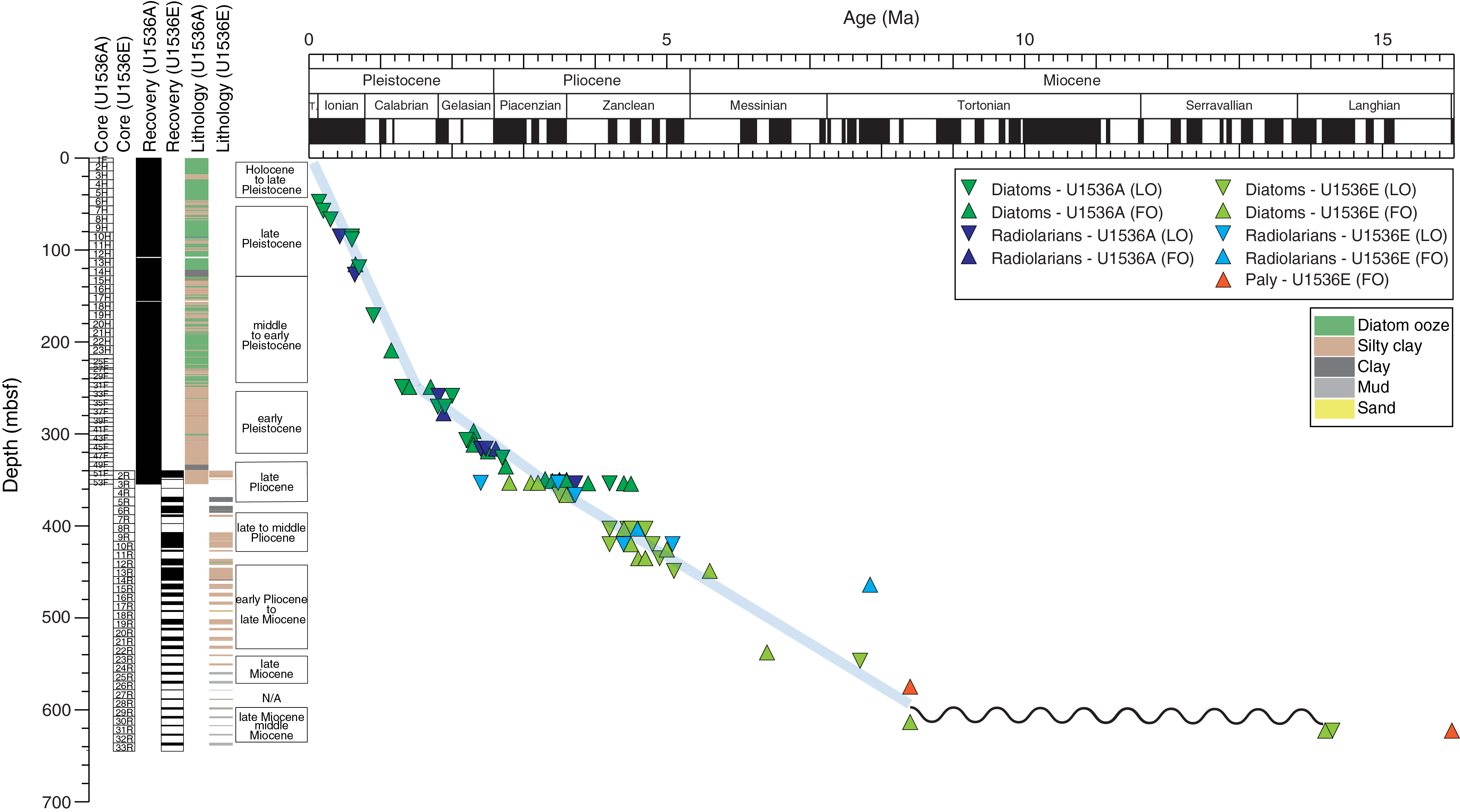
Figure F18. Biostratigraphic age-depth plot.
Siliceous microfossils
Diatoms
Most samples contain diatoms; overall diatom abundance, preservation, and species-specific occurrences and relative abundances for all samples are given in Table T5. Diatom dissolution is generally low, whereas fragmentation is commonly moderate (medium or medium–high), and both dissolution and fragmentation are variable. Diatoms tend to be better preserved in samples with a low siliciclastic component.
Reworking was consistently noted in diatom slides and includes but is not limited to the slumped intervals identified in the lithostratigraphy (see Lithostratigraphy). Some reworking (i.e., trace Pliocene diatoms in an otherwise late Pleistocene assemblage) was easy to identify and is common in Antarctic marine sediment cores. These fossils were excluded from the age model. Other diatom reworking was more difficult to determine (e.g., late Pleistocene diatoms in latest Pleistocene sediments). To address this issue, mudline samples from Holes U1536B and U1536C were analyzed. Fully and partially pyritized diatoms were found in the mudline samples, implying reworking. Additionally, several extinct species that must be reworked were identified in mudline samples: Actinocyclus ingens, Actinocyclus fasciculatus, Azpeitia endoi, Rhizosolenia harwoodii, Rouxia constricta, Thalassiosira elliptipora, and Thalassiosira fasciculata. A. ingens and R. harwoodii are well preserved in the mudline samples and other age-inappropriate samples (Figure F19). Complete frustules of A. ingens were also found in the mudline. The fossils found in the mudline samples were categorized into three groups: those whose last occurrence (LO) datums were used in biostratigraphic analysis (R. constricta, T. elliptipora, and T. fasciculata), those whose LO datums were not used to construct the biostratigraphic model because sediments of that age were not recovered (A. endoi), and those whose LO datums were excluded because a true LO could not be determined (A. fasciculatus, A. ingens, and R. harwoodii).
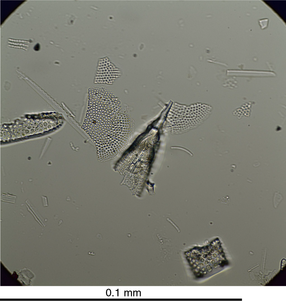
Figure F19. Rhizosolenia harwoodii.
The LO of A. fasciculatus (2.0 Ma; Harwood and Maruyama, 1992; Cody et al., 2008) is suspect because this datum was observed between Samples 382-U1536A-32F-CC and 34F-CC, which places it in Chron C1r.3r (see Paleomagnetism). However, this bioevent (2.0 Ma) should occur between the Olduvai and Reunion Chrons. Therefore, despite association with other contemporaneous diatoms, A. fasciculatus is likely reworked in this interval. A. ingens and R. harwoodii were excluded because persistent reworking caused these species to be identified at more than trace abundance. As such, we did not find a point of notable change in abundance downcore from a few reworked individuals to many in situ individuals that could have indicated an LO depth. A. ingens has been known to be frequently reworked in Southern Ocean sediments (e.g., Gersonde and Bárcena, 1998), and the original species description of R. harwoodii (Winter et al., 2012) notes that the robust portions of its valves can also be easily reworked. In Hole U1536A, A. ingens was found as high as Sample 2H-CC and R. harwoodii was found as high as Sample 4H-CC. Both of these diatoms occur almost continuously with at least rare abundance in sediments from Sample 10H-CC to their first occurrence (FO) depths.
Given the frequency of reworking and our inability to isolate true LO depths, Sample 382-U1536A-10H-CC was not chosen as true LO depth for A. ingens and R. harwoodii. Both taxa have an LO of 0.6 Ma. As such, their LOs should occur between the LO of R. constricta (0.3 Ma) and the FO of Thalassiosira antarctica (0.65 Ma). At Site U1536, the LO of R. constricta was confidently identified in Sample 8H-CC and the FO of Thalassiosira antarctica was confidently identified in Sample 13H-3, 75 cm. Using Sample 10H-CC as the LO datum of A. ingens and R. harwoodii would require large, unrealistic changes to the sedimentation rate, so this depth was rejected. In addition, this depth would be in conflict with paleomagnetic data (see Paleomagnetism). Therefore, the LOs of A. ingens and R. harwoodii were excluded from the age model (Figure F18).
Several other late Pleistocene datums were used to construct the age model in cores where A. ingens and R. harwoodii were problematic: the LOs of Rouxia leventerae (0.14 Ma), Hemidiscus karstenii (0.2 Ma), and R. constricta (0.3 Ma) and the FO of Thalassiosira antarctica (0.65 Ma). Although R. constricta was found in the mudline, it was not excluded from biostratigraphic analysis. This species was not observed in any samples higher than the LOs of R. leventerae and H. karstenii, implying it was found in proper stratigraphic position in all samples excluding the mudline.
Samples 382-U1536A-1F-CC to 5H-CC represent the Holocene to late Pleistocene. A well-preserved typical Southern Ocean diatom assemblage was identified, and these samples have abundant diatoms. The assemblage is dominated by Eucampia antarctica, Fragilariopsis kerguelensis, Thalassiosira lentiginosa, and Thalassiothrix antarctica. These diatoms imply an open-ocean setting with little sea ice influence. In addition, Actinocyclus actinochilus, Asteromphalus parvulus, Asteromphalus hookeri, Fragilariopsis curta, Fragilariopsis rhombica, Fragilariopsis ritscheri, Fragilariopsis separanda, Porosira glacialis, Porosira pseudodenticulata, Shionodiscus gracilis, Shionodiscus oestrupii, Thalassiosira antarctica, and Thalassiosira oliverana also occur in most samples. Chaetoceros resting spores and Dactyliosolen antarcticus girdle bands are common. Because of the low abundance of sea ice–related species (e.g., F. curta and Fragilariopsis cylindrus) and the high abundance of species associated with open water (e.g., F. kerguelensis and T. lentiginosa), this assemblage reflects a primarily open-ocean setting with only short durations of sea ice cover. A. ingens and R. harwoodii occur in some samples from this interval and are considered to be reworked because of the composition of the assemblage and LO datums found below.
Samples 382-U1536A-6H-CC to 14H-CC contain a late Pleistocene diatom assemblage. In addition to the diatoms in the interval above, these samples contain R. leventerae (occurring as high as Sample 6H-CC), H. karstenii (highest stratigraphic occurrence in Sample 7H-CC), and R. constricta (highest stratigraphic occurrence in Sample 8H-CC). A. ingens and R. harwoodii occur more commonly in this interval than in the interval above. The true LOs of both taxa fall within this interval, but at this stage it is impossible to determine the exact depth. Thalassiosira antarctica was not found below Sample 13H-3, 75 cm. Excluding the mudline sample, the highest stratigraphic occurrence of T. elliptipora was found in Sample 13H-7, 42 cm.
Samples 382-U1536A-15H-CC to 30F-CC contain middle to early Pleistocene diatom assemblages. In contrast to the above interval, these sediments notably also contain Proboscia barboi (highest stratigraphic occurrence in Sample 15H-CC) and T. fasciculata (excluding the mudline, highest stratigraphic occurrence in Sample 19H-CC). The lowest stratigraphic occurrences of Fragilariopsis obliquecostata, F. rhombica, and F. separanda were found in Sample 30F-CC.
Samples 382-U1536A-32F-CC to 46F-3, 75 cm, represent the early Pleistocene. Notably, these samples contain Fragilariopsis barronii. The lowest recorded instance of F. kerguelensis is in Sample 40F-CC. The lowest stratigraphic occurrence of S. gracilis and highest recorded occurrence of Fragilariopsis bohatyi are in Samples 40F-CC and 42F-CC, respectively. Shionodiscus tetraoestrupii var. reimeri is present in Samples 32F-CC to 44F-CC. Rouxia antarctica has its highest stratigraphic occurrence in Sample 36F-1, 75 cm, and continues below this interval. Thalassiosira inura first occurs in Sample 36F-3, 75 cm (excluding obvious reworking in selected samples above), whereas Thalassiosira insigna was first recorded in Sample 46F-3, 75 cm. The deepest instance of A. ingens occurs in Sample 46F-1, 75 cm, and the deepest instance of A. fasciculatus is in Sample 45F-2, 75 cm. The lowest stratigraphic occurrence of A. parvulus was recorded in Sample 42F-CC. Although increasing numbers of extinct species complicate paleoenvironmental analysis relative to sediments above, these assemblages indicate generally open water and little sea ice influence.
Samples 382-U1536A-48F-CC to 53F-3, 75 cm, date to the late Pliocene. Fragilariopsis interfrigidaria was found exclusively in this interval; it was recorded in every sample. The uppermost sample in this interval contains the highest stratigraphic occurrences of Fragilariopsis weaveri and Thalassiosira webbi and the lowest stratigraphic occurrence of F. bohatyi. Other lowest stratigraphic occurrences in this interval include F. barronii (Sample 53F-3, 75 cm), R. harwoodii (Sample 53F-1, 75 cm), R. antarctica (Sample 53F-3, 75 cm), and T. lentiginosa (also in Sample 53F-3, 75 cm). Unlike the previous intervals described above, species turnover is rapid between samples in this interval, especially in Samples 51F-1, 74 cm, to 53F-3, 74 cm.
Samples 382-U1536A-53F-4, 37 cm, and 53F-CC record a distinct assemblage from the base of Hole U1536A. Both samples contain Fragilariopsis aurica. However, neither sample contains R. antarctica, in contrast to the sediments immediately above. Rouxia heteropolara and Rouxia naviculoides are present in Sample 53F-CC. T. fasciculata is absent in Sample 53F-CC. Actinocyclus karstenii, S. oestrupii, T. inura, and Thalassiosira complicata are present in this lowest interval of Hole U1536A, just as they are in samples above. These lower samples date to the early Pliocene.
Only three samples were taken from Hole U1536C: 382-U1536C-38F-CC, 39F-CC, and 40F-CC. These samples are similar in diatom composition to the lowest three core catcher samples from Hole U1536A: 382-U1536A-51F-CC, 52F-CC, and 53F-CC, respectively. The assemblage in these three samples is the same as those of the three lowest Hole U1536A samples analyzed.
All available core catcher samples from Hole U1536E were analyzed for diatoms. Core catcher samples were not available from Sections 382-U1536E-3R-CC and 8R-CC because of poor recovery. Furthermore, Samples 17R-CC, 25R-CC, 27R-CC, and 28R-CC are barren with respect to diatoms. Overall, diatom preservation and abundance notably decline from Sample 14R-CC downcore, with only trace diatom abundance noted in many samples.
Sample 382-U1536E-2R-CC contains a late Pliocene assemblage. Actinocyclus maccollumii, F. bohatyi, F. interfrigidaria, T. lentiginosa, and Thalassiosira vulnifica occur exclusively in this sample with respect to Hole U1536E. In addition, A. karstenii, E. antarctica, F. barronii, F. weaveri, R. harwoodii, R. antarctica, R. naviculoides, T. complicata, T. fasciculata, T. inura, Thalassiosira nativa, and Thalassiothrix antarctica occur in this sample. It is biostratigraphically similar to Sample 382-U1536A-50F-CC.
Samples 382-U1536E-4R-CC and 5R-CC contain similar late Pliocene assemblages, although only Sample 4R-CC contains T. nativa. As with Sample 2R-CC, this interval contains A. karstenii, E. antarctica, F. barronii, R. antarctica, R. naviculoides, T. complicata, T. fasciculata, T. inura, and Thalassiothrix antarctica. Fragilariopsis fossilis, F. weaveri, and R. harwoodii were found only in Sample 4R-CC. This interval contains the highest stratigraphic occurrences of P. barboi, R. heteropolara, S. oestrupii, and Thalassiosira torokina and also exclusively contains Rouxia isopolica.
Samples 382-U1536E-6R-CC to 11R-CC contain a late to middle Pliocene diatom assemblage. Sample 7R-CC contains the lowest stratigraphic occurrence of F. barronii. A distinct shift in the assemblage was noted in Sample 9R-CC with the addition of Denticulopsis delicata, Fragilariopsis arcula, F. aurica, Fragilariopsis praecurta, and Fragilariopsis reinholdii. Sample 10R-CC also contains Denticulopsis simonsenii, Rouxia californica, and Rouxia diploneides and the lowest stratigraphic occurrences of R. antarctica, S. oestrupii, and T. fasciculata. Sample 11R-CC contains the lowest stratigraphic occurrences of R. heteropolara and T. complicata.
Samples 382-U1536E-12R-CC to 22R-CC represent the early Pliocene. Biostratigraphically, this interval could also include the latest Miocene. Many samples in this interval have low diatom abundance, and as such, many species occurrences are not continuous. Sample 12R-CC contains the lowest stratigraphic occurrences of T. inura and T. oliverana. However, this sample also contains the highest stratigraphic occurrence of Thalassiosira oliverana var. sparsa and the only occurrence of T. insigna in Hole U1536E. Sample 13R-CC contains the lowest stratigraphic occurrence of F. arcula and the highest stratigraphic occurrences of Fragilariopsis miocenica and Thalassiosira miocenica. The lowest stratigraphic occurrences of T. miocenica and T. nativa occur in Sample 15R-CC. Sample 20R-CC has the lowest stratigraphic occurrences of F. praecurta, P. barboi, and T. torokina observed. Finally, Sample 22R-CC contains the lowest stratigraphic occurrences of D. delicata, D. simonsenii, F. miocenica, and R. californica.
Diatoms occur at very low abundances in Samples 382-U1536E-23R-CC to 26R-CC. In addition, the specimens found are highly fragmented. Sample 23R-CC contains the lowest stratigraphic occurrence of A. karstenii. Sample 24R-CC contains the lowest stratigraphic occurrences of E. antarctica and Thalassiosira ritscherii. This sample also contains Thalassiosira mahoodii. Because of the presence of T. mahoodii, this sample is not considered to represent a true FO of E. antarctica. Instead, the absence of E. antarctica in samples below this stratigraphic level is likely taphonomic. Because of extremely poor preservation and low diatom abundance, the only biostratigraphically useful diatom found in Sample 26R-CC was R. naviculoides (a single individual). Trace fragments of both pennate and centric diatoms were found, and Rhizosolenia antennata f. semispina occurs rarely. Sample 30R-CC has very few diatoms, which were found in aggregates of sediment. However, the identification of F. aurica and T. mahoodii was possible, assigning this sample a late Miocene age. Sample 30R-CC contains the lowest stratigraphic occurrence of F. aurica.
Sample 382-U1536E-31R-CC contains a middle Miocene diatom assemblage. Although these diatoms are fragmented, enough well-preserved individuals were found for biostratigraphic analysis. This assemblage consists of A. ingens, Actinocyclus ingens var. nodus, A. endoi, Denticulopsis crassa, Denticulopsis hyalina, Denticulopsis lauta, D. simonsenii, and Nitzschia grossepunctata. Sample 32R-CC contains a similar assemblage that also includes Denticulopsis maccollumii but is lacking A. endoi and D. simonsenii. This assemblage is earlier middle Miocene.
Radiolarians
Radiolarian biostratigraphy in Hole U1536A is based on the examination of 43 samples. Radiolarian preservation is moderate to high, and diversity is high (Table T6).
The LO of Stylatractus universus (0.41 Ma) in Sample 382-U1536A-10H-CC indicates that samples above this level belong to the Omega Zone. Below Sample 10H-CC, samples are difficult to interpret, likely due to reworking. Antarctissa cylindrica occurs in Samples 10H-CC and 11H-CC together with other early Pleistocene–Pliocene biostratigraphic markers (Helotholus vema and Lychnocanium grande). However, the LO of S. universus in the same sample is in conflict with the previous biostratigraphic markers that are much older, and thus its presence may have been caused by reworking. Alternatively, A. cylindrica may have an extended age range in the region. Further examination of this event at nearby sites and a quantitative study will provide a more reliable evaluation of these results. The species A. cylindrica appears again in Sample 14H-5, 74–75 cm, and continues to be consistently present in samples below this depth, which suggests that this is the true LO of A. cylindrica, indicating the Psi Zone (i.e., no reworking).
Samples 382-U1536A-14H-5, 74–75 cm, to 32F-CC are difficult to interpret because of the absence of stratigraphic marker species. All samples contain a low abundance of Cycladophora davisiana and Phormocyrtis antarctica, which have broad stratigraphic ranges and are characteristic of the Psi and Chi Zones. Thus, it is not possible to determine whether this interval corresponds to the Psi Zone or the Chi Zone. The occurrence of Cycladophora pliocenica in Sample 32F-CC and the absence of P. antarctica below Sample 36F-CC mark the transition from the lower Chi Zone to the upper Phi Zone. The simultaneous occurrence of H. vema and Desmospyris spongiosa together with the absence of C. davisiana in Sample 44F-CC suggests that this sample is very close to the transition between the Phi and Upsilon Zones at 2.42 Ma. The occurrence of Larcopyle polyacantha titan and Lampromitra coronata in Samples 53F-2, 74–75 cm, and 53F-3, 74–75 cm, respectively, indicates the lower Upsilon Zone and ages older than 3.4 Ma.
Samples 382-U1536C-38F-CC and 39F-CC have the same fauna and thus are stratigraphically equivalent to the last three samples from Hole U1536A (Samples 382-U1536A-51F-CC, 52F-CC, and 53F-CC).
Hole U1536E core catchers examined for diatoms were also analyzed for radiolarians. Radiolarian preservation is mostly good to moderate, except for a few samples with poor preservation (Samples 382-U1536E-9R-CC, 12R-CC, 13R-CC, 17R-CC, and 21R-CC). Radiolarian abundance ranges between abundant and trace. Downcore from Sample 22R-CC, radiolarian abundance is trace or barren with poor preservation and high fragmentation, and often radiolarians are recrystallized and/or embedded in mud clasts (Figure F20). Sample 2R-CC contains the LOs of H. vema and D. spongiosa, indicating the Upsilon Zone. These events also occur in Sample 382-U1536A-44F-CC, suggesting an age overlap between holes. In that case, the shallower depth at which these events were found in Hole U1536A would be more accurate for placing these LOs. Sample 382-U1536E-2R-CC also contains the LO of L. polyacantha titan. The LO of L. coronata occurs in Sample 4R-CC.
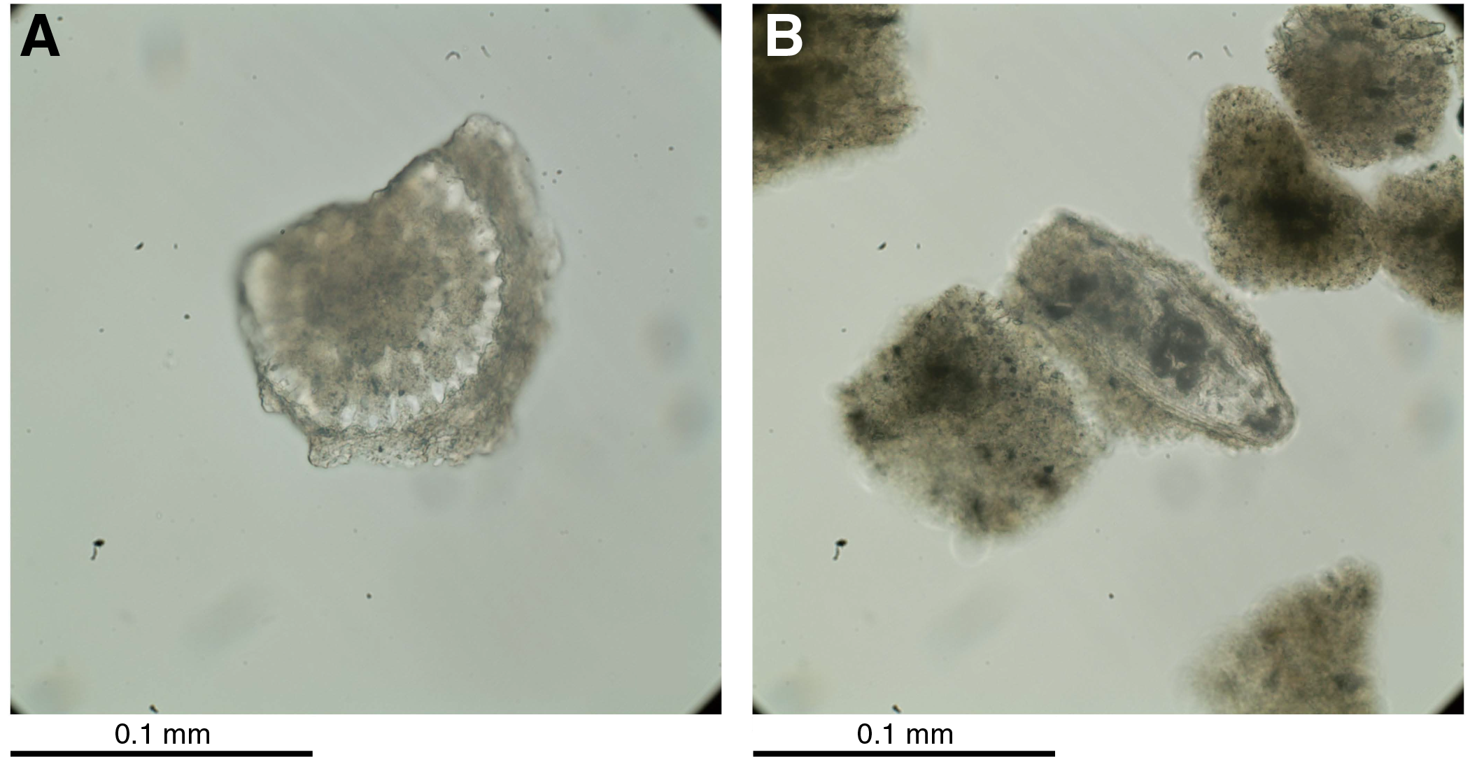
Figure F20. Unidentified reworked radiolarians, Hole U1536E.
The FO of H. vema occurs in Sample 382-U1536E-7R-CC, indicating the Upsilon/Tau Zone boundary. Sample 9R-CC contains the LO of L. grande. Sample 12R-CC contains the FO of Acrosphaera labrata that marks the base of the A. labrata Zone. The absence of radiolarian biostratigraphic markers along with extremely poor preservation and radiolarian abundance below Sample 22R-CC makes it difficult to determine the age of the sequence. The trace occurrence of Eucyrtidium pseudoinflatum in Sample 24R-CC indicates ages younger than 10.7 Ma.
Calcareous nannofossils
Calcareous nannofossils were found in Samples 382-U1536E-28R-CC and 29R-CC and in smear slides for sediment description (Samples 28R-1, 8 cm; 28R-1, 40 cm; and 29R-1, 21 cm). They are very abundant and well preserved. The occurrence of Reticulofenestra perplexa indicates ages between 8.6 and 10.6 Ma (Burns, 1975; van Heck, 1981; Wise, 1983) (Figure F21). Further examination of the interval with high calcium carbonate preservation will be made by nannofossil specialists after the expedition to refine ages based on this group.
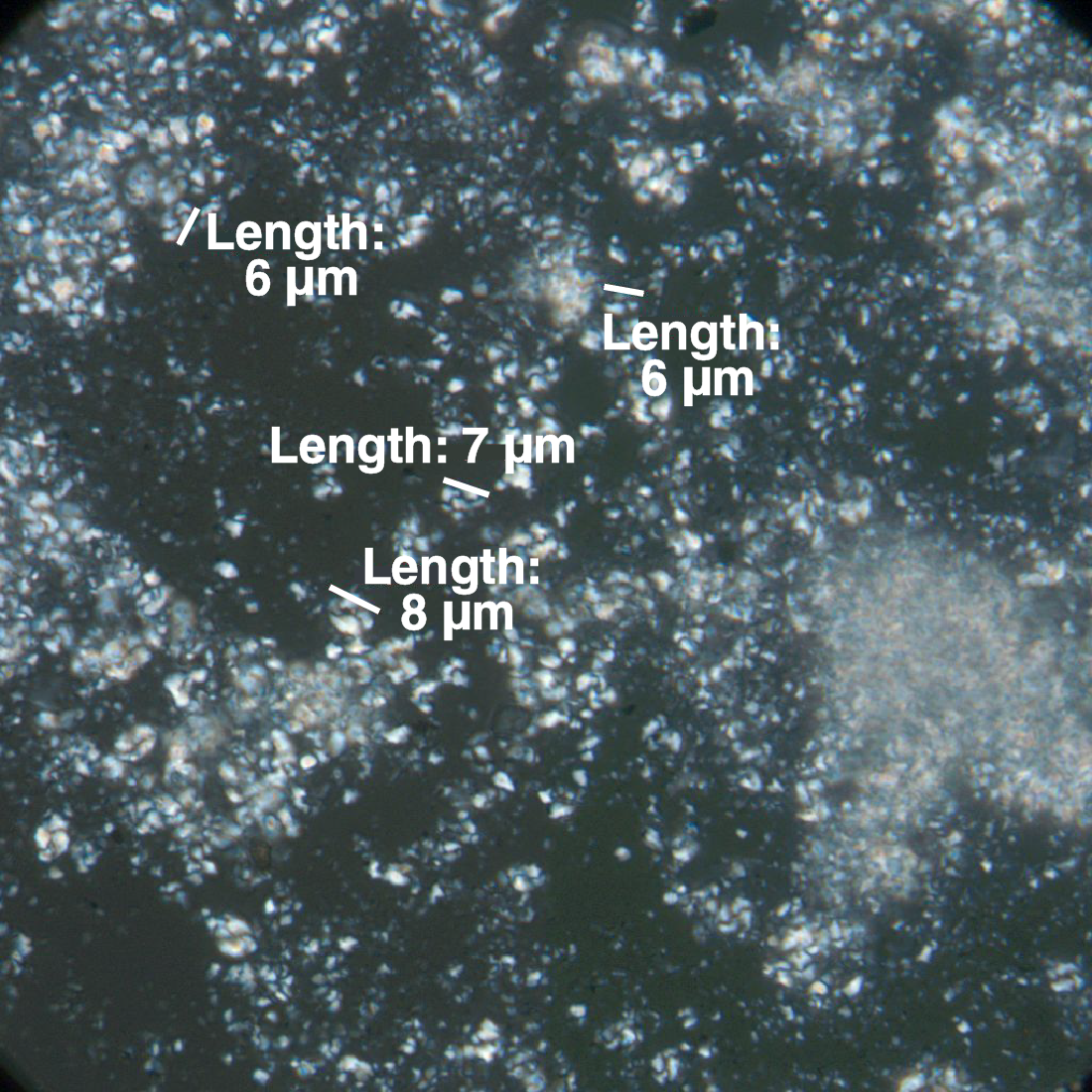
Figure F21. Reticulofenestra perplexa.
Palynology
A total of 51 core catcher samples from Site U1536 were processed and analyzed for palynological content (organic-walled dinoflagellate cysts [dinocysts], pollen, and spores). The presence of marine palynomorphs and semiquantitative estimates of the abundance of the different palynofacies together with the processing method used are shown in Table T7. Supportive age control from dinocysts is presented in Table T4 and Figure F18. Selected palynomorphs are shown in Figures F22 and F23.
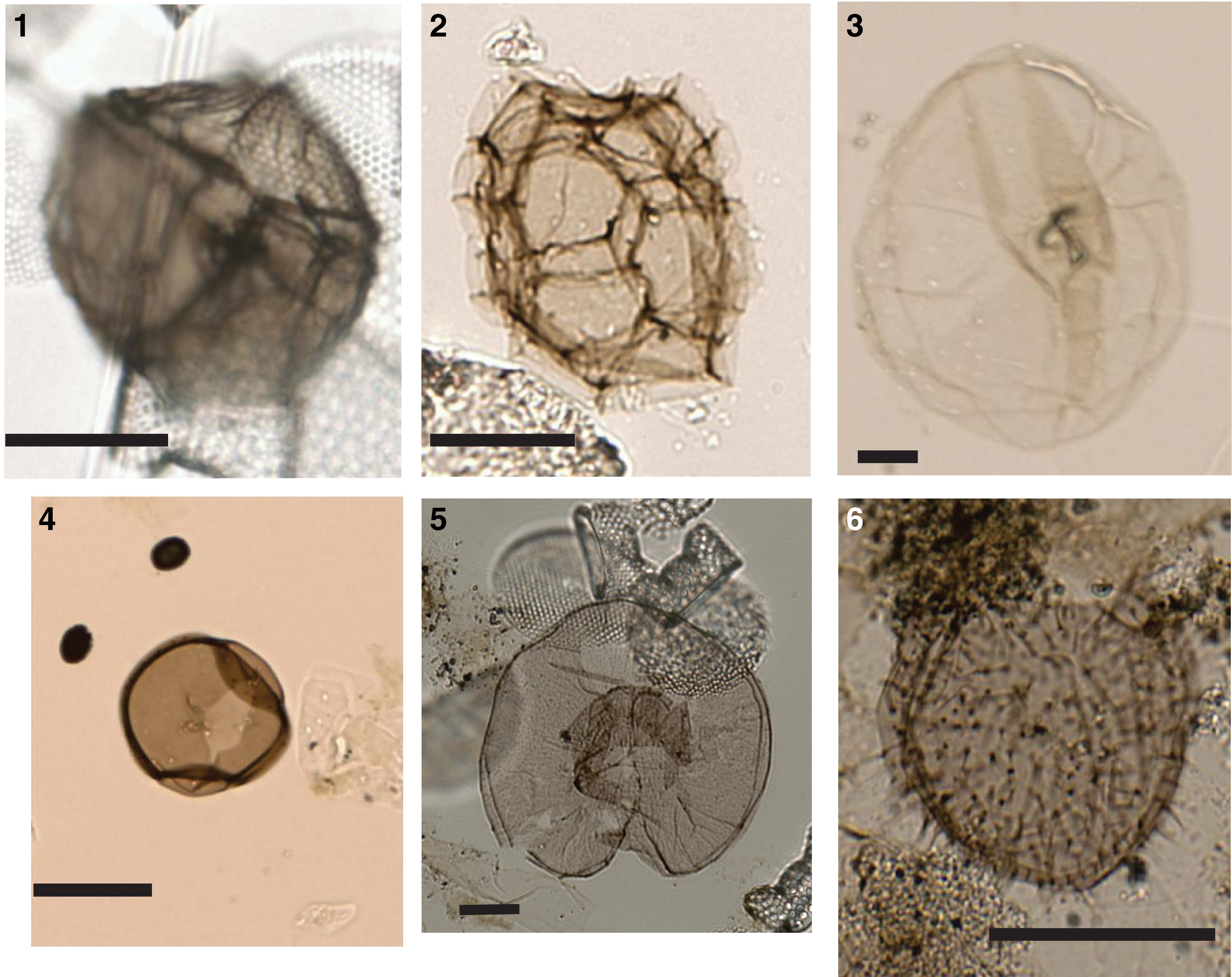
Figure F22. Palynomorphs, Hole U1536A.
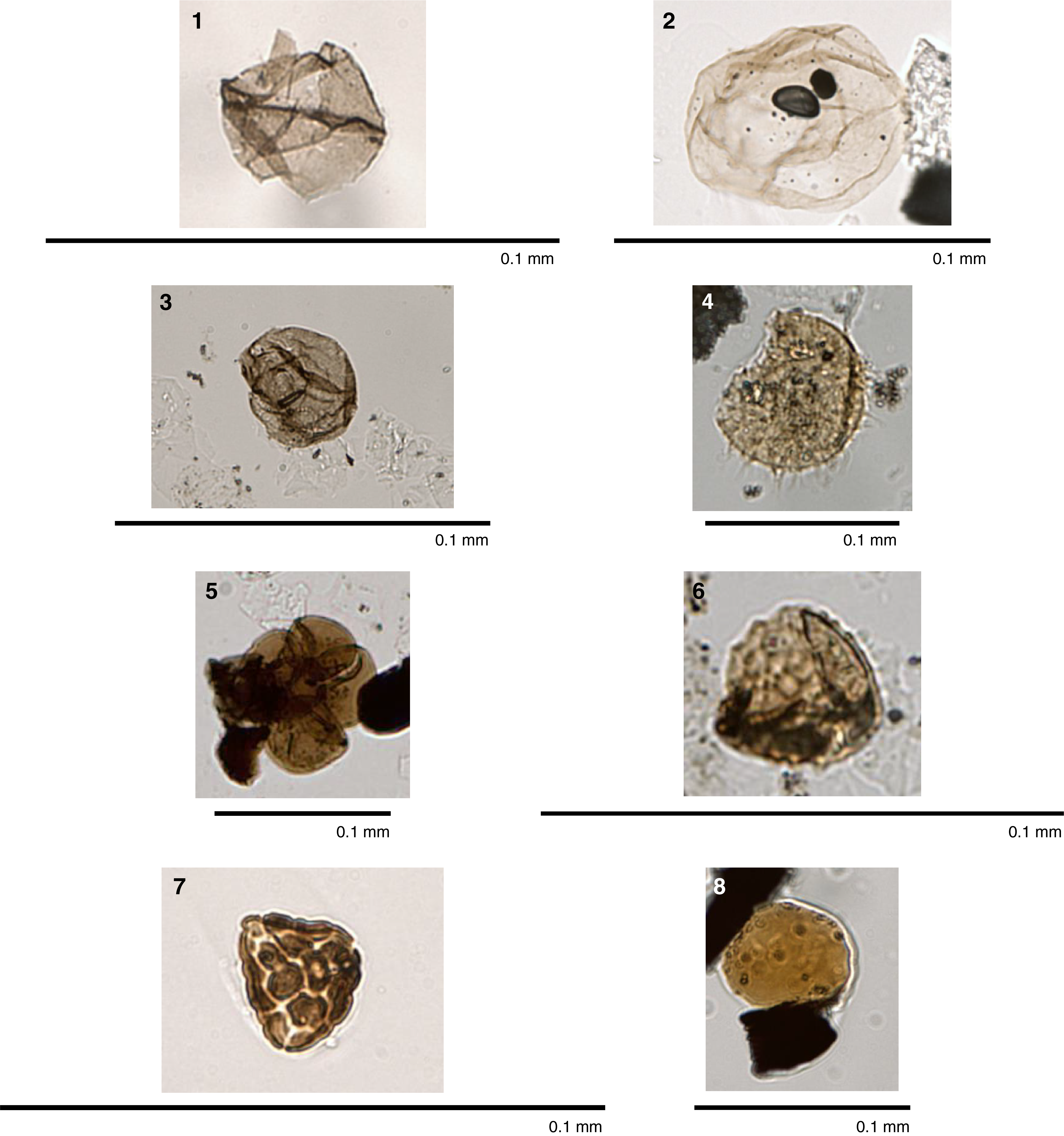
Figure F23. Palynomorphs, Hole U1536E.
All samples analyzed have a broad range in preservation, relative abundance, and diversity of palynomorphs. Few samples (382-U1536A-36F-CC and 46F-CC) are barren of palynomorphs. Generally, the dominant palynomorph association is composed of the heterotrophic dinocyst genera Brigantedinium spp. and Selenopemphix spp. and various reworked sporomorphs of Cenozoic and Mesozoic age. Reworking is evident in every core sample analyzed, and assemblages are largely composed of various reworked specimens of Cretaceous and Paleogene age. However, in situ dinocysts were recorded predominantly in Samples 382-U1536A-1F-CC to 28F-CC, 48F-CC to 50F-CC, 382-U1536C-40F-CC, and 382-U1536E-16R-CC and from Sample 25R-1, 131–134 cm, to the base of the hole. Most in situ dinocysts are protoperidinioids, except for the abundant Impagidinium spp., which is a gonyaulacoid, in Sample 31R-CC. The terrestrial pollen Nothofagidites spp. was found in Samples 382-U1536C-38F-CC and 382-U1536E-17R-CC and from Sample 30R-CC to the base of the hole. Podocarpidites spp. and other saccate (windblown) pollen were recorded sporadically throughout Site U1536, although most appear to be reworked. Other palynofacies such as acritarchs, prasinophyte algae, foraminifer test linings, copepod remains, black and brown phytoclasts, pyritized siliceous microfossils, and amorphous organic matter were also commonly recorded throughout Site U1536.
Most of the dinocysts and acritarchs identified during the shipboard analysis are long ranging and do not have much biostratigraphic significance. The occurrence of two species (Operculodinium? eirikianum [FO = 8.4 Ma] in Sample 382-U1536E-26R-CC and Impagidinium patulum [FO = 15.97 Ma] in Sample 31R-CC) provides useful age information for biostratigraphic interpretation and gives support to the interpreted ages from the other microfossil groups that have a higher abundance and sample resolution.
Marine sedimentary ancient DNA
Ancient DNA
Samples for ancient DNA (aDNA) were collected from Holes U1536B and U1536C. Sampling from Hole U1536B followed the previously outlined Hole B sampling methodology (see Biostratigraphy in the Expedition 382 methods chapter [Weber et al., 2021a]) and was conducted immediately after core retrieval on the catwalk. One sample (~10 mL) was retained from the Hole U1536B mudline. One to two samples were collected from Cores 382-U1536B-1H through 12H and 20H. Core 382-U1536C-1H was sampled at the top and bottom of Section 1 and at the bottom of Section 3. Cores 3H–6H, 8H, 11H, and 20H were sampled at the bottom of Section 6. Cores 7H, 9H, 11H, and 12H were sampled at the bottom of Section 2. This sampling scheme was intended to cover the Holocene and transitions into and out of glacial intervals as determined by preliminary physical property analyses. Core top samples from Cores 382-U1536C-1H and 2H were taken. In addition, aDNA samples were collected at 20, 50, and 70 cm from all sections except Sections 1H-5 (sampled at 20 and 70 cm only), 2H-5 (sampled at 30, 90, and 130 cm because of a clear change in sediment color), 2H-6 (sampled at 20, 50, and 70 cm), and 2H-7 (only one sample taken at 30 cm). All samples will be analyzed at the home laboratory, Australian Centre for Ancient DNA (ACAD), Adelaide (see Biostratigraphy in the Expedition 382 methods chapter [Weber et al., 2021a]).
Contamination control
One air control (empty tube) and one drilling fluid control with perfluoromethyl decaline (PFMD) tracer (~12 mL) were collected after both aDNA samplings from Holes U1536B and U1536C. After sampling Cores 382-U1536C-1H and 2H, laboratory surface swab control samples were also collected. Inner and outer sediment samples for chemical tracer testing (PFMD) were collected at the same depths as aDNA samples for Hole U1536B and at 69–70 cm (middle) in each section from Hole U1536C (except where sections were shorter and samples were taken higher up in the middle of the respective section). Samples were stored at 4°C and analyzed approximately 5 days after collection. PFMD concentrations were below the detection limit for all samples from Hole U1536B. All PFMD measurements for Hole U1536C were below the detection limit.
Summary
Diatom, radiolarian, foraminifer, palynomorph, and nannofossil biostratigraphic results are consistent for all samples from Holes U1536A, U1536C, and U1536E. These analyses identified 81 biostratigraphic events (Table T4). Based on these events, we estimate sedimentation rates of ~148 m/My from Samples 382-U1536A-1H-CC to 32F-CC, ~69 m/My from Samples 34F-CC to 53F-CC, and ~34 m/My from Samples 382-U1536E-2R to 30R-CC. A hiatus was observed between Samples 382-U1536E-30R-CC and 31R-CC, leaving a biostratigraphic gap spanning ~8.4–13.2 Ma. These approximate sedimentation rates and the suggested hiatus are illustrated in Figure F18. Estimated sedimentation rate changes may indicate variations in past ocean current strength, IRD delivery, taphonomic variability, and/or paleoproductivity. Our analyses suggest that an extended Pleistocene record was captured by the sediments acquired in Hole U1536A, underlain by a Pliocene section (around Sample 382-U1536A-45F-1, 75 cm). In Hole U1536E, a further extension of the Pliocene section was recovered, underlain by a Miocene section (around Cores 382-U1536E-20R through 22R). The bottommost sediments recovered date to the mid-Miocene (Samples 31R-CC to 33R-CC). Reworking was consistently noted, particularly in Hole U1536A.
Paleomagnetism
Paleomagnetic measurements were made on 393 APC and 163 HLAPC core sections from Holes U1536A (N = 145 APC/113 HLAPC), U1536B (N = 164 APC), and U1536C (N = 84 APC/50 HLAPC) and 77 RCB core sections from Hole U1536E to investigate the natural remanent magnetization (NRM). Orientation data were collected for Cores 382-U1536A-4H through 23H and 382-U1536B-1H through 25H using the Icefield MI-5 core orientation tool (see Paleomagnetism in the Expedition 382 methods chapter [Weber et al., 2021a]). No archive-half measurements were made on core catcher samples. All archive-half measurements were made on the initial magnetization and the magnetization following peak alternating field (AF) demagnetization at 10 and 15 mT. Cores 382-U1536A-2H through 19H were also demagnetized using a 20 mT peak AF to assess what fields were needed to remove the drill string overprint. The 20 mT step was discontinued after observing the drill string overprint was generally removed by the 10 mT step.
A total of 393 discrete cube samples were taken from the working halves from Holes U1536A, U1536B, and U1536E. In general, we took one sample per section from cores recovered in Hole U1536A (avoiding visually disturbed intervals) for a total of 253. These were supplemented by a limited number of samples (N = 26) taken from Hole U1536B to cover gaps and disturbed intervals in Hole U1536A. We took 114 samples from Hole U1536E with as many as three samples taken per section to verify the archive-half measurements in which the signal from intact biscuits is mixed with the signal from the surrounding mud and cuttings. We measured the NRMs of all cubes from Holes U1536A and U1536E on the superconducting rock magnetometer (SRM) using the discrete sample tray. The NRMs of 243 specimens were measured followed by stepwise demagnetization at peak AF steps of 5, 10, 15, and in some cases 20 mT. At 10 mT and subsequent steps, we demagnetized and measured the specimens in three orthogonal positions (top-away, top-right, and away-bottom settings in the SRM measurement program), averaging the three measurements to insure data quality. A subset of 23 specimens was subjected to an additional AF treatment at 30, 40, and 50 mT using the three-step procedure. These specimens were then given an anhysteretic remanent magnetization (ARM) in a 100 mT AF field with a 50 µT direct current (DC) bias field followed by AF demagnetization and then a stepwise isothermal remanent magnetization (IRM) acquisition experiment at 100, 200, 300, 400, 600, 800, and 1000 mT steps with AF demagnetization of the 300 mT IRM. Both the ARM and the IRM were demagnetized to 50 mT using the same steps as for the NRM.
The anisotropy of magnetic susceptibility (AMS) of 160 of the discrete cubes from Hole U1536A was investigated using the AGICO KLY 4S Kappabridge. Our goals were to conduct a preliminary assessment of the nature of magnetic fabrics in terrigenous-rich versus biosiliceous-rich lithologies, detect potential hiatuses, and assess the potential to use AMS to track past oceanographic processes at the core site.
Natural remanent magnetization
Site U1536 archive halves were initially AF demagnetized at 0 (NRM step), 10, 15, and 20 mT (Cores 382-U1536A-1H through 19H) to determine the peak field necessary to identify and remove the drilling overprint. The data from the 15 mT step prior to any editing are shown as black dots in Figures F24, F25, F26, and F27 for Holes U1536A, U1536B, U1536C, and U1536E, respectively. Cyan dots show the data after editing (see below), averaging core declinations, and adjusting each core to have a mean normal declination of 90° for purposes of plotting. We assessed the reliability of polarity determinations in several ways:
- Examination of lithologic descriptions and X-ray images for disturbance,
- Stepwise AF demagnetization of discrete samples,
- Examination of histograms of inclinations (which should be bimodal at the expected geocentric axial dipole [GAD] inclinations at the site; see Paleomagnetism in the Expedition 382 methods chapter [Weber et al., 2021a]) and declinations (which should be uniformly distributed owing to presumably random orientations of core double lines), and
- Agreement of the interpreted magnetostratigraphy with available biostratigraphic constraints.
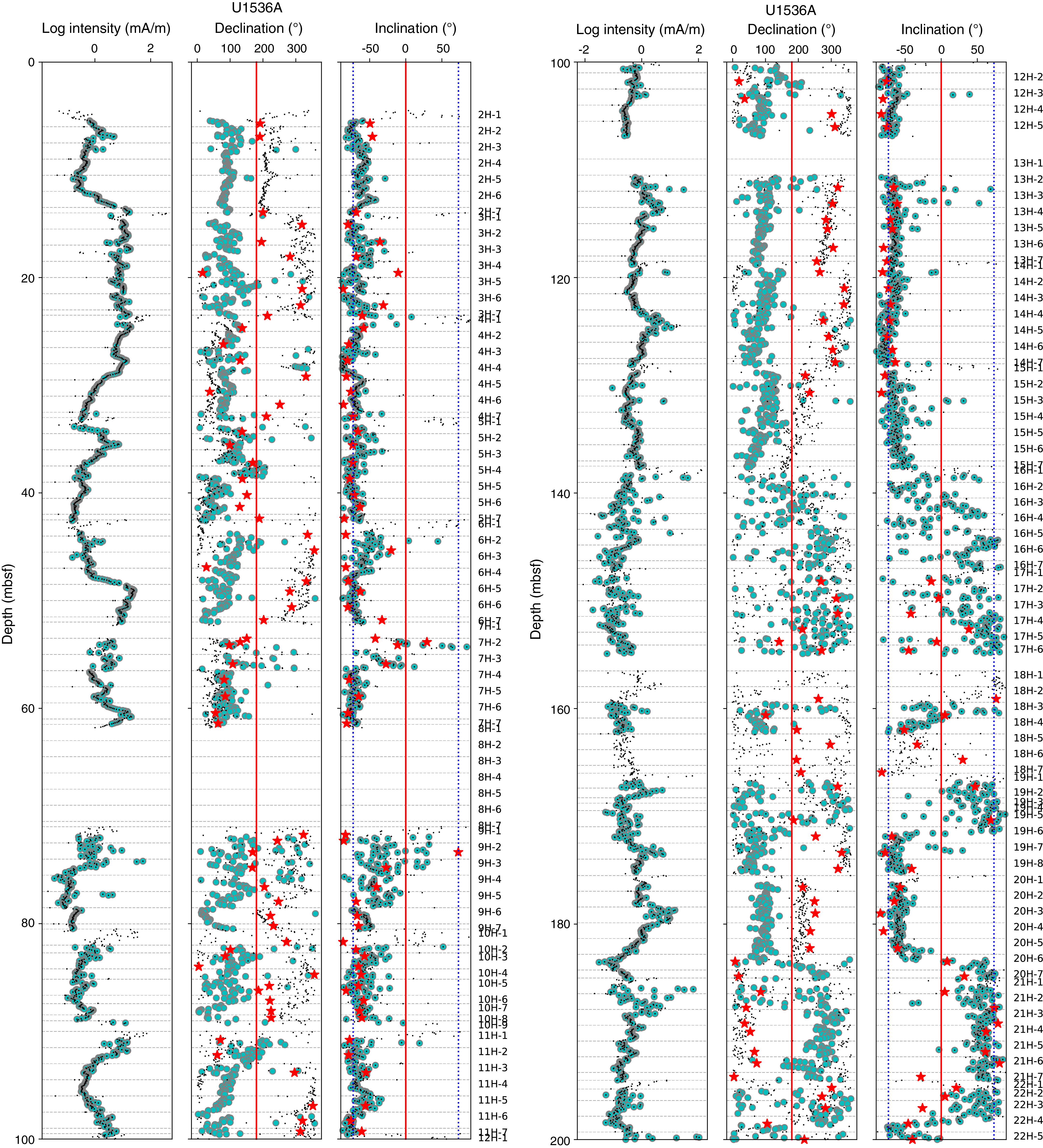
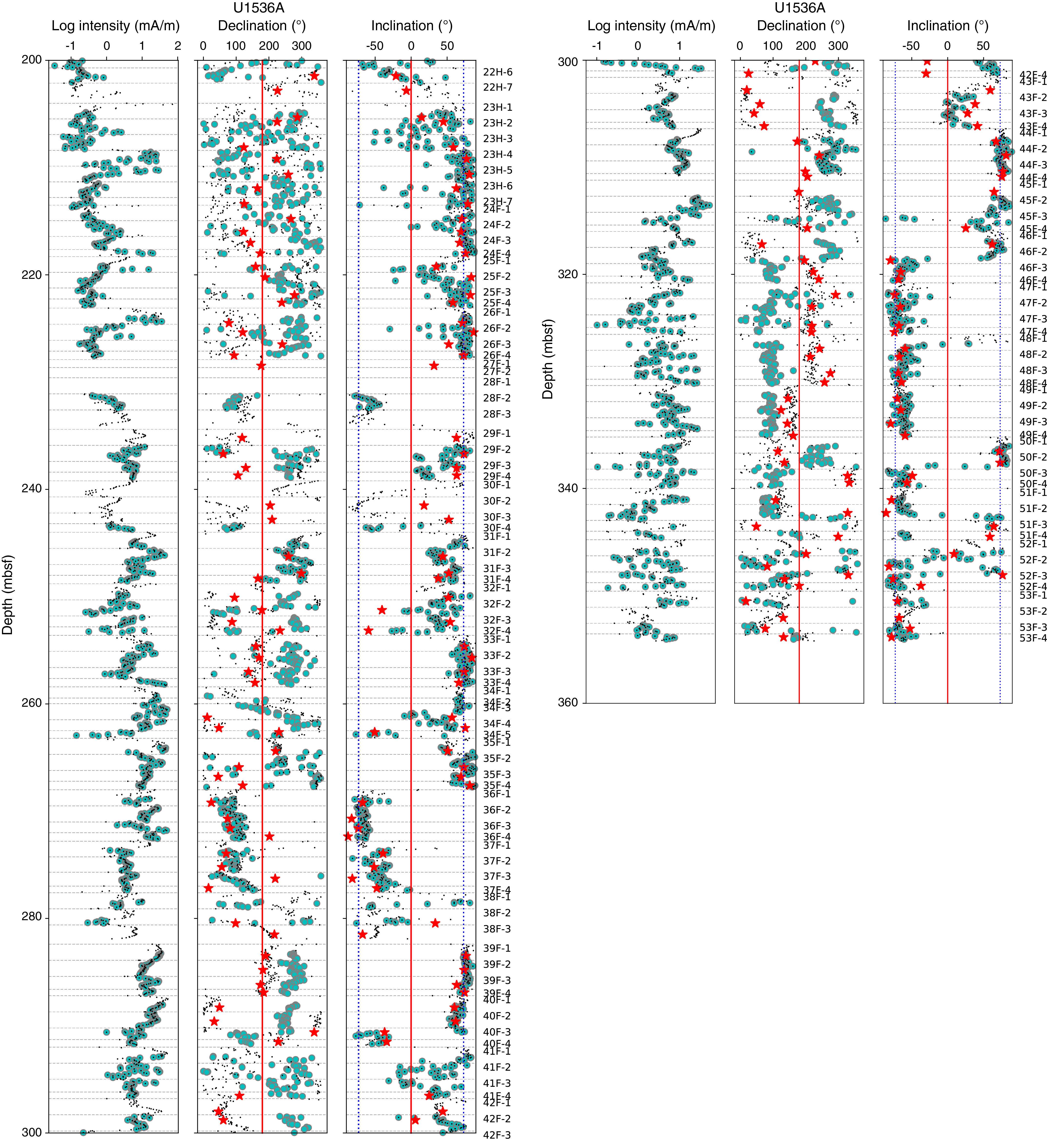
Figure F24. Intensity of remanence, declination, and inclination, Hole U1536A.
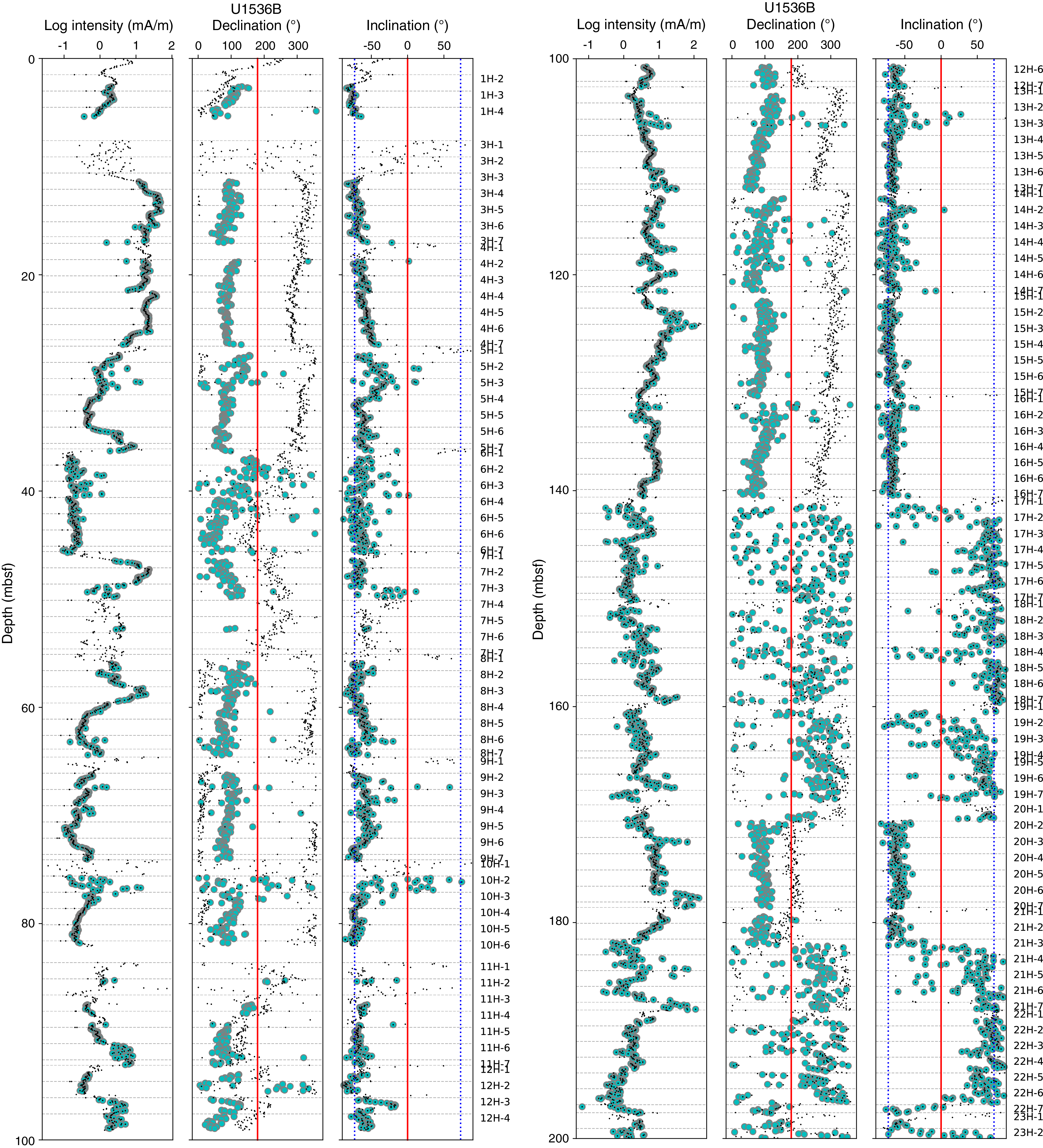
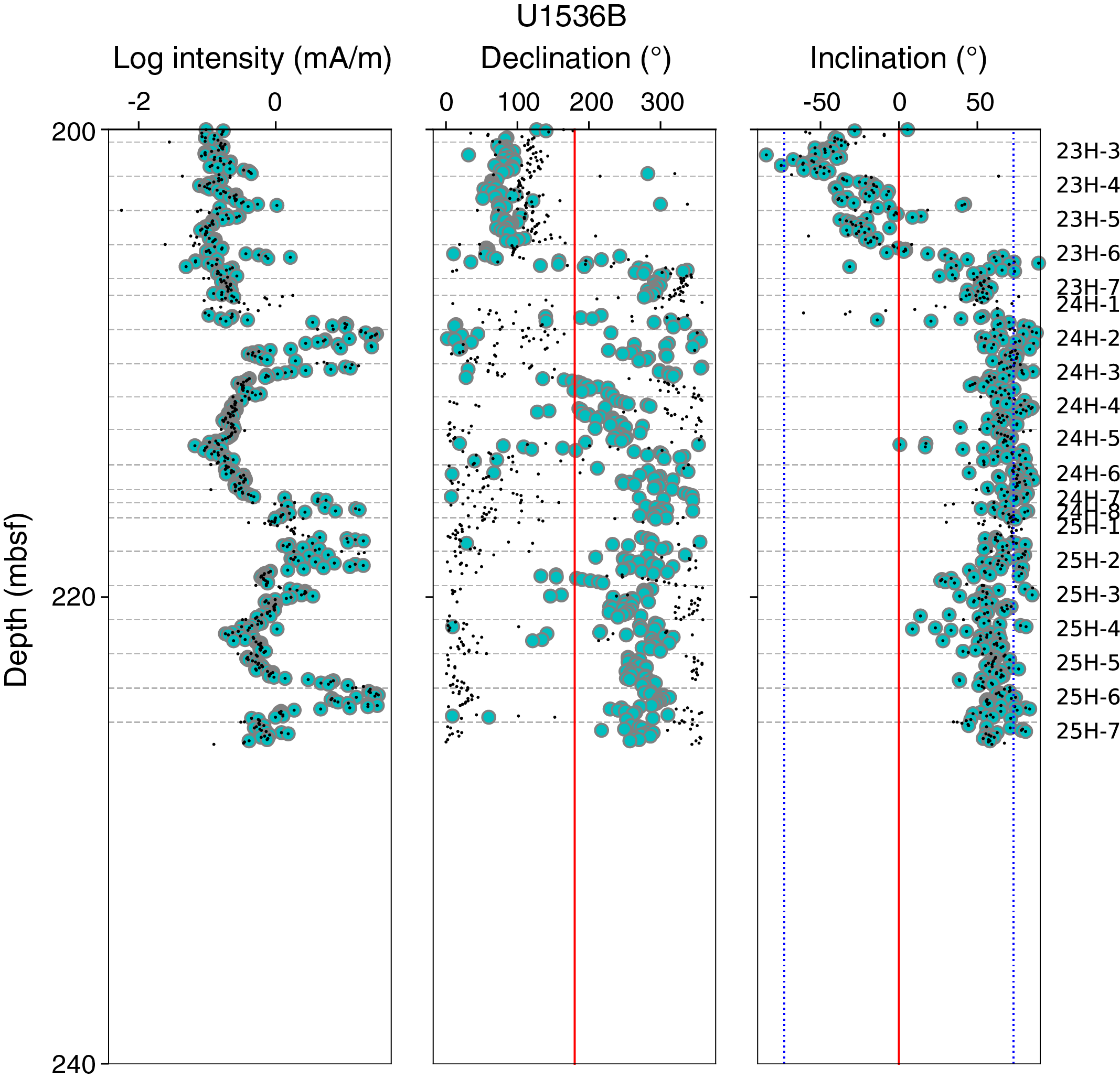
Figure F25. Intensity of remanence, declination, and inclination, Hole U1536B.
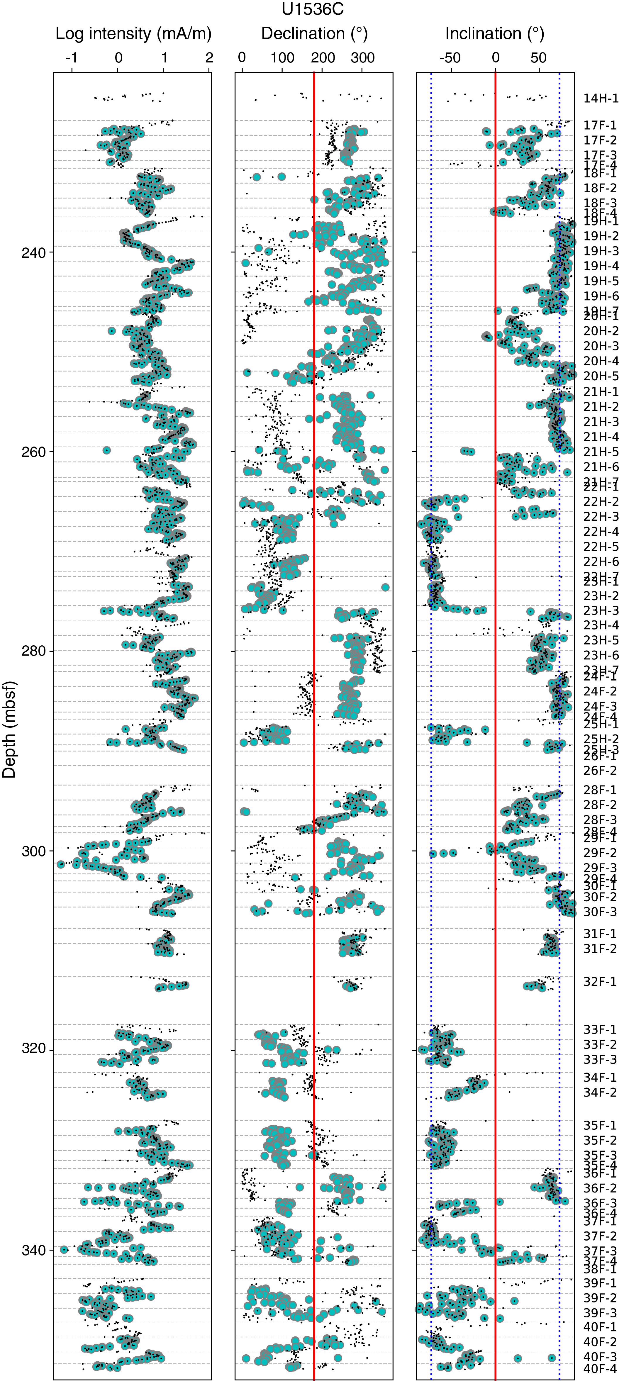
Figure F26. Intensity of remanence, declination, and inclination, Hole U1536C.
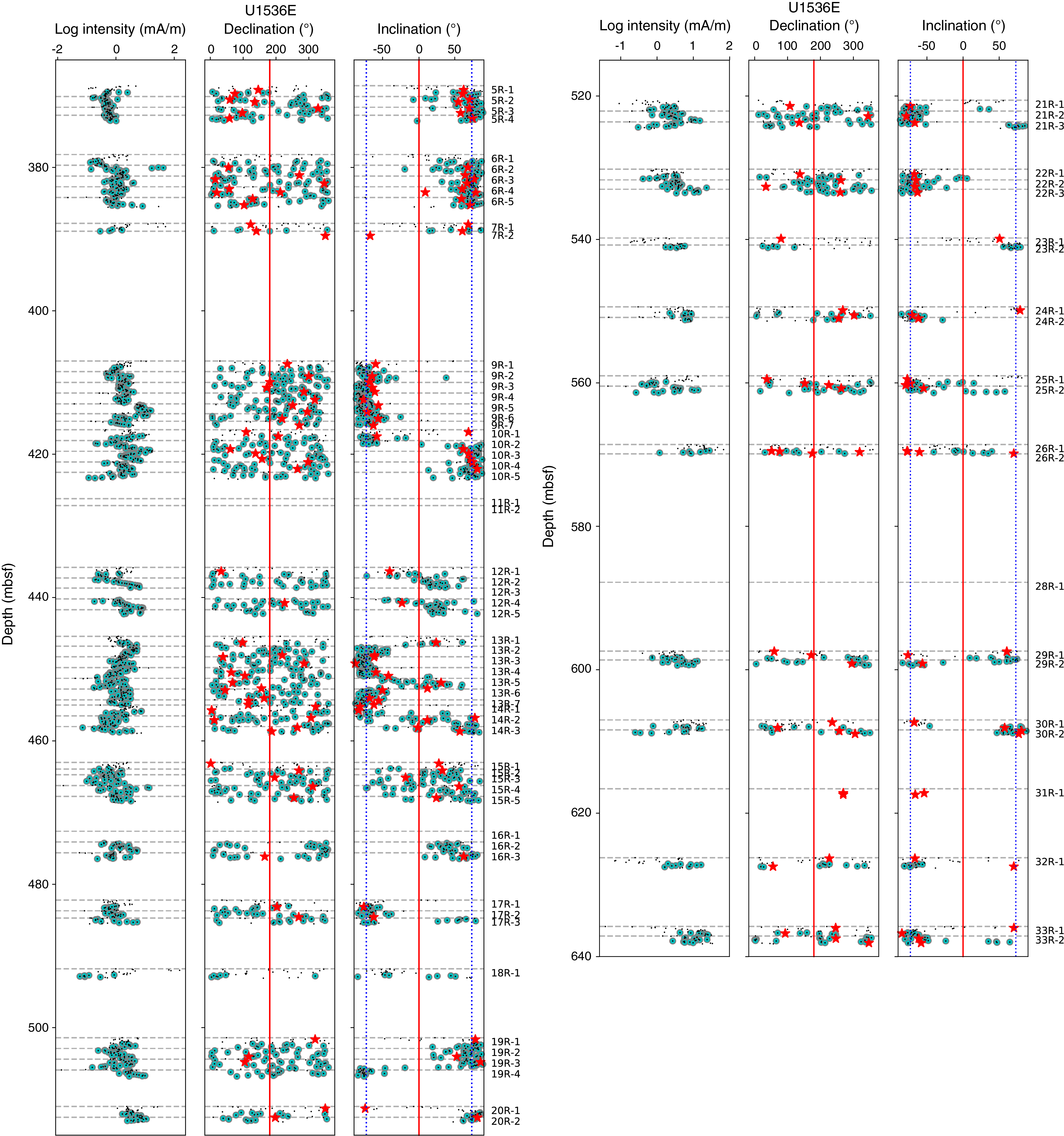
Figure F27. Intensity of remanence, declination, and inclination, Hole U1536E.
Editing of archive-half measurements for coring disturbance
Editing of the archive-half measurements was automated using Jupyter notebooks. These data were systematically filtered:
- We deleted all measurements within 10 cm of the section ends to remove the edge effect inherent in all pass-through measurement systems such as the SRM.
- We deleted all measurements in the upper 80 cm of Section 1 of all APC and HLAPC cores because they are the most susceptible to the accumulation of fall-in material during coring. Additionally, the strong vertical drilling overprint in these intervals often appeared to be more difficult to remove.
- We deleted all data from intervals that were assigned the "high" drilling disturbance intensity code entered during core description (see Lithostratigraphy) to remove data in intervals affected by coring-induced disturbance such as fall-in and flow-in.
Tables T8, T9, T10, and T11 are adapted from the DESClogik tables used to perform the editing.
We next inspected core composite photographs and X-radiographs for evidence of coring or sedimentary disturbance (see Paleomagnetism in the Expedition 382 methods chapter [Weber et al., 2021a]). Tables T12, T13, and T14 were used to edit data from Holes U1536A–U1536C based on X-ray images. X-ray images were not logged for Hole U1536D because these archive halves were not measured on the SRM. No X-ray information was used from Hole U1536E to edit the RCB cores.
Discrete sample data
We selected a set of 23 discrete samples for stepwise AF demagnetization experiments up to an AF of 50 mT. Representative examples of the behavior during demagnetization are shown in Figure F28. Examples from "high susceptibility" intervals are shown in Figure F28A–F28D, and those from "low susceptibility" intervals are shown in Figure F28E–F28H. A very minor drilling overprint was observed in a positive downward direction, and it was generally removed at the 10 mT step. Some specimens from the low susceptibility intervals were too weak to be reliably measured on the shipboard instruments (Figure F28G, F28H), but in general the data are quite encouraging. Both polarities are readily identified; normal directions (upward-directed vectors) are shown in Figure F28A, F28B, F28E, F28F, and reversed directions are shown in Figure F28C, F28D, F28G, F28H. Apart from the two weak examples, the data show a smooth decay to the origin with no apparent effect from laboratory-acquired remanences like ARM or gyroremanent magnetization. Based on these data, we subjected all archive halves to AF demagnetization at 10 and 15 mT. The 15 mT step after editing is shown as cyan dots in Figures F24, F25, F26, and F27. Discrete sample data measured after demagnetization to 15 mT are shown as red stars. Nearly all of these data agree well with the archive-half measurements. Note that the declinations of the discrete samples were not adjusted, so they should be compared with the small black dots and not the adjusted cyan dots from the archive-half measurements.
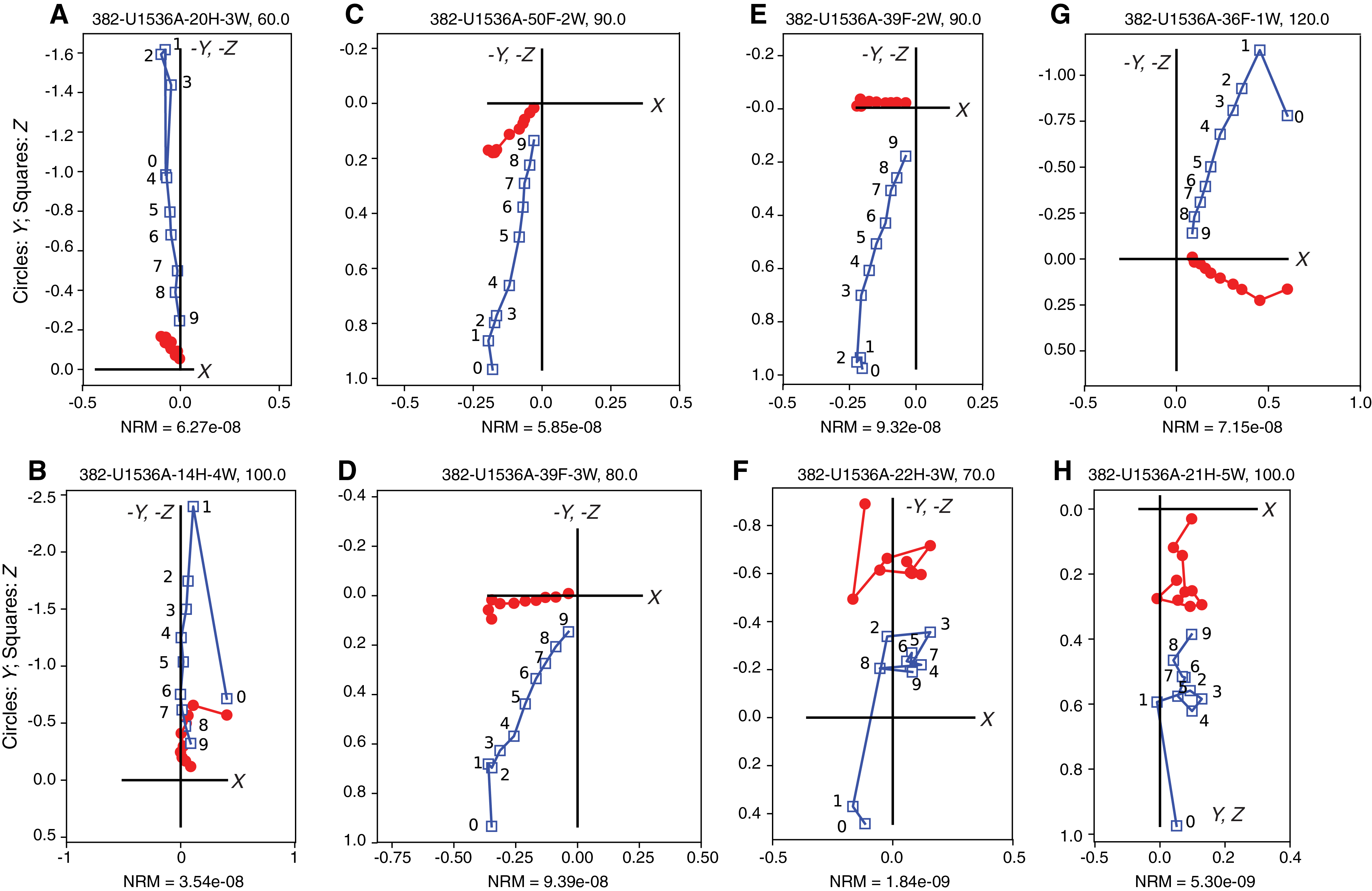
Figure F28. Vector endpoint diagrams.
ARMs imparted in a 100 mT peak field and 0.05 mT DC bias field and IRMs imparted at a 300 mT pulsed field were demagnetized at peak AFs in 5 mT steps to compare them with the NRM AF demagnetization behavior and to better understand the remanence carriers. Data for AF demagnetization of NRM, ARM, and IRM are shown in Figure F29. All measurements are normalized by magnetization (M) after AF demagnetization at 20 mT. The NRM data (Figure F29A) show smooth decay (apart from two very weak specimens mentioned before). ARM demagnetization generally shows little change in demagnetization behavior between 0 and 10 mT peak AF, whereas a significant change often occurs in the IRM over the same interval, indicating that ferrimagnetic mineral assemblages with a range of coercivities are present in each sample (Figure F29B, F29C). Coercivity appears to have a systematic relationship with MS; lower coercivity ferrimagnetic minerals are present in high MS samples, and higher coercivity ferrimagnetic minerals are present in low MS samples (see susceptibility color code in Figure F29D). This distinction can be most clearly seen in the demagnetization of the IRM imparted at 300 mT, suggesting much of this variability is being driven by low-coercivity ferrimagnetic minerals (Figure F29C). IRM acquisition experiments do not gain significant magnetization above 300 mT, suggesting high-coercivity magnetic minerals, like hematite and/or goethite, do not contribute greatly to the sediment remanence. These results are most consistent with the remanent magnetizations being carried by a population of detrital (titano)magnetite. The suggestion that low and high susceptibility intervals have distinct rock magnetic behaviors is further supported by the IRM800mT versus susceptibility plot in Figure F29E. The two groups have different slopes, supporting the notion that dilution alone cannot explain the behavior and there are two distinct grain size and/or mineralogic populations. However, postcruise work will be needed to further characterize the magnetic mineral assemblages.
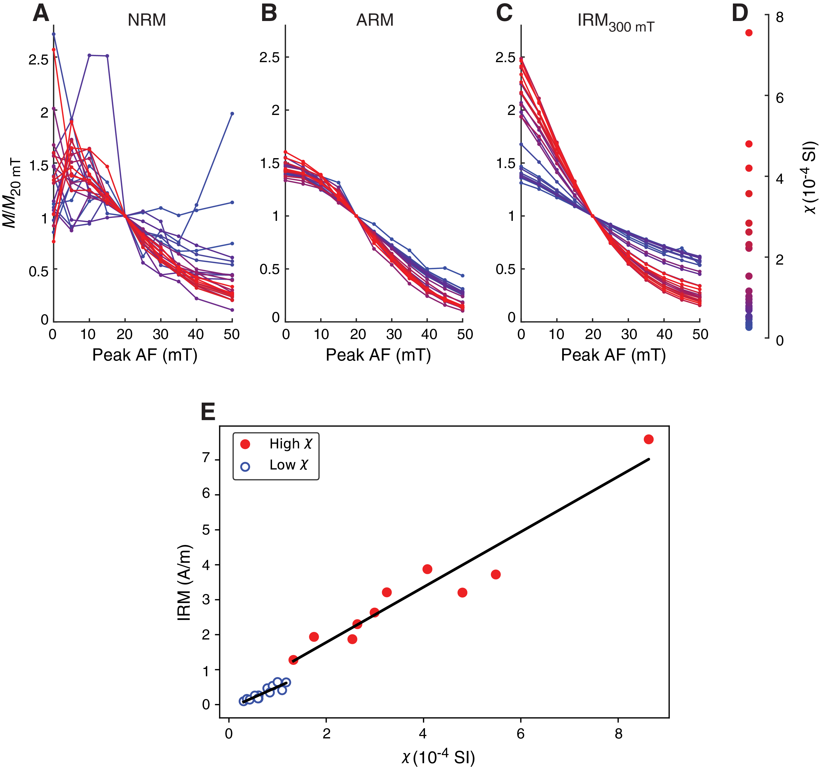
Figure F29. Stepwise AF demagnetization.
Distributions of inclinations and declinations
We plotted histograms of inclination values separated by coring type in Figure F30. All coring types (APC, HLAPC, and RCB) show two distinct groups with steep directions generally spanning ±45°–90°. The number of normal polarity observations (negative inclinations) is greater than the number of reversed observations (positive inclinations) in the APC cores, which is expected because these are the youngest cores and they are dominated by Brunhes age (normal) sediments. The older records sampled by the HLAPC and rotary cores are more or less equally distributed between the two polarities.
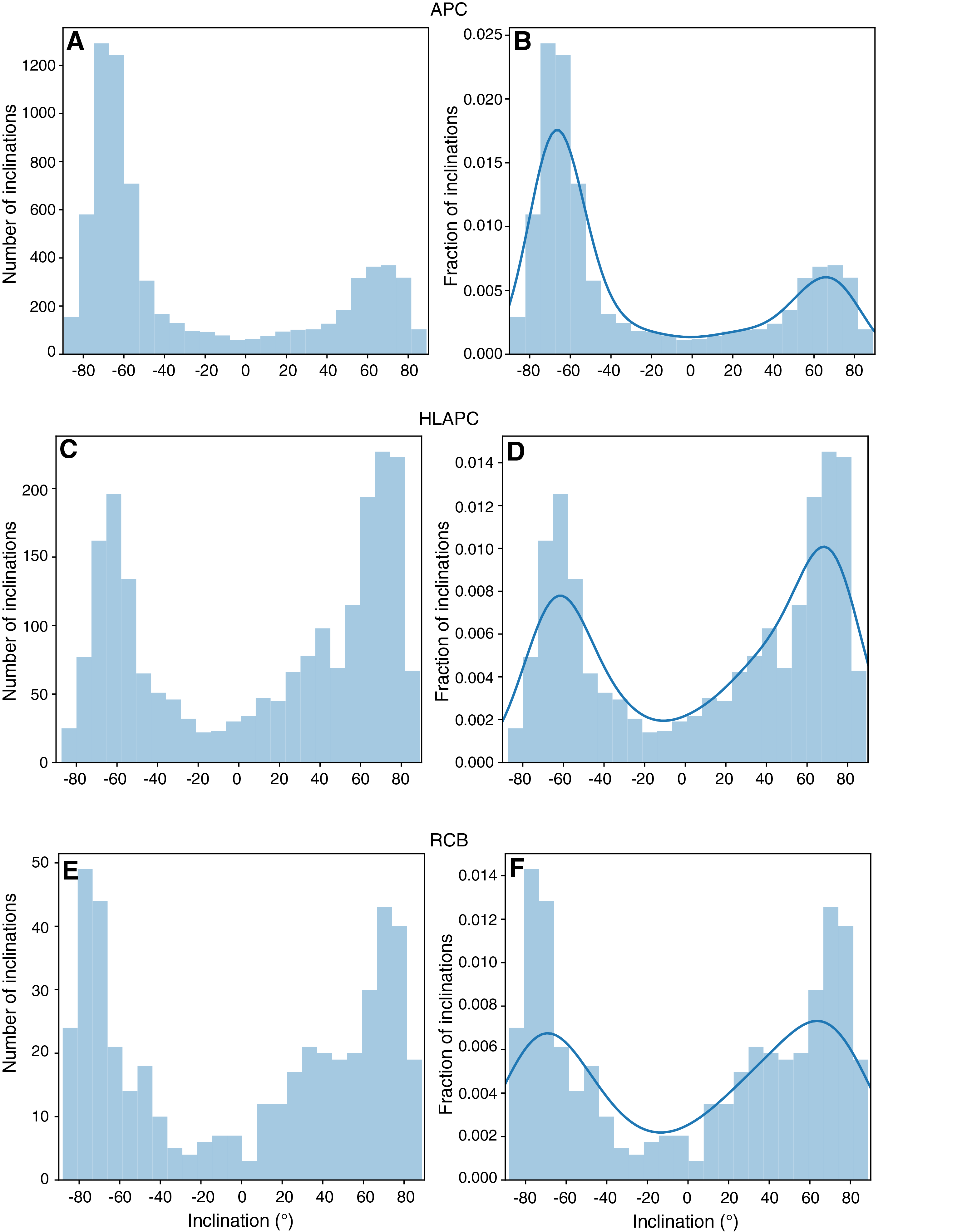
Figure F30. Inclination after editing.
Declinations for these unoriented cores would be expected to be uniformly distributed, and we plot histograms (Figure F31A–F31C) and quantile-quantile plots (Figure F31D–F31F) to test this hypothesis. Although the APC cores in particular appear to have a bias toward the 0° (and 360°) directions (the double line), none of the sets of declination data are in fact distinguishable from a uniform distribution at the 95% level of confidence based on a Kolmogorov-Smirnov test.
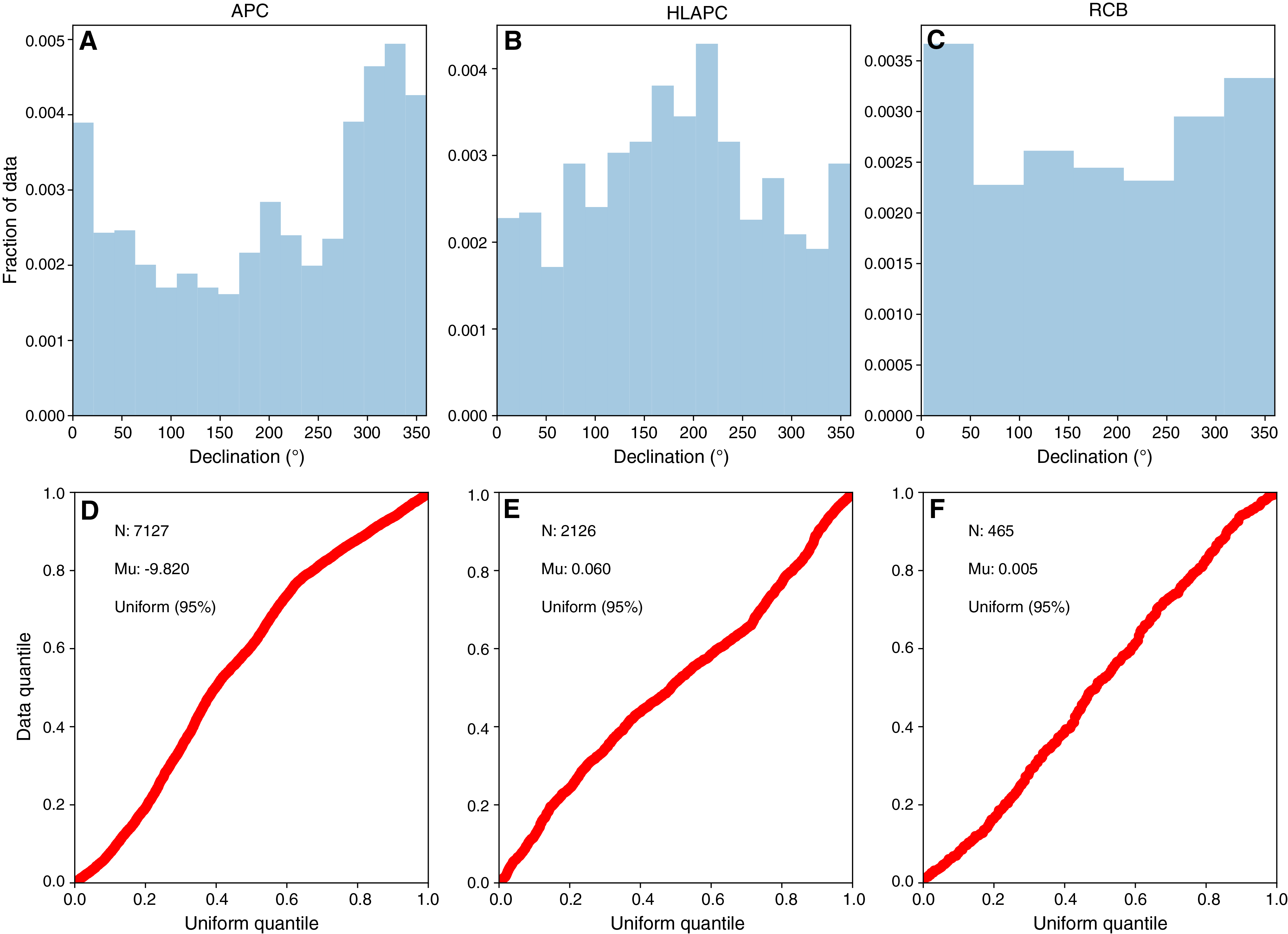
Figure F31. Declination after editing.
Icefield MI-5 core orientation tool orientation results
Two Icefield MI-5 tools were deployed during the collection of full-length APC cores (Table T15). Tool 2052 was used to orient Cores 382-U1536A-4H and 14H–23H. Tool 2043 was used for Cores 5H–13H. Tool 2043 was used for Cores 382-U1536B-1H through 15H. Tool 2052 was used for Cores 16H–25H. According to the manufacturer's conventions, which we confirmed during the expedition, −Z is down and −X is north (unlike in geological applications). Therefore, we took the antipode of the magnetic tool face (MTF) as output by the Icefield software.
The results for the two holes are shown in Figure F32. The red squares and triangles are average directions for each core after removal of disturbed intervals, as described in the previous section. Averages were calculated as principle components, and the upward directed vector (normal) was taken as the average core direction. The declination of this average direction was then adjusted by adding the azimuths determined by the Icefield MI-5 tool (Table T15). Directions determined by Tool 2052 are plotted as squares, and those from Tool 2043 are plotted as triangles.
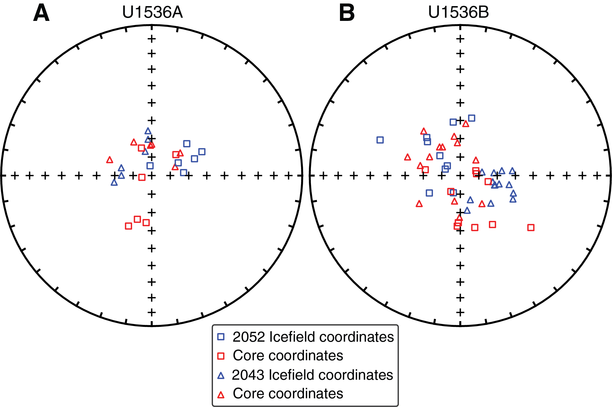
Figure F32. Equal-area projections of normal core mean directions.
Encouragingly, each tool produced better clustering of directions in each hole relative to the initial efforts at Site U1534 (see Paleomagnetism in the Site U1534 chapter [Peck et al., 2021]). However, the two tools behaved differently from one another, and puzzlingly, each tool behaved differently in the two different holes. Although Tool 2052 generated average directions in the northeastern quadrant in Hole U1536A, it generated directions in the northwestern quadrant in Hole U1536B. Tool 2043 produced directions in the northwestern quadrant in Hole U1536A and the southeastern quadrant in Hole U1536B. During the expedition, we continued to engage with Icefield engineers to identify potential issues or misunderstandings that could explain this behavior. However, we did not arrive at a solution during the expedition that would allow the Icefield data to be used for orientation (see Paleomagnetism in the Expedition 382 methods chapter [Weber et al., 2021a]).
Magnetic polarity stratigraphy
The preliminary magnetostratigraphic interpretations are based on inclinations from the 15 mT AF demagnetization step (Figures F24, F25, F26, F27, F33, F34). We defined polarity transition intervals by starting with two questions:
- Is the transitional interval directly observed (i.e., the starting polarity state, transitional directions, and final polarity state are all observed with no part of the phenomenon missing)?
- Is the transition "clean" (i.e., it occurs over a narrow interval and is unaffected by natural disturbance [slumps or soft-sediment deformation] and coring-induced disturbance)?
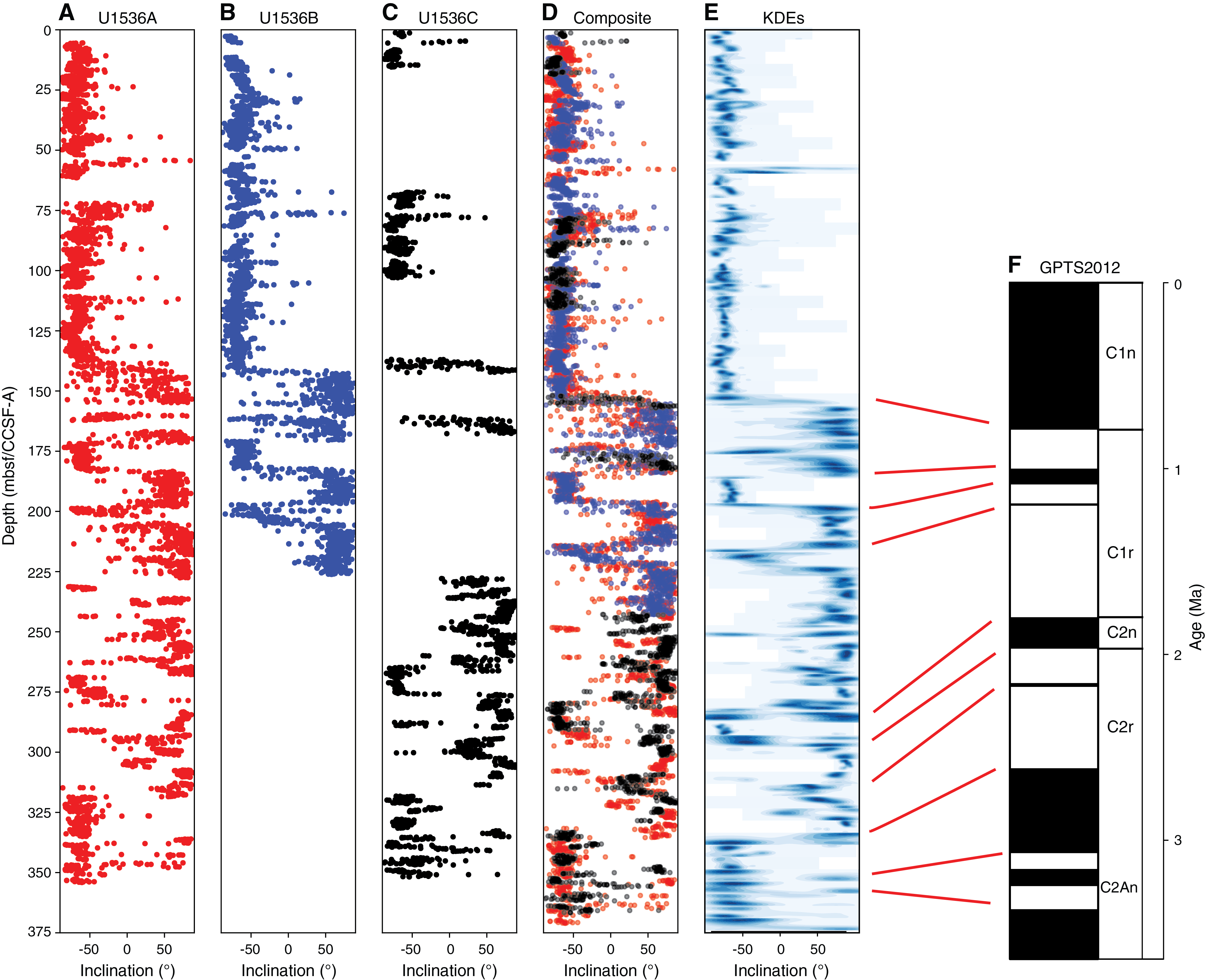
Figure F33. Magnetostratigraphic correlation, Holes U1536A–U1536C.
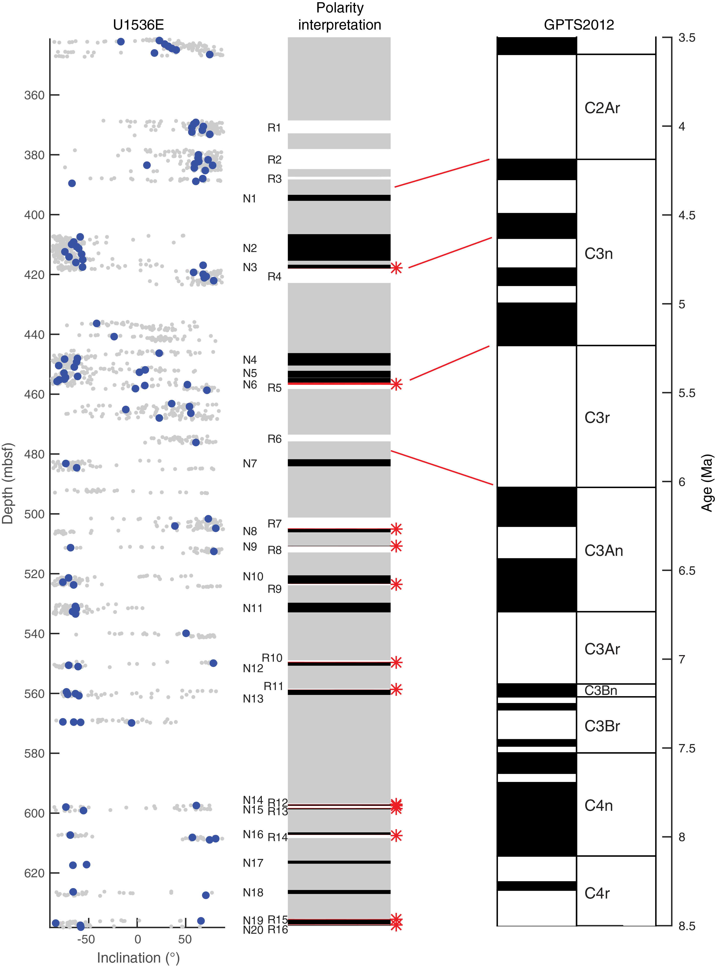
Figure F34. Magnetostratigraphic correlation, Hole U1536E.
If the answer to both questions was yes, we identified the closest observation of stable polarity above and below the transition interval, with stable defined as three consecutive measurements of inclinations steeper than ±45°. If the answer to either Question 1 or 2 was no, then the polarity transition was inferred to reside in a data gap between two cores or in a disturbed section. In this case, we identified the depth of stable polarity above and below the data gap. The magnetostratigraphic interpretations for Holes U1536A–U1536C and U1536E are shown in Figures F33 and F34, respectively. Figure F33 shows data in meters below seafloor and after transforming to core composite depth below seafloor, Method A (CCSF-A), using the affine table (Table T21). The depths of polarity transitions are listed in Table T16.
Hole U1536A preserves a succession of normal and reversed polarity zones that span Chron C1n (Brunhes) to below Chron C2An.2r (Mammoth) in Chron C2An.3n (early Gauss). Hole U1536B records a clear succession of six normal and reversed polarity zones (three of each) that we interpret as spanning Chrons C1n (Brunhes), C1r.1n (Jaramillo), and C1r.2n (Cobb Mountain), with the base of Hole U1536B in Chron C1r.3r (middle Matuyama). The coring strategy in Hole U1536C was aimed at recovering targeted intervals for the splice separated by washed down intervals without core recovery. This included Core 382-U1536C-10H, which captured the transition interval of the Matuyama/Brunhes boundary but not the immediate stabilization of normal polarity above the transition.
Following a washed down interval below Core 382-U1536C-10H, the magnetostratigraphy in Hole U1536C resumed in Cores 17H–40F. This interval contains nine polarity zones (four normal and five reversed), which we interpret as spanning the bottom of Chron Cr1.3r (middle Matuyama) through the middle of Chron C2An.3n (early Gauss). We did not observe the top of Chron C2An.1r (Kaena) in any of the holes; its location can nonetheless be inferred to lie between two cores in each of the holes.
Hole U1536E was rotary cored and was intended to penetrate to the basement. Despite discontinuous recovery, we can make tentative ties to the timescale for intervals between Chrons C2Ar and C3An after close consultation with the biostratigraphic team. Below this range, we interpret intervals of normal and reversed polarity that could be tied to the polarity timescale in future work with stronger biostratigraphic constraints.
The resulting magnetostratigraphic tie points are listed in Table T16, and age-depth relationships are plotted in Figure F35. The stars are magnetostratigraphic tie points, and the triangles are biostratigraphic datums. The cyan curve is a third order polynomial fit through the magnetostratigraphic ties in Table T16 to illustrate the age-depth relationship. Apart from a few exceptions, there is excellent agreement between the curve and the available biostratigraphic and magnetostratigraphic constraints. Transforming to the CCSF-A depth scale using the affine table (Table T21) led to the fit shown in Figure F35B.
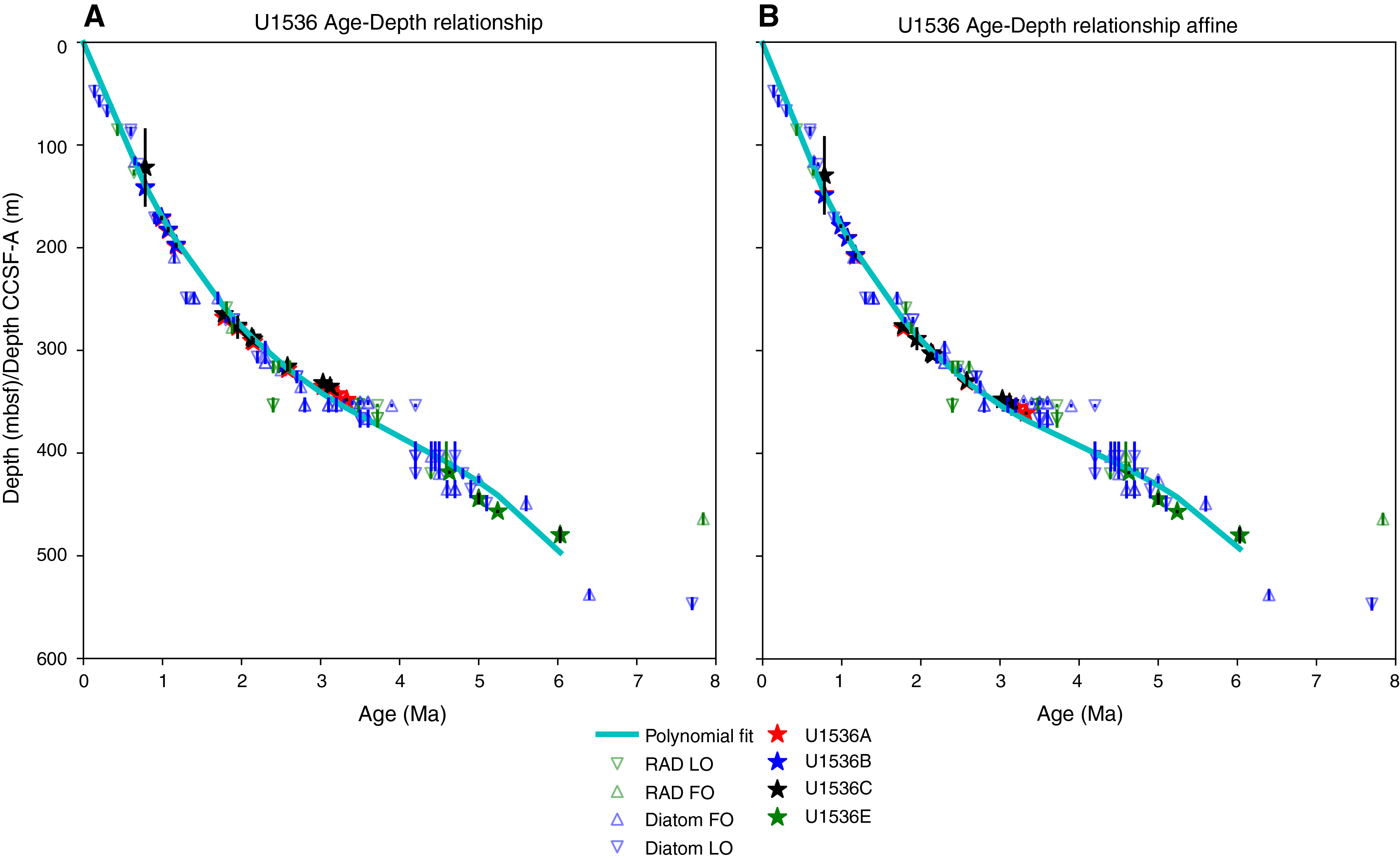
Figure F35. Age-depth plot.
Anisotropy of magnetic susceptibility
AMS was analyzed on a subset of 160 oriented discrete samples ("Japanese" cubes) from Hole U1536A. Our goals were to assess the nature of magnetic fabrics in terrigenous-rich versus biosiliceous-rich lithologies and assess the potential to use AMS for postcruise exploration of bottom current intensity and direction at Site U1536. We targeted three intervals:
- 0–200 mbsf, which consists of alternating diatom ooze units and silty clay units;
- 240–280 mbsf, which consists of diatom-bearing and diatom-rich silty clay with higher susceptibility values and higher amplitude changes in susceptibility than in the upper part of the core; and
- 300–350 mbsf, which consists of diatom-bearing and diatom-rich silty clay but has slightly lower susceptibility values and lower amplitude changes in susceptibility than 240–280 mbsf.
Samples from all three intervals generally display expected sedimentary fabrics with the minimum susceptibility axis (I3) oriented near vertical or within 20° of vertical and the maximum (I1) and intermediate axes (I2) distributed in a horizontal plane. A notable exception to this pattern is the 0–20 mbsf interval, in which I1 is oriented vertically (Figure F36C). This behavior of I1 has previously been used as an indicator of core stretching, which adversely affects the NRM (Thouveny et al., 2000).
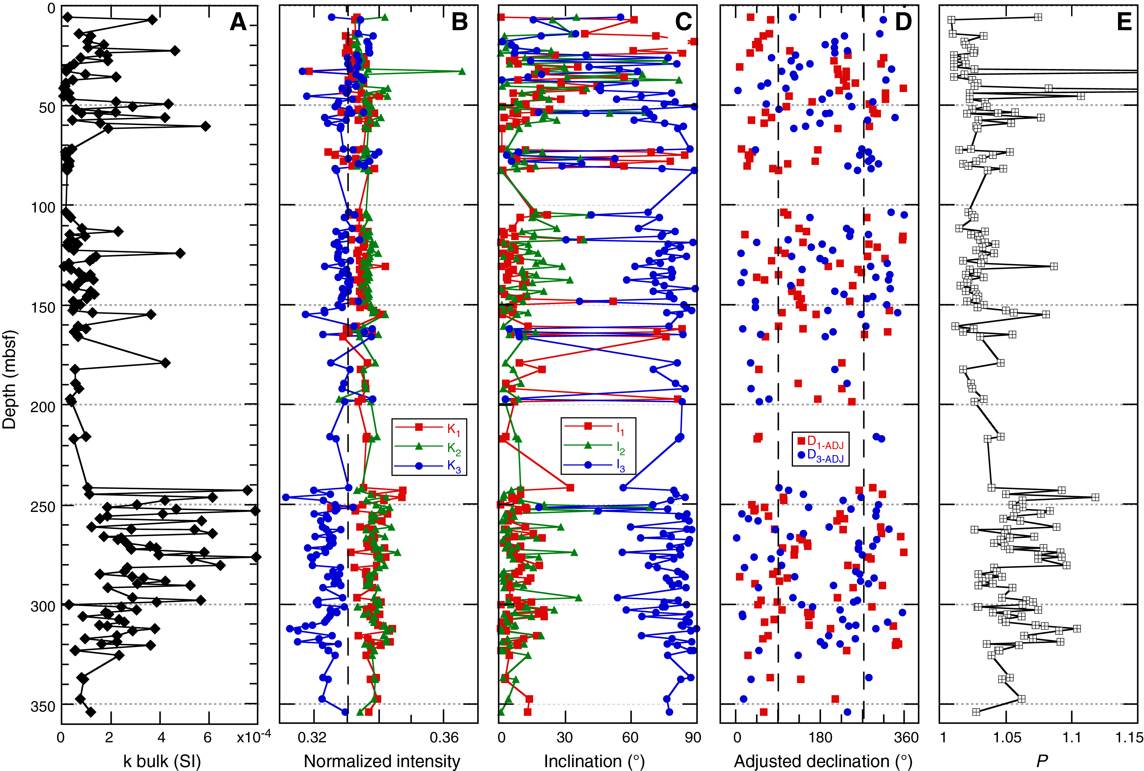
Figure F36. AMS summary data.
Samples from 0 to 90 mbsf were close to isotropic with nearly equal values of the maximum, intermediate, and minimum susceptibilities and P values generally below 1.03 (Figure F36B). This suggests little environmental influence on the magnetic fabric in this interval. Samples from 240 to 280 and from 300 to 350 mbsf have slightly higher degrees of anisotropy, with P values between 1.05 and 1.10. However, other than these large-scale observations, no consistent relationship exists between bulk susceptibility and the degree of anisotropy (R2 = 0.23).
AMS declinations (as measured D1 and D3 in the core coordinate system) tend to cluster around 90° and 270° in the upper 240 m, which are perpendicular to the specimen's x-axis. This could be an indicator of a fabric imparted when the cubes or the extruder are inserted into the core face (which is the x-direction).
AMS declinations were adjusted in the same manner as the NRM declinations. The NRM declinations after treatment at the 15 mT level were averaged for each APC and HLAPC core. Each core's mean value was set to zero, yielding a rotation factor that was applied to each individual NRM measurement. We applied these same rotation factors to the AMS declinations in the Jupyter notebook for Hole U1536A. We refer to these as adjusted AMS declinations D1-ADJ, D2-ADJ, and D3-ADJ. In the bottom section (below 240 mbsf), no consistent direction occurs in either core or declination adjusted coordinates (Figure F37), which means that interpretation of anisotropy may be a useful endeavor. Additional data analysis will be conducted postcruise to assess this observation.
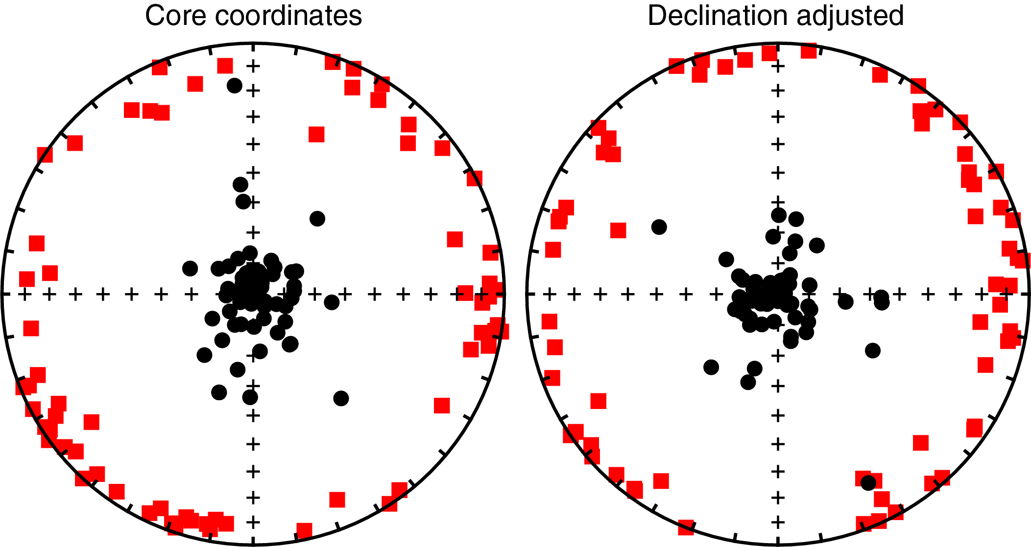
Figure F37. AMS eigenvectors.
Summary
Site U1536 APC cores preserve a well-defined succession of normal and reversed polarity zones. Paleomagnetic measurements made on archive halves were subjected to several quality control tests using discrete samples, removal of intervals affected by large-scale coring-induced disturbance as determined during visual core description, and removal of intervals with centimeter-scale deformation as determined from inspection of X-rays of every core section. The combined data from Holes U1536A–U1536C span Chron C1n (Brunhes) to below Chron C2An.2r (Mammoth) in Chron C2An.3n (early Gauss). Hole U1536E was rotary cored. Despite discontinuous recovery, biostratigraphic datums allow tentative ties to geomagnetic polarity timescale (GPTS) Chrons C2Ar and C3An in Hole U1536E. Below this range, we observed intervals of normal and reversed polarity that could potentially be tied to the polarity timescale through future work with stronger biostratigraphic constraints.
Geochemistry
Volatile hydrocarbons
Headspace gas analyses were performed at a resolution of one sample per full-length core (9.6 m advance) or one sample every other core for half-length cores (4.8 m advance) throughout Holes U1536A and U1536E (Cores 382-U1536A-1H through 53F and 382-U1536E-4R through 33R) as part of the routine environmental protection and safety monitoring program. Methane (CH4) is the dominant hydrocarbon present in low concentrations (2–4.6 parts per million by volume [ppmv]) throughout the sedimentary sequence (Figure F38). Ethane (C2H6) concentrations are below the detection limit through the core (Table T17).
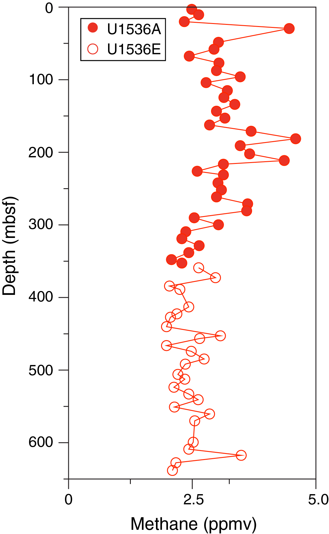
Figure F38. Methane.
Interstitial water chemistry
Shipboard chemical analysis of the IW from Site U1536 sediments followed the procedures detailed in Geochemistry in the Expedition 382 methods chapter (Weber et al., 2021a). Geochemical data were generated on 20 IW samples from Hole U1536A to 352 mbsf (Cores 382-U1536A-1F through 53F) and 7 samples from Hole U1536E to 550 mbsf (Cores 382-U1536E-6R through 24R). The geochemical properties are displayed in a single profile with different symbols for better distinction of IW properties from Holes U1536A and U1536E. The main results from the shipboard analyses are presented in Figures F39 and F40 and Table T18.
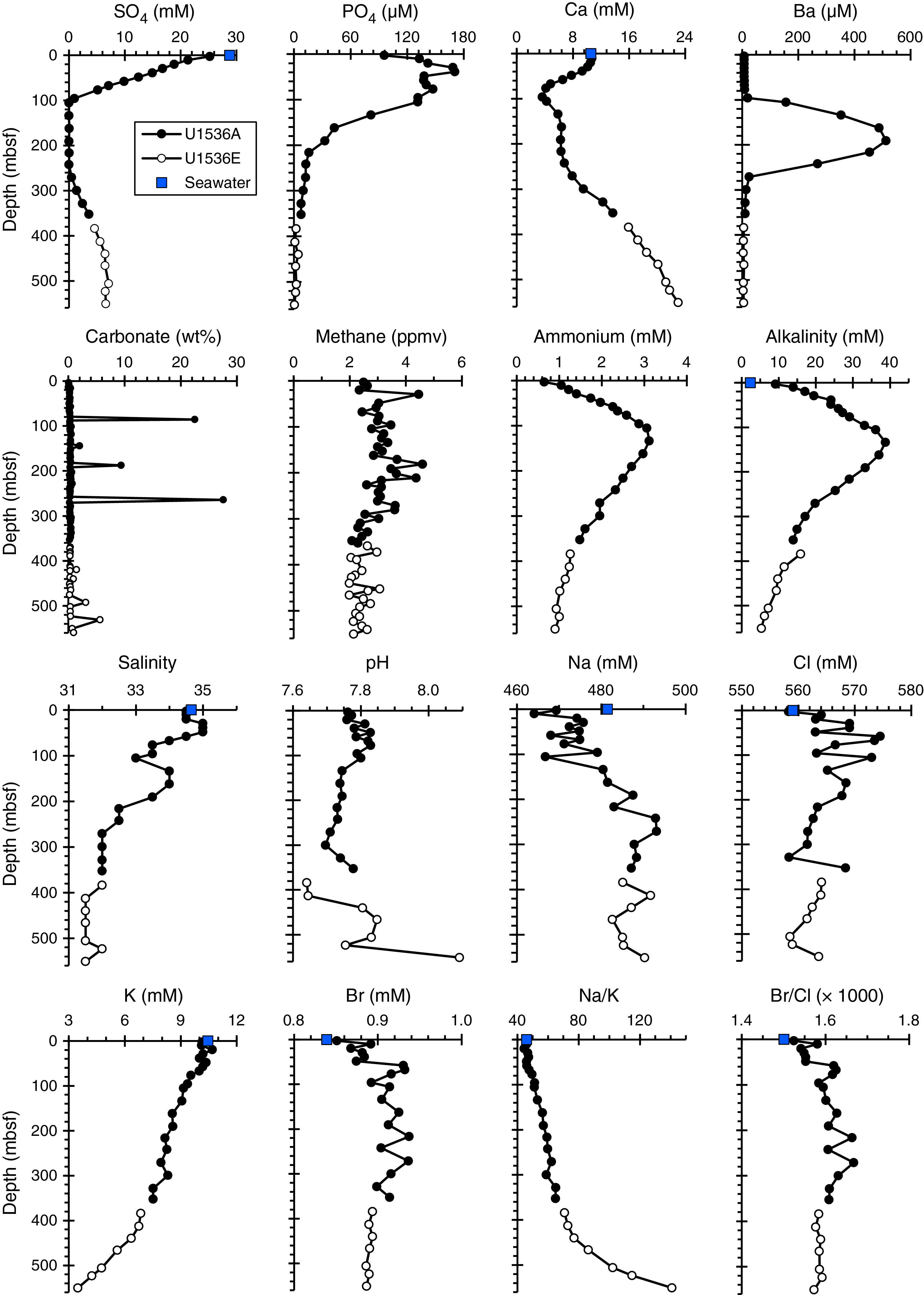
Figure F39. IW properties.
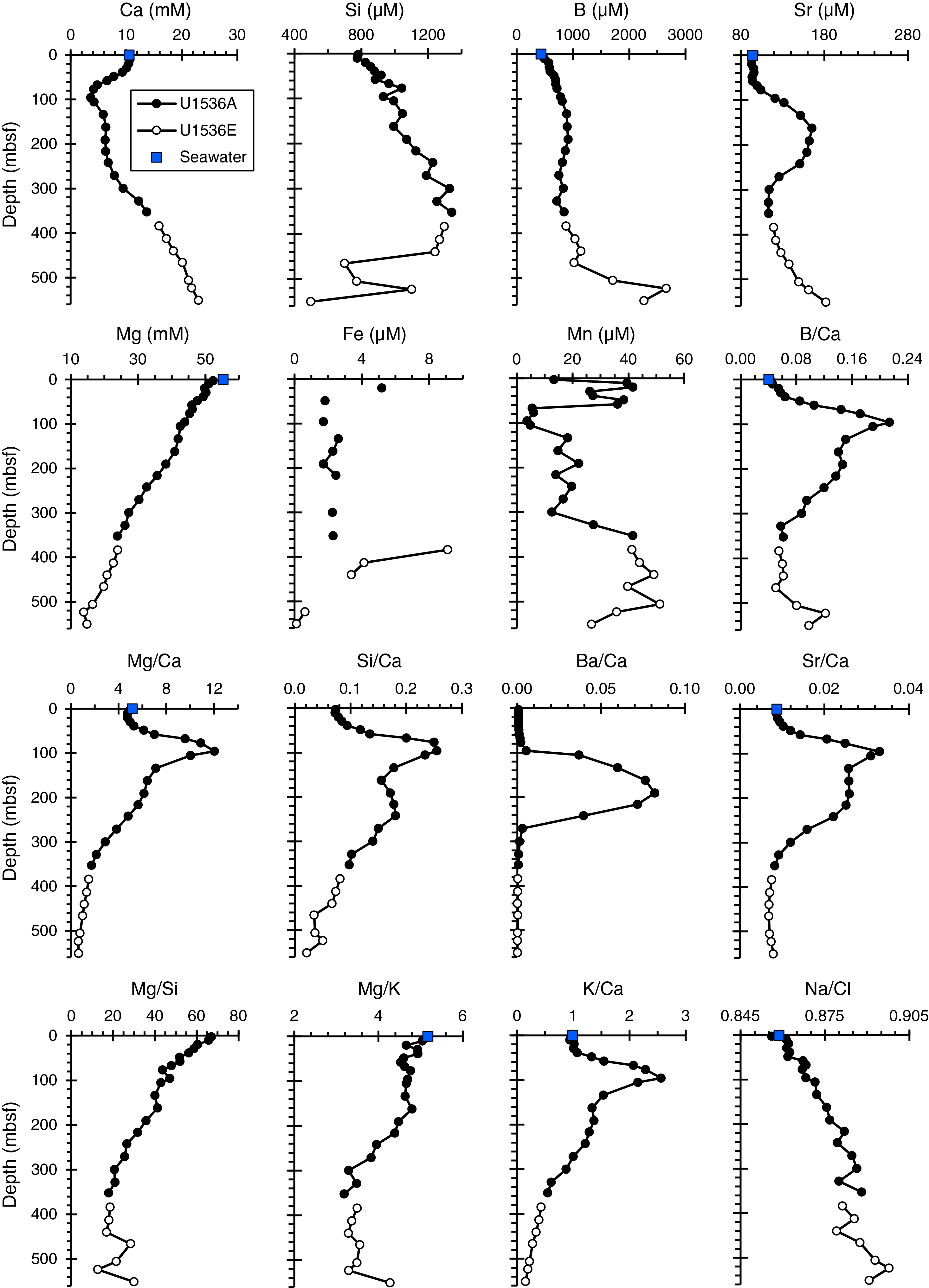
Figure F40. IW properties.
Salinity, sulfate, alkalinity, ammonium, pH, phosphate, iron, and manganese
Salinity in the upper 60 m matches local salinity values (34.7) within error and then decreases by ~2 to 105 mbsf. Below this depth, salinity increases again slightly to ~34 before leveling off to 32 at 270 mbsf and remaining relatively constant throughout the rest of the interval. Hole U1536A exhibits generally reducing sedimentary conditions, as indicated by the disappearance of dissolved sulfate concentrations at ~100 mbsf, yet Site U1536 is not methanogenic at any depth in the sedimentary column (Figure F39). Notably, dissolved sulfate concentrations increase again below 300 mbsf.
The reducing conditions, inferred to be associated with microbially mediated sulfate reduction, in the upper ~100 m are reflected in the IW profiles of several parameters from our shipboard analyses. Alkalinity increases from 9 mM close to the seafloor to a maximum of 39 mM at 134 mbsf. The steady increase in alkalinity, associated with high phosphate concentrations in the upper 100 m, is a consequence of organic matter degradation. Alkalinity levels are visually correlated with dissolved ammonium concentrations (Figure F39). Linear regression of these two parameters gives R2 = 0.93.
Elevated dissolved Mn concentrations (maximum of 42 µM at 20 mbsf) in the upper 60 m may in part be related to a tephra layer observed just below this depth (see Lithostratigraphy). However, given the invariant bulk geochemical composition in this interval (see below) this option is deemed less likely. Alternatively, the Mn enrichment could be controlled by release from Mn oxides in the upper 30 m (note that Fe is not enriched in this interval; i.e., the smaller data density in the Fe panel is due to the fact that several sampled depths had Fe concentrations below the detection limit) (Figure F40). A peak in dissolved Fe of 9.1 µM was, however, observed at 385 mbsf. This peak is not well defined, and the data return to low values below this depth. This Fe enrichment at 385 mbsf is accompanied by a second Mn enrichment at depth below the sulfate-depleted interval. This Fe peak at ~385 mbsf probably represents the typical diagenetic sequence for the reduction of potential electron acceptors for organic matter oxidation in marine sediments, where Mn oxides are reduced before Fe oxides based on the higher free energy available for oxidation of organic carbon by Mn oxides versus Fe oxides (Froelich et al., 1979):
Our data suggest that sulfate reduction is occurring or has occurred in these sediments, but it may have never developed persistently enough to clear the sedimentary column of reactive Mn and Fe oxides. The gradients in all the major cations and anions suggest processes occurring deep in the sedimentary column. We note that reported Fe and Mn concentrations only provide qualitative information on respective IW contents because both Fe and Mn in marine IW usually needs to be extracted under inert and anoxic atmosphere (e.g., Scholz et al., 2011).
Calcium, magnesium, silicon, barium, and other major and trace elements
Calcium is depleted in the upper sedimentary column and replenished below to concentrations as high as 23 mM at 550 mbsf. It displays a substantial decrease in the sulfate reduction zone from ambient seawater concentrations (10.5 mM) to 2 mM at 100 mbsf (Figure F39). This Ca depletion is most likely a function of authigenic carbonate fluorapatite formation, given that Ca is removed from IW and phosphorous is replenished via ongoing organic matter degradation (Ruttenberg and Berner, 1993), leading to generally elevated dissolved [P] in the upper 100 m. In addition, other authigenic carbonate or gypsum may form in this interval, both of which are commonly observed in reducing sedimentary conditions (Briskin and Schreiber, 1978).
Dissolved Mg concentrations steadily decrease downcore from typical seawater concentrations (~52 mM) to concentrations as low as ~15 mM at 550 mbsf (Figure F40). Notably, the removal of Mg from IW seems to be more effective in sedimentary depths below 160 mbsf, resulting in a slightly more pronounced Mg concentration gradient toward lower IW Mg below this depth. The strong dip in Ca concentration between 40 and 100 mbsf creates highly elevated Mg/Ca, B/Ca, Sr/Ca, and Si/Ca ratios in the IW (Figure F40). The observation that Mg/Ca reaches the highest ratios at ~100 mbsf argues against microbially mediated dolomite formation in this interval (Meister et al., 2007). Dissolved Ba concentrations have a strong peak in the sulfate-depleted interval between 100 and 190 mbsf, which is inferred to reflect barite dissolution, as suggested for similar patterns at other sites (Bolze et al., 1974; Torres et al., 1996; Riedinger et al., 2006). Below 190 mbsf, we observed rapidly decreasing dissolved Ba dropping to near zero at 299 mbsf, coincident with the reemergence of dissolved sulfate.
Below ~70 mbsf, both dissolved K concentrations and Na/K ratios suggest preferential K removal, a phenomenon that most likely reflects early diagenetic glauconite-smectite formation at Site U1536, as suggested by similar patterns at other sites (Meunier and El Albani, 2007; Baldermann et al., 2017). Increases in Sr approximately follow the Ba enrichment between 100 and 280 mbsf, albeit at smaller magnitude. Overall dissolved Sr shows a rather complex downcore behavior, with the lowest IW Sr concentrations of 93 µM over the uppermost 60 m, matching seawater concentrations within error. Levels increase rapidly from 100 to 165 mbsf, decrease to 350 mbsf, increase again more gradually below this depth, and peak at 182 µM at 550 mbsf. The behavior of Sr in the uppermost 100–200 m suggests multiple competing reactions controlling Sr concentrations in the sulfate reduction and barite dissolution zone beneath.
Two major processes are known to be important in influencing Ca and Mg concentrations in IW in settings such as seen here: (1) diagenetic alteration of silicic basement or volcanic ash with ΔMg/ΔCa = −2 (Baker, 1986) and (2) dissolution of calcite and recrystallization as dolomite, which in the case of increasing Ca and decreasing Mg would produce a ΔMg/ΔCa = −1 (Shipboard Scientific Party, 1988), although this process occurs only in very high organic carbon (Corg) sediments typically found in continental margin settings. From the shipboard data alone, it is not possible to determine what controls Sr, Ca, and Mg concentrations (Meister et al., 2007; Nöthen and Kasten, 2011). Finally, underlying controls behind the increasing Si concentrations downcore are inferred to be a combination of detrital mineral and biogenic silica dissolution complicated by authigenic clay formation (Dixit et al., 2001). Identifying the key control on dissolved Si at Site U1536 will require further work.
Bulk sediment geochemistry
Carbon, nitrogen, and carbonate
The results from shipboard analyses of total nitrogen (TN) and total carbon (TC) from Holes U1536A (N = 38) and U1536E (N = 27) are presented in Table T19 and Figure F41. Bulk sediment TOC and TN contents are generally low, and concentrations range from 0.1 to 0.8 wt% and from 0.02 to 0.09 wt%, respectively (Figure F41). Calcium carbonate (CaCO3) contents are also low (<1 wt%), except in a few narrow horizons with carbonate contents above 5 wt% (~86, 188, ~264, ~531, and ~588 mbsf). Overall downcore data indicate a predominance of marine organic material. At 588 mbsf, we observed a layer with 55 wt% CaCO3 and 0.49 wt% TOC and TN below the detection limit; however, it is hard to determine the source and/or processes behind these values because of our coarse sample resolution. No more samples were collected below this interval.
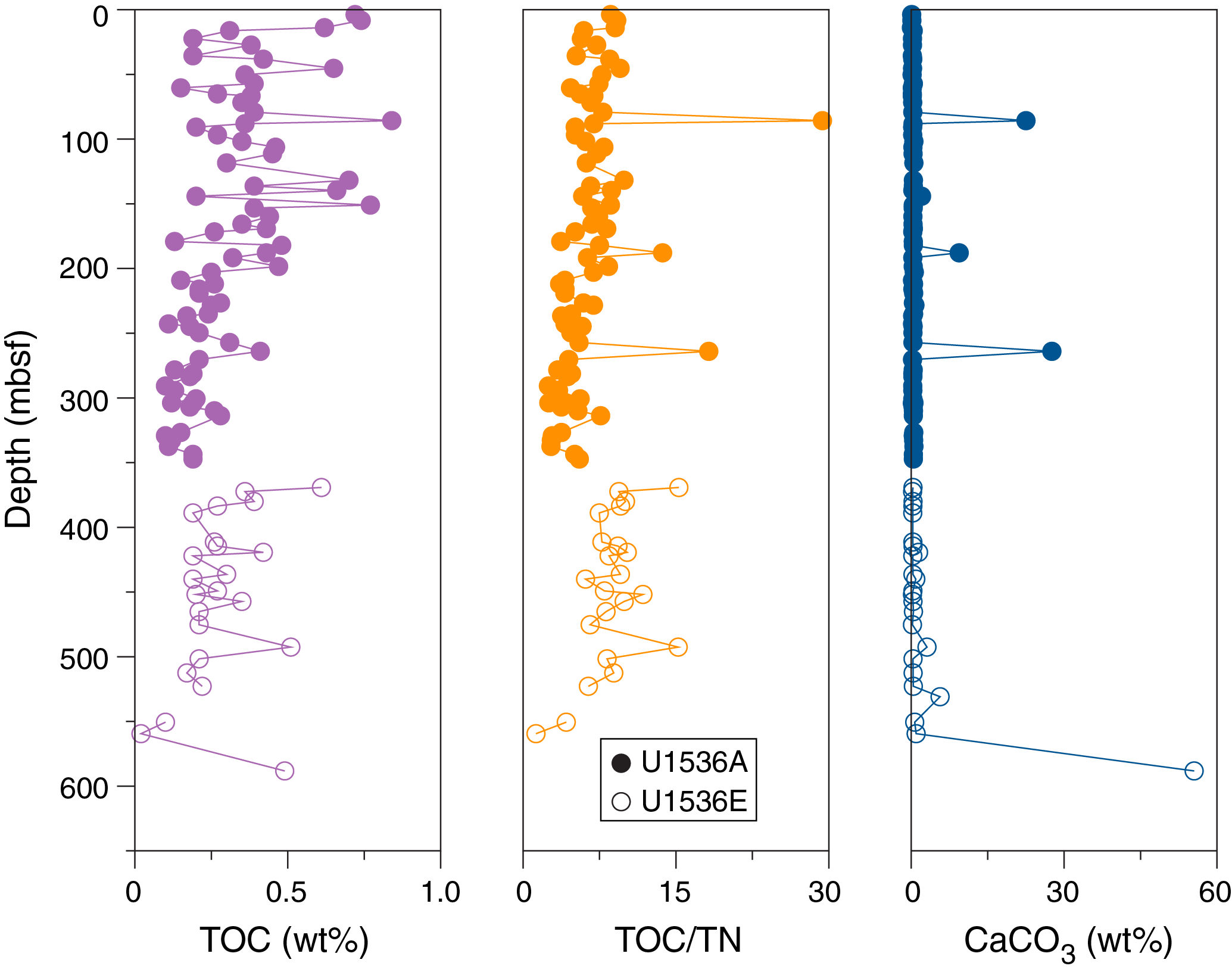
Figure F41. Bulk sediment TOC, TOC/TN ratio, and CaCO3.
Inorganic bulk sediment geochemistry
Inorganic bulk sediment analyses were carried out on 33 samples from Hole U1536A and 15 samples from Hole U1536E. All major and selected trace metal concentrations were measured, and a selection of key elements and ratios are displayed in Figures F42 and F43. The full suite of results is presented in Table T20. Sediments are dominantly terrigenous, and at all but two sampled sedimentary depths Ca concentrations are below 4 wt% (Figure F42; Table T20). Carbonate layers are associated with lower concentrations of most other major elements as well as lower La and Zr. Strontium is positively correlated with Ca. Two sample depths, 85 and 588 mbsf, display elevated Ca contents from CaCO3. Silicon concentrations are high throughout (57–83 wt% SiO2), although variable. Quantifying silicon contributions from opal will need further investigation. Two sedimentary phosphorous peaks were identified (85 and 190 mbsf) and may be associated with authigenic phosphate precipitation.
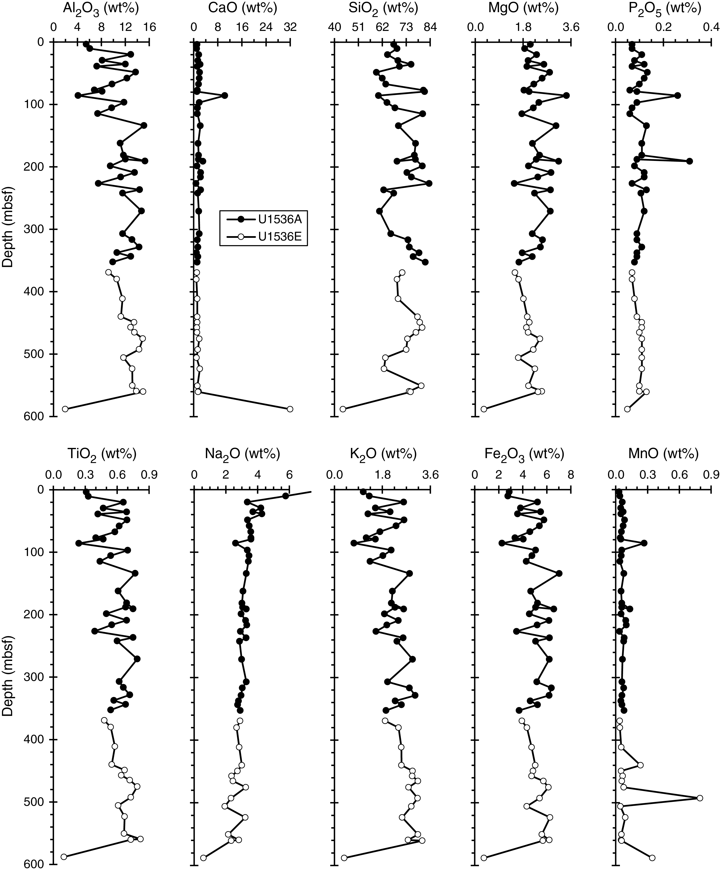
Figure F42. Bulk sediment major element compositions.
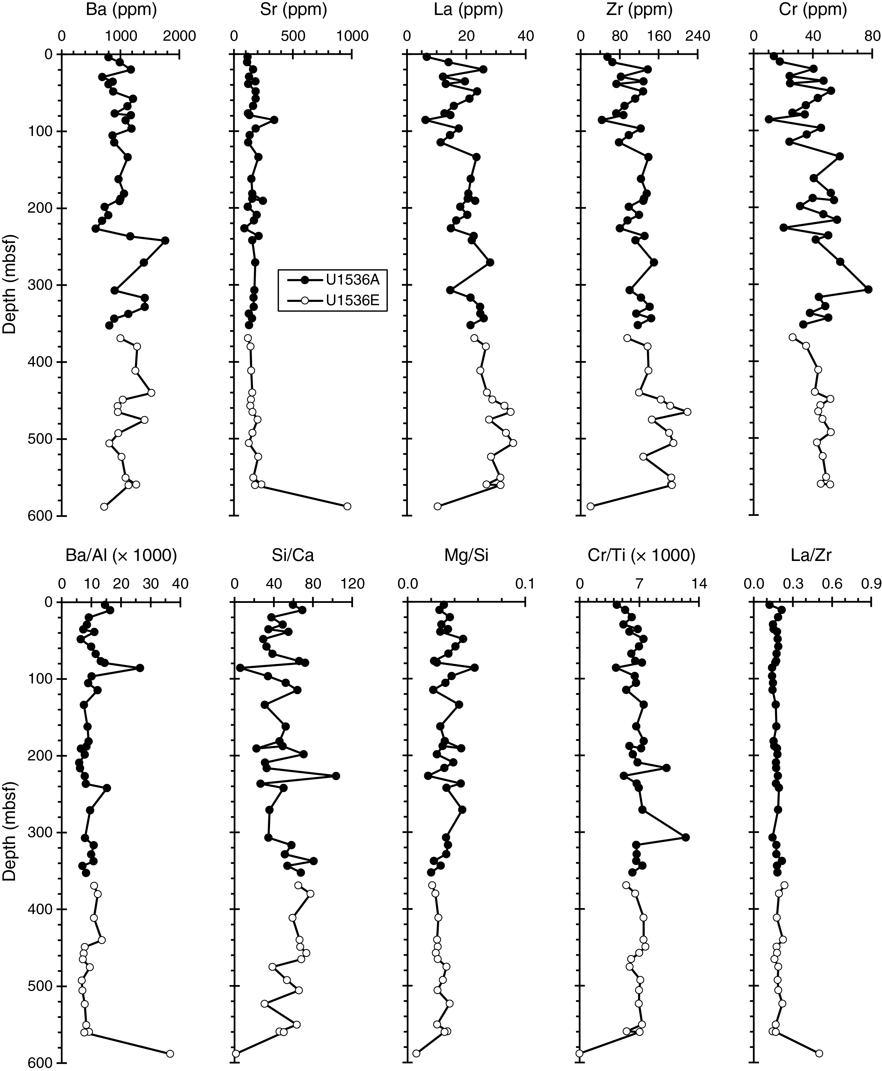
Figure F43. Sediment trace element compositions and elemental ratios.
Most elemental concentrations vary from core to core (hence on the scale of tens of meters) at Site U1536, and a subtle tendency downcore to higher concentrations, particularly throughout Hole U1536A, is seen for Al, Ti, K, and Zr. Barium concentrations scatter around an average lower concentration in the upper 230 m compared with higher concentrations below. This increase in sedimentary Ba concentrations was observed below the barite dissolution interval identified from highly elevated dissolved Ba in IW reported above (Figure F39). Overall, the deeper sections of core, largely sampled from Hole U1536E, are less variable than the upper intervals. Whether this is due to diagenetic sedimentary maturation or distinct depositional conditions in the respective intervals is unknown. Note that although bulk sediment sampling was usually paired with IW sampling, the spacing is somewhat random and did not target particular glacial or interglacial intervals.
Summary
Samples from Holes U1536A and U1536E were analyzed for headspace gas, IW chemistry, and bulk sediment geochemistry. Headspace methane concentrations are generally low (2–4.6 ppmv) throughout the sedimentary sequence. Ethane, propane, and higher molecular weight hydrocarbons are below their detection limits. Site U1536 is characterized by moderately reducing sedimentary conditions, as indicated by the disappearance of dissolved sulfate at ~100 mbsf and the reappearance of detectable dissolved sulfate below ~300 mbsf. The reducing conditions are inferred to be microbially mediated, and sedimentary redox processes in the upper section exert strong control over the IW profiles of several parameters measured shipboard, including alkalinity, Ca, PO4, Ba, Sr, and Mn. Bulk sediment TOC and TN contents are generally low and have concentrations ranging from 0.1 to 0.8 wt% and from 0.02 to 0.09 wt%, respectively. Virtually all solid samples are dominantly terrigenous, and only two samples have elevated Ca concentrations indicative of higher carbonate content. Hole U1536A features higher compositional variation than the lower Hole U1536E, and the majority of shorter timescale variations are likely attributable to variable sediment delivery on glacial–interglacial timescales (see Lithostratigraphy). A secular trend toward lower Al, Ti, K, Fe, La, Zr, and Cr toward the core top is subtle but consistent with greater diatom abundance in the upper part of Hole U1536A, whereas Ba shows a well-defined diagenetic boundary at 230 mbsf. Whether secular changes in sediment provenance can be detected from the geochemical data will need more highly resolved shore-based investigation.
Physical properties
High-resolution physical property measurements were made on all cores and most core catchers from Holes U1536A–U1536E to provide basic information on sediment composition and variability. The Whole-Round Multisensor Logger (WRMSL) was used to measure gamma ray attenuation (GRA) bulk density, MS, and compressional wave velocity on the P-wave logger (PWL) at 2.5 cm intervals. The PWL was used for all cores recovered with the APC system (Holes U1536A–U1536D) but not for cores retrieved with the RCB system (Hole U1536E). Material recovered with the RCB system has a slightly smaller core diameter and does not fill the liner entirely. Hence, proper contact between the caliper and the sediment does not occur, which leads to erroneous measurements. On whole-round cores, we also measured NGR (at 10 cm increments). Once the cores were split, the section halves were X-rayed and thermal conductivity measurements (one per core) were made for all holes. P-wave caliper (PWC) velocity was acquired in at least three sections per core for Holes U1536A–U1536D and in every section (if possible) for cores from Hole U1536E. On archive halves, point magnetic susceptibility (MSP) and color reflectance were measured at 2.5 cm increments using the Section Half Multisensor Logger (SHMSL) and digital color imaging was completed with the Section Half Imaging Logger (SHIL). Additionally, we took discrete samples from Holes U1536A and U1536E for moisture and density (MAD) measurements (1–3 samples per core; ideally representing different lithologies) to determine water content, wet bulk density, dry bulk density, porosity, and grain density.
Whole-Round Multisensor Logger measurements
Results from WRMSL measurements for Holes U1536A–U1536C and U1536E are compiled in Figures F44, F45, F46, and F47. We measured high-resolution data (2.5 cm intervals) for all cores and the majority of the core catchers. All cores from Holes U1536A, U1536C, and U1536E rested for about 4 h before measurement to adjust to room temperature (~20°), whereas cores from Hole U1536B were measured as soon as they arrived in the laboratory for stratigraphic correlation purposes.
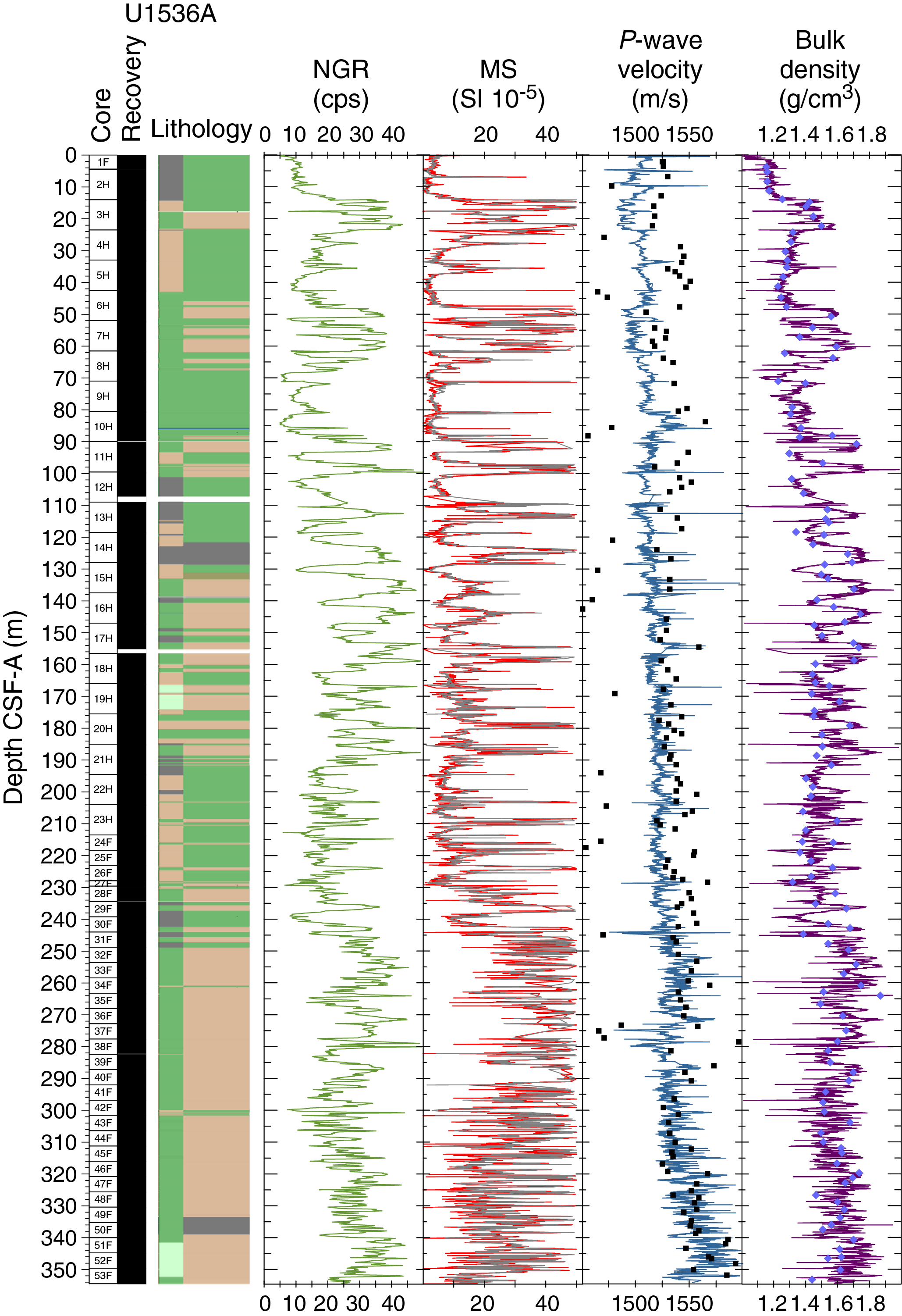
Figure F44. Physical property data, Hole U1536A.
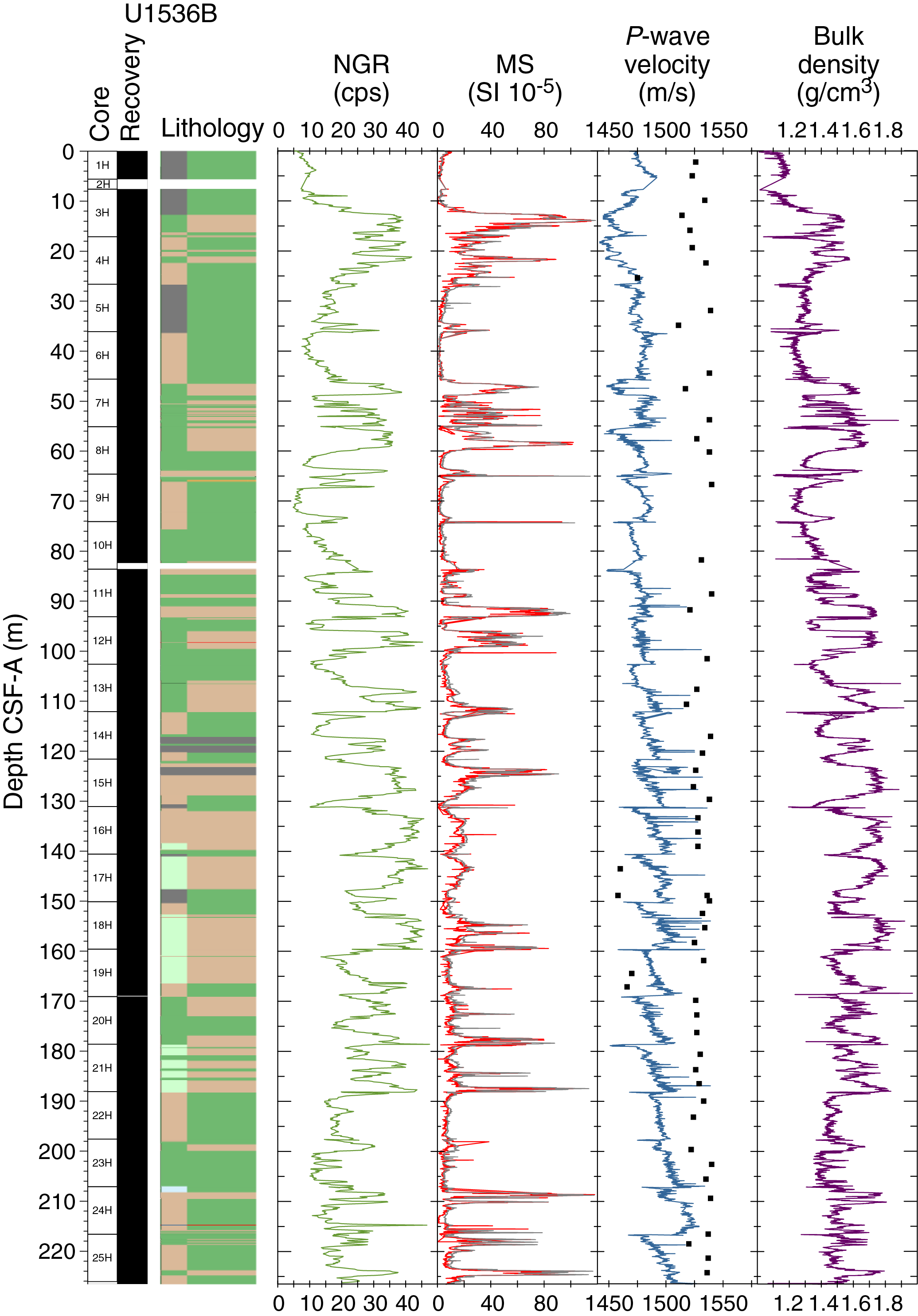
Figure F45. Physical property data, Hole U1536B.
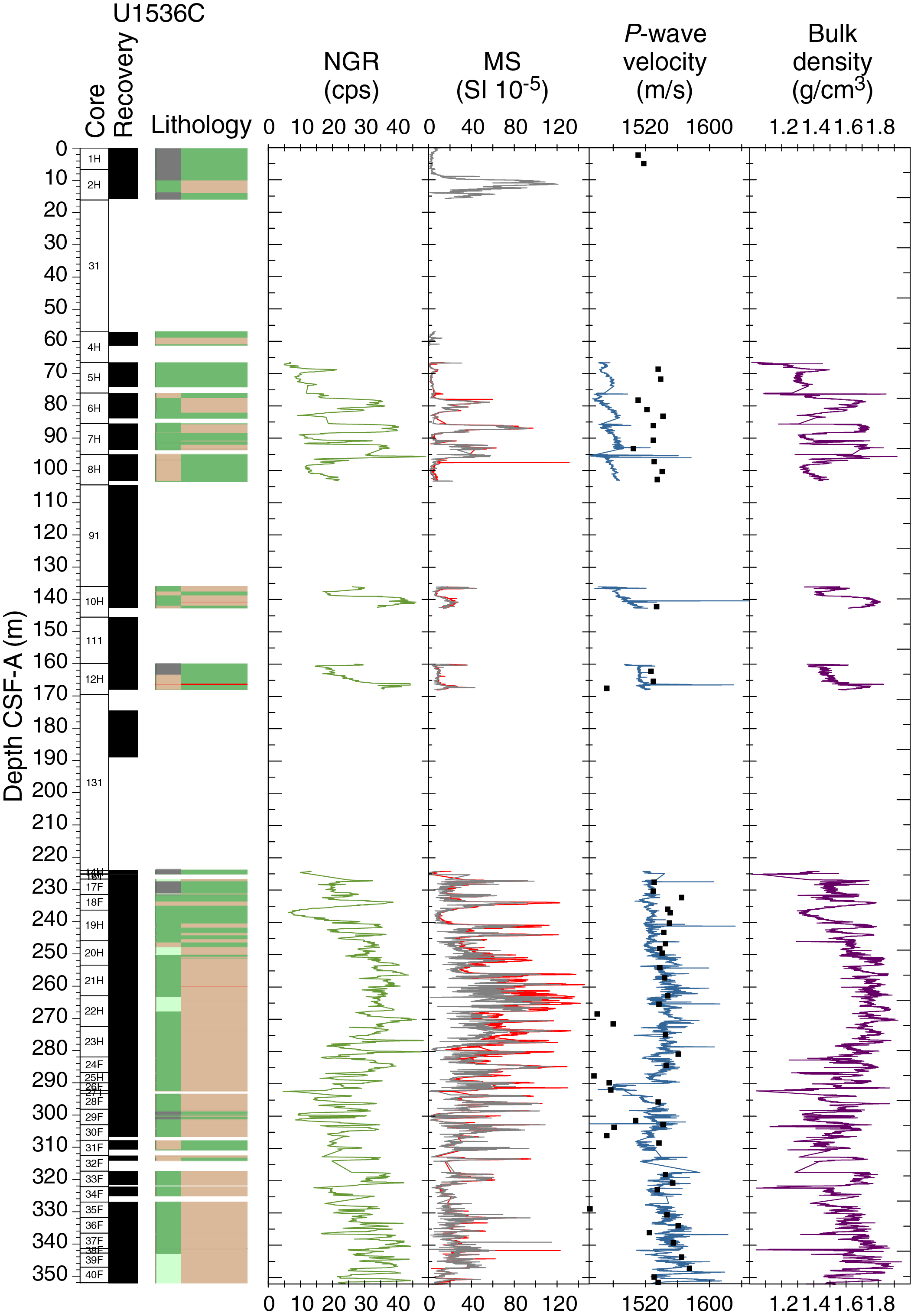
Figure F46. Physical property data, Hole U1536C.
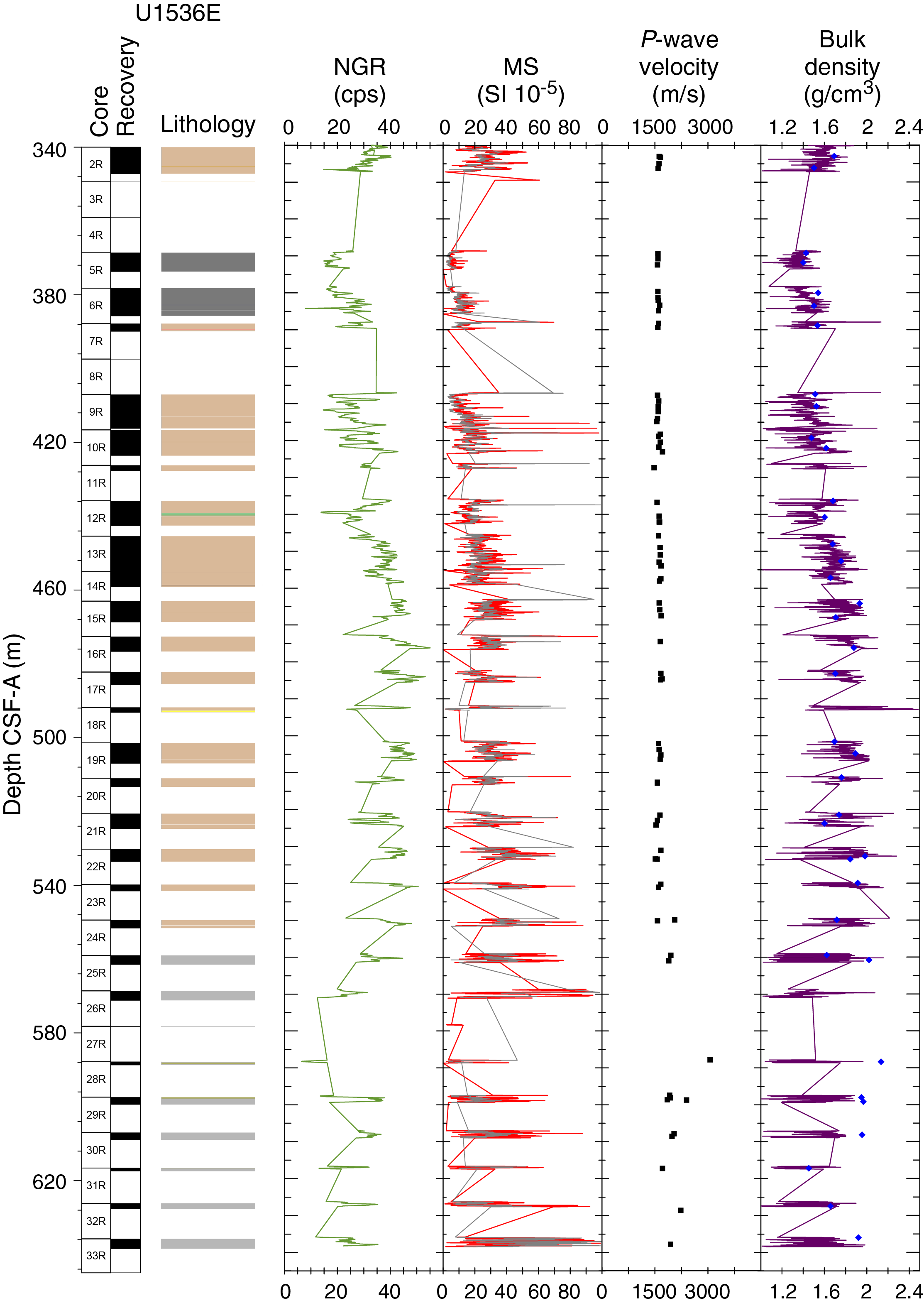
Figure F47. Physical property data, Hole U1536E.
Gamma ray attenuation bulk density
Wet bulk density values range from 1.3 to 2.2 g/cm3 and have a mean value of 1.6 g/cm3. Cyclicity is observed downhole for GRA bulk density together with a trend to increasing values through Core 382-U1536E-23R (~550 mbsf). The lowest values are found in Cores 382-U1536A-8H (~70 mbsf) and 382-U1536E-5R (370 mbsf), 9R (410 mbsf), and 12R (440 mbsf), whereas the highest values are located in Cores 382-U1536E-15R through 28R (470–590 mbsf) (Figures F44, F47). The observed cyclicity is highly correlated between Holes U1536A, U1536B, and U1536C. A positive correlation is found between density and NGR counts and between density and MS (Figure F48). GRA bulk density values agree with calculated density values from the MAD discrete samples and hence confirm the high quality of the data.
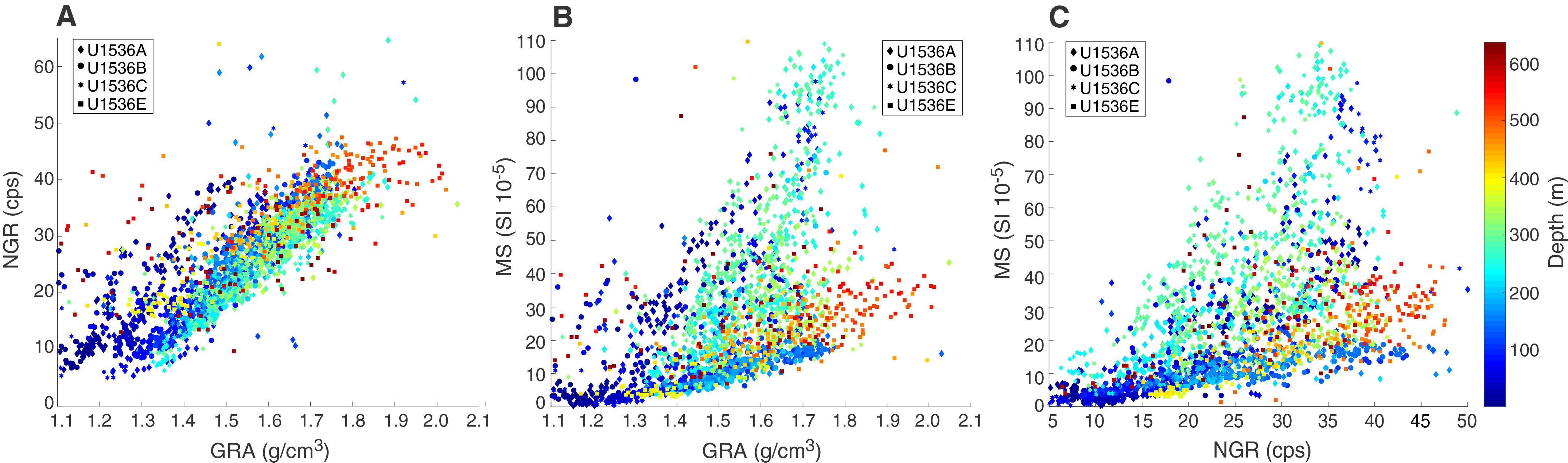
Figure F48. NGR, GRA, and MS.
Magnetic susceptibility
MS is sensitive to the concentration and type of magnetic minerals present in the sediments. The MS record contains sharp peaks and high-amplitude variability following the lithologic changes that are inferred to represent glacial–interglacial cycles, with high MS associated with silty clay intervals and low MS associated with diatom ooze intervals. Values range from 0 to 130 × 10−5 SI. High-amplitude variation is documented through Core 382-U1536A-31F. The baseline of the signal is relatively constant downhole through Core 31F, below which lower amplitude variability combined with an increase in the minimum values in MS is documented. This trend is especially notable through Core 45F and agrees with a major lithologic shift from more diatom ooze to silty clay.
The highest MS values are found in Cores 382-U1536A-31F through 42F and 382-U1536E-26R (>25 × 10−5 SI), and the lowest values (<10 × 10−5 SI) are in Cores 382-U1536A-8H and 10H and 382-U1536E-19R through 14R. Generally, we observe a strong correlation in the variability with depth for all physical properties determined with the WRMSL. In addition, a linear dependence with some scattering is found for MS and NGR for a given depth interval, although it is much less systematic than for the relationship between NGR and GRA (Figure F48), which is consistent with the observation that MS varies considerably in intervals of high NGR and GRA.
P-wave velocity
P-wave velocity values measured with the PWL are erroneous if cracks or poor contact with the liner wall occur. However, the measurements are generally good and range from 1400 to 2000 m/s. PWL values increase gradually and continuously downhole and reach almost 1600 m/s in Core 382-U1536A-52F and 2000 m/s from Core 382-U1536E-25R downhole. The lowest velocity values are in Cores 382-U1536A-3H, 6H, and 7H (23 and 43–61 mbsf), and the highest values are from Core 51F downhole (>340 mbsf).
Natural gamma radiation
Cyclic changes in NGR are observed throughout the hole. Higher NGR values are observed at 470–490 mbsf (>45 counts/s). NGR values display significant variation, and the lowest counts are in Cores 382-U1536A-8H through 10H and 382-U1536E-28R (~5–10 counts/s). High-amplitude variability is observed throughout the sediment column (Figures F44, F45, F46, F47). Cyclic variation in NGR follows glacial–interglacial cycles in which high NGR is associated with silty clay and low NGR is associated with diatom ooze.
Thermal conductivity
Thermal conductivity varies between 0.7 and 1.9 W/(m·K) in Holes U1536A–U1536C and U1536E (Figures F49, F50). A clear positive trend with depth occurs through Core 382-U1536E-28R (~590 mbsf), and then a subsequent decrease is maintained to the bottom of the hole. The average observed thermal conductivity is 1.15 W/(m·K) and has no clear dependence on sediment facies. The lowest values were measured in Cores 382-U1536A-9H through 13H (72–118 mbsf) where the highest variety of lithologies was found. The highest thermal conductivity values occur in Cores 382-U1536E-22R through 28R. Thermal conductivity measurements were combined with borehole temperatures to make heat flow estimates (see Downhole measurements).
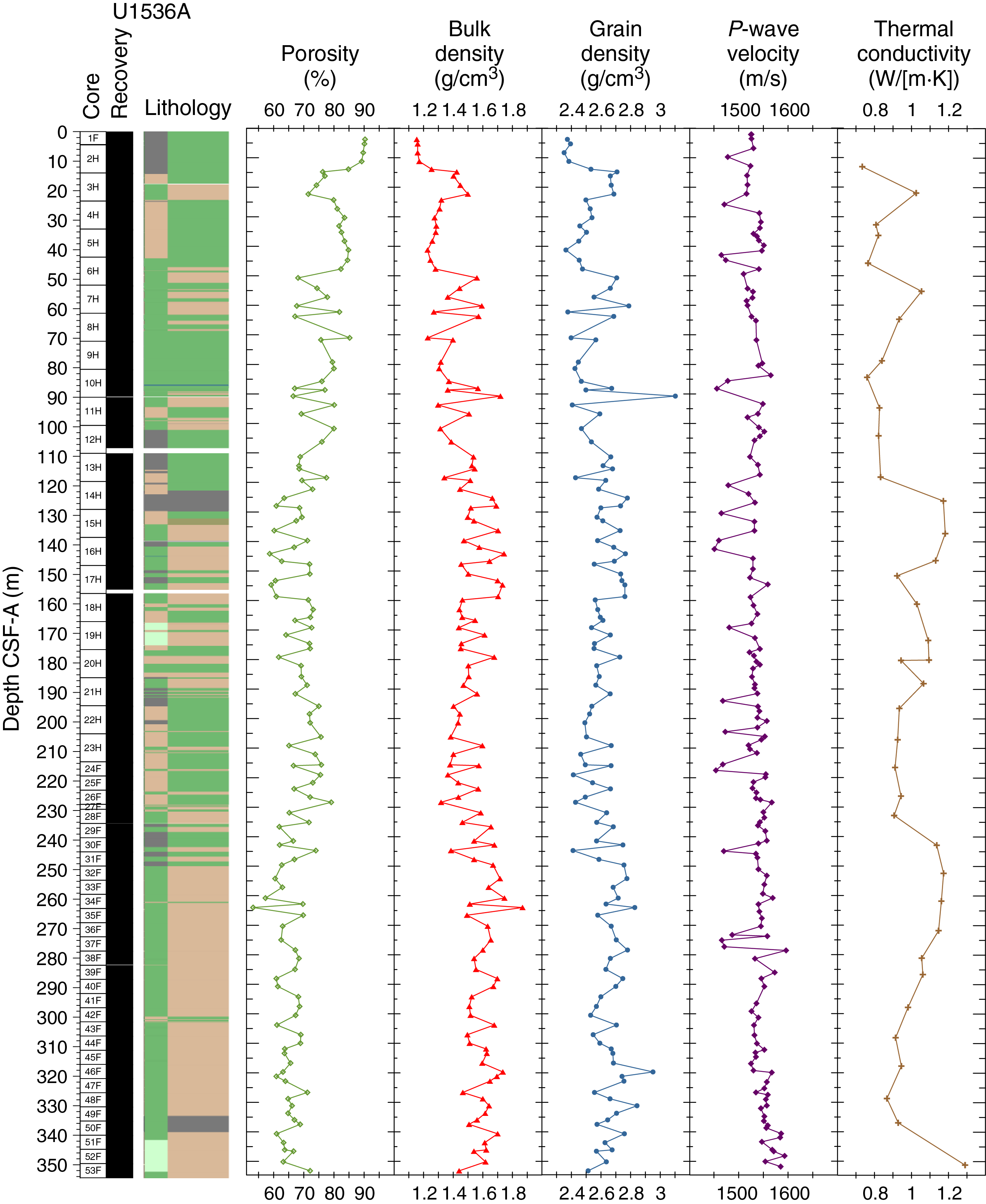
Figure F49. MAD results, Hole U1536A.
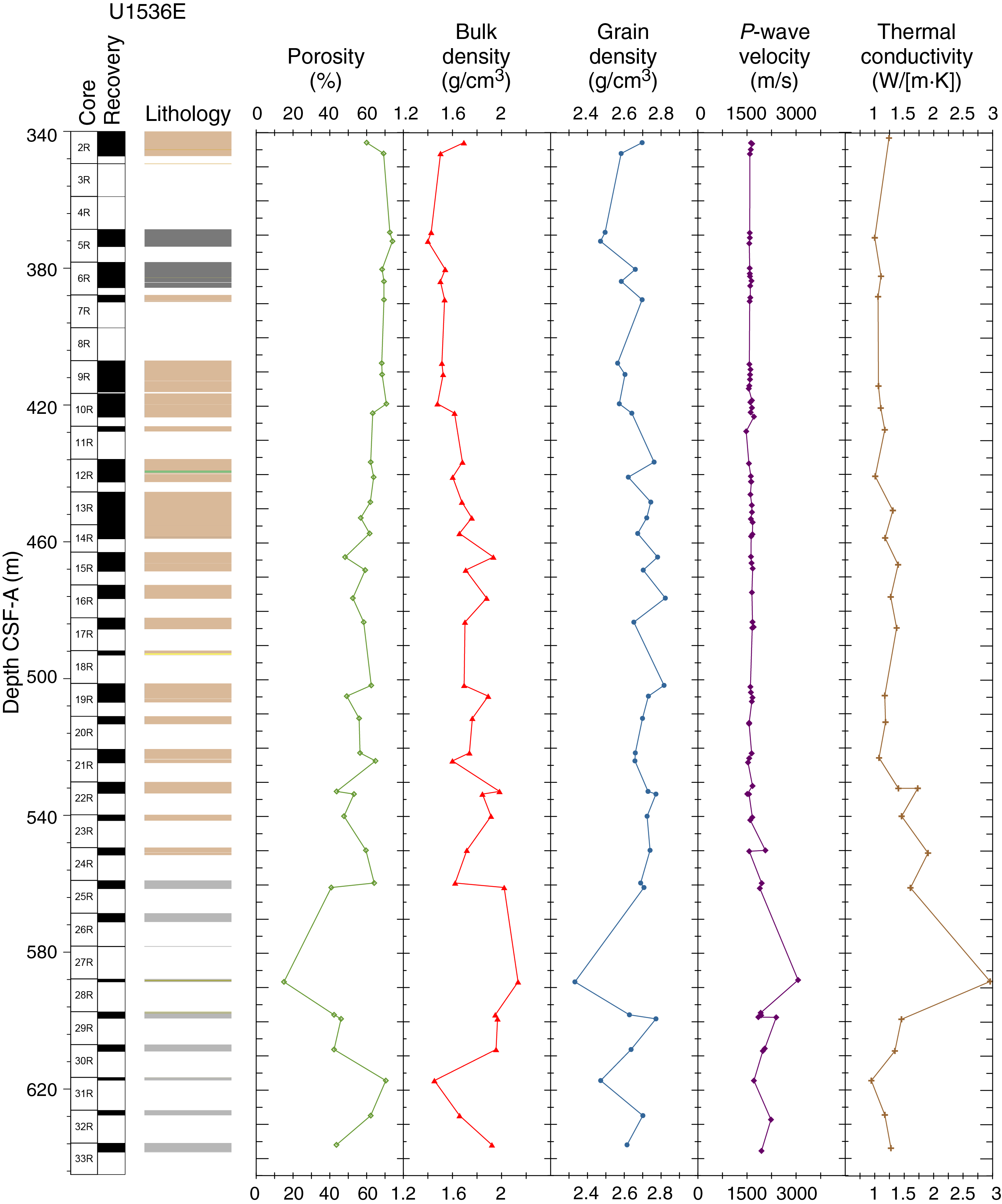
Figure F50. MAD results, Hole U1536E.
Point magnetic susceptibility
MSP measurements were performed on archive halves. Results agree with the WRMSL MS data (Figures F44, F45, F46, F47). MSP measurements were mostly acquired at 2.5 cm, the same resolution as the WRMSL. In some cases, higher variability is observed with the SHMSL because of the smaller integration volume of the sensor (~1 cm depth interval; 1σ) compared to the loop sensor (~18 cm depth interval; 1σ) used on the WRMSL (Weber et al., 1997).
Discrete compressional wave velocity
Discrete P-wave measurements were made using the PWC (see Physical properties in the Expedition 382 methods chapter [Weber et al., 2021a]). For Hole U1536A, 3–5 PWC measurements were made per APC core to provide a correlation for PWL values measured on whole-round cores with the WRMSL. For Holes U1536B–U1536D, we used a wider measurement spacing of 2–3 measurements per APC core. For Hole U1536E, we took one measurement per section to compensate for the lack of PWL measurements on the RCB cores. An automated algorithm determined PWC velocity values unless a weak signal or poor coupling required the instrument operator to manually determine a PWC velocity value.
PWC measurements from Holes U1536A–U1536D are consistent with the overall trends observed in the PWL values obtained from the WRMSL. However, some PWC values are systematically too low and others are consistently higher than the PWL values, specifically above 240 mbsf. From 240 mbsf downhole, values measured with the PWL and PWC are in agreement. The explanation for this disagreement for Hole U1536B is that the PWL measurements were made without waiting for cores to equilibrate to room temperature, thus providing PWL values that are too low. For the upper part of the remaining holes that show such a disagreement, the reason is unclear. Note also that the downhole logging velocity measurements at this site are generally higher than the PWC and PWL velocity values (see Downhole measurements).
PWC measurements made at the top of Hole U1536E are consistent with measurements made at the same stratigraphic interval (~343 mbsf) near the bottom of Holes U1536A and U1536C. PWC measurements from Holes U1536A–U1536E range from ~1500 to ~1600 m/s between 0 and 393 mbsf. Between ~390 and ~490 mbsf, P-wave velocity values increase, ranging from ~1550 to ~1700 m/s and coinciding with a transition in lithology from clay to silty clay. From 490 mbsf to the bottom of Hole U1536E, P-wave velocity values range from ~1600 to ~2000 m/s, and higher values are found in sandy and/or more compacted lithologies.
Moisture and density
Bulk density values were calculated from moisture and volume measurements made on discrete samples taken from the working halves (see Physical properties in the Expedition 382 methods chapter [Weber et al., 2021a]). The sample resolution in each core varied depending on lithology, recovery, and quality. At least three samples were taken per APC core, and at least two samples were taken per HLAPC core. A total of 169 samples were taken for MAD estimates: 129 from Hole U1536A, 2 from Hole U1536B, and 38 from Hole U1536E.
MAD density values correspond well to GRA bulk density values measured on the WRMSL for Holes U1536A, U1536B, and U1536E. Bulk density values for Hole U1536A range from ~1.2 to ~1.7 g/cm3 and exhibit an overall downhole increase due to compaction. Values increase quickly from ~1.2 g/cm3 at the top of the hole to ~1.5 g/cm3 at 22 mbsf. Bulk density values decrease to ~1.3 g/cm3 at 24 mbsf and then remain constant to 48 mbsf. From 48 mbsf to the bottom of the hole at ~350 mbsf, bulk density values exhibit cyclic variability, fluctuating between ~0.2 and 0.5 g/cm3 every ~3–5 m. Longer downhole trends are overlain by the observed cyclic variations. Between 48 and 159 mbsf, bulk density values increase overall, ranging from ~1.2 to 1.7 g/cm3. They decrease overall from 159 to 228 mbsf, ranging from ~1.3 to 1.9 g/cm3. Bulk density measurements do not exhibit a further overall trend through the remainder of Hole U1536A.
Hole U1536E bulk density values range from ~1.4 to 2.1 g/cm3 and exhibit a downhole increase through the entire hole (340–640 mbsf) with the exception of a brief decrease between 617 and 627 mbsf. Deeper than ~580 mbsf, MAD bulk density values are consistently higher than GRA bulk density values although the offset remains consistent. No cyclic variations are observed in Hole U1536E, although discontinuities in the sequence make it difficult to establish the degree of variability.
Trends observed in Holes U1536A, U1536B, and U1536E (Figures F49, F50) for grain density measurements closely follow those observed for bulk density. This likely reflects the grain density of the major lithologic components at this site: diatom opal has a grain density of 2.1–2.2 g/cm3, and quartz, common clays, and feldspar range from 2.5 to 2.8 g/cm3. Hole U1536A grain density values mostly range between ~2.4 and 2.8 g/cm3 between the top of the hole and 159 mbsf. An anomalously high value of 3.1 g/cm3 at 91 mbsf possibly represents the presence of dropstones. No overall trend occurs over this interval, but the amplitude of the values decreases from ~122 to 159 mbsf. Grain density values of similar amplitude persist from 159 to 228 mbsf, but values decrease downcore in Cores 382-U1536A-18H through 27F. Grain density values increase again at ~244 mbsf. Values range from ~2.6 to 3.0 g/cm3 with no change in the trend through the remainder of Hole U1536A. Hole U1536E grain density values range from ~2.3 to 2.8 g/cm3.
Porosity (percent of pore space of the wet sediment volume) generally decreases downhole (Figures F49, F50). Discrete porosity values range from ~90% near the top of Hole U1536A to ~60% at the bottom of the hole. Hole U1536E discrete porosity values increase rapidly from ~60% to ~70% between 343 and 369 mbsf. Porosity values then steadily decrease to ~40% at 560 mbsf. Deeper porosity values exhibit the greatest variability, ranging from 15% to 70% at the bottom of the hole.
Color reflectance
L*a*b* color reflectance measurements describe coordinates in a spherical system with 16.8 million possible variations (Weber, 1998; Blum, 1997). The L* axis measures the black–white color component and is known as the lightness or gray value. It is a reliable tracer for the content of biogenic carbonate in marine sediment (Weber, 1998). L* values for Holes U1536A and U1536B increase downhole, and they are essentially constant from Core 382-U1536E-2H downhole (Figures F51, F52, F53, F54).
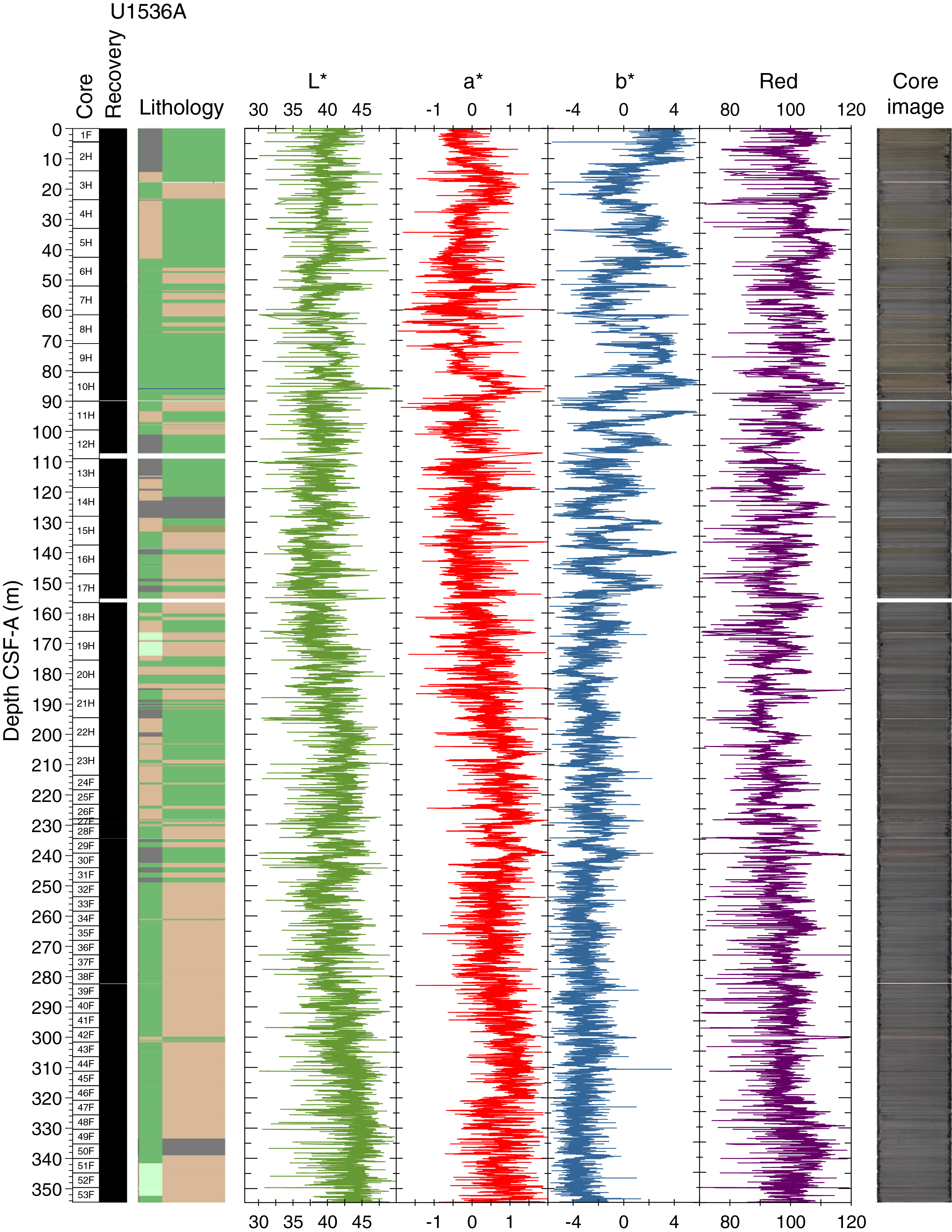
Figure F51. Color reflectance, Hole U1536A.
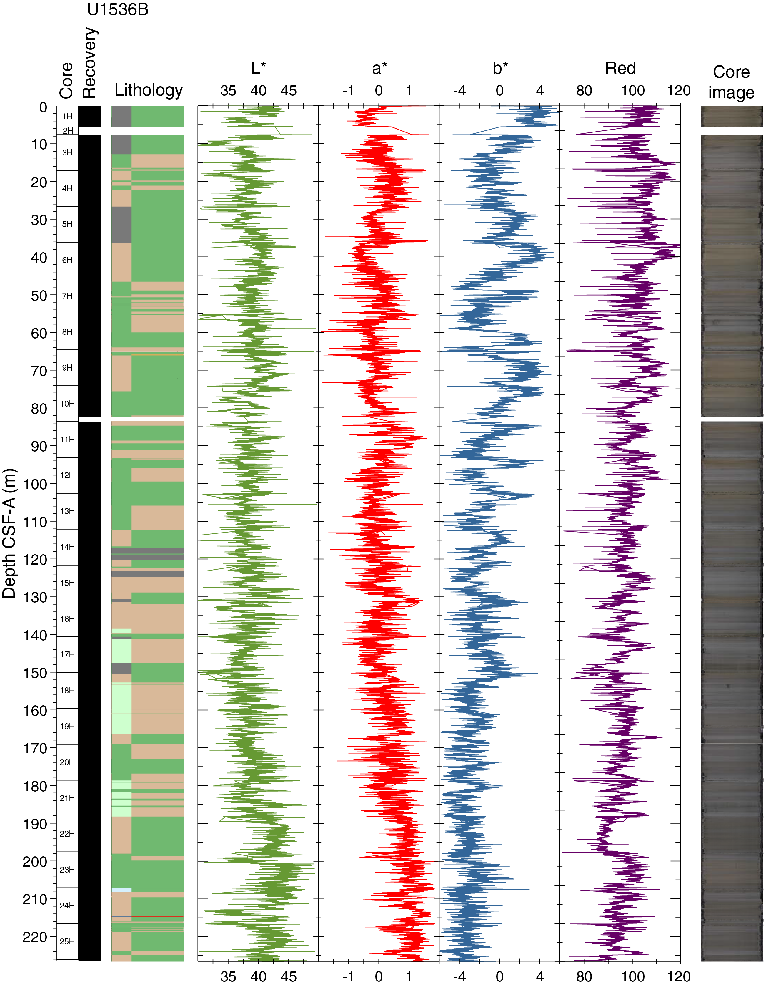
Figure F52. Color reflectance, Hole U1536B.
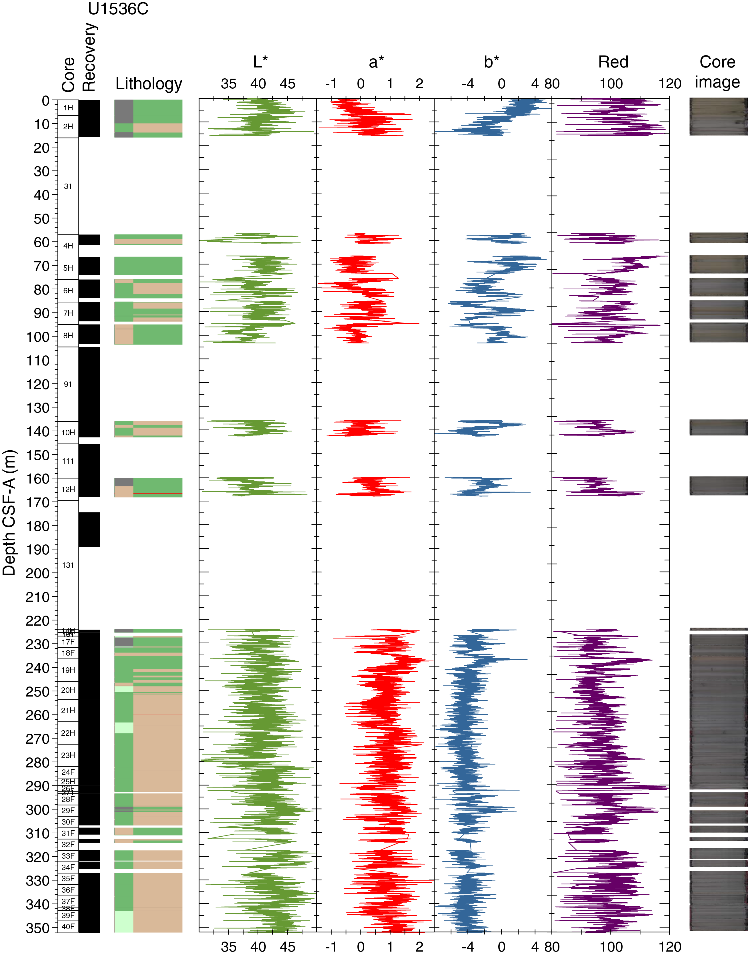
Figure F53. Color reflectance, Hole U1536C.
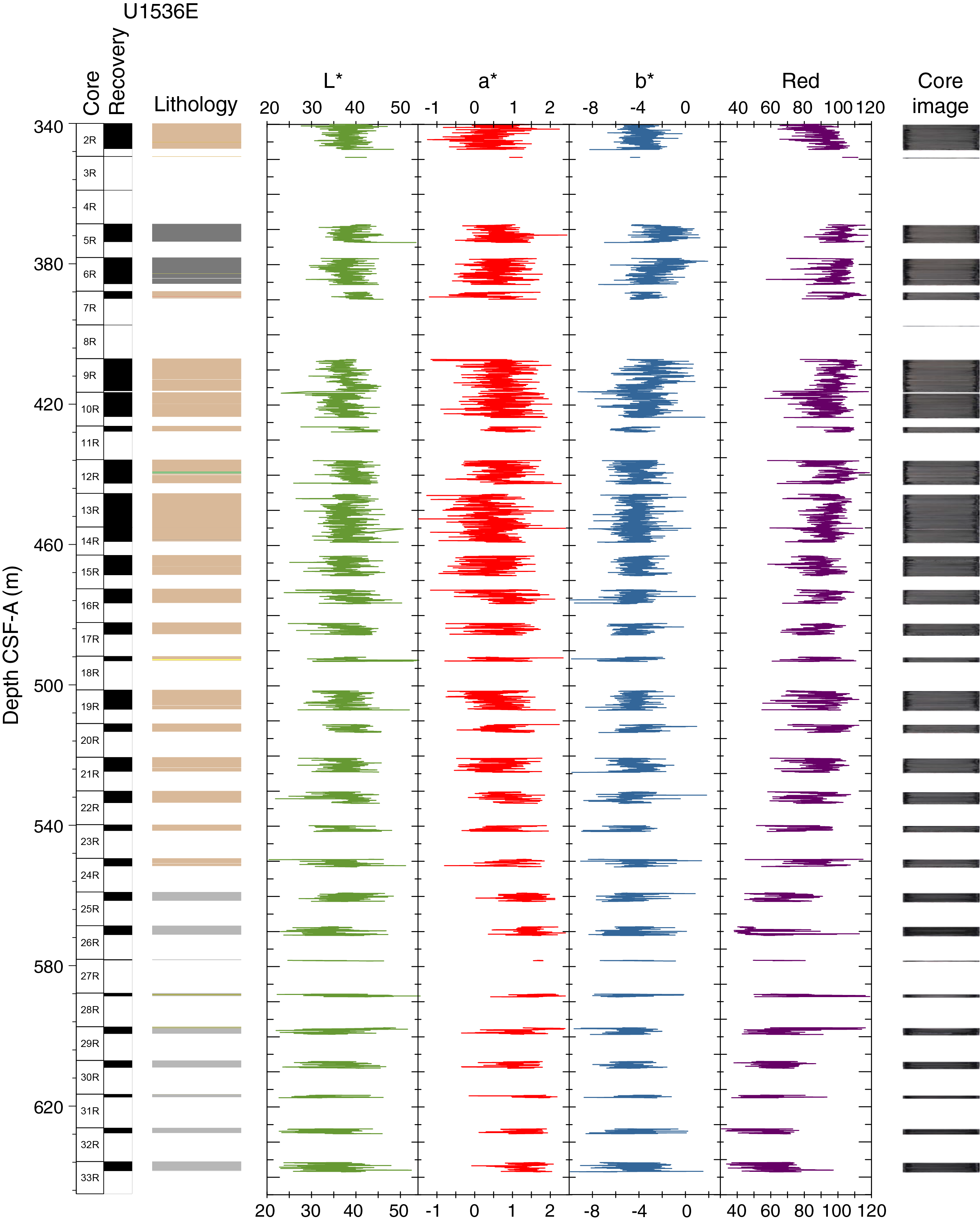
Figure F54. Color reflectance, Hole U1536E.
The a* axis is the green–red component and is usually a tracer of changing redox conditions in the sediments. For Holes U1536A and U1536B, a* values are low and present little amplitude variation throughout the entire hole and a slight increasing trend downhole, whereas Hole U1536E values decrease from Core 382-U1536E-5R downhole.
The b* axis is the yellow–blue component, and it is a proxy for the relative opal content in cores from the Scotia Sea (Sprenk et al., 2013); more positive values (yellower colors) correspond to higher opal (usually diatoms) contents. A decreasing downhole trend is observed for this component, reaching low and rather invariant values in Core 382-U1536A-31F. The highest values are found in Core 10H. All three color components (L*, a*, and b*) show cyclical variation downhole.
Physical properties and relationship with facies
In general, the sediments at Site U1536 are composed of greenish gray diatom-bearing/rich silty clay and greenish gray clay-bearing diatom ooze with low carbonate and TOC content. The silty clays are generally associated with higher MS, NGR, and density and lower P-wave velocity and b* values. Glauconite is present, and variations in its abundance likely play a strong role in controlling changes in sediment color and lightness.
The Pliocene–Pleistocene and late Miocene stratigraphy at Site U1536 is divided into two units. Lithostratigraphic Unit I (middle and late Pleistocene) spans the uppermost ~250 mbsf and consists of interbedded silty clay and diatom ooze with highly variable MS, NGR, density, P-wave velocity, and b* values. Lithostratigraphic Unit II (late Miocene to early Pleistocene) spans ~250–560 mbsf, consists largely of diatom-bearing/rich silty clay, and is associated with overall higher but equally variable MS, higher but more muted NGR and GRA density, and lower b* values.
It is most likely that changes in the physical properties of these units are the product of variations in the proportion of their biogenic particle (dominantly diatom opal) and terrigenous clastic content. In the case of MS, variations in these data are controlled by dilution of the terrigenous magnetic carrier by diamagnetic biogenic opal. This signal is further modulated by variations in the input of at least two distinct populations of magnetic minerals: lower coercivity magnetic minerals that appear to be associated with MS lows and higher coercivity magnetic minerals that appear to be associated with MS highs (see Paleomagnetism). The lower half of Lithostratigraphic Unit II between 370 and 560 mbsf was deposited during the late Miocene and is notably dropstone rich compared to the overlying Pliocene–Pleistocene sediments. Biscuiting (e.g., coring disturbance) in the deepest part of Hole U1536E made it difficult to obtain reliable physical property measurements.
The middle Miocene portion of the Site U1536 stratigraphy is represented by Lithostratigraphic Unit III, which was only recovered in Hole U1536E at ~560–650 mbsf. It is composed of interbedded semilithified to fully lithified dropstone-free mudstone and intermittent beds of limestone, some of which are nannofossil bearing/rich. Again, the low recovery and biscuited nature of these cores in Hole U1536E made it challenging to compare their sedimentology with trends in physical properties. They do, however, appear to be characterized by a similar range of MS, GRA, and b* values as Unit II but possibly by lower NGR, which may reflect the absence of dropstones (and other ice-rafted terrigenous sediment) in this interval.
Core disturbances and data quality
All physical property measurements were possible, but the PWL was not used for Hole U1536E because of RCB coring. Hole U1536A contains a number of cores that were excluded from consideration for affine ties in stratigraphic correlation because of core disturbance such as flow-in. For instance, Cores 382-U1536A-3H, 8H, 18H, and 38F feature considerable flow-in and/or other coring-related disturbances that make their physical property data questionable in terms of quality. These cores do not contain evidence for the slumped intervals observed in the seismic sections around 50–60 and 90–100 mbsf. A lot of the core fabric observed in all Site U1536 holes was negatively affected by weather conditions during coring (Hole U1536A more than Holes U1536B and U1536C). Core disturbances such as uparching of layers did not diminish the quality of the physical property data in a way that prevents meaningful core-seismic integration in the splice; however, flow-in does, although these cases are few.
Summary
Physical property data were acquired on all cores from Site U1536 using the WRMSL for GRA wet bulk density, MS, and P-wave velocity (PWL). We also measured NGR in all sections longer than 50 cm. Once the whole rounds were split in two halves, we acquired X-ray imaging on all the archive halves and measured thermal conductivity in one section per core. The SHMSL was then used to measure MSP and color reflectance using the L*a*b* color system, and the red-green-blue (RGB) color of the sediments was measured with digital color imaging (SHIL). In addition, we determined P-wave velocity values at discrete points on the working halves for all cores from Site U1536 and measured discrete samples for MAD (wet bulk density, dry bulk density, and grain density) for Holes U1536A and U1536E. The sensors worked correctly, and the data are of good quality.
Diatom ooze and silty clay dominate the lithology for the upper 250 m, whereas silty clay, clay, and mudstone dominate the rest of the sediment column (250–645 mbsf). Prominent variations in physical property signals are observed where the lithology varies in the core, such as in Core 382-U1536A-7H, whereas more uniform lithologies are reflected by more monotonous physical property signals. Diatom-dominated lithologies have lower NGR, density, and MS values than silty clay–dominated lithologies. Accordingly, the physical properties obtained for Holes U1536A–U1536E provide valid and reproducible information on sediment composition and variability for all cores. All the physical property records show characteristic 1–10 m scale variations that likely reflect the characteristic orbital-scale cyclicity of the Pleistocene and Pliocene.
Stratigraphic correlation
To achieve the research objectives, five holes were drilled at Site U1536 using the APC, HLAPC, and RCB coring systems. Mudlines were achieved for Holes U1536A–U1536C. More than 354 m of sediment from Hole U1536A and 226 m from Hole U1536B was recovered using APC/HLAPC coring before each hole had to be abandoned because of the near-approach of icebergs. Spot coring between wash downs was undertaken in Hole U1536C to ~224 mbsf, and then continuous APC/HLAPC coring was conducted to ~352 mbsf before this hole also had to be abandoned because of iceberg activity.
Whole-round cores from Holes U1536A–U1536C and U1536E were analyzed for their physical properties using the WRMSL (for MS, GRA density, and P-wave velocity; P-wave velocity was not measured in cores from Hole U1536E) and gamma ray track (for NGR intensity) and subsequently the SHMSL (for MS and color reflectance) once they were split into working and archive halves (see Physical properties; also see Physical properties in the Expedition 382 methods chapter [Weber et al., 2021a] for details). The whole rounds from Cores 382-U1536C-1H and 2H were not measured for their physical properties because they were split for aDNA sampling immediately upon collection to avoid modern-day DNA contamination and radiation damage to the DNA. Because the top two Hole U1536C cores were needed to bridge coring gaps between Cores 382-U1536A-1H and 2H and between Cores 382-U1536B-1H and 3H, MS of the archive halves of these cores determined using the SHMSL MSP sensor was used for correlation.
Correlation between holes
To minimize coring gap alignment, sequences from all holes were examined in near–real time using whole-round MS data, MSP data, and GRA density data measured at a 2.5 cm resolution with the WRMSL and SHMSL. Because of our objective to reach the basement, it was not possible to conduct triple APC offset coring at Site U1536, which is most commonly required to maximize the opportunity to make a complete splice. The difficulty was further magnified below ~250 mbsf because the cores were mostly aligned at their core breaks below this depth and because of the need to use HLAPC coring.
The top of Hole U1536C (which preserved a mudline) served as the anchor (zero depth point) for the generation of the CCSF-A depth scale at this site (see Stratigraphic correlation in the Expedition 382 methods chapter [Weber et al., 2021a] for an explanation of depth scales). Using this anchor core, we attempted to determine the relative depth offset of each core from this reference by establishing affine ties between cores from Holes U1536A–U1536C based on the optimized correlation of WRMSL-derived MS and GRA density data (see Figure F25 in the Expedition 382 methods chapter [Weber et al., 2021a]). These depth offsets (or affine ties) are reported in affine Table T21, and the resultant physical property correlations are shown in Figure F55. Note that although affine ties are established for Cores 382-U1536C-1H and 2H, data are not plotted in Figures F55 or F56 because GRA density, whole-round MS, and NGR data were not collected for these cores. Correlations for these two cores were based on MSP (not plotted). Core disturbances and other sporadic difficulties with coring meant that the stratigraphic quality of the sedimentary sequence recovered was variable. A significant number of cores (~20%) in Holes U1536A–U1536C achieved only partial strokes (50% of these were APC cores), and several instances of shattered core liners occurred. Most partial strokes were in Hole U1536C (~68%), which was cored during a period of relatively high heave. Nevertheless, Hole U1536B and U1536C cores typically appeared less disturbed than Hole U1536A cores and thus less noisy in their magnetic directions (see Paleomagnetism). We did not attempt to make affine correlations to 12 cores that were heavily disturbed by coring or had very low recovery (7 cores from Hole U1536A and 5 cores from Hole U1536C; Table T22). In addition, we were not able to establish double affine ties (needed to include them in a splice) to the CCSF-A depth scale for (1) 5 cores in the uppermost 242 m CCSF-A and 27 of the bottom 28 cores recovered from Hole U1536A, (2) 6 of the 25 cores recovered from Hole U1536B, and (3) 27 of the 40 cores recovered from Hole U1536C (Table T21). Our failure to establish correlations for these cores was due to the alignment of core breaks between holes and/or because some of them were recovered with partial strokes. The affine ties between several of the cores are also uncertain (see quality comments in Table T21) because in some instances the relevant core gaps are very close to being lined up between the two holes in question, because the correlating features are subtle, and/or because deformation occurs in one or both of the cores. In these cases, it may be possible to improve (or even make) ties with postcruise efforts, for instance, using X-ray fluorescence (XRF) core scanning elemental data.
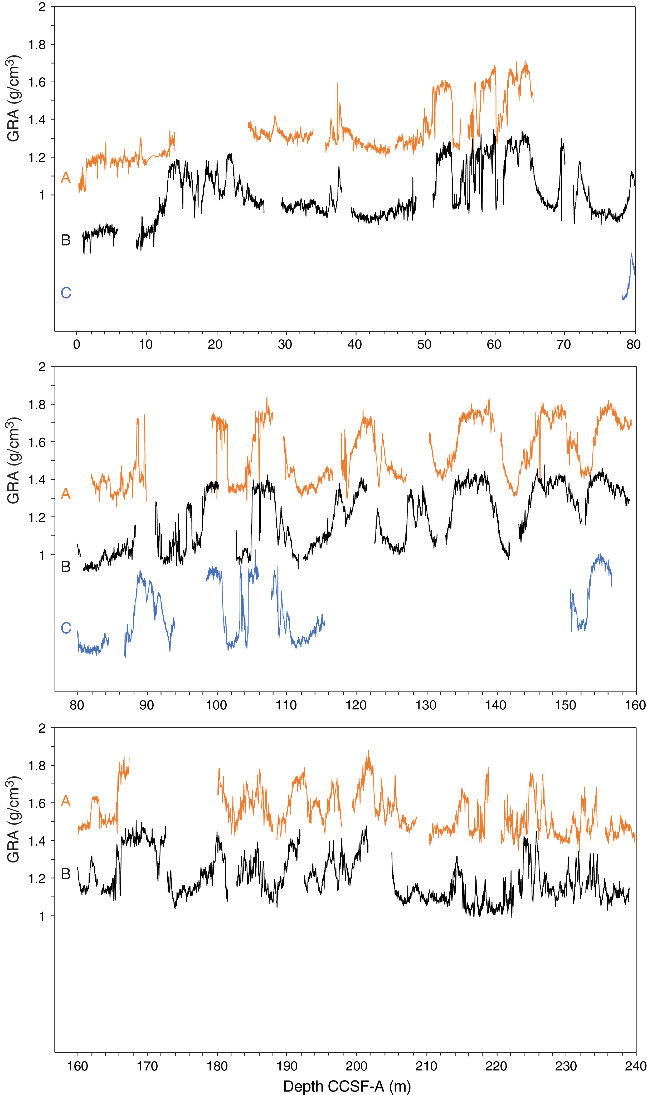
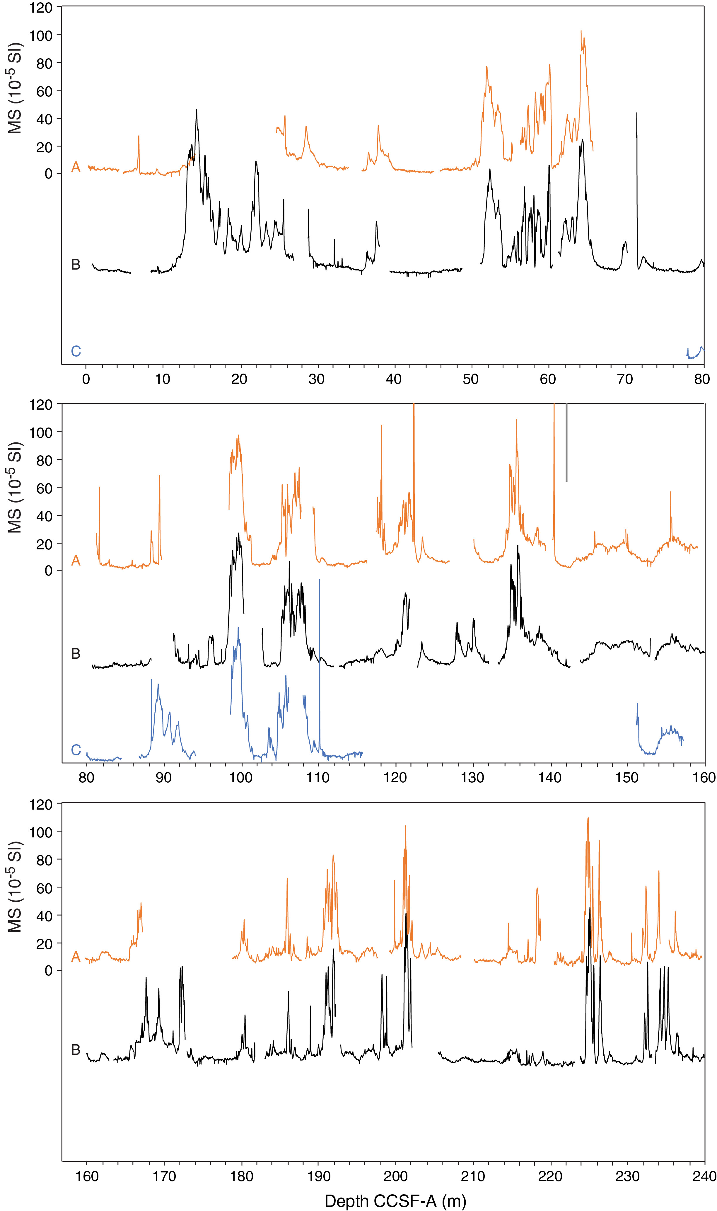
Figure F55. GRA density and MS.
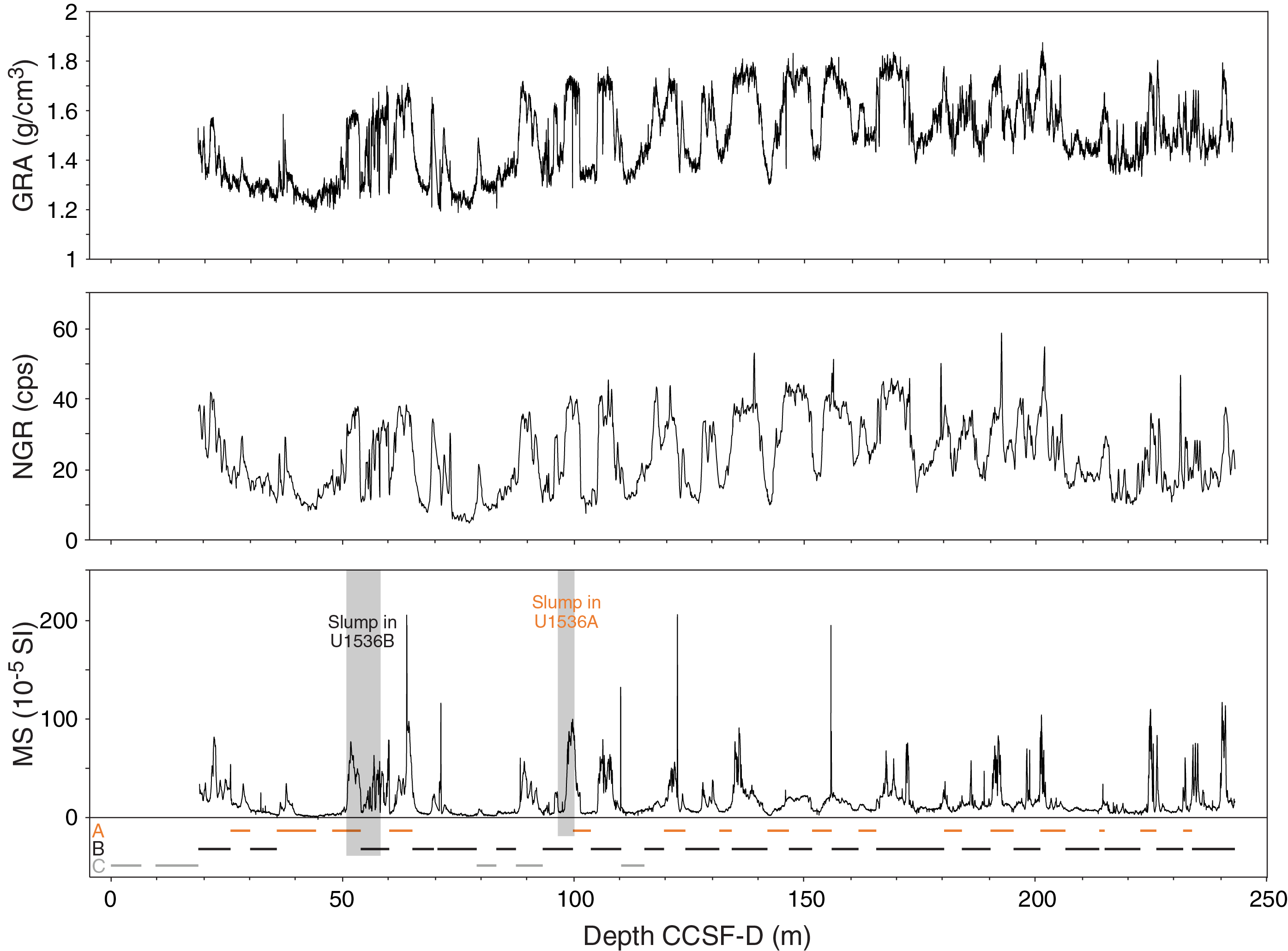
Figure F56. Spliced record of GRA density, MS, and NGR intensity.
One important interval that requires such attention is the expanded section (~39–49 m core composite depth below seafloor, Method D [CCSF-D]) that we infer records Marine Isotope Stage (MIS) 5e (~125 ka). The physical properties in this interval were correlated between Cores 382-U1536A-5H and 6H using a very subtle inflection and gentle trend in GRA density. The gap offset between Holes U1536A and U1536B across this append indicates that this interval is likely preserved in Core 382-U1536B-6H. However, the shipboard physical property data do not allow high confidence in the correlation. XRF scanning could potentially confirm if and where the gap is covered in Hole U1536B.
A similar uncertainty is observed in the Holocene where the physical property features are very subtle in the upper 11 m of the holes. It is possible that Core 382-U1536A-2H may allow ties to Cores 382-U1536C-1H and 2H that could complete the splice at the top; however, we are concerned about the quality of Core 382-U1536A-2H (it appears to be stretched relative to the same stratigraphic interval in Holes U1536B and U1536C).
In summary, even if all the uncertain ties could be confirmed, it is still not possible to build a complete CCSF-A depth scale for Site U1536. In addition, variable in-core stretching of sequences implies that single depth offsets derived from affine ties will result in inevitable and significant misalignment of features that can otherwise confidently be correlated between holes (e.g., see Figure F55).
The results of the effort to tie cores in Holes U1536A and U1536C are in the Laboratory Information Management System (LIMS) database and shown in Table T21.
Construction of the splice
Once the composite depth scale was created, selected sequences from Holes U1536A–U1536C were spliced together to create the most complete and representative section possible (Figure F56). In addition, we strove to have as much of Hole U1536B in our primary splice as possible because it was the least effected by drilling disturbance (Figure F56). However, because Hole U1536B was not drilled to the same depth as Hole U1536A, this was not possible below 226 mbsf. Detailed sedimentological logs and archive-half X-ray images were consulted in the process of splice construction to avoid the inclusion of any significantly disturbed intervals and/or sections with unique features (relative to the other holes). The end product is reported in Table T23.
The primary splice for Site U1536 spans 0–242.997 m CCSF-D. It is based predominantly on the correlation of sediment MS and GRA density data. The affine growth factor is 1.076 in Core 382-U1536A-26F and 1.077 in Core 382-U1536B-25F, the last tied cores in the splice. Cores from Holes U1536A and U1536C extend to 354.5 and 352.2 mbsf, respectively, but they are (mostly) APC/HLAPC cores; although it is possible to connect them to each other, the coring gaps are very close to aligned and it is only possible to make a few ties between them in this interval. Logging data may potentially be used to improve the depth accuracy of these cores (see Downhole measurements). Between 71.5 and 242.997 m CCSF-D, the splice contains only one stratigraphic gap (between Cores 382-U1536B-18H and 19H; Core 382-U1536A-18H is at the right drilling depth to fill the gap, but it is highly disturbed and thus deemed unusable for the splice).
Between the mudline and 71.5 m CCSF-D, one append is at the top of the site between Cores 382-U1536C-1H and 2H (it could potentially be filled with Core 382-U1536A-2H, but we are concerned about its quality) and another append is at 70.03 m CCSF-D. Below 243 m CCSF-A, multiple coring gaps of unknown length in Holes U1536A and U1536C prevent the extension of the splice to the bottom of this pair of holes. Below the splice, we observed correlation between many cores in Holes U1536A and U1536C, but it is not sufficient to warrant either constructing a floating splice or extending the splice below ~244 m CCSF-D. Hole U1536E was drilled with the RCB system. It overlapped with the basal 10 m of Hole U1536A. Coring quality and recovery, however, were poor throughout, and it is impossible to tie these cores to Hole U1536A or the logging data.
In addition to complications from gaps and coring disturbances, two slumped intervals are present in the upper 100 m CCSF-D of the primary splice. This deformation is a primary sedimentological feature of the sequence, not the product of coring disturbance. It could therefore not be avoided in the splice. The slumps were recognized (in core photographs and X-ray images) by steeply inclined (and often opposed) and sometimes recumbently folded beds and/or laminae and by slump-scar bases forming sharp boundaries between diatom ooze and clay-rich intervals (see Lithostratigraphy). We estimate that the uppermost slumped interval spans ~50.74–56.34 m CCSF-D (in Core 382-U1536B-7H) and the lower slumped interval spans ~95.90–99.31 m CCSF-D (in Core 382-U1536A-11H). Although the uppermost slumped interval has a comparable thickness in both Holes U1536A and U1536B, the lower slumped interval appears to be significantly thicker in Cores 382-U1536B-12H and 382-U1536C-7H than in Core 382-U1536A-11H.
We found evidence for another, older slumped interval in Cores 382-U1536A-43F and 382-U1536C-29F at ~299–301 mbsf; however, because we cannot correlate precisely between these two cores using Site U1536 physical property data, it is not currently possible to determine its thickness (the sequence in Core 382-U1536A-43F appears less disrupted than in Core 382-U1536C-29F). For depths where cores from both Holes U1536A and U1536B are available (above ~235 m CCSF-D), cored intervals from Hole U1536B dominate the splice; however, it is dominated by cored intervals from Hole U1536C below ~235 m CCSF-D (where they make up ~60% of the record). Overall, Hole U1536A makes up 29% of the splice, Hole U1536B makes up 58% of the splice, and Hole U1536C makes up 13% of the splice (Figure F56).
Comparison of core and downhole logging data and evaluation of cores below the splice
Logging was conducted in Hole U1536E (see Downhole measurements) to help with connections to seismic data (Pérez et al., 2017) and core information from drilling. The quality of the hole was variable, and the calipers were fully extended over much of the interval logged. Additionally, the WHC was not working properly, so there may be extra distortion on the depth scale at the 1–2 m interval. However, overall the log provides a continuous record that may allow better interpretation of the lithologies encountered.
We imported the NGR log into Correlator (version 3) in an effort to improve our understanding of the positions of short APC/HLAPC cores below the end of the splice (this was difficult enough that we did not even attempt it with the RCB cores). We were able to upload the logging data into Correlator by making a table in a format as if it were a core and making a section summary. In the first attempt, we made many cores with only one section. In the second attempt, we realized we could just load the whole thing as a single core. We first attempted to tie each core below the splice from Holes U1536A and U1536C into the logging data; this exercise has some significant uncertainties due to the presence of large-scale features that are unlike the pattern of NGR variation measured on the cores. However, the overall cyclicity is well matched between the log and the cores (Figure F57), and we feel that this information can be used to confidently place the age constraints onto the log to ~340 mbsf (Figure F58).
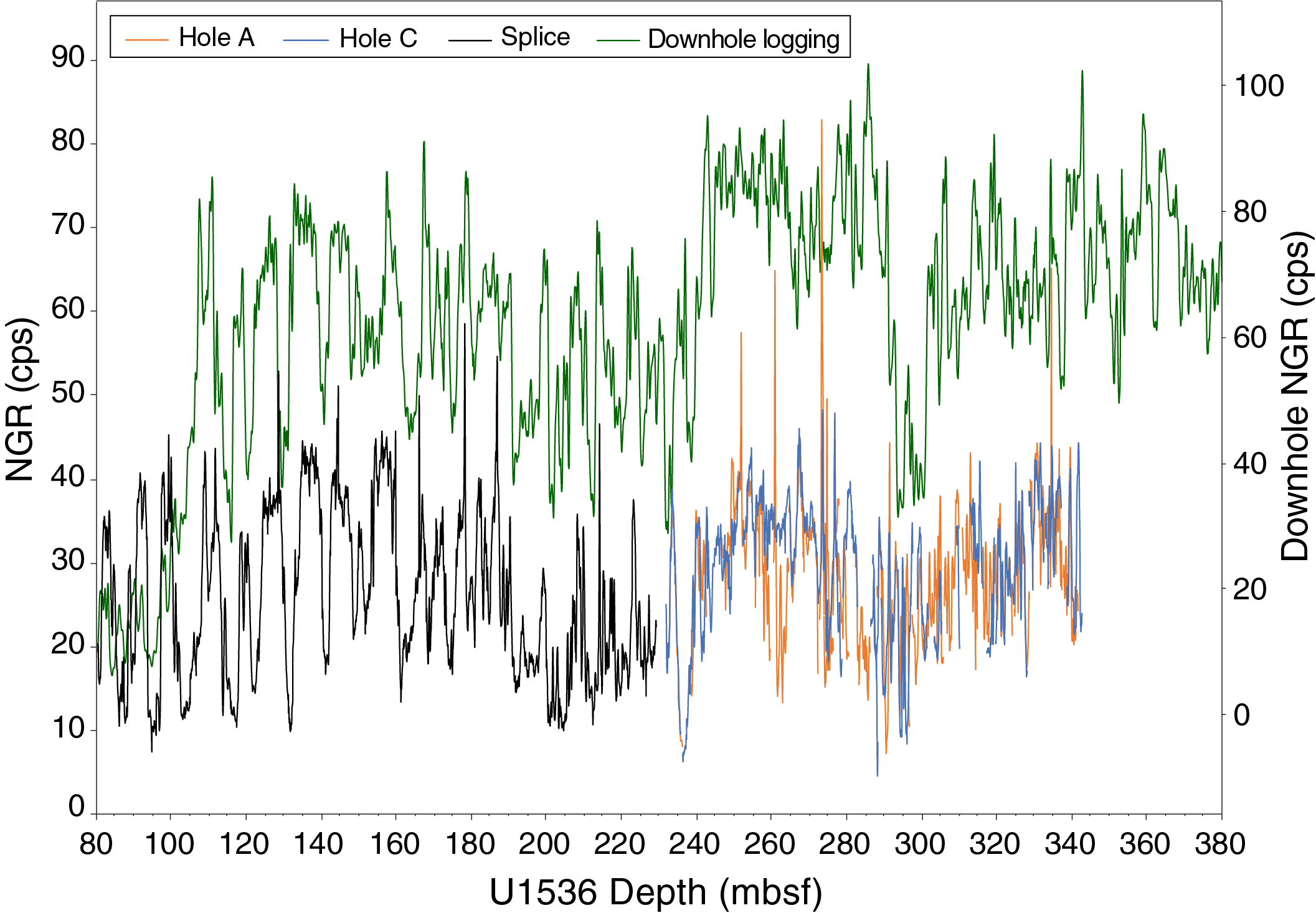
Figure F57. NGR logging data compared to NGR splice and core data.
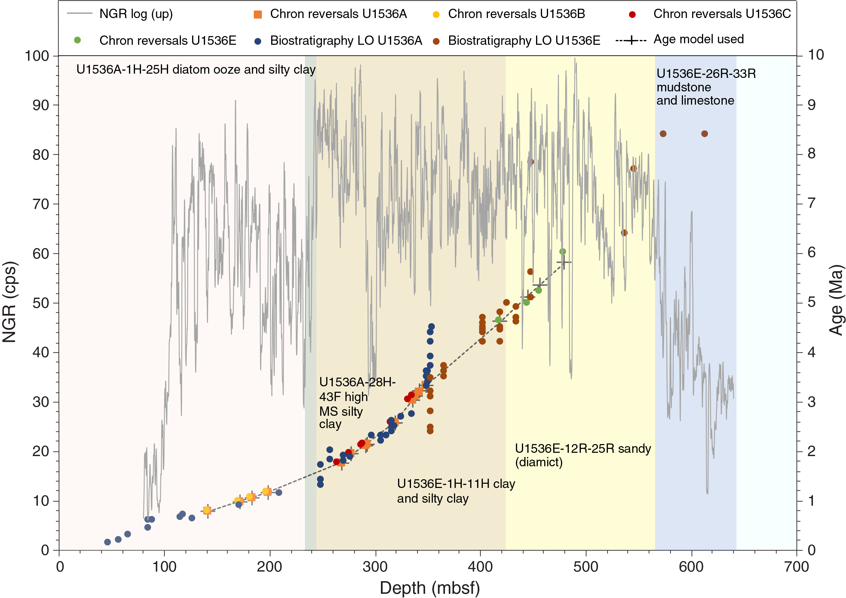
Figure F58. NGR and age vs. log depth, Hole U1536E.
NGR from the logging data also provides estimates of U, Th, and K concentrations, and ratios of these elements vary more smoothly than the total NGR signal from the logs (Figure F59). Under ideal circumstances, it is possible to extract U, Th, and K data from the shipboard NGR data on whole-round cores (e.g., Dunlea et al., 2013; De Vleeschouwer et al., 2017). During Expedition 382, Detector 7 was drifting across the energy range in such a way that the data from it cannot be used as is. Furthermore, there is clearly a significant range in the signal responses of the other seven detectors. If a program could be devised that could evaluate the energy peaks and revise them, and if a strategy to normalize the signals from the various detectors could be implemented, the data acquired during this expedition could be used to determine U, Th, and K concentrations. With such data, it may be possible to more precisely correlate the cores to the log.
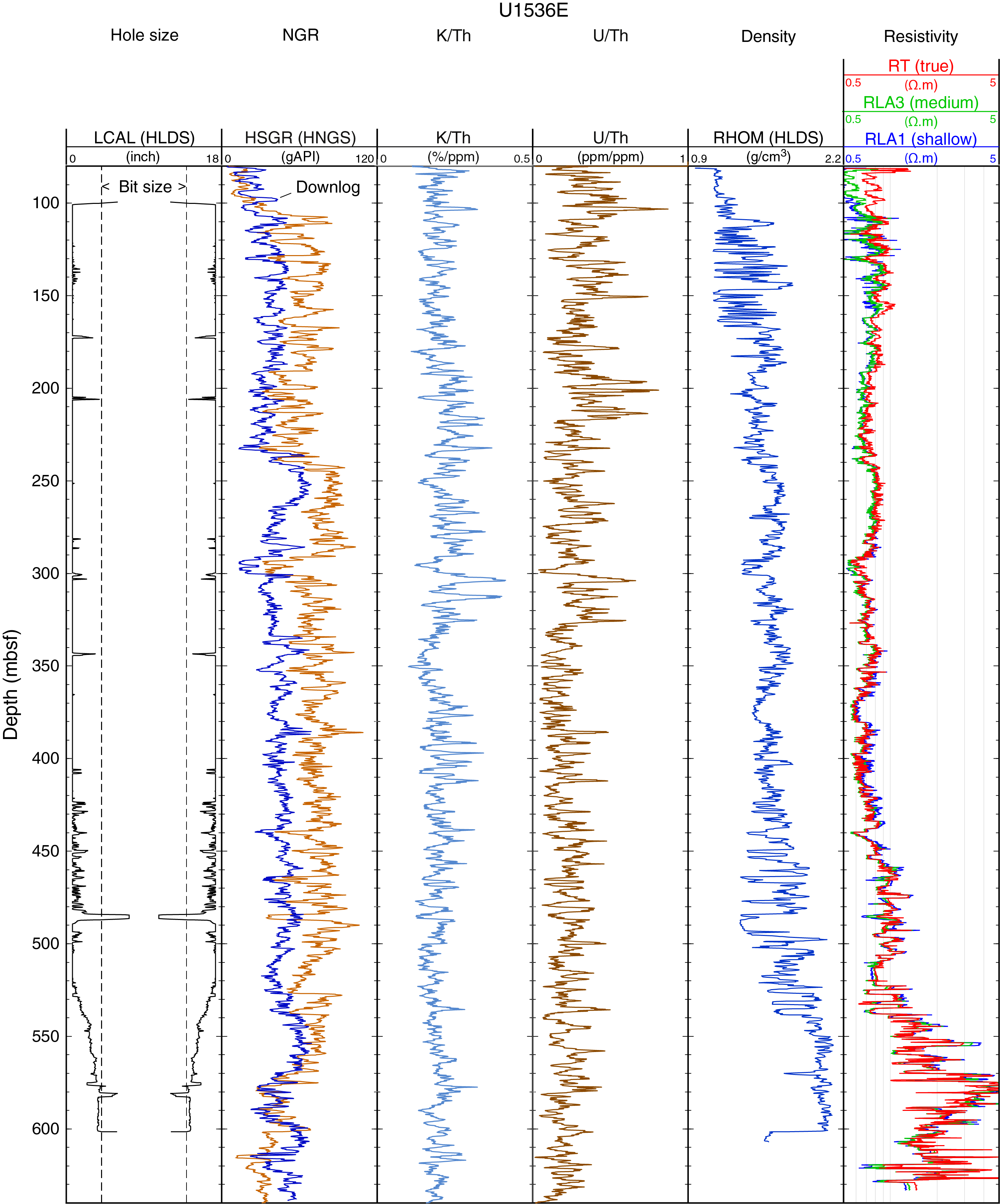
Figure F59. Logging data summary.
In the process of trying to connect to the log, we found that most of the cores from Holes U1536A and U1536C below the splice can be tied to each other through similar features. However, no way was found to estimate the amount of offset between successive cores and only a few instances occur where double ties can be made to string the cores together. We have partnered each of the cores from Hole U1536A with a core from Hole U1536C beneath the splice (except Core 382-U1536C-30F, which we removed from the correlation because of its disturbance). After connecting the cores with their GRA records, we added the inclination data to Correlator to confirm the connections are consistent with the identified reversals. It is possible that some improvement can be made to this process, but it would require significant postcruise effort.
It is impossible to tie cores from Hole U1536E to Hole U1536A because of both the minimal overlap and the lack of similarity in the nominally overlapping cores. Time constraints during the expedition made it impossible to refine the connection between Hole U1536E and the log, and it may not be possible except at the coarsest resolution because of the very poor recovery in Hole U1536E. However, it is possible to make a first-order age model by using the drilling depth constraints from biostratigraphy and (especially) magnetostratigraphy to estimate the age span covered by the log (Figure F58).
Hole U1536E revealed some interesting lithologies in the uppermost part of the record. Early Pliocene to late Miocene sediments (~4.5–7 Ma) have abundant sand-sized dropstones; below that interval (~570 mbsf), the Miocene sediments appear to have no evidence of glaciation. They are characterized by gray siltstone and some limestone layers. At the bottom of the record, the biostratigraphic ages jump dramatically, and it looks like drilling stopped at approximately 15 Ma (biostratigraphic markers older than 10 Ma are not shown in Figure F58 because of scaling). We used the shipboard timescale (Figure F58) to plot the log data in Figure F60.
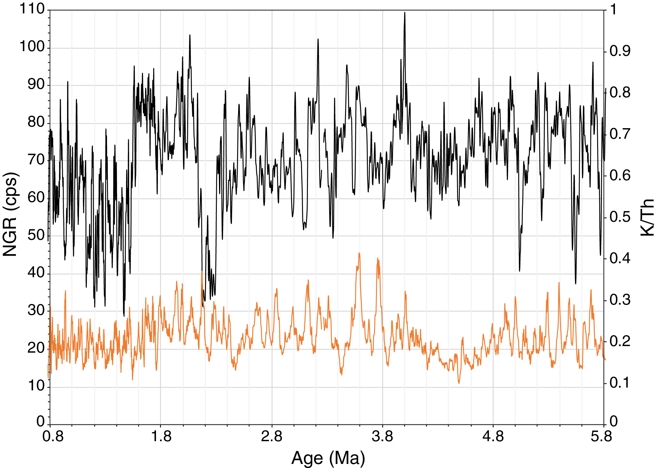
Figure F60. NGR and K/Th on timescale.
Downhole measurements
Logging operations
The last core from Hole U1536E arrived on deck at 1820 h on 24 April 2019. Hole preparation for the logging program included releasing the RCB drill bit and pumping the open hole with seawater and 10.5 lb/gal heavy mud with barite to help hole stability. The pipe was raised to a logging depth of 83.4 m wireline log depth below seafloor (WSF). The modified triple combo tool string was assembled on the rig floor on 25 April and was prepared on deck until an "all clear" of icebergs was announced by the bridge at 0615 h on 25 April. The WHC was not used to compensate for vertical ship motion on the wireline depth because the software that controls it was not receiving correct ship motion data, resulting in a fast drop of the upper pulleys to the lower end stop when it was switched on.
The modified triple combo tool string included MS, NGR, electrical resistivity, acoustic velocity, and density tools (see Downhole measurements in the Expedition 382 methods chapter [Weber et al., 2021a]), and it was run first downhole in Hole U1536E at 0837 h on 25 April. The density tool was included in the tool string together with the caliper (borehole diameter) measurement tool. The downlog started at 3129.5 mbrf and ended at 3872.3 mbrf. No problems were encountered getting down through pipe or the open hole. Total penetration was 645.4 mbsf, and just one run was made in this hole (downlog and uplog) because of time constraints caused by the deteriorating ship heave conditions and the presence of icebergs. Rig down run was completed at 1500 h, and total operating time was 14 h.
Log data quality
The main control on log data quality is the diameter of the borehole measured by the caliper on the Hostile Environment Litho-Density Sonde (HLDS) logging tool (Figure F61). The hole was wider than the maximum extent of the caliper arm (17 inches) from the end of the pipe to 425 mbsf, leading to questionable quality of the logs that require good contact with the borehole wall, such as the density log (Figure F61). Log data were transmitted to Lamont-Doherty Earth Observatory (LDEO) for depth matching and data processing and were returned to the ship a day later. All readings are within the expected range. Density ranges from 1.1 to 2 g/cm3 for the majority of the hole and is around 2.0 g/cm3 in the bottom part. Deep resistivity ranges mostly from 0.6 to 1.1 Ωm and rises to between 1.5 and 5 Ωm in the more lithified section below 540 mbsf. The borehole diameter was around 10.5–11 inches at the bottom of the hole (580–600 mbsf), and it widened to more than 17 inches at about 425 mbsf and above. The caliper had to be closed for a short interval (485–488 mbsf) because the cable tension increased, indicating that the formation was closing on the tool; the closed caliper helped the tool move past this tight spot. Average gamma ray values are lower than 50 gAPI in the open hole interval in the lower in-gauge hole and progressively increase, reaching 100 gAPI in the upper large hole section (Figure F62). P-wave velocity ranges from around 1530 m/s from 80 to 150 mbsf to between 2200 and 2700 m/s from 575 to 625 mbsf (Figure F63). From 80 to 350 mbsf, velocity increases gradually, and a major step change is observed at about 540 mbsf.
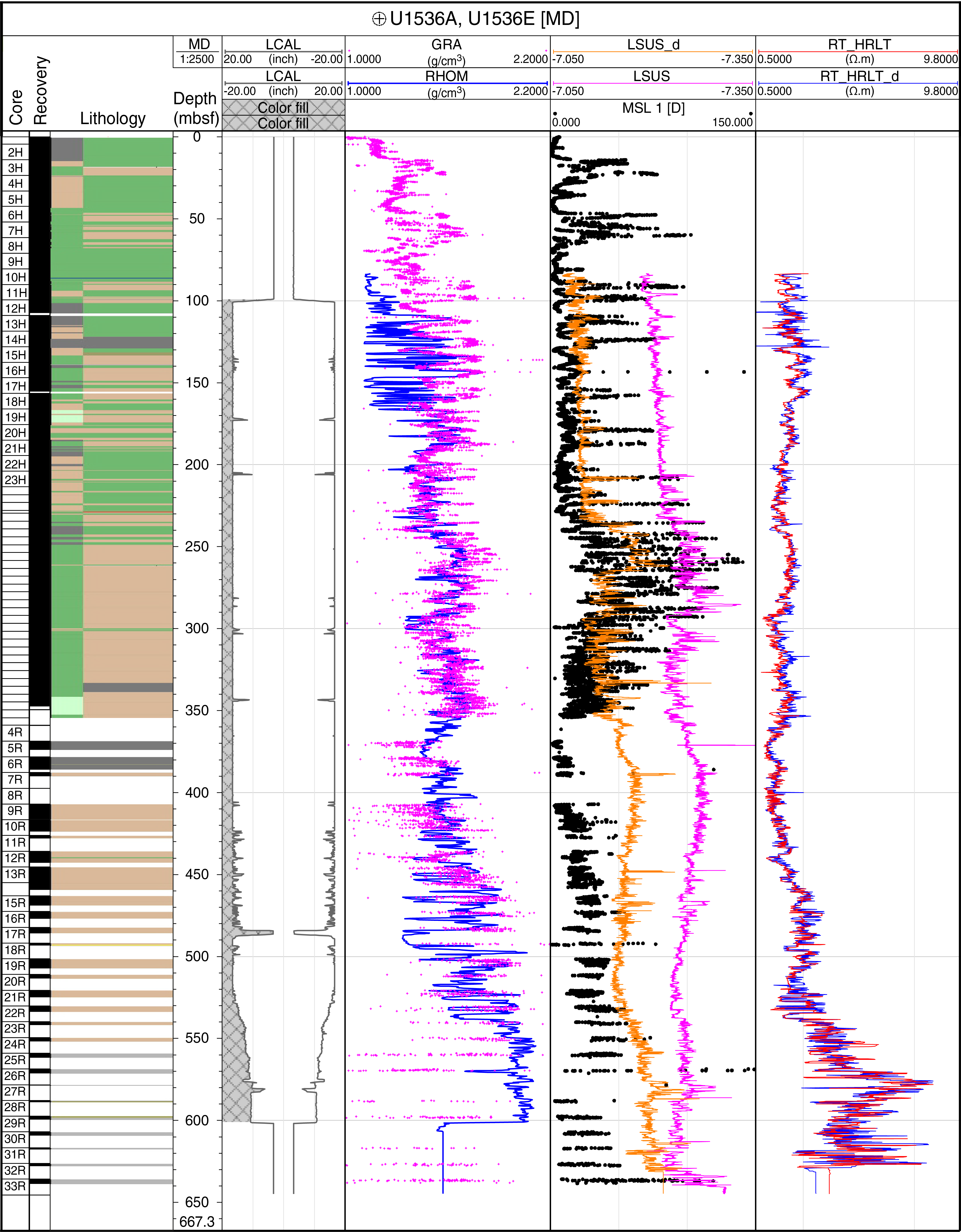
Figure F61. Laboratory GRA and MSL with logging density, MS, and resistivity.
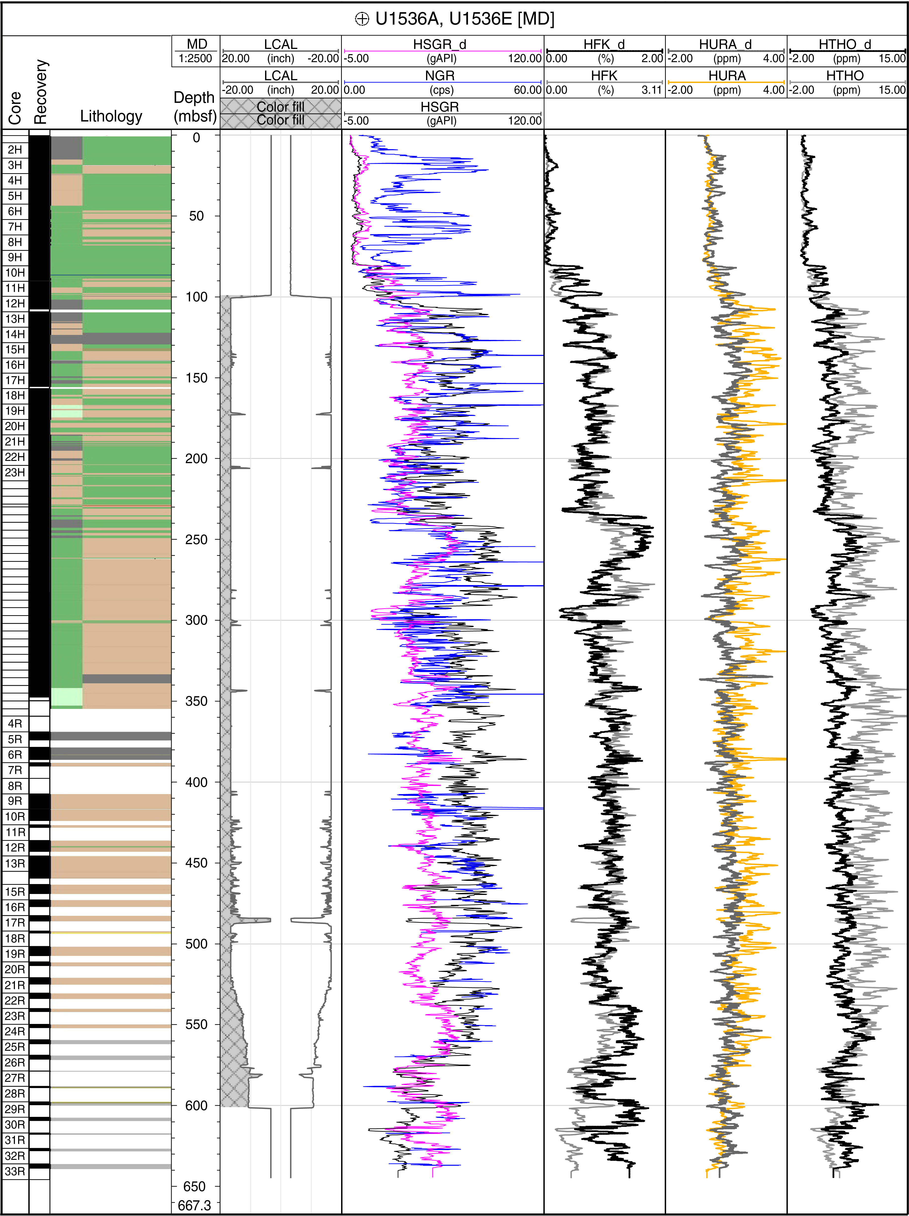
Figure F62. Laboratory NGR with logging NGR, K, U, and Th.
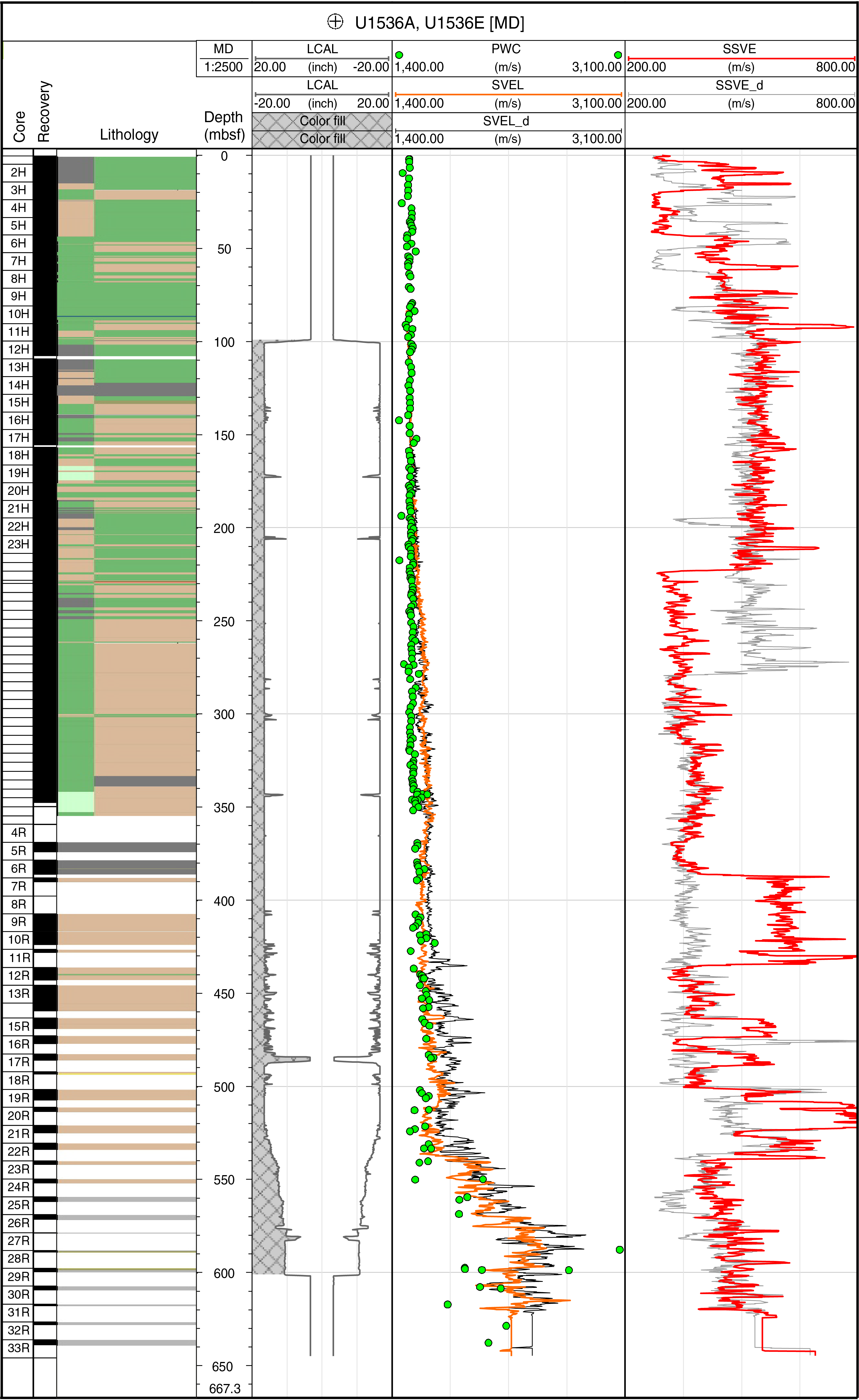
Figure F63. Laboratory PWC with logging sonic and shear velocities.
The downlog and uplog data of each measurement do not always perfectly match each other (Figures F61, F62, F63). In the case of gamma radiation, differences occur in absolute values because the uplog is corrected for borehole diameter (as measured by the caliper) and the presence of barite-weighted mud, whereas the downlog is not (because the caliper is closed when the tool is lowered downhole). The uplog and downlog P-wave velocity values differ in places because the software is not always able to pick the signal arrival well in low velocity formations. The downlog transmitter was run at standard (high) frequency, and the uplog was run at low frequency, which has less attenuation in the formations. Further processing would be needed to determine the S-wave velocity values from the original sonic waveforms.
Differences of as much as about 2 m occur in the depth location of individual layers recorded in the different logs as a result of variations in the tool speed during logging. The downhole NGR and P-wave velocity logs have features in common with the equivalent laboratory data from Site U1536 (Figures F62, F63), and small offsets between log and core data are due to the assignment of core depths when core recovery was not 100% and other effects. Downhole density trends and most of the measured features also agree with the density values measured by GRA and MAD values determined in the laboratory (Figure F61).
NGR is attenuated through the BHA (0–80 mbsf) but can be corrected to the equivalent open hole value by using a constant multiplication factor, which was not done here (Figure F63).
Comparison of log with core data and lithologic inferences
A detailed comparison of the logging data with the spliced record at Site U1536 is given in Stratigraphic correlation. The applied depth relationship used here is the one obtained from the synthetic seismogram derived by core measurements (see Core-log-seismic integration for details). The physical properties measured downhole are interpreted in a similar way to those measured on the cores in the laboratory (see Physical properties). Silty clay–bearing diatom ooze sediments were described as a common lithology to about 250 mbsf, where a high in NGR and resistivity is observed (Figures F61, F62). In this upper part of the hole, P-wave velocity increases downhole with relative highs in diatom-bearing and diatom-rich silty clay sediments (e.g., Figures F44, F45, F63). Mudstones with a few limestone interbeds form the lowermost part of the stratigraphic column from 585 mbsf to the base of the hole at 645 mbsf. These facies have lower NGR, potassium, thorium, and uranium content and higher P-wave velocity, density, and resistivity than the overlying stratigraphic unit (Figures F61, F62, F63).
Below 200 mbsf, sonic velocity values are consistently higher in downhole measurements compared to the values measured on cores (PWC) because downhole measurements are made under in situ conditions of pressure and temperature.
Downhole temperature and heat flow
Advanced piston corer temperature tool (APCT-3) downhole temperature measurements were made in Holes U1536A (Cores 382-U1536A-7H, 10H, 13H, 16H, 19H, and 22H) and U1536B (Cores 382-U1536B-5H, 8H, and 13H). Measurements on Cores 382-U1536B-5H and 382-U1536A-7H did not yield reliable results because the equilibration curve was not stable and presented asymptotic behavior. The obtained temperatures range from 3.5°C at 45.6 m drilling depth below seafloor (DSF) to 16.84°C at 204 m DSF (Table T24; Figures F64, F65), giving an approximately linear temperature increase with depth and a geothermal gradient of 85°C/km. The seafloor temperature was determined to be 0.3°C based on APCT-3 data taken while the tool was held at the mudline for 5 min during each run (Figure F64).
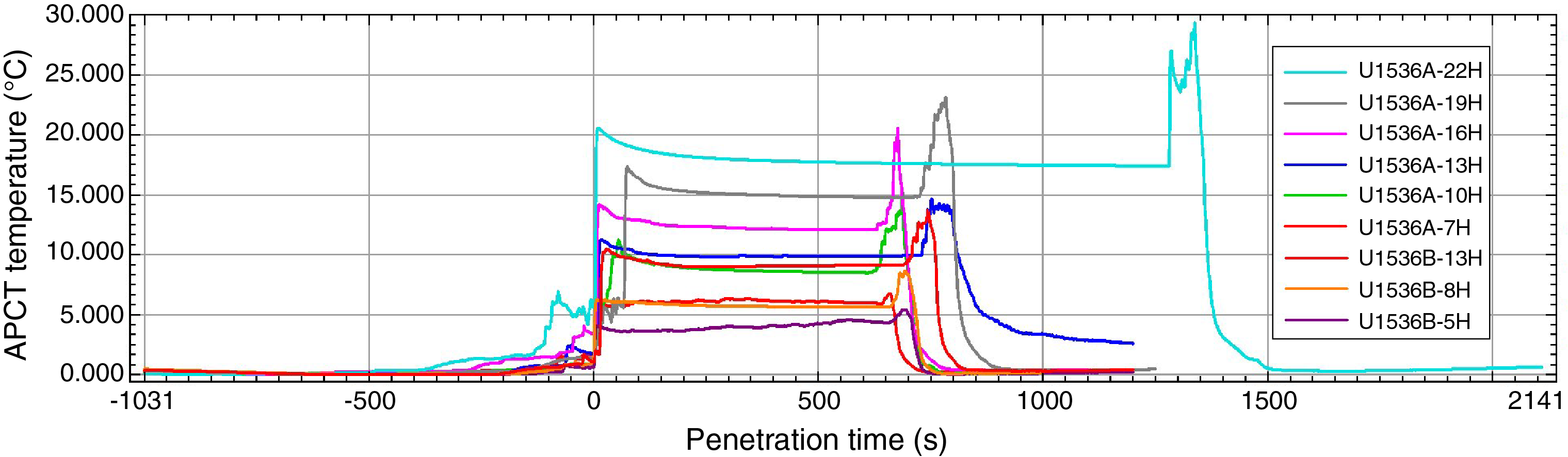
Figure F64. APCT-3 temperature-time series.
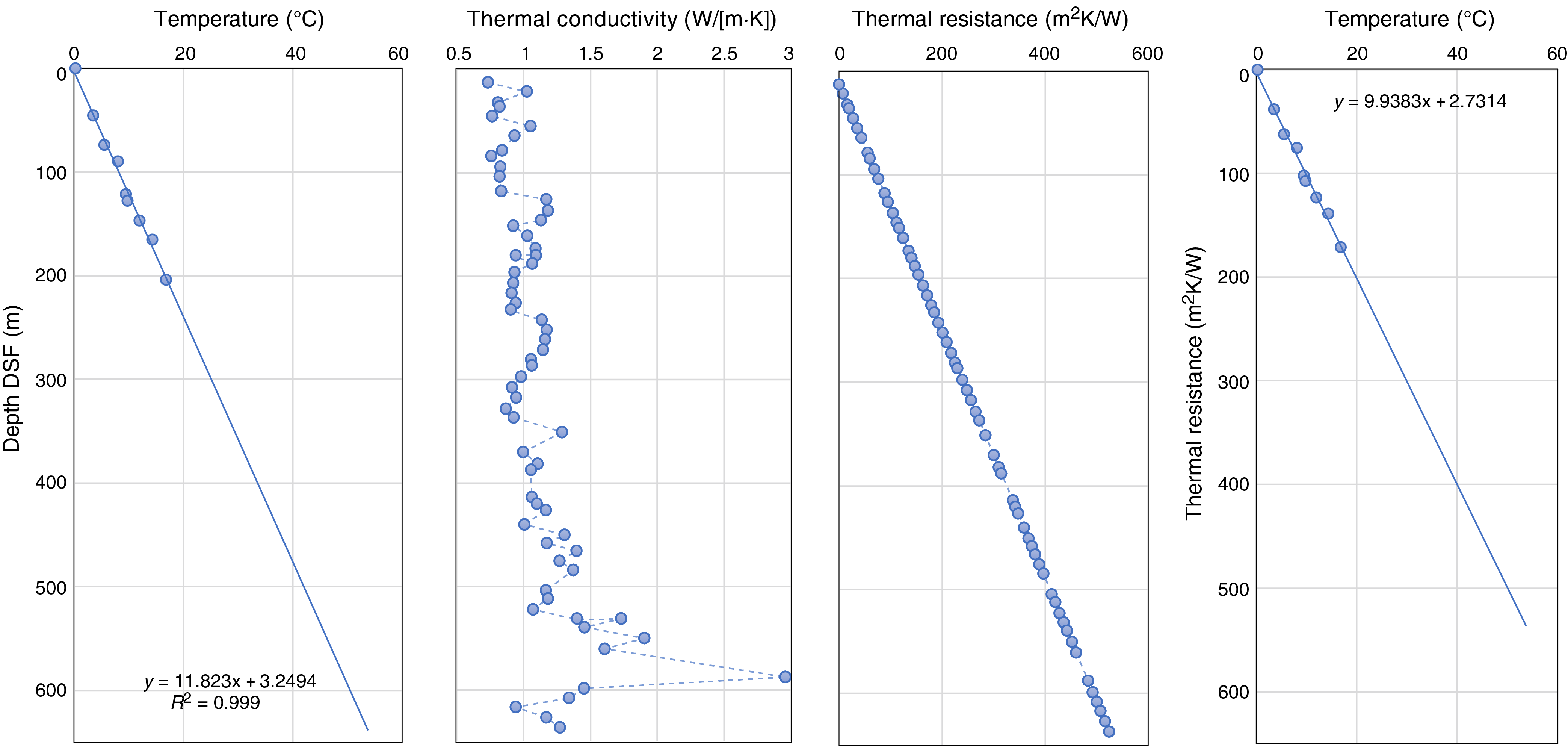
Figure F65. Heat flow calculation.
Thermal conductivity under in situ conditions was estimated from laboratory-determined thermal conductivity from Holes U1536A–U1536C and U1536E using the method of Hyndman et al. (1974) (see Physical properties in the Expedition 382 methods chapter [Weber et al., 2021a]). The calculated in situ values are within 2% of the measured laboratory values. Thermal resistance was calculated by integrating the inverse of the in situ thermal conductivity over depth. Considering all thermal conductivity measurements down the holes for Site U1536, a heat flow of 101 mW/m2 was estimated from the linear fit between temperature and thermal resistance based on the method of Pribnow et al. (2000).
Summary
The APCT-3 was deployed nine times at Site U1536, performing measurements while APC coring took place. The APCT-3 yielded reliable results on the geothermal gradient and heat flow, both consistent with an oceanic crust basement at Site U1536.
Downhole logging was carried out in Hole U1536E when coring operations were over. A modified triple combo tool string including MS, NGR, electrical resistivity, acoustic velocity, and density tools was deployed. One run was carried out, and the sensor values were recorded on the way down and up. Those instruments that depend on the caliper, such as density, yielded reliable measurements when it was operative on the way up. Some discrepancies between the uplog and downlog measurements were recorded, partly because the ship's heave was not able to be mechanically compensated during operations. Logging measurements were crucial for covering recovery gaps during RCB coring in Hole U1536E, and they provide in situ data to cross check with the physical property data measured on cores in the laboratory.
Core-log-seismic integration
The regional sedimentary record of the Scotia Sea is characterized by five seismic units (V–I from bottom to top) bounded by four stratigraphic discontinuities (Reflectors d–a from bottom to top) (e.g., Maldonado et al., 2006; Martos et al., 2013; Pérez et al., 2017). In some of the local basins, an additional stratigraphic discontinuity has been identified in Unit I and named as Reflector a′ (Pérez et al., 2017). For the purposes of this report, Reflector a′ divides Unit I into Subunits Ib and Ia from bottom to top. The sedimentary record recovered and logged at Site U1536 retrieved all of the three uppermost units of the regional seismic stratigraphy from Seismic Units III to I as well as the upper part of Unit IV. Physical properties measured on the cores and during downhole logging at Site U1536 as well as MCS Line SCAN2004-L10 and echo sounder topographic parametric sonar (TOPAS) Profile SCAN2004-L10 are integrated in this section (Figures F66, F67, F68, F69; see figures in Downhole measurements). Details of core-log physical property variability at Site U1536 are described in detail in Physical properties. Here, we focus on the comparison to seismic data and include overview figures only. Correlation of seismic reflectance in two-way traveltime (TWT) with depth was achieved using discrete PWC velocity measurements as the velocity model. In the downhole-seismic correlation, the depth-time conversion follows the created synthetic seismogram derived from PWC data (see Synthetic seismogram generation, below, for details in the selection). We note that some expected uncertainty occurs in the velocity model. Velocity tends to be faster under in situ conditions than velocity measurements after core expansion, but the magnitude of this effect is not known at this site. If the velocity model underestimates the in situ velocity, then a seismic reflector will appear at a shallower depth than if an in situ velocity was used. The uncertainty in reflector depth assignment is likely to be small in the upper few 100 m of the hole but increases in the deeper parts of the hole.
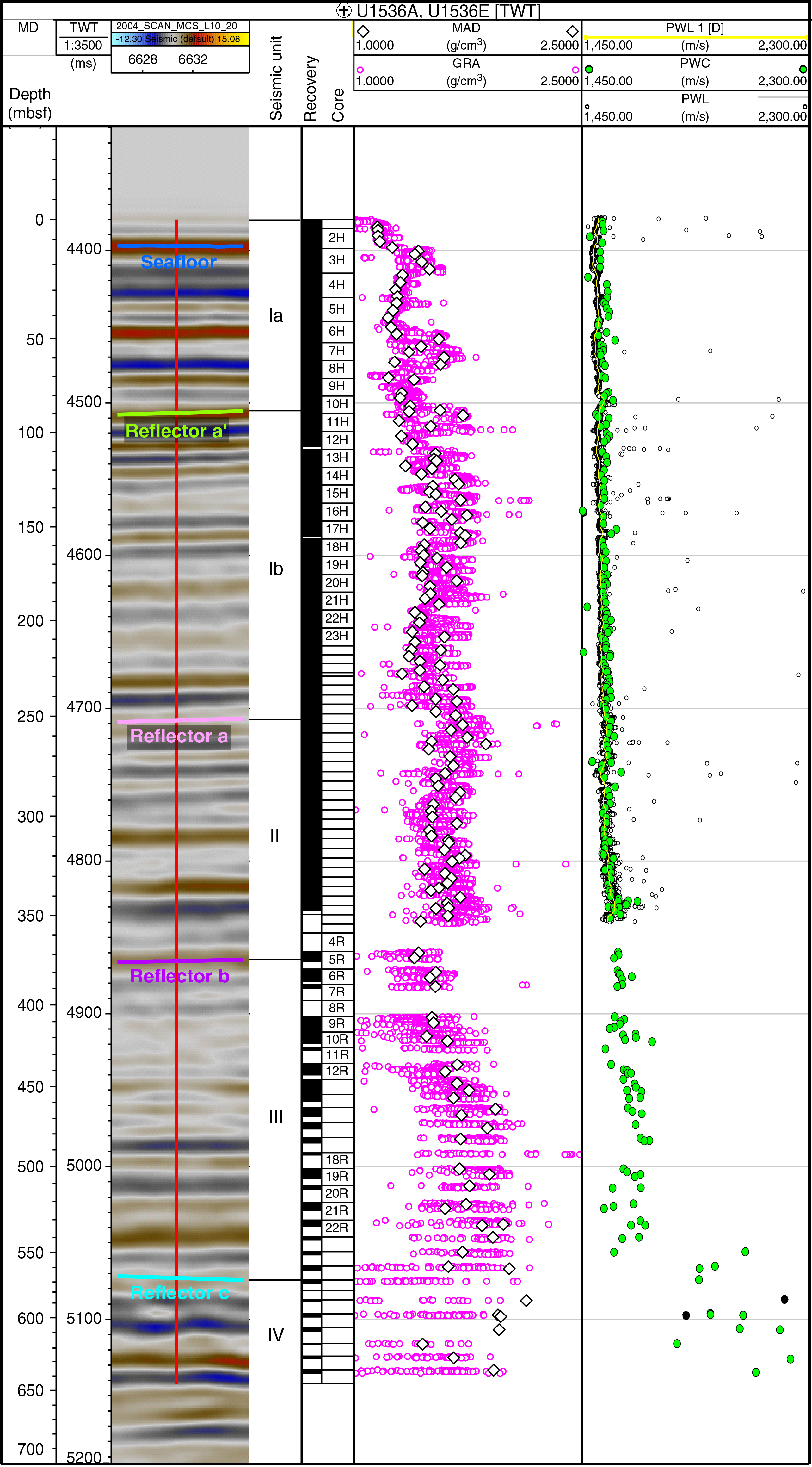
Figure F66. Physical properties with seismic reflections.
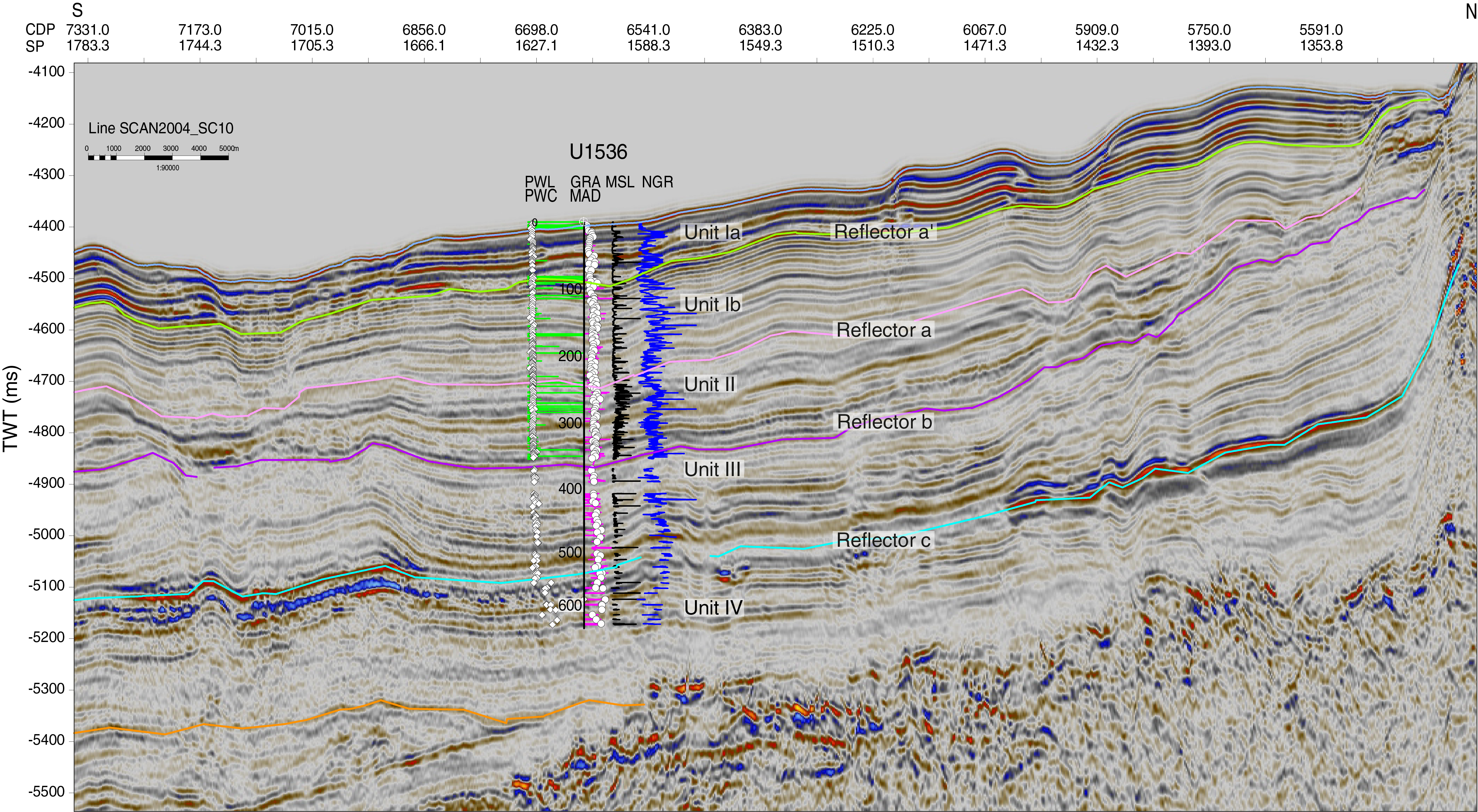
Figure F67. MCS Profile SCAN2004-L10 and physical properties.
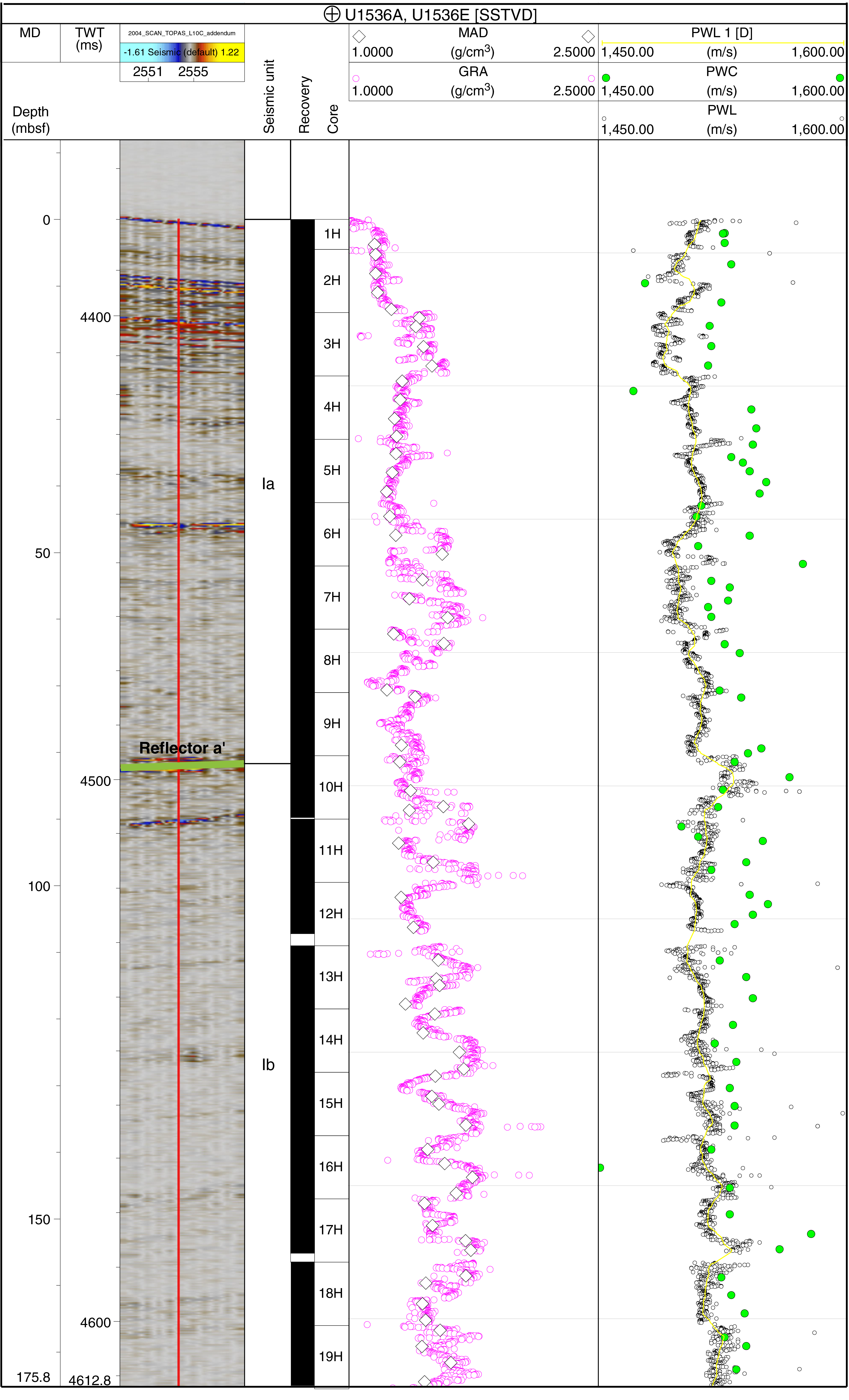
Figure F68. Physical properties with TOPAS Profile SCAN2014-L10.
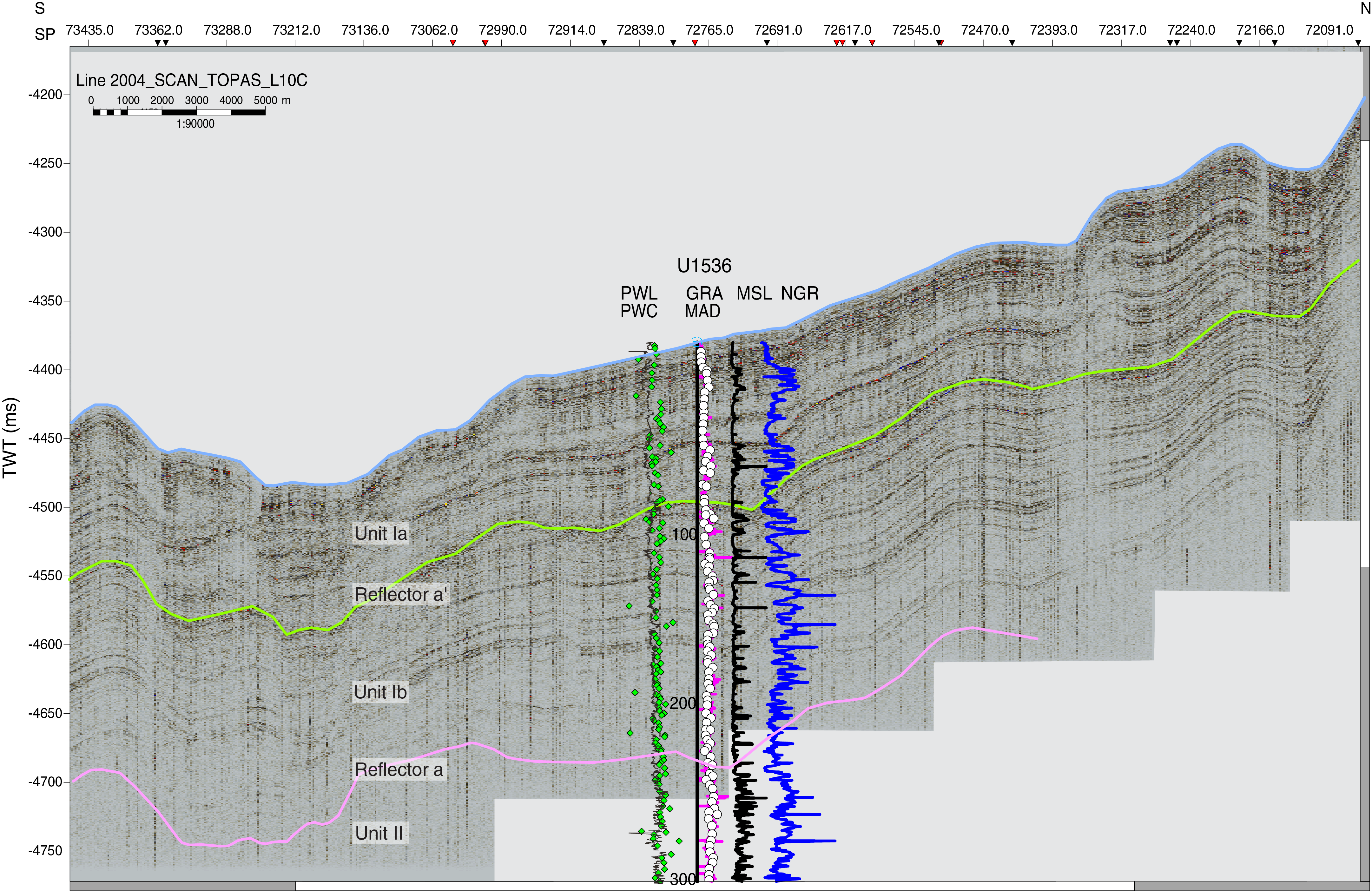
Figure F69. TOPAS Profile SCAN2004-L10 and physical properties.
The physical properties and chronostratigraphy obtained during Expedition 382 allow us to constrain the previously identified seismic units and develop an age model for the stratigraphic discontinuities (Table T25).
Physical properties and relationship with multichannel seismic interpretation
MCS Line SCAN2004-L10 allows the identification of Seismic Units IV–I at Site U1536. APC, HLAPC, and RCB coring at Site U1536 recovered the sedimentary record to 638.5 mbsf, reaching the upper part of regional Unit IV (e.g., Maldonado et al., 2006; Martos et al., 2013; Pérez et al., 2017). All five stratigraphic discontinuities represent marked changes in the reflectivity of the seismic record and anomalies or stepwise shifts in the shipboard physical property measurements (Figures F66, F67).
In the drilled part of Unit IV, GRA density is variable and has no discernible upward trend. NGR shows a slight increase upward, and loop magnetic susceptibility (MSL) varies in amplitude and has no clear upward trend. The highest PWC values at Site U1536 are recorded in Unit IV and the lowermost parts of Unit III. PWC values decrease sharply in Core 382-U1536E-24R (the lowermost part of Unit III), corresponding to high-amplitude reflections with low lateral continuity along the MCS profile. This sharp change in PWC values characterizes the top of Unit IV (Reflector c). Reflector c is located at 566 mbsf, or 5072 ms TWT, in Core 22R (or deeper).
Above Reflector c, Unit III displays highly variable MSL values with no upward trend. NGR values are similar to those in Unit IV in the lower parts of Unit III and decrease upward with a notable peak around 420 mbsf. NGR increases in the uppermost meters of Unit III. Wet bulk density (MAD) and GRA decrease upward through Unit III. Seismic profiles show very high amplitude reflections from the base of Unit III to ~460 mbsf. Above 460 mbsf, MSL, NGR, MAD, GRA, and PWL decrease as the seismic facies becomes more transparent. The top of Unit III (Reflector b) is located at 375 mbsf, or 4866 ms TWT, corresponding to Core 382-U1536E-5R, which has poor recovery. It constitutes a relative low in MSL, NGR, MAD, PWC, and GRA density values.
In Unit II, MSL values increase upward. The MSL values at the top of Unit II are comparable in value to the highest values seen in Units IV and III. MSL signal correlates to low-amplitude and low lateral continuity reflections in the seismic record.
In Unit II, NGR, MAD, and GRA density have no trend with regard to depth, and the seismic record shows high-amplitude and laterally continuous reflections. The variability in the values of these physical properties is slightly lower in the upper part of the unit, where the reflections show low amplitude. PWC and PWL decrease slightly from the base to the top of Unit II, although PWL values are highly variable from 310 to 270 mbsf. At the top of Unit II, Reflector a is located at 254 mbsf, or 4711 ms TWT, in Core 382-U1536A-32F and represents a sharp contact between higher MSL and NGR values below the reflector and lower values above it. MAD and GRA values also show a decrease above Reflector a, although the amplitude of the change is less than that observed in MSL and NGR.
Above Reflector a, Seismic Unit I presents relatively low MSL, GRA density, and MAD values compared to Unit II. However, MSL values are variable, as seen in Units IV and III, and individual peaks reach values greater than those of Unit II. NGR increases from the base of Subunit Ib to ~140 mbsf, with two distinct peaks visible at 187 and 128 mbsf. Above 140 mbsf, NGR decreases to Reflector a′, the base of Subunit Ia. In Subunit Ia, NGR data displays two broad positive excursions from a low baseline value. GRA density and MAD values decrease slightly upward in Unit I. Both of these measurements are less variable in Subunit Ia than in Subunit Ib. PWC values are relatively constant in Unit I. PWL values show numerous excursions from a baseline value of 1450 m/s. The reflections in Unit I are high amplitude and laterally continuous. Two distinct reflector patterns can be identified in Subunit Ib. From Reflector a to 165 mbsf, medium-amplitude reflections were observed in the seismic profile. From 165 mbsf to Reflector a′, medium- to high-amplitude reflections with high lateral continuity were observed. In Unit I, Reflector a′ is located at 90 mbsf, or 4508 ms TWT, between Cores 382-U1536A-10H and 11H and marks an overall decrease in the values and variability of all physical properties in Subunit Ia relative to Subunit Ib. Changes in physical properties in Subunit Ia correspond to highly variable seismic facies in the seismic profile.
Physical properties and relationship with parametric echo sounder interpretation
TOPAS Profile SCAN2004-L10 at Site U1536 allows the identification of reflections to about 4625 ms TWT, including the entirety of Unit I and the top of Unit II (Figures F68, F69). A rather transparent seismic package in the TOPAS profile is seen in the uppermost parts of Unit II and the lower parts of Subunit Ib near the limit of acoustic penetration. In the upper part of Subunit Ib, only a few medium-amplitude reflections can be identified in the TOPAS record. The most remarkable one is at 4562 ms TWT and corresponds to an increase in PWL values and high GRA density, MSL, and NGR values. At the top of Subunit Ib, all values show an increase in variability between 4520 and 4510 ms TWT that matches a lens-shaped body of transparent acoustic character in the TOPAS profile. Above Reflector a′, intervals of relatively constant PWL values and low density, MSL, and NGR values generally correlate with packages of transparent to chaotic facies in the TOPAS record. Low PWL values and high GRA density, MSL, and NGR values between 4435 and 4405 ms TWT correspond to high-frequency reflections of medium–high amplitude.
Downhole logging and relationship with seismic interpretation
Depths described in this section refer to those computed with the synthetic seismogram (see Synthetic seismogram generation).
The upper part of Unit IV is divided into two areas where the main changes on the physical properties measured during downhole logging match with a prominent change in the amplitude of the seismic reflections. At the bottom of the hole, an area of fluctuating gamma ray (total spectral gamma ray [HSGR]) and constant density (RHOM), velocity (SVEL), and shear velocity (SSVE) matches an increasing trend upward in resistivity and MS (MSSLSUS) to about 605 mbsf (Figures F70, F71, F72). Note that SSVE values alternate between likely valid values and offset artifact values caused by the automated velocity picking algorithm and the difficulties in picking shear wave arrivals in the slow formations logged here (see Downhole measurements).
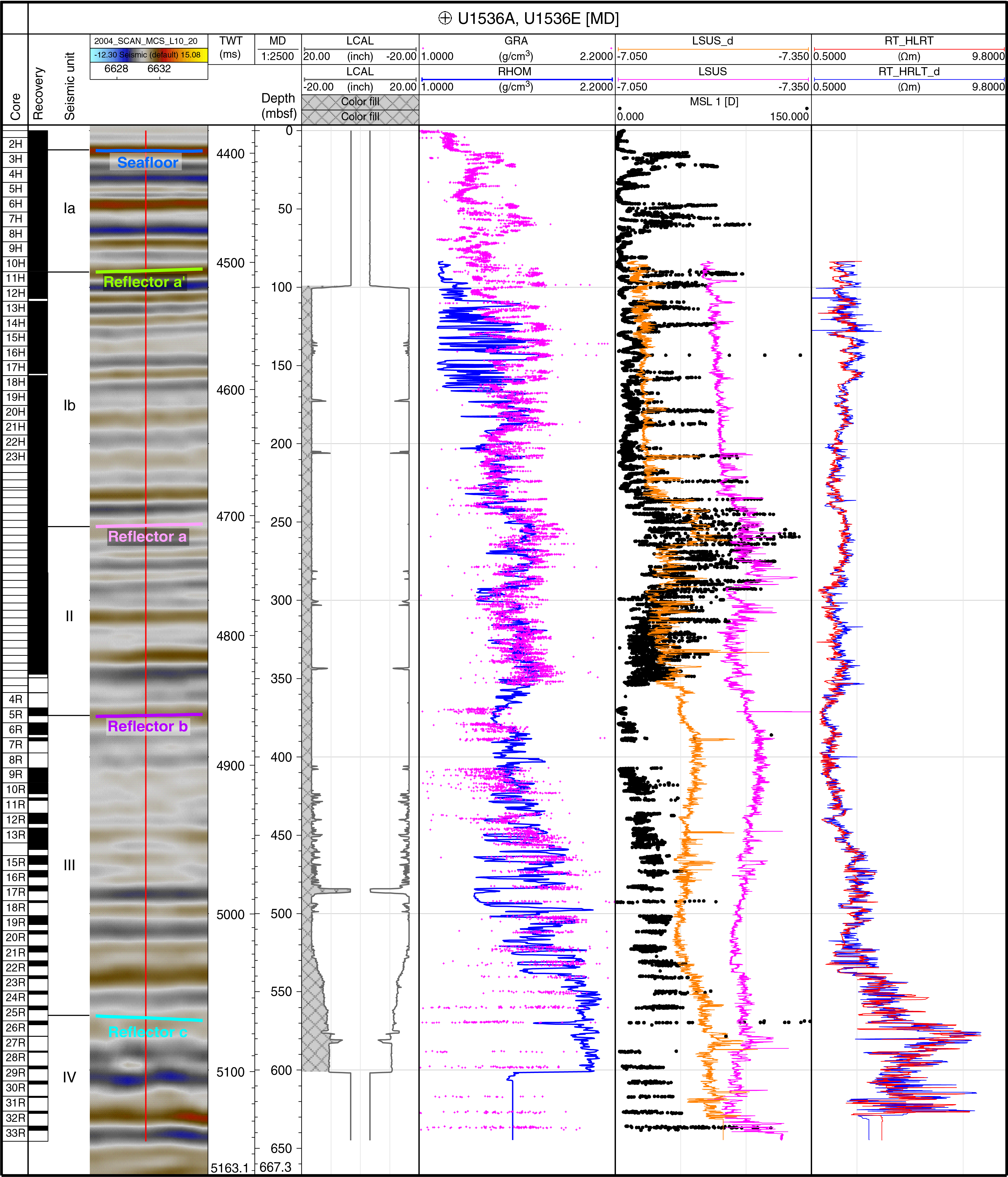
Figure F70. Seismic column with logging and laboratory density, MS, and resistivity.
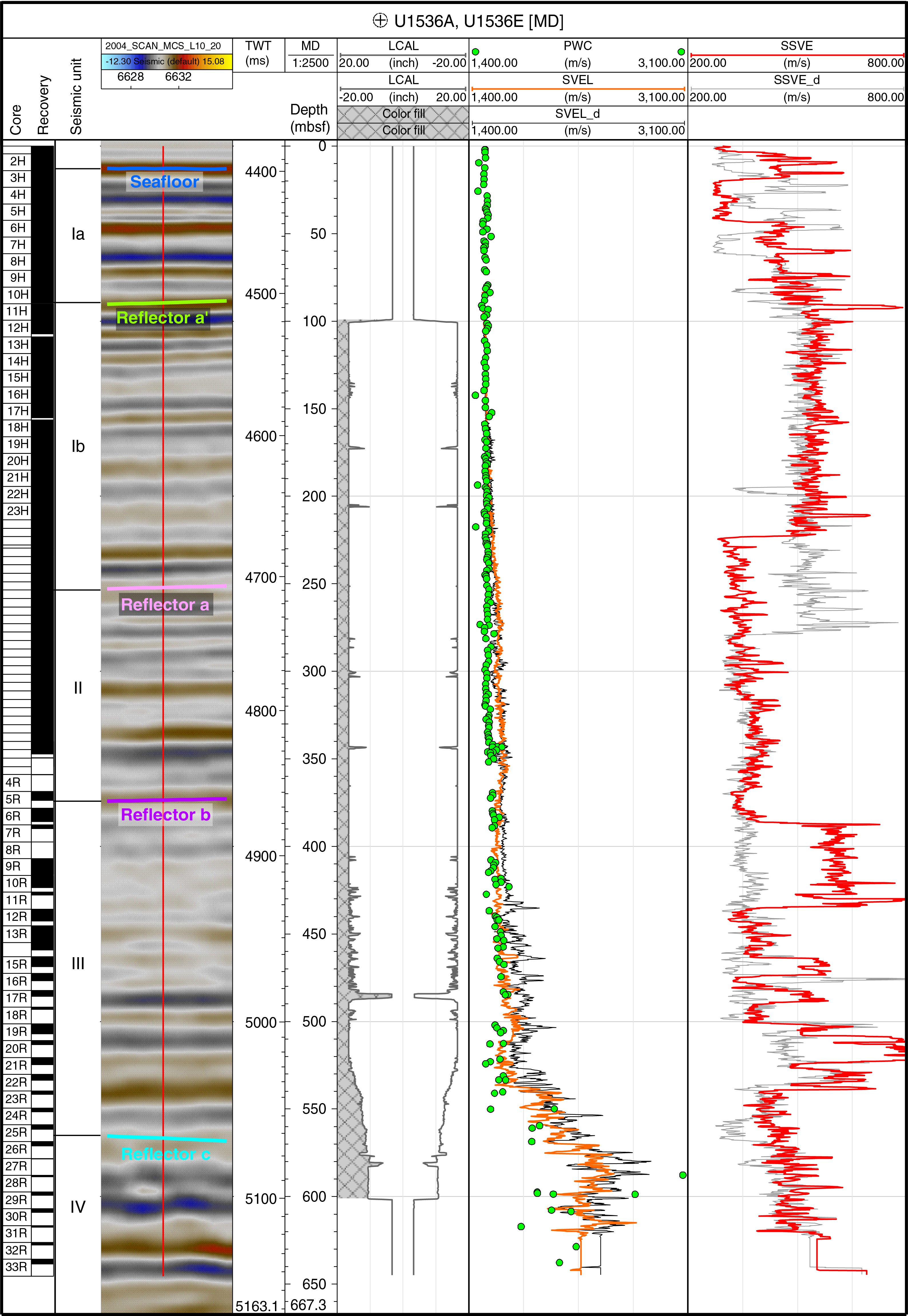
Figure F71. Seismic column with logging and laboratory velocities.
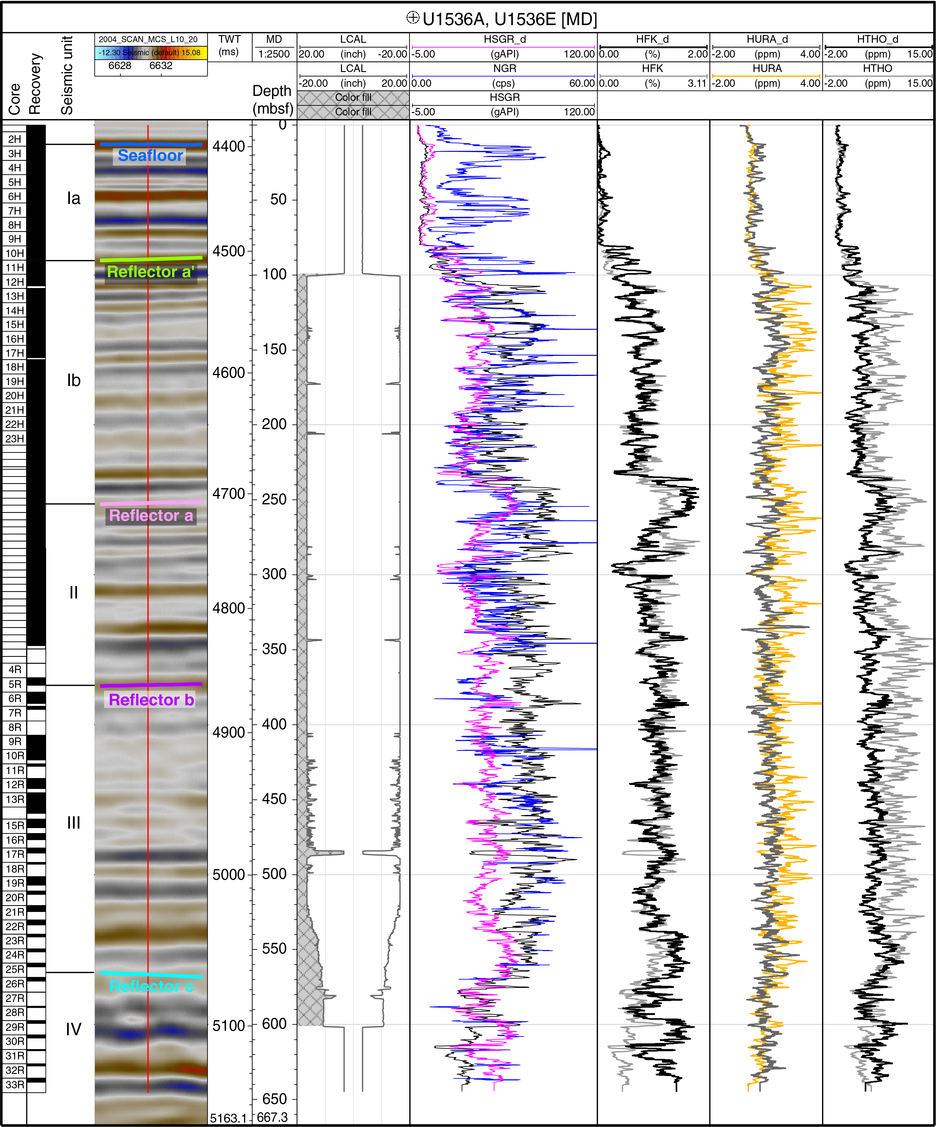
Figure F72. Seismic column with logging and laboratory NGR, K, U, and Th.
The 605 mbsf level correlates with layered reflections of high acoustic amplitude and low lateral continuity. From 605 mbsf to Reflector c, higher gamma ray and density values with low-amplitude variability occur, whereas velocity, resistivity, and MS show upward increasing values. This section corresponds to low, laterally continuous reflections in the seismic profile. At the top of Unit IV, Reflector c matches with a maximum and sharp increase in gamma ray values and a sharp decrease in velocity, resistivity, and MS.
The lower part of Unit III shows an upward increasing trend in gamma ray to 530 mbsf followed by a decrease to 490 mbsf. Velocity, resistivity, and MS decrease to 490 mbsf, corresponding to high-amplitude and lateral continuity reflections in the seismic profile. Density is highly variable but overall shows a slight decrease upward from the base of Unit III (Reflector c) to 490 mbsf. In the upper part of Unit III (from 490 mbsf to Reflector b), gamma ray and velocity values are relatively constant, whereas density and resistivity slightly decrease upward. MS increases in the uplog and downlog profiles but decreases in the MSL 1 data. The seismic reflections in Unit III show lower amplitude and lateral continuity. The top of Unit III (Reflector b) is characterized by a relative minimum in the values of all the downhole physical properties.
All logged properties maintain relatively constant values in Unit II, although gamma ray increases in the uppermost 50 m. Minimum values in Unit II are observed in gamma ray, density, resistivity, and MS at 295 mbsf and are matched by a very high amplitude reflection that is laterally continuous. Reflector a, which marks the upper boundary of Unit II, is situated at the peak of a local high in gamma ray, density, resistivity, and MS values. The observed highs in resistivity and MS are of smaller magnitude than those seen in gamma and density.
Subunit Ib displays lower gamma ray and density values than the units below it. Furthermore, density is more variable in Subunit Ib than the rest of the hole. Gamma ray, density, resistivity, and MS appear to fluctuate cyclically. An abrupt increase in variability above 165 mbsf to the top of the unit reflects higher amplitude and lateral continuity of the seismic reflections. Subunit Ia is masked by the drilling pipes.
Synthetic seismogram generation
A synthetic seismogram was produced at this site to assign specific depths to the logging data (see Downhole logging and relationship with seismic interpretation) and to correlate with the TWT seismic profile. Three synthetic seismograms were generated by considering discrete PWC and sonic velocity measurements taken uphole and downhole during downhole logging together with bulk density measured in the laboratory and with the active source during downhole logging. We selected the synthetic seismogram derived using PWC measured in the laboratory together with bulk density estimates from MAD samples (Figure F73). The selection was based on the final fits between the synthetic signal and the MCS at the site. The highest disagreement among the three synthetic signals was observed below 500 mbsf.
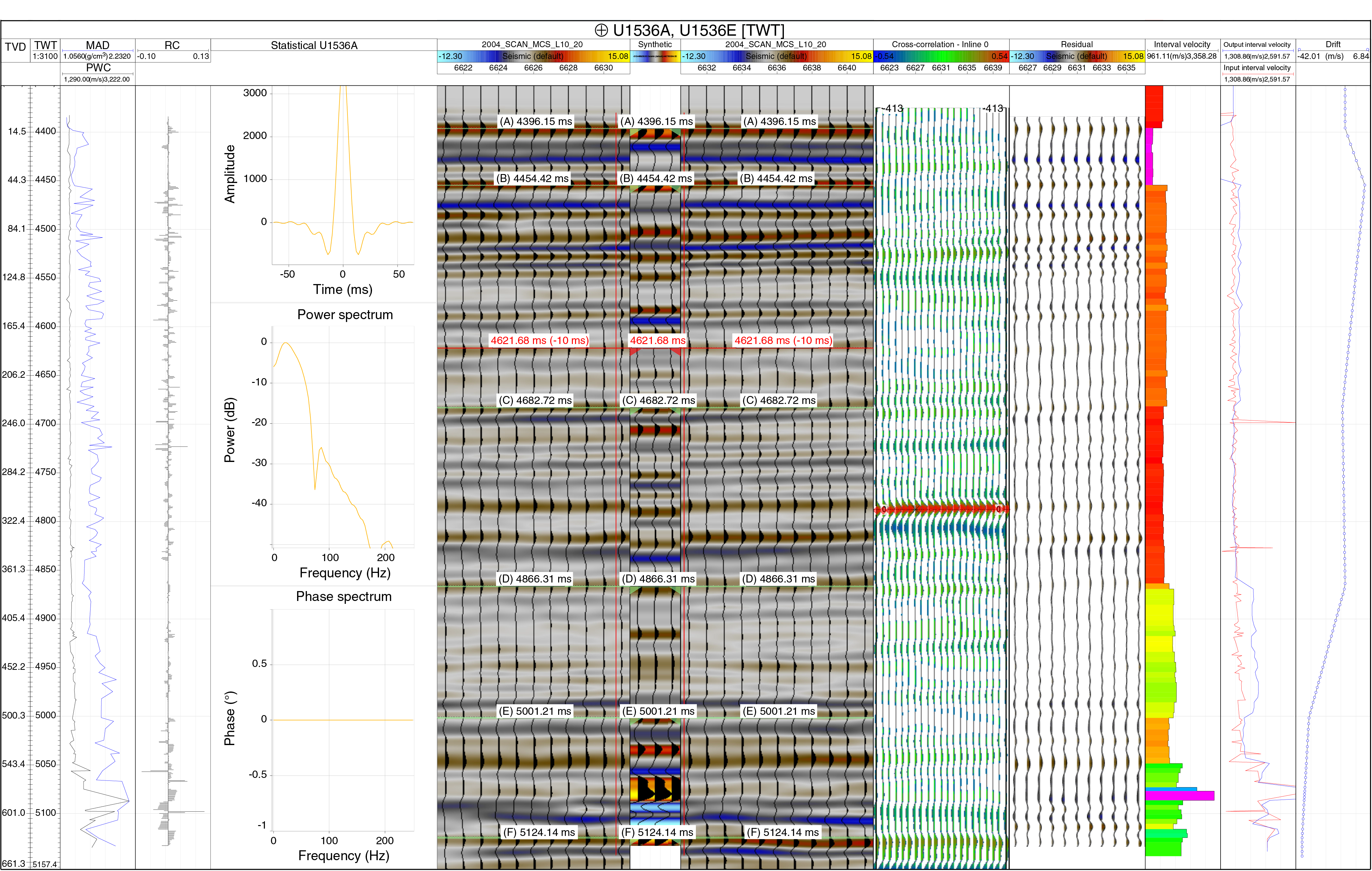
Figure F73. Generation of synthetic seismogram.
To construct the synthetic seismogram, PWC and bulk density from the cores were used to compute impedance downhole. Reflection coefficients were calculated from the impedance profile and then convolved with the estimated statistical wavelet to create the synthetic seismogram. Six ties were needed to obtain the best fit to the data. The synthetic seismogram and seismic data match, and higher discrepancies toward the bottom of the hole from around 500 mbsf downward are possibly related to larger changes in the velocity profile. The determined time-depth relationship was then applied to the downhole measurements (see Downhole measurements). We note that this synthetic seismogram and TWT-depth model is one of many possible solutions, and the results presented here will be refined in postcruise research.
References
Baldermann, A., Dietzel, M., Mavromatis, V., Mittermayr, F., Warr, L.N., and Wemmer, K., 2017. The role of Fe on the formation and diagenesis of interstratified glauconite-smectite and illite-smectite: a case study of Upper Cretaceous shallow-water carbonates. Chemical Geology, 453:21–34. https://doi.org/10.1016/j.chemgeo.2017.02.008
Baker, P.A., 1986. Pore-water chemistry of carbonate-rich sediments, Lord Howe Rise, Southwest Pacific Ocean. In Kennett, J.P., von der Borch, C.C., et al., Initial Reports of the Deep Sea Drilling Project, 90: Washington, DC (U.S. Government Printing Office), 1249–1256. https://doi.org/10.2973/dsdp.proc.90.132.1986
Blum, P., 1997. Technical Note 26: Physical Properties Handbook—A Guide to the Shipboard Measurement of Physical Properties of Deep-Sea Cores. Ocean Drilling Program. https://doi.org/10.2973/odp.tn.26.1997
Bolze, C.E., Malone, P.G., and Smith, M.J., 1974. Microbial mobilization of barite. Chemical Geology, 13(2):141–143. https://doi.org/10.1016/0009-2541(74)90006-0
Briskin, M., and Schreiber, B.C., 1978. Authigenic gypsum in marine sediments. Marine Geology, 28(1–2):37–49. https://doi.org/10.1016/0025-3227(78)90095-6
Burns, D.A., 1975. Distribution, abundance, and preservation of nannofossils in Eocene to recent Antarctic sediments. New Zealand Journal of Geology and Geophysics, 18(4):583–596. https://doi.org/10.1080/00288306.1975.10421558
Cody, R.D., Levy, R.H., Harwood, D.M., and Sadler, P.M., 2008. Thinking outside the zone: high-resolution quantitative diatom biochronology for the Antarctic Neogene. Palaeogeography, Palaeoclimatology, Palaeoecology, 260(1–2):92–121. https://doi.org/10.1016/j.palaeo.2007.08.020
De Vleeschouwer, D., Dunlea, A.G., Auer, G., Anderson, C.H., Brumsack, H., de Loach, A., Gurnis, M., et al., 2017. Quantifying K, U, and Th contents of marine sediments using shipboard natural gamma radiation spectra measured on DV JOIDES Resolution. Geochemistry, Geophysics, Geosystems, 18(3):1053–1064. https://doi.org/10.1002/2016GC006715
Dixit, S., Van Cappellen, P., and van Bennekom, A.J., 2001. Processes controlling solubility of biogenic silica and pore water build-up of silicic acid in marine sediments. Marine Chemistry, 73(3–4):333–352. https://doi.org/10.1016/S0304-4203(00)00118-3
Dunlea, A.G., Murray, R.W., Harris, R.N., Vasiliev, M.A., Evans, H., Spivack, A.J., and D'Hondt, S., 2013. Assessment and use of NGR instrumentation on the JOIDES Resolution to quantify U, Th, and K concentrations in marine sediment. Scientific Drilling, 15:57–63. https://doi.org/10.2204/iodp.sd.15.05.2013
Esper, O., and Zonneveld, K.A.F., 2007. The potential of organic-walled dinoflagellate cysts for the reconstruction of past sea-surface conditions in the Southern Ocean. Marine Micropaleontology, 65(3–4):185–212. https://doi.org/10.1016/j.marmicro.2007.07.002
Froelich, P.N., Klinkhammer, G.P., Bender, M.L., Luedtke, N.A., Heath, G.R., Cullen, D., Dauphin, P., Hammond, D., Hartman, B., and Maynard, V., 1979. Early oxidation of organic matter in pelagic sediments of the eastern equatorial Atlantic: suboxic diagenesis. Geochimica et Cosmochimica Acta, 43(7):1075–1090. https://doi.org/10.1016/0016-7037(79)90095-4
Gersonde, R., and Bárcena, M.A., 1998. Revision of the upper Pliocene: Pleistocene diatom biostratigraphy for the northern belt of the Southern Ocean. Micropaleontology, 44(1):84–98. https://doi.org/10.2307/1486086
Harwood, D.M., and Maruyama, T., 1992. Middle Eocene to Pleistocene diatom biostratigraphy of Southern Ocean sediments from the Kerguelen Plateau, Leg 120. In Wise, S.W., Jr., Schlich, R., et al., Proceedings of the Ocean Drilling Program, Scientific Results, 120: College Station, TX (Ocean Drilling Program), 683–733. https://doi.org/10.2973/odp.proc.sr.120.160.1992
Hein, J.R., O'Neil, J.R., and Jones, M.G., 1979. Origin of authigenic carbonates in sediment from the deep Bering Sea. Sedimentology, 26(5):681–705. https://doi.org/10.1111/j.1365-3091.1979.tb00937.x
Hyndman, R.D., Erickson, A.J., and Von Herzen, R.P., 1974. Geothermal measurements on DSDP Leg 26. In Davies, T.A., Luyendyk, B.P., et al., Initial Reports of the Deep Sea Drilling Project, 26: Washington, DC (U.S. Govt. Printing Office), 451–463. https://doi.org/10.2973/dsdp.proc.26.113.1974
Maldonado, A., Barnolas, A., Bohoyoa, F., Galindo-Zaldívar, J., Hernández-Molina, J., Lobo, F., Rodríguez-Fernández, J., Somoza, L., and Vázquez, J.T., 2003. Contourite deposits in the central Scotia Sea: the importance of the Antarctic Circumpolar Current and the Weddell Gyre flows. Palaeogeography, Palaeoclimatology, Palaeoecology, 198(1–2):187–221. https://doi.org/10.1016/S0031-0182(03)00401-2
Maldonado, A., Bohoyo, F., Galindo-Zaldívar, J., Hernández-Molina, J., Jabaloy, A., Lobo, F.J., Rodríguez-Fernández, J., Suriñach, E., and Vázquez, J.T., 2006. Ocean basins near the Scotia–Antarctic plate boundary: influence of tectonics and paleoceanography on the Cenozoic deposits. Marine Geophysical Researches, 27(2):83–107. https://doi.org/10.1007/s11001-006-9003-4
Martos, Y.M., Maldonado, A., Lobo, F.J., Hernández-Molina, F.J., and Pérez, L.F., 2013. Tectonics and palaeoceanographic evolution recorded by contourite features in southern Drake Passage (Antarctica). Marine Geology, 343:76–91. https://doi.org/10.1016/j.margeo.2013.06.015
Meister, P., McKenzie, J.A., Vasconcelos, C., Bernasconi, S., Frank, M., Gutjahr, M., and Schrag, D.P., 2007. Dolomite formation in the dynamic deep biosphere: results from the Peru Margin. Sedimentology, 54(5):1007–1032. https://doi.org/10.1111/j.1365-3091.2007.00870.x
Meunier, A., and El Albani, A., 2007. The glauconite-Fe-illite-Fe-smectite problem: a critical review. Terra Nova, 19(2):95–104. https://doi.org/10.1111/j.1365-3121.2006.00719.x
Nöthen, K., and Kasten, S., 2011. Reconstructing changes in seep activity by means of pore water and solid phase Sr/Ca and Mg/Ca ratios in pockmark sediments of the Northern Congo Fan. Marine Geology, 287(1–4):1–13. https://doi.org/10.1016/j.margeo.2011.06.008
Peck, V.L., Weber, M.E., Raymo, M.E., Williams, T., Armbrecht, L.H., Bailey, I., Brachfeld, S.A., Cardillo, F.G., Du, Z., Fauth, G., García, M., Glüder, A., Guitard, M.E., Gutjahr, M., Hemming, S.R., Hernández-Almeida, I., Hoem, F.S., Hwang, J.-H., Iizuka, M., Kato, Y., Kenlee, B., Martos, Y.M., O'Connell, S., Pérez, L.F., Reilly, B.T., Ronge, T.A., Seki, O., Tauxe, L., Tripathi, S., Warnock, J.P., and Zheng, X., 2021. Site U1534. In Weber, M.E., Raymo, M.E., Peck, V.L., Williams, T., and the Expedition 382 Scientists, Iceberg Alley and Subantarctic Ice and Ocean Dynamics. Proceedings of the International Ocean Discovery Program, 382: College Station, TX (International Ocean Discovery Program). https://doi.org/10.14379/iodp.proc.382.103.2021
Pérez, L.F., Maldonado, A., Hernández-Molina, F.J., Lodolo, E., Bohoyo, F., and Galindo-Zaldívar, J., 2017. Tectonic and oceanographic control of sedimentary patterns in a small oceanic basin: Dove Basin (Scotia Sea, Antarctica). Basin Research, 29(S1):255–276. https://doi.org/10.1111/bre.12148
Pribnow, D., Kinoshita, M., and Stein, C., 2000. Thermal Data Collection and Heat Flow Recalculations for Ocean Drilling Program Legs 101–180: Hanover, Germany (Institute for Joint Geoscientific Research, Institut für Geowissenschaftliche Gemeinschaftsaufgaben [GGA]). http://www-odp.tamu.edu/publications/heatflow/ODPReprt.pdf
Riedinger, N., Kasten, S., Gröger, J., Franke, C., and Pfeifer, K., 2006. Active and buried authigenic barite fronts in sediments from the Eastern Cape Basin. Earth and Planetary Science Letters, 241(3–4):876–887. https://doi.org/10.1016/j.epsl.2005.10.032
Ruttenberg, K.C., and Berner, R.A., 1993. Authigenic apatite formation and burial in sediments from non-upwelling, continental-margin environments. Geochimica et Cosmochimica Acta, 57(5):991–1007. https://doi.org/10.1016/0016-7037(93)90035-U
Scholz, F., Hensen, C., Noffke, A., Rohde, A., Liebetrau, V., and Wallmann, K., 2011. Early diagenesis of redox-sensitive trace metals in the Peru upwelling area – response to ENSO-related oxygen fluctuations in the water column. Geochimica et Cosmochimica Acta, 75(22):7257–7276. https://doi.org/10.1016/j.gca.2011.08.007
Shipboard Scientific Party, 1988. Site 679. In Suess, E., von Huene, R., et al., Proceedings of the Ocean Drilling Program, Initial Reports, 112: College Station, TX (Ocean Drilling Program), 159–248. https://doi.org/10.2973/odp.proc.ir.112.110.1988
Sprenk, D., Weber, M.E., Kuhn, G., Rosén, P., Frank, M., Molina-Kescher, M., Liebetrau, V., and Röhling, H.-G., 2013. Southern Ocean bioproductivity during the last glacial cycle—new decadal-scale insight from the Scotia Sea. Geological Society Special Publication, 381(1):245–261. https://doi.org/10.1144/SP381.17
Tauxe, L., 2010. Essentials of Paleomagnetism. With contributions by R.F. Butler, R. Van der Voo, and S.K. Banerjee: Berkeley, California (University of California Press).
Thouveny, N., Moreno, E., Delanghe, D., Candon, L., Lancelot, Y., and Shackleton, N.J., 2000. Rock magnetic detection of distal ice-rafted debris: clue for the identification of Heinrich layers on the Portuguese margin. Earth and Planetary Science Letters, 180(1–2):61–75. https://doi.org/10.1016/S0012-821X(00)00155-2
Torres, M.E., Brumsack, H.-J., Bohrmann, G., and Emeis, K.C., 1996. Barite fronts in continental margin sediments: a new look at barium remobilization in the zone of sulfate reduction and formation of heavy barites in diagenetic fronts. Chemical Geology, 127(1–3):125–139. https://doi.org/10.1016/0009-2541(95)00090-9
van Heck, S. (Ed.), 1981. Bibliography and taxa of calcareous nannoplankton. International Nannoplankton Association Newsletter, 3(1):4–41. http://ina.tmsoc.org/JNR/NINA/INANewsl3(1).pdf
Weber, M.E., 1998. Estimation of biogenic carbonate and opal by continuous non-destructive measurements in deep-sea sediments: application to the eastern equatorial Pacific. Deep-Sea Research, Part I: Oceanographic Research Papers, 45(11):1955–1975. https://doi.org/10.1016/S0967-0637(98)00028-4
Weber, M.E., Kuhn, G., Sprenk, D., Rolf, C., Ohlwein, C., and Ricken, W., 2012. Dust transport from Patagonia to Antarctica–a new stratigraphic approach from the Scotia Sea and its implications for the last glacial cycle. Quaternary Science Reviews, 36:177–188. https://doi.org/10.1016/j.quascirev.2012.01.016
Weber, M.E., Niessen, F., Kuhn, G., and Wiedicke, M., 1997. Calibration and application of marine sedimentary physical properties using a multi-sensor core logger. Marine Geology, 136(3–4):151–172. https://doi.org/10.1016/S0025-3227(96)00071-0
Weber, M.E., Raymo, M.E., Peck, V.L., Williams, T., Armbrecht, L.H., Bailey, I., Brachfeld, S.A., Cardillo, F.G., Du, Z., Fauth, G., García, M., Glüder, A., Guitard, M.E., Gutjahr, M., Hemming, S.R., Hernández-Almeida, I., Hoem, F.S., Hwang, J.-H., Iizuka, M., Kato, Y., Kenlee, B., Martos, Y.M., O'Connell, S., Pérez, L.F., Reilly, B.T., Ronge, T.A., Seki, O., Tauxe, L., Tripathi, S., Warnock, J.P., and Zheng, X., 2021a. Expedition 382 methods. In Weber, M.E., Raymo, M.E., Peck, V.L., Williams, T., and the Expedition 382 Scientists, Iceberg Alley and Subantarctic Ice and Ocean Dynamics. Proceedings of the International Ocean Discovery Program, 382: College Station, TX (International Ocean Discovery Program). https://doi.org/10.14379/iodp.proc.382.102.2021
Weber, M.E., Raymo, M.E., Peck, V.L., Williams, T., and the Expedition 382 Scientists, 2021b. Supplementary material, https://doi.org/10.14379/iodp.proc.382supp.2021. Supplement to Weber, M.E., Raymo, M.E., Peck, V.L., Williams, T., and the Expedition 382 Scientists, Iceberg Alley and Subantarctic Ice and Ocean Dynamics. Proceedings of the International Ocean Discovery Program, 382: College Station, TX (International Ocean Discovery Program). https://doi.org/10.14379/iodp.proc.382.2021
Winter, D., Sjunneskog, C., Scherer, R., Maffioli, P., and Harwood, D., 2012. Pliocene–Pleistocene diatom biostratigraphy of nearshore Antarctica from the AND-1B drillcore, McMurdo Sound. Global and Planetary Change, 96–97:59–74. https://doi.org/10.1016/j.gloplacha.2010.04.004
Wise, S.W., 1983. Mesozoic and Cenozoic calcareous nannofossils recovered by Deep Sea Drilling Project Leg 71 in the Falkland Plateau region, Southwest Atlantic Ocean. In Ludwig W.J., Krasheninnikov, V.A. et al., Initial Reports of the Deep Sea Drilling Project, 71: Washington (U.S. Government Printing Office), 481–550. https://doi.org/10.2973/dsdp.proc.71.121.1983
1 Weber, M.E., Raymo, M.E., Peck, V.L., Williams, T., Armbrecht, L.H., Bailey, I., Brachfeld, S.A., Cardillo, F.G., Du, Z., Fauth, G., García, M., Glüder, A., Guitard, M.E., Gutjahr, M., Hemming, S.R., Hernández-Almeida, I., Hoem, F.S., Hwang, J.-H., Iizuka, M., Kato, Y., Kenlee, B., Martos, Y.M., O'Connell, S., Pérez, L.F., Reilly, B.T., Ronge, T.A., Seki, O., Tauxe, L., Tripathi, S., Warnock, J.P., and Zheng, X., 2021. Site U1536. In Weber, M.E., Raymo, M.E., Peck, V.L., Williams, T., and the Expedition 382 Scientists, Iceberg Alley and Subantarctic Ice and Ocean Dynamics. Proceedings of the International Ocean Discovery Program, 382: College Station, TX (International Ocean Discovery Program). https://doi.org/10.14379/iodp.proc.382.105.2021
2 Expedition 382 Scientists' affiliations.
This work is distributed under the Creative Commons Attribution 4.0 International (CC BY 4.0) license. 