Webster, J.M., Ravelo, A.C., Grant, H.L.J., and the Expedition 389 Scientists
Proceedings of the International Ocean Discovery Program Volume 389
publications.iodp.org
https://doi.org/10.14379/iodp.proc.389.102.2025
Expedition 389 methods1
![]() J.M. Webster,
J.M. Webster,
![]() A.C. Ravelo,
A.C. Ravelo,
![]() H.L.J. Grant,
H.L.J. Grant,
![]() M. Rydzy,
M. Rydzy,
![]() M. Stewart,
M. Stewart,
![]() N. Allison,
N. Allison,
![]() R. Asami,
R. Asami,
![]() B. Boston,
B. Boston,
![]() J.C. Braga,
J.C. Braga,
![]() L. Brenner,
L. Brenner,
![]() X. Chen,
X. Chen,
![]() P. Chutcharavan,
P. Chutcharavan,
![]() A. Dutton,
A. Dutton,
![]() T. Felis,
T. Felis,
![]() N. Fukuyo,
N. Fukuyo,
![]() E. Gischler,
E. Gischler,
![]() S. Greve,
S. Greve,
![]() A. Hagen,
A. Hagen,
![]() Y. Hamon,
Y. Hamon,
![]() E. Hathorne,
E. Hathorne,
![]() M. Humblet,
M. Humblet,
![]() S. Jorry,
S. Jorry,
![]() P. Khanna,
P. Khanna,
![]() E. Le Ber,
E. Le Ber,
![]() H. McGregor,
H. McGregor,
![]() R. Mortlock,
R. Mortlock,
![]() T. Nohl,
T. Nohl,
![]() D. Potts,
D. Potts,
![]() A. Prohaska,
A. Prohaska,
![]() N. Prouty,
W. Renema,
N. Prouty,
W. Renema,
![]() K.H. Rubin,
K.H. Rubin,
![]() H. Westphal, and
H. Westphal, and
![]() Y. Yokoyama2
Y. Yokoyama2
1 Webster, J.M., Ravelo, A.C., Grant, H.L.J., Rydzy, M., Stewart, M., Allison, N., Asami, R., Boston, B., Braga, J.C., Brenner, L., Chen, X., Chutcharavan, P., Dutton, A., Felis, T., Fukuyo, N., Gischler, E., Greve, S., Hagen, A., Hamon, Y., Hathorne, E., Humblet, M., Jorry, S., Khanna, P., Le Ber, E., McGregor, H., Mortlock, R., Nohl, T., Potts, D., Prohaska, A., Prouty, N., Renema, W., Rubin, K.H., Westphal, H., and Yokoyama, Y., 2025. Expedition 389 methods. In Webster, J.M., Ravelo, A.C., Grant, H.L.J., and the Expedition 389 Scientists, Hawaiian Drowned Reefs. Proceedings of the International Ocean Discovery Program, 389: College Station, TX (International Ocean Discovery Program). https://doi.org/10.14379/iodp.proc.389.102.2025
2 Expedition 389 Scientists' affiliations.
1. Introduction
This chapter documents the primary shipboard procedures and methods employed by various operational and scientific groups during the offshore and onshore phases of International Ocean Discovery Program (IODP) Expedition 389. Methods for postexpedition research conducted on Expedition 389 samples and data will be described in individual scientific contributions to be published after the Onshore Science Party (OSP). Detailed drilling and engineering operations are described in Operations in each site chapter.
1.1. Operations equipment
1.1.1. Drilling platform
The drilling platform used for Expedition 389 was the dynamically positioned multipurpose vessel MMA Valour, operated by MMA Offshore. The MMA Valour is 84 m long with a gross tonnage of 4258 tons and an average economical speed of 10 kt. As with all European Consortium for Ocean Research Drilling (ECORD) mission-specific platform (MSP) expeditions, a suite of containerized laboratories and offices was installed on the MMA Valour aft deck area. The layout was designed to enable the most efficient core flow and core processing from core recovered through core curation, multisensor core logging, sampling and description, geochemical analyses, and refrigerated storage (Figure F1).
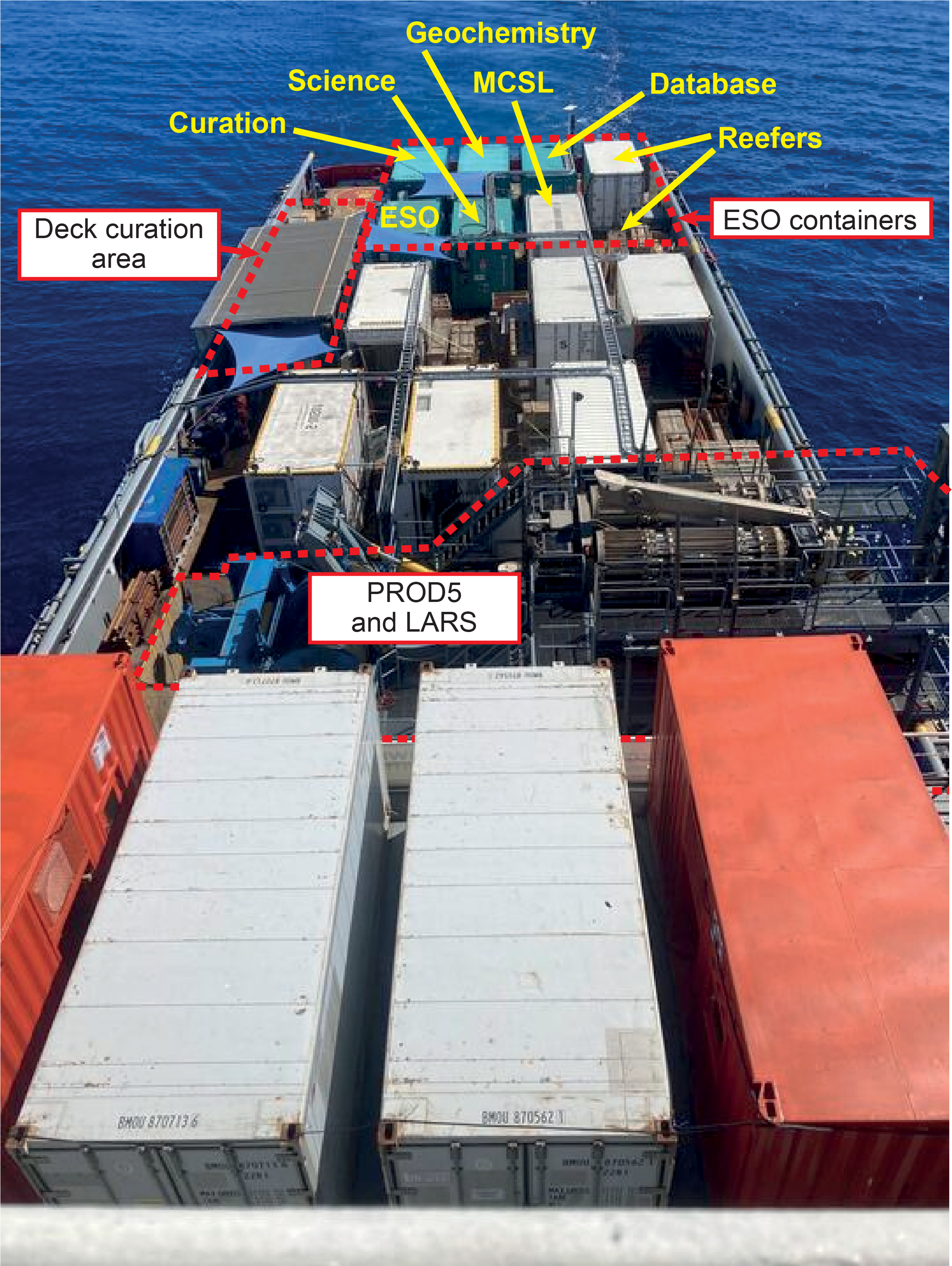
Figure F1. MMA Valour deck plan.
1.1.2. Coring operations
Coring operations were performed using Benthic’s fifth-generation Portable Remotely Operated Drill (PROD) (Figure F1). PROD5 is rated to a water depth of 4000 m, is unaffected by surface heave conditions, and consequently has good control on bit weight, increasing the likelihood of higher quality cores in shallow waters and challenging lithologies compared to ship-mounted systems that rely on heave compensation. Wave heights over approximately 3.5 m may be a limiting factor in operations. PROD5 is self-contained with its own launch and recovery system (LARS), occupying a basic deck footprint of 17.0 m × 8.0 m. The system additionally includes seven 20 ft containers for the drill control, mechanical and electrical workshops, and stores.
PROD5 is deployed using a power/hoist umbilical that also carries control communications and a video feed. The drill pipe, core barrels, and other tools are manipulated to and from a magazine using robotics while an onboard top drive provides the rotation for coring and an onboard mast feeds the drill pipe into the seafloor.
1.1.2.1. Coring methodology
PROD5 is a twin-magazine system, with one magazine for sampling tools and one for casing and rods. The 2.75 m sampling barrels have the same outside diameter, but the piston corers collect 75 mm diameter samples in soft sediment and the rotary corers collect 72 mm diameter samples in harder material. To give some flexibility during operations, two different rotary drill bits (diamond surface set and impregnated) were available for coring. Additionally, two core liner types were available: aluminum and polycarbonate. Finally, a small number of wash bores were usually loaded to allow for advancement without coring or to clean the borehole of material that may have fallen to the bottom during core runs or while setting casing. An onboard mud supply system on PROD5 can be switched on and off as required during the coring process.
A sample tool load is preselected before each deployment to take into consideration the expected formations. This load can be any mixture of sediment and rotary barrels, liner, and bit types. Each load is easily identifiable on the control screen for the operator to select. PROD5 is deployed from and recovered to the vessel using the LARS, which is controlled by a wireless belly box that allows the operator to be mobile during the different stages of launch and recovery.
The PROD5 computerized control system allows the corer to safely position on the seafloor by moving above the seafloor using its onboard thruster and subsea cameras to ensure there are no obstacles and/or significant macro benthos on the selected landing site. Each of its three legs can be independently adjusted to provide a level platform from which to deploy the core barrels.
During coring operations, the control system monitors a range of drilling parameters, including bit weight, rotation speed, and torque. Other important parameters are also displayed: penetration rate, water pressure, water flow rate, and hole depth. These and other feeds allow the operator to make precise and delicate adjustments while drilling to improve penetration, core recovery, and tool selection. All data are recorded in real-time and are available for download. During the offshore phase, these drilling parameters were compared directly to the recovered lithologies (i.e., lithologic type and level of disturbance) to optimize coring on subsequent deployments.
1.1.2.2. Site locations and water depth determination
At all Expedition 389 sites, GPS coordinates were used to position the MMA Valour on site (Figure F1). Once the vessel was positioned at a site, a dynamic positioning (DP) model was established. For each hole, a Sound Velocity Profiler (SVP) Valeport Midas SVX2, placed at the top of PROD5, was used to determine the water depth and to generate a sound velocity profile. During each PROD5 deployment to the seafloor, the probe collected depth from a pressure sensor, sound velocity, and temperature on the way down at a frequency of 1 Hz. After PROD5 landed, the water depth was given by the pressure sensor, to which was added its vertical distance from the baseplate of PROD5 and the distance between the baseplate and the seafloor, the latter changing for each landing due to the adjustment of the legs to the seafloor topography. The resulting depth was corrected to mean sea level to an accuracy of ±0.66 m and reported to the Lowest Astronomical Tide. The error takes into account pressure sensor accuracy, sensor offset measurement, and tide correction accuracy. Tide predictions used for the depth correction were from the two nearest tide stations.
After landing, the sound velocity profile was integrated to the ultra-short baseline method as part of the process to determine the latitude and longitude of the hole. A HiPAP 501 transducer was deployed 5 m below the hull of the ship to reduce noise pollution. The transducer communicated with two cNODE MiniS transponders located on the port and starboard sides at the top of PROD5. The two transponders were used to calculate the coordinates of the center of gravity of PROD5 (i.e., above the center of the hole). Using the ship’s coordinates as a reference, the hole coordinates were calculated by measuring (1) the time between a signal emitted from the transducer and pulses received back to the transponders and (2) the angle of the pulses emitted by the transponders. The ultra-short baseline method takes into account sound velocity error, offset measurement, and pitch and roll corrections (motion reference unit located next to the HiPAP 501). Hole coordinates are provided with an error of up to 1% of the water depth (Table T1).
1.2. Shipboard scientific procedures
1.2.1. Numbering and measurements of sites, holes, cores, and samples
Expedition numbers for IODP are sequential, starting with 301. Drilling sites are numbered consecutively, and for an ECORD Science Operator (ESO) operated platform, numbering starts with Site M0001. The “M” indicates the ESO-operated MSP. With the introduction of the new Mobile Drilling Information System (mDIS) database for Expedition 389, it was decided that site notation would no longer include additional zeros in the database system. For reporting and publishing results, the IODP standard naming convention including the leading zeros to fill the site number to four digits should be retained whenever a site is called out.
For Expedition 389, the first site was Site M0096, and multiple holes may be drilled at one site. The first hole drilled is assigned the site number with the character suffix “A,” the second hole takes the site number and the suffix “B,” and so forth. For operational and scientific reasons during the offshore phase of Expedition 389, new sites and revisions of original site locations were proposed and approved by the ECORD Facility Board and the IODP Environmental Protection and Safety Panel (EPSP). These sites and the original sites detailed in the Expedition 389 Scientific Prospectus (Webster et al., 2023) were represented as 150 m radius circles. All holes within that radius were given the corresponding site number and consecutive character suffixes in order of drill hole order, following the IODP naming convention (e.g., Holes M0096A and M0096B).
Meters below seafloor (mbsf) is the standard depth scale used during Expedition 389, conforming to drilling depth below seafloor (DSF) in the 2011 IODP Depth Scales Terminology guidelines (https://www.iodp.org/policies-and-guidelines/142-iodp-depth-scales-terminology-april-2011/file). Because the PROD5 corer is operating on the seafloor, there are no errors caused by length of pipe with a catenary in the water column, no stretching of drill pipe, and no errors induced by incorrect water depth measurements. The cored interval is calculated in meters below seafloor as measured by the PROD5 software, which measures the precise height of the elevator from the driller’s datum on the corer at millimeter accuracy. The distance between the driller’s datum and the seafloor is measured at the beginning of every borehole to the same accuracy, and the sum of these two measurements is the depth below seafloor. The mbsf depth of a sample is calculated by adding the depth of the sample below the section top and the lengths of all higher sections in the core to the core top datum measured with the drill rods.
Recovered core from 2.75 m core barrels is split into sections with a maximum length of 1.5 m and numbered sequentially from the top, starting at 1. By IODP convention, material recovered from the core catcher is treated as a separate section labeled “CC” and is placed below the last section recovered in the liner. When a recovered core is shorter than the cored interval, by convention it is assigned to the top of the cored interval (i.e., the mbsf depth at the top of the core barrel from which it was recovered) to achieve consistency in reporting depth in core. The core catcher is assigned to the top of the core barrel if no other material is recovered.
A coring gap typically occurs between cores, meaning some cored interval was lost during recovery or was never cut. Thus, a discrepancy can exist between the drilling meters below seafloor and the curatorial meters below seafloor. Conversely, a core can measure greater than the length cut if, for example, a rubble section occupies more space than a solid length of core or a solid section of core cut during the previous run is left behind or even dropped. Loose and disturbed sample material may be subsequently picked up or collected by the next core tube. These instances may mean the curatorial depth of the base of a core can be deeper than the top of the subsequent core.
Some intervals were drilled without coring, such as when washing down to a previously cored depth in an adjacent hole (Sites M0096, M0097, M0099, M0101, M0102, and M0108), or washing through intervals where hard to drill lithologies prevented effective progress (Sites M0096–M0098, M0101, and M0108) (Table T1).
Any sample removed from a core is designated by the distance measured in centimeters from the top of the section to the top and bottom of the sample removed. A full identification number for a sample consists of the following information: expedition, site, hole, core number, core type, section number, piece number (for hard rock), and interval in centimeters measured from the top of the section. For example, a sample identification of “389-M0097A-19R-2, 35–40 cm,” represents a sample removed from the interval 35–40 cm below the top of Section 2 of Core 19R (“R” designates that this core was taken using a rotary core barrel) from Hole M0097A during Expedition 389 (Figure F2).
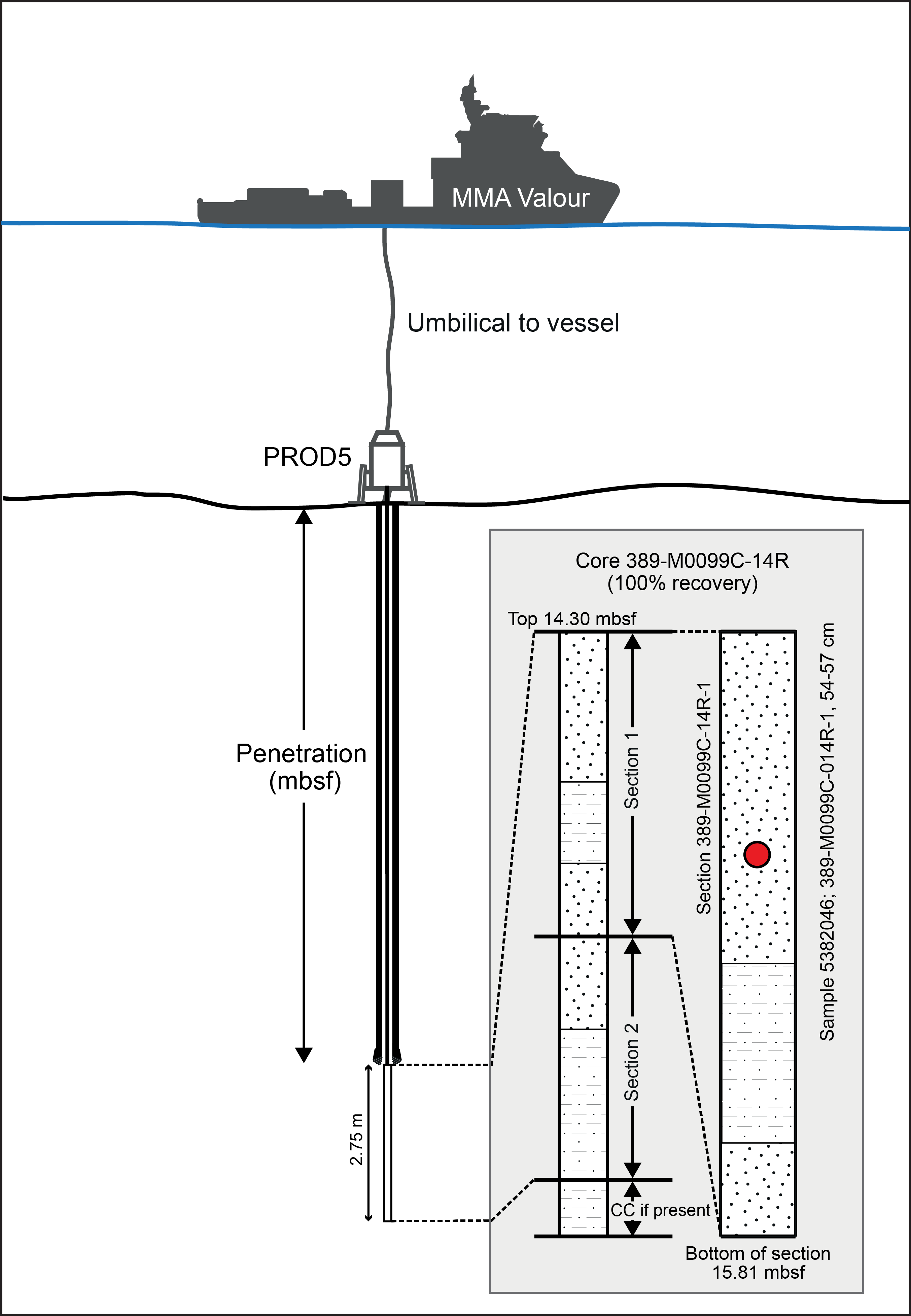
Figure F2. IODP depth and naming conventions.
All IODP core identifiers indicate core type. For Expedition 389, the following abbreviations are used:
1.2.2. Core handling during the offshore phase
Because of the nature of core collection from PROD5, all core material from each deployment of PROD5 arrived on deck at the same time. It was therefore necessary to modify the core flow to accommodate this process. Starting with the deepest core barrel, core barrels were removed from the tool rack on the PROD5 core magazine one by one, put onto a core elevator on the LARS gantry in groups of four, and lowered to the deck. The core barrel run number was written on each core barrel by a Benthic Geo-technician or Geo-engineer, and then up to eight core barrels were placed onto a core barrel trolley at the base of the core elevator, transported to the on-deck curation area, and stacked for core processing starting from the uppermost core barrel (Figure F3).
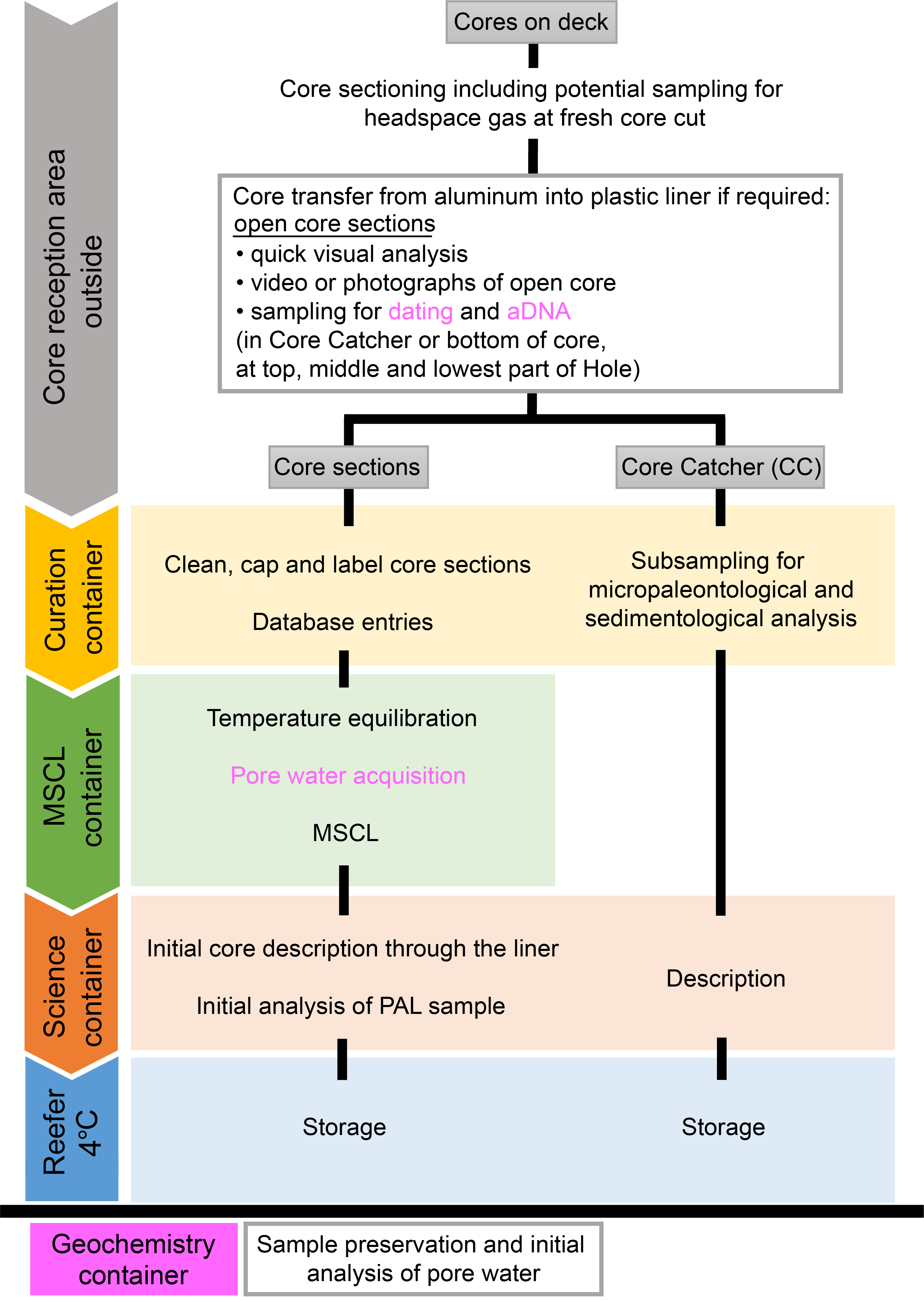
Figure F3. Offshore core flow.
The liners from each core barrel were extruded one at a time primarily by hand but where necessary using a hydraulic pusher. The extracted 2.75 m liners were cut into one or two sections with a maximum length of 1.5 m. The aluminum and polycarbonate liners used during Expedition 389 required different treatment at this initial curation stage. Aluminum liners were split along one axis using a liner saw with a special guide, and the cut edges of the liner were duct taped to ensure no material was lost when the liner was rotated 180°, rotated, and cut longitudinally again. The liner was rotated once more through 90°, and the lid was opened to expose the recovered core. Two nominated science party members per shift undertook a short visual core description on the exposed core and took high-resolution photographic pans along the entire core to acquire separate high-resolution close-up images for most holes. This provided an additional record of core quality and context prior to further core handling (i.e., transfer to polycarbonate liners and preliminary core curation). Where requested, and if appropriate, sample locations were identified by the science party, geochronology (14C and U-Th series) and ancient DNA (aDNA) samples were taken from the exposed core (or the bottom of polycarbonate liners) by the ESO curator, and samples were bagged, labeled, and delivered to the curation container for input into the mDIS (Figure F3). Close-up images of the locations of each dating and aDNA sample were also taken. The core then underwent preliminary curation by the ESO curator and, where required, was transferred into a polycarbonate liner of appropriate length according to the following method:
- Take an empty polycarbonate liner cut to the length of the curated section with a precut split on one side and insert a spacer to increase the diameter.
- Transfer the core, including one half of the aluminum liner, into the polycarbonate liner (the aluminum liner covers the split in the polycarbonate liner), turn the core upside down, and carefully pull out the aluminum half, with the split at the top.
- Seal the split polycarbonate liner with tape and put on end caps (not taped at this stage).
Potential locations for interstitial water (IW) sampling were identified at this stage and marked on the liner. Each section was capped at the top and bottom by a color-coded plastic cap: blue for the top of a core section (in line with IODP convention) and red for the bottom. Because only red caps were available for bottom caps, to keep with IODP convention of white or clear caps on section bottoms, white tape was used to seal the bottom cap. Cores were stored in a core rack either on deck or in the ESO curation container until the on-deck core processing of core barrels was completed (Figure F1). No core splitting took place during the offshore phase of Expedition 389. Daytime sunlight and ambient temperatures were very warm at times, so a shade was rigged up above the on-deck core rack and a tarp was placed directly over the cores to keep them out of direct sunlight. A contingency plan of directly cooling unprocessed core barrels by draping them with cold and wet cloths was ultimately not required.
Full core curation was undertaken from the uppermost to lowermost sections in the ESO curation container, and the core length of each section was entered into the mDIS. Core sections and end caps were taped up, and liners were permanently labeled with an engraving tool as per IODP core section naming convention. If available, a core catcher paleontology (PAL) sample was entered into the mDIS and given to the shipboard sedimentologists and coral specialist for initial visual or smear slide description as required (Figure F3).
After final curation, the cores were taken to the multisensor core logger (MSCL) container (Figure F1) and placed in drawers in section order (Figure F3). The cores were labeled with the time of arrival to inform of the end of the 6 h temperature equilibration period required prior to MSCL logging (see Physical properties). The geochemistry team could access the cores within the equilibration period as required to sample potential sites identified for IW sampling with Rhizon syringes (see Geochemistry).
After MSCL logging, the shipboard sedimentologists and/or coral specialists carried out a lithologic description for each core section through the clear polycarbonate liners using a visual core description (VCD) sheet specifically constructed for Expedition 389 (Figure F6). The high-resolution images of exposed core taken before primary curation also assisted in these descriptions, and once complete, the main facies (Table T2; Figure F10) were input into the mDIS. Core sections were returned to the MSCL container until all sections were logged or were directly transferred into the core reefer container for storage at 4°C (Figure F3). With the exception of samples taken for IW, aDNA, and geochronology, no additional sampling of the cores or core catchers was undertaken during the offshore phase of Expedition 389.
1.3. Data handling, database structure, and network
Data management during the offshore and onshore phases had two overlapping stages. The first stage was the capture of data and metadata during the expedition, both off shore and on shore. The second stage was the longer term postexpedition archiving of Expedition 389 data sets, core material, and samples after the moratorium period. This function was performed by the World Data Center (PANGAEA; http://www.pangaea.de) and at the IODP Bremen Core Repository (BCR; MARUM—Center for Marine Environmental Sciences, University of Bremen, Germany).
1.3.1. Mobile Drilling Information System
To capture metadata during the first stage of data management, the mDIS was used. The mDIS is a flexible and scalable database system originally developed for the International Continental Scientific Drilling Project (ICDP) and adapted for ESO so that it is compatible with the databases of the other IODP implementing organizations and ICDP. During Expedition 389, the Expedition mDIS instance was used to store coring information, core curation information, core images, sample information, lithology descriptions, smear slide descriptions, slabbed section linescan images, smear slide images, and split core close-up images during the offshore and onshore phases (Figure F4). All other data were captured in files and stored on the shared file server.
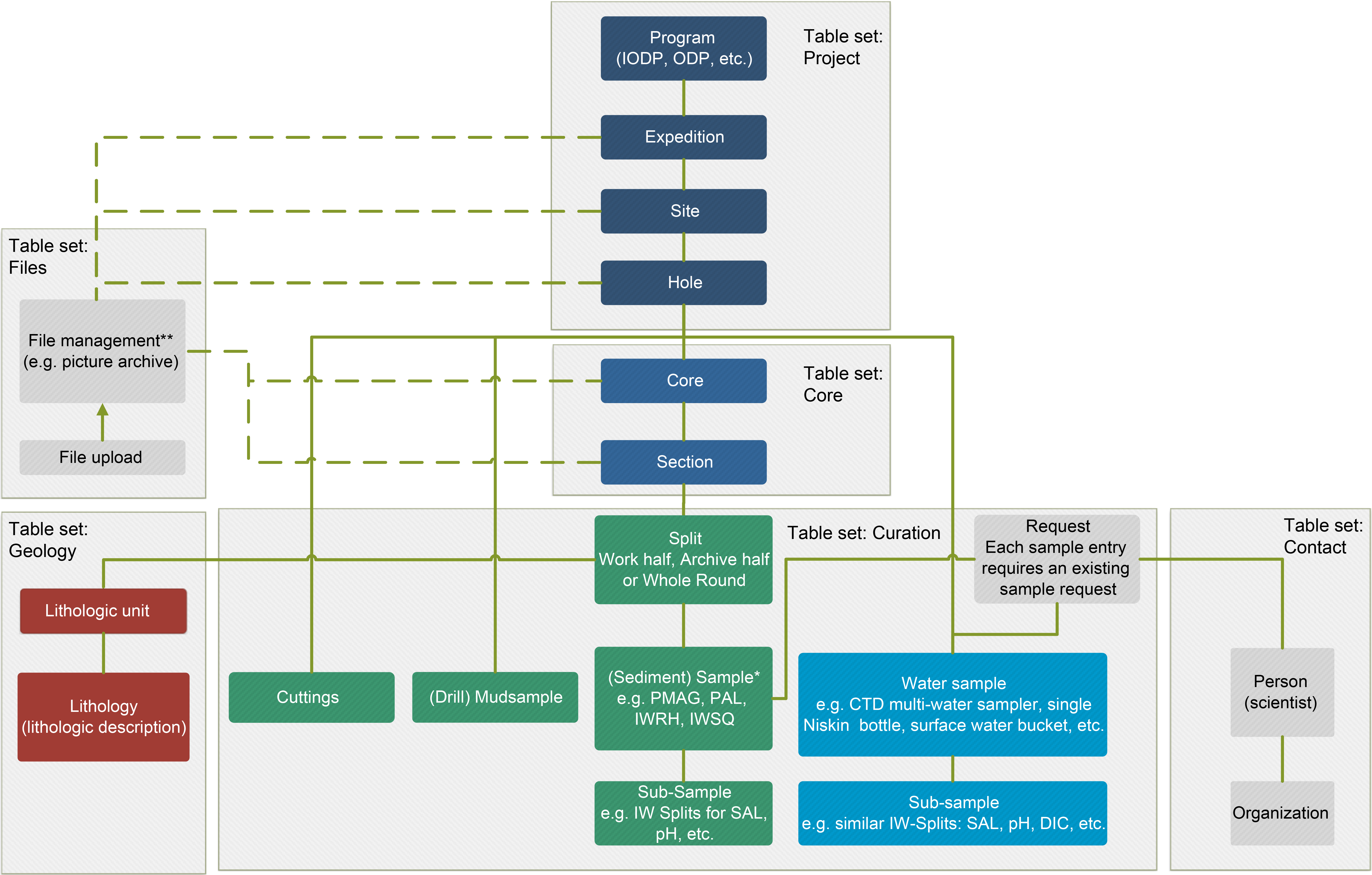
Figure F4. mDIS database hierarchy.
All cores, sections, and samples entered into the mDIS automatically receive an individual International Generic Sample Number (IGSN). The IGSN is a unique persistent identifier for physical samples. After the end of the moratorium, all data are transferred from the Expedition mDIS instance to the Curation mDIS instance (BCR core and sample management system); contemporaneously, the IGSNs are registered and can be accessed at http://www.igsn.org (to navigate to a particular IGSN, add the IGSN to the end of this link [e.g., http://www.igsn.org/IBCR0381EXI3001]).
1.3.2. Data portals
Simultaneously, the metadata captured in the Expedition 389 mDIS instance and the shipboard expedition data stored in the shared file server were transferred to PANGAEA (http://iodp.pangaea.de) for long-term archiving and public accessibility (second phase). PANGAEA is a member of the International Council of Scientific Unions World Data Center system and is used for processing, long-term storage, and publication of georeferenced data related to earth sciences. Until the end of the moratorium period, data access was restricted to the expedition scientists. Following the moratorium, all shipboard expedition data were published online in PANGAEA, and PANGAEA will continue to acquire, archive, and publish new results derived from Expedition 389 samples and data sets.
The central portal for all IODP data, including Expedition 389 data, is the Scientific Earth Drilling Information Service (SEDIS; http://sedis.iodp.org). IODP MSP data are also downloadable from the MSP Data Portal at PANGAEA.
2. Lithostratigraphy
This section summarizes the methods used to describe and document the lithology of cores recovered during Expedition 389. It outlines the offshore and onshore visual core description methods, together with details of sediment classification and descriptive terms used. For additional methods used to characterize the physical properties and sediment composition, see Physical properties and Geochemistry.
2.1. Visual core descriptions
Offshore sedimentologists, volcanologists, and coral specialists conducted preliminary visual inspections and prepared written descriptions of the whole cores and core catcher material recovered during the expedition. These observations were made in two steps.
On deck, after cutting the aluminum core liner and before curation, naked/uncovered cores were rapidly inspected for visual core description, and their main characteristics were summarized on VCD initial notes sheets (Figure F5). On-deck photographs and overlapping high-resolution close-up photos (see IMAGES in Supplementary material) were taken before transfer from the aluminum liners to plastic liners (see Introduction).
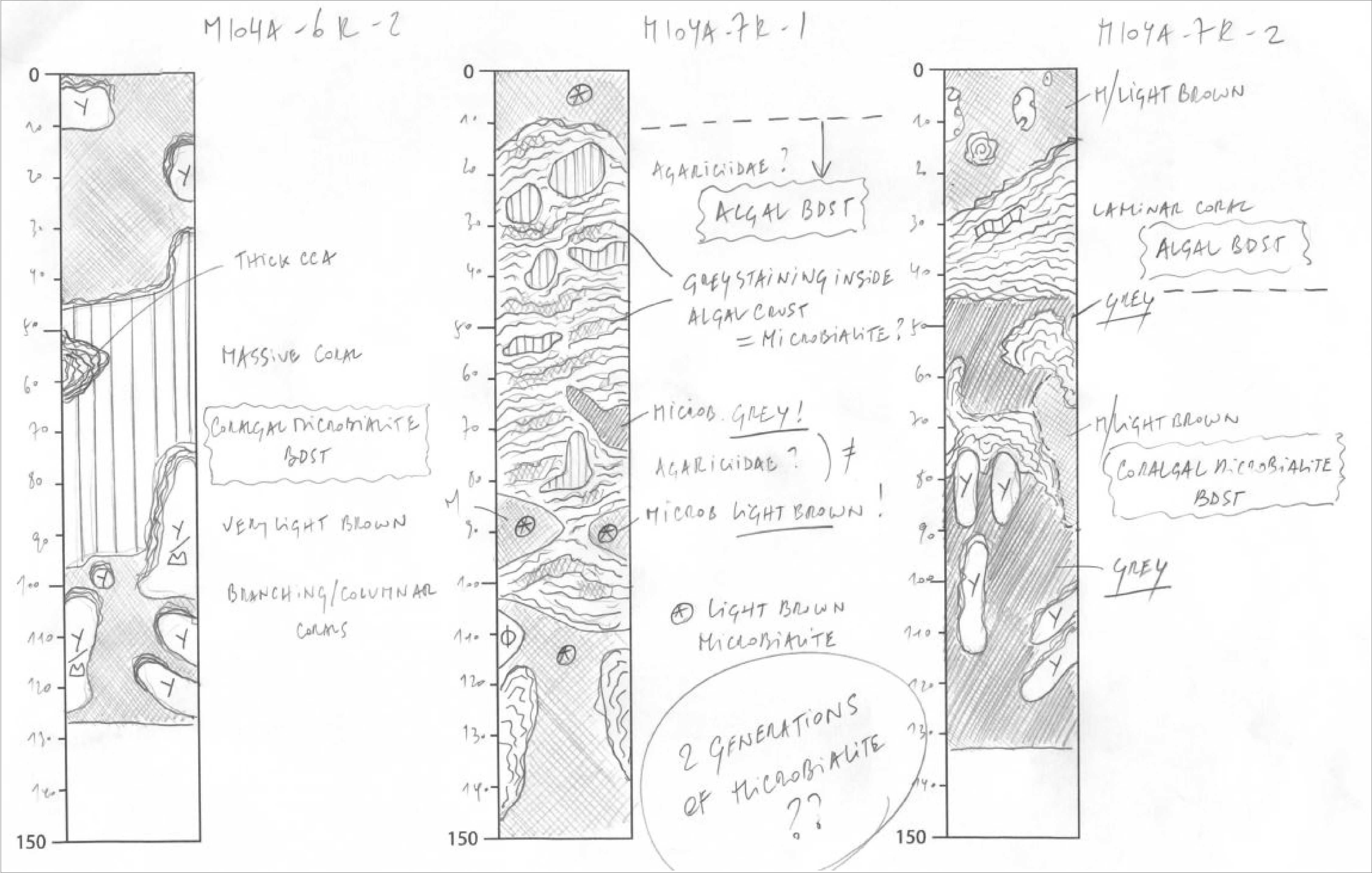
Figure F5. Offshore VCD initial notes sheet for whole-round cores.
After curation and physical properties measurements, cores were examined visually, both through the polycarbonate core liners by eye and with hand lenses. The close-up photographs were used to complete the description. The observations were recorded on offshore VCDs (Figures F5, F6). For further analysis, binocular microscopes were used on paleontology (PAL) samples selected from the core catchers or the lowermost part of core sections on a regular spacing of 4–5 m, depending on the availability of material. Where appropriate, photomicrographs were taken and labeled according to IODP convention and saved on the network.
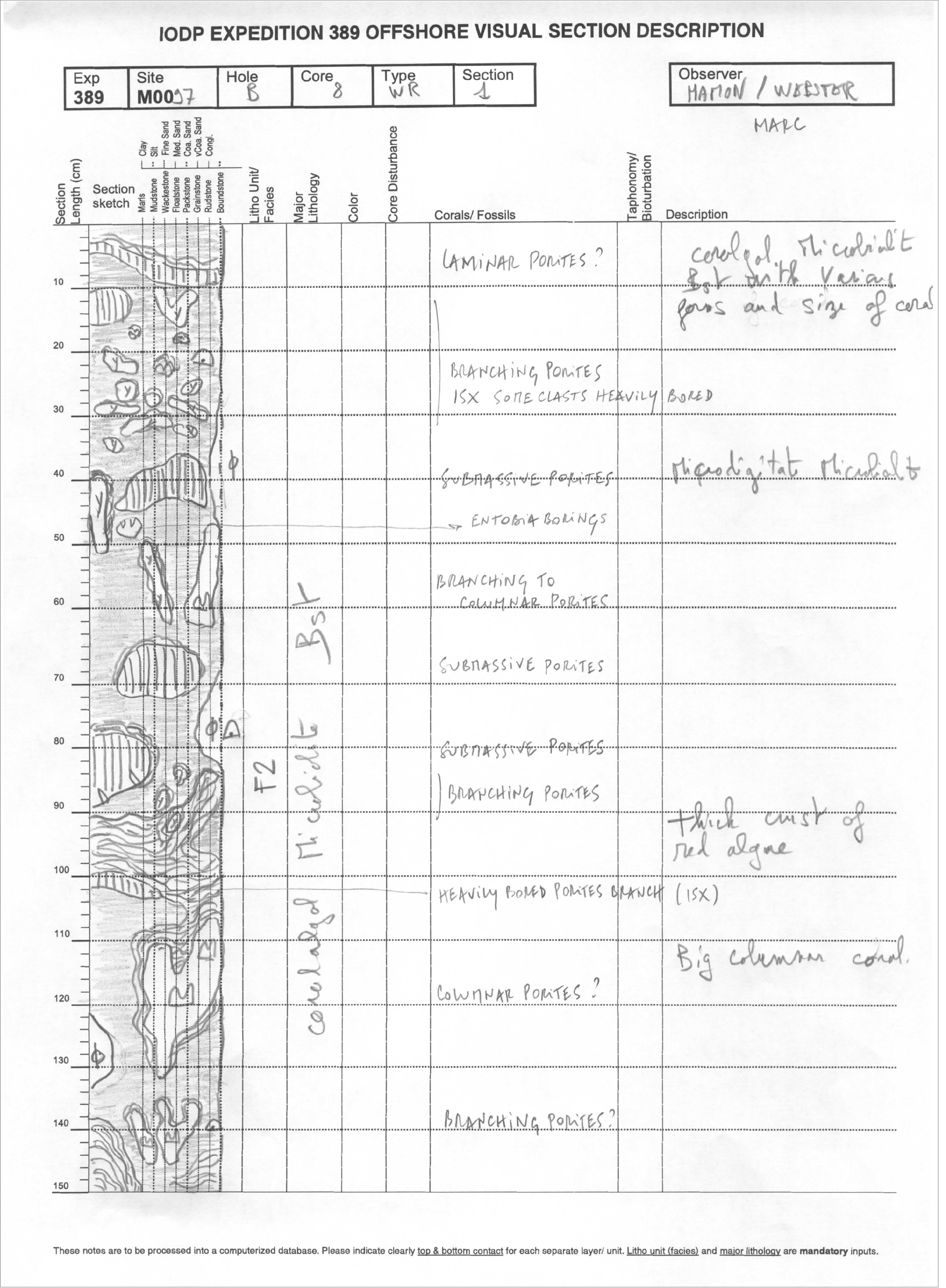
Figure F6. Whole-round offshore VCD.
During the OSP, sedimentologists conducted visual observations of the archive halves of the cores by eye and with hand lenses to describe their main characteristics. The Corelyzer 2.2 software (Ito et al., 2023) was used to visualize high-resolution linescan images (see IMAGES in Supplementary material), as well as X-ray computed tomography (CT)-scan images, to further facilitate visual core description. In addition, a binocular microscope was used to analyze and acquire photomicrographs of the core material. These observations were recorded on paper next to the printed image of archive halves on onshore VCDs (Figure F7; see ONSHORE_VCD in Supplementary material).
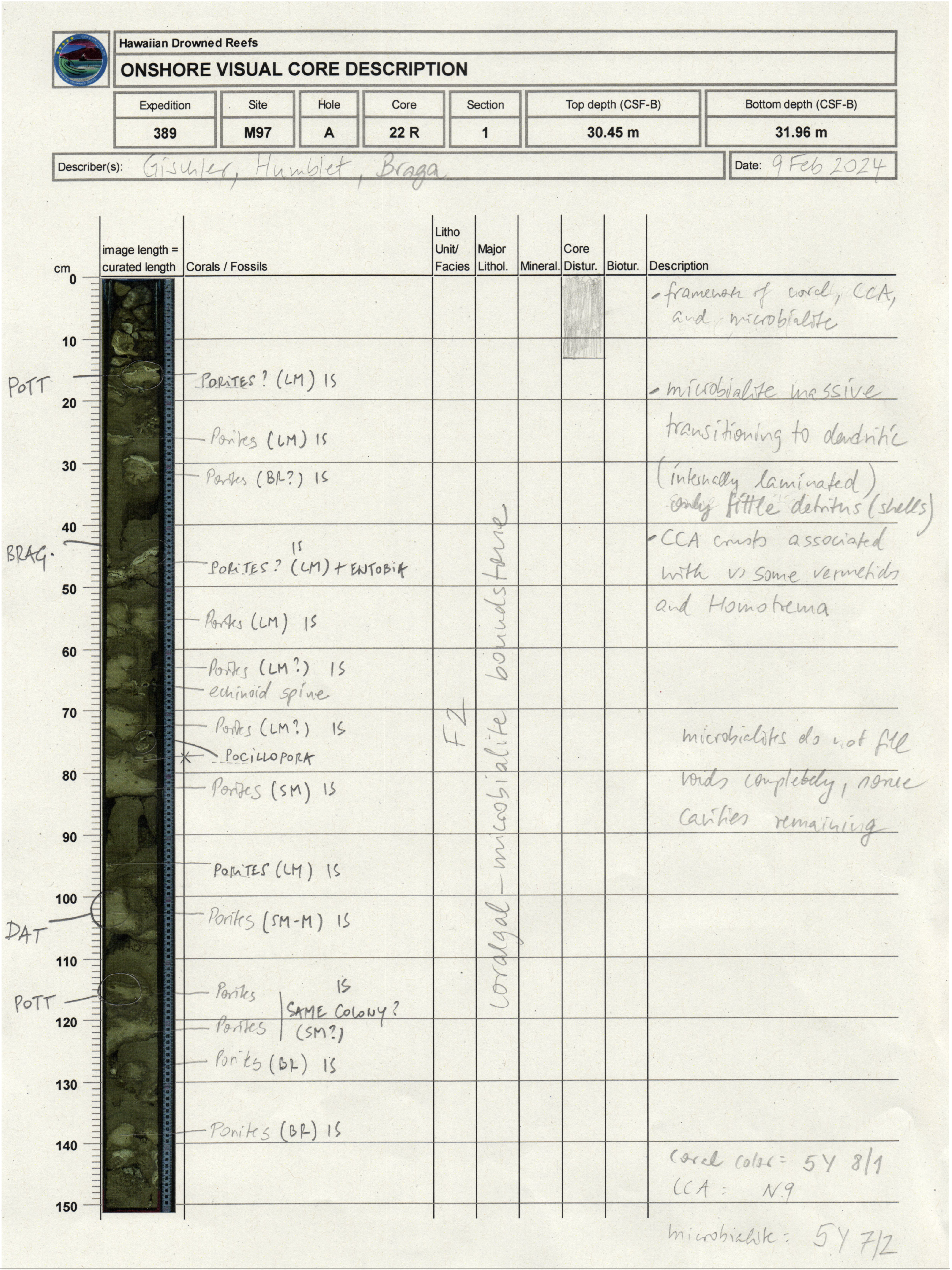
Figure F7. Onshore VCD for the archive half.
During both the offshore and onshore phases of the expedition, information recorded on VCDs was entered into the mDIS with two different section split labels: WR (whole round, off shore) and A (archive, on shore). Based on this information, lithostratigraphic logs, plots compiling MSCL data (Figure F8), and drilling information (Figure F9) were generated using the Strater 5 software (by Golden Software) for each hole, including composite logs and transects, with a legend.
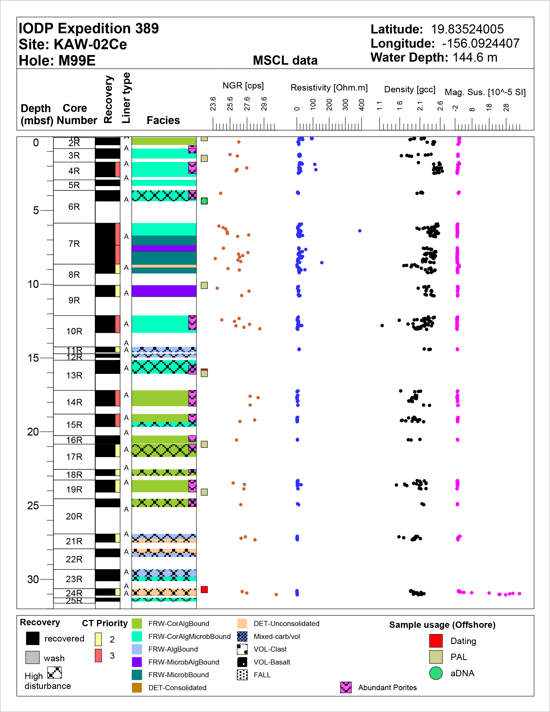
Figure F8. Offshore Strater plot with MSCL data.
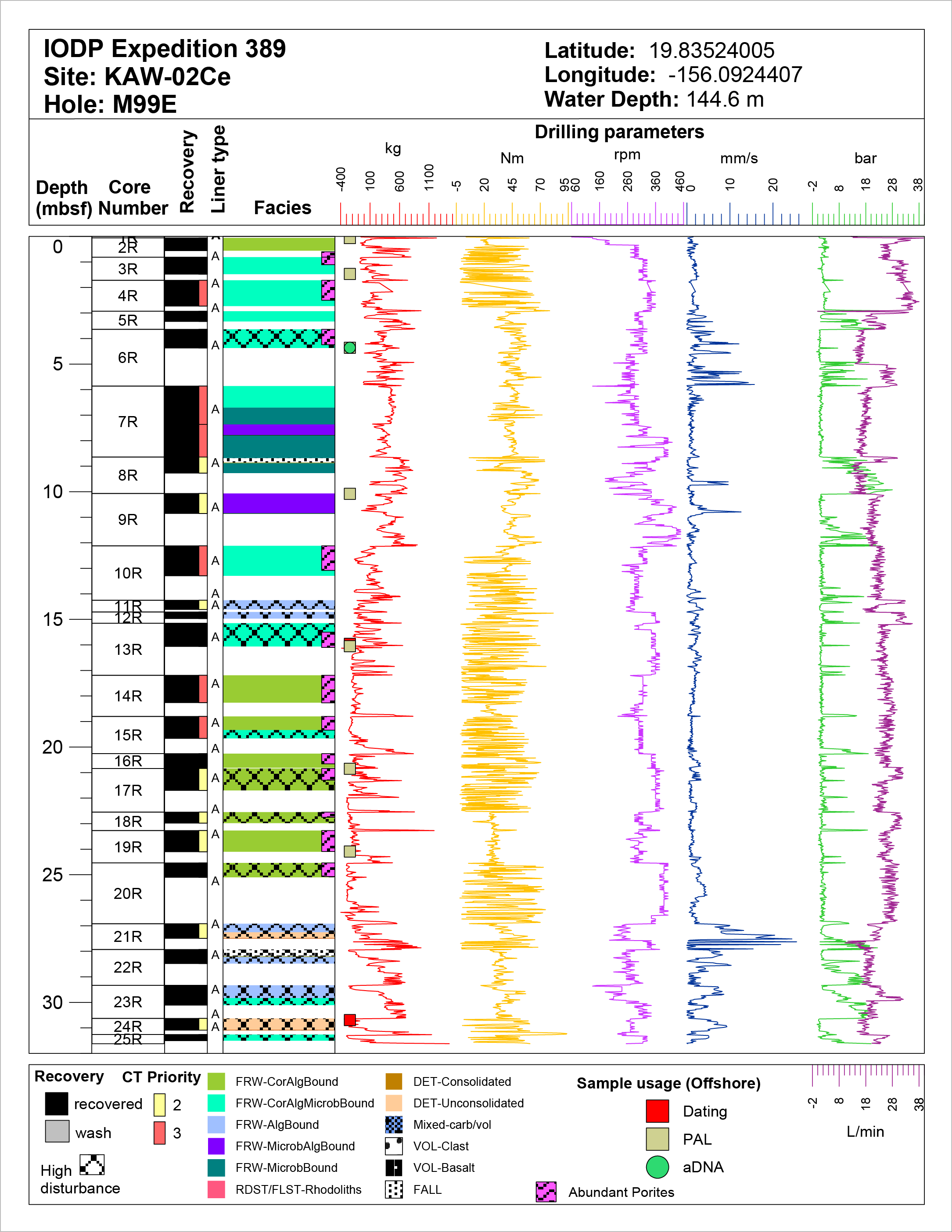
Figure F9. Offshore Strater plot with drilling parameters.
Each core can be composed of several core sections, where a single core is as long as 2.75 m and represents a single core run. If a core run recovered more than 1.5 m of material, it was split into two sections. In some cases, material from the core catcher was also retrieved (see Introduction). Each core section was described based on general facies, including lithology and the proportion of major components and/or changes in the dominant coral type (identified to the lowest taxonomic level possible), or volcanological nomenclature. The following features were described:
- Core disturbance and intervals of downhole fall-in sediment contamination in the upper parts of some cores;
- Lithologies (sediment and basalt); for sediment: texture, grain size, major and minor components (fossils, detrital grains, and matrix), and degree of consolidation;
- Morphology and taxonomy of individual corals;
- Boundaries between lithologies, including sedimentary boundaries (e.g., lithologic changes, depositional discontinuities, unconformities, erosional surfaces, etc.); and
- Taphonomic information (bioturbation, bioerosion, encrustation, and fragmentation).
2.1.1. Core disturbance
Disturbed intervals due to fracturing and/or grinding during drilling operations were marked on the VCDs (both on shore and off shore). Disturbance was also entered as a specific field in the mDIS using four levels of disturbance: none, slight, moderate, and high.
In the upper part of some cores, sedimentary breccias were clearly identifiable as downhole contamination. These intervals were flagged as “Facies F0 – fall-in material” based on the following criteria:
- Core recovery exceeds 100%.
- Reworked, brecciated material occurs at the top of the core, possibly with recoring or grinding marks on some debris.
- Brecciated material is different from a well-preserved interval of the facies defined below and in the core above.
2.1.2. Overall lithology
Overall lithology/texture was defined for carbonate sedimentary rocks following Embry and Klovan’s (1972) revision of Dunham’s (1962) classification. The following carbonate lithologies were distinguished:
- Boundstone: original components organically bound during deposition.
- Rudstone: granule/pebble-sized grains >2 mm; grain-supported textures with no matrix between the grains.
- Floatstone: granule/pebble-sized grains >2 mm; matrix supported.
- Grainstone: consolidated biodetrital material; sand-sized grains <2 mm; grain-supported textures with no mud between the sand grains.
- Packstone: consolidated biodetrital material; sand-sized grains <2 mm; grain-supported textures with mud between the sand grains.
- Wackestone: consolidated biodetrital material; mud-supported textures with sparse sand-sized grains floating in the mud.
- Mudstone: consolidated biodetrital material; mud-supported textures with sparse rare (<10%) sand-sized grains.
Note that “boundstone” is used as a generic term. Any material organically bound during deposition can form a boundstone, be it corals, algae, and/or microbialite.
Unlithified sediments were defined based on grain composition and size (Wentworth, 1922):
- Unconsolidated biodetrital sediments,
- Volcaniclastic sediments,
- Mixed carbonate-volcaniclastic sediments, and
- Hemipelagic mud.
Finally, because volcanic deposits were restricted primarily to extrusive solidified lava (i.e., lava rock with no significant pyroclastic or intrusive deposits observed), volcanic igneous rocks were described using four criteria relating to lava flow texture and alteration:
- Groundmass texture: aphanitic, phaneritic, and glassy.
- Phenocryst crystallinity: porphyritic and not porphyritic (including crystal phases when observed, primarily olivine and clinopyroxene).
- Vesicularity: percentage and roundness.
- Alteration: discoloration, vesicle filling, and infilled veins and cracks; lava with the absence of these features is referred to as “visually fresh.”
Additionally, textures indicative of lava flow morphotypes and/or eruption conditions were noted if evident (e.g., Pāhoehoe-texture, ʻaʻa-texture, hyaloclastite-texture, and pillow lava-texture).
Several volcanic lithology naming conventions were used:
- “Lava” or “lava rock” refers to lithology. Although the term “lava” can refer to both solidified and molten rock, in this report it always refers to the solidified material unless specifically noted.
- “Lava flow” refers specifically to instances where the textural and morphological features of an identifiable solidified lava unit are present (i.e., top, bottom, and/or internal features). When these features are absent, “flow” is not included in the description. It is generally not possible in these cores to visually distinguish between multiple simple lava flows (which represent discrete eruptions) and multiple lobes of a single extended duration compound lava flow (using the terminology of Walker, 1971). When multiple individual lava flow boundaries were observed they were not interpreted as being discrete flows or compound flow lobes unless there is clear evidence of a change in texture, crystallinity, or alteration that requires a flow boundary representing a significant time gap.
- “Basalt” and “basaltic” refer to composition of the magma and/or the crystal phases therein.
- “Vesicle” is used to refer to solidified void spaces originally formed from gas bubbles in the magma.
- “Phaneritic” and “aphanitic” refer to the groundmass texture, and “porphyritic” refers to the presence of phenocrysts. Although “phyric” is commonly used to refer to lava that is both apanitic and nonporphyritic in the literature, that terminology is not adopted here.
2.1.3. Major and minor components of a core
The major components of a core are defined as those that contribute to the highest percentage by volume of the sediment and/or rock. Framework facies can include corals, microbialite, or coralline algae as major components or may contain a mixture of these.
Components in the cores include the following:
- Basalt clasts and volcaniclastic sand grains;
- Bivalves;
- Bryozoans;
- Corals (for details on the determination of corals, see Coral descriptions), as well as derived clasts and rubbles;
- Coralline algae, crustose coralline algae (CCA) or fruticose coralline algae (FCA), and derived clasts and rubbles;
- Echinoderms;
- Foraminifers (large benthic foraminifers [LBFs] and encrusting foraminifers);
- Gastropods (including vermetid gastropods and Cypraeidae);
- Halimeda;
- Microbialite (meso-scale morphology: columnar, dendritic, and crust; internal morphology: structureless, laminated, and thrombolitic [clotted]; types not differentiated off shore);
- Rhodoliths;
- Serpulids, sabellariid tubes, and vermetids;
- Unknown lithoclast; and
- Unknown bioclasts.
Selected corals, CCA, FCA, and foraminifers were sampled during the OSP to conduct further analysis as part of the post-OSP phase to achieve a more precise taxonomic identification.
2.1.4. Sedimentary boundaries
Lithologic changes represented by discontinuities, unconformities, bioeroded surfaces, and other features (e.g., staining, cementation, or dissolution) associated with such boundaries were marked on the VCDs (both on shore and off shore).
2.1.5. Facies
The resulting combination of the overall lithology, major and minor components, and sedimentary boundaries enables association of each section unit with one facies (“lithological unit code” in the mDIS). Thirteen different facies were defined (Table T2; Figure F10).
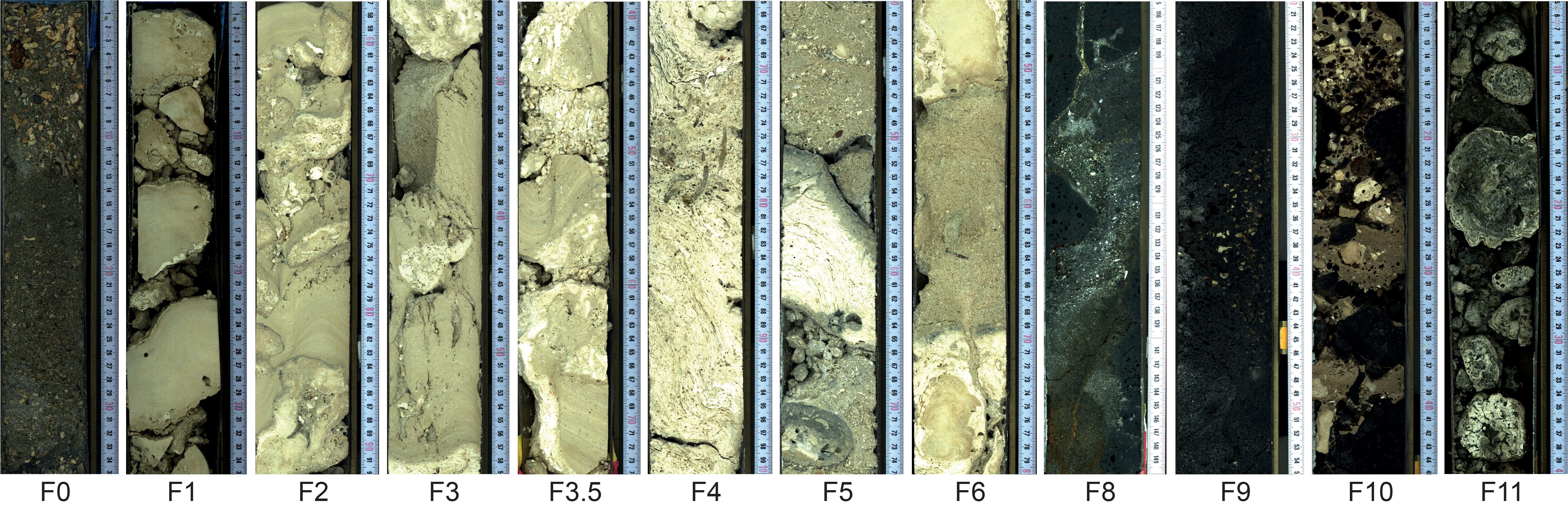
Figure F10. Lithostratigraphic facies.
2.1.6. Coral descriptions
Coral specialists mapped the preliminary stratigraphic positions of all visible corals on the VCDs, both off shore and during the OSP. Coral taxonomy and growth forms were also reported on the VCDs (both off shore and on shore) and entered into the mDIS (see Introduction).
2.1.6.1. Coral taxonomy
Coral identifications generally follow the usage of Veron (2000) with later modifications by Wallace et al. (2007), Budd et al. (2012), and Huang et al. (2014, 2016). Offshore identifications were usually only to family or genus, because species-level taxonomic characters were either not preserved or not able to be identified through the liner or because there was insufficient time for careful examination. Uncertain identifications pending further study are marked with an “?” on the VCDs (both off shore and on shore). Onshore description of the coral fauna was based on observations of the archive halves of the cores, and identifications were usually done to the genus level and up to the species level when well-preserved corallite sections were observed.
2.1.6.2. Coral growth forms
Coral growth forms were described as follows (Figure F11):
- Encrusting: base attached to substrate; <5 cm thick.
- Submassive: base attached to substrate; 5–10 cm.
- Massive: base attached to substrate; >10 cm.
- Platy: base unattached to substrate; >5 mm thick.
- Foliaceous: base unattached to substrate; <5 mm thick.
- Laminar: if it is not possible to distinguish encrusting from platy.
- Branching fine (BF): if branch diameter is <1 cm on average.
- Branching medium (BM): if branch diameter is 1–1.5 cm on average.
- Branching robust (BR): if branch diameter is >1.5 cm on average.
- Columnar: if the colony displays mostly nonbifurcating upright columns.
Figure F11. Most common coral morphologies and taxa.
Depositional context was described as follows (Table T3):
2.1.7. Diagenesis and other features
Where applicable, occurrences of such features as open cavities, geopetal infills, color staining, cementation, and diagenetic alteration of components were identified and marked on the VCDs (both on shore and off shore). Some of the cavities were filled locally by internal bioclastic (marine) sediment, whereas other cavities were filled by microbialite.
3. Physical properties
3.1. Offshore petrophysical measurements
Core recovered during Expedition 389 was logged with a Geotek MSCL (Figure F1). The MSCL has five primary measurement sensors mounted on an automated track that sequentially measure gamma density, P-wave velocity, noncontact resistivity (NCR), magnetic susceptibility, and natural gamma radiation (NGR) (Table T4). Measurements were taken on most core sections after they were allowed to equilibrate to ambient temperature for 6 h. Core catcher pieces, cores shorter than 15 cm, and cores composed of loose rubble were generally not included in the logging process. During Expedition 389 offshore operations, gamma density, NCR, magnetic susceptibility, and P-wave velocity measurements were recorded at 2 cm intervals and NGR was measured at 10 cm intervals. High-resolution data were acquired at 0.5 cm intervals for a small subset of core sections.
The quality of the MSCL data is a function of both sensor precision and core quality. Gamma density, magnetic susceptibility, and NGR are affected by measurement time, whereas NCR and P-wave velocity are impacted by temperature. P-wave velocity measurements also require good contact between the acoustic transducers, liner, and core. For best MSCL results, the core liners should be fully filled with core material and the core completely fluid saturated. Partial fluid saturation and drilling-induced core damage negatively impacted the data quality. During Expedition 389 offshore operations, the recovered core material was transferred from aluminum to plastic liners, thereby draining and to some extent further disturbing the recovered core sections in the process. Natural vugs and fractures, which are common in carbonates and lava rock, may mimic drilling-induced core damage in the sensor response.
A full calibration of the MSCL sensors was required (Table T4), from which the relationships between sensor output (e.g., gamma counts per second or millivolts) and petrophysical properties (e.g., density in grams per cubic centimeter and resistivity in ohm-meters) are derived. The initial calibration was conducted at the beginning of the expedition. Calibration checks were performed on gamma density, P-wave, NCR, and magnetic susceptibility sensors approximately once every 6 h (excluding wait times during drilling). These checks involved testing three calibration reference pieces: the magnetic susceptibility calibration-check piece, a standard core liner saturated with distilled water, and a standard core liner saturated with 8.75 g/L salinity-water solution. The results were compared to the values derived during the full calibration. The NGR sensor does not require calibration checks.
3.1.1. MSCL measurement principles
This section provides a brief overview of the measurement principle of each of the five MSCL sensors, as well as specifics about the calibration process and measurement procedure. More detailed information about the MSCL sensors can be found in the Geotek MSCL Manual (http://geotek.co.uk/downloads).
3.1.1.1. Gamma density
The core bulk density was determined through gamma ray attenuation densitometry. On the MSCL, the core is run in between a lead-shielded small (370 MBq) 137Cs gamma source and a lead-shielded NaI(Ti) scintillating detector. Through a 5 mm collimator, the source emits gamma rays with primary photon energies of roughly 0.662 MeV that attenuate (due to Compton scattering) as they pass through the lined core to the detector. The degree of attenuation depends on the electron density of the core material. This correlates well with bulk density because most rock-forming minerals have similar low atomic numbers. During Expedition 389, gamma density logs were recorded with a sampling interval of 2 cm and a count time of 10 s.
3.1.1.1.1. Gamma density calibration
A calibration is necessary to convert the recorded gamma intensity readings (in counts per seconds) to bulk density values (in grams per centimeter cubed). For the full initial calibration, a stepped aluminum standard (provided by Geotek) was placed inside a 30 cm long sample of the polycarbonate liner (inner diameter = 7.28 cm; wall thickness = 0.16 cm) used for the rotary cores during Expedition 389. The standard was run through the MSCL (1) filled with water (for saturated core) and (2) filled with air (for dry core). For the gamma counts per second, 30 s averages were recorded (Tables T5, T6) at each of the five thicknesses (6, 5, 4, 3, and 2 cm) of the stepped aluminum standard, as well as through the liner and air or the liner and distilled water. During Expedition 389, calibrations were performed at the beginning and the end of the expedition as well as two thirds of the way through the expedition. The calibrations were checked with a water-filled liner tube during the regular calibration checks, which were conducted before each new hole was drilled and every 6 h afterward.
3.1.1.1.2. Density calculations
MSCL rock density (ρ) is determined based on the following equation:
- I = measured gamma intensity (counts per second),
- D = core thickness (cm), and
- A, B, and C = calibration parameters obtained from the gamma density calibration measurements above (Table T7).
Solving the above equation for ρ yields the following relationship:
If A < 0, the negative square root is taken. If A > 0, the positive square root is taken.
3.1.1.1.3. Dry versus wet density calibration
The core sections recovered during Expedition 389 were transferred from aluminum to polycarbonate liners and were partially drained in the process (see Operations in each site chapter). Figure F12 shows the relationship between densities calculated using correlations from the dry and wet calibration. The difference in calibration becomes apparent (exceeding ±0.1 g/cm3) at densities lower than 1.5 g/cm3 (more void space).
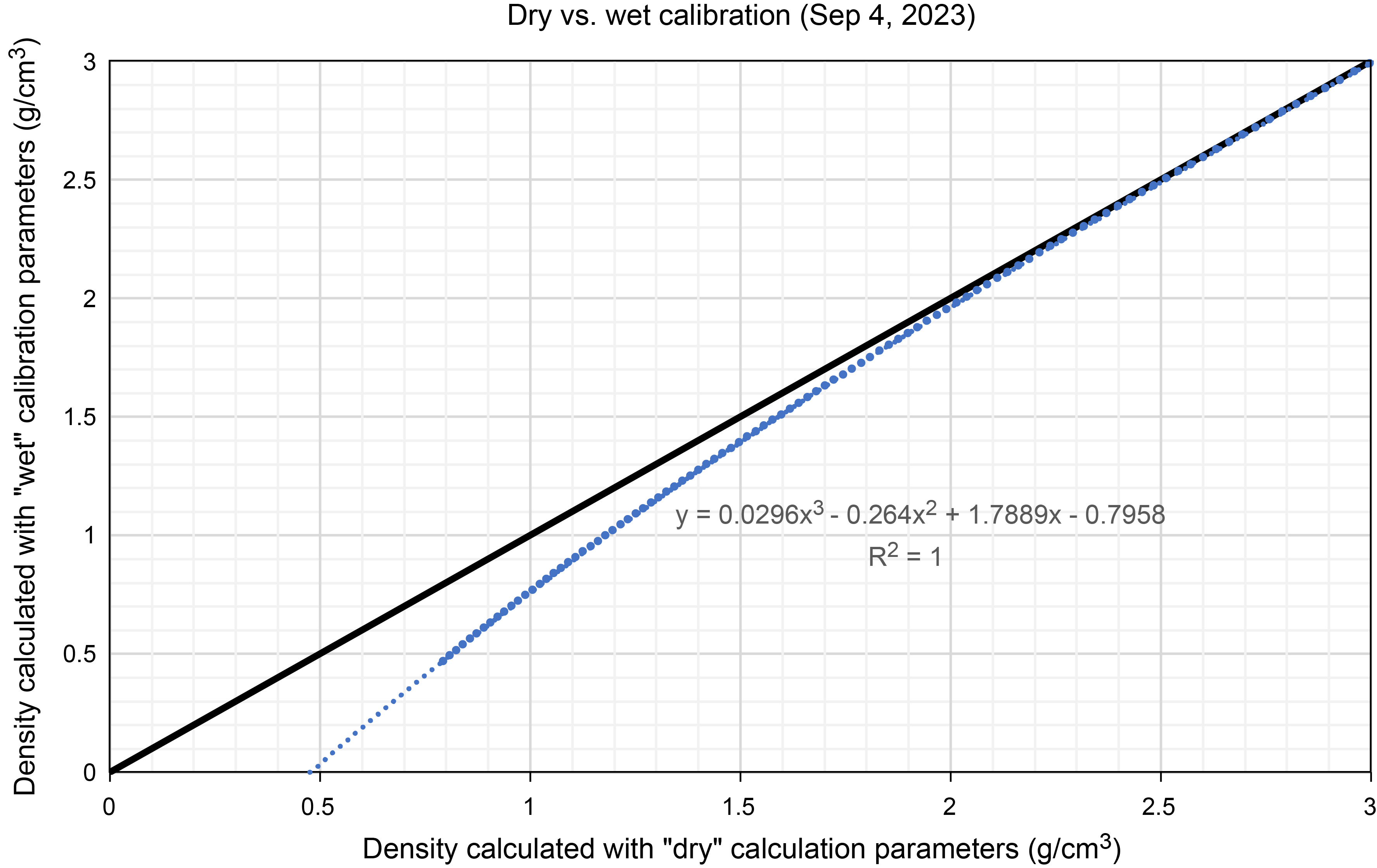
Figure F12. Dry vs. wet density.
MSCL density values for all cores were initially calculated using the previous equation and the wet calibration parameters. Inspection of the MSCL resistivity data (Figure F13) confirmed that competent core sections with fewer vugs retained water.
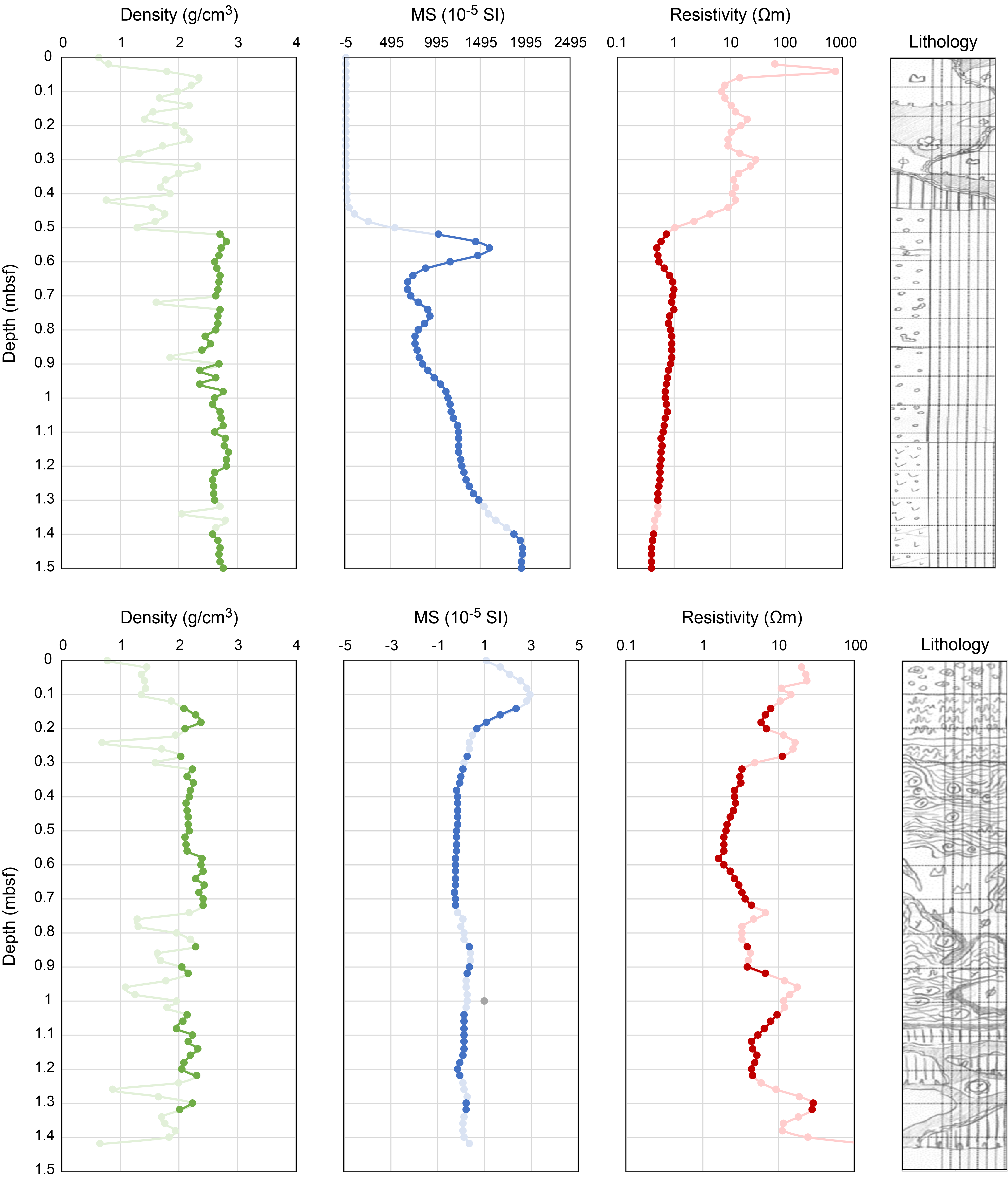
Figure F13. Vugs.
3.1.1.1.4. Sensor drift density correction
MSCL core measurements were conducted between 4 September and 1 November 2023 (Table T8). The calibration checks with a water-filled liner performed over that time period revealed a drift in the measured gamma intensity toward lower values, namely from 12,100 counts/s on 4 September to 11,500 counts/s on 31 October with a minimum of 11,000 counts/s recorded on 30 October (Figure F14). Because of the drift, the calculated density values with time increasingly overestimated the actual density of the core. Consequently, a correction was applied to the initially calculated densities to reduce them to their true value, as described below.
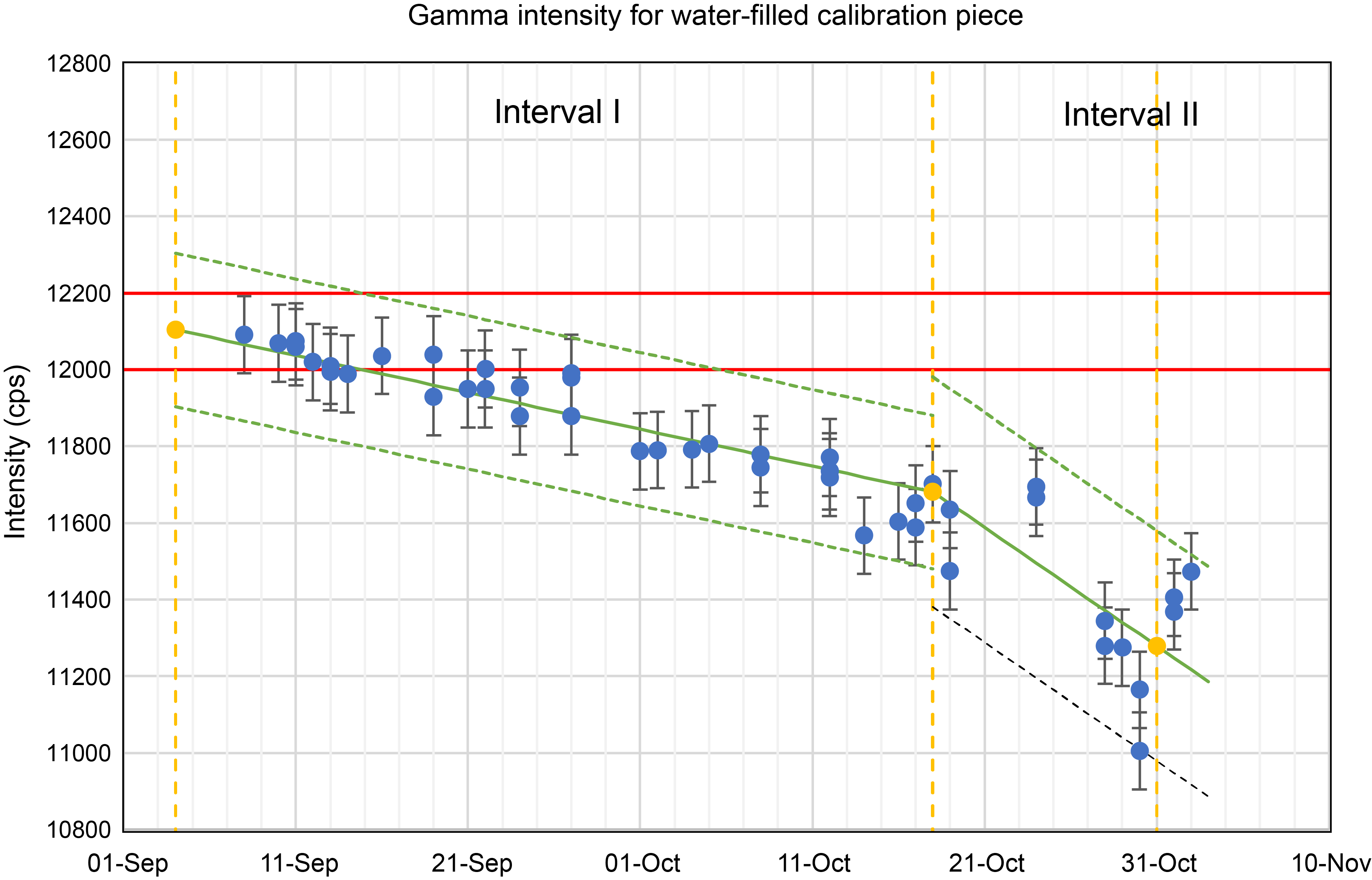
Figure F14. Calibration-check results.
In addition to the initial sensor calibration performed on 4 September, two more calibrations were performed: one on 18 October and one on 31 October. Comparison of density logs calculated for one core section using the three different sets of calibration parameters shows that the difference between values calculated with parameters from different calibrations (Δρ) depend not only on the day of the calibration but also on the density itself (Figure F15). Deviations are more pronounced at lower densities. The density dependence of Δρ can be expressed as the following relationships:
- Δρ18 = difference between densities calculated with 18 October and 4 September calibration parameters,
- Δρ31 = difference between densities calculated with 31 October and 4 September calibration parameters, and
- ρ = density calculated using 4 September calibration parameters.
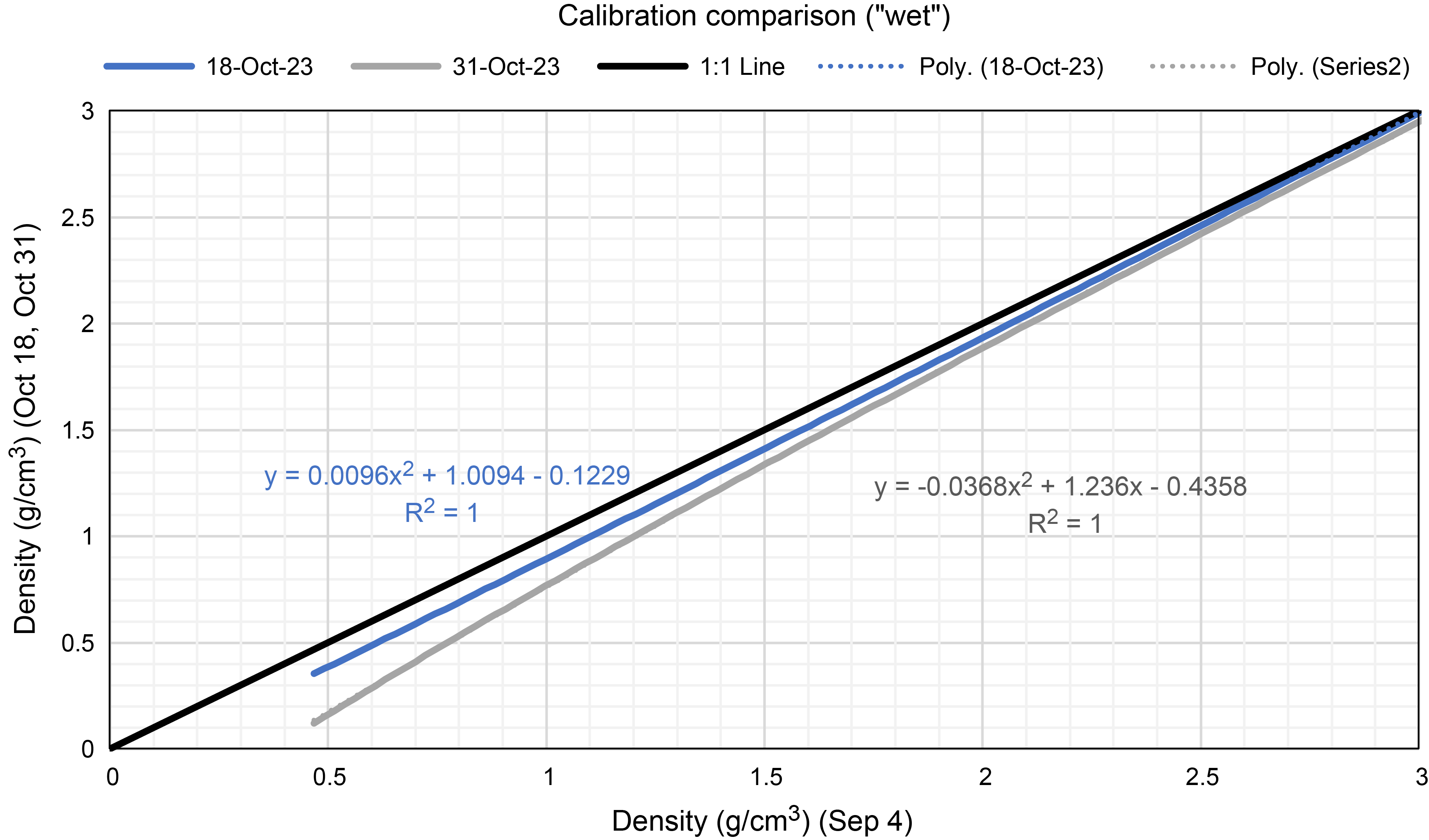
Figure F15. Relationship between densities calculated based on three calibrations.
For simplicity, we assume a linear time dependency between calibration points. This divides the total measurement period into two intervals (4 September–18 October and 18 October–1 November). The density correction subtrahend for given times are given by the following two equations:
- Δρx = density correction,
- tx = day of MSCL measurement (in days; 4 September = Day 0),
- t18 = day of 18 October calibration (= 43.5 days), and
- t31 = day of 31 October calibration (= 56.5 days).
Repeat measurements of the water-filled liner tube showed a variability in measured density values of ±100 counts/s. The uncertainty introduced through the density correction is based on the spread in the calibration check results (Figure F12). Data points measured for the water-filled liner between 4 September and 18 October roughly fall within ±200 counts/s, whereas those measured after 18 October roughly fall within ±300 counts/s. The ranges translate to uncertainties of ±0.04–0.07 g/cm3 (±1%–2%) and ±0.06–0.10 g/cm3 (±3%–4%), respectively.
3.1.1.2. P-wave velocity
Whole-core P-wave velocity (VP; in meters per second) was measured using two rolling ultrasonic P-wave transducers aligned perpendicular to the core axis. In this configuration (whole-core setup), 230 kHz compressional waves are transmitted horizontally across the core with a spatial resolution of 2 cm. In the recorded waveforms, the Geotek MSCL software automatically picks the time of first arrival (t0; in microseconds). P-wave traveltime through the liner and additional system-related delays (td; in microseconds) are subtracted from t0 to obtain the P-wave traveltime through the core (tp; in microseconds). The P-wave velocity is then calculated from tp and the inner diameter of the liner (core diameter [D]; in centimeters) using the following equation:
Knowing the velocity of water (Leroy, 1969), the traveltime offset, tp, is determined during the full initial calibration from P-wave velocity measurements on a 15 cm long polycarbonate liner of known inner and outer diameter that is filled with distilled water. The same calibration piece is also used in regular calibration checks (repeatability = ±1 µs). Core measurements were conducted at 2 cm intervals.
P-wave transmission depends on core quality, fluid saturation, and acoustic coupling between transducer, liner, and core material. A large number of the core sections that were recovered during Expedition 389 were minimally fluid saturated and often exhibited drilling-induced disturbances. Acoustic coupling between liner and core was generally too poor for wave propagation. As a result, minimal robust P-wave velocities could be successfully measured using the MSCL off shore.
3.1.1.3. Noncontact electrical resistivity
Electrical resistivity was measured using the NCR sensor. A transmitter coil generates a magnetic field that induces an electric current in the core. This current, in turn, generates a small magnetic field that is then measured with the receiver coil. An identical pair of transmitter-receiver coils at the bottom of the sensor measure the response in air. Comparison of the two measurements allows for the small magnetic fields induced in the core to be recorded (in millivolts). The NCR sensor has a spatial resolution of approximately 4 cm, and its output is given in millivolts. Calibration is required to convert the measured voltage into resistivity. For the full initial calibration, 6 × 30 cm long polycarbonate liner tubes were filled with distilled water containing different concentrations of sodium chloride (0.35, 1.75, 3.5, 8.75, 17.5, and 35 g/L). Each calibration piece was measured with the NCR, and its known resistivity (Schlumberger Gen-9 Chart) was correlated to the sensor output. The calibration piece containing the 8.75 g/L saline solution was used during the regular calibration checks. Important to note is that electrical resistivity is typically measured in fluid-saturated cores because it is a function of porosity, pore connectivity, saturation, and pore water salinity, clay content, and temperature. The cores recovered during Expedition 389 were mostly drained, similar to previous reef drilling during Integrated Ocean Drilling Program Expeditions 310 and 325. Consequently, the measured resistivity logs were primarily an indicator of areas with narrow pore structures, which retained some of the water, or areas in which water pooled at the bottom of the liner and were indicated by a drop in NCR values.
3.1.1.4. Magnetic susceptibility
Magnetic susceptibility is a measure of the degree of magnetization a material experiences when exposed to a magnetic field. The magnetic susceptibility of cores depends on their mineralogical composition or, more specifically, the concentration of magnetic minerals. It is dimensionless 10−5 SI (referring to the Système international d'unités (SI)/International System of Units). The MSCL magnetic susceptibility system comprises a Bartington MS2 loop sensor coupled with a Bartington MS3 meter. The loop has an inner diameter of 120 mm and operates on a frequency of 565 Hz. It has a field of influence of approximately 7 cm on either side. The sensitivity of the device is related to the sample integration time, which ranges 1–10 s. The main lithologies expected during Expedition 389, namely carbonate sediments, including coral framework, and lava rock, represent end-members in terms of expected range of magnetic susceptibility (Table T9). For this reason, the mean sample integration time of 5 s was chosen. Data points were collected every 2 cm. The sensor automatically zeros and takes a free-air reading at the start and end of each run to account for instrument drift. The drift correction is performed through subtraction of a linear interpolation between readings. The accuracy of the magnetic susceptibility sensor loop was checked using the corresponding 455 × 10–5 SI calibration standard (Bartington) made of impregnated resin during the full initial calibration and the regular calibration checks. Deviations from the expected value were less than 1.5%.
3.1.1.5. Natural gamma radiation
The NGR sensor detects natural radioactivity that is emitted from the core in the form of gamma rays in the energy range of 0–3 MeV. This radiation is primarily the result of the decay of radioactive isotopes of potassium, thorium, and uranium. The three lead-shielded NaI(Ti) scintillating detectors that make up the NGR sensor measure the total amount the gamma ray energy emitted in counts per second. The use of multiple detectors is necessary due to the low level of NGR in rocks. The sensor has a spatial resolution 10 cm, and readings are averaged over a period of 30 s. NGR readings were taken every 10 cm. An energy calibration was performed at the beginning of the expedition using a potassium (40K) calibration standard from the International Atomic Energy Agency (IAEA). The uncertainty range associated with NGR measurements is ±5%.
3.1.2. High-resolution MSCL logs
A small number of core sections (<10) were logged at a higher sampling rate of every 0.5 cm. Because of the relatively large field of influence of the NGR and magnetic susceptibility sensor, the actual resolution could not be increased. A comparison with standard data (Figure F16) confirmed that the sampling rate of 2 cm for magnetic susceptibility and density was appropriate to capture most if not all variations.
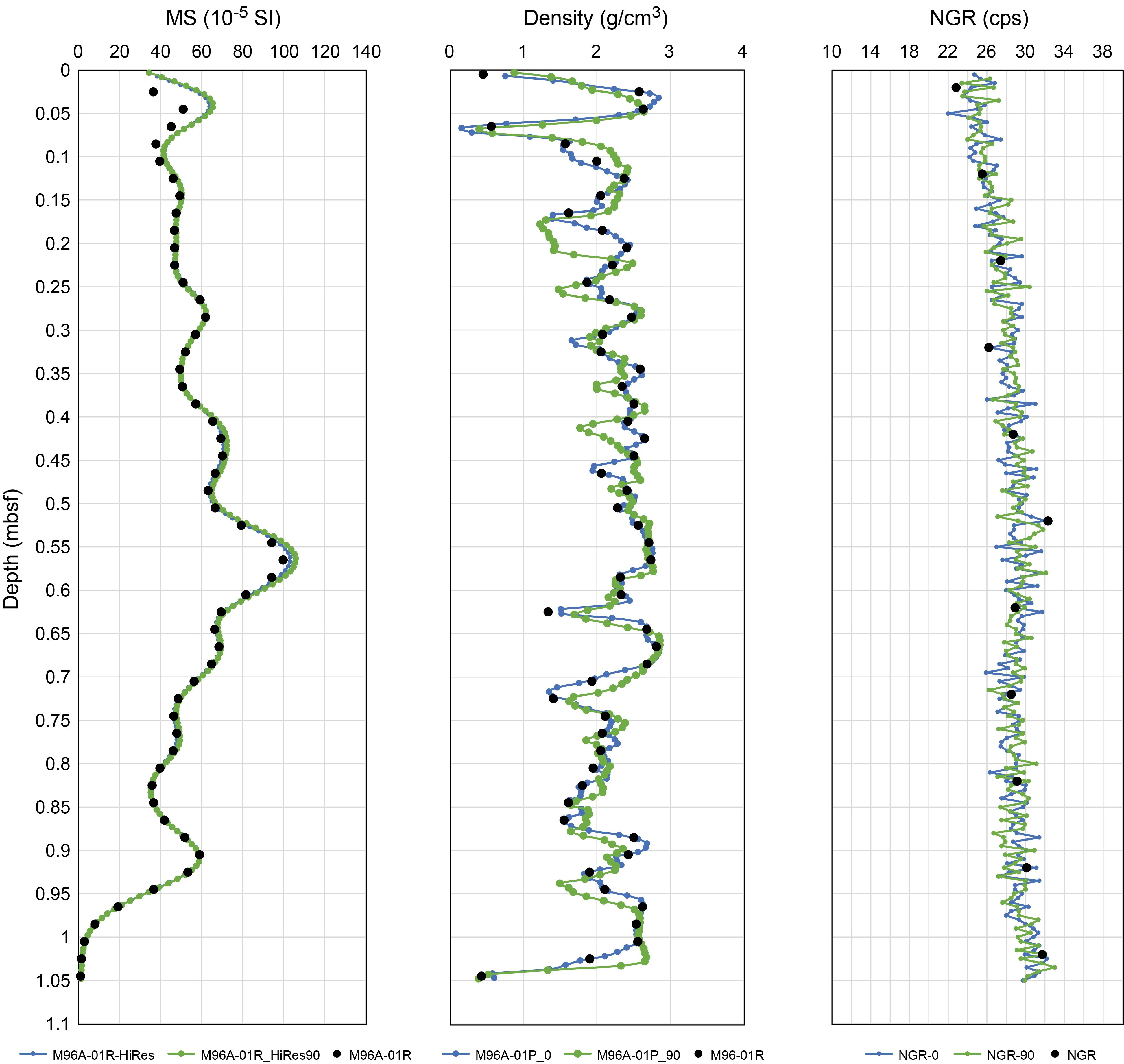
Figure F16. High- and low-resolution MSCL data sets.
3.1.3. Offshore QA/QC
QA/QC during the offshore phase involved regular calibration checks and thorough core quality assessments. Because of the nature of seafloor drilling operations, MSCL core measurements were run in batches. Calibration checks were conducted before each batch of core was logged and roughly every 6 h during a logging period. No calibration checks were performed during wait times. After a core section was logged, it was meticulously inspected. Any rubble, gaps, cracks, or other drilling-induced damage were recorded on a centimeter by centimeter basis. Data points collected over damaged core segments were removed from the final data set (Table T10). The percentage of data points retained for each section after QA/QC are listed in the table. The raw data sets, including all data points, were archived. In addition, data points recorded when a sensor’s field of influence reached beyond the end of a core section (magnetic susceptibility and NGR) were not included. Measurements over large-scale geological voids such as carbonate vugs (which have a similar sensor response to drilling-induced gaps) were retained.
3.2. Onshore petrophysical measurements
Most onshore measurements were taken at the BCR during the OSP. The one exception is X-ray CT scanning, which was performed on whole cores at the British Geological Survey (BGS) Core Scanning Facility (Keyworth, UK) in advance of the OSP. The X-ray CT images were utilized to determine the best orientation for splitting cores (see X-ray computed tomography). After the cores were split during the OSP, linescanning and color reflectance measurements were conducted on split core sections because it was necessary to do these measurements as soon after splitting as possible to preserve the integrity of the images and data. Because of the potential for nonsymmetrical structures in the cores, linescanning was performed on both the archive half and working half. Hyperspectral imaging of the split archive halves occurred after core description and was followed by thermal conductivity measurements. Lastly, P-wave velocity and moisture and density (MAD) measurements were conducted on discrete samples taken from the working halves.
3.2.1. Digital imaging
Digital linescan images of the split cores were obtained during the OSP using an Avaatech Superslit X-ray fluorescence (XRF) core scanner in operation at the MARUM. The XRF scanner was used as a linescan camera and linear light source; however, XRF measurements were not taken on the cores. The linescanner produces high-resolution color images. The Linescan Program uses the Stemmer Common Vision Blox platform to acquire and process color images.
The camera system contains a three charge-coupled device camera with beam-splitter and a manual controlled Pentax 50 mm lens. The image resolution is ~150 pixel/cm in the crosscore and downcore directions. With an exposure time of 5 ms, a scan speed of 125 mm/s was achieved. The image coverage is ~13.5 cm in the crosscore direction and a maximum of 153 cm in the downcore direction.
Every split core was imaged with a color and grayscale chart beside it. Four output files were generated for each core section: a high-resolution bitmap file (.bmp), a compressed image file (.jpg), a tagged image file format (.tif), and a numeric text file (.txt). Numeric data are in red-green-blue (RGB) units. The linescan system was calibrated every 24 h with black and white calibration with an aperture of f/11+. All split cores were measured using aperture setting f/11+ (a fixed value between 11 and 16). When cores were darker (e.g., in lava), the aperture was increased to up to f/5.6, and for lighter rocks (e.g., some corals) the aperture was decreased to f/13. Consistency of equipment settings was chosen over custom settings to ensure uniformity of the data set. Software features necessitated the length of linescan images to be a couple of centimeters longer than the curated core length. Because of this, the compressed image files were cropped to match the length of the cores after the image was taken. The numeric data files were corrected to the same length as the modified .jpg picture files. Both original and corrected files were uploaded to the database. All images were checked by the operator to ensure that the full core section had been captured and for general data quality of the scan.
3.2.2. Diffuse color reflectance spectrophotometry
Split halves were typically measured at 2 cm intervals using a handheld Konica Minolta spectrophotometer (Model CM-2600d). Interval spacing was adjusted appropriately depending on the nature of the core (i.e., the presence of rubble, vugs, and fractures) and commented on in the data report. Zero and white calibrations of the spectrophotometer were carried out when starting up the machine. Prior to measurement, the core surface was covered with clear plastic wrap to maintain a clean spectrometer window and prevent contact with the split core surface.
Spectrophotometric analysis produces three types of data:
- L*, a*, and b* values, where L* is a total reflectance index ranging 0%–100%, a* is the green (−) to red (+) chromaticity, and b* is the blue (−) to yellow (+) chromaticity;
- Munsell color values; and
- Intensity values for 31 contiguous 10 nm wide bands across the 360–740 nm interval of the light spectrum with a reflectance range of 0%–175% and a resolution of 0.01% (Minolta Spectrophotometer CM-2600d manual).
Measurements were taken with the instrument horizontal against the split core surface. The location of the measurement as depth in the section was recorded. Measurements were taken in the most visibly homogeneous areas at each depth downcore to obtain as pure a color reflectance signal as possible. When utilizing the spectrophotometric measurements, it is recommended that detailed examination of core photos/images and disturbance descriptions/tables is undertaken to cull unnecessary or spurious data. However, this screening process was minimized during the OSP measurements by targeting appropriate locations along the core for measurements with the handheld sensor.
3.2.3. Thermal conductivity
Thermal conductivity was measured with the TeKa TK04 system using the HLQ probe H11047 with a half-space line source for measurement of individual rock samples in half-space configuration (Von Herzen and Maxwell, 1959). The line source contains a heater wire and calibrated thermistor. It is assumed to be a perfect conductor because it is significantly more conductive than the samples it measures. The heating wire was covered in Wacker P12 thermal conductivity paste and probe surrounded by cling film to protect the core. Test measurements revealed the difference in results from measurements with and without paste and film to be negligible. The probe is heated for 80 s, and the temperature is recorded. Five measuring cycles are generally recorded with a 10 min pause between measurements. Archive split cores were measured at room temperature (20°–22°C) in the core description room during the OSP.
Generally, the coefficient of thermal conductivity (k, [W/(m·K)]) is calculated from the following equation:
- T = temperature (K),
- q = rate of heat flow through the material (W/m), and
- t1 and t2 = time interval (80 s duration) along the heating curve(s).
The correct choice of t1 and t2 is complex. Commonly, thermal conductivity is calculated from the maximum interval (t1 and t2) along the heating curve where k(t) is constant. In the early stages of heating, the source temperature is affected by the contact resistance between the source and the full space, and in later stages, it is affected by the finite length of the heating source (assumed infinite in theory). The special approximation method employed by the TK04 software is used to develop a best fit to the heating curve for all time intervals where 20 ≤ t1 ≤ 40, 45 ≤ t2 ≤ 80, and t2 − t1 > 25.
A good measurement results in a match of several hundred time intervals along the heating curve. The best solution (the output thermal conductivity) is that which most closely corresponds to the theoretical curve. Numerous measuring cycles were automatically performed at each sampling location, and, when obtained, the best five were used to calculate an average thermal conductivity.
Thermal conductivity measurements were generally taken every 10 m, and cores were sampled at locations with even surfaces to increase rock contact with the HQL probe. Most of the Expedition 389 cores were reef limestone and vesicular lava. Their uneven surface caused by void spaces in the rock prevented successful measurements of thermal conductivity in some sections. Sections on which thermal conductivity was measured successfully are listed in Table T11.
3.2.4. P-wave velocity from discrete samples
P-wave velocity on discrete samples was measured using a GEOTEK velocimeter. The equipment consists of two ultrasonic transducers, one transmitter, and one receiver, between which the sample is placed. A mechanical vise holds the transducers in place and applies nominal downward pressure. A laser distance meter measures the space between transducers (i.e., the length of the sample). The transmitter emits a 230 kHz acoustic pulse that travels through the sample to the receiver. The P-wave arrival time is picked automatically on a virtual oscilloscope that displays the digitized waveform with a sampling frequency of 12.5 MHz. From the P-wave traveltime and the measured sample length (l), the P-wave velocity can be calculated: Vp = l/tp. Traveltime offsets due to electronic delays, P-wave travel through the transducer endcaps, and picking methods are accounted for through zero-distance calibration.
Acoustic measurements were performed on cylindrical core plugs drilled roughly every 1.5 m perpendicular to the split surface of the working halves. P-wave velocity was measured first wet straight after sampling (initial), again after the samples had been dried in a convection oven at 105° ± 5°C for 24 h (dry), and then once more after being resaturated. Resaturation of the core plugs and the additional measurements took place post-OSP at the University of Leicester (UK). A desiccator-vacuum pump setup was used to flood the dry plugs with tap water. The plugs were fully submerged in water inside the desiccator, which was then placed under a vacuum for at least 24 h. The vacuum helped to extract any air trapped in the pore space and replace it with water. Full saturation may not have occurred in all samples due to difference in permeability among the sampled lithologies.
3.2.5. Moisture and density
MAD properties (bulk density, dry density, grain density, water content, porosity, and void ratio) were determined from measurements of the wet and dry masses of the sampled core plugs as well as their dry volumes.
Discrete samples were taken for both MAD and P-wave velocity measurements from the working-half sections (the same sample was used for both measurements). Where core quality allowed, samples were taken at an interval of 1 per core section. It was not possible to document or ensure that all core plugs were completely uncontaminated by fluid inundation during the core splitting and sampling process. Immediately after the initial P-wave measurements, the samples were transferred into previously weighed glass beakers. However, in areas of unconsolidated sediment, 3–15 cm3 samples were collected for only MAD measurements.
The wet samples and beakers were weighed to a precision of 0.001 g using an electronic balance (Mwet). Afterward, samples were dried in a convection oven at 105° ± 5°C for 24 h, followed by cooling to room temperature in a desiccator. Dry sediments were successively weighed (Mdry), and their volume (Vdry) was measured using a Quantachrome pentapycnometer (helium-displacement pycnometer). This equipment allowed the simultaneous analysis of four different samples and one standard (calibration spheres). Volume measurements were repeated a maximum of five times or until three consecutive measurements exhibited <0.01% standard deviation with a purge time of 1 min. Volume measurements were averaged per sample (Vdry). Calibration spheres were cycled from cell to cell of the pycnometer during each run to check for accuracy, instrument drift, and systematic error. Under optimal conditions, this technique has a precision of <0.02 cm3. However, in-run checks of the calibration spheres showed that they required frequent calibration, with individual runs varying by 0.04 cm3 or more from the known volume of the calibration spheres. Because of this, a precision of ± 0.05 cm3 was conservatively applied to the pycnometer measurements for Expedition 389 samples.
The mass of the evaporated pore water (Mpw) is given by
The volume of pore water (Vpw) is given by
where dpw = pore water density at standard laboratory conditions (1.024 g/cm3 and 3.5% salinity).
Salt precipitated in sample pores during the drying process is included in the Mdry and Vdry values, resulting in the following approximations:
- The mass of solids including salt (Msolid) is given by the dried mass of the sample (Mdry = Msolid).
- The volume of solids including salt (Vsolid) is given by the measured dry volume from the pycnometer (Vdry = Vsolid).
- The wet volume (Vwet) is given by Vwet = Vsolid + Vpw.
For all sediment samples, water content (w) is expressed as the ratio of the mass of pore water to the dry sediment (total) mass:
Wet bulk density (w), dry bulk density (d), sediment grain density (g), and porosity (φ) are calculated with the equations below using the values calculated with the previous equations:
Porosity values derived from MAD measurements may be underestimated, particularly in coral-dominated lithologies and volcanic lithologies. This is a consequence of the high permeability of these lithologies and the transfer process from liners. Both cause fluid to drain from the core material during the weighing process. Finer grained sediment samples are less susceptible to such draining, and as such, the porosity estimates are more accurate. Grain density is associated with the highest level of confidence because it is independent of water content.
3.2.6. Hyperspectral imaging
Hyperspectral imaging was introduced into the core flow of the OSP to provide near–real time carbonate mineralogical maps (see example of Section 389-M0099G-14R-1A in Figure F17). These maps were intended to facilitate targeted sampling of pristine aragonitic material from coral skeletons (reflecting well-preserved corals) and to identify intervals affected by various levels of diagenesis (e.g., calcite cements, recrystallization, bioerosion, and encrustation by microbialite, calcareous red algae, and other organisms).
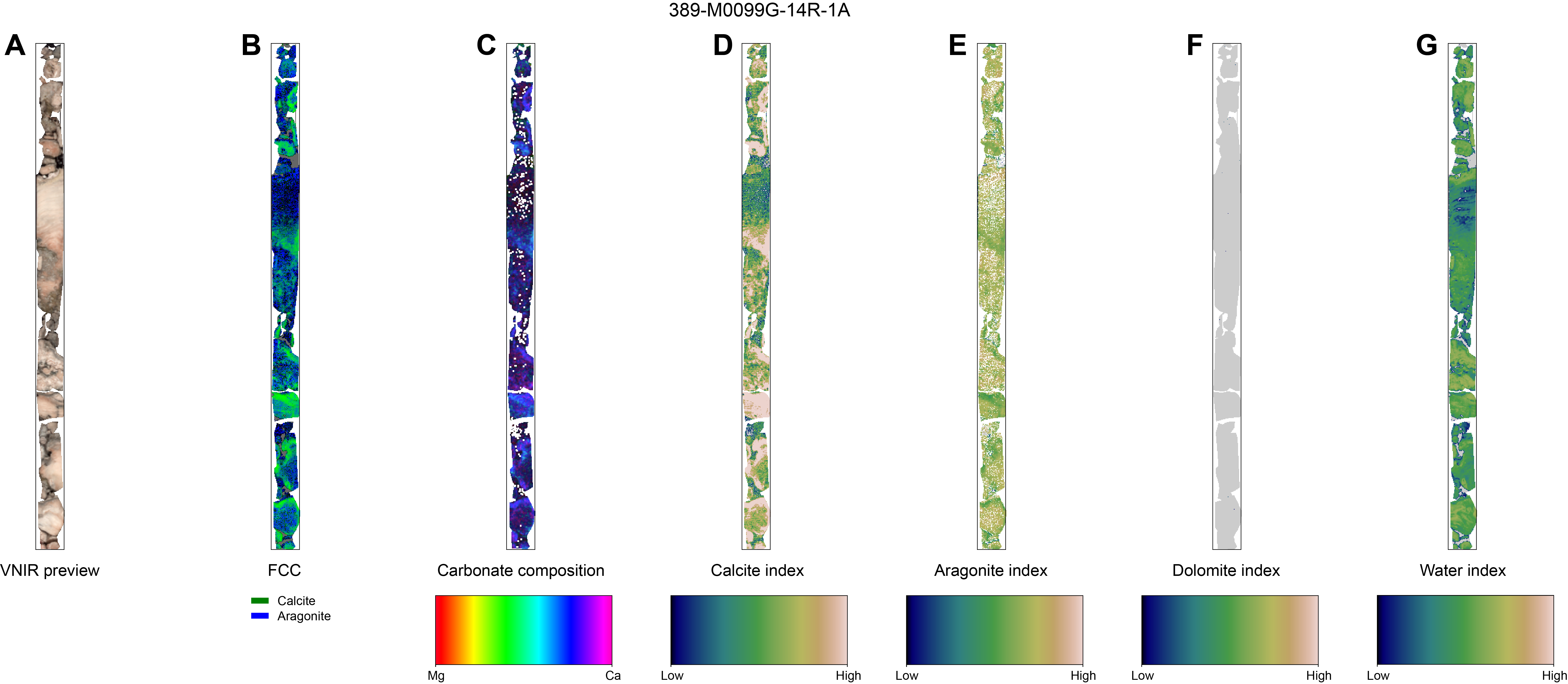
Figure F17. Carbonate maps produced using hyperspectral scanning.
Hyperspectral data were acquired on all archive halves using a SisuROCK drill-core scanner (Spectral Imaging Ltd., Oulu, Finland). The SisuROCK is a fully automatic hyperspectral imaging workstation that employs a moving table that moves the archive halves under the illumination source and field of view of the hyperspectral cameras. It is equipped with an AisaFENIX hyperspectral sensor. The AisaFENIX camera implements two sensors to cover the visible and near-infrared (VNIR) and short-wave infrared (SWIR) regions of the electromagnetic spectrum. Sensor specifications and acquisition settings are presented in Table T12.
QA/QC routines developed and established by TheiaX (Lorenz et al., 2019) were run prior to sample analysis to calibrate the spectra and sensor response. Prior to each scan, the sensor’s dark-current and a precalibrated PTFE Spectralon panel were measured. These are used for the conversion from digital numbers to radiance and from radiance to reflectance.
So-called white and gray reflectance panels were used as diffuse reflectors for better signal quality. The white reflectance panel generally has a reflectivity of >95% from 250 to 2500 nm. It was used for cores from Sites M0096 and M0098, as well as for Holes M0097A–M0097C, M0099A–M0099C, and M0099E. Despite extensive efforts to dry the core surface prior to scanning, residual water remained and negatively impacted signal acquisition. The gray reflectance panel with a reflectivity of >50% from 250 to 2500 nm helped to mitigate this issue and improve signal quality. The acquisition settings were adjusted for each panel (Table T12). The paleoclimate coral slabs were scanned with the white reflectance panel because they had been dried in the oven at 40°C for 24 h.
Geometric corrections to correct for sensor-specific optical distortions such as fish-eye effect, slit-bending effects, or line distortions were also applied. This yielded clear spectral absorption features, which occurred due to specific charge-transfer or molecular vibration processes (e.g., AlOH, FeOH, MgOH, CO3, and OH). Accurate discrimination of different mineral species was identified from these spectral signatures (Clark, 1999), which in the case of carbonate minerals was done by mapping the presence (or absence) and the exact wavelength of specific absorption features at ~2330 nm.
The hyperspectral imaging data for this expedition were analyzed using an adapted approach of a well-established method for spectral feature analysis (Bakker et al., 2011). Initially, the position and depth of diagnostic absorption features were mapped by applying a multiple minimum wavelength mapping technique (Thiele et al., 2021). This information was then used to interpret the presence or absence and relative abundance of carbonate minerals, clays, and FeOH–silicates. Because the core surface was too wet for standard hyperspectral characterization, a water index was derived following the same approach to quantify and monitor the degree of water present on the core surface. Compositional changes of carbonate minerals, going from Mg- to Ca-rich carbonates, were also mapped by evaluating the wavelength position from shorter to longer wavelengths. This approach allows for the identification and mapping of the spatial distribution of dolomite, aragonite, and calcite at a resolution of 1.5 mm/pixel. Finally, for an easier comparison of the calcite and aragonite mapping, a false color composite of the two was generated.
3.3. X-ray computed tomography
X-ray CT imaging helps to identify key structural and sedimentological features (e.g., diagenetic alteration, bioerosion, and sediment infilling) and, importantly during Expedition 389, enable determination of the optimal orientation for core splitting and coral slabbing. This ensured that the massive and columnar coral samples were prepared in a way that maximized the quality and quantity of data obtained from them. Coral paleoclimate scientists reviewed each X-ray CT image of every high-priority core section to identify the most promising massive and columnar Porites coral samples (see Identification of massive and columnar corals by CT scans). This selection process focused on choosing samples of the highest quality that met the specific requirements for paleoclimate analysis while also preserving materials for other expedition-related sampling and scientific objectives.
3.3.1. X-ray CT scanning
X-ray CT scanning for Expedition 389 was conducted at the BGS Core Scanning Facility in Keyworth (UK). The cores were delivered in two shipments, each housed in a 20 ft refrigerated container maintained at 4°C throughout transit. The first cores arrived on 2 January 2024, followed by the second on 7 February. To minimize the time exposed to higher temperatures, the cores were stored in the refrigerated container except during scanning sessions. Each session was kept to a maximum of 5 h to minimize thermal disturbance.
The cores were scanned using a GEOTEK Rotating XCT core scanner, which featured a rotating source detector assembly tailored for fragile sediment cores that cannot withstand rotation. During this process, the core sample was placed on a tray that moves horizontally past a rotating X-ray source-detector assembly. This setup enabled the execution of multiple scans from different angles, culminating in a full 3D data set made up of individual slices (i.e., reconstructed images that are perpendicular to the axis of the core). During the initial phase of scanning (before 12 January), the scanning orientation of the cores was random. After this period, each core was aligned according to offshore alignment markers on the core liner, with blue (top) and red (bottom) liner lids indicating orientation. Scanning was conducted according to a priority order (3, 2, 1, and 0) as set out by the offshore science party (see Identification of massive and columnar corals by CT scans). Cores designated as high priority (Priority 3) were scanned at a high resolution (with a pixel size of 0.254 mm), whereas those of Priority 2 were scanned at either a high or lower resolution (with a pixel size of 0.508 mm) depending on time constraints, and lower priority cores (1 and 0) underwent faster, low-resolution scanning. The instrument’s settings were adjusted based on the type of material (i.e., lava or carbonates) and the desired resolution for the scan (Table T13). Each high-resolution scan of a 150 cm core section generated approximately 16,750 axial slice images (Figure F18), with each slice being 0.089 mm thick. Additionally, a radiograph at 0° was also produced for each core section scan. Data were stored as a Tagged Image File Format (TIFF) images.
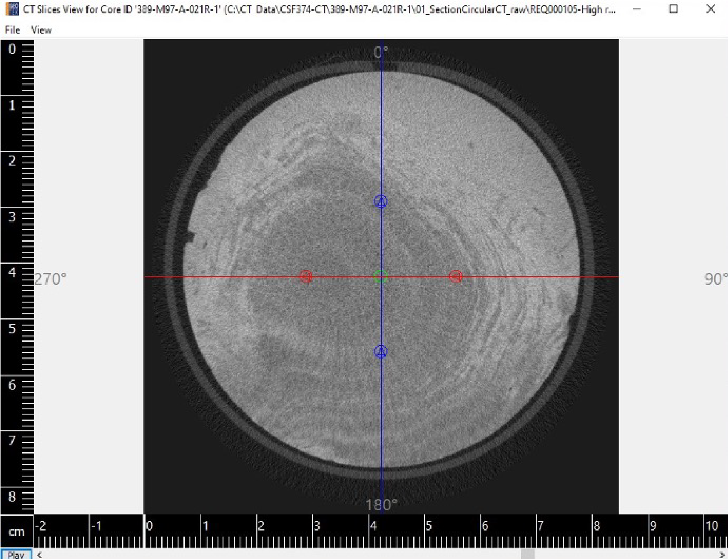
Figure F18. X-ray CT slice view.
3.3.2. X-ray CT data processing
Raw data were processed at the BGS Core Scanning Facility. Utilizing the axial slice images and the X-ray radiograph collected through CT scanning, full 3D reconstructions of the core were produced using the GEOTEK Reconstructor software. This software is designed to manage data volumes in a queue, facilitating the stitching of multiple sequential volumes to create a complete whole-core data volume. This process also produced orthogonal views (exported as a 16-bit stacked TIFF file) (Figure F19) and dynamic visualizations that navigate through the core’s internal structure. Further refinement of the 3D reconstruction is achieved through the use of the GEOTEK program LASARUS, which is specifically designed to reduce artifacts resulting from the joins between different scan jobs. However, it was observed that in some instances, the program’s adjustments could overcorrect, inadvertently introducing more artifacts. All adjustments were reviewed, and in such cases adjustments made by LASARUS were discarded. For the visualization of the core’s 3D structure, the GEOTEK CT Quick View software was employed. This tool enables the loading and manipulation of slice images, providing a detailed exploration of the core’s internal features. When required, slice images were utilized to ascertain the orientation of cores that had been scanned at random orientation, provided the cut in the core liner was visible.
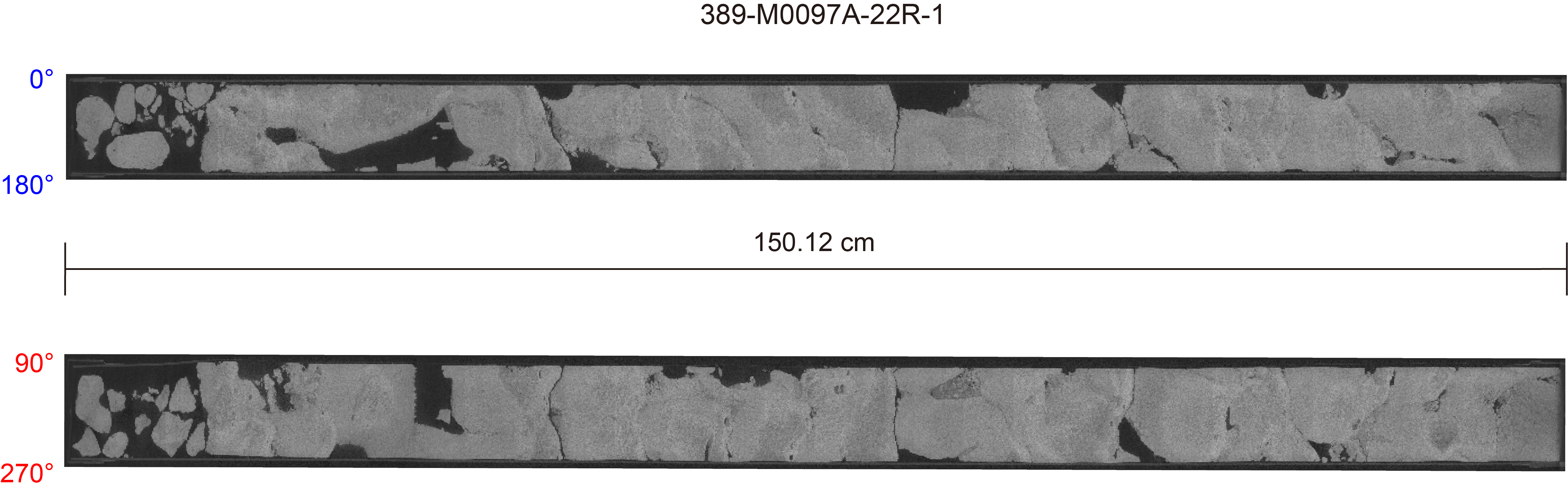
Figure F19. X-ray CT orthogonal views.
3.3.3. Identification of massive and columnar corals by CT scans
Corals (e.g., massive and columnar Porites) suitable for paleoclimatic studies were initially identified in core sections through the transparent liners or after aluminum liners were split off shore (see Introduction) and from descriptions contained in the offshore VCDs. Those sections containing corals with promising paleoclimate application were identified to prevent them from being split using the regular unoriented core splitting procedure and to aid in preliminary sample requests prior to the OSP. The major goal was to recover pristine, long, continuous intervals of coral skeletons from individual colonies along the major axis of growth because the regular IODP core splitting procedure does not take into account the major growth direction of coral colonies. The core axis, or holes within a colony as a result of bioerosion, can be different from the major growth direction and can interrupt an otherwise continuous interval of the coral skeleton. Therefore, with approval from the Sample Allocation Committee (SAC), some cores, identified by a core splitting subteam, required rotation with respect to the regular core splitting orientation.
Results from the X-ray CT scans were used to determine density bands and growth direction as well as possible alteration (e.g., diagenesis and intense bioerosion) in the cores that contained sections for paleoclimate studies. If the major axis of growth did not align with the standard IODP cutting orientation (i.e., along the 90°–270° plane) (Figure F20), an alternative orientation was identified in the X-ray CT scans using the Geotek Quick View software. The orthogonal views were exported as TIFF files (see IMAGES in Supplementary material) and printed as screenshots, and the preferred orientation was noted (Table T14). These core sections were marked with a red tape X prior to splitting, and the core splitting team directly consulted with nominated paleoclimate scientists prior to splitting these cores. Assessments based on the X-ray CT imagery were confirmed by visual inspection. When possible, the cores were rotated with respect to the plastic liner cut to the preferred orientation. If the X-ray CT image indicated that no special rotation was necessary or that the promising coral samples were influenced by diagenesis and/or poor growth banding, the X was removed. Once the cores were split, a 0.8 to 1 cm thick slab was cut from the sections designated for paleoclimate studies, with a second slab sometimes cut for other research purposes, such as dating or geochemical analyses, upon approval from the SAC. After cutting, the coral slabs were jet-washed, air-dried for about 12 h, and then oven-dried at 40°C for 12–24 h with the samples stored in labeled, heat-sealed bags for distribution to science party members.
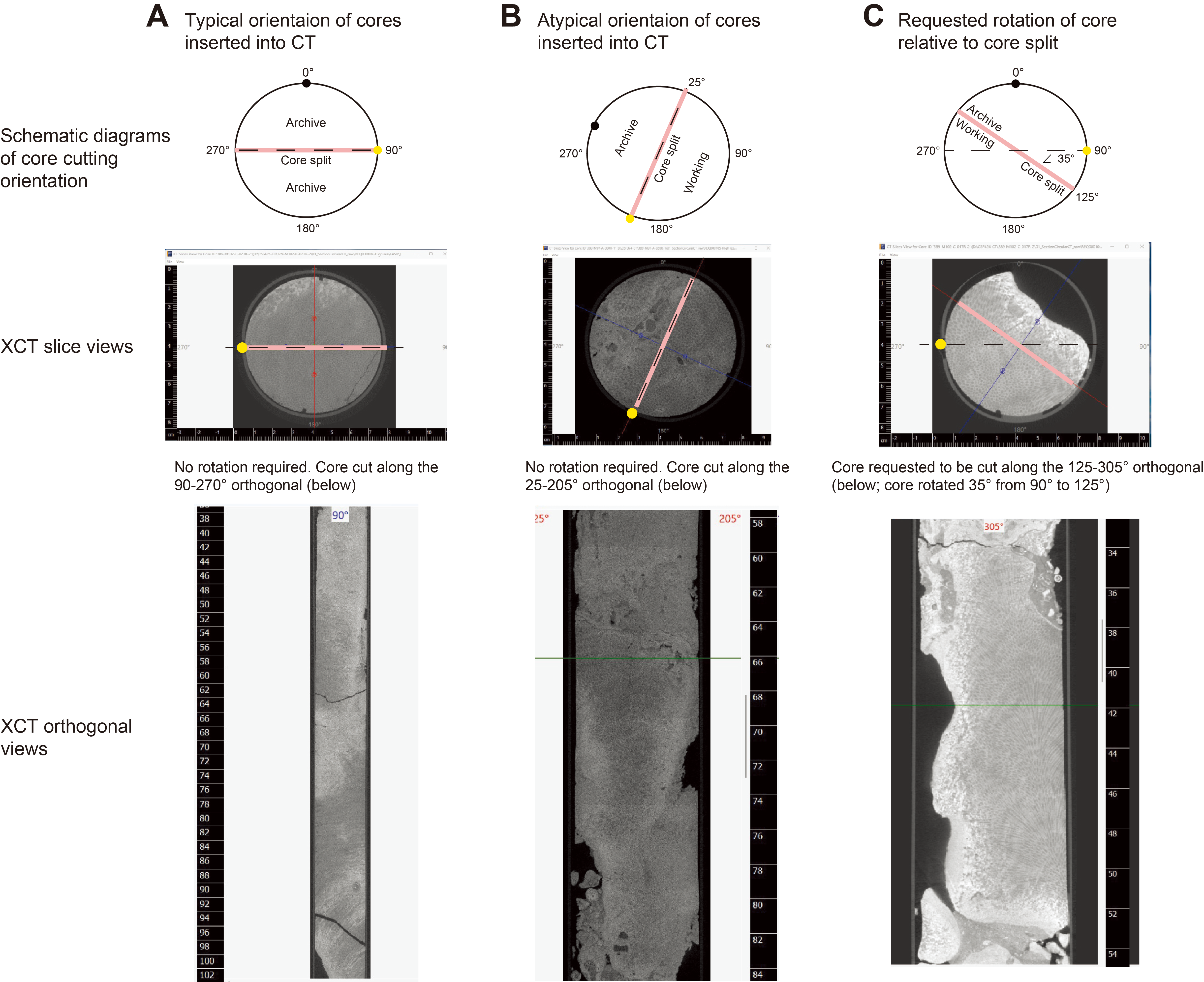
Figure F20. Core splitting orientations.
4. Geochemistry
4.1. Shipboard sampling procedures
4.1.1. Interstitial water sampling using Rhizon samplers
Where soft sediments were recovered, Rhizon samplers were employed during Expedition 389 to sample IW (Seeberg et al., 2005) (see Introduction). A total of 41 IW samples were collected, of which 5 did not have sufficient water volume for further analysis, leaving 36 samples that were measured for salinity, alkalinity, pH, and/or ammonium on board and/or cations and anions on shore (Tables T15, T16). The Rhizon sampler type used (CSS 5 cm; Rhizosphere Research Products, Netherlands) consists of a 5 cm microporous ceramic tube that is supported by a glass fiber strengthener and connected to a 13 cm polyethylene/polyvinylchloride (PE/PVC) tubing terminated with a female Luer connector so it can be easily attached to needles or syringes.
Before use, Rhizon samplers were prepared by immersing the microporous (white) tube end in a beaker of purified laboratory water (>18 MΩ) for a minimum of 30 min, after which the microporous tube was no longer air-permeable. The microporous tube had a pore width of 0.2 µm, so additional filtering was not needed.
A 3.8 mm diameter hole was carefully drilled in the liner at the depth of interest in a core with unconsolidated sediment. To avoid contaminating the sediment with the tip of the drill, the tip was cleaned with ethanol between sampling points. Where needed, a channel was preformed with a plastic knitting needle. The Rhizon sampler was gently pushed into the sediment all the way to the connector between the microporous tube and PE/PVC tubing. The connector was then used to seal the 3.8 mm hole where possible.
The blue protective cap from the Rhizon sampler was disconnected, and the Rhizon sampler was then connected to a new 24 mL all-plastic disposable sterile syringe. The plunger was slowly pulled back to create a vacuum and fixed with a wooden spacer provided with the Rhizon sampler to apply negative pressure. The Rhizon sampler was left in this position for a minimum of 2 h (Figure F21). All syringes and Rhizon samplers were used only once.
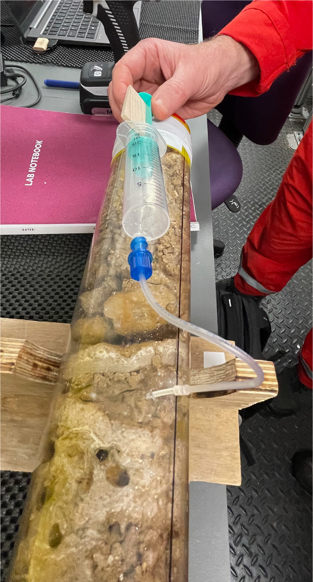
Figure F21. IW sampling using a Rhizon sampler.
Once collected, the ceramic tube was removed, air was pushed out of the syringe, and the opening on the syringe was closed with a blue Luer-lock plastic cap. Each IW sample was taken in the syringe to the geochemistry container for processing into splits for offshore and onshore analysis.
4.1.2. Seawater sampling
A total of 16 surface seawater (SSW) samples were collected, with one SSW sample from each site except Site M0099, where two samples were recovered. Each SSW sample was measured for alkalinity, pH, salinity, and ammonium on board the ship, with the SSW sample from Site M0103 measured in duplicate (Table T17). Samples during both legs of Expedition 389 were collected by hand-lowering a water sampling device overboard, filling it with ambient surface water, and recovering it to the ship. On deck, the sampling device was immediately covered with a clean plastic bag. The water sampling devices differed during Legs 1 and 2 (Figure F22). During Leg 1, samples were collected using an improvised device with approximately 1 L volume. During Leg 2, samples were collected in a 2 L Niskin bottle with manual closures, supplied by the University of Hawai'i (USA). Each device was washed multiple times with purified laboratory water (Elga Purelab Classic UV; >18 MΩ) after use and stored cleaned with a plastic bag over the inlet. Note that Site M0099 was drilled during both legs, and therefore the first sample was collected from Hole M0099A using the improvised device and the second one was recovered from Hole M0099G using a Niskin bottle.
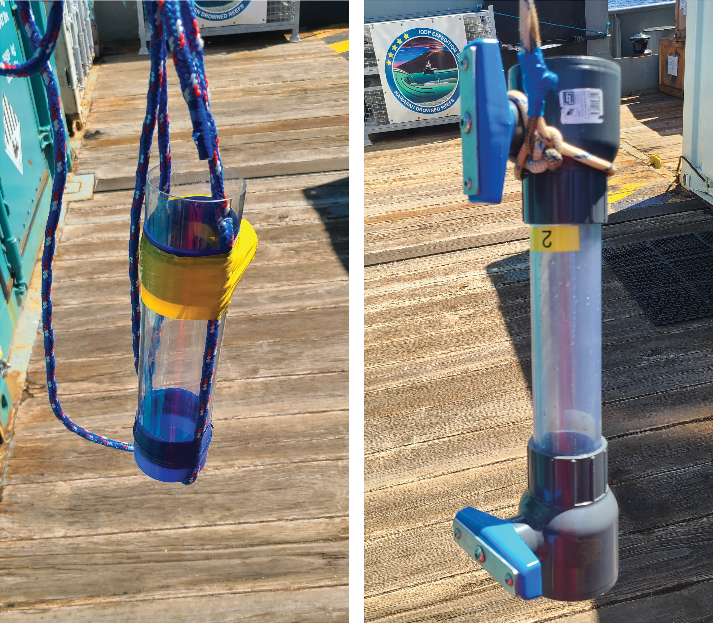
Figure F22. SSW sampling devices.
A sequence of water sampling photos using the Leg 2 device shows the basic actions of sampling (Figure F23). The device was deployed overboard with the bottom manual control valve in the closed position and the upper manual control valve in the open position. Care was taken to avoid interaction of either sampling device with the side of the ship. The cast was retaken if the bottle touched the ship at any point during a deployment.
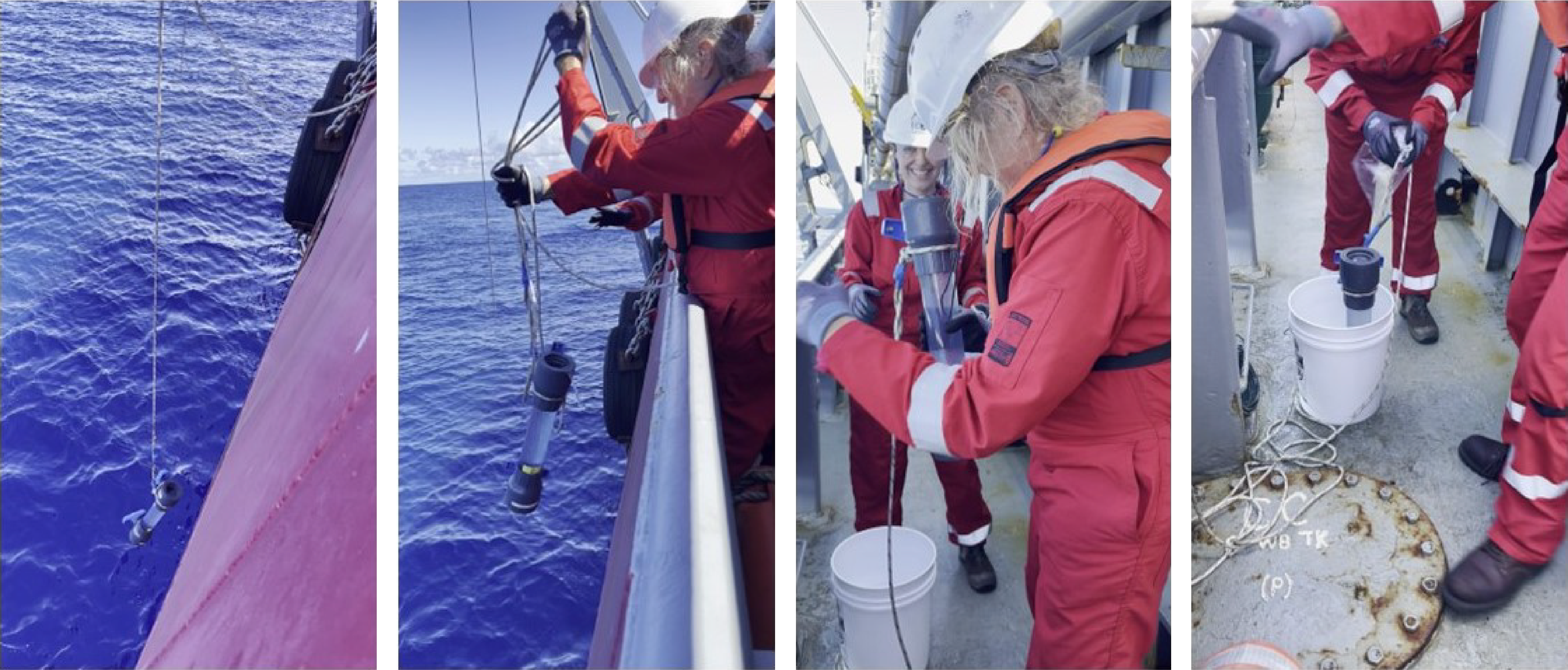
Figure F23. Seawater sampling.
Care was also taken during seawater sampling to avoid contamination from the ship (i.e., avoiding times of known discharges from the vessel or when aluminum liner cutting was in-progress on deck) and was done during daytime for safety reasons and better visibility. Occasionally, cloudy water was observed off the port or starboard sides of the ship, and sampling was delayed or moved to the other side of the ship to avoid these plumes. Seawater samples were taken into the geochemistry container, immediately decanted into an acid-washed 1 L high-density polyethylene (HDPE) beaker, and stored in a refrigerator for subsequent filtration and splitting into subsamples. Each SSW sample was logged into the mDIS database, and the time of sample collection was noted.
4.1.3. Sample splitting
IW and SSW sample splitting followed the agreed plan that included as many as 8 (IW) or 10 (SSW) fractions, depending on collected volume, for offshore, onshore, and postcruise analyses (Table T18).
The sample splits dedicated to onboard analysis were analyzed shortly after recovery (Tables T15, T18; see Table T2 in the Expedition 389 summary chapter [Webster et al., 2025]). The splits dedicated to further analysis on shore during the OSP or later during postcruise research were stored at 4°C (Table T16).
4.1.4. Pure water generation
Purified water (Elga Purelab Classic UV; >18 MΩ) was produced by ESO before the expedition and transported in acid-cleaned and thoroughly rinsed 10 L PE containers for use during offshore sampling and analyses.
4.1.5. Potential effects of drilling on sample quality
During IW sampling, precautions to avoid contamination were carefully followed. In many cases, the cores showed clear visual evidence of several drilling-related materials on the outer part that potentially could contaminate the IW samples, including white drilling mud (most evident on lava cores), aluminum shards (abundant in all cores and subsamples when aluminum core liners were used), and red grease (drill barrel connector lubrication), which was smeared on some cores and subsamples. These materials were manually removed as best as possible during subsample preparation. Aluminum shards were manually removed with tweezers, and drilling mud and grease were removed by washing with purified water. To help identify possible contamination, the drilling contractor (Benthic) provided six types of references of greases, fluids, drill mud, and hydraulic oil used on the drill barrels and during the drilling process.
Additionally, the majority of the cores were recovered in aluminum liners, which were cut open and transferred to plastic liners before IW sampling. Where no sample preservation methods were applied (e.g., acidification for subsequent cation measurements), the maximum duration between offshore sampling of IW and IODP standard measurements at the OSP was 145 days.
4.2. Offshore interstitial water and surface seawater analysis
4.2.1. Sample temperature
In situ temperatures of the IW and SSW samples could not be determined. Temperatures in the geochemistry container where the samples were stored between collection and measuring at the OSP were mostly stable, ranging 19.6°–21.5°C.
4.2.2. pH
The pH of samples was measured with a Mettler Toledo In-Lab 423 microcombination glass electrode with a 3 mm tip connected to a Radiometer TIM840 Autotitrator. The pH (and alkalinity, see below) were determined from 0.5 mL of sample in 2 mL Eppendorf vials. A constant reading was achieved by turning the vial around the electrode with a magnetically driven vial holder rather than stirring the sample with a stir bar. The pH meter was calibrated once a day using AppliChem color-coded National Bureau of Standards (NBS) scale pH buffer solutions of pH = 4.01 and 7.00. The instrument shows the pH with a resolution of 0.001 pH units, and the measurement has an accuracy of better than ±0.02 pH units. For pH measurement, temperature compensation was performed using the container temperature, which was measured with an external pt1000 T-sensor temperature sensor. Because measurements were performed in 1.5 or 2.0 mL Eppendorf vials, temperatures were expected to be equilibrated to ambient temperature. In certain weather situations, however, the air conditioning in the container van failed, causing the ambient temperature to rise well above 25°C. Measurements under such circumstances were avoided but, if they were unavoidable, were noted.
4.2.3. Alkalinity
Alkalinity for SSW and IW was determined by titration with 0.01 M HCl, where the equivalence point was detected by titrating known amounts of sample (usually 0.5 mL) while measuring the pH value. A Radiometer TIM840 Autotitrator with a 5 mL burette was used for titration and stopped at pH < 3.95. The algorithm used to calculate alkalinity accounts for the activity of seawater and dilution by the titration solution so that the results are comparable for different end point pH values. The measurement has an accuracy of better than 0.2 mM. For the titration, a 0.3 mm internal diameter polytetrafluoroethylene (PTFE) tube from the digital burette was placed in the liquid before the titration started. Both the PTFE tube and the pH electrode were rinsed with pure water and carefully dried with laboratory tissues before the measurement. The algorithm is a corrected version of the algorithm of Grasshoff et al. (1983, 1999):
- pHinitial = original pore water pH,
- pHfinal = pH at end point of titration (usually pH = 3.95),
- ƒH+ = activity coefficient of H+ (for standard seawater this is 0.755),
- cHCl = concentration of titration solution (usually 0.01 M),
- VHCl = titration volume depending on alkalinity of sample, and
- V0 = initial volume of sample (usually 0.0005 L [500 µL]).
4.2.4. Ammonium
Ammonium was measured using the PTFE tape gas separator technique, as described in the curation container manual (modified after Hall and Aller, 1992). With this technique, ammonium is stripped from a 100 µL sample by an alkaline carrier solution (0.2 M sodium citrate in 10 mM NaOH) passing a 200 mm × 5 mm PTFE membrane as ammonia (NH3), and redissolved as NH4+ in an acidic solution (1 mM HCl). The NH4+ causes a conductivity signal in the acidic carrier that is detected with an Amber Science 1056 conductivity meter with a model 529 temperature-compensated microflow-through cell. The conductivity signal was recorded with a Knauer stripchart recorder, and peak height was analyzed manually. This method is very precise and stable, practically insensitive to matrix changes, and shows a linear conductivity response for ammonium concentrations between 10 and 1000 µM. The detection limit is 5 µM, and accuracy is <2%. All SSW samples were below the detection limits for ammonium.
Generally, measurements were made on the original sample, which was only diluted if the sample volume was extremely low or the ammonium concentration exceeded the calibrated range (>1.6 mM). Ammonia calibration standards were freshly prepared off shore from a 55.6 mM (1000 ppm) certified standard solution using artificial seawater as a matrix.
A 200–300 µL sample split was taken from the primary sample vial with a Hamilton 1000 µL precision glass syringe and injected onto a 100 µL loop with a Rheodyne high-pressure liquid chromatography valve using the extra sample amount to flush the loop. The valve was then opened to the carrier solution stream to start the analysis. The Hamilton syringe was rinsed with pure water twice, before and after analysis.
4.2.5. Salinity
Salinity was optically measured using a Krüss Optronic digital refractometer DR6200. The measurement precision for the refractometer is 0.1%, so the data can only be used to detect samples with salinities that differ significantly more than 0.1% from seawater (i.e., 4 practical salinity units [psu] on seawater with a salinity of 35 psu). The refractometer was calibrated externally by measuring International Association for the Physical Sciences of the Ocean (IAPSO) standard seawater with salinity values of 10, 30, 35, and 38 and with purified water (>18 MΩ) as standard for zero salinity.
4.2.6. Headspace gas sampling
No standard headspace sediment gas samples for methane were collected during the offshore phase of Expedition 389 because no feasible core sample material for this sampling approach could be identified during the initial curation process on deck (core retrieval from the barrel, sectioning, and section liner transfer).
4.3. Onshore analysis of interstitial and surface seawater geochemistry
The concentrations of elements were measured in the IW and SSW samples to complement shipboard analyses (Expedition 302 Scientists, 2006). Analyses were carried out with the assistance of the technical staff and analytical facilities at the University of Bremen. The anions chloride, bromide, and sulfate were measured using ion chromatography, and a suite of major and trace elements (Al, B, Ba, Ca, Fe, K, Li, Mg, Mn, Na, S, Si, and Sr; cations) was analyzed using inductively coupled plasma–optical emission spectrometry (ICP-OES).
4.3.1. Cations measured using inductively coupled plasma–optical emission spectrometry
Dissolved cations were measured using a Varian Vista PrO simultaneous ICP-OES. Cation aliquots of IW and SSW samples used for these analyses were acidified directly on board following shipboard sampling with 1% (10 µL acid/1 mL sample) of concentrated trace metal grade HNO3.
During the OSP, IW and SSW aliquots were diluted 1:10 for measurements of Al, B, Ba, Ca, Fe, K, Li, Mg, Mn, Na, S, Si, and Sr using a 1.0% HNO3 solution (prepared with trace metal grade nitric acid and >18 MΩ water). Major and trace elements were analyzed using a Seaspray nebulizer with humidified Ar and a cyclonic spray chamber. Measurements of the intensity at each wavelength were performed in triplicate. The wavelengths used for the different elements are shown in Table T15.
In all cases, standardization was done against multielement solutions prepared from commercial single element standards (Table T15). Measurement precision was estimated by five repeated measurements of IAPSO standard seawater, salinity of 35.9, and three repeated measurements of IW sample. Precisions on the standard and repeats were between <1% and 7% (2 standard deviation [SD]) for different elements. Accuracy for major elements was established from the repeated measurements of the IAPSO standard seawater, as per the precision measurements, and comparison of those measurements to published literature values. Accuracy was better than 5% for most elements, with the exception of Li, which was 12% lower than recent literature values (Steiner et al., 2022) (accuracy factors in Table T15).
4.3.2. Anions measured using ion chromatography
Nonacidified aliquots of the samples were diluted 1:100 using purified water (>18 MΩ). Concentrations of Cl, Br, and S were measured using an 861 Advanced Compact ion chromatograph with Sequential Compression by Metrohm AG and an IC-Anion column Metrosep A Supp 5 (100 mm run length) in the Department of Geosciences at the University of Bremen. Measurement precision (2 SD) for Cl, Br, and S was better than 4%. Dilutions of IAPSO seawater served as a certified reference material. Calibration standards were prepared from certified commercial single-anion standards (CertiPUR by Merck).
Data for all water analyses are given in Tables T16 and T17 (see GEOCHEM in Supplementary material).
4.4. Onshore analysis of bulk sediments and rocks
Mineralogy, bulk elemental composition, and carbon content of sediment or rock were measured on samples taken approximately every 3–6 m for all holes. The lithology for each sample is recorded in the tables in Geochemistry in each site chapter and uses the lithology recorded on the VCDs. Sampling of massive or columnar corals was avoided where possible. All geochemical analyses on the sediment and rock samples were performed on shore in the Department of Geosciences at the University of Bremen.
4.4.1. Mineralogy using X-ray diffraction
Mineralogy samples were dried in an oven at 105°C, crushed in an impact mortar, and ground in an agate mortar or ball mill to ensure sample homogeneity and a grain size of <20 µm so as not to introduce mineral orientation biases during X-ray diffraction (XRD) measurement. XRD powder diffraction measurements were performed on a Bruker D8 Discover diffractometer equipped with a Cu-tube (Kαλ 1.541; 45 kV; 40 mA), a fixed divergence slit of 0.25°, a 90 sample changer, and a monochromatization by way of energy discrimination on the highest resolution Linxeye detector system. Measurements were performed as a continuous scan from 3° to 85°2θ with a step size of 0.016°2θ (calculated time per step was 50.1650 s). Mineral identification was performed using the Philips software X'Pert HighScore version 1.2 (Degen et al., 2014), which gave a semiquantitative estimate for the weight percent of each identified mineral on the basis of relative intensity ratio (RIR) values. RIR values are calculated as the ratio of the intensity of the most intense reflex of a specific mineral phase to the intensity of the most intense reflex of pure corundum (I/Ic), referring to the matrix-flushing method of Chung (1974). The quantification of mineral phases is based on Panalytical HighScore Quantification with PDF2003 Mineral Database (2024). Weight percent and percent are used interchangeably throughout the geochemistry site chapter sections when referring to the XRD results.
Three replicate measurements of each sample suggest that the analytical uncertainty, reported as a percent error, is ±2%–3% for aragonite, ±1% for calcite, ±2%–3% for Mg-calcite, ±1% for quartz, ±2%–5% for total feldspars, and as listed in Table T19 for clays and other minerals. For completeness, all mineralogy weight percent estimates are included in the XRD data tables for each hole, even if the values are below the analytical uncertainties. In some instances, this means that total percentages do not sum to 100%. This could indicate over- or underfitting of peak intensities or positions, or errors with the background subtraction, in the semiquantitative estimates of weight percent.
Quantifying the Ca:Mg ratio in Mg-calcite is hampered by the inclusion of the reference data being limited to only two examples of Mg-calcite ([Mg0.10Ca0.90]CO3 and [Mg0.14Ca0.86]CO3) available in the reference data set. Mg-calcite (high- or low-Mg calcite) could have a higher or lower Mg:Ca ratio than is covered by the two Mg-calcite reference examples (Schlager, 2005; Moore, 2001; Stanienda-Pilecki, 2023). Where the Mg content of sample Mg-calcite deviates from that of the reference data, additional uncertainty will be introduced into the estimation of weight percent for Mg-calcite. The d-spacing for the primary Mg-calcite peak is included in an table in each site chapter to assist with the interpretation of the Mg-calcite results. Lithologies listed in all such tables are from the VCDs.
In the XRD software report for many lava samples, and specifically the amount of orthopyroxene and clinopyroxene, which have been presented at face value but which are ambiguous, the clinopyroxene composition is presented as a forsterite-diopside ratio. This is ambiguous because forsterite is not a pyroxene, it is an olivine (MgSiO4). Clinoenstatite (Mg2Si2O6) is the corresponding Mg-rich clinopyroxene, which the XRD software may be confusing for or reporting as forsterite. This XRD report comment is likely referring to the olivine:clinopyroxene ratio or the clinoenstatite:diopside ratio.
XRD data for each sample are tabulated and reported in Geochemistry in the relevant site chapters.
4.4.2. Solid-phase elemental abundances
The elemental composition of sediment and rock samples was measured using energy dispersive X-ray fluorescence spectroscopy (ED-XRF). Approximately 4 g (±0.2 g) of a powdered and homogenized sample was weighed into a plastic cuvette consisting of a Mylar foil bottom covered with polypropylene film. The sample in the cuvette was then compacted twice manually, applying a force of approximately 25 kg/cm² on a plastic piston to obtain a smooth surface with limited void space, consistent density, and sufficient sample thickness. Elemental concentrations were measured using a PANalytical Epsilon 3-XLE benchtop ED-XRF spectrometer. ED-XRF calibration was based on eight certified or in-house natural and synthetic reference materials. Certified marine sediment reference material MESS-4 (NRC Canada) was measured five times during the run, and the mean values and standard deviations are given in Table T20. Precision and accuracy are calculated based on the repeat measurements of MESS-4 (Table T20). The following elements were measured with a precision of <1% and an accuracy of <10%: Al, Ba, Br, Ca, Fe, K, Si, Sr, Ti, and Zn. Rb had a precision of <1% but an accuracy >10%. The following elements had a precision >1% but an accuracy of <10%: As, Cu, Ni, Mn, Na, S, and V. The precision was >1% and accuracy was >10% for Cl, Cr, Mg, P, Pb, and Zr. However, given that most of the samples analyzed were either very pure carbonate or lava, the quality control measures for the MESS-4 marine sediment certified reference material are applicable for assessing the quality of the actual sample measurements in many instances. Lithologies listed in all element abundance tables in Geochemistry in the site chapters are from the VCDs.
XRF data are reported in Geochemistry in the relevant site chapters (see GEOCHEM in Supplementary material).
4.4.3. Carbon content
Sediment and rock samples were analyzed for total carbon (TC) and total organic carbon (TOC) concentrations using a CS744 LECO carbon-sulfur analyzer. Sediment samples were freeze-dried and finely ground by hand in an agate mortar. Approximately 100 mg of dried, ground sample was weighed into a ceramic cup and heated in a furnace. The evolved CO2 was then measured with a nondispersive infrared detector. A second aliquot of 1 g was weighed into a ceramic cup, reacted with 12.5% HCl twice, washed with deionized water twice, and reanalyzed as above. The CO2 measured in the second run was assumed to come from organic carbon. The analytical precision (1 SD) is ±0.01% for TOC and ±0.1% for TC based on repeat measurements of standards (see GEOCHEM in Supplementary material). Total inorganic carbon (TIC) was calculated as the difference between TC and TOC. CaCO3% was then calculated by multiplying the TIC by 8.33 (a stoichiometric factor calculated with molar masses). Lithologies listed in all carbon content tables in Geochemistry in the site chapters are from the VCDs.
TC, TOC, TIC data and CaCO3% calculation results are given in the relevant site chapters (see GEOCHEM in Supplementary material).
5. Paleomagnetism
The IODP standard paleomagnetic and rock magnetic studies carried out during the Expedition 389 OSP generated three types of paleomagnetic data: (1) a magnetic susceptibility profile for each site based on discrete samples of measured volume and mass, (2) where possible, relative paleointensity profiles that can be compared with global master curves for correlation between cores (e.g., Channel et al., 2009; Menabréaz et al., 2010), and (3) the magnetic characteristics of volcanic rocks recovered during Expedition 389.
5.1. Background paleomagnetic and rock magnetic studies of coral reefs
Building a paleomagnetic chronostratigraphy improves Quaternary marine stratigraphy by combining robust radiometric ages, oxygen isotope data, and ice-core chronologies. In particular, geomagnetic excursions are important for accurate and precise stratigraphies over the last 500 ky (e.g., Singer, 2014; Channell et al., 2020). Although 14 magnetic excursions were recorded for the last 500 ky, magnetic excursions remain controversial. For example, the Laschamp Excursion, which is the largest geomagnetic excursion for the last 50 ky, has rarely been reported from cores with sedimentation rates less than 10–20 cm/ky because this excursion has a submillenial duration (e.g., Channell et al., 2020; Hyodo et al., 2022). In addition, the acquisition (lock-in) of magnetization is not instantaneous but progressive below the bioturbated zone of the sediment surface (e.g., Roberts and Winklhofer, 2004). The use of coral reef archives potentially solves these problems. The coral reef archives will be ideal for paleomagnetic measurements, both in terms of sedimentation rates and acquisition (lock-in) of magnetization. First, vertical accretion rates of coral reefs can be two times faster than the sedimentation rate in Lake Suigetsu, one of the sites where the Laschamp Excursion was recorded (Hyodo et al., 2022). Thus, coral reef archives are sufficient to record excursions and have the potential to provide well-dated, high-resolution temporal data sets. Second, magnetization in the reefal carbonate is locked in within weeks of grain deposition (Lund et al., 2010). Therefore, the acquisition (lock-in) of sediment magnetization in coral reefs is also regarded as instantaneous.
The magnetic properties of coral reefs can also respond to environmental changes. Similar to the magnetic properties of sediments, their magnetic susceptibility might be associated with climatic changes (Wei et al., 2021). Sea level changes can also affect magnetic susceptibility. A decrease in sea level can lead to an increased supply of detrital sediment to coral reef depositional settings, which in turn can result in a higher supply of magnetic minerals. However, in various depositional environments, different depositional rates could invert the variations in magnetic susceptibility (da Silva et al., 2009). Thus, the study of environmental magnetism in coral reefs offers new perspectives on understanding environmental changes in coastal areas. Further research is essential to interpret geomagnetic parameters such as magnetic susceptibility in different regions.
5.2. Fundamentals of magnetic susceptibility and natural remanent magnetization
Magnetic susceptibility (χ) is a measure of how much a material will become magnetized in an applied magnetic field. It is a dimensionless proportionality constant that indicates the degree of magnetization of a material in response to an applied magnetic field. Volume-normalized magnetic susceptibility (k) is given by the equation k = M/H, where M is the magnetization induced in the material and H is the applied magnetic field. Magnetic susceptibility is often measured at room temperature and varies widely among different materials, from negative values for diamagnetic materials (e.g., carbonate) to positive values for paramagnetic (e.g., clays) and ferromagnetic (e.g., iron oxide magnetite) materials. In SI units, magnetic susceptibility is expressed in cubic meters per kilogram when normalized per unit mass (Tauxe, 2010).
Natural remanent magnetization (NRM) is the magnetization that a rock or sediment retains without the presence of an external magnetic field. It is a crucial parameter in paleomagnetic studies because it can provide insights into Earth’s past magnetic field orientation and intensity. NRM can be acquired through various mechanisms such as thermal remanent magnetization (TRM), chemical remanent magnetization (CRM), and detrital remanent magnetization (DRM). TRM occurs when magnetic minerals cool below their Curie temperature in the presence of an ambient magnetic field, locking in a record of that field’s direction and intensity. CRM is acquired as magnetic minerals precipitate from solution or undergo chemical changes, aligning with the ambient magnetic field during formation. DRM, on the other hand, is acquired by sedimentary particles that become aligned with the magnetic field as they settle through a fluid. Understanding NRM and its acquisition mechanisms is essential for reconstructing the geological past and deciphering the history of Earth’s magnetic field (Tauxe, 2010).
5.3. Paleomagnetic sampling and measurements
During the OSP, standard paleomagnetic and magnetic susceptibility measurements were performed on discrete samples from the working half of Expedition 389 core in the Paleomagnetism Laboratory of the Department of Geosciences, University of Bremen (Figure F24). Discrete samples were collected as 2.54 cm minicores, drilled perpendicular to the split face of the core sections and subsequently trimmed to approximately 23 mm. Where possible, samples were obtained from at least one specimen per section, depending on sample availability and core quality. Oriented paleomagnetic samples were recovered, where possible, from all core intervals in which the up–down orientation was preserved. Unfortunately, some intervals were composed exclusively of coral rubble material, so the azimuthal orientation of each individual core section was random in these intervals, and shorter intervals within each core section were clearly rotated relative to each other. As a result, any potential paleomagnetic analysis is limited to inclination and relative paleointensity.
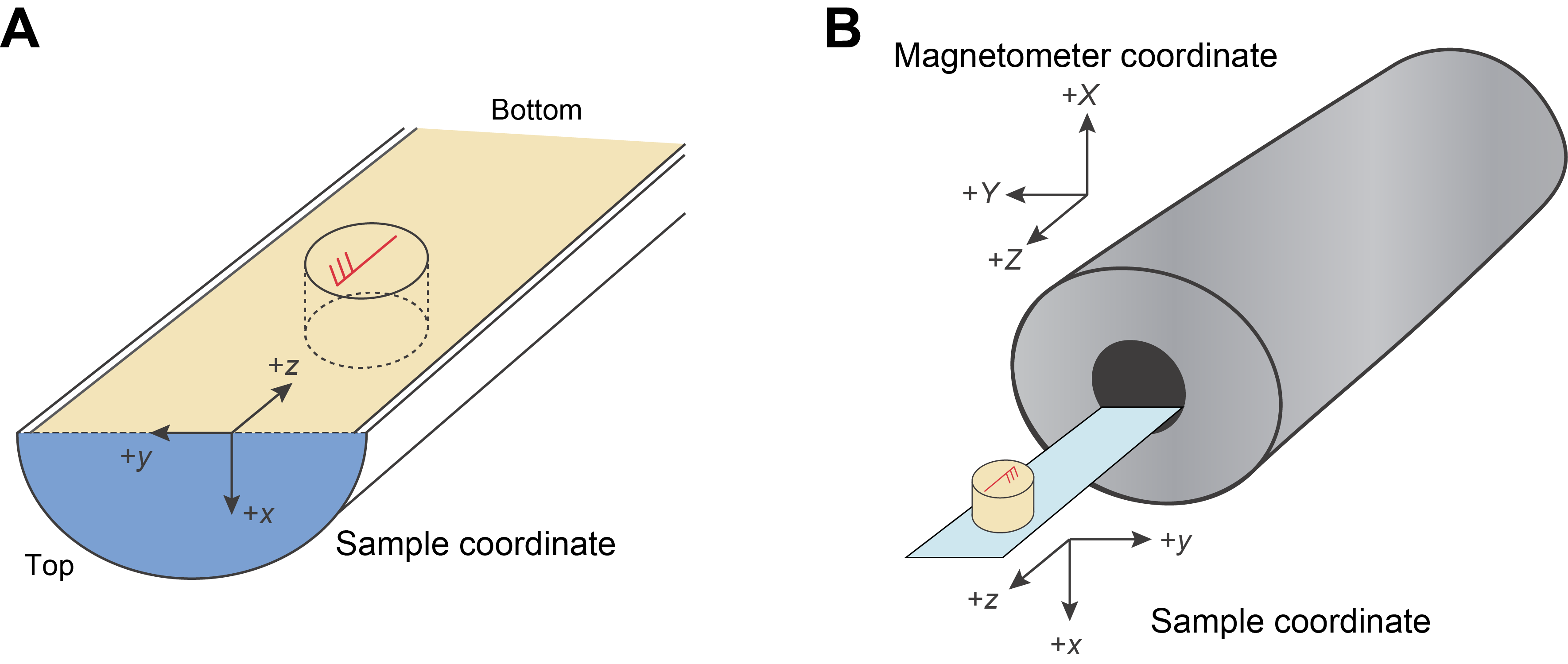
Figure F24. Orientation of the paleomagnetic plug; coordinate system.
No samples were collected for paleomagnetic analysis from Sites M0108 and M0109 because the friable core material did not allow cubes or minicores to be prepared.
5.3.1. Magnetic susceptibility
Magnetic susceptibility was measured using an AGICO KLY2 Kappabridge operating at a frequency of 920 Hz and magnetic induction of 0.4 mT (equivalent to a field intensity of 300 A/m) with a noise level of 2 × 10⁻¹⁰ m3/kg. The Kappabridge was calibrated using a standard with a bulk susceptibility of 1165 × 10−6 SI, and this procedure was repeated every morning before measurements began. The length and weight of the samples were measured using a caliper and electronic scale, respectively.
5.3.2. Natural remanent magnetization and alternating field demagnetization
NRM directions and intensities of discrete samples were measured using a 2G-Enterprises horizontal pass-through superconducting rock magnetometer (SRM 755) at the University of Bremen. Samples collected during the OSP were measured in batches of eight or fewer using an automated pass-through conveyor belt.
After the initial NRM was measured, the samples were sequentially subjected to several demagnetization steps, and the NRM was measured after each demagnetization step. During the initial demagnetization trials on both carbonate and volcanic (lava) samples from Holes M0096A and M0097A, a sequence of 12 increasing peak alternating field (AF) steps was used: 5, 10, 15, 20, 30, 40, 50, 60, 70, 80, 90, and 100 mT. Lava samples carried a strong remanence, whereas carbonate samples carried extremely weak remanences, close to background noise levels. The methods for subsequent samples were adjusted according to the lithology analyzed. Lava samples continued to undergo the full demagnetization-measurement sequence using the 12 established AF steps. The protocol for carbonate samples was modified: these samples were only demagnetized at peak AFs of 5, 10, 15, and 20 mT, with NRM measured after each step. During the moratorium, further demagnetization steps will take place on a discrete sample SRM for measurement in another laboratory that is equipped with a magnetically shielded room that minimizes the impact of external magnetic noise.
6. Geochronology
During the offshore phase of Expedition 389, 60 samples were opportunistically selected for rapid dating to provide a basic chronostratigraphic framework of the recovered material and to assist the subsequent onshore sampling phase. Of these, 55 were processed on shore for dating. This chronostratigraphic data set is intended to serve as a starting point for development of a more robust chronostratigraphy and to assist the entire scientific team to achieve their scientific objectives. The initial chronology will also enable a more effective description of the time intervals represented in the recovered cores until a more detailed chronology becomes available.
Geochronology samples were selected during the offshore phase and shipped to several laboratories for radiocarbon and uranium-thorium (U-Th) dating at the end of Legs 1 and 2. These rapid turnaround samples were run in the first instance to guide drilling during Leg 2 and in both instances to guide sampling of the cores at the OSP.
6.1. Offshore sampling procedure
The offshore geochronology sampling strategy consisted of limited sampling of corals and coralline algae for radiocarbon dating that were restricted to materials with ages thought to be less than ~50 thousand years before present (ky BP) and of coral samples identified for U-Th dating for material thought to be ~50 ky BP and older. Samples were taken in cases where suitable material was available either from core bottoms (i.e., if material was protruding from the core barrel), core catchers (i.e., loose fragments), or, in rare cases, from opportunistically fragmented pieces exposed within the core barrel during transfer from aluminum liners to polycarbonate liners.
The offshore geochronology specimens were broken into smaller subsamples using a hammer and chisel, with a tape-coated steel plate as the anvil. After subsampling, dating samples were washed in water multiple times. During Leg 1, this was accomplished by letting the sample chips sit in deionized water for several hours. During Leg 2, a sonic bath was added into the workflow, greatly aiding in the sample cleaning. After draining and removing excess water by pipettor, samples were dried in an oven at 50°C for 10–12 h, transferred to sterile sample bags, and entered into the mDIS.
6.2. Onshore dating methods for offshore samples
6.2.1. Preservation assessment
Because of the requirement to process the offshore samples quickly, sample preservation was not assessed with any additional analyses such as XRD to evaluate the mineralogy or scanning electron microscope (SEM) images. The offshore samples were shipped to three laboratories for analysis.
6.2.2. U-Th dating methods
A total of 43 offshore samples were dated using U-Th dating techniques at two different laboratories. A total of 22 samples were analyzed at Rutgers University (USA), including 15 samples from Leg 1 and 7 from Leg 2, and 21 samples were processed at the University of Minnesota Twin Cities (USA). The first step in processing was for samples to be cut with a band saw into small pieces and ultrasonically cleaned in Milli-Q (18 MΩ) water until the water was clear.
6.2.2.1. Rutgers University methods
Because of time considerations and a quick turnaround for results required to guide coring in the offshore phase, Leg 1 offshore samples were not ultrasonically cleaned prior to processing for U-Th dating. Leg 2 offshore samples were ultrasonically cleaned twice: once shipboard and once again on receipt at Rutgers University. Approximately 0.2–0.4 g of sample was selected for U-Th dating, and ~0.1 g was selected for XRD analysis to be performed at a future date. Samples were weighed, and a measured amount of a gravimetrically calibrated 233U-229Th mixed spike was added. Following dissolution, one drop of perchloric acid was added to remove organics, and samples were then refluxed overnight at 110°C to allow for equilibration. Iron hydroxide precipitation, ion-exchange column chemistry, and preparation of U and Th separates for analyses were performed as described in Mortlock et al. (2005). U and Th isotope ratios were measured using multicollector–inductively coupled–mass spectrometry (MC-ICP-MS) on a Thermo Fisher Scientific Neptune Plus, applying the methods and protocols described in Mortlock et al. (2005) as modified by Mondal et al. (2018).
6.2.2.2. University of Minnesota Twin Cities methods
For the samples that were analyzed at the University of Minnesota Twin Cities, subsampling of the coral samples was performed using dental tools. For thicker walled coral taxa, effort was made to remove the thinner septa material whenever possible because septa material has been shown to be more susceptible to diagenetic alteration compared to the surrounding theca walls (Obert et al., 2016). The subsampled coral pieces were then ultrasonically cleaned for a minimum of 5 min each in ultrapurified (18 MΩ) water followed by ethanol and left on the clean bench to dry. Replicates were run for two of the samples (i.e., a different physical subsample of the same coral piece), yielding a total of 23 analyses for 21 samples.
Chemical procedures were conducted in a metal-free Class 100 clean room following the approach of Edwards et al. (1987) and Shen et al. (2002, 2012). Approximately 50–100 mg of subsampled coral pieces were weighed and digested using nitric acid before being spiked with a gravimetrically calibrated, mixed 229Th-233U-236U tracer. U and Th were separated from the Ca matrix using Fe coprecipitation and then purified using anion-exchange chromatography into separate U and Th fractions. When needed, hydrogen peroxide was added to digest residual organic material. All U-series measurements were performed on a Thermo Fisher Scientific Neptune MC-ICP-MS instrument using a secondary electron multiplier in dynamic (peak jumping) mode with the retarding potential quadrupole (RPQ) engaged for improved abundance sensitivity (Shen et al., 2012). An aliquot of the U fraction was diluted so that the 235U signal was ~300,000 counts/s to minimize the impact of detector dead time effects, and 238U concentrations were calculated using the natural (i.e., bulk earth) 238U/235U ratio (137.82) (Heiss et al., 2012).
6.2.3. Radiocarbon dating methods
A total of 12 samples were selected off shore for radiocarbon dating and sent to the Atmosphere and Ocean Research Institute at the University of Tokyo (Japan). Prior to radiocarbon dating, a dental drill was used to subsample 1–2 mg of material for future XRD analysis to investigate potential diagenesis. The coral skeletal and coralline algal material was then transferred to a quartz tube and sonicated with Milli-Q (18 MΩ) water to clean the coral and coralline algal pieces before chemically etching the surface using weak hydrochloric acid (HCl) (~10–30 wt% equivalent). Samples were then graphitized employing the protocol reported in Yokoyama et al. (2007). The graphite target samples were analyzed with a single-stage accelerator mass spectrometer (Yokoyama et al., 2019).
6.2.4. Age interpretation for offshore samples
The U-Th geochemistry data and associated dates are reported in Tables T21 and T22, following the reporting guidelines of Dutton et al. (2017). Radiocarbon dates are reported in Table T23. Several factors limit the interpretation of these rapid turnaround radiocarbon and U-Th dates. Because of the compressed time frame for analysis, preservation of primary aragonite mineralogy was not assessed before dating occurred. Additionally, although we aimed to select offshore samples that appeared to be in situ, there is not enough information available at this stage regarding the full sedimentary context of these samples. Finally, an analysis of paleowater depths for these samples is also currently not available, limiting the interpretation of these dates in the context of a sea level reconstruction. For all of these reasons, interpretation of sample dates and associated chronology of the cores should be made with caution; the radiocarbon and U-Th dates are considered tentative and potentially unreliable because some of these samples have likely suffered from contamination, diagenetic alteration, and/or open-system behavior that would bias the age interpretation. For these same reasons, age reversals (i.e., where a sample’s date is younger/older compared to other dates from the same core) are identified in the site chapters, but we do not speculate on their potential causes, nor do we reject these dates outright.
All ages are reported in thousands of years before 1950 CE (ky BP), and no detrital Th correction was applied to the U-Th ages presented here. Postdepositional alteration of skeletal aragonite can impact the reliability of coral U-Th ages, which is commonly assessed using a combination of XRD and SEM. Although there are no XRD and SEM data to assist in the preservation assessment of the dated material, the geochemical measurements made for the U-Th dating themselves do provide some information that can be used to identify altered samples. Sample ages that should be rejected based on the U-Th geochemistry include those with anomalous values for 238U concentration (≫4 ppm) (e.g., Scholz and Mangini, 2007), those with anomalous δ234U initial values (below 130‰ or above 160‰), and one with a very high uncertainty due to being near secular equilibrium. A somewhat broader range of δ234U initial values was chosen for screening compared to modern seawater (144.9 ± 0.4‰) (Andersen et al., 2010; Chutcharavan et al., 2018). This was done for two reasons. First, the primary objective of the pre-OSP dating was to generate a rough chronostratigraphy of the Expedition 389 cores, so even information about which marine isotope stage the cores are from is useful for informing sampling strategies and future science objectives. Secondly, it is possible that the uranium isotopic composition of seawater has varied over the last few glacial cycles (i.e., there is evidence that seawater δ234U was as much as 5‰–7‰ lower during the last glacial maximum, and geochemical box modeling shows that seawater δ234U has varied by no more than ± 15‰ over the past 360 ky) (Henderson, 2002; Esat and Yokoyama, 2006, 2010; Chen et al., 2016; Chutcharavan et al., 2018). Samples with anomalous U-Th dating results outside the modeled maximum glacial–interglacial range are noted in Table T22. Most of the material that was U-Th dated does not suggest significant alteration on its own, although XRD and/or SEM data would need to be collected to help confirm this interpretation. The initial geochronology results, therefore, are promising and indicate good potential of recovering a robust chronology for the cores with more detailed dating and preservation analyses in the future.
7. Microbiology
7.1. Shipboard aDNA sampling procedures
Samples for aDNA were taken off shore and on shore. The objective of the offshore sampling was to examine the effect of (1) offshore handling and processing of the collected core material and (2) onshore handling prior to aDNA subsampling on DNA preservation within the cores. This includes the effects of prolonged exposure of cores to ambient temperatures and sunlight and exposure to irradiation during certain analytical processes such as X-ray CT scanning and MSCL measurements. The results should inform the feasibility of using aDNA from processed core material in general, as well as the suitability to reconstruct ecological and evolutionary responses of the Hawaiian drowned reefs to abrupt sea level and climate changes in the past.
The offshore aDNA sampling was designed to obtain samples of different ages following Webster et al. (2009, 2023). As such, the offshore sampling strategy was to obtain approximately three samples (near the top, middle, and base) from the first hole drilled on each of the terraces.
Offshore aDNA sampling was conducted alongside offshore geochronological sampling and followed the same selection criteria and subsampling procedure (well-preserved, clean, and unaltered coral pieces with approximate sample sizes of 2–3 cm3), and samples were entered into the mDIS. Where there was high-quality coral material left after geochronological sampling, an additional subsample was taken for aDNA analysis, in addition to the three samples already obtained for aDNA analysis from the hole. For a more detailed overview of the sampling workflow for geochronology, see Geochronology.
7.2. Onshore aDNA sampling procedures
The primary objective of the onshore aDNA sampling was to obtain suitable material for evaluating the response of reef-building coral populations and coral reef ecosystems in the Hawaiian archipelago to past climatic and environmental shifts, as well as identifying the microbial diversity preserved in the microbialites. An additional objective was to collect samples from the same corals as the samples taken off shore, which will allow direct comparison of the coral DNA preservation before and after the offshore and onshore handling and processing of the collected core material and the prolonged exposure of cores to ambient temperatures on deck and sunlight and exposure to irradiation during certain analytical processes such as X-ray CT scanning and MSCL measurements.
Samples were taken from cores collected from different drilling sites and holes across several reef terraces of various ages. Samples included both distinct coral pieces and microbialite formations. The focus was primarily on Porites spp. for coral samples. The following criteria were followed when selecting both types of samples: in situ, well-preserved, unaltered, clean (without sediment inclusions) pieces close to middle of the core; away from drilling marks, resins, and oils; and away from the very top and bottom edges of the core section.
The onshore sampling strategy was to collect 5–10 cm3 (minimum 2 cm3) of material for coral and microbialite samples. Samples were entered into the mDIS by a designated member of the sampling team. Sampling was performed on freshly opened cores, and as standard practice similar to offshore sampling, samples were taken close to the geochronological samples. Sterile gloves and face masks were used during sampling, and samples were placed in sterile sealable plastic bags. The sawing of samples was done in a room with no history of modern DNA work, and the persons working on the cores were not involved in modern DNA work immediately prior to handling the cores to minimize the chance of contamination. Following the completion of the onshore sampling, the samples were stored in a freezer at −4°C. Because the BCR sampling room and saws are not designed for aDNA work and are used for all sample types, onshore aDNA samples were taken with the knowledge that even with careful handling, there could be some cross-sample contamination. Ultimately, this can be mitigated because once samples are received in the dedicated aDNA laboratories, the interior of the specimen is sampled in a sterile environment with appropriate mechanical and chemical cleaning and only this part of the sample is further processed for aDNA analysis.
References
Andersen, M.B., Stirling, C.H., Zimmermann, B., and Halliday, A.N., 2010. Precise determination of the open ocean 234U/238U composition. Geochemistry, Geophysics, Geosystems, 11(12). https://doi.org/10.1029/2010GC003318
Bakker, W., van Ruitenbeek, F.J.A., and van der Werff, H.M.A., 2011. Hyperspectral image mapping by automatic color coding of absorption features: abstract. 56-57. Presented at the 7th EARSEL Workshop on Imaging Spectroscopy 2011, Edinburgh, UK, 11–13 November 2011. https://research.utwente.nl/en/publications/hyperspectral-image-mapping-by-automatic-color-coding-of-absorpti
Budd, A.F., Fukami, H., Smith, N.D., and Knowlton, N., 2012. Taxonomic classification of the reef coral family Mussidae (Cnidaria: Anthozoa: Scleractinia). Zoological Journal of the Linnean Society, 166(3):465–529. https://doi.org/10.1111/j.1096-3642.2012.00855.x
Channell, J.E.T., Singer, B.S., and Jicha, B.R., 2020. Timing of Quaternary geomagnetic reversals and excursions in volcanic and sedimentary archives. Quaternary Science Reviews, 228:106114. https://doi.org/10.1016/j.quascirev.2019.106114
Channell, J.E.T., Xuan, C., and Hodell, D.A., 2009. Stacking paleointensity and oxygen isotope data for the last 1.5 Myr (PISO-1500). Earth and Planetary Science Letters, 283(1–4):14–23. https://doi.org/10.1016/j.epsl.2009.03.012
Chen, T., Robinson, L.F., Beasley, M.P., Claxton, L.M., Andersen, M.B., Gregoire, L.J., Wadham, J., Fornari, D.J., and Harpp, K.S., 2016. Ocean mixing and ice-sheet control of seawater 234U/238U during the last deglaciation. Science, 354(6312):626–629. https://doi.org/10.1126/science.aag1015
Cheng, H., Lawrence Edwards, R., Shen, C.-C., Polyak, V.J., Asmerom, Y., Woodhead, J., Hellstrom, J., Wang, Y., Kong, X., Spötl, C., Wang, X., and Calvin Alexander, E., 2013. Improvements in 230Th dating, 230Th and 234U half-life values, and U–Th isotopic measurements by multi-collector inductively coupled plasma mass spectrometry. Earth and Planetary Science Letters, 371–372:82–91. https://doi.org/10.1016/j.epsl.2013.04.006
Chung, F., 1974. Quantitative interpretation of X-ray diffraction patterns of mixtures. I. Matrix-flushing method for quantitative multicomponent analysis. Journal of Applied Crystallography, 7(6):519–525. https://doi.org/10.1107/S0021889874010375
Chutcharavan, P.M., Dutton, A., and Ellwood, M.J., 2018. Seawater 234U/238U recorded by modern and fossil corals. Geochimica et Cosmochimica Acta, 224:1–17. https://doi.org/10.1016/j.gca.2017.12.017
Clark, R.N., 1999. Spectroscopy of Rocks and Minerals, and Principles of Spectroscopy In Rencz, A.N., Manual of Remote Sensing. 3:3–58.
da Silva, A.-C., Potma, K., Weissenberger, J.A.W., Whalen, M.T., Humblet, M., Mabille, C., and Boulvain, F., 2009. Magnetic susceptibility evolution and sedimentary environments on carbonate platform sediments and atolls, comparison of the Frasnian from Belgium and Alberta, Canada. Sedimentary Geology, 214(1):3–18. https://doi.org/10.1016/j.sedgeo.2008.01.010
Degen, T., Sadki, M., Bron, E., König, U., and Nénert, G., 2014. The HighScore suite. Powder Diffraction, 29(S2):S13–S18. https://doi.org/10.1017/S0885715614000840
Dunham, R.J., 1962. Classification of carbonate rocks according to depositional texture. In Ham, W.E., Classification of Carbonate Rocks. AAPG Memoir, 1: 108–121.
Dutton, A., Rubin, K., McLean, N., Bowring, J., Bard, E., Edwards, R.L., Henderson, G.M., Reid, M.R., Richards, D.A., Sims, K.W.W., Walker, J.D., and Yokoyama, Y., 2017. Data reporting standards for publication of U-series data for geochronology and timescale assessment in the earth sciences. Quaternary Geochronology, 39:142–149. https://doi.org/10.1016/j.quageo.2017.03.001
Edwards, R.L., Chen, J.H., and Wasserburg, G.J., 1987. 238U–234U–230Th–232Th systematics and the precise measurement of time over the past 500,000 years. Earth and Planetary Science Letters, 81(2):175–192. https://doi.org/10.1016/0012-821X(87)90154-3
Embry, A.F., and Klovan, J.E., 1972. Absolute water depth limits of late Devonian paleoecological zones. Geologische Rundschau, 61(2):672–686. https://doi.org/10.1007/BF01896340
Esat, T.M., and Yokoyama, Y., 2006. Variability in the uranium isotopic composition of the oceans over glacial–interglacial timescales. Geochimica et Cosmochimica Acta, 70(16):4140–4150. https://doi.org/10.1016/j.gca.2006.06.013
Esat, T.M., and Yokoyama, Y., 2010. Coupled uranium isotope and sea-level variations in the oceans. Geochimica et Cosmochimica Acta, 74(24):7008–7020.
Expedition 302 Scientists, 2006. Methods. In Backman, J., Moran, K., McInroy, D.B., Mayer, L.A., and the Expedition 302 Scientists, Proceedings of the Integrated Ocean Drilling Program. 302: Edinburgh (Integrated Ocean Drilling Program Management International, Inc.). https://doi.org/10.2204/iodp.proc.302.103.2006
Grasshoff, K., Kremling, K., and Ehrhardt, M. (Eds.), 1999. Methods of Seawater Analysis (3rd edition): Hoboken, NJ (Wiley-VCH). https://doi.org/10.1002/9783527613984
Grasshoff, K., Ehrhardt, M., and Kemling, K., 1983. Methods of Seawater Analysis (2nd edition): Weinham, Germany (Verlag Chemie).
Hall, P.J., and Aller, R.C., 1992. Rapid, small-volume, flow injection analysis for SCO2, and NH4+ in marine and freshwaters. Limnology and Oceanography, 37(5):1113–1119. https://doi.org/10.4319/lo.1992.37.5.1113
Henderson, G.M., 2002. Seawater (234U/238U) during the last 800 thousand years. Earth and Planetary Science Letters, 199(1):97–110. https://doi.org/10.1016/S0012-821X(02)00556-3
Hiess, J., Condon, D.J., McLean, N., and Noble, S.R., 2012. 238U/235U systematics in terrestrial uranium-bearing minerals. Science, 335(6076):1610-1614. https://doi.org/10.1126/science.1215507
Huang, D., Arrigoni, R., Benzoni, F., Fukami, H., Knowlton, N., Smith, N.D., Stolarski, J., Chou, L.M., and Budd, A.F., 2016. Taxonomic classification of the reef coral family Lobophylliidae (Cnidaria: Anthozoa: Scleractinia). Zoological Journal of the Linnean Society, 178(3):436–481. https://doi.org/10.1111/zoj.12391
Huang, D., Benzoni, F., Fukami, H., Knowlton, N., Smith, N.D., and Budd, A.F., 2014. Taxonomic classification of the reef coral families Merulinidae, Montastraeidae, and Diploastraeidae (Cnidaria: Anthozoa: Scleractinia). Zoological Journal of the Linnean Society, 171(2):277–355. https://doi.org/10.1111/zoj.12140
Hunt, C.P., Moskowitz, B.M., and Banerjee, S.K., 1995. Magnetic properties of rocks and minerals. In Ahrens, T.J. (Ed.), Rock Physics & Phase Relations: A Handbook of Physical Constants. AGU Reference Shelf Series, 3: 189–204. https://doi.org/10.1029/RF003p0189
Hyodo, M., Nakagawa, T., Matsushita, H., Kitaba, I., Yamada, K., Tanabe, S., Bradák, B., Miki, M., McLean, D., Staff, R.A., Smith, V.C., Albert, P.G., Bronk Ramsey, C., Yamasaki, A., Kitagawa, J., Schlolaut, G., Gotanda, K., Tsumura, K., Inagawa, K., Kumazawa, K., Abe, H., Sugo, S., Takahashi, K., Kitamura, A., and Suigetsu, P., 2022. Intermittent non-axial dipolar-field dominance of twin Laschamp excursions. Communications Earth & Environment, 3(1):79. https://doi.org/10.1038/s43247-022-00401-0
Ito, E., Higgins, S., Jenkins, C., Leigh, J., Johnson, A., and Grivna, B., 2023. Corelyzer, v.2.2.2. Continental Scientific Drilling Facility. https://github.com/corewall/corelyzer
Jaffey, A.H., Flynn, K.F., Glendenin, L.E., Bentley, W.C., and Essling, A.M., 1971. Precision measurement of half-lives and specific activities of 235U and 238U. Physical Review C, 4(5):1889–1906. https://doi.org/10.1103/PhysRevC.4.1889
Kontny, A., Vahle, C., and de Wall, H., 2003. Characteristic magnetic behavior of subaerial and submarine lava units from the Hawaiian Scientific Drilling Project (HSDP-2). Geochemistry, Geophysics, Geosystems, 4(2). https://doi.org/10.1029/2002GC000304
Lebrato, M., Garbe-Schönberg, D., Müller, M.N., Blanco-Ameijeiras, S., Feely, R.A., Lorenzoni, L., Molinero, J.-C., Bremer, K., Jones, D.O.B., Iglesias-Rodriguez, D., Greeley, D., Lamare, M.D., Paulmier, A., Graco, M., Cartes, J., Barcelos e Ramos, J., de Lara, A., Sanchez-Leal, R., Jimenez, P., Paparazzo, F.E., Hartman, S.E., Westernströer, U., Küter, M., Benavides, R., da Silva, A.F., Bell, S., Payne, C., Olafsdottir, S., Robinson, K., Jantunen, L.M., Korablev, A., Webster, R.J., Jones, E.M., Gilg, O., Bailly du Bois, P., Beldowski, J., Ashjian, C., Yahia, N.D., Twining, B., Chen, X.-G., Tseng, L.-C., Hwang, J.-S., Dahms, H.-U., and Oschlies, A., 2020. Global variability in seawater Mg:Ca and Sr:Ca ratios in the modern ocean. Proceedings of the National Academy of Sciences, 117(36):22281–22292. https://doi.org/10.1073/pnas.1918943117
Lee, K., Kim, T.-W., Byrne, R.H., Millero, F.J., Feely, R.A., and Liu, Y.-M., 2010. The universal ratio of boron to chlorinity for the North Pacific and North Atlantic oceans. Geochimica et Cosmochimica Acta, 74(6):1801–1811. https://doi.org/10.1016/j.gca.2009.12.027
Leroy, C.C., 1969. Development of simple equations for accurate and more realistic calculation of the speed of sound in seawater. The Journal of the Acoustical Society of America, 46(1B):216–226. https://doi.org/10.1121/1.1911673
Lorenz, S., Seidel, P., Ghamisi, P., Zimmermann, R., Tusa, L., Khodadadzadeh, M., Contreras, I.C., and Gloaguen, R., 2019. Multi-sensor spectral imaging of geological samples: a data fusion approach using spatio-spectral feature extraction. Sensors, 19(12):2787. https://doi.org/10.3390/s19122787
Lund, S., Platzman, E., Thouveny, N., Camoin, G., Corsetti, F., and Berelson, W., 2010. Biological control of paleomagnetic remanence acquisition in carbonate framework rocks of the Tahiti coral reef. Earth and Planetary Science Letters, 298(1):14–22. https://doi.org/10.1016/j.epsl.2010.07.010
Menabréaz, L., Thouveny, N., Camoin, G., and Lund, S.P., 2010. Paleomagnetic record of the late Pleistocene reef sequence of Tahiti (French Polynesia): a contribution to the chronology of the deposits. Earth and Planetary Science Letters, 294(1–2):58–68. https://doi.org/10.1016/j.epsl.2010.03.002
Millero, F.J., Feistel, R., Wright, D.G., and McDougall, T.J., 2008. The composition of standard seawater and the definition of the reference-composition salinity scale. Deep Sea Research, Part I: Oceanographic Research Papers, 55(1):50–72. https://doi.org/10.1016/j.dsr.2007.10.001
Mondal, D.R., McHugh, C.M., Mortlock, R.A., Steckler, M.S., Mustaque, S., and Akhter, S.H., 2018. Microatolls document the 1762 and prior earthquakes along the southeast coast of Bangladesh. Tectonophysics, 745:196–213. https://doi.org/10.1016/j.tecto.2018.07.020
Moore, C.H., 2001. The nature of the carbonate depositional system. In Moore, C.H., Carbonate Reservoirs - Porosity Evolution and Diagenesis in a Sequence Stratigraphic Framework. Developments in Sedimentology, 55: 1–17. https://doi.org/10.1016/S0070-4571(01)80002-9
Mortlock, R.A., Fairbanks, R.G., Chiu, T.-c., and Rubenstone, J., 2005. 230Th/234U/238U and 231Pa/235U ages from a single fossil coral fragment by multi-collector magnetic-sector inductively coupled plasma mass spectrometry. Geochimica et Cosmochimica Acta, 69(3):649–657. https://doi.org/10.1016/j.gca.2004.06.033
Obert, J.C., Scholz, D., Felis, T., Brocas, W.M., Jochum, K.P., and Andreae, M.O., 2016. 230Th/U dating of Last Interglacial brain corals from Bonaire (southern Caribbean) using bulk and theca wall material. Geochimica et Cosmochimica Acta, 178:20–40. https://doi.org/10.1016/j.gca.2016.01.011
Roberts, A.P., and Winklhofer, M., 2004. Why are geomagnetic excursions not always recorded in sediments? Constraints from post-depositional remanent magnetization lock-in modelling. Earth and Planetary Science Letters, 227(3):345–359. https://doi.org/10.1016/j.epsl.2004.07.040
Schlager, W., 2005. Carbonate Sedimentology and Sequence Stratigraphy. SEPM Concepts in Sedimentology and Paleontology, 8. https://doi.org/10.2110/csp.05.08
Scholz, D., and Mangini, A., 2007. How precise are U-series coral ages? Geochimica et Cosmochimica Acta, 71(8):1935–1948. https://doi.org/10.1016/j.gca.2007.01.016
Seeberg-Elverfeldt, J., Schlüter, M., Feseker, T., and Kölling, M., 2005. Rhizon sampling of porewaters near the sediment-water interface of aquatic systems. Limnology and Oceanography: Methods, 3(8):361–371. https://doi.org/10.4319/lom.2005.3.361
Shen, C.-C., Lawrence Edwards, R., Cheng, H., Dorale, J.A., Thomas, R.B., Bradley Moran, S., Weinstein, S.E., and Edmonds, H.N., 2002. Uranium and thorium isotopic and concentration measurements by magnetic sector inductively coupled plasma mass spectrometry. Chemical Geology, 185(3):165–178. https://doi.org/10.1016/S0009-2541(01)00404-1
Shen, C.-C., Wu, C.-C., Cheng, H., Lawrence Edwards, R., Hsieh, Y.-T., Gallet, S., Chang, C.-C., Li, T.-Y., Lam, D.D., Kano, A., Hori, M., and Spötl, C., 2012. High-precision and high-resolution carbonate 230Th dating by MC-ICP-MS with SEM protocols. Geochimica et Cosmochimica Acta, 99:71–86. https://doi.org/10.1016/j.gca.2012.09.018
Singer, B.S., 2014. A Quaternary geomagnetic instability time scale. Quaternary Geochronology, 21:29–52. https://doi.org/10.1016/j.quageo.2013.10.003
Spiegel, T., Vosteen, P., Wallmann, K., Paul, S.A.L., Gledhill, M., and Scholz, F., 2021. Updated estimates of sedimentary potassium sequestration and phosphorus release on the Amazon shelf. Chemical Geology, 560:120017. https://doi.org/10.1016/j.chemgeo.2020.120017
Stanienda-Pilecki, K.J., 2023. Crystals structures of carbonate phases with Mg in Triassic rocks, mineral formation and transitions. Scientific Reports, 13(1):18759. https://doi.org/10.1038/s41598-023-46013-2
Steiner, Z., Landing, W.M., Bohlin, M.S., Greaves, M., Prakash, S., Vinayachandran, P.N., and Achterberg, E.P., 2022. Variability in the concentration of lithium in the Indo-Pacific Ocean. Global Biogeochemical Cycles, 36(6):e2021GB007184. https://doi.org/10.1029/2021GB007184
Steiner, Z., Sarkar, A., Prakash, S., Vinaychandran, P.N., and Turchyn, A.V., 2020. Dissolved strontium, Sr/Ca ratios, and the abundance of Acantharia in the Indian and Southern Oceans. ACS Earth and Space Chemistry, 4(6):802–811. https://doi.org/10.1021/acsearthspacechem.9b00281
Tauxe, L., 2010. Essentials of Paleomagnetism: Oakland, CA (University of California Press).
Thiele, S.T., Lorenz, S., Kirsch, M., Cecilia Contreras Acosta, I., Tusa, L., Herrmann, E., Möckel, R., and Gloaguen, R., 2021. Multi-scale, multi-sensor data integration for automated 3-D geological mapping. Ore Geology Reviews, 136:104252. https://doi.org/10.1016/j.oregeorev.2021.104252
Veron, J., 2000. Corals of the World, Volumes 1–3: Townsville, AU (Australian Institute of Marine Science).
Vogt, C., Lauterjung, J., and Fischer, R.X., 2002. Investigation of the clay fraction (<2 µm) of the clay minerals society reference clays. Clays and Clay Minerals, 50(3):388–400. https://doi.org/10.1346/000986002760833765
Von Herzen, R., and Maxwell, A.E., 1959. The measurement of thermal conductivity of deep-sea sediments by a needle-probe method. Journal of Geophysical Research, 64(10):1557–1563. https://doi.org/10.1029/JZ064i010p01557
Walker, G.P.L., 1971. Compound and simple lava flows and flood basalts. Bulletin Volcanologique, 35(3):579–590. https://doi.org/10.1007/BF02596829
Wallace, C., Chen, C., Fukami, H., and Muir, P., 2007. Recognition of separate genera within Acropora based on new morphological, reproductive and genetic evidence from Acropora togianensis, and elevation of the subgenus Isopora Studer, 1878 to genus (Scleratinia: Astrocoeniidae; Acroporidae). Coral Reefs, 26:231–239. https://doi.org/10.1007/s00338-007-0203-4
Webster, J.M., Braga, J.C., Clague, D.A., Gallup, C., Hein, J.R., Potts, D.C., Renema, W., Riding, R., Riker-Coleman, K., Silver, E., and Wallace, L.M., 2009. Coral reef evolution on rapidly subsiding margins. Global and Planetary Change, 66(1–2):129–148. https://doi.org/10.1016/j.gloplacha.2008.07.010
Webster, J.M., Ravelo, A.C., and Grant, H.L.J., 2023. Expedition 389 Scientific Prospectus: Hawaiian Drowned Reefs. International Ocean Discovery Program. https://doi.org/10.14379/iodp.sp.389.2023
Webster, J.M., Ravelo, A.C., Grant, H.L.J., and the Expedition 389 Scientists, 2025. Supplementary material, https://doi.org/10.14379/iodp.proc.389supp.2025. In Webster, J.M., Ravelo, A.C., Grant, H.L.J., and the Expedition 389 Scientists, Hawaiian Drowned Reefs. Proceedings of the International Ocean Discovery Program, 389: College Station, TX (International Ocean Discovery Program).
Webster, J.M., Ravelo, A.C., Grant, H.L.J., Rydzy, M., Stewart, M., Allison, N., Asami, R., Boston, B., Braga, J.C., Brenner, L., Chen, X., Chutcharavan, P., Dutton, A., Felis, T., Fukuyo, N., Gischler, E., Greve, S., Hagen, A., Hamon, Y., Hathorne, E., Humblet, M., Jorry, S., Khanna, P., Le Ber, E., McGregor, H., Mortlock, R., Nohl, T., Potts, D., Prohaska, A., Prouty, N., Renema, W., Rubin, K.H., Westphal, H., and Yokoyama, Y., 2025. Expedition 389 summary. In Webster, J.M., Ravelo, A.C., Grant, H.L.J., and the Expedition 389 Scientists, Hawaiian Drowned Reefs. Proceedings of the International Ocean Discovery Program, 389: College Station, TX (International Ocean Discovery Program). https://doi.org/10.14379/iodp.proc.389.101.2025
Wei, L., Fan, T., Chen, J., and Yu, K., 2021. Progress in the study of coral reef rock magnetism, environmental magnetism and magnetostratigraphy. Bulletin of Mineralogy, Petrology and Geochemistry. https://doi.org/10.19658/j.issn.1007-2802.2021.40.067
Wentworth, C.K., 1922. A scale of grade and class terms for clastic sediments. The Journal of Geology, 30(5):377–392. https://doi.org/10.1086/622910
Yokoyama, Y., Miyairi, Y., Aze, T., Yamane, M., Sawada, C., Ando, Y., de Natris, M., Hirabayashi, S., Ishiwa, T., Sato, N., and Fukuyo, N., 2019. A single stage accelerator mass spectrometry at the Atmosphere and Ocean Research Institute, The University of Tokyo. Nuclear Instruments and Methods in Physics Research Section B: Beam Interactions with Materials and Atoms, 455:311–316. https://doi.org/10.1016/j.nimb.2019.01.055
Yokoyama, Y., Miyairi, Y., Matsuzaki, H., and Tsunomori, F., 2007. Relation between acid dissolution time in the vacuum test tube and time required for graphitization for AMS target preparation. Nuclear Instruments and Methods in Physics Research Section B: Beam Interactions with Materials and Atoms, 259(1):330–334. https://doi.org/10.1016/j.nimb.2007.01.176