Sager, W., Hoernle, K., Höfig, T.W., Blum, P., and the Expedition 391 Scientists
Proceedings of the International Ocean Discovery Program Volume 391
publications.iodp.org
https://doi.org/10.14379/iodp.proc.391.102.2023
Expedition 391 methods1
![]() W. Sager,
W. Sager,
![]() K. Hoernle,
K. Hoernle,
![]() T.W. Höfig,
T.W. Höfig,
![]() A.J. Avery,
A.J. Avery,
![]() R. Bhutani,
R. Bhutani,
![]() D.M. Buchs,
D.M. Buchs,
![]() C.A. Carvallo,
C.A. Carvallo,
![]() C. Class,
C. Class,
![]() Y. Dai,
Y. Dai,
![]() G. Dalla Valle,
G. Dalla Valle,
![]() A.V. Del Gaudio,
S. Fielding,
A.V. Del Gaudio,
S. Fielding,
![]() K.M. Gaastra,
K.M. Gaastra,
![]() S. Han,
S. Han,
![]() S. Homrighausen,
S. Homrighausen,
![]() Y. Kubota,
Y. Kubota,
![]() C.-F. Li,
C.-F. Li,
![]() W.R. Nelson,
W.R. Nelson,
![]() E. Petrou,
E. Petrou,
![]() K.E. Potter,
K.E. Potter,
![]() S. Pujatti,
S. Pujatti,
![]() J. Scholpp,
J. Scholpp,
![]() J.W. Shervais,
J.W. Shervais,
![]() S. Thoram,
S. Thoram,
![]() S.M. Tikoo-Schantz,
S.M. Tikoo-Schantz,
![]() M. Tshiningayamwe,
X.-J. Wang, and
M. Tshiningayamwe,
X.-J. Wang, and
![]() M. Widdowson
2
M. Widdowson
2
1 Sager, W., Hoernle, K., Höfig, T.W., Avery, A.J., Bhutani, R., Buchs, D.M., Carvallo, C.A., Class, C., Dai, Y., Dalla Valle, G., Del Gaudio, A.V., Fielding, S., Gaastra, K.M., Han, S., Homrighausen, S., Kubota, Y., Li, C.-F., Nelson, W.R., Petrou, E., Potter, K.E., Pujatti, S., Scholpp, J., Shervais, J.W., Thoram, S., Tikoo-Schantz, S.M., Tshiningayamwe, M., Wang, X.-J., and Widdowson, M., 2023. Expedition 391 methods. In Sager, W., Hoernle, K., Höfig, T.W., Blum, P., and the Expedition 391 Scientists, Walvis Ridge Hotspot. Proceedings of the International Ocean Discovery Program, 391: College Station, TX (International Ocean Discovery Program). https://doi.org/10.14379/iodp.proc.391.102.2023
2 Expedition 391 Scientists' affiliations.
1. Introduction
This chapter outlines the procedures and methods employed for coring and drilling operations as well as in the various shipboard laboratories of the R/V JOIDES Resolution during International Ocean Discovery Program (IODP) Expedition 391. The laboratory information applies only to shipboard work described in the Expedition Reports section of the Expedition 391 Proceedings of the International Ocean Discovery Program volume, using the shipboard sample registry, imaging and analytical instruments, core description tools, and the Laboratory Information Management System (LIMS) database. Methods used by investigators for shore-based analyses of Expedition 391 samples and data will be described in separate individual peer-reviewed scientific publications.
All shipboard scientists contributed in various ways to this volume, with the following primary responsibilities (authors are listed in alphabetical order; see Expedition 391 scientists for contact information):
Summary chapter: Expedition 391 Scientists
- Background and objectives: W. Sager, K. Hoernle
- Operations: S. Midgley, T.W. Höfig
- Lithostratigraphy: D. Buchs, G. Dalla Valle, M. Widdowson
- Igneous petrology and volcanology: D. Heaton, W. Nelson, J. Scholpp, J. Shervais, M. Tshiningayamwe, M. Widdowson
- Alteration: R. Bhutani, M. Widdowson
- Structural geology: C.-F. Li
- Biostratigraphy: A. Avery, A. Del Gaudio
- Paleomagnetism: C. Carvallo, K. Gaastra, S. Thoram, S. Tikoo-Schantz
- Pore water and sediment geochemistry: Y. Dai, S. Han
- Igneous geochemistry: C. Class, S. Homrighausen, Y. Kubota, X.-J. Wang
- Physical properties: S. Fielding, E. Petrou, K. Potter, S. Pujatti
This introductory section provides an overview of drilling and coring operations, core handling, curatorial conventions, depth scale terminology, and the sequence of shipboard analyses. Subsequent sections of this chapter document specific laboratory instruments and methods in more detail.
1.1. Locations of sites and holes
GPS coordinates (World Geodetic System 84 data) from preexpedition site surveys were used for the targeted position of the Expedition 391 drill sites. A SyQwest Bathy 2010 compressed high-intensity radar pulse (CHIRP) subbottom profiler was deployed to monitor the seafloor depth on the approach to the sites to reconfirm the depth profiles from preexpedition surveys. Once the ship was positioned at a site, the thrusters were lowered and the location of the ship was maintained over each hole using the Neutronics 5002 dynamic positioning (DP) system on JOIDES Resolution (Figure F1). DP control of the vessel used navigational input from the GPS. The final hole position was the calculated mean position derived from GPS data collected over a significant portion of the time the hole was occupied.
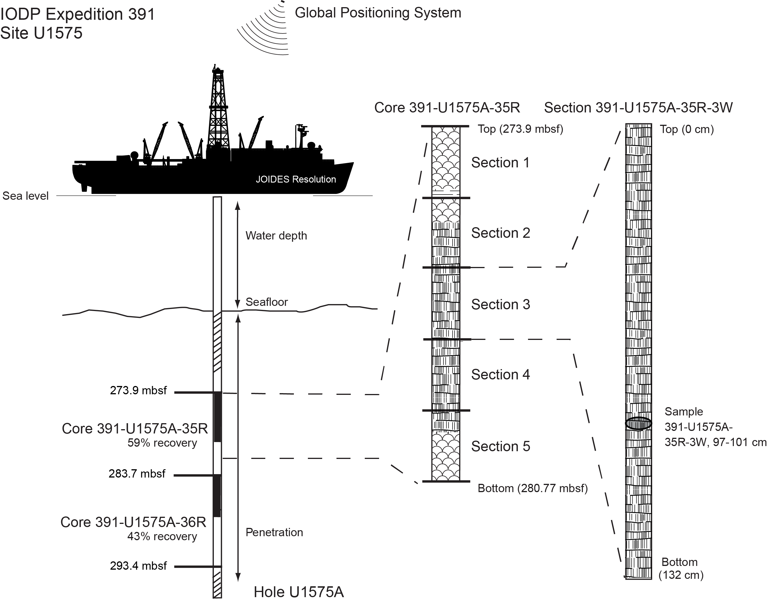
Figure F1. IODP naming convention.
The drilling sites were numbered according to the series that began with the first site drilled by the Glomar Challenger in 1968. Starting with Integrated Ocean Drilling Program Expedition 301, the prefix "U" defines sites occupied by JOIDES Resolution. For all IODP drill sites, a letter suffix distinguishes each hole drilled at the same site. The first hole drilled is assigned the site number modified by the suffix "A," the second hole takes the site number and the suffix "B," and so forth. During Expedition 391, four sites were drilled along the Tristan-Gough-Walvis (TGW) hotspot track in the southeastern Atlantic Ocean: Site U1575 (Hole U1575A), Site U1576 (Holes U1576A and U1576B), Site U1577 (Hole U1577A), and Site U1578 (Hole U1578A).
1.2. Drilling and logging operations
To successfully recover igneous rock cores from the TGW basement, the standard rotary core barrel (RCB) coring system was deployed. Operations took place on the Namibian extended continental shelf and in international waters in water depths of ~3000–4000 m.
The RCB coring system is a rotary system designed to recover firm to hard sediments and crystalline basement, such as igneous rocks. The RCB bottom-hole assembly (BHA), including the bit and outer core barrel, is rotated with the drill string while bearings allow the inner core barrel to remain stationary (Figure F2).
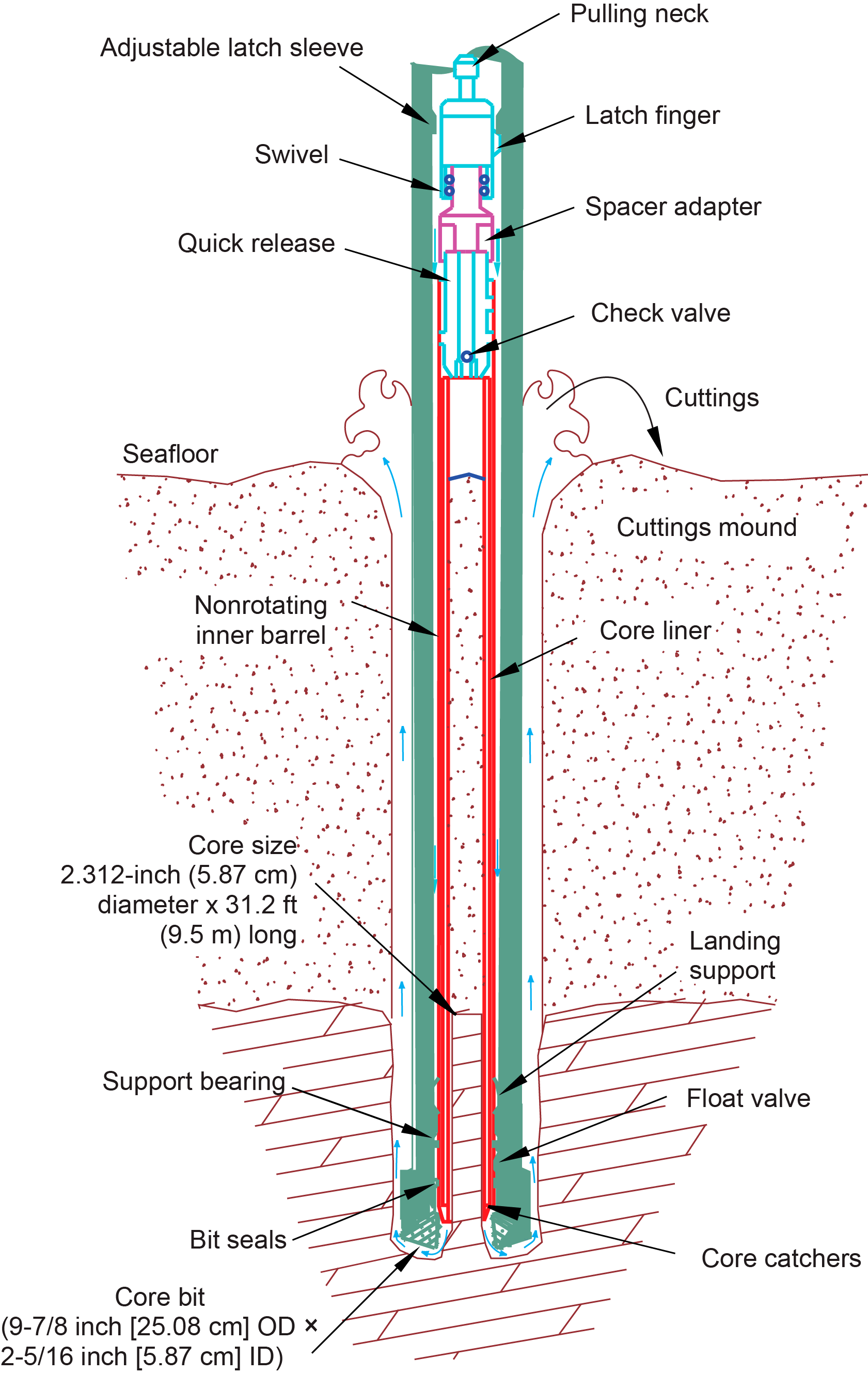
Figure F2. RCB coring system.
A typical RCB BHA consists of, from bottom to top, a drill bit (typically 9.875 inches in diameter, equivalent to 25.08 cm), a bit sub, an outer core barrel, a modified top sub, a modified head sub, a variable number of 8.25 inch control length drill collars, one tapered drill collar, two stands of 5.5 inch drill pipe (each stand measures ~28.5 m), and a crossover sub to the drill pipe that extends to the surface (Figure F3).
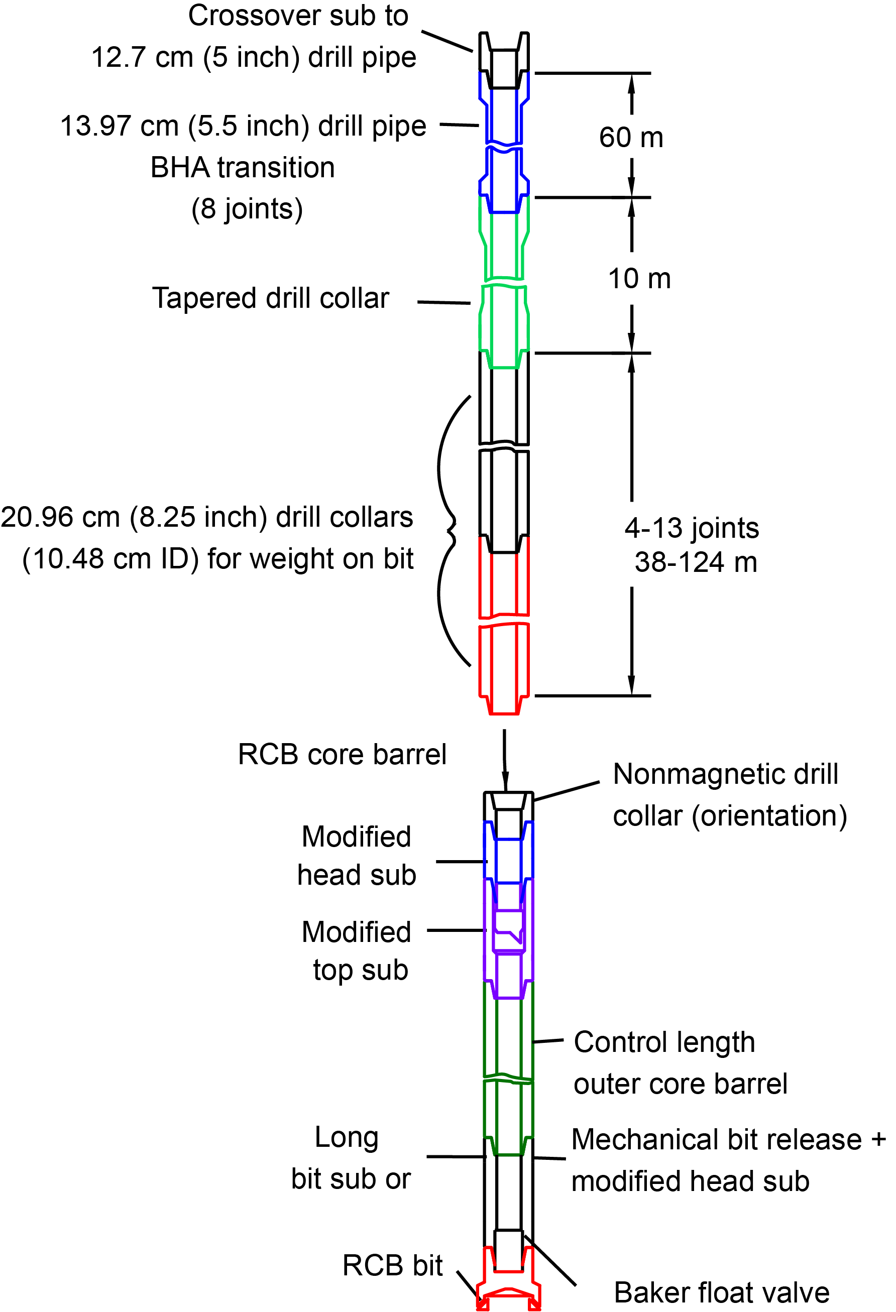
Figure F3. RCB BHA.
Nonmagnetic core barrels were used for all RCB deployments. Detailed information about recovered cores, drilled intervals, and related information are provided in the Operations section of each site chapter, as well as in the online hole/core/section summary and drilling reports of the LIMS database (https://web.iodp.tamu.edu/LORE).
As a result of lost time due to mitigation of a shipboard Coronavirus (COVID-19) outbreak, downhole logging had to be eliminated from the Expedition 391 operations plan in favor of allocating time to coring.
1.3. Curatorial core procedures and sampling depth calculations
Numbering of sites, holes, cores, and samples follows standard IODP procedures. A full curatorial identifier for a sample consists of the following information: expedition, site, hole, core number, core type, section number, section half, piece number (hard rocks only), and interval in centimeters measured from the top of the core section. For example, a sample identification of "391-U1575A-35R-3W, 97–101 cm," indicates a 4 cm long sample taken from the interval between 97 and 101 cm below the top of Section 3 (working half) of Core 35 ("R" designates that this core was taken with the RCB system) of Hole A at Site U1575 (Figure F1). The "U" preceding the hole number indicates the hole was drilled by a US platform (i.e., JOIDES Resolution). Integers are used to denote drilled intervals (e.g., a drilled interval between Cores 2R and 4R would be denoted by "Core 31").
The primary depth scales used are based on the length of the drill string deployed (e.g., drilling depth below rig floor [DRF] and drilling depth below seafloor [DSF]), the length of core recovered (e.g., core depth below seafloor [CSF] and core composite depth below seafloor [CCSF]) (see IODP Depth Scales Terminology at http://www.iodp.org/policies-and-guidelines/142-iodp-depth-scales-terminology-april-2011/file). All units are in meters. The relationship between scales is defined either by protocol, such as the rules for computation of CSF depth from DSF depth, or by user-defined correlations, such as core-to-log correlation. The distinction in nomenclature should keep the reader aware that a nominal depth value in different depth scales usually does not refer to the exact same stratigraphic interval.
Depths of cored intervals are measured from the rig floor based on the length of drill pipe deployed beneath the rig floor (DRF scale). The depth of the cored interval is referenced to the seafloor (DSF scale) by subtracting the seafloor depth of the hole from the DRF depth of the interval. Standard depths of cores in meters below seafloor, Method A (CSF-A scale), are determined based on the assumption that (1) the top depth of a recovered core corresponds to the top depth of its cored interval (on the DSF scale), and (2) the recovered material is a contiguous section even if core segments are separated by voids when recovered. Standard depths of samples and associated measurements (CSF-A scale) are calculated by adding the offset of the sample or measurement from the top of its section and the lengths of all higher sections in the core to the top depth of the core.
If a core has <100% recovery, for curation purposes all cored material is assumed to originate from the top of the drilled interval as a continuous section. In addition, voids in the core are closed by pushing core segments together, if possible, during core handling. Therefore, the true depth interval within the cored interval is unknown. This result should be considered a sampling uncertainty in age-depth analysis.
When core recovery is >100% (the length of the recovered core exceeds that of the cored interval), the CSF depth of a sample or measurement taken from the bottom of a core will be deeper than that of a sample or measurement taken from the top of the subsequent core (i.e., the data associated with the two core intervals overlap at the CSF-A scale). This overlap can happen when a soft to semisoft sediment core recovered from a few hundred meters below the seafloor expands upon recovery (typically by a few percent to as much as 15%). In hard rock sections, overlap may occur if a stub of the preceding core does not detach from the bedrock and it is then sampled by the subsequent core run. Therefore, a stratigraphic interval may not have the same nominal depth on the DSF and CSF scales in the same hole.
During Expedition 391, all core depths below seafloor were initially calculated according to the CSF-A depth scale. Unless otherwise noted, all depths presented are calculated on the CSF-A scale and reported in meters below seafloor (mbsf).
1.4. Core handling and analysis
1.4.1. Sediments
When the core barrel reached the rig floor, the core catcher from the bottom of the core barrel was removed and a sample was extracted for paleontological analysis. Next, the sediment core was extracted from the core barrel in its plastic liner. The liner was carried from the rig floor to the core processing area on the core receiving platform outside the core laboratory, where it was split into ~1.5 m sections. Blue (uphole) and clear (downhole) liner caps were glued with acetone onto the cut liner sections.
Once the core was cut into sections, whole-round samples were taken for interstitial water (IW) chemical analyses. Also, whole-round samples were taken for postexpedition microbiology studies from sediment cores recovered from sites in international waters. When a whole-round sample was removed, a yellow cap was used to denote the missing interval. Syringe samples were taken for headspace gas analyses according to the IODP hydrocarbon safety monitoring protocol.
Core sections were placed in a core rack in the laboratory. When they reached equilibrium with laboratory temperature (typically after 3 h), they were run through the Whole-Round Multisensor Logger (WRMSL) to acquire several data sets, including P-wave velocity data with the P-wave logger (PWL), magnetic susceptibility (MS), and gamma ray attenuation (GRA) bulk density (see Physical properties). Core sections were also run through the Natural Gamma Radiation Logger (NGRL), and thermal conductivity measurements were taken once per core when the material was suitable.
Core sections were split lengthwise from bottom to top into working and archive halves. Investigators should note that older material can be transported upward on the split face of each section during splitting.
The archive half of each core was described by the sedimentologists and structural geologist (the latter remotely for Expedition 391). Discrete samples were then taken from the working half of each core for moisture and density (MAD) and paleomagnetic analyses and for remaining shipboard analyses such as X-ray diffraction (XRD) and carbonate analyses. Samples were not collected when the lithology was a high-priority interval for expedition or postexpedition research (e.g., ash layers, sediment/basement contact zone, etc.), when there was unsuitable core material, or when the core was severely deformed. During the expedition, samples were taken for personal postexpedition research for all studies focused on examining ephemeral properties and for pilot studies of sedimentary and igneous basement intervals.
The archive half of each core was scanned on the Section Half Imaging Logger (SHIL). Archive halves were measured for point magnetic susceptibility (MSP) and reflectance spectroscopy and colorimetry (RSC) on the Section Half Multisensor Logger (SHMSL). Labeled foam pieces were used to denote missing whole-round intervals in the SHIL images. The archive-half sections were then described visually and by means of smear slides for lithostratigraphy. Finally, the magnetization of archive-half sections and working-half discrete pieces was measured with the cryogenic magnetometer and spinner magnetometer.
1.4.2. Sedimentary and igneous rocks
Upon recovery, the core liner was laid out on the core receiving platform, and rock pieces were pushed together to eliminate spaces. The core was divided into 1.5 m sections, and the total rock length was measured. This length was entered into the database as "recovered length" using the SampleMaster application. This number was used to calculate core recovery (in percent). The whole-round plastic liner sections were then transferred to the core splitting room.
Oriented pieces of core were marked on the bottom with a blue or red wax pencil to preserve orientation. Adjacent but broken pieces that could be fit together along fractures were curated as single pieces. The petrologists confirmed piece matches and marked the working-/archive-half split line on the pieces, which defined how they were to be cut into two equal halves. The aim was to maximize the expression of dipping structures on the cut face of the core while maintaining representative features in both archive and working halves. A plastic spacer was secured with acetone to the split core liner between individual pieces or reconstructed contiguous groups of subpieces. These spacers can represent substantial intervals of no recovery. The length of each section of core, including spacers, was entered into the database as "curated length," which commonly differs by several centimeters from the recovered length measured on the core receiving platform. Ultimately, the depth of each piece in the database was recalculated based on the curated length.
Core pieces were imaged around the full 360° circumference and then placed in a core rack in the laboratory. When the core sections reached equilibrium with laboratory temperature (typically after 3 h), the whole-round core sections were run through the WRMSL (GRA and MS only) and NGRL (see Physical properties).
Each piece of core was split with a diamond-impregnated saw into an archive half and a working half, and the positions of plastic spacers between pieces were maintained in both halves. Pieces were numbered sequentially from the top of each section, beginning with 1. Separate subpieces within a single piece were assigned the same number but lettered consecutively (e.g., 1A, 1B, etc.). Pieces were labeled only on the outer cylindrical surface of the core. If it was evident that an individual piece had not rotated around a horizontal axis during drilling, an arrow pointing to the top of the section was added to the label. The piece's oriented character was recorded in the database using the SampleMaster application.
The archive half of each core was first described by the petrologists and structural geologists. It was then scanned on the SHIL and measured for MSP and RSC on the SHMSL. Thermal conductivity measurements were made on selected archive-half samples (see Physical properties). After the archive halves were fully described, samples were then taken from the working halves for shipboard analyses, such as thin section preparation (polarization microscopy), paleomagnetic and physical properties analyses (e.g., MAD), as well as inductively coupled plasma–atomic emission spectroscopy (ICP-AES) and XRD. Finally, the magnetizations of archive-half sections, archive-half pieces, and discrete samples taken from the working half were measured with the cryogenic magnetometer and spinner magnetometer.
When all steps were completed, the cores were wrapped, sealed in plastic tubes, and transferred to cold storage space on board the ship. At the end of the expedition, the archive-half sections were sent to the IODP Gulf Coast Repository (Texas A&M University, College Station, TX [USA]) for X-ray fluorescence (XRF) core scanning and the working-half sections were sent to the IODP Bremen Core Repository (BCR; MARUM, Bremen, Germany) to prepare for a postexpedition sampling party for those who were not able to join the expedition due to COVID-19 pandemic restrictions and shipboard scientists focusing on sediment studies. Eventually, both section halves will be stored at the BCR permanently.
1.5. Drilling and core disturbance
Cores may be significantly disturbed and contain extraneous material because of the coring and core handling process (Jutzeler et al., 2014). In formations with loose sand layers, sand from intervals higher in the hole may be washed down by drilling circulation, accumulate at the bottom of the hole, and be sampled with the next core. The uppermost 10–50 cm of each core must therefore be examined critically during description for potential fall-in. Common coring-induced deformation includes the concave-downward appearance of originally horizontal bedding. Retrieval from depth to the surface can result in elastic rebound. Gas that is in solution at depth may become free and drive apart core segments in the liner. When gas content is high, pressure must be relieved for safety reasons before the cores are cut into segments. Holes are drilled into the liner, which forces some sediment as well as gas out of the liner. These disturbances are described in each site chapter and graphically indicated on the visual core descriptions (VCDs).
2. Lithostratigraphy
The lithologies of sediments and sedimentary rocks recovered during Expedition 391 were determined using visual (macroscopic) core description, smear slides, and thin sections. Integration of data from digital core images, color reflectance spectrophotometry, MS, XRD, and geochemistry provided complementary information. The methods employed during the expedition were adapted from those used during IODP Expeditions 367 and 368 in the South China Sea (Sun et al., 2018), along with those from Integrated Ocean Drilling Program Expeditions 324 and 330 and IODP Expedition 352, which drilled near-ridge, intraplate, and supra-subduction volcanic edifices in the Pacific Ocean (Expedition 324 Scientists, 2010b; Expedition 330 Scientists, 2012b; Reagan et al., 2015a). We used the DESClogik application to record and upload descriptive data to the LIMS database (see the DESClogik user guide at http://iodp.tamu.edu/labs/documentation). Spreadsheet templates were set up in DESClogik before the first core was brought on deck. The templates were used to record macroscopic core descriptions and microscopic data from smear slides and thin sections. The locations of all smear slide and thin section samples taken from the core were recorded in the SampleMaster application, and descriptive data retrieved from the LIMS database were used to produce the VCDs.
2.1. Core preparation
Standard methods for splitting core were performed either by pulling a wire lengthwise through the center of the core or by cutting the core with a rock saw. Each piece of core was split into an archive and a working half, and the archive half was used for visual description. When splitting the cores with a wire, we sometimes gently scraped across the cut surface of the archive-half section using a stainless steel or plastic scraper to prepare the surface for unobscured description and digital imaging, especially in the upper, poorly consolidated intervals. Most archive-half sections were imaged after they dried, except for the uppermost cores of unconsolidated (water-rich) sediments that cannot dry and were therefore imaged wet.
2.2. Visual core description
VCDs include a simplified graphical representation of each site on a core-by-core basis (Figure F4). The principal function of the VCD is to present the physical observations of the core in a columnar format. Site, hole, core, and the core depth below seafloor, Method A (CSF-A), are given at the top of each VCD. Depths and core section numbers are plotted along the left margin. Next to them, we plotted lithostratigraphic units and shipboard sample locations. Lithostratigraphic units were assigned by grouping intervals based on their lithologic similarities. Further definition of the lithostratigraphic units and their boundaries are included in each site chapter. Additional columns correspond to either core images, biostratigraphic ages (see Biostratigraphy), physical properties (natural gamma radiation [NGR], GRA bulk density, MS, and reflectance), or entries made in DESClogik. Data taken from DESClogik include core summary, principal lithology, sedimentary structures, bioturbation intensity, and drilling disturbances. The VCDs also include descriptive and lithostratigraphic information from the igneous rocks recovered at each site (see Igneous petrology and volcanology). Each column is described in more detail below.
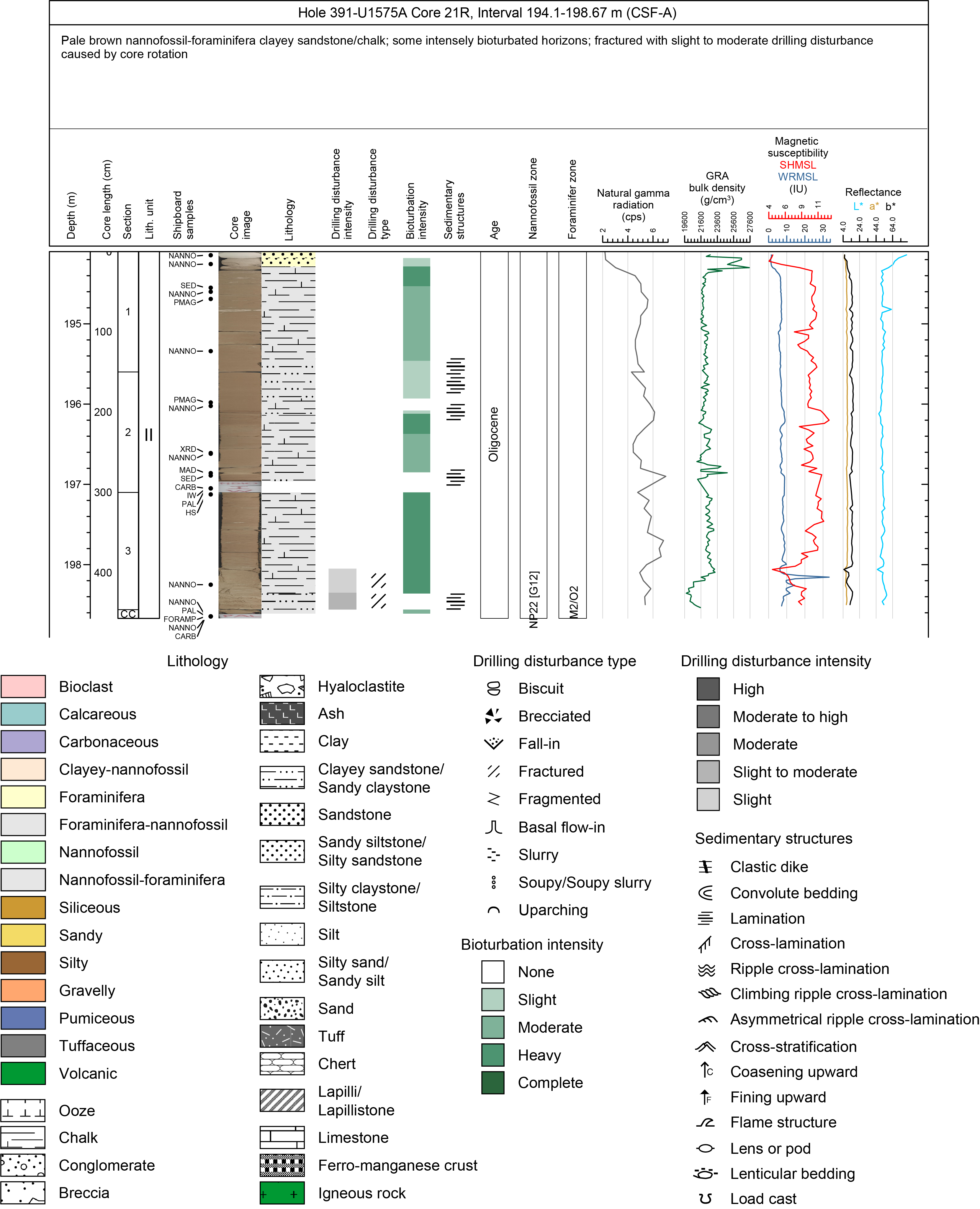
Figure F4. Example VCD.
2.2.1. Core summary
The core summary provides a brief overview of major and minor lithologies present in the core, as well as notable features (e.g., sedimentary structures). The summary is presented at the top of the VCDs and includes sediment color determined qualitatively using Munsell soil color charts. Because sediment color may evolve during drying and subsequent oxidization, color was described shortly after the sedimentary cores were split and imaged or measured using the SHIL and SHMSL. For lithified sedimentary and volcaniclastic deposits, we allowed cores to dry.
2.2.2. Core images
High-resolution color images of unlithified to poorly consolidated sediments were produced by scanning the flat surface of the archive-half sections with the SHIL. In unconsolidated water-rich sediments, the cores were scanned as soon as possible after splitting and scraping to avoid color changes caused by sediment oxidation and drying. In cases involving lithified rock, we photographed the archive-half sections dry.
The SHIL uses three pairs of advanced illumination, high-current-focused LED line lights (Cree XLamp CXB3590 LED) to illuminate large cracks and blocks in the core surface and sidewalls. Each LED pair has a color temperature of 6500 K. A linescan camera (JAI model CV107CL) images 20 lines/mm to create a high-resolution TIFF file. The camera height is adjusted so that each pixel images a 0.05 mm2 section of the core. However, actual core width per pixel varies because of differences in section-half surface height. High- and low-resolution JPEG files are subsequently created from the high-resolution TIFF file. Two different image types were uploaded to the LIMS database, one that includes a gray scale and ruler and one that is cropped to exclude the gray scale and ruler.
2.2.3. Graphic lithology
The Graphic lithology column illustrates an interval-by-interval record of the primary lithologies contained within each core. The column was constructed by pairing the principal lithology name assigned to each interval in DESClogik with a predetermined set of lithology patterns (Figure F4). The column plots to scale all intervals that are at least 2 cm thick. Principal lithology names were not assigned to intervals thinner than 2 cm unless they were of special significance (e.g., ash layers).
2.2.4. Drilling disturbance
The Drilling disturbance column indicates the type and intensity of disturbance in soft to lithified sediments. Typical examples of disturbance in soft sediments encountered during Expedition 391 include soupy, slurry, and uparching structures, whereas more consolidated sediments were commonly fractured with biscuit structures. The overall intensity of disturbance was categorized as slight, slight to medium, medium, medium to high, and high with increasing loss of primary sedimentary structures.
2.2.5. Sedimentary structures
The location and type of stratification and sedimentary structures visible on the surface of the archive-half sections (e.g., lamination, convolute bedding, normal grading, etc.) are shown in the Sedimentary structures column of the VCDs (Figure F4).
2.2.6. Bioturbation intensity
Five levels of bioturbation are recognized using a scheme like that of Droser and Bottjer (1986). These levels are illustrated with a numeric scale in the Bioturbation intensity column. Any identifiable trace fossils (ichnofossils) are identified in the general interval comment field in DESClogik and in the core summary. The levels are as follows:
- 1 = no bioturbation.
- 2 = slight bioturbation (<10%–30%).
- 3 = moderate bioturbation (30%–60%).
- 4 = heavy bioturbation (60%–90%).
- 5 = complete bioturbation (>90%).
2.2.7. Samples
The Shipboard sample column records the position of samples used for microscopic descriptions (i.e., smear slides and thin sections), biochronological determinations, and shipboard analyses of chemical and physical properties.
2.3. Sediment classification
Naming conventions follow the general guidelines of the Ocean Drilling Program (ODP) sediment classification scheme (Mazzullo et al., 1988) but do not include a separate "mixed sediment" category (Figure F5). A principal lithology name was assigned to each sediment interval based on the composition of the dominant lithology as identified by macroscopic observation, smear slides, thin sections, and other shipboard data. It is preceded by major modifiers, or prefixes (in order of increasing abundance), that refer to components making up at least 25% of the sediment. Minor components represent 10%–25% of the sediment and follow the principal name in order of increasing abundance. Thus, a well-indurated carbonate sediment containing 70% nannofossils, 25% clay minerals, and 5% foraminifera would be described as "clayey nannofossil limestone." Only the principal lithology and major modifiers are recorded in the Graphic lithology column, whereas minor components are available from the LIMS database. The major modifiers "calcareous" and "siliceous" were used where the determination of microfossils was not possible in fine-grained sediments due to time restrictions.

Figure F5. Sediment classification scheme.
Minor additional adjustments were made to the sediment classification scheme by Mazzullo et al. (1988). Detrital biogenic sediment that shows evidence of being reworked and transported by sedimentary processes was described using the terminology for siliciclastic rocks with a prefix that describes the main biogenic component. For example, the term "foraminifera sand" defines sediment composed of >50% foraminifera tests that are >63 µm in size. In addition, metalliferous sediments were simply described as "ferromanganese crust" without further description of their mineralogy, although some deposits can also include additional (e.g., phosphatic) components. Clastic wedges, debris fans, and turbiditic deposits predominantly composed of volcanic fragments can be important components on intraplate oceanic volcanic edifices, accumulating on shallow-marine shelfs, bathymetric benches, lower slopes, and at the foot of volcanoes (Carey and Schneider, 2011; Buchs et al., 2018). Because of this and significant advances in our understanding of deep marine volcano-sedimentary processes since the original ODP classification scheme was established by Mazzullo et al. (1988), special attention is given below to the presentation of the classification of volcaniclastic deposits.
2.3.1. Biogenic sediment
Fine-grained biogenic pelagic sediment was named according to the degree of lithification, with terms dependent on the dominant composition. For sediments derived predominantly from calcareous organisms (e.g., calcareous nannofossils and foraminifera) the terms "ooze," "chalk," and "limestone" are applicable depending on the degree of lithification. Variants of ooze that are compact are termed "chalk." For sediments derived predominantly from siliceous microfossils (diatoms, radiolarians, and siliceous sponge spicules), the terms "ooze," "radiolarite/spiculite/diatomite," and "chert" are applicable. If the sediment can be deformed with a finger, it is classified as ooze; if it cannot be easily deformed manually, it is radiolarite/spiculite/diatomite; and if it displays a glassy luster, it is chert. Principal lithology names of neritic carbonate rocks encountered as blocks in debris flow deposits were classified following Dunham (1962), as exemplified in Mazzullo et al. (1988).
2.3.2. Siliciclastic sediment
We followed the naming scheme of Shepard (1954), as modified in Sun et al. (2018), for the classification of siliciclastic sediment and sedimentary rock that reflects the relative proportion of sediments of different grain size (Figure F6). Sediment grain size divisions for siliciclastic and redeposited biogenic components are based on Wentworth (1922), with categories based on the relative proportions of gravel and sand-, silt-, and clay-sized particles (Figure F7). Distinguishing between some of these categories can be difficult at the macroscopic level, especially considering the relative abundance of the fine-grained fraction (e.g., silty clay versus clayey silt); therefore, smear slides and thin sections were used to classify fine-grained sediment abundances. For unlithified siliciclastic sediment, no lithification term was added and the sediment was named for the dominant grain size (i.e., gravel, sand, silt, or clay). For more lithified siliciclastic material, the suffix "-stone" was appended to the dominant size classification (e.g., claystone), except for sediment of gravel size, for which the terms "conglomerate" and "breccia" were used for well-rounded and angular clasts, respectively. The principal names "conglomerate" and "breccia" were modified using the terms "matrix-supported" and "clast-supported," depending on the matrix-to-clast ratio. The prefixes "monomict" and "polymict" were used for coarser volcaniclastic deposits to indicate homogeneous and heterogeneous textural composition of the clasts, respectively.

Figure F6. Siliciclastic sediment classification.
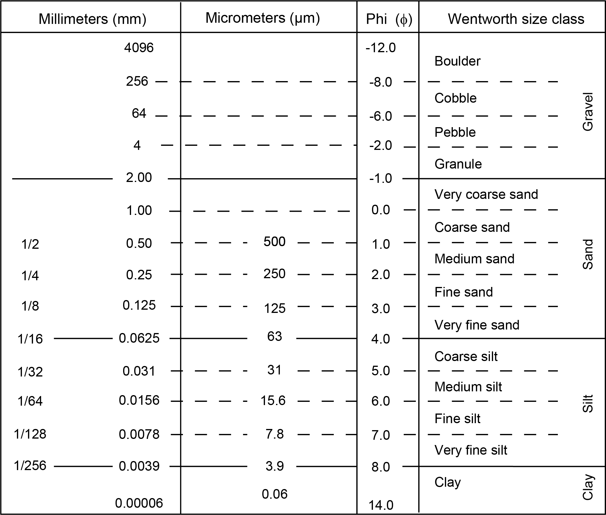
Figure F7. Wentworth grain-size classification.
2.3.3. Volcaniclastic deposits
Volcaniclastic deposits include a range of materials from rubbly, in situ volcanic debris to resedimented materials such as volcanic sands or tuffs. Volcanic materials of all sizes may be the direct product of eruptive processes (pyroclastic/primary) or may be accumulations through processes involving transport, sorting, and deposition (epiclastic/secondary). Pyroclastic activity includes hydrovolcanic deposits formed by explosive interaction between magma and water as well as nonexplosive quench fragmentation processes (e.g., hyaloclastite and peperite). Epiclastic volcanic sediment forms by the redeposition of volcanic detritus produced by erosion and/or reworking of volcanic rocks and unconsolidated deposits. Typically, there is a wide continuum of volcaniclastic materials in seamount environments that spans materials that are both pyroclastic/primary, existing at or near the point source of eruption, to locally resedimented volcanic materials (hyaloclastites and spalled debris from lava flows) to entirely resedimented volcanic material resulting from plume fallout or mass flow processes such as turbiditic resedimentation and debris flows. Classification and description are challenging because the componentry is essentially igneous, but the processes of accumulation ranges from primarily volcanic mechanisms to entirely sedimentary factors. Furthermore, the admixtures of nonvolcanic siliciclastics or, more commonly, biogenic sediments place some volcaniclastics in the mixture spectrum between purely igneous material and materials that are more appropriately described as entirely sedimentary (Figure F8).

Figure F8. Nongenetic lava and volcaniclastic classification.
Consequently, the classification of volcaniclastic deposits used here differs from the standard ODP classification (Mazzullo et al., 1988) in that we adopted a descriptive (nongenetic) terminology similar to that employed during ODP Leg 197 and Integrated Ocean Drilling Program Expeditions 324 and 330 (Shipboard Scientific Party, 2002a; Expedition 324 Scientists, 2010c; Expedition 330 Scientists, 2012a). We initially used "volcaniclastic" as a nongenetic term for any fragmental aggregate of volcanic parentage containing more than 50% volcanic grains and less than 50% other types of clastic and/or biogenic material (Figure F5). This definition is necessarily broader than that for pyroclastic deposits because the term "pyroclastic" strictly applies only to products of explosive volcanic activity, including hydroclastic deposits formed by explosive interaction between magma and water/sediment as well as nonexplosive quench fragmentation (i.e., hyaloclastite and peperite). Our adopted definition thus allows the inclusion of primarily detritus produced by erosion and/or transport of volcanic materials (i.e., epiclastic sediment). Accordingly, the term "volcaniclastic" does not necessarily imply active volcanism at the time of deposition.
Unless an unequivocally pyroclastic origin for the dominant volcanogenic particles could be determined, deposits composed of these materials were described according to the classification scheme for clastic sediments, with a generic "volcanic" modifier noting the composition of the clasts. For instance, a breccia with 80% basalt clasts and 10% bioclasts is called a "volcanic breccia with bioclasts." We followed the clastic textural classification of Wentworth (1922) to separate the various volcanic sediment types and sedimentary rocks (according to grain size) into volcanic breccia/conglomerate (>64 mm), gravel (2–64 mm), sand (62.5 μm to 2 mm), silt (62.5–3.9 μm), and clay (<3.9 μm). For coarse-grained and poorly sorted volcaniclastic sediments, such as those produced by gravity currents, we also applied the terms "volcanic breccia" (angular clasts) or "volcanic conglomerate" (rounded clasts) and used lithologic or structural modifiers for further description. Sedimentary structures recorded included graded bedding, cross-bedding, planar laminations, foreset bedding, dune forms, and ripples.
In those instances where evidence for a pyroclastic origin was compelling and most likely resulted from fragmentation through magmatic degassing or phreatomagmatism, we adopted the classification scheme of Fisher and Schmincke (1984) and used the grain-size terms "volcanic blocks/breccia" (>64 mm), "lapilli/lapillistone" (2–64 mm), and "ash/tuff" (<2 mm). We used the term "hyaloclastite" for a distinctive type of volcaniclastic deposit of predominantly pyroclastic origin formed by subaqueous eruptions. Hyaloclastite (which means glass-fragment rock) includes deposits commonly <64 mm in size that are dominated by glassy fragmental debris with, occasionally, a minor component of volcanic lithic clasts (e.g., fragments of pillow lava). Hyaloclastite can be abundant at seamounts, where it is a typical product of cooling contraction granulation and surficial spalling of lava flows, and it is often found in association with pillow basalt breccias (e.g., Staudigel and Schmincke, 1984). More rarely, hyaloclastite is also produced by magma fragmentation during submarine fire fountain eruptions (Simpson and McPhie, 2001). Characteristic environments of hyaloclastite production on intraplate oceanic volcanoes include lava deltas on the shelf of islands (Ramalho et al., 2017; Buchs et al., 2018) and slopes associated with the development and advancement of submarine eruptions at greater water depths (Staudigel and Schmincke, 1984; Dickinson et al., 2009). The glassy ash portion of hyaloclastite pillow breccias typically consists of flat glass shards spalled off of expanding pillows, with keystone-shaped fragments derived from the pillow rims. In contrast, hyaloclastites that represent submarine fire fountain deposits are characterized by rounded lapilli formed from quenched magma globules, along with angular glass shards formed by thermal shock fracturing of globules and shattered vesicle walls. The term "peperite" was used for volcanic-sediment facies occurring where submarine lava flows interacted with unconsolidated sediment as they erupted on the seafloor (Skilling et al., 2002). The mingling of lavas and wet sediments produces distinct volcanic textures resulting from the physical lava-sediment interaction (e.g., entrainment, baking, chilling, etc.). Physical and chemical fragmentation and alteration through steam-rock interaction occur during flash heating of the water, leading to local destruction of original sedimentary structures. The presence of peperites and their textures may provide important information regarding the nature of the eruptive environment. Importantly, occurrence of peperites is taken as evidence that the volcanism and affected sedimentary environment existed contemporaneously.
Accordingly, in those instances in which processes of emplacement or resedimentation can be appropriately identified, an extended version of the classification scheme in Figure F8 enabled a more precise genetic classification (Figure F9).
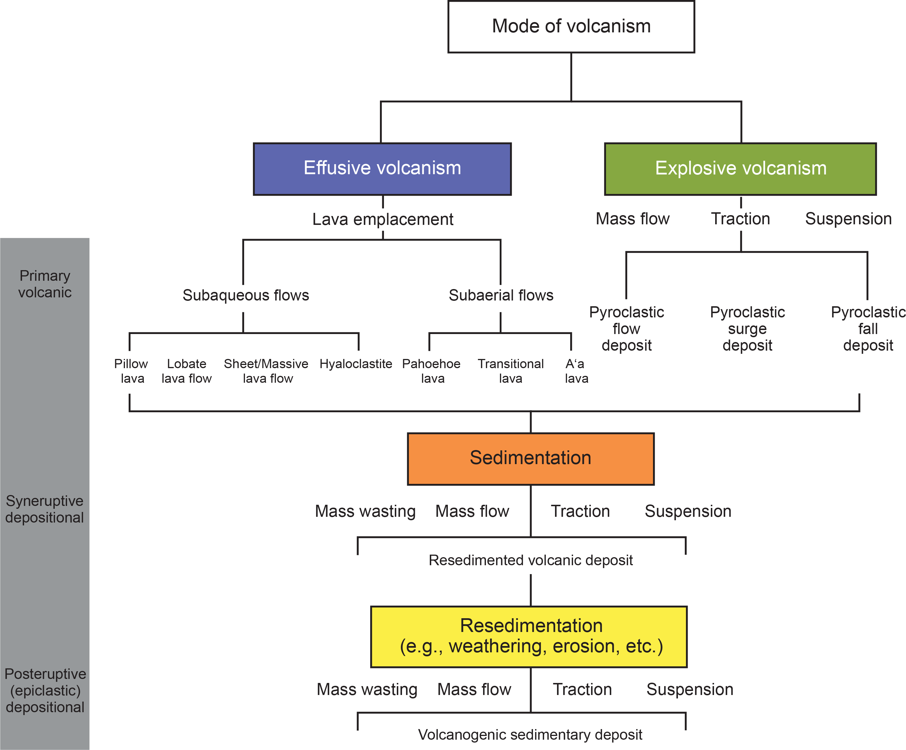
Figure F9. Genetic lava and volcaniclastic classification.
2.3.4. Smear slides and thin sections
The method and routine for smear slide (and XRD) preparation and analysis follow those employed during IODP Expedition 367/368 (Sun et al., 2018). Typically, at least one smear slide sample of the main lithologies was collected from the archive-half section of each core, depending on the amount of recovery, which was incomplete due to RCB coring. Where clear changes in sediment type were identified (i.e., color, grain size, composition, etc.) additional samples were collected to better characterize that change; similarly, areas of interest (e.g., unusual laminations, ash layers, and nodules) were also considered.
For smear slides, sampling involved extracting a small amount of sediment with a wooden toothpick and putting it on a 2.5 cm × 7.5 cm glass slide. The sediment sample was homogenized with a drop of deionized water and evenly spread across the slide to create a very thin (about <50 µm) uniform layer of sediment grains for quantification. The dispersed sample was dried on a hot plate. A drop of Norland optical adhesive was added as a mounting medium to a coverslip, which was carefully placed on the dried sample to prevent air bubbles from being trapped in the adhesive. The smear slide was then cured in an ultraviolet light box.
For thin sections of lithified sediment, billets were prepared by cutting 3–5 cm3 from the working half of the core. If necessary, the cut billet was impregnated with a clear epoxy to further consolidate the grains. Billets were then mounted on 2.5 cm × 4.5 cm glass slides and ground down to a thickness of ~30 µm.
Smear slides and thin sections were examined with a transmitted-light petrographic microscope equipped with a standard eyepiece micrometer. The texture of siliciclastic grains (relative abundance of sand-, silt-, and clay-sized grains) and the proportions and presence of biogenic and mineral components observed in thin sections or smear slides were recorded in DESClogik. Biogenic and mineral components were identified using IODP Technical Notes 1 and 2 for smear slides (Marsaglia et al., 2013, 2015), and their percentage abundances were visually estimated using Rothwell (1989). The mineralogy of clay-sized grains could not be determined from smear slides. Smear slide analyses routinely underestimate the amount of sand-sized and larger grains because they are difficult to incorporate onto the slide.
Relative abundances of identified components such as mineral grains, microfossils, and biogenic fragments were assigned on a semiquantitative basis using the following abbreviations:
- R = rare (<5 vol%).
- C = common (5–25 vol%).
- A = abundant (25–50 vol%).
- D = dominant (50–75 vol%).
- M = major (>75 vol%).
2.3.5. X-ray diffraction analysis
Samples for XRD analyses were selected from the working half, generally at the same depth as smear slide analyses. Approximately one 5 cm3 sample was taken of a representative lithology per core. Samples analyzed for bulk mineralogy were freeze-dried and homogenized by grinding in a metal ball mill. Prepared samples were top-mounted onto a sample holder and analyzed using a Malvern Panalytical AERIS diffractometer mounted with a PIXcel1D-Medipix3 detector using nickel-filtered CuKα radiation. Settings for the standard bulk sample scan were as follows:
- Voltage = 40 kV.
- Current = 15.0 mA.
- Goniometer scan = 4°–75°.
- Step size = 0.0108664°2θ.
- Time per step = 40 s/step.
- Divergence slit = 0.25°.
Diffractograms of bulk samples were evaluated with the aid of Malvern Panalytical's XRD High Score software suite, which allowed for mineral identification and basic peak characterization (e.g., baseline removal and characteristic peak intensity). Files were created that contained d-spacing values, diffraction angles, and peak intensities with and without the background removed. These files were scanned by the High Score software to find d-spacing values characteristic of a limited range of key minerals typically used to distinguish broad sediment types. Where appropriate, peak areas were further quantitatively estimated using the High Score software to yield semiquantitative results of the relative abundances of the most common mineralogical components.
3. Igneous petrology and volcanology
Igneous and volcaniclastic rock lithologies were determined using a combination of macroscopic and microscopic observations coupled with chemical and mineralogical data. These lithologies were further classified using their physical occurrence as volcanic units. Description procedures for physical volcanology and igneous petrology used during Expedition 391 were adapted from Integrated Ocean Drilling Program Expeditions 324 and 330 and IODP Expeditions 350, 352, and 376 (Expedition 324 Scientists, 2010b; Expedition 330 Scientists, 2012a; Arculus et al., 2015; Reagan et al., 2015b; de Ronde et al., 2019). Macroscopic observations were coordinated, where possible, with smear slides, thin section petrographic observations, and bulk rock chemical and mineralogical analyses of representative samples, using ICP-AES, XRD, and portable X-ray fluorescence spectrometry (pXRF) (see Geochemistry). Data for the macroscopic and microscopic descriptions of recovered cores were entered into the LIMS database using DESClogik. Volcanic rock characteristics were entered into the Extrusive hypabyssal tab, and alteration assemblages were entered into the Alteration tab.
Our shipboard studies sought to systematically describe the petrology, physical occurrence, and alteration of the cored rocks. First, phenocryst abundance and appearance, lithologic components (for volcaniclastic sediments), and characteristic igneous textures and vesicle distribution were described at the macroscopic level and investigated in more detail by thin section. Second, pXRF analysis was performed on selected core sections to inform physical observations. Third, the recovered, analyzed, and described material was divided into coherent units. Igneous and volcaniclastic unit boundaries were defined using complementary information, including petrography, volcanic and sedimentary structure/textures, chemical composition, and physical properties such as MS.
3.1. Volcanology
3.1.1. Eruptive products
Effusive basaltic volcanism in both the subaerial and submarine environments produces a range of common features typically associated with the development and inflation of flow lobes of varying sizes, pillow lavas, and pahoehoe or rubbly flow surfaces, as well as where lava interacts directly with seawater, hyaloclastites, and breccias.
Previous information regarding the nature of volcanism along Walvis Ridge is scant. However, volcanism sampled during this expedition is consistent with the literature on submarine volcanism.
3.1.1.1. Submarine lava eruptions
Submarine lavas represent the most abundant surficial igneous rock on the surface of the Earth, forming the greater proportion of the ocean floors. At spreading ridges, lava effusion is typically dominated by stacks of budding and anastomosing pahoehoe-like extrusions, resulting in piles of rounded or tubular masses (Batiza et al., 1999), the most readily recognized of which is the pillow basalt, often referred to as pillow lava. However, larger, pod-like inflation units, as well more laterally extensive sheet-like extrusions that are a few meters thick, have also been observed (e.g., Lonsdale and Spiess, 1980; Mitchell et al., 2008); massive flows that are several meters thick occur and likely result from extrusion rates approaching those more typical of subaerial lavas (Expedition 324 Scientists 2010c). The morphology of submarine flows is primarily controlled by local flow rate, which is itself a function of slope and eruption rate (Walker, 1992; Gregg and Fink, 1995; Mitchell et al., 2008, and references therein).
3.1.1.2. Volcaniclastic deposits
Volcaniclastic deposits, or volcaniclastites, are primary volcanogenic fragmental deposits produced during explosive volcanism (pyroclastic) and lava emplacement or resedimented (epiclastic) volcanic deposits. They include a range of materials from rubbly, in situ volcanic debris to resedimented materials such as volcanic sands or tuffs. Pyroclastic activity includes hydrovolcanic deposits formed by explosive interaction between magma and water as well as nonexplosive quench fragmentation processes (e.g., hyaloclastite and peperite). Epiclastic volcanic sediment forms by the redeposition of volcanic detritus produced by erosion and/or transport of volcanic rocks. (see Lithostratigraphy).
Hyaloclastites typically consist of glassy and/or lithic fragments <64 mm in diameter (hyaloclastite lapilli tuff) but may also include larger fragments (hyaloclastite breccia or tuff-breccia) or isolated pillows (hyaloclastite pillow breccia). These may be less than a meter to several meters thick and are commonly intercalated with pillow lava or sheet flows. The glassy ash portion of hyaloclastite pillow breccias typically consists of flat glass shards spalled off expanding pillows, with keystone-shaped fragments derived from the pillow rims. In contrast, hyaloclastites that represent submarine fire fountain deposits are characterized by rounded lapilli formed from quenched magma globules along with angular glass shards formed by thermal shock fracturing of globules and shattered vesicle walls.
3.1.1.2.1. Definition of lava and hypabyssal intrusive flow types
We adopt the following definitions of lava types based on their morphology and associated attributes from IODP Expeditions 349 and 352 (Li et al., 2015; Reagan et al., 2015b).
Pillow flows are subaqueous extrusions resulting from individual budding, inflation, and separation of lava pods from small vents or point sources along the advancing lava front. Depending on effusion rate, number of point sources, and internal plumbing architectures, pillow flows can accumulate into thick stacks and can be a major component of a developing volcanic edifice. They consist of discrete, subrounded units that are relatively small in size (diameter = <1.0 m), and characteristically, their exteriors are entirely bounded by curved, glassy rinds because of rapid cooling; their interiors typically display internally radiating vesicles and joint patterns. Submarine pillows occur at various depths, are the product of various volcanic settings (e.g., ocean spreading centers, off-ridge and isolated seamount edifices, ocean islands, and submarine large igneous provinces/oceanic plateaus), and display a range of extrusive compositions and forms (Batiza et al., 1999).
Lobate flows are larger, single inflation units (diameter = 1–2 m) that cover areas of several square meters or more and are developed by the same endogenous inflation process as pillow lavas. Their size and morphology are indicative of a higher effusion rate than that of pillow lavas, and they differ in that they have massive, coarser grained, and sparsely vesicular interiors, often with pipe vesicle domains. A larger size permits a slower rate of cooling, more effective degassing, and the maturation of internal vesicle patterns as a series of vesicle bands which develop through the inward migration of the cooling front; in contrast, the lower part of the inflation unit typically contains either sparse, poorly defined vesicle banding and/or teardrop-shaped vesicles at or just above the basal chill zone. Rather than being spherical or subspherical, these inflation units tend to have flattened, oblate, or tubular shapes, and they are most probably generated as a series of interconnected, semiadjacent inflation units fed simultaneously by internal plumbing or else merging through rupture and coalescence.
Sheet flows and massive flows are laterally extensive units forming sheet-like, internally massive basalt flows (van Andel and Ballard, 1979). They generally have relatively flat upper surfaces (unlike pillow lava) and may have a variety of surface features generated by deformation and disturbance of the solidifying lava crust while in a plastic/semiplastic state. The largest examples (>10 m thick) can resemble those of larger, subaerially erupted flows in dimension and internal features, but subaerial flows are generally characterized by basal and top breccias of broken up lava. Submarine flows often have texturally uniform massive interiors that are up to several meters thick, and they are characterized by sparse vesicle layering or vertical vesicle pipes containing late-stage melt segregation material. Thicker inflation units (similar to those documented in continental flood basalts) are often characterized by the threefold structure of a vesicular upper crust, a dense interior, and a thinner vesicular lower crust; aphanitic top and lower margins with glassy mesostasis are often present as part of the chilled upper and lower margins, and in some cases, glassy selvage may be preserved at the uppermost margin. Massive or sheet-like flows are a response to particularly high effusion rates and/or local slope and other controlling topographic conditions in which the lava is restricted from spreading (pooled). We use the terms "sheet lava flow" for sheet-like flows <3 m thick and "massive lava flow" for very thick (>3 m) units that may be comparable in lateral dimension to those observed in flood basalt provinces (Aubele et al., 1988; Thordarson and Self, 1998; Jerram and Widdowson, 2005).
The description above may be summarized as the following lava type definitions based on unit thicknesses and associated attributes:
- Pillow lava flows are 0.1–1 m thick and defined by curved chilled margins, spherulitic textures, glassy margins and/or hyaloclastites, and microcrystalline to cryptocrystalline groundmass grain size, as well as decreasing crystal abundances and sizes (phenocrysts, groundmass) toward the glassy rims.
- Lobate lava flows are 1–2 m thick and formed by the same inflationary process as pillow lavas; in lateral dimension, they present an elongate pod-like morphology and have massive, coarser grained, and sparsely vesicular flow interiors with pipe vesicle domains. Lower zones contain sparse, poorly defined vesicle banding and/or teardrop-shaped vesicles at the basal chilled zone.
- Sheet/massive lava flows are internally uniform below the upper chilled margin and vesicle zoning (if present) in the uppermost zones of the inflation unit. The lower margin contains sparse vesicle banding, and pipe vesicle domains may be common in the flow interior. These are often characterized by a readily identifiable increase in grain size toward the center of the flow. Sheet lava flows are <3 m thick, whereas massive lava flows are often significantly >3 m thick. Note that sheet flows and pillow/lobate flows may overlap in thickness; they are distinguished by the physical characteristics described below.
A key aim of Expedition 391 was to produce an integrated picture of the style and evolution of the later stages of volcanism (and postvolcanic fate) at each drill site. This was achieved by systematic rock descriptions and identification of key effusive volcaniclastic and igneous textures that are known to be diagnostic of specific modern physical volcanic processes. The first step involved defining boundaries of igneous units by either visual identification of actual lithologic contacts or inference of the position of such contacts using observed changes in volcanic characteristics and/or volcaniclastic features. This was followed by general description of the lithology, lithologic variation, and characteristic igneous textures; these macroscopic observations were combined with and tested and refined against those from detailed petrographic microscopy (mineralogy) and semicontinuous geochemical core analysis from pXRF.
3.1.1.3. Recognition of eruptive units
A methodology that permitted the logging and recording of the volcano-sedimentary succession at all four sites was developed. Most lava-type classifications are based on field observations that consider both the lateral and vertical variations of eruptive units and their stacking relationships. Such refined classifications are neither realistic nor justifiable from core observation alone, and they may only emerge through an integration of multiple data streams alongside the recorded core log data (e.g., petrography, downhole logging data, geochemical [chemostratigraphic], and paleomagnetic results). Lithofacies associations provide one such avenue of nongenetic description and have been successfully applied to a range of large igneous province types (e.g., Jerram and Widdowson, 2005; White et al., 2009).
In general, the most unequivocal evidence for dividing core into individual eruptive units is the presence of flow-to-flow contacts, although these are not always common in low-recovery sections. Alternatively, the presence of glassy material or finer grained chill zones can also provide a useful proxy for determining the presence or estimating the position of unit boundaries. Alteration is another aspect that can aid in placing lava unit boundaries in drill cores. Alteration is typically most accentuated toward the upper margin and to a lesser extent the lower margin of the flow. This is often manifest as visible discoloration from the blue-gray unaltered basalt (i.e., diffuse brown or green, depending on oxidation regime) and is aided by (1) proximity to the flow margin allowing fluid ingress and (2) increases in the degree of fracturing toward the upper flow boundary (e.g., brittle cooling fractures) allowing direct access by fluids. In the middle flow (i.e., flow interior) sections, alteration is at a minimum. In cases in which the interior (most massive sections) of units are preferentially recovered, changes in vesicularity can be valuable in identifying unit boundaries because systematic variation often occurs within lava inflation units of all sizes. This includes vesicle attributes such as the volume percentage and changes in vesicle size (i.e., fining- or coarsening-upward) and shape. Ideally, identification of unit boundaries in recovered core requires agreement of at least two of the above flow boundary diagnostics. However, of these diagnostics, the presence of intercalated sediment or, in exclusively igneous successions, the presence of glassy selvage (sheet or massive flows) or glassy rinds (pillow basalts) is considered unequivocal.
3.1.1.4. Pillow lava, lobate flows, and small phyric sheet flows
Where the drill core passes through pillow stacks, key components of the pillow lava or lava lobes are commonly intersected and recovered. In exceptional examples, whole interlinked pillow successions connected by welded glassy margins of interstitial glass spall (hyaloclastite) may be recovered. However, it is more challenging to distinguish larger units, which have a much more laterally extensive spread; these may be more appropriately termed sheet flows, whereas massive flows are even thicker (several meters) and laterally more extensive.
Identification of pillow lava and lobate flows in drill core and drill core fragments can be achieved by using key recurrent features that are ubiquitous to pillow masses. This aids in piecing together and describing pillow stacks when there is commonly incomplete or poor recovery due to the differing mechanical properties of pillow components. Pillow stacks of smallish pillow lavas are often easily identified because the drilled core readily intersects subvertical chill margins as well as those at the bases and tops of pillows. Such frequent intersections clearly indicate the limited lateral dimension of the pillows, effectively that they are tube- or balloon-shaped forms. To better describe the pillow stacks and to appropriately consider the intermediate types of eruptive units, the following protocol was adopted:
- Pillow lava: in core, the drill commonly passes through upper parts and into lower bases (and less frequently edges) and thus presents a particular sequence of features and textures (Figure F10). Ideally, a pillow lava should exhibit the following:
- Shape/size: a roughly equidimensional (ball- or pillow-like form) with an encasing chilled margin. In core, this is exhibited as contacts at a variety of angles from horizontal to near vertical, reflecting the different aspects of the chilled surface.
- Glassy rim: the most readily identifiable (and sought) feature of water-chilled lava. However, some examples lose much of their surface glass due to spalling, and others develop only an extremely thin (a few millimeters) glassy rind but a more readily identifiable discolored (brownish) chilled margin. The thickness of glass and chilled margin vary according to intrinsic factors including composition, crystal content, eruptive temperature, and external controls, such as whether the unit falls into cold sediment or is insulated by adjacent neoformed pillows (slower cooling).
- Chilled margin: chilled margins occur in all pillows and pass into the outer glassy rind (if present). They are micro- or cryptocrystalline and can often preserve (freeze in) any primary crystal cargo. They are typically discolored to pinkish brownish due to exchange with seawater (oxidation). Chilled margins are often nonvesicular or very sparsely vesicular because the freezing of the outer layer occurs before effective internal degassing.
- Radial joint/vesicle pattern crack pattern: radial joints are cooling/contraction joints that propagate orthogonally to the cooling surface; their development can act as conduits for internal degassing. Larger vesicles can coalesce along the propagating tips of cooling joints. Both cooling joints and radial vesicle patterns are often best developed in the upper half of the pillow unit.
- Pillow interior: pillow interiors often present a distinct zonation that is characteristic of pillows as compared with larger sheet flows:
- Upper: contains greater accumulation of small vesicles or even vesicle layer accumulations beneath the chilled margins. Because gas cannot readily escape through the glassy and chilled margins, the vesicles become trapped beneath the upper chill zone and accumulate in the upper third; this accumulation can develop into a spongy texture (vesicle diameter = 1–2 mm).
- Middle: more phenocryst rich if porphyritic and preserves the overall crystal cargo. In aphyric types, there may be a slightly coarser texture derived from a marginally slower cooling of the interior. Often present are short or longer (in bigger pillows) pipe vesicles that developed after the pillow completed inflation and was emplaced; they are vertical and therefore serve as a useful geopetal structure.
- Lower: the bulk is sparsely vesicular. All small (typically <1 mm) but larger aligned teardrop-shaped vesicles often occur, representing standing bubble trains that form at the lower cooling interface (i.e., inside the basal chill margin) during degassing of the stagnating pillow. This type of coalescing vesicles is common at a fixed location in the lower pillow and originates at the inner basal chilled margin.
- Basal chilled margins: basal chilled margins are similar to but commonly narrower than the top margin and may have a thin glassy outer layer. Commonly, basal chilled margins are flat or subhorizontal because they can plastically deform under the weight of the pillow body after eruption and mold themselves onto the substrate.

Figure F10. Pillow basalt.
By examining the nature of vesicle accumulation or their relationship with preserved chill margins, the size and number of pillow lavas in an otherwise fragmentary recovered section can be reconstructed. This is particularly useful in sections of poor recovery where pillow interiors are more resistant and thus preferentially represented. In such fragmentary sections, the order of appearance of the different components described above can be an effective method of determining where upper and lower pillow boundaries may have occurred even in poorly recovered and incomplete cores.
Small phyric sheet flow: in some parts of the igneous basement succession cored during Expedition 391, and especially at Site U1578, there were intervals that, despite their modest thickness (<1–2 m), could not be readily described as a pillow lava in the strictest sense because only top and basal chilled margins were recovered, indirectly indicating they likely had much greater lateral extent. In addition, these intervals showed clear evidence of significant internal mineralogical differentiation, which is more typical of much thicker (and volumetrically larger) sheet or massive flows. These are considered a form of sheet flow (see the Site U1578 chapter [Sager et al., 2023]). To recognize the unusual nature of these eruptive units and distinguish them from the remainder of the pillow stack, we suggest the term "small phyric sheet flow."
3.1.1.5. Sedimentary interbeds in the igneous basement
Although volcanic materials were described below the sediment/volcanic basement contact, sedimentary units were occasionally preserved between volcanic units. For ease of descriptive continuity, fundamental sedimentary rock names (limestone, silt, mud, clay, sand, conglomerate, breccia, and chert) are included with the list of principal lithology names in the Hypabyssal/volcanic tab. These names can be modified with compositional prefixes (volcanic, siliceous, calcareous, siliciclastic, pelagic, and neritic) and associated suffixes (sediment, rock, and ooze) (see Lithostratigraphy).
3.2. Igneous petrology
Volcanic and hypabyssal rocks are the dominant component of upper oceanic crust, commonly underlying a carapace of resedimented (epiclastic) volcanogenic sediment and typically, with increasing age, thick accumulations of pelagic sediment. Volcanic and hypabyssal rock units have principal names based on their inferred or measured chemical compositions as defined by the International Union of Geological Sciences subcommission on volcanic rock names. These names are modified by prefixes that describe mineralogical or textural characteristics of that rock and by suffixes that describe their physical occurrence. The composition of these lavas and their hypabyssal equivalents are representative of their mantle source regions and the processes of melting and fractionation that formed them. Understanding the formation and evolution of their parent magmas was a first-order goal of this expedition.
3.2.1. Volcanic unit classifications
At the fundamental level, volcanic successions typically comprise multiple cooling or inflation units of similar or shared evolutionary characteristics. To enable collation of observed volcanic elements into volcanically meaningful successions, we define the simple twofold numerical hierarchy for igneous products: (1) individual eruptive units such as lobate, sheet and massive flows, or volcanic facies, which represent a distinct eruptive event type such as pillow-lava stacks or hyaloclastic successions, and (2) packages that appear to be petrogenetically or volcanically related and can be grouped together within an eruptive episode. Igneous units are given consecutive Arabic numerals downhole (Igneous Units 1, 2, etc.). Subunits were used in cases where the mineralogy/composition is similar but frequent changes in texture were observed (e.g., Igneous Subunits 1a, 1b, etc.). These then form the following definition and numbering system:
- Individual eruptive or flow units are the basic units defined by the presence of lava contacts or identifiable flow tops (i.e., glassy or chilled margins, vesicle abundances, alteration, etc.). These are classified according to size/thickness as determined from thickness information derived from core logging and associated DESClogik entries (pillow, lobate, sheet and massive flows, etc.).
- Igneous units are given consecutive downhole Arabic numerals (i.e., Igneous Units 1, 2, etc.) and may be either distinct individual lava units or related lava units and packages that can be considered to be petrogenetically or volcanically distinct. In effect, the unit should aim to represent a distinct eruptive episode. Igneous units are separated from one another according to the following order of diagnostics:
- Division of the eruptive units on the basis of any intercalated sedimentary material. The rationale here is that occurrence of sedimentary interbeds records a significant hiatus in volcanic activity at the drill site.
- Identification of individual massive or sheet flows, or pillow and lobate stacks, based on physical criteria and thickness determinations. Each distinct eruptive unit is then given a consecutive Arabic numeral (i.e., Igneous Units 1, 2, etc.). Where units appear to have been rapidly and successively emplaced one upon another, the subunit nomenclature (e.g., Igneous Subunits 1a, 1b, etc.) is employed. Examples include successive massive flows with no discernible emplacement hiatus (e.g., no sediment or little/no flow top alteration) and uninterrupted pillow, lobate, and sheet flow stacks.
- If chemical differences can be determined using pXRF data, then units considered volcanologically continuous are divided using subunit nomenclature (e.g., Igneous Subunits 1a, 1b, etc.). The rationale here is that variable core recovery preferentially preserves flow interiors rather than upper and lower boundaries that are used to identify flow (igneous) unit boundaries. Chemical data can identify petrogenetically different units and, hence, boundaries where the physical evidence has been lost.
3.2.2. Core description workflow
The procedures used to document the composition, texture, and structures of rocks recovered during Expedition 391 included visual description of the core, petrographic thin section analysis, digital color imaging, color spectrophotometry, and pXRF analysis. Before the core was split into working and archive halves, each hard rock piece was oriented (if possible) and archived into numbered bins. Whole-round images of large sections of core were taken at 0°, 90°, 180°, and 270°. Hard rock pieces were split with a diamond-impregnated saw along lines chosen by a petrologist so that important compositional and structural features were preserved in both halves. Once split, each rock in both the working and the archive halves was labeled individually with unique piece/subpiece numbers from the top to the bottom of each section. If the top and bottom of a piece of rock could be determined, an arrow was added to the label to indicate the uphole direction. The archive halves were imaged using the SHIL, which also records red, green, and blue spectral colors along the centerline of the core. After imaging, the archive halves were analyzed for color reflectance and MS at 2 cm intervals using the SHMSL (see Physical properties). Selected pieces from the archive half were analyzed by pXRF (see Igneous geochemistry) to characterize the bulk chemistry of the core and then refine the chemostratigraphy around suspected unit boundaries. The working halves were sampled for shipboard physical properties, paleomagnetic studies, thin sections, and geochemical analysis by ICP-AES and XRD analysis. All cores that were sampled for shipboard ICP-AES analyses had complementary pXRF analyses performed on the archive half for comparative and data assessment purposes.
Each core section was first macroscopically and then microscopically examined and described for petrologic and alteration characteristics. Lithologic descriptions and most structural observations (see Structural geology) were made on the archive halves. For microscopic observations, up to 12 thin sections per day were made from the working halves. For macroscopic and microscopic observations and descriptions, DESClogik was used to record the primary igneous characteristics (e.g., groundmass and phenocryst mineralogy, as well as vesicle abundance and type) and alteration (e.g., color, vesicle filling, secondary minerals, and vein/fracture fillings) (Figure F11). Mineral modes and sizes were estimated using a 10× magnification field hand lens and a binocular microscope. The modal abundance and size of all phenocryst phases are recorded together with other parameters including the shape and habit of each phase. Other recorded descriptive parameters are rock texture (see below), grain size, phenocryst phase and abundance, vesicularity and vesicle shape, secondary minerals, and the nature of contacts between volcanic rock intervals.
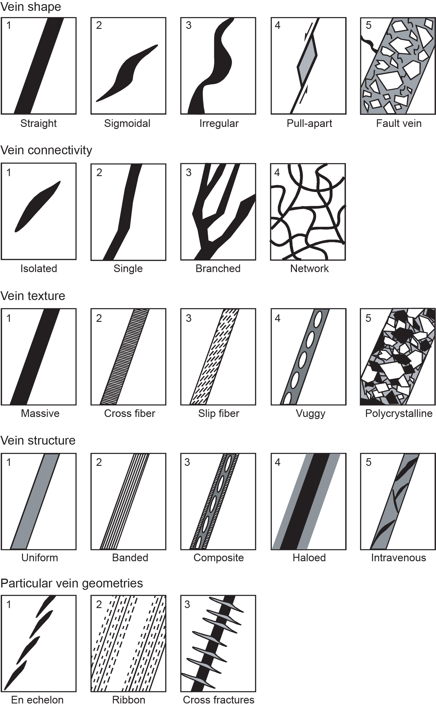
Figure F11. Vein description.
3.2.2.1. Principal lithology name and descriptive parameters
The lithologic name comprises a principal name, a prefix, and an optional suffix. The principal name is based on the nature of the phenocrysts, when present, the color of the groundmass, and, where available, the chemical composition as determined by ICP-AES or pXRF. Seven principal names are defined in DESClogik:
- Basalt: black to dark gray rock containing olivine, plagioclase, and/or pyroxene.
- Dolerite: black to dark gray rock with basaltic or basaltic andesite composition but typically coarser grained than basalt.
- Andesite: dark to light gray rock containing pyroxenes and/or feldspar and/or amphibole, typically devoid of olivine and quartz.
- Dacite: light gray to tan rock, usually plagioclase-phyric, and sometimes containing pyroxenes ± quartz ± hornblende.
- Rhyolite: light gray to pale white rock, usually plagioclase-phyric, and sometimes containing quartz ± hornblende.
- Volcaniclastite: this term is typically used as a principal lithology when the lithic-rich and ash-rich portions of hyaloclastite pillow breccias or tuff breccias are described as separate domains.
- Altered volcanic rock: general term for (formerly) primary volcanic rock that has been altered so that the primary rock type (apart from its texture indicating a volcanic origin) cannot be determined with certainty.
3.2.2.1.1. Prefixes
Porphyritic rocks are named according to major phenocryst phase(s) when the total abundance of phenocrysts is >1%. The term "phenocryst" is used to describe any crystal significantly larger (typically more than 5×) than the average size of groundmass and >1 mm in diameter. The term "microphenocryst" is used for crystals larger than the modal groundmass grain size but <1 mm. A prefix is applied as a modifier to the primary lithology names to indicate the phenocryst assemblage in the hand samples. The term "glomerocryst" is used to describe clusters of intergrown phenocrysts that represent a normal phenocryst assemblage. Rocks lacking visible phenocrysts are modified by the term "aphyric" to indicate a lack of phenocrysts.
There are two columns for modifiers that precede the principal lithology name. The first prefix indicates the total phenocryst abundances:
The second prefix identifies the phenocryst assemblage, with minerals listed in decreasing order of abundance. For example, a "moderately phyric plagioclase-pyroxene basalt" is a basalt that has 5%–10% phenocrysts and more plagioclase than pyroxene. These terms (the first and second prefix and the principal rock name) are concatenated with a suffix to complete the rock name.
3.2.2.1.2. Suffixes
The suffix in DESClogik indicates the nature of the volcanic body: glass, lava, pillow lava flow, lobate lava flow, sheet lava flow, massive lava flow, hyaloclastite, breccia, peperite, sediment, rock, or clast. The suffix "hyaloclastite" or "breccia" is used if the rock is in direct association with related lava. "Sediment" and "rock" are used to indicate sedimentary intercalations in the volcanic section.
3.2.2.1.3. Textures and vesicles
Textures are described macroscopically for all igneous rock core sections and microscopically for the subset of intervals having thin sections. Grain size modal names are as follows:
- Coarse grained = >5 mm.
- Medium grained = >1–5 mm.
- Fine grained = 0.3–1 mm.
- Microcrystalline = <0.3 mm.
- Cryptocrystalline = <0.1 mm.
Vesicularity is described according to the following proportions:
- Nonvesicular = 0%.
- Sparsely vesicular = <5%.
- Moderately vesicular = 5%–20%.
- Highly vesicular = >20%.
The modal size and roundness of vesicle populations are visually estimated, along with the extent of secondary vesicle filling phases (typically clays, zeolites, or calcite), in the Alteration tab.
3.2.2.1.4. Domains
Some core sections comprise two or more distinct domains. These domains may be described and named separately, with the proportion of each domain indicated in DESClogik. Domain names are based on the dominant characteristic of that domain. If a domain contact is visible, the nature of the contact is also noted. For Expedition 391, domain names include the following terms:
- Volcanic clast, mafic;
- Mafic lava;
- Felsic lava;
- Pillow matrix;
- Pillow top;
- Glass;
- Scoria;
- Sediment matrix;
- Vein matrix; and
- Xenolith.
The most prominent macroscopic and microscopic textures were identified for each unit or thin section, respectively. The proportion of each domain is indicated in DESClogik, and each domain is given a lithologic name. Phenocrysts and, in microscopic description, groundmass phase abundances were estimated, including altered versus unaltered populations. Likewise, phenocryst size (maximum and mode), shape (anhedral, subhedral, euhedral, or interstitial), and habit (subequant, tabular, equant, or elongate) were estimated along with any unique properties (e.g., extent and type of zoning).
3.2.2.2. Secondary minerals in igneous rocks
Alteration features in igneous rocks from Expedition 391 are based on macroscopic observations of the core aided by shipboard smear slide, thin section, and XRD and ICP-AES investigations. Secondary minerals in drill cores were recorded in DESClogik in the Macroscopic template under separate tabs for Alteration, Veins, and Halos as the percentage of rock consisting of secondary materials (including devitrification).
Descriptions of veins and halos record their mineralogy, geometry, contacts, and crosscutting relationships with the host rock. Vein texture selections are vuggy, cataclastic, saccharoidal, sutures, patchy, banded, comb structured, overgrowths, fibrous, or brecciated. Vein geometry selections are splayed, sinuous, irregular, planar, or curved. Vein contacts may be gradational, sharp-to-gradational, sharp, sutured, or diffuse. Vein connectivity is described as networked, anastomosing, branched, or isolated. Vein and halo minerals are described as dominant, second order, or third order.
3.2.3. pXRF measurements
The pXRF provides real-time characterization of drill core for assessment of broad chemical variations and how they may (or may not) tie to petrographic observables. Measurements are calibrated using reference materials and correction factors applied for some elements (see Geochemistry). Some limits were imposed on the use of pXRF data to determine unit boundaries. First, only elements that should be minimally affected by alteration are targeted for igneous unit distinction (e.g., Cr, Ti, and Zr). Second, only large shifts (>30%) in the abundance of Cr, Ti, and Zr are interpreted as suggestive of unit breaks. Real-time pXRF measurements proved invaluable for characterization of extrusive rocks in previous expeditions where the volcanic rocks were dominantly aphyric and microcrystalline, thus hindering more traditional initial unit definition based on petrographic variation. Finally, the rapid nature of data acquisition in the core laboratory allowed pXRF characterization to aid in shipboard sampling.
3.2.4. Visual core descriptions
Macroscopic features observed in the cores are summarized and presented in the VCDs. They display the following entries in terms of igneous, volcaniclastic, alteration, structural, and physical property features for each core section (Figure F12):
- Core depth below seafloor, Method A (CSF-A), depth scale in meters (equivalent to mbsf);
- Core length scale from 0 to 150 cm;
- Number of hard rock pieces;
- Igneous unit/subunit;
- Orientation of hard rock pieces;
- Interval and type of shipboard samples;
- Scanned digital image of the archive half; and
- Graphic representation of lithology.

Figure F12. Example igneous VCD.
Igneous VCDs display the following information (Figure F12):
- Phenocryst abundance (volume percent) for olivine, plagioclase, and clinopyroxene;
- TiO2 in ppm;
- NGR measurement;
- Plot showing SHMSL MSP measurements;
- Diagram displaying color reflectance parameters luminescence (L*), red-green (a*), and blue-yellow (b*); and
- Section unit summary of each igneous unit identified in the corresponding section.
The section unit summary (presented on the right side of the VCD; Figure F12) for each igneous unit contains the following:
- Expedition, site, hole, core, section number, interval, and core type (archive [A] or working [W] half);
- Igneous unit/subunit number(s);
- Lithology;
- Texture based on texture of primary phenocrysts and groundmass; and
- Description, phenocryst type, and percentage and groundmass texture or mineralogy based on minerals identifiable by the unaided eye, hand lens, or microscope (igneous).
3.2.5. Alteration
Expedition 391 provides an excellent opportunity to study the fluid-rock interaction of different volcanic units during diverse stages of volcanic eruptions and at different times during the evolution of the ocean crust corresponding to early-stage higher temperature (>300°C) to late-stage low-temperature (<100°C) interactions as volcanic/thermal activity diminishes.
In addition to the primary petrologic and tectonic objectives of the expedition, alteration due to seafloor fluid-rock interaction represents an important focus of study for two reasons. First, alteration observations help inform selection of unaltered/least altered materials for the various igneous and geochronological studies. Second, detailed study of primary igneous rock breakdown and associated hydrothermal mineralization provides the narrative of the chemical and mineralogical changes during seafloor aging. However, due to the reduced science party, the shipboard alteration methodology was necessarily adapted to deliver consistent general reconnaissance observations rather than comprehensive reporting of the predominant styles of hydrothermal mineralization. In effect, our approach is necessarily preliminary, and it aims to inform and help focus later detailed expert investigations and analysis of archived cores postexpedition by shore-based scientists.
Procedures developed specifically to aid visual description of hydrothermal mineralization and alteration encountered during Expedition 391 are detailed in the following sections; we adopted a simplified version of those described for IODP Expedition 376. These include observations related to alteration-related changes in primary minerals, secondary mineralization, veins, and halos; these are recorded under Alteration in the DESClogik software. The primary macroscopic observations are aided by thin section and XRD examination.
Alteration is known to affect key physicochemical properties of rock (Lee et al., 2021). The use of pXRF in core logging and additional XRF analyses on selected samples and associated powder preparation for XRD, together with and ICP-AES (see Geochemistry) provided useful additional information regarding the presence and degree of alteration in analyzed core sections. During core logging, the pXRF data yielded semiquantitative values for Ca, K, Sr, and Mg, which are typically mobile during alteration; deviation (typically depletion) beyond the normal concentration range of the primary lithology is thus often a good gauge of the presence of bulk rock alteration. Similarly, preparation of rock powders for geochemical analyses yielded loss on ignition (LOI) data, which offers a broad measure of the degree of bulk rock alteration within a sample.
3.2.5.1. Macroscopic description of alteration
Alteration observed in a core section is recorded in a broad and simplified manner. Alteration intensity/rank is an initial estimate of the alteration intensity (degree of alteration) that was reported for key intervals. It is reported based on the changes observed in the primary mineralogy of the parent rock and is indicated as follows (Table T1):
- Unaltered (<1% secondary replacement),
- Slightly altered (1%–5% secondary replacement),
- Moderately altered (5%–20% secondary replacement),
- Highly altered (20%–75% secondary replacement),
- Intensely altered (75% to <100% secondary replacement), or
- Completely altered (100% secondary replacement).
This alteration ranking was used to plot alteration intensity on the visual core logs. The proportions of altered minerals and secondary minerals are primarily estimated based on visual observations (including observation under a binocular stereoscope). In most cases, a comparison between macroscopic and microscopic estimates of alteration mineral proportions indicates that macroscopic estimates are consistently overestimated because features such as Fe staining/discoloration can impart the appearance of more pervasive alteration. Where appropriate/available, thin section descriptions and the relative intensities of XRD peaks were used to validate or adjust visual estimates for degree of alteration.
3.2.5.2. Alteration texture
Alteration texture was determined visually using descriptive terms established in the hydrothermal literature. Accordingly, the alteration can be described as coating, infilling, patchy, pseudomorphic, recrystallized, brecciated, fracture controlled, or corona (Table T2).
3.2.5.3. Alteration colors
The alteration of the primary assemblage typically results in black, brown, gray, red, yellow, green, white, or different shades of these colors.
3.2.5.4. Alteration mineralogy
The modal abundances of the main alteration products were determined macroscopically. The initial mineral identification and degree of alteration estimates were later refined by incorporating the results from thin section descriptions (using both transmitted and reflected light modes), XRD, and pXRF analysis, where available. Secondary minerals in the sedimentary succession and those in the volcaniclastics and volcanic successions are typically carbonates (calcite, magnesite, dolomite, and siderite), clay minerals (smectite-saponite), chlorite, epidote, iddingsite, iron oxyhydroxide, magnetite, mica (sericite or celadonite), silica (jasper, quartz, opal, or hydrated quartz), sulfides (chalcopyrite, covellite, pyrite, or sphalerite), talc, serpentine, and zeolites (and prehnite). Where minerals could not be identified confidently, they are listed as "unknown."
3.2.5.5. Alteration of clasts and matrix
Evidence of brecciation was reported according to the shape of both coherent and noncoherent clasts, clast size, whether the clast is matrix supported, and the degree of clast angularity (Figure F13). The dominant alteration mineralogy of clasts and matrix was reported.
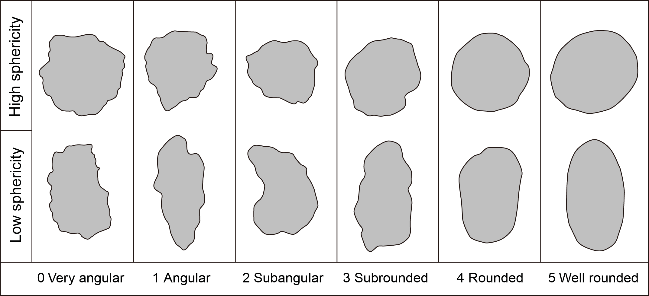
Figure F13. Clast angularity.
Vesicles in the volcanic rocks and vugs that developed during alteration of the sample were reported as visual estimates of the percent fill. The term "vein" was applied to any later crosscutting feature that precipitated from hydrothermal fluids. Veins are defined as secondary mineral-filled features crosscutting the primary rock fabric. The types of veins were described based on the scheme adopted for Expedition 376 (de Ronde et al., 2019) based on visual estimation of spatial density (defined as the percent of sample interval composed of vein-fill material), vein geometry (Table T3), description of the vein margin (e.g., sharp, diffusive, or irregular), maximum vein width, and vein fill texture (Figure F12; Table T4).
3.2.5.6. Microscopic description of alteration
The DESClogik application was used to record thin section observations of the altered domains. The materials selected for shipboard thin section preparation were generally fresh igneous rocks; therefore, the occasional alteration observed is recorded in broad and simplified ways as follows:
- Alteration domain: material in the altered domain was identified as groundmass, clast (igneous/metamorphic/sedimentary), phenocryst, xenolith, fault gauge, vein, halo, or glass. If there was more than one alteration domain in a thin section, an estimate of the relative percentages of the domains was recorded. The approximate percentage of the altered domain in the bulk section was recorded. Recrystallization of phenocryst and groundmass phases was classified as complete, strong, absent, or weak in accordance with the DESClogik spreadsheet.
- Alteration intensity/rank: this is largely based on the changes observed in primary mineralogy of the parent rock and indicated as unaltered (see Macroscopic description of alteration; Table T1). Because this relates to changes in the proportions of primary versus secondary igneous minerals, the observation is supplemented by thin section observation, where available; in fine-grained igneous rocks, the estimate will necessarily be an estimate of the percentage of color change and the degree of palagonitization in glass-rich examples.
Importantly, basalt-seawater interaction can result in a variety of secondary minerals and changes in the primary minerals depending on the temperature, pH, depth, and other environmental parameters. Early-stage alteration at higher temperatures (>300°C) causes formation of calcic amphibole (actinolite and hornblende) (Patterson et al., 2021), epidote, serpentine, and talc (Bach et al., 2004); alteration at intermediate temperatures (<300° to >100°C) causes formation of serpentine (Bach et al., 2004), chlorite (Inoue et al., 2010), and sulfides; and late-stage low-temperature (<100°C) fluid-rock interaction causes formation of quartz, zeolites (and prehnite), clays (smectite-saponite), celadonite, and Fe oxyhydroxides (Alt, 1993). Some of these minerals can also be present as constituents of vesicles, vugs, veins, and halos, and they are recorded in their respective fields in the DESClogik spreadsheet. Certain minerals were analyzed using XRD when they formed a significant proportion of the core interval of interest. An estimate of the combination of changes to primary mineralogy and/or the degree of development of secondary minerals is the basis for the assigned numerical value (0–5) used to denote the alteration intensity rank (Table T1).
3.2.6. X-ray diffraction analysis
Samples for XRD analyses were selected from the working half. Approximately one 5 cm3 sample that displays representative alteration was taken. Samples analyzed for bulk mineralogy were freeze-dried and homogenized by grinding in a metal ball mill. Prepared samples were top-mounted onto a sample holder and analyzed using a Malvern Panalytical AERIS diffractometer mounted with a PIXcel1D-Medipix3 detector using nickel-filtered CuKα radiation. Settings for the standard bulk sample scan were as follows:
- Voltage = 40 kV.
- Current = 15.0 mA.
- Goniometer scan = 4°–75°.
- Step size = 0.0108664°2θ.
- Time per step = 40 s.
- Divergence slit = 0.25°.
Diffractograms of bulk samples were evaluated with the aid of the Malvern Panalytical XRD High Score software suite, which allowed for mineral identification and basic peak characterization (e.g., baseline removal and characteristic peak intensity). Files were created that contained d-spacing values (inversely proportional to width of peak), diffraction angles, and peak intensities with and without the background removed. These files were scanned by the High Score software to find d-spacing values characteristic of a limited range of key minerals typically present in seafloor alteration. Where appropriate, peak areas were further quantitatively estimated using the High Score software to yield semiquantitative results of the relative abundances of the most common mineralogical components.
4. Structural geology
This section outlines methods and terminology for documenting structural features observed in Expedition 391 cores, such as bedding dips, faults, fractures, shear zones, breccia, and veins. After splitting the core and description by the sedimentologists and petrologists, features on the archive halves of each core were documented as follows (Figure F14) by noting the following:
- Identifying structural features and classifying their types,
- Determining the top and bottom location of structures in the core,
- Measuring the structural occurrence and displacement where applicable, and
- Determining the crosscutting relationship between structures.

Figure F14. Core reference frame.
Our methods largely follow those used by structural geologists of Integrated Ocean Drilling Program Expedition 344 (Harris et al., 2013) and IODP Expeditions 352 (Reagan et al., 2015a), 367/368 (Sun et al., 2018), and 376 (de Ronde et al., 2019). Definitions of structural measurements and descriptive parameters, as well as their corresponding description nomenclatures, were plotted on a spreadsheet (Figure F15) and then put into the LIMS database using DESClogik. Where possible, orientation data were corrected for rotation related to drilling using paleomagnetic declination and inclination information (see Paleomagnetism).
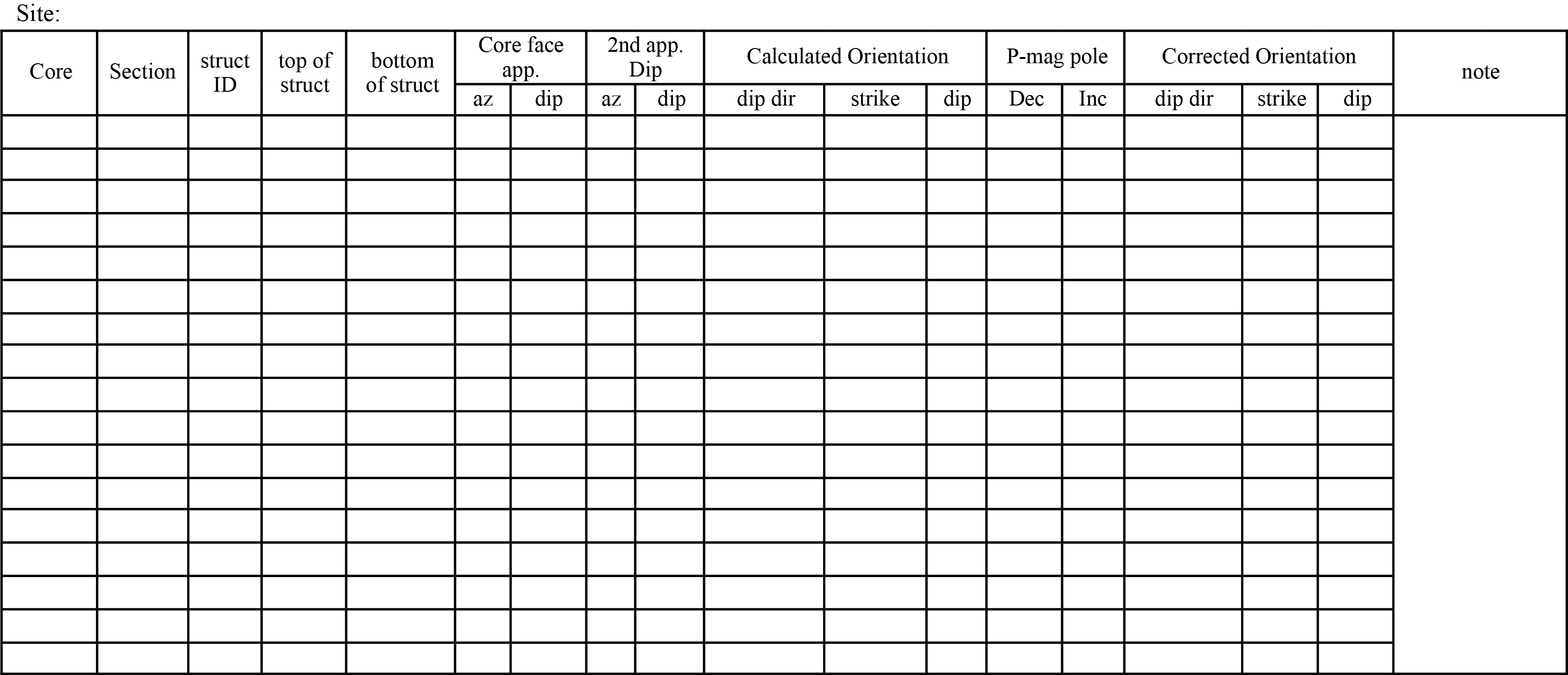
Figure F15. Example log sheet.
4.1. Graphic symbols and terminology
A predefined set of structural features was used to maintain consistency in the core descriptions. The major features identified include the following:
- Joints and fractures: brittle failure with no displacement and no secondary infill minerals. Breaks clearly resulting from drilling were not logged.
- Veins: fractures filled with secondary minerals.
- Fault rocks: brittlely deformed rocks such as fault breccia and fault gouge. The term "fault breccia" is defined as a clast-supported fault rock with angular clasts, and the term "fault gouge" is defined as a matrix-supported fault rock with rounded clasts.
- Shear zones: zones affected by ductile crystal-plastic deformation and surrounded by less deformed rocks.
- Sedimentary bedding: layering of sediments and sedimentary rocks.
- Igneous contacts: material contacts of extrusive igneous rocks.
- Magmatic fabrics: magmatic foliations defined by the preferred orientations of primary minerals with no evidence of crystal-plastic deformation.
4.2. Structural observation and description
Structural features were described from the top to the bottom of each section of the core.
For fractures, we examined and measured the following parameters:
- Location: measured in centimeters from the top of the section (Figure F16).
- Morphology and structure: morphological shape of a fracture (e.g., straight, curved, banded, irregular, composite, isolated, single, or branched).
- Displacement: lateral offset and/or opening of a fracture measured in centimeters; a closed fracture with no lateral offset was recorded as 0 cm of displacement.
- Orientation: dip angle, strike, and dip direction of a fracture measured in degrees; where applicable, reorientation of a fracture to geographic coordinates (i.e., relative to true north) was done to determine the real dip direction (see Orientation measurements and correction).
- Types: type of deformation of a fracture, if observable (e.g., normal, reverse, dextral, sinistral displacement, or a combination of the above).

Figure F16. Method for logging structures.
For veins, we examined and measured several parameters:
- Location: measured in centimeters from the top of the section.
- Morphology: main morphological characteristics of a vein, such as shape, connectivity, texture, structure, and particular vein geometries (Figure F11).
- Orientation: dip angle and dipping direction of a vein.
- Mineral infill and alteration: as described by petrologists.
For fault rocks, hydrothermal breccias, and shear zones, we examined and measured the following parameters:
- Location: interval where a shear zone occurs in a core measured in centimeters from the top of the section (Figure F16).
- Nature: type of fault rock, hydrothermal breccia, or shear zone, including fault gouge, fault breccia, cataclasite, and mylonite.
- Morphology: morphological shape of the deformed zone and of the clasts.
- Orientation: dip angle and dip direction of the preferred orientation of the clasts, where applicable.
- Deformation intensity: characterization of the deformation intensity, including foliation development.
- Mineral and alteration: matrix and clasts described by petrologists.
For sedimentary bedding, we described the following parameters:
- Location: where a nonsubhorizontal bedding occurs in a core (dip > 5°), measured in centimeters from the top of the section.
- Type of contact: type of sedimentary contact boundary.
- Orientation: dip angle, strike, and dip direction of sedimentary bedding.
For igneous contacts, we described the following parameters:
- Location: measured in centimeters from the top of the section.
- Type of contact: type of igneous contact boundary.
- Mineral infill and alteration: as described by petrologists.
4.3. Orientation measurements and correction
4.3.1. Orientation measurements
We used a plastic goniometer for orientation measurements (Figure F17). Orientations of planar and linear features in cored materials were determined relative to the core axis, which represents the vertical axis in the core reference frame, and the double line marked on the archive half of the split core liner, representing 180° in the plane perpendicular to the core axis (Figures F14, F17). To determine the orientation of a planar structural element, two apparent dips of the element were measured in the core reference frame and converted to a plane represented by dip angle and either a strike or dip direction (Figures F17, F18) using an Excel spreadsheet (Reagan et al., 2015b). One apparent dip is usually represented by the intersection of the planar feature with the split face of the core (Figure F18A) and is quantified by measuring the dip direction and angle in the core reference frame (β1) (Figure F19). Typical apparent dip measurements have a trend of 90° or 270° and range in plunge from 0° to 90°. The second apparent dip is usually represented by the intersection of the planar feature and a cut or fractured surface at a high angle to the split face of the core (β2) (Figures F18, F19). In most cases, this was a surface either parallel or perpendicular to the core axis (Figure F18B, F18C). In the former cases, the apparent dip lineation would trend 0° or 180° and plunge from 0° to 90° (Figure F18B); in the latter cases, the trend would range from 0° to 360° and plunge 0° (Figure F18C). Linear features observed in the cores were always associated with planar structures (e.g., striations on faults), and their orientations were determined by measuring either the rake (or pitch) on the associated plane or the trend and plunge in the core reference frame.
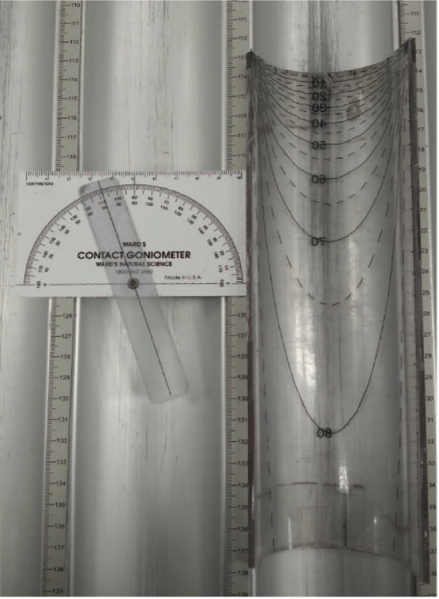
Figure F17. Goniometer.
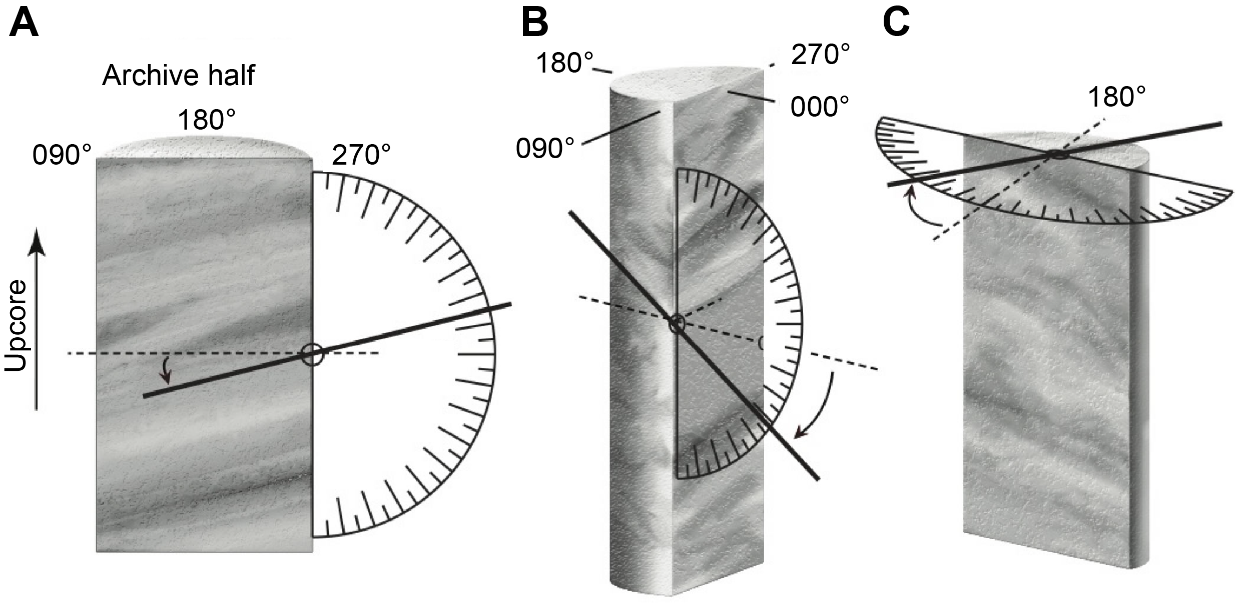
Figure F18. Core reference frame.
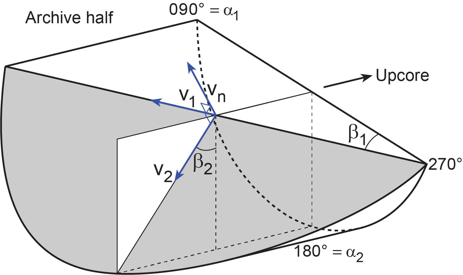
Figure F19. Plane orientation.
4.3.2. Plane orientation calculation
For a bedding or fault plane, two apparent dips on two different surfaces (e.g., the split core surface, which is east–west vertical, and the horizontal surface, which is north–south vertical) were measured in the core reference frame as azimuths (measured clockwise from north, looking down) and plunges (Figures F17, F18, F19). An x-y-z coordinate system was defined in such a way that the positive x, y, and z directions coincide with north, east, and vertical downward, respectively. If the azimuths and plunges of the two apparent dips are given as (α1, β1) and (α2, β2), respectively, as in Figure F19, the unit vectors representing these two lines (v1 and v2) are
The unit vector normal to plane (vn) (Figure F20) is then defined as
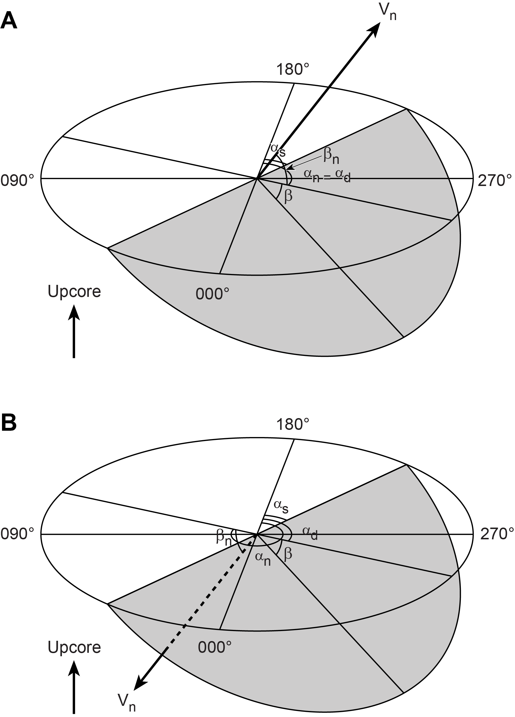
Figure F20. Plane dip.
The azimuth (αn) and plunge (βn) of vn are given by
The dip direction (αd) and dip angle (β) of this plane are αn and 90°+ βn, respectively, when βn < 0°, and αn ± 180° and 90° − βn, respectively, when βn ≥ 0°. The right-hand rule strike of this plane (αs) is then given by αd − 90° (Figure F20).
5. Biostratigraphy
5.1. Calcareous nannofossil methodology
Calcareous nannofossils were examined using smear slides prepared directly from unprocessed samples following standard techniques. The slides were analyzed under plane-polarized and cross-polarized light using a ZEISS Axiophot transmitted-light microscope at a magnification of 1000×. A total of 100 fields of view were used to scan for relevant marker taxa (~1 traverse across the slide; more if time permitted). For coarse material, the fine fraction was separated from the coarse fraction by settling through water before the smear slide was prepared. Photomicrographs were taken using a Spot RTS system with the IODP Image Capture and Spot commercial software.
Because of a condensed expedition schedule, abundance, assemblage, and preservation data were not recorded. Samples were scanned for marker taxa and zoned accordingly. Detailed counts will be produced in postexpedition research for biozonation refinement.
Biostratigraphic zonation determinations were carried out on calcareous nannofossils using the standard zonations of Martini (1971), Okada and Bukry (1980), and Backman et al. (2012). Age datums from the 2020 geologic timescale of Gradstein et al. (2012, 2020) were used for precise age dating where true biostratigraphic horizons were considered representative of their respective location within the core. Identification of calcareous nannofossils during this expedition followed the taxonomy of Perch-Nielsen (1985a, 1985b), Bown (1998), Young (1998), and Young et al. (2022). The core catcher sample from each core was examined. Additional samples were taken from working-half sections as necessary to refine the biostratigraphy, preferentially sampling hemipelagic intervals.
5.2. Scanning electron microscopy
Select samples containing calcareous nannofossils were viewed using the Hitachi TM3000 tabletop scanning electron microscope (SEM). This helped confirm the existence of many marker fossils with closely related taxa appearing in the same age range, which can sometimes make consistent identification difficult. It was especially useful in examining the youngest material recovered to confirm the presence or absence of recent and nearly recent taxa that are quite small, including Emiliania huxleyi, and small Gephyrocapsa species, such as Gephyrocapsa ericsonii. Unfortunately, time constraints did not allow for this detailed examination shipboard; it will be conducted postexpedition.
5.3. Planktonic foraminifera methodology
Planktonic foraminifera were prepared and analyzed from core catcher samples that were sieved through a 63 μm sieve. Hydrogen peroxide solution (30%) was used for more lithified samples. The sediment was then dried at 40°–50°C before being stored in labeled glass vials. Contamination between samples was avoided by using methylene blue (methylthioninium chloride) to clean the sieves.
Material from the 500, 250, and 125 μm size fractions was scanned using a ZEISS SteREO Discovery V8 stereo microscope to detect planktonic foraminifera biostratigraphic markers. Planktonic foraminifera were imaged using a Spot RTS system with the IODP Image Capture and Spot commercial software. SEM imaging was also used to obtain pictures of major taxa and to better define the state of preservation of specimens.
The taxonomy of planktonic foraminifera was based on Postuma (1971), Kennett and Srinivasan (1983), Bolli and Saunders (1985), Caron (1985), Toumarkine and Luterbacher (1985), and Huber et al. (2016). Planktonic foraminifera biozonations and biostratigraphic ages are from Wade et al. (2011) and Gradstein et al. (2012, 2020).
Preservation of planktonic foraminifera was defined as follows:
- VG = very good (all specimens identifiable at a species level, with well-preserved ornamentations, unbroken tests, and no evidence of dissolution).
- G = good (almost all individuals identifiable at a species level. More than 80% of the specimens were not etched or broken, with minor evidence of diagenetic overgrowth).
- M = moderate (30%–80% of the specimens are not etched, unbroken, and/or with modest evidence of diagenetic overgrowth. Most specimens can still be identified at the species level).
- P = poor (most specimens show severe etching and strong recrystallization and/or corrosion. Identification at the species level is more difficult).
Relative abundances of planktonic foraminifera taxa in each sample were defined as follows:
- D = dominant (>80% of the assemblage).
- A = abundant (>50%–80% of the assemblage).
- C = common (>10%–50% of the assemblage).
- F = few (1%–10% of the assemblage).
- R = rare (<1% of the assemblage).
- B = barren (washed sample contains no planktonic foraminifera specimens).
- * = reworked specimens.
The appropriate and intended method was to determine the abundances of major species of planktonic foraminifera within the assemblage to provide a more detailed evaluation of the sample; this was achieved exclusively for Site U1575. In practice, this level of detail was not achievable at the other sites, primarily due to the length of preparation time and rate of core recovery in the sedimentary succession. At the later sites, the method adopted was to determine the relative abundance data only for the planktonic foraminifera biostratigraphic markers. Relative abundances were estimated as follows:
- A = abundant (>30% planktonic foraminifera specimens in the washed sample).
- C = common (>10%–30% planktonic foraminifera specimens in the washed sample).
- F = few (>5%–10% planktonic foraminifera specimens in the washed sample).
- R = rare (1%–5% planktonic foraminifera specimens in the washed sample).
- VR = very rare (<1% planktonic foraminifera specimens in the washed sample).
6. Paleomagnetism
During Expedition 391, routine paleomagnetic and rock magnetic experiments were carried out on sedimentary and igneous cores recovered from Sites U1575–U1578. Remanent magnetization was measured on archive-half sections and on discrete cube samples taken from working-half sections. All continuous archive halves were partially demagnetized in an alternating field (AF), whereas discrete samples were subjected to either stepwise AF or thermal demagnetization. Because the azimuthal orientations of cores recovered by RCB drilling are not constrained, all magnetic data are reported relative to the sample core coordinate system. In this system, +x is perpendicular to the split core surface and points into the working half (i.e., toward the double line), +z is downcore, and +y is orthogonal to +x and +z in a right-hand sense (Figure F21). Discrete cube samples are marked with an arrow on the split face (or the corresponding face of the plastic box) in the upsection (i.e., −z) direction.

Figure F21. Paleomagnetic reference frame.
6.1. Archive-half measurements
Measurements of remanence and stepwise AF demagnetization were conducted on archive-half sections with the superconducting rock magnetometer (SRM), which is controlled by IMS SRM software (version 12.0). The SRM is a 2G Enterprises Model 760R-4K cryogenic magnetometer equipped with direct-current superconducting quantum interference devices (DC-SQUIDs) and an in-line automated three-axis AF demagnetizer capable of reaching a peak field of 80 mT. The spatial resolution, measured by the width at half height of the response of the pickup coils, is <10 cm for all three axes, although magnetization can be sensed over a core length of as much as 30 cm. The magnetic moment noise level of the SRM is ~2 × 10⁻¹⁰ A/m2. The practical noise level, however, is affected by the magnetization of the core liner and the background magnetization of the measurement tray, resulting in a lower limit of magnetization of ~2 × 10⁻⁵ A/m2, which can be reliably measured.
Sample trays were cleaned with deionized water and window cleaner at the beginning of every shift, at the start of new holes, or as deemed necessary. The sample tray was then demagnetized in an AF with a peak field of 30 mT, and its remanence was measured using the Section background routine to update the background correction values for the empty sample tray.
We measured the archive halves at 2 cm intervals, and they were passed through the sensor at a speed of 10 cm/s. A 5 cm long interval of empty track was measured before the start of the section passed the center of the pickup coils of the DC-SQUID sensors, and an equal interval of empty track was measured after the end of the section had passed through it. These are referred to as the leader and trailer measurements, and they serve the dual functions of monitoring the background magnetic moment and enabling future deconvolution analysis. After an initial measurement of natural remanent magnetization, we proceeded to demagnetize the archive halves to assess the presence of potential drilling-induced overprints. The exact demagnetization protocol used varied depending on lithology. Sediments were typically demagnetized using AF steps of 10 and 20 mT, although the 20 mT step was sometimes omitted due to time constraints associated with core workflow. Natural remanent magnetization and AF demagnetization data were plotted for each sampled point on vector endpoint plots (Zijderveld, 1967) to assess the effectiveness of removing overprints and to show variations with depth at individual demagnetization levels. We visually inspected the plots to judge whether the remanence after demagnetization at the highest AF demagnetization step likely reflected the characteristic remanent magnetization and geomagnetic polarity sequence observed in the discrete samples.
For sedimentary sections, all archive-half core material was measured and partially demagnetized in the SRM, whereas for volcanic basement, larger vertically oriented archive-half igneous rock pieces (as well as any intercalated sediments) were measured to gain additional paleomagnetic data. Vertically oriented pieces longer than 8 cm were selected for measurement because smaller pieces do not fill the sensing coil and may give spurious readings owing to perturbations of the sample magnetic field caused by edge effects. Igneous samples and intercalated basement sediments were demagnetized using AF steps of 5, 10, 15, and 20 mT.
6.2. Discrete samples
For sedimentary rocks, approximately one discrete sample was collected from each core for shipboard paleomagnetic measurements (with the exception of calcareous ooze samples, which were often skipped due to their low magnetization intensities). Lithified basal sediments overlying igneous rocks were sampled at a higher frequency of one sample per core section. All discrete samples taken from working halves for shipboard magnetic analysis were 7 cm3 cubes. Although standard 2.5 cm diameter minicores are more commonly used, cubic samples were preferred because they should have a more precisely determined vertical reference (based on a saw cut perpendicular to the core length) than the minicores, for which the arrow on the split core face must then be transferred to the long axis of the sample. Moreover, the use of cubes instead of minicores enabled sharing of the limited discrete samples for physical properties measurements.
Remanent magnetization of discrete samples was measured exclusively with the AGICO JR-6A spinner magnetometer and the automated sample holder. Measurements of the empty sample holder, after subtracting the stored holder magnetization, yielded intensities on the order of 4.0 × 10⁻⁶ A/m, representing the practical noise limit of the system. About half of the discrete samples were subjected to stepwise AF demagnetization and the other half to thermal demagnetization. AF demagnetization was performed using the D-Tech AF demagnetizer (model D-2000), which is capable of peak fields up to 200 mT. AF demagnetization was applied at 5, 10, 15, 20, 25, 30, 40, 50, 60, and 80 mT for all samples. Samples containing higher coercivity were further demagnetized using higher AF levels (up to 200 mT) as appropriate.
Discrete samples treated to thermal demagnetization were demagnetized using an ASC Scientific thermal demagnetizer (model TD-48 SC) capable of demagnetizing samples up to 700°C. The total magnetic field along the length of the TD-48 SC access tube has a maximum field in the sample chamber region of <50 mT from 30 cm onward (measured from the edge of the access opening). The large sample boat allowed samples to be spaced loosely, reducing sample interaction. Samples were held at the desired temperature for 20 min prior to cooling in the low-magnetic field chamber. MS was measured (using a Bartington MS2C MS sensor) after every heating step to monitor thermal alteration of magnetic minerals during heating. Heating was carried out from 150°C until the samples were demagnetized, in steps of 25°C or 50°C depending on the magnetic mineralogy. Thermal steps were typically conducted at 50°C intervals up to 300°C or 400°C and at 25°C intervals for temperatures up to complete demagnetization. Thermal demagnetization was terminated whenever a sample's individual magnetization appeared to have been completely eradicated or if substantial alteration took place.
6.3. Magnetic susceptibility and magnetic properties
At all drill sites, we carried out MS and anisotropy of magnetic susceptibility (AMS) measurements on at least one discrete sample per 50 m of recovered core for both consolidated sedimentary rocks and igneous rocks to explore properties such as sedimentary compaction and basalt flow orientation (Li and Kodama, 2016; Ellwood, 1978). Susceptibility measurements were made using an AGICO Kappabridge KLY 4 MS meter with a 300 A/m peak AF and an operating frequency of 875 Hz.
We also conducted a series of rock magnetic experiments to identify the remanence carriers in the discrete samples. The acquisition of stepwise partial anhysteretic remanent magnetization was measured on a few samples from each site, with a sliding window of 5 mT in a direct current field of 0.2 mT superimposed on a maximum AF field of 100 mT. Stepwise isothermal remanent magnetization acquisition up to 1.2 T and backfield remanence curves were also acquired using an ASC Scientific impulse magnetizer. These experiments provide crude information on magnetic mineralogy and magnetic domain state (e.g., Jackson et al., 1988; Thompson and Oldfield, 1986).
6.4. Data analysis
Paleomagnetic data analysis was primarily performed using the PmagPy analysis tools suite to facilitate easier upload to the Magnetics Information Consortium (MagIC) database postexpedition. The PuffinPlot software was also utilized for quick visualization of data (Lurcock and Wilson, 2012; Tauxe et al., 2016). Magnetization components were identified via visual inspection of demagnetization data. Best-fit magnetization directions and corresponding maximum angular deviations were obtained using principal component analysis (Kirschvink, 1980).
AMS data were processed using the AMSSpin software. We calculated anisotropy as the foliation F = K2/K3 and the lineation L = K1/K2, where K1, K2, and K3 are the maximum, intermediate, and minimum eigenvalues of the anisotropy tensor, respectively. We describe the shape of the anisotropy ellipsoid by the shape parameter T (Jelínek and Kropáček, 1978), where −1.0 < T < 1.0 indicate prolate and oblate fabrics, respectively. Additionally, we describe the strength of anisotropy using the corrected anisotropy degree Pj (Jelínek and Kropáček, 1978), where Pj = 1.0 indicates an isotropic fabric and, for example, Pj = 1.05 indicates 5% anisotropy. Both the shape parameter and anisotropy degree are dependent on the relationships between the eigenvalues of the anisotropy tensor.
6.5. Magnetostratigraphy
The Expedition 391 drill sites are located at midlatitudes between 21.9°S and 32.1°S. As such, identification of polarity is less complex than nearer the equator. Assuming a geocentric axial dipole geomagnetic field (i.e., tan(I) = 2tan(lat), where I is inclination and lat is latitude), the expected mean inclination of the Brunhes field is −46° at these sites, where the negative value indicates normal polarity. From magnetic inclination data, we assigned magnetic polarities to discrete samples and core sections where AF demagnetization enabled isolation of the characteristic magnetization component. Samples from disturbed sedimentary intervals or with poor paleomagnetic data that precluded robust determination of magnetic polarity were excluded from magnetostratigraphic analyses. The estimated polarities were correlated to the latest geomagnetic polarity timescale (Ogg, 2020) with the aid of biostratigraphic data.
7. Geochemistry
7.1. Sediment and pore water geochemistry
The Expedition 391 shipboard sediment and pore water geochemistry program included analyses of headspace gases (hydrocarbons), IW (pH, alkalinity, ammonium, phosphate, silicate, chloride, bromide, sulfate, sodium, strontium, magnesium, potassium, calcium, barium, boron, iron, lithium, and manganese), and bulk composition of sediment (total carbon [TC], total inorganic carbon [TIC], total organic carbon [TOC], and calcium carbonate [CaCO3]).
7.1.1. Headspace gas geochemistry
Hydrocarbon gases, including methane, ethane, and propane, were measured as part of the IODP shipboard hydrocarbon monitoring protocol to ensure safe drilling procedures. Immediately after recovering each core on the core receiving platform, headspace samples were collected following the methods of Kvenvolden and McDonald (1986) as summarized below. Instantaneously upon core retrieval, around 5 cm3 of sediment was collected from the top of a section in the middle of each core (Section 5 if recovery was 100%) using a cutoff syringe for soft to semiconsolidated sediment or a metal boring tool for more lithified sediments. The sample was placed in a 21.5 cm3 glass serum vial, sealed with an aluminum crimp cap fitted with a fluoropolymer septum, and transported to the geochemistry laboratory for headspace gas analyses. The glass serum vial was labeled with the core, section, and interval from which the sample was collected. The sample was then placed in an oven at 50°C for ~30 min to allow dissolved hydrocarbon gases to equilibrate with the headspace prior to analysis.
After heating the glass serum sample vial, a gas-tight glass syringe was used to extract headspace gases released from the sample. Light hydrocarbons within the headspace, including methane, ethane, ethylene, propane, and propylene, were quantified by an Agilent/HP 6890 Series II gas chromatograph (GC) equipped with a 2.4 m × 2.00 mm stainless steel column packed with 80/100 mesh HayeSep R and a flame ionization detector set to 250°C. Sample gases in syringes were injected into the GC through a 0.25 cm3 sample loop connected to the Valco valve, which can be switched automatically to backflush the column. The GC oven temperature was programmed to start at 80°C for 8.25 min, increase to 150°C for 5 min at a rate of 40°C/min, and return to 100°C postrun for 15 min. Helium was used as a carrier gas; it initially flowed into the column at a rate of 30 mL/min and subsequently ramped to 60 mL/min after 8.25 min to accelerate elution of propane and propylene. Data were collected and evaluated using the Agilent Chemstation software (2001–2006), and chromatographic responses were calibrated against different preanalyzed gas standards with variable quantities of low molecular weight hydrocarbons produced by Scott Specialty gases (Air Liquide). Concentrations of hydrocarbon gases are reported in parts per million by volume (ppmv; equivalent to µL/L).
7.1.2. Interstitial water chemistry
IW samples were collected for both onboard analyses and personal postexpedition analyses. During Expedition 391, alkalinity, pH, major cations and anions (Na+, Mg2+, K+, Ca2+, Cl−, Br–, and SO42–), phosphate (PO43−), ammonium (NH4+), and trace elements (B, Ba, Fe, Li, Mn, Si, and Sr) were determined for all or part of the collected IW samples following the procedures of Gieskes et al. (1991).
IW was extracted from 5–10 cm whole-round sections cut from cores immediately after core retrieval using a titanium squeezer. Whole-round samples were typically collected at a frequency of three samples per core (Sections 2, 4, and 6) in the first two cores and one sample per core (Section 4) from the third core to the bottom of the sediment succession for Sites U1575 and U1576. For Site U1577, whole-round samples were collected at a frequency of one sample per core (Section 4). For Site U1578, the sample frequency was two per core (Sections 2 and 4) in the first three cores and one sample per core (Section 4) for the remainder of the drilled sediment succession. Whole-round samples were carefully trimmed with a spatula to remove potential contamination from drilling fluid and oxidation due to exposure to the air during sampling. The cleaned sediments were transferred to 8 cm inner diameter titanium squeezers that were then placed into Carver hydraulic presses (Manheim and Sayles, 1974) and squeezed at pressures ranging 3,000–25,000 force pounds (1.335–1.112 × 10⁶ N) depending on the water content of the sediment and IW retrieval. The squeezed IW was filtered through a 0.45 μm syringe-tip filter and collected in a 60 mL acid-washed high-density polyethylene syringe attached to the squeezing assembly. Sample volume was generally greater than 20 mL. When the sample volume was less than 20 mL, shipboard analyses were prioritized. The onboard IW samples were split as outlined in the analytical workflow below.
- pH and alkalinity were determined immediately after squeezing using an autotitrator with ~3 mL of IW samples.
- Major anions and cations, namely sodium (Na+), magnesium (Mg2+), potassium (K+), calcium (Ca2+), chloride (Cl–), bromide (Br–), and sulfate (SO42), were determined using ion chromatography (IC) with ~100 μL of IW samples.
- Phosphate (PO43−) and ammonium (NH4+) were determined using ultraviolet spectrophotometry with ~600 and ~200 μL, respectively, of IW samples.
- Major and trace element analyses, namely sodium (Na), magnesium (Mg), potassium (K), calcium (Ca), sulfur (S), boron (B), barium (Ba), iron (Fe), lithium (Li), manganese (Mn), silicon (Si), and strontium (Sr), were determined using inductively coupled plasma–atomic emission spectroscopy (ICP-AES) with 500 μL acidified IW samples. Note that data produced on the Agilent 5110 inductively coupled plasma–optical emission spectrometer (ICP-OES) were collected in AES mode and are referred to as ICP-AES in the LIMS database. In this volume, ICP-AES is used to refer to these data.
IW was also extracted using Rhizon samplers from the uppermost 9, 20, 50, and 100 cm of Core 391-U1575A-1R and the uppermost 50 and 100 cm of Core 2R for personal samples. To extract IW using the Rhizon sampler, cores were recovered on the core receiving platform and immediately transported inside and holes were drilled into the plastic liner at designated depths. Acid-cleaned 5 cm long Rhizon samplers connected to precleaned 30 mL syringes were inserted into the sediment. The syringes were pulled and held by spacers to generate a vacuum, enabling IW extraction.
7.1.2.1. Alkalinity and pH
Alkalinity and pH were measured using a Metrohm Model 794 Basic Titrino autotitrator. pH was measured with a glass electrode immersed in 3 mL of constantly stirred IW. Alkalinity was analyzed by titrating the IW sample with 0.1 M HCl to an end point pH of 4.2. Both measurements were standardized using an International Association for the Physical Sciences of the Ocean (IAPSO) standard seawater (alkalinity 2.325 mM), yielding reproducibility better than 2% (the percent relative standard deviation of repeated measurements of IAPSO).
7.1.2.2. Major ions
Concentrations of Na+, Mg2+, K+, Ca2+, Cl–, Br–, and SO42– in the IW were analyzed by a Metrohm 85 Professional IC instrument. The 100 µL IW samples were diluted 1:100 with deionized water. The calibration curve was generated using varying dilutions of IAPSO standard seawater, constituent concentrations of which are summarized in Gieskes et al. (1991). These diluted IAPSO standard seawater samples were also analyzed as external standards every 10 samples for each batch run for data quality control. The reproducibility was better than 1.0% for all cations and anions.
7.1.2.3. Ammonium and phosphate
Ammonium (NH4+) and phosphate (PO43−) were determined by spectrophotometry using an Agilent Cary 100 UV-Vis spectrophotometer. Analyses of NH4+ were conducted by phenol diazotization and subsequent oxidation by sodium hypochlorite (NaClO) to yield a blue color. Prepared samples were kept in the dark for 6 h and measured spectrophotometrically at a wavelength of 640 nm. Ammonium chloride (NH4Cl) was used for calibration and standardization. Reproducibility of NH4+ standard measurement was ~5.0%. PO43– was measured using the ammonium molybdate method described by Gieskes et al. (1991) with commensurate dilutions. The PO43– concentration was determined at an absorbance of 885 nm wavelength after waiting for 30 min following the addition of the mixed reagent. The reproducibility for shipboard measurement of the standard PO43– solution was ~5.0%.
7.1.2.4. Dissolved major and minor elements
Major (Na, Mg, K, Ca, and S) and minor (B, Ba, Fe, Li, Mn, Si, and Sr) elemental concentrations in IW were determined using an Agilent 5110 ICP-OES with an SPS4 autosampler. The procedure followed that of Murray et al. (2000). Each 2 mL IW sample was preserved by adding 20 μL of concentrated, trace metal–grade nitric acid (HNO3). A molar concentration of 500 μM of each IW sample was diluted 1:10 in 2% HNO3 (v/v) and spiked with an internal standard for drift correction as well as atomic and ionic interferences. Specifically, 100 μL of internal standard solution containing 100 ppm beryllium (Be), indium (In), and scandium (Sc) and 200 ppm antimony (Sb) was added to 500 μL of IW sample and 4.4 mL of 2% HNO3 solution. For calibration, a series of dilutions of IAPSO standard seawater (0%, 1%, 5%, 10%, 25%, 50%, 75%, 100%, and 200%) were prepared for Na, Mg, K, Ca, and S to cover IW concentrations lower than or equal to normal seawater. Additional calibration solutions for the elemental concentrations higher than that of seawater were prepared with 3.5% sodium chloride (NaCl) as a matrix. Calibration solutions for B, Ba, Fe, Li, Mn, Si, and Sr were mixed with the internal standard in the same manner as IW samples. A complete set of in-house and IAPSO dilutions were analyzed at the beginning and the end of each batch ICP-AES run. In-house standards were run every 8–10 samples to monitor instrumental drift, and IAPSO standards were run at a similar frequency to monitor reproducibility, which was better than 2.0% for all elements.
7.1.3. Sedimentary geochemistry
7.1.3.1. Sedimentary total carbon and total inorganic carbon
Sediment samples (each amounting to a volume of ~5 cm3) were collected from IW squeeze cakes for onboard bulk sediment analyses. Each sample was freeze-dried for ~12 h, crushed to a fine powder using a solvent-cleaned agate pestle and mortar, and sampled for individual analyses. Average sample resolution was one to two samples per core.
TC, total nitrogen (TN), and total sulfur (TS) contents of the sediment samples were determined with a ThermoElectron Corporation FlashEA 1112 carbon-hydrogen-nitrogen-sulfur (CHNS) elemental analyzer equipped with a ThermoElectron packed column CHNS/nitrogen-carbon-sulfur (NCS) GC and a thermal conductivity detector (TCD). Approximately 15–25 mg of freeze-dried ground sediment was weighed into a tin cup. The amount varied slightly between sites, but in most cases, 15 mg of sediment was weighed per sample. A higher mass of 25 mg was weighed when TN and TS concentrations were lower than the detection limit of the CHNS analyzer. Even with the higher mass, TN and TS concentrations for most samples were still below the instrumental detection limit. Once weighed, samples were introduced automatically to the instrument after being loaded into a carousel with a 15-sample capacity. In the instrument, nitrogen oxides were reduced to N2, and the mixture of N2 and CO2 gases was separated by gas chromatography and measured using a TCD. All measurements were calibrated to the Buffalo River sediment (NIST SRM 2704, which contains 3.35 wt% TC, 0.18 wt% TN, and 0.40 wt% TS [Epstein et al., 1989]) and sulfanilamide (C6H8N2SO2) standards, which were run every 5 to 10 samples. Across all sites, the Buffalo River sediment standard gave a relative standard deviation of 1.7% for TC, and the sulfanilamide standard gave a relative standard deviation of 1.2% for TC.
TIC concentrations were determined using a CM 5011 CO2 coulometer coupled with a UIC, Inc. CM 5130 acidification module. An aliquot of ~15 mg of freeze-dried and crushed sediment was placed onto weighing paper to be transferred to the bottom of a glass tube. The glass tube containing the sample capsule was connected to the acidification module, and 2 M HCl was subsequently injected into the tube to dissolve the carbonate fraction of the sediment. The CO2 gas produced by the reaction continuously flows from the acidification module to the coulometer and is absorbed by a solution containing a colorimetric pH indicator with a known quantity. Accumulation of CO2 causes the solution's color to fade and increases the transmissivity of the solution as monitored by a photodetector of the instrument. An electric titration current was generated to neutralize the CO2-induced acidification to keep the transmissivity of the solution constant. CaCO3 content, expressed as weight percent, was calculated from the TIC content, assuming that all evolved CO2 was derived from dissolution of CaCO3, using the following equation:
Standard CaCO3 (>99.9% CaCO3; Fisher Scientific) was run every 10 samples to check for instrumental accuracy and drift before, during, and after each run. No correction was applied for the presence of other carbonate minerals. Relative standard deviation of internal standards (>99.9% CaCO3) was 0.32% for carbonate analysis. TOC content was calculated as the difference between TC and TIC:
7.2. Igneous geochemistry
7.2.1. Sample preparation
The objective of geochemical analyses is to describe, characterize, and evaluate the geochemical evolution of the recovered core material. To record geochemical variations, the freshest portions of distinct (1) lithologies, (2) eruptive units (i.e., distinct lava flows), and (3) intervals with significant changes in mineral assemblages and physical properties were sampled. pXRF measurements were used as an additional guide to identify and sample geochemically distinct portions of the recovered cores. In general, pXRF measurements were conducted along the entire core with ~3 measurements per recovered meter, and thin sections were usually made from the same interval or adjacent intervals.
Sample preparation was carried out on 2–8 cm3 of igneous rock, which was cut from the cores using a diamond blade rock saw. To remove altered rinds as well as saw marks and any drilling-related contamination from the exterior, the outer surfaces of the samples were ground off using a diamond-impregnated grinding wheel. Afterward, each rock sample was cleaned in a beaker with isopropanol in an ultrasonic bath for 15 min to remove dust. After decanting the isopropanol, the samples were agitated twice in an ultrasonic bath in nanopure deionized water (18 MΩ/cm) for 10 min. After drying the cleaned samples for 10–12 h at 110°C, the rock samples were crushed to <1 cm between two Delrin plastic disks in a hydraulic press. Some samples were amygdular, so before grinding, we handpicked chips under a binocular microscope to obtain material as free of amygdules as possible.
The crushed rock chips were ground to a fine powder using a tungsten carbide SPEX 8515 Shatterbox powdering system. Potential contamination from powdering in tungsten carbide mills was checked during ODP Leg 206 (Shipboard Scientific Party, 2003) and seems to be negligible for major elements and most of the trace elements measured onboard (Sc, V, Cr, Ni, Sr, Y, Zr, and Ba). A systematic analysis of the shipboard powders from Integrated Ocean Drilling Program Expedition 304/305, however, indicated possible Co contamination during powder preparation (Godard et al., 2009). For the majority of samples, the prepared powder was divided into two portions: one part was processed for XRD and pXRF analysis, and the other one was processed for ICP-AES and volatile measurements.
7.2.2. Volatile measurements
7.2.2.1. Total sulfur
TS contents were determined from an aliquot of ICP-AES sample powder by combustion at >900°C in a Thermo Electron FlashEA 1112 EA equipped with a Thermo Electron packed column CHNS analyzer and a TCD for TC, TS, and TN. Between 10 and 40 mg of powder was weighed into a tin cup and subsequently combusted in an oxygen gas stream at 900°C. The reaction gases were passed through a reduction chamber to reduce nitrogen oxides to N2, and the mixture of CO2, SO2, and N2 was separated by gas chromatography and detected by the TCD. Calibration was based on the NIST 2704 (Buffalo River sediment) and sulfanilamide reference material standards, which contain 0.40 wt% TS and 18.62 wt% TS, respectively. Measurement of the NIST 2704 standard material was run every nine samples.
Aliquots of powder (typically ~20 mg for igneous rocks) were weighed on a Cahn C-29 microbalance, with weighing errors conservatively estimated to be ±0.2 mg. The powders were packed into tin containers (Universal Tin Container light; Thermo Electron P/N 240-06400) and mixed with a spatula full of vanadium pentoxide (V2O5) estimated at 10 ± 3 mg. The samples were placed in a revolving autosampler with 31 spaces and dropped into a 900°C resistance furnace, where they were combusted in a reactor. The tin capsule creates a violent flash combustion (Sn has a melting point of only 230°C), and the V2O5 generates an oxygen-enriched atmosphere. The oxidized and liberated volatiles were then entrained by a constant helium gas flow through a commercial glass column (Costech P/N 061110) packed with an oxidation catalyst of tungsten trioxide (WO3) and a copper reducer. The gases were then separated by a packed gas chromatography column (Costech P/N 0581080) and a water trap. During the measurement time of 1000 s, the millivoltage at the TCD was continuously recorded, and N2, CO2, and SO2 peaks occurred at approximately 60, 98, and 770 s, respectively.
Peak areas from the TCD were calculated to determine the TS of the samples. Blank levels were determined by analyzing empty tin cups and were subtracted from each measurement. TS determination was based on the analysis of both blank cups and minimum detection limits obtained from calibration curves, which equates to a TS of 0.1 wt%.
7.2.2.2. Loss on ignition
On a Mettler Toledo balance, about 5 g of the sample powder was weighed into quartz crucibles, ignited for 4 h at 950°C, and weighed after cooling in a desiccator to determine the LOI. Estimated relative uncertainties on LOI values for 5 g samples are ~0.2% on the basis of duplicate measurements.
7.2.3. Inductively coupled plasma–atomic emission spectroscopy
The standard shipboard procedure for digestion of rocks and subsequent ICP-AES analysis is described in detail in Murray et al. (2000) and the shipboard user guide for ICP-AES, with modifications as indicated in Huber et al. (2019). The following protocol is a synopsis of this procedure with minor changes and additions used during Expedition 391.
7.2.3.1. Digestion procedure
On a Cahn C-31 microbalance, each previously ignited sample and standard was weighed to 125.0 ± 0.5 mg. The weighing errors are estimated to be ±0.2 mg under relatively smooth sea surface conditions, but they can be larger in case of high swell and bad weather conditions. Aliquots of ignited whole-rock powders were mixed with 800.0 ± 0.5 mg of LiBO2 flux (preweighed on shore). To prevent the fused bead from sticking to the crucible during cooling, an aqueous LiBr solution (10 µL of 0.172 mmol/L) was added to the flux and rock powder mixture as a nonwetting agent prior to sample fusion. Samples were fused individually in Pt-Au (95:5) crucibles for ~12 min at a maximum temperature of 1300°C in an internally rotating induction furnace (Bead Sampler NT-2100).
The beads were then transferred into 50 mL high-density polyethylene (HDPE) bottles and dissolved in a 50 mL solution of 10 wt% HNO3 (prepared from Optima-grade concentrated HNO3). The solution bottle was placed in a Burrell wrist-action shaker for 3 to 6 h at 7°C to aid dissolution, and then 0.5 mL was pipetted into a polyethylene centrifuge tube and diluted with 4.4 mL of 10 wt% HNO3 and 0.1 mL of internal standard solution containing Be, In (100 µg/g), and Sb (200 µg/g). The final solution-to-sample dilution factor was 5000×; this solution was analyzed for both major and trace elements.
7.2.3.2. Analysis
Major and trace element concentrations of standards and samples were determined using an Agilent 5110 ICP-AES instrument. The analyzed major elements include Si, Ti, Al, Fe, Mg, Mn, Ca, Na, K, and P, and the analyzed trace elements comprise Sc, V, Cr, Co, Ni, Cu, Zn, Sr, Y, Zr, and Ba. Wavelengths used for sample analysis are reported in Table T5. Certified international rock reference materials (BCR-2, BHVO-2, BIR-1, JA-1, JA-2, JA-3, JB-3, JGb-1, and MRG-1; Table T6), calibration and drift solutions, and chemical procedural blanks were included with the unknown samples for each sample run. Detection limits were calculated as three times the standard deviation of the mean for blank solution measurements.
The ICP-AES plasma was ignited at least 20 min before each sample run to allow the instrument to warm up and stabilize. The ICP-AES data were acquired using Agilent's ICP Expert software. The intensity curve for each element is defined by 20 measurements within the designated wavelength window. The Expert software integrates the area delineated by the baseline and the intensity curve. Each sample was analyzed three times from the same dilute solution in a given sample run. For several elements, measurements were made at two or more wavelengths in axial/radial mode. For each run, the wavelength yielding the best calibration line was identified and used to determine concentrations.
A drift-correction sample (in-house standard sample mixed with equal amounts of all samples to total 400 mg) was analyzed in every fifth sample position and at the beginning and end of each run. Procedural blank solutions were run near the beginning and end of each run as well as every approximately twenty-fifth sample position. As many as 40 unknown samples were analyzed during a single run. A 10% HNO3 wash solution was run for 90 s between each sample analysis.
7.2.3.3. Data reduction
Element concentrations in the samples were calculated from the relevant calibration lines for each element using the results for the certified rock standards in the ICP Expert software. Concentrations used for the calibrations are reported in Table T6 and represent the preferred values from Govindaraju (1994) and the GeoRem website (http://georem.mpch-mainz.gwdg.de) (Jochum et al., 2016). Total Fe oxide concentrations were reported as Fe2O3t. A drift correction was then applied to each element based on linear interpolation between drift-monitoring solutions run every fourth or fifth analysis. After drift correction, the average procedural blank value was subtracted. Estimates of accuracy and precision of major and trace element analyses were based on replicate analyses of international standards run as unknowns and not used for the calibration (Table T7). Run-to-run relative standard deviation using ICP-AES was typically ±1% for major elements and ±5%–10% for trace elements.
7.2.3.4. Low total issues
During this expedition, an unknown problem occurred with the sample preparation. The total mass percentages of the major elements should be around 100 wt% because the sample was weighed and the bead was made after ignition. In the first measurement made on 13 January 2022, however, the total mass percentages ranged 82.13–105.97 wt%. Of the 26 samples, 19 showed values outside the acceptable range (~96–102 wt%). In particular, SiO2 content decreased significantly as the total mass percent decreased (Figure F22). The calibration curve for SiO2 in the reference standard samples has a relatively weak correlation (R2 = 0.95), so it may be a calibration-related issue (Figure F22). However, the SiO2 raw data from the low SiO2/total samples are lower than most of the reference standard samples, so the SiO2 contents of these samples are obviously lower regardless of the calibration curve. Furthermore, the SiO2 and other elements are correlated with the total, suggesting that this issue was caused by the loss of sample material during sample preparation.
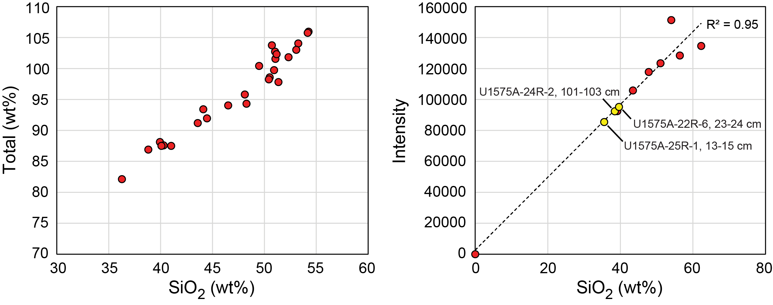
Figure F22. Total weight percentage v. SiO2 and intensity v. SiO2.
A trial run of the bead sampler during the port call showed that the powder did not fully melt at 1050°C according to the standard laboratory protocol. Therefore, the temperature of the bead sampler was raised to the maximum temperature of 1300°C. As a result, all the powders melted. The reason for the issue is unknown, but there may have been some trouble with the bead sampler's thermometer or heater. For the first measurement on 13 January, beads were prepared at 1300°C (this temperature may not be accurate). However, some of the beads contained black material inside, suggesting that melting was insufficient (Figure F23). In addition, the total values were significantly lower for the samples in which the beads contained the black material. Therefore, the low total issue is most likely related to insufficient melting and caused by problems with the bead sampler.
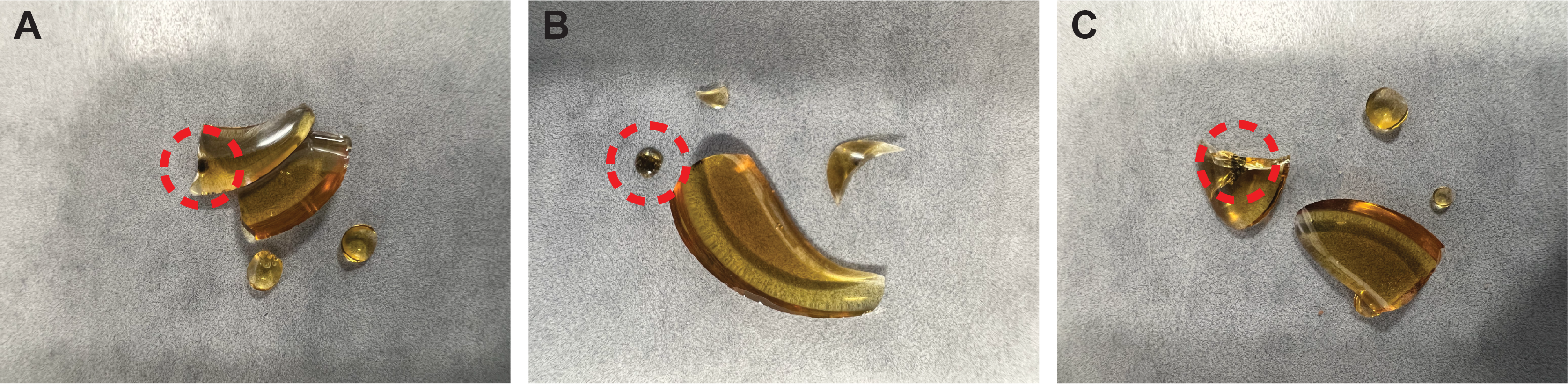
Figure F23. Beads.
The mixing ratio of flux to sample was changed to enable melting at low temperatures. In the standard laboratory method, 400 mg of flux and 100 mg of sample were mixed and melted, but we decided to use 800 mg of flux and 125 mg of sample for alkali melting. To validate this new method, preliminary experiments were conducted using four unknown samples (low total samples in the first measurement) and reference standard samples. In addition, three beads were prepared for reference standards JB-3 and BCR-2 and measured to verify uncertainties during sample preparation. The beads were prepared at 1300°C in this measurement. The results showed that the total, except for one sample, was within the 96–102 wt% range, indicating that the new method improved this issue (Table T8). Therefore, this new procedure was applied to all subsequent measurements during Expedition 391. The new method significantly diminished the problem, but some samples still showed low totals in the measurements for Sites U1575, U1576, and U1578 (Table T8).
7.2.4. Portable X-ray fluorescence spectrometry measurements
pXRF spectrometry measurements provided real-time characterization of cores for assessment of chemical variations and how they may (or may not) tie to petrographic observables. Measurements were calibrated using reference materials and correction factors applied to some elements (e.g., Ryan et al., 2017). Analysis was conducted on the core surface to facilitate material identification during core description (e.g., Johnston et al., 2018).
pXRF analysis was conducted using the Olympus DeltaX handheld instrument, which includes data corrections tailored for geological application. These data corrections were used for analysis during Expedition 391 and are based on the fundamental parameters methodology. A series of nonlinear equations is solved for each element analyzed. Parameters used in the equations comprise metrics for X-ray source, fluorescence intensities, absorption coefficients, and absorption edge effects for each wavelength analyzed, along with parameters for sample geometry and a Compton normalization scheme (e.g., Reynolds, 1963; van Sprang, 2000).
Shipboard data were collected using the geochemistry protocol. Calibration was conducted using modified methods from Ryan et al. (2017) and Johnston et al. (2018). Calibration curves measured via pXRF were determined by a suite of reference materials (Table T9). Powder mounts of the reference materials were analyzed to develop the working curves and for periodic checks on instrument performance during analysis of unknowns. Working curves were developed in Microsoft Excel, and slope and intercept values from working curves were used to calculate concentrations for the unknowns. Rock and powder samples were analyzed using powder-based working curves because previous work has shown no difference in instrument performance (i.e., Ryan et al., 2017; Reagan et al., 2015a).
Measurements were done directly on rock surfaces of the core using a shield sleeve analyzer mount. For these analyses, 3525 Ultalene 0.16 mil (4 µm) film was placed over the core to prevent contamination and/or damage to the X-ray analyzer (Johnston et al., 2018). Powders from X-ray powder diffraction and ICP-AES analysis were also analyzed using pXRF. Sample analyses were conducted using XRF powder mount assemblies based on methods outlined in Reagan et al. (2015a). Reference standard BHVO-2 was analyzed with each set of unknowns to track instrument performance over time (Table T10).
8. Physical properties
High-resolution physical properties measurements were taken during Expedition 391 to aid lithostratigraphic characterization and to link core observations from other shipboard science teams. In particular, physical properties data were used in hole-to-hole and site-to-site stratigraphic correlation, detection of lithologic discontinuities and heterogeneities, and identification of changes in the composition and morphology of igneous units. These physical properties include density (ρ), MS/MSP, P-wave velocity, and NGR, all of which provide insights into elemental bulk composition of the cores. Both thermal conductivity and porosity were measured to gain additional insights into rock properties. Cores were characterized using a variety of techniques and methods on recovered whole-round sections, section halves, and discrete samples. Physical properties methods for Expedition 391 were adapted from methods for IODP Expeditions 352, 367/368, 374, 376, and 385 (Reagan et al., 2015a; Sun et al., 2018; McKay et al., 2019; de Ronde et al., 2019; Teske et al., 2021).
8.1. Laboratory core flow
Cores were measured in the following sequence (workflow). Measurement techniques are described more fully in the following sections.
- Cores were left to equilibrate to ambient room temperature (~20°C; ~30–180 min).
- Whole-round sediment cores were run on the WRMSL.
- Whole-round sediment cores were run on the NGRL when the length of an individual section was >50 cm.
- Thermal conductivity was measured on one whole-round section per sediment core using a needle probe. When the sediment cores were too hard to insert the needle probe, a contact probe was used to measure the thermal conductivity on the working-half section after core splitting.
- Discrete pieces of recovered hard rock sections were shaken into a sterile split liner in the splitting room. Hard rock fragments were allocated by an igneous petrologist (see Igneous petrology and volcanology). Hard rock pieces were then returned to a full core liner and run through the WRMSL and NGRL.
- Whole-round 360° image scanning of the core was conducted.
- Cores were split, and the archive and working halves were labeled and imaged.
- The archive half was run on the SHMSL for MSP and RSC.
- Sediment samples were collected shortly after splitting to preserve the original moisture content of the samples.
- P-wave velocity measurements were made along the working halves of sediment cores using the P-wave Section Half Measurement Gantry (SHMG) system (P-wave caliper [PWC] and P-wave bayonet [PWB] system).
- Lithified sediment and igneous pieces from each core or representative unit were saturated in seawater for ~2 h at ambient temperature to remove air from pore spaces for thermal conductivity measurements.
- Thermal conductivity of saturated lithified sediment and igneous rock pieces was measured once per core or representative unit using a contact probe.
- Discrete samples for shipboard measurements were collected from each section and representative unit of the working half. Oriented cube samples (7 cm3) were shared between paleomagnetic, MAD, and P-wave velocity anisotropy measurements. Paleomagnetic measurements on discrete cubes were made prior to physical properties measurements.
- Where appropriate, wedge samples were collected in the same interval as oriented cube samples to test the effects of high-temperature experiments (e.g., thermal demagnetization) on physical properties measurements.
- Cubes and wedge pieces were saturated in seawater under vacuum conditions for ~6 h at ambient temperature to remove air from any pore spaces.
- The wet mass of discrete rock and sediment samples was obtained for MAD measurements.
- P-wave velocity was measured on saturated cube samples in the x-, y-, and z-directions.
- Samples were dried in a 105°C oven for 22–24 h and then cooled to room temperature in a desiccator for 3 h, after which their dry mass was obtained for MAD measurements. Samples were placed in the hexapycnometer for MAD volume and porosity measurements.
During Expedition 391, all raw data were uploaded to the LIMS database. A comprehensive discussion of methodologies and calculations used is found in the Physical Properties Handbook (Blum, 1997).
8.2. Whole Round Multisensor Logger measurements
The WRMSL was used to measure the GRA bulk density, MS, and P-wave velocity (x- and y-direction) of cores nondestructively at a 2 cm sampling interval. To optimize the measurement process, the same sampling intervals and measurement times were used for all sensors on each of the WRMSL instruments. For hard rock cores that did not fill the core liner, the PWL was turned off. Calibration was verified after each core measurement by running a freshwater-filled calibration core through the WRMSL. Calibrations were accepted if they were within 2% of the standard values for each measurement type. If deviations from expected values were observed, a recalibration procedure was performed.
8.2.1. Gamma ray attenuation bulk density measurements
GRA data indicate changes in lithology and porosity that can be used to estimate bulk density, and they are particularly useful for core-to-core correlation. The GRA densitometer on the WRMSL operates by passing gamma rays from a 137Cs source through a whole-round core and into a 75 mm3 sodium iodide (NaI) detector located directly below the core. The input gamma ray peak has a principal energy of 0.662 MeV and is attenuated as it passes through the core. Attenuation of gamma rays, mainly by Compton scattering, is related to electron density and is thereby related to material bulk density by
- ρb = bulk density,
- ρe = electron density,
- w = molecular weight, and
- N = atomic number of elements in the material.
For the majority of elements and for anhydrous rock-forming minerals, attenuation is ~1, whereas for hydrogen it is 1.9841. Therefore, for a known sample thickness, the gamma ray count is proportional to bulk density. The quality of GRA data is significantly affected by voids or incomplete filling of the core liner. For cores in this category, the GRA bulk density will be too low, so the highest density values are the most reliable. However, it is possible to correct the data from cores with variable thickness using a thickness log obtained from core photographs according to
- ρ = output density,
- d = assumed thickness (core diameter),
- ρ1 = actual density, and
- d1 = actual thickness.
Acquisition time for each measurement is 3 s. Calibration of the GRA densitometer was performed using a core liner filled with freshwater and aluminum density standards. Recalibration was performed if the measured density of the freshwater standard was not 1.00 ± 0.02 g/cm3. Bulk density was also acquired for discrete samples during MAD measurements (see below).
In general, WRMSL measurements are most accurate when taken on a completely filled core liner with minimal drilling disturbance; otherwise, measurements tend to underestimate true values. By default, the instrument reports measurements using the internal diameter of the core liner (66 mm) as the assumed sample diameter. However, for sediment and/or hard rock cored using the RCB system, core diameter is usually about 58 mm or smaller. Following Jarrard and Kerneklian (2007), the density measurements of cores obtained using the extended core barrel or RCB systems was corrected by multiplying the density values by 66/58 = 1.138 to account for this bias.
8.2.2. Magnetic susceptibility measurements
MS is measured on whole-round sections using a pass-through loop on the WRMSL. MS is a volume-specific measure of the degree to which a material can be magnetized by an external magnetic field:
where κ = MS and M = the magnetization induced in the material by an external field with strength H (using a very low field strength of ≤0.5 mT).
The MS of rocks varies in response to the type and concentration of magnetic grains, making it a useful indicator of mineralogical variations (e.g., terrigenous versus biogenic materials) and diagenetic overprint. MS measurements are also an important method for making core-to-core correlations. Materials such as clay generally have an MS several orders of magnitude lower than iron oxides, such as magnetite, that are common components of igneous and volcanogenic rocks. Water and plastics (such as the core liner) have a low MS of slightly negative value.
The WRMSL measures volume MS using a Bartington Instruments MS2 meter coupled to a MS2C sensor coil (88 mm in diameter) and operates at an AF of 250 μT and a frequency of 0.565 kHz (Bartington Instruments, Ltd., 2019). To convert results into dimensionless SI units, it is necessary to multiply the data by a correction factor determined by the probe type, core diameter, and loop size. The size of small rock pieces in incomplete cores varies, so application of a single correction factor is not justified, and therefore no correction is applied to the WRMSL data. This conversion factor does not change the order of magnitude of the measured susceptibility values, so the results are comparable with the susceptibility measured by the paleomagnetic group with the same physical units (SI). MS results are the average of three measurements made at each interval. Measurements are output in instrument units but reported in SI × 10−5.
The along-core response curve of the MS2C sensor coil has a full width at a half maximum of ~4 cm (Blum, 1997) and is consistent with the decay in magnetic intensity with distance from a dipole. Measurements on core pieces <8 cm long will thus significantly underestimate MS by >10%. MS data recorded on the WRMSL must therefore be interpreted with reference to breaks and variable diameters of fragmented cores; this information can be obtained from the 360° photo imaging record. Note that higher spatial resolution MSP data are collected on section halves on the SHMSL (see below), and bulk MS data are collected for AMS analyses of discrete cubes (see Paleomagnetism).
8.2.3. P-wave (sonic) velocity logger measurements
P-wave velocity is the distance traveled by a compressional P-wave through a medium per unit of time, expressed in meters per second (m/s). P-wave velocity is dependent on the composition, porosity, bulk density, fabric, and temperature of the material, which in turn are functions of consolidation and lithification, state of stress, and fracturing. Along with bulk density data, PWL data can be used to calculate acoustic impedance and reflection coefficients that are needed to estimate the depth of specific seismic horizons. P-wave velocity (VP) of a homogeneous isotropic material can be defined by the time required for a compressional wave to travel a specific distance:
where, in terms of a drill core, d is the path length of the wave across the core and tcore is the traveltime through the core.
The PWL system on the WRMSL transmits a 500 kHz P-wave pulse across the core liner at a repetition rate of 1 kHz. The pulse source and receiver are mounted on a caliper-type device and are aligned to ensure that wave propagation is perpendicular to the section's long axis. A linear variable differential transducer measures the P-wave travel distance between the pulse source and the receiver. Good coupling between transducers and the core liner is facilitated by water dripping onto the contact from a peristaltic water pump system. Signal processing software picks the first arrival of the wave at the receiver, and the processing routine also corrects for the thickness of the liner.
The total observed traveltime (to) is composed of the following:
- tdelay = time delay related to transducer faces and electronic circuitry.
- tpulse = delay related to the peak detection procedure.
- tliner = transit time through the core liner.
- tcore = traveltime through the cored material.
Traveltime through the core is expressed as
The system is calibrated using a core liner filled with distilled water, which provides control for tdelay, tpulse, and tliner. From these calibrations, VP can be calculated for the whole-round core in liners as
where dcl is the measured diameter of the core and liner and dliner is the liner wall thickness.
This equation assumes that the core completely fills the core liner, which is usually not the case for cores recovered with the RCB system. Hence, the measurements of VP made with the PWL are not useful when the core liner is not completely filled due to the presence of air-filled gaps. Therefore, PWL measurements were only obtained on whole-round cores containing ooze.
A series of acrylic cylinders of varying thicknesses are used to calibrate the PWL system. The regression of traveltime versus travel distance yields the P-wave velocity of the standard material, which should be 2750 ± 20 m/s. The thickness of the calibration samples, corrected for liner thickness, is divided by the traveltime to calculate P-wave velocity in meters per second. The calibration is confirmed by measuring a core liner filled with pure water, and the calibration passes if the measured velocity is within ±20 m/s of the expected value for water at room temperature (i.e., 1485 m/s).
8.2.4. Natural gamma radiation logger measurements
NGR is emitted from rocks as a result of the radioactive decay of mineral-hosted 238-uranium (238U), 232-thorium (232Th), and 40-potassium (40K) isotopes. NGR spectroscopy measures a wide energy spectrum that can be used to estimate the abundance of each isotope based on the strength of the signal at characteristic energies. Total counts were used for shipboard measurements. High counts often identify lithologies containing K-rich clay minerals and associated U and Th isotopes; therefore, NGR data can reveal stratigraphic details that can correlate to other shipboard data sets or sites. Measurement of NGR from recovered whole-round cores can also provide insight into many important geologic processes. For example, in hard rocks, NGR measurements can yield information about alteration and heat production (Dunlea et al., 2013) that are useful when correlating between lithologic sections (e.g., Révillon et al., 2002).
The NGRL installed on JOIDES Resolution was designed and built at IODP (Texas A&M University, USA) (Vasiliev et al., 2011). The main NGR detector unit consists of 8 sodium iodide (NaI) scintillator detectors (~1270 cm3 each), 7 plastic scintillation detectors, 22 photomultipliers, and passive lead shielding. The NaI detectors are spaced every 20 cm in the detector; the detectors themselves are semicylindrical annuli around the lower half of the core (each crystal is ~13 cm wide along the core). The detectors are shielded by lead to reduce external gamma radiation measurement, and the plastic scintillation detectors also detect and actively suppress the effect of high-energy gamma and muon components of cosmic radiation.
A single measurement run using the NGRL provides a total of 16 measurements at 10 cm intervals over a 150 cm section of core. Total counts are routinely summed over the range 100–3000 keV and depend on the concentration of radionuclides in the sample and the counting time; longer counting times provide better counting statistics. The default measurement time was set to 5 min for sediment and hard rock samples. The NGRL was calibrated using 137Cs and 60Co sources to identify peaks at 662 and 1330 keV, respectively.
8.3. Thermal conductivity
Thermal conductivity (k) is the coefficient of proportionality relating conductive heat flow to a thermal gradient. It reflects the rate at which heat is conducted through a material and is dependent on saturating fluid types, porosity, bulk density, water content, temperature, composition, texture of the mineral phases, and so on. At a steady state, thermal conductivity, is the coefficient of heat transfer (q) across a steady-state temperature difference (ΔT) over a distance (Δx):
For soft-sediment cores, the full-space needle probe (VLQ) was inserted into a 2 mm diameter hole drilled along one of the lines drawn along the core liner that later guided splitting. Measurement locations were selected at around 60–70 cm from the top of the section or in a massive sediment interval with low disturbance based on visual inspection. To avoid interference from air flow in the laboratory, the core was placed in an enclosed box insulated with foam during thermal conductivity measurements.
For hard rock cores, thermal conductivity was measured on working-half samples (≥6 cm) under ambient conditions using the TeKa TK04 system described in Blum (1997). Half-space determinations of thermal conductivity were made using a standard half-space (HLQ) needle probe puck (number H11028) and a mini-HLQ needle probe puck (number H51018). Both pucks are recommended for planar surfaces and consist of a Plexiglas block (k = 0.184 W/[m·K]) with a half-space needle probe embedded in the base. Heat is assumed to be transferred through the sample, and the TK04 documentation indicates that heat flow through the Plexiglas block itself is only significant for samples with thermal conductivities <1 W/(m·K).
Both the TeKa TK04 and full-space needle probe systems measure thermal conductivity by transient heating of the sample with a known heating power and geometry. Changes in temperature with time during heating were recorded and used to calculate thermal conductivity. Heating power is adjusted for each sample depending on the type of HLQ puck being used and can be varied from 1 to 1.6 W/m for a standard puck and from 0.5 to 1.2 W/m for a minipuck. For most samples, a heating power of 1.2 W/m for a standard puck and 0.8 W/m for a minipuck were used. The temperature of the superconductive needle probe has a quasilinear relationship with the natural logarithm of the time after the initiation of heating (Blum, 1997). The TeKa TK04 device uses a special approximation method to calculate conductivity and to assess the fit of the heating curve. This method fits discrete windows to the theoretical function of temperature (T) with time (t) for a constantly heated line source (Kristiansen, 1982):
where A1−A4 are constants that are calculated by linear regression. A1, A3, and A4 are related to the sample geometry and the material properties surrounding the needle probe, and A2 is related to heating power and thermal conductivity. Having determined these constants (and how well they fit the data), the apparent conductivity (ka) for the fitted curve is time dependent:
where Q is the input heat flux. The maximum value of ka and the time (tmax) at which it occurs on the fitted curve are used to assess the validity of that time window for calculating the thermal conductivity. The best solutions are those where tmax is greatest, and these solutions are selected for use. Data are considered good if ka has a maximum value, tmax is large, and the standard deviation of the least-squares fit is low. For each heating cycle, several output values can be used to assess the quality of the data, including the natural logarithm of extreme time, which should be large; the number of solutions (N), which should also be large; and the contact value, which assesses contact resistance between the probe and the sample and should be small and uniform for repeated measurements.
The measurement apparatus was evaluated frequently by measuring the thermal conductivity of a certified MACOR ceramic standard (k = 1.626 W/[m·K]). For measurement of the ceramic standard, the half-space standard puck or minipuck was coated in silicone thermal contact gel and then placed on the standard; if the measured thermal conductivity was within 2% of the known value, then the puck was used for sample measurements. After the standard and prior to sample measurement, the silicone gel was thoroughly removed from the puck to avoid potential geochemical contamination of core material.
Prior to analysis, hard rock pieces were left to equilibrate to room temperature in a seawater vacuum saturator for ~2 h, and then the sample piece and sensor needle were kept equilibrated at room temperature (k = ~0.6 W/[m·K]) in a seawater bath placed in a box insulated with foam (Figure F24). Seawater was used to improve the needle/sample contact. Isolation of the sample piece and sensor needle in the insulated box eliminated the effect of small but rapid temperature changes introduced by air currents in the laboratory. The instrument internally measures temperature drift and does not begin a heating run until sufficient thermal equilibrium is attained. Each reported measurement represents the averaged results of three successive heating cycles. All measurements were made at room temperature and pressure and were not corrected for in situ conditions.
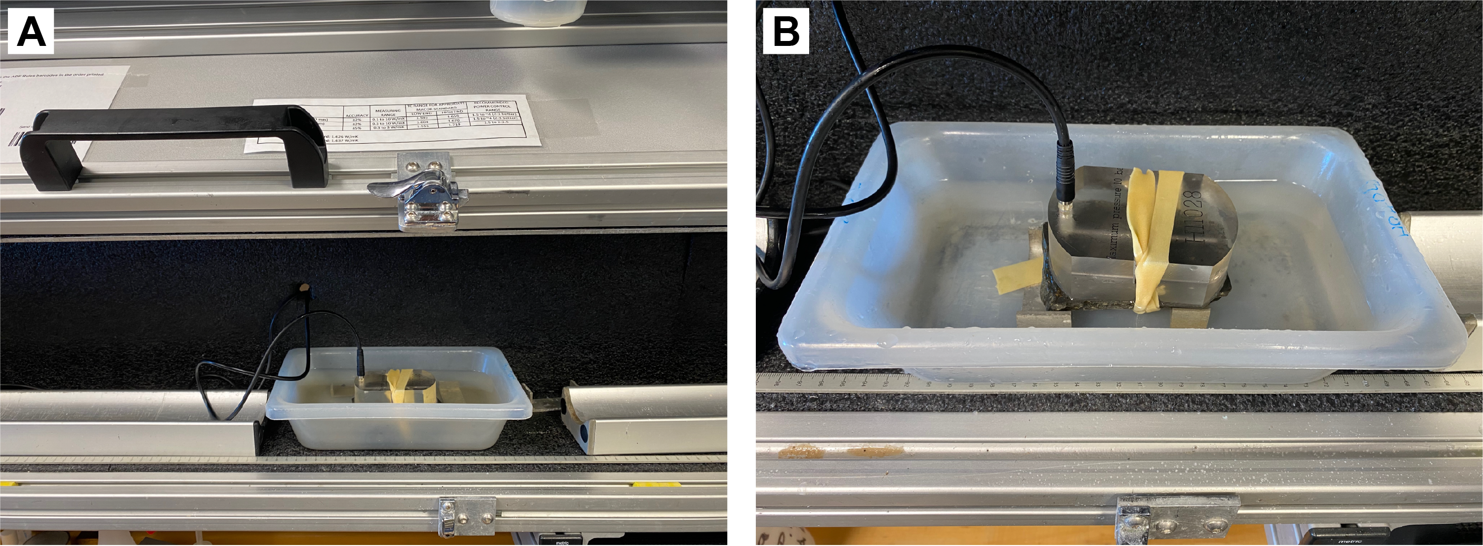
Figure F24. Insulated box.
8.4. Archive-half measurements
8.4.1. Section half multisensor logging
The SHMSL was used to measure spectral reflectance and MSP on archive halves. The SHMSL includes a platform that moves above the section half and records the sample height using a laser sensor. The laser profile establishes the location of the bottom of the core section and the characteristics of the rock being measured by locating gaps and cracks between pieces based on a laser distance exceeding a set value. After identifying the section length, the SHMSL then measures RSC and MSP at regular intervals along the section. Measurements were made at 2 cm intervals along the core.
8.4.2. Reflectance spectrophotometry and colorimetry
Spectral reflectance was measured using an Ocean Optics, Inc., system mounted on the SHMSL. The system emits UV through visible to near-infrared wavelengths (171–1100 nm) at 2 nm increments. Each measurement was recorded in wide (400–900 nm) spectral bands in 2 nm steps. Each measurement took ~5 s. For sediment and sedimentary rock, freshly split cores were covered with clear plastic wrap before measurement. Spectral data are routinely reduced to the L*a*b* color space for output and presentation, in which L* is luminescence or lightness in the range between 0 (black) and 100 (white), a* is the red–green value in the range between −60 (green) and 60 (red), and b* is the yellow–blue value in the range between −60 (blue) and 60 (yellow). The color reflectance spectrophotometer calibrates on two spectra, pure white (reference) and pure black (dark).
8.4.3. Point magnetic susceptibility
MSP was measured on the SHMSL using a Bartington MS2E contact probe with a flat 15 mm diameter sensor operating at a frequency of 0.580 kHz. The sensor averages three measurements made at 1 s intervals to an accuracy of 5%. The area of response of the MS2E sensor is 3.8 mm × 10.5 mm, with a depth response of 50% at 1 mm and 10% at 3.5 mm (Bartington Instruments, Ltd., 2011). MSP measurements were performed on archive halves and thus refer to a higher spatial resolution than MS measured by WRMSL on whole rounds. The probe is zeroed in air before each measurement, and a background magnetic field is measured and removed from the data. Measurements are output in instrument units but reported in SI × 10−5.
8.5. Working-half section measurements
Thermal conductivity, P-wave velocity, and MAD measurements were made on working halves and discrete samples. Thermal conductivity was measured once per core on seawater-saturated (igneous and sedimentary) rock pieces using a contact probe on a piece of section half in a bath of seawater. Samples from igneous rock material were shared for both paleomagnetic and MAD measurements; P-wave velocity measurements in the x-, y-, and z-directions were also made on these discrete samples.
8.5.1. Shear strength
Shear strength (τf) is the resistance to failure of a material under shear and can be expressed as a function of the effective normal stress at failure (σ′), the effective cohesion (c′), and friction angle (φ′):
where c′ and φ′ are the shear strength parameters that define a linear relationship between τf and φ′, according to the Mohr-Coulomb failure criterion.
During Expedition 391, the shear strength of soft-sediment cores was measured using the automated vane shear (AVS) system on the working half following core description. A representative location in each core or unit was selected as close as possible to the center of the core along the y-axis, and measurements were made with the vane rotation axis perpendicular to the split surface. Shear strength was determined by inserting a four-bladed vane (number 12) into the split core and applying shear stress, resulting in shearing of a cylindrical surface by the vane. This procedure provides a measurement of the peak shear strength expressed in kilopascals.
8.5.2. P-wave velocity (soft-sediment cores)
P-wave velocity in the x-direction was also obtained from the working halves of soft-sediment cores using the SHMG (Figure F25), which includes the PWC (x-direction) and PWB (y- and z-directions). P-wave velocity on section halves was calculated by applying a correction in the IMS 10 Velocity software to account for the thickness of the plastic core liner. The PWB and PWC record arrivals, and the peak of the first arrival is identified automatically by the IMS 10 Velocity software. After verification, the first arrival is then adjusted to the lowest possible threshold and the automatic first arrival pick and original waveform are saved. System calibration runs with standards were conducted periodically to ensure that system and transducer delay time settings were current.
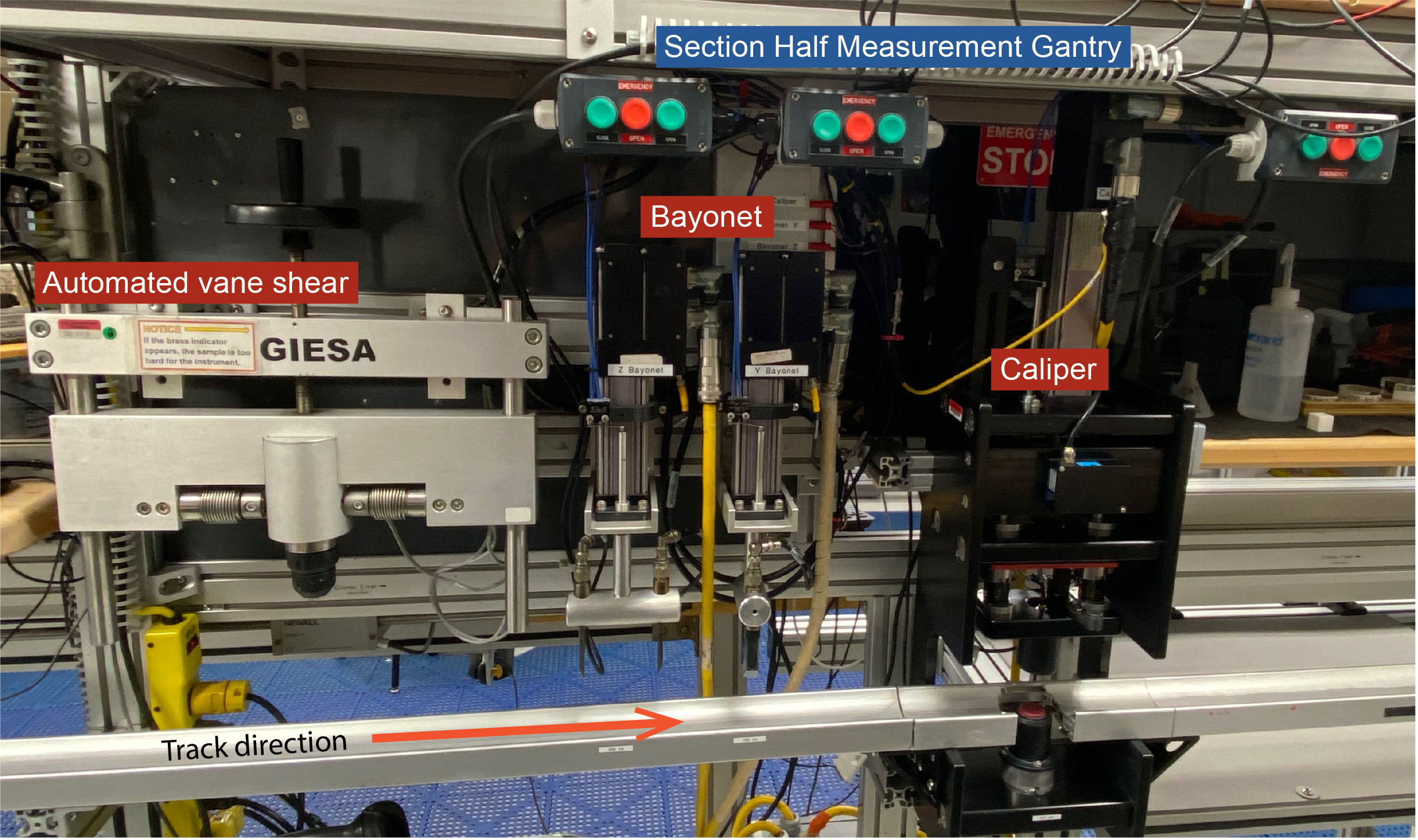
Figure F25. SHMG.
8.5.3. P-wave velocity (hard rocks)
Because igneous and sedimentary rock cores generally do not fill the core liner, PWL measurements on whole-round hard rock cores were not collected during WRMSL analyses. Thus, PWC measurements provide additional P-wave velocity data (x-axis) along the section to supplement the analyses of whole-round core pieces and discrete samples and may provide the most continuous record of P-wave velocity variation with depth. PWC was used to measure P-wave velocity on at least one section half per core. The same seawater-saturated hard rock working-half pieces used for thermal conductivity measurements were used for P-wave velocity measurements. Representative locations on relatively flat and uniform surfaces were selected, and the core was adjusted to ensure full contact with the transducer. Successful analyses require good contact between the transducers and the rock and core liner surfaces, which is enhanced by wetting both transducers with deionized water.
8.5.4. Discrete sample measurements
PWC measurements of P-wave velocity in the x-, y-, and z-directions were performed on the same 7 cm3 discrete cube samples of sedimentary and igneous rock that were used for paleomagnetic determinations and MAD measurements. Wedge samples from the same interval were also measured using the PWC (z-direction) to test the effect of high-temperature paleomagnetic experiments on P-wave velocity. Cubes and wedges were oriented following standard IODP conventions. Prior to measurement, samples were saturated in seawater in a vacuum chamber for ~6 h. The system consists of a vacuum pump and a plastic chamber that contains the cubes submerged in seawater in small plastic vials (Figure F26). After removal from the vacuum chamber, cubes and wedges were stored in sample containers to maintain saturation.
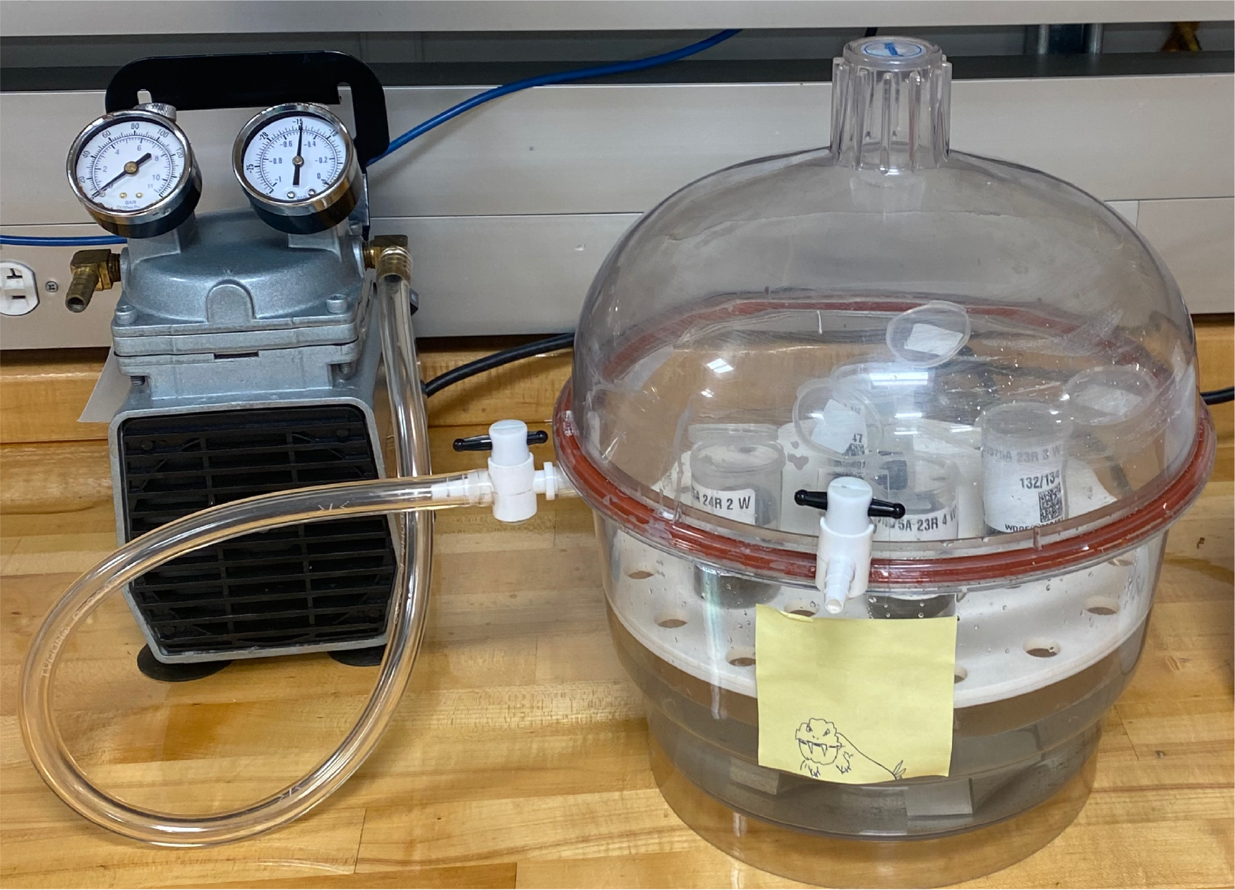
Figure F26. Seawater vacuum chamber.
8.5.5. Moisture and density measurements
Mass and volume measurements were made to determine bulk density, dry density, grain density, and porosity. The shipboard MAD facility consists of a dual-balance system and the hexapycnometer. Soft-sediment samples were placed in numbered, preweighed ~16 mL Wheaton glass vials for sediment weighing, drying, and dry volume measurements. For igneous and sedimentary rock samples, MAD measurements were made on discrete sample cubes and wedges that were also used for paleomagnetic and P-wave velocity (PWC) measurements. Prior to measuring, samples were saturated in seawater under vacuum conditions for ~6 h and then weighed to obtain their wet mass. Samples were then placed in an oven at 105° ± 5°C for 22–24 h and then allowed to cool in a desiccator for 3 h prior to dry mass and dry volume measurements.
8.5.5.1. Dual-balance system
A dual-balance system was used to measure wet and dry masses. Two analytical balances (Mettler-Toledo XS204) compensate for ship motion; one acts as a reference, and the other measures the sample relative to the reference. A standard mass of similar value to that of the sample mass was placed on the reference balance to increase accuracy. An accuracy of 0.005 g was readily attainable by using a reference mass within 10% of the sample mass. The default setting of the balances is 300 measurements (taking ~1.5 min).
8.5.5.2. Hexapycnometer system
The hexapycnometer is an IODP custom-built system that uses six MicroMetrics cell units, electronics, and control programs. The system measures dry sample volume using pressurized He-filled chambers with a precision of 0.02 cm3. Shipboard technical staff performed a calibration using stainless steel spheres of known volume at the start of the expedition and whenever the helium gas tank was changed. For each measurement, five cells containing samples and one cell containing two calibration spheres (3 and 7 cm3) with a total volume of 10 cm3 were run. Calibration spheres were cycled through the cells to identify any systematic error and/or instrument drift. Spheres were assumed to be known to within 1% of their total volume. If the volumes of the calibration spheres deviated by >1% from their known volumes, then that pycnometer cell was recalibrated.
8.5.5.3. Moisture and density calculations
MAD calculations were performed according to Method C in the IODP Physical Properties Handbook (Blum, 1997). For density calculations, both mass and volume are first corrected for the salt content of the pore fluid:
- Msalt = mass of salt,
- S = pore water salinity (seawater with salinity 35 or 0.035 g/cm3),
- Mw = wet mass of the sample, and
- Md = dry mass of the sample.
Grain density (ρg) is determined from the dry mass (Md) and dry volume (Vd) measurements:
where ρsalt is the density of salt (2.20 g/cm3).
The salt-corrected mass of pore water (Mpw) is calculated as
Then the volume of pore water (Vpw) is
where we assume the density of the pore fluid (ρpw) = 1.024 g/cm3 (seawater with salinity of 35).
To calculate sample bulk density (ρb) of the wet sample, bulk volume (Vb) of the wet sample is first computed:
Connected porosity (φ) is calculated from the two volume parameters obtained from MAD measurements and from the resulting bulk and pore water volume calculations:
References
Alt, J.C., 1993. Low-temperature alteration of basalts from the Hawaiian Arch, Leg 136. In Wilkens, R.H., Firth, J., Bender, J., et al., Proceedings of the Ocean Drilling Program, Scientific Results, 136: College Station, TX (Ocean Drilling Program), 133–146. https://doi.org/10.2973/odp.proc.sr.136.214.1993
Arculus, R.J., Ishizuka, O., Bogus, K., Aljahdali, M.H., Bandini-Maeder, A.N., Barth, A.P., Brandl, P.A., do Monte Guerra, R., Drab, L., Gurnis, M.C., Hamada, M., Hickey-Vargas, R.L., Jiang, F., Kanayama, K., Kender, S., Kusano, Y., Li, H., Loudin, L.C., Maffione, M., Marsaglia, K.M., McCarthy, A., Meffre, S., Morris, A., Neuhaus, M., Savov, I.P., Sena Da Silva, C.A., Tepley, F.J., III, van der Land, C., Yogodzinski, G.M., and Zhang, Z., 2015. Expedition 351 summary. In Arculus, R.J., Ishizuka, O., Bogus, K., and the Expedition 351 Scientists, Proceedings of the International Ocean Discovery Program, Expedition 351: Izu-Bonin-Mariana Arc Origins. College Station, TX (International Ocean Discovery Program). https://doi.org/10.14379/iodp.proc.351.101.2015
Aubele, J.C., Crumpler, L.S., and Elston, W.E., 1988. Vesicle zonation and vertical structure of basalt flows. Journal of Volcanology and Geothermal Research, 35(4):349–374. https://doi.org/10.1016/0377-0273(88)90028-5
Bach, W., Garrido, C.J., Paulick, H., Harvey, J., and Rosner, M., 2004. Seawater-peridotite interactions: first insights from ODP Leg 209, MAR 15°N. Geochemistry, Geophysics, Geosystems, 5(9):Q09F26. https://doi.org/10.1029/2004GC000744
Backman, J., Raffi, I., Rio, D., Fornaciari, E., and Pälike, H., 2012. Biozonation and biochronology of Miocene through Pleistocene calcareous nannofossils from low and middle latitudes. Newsletters on Stratigraphy, 45(3):221–244. https://doi.org/10.1127/0078-0421/2012/0022
Bartington Instruments, L., 2011. Operation Manual for MS2 Magnetic Susceptibility System: Oxford, UK (Bartington Instruments, Ltd.). https://gmw.com/wp-content/uploads/2019/03/MS2-OM0408.pdf
Bartington Instruments, L., 2019. MS2/MS3 Magnetic Susceptibility Systems: Oxford, United Kingdom (Bartington Instruments, Ltd.). http://www.bartington.com/Literaturepdf/Datasheets/MS2_MS3_DS0020.pdf
Batiza, R., and White, J., 1999. Submarine lava and hyaloclastite. In Sigurdsson, H., Houghton, B.F., Rymer, H., Stix, J., and McNutt (Eds.), Encyclopedia of Volcanoes. Amsterdam (Elsevier), 363–375.
Blum, P., 1997. Physical properties handbook: a guide to the shipboard measurement of physical properties of deep-sea cores. Ocean Drilling Program Technical Note, 26. https://doi.org/10.2973/odp.tn.26.1997
Bolli, H.M., and Saunders, J.B., 1985. Oligocene to Holocene low latitude planktic foraminifera. In Bolli, H.M., Saunders, J.B., and Perch-Nielsen, K. (Eds.), Planktic Foraminifera, Calcareous Nannofossils and Calpionellids. Plankton Stratigraphy, 1:155–262.
Bown, P.R. (Ed.), 1998. Calcareous Nannofossil Biostratigraphy: Dordrect, Netherlands (Kluwer Academic Publishing).
Buchs, D.M., Williams, R., Sano, S.-i., and Wright, V.P., 2018. Non-Hawaiian lithostratigraphy of Louisville seamounts and the formation of high-latitude oceanic islands and guyots. Journal of Volcanology and Geothermal Research, 356:1–23. https://doi.org/10.1016/j.jvolgeores.2017.12.019
Carey, S.N., and Schneider, J.-L., 2011. Volcaniclastic processes and deposits in the deep-sea. In HüNeke, H., and Mulder, T. (Eds.), Deep-Sea Sediments. Developments in Sedimentology. A.J. Van Loon (Series Ed.), 63: 457–515. https://doi.org/10.1016/B978-0-444-53000-4.00007-X
Caron, M., 1985. Cretaceous planktic foraminifera. In Bolli, H.M., Saunders. J.B., and Perch-Nielsen, K. (Eds.), Planktic Foraminifera, Calcareous Nannofossils and Calpionellids. Plankton Stratigraphy: 17–86.
de Ronde, C.E.J., Humphris, S.E., Höfig, T.W., Brandl, P.A., Cai, L., Cai, Y., Caratori Tontini, F., Deans, J.R., Farough, A., Jamieson, J.W., Kolandaivelu, K.P., Kutovaya, A., Labonté, J.M., Martin, A.J., Massiot, C., McDermott, J.M., McIntosh, I.M., Nozaki, T., Pellizari, V.H., Reyes, A.G., Roberts, S., Rouxel, O., Schlicht, L.E.M., Seo, J.H., Straub, S.M., Strehlow, K., Takai, K., Tanner, D., Tepley III, F.J., and Zhang, C., 2019. Expedition 376 methods. In de Ronde, C.E.J., Humphris, S.E., Höfig, T.W., and the Expedition 376 Scientists, Brothers Arc Flux. Proceedings of the International Ocean Discovery Program, 376: College Station, TX (International Ocean Discovery Program). https://doi.org/10.14379/iodp.proc.376.102.2019
Dickinson, J.A., Harb, N., Portner, R.A., and Daczko, N.R., 2009. Glassy fragmental rocks of Macquarie Island (Southern Ocean): mechanism of formation and deposition. Sedimentary Geology, 216(3):91–103. https://doi.org/10.1016/j.sedgeo.2009.02.001
Droser, M.L., and Bottjer, D.J., 1986. A semiquantitative field classification of ichnofabric. Journal of Sedimentary Research, 56(4):558–559. https://doi.org/10.1306/212F89C2-2B24-11D7-8648000102C1865D
Dunham, R.J., and Ham, W.E., 1962. Classification of carbonate rocks according to depositional texture. AAPG Memoir, 1.
Dunlea, A.G., Murray, R.W., Harris, R.N., Vasiliev, M.A., Evans, H., Spivack, A.J., and D'Hondt, S., 2013. Assessment and use of NGR instrumentation on the JOIDES Resolution to quantify U, Th, and K concentrations in marine sediment. Scientific Drilling, 15:57–63. https://doi.org/10.2204/iodp.sd.15.05.2013
Ellwood, B.B., 1978. Flow and emplacement direction determined for selected basaltic bodies using magnetic susceptibility anisotropy measurements. Earth and Planetary Science Letters, 41(3):254–264. https://doi.org/10.1016/0012-821X(78)90182-6
Epstein, M.S., Diamondstone, B.I., and Gills, T.E., 1989. A new river sediment standard reference material. Talanta, 36(1–2):141–150. https://doi.org/10.1016/0039-9140(89)80089-X
Expedition 324 Scientists, 2010a. Massive basalt flows on the southern flank of Tamu Massif, Shatsky Rise; a reappraisal of ODP Site 1213 basement units. In Sager, W.W., Sano, T., Geldmacher, J., and the Expedition 324 Scientists, Proceedings of the Integrated Ocean Drilling Program, 324: Tokyo (Integrated Ocean Drilling Program Management International, Inc.). https://doi.org/10.2204/iodp.proc.324.109.2010
Expedition 324 Scientists, 2010b. Methods. In Sager, W.W., Sano, T., Geldmacher, J., and the Expedition 324 Scientists, Proceedings of the Integrated Ocean Drilling Program, 324: Tokyo (Integrated Ocean Drilling Program Management International, Inc). https://doi.org/10.2204/iodp.proc.324.102.2010
Expedition 324 Scientists, 2010c. Expedition 324 summary. In Sager, W.W., Sano, T., Geldmacher, J., and the Expedition 324 Scientists, Proceedings of the Integrated Ocean Drilling Program, 324: Tokyo (Integrated Ocean Drilling Program Management International, Inc.). https://doi.org/10.2204/iodp.proc.324.101.2010
Expedition 330 Scientists, 2012a. Expedition 330 summary. In Koppers, A.A.P., Yamazaki, T., Geldmacher, J., and the Expedition 330 Scientists, Proceedings of the Integrated Ocean Drilling Program, 330: Tokyo (Integrated Ocean Drilling Program Management International, Inc.). https://doi.org/10.2204/iodp.proc.330.101.2012
Expedition 330 Scientists, 2012b. Methods. In Koppers, A.A.P., Yamazaki, T., Geldmacher, J., and the Expedition 330 Scientists, Proceedings of the Integrated Ocean Drilling Program, 330: Tokyo (Integrated Ocean Drilling Program Management International, Inc.). https://doi.org/10.2204/iodp.proc.330.102.2012
Fisher, R.V., and Schmincke, H.-U., 1984. Pyroclastic Rocks: Berlin (Springer). https://doi.org/10.1007/978-3-642-74864-6
Folk, R.L., 1965. Some aspects of recrystallization in ancient limestones. In Pray, L.C., and Murray, R.C. (Eds.), Dolomitization and Limestone Diagenesis. SEPM Special Publication, 13: 13–48. https://doi.org/10.2110/pec.65.07.0014
Gaidies, F., Milke, R., Heinrich, W., Abart, R., Heinrich, W., and Abart, R., 2017. Metamorphic mineral reactions: porphyroblast, corona and symplectite growth. In Heinrich, W., and Abart, R. (Eds.), Mineral Reaction Kinetics: Microstructures, Textures, Chemical and Isotopic Signatures. European Mineralogical Union Notes in Mineralogy, 16. https://doi.org/10.1180/EMU-notes.16.14
Gieskes, J.M., Gamo, T., and Brumsack, H.J., 1991. Chemical methods for interstitial water analysis aboard JOIDES Resolution. Ocean Drilling Program Technical Note, 15. https://doi.org/10.2973/odp.tn.15.1991
Gifkins, C.C., and Allen, R.L., 2001. Textural and chemical characteristics of diagenetic and hydrothermal alteration in glassy volcanic rocks: examples from the Mount Read volcanics, Tasmania. Economic Geology, 96(5):973–1002. https://doi.org/10.2113/gsecongeo.96.5.973
Gifkins, C.C., Herrmann, W., and Large, R.R., 2005. Altered Volcanic Rocks: a Guide to Description and Interpretation: Hobart, Australia (Centre for Ore Deposit Research, University of Tasmania). https://eprints.utas.edu.au/296/
Godard, M., Awaji, S., Hansen, H., Hellebrand, E., Brunelli, D., Johnson, K., Yamasaki, T., Maeda, J., Abratis, M., Christie, D., Kato, Y., Mariet, C., and Rosner, M., 2009. Geochemistry of a long in-situ section of intrusive slow-spread oceanic lithosphere: results from IODP Site U1309 (Atlantis Massif, 30°N Mid-Atlantic-Ridge). Earth and Planetary Science Letters, 279(1–2):110–122. https://doi.org/10.1016/j.epsl.2008.12.034
Govindaraju, K., 1994. 1994 compilation of working values and sample description for 383 geostandards. Geostandards Newsletter, 18(S1):1–158. https://doi.org/10.1046/j.1365-2494.1998.53202081.x-i1
Graber, K.K., Pollard, E., Jonasson, B., and Schulte, E. (Eds.), 2002. Overview of Ocean Drilling Program engineering tools and hardware. Ocean Drilling Program Technical Note, 31. https://doi.org/10.2973/odp.tn.31.2002
Gradstein, F.M., Ogg, J.G., Schmitz, M.D., and Ogg, G.M. (Eds.), 2012. The Geologic Time Scale 2012: Amsterdam (Elsevier). https://doi.org/10.1016/C2011-1-08249-8
Gradstein, F.M., Ogg, J.G., Schmitz, M.D., and Ogg, G.M. (Eds.), 2020. The Geologic Time Scale 2020: Amsterdam (Elsevier BV). https://doi.org/10.1016/C2020-1-02369-3
Gregg, T.K.P., and Fink, J.H., 1995. Quantification of submarine lava-flow morphology through analog experiments. Geology, 23(1):73–76. https://doi.org/10.1130/0091-7613(1995)023<0073:QOSLFM>2.3.CO;2
Harris, R.N., Sakaguchi, A., Petronotis, K., Baxter, A.T., Berg, R., Burkett, A., Charpentier, D., Choi, J., Diz Ferreiro, P., Hamahashi, M., Hashimoto, Y., Heydolph, K., Jovane, L., Kastner, M., Kurz, W., Kutterolf, S.O., Li, Y., Malinverno, A., Martin, K.M., Millan, C., Nascimento, D.B., Saito, S., Sandoval Gutierrez, M.I., Screaton, E.J., Smith-Duque, C.E., Solomon, E.A., Straub, S.M., Tanikawa, W., Torres, M.E., Uchimura, H., Vannucchi, P., Yamamoto, Y., Yan, Q., and Xhao, X., 2013. Methods. In Harris, R.N., Sakaguchi, A., Petronotis, K., and the Expedition 344 Scientists, Proceedings of the Integrated Ocean Drilling Program, 344: College Station, TX (Integrated Ocean Drilling Program). https://doi.org/10.2204/iodp.proc.344.102.2013
Huber, B.T., Hobbs, R.W., Bogus, K.A., Batenburg, S.J., Brumsack, H.-J., do Monte Guerra, R., Edgar, K.M., Edvardsen, T., Garcia Tejada, M.L., Harry, D.L., Hasegawa, T., Haynes, S.J., Jiang, T., Jones, M.M., Kuroda, J., Lee, E.Y., Li, Y.-X., MacLeod, K.G., Maritati, A., Martinez, M., O'Connor, L.K., Petrizzo, M.R., Quan, T.M., Richter, C., Riquier, L., Tagliaro, G.T., Wainman, C.C., Watkins, D.K., White, L.T., Wolfgring, E., and Xu, Z., 2019. Expedition 369 methods. In Hobbs, R.W., Huber, B.T., Bogus, K.A., and the Expedition 369 Scientists, Australia Cretaceous climate and tectonics. Proceedings of the International Ocean Discovery Program, 369: College Station, TX (International Ocean Discovery Program). https://doi.org/10.14379/iodp.proc.369.102.2019
Huber, B.T., Petrizzo, M.R., Young, J.R., Falzoni, F., Gilardoni, S.E., Bown, P.R., and Wade, B.S., 2016. Pforams@microtax: a new online taxonomic database for planktonic foraminifera. Micropaleontology, 62(6):429–438. https://www.jstor.org/stable/26645533
Inoue, A., Kurokawa, K., and Hatta, T., 2010. Application of chlorite geothermometry to hydrothermal alteration in Toyoha Geothermal System, Southwestern Hokkaido, Japan. Resource Geology, 60(1):52–70. https://doi.org/10.1111/j.1751-3928.2010.00114.x
Jackson, M., Gruber, W., Marvin, J., and Banerjee, S.K., 1988. Partial anhysteretic remanence and its anisotropy: applications and grainsize-dependence. Geophysical Research Letters, 15(5):440–443. https://doi.org/10.1029/GL015i005p00440
Jarrard, R.D., and Kerneklian, M.J., 2007. Data report: physical properties of the upper oceanic crust of ODP Site 1256: multisensor track and moisture and density measurements. In Teagle, D.A.H., Wilson, D.S., Acton, G.D., and Vanko, D.A., Proceedings of the Ocean Drilling Program, Scientific Results, 206: College Station, TX (Ocean Drilling Program). https://doi.org/10.2973/odp.proc.sr.206.011.2007
Jébrak, M., 1997. Hydrothermal breccias in vein-type ore deposits: a review of mechanisms, morphology and size distribution. Ore Geology Reviews, 12(3):111–134. https://doi.org/10.1016/S0169-1368(97)00009-7
Jelínek, V., and Kropáček, V., 1978. Statistical processing of anisotropy of magnetic susceptibility measured on groups of specimens. Studia Geophysica et Geodaetica, 22(1):50–62. https://doi.org/10.1007/BF01613632
Jerram, D.A., and Widdowson, M., 2005. The anatomy of Continental Flood Basalt Provinces: geological constraints on the processes and products of flood volcanism. Lithos, 79(3):385–405. https://doi.org/10.1016/j.lithos.2004.09.009
Jochum, K.P., Weis, U., Schwager, B., Stoll, B., Wilson, S.A., Haug, G.H., Andreae, M.O., and Enzweiler, J., 2016. Reference values following ISO guidelines for frequently requested rock reference materials. Geostandards and Geoanalytical Research, 40(3):333–350. https://doi.org/10.1111/j.1751-908X.2015.00392.x
Johnston, R.M., Ryan, J.G., Fryer, P., Wheat, C.G., Williams, T., Albers, E., Bekins, B.A., Debret, B.P.R., Jianghong, D., Yanhui, D., Eickenbusch, P., Frery, E.A., Ichiyama, Y., Johnson, K., Kevorkian, R.T., Kurz, W., Magalhaes, V., Mantovanelli, S.S., Menapace, W., Menzies, C.D., Michibayashi, K., Moyer, C.L., Mullane, K.K., Park, J.-W., Price, R.E., Shervais, J.W., Suzuki, S., Sissmann, O.J., Takai, K., Walter, B., and Rui, Z., 2018. pXRF and ICP-AES characterization of shipboard rocks and sediments; protocols and strategies. In Fryer, P., Wheat, C.G., Williams, T., and the Expedition 366 Scientists, Mariana Convergent Margin and South Chamorro Seamount. Proceedings of the International Ocean Discovery Program, 366: College Station, TX (Proceedings of the International Ocean Discovery Program). https://doi.org/10.14379/iodp.proc.366.110.2018
Jutzeler, M., White, J.D.L., Talling, P.J., McCanta, M., Morgan, S., Le Friant, A., and Ishizuka, O., 2014. Coring disturbances in IODP piston cores with implications for offshore record of volcanic events and the Missoula megafloods. Geochemistry, Geophysics, Geosystems, 15(9):3572–3590. https://doi.org/10.1002/2014GC005447
Kennett, J.P., and Srinivasan, M.S., 1983. Neogene Planktonic Foraminifera: A Phylogenetic Atlas: London (Hutchinson Ross).
Kirschvink, J.L., 1980. The least-squares line and plane and the analysis of palaeomagnetic data. Geophysical Journal International, 62(3):699–718. https://doi.org/10.1111/j.1365-246X.1980.tb02601.x
Kristiansen, J.I., 1982. The transient cylindrical probe method for determination of thermal parameters of earth materials [PhD dissertation]. Åarhus University, Åarhus, Denmark. http://digitallib.oit.edu/digital/collection/geoheat/id/2103/
Kvenvolden, K.A., and McDonald, T.J., 1986. Organic geochemistry on the JOIDES Resolution—an assay. Ocean Drilling Program Technical Note, 6. https://doi.org/10.2973/odp.tn.6.1986
Lee, E.Y., Tejada, M.L.G., Song, I., Chun, S.S., Gier, S., Riquier, L., White, L.T., Schnetger, B., Brumsack, H.-J., Jones, M.M., and Martinez, M., 2021. Petrophysical property modifications by alteration in a volcanic sequence at IODP Site U1513, Naturaliste Plateau. Journal of Geophysical Research: Solid Earth, 126(10):e2020JB021061. https://doi.org/10.1029/2020JB021061
Li, C.-F., Lin, J., Kulhanek, D.K., Williams, T., Bao, R., Briais, A., Brown, E.A., Chen, Y., Clift, P.D., Colwell, F.S., Dadd, K.A., Ding, W., Almeida, I.H., Huang, X.-L., Hyun, S., Jiang, T., Koppers, A.A.P., Li, Q., Liu, C., Liu, Q., Liu, Z., Nagai, R.H., Peleo-Alampay, A., Su, X., Sun, Z., Tejada, M.L.G., Trinh, H.S., Yeh, Y.-C., Zhang, C., Zhang, F., Zhang, G.-L., and Zhao, X., 2015. Expedition 349 summary. In Li, C.-F., Lin, J., Kulhanek, D.K., and the Expedition 349 Scientists, South China Sea Tectonics. Proceedings of the International Ocean Discovery Program, 349: College Station, TX (International Ocean Discovery Program). https://doi.org/10.14379/iodp.proc.349.101.2015
Li, Y.-X., and Kodama, K., 2016. Detecting and correcting for paleomagnetic inclination shallowing of sedimentary rocks: a review. Frontiers in Earth Science, 4:7. https://doi.org/10.3389/feart.2016.00007
Lonsdale, P., and Spiess, F.N., 1980. Deep-tow observations at the East Pacific Rise, 8°45′N, and some interpretations. In Rosendahl, B.R., Hekinian, R., et al., Initial Reports of the Deep Sea Drilling Project. 54: Washington, DC (US Government Printing Office), 43–62. https://doi.org/10.2973/dsdp.proc.54.104.1980
Lurcock, P.C., and Wilson, G.S., 2012. PuffinPlot: a versatile, user-friendly program for paleomagnetic analysis. Geochemistry, Geophysics, Geosystems, 13(6):Q06Z45. https://doi.org/10.1029/2012GC004098
Manheim, F.T., and Sayles, F.L., 1974. Composition and origin of interstitial waters of marine sediments, based on deep sea drill cores. In Goldberg, E.D., The Sea (Volume 5): Marine Chemistry: The Sedimentary Cycle. New York (Wiley), 527–568. http://pubs.er.usgs.gov/publication/70207491
Marsaglia, K., Milliken, K., and Doran, L., 2013. IODP digital reference for smear slide analysis of marine mud, Part 1: Methodology and atlas of siliciclastic and volcanogenic components. Integrated Ocean Drilling Program Technical Note, 1. https://doi.org/10.2204/iodp.tn.1.2013
Marsaglia, K., Milliken, K., Leckie, R., Tentori, D., and Doran, L., 2015. IODP smear slide digital reference for sediment analysis of marine mud, Part 2: Methodology and atlas of biogenic components. Integrated Ocean Drilling Program Technical Note, 2. https://doi.org/10.2204/iodp.tn.2.2015
Martini, E., 1971. Standard Tertiary and Quaternary calcareous nannoplankton zonation. Proceedings of the Second Planktonic Conference, Roma, 1970:739–785.
Mazzullo, J., Meyer, A., and Kidd, R., 1988. Appendix I: New sediment classification scheme for the Ocean Drilling Program. In Mazzullo, J., and Graham, A.G., Handbook for shipboard sedimentologists. Ocean Drilling Program Technical Note, 8: 44–67. https://doi.org/10.2973/odp.tn.8.1988
Mitchell, N., Beier, C., Rosin, P., Quartau, R., and Tempera, F., 2008. Lava penetrating water: submarine lava flows around the coasts of Pico Island, Azores. Geochemistry Geophysics Geosystems, 9:Q03024. https://doi.org/10.1029/2007GC001725
Murray, R.W., Miller, D.J., and Kryc, K.A., 2000. Analysis of major and trace elements in rocks, sediments, and interstitial waters by inductively coupled plasma–atomic emission spectrometry (ICP-AES). Ocean Drilling Program Technical Note, 29. https://doi.org/10.2973/odp.tn.29.2000
Ogg, J.G., 2020. Geomagnetic Polarity Time Scale. In Gradstein, F.M., Ogg, J.G., Schmitz, M., and Ogg, G. (Eds.), Geologic Time Scale 2020. Amsterdam (Elsevier), 159–192.
Okada, H., and Bukry, D., 1980. Supplementary modification and introduction of code numbers to the low-latitude coccolith biostratigraphic zonation (Bukry, 1973; 1975). Marine Micropaleontology, 5(3):321–325. https://doi.org/10.1016/0377-8398(80)90016-X
Patterson, S.N., Lynn, K.J., Prigent, C., and Warren, J.M., 2021. High temperature hydrothermal alteration and amphibole formation in Gakkel Ridge abyssal peridotites. Lithos, 392–393:106107. https://doi.org/10.1016/j.lithos.2021.106107
Perch-Nielsen, K., 1985a. Cenozoic calcareous nannofossils. In Bolli, H.M., Saunders, J.B., and Perch-Nielsen, K. (Eds.), Plankton Stratigraphy (Volume 1). Cambridge, UK (Cambridge University Press), 427–554.
Perch-Nielsen, K., 1985b. Mesozoic calcareous nannofossils. In Bolli, H.M., Saunders, J.B., and Perch-Nielsen, K., Plankton Stratigraphy (Volume 1). Cambridge, UK (Cambridge University Press), 329–426.
Postuma, J.A., 1971. Manual of Planktonic Foraminifera: Amsterdam (Elsevier).
Putnis, A., 2002. Mineral replacement reactions: from macroscopic observations to microscopic mechanisms. Mineralogical Magazine, 66(5):689–708. https://doi.org/10.1180/0026461026650056
Ramalho, R.S., Helffrich, G., Madeira, J., Cosca, M., Thomas, C., Quartau, R., Hipólito, A., Rovere, A., Hearty, P.J., and Ávila, S.P., 2017. Emergence and evolution of Santa Maria Island (Azores)—the conundrum of uplifted islands revisited. Geological Society of America Bulletin, 129(3–4):372–390. https://doi.org/10.1130/B31538.1
Reagan, M.K., Pearce, J.A., Petronotis, K., Almeev, R., Avery, A.A., Carvallo, C., Chapman, T., Christeson, G.L., Ferré, E.C., Godard, M., Heaton, D.E., Kirchenbaur, M., Kurz, W., Kutterolf, S., Li, H.Y., Li, Y., Michibayashi, K., Morgan, S., Nelson, W.R., Prytulak, J., Python, M., Robertson, A.H.F., Ryan, J.G., Sager, W.W., Sakuyama, T., Shervais, J.W., Shimizu, K., and Whattam, S.A., 2015a. Expedition 352 methods. In Reagan, M.K., Pearce, J.A., Petronotis, K., and the Expedition 352 Scientists, Izu-Bonin-Mariana Fore Arc. Proceedings of the International Ocean Discovery Program, 352: College Station, TX (International Ocean Discovery Program). https://doi.org/10.14379/iodp.proc.352.102.2015
Reagan, M.K., Pearce, J.A., Petronotis, K., and the Expedition 352 Scientists, 2015b. Supplementary material, https://doi.org/10.14379/iodp.proc.352supp.2015. In Reagan, M.K., Pearce, J.A., Petronotis, K., and the Expedition 352 Scientists, Izu-Bonin-Mariana Fore Arc. Proceedings of the International Ocean Discovery Program: College Station, TX (International Ocean Discovery Program).
Révillon, S., Barr, S.R., Brewer, T.S., Harvey, P.K., and Tarney, J., 2002. An alternative approach using integrated gamma-ray and geochemical data to estimate the inputs to subduction zones from ODP Leg 185, Site 801. Geochemistry, Geophysics, Geosystems, 3(12):1–22. https://doi.org/10.1029/2002GC000344
Reynolds, R.C., Jr., 1963. Matrix corrections in trace element analysis by X-ray fluorescence: estimation of the mass absorption coefficient by Compton scattering. American Mineralogist, 48(9–10):1133–1143. http://www.minsocam.org/ammin/AM48/AM48_1133.pdf
Rothwell, R.G., 1989. Minerals and Mineraloids in Marine Sediments: An Optical Identification Guide: London (Elsevier). https://doi.org/10.1007/978-94-009-1133-8
Ryan, J.G., Shervais, J.W., Li, Y., Reagan, M.K., Li, H.Y., Heaton, D., Godard, M., Kirchenbaur, M., Whattam, S.A., Pearce, J.A., Chapman, T., Nelson, W., Prytulak, J., Shimizu, K., and Petronotis, K., 2017. Application of a handheld X-ray fluorescence spectrometer for real-time, high-density quantitative analysis of drilled igneous rocks and sediments during IODP Expedition 352. Chemical Geology, 451:55–66. https://doi.org/10.1016/j.chemgeo.2017.01.007
Sager, W., Hoernle, K., Höfig, T.W., Avery, A.J., Bhutani, R., Buchs, D.M., Carvallo, C.A., Class, C., Dai, Y., Dalla Valle, G., Del Gaudio, A.V., Fielding, S., Gaastra, K.M., Han, S., Homrighausen, S., Kubota, Y., Li, C.-F., Nelson, W.R., Petrou, E., Potter, K.E., Pujatti, S., Scholpp, J., Shervais, J.W., Thoram, S., Tikoo-Schantz, S.M., Tshiningayamwe, M., Wang, X.-J., and Widdowson, M., 2023. Site U1578. In Sager, W., Hoernle, K., Höfig, T.W., Blum, P., and the Expedition 391 Scientists, Walvis Ridge Hotspot. Proceedings of the International Ocean Discovery Program, 391: College Station, TX (International Ocean Discovery Program). https://doi.org/10.14379/iodp.proc.391.106.2023
Salvatore, M.R., Mustard, J.F., Head, J.W., Cooper, R.F., Marchant, D.R., and Wyatt, M.B., 2013. Development of alteration rinds by oxidative weathering processes in Beacon Valley, Antarctica, and implications for Mars. Geochimica et Cosmochimica Acta, 115:137-161. https://doi.org/10.1016/j.gca.2013.04.002
Shepard, F.P., 1954. Nomenclature based on sand-silt-clay ratios. Journal of Sedimentary Research, 24(3):151–158. https://doi.org/10.1306/D4269774-2B26-11D7-8648000102C1865D
Shipboard Scientific Party, 2002a. Explanatory notes. In Tarduno, J.A., Duncan, R.A., Scholl, D.W., et al., Proceedings of the Ocean Drilling Program, Initial Reports, 197. College Station, TX (Ocean Drilling Program), 1–89. https://doi.org/10.2973/odp.proc.ir.197.102.2002
Shipboard Scientific Party, 2002b. Site 1188. In Binns, R.A., Barriga, F.J.A.S., Miller, D.J., et al., Proceedings of the Ocean Drilling Program, Initial Reports, 193. College Station, TX (Ocean Drilling Program), 1–305. https://doi.org/10.2973/odp.proc.ir.193.103.2002
Shipboard Scientific Party, 2003. Explanatory notes. In Wilson, D.S., Teagle, D.A.H., Acton, G.D., et al., Proceedings of the Ocean Drilling Program, Initial Reports. 206: College Station, TX (Ocean Drilling Program). https://doi.org/10.2973/odp.proc.ir.206.102.2003
Simpson, K., and McPhie, J., 2001. Fluidal-clast breccia generated by submarine fire fountaining, Trooper Creek Formation, Queensland, Australia. Journal of Volcanology and Geothermal Research, 109(4):339–355. https://doi.org/10.1016/S0377-0273(01)00199-8
Skilling, I.P., White, J.D.L., and McPhie, J., 2002. Peperite: a review of magma–sediment mingling. Journal of Volcanology and Geothermal Research, 114(1–2):1–17. https://doi.org/10.1016/S0377-0273(01)00278-5
Staudigel, H., and Schmincke, H.-U., 1984. The Pliocene seamount series of La Palma/Canary Islands. Journal of Geophysical Research: Solid Earth, 89(B13):11195–11215. https://doi.org/10.1029/JB089iB13p11195
Sun, Z., Jian, Z., Stock, J.M., Larsen, H.C., Klaus, A., Alvarez Zarikian, C.A., Boaga, J., Bowden, S.A., Briais, A., Chen, Y., Cukur, D., Dadd, K.A., Ding, W., Dorais, M.J., Ferré, E.C., Ferreira, F., Furusawa, A., Gewecke, A.J., Hinojosa, J.L., Höfig, T.W., Hsiung, K.-H., Huang, B., Huang, E., Huang, X.-L., Jiang, S., Jin, H., Johnson, B.G., Kurzawski, R.M., Lei, C., Li, B., Li, L., Li, Y., Lin, J., Liu, C., Liu, C., Liu, Z., Luna, A., Lupi, C., McCarthy, A.J., Mohn, G., Ningthoujam, L.S., Nirrengarten, M., Osono, N., Peate, D.W., Persaud, P., Qiu, N., Robinson, C.M., Satolli, S., Sauermilch, I., Schindlbeck, J.C., Skinner, S.M., Straub, S.M., Su, X., Tian, L., Van der Zwan, F.M., Wan, S., Wu, H., Xiang, R., Yadav, R., Yi, L., Zhang, C., Zhang, J., Zhang, Y., Zhao, N., Zhong, G., and Zhong, L., 2018. Expedition 367/368 methods. In Sun, Z., Jian, Z., Stock, J.M., Larsen, H.C., Klaus, A., Alvarez Zarikian, C.A., and the Expedition 367/368 Scientists, South China Sea Rifted Margin. Proceedings of the International Ocean Discovery Program, 367/368: College Station, TX (International Ocean Discovery Program). https://doi.org/10.14379/iodp.proc.367368.102.2018
Tauxe, L., Shaar, R., Jonestrask, L., Swanson-Hysell, N.L., Minnett, R., Koppers, A.A.P., Constable, C.G., Jarboe, N., Gaastra, K., and Fairchild, L., 2016. PmagPy: software package for paleomagnetic data analysis and a bridge to the Magnetics Information Consortium (MagIC) Database. Geochemistry, Geophysics, Geosystems, 17(6):2450–2463. https://doi.org/10.1002/2016GC006307
Teske, A., Lizarralde, D., Höfig, T.W., Aiello, I.W., Ash, J.L., Bojanova, D.P., Buatier, M.D., Edgcomb, V.P., Galerne, C.Y., Gontharet, S., Heuer, V.B., Jiang, S., Kars, M.A.C., Kim, J.-H., Koornneef, L.M.T., Marsaglia, K.M., Meyer, N.R., Morono, Y., Neumann, F., Negrete-Aranda, R., Pastor, L.C., Peña-Salinas, M.E., Pérez Cruz, L.L., Ran, L., Riboulleau, A., Sarao, J.A., Schubert, F., Khogenkumar Singh, S., Stock, J.M., Toffin, L.M.A.A., Xie, W., Yamanaka, T., and Zhuang, G., 2021. Expedition 385 methods. In Teske, A., Lizarralde, D., Höfig, T.W. and the Expedition 385 Scientists, Guaymas Basin Tectonics and Biosphere. Proceedings of the International Ocean Discovery Program, 385: College Station, TX (International Ocean Discovery Program). https://doi.org/10.14379/iodp.proc.385.102.2021
Thompson, R., and Oldfield, F., 1986. Environmental Magnetism: London (Allen and Unwin).
Thordarson, T., and Self, S., 1998. The Roza Member, Columbia River Basalt Group: a gigantic pahoehoe lava flow field formed by endogenous processes? Journal of Geophysical Research: Solid Earth, 103(B11):27411–27445. https://doi.org/10.1029/98JB01355
Toumarkine, M., and Luterbacher, H., 1985. Paleocene and Eocene planktic foraminifera. In Bolli, H.M., Saunders, J.B., and Perch-Nielsen, K., Plankton stratigraphy. Cambridge, United Kingdom (Cambridge University Press), 87–154.
van Andel, T.H., and Ballard, R.D., 1979. The Galapagos Rift at 86°W: 2. Volcanism, structure, and evolution of the Rift Valley. Journal of Geophysical Research: Solid Earth, 84(B10):5390–5406. https://doi.org/10.1029/JB084iB10p05390
van Sprang, H.A., 2000. Fundamental parameter methods in XRF spectroscopy. Advances in X-ray Analysis, 42:1–10.
Vasiliev, M.A., Blum, P., Chubarian, G., Olsen, R., Bennight, C., Cobine, T., Fackler, D., Hastedt, M., Houpt, D., Mateo, Z., and Vasilieva, Y.B., 2011. A new natural gamma radiation measurement system for marine sediment and rock analysis. Journal of Applied Geophysics, 75(3):455–463. https://doi.org/10.1016/j.jappgeo.2011.08.008
Wade, B.S., Pearson, P.N., Berggren, W.A., and Pälike, H., 2011. Review and revision of Cenozoic tropical planktonic foraminiferal biostratigraphy and calibration to the geomagnetic polarity and astronomical time scale. Earth-Science Reviews, 104(1–3):111–142. https://doi.org/10.1016/j.earscirev.2010.09.003
Walker, G.P.L., 1992. "Coherent intrusion complexes" in large basaltic volcanoes — a new structural model. Journal of Volcanology and Geothermal Research, 50(1):41–54. https://doi.org/10.1016/0377-0273(92)90036-D
Wentworth, C.K., 1922. A scale of grade and class terms for clastic sediments. The Journal of Geology, 30(5):377–392. https://doi.org/10.1086/622910
White, J.D.L., Bryan, S.E., Ross, P.S., Self, S., and Thordarson, T., 2009. Physical volcanology of continental large igneous provinces: update and review. In Thordarson, T., Self, S., Larsen, G., Rowland, S.K. and Höskuldsson, Á., Studies in Volcanology: The Legacy of George Walker, 2: London (Geological Society of London). https://doi.org/10.1144/IAVCEl002.15
Young, J.R., 1998. Neogene. In Bown, P.R., Calcareous Nannofossil Biostratigraphy. Dordrecht, The Netherlands (Kluwer Academic Publishing), 225–265.
Young, J.R., Bown, P.R., and Lees, J.A., 2022. Nannotax3 website. International Nannoplankton Association. https://www.mikrotax.org/Nannotax3
Zijderveld, J.D.A., 1967. AC demagnetization of rocks: analysis of results. In Runcorn, S.K.C., Creer, K.M., and Collinson, D.W. (Eds.), Methods in Palaeomagnetism. Developments in Solid Earth Geophysics, 3: 254–286. https://doi.org/10.1016/B978-1-4832-2894-5.50049-5