Planke, S., Berndt, C., Alvarez Zarikian, C.A., and the Expedition 396 Scientists
Proceedings of the International Ocean Discovery Program Volume 396
publications.iodp.org
https://doi.org/10.14379/iodp.proc.396.102.2023
Expedition 396 methods1
![]() S. Planke,
S. Planke,
![]() C. Berndt,
C. Berndt,
![]() C.A. Alvarez Zarikian,
C.A. Alvarez Zarikian,
![]() A. Agarwal,
A. Agarwal,
![]() G.D.M. Andrews,
G.D.M. Andrews,
![]() P. Betlem,
P. Betlem,
![]() J. Bhattacharya,
J. Bhattacharya,
![]() H. Brinkhuis,
H. Brinkhuis,
![]() S. Chatterjee,
S. Chatterjee,
![]() M. Christopoulou,
M. Christopoulou,
![]() V.J. Clementi,
V.J. Clementi,
![]() E.C. Ferré,
E.C. Ferré,
![]() I.Y. Filina,
I.Y. Filina,
![]() J. Frieling,
J. Frieling,
![]() P. Guo,
P. Guo,
![]() D.T. Harper,
D.T. Harper,
![]() M.T. Jones,
M.T. Jones,
![]() S. Lambart,
S. Lambart,
![]() J. Longman,
J. Longman,
![]() J.M. Millett,
J.M. Millett,
![]() G. Mohn,
G. Mohn,
![]() R. Nakaoka,
R. Nakaoka,
![]() R.P. Scherer,
R.P. Scherer,
![]() C. Tegner,
C. Tegner,
![]() N. Varela,
N. Varela,
![]() M. Wang,
M. Wang,
![]() W. Xu,
W. Xu,
![]() S.L. Yager2
S.L. Yager2
1 Planke, S., Berndt, C., Alvarez Zarikian, C.A., Agarwal, A., Andrews, G.D.M., Betlem, P., Bhattacharya, J., Brinkhuis, H., Chatterjee, S., Christopoulou, M., Clementi, V.J., Ferré, E.C., Filina, I.Y., Frieling, J., Guo, P., Harper, D.T., Jones, M.T., Lambart, S., Longman, J., Millett, J.M., Mohn, G., Nakaoka, R., Scherer, R.P., Tegner, C., Varela, N., Wang, M., Xu, W., and Yager, S.L., 2023. Expedition 396 methods. In Planke, S., Berndt, C., Alvarez Zarikian, C.A., and the Expedition 396 Scientists, Mid-Norwegian Margin Magmatism and Paleoclimate Implications. Proceedings of the International Ocean Discovery Program, 396: College Station, TX (International Ocean Discovery Program). https://doi.org/10.14379/iodp.proc.396.102.2023
2 Expedition 396 Scientists’ affiliations.
1. Introduction
This chapter outlines the procedures and methods employed for coring and drilling operations as well as in the various shipboard laboratories of the R/V JOIDES Resolution during International Ocean Discovery Program (IODP) Expedition 396. The laboratory information applies only to shipboard work described in the Expedition reports section of the Expedition 396 Proceedings of the International Ocean Discovery Program volume that used the shipboard sample registry, imaging and analytical instruments, core description tools, and the Laboratory Information Management System (LIMS) database. The shipboard workflow followed standard IODP procedures (as previously described by, e.g., Huber et al., 2019; Sutherland et al., 2019; Wallace et al., 2019), with revisions and refinements as described in this chapter. Methods used by investigators for shore-based analyses of Expedition 396 data will be documented in separate publications.
All shipboard scientists contributed in various ways to this volume with the following primary responsibilities (authors are listed in alphabetical order; see Expedition 396 scientists for contact information):
Summary chapter: Expedition 396 Scientists
- Background and objectives: C. Berndt, S. Planke
- Operations: C.A. Alvarez Zarikian, S. Midgley
- Lithostratigraphy: J. Bhattacharya, M. Christopoulou, D. Harper, W. Xu
- Igneous petrology, alteration, and structural geology: G. Andrews, P. Guo, S. Lambart, G. Mohn, C. Tegner
- Biostratigraphy: C.A. Alvarez Zarikian, H. Brinkhuis, J. Frieling, R. Scherer, S. Yager
- Paleomagnetism: A. Agarwal, E. Ferré, N. Varela
- Geochemistry: S. Chatterjee, V. Clementi, J. Longman, M. Jones, M. Wang
- Petrophysics (physical properties and downhole measurements): P. Betlem, I. Filina, J. Millet, R. Nakaoka
This introductory section provides an overview of drilling and coring operations, core handling, curatorial conventions, depth scale terminology, and the sequence of shipboard analyses. Subsequent sections of this chapter document specific laboratory instruments and methods in detail.
1.1. Operations
The IODP Environmental Protection and Safety Panel (EPSP) approved the primary (9) and alternate (14) drilling sites for Expedition 396 described in the expedition Scientific Prospectus (Planke et al., 2021). The proposed sites encompass a combination of Paleogene sedimentary and igneous rock formations below some tens to a few hundreds of meters thick younger biogenic ooze–rich and terrigenous sediments. The sites were located using primarily a very extensive database of industry-standard 2-D and 3-D seismic reflection data (e.g., Zastrozhnov et al., 2020; Gernigon et al., 2021). Subsequently, academic high-resolution 2-D, P-Cable 3-D, subbottom profiler, multibeam echo sounder, and seabed coring data were acquired across five of the primary sites in August 2020 (Bünz et al., 2020; Lebedeva-Ivanova et al., 2021). The first hole of each site was drilled as close to the location set out in the prospectus as operationally possible. The location of subsequent holes at the Modgunn, Mimir, and Skoll sites were optimized using high-resolution P-Cable and conventional 3-D seismic data constrained by the initial drilling results (up to 1772 m from the main location; e.g., Hole U1570B).
For historical reasons, all Norwegian governmental and industry seismic and well data are specified using the ED50 datum, whereas IODP uses the WGS84 datum. Therefore, the original positions of all Expedition 396 were originally defined using the ED50 datum and later transformed to WGS84 (Planke et al., 2021). The difference in location of the sites between the two datums is about 230 m. Transformation from ED50 to WGS84 datum can be done using numerous software applications, including web-based solutions such as ToolOnline (https://tool-online.com/en/coordinate-converter.php).
The shipboard GPS navigation system (WGS84 datum) was used to position the vessel at the Expedition 396 sites. A SyQwest Bathy 2010 CHIRP subbottom profiler was used to monitor seafloor depth during the approach to each site to confirm the seafloor depth once on site. Time to depth conversion was done using the Echo-Sounding Correction Tables (Carter, 1980). Once the vessel was positioned at a site, the thrusters were lowered. Dynamic positioning control of the vessel was constrained by navigational input from the GPS system (Figure F1). No seafloor positioning beacons were deployed during the expedition. The final hole position was calculated as the mean position of at least 1000 GPS position fixes since the beginning of the time the hole was occupied. The ship’s position is better than 1 m, but the exact position of the hole is less well known because of the deviation of the pipe below the ship, which can vary depending on water currents, tides, and water depth; the hole position is thus known typically within 10 m accuracy.

Figure F1. IODP naming convention.
Drilling sites were numbered according to the series that began with the first site drilled by the D/V Glomar Challenger in 1968. Starting with Integrated Ocean Drilling Program Expedition 301, the prefix “U” designates sites occupied by JOIDES Resolution. When drilling multiple holes at a site, hole locations are typically offset from each other by ~20 m. During Expedition 396, we offset holes at an average of 115 m, except for Site U1570, where holes were offset as far as 1772 m. Site U1570 was approved by EPSP as a 2 km long “ribbon” or transect west of Site U1569 with start and end coordinates. This ribbon provided an alternate coring strategy to Site U1569, where deep stratigraphic targets were outcropping at shallower subseafloor depths. A letter suffix distinguishes each hole drilled at the same site. The first hole drilled is assigned the site number modified by the suffix “A,” the second hole takes the site number and the suffix “B,” and so forth. During Expedition 396, 21 holes were drilled at 10 sites (U1565–U1574; see Figure F4 in the Expedition 396 summary chapter [Planke et al., 2023a]).
1.2. JOIDES Resolution standard coring systems
The advanced piston corer (APC) and half-length APC (HLAPC) coring systems cut soft-sediment cores with minimal coring disturbance relative to other IODP coring systems and are suitable for the upper portion of each hole (Figure F2). After the APC core barrel is lowered through the drill pipe and lands near the bit, the inside of the drill pipe is pressured up until one or two shear pins that hold the inner barrel attached to the outer barrel fail. The inner barrel then advances into the formation at high speed and cuts a core with a diameter of 66 mm (2.6 inches). The driller can detect a successful cut, or “full stroke,” from the pressure gauge on the rig floor. The depth limit of the APC system, often referred to as APC refusal, is indicated in two ways: (1) the piston fails to achieve a complete stroke (as determined from the pump pressure reading) because the formation is too hard, or (2) excessive force (>60,000 lb; ~267 kN) is required to pull the core barrel out of the formation. When a full stroke is not achieved, typically additional attempts are made. The assumption is that the barrel penetrated the formation by the length of core recovered (nominal recovery = ~100%), so the bit is advanced by that length before cutting the next core. Typically, nonmagnetic core barrels are used, and a downhole orientation tool is deployed, except when refusal appears imminent. Formation temperature measurements can be taken with the advanced piston corer temperature (APCT-3) tool, embedded in the APC coring shoe, at specified intervals. These measurements can be used to obtain temperature gradients and heat flow estimates. During Expedition 396, formation temperature measurements were taken in Holes U1572B and U1574C.
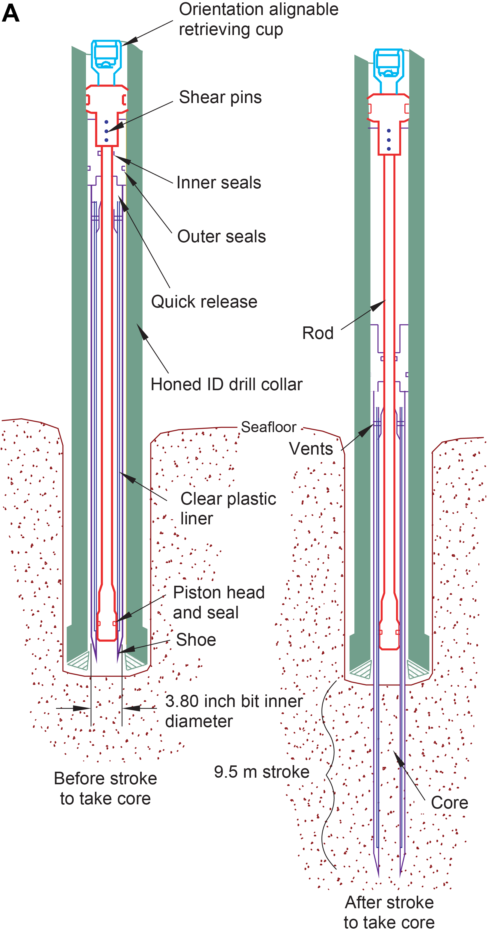
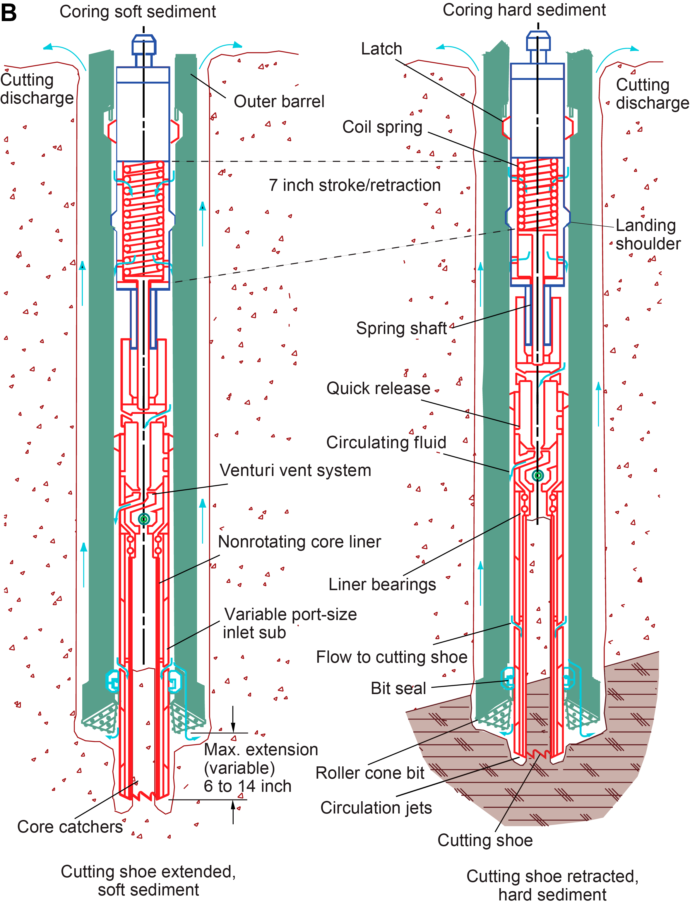

Figure F2. Core, section, analysis, and sampling flow.
The extended core barrel (XCB) rotary system has a small cutting shoe that extends below the large rotary APC/XCB bit (Figure F2). The smaller bit can cut a semi-indurated core with less torque and fluid circulation than the main bit, optimizing recovery. The XCB cutting shoe (bit) extends ~30.5 cm ahead of the main bit in soft sediment but retracts into the main bit when hard formations are encountered. It cuts cores with a nominal diameter of 5.87 cm (2.312 inches), slightly less than the 6.6 cm diameter of APC cores. XCB cores are often broken (torqued) into “biscuits,” which are disc-shaped pieces a few to several centimeters long with remolded sediment (including some drilling slurry) interlayering the discs in a horizontal direction and packing the space between the discs and the core liner in a vertical direction. This type of drilling disturbance may give the impression that the XCB cores have the same thickness (66 mm) as the APC cores. Although both XCB and rotary core barrel (RCB) recovery (below) generally lead to drilling disturbance in similar sedimentary material, switching from an APC/XCB bottom-hole assembly (BHA) to an RCB BHA requires a pipe trip.
The RCB system is the most conventional rotary coring system and is suitable for lithified rock material. During Expedition 396, it was the coring system of choice for most sites because the depth objectives targeted semilithified and lithified material (claystone, siltstone, etc.) and basement, which were out of reach of the XCB system. Like the XCB system, the RCB system cuts a core with a nominal diameter of 5.87 cm. RCB coring can be done with or without the core liners used routinely with the APC/XCB soft-sediment systems. Coring without the liners is sometimes done when core pieces seem to get caught at the edge of the liner, leading to jamming and reduced recovery. During Expedition 396, all RCB cores were drilled with a core liner in place.
The BHA is the lowermost part of the drill string and is typically ~130–170 m long, depending on the coring system used and total drill string length. A typical APC/XCB BHA consists of a drill bit (outside diameter = 11 inches), a bit sub, a seal bore drill collar, a landing saver sub, a modified top sub, a modified head sub, a nonmagnetic drill collar (for APC/XCB coring), a number of 8 inch (~20.32 cm) drill collars, a tapered drill collar, 6 joints (two stands) of 5½ inch (~13.97 cm) drill pipe, and a crossover sub. A lockable flapper valve was used to collect downhole logs without dropping the bit when APC/XCB coring. A typical RCB BHA consists of a drill bit, a bit sub, an outer core barrel, a top sub, a head sub, 8 joints of 8¼ inch drill collars, a tapered drill collar, 2 joints of standard 5½ inch drill pipe, and a crossover sub to the regular 5 inch drill pipe.
Cored intervals may not be contiguous if separated by intervals drilled but not cored. During Expedition 396, we drilled ahead without coring using a center bit with the RCB system in four holes: 0–26 m in Hole U1567B, 0–30 m in Hole U1567C, 0–30 m in Hole U1568B, and 0–300 m in Hole U1573A. Drilling ahead was necessary during Expedition 396 to accelerate penetration because (1) an interval had already been cored in an adjacent hole and/or (2) the stratigraphically lower interval was of higher priority. Thus, these holes consist of a sequence of one drilled interval or advancement followed by coring. Drilling advancements are numbered sequentially from the top of the hole downward. Numbers assigned to physical cores correspond to advancements and may not be consecutive.
1.3. Drilling disturbance
Cores may be significantly disturbed by the drilling process and contain extraneous material because of the coring and core handling process. In formations with loose granular layers (sand, ash, foraminiferal ooze, chert fragments, shell hash, etc.), granular material from intervals higher in the hole may settle and accumulate in the bottom of the hole as a result of drilling circulation and be sampled with the next core. The uppermost 10–50 cm of each core must therefore be examined critically for potential “fall-in.”
Common coring-induced deformation includes the concave-downward appearance of originally horizontal bedding. Piston action may result in fluidization (“flow-in”) at the bottom of, or sometimes in, APC cores. Retrieval of unconsolidated (APC) cores from depth to the surface typically results to some degree in elastic rebound, and gas that is in solution at depth may become free and drive core segments in the liner apart. When gas content is high, pressure must be relieved for safety reasons before the cores are cut into segments. Holes are drilled into the liner, which forces some sediment and gas out of the liner. As noted above, XCB coring typically results in biscuits mixed with drilling slurry. RCB coring typically homogenizes unlithified core material and often fractures lithified core material. During Expedition 396, the main drilling disturbance observed was XCB coring-induced “biscuiting,” which was pervasive in some intervals at Sites U1567 and U1568. Drilling disturbances are described in the Lithostratigraphy section of each site chapter and are indicated on graphic core summary reports, also referred to as visual core descriptions (VCDs).
1.4. Downhole measurements
1.4.1. Formation temperature
During APC coring operations in Holes U1572B and U1574C, the formation temperature was measured with an APCT-3 tool that replaces the normal coring shoe. Normally, these measurements were made while coring Hole A; however, Hole U1572A was cored with the RCB coring system, and APCT-3 measurements could not be taken.
1.4.2. Wireline logging
During wireline logging operations, the logs are recorded with Schlumberger logging tools combined into tool strings, which are lowered into the hole after the completion of coring operations. All four tool strings were used during Expedition 396: the modified triple combination (triple combo), the Versatile Seismic Imager (VSI), the Formation MicroScanner (FMS)-sonic, and the Ultrasonic Borehole Imager (UBI). The modified triple combo tool included the Hostile Environment Litho-Density Sonde (HLDS), Hostile Environment Natural Gamma Ray Sonde (HNGS), Enhanced Digital Telemetry Cartridge (EDTC-B), High-Resolution Laterolog Array (HRLA), Magnetic Susceptibility Sonde (MSS-B), and Dipole Sonic Imager (DSI). These tools measure gamma radiation, porosity, density, resistivity, magnetic susceptibility (MS), and P- and S-wave velocity. Each tool string contains a telemetry cartridge for communicating through the wireline to the Schlumberger multi-tasking acquisition and imaging system (MAXIS) on the ship.
In preparation for logging, the boreholes were flushed of debris by circulating drilling fluid and were at least partially filled with seawater-based logging gel (sepiolite mud mixed with seawater and weighted with barite; density = ~1258 kg/m3) to help stabilize the borehole walls in sections where instability was expected from drilling and coring disturbance. To improve the performance of the UBI logging tool, the hole was cleaned with twice the hole volume with surface salt water after circulating the mud through the hole. The BHA was pulled up to ~80 m drilling depth below seafloor (DSF), where it protected the unstable upper part of the hole. The tool strings were then lowered downhole on a seven-conductor wireline cable before being pulled up at a constant speed of 550 m/h to provide continuous log measurements of several properties simultaneously. Further details on the logging operations are described in Downhole measurements.
1.5. Core and section handling
1.5.1. Whole core handling
All APC, XCB, and RCB cores recovered during Expedition 396 were extracted from the core barrel in plastic liners. These liners were carried from the rig floor to the core processing area on the catwalk outside the core laboratory and cut into ~1.5 m sections (Figure F3). The exact section length was noted and entered into the database as “created length” using the Sample Master application. This number was used to calculate core recovery. Subsequent processing differed for sediment and igneous rock material.
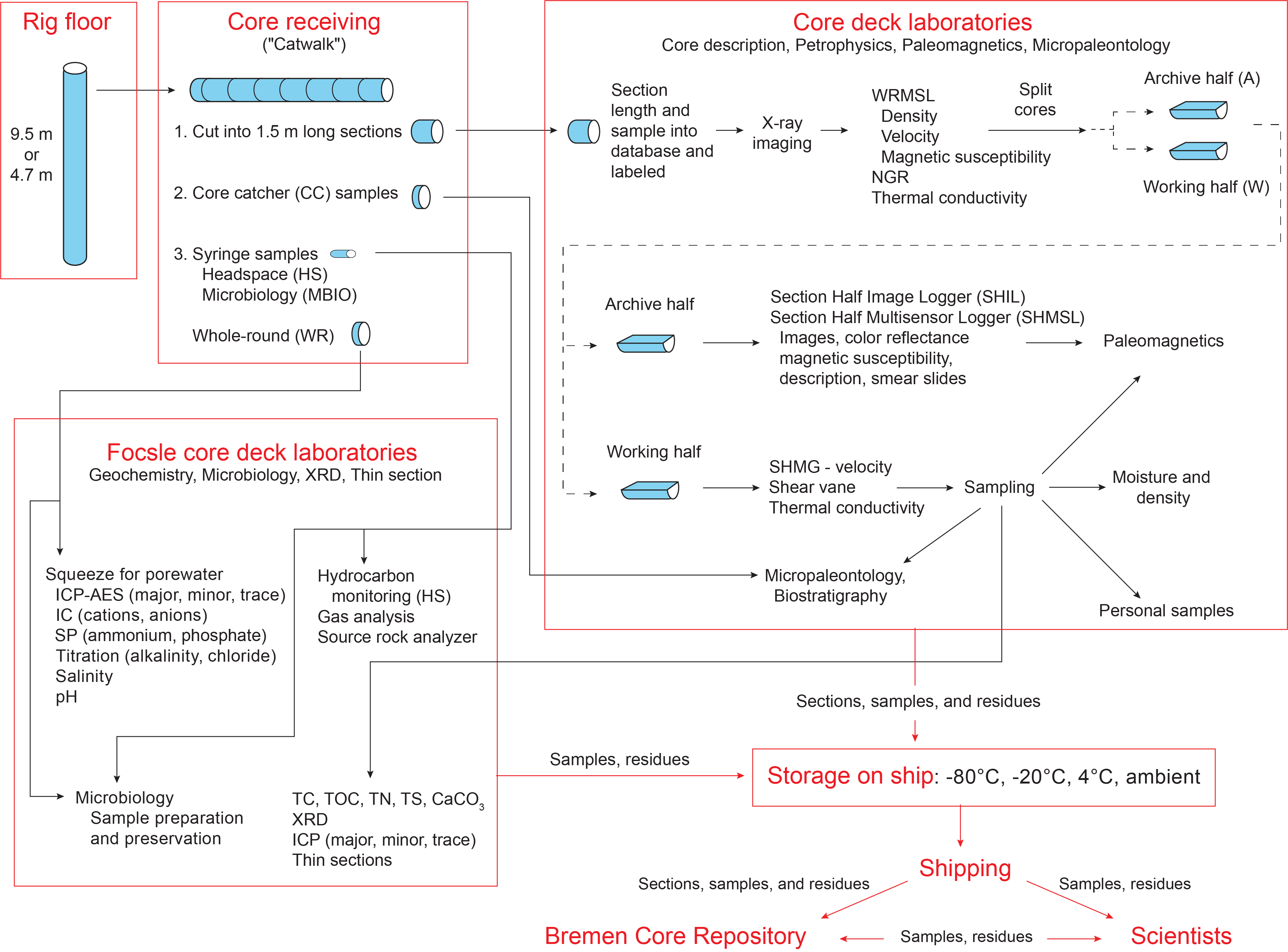
Figure F3. Coring systems.
1.5.2. Sediment section handling
Headspace samples were taken from selected section ends (typically one per core) using a syringe for immediate hydrocarbon analysis as part of the shipboard safety and pollution prevention program. Whole-round samples for interstitial water (IW) analysis were also taken immediately after the core was sectioned. Core catcher samples were taken for biostratigraphic analysis. When catwalk sampling was complete, liner caps (blue = top, colorless = bottom, and yellow = top of a whole-round sample removed from the section) were glued with acetone onto liner sections, and sections were placed in core racks for analysis.
For sediment cores, the curated length was set equal to the created length and was updated very rarely (e.g., in cases of data entry errors or when section length kept expanding by more than ~2 cm). Depth in hole calculations are based on the curated section length (see Depth calculations).
After completion of whole-round section analyses, the sections were split lengthwise from bottom to top into working and archive halves. The softer cores were split with a wire, and harder cores were split with a diamond saw. Investigators should note that older material can be transported upward on the split face of a section during splitting.
1.5.3. Rock piece handling
At Sites U1565, U1566, and U1571–U1574, we performed “hard rock curation,” whereby pieces are separated with dividers and logged separately. Rock pieces were washed and arranged in section half liners. Plastic dividers made from core liner caps were inserted between core pieces to keep them in place for curation, which typically led to curated section lengths that exceeded created section lengths. Note that curated core lengths, defined by the sum of curated section lengths, can exceed the length of the cored interval, resulting in recovery rates >100%. Adjacent core pieces that could be fitted together along fractures were curated as single pieces. The spacers may represent substantial intervals of no recovery. Core pieces that appeared susceptible to crumbling were encased in shrink wrap.
A splitting line was marked on each piece with a red wax pencil so that the piece could be split into representative working and archive halves, ideally maximizing the expression of dipping structures on the cut face of the core in addition to maintaining representative features in both archive and working halves. To ensure a consistent protocol for whole-core imaging, the splitting line was drawn so that the working half was on the right side of the line with the core upright. The working half of each piece was marked with a “W” to the right of the splitting line. Where fabrics were present, cores were marked for splitting with the fabric dipping to the east (090°) in the IODP core reference frame. This protocol was sometimes overridden by the presence of specific features (e.g., mineralized patches) that were divided between the archive and working halves to ensure preservation and/or allow shipboard or postexpedition sampling.
Once the split line was drawn, the plastic spacers were secured with acetone, creating bins that constrained movement of pieces during core transport. Spacers were mounted into the liners with the angle brace facing uphole, ensuring that the top of each piece had the same depth as the top of the curated interval for each bin. The top and bottom offsets of each bin were entered into Sample Master. Based on the calculated bin lengths, the cumulative length of all bins, including spacers, was computed as the curated length of the section. The empty split liner with spacers glued in was then placed over the split liner containing the pieces, and the two halves were taped together in a few places for temporary storage until core pieces were dry and equilibrated to laboratory conditions (usually <1 h after arrival from the catwalk).
1.6. Sample naming
1.6.1. Editorial practice
Sample naming in this volume follows standard IODP procedure. A full sample identifier consists of the following information: expedition, site, hole, core number, core type, section number, section half, and offset in centimeters measured from the top of the core section. For example, a sample identification of “396-U1567A-1H-2W, 10–12 cm,” represents a sample taken from the interval between 10 and 12 cm below the top of the working half of Section 2 of Core 1 (“H” designates that this core was taken with the APC system) of Hole U1567A during Expedition 396.
When working with data downloaded from the LIMS database or physical samples that were labeled on the ship, three additional sample naming concepts may be encountered: text ID, label ID, and printed labels.
1.6.2. Text ID
Samples taken on JOIDES Resolution are uniquely identified for use by software applications using the text ID, which combines two elements:
- Sample type designation (e.g., SHLF for section half) and
- A unique sequential number for any sample and sample type added to the sample type code (e.g., SHLF30495837).
The text ID is not particularly helpful to most users but is critical for machine reading and troubleshooting.
1.6.3. Label ID
The label ID is used throughout the JOIDES Resolution workflows as a convenient, human-readable sample identity. However, a label ID is not necessarily unique. The label ID is made up of two parts: primary sample identifier and sample name.
1.6.3.1. Primary sample identifier
The primary sample identifier is very similar to the editorial sample name described above, with two notable exceptions:
- Section halves always carry the appropriate identifier (396-U1567B-11X-2-A and 396-U1567B-11X-2-W for archive and working half, respectively).
- Sample top and bottom offsets, relative to the parent section, are indicated as “35/37” rather than “35–37 cm.”
1.7. Depth calculations
Sample and measurement depth calculations were based on the methods described in IODP Depth Scales Terminology v.2 (https://www.iodp.org/policies-and-guidelines/142-iodp-depth-scales-terminology-april-2011/file) (Table T1). The definition of multiple depth scale types and their distinction in nomenclature should keep the user aware that a nominal depth value at two different depth scale types (and even two different depth scales of the same type) generally does not refer to exactly the same stratigraphic interval in a hole. The SI unit for all depth scales is meters (m).
Depths of cored intervals were measured from the drill floor based on the length of drill pipe deployed beneath the rig floor and referred to as drilling depth below rig floor (DRF); it is traditionally referred to with custom units of meters below rig floor (mbrf). The depth of each cored interval, measured on the DRF scale, can be referenced to the seafloor by subtracting the seafloor depth measurement (on the DRF scale) from the cored interval (on the DRF scale). This seafloor-referenced depth of the cored interval is reported on the DSF scale, and the traditionally used custom unit designation is meters below seafloor (mbsf). In the case of APC coring, the seafloor depth was the length of pipe deployed minus the length of the mudline core recovered. In the case of RCB coring, the seafloor depth was estimated by the length of pipe deployed when torque was experienced or when weight on bit was reduced while lowering the drill string. In the case of Hole U1572A, which was rotary cored, the initial seafloor depth was corrected based on the depth calculated for Hole U1572B, which was APC cored, because the precision depth recorder (PDR) depth estimated for both holes was the same, as was their depth on the seismic line.
Depths of samples and measurements in each core were computed based on a set of rules that result in the core depth below seafloor, Method A (CSF-A), depth scale. The two fundamental rules for this scale are that (1) the top depth of a recovered core corresponds to the top depth of its cored interval (top DSF depth = top CSF-A depth) regardless of type of material recovered or drilling disturbance observed and (2) the recovered material is a contiguous stratigraphic representation even when core segments are separated by voids when recovered, the core is shorter than the cored interval, or it is unknown how much material is missing between core pieces. When voids were present in the core on the catwalk, they were closed by pushing core segments together whenever possible. The length of missing core should be considered a depth uncertainty when analyzing data associated with core material.
When core sections were given their curated lengths, they were also given a top and a bottom depth based on the core top depth and the section length. Depths of samples and measurements on the CSF-A scale were calculated by adding the offset of the sample (or measurement from the top of its section) to the top depth of the section.
Per IODP policy established after the introduction of the IODP Depth Scales Terminology v.2, sample and measurement depths on the CSF-A depth scale are commonly referred to with the custom unit mbsf, just like depths on the DSF scale. The reader should be aware, though, that the use of mbsf for different depth scales can cause confusion in specific cases because different “mbsf depths” may be assigned to the same stratigraphic interval. For example, a soft-sediment core from less than a few hundred meters below seafloor often expands upon recovery (typically by a few percent to as much as 15%), and the length of the recovered core exceeds that of the cored interval. Therefore, a stratigraphic interval in a particular hole may not have the same depth on the DSF and CSF-A scales. When recovery in a core exceeds 100%, the CSF-A depth of a sample taken from the bottom of the core will be deeper than that of a sample from the top of the subsequent core (i.e., some data associated with the two cores overlap on the CSF-A scale). To overcome the overlap problem, core intervals can be placed on the core depth below seafloor, Method B (CSF-B), depth scale. The Method B approach scales the recovered core length back into the interval cored, from >100% to exactly 100% recovery. If cores had <100% recovery to begin with, they are not scaled. When downloading data using the JOIDES Resolution Science Operator (JRSO) LIMS Reports pages (http://web.iodp.tamu.edu/LORE), depths for samples and measurements are by default presented on both the CSF-A and CSF-B scales. The CSF-B depth scale can be useful for data analysis and presentations at sites with a single hole.
Wireline logging data are collected at the wireline log depth below rig floor (WRF) scale, from which a seafloor measurement is subtracted to create the wireline log depth below seafloor (WSF) scale. For Expedition 396, WSF depths were only used for preliminary data usage on the ship. Immediately after data collection was completed, the wireline logging data were transferred to the Lamont-Doherty Earth Observatory Borehole Research Group (LDEO-BRG), where multiple passes and runs were depth matched using the natural gamma radiation (NGR) logs. The data were returned to the ship at the wireline log matched depth below seafloor (WMSF) scale, which is the final and official logging depth scale type for investigators.
1.8. Shipboard core analysis
After letting cores thermally equilibrate for at least 1 h, whole-round core sections were run through the Whole-Round Multisensor Logger (WRMSL), which measures P-wave velocity, density, and MS, the Natural Gamma Radiation Logger (NGRL), and the X-ray Multisensor Logger (XMSL) (Figure F3). Thermal conductivity measurements were also taken before the cores were split lengthwise into working and archive halves. The working half of each core was sampled for shipboard analysis, routinely for biostratigraphy, paleomagnetism, physical properties, and geochemistry and more irregularly for thin sections. The archive half of each core was scanned on the Section Half Imaging Logger (SHIL) and measured for color reflectance and MS on the Section Half Multisensor Logger (SHMSL). The archive halves were described macroscopically and microscopically in smear slides, and the working halves were sampled for thin section microscopic examination. Finally, the archive halves were run through the cryogenic magnetometer. Both halves of the core were then put into labeled plastic tubes that were sealed and transferred to cold storage space aboard the ship.
A total of 11,359 samples were taken for shipboard analysis during Expedition 396. At the end of the expedition, all archive halves and thin sections were shipped to the Gulf Coast Repository in preparation for programmatic X-ray fluorescence (XRF) core scanning from 11 January to 11 March 2022. All working halves of the core sections were sent to the Bremen Core Repository (BCR) in preparation for a shore-based sampling party planned for 21–28 April 2022. All the cores from Expedition 396 eventually will be stored permanently at the BCR.
2. Lithostratigraphy
The lithostratigraphy group mostly followed the workflow used by previous IODP expeditions that recovered sedimentary (e.g., Sutherland et al., 2018; Tamura et al., 2015b; Norris et al., 2014a) and igneous rocks (e.g., Sun et al., 2018; Arculus et al., 2015; Expedition 352 Scientists, 2014; Expedition 345 Scientists, 2014). This involved describing, sampling, and analyzing core sections following core splitting, utilizing both archive and working halves. Here, we outline the details of the procedure, providing a description of the workflow and approaches applied to sedimentary and igneous rock description and analysis.
2.1. Core description workflow
The core description workflow is illustrated in Figure F4. Different procedures were followed for unconsolidated sediments, sedimentary rocks, and igneous rocks.

Figure F4. Core description workflow.
Sediments and rocks recovered during Expedition 396 were described macroscopically from archive-half sections and microscopically using stereoscopy, smear slides, and thin sections. Digital color images of all archive-half sections were produced using the SHIL, and visual color determination was performed using Munsell soil color charts (Munsell Color Company, 2010). Observations were entered in separate macroscopic (drilling disturbance, sediments, intrusive mantle, extrusive hypabyssal, alteration, veins, halos, and structure) and microscopic (thin section description) DESClogik templates (version x.16.1.0.14; see the DESClogik user guide at http://iodp.tamu.edu/labs/documentation). Selected data are presented in VCD forms (Figure F5), and synthesized descriptions and lithostratigraphic units are presented in the Lithostratigraphy section of each site chapter.
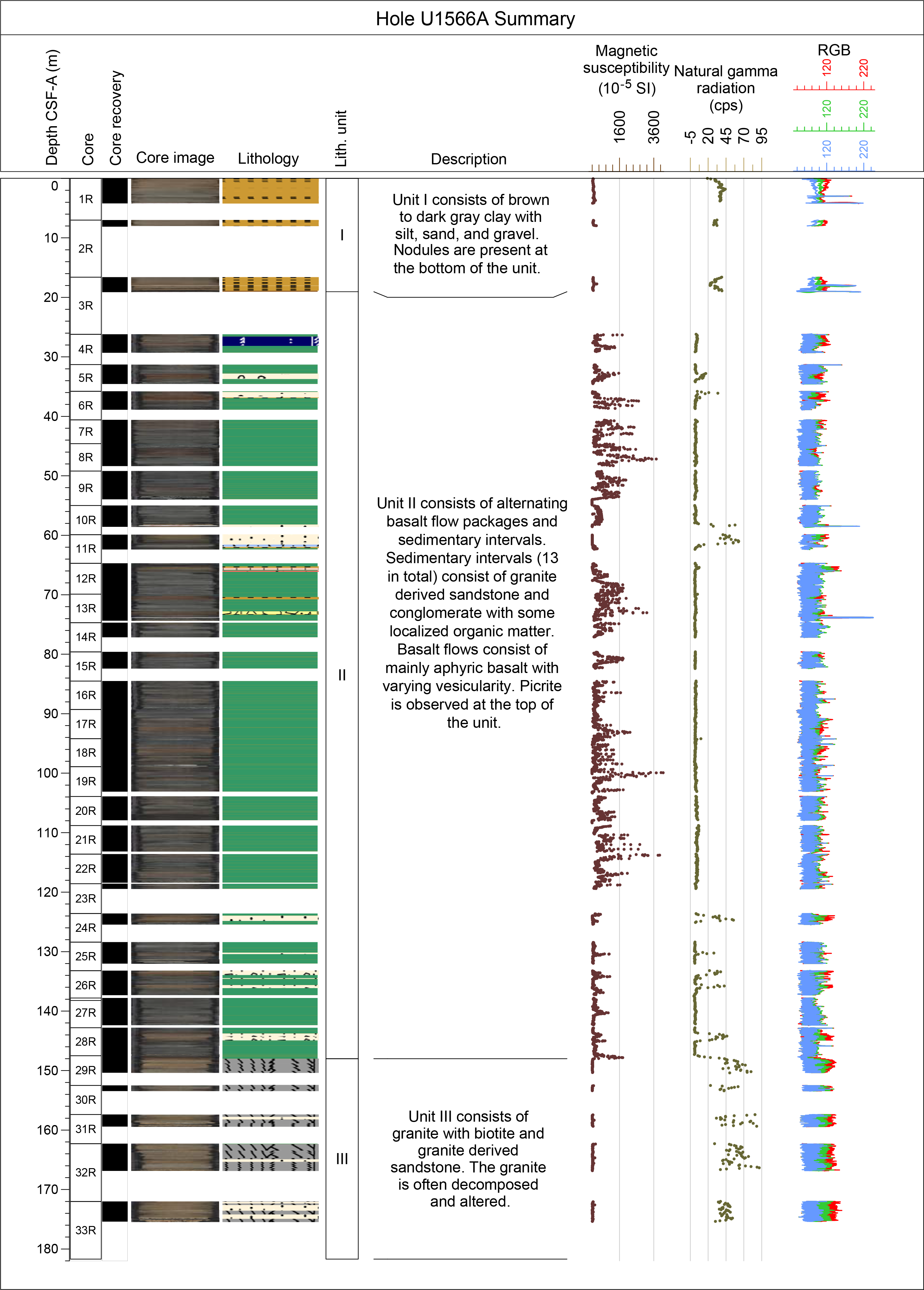
Figure F5. Example VCD.
Finalized lithostratigraphic columns were generated for all holes to document defining features and variability across lithostratigraphic units. Proximal sites are normally combined into one site report, and lithostratigraphic unit definitions are shared for the area (i.e., Sites U1567 and U1568 [Modgunn hydrothermal vent complex], Sites U1569 and U1570 [Mimir High], and Sites U1571 and U1572 [Skoll High]). Where applicable, holes are preliminarily correlated using lithostratigraphic unit boundaries. These ties are supported by physical properties and biostratigraphic observations.
2.2. Core images and archive-half scans
The archive halves were scanned using the SHIL. Three pairs of advanced illumination high-current, focused LED line lights with adjustable angles to the lens axis illuminated any large cracks and blocks in the core surface and sidewalls. Each of the LED pairs has a color temperature of 6500 K. Digital images were taken using a linescan camera at an interval of 10 lines per millimeter to create a high-resolution TIFF file. The camera height was set so that each pixel imaged a 0.1 mm2 section area. Compressed JPEG files were created from the TIFF files. One set of image files shows a grayscale and a depth ruler. The second set is cropped to include only the section-half surface.
2.2.1. Imaging of the sediments and sedimentary rocks
Standard core splitting can affect the appearance of the split core surface, obscuring fine details of lithology and sedimentary structures. Therefore, when appropriate, the archive-half sections were scraped parallel to bedding using a stainless steel or glass scraper. After cleaning the core surface, the archive half was scanned as soon as possible to avoid color changes brought on by oxidation and drying of sediment. Very dark gray, dark brown, and black sediments were occasionally briefly dried to avoid reflections in images.
2.2.2. Imaging of the igneous rocks
Prior to splitting the core into working and archive halves, each core was imaged using the SHIL on a wet outside surface at four different angles (0°, 90°, 180°, and 270°) that were combined to form a 360° whole-round image. The coherent hard rock sections and/or hard rock pieces were then split using a diamond-impregnated saw along lines drawn by a petrologist or a structural geologist to preserve significant compositional and structural features in both the archive and working halves. Fragmented pieces of hard rock that fit together were assigned a joint number and labeled with a letter in consecutive order downsection (e.g., 1a, 1b, and 1c). Plastic spacers were used to separate pieces with different numbers. An arrow added to the labels of single pieces that showed no evidence of rotation indicates the orientation by pointing to the top of the section. Scanning the cut dry and wet archive-half surfaces using the SHIL produced high-resolution color images and measured red-green-blue (RGB) color values at 2.5 cm resolution.
Once imaged using the SHIL, sedimentary and igneous cores were scanned through the SHMSL to obtain discrete point magnetic susceptibility (MSP) measurements and light parameters (L*, a*, and b*) at 2.5 cm resolution. L* defines the lightness of a color, a* denotes the red/green value, and b* denotes the yellow/blue value.
Shipboard samples were taken from working halves for thin section and X-ray diffraction (XRD) analyses (see Geochemistry).
2.3. Thin section preparation
Billets were ground for mounting using a Buehler MetaServ 250 grinding and polishing wheel with 200, 400, and 600 grit polishing paper. The billets were left to dry on a hot plate (~50°C) prior to mounting. Drying time varied depending on the porosity/vesicularity of each sample. The billets were then mounted on 27 mm × 46 mm frosted slides using Epo-Tek epoxy and placed back on the hot plate, and light pressure was applied to help the epoxy set overnight.
A Buehler Petrothin was used to cut off the billet from the glass slide and grind the remaining mounted sample to ~50 µm above optical thickness (30 µm). The remaining 50 µm was removed using a glass plate and a slurry of 600 grit silica carbide powder mixed with ethylene glycol. Once optical thickness was achieved, the sample was hand polished using a slurry of 1000 grit silica carbide and ethylene glycol before receiving a final polish on the Logitech PM-5. Polishing time on the PM-5 varied depending on the hardness of the sample (basalts = 25 min; clays or soft sediments = 15 min).
2.4. Visual core description and lithostratigraphic columns
Sediment lithology, structures, accessories, disturbances, and other observations recorded through DESClogik as well as physical properties data obtained during the shipboard analysis were used to produce graphic summaries for each hole. These graphic summaries, also known as VCDs (Figure F5), were produced by the publication office using the Strater software package. VCDs include core numbers, core recovery, core images, graphic lithology (as in Figure F6), lithostratigraphic units, unit descriptions, MS, NGR, and RGB plotted versus depth on a CSF-A scale.

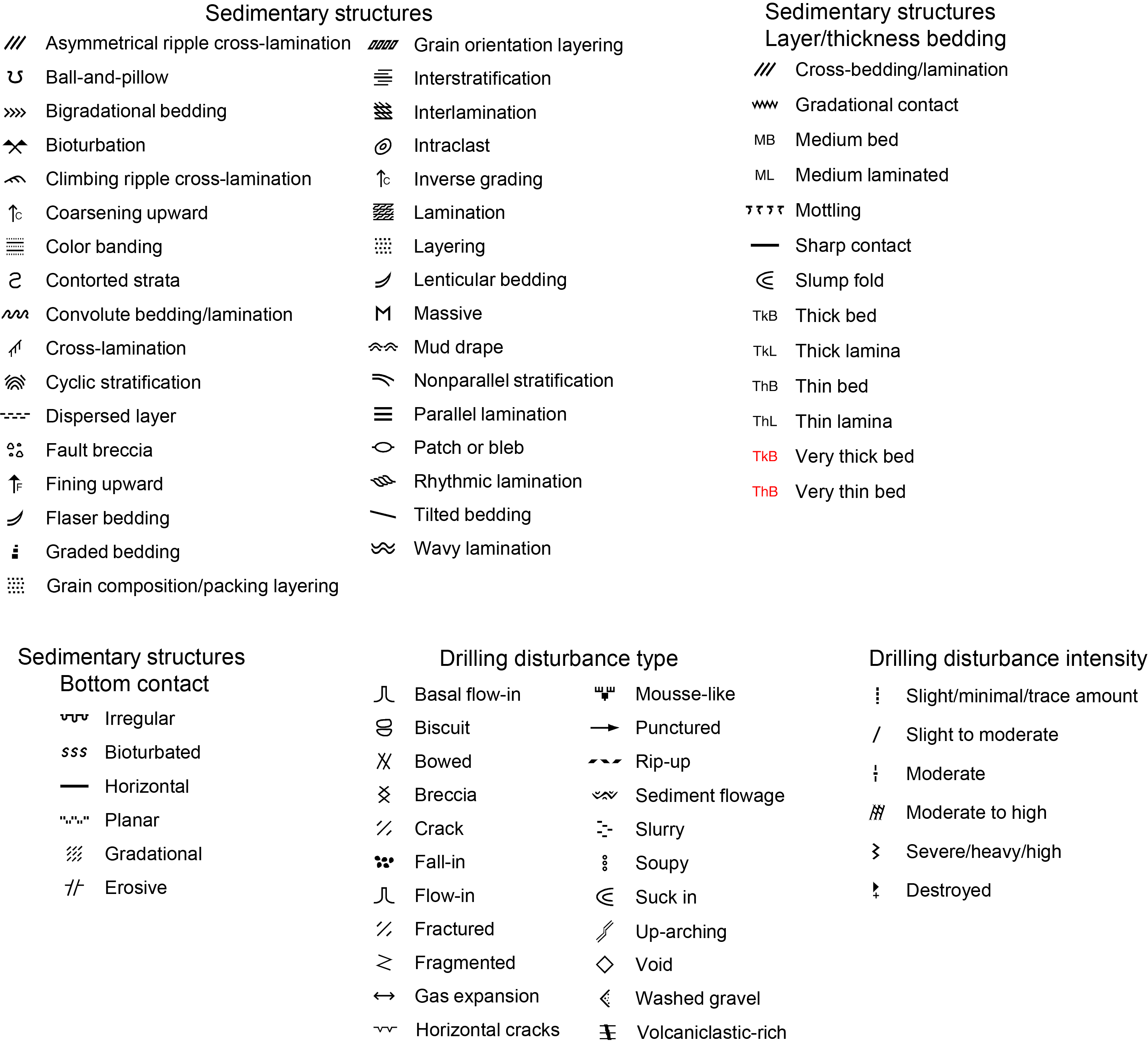

Figure F6. Graphic lithology and symbols for VCDs.
Subsequently, VCDs were updated into lithostratigraphic columns to better reflect the primary representative lithologies without including line-by-line information recorded in detailed DESClogik descriptions. Graphic lithology intervals are plotted in Kaleidagraph or Excel, and graphics are designed in Adobe Illustrator. Graphic lithologies follow the simplified lithologic key shown in Figure F7. For holes dominated by sediments of variable texture, a grain size profile (clay to gravel) is included in the graphic lithologies. Distinguishing characteristics are highlighted in the graphic lithologies and placed on a CSF-A depth scale. Ages, confirmed with biostratigraphy (i.e., dinocyst zones, or “dino zones”) based on Bujak and Mudge (1994), Mudge and Bujak (1994), and Mudge and Bujak (1996a, 1996b), are plotted. Core number, core recovery, lithostratigraphic units and descriptions, and core image are included in these finalized lithostratigraphic columns. A column indicating intervals of ash or ash-rich (i.e., ≥25%) sediments is provided for holes with extensive ash deposits.
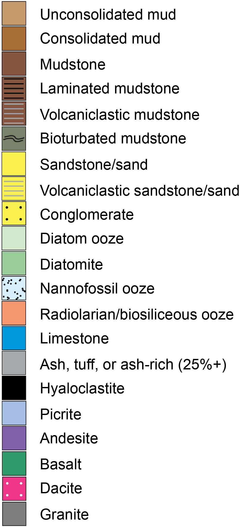
Figure F7. Graphic lithology for lithostratigraphic columns.
If multiple holes from one site or area (i.e., combination of two sites) are correlative with lithostratigraphic unit boundaries, an additional figure is included in the site report that shows simplified lithostratigraphic columns with preliminary ties on vertical (CSF-A) and horizontal (meter) scales. The simplified lithostratigraphic columns include ages, core numbers, lithostratigraphic units and descriptions, and graphic lithologies, as well as ties (black lines) and an indication of the bearing of the drilled transect of holes.
2.4.1. Core summaries
Core summaries are written to briefly describe the primary lithologic observations for each core. This includes principal lithologies, a description of lithologic variability (if any), Munsell-derived colors, and notable sedimentary structures and features. VCDs are also available online (see Core descriptions) but were not utilized in site reports.
2.5. Definition of lithostratigraphic units
Lithostratigraphic units (e.g., I, II, and III) are defined based on major changes in the principal lithology, degree of lithification, or shift in dominant sedimentary structure or features. Often, these boundaries correspond to changes in physical properties, although this was not a requirement for defining a lithostratigraphic unit. Physical properties and biostratigraphic observations are used to aid in the identification of lithologic transitions and unconformities. Unit descriptions are based on the overall lithology observed through the interval and across correlative holes and sites, taking into consideration a degree of lateral and vertical variability. Units are present in at least one hole, and often at multiple holes in an area, and mostly span tens of meters. When more subtle shifts are observed in lithology downhole, especially when they occur over an interval less than 10 m, subunits are defined (e.g., IIa and IIb).
2.6. Drilling disturbance
Drilling-related disturbances are recorded where applicable (in the Disturbance column in DESClogik). The type of drilling disturbance for soft and firm sediment and igneous rocks was described using the following terms:
- Fall-in: out of place material at the top of a core that has fallen downhole onto the cored surface.
- Uparching: material retains its coherency, and material closest to the core liner is bent downward.
- Void: empty space appears within the cored material (e.g., caused by gas expansion during core retrieval; note that voids related to partial strokes during the coring process are curated on the catwalk and do not appear in any core description).
- Flow-in, coring/drilling slurry, along-core gravel/sand contamination: soft-sediment stretching and/or compressional shearing structures occur when severe.
- Soupy: intervals are water saturated and have lost all aspects of original bedding.
- Biscuited: sediment of intermediate stiffness shows vertical variations in the degree of disturbance, whereas firmer intervals are relatively undisturbed.
- Fractured: firm sediment is broken during drilling but not displaced or rotated significantly.
- Fragmented or brecciated: firm sediment is pervasively broken by drilling and may be displaced or rotated.
The degree of drilling disturbance is included for each noted disturbance and include the following:
- Slight: core pieces are in place but broken.
- Moderate: core pieces are in place or partly displaced, but original orientation is preserved or recognizable.
- High: core pieces are probably in correct stratigraphic sequence, but original orientation is lost.
2.7. Sediment, sedimentary rock, and volcaniclastic rock classification
2.7.1. Sedimentary classification
Three main sedimentary lithologic classes are defined based on the primary origin of the sediment constituents (but not the depositional process):
- Biogenic: >50% carbonate, chemical, and biogenic particles.
- Siliciclastic: >50% siliciclastic particles, <25% volcanic particles, and <50% biogenic particles; therefore, nonvolcanic siliciclastic particles dominate chemical and biogenic particles.
- Ash and volcaniclastic: ash is applied to fine-grained (smaller than gravel) volcanic sediments that contain >50% volcanic particles. The volcaniclastic prefix is applied to biogenic and siliciclastic sediments that contain >25% volcanic clasts and grains mixed with nonvolcanic particles (either nonvolcanic siliciclastic, biogenic, or both). Note that the term “volcaniclastic” is used sensu Fisher (1961) and therefore includes both volcanic and tuffaceous lithologies.
These lithologic classes form the basis of the principal name of the described sediments and rocks, with appropriate prefixes and suffixes that may be chosen for mixed lithologies (see Principal names and modifiers).
Sediments and sedimentary rocks recovered during Expedition 396 are classified using a modified scheme initially developed during IODP Expedition 350 (Tamura et al., 2015a). This scheme integrates volcanic particles into the sedimentary descriptive scheme typically used (e.g., Norris et al., 2014b) to describe siliciclastic and biogenic sediments during IODP expeditions. The methodology allows a comprehensive description of mixed sediments, including volcaniclastic, biogenic, and siliciclastic sediment and sedimentary rocks (Figure F8). The purposes of this classification scheme are to (1) include volcanic particles in the assessment of sediment and rock recovered in cores, (2) make rock information accessible to scientists with diverse research backgrounds and experiences, (3) allow relatively quick and smooth data entry, and (4) display data seamlessly in graphical presentations. In this scheme, inferred fragmentation, transport, deposition, and alteration processes are not part of the lithologic name. Observations implying those processes are recorded in the relevant columns (bedding, lamination, grain size, sedimentary structures, etc.) and as comments in the macroscopic DESClogik template. Therefore, sizes of volcanic grains inferred to have formed by a variety of processes (i.e., pyroclasts, autoclasts, epiclasts, and reworked volcanic clasts) (Fisher and Schmincke, 1984) are classified using a common grain size terminology that allows for a more descriptive (i.e., nongenetic) approach.

Figure F8. Sedimentary and volcaniclastic lithology naming conventions.
2.7.2. Principal names and modifiers
The principal name is based on the most abundant sediment class. Principal names for the siliciclastic class are adapted from the grain size classes of Wentworth (1922), and principal names for the volcaniclastic class are adapted from the grain size classes of Fisher and Schmincke (1984) (Figure F9). Thus, the Wentworth (1922) and Fisher and Schmincke (1984) classifications are used to refer to particle type (siliciclastic versus volcanic, respectively) and the maximum size of the particles (Figure F9). For the biogenic class sediments, commonly used terms are used (e.g., ooze or chalk) and do not have a separate size or texture notation. As such, nannofossil and foraminiferal ooze imply the dominant grain size is clay and sand, respectively. Note the principal name is thus purely descriptive and does not include interpretive classifications relating to fragmentation, transport, depositional, or alteration processes.

Figure F9. Grain size classification.
Observations associated with those processes are recorded in the relevant columns (Layer/Bedding, Lamination, Grading, Grain Size, etc.) and as comments in the macroscopic DESClogik template. Sorting is entered into DESClogik for all sediments and sedimentary rocks. For each principal name, both a consolidated (i.e., semilithified to lithified) and a nonconsolidated term exists; they are mutually exclusive (e.g., clay or claystone; ash or tuff). For some descriptions of variable texture (e.g., lithostratigraphic unit descriptions), Wentworth’s clay and silt sizes are combined in a “mud” class; similarly, fine, medium, and coarse sand are combined in a “sand” class.
For all lithologies, the principal lithologic name can be modified by prefixes and/or suffixes for secondary components as follows (Figure F8):
- Prefixes describe a secondary component with an abundance between 25% and 50% (corresponding to “abundant” in smear slide descriptions).
- Suffixes are secondary or tertiary components with abundances of 10%–25% (corresponding to “common” in smear slide descriptions) and are indicated by the suffix “with” (e.g., “with clay” or “with radiolarians”) in order of decreasing abundance.
For example, a nonlithified sediment containing 45% nannofossils, 30% clay, and 10% radiolarians is described as “clay-rich nannofossil ooze with radiolarians.”
When the mineralogic, chemical, or structural composition of the sediments or sedimentary rocks have been altered or changed from their original form, the prefix “meta-” is used in conjunction with principal lithology (e.g., metasandstone). These rocks are described under the Metamorphic tab in DESClogik. In many cases, however, no clear distinction of boundary between well-lithified sediments and metasedimentary rock exists. Furthermore, extensive alteration by veins, fractures, and other structural features requires special treatment, particularly when a sedimentary rock is crosscut by a mesh network of veins. For this reason, the name “breccia” is applied in several different ways (see also Igneous petrology).
The degree of lithification is determined by observing the amount of deformation the sediment can accommodate and the level of sediment consolidation. Sediment is considered lithified when the sediment is not deformed easily with a finger, toothpick, or metal scraper. Lithification is ranked using a qualitative scale: slightly consolidated, moderately consolidated, well consolidated, and lithified. The degree of lithification is expressed in the principal name using alternate terms common in geology:
- Siliciclastic class: if the sediment can be easily deformed with a finger, no term is applied. If the sediment cannot be easily deformed with a finger, the suffix “-stone” is added to the grain size identifier (e.g., claystone). Exceptions are for gravel-sized sediments where the terms “conglomerate” or “breccia” are used for rocks with well-rounded and angular clasts, respectively. The principal names “conglomerate” and “breccia” are modified using the terms “matrix-supported” and “clast-supported,” depending on the matrix to clast ratio.
- Biogenic class: if the sediment can be easily deformed with a finger, the nonlithified term “ooze” is used in conjunction with the most abundant component (e.g., nannofossil ooze or radiolarian ooze). If the calcareous sediment cannot be easily deformed with a finger but can be easily scratched with a fingernail, the semilithified term “chalk” is used for calcareous sediments (e.g., nannofossil chalk) and the terms “radiolarite,” “diatomite,” and “porcellanite” are used for siliceous sediments. If the sediment cannot be easily scratched with a fingernail, the lithified term “limestone” is used for calcareous sediments (e.g., nannofossil limestone). If siliceous sediment cannot be scratched with a fingernail and displays a glassy luster, the term “chert” is used. Note that in this volume, the terms “porcellanite” and “chert” do not imply crystallinity of silica, in contrast to other usages of those terms.
2.7.3. Sedimentary structures, stratification, and lithologic features
The locations and types of stratification and sedimentary structures visible on the prepared surfaces of the section halves are respectively entered in the Bedding and Sedimentary structures columns of the macroscopic DESClogik worksheet. Locations and scales of interstratification and the locations of individual bedding and sedimentary features, such as scours, graded bedding, parallel laminations, imbrication, flame structures, flute casts, patches, or blebs, are recorded in DESClogik. Where visible, bottom contact type and attitude, macroscopic fossils (e.g., echinoderm, gastropods, and bivalves), and secondary mineralization (diagenetic constituent and composition; e.g., pyrite and glauconite) are noted in the corresponding columns in DESClogik. The following terminology (based on Stow, 2005) was used to describe the scale of stratification:
- Thin lamination = <3 mm thick.
- Medium lamination = 0.3–0.6 cm thick.
- Thick lamination = 0.6–1 cm thick.
- Very thin bed = 1–3 cm thick.
- Thin bed = 3–10 cm thick.
- Medium bed = 10–30 cm thick.
- Thick bed = 30–100 cm thick.
- Very thick bed = >100 cm thick.
2.7.4. Bioturbation intensity
Four degrees of bioturbation intensity are reported in the Bioturbation intensity column using the following numeric scale. If no bioturbation is observed, this is kept blank.
- Slight bioturbation (10%–30%),
- Moderate bioturbation (30%–60%),
- Heavy bioturbation (60%–90%), and
- Complete bioturbation (>90%).
2.7.5. Smear slide descriptions
Size, composition, and abundance of sediment constituents are estimated microscopically using smear slides. Smear slide samples of the main lithologies were collected from the archive-half sections unless lithification made sampling impossible.
For each smear slide, a small amount of sediment is removed from the section half using a wooden toothpick and put on a 25 mm × 75 mm glass slide (Marsaglia et al., 2013). A drop of deionized water is added, and the sediment is homogenized and evenly spread across the glass slide. The dispersed sample is dried on a hot plate at a low setting (50°C). A drop of adhesive (Norland optical adhesive Number 61) is added as a mounting medium for a glass coverslip, which is carefully placed on the dried sample to prevent air bubbles from being trapped in the adhesive. The smear slide is then fixed in an ultraviolet light box for 5 min to cure the adhesive.
Smear slides are examined using a transmitted-light petrographic microscope equipped with a standard eyepiece micrometer. Biogenic and mineral components are identified following standard petrographic techniques as stated in reference manuals Rothwell (1989a) and Marsaglia et al. (2013). Several fields of view are examined at 10×, 20×, and 40× to assess the abundance of detrital (e.g., quartz, feldspar, clay minerals, mica, and heavy minerals), biogenic (e.g., nannofossils, other calcareous bioclasts, diatoms, foraminifers, and radiolarians), and authigenic (e.g., carbonate, iron sulfide, iron oxides, and glauconite) components. Average grain size of clay (<4 µm), silt (4–63 µm), and sand (>63 µm) is estimated for sediments dominated by siliciclastic material. The relative percent abundances of the sedimentary constituents are visually estimated using the techniques of Terry and Chilingar (1955) and Rothwell (1989b). The texture of siliciclastic lithologies (relative abundance of sand-, silt-, and clay-sized grains) and the proportions and presence of biogenic and mineral components are recorded in the smear slide worksheet of the microscopic DESClogik template. Components observed in smear slides are categorized as follows:
- T = trace (<1%).
- R = rare (1%–10%).
- C = common (>10%–25%).
- A = abundant (>25%–50%).
- D = dominant (>50%).
Smear slides provide only a rough estimate of the relative abundance of sediment constituents. On occasion, the lithologic name assigned based on smear slide observation does not match the name in the macroscopic lithology description. This is because a small sample may not represent the macroscopic description of a much larger sediment interval. Additionally, very fine and coarse grains are difficult to observe in smear slides, and their relative proportions in the sediment can be affected during slide preparation. Therefore, intervals dominated by sand and larger size constituents are examined by macroscopic comparison to grain size reference charts.
2.8. Igneous petrology
Expedition 396 core description procedures for igneous rocks are based on those from IODP Expeditions 367/368 (Sun et al., 2018), 351 (Arculus et al., 2015), and 349 (Expedition 352 Scientists, 2014), Integrated Ocean Drilling Program Expedition 345 (Expedition 345 Scientists, 2014), and Ocean Drilling Program (ODP) Leg 104 (Eldholm et al., 1987).
Units and subunits are divided on the basis of significant lithologic changes. The groundmass texture and color, as well as the primary modal composition, based on the International Union of Geological Sciences (IUGS) system (Le Maitre, 1989), were used to give a principal lithology name to a given igneous rock.
2.8.1. Volcanic (extrusive and hypabyssal) rocks
Four main volcanic rock categories were observed and defined during Expedition 396 (Figure F10):
- Basalt: black to dark gray rock containing plagioclase, pyroxene, and rare olivine (replaced by iddingsite and saponite) in the size range glassy to fine grained. When presenting a fragmented aspect, the prefix “brecciated” is used (i.e., clast-supported basaltic breccia associated with a lava flow). Picrite is a subdivision of basalt characterized by high-olivine phenocryst (typically replaced by saponite) content (>20%).
- Andesite: a dark to light gray rock with a microcrystalline groundmass dominated by plagioclase that can also contain pyroxenes and amphibole but is devoid of olivine and quartz.
- Dacite: light gray to tan rock, usually plagioclase-phyric, that can contain pyroxenes ± quartz ± hornblende with a glassy to cryptocrystalline groundmass.
- Peperite and hyaloclastite are distinguished based on their fragmented aspect: peperite is defined by White et al. (2000) as a rock formed by disintegration of magma intruding and mingling with unconsolidated or poorly consolidated, typically wet sediments. Hyaloclastites are defined as glass-rich volcanic rocks formed by lava-water (and lava-sediment) interaction where the lava is shattered into small angular glassy fragments.
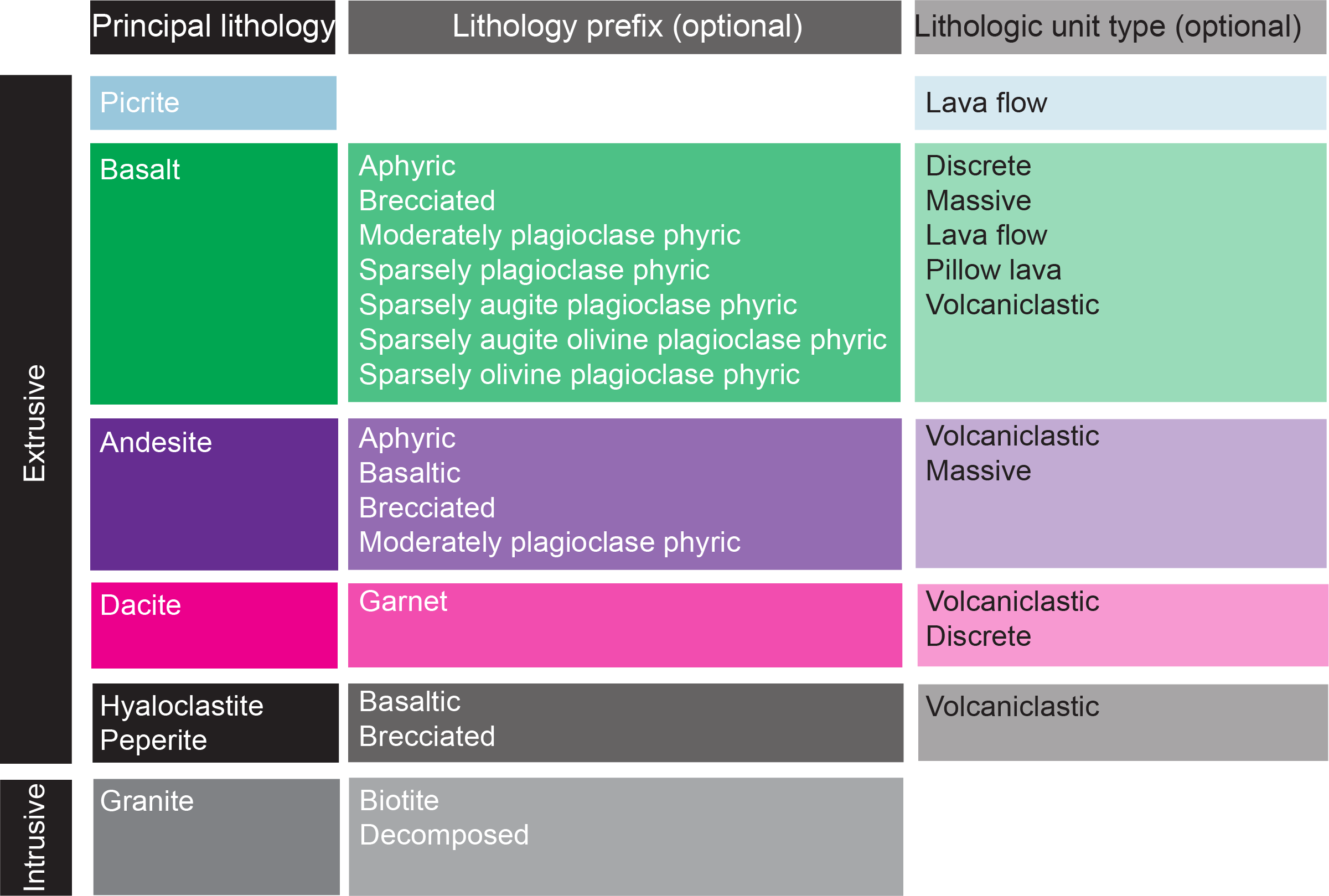
Figure F10. Igneous lithology naming conventions.
Matrix-supported breccias not related to lava flows are described in the Sedimentary tab in DESClogik. Large (>1 cm) volcanic clasts in sediments and sedimentary rocks were classified in the LITH 1 Clast 1 igneous columns.
A prefix can indicate the phenocryst assemblage and total phenocryst abundances:
If present in a given sample, multiple phenocryst minerals were used as modifiers appearing in the order of increasing abundance. For example, in plagioclase-olivine phyric basalt, olivine is the most abundant phenocryst mineral.
The prefix can also indicate the following:
- A compositional distinction: the prefix “basaltic” is sometimes used with the primary lithology “andesite” to highlight the association of clinopyroxene and plagioclase in the groundmass. This naming convention was also corroborated using inductively coupled plasma–atomic emission spectrometry (ICP-AES) geochemical analyses (see Geochemistry).
- A fragmented aspect: when presenting a fragmented aspect, the prefix “brecciated” was used with the primary lithology (i.e., clast-supported breccia associated with a lava flow).
2.8.2. Lithologic unit type
The lithologic unit type indicates the nature of the volcanic body. We applied the classification scheme used during Leg 104 (Shipboard Scientific Party, 1987):
- Discrete: usually small (<1 m) lava flow generally bounded by chilled margins but also by faults or sharp textural and color changes.
- Lava flow: core/section with flow structure and/or brecciated or vesiculated flow top and bottom, >1 m thick.
- Massive: core is little affected by drilling, is recovered in long and intact pieces, and is usually non to sparsely vesicular.
- Pillow lava: core is 0.1–1 m thick and defined by curved chilled margins, spherulitic textures, glassy margins and/or hyaloclastites, and microcrystalline to cryptocrystalline groundmass grain size, as well as decreasing crystal abundances and sizes (phenocrysts; groundmass) toward the glassy rims.
- Volcaniclastic: fragmented volcanic rocks.
2.8.3. Contact types
Margins and contacts of flows were described by observing the features of the chilled sections that indicate a possible hiatus between two flows/pillows. A chilled contact, with or without glass, was recognized by observing the terminal end of the margin for sediment that was not entrenched into the rock but rather baked or cooked onto the rock, indicating a baked or chilled contact with the rock.
A chilled margin was recognized through identification of a sudden change in groundmass over a very short distance. Unlike a chilled contact, sediment at the terminal end of the unit was not required to determine its nomenclature.
Glassy margins, chilled margins, and contact boundaries were inserted individually for the top and bottom of each section where they could be determined to discriminate individual flows and allow for a greater level of precision in the descriptions.
The following contact types were defined:
- Baked contact: contact with sediments that were baked by proximity of lava.
- Chilled contact: chilled contact with sediments, with or without glass, in direct contact with sediments. “Bottom” or “top” was added as a prefix where the orientation could be determined.
- Chilled margin: chilled contact without sediments, without glass, determined by cryptocrystalline groundmass, typically found quenched adjacent to the chilled contact. “Bottom” or “top” was added as a prefix where the orientation could be determined.
- Glassy margin: a margin between two pillows that has no sediment and the pillows have fused together. There is no clear indication of the boundary between the pillows as originally deposited.
2.8.4. Degree of crystallinity
For the degree of crystallinity description, the following terms were used:
- Holohyaline = 100% glass.
- Hypohyaline = glass > crystals.
- Hypocrystalline = glass < crystal.
- Holocrystalline = 100% crystals.
2.8.5. Igneous texture and grain size distribution
For the textural description of volcanic rocks, the following nomenclature was applied to describe the groundmass, predominantly at the macroscopic level:
- Aphanitic: crystalline but individual grains not discernible with a hand lens.
- Phaneritic: crystals are discernible with a hand lens.
- Glomeroporphyritic: containing clusters of phenocrysts.
- Intergranular: plagioclase crystals surrounded by interstitial granular pyroxene, olivine, and/or oxide minerals.
- Interstitial: glass, crypto-, or microcrystalline material between coarser grained crystals.
- Porphyritic: increasing presence of phenocrysts.
- Spherulitic: fan-like arrangement of divergent microlites.
- Vitrophyric: phenocrysts in a glassy groundmass.
Terms used to describe the grain size distribution are bimodal (two dominant mineral sizes), equigranular (principal minerals are in the same size range), inequigranular (principal minerals have different grain sizes), and seriate (continuous range in grain size).
2.8.6. Vesicularity
Vesicularity is characterized by the abundance of vesicles:
- Nonvesicular = <1% vesicles.
- Sparsely vesicular = 1%–5% vesicles.
- Moderately vesicular = >5%–20% vesicles.
- Highly vesicular = >20% vesicles.
The description of the size, shape, and roundness of vesicles is based on the classification charts from Expedition 367/368 (Sun et al., 2018) (Figure F11). An estimate of the percentage abundance of vesicles is included in the VCDs (see Core descriptions).

Figure F11. Vesicle sphericity and roundness.
2.8.7. Intrusive rocks
Weathered granitic basement was drilled at Sites U1565 and U1566. We used the quartz-alkali feldspar-plagioclase-feldspathoid (QAPF) Streckeisen classification (Streckeisen, 1974) to name the principal lithology: monzogranite. The prefix “biotite” is used for the least altered sections. The prefix “decomposed” is used for sections showing intense alteration.
2.8.8. Alteration
Low-temperature and low-pressure (i.e., seafloor) mineralization, veins, and background alteration are defined as alteration. Alteration description includes primary alteration mineralogy and infilling of vesicles (when applicable) and halos. Textures used to define groundmass alteration are patchy, corona, pseudomorphic, and recrystallized. Levels of background alteration are recorded as follows:
- Fresh = <2 vol%.
- Slight = 2–10 vol%.
- Moderate = >10–50 vol%.
- High = >50–95 vol%.
- Complete = >95 vol%.
An estimate of the level of alteration is included in the VCDs (see Core descriptions).
2.8.9. Veins
We used the term “vein” to refer to any later crosscutting feature formed by sediment injection or precipitation from hydrothermal fluids and reserved the word “dike” to describe any later crosscutting feature that formed by introduction of magma. The density (i.e., the percentage of veins within a piece or an interval estimated visually), mineralogy, width, color, vein type (e.g., banded, composite, en echelon, haloed, intravenous, and uniform), connectivity (isolated, single, branched, and network), texture (cross-fiber, slip-fiber, massive, polycrystalline, and vuggy), and contacts with host rocks (diffuse, irregular, and sharp) were described, modified from the criteria from ODP Leg 209 (Shipboard Scientific Party, 2004) (Figure F12). The length, width, and orientation of representative veins in a section were measured.

Figure F12. Vein description.
2.8.10. Microscopic (thin section) description
The characterization of thin sections was used to complement and refine macroscopic core observations for igneous rocks. All thin section observations were entered into the LIMS database through a DESClogik microscopic template. Thin section descriptions include primary (igneous) rock-forming minerals (including phenocrysts, groundmass, etc.) and secondary (alteration) mineral phases (in veins, vesicles, groundmass, etc.). When applicable, vesicles size, abundance, and filling were also documented.
Thin section descriptions include the following terms:
- Sample domain: if there is more than one domain on the slide, each domain is described separately. For example, a slide that shows a large sedimentary vein (25% of the slide) in a basaltic matrix (75% of the slide) is described as two slides (samples): one sample domain is described as “vein” and the second one as “host rock.” Other possible domains include sharp change of mineralogy, grain size, or texture.
- Lithology prefix: lithology prefix for the described sample domain.
- Principal lithology: refers only to the lithology of the described sample domain, which includes picrite, basalt, basaltic andesite, andesite, and granite.
- Texture: volcanic rock is described as holohyaline (100% glass) to holocrystalline (100% crystals). The terms “phyric” and “glomeroporphyritic” indicate the presence of phenocrysts and clusters of phenocrysts, respectively. “Seriate” texture indicates a continuous range in grain size. The presence of flow textures is also added in texture comments. In cases where there is no significant grain size difference between groundmass crystals and somewhat larger and more euhedral crystals, which do not adhere to the definition of phenocrysts, the larger crystals are described in the groundmass. When glass is present in the lithology, the percentage of fresh glass is indicated.
The following terms are used for grain size:
- Average groundmass grain size modal name: grain sizes follow Neuendorf et al. (2005) using the divisions glass, cryptocrystalline, microcrystalline, and fine, medium, and coarse grained (as defined in Volcanic (extrusive and hypabyssal) rocks).
- Maximum grain size modal name: analogous to “average groundmass grain size modal name.”
The following terms are used for mineralogy:
- Mineral phenocryst shape: euhedral, subhedral, or anhedral.
- Mineral phenocryst habit: elongate, equant, subequant, or tabular.
- Clinopyroxene (cpx) and orthopyroxene (opx) phenocryst exsolution: blebs and lamellae.
- Vesicle shape: see Figure F11.
For plagioclase, a qualifier for zoning was recorded following the convention used during Expedition 345 (Expedition 345 Scientists, 2014):
- 0 = none.
- 1 = zoning is rare and weakly developed.
- 2 = abundant zoning that can range from weak to strong.
- 3 = nearly ubiquitous, generally strong zoning.
The type of zoning in plagioclase was also documented as follows:
- Continuous: zoning is optically continuous from core to rim.
- Discontinuous: zoning occurs from core to rim, but with distinct break(s).
- Patchy: zoning occurs in patches randomly throughout the grain.
- Oscillatory.
2.8.11. Geochemical observations
Our petrographic observations were corroborated with >450 analyses on the archive halves of the core (see Geochemistry) performed using an Olympus Delta handheld portable XRF (pXRF) spectrometer. Rock samples that were small enough and could be removed from the core without damage were placed in a specially made shielded sample analysis assembly (Figure F13). Core sections that were too large to be removed were analyzed in situ using a shielded sleeve analyzer mount (Figure F13). In this case, core sections were raised using core holders to ensure good contact between the handheld spectrometer and the sample.

Figure F13. pXRF.
Real-time pXRF measurements proved invaluable for characterization of extrusive rocks at Sites U1566 and U1571–U1573, where igneous rocks are dominated by aphyric basalts, thus hindering more traditional initial unit definition based on petrographic variation. Chemical stratigraphy obtained from pXRF analyses will be used postcruise to identify and define discrete magmatic events in the basaltic sequence.
Finally, we also used ICP-AES analyses (see Geochemistry) performed on discrete samples selected from the working halves (Figure F13) to (1) confirm the results of the pXRF analyses and (2) confirm the lithology compositional names (i.e., picrite, basalt, basaltic andesite, and andesite).
2.9. Structural geology
This section outlines the methods for documenting structural features observed in cores such as faults, fractures, fault rocks, shear zones, folds, bedding, and veins. The structural geology observations are directly integrated into the Lithostratigraphy section of each site chapter.
Structural features observed on the archive half are documented using the following:
- Identifying structural features and classifying their structural types;
- Determining the top and bottom location of structural features in the core;
- Measuring the orientation of a structural feature where applicable;
- Determining the sense of displacement on a structural feature where applicable;
- Determining the temporal relation between structures (especially for crosscutting structures and shear zones); and
- Assessing the role of fluids in deformation processes.
Our methods largely follow those used by the structural geologists for Integrated Ocean Drilling Program Expedition 344 and Expeditions 349 and 367/368/368X (Harris et al., 2013; Li et al., 2015; Sun et al., 2018). The types of structural measurements and key parameters (either observed or calculated) are recorded on a spreadsheet (Figure F14). These data are then input into the LIMS database using DESClogik.
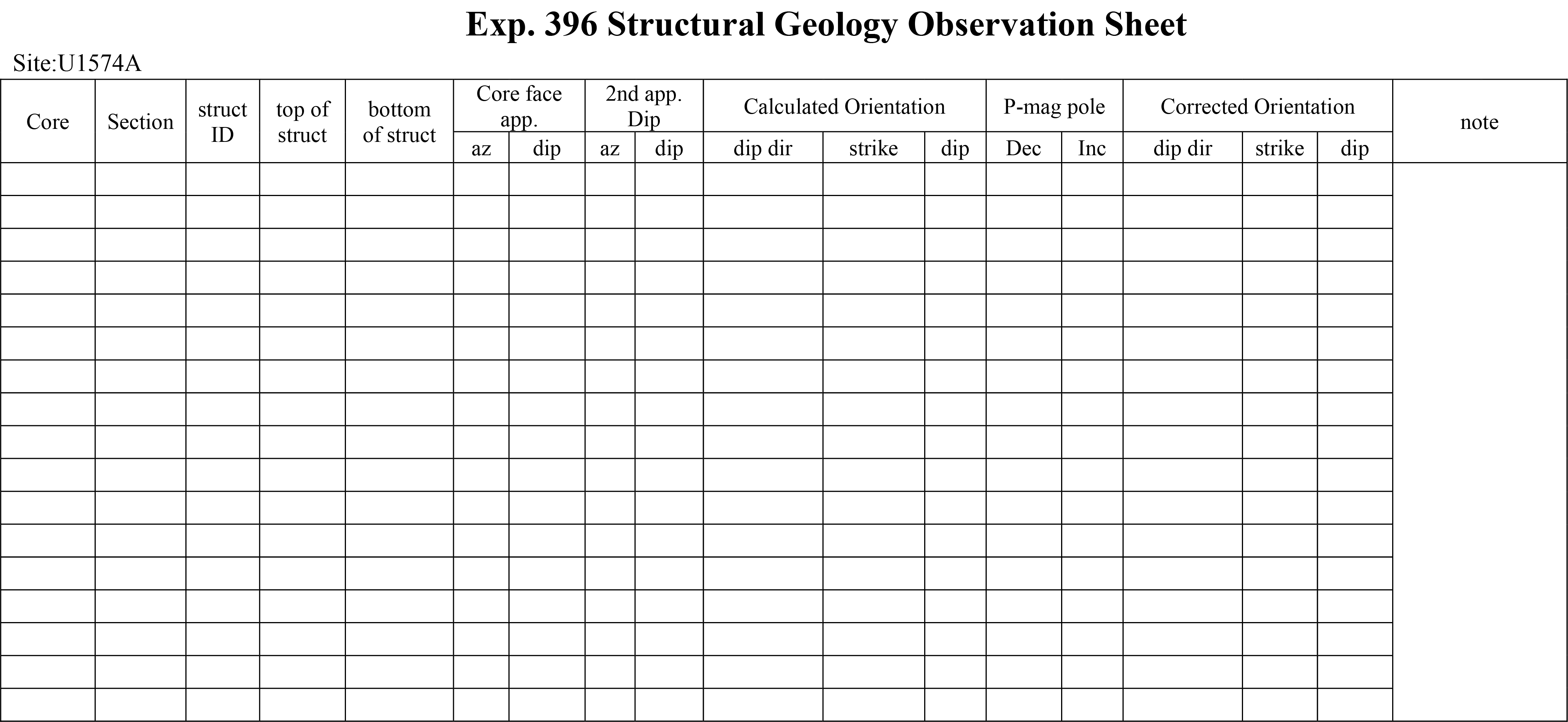
Figure F14. Structural geology observation sheet.
2.9.1. Graphic symbols and terminology
A predefined set of commonly observed structural features was used in the structural description of cores. The terminology and graphic symbols used are presented in Figure F6. The major structural features identified include the following:
- Joints and fractures: brittle failure with no displacement and no secondary infill minerals. Breaks clearly resulting from drilling were logged separately as drilling-induced fractures in the Drilling disturbance spreadsheet in DESClogik.
- Veins: fractures filled with secondary minerals; veins were described in both the Structure and Veins/halos tabs in DESClogik.
- Fault rocks: brittlely deformed rocks such as fault breccia and fault gouge. For the sake of simplicity, the term “fault breccia” is defined as a clast-supported fault rock with angular clasts, and the term “fault gouge” is defined as a matrix-supported fault rock with rounded clasts in this report.
- Hydrothermal breccia: fluid-assisted deformation leading to the fragmentation and brecciation of the rocks.
- Shear zones: zones affected by ductile crystal-plastic deformation, surrounded by less deformed rocks.
- Folds: folded sedimentary or rock layers.
- Sedimentary bedding: layering of sediments and sedimentary rocks and igneous contacts were respectively described in the Sediment and Extrusive_hypabyssal tabs in DESClogik.
2.9.1. Structural observation and description
Structural features were described from the top to bottom of each section of the core.
For fractures, we examined and measured the following parameters:
- Location: where a fracture occurs in a core, measured in centimeters from the top of the section.
- Morphology: morphological shape of a fracture (e.g., straight, curved, banded, irregular, composite, isolated, single, or branched).
- Displacement: lateral offset and/or opening of a fracture measured in centimeters; a closed fracture with no lateral offset is recorded as 0 cm of displacement.
- Orientation: dip angle, strike, and dip direction of a fracture measured in degrees; where applicable, reorientation of a fracture to geographic coordinates (i.e., relative to true north) was done to determine the real dip direction (see Orientation measurements and correction).
- Frequency: occurrence frequency of fractures per section.
- Types: type of deformation of a fracture (e.g., normal, reverse, dextral, sinistral displacement, or a combination of the above).
For veins, we examined and measured several parameters (Figure F12):
- Location: where a vein occurs in a core, measured in centimeters from the top of the section.
- Morphology: morphological shape of a vein.
- Orientation: dip angle and dipping direction of a vein.
- Frequency: occurrence frequency of veins per section.
- Mineral infill and alteration: these features are recorded as described by petrologists.
For fault rocks and shear zones, we examined and measured the following parameters:
- Location: interval where a shear zone occurs in a core, measured in centimeters from the top of the section.
- Nature: type of shear zone (e.g., mylonite, cataclasite, fault gouge, or fault breccia).
- Morphology: morphological shape of the deformed zone and the clasts.
- Orientation: dip angle and dip direction of the preferred orientation of the clasts, where applicable.
- Frequency: occurrence frequency of shear zones per section.
- Mineral and alteration: matrix and clasts as described by petrologists.
For sedimentary bedding, we described the following parameters:
- Location: where a nonsubhorizontal bedding occurs in a core (dip >3°), measured in centimeters from the top of the section.
- Type of contacts: type of sedimentary contact boundary.
- Orientation: dip angle, strike, and dip direction of sedimentary bedding.
For folds, we described the following parameters:
- Location: where a fold contact occurs in a core, measured in centimeters from the top of the section.
- Type: type of fold.
- Frequency: occurrence frequency of fold axis per section.
For igneous contacts, we described the following parameters:
- Location: where an igneous contact occurs in a core, measured in centimeters from the top of the section.
- Type of contacts: type of igneous contact boundary.
- Orientation: dip angle and dip direction of an igneous contact.
- Frequency: occurrence frequency of igneous contacts per section.
- Mineral infill and alteration: these features are recorded as described by petrologists.
All measured data were manually typed into the log sheet together with the measured depths in the core section and descriptive information (Figure F14). The occurrence frequency of a structure per section is normalized on a 10 cm section.
2.9.3. Orientation measurements and correction
2.9.3.1. Orientation measurements
We used a plastic goniometer for orientation measurements. For sealed structures, we wrapped a transparent plastic protractor template around the core to determine the true dip (Figure F15). Orientations of planar and linear features in a core section were determined relative to the core reference frame (Figure F16). The vertical axis of the core reference frame is aligned with the upcore direction of the core section, and the double line marked on the archive half of the core liner is defined as 180° in the cross-sectional plane perpendicular to the core vertical axis.

Figure F15. Goniometer and protractor template.
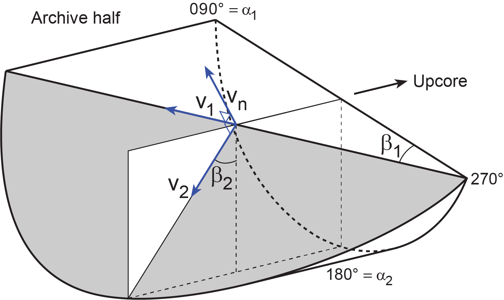
Figure F16. Core reference frame.
To determine the orientation of a planar structural element (shaded plane in Figure F16), two apparent dips of the element were measured in the core reference frame. The first apparent dip measures the intersection angle between the planar structural element and the split face of the core (β1 in Figure F16); it is determined by measuring the dip direction and angle of the planar structural element in the core reference frame. A planar structural element could have a trend of 90° or 270° and a plunge angle ranging 0°–90°. The second apparent dip measures the intersection angle between the central line of the planar structural element and the split face of the core (β2 in Figure F16). In most cases, this was a plane either parallel or perpendicular to the core axis. In the former case, the apparent dip would trend 0° or 180° with plunge angle ranging 0°–90°; in the latter case, the trend would range 0°–360° with a plunge angle of 0°.
A linear feature observed in the surface of a split core is often associated with a planar structural element (e.g., a fault plane) in the core; the orientation of the planar structural element is determined by measuring either the rake (or pitch) of the associated plane or the trend and plunge of the planar element in the core reference frame.
2.9.3.2. Plane orientation calculation
For a planar structural element (e.g., a bedding or fault plane), two apparent dips on two different surfaces (e.g., one being the split core surface, which is east–west vertical, and the other being a horizontal or north–south vertical surface) were measured in the core reference frame. The two apparent dips are the azimuth (measured clockwise from north, looking down) and plunge. An x, y, z coordinate system was defined in such a way that the positive x-, y-, and z-directions coincide with north, east, and vertical downward, respectively. If the azimuths and plunges of the two apparent dips are given as (α1, β1) and (α2, β2), respectively, as in Figure F16, the unit vectors representing these two lines, v1 and v2, are given by the following expression:
where l, m, and n represent the x-, y-, and z-components of the vectors.
For any plane, the direction of the normal to the plane can be found by taking the cross product of two (nonparallel) vectors that lie within the plane. Using the above equations for v1 and v2, therefore, the unit vector normal to plane (vn) (Figure F17) is then defined as follows:
The azimuth (αn) and plunge (βn) of vn are given by
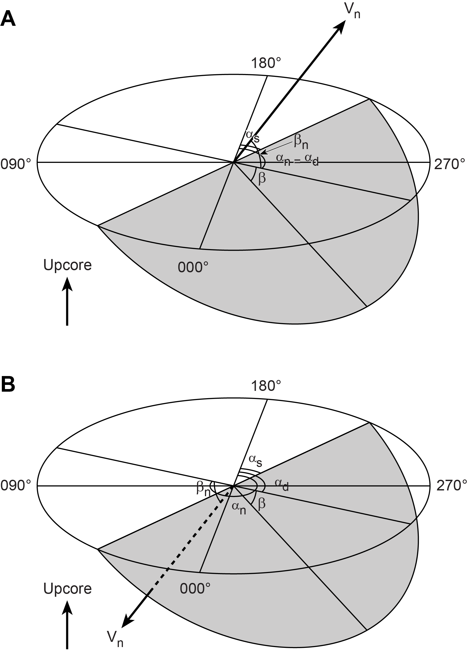
Figure F17. Dip direction, right-hand rule strike, and dip of a plane.
The dip direction (αd) and dip angle (β) of this plane are αd = αn and β = 90° + βn, respectively, when βn < 0°, and are αd = αn ± 180° and β = 90° − βn, respectively, when βn ≥ 0°. The strike of this plane (αs) according to the right-hand rule is then given by αs = αd − 90° (Figures F17, F18).

Figure F18. Azimuth correction.
3. Biostratigraphy
Microfossils were examined for most sedimentary core catcher samples, as well as mudline samples from each site and notable intervals from split cores. Organic-walled dinoflagellate cysts (dinocysts), other categories of palynomorphs, planktonic foraminifers, diatoms, and silicoflagellates provided preliminary shipboard biostratigraphic and paleoenvironmental information during Expedition 396. Occurrences of other groups were documented, including ostracods, radiolarians, ebridians, calcareous nannofossils, benthic foraminifers, and ichthyoliths. These were utilized for their paleoenvironmental significance. Postcruise analysis of some of these groups by approved shore-based colleagues to refine biostratigraphic control is likely. Several microfossil groups will be analyzed in the postcruise period as carriers of important geochemical signals, especially in key intervals.
Shipboard paleontologists also documented occurrences of transported terrestrially derived microfossils, including pollen, spores, and associated terrestrial kerogen debris and siliceous phytoliths and freshwater diatoms. Fossils identifiable as brackish water or coastal taxa were also documented. Additional microfossil groups encountered during shipboard analysis were noted, as were known older microfossils reworked into younger strata.
Methods employed for each group are described below, including sample processing, taxonomic frameworks, and literature sources and calibrations used to establish preliminary age assessments. Working with the shipboard paleomagnetic data, we establish tentative correlations to the timescale of Gradstein et al. (2012) (GTS2012). Age assignments were based on analyses of microfossils from all mudline and core catcher samples. Additional discrete samples from split core sections were analyzed to refine biostratigraphic boundaries (e.g., across lithologic transitions).
The Paleogene epochs are in this publication divided into Early/Middle/Late intervals as follows: Oligocene (Early: Rupelian; Late: Chattian), Eocene (Early: Ypresian; Middle: Lutetian, Bartonian; Late: Priabonian), and Paleocene (Early: Danian; Middle: Selandian; Late: Thanetian). Similarly, the series are divided into Lower/Middle/Upper intervals.
The Biostratigraphy section in each site chapter presents a summary of biostratigraphical information, paleoenvironmental interpretation provided by each microfossil group, and information regarding approaches and literature used to guide taxonomic identifications. Data for each microfossil group are presented in the form of abundance and taxonomic distribution charts that record occurrences of key taxa observed in samples from each hole. Taxonomic occurrence charts also record suspected upsection reworking or other stratigraphic displacement such as erosion and downslope transport.
Occurrences of biostratigraphically important taxa, as well as relative abundance and preservation data, were entered through the DESClogik application into the IODP LIMS database for identified microfossil taxa and paleontological data gathered during shipboard investigations. These data are available from the LIMS database in accordance with IODP policy.
Distribution charts for microfossil groups presented in each site chapter are based exclusively on shipboard analysis. Shipboard biostratigraphic studies focused primarily on the identification of biostratigraphic events in the cores and are biased toward the reporting of age diagnostic species and identifying intervals and ages of reworking. Events reported include the first occurrence (FO) and last occurrence (LO) of a taxon’s stratigraphic range, in some cases with modification to identify the last common/abundant appearance datum (LCAD/LAAD) or first common/abundant appearance datum (FCAD/FAAD) to identify an abundance change within a taxon’s range. Where possible, identification of a sequence of biohorizons in stratigraphic order were used to assign biostratigraphic zones and subzones to previously established schemes. A summary table of the main microfossil occurrences at each site is presented in the site chapters. The chronostratigraphic compilation provides a framework for estimating sediment accumulation rates, identifying hiatuses, guiding correlation between holes, and assessing recovery as compared with the Scientific Prospectus. All age models presented in this volume are preliminary and will be subject to revision following postcruise research updates.
Biochronologic age assessments were shared with the paleomagnetism team and utilized in stratigraphic correlation and the construction of age-depth plots to assess sediment accumulation rates and hiatuses.
3.1. Siliceous microfossils
3.1.1. Taxonomy and dating
Diatoms, silicoflagellates, ebridians, endoskeletal dinoflagellates, and other small biosiliceous phytoplankton fossils (excluding radiolarians and sponge spicules) were analyzed from the same sample preparations for preliminary age control and paleoenvironmental interpretation.
Taxonomic concepts and biostratigraphic constraints for these groups, many of which may be endemic to the high-latitude North Atlantic, have developed through 50 y of stratigraphic drilling and more than 100 y of analysis of some Paleogene diatomites exposed in several land sections. Scherer et al. (2007) summarized regional and global Cenozoic diatom biostratigraphic schemes and zonations for the major ocean basins, but chronostratigraphic dating of many these events was still largely in development until recently, with efforts to calibrate both Neogene and Paleogene diatom events and zones to the GTS2012 and subsequent updates to the timescale of Gradstein et al. (2020) (GTS2020). The most up-to-date correlations to the GTS2012 is an ongoing database maintained by Dr. John Barron (J. Barron, pers. comm., 2021), built and continuously revised from that published by Lazarus et al. (2014; available via the JANUS database [http://www-odp.tamu.edu/database]). The most up-to-date version of this database has been provided to the LIMS database (September 2021), and updates will be published in the JANUS database (J. Barron, pers. comm., 2021). This database currently contains 475 FO and LO diatom datums. It is focused on the Southern Ocean but contains many global datums.
Recent detailed taxonomic work with biostratigraphic correlations by Witkowski (2018) and colleagues (Witkowski et al., 2020a) have significantly advanced Lower Paleogene diatom biostratigraphy. Unfortunately, many of the taxa discussed in these recent works are absent from the Norwegian Sea deposits recovered during Expedition 396, indicating that there is more provincialism in the Paleogene than has often been assumed (Scherer et al., 2007; Witkowski, 2018).
For Expedition 396, we drew heavily on results of prior regional drilling on the Vøring Plateau, including work on Deep Sea Drilling Project (DSDP) Leg 38 Sites 336–342 by Schrader and Fenner (1976), who developed the first regional diatom zonation based on spot cored and often poorly recovered sections. This work was augmented by Dzinoridze et al. (1978). Later drilling on the Vøring Plateau as part of ODP Leg 104 yielded biostratigraphic research on Neogene silicoflagellates and ebridians (Ciesielski and Case, 1989; Ciesielski et al., 1989; Locker and Martini, 1989), but little detailed stratigraphic work on diatoms has been published. Other diatom research from the circum-North Atlantic and beyond helped construct diatom zonations for the Neogene (Koç and Scherer, 1996) and late Paleogene (Scherer and Koç, 1996), but these stratigraphic sections are also incomplete and do not extend into strata older than latest Eocene (Scherer and Koç, 1996).
Recent advances in Atlantic biostratigraphy include extending calibration into the Paleogene, like the work of Barron et al. (2015), who compiled global distributions of Eocene diatoms and silicoflagellates. Witkowski et al. (2020a) focused on the western North Atlantic (Blake Nose) for calibration of Eocene datums, and Renaudie et al. (2018) presented a brief compilation of the global distribution of key Paleocene marine diatoms.
Recognized Lower Paleogene diatom assemblages and species successions of Paleocene and Lower Eocene (including the Paleocene–Eocene Thermal Maximum [PETM]) in recovered materials most closely correspond to exposures and wells on the Russian Platform (Oreshkina and Aleksandrova, 2007; Oreshkina and Radionova, 2014) and the Fur Formation of Denmark (Homann, 1991; Fenner, 1994). These publications proved very useful during recovery of similar aged materials of Expedition 396, but most of these are not closely calibrated to independent timescales, although such efforts are underway, especially with regard to new dating of ashes in the Fur Formation.
3.1.2. Methods for diatoms, silicoflagellates, ebridians, and other siliceous flagellates
Smear slides provide a useful guide to subsequent sediment processing because they provide unadulterated views of the sediment. Smear slides were used for initial characterization of occurrences of biosiliceous components and calcareous nannofossils and were prepared at every interval analyzed, including core catchers and split core samples. They were used both for initial biostratigraphic analysis and as a guide to methods to be employed to concentrate and enhance production of biostratigraphic data. A toothpick sample of sediment was placed on a 22 mm × 40 mm coverslip, coated to break surface tension, as described by Scherer (1994), wetted with deionized water, disaggregated as much as possible, and spread in a thin coating and dried on a hot plate. When dried, each sample was permanently affixed to a microscope slide using Norland optical adhesive Number 61 (refractive index = 1.56) and cured under ultraviolet light. Samples included all sedimentary core catchers and numerous samples from intervals of interest from the split cores.
Most sediment core catchers that contain biosilica were processed to concentrate biosiliceous components. Most samples, which typically have an ~2 cm3 initial size, were processed in 125 or 250 mL beakers. Indurated sediments were initially crushed to granule-sized components and placed in the beakers with 10% hydrogen peroxide (H2O2) to oxidize organics and disaggregate sediments. Carbonate was rare in most samples, so there was no need to use HCl. Likewise, the use of dispersing salts (e.g., sodium hexametaphosphate (Na₆[(PO₃)₆]) or sodium tetraborate [borax] (Na₂[B₄O₅(OH)₄]·8H₂O)) was mostly not needed with Expedition 396 sediments. Several samples contained no remaining biosilica but did include diatoms replaced by pyrite. To prepare these, clays were dispersed with Calgon solution and then sieved as described below. When the H2O2 reaction was complete and the sample was chemically neutralized by dilution and decanting, strewn slides of unsieved material were prepared. Aliquots of selected samples were then sieved using either a 15 µm nylon, 20 µm stainless steel, or 38 µm stainless steel sieve to remove fragmented diatoms and concentrate biostratigraphic markers.
We acknowledge that this approach likely increased the presence of larger, more heavily silicified species and reduced numbers of potentially biostratigraphically important, smaller diatoms from these slides. However, this approach was deemed essential for providing a sufficient number of specimens to allow rapid age interpretation of core catcher samples. Furthermore, both smear and strewn slide preparations were analyzed. All slides were mounted on cover glasses and permanently fixed to labeled glass slides using Norland adhesive and cured under an ultraviolet lamp.
Samples prepared for diatom analysis were examined using a Zeiss Axioskop transmitted-light microscope. Photomicrographs were taken using a SPOT Flex 64 Mp digital camera. A Hitachi TM3000 tabletop scanning electron microscope (SEM) was utilized to analyze sedimentary microstructure in a laminated diatomite. Qualitative siliceous microfossil group abundances were determined from smear slides using 630× magnification. Care was taken to ensure smear slides were prepared with similar amounts of sediment to ensure consistency.
Visual estimates of percentages followed standard guidelines (e.g., Rothwell, 2012) (Table T2). For each sample, the following abundances of diatoms were qualitatively estimated by light microscopic observations with the examination of five random fields of view (FOVs):
- B = barren: no diatom debris.
- T = trace: trace quantities (<1%) occur. Trace quantities generally means that there is some evidence that diatoms had been present, but because of recrystallization or extreme fragmentation they are of no use for biostratigraphic interpretation.
- R = rare (1%–5% diatoms). Some biostratigraphic application may be possible, but only with further processing.
- F = few (5%–10% diatoms). Typically, only heavily silicified diatoms are present, but they may provide some biostratigraphic information.
- C = common (10%–20% diatoms). Biostratigraphic analysis is possible.
- A = abundant (>20% diatoms).
- M = mass abundance (nearly pure diatoms, usually with strong dominance of a single species). Mass occurrence can exist with excellent preservation or may include partial recrystallization of the assemblage, which may limit identification.
The following relative abundances of individual taxa (including diatoms and silicoflagellates) were categorized in reference to their occurrence in FOVs or to a traverse across a 40 mm wide coverslip (~100 FOVs at 630× magnification):
- T = trace (<1 specimen per 5 average horizontal transects [40 mm]).
- R = rare (1 specimen within 1–5 transects).
- F = few (1–5 specimens per transect).
- C = common (1–5 specimens per ~5 FOVs).
- A = abundant (2 or more specimens per FOV).
- D = dominant (the taxon represents >50% of all diatoms in diatom-rich samples).
Preservation of diatoms and silicoflagellates was qualitatively assessed with regard to both the degree of dissolution and fragmentation. The degree of siliceous microfossil fragmentation often mirrors dissolution, but the two factors are not always directly correlated. Diatoms with well-preserved fine structures can be highly fragmented. Dissolution is a wholly chemical/diagenetic process (Warnock and Scherer, 2015), but fragmentation can be dominantly or entirely due to mechanical processes (Scherer et al., 2004). Fragmentation of finely silicified diatoms can occur in sediments as a result of digestion by grazers and deposition in fecal pellets or by compaction of diatomite from overburden.
The degree of diatom dissolution was qualitatively graded as follows:
- L = low (slight to no apparent dissolution and fine structures generally preserved).
- M = moderate (some dissolution and fine structures generally lost).
- H = high (severe effects of dissolution, including widened areolae, relatively abundant margins and cingula compared with valves, and notably higher proportions of heavily silicified forms).
The degree of fragmentation was graded as follows:
- L = low (a majority of valves are unbroken).
- M = moderate (>50% of diatom valves are broken, but most are identifiable).
- H = high (valves highly fragmented with very few complete valves present, hampering identification).
Shipboard data for the initial report integrate fragmentation and dissolution and report diatom preservation as good (G), moderate (M), and poor (P) for samples containing identifiable diatoms.
3.1.3. Diatom age assignment
Initial shipboard diatom age assignment of individual Paleogene and Neogene samples was based on identification of primary and secondary diatom datum events, many of which are calibrated for the Neogene, and fewer for the Paleogene. The best calibrated occurrences are for the Southern Ocean and low latitudes; thus, a degree of uncertainty currently exists for these datums. Consequently, shipboard age assignments based on diatoms, especially for the Paleogene, are considered supplementary to better calibrated dinocyst biostratigraphy. Published diatom biostratigraphic zones were informally assigned, where possible, but postcruise analysis will lead to modification of existing schemes.
No continuous, published, well-dated stratigraphic succession of biosiliceous sediments exists for the high-latitude North Atlantic. Schrader and Fenner (1976) developed an Eocene through Miocene high-latitude North Atlantic diatom zonation for the Vøring Plateau based on poorly dated and discontinuous materials recovered during Leg 38, much of which was spot cored. Dzinoridze et al. (1978) added additional biostratigraphic and taxonomic data on these cores. Scherer and Koç (1996) and Koç and Scherer (1996) updated the zonation of Schrader and Fenner (1976) to include 11 Neogene and 13 upper Paleogene diatom zones based on cores from ODP Leg 151 Site 908 on the Hovgård Ridge, Fram Strait, and Site 913 on the East Greenland Margin. Much of the Cenozoic record is missing and none of the pre-Pleistocene section from these cores included a good paleomagnetic record at the time, so dating of these zones is relative. More recently, Suto (2003, 2004) and Suto et al. (2008, 2009, 2011) contributed new biostratigraphic data based on resting spores, expanding on similar studies from the North Pacific. Diatomaceous Eocene sediments have been recovered from the Lomonosov Ridge in the high Arctic with taxa comparable to some Norwegian Sea assemblages (Suto et al., 2009). Additionally, there are some notable terrestrial exposures of diatomaceous Lower Eocene sediments from Denmark’s Fur Formation (Homann, 1991; Fenner, 1994) and Paleocene and Lower Eocene deposits on the Eurasian Plateau (Strelnikova, 1992; Oreshkina and Radionova, 2014; Oreshkina and Aleksandrova, 2007; Aleksandrova et al., 2012; Radionova and Khokhlova, 1994, 2000). These assemblages mostly reflect neritic plankton with abundant resting spores (Suto, 2003, 2004, 2005; Suto et al., 2011). Recent work by Witkowski (2018) and Witkowski et al. (2012, 2015, 2020a, 2020b) added significant detail to dating key Eocene intervals in the North Atlantic, with improvements in both dating and taxonomic definition of key species, but many of the identified datums could not initially be applied to Expedition 396 materials.
3.2. Palynology
3.2.1. Sample processing
Several processing methods may be employed depending on, for example, biogenic or detrital silica concentrations, the relative compaction and silicification, and/or whether conditions on the ship were deemed safe enough (e.g., no rough seas) to use hydrofluoric acid (HF).
3.2.1.1. Simple non–hydrofluoric acid method with HCl only
Approximately 10–20 cm3 (~10–20 g) of soft, clay-rich material is treated with 10% HCl to dissolve the bulk of the carbonate using a disaggregation/sieving method described in Riding and Kyffin-Hughes (2011), specifically, density separation in an ultrasonic bath.
3.2.1.2. Hydrofluoric acid method
Approximately 5–10 cm3 (~10 g) of material is taken for HF processing, for which we followed standard palynological laboratory protocols (Brinkhuis et al., 2004). Carbonate-rich samples were first treated with HCl to dissolve the bulk of the carbonate before further digestion with HF. Carbonate-lean samples were digested with cold 48% HF to dissolve carbonates and silicates, followed by a step with 30% HCl to remove silicate gels. Finally, the samples were rinsed with demineralized (or deionized or tap) water to neutralize any remaining acids. After each of these steps, samples were centrifuged and supernatants were decanted. The organic residues were then sieved to remove large (phytoclasts and palynodebris) and small particles (amorphous organic matter and minor amounts of clays, usually phyllosilicates) using 250 and 15 µm nylon sieves and an ultrasonic bath. The >250 µm fraction was used for cuticle analysis where feasible, and the smaller fraction (15–250 µm) was concentrated again using a centrifuge and mounted on glass microscope slides using glycerine jelly (refractive index = 1.47) as the mounting medium. Finally, the cover slides were sealed with nail varnish for more permanent conservation.
3.2.2. Marine palynological associations (palynofacies)
The acid-resistant residue, or palynofacies, of a given sample after the processing described above, incorporates (1) palynodebris, specifically, fragments of larger multicellular entities or related elements (e.g., from bits and pieces of plant tissue to remains of resin droplets) and (2) palynomorphs, identifiable (semi)complete elements, or remains of uni- or multicellular biota. The latter are composed of both aquatic elements (freshwater and/or marine derived) and terrestrial components such as elements related to higher plants (spores, gymnosperm pollen, and angiosperm pollen), sometimes including remnants of freshwater plants (e.g., the massulae and glochidia of freshwater ferns like those from Azolla spp.) (e.g., Brinkhuis et al., 2006; Barke et al., 2011), various fungal remains, or even animal-derived bits and pieces (e.g., jaws of marine worms, so-called scolecodonts, and various insect remains). The aquatic fresh- to brackish water elements may include single-celled palynomorphs such as Cymatiosphaera, Pterospermella, and Tasmanites spp.; cysts of freshwater dinoflagellates; and multicellular (colonial) forms such as Pediastrum, Palambages, and Botryococcus spp. The marine portion typically consists of organic-walled dinocysts of either gonyaulacoid or (proto)peridinioid dinoflagellates and various organic-walled microfossils of unknown affinity (so-called Acritarchs), but it may also yield remains of many other marine microbiota, including, but not limited to, the inner linings of benthic foraminifers and tintinnid loricae.
3.2.2.1. (Semi)quantitative palynofacies analysis
Palynofacies analysis and data collection was carried out using a Zeiss Axiophot microscope with brightfield illumination at 400×, 630× (oil), and 1000× (oil) magnification. For each sample, one 22 mm × 40 mm slide was scanned and semiquantitatively (+ to +++) characterized for palynodebris categories (see below) and counted to ≥200 palynomorphs (Table T3).
Photomicrography was conducted using a SPOT Flex digital camera, and images were uploaded to the LIMS database.
The following broad palynodebris categories were employed:
- Black phytoclasts,
- Brown phytoclasts,
- Plant tissue general,
- Leaf/cuticle remains,
- Amorphous organic matter (aggregates),
- Amorphous organic matter (filaments),
- Transparent filaments/fungal affinity,
- Opaque elements of unknown affinity,
- Pyritized microfossils, and
- Indeterminable elements (palynomorphs).
The following palynomorph categories were employed:
- In situ dinocysts (≥0.5 cyst) (determined to group to species level),
- Operculae of dinocysts,
- Indeterminable (likely) remains of dinocysts (fragments),
- Reworked marine dinocysts (and ages),
- Organic linings of (benthic) foraminifers,
- Acritarchs (various groups),
- In situ pollen and spores,
- Reworked pollen and spores,
- Massulae and seeds/eggs of Azolla spp.,
- Single-celled brackish/freshwater palynomorphs,
- Multicelled brackish/freshwater palynomorphs, and
- Indeterminable elements (palynomorphs).
Palynomorph preservation, focused on the in situ dinocysts, was qualitatively classified as one of the following levels:
- G = good (little or no evidence of degradation or oxidation).
- M = moderate (some evidence of degradation or oxidation).
- P = poor (major degradation or oxidation has occurred).
The palynomorph categories are counted to a total of (a minimum of) 200 specimens and are reported in percentages of the total palynomorph count. If the first 200 palynomorphs contained fewer than 100 in situ identifiable dinocysts, palynomorph counting continued until a minimum of 100 in situ identifiable dinocysts were found.
Above the (minimum of) 200 palynomorph and 100 in situ dinocyst count, remaining material were entirely scanned for rare and stratigraphically important taxa, and these are reported irrespective of their abundance (present [p]). Furthermore, the abundance of taxa, genera, and groups were employed for paleoenvironmental reconstructions. It is common practice (cf. Pross and Brinkhuis, 2005; Sluijs et al., 2005) to group taxa that are morphologically related and/or have similar ecological affinities into “ecogroups” (see Environmental reconstructions using dinocysts and palynofacies). Like the palynomorph assemblage, we report the relative dinocyst abundance in percentages for select groups. Grouping of taxa to their ecological preference and morphology is based on extensive previous work (e.g., Brinkhuis, 1994; Pross and Brinkhuis, 2005; Sluijs et al., 2005; Sluijs and Brinkhuis, 2009; Frieling and Sluijs, 2018).
3.3. Organic-walled dinoflagellate cyst taxonomy and age assignments
The dinocyst taxonomy generally follows that cited in Williams et al. (2017a), except for members of the subfamily Wetzelielloideae (see Williams et al. [2015], comments by Bijl et al. [2017], and reply by Williams et al. [2017b]).
Mesozoic–Cenozoic chronostratigraphically important dinocyst events, mostly FOs and LOs of genera and species, have been widely documented, and over the past decades these events have been relatively well calibrated against meaningful chronostratigraphic information (for an overview see, e.g., Williams et al., 2004). Many of these FO/LO events have global significance, but others have been shown to be hemispheric or more regional in nature. It is therefore important to compare shipboard generated data with the large body of previous dinocyst work from the North Atlantic region, including the Norwegian Margin, and palynological studies using core material from earlier expeditions to the Vøring Plateau (e.g., Boulter and Manum, 1989; Mudie, 1989; Eldrett et al., 2004). Here, we employ the latest global and regional compilations (Bijl, 2022), wherein dinocyst events are calibrated against the GTS2012.
Available Neogene North Atlantic regional “oceanic” dinocyst events and (informal) zonations are, at best, tied to magnetic reversals and a limited number of nannofossil datums (de Schepper and Head, 2009; Schreck et al., 2012). More nearshore accounts were established for the Danish (Dybkjær et al., 2021) and Dutch North Sea area (Munsterman and Brinkhuis, 2004), but these are even less well calibrated compared to the oceanic records. For the Paleogene, an extensive range of North Atlantic and North Sea dinocyst events has been documented (e.g., Mudge and Bujak, 1994; Mudge and Bujak, 1996a, 1996b; Bujak and Brinkhuis, 1998; Eldrett et al., 2004; Eldrett and Harding, 2009; Eldrett et al., 2019; Vieira et al., 2020), many of which, notably Eocene and younger, are well calibrated against magnetostratigraphy, nannofossil, and foraminifer datums (e.g., Eldrett et al., 2004, 2019). The various transient, globally approximately synchronous, stable carbon isotope excursions provide tight constraints on the absolute and relative datums of dinocyst events, notably during the early Paleogene hyperthermals, including the PETM (Crouch et al., 2001; Sluijs and Brinkhuis, 2009; Harding et al., 2011; Kender et al., 2012).
Aside from biochronostratigraphic purposes, shipboard quantitative marine palynological analysis included palynofacies assemblage characterization in terms of paleoenvironment.
3.4. Environmental reconstructions using dinocysts and palynofacies
Both dinocysts and the general composition of the palynofacies present useful insights for reconstruction of paleoenvironments (e.g., Brinkhuis, 1994; Batten, 1996). Organic-walled cyst-producing dinoflagellates are sensitive to even minor changes in their physical and biochemical environment, and assemblage characteristics can be used to qualitatively and semiquantitatively reconstruct a range of ancient environmental parameters and conditions, including salinity, shore proximity (paleodepth), productivity, upwelling, and temperature. Ecological preferences of extant species are well documented using modern core-top data (Zonneveld et al., 2013; Marret et al., 2020), whereas, for extinct species, researchers have utilized independent proxy data and field observations to assign groups of taxa (ecogroups) to specific paleoenvironmental conditions (Pross and Brinkhuis, 2005; Sluijs et al., 2005; Barke et al., 2011; Hennissen et al., 2017; Frieling and Sluijs, 2018). These studies allowed us to make coarse, low-resolution, environmental reconstructions for all cores that yielded sufficiently well preserved dinocyst assemblages and palynofacies.
3.5. Thermal alteration
Thermal alteration indexes (TAIs) based on progressive discoloration of palynomorphs from transparent to yellow, brown, and black are useful first-order estimators of sedimentary organic matter maturity. Various factors contribute to organic matter thermal maturation, but most often thermal alteration of organic matter results from deep burial. However, sediments in the close vicinity of erupting (flood) basalts and intruded volcanic rocks may also undergo rapid maturation (Pross et al., 2007; Aarnes et al., 2011). We monitored the thermal alteration of recovered palynomorphs, both in situ and reworked dinocysts and pollen. The influence of thermal alteration on the palynomorphs from intrabasalt sediments, such as those recovered from ODP Site 642E (Boulter and Manum, 1989; Abdelmalak et al., 2016), and the subbasalt sediments on the Kolga High (Sites U1565 and U1566) show short-term interactions between volcanic and sedimentary deposits. Lastly, reports have shown the presence of mature organic matter in the hydrothermal crater sediments (Svensen et al., 2004; Frieling et al., 2016). For these sites (U1567 and U1568), the TAIs provided a first line of evidence for when the main thermal alteration of the sediments, as a result of hot fluid or gas venting, took place.
3.6. Foraminifers
3.6.1. Planktonic foraminiferal taxonomy and biozonation schemes
Quaternary and Neogene planktonic foraminifer taxonomy follow Kennett and Srinivasan (1983), Spiegler and Jansen (1989), and Spiegler (1996). Paleogene planktonic foraminifer taxonomy follow Wade et al. (2011) modified from Pearson et al. (2006) and Wade et al. (2018).
High-latitude planktonic foraminiferal associations comprise low-diversity and long-ranged species (Spiegler and Jansen, 1989; Spiegler, 1996). Because of this, local zonation schemes of ODP Legs 104 and 162 are utilized for the Miocene to Quaternary (Spiegler and Jansen, 1989; Spiegler, 1996). Wade et al. (2011) modified from Pearson et al. (2006) zonation schemes are utilized for the Paleocene–Oligocene.
3.6.2. Foraminifer sample preparation and analysis
Sediment samples (~10–20 cm3) were placed in a 200 mL beaker of water, disaggregated, washed over a 63 µm sieve, and then dried in an oven at ~45°C. A 10% hydrogen peroxide solution was used to aid in the disaggregation of the sediment because of the abundance of clay in samples. The dried sand fraction was weighed and then sifted through a USA Standard Sieve Series 150–250 µm to separate the dry material into the desired size range needed for identification and classification. All size fractions will be preserved for further exploration of the processed sediment material.
The samples were observed under a binocular light microscope after drying. Specimens were picked using a 0000 brush and mounted on a gridded micromount slide. A sieved sample, including mineral matter (sand and larger clasts) was made available to the lithostratigraphy team after foraminifers were picked. Specimen images were taken using either SEM or the digital camera attached to the binocular microscope.
3.6.3. Microscopy and identification
A Zeiss Discovery V8 binocular light microscope was used for foraminifer species identification. Images were taken using SPOT Idea digital camera and uploaded to the LIMS database. Foraminifer species identifications utilized the >150 µm size fraction. Time permitting, an analysis of the 38–150 µm size fraction was conducted for small or rare species.
The preservation states of planktonic foraminifers are defined by evidence of overgrowth, dissolution, abrasion, and fragmentation (Table T4):
- E = excellent (specimen have little to no evidence of overgrowth, dissolution, abrasion, or fragmentation).
- VG = very good (some minor evidence of overgrowth, dissolution, abrasion, or fragmentation).
- G = good (little evidence of overgrowth, dissolution, abrasion, or fragmentation).
- M = moderate (common but minor calcite overgrowth, dissolution, abrasion, or fragmentation).
- P = poor (considerable overgrowth, dissolution, abrasion, or fragmentation).
Abundances of total planktonic foraminifers are categorized as follows:
- A = abundant (>50% foraminifers).
- C = common (25%–50% foraminifers).
- F = frequent (10%–25% foraminifers).
- T = trace (5–10% foraminifers).
- R = rare (<5% foraminifers).
- B = barren (no foraminifers found in sample).
3.7. Ostracods
Dry samples prepared for foraminifer examination also were examined for the presence of ostracods at selected sites. Ostracod assignments follow Ducasse and Peypouquet (1979), Coles and Whatley (1989), Malz (1989), Coles et al. (1994), Guernet and Bellier (2000), Aumond et al. (2009), Alvarez Zarikian (2009, 2015), Yamaguchi (2018), Yamaguchi and Norris (2012), and Yamaguchi et al. (2017a, 2017b). Species identification was made routinely on core catcher samples and occasionally on samples taken from selected working-half sections.
3.7.1. Ostracod abundance estimates
The following ostracod abundance categories relative to total sediment particles >150 µm were estimated from visual examination of the dried sample (Table T5):
- D = dominant (>30% of total sediment particles).
- A = abundant (>10%–30% of total sediment particles).
- F = few (>5% to <10% of total sediment particles).
- R = rare (>1% to <5% of total sediment particles).
- P = present (<1% of total sediment particles).
- B = barren.
The number of individuals of each ostracod species was categorized as follows:
- D = dominant (>30% of benthic assemblage).
- A = abundant (>10%–30% of benthic assemblage).
- F = few (>1% to <10% of benthic assemblage).
- P = present (<1% of benthic assemblage).
Ostracod preservation was estimated using the following definitions:
- VG = very good (valves translucent; no evidence of overgrowth, dissolution, or abrasion).
- G = good (valves semitranslucent; little evidence of overgrowth, dissolution, or abrasion).
- M = moderate (common but minor calcite overgrowth, dissolution, or abrasion).
- P = poor (substantial overgrowth, dissolution, or fragmentation of the valves).
4. Paleomagnetism
Shipboard paleomagnetic investigations were conducted on both the archive and working halves of cores recovered during Expedition 396. The primary objectives were to determine directions of natural remanent magnetization (NRM) components, including magnetic polarity, and downhole variation of magnetic properties. The goal of these experiments was to place chronological constraints on the timing of magnetization as a function of stratigraphy.
Shipboard paleomagnetic investigations combined three complementary approaches: (1) NRM measurement and in-line alternating field (AF) demagnetization of the NRM of archive-half sections on the pass-through 2G Enterprises (Model 760R-4K) superconducting rock magnetometer (SRM), (2) measurement and AF demagnetization of oriented discrete samples on the spinner magnetometer (AGICO Model JR6), and (3) measurement of the anisotropy of magnetic susceptibility (AMS) in low field (300 A/m) on discrete samples using the AGICO KLY 4S Kappabridge.
The discrete sampling strategy was adjusted based on lithology (sediments versus basement), type of drilling used (e.g., soft sediments can be disturbed by RCB and XCB coring to the point of being unusable for magnetic inclination), and recovery rate. For hard materials, discrete cube samples (~20 mm) were collected from the central part of working-half sections to reduce the effect of drilling disturbance. For soft materials, plastic boxes were used to extract sediment from the core. For basement rocks, at least one cube was collected per major lithostratigraphic unit (as defined by petrologists) to characterize the magnetic properties, magnetic grain size distributions, and deformation of these units. These data were used to construct the shipboard magnetostratigraphic timescale. Because of the relatively low recovery in basement, hard rock samples were used to measure porosity and moisture (i.e., discrete samples were shared with the physical properties team during this expedition).
Section-half and discrete data, collected using the pass-through SRM and spinner magnetometer, respectively, were uploaded to the LIMS database. We then analyzed the stepwise demagnetization data of the discrete samples using principal component analysis (PCA) to define the characteristic remanent magnetization (ChRM) (Kirschvink, 1980). Data visualization (Zijderveld demagnetization plots and equal area projections) and PCA were conducted using the Remasoft 3.0 software (Chadima and Hrouda, 2006).
4.1. Archive-half section magnetic measurements
The remanent magnetization of archive-half sections was measured using a pass-through SRM equipped with direct-current superconducting quantum interference devices (DC-SQUIDs) and an in-line, automated three-axis AF demagnetizer capable of reaching a peak field of 80 mT.
Measurement of archive halves was conducted using the SRM software (IMS-SRM Version 10.2) and assumed a sample area of 17.5 cm2 for conversion to volume-normalized magnetization units (A/m). The interval between NRM measurement points was 2.5 cm, and measurements occurred at a speed of 10 cm/s. The response functions for the pick-up coils of the DC-SQUID sensors have a full width of 7.25–8.8 cm at half height. Therefore, data collected within less than ~4 cm of piece boundaries (or voids) can be significantly affected by edge effects and must be treated with caution.
We performed successive AF demagnetizations using the SRM in-line AF demagnetizer on all archive-half sections. The in-line AF demagnetizer applies a field to the x-, y-, and z-axes of the SRM in this fixed order (Figure F19). Considering this limitation, we only used demagnetization steps up to 20 mT to demagnetize the sections. For most of the sediment sections we performed 3–6 steps from NRM up to 15 or 20 mT depending on time constraints imposed by the rate of core recovery. For basement rocks, we adopted a set of narrower AF steps of 2 mT from NRM to 10 mT and steps of 5 mT from 10 to 20 mT. AF demagnetization results were plotted individually as vector plots (Zijderveld, 1967) and as downhole variations with depth. We inspected the plots visually to evaluate whether the remanence after demagnetization at the highest AF step reflects the ChRM and geomagnetic polarity sequence. We used the directional and intensity data of archive-half sections (measured at 20 mT) to determine magnetic polarity along the core. Directional and intensity data from discrete samples were used to validate the polarities inferred from section measurements. Directional data were analyzed using Zijderveld diagrams (Zijderveld, 1967). The ChRM direction(s) were determined using the Remasoft 3.0 software.
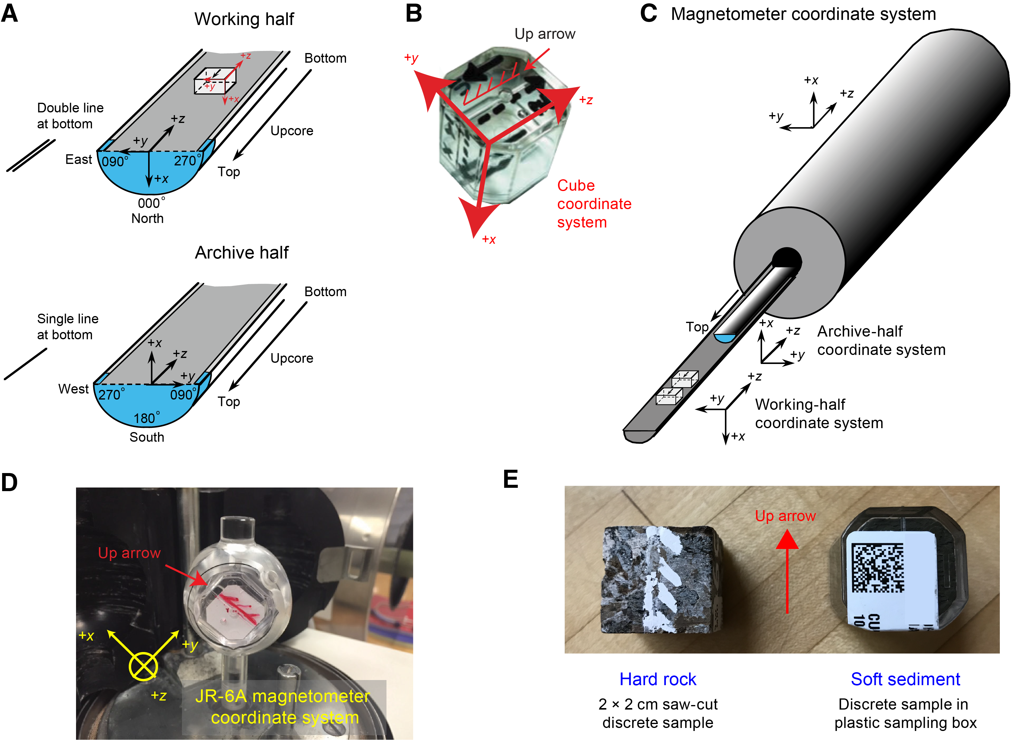
Figure F19. Paleomagnetic coordinate systems.
Low-field MS (κ) measured on whole-round sections using the WRMSL and archive-half sections using the SHMSL (see Physical properties) were used to assess the concentration of magnetic minerals and determine the downhole relative paleointensity (NRM/κ). These whole-round records of MS were compared to visual features in the section halves to identify possible artifacts.
The magnetic intensity of marine sediments generally reflects the intensity of the geomagnetic field at the time of deposition, the nature and concentration of magnetic minerals (e.g., magnetite versus hematite), and any possible postdepositional disturbance due to drilling or bioturbation.
4.2. Discrete sample magnetic measurements
Discrete samples were measured on the spinner magnetometer. These samples were subjected to AF demagnetization treatments using both the 2G in-line AF demagnetizer (as described above) and the standalone DTECH (Model D-2000) AF demagnetizer. Because the resultant demagnetization behavior of the discrete samples becomes noisy at higher AFs, measurement using the SRM is not recommended for discrete samples. The routine AF demagnetization treatment was performed using the DTECH (Model D-2000) AF demagnetizer. In addition, to avoid contamination by the ambient magnetic field during shipboard measurements, two cylindrical mu-metal shields provided a suitable low-field environment for temporary sample storage.
Oriented discrete samples were collected preferentially in fine-grained sedimentary intervals where drilling deformation was minimal. In soft sediment, oriented discrete samples were taken in plastic Natsuhara-Giken sampling cubes (sample volume = 7 cm3) (Figure F19). Cubes were pushed into the working half of the core with the “up” arrow on the cube pointing upsection in the core, occasionally using a rubber mallet. In lithified sediments and hard rocks, 2 cm cubes (sample volume = 8 cm3) were cut using the parallel saw.
Incremental AF demagnetization of discrete samples was performed using the DTECH AF demagnetizer (Model D-2000) at fields up to 45 or 50 mT for low-coercivity samples and 120 or 200 mT for high-coercivity samples. The ratio of magnetization remaining after AF demagnetization to 20 mT and NRM (I20mT/NRM) was used as a proxy for degree of coercivity. Samples with I20mT/NRM > 1.0 were not included in the graphs. AMS was measured on an AGICO KLY 4S Kappabridge at a field of 300 A/m using the SUFAR (AGICO) software. The KLY 4S Kappabridge measures AMS by rotating the sample along three axes, stacking the data, and calculating the best-fit second-order tensor. It also measures the volume-normalized calibrated bulk susceptibility (χ).
4.3. Coordinates
All magnetic data are reported relative to the IODP orientation conventions: +x is into the face of the working half, +y points toward the left side of the face of the working half, and +z points downsection. The relationship of the SRM coordinates (x-, y-, and z-axes) to the data coordinates (x-, y-, and z-directions) is as follows: for archive halves, x-direction = x-axis, y-direction = −y-axis, and z-direction = z-axis; for working halves, x-direction = −x-axis, y-direction = y-axis, and z-direction = z-axis (Figure F19). The coordinate systems for the spinner magnetometer and Natsuhara-Giken sampling cubes are shown in Figure F19.
4.4. Core orientation
Paleomagnetic study of marine sediment cores is greatly enhanced if the angle between magnetic north and the double line marked on the core liner can be determined. The ChRMs can provide a reference frame to reorient cores. Provided that the reference magnetic pole is known, the orientation of the paleomagnetic vector could be used to restore the azimuth of the +x core axis (e.g., Fuller, 1969).
4.5. Magnetostratigraphy reference scale and interpretations
The magnetostratigraphy at each site was constructed by correlating observed polarity sequences with a reference geomagnetic polarity timescale (GPTS) in combination with biostratigraphic biohorizons. The GPTS used for Expedition 396 is the GPTS2020 synthesis of astronomical tuning of Cenozoic through latest Cretaceous polarity zones updated in Ogg (2020).
We applied the following protocol to establish magnetozones:
- Pass-through measurements on long coherent core sections after AF demagnetization up to 20 mT must display a near-180° shift in declinations and significant changes in inclinations. The observed magnetozones are then validated with the ChRM directions of the discrete samples from the corresponding intervals.
- The inclination trends with predicted paleolatitudes of the drill sites are compared with the absolute plate motion of the European plate on global plate circuit reconstructions (e.g., Scotese, 2014a, 2014b).
Whenever possible, we provide an interpretation of the magnetic polarity, including a naming convention which includes correlative chron and anomaly numbers prefaced by the letter C (e.g., Ogg, 2020). Normal polarity subchrons are referred to by adding suffixes (n1, n2, etc.) that increase with age. For the younger part of the timescale (Pliocene–Pleistocene), where possible, we use traditional names to refer to the various chrons and subchrons (e.g., Brunhes, Jaramillo, Olduvai, etc.). In general, polarity reversals occurring at the end of core sections have been treated with extreme caution.
5. Geochemistry
The shipboard geochemistry program for Expedition 396 included the following measurements:
- Headspace gas content;
- IW composition;
- Bulk geochemical parameters, including total inorganic carbon (TIC), total organic carbon (TOC), total carbon (TC), total nitrogen (TN), total sulfur (TS), and organic matter source rock analyses;
- Bulk elemental composition of igneous and sedimentary rocks (ICP-AES);
- XRD analysis of mineralogic composition;
- pXRF spectrometer analysis of bulk geochemical composition; and
- Deconvolution of NGR data to obtain geochemical composition.
These analyses were carried out to satisfy routine shipboard safety and pollution prevention requirements, characterize the diagenetic regime by IW analysis, and provide bulk sediment geochemistry data for shipboard interpretation and guiding the sampling strategy for shore-based research. All methods were adapted from those of Norris et al. (2014b) and Sutherland et al. (2019).
5.1. Headspace gas content and composition
Hydrocarbon gas concentrations and distributions were routinely monitored from headspace samples to ensure safety and prevent any potential contamination. Sediment plugs of ~5 cm3 were collected from each core immediately after retrieval on deck using a brass boring tool. The headspace samples were collected from the top of a section from the middle of a core, adjacent to an IW sample where possible. The headspace sample was placed in a 21.5 cm3 glass serum vial that was sealed with an aluminum crimp cap fitted with a Teflon septum. Each vial was labeled with the core, section, and interval from which the sample was taken. The vial was heated at 70°C for ~35 min to evolve hydrocarbon gases from the sediment plug. In the case of lithified or consolidated samples, chips of rock equaling ~5 cm3 were placed in the headspace vial and processed as above.
The hydrocarbons that were analyzed using this procedure included methane (C1), ethane (C2), ethylene (C2=), propane (C3), and propylene (C3=). To detect and quantify these light hydrocarbons, samples were extracted from the sealed sample vial by piercing the septum with a gas-tight glass syringe. The samples were then injected into an Agilent/HP 6890 Series II gas chromatograph (GC) equipped with a 2.4 m × 2.00 mm stainless steel column packed with 80/100 mesh HayeSep R and a flame ionization detector set to 250°C. Samples were introduced into the GC through a 0.25 cm3 sample loop connected to the Valco valve, which can be switched automatically to backflush the column. The starting oven temperature for the GC was set to 80°C for 8.25 min, followed by a progressive increase to 150°C at a rate of 40°C/min and finally a return to 100°C postrun for a total of 15 min. The initial helium flow that was used as the gas carrier was set to 30 mL/min. Flow was then increased to 60 mL/min after 8.25 min to accelerate elution of C3 and C3= at the end of the run. The GC was also equipped with an electronic pressure control module to monitor the overall flow into the GC. Data were collected and evaluated using the Agilent Chemstation software (2001–2006), and the chromatographic response was calibrated against different preanalyzed gas standards with variable quantities of low–molecular weight hydrocarbons, as stipulated by Scott Specialty Gases (Air Liquide). Concentrations of hydrocarbon gases are reported in parts per million by volume (ppmv).
5.2. Interstitial water composition
5.2.1. Collection and processing
Alkalinity, pH, salinity, chlorinity, phosphate (PO43−), ammonium (NH4+), sulfate (SO42−), and major and minor trace elements in IW were determined by squeezing whole-round core samples that were cut, collected, and capped on the catwalk immediately after core retrieval. The whole-round samples were 5 cm long but increased to 10 cm as water content decreased downhole to yield enough fluid for both shipboard and shore-based analyses.
Shipboard IW analyses were performed on three whole-round samples per core (typically the bottom of Sections 2, 4, and 6) between 0 and 50 m CSF-A and one whole-round sample per core (typically the bottom of Section 3) between 50 m CSF-A and roughly 30 m above basement. Below this point, samples were taken at a frequency of three samples per core. All collected samples were split, transferred to storage vials (either sealed glass ampoules or acid-washed 8 mL tubes), and archived for shore-based analysis following protocols for sampling priority in Table T6. At each site, a ~50–100 mL sample was taken from the mudline of the first section to allow comparison of bottom waters with the pore space.
Upon recovery on the catwalk, whole-round samples were brought to the geochemistry laboratory for immediate processing. The outer surface of each sample was scraped off with a pallet knife to remove contaminants from seawater, drilling, and oxidation that might have occurred during transfer. The remaining sample was placed in an 8 cm titanium squeezer and transferred to Carver hydraulic presses (Manheim and Sayles, 1974), where gauge forces as high as 35,000 lb were applied to extract interstitial fluid from the squeeze cakes. The squeezed IW was washed through a Whatman Number 1 filter (11 µm) placed in the hydraulic press. The fluid was filtered through a 0.45 µm syringe-tip filter and collected in acid-washed polyethylene syringes attached to the squeezing apparatus.
5.2.2. Shipboard interstitial water analysis
IW samples were analyzed in the shipboard geochemistry laboratory following the protocols outlined in Gieskes et al. (1991) and Murray et al. (2000).
5.2.2.1. Alkalinity, pH, and salinity
Alkalinity and pH were measured using an autotitrator (Metrohm 794 basic Titrino) equipped with a glass pH electrode and stirrer (Model 728 stirrer). The pH was recorded directly into the LabView Alkalinity program. Alkalinity was measured by titrating 3 mL of sample with a 0.1 N HCl solution to reach an end point at about pH = 4.2. The International Association for the Physical Sciences of the Oceans (IAPSO) seawater standard was used to ensure accuracy of alkalinity measurements. Salinity was analyzed with a Fisher Model S66366 refractometer calibrated using 18 MΩ Millipore deionized water. The known salinity of the IAPSO seawater standard was used as a check value. Salinity was measured on untreated IW samples.
5.2.2.2. Ion chromatography
IW concentrations for select anions (SO42−, Br−, and Cl−) and cations (Ca2+, Mg2+, and K+) were measured using a Metrohm 850 professional ion chromatograph (IC) after aliquots were diluted at 1:100. The IAPSO seawater standard was used for QC, and standards were prepared in the same manner as samples.
5.2.2.3. Spectrophotometer
Phosphate (PO43−) and ammonium (NH4+) were measured in IW samples via spectrophotometer using an Agilent Cary 100 UV-Vis instrument. Phosphate was measured after reaction of orthophosphate with Mo(VI) and Sb(III) in acid to form an antimony phosphomolybdate complex. This was then reduced using ascorbic acid to form a blue solution, the absorbance of which was measured at a wavelength of 885 nm. A calibration curve was created using a range of dilutions of a solution containing potassium phosphate monobasic (KH2PO4), and this solution was also used as an internal standard. For analysis, 600 µL of IW was diluted with 18 MΩ Millipore deionized water and KH2PO4, with a final dilution of 1:10.
Ammonium was measured after phenol diazotization and oxidation by sodium hypochlorite. This solution was then measured spectrophotometrically at a wavelength of 640 nm. Ammonium chloride (NH4Cl) was used to produce a calibration curve and as an internal standard. Both IW samples and standard solutions were diluted at 1:31 with 18 MΩ Millipore deionized water and prepared reagent.
5.2.2.4. Major and minor elements by inductively coupled plasma–atomic emission spectrometry
A range of selected elements (Ca, Mg, Na, K, Li, Sr, B, Si, Mn, Fe, and Ba) were analyzed using an Agilent 5110 ICP-AES with an SPS 4 autosampler. Samples were analyzed following the methods in Murray et al. (2000), and major and trace elements were measured separately. IW samples were diluted prior to analysis with a dilution factor of 1:10. The diluent was 2% HNO3 spiked with 10 ppm Y. The IAPSO seawater standard was used as a standard for major elements. Standards for minor elements were prepared separately following the same protocol. Standards were diluted at the same ratio as IW samples.
Samples were run in batches; each sample was analyzed five times, and the average of these five runs was taken as the reported measurement. Each batch (of ~50 samples) contained six artificial standards with known concentrations of all elements of interest. Two further standards were regularly measured to monitor instrumental drift. All raw intensity data were downloaded after analysis and converted to concentration values based on the standards data using the ICP-AES software. Replicate analyses of standard solutions were used to estimate precision and accuracy. These values were typically lower than 5%. Results from any samples with an error higher than 5% were discarded and not used.
5.2.3. Interstitial water samples for shore-based analysis
Any IW remaining after shipboard analyses was split into aliquots for shore-based analyses, including δ18Ο, δD, δ13C, δ26Mg, δ41K, δ56Fe, δ30Si and 87Sr/86Sr; sample and analysis priority is indicated in Table T6. Squeeze cake samples were also split for shore-based major element and isotopic analysis. Any remaining IW and squeeze cake sediments were archived in 15 mL Falcon tubes.
5.2.4. Sediment samples for shore-based microbiological analysis
Samples for shore-based microbiological community analysis, consisting of RNA and DNA analysis, and cell counting were taken using cutoff 5 mL syringes. Ash-containing horizons and the sediments directly above and below these horizons were specifically targeted, along with basalt/sediment interfaces. Samples were immediately frozen aboard ship and stored at −80°C. A small number of horizons were also sampled for shore-based iron reduction experiments. Collected sample material was placed into a rubber-stoppered glass bottle, which was then flushed with nitrogen to prevent further microbial degradation. These samples were also immediately transferred to a freezer and stored at −80°C.
5.3. Bulk sediment geochemistry
5.3.1. Elemental analysis
5.3.1.1. Collection and processing
Sediment samples were collected from IW squeeze cakes and intervals with distinct lithologies of interest. Samples were freeze-dried for ~12 h, crushed using an agate pestle and mortar, and then analyzed for TIC, TOC, TS, and TN. TC, sulfur, and nitrogen were determined using a ThermoElectron Corporation FlashEA 1112 carbon-hydrogen-nitrogen-sulfur (CHNS) analyzer equipped with a ThermoElectron packed column CHNS/nitrogen-carbon-sulfur (NCS) GC and a thermal conductivity detector (TCD). A 10–15 mg subsample was weighed into a tin cup and combusted at 950°C under a constant stream of oxygen. The reaction gases were passed through a reduction chamber to reduce nitrogen oxides to nitrogen and were then separated by the GC before detection by the TCD. All measurements were calibrated to a standard (Soil Reference Material [NIST2704]), which was run every 10 samples. The peak areas from the TCD were calculated to determine the TC and TN of the samples.
TIC was determined using a Coulometrics 5015 CO2 coulometer. Between 10 and 20 mg of sediment was weighed into glass vials and acidified with 2 N HCl. The liberated CO2 was titrated, and the corresponding change in light transmittance in the coulometric cell was monitored using a photo-detection cell. The weight percent of calcium carbonate (CaCO3) was calculated from the inorganic carbon content using the following equation:
A pure CaCO3 standard (>99.9%; Fisher Scientific) was used to confirm accuracy. TOC content was calculated by subtraction of inorganic carbon from the TC obtained from CHNS analysis or using the source rock analyzer (SRA) for selected intervals (see below). The former calculation relies on two methods that are dependent on the accuracy of sample masses measured at sea, so it should be taken as a rough estimate of TOC content.
5.3.1.2. Organic matter characterization with pyrolysis
The type and quantity of organic matter in intervals of specific interest at Sites U1567–U1570 were evaluated by pyrolysis assay using an SRA (Weatherford Laboratories). Between 60 and 180 mg of freeze-dried, crushed sediment was weighed into SRA crucibles. Each sample was heated in stepwise fashion. The first heat step was at 340°C for 3 min to measure volatile hydrocarbon (HC) as the S1 peak (mg HC/g rock). The second temperature step was 640°C at 25°C/min, which yields hydrocarbon release through the pyrolysis of kerogen (area S2 peak; mg HC/g rock). The position of the maximum of the S2 peak represents the Tmax. The S3 peak constitutes CO2 (as mg C/g rock) released during pyrolysis between 340° and 390°C. The S4 peak is CO2 (as mg C/g rock) produced by oxidizing the pyrolysis residue at 580°C, but this value is estimated rather than directly measured. TOCSRA (to distinguish SRA-based TOC from calculated TOC derived from the elemental analyzer) was calculated from S1, S2, and S4, assuming that S1 and S2 are 83% carbon:
The carbon-normalized hydrogen index (HI) (mg HC/g TOC) and the oxygen index (OI) (mg CO2/g TOC) were calculated from pyrolysis values:
Production index (PI) was calculated with the following equation:
All measurements were preceded by a blank and then calibrated to a rock standard from Weatherford Laboratories (533; PN:810-141-B). The same standard was used for QC every 10 samples.
5.4. Elemental analysis of igneous samples
5.4.1. Sample collection and preparation
During Expedition 396, chemical analyses of rock samples were performed using ICP-AES for major and trace element analyses using the Leeman ICP-AES. Samples were prepared from ~2 to ~8 cm3 of rock for basalts. The solid rock samples were cut from the core with a diamond saw blade. Thin or thick sections (dependent upon sample) were taken from the same or an adjacent interval for petrographic analysis (see Lithostratigraphy). Outer surfaces of rock samples were ground on a diamond-impregnated disk to remove saw marks and altered rinds resulting from drilling. Each cleaned sample was then placed in a beaker containing acetone and washed ultrasonically for 15 min. The acetone was decanted, and the samples were then sonicated in deionized water (18 MΩ/cm) twice for 10 min. The cleaned pieces were dried for 10–12 h at 110°C.
The cleaned, dried samples were crushed to <1 cm chips between two disks of Delrin plastic in a hydraulic press. The rock chips were then ground to a fine powder in a tungsten carbide mill in a SPEX 8515 Shatterbox. After grinding, a 5.0 ± 0.5 g aliquot of the sample powder was weighed on a Mettler Toledo balance and ignited at 1025°C for 4 h to determine loss on ignition (LOI) with an estimated precision of 0.02 g (0.4%).
The standard shipboard procedure for digestion of rock and subsequent ICP-AES analysis is described in detail in Murray et al. (2000). The following protocol is an abbreviated form of this procedure with minor modifications. After determination of LOI, 100.0 ± 0.2 mg splits of the ignited whole-rock powders were weighed and mixed with 400.0 ± 0.5 mg of lithium metaborate (LiBO2) flux that was preweighed on shore. Standard rock powders and full procedural blanks were included with unknowns in each ICP-AES run (note that among the elements analyzed, contamination from the tungsten carbide mills is negligible) (Shipboard Scientific Party, 2003). All samples and standards were weighed on a microbalance (designed to measure on a moving platform) with weighing errors estimated to be ±0.05 mg under relatively smooth sea-surface conditions.
A 10 µL aliquot of 0.172 mM aqueous LiBr solution was added to the mixture of flux and rock powder as a nonwetting agent to prevent the cooled bead from sticking to the crucible. Samples were then fused individually in Pt-Au (95:5) crucibles for ~12 min at a maximum temperature of 1050°C in an internally rotating induction furnace (Bead Sampler NT-4100). After cooling, beads were transferred to 125 mL high-density polypropylene (HDPE) bottles and dissolved in 50 mL of 10% (by volume) dilution of concentrated trace-metal grade HNO3 (hereafter referred to as 10% HNO3), aided by shaking with a Burrell wrist-action bottle shaker for 1 h. After digestion of the glass bead, the solution was passed through a 0.45 µm filter into a clean 60 mL wide-mouth HDPE bottle. Next, 1.25 mL of this solution was transferred to a plastic vial and diluted with 10% HNO3 to a total volume of 10 mL. The final solution-to-sample dilution factor was ~4000×. Dilutions were made using a Brinkman Dispensette.
5.4.2. Inductively coupled plasma–atomic emission spectroscopy
5.4.2.1. Analyses
Major (Al, Ca, Fe, K, Mg, Mn, Na, Si, and Ti) and trace (Ba, Co, Cr, Cu, Sc, Sr, V, Zn, and Zr) element concentrations of standards and samples were determined using a Teledyne Leeman Labs Prodigy ICP-AES instrument. The analyzed elements and the wavelengths used for sample analysis during Expedition 396 are provided in Table T7. The plasma was ignited at least 30 min before each run of samples to allow the instrument to warm up and stabilize.
The ICP-AES data presented in the Inorganic geochemistry section of each site chapter were acquired using the Gaussian mode of the Prodigy software. This mode fits a curve to points across a peak and integrates the area under the curve for each element measured. Each sample was analyzed four times from the same dilute solution (i.e., in quadruplicate) within a given sample run. For elements measured at more than one wavelength, we either used the wavelength that gave the best calibration line in a given run or, if the calibration lines for more than one wavelength were of similar quality, we used the data from all wavelengths and reported the average concentration.
The ICP-AES run included the following:
- Certified rock standards, analyzed twice during each run, chosen to cover a wide range of compositions to calibrate the analyses (peridotite: JP-1; basalt: BIR-1, BHVO-2, and BCR-2; gabbro: MRG-1; andesite: AGV-1; and granodiorite: JG-1A);
- Samples (unknowns) analyzed in quadruplicate;
- A drift-correcting standard (BHVO-2) analyzed in every eighth sample position and at the beginning and end of each run;
- A blank solution analyzed near the beginning;
- Two or three “check” standards run as unknowns, each also analyzed in quadruplicate; check standards were chosen for their compositions similar to that of the analyzed material (ultramafic: DTS-1; basalt: JB-1a, JB-2; and felsic rocks: JG-2, JG-3, etc.); and
- A 10% HNO3 wash solution run for 60 s between each analysis.
5.4.2.2. Data reduction for inductively coupled plasma–atomic emission spectroscopy
Following each run of the instrument, raw intensities were transferred to a data file, and all analyses were corrected for instrument drift and then corrected for the procedural blank. Drift correction was applied to each element by linear interpolation between the drift-monitoring solutions run in every eighth sample position. After drift correction and subtraction of procedural blank, a calibration line for each element was calculated using the results for the certified rock standards. Element concentrations in the samples were then calculated from the relevant calibration lines. Individual analyses of both standards and samples produced total volatile-free major element weight percentages that vary from 100 wt% by as much as several percent. Possible causes include some combination of errors in weighing the sample and/or flux powders (although even when weighed on land, weighing errors are possible), variability in the dilutions (which were done volumetrically), and the duration and relatively low temperature of ignition.
Estimates of accuracy and precision of major and trace element analyses were based on replicate analyses of check standards compared to values published in Govindaraju et al. (1994) and the GeoReM database (http://georem.mpch-mainz.gwdg.de) for international rock standards and to values published in Puchelt et al. (1996) (Table T8). Expedition 396 experienced some analytical issues with silica (SiO2) concentration being slightly overestimated, and we therefore considered all oxide values as semiquantitative and did not recalculate totals to 100 wt% so as not to distort the other oxide values. However, the excellent match between the ICP-AES analyses and pXRF data suggests that the issue only affects silica and the results obtained on other elements are robust.
5.4.3. X-ray diffraction
Bulk XRD analysis was performed at a resolution of roughly one sample per core to attain information on bulk mineralogy of the sediments. Additional sampling of clay-rich layers was carried out intermittently to investigate the mineralogic composition of the clay fraction. Sampling locations are noted on the VCDs. Bulk XRD samples were freeze-dried and homogenized using the SPEX 8515 Shatterbox. Samples for clay analysis XRD were initially treated with acetic acid to remove carbonates prior to the addition of Borax and suspension using a sonic dismembrator; the samples were then left to settle. The clay fraction was then removed by sampling the top of the settled solids with a pasteur pipette before being dried. Powders were mounted on a sample holder and analyzed using a Bruker D-4 Endeavor diffractometer mounted with a Vantec-1 detector using nickel-filtered CuKα radiation. Analysis was completed under the following conditions:
- Voltage = 40 kV.
- Current = 40 mA.
- Goniometer scan = 4°–70°2θ.
- Step size = 0.0087°2θ.
- Scan speed = 0.2 s/step.
- Divergence slit = 0.3 mm.
Shipboard results consist of qualitative information regarding the primary composition of the sample mineralogy. For this, diffractograms were processed, which included baseline removal, and interpreted using the software package EVA. Processed files include d-spacing values, diffraction angles, and peak intensities with background removed. D-spacing results were compared to expected values of d-spacing for minerals in the EVA database using a range of standards to monitor data quality. Muscovite/illite/glauconite and kaolinite/chlorite have similar diffraction patterns and could not be distinguished in the shipboard results.
5.4.4. Portable X-ray fluorescence analysis
For the rapid identification of elemental composition of layers of interest or changes in lithology, an Olympus Delta handheld pXRF spectrometer was used. Analysis was carried out mostly on hard rocks and archive halves of split cores. For these measurements, rock samples that could be removed from the core without damage were placed in a specially made shielded sample analysis assembly. Samples that were too fragile to be removed were analyzed in situ using a shielded sleeve analyzer mount. A few additional analyses were performed on selected sediments from the archive halves. When these sediments were wet or unconsolidated, a 4 µm film of 3525 Ultralene 0.16 mil was placed over the core to prevent contamination and/or damage to the X-ray analyzer on billet residues used for thin section preparation and on cuvettes collected from the working halves for XRD analysis.
We followed the analytical procedure described in Johnston et al. (2018). We utilized the “geochemistry” correction protocol in the “geochemistry and soil” submenu, which analyzes for elements in three energy ranges (low = Al, Si, K, Ca, Ti, Mn, Fe, Cr, P, S, and Mg; main = Ca, Ti, Mn, Fe, Ni, Sr, Rb, Zr, Zn, and others; high = Sr, Rb, Zr, Ba, La, and Ce). A powder-mounted standard reference material (BHVO-2) was analyzed every 8–10 analyses to track instrument performance over time. No drift was observed with time (Figure F20). The total variation among individual measurements of the same sample was always well within the measurement uncertainties reported by the instrument. Day-to-day variation in results for BHVO-2 indicated variability between 0.8% and 8.8% over the course of the expedition (Table T9).
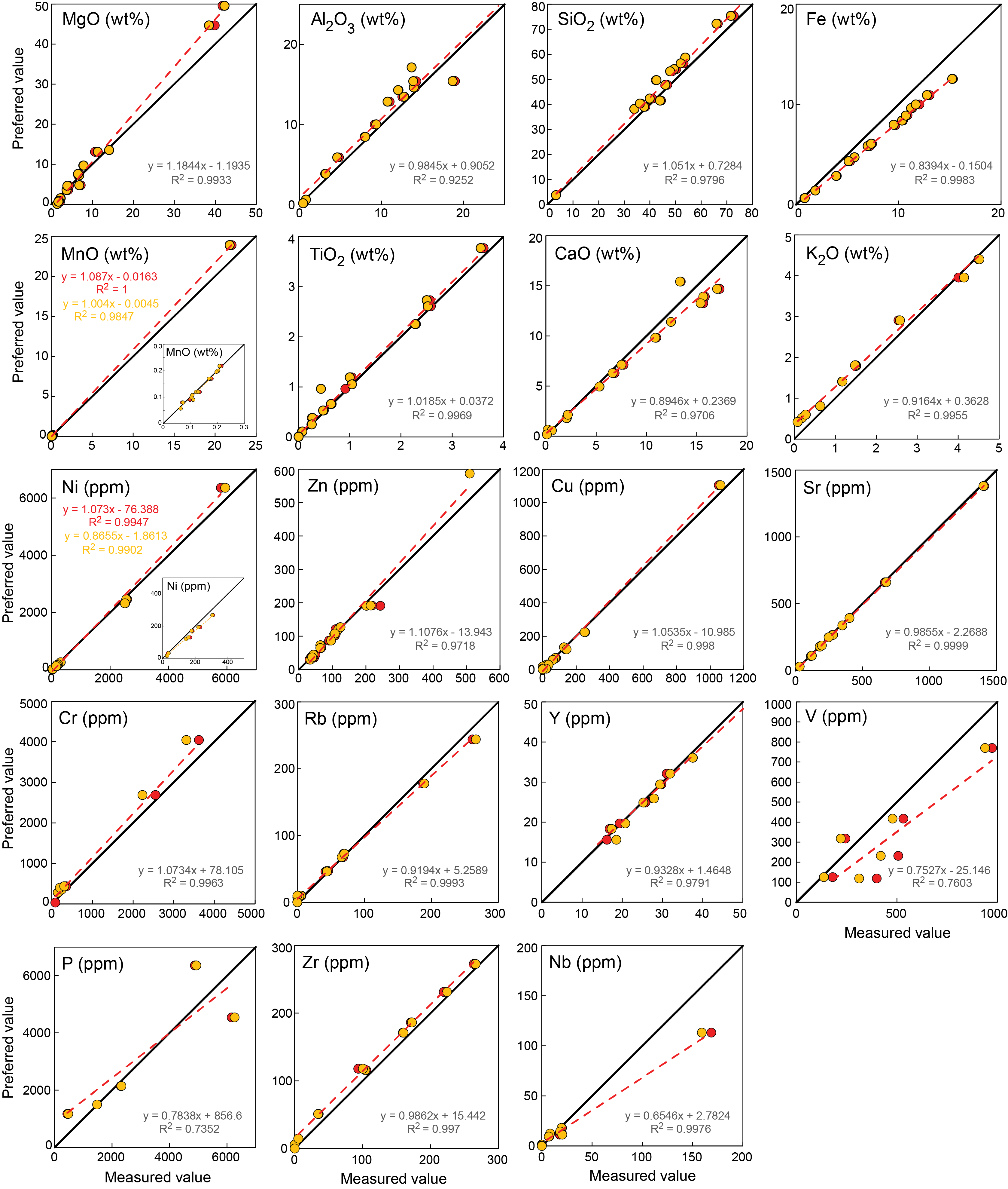
Figure F20. Calibration curves.
5.4.1.1. Portable X-ray fluorescence calibration of geologic materials
Calibration curves for the different elements measured via pXRF were determined using the same suite of standard reference materials used for ICP-AES analyses to improve interinstrument data comparisons (Table T8). Powder mounts for each of the reference materials were analyzed to develop the calibration lines. Slope and intercept values from the calibration lines were used to correct concentration results for unknowns (Figure F21). Analyses of reference materials were repeated at the end of the expedition to detect potential drift with time. No significant change was observed. Both rock and powder samples were analyzed using powder-based working curves because past results indicated no differences in instrument performance between rocks and powders (Ryan et al., 2017; Reagan et al., 2015). Following the approaches taken during IODP Expeditions 352 and 366, we made interpretive quantitative use of pXRF data for elements with calibration curves with high correlation r values (>0.95) and good intercepts. These elements were Ca, K, Ti, and Mn (calibrated as oxides: CaO, K2O, TiO2, and MnO) and Fe, Ni, Cr, Cu, Zn, Sr, Rb, Zr, and Y. For MnO and Ni, two calibrations curves were built: one for samples with >1 wt% MnO and >1000 ppm Ni (red dashed lines in Figure F20), and one for samples with <1 wt% MnO and <1000 ppm Ni (orange dashed line). An insufficient number of standards were available with sulfur data to produce a reasonable working curve. Analyses of P, Nb, and V were only considered as qualitative. For Si, Mg, and Al (i.e., elements that produce low-energy X-rays that are readily absorbed in air), we used the pXRF results to aid in lithologic identification prior ICP-AES analyses.
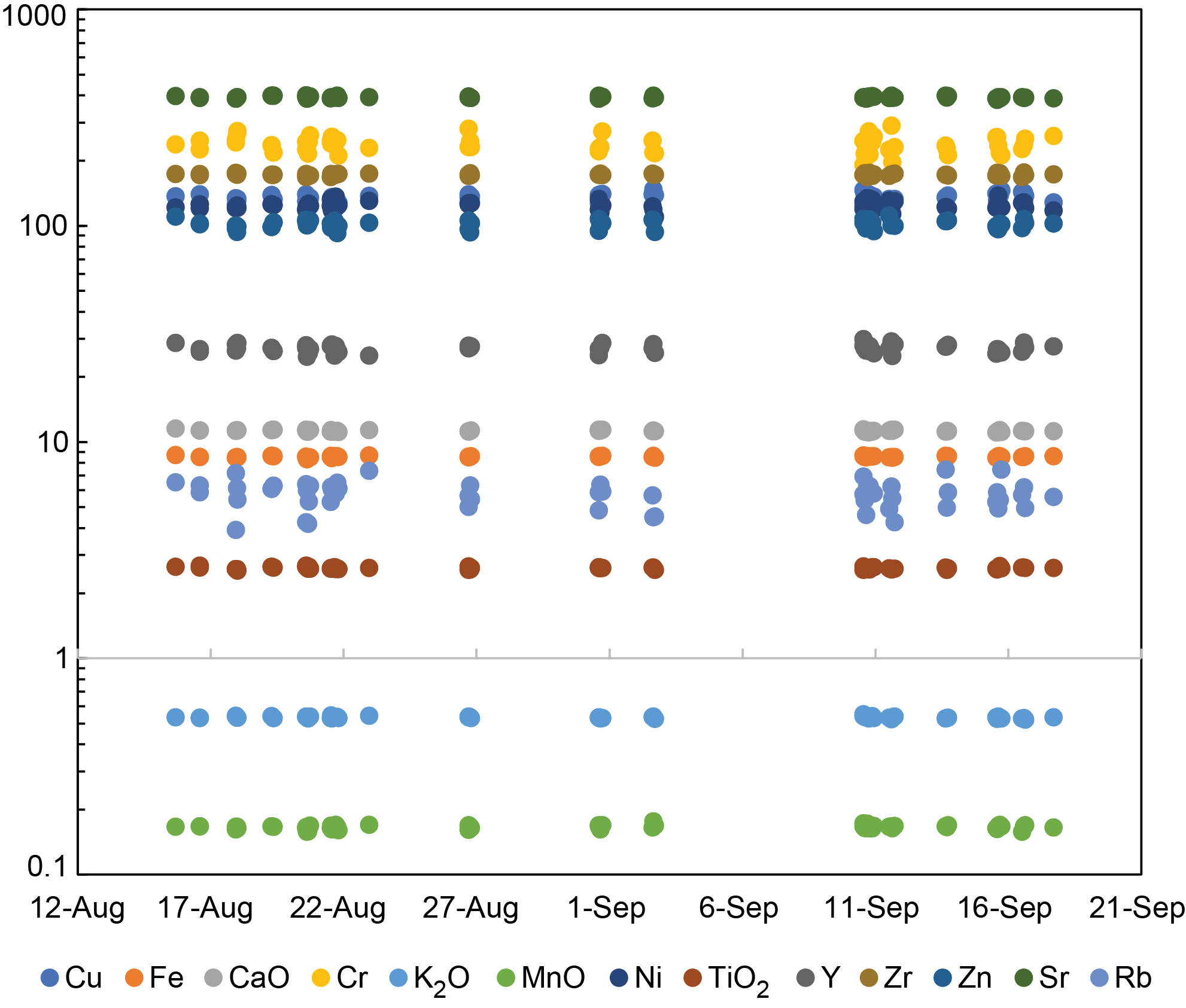
Figure F21. BHVO-2 composition over time.
Unknown samples were measured manually for 60 s, and three measurements per unknown constituted a single analysis. On sites where alternating sequences of basalts and sediments were observed (Sites U1566, U1571, U1572, and U1573), at least one analysis per core was performed. When multiple flows were observed (defined by the presence of a chilled margin or the presence of interbasaltic sediments), one analysis per flow was performed. Analyses performed on standard BHVO-2 as an unknown show that TiO2 and Cr are slightly underestimated and K2O and Rb are slightly overestimated. All other elements overlap with the preferred value (Table T8) (Jochum et al., 2016).
5.4.5. Deconvolution of natural gamma radiation spectra
To attain an estimate of the amount of K, Th, and U in the samples, we used the approach of De Vleeschouwer et al. (2017) to deconvolve the NGR spectra (see Physical properties). Briefly, this approach utilizes an algorithm to first remove the background data from the spectra and isolate the characteristic gamma ray (GR) peaks of the three decay series (40K, 232Th, and 238U). The algorithm then integrates the counts over these specific spectral regions to attain estimates of concentration for each of the measured samples. For this deconvolution, we used the raw spectral output of the NGR measurements and the bulk density estimates of the GR attenuation (GRA) method (see Physical properties). The algorithm code, published in De Vleeschouwer et al. (2017), was run in Matlab R2021a.
6. Physical properties
Physical properties measurements were made utilizing a variety of techniques applied at various stages of the core recovery and archiving process to aid lithostratigraphic characterization, magnetostratigraphy, core-log-seismic integration, and hard rock reservoir characterization. Physical properties include NGR; P-wave velocity; bulk, grain, and dry density; porosity; MS; thermal conductivities; and X-ray and photo imaging. Measurements were taken on whole-round and section-half cores and various discrete samples to integrate all available scales.
6.1. General sampling and measurement sequence
Prior to sampling and analyses, whole-round cores were allowed to equilibrate at ambient room temperature (~20°C) and pressure for at least 4 h. X-ray images of the whole rounds were typically taken with the XMSL during this equilibration period. After thermal equilibration, core sections were run through the WRMSL for GRA bulk density, MS, and compressional wave (P-wave) velocity using the P-wave logger (PWL).
Thermal conductivity was measured on at least one whole-round section per core (typically chosen from a section central to the retrieved core) for sediment cores and on one or more hard rock intervals per core according to lithofacies variations. For soft sediments, thermal conductivity was measured using a needle probe inserted into the section through a small hole drilled into the plastic core liner in the middle of the section. Where sediment cores were too hard to insert the needle probe, and for hard rock samples, a contact probe was used on the section-half surface after core splitting. The contact probe was not used on section halves that were heavily disturbed (e.g., biscuited).
MSP and color reflectance were measured on the archive-half sections using the SHMSL. P-wave velocity measurements were made on every working-half section and were typically chosen from undisturbed areas close to moisture and density (MAD) samples, along with other sections of interest based on lithology variations, and for sections that were not measured adequately on the whole round by the PWL. Discrete samples were collected from the working halves at a sampling density of one per section to one per core depending on lithology variations and section sampling history (i.e., a reduced number of samples were taken for the secondary holes that drilled overlapping sections previously sampled with Hole A). These samples were then used to measure wet and dry mass, volume, and P-wave velocities. Wet and dry mass and volume were used to calculate wet bulk density, dry bulk density, water content, porosity, and grain density with MAD procedures. In addition, selected whole-round samples and minicores (diameter = 2.5 cm; perpendicular to the core axes) of hard rock were sampled for specific postcruise research objectives requiring larger samples. In such cases, the core sections were scanned using the WRMSL and 360° images were taken prior to minicore drilling.
Details on the analytical protocols and performance, including variations for sedimentary and hard rock cores, are described in the relevant sections below (Figure F22; Table T10). Only raw data as retrieved from the physical properties instruments have been deposited in the LIMS database. Processing the data according to the information in Processing and data availability is recommended to retain only high-confidence data. Details on the physical properties measurement systems and theory in this chapter benefited significantly from the extensive previous IODP expedition methodologies (including Tamura et al., 2015a; Sun et al., 2018; Sutherland et al., 2019).

Figure F22. Soft and hard rock workflows.
6.2. Whole-Round Multisensor Logger measurements
GRA bulk density, P-wave velocity, and MS were measured nondestructively using the WRMSL (Figure F23). To optimize the measurement process and for consistency, uniform sampling intervals (2.5 cm) and measurement integration times (5 s/measurement) were set for all sensors. These sampling intervals are common factors for the distances between the sensors installed on the WRMSL (30–50 cm), which allows sequential and simultaneous measurements. QC was ensured by running a single core liner filled with deionized water through the WRMSL after every core run. Where deviations from expected values were observed, recalibrations were applied as needed.
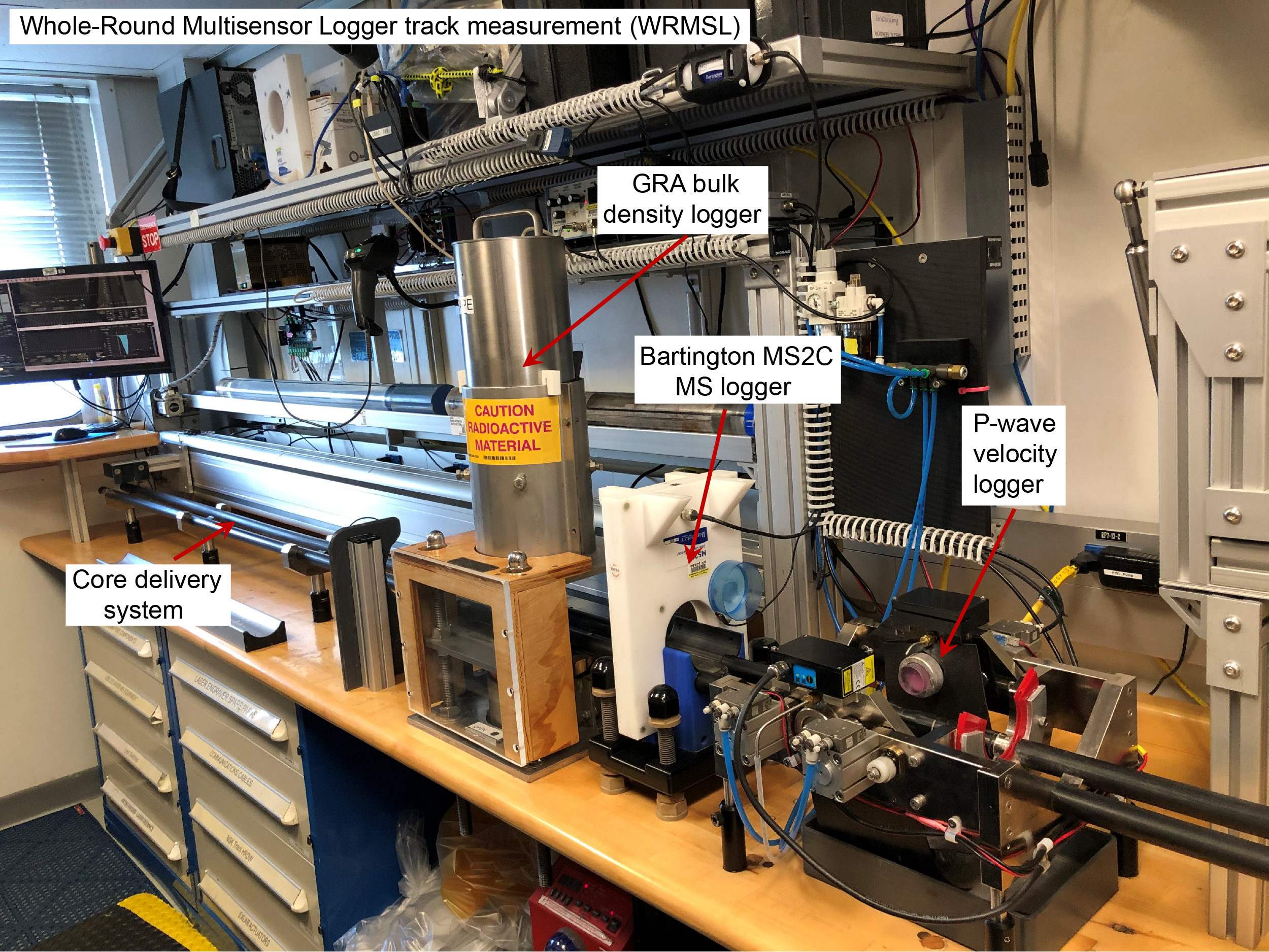
Figure F23. WRMSL.
6.2.1. Gamma ray attenuation bulk density
Bulk density is a fundamental rock property that can be used to estimate the pore volume in rocks where grain density is either measured or can be reasonably estimated. It is integral to rock physics and core-log-seismic applications. GRA bulk density is an estimate of bulk density based on the attenuation of a GR beam. The beam is produced by a 137Cs GR source at a radiation level of 370 MBq within a lead shield with a 5 mm collimator that is directed through the whole-round core. The GR detector on the opposite side of the core from the source includes a scintillation detector and an integral photomultiplier tube to record the gamma radiation that passes through the core. The attenuation of gamma rays occurs primarily by Compton scattering, in which gamma rays are scattered by electrons in the sample, with the degree of scattering related to the material bulk density. Therefore, for a known thickness of sample, the density (ρ) is related to the intensity of the attenuated gamma rays and can be expressed as follows:
- I = measured intensity of gamma rays passing through the sample,
- I0 = GR source intensity,
- µ = Compton attenuation coefficient, and
- d = sample diameter.
µ and I0 are treated as constants, such that ρ can be calculated from I.
The spatial resolution of the GRA densitometer is less than ±1 cm. The GR detector is calibrated with sealed calibration cores (one standard core liner filled with distilled water and aluminum cylinders of various diameters). To establish the calibration curves, GR counts were taken through each aluminum cylinder for 60 s. Each aluminum cylinder has a density of 2.7 g/cm3, and d is 1, 2, 3, 4, 5, or 6 cm. The relationship between I and µd is as follows:
where A, B, and C are coefficients determined from the calibration. Recalibration was performed as needed when the deionized water QC standard density deviated significantly (more than a few percent) from 1 g/cm3.
6.2.2. Magnetic susceptibility
MS (χ) is a dimensionless measure of the degree to which a material can be magnetized by an external magnetic field:
where M is the magnetization induced in the material by an external field of strength H. MS is primarily sensitive to the concentration of ferrimagnetic minerals (e.g., magnetite and maghemite). MS can also give insights into magnetic mineral origins and subsequent diagenetic processes, and in igneous rocks, MS may be reduced by orders of magnitude due to extensive alteration, for example from magnetite to maghemite or to hematite.
MS was measured using a Bartington MS3 susceptometer coupled with a Bartington MS2C loop sensor with an 8 cm internal diameter that comes precalibrated. An oscillator circuit in the sensor, which operates at a frequency of 0.565 kHz and an AF of ~140 A/m, produces a low-intensity, nonsaturating alternating magnetic field. Sediment or hard rock core sections passing through this field cause a change in oscillator frequency. Frequency information returned in pulse form to the susceptibility meter can then be converted into MS.
6.2.3. Compressional P-wave velocity
Core measurements of sonic P-wave velocity data forms a vital link for core-log-seismic integration and for the associated scaling up of lithofacies inferences. P-wave velocity can also be used to estimate porosity, especially where downhole conditions are poor, such as caved sections, and forms a vital component of geomechanical and stress state calculations. P-wave velocity (VP) is defined by the time required for a compressional wave to travel a specific distance:
where dcore is the path length of the wave across the core and tcore is the traveltime through the core. P-wave velocity was measured on whole-round cores using the PWL. The P-wave velocity systems use Panametrics-NDT Microscan delay line transducers, which transmit a 500 kHz pulse.
The PWL measures the traveltime of 500 kHz ultrasonic waves horizontally across the whole-round core at 2 cm intervals with the core still in the liner. Waves are transmitted to the core by transducer contacts connected to linear actuators. Pressure is applied to the actuators to ensure coupling between the transducers and the core liner, and the space between the core liner and transducers is kept wet to ensure good coupling. P-wave velocity transducers measure total traveltime (t) of the compressional wave between transducers separated by the total distance (d) measured using a laser beam. By measuring the traveltime through a standard block of aluminum with a known velocity (6295 m/s), a system delay correction (δt) is defined. The core is surrounded by a core liner of known thickness (δL), and a traveltime correction (δtL) is determined by measuring through the core liner filled with distilled water of known velocity, which is corrected for the influence of temperature. Arrival times are taken for the second lobe of the waveform, requiring a correction (δtpulse) to get the first arrival. The velocity in the core is as follows:
P-wave measurements are not typically made on the WRMSL for cores drilled with the XCB and RCB systems because the smaller core diameters generally result in poor contacts and noise results. However, we made the decision to keep logging the P-wave velocities for sediments whenever possible and quality check the signal by measuring discrete samples using the P-wave calipers (PWC) and P-wave bayonets (PWB). For lithified sediments and hard rock samples, the PWL was turned off and P-wave velocity was instead measured using the PWC on section halves or discrete cube samples prior to MAD analyses.
6.3. Natural Gamma Radiation Logger measurements
NGR data are critical for several aspects of borehole studies, including identification of various lithostratigraphic units, stratigraphic correlation, core-log calibration, and chemical/mineralogic appraisal. For sedimentary sequences, NGR data often give important insights into grain size. Fine-grained sediments often contain NGR attenuating isotopes of K, Th, and U. For volcanic rocks, NGR data give important insights into igneous differentiation (basic rocks = low NGR; evolved rocks = high NGR) and alteration processes. In sedimentary successions, NGR can also reveal important constraints on the presence and composition of volcanic ash layers.
NGR is emitted from the decay of 238U, 232Th, and 40K in the core sample. The NGRL measures gamma emissions on whole-round cores using a system designed and built at Texas A&M University (USA) (Vasiliev et al., 2011; Dunlea et al., 2013) (Figure F24). When 238U, 232Th, and 40K radioisotopes decay, NGR is emitted at specific energy levels. NGR spectroscopy measures a wide energy spectrum that can be used to estimate the abundance of each isotope based on the strength of the signal at characteristic energies (Blum, 1997; Gilmore, 2008). Spectral data were collected and can be used for processing for U, Th, and K abundance calculations (see Geochemistry).

Figure F24. NGRL.
The main NGRL detector unit consists of eight sodium iodide (NaI) detectors arranged along the core measurement axis at 20 cm intervals surrounding the lower half of the section (Vasiliev et al., 2011). The detector array has passive (layers of lead) and active (plastic scintillators) shielding to reduce the background environmental and cosmic radiation. The overlying plastic scintillators detect incoming high-energy NGR and cosmic radiation and cancel this signal from the total counted by the NaI detectors. The quality of the energy spectrum measured in a core depends on the concentration of radionuclides in the sample but also on the counting time, with higher times yielding better spectra. Therefore, a measurement run consisted of 10 cm spaced, 300 s interval counts on each core. Calibration of the NGRL was done in January 2021 according to standard IODP protocols. No calibration of NGRL spectra for analyses of 40K, 238U, and 232Th concentrations was conducted during Expedition 396.
6.4. Thermal conductivity measurements
After NGR measurements were completed, thermal conductivity was measured with the TK-04 (Teka Bolin) system Figure F25). Thermal conductivity defines how material conducts heat and is essential to determine heat flow and geothermal gradient. Thermal conductivity was measured for all types of rocks recovered during Expedition 396. A needle probe tool was used on the soft sediments of whole-round cores if the material was soft enough to be penetrated effectively (Von Herzen and Maxwell, 1959). The probes contain a heater wire and a calibrated thermistor. For soft sediments, the needle probe was inserted into a 2 mm diameter hole drilled through the liner along one of the lines that guided later core splitting. To avoid interference from air flow in the laboratory, the core was placed in an enclosed foam insulated box.
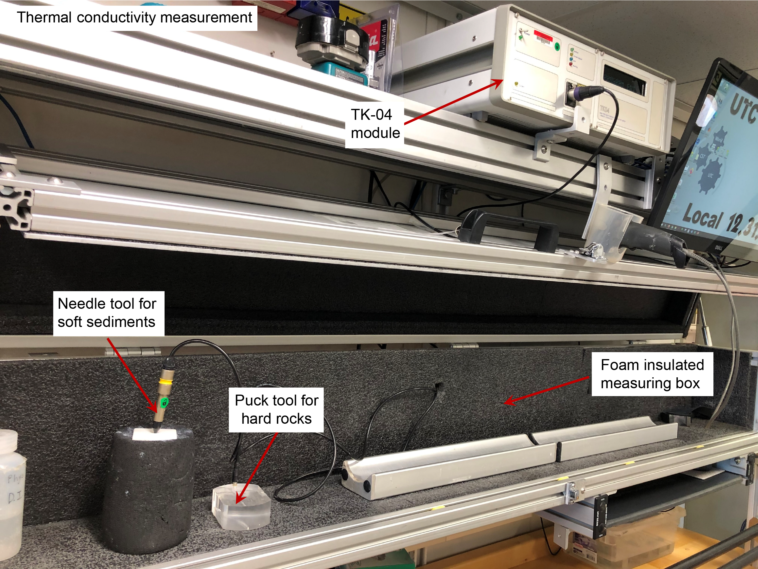
Figure F25. Thermal conductivity station.
A contact probe method with the puck tool was used on section-half cores for lithified sediments and hard rock samples that were selected from the working-half sections and returned unaltered to the core liner upon completion of the measurements. The contact probe was embedded in the surface of an epoxy block with a low thermal conductivity (Vacquier, 1985) and was maintained in contact with the sample. For igneous rock samples, both the rock and probe were equilibrated together in a bath of seawater at room temperature in a cooler insulated with extruded polystyrene foam.
The calibrated heat source of the probe was then turned on, and the increase in temperature was recorded over 80 s. A heating power of 2.5 W/m was typically used. The solution to the heat conduction equation with a line source of heat was then fitted to the temperature measurements to obtain the thermal conductivity. Because the probe is much more conductive than sediment or hard rock, the probe is assumed to be a perfect conductor. Under this assumption, the temperature of the superconductive probe has a ( linear relationship with the natural logarithm of the time after the initiation of the heat:
- T = temperature (K),
- q = heat input per unit length per unit time (J/m/s),
- k = thermal conductivity (W/[m·K]),
- t = time after the initiation of the heat (s), and
- C = instrumental constant.
Three measuring cycles were automatically performed to calculate average conductivity. A self test, which included a drift study, was conducted at the beginning of each measurement cycle. Once the probe temperature stabilized, the heater circuit was closed and the temperature rise in the probe was recorded. Thermal conductivity was calculated from the rate of temperature rise while the heater current was flowing. Temperatures measured during the first 80 s of the heating cycle were fitted to an approximate solution of a constantly heated line source (Kristiansen, 1982; Blum, 1997). Measurement errors were typically 5%–10%. Thermal conductivity measurements were routinely taken in one section per core (usually the third section of each core).
6.5. X-Ray Multisensor Logger
X-ray imaging provides a powerful tool for appraising internal features of core samples from either whole-round or section-half cores. X-ray images can give insights into features such as fractures, bedding, shells, dropstones, clast variations, and burrows in sediments and features such as jointing, vesicles, clast morphology, and alteration in igneous samples. The XMSL aboard JOIDES Resolution (Figure F26) is composed of a 120 kV, 1 mA constant potential X-ray source and a detector unit. The source is a Teledyne ICM CP120B portable X-ray generator with a 0.8 mm × 0.5 mm focal spot. The beam angle is 50° × 50°, generating a directional cone onto the detector, which is located 65 cm from the source. The detector is a Go-Scan 1510 H unit composed of an array of complementary metal oxide semiconductor (CMOS) sensors with an active area of 102 mm × 153 mm and a resolution of 99 µm. A voltage is established between the filament and the material used for X-ray generation (kVp), and a current is run through a filament, heating it up and emitting electrons. The number of electrons is controlled by the current (mA), and the electrons collide with the anode material (e.g., Rh or W), leading to the generation of broad-spectrum X-rays that exit the tube through a window of thin metal (typically Be) to minimize absorption. The XMSL is run by the Integrated Measurement System (IMS) XMSL software application, which can optimize acquisition and image processing. Typically, 20 images are collected and stacked to create a composite 2-D image. These images are processed using the Image Processing Utility to optimize observed features.
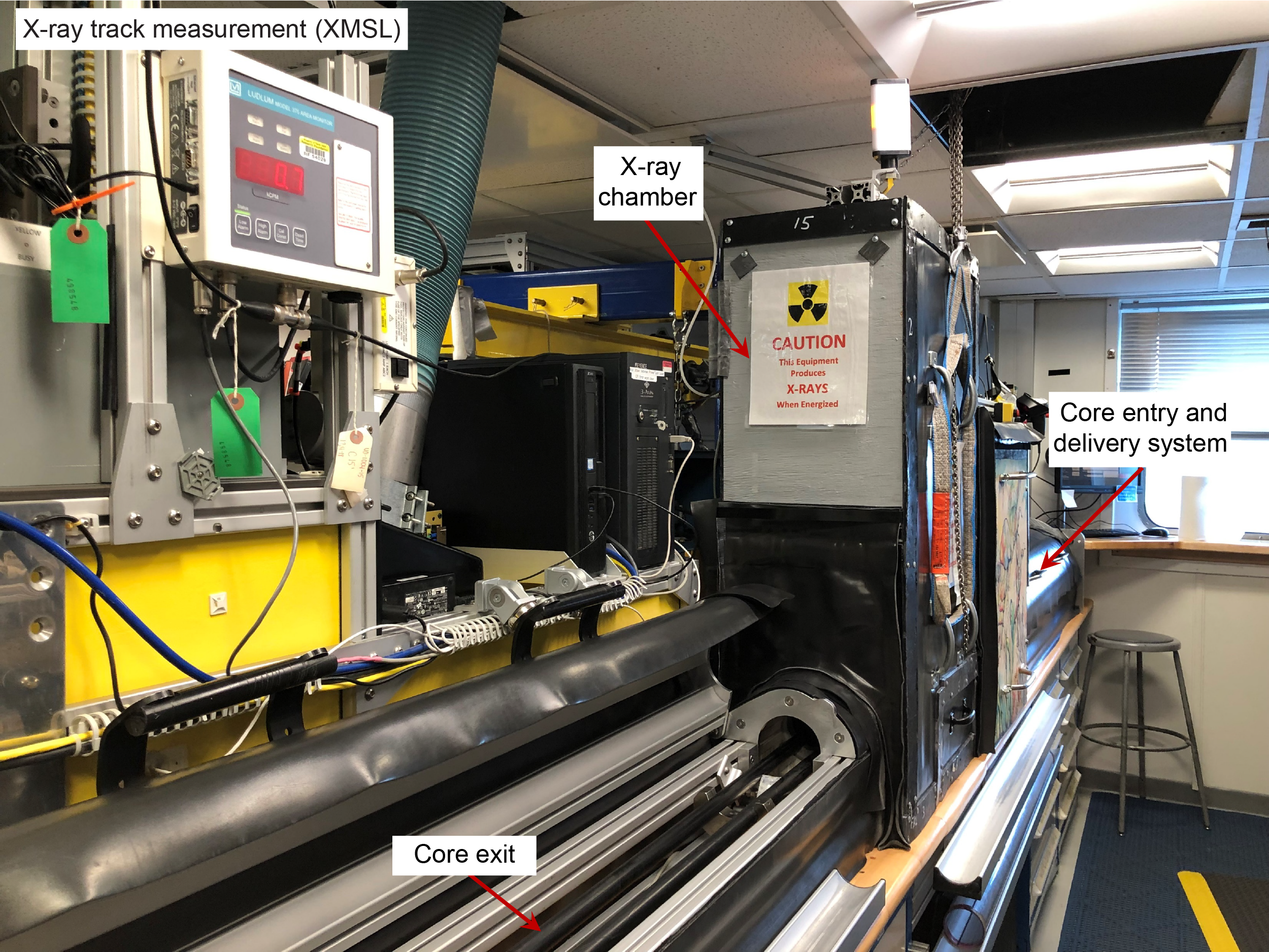
Figure F26. XMSL.
6.6. Section Half Multisensor Logger measurements
Color reflectance and MS were measured on the archive-half sections using the SHMSL. The archive half of the split core was placed on the core holder under a track-mounted electronic platform that moves along the core recording the height of the split-core surface with a laser sensor. MSP and color reflectance are measured. All foam inserts were removed from the section-half cores before measurement to restrict the measurements to the core material only. MSP and color reflectance data were collected at constant intervals of 2.5 cm for each core.
The color reflectance spectrometer uses an Ocean Optics 30 mm integrating sphere with both halogen and LED light sources covering wavelengths from ultraviolet through visible to near infrared. Measurements were taken from 380 to 900 nm wavelengths at 2 nm intervals. The approximate 3 s data acquisition offset was applied for the entire scan of the archive-half section. The data are reported using the L*a*b* color system, in which L* is lightness, a* is redness (positive) versus greenness (negative), and b* is yellowness (positive) versus blueness (negative) of the rock. The color reflectance spectrometer calibrates on two spectra, pure white (reference) and pure black (dark). Color calibration was conducted automatically approximately once every 6 h (twice per shift).
6.6.1. Point magnetic susceptibility
MSP was measured with a Bartington MS2 meter and an MS2K contact probe with a flat 15 mm diameter round sensor with a field of influence of 25 mm and an operation frequency of 930 Hz. The instrument averages three measurements from the sensor for each offset, leading to an accuracy of ~5%. The spatial resolution of the MSP instrument is ~3.8 mm, significantly higher than that of the whole-round MS at 23–27 mm. This resolution is useful for core sections containing smaller broken pieces. The output displayed by the MSP sensor must be converted to dimensionless SI units by multiplying by 10−5. The probe was zeroed in air before each measurement location to avoid influence from the metal track. The MSP meter was calibrated by the manufacturer before installation on the ship and is quality checked approximately every 6 h simultaneously with color reflectance sensor calibration.
6.7. Digital color imaging
The SHIL captures continuous high-resolution images of the archive-half surface to aid analysis and description. The system was used to image both dry and wet sections and uses a commercial linescan camera lens (AF Micro Nikon; 60 mm; 1:2.8 D). Illumination is provided by a custom assembly of three pairs of light-emitting diode strip lights that provide constant illumination over a range of surface elevations. Each pair of lights has a color temperature of 6,500 K and emits 90,000 lux at 3 inches. The resolution of the linescan camera was set at 10 pixels/mm. The focus area for analyses is targeted by cropping the analytical field to optimize operations. Images are saved as high-resolution TIFF files along with a gray scale and ruler and reduced JPEG images cropped to show only the section-half surfaces.
6.8. Section Half Measurement Gantry measurements
For soft-sediment cores, P-wave velocity measurements were performed on working-half cores before any samples were taken. P-wave velocity measurements were taken using the x-axis PWC and z-axis PWB contact probe transducers on the Section Half Measurement Gantry (SHMG) (Figure F27), and typically one analysis was completed every other section. The y-axis PWB was collected for the first two holes, but because of consistently poor coupling of the probes to the sample and generally poor or erroneous results, this measurement was dropped from the analytical program. For the same reason, the z-axis PWB measurements were not taken for hard sediments and rocks. Measurements were usually taken from the least disturbed parts of the section depending on core recovery because good core/transducer coupling is a requirement for viable data. XCB cores sometimes did not provide usable data because of bad sediment/liner contact and disturbed sediment.

Figure F27. SHMG.
Velocity variations within the hard rock volcanic sequences are crucial for the scientific objectives of Expedition 396, and as such, high-resolution P-wave measurements were taken using the PWC throughout the cored sections. Early in the process of measuring P-wave velocities it was realized that removing half-round hard rock sections (individual core pieces typically 5–30 cm long) from the core liner for PWC P-wave measurements returned superior signal-to-noise ratios and in turn enabled significantly more measurements per core section than with the in-liner method.
Providing wet and dry results, P-wave velocities in x-, y-, and z-orientations using the PWC were also measured on the discrete ~8 cm3 cubes chosen for both physical properties (MAD) and paleomagnetic measurements. Cubes were first saturated with seawater in a vacuum cell for 12 h prior to the first P-wave velocity measurement, and a second measurement was made after drying for 24 h at 105°C during standard MAD procedures.
The PWC measures the traveltime of 500 kHz ultrasonic waves vertically across the section half while still in the half liner at selected intervals or on discrete sample cubes cut from the section halves. The distance between transducers is measured with a built-in linear voltage displacement transformer and regular calibration was performed using acrylic cylinders of differing thicknesses with a known P-wave velocity of 2730 ± 20 m/s. The calibration-derived system time delay was subtracted from the picked arrival time to give a traveltime of the P-wave through the sample. The thickness of the sample after appropriate subtraction of the liner thickness was divided by the traveltime to calculate P-wave velocity in meters per second. All first arrival picks for P-wave measurements were manually quality controlled and revised from the automatic picking function, which often underestimated the first-break arrival by ~50–300 m/s for fresh samples with a good signal and often became unreliable for noisier signals (e.g., within interlava sediments).
6.9. Discrete sample measurements
Discrete samples were collected from the working-half sections to measure wet and dry mass and dry volume and to calculate wet bulk density, dry bulk density, water content, porosity, and grain density using MAD procedures (Figure F28). Soft-sediment samples were collected in ~10 cm3 volume plastic syringes. Samples were typically taken from every other core section (e.g., Sections 1, 3, and 5). Lithified sediment and hard rock lithologies were also sampled via minicores or small pieces from the working-half sections for physical properties measurements, and samples from igneous basement were also used for paleomagnetic measurements.

Figure F28. MAD equipment.
Soft-sediment samples were placed in numbered, preweighed, ~16 mL Wheaton glass vials for wet and dry sediment weighing, drying, and dry volume measurements. To accurately determine the wet mass of minicore samples, the pore space of the samples must be completely saturated with seawater. To achieve this, samples were placed in individual plastic vials filled with seawater in a vacuum chamber. Air was removed from the chamber using a vacuum pump at pressures of ~40–50 kPa below atmospheric pressure, forcing seawater into the samples. Samples were kept saturated for at least 24 h, and the vacuum was maintained in the chamber by turning the pump on for 30 min every 5 h. Minicores were patted dry with a paper towel after removal from the saturator before the wet mass was determined immediately afterward using the dual balance system. P-wave velocities were then also measured on the wet samples. Samples were then dried in a convection oven for at least 24 h at 105° ± 5°C, followed by cooling of the dried samples in a desiccator for at least 4 h before the dry mass and the volume were measured. P-wave velocities were then measured on the dry samples to appraise saturation effects on velocity.
Weights of wet and dry sample masses were determined to a precision of 0.005 g using two Mettler Toledo electronic balances, with one acting as a reference. A standard weight of similar value to the sample was placed upon the reference balance to increase accuracy. The ship’s motion was also compensated for using a computer averaging system, with the default setting of the balances collecting 300 measurements and taking approximately 1.5 min.
The volume of porous samples that cannot be confidently saturated, such as vesicular basalts, was determined by caliper measurements, resulting in a wet volume. Each dimension was either measured manually (i.e., the mean of at least three measurements) with an EZCal Fractional Digital Caliper (precision = 0.01 mm) or extracted from the PWC measurements on discrete wet samples. Height, width, and length were measured for cubes, and length and diameter were recorded for cylinders (e.g., minicores).
The volume of dry samples was determined using a hexapycnometer system of a six-celled, custom-configured Micrometrics AccuPyc 1330TC helium-displacement pycnometer. The precision of each cell is 1% of the full-scale volume. The sample chamber was purged three times with helium warmed to ~28°C prior to volume measurement, and three measurement cycles were run for each sample. A reference volume (a set of two calibration spheres) was placed sequentially in one of the chambers to check for instrument drift and systematic error. The volumes occupied by the numbered Wheaton vials were calculated before the cruise by multiplying each vial’s weight against the average density of the vial glass. The procedures for the determination of these physical properties comply with the American Society for Testing and Materials (ASTM) designation (D) 2216 (ASTM International, 1990). The fundamental relation and assumptions for the calculations of all physical properties parameters are discussed by Blum (1997) and summarized below.
MAD properties reported and plotted in the physical properties section of the site chapter were calculated with the MADMax shipboard program (v 2.0.0.7). Two submethods (C and D) were applied to calculate mass and volume, depending on suitability of the sample, and are explained in greater detail below.
Submethod C is only suitable for fine-grained, saturated sediments or fine-grained igneous materials. It requires known wet mass (Mwet), dry mass (Mdry), and dry volume (Vdry) to calculate densities and porosities. Salt precipitated in sediment pores during the drying process is included in the Mdry and Vdry values. The mass of the evaporated water (Mwater) and salt (Msalt) in the sample are given as follows:
where s is the assumed saltwater salinity (35‰) corresponding to a pore water density (ρpw) of 1.024 g/cm3 and a salt density (ρsalt) of 2.22 g/cm3. The corrected mass of pore water (Mpw), volume of pore water (Vpw), mass of solids excluding salt (Msolid), volume of salt (Vsalt), volume of solids excluding salt (Vsolid), and wet volume (Vwet) are as follows:
Submethod D is suitable for porous rocks that cannot be confidently saturated. The submethod requires known dry mass (Mdry), wet volume (Vwet), and dry volume (Vdry), from which saturated wet mass, porosity, and densities can be calculated. Total (Mt), wet (Mwet) and pore water mass (Mpw), and pore water volume (Vpw) are calculated as follows:
where the volume ratio (rv) is a computational constant of 0.988 (corresponding to 0.988 cm3 of freshwater per 1 cm3 of seawater), and Vpw, ρpw, and ρwater are the volume and density of the pore water and water (1 g/cm3), respectively. The water density (ρwater) is a computational constant of 1. Pore water density is a computational constant and assumes a salinity of 35‰. The mass and volume of the solids is then calculated as follows:
Regardless of the chosen submethod, water content (w) is expressed as the ratio of mass of pore water to wet sediment (total) mass:
Wet bulk density (ρwet), dry bulk density (ρdry), sediment grain density (ρsolid), porosity ( φ), and void ratio (VR) are calculated as follows:
6.10. Processing and data availability
All acquired data and metadata have been archived in the LIMS database without further processing aside from instrument-specific acquisition parameters. Data appraisal and filtering of these data were applied to the results described in the site chapters. Data appraisal did not include removal of data associated with intervals interpreted as fall-in (see Lithostratigraphy). The outlined data appraisal was automated through use of custom Python scripting (Betlem et al., 2022) that takes LIMS data (in CSV format) and exports statistics (in Microsoft Excel format) and LAS files compatible with Advanced Logic Technology WellCAD and Schlumberger Petrel/TechLog software.
Hard rock whole-round cores are separated into different segments during sample curation prior to whole-round scanning, and extra space is added between core pieces. The raw measurements on sections dominated by hard sediments and rocks (in XCB or RCB cores) should therefore be taken with caution because the void space in the core liner affects density values as exemplified by increased scatter in whole-round core scanning data and the recording of untenably low values of GRA bulk density and P-wave velocities.
WRMSL measurement accuracy is affected by both the core diameter and competence (degree of core disturbance/breakages), with thin diameter or damaged cores often leading to measurement underestimates compared to true values. As a standard, the instrument reports measurements using the internal diameter of the common core liner (66 mm) as the assumed sample diameter. This assumption is suitable for typical sediment cores obtained by the APC system. However, for sediment and/or hard rock cored by the XCB or RCB systems, core diameter is often around 58 mm or less. Following Jarrard and Kerneklian (2007), the GRA bulk density measurements of cores obtained using the XCB or RCB system may be corrected by multiplying the density values by 66/58 = 1.138 to account for this bias. Caliper measurements of whole-round core diameters at Site U1565 were taken to appraise this factor (see Physical properties in the Site U1565 chapter [Planke et al., 2023b]), confirming its applicability; this liner correction was then applied for GRA bulk density values as part of the processing procedures.
To address scatter in the WRMSL data, any values measured within ± 1.5 cm of the core piece dividers (recorded during curation; see LIMS database) were filtered out of the WRMSL GRA bulk density and P-wave velocity data. Unlike the GRA density sensor and P-wave velocity caliper, the MS meter can still deliver important information about sample properties even with a very low core-to-liner volume ratio. For example, if a small recovered core volume has high MS, it still gives a clear signal. MS values were therefore not filtered based on bin proximity but were screened to remove all negative values.
Because of the larger integration volume of the NGR compared to the WRMSL, no standard data removal was undertaken based on hard rock core piece spacers. However, all NGRL data were screened to remove clearly anomalous negative values, along with those values with errors above 20%.
As a final standardized quality assurance step, the acquired data were screened against property-specific thresholds, as reported in the site chapters. WRMSL and PWC P-wave velocity data implemented a lower cutoff of 1480 m/s, below which values were removed during processing. GRA bulk density data screening typically implemented a lower threshold of 1.2 g/cm3, 1.5 g/cm3 for certain hard rock successions (as reported in the site chapters), corresponding in each case to a value significantly below realistic minimum bulk density for the encountered lithologies; as such, these thresholds are regarded as conservative.
Discrete sample MAD data were filtered based on realistic minimum bulk and grain density values of 1 g/cm3. MAD data calculated by Submethod A were removed in line with IODP recommended practice.
The LIMS database reports calculated thermal conductivity values that should be ignored because they are calculated regardless of whether robust measured values were obtained. Instead, mean measured thermal conductivity readings at identical intervals (typically up to three are taken during a single measurement) are provided and should be used for further analyses. Special caution should be given to measurements consisting only of a single reading, which have failed the triplicate measurement that is in place to ensure repeatability.
7. Downhole measurements
Wireline logging tools were deployed in eight holes during Expedition 396 to determine the physical, chemical, and structural properties of the drilled formations. Wireline deployed logging tools collect continuous data series at logging speeds up to several hundreds of meters per hour and measure the in situ properties of the drilled formations. Wireline logging data have several advantages over core measurements because the core recovery is often incomplete and the cores are variably damaged and nonuniformly spaced because of partial recovery. In addition, cores undergo changes due to extraction such as pressure release, cooling, and drying, which can have a potentially significant influence on surface measurements. Together with core-based data calibration, logging data enables drilled holes to be interpreted in terms of the continuous stratigraphy, lithology, mineralogy, magnetic characteristics, and geochemical composition of the penetrated formation along with assessments of in situ stress states in holes where image logs are acquired. Logging data are also integral to the accurate depth matching and stratigraphic interpretation of boreholes with incomplete core recovery.
Downhole logs measure formation properties on a scale that is intermediate between those obtained from laboratory measurements on core samples and those from geophysical surveys such as seismic-gravity-magnetics and therefore form a critical component for accurate core-log-seismic integration. Details on the wireline logging tool instrumentation and background measurement theory in this chapter are compiled based on extensive previous IODP expedition methodologies (including Tamura et al., 2015a; Sun et al., 2018; Sutherland et al., 2019).
7.1. Logging tool strings
During wireline logging operations, data were collected with Schlumberger logging tools combined into several tool strings and lowered into the hole after completion of coring operations. Four IODP tool string configurations were used (Figure F29). The modified triple combo tool string was typically run first to measure borehole fluid temperature, NGR, bulk density, and photoelectric effect (PEF), electrical resistivity, and MS. The FMS-sonic tool string was typically run next to measure sonic velocity (P-wave [VP] and S-wave [VS]) and FMS resistivity images of the borehole wall. The UBI, which gives acoustic amplitude images of the borehole wall, was run in Holes U1566A and U1571A only. The VSI tool string, which is used to generate a vertical seismic profile (VSP), was run in Hole U1566A only. Each tool string also contains an EDTC for communicating through the wireline to the Schlumberger data acquisition system (i.e., MAXIS on the drillship). The main tool strings, their measurements, and their typical resolutions are summarized in Table T11. A summary of the tool acronyms and measurement units for the deployed logging tools is given in Table T12.
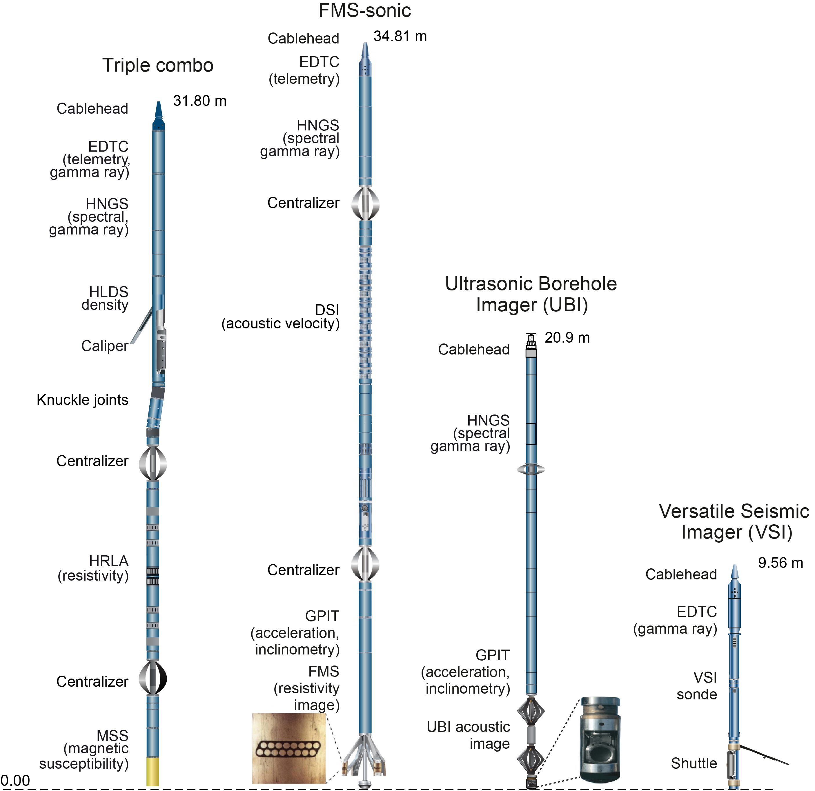
Figure F29. Downhole logging tool strings.
7.2. Wireline logging operations
In preparation for logging, the boreholes were reamed in their lower sections, flushed of debris by circulating drilling fluid, and filled with seawater-based logging gel (i.e., sepiolite mud mixed with seawater and weighted with barite) to help stabilize the borehole walls. The BHA was pulled up to a logging depth determined by the borehole conditions (typically between 50 and 85 m DSF). Tool handling, deployment, and field data collection were undertaken by the onboard Schlumberger wireline logging engineer prior to the data being sent onshore for processing. GR log data was typically collected while running the tool string into the hole from just above seafloor for QC and in case of any downhole logging problems, such as a stuck tool, which could render the main logging pass impossible. The bottom of the open hole was confirmed during the first triple combo logging run and was typically a few meters higher than the final coring depth because of cave-ins and the onset of hole collapse above. The first upward triple combo logging run also served to assess the hole conditions using the single arm HLDS caliper. In some cases, the borehole had already collapsed or bridged off by the time logging tools could be run into the hole, resulting in limited logging recovery. The primary data logging run was collected while raising the tool string upward at a constant speed, typically at around 300 m/h for the triple combo and 130–600 m/h for the FMS-sonic and UBI. A partial repeat logging run was also acquired for all tool strings to aid depth matching and logging data QC, often prior to the main run.
During wireline logging operations, the ship’s heave and ocean conditions affect the wireline tension and tool position in the well. A wireline heave compensator (WHC) system is used in conditions of increased swell to maintain a steady motion of the logging tools and to ensure high-quality logging data acquisition (Liu et al., 2013; Iturrino et al., 2013). The WHC was used for all open hole logging operations regardless of sea state. The WHC uses a vertical accelerometer (motion reference unit [MRU]) positioned under the rig floor near the ship’s center of gravity to calculate the vertical motion of the ship with respect to the seafloor. The length of the wireline is adjusted by varying the distance between two sets of pulleys through which the cable passes to minimize downhole tool motion. Real-time measurements of uphole (surface) and downhole acceleration are made simultaneously by the MRU and the EDTC, respectively, and software analyzes and compares the real-time data to monitor the efficiency of the compensator.
7.3. Data processing
Collected wireline data were sent for onshore processing by the LDEO-BRG. All original logging data was first depth matched to the total GR logging value from the main pass of the triple combo logging run. Prominent features were matched manually between GR within all tool runs and the reference GR log, and then all logging data within the same tool run were depth shifted by the same set of corrections. All depth-matched logs were then shifted to the seafloor (0 m) as defined by the clear increase in GR for this transition, resulting in the common depth reference WMSF in meters. The Schlumberger Techlog software package was used for most of the wireline log data processing.
Standard borehole size environmental corrections were applied to the HNGS (GR), HRLA (resistivity), and HLDS (density/photoelectric) of the triple combo tool string automatically during acquisition and quality checked by the Schlumberger wireline technician on board. The DSI was operated in the monopole P-wave/S-wave, upper and lower dipole, and Stoneley modes during acquisition for all passes.
FMS image log data were processed by applying speed corrections, equalization, button corrections, and depth shifting. Processing transforms the current intensity measurements into high-resolution gray or color images of variable intensities. Intensity reflects the microresistivity variations of the formation. The darker colors reveal more conductive rock such as porous or deeply altered zones along with fractures, whereas the lighter colors reveal more resistive units such as dense crystalline units or cemented horizons. The integrated General Purpose Inclinometry Tool (GPIT) provides accelerometer and magnetometer data for constraining the tool position and spatial orientation relative to north, enabling features such as fractures to be measured for in situ orientations.
UBI image log data were processed by applying GPIT speed corrections, transit time radius conversions, amplitude eccentering corrections, transit time eccentering correction, radius eccentering correction, azimuth equalization, image rotation, depth adjustments, and image normalization. Data were delivered as processed digital log information standard (DLIS) format image log files.
7.4. Quality control and data presentation
The quality of the wireline data was assessed during both acquisition and processing by checking recorded values against reference values for the logged lithologies, evaluating repeatability between different passes of the same tool (down, main, and repeat), and assessing the correspondence between logs affected by the same formation property (e.g., the resistivity log should show similar features to the sonic velocity log). In general, very good correlation exists between the density, resistivity, and compressional velocities for logged intervals. Wireline GR and the MSS also generally reveal good quality data, in most cases matching well with equivalent core-based values. GR logs recorded through the BHA and drill pipe are influenced by significant attenuation of the incoming signal, resulting in reduced absolute GR values that should be used only qualitatively. Detailed comparison between these sections and the open hole data are restricted for this reason.
A wide (>12 inches) or irregular borehole affects most wireline logging recordings, in particular those that require eccentralization and good contact with the borehole wall such as the HLDS and FMS.
Mechanical caliper arms in the triple combo HLDS (LCAL) and FMS-sonic (C1 and C2) logging runs were often closed from 3 to 10 m or sometimes greater distances below the end of the drill string casing. Closure of the calipers causes nongeological changes in caliper-calibrated wireline measurements such as density, PEF, and GR. Furthermore, the depth at which the calipers closed is often not the same between the FMS-sonic and triple combo logging runs; therefore, data comparisons between these runs and the rest of the borehole and the core data are integral for robust integration.
Data received back on board by the downhole logging scientist group were uploaded into the WellCAD software along with associated core-derived physical properties data. WellCAD templates were developed for consistent data presentation and used for all Expedition 396 sites.
FMS image log data is in general very good with high-resolution images returned for all intervals where the logging tool was deployed. Minor sticking artifacts were recorded and flagged, whereas for intervals with good imaging, key geological and structural features such as fractures, bedding planes, and vesicles were recorded.
The UBI acoustic image log tool delivered mixed results with generally lower image resolution than overlapping FMS images. However, the fact that the UBI gives an image of the entire borehole wall rather than the thin strips of the FMS pads proved useful for appraising the presence and continuity of subvertical fractures and contacts in certain cases.
7.5. Measurement principals
7.5.1. Natural gamma radiation
The HNGS measures the NGR of a formation. Standard (total) GR is reported as total spectral GR (HSGR) in American Petroleum Institute gamma radiation units [gAPI] throughout the Downhole measurements section in each site chapter. The HNGS response is influenced by borehole diameter and requires borehole diameter corrections (caliper derived) during acquisition. Two bismuth germanate scintillation detectors in the HNGS tool string measure potassium (weight percent), thorium (parts per million), and uranium (parts per million) concentrations from the characteristic GR energies of isotopes in the 40K, 232Th, and 238U radioactive decay series that dominate the natural radiation spectrum.
In addition to the HNGS, the EDTC also houses a total GR sensor. The inclusion of a GR tool in every tool string allows the use of GR data for precise depth matching between logging runs, aids core-log integration, and enables precise identification of the seafloor.
7.5.2. Density and photoelectric effect
Formation density is measured using the HLDS. The HLDS contains a radioactive cesium (137Cs) GR source (622 keV) and far and near GR detectors mounted on a shielded skid that is pressed against the borehole wall by a decentralizing arm. The tool emits gamma radiation, which undergoes Compton scattering, and the GR signal received by the detectors is proportional to the density of electrons in the formation, which is in turn related to bulk density. Throughout this report, wireline bulk density is presented as the HLDS corrected bulk density (RHOM) in grams per cubic centimeter. The density log is commonly the best downhole tool for assessing porosity where the matrix (grain) density is known or can be accurately estimated and is particularly important for volcanic and clay-bearing rocks, which suffer from poor neutron porosity determinations because of clay-bound water (Broglia and Ellis, 1990).
PEF gives a measure of the photoelectric absorption of low-energy gamma radiation and is also measured using the HLDS. Photoelectric absorption occurs when the energy of the gamma rays falls below 150 keV as a result of scattering by electrons in the formation. PEF is determined by comparing the counts from the far detector in the high-energy region, where only Compton scattering occurs, to those in the low-energy region, where count rates depend on both reactions. Because PEF depends on the atomic number of the elements in the formation (heavier elements have higher PEF), it also varies according to the chemical composition of the minerals present and can aid assessment of the matrix mineralogy. The PEF delivers data in barn/e− units and requires good contact between the tool and the borehole wall; poor contact results in underestimation of density values. Both the density correction and caliper measurement of the hole are used to check hole conditions and assess likely contact quality. Barium in the logging mud can distort PEF signals even with corrections for mud effects and should therefore be treated with extra caution in poor hole conditions.
7.5.3. Electrical resistivity
The HRLA tool records six resistivity measurements with different depths of investigation (including the borehole fluid resistivity and five progressively deeper measurements of formation resistivity). The HRLA tool sends a focused current into the formation and measures the intensity necessary to maintain a constant drop in voltage across a fixed interval, providing direct resistivity measurement. Three depths of investigation, including shallow (RLA1), medium (RLA3), and true (RT_HRLT) resistivity measurements are presented in the Downhole measurements section in each site chapter, with RT_HRLT representing an estimate of the true formation from the area least influenced by drilling fluid invasion. The tool is designed to ensure that all signals are measured at exactly the same time and tool position and to reduce the sensitivity to “shoulder bed” effects when crossing beds thinner than the electrode spacing. The HRLA is run centralized in the borehole for optimal results. Knuckle joints are used to centralize the HRLA while allowing the density tool to maintain good contact with the borehole wall. The HRLA gives an effective measurement of formation resistivity, allowing the full range of resistivity to be measured, from high-porosity brine saturated sediments (low resistivity) to hard dense basalt formations (high resistivity).
7.5.4. Acoustic velocity
The DSI generates acoustic pulses from various sonic transmitters and records the waveforms with an array of eight receivers. The waveforms are then used to calculate sonic VP and VS velocities in the formation. The omnidirectional monopole transmitter emits high-frequency (5–15 kHz) pulses to extract the VP of the formation, as well as VS when it is faster than the sound velocity in the borehole fluid. The DSI also has two cross-dipole transmitters that allow an additional measurement of shear wave velocity in slow (e.g., poorly consolidated) formations, where VS is slower than the velocity in the borehole fluid. The waveforms produced by the two orthogonal dipole transducers can be used to identify sonic anisotropy that can potentially be associated with variations in the local stress regime.
7.5.5. Formation MicroScanner
The FMS imaging sonde is used to map bedding features, fractures, faults, igneous jointing, and large pore structures such as volcanic vesicles and alteration features and can aid in the correlation of coring and logging depths. High-resolution FMS data can also substantially improve lithofacies assessments for intervals where poor or incomplete core recovery prevails. The sonde consists of four imaging pads each with 16 microelectrode buttons that must be in direct contact with the borehole wall during recording. The four pads emit a focused electric current into the formation. The button array on each pad is spaced at 2.5 mm intervals to measure current intensity variations. In smooth boreholes with homogeneous bedding, the depth of investigation is about 25 cm (10 inches). The vertical resolution is typically 5 mm (0.2 inches). The FMS log delivers four pad traces that give approximately 25% borehole wall coverage for a 10 inch diameter hole and are oriented north to enable oriented feature mapping.
7.5.6. Ultrasonic Borehole Imager
The UBI features a high-resolution transducer that provides acoustic images of the borehole wall including amplitude and transit time. The UBI, similar to the FMS tool, gives important information about bedding planes, fractures, dips, etc., along with important information on borehole conditions, drilling-induced fractures, and breakouts. Unlike the FMS, the UBI gives a complete 360° image of the borehole wall and can therefore significantly help in facies appraisal and core-log-seismic integration. The rotating transducer incorporated in the UBI is both a transmitter and a receiver. The UBI is logged with the transducer operating at either 250 or 500 kHz with associated implications for both image quality and operational timings (e.g., 250 kHz; 648 m/h; 1.02 cm vertical resolution compared to 500 kHz; 130 m/h; 0.51 cm vertical resolution).
The tool is relatively insensitive to eccentralization as high as 0.6 cm and can yield high-resolution images where borehole conditions are good and on gauge. Processing software further enhances UBI images by correcting amplitude and transit time information for the effects of logging speed variations and tool eccentering and by applying noise filtering. UBI images are oriented with inclinometry data from the combinable GPIT. Both static and normalized images are generated, and each gives different insights into the drilled formation.
7.5.7. Magnetic susceptibility
The MSS uses a single-coil sensor to measure borehole MS in approximate SI units referred to here as noncalibrated instrument units (IU) at a vertical resolution of ~12 cm with shallow (~3 cm) depth of penetration. A lower resolution (~36 cm) but greater depth of penetration (36 cm) is also collected (LSUSR), which provides a quality check for the higher resolution reading. MS is the ease with which formations are magnetized when subjected to a magnetic field. The ease of magnetization is related to the size, distribution, and composition of magnetic minerals in the formation (e.g., magnetite). These measurements are extremely useful both for correlation and stratigraphic analyses and give critical insights into the presence and nature of volcanic ash layers, which is important for Expedition 396. The MSS is run as the lowest logging tool in the triple combo tool string and therefore collects one of the largest open hole coverages of all the logging tools. The sensor is an electric inductor constructed such that when positioned against the borehole wall, its inductance is affected by the volume susceptibility of the formation within the measured formation rock volume.
The tool is calibrated to a 9⅞ inch borehole diameter, and larger or washed out holes will result in lower susceptibility measurements, whereas higher temperatures lead to higher susceptibility measurements. Temperature measurements were not run alongside the MSS. For QC and environmental corrections, the MSS also measures internal tool temperature, z-axis acceleration, and low-resolution borehole conductivity.
7.5.8. Acceleration and inclinometry
The GPIT was also run as part of the FMS-sonic and UBI tool strings. The GPIT uses a three-axis inclinometer and a three-axis magnetometer to determine tool deviation, tool azimuth, and relative bearing. It relies on the accurate measuring of the tool system axis with respect to the Earth’s gravity (G) and magnetic field (F). A relation between the tool and the Earth system can then be defined because both G and F are well defined. The MAXIS computes deviation, azimuth, and relative bearing from the magnetometer (Fx, Fy, and Fz) and inclinometer (Ax, Ay, and Az) readings at a vertical resolution of 15.24 cm and accuracy of ±2%.
7.5.9. Versatile Seismic Imager
The VSI consists of three parts (a measurement sonde, power cartridge, and control cartridges). The configuration of the tool, including the number of sensor packages, sensor spacing, and type of connection, can all be varied to optimize acquisition for specific hole targets.
The tool collects seismic data by anchoring itself in the hole at the desired depth using a caliper arm. The accelerometer package is then pressed firmly against the formation while remaining decoupled acoustically from the body of the shuttle. Air guns are deployed at the surface from the ship by crane, and the resulting acoustic wave is recorded downhole on three axes. The anchoring, size, and acoustic isolation of the sensors allow for suppression of the tool's harmonic noise and removal of tube waves from the borehole-seismic band. A single shuttle comprising in total one measurement sonde, one power cartridge, and one control cartridge was employed during Expedition 396. The VSI tool was run with the standard HNGS GR tool, which enabled GR readings from deeper in the well section of Hole U1566A because GR has to be run at the top of the tool string in the triple combo so as not to be affected by active sources.
7.5.10. Downhole temperature measurement
In situ temperature measurements were made using the APCT-3 tool when the APC system was deployed in Holes U1572B and U1574C. The APCT-3 tool fits into the APC coring shoe and includes a battery pack, data logger, and platinum resistance-temperature device calibrated over a temperature range of 0°–30°C. During deployment, the tool is first stopped at the mudline to thermally equilibrate with bottom water for 5 min. When the APC system is deployed into the formation, there is an instantaneous temperature rise from frictional heating. This heat gradually dissipates into the surrounding formation as the temperature at the APCT-3 tool equilibrates toward the temperature of the sediment. After the APC system penetrates the sediment, it is held in place for 5 min while the APCT-3 tool records the temperature of the cutting shoe every second.
A preliminary APCT-3 tool measurement evaluation was carried out aboard ship using the TP-Fit v.3 software (Heesemann, 2008). This involved picking the entry time and two points on the temperature equilibration path to capture the temperature decay after the frictional heating caused by lance entry and the second frictional heat pulse caused by lance retrieval. APCT-3 tool temperature data is combined with thermal conductivity measurements on the core (see Physical properties) to retrieve heat flow values.
References
Aarnes, I., Svensen, H., Polteau, S., and Planke, S., 2011. Contact metamorphic devolatilization of shales in the Karoo Basin, South Africa, and the effects of multiple sill intrusions. Chemical Geology, 281(3–4):181–194. https://doi.org/
Abdelmalak, M.M., Meyer, R., Planke, S., Faleide, J.I., Gernigon, L., Frieling, J., Sluijs, A., Reichart, G.J., Zastrozhnov, D., Theissen-Krah, S., Said, A., and Myklebust, R., 2016. Pre-breakup magmatism on the Vøring margin; insight from new sub-basalt imaging and results from Ocean Drilling Program Hole 642E. Tectonophysics, 675:258–274. https://doi.org/
Aleksandrova, G.N., Oreshkina, T.V., Iakovleva, A.I., and Radionova, E.P., 2012. Late Paleocene-Early Eocene diatoms and dinocysts from biosiliceous facies of the middle Trans-Urals region. Stratigraphy and Geological Correlation, 20(4):380–404. https://doi.org/
Alvarez Zarikian, C.A., 2009. Data report: late Quaternary ostracodes at IODP Site U1314 (North Atlantic Ocean). In Channell, J.E.T., Kanamatsu, T., Sato, T., Stein, R., Alvarez Zarikian, C.A., Malone, M.J., and the Expedition 303/306 Scientists, Proceedings of the Integrated Ocean Drilling Program. 303/306: College Station, TX (Integrated Ocean Drilling Program Management International, Inc.). https://doi.org/
Alvarez Zarikian, C.A., 2015. Cenozoic bathyal and abyssal ostracods beneath the oligotrophic South Pacific Gyre (IODP Expedition 329 Sites U1367, U1368 and U1370). Palaeogeography, Palaeoclimatology, Palaeoecology, 419:115–142. https://doi.org/
Arculus, R.J., Ishizuka, O., Bogus, K., Aljahdali, M.H., Bandini-Maeder, A.N., Barth, A.P., Brandl, P.A., do Monte Guerra, R., Drab, L., Gurnis, M.C., Hamada, M., Hickey-Vargas, R.L., Jiang, F., Kanayama, K., Kender, S., Kusano, Y., Li, H., Loudin, L.C., Maffione, M., Marsaglia, K.M., McCarthy, A., Meffre, S., Morris, A., Neuhaus, M., Savov, I.P., Sena Da Silva, C.A., Tepley, F.J., III, van der Land, C., Yogodzinski, G.M., and Zhang, Z., 2015. Expedition 351 summary. In Arculus, R.J., Ishizuka, O., Bogus, K., and the Expedition 351 Scientists, Proceedings of the International Ocean Discovery Program, Expedition 351: Izu-Bonin-Mariana Arc Origins. College Station, TX (International Ocean Discovery Program). https://doi.org/
ASTM International, 1990. Standard method for laboratory determination of water (moisture) content of soil and rock (Standard D2216–90). In Annual Book of ASTM Standards for Soil and Rock Philadelphia (American Society for Testing Materials).
Aumond, G.N., Kochhann, K.G.D., Florisbal, L.S., Fauth, S.B., Bergue, C.T., and Fauth, G., 2009. Maastrichtian-early Danian radiolarians and ostracodes from ODP Site 1001B, Caribbean Sea. Revista Brasileira de Paleontologia, 12(3):195–210. https://doi.org/
Barke, J., Abels, H.A., Sangiorgi, F., Greenwood, D.R., Sweet, A.R., Donders, T., Reichart, G.-J., Lotter, A.F., and Brinkhuis, H., 2011. Orbitally forced Azolla blooms and middle Eocene Arctic hydrology; clues from palynology. Geology, 39(5):427–430. https://doi.org/
Barron, J.A., Stickley, C.E., and Bukry, D., 2015. Paleoceanographic, and paleoclimatic constraints on the global Eocene diatom and silicoflagellate record. Palaeogeography, Palaeoclimatology, Palaeoecology, 422:85–100. https://doi.org/
Batten, D.J., 1996. Palynofacies and paleoenvironmental interpretation. In Jansonius, J., and McGregor, D.C. (Eds.), Palynology: Principles and Applications. Dallas, TX (American Association of Stratigraphic Palynologists Foundation).
Betlem, P., Millett, J., Filina, I., and IODP Expedition 396 Scientists, 2022. IODP Exp 396 - Python scripts for processing LIMS data. Zenodo. https://doi.org/
Bijl, P.K., 2022. DINOSTRAT: a global database of the stratigraphic and paleolatitudinal distribution of Mesozoic–Cenozoic organic-walled dinoflagellate cysts. Earth Syst. Sci. Data, 14(2):579–617. https://doi.org/
Bijl, P.K., Brinkhuis, H., Egger, L.M., Eldrett, J.S., Frieling, J., Grothe, A., Houben, A.J.P., Pross, J., Śliwińska, K.K., and Sluijs, A., 2017. Comment on ‘Wetzeliella and its allies – the ‘hole’ story: a taxonomic revision of the Paleogene dinoflagellate subfamily Wetzelielloideae’ by Williams et al. (2015). Palynology, 41(3):423–429. https://doi.org/
Blum, P., 1997. Physical properties handbook: a guide to the shipboard measurement of physical properties of deep-sea cores. Ocean Drilling Program Technical Note, 26. https://doi.org/
Boulter, M.C., and Manum, S.B., 1989. The Brito-Arctic igneous province flora around the Paleocene/Eocene boundary. In Eldholm, O., Thiede, J., Taylor, E., et al., Proceedings of the Ocean Drilling Program, Scientific Results. 104: College Station, TX (Ocean Drilling Program), 663–680. https://doi.org/
Brinkhuis, H., 1994. Late Eocene to Early Oligocene dinoflagellate cysts from the Priabonian type-area (Northeast Italy): biostratigraphy and paleoenvironmental interpretation. Palaeogeography, Palaeoclimatology, Palaeoecology, 107(1–2):121–163. https://doi.org/
Brinkhuis, H., Munsterman, D.K., Sengers, S., Sluijs, A., Warnaar, J., and Williams, G.L., 2004. Late Eocene-Quaternary dinoflagellate cysts from ODP Site 1168, off western Tasmania. In Exon, N.F., Kennett, J.P., and Malone, M.J. (Eds.), Proceedings of the Ocean Drilling Program, Scientific Results, 189: College Station, TX (Ocean Drilling Program). https://doi.org/
Brinkhuis, H., Schouten, S., Collinson, M.E., Sluijs, A., Sinninghe Damsté, J.S., Dickens, G.R., Huber, M., Cronin, T.M., Onodera, J., Takahashi, K., Bujak, J.P., Stein, R., van der Burgh, J., Eldrett, J.S., Harding, I.C., Lotter, A.F., Sangiorgi, F., van Konijnenburg-van Cittert, H., de Leeuw, J.W., Matthiessen, J., Backman, J., and Moran, K., 2006. Episodic fresh surface waters in the Eocene Arctic Ocean. Nature, 441(7093):606–609. https://doi.org/
Broglia, C., and Ellis, D.V., 1990. Effect of alteration, formation absorption, and standoff on the response of the thermal neutron porosity log in gabbros and basalts; examples from Deep Sea Drilling Project-Ocean Drilling Program sites. Journal of Geophysical Research: Solid Earth, 95(B6):9171–9188. https://doi.org/
Bujak, J., and Mudge, D., 1994. A high-resolution North Sea Eocene dinocyst zonation. Journal of the Geological Society (London, UK), 151(3):449–462. https://doi.org/
Bujak, J.P., and Brinkhuis, H., 1998. Global warming and dinocyst changes across the Paleocene/Eocene epoch boundary. In Aubry, M.-P., Lucas, S., and Berggrenn, W.A. (Eds.), Late Paleocene-Early Eocene Biotic and Climatic Events in the Marine and Terrestrial Records. New York (Columbia University Press), 277–295.
Bünz, S., and Shipboard Scientists, 2020. CAGE-20-4 cruise report. High-resolution 2D and 3D seismic investigations on the Møre and Vøring margins. UiT The Arctic University of Norway report, 47.
Carter, D.J.T., 1980. Echo-Sounding Correction Tables: Formerly Matthews’ Tables (3rd edition): Taunton, England (Hydrographic Department Ministry of Defence).
Chadima, M., and Hrouda, F., 2006. Remasoft 3.0 a user-friendly paleomagnetic data browser and analyzer. Travaux Géophysiques, 27:20–21.
Ciesielski, P.F., and Case, S.M., 1989. Neogene paleoceanography of the Norwegian Sea based upon silicoflagellate assemblage changes in ODP Leg 104 sedimentary sequences. In Eldholm, O., Thiede, J., Taylor, E., et al., Proceedings of the Ocean Drilling Program, Scientific Results. 104: College Station, TX (Ocean Drilling Program), 527–541. https://doi.org/
Ciesielski, P.F., Hasson, P., and Turner, J.W., Jr., 1989. The stratigraphy of Neogene silicoflagellates from the Norwegian Sea, ODP Leg 104. In Eldholm, O., Thiede, J., Taylor, E., et al., Proceedings of the Ocean Drilling Program, Scientific Results. 104: College Station, TX (Ocean Drilling Program), 497–525. https://doi.org/
Coles, G., and Whatley, R., 1989. New Palaeocene to Miocene genera and species of Ostracoda from DSDP sites in the North Atlantic. Revista Espanola de Micropaleontologia, 211:81–124.
Coles, G.P., Whatley, R.C., and Moguilevsky, A., 1994. The ostracod genus Krithe from the Tertiary and Quaternary of the North Atlantic. Palaeontology, 37(1):71–120. https://www.palass.org/
Crouch, E.M., Heilmann-Clausen, C., Brinkhuis, H., Morgans, H.E.G., Rogers, K.M., Egger, H., and Schmitz, B., 2001. Global dinoflagellate event associated with the late Paleocene thermal maximum. Geology, 29(4):315–318. https://doi.org/
de Schepper, S., and Head, M.J., 2009. Pliocene and Pleistocene dinoflagellate cyst and acritarch zonation of DSDP Hole 610A, eastern North Atlantic. Palynology, 33(1):179–218. https://doi.org/
de Vleeschouwer, D., Dunlea, A.G., Auer, G., Anderson, C.H., Brumsack, H., de Loach, A., Gurnis, M.C., Huh, Y., Ishiwa, T., Jang, K., Kominz, M.A., März, C., Schnetger, B., Murray, R.W., Pälike, H., and Expedition 356 Shipboard Scientists, 2017. Quantifying K, U, and Th contents of marine sediments using shipboard natural gamma radiation spectra measured on DV JOIDES Resolution. Geochemistry, Geophysics, Geosystems, 18(3):1053–1064. https://doi.org/
Ducasse, O., and Peypouquet, J.P., 1979. Cenozoic ostracodes; their importance for bathymetry, hydrology, and biogeography. In Montadert, L., Roberts, D.G., et al., Initial Reports of the Deep Sea Drilling Project. 48: Washington, DC (US Government Printing Office), 343–363. https://doi.org/
Dunlea, A.G., Murray, R.W., Harris, R.N., Vasiliev, M.A., Evans, H., Spivack, A.J., and D’Hondt, S., 2013. Assessment and use of NGR instrumentation on the JOIDES Resolution to quantify U, Th, and K concentrations in marine sediment. Scientific Drilling, 15:57–63. https://doi.org/
Dybkjær, K., Rasmussen, E.S., Eidvin, T., Grøsfjeld, K., Riis, F., Piasecki, S., and Śliwińska, K.K., 2021. A new stratigraphic framework for the Miocene – Lower Pliocene deposits offshore Scandinavia: a multiscale approach. Geological Journal, 56(3):1699–1725. https://doi.org/
Dzinoridze, R.N., Jouse, A.P., Koroleva-Golikova, G.S., Kozlova, G.E., Nagaeva, G.S., Petrushevskaya, M.G., and Strelnikova, N.I., 1978. Diatom and radiolarian Cenozoic stratigraphy, Norwegian Basin: DSDP Leg 38. In Talwani, M., Udintsev, G., et al., Initial Reports of the Deep Sea Drilling Project. 38: Washington, DC (US Government Printing Office), 289–427. https://doi.org/
Eldholm, O., Thiede, J., Taylor, E., and the Shipboard Scientific Party, 1987. Summary and preliminary conclusions, ODP Leg 104. In Eldholm, O., Thiede, J., Taylor, E., et al., Proceedings of the Ocean Drilling Program, Initial Reports. 104: College Station, TX (Ocean Drilling Program), 751–771. https://doi.org/
Eldrett, J.S., Harding, I.C., Wilshaw, R., and Xuan, C., 2019. A new high northern latitude dinocyst-based magneto-biostratigraphic calibration for the Norwegian-Greenland Sea. Newsletters on Stratigraphy, 52(4):435–460. https://doi.org/
Eldrett, J.S., and Harding, I.C., 2009. Palynological analyses of Eocene to Oligocene sediments from DSDP Site 338, Outer Vøring Plateau. Marine Micropaleontology, 73(3–4):226–240. https://doi.org/
Eldrett, J.S., Harding, I.C., Firth, J.V., and Roberts, A.P., 2004. Magnetostratigraphic calibration of Eocene–Oligocene dinoflagellate cyst biostratigraphy from the Norwegian–Greenland Sea. Marine Geology, 204(1–2):91–127. https://doi.org/
Expedition 345 Scientists, 2014. Hess Deep plutonic crust: exploring the plutonic crust at a fast-spreading ridge: new drilling at Hess Deep. Integrated Ocean Drilling Program Preliminary Report, 345. https://doi.org/
Expedition 352 Scientists, 2014. Expedition 352 Preliminary Report: Izu-Bonin-Mariana Fore Arc. International Ocean Discovery Program. https://doi.org/
Fenner, J., 1994. Diatoms of the Fur Formation, their taxonomy and biostratigraphic interpretation–results from the Harre borehole, Denmark. Aarhus Geoscience, 1(99):131.
Fisher, R.V., 1961. Proposed classification of volcaniclastic ssediments and rocks. Geological Society of America Bulletin, 72(9):1409–1414. https://doi.org/
Fisher, R.V., and Schmincke, H.U., 1984. Submarine volcaniclastic rocks. In Fisher, R.V., and Schmincke, H.U. (Eds.), Pyroclastic Rocks. Geological Society Special Publication, 16: 265–296. https://doi.org/
Frieling, J., and Sluijs, A., 2018. Towards quantitative environmental reconstructions from ancient non-analogue microfossil assemblages: ecological preferences of Paleocene–Eocene dinoflagellates. Earth-Science Reviews, 185:956–973. https://doi.org/
Frieling, J., Svensen, H.H., Planke, S., Cramwinckel, M.J., Selnes, H., and Sluijs, A., 2016. Thermogenic methane release as a cause for the long duration of the PETM. Proceedings of the National Academy of Sciences of the United States of America, 113(43):12059–12064. https://doi.org/
Fuller, M., 1969. Magnetic orientation of borehole cores. Geophysics, 34(5):772–774. https://doi.org/
Gernigon, L., Zastrozhnov, D., Planke, S., Manton, B., Abdelmalak, M.M., Olesen, O., Maharjan, D., Faleide, J.I., and Myklebust, R., 2021. A digital compilation of structural and magmatic elements of the mid-Norwegian continental margin. Norwegian Journal of Geology, 101. https://doi.org/
Gieskes, J.M., Gamo, T., and Brumsack, H.J., 1991. Chemical methods for interstitial water analysis aboard JOIDES Resolution. Ocean Drilling Program Technical Note, 15. https://doi.org/
Gilmore, G.R., 2008. Practical Gamma-Ray Spectrometry, 2nd Edition: New York (Wiley). https://doi.org/
Govindaraju, K., Rubeska, I., and Paukert, T., 1994. 1994 Report on Zinnwaldite ZW-C analysed by ninety-two GIT-IWG member-laboratories. Geostandards Newsletter, 18(1):1–42. https://doi.org/
Graber, K.K., Pollard, E., Jonasson, B., and Schulte, E. (Eds.), 2002. Overview of Ocean Drilling Program engineering tools and hardware. Ocean Drilling Program Technical Note, 31. https://doi.org/
Gradstein, F.M., Ogg, J.G., Schmitz, M.D., and Ogg, G.M. (Eds.), 2012. The Geological Time Scale 2012: Amsterdam (Elsevier). https://doi.org/
Gradstein, F.M., Ogg, J.G., Schmitz, M.D., and Ogg, G.M. (Eds.), 2020. The Geologic Time Scale 2020: Amsterdam (Elsevier BV). https://doi.org/
Guernet, C., and Bellier, J.-P., 2000. Ostracodes Paléocènes et Éocènes du Blake Nose (Leg ODP 171B) et évolution des environnements bathyaux au large de la Floride. Revue de Micropaléontologie, 43(4):249–279. https://doi.org/
Harding, I.C., Charles, A.J., Marshall, J.E.A., Pälike, H., Roberts, A.P., Wilson, P.A., Jarvis, E., Thorne, R., Morris, E., Moremon, R., Pearce, R.B., and Akbari, S., 2011. Sea-level and salinity fluctuations during the Paleocene-Eocene Thermal Maximum in Arctic Spitsbergen. Earth and Planetary Science Letters, 303(1–2):97–107. https://doi.org/
Harris, R.N., Sakaguchi, A., Petronotis, K., Baxter, A.T., Berg, R., Burkett, A., Charpentier, D., Choi, J., Diz Ferreiro, P., Hamahashi, M., Hashimoto, Y., Heydolph, K., Jovane, L., Kastner, M., Kurz, W., Kutterolf, S.O., Li, Y., Malinverno, A., Martin, K.M., Millan, C., Nascimento, D.B., Saito, S., Sandoval Gutierrez, M.I., Screaton, E.J., Smith-Duque, C.E., Solomon, E.A., Straub, S.M., Tanikawa, W., Torres, M.E., Uchimura, H., Vannucchi, P., Yamamoto, Y., Yan, Q., and Zhao, X., 2013. Expediton 344 summary. In Harris, R.N., Sakaguchi, A., Petronotis, K., and the Expedition 344 Scientists, Proceedings of the Integrated Ocean Drilling Program, 344: College Station, TX (Integrated Ocean Drilling Program). https://doi.org/
Heesemann, M., 2008. Advances in the acquisition and processing of subseafloor temperature and pressure data and their interpretation in the context of convergent margin processes [PhD dissertation]. University of Bremen, Bremen, Germany.
Hennissen, J.A.I., Head, M.J., De Schepper, S., and Groeneveld, J., 2017. Dinoflagellate cyst paleoecology during the Pliocene–Pleistocene climatic transition in the North Atlantic. Palaeogeography, Palaeoclimatology, Palaeoecology, 470:81–108. https://doi.org/
Homann, M., 1991. Diatomeen der Fur-Formation (Alttertiär) aus dem Limfjord-Gebiet, Nordjütland/Dänemark. Geologisches Jahrbuch, Reihe A: Allgemeine und Regionale Geologie Bundesrepublik Deutschland und Nachbargebiete, Tektonik, Stratigraphie, Palaeontologie, 123:3–285.
Huber, B.T., Hobbs, R.W., Bogus, K.A., Batenburg, S.J., Brumsack, H.-J., do Monte Guerra, R., Edgar, K.M., Edvardsen, T., Garcia Tejada, M.L., Harry, D.L., Hasegawa, T., Haynes, S.J., Jiang, T., Jones, M.M., Kuroda, J., Lee, E.Y., Li, Y.-X., MacLeod, K.G., Maritati, A., Martinez, M., O’Connor, L.K., Petrizzo, M.R., Quan, T.M., Richter, C., Riquier, L., Tagliaro, G.T., Wainman, C.C., Watkins, D.K., White, L.T., Wolfgring, E., and Xu, Z., 2019. Expedition 369 methods. In Hobbs, R.W., Huber, B.T., Bogus, K.A., and the Expedition 369 Scientists, Australia Cretaceous climate and tectonics. Proceedings of the International Ocean Discovery Program, 369: College Station, TX (International Ocean Discovery Program). https://doi.org/
Iturrino, G., Liu, T., Goldberg, D., Anderson, L., Evans, H., Fehr, A., Guerin, G., Inwood, J., Lofi, J., Malinverno, A., Morgan, S., Mrozewski, S., Slagle, A., and Williams, T., 2013. Performance of the wireline heave compensation system onboard D/V JOIDES Resolution. Scientific Drilling, 15:46–50. https://doi.org/
Jarrard, R.D., and Kerneklian, M.J., 2007. Data report: physical properties of the upper oceanic crust of ODP Site 1256: multisensor track and moisture and density measurements. In Teagle, D.A.H., Wilson, D.S., Acton, G.D., and Vanko, D.A. , Proceedings of the Ocean Drilling Program, Scientific Results, 206: College Station, TX (Ocean Drilling Program). https://doi.org/
Jochum, K.P., Weis, U., Schwager, B., Stoll, B., Wilson, S.A., Haug, G.H., Andreae, M.O., and Enzweiler, J., 2016. Reference values following ISO guidelines for frequently requested rock reference materials. Geostandards and Geoanalytical Research, 40(3):333–350. https://doi.org/
Johnston, R.M., Ryan, J.G., Fryer, P., Wheat, C.G., Williams, T., Albers, E., Bekins, B.A., Debret, B.P.R., Jianghong, D., Yanhui, D., Eickenbusch, P., Frery, E.A., Ichiyama, Y., Johnson, K., Kevorkian, R.T., Kurz, W., Magalhaes, V., Mantovanelli, S.S., Menapace, W., Menzies, C.D., Michibayashi, K., Moyer, C.L., Mullane, K.K., Park, J.-W., Price, R.E., Shervais, J.W., Suzuki, S., Sissmann, O.J., Takai, K., Walter, B., and Rui, Z., 2018. pXRF and ICP-AES characterization of shipboard rocks and sediments; protocols and strategies. In Mariana Convergent Margin and South Chamorro Seamount. Proceedings of the International Ocean Discovery Program, 366: (Proceedings of the International Ocean Discovery Program). https://doi.org/
Kender, S., Stephenson, M.H., Riding, J.B., Leng, M.J., Knox, R.W.O.B., Peck, V.L., Kendrick, C.P., Ellis, M.A., Vane, C.H., and Jamieson, R., 2012. Marine and terrestrial environmental changes in NW Europe preceding carbon release at the Paleocene–Eocene transition. Earth and Planetary Science Letters, 353–354:108–120. https://doi.org/
Kennett, J.P., and Srinivasan, M.S., 1983. Neogene Planktonic Foraminifera: A Phylogenetic Atlas: London (Hutchinson Ross).
Kirschvink, J.L., 1980. The least-squares line and plane and the analysis of palaeomagnetic data. Geophysical Journal International, 62(3):699–718. https://doi.org/
Koç, N., and Scherer, R.P., 1996. Neogene diatom biostratigraphy of the Iceland Sea Site 907. In Thiede, J., Myhre, A.M., Firth, J.V., Johnson, G.L., and Ruddiman, W.F. (Eds.), Proceedings of the Ocean Drilling Program, Scientific Results. 151: College Station, TX (Ocean Drilling Program), 61–74. https://doi.org/
Kristiansen, J.I., 1982. The transient cylindrical probe method for determination of thermal parameters of earth materials [PhD dissertation]. Åarhus University, Åarhus, Denmark. http://digitallib.oit.edu/
Lazarus, D., Barron, J., Renaudie, J., Diver, P., and Türke, A., 2014. Cenozoic planktonic marine diatom diversity and correlation to climate change. PloS One, 9(1):e84857. https://doi.org/
Le Maitre, R.W. (Ed.), 1989. A Classification of Igneous Rocks and Glossary of Terms: Boston (Blackwell).
Lebedeva-Ivanova, N., Millett, J., et al., 2021. Fast-track seismic data processing report for data from CAGE20-4 cruise. VBPR Report.
Li, C.-F., Lin, J., Kulhanek, D.K., Williams, T., Bao, R., Briais, A., Brown, E.A., Chen, Y., Clift, P.D., Colwell, F.S., Dadd, K.A., Ding, W., Almeida, I.H., Huang, X.-L., Hyun, S., Jiang, T., Koppers, A.A.P., Li, Q., Liu, C., Liu, Q., Liu, Z., Nagai, R.H., Peleo-Alampay, A., Su, X., Sun, Z., Tejada, M.L.G., Trinh, H.S., Yeh, Y.-C., Zhang, C., Zhang, F., Zhang, G.-L., and Zhao, X., 2015. Expedition 349 summary. In Li, C.-F., Lin, J., Kulhanek, D.K., and the Expedition 349 Scientists, South China Sea Tectonics. Proceedings of the International Ocean Discovery Program, 349: College Station, TX (International Ocean Discovery Program). https://doi.org/
Liu, T., Iturrino, G., Goldberg, D., Meissner, E., Swain, K., Furman, C., Fitzgerald, P., Frisbee, N., Chlimoun, J., Van Hyfte, J., and Beyer, R., 2013. Performance evaluation of active wireline heave compensation systems in marine well logging environments. Geo-Marine Letters, 33(1):83–93. https://doi.org/
Locker, S., and Martini, E., 1989. Cenozoic silicoflagellates, ebridians, and actiniscidians from the Voring Plateau (ODP Leg 104). In Eldholm, O., Thiede, J., Taylor, E., et al., Proceedings of the Ocean Drilling Program, Scientific Results. 104: College Station, TX (Ocean Drilling Program), 543–585. https://doi.org/
Malz, H., 1989. Cenozoic ostracodes of the Voring Plateau (ODP Leg 104, Sites 642, 643 and 644). In Eldholm, O., Thiede, J., Taylor, E., et al., Proceedings of the Ocean Drilling Program, Scientific Results. 104: College Station, TX (Ocean Drilling Program), 769–775. https://doi.org/
Manheim, F.T., and Sayles, F.L., 1974. Composition and origin of interstitial waters of marine sediments, based on deep sea drill cores. In Goldberg, E.D., The Sea (Volume 5): Marine Chemistry: The Sedimentary Cycle. New York (Wiley), 527–568. http://pubs.er.usgs.gov/
Marret, F., Bradley, L., de Vernal, A., Hardy, W., Kim, S.-Y., Mudie, P., Penaud, A., Pospelova, V., Price, A.M., Radi, T., and Rochon, A., 2020. From bi-polar to regional distribution of modern dinoflagellate cysts, an overview of their biogeography. Marine Micropaleontology, 59:101753. https://doi.org/
Marsaglia, K., Milliken, K., and Doran, L., 2013. IODP digital reference for smear slide analysis of marine mud, Part 1: Methodology and atlas of siliciclastic and volcanogenic components. Integrated Ocean Drilling Program Technical Note, 1. https://doi.org/
Mudge, D.C., and Bujak, J.P., 1994. Eocene stratigraphy of the North Sea Basin. Marine and Petroleum Geology, 11(2):166–181. https://doi.org/
Mudge, D.C., and Bujak, J.P., 1996a. An integrated stratigraphy for the Paleocene and Eocene of the North Sea. In Knox, R.W.O., Corfield, R.M., and Dunay, R.E. (Eds.), Correlation of the Early Paleogene in Northwest Europe. Geological Society Special Publication, 101: 91–113. https://doi.org/
Mudge, D.C., and Bujak, J.P., 1996b. Palaeocene biostratigraphy and sequence stratigraphy of the UK central North Sea. Marine and Petroleum Geology, 13(3):295–312. https://doi.org/
Mudie, P.J., 1989. Palynology and dinocyst biostratigraphy of the late Miocene to Pleistocene, Norwegian Sea: ODP Leg 104, Sites 642 and 644. In Eldholm, O., Thiede, J., Taylor, E., et al., Proceedings of the Ocean Drilling Program, Scientific Results, 104: College Station, TX (Ocean Drilling Program), 587–610. https://doi.org/
Munsell Color Company, 2010. Munsell soil color charts: with genuine Munsell color chips: Grand Rapids, MI (Munsell Color). https://search.library.wisc.edu/
Munsterman, D.K., and Brinkhuis, H., 2004. A southern North Sea Miocene dinoflagellate cyst zonation. Geologie en Mijnbouw, 83(4):267–285. https://doi.org/
Murray, R.W., Miller, D.J., and Kryc, K.A., 2000. Analysis of major and trace elements in rocks, sediments, and interstitial waters by inductively coupled plasma–atomic emission spectrometry (ICP-AES). Ocean Drilling Program Technical Note, 29. https://doi.org/
Neuendorf, K.K.E., Mehl, J.P., Jr., and Jackson, J.A. (Eds.), 2005. Glossary of Geology (Fifth edition, revised): Alexandria, VA (American Geosciences Institute).
Norris, R.D., Wilson, P.A., Blum, P., Fehr, A., Agnini, C., Bornemann, A., Boulila, S., Bown, P.R., Cournede, C., Friedrich, O., Ghosh, A.K., Hollis, C.J., Hull, P.M., Jo, K., Junium, C.K., Kaneko, M., Liebrand, D., Lippert, P.C., Liu, Z., Matsui, H., Moriya, K., Nishi, H., Opdyke, B.N., Penman, D., Romans, B., Scher, H.D., Sexton, P., Takagi, H., Turner, S.K., Whiteside, J.H., Yamaguchi, T., and Yamamoto, Y., 2014a. Expedition 342 summary. In Norris, R.D., Wilson, P.A., Blum, P., and the Expedition 342 Scientists, Proceedings of the Integrated Ocean Drilling Program, 342: College Station, TX (Integrated Ocean Drilling Program). https://doi.org/
Norris, R.D., Wilson, P.A., Blum, P., Fehr, A., Agnini, C., Bornemann, A., Boulila, S., Bown, P.R., Cournede, C., Friedrich, O., Ghosh, A.K., Hollis, C.J., Hull, P.M., Jo, K., Junium, C.K., Kaneko, M., Liebrand, D., Lippert, P.C., Li, Z., Matsui, H., Moriya, K., Nishi, H., Opdyke, B.N., Penman, D., Romans, B., Scher, H.D., Sexton, P., Takagi, H., Turner, S.K., Whiteside, J.H., Yamaguchi, T., and Yamamoto, Y., 2014b. Methods. In Norris, R.D., Wilson, P.A., Blum, P., and the Expedition 342 Scientists, Proceedings of the Integrated Ocean Drilling Program, 342: College Station, TX (Integrated Ocean Drilling Program). https://doi.org/
Ogg, J.G., 2020. Geomagnetic Polarity Time Scale. In Gradstein, F.M., Ogg, J.G., Schmitz, M., and Ogg, G.M. (Eds.), Geologic Time Scale 2020. Amsterdam (Elsevier), 159–192.
Oreshkina, T.V., and Aleksandrova, G.N., 2007. Terminal paleocene of the Volga middle reaches: biostratigraphy and paleosettings. Stratigraphy and Geological Correlation, 15(2):206–230. https://doi.org/
Oreshkina, T.V., and Radionova, E.P., 2014. Diatom record of the Paleocene–Eocene Thermal Maximum in marine paleobasins of Central Russia, Transuralia and adjacent regions. Nova Hedwigia, Beiheft, 143:307–336.
Pearson, P.N., Olsson, R.K., Huber, B.T., Hemleben, C., and Berggren, W.A., 2006. Atlas of Eocene planktonic foraminifera. Special Publication - Cushman Foundation for Foraminiferal Research, 41.
Planke, S., Berndt, C., and Alvarez Zarikian, C.A., 2021. Expedition 396 Scientific Prospectus: Mid-Norwegian Continental Margin Magmatism: International Ocean Discovery Program https://doi.org/
Planke, S., Berndt, C., Alvarez Zarikian, C.A., Agarwal, A., Andrews, G.D.M., Betlem, P., Bhattacharya, J., Brinkhuis, H., Chatterjee, S., Christopoulou, M., Clementi, V.J., Ferré, E.C., Filina, I.Y., Frieling, J., Guo, P., Harper, D.T., Jones, M.T., Lambart, S., Longman, J., Millett, J.M., Mohn, G., Nakaoka, R., Scherer, R.P., Tegner, C., Varela, N., Wang, M., Xu, W., and Yager, S.L., 2023a. Expedition 396 summary. In Planke, S., Berndt, C., Alvarez Zarikian, C.A., and the Expedition 396 Scientists, Mid-Norwegian Margin Magmatism and Paleoclimate Implications. Proceedings of the International Ocean Discovery Program, 396: College Station, TX (International Ocean Discovery Program). https://doi.org/
Planke, S., Berndt, C., Alvarez Zarikian, C.A., Agarwal, A., Andrews, G.D.M., Betlem, P., Bhattacharya, J., Brinkhuis, H., Chatterjee, S., Christopoulou, M., Clementi, V.J., Ferré, E.C., Filina, I.Y., Frieling, J., Guo, P., Harper, D.T., Jones, M.T., Lambart, S., Longman, J., Millett, J.M., Mohn, G., Nakaoka, R., Scherer, R.P., Tegner, C., Varela, N., Wang, M., Xu, W., and Yager, S.L., 2023b. Site U1565. In Planke, S., Berndt, C., Alvarez Zarikian, C.A., and the Expedition 396 Scientists, Mid-Norwegian Margin Magmatism and Paleoclimate Implications. Proceedings of the International Ocean Discovery Program, 396: College Station, TX (International Ocean Discovery Program). https://doi.org/
Pross, J., and Brinkhuis, H., 2005. Organic-walled dinoflagellate cysts as paleoenvironmental indicators in the Paleogene; a synopsis of concepts. Paläontologische Zeitschrift, 79(1):53–59. https://doi.org/
Pross, J., Pletsch, T., Shillington, D.J., Ligouis, B., Schellenberg, F., and Kus, J., 2007. Thermal alteration of terrestrial palynomorphs in mid-Cretaceous organic-rich mudstones intruded by an igneous sill (Newfoundland Margin, ODP Hole 1276A). International Journal of Coal Geology, 70(4):277–291. https://doi.org/
Puchelt, H., Prichard, H.M., Berner, Z., and Maynard, J., 1996. Sulfide mineralogy, sulfur content, and sulfur isotope composition of mafic and ultramafic rocks from Leg 147. In Mével, C., Gillis, K.M., Allan, J.F., and Meyer, P.S. (Eds.), Proceedings of the Ocean Drilling Program, Scientific Results. 147: College Station, TX (Ocean Drilling Program), 91–101. https://doi.org/
Radionova, E.P., and Khokhlova, I.E., 1994. Paleogene episodes of biogenic silica accumulation in the northern Caucasus and adjacent Tethyan regions. Stratigraphy and Geological Correlation, 2(5):161–169.
Radionova, E.P., and Khokhlova, I.E., 2000. Was the North Atlantic connected with the Tethys via the Arctic in the early Eocene? Evidence from siliceous plankton. GFF, 122(1):133–134. https://doi.org/
Reagan, M.K., Pearce, J.A., Petronotis, K., Almeev, R., Avery, A.A., Carvallo, C., Chapman, T., Christeson, G.L., Ferré, E.C., Godard, M., Heaton, D.E., Kirchenbaur, M., Kurz, W., Kutterolf, S., Li, H.Y., Li, Y., Michibayashi, K., Morgan, S., Nelson, W.R., Prytulak, J., Python, M., Robertson, A.H.F., Ryan, J.G., Sager, W.W., Sakuyama, T., Shervais, J.W., Shimizu, K., and Whattam, S.A., 2015. Expedition 352 methods. In Reagan, M.K., Pearce, J.A., Petronotis, K., and the Expedition 352 Scientists, Izu-Bonin-Mariana Fore Arc. Proceedings of the International Ocean Discovery Program, 352: College Station, TX (International Ocean Discovery Program). https://doi.org/
Renaudie, J., Drews, E.L., and Böhne, S., 2018. The Paleocene record of marine diatoms in deep-sea sediments. Fossil Record, 21(2):183–205. https://doi.org/
Riding, J.B., and Kyffin-Hughes, J.E., 2011. A direct comparison of three palynological preparation techniques. Review of Palaeobotany and Palynology, 167(3–4):212–221. https://doi.org/
Rothwell, R.G., 1989a. Minerals and Mineraloids in Marine Sediments: An Optical Identification Guide: London (Elsevier). https://doi.org/
Rothwell, R.G., 1989b. The smear slide method. In Rothwell, R.G., Minerals and Mineraloids in Marine Sediments: An Optical Identification Guide. Dordrecht (Springer Netherlands), 21–24. https://doi.org/
Rothwell, R.G., 2012. Minerals and Mineraloids in Marine Sediments: An Optical Identification Guide:: Berlin (Springer).
Ryan, J.G., Shervais, J.W., Li, Y., Reagan, M.K., Li, H.Y., Heaton, D., Godard, M., Kirchenbaur, M., Whattam, S.A., Pearce, J.A., Chapman, T., Nelson, W., Prytulak, J., Shimizu, K., and Petronotis, K., 2017. Application of a handheld X-ray fluorescence spectrometer for real-time, high-density quantitative analysis of drilled igneous rocks and sediments during IODP Expedition 352. Chemical Geology, 451:55-66. https://doi.org/
Scherer, R.P., 1994. A new method for the determination of absolute abundance of diatoms and other silt-sized sedimentary particles. Journal of Paleolimnology, 12(2):171–179. https://doi.org/
Scherer, R.P., Gladenkov, A.Y., and Barron, J.A., 2007. Methods and applications of Cenozoic marine diatom biostratigraphy. In Strratt, S., Pond Scum to Carbon Sink: Geological and Environmental Applications of the Diatoms The Paleontological Society Papers, 13: 61–83. https://doi.org/
Scherer, R.P., and Koç, N., 1996. Late Paleogene diatom biostratigraphy and paleoenvironments of the northern Norwegian-Greenland Sea. In Thiede, J., Myhre, A.M., Firth, J.V., Johnson, G.L., and Ruddiman, W.F., Proceedings of the Ocean Drilling Program, Scientific Results, 151. College Station, TX (Ocean Drilling Program), 75–99. https://doi.org/
Scherer, R.P., Sjunneskog, C.M., Iverson, N.R., and Hooyer, T.S., 2004. Assessing subglacial processes from diatom fragmentation patterns. Geology, 32(7):557–560. https://doi.org
Schrader, H.-J., and Fenner, J., 1976. Norwegian Sea Cenozoic diatom biostratigraphy and taxonomy: Part I: Norwegian Sea Cenozoic diatom biostratigraphy. In Andrews, J.E., Packham, G. et al., Initial Reports of the Deep Sea Drilling Project. 38: Washington, DC (US Government Printing Office), 921–1099. https://doi.org/
Schreck, M., Matthiessen, J., and Head, M.J., 2012. A magnetostratigraphic calibration of Middle Miocene through Pliocene dinoflagellate cyst and acritarch events in the Iceland Sea (Ocean Drilling Program Hole 907A). Review of Palaeobotany and Palynology, 187:66–94. https://doi.org/
Scotese, C., 2014a. Atlas of Paleogene Paleogeographic Maps (Mollweide Projection), Maps 8–15 (Volume 1): The Cenozoic. In PALEOMAP Atlas for ArcGIS, 1: Evanston, IL (PALEOMAP Project).
Scotese, C., 2014b. The PALEOMAP Project PaleoAtlas for ArcGIS, version 2 (Volume 2): Cretaceous Plate Tectonic, Paleogeographic, and Paleoclimatic Reconstructions, Maps 16–32.
Shipboard Scientific Party, 1987. ODP Leg 104 (Norwegian Sea): explanatory notes. In Eldholm, O., Thiede, J., Taylor, E., et al., Proceedings of the Ocean Drilling Program, Initial Reports, 104: College Station, TX (Ocean Drilling Program), 27–43. https://doi.org/
Shipboard Scientific Party, 2003. Explanatory notes. In Wilson, D.S., Teagle, D.A.H., Acton, G.D., et al., Proceedings of the Ocean Drilling Program, Initial Reports, 206: College Station, TX (Ocean Drilling Program). https://doi.org/
Shipboard Scientific Party, 2004. Explanatory notes. In Kelemen, P.B., Kikawa, E., Miller, D.J., et al., Proceedings of the Ocean Drilling Program, Initial Reports, 209: College Station, TX (Ocean Drilling Program). https://doi.org/
Sluijs, A., and Brinkhuis, H., 2009. A dynamic climate and ecosystem state during the Paleocene-Eocene Thermal Maximum: inferences from dinoflagellate cyst assemblages on the New Jersey Shelf. Biogeosciences, 6(8):1755–1781. https://doi.org/
Sluijs, A., Pross, J., and Brinkhuis, H., 2005. From greenhouse to icehouse; organic-walled dinoflagellate cysts as paleoenvironmental indicators in the Paleogene. Earth-Science Reviews, 68(3):281–315. https://doi.org/
Spiegler, D., 1996. Planktonic foraminifer Cenozoic biostratigraphy of the Arctic Ocean, Fram Strait (Sites 908–909), Yermak Plateau (Sites 910-912), and East Greenland Margin (Site 913). In Thiede, J., Myhre, A.M., Firth, J.V., Johnson, G.L., and Ruddiman, W.F. (Eds.), Proceedings of the Ocean Drilling Program, Scientific Results, 151: College Station, TX (Ocean Drilling Program), 153–167. https://doi.org/
Spiegler, D., and Jansen, E., 1989. Planktonic foraminifer biostratigraphy of Norwegian Sea sediments: ODP Leg 104. In Eldholm, O., Thiede, J., Taylor, E., et al., Proceedings of the Ocean Drilling Program, Scientific Results, 104: College Station, TX (Ocean Drilling Program), 681–696. https://doi.org/
Stow, D.A.V., 2005. Sedimentary Rocks in the Field. A Colour Guide: London (Manson Publishing).
Streckeisen, A., 1974. Classification and nomenclature of plutonic rocks recommendations of the IUGS subcommission on the systematics of Igneous Rocks. Geologische Rundschau, 63(2):773–786. https://doi.org/
Strelnikova, N.I., 1992. Paleogene Diatoms: Saint-Petersburg, Russia (Saint-Petersburg University Press). [in Russian]
Sun, Z., Jian, Z., Stock, J.M., Larsen, H.C., Klaus, A., Alvarez Zarikian, C.A., Boaga, J., Bowden, S.A., Briais, A., Chen, Y., Cukur, D., Dadd, K.A., Ding, W., Dorais, M.J., Ferré, E.C., Ferreira, F., Furusawa, A., Gewecke, A.J., Hinojosa, J.L., Höfig, T.W., Hsiung, K.-H., Huang, B., Huang, E., Huang, X.-L., Jiang, S., Jin, H., Johnson, B.G., Kurzawski, R.M., Lei, C., Li, B., Li, L., Li, Y., Lin, J., Liu, C., Liu, C., Liu, Z., Luna, A., Lupi, C., McCarthy, A.J., Mohn, G., Ningthoujam, L.S., Nirrengarten, M., Osono, N., Peate, D.W., Persaud, P., Qiu, N., Robinson, C.M., Satolli, S., Sauermilch, I., Schindlbeck, J.C., Skinner, S.M., Straub, S.M., Su, X., Tian, L., Van der Zwan, F.M., Wan, S., Wu, H., Xiang, R., Yadav, R., Yi, L., Zhang, C., Zhang, J., Zhang, Y., Zhao, N., Zhong, G., and Zhong, L., 2018. Expedition 367/368 methods. In Sun, Z., Jian, Z., Stock, J.M., Larsen, H.C., Klaus, A., Alvarez Zarikian, C.A., and the Expedition 367/368 Scientists, South China Sea Rifted Margin. Proceedings of the International Ocean Discovery Program, 367/368: College Station, TX (International Ocean Discovery Program). https://doi.org/
Sutherland, R., Dickens, G.R., Blum, P., and the Expedition 371 Scientists, 2018. Expedition 371 Preliminary Report: Tasman Frontier Subduction Initiation and Paleogene Climate. International Ocean Discovery Program. https://doi.org/
Sutherland, R., Dickens, G.R., Blum, P., Agnini, C., Alegret, L., Asatryan, G., Bhattacharya, J., Bordenave, A., Chang, L., Collot, J., Cramwinckel, M.J., Dallanave, E., Drake, M.K., Etienne, S.J.G., Giorgioni, M., Gurnis, M., Harper, D.T., Huang, H.-H.M., Keller, A.L., Lam, A.R., Li, H., Matsui, H., Morgans, H.E.G., Newsam, C., Park, Y.-H., Pascher, K.M., Pekar, S.F., Penman, D.E., Saito, S., Stratford, W.R., Westerhold, T., and Zhou, X., 2019. Expedition 371 methods. In Sutherland, R., Dickens, G.R., Blum, P., and the Expedition 371 Scientists, Tasman Frontier Subduction Initiation and Paleogene Climate. Proceedings of the International Ocean Discovery Program, 371: (International Ocean Discovery Program). https://doi.org/
Suto, I., 2003. Taxonomy of the marine diatom resting spore genera Dicladia Ehrenberg, Monocladia gen. nov. and Syndendrium Ehrenberg and their stratigraphic significance in Miocene strata. Diatom Research, 18(2):331–356. https://doi.org/
Suto, I., 2004. Fossil marine diatom resting spore morpho-genus Xanthiopyxis Ehrenberg in the North Pacific and Norwegian Sea. Paleontological Research, 8(4):283–310. https://doi.org/
Suto, I., 2005. Taxonomy and biostratigraphy of the fossil marine diatom resting spore general Dicladia Ehrenberg, Monocladia Suto and Syndendrium Ehrenberg in the North Pacific and Norwegian Sea. Diatom Research, 20(2):351–374. https://doi.org/
Suto, I., Jordan, R.W., and Watanabe, M., 2008. Taxonomy of the fossil marine diatom resting spore genus Goniothecium Ehrenberg and its allied species. Diatom Research, 23(2):445–469. https://doi.org/
Suto, I., Jordan, R.W., and Watanabe, M., 2009. Taxonomy of middle Eocene diatom resting spores and their allied taxa from the central Arctic Basin. Micropaleontology, 55(2–3):259–312. https://www.jstor.org/
Suto, I., Watanabe, M., and Jordan, R.W., 2011. Taxonomy of the fossil marine diatom resting spore genus Odontotropis. Diatom Research, 26(3):255–272. https://doi.org/
Svensen, H., Planke, S., Malthe-Sørenssen, A., Jamtveit, B., Myklebust, R., Rasmussen Eidem, T., and Rey, S.S., 2004. Release of methane from a volcanic basin as a mechanism for initial Eocene global warming. Nature, 429(6991):542–545. https://doi.org/
Tamura, Y., Busby, C.J., Blum, P., Guèrin, G., Andrews, G.D.M., Barker, A.K., Berger, J.L.R., Bongiolo, E.M., Bordiga, M., DeBari, S.M., Gill, J.B., Hamelin, C., Jia, J., John, E.H., Jonas, A.-S., Jutzeler, M., Kars, M.A.C., Kita, Z.A., Konrad, K., Mahony, S.H., Martini, M., Miyazaki, T., Musgrave, R.J., Nascimento, D.B., Nichols, A.R.L., Ribeiro, J.M., Sato, T., Schindlbeck, J.C., Schmitt, A.K., Straub, S.M., Vautravers, M.J., and Yang, Y., 2015a. Expedition 350 methods. In Tamura, Y., Busby, C.J., Blum, P., and the Expedition 350 Scientists, Izu-Bonin-Mariana Rear Arc. Proceedings of the International Ocean Discovery Program, 350: College Station, TX (Proceedings of the International Ocean Discovery Program). https://doi.org/
Tamura, Y., Busby, C.J., Blum, P., Guèrin, G., Andrews, G.D.M., Barker, A.K., Berger, J.L.R., Bongiolo, E.M., Bordiga, M., DeBari, S.M., Gill, J.B., Hamelin, C., Jia, J., John, E.H., Jonas, A.-S., Jutzeler, M., Kars, M.A.C., Kita, Z.A., Konrad, K., Mahony, S.H., Martini, M., Miyazaki, T., Musgrave, R.J., Nascimento, D.B., Nichols, A.R.L., Ribeiro, J.M., Sato, T., Schindlbeck, J.C., Schmitt, A.K., Straub, S.M., Vautravers, M.J., and Yang, Y., 2015b. Expedition 350 summary. In Tamura, Y., Busby, C.J., Blum, P., and the Expedition 350 Scientists, Izu-Bonin-Mariana Rear Arc. Proceedings of the International Ocean Discovery Program, 350: College Station, TX (International Ocean Discovery Program). https://doi.org/
Terry, R.D., and Chilingar, G.V., 1955. Summary of “Concerning some additional aids in studying sedimentary formations,” by M. S. Shvetsov. Journal of Sedimentary Research, 25(3):229–234. https://doi.org/
Vacquier, V., 1985. The measurement of thermal conductivity of solids with a transient linear heat source on the plane surface of a poorly conducting body. Earth and Planetary Science Letters, 74(2–3):275–279. https://doi.org/
Vasiliev, M.A., Blum, P., Chubarian, G., Olsen, R., Bennight, C., Cobine, T., Fackler, D., Hastedt, M., Houpt, D., Mateo, Z., and Vasilieva, Y.B., 2011. A new natural gamma radiation measurement system for marine sediment and rock analysis. Journal of Applied Geophysics, 75(3):455–463. https://doi.org/
Vieira, M., Mahdi, S., and Holmes, N., 2020. High resolution biostratigraphic zonation for the UK central North Sea Paleocene. Marine and Petroleum Geology, 117:104400. https://doi.org/
Von Herzen, R., and Maxwell, A.E., 1959. The measurement of thermal conductivity of deep-sea sediments by a needle-probe method. Journal of Geophysical Research, 64(10):1557–1563. https://doi.org/
Wade, B.S., Olsson, R.K., Pearson, P.N., Huber, B.T., and Berggren, W.A., 2018. Atlas of Oligocene Planktonic Foraminifera. Special Publication - Cushman Foundation for Foraminiferal Research, 46.
Wade, B.S., Pearson, P.N., Berggren, W.A., and Pälike, H., 2011. Review and revision of Cenozoic tropical planktonic foraminiferal biostratigraphy and calibration to the geomagnetic polarity and astronomical time scale. Earth-Science Reviews, 104(1–3):111–142. https://doi.org/
Wallace, L.M., Saffer, D.M., Barnes, P.M., Pecher, I.A., Petronotis, K.E., LeVay, L.J., Bell, R.E., Crundwell, M.P., Engelmann de Oliveira, C.H., Fagereng, A., Fulton, P.M., Greve, A., Harris, R.N., Hashimoto, Y., Hüpers, A., Ikari, M.J., Ito, Y., Kitajima, H., Kutterolf, S., Lee, H., Li, X., Luo, M., Malie, P.R., Meneghini, F., Morgan, J.K., Noda, A., Rabinowitz, H.S., Savage, H.M., Shepherd, C.L., Shreedharan, S., Solomon, E.A., Underwood, M.B., Wang, M., Woodhouse, A.D., Bourlange, S.M., Brunet, M.M.Y., Cardona, S., Clennell, M.B., Cook, A.E., Dugan, B., Elger, J., Gamboa, D., Georgiopoulou, A., Han, S., Heeschen, K.U., Hu, G., Kim, G.Y., Koge, H., Machado, K.S., McNamara, D.D., Moore, G.F., Mountjoy, J.J., Nole, M.A., Owari, S., Paganoni, M., Rose, P.S., Screaton, E.J., Shankar, U., Torres, M.E., Wang, X., and Wu, H.-Y., 2019. Expedition 372B/375 methods. In Wallace, L.M., Saffer, D.M., Barnes, P.M., Pecher, I.A., Petronotis, K.E., LeVay, L.J., and the Expedition 372/375 Scientists, Hikurangi Subduction Margin Coring, Logging, and Observatories. Proceedings of the International Ocean Discovery Program, 372B/375: College Station, TX (International Ocean Discovery Program). https://doi.org/
Warnock, J.P., and Scherer, R.P., 2015. A revised method for determining the absolute abundance of diatoms. Journal of Paleolimnology, 53(1):157–163. https://doi.org/
Wentworth, C.K., 1922. A scale of grade and class terms for clastic sediments. The Journal of Geology, 30(5):377–392. https://doi.org/
White, J.D.L., McPhie, J., and Skilling, I., 2000. Peperite: a useful genetic term. Bulletin of Volcanology, 62:65–66. https://doi.org/
Williams, G.L., Fensome, R.A., and MacRae, R.A., 2017a. The Lentin and Williams index of fossil dinoflagellates (2017 edition). AASP Contributions Series, 48. https://palynology.org/
Williams, G.L., Brinkhuis, H., Pearce, M.A., Fensome, R.A., and Weegink, J.W., 2004. Southern Ocean and global dinoflagellate cyst events compared; index events for the Late Cretaceous-Neogene. In Exon, N.F., Kennett, J.P., and Malone, M.J. (Eds.), Proceedings of the Ocean Drilling Program, Scientific Results, 189: College Station, TX (Ocean Drilling Program). https://doi.org/
Williams, G.L., Damassa, S.P., Fensome, R.A., and Guerstein, G.R., 2015. Wetzeliella and its allies – the ‘hole’ story: a taxonomic revision of the Paleogene dinoflagellate subfamily Wetzelielloideae. Palynology, 39(3):289–344. https://doi.org/
Williams, G.L., Damassa, S.P., Fensome, R.A., and Guerstein, G.R., 2017b. A response to ‘Comment to Wetzeliella and its allies – the ‘hole’ story: a taxonomic revision of the Paleogene dinoflagellate subfamily Wetzelielloideae by Williams et al. (2015)’. Palynology, 41(3):430–437. https://doi.org/
Witkowski, J., Sims, P.A., Strelnikova, N.I. and Williams, D.M., 2015. Entogoniopsis gen. nov. and Trilamina gen. nov. (Bacillariophyta): a survey of multipolar pseudocellate diatoms with internal costae, including comments on the genus Sheshukovia Gleser. Phytotaxa, 209(1). https://doi.org/
Witkowski, J., 2018. From museum drawers to ocean drilling: Fenneria gen. nov. (Bacillariophyta) offers new insights into Eocene marine diatom biostratigraphy and paleobiogeography. Acta Geologica Polonica, 68(1):53–88.
Witkowski, J., Bohaty, S.M., McCartney, K., and Harwood, D.M., 2012. Enhanced siliceous plankton productivity in response to middle Eocene warming at Southern Ocean ODP Sites 748 and 749. Palaeogeography, Palaeoclimatology, Palaeoecology, 326–328:78–94. https://doi.org/
Witkowski, J., Harwood, D.M., Wade, B.S., and Bryłka, K., 2020a. Rethinking the chronology of early Paleogene sediments in the western North Atlantic using diatom biostratigraphy. Marine Geology, 424:106168. https://doi.org/
Witkowski, J., Penman, D.E., Bryłka, K., Wade, B.S., Matting, S., Harwood, D.M., and Bohaty, S.M., 2020b. Early Paleogene biosiliceous sedimentation in the Atlantic Ocean: testing the inorganic origin hypothesis for Paleocene and Eocene chert and porcellanite. Palaeogeography, Palaeoclimatology, Palaeoecology, 556:109896. https://doi.org/
Yamaguchi, T., 2018. Data report: late Eocene-early Oligocene ostracods at IODP Site U1411, off Newfoundland, North Atlantic. In Norris, R.D., Wilson, P.A., Blum, P., and the Expedition 342 Scientists, Proceedings of Integrated Ocean Drilling Program. 342: College Station, TX (Integrated Ocean Drilling Program). https://doi.org/
Yamaguchi, T., Matsui, H., and Nishi, H., 2017a. Taxonomy of Maastrichtian-Thanetian deep-sea ostracodes from U1407, IODP Exp 342, off Newfoundland, northwestern Atlantic, Part 1. Families Cytherellidae, Bairdiidae, Pontocyprididae, Bythocytheridae, and Cytheruridae. Paleontological Research, 21(1):54–75. https://doi.org/
Yamaguchi, T., Matsui, H., and Nishi, H., 2017b. Taxonomy of Maastrichtian-Thanetian deep-sea ostracodes from U1407, IODP Exp 342, off Newfoundland, northwestern Atlantic, Part 2. Families Eucytheridae, Krithidae, Thaerocytheridae, Trachyleberididae, and Xestoleberididae. Paleontological Research, 21(2):97–121. https://doi.org/
Yamaguchi, T., and Norris, R.D., 2012. Deep-sea ostracode turnovers through the Paleocene–Eocene Thermal Maximum in DSDP Site 401, Bay of Biscay, North Atlantic. Marine Micropaleontology, 86-87:32-44. https://doi.org/
Zastrozhnov, D., Gernigon, L., Gogin, I., Planke, S., Abdelmalak, M.M., Polteau, S., Faleide, J.I., Manton, B., and Myklebust, R., 2020. Regional structure and polyphased Cretaceous-Paleocene rift and basin development of the mid-Norwegian volcanic passive margin. Marine and Petroleum Geology, 115:104269. https://doi.org/
Zijderveld, J.D.A., 1967. AC demagnetization of rocks: analysis of results. In Runcorn, S.K.C., Creer, K.M., and Collinson, D.W., Methods in Palaeomagnetism. Amsterdam (Elsevier), 254–286.
Zonneveld, K.A.F., Marret, F., Versteegh, G.J.M., Bogus, K., Bonnet, S., Bouimetarhan, I., Crouch, E., de Vernal, A., Elshanawany, R., Edwards, L., Esper, O., Forke, S., Grøsfjeld, K., Henry, M., Holzwarth, U., Kielt, J.-F., Kim, S.-Y., Ladouceur, S., Ledu, D., Chen, L., Limoges, A., Londeix, L., Lu, S.H., Mahmoud, M.S., Marino, G., Matsouka, K., Matthiessen, J., Mildenhal, D.C., Mudie, P., Neil, H.L., Pospelova, V., Qi, Y., Radi, T., Richerol, T., Rochon, A., Sangiorgi, F., Solignac, S., Turon, J.-L., Verleye, T., Wang, Y., Wang, Z., and Young, M., 2013. Atlas of modern dinoflagellate cyst distribution based on 2405 data points. Review of Palaeobotany and Palynology, 191:1–197. https://doi.org/