Knutz, P.C., Jennings, A.E., Childress, L.B., and the Expedition 400 Scientists
Proceedings of the International Ocean Discovery Program Volume 400
publications.iodp.org
https://doi.org/10.14379/iodp.proc.400.104.2025
Site U16041
![]() P.C. Knutz,
P.C. Knutz,
![]() A.E. Jennings,
A.E. Jennings,
![]() L.B. Childress,
L.B. Childress,
![]() R. Bryant,
R. Bryant,
![]() S.K. Cargill,
S.K. Cargill,
![]() H.K. Coxall,
H.K. Coxall,
![]() T.D. Frank,
T.D. Frank,
![]() G.R. Grant,
G.R. Grant,
![]() R.E. Gray,
R.E. Gray,
![]() L. Ives,
L. Ives,
![]() V. Kumar,
V. Kumar,
![]() S. Le Houedec,
S. Le Houedec,
![]() J. Martens,
J. Martens,
![]() F. Naim,
F. Naim,
![]() M. Nelissen,
M. Nelissen,
![]() V. Özen,
V. Özen,
![]() S. Passchier,
S. Passchier,
![]() L.F. Pérez,
L.F. Pérez,
![]() J. Ren,
J. Ren,
![]() B.W. Romans,
B.W. Romans,
![]() O. Seki,
O. Seki,
![]() P. Staudigel,
P. Staudigel,
![]() L. Tauxe,
L. Tauxe,
![]() E.J. Tibbett,
E.J. Tibbett,
![]() Y. Yokoyama,
Y. Yokoyama,
![]() Y. Zhang, and
Y. Zhang, and
![]() H. Zimmermann2
H. Zimmermann2
1 Knutz, P.C., Jennings, A.E., Childress, L.B., Bryant, R., Cargill, S.K., Coxall, H.K., Frank, T.D., Grant, G.R., Gray, R.E., Ives, L., Kumar, V., Le Houedec, S., Martens, J., Naim, F., Nelissen, M., Özen, V., Passchier, S., Pérez, L.F., Ren, J., Romans, B.W., Seki, O., Staudigel, P., Tauxe, L., Tibbett, E.J., Yokoyama, Y., Zhang, Y., and Zimmermann, H., 2025. Site U1604. In Knutz, P.C., Jennings, A.E., Childress, L.B., and the Expedition 400 Scientists, NW Greenland Glaciated Margin. Proceedings of the International Ocean Discovery Program, 400: College Station, TX (International Ocean Discovery Program). https://doi.org/10.14379/iodp.proc.400.104.2025
2 Expedition 400 Scientists’ affiliations.
1. Background and objectives
Site U1604 (proposed Site MB-02C) was cored on the lower slope below the Melville Bugt Trough Mouth Fan (TMF) at 1943 meters below sea level (mbsl) at 73°06.9077′N, 63°47.3996′W below a prominent crescent-shaped protrusion of the Melville Bugt TMF on the northwest Greenland shelf margin (Figure F1). The site was aimed at retrieving a continuous high-resolution record of ice sheet–ocean interactions and processes going back to early Pleistocene. The depth target was the base of an expanded drift channel succession situated on the lower slope between two paleo–ice sheet outlets representing major drainage routes for the northern Greenland ice sheet (NGrIS) into Baffin Bay (Knutz et al., 2019; Newton et al., 2017, 2020, 2021). The sedimentary succession is covered by regional 2D industry data as well as high-resolution multichannel seismic data providing a detailed seismic stratigraphy to guide the drilling objectives (Figure F2). The strategy at Site U1604 was to core through the youngest seismic units (9–11) to capture the expanded depositional sequence within Seismic Unit 8 showing stratified intervals with asymmetric geometries resembling contourite drifts. Site U1604 is paired seismic-stratigraphically with Site U1603, located 16 nmi (~30 km) to the southeast adjacent to a deepwater channel. With Horizon 7 as a stratigraphic target (about 420 meters below seafloor [mbsf]), the succession cored at Site U1604 is complementary to Site U1603 but records sedimentation that is more distal to the channel system and presumably recovers an interval older than at Site U1603.
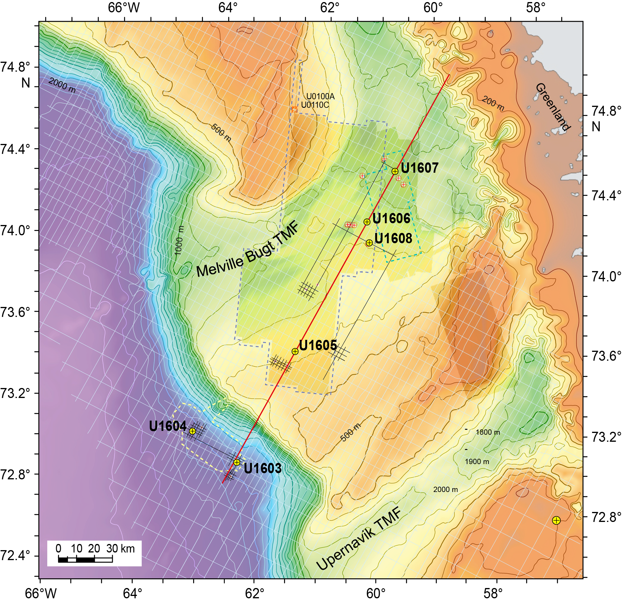
Figure F1. Bathymetry map.
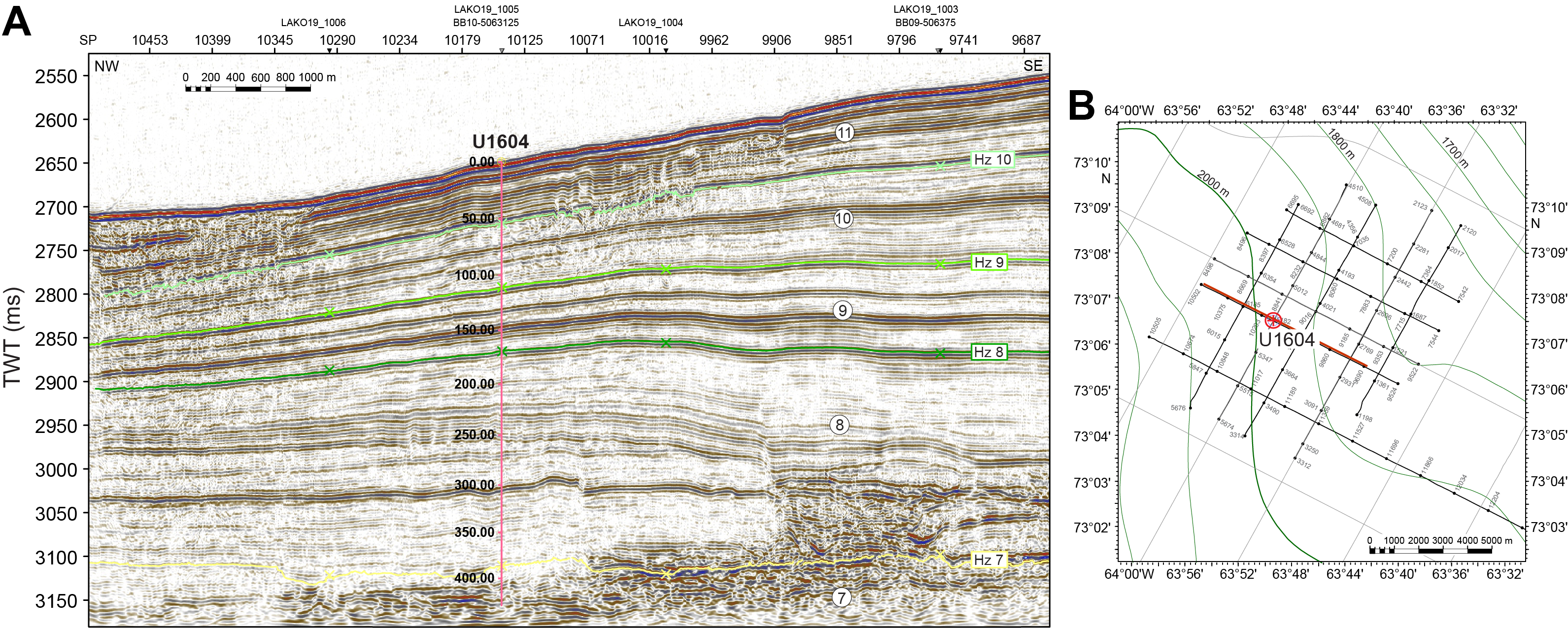
Figure F2. Seismic profile and close-up bathymetry map.
The drift-channel succession cored at Site U1604 is influenced by the circulation of deepwater masses in Baffin Bay, which is poorly constrained by oceanographic data but may be influenced by a southward flow along the Greenland margin that counters the surface currents (Tang et al., 2004). Gyre pulses of the West Greenland Current may overflow the site at intermediate water depths (e.g., down to 800 mbsl) (Münchow et al., 2015). The sediment sequence thickens in a southward direction nearer to a series of channel features.
The succession is hypothesized to represent interactions between bottom contour currents and sediments supplied by the NGrIS through glacial–interglacial cycles (Knutz et al., submitted). Increased glacigenic sediment fluxes may be expected during periods when ice was grounded on the outer shelf and during phases of ice sheet retreat. The scientific objectives for drilling Site U1604 are (1) to test the hypothesis that the NGrIS underwent significant deglaciation at intervals within the frequency range of orbital eccentricity (~100–400 ky) (Schaefer et al., 2016; Knutz et al., 2019) potentially related to exceptionally warm or prolonged super-interglacials (Melles et al., 2012; Christ et al., 2023) and (2) to achieve a long-term understanding (e.g., the last 0.5 My or older) of marine-based ice sheet dynamics and phasing relations between ice streams draining different sectors of the North American and Greenland ice sheets. In particular, we hope that the records can provide insights to ocean conditions through glacial terminations and ice-ocean dynamics associated with the different stages of ice sheet configurations (Hiscott et al., 1989; Simon et al. 2014), which may have far-field effects such as those associated with opening/closing of the Canadian Arctic straits (Jennings et al., 2022; Kelleher et al., 2022; Lofverstrom et al., 2022) (Figure F3). Finally, (3) the multiproxy data collected at the two deepwater sites (U1603 and U1604) will contribute to the objective of testing the regolith hypothesis for the change in orbital insolation frequency across the mid-Pleistocene transition (Clark and Pollard, 1998; Willeit et al., 2019).
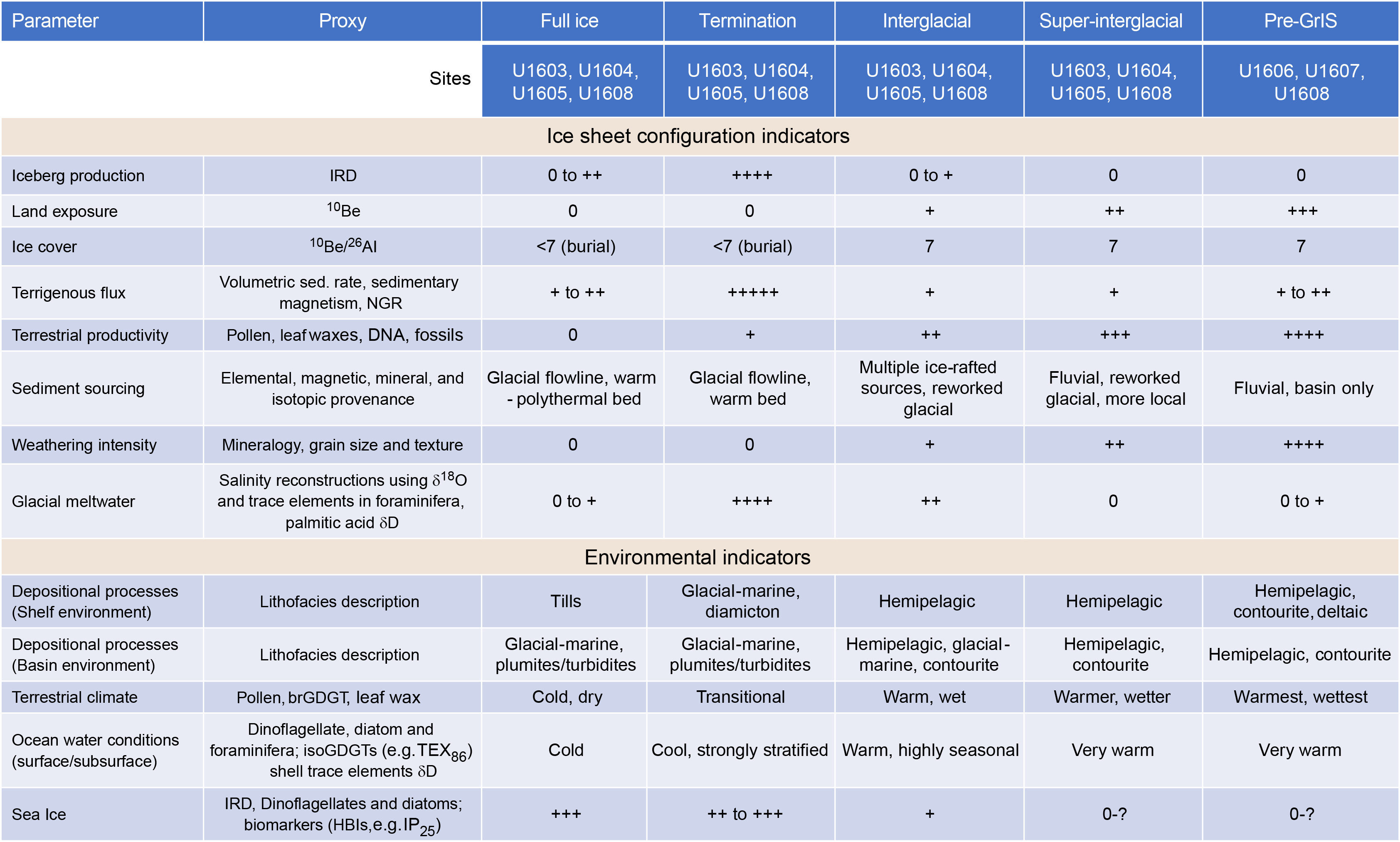
Figure F3. Diagnostic template for ice sheet evolution.
Coring was planned in two holes at Site U1604, both with a target depth of 432 m core depth below seafloor, Method A (CSF-A), using the advanced piston corer/half-length advanced piston corer (APC/HLAPC) systems. Downhole logging with the triple combo, Versatile Seismic Imager (VSI), and Formation MicroScanner (FMS)-sonic tool strings was planned for Hole U1604B.
2. Operations
Site U1604 hole locations, water depths, and the number of cores recovered are listed in Table T1. All times are local ship time (UTC − 3 h) unless otherwise noted.
2.1. Hole U1604A
The vessel transited 16 nmi from Site U1603 to Site U1604, arriving on location at 0306 h on 3 September 2023. The thrusters were lowered and secured at 0324 h, and the ship was fully in dynamic positioning mode at 0337 h. The rig crew made up an APC/extended core barrel (XCB) bottom-hole assembly (BHA) and began tripping the drill pipe. Hole U1604A was spudded at 1020 h, and Core 1H recovered 2.04 m. The seafloor was calculated as 1942.2 mbsl. Cores 1H–26H advanced from 0 to 206.8 m CSF-A and recovered 195.34 m (96%). Temperature measurements were made on Cores 4H, 7H, 10H, and 13H.
We switched to the HLAPC coring system; however, Core 400-U1604A-27F only recovered 2.81 m after a partial stroke. We then switched to the XCB coring system, and Cores 28X–30X advanced from 209.6 to 233.0 m CSF-A and recovered 23.71 m (103%). At 1930 h on 4 September, ice moved within 3 nmi of the vessel, and we raised the drill string to 16.2 m CSF-A by 2045 h and began waiting on ice. By 2300 h, the ice had moved a sufficient distance from the vessel, and we began to lower the drill string back into Hole U1604A.
The drill string was lowered into Hole U1604A and washed back to 233.0 m CSF-A by 0100 on 5 September. Cores 31X and 32X advanced from 233.0 to 250.6 m CSF-A and recovered 11.05 m (63%). At 0430 h, ice moved within 3 nmi of the vessel, and we raised the drill string to 16.7 m CSF-A by 0545 h and began waiting on ice. Ice then entered the 1 nmi exclusion zone, and we raised the drill string, clearing the seafloor at 0715 h and ending Hole U1604A. The vessel was moved 700 m north and then 700 m west to maintain a safe distance from the ice.
A total of 32 cores were taken in Hole U1604A over a 250.6 m interval with 93% recovery. Temperature measurements using the advanced piston corer temperature (APCT-3) tool were taken on Cores 4H, 7H, 10H, and 13H. Total time on Hole U1604A was 51.84 h (2.16 days). In total, 4.75 h were spent waiting on ice, and an additional 3.75 h of operational time was spent tripping pipe in and out of Hole U1604A to wait on ice.
2.2. Hole U1604B
By 1600 h on 5 September 2023, we began to move back toward the site, and the vessel was in position over Hole U1604B (20 m northeast of Hole U1604A) by 1630 h. Hole U1604B was spudded at 1755 h, and the seafloor was established as 1943.6 mbsl. Cores 1H–14H advanced from 0 to 105.3 m CSF-A and recovered 98.14 m (93%). However, Core 14H only recovered 0.16 m of material. An XCB core barrel was dropped, and Core 15X advanced from 105.3 to 105.5 m CSF-A and recovered 0.22 m of hard material. We then switched back to APC coring, and Cores 16H–22H advanced from 105.5 to 163.1 m CSF-A and recovered 59.68 m (103%). Cores 21H and 22H were only partial strokes, so we switched to the HLAPC system for Core 23F, which advanced from 163.1 to 167.9 m CSF-A and recovered 4.78 m (100%). We switched back to APC coring, and Cores 24H–30H advanced from 167.9 to 216.8 m CSF-A and recovered 49.87 m (102%). We then switched to the HLAPC coring system, and Cores 31F–35F advanced from 216.8 to 237.6 m CSF-A and recovered 16.89 m (83%). With ice still in the general area, we decided to install a free-fall funnel (FFF) to allow us to complete coring and logging of the site in Hole U1604B. The FFF was deployed at 1530 h on 7 September, and by 1630 h, we resumed coring Hole U1604B. Cores 36X–55X advanced from 237.6 to 429.6 m CSF-A and recovered 88.25 m (46%).
Sepiolite (drilling mud) was swept into the hole, and heavy barite mud was added in preparation for logging Hole U1604B. The drill string was tripped up, and the end of the pipe was set at 58.7 m CSF-A. The quad combo tool string was rigged up by 0100 h on 9 September and deployed to the base of Hole U1604B. Following a complete pass of the hole, the quad combo was pulled to the rig floor and broken down. The FMS was then assembled and deployed at 0640 h. The FMS was run, and the tools were back on deck by 1200 h. With logging completed, we tripped the pipe out of Hole U1604B and cleared the rig floor at 1720 h. The drill floor was secured for transit, and the thrusters were raised and secured for transit at 1824 h, ending Hole U1604B and Site U1604.
A total of 55 cores were taken in Hole U1604B over a 429.6 m interval with 74% recovery. Total time on Hole U1604B was 107.28 h (4.47 days). In total, 8.50 h were spent waiting on ice, and an additional 1.75 h of operational time was spent starting a new hole after needing to abandon Hole U1604A to ice.
3. Lithostratigraphy
Site U1604 consists of two overlapping holes (U1604A and U1604B) cored to a total depth of 429.6 m CSF-A. Hole U1604A reached 250.6 m CSF-A with 92.9% recovery. Hole U1604B reached 429.6 m CSF-A with 74.0% recovery. There were no drilled intervals at Site U1604.
The stratigraphy of Site U1604 is divided into three lithostratigraphic units (I–III; Figure F4; Table T2). named sedimentary lithofacies include massive mud, weakly stratified mud, calcareous mud, thinly laminated mud, interlaminated sand and mud, and gravel-bearing sediment (Figure F5).
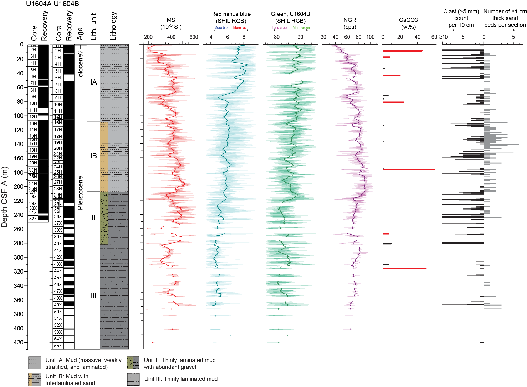
Figure F4. Lithostratigraphic summary.
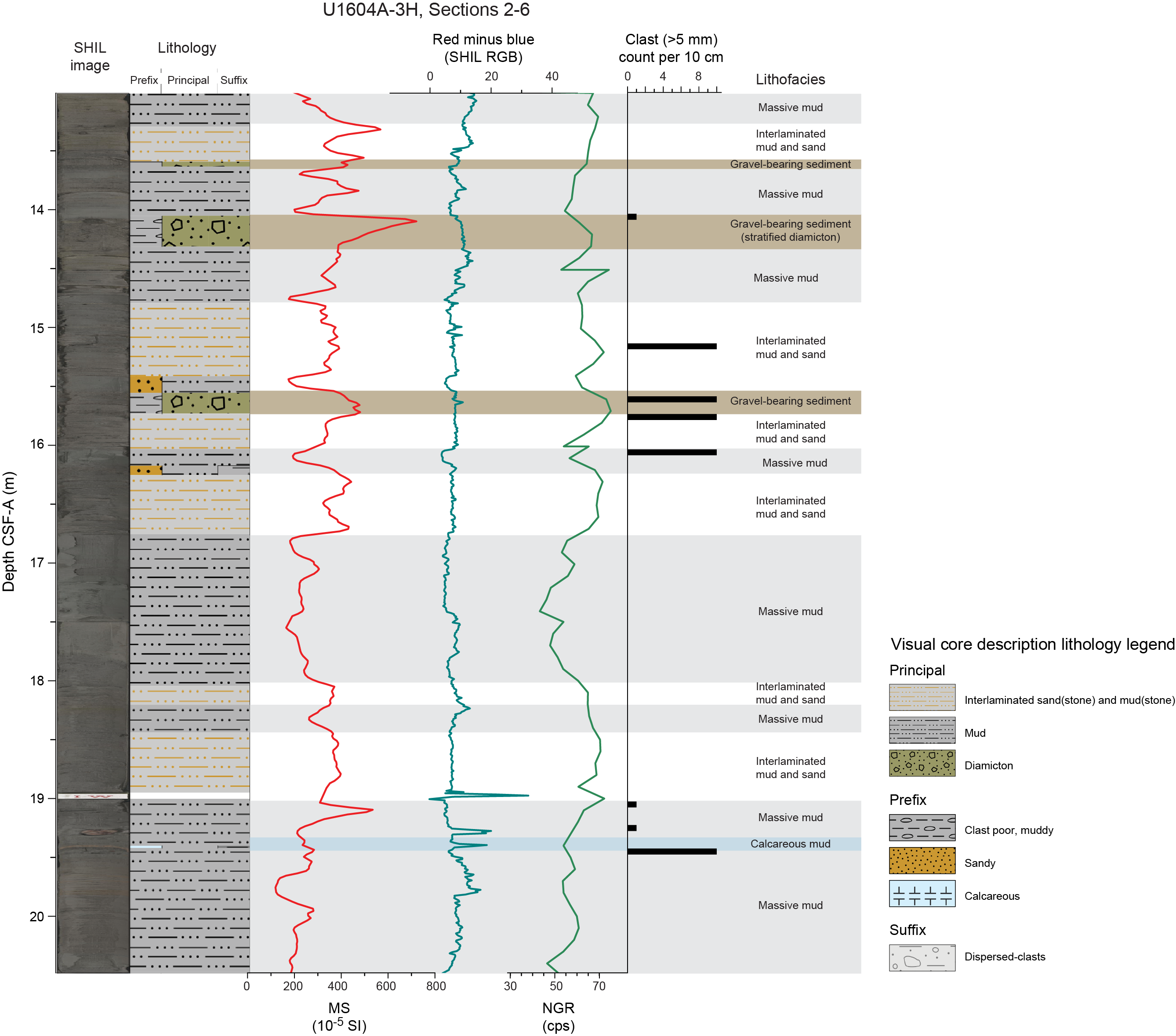
Figure F5. Multiple lithofacies.
Lithostratigraphic Unit I contains the uppermost ~210 m of this site, and all facies are present in various proportions. Unit I is divided into two subunits (IA and IB). Subunit IA is ~110 m thick and contains massive mud, weakly stratified mud, and laminated mud lithofacies with interbeds of calcareous mud and gravel-bearing sediment. Subunit IB spans ~100 m; it is lithologically very similar to Subunit IA but contains a larger proportion of interlaminated sand and mud and has relatively fewer outsized clasts (>2 mm diameter). Unit II is dominated by laminated mud and diamicton, often occurring as decimeter-scale interbeds. The laminated mud lithofacies continues downhole into Unit III, which is characterized by a significant reduction in sand laminae and gravel-bearing sediment compared to Unit II.
Compared to Site U1603, Site U1604 is located farther north at a slightly deeper water depth (~1943 mbsl) and is more distal from any present or past submarine channels. Both sites record approximately the same time interval, from the Early Pleistocene to the present, although Site U1604 recovered a sedimentary section that is relatively older based on the seismic data (Knutz et al., 2022). Site U1604 has lower average sediment accumulation rates (SARs) (above ~101 m CSF-A: ~15 cm/ky; below ~101 m CSF-A: ~46 cm/ky) (see Age model) than Site U1603 (above ~240 m CSF-A: ~28 cm/ky; below ~240 m CSF-A: ~75 cm/ky) (see Age model in the Site U1603 chapter [Knutz et al., 2025b]). Sediments deposited at Site U1604 are generally finer grained and contain fewer sand laminae than those at Site U1603. These differences in accumulation rates and grain size are likely due to the relatively proximal position of Site U1603 to a submarine channel.
Overall, the sedimentary succession recovered at Site U1604 is consistent with a continental slope environment with inputs from a combination of hemipelagic, contour current, and rare downslope processes, as well as likely ice rafting (providing granule- to boulder-sized clasts) and plumites.
3.1. Unit descriptions
Site U1604 is divided into three lithostratigraphic units (I–III; youngest to oldest) (Figure F4; Table T2). Significant downhole changes in lithology were determined using a combination of visual core description, microscopic characterization (using smear slides, thin sectioned grain mounts, and thin sections), reflectance spectroscopy and colorimetry, and bulk and clay mineralogical analyses using X-ray diffraction (XRD) (see Lithostratigraphy in the Expedition 400 methods chapter [Knutz et al., 2025a]).
3.1.1. Unit I
3.1.1.1. Subunit IA
- Intervals: 400-U1604A-1H-1, 0 cm, to 13H-3, 0 cm; 400-U1604B-1H-1, 0 cm, to 16H-3, 75 cm
- Depths: Hole U1604A = 0–109.27 m CSF-A; Hole U1604B = 0–109.27 m CSF-A
- Thicknesses: Hole U1604A = 109.27 m; Hole U1604B = 109.27 m
- Age: Middle? Pleistocene–Holocene
- Lithology: massive mud with dispersed to common clasts, laminated mud with interbeds of calcareous mud and gravel-bearing sediment
Lithostratigraphic Subunit IA is characterized by an alternating facies assemblage of massive mud with dispersed to common clasts, mud with weak stratification (including color banding), and mud with silt laminae. The mud lithofacies vary in color and include hues of grayish brown, gray, and greenish gray. Interlaminated sand and mud lithologies are also present but not dominant. Buff- to weak red–colored calcareous and gravel-bearing interbeds are common throughout.
3.1.1.2. Subunit IB
- Intervals: 400-U1604A-13H-3, 0 cm, to 27F-2, 43 cm; 400-U1604B-16H-3, 75 cm, to 30H-2, 0 cm
- Depths: Hole U1604A = 109.27–208.74 m CSF-A; Hole U1604B = 109.27–215.90 m CSF-A
- Thicknesses: Hole U1604A = 99.47 m; Hole U1604B = 106.63 m
- Age: Early Pleistocene–Late? Pleistocene
- Lithology: interlaminated sand and mud, massive mud with dispersed to common clasts, laminated mud with interbeds of calcareous mud and gravel-bearing sediment.
Lithostratigraphic Subunit IB has a facies assemblage similar to that of Subunit IA, but it is characterized by a greater abundance of interlaminated mud and sand intervals and a lower frequency of calcareous mud and sand beds or beds with a gravel component. The upper boundary of Subunit IB is defined by an increase in the abundance of >1 cm thick sand laminae downhole. The lower boundary of this subunit is defined by a downhole decrease in the sorting of sand strata, an increase in the thickness of the sand beds and laminae, and an increase in overall clast abundance.
3.1.2. Unit II
- Intervals: 400-U1604A-27F-2, 43 cm, to 32X-CC, 35 cm (bottom of the hole); 400-U1604B-30H-2, 0 cm, to 40X-4, 82 cm
- Depths: Hole U1604A = 208.74–246.87 m CSF-A (bottom of the hole); Hole U1604B = 215.90–281.28 m CSF-A
- Thicknesses: Hole U1604A = 38.13 m; Hole U1604B = 65.38 m
- Age: Early Pleistocene
- Lithology: laminated mud, gravel-bearing sediment, calcareous mud, massive mud
Lithostratigraphic Unit II is characterized by intervals of dark gray thinly laminated mud alternating with thick beds of dark gray stratified sandy mud with dispersed clasts to clast-poor sandy diamicton. Bioturbation is absent throughout most of the unit but does occur in rare, thin intervals above the boundary with Unit III. The defining characteristic of Unit II is that it contains much more of the gravel-bearing sediment lithofacies than Units I or III and lesser amounts of interlaminated sand and mud than Unit I. The upper boundary of Unit II is defined by the first downhole occurrence of thick beds of stratified sand with a gravel component, and the lower boundary is defined by the lowermost occurrence of a decimeter-scale–thick diamicton interbed. The transition between Units II and III is also associated with a gradual downhole decrease in the abundance of outsized clasts and interlaminated sand, as well as a downhole increase in bioturbated intervals.
3.1.3. Unit III
- Interval: 400-U1604B-40X-4, 82 cm, to 55X-CC, 29 cm
- Depth: 281.28–420.29 m CSF-A
- Thickness: 139.01 m
- Age: Early Pleistocene
- Lithology: laminated mud, calcareous mud, weakly stratified mud, gravel-bearing sediment, interlaminated sand and mud
Lithostratigraphic Unit III is dominated by dark gray to dark grayish brown thinly laminated mud of the laminated mud lithofacies. Within the laminated mud are interbeds of the calcareous mud, greenish gray weakly stratified mud, and rare gravel-bearing sediment lithofacies. Sand is rare, occurring as individual parallel- and cross-stratified laminae. Rare clasts that are unsorted and unstratified occur throughout. Bioturbation, which is observed in the massive to weakly stratified greenish gray muds, is more common than in Unit II. Black laminae become common below ~335 m CSF-A in Hole U1604B. The upper boundary of Unit III is defined by the lowermost occurrence of a decimeter-scale thick diamicton interval, and the lower boundary is the end of Hole U1604B.
3.2. Lithofacies descriptions
At Site U1604, six main lithofacies are identified based on lithology, sedimentary structures, and textural and other common characteristics.
3.2.1. Lithofacies 1: massive mud
Lithofacies 1 consists of beds of clay- and silt-sized terrigenous material that range in color from greenish gray to grayish brown and green hues. This lithofacies may contain occasional clasts or sand blebs but otherwise is distinctive in lacking any clear internal sedimentary structure (Figure F6). Although most beds are 5–25 cm thick, a bed approximately 9.4 m thick occurs throughout Core 400-U1604A-7H and continues in Section 8H-1 (Figure F6A). Rare clasts range in size from sand (0.063–2 mm) to pebble-grade clasts up to 4 cm in diameter. Where clasts and sand blebs occur in green mud, they often appear black due to coatings of iron sulfide (i.e., interval 400-U1604B-16H-6, 121–130 cm) (see Diagenesis). Smear slides indicate that this massive mud lithofacies is composed of a mixture of clay minerals and silt-sized particles that include abundant quartz and feldspar with common biotite, chlorite, and opaque components such as iron sulfide minerals. Sparse to common bioturbation is observed in this facies, where the lithology is more indurated.

Figure F6. Lithofacies 1.
Lithofacies 1 likely represents processes such as suspension settling (hemipelagic); low-concentration density flows; and, in the case of the thick bed in Cores 400-U1604A-7H and 8H, emplacement associated with mass movement (see Paleomagnetism). The sparse isolated clasts were likely delivered from ice rafting.
3.2.2. Lithofacies 2: weakly stratified mud
Lithofacies 2 consists of clay- and silt-sized terrigenous material that ranges in color from greenish gray to grayish brown. It is distinct from Lithofacies 1 in that it contains internal structures such as color banding, bioturbation, and other features (e.g., sparse silt or sand laminae) suggestive of deposition in beds. This lithofacies is often associated with color banding in the form of alternating reddish and greenish layers (Figure F7A), which may be associated with early diagenetic changes in the iron oxidation state below the sediment/water interface (see Diagenesis) or related to color variations related to grain size and/or sediment source variations. Although dispersed mottling that may reflect the burrowing actions of organisms is common (Figure F7B), clear evidence of bioturbation is typically sparse to absent. Very few intervals clearly show uncommon to moderate bioturbation (Figure F7C). Smear slide analysis shows that this lithofacies consists of a mixture of clay minerals and silt-sized particles that include abundant quartz and feldspar with biotite, chlorite, and other accessory minerals.
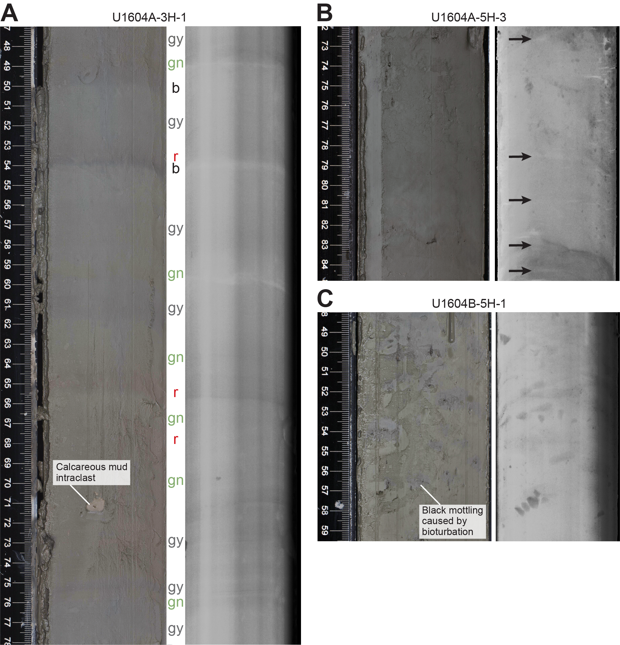
Figure F7. Lithofacies 2.
Lithofacies 2 represents depositional processes that include suspension settling (hemipelagic) and low-concentration density flows, with later overprinting by bioturbation and possibly by diagenetic processes that result in color banding.
3.2.3. Lithofacies 3: calcareous mud and sand
Lithofacies 3 consists of light yellow to dark brown mud to sand sediments with a calcareous matrix, which occurs in 1–50 cm thick beds. Smear slide analyses show that this lithofacies is dominated by mud- to sand-sized particles of abiotic carbonate, including rhombs, with minor siliciclastic components. Carbonate contents, which range 20.4–60.1 wt% (n = 6), are significantly higher than those of enclosing sediments (average = 1.3 wt%; median = 0.56 wt%; n = 83) (see Geochemistry). In the physical properties measurements, Lithofacies 3 is typically indicated by a combination of low magnetic susceptibility (MS) values, an increase in the difference between red and blue color space, and a low natural gamma radiation (NGR) value. The expression of this lithofacies varies through the succession (Figure F8), with some isolated laminae occurrences to multidecimeter-thick beds. Lithofacies 3 is enclosed by siliciclastic-dominated deposits, including massive mud, laminated mud, and interlaminated sand and mud.

Figure F8. Lithofacies 3.
The proportion of outsized clasts in this lithofacies is highly variable, ranging from dispersed to abundant (Figure F8). Some intervals are classed as diamicton. Upper and lower contacts may be sharp or gradational due to changes in color or their clast content (Figure F8A–F8C). More complex occurrences are characterized by isolated blebs, laminae, or thin beds that grade upward into a thicker bed of calcareous mud or sand before transitioning upward to isolated laminae within dark gray enclosing lithofacies (Figure F8D, F8E).
Lithofacies 3 occurs throughout the entire succession but remains relatively rare compared to other lithofacies. Thus, it may indicate depositional events involving a drastic change in sediment provenance. The depositional processes that led to the emplacement of these layers do not appear to deviate strongly from adjacent, noncalcareous lithofacies.
3.2.4. Lithofacies 4: laminated mud
Lithofacies 4 consists of clay- and silt-sized terrigenous material ranging in color from dark grayish brown to dark gray. This lithofacies is distinguished from the other mud-dominated lithofacies primarily by the presence of distinct parallel laminations, low-angle stratification, and rare ripple cross lamination (Figure F9). Individual mud laminae range ~0.1–0.5 cm in thickness with examples of sharp-based, millimeter-scale normal grading (likely from coarse silt at the base to fine silt or clay). Intervals exhibiting centimeter- to decimeter-scale variability in the inclination of lamination are observed and may represent low-angle stratification. In some occurrences, a vertical change in the angle of lamination is accompanied by thickness change (wedging or fanning geometry) and/or truncation of underlying laminae (Figure F9). Rare occurrences of distinct ripple cross lamination are also observed (Figure F9D). Lithofacies 4 contains rare very fine-grained sand laminae that are typically <0.3 cm thick. Rare dispersed clasts are present in some intervals, ranging from sand-sized grains (0.063–2 mm) to blebs containing sand-sized material and pebble-sized clasts. Bioturbation is absent to sparse. Smear slides indicate that this mud lithofacies is composed of a mixture of clay and silt with a trace or rare amount of sand. The silt particles are dominated by quartz and feldspar with common muscovite and other rare accessory minerals.
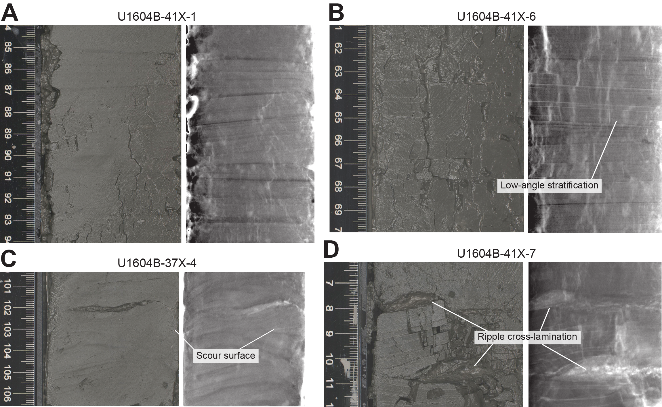
Figure F9. Lithofacies 4.
Lithofacies 4 represents deposition in an environment potentially influenced by a range of processes: from hemipelagic settling, bottom current traction sedimentation, and winnowing to low-concentration sediment-gravity flows. The sparse isolated clasts were likely delivered by ice rafting.
3.2.5. Lithofacies 5: interlaminated mud and sand
Lithofacies 5 consists of interlaminated to interbedded mud and sand with variable proportions of mud versus sand throughout the succession. The mud component is dark gray to dark brown and commonly laminated (Figure F10). Bioturbation in the mud component occurs locally but is typically absent to sparse. The composition of the mud component based on smear slide analysis reveals varying mixtures of clay and silt, with the silt particles dominated by quartz and feldspar and with muscovite and amphibole as accessory minerals. The sand component of this lithofacies is laminated (<1 cm) to very thinly bedded (1–2 cm). Sand grain size varies from very fine sand in the thinnest laminations to fine sand in the >1 cm thick beds. Normal grading is observed in >0.5 cm thick beds. Some of the sand beds displaying thicknesses ≥1 cm have internal structures including parallel lamination, ripple cross lamination, and centimeter-scale scour surfaces (Figure F10). Microfaults with millimeter- to centimeter-scale normal offset are observed in this lithofacies (Figure F10C). Bioturbation in the sand component is variable but is typically absent to sparse. The sand composition based on smear slide analysis is dominated by angular quartz and feldspar grains, with lesser amounts of amphibole, mica (muscovite and biotite), and igneous rock fragments. Grains are typically angular and show little to no evidence of alteration. In general, this lithofacies does not contain abundant dispersed clasts, but there are some intervals where isolated grains and granule- to small pebble–sized clasts are observed (Figure F10D).
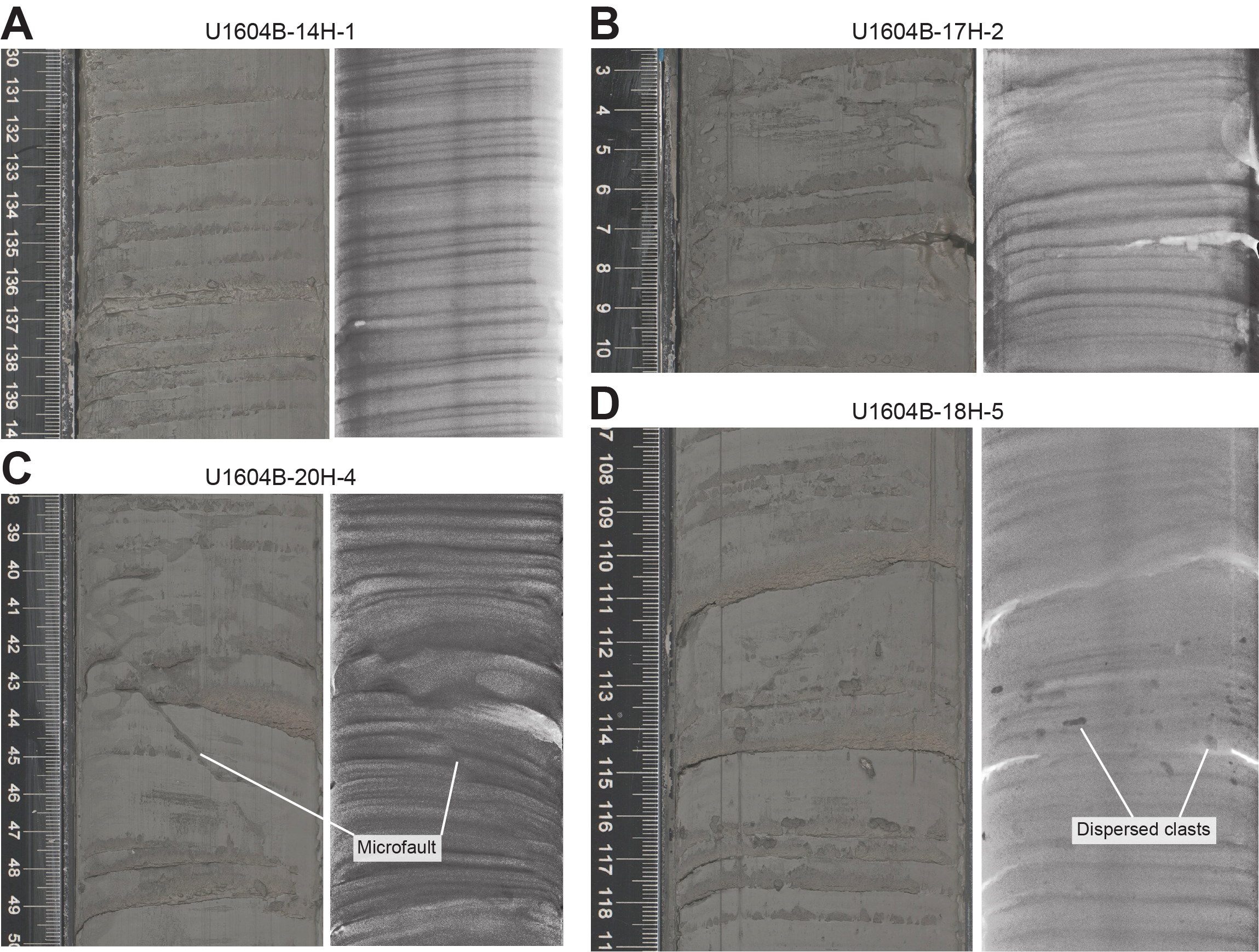
Figure F10. Lithofacies 5.
Lithofacies 5 represents a mixture of depositional processes on the continental slope, including downslope (turbidity current) processes, contour-current deposition, and suspension settling from plumes. The thicker, coarser grained, and normally graded sand beds are likely derived from turbidity currents, whereas the specific depositional process of the mud component is similar to Lithofacies 4. The sparse isolated clasts were likely delivered by ice rafting.
3.2.6. Lithofacies 6: gravel-bearing sediment
Lithofacies 6 consists of dark gray poorly sorted siliciclastic (noncalcareous) sediments with a matrix of sand and mud and a clast abundance of more than 1%. This lithofacies includes diamicton and sandy mud with common clasts (Figure F11). Stratification consists of centimeter-scale interbedding of mud and sandy mud with dispersed clasts or interlaminated sandy mud and mud. This lithofacies rarely exceeds more than 1 m in thickness, and both upper and lower bed boundaries are typically gradational, although a few intervals are sharply based. The sand component is poorly sorted. Clast sizes range up to large cobble size (25 cm). Clasts consist mainly of polymict assemblages of igneous, metamorphic, and sedimentary lithologies and occur both as isolated outsized clasts and as clast clusters. The matrix is typically crudely stratified and locally can be organized into horizontal planar millimeter- to centimeter-scale poorly sorted laminae of sand and granules. The sandy mud is characterized by sand-rich (>25%) mud with thin (<3 mm) to thick (3–10 mm) parallel laminations that are generally less visually distinctive than the interlaminated lithofacies. Sparse to moderate bioturbation may obscure the laminations.

Figure F11. Lithofacies 6.
Lithofacies 6 represents sedimentation in a glacially influenced lower continental slope environment with sedimentation from floating ice and reworking by currents. Sandy mud and muddy diamicton with clast clusters can be interpreted as hemipelagic sediment with ice-rafted debris, whereas some of the stratified clast-poor sandy diamicton and sandy mud could have originated as gravity flows or through winnowing of mud with dispersed clasts.
3.3. Diagenesis
Diagenetic features at Site U1604 include iron sulfide minerals, carbonate concretions, and color banding. The iron sulfide minerals often nucleate on sand or silt layers, forming prominent black laminae, and may form coatings on outsized clasts or sand blebs (Figure F12A, F12B). Dispersed iron sulfide is also present as black mottling or diffuse staining. Iron sulfide–stained laminae are first observed downhole between 22 and 24 m CSF-A: intervals 400-U1604A-4H-2, 132–150 cm (23.82–24.00 m CSF-A), and 400-U1604B-3H-7, 0–42 cm (22.12–22.38 m CSF-A). Carbonate-cemented concretions (Figure F12C) are present below 208 m CSF-A in Holes U1604A (interval 29X-1, 18–21 cm) and U1604B (interval 3H-7, 0–42 cm). Continuation of primary sedimentary laminae without deformation through concretions and, in thin sections, floating to point grain contacts among silt and sand grains suggest that cementation occurred at depths above the onset of physical sediment compaction. A broad correspondence to the sulfate reduction and sulfate–methane transition zone (see Geochemistry) is consistent with cementation being driven by alkalinity production during sulfate reduction as sediments pass through that interval. Throughout the succession recovered at Site U1604, decimeter-scale intervals of color-banded mud characterized by alternating reddish and greenish laminae or beds may reflect changes in iron oxidation (redox) state near the sediment/water interface (Figure F12D).
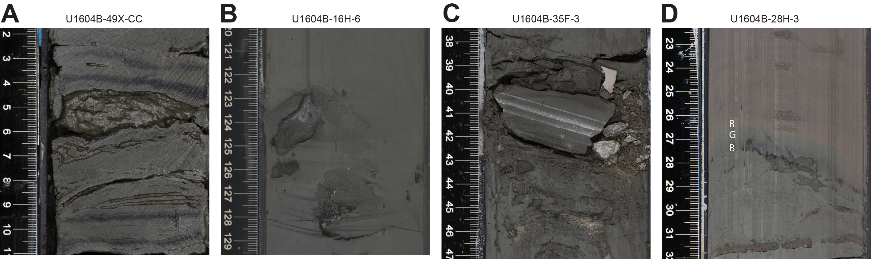
Figure F12. Diagenetic features.
3.4. Smear slide and thin section analysis
A series of smear slides were taken during core description to ascertain the characteristics and composition of mud and very fine sand. Clay was too fine grained for mineralogical identification using petrographic methods. Silt- and sand-sized grains are of terrigenous origin, dominated by quartz and feldspar minerals, with lesser amounts of mica, chlorite, amphibole, and other accessory minerals. Grains are typically angular to subangular, and minerals such as feldspar show no signs of alteration. Smear slides of calcareous mud intervals were also prepared and are dominated by clay- to silt-sized fragments and rhombs of calcite and dolomite. Quartz, feldspar, and clay are present in the calcareous mud samples in minor amounts.
A total of 11 thin sections were made from material in Holes U1604A and U1604B. Four thin sections (TS07–TS10) were made from grain mounts of paleontological (PAL) core catcher samples that were sieved to various sand size fractions. The sand in the grain mounts generally shows low textural maturity and low mineralogical maturity. Quartz and feldspar are the dominant lithologies, with accessory grains of pyroxene, diverse felsic-plutonic and metamorphic lithics, and rare calcareous lithics (including both dolomite and calcite). Three thin sections were made from limestone (TS11 and TS16) and plutonic igneous (TS12) outsized clasts. The remaining four thin sections were made from calcite-cemented mud concretions (TS13–TS15 and TS17). These samples show excellent examples of normally graded mud laminae, which is consistent with the observations of normal grading in the laminated mud and interlaminated mud and sand lithofacies.
3.5. Clay and bulk mineralogy results
XRD analyses were performed on 14 samples from Hole U1604A and 10 samples from Hole U1604B to determine the clay mineral compositions in Lithostratigraphic Subunits IA and IB and Units II and III. A qualitative and ratio-based summary of XRD results is given in Table T3 for clay compositions. The clay composition of Holes U1604A and U1604B is dominated by illite and chlorite, with no systematic change in their ratio downhole. In Hole U1604A, two samples from Sections 6H-3 and 17H-3 are marked by a higher chlorite/illite ratio. These samples were collected from diamicton and greenish gray massive mud lithologies.
An additional sample was collected for bulk analysis from a dark interval in Section 400-U1604A-5H-4. It is composed mainly of quartz, with feldspars, dolomite, kaolinite, and illite as minor components. Siderite is also identified in this sample.
3.6. Preliminary depositional interpretation
Site U1604 recovered a succession of Holocene to Early Pleistocene sediments from the continental slope and base of slope offshore northwest Greenland. This environment is consistent with that observed at Site U1603 but more distal from a submarine channel. Lithostratigraphic Subunits IA and IB and Unit III record a complex mixture of depositional processes on the continental slope that include suspension settling from plumes, turbidity currents, contour-current processes, and ice rafting. The prevalence of outsized clasts in the sandy mud, diamicton, and mud with dispersed clasts lithologies, especially in Unit II, indicate the glacigenic origin of the sediments and may record ice sheet processes that occurred on the shelf. Several calcareous mud intervals in an otherwise siliciclastic-dominated succession may suggest episodes of variable sediment provenance in the depositional evolution.
4. Biostratigraphy
4.1. Biostratigraphy and paleoenvironment
Site U1604, situated ~30 km northwest of Site U1603 and at water depths 142.6 m deeper, was aimed at recovering an expanded sequence of Seismic Unit 8, capturing the Pleistocene development of the Melville Bugt TMF complex. Core catcher samples and additional split core samples from the 32 cores from Hole U1604A and 21 cores from Hole U1604B were examined for foraminifera, diatoms, dinocysts, and other palynomorphs, as well as marine sedimentary ancient DNA (sedaDNA). Core catcher samples were not collected from the uppermost 35 cores of Hole U1604B because they represent a copy of the uppermost ~240 m of material cored in Hole U1604A. The additional samples from working section halves were taken within intervals of muds and muds with dispersed clasts, avoiding interlaminated mud and sand intervals. Mudline samples from Hole U1604A were also examined. Observations of foraminifera from palynomorph and diatom slide preparations were integrated in the overall foraminifera evaluations.
The mud and interlaminated sand and mud sediments of Site U1604 are generally barren of microfossils, apart from occasional horizons where trace to rare microfossils are found among the clast-rich samples (Figure F13). Where foraminifera appear, they remain as trace to rare occurrences, except in two samples (400-U1604A-9H-4, 80–82 cm, and 9H-6, 84–86 cm) where foraminifera are common in >63 µm residues. Juvenile foraminifera were also observed in palynomorph 10 µm sieved preparations. Diatoms were found in ~5% of all samples examined, with specimens presenting as fragments or trace individuals. Palynomorph preparations revealed generally low abundances of in situ dinocysts and varying abundances of reworked terrestrial and marine palynomorphs. The observed microfossil specimens and assemblages for all groups are broadly consistent with a Pleistocene age. The observed taxa have long stratigraphic ranges and thus provide limited age control. Specimens and assemblages of all groups are typical of cold-water, polar environments. Samples for sedaDNA analysis were collected in the APC sequence of Hole U1604B.

Figure F13. Trends across fossil groups.
4.1.1. Foraminifera
The mudline sample from Hole U1604A is barren of foraminifera, although it contains evidence of other lifeforms, including centric diatoms, diatom setae, organic mats (Figure F14A), polychaete worms, and an isopod. The sticky gray clays from the uppermost ~100 m of Hole U1604A were challenging to disaggregate. Because of the high clay content in much of the recovered sediment and the limited occurrences of fossil foraminifera observed at Site U1604 in some intervals, volumes of core catcher samples reached up to 30 cm3 bulk sediment volume. In other intervals where lithic grains swamped the bulk sediment, core catcher samples were limited to 10 cm3 for processing. In some cases, smear slides were prepared first to diagnose the presence of foraminifera and then a subsample was taken to recover assemblages. The washed sand residues (>63 µm) yielded variable amounts of sand for faunal analysis, from almost nothing to ~10 cm3 or more.

Figure F14. Lithics and coarse grain fractions.
Of the processed foraminifera samples, 34 of the 51 core catcher samples from Site U1604 are devoid of foraminifera and 17 have rare to trace foraminifera. Of the 34 additional samples taken from targeted intervals, 24 are also devoid of foraminifera. Rare to common calcareous foraminifera appeared in 10 residues. The >125 µm and 63–125 µm sieved fractions were examined separately, but because of the typically low numbers of foraminifera, observations are combined. Planktonic and benthic foraminifera are also presented together here. The foraminifera sand fractions provide an opportunity to observe variability in lithic grains throughout the section (Figure F14). End-members include samples dominated by well-sorted quartz sand with variable additional coarser grain components (Figure F14E, F14O) derived from the mud and interlaminated sand and mud lithofacies, as well as horizons with abundant large lithic grains of quartz, feldspar, and granite (Figure F14B, F14E), to samples containing large transported carbonate and dolomite clasts and/or carbonate-cemented sandstones of various types (Figure F14B, F14G–F14M), including clasts of fine-grained carbonate-cemented sandstone and conglomerate (Figure F14G–F14J). Other grains of interest are large, well-rounded, and spherical quartz grains, which are present in many samples (Figure F14C, F14D, F14G, F14K, F14M), concentrations of pyrite (Figure F14F), and dark gray metallic-looking grains that often have rusty oxide coatings (Figure F14N).
The core catchers and additional samples in which foraminifera (planktonic and benthic) are observed are shown in Table T4. The polar species Neogloboquadrina pachyderma is the only species of planktonic foraminifera observed, and it usually appears only as rare to trace occurrences (Figure F15B, F15I). However, there are few to abundant N. pachyderma in Samples 400-U1604A-9H-3, 100–102 cm (Figure F15F), 9H-4, 80–82 cm (Figure F15H), and 28X-7, 23–25 cm. Small foraminifera, both planktonic and benthic, are also common in the palynology slide of Sample 28X-7, 24–25 cm. A relatively large five- to six-chambered morphotype of N. pachyderma is generally common in the pachyderma-bearing samples. This is likely attributable to the morphotype Nps-4 (Eynaud et al., 2009; El Bani Altuna et al., 2018). Coiling counts on these samples, which are consistent with a 5% dextral contribution, suggest the absence of Neogloboquadrina incompta in Site U1604 samples.
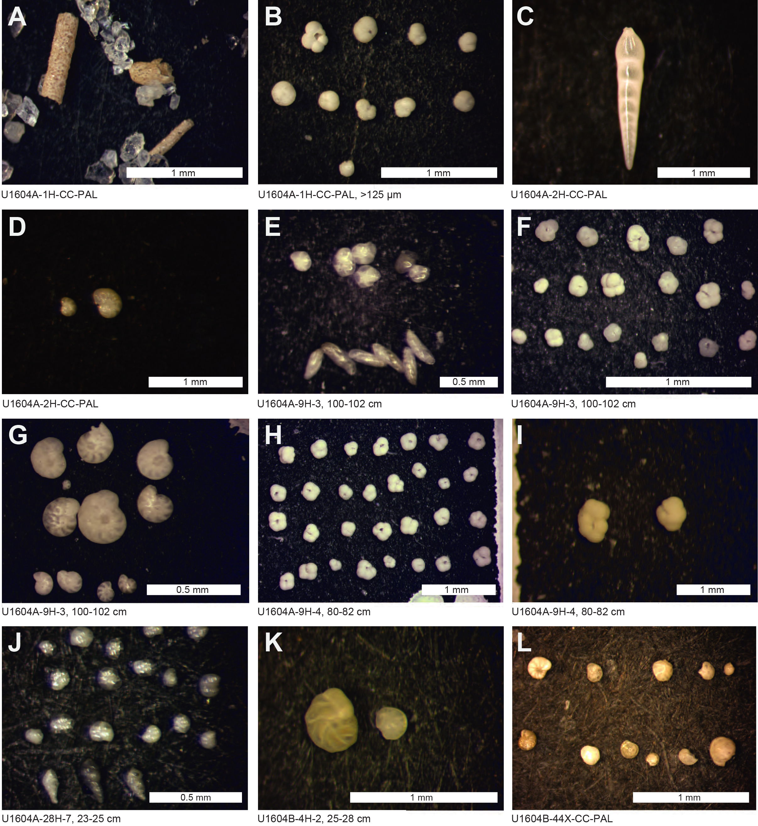
Figure F15. Benthic and planktonic foraminifera.
In terms of benthic foraminifera, rare agglutinated tubular benthics are observed in Section 400-U1604A-1H-CC (Figure F15A). The rest of the benthic foraminifera observed are calcareous and usually appear in trace to rare amounts with the exception of Samples 9H-3, 100–102 cm, 9H-4, 80–82 cm, 28H-7, 23–25 cm, and 400-U1604B-44X-CC, where some benthic species are common (Figure F15E, F15G, F15H, F15J, F15L). The most commonly encountered benthic species are Elphidium clavatum, Cassidulina reniforme, Islandiella helenae, Stainforthia feylingi, Buliminella elegantissima hensoni, and Stetsonia horvathi. Other species observed include Astrononion gallowayi, Dentalina frobisherensis, Triloculina trihedra, Bolivina arctica, and species of milliolids (Figure F15C, F15D, F15K). A more complete benthic assemblage in Section 400-U1604B-44X-CC (Figure F15L) contains Haynesina orbiculare, Cibicides sp., Buccella frigida, Buccella tenerrima, Epistominella takayanagi, Cassidulina teretis/neoteretis group (which are difficult to separate without scanning electron microscope [SEM] work) (Cage et al., 2021), and Nonionellina labradorica. The benthic species recognized are typical of Quaternary Arctic shelf and slope environments. As at Site U1603, the benthic assemblages are similar to those found by Kaminski et al. (1989) at Ocean Drilling Program Site 645 and Feyling-Hansen (1976) in the Clyde Foreland Formation (western Baffin Bay). Together with the presence of rich N. pachyderma populations, where present, these foraminifera constraints are consistent with a Pleistocene age for Site U1604.
In six cases, foraminifera appear in palynology slides, although they do not appear in the >63 µm residues (Samples 400-U1604A-2H-1, 45–47 cm, 2H-4, 67–69 cm, 7H-1, 91–92 cm, 9H-1, 19–20 cm, 14H-CC, and 400-U1604B-43X-4, 15–16 cm). These slides record foraminifera specimens smaller than the typical 63 µm preparations routinely examined by the foraminifera team, suggesting incomplete recovery of all foraminifera specimens.
4.1.2. Diatoms
At Site U1604, a total of 131 samples from core catchers and split cores were examined for diatoms. The majority of the samples are barren of diatoms, whereas trace amounts of diatoms were observed in seven samples (~5% of all samples): 400-U1604A-1H-1, 0 cm (mudline), 9H-3, 100–101 cm, 9H-4, 80–81 cm, 28X-7, 23–24 cm, 28X-7, 30–31 cm, 400-U1604B-1H-1, 0 cm (mudline), and 40X-4, 30–31 cm.
In mudline Samples 400-U1604A-1H-1, 0 cm, and 400-U1604B-1H-1, 0 cm, Actinocyclus curvatulus, Chaetoceros spp. resting spore, and Melosira arctica are observed. Their relative abundances range from trace to a few. Additionally, Podosira sp. (montagnei?) is detected in trace amounts in Samples 400-U1604A-9H-3, 100–101 cm, 9H-4, 80–81 cm, 28X-7, 23–24 cm, and 28X-7, 30–31 cm. A few Podosira sp. (montagnei?) specimens and fragments, likely derived from this species, are encountered in Sample 400-U1604B-40X-4, 30–31 cm.
The trace occurrence and poor preservation of diatoms at Site U1604 preclude any stratigraphic analysis and, thus, age determination.
4.1.3. Palynology
In total, 29 core catcher samples and 36 additional samples from targeted intervals were processed following the procedure described in Biostratigraphy in the Expedition 400 methods chapter (Knutz et al., 2025a). Because of time limitations, only the even-numbered core catcher samples were analyzed on board.
Overall, palynomorphs, and notably the dinocysts among them, were found to be scarce, with the exception of a few intervals, and no quantitative analyses were conducted (Table T5; Figure F13). Most samples are dominated by high mica concentrations and green crystals (Figure F16A). Compared to the palynomorph assemblage of Site U1603, concentrations of in situ dinocysts and pollen, as well as reworked material, are much lower in Site U1604.

Figure F16. Palynomorphs.
All dinocyst species observed are consistent with a Pleistocene age. Preservation of in situ dinocysts is good where they occur, although abundances are very low across the entire studied interval. Rarity of palynomorphs in the Quaternary in the Arctic Ocean can be explained by the small number of dinoflagellates around the Arctic that form fossilizable cysts (Okolodkov, 1998) and the general ecological preference of dinoflagellates for warmer waters (e.g., de Vernal et al., 2013).
Dinocyst species belonging to the genus Brigantedinium spp. are observed in 20 of 65 samples throughout the entire interval. This taxon is abundant in Samples 400-U1604A-16H-CC, 38X-CC, and 42X-CC (Figure F16B). Brigantedinium spp. is also common in Samples 3H-CC, 6H-CC, 8H-2, 65–66 cm, 10H-3, 11–12 cm, 21H-7, 21–22 cm, and 32X-CC. Other species of dinocyst are very rare but include Islandinium brevispinosum and Islandinium minutum. Intervals with higher abundances of these dinocysts include Samples 6H-CC, 9H-6, 85–86 cm, 10H-3, 11–12 cm, and 400-U1604B-38X-CC.
In addition to in situ palynomorphs, varying abundances of reworked palynomorphs were recorded in 49 samples, with abundant terrestrial reworking recognized in Sample 400-U1604A-10H-3, 11–12 cm. The reworked terrestrial material includes bisaccate pollen, other gymnosperm pollen, and fern spores. Especially in Sample 21H-4, 17–18 cm, a variety of (reworked) big fern spores are present (Figure F16C–F16F), but fern spores are not restricted to this sample. Future study by a pollen and spore specialist would be a valuable contribution to constrain the age of the reworked sediments. In some samples, palynomorph reworking involved marine material, represented by high numbers of dinocysts. Typical reworked assemblages (Figure F16H–F16J) include various dinocyst species belonging to the genera Thalassiphora, Deflandrea, Lingulodinium, and others. Two concentrated pulses of reworking of dinocysts were observed in Samples 5H-4, 18–19 cm, and 10H-3, 11–12 cm. Sample 5H-4, 18–19 cm, represents a black clast embedded in mud (Figure F16G) that was specifically targeted to study the provenance of this clast. Sedimentary clasts have great potential to further constrain the source of reworked material.
Palynomorph preparations also include high abundances of amorphous clay clasts (Figure F16K) in Samples 400-U1604A-6H-CC and 28X-7, 40–41 cm, with 10% and 20% coverage of these clasts, respectively. Also, in the uppermost three core catcher samples (1H-CC, 2H-CC, and 3H-CC) and Samples 2H-1, 45–47 cm, and 2H-4, 67–69 cm, yellow palynomorphs and agglutinated foraminifera are present (Figure F16L). These yellow palynomorphs have not been identified, although they resemble the green algae Botryococcus. Very small benthic and planktonic foraminifera were also recorded in other samples, with the highest abundances in samples from Sections 9H-3, 9H-4, and 9H-6 (Figures F13, F16M, F16N).
4.1.4. Marine sedimentary ancient DNA
Samples for sedaDNA analysis were collected from Hole U1604B through Core 35F (~237 m CSF-A), below which we switched to the XCB system and no further samples were collected. A mudline sample (~10 g) was collected as a modern reference, and a total of 110 samples were collected for sedaDNA analysis (Table T6, Figure F17) following the catwalk and the split core sampling methodologies (see Biostratigraphy in the Expedition 400 methods chapter [Knutz et al., 2025a]). On the catwalk, a total of 79 samples were taken, usually at the bottom of Sections 1, 3, and 5 if the sections were available and the section bottom was undisturbed. Additionally, 31 samples were collected from the working half of split sections, targeting nonstratified mud layers with little or no clasts, characterized by low MS and low NGR, predominantly above and/or below calcareous mud layers. Based on the lithofacies observed (see Lithostratigraphy), 47 sedaDNA samples were taken within interlaminated sand(stone) and mud(stone), 1 within interlaminated sand(stone) and mud(stone) with dispersed clasts, 50 in mud, 11 in mud with dispersed clasts, and 1 in mud with common clasts. All samples were immediately stored at −86°C. The majority of sediment samples (interior) have a contamination level close to or below the detection limit (Table T7). However, four samples taken on the catwalk show elevated tracer levels (mostly below 1 ppb), and one sample contained up to 6.3238 ppb. Lithology does not seem to have an effect on the level of contamination.
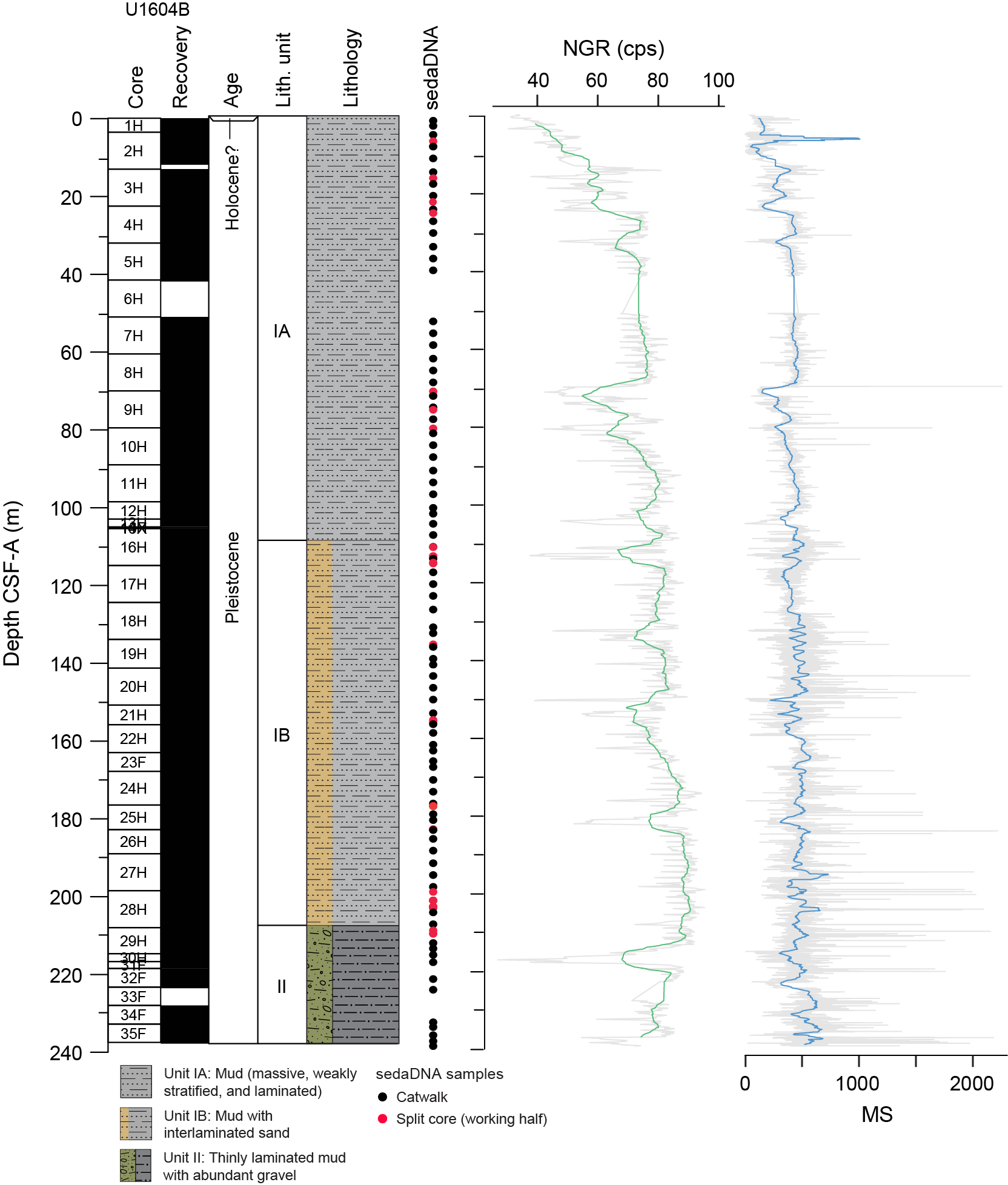
Figure F17. sedaDNA samples.
5. Paleomagnetism
Pass-through paleomagnetic measurements for Site U1604 were performed using the superconducting rock magnetometer (SRM) to investigate the natural remanent magnetization (NRM) on a total of 389 archive section halves. Measurements were not made on archive section halves that had highly disturbed sediments or on core catcher sections. All measurements on section halves were made at 2 cm intervals up to a peak alternating field (AF) demagnetization of 20 mT.
A total of 248 discrete cube samples were taken from the working section halves. Generally, we collected one sample per core section, avoiding visually disturbed intervals and filling in gaps where the other hole did not have recovery. Discrete specimens were measured on the SRM or the AGICO JR-6A spinner magnetometer.
5.1. Discrete sample measurements
A total of 248 discrete cube samples were collected from working section halves from Site U1604: 157 from Hole U1604A and 91 from Hole U1604B. Two discrete samples were disturbed in the sampling process and were not measured. A total of 55 discrete specimens were measured after stepwise demagnetization up to a peak field of 80 mT on the JR-6A to assess demagnetization behavior; Zijderveld diagrams (Zijderveld, 1967) of representative specimens are shown in Figure F18, along with plots of the remaining remanence versus AF demagnetization step. The specimen in Figure F18A and F18E shows behavior typical of normally magnetized specimens with a vertical drill string overprint, which is removed by the second demagnetization step (10 mT), after which the magnetization decays linearly to the origin. The drill string overprint is also removed by 15 mT in a typical reversely magnetized specimen (Figure F18B, F18F). Both are nearly completely demagnetized by 80 mT, a behavior that is typical of a magnetization carried by magnetite. In contrast, the behavior of the specimen in Figure F18C and F18G is nearly completely demagnetized by 15 mT, and the downward-directed magnetization is most likely solely that of the drill string overprint and cannot be trusted. The specimen in Figure F18D and F18H shows evidence of a gyromagnetic remanent magnetization (GRM; Stephenson, 1993), particularly at the 80 mT step (see equal area projection in the inset to Figure F18D). We subjected all specimens to the three-step test for GRM of Stephenson (1993), and in this example, instead of demagnetizing, the specimen gained a remanence orthogonal to the last direction subjected to AFs, which is the effect of GRM and is frequently attributed to the mineral greigite, a magnetic iron sulfide (Stephenson and Snowball, 2001). Greigite is thought to be a diagenetic mineral, and the magnetic vectors of specimens with significant GRM should also be viewed as suspect.

Figure F18. AF demagnetization behavior.
All other specimens not measured on the JR-6A were measured after stepwise demagnetization up to a peak field of 20 mT on the SRM to remove the drill string overprint. The preliminary magnetostratigraphy is based on inclination from measurements of the 20 mT AF demagnetization step. Declination is not used to constrain polarity because the cores are not azimuthally oriented and the field at the latitude of this site is nearly vertical.
Anisotropy of MS (AMS) and volume-normalized bulk MS were measured on 246 discrete specimens. The data are reduced to a 3 × 3 tensor with eigenvalues (τ1, τ2, and τ3) and eigenvectors (V1, V2, and V3), where τ1 is the maximum eigenvalue associated with eigenvector V1 and τ1 > τ2 > τ3. When the ratio of the maximum eigenvalue to the intermediate eigenvalue (τ1/τ2) is significantly different from unity, those intervals are likely disturbed either from sedimentary processes or coring disturbance. A cumulative distribution function of this ratio is plotted in Figure F19A. As discussed in Paleomagnetism in the Expedition 400 Site U1603 chapter (Knutz et al., 2025b), we suggest a value for τ1/τ2 > 1.02 can be interpreted to mean that the sediments were disturbed either by natural processes or during coring. We plot the eigenvector directions in Figure F19B. The inclination of the minimum axis (V3; blue circles) is expected to be vertical in most sediments, which is the case for the majority of our specimens.
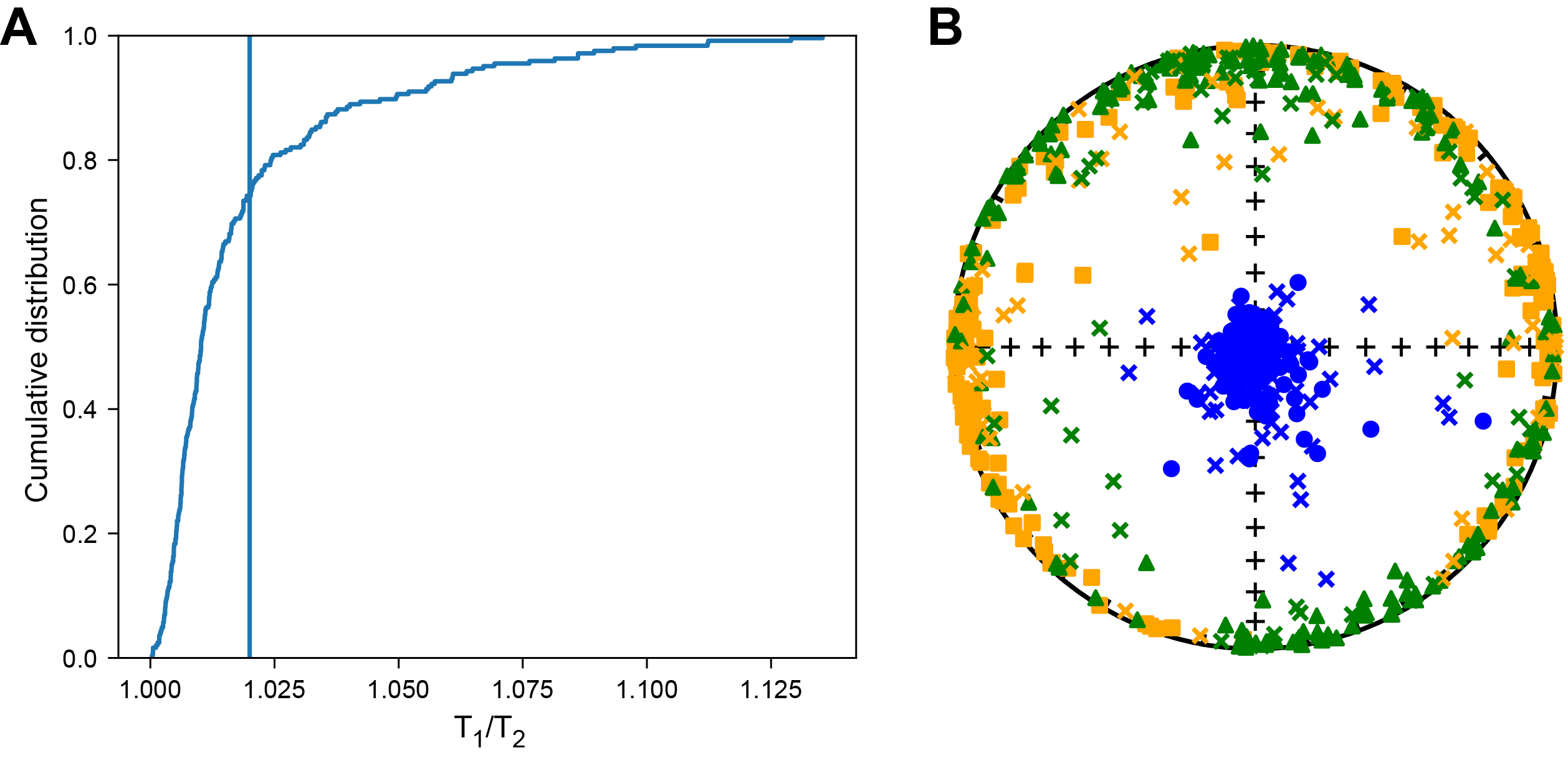
Figure F19. AMS data.
To examine the behavior of the eigenparameters versus depth, we plot the eigenvalues downcore in Figure F20A, along with the inclination of the eigenvector V3 (Figure F20B) and the ratio τ1/τ2 (Figure F20C). Data from disturbed specimens are plotted as Xs in Figures F20A and F19.
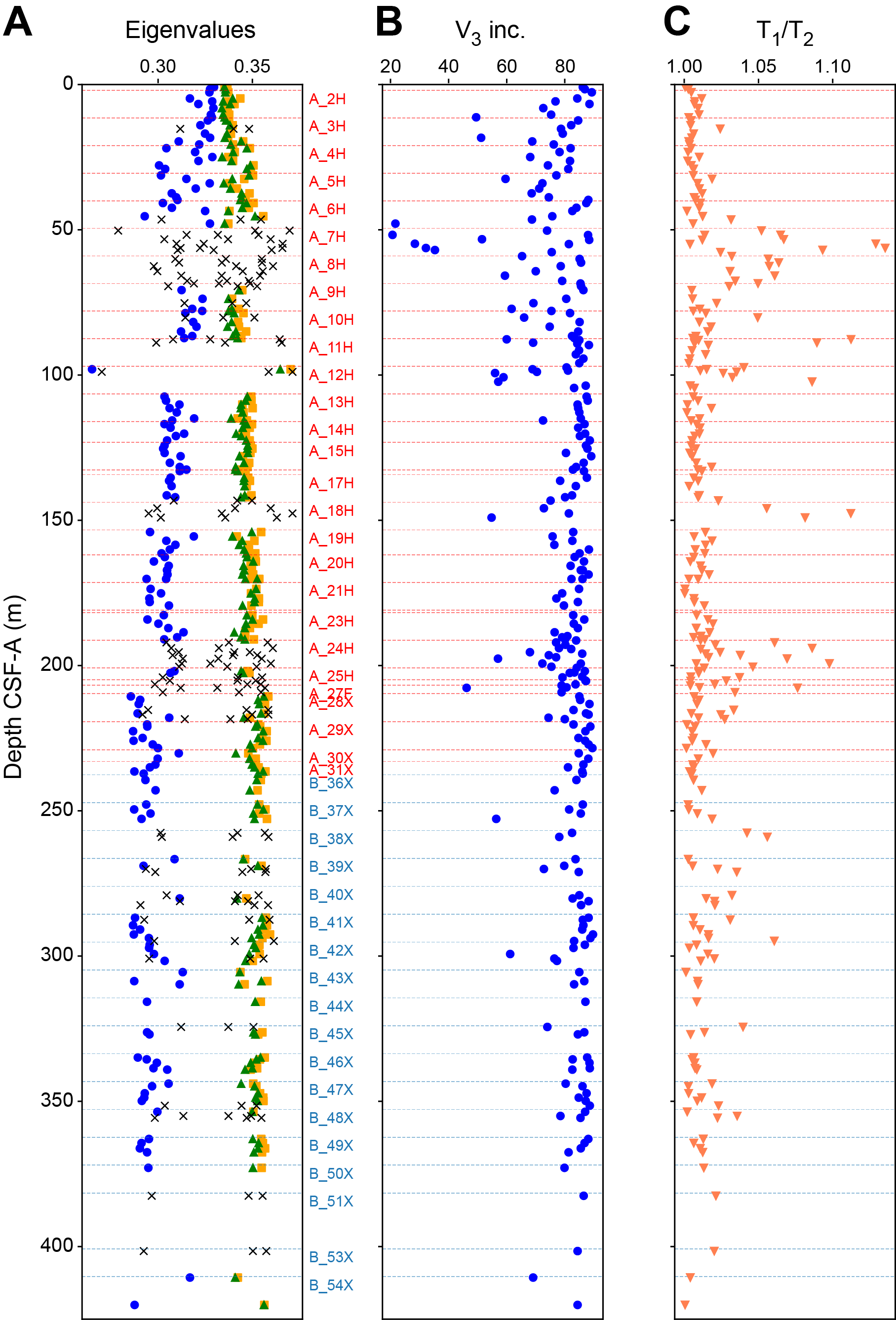
Figure F20. AMS parameters with depth.
Anhysteretic remanent magnetization (ARM) was measured on a subset of 29 discrete specimens from Hole U1604A. For this subset, we demagnetized the specimens to 100 mT on all three axes and measured the remanence. We then imparted an ARM with a peak 100 mT AF and 50 µT direct current (DC) field and measured the remanence. These measurements were compared with volume-normalized bulk MS. The relationship between ARM and MS (Figure F21) is quasilinear, suggesting that the concentration of magnetic minerals is the primary control on both measurements and supporting the use of normalized remanence for estimating relative paleointensity (RPI) (see Age model).
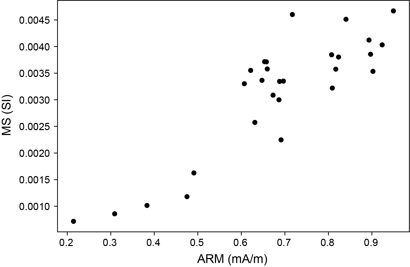
Figure F21. ARM versus bulk MS.
5.2. Archive-half measurements
Site U1604 archive section halves were stepwise demagnetized to 20 mT to remove the drill string overprint. All measured sections from Hole U1604A and Cores 400-U1604B-1H and 2H were measured after 0, 5, 10, 15, and 20 mT peak AF demagnetization steps. To decrease the time required for measurements, Sections 400-U1604B-3H-1 through 23H-1 were measured after 0, 10, 15, and 20 mT peak AF demagnetization steps, and core sections from Section 23H-2 to the bottom of Hole U1604B were measured after 0, 10, and 20 mT peak AF demagnetization steps. Data were filtered as follows:
- All measurements within 10 cm of section ends were deleted to remove the edge effects associated with pass-through measurements.
- Intervals with drilling disturbances as defined by the disturbance intensity code of “moderately disturbed” or greater (see Lithostratigraphy in the Expedition 400 methods chapter [Knutz et al., 2025a]) were removed.
- Core linescan images and X-radiographs in intervals of suspect directions were examined to assess where lithologic features such as dropstones or concretions necessitated removal of intervals.
Data from the 20 mT demagnetization step are shown in Figures F22 and F23. Where the AMS data in Figure F20 indicate disturbance, specimens are plotted as Xs to identify horizons with potentially unreliable magnetic vectors. The inclinations from the filtered 20 mT step data are also shown as kernel density plots in Figure F24. The inclination values are generally bimodal, centered at the estimates from geocentric axial dipole (GAD) inclinations for normal and reversed polarities at this latitude, suggesting that intervals of both normal and reversed polarity were recovered at Site U1604.

Figure F22. Intensity, declination, and inclination, Hole U1604A.
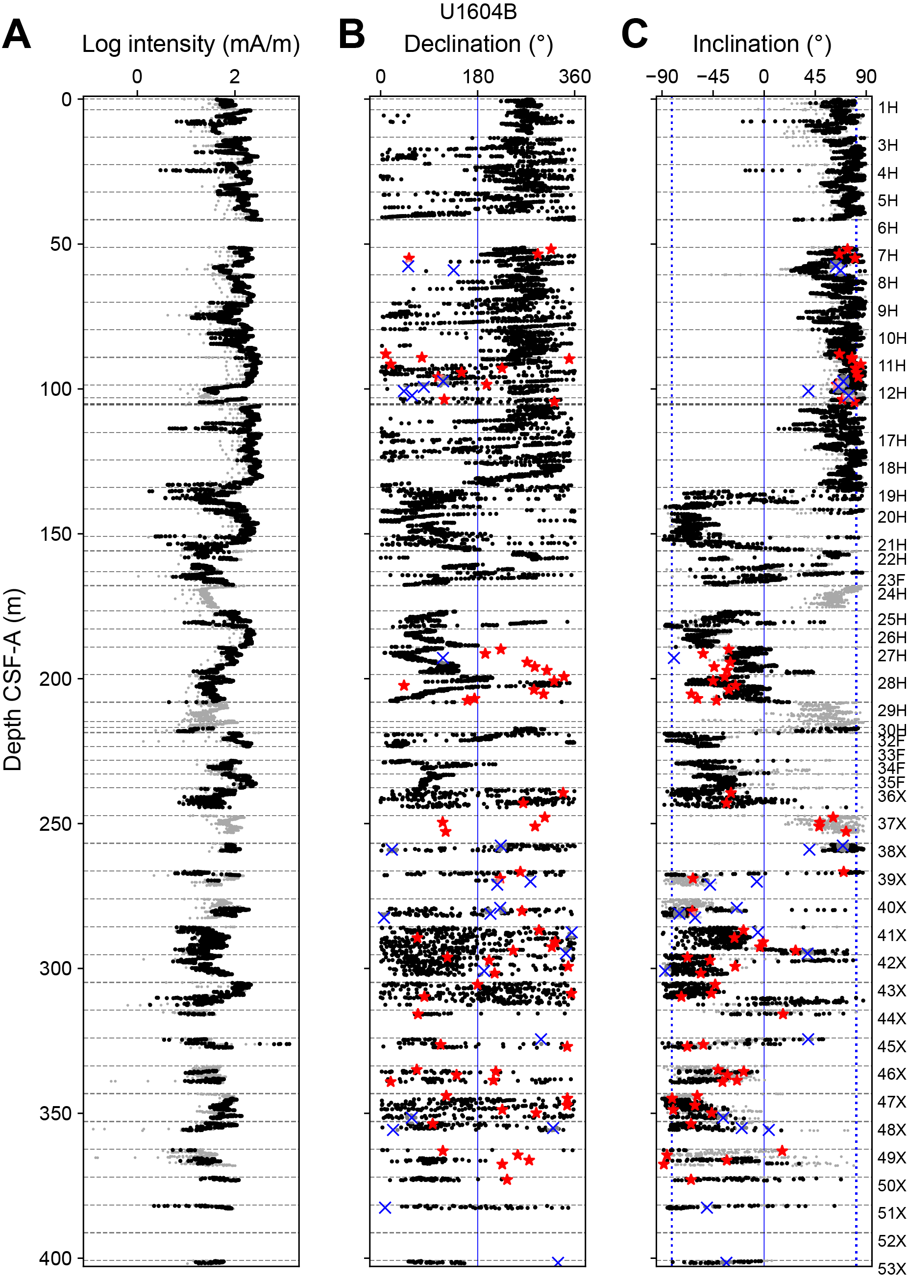
Figure F23. Intensity, declination, and inclination, Hole U1604B.
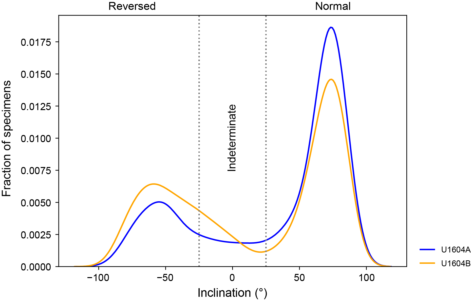
Figure F24. Inclination.
5.3. Magnetostratigraphy
Magnetostratigraphic interpretations are based on inclinations calculated from archive section half and discrete specimen measurements made after the 20 mT AF demagnetization step. We observe an interval of normal polarity (Polarity Zone N1 in Figure F25) from the surface to 137.6 m CSF-A in Hole U1604B (Table T8), below which inclinations are reversed polarity (Polarity Zone R1). We tentatively suggest another interval of normal polarity (Polarity Zone N2) below 247.5 m CSF-A in Hole U1604B, with a lower boundary of 267.4 m CSF-A (Table T8). Although the pass-through data from this core have been filtered following the disturbance code assigned during the description process, our assessment of the fidelity of the discrete cube measurements (through AF demagnetization and AMS measurements) supports the presence of a normal polarity zone. Below 267.4 m CSF-A, we assign mainly reversed polarity (Polarity Zone R2) with an unclear lower boundary. The other apparently normal intervals within Polarity Zone R1 and Polarity Zone R2 are likely disturbed. We interpret the magnetostratigraphic patterns in combination with the geomagnetic polarity timescale of Ogg (2020), correlating Polarity Zone N1 to the Brunhes Chron (C1n) and Polarity Zone R1 to the end of the Matuyama Chron (C1r.1r). We correlate Polarity Zone N2 to the Jaramillo Subchron (C1r.1n) and Polarity Zone R2 to Chron C1r.2r. See Age model for further discussion.
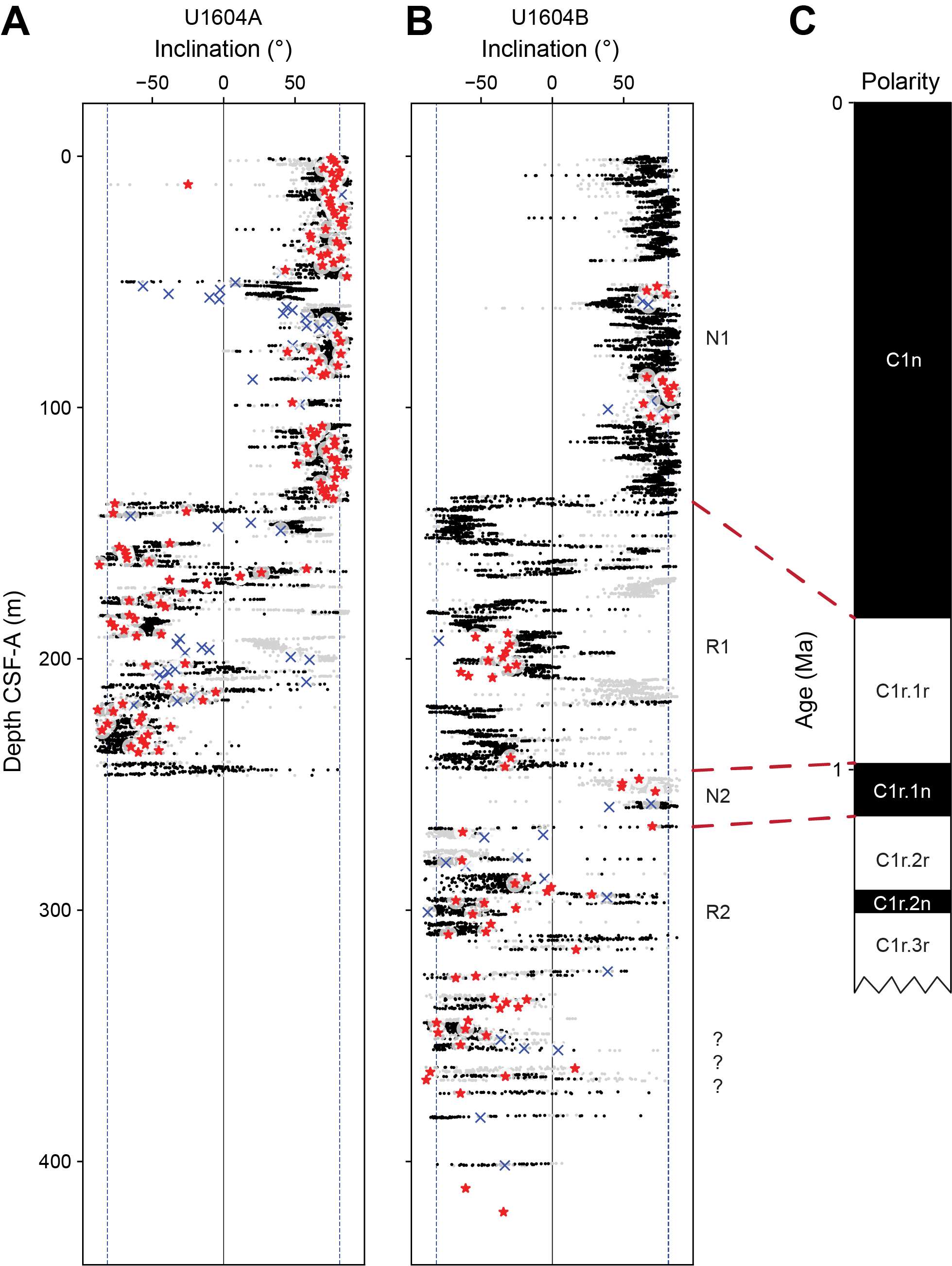
Figure F25. Magnetostratigraphic correlation.
6. Physical properties
Physical property data were acquired on all cores from Holes U1604A and U1604B using the Whole-Round Multisensor Logger (WRMSL) for wet bulk density based on gamma ray attenuation (GRA), MS, and P-wave velocity (using the P-wave logger [PWL]). We also measured NGR in all sections longer than 50 cm. Thermal conductivity was measured in one whole-round section per core from Hole U1604A and below 250 m CSF-A in Hole U1604B wherever possible. However, thermal conductivity was measured on the working section halves if the sediment was too hard or the whole-round measurement readings were unreliable. In the uppermost 250 m of Hole U1604B (Cores 1H–35F), only NGR and low-resolution (5 cm) MS were logged. Cores 1H–35F constitute a replica of Hole U1604A, so equalization to room temperature and GRA bulk density measurements were avoided in the interest of stratigraphic correlation and sedaDNA sampling. Thus, PWL measurements were not made, and the GRA source was kept inactive during WRMSL logging.
After the whole rounds were split into halves, we acquired X-ray imaging on the archive halves of every core. The Section Half Multisensor Logger (SHMSL) was used to measure point MS (MSP) and color reflectance using the L*a*b* color system, and the red-green-blue color space (RGB) of the sediments was captured with the Section Half Imaging Logger (SHIL). In addition, we determined P-wave velocities at discrete points on the working section halves for almost all cores at Site U1604. P-wave velocities were measured at variable intervals to accommodate lithologic variations but in general were measured on three sections per APC core and two sections per HLAPC and XCB core. To compensate for gaps in PWL measurements, P-wave caliper (PWC) velocity measurements were obtained on all sections of Cores 400-U1604B-1H through 35F. Two moisture and density (MAD) samples per core were taken and processed for Hole U1604A and from Core 400-U1604B-36X to the bottom of Hole U1604B to obtain discrete wet bulk density, dry bulk density, grain density, and porosity. No MAD samples were taken on Cores 1H–35F.
Prominent variations in physical property values occur at similar depths to those in the NGR, density, and MS measurements and are associated with major lithologic changes in the cores. More uniform lithologies are reflected by more monotonous physical property signals. The sensors worked correctly, and the data are of good quality. Accordingly, the physical properties obtained from Site U1604 provide valid and reproducible information on sediment composition and its variability for all cores.
6.1. Physical property measurements and measurement intervals
High-resolution physical property measurements were made on all core sections and most core catchers from Holes U1604A and U1604B to provide basic information on sediment composition and variability. The WRMSL measured bulk density by GRA, MS, and compressional P-wave velocity on the PWL at 2 cm intervals. The GRA source was not fully open during the measurement of Core 400-U1604A-1H; thus, the measurements on this core might be unreliable. PWL measurements were not obtained on Cores 400-U1604B-1H through 35F because logging those cores lacked the time for equilibration to room temperature (fast-tracked for stratigraphic correlation) required to obtain reliable measurements of compressional wave velocity. In general, PWL readings are robust on cores recovered with the APC system, but material recovered with the XCB system has more cracks and gaps, which leads to large standard deviations on the measurements. Thus, PWL values for XCB cores are only of use in correlation with PWC velocities. GRA measurements were not made on Cores 1H–35F because they were sampled for sedaDNA and the GRA source might induce unknown effects on the DNA preservation. Only MS was measured on the WRMSL on these cores at a 5 cm resolution for correlation purposes. NGR was measured with a counting period of 300 s at 10 cm intervals (see Physical properties in the Expedition 400 methods chapter [Knutz et al., 2025a]) on every section of all cores from Site U1604. Thermal conductivity was measured using the TK04 (Teka Bolin) system in the whole-round sections (one section per core), but if the needle probe could not penetrate (indurated sediment) or if the readings were not accurate, a puck probe measurement was applied to the working section halves. Needle and puck probes provide comparable data.
After the cores were split, the section halves were X-rayed and any missing thermal conductivity measurements were made. PWC velocity was acquired in three working sections per core for Hole U1604A and Cores 400-U1604B-36X through 54X and in all sections from Cores 1H–35F. Lithology and core disturbance resulted in a lack of PWC values for 2 cores out of 32 from Hole U1604A and 2 cores out of 56 from Hole U1604B. MSP and color reflectance were measured at a 2 cm resolution using the SHMSL, and digital color imaging was measured with the SHIL on all archive section halves for every core. Discrete samples from all cores from Hole U1604A and Cores 400-U1604B-36X through 54X were taken for MAD measurements as two samples per core, ideally representing different lithologies. They were processed on board to determine water content, wet bulk density, dry bulk density, porosity, and grain density.
All physical property measurements were acquired with the exception of the PWC measurements mentioned above. Low-quality PWL measurements and deviated density values were noted on XCB cores from Site U1604. Core disturbances, such as upbowing of layers, did not diminish the quality of the physical property data in a way that prevents meaningful core-seismic integration.
6.1.1. Whole-Round Multisensor Logger measurements
Results from WRMSL measurements for Holes U1604A and U1604B are compiled in Figures F26 and F27, respectively. We measured high-resolution data (2 cm intervals) for all the core sections and the majority of the core catchers from Hole U1604A and Cores 400-U1604B-36X through 54X; however, only low-resolution (5 cm) MS was logged on Cores 1H–35F. All cores from Hole U1604A and Cores 400-U1604B-36X through 54X rested for around 5 h to equilibrate to room temperature (~19°C) before being logged in the WRMSL. Cores 1H–35F were logged for MS upon arrival in the laboratory for stratigraphic correlation purposes. We measured NGR for all cores from Site U1604 upon arrival to the laboratory (Figures F26, F27). The logs described in this chapter have undergone preliminary processing including clipping, despiking, and smoothing. A positive correlation is found between density and NGR counts, as well as between density and MS, governing all measurements collected for Site U1604 (Figures F26, F27, F28). The correlation between these physical properties distinguishes four physical properties units (I–IV) at Site U1604; the main signatures of these units are summarized in Table T9.
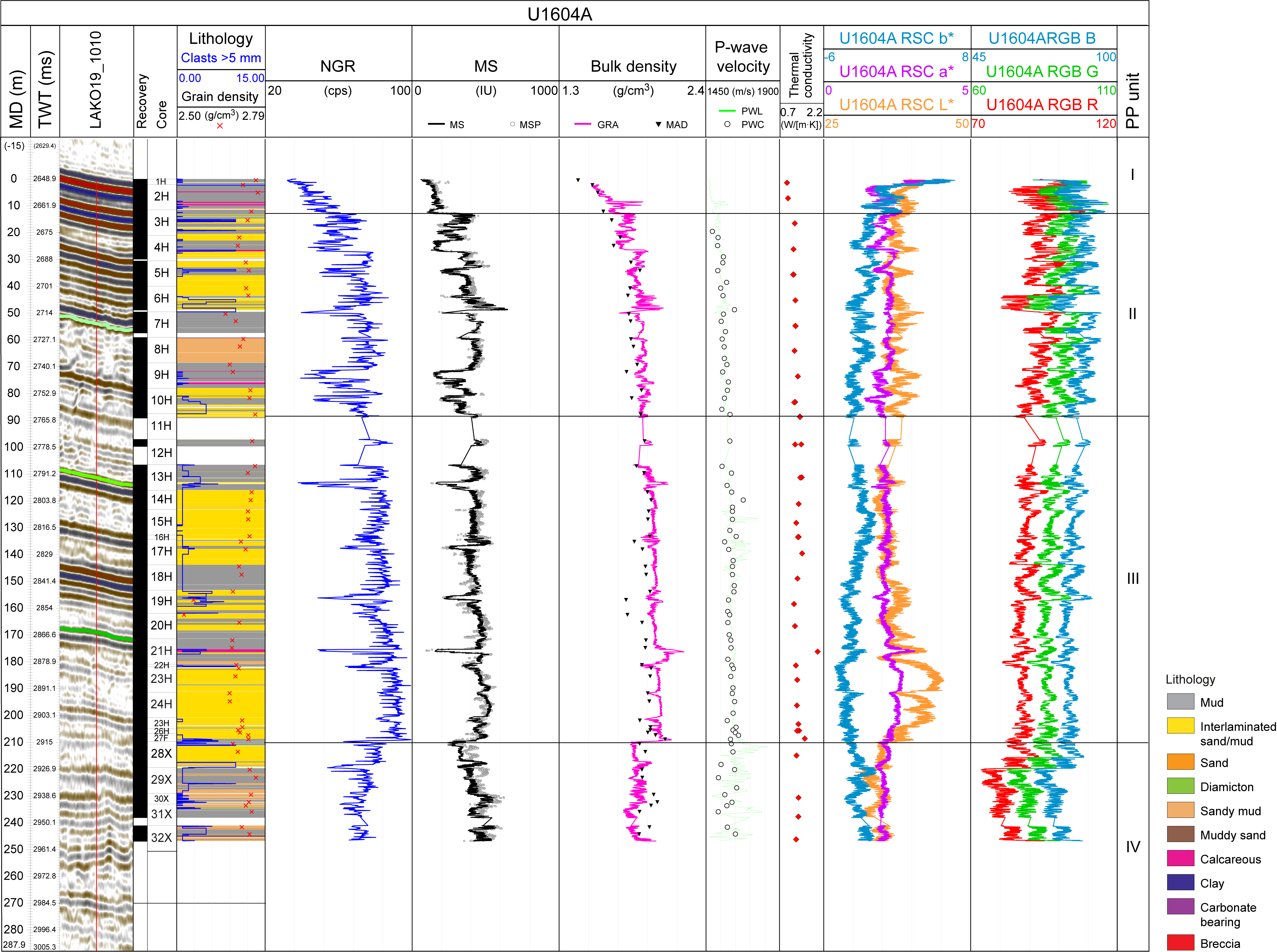
Figure F26. Physical properties, Hole U1604A.
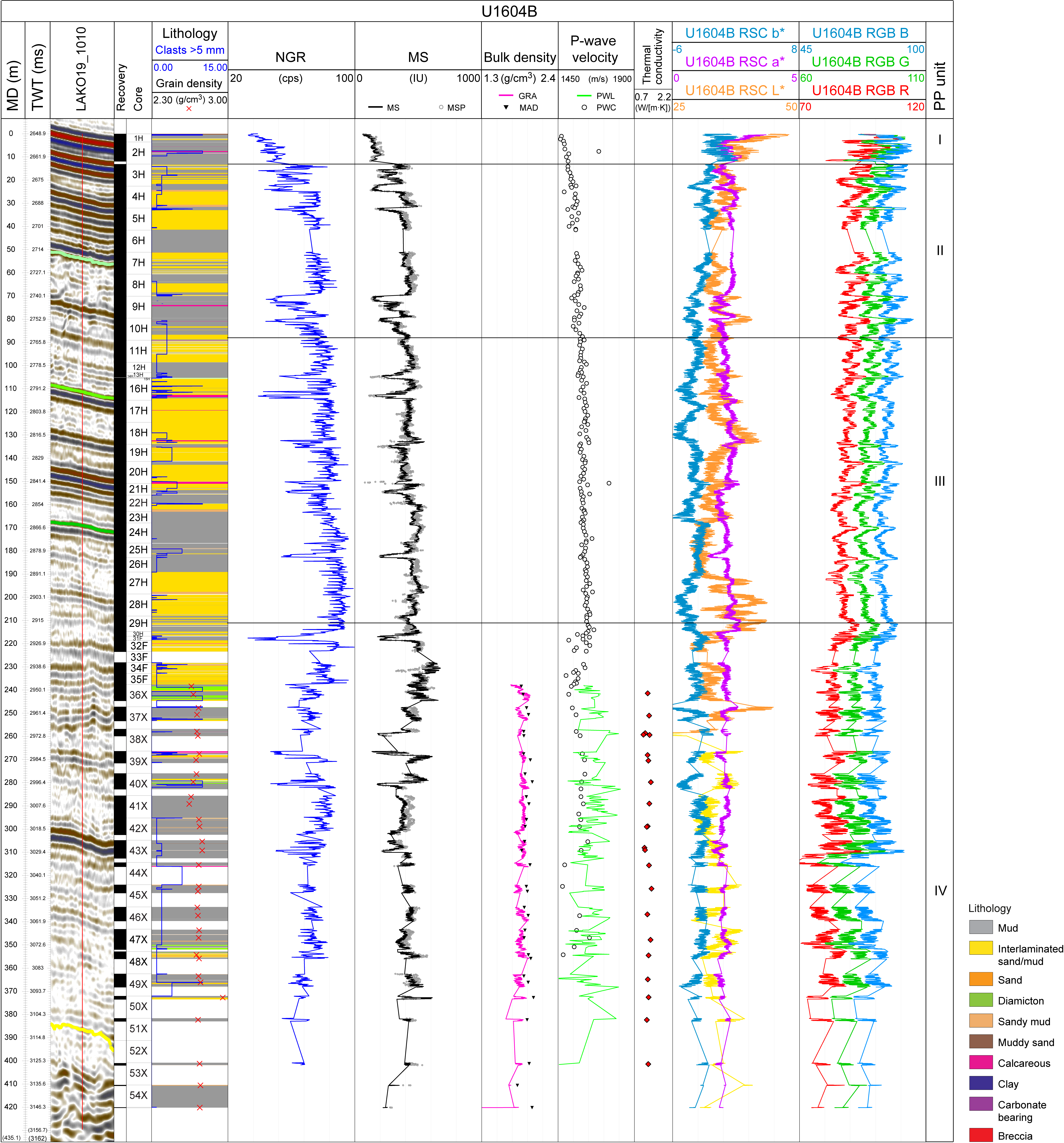
Figure F27. Physical properties, Holes U1604B.
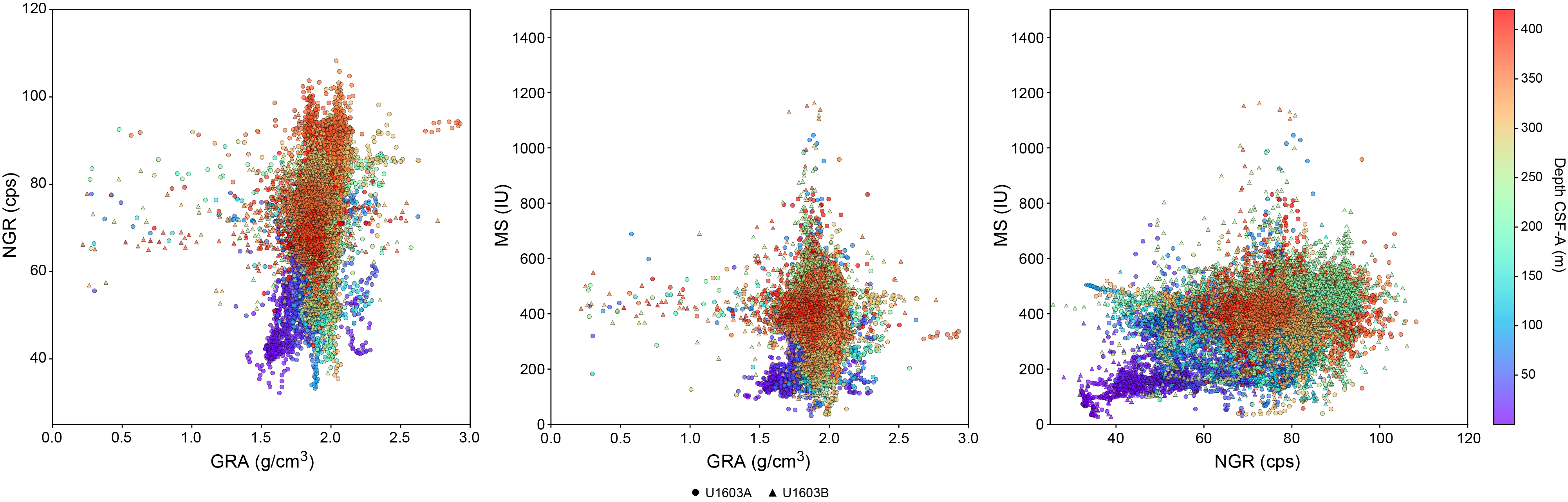
Figure F28. NGR, GRA bulk density, and MS.
6.1.1.1. Gamma ray attenuation bulk density
The GRA source on the WRMSL was not fully open during the measurement of Core 400-U1604A-1H. Thus, the measurements on this core might be unreliable. In general, wet bulk densities range 1.0–2.2 g/cm3 at Site U1604 with a mean value of 1.9 g/cm3. A trend of downhole increasing GRA density is observed above Core 28X (~210 m CSF-A), whereas below this depth, GRA values show a constant baseline. The lowest values are found in the uppermost ~25 m, and the highest values are observed in Cores 6H (45–48 m CSF-A), 21H (175–180 m CSF-A), and 27H (209 m CSF-A) (Figure F26). A positive correlation is found between density and NGR counts, as well as between density and MS with depth downcore (Figures F26, F27, F28). The trends of GRA bulk density values and the calculated densities from the MAD discrete samples generally agree. However, MAD density values are slightly lower than GRA density values, differing by up to 0.2 g/cm3 (Figures F26, F27).
6.1.1.2. Magnetic susceptibility
MS is sensitive to the concentration and type of magnetic minerals deposited in the sediments. Although it usually appears as sharp peaks of high-amplitude variability, MS also tracks lithologic changes. Values at Site U1604 range 58 × 10−5 to 673 × 10−5 SI with a mean of 397 × 10−5 SI (Figures F26, F27). The baseline of the MS signal shows high-amplitude variability between ~11 and ~285 m CSF-A with a steady increase downhole to 230 m CSF-A. Between this depth and the base of the hole, MS values are relatively constant.
The highest MS values are found in Core 400-U1604A-6H (>600 × 10−5 SI), and the lowest values are observed in the uppermost Cores 1H and 2H and in Core 21H (~171 × 10−5 SI). Generally, we observe covariability with depth of all physical properties determined with the WRMSL (Figures F26, F27, F28).
6.1.1.3. P-wave velocity using the P-wave logger
PWL measurements for Site U1604 show unreliable values on sections with cracks or poor contact between the sediment and the liner. However, the measurements are generally good and range 1455–1829 m/s. PWL values gradually increase downhole (Figures F26, F27). The lowest velocity values were observed for Cores 400-U1604A-1H and 2H (above 5 m CSF-A) and the highest for Core 28X downward (below 215 m CSF-A).
6.1.2. Natural gamma radiation
NGR values display high-amplitude variability with cyclic changes at Site U1604 (Figures F26, F27). NGR values oscillate between 32 and 100 counts/s with a mean of 75 counts/s. The baseline of the signal responds to high NGR values between Cores 400-U1604B-4H and 29H (24–215 m CSF-A). In this interval, the lowest counts in NGR are for Cores 9H, 10H, 16H, 18H, and 25H. The NGR baseline is lower from Core 29H to the base of the hole (215–420 m CSF-A).
6.1.3. Thermal conductivity
Thermal conductivity varies between 0.9 and 1.9 W/(m·K) at Site U1604 (Figures F26, F27). There is a slight positive trend with depth through Core 400-U1604B-36X and a slight negative trend with depth from this core to the base of the site. Mean values are 1.3 W/(m·K). The highest thermal conductivity value was observed in Core 24H (175 m CSF-A). The observed thermal conductivity does not present a clear dependence on sediment facies.
6.1.4. Point magnetic susceptibility
MSP measurements show a good match to values obtained from the WRMSL (Figures F26, F27). However, higher variability is observed with this instrument due to the smaller volume integration of the sensor (~1 cm; 1σ) compared to the loop (~18 cm; 1σ) used for the WRMSL (Weber et al., 1997).
6.1.5. Color reflectance
L*a*b* color reflectance measurements describe coordinates in a spherical system with 16.8 million possible variations (Weber, 1998; Blum, 1997). The L* axis measures the black–white color component, known as lightness or gray value. It is a reliable tracer for the content of biogenic carbonate in marine sediment (Weber, 1998). The L* baseline is relatively constant at Site U1604, with two intervals of above average L* values between Cores 400-U1604A-23H and 27H (180–210 m CSF-A) and Cores 400-U1604B-27H and 30H (190–220 m CSF-A) (Figures F26, F27).
The a* axis is the green–red component, which often reflects changing redox conditions in the sediments but may also correspond to variations of detrital components (i.e., sediment provenance). At Site U1604, a* values oscillate between 1.4 and 4.0 with a relatively constant trend downhole. A peak in a* values is observed in Core 400-U1604A-21H at the same depth as the interval of high L* values. The b* axis is the yellow–blue component, with more positive values (yellower colors) often associated with higher opal (usually diatoms) contents (Weber, 1998). However, for Site U1604 we associate this property mainly with an enhanced supply of detrital carbonate material. At Site U1604, b* values vary from −4.0 to 6.5 with a slight decreasing trend downward (Figures F26, F27).
6.1.6. Gantry
Results of section-half gantry measurements for Holes U1604A and U1604B are compiled in Figure F29. Correlation between GRA and MAD density and PWC and PWL values confirms the high quality of the data (Figures F26, F27).
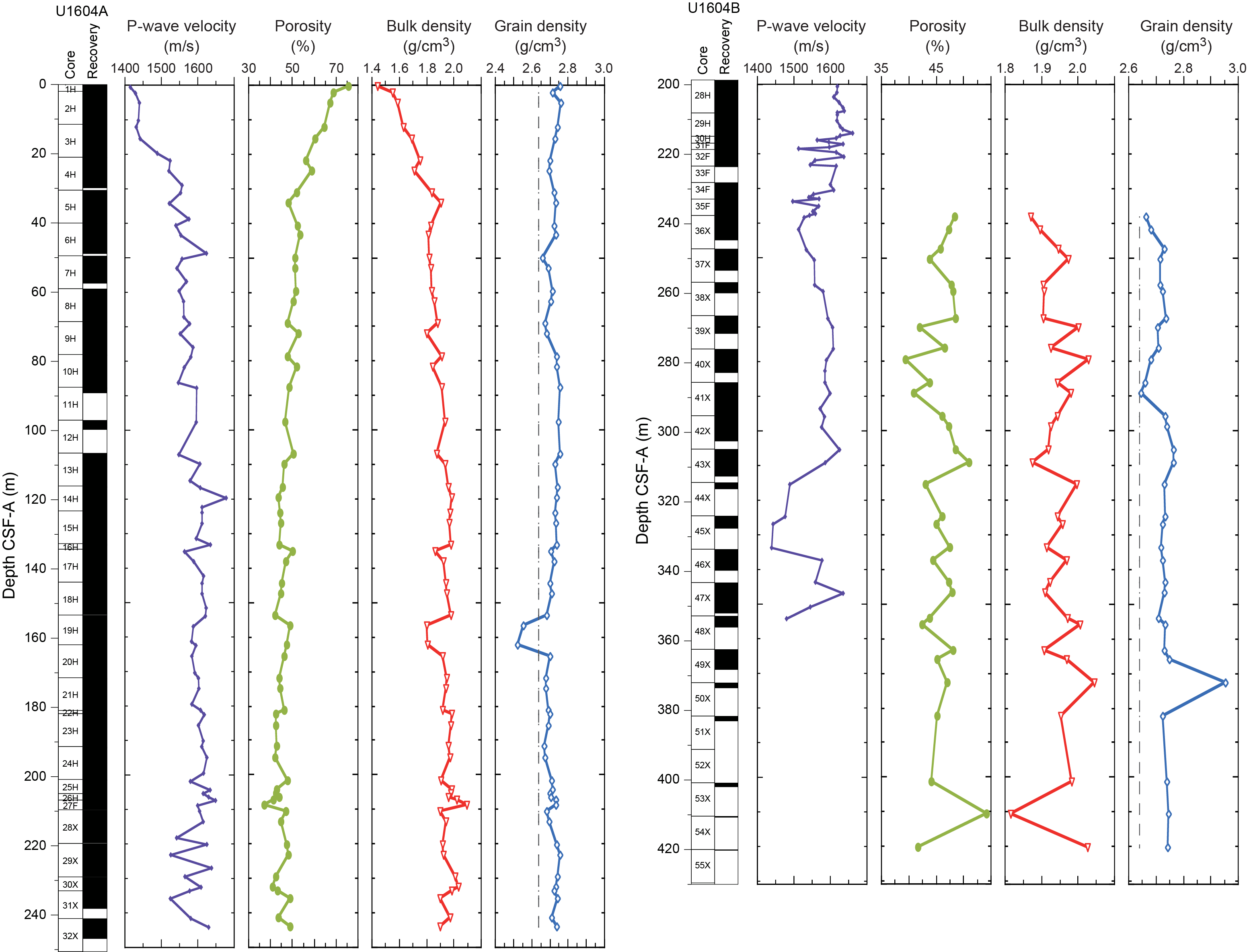
Figure F29. Gantry and MAD analyses.
6.1.6.1. P-wave velocity using the P-wave caliper
Discrete P-wave measurements were carried out using the PWC (see Physical properties in the Expedition 400 methods chapter [Knutz et al., 2025a]). At least three measurements were performed per core, but otherwise the intracore resolution varied depending on lithology, recovery, and section quality. The PWC measurements provide a correlation for PWL values measured on the whole-round cores with the WRMSL (Figures F26, F27). PWC measurements were made in every core from Site U1604; however, unreliable or no results were obtained on several cores.
Values obtained for Holes U1604A and U1604B are consistent with the trends observed in the PWL values from the WRMSL up to ~210 m CSF-A. Here, PWC values range from ~1415 to ~1650 m/s (Figures F26, F27, F29).
6.1.6.2. Moisture and density
Sediment samples were taken from the working halves of split cores for measuring MAD on all cores from Hole U1604A and Cores 400-U1604B-36X through 54X. No MAD samples were taken on Cores 1H–35F because they constitute a replica of the material recovered in Cores 400-U1604A-1H through 32X. Bulk density values were calculated from moisture and volume measurements (see Physical properties in the Expedition 400 methods chapter [Knutz et al., 2025a]). At least two MAD samples were acquired per core, although intracore sample resolution varied depending on lithology, recovery, and section quality. MAD samples were taken adjacent to the PWC measurement so that a correlation between P-wave velocity and bulk density can be made. A total of 82 samples were taken for MAD estimates: 59 from Hole U1604A and 23 from Hole U1604B.
MAD density values correlate in general with GRA bulk density measured on the WRMSL (Figures F26, F27). However, MAD density presents slightly lower values than GRA bulk density for Holes U1604A and U1604B. Bulk density values for Site U1604 range 1.4–2.1 g/cm3 with a mean of 1.9 g/cm3 and exhibit an overall downhole increase.
The trends for grain density measurements observed at Site U1604 (Figures F26, F27, F29) closely follow those observed for bulk density. This likely reflects the grain density of the major lithologic components at this site: quartz (2.65 g/cm3), biotite (~3 g/cm3), dolomite (2.84 g/cm3), common clays, and feldspars (~2.56 g/cm3).
Porosity represents the percent of pore space of wet sediment volume and generally decreases downhole (Figure F29). Discrete porosity values range from ~76% near the top of Site U1604 to 37% below 405 m CSF-A. Average porosity at Site U1604 is 48%.
6.2. Core-log-seismic correlation
The seismic facies distinct in the units defined by physical properties are described in Table T9. General changes on seismic facies in the seismic profile correspond to changes in the physical properties and lithologic units. Correlation of the seismic signal in two-way traveltime (TWT) with depth in meters has been achieved through the construction of two velocity models. The time-depth relationship resulting from discrete laboratory measurements of the P-wave velocity (PWC) provided unreliable seismic-core correlations. PWC values were generally lower than expected from the lithologies recovered, perhaps due to core expansion in the laboratory. A more robust time-depth relationship resulted from the velocity model obtained during the Dipole Sonic Imager (DSI) downhole logging in Hole U1604B (see Downhole measurements in the Expedition 400 methods chapter [Knutz et al., 2025a]). The observations on the FMS log and lithologic variability in correlation with major changes on the seismic facies confirm a reasonable time-depth model. Thus, the resulting time-depth relationship has been applied in Figures F26 and F27.
7. Geochemistry
Samples for headspace gas, interstitial water (IW) chemistry, and bulk sediment geochemistry were analyzed at Site U1604. Headspace hydrocarbon gas measurements showed low concentrations in the uppermost 200 m and higher concentrations of methane, with a low yet consistent presence of ethane, in sediments below 200 m CSF-A. The main findings from IW analysis include decreases in lithium and potassium with depth, possibly suggesting clay formation. A decrease in sulfate with depth to a minimum around 200 m CSF-A provides evidence for a sulfate–methane transition zone. IW iron, manganese, and phosphate show elevated concentrations near the seafloor and sharp decreases to low concentrations with depth. Increases in IW calcium and alkalinity in the upper depths may indicate dissolution of calcium carbonate (CaCO3) minerals. Elemental analysis of solid material revealed overall low concentrations of carbon and nitrogen across most intervals, whereas individual layers were rich in CaCO3 with contents of up to 60%.
7.1. Volatile hydrocarbons
As part of routine environmental protection and safety monitoring, headspace hydrocarbons were analyzed for Holes U1604A and U1604B (Figure F30). We aimed for two headspace samples per core (9.6 m advance) throughout Hole U1604A and for Hole U1604B at depths below 220 m CSF-A, but only one sample was taken when recovery was <50%. A total of 89 samples were analyzed for headspace gases. Methane (CH4) concentrations were generally low (2–9 ppm) in the uppermost 200 m of Hole U1604A before promptly increasing to concentrations of 20,000 ppm, and they remained high (20,000–46,000 ppm) throughout Hole U1604B. Ethane (C2H6) concentrations were below the detection limit above 200 m CSF-A and were 0.10–3.5 ppm across headspace samples sampled below 200 m CSF-A (Hole U1604B).
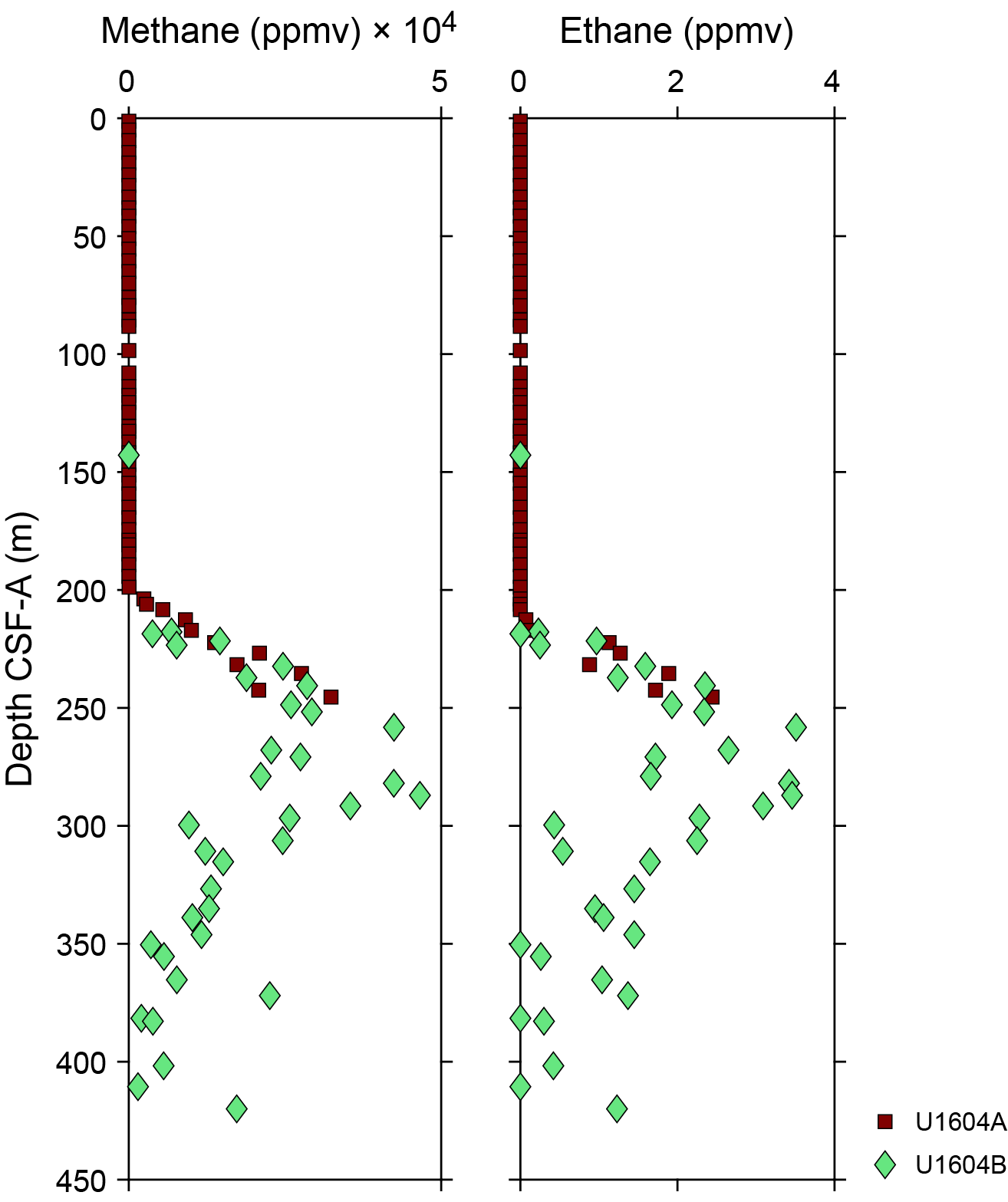
Figure F30. Hydrocarbon gas concentrations.
7.2. Interstitial water chemistry
A total of 42 IW samples were squeezed from 5 or 10 cm whole-round samples from Holes U1604A and U1604B. Typical samples yielded 15–30 cm3 of water for subsequent analysis. Samples from poorly lithified horizons and intervals with significant dropstone content often resulted in lower yields because much of the material was discarded to mitigate the possibility of contamination with drilling fluid. Two additional samples were collected and analyzed, one from the mudline of Hole U1604A and one from the surface seawater. Additional high-resolution (approximately one per meter) Rhizon water samples were taken from Hole U1604B in the uppermost 20 m.
7.2.1. pH and alkalinity
The measured pH values range 7.51–8.00 (Figure F31). The mudline sample from Hole U1604A has a pH of 7.51, and pH generally increases over the uppermost 15 m to ~7.9. The pH fluctuates between ~7.6 and 7.7 to 190 m CSF-A, where it notably increases to 260 m CSF-A, with a maximum value of 8.01 at 231 m CSF-A. Values below this interval range 7.64–7.94 with no discernible trends. Alkalinity values increase from 2.3 mM at the sediment/water interface to a maximum of 4.2 mM at 18.95 m CSF-A (Figure F31). Values generally decrease downcore to a minimum of 1.5 mM at the bottom of Hole U1604B.
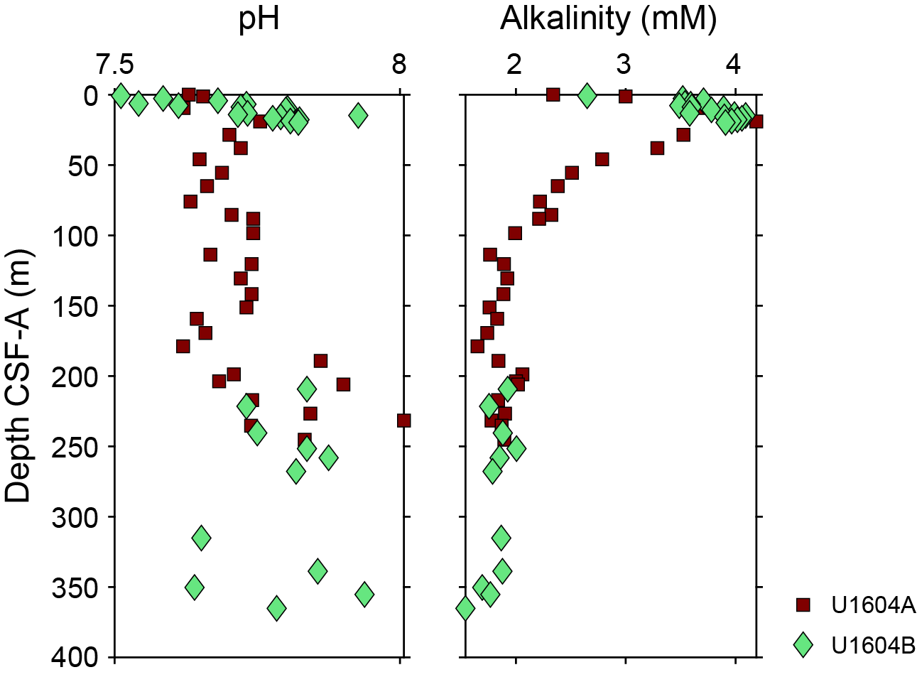
Figure F31. IW pH and alkalinity.
7.2.2. Salinity, sodium, chloride, lithium, potassium, and bromide
IW salinity decreases downcore from 35 to a minimum of 31 at 209.31 m CSF-A (Figure F32). Sodium concentration (as measured by ion chromatography) increases from 472 mM at the sediment/water interface to 496 mM at 19.75 m CSF-A and shows a general decrease from 131 m CSF-A to the bottom of Hole U1604B, where it reaches a minimum of 467 mM. Lithium and potassium decrease downcore from peak values of 23 µM and 12 mM, respectively. Lithium decreases over the uppermost 20 m, whereas potassium decreases over the uppermost ~180 m, possibly indicating chemical interactions between sediments and pore fluids throughout the core. Bromide increases consistently downcore from a mudline value of 0.8 mM to a maximum value of 1.6 mM at the bottom of Hole U1604B.
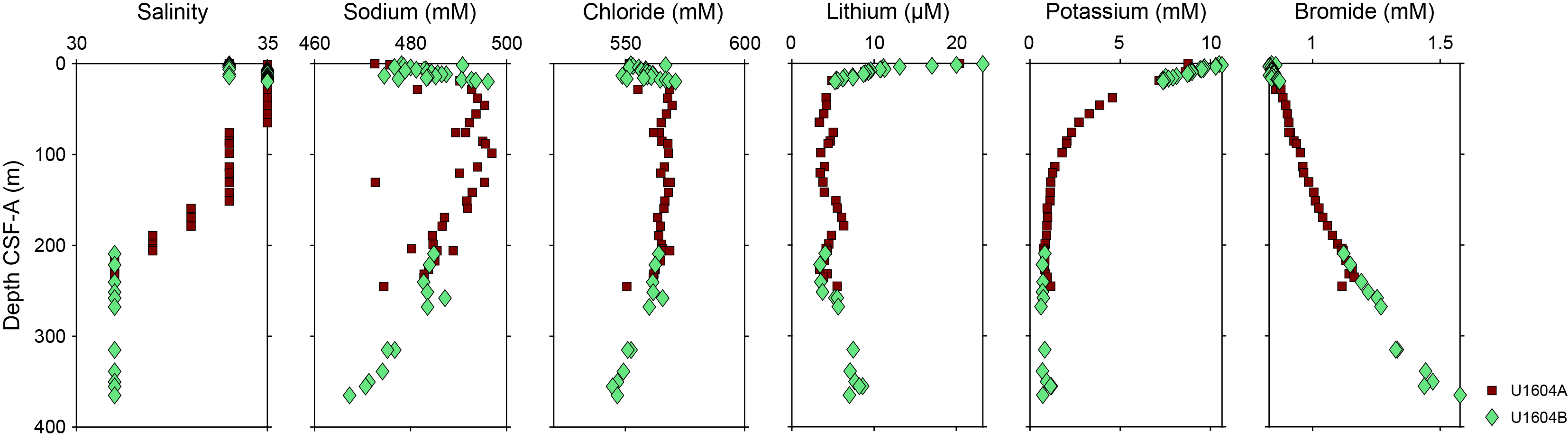
Figure F32. IW salinity, Na, Cl, Li, K, and Br.
7.2.3. Ammonium, manganese, iron, sulfate, phosphate, and boron
Ammonium increases from 7 µM in the mudline water to a maximum 422 µM at 75.6 m CSF-A. It then decreases downcore to 365 µM at the bottom of Hole U1604B (Figure F33). Dissolved manganese increases from trace quantities at the sediment/water interface to a maximum of 94.3 µM at 2.66 m CSF-A. Below this depth, concentrations decrease to approximately 110 m CSF-A. Concentrations remain roughly constant between ~7 and 15 µM to the bottom of the hole. Iron sharply increases in concentration in the IW from concentrations below the detection limit at the sediment/water interface to a maximum of 34.3 µM at 7.75 m CSF-A. Below 20 m CSF-A, the concentration of dissolved iron is generally 5 µM or less. Sulfate concentrations decrease downcore from seawater concentrations of 28 mM to ~1 mM over the uppermost 200 m. Water extracted below this depth had consistently low (<5 mM) concentrations of sulfate.
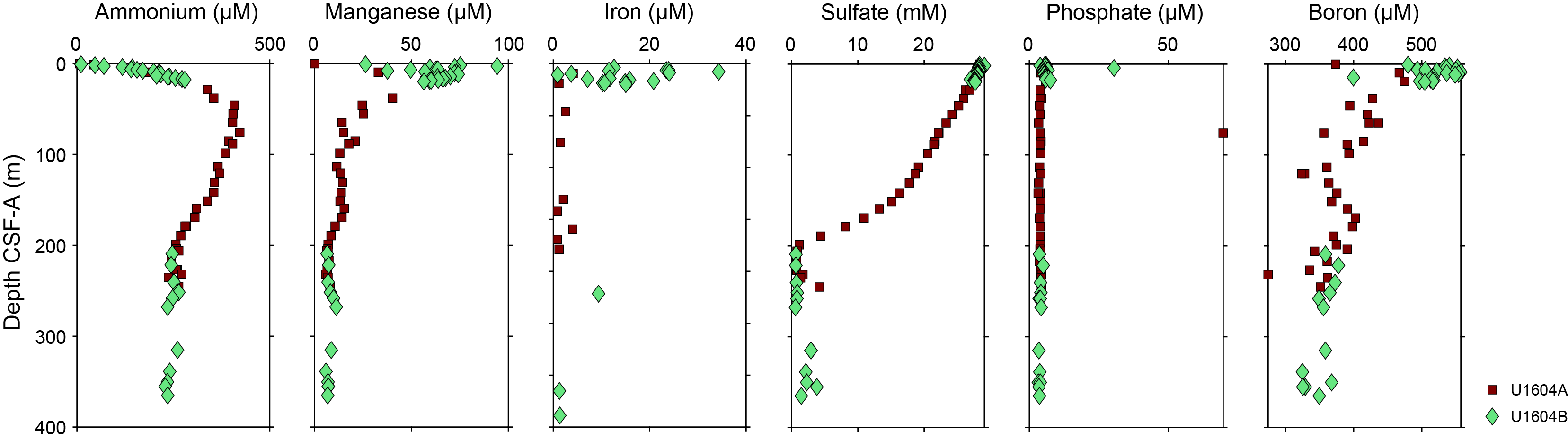
Figure F33. IW ammonium, Mn, Fe, sulfate, phosphate, and B.
Phosphate concentrations increase from a seawater concentration of 4.5 µM in the mudline water to values typically ranging 4–7 µM in the uppermost 20 m of sediment. The maximum value in these upper sediments is 30.5 µM, although all other samples fall within the aforementioned 4–7 µM range. Below 20 m CSF-A, all but one sample range 3–5 µM, with one sample at 75.95 m CSF-A reporting a dissolved phosphate concentration of 69.8 µM.
Boron increases from a seawater concentration of 373.6 µM at the mudline to a maximum value of 557.2 µM at 8.75 m CSF-A (Figure F33). Below this peak value, values decrease to 100 m CSF-A, below which the gradient is largely unchanged.
7.2.4. Calcium, magnesium, strontium, silicon, and barium
Calcium concentrations increase in the uppermost core from a measured seawater value of 9.1 mM at the mudline to a maximum measured value of 21.1 mM at 151.26 m CSF-A (Figure F34). This ~12 mM increase in calcium concentration correlates with the increase in alkalinity (Figure F31) for the uppermost 25 m of sediment, which may indicate dissolution of detrital or biogenic carbonate minerals in the upper sediment. Below 25 m CSF-A, calcium concentration and alkalinity appear to be more independent, with calcium concentrations decreasing from 20.8 to 15.0 mM between 169.38 and 209.31 m CSF-A and subsequently increasing to 19.0 mM in the deepest sample recovered from Hole U1604B.
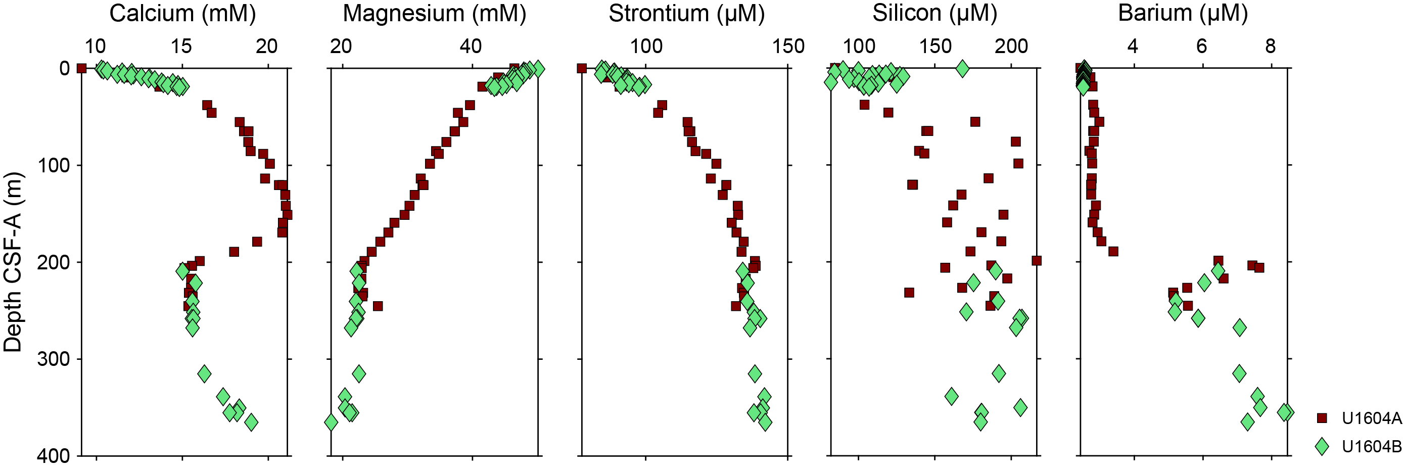
Figure F34. IW Ca, Mg, Sr, Si, and Ba.
Magnesium concentrations decrease from a seawater concentration of 46.5 mM at the mudline to a minimum in the lowest sample of 18.2 mM at 365.18 m CSF-A (Figure F34). Strontium values increase sharply in the upper sediment from a minimum concentration of 77.5 µM at the mudline to a maximum concentration of 142 µM in the deepest IW sample from 365.18 m CSF-A (Figure F34). Dissolved silicon concentrations increase over the uppermost 30 m of sediment from a measured bottom water value of 93.7 µM at the mudline. Above 30 m CSF-A, measured concentrations typically range 90–120 µM. Below this depth, dissolved silicon ranges 130–220 µM (Figure F34).
Dissolved barium concentrations increase from a value of 2.4 µM at the mudline to 2.8 µM at 18.95 m CSF-A (Figure F34). Below this depth, values remain largely unchanged to 178.84 m CSF-A, below which concentrations increase to 7.6 µM at 206 m CSF-A. Below this point, barium concentrations vary slightly but remain consistently elevated, reaching a maximum value of 8.5 µM at 355.31 m CSF-A. Notably, the increase in barium concentrations between 160 and 200 m CSF-A coincides with the depletion of dissolved sulfate (Figure F33) and calcium and an increase in headspace methane concentrations (Figure F30).
7.3. Bulk sediment geochemistry
7.3.1. Carbon, nitrogen, and carbonate
The shipboard solid phase analysis at Site U1604 from all major lithostratigraphic units identified consisted of measurements of CaCO3, total carbon (TC), and total nitrogen (TN) using shipboard plastic cylinder sampling. Bulk sediment geochemistry samples were taken for Holes U1604A and U1604B at a resolution of two to four samples per core (9.6 m advance), depending on downcore variety. A total of 88 bulk sediment samples were collected and analyzed. Total organic carbon (TOC) was calculated from measurements of CaCO3 and TC. Downhole profiles of CaCO3, TOC, and TN contents (weight percent) at Site U1604 are shown in Figure F35. The CaCO3 content is below 1% throughout most intervals, although a few intervals described as calcareous mud contain CaCO3 to up to 60%. The TOC content ranges 0.1%–2.1% throughout Holes U1604A and U1604B, and most samples have values less than 0.4%. The TN content is <0.07% throughout all samples analyzed.
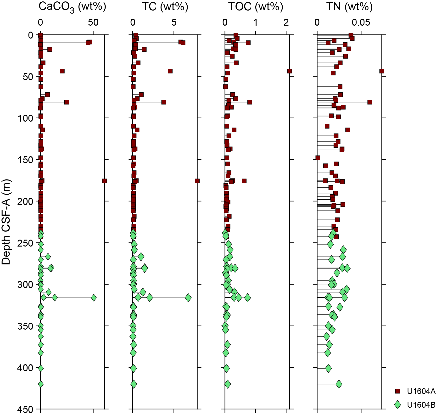
Figure F35. CaCO3, TC, TOC, and TN.
8. Stratigraphic correlation
To minimize coring gap alignment, sequences from Hole U1604A were examined using NGR data measured at 10 cm intervals and MS measured at a 2 cm resolution with the WRMSL. In addition, 10 cm interval NGR data and 5 cm resolution MS data were measured on sections from Hole U1604B and examined in near–real time to ensure adequate coring depths to fill the gaps in Hole U1604A (see Physical properties for details on Site U1604 core measurements). Because triple APC offset coring was not planned at Site U1604, a splice for this site could not be completed. Recovery gaps commonly overlap between Holes U1604A and U1604B. The difficulty was further magnified by the deformation related to XCB coring. Thus, Holes U1604A and U1604B were aligned based on the mudline and correlated to each other to the extent possible.
The top of Hole U1604A (which preserved a mudline) served as the anchor (zero depth point) for generation of the core composite depth below seafloor, Method A (CCSF-A), depth scale at this site (see Stratigraphic correlation in the Expedition 400 methods chapter [Knutz et al., 2025a] for an explanation of depth scales). We attempted to determine the relative depth offset of each core from this reference by establishing depth offsets, or affine ties, between cores from the two holes based on optimized correlation of WRMSL-derived MS and NGR data (see Figure F22 in the Expedition 400 methods chapter [Knutz et al., 2025a]). These depth offsets are reported in Table T10, and the resulting CCSF-A depth scale is shown in Figure F36. The upper part of the sequence, to 13 m CCSF-A, is tied through Cores 400-U1604A-1H through 400-U1604B-2H. Cores 400-U1604A-3H through 6H and 400-U1604A-7H through 400-U1604B-10H are tied down to 94 m CCSF-A. Below this depth, cores are placed on a relative depth to each other, except where core ties occur in clusters of two to three cores (Table T10). At the base of Hole U1604A, Cores 400-U1604A-32X and 400-U1604B-36X are tied to each other, but their relative depth cannot be determined. Core disturbances, shattered core liners, and other issues impacting core quality mean that the stratigraphic coherence of the recovered sequence is variable. Below 223 m CCSF-A, NGR and MS are less coherent between Holes U1604A and U1604B, which makes the stratigraphic correlation of the lowermost overlapping sections dubious.
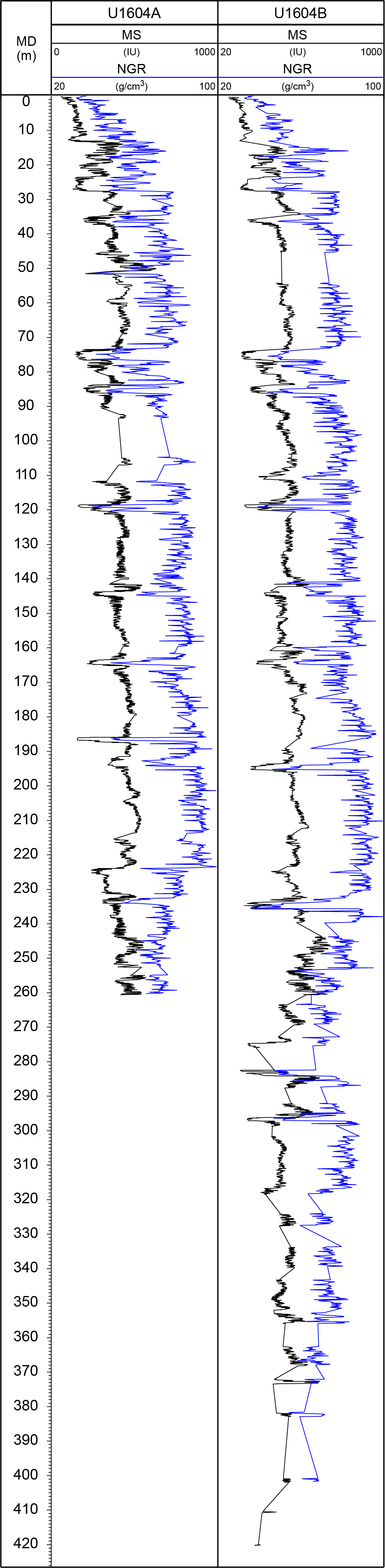
Figure F36. WRMSL-derived MS and NGR data.
In summary, the high recovery and core alignment between Holes U1604A and U1604B allow for the construction of a preliminary CCSF-A depth scale, but the gaps between cores are unknown (Table T10). Thus, the CCSF-A depth scale for Site U1604 reflects uncertainties on the absolute depth of the correlated intervals.
8.1. Comparison of core and downhole logging data
Downhole logging was conducted in Hole U1604B (see Downhole logging) to establish connections to seismic data and provide additional data for cored (but possibly not recovered) intervals. The quality of the hole was generally good, although washouts were common. Overall, the log provides a continuous record that may allow better interpretation of the lithologies encountered.
We imported the MS and total spectral gamma ray (HSGR) downhole logs into Correlator (v. 4) to improve our understanding of the positions of the cores. We were able to upload downhole logs into Correlator by making a single core table with the log data. We attempted to tie each core from Holes U1604A and U1604B into the logging data. This procedure has some significant uncertainties due to the presence of large-scale features in the downhole logging data that do not resemble the record measured on cores in the laboratory. However, the overall cyclicity is well matched between the logs and the cores, providing additional depth constraint to the cores (Table T11).
9. Age model
The initial age constraints for Site U1604 are based on magnetostratigraphic interpretations of inclination. From the surface to 147 m CCSF-A (137.6 m CSF-A; Hole U1604B) (Table T12), the sediment is characterized by normal polarity (Polarity Zone N1 in Figure F25) and is interpreted as the Brunhes Chron (C1n, 0–0.773 Ma; Ogg, 2020). Below this depth, a transition to reversed polarity (Polarity Zone R1) likely represents the Brunhes/Matuyama boundary (0.773 Ma). The normal polarity zone below 247.5 m CSF-A in Hole U1604B (Polarity Zone N2) is not well constrained due to gaps in recovery and drilling disturbance, but we assign an uncertain lower boundary at 267.4 m CSF-A in Hole U1604B. We suggest correlation of Polarity Zone N2 with the Jaramillo Subchron (C1r.1n, 0.990–1.070 Ma; Ogg, 2020). Below Polarity Zone N2, polarity is mainly reversed, and further divisions are ambiguous.
To constrain the age of sediments beyond the interpretation of the polarity stratigraphy, we constructed an RPI time series. The magnetic remanence of the archive section halves after demagnetization in a peak AF of 20 mT (NRM20mT), filtered as described in Paleomagnetism, was normalized by the point-source MS collected on the archive section halves. To create a more continuous time series, a filtered RPI data set was constructed using the composite depth scale for the site (CCSF-A), combining sections of Holes U1604A and U1604B to fill gaps in the recovery (Figure F37; Table T12).
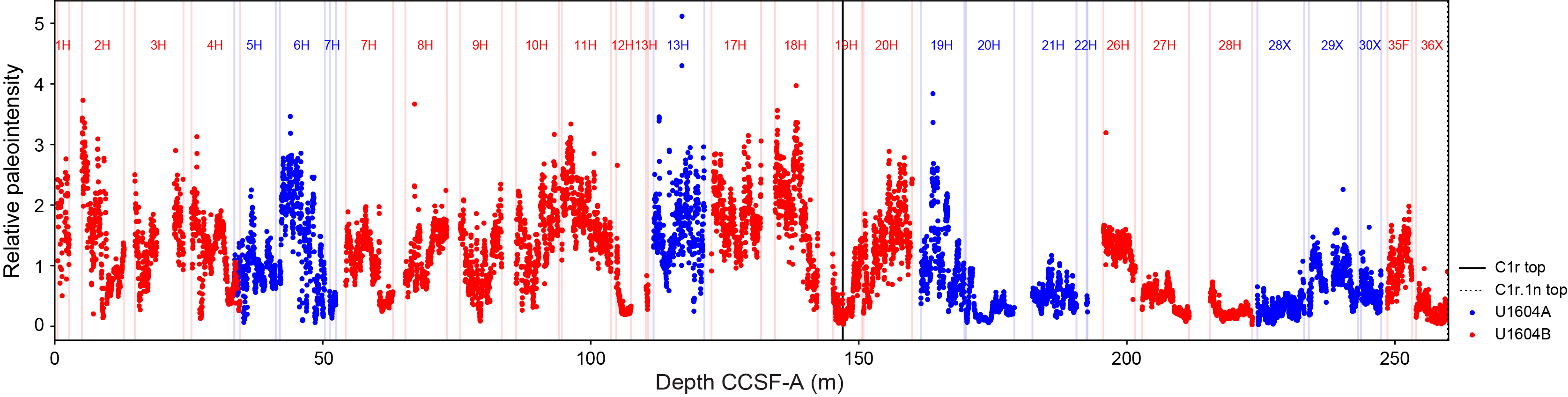
Figure F37. Composite series of RPI.
With the chronostratigraphic tie point provided by the Brunhes/Matuyama boundary, we identify additional tie points using decreases in paleointensity (DIPs) and comparison with a model of the paleomagnetic axial dipole moment. The paleomagnetic axial dipole moment for the last 2 My (PADM2M; Ziegler et al., 2011) is a model constructed based on a stack of more than 80 globally distributed records calibrated to a consistent age model by Tauxe and Yamazaki (2007). Note that the age of the Brunhes/Matuyama boundary in the age model used by Tauxe and Yamazaki (2007) was 0.78 Ma, and individual records were calibrated using the stacked benthic δ18O timescale (LR04) of Lisiecki and Raymo (2005). Comparison with PADM2M also provides the opportunity to predict where the marine isotopic stages of the LR04 δ18O stack (Lisiecki and Raymo, 2005) may appear at Site U1604 (Figures F38C, F39C). We identified 11 tie points, including the reversal boundaries (Table T13; Figures F38, F39), in our RPI record, that are also recognizable in the PADM2M model. In addition to the DIPs associated with the Brunhes/Matuyama boundary (C1r.1r (top) in Table T13) and the top and bottom of the Jaramillo Subchron (C1r.1n (top) and C1r.2r (top), respectively), we identified six DIPs between the seafloor and the Brunhes/Matuyama boundary (Figure F38) and two between the Brunhes/Matuyama and the top of the Jaramillo Subchron (Figure F39).

Figure F38. DIPs in the Brunhes Chron.

Figure F39. DIPs in the Matuyama Chron.
Our paleomagnetic constraints allow us to create an age-depth model (Figure F40). We estimate average SARs are ~15 cm/ky through the uppermost 107 m CCSF-A and ~46 cm/ky below 107 m CCSF-A to at least the beginning of the Jaramillo Subchron. This change in SAR at about 100 m CCSF-A is consistent with the boundary between Lithostratigraphic Subunits IA (massive mud with dispersed to common clasts, laminated mud with interbeds of calcareous mud and gravel-bearing sediment) and IB (interlaminated sand and mud, massive mud with dispersed to common clasts, laminated mud with interbeds of calcareous mud and gravel-bearing sediment) (see Lithostratigraphy). The lithology of Subunit IA is described as mud and would likely have a lower SAR than Subunit IB, which contains significant sandy layers. In the deeper part of the age model, the SAR is much higher and consistent with Unit II, which has abundant gravel.
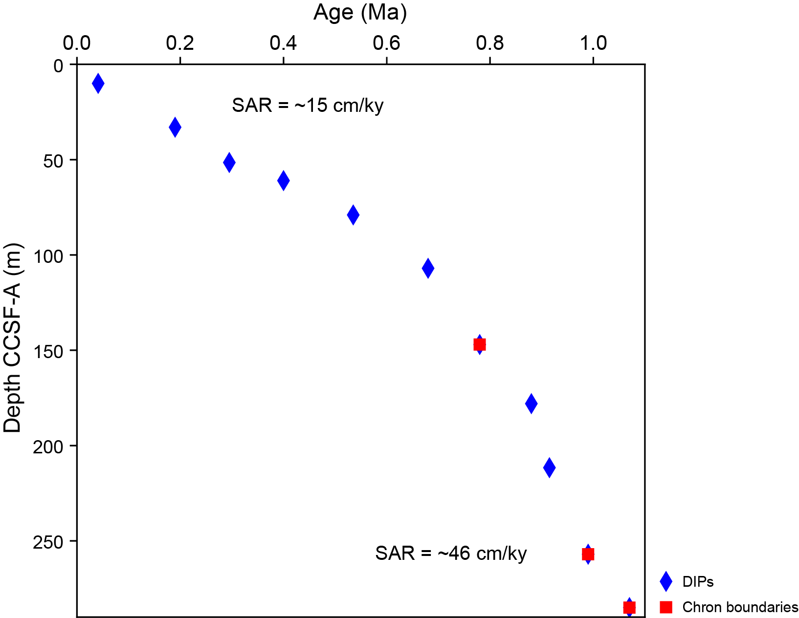
Figure F40. Age-depth plot.
10. Downhole logging
Downhole logging was carried out in Hole U1604B upon completion of coring operations. A modified triple combo (quad combo) tool string deployed the MS, natural gamma ray, electrical laterolog resistivity, acoustic velocity, and density tools. Three runs (a down pass, a repeat pass, and a main pass) were carried out, covering almost the full length of the open hole (to 427.6 mbsf; i.e., 2 m above the bottom of the hole). The repeat or calibration run logged the deepest 100 m of the hole. The caliper showed a relatively stable hole with frequent washouts, and the instruments yielded reliable measurements.
Upon completion of the downhole logging with the quad combo tool string, the FMS was lowered downhole. Three runs (a down pass plus two up passes) were completed. On the down passes, only the gamma ray was measured because the caliper of the FMS was closed. The FMS resulted in a high-quality resistivity image of Hole U1604B.
Logging measurements were crucial for covering recovery gaps and for providing in situ values of the formation. Core logging and downhole logging results differ on absolute values, but the relative trends of the logs are comparable. Hence, logging data could be used for correlation purposes and for covering the formation recovery gaps with confidence. Additionally, the APCT-3 tool was deployed four times in Hole U1604A to determine formation temperature.
10.1. Logging operations
The last core from Hole U1604B arrived on deck on 8 September 2023 at 1930 h (all times provided in local ship time, UTC − 3 h, unless otherwise noted). Hole preparation for the logging program included a high-viscosity mud sweep and displacing the open hole with 10.5 lb/gal heavy mud (barite) to help hole stability. The APC/XCB drill bit was raised to 46 mbsf and maintained at this depth throughout the entire logging operation, leaving ~380 m of open hole. The two main up pass logging runs were implemented to 1943 and 1954 meters below rig floor (mbrf). The wireline heave compensator was used to reduce the effect of vertical ship motion on the wireline depth. Rigup for downhole logging started at 2331 h on 8 September under good weather and ice conditions.
The quad combo tool string was assembled for the first run and consisted of the following tools from bottom to top (see Downhole measurements in the Expedition 400 methods chapter [Knutz et al., 2025a]): Magnetic Susceptibility Sonde (MSS), DSI, High-Resolution Laterolog Array (HRLA), Hostile Environment Litho-Density Sonde (HLDS; with source), Hostile Environment Natural Gamma Ray Sonde (HNGS), and Enhanced Digital Telemetry Cartridge (EDTC). The quad combo tool string was lowered into Hole U1604B at 0221 h on 9 September. All tools were run on the downlog except the density tool, which was run together with the caliper to measure borehole diameter on the uplog. The downlog started at 1950 mbrf and captured the seafloor with a gamma peak at 1955 mbrf, and the bottom of the tool string reached 2386 mbrf (431 mbsf). No problems were encountered getting down through the pipe or the open hole. The mismatch on the drilled hole depth and the logging penetration length is due to the fact that the base of the hole was formed by very soft sediments, which were penetrated by the end of the tool string. After reaching total depth, the caliper arms were opened and the density tool was enabled. The hole was logged up for a 99 m calibration pass. The tool was lowered back to 2386 mbrf, and the main uplog was collected. Downhole logging with the quad combo tool string was completed, and it was out of the hole by 0515 h on 9 September.
The second logging run deployed the FMS tool string (see Downhole measurements in the Expedition 400 methods chapter [Knutz et al., 2025a]), which included the HNGS and EDTC for calibration purposes. DSI results from the quad combo run were excellent, so it was not included in this run. The FMS tool string was lowered into Hole U1604B at 0742 h on 9 September. The tool string reached the base of the hole at 2382 mbrf. Two completed uplogs were recorded to 2021 mbrf. The FMS resulted in a high-quality resistivity image of Hole U1604B. The tool string was returned to the rig floor at 1020 h. All logging equipment was rigged down by 1200 h on 9 September.
10.1.1. Log data quality
The main control on log data quality is the diameter of the borehole measured by the caliper on the HLDS logging tool (Figure F41). The borehole diameter was around 13 inches with a standard deviation of 1.4 inches and was similar during Runs 1 and 2. The hole was wider than the maximum extent of the caliper arm (17 inches) just below the drilling pipe and in local points between 2070 and 2280 mbrf, resulting in robust quality logs by tools that require good contact with the borehole wall, such as the density log (Figure F41). Log data were transmitted to the Lamont-Doherty Earth Observatory for depth matching and data processing. All readings are within the expected ranges.
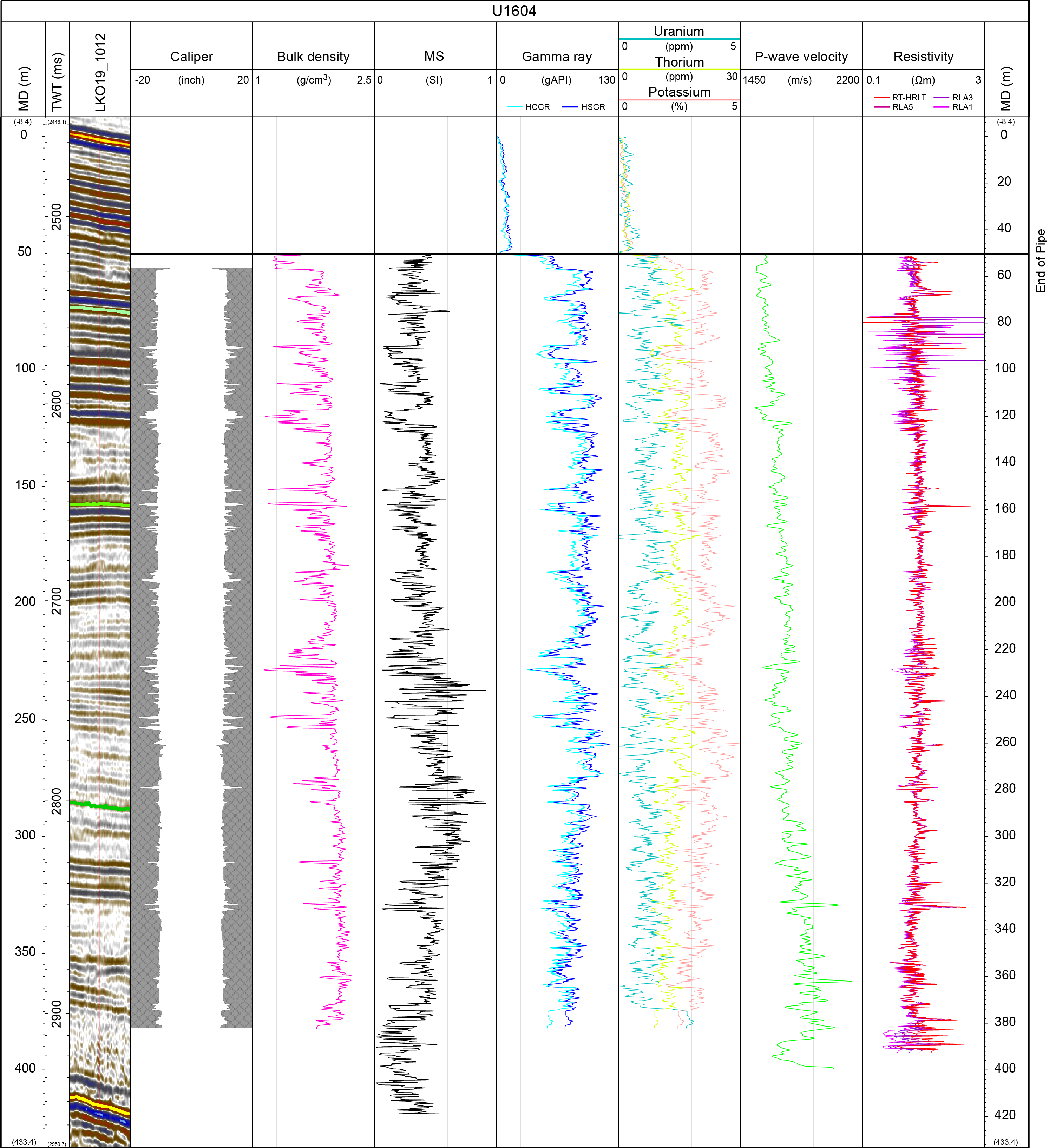
Figure F41. Main downhole logs.
The bottom of the drill pipe was located at 46 mbsf during all main logs; thus, the upper section of the formation is not described in the following text. Density ranges 1.1–2.2 g/cm3 for the majority of the hole, with a baseline slightly increasing downward. Deep resistivity ranges 0.5–5 Ωm. Average open hole gamma ray (HSGR) values are 93 American Petroleum Institute gamma ray units (gAPI) and progressively increase downhole to about 200 mbsf. Below this depth, gamma ray baseline values decrease to the base of the hole. MS oscillates between 0.479 and 0.728 SI with mean values of 0.547 SI. Low-frequency monopole P-wave velocity increases downhole and ranges 1512–2036 m/s with an average of 1719 m/s.
The downlog and uplog data of each measurement do not always perfectly match. In the case of gamma radiation, differences occur in absolute values because the uplog is corrected for borehole diameter as measured by the caliper and the presence of barite-weighted mud whereas the downlog is not corrected because the caliper is closed when the tool is lowered downhole. The uplog and downlog P-wave velocity values differ in places because the software is not always able to pick the signal arrival. The DSI was run at standard and low frequencies. Processing was not required for the main sonic log at this site.
The downhole natural gamma ray and density logs display variation in common with the equivalent laboratory data from Site U1604 (Figure F42). Small offsets between log and core data were assigned to core depths with <100% core recovery and other effects.
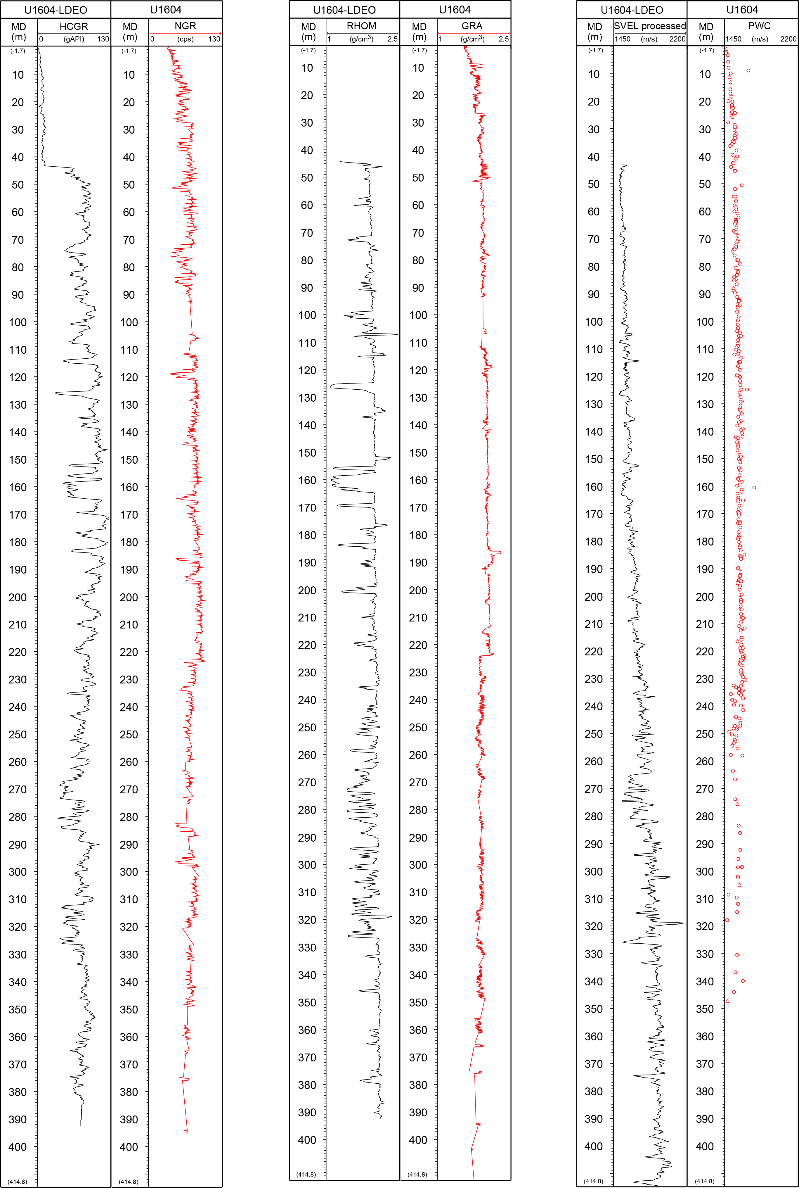
Figure F42. Gamma radiation, density, and velocity.
The physical properties (PP) units distinguished based on the values from the core measurements (Figure F26) can be extended to the downhole logs with the exception of PP Unit I, which lies within the interval covered by the drilling pipe (Figure F41). However, the boundary between PP Units III and IV, characterized by a transition from high-amplitude variability to a relatively constant baseline on density, natural gamma ray, and MS, is observed at 200 mbsf on the downhole logs versus 210 m CSF-A on the core logs and is related to a major decrease in gamma radiation and MS. Major differences in depths could be related to the low core recovery below 240 m CSF-A.
Sonic velocity values are consistently higher in downhole measurements compared to the values measured on cores (PWC) because downhole measurements are made under in situ conditions of pressure and temperature. For this reason, the applied TWT to meter depth relationship is the one obtained from the low-frequency sonic data (see Core-log-seismic correlation). The physical properties measured downhole are interpreted in a similar way to those measured on the cores in the laboratory (see Physical properties).
10.2. Downhole temperature and heat flow
Four APCT-3 tool formation temperature measurements were made in Hole U1604A (Cores 4H, 7H, 10H, and 13H), yielding reliable results. The obtained temperatures range from 1.3°C at 30.5 m drilling depth below seafloor (DSF) to 5.78°C at 116.0 m DSF (Table T14), giving an approximately linear temperature increase with depth and a geothermal gradient of 52°C/km. The seafloor temperature was determined to be −0.3°C based on APCT-3 data taken while the tool was held at the mudline for 5 min during each run.
Thermal conductivity under in situ conditions was estimated from laboratory-determined thermal conductivity from Hole U1604A using the method of Hyndman et al. (1974) (see Physical properties in the Expedition 400 methods chapter [Knutz, 2024a]). The calculated in situ values are within 2% of the measured laboratory values. Thermal resistance was then calculated by integrating the inverse of the in situ thermal conductivity over depth. Considering all thermal conductivity measurements for Site U1604, a heat flow of 65 mW/m2 was estimated from the linear fit between temperature and thermal resistance (Pribnow et al., 2000).
References
Blum, P., 1997. Physical properties handbook: a guide to the shipboard measurement of physical properties of deep-sea cores. Ocean Drilling Program Technical Note, 26. https://doi.org/10.2973/odp.tn.26.1997
Cage, A.G., Pieńkowski, A.J., Jennings, A., Knudsen, K.L., and Seidenkrantz, M.S., 2021. Comparative analysis of six common foraminiferal species of the genera Cassidulina, Paracassidulina, and Islandiella from the Arctic–North Atlantic domain. Journal of Micropalaeontology, 40(1):37–60. https://doi.org/10.5194/jm-40-37-2021
Christ, A.J., Rittenour, T.M., Bierman, P.R., Keisling, B.A., Knutz, P.C., Thomsen, T.B., Keulen, N., Fosdick, J.C., Hemming, S.R., Tison, J.-L., Blard, P.-H., Steffensen, J.P., Caffee, M.W., Corbett, L.B., Dahl-Jensen, D., Dethier, D.P., Hidy, A.J., Perdrial, N., Peteet, D.M., Steig, E.J., and Thomas, E.K., 2023. Deglaciation of northwestern Greenland during Marine Isotope Stage 11. Science, 381(6655):330–335. https://doi.org/10.1126/science.ade4248
Clark, P.U., and Pollard, D., 1998. Origin of the Middle Pleistocene transition by ice sheet erosion of regolith. Paleoceanography, 13(1):1–9. https://doi.org/10.1029/97PA02660
Cox, D.R., Huuse, M., Newton, A.M.W., Sarkar, A.D., and Knutz, P.C., 2021. Shallow gas and gas hydrate occurrences on the northwest Greenland shelf margin. Marine Geology, 432:106382. https://doi.org/10.1016/j.margeo.2020.106382
de Vernal, A., Rochon, A., and Radi, T., 2013. Dinoflagellates. In Elias, S.A. and Mock, C.J., Encyclopedia of Quaternary Science (Second Edition). Amsterdam (Elsevier), 800–815. https://doi.org/10.1016/B978-0-444-53643-3.00283-1
El Bani Altuna, N., Pieńkowski, A.J., Eynaud, F., and Thiessen, R., 2018. The morphotypes of Neogloboquadrina pachyderma: isotopic signature and distribution patterns in the Canadian Arctic Archipelago and adjacent regions. Marine Micropaleontology, 142:13–24. https://doi.org/10.1016/j.marmicro.2018.05.004
Eynaud, F., Cronin, T.M., Smith, S.A., Zaragosi, S., Mavel, J., Mary, Y., Mas, V., and Pujol, C., 2009. Morphological variability of the planktonic foraminifer Neogloboquadrina pachyderma from ACEX cores: implications for late Pleistocene circulation in the Arctic Ocean. Micropaleontology, 55(2/3):101–116. http://www.jstor.org/stable/40607109
Feyling-Hansen, R.W., 1976. The stratigraphy of the Quaternary Clyde Foreland Formation, Baffin Island, illustrated by the distribution of benthic foraminifera. Boreas, 5(2):77–94. https://doi.org/10.1111/j.1502-3885.1976.tb00333.x
Hiscott, R.N., Aksu, A.E., and Nielsen, O.B., 1989. Provenance and dispersal patterns, Pliocene-Pleistocene section at Site 645, Baffin Bay. In Srivastava, S.P., Arthur, M., Clement, B., et al., Proceedings of the Ocean Drilling Program, Scientific Results. 105: College Station, TX (Ocean Drilling Program), 31–52. https://doi.org/10.2973/odp.proc.sr.105.117.1989
Hyndman, R.D., Erickson, A.J., and Von Herzen, R.P., 1974. Geothermal measurements on DSDP Leg 26. In Davies, T.A., Luyendyk, B.P., et al., Initial Reports of the Deep Sea Drilling Project. 26: Washington, DC (US Government Printing Office), 451–463. https://doi.org/10.2973/dsdp.proc.26.113.1974
Jakobsson, M., Mayer, L., Coakley, B., Dowdeswell, J.A., Forbes, S., Fridman, B., Hodnesdal, H., Noormets, R., Pedersen, R., Rebesco, M., Schenke, H.W., Zarayskaya, Y., Accettella, D., Armstrong, A., Anderson, R.M., Bienhoff, P., Camerlenghi, A., Church, I., Edwards, M., Gardner, J.V., Hall, J.K., Hell, B., Hestvik, O., Kristofferson, Y., Marcussen, C., Mohammad, R., Mosher, D., Nghiem, S.V., Pedrosa, M.T., Travaglini, P.G., and Weatherall, P., 2012. The International Bathymetric Chart of the Arctic Ocean (IBCAO) Version 3.0. Geophysical Research Letters, 39(12):L12609. https://doi.org/10.1029/2012GL052219
Jennings, A., Reilly, B., Andrews, J., Hogan, K., Walczak, M., Jakobsson, M., Stoner, J., Mix, A., Nicholls, K.W., O’Regan, M., Prins, M.A., and Troelstra, S.R., 2022. Modern and Early Holocene ice shelf sediment facies from Petermann Fjord and northern Nares Strait, northwest Greenland. Quaternary Science Reviews, 283:107460. https://doi.org/10.1016/j.quascirev.2022.107460
Kaminski, M.A., Gradstein, F.M., Scott, D.B., and MacKinnon, K.D., 1989. Neogene benthic foraminifer biostratigraphy and deep-water history of Sites 645, 646, and 647, Baffin Bay and Labrador Sea. In Srivastava, S.P., Arthur, M., Clement, B., et al., Proceedings of the Ocean Drilling Program, Scientific Results. 105: College Station, TX (Ocean Drilling Program), 731–756. https://doi.org/10.2973/odp.proc.sr.105.123.1989
Kelleher, R., Jennings, A., Andrews, J., Brooks, N.K.S., Marchitto, T., Feng, S., Woelders, L., Normandeau, A., Jenner, K., Bennett, R., and Brookins, S., 2022. Late glacial retreat of the Lancaster Sound Ice Stream and early Holocene onset of Arctic/Atlantic throughflow in the Arctic Island channels. Arctic, Antarctic, and Alpine Research, 54(1):395–427. https://doi.org/10.1080/15230430.2022.2110689
Knutz, P., Jennings, A., and Childress, L.B., 2022. Expedition 400 Scientific Prospectus: NW Greenland Glaciated Margin. International Ocean Discovery Program. https://doi.org/10.14379/iodp.sp.400.2022
Knutz, P.C., Jennings, A.E., Childress, L.B., Bryant, R., Cargill, S.K., Coxall, H.K., Frank, T.D., Grant, G.R., Gray, R.E., Ives, L., Kumar, V., Le Houedec, S., Martens, J., Naim, F., Nelissen, M., Özen, V., Passchier, S., Pérez, L.F., Ren, J., Romans, B.W., Seki, O., Staudigel, P., Tauxe, L., Tibbett, E.J., Yokoyama, Y., Zhang, Y., and Zimmermann, H., 2025. Expedition 400 methods. In Knutz, P.C., Jennings, A.E., Childress, L.B., and the Expedition 400 Scientists, NW Greenland Glaciated Margin. Proceedings of the International Ocean Discovery Program, 400: College Station, TX (International Ocean Discovery Program). https://doi.org/10.14379/iodp.proc.400.102.2025
Knutz, P.C., Jennings, A.E., Childress, L.B., Bryant, R., Cargill, S.K., Coxall, H.K., Frank, T.D., Grant, G.R., Gray, R.E., Ives, L., Kumar, V., Le Houedec, S., Martens, J., Naim, F., Nelissen, M., Özen, V., Passchier, S., Pérez, L.F., Ren, J., Romans, B.W., Seki, O., Staudigel, P., Tauxe, L., Tibbett, E.J., Yokoyama, Y., Zhang, Y., and Zimmermann, H., 2025. Site U1603. In Knutz, P.C., Jennings, A.E., Childress, L.B., and the Expedition 400 Scientists, NW Greenland Glaciated Margin. Proceedings of the International Ocean Discovery Program, 400: College Station, TX (International Ocean Discovery Program). https://doi.org/10.14379/iodp.proc.400.103.2025
Knutz, P.C., Newton, A.M.W., Hopper, J.R., Huuse, M., Gregersen, U., Sheldon, E., and Dybkjær, K., 2019. Eleven phases of Greenland Ice Sheet shelf-edge advance over the past 2.7 million years. Nature Geoscience, 12(5):361–368. https://doi.org/10.1038/s41561-019-0340-8
Knutz, P.C., Perez, L., Hopper, J.R., Andreasen, K.J., Newton, A., Cox, D., Huuse, M., Dorschel, B., Campbell, C., and BIOS Team, submitted. Pleistocene sediment drifts on the north-west Greenland margin formed by contour current and downslope interactions. Marine Geology.
Lisiecki, L.E., and Raymo, M.E., 2005. A Pliocene-Pleistocene stack of 57 globally distributed benthic δ18O records. Paleoceanography, 20(1):PA1003. https://doi.org/10.1029/2004PA001071
Lofverstrom, M., Thompson, D.M., Otto-Bliesner, B.L., and Brady, E.C., 2022. The importance of Canadian Arctic Archipelago gateways for glacial expansion in Scandinavia. Nature Geoscience, 15(6):482–488. https://doi.org/10.1038/s41561-022-00956-9
Melles, M., Brigham-Grette, J., Minyuk, P.S., Nowaczyk, N.R., Wennrich, V., DeConto, R.M., Anderson, P.M., Andreev, A.A., Coletti, A., Cook, T.L., Haltia-Hovi, E., Kukkonen, M., Lozhkin, A.V., Rosén, P., Tarasov, P., Vogel, H., and Wagner, B., 2012. 2.8 million years of Arctic climate change from Lake El’gygytgyn, NE Russia. Science, 337(6092):315–320. https://doi.org/10.1126/science.1222135
Münchow, A., Falkner, K.K., and Melling, H., 2015. Baffin Island and West Greenland current systems in northern Baffin Bay. Progress in Oceanography, 132:305–317. https://doi.org/10.1016/j.pocean.2014.04.001
Newton, A.M.W., Huuse, M., Cox, D.R., and Knutz, P.C., 2021. Seismic geomorphology and evolution of the Melville Bugt trough mouth fan, northwest Greenland. Quaternary Science Reviews, 255:106798. https://doi.org/10.1016/j.quascirev.2021.106798
Newton, A.M.W., Huuse, M., Knutz, P.C., and Cox, D.R., 2020. Repeated ice streaming on the northwest Greenland continental shelf since the onset of the Middle Pleistocene Transition. The Cryosphere, 14(7):2303–2312. https://doi.org/10.5194/tc-14-2303-2020
Newton, A.M.W., Knutz, P.C., Huuse, M., Gannon, P., Brocklehurst, S.H., Clausen, O.R., and Gong, Y., 2017. Ice stream reorganization and glacial retreat on the northwest Greenland shelf. Geophysical Research Letters, 44(15):7826–7835. https://doi.org/10.1002/2017GL073690
Ogg, J.G., 2020. Geomagnetic Polarity Time Scale. In Gradstein, F.M., Ogg, J.G., Schmitz, M., and Ogg, G. (Eds.), Geologic Time Scale 2020. Amsterdam (Elsevier), 159–192. https://doi.org/10.1016/B978-0-12-824360-2.00005-X
Okolodkov, Y.B., 1998. A checklist of dinoflagellates recorded from the Russian Arctic seas. Sarsia, 83(4):267–292. https://doi.org/10.1080/00364827.1998.10413687
Pribnow, D.F.C., Kinoshita, M., and Stein, C.A., 2000. Thermal data collection and heat flow recalculations for ODP Legs 101–180: Hannover, Germany (Institute for Joint Geoscientific Research, GGA). http://www-odp.tamu.edu/publications/heatflow/
Schaefer, J.M., Finkel, R.C., Balco, G., Alley, R.B., Caffee, M.W., Briner, J.P., Young, N.E., Gow, A.J., and Schwartz, R., 2016. Greenland was nearly ice-free for extended periods during the Pleistocene. Nature, 540(7632):252–255. https://doi.org/10.1038/nature20146
Simon, Q., Hillaire-Marcel, C., St-Onge, G., and Andrews, J.T., 2014. North-eastern Laurentide, western Greenland and southern Innuitian ice stream dynamics during the last glacial cycle. Journal of Quaternary Science, 29(1):14–26. https://doi.org/10.1002/jqs.2648
Stephenson, A., 1993. Three-axis static alternating field demagnetization of rocks and the identification of natural remanent magnetization, gyroremanent magnetization, and anisotropy. Journal of Geophysical Research: Solid Earth, 98(B1):373–381. https://doi.org/10.1029/92JB01849
Stephenson, A., and Snowball, I.F., 2001. A large gyromagnetic effect in greigite. Geophysical Journal International, 145(2):570–575. https://doi.org/10.1046/j.0956-540x.2001.01434.x
Tang, C.C.L., Ross, C.K., Yao, T., Petrie, B., DeTracey, B.M., and Dunlap, E., 2004. The circulation, water masses and sea-ice of Baffin Bay. Progress in Oceanography, 63(4):183–228. https://doi.org/10.1016/j.pocean.2004.09.005
Tauxe, L., and Yamazaki, T., 2007. Paleointensities. In Schubert, G., Treatise on Geophysics. Amsterdam (Elsevier), 509–563. https://doi.org/10.1016/B978-044452748-6.00098-5
Weber, M.E., 1998. Estimation of biogenic carbonate and opal by continuous non-destructive measurements in deep-sea sediments: application to the eastern equatorial Pacific. Deep Sea Research, Part I: Oceanographic Research Papers, 45(11):1955–1975. https://doi.org/10.1016/S0967-0637(98)00028-4
Weber, M.E., Niessen, F., Kuhn, G., and Wiedicke, M., 1997. Calibration and application of marine sedimentary physical properties using a multi-sensor core logger. Marine Geology, 136(3–4):151–172. https://doi.org/10.1016/S0025-3227(96)00071-0
Willeit, M., Ganopolski, A., Calov, R., and Brovkin, V., 2019. Mid-Pleistocene transition in glacial cycles explained by declining CO2 and regolith removal. Science Advances, 5(4):eaav7337. https://doi.org/10.1126/sciadv.aav7337
Ziegler, L.B., Constable, C.G., Johnson, C.L., and Tauxe, L., 2011. PADM2M: a penalized maximum likelihood model of the 0–2 Ma palaeomagnetic axial dipole moment. Geophysical Journal International, 184(3):1069–1089. https://doi.org/10.1111/j.1365-246X.2010.04905.x
Zijderveld, J.D.A., 1967. AC demagnetization of rocks: analysis of results. In Runcorn, S.K.C., Creer, K.M., and Collinson, D.W. (Eds.), Methods in Palaeomagnetism. Developments in Solid Earth Geophysics. J.R. Balsley (Series Ed.), 3: 254–286. https://doi.org/10.1016/B978-1-4832-2894-5.50049-5