Site C0019

Regalla, Christine; Ujiie, Kohtaro; Fulton, Patrick M.; Kirkpatrick, James D.; Conin, Marianne; Kodaira, Shuichi; Okutsu, Natsumi; Maeda, Lena; Toczko, Sean; Eguchi, Nobuhisa; Bellanova, Piero; Brown, Cameron; Brunet, Morgane; Castillo, Marissa R.; Chang, Yu-Chun 'C.; Doan, Mai Linh; Everard, Jenna; Fintel, Alysa; Ford, Jonathan; Fukuchi, Rina; Gough, Amy; Guo, Huiyun; Gürer, Derya; Hackney, Ron; Hagino, Minori; Hamada, Yohei; Hosono, Hinako; Ijiri, Akira; Ikari, Matt J.; Ishikawa, Tsuyoshi; Iwai, Masao; Jeppson, Tamara N.; Jurado Rodriguez, Maria J.; Kamiya, Nana; Kanamatsu, Toshiya; LaPlante, Aubrey; Lin, Weiren; Miyakawa, Ayumu; Morono, Yuki; Nakamura, Yasuyuki; Nicholson, Uisdean; Okuda, Hanaya; Pei, Pei; Pizer, Charlotte; Rasbury, Troy; Robertson, Rebecca V.M.; Ross, Catherine H.; Satolli, Sara; Savage, Heather M.; Schaible, Kaitlin; Shreedharan, Srisharan; Sone, Hiroki; Sun, Chijun; Turel, Cédric; Uchida, Taizo; Yamaguchi, Asuka; Yamamoto, Yuzuru; Yoshimoto, Takeru; Zhang, Junli; Wspanialy, Adam; Le Ber, Erwan; Rydzy, Marisa; Schuba, Nur

doi:10.14379/iodp.proc.405.103.2025

Site C0019

Figure F1. Bathymetric maps.

Figure F2. Location of Site C00019.

Figure F3. Mudline identification, Hole C0019F.

Figure F4. Log quality control log, Hole C0019F.

Figure F5. LWD log data, Holes C0019F and Hole C0019H.

Figure F6. Mudline identification, Hole C0019H.

Figure F7. Log quality control log, Hole C0019H.

Figure F8. Comparison of gamma ray and resistivity data.

Figure F9. Sonic data QC.

Figure F10. Waveforms.

Figure F11. Shot gathers.

Figure F12. LWD log data, Hole C0019H.

Figure F13. LWD log data with resistivity and sonic velocity logs scaled.

Figure F14. Electrical resistivity measurements vs. extra deep button resistivity.

Figure F15. Good breakouts.

Figure F16. LWD log data for Unit IV.

Figure F17. LWD log data for Unit V.

Figure F18. Electrical resistivity measurements.

Figure F19. Gamma ray, deep resistivity, and P-wave velocity for logging units.

Figure F20. Physical properties for logging subunits.

Figure F21. Preliminary interpretation of borehole images.

Figure F22. Bedding dip and fracture distribution.

Figure F23. Interpreted bedding dips for Subunit IIA.

Figure F24. Interpreted bedding and fractures.

Figure F25. Fractures in Unit V.

Figure F26. Bedding with girdle distributions.

Figure F27. Basalt features and fractures in Unit V.

Figure F28. Breakout azimuth and width.

Figure F29. Lithostratigraphic units, Holes C0019J, C0019L, and C0019M.

Figure F30. Unit 1 images.

Figure F31. Sediment grain size.

Figure F32. Sediment composition.

Figure F33. Unit 1 smear slides.

Figure F34. Semiquantitative mineral abundance analysis, Holes C0019J, C0019L, and C0019M.

Figure F35. Major element compositions, Holes C0019J and C0019M.

Figure F36. Unit 2 images.

Figure F37. Unit 2 smear slides.

Figure F38. Core colorimetry, Holes C0019J, C0019L, and C0019M.

Figure F39. Unit 3 images.

Figure F40. Sedimentary structures, Holes C0019J, C0019L, and C0019M.

Figure F41. Unit 3 smear slides.

Figure F42. Unit 4 images.

Figure F43. Unit 4 smear slides.

Figure F44. Unit 5 images.

Figure F45. Unit 5 smear slides.

Figure F46. Transition and boundary layer between Subunits 5C and 6A.

Figure F47. Unit 6 images.

Figure F48. Unit 6 smear slides.

Figure F49. Transition and boundary layer between Subunit 6B and Unit 7.

Figure F50. Unit 7 smear slides.

Figure F51. Lithostratigraphic units, Hole C0019K.

Figure F52. Unit K1 images.

Figure F53. Sedimentary structures, Hole C0019K.

Figure F54. Core colorimetry, Hole C0019K.

Figure F55. Sediment composition and grain size.

Figure F56. Unit K1 smear slides.

Figure F57. Semiquantitative mineral abundance analysis, Hole C0019K.

Figure F58. Major element compositions, Hole C0019K.

Figure F59. Transition and boundary layer between Units K1 and K2.

Figure F60. Unit K2 images.

Figure F61. Unit K2 smear slides.

Figure F62. Unit K3 images.

Figure F63. Unit K2–K3 transition.

Figure F64. XRD patterns, Hole C0019K.

Figure F65. Lithostratigraphic units, Hole C0019P.

Figure F66. Pillow basalt, dolerite, and basalt sill.

Figure F67. Sediments.

Figure F68. Rock samples.

Figure F69. XRD patterns, Hole C0019P.

Figure F70. Major element compositions, Hole C0019P.

Figure F71. Composition of igneous rocks, Hole C0019P.

Figure F72. Transitions between Units P1, P2, and P3.

Figure F73. Orientation and density of structural features, Holes C0019L, C0019M, and C0019J.

Figure F74. Representative structures.

Figure F75. Structural orientations, Holes C0019M and C0019J.

Figure F76. Fault.

Figure F77. Plate boundary fault, Hole C0019J.

Figure F78. Orientation and density of structural features, Hole C0019K.

Figure F79. Structural orientations, Hole C0019J.

Figure F80. Plate boundary fault, Hole C0019K.

Figure F81. Dip angles and vein density.

Figure F82. Mineralized fluid injections.

Figure F83. Mineral veins.

Figure F84. Diatoms.

Figure F85. Diatom and radiolarian age constraint.

Figure F86. Demagnetization behaviors, Holes C0019M and C0019J.

Figure F87. NRM measurements, Holes C0019L, C0019M, and C0019J.

Figure F88. Paleomagnetism results, Holes C0019L, C0019M, and C0019J.

Figure F89. AMS data, Hole C0019J.

Figure F90. AMS parameters, Hole C0019J.

Figure F91. Demagnetization behaviors, Hole C0019K.

Figure F92. Paleomagnetism results, Hole C0019K.

Figure F93. NRM measurements, Hole C0019K.

Figure F94. AMS data, Hole C0019K.

Figure F95. AMS parameters, Hole C0019K.

Figure F96. Demagnetization behaviors, Hole C0019P.

Figure F97. Paleomagnetism results, Hole C0019P.

Figure F98. NRM measurements, Hole C0019P.

Figure F99. AMS data, Hole C0019P.

Figure F100. AMS parameters, Hole C0019P.

Figure F101. GRA density, MS, P-wave velocity, and NGR, Holes C0019J and C0019M.

Figure F102. GRA density, MS, P-wave velocity, and NGR, focusing on the overlapping section in Holes C0019J and C0019M.

Figure F103. P-wave velocity and shear strength.

Figure F104. Bulk density, grain density, and porosity, Holes C0019J and C0019M.

Figure F105. Electrical resistivity and anisotropy, Holes C0019J and C0019M.

Figure F106. Electrical resistivity and vertical anisotropy, Hole C0019M.

Figure F107. Electrical resistivity, Holes C0019J, C0019K, and C0019M.

Figure F108. P- and S-wave velocity measurements and anisotropy, Hole C0019J.

Figure F109. P-wave velocity, Holes C0019J and C0019K.

Figure F110. Penetration strength and undrained shear strength, Holes C0019M and C0019J.

Figure F111. Thermal conductivity measurements, Holes C0019J and C0019M.

Figure F112. Anelastic strain recovery, Hole C0019J.

Figure F113. APCT-3 measurements, Hole C0019M.

Figure F114. Formation temperatures, Hole C0019M..

Figure F115. GRA density, MS, P-wave velocity, and NGR, Hole C0019K.

Figure F116. Bulk and grain density and porosity, Hole C0019K.

Figure F117. Electrical resistivity and anisotropy, Hole C0019K.

Figure F118. P- and S-wave velocity measurements and anisotropy, Hole C0019K.

Figure F119. Thermal conductivity measurements, Hole C0019K.

Figure F120. Anelastic strain recovery, Hole C0019K.

Figure F121. GRA density, MS, P-wave velocity, and NGR, Hole C0019P.

Figure F122. TSCL images and NGR data, Hole C0019P.

Figure F123. Bulk density, grain density, and porosity, Hole C0019P.

Figure F124. Electrical resistivity and anisotropy, Hole C0019P.

Figure F125. Electrical resistivity, Hole C0019P.

Figure F126. P- and S-wave velocity and anisotropy, Hole C0019P.

Figure F127. Average P-wave and S-wave velocity, Hole C0019P.

Figure F128. Thermal conductivity measurements, Hole C0019P.

Figure F129. Physical property measurements, Holes C0019J and C0019K.

Figure F130. IW samples.

Figure F131. Dissolved chemical components in IW samples.

Figure F132. Major, minor, and trace element concentrations in IW samples.

Figure F133. Gas components in headspace gas samples.

Figure F134. CaCO₃, TOC, TN, and TS contents and TOC/TN ratio.

Figure F135. Seismic-well tie for high-resolution Seismic Line HD33L.

Figure F136. Seismic-well tie for lower resolution Seismic Line JFD1.

Figure F137. Close-up of seismic-well tie around plate boundary fault for high-resolution Seismic Line HD33L.

Figure F138. Close-up of seismic-well tie around plate boundary fault the lower resolution Seismic Line JFD1.

Figure F139. LWD gamma ray data and COMET gamma ray profiles.

Figure F140. LWD electrical resistivity data and discrete sample resistivity.

Figure F141. LWD P-wave velocity data and P-wave velocity measured on discrete core samples.

Figure F142. LWD S-wave velocity data and S-wave velocity measured on discrete core samples.

Figure F143. Bedding and fracture/fault dips.

Figure F144. Gamma ray data from around the PBFZ and measured on cores.

Figure F145. Electrical resistivity data from around the PBFZ and measured on discrete samples.

Figure F146. P-wave velocity data from around the PBFZ and measured on discrete samples.

Figure F147. LWD S-wave velocity data from around the PBFZ and measured on discrete samples.

Figure F148. LWD gamma ray, electrical resistivity, P- and S-wave velocity curves and measured on core sections and discrete samples.

Figure F149. Log, lithostratigraphic, and seismic units.

Figure F150. Bedding and fracture/fault orientations around the PBFZ.

Figure F151. LWD gamma ray, electrical resistivity, P- and S-wave velocity curves and resistivity measured on discrete samples.

Figure F152. Structures in intervals interpreted as basalt on the underthrust plate.

Figure F153. Log, lithostratigraphic, and seismic units and Seismic Profile JFD1.

Table T1. Daily operations summary.

Table T2. Core summary, Hole C0019J.

Table T3. Core summary, Hole C0019K.

Table T4. Core summary, Holes C0019L and C0019M.

Table T5. Core summary, Hole C0019P.

Table T6. Bedding planes.

Table T7. Conductive fractures.

Table T8. Resistive fractures.

Table T9. Bounding surfaces.

Table T10. Basalt features.

Table T11. Basalt fractures.

Table T12. Breakouts.

Table T13. Lithostratigraphic units, Holes C0019J, C0019L, and C0019M.

Table T14. Grain size and compositional smear slide data, Holes C0019J, C0019L, and C0019M.

Table T15. XRD measurements, Holes C0019J, C0019L, and C0019M.

Table T16. Major element oxides, Holes C0019J, C0019L, and C0019M.

Table T17. Lithostratigraphic units, Hole C0019K.

Table T18. Grain size and compositional smear slide data, Hole C0019K.

Table T19. XRD measurements, Hole C0019K.

Table T20. Major element oxides, Hole C0019K.

Table T21. Lithostratigraphic units, Hole C0019P.

Table T22. Major element oxides, Hole C0019P.

Table T23. Sedimentary features.

Table T24. Lithostratigraphic units, Sites C0019 and C0026.

Table T25. Major faults.

Table T26. Diatoms, Holes C0019M and C0019J.

Table T27. Diatoms, Hole C0019K.

Table T28. Radiolarians, Holes C0019L and C0019M.

Table T29. Samples used in the automated AI-based classification system, Hole C0019M.

Table T30. Radiolarians, Holes C0019J and C0019K.

Table T31. APCT-3 measurements, Hole C0019M.

Table T32. IW samples.

Table T33. Geochemistry of IW samples.

Table T34. Geochemistry of LMW and LCL samples.

Table T35. Hydrocarbon gas compositions and concentrations.

Table T36. CaCO₃, TOC, TN, and TS contents and TOC/TN ratio.

Table T37. Instrument string deployed in Hole C0019D.

Table T38. Instrument string deployed in Hole C0019Q.

Table T39. TWT for Seismic Profiles HD33L and JFD1 and synthetic seismogram used for seismic-well tie.

References (RIS)

Acton, G.D., Okada, M., Clement, B.M., Lund, S.P., and Williams, T., 2002. Paleomagnetic overprints in ocean sediment cores and their relationship to shear deformation caused by piston coring. Journal of Geophysical Research: Solid Earth, 107:2067–2081. https://doi.org/10.1029/2001JB000518

Alken, P., Thébault, E., Beggan, C.D., Amit, H., Aubert, J., Baerenzung, J., Bondar, T.N., Brown, W.J., Califf, S., Chambodut, A., Chulliat, A., Cox, G.A., Finlay, C.C., Fournier, A., Gillet, N., Grayver, A., Hammer, M.D., Holschneider, M., Huder, L., Hulot, G., Jager, T., Kloss, C., Korte, M., Kuang, W., Kuvshinov, A., Langlais, B., Léger, J.M., Lesur, V., Livermore, P.W., Lowes, F.J., Macmillan, S., Magnes, W., Mandea, M., Marsal, S., Matzka, J., Metman, M.C., Minami, T., Morschhauser, A., Mound, J.E., Nair, M., Nakano, S., Olsen, N., Pavón-Carrasco, F.J., Petrov, V.G., Ropp, G., Rother, M., Sabaka, T.J., Sanchez, S., Saturnino, D., Schnepf, N.R., Shen, X., Stolle, C., Tangborn, A., Tøffner-Clausen, L., Toh, H., Torta, J.M., Varner, J., Vervelidou, F., Vigneron, P., Wardinski, I., Wicht, J., Woods, A., Yang, Y., Zeren, Z., and Zhou, B., 2021. International Geomagnetic Reference Field: the thirteenth generation. Earth, Planets and Space, 73(1):49. https://doi.org/10.1186/s40623-020-01288-x

Argus, D.F., Gordon, R.G., and DeMets, C., 2011. Geologically current motion of 56 plates relative to the no-net-rotation reference frame. Geochemistry, Geophysics, Geosystems, 12(11). https://doi.org/10.1029/2011GC003751

Baldauf, J.G., and Iwai, M., 1995. Neogene diatom biostratigraphy for the eastern Equatorial Pacific Ocean, Leg 138. In Pisias, N.G., Mayer, L.A., Janecek, T.R., Palmer-Julson, A., and van Andel, T.H. (Eds.), Proceedings of the Ocean Drilling Program, Scientific Results, 138: College Station, TX (Ocean Drilling Program), 105–128. https://doi.org/10.2973/odp.proc.sr.138.107.1995

Barron, J.A., 1985. Late Eocene to Holocene diatom biostratigraphy of the equatorial Pacific Ocean, Deep Sea Drilling Project Leg 85. In Mayer, L., Theyer, E., et al., Initial Reports of the Deep Sea Drilling Project, 85: Washington, DC (US Government Printing Office), 413–456. https://doi.org/10.2973/dsdp.proc.85.108.1985

Basma, A.A., Al-Homoud, A.S., and Al-Tabari, E.Y., 1994. Effects of methods of drying on the engineering behavior of clays. Applied Clay Science, 9(3):151–164. https://doi.org/10.1016/0169-1317(94)90017-5

Bell, J.S., and Gough, D.I., 1982. 1982, The use of borehole breakouts in the study of crustal stress. U.S. Geological Survey Open-File Report 82–1575:539–557.

Boiron, T., Bascou, J., Camps, P., Ferré, E.C., Maurice, C., Guy, B., Gerbe, M.-C., and Launeau, P., 2013. Internal structure of basalt flows: insights from magnetic and crystallographic fabrics of the La Palisse volcanics, French Massif Central. Geophysical Journal International, 193(2):585–602. https://doi.org/10.1093/gji/ggs115

Brie, A., Pampuri, F., Marsala, A.F., and Meazza, O., 1995. Shear sonic interpretation in gas-bearing sands. Presented at the SPE Annual Technical Conference and Exhibition. https://doi.org/10.2118/30595-MS

Brothers, R.J., Kemp, A.E.S., and Maltman, A.J., 1996. Mechanical development of vein structures due to the passage of earthquake waves through poorly-consolidated sediments. Tectonophysics, 260(4):227–244. https://doi.org/10.1016/0040-1951(96)00088-1

Brown, K.M., and Ransom, B., 1996. Porosity corrections for smectite-rich sediments: Impact on studies of compaction, fluid generation, and tectonic history. Geology, 24(9):843–846.
https://doi.org/10.1130/0091-7613(1996)024<0843:PCFSRS>2.3.CO;2

Burckle, L., 1972. Late Cenozoic planktonic diatom zones from the eastern equatorial Pacific. Presented at the First Symposium on Recent and Fossil Marine Diatoms, Bremenhaven, Germany, 21–26 September 1970.

Chester, F.M., Rowe, C., Ujiie, K., Kirkpatrick, J., Regalla, C., Remitti, F., Moore, J.C., Toy, V., Wolfson-Schwehr, M., Bose, S., Kameda, J., Mori, J.J., Brodsky, E.E., Eguchi, N., and Toczko, S., 2013. Structure and composition of the plate-boundary slip zone for the 2011 Tohoku-Oki earthquake. Science, 342(6163):1208–1211. https://doi.org/10.1126/science.1243719

Choe, H., and Dyment, J., 2020. Fading magnetic anomalies, thermal structure and earthquakes in the Japan Trench. Geology, 48(3):278–282. https://doi.org/10.1130/G46842.1

Conin, M., Kirkpatrick, J., Regalla, C., Ujiie, K., Fulton, P., Kodaira, S., Okutsu, N., Maeda, L., Toczko, S., Eguchi, N., Bellanova, P., Brown, C., Brunet, M., Castillo, M., Chang, Y.-C., Doan, M.-L., Everard, J., Fintel, A., Ford, J., Fukuchi, R., Gough, A., Guo, H., Gürer, D., Hackney, R., Hagino, M., Hamada, Y., Hosono, H., Ijiri, A., Ikari, M., Ishikawa, T., Iwai, M., Jeppson, T., Jurado, M.-J., Kamiya, N., Kanamatsu, T., LaPlante, A., Lin, W., Miyakawa, A., Morono, Y., Nakamura, Y., Nicholson, U., Okuda, H., Pei, P., Pizer, C., Rasbury, T., Robertson, R.V.M., Ross, C., Satolli, S., Savage, H., Schaible, K., Shreedharan, S., Sone, H., Sun, C., Turel, C., Uchida, T., Yamaguchi, A., Yamamoto, Y., Yoshimoto, T., Zhang, J., Wspanialy, A., Le Ber, E., Rydzy, M.B., and Schuba, N., 2025. Site C0026. In Kodaira, S., Conin, M., Fulton, P., Kirkpatrick, J., Regalla, C., Ujiie, K., Okutsu, N., Maeda, L., Toczko, S., Eguchi, N., and the Expedition 405 Scientists, Tracking Tsunamigenic Slip Across the Japan Trench (JTRACK). Proceedings of the International Ocean Discovery Program, 405: College Station, TX (International Ocean Discovery Program). https://doi.org/10.14379/iodp.proc.405.104.2025

DeMets, C., Gordon, R.G., and Argus, D.F., 2010. Geologically current plate motions. Geophysical Journal International, 181(1):1–80. https://doi.org/10.1111/j.1365-246X.2009.04491.x

Druitt, T., Kutterolf, S., Ronge, T.A., Hübscher, C., Nomikou, P., Preine, J., Gertisser, R., Karstens, J., Keller, J., Koukousioura, O., Manga, M., Metcalfe, A., McCanta, M., McIntosh, I., Pank, K., Woodhouse, A., Beethe, S., Berthod, C., Chiyonobu, S., Chen, H., Clark, A., DeBari, S., Johnston, R., Peccia, A., Yamamoto, Y., Bernard, A., Perez, T.F., Jones, C., Joshi, K.B., Kletetschka, G., Li, X., Morris, A., Polymenakou, P., Tominaga, M., Papanikolaou, D., Wang, K.-L., and Lee, H.-Y., 2024. Giant offshore pumice deposit records a shallow submarine explosive eruption of ancestral Santorini. Communications Earth & Environment, 5(1):24. https://doi.org/10.1038/s43247-023-01171-z

Erickson, S.N., and Jarrard, R.D., 1998. Velocity-porosity relationships for water-saturated siliciclastic sediments. Journal of Geophysical Research: Solid Earth, 103(B12):30385–30406. https://doi.org/10.1029/98JB02128

Expedition 343/343T Scientists, 2013a. Expedition 343/343T summary. In Chester, F.M., Mori, J., Eguchi, N., Toczko, S., and the Expedition 343/343T Scientists, Proceedings of the Integrated Ocean Drilling Program, 343/343T: Tokyo (Integrated Ocean Drilling Program Management International, Inc.). https://doi.org/10.2204/iodp.proc.343343T.101.2013

Expedition 343/343T Scientists, 2013b. Site C0019. In Chester, F.M., Mori, J., Eguchi, N., Toczko, S., and the Expedition 343 Scientists, Proceedings of the Integrated Ocean Drilling Program, 343/343T: Tokyo (Integrated Ocean Drilling Program Management International, Inc.). https://doi.org/10.2204/iodp.proc.343343T.103.2013

Fornero, S.A., Marins, G.M., Lobo, J.T., Freire, A.F.M., and de Lima, E.F., 2019. Characterization of subaerial volcanic facies using acoustic image logs: Lithofacies and log-facies of a lava-flow deposit in the Brazilian pre-salt, deepwater of Santos Basin. Marine and Petroleum Geology, 99:156–174.
https://doi.org/10.1016/j.marpetgeo.2018.09.029

Fulton, P.M., Brodsky, E.E., Kano, Y., Mori, J.J., Chester, F.M., Ishikawa, T., Harris, R.N., Lin, W., Eguchi, N., and Toczko, S., 2013. Low coseismic friction on the Tōhoku-Oki fault determined from temperature measurements. Science, 342(6163):1214–1217. https://doi.org/10.1126/science.1243641

Gough, D.I., and Bell, J.S., 1981. Stress orientations from oil-well fractures in Alberta and Texas. Canadian Journal of Earth Sciences, 18(3):638–645. https://doi.org/10.1139/e81-056

Gradstein, F.M., Ogg, J.G., Schmitz, M.D., and Ogg, G.M. (Eds.), 2020. Geologic Time Scale 2020: Amsterdam (Elsevier BV). https://doi.org/10.1016/C2020-1-02369-3

Hanamura, Y., and Ogawa, Y., 1993. Layer-parallel faults, duplexes, imbricate thrusts and vein structures of the Miura Group: keys to understanding the Izu fore-arc sediment accretion to the Honshu fore arc. Island Arc, 2(3):126–141. https://doi.org/10.1111/j.1440-1738.1993.tb00081.x

Ienaga, M., McNeill, L.C., Mikada, H., Saito, S., Goldberg, D., and Moore, J.C., 2006. Borehole image analysis of the Nankai Accretionary Wedge, ODP Leg 196: Structural and stress studies. Tectonophysics, 426(1):207–220. https://doi.org/10.1016/j.tecto.2006.02.018

Iwai, M., Motoyama, I., Lin, W., Takashima, R., Yamada, Y., and Eguchi, N., 2025. Diatom and radiolarian biostratigraphy in the vicinity of the 2011 Tohoku Earthquake source fault in IODP Hole 343-C0019E of JFAST. Island Arc, 34(1):e70009. https://doi.org/10.1111/iar.70009

Kameda, J., Shimizu, M., Ujiie, K., Hirose, T., Ikari, M., Mori, J.J., Oohashi, K., and Kimura, G., 2015. Pelagic smectite as an important factor in tsunamigenic slip along the Japan Trench. Geology, 43(2):155–158. https://doi.org/10.1130/G35948.1

Kamikuri, S.-i., 2010. New late Neogene radiolarian species from the middle to high latitudes of the North Pacific. Revue de Micropaléontologie, 53(2):85–106. https://doi.org/10.1016/j.revmic.2008.06.005

Kamikuri, S.-i., 2017. Late Neogene radiolarian biostratigraphy of the eastern North Pacific ODP Sites 1020/1021. Paleontological Research, 21(3):230–254. https://doi.org/10.2517/2016PR027

Kamikuri, S.-i., Nishi, H., and Motoyama, I., 2007. Effects of late Neogene climatic cooling on North Pacific radiolarian assemblages and oceanographic conditions. Palaeogeography, Palaeoclimatology, Palaeoecology, 249(3):370–392. https://doi.org/10.1016/j.palaeo.2007.02.008

Kamikuri, S.-i., Nishi, H., Motoyama, I., and Saito, S., 2004. Middle Miocene to Pleistocene radiolarian biostratigraphy in the Northwest Pacific Ocean, ODP Leg 186. Island Arc, 13(1):191–226.
https://doi.org/10.1111/j.1440-1738.2003.00421.x

Keren, T.T., and Kirkpatrick, J.D., 2016. The damage is done: low fault friction recorded in the damage zone of the shallow Japan Trench décollement. Journal of Geophysical Research: Solid Earth, 121(5):3804–3824. https://doi.org/10.1002/2015JB012311

Kirkpatrick, J., Fulton, P., Ujiie, K., Conin, M., Regalla, C., Kodaira, S., Okutsu, N., Maeda, L., Toczko, S., Eguchi, N., Bellanova, P., Brown, C., Brunet, M., Castillo, M., Chang, Y.-C., Doan, M.-L., Everard, J., Fintel, A., Ford, J., Fukuchi, R., Gough, A., Guo, H., Gürer, D., Hackney, R., Hagino, M., Hamada, Y., Hosono, H., Ijiri, A., Ikari, M., Ishikawa, T., Iwai, M., Jeppson, T., Jurado, M.-J., Kamiya, N., Kanamatsu, T., LaPlante, A., Lin, W., Miyakawa, A., Morono, Y., Nakamura, Y., Nicholson, U., Okuda, H., Pei, P., Pizer, C., Rasbury, T., Robertson, R.V.M., Ross, C., Satolli, S., Savage, H., Schaible, K., Shreedharan, S., Sone, H., Sun, C., Turel, C., Uchida, T., Yamaguchi, A., Yamamoto, Y., Yoshimoto, T., Zhang, J., Wspanialy, A., Le Ber, E., Rydzy, M.B., and Schuba, N., 2025. Expedition 405 methods. In Kodaira, S., Conin, M., Fulton, P., Kirkpatrick, J., Regalla, C., Ujiie, K., Okutsu, N., Maeda, L., Toczko, S., Eguchi, N., and the Expedition 405 Scientists, Tracking Tsunamigenic Slip Across the Japan Trench (JTRACK). Proceedings of the International Ocean Discovery Program, 405: College Station, TX (International Ocean Discovery Program). https://doi.org/10.14379/iodp.proc.405.102.2025

Kirkpatrick, J.D., Rowe, C.D., Ujiie, K., Moore, J.C., Regalla, C., Remitti, F., Toy, V., Wolfson-Schwehr, M., Kameda, J., Bose, S., and Chester, F.M., 2015. Structure and lithology of the Japan Trench subduction plate boundary fault. Tectonics, 34(1):53–69. https://doi.org/10.1002/2014TC003695

Kodaira, S., Conin, M., Fulton, P., Kirkpatrick, J., Regalla, C., Ujiie, K., Okutsu, N., Maeda, L., Toczko, S., Eguchi, N., and the Expedition 405 Scientists, 2025. Supplementary material, https://doi.org/10.14379/iodp.proc.405supp.2025. In Kodaira, S., Conin, M., Fulton, P., Kirkpatrick, J., Regalla, C., Ujiie, K., Okutsu, N., Maeda, L., Toczko, S., Eguchi, N., and the Expedition 405 Scientists, Tracking Tsunamigenic Slip Across the Japan Trench (JTRACK). Proceedings of the International Ocean Discovery Program, 405: College Station, TX (International Ocean Discovery Program).

Kodaira, S., Fujiwara, T., Fujie, G., Nakamura, Y., and Kanamatsu, T., 2020. Large coseismic slip to the trench during the 2011 Tohoku-Oki earthquake. Annual Review of Earth and Planetary Sciences, 48(1):321–343. https://doi.org/10.1146/annurev-earth-071719-055216S

Kodaira, S., Nakamura, Y., Yamamoto, Y., Obana, K., Fujie, G., No, T., Kaiho, Y., Sato, T., and Miura, S., 2017. Depth-varying structural characters in the rupture zone of the 2011 Tohoku-oki earthquake. Geosphere, 13(5):1408–1424. https://doi.org/10.1130/GES01489.1

Lofts, J.C., and Bourke, L.T., 1999. The recognition of artefacts from acoustic and resistivity borehole imaging devices. In Lovell, M., Williamson, G., and Harvey, P. (Eds.), Borehole Imaging: Applications and Case Histories. Geological Society Special Publication, 159: 59–76. https://doi.org/10.1144/GSL.SP.1999.159.01.03

Maltman, A.J., Byrne, T., Karig, D.E., and Lallemant, S., 1993. Deformation at the toe of an active accretionary prism: synopsis of results from ODP Leg 131, Nankai, SW Japan. Journal of Structural Geology, 15(8):949–964. https://doi.org/10.1016/0191-8141(93)90169-B

Maruyama, T., and Shiono, M., 2003. Middle Miocene to Pleistocene diatom biostratigraphy of the Northwest Pacific at Sites 1150 and 1151. In Suyehiro, K., Sacks, I.S., Acton, G.D., and Oda, M. (Eds.), Proceedings of the Ocean Drilling Program, Scientific Results, 186: College Station, TX (Ocean Drilling Program), 1–38. https://doi.org/10.2973/odp.proc.sr.186.106.2003

Nagata, T., 1961. Rock Magnetism: Tokyo, Japan (Maruzen).

Nakamura, Y., 2015. R/V Kaiyo Cruise Report KY15-14. JAMSTEC. https://doi.org/10.17596/0002832

Nakamura, Y., Fujiwara, T., Kodaira, S., Miura, S., and Obana, K., 2020. Correlation of frontal prism structures and slope failures near the trench axis with shallow megathrust slip at the Japan Trench. Scientific Reports, 10(1):11607. https://doi.org/10.1038/s41598-020-68449-6

Nakamura, Y., Kodaira, S., Cook, B.J., Jeppson, T., Kasaya, T., Yamamoto, Y., Hashimoto, Y., Yamaguchi, M., Obana, K., and Fujie, G., 2014. Seismic imaging and velocity structure around the JFAST drill site in the Japan Trench: low Vp, high Vp/Vs in the transparent frontal prism. Earth, Planets and Space, 66(1):121.
https://doi.org/10.1186/1880-5981-66-121

Nakamura, Y., Kodaira, S., Miura, S., Regalla, C., and Takahashi, N., 2013. High-resolution seismic imaging in the Japan Trench axis area off Miyagi, northeastern Japan. Geophysical Research Letters, 40(9):1713–1718. https://doi.org/10.1002/grl.50364

Onoue, T., Hori, S., Tomimatsu, Y., and Rigo, M., 2024. A dilute sodium hydroxide technique for radiolarian extraction from cherts. Scientific Reports, 14(1):12831. https://doi.org/10.1038/s41598-024-63755-9

Plona, T., Endo, T., Wielemaker, E., Walsh, J., and Yamamoto, H., 2006. Slowness-frequency-projection logs: A QC for accurate slowness estimation and formation property identification. In SEG Technical Program Expanded Abstracts 2006. (Society of Exploration Geophysicists), 334–338. https://doi.org/10.1190/1.2370227

Rabinowitz, H.S., Savage, H.M., Plank, T., Polissar, P.J., Kirkpatrick, J.D., and Rowe, C.D., 2015. Multiple major faults at the Japan Trench: chemostratigraphy of the plate boundary at IODP Exp. 343: JFAST. Earth and Planetary Science Letters, 423:57–66. https://doi.org/10.1016/j.epsl.2015.04.010

Regalla, C., Bierman, P., and Rood, D.H., 2019. Meteoric ¹⁰Be reveals a young, active accretionary prism and structurally complex décollement in the vicinity of the 2011 Tohoku earthquake rupture. Geochemistry, Geophysics, Geosystems, 20(11):4956–4971. https://doi.org/10.1029/2019GC008483

Shackleton, N.J., Baldauf, J.G., Flores, J.-A., Iwai, M., Moore, T.C., Jr., Raffi, I., and Vincent, E., 1995. Biostratigraphic summary for Leg 138. In Pisias, N.G., Mayer, L.A., Janecek, T.R., Palmer-Julson, A., and van Andel, T.H. (Eds.), Proceedings of the Ocean Drilling Program, Scientific Results, 138: College Station, TX (Ocean Drilling Program), 517–536. https://doi.org/10.2973/odp.proc.sr.138.127.1995

Shilov, V.V., 1995. Miocene-Pliocene radiolarians from Leg 145, North Pacific. In Rea, D.K., Basov, I. A., Scholl, D.W. and Allan, J.F., (Eds.), Proceedings of the Ocean Drilling Program, Scientific Results, 145: College Station, TX (Ocean Drilling Program), 93–116. https://doi.org/10.2973/odp.proc.sr.145.111.1995

Shiono, M., and Koizumi, I., 2000. Taxonomy of the Thalassiosira trifulta group in late Neogene sediments from the northwest Pacific Ocean. Diatom Research, 15(2):355–382. https://doi.org/10.1080/0269249X.2000.9705502

Shipboard Scientific Party, 1980. Site 436: Japan Trench outer rise, Leg 56. In Scientific Party, Initial Reports of the Deep Sea Drilling Program, 56: Washington, DC (US Government Printing Office), 399–446. https://doi.org/10.2973/dsdp.proc.5657.107.1980

Shipboard Scientific Party, 2003. Explanatory notes. In Mix, A.C., Tiedemann, R., Blum, P., et al., Proceedings of the Ocean Drilling Program, Initial Reports, 202: College Station, TX (Ocean Drilling Program), 1–76. https://doi.org/10.2973/odp.proc.ir.202.102.2003

Snowball, I.F., 1991. Magnetic hysteresis properties of greigite (Fe₃S₄) and a new occurrence in Holocene sediments from Swedish Lappland. Physics of the Earth and Planetary Interiors, 68(1–2):32–40. https://doi.org/10.1016/0031-9201(91)90004-2

Takahashi, K., 1986. Seasonal fluxes of pelagic diatoms in the subarctic Pacific, 1982–1983. Deep Sea Research Part A. Oceanographic Research Papers, 33(9):1225–1251. https://doi.org/10.1016/0198-0149(86)90022-1

Thomson, G.F., 1990. The anomalous demagnetization of pyrrhotite. Geophysical Journal International, 103(2):425–430. https://doi.org/10.1111/j.1365-246X.1990.tb01781.x

Tobin, H., Hirose, T., Ikari, M., Kanagawa, K., Kimura, G., Kinoshita, M., Kitajima, H., Saffer, D., Yamaguchi, A., Eguchi, N., Maeda, L., Toczko, S., Bedford, J., Chiyonobu, S., Colson, T.A., Conin, M., Cornard, P.H., Dielforder, A., Doan, M.-L., Dutilleul, J., Faulkner, D.R., Fukuchi, R., Guérin, G., Hamada, Y., Hamahashi, M., Hong, W.-L., Ijiri, A., Jaeger, D., Jeppson, T., Jin, Z., John, B.E., Kitamura, M., Kopf, A., Masuda, H., Matsuoka, A., Moore, G.F., Otsubo, M., Regalla, C., Sakaguchi, A., Sample, J., Schleicher, A., Sone, H., Stanislowski, K., Strasser, M., Toki, T., Tsuji, T., Ujiie, K., Underwood, M.B., Yabe, S., Yamamoto, Y., Zhang, J., Sanada, Y., Kido, Y., Le Ber, E., and Saito, S., 2020. Expedition 358 summary. With contributions by T. Kanamatsu. In Tobin, H., Hirose, T., Ikari, M., Kanagawa, K., Kimura, G., Kinoshita, M., Kitajima, H., Saffer, D., Yamaguchi, A. Eguchi, N., Maeda, L., Toczko, S., and the Expedition 358 Scientists, NanTroSEIZE Plate Boundary Deep Riser 4: Nankai Seismogenic/Slow Slip Megathrust. Proceedings of the International Ocean Discovery Program, 358: College Station, TX (International Ocean Discovery Program). https://doi.org/10.14379/iodp.proc.358.101.2020

Tsuru, T., Park, J.-O., Miura, S., Kodaira, S., Kido, Y., and Hayashi, T., 2002. Along-arc structural variation of the plate boundary at the Japan Trench margin: Implication of interplate coupling. Journal of Geophysical Research: Solid Earth, 107(B12):2357. https://doi.org/10.1029/2001JB001664

von Huene, R., Klaeschen, D., Cropp, B., and Miller, J., 1994. Tectonic structure across the accretionary and erosional parts of the Japan Trench margin. Journal of Geophysical Research: Solid Earth, 99(B11):22349–22361. https://doi.org/10.1029/94JB01198

von Huene, R., Langseth, M., Nasu, N. and Okada, H., 1982. A summary of Cenozoic tectonic history along the IPOD Japan Trench transect. Geological Society of America Bulletin, 93(9):829–846.
https://doi.org/10.1130/0016-7606(1982)93<829:ASOCTH>2.0.CO;2

Yanagisawa, Y., and Akiba, F., 1998. Refined Neogene diatom biostratigraphy for the Northwest Pacific around Japan, with an introduction of code numbers for selected diatom biohorizons. The Journal of the Geological Society of Japan, 104(6):395–414. https://doi.org/10.5575/geosoc.104.395

Zijderveld, J.D.A., 1967. AC demagnetization of rocks: analysis of results. In Runcorn, S.K.C., Creer, K.M., and Collinson, D.W. (Eds.), Methods in Palaeomagnetism. Developments in Solid Earth Geophysics. J.R. Balsley (Series Ed.), 3: 254–286. https://doi.org/10.1016/B978-1-4832-2894-5.50049-5

Zoback, M.D., 2007. Reservoir Geomechanics: Cambridge (Cambridge University Press). https://doi.org/10.1017/CBO9780511586477

PDF

Figures

Tables

Volume 405 front matter

Volume 405 expedition-related bibliography

Core descriptions

Supplementary material

J-SODD datasets

https://doi.org/10.14379/iodp.proc.405.103.2025

ISSN: World Wide Web: 2377-3189

ISBN: 978-1-954252-97-4

Cited by

MS 405-103

Published 20 December 2025

Funded by JAMSTEC, ECORD, and NSF OCE1326927

Keywords

International Ocean Discovery Program, IODP, Chikyu, Expedition 405, Tracking Tsunamigenic Slip Across the Japan Trench (JTRACK), Earth in Motion, Site C0019, convergent margin, borehole observatory, hydrogeology, fluid chemistry, logging while drilling, LWD, subduction zone, megathrust, fault, Tohoku-oki earthquake, chert, pelagic clay, basalt, frontal prism

Kodaira, S., Conin, M., Fulton, P., Kirkpatrick, J., Regalla, C., Ujiie, K., Okutsu, N., Maeda, L., Toczko, S., Eguchi, N., and the Expedition 405 Scientists
Proceedings of the International Ocean Discovery Program Volume 405
publications.iodp.org

https://doi.org/10.14379/iodp.proc.405.103.2025

Site C0019¹

C. Regalla, K. Ujiie, P. Fulton, J. Kirkpatrick, M. Conin, S. Kodaira, N. Okutsu, L. Maeda, S. Toczko, N. Eguchi, P. Bellanova, C. Brown, M. Brunet, M. Castillo, Y.-C. Chang, M.-L. Doan, J. Everard, A. Fintel, J. Ford, R. Fukuchi, A. Gough, H. Guo, D. Gürer, R. Hackney, M. Hagino, Y. Hamada, H. Hosono, A. Ijiri, M. Ikari, T. Ishikawa, M. Iwai, T. Jeppson, M.-J. Jurado, N. Kamiya, T. Kanamatsu, A. LaPlante, W. Lin, A. Miyakawa, Y. Morono, Y. Nakamura, U. Nicholson, H. Okuda, P. Pei, C. Pizer, T. Rasbury, R.V.M. Robertson, C. Ross, S. Satolli, H. Savage, K. Schaible, S. Shreedharan, H. Sone, C. Sun, C. Turel, T. Uchida, A. Yamaguchi, Y. Yamamoto, T. Yoshimoto, J. Zhang, A. Wspanialy, E. Le Ber, M.B. Rydzy, and N. Schuba ²

¹ Regalla, C., Ujiie, K., Fulton, P., Kirkpatrick, J., Conin, M., Kodaira, S., Okutsu, N., Maeda, L., Toczko, S., Eguchi, N., Bellanova, P., Brown, C., Brunet, M., Castillo, M., Chang, Y.-C., Doan, M.-L., Everard, J., Fintel, A., Ford, J., Fukuchi, R., Gough, A., Guo, H., Gürer, D., Hackney, R., Hagino, M., Hamada, Y., Hosono, H., Ijiri, A., Ikari, M., Ishikawa, T., Iwai, M., Jeppson, T., Jurado, M.-J., Kamiya, N., Kanamatsu, T., LaPlante, A., Lin, W., Miyakawa, A., Morono, Y., Nakamura, Y., Nicholson, U., Okuda, H., Pei, P., Pizer, C., Rasbury, T., Robertson, R.V.M., Ross, C., Satolli, S., Savage, H., Schaible, K., Shreedharan, S., Sone, H., Sun, C., Turel, C., Uchida, T., Yamaguchi, A., Yamamoto, Y., Yoshimoto, T., Zhang, J., Wspanialy, A., Le Ber, E., Rydzy, M.B., and Schuba, N., 2025. Site C0019. In Kodaira, S., Conin, M., Fulton, P., Kirkpatrick, J., Regalla, C., Ujiie, K., Okutsu, N., Maeda, L., Toczko, S., Eguchi, N., and the Expedition 405 Scientists, Tracking Tsunamigenic Slip Across the Japan Trench (JTRACK). Proceedings of the International Ocean Discovery Program, 405: College Station, TX (International Ocean Discovery Program). https://doi.org/10.14379/iodp.proc.405.103.2025

² Expedition 405 Scientists’ affiliations.

1. Background and objectives

1.1. Objectives

The 11 March 2011 Mw 9.0 Tohoku-oki earthquake was one of the largest earthquakes ever recorded. The earthquake involved an unusually large slip at shallow depths along the plate boundary fault, which was a key factor in generating the devastating tsunami that followed (e.g., Kodaira et al., 2020). However, the physical, mechanical, and hydrologic properties that allowed for this large shallow slip remain poorly understood. The primary objectives of International Ocean Discovery Program (IODP) Expedition 405 (Tracking Tsunamigenic Slip Across the Japan Trench [JTRACK]) were to determine the conditions and processes that facilitated extremely large slip on the shallow subduction interface during the 2011 earthquake and to evaluate spatiotemporal changes in stress state, healing, and hydrologic properties in the ~13 y following the earthquake. Understanding the factors that control the magnitude of shallow earthquake slip is a priority for the geoscience community and essential for mitigating the risks of future tsunamigenic earthquakes at the Japan Trench and other subduction zones worldwide.

Expedition 405 revisited Site C0019 (Figure F1), which was initially drilled approximately 1 y after the 2011 Tohoku-oki earthquake during Integrated Ocean Drilling Program Expedition 343/343T (Japan Trench Fast Earthquake Drilling Project [JFAST]). This site was selected to access samples across the frontal prism, décollement, and underthrust section in the region of large-magnitude shallow slip during the earthquake. Prior drilling operations at Site C0019 during Expedition 343/343T, although successful, included only partial transects across the lower prism and décollement, with limited core recovery and logging-while-drilling (LWD) data types. Advances in borehole instrumentation drilling technologies since Expedition 343/343T permitted collection of higher resolution LWD data and better recovery of higher quality cores in the challenging deepwater environment of the Japan Trench. New drilling at Site C0019 during Expedition 405 was designed with three sets of objectives to achieve the expedition’s scientific goals. First, LWD operations collected high-resolution logging data across the prism, décollement, and underthrust plate in a transect to the top of the subducted oceanic crust. Second, coring operations recovered sediment and rock from the entire frontal prism, the décollement, underthrust sediment, and oceanic basalt. Third, two borehole temperature observatories were installed to monitor borehole fluid conditions both during and after drilling operations. These operations at Site C0019 provide critical data necessary to determine the structure and composition of the prism, décollement, and underthrust plate; to quantify stress state and changes in stress over time; and to quantify subduction zone hydrogeology across the décollement and prism. Collectively, the results from Site C0019 will reveal the conditions that lead to large shallow tsunamigenic slip in Tohoku and provide critical information that could directly influence earthquake and tsunami hazard assessments globally.

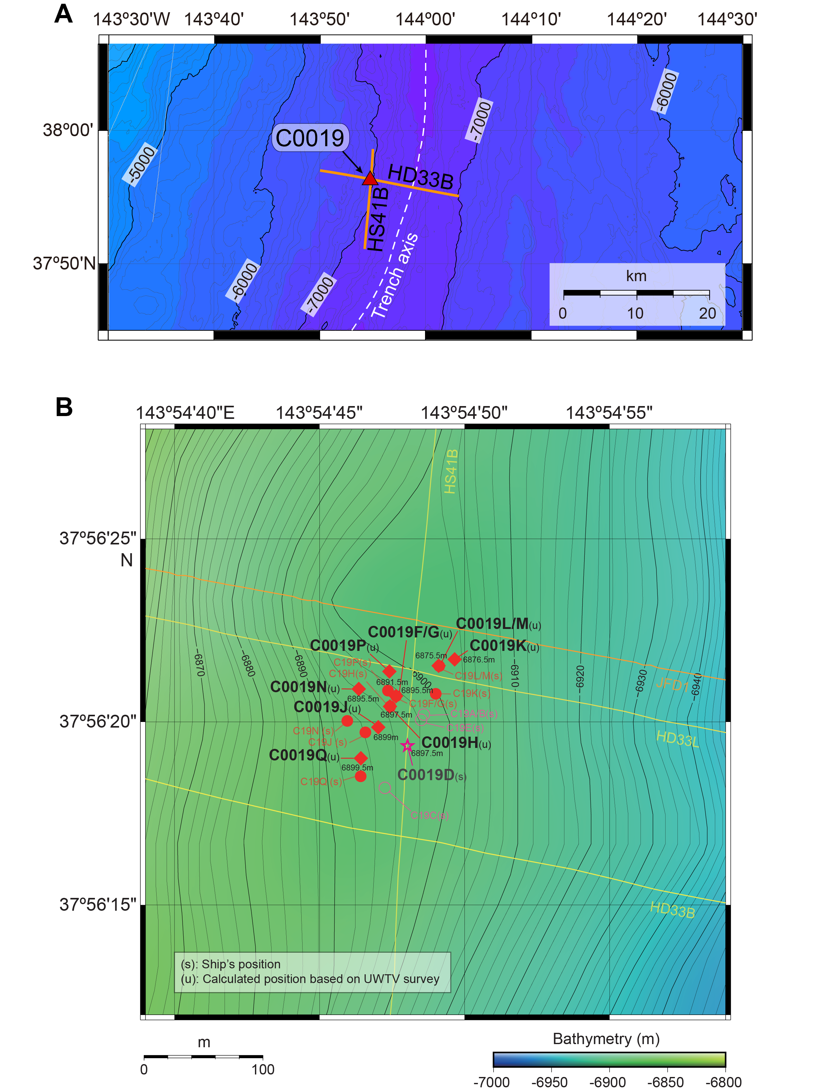
Figure F1. Bathymetric maps.

1.2. Background

1.2.1. Geologic setting

The Japan Trench subduction zone is located off the east coast of northeast Japan where the Pacific plate subducts beneath Japan at a rate of 85 mm/y (DeMets et al., 2010; Argus et al., 2011). The plate margin is characterized by an ~8 km deep trench with a shallowly dipping (~8°) décollement separating the subducting (Pacific) and overriding North American/Okhotsk plate (von Huene et al., 1982). The structure and composition of the prism, décollement, and underthrust material are largely constrained based on prior multichannel seismic profile data, coring during Expedition 343, and correlations to units recovered during Deep Sea Drilling Project (DSDP) Legs 56 and 57 at Site 436. The frontal prism consists of a low-velocity (V_P = 2–3.5 km/s), ~20–30 km wide, seismically chaotic sedimentary wedge (Kodaira et al., 2017; Tsuru et al., 2002). Because of time limitations, Expedition 343 began continuous coring at Site C0019 at ~680 meters below seafloor (mbsf). Sediments collected from ~680 to 800 mbsf consist of ~0–15 Ma biogenic and siliciclastic mudstones (Expedition 343/343T Scientists, 2013a; Rabinowitz et al., 2015; Regalla et al., 2019) and have been interpreted as comprising a frontal accretionary prism (von Huene et al., 1994; Regalla et al., 2019). The décollement at Site C0019 is visible in seismic reflection lines as a high-amplitude semicontinuous reflection that separates undeformed shallowly dipping strata in the subducting plate from deformed material in the overriding plate (Nakamura et al., 2013, 2020). At the position of Site C0019, the décollement occurs above a subducted host block (Chester et al., 2013; Nakamura et al., 2013). Cores recovered from Site C0019 during Expedition 343 indicated that at the décollement zone there is a less than 5 m thick zone of sheared clays with scaly fabrics and sharp planar faults surrounded by a few tens of meters of fractured mudstones and several additional faults (Chester et al., 2013; Kirkpatrick et al., 2015; Keren and Kirkpatrick, 2016). Materials within this zone have been correlated to pelagic clays and clayey mudstones at the base of the incoming sediment section, as represented by the stratigraphy at Site 436 (Chester et al., 2013; Kameda et al., 2015; Rabinowitz et al., 2015). Underthrust material below the décollement consists of two seismically identified units: SU3 and SU4. Seismic Unit SU3 is characterized by relatively strong reflections, and the base of this unit is marked by a high-amplitude semicontinuous reflection. Unit SU3 is correlated to cherts recovered below the décollement during Expedition 343 as well as those recovered at the base of the incoming sediment section at Site 436 (Nakamura et al., 2013; Expedition 343/343T Scientists, 2013a). Unit SU4 is a seismic basement, which is interpreted to be the igneous basaltic crust of the Pacific plate. This unit was not drilled during Expedition 343 or Legs 56 and 57.

1.2.2. Motivation for hole positioning

Site C0019 is positioned within the overriding plate approximately 6 km landward of the Japan Trench axis, near the intersection of Japan Agency for Marine-Earth Science and Technology (JAMSTEC) Multichannel Seismic Lines HD33B and HS41B (Figure F1). Drilling at this site allows direct access to the materials above, within, and below the shallow plate boundary décollement that experienced large shallow slip during the 2011 Tohoku-oki earthquake (Figure F2). This same site was drilled previously during Expedition 343, but coring intervals were very limited because of the short duration of coring (Expedition 343/343T Scientists, 2013a). New drilling activities at Site C0019 during Expedition 405 aimed for continuous data collection across the prism, décollement, and underthrust plate and direct comparison of time variable properties within the high slip region.

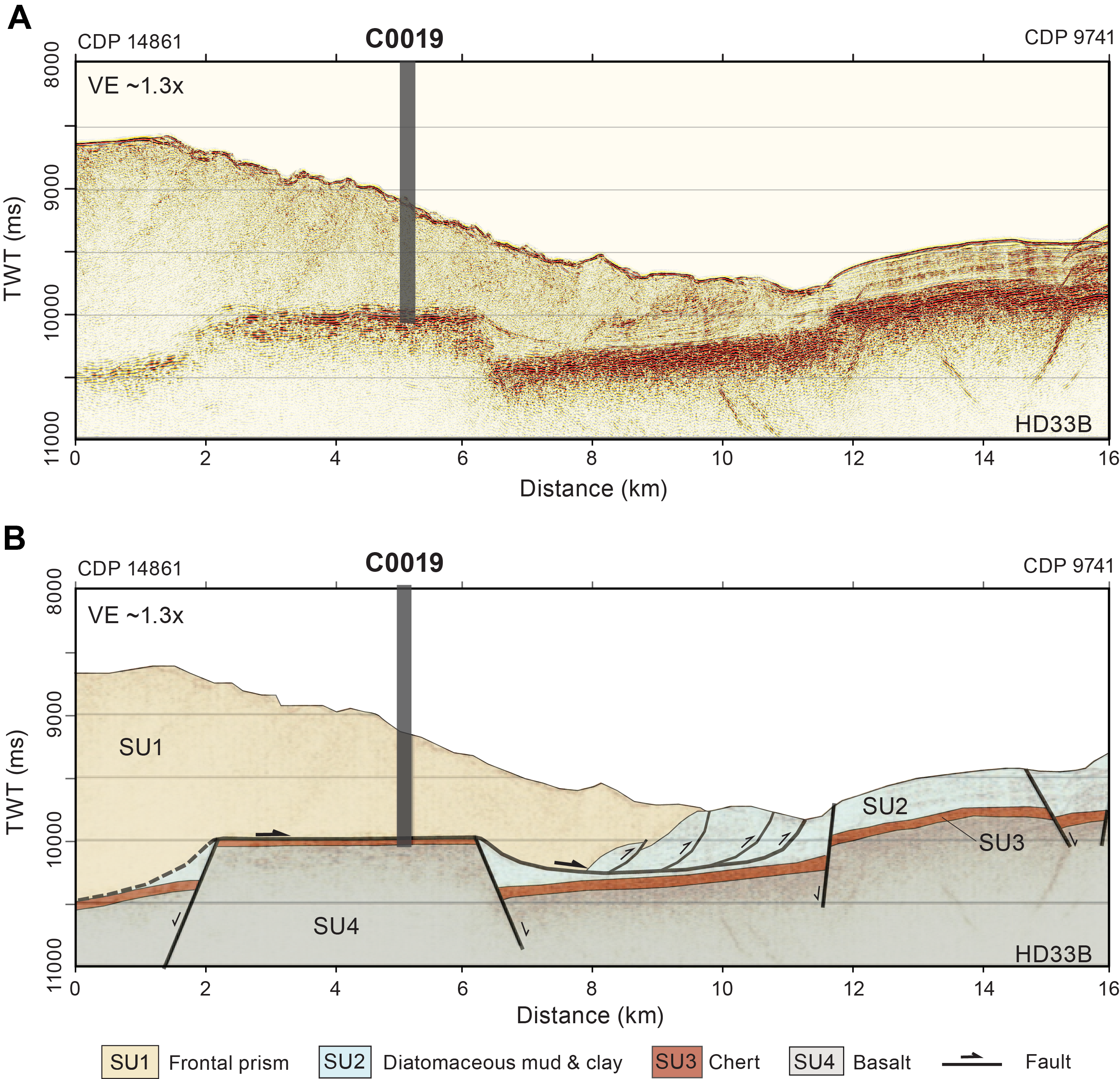
Figure F2. Location of Site C00019.

Drilling activities at Site C0019 during Expedition 405 were divided into four phases: installation of a temperature observatory by reoccupying Expedition 343 Hole C0019D, collection of LWD data, continuous coring, and installation of a second temperature observatory. The first observatory reoccupied Expedition 343 Hole C0019D to monitor temperature and fluid conditions near the décollement and capture perturbations to the formation conditions caused by Expedition 405 drilling. A complete transect across the entire prism, décollement, and underthrust sequence was achieved by separating LWD and coring operations in multiple holes, allowing for use of different borehole assemblies that were best suited for the variable material properties with depth (Figure F1). We note that drilling depths are herein reported as either meters below sea level (mbsl), meters below sea floor (mbsf), or meters below rotary table (m BRT), where the rotary table is 28.5 m above sea level. LWD data collection was completed in the shallow prism in Hole C0019F without bottom-hole assembly (BHA) rotation (0–86 mbsf; 6926.4–7012.4 m BRT) and then subsequently across the prism, décollement, and lower plate in Hole C0019H with BHA rotation (90–980 mbsf; 7016–7906 m BRT). Coring included small-diameter rotary core barrel (SD-RCB) coring in Hole C0019J, which transected the prism to the décollement (82–830 mbsf; 7009.5–7757.5 m BRT), Hole C0019K, which transected the décollement and underthrust sequence (815–875.5 mbsf; 7719–7779.5 m BRT), and Hole C0019P, which transected the lower cherts and upper basalts of the underthrust Pacific plate. The hydraulic piston coring system (HPCS) sampled the shallow prism in Holes C0019L and C0019M (0–114.5 mbsf; 6905–7019.5 m BRT). Finally, the second observatory was installed in the newly drilled Hole C0019P for long-term monitoring.

The locations of holes at Site C0019 were initially designed to be aligned along a trend of ~025°–205°, parallel to the average strike of bedding observed in LWD data from Expedition 343 (Expedition 343/343T Scientists, 2013a) and approximately perpendicular to the local convergence direction (~110°). Positioning of holes along a strike transect was chosen to facilitate correlation of structures between LWD, core, and observatory holes to aid in data analysis and real-time adjustment of operations to target specific intervals of interest. The Expedition 405 strike transect is located ~30 m west of a parallel transect drilled during Expedition 343 (Holes C0019A–C0019E; Figure F1). Holes C0019F–C0019H, C0019J, and C0019Q were sighted along this strike transect and maintain the targeted ~025°–205° trend. Hole C0019N was positioned 30 m west of the strike line near the seabed position of LWD Hole C0019H. Hole C0019K is along the same trend but located on the previous Expedition 405 transect, north of the holes drilled in 2012. HPCS Holes C0019L and C0019M were positioned ~20 m east of the Expedition 405 strike transect. Their position was chosen to be on a bathymetrically higher portion of the seafloor than LWD, SD-RCB coring, and observatory holes, with the objective of obtaining a more complete shallow sedimentary record.

2. Operations

Daily summaries of operations at Site C0019 are listed in Table T1. Daily operations summaries can be found in DAILYRPT in Supplementary material. Coring intervals for Holes C0019J, C0019K, C0019L/C0019M, and C0019P are summarized in Tables T2, T3, T4, and T5, respectively.

2.1. Port call and transit to Site C0019

Expedition 405 began at 1000 h on 6 September 2024, departing from the Port of Shimizu, Shizuoka Prefecture. The drilling vessel (D/V) Chikyu arrived at Site C0019 on 7 September, and all preparations related to setting dynamic positioning were completed at 1530 h 8 September.

2.2. Hole C0019D

Making up and running the Re-engaging Tool to connect to the Hole C0019D wellhead started at 1730 h on 8 September 2024 while drifting from around 4 nmi upstream of the surface current and reached 6353.0 m at 0930 h. The underwater TV camera (UWTV) system was run down at 0930 h on 9 September but was recovered from 2107 meters below mean sea level (m MSL) because of lost communication with a sonar. The UWTV was run down again at 1845 h after the sonar was replaced with a spare one. Running the Re-engaging Tool was resumed when the UWTV reached 6000 m MSL at 2045 h. A seabed survey and search for the wellhead was conducted starting at 0615 h on 10 September. It took almost 13 h to find the wellhead. The Re-engaging Tool was landed on the wellhead at 2030 h. Before running the sensor assembly in the hole, two dummy assembly runs were made to confirm the borehole condition and the bottom depth. Making up and running the sensor assembly in the hole started at 0900 h on 12 September, and landing the sensor assembly was confirmed at 1715 h. All operations in Hole C0019D were completed when the Re-engaging Tool was pulled out to the surface at 1930 h on 13 September.

2.3. Hole C0019F

Drilling down without rotating a BHA is required to drill a borehole straight down when drilling in ultradeep water, whereas a LWD BHA needs rotation to acquire the hole borehole image data. The target depth for the first LWD hole was 100 mbsf. Making up and running LWD started at 0000 h on 14 September 2024 and continued to 0100 h on 15 September while LWD signal tests were conducted at 138.0, 3009.0, 6004.5, 6542.5, 6772.5, and 6851.0 m BRT. The UWTV was run down at 0100 h, and a seabed survey was conducted from 0545 to 1000 h. Seabed surveys were initiated by finding Hole C0019D to use as a reference position. The location for LWD operations was finalized ~30 m north of Hole C0019D. Spud-in of Hole C0019F was achieved at 6926.5 m BRT at 1000 h, followed by washing down to 6936.5 m BRT (10.0 mbsf). Drilling down with rotation started at 1500 h and reached the target depth of 7012.4 m BRT (86.0 mbsf) at 2145 h. The LWD BHA was pulled out to 6921.0 m BRT at 2215 h for the next LWD operation.

2.4. Hole C0019G

The ship position for Hole C0019F was used for Hole C0019G because the latter hole targeted a deeper section of the formation. The LWD BHA tagged Hole C0019G at 6924.0 m BRT at 2215 h on 15 September 2024 but showed mud pulse telemetry signal failure from the measurement-while-drilling (MWD) tool (TeleScope) at 6936.5 m BRT (12.5 mbsf) at 2300 h. Troubleshooting efforts, including downlink and increasing the pump rate to 500 gal/min, were attempted but did not resolve the signal failure. The decision was made to pull the BHA to the surface at 0130 h on 16 September, and the BHA was recovered on deck at 1900 h.

2.5. Hole C0019H

A new LWD BHA was made up with the backup TeleScope and mud motor, and it was run in the hole at 1900 h on 16 September 2024. Running in the hole continued until 0045 h on 18 September while signal tests were conducted at 117.0, 1274.0, 2404.0, 3561.0, 4667.5, 5812.0, and 6837.0 m BRT. The UWTV was run down to 6800 m MSL at 0530 h to finalize the hole location. Hole C0019H was established a few meters southwest of Holes C0019F and C0019G at 0657 h on 18 September. Washing down without rotation was maintained to 7016.0 m BRT (90.0 mbsf) at 1215 h. Drilling down with the LWD BHA started at 1700 h after the UWTV was recovered. The LWD BHA reached the target depth of 7906.0 m BRT (980.0 mbsf) at 0730 h on 21 September and was pulled out of the hole to 7784.0 m BRT (858.0 mbsf). Overpull and hydraulic power swivel (HPS) stall were observed at 7804.0 and 7791.5 m BRT, respectively. Repeat logs were acquired from 7780.0 to 7572.0 m BRT (854.0–646.0 mbsf) and completed at 2130 h. The LWD BHA was recovered on deck at 1700 h on 22 September.

2.6. Hole C0019J

The vessel started sailing back to Site C0019 from the Typhoon 17 (JEBI) evacuation area at 1100 h on 2 October 2024 while maintenance and preparations for coring operations were conducted. An SD-RCB BHA with dual drill collars was made up and run in the hole at 2300 h on 3 October and reached 6832.0 m BRT at 1930 h on 4 October. The center bit was dropped after break circulation, followed by running the UWTV down. A seabed survey was held to confirm the hole location, which was finalized ~30 m southwest of Hole C0019H. Hole C0019J was spudded in at 6927.5 m BRT at 0227 h on 5 October and washed/drilled down with the SD-RCB BHA to the coring starting depth of 7009.5 m BRT (82.0 mbsf). The center bit was recovered at 1930 h, and coring operations began. The first core of this expedition, Core 405-C0019J-1K, was on deck at 0045 h on 6 October. Coring operations continued to 2100 h on 23 October with two interruptions.

The first interruption was caused by waiting on weather. The SD-RCB BHA was pulled out from 7209.0 to 6963.5 m BRT (281.5–36.0 mbsf) after recovering Core 405-C0019J-21K on deck at 2200 h on 9 October to allow an emergency pull out of the hole in case maintaining dynamic positioning became difficult. During the waiting on weather period, >20 m/s wind (gusts) with ~6 m wave height were observed from 2300 to 0200 h on 11 October. The SD-RCB BHA was then run back to the bottom at 0500 h, and coring operations resumed. The second interruption occurred after Core 74K was recovered on deck at 0615 h on 20 October. A passing cold front left strong winds and ~6 m wave height on site while the drilling depth approached the estimated depth of the most important formations to be recovered. A short wiper trip was conducted to check and clean the borehole. While pulling the SD-RCB BHA out from 7712.0 to 7450.0 m BRT (784.5–522.5 mbsf), damage was found on the Lower Main Roller on the FWD side of the Traveling Block Dolly at 0900 h. The short trip was resumed after it was replaced with a new Main Roller Assembly at 1500 h. Tight spots were observed as discrete peaks in weight on bit from 7560.0 to 7583.0 m BRT and from 7712.0 to 7715.0 m BRT. To remedy this, the hole was reamed down and then swept out with 10 and 15 m³ of seawater gel, respectively. Coring resumed at 0030 h on 21 October and reached the target depth of 7757.5 m BRT (830.0 mbsf) at 2100 h on 23 October.

The coring advance was set 9.5 or 10 m for Cores 405-C0019J-1K through 74K; however, this coring advance was halted to prevent missing or damaging the fragile formation when high standpipe pressure was observed for Cores 75K–88K and instead set to 2.0–4.5 m advance. In total, 88 cores (total length of initial recovery = 370.5 m) were collected from 82.0 to 830.0 mbsf (748.0 m interval) with an average recovery of 49.5% (Table T2). Because of incomplete recovery of key intervals in the décollement and underthrust section, we decided to core a second plate boundary interval east of Hole C0019H near the Expedition 343 transect in Hole C0019K. The SD-RCB BHA was pulled out of Hole C0019J to 6801.0 m BRT at 0200 h on 24 October and kept close to the seafloor while moving to the next hole.

2.7. Hole C0019K

The UWTV was run to 6800 m MSL while dropping the center bit at 1530 h on 24 October 2024. Hole C0019K, which lies ~30 m east of Hole C0019H, was spudded in at 1630 h. The SD-RCB BHA reached 7719.0 m BRT (815.0 mbsf) at 0730 h on 26 October. The center bit was recovered to the surface after a short trip between 7719.0 and 7544.0 m BRT, and coring began at 1445 h and continued until 1115 h on 30 October. The coring advance varied between 2.0 and 6.0 m because of adjustments when standpipe pressure increased so that the chances of missing the collection of fragile formations would be minimized. In total, 17 cores (total length of initial recovery = 41.6 m) were collected from 815.0 to 875.5 mbsf (60.5 m interval) with an average recovery of 68.8% (Table T3). The SD-RCB BHA was pulled out to the surface at 0930 h on 31 October.

2.8. Hole C0019L

As at Site C0026, at least two holes were planned for HPCS operations to sample the surface sediment and mudline. A HPCS BHA was made up and run in the hole to 6893.0 m BRT at 1100 h on 12 November. A seabed survey with the UWTV was carried out from 1430 to 1900 h to check the shallow coring hole and prepare for additional planned deep coring operations with the SD-RCB. Hole C0019L was shot from above the seabed at 2025 h, and the inner barrel was pulled out using the drawworks assist. Core 405-C0019-1H successfully collected the surface sediment and mudline with bottom water at 2130 h (Table T4).

2.9. Hole C0019M

Hole C0019M was shot from above the seabed at 2232 h on 12 November 2024. Core 405-C0019M-1H was retrieved with the mudline and bottom water at 2400 h. Coring continued with full stroke for Cores 1H–6H, although assistance from the drawworks was required to pull out the inner barrel. Partial penetration while shooting and overpull while pulling the inner barrel were observed for Cores 7H–10H. Overdrilling while pulling with the drawworks was applied to pull out these cores. Core 10H showed 9.82 m of the initial core length even though the coring advance was only 2.5 m.

The coring system was changed to the extended shoe coring system (ESCS) for Core 405-C0019M-11X. ESCS coring continued through Core 14X with a 9.5 m coring advance. In total, 14 cores (total length of initial recovery = 95.0 m) were collected from 0 to 114.5 mbsf (114.5 m interval) with an average recovery of 83.0% (Table T4). The HPCS BHA was pulled out of the hole to the surface at 2300 h on 15 November.

2.10. Hole C0019N

To minimize the risk of getting stuck in the hole based on lessons learned from operations in Hole C0026A, an SD-RCB BHA without any drill collars was built up to collect cores below the chert layers. The SD-RCB BHA was made up and run in the hole at 2315 h on 16 November 2024, and it reached 6825.0 m BRT at 2130 h on 17 November. The center bit was dropped before running the UWTV at 0100 h on 18 November. Spud-in of Hole C0019N was performed at 6924.0 m BRT ~30 m west northwest of Hole C0019H at 0815 h, followed by washing down to 6974.0 m BRT (50.0 mbsf). Drilling down with the SD-RCB BHA began at 1530 h after the UWTV was recovered to the surface and continued to 7752.5 m BRT (828.5 mbsf) with an average rate of penetration (ROP) of ~55 m/h. A short trip was carried out from 7752.5 to 7487.5 m BRT because the ROP decreased from 0430 to 0815 h on 20 November. Drilling paused because of maintenance for a HPS motor malfunction and then resumed at 1445 h from 7785.5 m BRT. The ROP dropped and intermittently arrested with observed torque spikes. To continue drilling, the hole was swept up and down, but no progress was made from 7825.0 m BRT (901 mbsf).

At 0915 h on 21 November, the decision was made to quit drilling ahead instead of coring at the current depth. The center bit was recovered at 1300 h, and we observed that no cutters remained. After circulating bottoms up, the core barrel was dropped and we attempted to cut a core at 1530 h. The coring barrel was retrieved at 2200 h without any advance. Junk cuttings were found in the core liner, and the decision was made to pull out of the hole. A free-fall funnel was deployed at 0230 h on 22 November, when the BHA pulled out to 7024.0 m BRT (100.0 mbsf). The UWTV was run and recovered to let the free-fall funnel land properly at 1400 h. The BHA was recovered to the surface at 0545 h on 23 November. The top section of the coring bit was found to be severely worn out.

2.11. Hole C0019P

We decided that the center bit was not strong enough to drill through the chert layers and applied the following operations plan:

Drill down with a noncoring bit.
Deploy a free-fall funnel.
Reenter the hole with the SD-RCB BHA.
Core below the chert layers.

The 8½ inch drilling BHA was made up and run in the hole at 0745 h on 23 November 2024. The UWTV seabed survey was performed from 1000 to 1630 h on 24 November. The 8½ inch drilling BHA was spudded into Hole C0019P at 1630 h and washed down from 6920.0 to 6970.0 m BRT (0–50 mbsf). Drilling down started at 0600 h after the UWTV was recovered to the surface and reached the planned coring depth of 7850.0 m BRT (930.0 mbsf) at 2100 h on 26 November. A free-fall funnel was deployed when the 8½ inch drilling BHA was pulled out to 7020.0 m BRT (100.0 mbsf). Mechanical trouble occurred while pulling out of the hole to 3462.0 m BRT at 1400 h on 27 November. Two bolts connecting the 750T Elevator and Adapter sheared and dropped onto the rig floor. The Elevator was replaced to 500T, and we resumed pulling out the 8½ inch drilling BHA to the surface at 0500 h on 28 November. The 750T Elevator was repaired with spare parts and set back again at 0345 h on 29 November.

The SD-RCB BHA with a new coring bit and without drilling collars was made up and run at 0845 h, and it reached 6830.0 m BRT at 0300 h on 30 November. The UWTV found the free-fall funnel at 0730 h, which tilted while we attempted reentry at 1200 h. We managed to pass through the free-fall funnel and successfully reentered Hole C0019P at 1730 h while adjusting the vessel position and pushing with the BHA. The UWTV was recovered to the surface at 2100 h, and running the SD-RCB BHA began. The center bit was recovered to the surface at 1015 h on 1 December, followed by conducting circulation and then bottoms up. Coring operations began at 1215 h, and the last core was recovered on deck at 2330 h on 2 December. Five cores were collected from 930.0 to 946.4 mbsf (16.4 m interval) with various advances between 0.9 and 5.0 m and an average recovery of 76.5% (Table T5). The SD-RCB BHA was pulled out to the surface at 2115 h on 3 December. With this, all coring operations for this expedition were complete.

2.12. Hole C0019Q

The operations to install the temperature sensor assembly consisted of five steps:

Jetting a 13⅜ inch casing with a 20 inch wellhead.
Drilling down to the target depth.
Reentering and running a 4½ inch tubing in the hole.
Running, landing, and releasing the sensor assembly in the hole by coring line.
Landing and releasing the 4½ inch tubing from the drill string.

Preparing the BHA for 13⅜ inch casing with the 20 inch wellhead, jetting, and drill ahead tool (DAT) in one pipe trip (the jetting and DAT BHA) began at 2115 h on 3 December 2024. The vessel moved to Site C0026 and recovered all transponders while preparing the jetting and DAT BHA.

The jetting and DAT BHA was made up and run at 1630 h on 4 December, and it reached 6828.0 m BRT at 0400 h on 6 December. Spud-in of Hole C0019Q was performed at 6928.0 m BRT at 1015 h after a UWTV seabed survey. The 13⅜ inch casing with 20 inch wellhead was successfully jetted into the planned depth of 6970.0 m BRT (42.0 mbsf) at 1415 h. After releasing the DAT from the wellhead housing was confirmed at 2330 h, the UWTV was recovered to the surface at 0400 h on 7 December. The DAT drilled from 7567.0 to 7853.0 m BRT (639.0–925.0 mbsf) after washing down to 7003.0 m BRT (75.0 mbsf) at 1230 h on 8 December, followed by short trips between 7853.0 and 7474.0 m BRT and spotting 20 m³ of seawater gel at 1800 h, and was finally recovered to the surface at 2230 h on 9 December.

A 4½ inch tubing assembly was made up and run starting at 0045 h on 10 December. The UWTV was run to 7 m above the shoe, where the 4½ inch tubing assembly reached 6873.0 m BRT. The Hole C0019Q wellhead was found, and the 4½ inch tubing assembly reentered the hole at 2330 h on 11 December. After confirming the 4½ inch tubing assembly landed on the casing hanger of the wellhead, we attempted to run the sensor assembly. However, the sensor assembly could not pass through 6915.5 m BRT. The 4½ inch tubing assembly with sensor assembly was pulled out of the hole to the surface, and we found two sensors (#104 and #123) were stuck in a narrow part of the casing hanger of the 4½ inch tubing assembly at 1730 h on 13 December.

The 4½ inch tubing assembly was run and reentered Hole C0019Q again at 1800 h on 14 December. The sensor assembly, with a slightly heavier weight of sinker bars (from 15 to 30 kg) to avoid the same kind of failure, was made up and run in the hole with pumping, and it successfully landed on the sensor hanger. Jarring down was applied to release the sensor hanger from the sinker bar, and we confirmed the release by coring line tension at 0230 h on 15 December. The hydraulic assist running tool (HART) was activated to release the 4½ inch tubing assembly. Landing and releasing were confirmed visually by the UWTV at 1145 h. Pulling the HART out of the hole to the surface was completed at 0745 h on 16 December.

2.13. Transit to Shimizu port

The vessel started to sail back to the Port of Shimizu after all four transponders at Site C0019 were recovered at 1345 h on 17 December 2024 and arrived at the standby point off the Port of Shimizu at 1300 h on 19 December. The expedition was completed after docking quayside at the Port of Shimizu at 1000 h on 20 December.

3. Logging while drilling

Three holes (C0019F–C0019H) were drilled for LWD measurements at Site C0019. Logging data were acquired using an LWD/MWD assembly that consisted of the SLB TeleScope, MicroScope, and SonicScope tools (see Logging while drilling in the Expedition 405 methods chapter [Kirkpatrick et al., 2025]). Logging data were acquired in Holes C0019F and C0019H. Hole C0019F was drilled to a maximum depth of 7022.7 m BRT (96.3 mbsf) to obtain LWD/MWD data and LWD images from the shallow strata. Hole C0019G was abandoned because of technical difficulties with the mud-pulse telemetry module of the TeleScope tool, which meant that no real-time data were transmitted. Following disconnection from the BHA, drilling stopped and the BHA was recovered. No data are available for Hole C0019G. Hole C0019H was jetted down to 7014 m BRT (88.3 mbsf) and then drilled to total depth at 7905.7 m BRT (980 mbsf) to obtain a full suite of LWD/MWD data through the upper plate down to the basalts of the incoming plate. The interval 7572–7774 m BRT was relogged while tripping out to acquire additional resistivity image logs.

3.1. Data and log quality

See Logging while drilling in the Expedition 405 methods chapter (Kirkpatrick et al., 2025) for a detailed description of operations, tools, and data processing.

3.1.1. Hole C0019F

3.1.1.1. Available data

Hole C0019F was drilled to 96.3 mbsf and logged with MWD data, which provided a limited subset of the LWD data in real time. When the LWD tools were recovered on the rig floor, recorded mode data were successfully downloaded and processed.

3.1.1.2. Depth shift

The mudline was identified from the midpoint of the first significant break in the gamma ray and resistivity logs (Figure F3). A mudline was picked at 6926.4 m BRT in Hole C0019F. All LWD data were converted to the LWD depth below seafloor (LSF) depth scale. In this section, LSF depths are referred to as mbsf, based on the mudline depth.

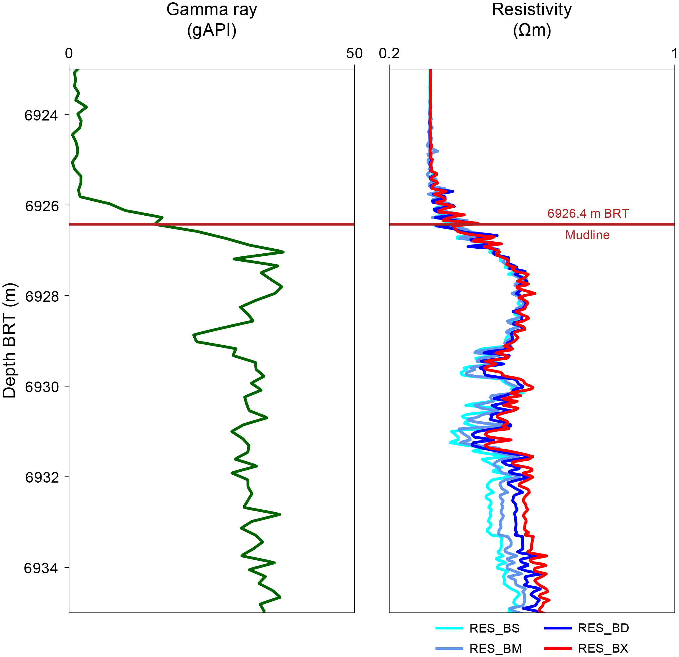
Figure F3. Mudline identification, Hole C0019F.

3.1.1.3. Logging data quality

Figure F4 shows an overview of the log QC. The use of rotary drilling in soft sediments may lead to significant deviation of the borehole. Static borehole survey points were scarce but showed that the borehole was inclined by 8° below 4 mbsf. The other drilling parameters show that the borehole was drilled smoothly with an average ROP of ~30 m/h.

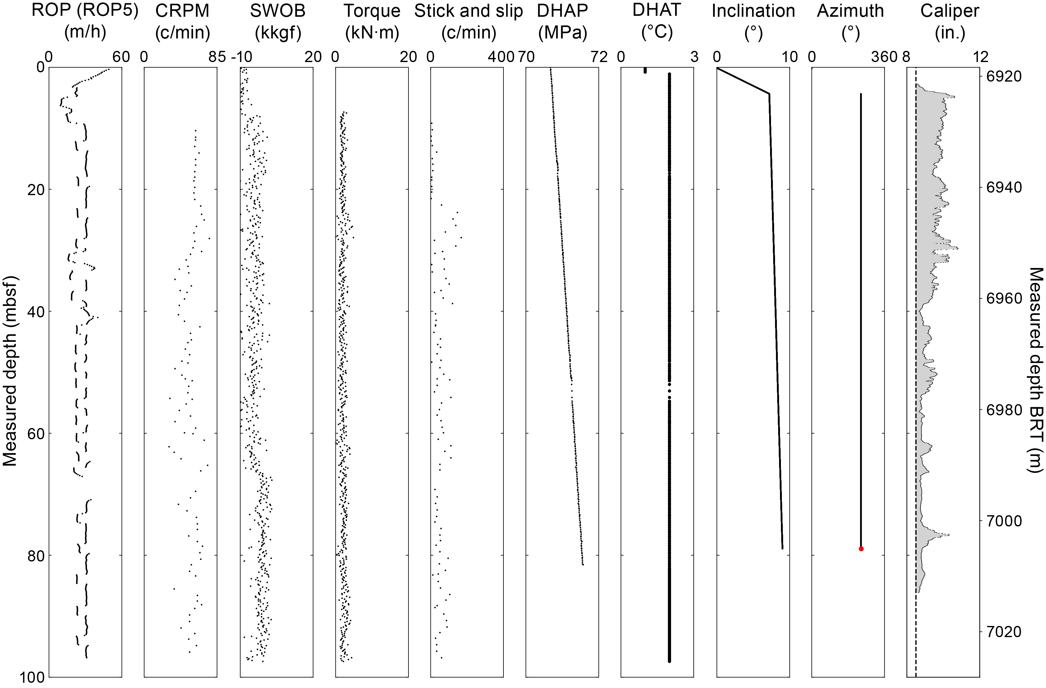
Figure F4. Log quality control log, Hole C0019F.

Logging data quality is strongly dependent on the borehole diameter and therefore rugosity. To evaluate borehole conditions, SLB provided an electrical caliper (e-caliper) pseudo-log derived from the MicroScope resistivity data at various investigation depths using a proprietary method. This log was used as an indicative measure of the borehole diameter and shape. Intervals where the diameter exceeded the drill bit size (8.5 inches; 21.59 cm) indicate enlargement aligned along the azimuth of the borehole. The logs indicated that the upper section of LWD data from seafloor to around 20–40 mbsf was affected by poor borehole conditions, with both image logs and the e-caliper log indicating consistent hole enlargement.

Resistivity images were acquired from the seafloor to 86 mbsf (Figure F5). The upper 20–40 m of the ultrahigh-resolution images (UHRIs) are poor quality due to poor borehole conditions in the shallow interval. The images from 40 to 80 mbsf are good quality. Throughout the entire logged interval of Hole C0019F, borehole image quality was severely affected in washed out sections. Poor borehole condition and eventually poor tool centralization and contact between the MicroScope tool electrodes and formation resulted in bad and irregular resistivity readings. This resulted in typical washed-out images. Resistivity images from the extra deep, deep, medium, and shallow buttons are of similar quality but have lower resolution.

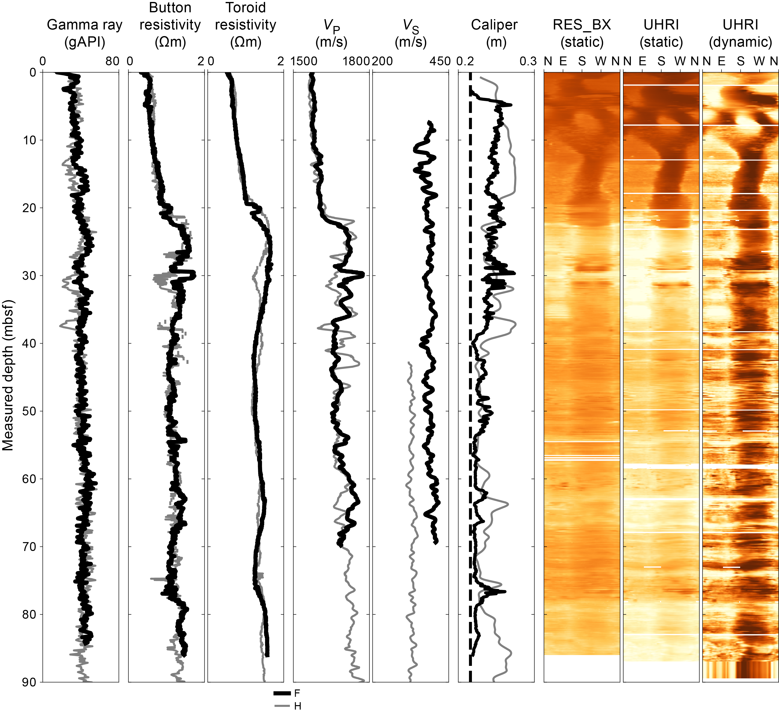
Figure F5. LWD log data, Holes C0019F and Hole C0019H.

3.1.2. Hole C0019G

3.1.2.1. Available data

Hole C0019G was drilled with the LWD/MWD tools. Unfortunately, because of a technical issue with the TeleScope tool, no data points were transmitted in real time through mud-pulse telemetry. Following disconnection with the BHA, drilling stopped and the BHA was recovered. No LWD data are available for Hole C0019G.

3.1.3. Hole C0019H

3.1.3.1. Available data

Hole C0019H was drilled to 980 mbsf, and the borehole was logged successfully with the LWD/MWD tools. The hole was jetted down to ~90 mbsf to avoid deviation in the poorly consolidated shallow section. This meant that continuous image logs were not obtained for the upper ~90 m because the mud motor powering the LWD tools was not active during jetting. MWD data were transmitted in real time with a limited set of LWD data through the mud-pulse telemetry system. When the LWD tools were recovered on the rig floor, memory data were successfully downloaded and processed.

3.1.3.2. Depth shift

The mudline was identified from the midpoint of the first significant break in the gamma ray and resistivity logs (Figure F6). A mudline was picked at 6925.7 m BRT in Hole C0019H. All LWD data were converted to the LSF depth scale.

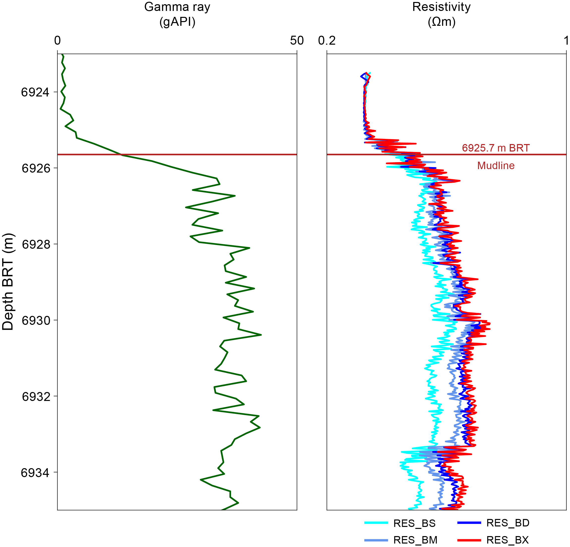
Figure F6. Mudline identification, Hole C0019H.

3.1.3.3. Logging data quality

Three elements are used to assess the borehole quality of the LWD data: (1) borehole conditions, (2) comparison between logs done in the same interval, and (3) consistency of the measured sonic and electrical logging data with QC information provided by the contractor.

3.1.3.3.1. Borehole conditions and drilling parameters

Figure F7 shows an overview of the Hole C0019H QC with drilling parameters and frequency of stick-slip. The logs indicate that the borehole was drilled relatively smoothly. However, stick-slip behavior of the drill bit occurred in various intervals, which influenced the quality of the image logs. Large sections of the real-time image logs were not transmitted because of the stick-slip of the BHA. These intervals were later recovered in the memory data. Horizontal image artifacts are common throughout the entire imaged interval and are thought to be related mainly to the stick-slip of the MicroScope tool as the buttons rotate (Lofts and Bourke, 1999).

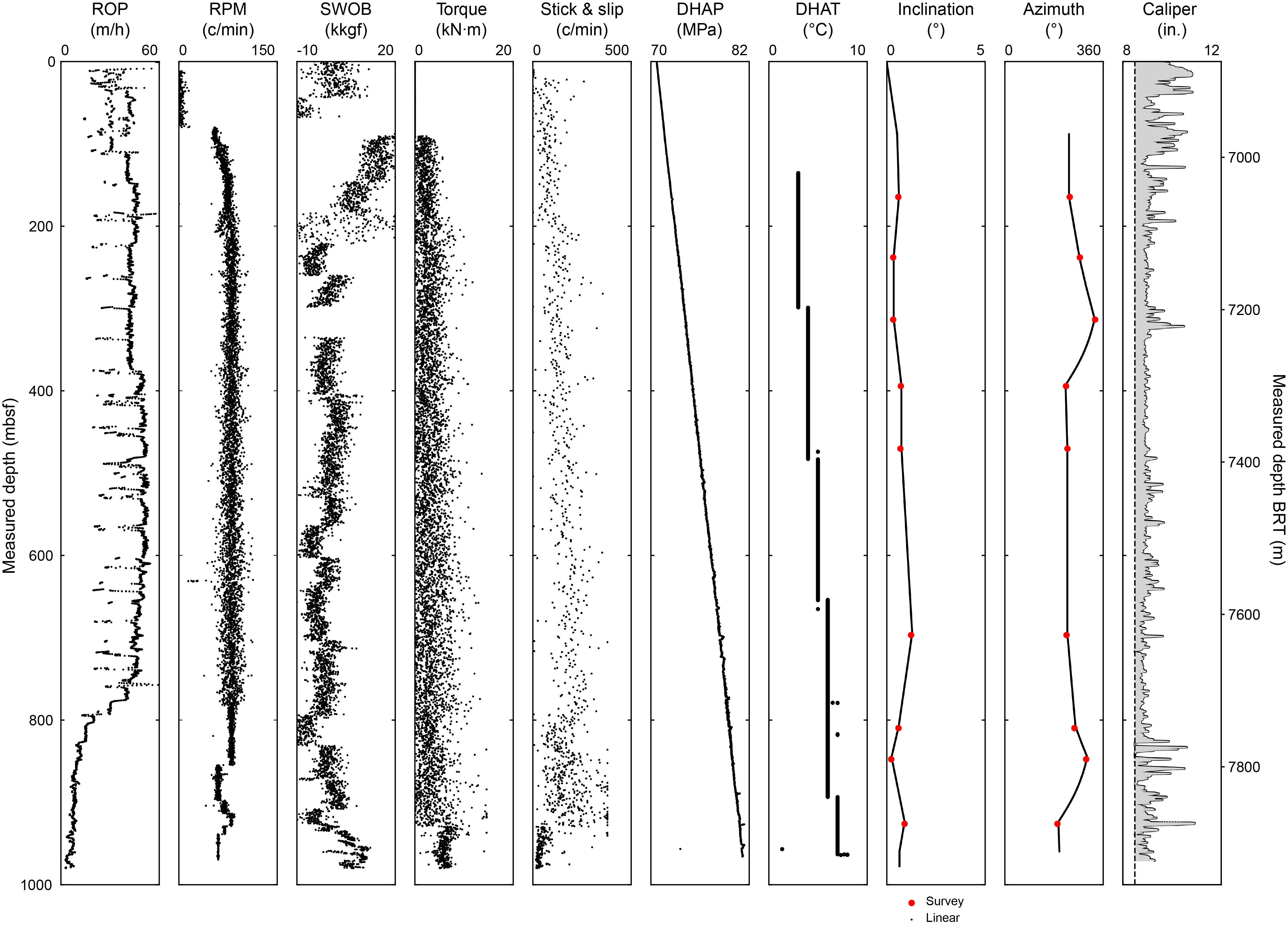
Figure F7. Log quality control log, Hole C0019H.

The ROP was reduced from an average of 40–50 m/h to around 15 m/h around 793 mbsf to mitigate stick-slip, resulting in improved quality of image logs below this depth. The overall quality of the image data above 793 mbsf is variable, where depths with high stick-slip have lower image quality and increased artifacts (e.g., 460–480 and 522–536 mbsf). The overall quality of the image data below 793 mbsf is very good, with ~99% of the logged section imaged.

The real-time borehole survey is the basis for the borehole orientation data. Hole C0019H was drilled with the spare TeleScope tool and tended to have more variable orientation records compared to Hole C0019F, which was drilled with the primary TeleScope tool. Few reliable survey points were obtained, and the orientation of the borehole was linearly interpolated between these points (Figure F7). The borehole stays vertical with a maximal inclination of 1.25° at 696 mbsf. Borehole images are reoriented using the borehole surveys provided by the Telescope (inclination and azimuth). Geographic reorientation of structural features is further discussed in Resistivity image interpretation.

3.1.3.3.2. Comparison of main and relogged sections

The interval from 646 to 846 mbsf was logged a second time during pipe retrieval to ensure that a full suite of image logs was acquired over this interval and to observe the evolution of the borehole conditions over time. Five resistivity logs (shallow, medium, deep, extra deep, and UHRI) were collected during relogging. The Logging Staff Scientist adjusted the depths of the relogged data by correlating variations in the gamma ray log with the main run.

The relogged data show similar deep resistivities to the main run, but shallow resistivities are lower during the relog, which suggests enlargement of the borehole between 740 and 825 mbsf. The poorer quality of the image logs for this second logging run indicates that borehole conditions degraded between the runs (Figure F8). This negatively affected the quality of the repeat resistivity images, which exhibit lower electrical resistivities recorded on the damaged side. Gamma ray is also lower at the location of the borehole enlargement.

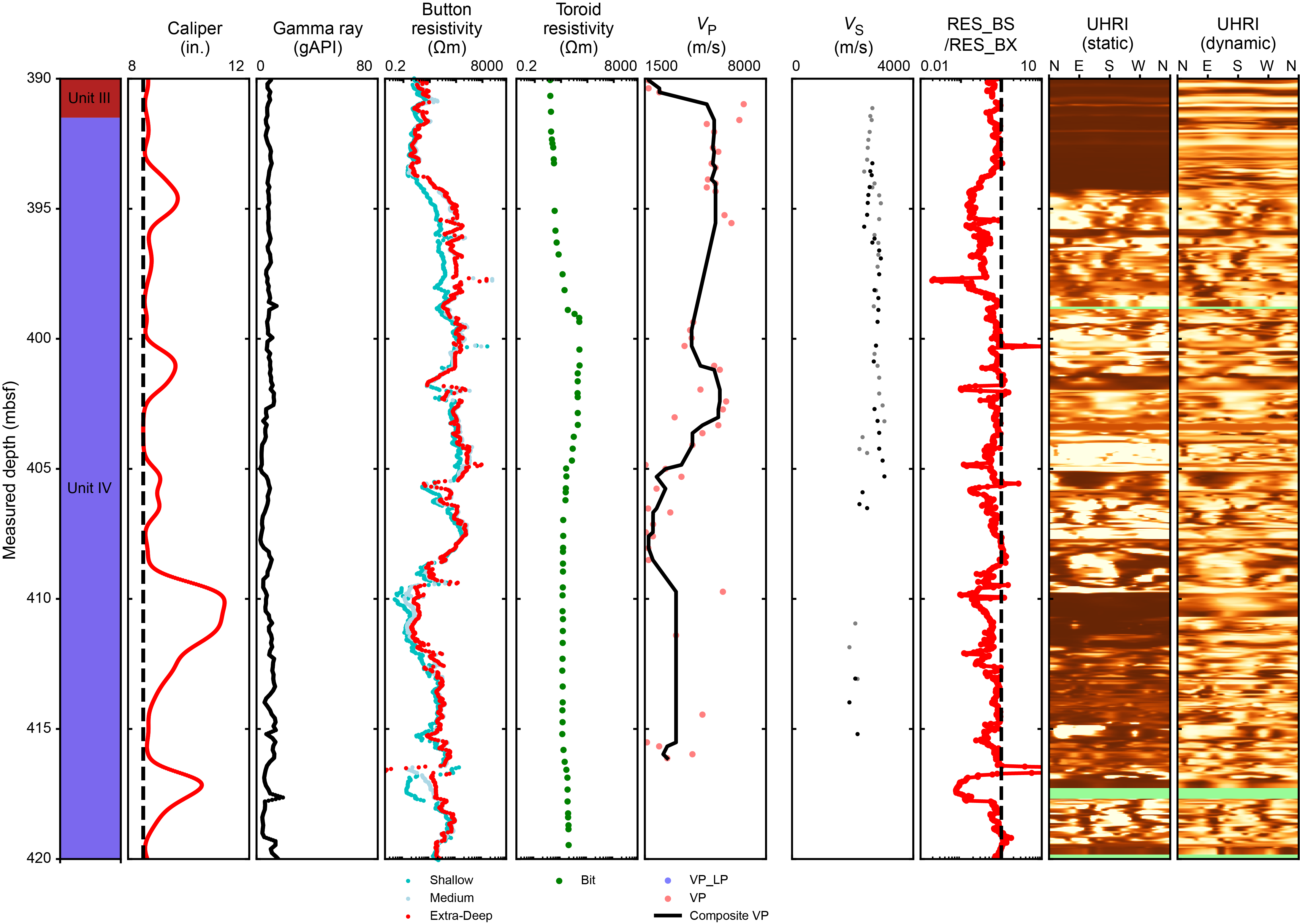
Figure F8. Comparison of gamma ray and resistivity data.

3.1.3.3.3. Consistency of sonic logging data

SLB provided a composite P-wave log by merging the velocity determined from Leaky P analysis to 920 mbsf and P-wave analysis to total depth (Figure F9). For Leaky P, the reference QC curve is the slowness-frequency analysis (SFA) obtained from dispersion analysis of the low-frequency band of the monopole waveforms; the picked slowness should lie on the left edge of the SFA projection (Plona et al., 2006). For the P-wave analysis, the reference QC curve is the slowness-time projection (SPR) for the high-frequency band of the monopole waveforms; the picked slowness should lie at the maximum of this projected coherence log. There is no interval where both analyses were conducted simultaneously.

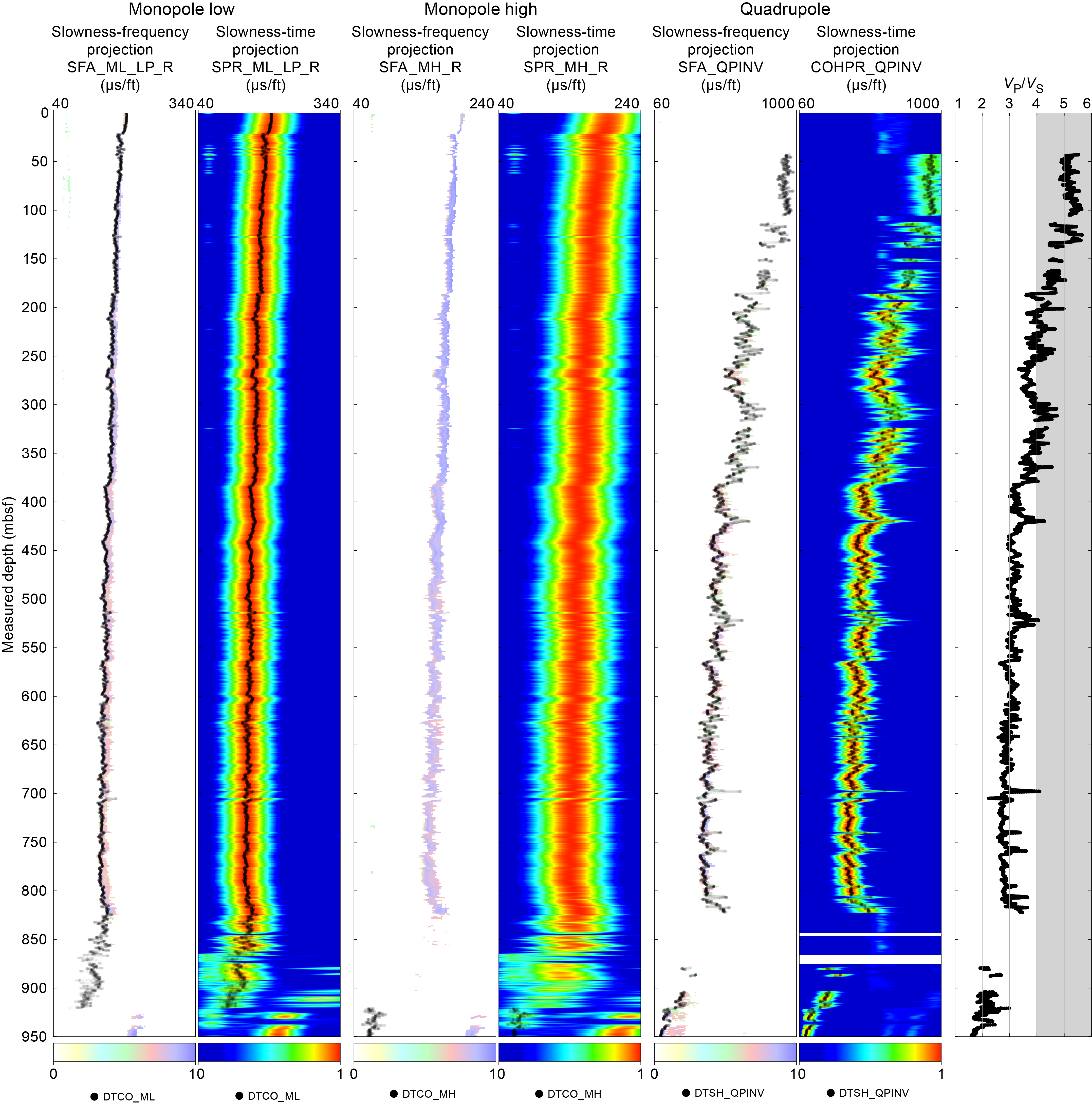
Figure F9. Sonic data QC.

Figure F9 summarizes the QC plots provided by SLB. Above 825 mbsf, the SFA intensity is strong and the picked P-wave slowness is reliable. The SFA intensity becomes much weaker below 825 mbsf and vanishes at 920 mbsf. The P-wave velocities estimated with the Leaky P method are therefore much noisier, but the picked slowness is consistent with the coherence plot. The picked estimate is likely to be reliable between 825 and 920 mbsf. Although the SPR plot of the high-frequency monopole waveform is strong in this interval, SLB chose not to use this to better constrain the P-wave velocity estimate and instead used only the Leaky P method.

Below 920 mbsf, P-wave velocities are picked from the high-frequency monopole data. The coherence on which the P-wave slowness is picked seems weak, but this may be biased by another strong coherent phase in the waveform. Direct observation of the waveforms provides additional insight on the quality of the picking (Figures F10, F11). Below 925 mbsf, the P-wave velocities are large enough for the arrival times to coincide with those of the collar wave. In two intervals (920–925 and 931.5–938 mbsf) the sonic signal is strongly attenuated. However, high P-wave velocities were estimated at those intervals, possibly due to incorrect picking of the collar wave arrivals. Accordingly, P-wave velocities should be treated as unreliable in these two intervals.

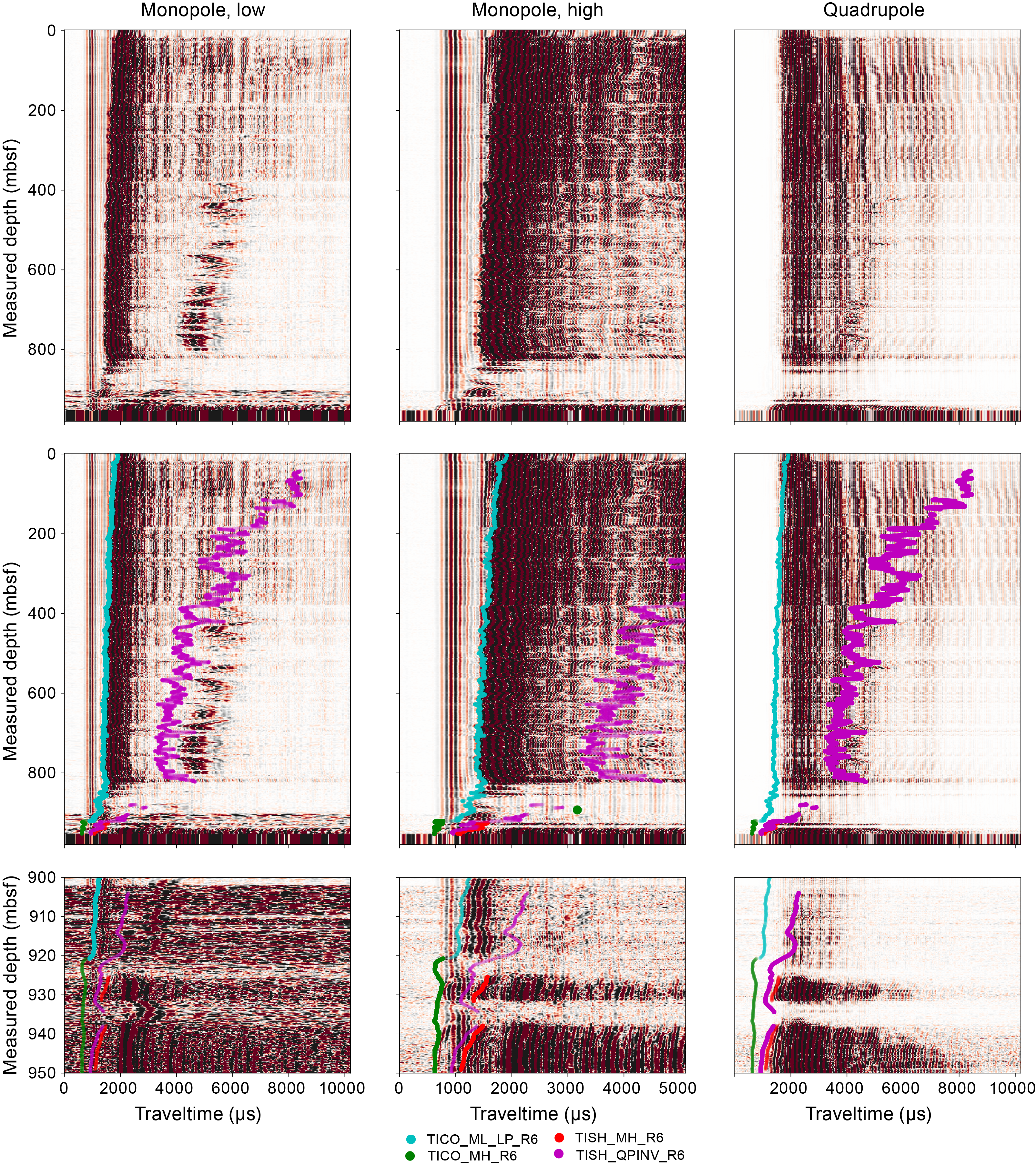
Figure F10. Waveforms.

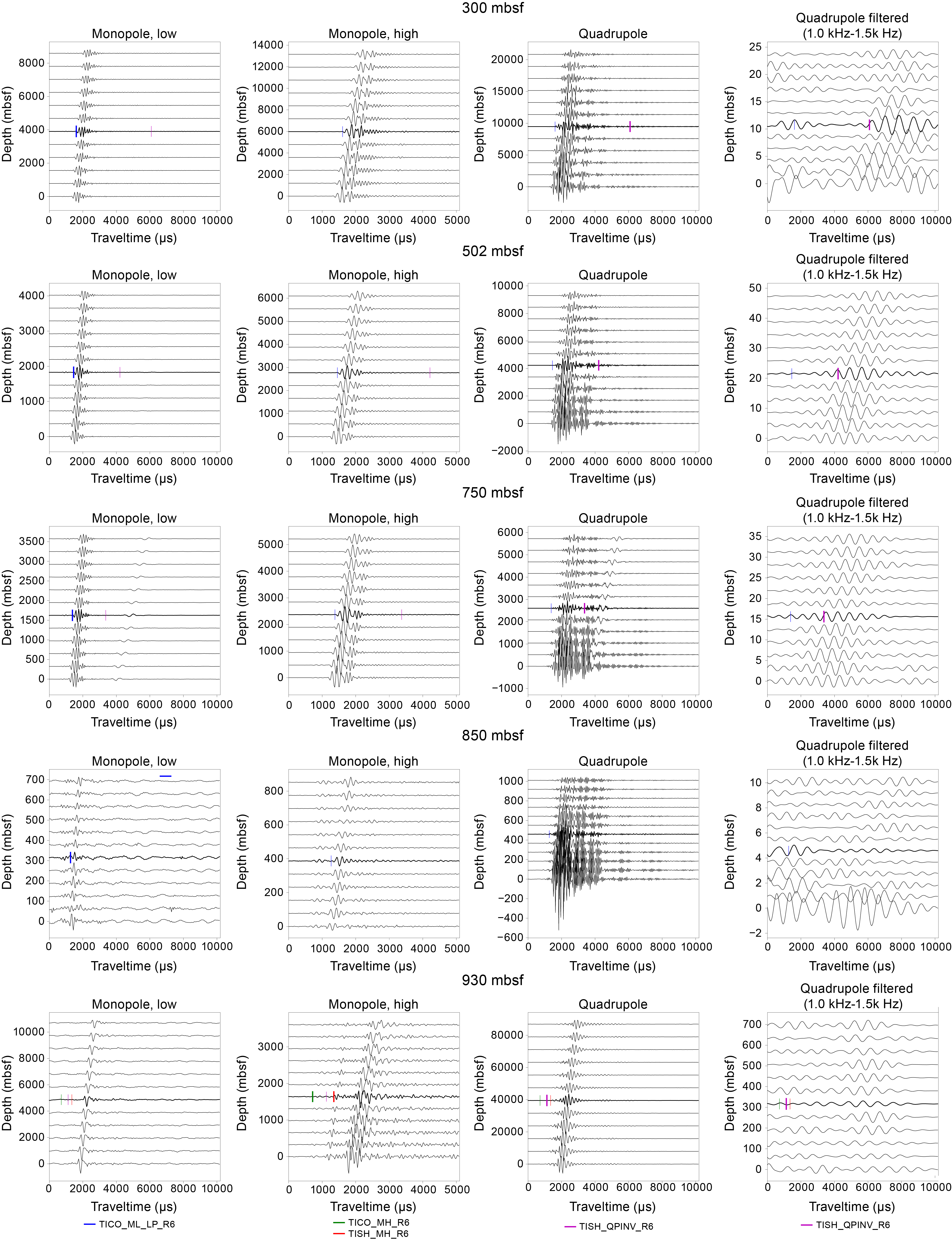
Figure F11. Shot gathers.

The reference QC plot for the quadrupole signal is the SFA plot (Figure F9). The signal-to-noise ratio of S-wave velocity (V_S) is often very low. No V_S could be picked between 825 and 925 mbsf. In their processing report, SLB stated that V_S data may be unreliable for depths shallower than 200 mbsf. However, the arguments listed below suggest that V_S data should also be unreliable in other intervals of the borehole. Firstly, large nonrealistic V_P/V_S ratios (>4) are observed in the shallow part of the hole. These values coincide with the lower intensity slowness-frequency projection for the quadrupole signal. Also, the picked velocity tends not to align with the left part of the SFA plot, suggesting lower slowness and hence higher shear-wave velocity than measured. Finally, Figure F10 shows that the quadrupole waveforms are dominated by high-frequency oscillations that are much larger than the target bandwidth of 1–1.5 kHz (Figure F11). After bandpass filtering, screw waves can be tracked along the receivers for the depths between 300 and 825 mbsf (e.g., at 502 mbsf) at times earlier than the picked arrival time. A further in-depth analysis of the sonic data might provide more reliable velocities. For the current data set, V_S values shallower than 350 mbsf should be considered with great care.

3.1.3.3.4. Consistency of electrical logging data

A qualitative QC criterion is the agreement between the different resistivity channels (at different depths of investigation). Except for shallow resistivity, the button resistivity channels are consistent for most of the borehole. However, the bit resistivity is smoother and higher than the other toroid resistivity channels (Figures F12, F13, F14). This could be attributed to the following:

A change in the BHA compared to the planned BHA for Hole C0019H set prior to the expedition, which would change the geometrical factor used to compute the bit resistivity (see Logging while drilling in the Expedition 405 methods chapter [Kirkpatrick et al., 2025]);
Potential electromagnetic interference with the downhole motor; and/or
A scale effect associated with the difference in depth of investigation between the bit and button resistivity measurements (see Logging while drilling in the Expedition 405 methods chapter [Kirkpatrick et al., 2025]).

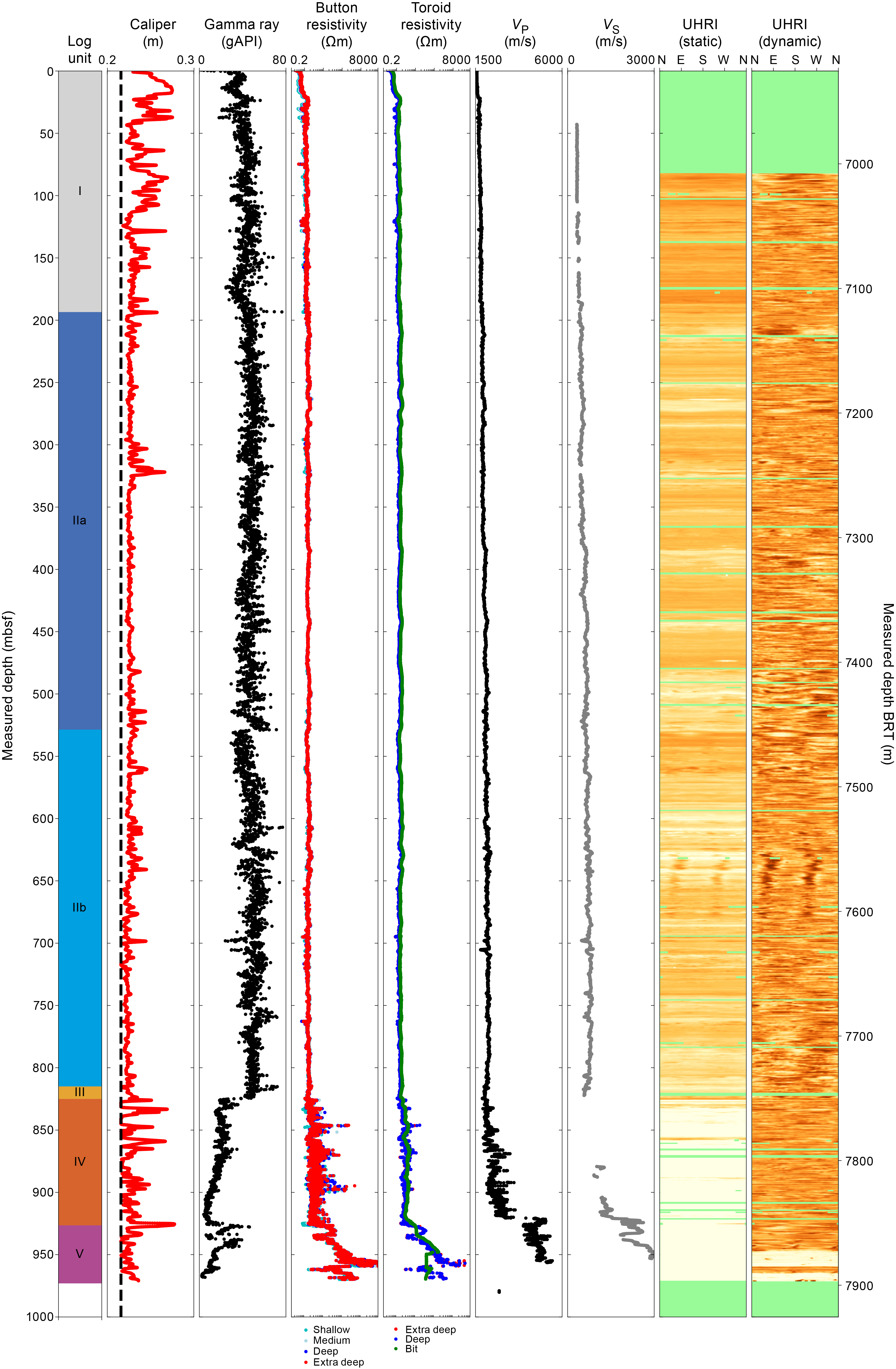
Figure F12. LWD log data, Hole C0019H.

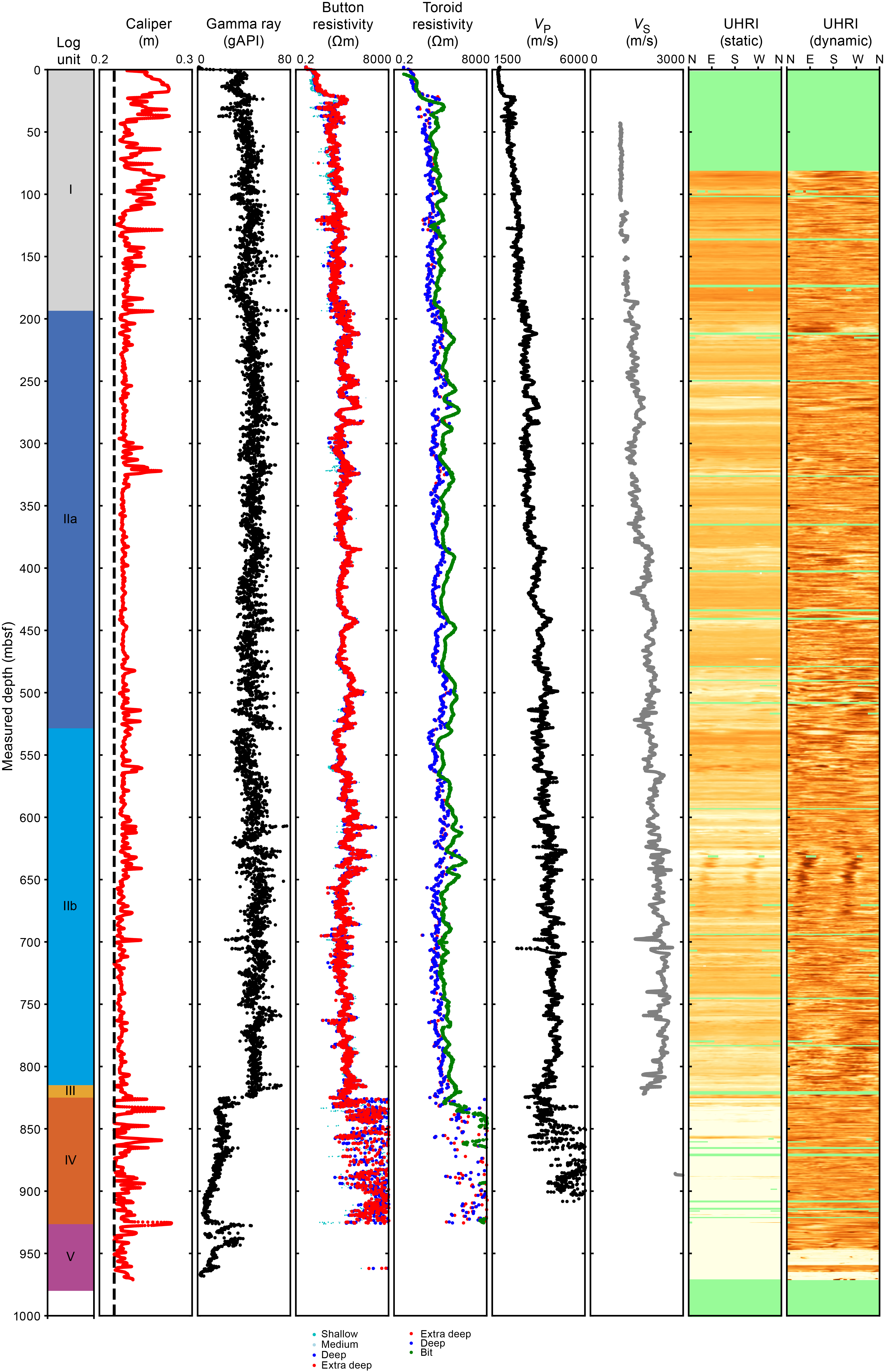
Figure F13. LWD log data with resistivity and sonic velocity logs scaled.

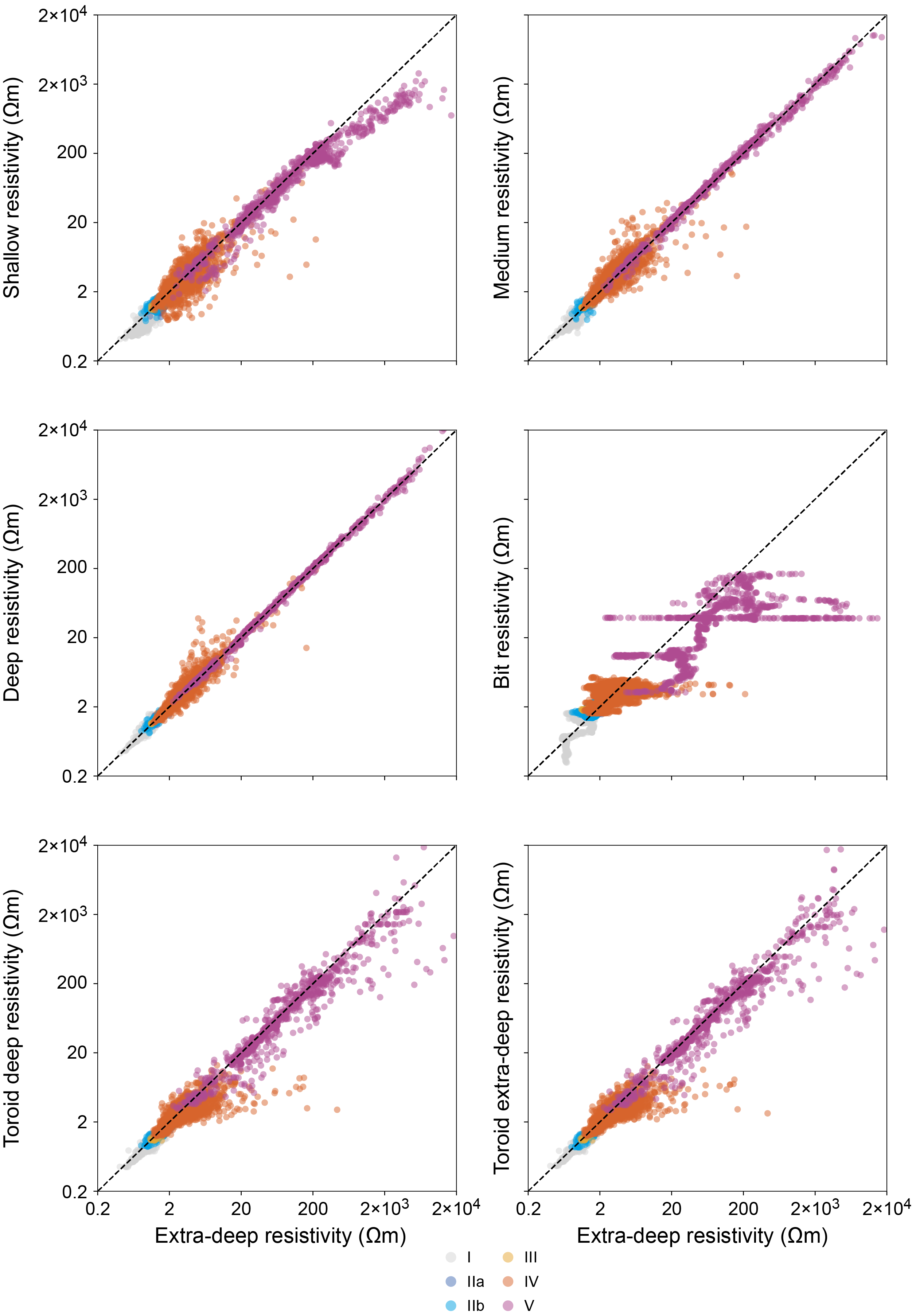
Figure F14. Electrical resistivity measurements vs. extra deep button resistivity.

3.1.3.4. Issues encountered in logging data

The quality of the LWD data is generally good, but some care is needed when using this data set:

Bit resistivity data are systematically offset from the other resistivity logs (see above).
The borehole directional survey data (inclination and azimuth) initially showed spikes and some unrealistic jumps that were filtered and smoothed in the final dataset.
Sonic velocities must be considered with great care. P-wave velocities between 920 and 925 mbsf and between 931.5 and 938 mbsf are to be discarded. S-wave velocities are unreliable in the uppermost interval to 300 mbsf because of the low intensity of the quadrupole signal and the unrealistically large V_P/V_S values (>4) implied by the picked estimate.

3.2. Logging units

Using a combination of different LWD measurements, particularly gamma ray, resistivity, and sonic logs, we defined five logging units (I–V) (Figures F12, F13). Because Holes C0019F and C0019H were drilled in close proximity (~30 m separation) and show similar variations in their physical properties (Figure F5), logging units for those holes were combined. These holes are also in close proximity to previously drilled Expedition 343 Hole C0019B (Expedition 343/343T Scientists, 2013b) and Site C0026 drilled during this expedition (see Lithostratigraphy in the Site C0026 chapter [Conin et al., 2025]). Logging units from Hole C0019B were taken as reference to facilitate comparison between all Site C0019 holes.

3.2.1. Logging Unit I (0–193.5 mbsf)

Logging Unit I is characterized by moderate gamma ray values ranging ~20–50 American Petroleum Institute gamma radiation units (gAPI) (average = 41 gAPI), very low resistivity (typically 0.5–1.8 Ωm), and low P-wave velocity (V_P) values (~1550–1750 m/s), with both P-wave velocity and resistivity values increasing slightly with depth (Figure F13). This is consistent with a burial compaction trend for shallow unconsolidated sediments. Based on these log characteristics and lithologic description from Hole C0019J (see Lithostratigraphy), this unit likely consists of poorly compacted siliceous mudstone. The uppermost ~20–30 m interval has very low P-wave velocity, gamma ray, and resistivity values (Figure F5), likely caused by poor borehole conditions, evident from the borehole image logs.

3.2.2. Logging Unit II (193.5–815 mbsf)

Logging Subunit IIa (193.5–528.6 mbsf) is defined as an interval of slightly higher gamma ray, resistivity, and P-wave velocity values compared to the unit above. The top of the unit is defined at a sharp gamma ray peak at 193.5 mbsf, below which gamma ray values range ~40–60 gAPI with an average value of ~50 gAPI. Resistivity values are typically ~1.2–3 Ωm, and P-wave velocity is typically 1900 m/s. Gamma ray, resistivity, and P-wave velocity are relatively consistent with only minor excursions from this range, suggesting that the lithology is similar throughout. Borehole images show several 1–10 m thick resistive intervals not correlated with the e-caliper log but correlated with slightly higher gamma ray values, indicating subtle compositional differences. Borehole breakouts are observed between 310 and 410 mbsf; however, they are of lower quality than the breakouts that reappear in Subunit IIb (Figure F15). The lower section of this logging unit (~479–528.6 mbsf) is characterized by higher gamma ray and resistivity values.

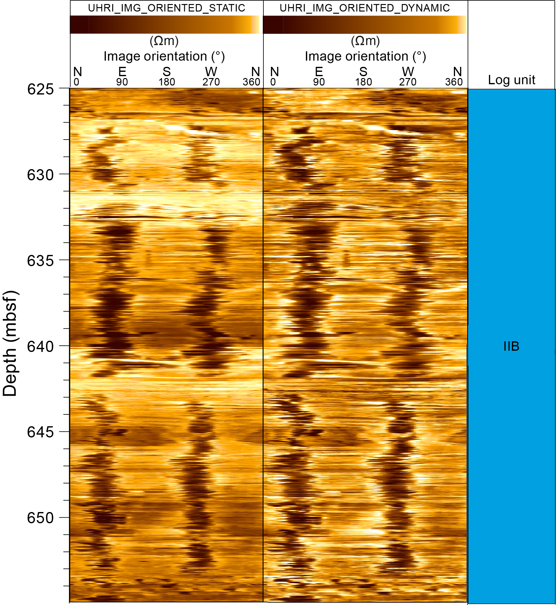
Figure F15. Good breakouts.

Subunit IIb (528.6–815 mbsf) is defined at the top by an abrupt decrease in gamma ray values from 70 to 40 gAPI at 528.6 mbsf and generally lower gamma ray and resistivity values compared to Subunit IIa. Gamma ray values generally range 40–60 gAPI, and resistivity values generally increase slightly with depth. Borehole breakouts are clearly resolved between 570 and 670 mbsf and become less common at the base of Subunit IIb (Figure F15).

3.2.3. Logging Unit III (815–825 mbsf)

Logging Unit III is characterized by high gamma ray values of up to 72 gAPI in a few meters thick interval at the top of the unit that is interpreted to correspond to clays. Beneath this interval is an interval of slightly lower gamma ray values similar to those in Subunit IIb. This interval is also marked by a gradual downhole decrease in resistivity from ~2 to 1 Ωm and a decrease in P-wave velocity. Overall, this pattern presents similarities with units recovered in Cores 343-C0019E-17R through 20R, in which a sheared clay lithology was underlain by mudstone and banded clay and chert (Expedition 343/343T Scientists, 2013b; Shipboard Scientific Party, 1980).

3.2.4. Logging Unit IV (825–926.5 mbsf)

The top of Logging Unit IV is characterized by a sharp decrease in gamma ray values and a significant increase in resistivity. Gamma ray values for this unit are consistently lower than in the units above, with a typical range of 10–20 gAPI and an average of 16.56 gAPI. Gamma ray log values show a decreasing trend with depth from an average value of around 20 gAPI to consistently less than 10 gAPI near the base of the unit. Resistivity values increase from 1.34 Ωm at the top of the unit to 6.52 Ωm at the base of the unit. Borehole images show alternating layers of lower and higher resistivity (Figure F16). This interval caused significant drilling issues with persistent stick-slip behavior. Only the upper ~15 m of this sequence was drilled this site during Expedition 343/343T, but based on Expedition 343 (Expedition 343/343T Scientists, 2013b), DSDP Site 436 (Shipboard Scientific Party, 1980), the Site C0019 log responses described here, and cores from Holes C0019J, C0019K, and C0026B (see Lithostratigraphy), this sequence likely consists of chert, possibly interbedded with other sedimentary rocks.

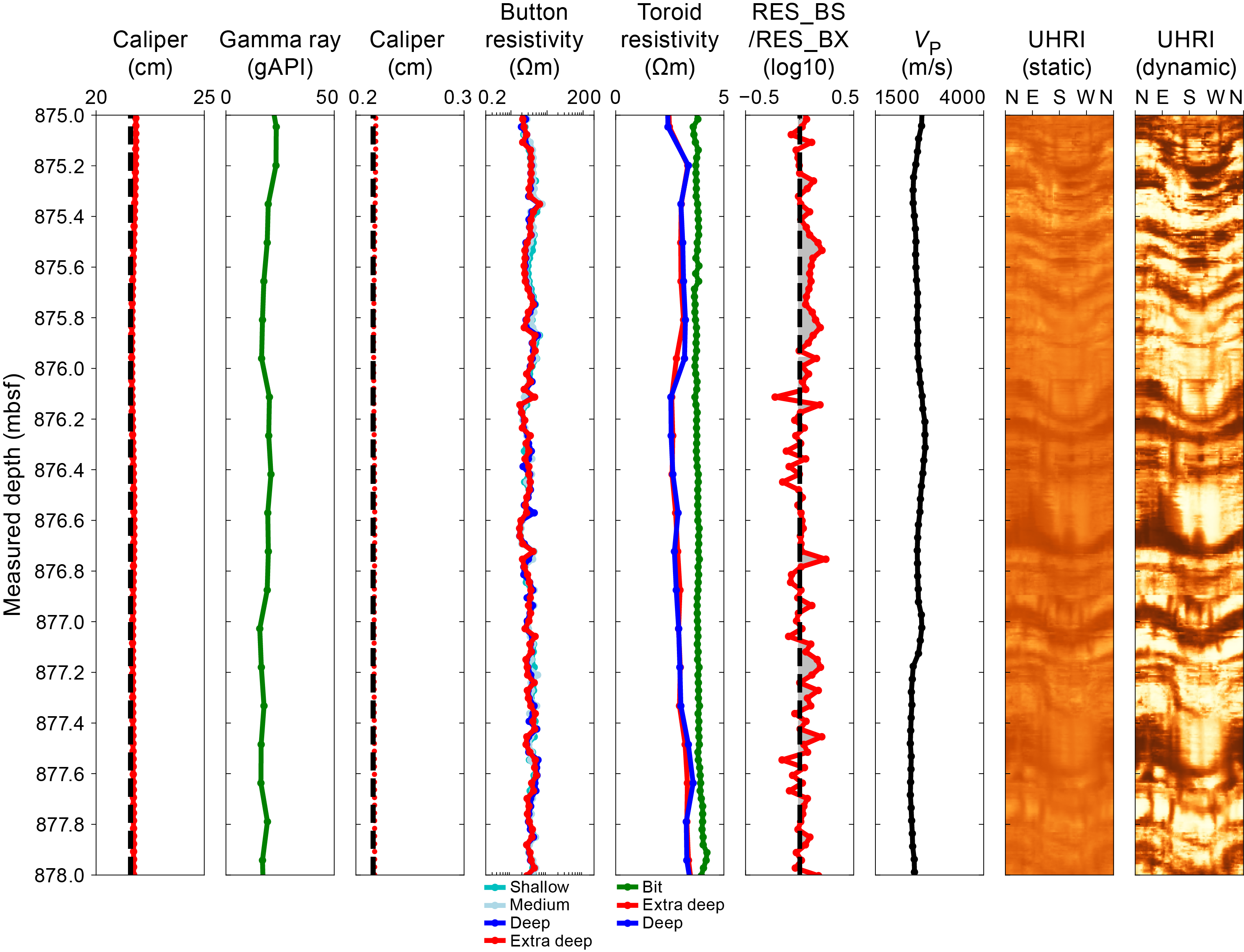
Figure F16. LWD log data for Unit IV.

3.2.5. Logging Unit V (926.5–980 mbsf)

The top of Logging Unit V is characterized by an abrupt increase in gamma ray values, resistivity, and P-wave velocity at 926.5 mbsf (Figure F17). These logs exhibit significant variation in this unit that can be used to define five distinct subunits. This unit has not been previously drilled elsewhere in this region.

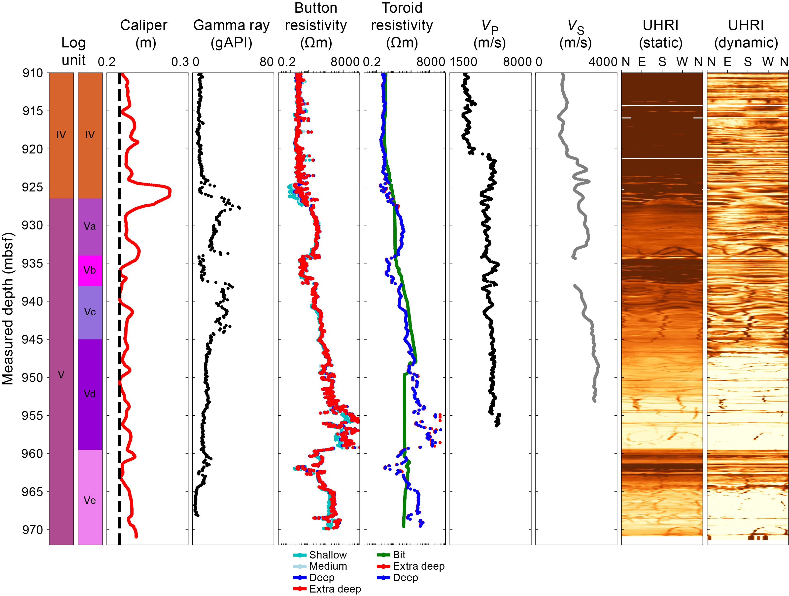
Figure F17. LWD log data for Unit V.

Subunit Va (926.5–934 mbsf) is characterized by high gamma ray values with a peak at 55 gAPI, which then decline to 20–30 gAPI at the base of the subunit. Both resistivity and P-wave velocity are relatively high, up to 40 Ωm and an average of 4402 m/s, respectively. Resistivity image logs show distinctive nonplanar resistive bands that indicate curved surfaces with varying dip angles and azimuths. Although there are no drilled analogs in the region, the log character is consistent with basalt or mixed basalt and sedimentary rocks.

Subunit Vb (934–938 mbsf) is characterized by relatively low gamma ray (~5 gAPI) and moderate resistivity values similar to those in Unit IV. P-wave velocities are unreliable in this interval (see Logging data quality in Hole C0019H). Borehole image logs show alternating high and lower resistive bands with a ~50 cm spacing, again similar to those observed in Unit IV. This suggests the presence of chert or similar siliceous sedimentary rocks.

Subunit Vc (938–945 mbsf) is characterized by moderately high gamma ray values between 30 and 45 gAPI and moderately high resistivity increasing downhole from 30 to 300 Ωm. Borehole images show nonplanar features of contrasting resistivity similar to those in Subunit Va. These appear lenticular in the wraparound image logs, indicating curved surfaces. The log character is consistent with basalt or mixed basalt and sedimentary rocks.

Subunit Vd (945–959.5 mbsf) is characterized by low gamma ray values ranging 5–10 gAPI. Resistivity values are high throughout, ranging 80–300 Ωm near the top of the sequence. This increases gradually to 955 mbsf, below which resistivity values become very high, up to 8000 Ωm. This lower interval shows significant separation between the shallow and extra deep resistivity, with the shallow resistivity typically around half of the extra deep values. Borehole images show low-angle bands of alternating resistivity to ~657 mbsf and a massive high resistivity unit with spiraling near-vertical conductive features that may be consistent with fractures.

Subunit Ve (959.5–980 mbsf) is characterized by moderate gamma ray values at the top of up to 50 gAPI, decreasing to less than 5 gAPI at the base of the unit at 969 mbsf. Resistivity increases from ~3–80 gAPI at the top of the section to ~500 Ωm at the base of the section. Borehole images show nonlinear alternating resistivity bands and near-vertical conductive features.

3.3. Physical properties

The LWD data provide information on the natural radioactivity (gamma ray), electrical resistivity (button and toroid velocities), and sonic velocities for both P- and S-waves.

3.3.1. Electrical resistivity

The four channels of button resistivity (shallow, medium, deep, and extra deep) are also provided as 360° borehole images, but only scalar channels (RES_BS, RES_BM, RES_BD, and RES_BX) will be discussed here. These channels have different depths of investigation (see Logging while drilling in the Expedition 405 methods chapter [Kirkpatrick et al., 2025]) to discriminate the true resistivity of the rock from the effects of borehole mud and an eventual invaded zone. Because borehole mud has lower resistivity (0.11 Ωm) than the formation, borehole enlargement induces a decrease in the measured resistivities, especially for the shallowest channels. This effect is used to infer the e-caliper from the resistivity measurements (Channel HD_MI6). Hence, this caliper is included with the other electrical channels in Figure F18.

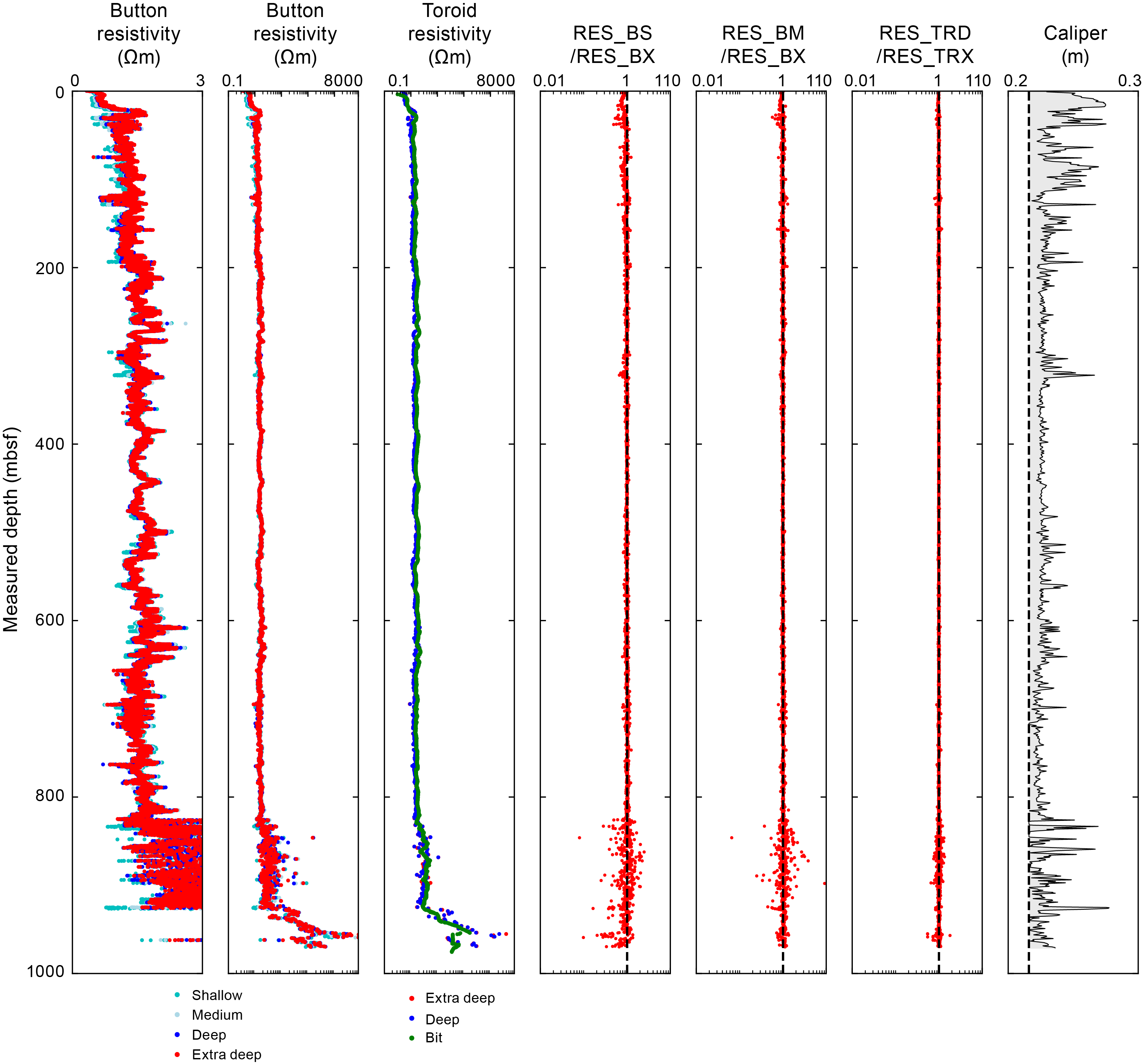
Figure F18. Electrical resistivity measurements.

Figures F14 and F18 show good agreement between the electrical logs, except for Units IV and V, so the deep resistivities can be considered representative of the true formation resistivity. These units have strong excursions of the ratio RES_BS/RES_BX to low values, which in Unit IV is consistent with an increase in borehole diameter. In Unit IV, several depths exhibit shallow resistivity larger than deep resistivity (Figure F16) that cannot be explained by borehole enlargement, which would decrease shallow resistivity more strongly than deep resistivity. The ratio between medium and extra deep resistivity also exceeds 1 at those depths, suggesting this is related to the formation rather than borehole diameter. Because Unit IV is interpreted to be chert, which is strongly banded, this effect may be due to the strong formation anisotropy.

Given the good agreement between the deep resistivity logs, these resistivities are considered to be representative of the true formation resistivity. Between these, the extra deep resistivity (RES_BX) was chosen as a reference log because of its higher sampling rate (see Table T3 in the Expedition 405 methods chapter [Kirkpatrick et al., 2025]).

3.3.2. Statistics of physical properties

Figure F19 shows the statistical properties of the major physical properties for each logging unit (given their extent, Subunits IIa and IIb are considered separately), for which the mean and standard deviation are reported below. Hole C0019H shows strong petrophysical contrasts between the logging units.

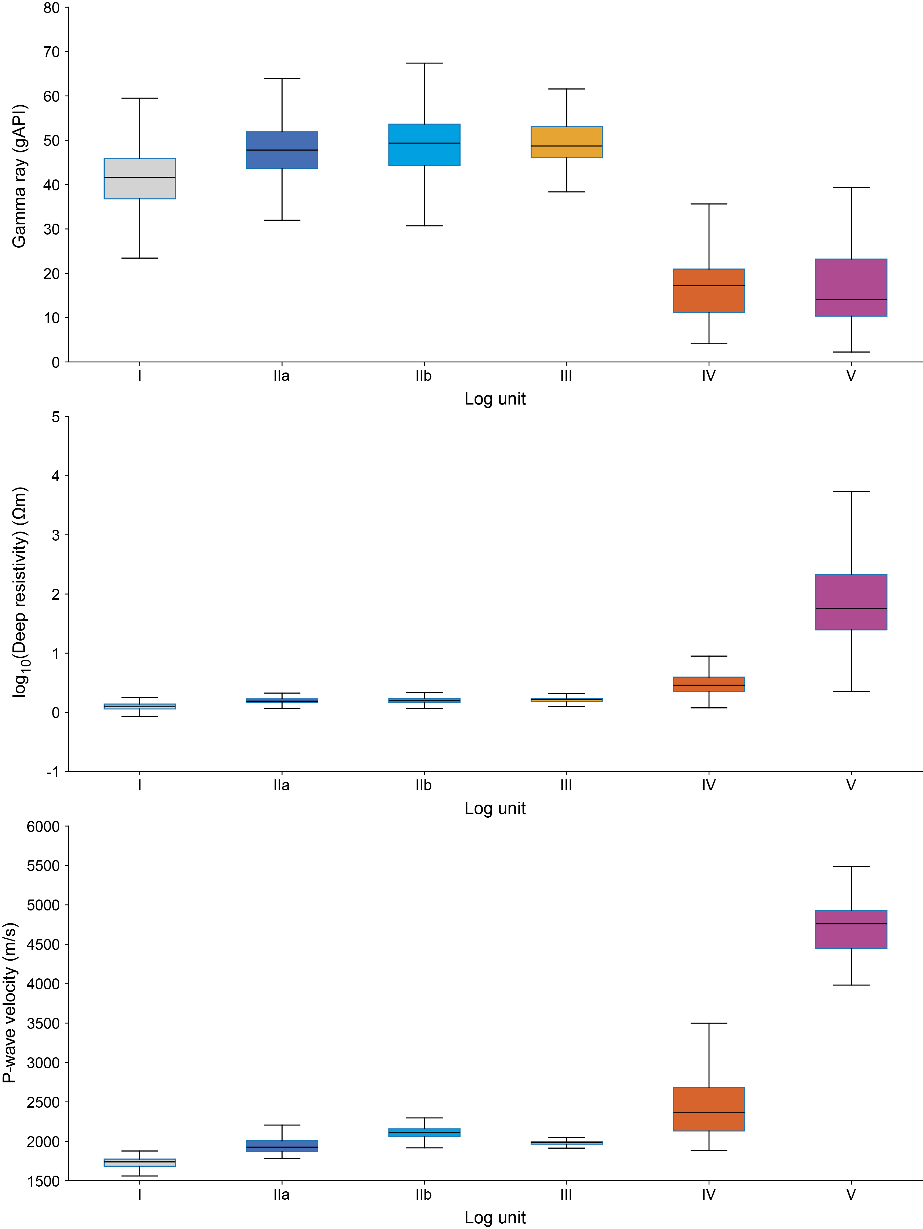
Figure F19. Gamma ray, deep resistivity, and P-wave velocity for logging units.

Gamma ray is 41 ± 7 gAPI in Unit I and increases to 48 ± 6 gAPI in Subunit IIa. Subunit IIb and Unit III have similar values, 49 ± 7 and 51 ± 8 gAPI, respectively. Gamma ray decreases in Units IV and V, to 16 ± 7 and 17 ± 9 gAPI, respectively.

Electric resistivity in Figure F19 is on a logarithmic scale to capture the full extent of variation: the quantity log₁₀(RES_BX) was used to generate the box plot. In the following paragraph, the measured values (RES_BX) are used instead to compute the statistics. In Unit I, extra deep resistivity is 1.23 ± 0.23 Ωm. It increases to 1.59 ± 0.20 Ωm in Subunit IIa. Subunit IIb and Unit III have similar values, 1.58 ± 0.16 and 1.64 ± 0.22 Ωm, respectively. The mean resistivity in Unit IV increases to 4.3 Ωm with an interquartile extent of 1.4 Ωm, reflecting the large variability within this unit. In Unit V, the mean value of the electrical resistivity reaches 379 Ωm, but its median is 59 Ωm. This reflects the large variability in this unit, in which the resistivity varies between 2 Ωm and 20 kΩm.

P-wave velocity is 1730 ± 70 m/s in Unit I. It increases from Unit I to Unit II, and it also increases between Subunits IIa and IIb, to 1940 ± 80 and 2110 ± 70 m/s, respectively. Velocity decreases to 1990 ± 60 m/s in Unit III. P-wave velocity strongly increases to 2540 ± 650 m/s in Unit IV. In Unit V, very high P-wave velocities with values of 4710 ± 320 m/s were measured.

Units I–III are similar, in sharp contrast to Units IV and V.

3.3.3. Relations between physical properties

Figure F20 shows crossplots between the main physical properties (gamma ray, P-wave velocity, and electrical resistivity) as well as the Brie plot to interpret the relationship between P- and S-wave velocities. This plot is a graphical representation used to identify zones of free gas in sedimentary rocks (Brie et al., 1995). It is based on the crossplot between 1/V and V_P/V_S that represents a convenient method to compare V_P and V_S data.

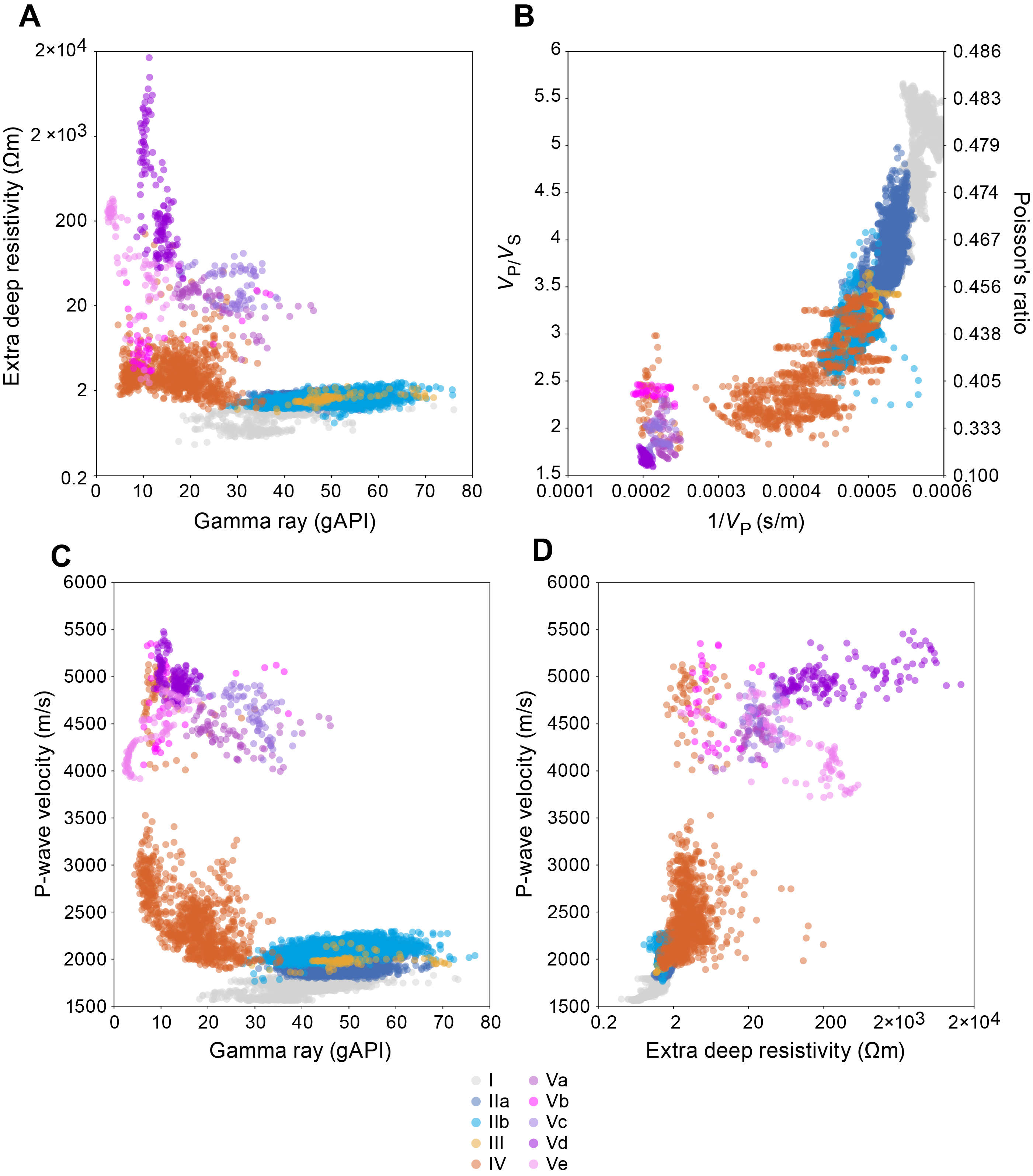
Figure F20. Physical properties for logging subunits.

Figure F20A compares electrical resistivity to gamma ray. In this crossplot, the points represent the Unit I transition from a cluster of low resistivity corresponding to the uppermost 25 m of Hole C0019H to values close to those of Unit II (Figure F5). Subunits IIa and IIb and Unit III overlap. Unit IV is distinctive in its lower gamma ray values, and Unit V is distinctive in its higher resistivity values (except for Subunit Vb, which overlaps with Unit IV).

The crossplot between P-wave velocity and gamma ray (Figure F20C) is similar, with Units I–III clustering at high gamma ray and low resistivity values and the Unit IV and V data points gathering in two independent low and high velocity clusters, respectively. The data points of Unit IV at high velocity correspond to the erroneous intervals identified in the QC and should be considered unreliable. The Subunit Vb data points should be also considered with great care. In Unit IV, there is a negative correlation between gamma ray and P-wave velocity.

Figure F20D shows a positive correlation between resistivity and P-wave velocity, which is particularly well defined for Units I–III. A positive but more scattered correlation is also observed in Unit IV if the erroneously high V_P between 920 and 925 mbsf are not taken into account. Unit V is characterized as a high velocity zone (but the V_P of low resistivity zones were not measured).

In Figure F20B the high V_P/V_S values recorded in Hole C0019H correspond to very large Poisson ratios, which prevent comparison with reference curves. Despite the high value of V_P/V_S, the Unit I–III data points align along a typical convex shape. Unit IV is in continuity with this trend, with wide scatter. There is no significant excursion away from this trend toward the region of high 1/V and low V_P/V_S that would indicate in situ free gas (Brie et al., 1995). Unit V data form an isolated cluster of lower 1/V and V_P/V_S ranging 1.7–2.5.

3.3.4. Resistivity image interpretation

The overall image quality is good for Hole C0019H. Geologic features (bedding and fractures) as well as wellbore failures (breakouts) were identified from the images. Horizontal image artifacts are common throughout the entire imaged interval and are thought to be related to the stick-slip of the MicroScope tool as the buttons rotate (Lofts and Bourke, 1999). All images were oriented to north using the orientation information from the TeleScope (Figure F7), and the inclination of the hole was accounted for. Geologic features are identified and characterized with the true orientation reported.

3.3.5. Bedding and fractures

Structural and sedimentary features are identified and interpreted using the UHRIs (Figures F21, F22). Critical examination of each pick was made by three simultaneous observers to confirm (1) clear sinusoidal curves on the unwrapped images of the cylindrical borehole wall and (2) consistent criteria for structural and bedding interpretation. The image data contain various artifacts (Lofts and Bourke, 1999), including horizontal stripes caused by ship heave, processing, and stick-slip of the tool, and some vertical conductive stripes indicative of tool scraping were observed locally, making image interpretation challenging. Planar features in the logs were divided into five categories. The criteria are as follows:

Bedding: a planar feature, visible as a sinusoid in the unwrapped static and dynamic UHRIs, that belongs to a series of planar features with consistent orientation (Figure F23). Bedding planes are reported in Table T6.
Conductive/resistive fracture: a planar feature, visible as a sinusoid in the flattened image, that may or may not host shear displacement. The orientation crosscuts the orientation of nearby bedding. We note whether the fracture is predominantly resistive or conductive (Figure F24). Conductive and resistive fractures are reported in Tables T7 and T8, respectively.
Bounding surface/feature: when a crosscutting relationship is not evident but a planar discontinuity or distinctive change in resistivity (i.e., more conductive to less conductive across a sinusoidal feature) is clear, we note the feature as a bounding surface. This may be indicative of a change in bulk rock properties or a fault/fracture along a plane of weakness aligned with nearby bedding. Bounding surfaces are reported in Table T9.
Basalt feature: conductive bands in Unit V, interpreted to be basalt, with consistent orientation and spacing of ~10–20 cm (Figure F24B). Bands are crosscut and disrupted by other features in the unit that may be associated with emplacement or later stage deformation and fracturing. Basalt features are reported in Table T10.
Fracture in basalt: dark features in Unit V (Figure F25). These fractures may be indicative of contacts between basalt and other sediments, cooling fractures, boundaries between lava flows, or related to late-stage deformation and fracturing. Fractures are reported in Table T11.

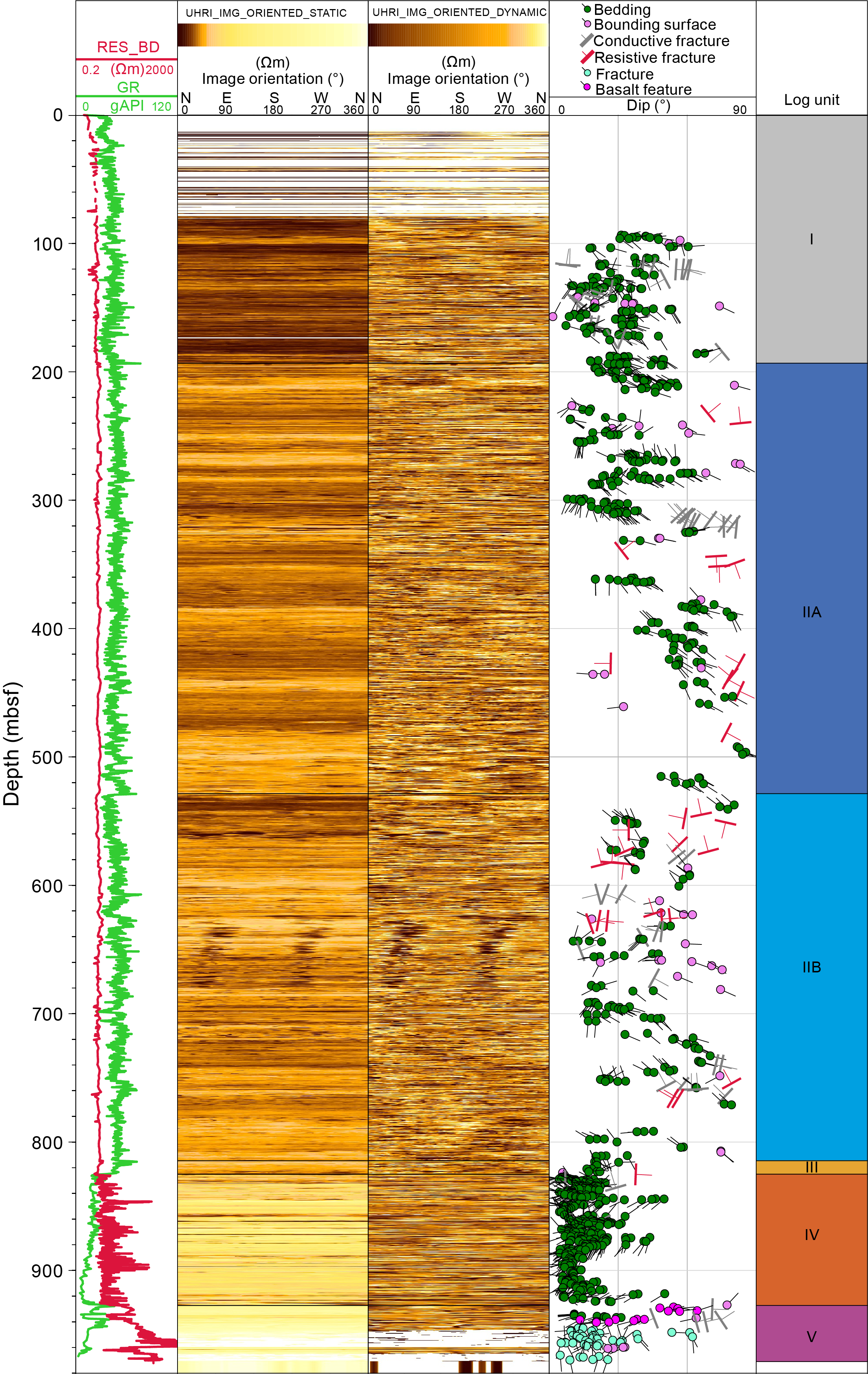
Figure F21. Preliminary interpretation of borehole images.

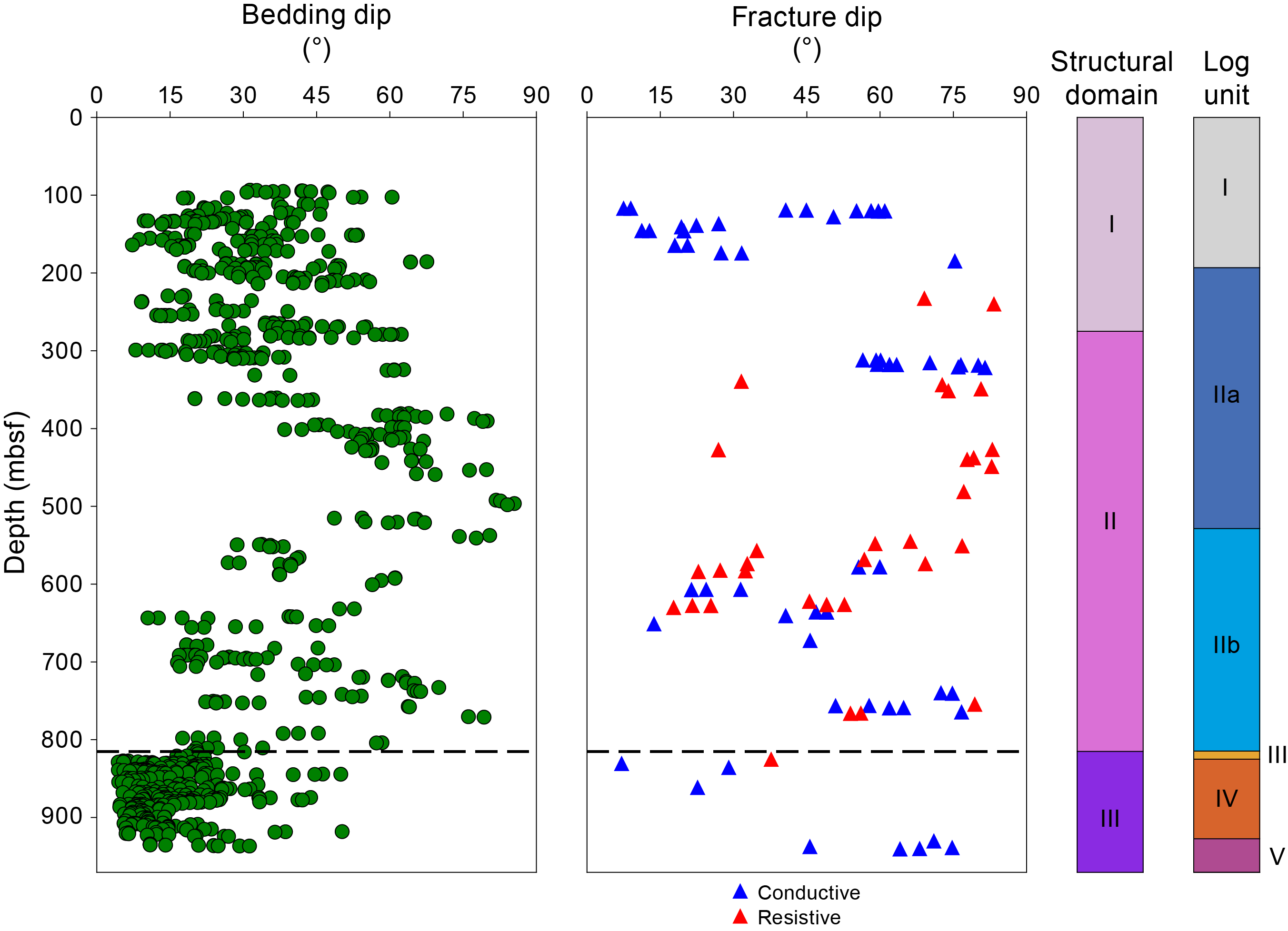
Figure F22. Bedding dip and fracture distribution.

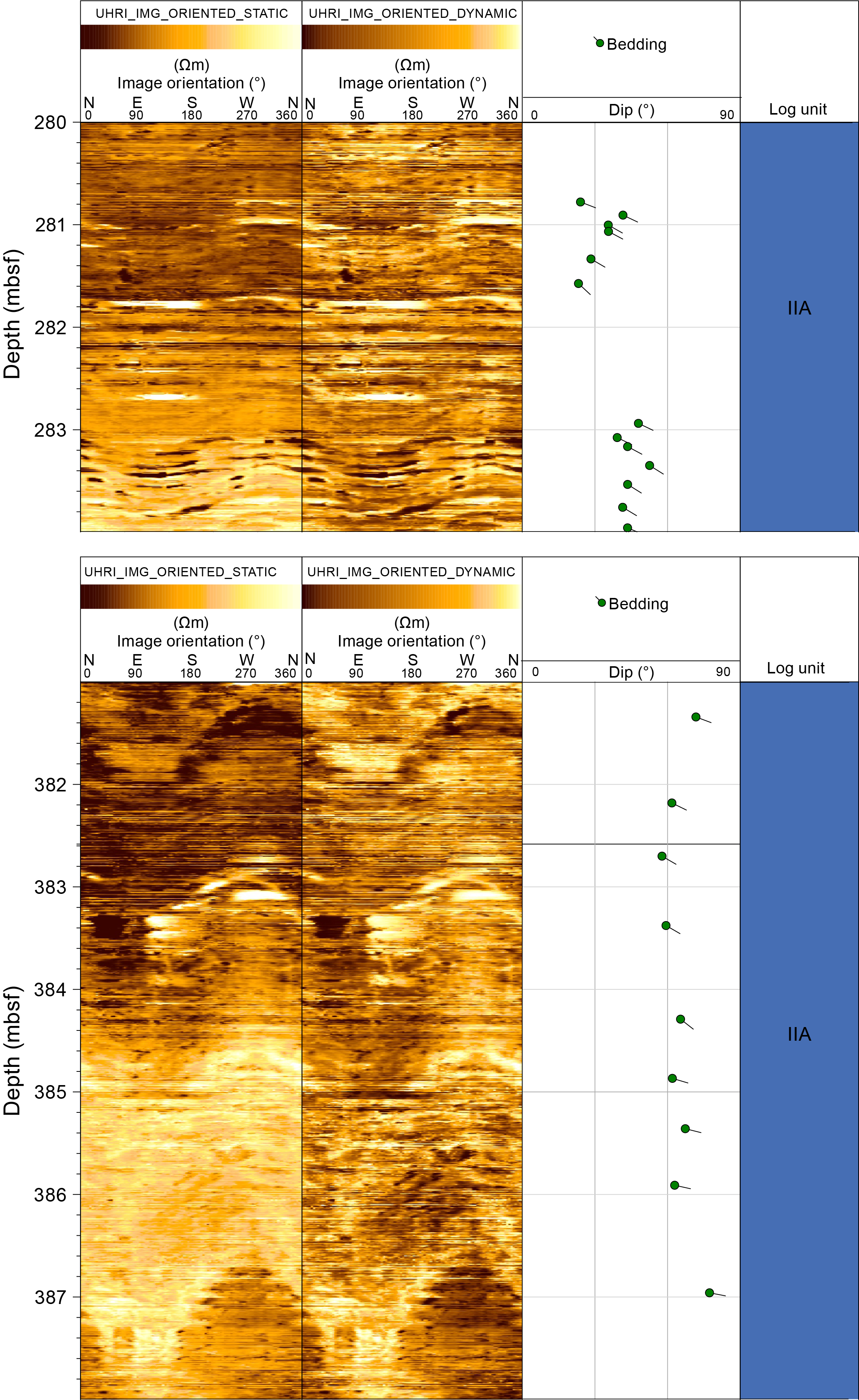
Figure F23. Interpreted bedding dips for Subunit IIA.

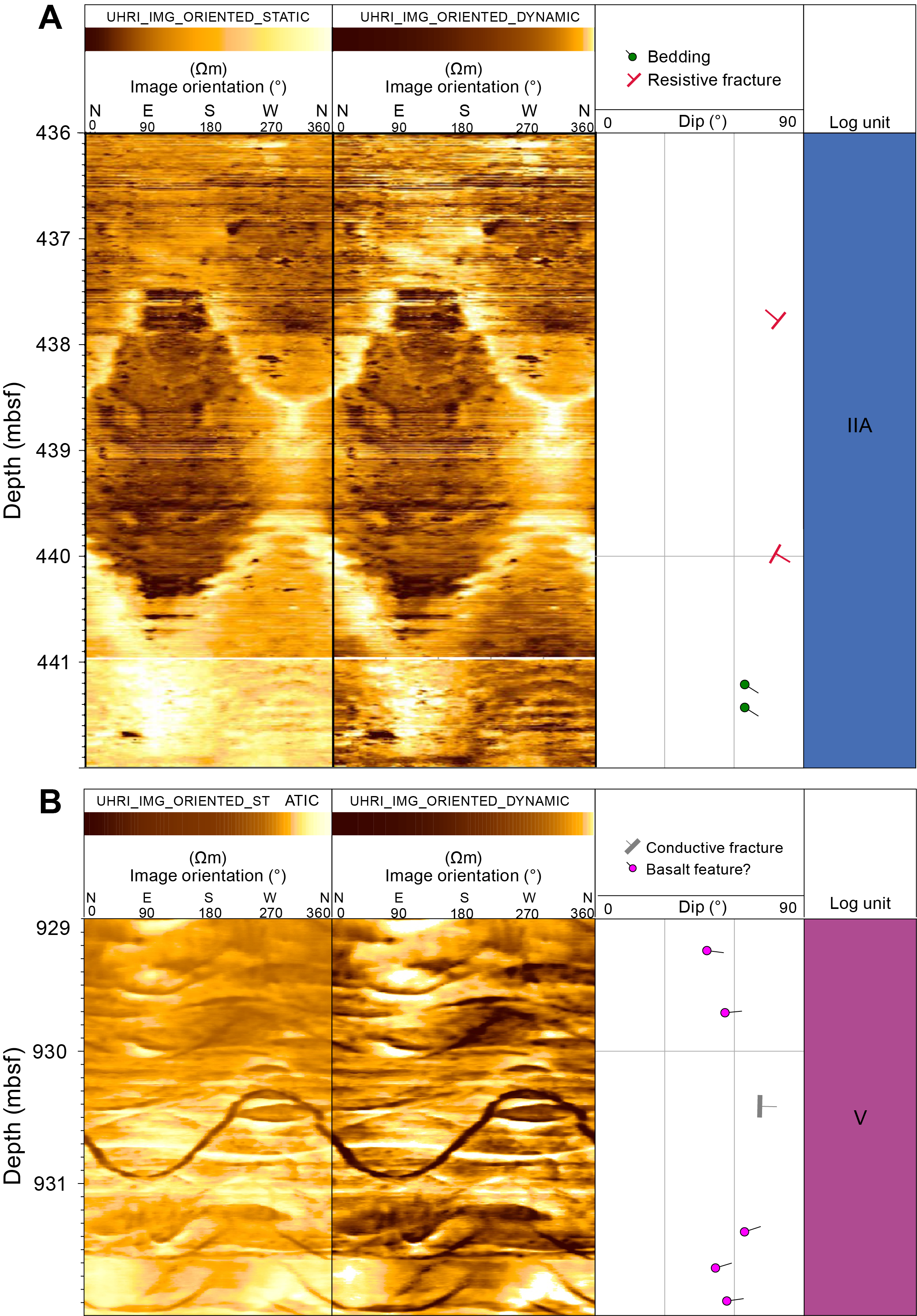
Figure F24. Interpreted bedding and fractures.

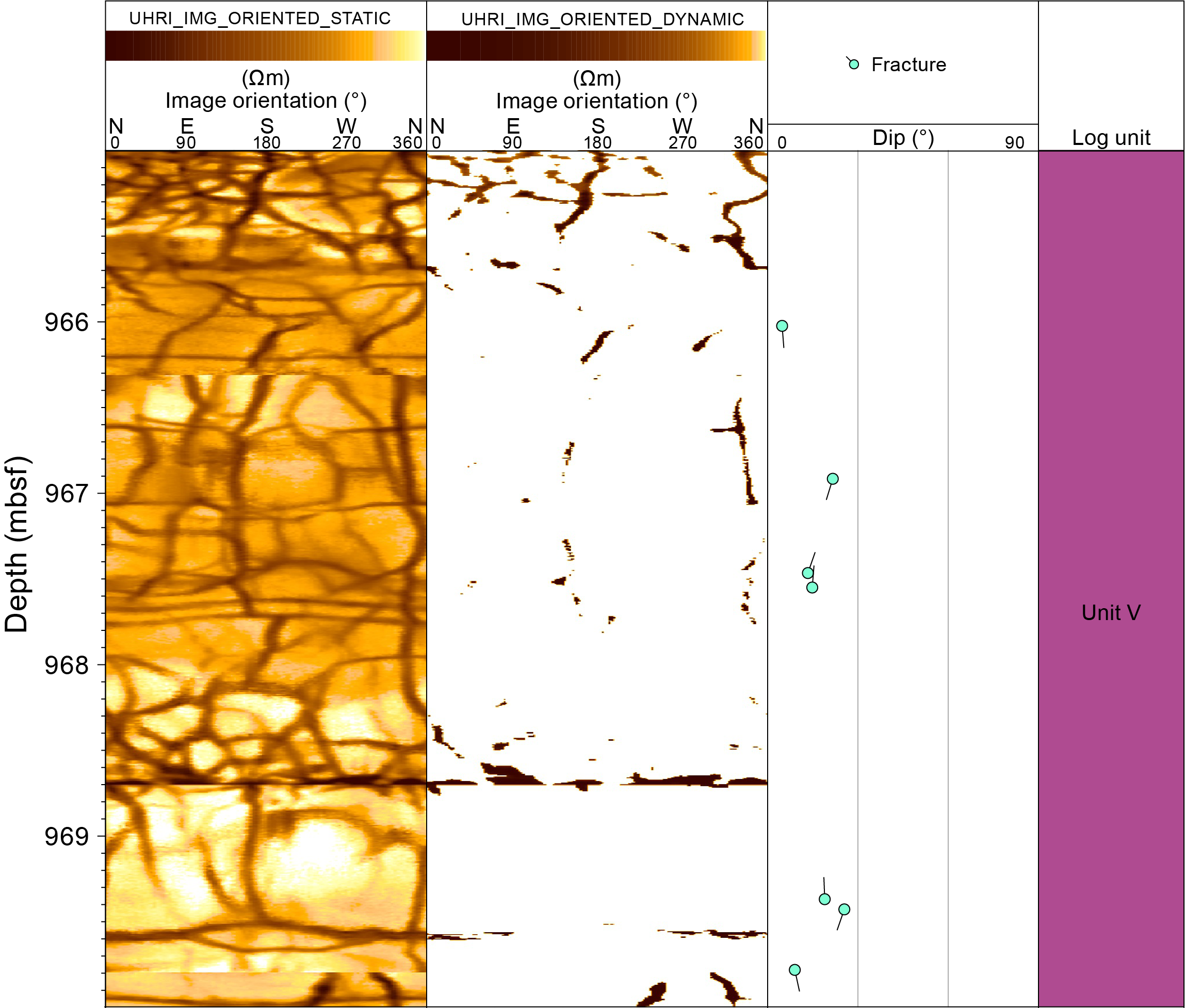
Figure F25. Fractures in Unit V.

Differentiation between fractures and bedding planes is complex in regions of high deformation, and we acknowledge that some features may have been misclassified during the shipboard analysis. Additionally, faults and fractures can form along weakened bedding planes, and we are unable to distinguish between slip surfaces and bedding when there is no crosscutting relationship.

Three structural domains are defined based on bedding orientations: Domain 1 (0–275 mbsf), Domain 2 (275–815 mbsf), and Domain 3 (815–980 mbsf) (Figure F22). Domain 1 features 20–80 m thick packages of bedding that alternate between eastward and westward dips, with a high concentration of conductive fractures observed between 100 and 200 mbsf. The average bedding dip in this domain is moderate at approximately 30° ± 12°. Domain 2 displays a wider range of bedding dips from 8° to 85°, with an interval of steeply dipping bedding between 400 and 600 mbsf. On a stereographic projection, the poles to bedding between 300 and 560 mbsf and between 700 and 760 mbsf have girdle distributions indicative of cylindrical folding (Figure F26). The section between 550 and 670 mbsf is densely fractured and may be part of a fold limb or a different structural package. Below 815 mbsf, a sharp transition to shallowly dipping bedding, averaging 15° ± 8°, marks the onset of Domain 3.

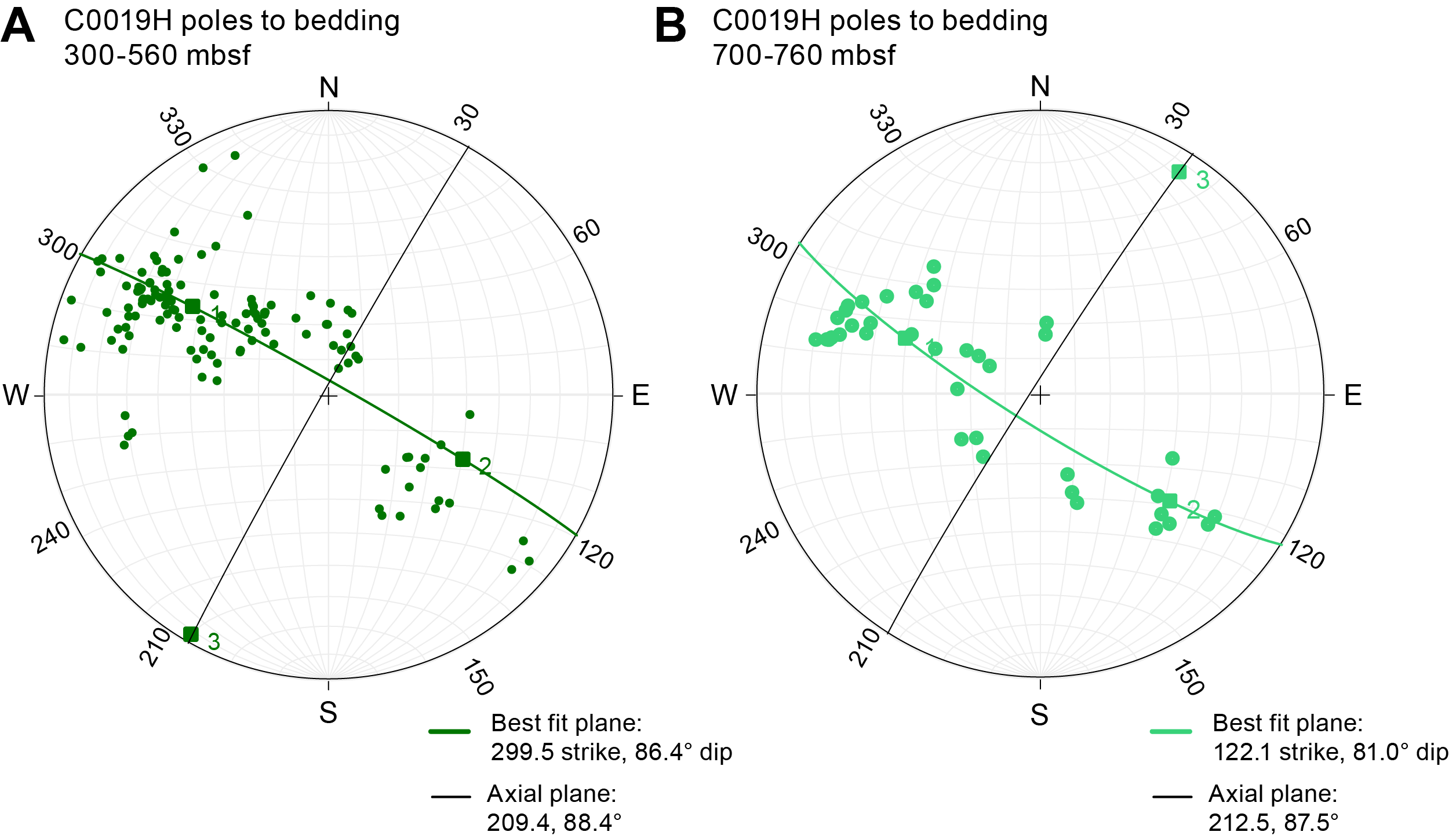
Figure F26. Bedding with girdle distributions.

The bounding surfaces identified in Hole C0019H are detailed in Table T9. These structures may indicate fractures formed along weakened bedding planes or represent a change in bulk rock properties. However, we did not classify these features as either bedding or fractures because no crosscutting relationships with adjacent bedding planes were observed.

The UHRIs in Unit V show rounded to subrounded features consistent with basalt (Ienaga et al., 2006; Fornero et al., 2019) (Figure F25). Evenly spaced conductive bands are interpreted to be basalt features that could correspond to emplacement or tectonic deformation (Figure F24B). These features are moderately dipping (~48°–65°) in Subunit Va and shallowly dipping (~13°–40°) in Subunit Vc (Figure F27. Other features, possibly fractures, crosscut and offset the orientation of these basalt features. Subunits Ve and Vd exhibit a dense network of shallow conductive fractures that are highly deformed (Figure F25). These fractures may have originated during the deposition and cooling of the basalt or as a result of later tectonic activity.

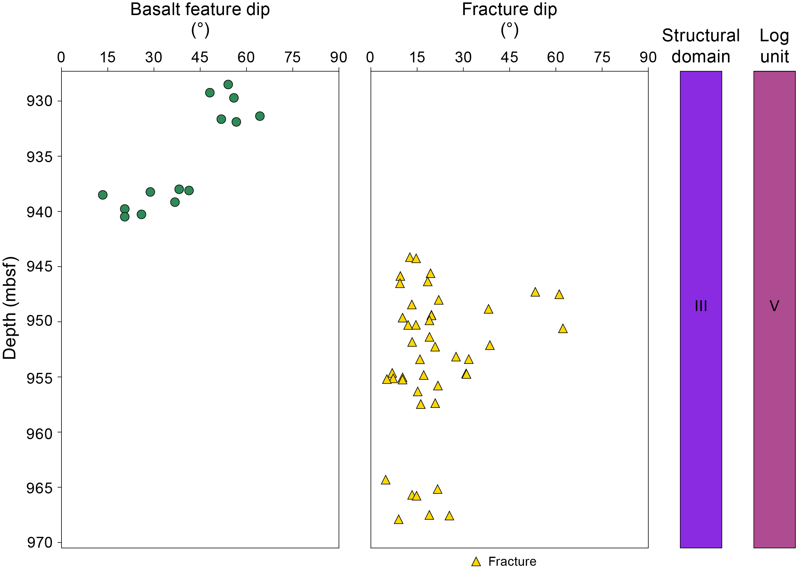
Figure F27. Basalt features and fractures in Unit V.

3.3.6. Wellbore failure

In Hole C0019H, LWD images show dark conductive tracks approximately 180° apart that are consistent with borehole breakouts (Figure F15) (Gough and Bell, 1981; Bell and Gough, 1982; Zoback, 2007). Breakouts occur between 312 and 824 mbsf but are concentrated within Unit III in two intervals: 530–570 and 615–680 mbsf (Figure F28). Variable image quality and ambiguous artifacts in the images result in uncertain breakout picks in some depth intervals (e.g., 310–410 mbsf). Quality codes of “good” and “fair” are assigned to the breakout picks. Good breakouts are identified by two continuous conductive tracks 180° apart that are identifiable in both the UHRIs and lower resolution images. In addition, good quality breakouts are located at depths free from known drilling-related artifacts (i.e., horizontal stick-slip, stretching, or plausible damage from the tool scraping). The quality code fair is used when breakouts are identified at depths with image artifacts or when the conductive tracks are not continuous.

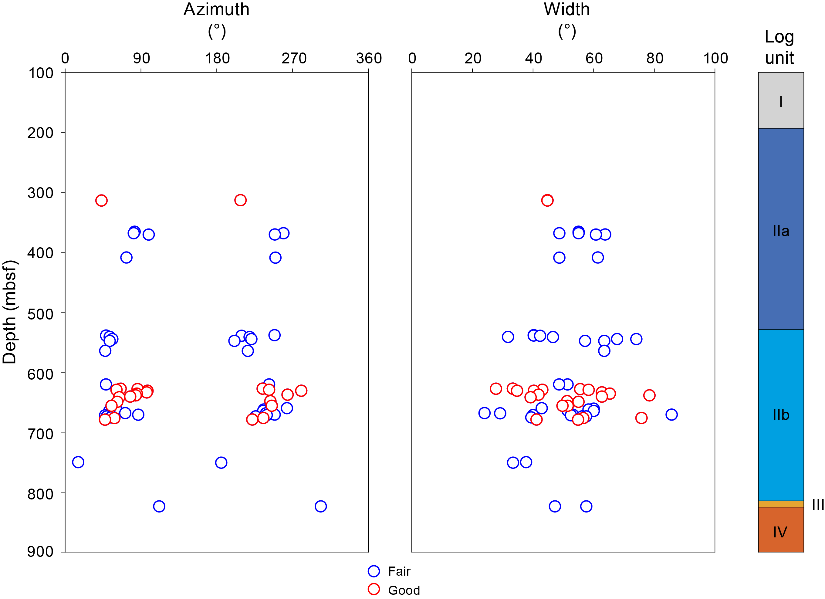
Figure F28. Breakout azimuth and width.

A total of 61 breakouts were identified in the images, of which 23 breakouts were good and 38 breakouts were fair (Figure F28; Table T12). The cumulative length of breakouts reached ~100 m, corresponding to ~10% of the total borehole depth. The mean breakout orientation is 062° (or 242°) with a standard deviation of 22°. The orientation of maximum horizontal stress (S_Hmax) is interpreted to be 152° ± 22°. The breakout azimuths near the interpreted plate boundary fault at ~823 mbsf are rotated approximately 50°–60° to the east-southeast from the breakouts in the overlying prism. Breakout widths range 24°–86° with a mean value of 51° (±13° standard deviation).

4. Lithostratigraphy

We report here on the lithostratigraphy of the five holes at Site C0019. Cores from Holes C0019L, C0019M, and C0019J were collected in close proximity (Figure F1) and represent a complete depth transect through the frontal prism to the décollement and are therefore presented together. Holes C0019K and C0019P were located farther apart and represent different depths beyond the décollement into the lower plate. The lithologies for these holes are therefore presented separately and are ascribed unit prefixes K (Hole C0019K) and P (Hole C0019P).

4.1. Lithostratigraphic units of Holes C0019L, C0019M, and C0019J

Seven lithostratigraphic units were identified in the composite stratigraphy from Holes C0019L, C0019M, and C0019J, and all lithostratigraphic units are present in Hole C0019J (Figure F29). The units are numbered from 1 to 7 sequentially with depth from the seafloor to the base of the cored interval (Table T13) (for differentiation methods, see Lithostratigraphy in the Expedition 405 methods chapter [Kirkpatrick et al., 2025]). Units 2–6 are divided into subunits labeled A, B, and C from top to bottom. Units 2–6 contain a similar lithologic sequence: Subunit A is olive-black siliceous vitric mud(stone), Subunit B is olive-gray to gray siliceous vitric mud(stone), and Subunit C (only present in Unit 5) is dull yellowish brown siliceous vitric mud(stone).

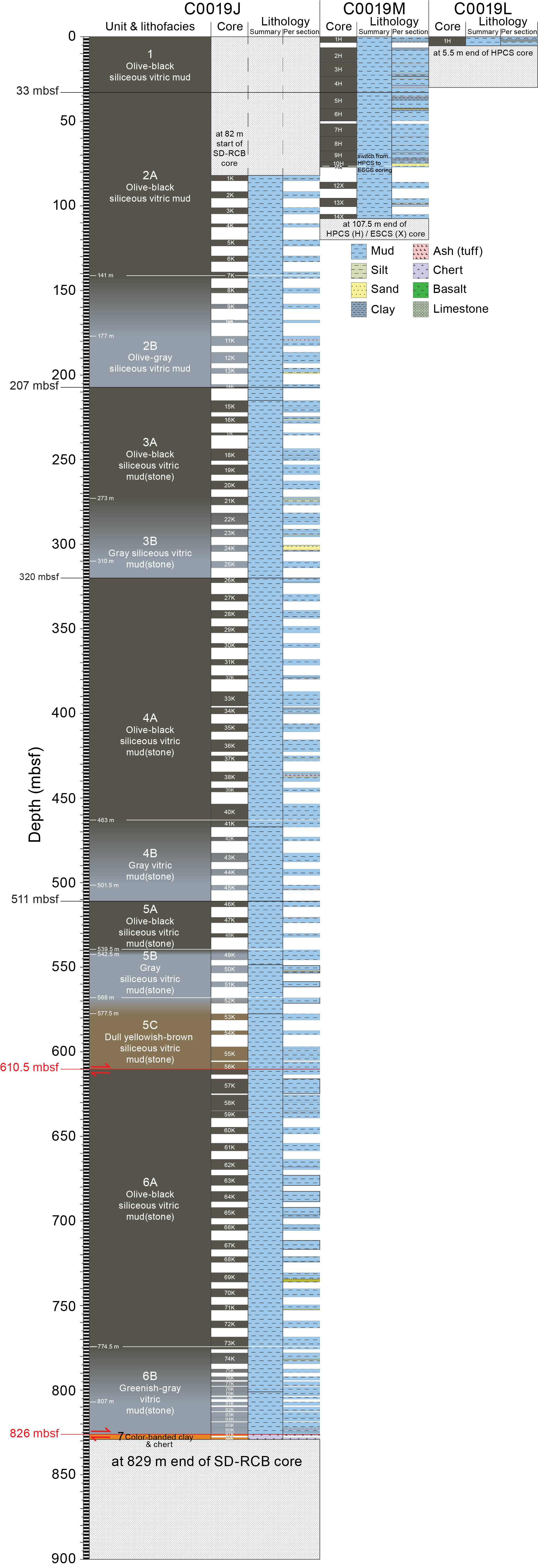
Figure F29. Lithostratigraphic units, Holes C0019J, C0019L, and C0019M.

Representative intervals of each unit and the unit boundaries are illustrated by Tri-Sensor Core Logger (TSCL) linescan images, modified linescan images, and X-ray computed tomography (XCT) images (Figures F30, F36, F39, F40, F42, F44, F46, F47, F49). Additional notable features in the cores, alongside corresponding TSCL images, are recorded on the visual core descriptions (VCDs) in Core descriptions. Semiquantitative sediment compositions derived from smear slides are summarized in ternary diagrams (Figures F31, F32), and key classifications are displayed in selected microscopic images (Figures F33, F37, F41, F43, F45, F48, F50). The grain size and compositional ranges presented for each unit and subunit discussed below and in Tables T14 and T18 report the range between the lowest (L) recorded and highest (H) recorded percent of each grain size fraction (displayed as L%–H%). It is noted that, because smear slide analysis is semiquantitative, further grain size distribution analysis is needed. Core colorimetry data from the TSCL provided important information on color variations across the units in Hole C0019J (Figure F38). TSCL colorimetry data are not available for Holes C0019L and C0019M due to equipment malfunction during coring operations. Variations in bulk composition throughout the holes are documented using X-ray diffraction (XRD) analysis for mineral phases and abundance (Figure F34; Table T15) and X-ray fluorescence (XRF) analysis for elemental composition (Figure F35; Table T16). Age estimates for each unit are provided from preliminary shipboard biostratigraphy (see Biostratigraphy).

Unit depths are calculated on the core depth below seafloor scale, Method A (CSF-A), but are listed as mbsf depths here.

4.1.1. Unit 1

Interval: 405-C0019L/M-1H-1, 0 cm, to 405-C0019M-5H-1, 0 cm
Depth: 0–33.00 mbsf
Age: 0–? (2.7) Ma
Lithology: olive-black siliceous vitric mud

4.1.1.1. Visual core description lithology

Unit 1 is present in Hole C0019L from 0 to 5.38 mbsf and in Hole C0019M from 0 to 33.00 mbsf (Figure F29; Table T13). Unit 1 is an olive-black to gray (7.5Y 3/1, 5Y 3/1, and 10Y 4/2) siliceous vitric mud with frequent intervals of chaotic and inclined bedding interspersed with clasts and occasional layers of ash (occasionally deformed) and graded bedding (Figure F30). Unit 1 contains large rip-up clasts of variable color composed of a lithology similar to, but more indurated than, the background sedimentation. Color banding (millimeter-scale and usually highlighted by bands of black and green) is frequent throughout Unit 1, often parallel with interbedded ash. Sometimes these color bands delineate folding and deformation (e.g., Section 405-C0019M-4H-4). Fining-upward sand layers (sometimes with multiple pulses) occur infrequently throughout Unit 1 (e.g., Section 405-C0019L-1H-3). There is evidence of sediment remobilization and liquefaction; for example, a sand-hosted mud-injectite sourced from underlying mud intruding into a small-scale reverse fault (Section 405-C0019M-4H-5, 110–112 cm). Unit 1 also contains moderate bioturbation, areas rich in pyritization, and calcite concretions.

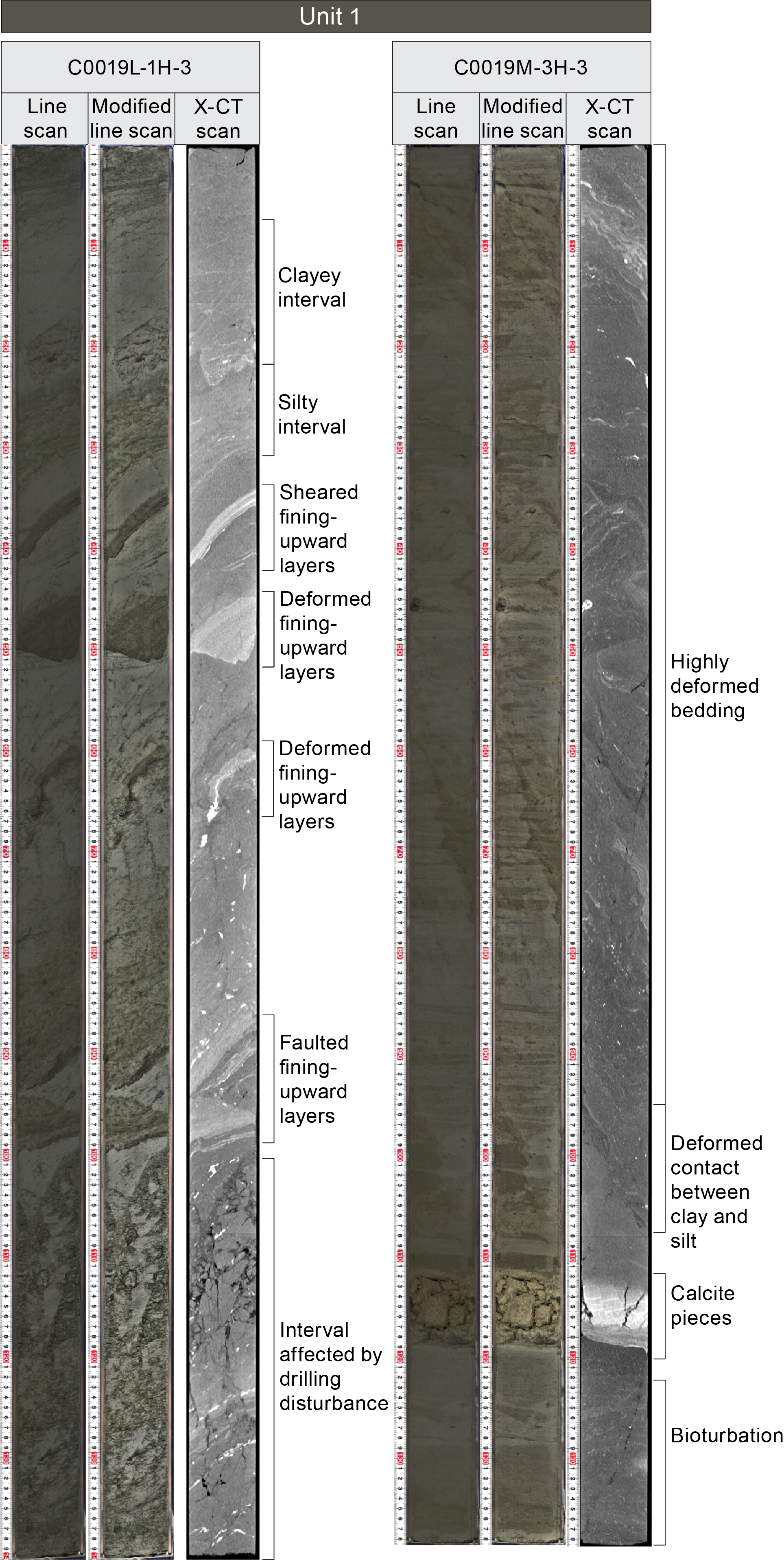
Figure F30. Unit 1 images.

A total of 15 ash horizons were identified in Unit 1 either as laterally continuous layers with thicknesses from <1 cm to several centimeters thick or as subrounded patches (e.g., Section 405-C0019M-4H-6). Where bedding is distinguishable, ash layers commonly have sharp contacts with the background sedimentation. Both the ash layers and bedded background sedimentation are mostly inclined (e.g., Section 405-C0019L-1H-3; Figure F30) (see Structural geology). The continuous laminated ash layers tend to be dark green-gray in color, whereas the patches can also be light gray and blue (e.g., Section 405-C0019M-2H-3). Pumice pieces disseminated throughout the background sedimentation are occasionally present and sometimes pyritized (e.g., Sections 3H-6, 77 cm, and 5H-1, 56 cm).

4.1.1.2. Smear slide petrography

The grain size of the background sedimentation in Unit 1 predominately plots as mud (Figure F31) with 0%–30% sand, 25%–92% silt, and 5%–75% clay (Table T14), and the composition predominantly plots as siliceous to siliceous-vitric mud (Figure F32) with 8%–68% siliciclastic, 2%–46% volcanic, and 6%–72% biogenic grains. The siliciclastic material is predominantly clay minerals (2%–60%), quartz (0%–31%), and mudstone aggregates (0%–20%). Volcanic material is mostly clear glass (1%–37%) and pumice (0%–20%) with some colored glass (0%–10%). Biogenic material is mostly diatoms (2%–32%), radiolarians (0%–15%), silicoflagellates (0%–10%), and sponge spicules (2%–38%) (Figure F33). The remainder of the material (2%–35%) includes pyrite framboids, glauconite, micas, and opaque and dense minerals.

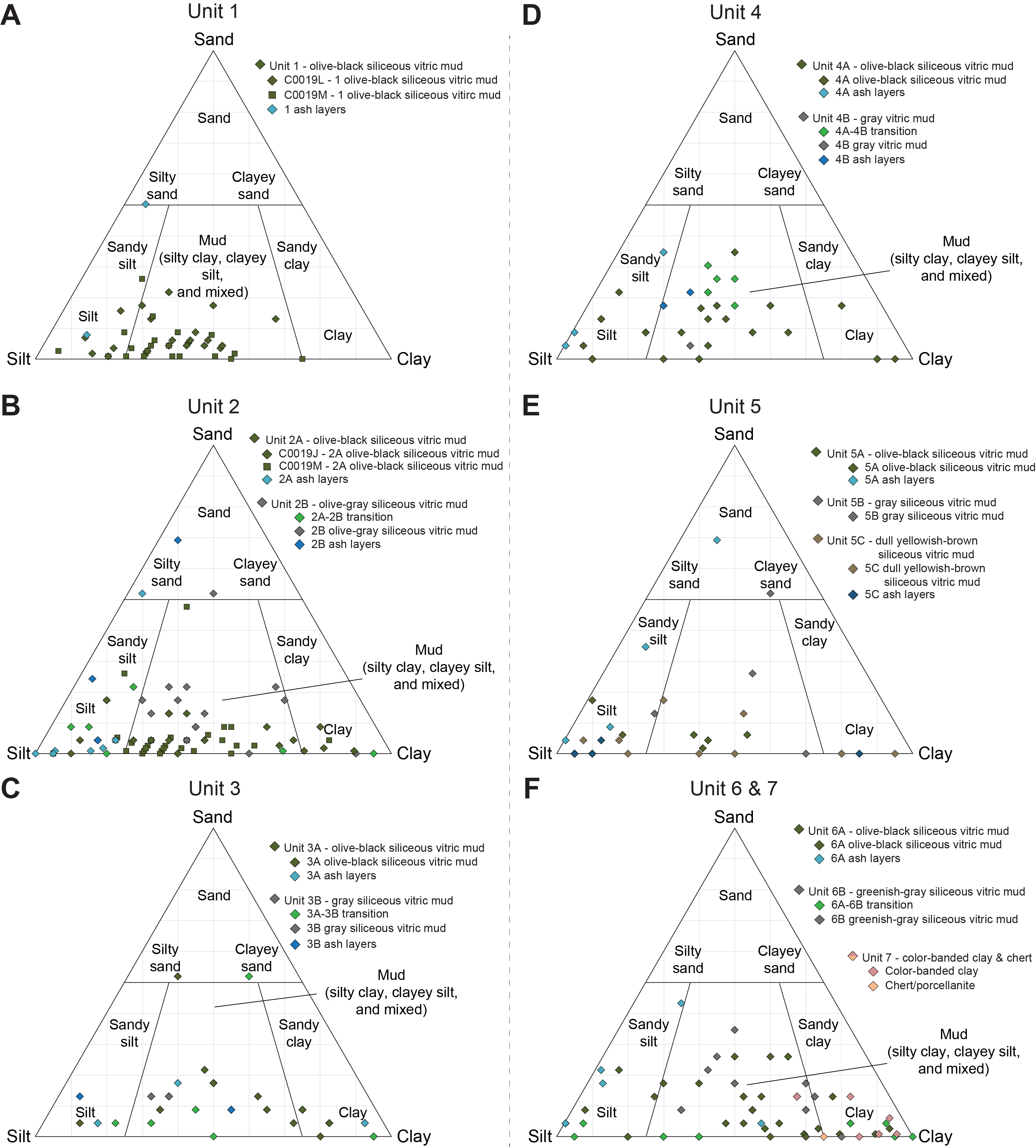
Figure F31. Sediment grain size.

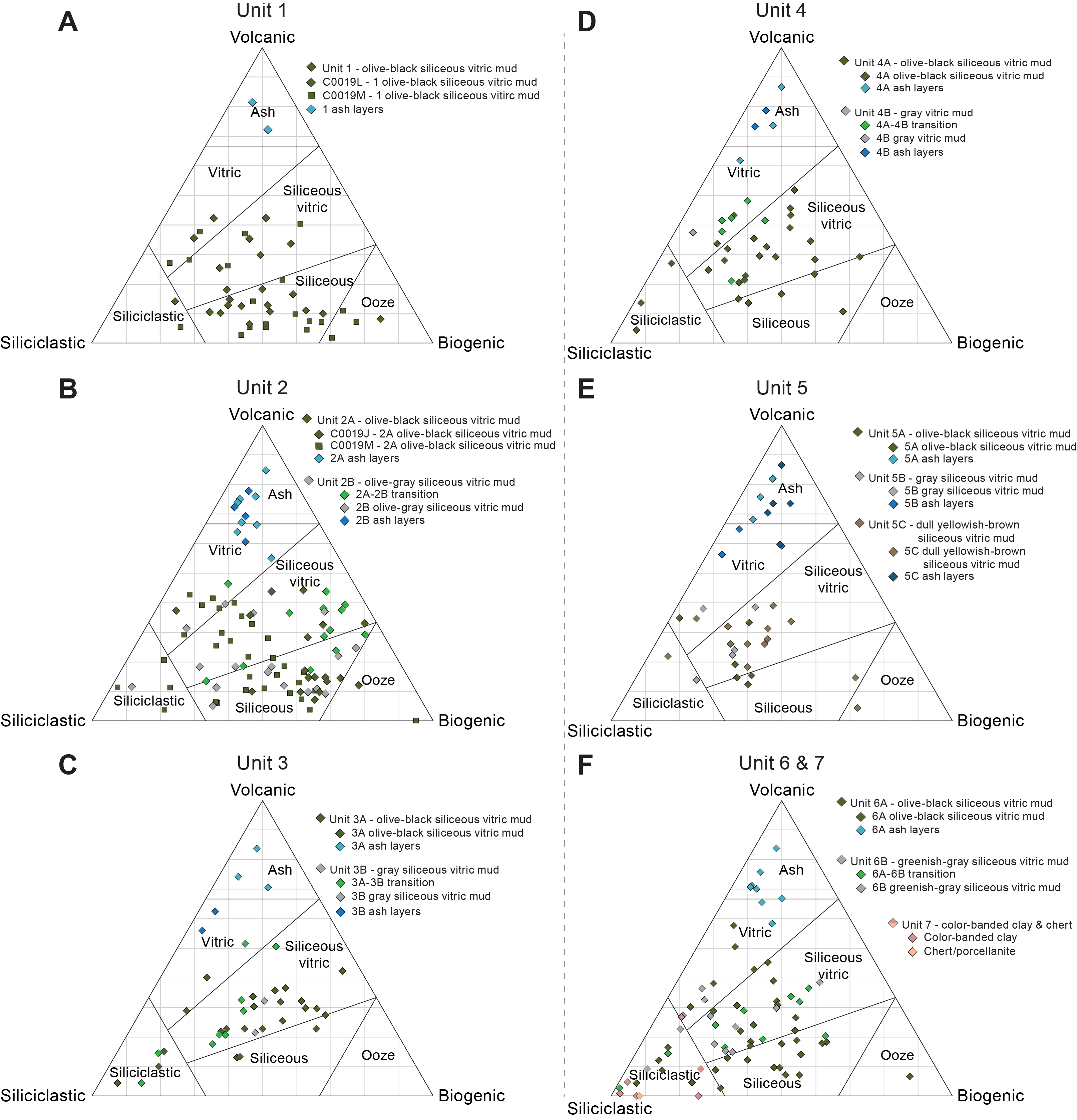
Figure F32. Sediment composition.

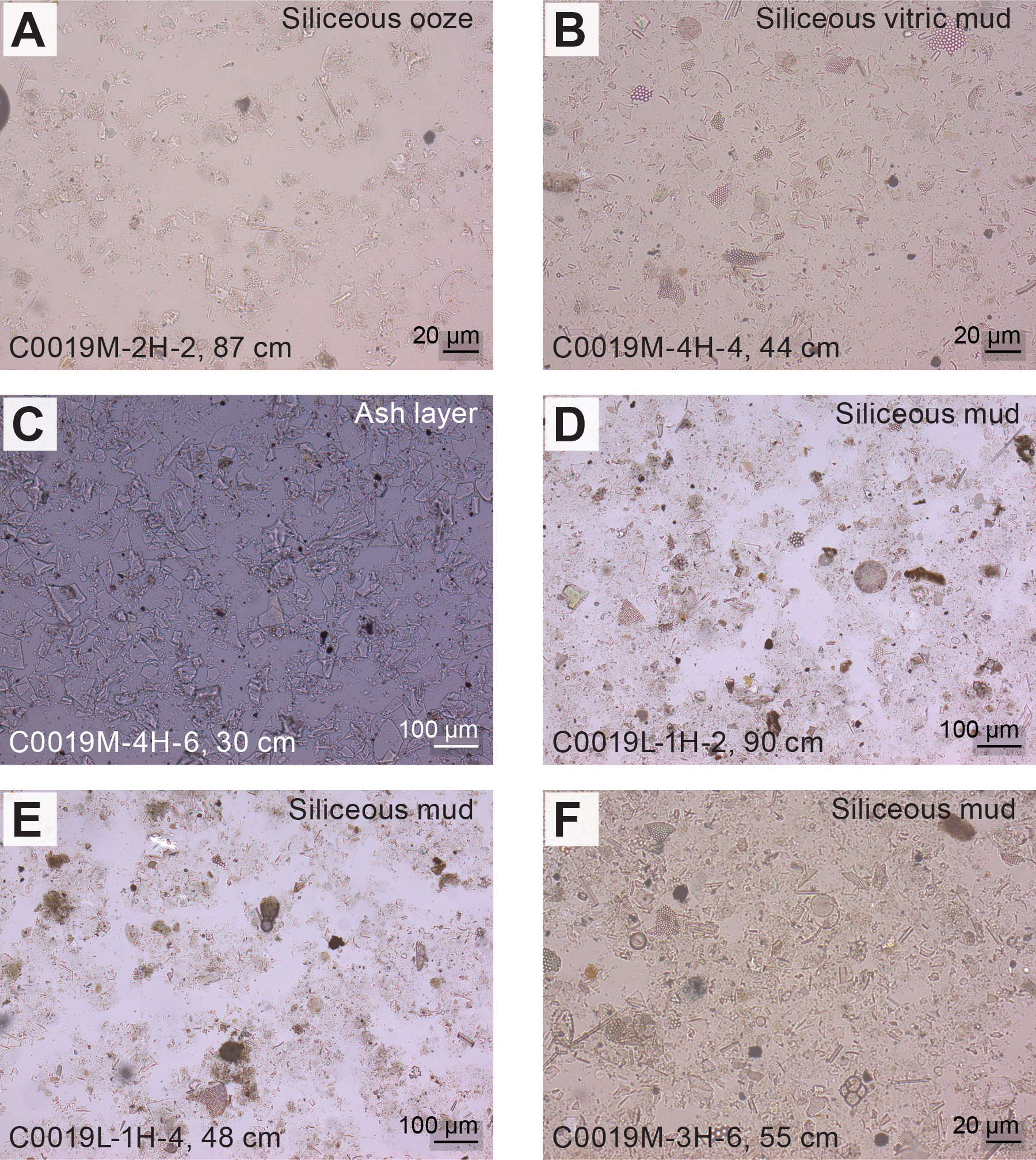
Figure F33. Unit 1 smear slides.

The occasional ash layers are generally coarser, plotting as silty sand to silt (Figure F31) with 9%–58% sand, 40%–81% silt, and 2%–10% clay. They are compositionally volcanic with siliciclastic (5%–6%), volcanic (76%–81%), and biogenic (0%–9%) material (Table T14).

4.1.1.3. Mineralogy and sediment geochemistry

A total of five bulk samples representative of Unit 1 were analyzed for XRD. Clay mineral content dominates the composition (55–69 wt%), with lesser amounts of quartz (13–21 wt%) and plagioclase (18–24 wt%) (Figure F34; Table T15). The variability in the relative abundances of clay, quartz, and feldspar is consistent with the observed differences in the VCDs and smear slides. XRF and loss on ignition (LOI) analyses on the same samples yield the following elemental abundances (Figure F35; Table T16): 3.67–3.79 wt% Na₂O, 1.61–2.55 wt% MgO, 12.45–15.22 wt% Al₂O₃, 66.23–72.84 wt% SiO₂, 0.09–0.12 wt% P₂O₅, 2.41–2.67 wt% K₂O, 1.62–2.35 wt% CaO, 0.44–0.68 wt% TiO₂, 0.06–0.07 wt% MnO, 3.97–6.29 wt% Fe₂O₃, and 6.51–7.74 wt% LOI. The concentration of SiO₂ is consistent with the relatively high proportions of volcanic glass and siliceous biogenic components in this unit.

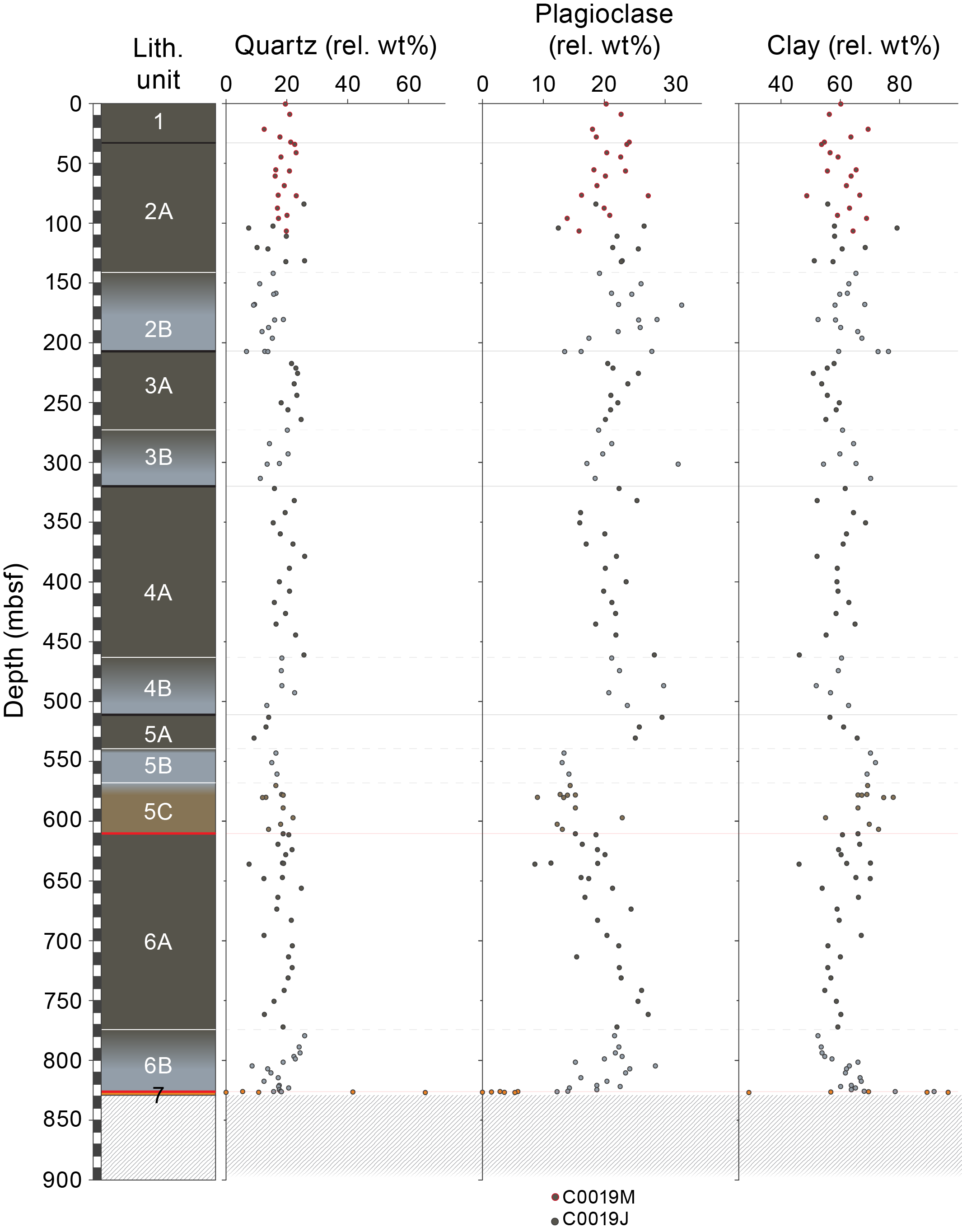
Figure F34. Semiquantitative mineral abundance analysis, Holes C0019J, C0019L, and C0019M.

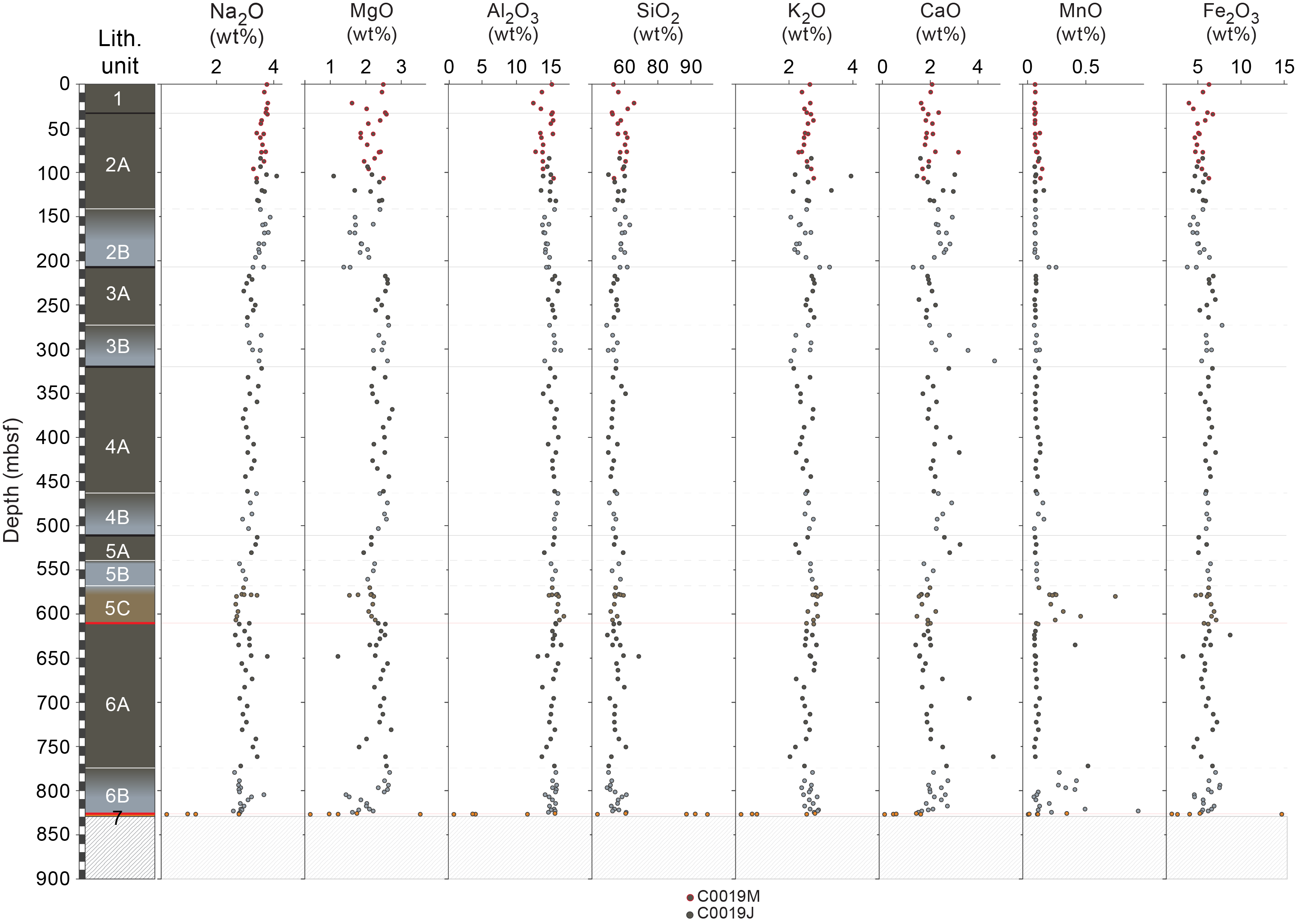
Figure F35. Major element compositions, Holes C0019J and C0019M.

4.1.1.4. Summary and preliminary interpretation

Unit 1 consists of olive-black siliceous vitric mud with 15 interspersed ash horizons. This unit is characterized by inclined bedding with frequent fining-upward layers. In contrast to typical seafloor sediments, the uppermost sediments of Unit 1 are already semiconsolidated. These properties, alongside the chaotic and inclined bedding, are consistent with deposition from mass transport processes (i.e., mass transport deposit) originating from a landward position in a shallower section of the trench slope.

4.1.2. Unit 2

4.1.2.1. Subunit 2A

Interval: 405-C0019M-5H-1, 0 cm, to 405-C0019J-7K-2, 0 cm
Depth: 33.00–141.24 mbsf
Age: 0–2.7 Ma
Lithology: olive-black siliceous vitric mud(stone)

4.1.2.1.1. Visual core description lithology

Subunit 2A is an olive-black (10Y 3/1) siliceous vitric mud(stone) with distinctive dark mottles, green color banding, episodic darker black laminae, and occasional disseminated pumice. In Section 405-C0019M-5H-1, the sediments are softer (less lithified) than, but a similar color to, those in Subunit 1. Subunit 2A is present in Hole C0019M from 33.00 mbsf (5H-1, 0 cm) to 107.50 mbsf and in Hole C0019J from 83.00 to 141.24 mbsf (7K-2, 0 cm) (Figure F29; Table T13). The background mottled siliceous vitric mud(stone) is occasionally interbedded with intervals (several centimeters thick) of inclined and deformed gray ash layers (Figure F36) and coarser grained gray to olive-black graded beds.

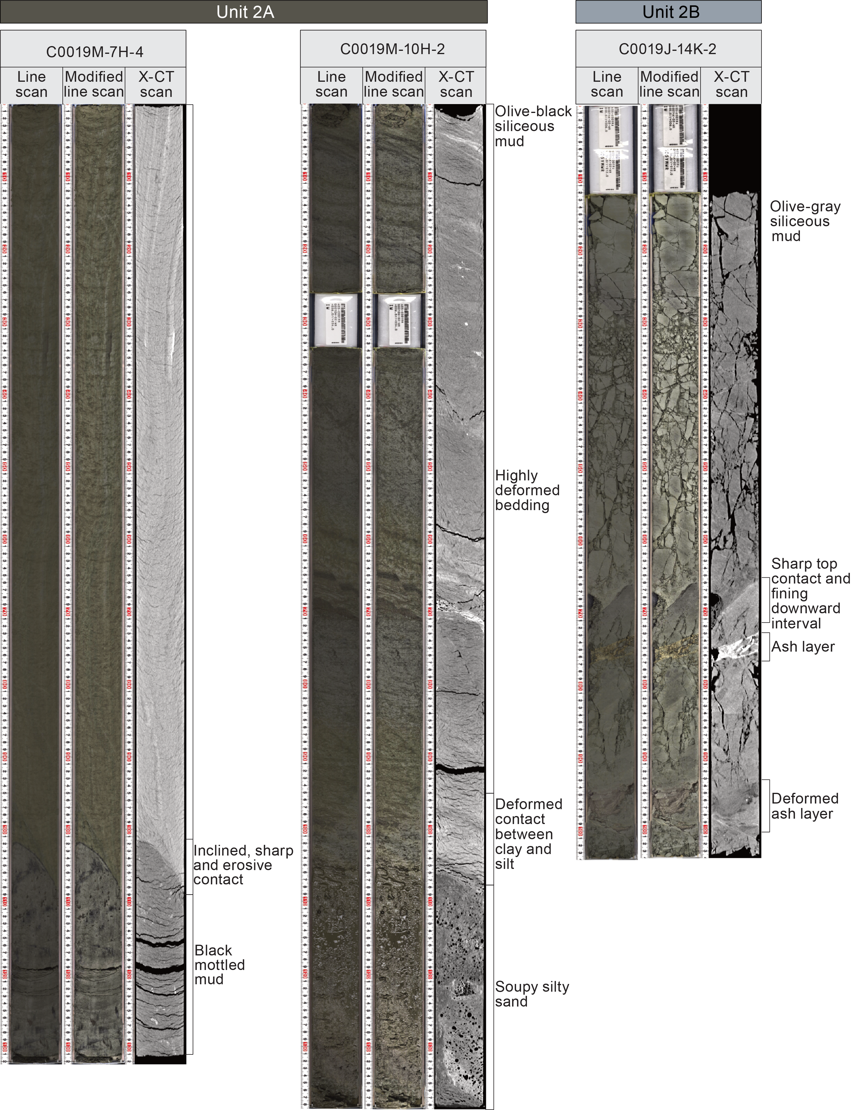
Figure F36. Unit 2 images.

Throughout Subunit 2A, dark gray to black mottles (identified in some locations as iron mono-sulfides) and pyrite-rich patches are present and are particularly evident on XCT images. The black mottles disappeared quickly after being exposed to air (~2–3 h after splitting). Sedimentary structures include occasional color banding (0.5–1.5 cm thick), graded sand beds (e.g., Section 405-C0019M-5H-7), interspersed ash horizons (e.g., Section 5H-2), and granule-, cobble-, to boulder-grade intraformational clasts that sometimes internally preserve grading (e.g., Section 8H-3). Many of the sedimentary structures are inclined (see Structural geology), with occasional downward steepening of the dip (e.g., Sections 7H-2, 70 cm, to 7H-4, 102 cm) underlain by a discordant sedimentary contact with the black mottled mudstone (Section 7H-4, 102 cm; Figure F36).

A total of 17 light yellowish gray to light olive-gray ash layers were identified in Subunit 2A, varying from several centimeter-thick wavy layers to discontinuous elongate patches up to a few centimeters long. These layers typically appear bright in XCT images. Disseminated pyritized pumice clasts are common throughout Subunit 2A. The edges of the ash-rich layers exhibit interfingering with the surrounding background sedimentation (siliceous mud) and display occasional silica mineralization. Burrows can also be observed throughout the unit, highlighted by subtle mottling, pyritization, and patches of different colors ranging from olive-brown to dark gray. Isolated, simple, nonbranching burrows in discrete layers visible in core and XCT images are interpreted as Planolites.

4.1.2.1.2. Smear slide petrography

The grain size of the background sedimentation in Subunit 2A predominately plots as mud (Figures F31, F37) with 0%–55% sand, 10%–95% silt, and 5%–89% clay (Table T14). The composition of the background sedimentation is also a variable mixture of siliciclastic (1%–86%), volcanic (0%–49%), and biogenic (1%–95%) material. The siliciclastic material is mostly clay minerals (0%–75%) with subordinate quartz (0%–35%) and mudstone aggregates (0%–32%). Volcanic material is mostly clear glass (0%–48%), colored glass (0%–4%), and pumice (0%–12%). Biogenic material is mostly diatoms (0%–53%), radiolarians (0%–54%), silicoflagellates (0%–7%), and sponge spicules (0%–50%). Other material (0%–25% of total composition) includes occasional pyrite framboids, dense and opaque minerals, and calcite.

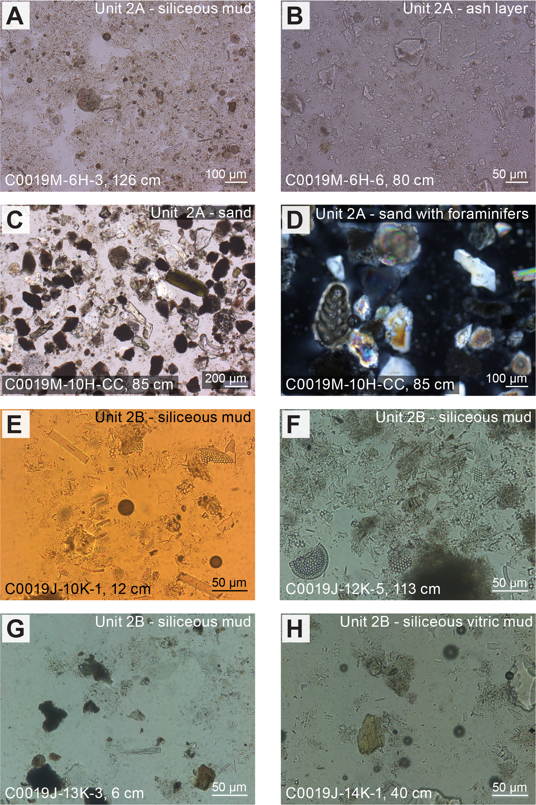
Figure F37. Unit 2 smear slides.

The interbedded ash layers are generally coarser and plot as silt to sand (Figure F31) with 0%–60% sand, 40%–100% silt, and 0%–40% clay. Compositionally, they plot in the siliceous to siliceous-vitric mud sections and are composed of siliciclastic (0%–18%), volcanic (61%–98%), and biogenic (0%–20%) material (Table T14).

4.1.2.1.3. Mineralogy and sediment geochemistry

A total of 20 bulk samples representative of Subunit 2A were collected for XRD (Figure F34; Table T15). Clay mineral content dominates the composition (49–69 wt%), with lesser components of quartz (10–26 wt%) plagioclase (14–27 wt%), and calcite (0–1 wt%). One ash sample contained 79 wt% clay minerals, 7 wt% quartz, 12 wt% plagioclase, and 1 wt% calcite. XRF and LOI analyses on the bulk lithologic and ash samples yielded the following elemental abundances (Table T16; Figure F35): 3.29–4.10 wt% Na₂O, 1.09–2.58 wt% MgO, 12.77–15.70 wt% Al₂O₃, 65.15–70.81 wt% SiO₂, 0.07–0.13 wt% P₂O₅, 2.13–3.94 wt% K₂O, 1.45–3.18 wt% CaO, 0.38–0.69 wt% TiO₂, 0.06–0.14 wt% MnO, 4.42–6.74 wt% Fe₂O₃, and 4.89–8.65 wt% LOI. The high concentration of silica is consistent with the smear slide analysis, which includes predominantly volcanic glass and biogenic silica alongside minor siliciclastic grains. Aluminum corresponds to the presence of clay minerals and plagioclase. The relatively high concentration of iron is likely due to the presence of terrigenous material.

4.1.2.1.4. Summary and preliminary interpretation

Subunit 2A consists of olive-black siliceous vitric mud(stone) interspersed with 17 ash layers and patches. The unit is characterized by inclined (occasionally folded) bedding with rare intervals of chaotic bedding. The upper part of Subunit 2A is relatively unconsolidated compared to Unit 1. This horizon experienced a lot of gas expansion. The extensive pyrite-rich dark mottles suggest low-oxygen subseafloor conditions. Polycrystalline quartz, lithic fragments, and fragmented foraminifera suggest an influx of terrestrial sediment in Subunit 2A. These characteristics, alongside tilted bedding, are consistent with mass transport deposits (slides) sourced from the landward shelf.

4.1.2.2. Subunit 2B

Interval: 405-C0019J-7K-2, 0 cm, through 14K-CC
Depth: 141.24–207.56 mbsf
Age: ~0–12.1 Ma
Lithology: olive-gray siliceous vitric mud(stone)

4.1.2.2.1. Visual core description lithology

The background sedimentation of Subunit 2B is composed of olive-gray siliceous mud(stone) with abundant black and green laminae, which are occasionally wavy. Occasional centimeter-scale soft-sediment deformation is present, including flame structures. There are eight discrete ash layers alongside rare layers of silt and fine-grained sand. Beds are often inclined (e.g., Section 405-C0019J-12K-4) (see Structural geology). The top of Subunit 2B is marked by a gradational change in color from olive-black (10Y 3/1) to olive-gray (10Y 4/2) (Figure F38) between 141.24 and 177.00 mbsf (Sections 7K-2, 0 cm, to 11K-1, 0 cm) (Figure F29; Table T13). Below 177.00 mbsf, the characteristic olive-gray siliceous vitric mud of Subunit 2B is established.

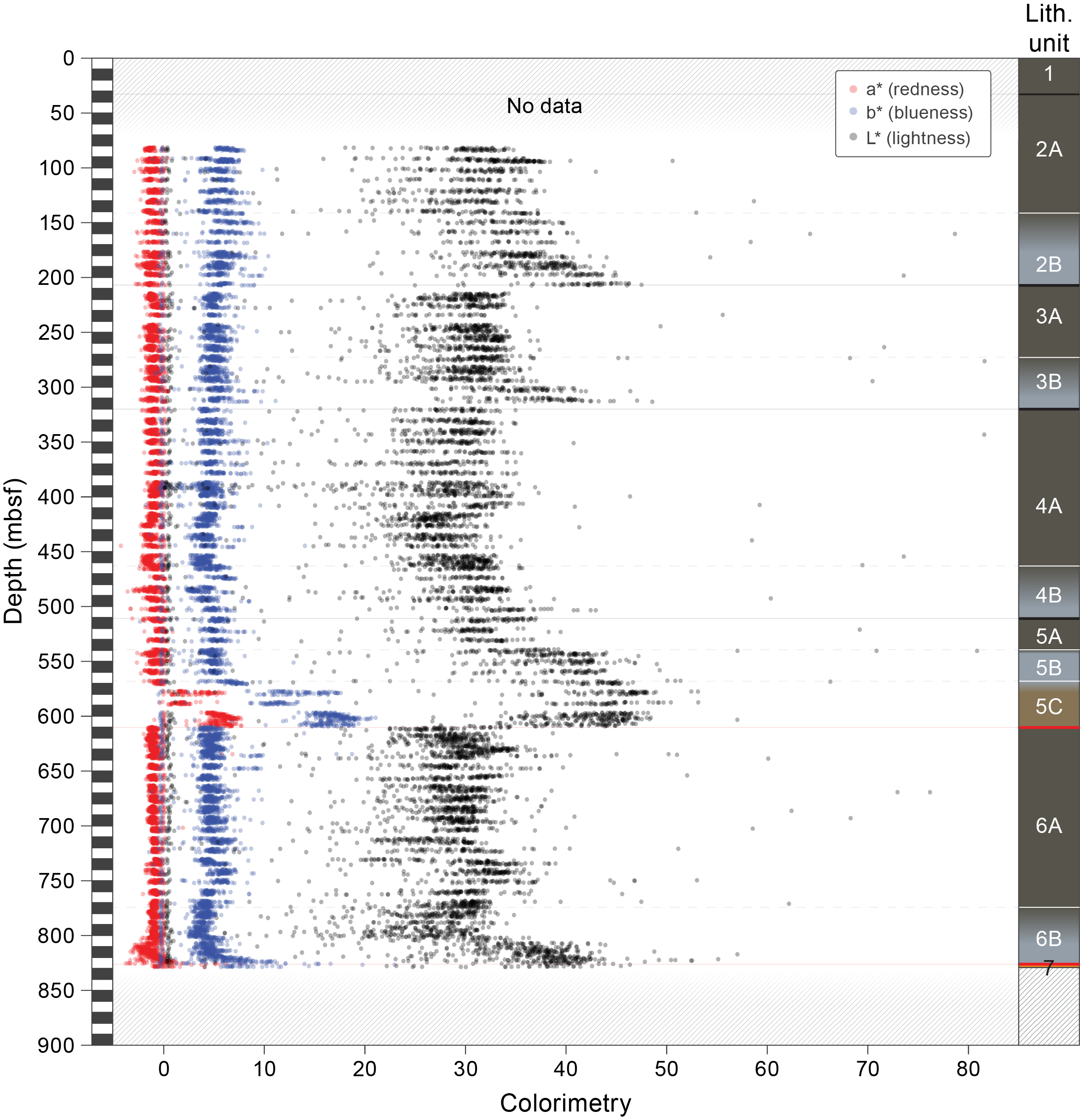
Figure F38. Core colorimetry, Holes C0019J, C0019L, and C0019M.

The ash layers (1–4 cm scale) are often altered and are commonly accompanied by disseminated pumice clasts in the overlying units (e.g., Section 405-C0019J-12K-5; Figure F36) which frequently have altered rims (bright green in color).

The background sedimentation of Subunit 2B is bioturbated to varying degrees. There are isolated simple nonbranching burrows in discrete layers that are interpreted as Planolites with rare layers of boxwork burrows with a branched cylindrical shape interconnected by vertical shafts, suggesting Thalassinoides, and simple burrow communities (often 2+) lined with pelletoidal sediment interpreted as Ophiomorpha. These burrows are evident as cylindrical forms on the XCT images, showing up as bright patches throughout the sections. Notably, bioturbation is most apparent in the sediments above ash layers (e.g., Section 405-C0019J-12K-4).

4.1.2.2.2. Smear slide petrography

The color change zone between Subunits 2A and 2B (141.24–177.00 mbsf) is slightly coarser grained (silt) compared to the background sedimentation (Figures F31, F37), with 0%–25% sand, 5%–85% silt, and 5%–95% clay (Table T14). Compositionally, the transition plots as siliceous vitric mud but with significantly lower siliciclastic components compared to Subunits 2A and 2B (Figure F32), with 3%–57% siliciclastic, 15%–53% volcanic, and 13%–62% biogenic material.

The grain size of the background sedimentation in Subunit 2B plots as mud (Figure F31) with 0%–60% sand, 10–70% silt, and 10%–90% clay (Table T14). The composition plots as siliceous to siliceous vitric mud (Figure F32) with siliciclastic (8%–80%), volcanic (5%–42%), and biogenic (5%–60%) material. There is a notable decrease in volcanic material and corresponding increase in clastic material compared to Subunit 2A. Siliciclastic material contains clay minerals (2%–80%), mud aggregates (0%–35%), quartz (0%–7%), and feldspar (0%–10%). Biogenic material contains diatoms (3%–55%), radiolarians (0%–2%), silicoflagellates (0%–10%), and sponge spicules (2%–40%). Volcanic material comprises clear glass (5%–40%). Other material (0%–17% of total composition) includes pyrite framboids, micas, opaque minerals, and dense minerals.

The ash layers are generally coarser, plotting as silt to sand (Figure F31) with 5%–80% sand, 20%–80% silt, and 0%–35% clay. Compositionally, the samples include siliciclastic (15%–48%), volcanic (16%–82%), and biogenic (0%–30%) material (Table T14).

4.1.2.2.3. Mineralogy and sediment geochemistry

A total of 11 bulk samples representative of Subunit 2B were collected for XRD analysis (Figure F34; Table T15). Clay mineral content dominates the composition and ranges 52–68 wt%. Plagioclase ranges 17%–33 wt%, and quartz ranges 9%–19 wt%. Notably, the reported ranges are less variable than in Subunit 2A. XRF and LOI measurements were performed at the same intervals as XRD. The results indicated 3.36–3.88 wt% Na₂O, 1.55–2.40 wt% MgO, 13.76–15.52 wt% Al₂O₃, 66.86–71.55 wt% SiO₂, 0.08–0.10 wt% P₂O₅, 2.06–2.68 wt% K₂O, 2.17–2.93 wt% CaO, 0.48–0.64 wt% TiO₂, 0.06–0.08 wt% MnO, 4.11–6.34 wt% Fe₂O₃, and 4.95–6.28 wt% LOI (Figure F35; Table T16).

4.1.2.2.4. Summary and preliminary interpretation

Subunit 2B consists of olive-gray siliceous vitric mud(stone) with a gradual color transition zone from Subunit 2A. The subunit contains eight ash layers alongside subordinate disseminated pumice, which is often altered. Bedding is characterized by color banding, occasionally inclined, alongside frequent intervals of graded beds. These properties are consistent with deposition from mass transport processes, as supported by the ichnofacies (Planolites, Thalassinoides, and Ophiomorpha), which are all commonly associated with shallower water depths supporting sediment transport from the slope.

4.1.3. Unit 3

4.1.3.1. Subunit 3A

Interval: 405-C0019J-14K-2, 70 cm, to 21K-2, 0 cm
Depth: 215.00–272.85 mbsf
Age: 0–12.1 Ma
Lithology: olive-black siliceous mud(stone)

4.1.3.1.1. Visual core description lithology

Subunit 3A is predominantly an olive-black (7.5Y to 10Y 3/1) siliceous vitric mud(stone) interspersed with occasional silt and medium- to coarse-grained sand layers (few to several centimeters thick), alongside 15 ash layers and scattered pumice clasts. Subunit 3A is interbedded with graded layers that are often inclined and deformed alongside dark greenish color banding (2–10 cm thick). Subunit 3A is separated from Subunit 2B by an inferred fault based on an age reversal defined by diatom biostratigraphy (see Biostratigraphy and Structural geology). However, this fault was not recovered in core, so the Subunit 2B/3A contact was not observed. Subunit 3A continues to 272.85 mbsf (Section 405-C0019J-21K-2, 0 cm) (Figure F29; Table T13).

Sedimentary structures include dispersed light gray pumice clasts (millimeter to centimeter size), often proximal to ash layers or disseminated within the background sedimentation (e.g., Section 405-C0019J-18K-2) that are easily identifiable on XCT images (e.g., Figures F39, F40). Seven graded beds (2–5 cm thick) are identified in the silt and ash layers in Subunit 3A and are occasionally associated with erosional bases.

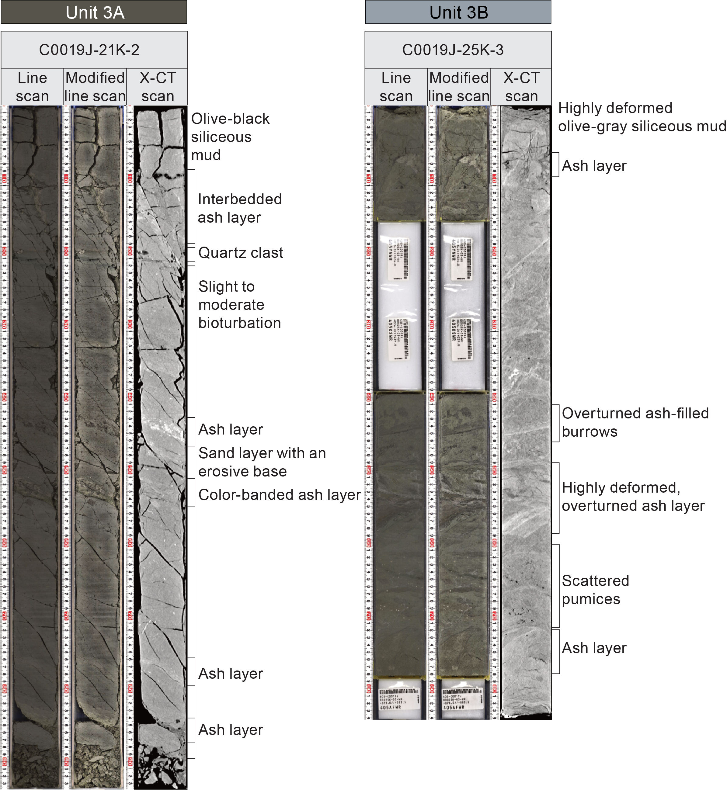
Figure F39. Unit 3 images.

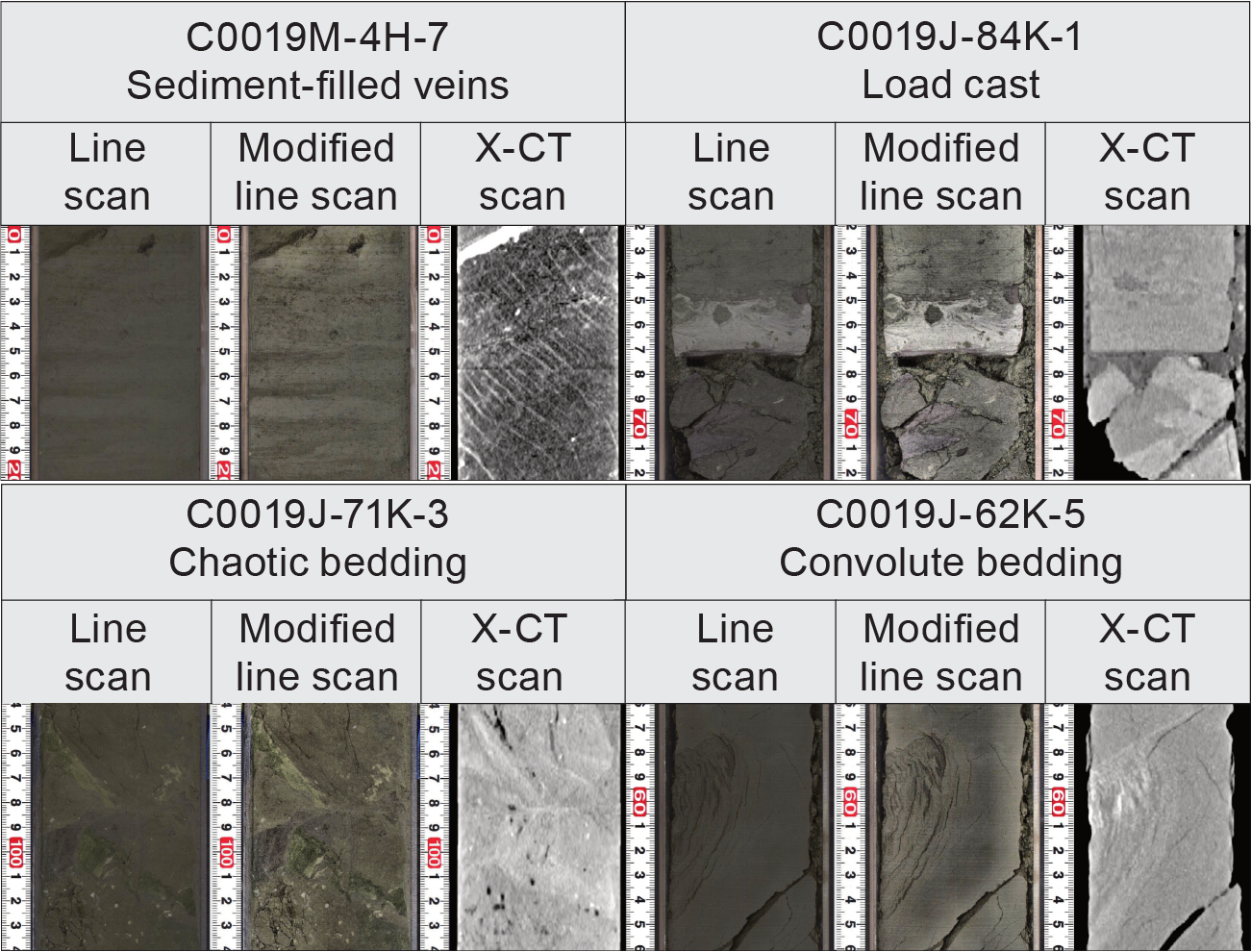
Figure F40. Sedimentary structures, Holes C0019J, C0019L, and C0019M.

Intervals of ash layers and/or ash-rich mud or sand layers (few centimeters to 80 cm thick) are observed in Subunit 3A (e.g., Sections 405-C0019J-14K-2, 15H-5, 16K-1, 16K-4, and 18K-4). These are often inclined or deformed and sometimes display dark gray to greenish color banding. The ash occurs in either wavy layers or as discontinuous elongate patches up to a few centimeters long that interfinger with the background sedimentation and occasionally exhibit silica mineralization (Figure F39). These layers mostly appear brighter in XCT images than the surrounding mudstone.

Subunit 3A is moderately bioturbated. Burrows are mostly concentrated above ash layers and are mostly pyritized, highlighted by subtle mottling and patches of different color ranging from olive-brown to dark gray. Isolated simple nonbranching burrows in discrete layers are interpreted as Planolites. Simple burrow communities (often 2+) lined with pelletoidal sediment are interpreted as Ophiomorpha. In general, burrows are simple, unlined, and subhorizontal, evident as bright cylindrical forms on the XCT images.

4.1.3.1.2. Smear slide petrography

The grain size of the background sedimentation in Subunit 3A plots as mud (Figures F31, F41) with 0%–60% sand, 5%–85% silt, and 10%–95% clay (Table T14). The composition is siliceous vitric mud (Figure F32) and is composed of siliciclastic (2%–90%), volcanic (5%–53%), and biogenic (5%–50%) material. It is more volcanic and less siliceous compared to Units 1 and 2. Siliciclastic material is mostly clay minerals (0%–80%) with subordinate quartz (0%–15%) and feldspar (0%–15%). Volcanic material is clear glass (5%–50%), colored glass (0%–10%), and pumice (0%–10%). Biogenic material is diatoms (0%–40%), radiolarians (0%–40%), silicoflagellates (0%–5%), and sponge spicules (0%–15%). Other material (8% of total composition) includes framboidal and euhedral pyrite, mica, and dense and opaque minerals.

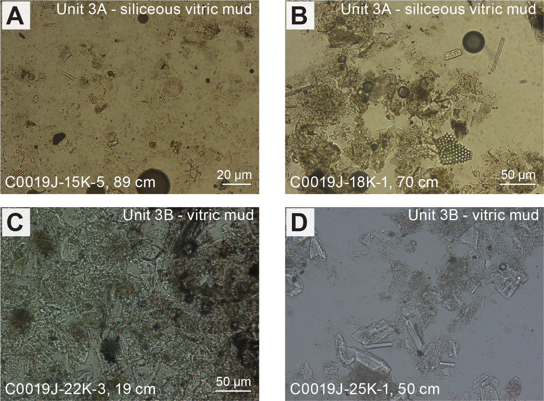
Figure F41. Unit 3 smear slides.

The ash layers are generally coarser (silt) with 5%–20% sand, 5%–80% silt, and 15%–90% clay (Figure F31). They are composed of clastic (3%–10%), volcanic (60%–87%), and biogenic (0%–10%) material (Table T14).

4.1.3.1.3. Mineralogy and sediment geochemistry

A total of 10 bulk samples representative of Subunit 3A were collected for XRD analysis (Figure F34; Table T15). Clay mineral content dominates the composition and ranges 51–76 wt% alongside 7–24 wt% quartz, 14–28 wt% plagioclase, and ~1 wt% calcite. XRF and LOI analyses from the same samples yielded the following elemental abundances: 2.95–3.65 wt% Na₂O, 1.38–2.62 wt% MgO, 14.34–16.18 wt% Al₂O₃, 65.94–70.80 wt% SiO₂, 0.08–0.14 wt% P₂O₅, 2.53–3.27 wt% K₂O, 1.29–2.22 wt% CaO, 0.45–0.71 wt% TiO₂, 0.06–0.24 wt% MnO, 3.78–7.03 wt% Fe₂O₃, and 4.95–7.35 wt% LOI (Figure F35; Table T16). The concentration of silica is consistent with the amount of volcanic glass, biogenic silica, and siliciclastic grains. Aluminum correlates to clay minerals and plagioclase. The presence of terrigenous grains in smear slides helps explain the relatively high concentration of iron.

4.1.3.1.4. Summary and preliminary interpretation

Subunit 3A consists of olive-black siliceous mud(stone) containing 15 ash layers alongside scattered pumice. The subunit contains frequent fining-upward layers (often inclined) with occasional erosional bases. Some localized deformation is identified. Basal load structures indicate soft-sediment deformation. The notably lower frequency of chaotic beds indicates less influence from mass transport processes compared to other units, but the ichnology still indicates some transport from the shelf.

4.1.3.2. Subunit 3B

Interval: 405-C0019J-21K-2, 0 cm, to 26K-1, 0 cm
Depth: 272.85–320.00 mbsf
Age: 0–2.7 Ma
Lithology: olive-gray siliceous vitric mud(stone)

4.1.3.2.1. Visual core description lithology

Subunit 3B is an olive-gray (7.5Y 5/1 and 2.5 GY 3/1) siliceous vitric mud(stone) with interbedded silty to fine to very coarse sandy layers (few to several tens of centimeters thick) and 27 ash layers (Figure F39). Subunit 3B locally exhibits scattered pumice clasts, dark and greenish color banding, bioturbation, fining-upward and -downward graded layers (e.g., Section 405-C0019J-24K-3), and interspersed clasts. The boundary between Subunit 3A and Subunit 3B is marked by a gradual transition in color from olive-black (7.5Y 3/1; 5Y 3/1) to gray (7.5Y 4/1 and 5Y 4/A) from 272.85 to 310.00 mbsf (Sections 21K-2, 0 cm, to 25K-1, 0 cm) (Figure F29; Table T13). Below 310.00 mbsf (Sections 25K-1, 0 cm, to 26K-1, 0 cm), the background sedimentation of Subunit 3B is established.

Light gray pumice clasts (millimeter to centimeter size) are disseminated either near ash layers or throughout the background sedimentation (e.g., Section 405-C0019J-22K-5) and are identifiable as high-density patches on XCT images (Figure F39). Six graded beds are identified in Subunit 3B, often with erosional bases. Graded beds are interbedded with background sedimentation or occur in stacked sequences, which are sometimes inclined. These mostly occur in sandy (several centimeter thick) and ash-rich layers (millimeter to several centimeter thick), and exhibit both fining-upward and -downward intervals (e.g., Section 24K-3). Notably, there is a 106 cm thick fining-upward sandy interval in Sections 24K-1 through 24K-2. Color banding occurs locally or over several sections, highlighting inclined or disrupted bedding. Convolute bedding occurs in Sections 24K-3 through 25K-3.

Ash occurs in several-centimeter-thick wavy layers and as discontinuous elongate patches up to a few centimeters long that interfinger with the background sedimentation and show occasional silica mineralization. Dark green color bands are clearly identified within ash layers, which appear brighter in XCT images than the surrounding siliceous mud(stone).

Subunit 3B is moderately to heavily bioturbated, mostly concentrated around the top of ash layers (e.g., Section 405-C0019J-25K-2). Overturned burrows are found in some cores (e.g., Sections 25K-2 and 25K-3). Bioturbation is mostly characterized by pyrite-filled burrows, highlighted by subtle mottling and patches of different color ranging from olive-brown to dark gray (e.g., Section 25K-2). Isolated simple nonbranching burrows in discrete layers are interpreted as Planolites. Rare layers of boxwork burrows with a branched cylindrical shape interconnected by vertical shafts are interpreted as Thalassinoides. Simple burrow communities (often 2+) lined with pelletoidal sediment are interpreted as Ophiomorpha. In general, burrows are simple, unlined, and subhorizontal, evident as bright cylindrical forms on the XCT images.

4.1.3.2.2. Smear slide petrography

The zone of color change (272.85–310.00 mbsf) between Subunits 3A and 3B makes up the majority of Subunit 3B. The grain size of this zone is slightly coarser (silt and mud) compared to the background sedimentation of Subunits 3A and 3B (Figures F31, F41), with 0%–60% sand, 5%–75% silt, and 20%–95% clay (Table T14). Compositionally, the color change zone is siliceous vitric mud with a slightly higher siliciclastic component compared to Subunit 3A (Figure F32). The composition is 15%–83% siliciclastic, 5%–59% volcanic, and 10%–25% biogenic material.

The background sedimentation of Subunit 3B plots as mud (Figure F31) and consists of 15% sand, 55%–60% silt, and 25%–30% clay (Table T14). The composition of the background sedimentation is siliceous to siliceous vitric mud (Figure F32), a mixture of siliciclastic (29%–37%), volcanic (23%–35%), and biogenic (30%–33%) material. Throughout both the color change zone and the background sedimentation, clastic material in Subunit 3B is dominated by clay minerals (10%–80%), mud aggregates (10%–15%), some quartz (1%–5%), and feldspar (3%–7%). Biogenic material is mainly diatoms (0%–20%), radiolarians (0%–1%), silicoflagellates (0%–5%), and sponge spicules (2%–10%). Volcanic material is mostly clear glass (5%–55%), colored glass (0%–7%), and pumice (0%–15%). Other material (0%–25% of total composition) includes pyrite (framboids and euhedral), micas, opaque minerals, and dense minerals.

The ash layers plot as mud and silt (Figure F31) with 10%–15% sand, 40%–80% silt, and 5%–50% clay. Compositionally, the samples plot as ashy/vitric mud (Figure F32) with siliciclastic (25%–30%) and volcanic (55%–65%) material (Table T14).

4.1.3.2.3. Mineralogy and sediment geochemistry

A total of six bulk samples representative of Subunit 3B were collected for XRD analysis (Figure F34; Table T15). Clay mineral content dominates the composition (54%–70%), with lesser quartz (11–20 wt%) and plagioclase (17–32 wt%). XRF and LOI analyses from the same samples yield the following elemental abundances: 3.07–3.56 wt% Na₂O, 2.22–2.65 wt% MgO, 14.09–16.42 wt% Al₂O₃, 64.62–67.82 wt% SiO₂, 0.10–0.12 wt% P₂O₅, 2.06–2.69 wt% K₂O, 1.97–4.69 wt% CaO, 0.62–0.68 wt% TiO₂, 0.06–0.10 wt% MnO, 5.45–7.81 wt% Fe₂O₃, and 3.36–4.31 wt% LOI (Figure F35; Table T16).

The concentration of silica is consistent with VCDs and smear slides of the background sediment that include volcanic glass, biogenic silica, and siliciclastic grains. Aluminum corresponds to clay minerals and plagioclase. Additionally, the presence of terrestrial detrital minerals explains the relatively high concentration of iron. The high CaO concentration is one outlier measurement from a sample taken at the base of the entire unit (Section 405-C0019J-25K-3) in a locally very chaotic interval containing many small pumice pieces and other clasts, which may be drilling-induced injection.

4.1.3.2.4. Summary and preliminary interpretation

Subunit 3B (272.85–320.00 mbsf) consists of olive-gray siliceous mud(stone) with a gradual color change from Subunit 3A that spans most of the unit. A total of 27 ash layers were identified. Subunit 3B is characterized by inclined and chaotic bedding with fining-upward and coarsening-upward intervals, as well as interspersed clasts and altered ash patches. Inverted burrows indicating overturned strata and convolute beddings are observed in Cores 405-C0019J-24K and 25K. These characteristics are consistent with deposition by mass transport processes.

4.1.4. Unit 4

4.1.4.1. Subunit 4A

Interval: 405-C0019J-26K-1, 0 cm, to 41K-1, 0 cm
Depth: 320.00–463.00 mbsf
Age: 0–5.6 Ma
Lithology: olive-black siliceous vitric mud(stone)

4.1.4.1.1. Visual core description lithology

Subunit 4A starts at 320.00 mbsf (Section 405-C0019J-26K-1, 0 cm) with a sharp change in color from Subunit 3B and continues to 463.00 mbsf (Section 41K-1, 0 cm) (Figure F29; Table T13). The background sedimentation of Subunit 4A is olive-black (10Y 3/1 and 7.5Y 3/1) siliceous vitric mud(stone), with a few interbedded layers (~1 to 10 cm thick) containing coarser grained pumice clasts, ash, and pyritized pebbles (Figure F42). Subunit 4A is characterized by an upper part (320.00–396.50 mbsf; Sections 26K-1, 0 cm, to 34K-1, 0 cm) with thin, planar, coherent laminated beds and infrequent interbedded inclined layers and a lower part (396.50–463.00 mbsf; Sections 34K-1, 0 cm, to 41K-1, 0 cm) with frequent chaotic intervals (including slumps and slump folding) interspersed with clasts and inclined beddings (e.g., Sections 34K-1, 34K-3, 35K-1, and 36K-2). In the lower part, there is a slight color shift from olive-black (10Y 3/1 and 7.5Y 5/3) to a lighter shade of olive-black (5Y 3/2). This corresponds to an increase in the volcanic component. Mottling and thin black and green, discontinuous color bands (e.g., Section 27K-3) are common throughout Subunit 4A. Color bands and beds in the chaotic lower part of Subunit 4A show deformation and inclination (see Structural geology). Dark seams and bands range from 1 to >10 mm thick and occasionally contain discontinuous lenses of pyrite.

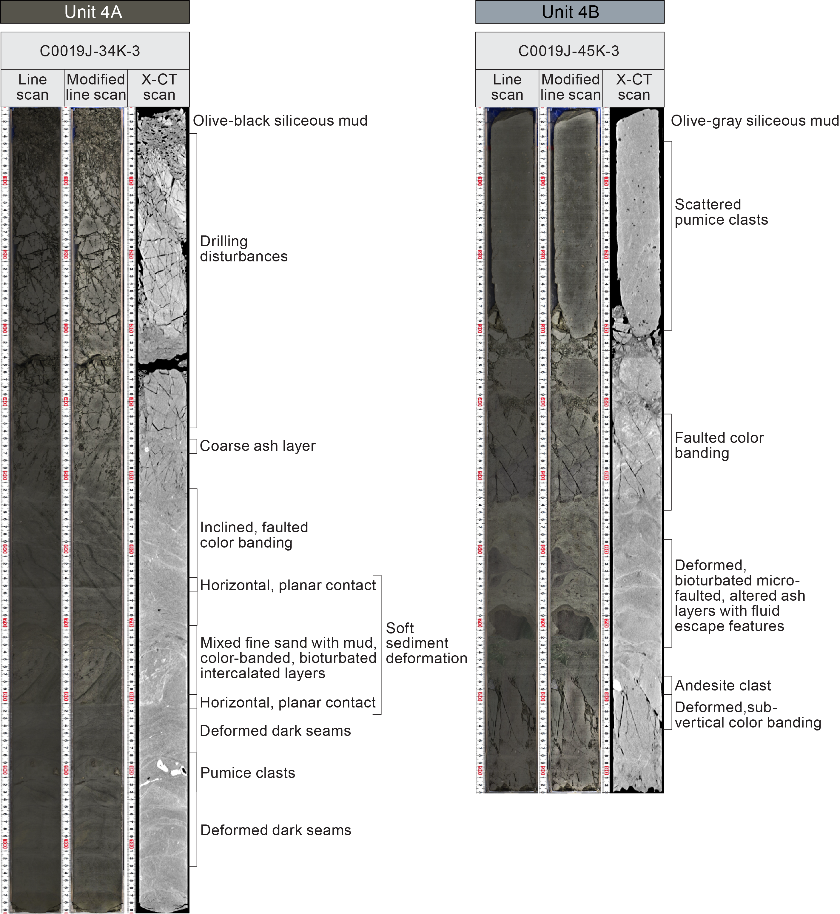
Figure F42. Unit 4 images.

Subunit 4A is moderately to heavily bioturbated. Some burrows are black due to the presence of pyrite or iron monosulfides. Although bioturbation is often too heavy to identify discrete ichnofacies, the XCT imagery shows some examples of sediment-filled burrows that appear round to ellipsoidal, with simple, unlined, and simple unbranched structures suggesting Planolites.

4.1.4.1.2. Smear slide petrography

The grain size of the background sedimentation in Subunit 4A predominately plots as mud (Figures F31, F43) with 0%–40% sand, 5%–90% silt, and 5%–95% clay (Table T14). There is a general fining-upward trend, with the uppermost interval composed predominantly of clay (Sections 405-C0019J-26K-1, 0 cm, to 30K-CC, 36 cm), the middle interval composed of silt (Sections 31K-1, 0 cm, to 33K-CC, 29 cm), and the lower interval showing an increase in sand (Sections 34K-1, 0 cm, to 40K-CC, 23 cm).

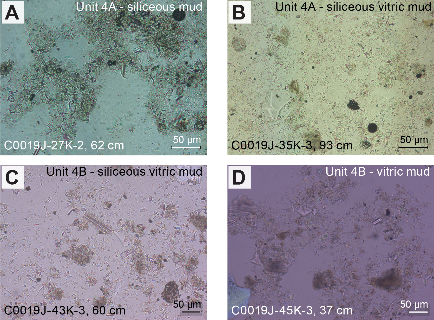
Figure F43. Unit 4 smear slides.

The composition of the background sedimentation in Subunit 4A is siliceous vitric mud (Figure F32) composed of siliciclastic (10%–90%), volcanic (5%–55%), and biogenic (1%–60%) material (Table T14), which is consistent through the general fining-upward trend. Siliciclastic material is mostly clay minerals (2%–90%) with some quartz (0%–25%) and feldspar (0%–20%). Volcanic material is mostly clear glass (5%–50%), colored glass (0%–10%), and pumice (0%–20%). Biogenic material is mostly diatoms (1%–40%), radiolarians (0%–10%), silicoflagellates (0%–5%), and sponge spicules (0%–20%). Other material (9% of total composition) includes glauconite, framboidal and euhedral pyrite, micas, and dense and opaque minerals. Notable is the presence of 1%–2% calcite (Sections 405-C0019J-37K-1, 17 cm, and 37K-1, 93 cm) and a calcite-bearing (20%) pumice clast (Section 37K-3, 63 cm).

The ash layers are generally coarser (silt) with 5%–40% sand, 30%–95% silt, and 0%–60% clay (Figure F31). The samples plot as volcanic and are composed of siliciclastic (0%–45%), volcanic (35%–85%), and biogenic (0%–15%) material (Table T14).

4.1.4.1.3. Mineralogy and sediment geochemistry

A total of 15 bulk samples representative of Subunit 4A were collected for XRD analysis (Figure F34; Table T15). Clay mineral content dominates the composition and ranges 46–69 wt% alongside 16–28 wt% plagioclase and 16–26 wt% quartz. XRF and LOI analyses on these same samples show that Subunit 4 contains 2.65–3.58 wt% Na₂O, 2.17–2.75 wt% MgO, 13.87–15.86 wt% Al₂O₃, 64.41–70.28 wt% SiO₂, ~0.1 wt% P₂O₅, 2.15–2.76 wt% K₂O, 1.69–3.22 wt% CaO, 0.59–0.71 wt% TiO₂, ~0.1 wt% MnO, 5.31–7.06 wt% Fe₂O₃, and 5.03–6.9 wt% LOI (Figure F35; Table T16). The concentration of SiO₂ is consistent with the relatively high proportions of volcanic glass and siliceous biogenic components in this unit.

4.1.4.1.4. Summary and preliminary interpretation

Subunit 4A consists of olive-black siliceous vitric mud(stone) with a relatively sharp color change from Subunit 3B. Notably, Subunits 4A and 3B are separated by a slight age inversion (see Biostratigraphy) and a sharp shift in lithology between Cores 405-C0019J-25K and 26K. Seven ash layers are identified. The upper part (320.00–396.50 mbsf) is characterized by inclined, planar beds with thin graded sequences at the base and higher biogenic content. The upper part is tentatively interpreted as a relatively coherent package containing an undisturbed sedimentary sequence. The lower part (396.50–463.00 mbsf) is characterized by frequent intervals of chaotic bedding interspersed with clasts, as well as lower biogenic and higher volcanic content. Calcite and calcite-bearing ash layers are occasionally found in chaotic beds, suggesting mass transport from the shelf (above the carbonate compensation depth) into deeper waters.

4.1.4.2. Subunit 4B

Interval: 405-C0019J-41K-1, 0 cm, to 46K-1, 0 cm
Depth: 463.00–511.00 mbsf
Age: 0–5.6 Ma
Lithology: gray vitric mud(stone)

4.1.4.2.1. Visual core description lithology

The transition from Subunit 4A to Subunit 4B is defined by a gradational color change of the vitric mud(stone) from olive-black (7.5Y 3/1; 5Y 3/1) to gray (7.5 4/1 and 5Y 4/1) between 463.00 and 501.50 mbsf (Sections 405-C0019J-41K-1, 0 cm, to 45K-1, 0 cm) (Figure F29; Table T13). This unit contains two deformed ash layers (intervals 41K-1, 19–23 cm, and 45K-3, 52–77 cm). Throughout Subunit 4B, chaotic bedding is commonly interbedded with centimeter-scale layers of coarser grained disseminated pumice clasts, ash aggregates, and/or pyritized pebbles (Figure F42). Black seams and color banding ranging from less than a millimeter to several millimeters thick are common and sometimes show deformation and (sub)vertical inclinations (see Structural geology). Subunit 4B contains low to moderate bioturbation. Occasionally, the burrow fill varies from light gray (ash fill) to black (pyrite or iron monosulfides).

4.1.4.2.2. Smear slide petrography

The grain size of the color change zone is slightly coarser compared to the background sedimentation but still plots as mud (Figures F31, F43) with 20%–35% sand, 35%–45% silt, and 25%–40% clay (Table T14). Compositionally, the zone of color change plots as ashy/vitric mud (Figure F32) with siliciclastic (26%–50%), volcanic (23%–45%), and biogenic (8%–22%) material. The grain size of the background sedimentation of Subunit 4B (n = 1) plots as mud with 5% sand, 60% silt, and 35% clay. The composition is vitric mud with siliciclastic (44%), volcanic (35%), and biogenic (2%) material. Throughout Subunit 4B, the siliciclastic material is dominated by clay minerals (6%–30%) and some quartz (7%–16%). Biogenic material is mainly diatoms (2%–12%), radiolarians (0%–1%), and sponge spicules (0%–10%). Volcanic material is mostly clear glass (0%–25%), colored glass (2%–10%), and pumice (6%–30%). Other material (5%–19% of total composition) includes framboidal and euhedral pyrites, micas, opaque minerals, and dense minerals. Notable is the presence of 8% calcite in a chaotic bedding of clasts at the base of Subunit 4B (Section 405-C0019J-45K-3, 37 cm).

The ash layers (n = 2) are generally coarser (silt), with 20%–25% sand, 50%–60% silt, and 20%–25% clay (Figure F31). Compositionally, the samples represent ashy/vitric mud (Figure F32) with siliciclastic (5%–6%), volcanic (33%–50%), and other (45%–61%) material (Table T14).

4.1.4.2.3. Mineralogy and sediment geochemistry

A total of five bulk samples representative of Subunit 4B were collected for XRD analysis (Table T15). Clay mineral content dominates the composition and ranges 52–63 wt% clay alongside 21–30 wt% plagioclase and 13–23 wt% quartz (Figure F34). XRF and LOI analysis from the same samples yield the following elemental abundances for Unit 4 (Figure F35; Table T16): 2.91–3.40 wt% Na₂O, 2.35–2.61 wt% MgO, 15.48–16.02 wt% Al₂O₃, 65.42–67.68 wt% SiO₂, ~0.1 wt% P₂O₅, 2.5–2.76 wt% K₂O, 2.26–2.9 wt% CaO, 0.62–0.69 wt% TiO₂, ~0.1 wt% MnO, 5.90–6.30 wt% Fe₂O₃, and 5.21–6.43 wt% LOI. The relative lower concentration of SiO₂ in Subunit 4B compared to Subunit 4A is consistent with the lower abundance of siliceous biogenic components.

4.1.4.2.4. Summary and preliminary interpretation

Subunit 4B consists of gray vitric mud(stone) with a gradual color change from Subunit 4A. The unit contains two deformed ash layers and is characterized by inclined and chaotic bedding interspersed with fining-upward layers. Notable is a decrease in biogenic pelagic material (increase in volcanic). These characteristics are consistent with deposition from mass transport processes.

4.1.5. Unit 5

4.1.5.1. Subunit 5A

Interval: 405-C0019J-46K-1, 0 cm, to 49K-1, 0 cm
Depth: 511.00–539.50 mbsf
Age: 0–4.0 Ma
Lithology: olive-black siliceous vitric mud(stone)

4.1.5.1.1. Visual core description lithology

The background sedimentation of Subunit 5A from 511.00 to 539.50 mbsf (Sections 405-C0019J-46K-1, cm, to 49K-1, 0 cm) is composed of olive-black (7.5Y 3/1) siliceous vitric mud(stone) (Figure F44). Color variations between yellowish gray (2.5Y 4/1), olive-black (5Y 3/2), and gray (7.5GY 4/1) reflect either changes in the relative abundance of volcanic and biogenic material or chemical alteration. Six ash layers are identified in Subunit 5A. Throughout Subunit 5A, the lithology shows chaotic bedding with frequent interspersed clasts and inclined and deformed beds. Color banding and silty to sandy ashy patches, scattered pumice, and dark seams are commonly identified throughout Subunit 5A.

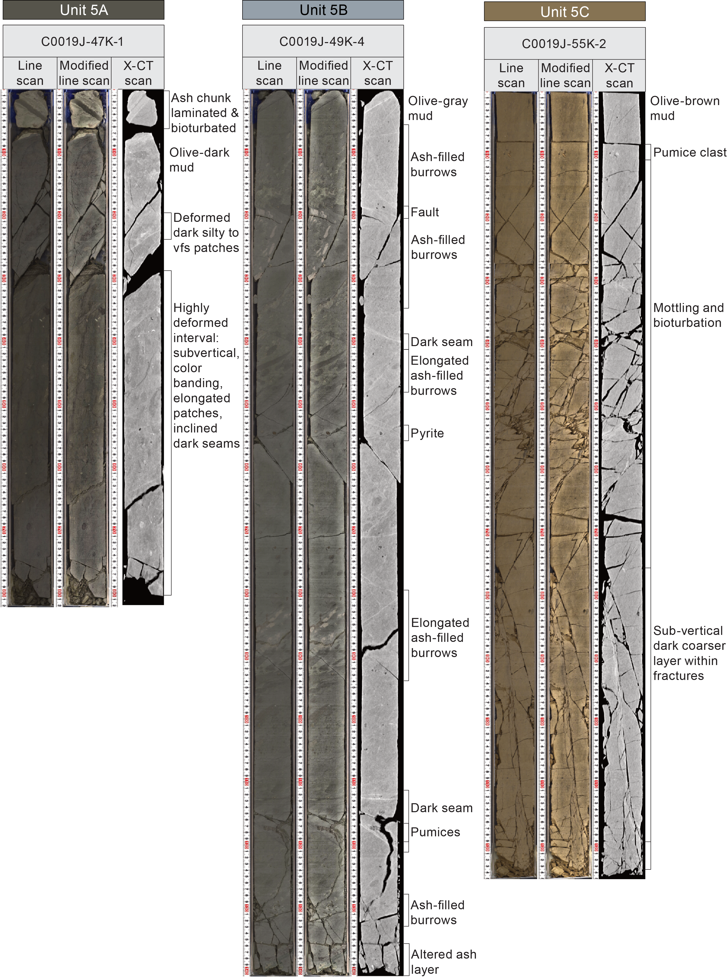
Figure F44. Unit 5 images.

Subunit 5A is moderately to heavily bioturbated and identifiable by many yellowish to brownish mottles and silt-filled burrows. These are visible in the XCT image and appear round to ellipsoidal with simple, unlined, and unbranched structures interpreted as Planolites.

4.1.5.1.2. Smear slide petrography

The grain size of the background sedimentation in Subunit 5A plots as mud (Figures F31, F45) with 2%–7% sand, 43%–78% silt, and 15%–50% clay (Table T14). The composition of the background sedimentation is siliceous to siliceous vitric mud (Figure F32) and is composed of siliciclastic (38%–52%), volcanic (13%–36%), and biogenic (20%–31%) material. Siliciclastic material is mostly clay minerals (24%–30%) and mud aggregates (0%–20%) with some quartz (3%–8%) and feldspar (0%–1%). Volcanic material is mostly clear glass (7%–31%), colored glass (0%–2%), and pumice (3%–9%). Biogenic material is mostly diatoms (10%–15%), radiolarians (0%–5%), and sponge spicules (5%–15%). Other material (4%–9% of total composition) includes framboidal pyrite and dense and opaque minerals. Notable is the presence of 2% calcite in what appears to be a calcite vein (Section 405-C0019J-46K-1, 70 cm).

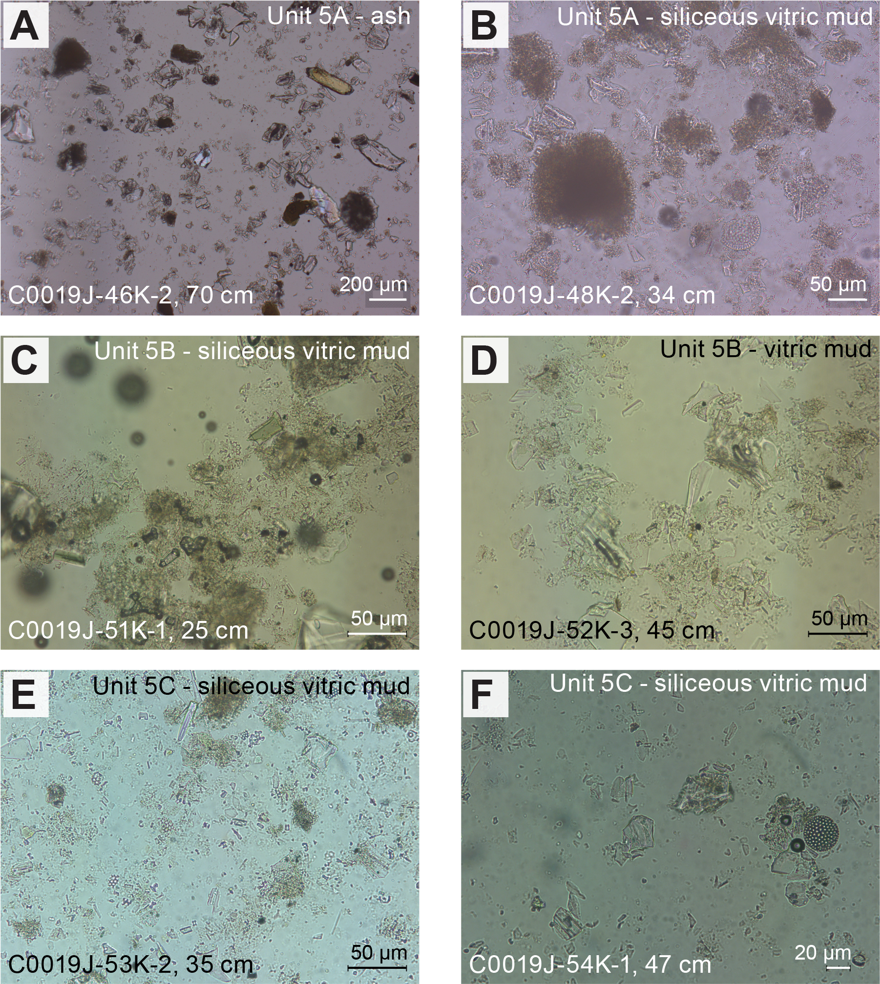
Figure F45. Unit 5 smear slides.

The ash layers (n = 4) are generally coarser than the background sedimentation, with 5%–80% sand, 15%–95% silt, and 0%–10% clay (Figure F31), and contain siliciclastic (5%–17%), volcanic (70%–90%), biogenic (0%–2%), and other (5%–12%) material (Table T14). Notable is the presence of a calcite-bearing (5%) ash layer in Subunit 5A (Section 405-C0019J-46K-2, 70 cm) and a calcite-bearing (5%) pumice clast (Section 46K-3, 70 cm).

4.1.5.1.3. Mineralogy and sediment geochemistry

A total of three bulk samples representative of Subunit 5A were collected for XRD analysis (Table T15). Clay mineral content dominates the composition and ranges 57–66 wt% clay minerals alongside 25–29 wt% plagioclase and 9–14 wt% quartz (Figure F34). The proportions of the quartz and plagioclase slightly decrease downcore in Subunit 5A, whereas clay content increases downcore (Figure F34). XRF and LOI analysis of the same samples yield the following elemental abundances (Figure F35; Table T16): 3.22–3.42 wt% Na₂O, 1.94–2.16 wt% MgO, 14.03–15.5 wt% Al₂O₃, 66.87–69.57 wt% SiO₂, ~0.1 wt% P₂O₅, 2.21–2.58 wt% K₂O, 2.59–3.25 wt% CaO, 0.5–0.66 wt% TiO₂, 0.06–0.07 wt% MnO, 5.07–6.02 wt% Fe₂O₃, and 5.21–5.34 wt% LOI.

4.1.5.1.4. Summary and preliminary interpretation

Subunit 5A consists of olive-black siliceous vitric mud(stone) with a sharp color shift from Subunit 4B. Six ash layers were observed (some bearing calcite) in addition to ash patches and pumice. The unit is characterized by inclined (sometimes subvertical) and chaotic bedding consistent with deposition from mass transport processes.

4.1.5.2. Subunit 5B

Interval: 405-C0019J-49K-1, 0 cm, to 52K-1, 0 cm
Depth: 539.50–568.00 mbsf
Age: 2.7–13.0 Ma
Lithology: gray siliceous vitric mud(stone)

4.1.5.2.1. Visual core description lithology

Subunit 5B is composed of gray (7.5Y 4/1) siliceous vitric mud(stone) and is distinguished from Subunit 5A by a gradual color change from olive-black (7.5Y 3/1) to gray (7.5Y 4/1) between 539.50 and 542.39 mbsf (Sections 405-C0019J-49K-1, 0 cm, to 49K-3, 0 cm). Because of the chaotic nature of this unit, color variations occur throughout the core, including grayish yellow-brown (10YR 4/2), olive-black (7.5Y 3/1), and light gray (7.5Y 7/1), which result from variations in the relative abundance of volcanic and biogenic material. Subunit 5B contains chaotic bedding with frequent interspersed clasts. Deformed color banding, silty ash patches, ash layers, and scattered pumice are common (Figure F44). A total of 10 thin (<3 cm) volcanic ash layers were identified. Subunit 5A is moderately to heavily bioturbated, highlighted by abundant yellowish to brownish mottles, bioturbated ash beds, and ellipsoidal silt-filled burrows visible in the XCT images.

4.1.5.2.2. Smear slide petrography

The grain size of the background sedimentation in Subunit 5B plots as mud (Figures F31, F45) with 0%–60% sand, 10%–30% silt, and 30%–80% clay (Table T14). The composition of the background sedimentation is siliceous vitric mud (Figure F32) composed of siliciclastic (45%–63%), volcanic (15%–43%), and biogenic (5%–22%) material. Siliciclastic material is mostly clay minerals (20%–35%) and mud aggregates (0%–30%) with some quartz (0%–10%) and feldspar (5%–10%). Volcanic material is mostly clear glass (10%–40%), colored glass (0%–5%), and pumice (0%–3%). Biogenic material is mostly diatoms (1%–3%), radiolarians (0%–1%), silicoflagellates (0%–5%), and sponge spicules (3%–20%), which marks a significant decrease in the abundance of diatoms and radiolarians compared to other units. Other material (2%–10% of total composition) includes euhedral pyrite and dense and opaque minerals.

4.1.5.2.3. Mineralogy and sediment geochemistry

A total of three bulk samples representative of Subunit 5B were collected for XRD analysis (Table T15). Clay mineral content dominates the composition and ranges 69–72 wt% clay minerals alongside 13–14 wt% plagioclase and 15–17 wt% quartz (Figure F34). These data show Subunit 5B has a significant decrease in plagioclase and an increase in clay mineral content relative to Subunit 5A. XRF and LOI analysis from the same horizons give the following element compositions (Figure F35; Table T16): 2.8–3.02 wt% Na₂O, 2.05–2.25 wt% MgO, 15.01–15.66 wt% Al₂O₃, 66.24–68.75 wt% SiO₂, ~0.08 wt% P₂O₅, 2.67–2.73 wt% K₂O, 1.74–2.13 wt% CaO, ~0.6 wt% TiO₂, ~0.08 wt% MnO, 6.15–6.47 wt% Fe₂O₃, and 5.25–5.34 wt% LOI. These elemental concentrations are similar to those of Subunit 5A.

4.1.5.2.4. Summary and preliminary interpretation

Subunit 5B consists of gray siliceous vitric mud(stone) with a gradual color transition from Subunit 5A. A total of 10 ash layers are identified. The unit shows a decrease in biogenic material (occasionally as low as 0%) and an increase in volcanic material and discrete ash intervals compared to Unit 4 and Subunit 5A. Intervals of inclined bedding are interspersed with intervals of chaotic bedding with clasts, again suggesting deposition from mass transport processes.

4.1.5.3. Subunit 5C

Interval: 405-C0019J-52K-1, 0 cm, to 56K-5, 50 cm
Depth: 568.00–610.31 mbsf
Age: 2.7–13.0 Ma
Lithology: dull yellowish brown siliceous vitric mud(stone)

4.1.5.3.1. Visual core description lithology

Subunit 5C is composed of dull yellowish brown siliceous vitric mud(stone). The boundary between Subunits 5B and 5C is marked by a gradual transition in color from gray (7.5Y 4/1) to dull yellowish brown (10YR 5/4) from 568.00 to 577.50 mbsf (Sections 405-C0019J-52K-1, 0 cm, to 53K-1, 0 cm) (Figure F38). From 577.50 mbsf to the base of Subunit 5C at 610.30 mbsf (Section 56K-5, 50 cm) color variations include grayish yellow brown (10YR 5/2), dull brown (7.5YR 5/4), and dark grayish yellow (2.5Y 5/2). Deformed and inclined color-banded sediments are commonly identified throughout Subunit 5C alongside continuous silty ash layers and discontinuous patches and disseminated pumice (Figure F44). Notably, there is abundant evidence of dewatering and slumping features throughout. In Section 54K-1, there is a vertically stacked (not quite overturned) slump feature that shows evidence of loading between the ash and the background sedimentation.

The background sedimentation of Subunit 5C is moderately to heavily bioturbated, identified by abundant brownish gray mottles (Figure F44) and bioturbated ash beds visible in the XCT images as round to ellipsoidal structures. Occasionally, this heavy bioturbation obscured some of the features of the slumps. Isolated simple and unbranched burrows are identified as Planolites, alongside cross sections of unlined and unbranched burrows with uniformly thick arcuate backfill with a sharp burrow boundary, which have been interpreted as Taenidium. At the base of Subunit 5C, Section 405-C0019J-56K-5 includes an ~57 cm thick gradational change to a sharp fault contact. This interval is marked by three distinct layers from the top down: (1) a dull yellowish brown layer of Subunit 5C (Sections 56K-5, 0 cm, to 56K-5, 48 cm), (2) a 6 cm thick bluish gray clay (Sections 56K-5, 48 cm, to 56K-5, 54 cm), and (3) a dark olive-black layer of Subunit 6A (Sections 56K-5, 54 cm, to 56K-5, 56 cm) (Figure F46; Table T13). These layers comprise the fault (see Structural geology).

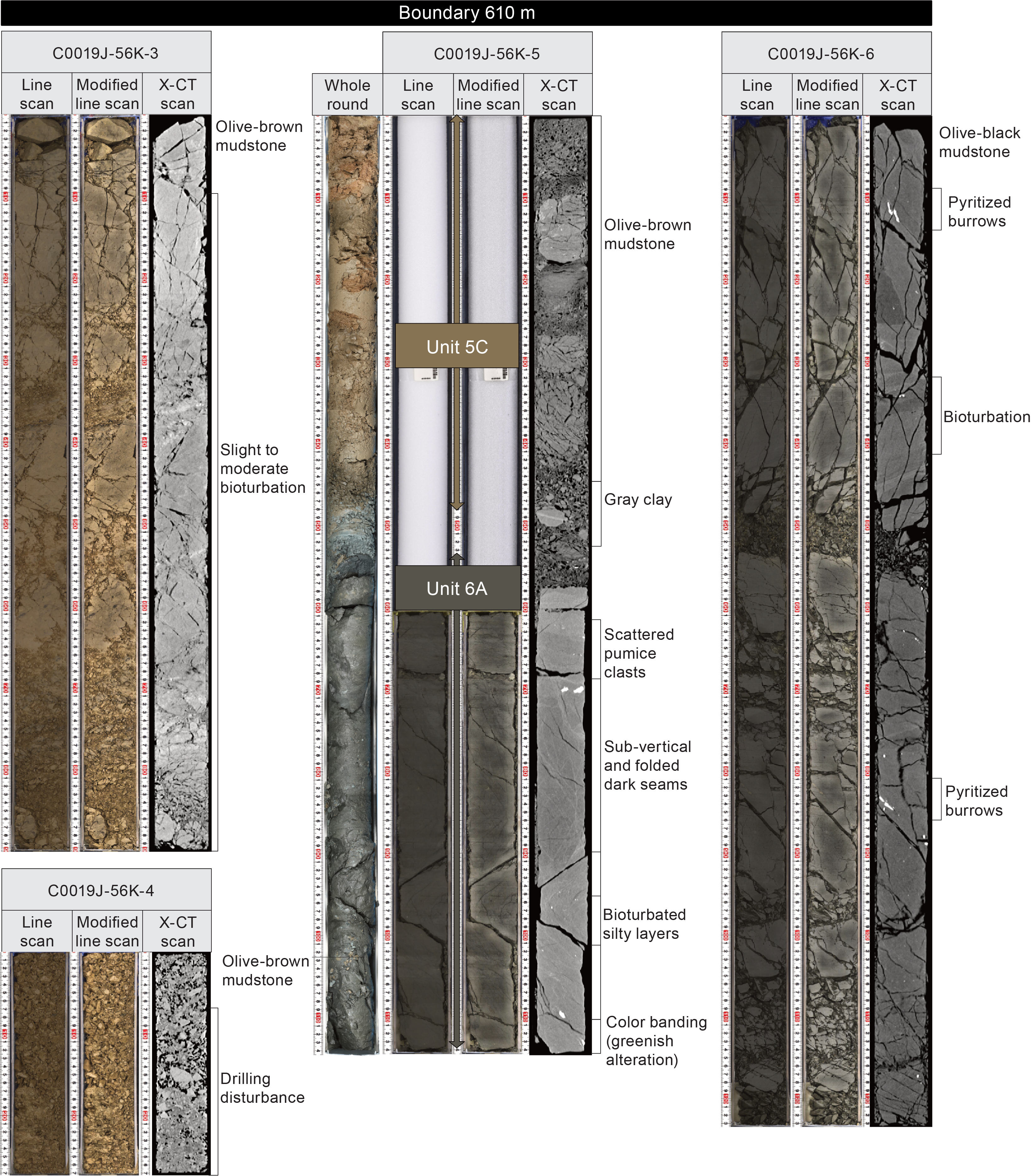
Figure F46. Transition and boundary layer between Subunits 5C and 6A.

4.1.5.3.2. Smear slide petrography

The grain size of the background sedimentation in Subunit 5C plots as clay (Figures F31, F45) with 0%–20% sand, 5%–90% silt, and 5%–95% clay (Table T14). The background sedimentation in Subunit 5C is siliceous vitric mud (Figure F32) composed of siliciclastic (19%–70%), volcanic (5%–45%), and biogenic (4%–69%) material. The siliciclastic material is mostly clay minerals (5%–70%) and mud aggregates (0%–15%) with some quartz (0%–10%) and feldspar (0%–5%). Volcanic material is mostly clear glass (5%–40%), colored glass (0%–10%) and pumice (0%–20%). Biogenic material is mostly diatoms (1%–25%), radiolarians (0%–3%), and sponge spicules (2%–35%). Other material (0%–10% of total composition) includes micas, framboidal and euhedral pyrite, Fe/Mn oxides, and opaque minerals. Notably, one sample near the base of Unit 5C (405-C0019J-55K-7, 39 cm) contains 62% calcareous nannofossils. Samples above (55K-7, 19 cm) and below (56K-1, 100 cm) include 50% and 25% calcite, respectively. All three samples were taken from the dull yellowish-brown mud(stone) lithology.

The ash layers are generally coarser (silt) with 0%–5% sand, 15%–95% silt and 5%–85% clay (n = 6) (Figure F31). The composition is volcanic with siliciclastic (0%–13%), volcanic (79%–100%), biogenic (0%–10%), and other (0%–5%) material (Table T14).

4.1.5.3.3. Mineralogy and sediment geochemistry

A total of 10 bulk samples representative of Subunit 5C were collected for XRD analysis (Table T15). Clay minerals are dominant (55–78 wt%), with lesser plagioclase (9–23 wt%) and quartz (12–22 wt%) (Figure F34). The overall proportions of the three components are consistent throughout the subunit.

XRF and LOI analysis yield elemental abundances of 2.67–3.42 wt% Na₂O, 1.54–2.27 wt% MgO, 14.71–16.87 wt% Al₂O₃, 65.83–69.66 wt% SiO₂, 0.08–0.11 wt% P₂O₅, 2.59–2.99 wt% K₂O, 1.45–2.23 wt% CaO, 0.52–0.67 wt% TiO₂, 0.1–0.75 wt% MnO, 4.76–7.12 wt% Fe₂O₃, and 4.01–6.5 wt% LOI, respectively (Figure F35; Table T16). A clear distinction can be made between the color transition zone from Subunit 5B to Subunit 5C (first six measurements) and the background sedimentation of Subunit 5C. Additionally, a distinct peak in MnO (0.75 wt%) is noted in interval 405-C0019J-53K-3, 0–15 cm. Interestingly, no increase in CaO is observed in the interval where calcite/nannofossils are observed.

4.1.5.3.4. Summary and preliminary interpretation

Subunit 5C consists of dull yellowish brown siliceous vitric mud(stone) with a gradual color transition from Subunit 5B. Six ash layers were identified. This unit has a pronounced increase of diatoms and pelagic biogenic material compared to Subunit 5B. It is characterized by chaotic bedding. Flame structures at the top of ash layers indicate soft-sediment deformation. Samples close to the base of the unit are enriched in calcareous nannofossils and calcite. These characteristics suggest deposition from mass transport processes, with some sediment input from shallower regions of the slope.

4.1.6. Unit 6

4.1.6.1. Subunit 6A

Interval: 405-C0019J-56K-5, 50 cm, to 73K-6, 0 cm
Depth: 610.27–774.31 mbsf
Age: 0–2.7 Ma
Lithology: olive-black siliceous vitric mud(stone)

4.1.6.1.1. Visual core description lithology

The upper boundary of Subunit 6A at 610.27 mbsf (Section 405-C0019J-56K-5, 50 cm) is marked by a fault (see Structural geology) with a sharp change from the yellowish brown mud(stone) of Subunit 5C to olive-black mud(stone) (Figure F46). The background sedimentation of Subunit 6A consists of olive-black siliceous vitric mud(stone) interbedded with intervals of chaotic sediments including calcareous material mixed into the background sedimentation and disseminated pumice clasts. The background sedimentation is characterized by mottling, scattered pumice clasts, and pyritized burrows (e.g., Section 57K-4). Thin, millimeter-scale, wispy, black and green color banding is common (Figure F47). Color-banded intervals tend to be more clay rich and occasionally display convolute laminae (e.g., Section 62K-5). These intervals often include clasts or blocks of a mixture of sediments including a calcareous component and one chert granule (e.g., Section 69K-4; Figure F40). Three other thin (2 cm) layers of calcareous mud were observed in Sections 60K-3, 30 cm, 63K-4, and 69K-2 (tested with HCl). In general, bioturbation is relatively uncommon in Subunit 6A, with heavy bioturbation only within ash beds. Where bioturbation does occur, the burrows are often pyritized.

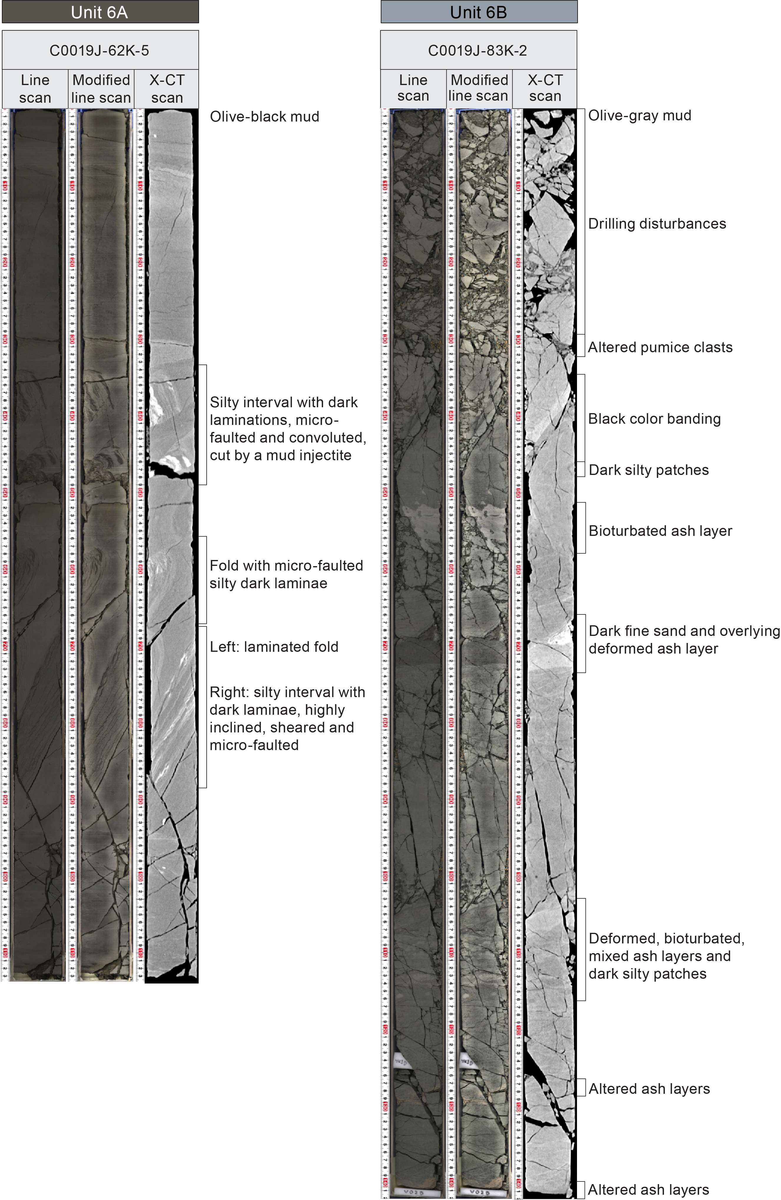
Figure F47. Unit 6 images.

4.1.6.1.2. Smear slide petrography

The grain size of the background sedimentation in Subunit 6A is mud (Figures F31, F48) with 0%–30% sand, 5%–95% silt, and 0%–92% clay (Table T14). The composition of the background sedimentation is siliceous to siliceous vitric mud (Figure F32) composed of siliciclastic (8%–90%), volcanic (3%–52%), and biogenic (2%–77%) material. Siliciclastic material is mostly clay minerals (0%–55%) and mud aggregates (0%–65%) with some quartz (0%–15%) and feldspar (0%–15%). Volcanic material is mostly clear glass (2%–49%), colored glass (0%–10%), and pumice (0%–15%). Biogenic material is mostly diatoms (3%–50%), radiolarians (0%–30%), silicoflagellates (0%–10%), and sponge spicules (0%–20%). Some intervals contain notable abundances of calcareous mud with calcite (0%–15%) (e.g., Sections 405-C0019J-59K-2, 72 cm, and 60K-3, 23 cm) and/or calcareous nannofossils (16%) (e.g., Sections 58K-6, 74 cm, and 59K-2, 72 cm). Other material (0%–25% of total composition) includes dense or opaque minerals, micas, pyrite, glauconite, organic matter, and calcite.

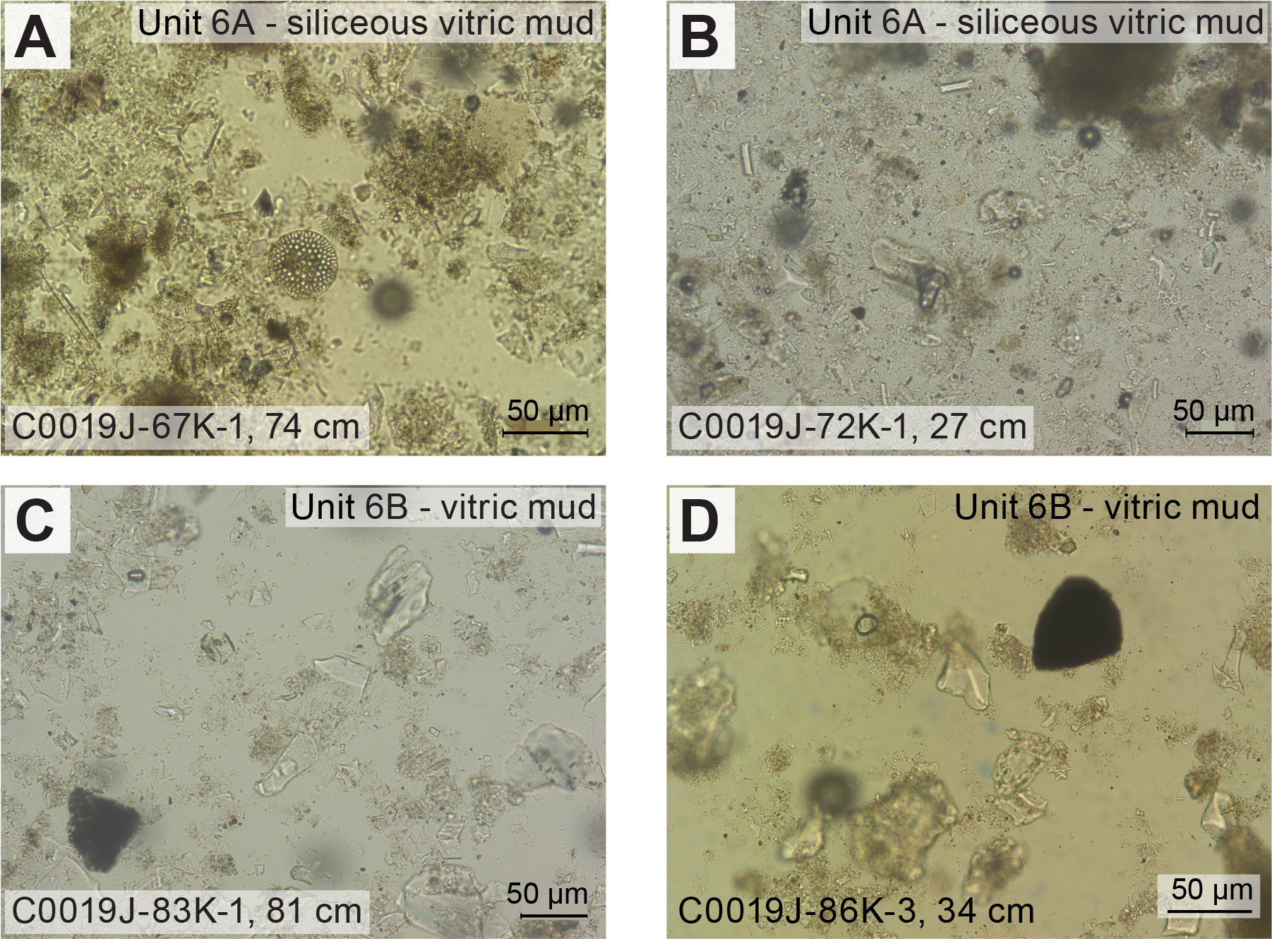
Figure F48. Unit 6 smear slides.

The scattered ash patches and pumice clasts are coarser (silt) than the background sedimentation (Figure F31), with 5%–50% sand, 40%–95% silt, and 0%–55% clay (n = 5). They are composed of siliciclastic (15%–17%), volcanic (60%–77%), biogenic (0%–12%), and other (5%–18%) material (Table T14). In places, pumice clasts appear to have been compressed to become more elongated (e.g., Section 405-C0019J-65K-2). Notable is one calcite- (2%) and zeolite-bearing (10%) ash layer (Section 69K-4, 29 cm).

4.1.6.1.3. Mineralogy and sediment geochemistry

A total of 23 bulk samples representative of Subunit 6A were collected for XRD analysis (Table T15). Clay mineral content dominates the composition (46–70 wt%), with lesser plagioclase (9–27 wt%) and quartz (8–25 wt%) (Figure F34). Plagioclase concentrations show an overall increase toward the base of the subunit. Two samples have anomalous calcite results of 38% (interval 405-C0019J-59K-2, 59.0–61.0 cm) and 4% (interval 67K-2, 56.0–58.5 cm), supporting the observation of calcareous rich intervals in the VCDs and smear slides.

XRF and LOI analysis show that Subunit 6A contains the following (Figure F35; Table T16): 2.08–3.78 wt% Na₂O, 1.22–4.21 wt% MgO, 10.89–16.47 wt% Al₂O₃, 48.41–74.27 wt% SiO₂, 0.07–0.44 wt% P₂O₅, 1.51–2.86 wt% K₂O, 1.39–18.69 wt% CaO, 0.35–0.73 wt% TiO₂, 0.06–0.87 wt% MnO, 3.29–11.41 wt% Fe₂O₃, and 1.86–19.74 wt% LOI. The sample that yielded 38 wt% calcite in XRD also yielded high CaO results of 18.69 wt%.

4.1.6.1.4. Summary and preliminary interpretation

Subunit 6A consists of olive-black siliceous vitric mud(stone). Its upper contact at 610.31 mbsf is a fault contact (see Structural geology) with Subunit 5C. The fault is accompanied by an age reversal from Miocene to Pleistocene age (see Biostratigraphy) and a sharp shift in lithology and color. A total of 20 ash layers were identified. The unit is characterized by frequent intervals of inclined (sometimes subvertical) bedding as well as chaotic, deformed bedding interspersed with scattered pumice clasts, localized appearances of calcareous nannofossils, mudstone clasts, and one chert granule. Convolute laminae indicate soft-sediment deformation. These features suggest deposition driven by mass transport processes from shallower regions of the slope.

4.1.6.2. Subunit 6B

Interval: 405-C0019J-73K-6, 0 cm, to 87K-2, 60 cm
Depth: 774.31–826.08 mbsf
Age: 0–6.7 Ma
Lithology: greenish gray siliceous vitric mud(stone)

4.1.6.2.1. Visual core description lithology

The top of Subunit 6B from 774.31 to 807.00 mbsf (Sections 405-C0019J-73K-6, 0 cm, to 81K-1, 0 cm) is marked by a gradual color change from olive-black (7.5Y 3/1) to greenish gray (7.5GY 3/1) (Figure F38). Sedimentary features in this transitional interval include green-black color banding, chaotic bedding with subvertical contacts, scattered pyrite, and frequent beds of sandy laminae (e.g., Sections 77K-2 and 77K-3; Figure F47). Below 807.00 mbsf (Section 81K-1, 0 cm), the background sedimentation of Subunit 6B consists of greenish gray siliceous vitric mud(stone) with frequent chaotic bedding; subrounded pumice patches; and ~30 inclined, deformed beds of light brown, reddish, or greenish altered ash. Other sedimentary features within the background sedimentation of Subunit 6B are green-black color banding and calcite-bearing ash layers (e.g., Section 85K-3, 56 cm). At the base of the unit in Section 86K-2, 85 cm, there is a color change to a dull yellowish gray. Moderate bioturbation is common throughout Subunit 6B, with an example of ribbed burrows (possibly Rhizocorallium) in Section 81K-1.

4.1.6.2.2. Smear slide petrography

The grain size of the zone of color change (774.31–807.00 mbsf) is mud with 0%–20% sand, 0%–95% silt, and 5%–100% clay and a composition of vitric mud(stone) with clastic (20%–95%), volcanic (3%–40%), and biogenic (1%–50%) materials (Table T14; Figures F31, F32, F48). Below the color change zone, the grain size is mud with 0%–40% sand, 20%–60% silt, and 30%–80% clay. The background sedimentation plots as a siliceous vitric mud composed of siliciclastic (15%–80%), volcanic (10%–40%), and biogenic (5%–35%) material. The siliciclastic material is dominated by clay minerals (0%–45%) and mud aggregates (2%–45%) with some quartz (0%–20%) and feldspar (1%–15%). Biogenic material is mainly diatoms (0%–30%), radiolarians (0%–10%), silicoflagellates (0%–5%), and sponge spicules (0%–15%). Volcanic material is mostly clear glass (10%–32%), colored glass (0%–10%), and pumice (0%–15%). Other material (1%–15% of total composition) includes pyrite, micas, opaque minerals, and dense minerals. Several samples throughout the transition zone and the rest of Subunit 6B contain low amounts of calcite (0%–7%), and one sample from a calcite vein in Section 405-C0019J-85K-3, 42 cm, is composed of 70% calcite.

The ash layers within Subunit 6B are generally coarser (silt) with 0%–50% sand, 40%–80% silt, and 10%–20% clay (Figure F31). They are compositionally ashy/vitric mud to ash and composed of siliciclastic (11%–25%), volcanic (68%–86%), and other (3%–11%) material (Table T14).

4.1.6.2.3. Mineralogy and sediment geochemistry

A total of 18 bulk samples representative of Subunit 6B were collected for XRD analysis (Table T15). Clay mineral content dominates the composition and ranges 52–92 wt% (Figure F34). Plagioclase ranges 3–28 wt%, and quartz ranges 5–26 wt%. Plagioclase exhibits variability with an overall declining trend with depth. Conversely, clay concentrations initially gradually increase and then stabilize from Core 405-C0019J-80K to two increased values at the base of the unit in Core 87K. XRF and LOI results indicate 2.59–3.66 wt% Na₂O, 1.44–2.67 wt% MgO, 14.15–15.82 wt% Al₂O₃, 64.73–70.54 wt% SiO₂, 0.07–0.23 wt% P₂O₅, 2.40–2.92 wt% K₂O, 1.42–2.74 wt% CaO, 0.52–0.72 wt% TiO₂, 0.05–0.95 wt% MnO, 4.59–7.56 wt% Fe₂O₃, and 5.12–9.01 wt% LOI (Figure F35; Table T16). Most elements exhibit concentrations comparable to those in the subunits above and below, except for MnO and MgO. MgO concentrations show a sharp decline in the middle of Subunit 6B, followed by a gradual return to baseline levels. In contrast, MnO concentrations are elevated to Core 79K before dropping back to the normal range.

4.1.6.2.4. Summary and preliminary interpretation

Subunit 6B consists of greenish gray vitric mud(stone) with a gradual color transition from Subunit 6A. A total of 30 lighter gray ash layers and discontinuous patches were identified (some bearing calcite). There is an increase of altered pumice. The unit is characterized by inclined and chaotic bedding interspersed with clasts. Convolute bedding indicates soft-sediment deformation. These properties alongside the occasional presence of calcite are consistent with deposition from mass transport processes.

4.1.7. Unit 7

Interval: 405-C0019J-87K-2, 60 cm, to 88K-CC, 14 cm
Depth: 826.07–829.09 mbsf
Age: 6.3–6.6 Ma
Lithology: color-banded clay and chert

4.1.7.1. Visual core description lithology

Unit 7 consists of color-banded clays and chert covering the interval 826.07–29.09 mbsf (Sections 405-C0019J-87K-2, 60 cm, to 88K-CC, 14 cm) (Figure F29; Table T13). The unit begins at 826.07 mbsf (Section 87K-2, 60 cm; Figure F49) and is marked by a sharp contact between the overlying blueish gray (5BG 5/1), olive-gray (10Y 4/2), and yellowish gray (2.5Y 5/1) mud and the dark grayish brown clay (10YR 4/2) (Figure F38). This contact is identified as the upper contact of a layer of fault rock that defines the plate boundary fault zone (PBFZ) (see Structural geology). In the XCT image, the brown clay appears slightly brighter than the underlying color-banded clays. Immediately beneath the brown clay, in interval 87K-2, 87–115 cm, color-banded clays show centimeter-scale alternations of orange (5YR 6/6 to 5YR 4/6), black (10YR 1.7/1), and dull yellow-orange (10YR 7/3) layers. Among these, dull yellow-orange is the dominant color, with black layers at 96–97 cm, 98–100 cm, and 107–110 cm in Section 87K-2.

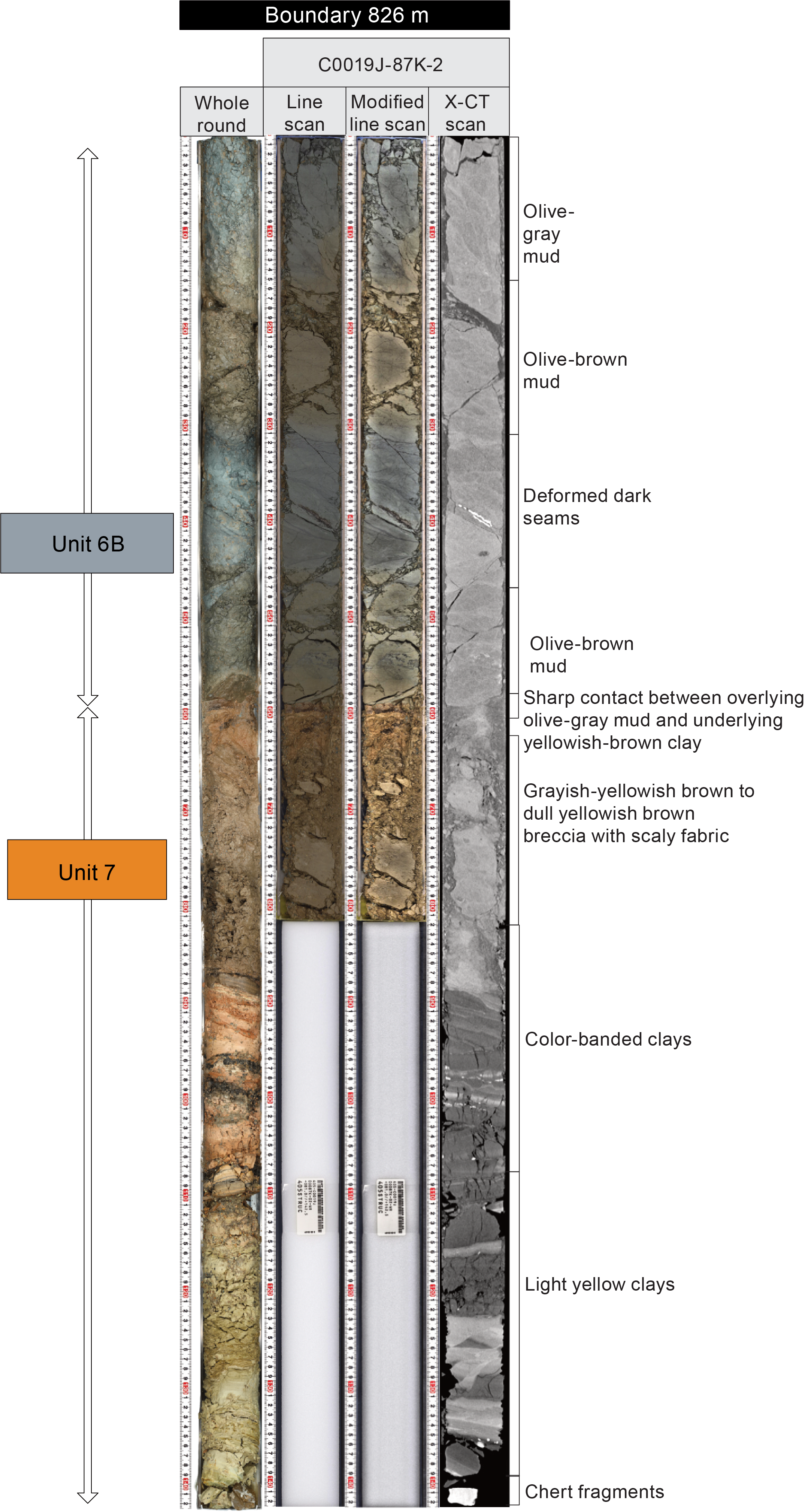
Figure F49. Transition and boundary layer between Subunit 6B and Unit 7.

Below the color-banded clays, light yellow clay (5Y 7/3) is observed in Sections 405-C0019J-87K-2, 115 cm, to 87K-CC, 12 cm. This clay has millimeter-scale gray laminae and shows enrichment in SiO₂ microlites in smear slide observations. Three intervals within this section appear brighter in XCT. A subangular pebble of light gray chert (5Y 7/2) is present at the bottom of Section 87K-2 (140–142 cm) (Figure F49). Bright reddish brown chert (5YR 5/8) only appears in this core as pebbles of the drilling breccia.

4.1.7.2. Smear slide petrography

The grain size of the sediments of Unit 7 is predominantly mud with 60%–95% clay, 0%–15% sand, and 3%–25% silt (Figures F31, F50). Compositionally, Unit 7 is predominantly siliciclastic (62%–94%) with minor contributions of volcanic (0%–30%), biogenic (2%–25%), and other material (2%–17%) (Figure F32; Table T14). One sample from Section 405-C0019J-87K-2, 137 cm (although we note smear slide samples were taken from the outside of a whole round and may be contaminated), contains approximately 20% calcareous nannofossils.

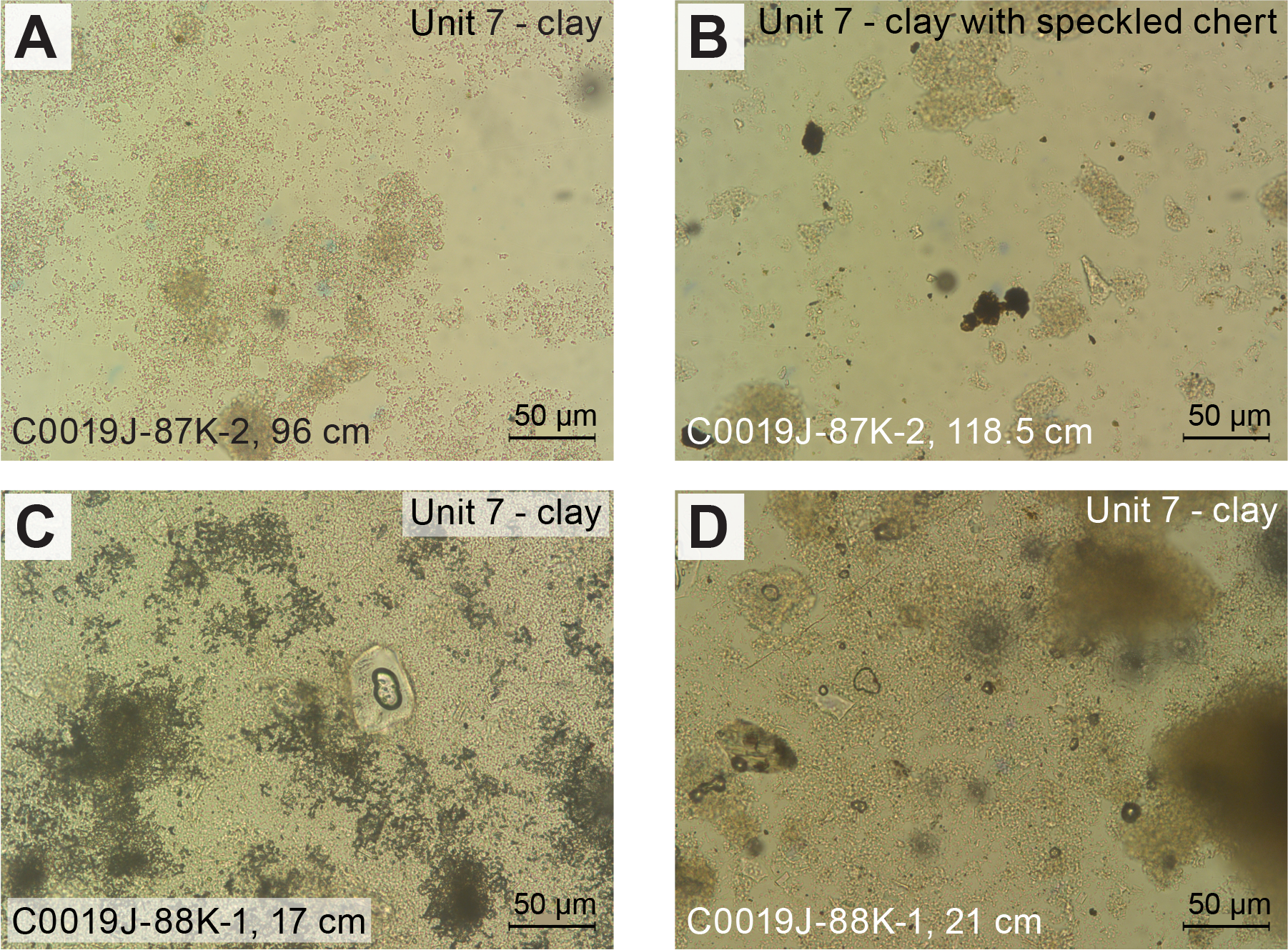
Figure F50. Unit 7 smear slides.

4.1.7.3. Mineralogy and sediment geochemistry

A total of five samples representative of Unit 7 were collected for XRD analysis (Table T15): one from brown clay (interval 405-C0019J-87K-2, 73–74 cm), one from color-banded clay (dull yellowish brown in interval 87K-2, 94–98 cm), two from light yellow clay (intervals 87K-2, 117–119 cm, and 124–126 cm), and one from chert (interval 87K-2, 140–142 cm) (Figure F34). The brown and light yellow clays exhibit high clay contents (70–96 wt%) with low quartz (<18 wt%) and plagioclase (<12 wt%). The dull yellowish brown clay shows a high quartz content (42 wt%), whereas the chert sample indicates an unexpectedly lower quartz content (66 wt%).

Four samples from the color-banded clays were analyzed for element composition using XRF (Table T16; Figure F35). The results for the semisilicified dull yellowish brown color-banded clay (interval 405-C0019J-87K-2, 94–98 cm) are 0.99 wt% Na₂O, 0.97 wt% MgO, 3.64 wt% Al₂O₃, 91.26 wt% SiO₂, 0.26 wt% P₂O₅, 0.85 wt% K₂O, 0.58 wt% CaO, 0.16 wt% TiO₂, 0.014 wt% MnO, 1.98 wt% Fe₂O₃, and 3.63 wt% LOI. The results for the light yellow clays (intervals 405-C0019J-87K-2, 117–119 cm, and 124–126 cm) are 1.27–2.79 wt% Na₂O, 1.22–3.54 wt% MgO, 4.06–11.59 wt% Al₂O₃, 61.83–88.62 wt% SiO₂, 0.13–0.21 wt% P₂O₅, 1.00–2.55 wt% K₂O, 0.46–1.61 wt% CaO, 0.19–0.73 wt% TiO₂, 0.083–0.088 wt% MnO, 4.05–14.72 wt% Fe₂O₃, and 4.02–8.31 wt% LOI. For the chert (interval 87K-2, 140–142 cm) the results are 0.26 wt% Na₂O, 0.44 wt% MgO, 0.92 wt% Al₂O₃, 94.94 wt% SiO₂), 0.048 wt% P₂O₅, 0.50 wt% K₂O, 0.093 wt% CaO, 0.066 wt% TiO₂, 0.005 wt% MnO, 2.64 wt% Fe₂O₃, and 2.43 wt% LOI. XRF results show high SiO₂values for all color-banded clays, indicating their enrichment in silica. For the chert, the SiO₂ value is characteristic.

4.1.7.4. Summary and preliminary interpretation

Unit 7 consists of semilithified color-banded clay and chert separated from Subunit 6B by a major fault (826.08 mbsf). Both lithologies exhibit millimeter-scale laminae and enrichment of SiO₂ microlites and SiO₂ content measured by XRF increases downcore, indicating a progressive change.

4.2. Lithostratigraphic units of Hole C0019K

Three main lithostratigraphic units were recognized in cores from Hole C0019K (Table T17; Figure F51). The lithostratigraphic units are numbered from top to bottom as Units K1–K3. The detailed lithologic descriptions of each presented below are based on the same sets of shipboard data described above for Holes C0019L, C0019M, and C0019J (Figures F52, F47, F59, F60, F62).

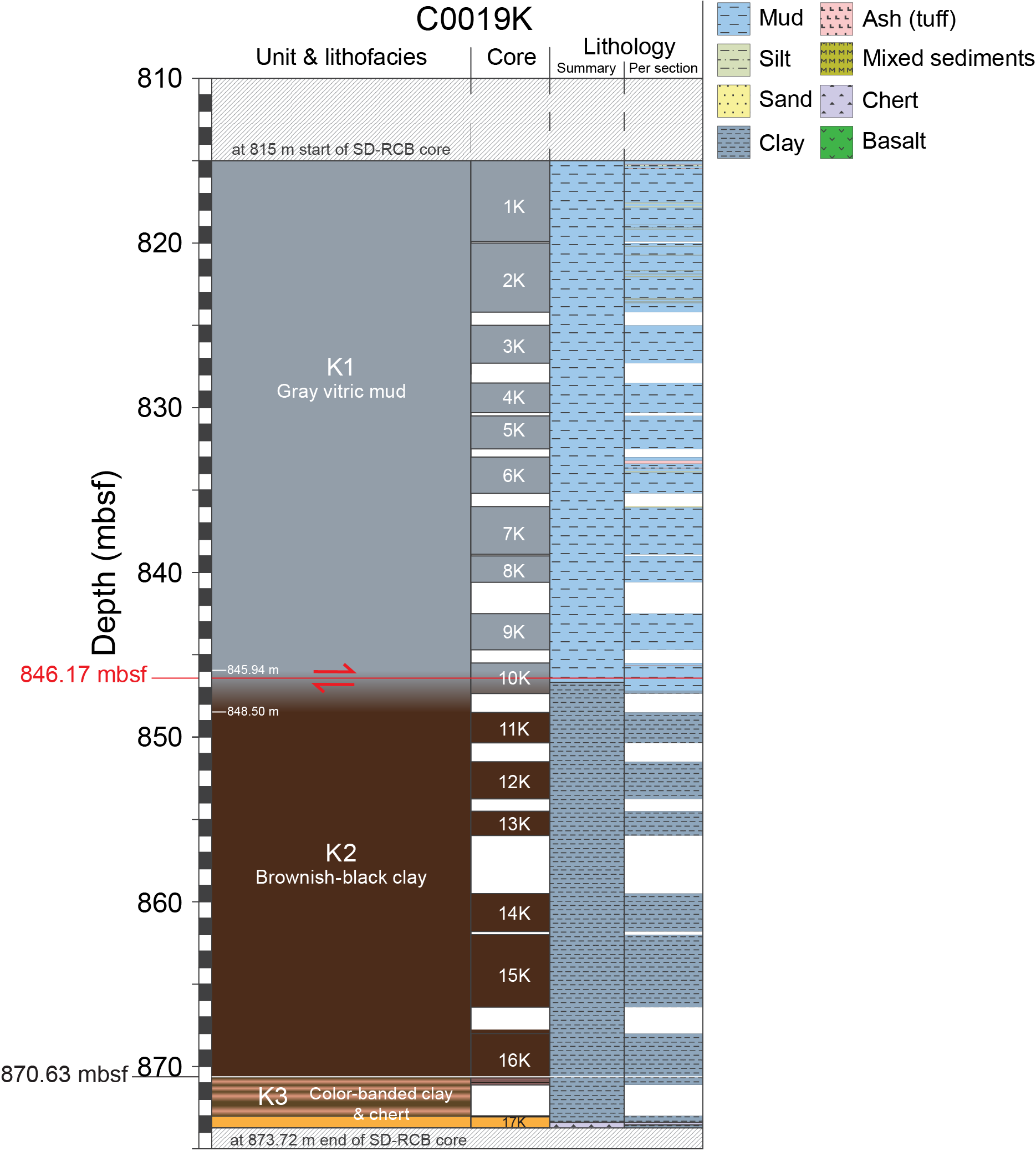
Figure F51. Lithostratigraphic units, Hole C0019K.

4.2.1. Unit K1

Interval: 405-C0019K-1K-1, 0 cm, to 10K-2, 87 cm
Depth: 815.00–846.70 mbsf
Age: 0.30–7.7 Ma
Lithology: olive-gray vitric mud(stone)

4.2.1.1. Visual core description lithology

Unit K1 consists of gray (2.5GY 3/1) vitric mud(stone) (Figure F52) interbedded with (1) upward-fining light gray or dark green ash layers and patches (2 mm to 5 cm thick) and (2) intervals of chaotic, mixed sediment composed of variable clay/silt compositions and ash, occasionally with a block and matrix texture (Figure F53). Chaotic bedding and inclined bedding with occasionally folded and truncated structures are observed (e.g., Section 405-C0019K-6K-1). In Cores 4K–6K, there is a chaotic mix of clasts of different lithologies with sharp edges intercalated within a mud(stone) background that has convolute or irregular laminae (e.g., intervals 6K-1, 10–15 cm, and 4K-2, 58–63 cm). Within the chaotic intervals, stacked layers and remobilized clasts often display a fining-upward texture from very fine sand to silt, occasionally with coarse, pyritized grains at the base (e.g., interval 4K-2, 39–48 cm). The presence of wispy convolute laminae within chaotic intervals and the background sedimentation indicates soft-sediment deformation (e.g. interval 4K-2, 92–108 cm).

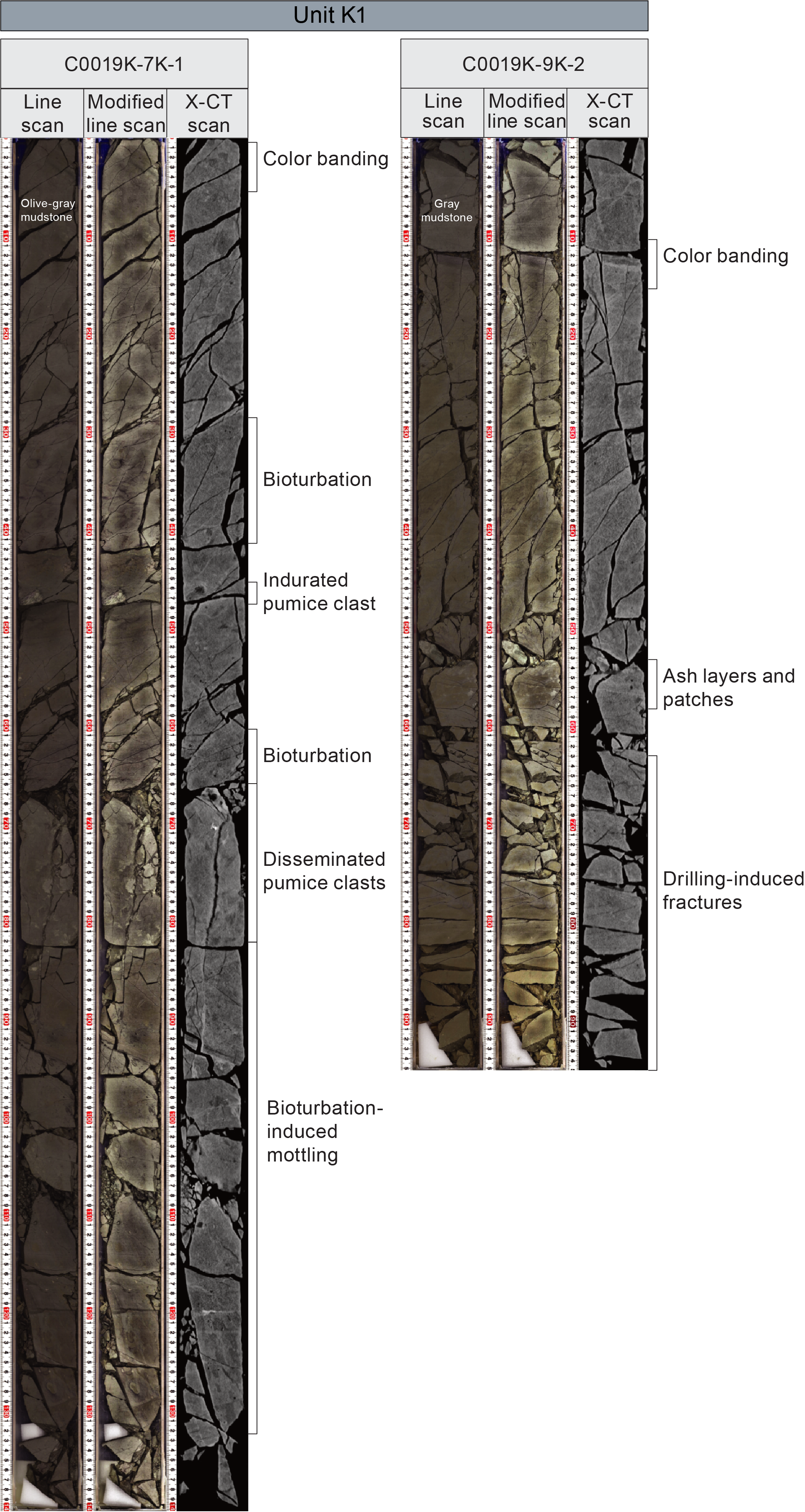
Figure F52. Unit K1 images.

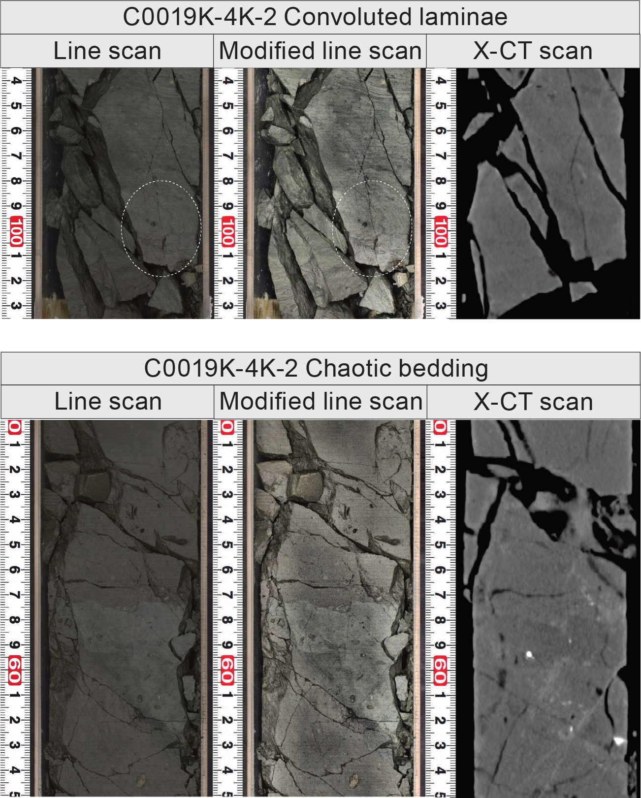
Figure F53. Sedimentary structures, Hole C0019K.

The color of the graded ash-rich layers and patches ranges between dark greenish gray (10GY 4/1 to 5G 3/1), gray (10Y 4/1), greenish gray (10GY 5/1), and brownish gray (10Y 3/2), mostly reflecting changes in the abundance and alteration of volcanic components (e.g., interval 405-C0019K-4K-2, 58–63 cm). Subrounded pumice clasts (4 cm to <10 mm) are disseminated throughout Unit K1 (Figure F52). Pumice clasts are usually light gray but often display green or red alteration and occasionally black if they are pyritized. Both background sedimentation and chaotic intervals in Unit K1 are moderately bioturbated and identifiable by subhorizontal and subvertical lighter or darker mottles in contrast with the gray background sedimentation (e.g., interval 6K-2, 71–77 cm). Some burrows show black coloration due to the presence of pyrite. In particular, bioturbation with distinct crosscutting relationships is often present above ash layers.

Near the base of Unit K1 in Section 405-C0019K-10K-2 (845.94 mbsf), there is a zone where the color changes from olive-gray (2.5GY 3/1) to brownish gray (10Y 3/2) between 0 and 11 cm and then to yellowish brown (10YR 4/2) between 11 and 34 cm (Figure F54). The boundary between Unit K1 and Unit K2 underlies this zone at 846.17 mbsf (Section 10K-2, 34 cm). This boundary is noted as the PBFZ (see Structural geology).

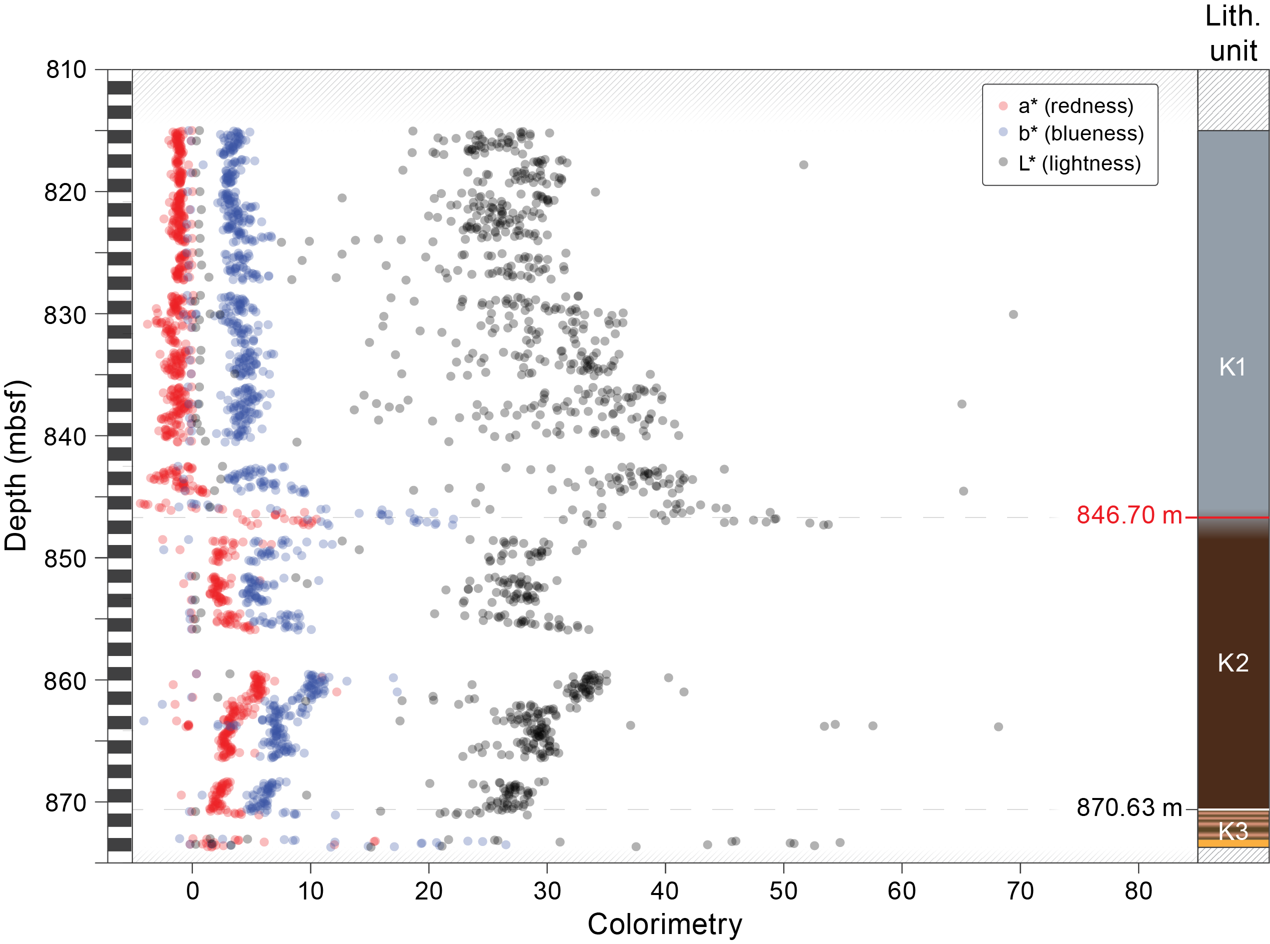
Figure F54. Core colorimetry, Hole C0019K.

4.2.1.2. Smear slide petrography

The grain size of the background sediments in Unit K1 is mud (Figure F55) with 20%–85% clay, 0%–65% silt, and 0%–30% sand (Table T18). The average composition of Unit K1 is vitric mud, and it consists of siliciclastic grains (33%–80%) and volcanic (10%–50%) and biogenic (4%–25%) components. The abundance of siliciclastic material generally increases with depth throughout Unit K1, whereas volcanic material decreases. Siliciclastic grains are mostly clay minerals (20%–65%), mud aggregates (0%–15%), quartz (1%–20%), and feldspar (1%–20%). The biogenic component is a mixture of diatoms (0%–12%), radiolarians (0%–5%), and sponge spicules (0%–15%). Other minor components (1%–25%) include dense and opaque minerals, calcite, and framboidal pyrite.

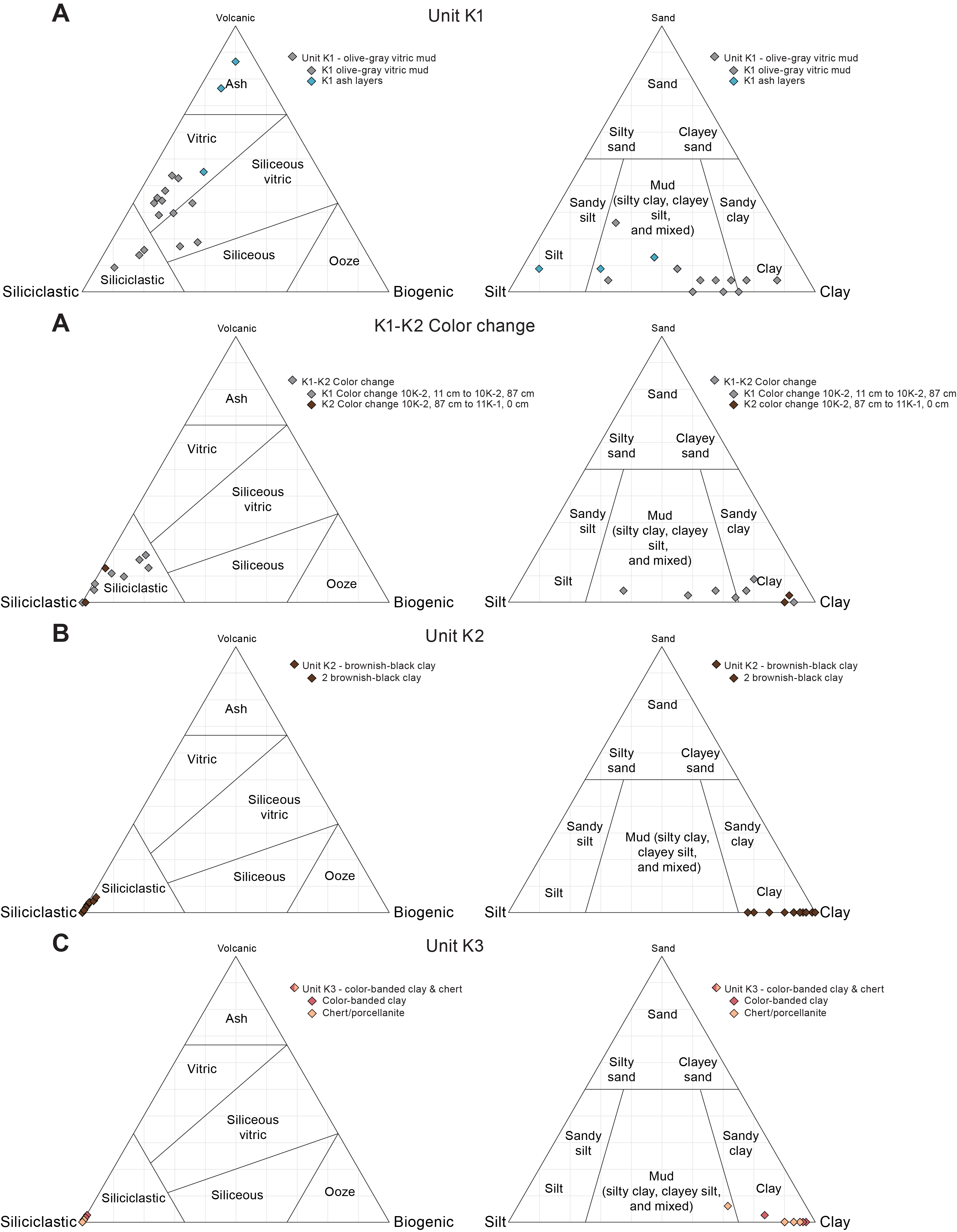
Figure F55. Sediment composition and grain size.

The grain size of ash layers is silt (45%–85%) with sand (10%–15%) and clay (5%–40%). It is compositionally volcanic and contains primarily volcanic components (50%–97%), with lesser amounts of siliciclastic (0%–33%) and biogenic (0%–13%) material. The volcanic component contains clear glass (35%–80%), colored glass (4%–7%), and pumice (10%) (Figure F56). Few samples (Sections 405-C0019K-2K-3, 56.5 cm, 5K-1, 19 cm, and 6K-2, 23 cm) contain calcite (2%–10%), and one section (2K-3, 56.5 cm) contains calcareous nannofossils (2%).

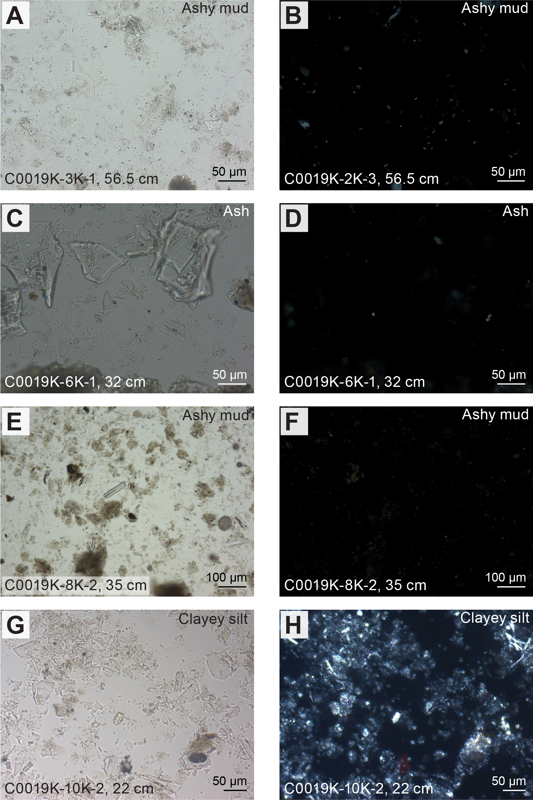
Figure F56. Unit K1 smear slides.

Within the color change zone at the base of Unit K1, the grain size of the mud(stone) decreases to mud and clay, with only 0%–10% sand, 7%–60% silt, and 35%–93% clay (Figure F55; Table T18). Siliciclastic material still dominates the composition (66%–92%) but has significantly decreased volcanic (0%–20%) and biogenic (0%–13%) components.

4.2.1.3. Mineralogy and sediment geochemistry

A total of 12 bulk samples representative of Unit K1 were collected for XRD analysis (Table T19). Clay mineral content dominates the composition (50–73 wt%), with lesser amounts of quartz (13–24 wt%) and plagioclase (13–32 wt%) (Figure F57). There are no observable downcore trends in XRD data in Unit K1, despite color changes near the base of the unit.

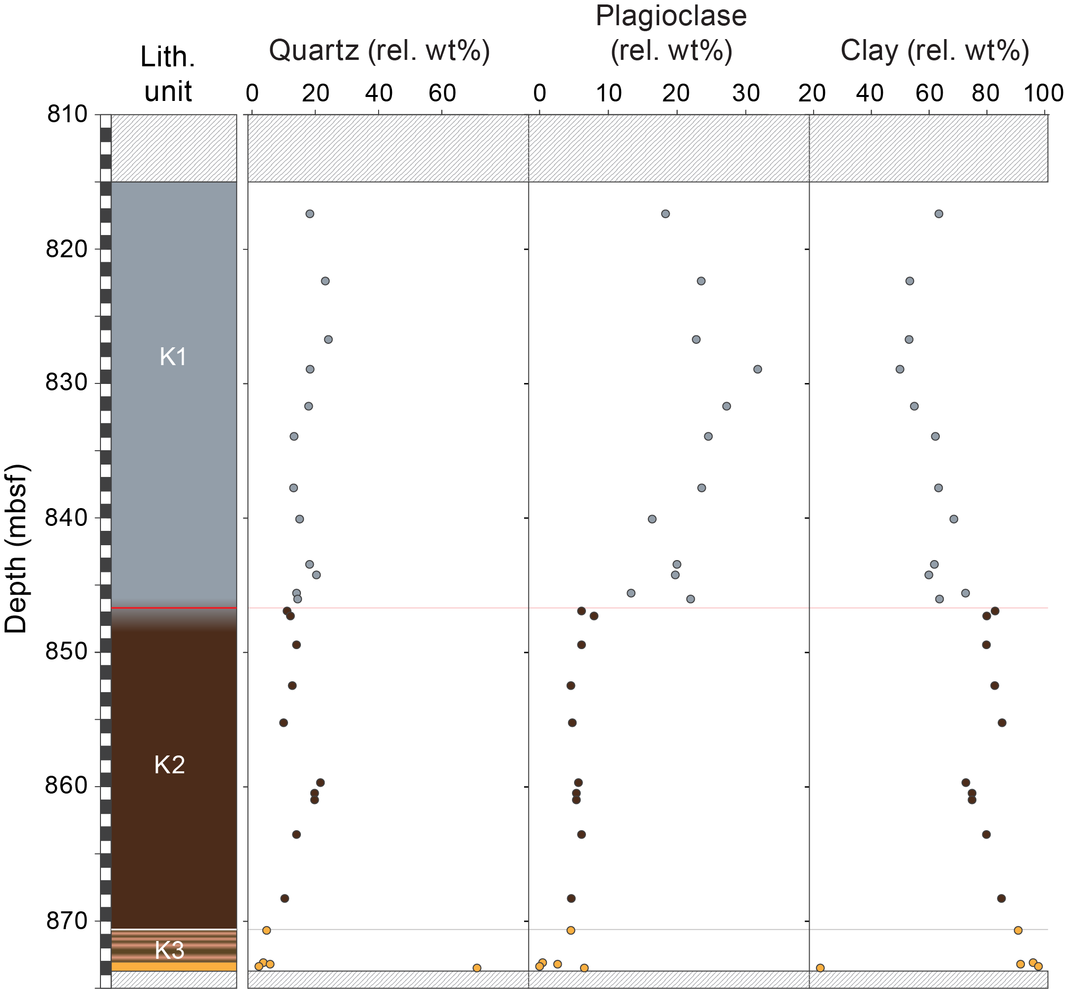
Figure F57. Semiquantitative mineral abundance analysis, Hole C0019K.

XRF and LOI analysis on the same samples yield the following: 2.83–3.20 wt% Na₂O, 1.52–2.51 wt% MgO, 13.86–15.88 wt% Al₂O₃, 66.12–70.51 wt% SiO₂, 0.07–0.30 wt% P₂O₅, 2.11–2.85 wt% K₂O, 1.88–2.70 wt% CaO, 0.51–0.70 wt% TiO₂, 0.06–0.26 wt% MnO, 4.86–6.29 wt% Fe₂O₃, and 4.14–7.52 wt% LOI (Figure F58; Table T20). Silica likely occurs in volcanic glass, biogenic silica, and clastic grains. Aluminum likely occurs in clay minerals and plagioclase. High iron concentrations likely occur in terrigenous components.

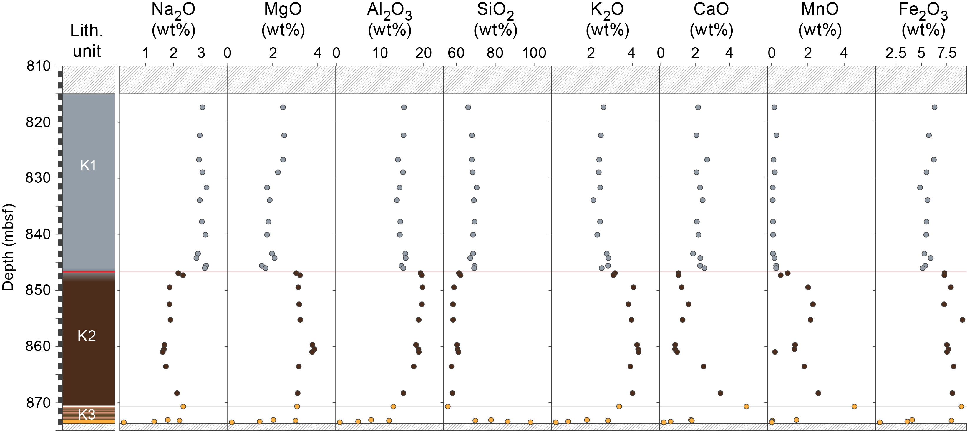
Figure F58. Major element compositions, Hole C0019K.

4.2.1.4. Summary and preliminary interpretation

Unit K1 consists of gray vitric mud(stone) interspersed with seven ash layers. The unit is characterized by chaotic bedding with fining-upward layers and deformed discontinuous ash patches. Some layers include occasional calcareous nannofossils and calcite. Flame structures, load structures, and convolute laminae indicate soft-sediment deformation. These properties are consistent with deposition from mass transport processes, likely sourced from shallower water depths on the slope.

4.2.2. Unit K2

Interval: 405-C0019K-10K-2, 34 cm, to 16K-2, 119 cm
Depth: 846.17–870.63 mbsf
Age: TBD
Lithology: brownish black clay

4.2.2.1. Visual core description lithology

Unit K2 is composed of relatively homogeneous brownish black (5YR 2/2) to dark reddish brown (5YR 3/2) (Figure F54) clay. The top of Unit K2 (interval 405-C0019K-10K-2, 34 cm, to 11K-1, 0 cm) consists of heavily disrupted lithologies including orange-brown (7.5YR 4/3) mudstone, brown (7.5YR 4/4) brecciated clay, dull reddish brown (5YR 4/4) mud, and brownish black (7.5YR 3/1) clay (Figure F59). The interval occupied by these disrupted lithologies is identified as the PBFZ (see Structural geology). Below the color change zone (Figure F51), the background sedimentation of Unit K2 is consistent throughout the remaining ~25 m interval of this unit. Occasional scattered millimeter to centimeter scale, rounded and elongated dull reddish brown (5YR 4/4) patches and layers are present throughout the unit (Figure F60) but are not associated with any changes in density, texture, or composition. No other structures (including bioturbation) or variations in texture/composition (including ash/pumice) were visible during visual core description or in the XCT data.

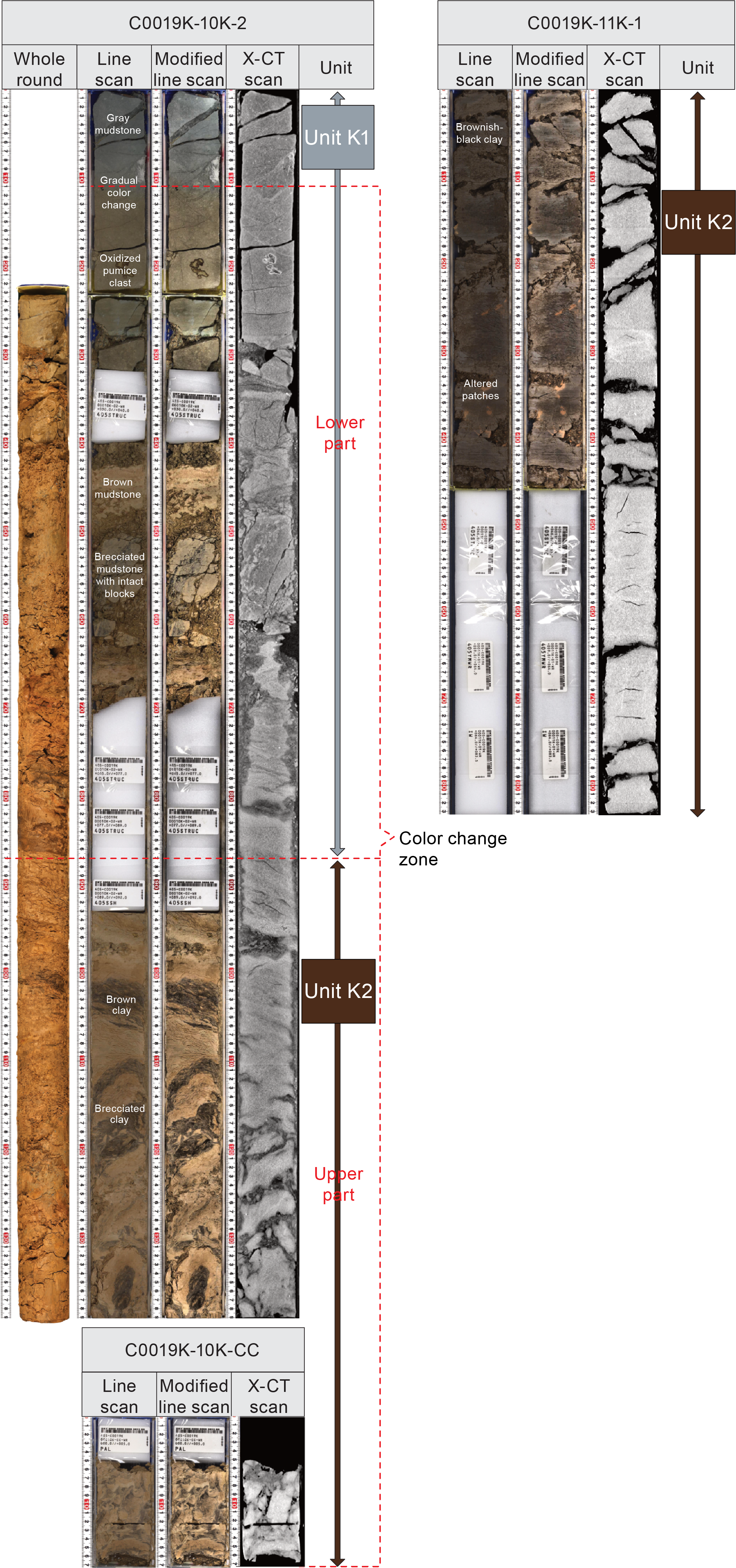
Figure F59. Transition and boundary layer between Units K1 and K2.

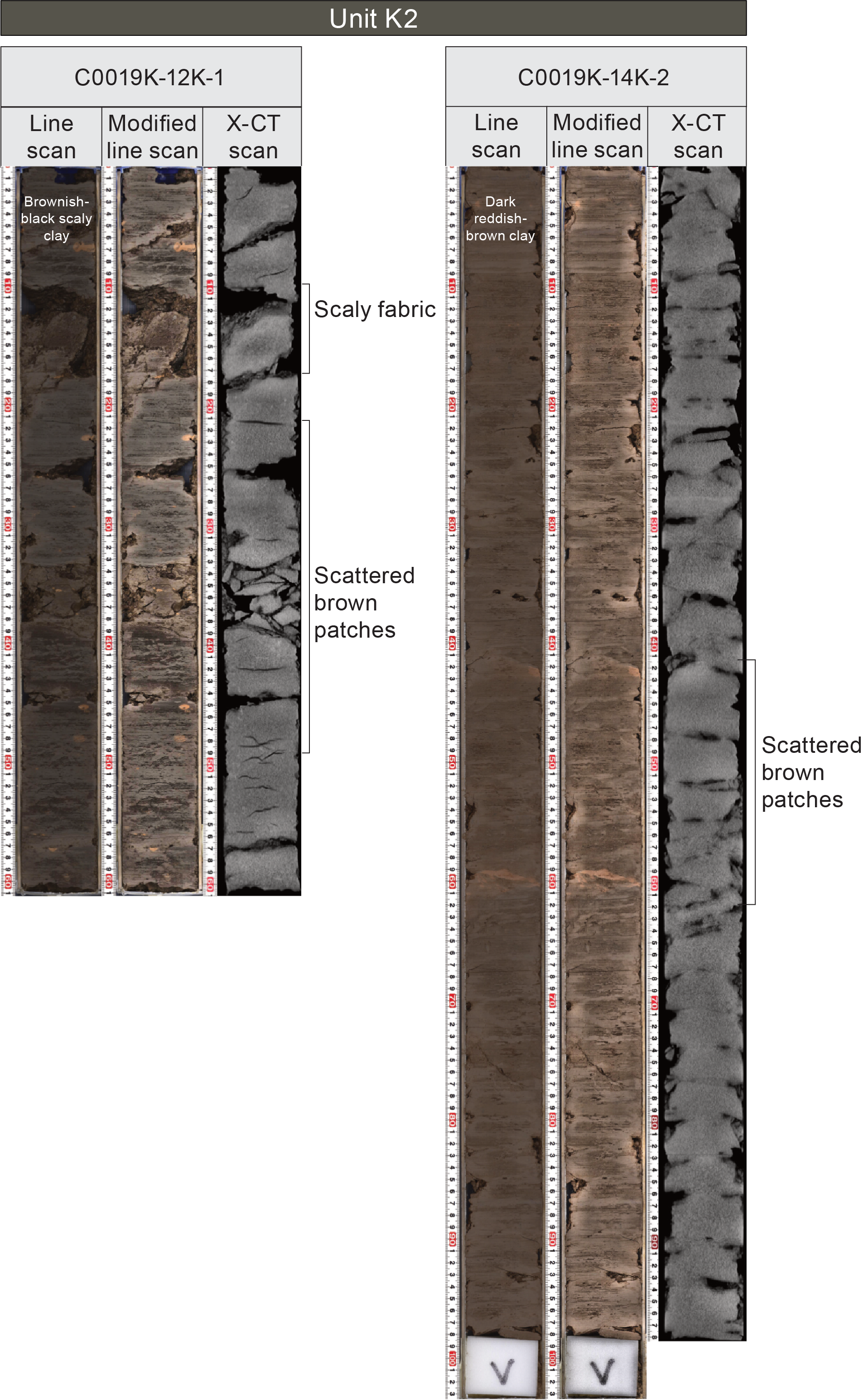
Figure F60. Unit K2 images.

4.2.2.2. Smear slide petrography

The color-change zone at the top of Unit K2 zone has a significant decrease in grain size (clay) compared to Unit K1, with 90% clay, 7%–10% silt, and 0%–3% sand (Table T18; Figure F55). The composition is siliciclastic dominated (80%–98%) with subordinate volcanic (0%–14%) and biogenic (0%–1%) materials. Compositionally, Unit K2 is predominately clay minerals (60%–95%).

The grain size of Unit K2 is 78%–100% clay, 0%–22% silt, and 0% sand (Figure F55; Table T18). The composition is siliciclastic (78%–100%), volcanic (0%–6%), and biogenic (0%–1%). Other material (0%–20%) includes dense minerals, mica, opaque minerals, and framboidal pyrite. Siliciclastic grains are mostly clay minerals (60%–98%) and quartz (0%–30%), with low amounts of mud aggregates (0%–7%). Biogenic material is generally absent, with rare sponge spicules (<1%) in only four samples (Figure F61).

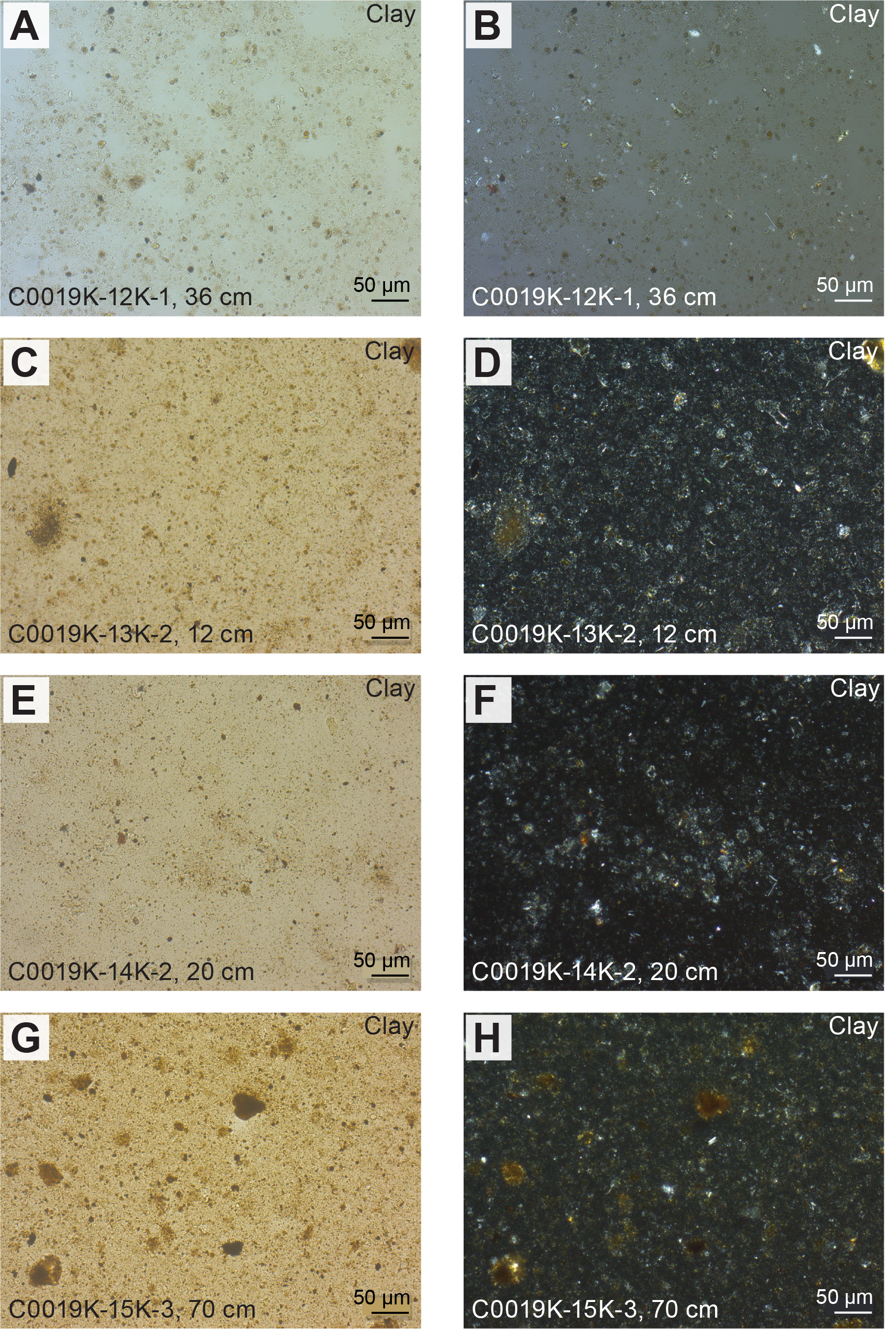
Figure F61. Unit K2 smear slides.

4.2.2.3. Mineralogy and sediment geochemistry

Seven bulk samples representative of Unit K2 were collected for XRD analysis (Figure F57; Table T19). Clay minerals dominate the composition (72–85 wt%), with lesser quartz (10–14 wt%) and plagioclase (4–7 wt%), thus supporting observations of high clay content from smear slides. Two samples from the color change zone at the top of Unit K2 show no discernible difference.

Major and minor elemental abundances in Unit K2 are significantly different than Unit K1 (Figure F58; Table T20). Unit K2 contains 1.66–2.13 wt% Na₂O, 3.11–3.86 wt% MgO, 15.35–19.72 wt% Al₂O₃, 57.54–60.68 wt% SiO₂, 0.33–2.0 wt% P₂O₅, 3.83–4.31 wt% K₂O, 0.83–3.47 wt% CaO, 0.69–1.0 wt% TiO₂, 1.25–2.57 wt% MnO, 7.23–9.04 wt% Fe₂O₃, and 6.07–7.99 wt% LOI. Two samples from the color change zone at the top of Unit K2 yield similar results to the rest of Unit K2, with slightly lower P₂O₅, K₂O, MnO, and LOI. Compared to Unit K1, the notably higher MgO and Al₂O₃ indicates more clay minerals, consistent with smear slide observations. Higher K₂O, could potentially indicate greater illite or K-feldspar content, and higher MnO could link to diagenetic Mn enrichment. The lower SiO₂ in Unit K2 compared to Unit K1 reflects the relative absence of siliceous microfossils and reduced abundance of volcanic ash.

4.2.2.4. Summary and preliminary interpretation

Unit K2 consists of homogeneous and structureless brownish black clay with scattered reddish brown patches. The upper boundary of Unit K2 represents the plate boundary fault. The unit is devoid of biogenic material and vitric components (including ash layers). The sediments are consistent deposition in pelagic marine environments.

4.2.3. Unit K3

Interval: Sections 405-C0019K-16K-2, 119 cm, to 17K-CC, 25 cm
Depth: 870.63–873.72 mbsf
Age: TBD (occurrence of radiolarians exclusive to Mesozoic [Jurassic–Cretaceous])
Lithology: color-banded clay and chert

4.2.3.1. Visual core description lithology

Unit K3 begins in Section 405-C0019K-16K-2, 119 cm (870.63 mbsf), where the dark brownish black clay of Unit K2 starts to display thin millimeter-scale, multicolor, horizontal laminae (Figure F51). In the uppermost 30 cm of Section 17K-1, the laminae are thicker (larger than centimeter scale) and semilithified. They form color-banded clay layers of alternating black (7.5YR 2/1), dull yellow-orange (10YR 7/3), brown (7.5YR 4/6 to 7.5YR 4/4), dull orange (7.5YR 6/4), and light yellow (2.5Y 7/3) hues (Figure F62). Below the dark color-banded clays (Section 17K-1, 30 cm) is a 10 cm thick interval of light yellow (2.5Y 7/3) SiO₂ microlite-rich clay with gray laminae (millimeter scale, similar to the color-banded clays). Below this interval, loose clasts of red-brown chert were recovered from the base of Section 17K-1 (Figure F63). The presence of conchoidal fractures in the chert indicates that it is composed of cryptocrystalline material. At the base of Section 17K-CC is a mixture of yellowish gray clay and red chert fragments likely mixed and fragmented by drilling disturbance. Overall, the gradational nature of the transition from color-banded clay to chert indicates an ongoing process of silicification.

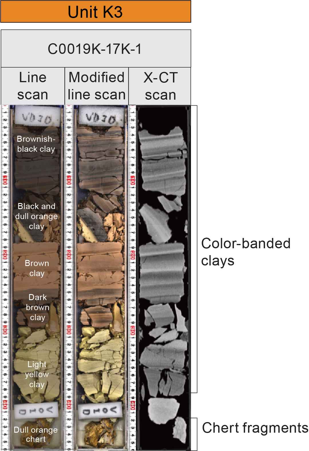
Figure F62. Unit K3 images.

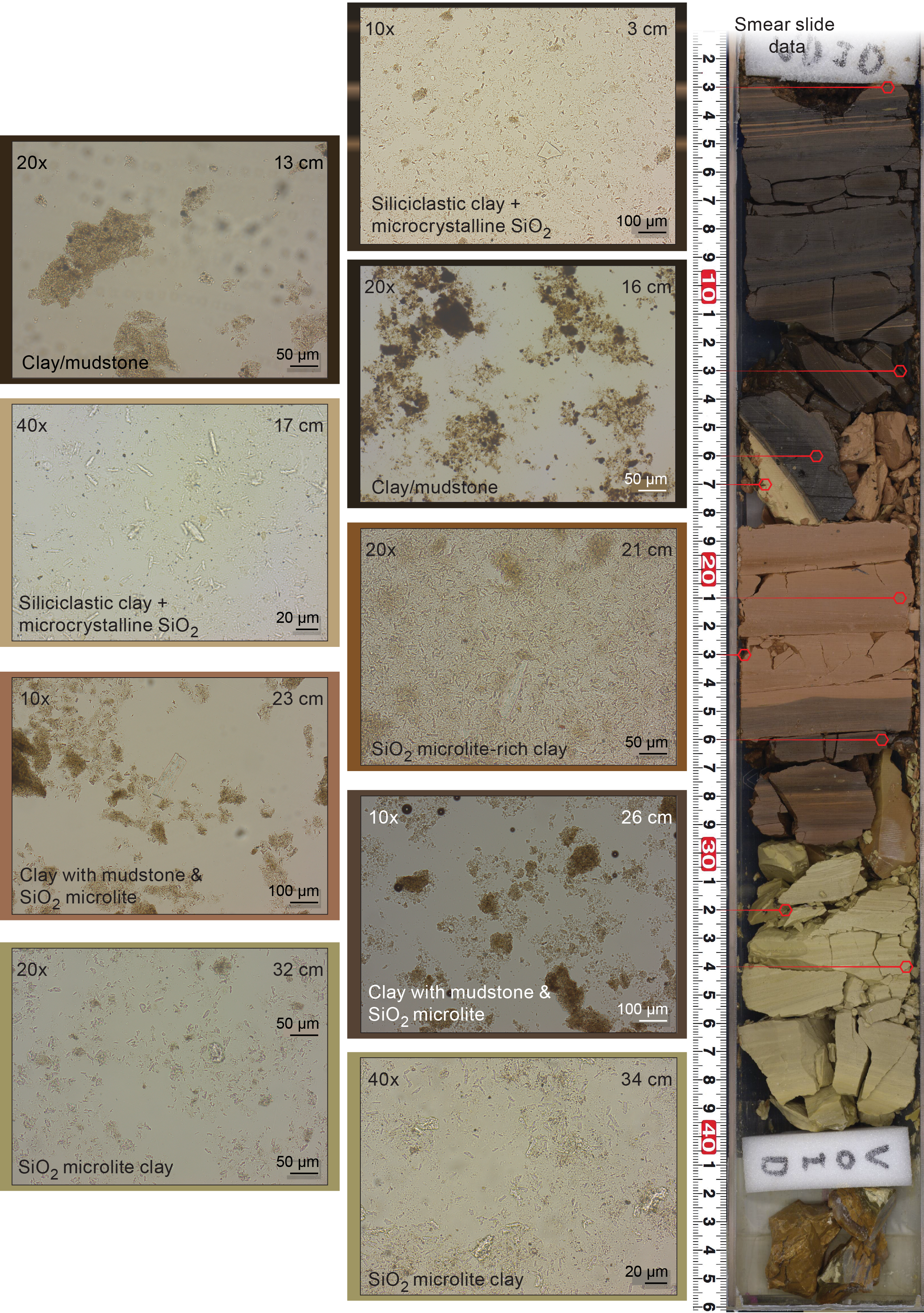
Figure F63. Unit K2–K3 transition.

4.2.3.2. Smear slide petrography

In Unit K3, smear slide analysis is limited to soft/semilithified sediment because samples cannot be taken from lithified clay/chert. The grain size of this sediment includes sand (0%–3%), silt (3%–15%), and clay (82%–97%). The composition is siliciclastic (90%–99%), made up of quartz (1%–80%), clay minerals (10%–80%), and mud aggregates (0%–85%) (Figure F55).

4.2.3.3. Mineralogy and sediment geochemistry

Five samples from Unit K3 were analyzed for XRD, four from the color-banded clays and one sample of red chert (Table T19). The four color-banded clays are compositionally similar with a high percentage of clay minerals (>90 wt%), very low quartz and plagioclase (<6 wt%), and a characteristic cristobalite peak that increases in intensity with depth (Figures F57, F64). Note that the peak for cristobalite is included in “clay minerals” in this analysis. The sample of red chert (interval 405-C0019K-17K-CC, 2–5 cm), in contrast, has high quartz content (71 wt%) and relatively low clay content 22 wt%.

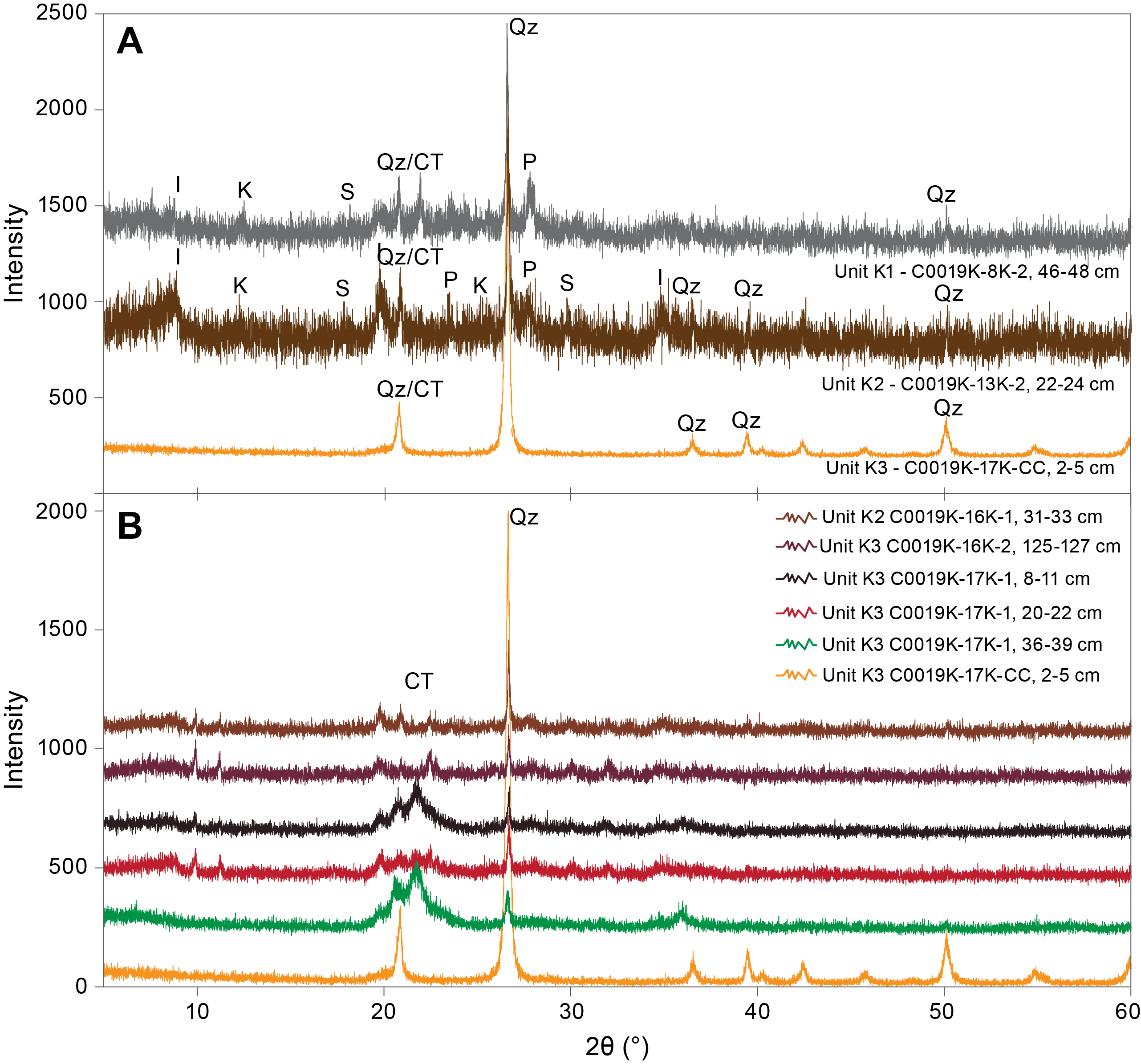
Figure F64. XRD patterns, Hole C0019K.

The same samples were analyzed for element compositions using XRF (Table T20; Figure F58). Color-banded clays contain 1.31–2.36 wt% Na₂O, 1.42–3.08 wt% MgO, 5.0–13.05 wt% Al₂O₃, 55.62–86.43 wt% SiO₂, 0.15–2.83 wt% P₂O₅, 0.89–3.38 wt% K₂O, 0.58–4.99 wt% CaO, 0.29–0.53 wt% TiO₂, 0.01–4.57 wt% MnO, 3.61–8.94 wt% Fe₂O₃, and 4.79–9.33 wt% LOI. The high amount of Al₂O₃ reflects the dominance of clay in the samples. In contrast, the XRF results for the chert sample are 0.21 wt% Na₂O, 0.18 wt% MgO, 0.8 wt% Al₂O₃, 98.16 wt% SiO₂, 0.11 wt% P₂O₅, 0.28 wt% K₂O, 0.18 wt% CaO, 0.05 wt% TiO₂, 0.01 wt% MnO, 0.89 wt% Fe₂O₃, and 1.87 wt% LOI. The high abundance of SiO₂ is characteristic of chert.

4.2.3.4. Summary and preliminary interpretation

Unit K3 consists of semilithified color-banded clays that grade downward into yellow SiO₂-microlite-rich clay and orange chert. Millimeter-scale laminae are common throughout the unit, with a progressively brighter color downward, corresponding to increasing SiO₂. The preserved laminae in the pelagic clay, the silica-rich materials, and the emergence and transition of a cristobalite peak to quartz in the XRD spectra of the color-banded clay suggest progressive replacement of pelagic clay by silica to form the chert. The downward transition to chert may also suggest increasing contribution from biogenic and volcanic sources or enhanced silica preservation over time.

4.3. Lithostratigraphic units of Hole C0019P

Hole C0019P was drilled using a SD-RCB system, with cores recovered from 930.00 to 946.61 mbsf. Cores from Hole C0019P were divided into three lithostratigraphic units, numbered from the top down (Units P1–P3). Units P1 and P3 consist of igneous rocks including pillow basalt, massive basalt, and dolerite, whereas Unit P2 is composed of sedimentary rocks including limestone, chert, and siliceous mudstone. The overall lithologic characters and the depths of the unit boundaries are summarized in Table T21 and Figure F65. TSCL images of representative lithology of igneous rocks are shown in Figure F66. Boundaries between each unit are shown in Figure F72. Smear slides were prepared as a supplement to confirm the mineralogy of sediments and accessory minerals in igneous rocks. We do not report the percentage of each component observed in the smear slides for igneous rocks because they do not represent the overall lithology and results are biased by the presence of lithified grains. Selected microscope images are shown in Figure F67. Results of XRD patterns are shown in Figure F69. Results of XRF analysis (Table T22) are displayed with depth in Figure F70 and in a total alkali-silica diagram in Figure F71.

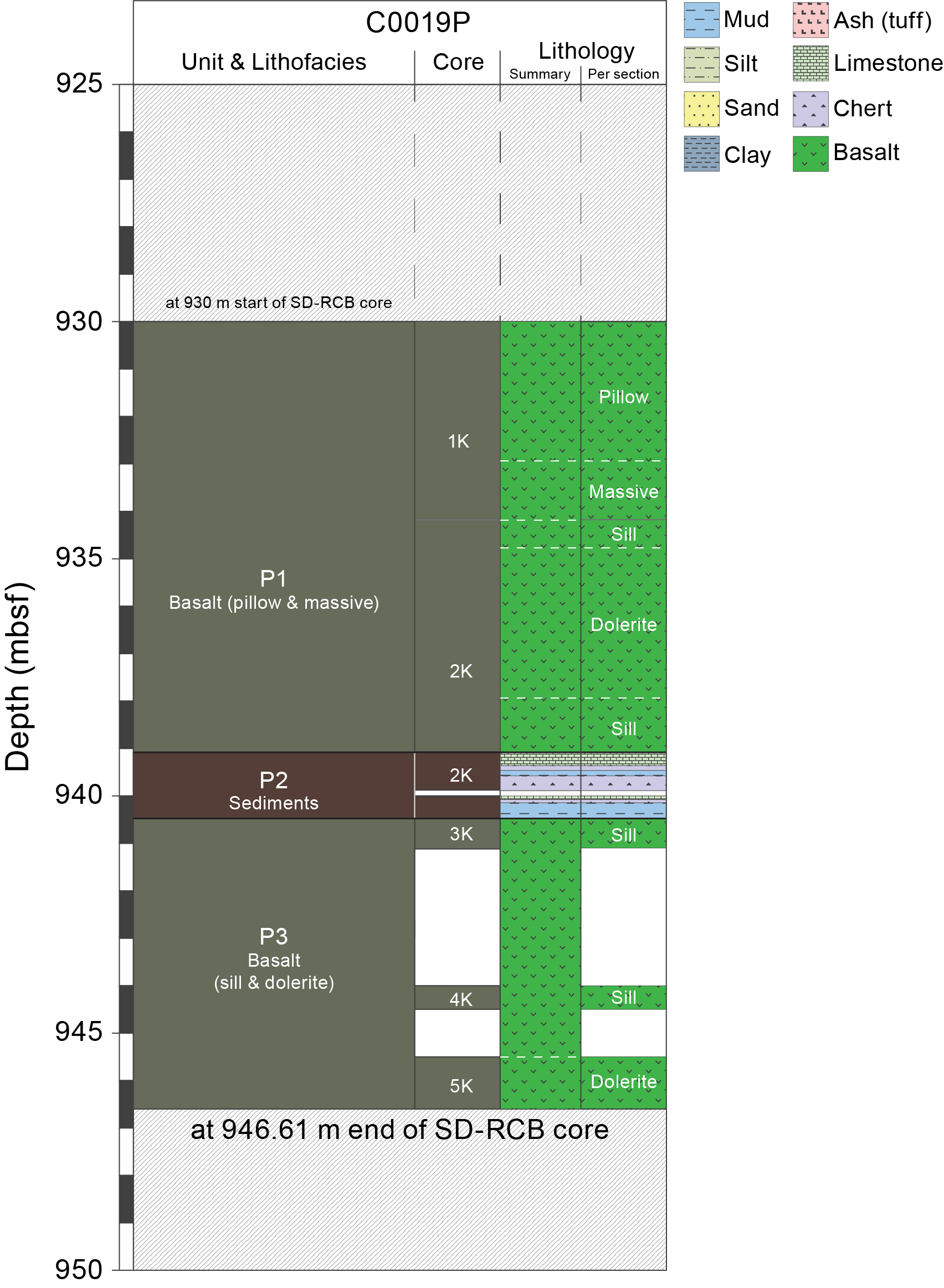
Figure F65. Lithostratigraphic units, Hole C0019P.

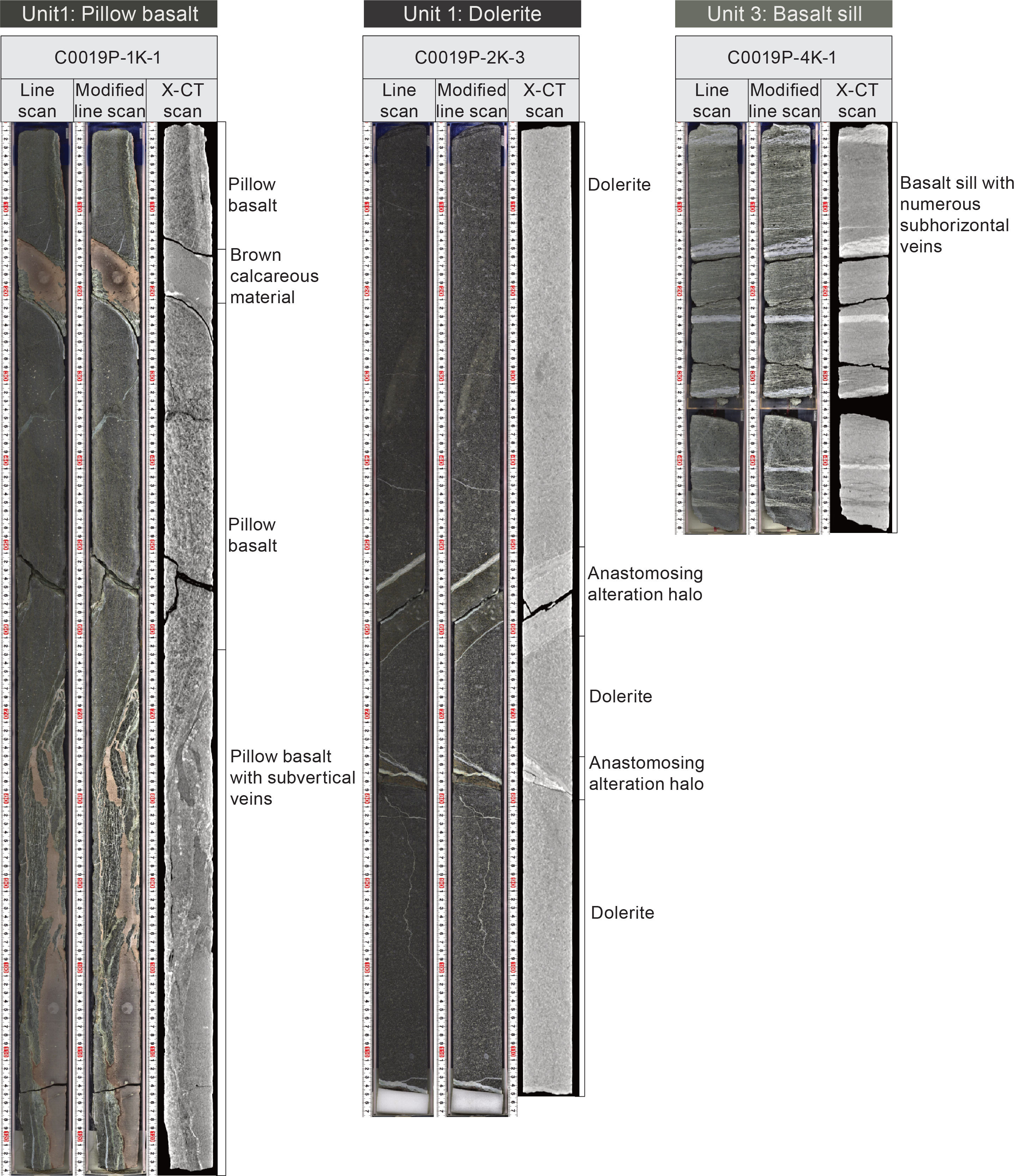
Figure F66. Pillow basalt, dolerite, and basalt sill.

4.3.1. Unit P1

Interval: 405-C0019P-1K-1, 0 cm, to 2K-6, 77 cm
Depth: 930.00–939.10 mbsf
Age: TBD
Lithology: pillow basalt, massive basalt, and dolerite

4.3.1.1. Visual core description lithology

Unit P1 consists of pillow basalt, massive basalt, and dolerite. The transition between pillow basalt and massive basalt is observed in Core 405-C0019P-1K between Sections 1K-3 and 1K-4, whereas the massive basalt gradually changes to dolerite within Section 2K-2. The pillow basalt (Sections 1K-1, 0 cm, to 1K-3, 90 cm) is characterized by fine-grained basalt in curved glassy pillows, with rims altered to green clay minerals. Brown carbonaceous material is sandwiched between the pillows. The brown carbonaceous material is 2–4 cm thick, contains clasts of fragmented glassy basalts, and exhibits branching structures (interval 1K-3, 29–44 cm). Calcite and zeolite amygdules are observed in interval 1K-1, 25–72 cm, infilling vesicles. Phenocrysts of plagioclase and clinopyroxene are visible on the split surface of the core. Two types of alteration are present throughout the pillow basalt: dark greenish gray alteration to clay minerals and orange alteration halos formed from Fe hydroxide or Fe oxyhydroxide. The orange alteration halos show anastomosing textures and overprint the pervasive greenish alteration. Subvertical veins are prominent in Sections 1K-1, 66 cm, to 1K-3, 12 cm, and contain brown carbonaceous material, white minerals (likely calcite and zeolite), and greenish clay minerals alongside fragments of altered glassy basalt. Occasionally, the basalt with orange alteration halos is incorporated into the veins.

Massive basalt is observed in Sections 405-C0019P-1K-4, 0 cm, to 2K-1, 31 cm, and is crystal rich (e.g., larger plagioclase phenocrysts up to ~4 mm) compared to the pillow basalt. The alteration is more subtle, but light gray patches lacking basaltic phenocrysts (<1 cm) are present. Subhorizontal to steeply dipping veins filled with white minerals are also present within massive basalt, and pyrite is observed as an accessory mineral in interval 2K-1, 0–17 cm. The gradual transition into dolerite occurs between Sections 2K-2 and 2K-4.

The dolerite has larger plagioclase phenocrysts (5–10 mm), gray aggregates of minerals (possibly clinopyroxene; <1.5 cm), and amygdules filled with greenish gray clay, zeolite, or calcite (<1 mm). Alteration of the dolerite is less pronounced than that of both the pillow basalt and massive basalt. Subhorizontal veins of white minerals are present in the dolerite, with meandering vein/wall rock contacts. Anastomosing orange alteration halos occur only along the white veins.

From Section 405-C0019P-2K-5 downward, the dolerite becomes increasingly fine grained (plagioclase crystal size = <5 mm), and in Section 2K-6, a gradual color transition from gray at the top to greenish gray near the P2 boundary is observed. Subvertical elongate white patches truncated by subhorizontal veins, occasionally filled instead with dark green minerals, occur throughout the dolerite.

The Unit P1/P2 boundary is formed of a dark greenish gray zone (interval 405-C0019P-2K-6, 70.5–76 cm) topped with ~7 mm thick yellowish brown layers. A 10 mm thick greenish gray to gray fine-grained layer occurs just above the contact with sedimentary rock (interval 2K-6, 75–77 cm) and is identified as a chilled margin, suggesting that this is an intrusive boundary.

4.3.1.2. Smear slide and thin section petrography

Smear slides were made to confirm the mineralogy of the amygdules in the basalt and brown carbonaceous material occurring as interpillow material. White amygdules are composed of calcite and zeolite, whereas the carbonaceous material is mostly composed of carbonate minerals (Figure F67). No fossils were found within the carbonaceous material samples.

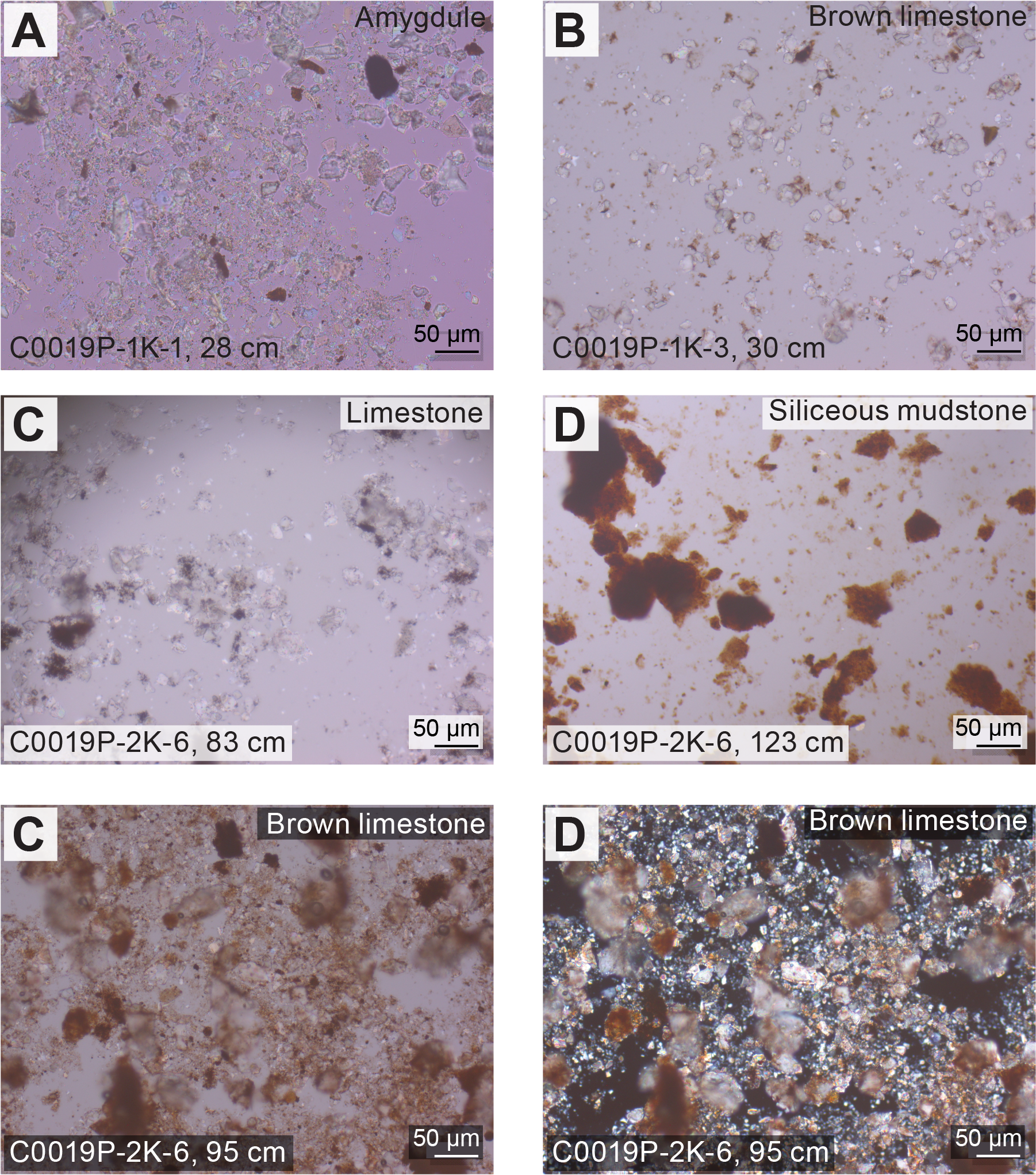
Figure F67. Sediments.

Three samples for thin section petrography were taken from Unit P1 (Figure F68; [A, B] brown carbonaceous material/basalt boundary in interval 405-C0019P-1K-1-1b, 17–19 cm; [C, D] pillow basalt in interval 1K-1-1c, 45–47 cm; [E, F] dolerite in interval 2K-3-1b, 108–110 cm). In Sample 1K-1-1b, 17–19 cm, the carbonaceous material portion is composed of ~20 µm euhedral calcite grains. Spaces between calcite crystals are filled with brownish (under plane-polarized light [PPL]) clay minerals. Greenish (under PPL) clay minerals (possibly saponite or celadonite) are the main component of the basaltic portion of the sample. Calcite cementations and calcite replacement of plagioclase crystals were commonly observed in the basaltic portion. Calcite veins were also present. Minor occurrences of pyroxene were observed.

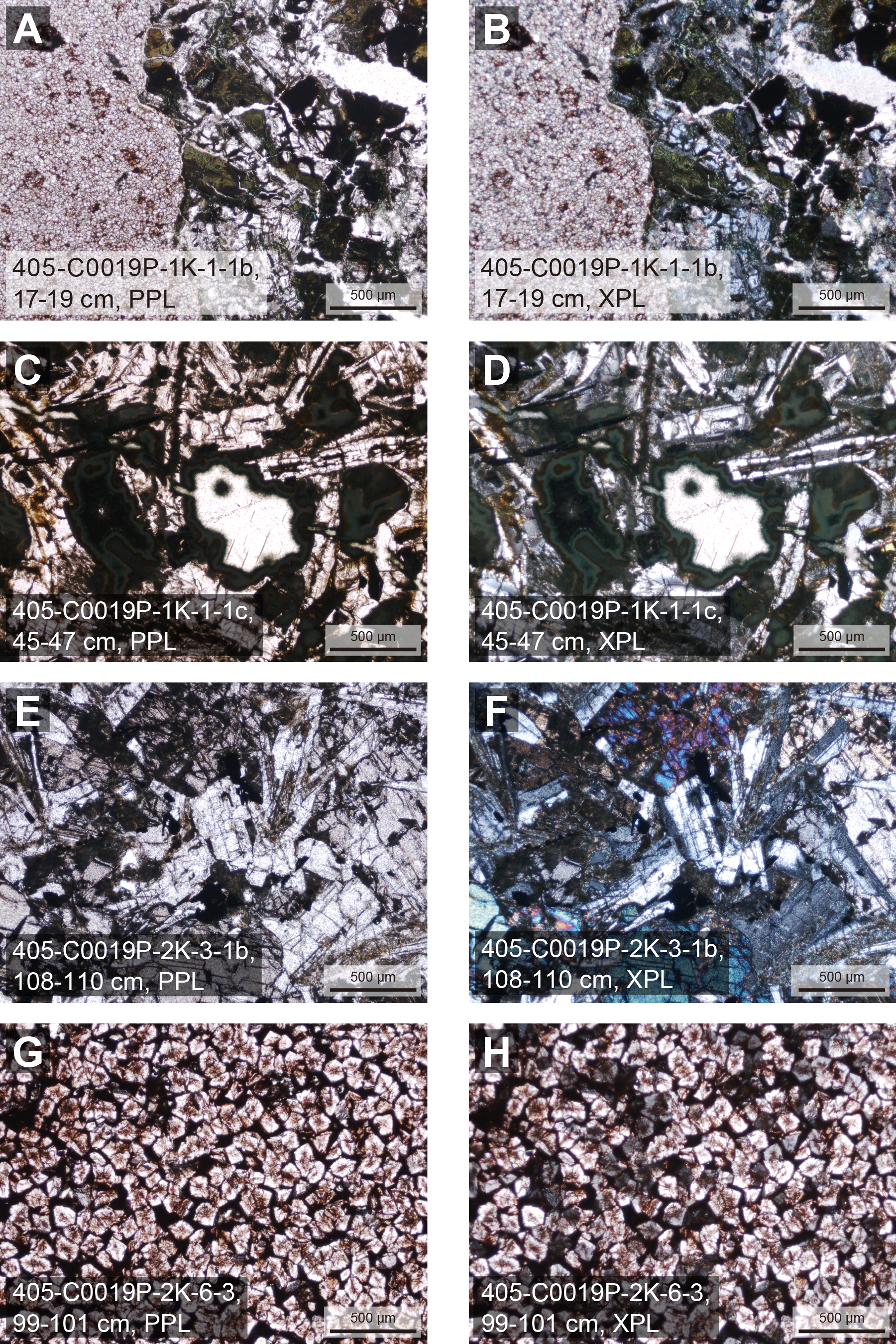
Figure F68. Rock samples.

In the pillow basalt (interval 405-C0019P-1K-1-1c, 45–47 cm), plagioclase, pyroxene, and clay minerals are the major mineral species observed. Plagioclase and pyroxene crystals are partially altered and replaced by clay minerals. Greenish clay minerals (possibly saponite or celadonite) have replaced zeolite in vesicles, as well as glass with several precipitation/crystallization stages characterized by zones with different colors.

The dolerite sample (interval 405-C0019P-2K-3-1b, 108–110 cm) is mainly composed of plagioclase and pyroxene. These crystals are bigger than in the pillow basalt (interval 1K-1-1c, 45–47 cm); some crystals have sizes >1 mm. Grain boundaries among plagioclase and pyroxene crystals are replaced by clay minerals.

4.3.1.3. Mineralogy and geochemistry

A total of three representative samples (pillow basalt, massive basalt, and dolerite) from Unit P1 were collected for XRD analysis. The XRD results for all three samples exhibit similar peak positions corresponding to anorthite, albite, augite, and saponite, all of which are commonly found in ocean floor basalts (Figure F69). XRF results of basaltic rocks indicate 3.04–3.07 wt% Na₂O, 5.37–8.63 wt% MgO, 14.71–17.10 wt% Al₂O₃, 46.19–51.43 wt% SiO₂, 0.35–0.45 wt% P₂O₅, 0.85–2.65 wt% K₂O, 7.29–8.86 wt% CaO, 2.02–2.47 wt% TiO₂, 0.11–0.15 wt% MnO, 8.44–12.18 wt% Fe₂O₃, and 2.31–2.81 wt% LOI (Figure F70). In the total alkali-silica diagram, the pillow basalt from Section 405-C0019P-1K-1 is classified as a basaltic trachyandesite, whereas the massive basalt and dolerite plot in the basalt field (Figure F71). The high total alkali content (Na₂O 3.07 wt% and K₂O 2.65 wt%) of the pillow basalt suggests it is a slightly evolved basalt, potentially transitional between tholeiitic and alkaline compositions, which is common in pillow basalts formed in mid-ocean ridges or volcanic arcs. Alternatively, the alkaline composition could be explained by the presence of K-rich clay minerals such as celadonite formed during low-temperature alteration. In contrast, the lower alkali (Na₂O and K₂O) content in massive basalt or dolerite indicates either a more primitive magma or less alteration.

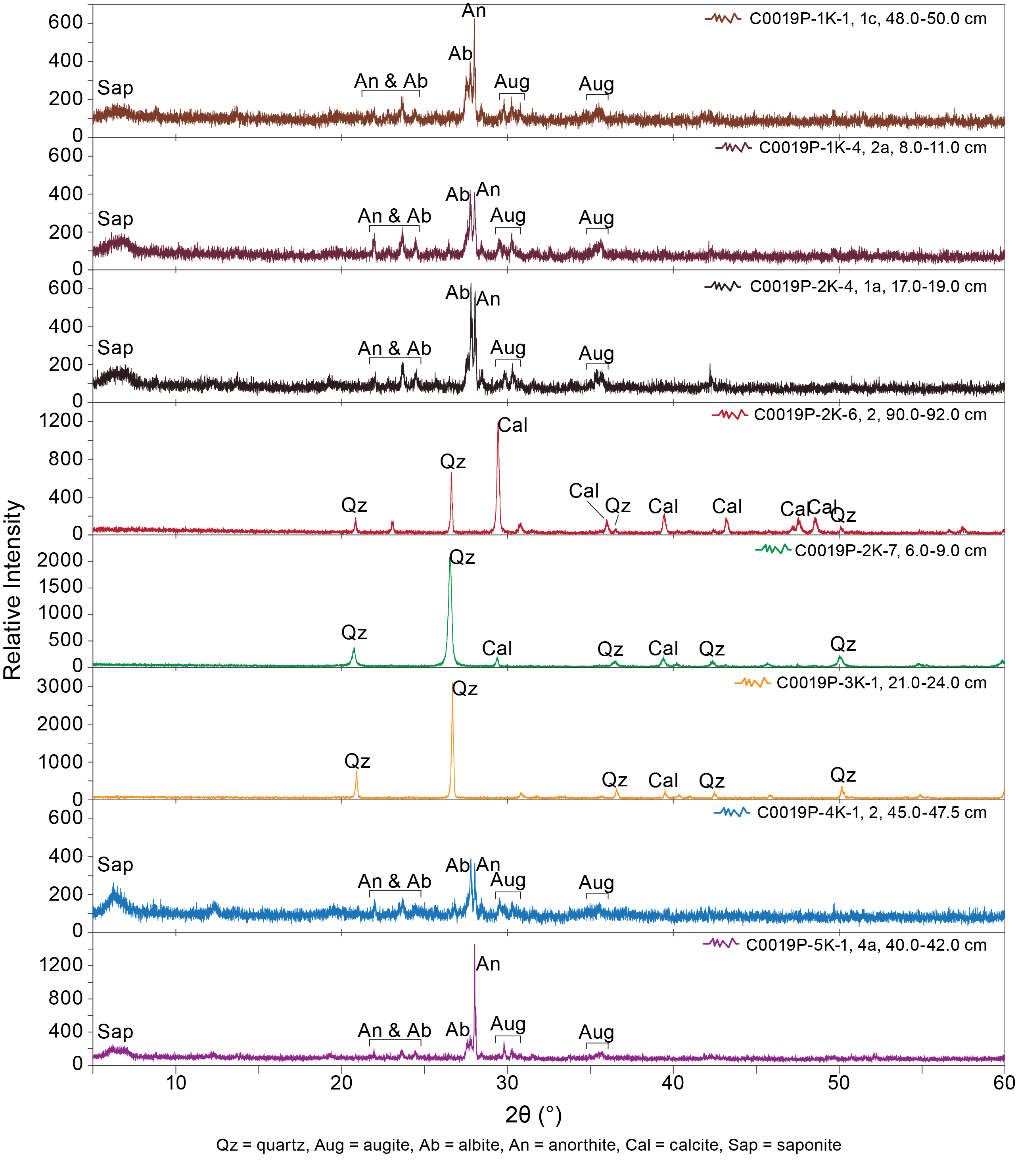
Figure F69. XRD patterns, Hole C0019P.

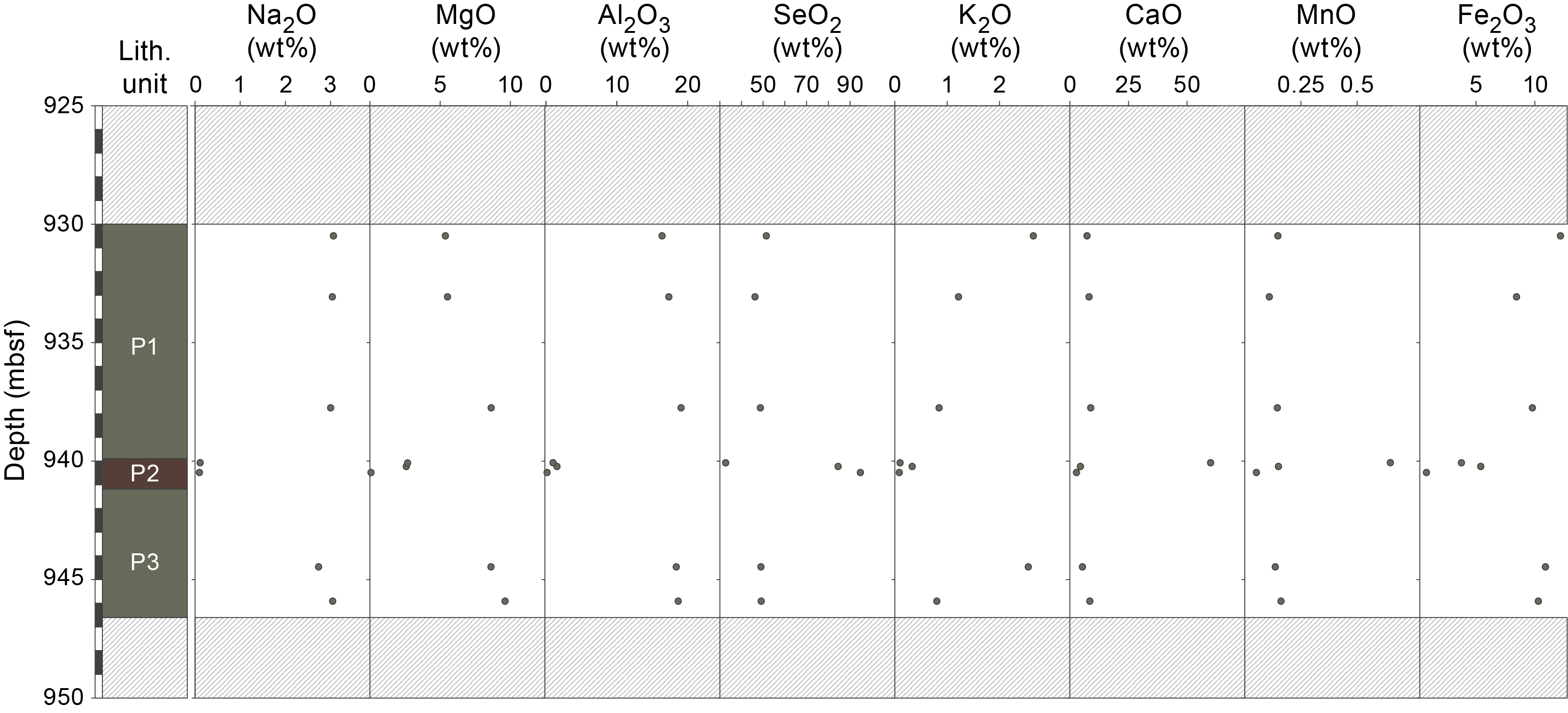
Figure F70. Major element compositions, Hole C0019P.

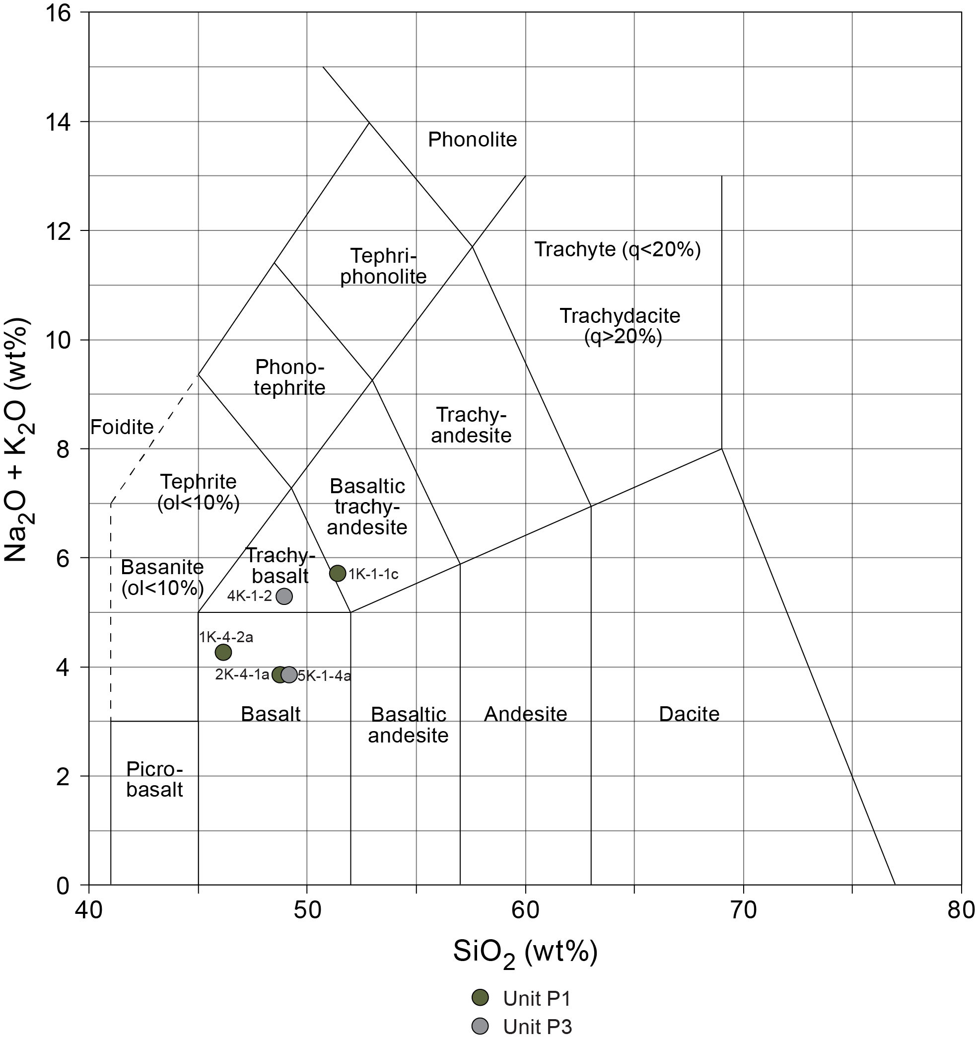
Figure F71. Composition of igneous rocks, Hole C0019P.

4.3.1.4. Summary and preliminary interpretation

Unit P1 consists of mafic igneous rocks, including altered pillow basalt with subvertical veins sandwiched with brown carbonaceous material, crystal-rich massive basalt, and dolerite with subhorizontal veins. These rocks represent the subducted Pacific plate. The pillow basalts have experienced varying degrees of alteration. Euhedral calcite crystals in the carbonaceous material indicate precipitation from hydrothermal fluids. These observations suggest that the depositional, eruptive, and intrusive events likely occurred near a mid-ocean ridge, followed by low-temperature alteration influenced by the rock textures.

4.3.2. Unit P2

Interval: 405-C0019P-2K-6, 77 cm, to 3K-1, 46 cm
Depth: 939.10–940.46 mbsf
Age: TBD
Lithology: limestone, chert, and siliceous mudstone

4.3.2.1. VCD lithology

Unit P2 consists of red pelagic sediments, fragments of limestone, chert, and siliceous mudstone. The top of Unit P2 consists of white limestone. In interval 405-C0019P-2K-6, 77–78 cm, a ~8–12 mm thick light gray layer is observed (Figure F72). Below this layer, a ~2 cm thick grayish brown zone with a high XCT number is present. These layers are recognized as a baked margin and a reaction zone, respectively. From Section 2K-6, 80 cm, downward, the lithology gradually changes to a dark reddish brown limestone. Smear slide analysis revealed an abundance of carbonate particles in the limestone, with some sand-sized grains of carbonate minerals. No fossils were observed. The cherts in Unit P2 are dark red in color. They have sharp upper and lower contacts with the overlying limestone (Section 405-C0019P-2K-6, 103 cm) and the underlying siliceous mudstone (Section 405-C0019P-2K-6, 112 cm). The siliceous mudstone is dark red to dull reddish brown, with cherty lithics and carbonate particles visible in smear slides (Figure F67).

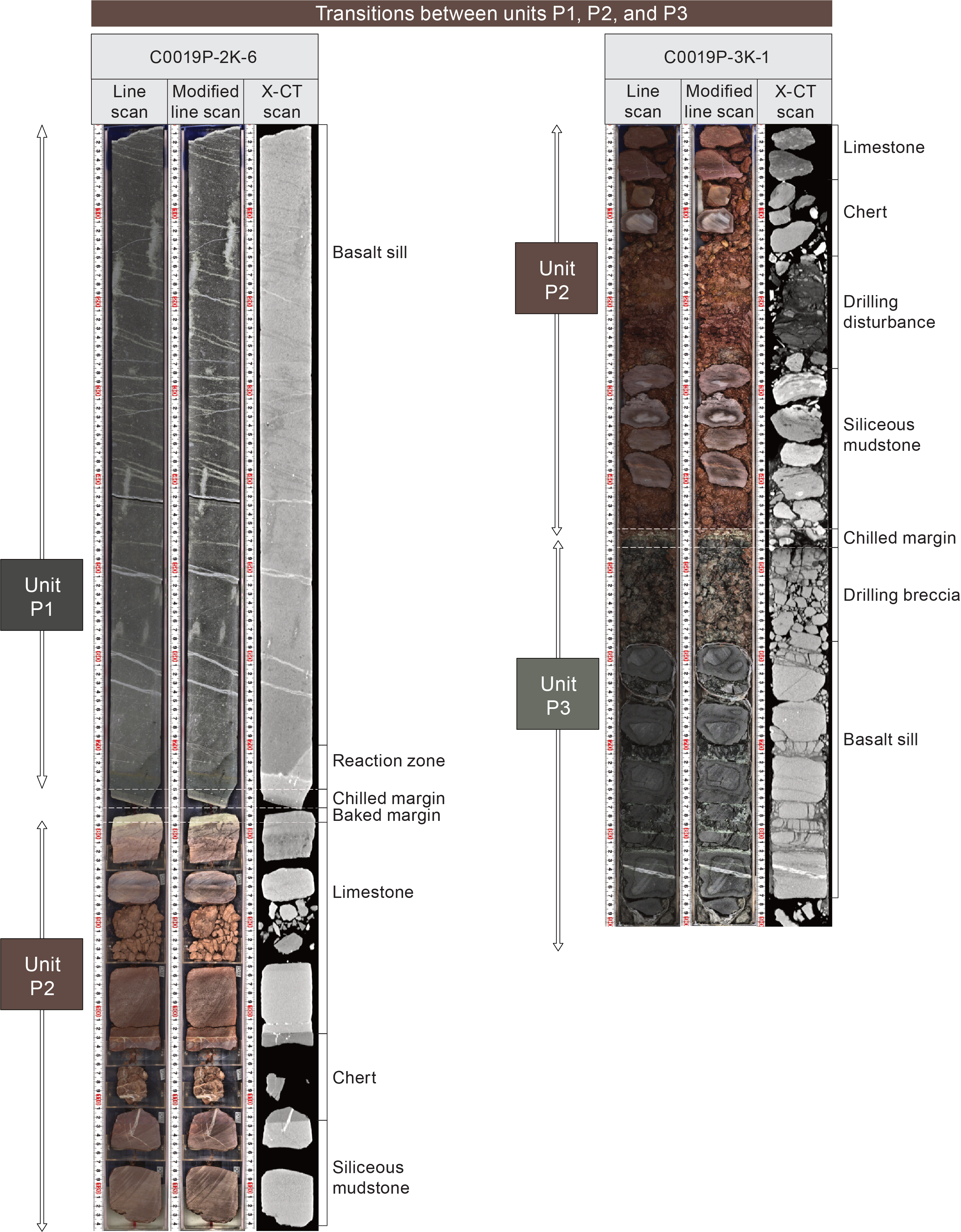
Figure F72. Transitions between Units P1, P2, and P3.

Although the bottom of Unit P2 is brecciated due to drilling, the boundary between Units P2 and P3 contains a chilled margin (where magma has cooled rapidly along the margin of an intrusion) at the top of Unit P3, which indicates an intrusive contact.

4.3.2.2. Smear slide and thin section petrography

Limestones in Unit P2 are characterized by high contents of carbonate particles, whereas smear slides of siliceous mudstone include fragmented reddish mudstone and small amounts of carbonates (Figure F67). No fossils were found. One sample for thin section petrography was taken from Unit P2 (Figure F68G, F68H; limestone in interval 405-C0019P-2K-6-3, 99–101 cm). The limestone portion is composed of more euhedral calcite grains than interval 1K-1-1b, 17–19 cm (~100 µm diameter). The intercrystalline space is filled with brownish clay minerals.

4.3.2.3. Mineralogy and sediment geochemistry

A total of three bulk samples representative of the different sedimentary rocks in Unit P2 were collected for XRD analysis (limestone in Sample 405-C0019P-2K-6, 90–92 cm, chert in Sample 2K-7, 6–9 cm, and siliceous mudstone in Sample 3K-1, 21–24 cm). XRD spectra from the limestone had a strong calcite peak with subordinate quartz, and XRF analysis yielded 0.10 wt% Na₂O, 2.66 wt% MgO, 1.03 wt% Al₂O₃, 32.73 wt% SiO₂, 0.13 wt% P₂O₅, 0.10 wt% K₂O, 60.08 wt% CaO, 0.06 wt% TiO₂, 0.65 wt% MnO, 3.75 wt% Fe₂O₃, and 33.06 wt% LOI (Figure F70). The high CaO content and high LOI are consistent with the smear slide analysis and XRD results. XRD analysis of the chert and siliceous mudstones show high quartz peaks and subtle calcite peaks (Figure F69).

XRF analysis of chert (interval 405-C0019P-2K-7, 6–9 cm) yielded 0.10 wt% Na₂O, 0.08 wt% MgO, 0.25 wt% Al₂O₃, 94.92 wt% SiO₂, 0.02 wt% P₂O₅, 0.09 wt% K₂O, 2.74 wt% CaO, 0.01 wt% TiO₂, 0.05 wt% MnO, 0.79 wt% Fe₂O₃, and 3.01 wt% LOI, whereas the siliceous mudstone yielded 0.70 wt% Na₂O, 2.59 wt% MgO, 1.50 wt% Al₂O₃, 84.55 wt% SiO₂, 0.26 wt% P₂O₅, 0.33 wt% K₂O, 4.51 wt% CaO, 0.10 wt% TiO₂, 0.15 wt% MnO, 5.40 wt% Fe₂O₃, and 6.76 wt% LOI (Figure F70). These XRF data show that the mudstone has lower SiO₂ and higher Al₂O_3, CaO, Fe₂O₃ and LOI than the chert.

4.3.2.4. Summary and preliminary interpretation

Unit P2 consists of red sedimentary rocks, including limestone, chert, and siliceous mudstone. The chert and mudstone are interpreted as pelagic sediments. Euhedral calcite crystals in the limestone, however, suggest their precipitation from hydrothermal fluid. The presence of such limestone suggests that the pelagic sediments were deposited above the carbonate compensation depth during the early stage of the movement of the oceanic plate.

4.3.3. Unit P3

Interval: 405-C0019P-3K-1, 46 cm, to 5K-1, 111 cm
Depth: 940.46–946.61 mbsf
Age: TBD
Lithology: basalt sill and dolerite

4.3.3.1. VCD lithology

Unit P3 was recovered in four short sections from the base of Hole C0019P and consists of a combination of fine-grained intrusive basalt and massive dolerite. Unit P3 begins in Section 405-C0019P-3K-1, 46 cm (Figures F65, F72). Although the top part of Unit P3 is brecciated by drilling, the nature of boundary between Units P2 and P3 can be determined because of the presence of the chilled margin at the top of Unit P3 (interval 405-C0019P-3K-1, 46–47 cm). The igneous rock in Core 3K is identified as a basalt sill based on the fine grain size and absence of flow structures. A few subhorizontal white veins are present in Core 3K. In Core 4K, numerous closely spaced, thin (<0.5 cm), discontinuous veins and five relatively thick (2 cm) veins spaced approximately 10 cm apart are observed cutting a crystal-rich, altered greenish gray basalt. Core 4K also contains ~1 mm dark green to black spherical patches, possibly representing amygdules or olivine pseudomorph. Core 5K marks a change (transition occurs between cored intervals) to an intact section of less altered, relatively massive dolerite.

4.3.3.2. Smear slide and thin section petrography

No shipboard sample was taken from Unit P3 for microscopic observations.

4.3.3.3. Mineralogy and sediment geochemistry

A total of two bulk samples representative of Unit P3 were collected for XRD analysis, a basalt sill (interval 405-C0019P-4K-1, 45–47.5 cm) and a dolerite (interval 5K-1, 40–42 cm) (Figure F69). The XRD spectra from the basalt sill has a high saponite peak, whereas the dolerite has a lower saponite peak and a very high anorthite peak. XRF analysis of the basalt sill yielded 2.74 wt% Na₂O, 8.62 wt% MgO, 16.50 wt% Al₂O₃, 48.97 wt% SiO₂, 0.29 wt% P₂O₅, 2.55 wt% K₂O, 5.26 wt% CaO, 1.91 wt% TiO₂, 0.14 wt% MnO, 10.90 wt% Fe₂O₃, and 4.85 wt% LOI (Figure F70). The dolerite sample yielded 3.05 wt% Na₂O, 9.62 wt% MgO, 16.74 wt% Al₂O₃, 49.18 wt% (SiO₂), 0.32 wt% P₂O₅, 0.80 wt% K₂O, 8.40 wt% CaO, 2.03 wt% TiO₂, 0.16 wt% MnO, 10.29 wt% Fe₂O₃, and 2.44 wt% LOI. The relative abundances of Si, K, and Na classify these sample as trachy basalt and basalt, respectively (Figure F71). The higher LOI and presence of saponite in the basalt sill suggests alteration or hydration, whereas the higher CaO and MgO in the dolerite suggest a less evolved composition and potentially more primitive magma source.

4.3.3.4. Summary and preliminary interpretation

Unit P3 is composed of igneous rocks including an altered basalt sill with crystal-rich veins in Cores 405-C0019P-3K and 4K and intact, massive dolerite in Core 5K. The rocks of Unit P3 represent the subducted Pacific plate. The basalt sills and dolerite have undergone various degrees of alteration. These observations suggest that all the depositional, eruptive, and intrusive events likely occurred near a mid-oceanic ridge, followed by various degrees of low-temperature alteration influenced by the rock textures.

4.4. Summary and preliminary assessment of Site C0019

4.4.1. Key observations from each unit at Site C0019

Site C0019 consists of five boreholes (C0019J, C0019K, C0019L, C0019M, and C0019P). Together, the data collected provide documentation of the entire sequence of subseafloor materials through the frontal prism and the plate boundary to the basaltic basement from 0 to 946.61 mbsf, representative of the logging units and seismic units described previously at Site C0019. Key observations of all units across the different holes of Site C0019 are summarized in Table T23, and a correlation of the lithostratigraphic units (where possible) is provided in Table T24.

4.4.2. Discussion

The lithostratigraphy of Site C0019 can be summarized into three components: (1) repeated olive-black and gray siliceous vitric mud(stone) sequences in the frontal prism above the PBFZ (Units 1–6 and K1), (2) structureless brownish black clay (Unit K2) transitioning to color-banded clay and chert (Units 7 and K3) below the plate boundary fault, and (3) oceanic basement of basalt and dolerite intercalated with thin units of sedimentary rocks (Units P1–P3). The composite lithostratigraphy from Holes C0019J–C0019M and C0019P is similar to the stratigraphy described for Hole C0019E during Expedition 343 (Expedition 343/343T Scientists, 2013b). Thanks to higher recovery during Expedition 405, the presented lithostratigraphy illustrates an almost complete sequence of the frontal prism from the seafloor and shallow surficial sediments (Holes C0019L and C0019M), through the plate boundary (Holes C0019J and C0019K) to the basement (Hole C0019P).

The sedimentary rocks within the frontal prism, above the plate boundary (Units 1–6 and K1), appear to comprise at least five repeated sequences of siliceous vitric mud(stone) ranging in age from the Pleistocene to the Miocene. These sequences typically display olive-black to gray coloration, although Unit 5 is distinguished by a dull yellowish brown hue. Boundaries between sequences are marked either by color changes or faults (e.g., at 610.31 mbsf). In some cases, notable age reversals are observed at unit boundaries (e.g., Subunits 2B/3A and 5C/6A). Site C0019, in particular, shows extensive chaotic and inclined bedding, likely the result of complex deformation including mass transport and gravitational sliding. This interpretation is supported by the localized occurrence of calcareous nannofossils and calcite as well as shallow-water ichnofacies, which together support the interpretation that sediment from the shelf has been destabilized and transported into deeper water.

The PBFZ is located between Subunit 6B and Unit 7 in Hole C0019J and between Units K1 and K2 in Hole C0019K. It separates the highly disrupted and deformed sediments of the frontal prism above from the less deformed underthrust sediments of the Pacific plate in the footwall below. Subunit 6B and Unit K1, which lie directly above the fault zone, are compositionally similar. Both consist of greenish to gray siliceous vitric mud(stones) with chaotic bedding. The fault zone itself is composed primarily of clay-rich fault rocks, interlayered with short intervals of fractured and brecciated mudstone. Beneath the fault, the footwall contains sediments from the Late Miocene and older and lacks the Pleistocene to Miocene deposits found in the overlying prism. Although similar lithologies are present below the plate boundary in both Holes C0019J and C0019K, the recovered sequences differ. The deepest cores, from Hole C0019P, lie below the chert layer and contain basalt interbedded with sedimentary rocks such as limestone, mudstone, and chert. These preserve the oceanic basement stratigraphy of the subducted Pacific plate.

Based on the descriptions and analyses presented above, several key correlations can be drawn between the units at Site C0019 and those at Site C0026 (see Lithostratigraphy in the Site C0026 chapter [Conin et al., 2025]) (Table T24). First, the brownish black clay, color-banded clay, and chert recovered below the plate boundary at Site C0019 (Units K2 and K3) are lithologically correlative to the brownish black clay, color-banded clay, and chert recovered at Site C0026 (Units 2 and 3). These lithologic correlations are supported by similarities in biostratigraphic ages, logging properties, and stratigraphic position above the oceanic crust of the pacific plate. Clay-rich units within the PBFZ are compositionally similar to those found at the base of Site C0026 Subunit 1c and within Unit 2 and may be their deformed equivalents. The olive-black and gray siliceous vitric mud(stone) sequences in the frontal prism have lithologic similarities to Subunits 1a, 1b, and 1c at Site C0026 and have similar biostratigraphic ages (Table T24). However, these units are not directly correlative, given that frontal prism units above the plate boundary at Site C0019 contain mass transport deposits and shallow water fossils and ichnofacies that indicate landward sediment sources and appear to be absent or uncommon at Site C0026.

5. Structural geology

Coring at Site C0019 recovered samples from the frontal prism, plate boundary décollement, and underthrust sediments. Structures were described in cores recovered from 0 to 6.5 mbsf in Hole C0019L, from 0 to 114.5 mbsf in Hole C0019M, from 82.0 to 830 mbsf in Hole C0019J, from 815 to 875.5 mbsf in Hole C0019K, and from 930 to 946.61 mbsf in Hole C0019P. Measured primary structures include (1) planar bedding, (2) chaotic and/or convolute bedding, (3) laminations, and (4) contacts. Secondary deformation-related structures are classified into five categories: (1) major and minor faults with reverse, normal, or undetermined senses of slip; (2) fractures and fracture networks; (3) veins; (4) dark seams and dark seam networks; and (5) scaly fabric. Within the prism (Hole C0019J [83–826.07 mbsf], Hole C0019K [815–847.17 mbsf], and Holes C0019L and C0019M [0–114.5 mbsf]), slip senses on faults may be apparent. Major structures recovered include the plate boundary décollement (Holes C0019J and C0019K) and two major fault zones in the frontal prism (Hole C0019J) that were identified from structural observations or inferred from biostratigraphic age reversals (Table T25) (see Biostratigraphy). The location and orientation of all primary sedimentary structures and secondary deformation-related structures are summarized in STRUCTURE in Supplementary material.

5.1. Hole C0019L

One core was recovered from 0 to 6.5 mbsf in Hole C0019L. The sedimentary rocks at this site consist of olive-black siliceous vitric mud (Lithostratigraphic Unit 1; see Lithostratigraphy). Primary structures in Hole C0019L include dipping beds, and several minor faults were identified (Figure F73).

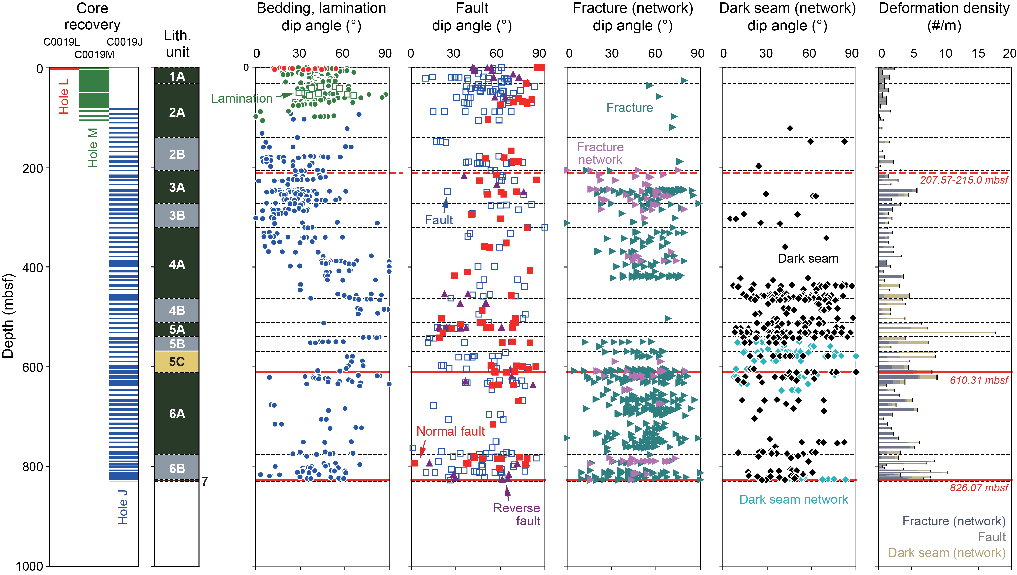
Figure F73. Orientation and density of structural features, Holes C0019L, C0019M, and C0019J.

5.1.1. Primary structures

A total of 16 bedding orientations were measured in this core (Figure F73). Measured dips range 12°–46° with an average bedding dip of 27°.

5.1.2. Deformation structures

In total, 10 minor faults were documented in Hole C0019L. Measured dips range 24°–79° with an average dip of 61° (Figure F73). Of the 10 minor faults identified, 3 had a normal sense of displacement and 7 had a reverse motion.

5.2. Hole C0019M

Hole C0019M recovery was from 0 to 114.5 mbsf. The sedimentary rocks in this depth interval consist of olive-black siliceous vitric mud (Lithostratigraphic Unit 1 and Subunit 2A; see Lithostratigraphy). Several primary and secondary structures were observed and measured in these cores, including dipping bedding and laminae, minor faults, fractures, and sediment-filled veins (Figure F74). The distribution of structures is illustrated in Figure F73. In select sections, discrete samples were measured for paleomagnetic orientations (see Paleomagnetism) that were used to correct the strikes of planar features for drilling-related rotation and identify the true in situ (before core rotation) alignment with magnetic north (see Structural geology in the Expedition 405 methods chapter [Kirkpatrick et al., 2025]). Additionally, drilling-related core disturbances are common in Hole C0019M. Beginning at ~32 mbsf, gas expansion in the cores led to pervasive, densely spaced fracturing. Below 89 mbsf (from Core 405-C0019M-11X downhole), use of the ESCS led to pervasive fracturing and biscuiting in the core.

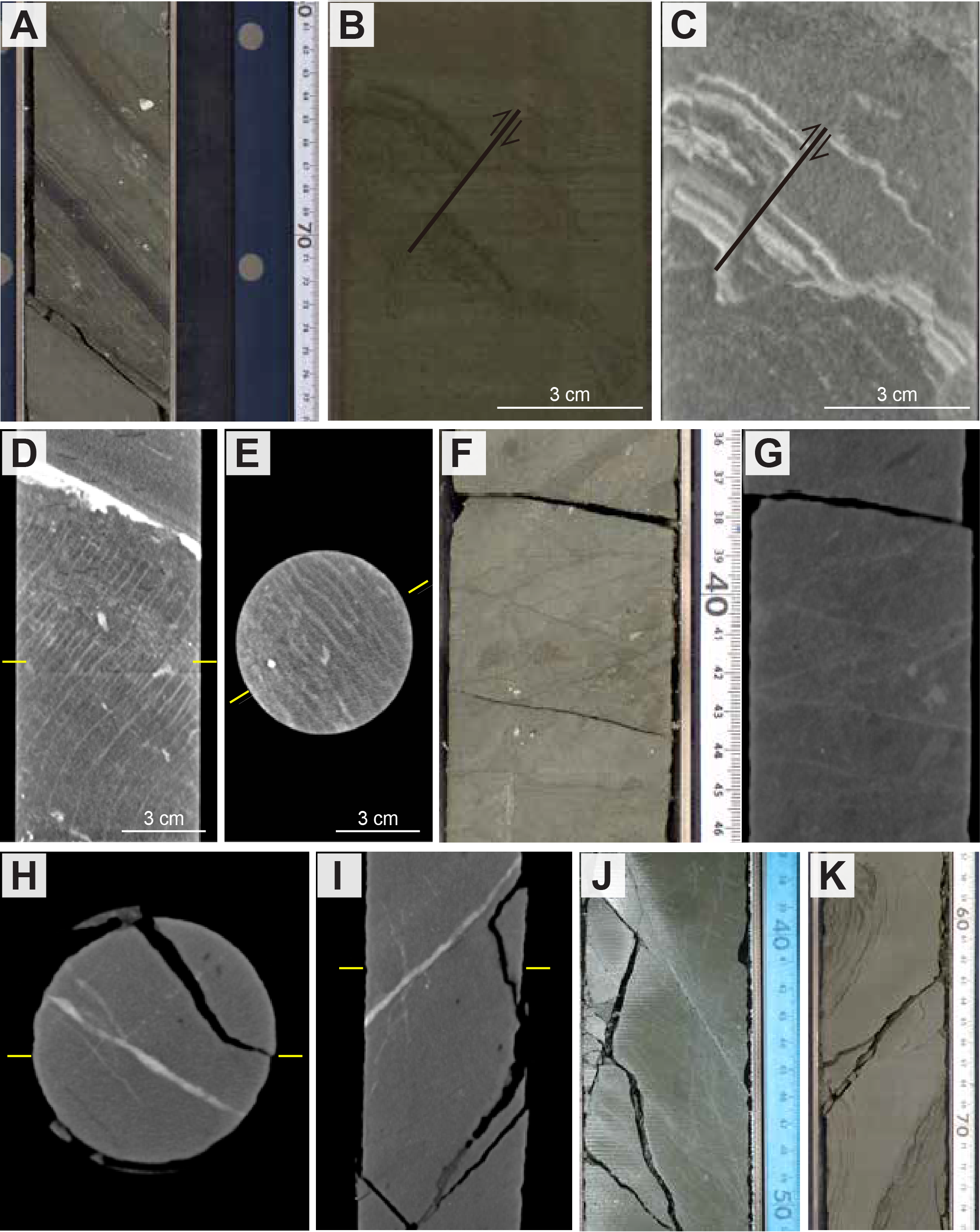
Figure F74. Representative structures.

5.2.1. Primary structures

In total, the orientations of 167 bedding planes and 11 laminations were measured in the uppermost part of the frontal prism in Hole C0019M. Here, bedding and laminations dip moderately to steeply, with an average bedding dip of 41° (total range = 0°–88°) and laminae dip of 44° (total range = 29°–66°) (Figure F73). A paleomagnetic correction of dip directions was applied to 141 beddings and laminae for Hole C0019M. In general, corrected bedding dips northeast, but several northwest-dipping beds are also observed in Lithostratigraphic Subunit 2A (Figure F75; see Lithostratigraphy).

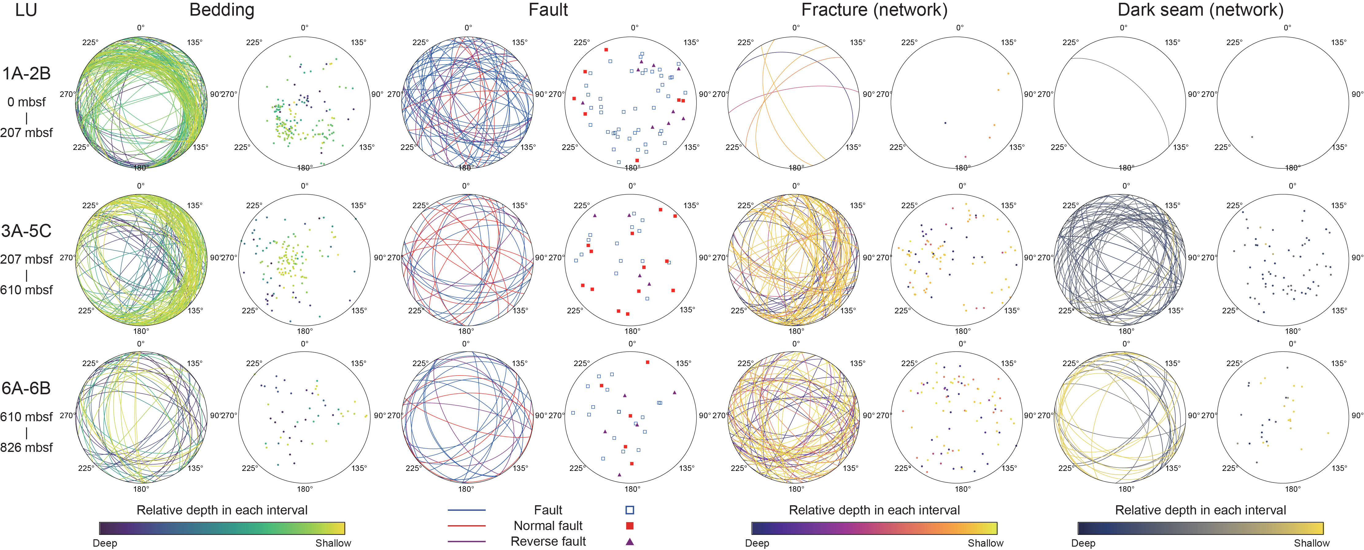
Figure F75. Structural orientations, Holes C0019M and C0019J.

5.2.2. Deformation structures

5.2.2.1. Minor faults and fractures

The strike and dip of 88 minor faults and 5 fractures were observed in Hole C0019M, some of which are at the same depths as faults in Hole C0019L. Of the 88 minor faults, 13 had a reverse sense of slip, 10 had a normal sense of slip, and 65 did not have identifiable sense of slip indicators (Figure F73). The average dip angle of minor faults recovered from Hole C0019M is 54° (total range = 9°–88°), and the average dip angle of fractures is 60° (total range = 35°–79°). Fault dip angles do not change significantly as a function of depth. Although the dip directions of 67 minor faults and 5 fractures were corrected using the paleomagnetically measured declination and inclination obtained from discrete samples (see Paleomagnetism), these corrected dip directions produced no significant trends with depth (Figure F75). Representative minor faults are shown in Figure F74B and F74C.

5.2.2.2. Sediment-filled veins

Sediment-filled veins are observed in Sections 405-C0019M-3H-5, 3H-6, 4H-2, 4H-3, 4H-4, 4H-5, 4H-6, 4H-7, and 4H-8, spanning from 22.56 to 32.35 mbsf. These veins are characterized by several subparallel, curviplanar to sigmoidal millimeter-scale bands that are on average perpendicular to bedding (Figure F74D, F74E). The vertical (bedding-perpendicular) extent of the vein arrays ranges 1–16 cm, with millimetric average intervein spacings. These veins are well-resolved on XCT images from Hole C0019M because they occur as bright white features.

5.3. Hole C0019J

Hole C0019J recovery was from 82 to 829.09 mbsf, which encompassed the bulk of the frontal prism sediments, the plate boundary fault, and the uppermost section of the footwall (Figure F73). In the accretionary prism above the plate boundary fault, one fault was inferred at 207.57–215.00 mbsf (7135.07–7142.5 m BRT) and a major fault was visibly identified at 610.31 mbsf (7537.81 m BRT) (Figure F76). These faults are accompanied by changes in bedding dips, boundaries between lithostratigraphic units, changes in physical properties (see Physical properties), and major age reversals (see Biostratigraphy). The top of the plate boundary fault in Hole C0019J was identified at 826.07 mbsf, characterized by a transition from strongly fractured mudstones in the hanging wall to strongly fractured, foliated, and/or striated layers of mudstones, clays, and chert (Figure F77).

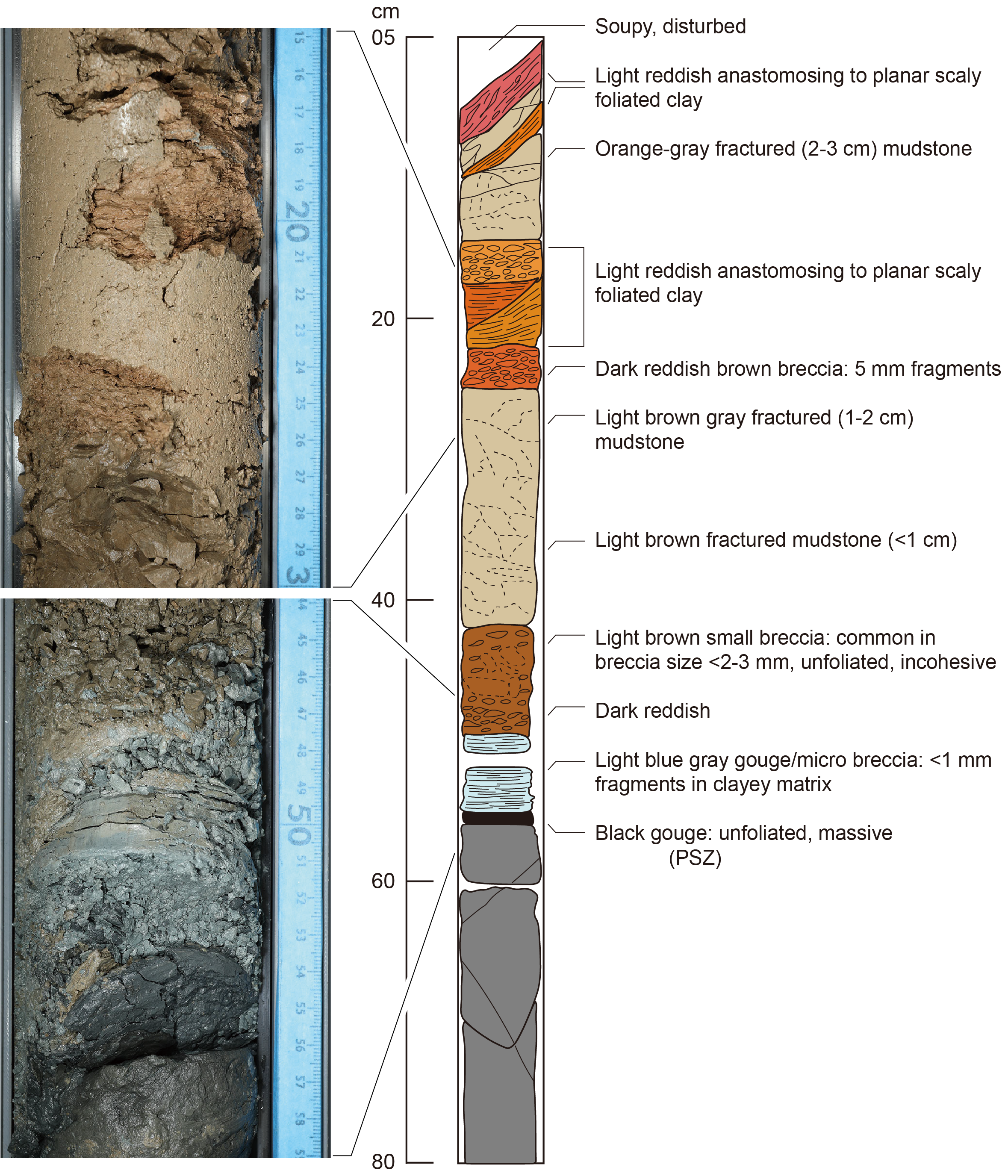
Figure F76. Fault.

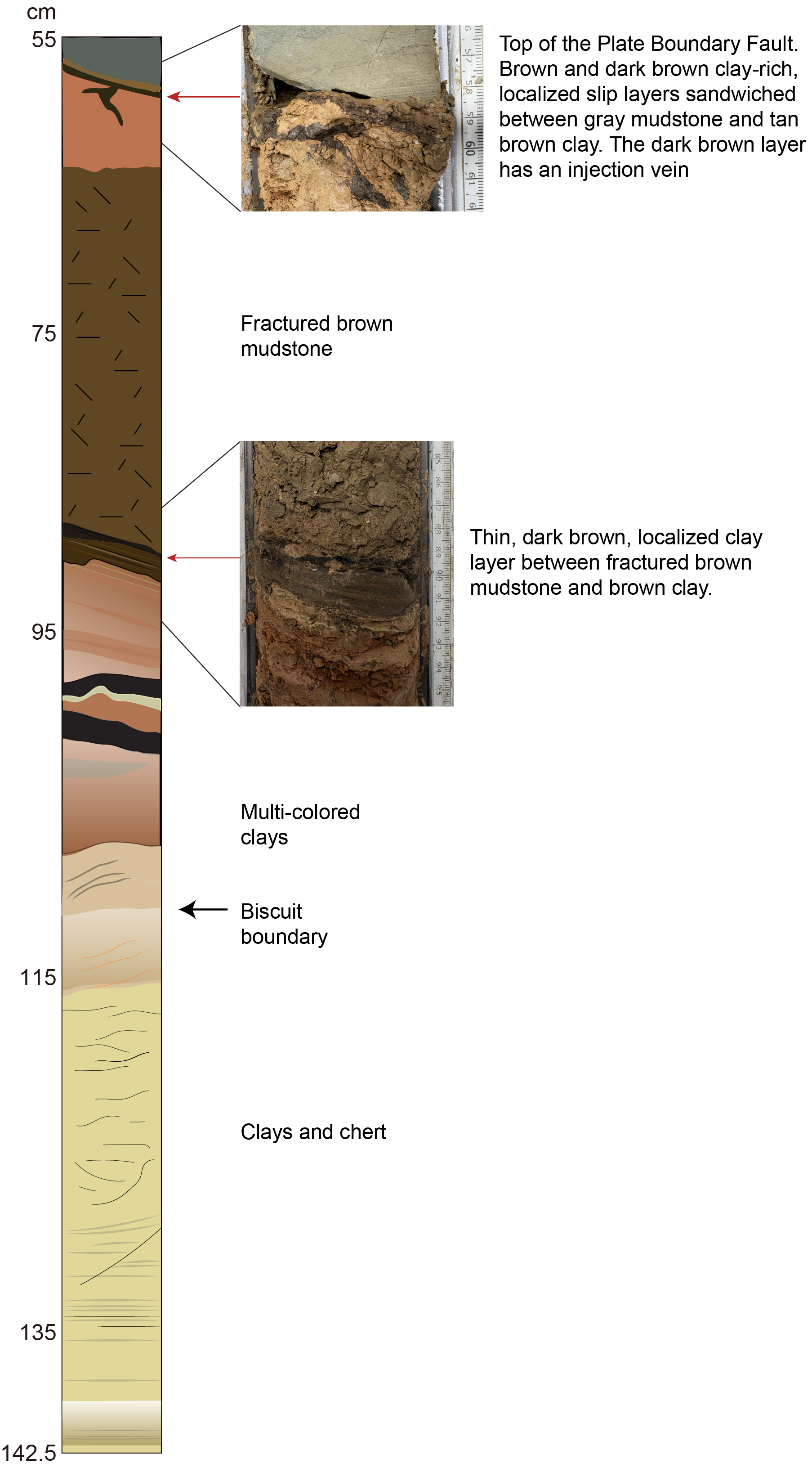
Figure F77. Plate boundary fault, Hole C0019J.

5.3.1. Primary structures

In total, 395 measurements of bedding and laminations were measured in Hole C0019J. Between 80 and 829 mbsf, the prism contains meter-scale intervals of planar bedding and meter-scale intervals of chaotic to convolute bedding separated by very sharp, centimeter- to meter-scale transitions. In the shallowest cores recovered from Hole C0019J, between 80 and 207 mbsf, the average bedding dip is 27° and ranges 4°–70°. This average bedding dip is comparable to the average bedding dip of 27° measured in Hole C0019L but is slightly shallower than the ~40° average dip of primary structures measured from 0 to 80 mbsf in Hole C0019M (Figure F73). Between 207 and 610 mbsf, the average bedding dip is 38°, and measured dips have a large range of horizontal to vertical orientations (0°–90°). Overall, dips follow a general trend of increasing steepness with depth in this interval but also exhibit intervals of chaotic bedding (Figure F75). LWD bedding measurements suggest that this interval represents large-scale folding (see Logging while drilling), but the bedding data seen in the core is too variable to determine whether the changes in dip that we see can be ascribed to folding.

Between 610.31 mbsf (Section 405-C0019J-56K-5, 54 cm) and 826.07 mbsf (Section 87K-2, 59 cm), the average bedding dip angle is 43° and dips range from subhorizontal to vertical (3°–90°) (Figure F73). Beneath the plate boundary fault, deeper than 826.07 mbsf, no primary structures were identified.

5.3.2. Deformation structures

5.3.2.1. Minor faults

A total of 253 minor faults are observed in Hole C0019J (Figure F73). The dips of minor faults exhibit a broad range throughout the cored interval in the hole. Although minor faults occur throughout the core, fault density increases in the vicinity of the two major faults and the plate boundary fault encountered in Hole C0019J. Normal faults constitute the majority of faults whose slip sense could be identified in Hole C0019J, representing 77 out of 253 faults. They show displacements of more than a few millimeters, and striations are commonly observed on the fault plane surfaces. The normal faults have dip angles with an average of ~57˚, steeper than the average dip angle of ~51° for all faults measured in Hole C0019J. Normal faults, which are less than 1 mm thick, show millimeter offsets on the core scale. These faults commonly cut chaotic bedding. Because of their orientation, we cannot rule out whether at least some of these faults are related to drilling operations. Reverse faults comprise a small proportion of the identified faults (28 of the 253 faults), and we did not find crosscutting relationships between the reverse and normal faulting. Of the total 253 faults measured, the dip directions of 73 faults were corrected using declination and inclination of the cores obtained using paleomagnetic analysis. Similar to Hole C0019M, dip directions of the faults in Hole C0019J are highly scattered and show no systematic variation with depth (Figure F75).

5.3.2.2. Fractures and fracture networks

Fractures and fracture networks were documented throughout Hole C0019J, with large dip ranges seen at all depths. As with minor faulting, the areas around the two major faults documented in the prism (200–300 and 590–630 mbsf), as well as the plate boundary zone, show high fracture density (Figure F73). The recorded fracture density is variable throughout the core, most likely due to differences in how Window 1 and 2 scientists determined whether a fracture was natural or drilling induced. This is most clearly seen in the sharp decrease in fracture density between 425.0 and 549.0 mbsf. Window 2 scientists described core for this interval, which lies between the intervals above and below described by Window 1 scientists.

5.3.2.3. Sediment-filled veins

In Hole C0019J, sediment-filled veins were noted in a section of olive-black siliceous vitric mud(stone) (Lithostratigraphic Subunit 5A; see Lithostratigraphy) at 530.9 mbsf. These sediment-filled veins formed in diatom-rich sediments that are compositionally similar to the sediments containing sediment-filled veins at the incoming plate Site C0026.

5.3.2.4. Dark seam and dark seam networks

A total of 398 dark seams and dark seam networks were identified in Hole C0019J. Of these, 97 dark seams were reoriented using paleomagnetic constraints. Dark seams are sometimes coincident with fractures in the core (Figure F74F, F74G). They are widely distributed throughout prism sediments, with a broad range of dips and orientation (Figure F73). The range of attitudes of dark seams is similar to those of the fractures. The density of dark seams increases with depth and in the areas surrounding the major faults.

5.3.2.5. Scaly fabric

In Hole C0019J, scaly fabrics were identified within the major fault zone at 610.9 mbsf and throughout the plate boundary fault at 826.07 mbsf (see descriptions below). Scaly fabrics in Hole C0019J consist of platy, anastomosing, phacoidal clay to mud lenses that form centimeter-scale foliated sheared bands with preferred long-axis orientations that generally dip <30°.

5.3.2.6. Calcite veins

Calcite growth on fracture surfaces and calcite veins are present in Cores 405-C0019J-85K through 87K (~820–826 mbsf) (Figure F74H, F74J) and are likely related to fluid flow along the fault.

5.3.3. Major faults in the frontal prism

Two major faults were identified in the frontal prism. The first was inferred to occur between Cores 405-C00019-14K and 15K (207.87–215.00 mbsf; 7135.07–7142.5 m BRT) because of an increase in minor fault and fracture density, changes in physical properties and lithology, and an age reversal between the two cores, but no discrete major fault structures were visually identified (see Lithostratigraphy, Biostratigraphy, and Physical properties). A second major fault was visually identified at 610.31 mbsf (7537.81 m BRT) at the contact between Lithostratigraphic Subunits 5C and 6A (Section 405-C0019J-56K-5, 54 cm). This fault is associated with a major age reversal, suggesting it is a reverse fault (see Biostratigraphy), and it contains a black layer inferred to be fault gouge that marks a localized slip zone. Much of the structure and fabric of the fault rock was disturbed upon cutting of the core liner because of the rapid expansion of accumulated gas. However, it is estimated that tectonically brecciated fault rocks and scaly clays start to appear within 50 cm above localized slip zone.

This brecciated damage zone mostly comprises orange to orange-gray breccia that hosts several intervals 5–10 cm in size (Figure F76). The intervals are fractured, and polished striated surfaces are observed where the internal crack faces were exposed. The breccia and light reddish clay have anastomosing scaly foliations with <1 mm spacing, but visual observations are difficult because of the coverage by drilling mud. The orange color of the breccia transitions to dark brown about 15 cm above the localized slip zone. A light blue foliated gouge/microbreccia about 2 cm thick appears just above the localized slip zone. The localized slip zone itself is a black gouge layer about 0.5 cm thick where it was exposed for visual core description.

Olive-black siliceous vitric mud(stone) (Lithostratigraphic Subunit 6A) is present below the fault. The footwall does not show any substantial deformation and is only moderately fractured or faulted by minor amounts of normal slip to the bottom of Core 405-C0019J-56K.

Note that distances described above and in Figure F76 may be expanded because of the rapid gas expansion that disturbed the original fault zone structure.

5.3.4. Plate boundary fault zone

The base of the prism mudstone (Lithostratigraphic Unit 6) at 826.07 mbsf (7753.57 m BRT; Section 405-C0019J-87K-2, 59 cm) is present as a discrete edge, interpreted to be a fracture surface from lineations observed on the surface, that dips 26° (Figure F77). Below this boundary, the deformation fabric changes from fractured mudstones with dark seams to foliated clay-rich rocks. Additionally, there is a large age gap at this boundary; therefore, everything described below is interpreted to be the plate boundary fault (Lithostratigraphic Unit 7; see Lithostratigraphy). The fault is <1 m thick and composed of intercalated units of various clays and mudstones. There are potentially several localized slip zones, and we describe two of these zones here in detail. Immediately beneath the mudstone is a pair of layers of extremely fine grained material in which individual grains could not be observed. The uppermost layer in the pair is ~0.5 cm thick, brown, and homogeneous. Rare faces undisturbed by core splitting and handling appear to reveal a weak penetrative foliation suggesting the presence of aligned platy minerals like clays. The lower of the two layers is dark brown and contains a millimeter-scale scaly fabric. The interface between these two layers appears sharp and approximately planar, which we identify as a potential localized slip zone. The lower edge of the dark brown layer is wavy. Beneath the wavy surface, there is a grayish yellowish brown to dull yellowish brown clay-rich rock in which the scaly fabric has an irregular pattern. One prominent dark brown vein crosscuts the tan-brown rock that appears to branch from the dark brown layer with millimetric scaly fabric. This vein has sharp edges, is homogeneous, and lacks scaly fabric; the shape of the vein suggests that it is an injection. The tan-brown clay-rich rock grades into a brown mudstone that is heavily brecciated into approximately centimeter-sized phacoidal clasts. The brecciated brown mudstone contains rare 1–8 cm clasts and is present for ~25 cm downcore.

The base of the fractured brown mudstone is a sharp planar contact beneath which is a sequence of clay layers with a variety of colors, similar to the section of clay observed in Cores 405-C0019E-20R (Expedition 343/343T Scientists, 2013b), 405-C0019K-16K (see Lithostratigraphy), and 405-C0026B-30K (see Lithostratigraphy in the Site C0026 chapter [Conin et al., 2025]). Immediately beneath the mudstone is a 3–4 mm thick dark brown layer containing a millimetric scaly fabric with asymmetric phacoids, which we interpret to be a potential localized slip zone. The dark brown layer bifurcates on one side to surround a ~1 cm thick lens of brown clay. A vein branches from the dark brown layer at a high angle and appears to contain the same material as the dark brown layer. This vein projects upward into the brecciated mudstone. The clay beneath the dark brown layer is slightly oblique to the dark brown layer in the upper portion of this section. The clay layers contain a weak scaly fabric in some sections that is apparently massive in others.

Around Section 405-C0019J-87K-2, 112 cm, the core is biscuited. Beneath the biscuit, the clay color grades from dull yellow orange to light yellow over an interval of ~4 cm. The light yellow interval contains a scaly fabric with millimeter- to centimeter-sized phacoids. Phacoid long axes are mostly subperpendicular to the core axis, except where a small fault with normal sense offset cuts the layering. Adjacent to the fault, the scaly fabric wraps around the fault plane. The light yellow rock is brecciated because of drilling-induced damage in Cores 87K and 88K and mixed with red chert fragments.

5.4. Hole C0019K

Hole C0019K penetrated the basal sediments of the frontal prism and the plate boundary fault. Core recovery was from 815.0 to 875.5 mbsf (Figure F78). The top of the plate boundary fault was identified at 846.17 mbsf, characterized by strongly localized deformation at the juxtaposition of mudstones and clays, which was overlain by a coherent hanging wall consisting of accretionary prism sediments. The footwall below the fault is composed of foliated clays and fractured chert. Structural features identified in Hole C0019K include (1) fractures, minor faults, dark seam networks, and dark seams in the hanging wall; (2) foliated clays and mudstones with localized fault gouge zones; and (3) banded and/or weakly foliated clays, mudstones, and cherts in the footwall. In select sections, discrete samples were analyzed paleomagnetically to correct the strikes of planar features for drilling-related rotation, representing the true in situ alignment.

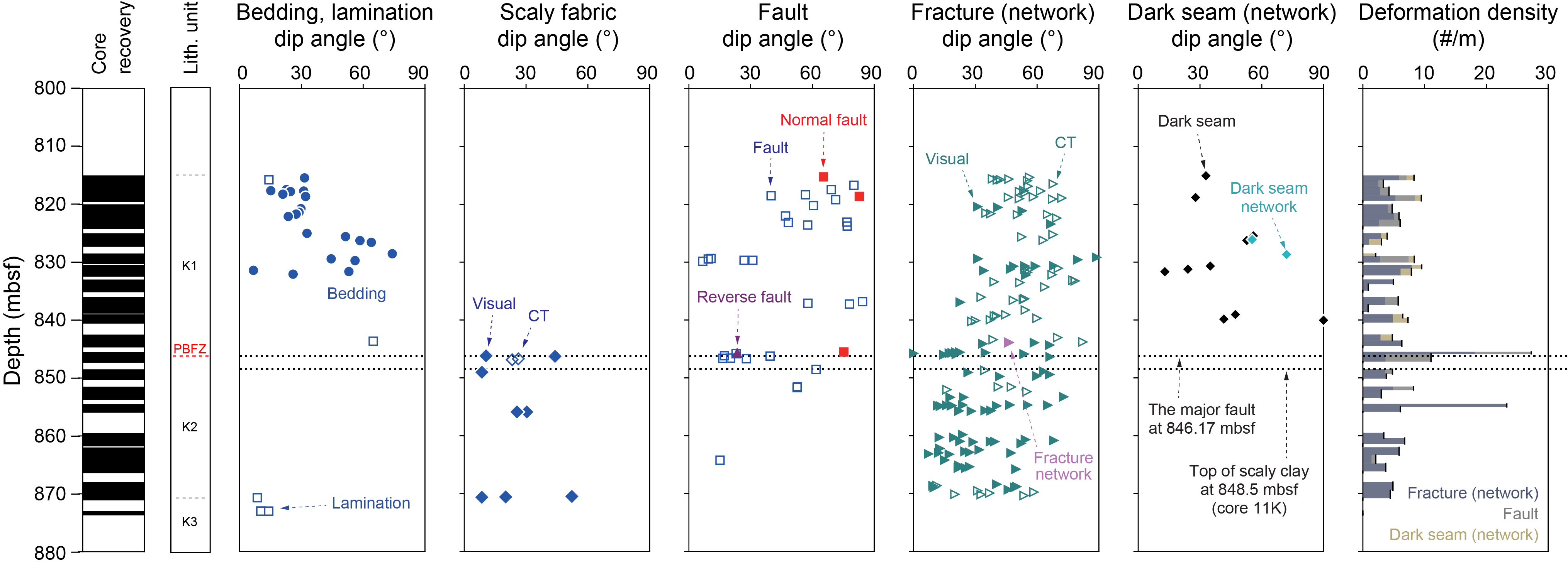
Figure F78. Orientation and density of structural features, Hole C0019K.

5.4.1. Primary structures

In total, 27 measurements of bedding and laminae orientations were obtained on the working-half sections of cores using visual core description and complemented by XCT measurements. In the hanging wall, bedding in Lithostratigraphic Unit K1 dips approximately 36° to 825 mbsf, where bedding dips become more varied (~7°–74°) (Figure F78), showing a girdle despite small numbers of bedding with corrected orientations (Figure F79). Below the hanging wall, bedding was difficult to identify. However, attitudes of thin color-banded laminae in part of Lithostratigraphic Unit K3 (color-banded chert and clay) were measured as likely representative of bedding. These laminae dip <20°.

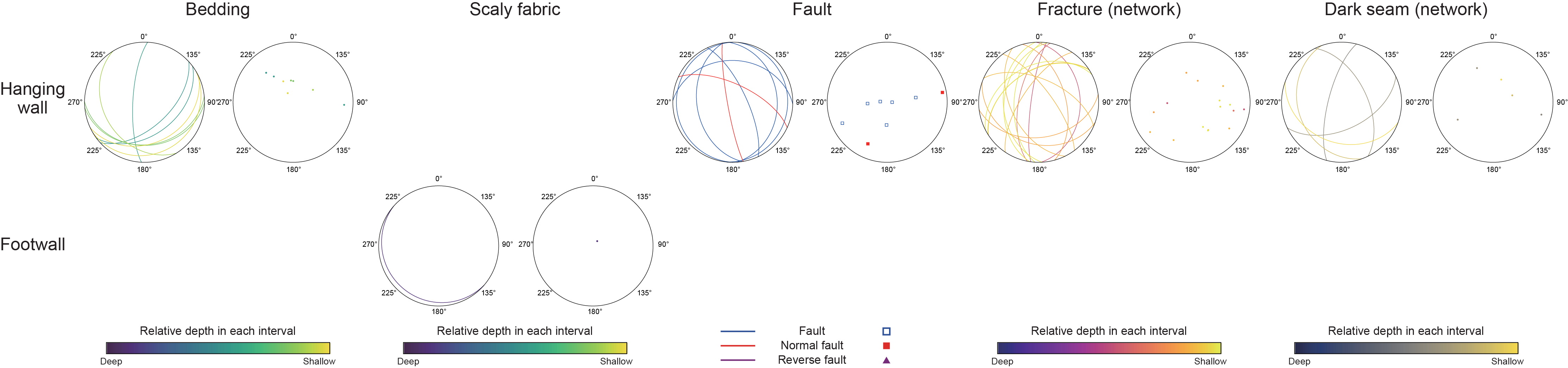
Figure F79. Structural orientations, Hole C0019J.

5.4.2. Deformation structures

5.4.2.1. Minor faults

We identified 34 minor faults with small (≤1 cm) measurable offsets defined by truncations of primary structures (bedding, laminations, or clasts) and smaller fractures. Slip sense for some faults could be determined by measuring striations on fault plane surfaces that intersected the cut face of the working-half core sections (Figure F78). Fault dips are highly variable in both the hanging wall and within and below the fault. Faults are more common in the hanging wall, and the peak in minor fault density occurs just above the plate boundary fault. Of the 34 minor faults identified, the sense of slip was determined for 3 normal faults and 1 reverse fault, with the remaining 30 minor faults lacking sense of slip indicators. Similar to Hole C0019J, minor fault dips exhibit a broad range at all depths (7°–84°).

5.4.2.2. Fractures and fracture zones

The strike and dip of 152 fractures and fracture zones were obtained on the working-half sections through visual core description and complemented by XCT measurements (Figure F78). Fracture zones in Hole C0019K are composed of sets of parallel to subparallel and/or crosscutting fractures that result in partially disaggregated blocks ranging from 1 cm to a few centimeters in size. Fractures in the hanging wall (above 846.17 mbsf) dip an average of 54° (range = 23°–89°), whereas fractures in the footwall (deeper than ~846 mbsf) have a lower average dip of 34° (range = 7°–73°), but both zones have a wide variation in fracture dip. Fracture density was calculated by determining an average number of fractures per section. Fracture density increases at the top of the fault zone (846.17 mbsf) and at ~855 mbsf.

5.4.2.3. Dark seams and dark seam networks

In Hole C0019K, 12 dark seams are located in the hanging wall of the fault at depths shallower than ~843.4 mbsf (Figure F78). The dark seams are characterized as singular, planar, brownish black to black structures that are typically less than 1 mm thick and are either layer parallel or crosscutting across other sedimentary features (e.g., bedding planes). We identified two dark seam networks in Hole C0019K between 820 and 830 mbsf and in the hanging wall of the fault located at 845.8 mbsf. Dark seams typically have higher computed tomography (CT) values than the surrounding rock and appear as bright, highly reflective features on the XCT images. In general, dark seams are widely distributed within the prism, generally dip <60°, and are commonly collocated with fractures and fracture zones.

5.4.2.4. Scaly fabric

Scaly fabric of variable intensity (weak, moderate, or penetrative) was observed in clays within and below the major fault (starting in Section 405-C0019K-10K-2, 63 cm). These contain phacoidal lenses, the surfaces of which define a scaly fabric texture and are often associated with anastomosing polished surfaces. Scaly fabrics generally dip <30°.

5.4.3. Plate boundary fault zone

At 846.17 mbsf (7750.2 m BRT; Section 405-C0019K-10K-2, 34 cm), there is a sharp transition from fractured but otherwise apparently undeformed olive-gray vitric mud(stone) (Lithostratigraphic Unit K1; see Lithostratigraphy) to less indurated, strongly foliated, siliceous and ashy mudstone and clay with localized slip layers. This transition is the top of a fault that we interpret to be the plate boundary fault (Expedition 343/343T Scientists, 2013b). The fault contains an ~85 cm thick interval of mudstones and clays with variable degrees of deformation as expressed by fabric intensity and slip localization, which we interpret to be more deformed than the rocks above and below.

The top of the fault occurs at 846.17 mbsf (Section 405-C0019K-10K-2, 34 cm) (Figure F80), where a fracture surface separates an overlying gray mudstone from an underlying layer of foliated gouge. This gouge layer is ~1.5 cm thick and consists of three alternating bands: a 2–3 mm thick dull brown layer, a 5–8 mm thick brownish black layer, and a 2–5 mm thick dull brown layer. The surfaces bounding the top and bottom of the gouge layer dip 23° and 17°, respectively. Beneath the gouge, there is a grayish yellow brown mudstone that is lithologically similar to the mudstone in sharp contact with the top of the fault at 846.17 mbsf (Section 10K-2, 34 cm). The base of this mudstone is in sharp contact with a brown scaly mudstone at 846.24 mbsf (Section 10K-2, 41 cm), with a 1–2 mm dark brown gouge layer in between. Beneath the foliated brown mudstones is a relatively undeformed dark brown black mudstone. From 846.46 to 846.66 mbsf (Section 10K-2, 63–83 cm), brown and dark brown banded clays (see Lithostratigraphy) have well-developed scaly fabric and exhibit vitreous surfaces. Within this interval of clays, there is a 0.5 cm thick brownish black clay layer at 846.53 mbsf (Section 10K-2, 70 cm) (Figure F80) that has a dip of 20° and is surrounded by more vitreous material. Beneath the brown clays with dark bands, there is a brownish gray clay unit from 846.66 to 846.71 mbsf (interval 10K-2, 83–88 cm) that appears massive because of smearing of the clay against the core liner but in fact has a penetrative scaly fabric. The base of the brownish gray clay layer is in sharp contact with dull brown scaly clay with intense fabric formed by millimeter- to centimeter-scale phacoids across a 1–2 mm gouge layer with a dip of 28°. From 846.71 to 846.93 mbsf (interval 10K-2, 88–110 cm), there is more dull brown clay with scaly fabric that decreases in intensity with depth. Below this portion, the core is too affected by drilling disturbance to interpret structure.

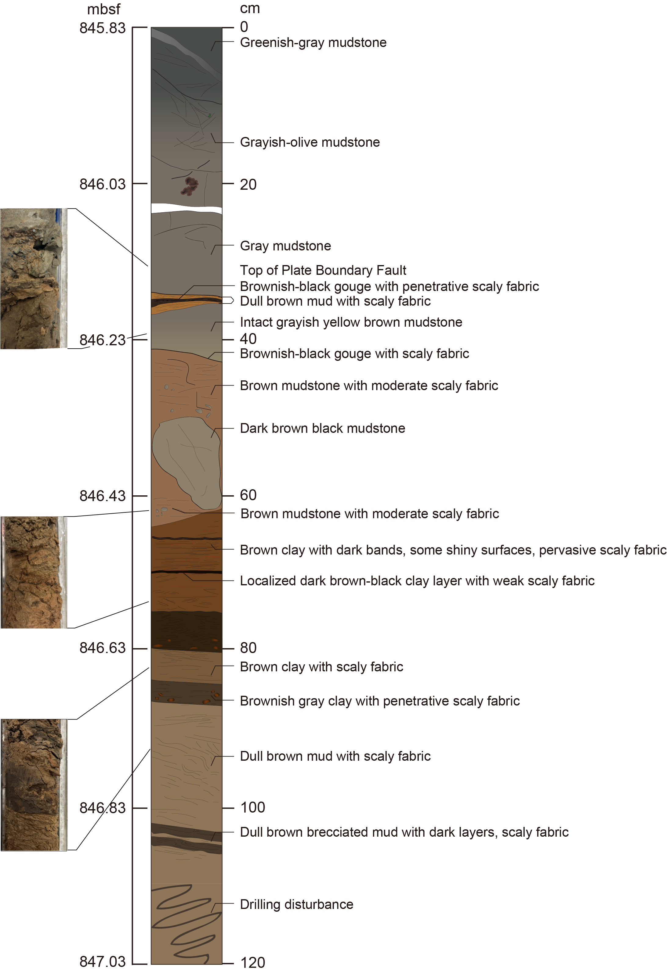
Figure F80. Plate boundary fault, Hole C0019K.

Beneath the intensely deformed rocks in Core 405-C0019K-10K is ~25 m of dark brown-black scaly clay (Cores 11K–16K). The scaly fabric in Cores 11K–16K is defined by millimeter-scale layering of lenticular phacoids with vitreous plane-parallel surfaces, with abundant drilling-related smearing of whole-round faces and split core faces. If we include the brown scaly clay as a part of the fault zone, the plate boundary fault here is much thicker than seen in Holes C0019J and C0019E during Expedition 343. Underlying these dark brown-black clays, a 309 cm thick section of color-banded pelagic clay and chert (Lithostratigraphic Unit K3) was recovered in Cores 16K and 17K. The color-banded pelagic clay is more indurated toward the base of Core 17K, likely related to different stages of silicification and diagenesis. No continuous, intact section of chert-rich sediments was recovered beneath 873.4 mbsf (Core 17K) because of the resistance of chert to current coring methods.

5.5. Hole C0019P

Five cores were recovered in Hole C0019P from 930 to 946.4 mbsf. The recovered rocks consist of basalt, chert, and carbonate (see Lithostratigraphy). Deformation features in these cores consist of small white veins as well as larger structures containing pink, green, and white materials that are interpreted to be the result of fluid injections.

5.5.1. Deformation structures

5.5.1.1. Veins

In total, 156 basalt-hosted mineral veins were documented in Hole C0019P. Their thickness varies between millimeters and centimeters. Mineral vein orientations have an average dip of 24° and range 1°–90° (Figure F81). The dip angle of the mineral veins decreases below 940 mbsf to an average of 10° with a range of 1°–20°. Several veins show crosscutting relationships and crack-seal textures, implying multiple episodes of veining (Figure F82). Some veins have several bands marked by different colors (white and green) in the middle, suggesting multiple phases of opening. Additionally, some veins have alteration halos. In Core 405-C0019P-3K, concentrated areas of subhorizontal mineral veins are prevalent (see Lithostratigraphy) (Figure F83). The number of mineral veins was difficult to quantify because in some areas they were extremely thin and dense. The average density of the veins that were counted was ~15 veins/m with a peak density of ~30 veins/m at 939 mbsf.

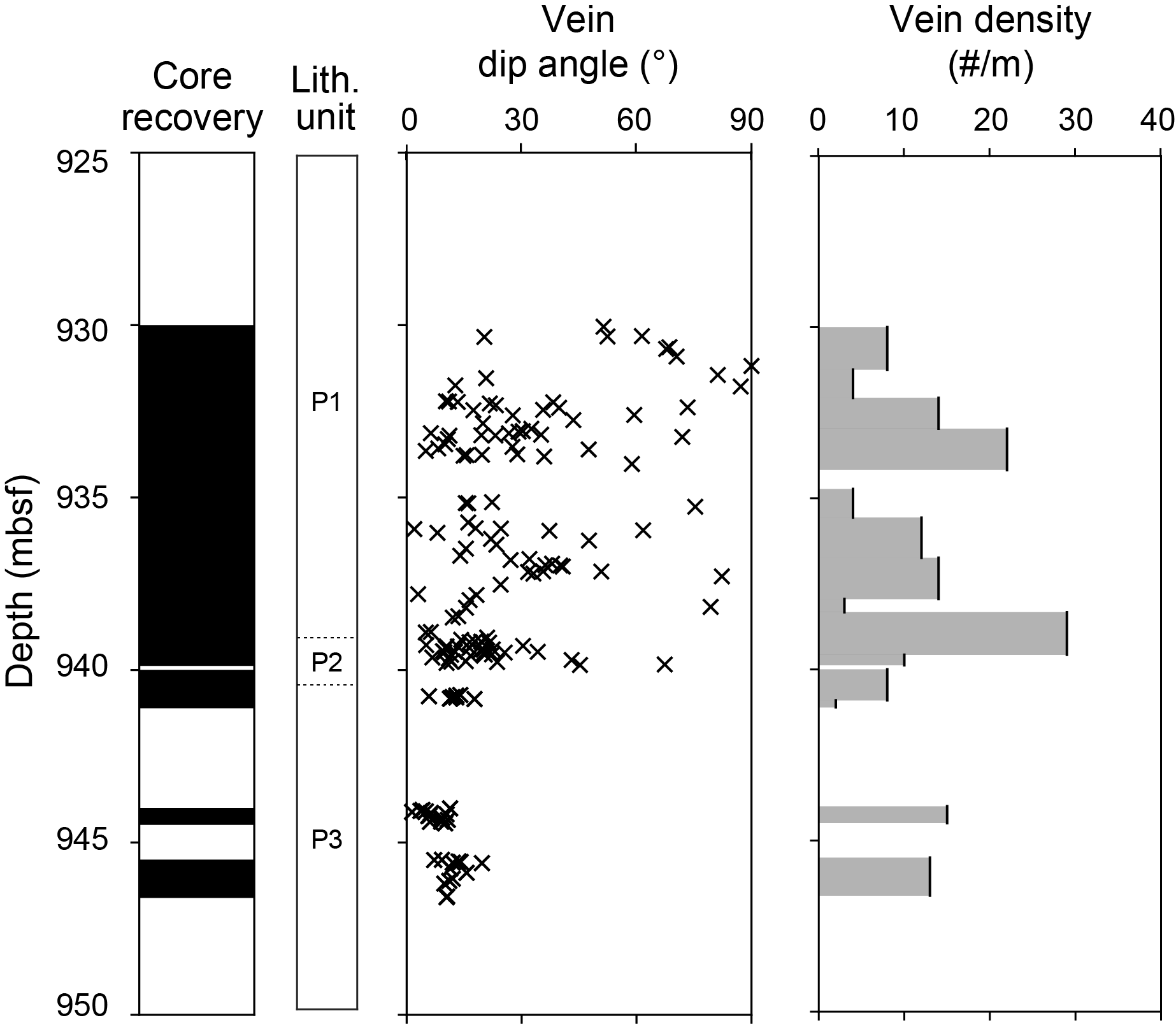
Figure F81. Dip angles and vein density.

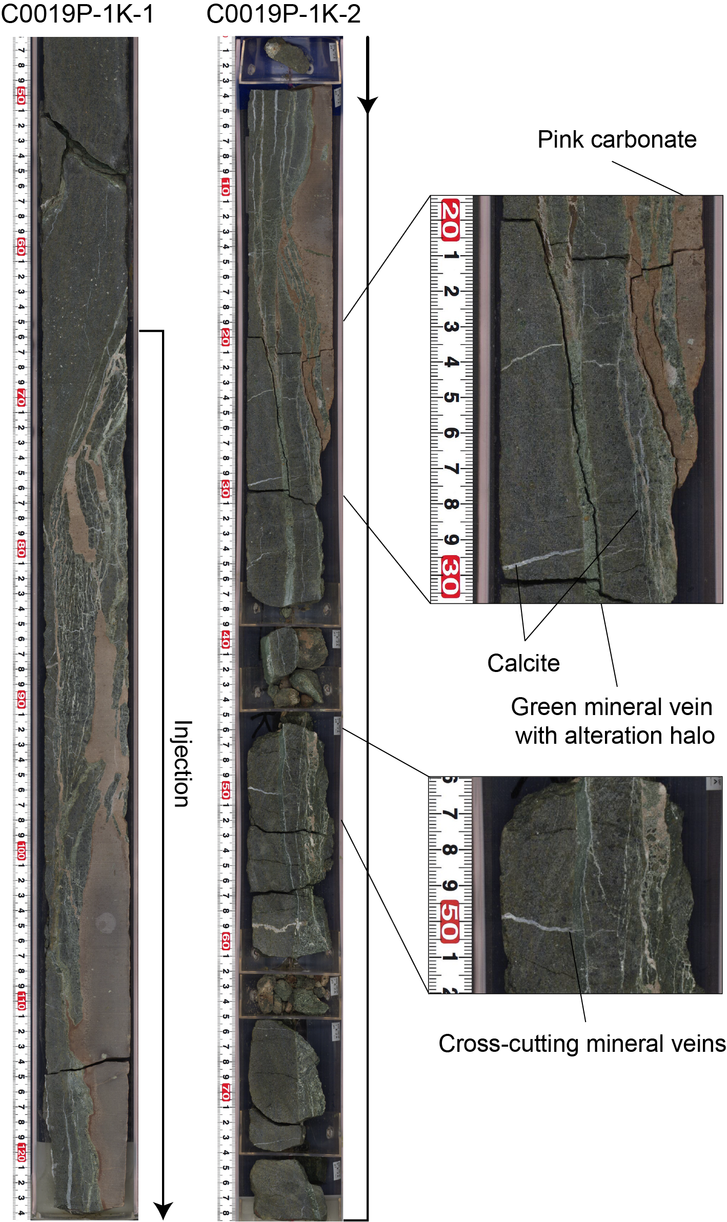
Figure F82. Mineralized fluid injections.

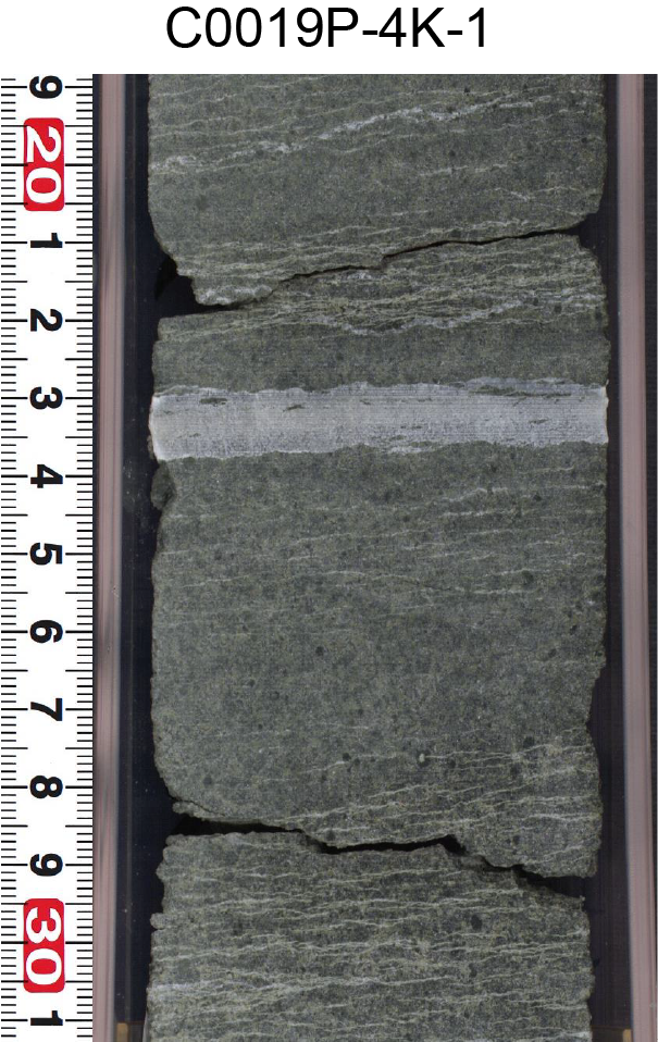
Figure F83. Mineral veins.

5.5.1.2. Injection

A portion of a large (~1 m long) body of brown carbonaceous material was documented from Section 405-C0019P-1K-1, 65 cm, to the bottom of Section 1K-2 (930.7–932.0 mbsf) (Figure F82) and is interpreted to be a part of a fluid injection structure into the basalt based on the vein-like geometry of this body, which crosscuts the basalt. The injection is in the vertical/longitudinal direction of the core, tapering slightly toward the top of the core. The fill in this feature consists of brown carbonaceous material (similar to the interstitial material between pillows; see Lithostratigraphy), an unidentified green mineral, and white calcite. The thickest section of the structure consists of brown carbonaceous material, and the edges of the main body and veins that branch from the structure often gradually change from brown to green or pink to white with distance from the edge of the structure or with distance along the branched vein.

5.6. Interpretation

The prism includes both large- and small-scale structures that may be related to a combination of tectonic and mass transport processes. Prism structures include faulting, potential folding, and chaotic bedding, potentially related to mass transport. Minor faults and fractures as well as dark seams constitute most of the small-scale deformation fabric of the accretionary prism. Sediment-filled veins were also noted and are commonly found in sediments in subduction zones such as the Nankai Trough (Tobin et al., 2020), Miura-Boso accretionary prism (Hanamura and Ogawa, 1993; Maltman et al., 1993), and Anafi Island Basin (Druitt et al., 2024). Based on field and experimental studies, such veins are thought to form because of shaking and dewatering during earthquakes (Hanamura and Ogawa, 1993; Brothers et al., 1996).

Three major faults were encountered in Hole C0019J. Based on age reversals across the faults identified from biostratigraphy, the faults at 210 and 610 mbsf are interpreted to be reverse faults within the accretionary prism. Between these faults, wide variations in bedding dips, including subvertical bedding, indicate possible large-scale folding within the accretionary wedge, although this is clearer in LWD observations from Holes C0019B (Expedition 343/343T Scientists, 2013b) and C0019H (see Logging while drilling) than in the bedding data measured within the cores. The plate boundary fault was encountered at 826.07 mbsf in Hole C0019J as a sharp upper surface and is characterized by foliated clays and fractured mudstones with zones of localized slip within the wider fault zone structure. The fault is approximately 1 m thick and ends at the underlying relatively undeformed chert unit.

We cored three tectonic units in Hole C0019K: the basal part of the accretionary prism, the entirety of the plate boundary fault, and part of the footwall. The plate boundary fault has a sharp upper surface, and deformation in Section 10K-2 is the most intense deformation encountered in the core based on the occurrence of localized gouge zones and strong scaly fabric intensity. The base of the PBFZ is less clear, in part due to the drilling disturbance at the base of Section 10K-2. It is unclear whether the pelagic clays below are part of the fault zone or footwall rocks whose fabric may be related to compaction, as suggested by the anisotropy of magnetic susceptibility (AMS) of the pelagic clays, which shows subvertical inclinations of the minimum axis (k₃) (see Paleomagnetism). If the brown clay is included as part of the plate boundary fault in Hole C0019K, the fault is much thicker than the fault found in Hole C0019J.

6. Biostratigraphy

All core catcher samples drilled with the SD-RCB system in Holes C0019J and C0019K were examined for diatom biostratigraphy on board the ship. In addition, two core catcher samples (405-C0019M-1H-CC and 2H-CC) drilled with the HPCS were examined off shore during the expedition for diatom analysis. In addition, smear slides were prepared from selected key horizons following recommendations of the location by the sedimentologists, structural geologists, and Co-Chief Scientists. Radiolarians were examined from all core catcher samples drilled with the SD-RCB system in Hole C0019K, the HPCS in Holes C0019L and C0019M, and the ESCS in Hole C0019M. In addition, chert samples from Holes C0019J and C0019K were also used for radiolarian analysis.

6.1. Diatoms

Diatom abundance is common to rare with moderate to poor preservation from sample to sample. In general, the North Pacific diatom (NPD) zonal scheme of Yanagisawa and Akiba (1998) was applied to the examined samples. Diatom zones were identified from the Pleistocene Zone NPD12 through the upper Miocene Zone NPD7A and middle Miocene Zone NPD5A for each sample. However, secondary datums based on the revised species concepts of Shiono and Koizumi (2000), along with equatorial Pacific zonal markers (Burckle, 1972; Barron, 1985; Baldauf and Iwai, 1995), were also used when necessary. These were supplemented with biochronological information from various sources (e.g., Maruyama and Shiono, 2003; Shackleton et al., 1995; Shipboard Scientific Party, 2003; Iwai et al., 2025). The age-depth profile in Hole C0019J reconstructed by diatom biostratigraphy is summarized in Figure F84.

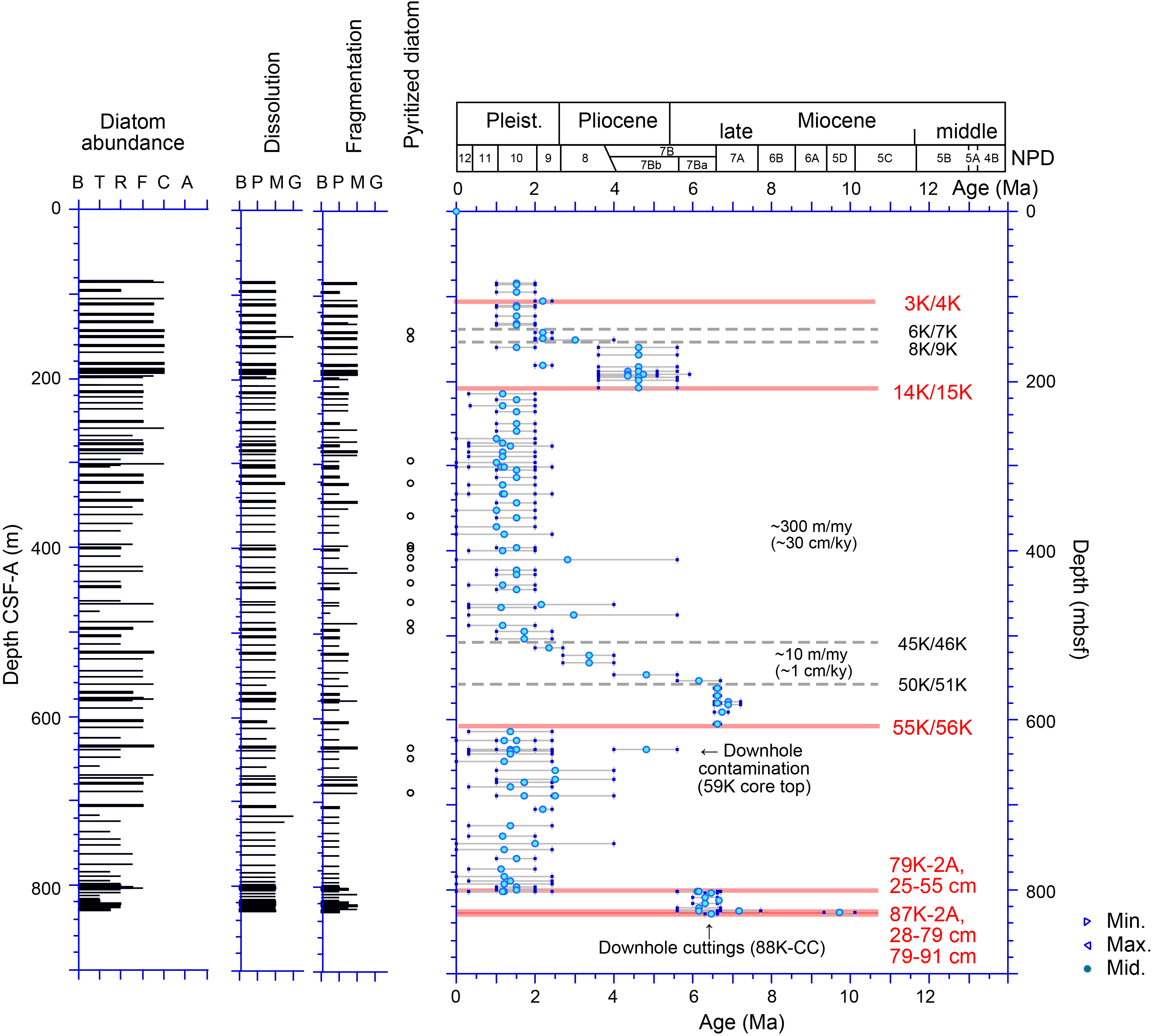
Figure F84. Diatoms.

6.1.1. Hole C0019M

For Hole C0019M, core catcher Samples 1H-CC and 2H-CC were examined (Table T26). The occurrence of Fragilariopsis doliolus in both samples suggests that these samples are younger than the first occurrence (FO) of F. doliolus at 2.0 Ma. The absence of Proboscia curvirostris in these samples suggests the samples might be younger than the last occurrence (LO) of P. curvirostris at 0.30 Ma, although reworked Miocene–middle Pleistocene diatoms such as Neodenticula kamtschatica, Neodenticula koizumii, Denticulopsis simonsenii s.l., and Thalassiosira convexa v. aspinosa are also observed in the samples. Framboidal pyrite is common in both samples. In addition, Sample 1H-CC, 16.5–21.5 cm (3.275–3.325 mbsf), contains calcareous nannofossils and planktonic foraminifera.

Additional samples taken from core catchers or core sections will be examined during postexpedition research to refine the age determination of the Pleistocene section at Site C0019.

6.1.2. Hole C0019J

Multiple age reversal events were detected in cores recovered from Hole C0019J (Figure F84):

Between Sample 3K-CC, 20–25 cm (104.70–104.75 mbsf), lower Pleistocene (NPD9; 1.98–2.4 Ma), and Sample 4K-1A, 54 cm (104.74 mbsf), middle to upper Pleistocene (NPD11–NPD10; 0.3–2.0 Ma);
Between Sample 14K-CC, 25.5–30.5 cm (207.82–207.87 mbsf), uppermost Miocene to Pliocene (NPD7Bb; 3.6/4.0–5.6 Ma), and Sample 15K-1W, 4 cm (215.04 mbsf), middle to upper Pleistocene (NPD11–NPD10; 0.30–2.0 Ma);
Between Sample 55K-CC, 15.5–20.5 cm (605.15–605.2 0 mbsf), middle of late Miocene (NPD7A; 6.55–6.7 Ma), and Sample 56K-CC, 19-24 cm (613.405–613.455 mbsf), Pleistocene (NPD11–NPD9; 0.35–2.4 Ma);
Between Sample 79K-2A, 25 cm (802.13 mbsf), Pleistocene (NPD11–NPD10; 0.30–2.0 Ma), and Sample 79K-2A-53 cm (802.41 mbsf), late Miocene (NPD7Ba; 5.6–6.6 Ma); and
Between Sample 87K-2A, 28 cm (825.76 mbsf), middle late Miocene (NPD7A; 6.6–7.7 Ma), and Sample 87K-2A, 43 cm (825.91 mbsf), late/middle Miocene (~NPD5D; 9.3–10.1 Ma or older).

These age gaps appear to correlate with lithologic and structural observations made on cores (see Lithostratigraphy and Structural geology), especially where potential faults or unconformities were identified between Sections 405-C0019J-14K-CC and 15K-1 (207.57 mbsf) (also a major fault in Section 56K-5, 54 cm [610.31 mbsf] and the PBFZ in Section 87K-2, 59 cm [826.07 mbsf]), as well as with specific lithologic changes or with structures observed on the LWD dataset at ~98, 210, 607.5, ~807, and 825 mbsf in Hole C0019H (see Logging while drilling).

Diatom biostratigraphy suggests most of the age discontinuities are due to thrust faults (age reversal), except two normal-sense observations (age gap) in Sections 405-C0019J-79K-2A (~802 mbsf) and 87K-2A (~825 mbsf).

The occurrence of Actinocyclus oculatus without N. koizumii in samples from Cores 405-C0019J-1K and 2K (84.38–95.38 mbsf) indicates the samples belong to the middle Pleistocene A. oculatus Zone (NPD10), dated 1.02–1.98 Ma. The presence of Thalassiosira jouseae, P. curvirostris, Thalassiosira antiqua, Alveus marinus, Shionodiscus oestrupii s.s., and Neodenticula seminae supports this interpretation. The occurrence of N. kamtschatica, Denticulopsis, and Crucidenticula species in these samples is interpreted as reworked material from the lower Pleistocene through middle Miocene. The co-occurrence of N. koizumii, N. seminae, and S. oestrupii s.s. in Sample 3K-CC, 20–25 cm (104.70–104.75 mbsf) suggests that this sample falls within the upper part of the N. koizumii Zone (NPD9), dated 1.98–2.4 Ma in previous publications.

The occurrence of A. oculatus with N. seminae, S. oestrupii s.s., and/or F. doliolus in Samples 405-C0019J-4K-1A, 54 cm (111.04 mbsf), to 6K-CC, 30.5–35.5 cm (132.92–132.97 mbsf) indicates that these samples belong to the middle Pleistocene (NPD10). The trace and/or sporadic occurrence of N. koizumii in these samples is interpreted as a result of reworking. Conversely, the co-occurrence of N. koizumii and N. seminae in Samples 7K-CC, 16.5–21.5 cm (142.755–142.805 mbsf), to 8K-3A, 43 cm (150.24 mbsf), and in Sample 11K-5A, 56.5 cm (181.795 mbsf), places these samples within the lower Pleistocene, especially in the upper portion of Zone NPD9 (2–2.4 Ma). The trace and sporadic occurrence of N. kamtschatica in these samples is interpreted as a result of reworking. The occurrence of S. oestrupii s.l. with only sporadic traces of N. kamtschatica in Samples 9K-CC, 39–44 cm (160.80–160.85 mbsf), to 14K-CC, 25.5–30.5 cm (207.82–207.87 mbsf), allowed us to assign these samples to the Pliocene S. oestrupii Zone (NPD7Bb).

The occurrences of S. oestrupii s.s. and N. seminae in Samples 405-C0019J-15K-1, 4 cm (215.04 mbsf), to 45K-CC, 26.5–31.5 cm (504.455–504.505 mbsf), indicate that these samples are younger than the FO biohorizon at 2.4 Ma within the Pleistocene. The occurrence of P. curvirostris and/or T. jouseae in samples from 215 to 504.5 mbsf constrains the samples to be older than the LO datum at 0.30 Ma, whereas the occurrence of A. oculatus similarly constrains the samples as older than 1.02 Ma. Conversely, no marker species were identified in Samples 35K-CC, 38–43 cm (410.755–410.805 mbsf), 40K-CC, 18–23 cm (462.99–463.04 mbsf), or 42K-CC, 38–43 cm (475.38–475.43 mbsf), that would allow for chronological constraint within the Pleistocene.

Between Samples 405-C0019J-46K-CC and 50K-CC (~514 to ~553 mbsf), the samples apparently increase in age downhole from ~2 to 6.7 Ma at a slower average sedimentation rate of 14 m/My compared with above and below the section where thick Pleistocene or late Miocene sediments were deposited. The LO of N. kamtschatica is tentatively placed between Samples 46K-CC, 21.4–26.5 cm (514.345–514.395 mbsf), and 47K-CC, 41.5–46.5 cm (523.73–523.78 mbsf); the FO of N. koizumii is between Samples 48K-CC, 31–36 cm (532.345–532.395 mbsf), and 49K-CC, 15.5–20.5 cm (545.685–545.735 mbsf); and the FO of S. oestrupii s.l. is between Samples 49K-CC, 15.5–20.5 cm (545.685–545.735 mbsf), and 50K-CC, 25–30 cm (553.37–553.42 mbsf).

The absence of N. kamtschatica and Thalassionema schraderi and presence of A. marinus, Fragilariopsis cf. kanayae (Fragilariopsis reinholdii), and T. convexa v. aspinosa in Samples 405-C0019J-51K-CC, 40–45 cm (561.605–561.655 mbsf), to 55K-CC, 15.5–20.5 cm (605.15–605.20 mbsf), assigns the samples to the upper Miocene Rouxia californica Zone (NPD7A), although R. californica, which defines the top of Zone NPD7A, was not recovered in this hole. Cores 53K–55K are composed of yellowish brown siliceous vitric mudstone (Subunit 5C), and there is a sharp contact with the overlying gray siliceous vitric mudstone (Subunit 5B) in Core 52K. However, no age gap was detected at this lithologic boundary in terms of diatom biochronology.

Samples 405-C0019J-56K-CC to 79K-2A, 25 cm (~613 to ~784 mbsf), contain Pleistocene diatoms, as do Cores 15K–42K. The occurrence of N. kamtschatica and Thalassiosira miocenica without S. oestrupii s.l. in Sample 79K-2A, 5 cm (801.93 mbsf), assigns this sample to Zone NPD7Ba (5.6–6.6 Ma; Messinian/latest Miocene).

The occurrence of T. convexa v. aspinosa and/or the common occurrence of N. kamtschatica without S. oestrupii in Samples 405-C0019J-79K-2A, 53 cm (802.41 mbsf), to 87K-2A, 28.0 cm (825.145 mbsf), allows us to place these samples in upper Miocene Zones NPD7Ba and NPD7A. The occurrence of a complete cell of D. simonsenii s.l. with Denticulopsis dimorpha s.s. in Sample 87K-2A, 79.0 cm (826.27 mbsf), suggests that this sample should be assigned to the D. dimorpha Zone (NPD5D; 9.4–10.1 Ma).

Lithostratigraphic Unit 7, the color-banded clay and chert, does not contain any biogenic component but is mainly composed of SiO₂ (see Lithostratigraphy). Diatoms from downhole contaminated cuttings are assigned to the latest Miocene Zone NPD7Ba, suggesting that those cuttings came from just above the plate boundary fault.

6.1.3. Hole C0019K

Core catcher Samples 405-C0019K-1K-CC, 0–5 cm (819.41–819.46 mbsf), to 17K-CC, 0–1 cm (873.46-873.47 mbsf), along with samples of matrix and blocks in Sections 6K-2A and 7K-1A and selected samples taken under Sample Code PALW, were examined for diatom analysis. This investigation followed a preliminary inspection of smear slides prepared by a sedimentologist near the fault zone in Core 10K, under Sample Code SS (Table T27; Figure F85).

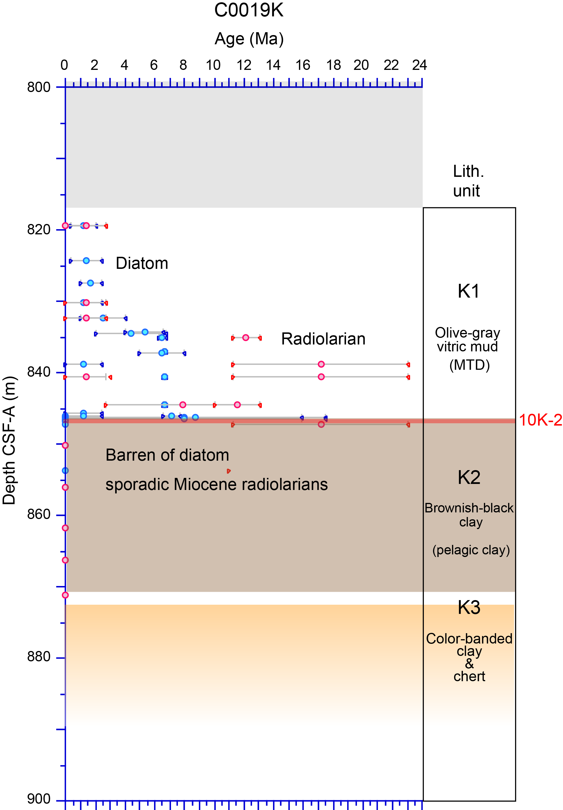
Figure F85. Diatom and radiolarian age constraint.

The occurrence of P. curvirostris and the absence of N. koizumii in Sample 405-C0019K-1K-CC allows us to place this sample in Zones NPD11–NPD10. The common occurrence of S. oestrupii s.s. in this sample supports this interpretation. The trace occurrence of A. oculatus and Fragilariopsis fossilis in this sample may suggest assignment to the A. oculatus Zone (NPD10); however, these taxa are frequently observed as reworked within the P. curvirostris Zone (NPD11). The occurrence of N. seminae in Samples 2K-CC, 33.0–38.0 cm (824.16–824.21 mbsf), to 4K-CC, 16.5–21.5 cm (830.225–830.275 mbsf), indicates these samples are younger than the FO of N. seminae (2.4–2.7 Ma). Sample 2K-CC contains P. curvirostris, and Sample 3K-CC contains P. curvirostris, A. oculatus, and common N. seminae. We tentatively placed Samples 2K-CC and 3K-CC in Zones NPD11–NPD9 and NPD10–NPD9, respectively.

The diatom assemblage in Sample 405-C0019K-5K-CC, 0–5 cm (832.275–832.325 mbsf), seems to be different to those in Pleistocene Samples 1K-CC through 4K-CC. Neodenticula and boreal taxa are only in trace abundance in Sample 5K-CC, except for common Coscinodiscus marginatus, known as a late fall to winter producer in the North Pacific (Takahashi, 1986). On the other hand, various warm water taxa such as Aspeitia nodulifera, A. marinus, and Hemidiscus cuneiformis are observed in this sample. The presence of A. oculatus in this sample allows us to tentatively place this sample within the lineage of these taxa between 1.0 and 4.0 Ma.

Closely spaced samples were taken from Section 405-C0019K-6K-2 to test for age differences between an apparent clast surrounded by a matrix in the lithology at this depth interval. The co-occurrence of N. kamtschatica and T. convexa v. aspinosa without S. oestrupii s.l. and N. koizumii in the matrix of Sample 405-C0019K-6K-2A, 40 cm (834.205 mbsf) (see Lithostratigraphy in the Site C0026 chapter [Conin et al., 2025]), allows us to place this sample in the latest Miocene N. kamtschatica–Nitzschia rolandii Zone (NPD7Ba; 5.6–6.55 Ma). This matrix sample contains many more reworked middle–late Miocene taxa, such as Actinocyclus ingens v. planus, Denticulopsis praedimorpha var. minor, and D. dimorpha. Conversely, reworked diatoms and N. kamtschatica are only traces in the clast (Sample 6K-2A, 54 cm; 834.345 mbsf) (see Lithostratigraphy in the Site C0026 chapter [Conin et al., 2025]). The co-occurrence of T. convexa v. aspinosa and T. convexa, the absence of S. oestrupii s.l., and the trace presence of N. kamtschatica in Sample 6K-2A, 54 cm (834.345 mbsf), suggest that this sample corresponds to the upper part of the R. californica Zone (NPD7), dated approximately 6.7–6.55 Ma. Although R. californica, which defines the upper boundary of this zone, is absent, the assemblage indicates an age slightly older than that of the surrounding matrix. The diatom composition and its age assignment in Sample 6K-CC, 20–25 cm (835.125–835.175 mbsf), are the same as the clast in Section 6K-2A.

Samples 405-C0019K-7K-1A, 99 cm (836.99 mbsf; massive mud), and 7K-1A, 119 cm (837.19 mbsf), are characterized by the common occurrence of C. marginatus. The trace presence of N. kamtschatica and the absence of Thalassionema schraderii, a taxon commonly observed in several samples from Expedition 343 Hole C0019E (Iwai et al., 2025), tentatively places these samples within the R. californica Zone (NPD7) of the middle Late Miocene.

The occurrence of T. convexa v. aspinosa with trace of N. kamtschatica and the absence of T. schraderii in Samples 405-C0019K-8K-CC, 10–15 cm (840.54–840.59 mbsf), and 9K-CC, 0–5 cm (844.495–844.545 mbsf), assigns these samples to the upper portion of the R. californica Zone (NPD7).

Varicolored mudstone with color-banded clay (Lithostratigraphic Unit 7; see Lithostratigraphy) was recovered in Section 405-C0019K-10K-2 (845.500–847.360 mbsf), the depth range corresponding to the PBFZ in this core (see Structural geology). The occurrence of N. seminae in Samples 10K-1A, 13 cm (845.63 mbsf), and 10K-2A, 19 cm (846.02 mbsf), assigns these samples to the Pleistocene. Lithostratigraphic Unit K1 is composed of mass transport deposits. Diatom biostratigraphy suggests that these mass transport deposits repeated several times from the middle Late Miocene through late Pleistocene. The black fault gouge in Sample 10K-2, 34.5 cm (846.175 mbsf), does not contain any biogenic material. However, samples between Sample 10K-2, 35 cm (846.18 mbsf), and 10K-2, 52 cm (846.35 mbsf), contain Middle to early Late Miocene diatoms. Additional onshore analysis is required under clean conditions to confirm this interpretation.

Diatoms are completely barren in samples from the deformed clays in Core 405-C0019K-10K and the brownish black clays to Sample 17K-CC (~873.47 mbsf) at the bottom of the hole.

6.2. Radiolarians

6.2.1. Hole C0019L

Hole C0019L was cored using the HPCS, with only one core (405-C0019L-1H; 0.00–5.38 mbsf) recovered. The occurrence of Cycladophora davisiana in a sample from Core 405-C0019L-1H (5.33–5.38 mbsf) allows this sample to be correlatable between the Cycladophora sphaeris Zone’s Hexacontium dionysus Subzone and Botryostrobus aquilonaris Zone, 2.7–0 Ma in age (Table T28).

6.2.2. Hole C0019M

Cores 405-C0019M-1H through 10H were drilled with the HPCS, and Cores 11X–14X were drilled with the ESCS. In nearly all samples, the Northwest Pacific Neogene radiolarian zonation could be applied, based on the framework established by previous studies (Kamikuri, 2010; Kamikuri et al., 2004, 2007). In addition, an automated AI-based classification system for radiolarians was conducted by taking a tiny amount of sample material once per section from Cores 1H–14X (Table T29). The results of the AI-based classification were reviewed, and the presence or absence of age-determinable species occurrence was used as a reference for age determination in the core catcher samples.

6.2.2.1. Cores 405-C0019M-1H through 14H (excluding Cores 8H and 13X)

The occurrence of C. davisiana in samples from Cores 405-C0019M-1H through 7H (0.00–61.20 mbsf), 9H–12X (67.50–89.77 mbsf), and 14X (105.00–107.51 mbsf) allow these samples to be correlated with the C. sphaeris Zone’s H. dionysus Subzone and B. aquilonaris Zone, corresponding to an age range of 2.7–0 Ma. In addition, B. aquilonaris is also observed in several samples (Table T28).

Incidentally, foraminifera are observed in Samples 405-C0019M-5H-CC, 37.0–42.0 cm (43.10–43.15 mbsf), and 10H-CC, 85.0–90.0 cm (81.76–81.81 mbsf). In particular, Sample 10H-CC, 85.0–90.0 cm, included 54 specimens of foraminifera on a single slide. Under microscopic observation, these foraminifera appear to be pyritized, and the tests are well preserved.

6.2.2.2. Cores 405-C0019M-8H and 13X

In samples from Cores 405-C0019M-8H (59.00–69.14 mbsf) and 13X (95.50–100.41 mbsf), age-determinable species are not observed, so we cannot give any age constraints.

6.2.3. Hole C0019J

Only one sample, taken from the lowest part of Hole C0019J (Sample 88K-CC, 12.5–14.0 cm; 829.08–829.09 mbsf), consisting of varicolored chert clasts was analyzed for radiolarians on the ship. Following the method of Onoue et al. (2024), we etched the chert clasts using sodium hydroxide, followed by sample preparation with hydrogen peroxide and sodium pyrophosphate (see Biostratigraphy in the Expedition 405 methods chapter [Kirkpatrick et al., 2025]).

As a result, Sample 405-C0019J-88K-CC yielded several specimens that appear to be Cretaceous radiolarians. These specimens are generally recrystallized, but fragmentation is moderate (Table T30).

6.2.4. Hole C0019K

We prepared slides and analyzed radiolarians in all core catcher samples obtained from Hole C0019K. For Cores 1K–10K, at least two slides per sample were created. Radiolarian abundance ranges from common to barren with good to poor preservation (Table T30). For some samples, we were able to apply the Northwest Pacific Neogene radiolarian zonation (Kamikuri, 2017; Kamikuri et al., 2004, 2007; Shilov, 1995). However, more than half of the samples were not dated because of the poor occurrence of zonal marker species.

6.2.4.1. Cores 405-C0019K-1K, 4K, and 5K

The occurrence of C. davisiana and B. aquilonaris in samples from Cores 405-C0019K-1K (815.00–819.50 mbsf), 4K (828.50–830.23 mbsf), and 5K (830.50–832.48 mbsf) indicate these samples are correlatable between the C. sphaeris Zone’s H. dionysus Subzone and B. aquilonaris Zone (2.7–0 Ma in age).

6.2.4.2. Cores 405-C0019K-2K and 3K

In samples from Cores 405-C0019K-2K (820.00–824.21 mbsf) and 3K (825.00–827.34 mbsf), age-determinable species are not identified; there are more diatoms than radiolarians. These samples reacted with hydrogen peroxide very well. This suggests that there may be more organic components in the sediments than in the intervals before and after.

6.2.4.3. Cores 405-C0019K-6K through 12K (excluding 8K)

From the occurrence of species such as Cyrtocapsella tetrapera, Stichocorys delmontensis, and Stichocorys peregrina, it can be assumed that samples from Cores 405-C0019K-6K through 12K (excluding 8K) were deposited after the Miocene. In Cores 6K (833.00–835.18 mbsf) and 9K (842.50–844.71 mbsf), the age can be determined to some extent from the occurrence of two species that occur after the Miocene. C. tetrapera and S. peregrina are identified in Core 6K, and Cyrtocapsella japonica and S. peregrina are identified in Core 9K. These samples are therefore correlatable with the Eucyrtidium inflatum Zone and Lychnocanoma magnacornuta Zone’s C. japonica Subzone. Samples that yielded only C. tetrapera were deposited after the Miocene, but no further age constraints could be provided.

6.2.4.4. Core 405-C0019K-8K

Two slides made from one sample from Core 405-C0019K-8K (839.00–840.59 mbsf) yielded independent ages. One of the two slides suggests a Miocene age based on the occurrence of C. tetrapera, and the other suggests a Pleistocene age based on the occurrence of C. tetrapera, S. peregrina, and B. aquilonaris (the occurrence of C. tetrapera in the other is considered mixing or contamination), which is correlatable to the C. sphaeris Zone’s H. dionysus Subzone, about 2.7 Ma in age. This suggests that mixing occurred in the sediment.

6.2.4.5. Cores 405-C0019K-13K through 16K

Samples from Cores 405-C0019K-13K through 16K contain poorly preserved radiolarians, and their occurrence is very rare or barren. Therefore, age constraints were not possible.

6.2.4.6. Core 405-C0019K-17K

Like Sample 405-C0019J-88K-CC, treatment with sodium hydroxide according to Onoue et al. (2024) yielded several radiolarian specimens that appear to be from the Cretaceous in Core 405-C0019K-17K (873.00–873.72 mbsf).

7. Paleomagnetism

Natural remanent magnetization (NRM) for Site C0019 was measured on archive halves at 2 cm intervals and on discrete samples taken from working halves. NRM measurements after stepwise alternating field (AF) demagnetization were performed: up to 25 mT peak fields for Cores 405-C0019J-1K through 36K, 50K–88K, and 405-C0019K-1K through 17K and up to 20 mT for Cores 405-C0019J-37K through 49K, 405-C0019L-1H, and 405-C0019M-1H through 14X (see Paleomagnetism in the Expedition 405 methods chapter [Kirkpatrick et al., 2025]). NRM was not measured on whole-round samples (405-C0019J-56K-5, 0–60.5 cm, 87K-2, 59–63 cm, 87K-2, 81–142.5 cm, 405-C0019K-10K, 20–40 cm, and 10K-2, 65–89 cm), which were taken as community samples and preserved to be curated and analyzed on shore. Discrete samples were demagnetized with 8–13 steps between room temperature and an 80 mT peak field. Three samples from the red sediments in Hole C0019P underwent an unconventional demagnetization procedure and were thermally demagnetized in 15 steps (see Paleomagnetism in the Expedition 405 methods chapter [Kirkpatrick et al., 2025]) after AF demagnetization at 80 mT and after moisture and density (MAD) measurements (see Physical properties in the Expedition 405 methods chapter [Kirkpatrick et al., 2025]).

7.1. Holes C0019L, C0019M, and C0019J

7.1.1. Demagnetization behavior

We measured 365 discrete samples with stepwise AF demagnetization from Holes C0019M and C0019J; no samples were collected from Hole C0019L.

A low field component with high intensity of magnetization, evident both in discrete samples (Figure F86) and archive halves (Figures F87, F88), was removed by 5 or 7.5 mT (10 mT in archive halves) and interpreted to be a drilling overprint. This drilling component caused steep inclinations and declinations grouped around the 0° and 180° values in NRM at room temperature (Acton et al., 2002). Some samples show an intermediate coercivity component (7.5 to 15 or 20 mT) that could be either a thermoviscous component or a chemical overprint and will need further characterization during postexpedition research. Afterward, the characteristic remanent magnetization (ChRM) shows stable directions along with the decrease in intensity (Figure F86). Some samples show a gain in magnetization, usually starting at 40 mT, typical of gyroremanence, particularly in the 0–140, 207–270, and 610–810 m CSF-A intervals. Gyroremanence may indicate the presence of pyrrhotite or greigite (e.g., Thomson, 1990; Snowball, 1991). The principal component analysis (PCA) from discrete samples demonstrates that the ChRM direction is resolved well; thus, a single demagnetization step at 20 or 25 mT from the archive halves is interpreted as a reliable representation of the primary paleomagnetic direction.

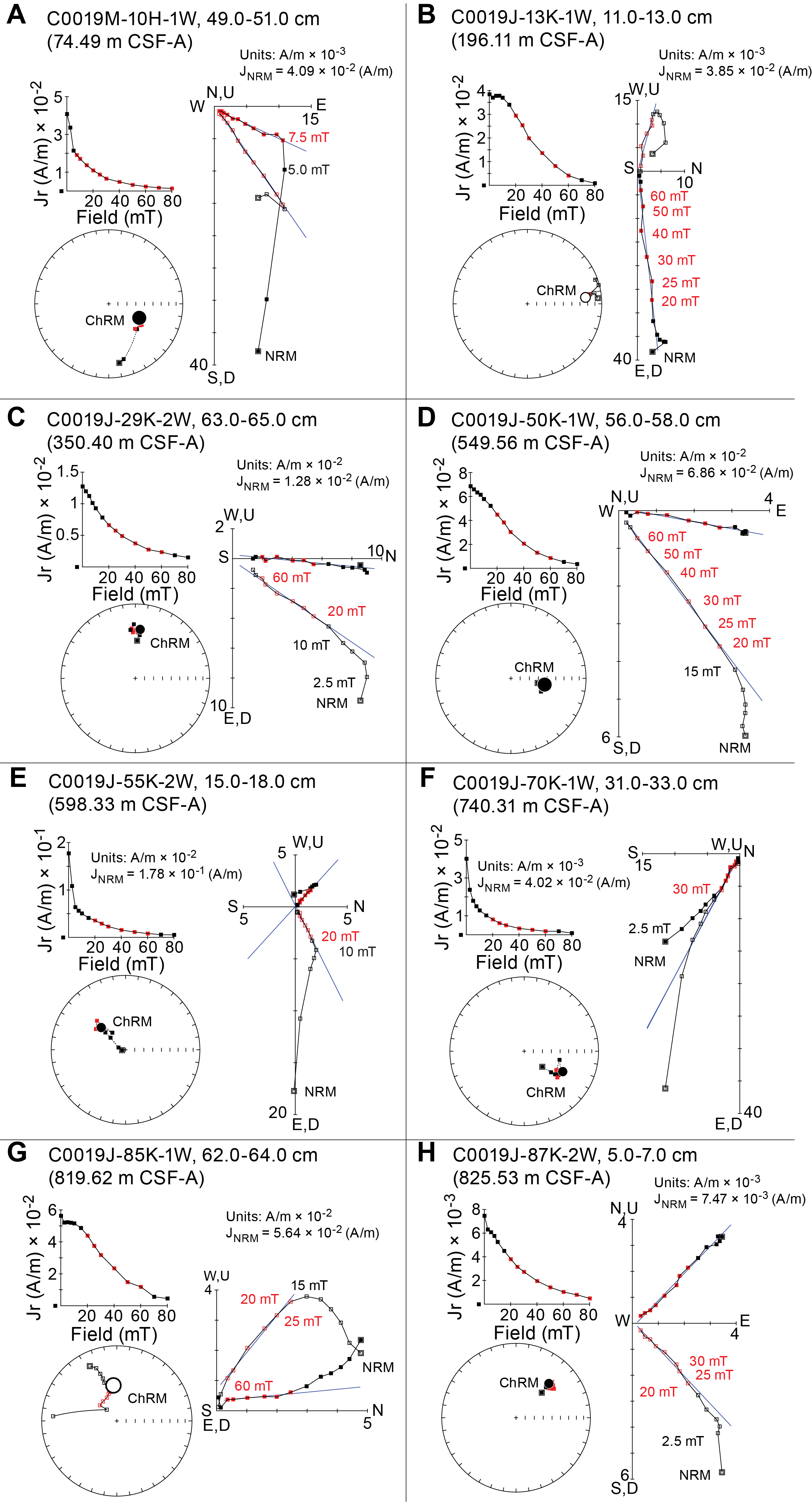
Figure F86. Demagnetization behaviors, Holes C0019M and C0019J.

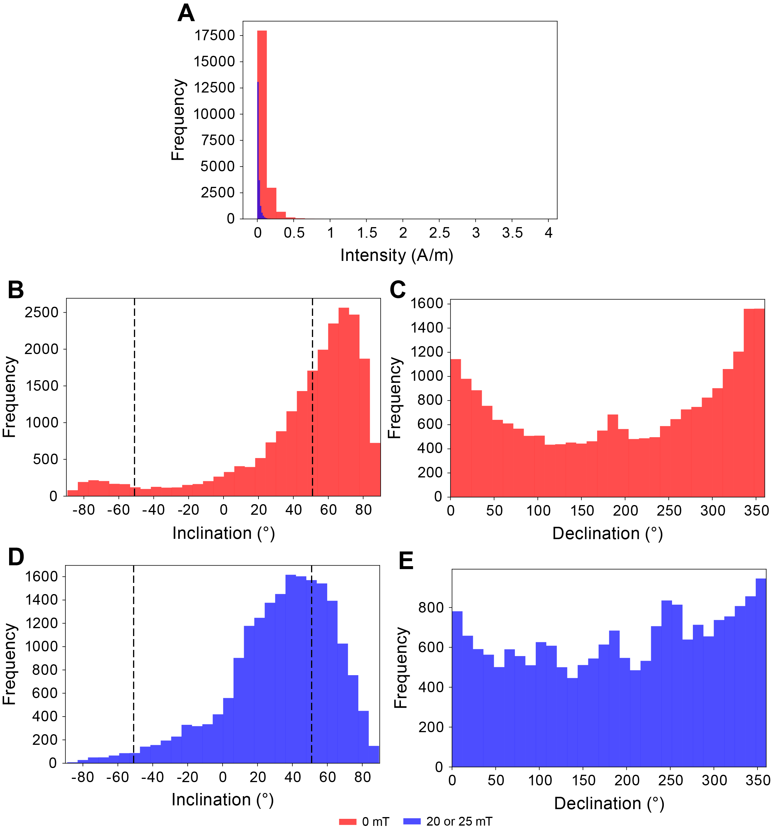
Figure F87. NRM measurements, Holes C0019L, C0019M, and C0019J.

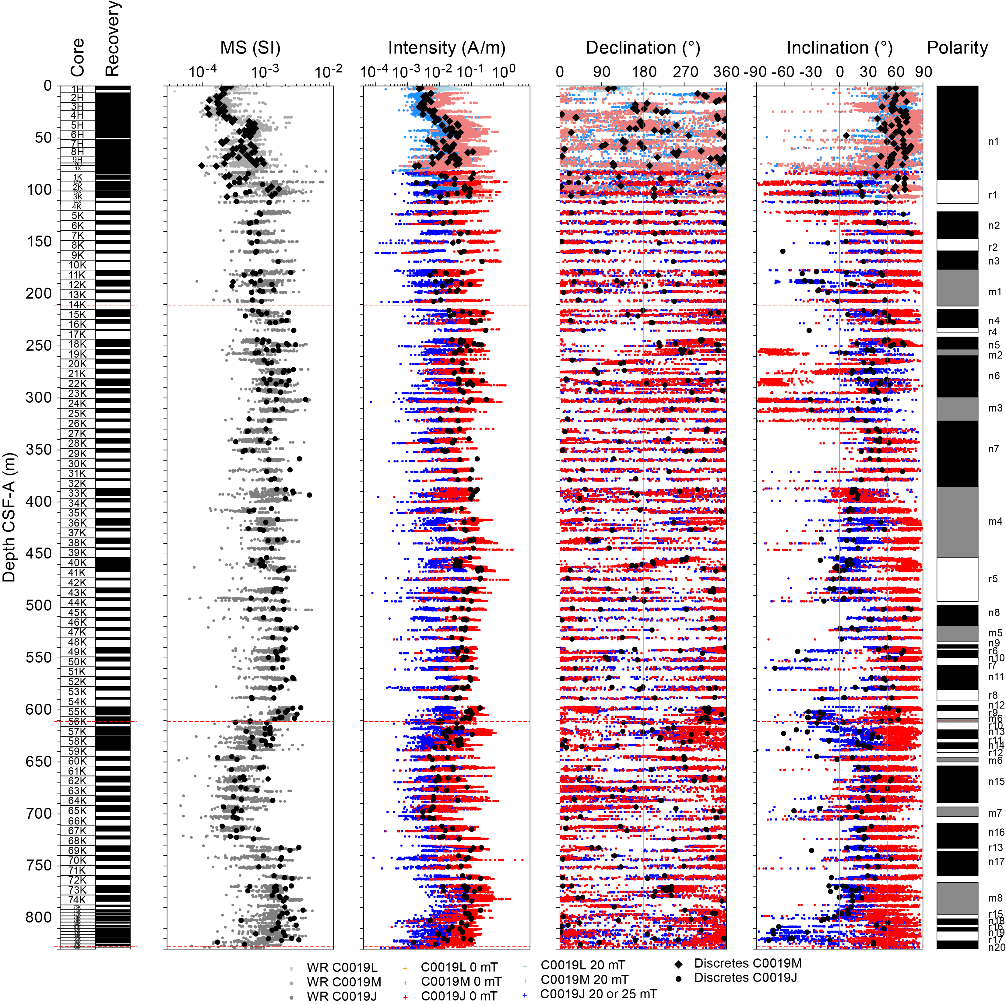
Figure F88. Paleomagnetism results, Holes C0019L, C0019M, and C0019J.

Figure F88 shows the NRM intensity, inclination, and declination results after the highest demagnetization step applied for archive halves. The direction of discrete samples that were analyzed using PCA are also plotted, generally showing a good agreement that validates their reliability. Results from a particular core (405-C0019M-10H) that experienced an almost 400% expansion are considered not reliable.

NRM at room temperature shows a value of 7.89 × 10⁻² A/m averaged over Holes C0019L, C0019M, and C0019J, with 76% of the intensity removed at the highest demagnetization step applied (Figure F87A). The average MS is 9.43 × 10⁻⁴ SI. Both magnetic intensity and MS show relatively lower values in Unit 1 (see Lithostratigraphy). The major faults (see Structural geology) roughly divide Holes C0019L, C0019M, and C0019J into four intervals with distinct magnetic intensity and MS. The interval between ~33 and 207.57 m CSF-A (where the presence of a fault is inferred by the age change detected between Cores 405-C0019J-14K and 15K) (see Biostratigraphy) shows constant values of magnetic intensity, whereas MS is lower between 33 and ~100 m CSF-A. The 215–610.31 m CSF-A interval initially shows an increase in both values and then fluctuates. The 610.31–826.07 m CSF-A interval is initially marked by a sharp decrease in both magnetic intensity and MS, which show some fluctuation before decreasing again above the fault at 826.07 m CSF-A. Finally, the 826.07–828.92 m CSF-A interval is characterized by lower values of both parameters.

Declinations show consistent values at the core level in Holes C0019L and C0019M, but there is considerable scatter observed in the declination in Hole C0019J caused by biscuiting from rotary coring (Figure F88). Indications of biscuiting are sometimes evident as abrupt changes in declination occurring over several to a few tens of centimeter intervals in sections. Biscuiting was commonly observed in the visual description of the working halves (see Structural geology).

Because of the inclined bedding (see Structural geology), the ChRM directions vary depending on the dip direction and dip angle of the strata. After demagnetization, inclinations are almost always positive but widely scattered with respect to the present-day value of 51.5° (Figure F87D) calculated at the site coordinates using the International Geomagnetic Reference Field (IGRF) model (Alken et al., 2021).

Because the bedding planes are tilted to varying degrees (see Structural geology), bedding tilt correction is required to determine primary NRM directions that were acquired before tilting. However, here we only report paleomagnetic inclinations and declinations using the core coordination system (see Paleomagnetism in the Expedition 405 methods chapter [Kirkpatrick et al., 2025]). Negative and shallow inclinations documented in the 90–130, 177–215, 300–320, 430–500, 580–620, 690–710, and 760–780 m CSF-A intervals may effectively correspond to negative polarities. The interval between 810 m CSF-A and the bottom of Hole C0019J is characterized by alternating normal and negative polarities.

7.1.2. Anisotropy of magnetic susceptibility

AMS parameters were measured for discrete samples in Holes C0019M and C0019J (Figures F89, F90). The Flinn diagram of AMS ellipsoids shows magnetic foliation (F = K_int/K_min) relatively higher than magnetic lineation (L = K_max/K_int), indicating that the flattening fabric is dominant.

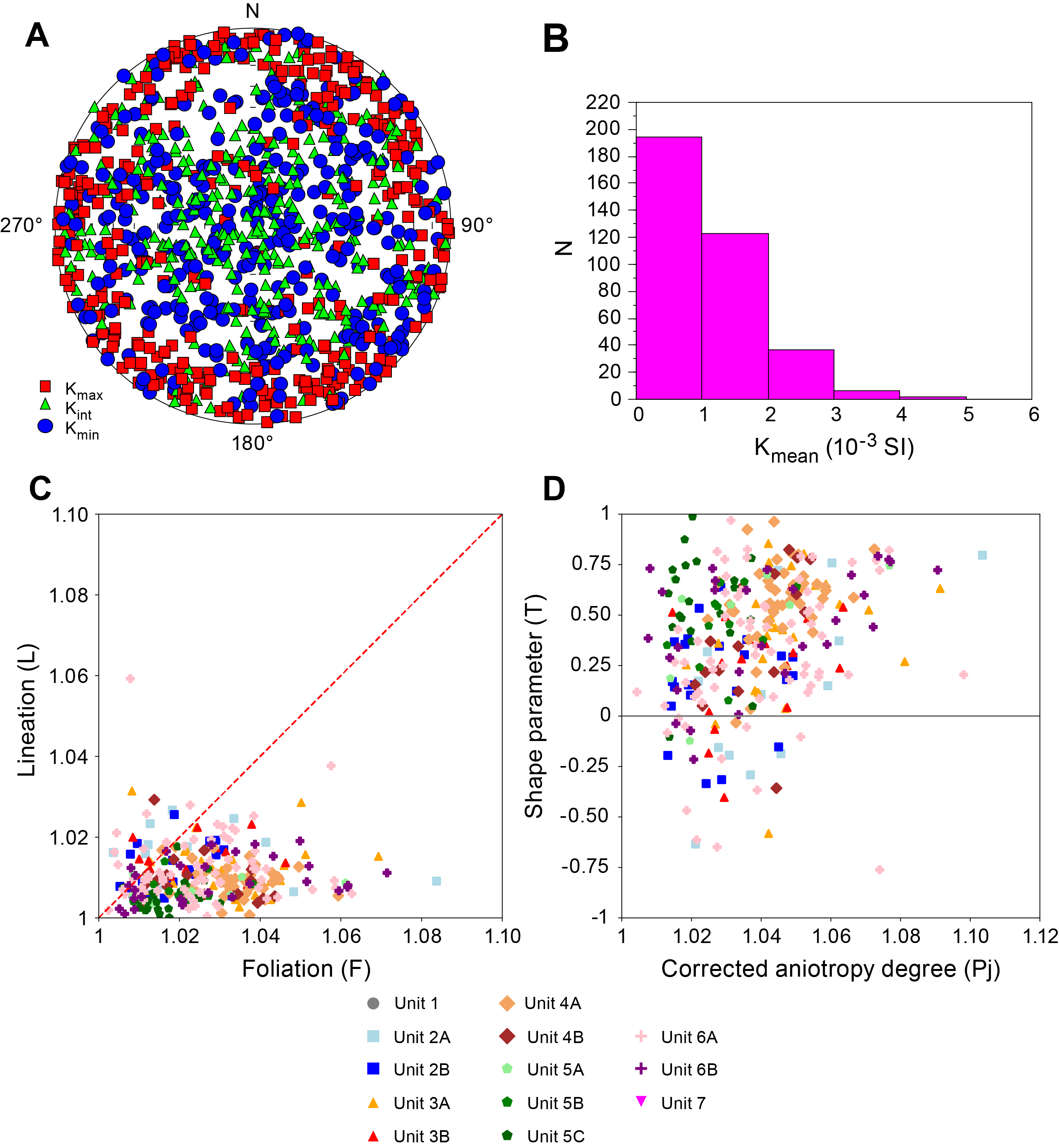
Figure F89. AMS data, Hole C0019J.

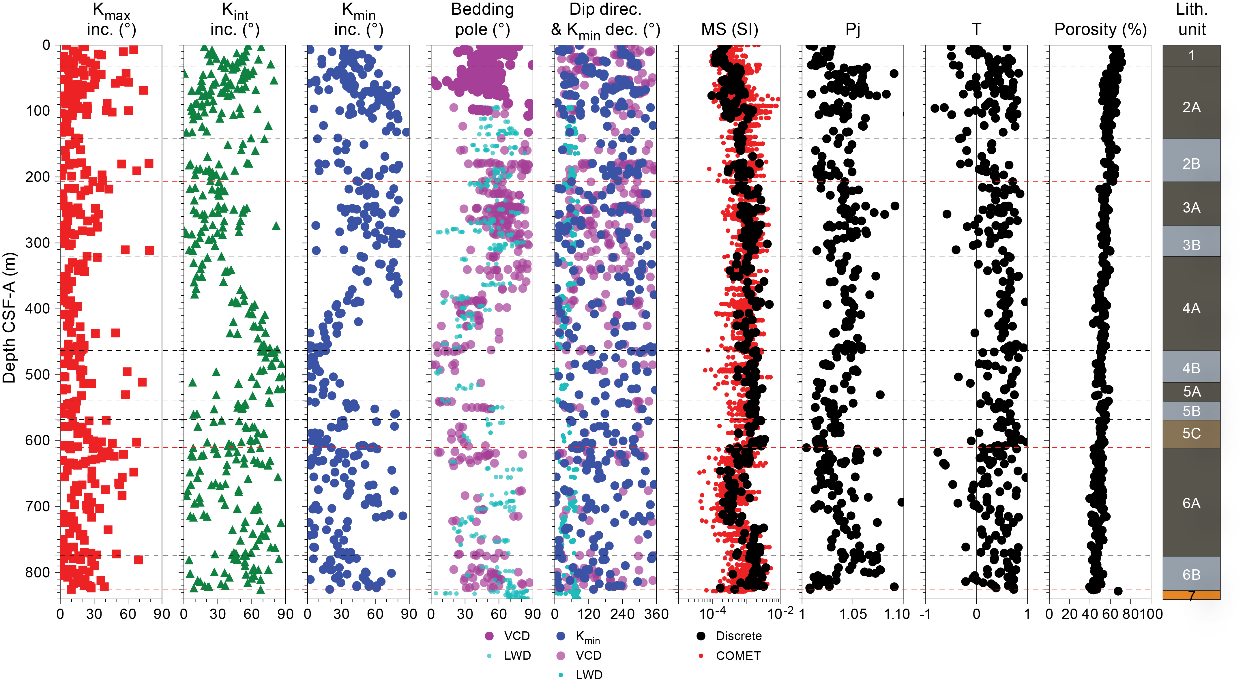
Figure F90. AMS parameters, Hole C0019J.

A plot of AMS fabric with depth shows distinct variations. Corrected anisotropy degree (Pj) shows the lowest values in Unit 1 (see Lithostratigraphy) and a sharp step to higher values in Subunit 2A. Starting from here, Pj is characterized by high scatter, possibly due to the abundant mass transportation deposits. A considerable drop in anisotropy degree is observed above all the fault zones. The inclination of the minimum susceptibility axes (K_min) ranges 1°–88°. From the top to ~320 m CSF-A, K_min inclination and shape parameter (T) do not show any systematic variations with depth. Below this depth, K_min inclination gets shallower, reaching the minimum values between 463 and 511 m CSF-A. This trend is consistent with the variation of dip in bedding poles (see Structural geology) and LWD measurements (see Logging while drilling). A similar curved trend is shown between ~539 and ~610 m CSF-A. Between the faults at 610.31 and 826.07 m CSF-A, the susceptibility axes fluctuate, but K_min gets shallower starting at 700 m CSF-A. The shape parameter usually shows oblate to neutral shape; AMS ellipsoid to prolate shape is documented in the footwall of the fault at 610.31 m CSF-A. To fully understand the AMS parameters at Site C0019, tilt correction of the data will be conducted during postexpedition data processing.

7.2. Hole C0019K

7.2.1. Demagnetization behavior

We collected and measured 34 shipboard samples from Hole C0019K (Figure F91). A low-field component attributed to a drilling overprint, although not always evident, is generally removed before 5 mT. Some samples, especially from Unit K2 (see Lithostratigraphy), show the presence of a secondary component. Other samples show stable ChRM directions, but some demagnetize rapidly or are affected by the presence of gyroremanence. Notwithstanding, the remanent magnetization at 25 mT is still considered to be representative of the ChRM.

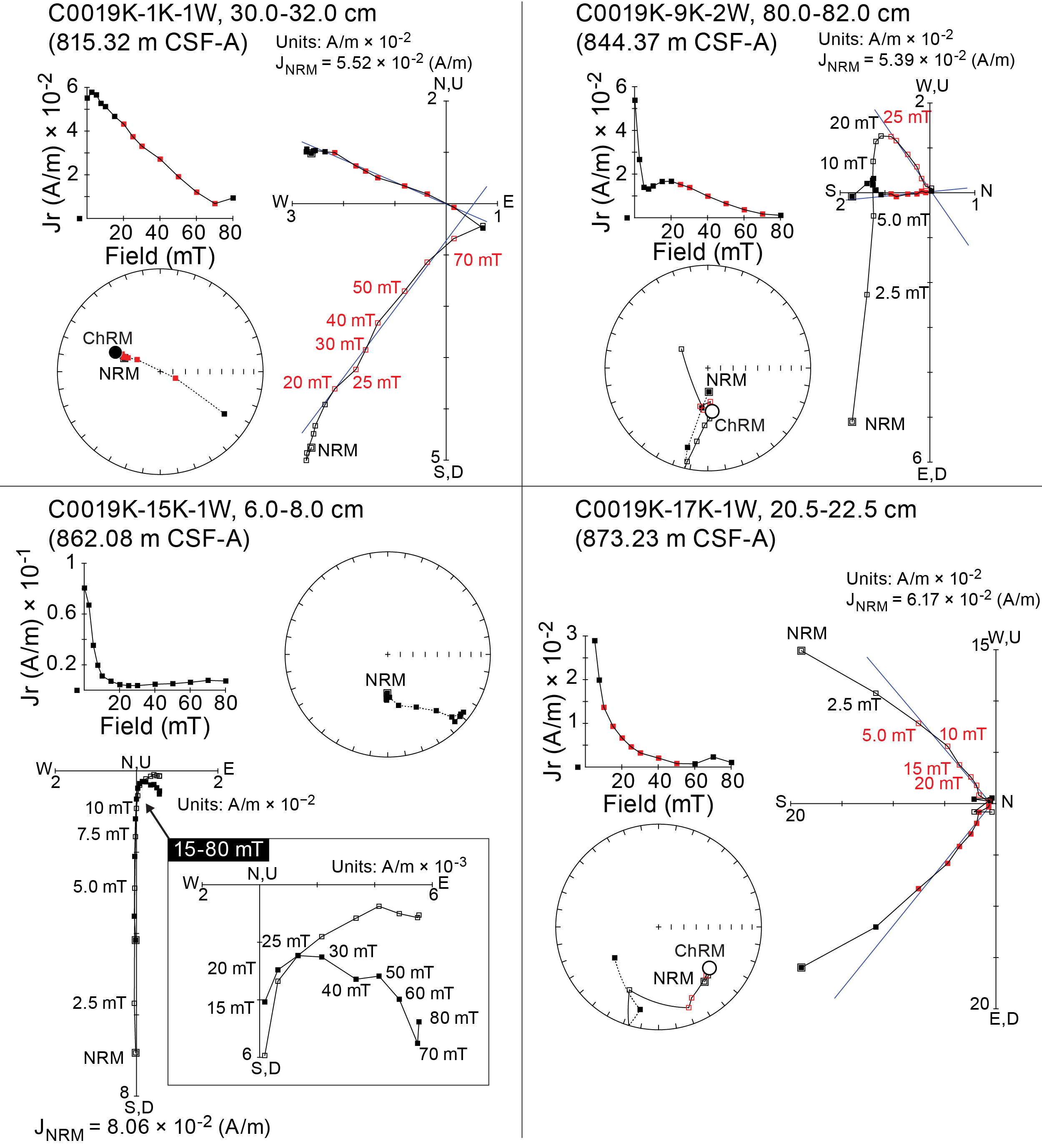
Figure F91. Demagnetization behaviors, Hole C0019K.

Figure F92 shows the results of NRM intensity, inclination, and declination measurements after demagnetization at 25 mT for archive halves. The results from discrete samples, which were analyzed using PCA, are also plotted, generally showing a good agreement and therefore validating their reliability.

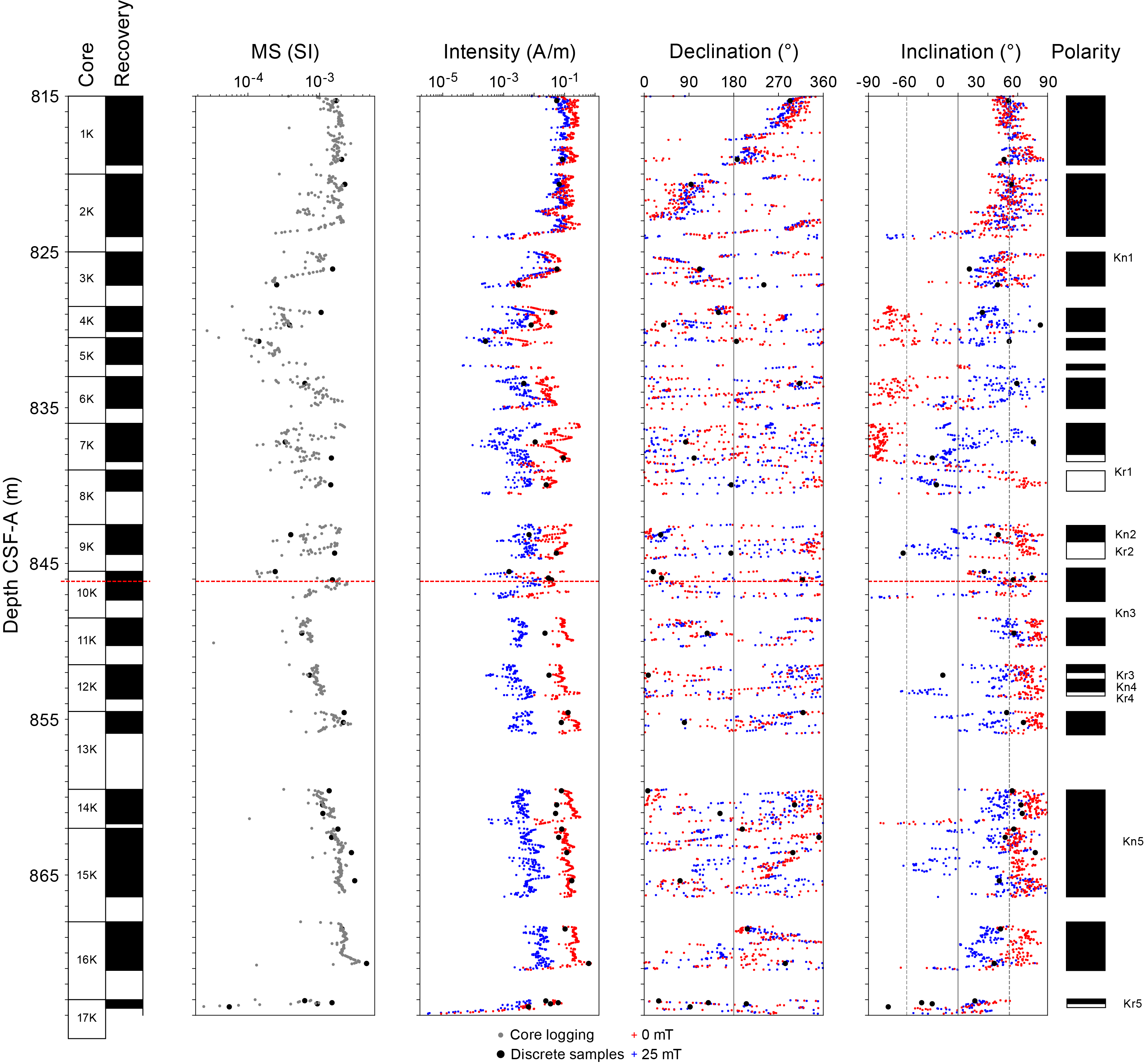
Figure F92. Paleomagnetism results, Hole C0019K.

Because the bedding planes of the cores recovered from Hole C0019K are rotated and tilted to varying degrees (see Structural geology), it is necessary to restore the bedding planes to obtain primary NRM directions that were acquired before tilting. However, we only report paleomagnetic inclinations and declinations using the core coordinate system (see Paleomagnetism in the Expedition 405 methods chapter [Kirkpatrick et al., 2025]).

NRM at room temperature varies from 8.87 × 10⁻⁶ to 7.27 10⁻⁶ A/m with an average value of 9.93 × 10⁻² A/m (Figure F93), consistent with the values documented in the last meters of Hole C0019J. Here, the decrease in intensity toward the fault is not as evident.

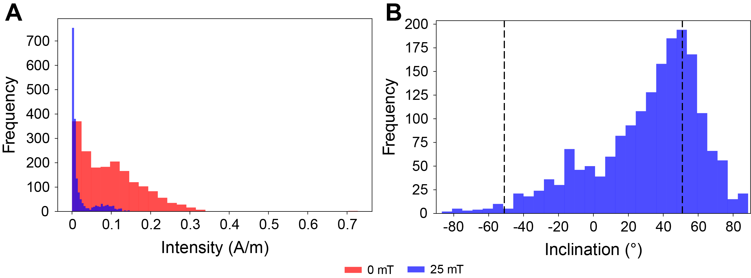
Figure F93. NRM measurements, Hole C0019K.

As in Hole C0019J, declination values are scattered because of biscuiting, which is typical of rotary coring. Inclination is predominantly positive and generally consistent with the expected present-day value at the site coordinates (51.5°) in the upper part of the hole but shows shallower values starting at ~825 m CSF-A.

7.2.2. Anisotropy of magnetic susceptibility

AMS parameters were measured for discrete samples in Hole C0019K (Figures F94, F95). The mean MS varies between 5.49 × 10⁻⁵ and 4.52 × 10⁻³. The Flinn diagram of MS ellipsoids dominantly shows a flattening fabric in Unit K1 (see Lithostratigraphy) and a nearly oblate fabric in Unit K2; magnetic foliation (F = K_int/K_min) is much higher than magnetic lineation (L = K_max/K_int), indicating that the flattening fabric is dominant.

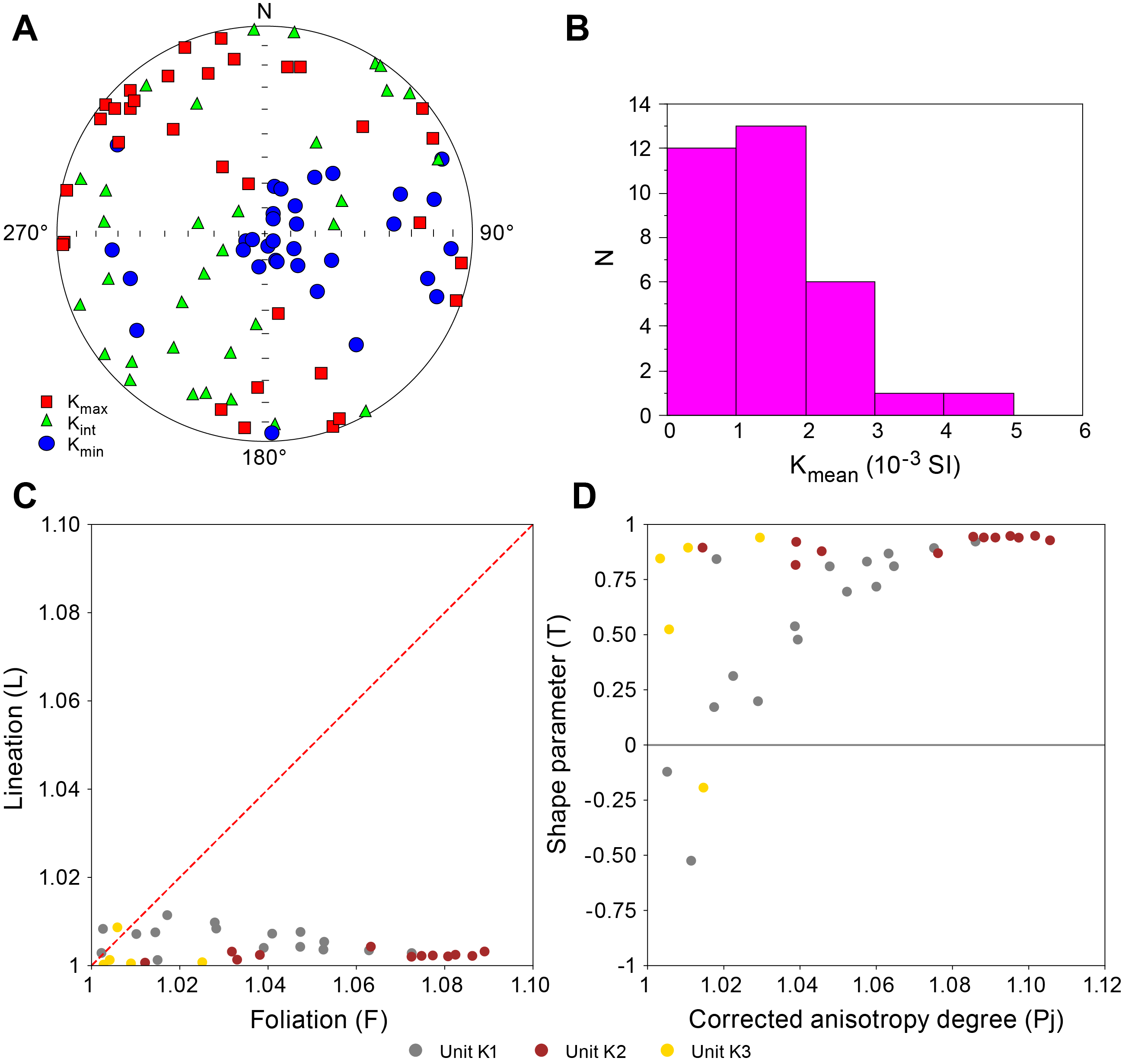
Figure F94. AMS data, Hole C0019K.

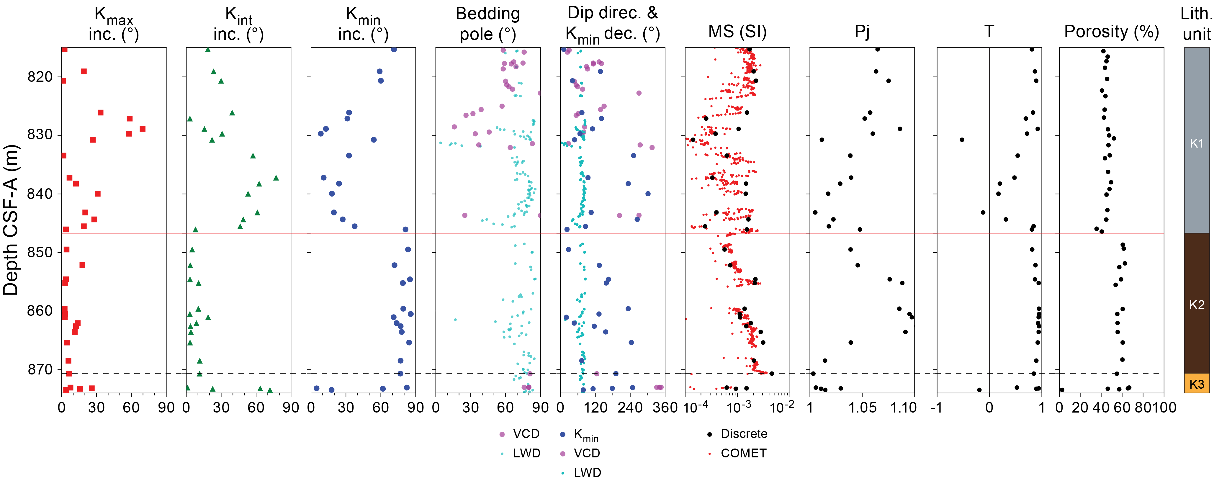
Figure F95. AMS parameters, Hole C0019K.

A plot of anisotropy with depth shows distinct properties with respect to lithostratigraphic units. Unit K1 (see Lithostratigraphy) shows a downhole change in AMS fabric from flattening to neutral and then to a nearly oblate fabric as it approaches the fault (see Structural geology); this trend is associated with a decrease in anisotropy degree (Pj). Here, shallow K_min inclinations in the ~830–845 m CSF-A interval support the presence of steep bedding documented by LWD (see Logging while drilling). Unit K2 shows a well-defined magnetic foliation, a generally higher anisotropy Pj (with a peak around 860 m CSF-A), a shape parameter close to 1, and an inclination of K_min close to vertical. All these factors indicate a sedimentary fabric with strong compaction and a subhorizontal bedding. Such high compaction agrees with porosity data (see Physical properties). In Unit K3, MS and anisotropy Pj drop. The inclination of AMS axes fluctuates because of low susceptibility and anisotropy degree in the chert layers.

We note that Pj shows a similar decreasing trend in the hanging wall of the fault in both Holes C0019J and C0019K, whereas the footwall in Hole C0019K shows virtually identical magnetic fabric with the similar lithology documented at the input site (Unit 2; see Lithostratigraphy in the Site C0026 chapter [Conin et al., 2025]).

7.3. Hole C0019P

We collected and measured 15 shipboard samples from Hole C0019P, 12 from basalts and 3 from the red sediments (see Lithostratigraphy).

7.3.1. Demagnetization behavior of basalts

The discrete samples show two components (Figure F96). The softer component is demagnetized at up to 20 mT, whereas the harder component is completely demagnetized between 50 and 80 mT. The softer component shows steeper inclination but does not show the characteristics of a drilling-induced remagnetization and could be attributed to a viscous remanent magnetization.

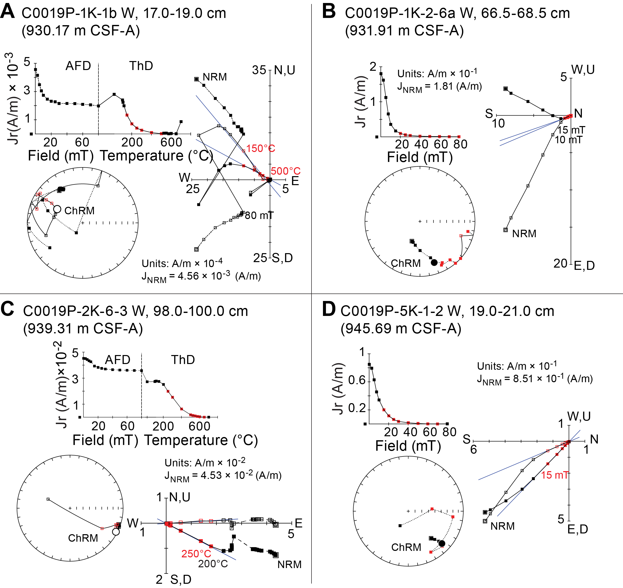
Figure F96. Demagnetization behaviors, Hole C0019P.

The demagnetization behavior of discrete samples show that the step at 20 mT from archive halves is representative of the primary component of magnetization. NRM is characterized by high intensity, ranging 1.06 × 10⁻¹ to 6.05 A/m. NRM is 93% demagnetized at 20 mT (Figure F97). Both archive halves and PCA from discrete samples show subhorizontal inclinations, except for the pillow basalts in Core 405-C0019P-1K (see Lithostratigraphy), where inclination fluctuates and is generally steeper.

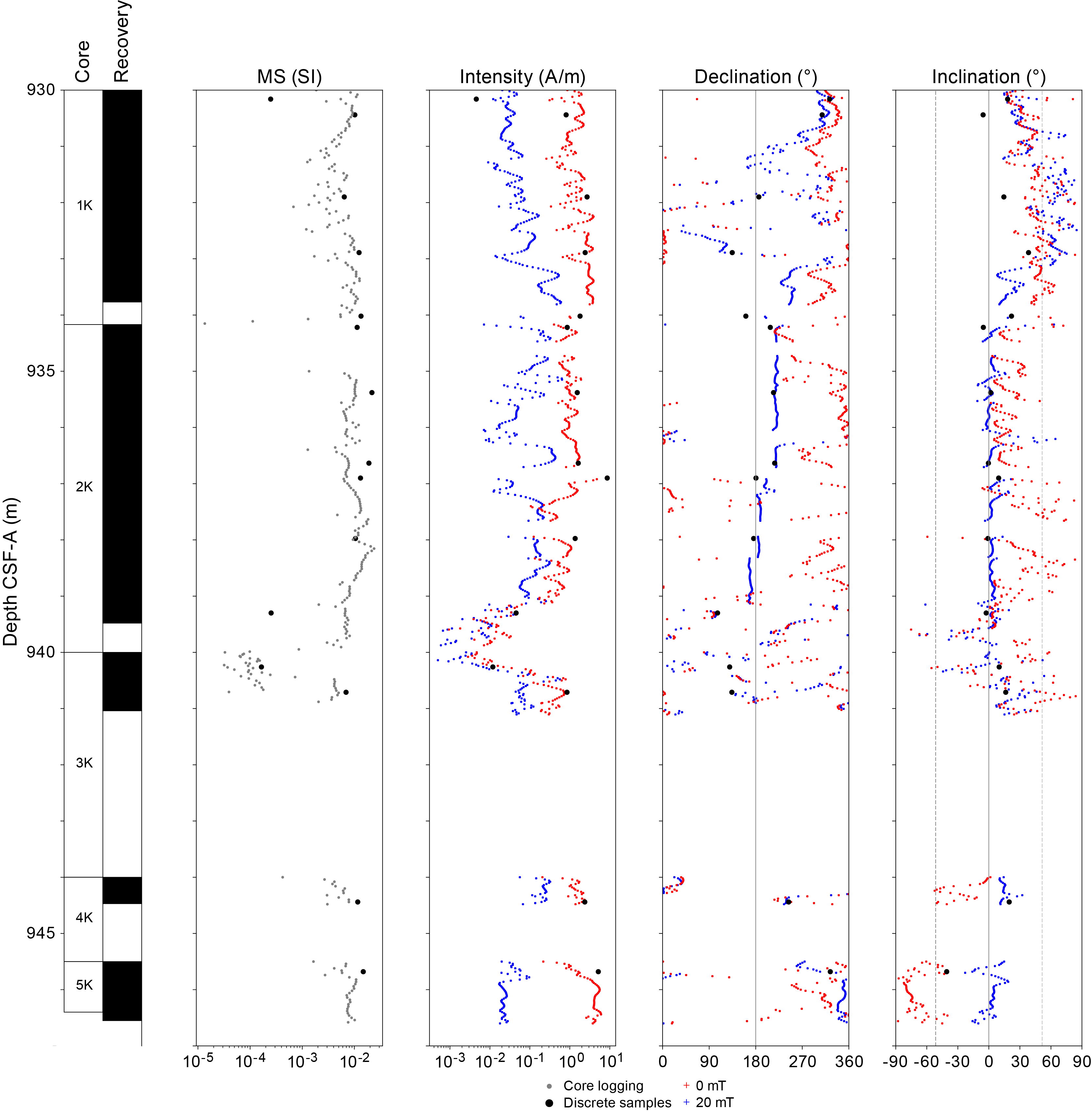
Figure F97. Paleomagnetism results, Hole C0019P.

7.3.2. Demagnetization behavior of sediments

Three red sediment samples were collected: one from around the pillow basalt in Core 405-C0019P-1K and the other two from Unit P2 (see Lithostratigraphy). The red sediments are characterized by lower NRM intensity than basalts, between 1.80 × 10⁻³ and 7.85 × 10⁻¹ A/m. After demagnetization at 80 mT (see Paleomagnetism in the Expedition 405 methods chapter [Kirkpatrick et al., 2025]), samples from the red sediments were barely or not at all demagnetized, highlighting the presence of a high-coercivity component (Figure F96). To isolate the primary component of demagnetization, we performed stepwise thermal demagnetization after the samples underwent MAD measurements (see Physical properties in the Expedition 405 methods chapter [Kirkpatrick et al., 2025]). A low-temperature component was removed at around 150°C. The high-temperature component was completely demagnetized between 650° and 700°C except for the shallowest samples, which were demagnetized at 500°C. The high coercivity (>80 mT) and demagnetization temperatures (650°/700°C) indicate that the carrier of magnetization is hematite; the sample from the rim of the pillow basalt shows lower demagnetization temperatures, suggesting a mixture of titanohematite (Nagata, 1961). Consistent with the basalts, the direction of ChRMs shows subhorizontal inclination. Because the discrete samples do not demagnetize at high AF, the AF demagnetization step at 20 mT from archive sections cannot be considered representative of the ChRM in the red sediments.

7.3.3. Contribution to the oceanic magnetic anomalies

NRM at room temperature and MS from both archive halves and discrete samples were used to compute the Königsberger ratio (Q_n), which indicates the capacity of a rock to carry magnetic anomalies. The Königsberger ratio is defined as the ratio of remanent magnetization to the induced magnetization in Earth’s magnetic field:

$Q_{n} = N R M / [K \times H],$

where

H = local geomagnetic field (A/m),
K = MS (SI), and
NRM = intensity (A/m).

The current total field value of the IGRF (Alken et al., 2021) at Site C0019 (46,970.6 nT = 37.3 A/m), was used to calculate Q_n. In general, Q_n is >1 (Figure F98), suggesting that the total magnetization of the recovered basalts is contributing to the oceanic magnetic anomalies in this area. The basalts from Cores 1K and 5K have a higher contribution, with Q_n closer to 10. Although the basalts do not show clear evidence of drilling overprint, their contribution to the oceanic anomalies was also evaluated at the 10 mT step, and the results were slightly lower.

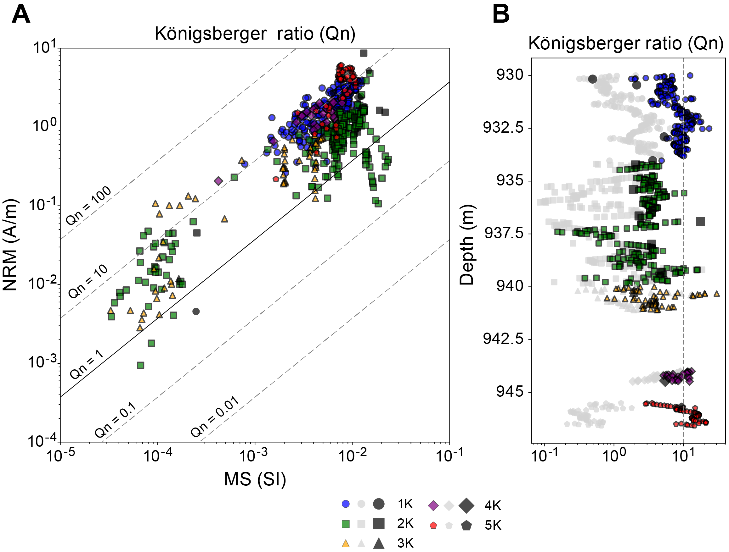
Figure F98. NRM measurements, Hole C0019P.

7.3.4. Implications for plate motion

Notwithstanding that we recovered few materials, paleomagnetic data from Hole C0019P are important because they could constrain the Pacific plate motion for the Cretaceous (the expected anomaly in the area is ca. 135 Ma; e.g., Choe and Dyment, 2020). Save for the basalt pillow and surrounding altered sediments in Core 1K (see Lithostratigraphy), both sediments PCA and basalt at the 20 mT demagnetization step from Hole C0019P show very shallow inclinations. The inclination between 0° and 10° indicates an origin of the basalts close to the equator.

7.3.5. Anisotropy of magnetic susceptibility

AMS parameters were measured for discrete samples in Hole C0019P and their variation with depth (Figures F99, F100). The Flinn diagram of AMS ellipsoids tend to constriction fabric and magnetic lineation (L = K_max/K_int) stronger than magnetic foliation (F = K_int/K_min), suggesting the presence of an emplacement flow in some of the recovered basalts (mainly in Core 2K), also supported by the direction of the K_min axes.

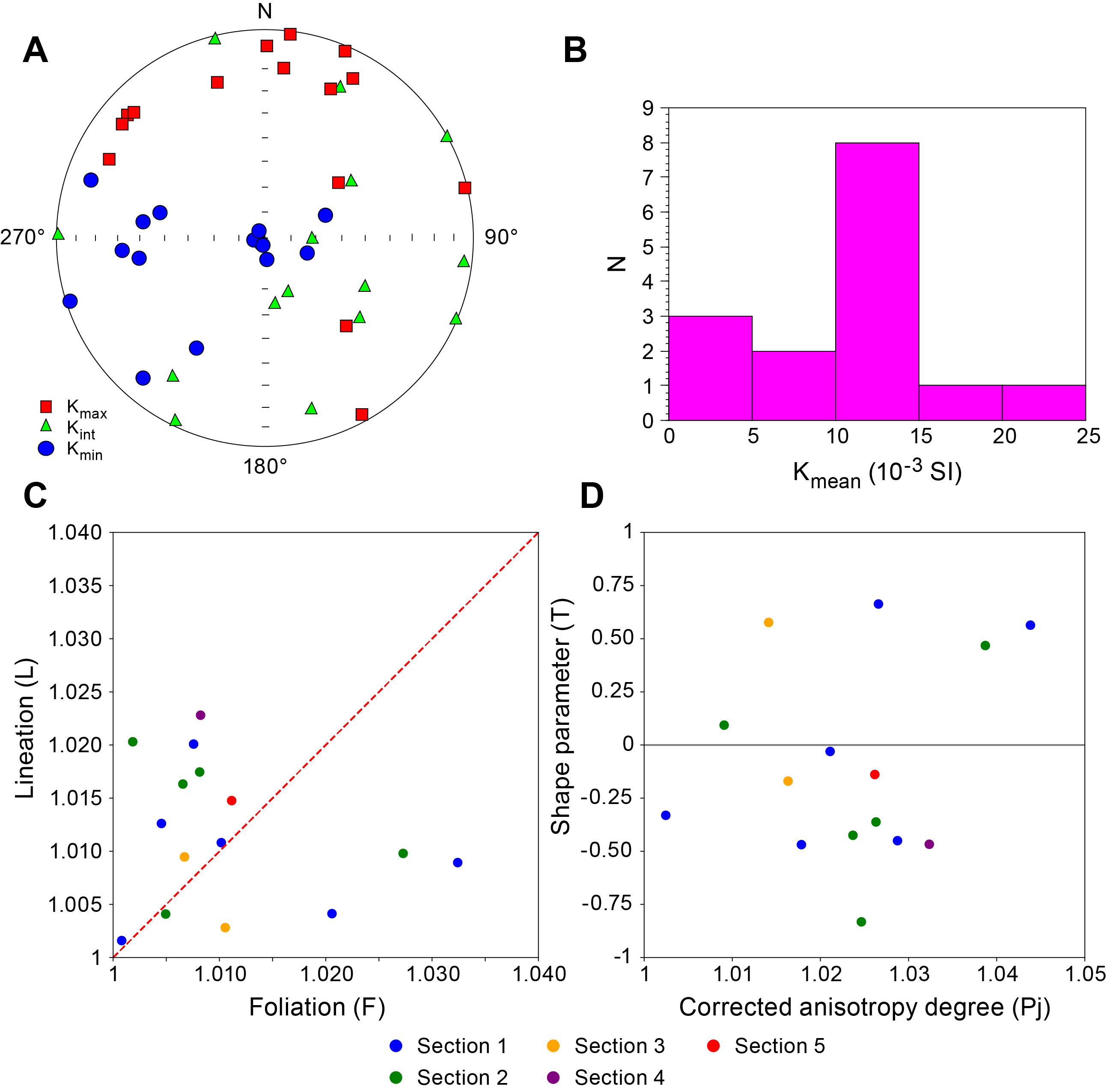
Figure F99. AMS data, Hole C0019P.

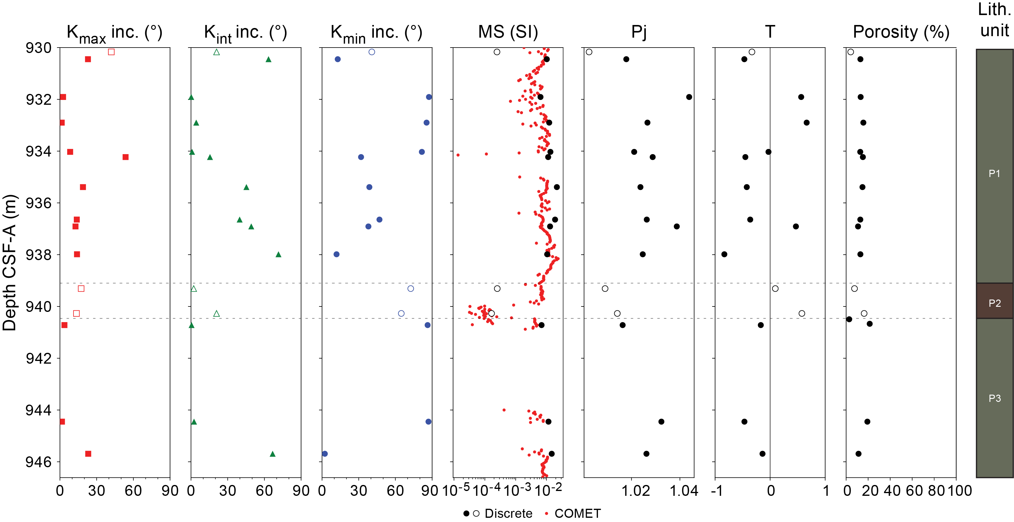
Figure F100. AMS parameters, Hole C0019P.

MS and Pj show distinct differences between basalts and red sediments. Pj is small overall, as documented in basaltic flows that rapidly cooled on gentle slopes with <10° of dip (e.g., Boiron et al., 2013). All the AMS parameters show high variability, probably related to the different emplacement mechanisms of the different types of recovered basalts (see Lithostratigraphy).

7.4. Magnetostratigraphy

Notwithstanding that the ChRMs are successfully isolated in discrete samples and the step at 20 or 25 mT from archive sections reliably indicates the primary component of magnetization, it is not possible to reconstruct a magnetostratigraphy from Site C0019.

In Holes C0019L, C0019M, and C0019J, this is due to bedding planes tilted to varying degrees (see Structural geology). As a result, the inclinations are biased toward normal polarity (Figure F87). A bedding tilt correction is required to determine the primary NRM directions acquired before tilting. However, here we only report paleomagnetic inclinations and declinations using the core coordination system (see Paleomagnetism in the Expedition 405 methods chapter [Kirkpatrick et al., 2025]). In Hole C0019K, the reconstruction of a magnetostratigraphy is hampered by the lack of precise age constraints (see Biostratigraphy).

We recognize a series of normal, reversed, and mixed polarity intervals (Figure F87) within which polarity is difficult to assess. Furthermore, there is no correspondence in the inclinations in the overlapping interval between Holes C0019M and C0019J (Figure F88), probably because cores from Hole C0019M underwent significant expansion, causing a distortion of the signal as well as an inaccurate overlap between the CSF-A depth scales of the two holes. The biostratigraphy (see Biostratigraphy) indicates an age of 0–2.7 Ma for Hole C0019M, and the ages of Cores 405-C0019J-3K and 4K (100–110 m CSF-A) range 0.3–2.4 Ma. Considering these constraints, the transition from n1 to r1 around 90 m CSF-A could be tentatively attributed to the Brunhes/Matuyama boundary (0.773 Ma). The age of Cores 11K and 12K ranges 4.0–5.6 Ma. This interval is correlated somewhere in the Gilbert Chron (3.596–5.235 Ma). However, the bias of inclination toward normal polarities precludes a reliable correlation with the global polarity scale, and these considerations have to be used with caution.

The lowermost part of Hole C0019K, which shows subhorizontal layers below the fault zone (see Structural geology), is characterized by inclinations lower than the expected values at the site coordinates (Figure F92), suggesting an older age for Units K2 and K3, as also suggested by the presence of sporadic Miocene radiolarians (see Biostratigraphy).

8. Physical properties

This section examines the physical properties measured on cores recovered at Site C0019 during Expedition 405. Physical properties were measured on cores from Holes C0019J–C0019M and C0019P. These data provide insight into the properties of the frontal prism, PBFZ, underthrust sediments, and Pacific plate basalts. In general, the bulk density, P- and S-wave velocities, thermal conductivity, and electrical resistivity increase with depth, whereas porosity decreases. Variations observed in the measured properties are often associated with structures and changes in lithology. These variations and trends in physical properties are described in greater detail below. All depths are provided as mbsf (equivalent to m CSF-A) unless otherwise indicated. All of the physical properties data for this site are found in PHYSPROPS in Supplementary material.

8.1. Holes C0019J, C0019L, and C0019M

Physical property analysis was conducted on all 88 cores recovered from SD-RCB Hole C0019J, covering the depth range 82.0–829.1 mbsf (7009.5–7756.6 m BRT). Prior to splitting, all cores were logged using the COMET, which measured gamma ray attenuation (GRA) density, MS, P-wave velocity, and natural gamma radiation (NGR). After splitting, thermal conductivity and shear strength (vane shear and penetrometer, where possible) were measured on the working halves of the cores. Discrete samples were taken for measurements of MAD, electrical resistivity, and ultrasonic wave velocities. In the shallow cores where the sediments were too soft to make discrete cubes, pin resistivity measurements were made and no discrete wave velocities were measured.

HPCS Holes C0019L and C0019M covered the same 0–5 mbsf depth interval, but because Hole C0019M also extends deeper (to 107.5 mbsf), it is used as a representative and the only physical property measurements performed on Core 405-C0019L-1H were the COMET scans. In Hole C0019M, formation temperature was measured using an advanced piston corer temperature (APCT-3) tool installed in the HPCS cutting shoe (see Physical properties in the Expedition 405 methods chapter [Kirkpatrick et al., 2025]) for every other core, starting with Core 3H. All whole-round cores were logged with the COMET. After splitting, electrical resistivity, strength, and thermal conductivity were measured on the working halves. Discrete samples were taken for MAD measurements. The cores expanded whenever the core liner was cut; as a result, many of the measured physical properties could be biased. For example, porosity may be overestimated and bulk density may be underestimated. The recovered cores captured the mudline and overlapped with the shallowest cores recovered from Hole C0019J by about 3 m (referenced from the rig table), providing a nearly continuous record of the physical properties at Site C0019.

8.1.1. Core Measurement Track

COMET measurements were made on cores recovered from Holes C0019J, C0019L and C0019M (Figure F101). Figure F102 compares the COMET data taken on the cores recovered from Holes C0019J and C0019M over the depth interval where the two holes overlap (7009.5–7012.5 m BRT). Over this depth interval, measurements are consistent between the two holes for all measurement types. In COMET measurements, the ends of the core may not yield accurate values due to the absence of core material on one side or the influence of the liner cap. Therefore, the following analysis is based on data after removing values acquired within 4 cm of both ends of each core section.

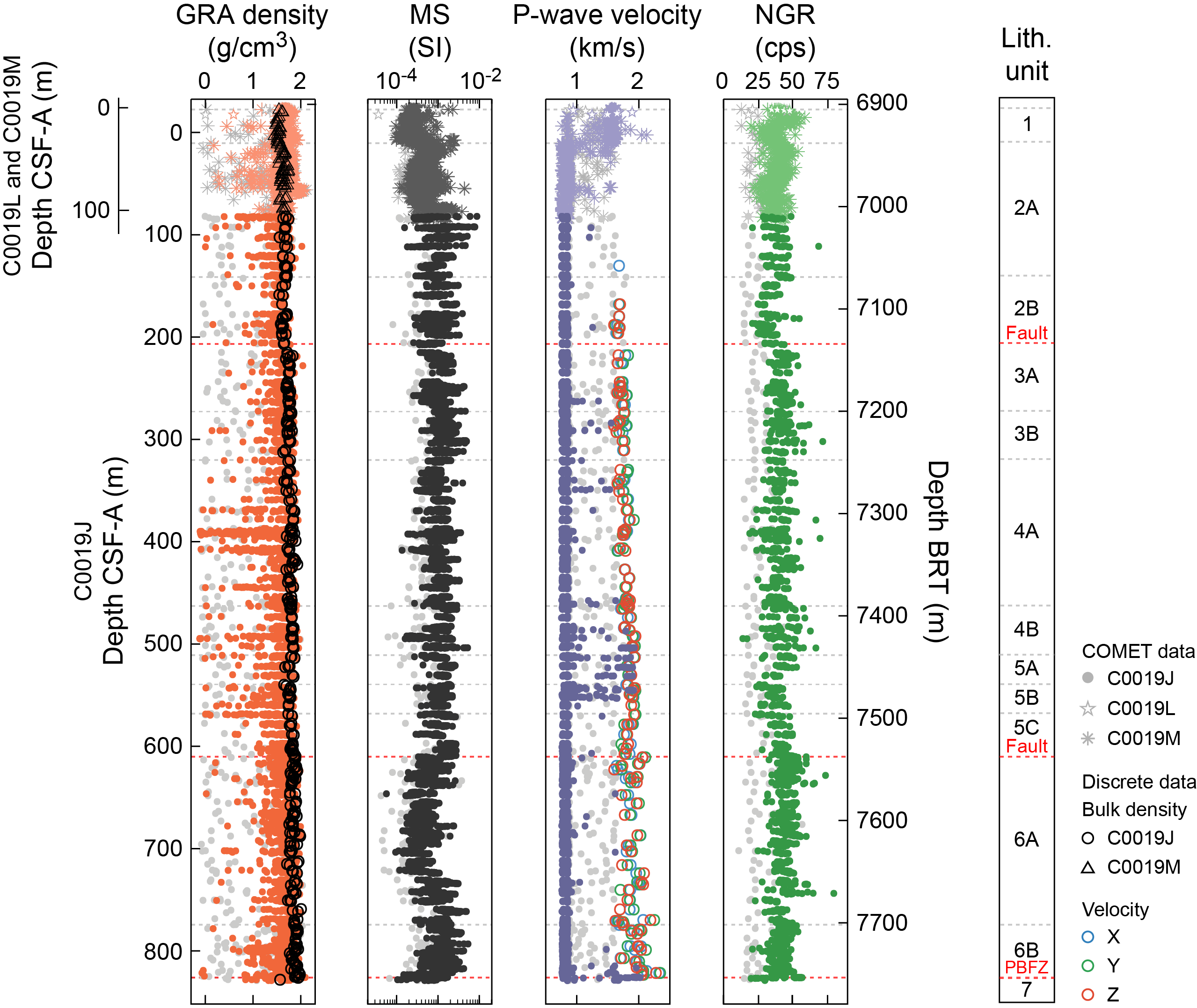
Figure F101. GRA density, MS, P-wave velocity, and NGR, Holes C0019J and C0019M.

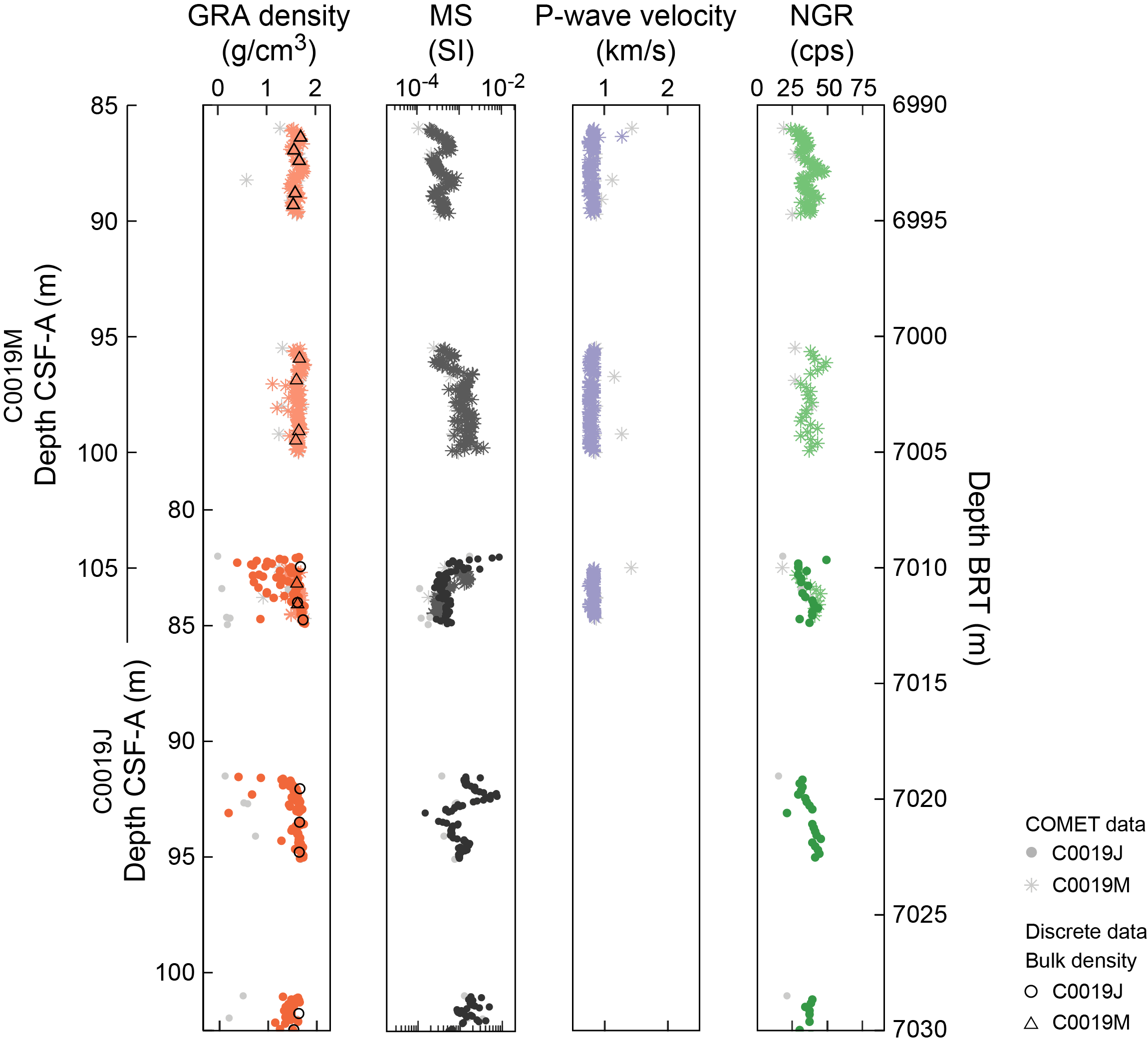
Figure F102. GRA density, MS, P-wave velocity, and NGR, focusing on the overlapping section in Holes C0019J and C0019M.

8.1.1.1. GRA density

Measured bulk density determined by GRA ranges −0.12–2.09 g/cm³ (Figure F101). The large scatter and unrealistically low values are due to incompletely filled core liners and/or damaged/fractured core material, which results in underestimation of the density. However, the maximum GRA densities are generally consistent with discrete measurements of bulk density (see Moisture and density for Holes C0019J, C0019L, and C0019M), so the higher GRA densities appear to provide a reasonable estimate of the bulk density. In Hole C0019M, the average density is 1.64 g/cm³ and the data representing the upper envelope of the scatter indicate that the realistic bulk density range is ~1.6–2.07 g/cm³. In Hole C0019J, the average is 1.61 g/cm³ and the upper envelope ranges ~1.5–2.09 g/cm³.

The bulk density is almost constant in Lithostratigraphic Unit 1 and Subunit 2A (~1.6 to ~1.8 g/cm³). The bulk density slightly decreases to ~1.5 g/cm³ at the bottom of Subunit 2B. In Units 3 and 4, the bulk density gradually increases, ranging ~1.6 to ~1.95 g/cm³. In Subunit 5B, a slight reduction (~1.8 g/cm³) is evident around 540 mbsf, but these values subsequently recover, returning to the generally increasing trend to the bottom of Subunit 6B (2.09 g/cm³ at 825 mbsf).

In Unit 1, the HPCS interval, the cored material generally filled the liner and the confinement provided by the liner allowed the sediment to remain in a state of consolidation. However, with subsequent whole-round sampling and splitting, the sediments expanded to occupy a larger volume, reducing the measured discrete bulk density (see Moisture and density). In the case of SD-RCB cores, comprising materials with varying degrees of lithification, the liner was not completely filled by the cored material. Therefore, the reported GRA densities included void space filled with water or air, resulting in an underestimation of densities.

8.1.1.2. Magnetic susceptibility

MS varies between 5.65 × 10⁻⁵ and 8.74 × 10⁻³ SI, with no obvious difference between the HPCS, ESCS, and SD-RCB cores (Figures F101, F102). In Unit 1, MS values are nearly constant with depth at ~2.0 × 10⁻⁴ SI. At the top of Subunit 2A, MS shows a step increase with depth to ~7.0 × 10⁻⁴ SI and remains nearly constant to ~90 mbsf. At 92 mbsf, MS shifts to ~1.4 × 10⁻³ SI and exhibits values ranging ~2.55 × 10⁻⁴ to ~8.74 × 10⁻³ SI throughout Subunit 2B and Unit 3, without any distinctive trends observed in these units. Near the boundary between Units 3 and 4, MS decreases sharply from ~2.1 × 10⁻³ to ~7.0 × 10⁻⁴ SI and then shows an increasing trend with depth throughout Units 4 and 5, reaching ~2.76 × 10⁻³ SI at the bottom of Unit 5 (604.2 mbsf). In Subunit 6A, MS follows a decreasing trend with depth to 703 mbsf, where it reaches a minimum value of ~9.42 × 10⁻⁵ SI. Subsequently, MS begins to increase again, reaching ~1.89 × 10⁻³ SI near the bottom of Subunit 6A (772.7 mbsf). In Subunit 6B, MS shows a decreasing trend with depth, with values reaching ~1.48 × 10⁻⁴ SI near the bottom of Subunit 6B (823.2 mbsf). In Unit 7, MS remains relatively constant with depth at ~6.0 × 10⁻⁴ SI.

8.1.1.3. P-wave velocity

As with the GRA measurements, the P-wave velocity recorded with the COMET was adversely affected by incomplete liner filling and core damage or fracture. In Holes C0019J and C0019M, most recorded values are lower than the P-wave velocity of seawater (~1.5 km/s) (Figure F101). In Hole C0019M, where HPCS coring ensured better liner filling, relatively continuous P-wave velocities exceeding 1.5 km/s were observed at shallow depths. However, below 31.95 mbsf, even in HPCS cores, most values fall below 1.5 km/s. This depth corresponds to intervals where gas expansion causes significant fracturing of the core (Figure F103), suggesting that the presence of gas and resulting fractures significantly impacted the quality of the velocity measurements. In Hole C0019J, drilled with the SD-RCB system, the majority of recorded values were also less than 1.5 km/s, lower than the P-wave velocity in seawater. Despite these issues, the maximum values measured with the COMET are generally consistent with the P-wave velocity measurements performed on discrete samples (see Discrete P-wave velocity). The envelope of the maximum P-wave velocity values shows an increasing trend from shallow depths in Subunit 1A (~1.54 km/s at 0.24 mbsf) to the bottom of the hole (~2.0 km/s at 826 mbsf).

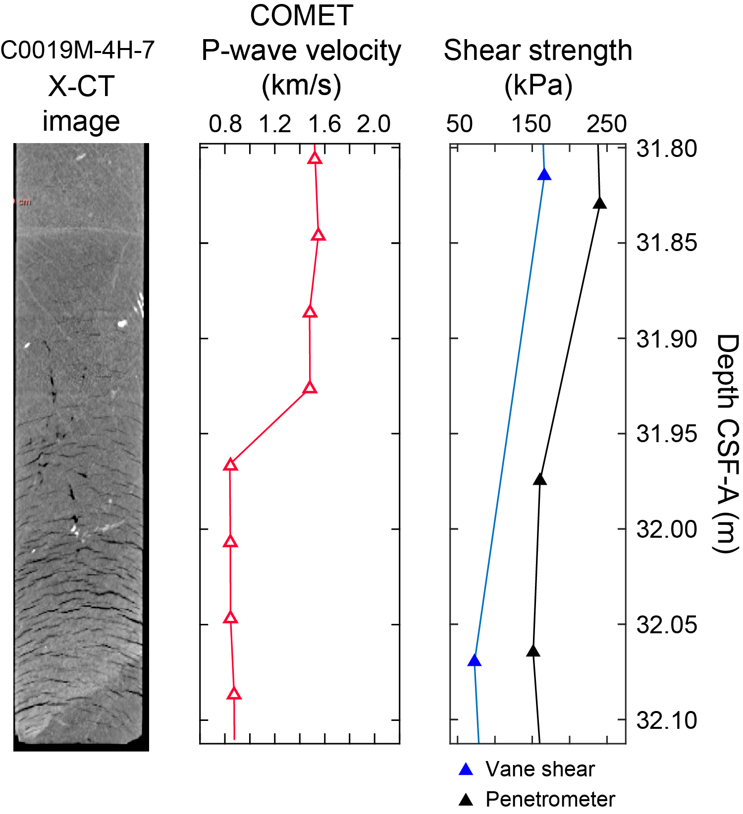
Figure F103. P-wave velocity and shear strength.

The P-wave amplitude was also measured by COMET; however, because the gain settings may vary between measurements and the associated gain (or magnitude of the input amplitude) is unknown, the resulting amplitude is of limited use and is not reported here.

8.1.1.4. Natural gamma radiation

NGR values generally range ~14 to 80 counts/s with an average of ~41 counts/s (Figure F101). Data from the HPCS, ESCS, and SD-RCB cores are consistent with each other (Figure F102). In Unit 1, NGR values are relatively high at very shallow depths (~50 counts/s above 15 mbsf) but decrease to ~35 counts/s near the bottom of the unit. In Unit 2, NGR decreases from ~45 counts/s at the top of Subunit 2A to ~25 counts/s at the bottom of Subunit 2B. At the top of Unit 3, NGR shifts to ~40 counts/s. From Unit 3 to the bottom of Unit 4, the values are scattered, ranging ~14 to 72 counts/s, without showing a clear increasing or decreasing trend with depth. In Unit 5, NGR decreases to ~23 counts/s in Subunit 5B before increasing to ~52 counts/s near the bottom of Subunit 5C. In Subunit 6A, NGR values remain relatively constant around 45 counts/s, but near the bottom of Subunit 6A (750–774 mbsf), NGR decreases to ~30 counts/s. In Subunit 6B, NGR is consistently low at ~42 counts/s. NGR values in Unit 7 are ~36 counts/s.

8.1.2. Moisture and density

MAD measurements were performed to characterize grain density, bulk density, porosity, void ratio, and water content in Holes C0019J and C0019M. A total of 72 MAD measurements were performed between the shallow Cores 405-C0019M-1H and 14X (0.31–106.58 mbsf), and 318 MAD measurements were made between the deeper, SD-RCB Cores 405-C0019J-1K and 88K (82.46–828.12 mbsf) at a frequency of one sample per core section where possible (approximately every 1.5 m). In general, there are no remarkable differences between the values of these index properties estimated on Hole C0019M HPCS and ESCS cores. Furthermore, there is strong continuity between values estimated from the last HPCS core (405-C0019M-10H; 77.08 mbsf) and the first ESCS core where MAD measurements could be made (12X; 86.4 mbsf), as well as in the overlapping interval (7009.5–7012.5 m BRT) of Holes C0019J and C0019M. Below, we summarize the bulk density, grain density, and porosity measurement results. The variations of these parameters with depth are shown in Figure F104.

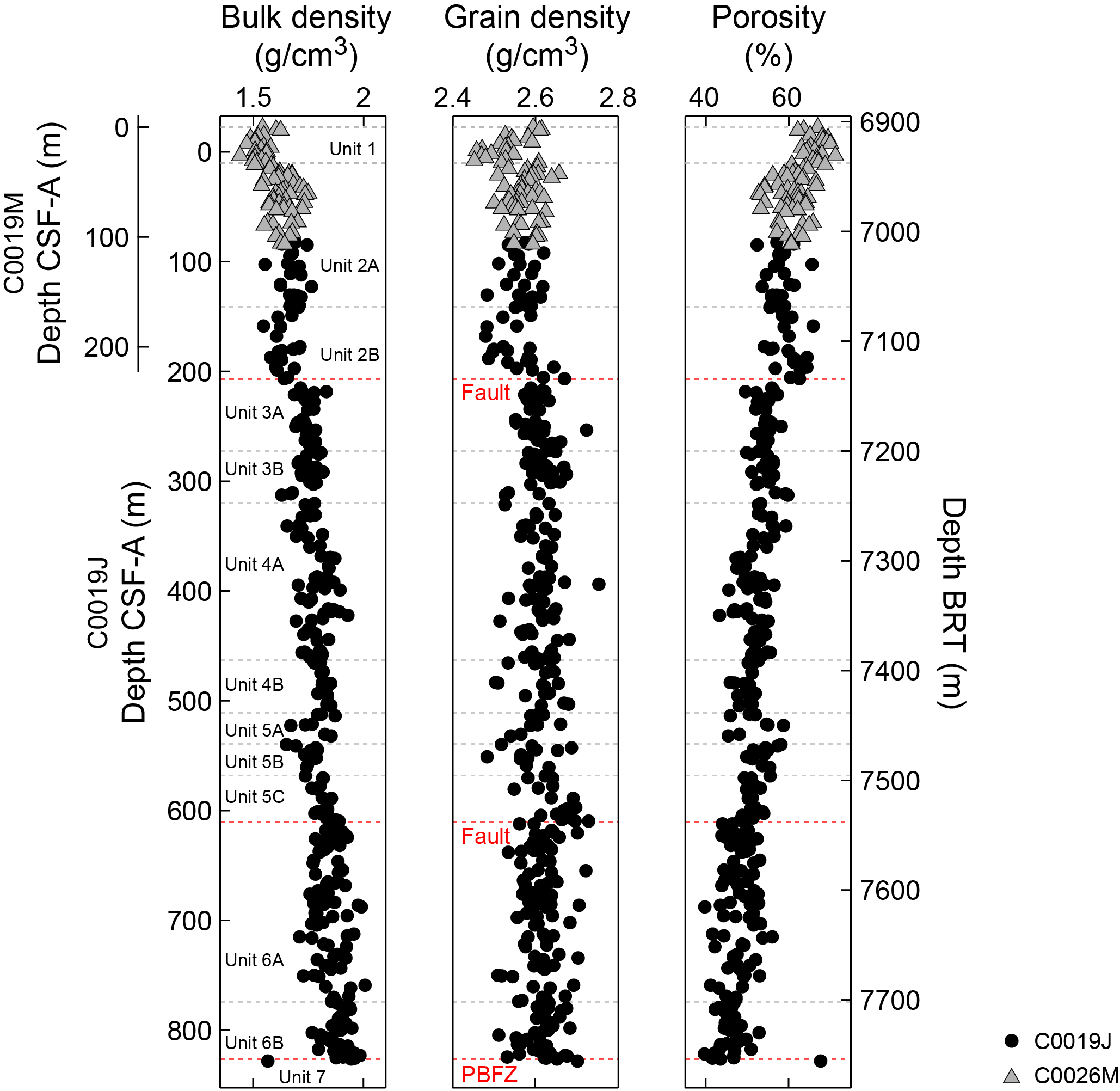
Figure F104. Bulk density, grain density, and porosity, Holes C0019J and C0019M.

8.1.2.1. Bulk and grain density

In Cores 405-C0019M-1H through 4H (0.31–32.52 mbsf), bulk densities in the olive-black siliceous vitric muds of Lithostratigraphic Unit 1 vary between 1.44 and 1.62 g/cm³ (average = 1.53 g/cm³) and grain densities range 2.45–2.62 g/cm³ (average = 2.53 g/cm³). Although the grain densities are relatively constant in this depth interval, the bulk densities exhibit a slight increase with depth from the seafloor to ~50 mbsf (i.e., into Subunit 2A). This overall increase in bulk density with depth likely reflects a compaction trend due to lithostatic loading. Below this point, bulk densities remain approximately constant to the bottom of Hole C0019M (106.58 mbsf). The lack of a density reduction in this section could be due to the numerous thick volcanic layers that are documented in these cores (see Lithostratigraphy), which potentially inhibit compaction.

In Cores 405-C0019M-5H through 405-C0019J-14K (34.17–206.66 mbsf), bulk densities and grain densities in Unit 2 are relatively constant with depth across Holes C0019J and C0019M. The bulk densities in the olive-black siliceous vitric muds of Subunit 2A (33–141.24 mbsf) vary between 1.51 and 1.76 g/cm³ (average = 1.65 g/cm³), and grain densities range 2.25–2.81 g/cm³ (average = 2.57 g/cm³). The bulk densities in the olive-gray siliceous vitric muds of Subunit 2B (141.24–206.95 mbsf) vary between 1.55 and 1.71 g/cm³ (average = 1.63 g/cm³), and grain densities range 2.48–2.67 g/cm³ (average = 2.56 g/cm³). Across the boundary between Unit 2 and Unit 3 (207.57 mbsf), interpreted as a fault (see Structural geology), both bulk and grain densities exhibit a sharp step increase with depth (Figure F104).

Bulk and grain densities are relatively constant with depth in the Unit 3 interval (Cores 405-C0019J-15K through 25K; 215.09–320 mbsf) and are higher than their respective values in Unit 2. In this Unit 3 interval, bulk and grain densities average 1.75 and 2.61 g/cm³, respectively.

Unit 4 (Cores 405-C0019J-26K through 45K; 320.25–504.16 mbsf) is marked by a consistent increase in bulk density from the top of Subunit 4A to the base of Subunit 4B, although grain density is relatively constant in this interval. In this interval, bulk density values vary between 1.65 and 1.93 g/cm³ (average = 1.79 g/cm³) and grain density values vary between 2.50 and 2.75 g/cm³ (average = 2.61 g/cm³).

Bulk density values continue to increase slightly within Unit 5 (511–610.31 mbsf), which consists of the olive-black siliceous vitric mud(stones) of Subunit 5A, the gray siliceous vitric mud(stones) of Subunit 5B, and the dull yellowish brown ashy vitric mud(stones) of Subunit 5C. Bulk densities in this interval vary between 1.65 and 1.89 g/cm³ (average = 1.79 g/cm³), and grain densities vary between 2.48 and 2.73 g/cm³ (average = 2.62 g/cm³).

At ~312.65, 422.18, and 513.69 mbsf, apparent reversals (or abrupt reductions) in bulk density values with depth are evident. However, it is unclear whether these apparent reversals in trend are indicative of faults, mass transport deposits, other processes or are simply observational scatter because similar changes are not consistently present across other physical property measurements or in the colorimetry (see Lithostratigraphy).

Across the boundary between Units 5 and 6 at 610.31 mbsf, which is interpreted as a fault (see Structural geology), the bulk and grain density values show little to no variability. Within Unit 6 (Cores 405-C0019J-56K through 87K; 610.31–826.07 mbsf), bulk densities range 1.71–2 g/cm³ with an average of 1.86 g/cm³. Grain density values within this interval range 2.51–2.72 g/cm³ with an average of 2.61 g/cm³.

Below this interval, only two MAD measurements were made in the color-banded clays and cherts of Unit 7 (826.25–828.12 mbsf). Although the bulk densities of these two samples are significantly different (1.57 and 1.94 g/cm³ for the shallower and deeper samples, respectively), the grain densities are similar (2.65 and 2.70 g/cm³ for the shallower and deeper samples, respectively).

8.1.2.2. Porosity

Samples in the Unit 1 interval of olive-black siliceous vitric mud from Hole C0019M show porosities between 62.2% and 71.3% (average = 66.5%), and corresponding void ratios range 1.64–2.48 (average = 2.0). Following trends in bulk density, porosities exhibit a gradual reduction from the seafloor to ~50 mbsf in Hole C0019M, after which they are relatively constant with depth at ~50% across Holes C0019M and C0019J to the base of Unit 2 in Hole C0019J (206.95 mbsf). There is some scatter in porosity values within this interval that could result from the numerous thick volcanic layers that were documented in these cores (see Lithostratigraphy). In the olive-black and olive-gray siliceous vitric muds of Subunits 2A and 2B, porosities vary between 52.3% and 68.8% (average = 59.8%), and corresponding void ratios range 1.10–2.20 (average = 1.51). Across the boundary between Subunits 2B and 3A (207.57 mbsf), interpreted as a fault (see Structural geology), the porosity exhibits a sharp step decrease (Figure F104).

Within the olive-black siliceous vitric mud(stones) and gray siliceous vitric mud(stones) of Unit 3, porosities and void ratios are relatively constant with depth, with average values of 54.5% and 1.20, respectively. Beginning at the base of Unit 3 (Core 405-C0019J-26K; 320.25 mbsf), porosity and void ratio values show a general decrease with depth throughout Hole C0019J. In Cores 26K–45K (320.25–504.16 mbsf), porosity in the olive-black siliceous vitric mud(stones) and gray vitric mud(stones) of Subunits 4A and 4B range between 43.3% and 59.3% (average = 51.6%) and void ratios range between 0.76 and 1.46 (average = 1.07).

Porosities continue to decrease with depth slightly within the Unit 5 interval (511.00–610.31 mbsf). Porosities and void ratios in this interval vary between 45.4% and 58.7% (average value = 51.9%) and between 0.83 and 1.42 (average = 1.09), respectively.

Although porosity generally decreases with increasing depth throughout Units 3–5 (207.57–610.31 mbsf), as described above, there are several locations where porosity appears to increase suddenly followed by a gradual decrease. These excursions occur at ~312, ~416, and ~522 mbsf (Figure F104). The 312 mbsf excursion occurs near the boundary between Units 3 and 4, but the other two (416 and 522 mbsf) occur within Subunits 4A and 5A, respectively. The 522 mbsf excursion is also located within the same zone as anomalies in pore water chemistry (see Geochemistry).

Across the unit boundary at 610.31 mbsf, which is interpreted as a fault, a small reduction in porosity is observed. Within Unit 6 (Cores 405-C0019J-56K through 87K; 610.31–826.07 mbsf), porosities range 39.6%–55.99% (average = 47.3%). Void ratios within this interval range 0.66–1.27 (average = 0.91).

Below this interval, the two measurements made in the color-banded clays and cherts of Unit 7 (826.25–828.12 mbsf) have highly contrasting porosities of 43.5% and 67.7% and equally contrasting void ratios of 0.77 and 2.10 for the shallower (826.25 mbsf) and deeper (828.12 mbsf) samples, respectively. The difference in porosity may reflect variations in clay mineral content and associated loss of bound water during measurement. All shipboard MAD samples were dried at 105°C for 24 h (see Physical properties in the Expedition 405 methods chapter [Kirkpatrick et al., 2025]). When abundant hydrous clays are present in a sample, drying at high temperatures can result in an underestimation of the bulk density due to the loss of bound water (Basma et al., 1994). Similar laminated clays recovered from Hole C0019E during Expedition 343 (Expedition 343/343T Scientists, 2013a) were found to be up to 99% smectite (Kameda et al., 2015), in which the bound water can account for up to 25% of the hydrated mineral mass (Brown and Ransom, 1996).

8.1.3. Electrical resistivity

The 4-pin 2 kHz Wenner array for soft sediments (see Physical properties in the Expedition 405 methods chapter [Kirkpatrick et al., 2025]) was used to make 35 impedance measurements in the y- and z-directions within the working half of split cores to ~99 mbsf in Hole C0019M and 5 impedance measurements in the upper part of Hole C0019J (~104–132 mbsf; Sections 3K-3, 4K-1, 4K-2, 5K-3, and 6K-3). Below ~168 mbsf (Core 10K), the rocks were indurated enough to measure resistivity on discrete cube samples in the x-, y-, and z-directions. Measurements were attempted on 102 cube samples, but a small number of these measurements were affected by poor sample quality.

From the combined data for Holes C0019J and C0019M, electrical resistivity generally increases with depth. Average values are 1.53 Ωm in the x- and y- (horizontal) directions and 1.59 Ωm in the z-direction (Figure F105).

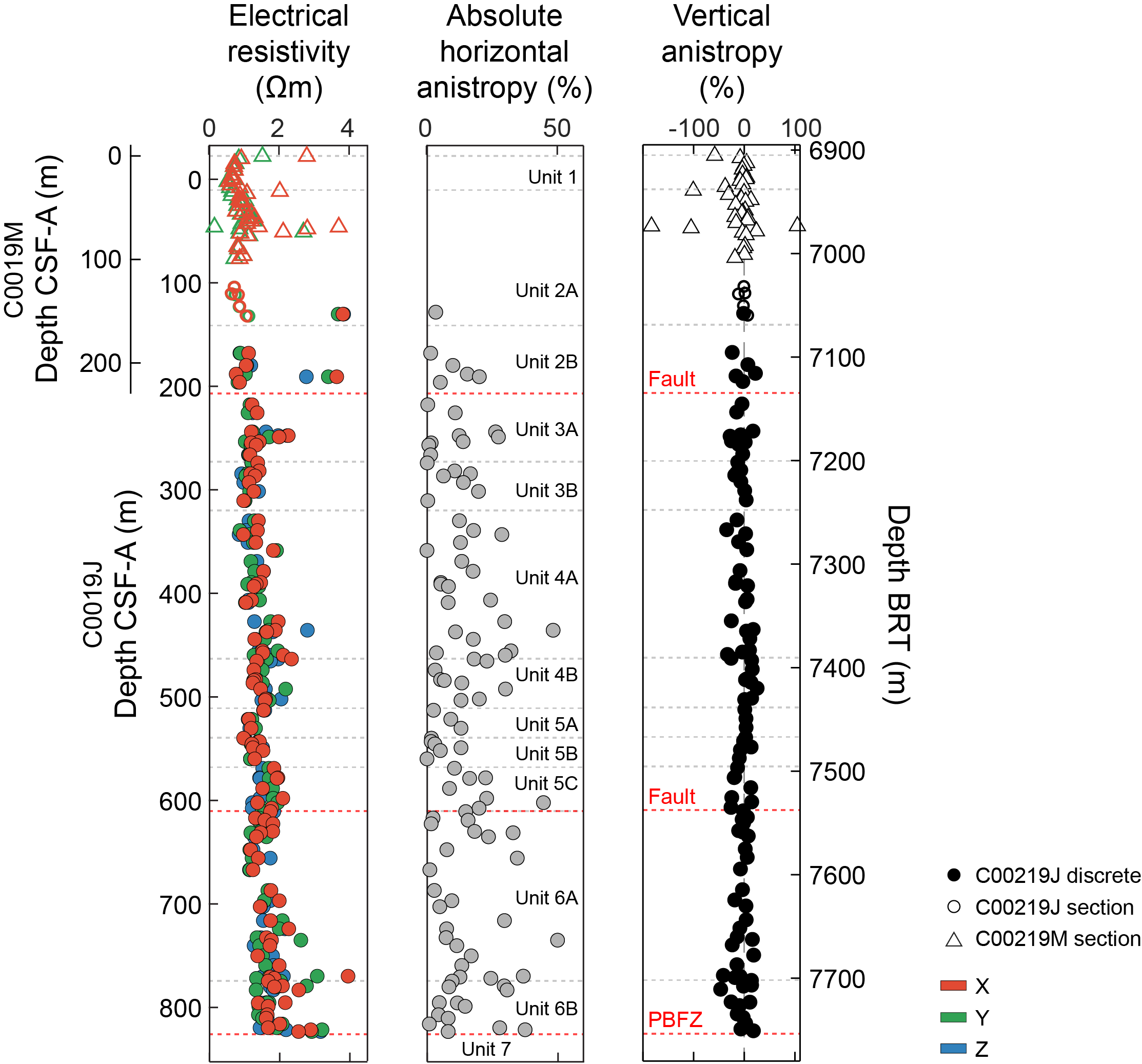
Figure F105. Electrical resistivity and anisotropy, Holes C0019J and C0019M.

The general increase in resistivity with depth occurs both gradually and through several steps that are evident in the data. An increase of ~0.2 Ωm corresponds with the inferred fault boundary between Lithostratigraphic Units 2 and 3 at ~210 mbsf (between Sections 405-C0019J-13K-1 and 15K-3) (see Structural geology), whereas an increase of less than 0.5 Ωm at ~430 mbsf (between Sections 37K-3 and 38K-1, within Subunit 4A) does not correspond with any inferred unit boundaries, nor with distinct steps in other physical property data. Between 512.9 and 521.6 mbsf, resistivity decreases abruptly by ~0.4 Ωm and then gradually increases with depth (Subunits 5A and 5B), reaching 1.71 Ωm at 569.0 mbsf (near the top of Subunit 5C). There is no obvious resistivity offset associated with the faulted boundary between Units 5 and 6 at 610.31 mbsf (see Structural geology). However, the trend of resistivity increasing with depth in Subunits 5A and 5B does not continue in Unit 6. Instead, the resistivity values within Unit 6 are relatively consistent within a range of scatter between 1.5 and 2.2 Ωm. No electrical resistivity measurements were made in Lithostratigraphic Unit 7.

Beyond the general trends in resistivity described above, anomalous values as low as 0.16 Ωm and as high as 4.5 Ωm were measured from 68 to 73 mbsf (Sections 405-C0019M-8H-8, 9H-2, 9H-4 and 9H-6). There is no evidence for similarly anomalous values for other data measured in this depth interval, but XCT core images do provide evidence for core fracturing at the measurement locations (Figure F106). Further investigation is recommended prior to interpreting electrical resistivities in this depth interval.

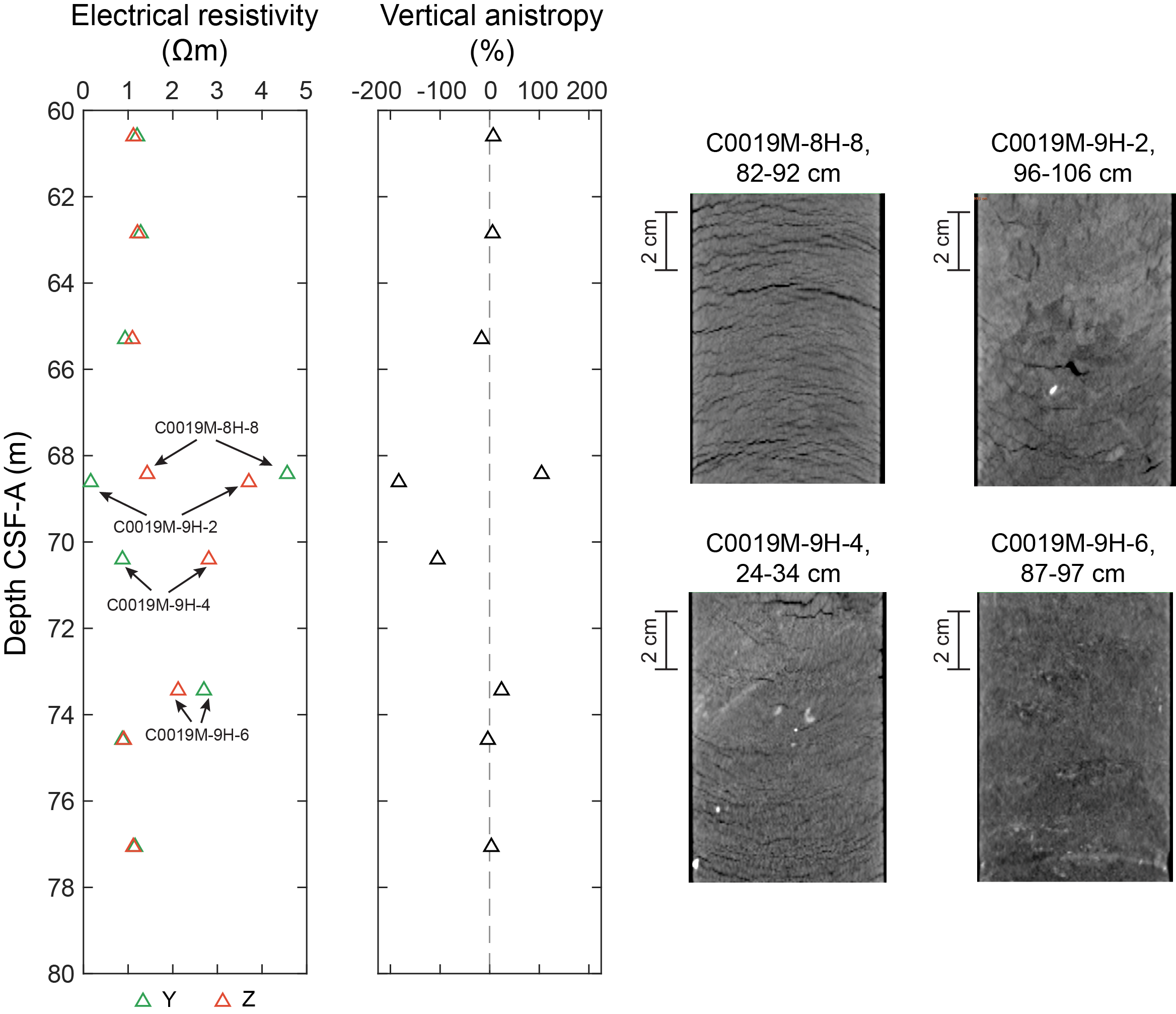
Figure F106. Electrical resistivity and vertical anisotropy, Hole C0019M.

In addition, there is a large discrepancy between 4-pin and discrete cube measurements in Sections 405-C0019J-6K-1 (130.3 mbsf) and 6K-3 (132.1 mbsf), but the anomalously high resistivity measured for Section 6K-1 is likely affected by imperfections in cube shape. An explanation for similar outlier values in Sections 12K-4 (190.8 mbsf) and 18K-3 (247.6 mbsf) is unclear.

Anisotropy was calculated from the resistivity measurements in the x-, y-, and z-directions for cube samples taken from Hole C0019J cores and from measurements in the y- and z-directions made with the 4-pin system for soft sediments in Hole C0019M and the uppermost part of Hole C0019J (see Physical properties in the Expedition 405 methods chapter [Kirkpatrick et al., 2025]).

Because the cores are not horizontally oriented, only absolute values of horizontal anisotropy (x-y plane) are presented (Figure F105). These values show a large scatter ranging 0%–50%. Vertical anisotropy is scattered between about Hole C0019J 40% and ±20%, except in the 68–73 mbsf interval discussed above, where anisotropy values reach more than ±100%.

The overall skew toward negative vertical anisotropy means that vertical resistivity generally exceeds horizontal resistivity (see Physical properties in the Expedition 405 methods chapter [Kirkpatrick et al., 2025]). This is particularly evident for the deepest parts of Unit 6, which form the base of the PBFZ hanging wall (see Structural geology). This relationship is consistent with higher electrical resistivity measured across bedding that is dominantly subhorizontal to moderately dipping (see Logging while drilling and Structural geology). In contrast, in the ~460–550 mbsf interval, where vertical anisotropy scatters more tightly around 0%, the bedding is subvertical.

Figure F107 shows a prominent inverse relationship between electrical resistivity and porosity (i.e., increasing resistivity with decreasing porosity and increasing depth). There is significant scatter in the high porosity (>50%) data, mainly for Unit 2 which was impacted by gas expansion cracking (Figure F106).

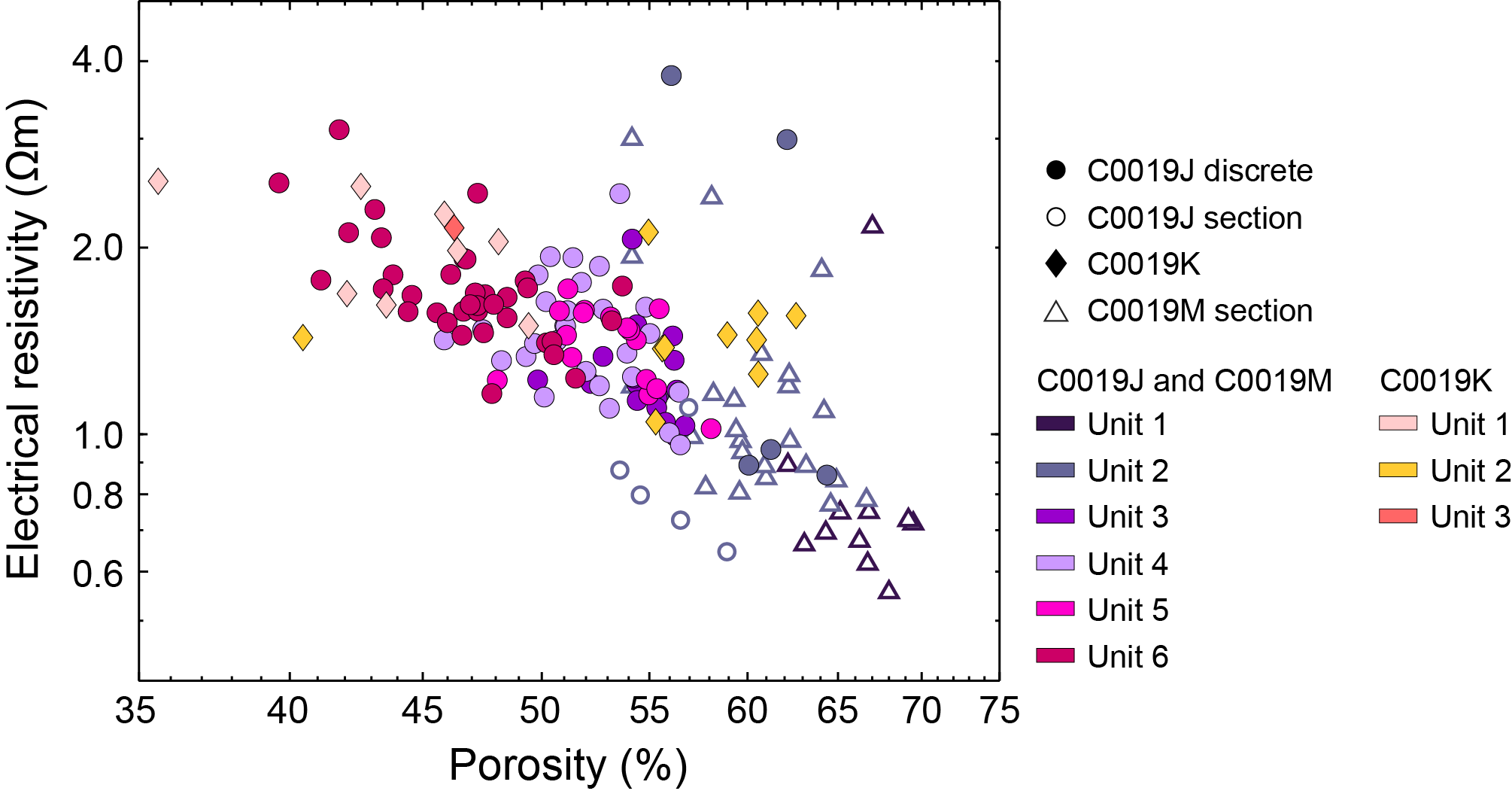
Figure F107. Electrical resistivity, Holes C0019J, C0019K, and C0019M.

8.1.4. Discrete P-wave velocity

P-wave velocity was measured on discrete cube samples from 130.3 to 823.27 mbsf in Hole C0019J. The measured velocities range 1.6–2.35 km/s with an average of 1.83 km/s. There is a general trend of increasing velocity with depth, likely due to compaction, and the anisotropy is generally low, less than 12% (Figure F108). There is a small increase in P-wave velocity of ~0.15 km/s at ~215 mbsf, between Cores 13K and 15K. This shift is only seen in the two horizontal directions (x and y) and not in the vertical (z) direction, resulting in larger vertical anisotropy. This change with depth coincides with a shift to higher bulk and grain densities and lower porosity in MAD measurements. The vertical anisotropy decreases at ~369 mbsf because velocities measured in the x- and y-directions approach those measured in the z-direction. From ~215 to ~610 mbsf, P-wave velocity values follow a slight sawtooth pattern, with repeated intervals of increasing (e.g., 330–379 and 520–569 mbsf) and decreasing (e.g., 379–406 and 569–608 mbsf) velocity with depth. The base of this sawtooth section at ~610 mbsf coincides with a change in lithostratigraphic unit and the upper boundary of a major fault zone in Core 53K (see Lithostratigraphy and Structural geology). Deeper in the section, below ~617 mbsf, the spread in velocity measured in the x-, y-, and z-directions increases, leading to an increase in both vertical and horizontal anisotropy. This increased anisotropy continues to ~816 mbsf and may be related to the inclined bedding that is interspersed with occasional intervals of highly variable bedding orientations cut by faults and folds, or possibly to an increase in fracture density in Unit 6 relative to Unit 5 (see Lithostratigraphy and Structural geology).

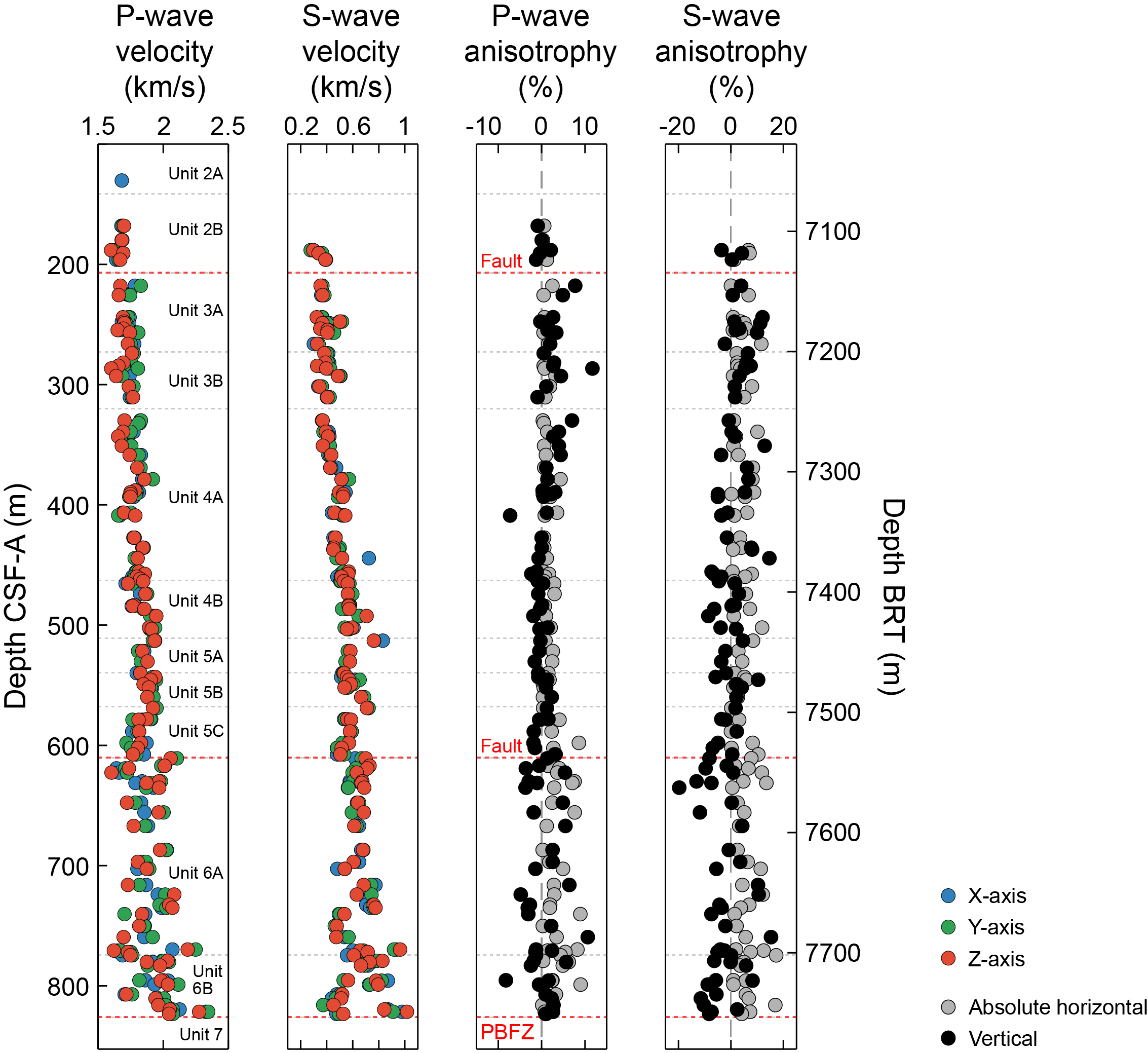
Figure F108. P- and S-wave velocity measurements and anisotropy, Hole C0019J.

P-wave velocities exhibit an inverse correlation with porosity, as expected for marine sediments undergoing burial compaction with increasing depth (Erickson and Jarrard, 1998) (Figure F109). In Unit 2, velocity exhibits little dependence on porosity, whereas Units 3–6 show that P-wave velocity and porosity are anticorrelated.

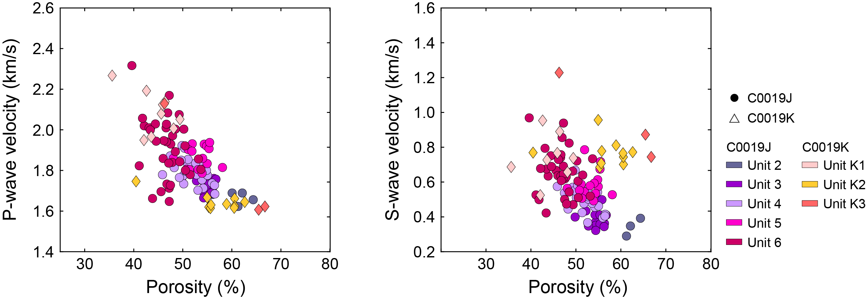
Figure F109. P-wave velocity, Holes C0019J and C0019K.

8.1.5. Discrete S-wave velocity

S-wave velocities measured on discrete cube samples show a generally increasing trend with depth and local excursions consistent with the P-wave measurements. Overall, values increase from ~0.3–0.4 to ~0.6–0.8 km/s from 188 to 800 mbsf (Figure F108). At ~215 mbsf, an increase in velocity in the x- and y-directions is not observed, unlike in the P-wave velocity data. Similar to the P-wave values, the S-wave velocities exhibit sawtooth variations to ~610 mbsf. At ~610 mbsf, the S-wave velocity increases by ~0.16 km/s, followed by an increase in the scatter, with velocities below 700 mbsf ranging ~0.5–1.0 km/s. There is a weak inverse correlation between S-wave velocity and porosity in Hole C0019J (Figure F109).

From 188 to 390 mbsf, vertical S-wave anisotropy is dominantly positive, ranging −4%–13% (Figure F108). Below 390 mbsf, vertical anisotropy becomes dominantly negative. The largest magnitude (−20%) is observed at 635 mbsf. The absolute values of horizontal anisotropy in S-wave velocity remain fairly uniform, ranging 0%–19%.

8.1.6. Shear strength

The undrained shear strength of soft sediments in the working half of the core was measured using an analog vane shear device and a pocket penetrometer (see Physical properties in the Expedition 405 methods chapter [Kirkpatrick et al., 2025]). Undrained shear strength measured by penetrometer increases from 95 to ~240 kPa with depth from 0 to 32 mbsf and is scattered below ~32 mbsf, ranging 84–286 kPa (Figure F110). Vane shear strength increases from 35 to 182 kPa with depth from 0 to 32 mbsf. There is a transition zone around 31.95 mbsf, and the strength through Subunit 2A tends to be lower and scattered, ranging 32–139 kPa below 33 mbsf (Figure F110). The core below ~31.95 mbsf is pervasively cracked due to gas expansion upon core recovery, and a shift to lower values at ~31.95 mbsf is consistent with the top of the cracked core (Section 405-C0019M4H-7) (Figure F103). Both strength estimates have minor high strength anomalies at 45–48, 55, and 63 mbsf. These anomalies tend to be associated with locations of slightly lower porosity (Figure F104).

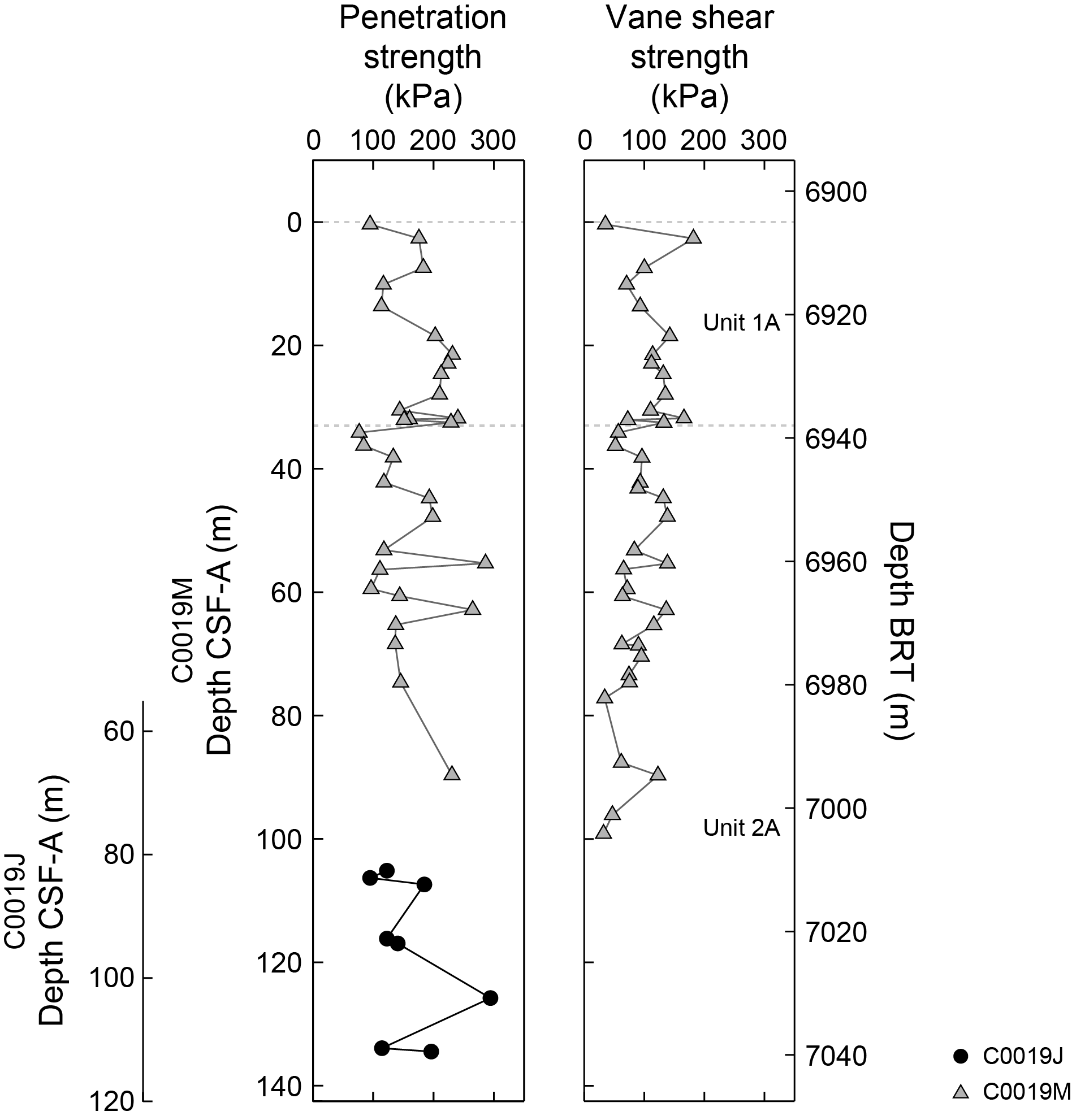
Figure F110. Penetration strength and undrained shear strength, Holes C0019M and C0019J.

8.1.7. Thermal conductivity

Thermal conductivity measurements for Holes C0019J and C0019M were carried out using the half-space probe on the working halves of selected core sections. Even in the shallowest cores, the sediments were too stiff to ensure complete contact without gaps between the full-space needle probe and the sediments. A total of 301 discrete points were measured where rock integrity met the established methodological standards (see Physical properties in the Expedition 405 methods chapter [Kirkpatrick et al., 2025]). These measurements include 226 data points from Hole C0019J and 75 from Hole C0019M. The data set spans Sections 405-C0019M-1H-1 through 87K-2 (6905.4–7753.3 m BRT).

Quality assurance included a review of standard deviations. Data points of poor quality (e.g., samples with visible internal cracks observed in XCT images) or missing standard deviation are marked separately in Figure F111. This process resulted in data from 276 measurements being retained for further analysis, including 208 measurements from Hole C0019J and 68 from Hole C0019M. The scattering of the measured data is consistent with compositional and textural changes in the sediments. Changes in porosity and composition observed in the cores are likely contributors to much of the variation in thermal conductivity values.

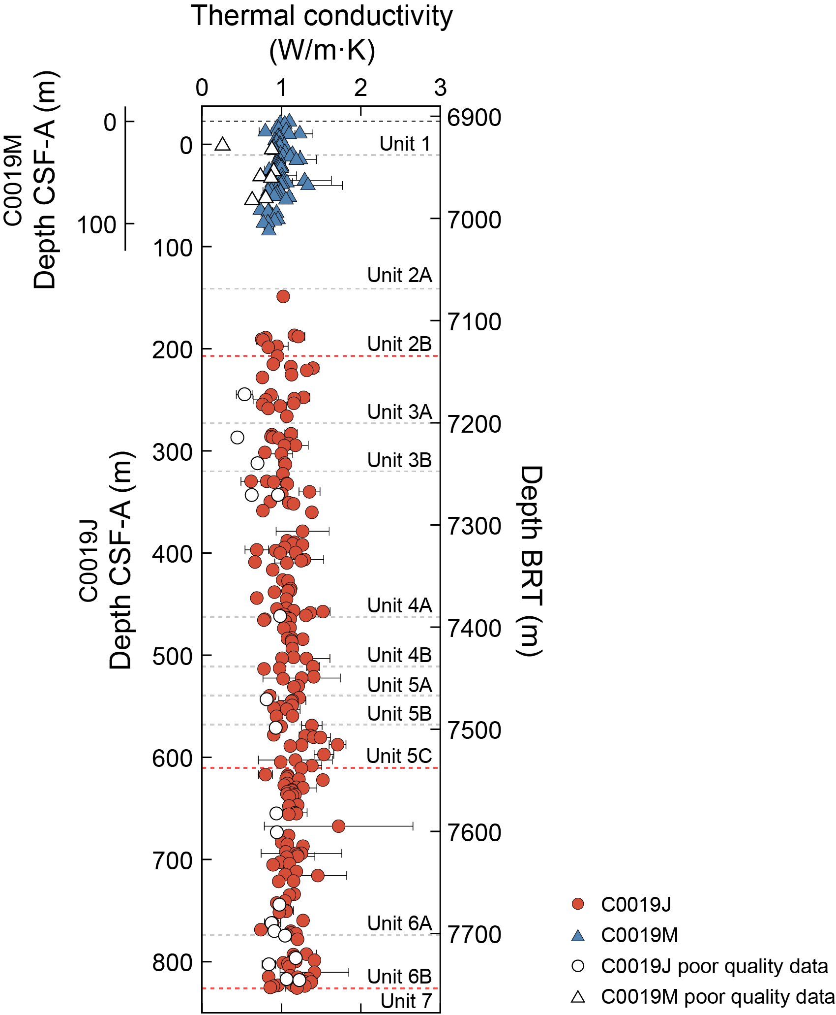
Figure F111. Thermal conductivity measurements, Holes C0019J and C0019M.

Thermal conductivity values in Hole C0019M range 0.733–1.334 W/(m·K) with an average of 0.977 W/(m·K) and a standard deviation of 0.115 W/(m·K). The lowest value was recorded in Section 12X-1 (86.86 mbsf), which corresponds to the olive-black siliceous vitric mud of Lithostratigraphic Subunit 2A but contains numerous small fissures on the surface and within the sample. The highest value was recorded in Section 8H-4 (62.775 mbsf) at a shallower depth within the same unit, where the sample also exhibited high vane shear strength and penetration strength (see Shear strength), indicating good sample integrity. No clear depth-dependent trend in thermal conductivity is evident (Figure F111). However, the ESCS cores retrieved below 80 mbsf generally display lower thermal conductivity, potentially due to the presence of hidden cracks and small fissures in the samples.

In Hole C0019J, thermal conductivity values range from a minimum value of 0.617 W/(m·K) to a maximum of 1.720 W/(m·K) with a mean value of 1.097 W/(m·K) and a standard deviation of 0.187 W/(m·K). The lowest value, 0.617 W/(m·K), was recorded for Section 27K-1 (329.83 mbsf), corresponding to the olive-black siliceous vitric mud(stone) of Subunit 4A. The highest value was recorded in Section 62K-5 (667.395 mbsf) in deeper Subunit 6A.

Overall, the average thermal conductivity in Holes C0019J and C0019M is 1.067 W/(m·K) with a standard deviation of 0.179 W/(m·K).

8.1.8. Anelastic strain recovery analysis

Shipboard anelastic strain recovery (ASR) measurements were conducted on six whole-round core samples from Hole C0019J (19K-3, 128–142 cm, 35K-1, 96–118 cm, 40K-6, 0–17 cm, 49K-2, 50–70 cm, 70K-1, 36–54 cm, and 84K-2, 41–48 cm). The measurements were started within a few hours after the samples were cut from the formation. To illustrate the results of the shipboard ASR measurements, the anelastic strain data, three principal strains, and mean strains are shown in Figure F112, which shows clear evidence of strain recovery with time in each measurement direction. The full analysis of this data will continue as postexpedition research.

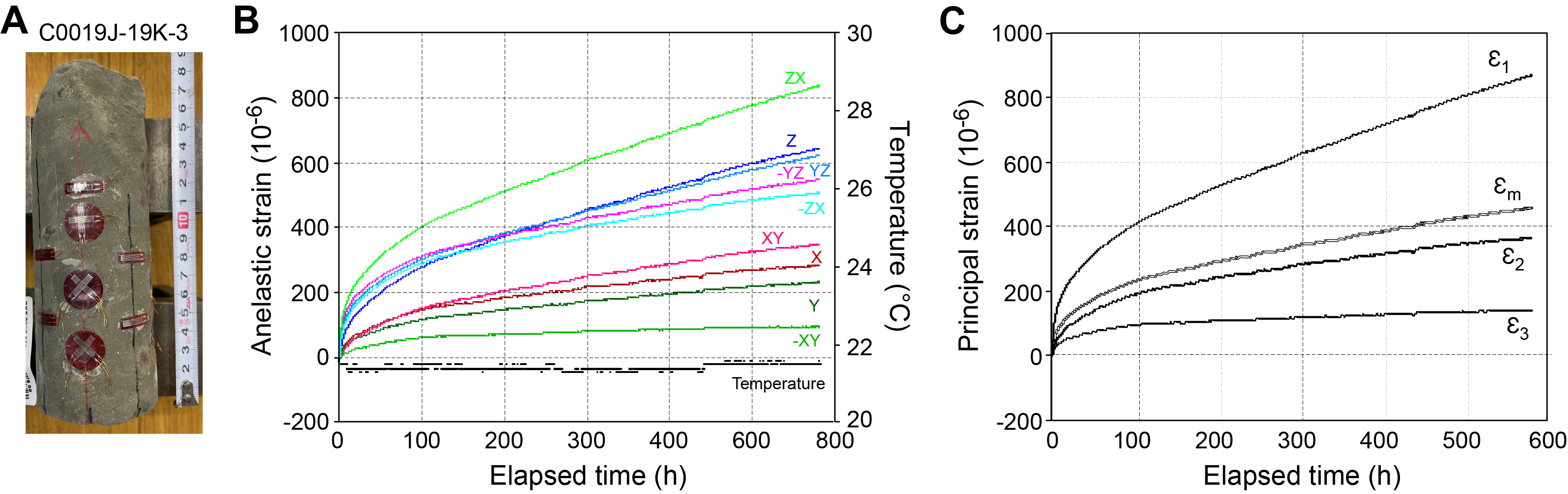
Figure F112. Anelastic strain recovery, Hole C0019J.

8.1.9. Formation temperature and heat flow

Formation temperature measurements were conducted in Hole C0019M using the APCT-3 tool during HPCS coring operations (see Physical properties in the Expedition 405 methods chapter [Kirkpatrick et al., 2025]). Two separate recording sensors were used, starting from Core 405-C0019M-3H and alternating between sensors for every subsequent core advance (Table T31).

All temperature measurements show a clear frictional heating spike upon cutting shoe insertion, which confirms that the tool penetrated the sediment ahead of the drill bit. Measurement 1 at 23.5 mbsf (Core 405-C0019M-3H), Measurement 2 at 42.5 mbsf (Core 5H), and Measurement 4 at 67.5 mbsf (Core 9H) show a smooth temperature decay following insertion (Figure F113A, F113B, F113D). These measurements are of very high quality. In contrast, Measurement 3 at 59.0 mbsf (Core 7H) shows variations in temperature, suggesting that the tool moved after initial penetration, disturbing the postinsertion temperature decay curve (Figure F113C). For this particular measurement, the insertion time used for the analysis of the temperature-time series was reset to the time just after the disturbance.

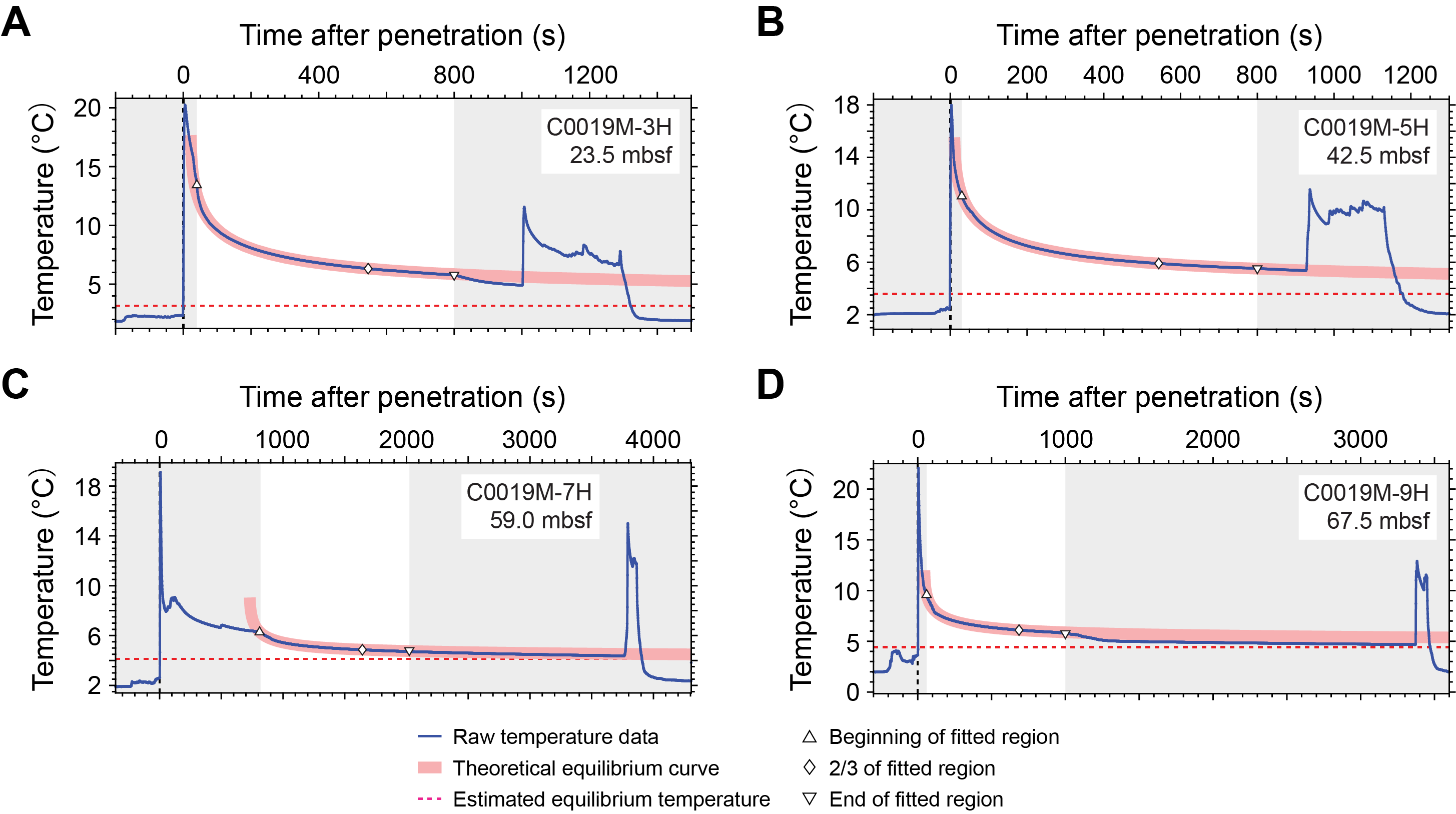
Figure F113. APCT-3 measurements, Hole C0019M.

Equilibrium formation temperatures, estimated from the time-series temperature measurements, are plotted as a function of measurement depth in Figure F114. Inferred formation temperatures increase from about 3.07°C at 23.5 mbsf to 4.44°C at 67.5 mbsf. This yields a geothermal gradient of 31.7°C/km. Because thermal conductivity measurements exhibit little variation values depth (see Thermal conductivity), we use the average value of thermal conductivity of 1.010 ± 0.112 W/(m·K) over this depth interval (23.5–67.5 mbsf) and estimate a preliminary determination of heat flow to be 32.01 ± 3.50 mW/m². This value is close to the vertical heat flow (30.50 ± 2.52 mW/m²) previously determined at the same site using fully equilibrated temperature data from greater depths within the Expedition 343 observatory installed in Hole C0019D (Fulton et al., 2013).

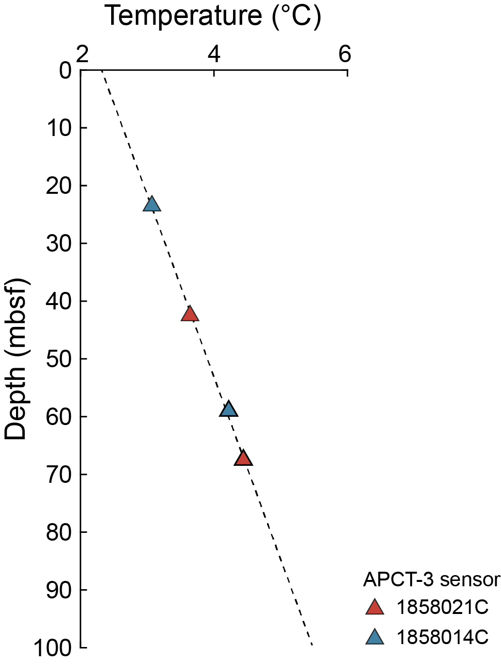
Figure F114. Formation temperatures, Hole C0019M..

8.2. Hole C0019K

Physical property measurements from Hole C0019K provide information about the lithology, porosity, strength, and deformation of materials within about 30 m above and below the inferred location of the PBFZ (see Structural geology). A total of 17 cores were recovered from 815.0 to 875.5 mbsf (7719.0–7779.5 m BRT). The same measurements performed in Hole C0019J were performed in Hole C0019K, except for the soft-sediment measurements (e.g., shear strength).

8.2.1. Core Measurement Track

8.2.1.1. GRA density

GRA bulk density was heavily affected by incompletely filled core liners and damaged/fractured core material, as shown by the large scatter and the high frequency of unrealistically low values (Figure F115). The maximum GRA densities are generally consistent with discrete measurements of bulk density (see Moisture and density), so the higher GRA densities appear to provide a reasonable estimate of the bulk density. The data representing the high end (or envelope) of the scatter suggest a bulk density of about 1.6–2.0 g/cm³.

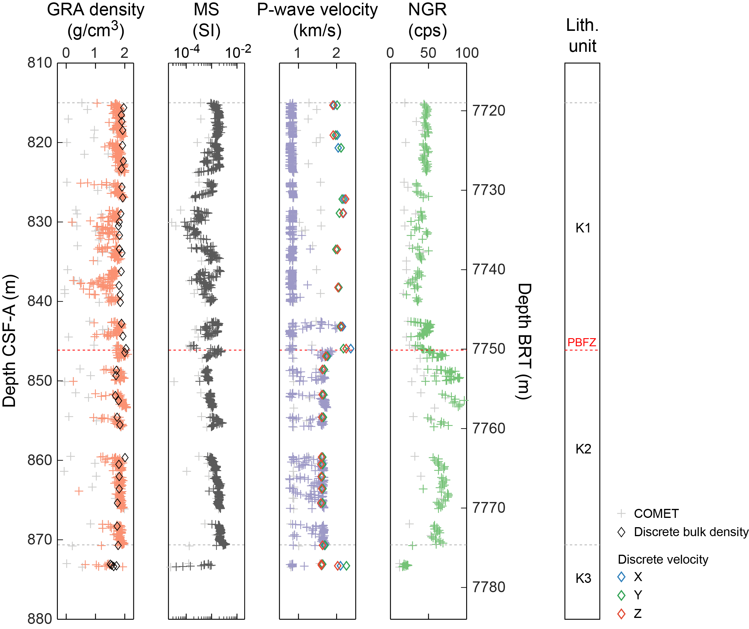
Figure F115. GRA density, MS, P-wave velocity, and NGR, Hole C0019K.

In Unit K1, bulk density increases from ~1.8 to ~2.0 g/cm³ from 815 to 824 mbsf and then decreases to 1.6 g/cm³ at 838 mbsf. The bulk density increases again to 2.0 g/cm³ at a depth where the PBFZ has been interpreted (846.17 mbsf) (see Structural geology) and then remains almost constant until the bottom of Unit K2. The bulk density at the bottom of the hole in Unit K3 is 1.33 g/cm³ on average and 1.93 g/cm³ where chert is present (873.4 mbsf). The maximum values observed below the PBFZ are slightly higher than the bulk density values obtained from MAD measurements on discrete samples.

8.2.1.2. Magnetic susceptibility

MS varies between 2 × 10⁻⁵ and 358 × 10⁻⁵ SI with an average value of ~120 × 10⁻⁵ SI (Figure F115). There is a decrease in MS with depth to 830 mbsf and then an increase toward the deeper parts of the hole (870 mbsf). There is a slight spike (2.5 × 10⁻³ SI) in MS at 855 mbsf, but this does not correspond to any visible changes in the core. From 870 to 871 mbsf, high values exceed 350 × 10⁻⁵ SI. This high MS corresponds to the bottom of the brownish black clay unit in Hole C0019K (Unit K2). At Site C0026B on the incoming plate, high MS is also observed at the bottom of the brownish black clay unit (Unit 2 in Hole C0026B) (see Physical properties in the Site C0026 chapter [Conin et al., 2025]). This indicates that this increase is a natural and potentially traceable marker. In the deepest part of the hole at 873.44 mbsf, the lowest MS value of 2.42 × 10⁻⁵ SI was measured in the chert of Unit K3.

8.2.1.3. P-wave velocity

Like GRA measurements, P-wave velocity recorded with the COMET was adversely affected by incomplete core liner filling and core damage and fracturing. This was evidenced by the fact that most of the values are <1500 m/s, lower than the P-wave velocity of seawater (Figure F115). Very few realistic values were obtained for the P-wave velocity of sediment in the layers above the PBFZ. However, like GRA, the maximum values provide an estimate of P-wave velocity. The maximum velocities measured with the COMET are roughly consistent with the P-wave velocity measurements on discrete samples (see Discrete P-wave velocity), although the COMET velocities below the PBFZ are slightly lower than the discrete measurements. The maximum values were generally 1.6–1.7 km/s, with higher values observed on both the hanging wall and footwall of the PBFZ: ~1.9–2.0 km/s above the PBFZ (843.0–843.3 mbsf) and ~1.8–1.9 km/s just below the PBFZ (846.3–846.8 mbsf).

8.2.1.4. Natural gamma radiation

NGR ranges ~10–76 counts/s with an average of ~50 counts/s (Figure F115). NGR measured with the COMET is almost constant with depth at ~50 counts/s from top of the hole to the PBFZ (815–846 mbsf). Below the PBFZ, NGR increases and measured values regularly exceed 60 counts/s. In the deepest parts of the hole, there is an abrupt decrease in NGR to values less than 25 counts/s. This decrease is associated with the transition to chert in Unit K3 at around 873 mbsf.

8.2.2. Moisture and density

MAD measurements were performed to characterize grain density, bulk density, porosity, void ratio, and water content in Hole C0019K. A total of 41 MAD measurements were performed on Cores 405-C0019K-1K through 17K (815.62–873.47 mbsf) at a frequency of one sample per core section where possible (approximately every 1.5 m). Below, we summarize the results of the bulk density, grain density, and porosity measurements. The variations in these parameters with depth are shown in Figure F116.

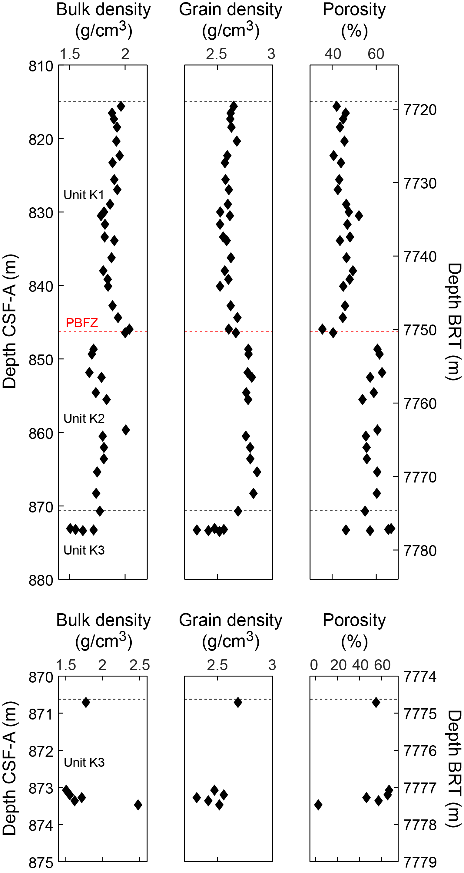
Figure F116. Bulk and grain density and porosity, Hole C0019K.

8.2.2.1. Bulk and grain density

For Cores 405-C0019K-1K through 10K (815.62–846.43 mbsf), bulk densities in Unit K1 range 1.78–2.04 g/cm³ (average = 1.89 g/cm³) and grain densities range 2.52–2.78 g/cm³ (average = 2.60 g/cm³). Although the grain densities are generally the same within this depth interval, the bulk densities exhibit a slight increase with depth from ~831.68 to 846.43 mbsf. This overall increase in bulk density with depth likely reflects a compaction trend due to lithostatic loading. Smaller scale variability in this unit may reflect variations between coherent blocks of different lithologies and the surrounding matrix observed in the core (see Lithostratigraphy). The PBFZ, interpreted to be at 846.17 mbsf at the base of the accretionary prism (see Structural geology), represents a boundary across which bulk densities sharply reduce by ~0.3 g/cm³ and grain densities are slightly elevated by ~0.11 g/cm³ (Figure F116).

Bulk densities in Cores 405-C0019K-11K through 16K (848.7–870.7 mbsf; brownish black clay of Unit K2) are relatively constant, varying between 1.68 g/cm³ and 2.01 g/cm³ (average = 1.78 g/cm³). In this depth interval, grain density remains roughly the same to 868.29 mbsf, with an average value of 2.85 g/cm³. Below this depth, grain densities decrease with depth consistently to a minimum of 2.31 g/cm³.

The interval from 870.7 to 873.47 mbsf is marked by bulk densities that range 1.51–2.48 g/cm³ (Figure F116). Similarly, grain densities in this interval vary from 2.31 to 2.56 g/cm³. The heterogeneities in this interval are consistent with observations of heterogeneous sediment layers underlain by siliceous cherts of Unit K3 at the bottom of Core 405-C0019K-17K (see Lithostratigraphy).

8.2.2.2. Porosity

Porosity and void ratios are generally constant in Hole C0019K in the depth interval represented by Cores 1K through 10K (815.62–846.43 mbsf; Unit K1) (Figure F116). Samples in this interval show porosities between 35.6% and 60.6% (average = 45%), and corresponding void ratios range 0.55–1.54 (average = 0.82). There is a stepwise increase in porosity across the interpreted PBFZ from ~40% to an average of 58%. The high porosities measured in Unit K2 likely do not reflect the in situ porosity. Kameda et al. (2015) found that the brown clays recovered from Hole C0019E during Expedition 343 and Site 436 drilled during DSDP Leg 56 contained up to 94% smectite. Loss of bound water from the clays in Unit K2 during sample drying at high temperature have likely resulted in an overestimation of the water content in the pore space (Basma et al., 1994). Below this interval, to ~871 mbsf, porosities remain relatively constant with an average of 58% (848.7–870.7 mbsf). This signature could represent a lithologic contrast or a different compaction history between the units on either side of the fault. From 870.7 to ~873.5 mbsf, porosities vary considerably from ~3% to 67% (Figure F116). Similar to the range observed in the bulk and grain densities, these heterogeneous porosities are likely indicative of a lithologic transition from pelagic clays to more siliceous cherts (see Lithostratigraphy), the latter having a characteristically higher bulk density and significantly lower porosity than the clay-rich semilithified sediments that overlay them. The high porosities measured in the banded clays may be the result of bound water loss. Similar laminated clays recovered from Hole C0019E were found to be up to 99% smectite (Kameda et al., 2015).

8.2.3. Electrical resistivity

For the entire drilled section in Hole C0019K, rocks were indurated enough to measure electrical resistivity on cube samples. In total, 20 cube samples were obtained from all cores except Cores 405-C0019K-2K, 5K, and 8K. Excluding the chert sampled in Section 17K-CC, resistivity is nearly constant, with average values of 1.73 Ωm in the horizontal direction and 2.13 Ωm in the z-direction (Figure F117). Electrical resistivity of the single chert sampled from Section 17K-CC is much higher, about 1100 Ωm in the x- and z-directions and about 1700 Ωm in the y-direction.

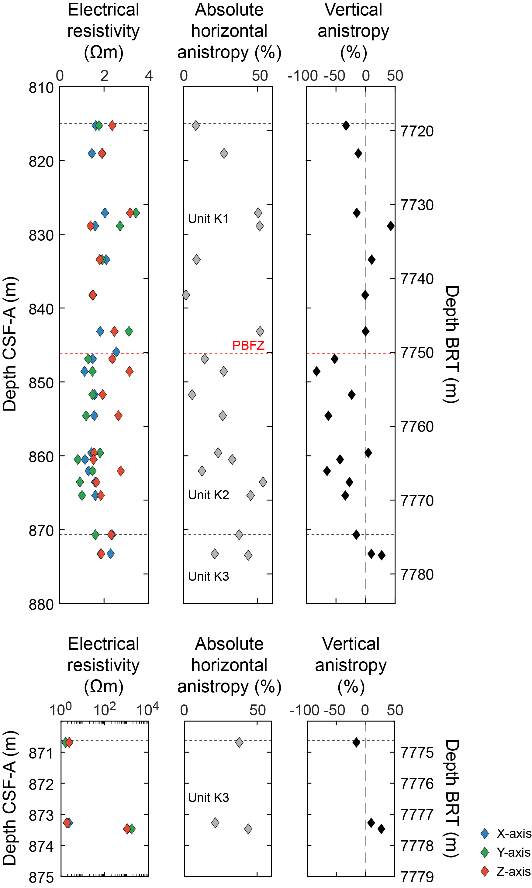
Figure F117. Electrical resistivity and anisotropy, Hole C0019K.

Above the PBFZ (Sections 405-C0019K-1K-1 through 9K-1), mean resistivities are 2.05 and 2.09 Ωm in the horizontal and z-directions, respectively. Below the PBFZ (Sections 11K-1 through 17K-1), the mean resistivities in the horizontal and z-directions are 1.50, 1.38, and 2.13 Ωm. This difference in electrical resistivity across the PBFZ is far more subtle than the prominent (~10%) step in porosity observed across the PBFZ (Figure F116).

Anisotropy was calculated from the resistivity measurements on sample cubes in the x-, y-, and z-directions (see Physical properties in the Expedition 405 methods chapter [Kirkpatrick et al., 2025]). As the cores are not horizontally oriented, only absolute values of horizontal anisotropy (x-y plane) are presented. The absolute value of horizontal anisotropy of resistivity measured from cubes shows a large scatter within a range of 0%–50%. Vertical anisotropy changes across the PBFZ (~847 mbsf) from values in the range of ±50% above the PBFZ in Unit K1 to dominantly negative anisotropy that reaches about −80% below the PBFZ in Unit K2. This indicates that vertical electrical resistivity is significantly higher than horizontal resistivity in Unit K2, which is characterized by a subhorizontal scaly fabric (see Structural geology). An increase in anisotropy in Unit K2 is also evident in the magnetic susceptibility data (see Paleomagnetism).

The relationship between porosity and resistivity is illustrated in Figure F107. Although measurements for Hole C0019K are limited, data from Units K1 and K2 exhibit a linear relationship with porosity (increasing resistivity with decreasing porosity).

8.2.4. Discrete P-wave velocity

P-wave velocity measured on discrete cubic samples taken from 815 to 873 mbsf range ~1.6 km/s to nearly 2.3 km/s (Figure F118). A general trend of increasing velocity with depth is observed throughout Unit K1 (815.00–846.17 mbsf), but there is some variability, including a ~0.2 km/s decrease at ~830 mbsf, between Cores 405-C0019K-4K and 6K. P-wave velocity drops from ~2.3 to ~1.6 km/s across the PBFZ, which is at 846.17 mbsf (see Structural geology), and P-wave velocity is consistently at ~1.6 km/s throughout Unit K2. In the interval containing chert (~873 mbsf in Unit K3), large scatter is observed, with values of ~2 km/s in the layered clays overlaying chert and more than 5 km/s for the chert sample from Core 17K.

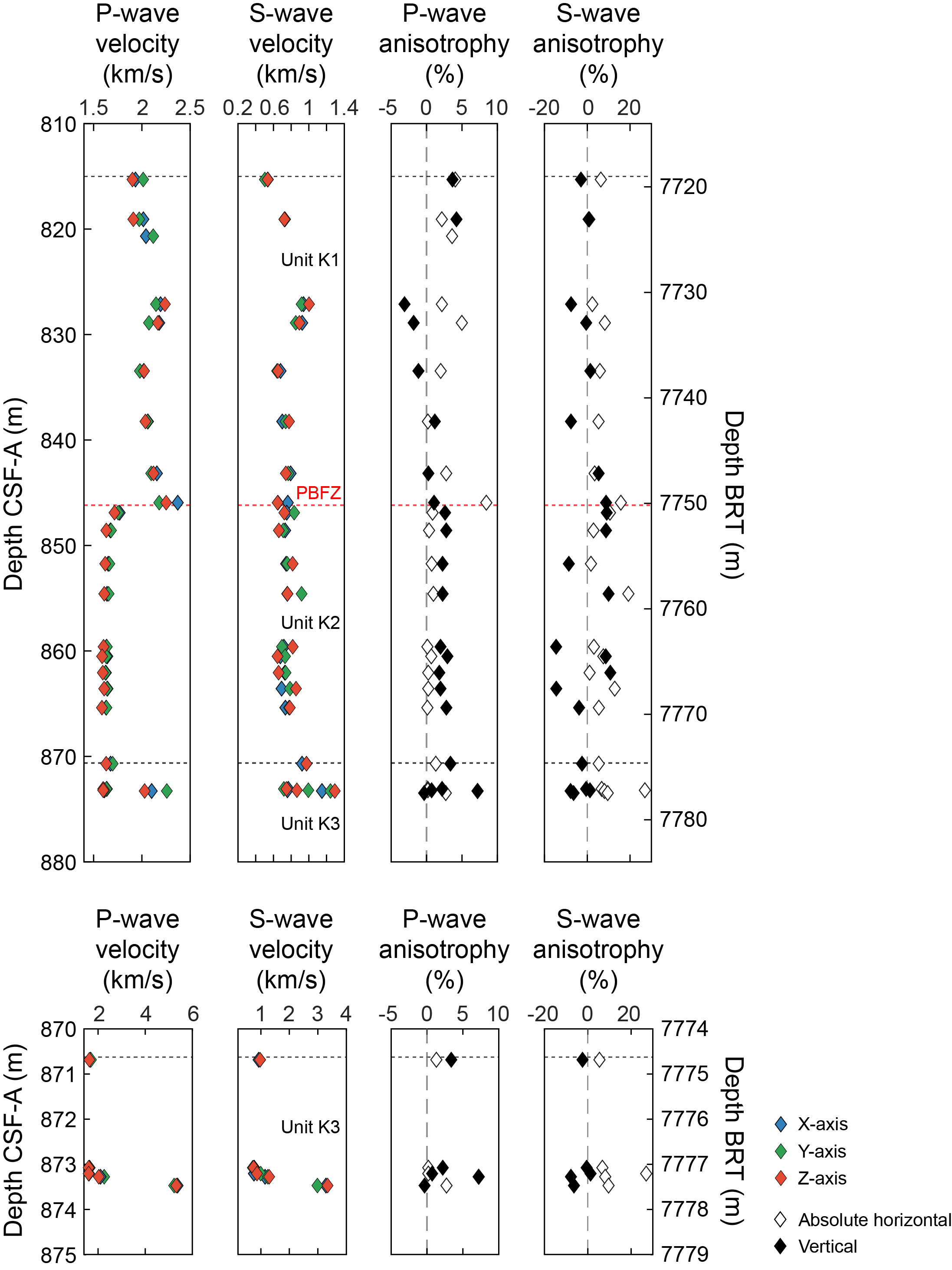
Figure F118. P- and S-wave velocity measurements and anisotropy, Hole C0019K.

The horizontal P-wave anisotropy, measured in the plane perpendicular to the core axis (x-y plane), is reported in absolute terms because the cores are not horizontally oriented. The absolute values of horizontal anisotropy are scattered between 0% and 9% over the depth interval of Unit K1 (815–846 mbsf); however, horizontal anisotropy in Unit K2 is less than 1.3% (Figure F118). The absolute values increase in Unit K3 (~870 mbsf), and the highest values, up to 7.2%, are found at 873 mbsf.

Vertical P-wave anisotropy, measured in the plane parallel to the core axis, in Unit K2 is scattered mostly between ±4% (Figure F118). At the PBFZ (~846 mbsf), where the decrease in horizontal anisotropy is evident, there is a switch from small and scattered anisotropy to consistently positive anisotropy, which indicates a relatively faster horizontal velocity. The vertical anisotropy is ~2.5% over the depth interval of Unit K2 (846–870 mbsf) and is scattered between −0.3% and 7.2% below 870 mbsf.

P-wave velocity is inversely correlated with porosity (Figure F109), as is expected for marine sediments undergoing burial compaction with increasing depth (Erickson and Jarrard, 1998). All lithostratigraphic units generally lie along the same trend. P-wave velocity in Unit K2 is generally constant with decreasing porosity, but velocities in Units K1 and K3 increase with decreasing porosity.

8.2.5. Discrete S-wave velocity

S-wave velocity measured on discrete cubic samples taken from 815 to 873 mbsf ranges ~0.5 km/s to nearly 1.0 km/s (Figure F118). S-wave velocities show a generally increasing trend with depth and a local decrease at ~830 mbsf, consistent with P-wave measurements. Below ~830 mbsf, S-wave velocities increase slightly from ~0.65 to ~1.0 km/s. At the PBFZ (~846 mbsf), where P-wave velocities decrease, the S-wave velocities increase continuously. In samples from this interval, a strong P-wave arrival recorded by the measuring instrument made it difficult to identify the S-wave arrival. The reduction in velocity may, therefore, not be observed because of the incorrect identification of the S-wave. S-wave velocities in the deeper section, below ~873 mbsf in Unit K3, are scattered between 0.75 and 1.3 km/s, and the highest values of up to ~3.0 km/s are found in chert at 873 mbsf. There is no clear dependence of S-wave velocity on porosity (Figure F109).

Absolute horizontal S-wave anisotropy scatter ranges primarily 2%–16% in Unit K1 (815–846 mbsf) and 1%–26% below the PBFZ (Figure F118). Vertical S-wave anisotropy in Unit K1 is scattered around 0, mostly between ±8%. Below the PBFZ, where there is a slight increase in horizontal anisotropy, the scatter in vertical anisotropy also increases to between −15% and 10%.

8.2.6. Thermal conductivity

Thermal conductivity measurements in Hole C0019K were conducted on the working half of selected core sections at 34 discrete points where the rock integrity met the methodological standards (see Physical properties in the Expedition 405 methods chapter [Kirkpatrick et al., 2025]) in Sections 1K-1 through 16K-1 (815.05–869.755 mbsf). Unfortunately, because of lack of a viable surface for measurement, data are unavailable for Core 17K, situated near the bottom of the hole and approaching the zone of chert in Unit K3, due to lack of a viable surface for measurement.

Thermal conductivity was measured at least three times at each measurement position, and quality assurance was performed for all determinations, including a review of standard deviations. Data points with poor quality or missing standard deviation values are marked separately in Figure F119. This process resulted in data from 28 measurements being retained for further analysis.

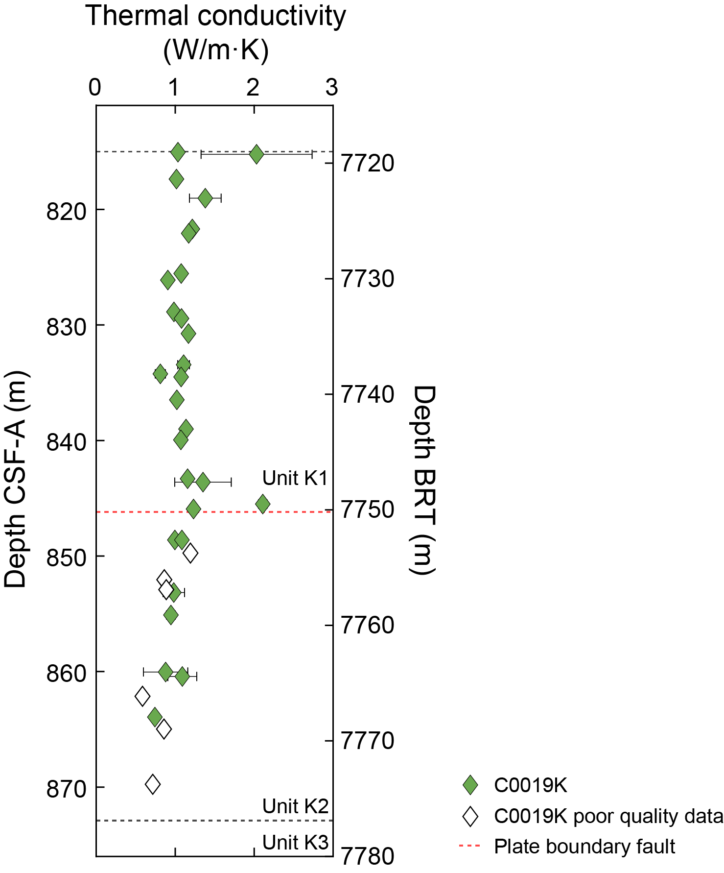
Figure F119. Thermal conductivity measurements, Hole C0019K.

In the data set for Hole C0019K through Core 16K, thermal conductivity values span from a minimum of 0.743 W/(m·K) to a maximum of 2.109 W/(m·K) with a mean of 1.138 W/(m·K) and a standard deviation of 0.299 W/(m·K) (Figure F119). In general, thermal conductivity is relatively consistent in value without an observable trend with depth in the olive-gray vitric mud of Unit K1. In the brownish black clay of Unit K2, a decreasing trend with depth is evident.

The highest thermal conductivity was recorded in Section 405-C0019K-10K-1 in the olive-gray vitric mud of Unit K1, close to the PBFZ, and a second high thermal conductivity value of 2.030 W/(m·K) was measured in Section 1K-1 in a compact silt layer (see Lithostratigraphy). The lowest value was measured in Section 15K-2, in the brownish black clay of Unit K2. Measurements made below the PBFZ are often of poor data quality (Figure F119) due to fractures or fissures that are evident in XCT images of the core (see Structural geology). For good quality measurements in Unit K2, the values of thermal conductivity are often lower than those from Unit K1. This might be related to other properties, such as porosity or composition.

8.2.7. Anelastic strain recovery analysis

At Site C0019K, shipboard ASR measurements were made for two whole-round core samples (405-C0019K-8K-1, 29–43 cm, and 16K-2, 7–25 cm). To illustrate the results of the shipboard ASR measurements, the anelastic strain data, three principal strains, and mean strains are shown in Figure F120. Data from Section 8K-1 show a high strain anomaly in the beginning of measurement; however, generally a gradual recovery of strain with time is observed. The analysis of the ASR data will continue as postexpedition research.

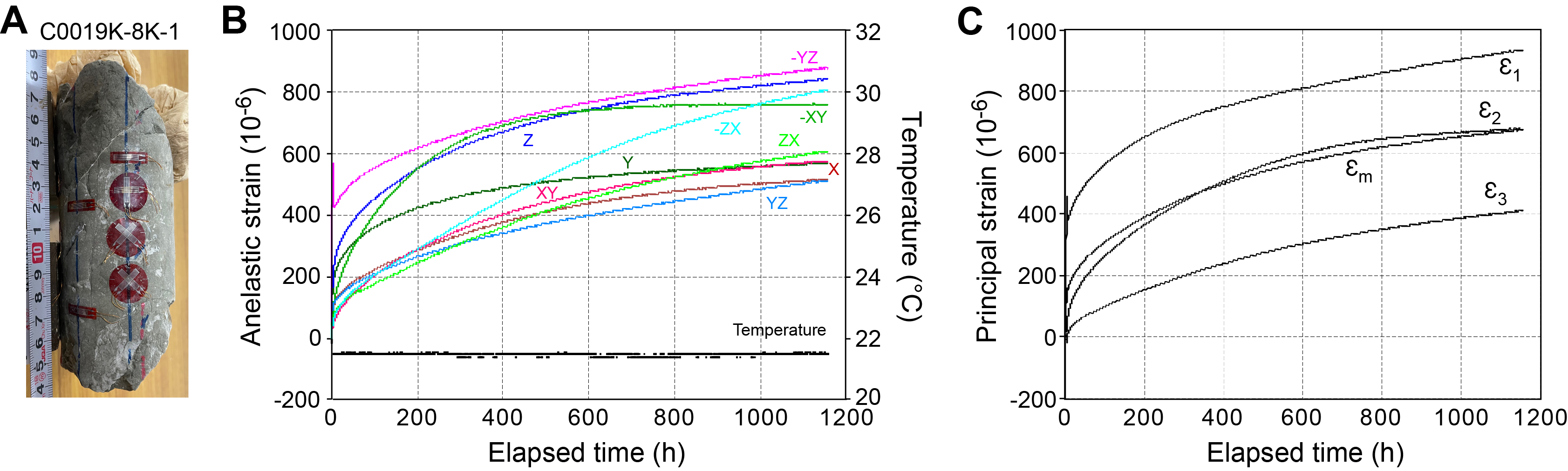
Figure F120. Anelastic strain recovery, Hole C0019K.

8.3. Hole C0019P

Physical properties measurements from Hole C0019P provide information on igneous and sedimentary rocks recovered from depths greater than 930.0 mbsf. Procedures for hard rock were followed (see Physical properties in the Expedition 405 methods chapter [Kirkpatrick et al., 2025]), but the same suite of measurements performed for Hole C0019K were also undertaken for Hole C0019P.

8.3.1. Core Measurement Track

For COMET measurements, the ends of the core may not yield accurate values due to the absence of core material on one side or the influence of the liner cap. Therefore, the following analysis does not include data acquired within 4 cm of both ends of each core section (Figure F121).

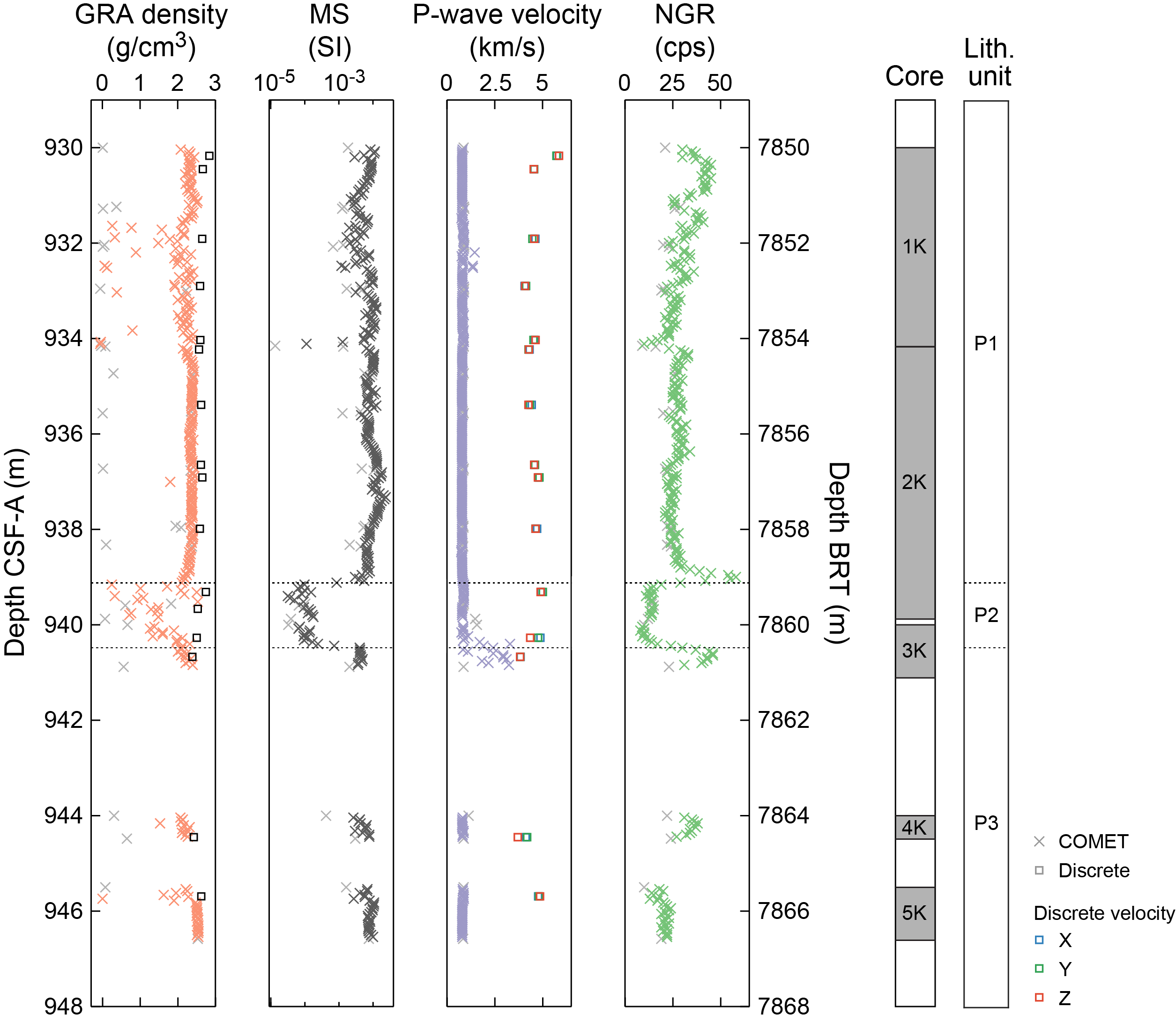
Figure F121. GRA density, MS, P-wave velocity, and NGR, Hole C0019P.

8.3.1.1. GRA density

Bulk density determined by GRA ranges −0.06–2.55 g/cm³ (Figure F121). The maximum GRA densities are generally consistent with measurements of bulk density (see Moisture and density) performed on discrete samples from the working half of the cores, but compared to discrete bulk density, GRA density is lower overall. The liner was not completely filled by the cored material, so the reported GRA density includes void space filled with water or air, resulting in an underestimation of density. The average GRA density is 2.15 g/cm³, and the upper envelope ranges ~1.9–2.55 g/cm³.

GRA density is largely scattered (~1.8–2.53 g/cm³) in Core 405-C0019P-1K (930.04–934.15 mbsf). GRA density is almost constant from ~935.5 to ~939.9 mbsf (~2.2 to ~2.4 g/cm³) and is scattered within a range of ~1.9–2.53 g/cm³ from the bottom of Core 2K through Core 3K (939.1–940.9 mbsf). Core 3K is heavily disturbed, containing a few biscuits of coherent material surrounded by rubble, and the condition of the core likely contributed to the observed scatter in the data. This depth interval also corresponds to an area with interbeds of limestone, chert, calcareous pelagic sediment, and siliceous mudstone with a basalt sill at the base of Core 3K (see Lithostratigraphy). This heterogeneity also contributes to scatter in the data. In Core 4K, GRA density varies between ~2.1 and ~2.3 g/cm³ without any distinctive trends. In Core 5K, GRA density scatters at the top of the core (~1.6 to ~2.3 g/cm³) and then slightly increases to the bottom of the section (~2.5 to ~2.55 g/cm³).

8.3.1.2. Magnetic susceptibility

In Hole C0010P, MS varies between 3.18 × 10⁻⁵ and 2.39 × 10⁻² SI (Figure F121). MS values remain relatively constant overall, 7.101 × 10⁻³ on average, but there are some meter-scale regions where MS noticeably varies. Between 931 and 932.5 mbsf, MS shows lower and more scattered values, ranging 1.196 × 10⁻³ to 8.043 × 10⁻³ SI. This is the location of a large intrusive feature (see Structural geology) where a carbonate is intercalated with pillow basalts (see Lithostratigraphy). At the bottom of Core 405-C0019P-2K and top of Core 3K (939.1–940.5 mbsf), MS exhibits notably lower values, ranging 3.183 × 10⁻⁵ to 8.606 × 10⁻⁴ SI. This is a location of interbedded siliceous and carbonate sedimentary rock. MS returns to ~4.1 × 10⁻³ SI at 940.5 mbsf, which coincides with the occurrence of a basalt sill in Core 3K.

8.3.1.3. P-wave velocity

As with the GRA measurements, the P-wave velocity recorded with the COMET is adversely affected by incomplete liner filling and core damage or fracture. In Hole C0019P, most recorded values were lower than the P-wave velocity in seawater (~1.5 km/s) (Figure F121). Only the interval from 940.3 to 940.8 mbsf in Core 405-C0019P-3K shows P-wave velocity values larger than seawater, with values reaching higher than 3.0 km/s. Nevertheless, P-wave velocity measured with the COMET at this depth is significantly lower than the values measured on discrete samples and likely does not reflect the actual velocity of the recovered material.

8.3.1.4. Natural gamma radiation

NGR generally ranges ~8–58 counts/s with an average of ~27.54 counts/s (Figure F121). In Core 405-C0019P-1K, NGR values decrease from ~45 counts/s near the top of Section 1K-1 (930.4 mbsf), where the intrusive feature is located (Figure F122) (see Structural geology), to 10 counts/s at the bottom of Core 1K (934.2 mbsf). In Core 2K, the overall value is constant (~20 to ~30 counts/s), but then it increases sharply at the bottom of the core, with a very high value (58 counts/s) at 939 mbsf. This is followed by a rapid reduction to ~10 counts/s, and NGR stays around 10 counts/s through Core 3K at 940.64 mbsf, where there is a second spike to 46 counts/s. The two high NGR spikes are located within basalt sills associated with chilled margins identified in the core, whereas the low NGR region is associated with carbonate and siliceous sediments (see Lithostratigraphy). In Cores 4K and 5K, NGR ranges 27–38 and 13–24 counts/s, respectively. These cores are too short to identify any distinctive trends or variations.

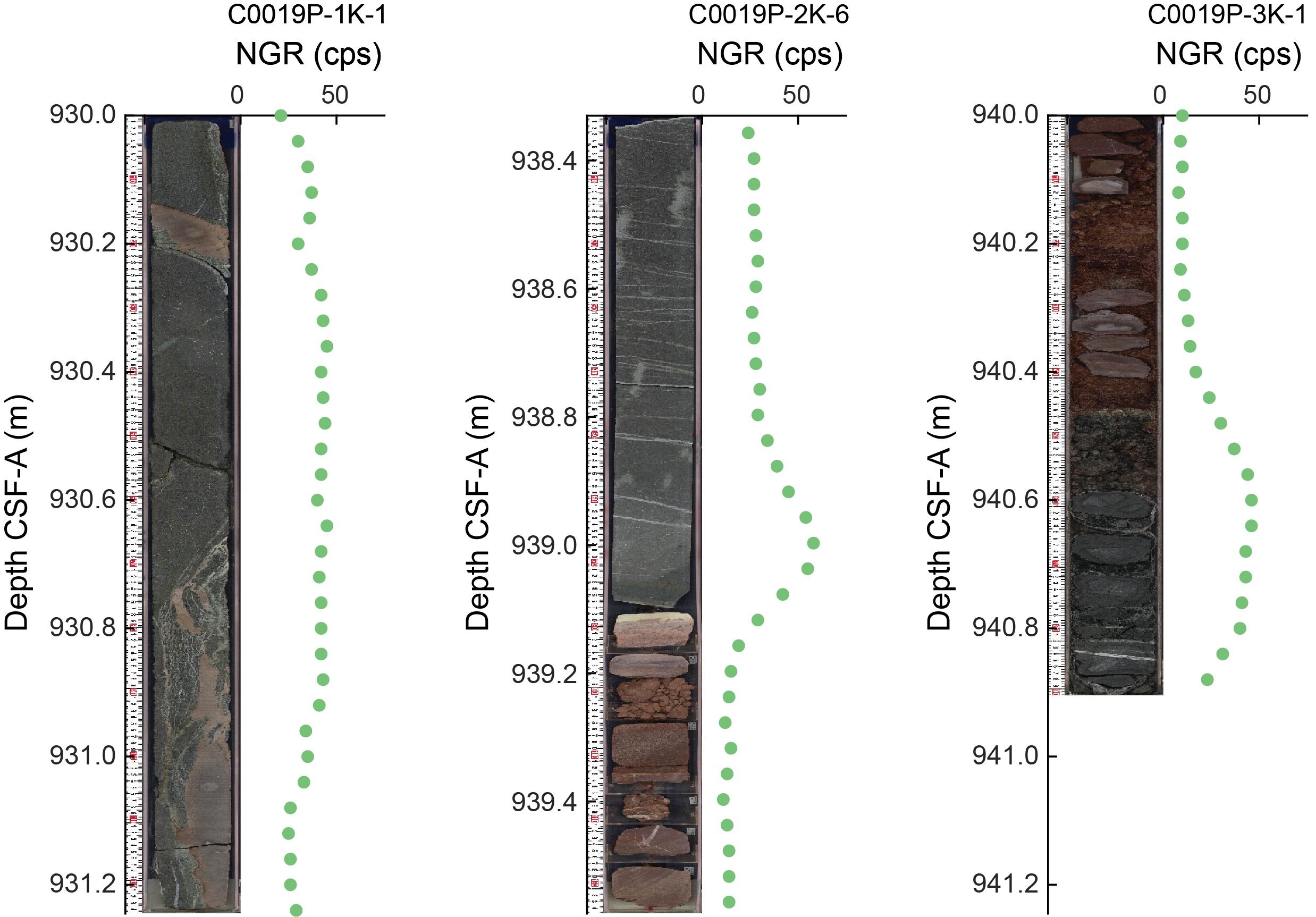
Figure F122. TSCL images and NGR data, Hole C0019P.

8.3.2. Moisture and density

MAD measurements were performed to characterize grain density, bulk density, porosity, void ratio, and water content in Hole C0019P. A total of 16 MAD measurements (12 in basalt and 4 in sedimentary intervals) were performed between Cores 405-C0019P-1K and 5K (930–946.6 mbsf) at a frequency of one sample per core section where possible (approximately every 1.5 m). Out of 12 MAD measurements, 11 were performed on discrete cube samples that were also used for other physical property and paleomagnetic measurements (see Physical properties in the Expedition 405 methods chapter [Kirkpatrick et al., 2025]). Below, we summarize the most important parameters: bulk density, grain density, and porosity. The variations of these parameters with depth are shown in Figure F123.

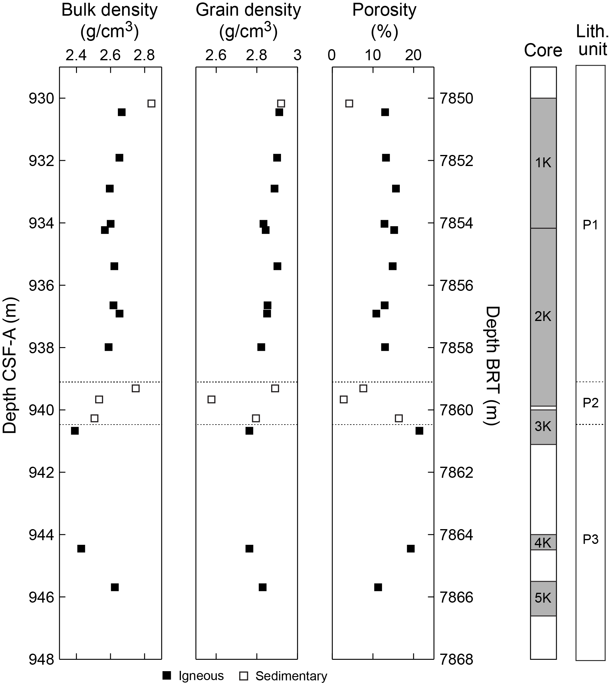
Figure F123. Bulk density, grain density, and porosity, Hole C0019P.

8.3.2.1. Bulk and grain density

The bulk and grain densities of the basalts are generally consistent throughout Hole C0019P and range 2.39–2.67 g/cm³ (average = 2.58 g/cm³) and 2.76–2.91 g/cm³ (average = 2.85 g/cm³), respectively. There is little to no indication of the alteration state of the basalt in the bulk or grain density data from this hole (Figure F123).

Core 405-C0019P-1K is interpreted to include a section through pillow basalts with carbonates infilling void spaces between basalt blocks (see Lithostratigraphy). Similarly, carbonate rocks, chert, and siliceous mudstones are observed at ~939.1 mbsf (Sections 405-C0019P-2K-6 through 3K-1). Samples from these intervals have variable bulk and grain densities that range 2.51–2.84 g/cm³ (average = 2.66 g/cm³) and 2.58–2.92 g/cm³ (average = 2.80 g/cm³), respectively, with the carbonate-rich sedimentary intervals having higher bulk densities than the basalt/igneous intervals.

8.3.2.2. Porosity

The porosities and void ratios of the basalts from Hole C0019P range 10.8%–21.4% (average = 14.5%) and 0.12–0.27 (average = 0.17), respectively. As with the density data, any clear indication of basalt alteration state in the porosity or void ratio data is lacking, with two exceptions (Figure F123): basalt samples from Section 405-C0019P-3K-1 have high NGR values, and the sample from Section 4K-1 has numerous tightly spaced white veins (interpreted to be calcite; see Lithostratigraphy). These samples have elevated porosities of 21.4% and 19.3%, respectively.

Samples from the sedimentary intervals have variable porosities and void ratios that range 2.8%–16.36% (average = 7.74%), and 0.03–0.20 (average = 0.09), respectively.

8.3.3. Electrical resistivity

The cores from Hole C0019P were indurated enough to measure resistivity on 15 cube samples in the x-, y-, and z-directions. Measured electrical resistivity for 12 igneous samples, dominantly basalt and dolerite, is generally constant with depth, averaging 16.28 Ωm in the horizontal direction, and 17.66 Ωm in the z-direction (Figure F124). Values for igneous samples range from as low as 6–10 Ωm for a heavily veined basalt sample from Section 405-C0019P-4K-1 to 25–30 Ωm for dolerite from Section 5K-1.

Electrical resistivity values for sedimentary samples differ from those of igneous samples. Limestone in Section 405-C0019P-1K-1 has a relatively high electrical resistivity of ~22–24 Ωm, whereas the resistivity of limestone in Section 2K-6 is similar to that of igneous samples, ~16–18 Ωm. A siliceous mudstone sample from Section 3K-1 has resistivity of ~9.5 Ωm in the x- and y-directions but significantly higher resistivity of ~50 Ωm in the z-direction. This could be related to the subhorizontal layering in this sample (see Lithostratigraphy).

Anisotropy was calculated from the resistivity measurements in the x-, y-, and z-directions on cube samples (see Physical properties in the Expedition 405 methods chapter [Kirkpatrick et al., 2025]). Because the cores are not horizontally oriented, only absolute values of horizontal anisotropy (x-y plane) are presented (Figure F124). These values are generally <10%. Vertical anisotropy is dominantly in the range of −10% to 0%, meaning that vertical electrical resistivity along the core axis is higher than in the directions perpendicular to the core axis. Exceptions to the generally low vertical anisotropy include a value of −136% (high electrical resistivity in the z-direction) for the layered siliceous mudstone from Section 405-C0019P-3K-1. Vertical anisotropy is also strongly negative (−45%) for the heavily veined basalt sample in Section 4K-1.

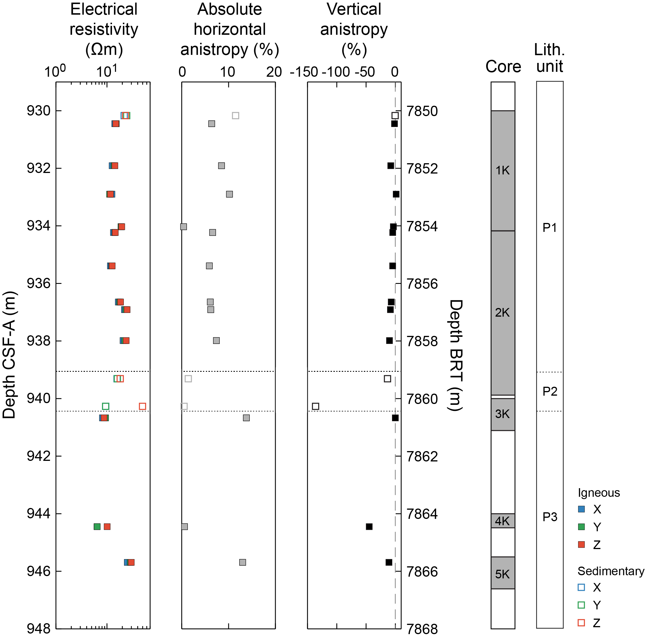
Figure F124. Electrical resistivity and anisotropy, Hole C0019P.

Figure F125 shows an inverse relationship between electrical resistivity and porosity (i.e., increasing resistivity with decreasing porosity [and increasing depth]). The trends are different for sedimentary and igneous samples (i.e., compared to the basalts and dolerite, sedimentary samples display a greater range of porosities for a similar range of electrical resistivities).

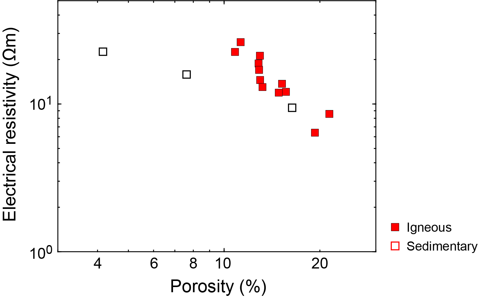
Figure F125. Electrical resistivity, Hole C0019P.

8.3.4. Discrete P-wave velocity

Values of P-wave velocity measured on discrete cubic samples recovered from Hole C0019P range 3.70–5.86 km/s (Figure F126). The highest velocity comes from a limestone at 930.2 mbsf (see Lithostratigraphy). Below 930.2 mbsf, the velocities are generally constant around 4.57 km/s. However, there is an excursion to lower velocities, around 3.92 km/s, between 940.7 and 944.5 mbsf. The igneous cube sample at 940.7 mbsf was taken from a block in a biscuit in Section 405-C0019P-3K-1 that had significant drilling disturbance (see Structural geology). The igneous cube at 944.5 mbsf has many thin mineral veins (Section 4K-1).

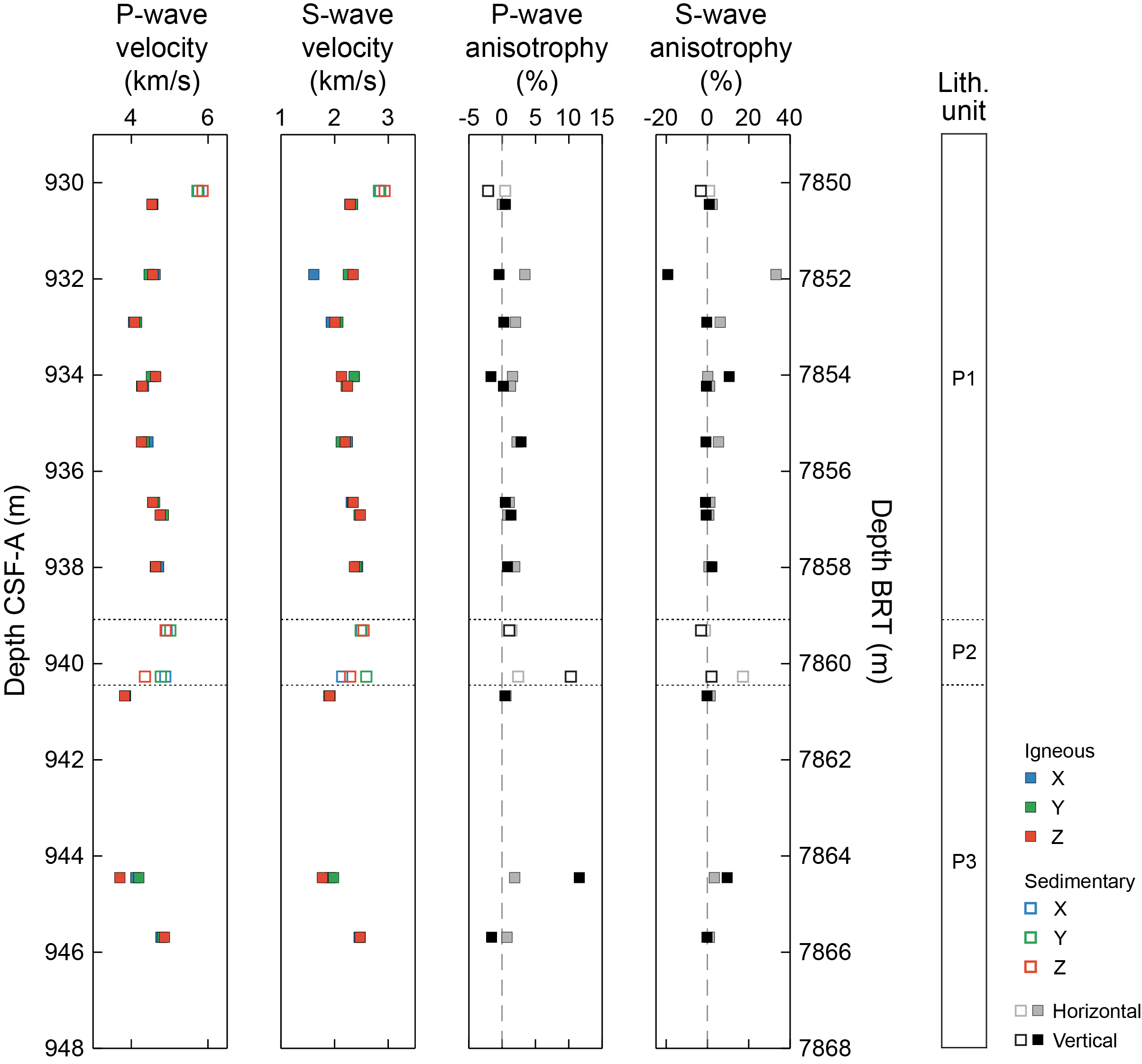
Figure F126. P- and S-wave velocity and anisotropy, Hole C0019P.

The absolute horizontal P-wave anisotropy, measured in the plane perpendicular to the core axis (see Physical properties in the Expedition 405 methods chapter [Kirkpatrick et al., 2025]) ranges 0.%–3.5% (average = ~1.5%) (Figure F126). Vertical P-wave anisotropy generally ranges −2.1% to 2.8%, except from 940.7 to 944.5 mbsf. A sample of siliceous mudstone at 940.3 mbsf has a vertical anisotropy of 10.3%, whereas a sample from a basalt sill at 944.5 mbsf has many thin mineral veins and vertical anisotropy of 11.6%. Both anisotropy values are positive, which is due to a horizontal velocity that is faster than the vertical velocity.

A crossplot of P-wave velocity versus the corresponding porosity for the same sample (Figure F127A) indicates that the two properties are well correlated. The igneous cubes fall along a tight linear trend, whereas the sedimentary cubes are more scattered. Some of the scatter, especially for the siliceous mudstone at 940.27 mbsf (average velocity = 4.67 km/s; porosity = 16.4%), may be related to high anisotropy skewing the average.

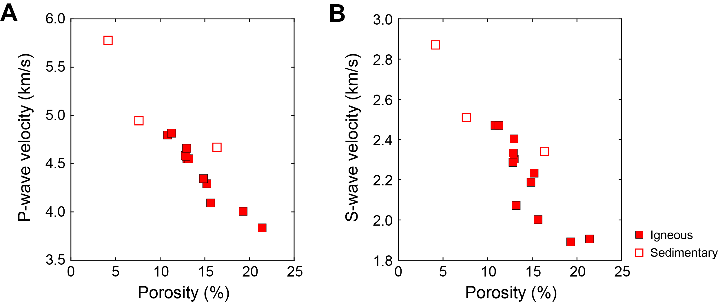
Figure F127. Average P-wave and S-wave velocity, Hole C0019P.

8.3.5. Discrete S-wave velocity

Values of S-wave velocity measured on discrete cubic samples range 1.61–2.93 km/s, and S-wave velocity exhibits a similar variability to that of P-wave velocity (Figure F126). The limestone sampled at 930.2 mbsf shows the highest values (~2.87 km/s). Velocities below 930.2 mbsf are nearly constant at around 2.34 km/s, except for the low-velocity excursion at 940.7–944.5 mbsf. This zone has low velocities ranging 1.77–1.98 km/s. The igneous cube at 940.7 mbsf was taken from a biscuit in the drilling disturbed core (Section 405-C0019P-3K-1), and the igneous cube at 944.5 mbsf has many thin mineral veins (Section 4K-1).

Excluding the values at 931.9 and 941.0 mbsf, the absolute horizontal S-wave anisotropy ranges 0.1%–6.2% (average = 1.9%) (Figure F126). The basalt pillow lava sampled at 931.9 mbsf and limestone sampled at 940.3 mbsf have horizontal anisotropies of 33.2% and 19.0%, respectively.

Other than a few high anisotropy values, the vertical S-wave anisotropy ranges −1.8%–3.2%. The value at 931.9 mbsf has a negative anisotropy of −19.2%, which is the highest vertical anisotropy measured. The x-axis anisotropy in the basalt pillow lava is lower than that for the y-axis, which is similar to the z-axis (vertical) anisotropy. There is, however, no obvious fabric in the samples. The samples at 934.0 and 944.5 mbsf have positive vertical anisotropies of 10.5% and 9.5%, respectively, which shows that the horizontal velocity is higher than the vertical velocity. The igneous cube at 944.5 mbsf has many thin horizontal mineral veins that would reduce the vertical S-wave velocity.

S-wave velocities are linearly correlated with porosity (Figure F127B). The sample that lies the farthest from the general trend is an igneous sample with a lower average S-wave velocity of 2.07 km/s and a porosity of 7.6%. This cube is the basalt pillow lava at 931.9 mbsf with high horizontal and vertical anisotropies. Because the average values of S-wave velocities in three directions are plotted on the figure, the slow x-axis velocity of this sample is causing the average to fall slightly off the linear trend.

8.3.6. Thermal conductivity

Thermal conductivity measurements from Hole C0019P were conducted on the working halves of selected core sections, totaling 12 discrete points where core conditions met the methodological standards (see Physical properties in the Expedition 405 methods chapter [Kirkpatrick et al., 2025]). The data set spans Sections 405-C0019P-1K-1 through 5K-1 (930.07–945.96 mbsf) (Figure F128).

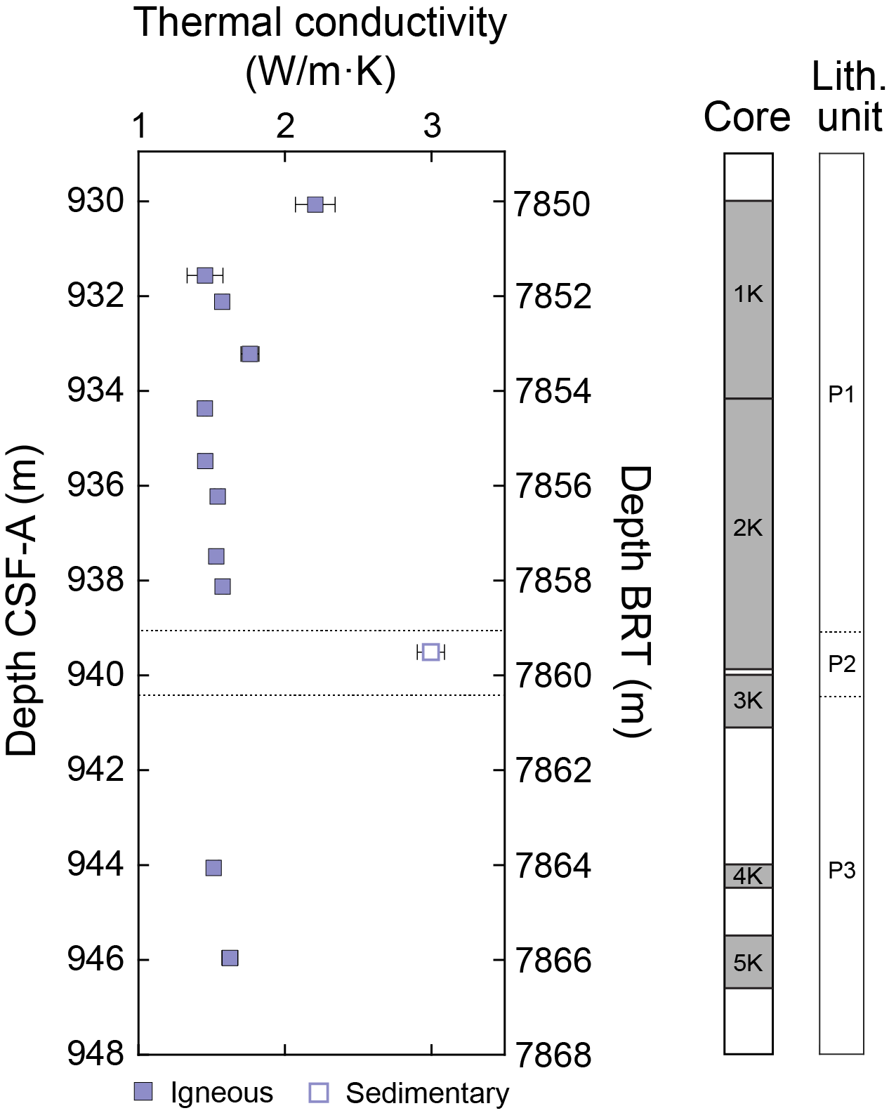
Figure F128. Thermal conductivity measurements, Hole C0019P.

Thermal conductivity for Hole C0019P ranges 1.453–2.996 W/(m·K) with a mean of 1.723 W/(m·K) and a standard deviation of 0.452 W/(m·K). The lowest value was recorded in Section 405-C0019P-2K-1 (934.37 mbsf) and corresponded to a basalt sill. All measurements of the same igneous lithology are close to this lowest value (Figure F128). The highest value was measured from a siliceous mudstone from Section 2K-6 (939.51 mbsf). This is the only measurement for siliceous mudstone.

In general, thermal conductivity measured for this hole is higher than the values for other holes at Site C0019. The siliceous mudstone has a thermal conductivity value of 2.996 W/(m·K), the basalt pillow lava and massive basalt in Core 405-C0019P-1K have an average thermal conductivity of 1.748 ± 0.331 W/(m·K), and the basalt sills and dolerite in Cores 2K, 4K, and 5K have a similar thermal conductivity value of 1.527 ± 0.062 W/(m·K).

8.3.7. Anelastic strain recovery analysis

Shipboard ASR measurements were conducted on one whole-round core sample from Hole C0019P (1K-4, 110–120.5 cm). The measurements were started within a few hours after samples were cut from the formation. The anelastic strain measurement for this sample continued beyond the end of the expedition, and the data will be processed as postexpedition research.

8.4. Summary

Holes C0019J and C0019K both intersected the PBFZ (see Structural geology), but the lithologies encountered immediately above and below the PBFZ were different in each hole (see Lithostratigraphy). Physical properties between the two holes also have similarities and differences.

Porosity in the unit directly above the PBFZ is similar in both holes (Figure F129). In Subunit 6B and Unit K1, porosity increases with depth and has an average value of 45%. Additionally, there appears to be a slight decrease in porosity immediately above the PBFZ. This decrease is more pronounced in Hole C0019J. Below the PBFZ, Hole C0019J encountered the banded clays and cherts comprising Unit 7, whereas the PBFZ and color-banded clays and cherts (Unit K3) in Hole C0019K were separated by ~24 m of brownish black clay (Unit K2) (see Lithostratigraphy). However, the porosity measured in the color-banded clays in both holes was high, up to 67% in both holes, although this high porosity may result from loss of clay-bound water during the oven-drying that is part of the measurement procedure.

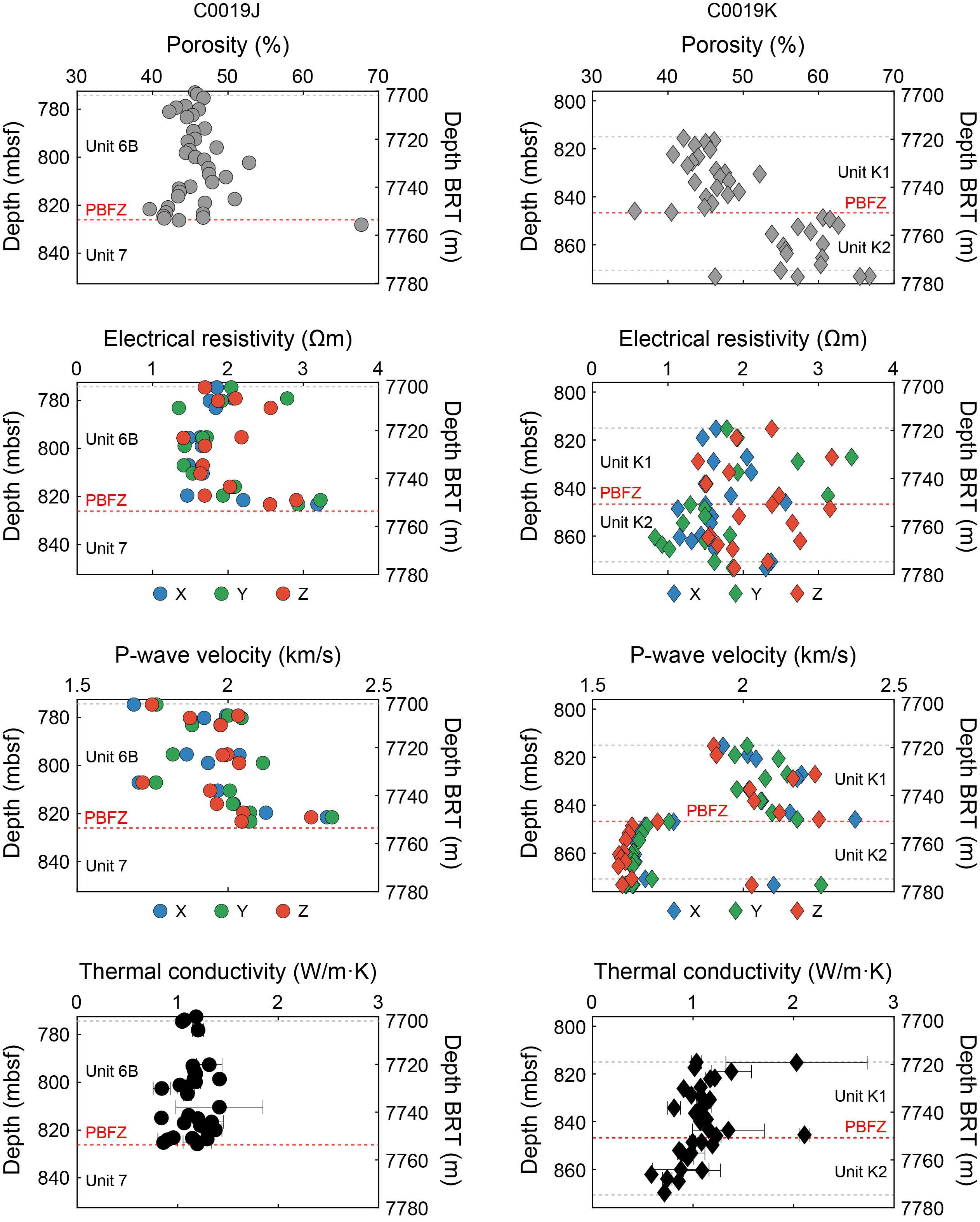
Figure F129. Physical property measurements, Holes C0019J and C0019K.

Electrical resistivity above the PBFZ is of similar magnitude in both holes, but there is significantly more scatter in Hole C0019K (Figure F129). Vertical anisotropy of electrical resistivity is dominantly negative in both holes, which is consistent with higher electrical resistivity in the z-direction. This anisotropy is particularly evident in Unit K2 brownish black clays with prominent subhorizontal scaly fabric that were intersected immediately below the PBFZ in Hole C0019K (Figure F117). The relationship between electrical resistivity and porosity is similar in both holes, and data from Unit K1 from Hole C0019K and Unit 6 from Hole C0019J reside in the same resistivity-porosity region (Figure F107).

P-wave velocity in the unit above the PBFZ increases with depth and is anisotropic in both holes (Figure F129). Both have a noticeable peak at ~7750 m BRT, which is less than 5 m above the PBFZ in Hole C0019J and less than 1 m above the PBFZ in Hole C0019K. Comparing the relationship between P-wave velocity and porosity in Hole C0019J to Hole C0019K, the materials recovered in both holes follow similar trends (i.e., P-wave velocity is generally anticorrelated with porosity) (Figure F109).

In the relationship between S-wave velocity and porosity, S-wave velocity in Hole C0019K does not appear to vary as a function of porosity (Figure F109). S-wave velocity in Units K2 and K3 is higher than the velocities measured in Hole C0019J for the same porosity. S-wave velocities and porosities in Unit K1 are consistent with those measured in Unit 6 in Hole C0019J.

Thermal conductivity is similar in Hole C0019J Subunit 6B and Hole C0019K Unit K1, averaging 1.15 and 1.20 W/(m·K), respectively (Figure F129). However, in Unit K2 the thermal conductivity drops significantly. With an average value of 0.91 W/(m·K), thermal conductivity measurements in Unit K2 are less than those in the rest of Hole C0019K and in all of Hole C0019J.

Hole C0019P does not overlap with either Hole C0019J or Hole C0019K, but fragments of chert were recovered in all three holes. Samples of the chert were collected for physical property analysis in Holes C0019K and C0019P, but the noncube sample from C0019P could only be used for MAD. Both samples have a bulk density of 2.5 g/cm³ and a porosity of ~3%. This is the lowest porosity observed at Site C0019. Electrical resistivities measured on the chert from Section 405-C0019K-17K-CC are on the order of 1000 Ωm, higher than the resistivities measured in any of the basalts or sedimentary rocks in Hole C0019P. Similarly, the average P- and S-wave velocities of the chert are 5.3 and 3.2 km/s, respectively, which is faster than all velocities measured in Hole C0019P, except for the limestone from Section 1K-1.

9. Geochemistry

9.1. Interstitial water geochemistry

A total of 78, 7, and 20 interstitial water (IW) samples were extracted from the cores from Holes C0019J (93–825 mbsf), C0019K (817–864 mbsf), and C0019M (2–107 mbsf), respectively (all depths are provided as mbsf, equivalent to the CSF-A depth scale). IW samples were not collected from the hard rock cores of Hole C0019P. The recovery of IW is summarized in Table T32 and Figure F130. Whole-round cores used for IW extraction were typically 6–15 cm in length at <500 mbsf and 20–25 cm below 500 mbsf. The ratio of recovered IW volume to IW squeezed cake volume/weight shows that with increasing depth, the volume of IW recoverable from the whole-round core sample gradually decreased due to progressive consolidation of the sediments. Recovered IW was typically 20–50 mL at <100 mbsf but 10 mL or less below 760 mbsf. However, core recovery was good enough to allow for sufficient IW samples to construct detailed profiles of fluid chemistry over the length of the holes (Table T33; Figures F131, F132). To trace drilling fluid contamination in the collected IW, liquid from mud water (LMW) was collected daily, and liquid (water) in the core liner (LCL) was also collected for each core when available and then analyzed along with the IW samples (Table T34). Methods used for IW sample analyses are described in Geochemistry in the Expedition 405 methods chapter (Kirkpatrick et al., 2025). IW data from Expedition 343 Hole C0019E (Expedition 343/343T Scientists, 2013b) are also used for comparison.

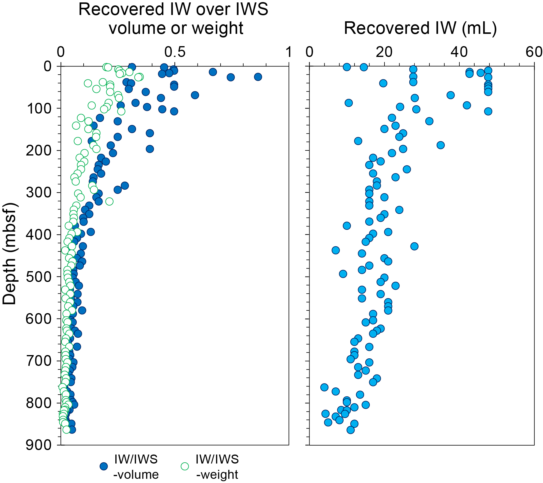
Figure F130. IW samples.

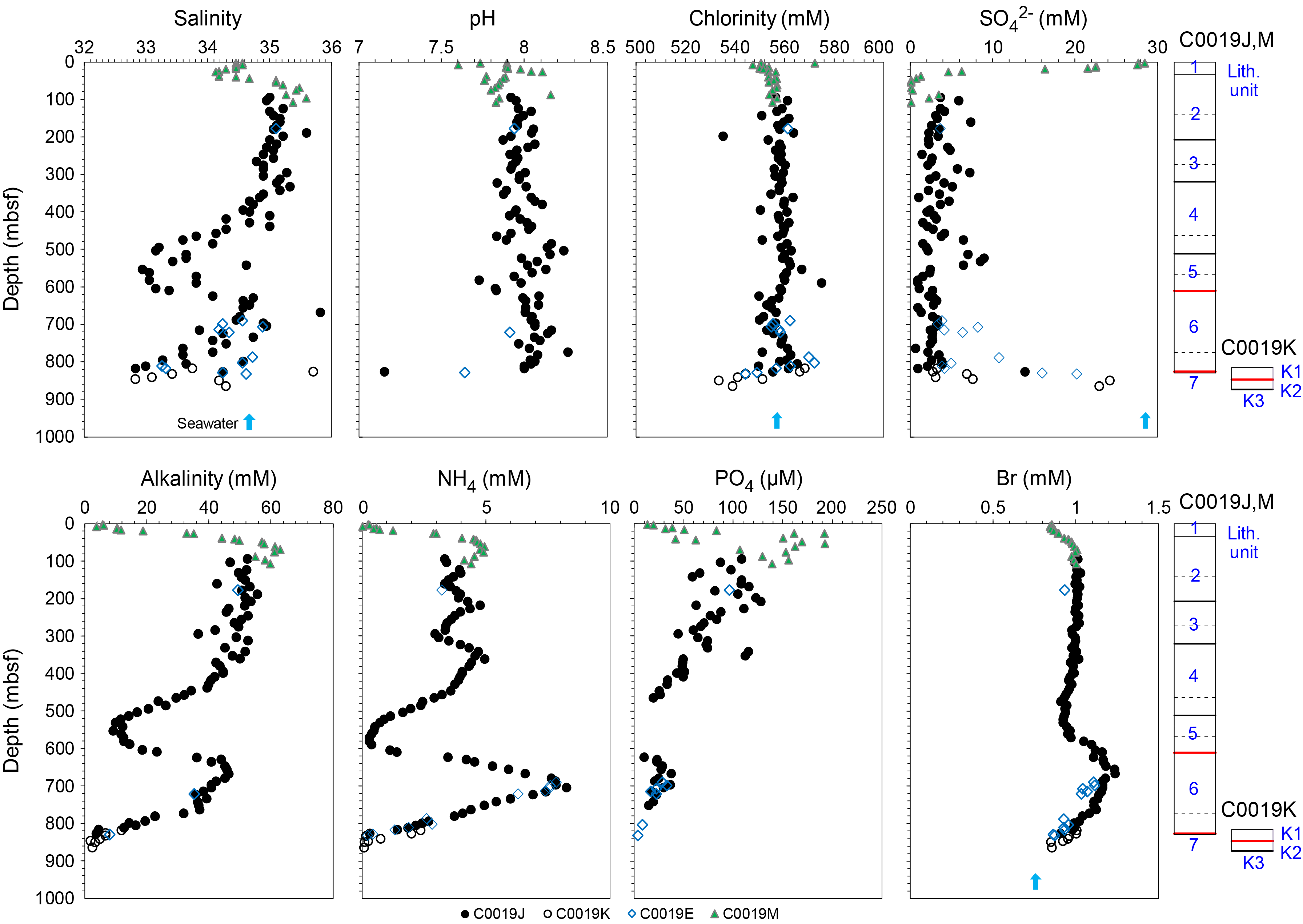
Figure F131. Dissolved chemical components in IW samples.

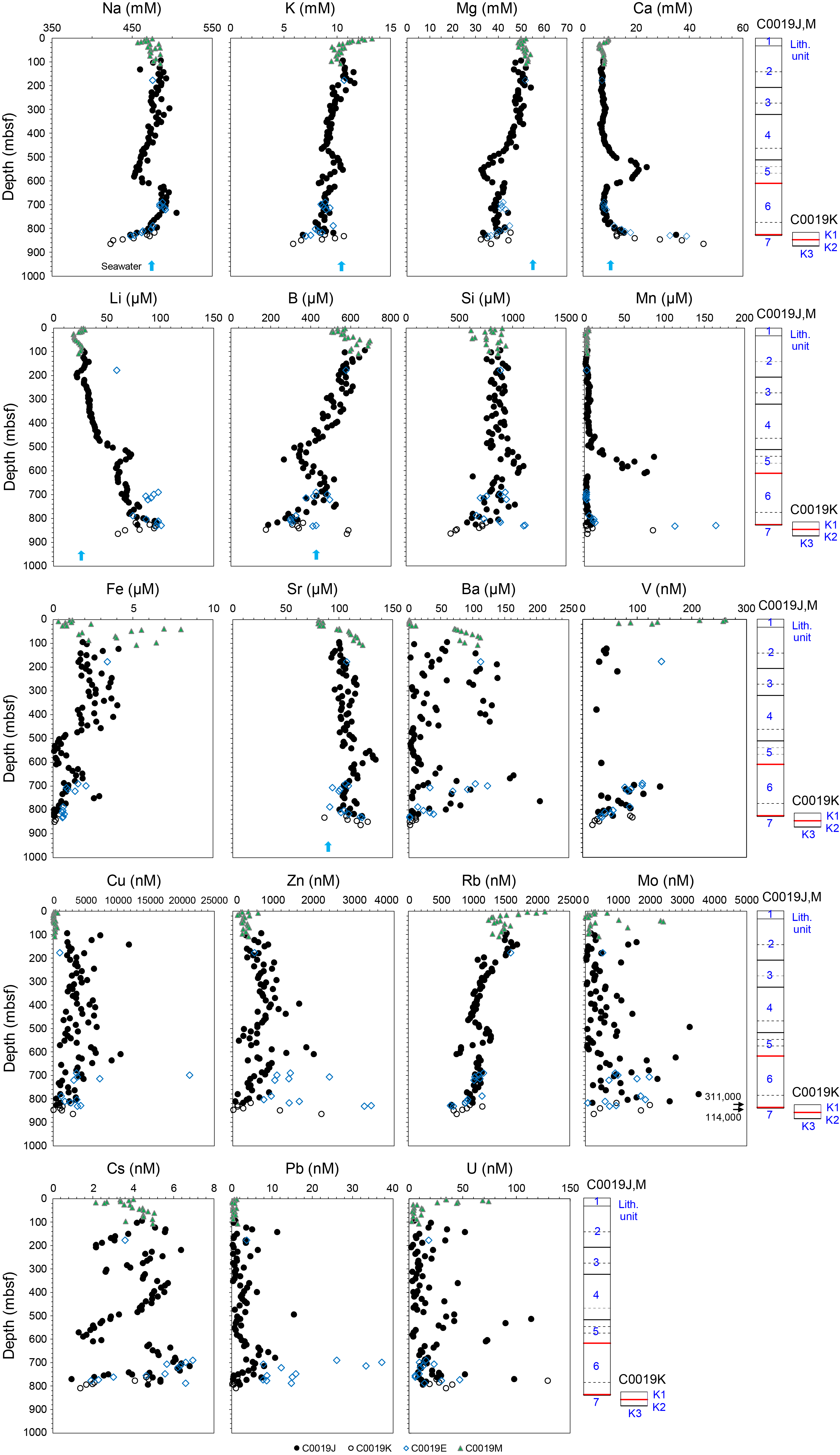
Figure F132. Major, minor, and trace element concentrations in IW samples.

9.1.1. Holes C0019M and C0019J

Depth profiles of dissolved components and elements in the IW samples from Holes C0019M and C0019J are shown in Figures F131 and F132, along with the lithologic units (see Lithostratigraphy). The trends observed in the two holes are broadly coherent at the overlapping depths for many components/elements, even though the hole locations are different (Hole C0019M is located approximately 90 m northeast of Hole C0019J; see Operations). The data from these two holes are used here as a continuous record with depth. In some components/elements, however, there is some offset between the data from the two holes. Such an offset may represent local hydrogeological variations.

9.1.1.1. Salinity, pH, and chlorinity

The salinity of the IW from Hole C0019M near the seafloor is 34.6, which is consistent with the ambient seawater value (34.7) (LCL was collected just above the mudline in Core 1H; hereafter, seawater value indicates the value for this LCL sample). In Hole C0019M, the salinity decreases to 34.2 at 25 mbsf and then increases to 35.6 at 97 mbsf toward the bottom of the hole (Figure F131). In Hole C0019J, relatively constant seawater-like salinities of about 35 are observed from the top of the hole to ~350 mbsf, with a few exceptions. From 350 mbsf in Unit 4, salinity gradually decreases with depth to a minimum of about 33 at 550–560 mbsf in Unit 5. Salinity then rises sharply near the base of Unit 5, reaching 34.7 at 628 mbsf in Unit 6. Below this, salinity generally decreases to 32.8 toward the bottom of Hole C0019J, with an exceptional value of 35.8 at 667 mbsf. The IW in Holes C0019M and C0019J shows pH values of 7.6–8.3 and tends to increase slightly with depth from 2 to 816 mbsf. Near the bottom of Hole C0019J, a distinctly low pH of 7.2 is observed.

The chlorinities of the IW observed in Holes C0019M and C0019J on the whole show seawater-like values with a few exceptions (Figure F131). In the shallow part (<45 mbsf) of Hole C0019M, the chlorinity is 550–557 mM, with one exception. IW chlorinity then increases slightly to about 560 mM and remains constant to 560 mbsf. A slight decrease in chlorinity to 550 mM occurs between 560 and 690 mbsf in Units 5 and 6, and chlorinity increases below 700 mbsf, reaching a maximum of ~565 mM at 804 mbsf before it decreases to ~550 mM near the bottom of Hole C0019J.

LMW shows a constant salinity of 34.54 ± 0.11 (1SD) and 34.29–34.51 in Holes C0019J and C0019M, respectively (Table T34). Chlorinity values for LMW are also constant at 546.1 ± 8.9 mM in Hole C0019J. The IW chlorinity from Holes C0019M and C0019J has relatively constant and systematically higher values compared to LMW, whereas its salinity varies widely in contrast to LMW. This suggests that the IW salinity and chlorinity are little affected by drilling fluid contamination.

9.1.1.2. Sulfate and alkalinity

The IW from HPCS cores closest to the seafloor in Hole C0019M (2–3 mbsf) shows sulfate concentrations of 27.7–28.4 mM, consistent with the seawater value. The IW sulfate value decreases dramatically to <1 mM over the following 40 m, suggesting sulfate reduction by microbial activity (Figure F131). In Hole C0019J, with a few exceptions, IW shows low sulfate concentrations of 1–5 mM from 90 to 440 mbsf. Given the high LMW sulfate concentrations (29.03 ± 0.28 mM), the consistently low IW sulfate concentrations observed indicate minimal IW contamination by the drilling fluid. However, with the drilling technique used here (SD-RCB), complete avoidance of drilling fluid contamination may be difficult, even though the exterior part of the whole-round core sample was removed prior to sample squeezing for IW collection. The IW sulfate values of >5 mM in this depth interval are potentially attributable to some drilling fluid contamination, considering that all IW samples were collected well below the sulfate-methane transition zone. Below 440 mbsf in Hole C0019J, an increase in IW sulfate concentration to 9 mM is observed at 450–540 mbsf in Units 4 and 5, which is striking compared to baseline values of around 2.5 mM. Below that, IW sulfate values remain as low as <3 mM to 816 mbsf. Near the bottom of the hole, IW sulfate suddenly rises to 13.9 mM at 825 mbsf. The increases in sulfate observed at 450–540 mbsf and near the bottom of the hole are both associated with distinct increases in calcium and are coherent with IW data of greater depths from Holes C0019K and C0019E. Thus, these changes are unlikely to be derived from drilling fluid contamination.

The IW alkalinity closest to the seafloor in Hole C0019M (2–3 mbsf) is relatively low at 6 mM, but it rises dramatically to 63 mM at 69 mbsf, corresponding to the inferred progress of sulfate reduction by microbes (Figure F131). The alkalinity of the IW in Hole C0019J slightly decreases from about 50 mM at 100 mbsf to about 45 mM at 350 mbsf and then shows striking variation with depth below 350 mbsf. It decreases from 50 mM to 9 mM with a minimum at 551 mbsf in Unit 5 and then increases rapidly near the base of Unit 5, returning to 45 mM at about 660 mbsf in Unit 6. Below this, the IW alkalinity decreases again to 3.5 mM at 825 mbsf. This depth profile in Hole C0019J correlates closely to the salinity profile.

9.1.1.3. Ammonium, phosphate, and bromide

IW ammonium concentrations near the seafloor in Hole C0019M are 0.3 mM and increase dramatically with depth to 5 mM at 61 mbsf, a pattern similar to that observed in alkalinity, which is possibly associated with sulfate reduction and related reactions by microbes (Figure F131). The IW ammonium in Hole C0019J shows a jagged depth profile varying from 3 to 5 mM between 90 and 350 mbsf, with two local minima at ~160 mbsf in Unit 2 and 300 mbsf in Unit 3 and a local maximum at 220 mbsf near the base of Unit 2. Below 350 mbsf, the IW ammonium concentration steadily decreases to 0.3 mM at 580 mbsf in Units 4 and 5 and then increases rapidly near the base of Unit 5, reaching 8.3 mM at 703 mbsf in Unit 6. Below this depth, it decreases to 0.3 at 825 mbsf near the bottom of the hole. The depth profile of IW ammonium observed below 350 mbsf is similar to those of salinity and alkalinity.

The IW phosphate concentration in Hole C0019M increases from 13 µM at 2 mbsf to 190 µM at 25–54 mbsf, correlating with alkalinity and ammonium (Figure F131). The IW phosphate in Hole C0019J varies significantly from 19 to 128 µM between 90 and 460 mbsf but shows a general trend of decreasing with depth. Between 470 and 610 mbsf, IW phosphate values are very low, all below the detection limit. This low-phosphate interval corresponds to the depths of the minima observed for IW salinity, alkalinity, and ammonium. Below 620 mbsf, a small maximum of 36–37 µM occurs at 670–700 mbsf, which also appears to correspond to the peaks observed in salinity, alkalinity, and ammonium. Below this, the IW phosphate concentration decreases toward the bottom of the hole.

IW Bromide concentrations in Hole C0019M increase with depth from a seawater-like value of 0.85 mM at 2 mbsf to 1.0 mM at 50 mbsf (Figure F131). In Hole C0019J, a steady trend of approximately 1.0 mM is observed between 90 and 350 mbsf. Below this depth, the IW bromide concentration decreases slightly to 0.9 mM between 460 and 540 mbsf and then gradually increases to a maximum of 1.2 mM at 670 mbsf in Unit 6. Below that, it decreases to 0.9 mM toward the bottom of the hole.

9.1.1.4. Major cations (Na, K, Mg, and Ca)

The IW sodium (Na) concentration in Hole C0019M near the seafloor is 475 mM, which is consistent with the ambient seawater value, 475 mM. The IW Na concentrations in Hole C0019J show a depth profile with trends and variations that are relatively similar to those of salinity (Figure F132). With a few exceptions, IW Na concentrations show seawater-like values around 480 mM to 350 mbsf with some fluctuations and then gradually decrease to 450 mM at ~580 mbsf. Below this, the IW Na concentration increases rapidly near the base of Unit 5, reaching approximately 500 mM between 630 and 730 mbsf, and then decreases to 450 mM toward the bottom of the hole.

The IW potassium (K) concentration near the seafloor in Hole C0019M is 13.3 mM, which is higher than the ambient seawater value of 10.4 mM. The IW K concentration decreases with depth to seawater-like value at 25 mbsf (Figure F132). The IW K value then shows a steady decrease to 6.8–9.6 mM in the deepest part of Hole C0019J with a slight positive peak at around 550 mbsf in Unit 5 and a minimum near the Unit 5/6 boundary.

IW magnesium (Mg) and calcium (Ca) concentrations near the seafloor in Hole C0019M are 52.0 and 9.6 mM, respectively, which are slightly lower than ambient seawater values of 55.0 and 10.4 mM, respectively. The IW Mg and Ca values decrease slightly with depth to 49 mM and 6 mM, respectively, at 25 mbsf (Figure F132). Below this depth, the IW Mg and Ca concentrations show anticorrelated depth profiles to 700 mbsf. At <350 mbsf, IW Mg and Ca are slightly below seawater values. Below this, the Ca concentration increases, forming a high-Ca zone from 513 to 588 mbsf with a Ca maximum of 24 mM at around 540 mbsf, and then decreases sharply to seawater-like concentrations at around 600 mbsf. The high-Ca zone is distributed just above the base of Unit 5 and extends up to near the boundary with Unit 4. An inverted depth profile is observed for IW Mg concentrations, where the Mg concentration decreases to 32 mM around 550 mbsf and then increases to 43 mM around 600 mbsf. Below 700 mbsf, the IW Ca concentration gradually increases with depth and suddenly jumps to 35 mM near the bottom of the hole, whereas Mg is roughly constant but becomes more scattered at the bottom.

9.1.1.5. Minor elements (Li, B, Si, Mn, Fe, Sr, and Ba)

The IW lithium (Li) concentration near the seafloor in Hole C0019M is 28 µM and declines to 19 µM by 25 mbsf (Figure F132). These values bracket the seawater value of 26 µM. IW Li concentrations increase with depth to 33 µM at 141 mbsf and then decrease to 22 µM at 207 mbsf. At this depth, corresponding to the Unit 2/3 boundary, the IW Li value is offset to 29 µM. Below this depth, IW Li concentrations increase steadily to 43 µM at 470 mbsf, where there is a sharp increase in Li values to a peak of 73 µM at 531 mbsf in Unit 5. This sharp rise in IW Li is co-located with the boundary between Subunit 4B and Unit 5. Below this peak, the IW Li value increases with depth with substantial scatter from 60 µM at 580 mbsf to 96 µM near the bottom of Hole C0019J.

The IW boron (B) concentration near the seafloor in Hole C0019M is 570 µM, which is higher than the ambient seawater value of 428 µM. IW B value decreases with depth to 500 µM at 16 mbsf and then increases to 700 mM at 54 mbsf (Figure F132). IW B values fall from here with fluctuations to 460 µM at 456 mbsf, where the trend makes a steeper decline to a minimum of 340 µM at 540 mbsf in Unit 5, followed by an increase to a maximum of 480 µM at 670 mbsf in Unit 6. The IW B value then gradually decreases to 190 µM near the bottom of Hole C0019J.

IW silica (SiO₂) concentrations, expressed here as Si concentrations, show significant scatter in Hole C0019M, ranging 610–930 µM at 2–107 mbsf (Figure F132). In Hole C0019J, IW Si shows similar values of 750–950 µM throughout Units 2–4. At 500 mbsf, near the base of Unit 4, there is an offset of the IW Si value from 800 to 960 µM, and then the IW Si value increases with depth to 1100 µM at 580 mbsf. At 608 mbsf, near the base of Unit 5, IW Si values shift back by about 200 µM and decrease to 570 µM near the bottom of Hole C0019J.

IW manganese (Mn) concentrations range 1–8 µM at <445 mbsf (Figure F132). There is a small peak to 13 µM at 456 mbsf and a return to the background value at 493 mbsf. At 493 mbsf, near the base of Unit 4, IW Mn concentrations rise sharply to 87 µM at 541 mbsf and form a Mn-rich zone to 608 mbsf in Unit 5. This Mn-rich zone terminates abruptly just above the Unit 5/6 boundary. Below this, IW Mn values return to low background values of 2–4 µM but tend to increase from around 700 mbsf, reaching 8 µM near the bottom of the hole.

Iron (Fe) in the IW is highly variable in Hole C0019M, ranging 0.3–8 µM with the highest value at 41 mbsf (Figure F132). In Hole C0019J, IW Fe values are scattered but range 1.5–4 µM to 474 mbsf and then plummet to <0.8 µM. A minimum of 0.07 µM is observed at 551 mbsf in Unit 5, and IW Fe values remain low to 608 mbsf. IW Fe values increase sharply near the base of Unit 5, reaching a maximum of 1.9 µM at 667 mbsf in Unit 6. Values then generally decrease to <0.07 µM toward the bottom of the hole with a few exceptions.

The IW strontium (Sr) concentration in Hole C0019M is a seawater-like value of 81 µM near the seafloor and rises to 120 µM at 107 mbsf (Figure F132). At this depth, IW Sr values in Hole C0019J show a clear offset to lower values around 100 µM relative to those in Hole C0019M. Although scattered, the IW Sr concentration shows a gentle rise to 110 µM at 541 mbsf with an abrupt shift to 128 µM at 551 mbsf in Unit 5, peaking at 134 µM at 588 mbsf. Near the base of Unit 5, IW Sr drops sharply to 114 µM at 608 mbsf. After decreasing to 100 µM at 800 mbsf, the IW Sr trend reverses and rises to 120 µM near the bottom of the hole in Unit 6.

Barium (Ba) in the IW is as low as <1 µM near the seafloor. Below 30 mbsf, IW Ba shows extreme variability from lows of <10 µM to highs of over 140 µM to 445 mbsf (Figure F132). Between 456 mbsf in Unit 4 and 608 mbsf near the base of Unit 5, IW Ba concentrations are consistently low at 3-19 µM. Below this, IW Ba concentrations return to the highly variable pattern, ending at a low value of 3 µM near the bottom of the hole.

9.1.1.6. Trace elements (V, Cu, Zn, Rb, Mo, Cs, Pb, and U)

The IW vanadium (V) concentration near the seafloor at 2 mbsf is 260 nM, and it drops rapidly to 66 nM at 16 mbsf in Unit 1 (Figure F132). Below this, V concentrations are consistently <64 nM or below the detection limit throughout Units 2–5 to 680 mbsf. A peak V value of 140 nM is observed in Unit 6 at 703 mbsf, and the V value decreases with depth to 29–55 nM toward the bottom of Hole C0019J.

IW copper (Cu) and zinc (Zn) have broadly similar depth profiles (Figure F132). Cu and Zn values are <700 and <640 nM near the seafloor and gradually increase to 6,800 and 1,600 nM, respectively, at 400–500 mbsf in Unit 4, with a few spikes up to 12,000 nM in the case of Cu. Below this, Cu and Zn values decrease to reach minima at 1,100 and 150 nM in Unit 5 and then increase to maxima at 10,000 and 2,000 nM, respectively, near the Unit 5/6 boundary. Cu and Zn values then gradually decrease with depth to 510 and 60 nM, respectively, in Unit 6 near the bottom of Hole C0019J.

IW rubidium (Rb) concentrations in Holes C0019M and C0019J show a depth profile similar to that of K (Figure F132). The highest and lowest Rb values, 2100 and 660 nM, are observed at 2 mbsf in Unit 1 near the seafloor and 825 mbsf in Unit 6 near the bottom of Hole C0019J, respectively. Rb exhibits a steadily decreasing concentration with depth, except for a local maximum at about 550 mbsf and a minimum near the Unit 5/6 boundary, both of which are more pronounced for Rb than for K.

IW molybdenum (Mo) concentrations show scattered values between 28 and 3200 nM throughout Units 1–5 (Figure F132). In Unit 6, IW Mo averages relatively high values and has a very high value of 311,000 nM at 825 mbsf near the bottom of Hole C0019J.

IW cesium (Cs) concentrations show a highly jagged depth profile varying from 0.93 to 6.8 nM (Figure F132). The oscillation observed in the Cs profile is synchronous with that of ammonium (Figure F131) but is more pronounced in Units 1–4.

Lead (Pb) in the IW varies between <0.3 and 6.5 nM in Units 1–5 with a few exceptions (Figure F132). There is a maximum of 11 nM at 680 mbsf in Unit 6, and then the Pb value decreases with depth to 0.3 nM near the bottom of Hole C0019J.

IW uranium (U) concentrations in Holes C0019M and C0019J generally range 2.8–52 nM (Figure F132). However, exceptionally high values of 69–74, 71–113, and 97 nM are observed at 7–10 mbsf in Unit 1, 510–610 mbsf in Units 4–5, and 825 mbsf in Unit 6, respectively.

9.1.2. Hole C0019K

The chemical composition of the IW in Hole C0019K is described and compared with that in Holes C0019J and C0019E (Expedition 343/343T Scientists, 2013b). The depths to the rig floor in Holes C0019J, C0019K, and C0019E are 6927.5, 6903.5, and 6918.0 m BRT, respectively (see the Expedition 405 summary chapter [Kirkpatrick et al., 2025]). On the other hand, the depths to the chert layer below the seafloor in these holes are 826, 873, and 834 mbsf, respectively (see Lithostratigraphy) (Expedition 343/343T Scientists, 2013b). This raises the question of what depth criterion should be used to compare the depth profiles in the IW geochemistry observed in these three holes. Despite the significant differences in lithology around the plate boundary between these three holes, the IW geochemistry trends observed are broadly similar when plotted against depth on the mbsf scale. Therefore, for simplicity, the comparison is made here using mbsf depths (Figures F131, F132). The possibility remains that the small offset in the depth of the trend apparently observed between the data for some elements/components from these holes is due to, for example, differences in seafloor depth or depth to the chert layer.

9.1.2.1. Salinity, pH, and chlorinity

Salinity data from Hole C0019K, with the exception of one value at 826 mbsf, are essentially consistent with the trend observed in Hole C0019J, where the salinity decreases from about 35 at 700 mbsf to 32.8 near the bottom of the hole (Figure F131). However, at the very bottom of Hole C0019K (864 mbsf in Unit K2) (see Lithostratigraphy), salinity appears to be as high as 34.3. The salinity data from Hole C0019E (Expedition 343/343T Scientists, 2013b), which is located in the vicinity of Hole C0019K, are also consistent with those from Holes C0019J and C0019K. There is only one IW pH measurement: 7.56 at 849 mbsf for Hole C0019K. The pH values observed in Holes C0019J, C0019K, and C0019E are consistent, including the presence of relatively low pH near the bottom of the holes.

The IW chlorinity in Hole C0019K shows a significant decrease from 568 mM at 817 mbsf in Unit K1 to 533–539 mM below 849 mbsf in Unit K2 near the bottom of the hole (Figure F131). This trend seems to be consistent with that observed in the lowermost part of Hole C0019J, although in Hole C0019J, the decrease in IW chlorinity with depth is not as large. A decrease in chlorinity below 800 mbsf, around and below the plate boundary, is also observed in Hole C0019E, which is consistent with that observed in Hole C0019K.

Salinity and chlorinity in LMW sampled during drilling of Hole C0019K are 34.51 ± 0.16 and 549.7 ± 1.9 mM, respectively (Table T34).

9.1.2.2. Sulfate and alkalinity

The IW sulfate in Hole C0019K increases rapidly with depth from 3.2 mM at 817 mbsf in Unit K1 to 23–24 mM below 849 mbsf in Unit K2, approaching the seawater value (Figure F131). The high IW sulfate value of 14 mM observed in the lowermost part of Hole C0019J (825 mbsf) is consistent with this trend of sulfate increasing with depth over this interval. Furthermore, the IW sulfate in C0019E also shares this characteristic, although another peak in sulfate is also observed at around 700 mbsf. These observations suggest that a rapid increase in IW sulfate is a common chemical signature near the plate boundary at Site C0019.

IW alkalinity in Hole C0019K shows a decreasing trend with depth, which is consistent with the trends observed in Holes C0019J and C0019E below 700 mbsf (Figure F131).

9.1.2.3. Ammonium, phosphate, and bromide

The IW ammonium concentration in Hole C0019K decreases with depth from 2.4 mM at 817 mbsf in Unit K1 to 0.1 mM below 849 mbsf in Unit K2 (Figure F131). This is consistent with the trend observed in Hole C0019J, where IW ammonium gradually decreases from 8.3 mM at 700 mbsf to 0.3 at 825 mbsf near the bottom of the hole. An almost identical depth profile is also observed in Hole C0019E below 690 mbsf. These observations suggest that the decreasing IW ammonium trend represents the chemical signature around the plate boundary at Site C0019.

IW phosphate concentrations in Hole C0019K are all below the detection limit. In Hole C0019E, in the vicinity of Hole C0019K, a decrease in IW phosphate with depth is observed from 28 µM at 690 mbsf to 4 µM at 831 mbsf (Figure F131). This is consistent with the trend observed in Hole C0019J.

IW bromide concentrations in Hole C0019K decrease slightly with depth (Figure F131). This decreasing IW bromide trend accords with that in Hole C0019J. Data from Hole C0019E show a similar trend, but the observed IW bromide values seem to be systematically lower than those in Holes C0019J and C0019K at the same depths.

9.1.2.4. Major cations (Na, K, Mg, and Ca)

IW sodium (Na) concentrations in Hole C0019K decrease from 478 mM at 817 mbsf in Unit K1 to 423 mM at 864 mbsf in Unit K2 (Figure F132). This trend is indistinguishable from that observed in Hole C0019J below 670 mbsf. IW Na concentrations in Hole C0019E are also consistent with those in Holes C0019J and C0019K, particularly below 780 mbsf, which may characterize the IW Na distribution around the plate boundary at Site C0019.

IW potassium (K) concentrations in Hole C0019K scatter between 5.9 and 10.6 mM but tend to decrease with depth (Figure F132). Somewhat scattered IW K values are also observed in Holes C0019J and C0019E below 770 mbsf.

IW magnesium (Mg) concentrations in Hole C0019K scatter between 32 and 45 mM, similar to those in Holes C0019J below 780 mbsf (Figure F132), whereas Mg values for Hole C0019E show a decrease from 45 mM at 788 mbsf to 35 mM at 832 mbsf. On the other hand, IW calcium (Ca) concentrations in Hole C0019K show a clear, rapidly increasing trend with depth, from 14 mM at 817 mbsf in Unit K1 to 45 mM at 864 mbsf in Unit K2. This trend is consistent with those observed in Holes C0019J and C0019E below 690 mbsf, and the IW Ca values are far above the seawater value (10.4 mM) near the bottom of the holes. This remarkable IW Ca signature characterizes the plate boundary region at Site C0019.

9.1.2.5. Minor elements (Li, B, Si, Mn, Fe, Sr, and Ba)

IW lithium (Li) concentrations in Hole C0019K increase from 77 to 96 µM from 817 to 832 mbsf in Unit K1 and then decrease to 60 µM at 864 mbsf in Unit K2 (Figure F132). The IW Li values observed in Unit K1 are consistent with those observed in Hole C0019J at corresponding depths. This is also true for Hole C0019E below 790 mbsf. However, the IW Li values observed in Hole C0019E at <730 mbsf are significantly higher than those observed in Hole C0019J.

IW boron (B) concentrations in Hole C0019K tend to increase with depth from 307–361 µM at 817–840 mbsf in Unit K1 to 580–587 µM at 849–864 mbsf in Unit K2, except for one measurement of 176 µM at 846 mbsf (Figure F132). This increasing IW B trend with depth is not observed in Hole C0019J but is consistent with that observed in Hole C0019E at similar depths. Interestingly, the exceptional data at 846 mbsf in Hole C0019K appears to be consistent with the decreasing IW B trend with depth observed in Hole C0019J.

IW silica (SiO₂) concentrations, expressed here as Si concentrations, in Hole C0019K show the trend of decreasing values with depth from 750 µM at 817 mbsf in Unit K1 to 417 µM at 864 mbsf in Unit K2, which is consistent with that observed in Hole C0019J (Figure F132). In contrast, the IW Si values in Hole C0019E below 790 mbsf gradually increase to about 1110 µM at the bottom of C0019E, which are higher values than those from Holes C0019J and C0019K at similar depths.

IW manganese (Mn) concentrations in Hole C0019K range 2–10 µM throughout Units K1 and K2, except for a spike to 86 mM at 849 mbsf (Figure F132). These IW Mn values are consistent with those observed in Holes C0019J and C0019E below 620 mbsf. Notably, Hole C0019E also shows extreme high IW Mn values of 110–160 µM at 829–832 mbsf.

IW iron (Fe) concentrations in Hole C0019K show very low values, all <0.4 µM. These low IW Fe values are consistent with those observed in Holes C0019J and Hole C0019E (Figure F132).

IW strontium (Sr) concentrations in Hole C0019K increase with depth from 110 µM at 826 mbsf in Unit K1 to 120–127 µM at 849–864 mbsf in Unit K2, with one exception at 832 mbsf (Figure F132). This increasing IW Sr trend with depth is consistent with those observed in Holes C0019J and C0019E.

IW barium (Ba) concentrations in Hole C0019K are 1–11 µM throughout Units K1 and K2. These consistently low IW Ba values are in accord with those observed in Holes C0019J and C0019E below 820 mbsf (Figure F132). The scattered IW Ba values of 14–123 µM observed in Hole C0019E at 690–817 mbsf are also consistent with the data from Hole C0019J at corresponding depths.

9.1.2.6. Trace elements (V, Cu, Zn, Rb, Mo, Cs, Pb, and U)

IW vanadium (V) and copper (Cu) concentrations in Hole C0019K range 18–92 and 62–3100 nM, respectively, consistent with the generally decreasing trends with depth observed in Unit 6 of Hole C0019J (Figure F132). The V and Cu values in Hole C0019E are also similar to the other two holes, with the exception of a Cu spike of 21,000 nM at 698 mbsf.

Zinc (Zn) in the IW of Hole C0019K is as low as 24–450 nM in Unit K1, which is consistent with the trend observed in Unit 6 of Hole C0019J (Figure F132). However, the Zn values in Unit K2, 1200–2200 nM, are substantially higher than those in Unit K1. Such high IW Zn values are also observed in Hole C0019E, where the Zn value reaches 3400 nM near the bottom of the hole.

Rubidium (Rb) and Cesium (Cs) in Hole C0019K show generally decreasing trends with depth to 700 and 1.4 nM, respectively, consistent with those observed in the deepest part of Hole C0019J (Figure F132). The IW Rb and Cs data in Hole C0019E are also consistent with the trends in Holes C0019J and C0019K.

IW molybdenum (Mo) concentrations in Hole C0019K generally range 270–7,700 nM with a spike of 110,000 nM at 846 mbsf (Figure F132). These Mo values are similar to those observed in Holes C0019J and C0019E.

Lead (Pb) in Hole C0019K shows low values of 0.24–1.5 nM throughout Units K1 and K2, consistent with the trend in Hole C0019J (Figure F132). On the other hand, IW Pb values in Hole C0019E are systematically higher than those in Holes C0019J and C0019K below 680 mbsf but show similar trends with depth. The Pb value in Hole C0019E reaches 37 nM at 698 mbsf.

Uranium (U) in Hole C0019 K shows a spike of 130 nM at 832 mbsf and otherwise ranges 8.6–40 nM (Figure F132). These U values, including the presence of the spike, are consistent with observations for Hole C0019J. The U values in Hole C0019E are also similar to those in Holes C0019J and C0019K, although no U value above 50 nM is observed there.

9.2. Gas chemistry

9.2.1. Holes C0019M and C0019J

9.2.1.1. Hydrocarbon gases in headspace samples

Concentrations of hydrocarbon gases in headspace samples collected from Holes C0019M and C0019J are summarized in Table T35 and Figure F133. In the shallow part of Hole C0019M, the methane (CH₄) concentration is less than 203 ppm above 25 mbsf. However, the methane concentration increases rapidly to 27,400 ppm at 37 mbsf and remains high at about 1,500–36,000 ppm to 490 mbsf with an average concentration of about 9,000 ppm. The abrupt increase in methane at 37 mbsf is likely to be associated with the initiation of biogenic methane production in response to sulfate consumption by sulfate reduction. Positive peaks in methane concentration are observed at 37, 69, 207, 321, and 417–456 mbsf in Units 2–4. In contrast, between 500 and 550 mbsf across the boundary between Units 4 and 5, methane concentrations dramatically decrease to 3–16 ppm. From 560 to 620 mbsf, methane concentrations increase to 24,600 ppm, peaking at 621 mbsf in Unit 6. Between 620 and 800 mbsf in Unit 6, methane concentrations remain at an elevated level, fluctuating between 6,600 and 25,000 ppm with high peaks at 675, 732, and 770 mbsf. Below this interval, the methane concentration decreases rapidly with depth, reaching very low values of 6–19 ppm near the bottom of Hole C0019J. Ethane (C₂H₆) concentrations in Holes C0019M and C0019J are all below 2 ppm and are undetectable in some depth intervals. Methane and ethane values tend to vary synchronously, except for the significant presence of ethane even in the shallowest part of the hole. Propane (C₃H₈) concentrations are lower than 0.8 ppm or undetectable. Relatively high propane concentrations of ~0.2–0.7 ppm are observed between 620 and 800 mbsf, and interval that underlies a 450–610 mbsf interval spanning Unit 4 and all of Unit 5, where propane is undetectable. Concentrations of n-butane (C₄H₁₀) are <0.22 ppm and detectable only at 61–69, 360, 621–722, 621–722, and 770 mbsf.

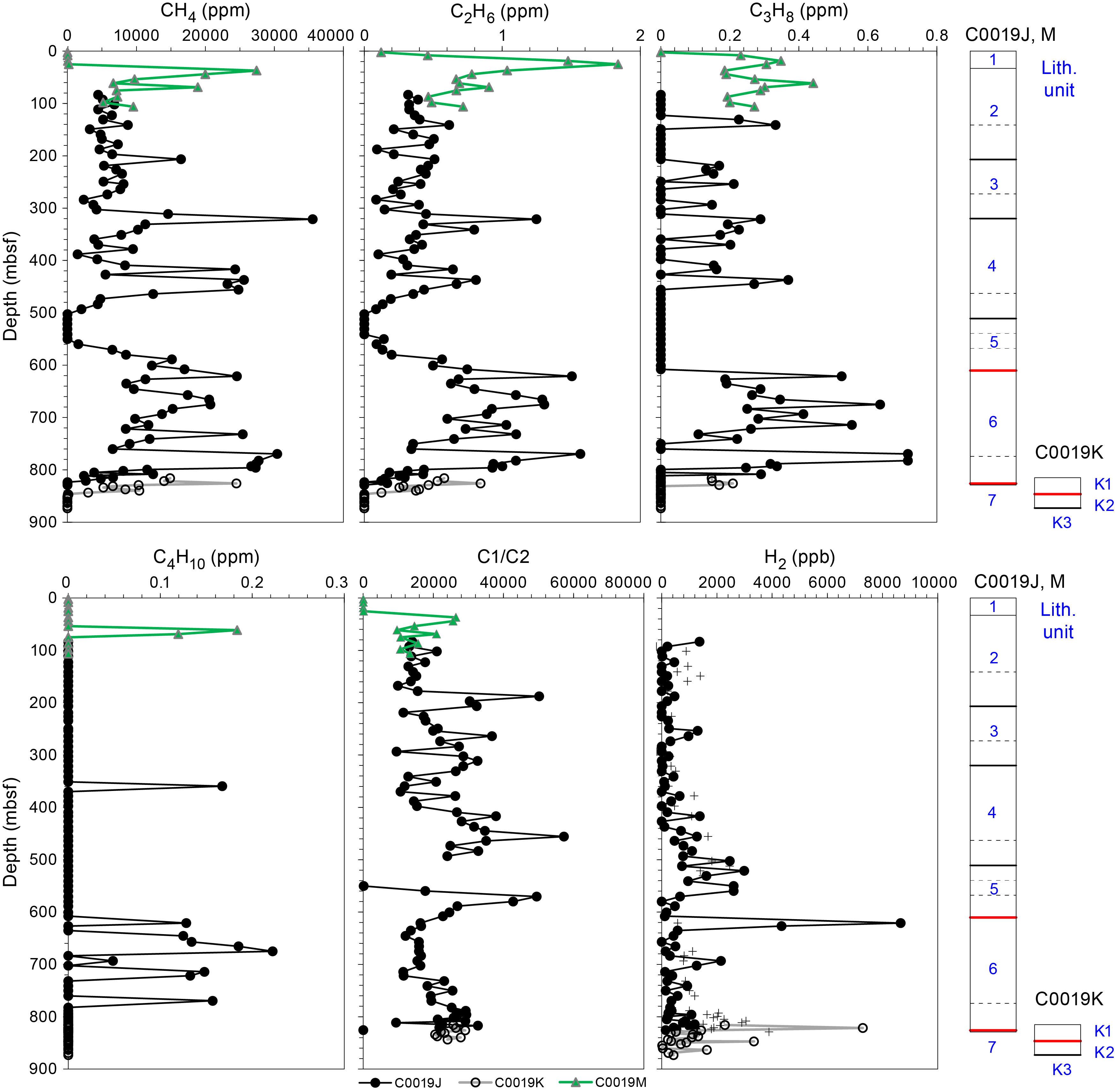
Figure F133. Gas components in headspace gas samples.

Methane to ethane concentration ratios (C1/C2) in Holes C0019M and C0019J generally range from about 9,500 to 57,000 (Figure F133). From 30 to 490 mbsf, C1/C2 ratios tend to increase from ~14,000 to ~32,000 with notable peaks at 37, 188, 264, and 456 mbsf. Between 502 and 541 mbsf, C1/C2 ratios are not calculated because ethane is not detected. Below this interval, C1/C2 increases rapidly to nearly 50,000 at 570 mbsf before it returns to about 12,000 at 646 mbsf. The C1/C2 ratio shows a steady increase from 646 to 817 mbsf to 32,700. Below that interval, the C1/C2 ratio becomes very low again to <810. The high C1/C2 ratios through most parts of Hole C0019J indicate that the observed methane is of biogenic origin. On the other hand, at 2–25 mbsf in Hole C0019M and 550 and 825 mbsf in Hole C0019J, where methane concentrations are very low, C1/C2 ratios as low as 30–110 are observed, suggesting a smaller contribution from biogenic methane production.

9.2.1.2. Hydrogen gas in head space samples

Concentrations of hydrogen gas (H₂) in headspace samples collected from Hole C0019J are shown in Table T35 and Figure F133. Between 80 and 440 mbsf in Units 2–4, H₂ concentrations are generally <400 ppb, but relatively high concentrations of 1370, 1300, and 1380 ppb are observed at 83, 254, and 417 mbsf, respectively (Figure F133). Below 440 mbsf, the H₂ concentrations increase, reaching as high as 2990 ppb between 502 and 560 mbsf near the base of Unit 4 and in Unit 5. At around 600 mbsf, H₂ concentrations are low or undetectable. However, the H₂ concentration is very high at 8660 ppb at 621 mbsf near the top of Unit 6, followed by 4340 ppb at 627 mbsf. Below 665 mbsf, H₂ was detected in all samples and shows a relatively high concentration of 2150 ppb at 693 mbsf. H₂ concentrations in the LCL range 0–3900 ppb, which tend to be higher than most sediment samples.

9.2.2. Hole C0019K

9.2.2.1. Hydrocarbon gases in headspace samples

Concentrations of hydrocarbon gases in headspace samples collected from Hole C0019K are summarized in Table T35 and Figure F133. Methane (CH₄) concentrations in Hole C0019K are relatively high between 816 and 826 mbsf with a peak of 24,500 ppm at 826 mbsf in Unit K1. Below this depth, the methane concentration decreases rapidly with depth, reaching very low values of 0–4 ppm below 852 mbsf. Although a rapid decrease in methane with depth near the plate boundary is also observed in Hole C0019J, it occurs at greater depths in Hole C0019K than in Hole C0019J. Ethane (C₂H₆) concentrations in Hole C0019K are all below 0.9 ppm and vary synchronously with methane, but they are below the detection limit below 846 mbsf. Propane (C₃H₈) is only detectable at <829 mbsf, and its concentration is lower than 0.2 ppm. Concentrations of n-butane (C₄H₁₀) in Hole C0019K are all below the detection limit.

Methane to ethane concentration ratios (C₁/C₂) in Hole C0019K show relatively stable values between 21,000 and 29,000, except below 846 mbsf where ethane is undetectable (Figure F132). These C₁/C₂ ratios observed are consistent with those observed in Hole C0019J below 730 mbsf. These high C₁/C₂ ratios are indicative of methane of biogenic origin, similar to most cases in Holes C0019M and C0019J.

9.2.2.2. Hydrogen gas in head space samples

Concentrations of hydrogen gas (H₂) in headspace samples collected from Hole C0019K are shown in Table T35 and Figure F133. The H₂ concentrations observed in Hole C0019K are generally consistent with those observed in Hole C0019J. However, high H₂ concentrations of 7280 and 3340 ppb are observed at 821 and 847 mbsf, respectively, near the plate boundary.

9.3. Carbon, nitrogen, and sulfur

9.3.1. Holes C0019M and C0019J

Analytical results for calcium carbonate (CaCO₃), total organic carbon (TOC), total nitrogen (TN), and total sulfur (TS) in the core samples from Holes C0019M and C0019J are presented in Table T36 and Figure F134. Most of the samples from Holes C0019M and C0019J show CaCO₃ contents between 0 and 2.5 wt%. However, a peak of CaCO₃ up to 3.2 wt% is observed at 55–120 mbsf in Unit 2. Below this, the upper limit of CaCO₃ contents tends to increase with depth from 0.45 wt% at 207 mbsf to 2.3 wt% at 789 mbsf, with two exceptionally high values of 37.5 wt% and 4.7 wt% at 636 and 713 mbsf, respectively, in Unit 6. Below 800 mbsf, CaCO₃ contents are all lower than 1.5 wt%, with a general decreasing trend.

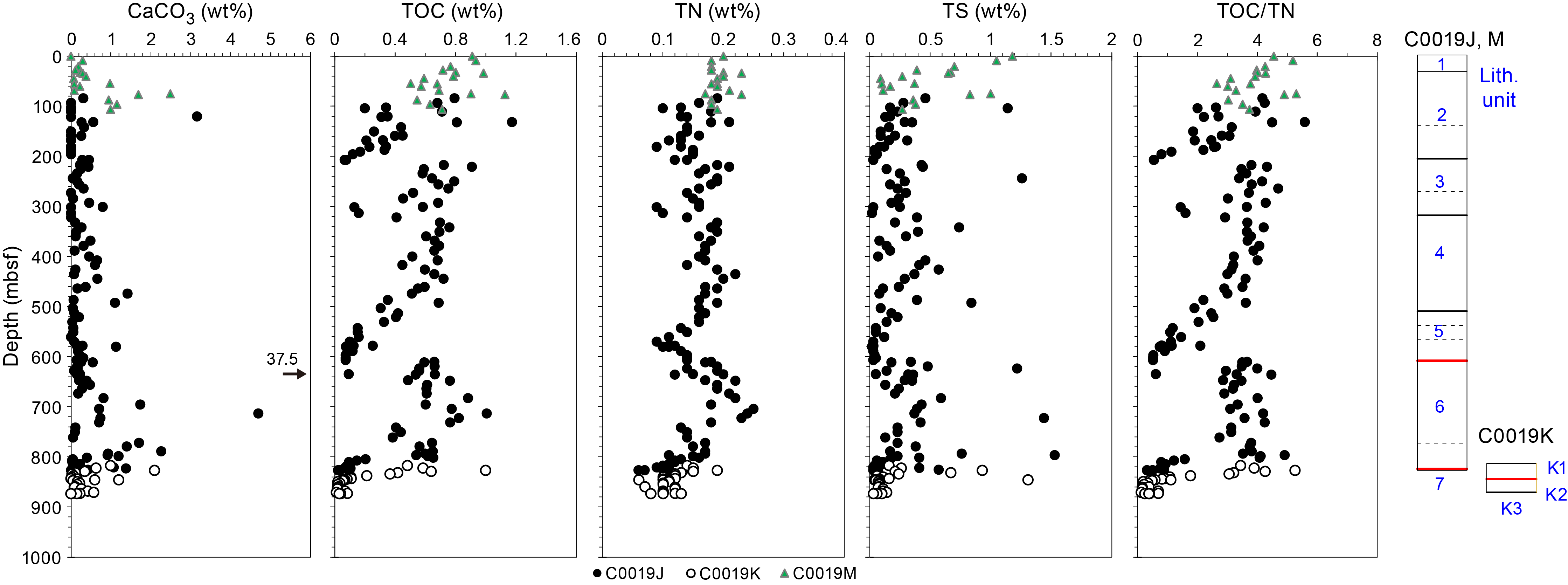
Figure F134. CaCO₃, TOC, TN, and TS contents and TOC/TN ratio.

TOC content in the core samples ranges 0–1.2 wt% (Table T36). From close to the seafloor to 207 mbsf, near the top of Unit 3, TOC shows a general decreasing trend, dropping from 0.9 to 0.1 wt% (Figure F134). This is followed by a sharp increase to 0.9 wt% at 221 mbsf, after which TOC declines to 0.2 wt% at 313 mbsf in Unit 3. Near the boundary between Units 3 and 4, an increase in TOC to 0.7 wt% occurs, followed by a gradual decrease to 0.1 wt% close to the boundary between Units 5 and 6. Subsequently, TOC rises to a peak of 1.0 wt% at 713 mbsf before entering a general downward trend, reaching 0.03 wt% at 827 mbsf.

TN content in the core samples varies between 0.06 and 0.25 wt%. Although the data are scattered, TN follows a broadly similar trend to TOC with increasing depth (Figure F134). From close to the seafloor to the top of Unit 3 at 207 mbsf, TN displays a gradual decline from 0.2 to 0.1 wt%. TN rises abruptly to 0.21 wt% at 221 mbsf below the boundary between Unit 2 and 3, after which TN decreases back to 0.1 wt% at 300 mbsf and fluctuates between 0.14 and 0.22 wt% to 435 mbsf in Unit 4. Below this depth, TN content steadily diminishes, reaching 0.09 wt% at 570 mbsf, before climbing to a maximum of 0.25 wt% at 704 mbsf. Below this point, the TN follows a consistent downward trajectory, eventually reaching 0.06 wt% toward the bottom of Hole C0019J.

TS content data exhibits a much larger scatter compared to TN or TOC (Figure F134). From close to the seafloor to 69 mbsf, TS undergoes a steep decline, dropping from 1.2 to 0.1 wt%, followed by a sudden surge to 1.1 wt% at 104 mbsf. This is then followed by a dramatic decrease to 0.03 wt% at the top of Unit 3 at 207 mbsf. Below this depth, the TS content is generally 0–0.5 wt% with episodic high values up to 1.5 wt%.

The TOC/TN ratio exhibits a pattern analogous to TOC (Figure F134). From close to the seafloor, TOC/TN steadily decreases from 5.2 to 0.5 by the top of Unit 3 at 207 mbsf. After a sudden shift to ~4.3 at 221 mbsf, TOC/TN fluctuates between 3 and 5 to 408 mbsf, with the exception of two data points around 1.5 near 310 mbsf. From 408 to 607 mbsf, TOC/TN gradually decreases from 4.0 to 0.5 at the base of Unit 5. At the top of Unit 6, TOC/TN rises to 3.5. At greater depths, TOC/TN begins a gradual upward trend, peaking at 4.9 at 797 mbsf, before dropping to 0.3 near the bottom of Hole C0019J.

9.3.2. Hole C0019K

Analytical results for CaCO₃, TOC, TN, and TS in the core samples from Hole C0019K at 817–874 mbsf are presented in Table T36 and Figure F134. CaCO₃ contents range 0–2.1 wt%. Although the data are scattered, a slightly decreasing trend in CaCO₃ is observed, consistent with the trend observed in Holes C0019J. TOC content also exhibits a general decreasing trend, declining from 0.5–1.0 to 0.03 wt%. TN content varies between 0.06 and 0.19 wt%. TS content shows significant variations, ranging 0.03–1.3 wt%. The TOC/TN ratio predominantly remains below 5 with a maximum of 5.3 observed at 827 mbsf. Similar to the TOC content, a general decreasing trend is observed for the TOC/TN ratio.

9.3.3. Hole C0019P

CaCO₃, TOC, TN, and TS contents in core samples from Hole C0019P are shown in Table T36. The core samples analyzed include limestone (939.2 mbsf), chert (939.7 mbsf), red shale (940.2 mbsf) and basalts (all others). CaCO₃ content is 75 wt% in limestone, 4.7 wt% in chert, 11 wt% in red shale, and 0.1–3.1 wt% in basalts. TOC contents are all low: 0 wt% in limestone, 0.04% in chert, 0.04 wt% in red shale, and <0.05 wt% in basalts. TN and TS contents are all lower than 0.08 and 0.12 wt%, respectively. The TOC/TN ratio is 0 in limestone, 0.88 in chert, 0.74 in red shale, and 0.46–1.2 in basalts.

10. Microbiology

10.1. Sampling

During the Window 1 period (September–October 2024), whole-round core samples for microbiological studies were obtained from cores retrieved from Hole C0019J using the SD-RCB coring system. A total of 74 whole-round samples were obtained out of 87 cores recovered. Also, 19 IW squeezed cake samples were obtained for comparison with microbiology whole-round cores located next to them. The seawater sample used for drilling fluid was sampled every morning (at around 1100 h) when coring operations were conducted. In total, 22 drilling fluid (LMW) samples were obtained to check for any contaminating microbiome from the drilling fluid. In addition, 80 liner fluid (LCL) samples were obtained to check for any contaminating microbiome in the fluid directly in contact with the cored materials.

During the Window 2 period (November–December 2024), 5 whole-round core, 4 LMW, and 15 LCL samples were obtained from Hole C0019K. A total of 4 whole-round core, 20 IW squeezed cake, 2 LMW, and 5 LCL samples were obtained from Hole C0019M.

10.2. Subsampling in an anaerobic chamber

Subsampling of the whole round cores was conducted following methods described in Microbiology in the Expedition 405 methods chapter (Kirkpatrick et al., 2025). The number of floating particles before the subsampling work was measured to ensure clean sample handling conditions in the anaerobic chamber and ranged 0–40, 0–20, and 0–10 particles/ft³ for particle sizes of 0.1, 0.3, and 0.5 µm, respectively. After subsampling, the inside of the anaerobic chamber was thoroughly cleaned by spraying RNase AWAY and wiped with a laboratory wiper before checking particle concentration after the subsampling work. Because no microbiologist was on board during the Window 2 period, minimized subsampling was conducted (see Microbiology in the Expedition 405 methods chapter [Kirkpatrick et al., 2025]).

10.3. Activity staining with Cell Tracker Green CFMDA

Activity staining with Cell Tracker Green 5-chloromethyllfluorescein diacetate (CMFDA) was initiated on board by adding 40 µL of 25 µM CMFDA dye dissolved in dimethyl sulfoxide (DMSO) to all 74 samples obtained. Incubations were continued for 14 days, followed by fixing and freezing for detailed analysis at the onshore laboratory.

11. Observatory

11.1. Hole C0019D

An observatory instrument string consisting of an array of temperature sensors was deployed into the existing cased observatory Hole C0019D (J-FAST observatory). This hole was originally drilled during Expedition 343/343T (Expedition 343/343T Scientists, 2013a), and the original instrument string was recovered in 2013 (Fulton et al., 2013). Deployment of a new instrument string into this hole was made possible with Chikyu via a reengaging tool attached to the end of the drill pipe and lowered atop the Hole C0019D wellhead.

Reengagement with the wellhead allowed deployment of the complete sensor string, including the sinker bar and miniature temperature logger (MTL) hanger (see Observatory in the Expedition 405 methods chapter [Kirkpatrick et al., 2025]), through the drill pipe and into the 4½ inch (11.43 cm) outer diameter (OD) wellbore tubing by the core barrel retrieving tool (CBRT) connected to the core line and core line winch. Prior to the instrument string deployment, drift runs were conducted to assess whether the interior of the borehole casing remained unobstructed at depth or had been deformed (e.g., bent or pinched), which could potentially restrict emplacement of the instrument string.

11.1.1. Drift Run 1

The first drift run was completed on 12 September 2024, involving a 17.253 m long 600 kg sinker bar suspended on a 0.3 m length of rope below a MTL hanger. The assembly was attached to the CBRT and lowered through the drill pipe engaged to the wellhead. The MTL hanger landed in the wellhead above the seafloor at the appropriate landing seat position corresponding to −3.32 mbsf. A noticeable reduction in load on the winch indicated the core line reference depth at which the landing point was reached, providing a baseline depth for the landing seat at the top of the observatory.

11.1.2. Drift Run 2

A second drift run was completed on 12 September 2024. The core line was connected to a MTL hanger with a 200 kg sinker bar that hung immediately below it by connection with a short section of rope. An additional 400 kg sinker bar, measuring 3 inches (7.62 cm) in diameter and 11.508 m in length, was attached further below by a rope with weak links on both ends such that the bottom of the lower sinker bar extended 825.64 m below the 200 kg sinker bar. The extended rope length between the sinker bars was designed to enable the lower sinker bar to potentially reach the tubing float collar at the bottom of the tubing before the MTL hanger seated. Monitoring of the load on the core line revealed unloading of the lower sinker bar, followed by unloading of the MTL hanger. Data analysis indicates that the tubing is obstructed at 821.09 mbsf, approximately 4 m above the tubing float collar.

11.1.3. Hole C0019D deployment

An instrument string with 57 temperature sensors was installed into the observatory Hole C0019D at approximately 1715 h Japan Standard Time (JST) on 12 September 2024. The deployment was performed using the core line and CBRT through the drill pipe that was connected to the existing observatory wellhead above the seafloor via a wellhead reengagement tool. The deployed instrument string consists of eight lengths of Vectran line, connected by either hard link carabiner or one of two weak links, an MTL hanger at the top that sits within the wellhead with a 400 kg sinker bar immediately below it, and a 15 kg 0.467 m long sinker bar positioned at the bottom, extending to 820.69 mbsf (see Observatory in the Expedition 405 methods chapter [Kirkpatrick et al., 2025]). The total length of the instrument string was configured to avoid the identified borehole obstruction at depth. Table T37 describes the set position of instruments and associated components following installation. Programming details for the instruments are also described in Observatory in the Expedition 405 methods chapter (Kirkpatrick et al., 2025).

11.2. Hole C0019Q

11.2.1. Hole C0019Q deployment

The installation of an instrument string into Hole C0019Q (JTRACK observatory) was completed on 15 December 2024. This followed an unsuccessful attempt in the preceding days that was hampered by the lowermost sinker bar of the instrument string failing to clear the casing hanger, eventually getting stuck, and requiring the weak link to be broken. After retrieving both the instrument string and tubing, the sinker bar and broken weak link were recovered and replaced. A second attempt at installation was then successfully completed with the casing hanger landing on the casing at 1410 h JST on 15 December.

The instrument string was installed in 4.5 inch (11.43 cm) OD tubing with a 3.958 inch (10.053 cm) inner diameter. The tubing extends to 906.41 mbsf, with the top of the float collar (tag point) at 905.74 mbsf. The deployed instrument string consists of eight lengths of Vectran line connected by either hard link carabiner or one of four weak links, a MTL hanger at the top that sits in the wellhead with a 400 kg sinker bar immediately below it, and a 30 kg 0.982 m long sinker bar positioned at the bottom, extending to 902.89 mbsf (see Observatory in the Expedition 405 methods chapter [Kirkpatrick et al., 2025]). Table T38 provides a detailed description of the set positions of the instruments and the associated components upon installation. Programming details for the instruments are described in Observatory in the Expedition 405 methods chapter (Kirkpatrick et al., 2025).

12. Core-log-seismic integration

12.1. Log-seismic tie

A seismic-well tie was established using the P-wave velocity data obtained by LWD in Hole C0019H and seismic reflection profiles acquired around Site C0019. The seismic reflection profiles used at this site were Profile HD33L (a high-resolution poststack time-migrated profile acquired with a small source array; Nakamura, 2015) and Profile JFD1 (a deeper penetration prestack time-migrated profile acquired with a large source array; Nakamura et al., 2014). Hole C0019H is located ~14 and ~57 m from Profiles HD33L and JFD1, respectively, according to the ship positions at the time of the survey and the drilling. Because we used two types of seismic reflection data with different frequency contents, the synthetic seismograms for each seismic-well tie were established using different wavelets (see Core-log-seismic integration in the Expedition 405 methods chapter [Kirkpatrick et al., 2025]). Initially, the time-domain synthetic seismogram and time-converted log data were bulk-shifted to match the mudline of the gamma ray log to the seafloor reflection of the seismic profile (Table T39). After that, the synthetic reflections from the top of the basalt layer were tied to the top of the Seismic Unit 4 reflection in the seismic reflection profiles. We also used other prominent reflections to adjust (i.e., stretch and squeeze) the time-domain synthetic seismograms and log curves. We generally did not use reflections within the hanging wall prism (Seismic Unit 1) to tie because continuous strong reflections are not identified in the prism (with the exception of one strong reflection at 9851.9 ms in the JFD1 profile).

Figures F135 and F136 show the results of the seismic-well ties at Site C0019. The stretch-squeeze adjustment was small for both profiles (e.g., 30 ms at the top of the basalt for the HD33L after bulk-shifted at the seafloor) (Table T39). Strong reflections within the chert layer (Logging Unit 4) lacked a clear correlation, probably because of the low quality of the sonic log in this interval (Figures F137, F138) (see Logging while drilling). Within most of the prism, the correlation between the seismic reflection profiles, both JFD1 and HD33L, and synthetic seismograms was poor, especially in the wavelet phases. However, intervals with higher amplitude in the synthetic seismograms do correspond to those with relatively high amplitude in Seismic Reflection Profile JFD1 at ~9540–9550 ms (~380–390 m LSF; ~7305.5–7315.5 m BRT) and ~9725–9745 ms (~562–573 m LSF; ~7487.5–7498.5 m BRT). In Seismic Reflection Profile HD33L, detailed matching was not conducted between the seafloor and the top of the basalt; however, synthetic seismograms show a strong correlation with the seismic reflection profile between ~9,900 and 10,000 ms (~750–850 m LSF; ~7675.5–7775.5 m BRT).

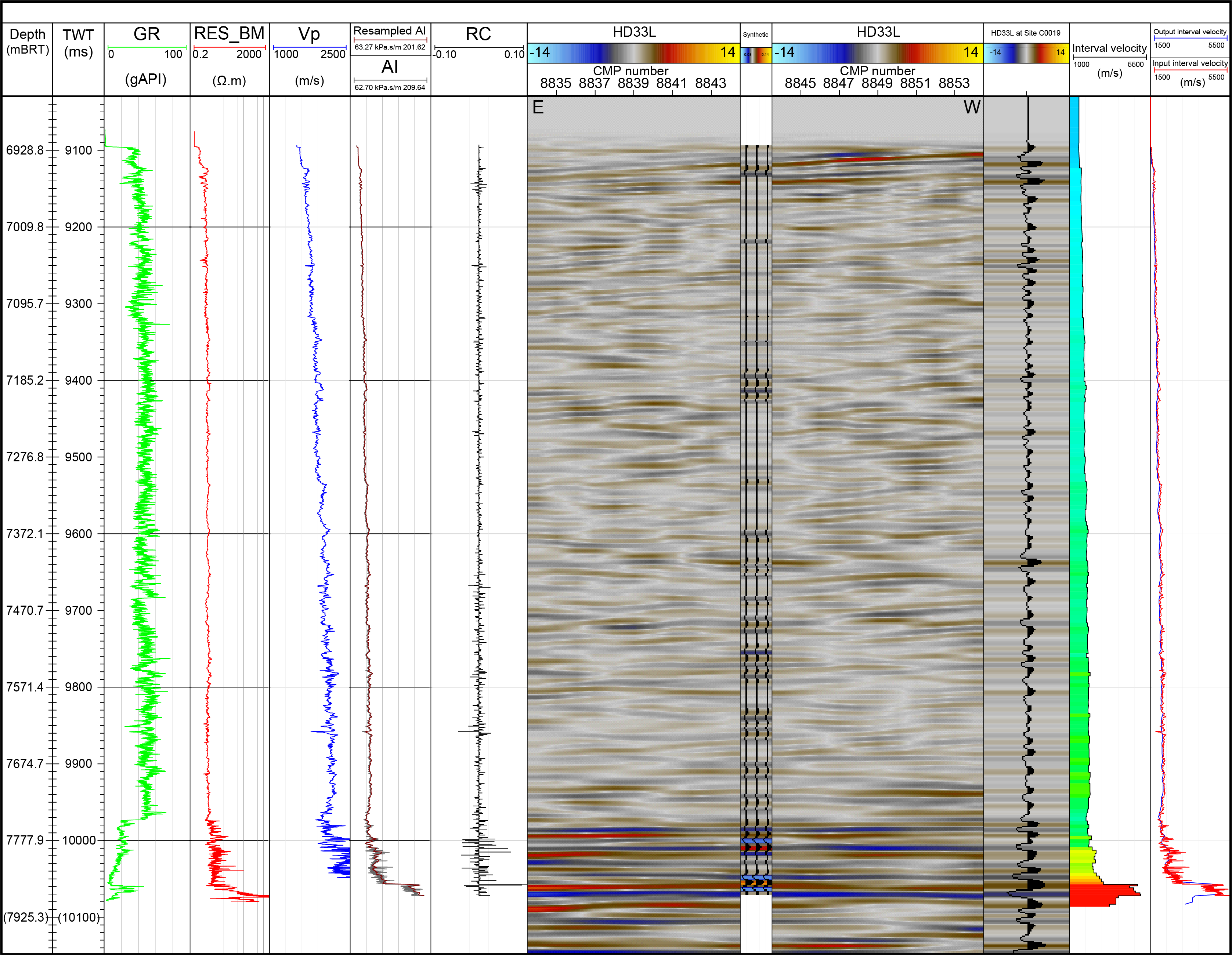
Figure F135. Seismic-well tie for high-resolution Seismic Line HD33L.

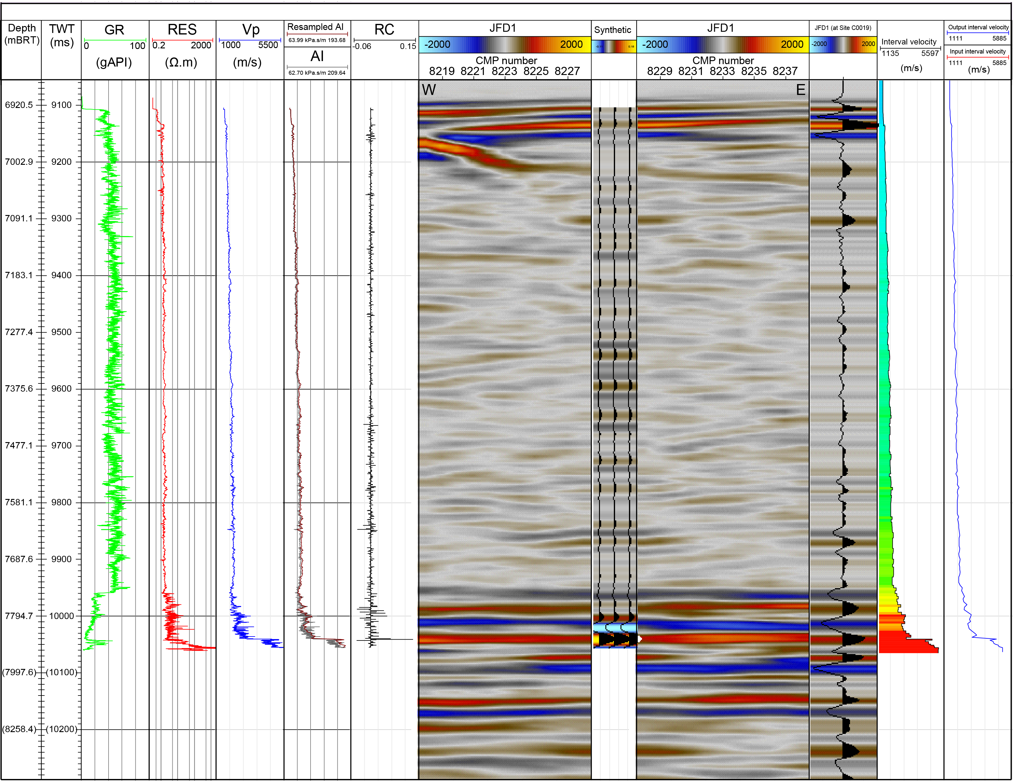
Figure F136. Seismic-well tie for lower resolution Seismic Line JFD1.

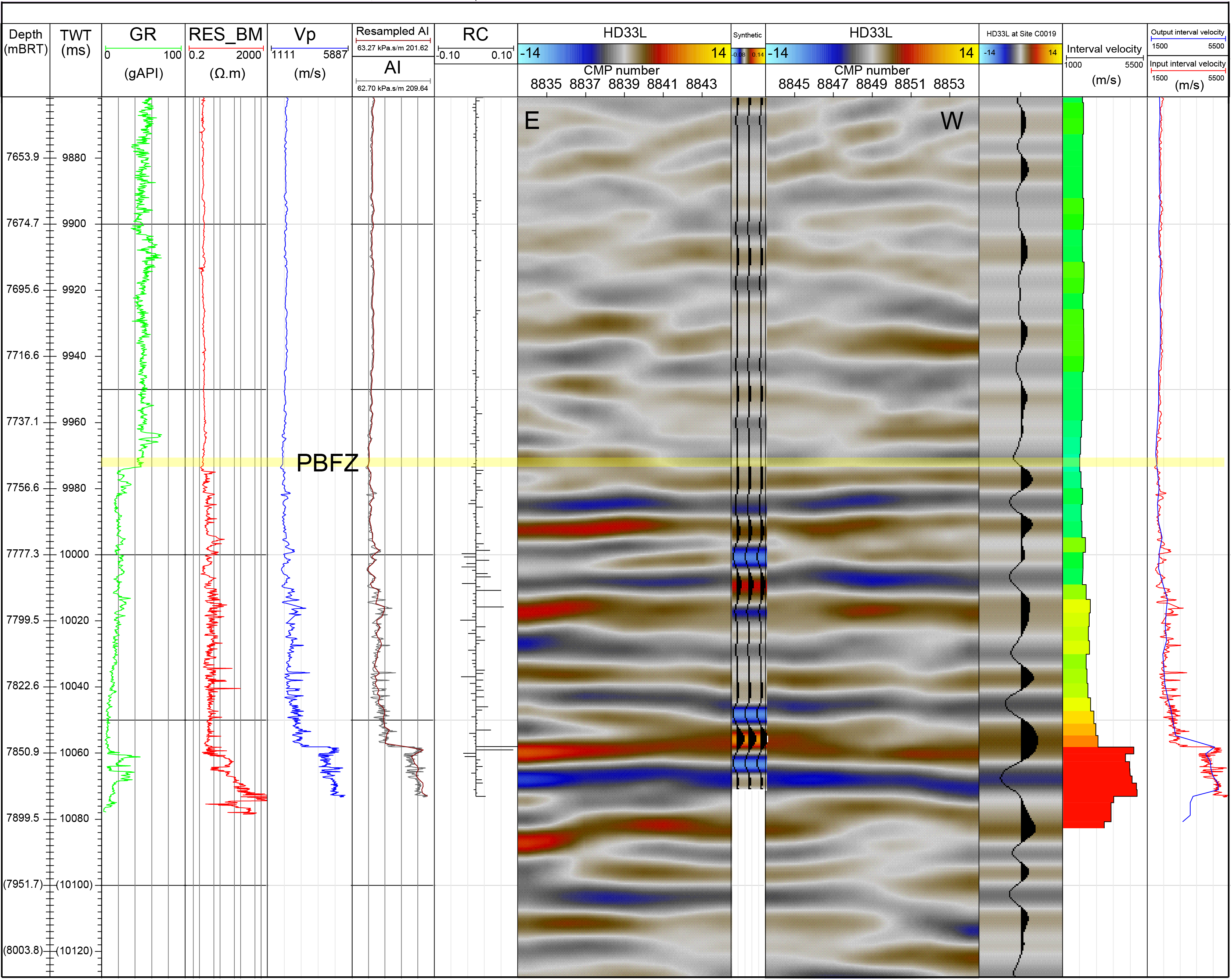
Figure F137. Close-up of seismic-well tie around plate boundary fault for high-resolution Seismic Line HD33L.

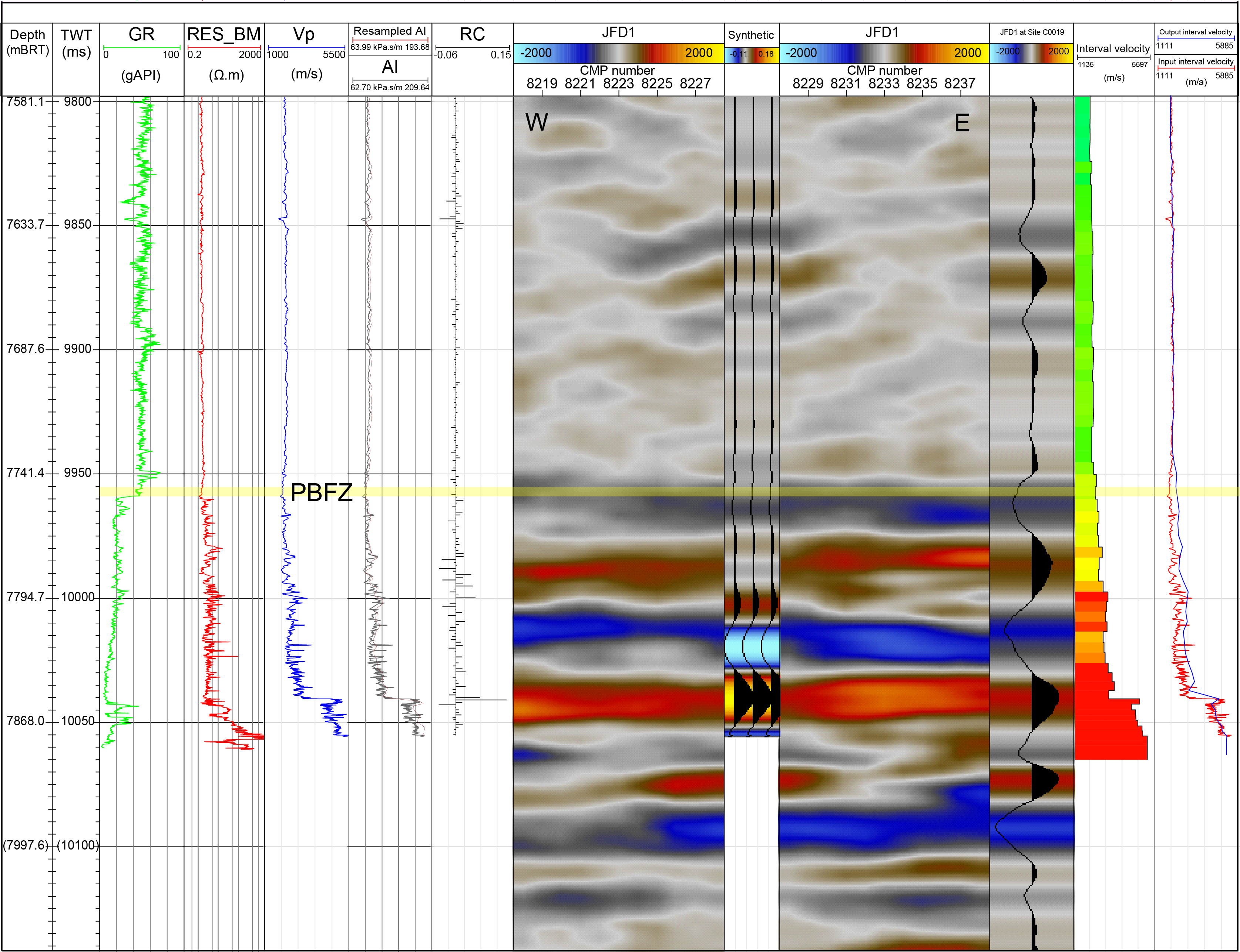
Figure F138. Close-up of seismic-well tie around plate boundary fault the lower resolution Seismic Line JFD1.

12.2. Core-log integration

Core-log integration is based on the correlation between the physical properties recorded by LWD in Hole C0019H (see Logging while drilling), discrete physical properties measurements on discrete samples or core sections, and with the COMET for Holes C0019J, C0019K, and C0019M. For a comparison and verification of COMET data with discrete sample measurements, see Physical properties.

The core-log integration at Site C0019 is based on a comparison of NGR (Figure F139), electrical resistivity (Figure F140), and P-wave and S-wave velocity (Figures F141, F142). Additionally, analysis of fractures and bedding is based on comparing LWD resistivity images with visual core descriptions (see Structural geology). Because of the partial core recovery, only significant trends or variations spanning several cores were considered.

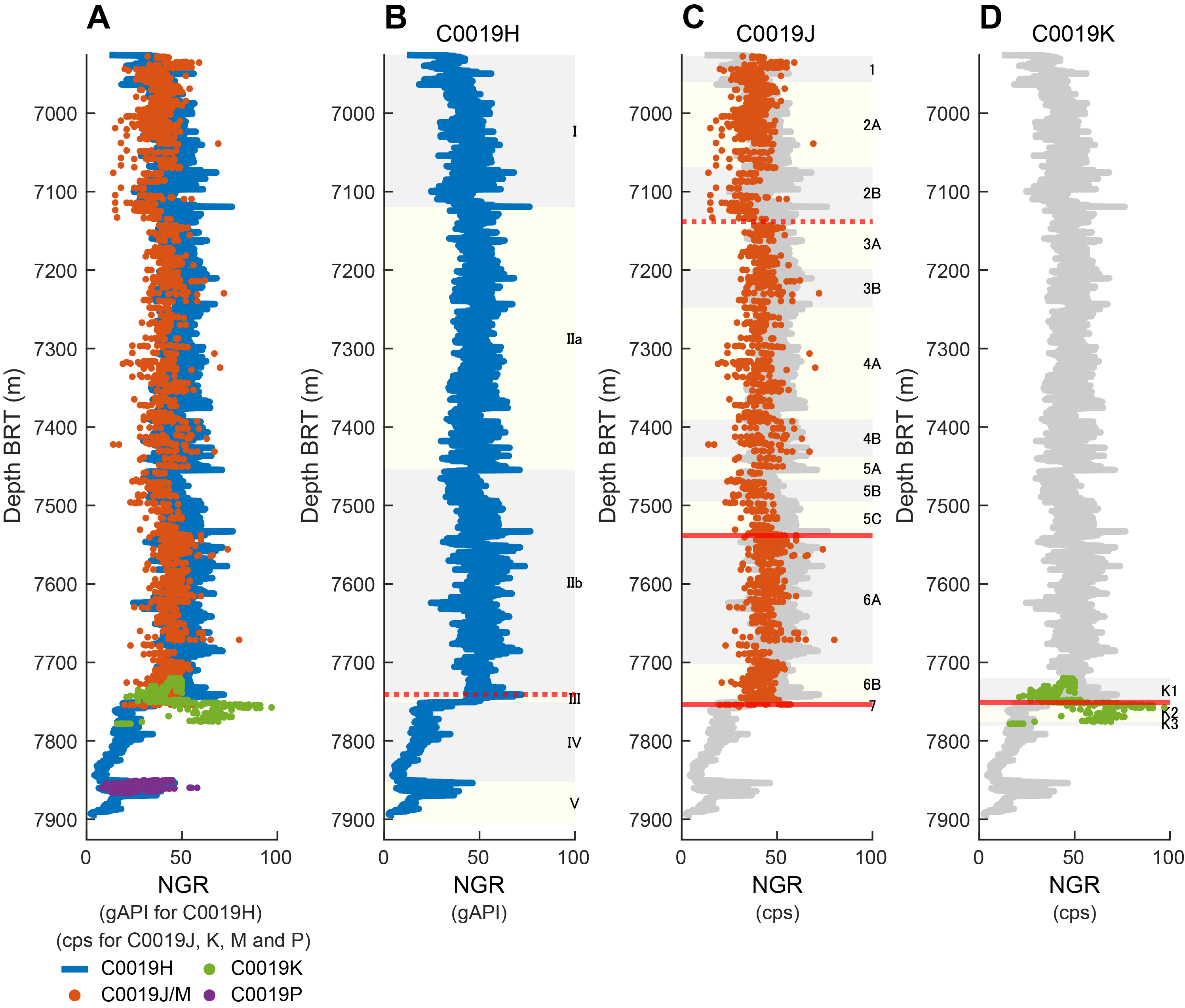
Figure F139. LWD gamma ray data and COMET gamma ray profiles.

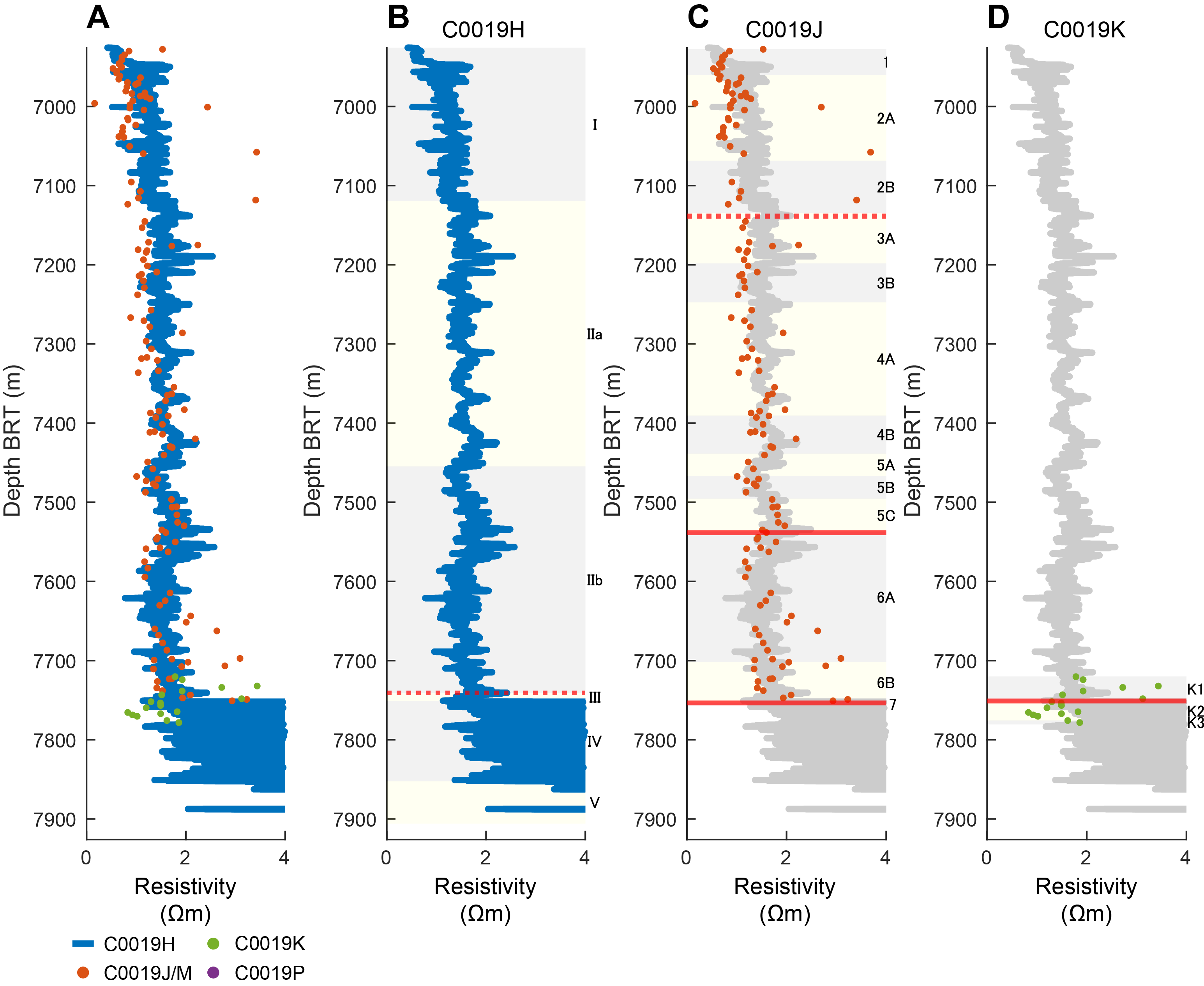
Figure F140. LWD electrical resistivity data and discrete sample resistivity.

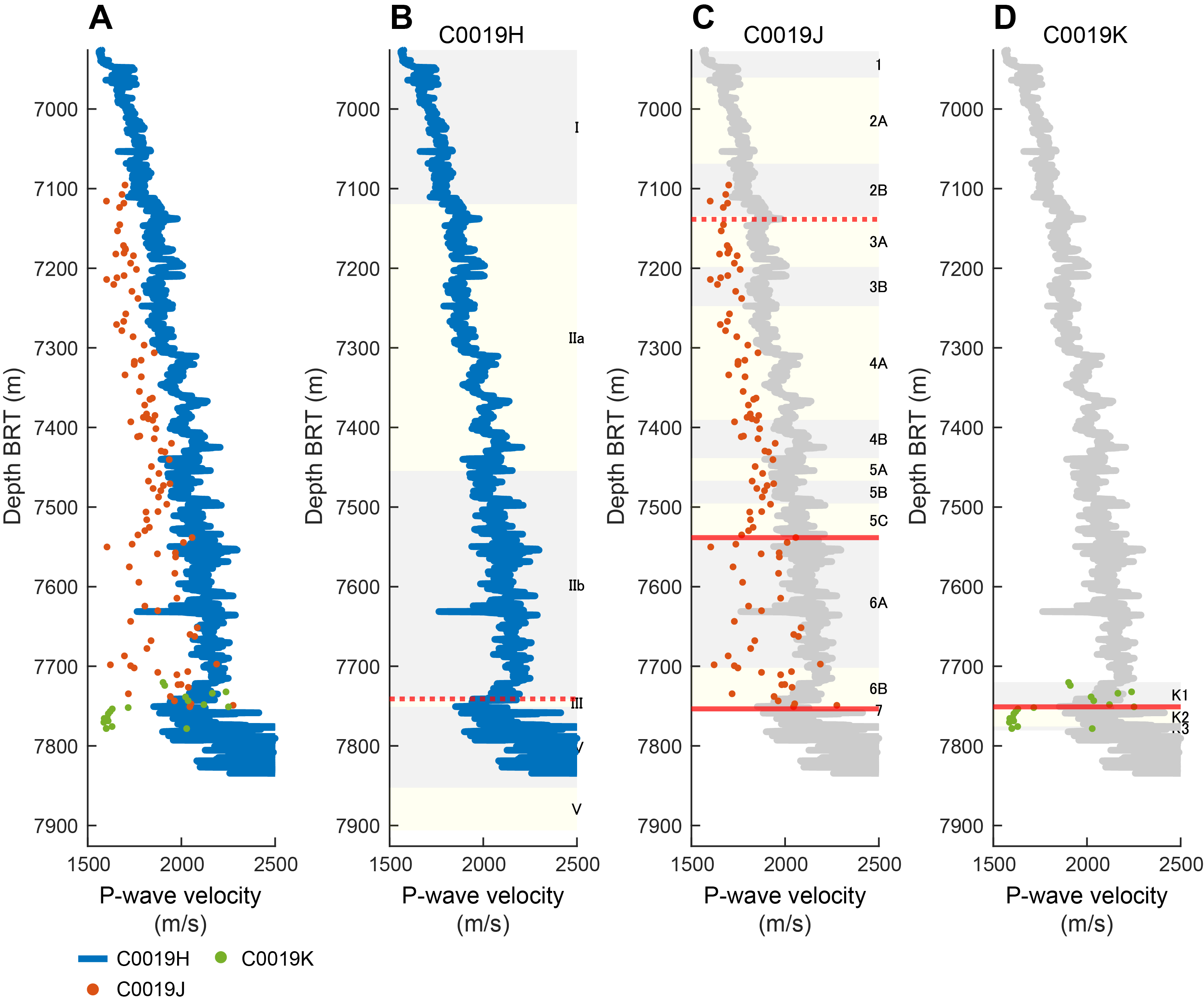
Figure F141. LWD P-wave velocity data and P-wave velocity measured on discrete core samples.

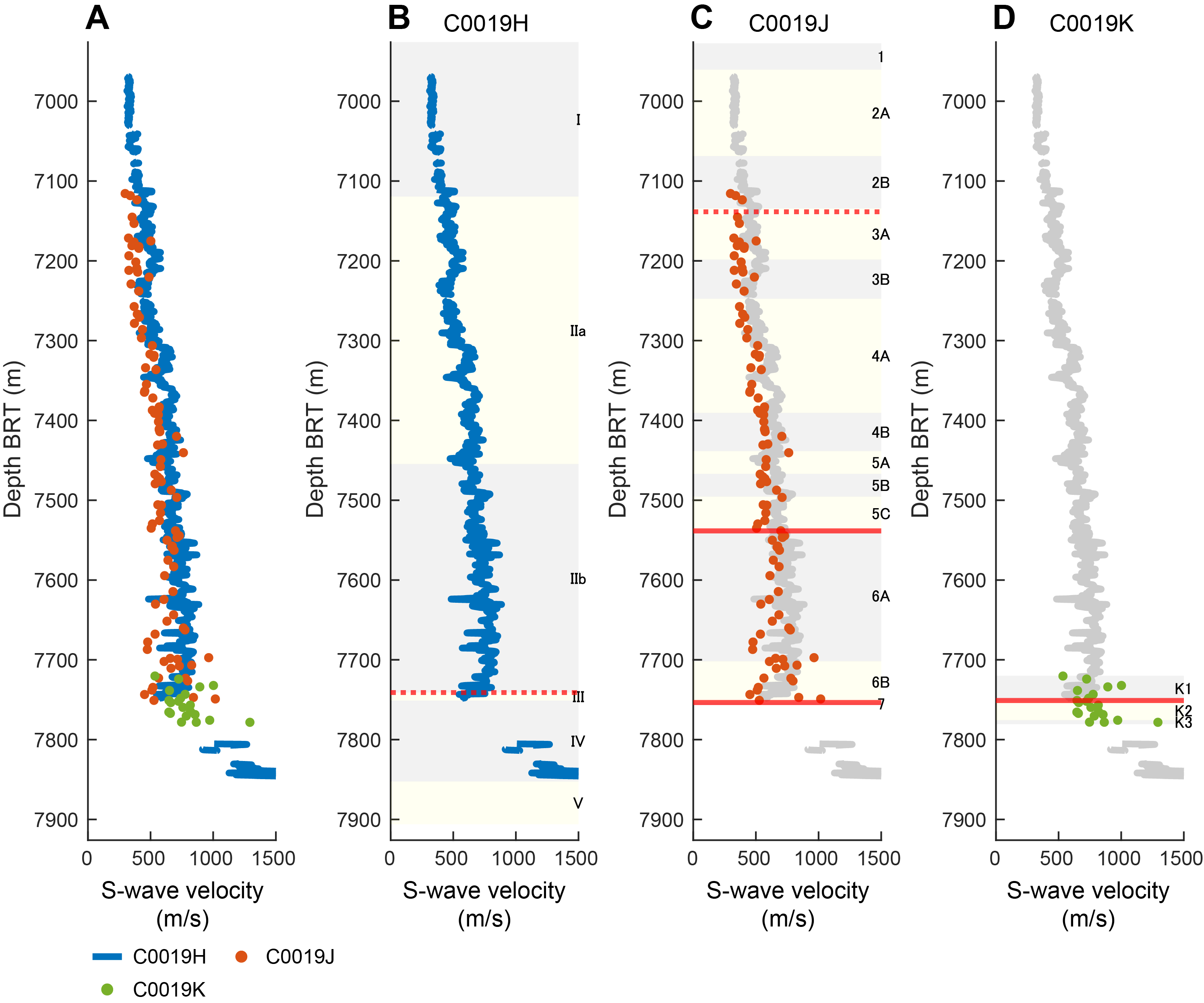
Figure F142. LWD S-wave velocity data and S-wave velocity measured on discrete core samples.

It should be noted that the scale of investigation differs between LWD and core samples. LWD measurements integrate both the effects of the matrix and fractures, whereas core samples provide information primarily on the matrix properties. Discrepancies between the two data sets could provide insights into fracture density.

Interpretation of the seismic reflection profiles (Nakamura et al., 2014), combined with the results from Expedition 343 (Chester et al., 2013), indicate that the tectonic setting at Site C0019 consists of (1) a seismically chaotic frontal prism, (2) a PBFZ beneath the prism, and (3) less deformed strata of the Pacific plate beneath the plate boundary. Below, we discuss the integration of core and log observations for each of these components. For information on the lithostratigraphic units referred to below, see Lithostratigraphy.

12.2.1. Core-log integration in the frontal prism

12.2.1.1. Natural gamma ray radiation

The NGR profiles for Holes C0019H, C0019J, and C0019M are very similar (Figure F139). The overall constant trends are similar, and the depths of excursions also appear to align closely. However, the range and mean values are not directly comparable because the COMET measurements are consistently lower than the LWD values. This offset is likely due to the COMET measurements being affected by the amount of core material filling the liner; cores that do not fully fill the liner during recovery can result in reduced NGR values in the COMET data. Given the similarity of the gamma ray patterns, particularly the step increase observed in both the COMET and LWD data, it can be considered that the boundaries between Logging Units I and II in Hole C0019H (7119.5 m BRT) and Lithostratigraphic Units 2 and 3 in Hole C0019J (7135.07 m BRT) correspond. It should be noted, however, that the depth of each unit boundary differs. Therefore, when comparing the unit depths between log and core, care should be taken regarding these discrepancies.

The boundary between Logging Subunits IIa and IIb in Hole C0019H is marked by a substantial step down in NGR values observed in both the LWD (Hole C0019H) and core (Hole C0019J) data sets at similar depths (~7458 m BRT) (Figure F139). This consistency suggests that the factor responsible for the NGR step exists at the same depth in both Holes C0019H and C0019J. Despite this correlation, the depth identified as the boundary between Logging Subunits IIa and IIb is not recognized as a lithostratigraphic unit boundary based on core observations. This distinction is more subtle; without prior knowledge of the boundary from the LWD data, it would be challenging to identify it solely from the COMET measurements. Similarly, it was difficult to identify lithologic differences between logging units in the core that could explain the change observed in the NGR data. Conversely, the boundary between Lithostratigraphic Subunits 6A and 6B coincides with a change from more scattered LWD NGR values above about 7700 m BRT to less scattered data below, but this change is not identified as a logging unit boundary.

12.2.1.2. Electrical resistivity

The electrical resistivity values are consistent for the LWD data from Hole C0019H and measurements from discrete core samples and core sections from Holes C0019J, C0019M, and C0019K (Figure F140). The resistivity was measured in two (y- and z-) or three (x-, y-, and z-) directions for the core section or discrete samples, but for comparison with the log, the resistivity in the y-direction perpendicular to the drilling direction was used. The depth-increasing trends are consistent, and the values are generally in good agreement. In the shallow section (~7100 m BRT or shallower), the resistivity measured from the core sections is lower than that of the LWD data. On the other hand, in the deeper section (~7600 m BRT or deeper), the resistivity measured from some discrete samples is higher than that of the LWD data. This difference can be attributed to the discrete samples being selectively measured from intact portions of the core, whereas the LWD data represent a broader region that includes cracks and fractures.

The LWD resistivity values exhibit a transition from low to high values across a major fault that bounds Lithostratigraphic Units 2 and 3 at 7135.1 m BRT, as inferred from an age inversion defined from biostratigraphy in the Hole C0019J core (Figure F140) (see Structural geology). This increase in resistivity across the fault is consistent with an observed decrease in porosity across the fault (see Physical properties). Additionally, a sharp spike in the LWD resistivity values is evident across a deeper major fault at 7537.8 m BRT (see Structural geology), as determined from the Hole C0019J core. Beneath this fault, both LWD and discrete sample resistivity values exhibit a decreasing trend. Below this interval, within the middle of Lithostratigraphic Subunit 6A (~7600 m BRT) and deeper, the resistivity measured from discrete samples shows an increasing trend and increasing scatter. Although the LWD resistivity also begins to increase in this interval, the magnitude of the increase is minimal compared to that observed in the discrete sample measurements. The onset of this change represents the boundary between Lithostratigraphic Units 5 and 6. Comparable trends are also evident in the measurements of discrete samples, although they are less distinct. This discrepancy may be attributed to the sampling differences between the LWD and discrete samples.

12.2.1.3. P-wave and S-wave velocities

Figures F141 and F142 illustrate the elastic velocities derived from LWD and those derived from onboard discrete sample measurements. The elastic velocities were measured in three (x-, y-, and z-) directions for the discrete samples, but for comparison with the log, the elastic velocities in the z-direction parallel to the drilling direction were used. A detailed depth correlation based on P-wave velocities between Hole C0019H (LWD) and Holes C0019J and C0019K (RCB coring) shows that the majority of the P-wave velocities from sample measurements are systematically lower than those from the LWD data (Figure F141). This discrepancy may be attributed to several factors. Discrete core sample measurements are conducted under atmospheric or low confining pressure (see Physical properties in the Expedition 405 methods chapter [Kirkpatrick et al., 2025]), whereas LWD measurements are performed under in situ conditions with consequently high confining pressure. Additionally, the volume of investigation differs between the two methods: LWD measurements integrate the properties of both the rock matrix and fractures, whereas discrete sample measurements reflect only the intact matrix properties. Furthermore, the discrepancy may also stem from the use of different acoustic pulse frequencies between the two methods. The LWD tool operates in the kilohertz frequency band, whereas discrete sample measurements onboard were conducted in the megahertz frequency band (see Physical properties in the Expedition 405 methods chapter [Kirkpatrick et al., 2025]).

From the shallow sections to the major fault between Lithostratigraphic Units 5 and 6 (7537.8 m BRT), both LWD and discrete sample P-wave velocities increase with depth at a similar rate, although their absolute values differ. Within this interval, there is some scatter in both data sets, but no clear correspondence is observed between the P-wave velocities and lithostratigraphic unit boundaries. Just above the fault at 7538.4 m BRT (610.31 mbsf), the P-wave velocity measured from discrete samples shows a slight decrease, whereas no corresponding decrease is observed in the LWD data. At this depth, where a decrease in P-wave velocity is observed in the discrete sample data, an increase in porosity is also noted (see Physical properties). Below the boundary between Lithostratigraphic Units 5 and 6, the LWD P-wave velocities exhibit slight fluctuations but discrete sample P-wave velocity values show significant scatter. This suggests that the discrete samples captured small-scale heterogeneity, whereas the LWD tool averaged properties over a larger volume. Again, the P-wave velocities do not change significantly across lithostratigraphic unit boundaries. The largest excursion in the LWD P-wave velocities occurs at ~7630 m BRT, which is within Logging Subunit IIB/Lithostratigraphic Subunit 6A.

For all depths above the PBFZ, S-wave velocities from core samples tend to have similar values to LWD S-wave velocities (Figure F142). However, it should be noted that the LWD S-wave velocity values shallower than 7276 m BRT (350 mbsf) should be considered with caution because they might not be reliable (see Logging while drilling). Similar to the P-wave velocity, a slight decrease in S-wave velocity is observed in the discrete sample data just above the faulted boundary between Lithostratigraphic Units 5 and 6, but there is no corresponding decrease in the LWD data. From the unit boundary between Units 5 and 6 to the PBFZ, there is a strong correlation between S-wave core velocity and LWD S-wave velocity, despite the presence of considerable scatter in the S-wave core velocities within this interval.

12.2.1.4. Core-log structure comparison

Downhole logs and core samples together offer critical insights into the subsurface geology, revealing deformation mechanisms within the active accretionary prism. Sedimentary and structural features were identified and interpreted at both core and log scales (Figure F143) (see Logging while drilling and Structural geology). The structures from core samples, shown in the figure, are rotated using paleomagnetic data (see Structural geology in the Expedition 405 methods chapter [Kirkpatrick et al., 2025]). Logging resistivity images resolve features on a few centimeters to decimeter scale, whereas cores offer millimeter scale detail. Moreover, bedding identification from logging images is sometimes difficult in some intervals because of the image quality and/or possible confusion with fractures (see Logging while drilling in the Expedition 405 methods chapter [Kirkpatrick et al., 2025] for a more detailed description of structure identification), but they provide a continuous data set where coring might have missing intervals in zones with low core recovery. Owing to their respective characteristics, the two data sets are complementary and enable the identification of lithologic or structural features, such as consistent sedimentary packages or folds of various scales. LWD bedding interpretation started at 7010 m BRT because no borehole images were acquired above that depth (see Logging while drilling). In the core, bedding was described in the shallow HPCS interval in Hole C0019M as well as throughout Holes C0019J and C0019K to total depth. In Hole C0019J, the number of measured bedding planes in the core is limited in the 7010ؘ–7100 m BRT because the rotary core barrel (RCB) coring technique is not fully adapted to the level of induration of those shallow sediments. For structures certified with LWD and core data, see Logging while drilling and Structural geology.

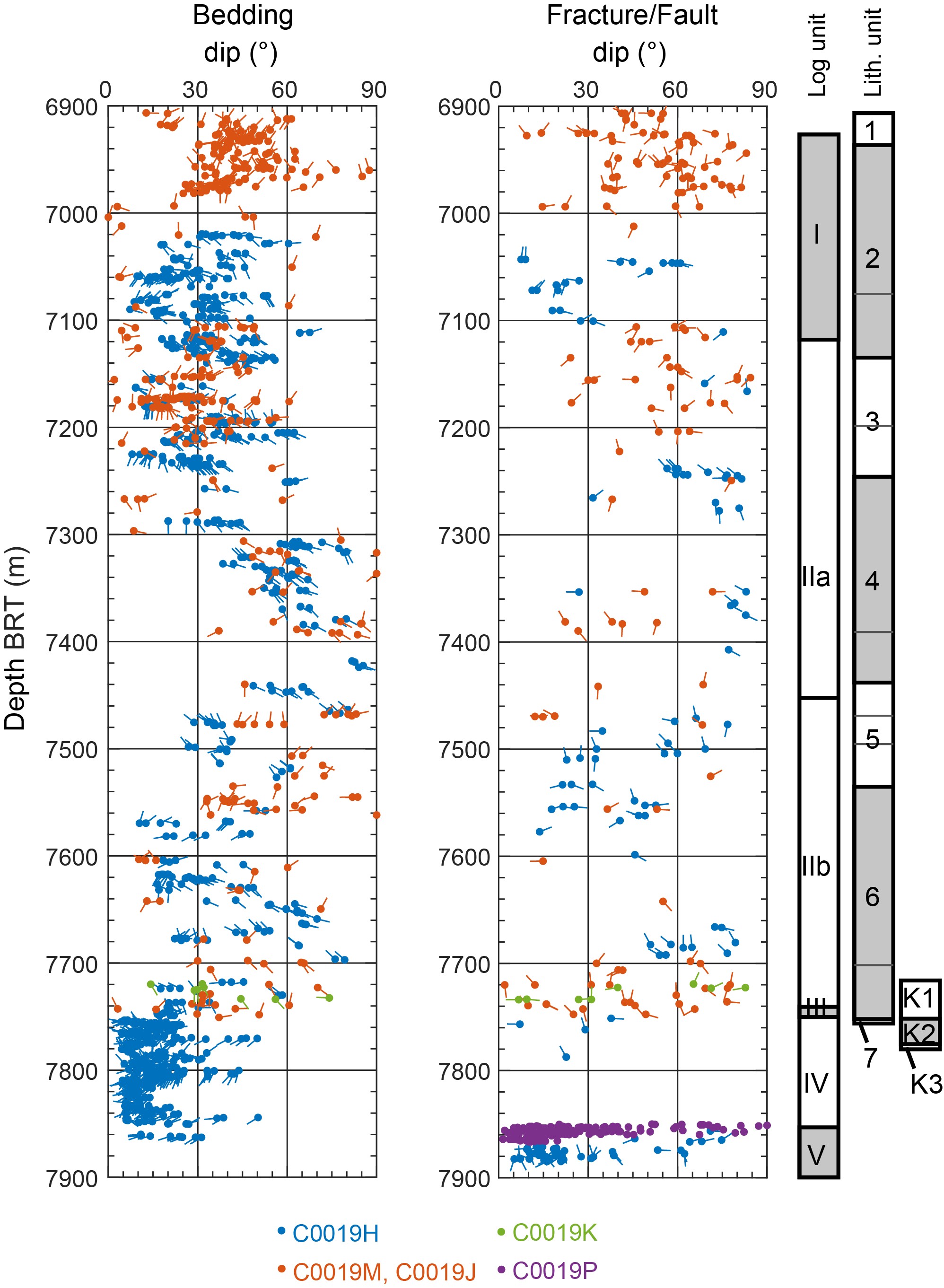
Figure F143. Bedding and fracture/fault dips.

Bedding dips estimated from LWD and core observations are generally in good agreement. In the section shallower than 7000 m BRT, relatively high angle (30°–60°) bedding dips are observed in the core. LWD bedding dips below 7000 m BRT indicate that the dip angle gradually decreases to 7100 m BRT. At depths greater than 7100 m BRT, the core and LWD bedding dips co-vary. In the interval to 7300 m BRT, both data sets show considerable scatter with dips mainly between 15° and 45°, with east to south dip directions. Below 7300 m BRT, the dip angle increases in both the core and the LWD bedding. Both indicate dip directions mainly east to 7460 m BRT and then north-east to west to 7560 m BRT, showing dip angles of less than 45°, and the LWD bedding then shows a gradual increase in dip angle with a south–east dip that changes to a decreasing dip trend with a north–west dip (7640–7680 m BRT). In this interval, although the core samples also show an increase in dip, there is no confirmation of a systematic change in dip direction from the LWD picks. From 7680 to 7730 m BRT, the bedding dip demonstrates a precipitous rise and decline in both LWD and cores. The dip direction is northwest to west in LWD, whereas the cores exhibit a predominantly southeast inclination. At 7730–7750 m BRT, the bedding in LWD undergoes a change in dip direction shifting to southeast to east and that of the core exhibits a distinct change in dip direction to northward. It is notable that no discernible correlation exists between the LWD and core bedding at this depth, with the exception of the dip angle.

Conductive-resistive fractures identified by LWD and the faults measured from the core indicate discrepancies in the measured locations from 6900 to 7750 m BRT. For instance, from 6900 to 7020 m BRT, the faults were identified on the core (Hole C0019M), whereas from 7020 to 7100 m BRT, the fractures were only interpreted by LWD. Some intervals of the faults identified in Holes C0019M and C0019J (7100–7170, 7250–7260, and 7470–7560 m BRT) exhibit overlap with the identifications of LWD fractures, and the magnitude of the dip angle of both is in agreement. However, the characteristic increase in minor faults measured in the core in the 7700–7750 m BRT cannot be seen in LWD.

12.2.2. Core-log integration around the PBFZ and lower plate

Holes C0019J and C0019K both recovered cores from the PBFZ (see Structural geology); however, the lithologies encountered immediately above and below the PBFZ were different in each hole (see Lithostratigraphy). Furthermore, the physical properties of the rocks recovered from the two holes also have similarities and differences (see Physical properties). To gain insight into the characteristics of the PBFZ, the data from Holes C0019J and C0019K are integrated with LWD data from Hole C0019H at comparable depths. This comparison is intended to elucidate the nature of the PBFZ and to identify any similarities or differences in its structural composition.

12.2.2.1. Natural gamma ray radiation

If the boundary between Logging Units II and III, estimated from LWD (see Logging while drilling), is taken as the top of the PBFZ in Hole C0019H, then the depth of the PBFZ varies by up to 12 m between the three holes (C0019H, C0019J, and C0019K) (Figure F144). The shallowest depth is at 7741 m BRT in Hole C0019H, followed by 7751.7 m BRT in Hole C0019K, and the deepest is at 7753.58 m BRT in Hole C0019J.

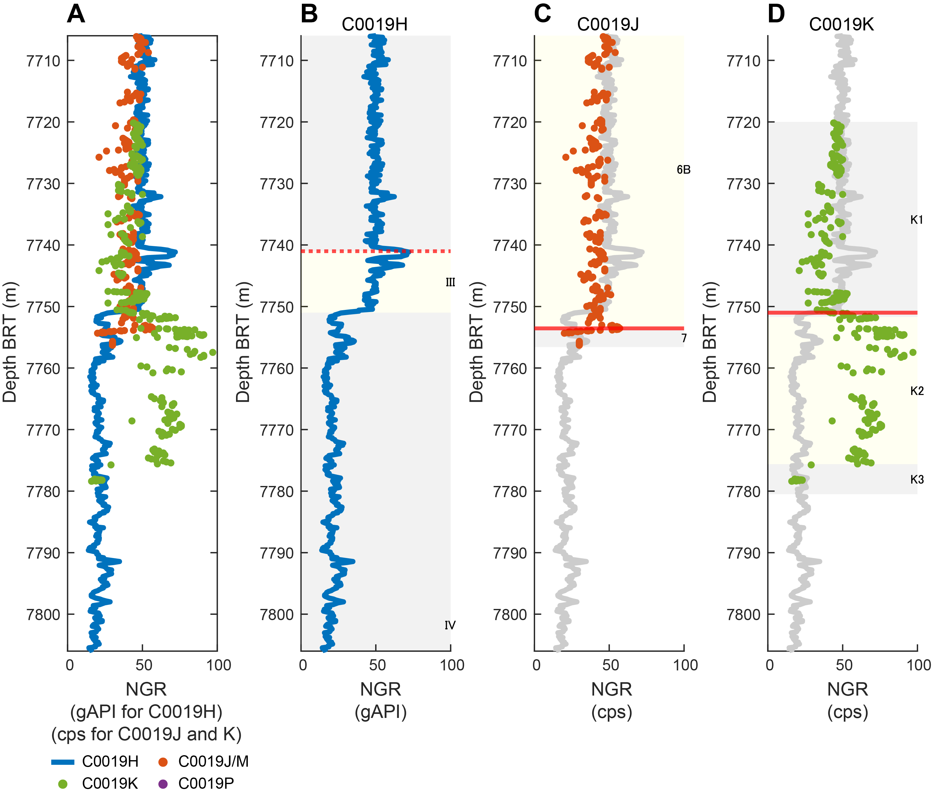
Figure F144. Gamma ray data from around the PBFZ and measured on cores.

The NGR characteristics are distinct in each of the three holes. In Hole C0019H, which has the shallowest PBFZ, NGR values are nearly constant above the PBFZ but show high values around the PBFZ (see Logging while drilling). However, these high NGR values are only present in the upper few meters of Logging Unit III, whereas values in the deeper parts of Unit III are similar to those of Logging Subunit IIb above the PBFZ, before dropping significantly at the boundary between Logging Units III and IV. In the PBFZ of Hole C0019K, NGR values measured with the COMET decrease in the 15 m interval from 20 m above the PBFZ (7730–7745 m BRT) before returning to the original levels (~50 counts/s) directly above the PBFZ. After entering the PBFZ, NGR values increase to a high level (~100 counts/s). Although they subsequently gradually decrease, the brownish black clay section within Lithostratigraphic Unit K2 maintains high values exceeding 50 counts/s. In Unit K3 (color-banded clay and chert), a small number of NGR values are significantly lower (~20 counts/s). In Hole C0019J, which has the deepest upper contact to the PBFZ, NGR values are relatively constant (~40 counts/s) to just above the PBFZ, where they spike to ~60 counts/s for about 1 m at the PBFZ. Subsequently, the values drop to around 20 counts/s in Lithostratigraphic Unit 7, which comprises color-banded clay and chert. The value of NGR below the plate PBFZ is characterized by high NGR in three holes, but the increase is largest in Hole C0019K.

12.2.2.2. Electrical resistivity

In the vicinity of the PBFZ, the resistivity profile from LWD data in Hole C0019H is the most distinctive (Figure F145). At the boundary between Logging Units II and III, which corresponds to the PBFZ, LWD resistivity values show a sharp spike. There is a second spike ~1 m below the Unit II/III contact, after which resistivity values decrease monotonically in Unit III. Then, the resistivity exhibits large fluctuations and high values upon entering Unit IV. In Hole C0019J, measurements of discrete samples were only conducted at depths shallower than the PBFZ; however, at these shallower depths, the resistivity values of discrete samples in Holes C0019J and C0019K generally align with those from LWD data. In Hole C0019K, despite considerable scatter, the resistivity values do not change significantly at depths deeper than the PBFZ.

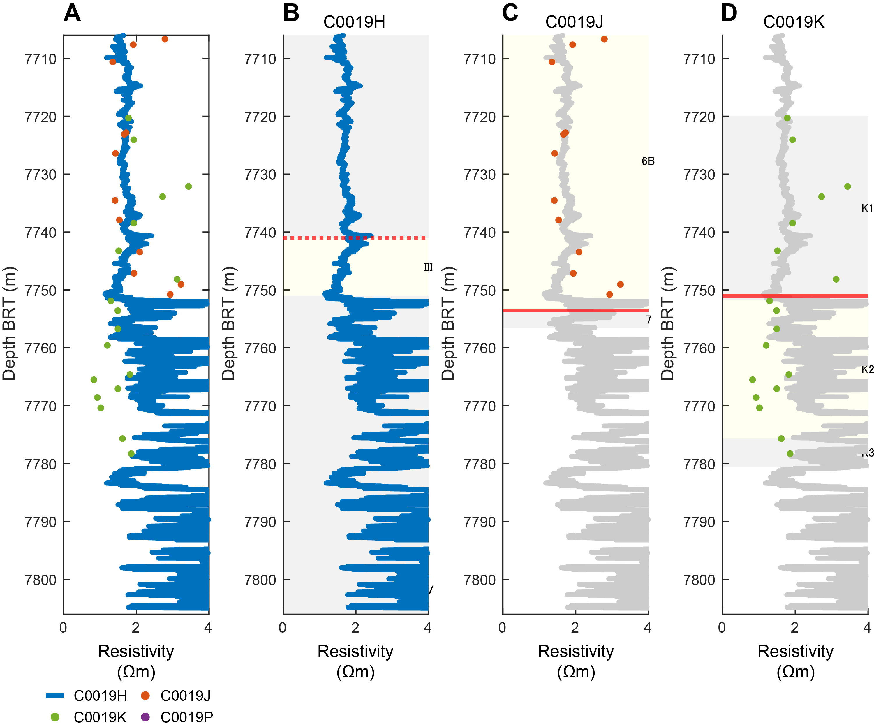
Figure F145. Electrical resistivity data from around the PBFZ and measured on discrete samples.

12.2.2.3. P-wave and S-wave velocities

Figures F146 and F147 illustrate the elastic velocities obtained in the vicinity of the PBFZ from LWD and onboard discrete sample measurements (vertical component of discrete sample measurements). The P-wave velocity measured by LWD (Hole C0019H) decreases toward the PBFZ and exhibits a spike of higher values just below the PBFZ. Within Logging Unit III, P-wave velocities remain at lower level compared to those above the PBFZ before beginning to increase in Logging Unit IV.

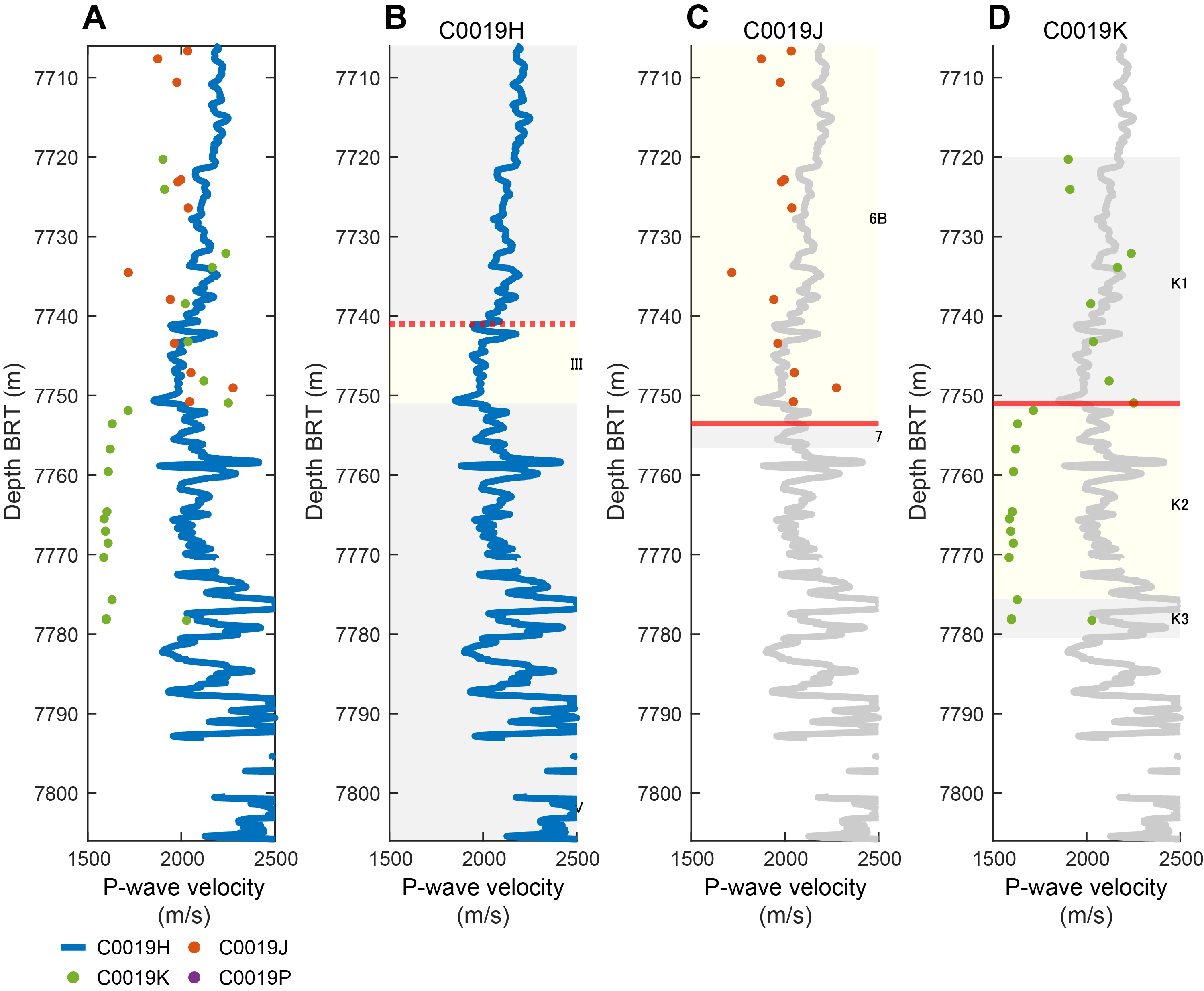
Figure F146. P-wave velocity data from around the PBFZ and measured on discrete samples.

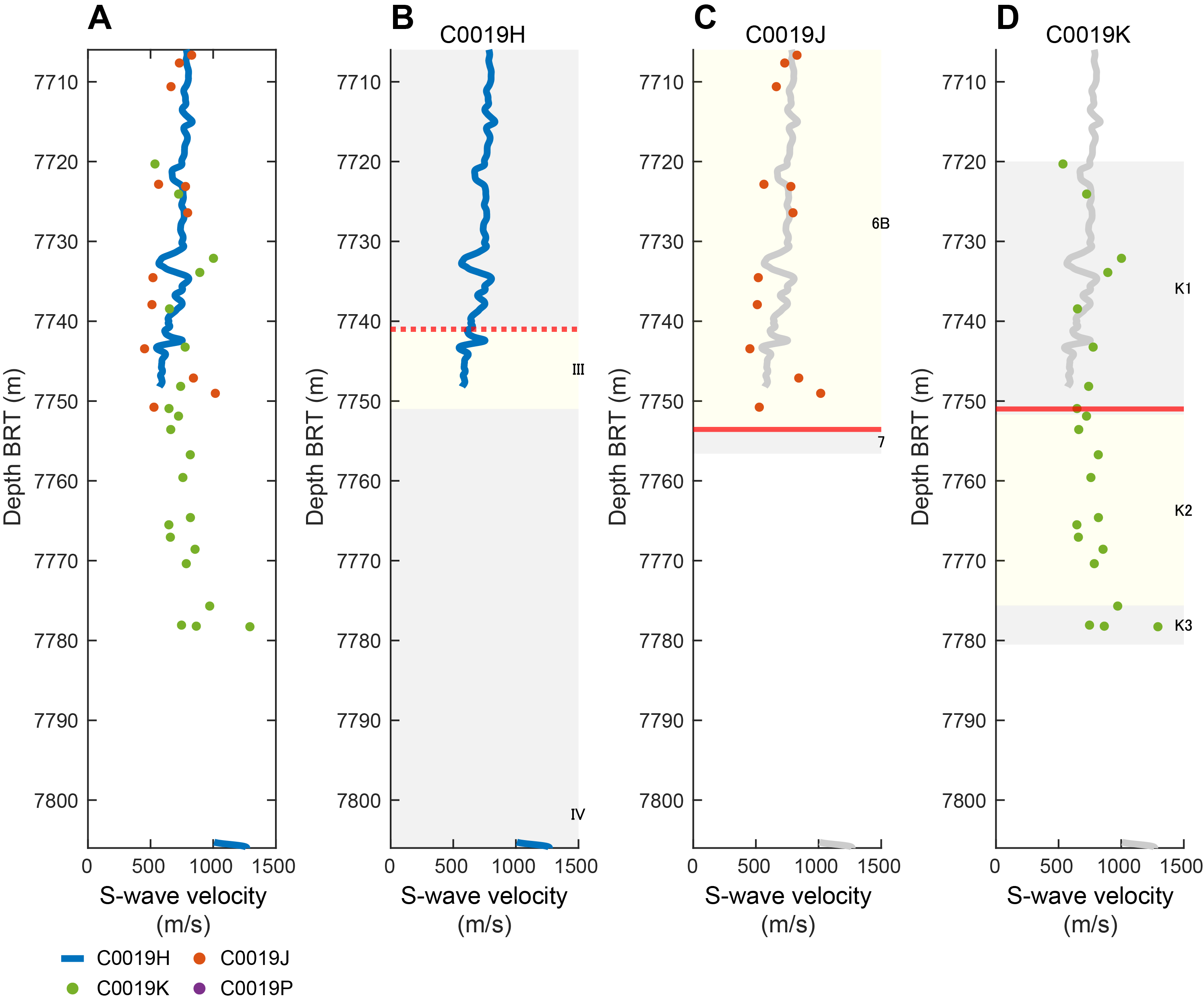
Figure F147. LWD S-wave velocity data from around the PBFZ and measured on discrete samples.

P-wave velocities above the PBFZ in Holes C0019J and C0019K are consistent with the values recorded by LWD but are more scattered. No discrete sample measurements were conducted below the PBFZ in Hole C0019J, but the measurements from Hole C0019K discrete samples demonstrate distinctly low P-wave velocities below the PBFZ. These low P-wave velocities are measured within Lithostratigraphic Unit K2, which is characterized by brownish black clay. Despite this, the P-wave velocity measured in chert with high velocity obtained from Lithostratigraphic Unit K3 in Hole C0019K exceeds 5000 m/s (Figures F148, F149). This indicates that the increase in P-wave velocity observed in Logging Unit IV defined based on the LWD data is likely attributable to the presence of chert within the formation.

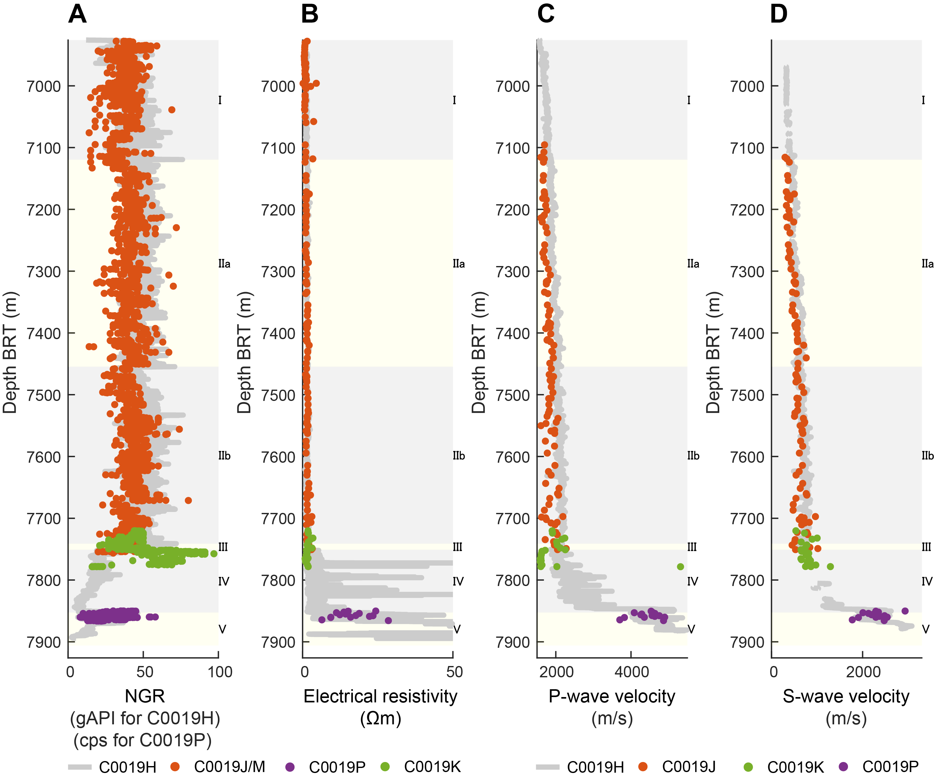
Figure F148. LWD gamma ray, electrical resistivity, P- and S-wave velocity curves and measured on core sections and discrete samples.

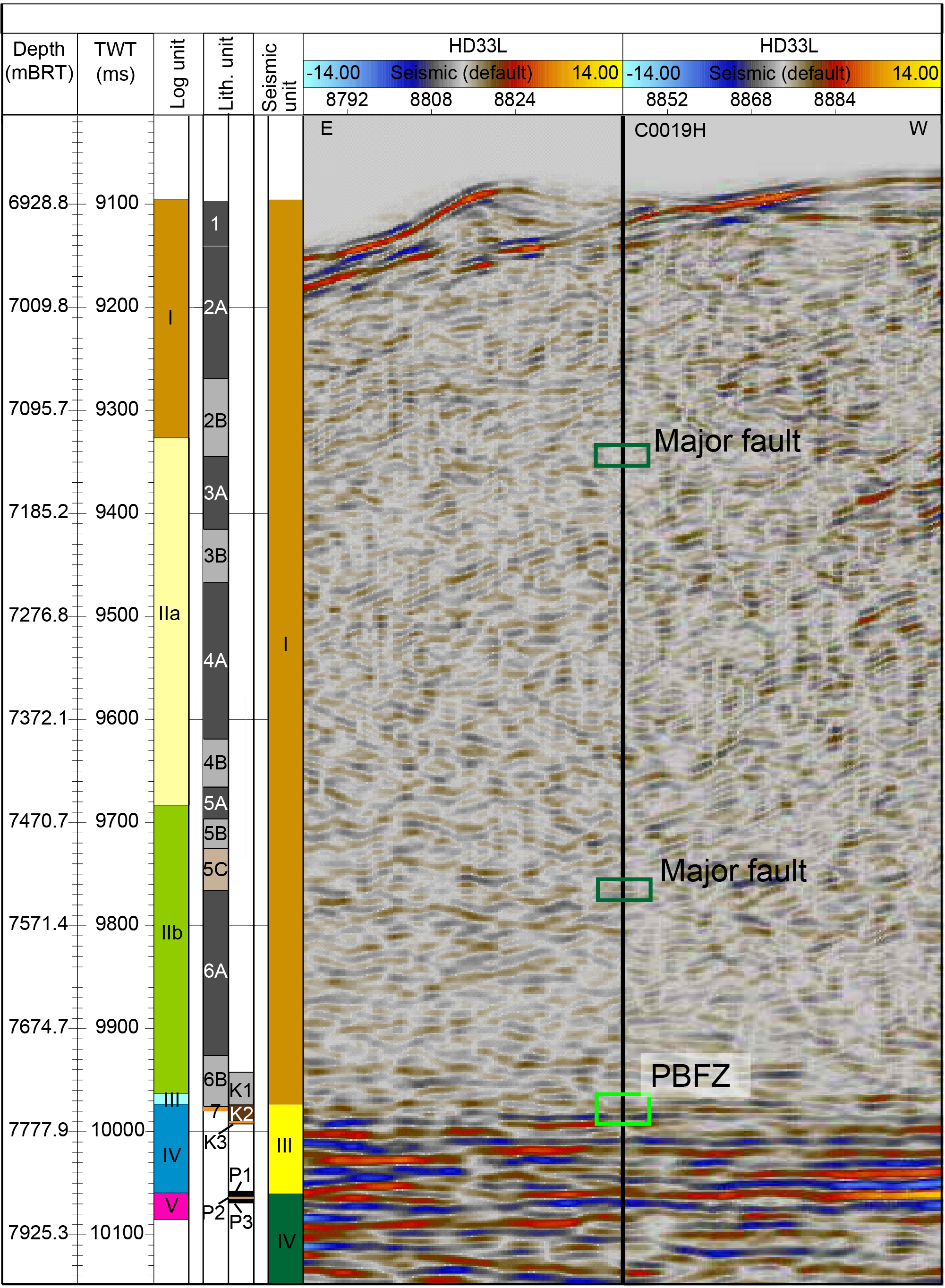
Figure F149. Log, lithostratigraphic, and seismic units.

LWD S-wave velocity data from Hole C0019H are only available down to the middle of Logging Unit III, situated just below the PBFZ, because of the low data quality in this interval (see Logging while drilling). In contrast, the Hole C0019J core sample measurements extend only to a depth just above the inferred PBFZ, making interhole comparisons difficult (Figure F147). Nevertheless, in the depth interval above the PBFZ, where S-wave velocity data were acquired in all three holes, the values across the three holes are consistent. The LWD data show a slight S-wave velocity spike just below the PBFZ, but similar localized variations in S-wave velocity are not captured in the discrete sample measurements from Hole C0019K.

12.2.2.4. Core-log structure comparison

The interpretation of the LWD resistivity images around the PBFZ, along with the distribution of bedding and fractures/faults as observed in the core samples, are presented in Figure F150. The position of the PBFZ is indicated by the colored lines and box in the figure, with the colors indicative of the respective borehole in which the fault was identified. The bedding exhibits a relatively high (>30°) dip angle, predominantly above the PBFZ, as observed in both the LWD and core data. In the LWD, west-dipping bedding is interpreted to occur between 7717 and 7730 m BRT. The bedding exhibits a sudden transition to a southerly dip in the vicinity of the fault, occurring near 7736 m BRT. The bedding measurements obtained from the core exhibit a southward trend to 7730 m BRT, which differs from the trend observed in the LWD. Subsequently, the bedding exhibits a divergent trend from that observed in the LWD, with fluctuations in both the azimuth and dip angle. In the vicinity of the PBFZ, both LWD and core data indicate a dip angle of less than 40° toward the east. A low-angle (<30°) west-trending bedding corresponding to the chert bedding plane was identified in the footwall of the PBFZ, near the top of Logging Unit IV. Fractures and faults were observed primarily in the core samples. The number of faults in the core samples increased from approximately 7650 m BRT toward the PBFZ (Figure F143), but their orientations were more dispersed than those of the bedding, and no clear trend could be identified. The lower part of the fault that straddles both fracture/fault exhibited minimal or no structures; most of the fractures in LWD and faults on core samples were found in the hanging wall side of PBFZ, and no comparable fracture or minor faults have been identified in the mud layer below the PBFZ in any of them. Note that the PBFZ identified in the LWD hole and the two coring holes are all at different depths (Figure F150).

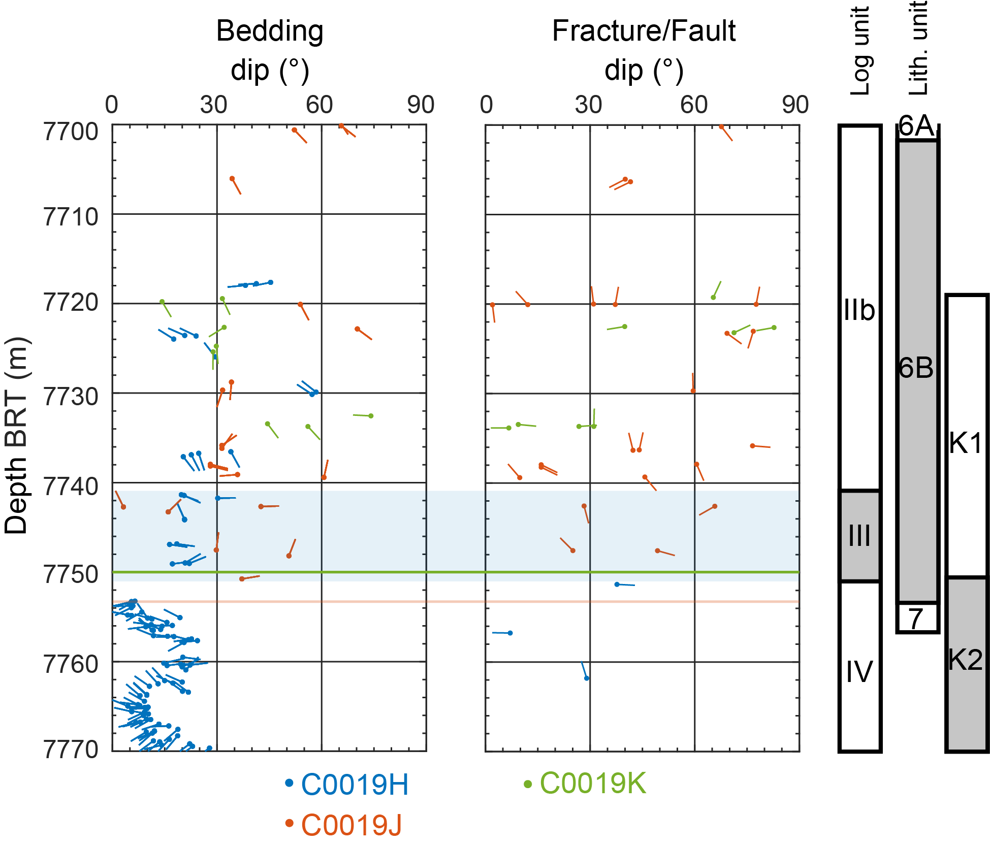
Figure F150. Bedding and fracture/fault orientations around the PBFZ.

12.2.3. Core-log integration around basalt

Hole C0019P passed through the PBFZ and targeted a coring interval within the subducting plate deeper than 7850 m BRT. This target interval was defined from the LWD logs, from which shipboard interpretations suggested the presence of intercalated basalt and chert (see Logging while drilling). Coring in Hole C0019P targeted these hard rocks, with successful recovery confirming the identification of the primary lithologies as basalt and chert. These hard rock lithologies are in contrast to the cores from Holes C0019J, C0019K, and C0019M, which primarily sampled sediments and sedimentary rocks. The Hole C0019P core physical properties and corresponding LWD data in Hole C0019H are therefore significantly different. In particular, the electrical resistivity, P-wave velocity, and S-wave velocity values in Hole C0019P are substantially higher than those observed in the shallower parts of Holes C0019J, C0019K, and C0019M. To appropriately capture the distinct characteristics of the physical properties in Hole C0019P, a new set of plots with adjusted scales was made (Figures F148 and F151). Lithostratigraphic units (P1, P2, and P3) were defined for the cores in Hole C0019P (see Lithostratigraphy). Furthermore, Logging Units IV and V and Subunits Va–Ve were defined based on LWD data from Hole C0019H (see Logging while drilling).

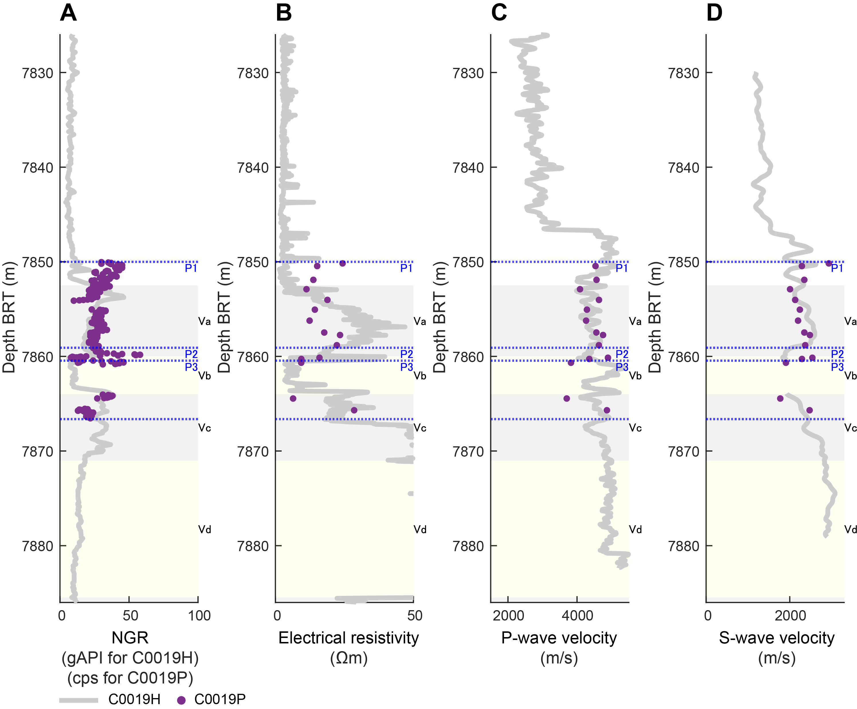
Figure F151. LWD gamma ray, electrical resistivity, P- and S-wave velocity curves and resistivity measured on discrete samples.

12.2.3.1. Natural gamma ray radiation

The NGR values in Hole C0019P are lower than those observed in Holes C0019J, C0019K, and C0019M (Figure F148A). However, the NGR patterns observed in Holes C0019H (LWD) and C0019P (COMET measurements) are consistent with each other (Figure F151A). For example, the NGR peak at the top of Logging Unit V in Hole C0019H (7853.8 m BRT) and the NGR peak at the top of Hole C0019P (Core 1K; 7850.38 m BRT) demonstrate a depth discrepancy of about 3 m, but both exhibit a decline with depth below the peak. The NGR patterns in Holes C0019H and C0019P align closely below the middle of Logging Subunit Va (~7855 m BRT) to the bottom of the Lithostratigraphic Unit P1 (7859.1 m BRT). Notably, both data sets exhibit a spike in NGR values in the interval of Lithostratigraphic Unit P2, which contains limestone, chert, and siliceous mudstone. The boundary between Lithostratigraphic Units P2 and P3 and Logging Subunits Va and Vb (~7859 m BRT) coincides, and below this boundary is a transition to lower NGR levels. A comparable pattern of high NGR values transitioning to lower levels is evident at the bottom of Unit P3 within Logging Subunit Vc (~7864 m BRT) in both Holes C0019H and C0019P. These positive spikes in NGR values from COMET measurement on core samples were measured in altered basaltic sections that are in contact with the cherts and associated sediments (see Physical properties).

12.2.3.2. Electrical resistivity

The electrical resistivity measured from discrete samples in Hole C0019P is markedly higher than measured at shallower depths in Holes C0019J, C0019K, and C0019M, but comparably high values were obtained by LWD at similar depth intervals in Hole C0019H (Figure F148B). The discontinuous nature of discrete sampling makes direct comparison with the trends observed in the continuous LWD data challenging. However, the discrete data are consistent with LWD data (Figure F151B). For example, at the depth corresponding to a sharp drop in resistivity within Lithostratigraphic Unit P2 and at the top of Logging Subunit Vb (~7860 m BRT), the discrete sample measurements also record a decrease in resistivity. Below this, the stepwise increase in LWD resistivity is also reflected in the discrete sample data. These examples indicate good agreement between the discrete and LWD measurements.

12.2.3.3. P-wave and S-wave velocities

The P-wave and S-wave velocities measured from discrete samples in Hole C0019P are significantly higher than those measured at shallower depths in Holes C0019J, C0019K, and C0019M but are generally in good agreement with the values obtained through LWD in the same depth intervals (Figure F148C, F148D). It is noteworthy that both P-wave and S-wave velocities show strong consistency between LWD and discrete sample results within Lithostratigraphic Units P1 and P2 and Logging Subunit Va. Furthermore, the observed decrease in LWD S-wave velocity in Unit P2, which coincides with Logging Subunit Va and the top of Subunit Vb, is accompanied by a similar reduction in S-wave velocity measured from discrete samples.

12.2.3.4. Core-log structure comparison

Structures or other features within the basalts of Logging Unit V were mainly identified from LWD resistivity images, and mineral-filled veins were identified as the predominant type of structures in the cores (Figure F152). It should be noted that no paleomagnetic azimuthal rotation of the structures identified in the core samples has been carried out; therefore, only dip angles are shown. In the coring interval (7850–7867 mbsf), mineral veins display some high-angle dip, though they are predominantly observed to be less than 30° horizontal. One subvertical injection structure has been identified at the top of this interval. In the vicinity of this injection structure, pillow basalt is interpreted as being characterized by the curved occurrence of a glassy pillow rim. Discrete structures were rarely identified in the LWD, so it is challenging to discuss their correspondence with the core. However, the majority of basalt features identified in LWD are also structures that dip less than 30° below 7870 m BRT, which may indicate some relationship with mineral veins. The lower logging section (Subunits Vd and Ve) (see Logging while drilling) display the presence of vertical meter-scale fractures, suggesting the possibility of contrasting with vertical injection structures observed in pillow basalt in cores, although at distinguishably different observation depths.

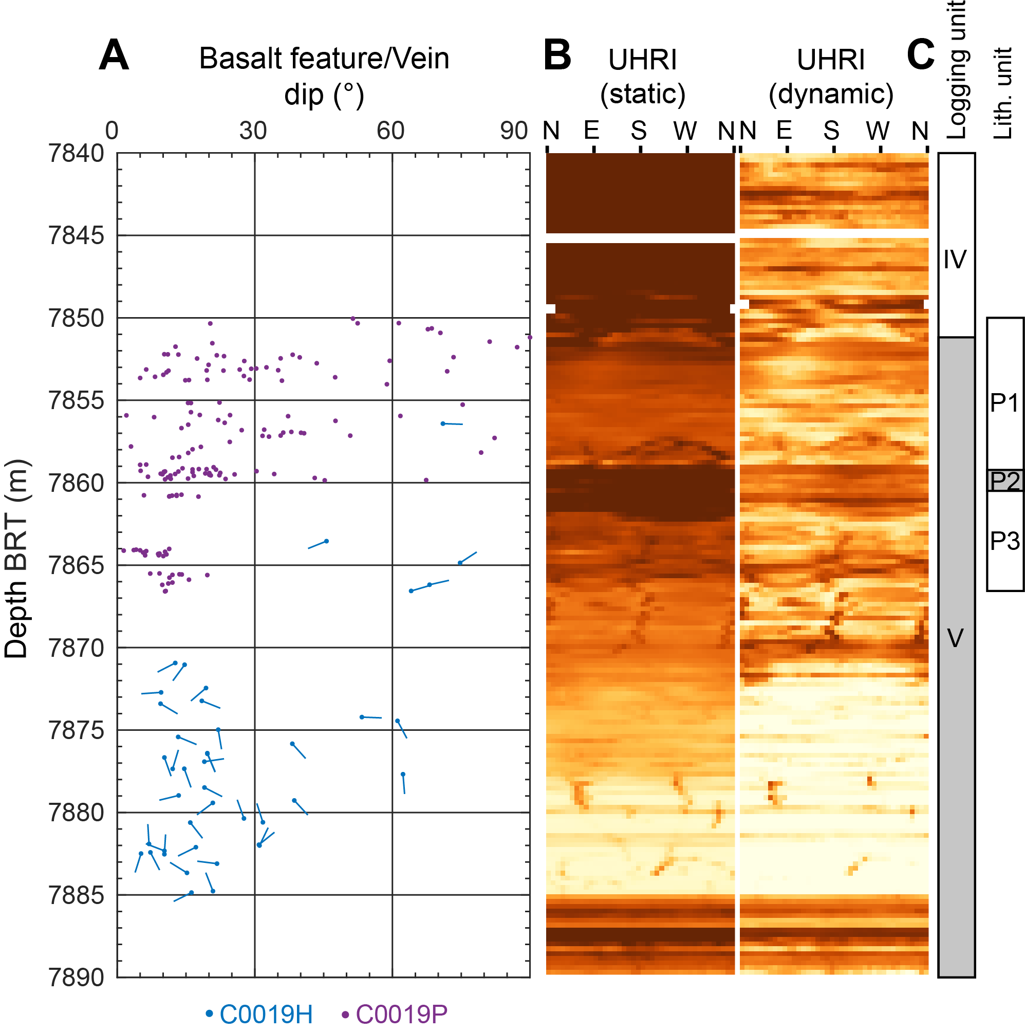
Figure F152. Structures in intervals interpreted as basalt on the underthrust plate.

12.3. Overall core-log-seismic integration

Figures F149 and F153 show logging units, lithostratigraphic units, and seismic units along with the time-domain seismic profiles around the site. Note that the depth of the units was time-converted with the time-depth relationship obtained through the seismic-well ties.

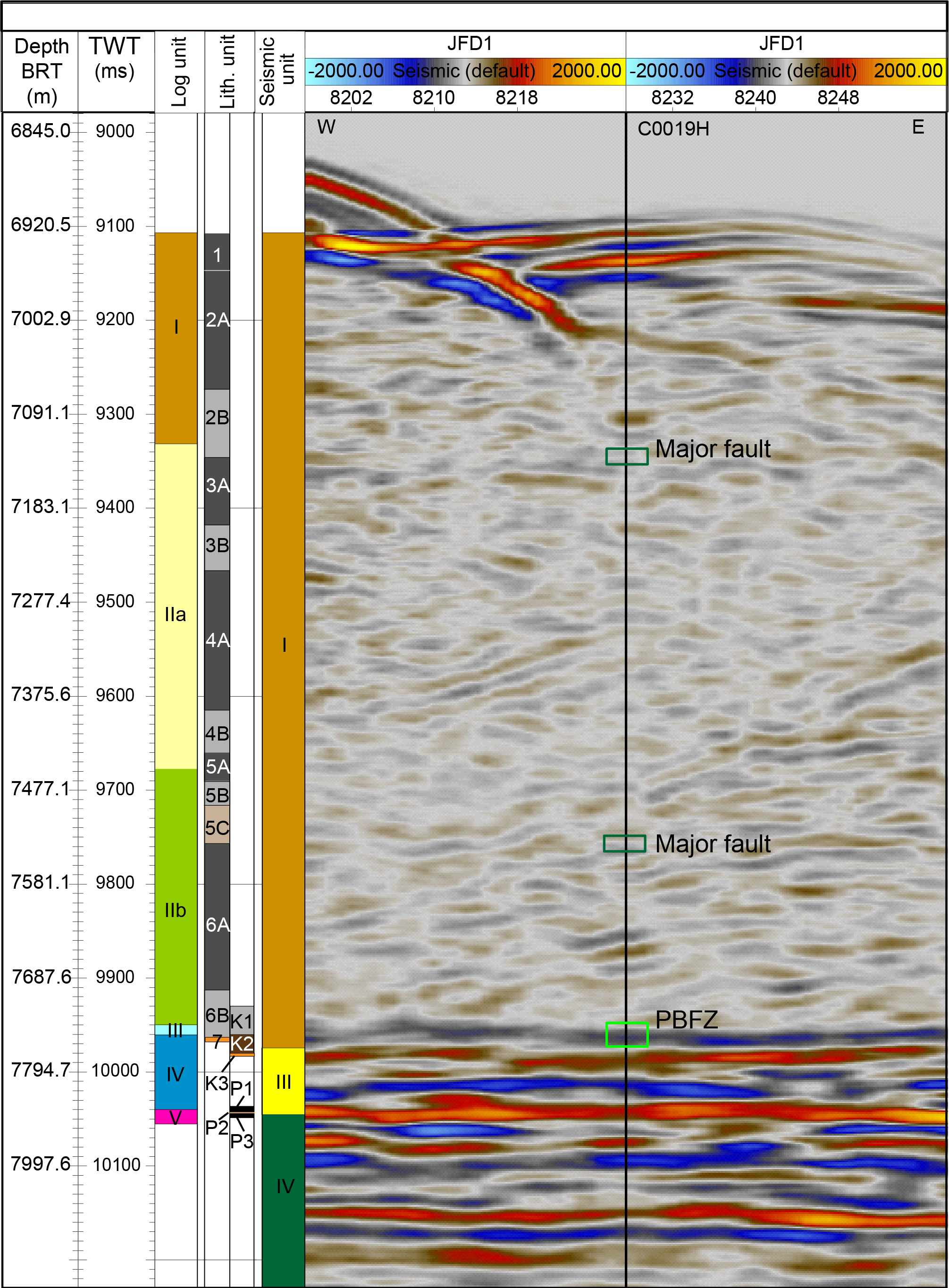
Figure F153. Log, lithostratigraphic, and seismic units and Seismic Profile JFD1.

Overall, there is good correspondence between the interpretation of the seismic profile, the logging data, and the observations of the core. Seismic Unit 1, interpreted as the hanging wall sediments, corresponds to Logging Units I–III and Lithostratigraphic Units 1–6. Seismic Units III and IV correspond to Logging Units IV and V, respectively. Given the depth difference between Holes C0019H and C0019J as mentioned in Core-log integration, Lithostratigraphic Units 1 and 2 are likely to correspond to Logging Unit I. Lithostratigraphic Units 3–6 correspond to Logging Unit II. Although the boundary between Logging Subunits IIa and IIb in Hole C0019H is characterized by a distinct step decrease in NGR values, no corresponding lithostratigraphic unit boundary has been identified based on core observations (see Core-log integration in the frontal prism). Therefore, it is difficult to establish a clear one-to-one correspondence between Logging Subunits IIa and IIb and individual lithostratigraphic units. Logging Unit III corresponds to Lithostratigraphic Unit 7.

Figures F149 and F153 also show the locations of the major faults and the PBFZ and the lithostratigraphic and logging units identified from the core samples and LWD resistivity images. Although the boundaries of the lithostratigraphic and logging units in the upper prism and the major faults coincide with the high-angle reflectors, it is difficult to identify clear, continuous reflectors. On the other hand, the PBFZ identified by the LWD and the core are both consistent with the subhorizontal reflection on the seismic section. The location of the PBFZ also shows good agreement with the boundary of the seismic unit.

A clear decrease in the elastic wave velocities (discrete sample and COMET measurements) was observed in the core sample on the footwall side of the PBFZ (7751 m BRT; Hole C0019K). This corresponds to the step-down in sonic velocity at the PBFZ in Hole C0019H (7741 m BRT) and the negative seismic reflection with ~9965 ms of the Seismic Profile JFD1 around Site C0019, regardless of the different scales of the core, LWD, and seismic measurements. The negative reflection corresponding to the PBFZ could be caused by the combination of low V_P in the PBFZ and high V_P below the PBFZ. However, in light of the depth of the PBFZ and the thickness distribution of the clay layer below it identified in the core sample, in situ physical properties measured by LWD, and the continuity of the structure in the seismic reflection image, it is proposed that the PBFZ, or the deformed and underthrusting clay, has a low elastic wave velocity and displays heterogeneity in the thickness direction, as well as lateral continuity.

In addition, the location of the basalt top is clearly observed as a boundary in the core (Hole C0019P), LWD data, and seismic reflection. Both the PBFZ and the basalt top show subtle undulations at tens of meters intervals in the reflection cross section. This may account for differences in structural depth between holes.

References