Kodaira, S., Conin, M., Fulton, P., Kirkpatrick, J., Regalla, C., Ujiie, K., Okutsu, N., Maeda, L., Toczko, S., Eguchi, N., and the Expedition 405 Scientists
Proceedings of the International Ocean Discovery Program Volume 405
publications.iodp.org
https://doi.org/10.14379/iodp.proc.405.102.2025
Expedition 405 methods1
![]() J. Kirkpatrick,
J. Kirkpatrick,
![]() P. Fulton,
P. Fulton,
![]() K. Ujiie,
K. Ujiie,
![]() M. Conin,
M. Conin,
![]() C. Regalla,
C. Regalla,
![]() S. Kodaira,
S. Kodaira,
![]() N. Okutsu,
N. Okutsu,
![]() L. Maeda,
L. Maeda,
![]() S. Toczko,
S. Toczko,
![]() N. Eguchi,
N. Eguchi,
![]() P. Bellanova,
P. Bellanova,
![]() C. Brown,
C. Brown,
![]() M. Brunet,
M. Brunet,
![]() M. Castillo,
M. Castillo,
![]() Y.-C. Chang,
Y.-C. Chang,
![]() M.-L. Doan,
M.-L. Doan,
![]() J. Everard,
J. Everard,
![]() A. Fintel,
A. Fintel,
![]() J. Ford,
J. Ford,
![]() R. Fukuchi,
R. Fukuchi,
![]() A. Gough,
A. Gough,
![]() H. Guo,
H. Guo,
![]() D. Gürer,
D. Gürer,
![]() R. Hackney,
R. Hackney,
![]() M. Hagino,
M. Hagino,
![]() Y. Hamada,
Y. Hamada,
![]() H. Hosono,
H. Hosono,
![]() A. Ijiri,
A. Ijiri,
![]() M. Ikari,
M. Ikari,
![]() T. Ishikawa,
T. Ishikawa,
![]() M. Iwai,
M. Iwai,
![]() T. Jeppson,
T. Jeppson,
![]() M.-J. Jurado,
M.-J. Jurado,
![]() N. Kamiya,
N. Kamiya,
![]() T. Kanamatsu,
T. Kanamatsu,
![]() A. LaPlante,
A. LaPlante,
![]() W. Lin,
W. Lin,
![]() A. Miyakawa,
A. Miyakawa,
![]() Y. Morono,
Y. Morono,
![]() Y. Nakamura,
Y. Nakamura,
![]() U. Nicholson,
U. Nicholson,
![]() H. Okuda,
H. Okuda,
![]() P. Pei,
P. Pei,
![]() C. Pizer,
C. Pizer,
![]() T. Rasbury,
T. Rasbury,
![]() R.V.M. Robertson,
R.V.M. Robertson,
![]() C. Ross,
C. Ross,
![]() S. Satolli,
S. Satolli,
![]() H. Savage,
H. Savage,
![]() K. Schaible,
K. Schaible,
![]() S. Shreedharan,
S. Shreedharan,
![]() H. Sone,
H. Sone,
![]() C. Sun,
C. Turel,
C. Sun,
C. Turel,
![]() T. Uchida,
T. Uchida,
![]() A. Yamaguchi,
A. Yamaguchi,
![]() Y. Yamamoto,
Y. Yamamoto,
![]() T. Yoshimoto,
T. Yoshimoto,
![]() J. Zhang,
A. Wspanialy,
J. Zhang,
A. Wspanialy,
![]() E. Le Ber,
E. Le Ber,
![]() M.B. Rydzy, and
N. Schuba2
M.B. Rydzy, and
N. Schuba2
1 Kirkpatrick, J., Fulton, P., Ujiie, K., Conin, M., Regalla, C., Kodaira, S., Okutsu, N., Maeda, L., Toczko, S., Eguchi, N., Bellanova, P., Brown, C., Brunet, M., Castillo, M., Chang, Y.-C., Doan, M.-L., Everard, J., Fintel, A., Ford, J., Fukuchi, R., Gough, A., Guo, H., Gürer, D., Hackney, R., Hagino, M., Hamada, Y., Hosono, H., Ijiri, A., Ikari, M., Ishikawa, T., Iwai, M., Jeppson, T., Jurado, M.-J., Kamiya, N., Kanamatsu, T., LaPlante, A., Lin, W., Miyakawa, A., Morono, Y., Nakamura, Y., Nicholson, U., Okuda, H., Pei, P., Pizer, C., Rasbury, T., Robertson, R.V.M., Ross, C., Satolli, S., Savage, H., Schaible, K., Shreedharan, S., Sone, H., Sun, C., Turel, C., Uchida, T., Yamaguchi, A., Yamamoto, Y., Yoshimoto, T., Zhang, J., Wspanialy, A., Le Ber, E., Rydzy, M.B., and Schuba, N., 2025. Expedition 405 methods. In Kodaira, S., Conin, M., Fulton, P., Kirkpatrick, J., Regalla, C., Ujiie, K., Okutsu, N., Maeda, L., Toczko, S., Eguchi, N., and the Expedition 405 Scientists, Tracking Tsunamigenic Slip Across the Japan Trench (JTRACK). Proceedings of the International Ocean Discovery Program, 405: College Station, TX (International Ocean Discovery Program). https://doi.org/10.14379/iodp.proc.405.102.2025
2 Expedition 405 Scientists’ affiliations.
1. Introduction
This chapter documents the methods used for shipboard measurements and analyses during International Ocean Discovery Program (IODP) Expedition 405, Tracking Tsunamigenic Slip Across the Japan Trench (JTRACK). We conducted riserless operations at Sites C0019 and C0026 (Table T1). Two temperature sensor observatories were installed at Site C0019. Logging while drilling and coring were performed at Sites C0019 and C0026. Methods for postexpedition research conducted on Expedition 405 samples and data will be described in individual scientific contributions published after the expedition.
All shipboard scientists contributed to the completion of this volume. Because of the long length of Expedition 405 (106 days, 6 September–20 December 2024), staffing was staggered. The shipboard science party was divided into two science party staffing windows. Window 1 included 26 scientists (6 September–30 October), and Window 2 included 25 scientists (25 October–21 December). The Window 1 to Window 2 handover occurred during a 6 day crossover period with staggered onboarding and offboarding. Six Co-Chief Scientists served in overlapping shifts of two or three at a time, and at least one Expedition Project Manager was on board at all times.
1.1. Numbering of sites, holes, cores, sections, and samples
Sites drilled by the drilling vessel (D/V) Chikyu are numbered consecutively from the first site with a prefix “C.” A site refers to one or more holes drilled while the ship is positioned within 300 m of the first hole, and a letter suffix distinguishes each hole drilled at the same site. The first hole drilled at a given site is assigned the site number modified by the suffix “A,” the second hole takes the site number and the suffix “B,” and so forth (Figure F1). To avoid confusion with numbers and letters, I and O are not used as hole letter suffixes. Hole suffixes are assigned regardless of recovery as long as penetration takes place. Note that during Expedition 405, Chikyu returned to Site C0019, which was previously drilled during Integrated Ocean Drilling Program Expedition 343, Japan Trench Fast Drilling Project (JFAST). Therefore, the hole assignments for Expedition 405 begin with C0019F, which continues from the last hole (C0019E) drilled during Expedition 343.
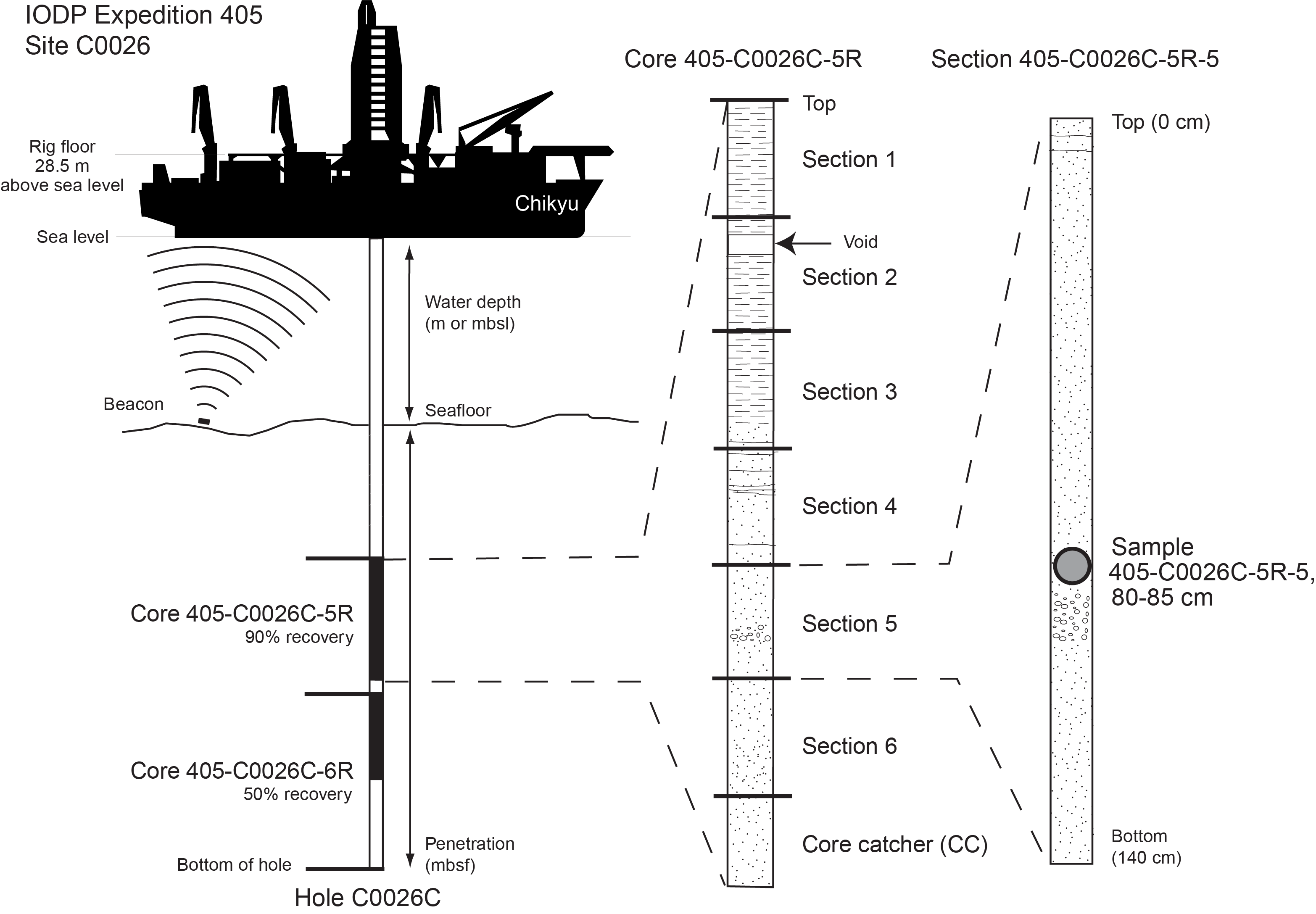
Figure F1. IODP convention for naming sites, holes, cores, and samples.
Cores taken from a hole are numbered sequentially from the top of the hole downward. Core numbers and their associated cored intervals are unique in a given hole (Figure F1). The core number is followed by a letter suffix that indicates the type of coring system. The coring systems used during Expedition 405 are as follows:
- A hydraulic piston coring system (HPCS; core type = H). This system is equivalent to the advanced piston corer (APC) system used on the research vessel (R/V) JOIDES Resolution.
- An extended shoe coring system (ESCS; core type = X). This system is equivalent to the extended core barrel (XCB) system used on JOIDES Resolution.
- A small diameter rotary core barrel (SD-RCB) system (core type = K). This system was newly developed for use on Chikyu during Expedition 405.
The cored interval is measured in meters below seafloor according to depth determinations described in IODP Depth Scales Terminology (https://www.iodp.org/policies-and-guidelines). This depth scale is equivalent to the Ocean Drilling Program (ODP) meters below seafloor (mbsf) depth scale. In general, depth below seafloor is determined by subtracting the water depth estimated from the initial drill pipe measurement to the seafloor from the total drill pipe measurement. The depth interval assigned to an individual core begins with the depth below seafloor at which coring began and extends to the depth through which coring advanced. For some measurements, depths are reported in meters below rig table (m BRT), such as logging-while-drilling (LWD) data and major faults or lithologic boundaries. This was done to provide a common datum for depth correlations between cores, log, and seismic data, which was necessary where the seafloor was not flat. The rig table on Chikyu is 28.5 m above sea level.
Core depths and recoveries are calculated based on the total advance and recovered core length. For each core, recovery is typically calculated based on a 9.5 m advance, which corresponds to the standard core barrel length for each coring system. However, some Expedition 405 SD-RCB cores had short advances of ~3–5 m to promote core recovery in key intervals. Short advances were applied in the ~20 m above and below the plate boundary to the top of the chert at Site C0019 and in the pelagic clay to chert interval at Site C0026. In addition, HPCS cores may have advances less than 9.5 m if there is partial penetration of the core barrel. Partial penetration of the HPCS core barrel is generally detectable while coring by measuring the pressure drop in the hydraulic system that powers the piston core. Partial pressure drop and gradual release of pressure are used to calculate the estimated penetration depth in these cases. Total recovery may be less than 100% if there are gaps due to nonrecovered material. Total recovery may be greater than 100% if there is core expansion or sucked-in materials, which can be especially prevalent in shallow HPCS cores. Core depths are converted to the core depth below seafloor, Method A (CSF-A), scale, in which overlapping sections are compressed when recovery is >100%. Short cores (incomplete recovery) are all assumed to start from the initial depth of the advance for that core by convention.
A recovered core is typically divided into ~1.4 m long sections that are numbered sequentially from 1, beginning at the top. Section length varies from core to core because the locations for cutting sections are chosen to avoid intervals of scientific interest. Material recovered from the core catcher is assigned to a separate section, labeled core catcher (CC), and placed at the bottom of the lowermost section of the recovered core.
A full identification number for a sample from a core section consists of the following information: expedition, site, hole, core number, core type, section number, and top to bottom interval in centimeters measured from the top of the section. For example, a sample identification of “405-C0026C-6K-5, 80–85 cm,” represents a sample removed from the interval between 80 and 85 cm below the top of Section 5 of the sixth core taken with the SD-RCB from Hole C0026C during Expedition 405 (Figure F1). In this report, sample depths are reported to the nearest 0.5 cm when using full identification numbers. Sample or interval depths reported on the mbsf, meters below sea level (mbsl), or m BRT scales are rounded to the nearest centimeter.
1.2. Core handling
The following sections describe the flow of core from the drill floor through the laboratory. Core handling during Expedition 405 followed the general core flow procedure implemented during recent IODP expeditions on Chikyu but was optimized to process and store the samples properly for the scientific objectives of the expedition. The specific core flow for this expedition is illustrated in Figure F2.
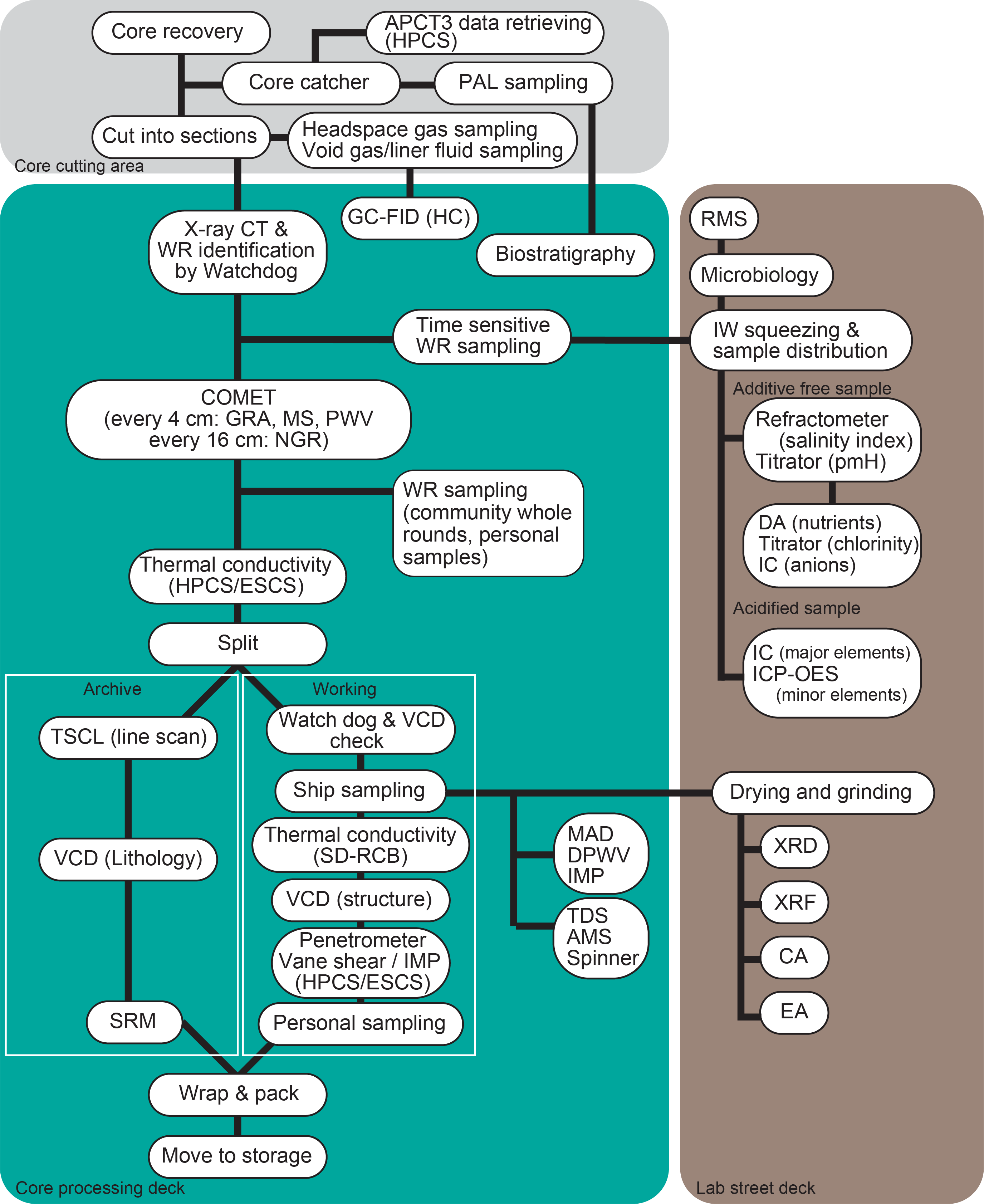
Figure F2. Core processing and measurement flow.
1.2.1. Core cutting area
As soon as a core was retrieved on deck, the core catcher was delivered to the core cutting area. A ~5 cm whole round was taken for micropaleontological analysis, and the remainder of the core catcher sample was packed into a core liner and entered into the general core flow. The core was then transferred to the core cutting area. The recovered core length and the total length of void space were then measured and entered into the J-CORES database, along with core identification information, drilling advance, recovery, and depth information. Void space gas samples were collected if appropriate sample locations were identified. The core was cut into sequentially numbered ~1.4 m long sections. Two small (5 cm3) plugs of sediment were immediately removed from the bottom of appropriate core sections for headspace gas analysis, typically from the base of the first section. In addition, samples of the liner fluid, where present, were collected for geochemical analysis. Each section was then sealed at the top (blue cap and blue tape) and bottom (clear cap and white tape). All sections were marked and labeled, and sections were moved to the core processing deck.
For hard rock cores (405-C0019P-1K through 5K), core flow in the core cutting area was modified. If recovered materials were discontinuous pieces, each piece was extracted from the core liner in the core cutting area, pieces were then pushed to the bottom of the 1.4 m liner sections, and the total rock length was measured. Pieces were subsequently put into split plastic liners in consecutive order. Each piece of core was marked on the bottom with a red wax pencil to preserve orientation through the subsequent core flow. Broken pieces that could be fit together along fractures were curated as single pieces. A watchdog assigned from the structural geology and/or sedimentology visual core description team confirmed piece matches. The split line, which defined how the pieces were to be cut into two equal halves, was marked on all pieces, with a continuous line applied across broken pieces that were fit back together as single pieces. The working half was labeled with the letter “W,” and the archive half was labeled with the letter “A.” For the archive half, a plastic spacer was welded with an ultrasonic welding machine to the split core liner between individual pieces or reconstructed contiguous groups of subpieces. These spacers may represent substantial intervals of no recovery. The length of each section of core, including spacers, was entered into the database as “curated length.”
1.2.2. Core processing deck
All sections except for Section 405-C0019J-4K-1 and Cores 5K–10K were scanned using the X-ray computed tomography (XCT) scanner (GE Healthcare Discovery 750HG) (see Structural geology). For Section 4K-1 and Cores 5K–10K, XCT imaging was only performed on the split section (archive half) and whole-round core samples because of a temporary malfunction of the XCT scanner.
Each shift had a structural geologist acting as a watchdog to oversee the collection and selection of whole-round core samples to identify sections or intervals of special interest or unique characteristics that should be avoided for whole-round sampling to prevent destruction of any critical samples. For sections of sedimentologic interest, a sedimentology computed tomography (CT) watchdog helped approve samples.
Following XCT scanning and time-sensitive whole-round core sampling, core sections were allowed to equilibrate to ambient laboratory temperature (2–3 h; ~20°C), after which they were run through the Core Measurement Track (COMET; NS Design) (see Physical properties) to measure gamma ray attenuation (GRA) bulk density, P-wave velocity, magnetic susceptibility (MS), and natural gamma radiation (NGR). Thermal conductivity (TeKa TK04) measurements were also made on whole-round core sections for soft-sediment cores. After COMET and thermal conductivity (soft-sediment) measurements, non-time-sensitive whole-round core samples were taken based on examination of the XCT images. Cut section ends were sealed with a yellow cap to indicate removed whole-round core samples.
After completion of all the above measurements and sampling on whole-round cores, the core sections were split axially into working and archive halves. The archive half was subject to lithologic visual core description and smear slide analysis, nondestructive measurements/observation such as digital photo image scanning, and superconducting rock magnetometer (SRM) measurements. Following these analyses, the archive half was covered in plastic film, shrink-wrapped in plastic, and stored at ~4°C until needed for further analysis. The working half was subjected to structural analysis, shipboard sampling (physical properties [PP], paleomagnetism [PMAG], and X-ray diffraction [XRD]/X-ray fluorescence [XRF]/carbonate [CARB] analyses) and measurements (e.g., impedance analyzer, vane shear strength, and anisotropy of magnetic susceptibility [AMS]), and then sampled for postexpedition research. Following completion of sampling, the working half was also wrapped, sealed, and stored at ~4°C in preparation for shipping to the Kochi Core Center (KCC) in Kochi, Japan. All samples collected are labeled, packaged, stored, and shipped to their final destinations according to standard practice.
2. Logging while drilling
During Expedition 405, the LWD/measurement-while-drilling (MWD) assembly deployed a combination of three Schlumberger (SLB) logging tools in the following order (from bottom to top): MicroScope HD 675, TeleScope 675, and SonicScope 675. The sections of the bottom-hole assembly (BHA) that include the tools and their respective measurement offsets from the drill bit are illustrated in Figure F3. More details about the location of the sensors are given in Table T2, and the resolution of the measurements are given in Table T3. The tool string collar outer diameter was 6¾ inches (17.526 cm), and it was powered solely by a mud turbine located in the TeleScope 675. Because the tools had no batteries, data collection required fluid circulation greater than 400 gal/min through the TeleScope 675 turbine to power all three tools and send (real-time [RT]) and record (recorded mode [RM]) data. All recorded gamma ray and resistivity and sonic data were stored in the tool memory of the MicroScope and SonicScope, respectively. A lower resolution subset of the data was transmitted to the surface in real time through mud-pulse telemetry. The RT data set also contained a subset of surface drilling parameters (e.g., rate of penetration [ROP], weight on bit, rotations per minute, and torque) that were used for drilling performance monitoring and data quality assessment and control (QA/QC). The memory data were retrieved after recovering the BHA to the surface.
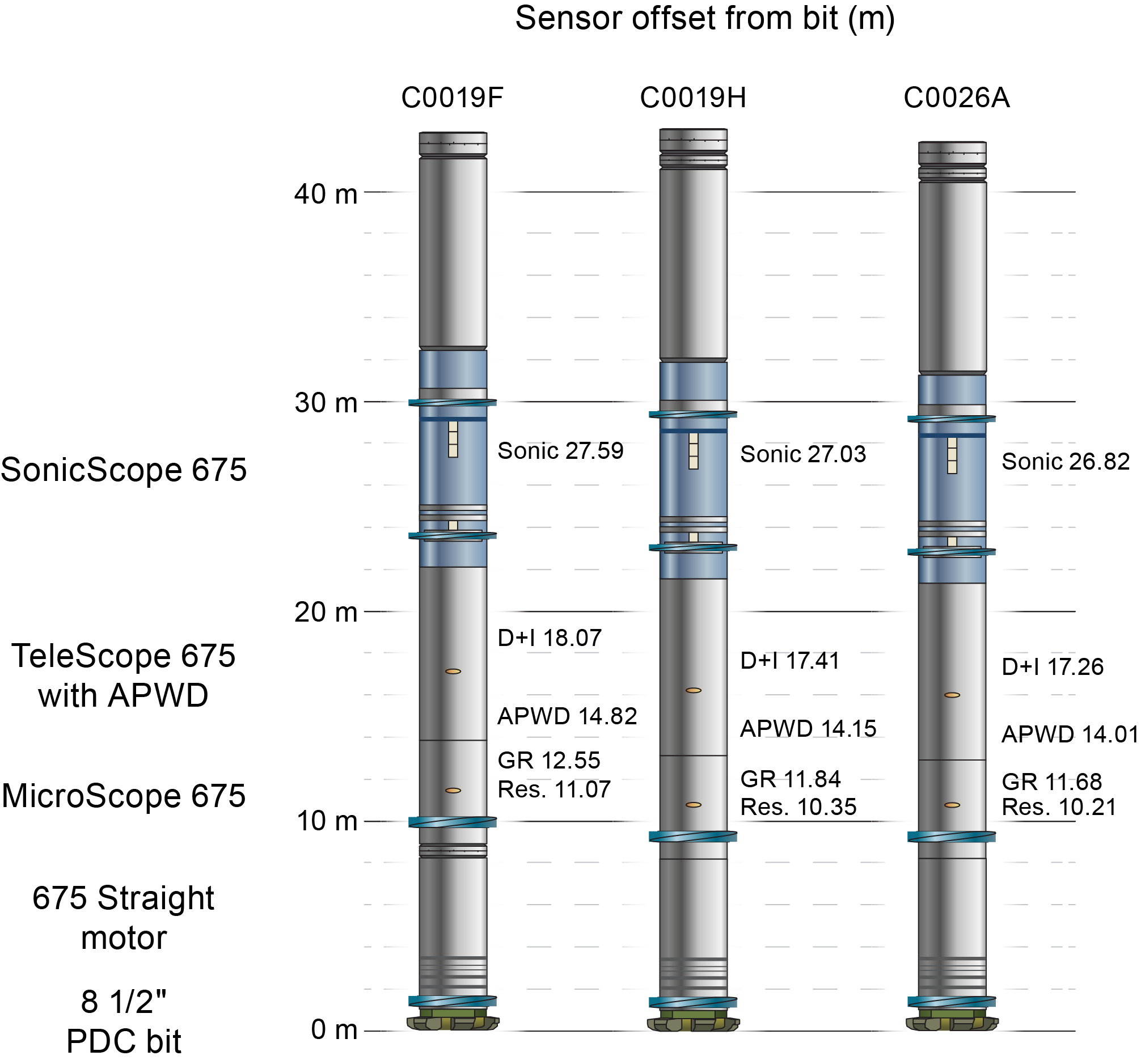
Figure F3. LWD BHA.
2.1. LWD/MWD acquisition systems and tools
2.1.1. Depth tracking system
LWD/MWD data are recorded as a function of time. The tool clock is synchronized with the clock inside the SLB Maxwell data acquisition system on board. The Maxwell system is used to communicate with and receive data from the tools downhole using continuous mud-pulse telemetry while fluid circulation greater than 400 gal/min is sustained. In addition, the Maxwell system allows the SLB field engineers to track and monitor depth using a geolograph in combination with the rig’s depth tracking system (utilizing the position of the traveling block from the drill floor, known length of the cable on the drawworks, and known length of the drill pipe). The time-depth correlation created in the Maxwell system can then be used to convert the data timestamps into depth.
For RT data transmission, different configurations were programmed by SLB because the quality and transmission rate of the signal (and its demodulation) received through mud-pulse telemetry can be altered as depth increases. Either MicroScope HD ultrahigh-resolution images (UHRIs) or SonicScope 675 data were to be removed from RT downhole data transmission in case of poor mud-pulse telemetry signal. Tools were set to record data (RM) at three different rates depending on operations. The primary data recording rate was every 10 s, and it decreased to 15 s when drilling progression was slower in harder formation. For the relogged section (Hole C0019H), the rate was set to 1 s.
2.1.2. MicroScope HD 675
The MicroScope HD 675 was positioned above the drill bit and mud motor (and in the case of Hole C0019F, a float sub) (Figure F3). Total gamma ray and formation resistivity logs, as well as high-resolution resistivity images, were acquired with the MicroScope HD.
2.1.2.1. Gamma ray
The azimuthal gamma ray tool measures the total background gamma radiation emitted from radioactive elements in the formation. The gamma ray detector is located toward the top of the MicroScope HD (Table T2) and measures the average value of incoming gamma rays across four quadrants (up/down and left/right) in the formation as the tool rotates. The depth of investigation of the logging tool is relatively shallow (often <50 cm) and depends on formation mineralogy. The gamma ray measurements are also impacted by the borehole size, drilling fluid, and tool design. The gamma ray values are delivered in American Petroleum Institute gamma radiation units (gAPI). The axial resolution of the gamma ray tool is 10 inches (25.4 cm), and its measurement accuracy is listed as 5%.
2.1.2.2. Resistivity
The MicroScope HD contains two button electrodes placed 180° apart with three unequally spaced toroid electrodes above and two below (Figure F4). Using different configurations between buttons and toroids (that can also be used as transmitters and receivers), the MicroScope HD generates focused currents and acquires resistivities at seven different depths in the formation: button resistivity (shallow [1.5 inches; 38.1 mm], medium [3 inches; 76.2 mm], deep [5 inches; 126 mm], and extra deep [7 inches; 177.8 mm]), toroid resistivity (deep [5 inches; 126 mm] and extra deep [7 inches; 177.8 mm]), and bit resistivity (30 inches; 762 mm). For the button resistivity measurements, the buttons act as measurement electrodes, two toroids act as transmitters (radial current), and one or two toroids act as monitors (axial current through the tool). For the toroid resistivity measurements, toroids can serve as transmitter, monitor, or measurement electrodes depending on the depth of investigation targeted. When measuring bit resistivity, the closest toroid to the bit induces an axial current that travels down the tool. The current exits at the bit and returns to the second closest electrode to the bit. The geometry of the borehole assembly is taken into account to compute the geometrical factor of the bit resistivity measurement. For more details about the tool measurement principles, refer to Allouche et al. (2010). Resistivity curves were used by SLB to calculate an estimate of the borehole diameter (e-caliper).
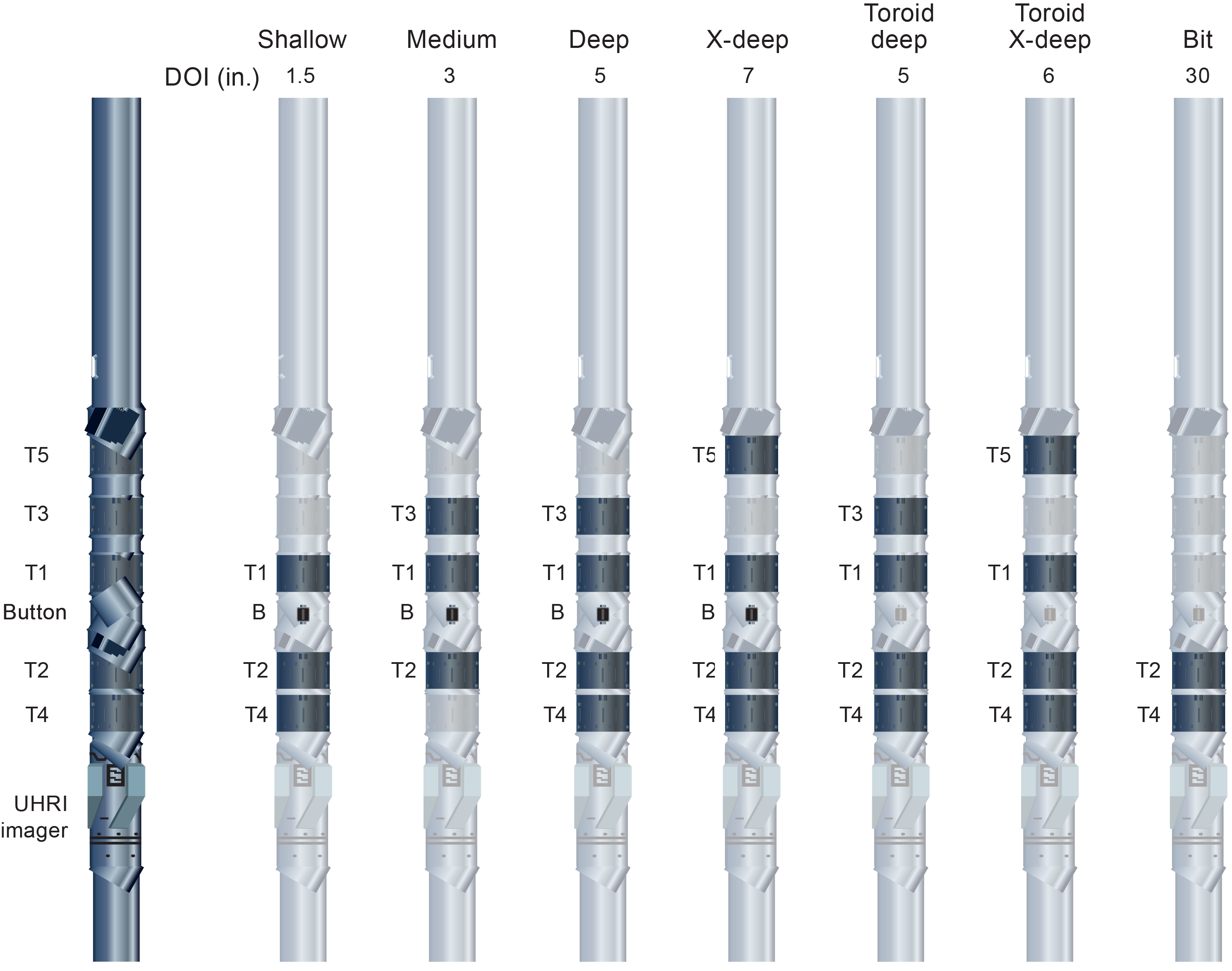
Figure F4. MicroScope tool configurations.
2.1.2.3. Resistivity images
Button resistivity measurements (Figure F4) are acquired during downhole tool rotation only. They are recorded and processed to produce a 360° resistivity image of the borehole wall with 56 azimuthal bins. The button electrode measures resistivity at four depths of investigation that depend on the ratio between the resistivity of the invaded zone and the resistivity of the formation. In an 8.5 inch borehole (20.32 cm), SLB tool specification indicates that the shallow, medium, deep, and extra deep button resistivities have depths of investigation of 1.5 inches (38.1 mm), 3 inches (76.2 mm), 5 inches (12.7 mm), and 7 inches (17.8 mm), respectively (Table T3). The MicroScope HD is also mounted with an UHRI sleeve equipped with eight button electrodes. UHRIs are divided into 208 azimuthal bins and have an axial resolution of 0.4 inches (10.16 mm), better than the axial resolution of the resistivity image (1.5 inches = 38.1 mm). The tool’s orientation system uses Earth’s magnetic field as a reference to determine the tool position with respect to the borehole as the drill string rotates.
2.1.3. TeleScope 675
The TeleScope 675 is located above the MicroScope HD and below the SonicScope 675 (Figure F3; Table T2). The tool serves as a power generator for the MWD/LWD present in the BHA, provides mud-pulse telemetry, takes borehole directional surveys, and measures annular pressure and temperature. It contains a hydraulic mud turbine and electrical power generator that generate electricity as the drilling fluid is pumped through the system. The electricity is used to power the other MWD/LWD tools of the BHA and enables intertool communication and data connectivity.
A magnetometer and accelerometer inside the TeleScope 675 measure borehole azimuth and inclination, respectively. Static borehole survey data are taken when the drill pipe is not moving generally after stand connection (i.e., between stands every 90 m). Continuous azimuth and inclination are also acquired during drilling. Because of the drilling-induced vibrations, the continuous inclination values are less accurate than the static values.
RT data transmission is performed through mud-pulse telemetry. A modulator (rotating valve) present in the TeleScope 675 creates a continuous oscillating pressure pulse that propagates through the drilling fluid up the drill pipe. At the surface, the fluid pulse oscillations are decoded into numerical values. The bandwidth of mud-pulse telemetry during Expedition 405 was 3–4 bits per second (bits/s, or bps).
2.1.4. SonicScope
The SonicScope 675 is located at the top of the logging tool assembly (Figure F3). The tool comprises both monopole and quadrupole acoustic transmitters. The monopole transmitter generates a dilatational wave that travels radially out from the tool, and the quadrupole transmitter generates perpendicular dilation and compression. The arrival times of the compressional and shear waves are measured at an array of 48 receivers spaced over 12 levels, 4 inches apart vertically and 90° apart radially (Table T2). The SonicScope 675 has a vertical resolution of 10 inches (Table T3) and stored stacked waveform data from 12 receiver levels at 10 s intervals. First P-wave arrivals were picked from high-frequency monopole data automatically based on semblance and slowness-time-coherence information within the SLB processing workflow. For slow formations, Leaky P analysis was required (Wang et al., 2020). For Leaky P, the reference QC curve is the slowness-frequency analysis obtained from dispersion analysis of the low-frequency band of the monopole waveforms; the picked slowness should lie on the left edge of the slowness-frequency analysis projection (Plona et al., 2006). Shear wave slowness was extracted from model-based inversion of the quadrupole sonic data (Alford et al., 2012). Final P-wave logs were delivered as composite logs, stitching different depth intervals processed with different methods depending on data quality.
2.2. Shipboard data flow and quality check
The RT data is easily accessible to scientists through live on-screen logs and digital files delivered every 12 h. However, the quality of the RT data is somewhat reduced because of the limitations of mud-pulse telemetry. On the other hand, the memory (RM) data sets offer higher resolution measurements to produce a more detailed insight into downhole conditions and geologic structures.
All depth-converted LWD/MWD data were provided in digital log information standard (DLIS) format by the SLB field engineers. Additionally, a subset of RT time-based and both RT and RM depth-based curves were also delivered as log ASCII standard (LAS) files.
Data delivery from SLB consisted of the following:
- RT data displayed on witness screens as drilling progressed, with the possibility to adjust/modify the reference (depth or time) and displayed tracks;
- RT data every 12 h, provided by the field engineers on board as DLIS and LAS files;
- Rush RM data after recovering the tool (consisting of most logs except SonicScope data, processed data, and e-caliper estimation), provided by the field engineers as DLIS and LAS files;
- SonicScope 675 processed RM data, provided from the shore-based analysis and interpretation team as DLIS and LAS files;
- Reprocessed RM MicroScope HD images, provided from the shore-based analysis and interpretation team as DLIS and LAS files (for Hole C0026A where only RT data were available, RT UHRIs were reprocessed by SLB to improve data quality);
- E-caliper estimation from RM MicroScope HD data, provided from the shore-based analysis and interpretation team as DLIS and LAS files (for Hole C0026A where no RM data was recovered, the e-caliper was calculated based on RT data); and
- Final well construction measurement RM field data, provided by the field engineers as DLIS and LAS files.
After defining the position of the mudline on the gamma ray and resistivity logs, all logging data were depth shifted to the seafloor (LWD depth below seafloor [LSF] depth scale). The depth-shifted versions of the LWD/MWD data were made available in DLIS format, and the main scalar logs were also made available as LAS files. All files were distributed to the shipboard scientists using the shipboard intranet data servers. Analyses, integration results, and reports produced by the shipboard scientists were archived on the server for further distribution. The MicroScope HD resistivity images were processed on board Chikyu using the SLB Techlog (version 2023) software package.
Both the SLB field engineers and Logging Staff Scientists used drilling mechanics logs to identify the sequence of drilling events and assess any possible impact on data quality. The SLB engineers informed the Logging Staff Scientists and drilling engineers of any concerns (e.g., MWD signal quality, stick-slip, shock and vibration flags, and ROP/rpm ratio) that could affect overall data quality. The SLB and drilling engineers adjusted drilling parameters accordingly to ensure the best balance between drilling progress and data quality. Drilling mechanics logs include drilling surface parameters (e.g., ROP, surface weight on bit [SWOB], hook load [HKLD], and standpipe pressure [SPPA]) and downhole drilling parameters (e.g., collar [bit] rotation [CRPM], survey data, shock rate [SHKR], and stick ratio [STICKRATIO]). Elapsed time of the main geophysical measurements after bit penetration, including annular pressure and temperature logs, were also assessed to identify any anomalous zones. To obtain the best image quality from the MicroScope HD, the SLB engineers recommended the ratio between ROP (in m/h) and rpm (in c/min) remain below 0.6. These recommendations were followed throughout the majority of the drilling operations during Expedition 405. It is worth noting that the overall quality of the logs and data is good; however, caution should be exercised when interpreting the images because they were affected by stick-slip, shocks, and heave motion.
2.3. Log characterization and log unit definitions
LWD measurements provide in situ petrophysical information on sediment, rock, and pore fluids while the hole is being drilled, as well as 360° oriented images of the borehole wall. These measurements are sensitive to changes in composition, texture, and structure. Changes in the log response are commonly associated with geologic unit boundaries. This section addresses the characterization of LWD measurements and imaging tool response, focusing on dividing the well logs into log units. For Expedition 405, the aim was to provide a preliminary assessment of expected lithostratigraphy from LWD data prior to coring.
2.3.1. Log characterization and identification of logging units: qualitative analysis
The borehole interval over which LWD logs were acquired was separated into log units by qualitative examination of the log responses and downhole trends: the variations in log curve shape and magnitude, as well as peak amplitude and frequency, and thorough examination of the image logs. Natural radioactivity, resistivity, sonic velocities, and borehole images were the main input logs for determining unit boundaries. In addition to defining and characterizing the logging units, the logging team identified any compositional features/variations within each unit and interpreted them in terms of geological features (unit boundaries, transitions, sequences, and likely lithologic composition).
2.3.2. Log-based geologic/lithologic interpretation
After log characterization and classification, logs were lithologically and geologically interpreted using a combination of log characteristics and borehole images. Composition-sensitive logs, such as NGR, were used to determine unit-scale to bed-scale lithology, and resistivity logs were used to identify lithologies with different physical properties, such as mudstone, chert, and basalt. Borehole images provided information used to identify and characterize other geological features such as bedding, sedimentary structures, bed boundaries, and faults. Interpretation was also informed by existing data from nearby ocean drilling sites.
2.4. Physical properties
We present the resistivity, sonic, and gamma ray logs as a function of depth and describe their features and variation, considering information from structural geology and seismic reflection data. Statistical summaries of these petrophysical properties were compiled for each logging unit. Sharp variations in physical properties are of particular interest because they can be indicators of a fault zone, permeable horizon, or lithologic change. Gradual transitions are also potent indicators of damage and compaction trends.
2.5. Structural analysis: bedding, fractures, and faults
Structural analysis was performed primarily on MicroScope resistivity images using Techlog (SLB Ltd.) software. Resistivity images show the borehole wall as a planar “unwrapped” 360° image. The orientations of planar surfaces cutting the borehole (bedding, fractures, and faults) are identified through sinusoidal fitting of the unwrapped image. In identifying bedding, care must be taken to avoid horizontal artifacts caused by problems in data acquisition that appear as sharp horizontal lines. For shipboard analysis, the dips of the picked planar structures were computed using the bit size as the borehole diameter. We distinguished fractures, faults, and bedding from one another by looking for crosscutting relationships. The fractures and faults were classified as to whether they were conductive, resistive, or undetermined/unclassified. Where resolved, the thickness of faults and fractures was noted.
2.5.1. Borehole wall failure analysis
Borehole breakouts and tensile fractures are wall failures that form when the state of the local stress field at the borehole wall exceeds rock/sediment strength (Zoback, 2007). In a vertical borehole, breakouts form along the borehole in the direction of the minimum horizontal stress (Shmin) and perpendicular to the maximum horizontal stress (SHmax). Breakouts are recorded in resistivity images as two parallel conductive vertical features 180° apart. We recorded the orientation and width of breakouts with the available image analysis software, considering all three borehole images (shallow, medium, and deep), and determined the maximum and minimum horizontal stress orientations.
3. Lithostratigraphy
Characterization of sediments encountered during Expedition 405 required the development of a consistent methodology that could (1) be efficiently applied during two shifts and two windows of shipboard scientists during the expedition and (2) produce consistent and informative data for future analysis. To keep consistency with previous IODP expeditions, the applied approach considered previous drilling reports from the Japan Trench area targeting similar sediments across the accretionary prism, the trench, and the incoming plate (e.g., Deep Sea Drilling Project [DSDP] Legs 56 and 57, Integrated Ocean Drilling Program Expedition 343/343T, and IODP Expedition 386, [Shipboard Scientific Party, 1980; Expedition 343/343T Scientists, 2013b; Ikehara et al., 2023]). Several methodologies were used to summarize the lithologies: (1) visual core descriptions to qualitatively document primary observations (e.g., sedimentary structures, textures, color, and composition) at the macroscale, (2) smear slide analysis of sediment to provide a semiquantitative estimate of grain size and relative siliciclastic/biogenic/volcanic components at the microscale, (3) XCT to provide 3D visualization of changes in density, (4) digital linescan imagery and colorimetry values from the Tri-Sensor Core Logger (TSCL), and (5) XRD and XRF analyses to measure the whole-rock mineral and element composition. The data sets were compiled, and the combined information was used to define discrete lithostratigraphic units named for the primary lithology, with color as an additional descriptor to differentiate similar units (see Classification of lithostratigraphic units).
3.1. Visual core description
Visual core description aimed to characterize variations in grain size, texture, sedimentary structures, and color along the cores. Archive-half cores were observed and described after noninvasive measurements (e.g., XCT and COMET), whole-round sampling, core splitting, and imaging with the TSCL (see Core handling). Visual core description for structural whole-round samples not split on board (e.g., Sections 405-C0019J-56K-5 and 87K-2 and 405-C0019K-10K-2) used the whole-round surfaces. Observations were recorded on visual core description (VCD) sheets. VCD sheets for HPCS, ESCS, SD-RCB system, and hard rock all include columns for visual representation, lithologic boundaries, symbology, bioturbation level, grain size, coring disturbance, and Munsell color. Slight modifications to the layout of the sheets for HPCS/ESCS cores were adapted from those used during Expedition 386 to allow more detailed documentation of subtle grain size changes, sedimentary structures, and features encountered in surficial soft sediments. Bioturbation intensity was separated into light (bedding preserved), moderate (bedding disturbed), or heavy (bedding obliterated).
Specific descriptive terminology generally followed Folk (1954) for siliciclastic sediment classification, with modifications for sediment composition based on site-specific observations and previous IODP volumes (e.g., Expeditions 343 and 386). Further descriptions documented variations in predominant and subordinate lithologies; sedimentary structures; and the nature of contacts between layers, textures, and compositions at the millimeter scale. XCT images of each core section were used during visual core description to aid observations linked to changes in density, identify intervals of drilling-induced deformation, and help distinguish sedimentary structures that are difficult to interpret visually. Upon completion, all descriptions were uploaded to the J-CORES database and the VCD sheets were scanned and archived. A concise summary for each core was included at the end of each J-CORES description.
Visual core description of hard rock cores was conducted for Hole C0019P. Descriptions included lithologic classifications, phenocryst size and mineralogy, crystal abundance, and the presence of vitric components. Because thin sections were not available during the visual core description of hard rock cores, the term “basalt” was generally used for fine-grained mafic igneous rocks and was further classified into pillow basalt and massive basalt based on the meter- to centimeter-scale characteristics and textures observed on split core surfaces. The term “dolerite” was applied to crystalline (or holocrystalline) igneous rocks primarily composed of plagioclase and clinopyroxene. For sedimentary rocks, “chert” was used for silica-rich, glassy rocks that could not be scratched with metal tweezers, and “limestone” was applied to rocks primarily composed of carbonate minerals (undifferentiated), as confirmed by smear slide observations.
For both sediments and hard rocks, the J-CORES database was used to provide stratigraphic summaries of all data sets and samples alongside XCT and TSCL images. To condense the detailed visual core descriptions, several simplifications were required:
- Distinct layering of sediments with slightly different grain size and composition is present throughout the cores (e.g., graded layers of sands and silts). For simplicity, a minimum thickness of >2 cm was adopted for entering this information into the J-CORES database. Layers thinner than 2 cm were recorded using the laminae lithology symbol.
- The lithology of each siliciclastic layer was entered based on its visually estimated grain size descriptor (e.g., clay, sand, or mud) because grain size could be visually estimated for the entire core, whereas composition could only be quantified at discrete locations with smear slide samples (see Smear slide analysis). The volcaniclastic material was grouped under the term “ash.” Lithology was recorded alongside sedimentary features such as bioturbation, color banding, pumice clasts, and so on. Symbology for all lithologies and sedimentary features is shown in Figure F5.
- Subvertical to vertical bedding may result in the coexistence of coarse- and fine-grained layers at the same depths. These intervals were recorded in the J-CORES database based on the dominant grain size composition alongside the chaotic lithology symbology.
- Distinguishing a clear boundary between unconsolidated sediment and lithified rock was challenging because of the gradual nature of consolidation during burial and the interbedding of different lithologies. For all holes except Hole C0019P, individual layers in the J-CORES database were named without differentiation between sediments and rocks. The suffix “-stone” was applied for summarizing the name of the lithostratigraphic units in core sections that required a band saw for splitting.
- Ash layers were assigned in the database as a distinctive lithology (also for thicknesses <2 cm). A single consistent lithology, “ash,” irrespective of grain size differences, was used for clarity and to avoid introducing redundant symbols.
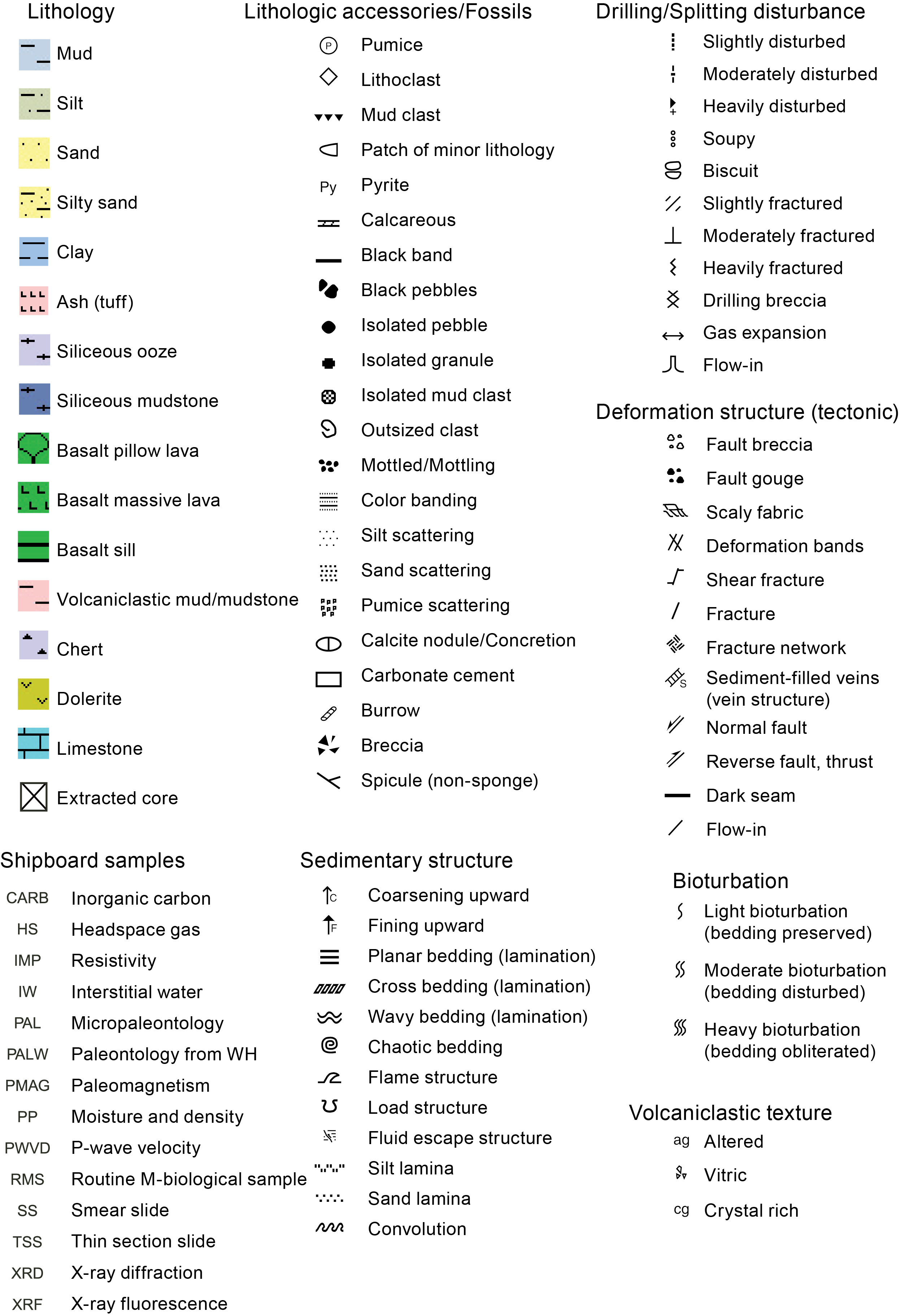
Figure F5. J-CORES lithologic symbols.
These criteria ensured systematic classification while still reflecting the lithologic characteristics of the sites. Data from the J-CORES database were compiled to make stratigraphic logs using Strater software.
3.2. Smear slide analysis
Smear slide analysis aimed to provide semiquantitative insights into grain size and composition of biogenic, volcanic, and siliciclastic material. One or two smear slides per section were collected from the archive-half cores, targeting representative lithologies. Occasional nonrepresentative samples were collected from specific areas of interest, such as ash layers, calcite veins, and clasts. These samples were clearly marked to ensure they did not influence the overall compositional analysis. Sample depths were recorded and entered into the J-CORES database with a sample code of SS.
Slides were examined in transmitted light using an Axioskop 40A polarizing microscope (Carl Zeiss) equipped with a Nikon DS-Fi1 digital camera. At least one representative photograph was taken per sample. Observations were recorded on preformatted sheets (subsequently scanned and archived) for consistent tracking across all samples. The relative percentages of different constituents were estimated with the help of a visual comparison chart (Rothwell, 1989) (Figure F6), while recognizing the presence of personal bias and associated uncertainty in the results. Each major compositional component was divided based on the following criteria:
- Siliciclastic material was divided into quartz, feldspar, clay minerals, and lithic grains, including sedimentary lithics (e.g., chert, mudstone, siltstone/sandstone, and limestone), metamorphic lithics, and plutonic lithics.
- Volcanic material was divided into clear glass, colored glass, pumice, volcanic lithics (e.g., felsitic, microlitic, and lathwork), and altered volcanics.
- Biogenic material was divided into pelagic grains and other bioclasts. The pelagic grains were divided into calcareous microfossils (nannofossils and foraminifers) and siliceous microfossils (diatoms, radiolarians, silicoflagellates, and sponge spicules).
- Other material was divided into other carbonate allochems (e.g., peloids, ooids, etc.), minor grain types (e.g., dense minerals, micas, glauconite, opaque minerals, etc.), and authigenic components (e.g., pyrite, calcite, zeolites, and Fe/Mn oxides).
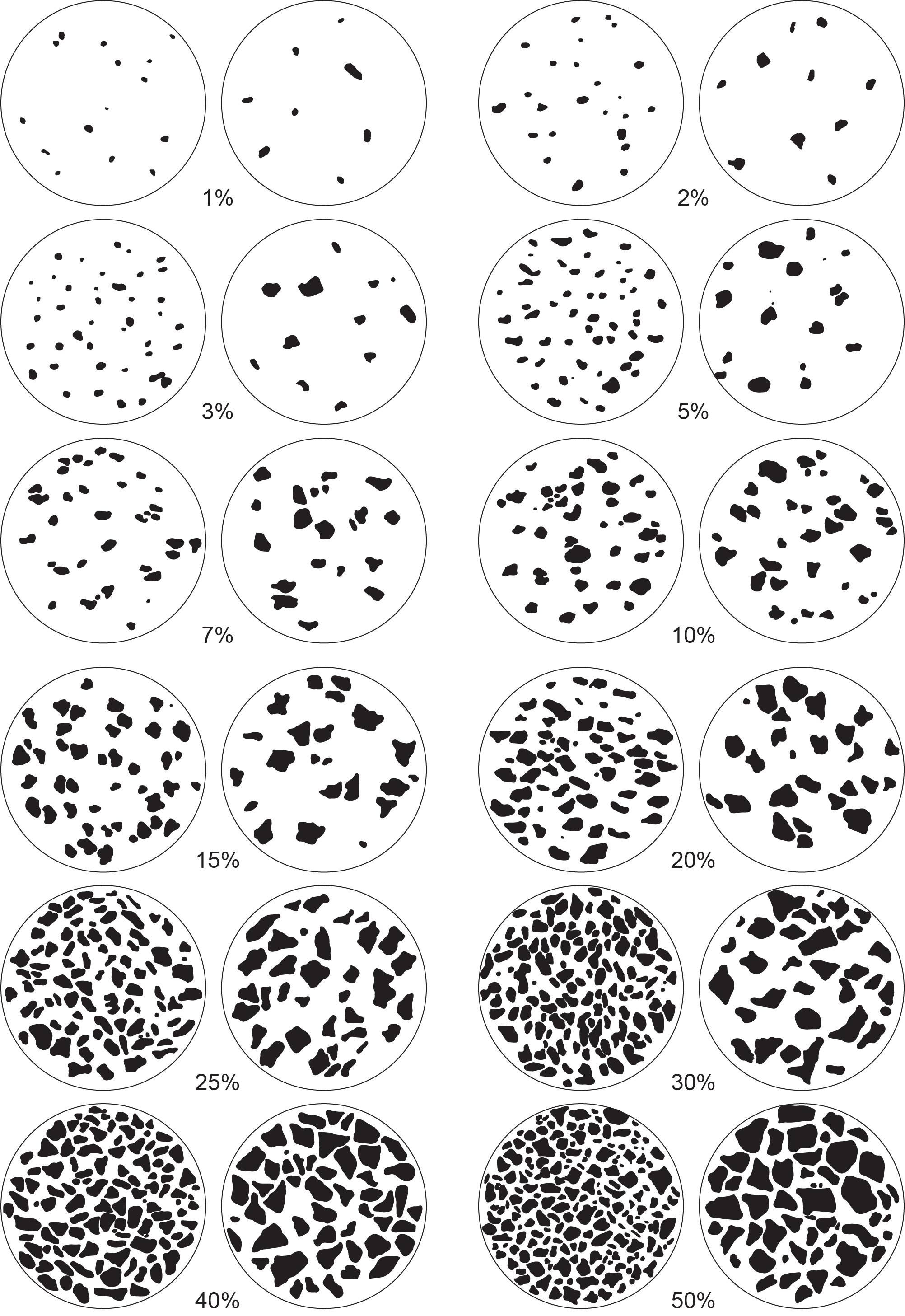
Figure F6. Optical mineral abundances.
Visual estimation of grain size also used comparison charts (Rothwell, 1989). However, sand-sized particles may be underrepresented because of potential preferential removal during smear slide preparation, so quantitative estimates may be biased toward fine-grained fractions. Results were uploaded to an abridged spreadsheet for plotting ternary diagrams and downhole trends.
The results from the smear slide analysis were used to summarize the composition of different lithologies. Two sets of ternary plots were used to illustrate the composition and grain size of each unit in the accretionary prism (Site C0019) and incoming plate (Site C0026). Ternary diagrams used for grain size and compositions were adapted from Folk (1954) and Integrated Ocean Drilling Program Expedition 308 (Expedition 308 Scientists, 2006), enabling variations in different components across units to be more effectively highlighted. Within the adapted ternary diagram for composition, each apex represents 100% of each respective end-member sediment type (Figure F7). The principal end-members of siliciclastic, biogenic, and volcanic components are therefore normalized to 100% in reported figures. This means sediment compositions dominated by more than two-thirds (>66.6%) of a single component are classified as ash, siliciclastics, or ooze, respectively. For sediments containing one- to two-thirds (~33.3%–66.6%) siliciclastic, volcanic, or biogenic components, a compositional modifier (vitric, siliceous, or siliceous vitric) was added to further characterize intermediate sediment. The terms “vitric” and “siliceous” were used instead of “ashy” and “biogenic” because most of the volcanic grains observed during Expedition 405 were vitric (i.e., mainly volcanic glass and pumice; rare lithic and volcanic minerals), and most of the biogenic grains were siliceous (i.e., diatom, radiolarian, siliceous spicule, or silicoflagellate); however, we noted the presence of calcareous nannofossils and foraminifers where present.
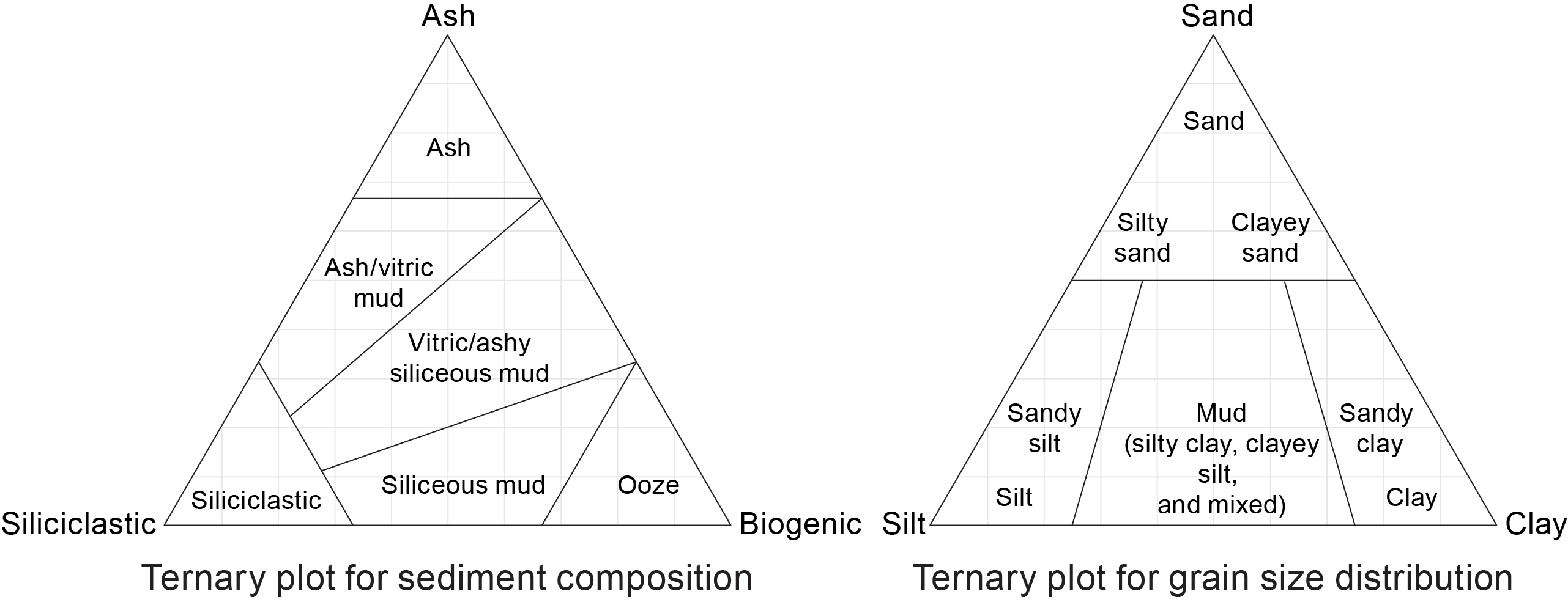
Figure F7. Sediment composition and grain size.
The adapted ternary diagram for grain size distinction was governed by three visually distinguishable end-members of sand (>63 µm), silt (63–4 µm), and clay (<4 µm). Sediment composed of >50% sand was classified as sand. Three segments divide the remaining <50% siliciclastic portion between silt and clay end-members. Between the >75% end-member silt and clay portions, “mud” was used to summarize sediments with mixed composition (e.g., silty-clay, clayey-silt, and equally mixed). The combination of composition and grain size descriptors from these two ternary plots defined the sediment type for each smear slide sample.
3.3. Split core digital photography
Split core digital photography imaging on the TSCL acquires color spectrophotometry and illustrates color variations across different units. The NS Design TSCL was used to capture continuous digital linescan imagery of each archive-half core. TSCL imaging was conducted as soon as possible after core splitting to avoid time-dependent color changes resulting from sediment drying and oxidation. Cores were prepared by carefully removing bumps, dust, and (core splitting–related) plastic particles on the split core surface. TIFF-formatted images were obtained with a spatial resolution of 100 pixels/cm (2K) and occasionally at 200 pixels/cm (4K) in sections with high-resolution changes. Scanned images and data were uploaded to the J-CORES database so that image files could be observed through the Composite Log Viewer. Linescans were modified to enhance image contrast using the plugin Contrast Limited Adaptive Histogram Equalization (CLAHE) in the open-source Fiji image processing package (LOCI University ImageJ). This plugin enhances contrast by applying histogram equalization to small, localized regions (tiles) of the image rather than the entire image. This method is particularly effective for improving visibility in areas with poor contrast or uneven illumination. To prevent noise amplification, CLAHE includes a clipping threshold that limits the enhancement of high-frequency variations, ensuring a balanced and clear result. Applying this plugin to linescans allowed us to distinguish color changes, structures, and contacts that might be difficult to see with the naked eye. In addition to TIFF images, the camera provides a measure of 16 bit red-green-blue (RGB) colorimetry. Quantitative colorimetry data are available for Holes C0019J and C0019K but not for some cores from Holes C0026B, C0019E, C0019L, C0019M, and C0019P because of a failure of the sensor partway during operations.
3.4. X-ray computed tomography
XCT offers a 3D view of sediment cores. Shipboard XCT scanning was performed on whole-round cores directly after section cutting. The shipboard medical-grade XCT scanner (Discovery CT 750HD) acquires radiographic images with a slice thickness of 0.625 mm. The resulting data consist of core-axis-normal planes of X-ray attenuation values recorded at a resolution of 512 pixels × 512 pixels per slice. The results are a sequence of radiographic images collected from a 360° perspective, generating 2D cross-sectional core images. Raw data were stored on the server in the Digital Imaging and Communication in Medicine (DICOM) format.
Initially, a preliminary 3D model reconstructed from stacked radiographic images was used to guide the selection of sections for whole-round shipboard sampling. Afterward, raw XCT data were processed using HOROS software and the Fiji package. Images are displayed in grayscale, with brighter areas indicating higher CT numbers (e.g., sand/ash layers) and darker areas showing lower CT numbers (e.g., bioturbated intervals, air, or fractures). The CT number (also known as the Hounsfield unit [HU]) is a measure of the relative density of scanned materials (Renter, 1989), and its variations represent the attenuation of X-ray beams while passing through different materials (e.g., air CT number = −1000; water CT number = 0). Variations in the downcore CT number can therefore be used as an additional quantitative proxy for distinguishing density differences and boundaries between lithostratigraphic units. Thus, the resulting 2D images were used to support visual core descriptions by highlighting sedimentary and structural features that were obscured or invisible on the split core surface.
3.5. X-ray diffraction
To further characterize sediment composition within lithostratigraphic units, bulk powder XRD analysis was conducted to examine downcore trends in mineralogy. At least one 2–2.5 cm long quarter-round bulk sample for XRD, XRF, and CARB per core was taken from representative intervals within each unit. Bulk samples were vacuum-dried at room temperature for 24 h before being crushed to a fine powder with a tungsten ball mill. The powdered sample was divided into three glass vials, one each for XRD, XRF, and CARB measurements, with approximately 4 g of the powder reserved for XRD. The XRD sample was mounted to a backload-type sample holder as a pressed powder and measured using a PANalytical CubiX3 X-ray diffractometer. The instrument settings were as follows:
- Generator = 40 kV and 45 mA.
- Tube anode = Cu.
- Wavelength = 1.54184 Å (CuKα).
- Step spacing = 0.01°2θ.
- Rate = 0.1 s/step.
- Slits = automatic.
- Measuring diameter = 10 mm.
- Scanning range = 2°–60°2θ.
XRD spectra were exported from the PANalytical X’Pert software with labels highlighting peaks corresponding to the individual mineral phases present in the samples. To provide semiquantitative estimates for relative abundances of four major mineral components (quartz, plagioclase, calcite, and clay), a least-squares best-fit approach was used against a reference XRD spectrum defined from standards (Underwood et al., 2003) prepared by Integrated Ocean Drilling Program Expedition 316 Scientists for the Nankai Trough sediments (Expedition 316 Scientists, 2009a). However, there are many potential limitations in estimating a range of mineral components from XRD in this way, largely related to the difference in peak response between poorly crystalline minerals at low diffraction angles (e.g., clay minerals) and highly crystalline minerals at higher diffraction angles (e.g., quartz and plagioclase). It should also be noted that these approximations also do not allow for the detection of other components such as glass or alkali feldspar from volcanic sources or opaline biogenic silica and therefore should be considered as the upper bounds. These issues are extensively reported by Expedition 316 Scientists (2009a), but the use of this analysis remains valuable for rapidly approximating relative proportional mineralogy during expeditions, hence its inclusion alongside figures of bulk XRD spectra for Expedition 405.
3.6. Loss on ignition and X-ray fluorescence
Approximately 10 g of dried powder was subsampled for XRF and loss on ignition (LOI) analyses from the same sample used for XRD and CARB. The subsampled powder was weighed, heated to 100°C for 2 h to remove moisture, and reweighed. Samples were then ignited at 1000°C for 3 h to remove all volatiles and reweighed a final time. Weight differences of the samples between the two heating processes were used to calculate the LOI, reported as weight percent of the original mass of the sample. LOI provides an estimate of organic material, carbonate minerals, or other volatiles that are removed during heating of sediment samples to high temperatures. This analysis can be done during the preparation of glass beads for XRF spectrometry, which provides data on the bulk sample elemental composition.
Subsamples (0.8950–0.9040 g) of the ignited material were fused with 4.5 g of Spectromelt A12 flux for 7 min at 1150°C to create glass beads for XRF analysis. Measurements were performed on the wavelength dispersive XRF spectrometer Zetium (PANalytical) equipped with a 2400 W rhodium anode X-ray tube at 60 kV and 100 mA. Data were reported as total counts on the peak and as semiquantitative oxide weight percent (Na2O, MgO, Al2O3, SiO2, P2O5, K2O, CaO, TiO2, MnO, and Fe2O3).
3.7. Classification of lithostratigraphic units
The primary criteria used to classify boundaries between lithostratigraphic units were variations in grain size and/or composition, as defined from visual core description and smear slide analysis. However, because much of the sediment described displayed only subtle variations in composition, color changes identified during visual core description and confirmed with colorimetry values (where available) were also considered as differentiating criteria. For example, several boundaries were characterized by gradual rather than abrupt changes in composition and color. As a result, many lithostratigraphic units include a zone of gradational changes in both color and composition. Units with internal gradational color changes that were not necessarily accompanied by major compositional changes were separated into subunits.
After depth boundaries were defined, lithostratigraphic units were numbered from the top to the bottom of the cored interval at each site. For Holes C0019J, C0019L, and C0019M, continuous unit numbers were adopted to reconstruct the longest possible composite lithostratigraphy section through Site C0019. However, Hole C0019K was described separately (unit names are prefaced with the letter K) because it was recovered from an overlapping depth interval with Hole C0019J but showed clear differences, indicating heterogeneity between holes. Hole C0019P was also described separately (unit names are prefaced with the letter P) because the coring depth interval for Hole C0019P was much deeper and different lithostratigraphic units were targeted.
Each lithostratigraphic unit and subunit was assigned an overall descriptor based on the predominant lithology, which we interpret to correspond to the background sedimentation during deposition, and a summary of the following:
- Color: from the Munsell chart defined during visual core description (e.g., olive-black [10Y 2/1]).
- Composition: from ternary plot of smear slides (e.g., siliceous vitric).
- Grain size: from ternary plot of smear slides, cross-checked with visual core description (e.g., mud).
This system provides an overarching summary (e.g., olive-black siliceous vitric mud) of the background lithology of each unit. However, most units contain not only the background sedimentation but also intercalated diverse components (e.g., ash beds, clasts, graded layers, etc.). All are described in detail in the complete lithologic descriptions as sedimentary structures (e.g., soft-sediment deformation and chaotic bedding) and features (e.g., mottling and ichnofacies).
4. Structural geology
4.1. X-ray computed tomography
XCT imaging provided real-time information, which was used to guide time-sensitive and whole-round core sampling during Expedition 405. The methods for collecting XCT imagery followed those in the measurement manual prepared for the Institute for Marine-Earth Exploration and Engineering (MarE3) by laboratory technicians from Marine Works Japan (3D X-ray CT Scanning, Version 3.00, 24 March 2015; based on GE Healthcare, 2013a, 2013b, 2013c; Mees et al., 2003; Nakano et al., 2000).
The XCT instrument on Chikyu is a Discovery CT 750HD (GE Medical Systems) capable of generating 16 cross-sectional images of the core at 0.625 mm spacing every 0.5 s, the time for one revolution of the X-ray source around the sample (Table T4). As a result of the high scanning rate, 1.5 m sections of core were typically imaged in 3 min. The imagery generated for each core consists of 512 × 512 pixel axis-normal images of X-ray attenuation values with 0.176 mm pixel resolutions. These data were stored as DICOM format files.
4.1.1. Background
The theory behind XCT has been well established through medical research and is briefly outlined in Carlson (2006). X-ray intensity (I) varies as a function of X-ray path length and the linear attenuation coefficient (LAC) of the target material:
- I = transmitted X-ray intensity,
- I0 = initial X-ray intensity,
- µ = LAC of the target material, and
- L = X-ray path length through the material.
LAC is a function of the chemical composition and density of the target material. The basic measure of attenuation, or radiodensity, is the CT number given in Hounsfield units (HU):
where µt is the LAC of the target material and µw is the LAC of water.
The distribution of attenuation values mapped to an individual slice comprises the raw data that are used for subsequent image processing. Successive 2D slices yield a representation of attenuation values in 3D pixels, referred to as voxels. Visualizations are generally accomplished by varying how the distribution of CT numbers is assigned to 256 shades of gray or a color palette. In general, high CT numbers correspond to bright colors in CT images, representing relatively high bulk density that may be caused by high density and/or an increase in elements with relatively higher atomic numbers (e.g., Fe). Shipboard analysis of CT images was done using both the Advantage Workstation (Lightspeed Ultra 16; General Electric Medical Systems) and the Horos 32-bit DICOM viewer running on a Macintosh computer (OSX 13.1).
Every 24 h during coring operations, an acrylic core mockup (calibration standard) was used to calibrate the XCT. The core mockup enables the calibration of the CT numbers for air (CT number = −1000), water (CT number = 0), and aluminum (2477 < CT number < 2487). For each calibration analysis, the CT number was determined for a 24.85 mm2 area at fixed coordinates near the center of the cylinder.
4.1.2. XCT scan data usage
XCT scans were used routinely during Expedition 405 throughout the core processing workflow for the following:
- To provide an assessment of core recovery and liner integrity for drilling operations,
- To inform and guide destructive whole-round sampling and provide an archival record of samples taken for whole-round sampling, and
- To support real-time lithologic and structural visual core description and structure measurement in the core description laboratory.
XCT scans were initiated immediately after core sections were cut so that ideal sections for time-sensitive whole-round samples could be identified using XCT imagery. In this way, all core sections were screened using 3D XCT imagery prior to whole-round sampling and core splitting to avoid destructive testing on sections of core that may contain key structural or sedimentary features necessary for core interpretation. This included identification of critically important intervals (e.g., thin principal slip zones and sequences of graded beds) that warranted detailed study and special handling during visual core description and sampling. Furthermore, collecting XCT imagery prior to whole-round sampling provided key archival data for all recovered core sections. The use of XCT screening also ensured that the selection of whole-round samples for shipboard and personal measurements included sections with minimal drilling disturbance and targeted relatively homogeneous representative sections of core for interstitial water (IW), mechanical properties, or microbiological analyses.
XCT imagery was used extensively throughout lithologic and structural visual core descriptions because many subtle or obscured features in split core faces may be easier to identify in XCT imagery. The reconstructed 3D XCT volumes were used to determine 3D geometries, crosscutting and other spatial relations, and orientation of primary and secondary structures. Fractures and other planar features that can be identified in the XCT scans can be oriented directly from the imagery by measuring the apparent dip and dip directions strike in various 2D sections (e.g., transverse, coronal, and sagittal) (Figure F8). Finally, XCT imagery was used to distinguish drilling-induced breccia from tectonic breccia.
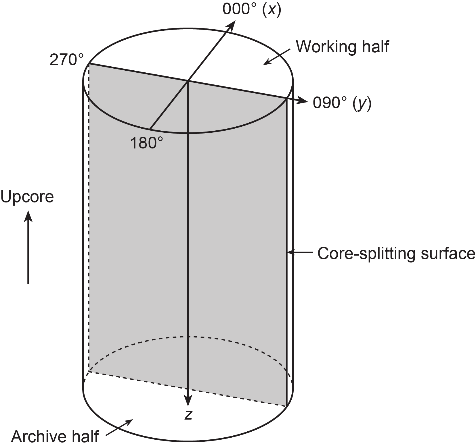
Figure F8. Core reference frame and coordinates used for orientation data.
4.2. Visual core description
We documented the preserved structures in the cores using VCDs and by measuring the apparent structure orientations on the working half of split core faces and whole cores (from the XCT images). Our methods and procedures follow those outlined in previous ODP, Integrated Ocean Drilling Program, and IODP expeditions (e.g., ODP Legs 131, 170, and 190; Integrated Ocean Drilling Program Expeditions 315, 316, 319, 322, 333, 338, 343, and 348; and IODP Expeditions 358 and 370). We documented the primary and secondary structures observed by classifying structure type, determining the depth extent, measuring the orientation relative to the orientation of the core, and identifying and measuring any sense-of-slip indicators. These VCD data were hand logged onto a printed form at the core table, entered into an electronic spreadsheet, and entered into the J-CORES database using existing symbology. Where possible, the orientation data were also reoriented in the geographical coordinate system using shipboard discrete sample paleomagnetic declination and inclination information.
4.2.1. Core description and orientation data collection
Each structure was recorded manually on a structural description sheet that was modified from similar tables used during Expedition 316 and subsequent expeditions (Figure F9). We used a plastic protractor for orientation measurements (Figure F10) and provided detailed observations, sketches, and core descriptions on the observation sheets. Using the working half of the split core provided greater flexibility to remove and cut (if necessary) pieces of the core for more careful study and measurement.
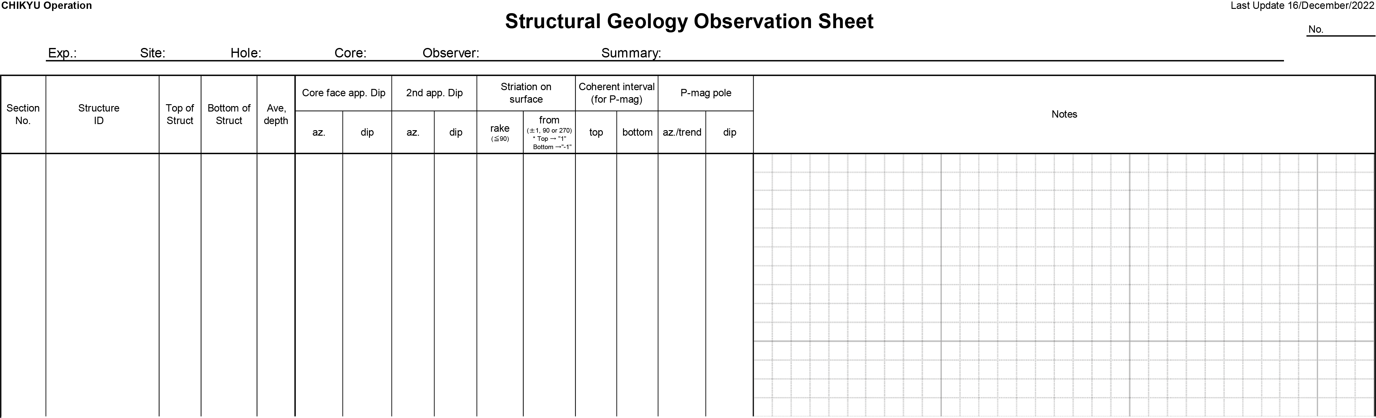
Figure F9. Structural data log sheet.
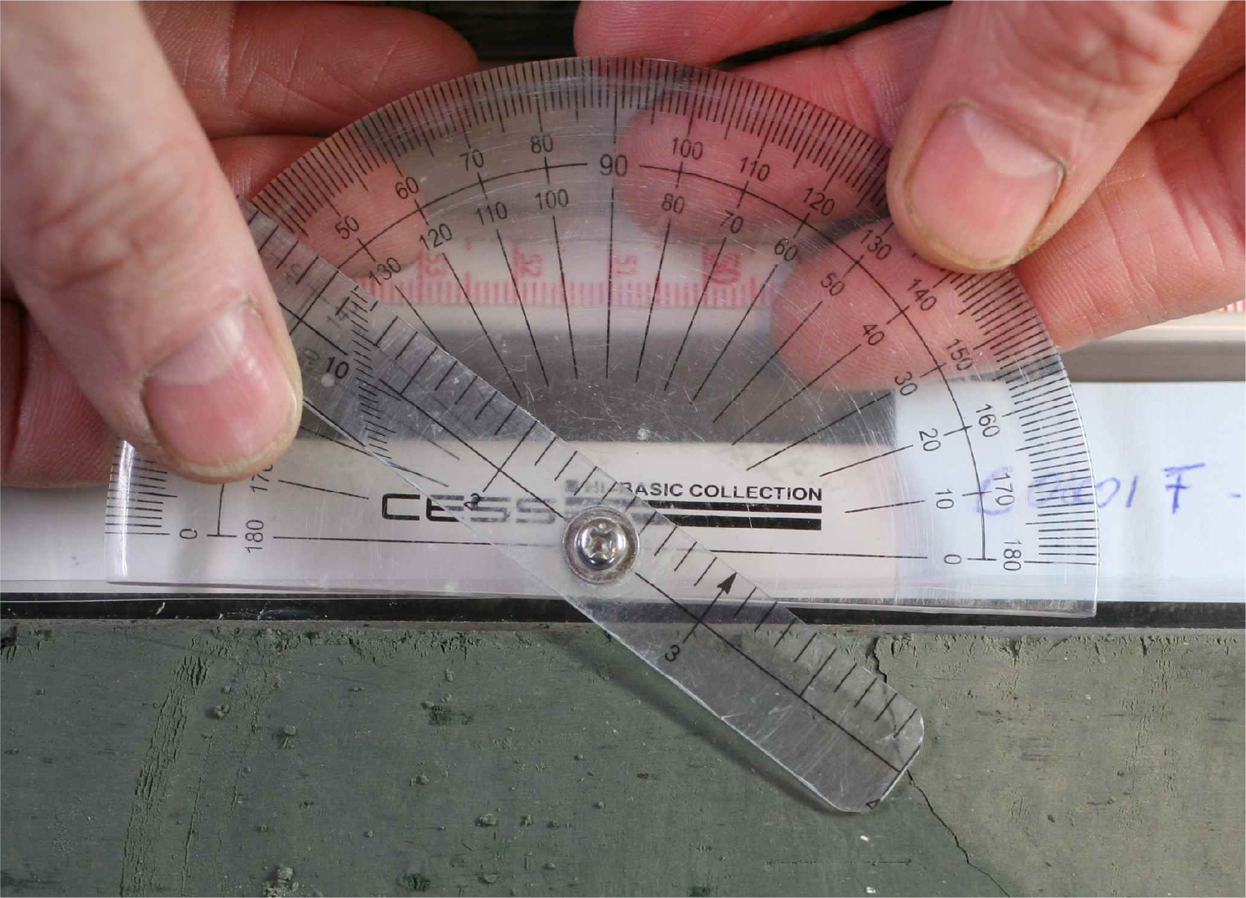
Figure F10. Modified protractor.
4.2.2. Orientation data analysis and true north correction
During Expedition 405, we adopted the spreadsheet template for orientation data calculation in the core reference frame (Figure F11). The core reference frame is such that the upcore direction is vertical upward, the core-splitting plane is 90°–270° and vertical, and the double line points toward 0° (Figure F8).

Figure F11. Orientation data spreadsheet.
4.2.2.1. Calculation of plane orientation
For planar structures (e.g., bedding or faults), two apparent dips on two different surfaces (e.g., one being the split core surface, which is 90°–270° and vertical, and the other being the horizontal or 0°–180° vertical surface) were measured in the core reference frame as trends (measured clockwise from 0°, looking down) and plunges. An xyz coordinate system was defined in such a way that the positive x-, y-, and z-directions coincide with 0°, 90°, and vertical downward, respectively (Figure F8). If the trends and plunges of the two apparent dips are given as (α1, β1) and (α2, β2), respectively, as in Figure F12, then the unit vectors representing these two lines (v1 and v2) are
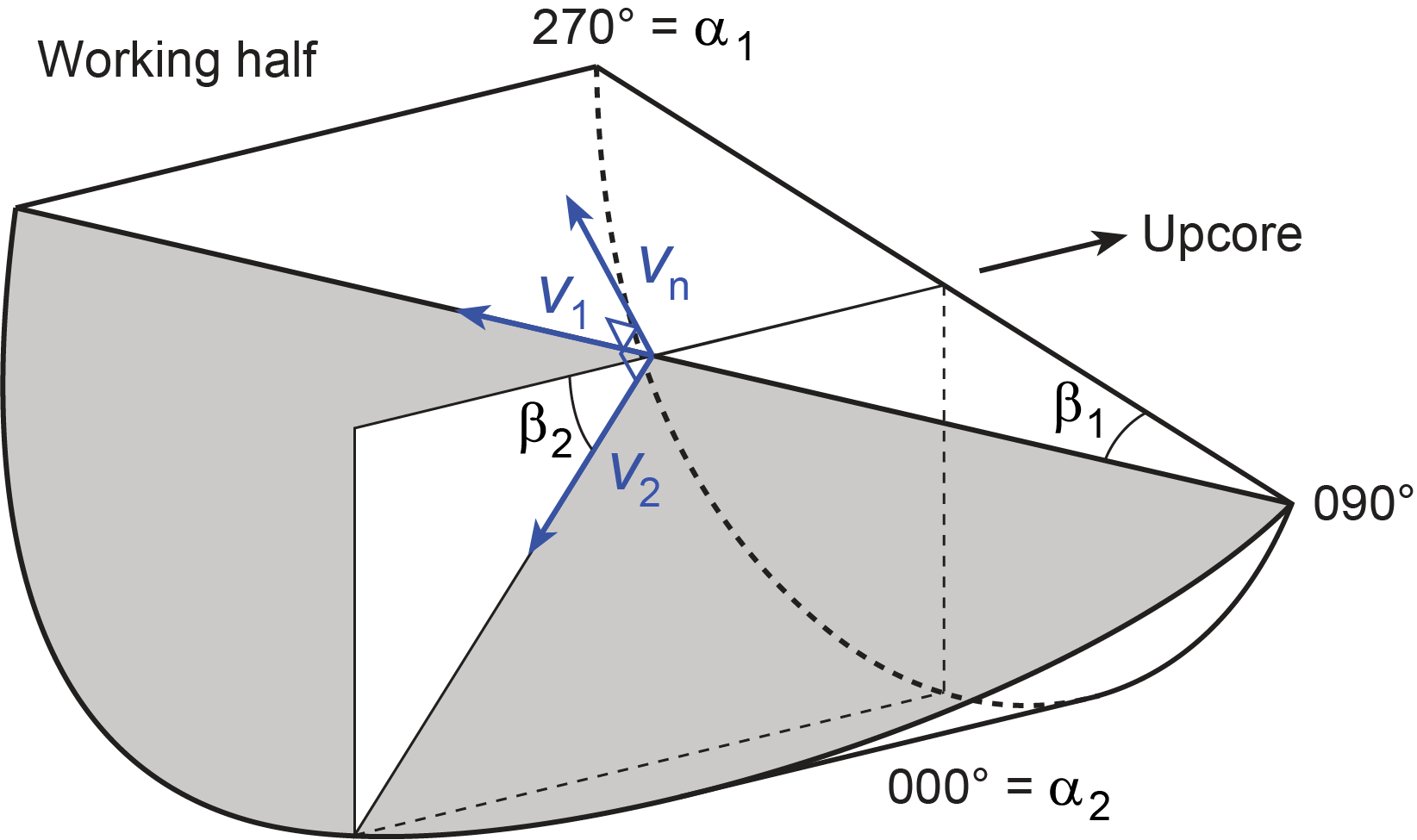
Figure F12. Calculation of plane orientation.
The unit vector normal to this plane (vn) is then defined as follows:
The azimuth (αn) and plunge (βn) of vn are given by
The dip direction (αd) and dip angle (β) of this plane are αn and 90° + βn, respectively, when βn < 0° and αn ± 180° and 90° − βn, respectively, when βn ≥ 0° (Figure F13). The right-hand rule strike of this plane (αs) is then given by αd − 90°.
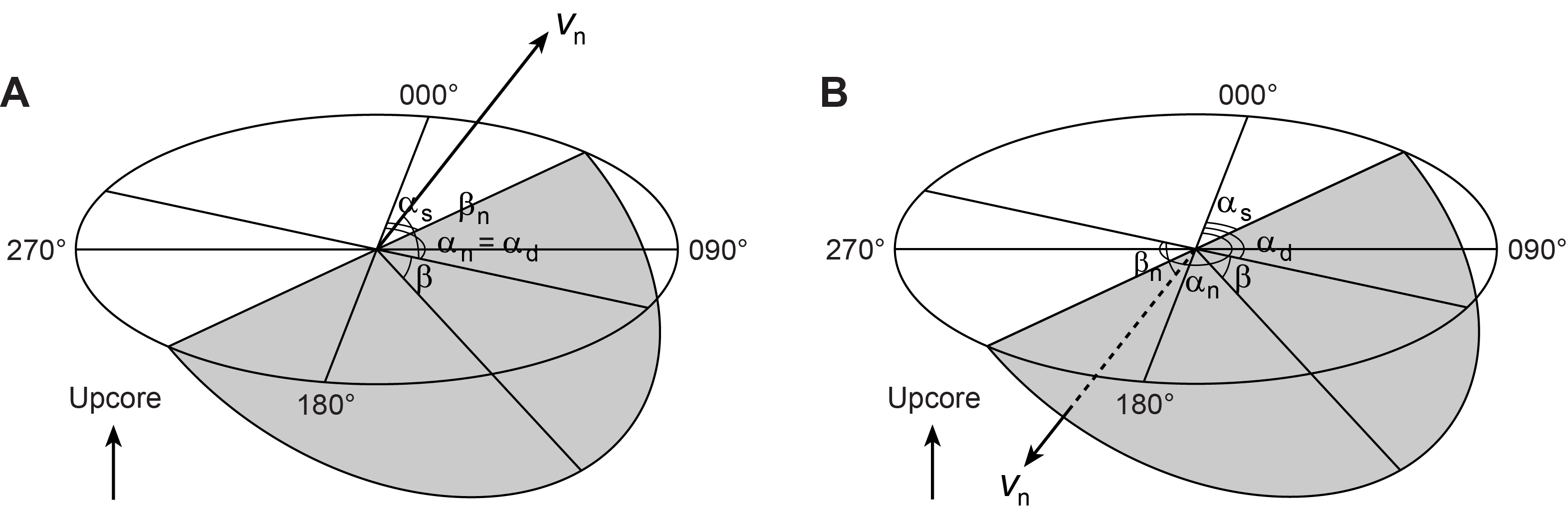
Figure F13. Dip direction, right-hand rule strike, and dip.
4.2.2.2. Calculation of slickenline rake
For a fault with slickenlines, the apparent rake angle of the slickenline (ϕa) is measured on the fault surface from either the 090° or 270° direction of the split core surface trace (Figure F14). The fault orientation was measured as described above. Provided that vn and vc are unit vectors normal to the fault and split core surfaces, respectively, the unit vector of this intersection line (vi) is perpendicular to both vn and vc and therefore defined as follows:
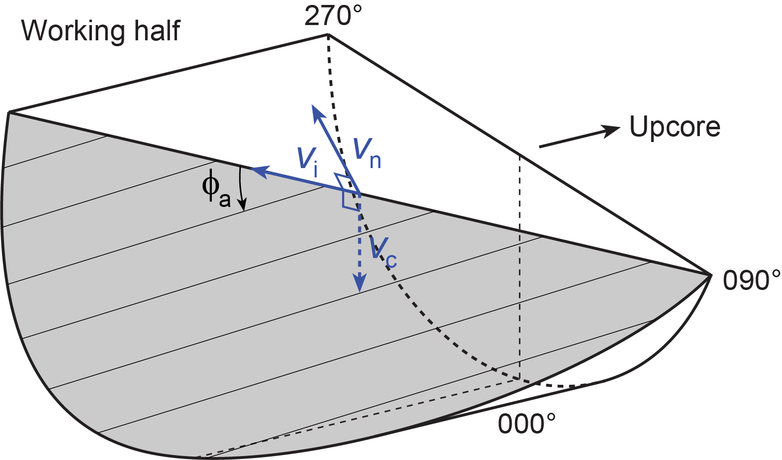
Figure F14. Apparent rake measurement of slickenlines.
Knowing the right-hand rule strike of the fault plane (αs), the unit vector (vs) toward this direction is
The rake angle of the intersection line (ϕi) measured from the strike direction is given by
The rake angle of the slickenline (ϕ) from the strike direction is ϕi ± ϕa, depending on which direction the apparent rake was measured from and which direction the fault plane dips toward (Figure F15). ϕa should be subtracted from ϕi when the fault plane dips toward 270° and ϕa was measured from either the top or 090° direction or when the fault plane dips toward 90° and ϕa was measured from either the bottom or 090° direction. On the other hand, ϕa should be added to ϕi when the fault plane dips toward 90° and ϕa was measured from either the top or 270° direction or when the fault plane dips toward 270° and ϕa was measured from either the bottom or 270° direction.
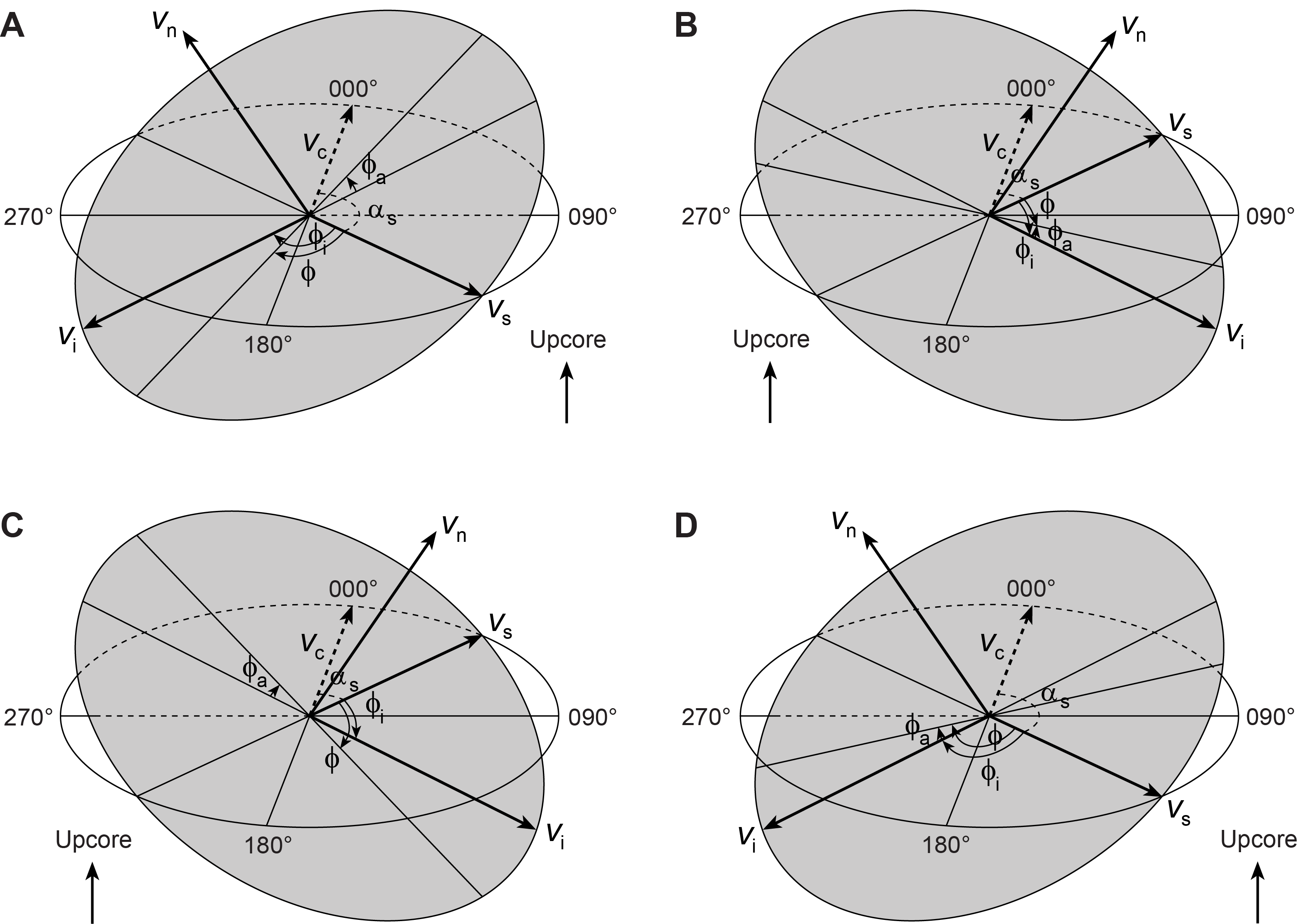
Figure F15. Rake of slickenlines.
4.2.2.3. Azimuth correction based on paleomagnetic data
Discretely sampled paleomagnetic data were used where possible to correct drilling-induced rotations of the cored sediments. Provided that a core is vertical, its magnetization is primary, and a planar structure is horizontal (approximately <10°), the strike and dip direction of the plane can be rotated about a vertical axis in a geographic reference frame to restore it back to an in situ orientation. In a time of normal geomagnetic polarity, when the paleomagnetic inclination (βp) is ≥0°, the in situ strike (αs*) and in situ dip direction (αd*) of a plane in the geographic reference frame can be represented as the following (Figure F16A):
- αs = apparent strike,
- αd = apparent dip direction, and
- αp = direction of magnetic north (paleomagnetic declination).
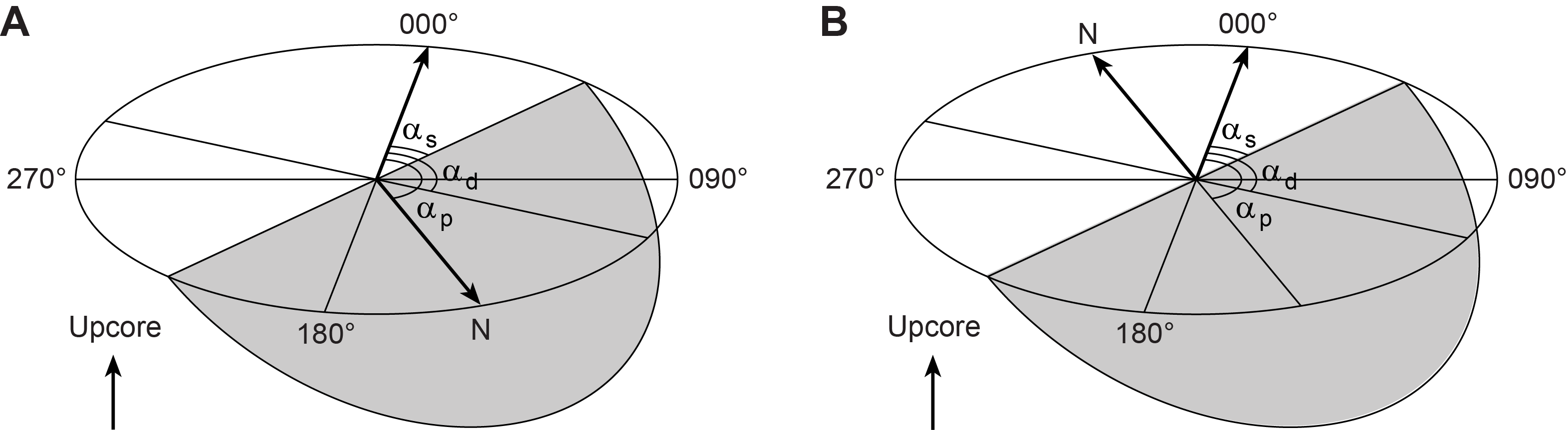
Figure F16. Azimuth correction.
When the geomagnetic polarity is reversed and the paleomagnetic inclination is βp < 0° (Figure F16B), the in situ strike and dip direction are represented as
If the structure is not approximately horizontal within the core, the plane must first be rotated back to horizontal (about a horizontal axis), thus rotating its paleomagnetic declination by the same degree with respect to the bedding plane, to obtain the original geographic orientation. The structure is then rotated around the vertical axis back to magnetic north. Each rotated structure must be contained within the same coherent interval in which the discrete paleomagnetic samples were taken.
4.2.3. Description and classification of structures
The VCD interface in the J-CORES database provides a compilation of the visual (macroscopic and/or microscopic) descriptions of core structures at a given section index and a record of planar structures in the core reference frame. In general, we described and classified the structures observed using the J-CORES and Expedition 316 terminology, which in turn is based on the J-DESC VCD scheme and ODP Legs 131, 156, 170, and 190 (Shipboard Scientific Party, 1991, 1995b, 1997, 2001b). Terminologies were also kept consistent with Expedition 343 as much as possible to facilitate comparison. Below, we further clarify how individual primary and secondary structures are classified.
4.2.3.1. Primary structures
We measured the orientations of primary sedimentary structures, including (1) planar bedding, (2) chaotic and/or convolute bedding, (3) laminations, and (4) contacts. Bedding was defined by parallel, centimeter- to meter-scale layers of sediment that coincide with compositional layering, fining-upward sequences, and/or color banding. Chaotic and/or convolute bedding was noted where layering within a single sedimentary bed changed orientation within millimeter- to centimeter-scale lengths within cores and was often associated with small centimeter-scale folds and cobble- to boulder-sized block-in-matrix textures. Chaotic bedding was measured on fragments where a plane could be approximated. Laminations were defined where sequences of planar sedimentary layers were <1 cm thick. Contacts were measured where there was a well-defined planar boundary between lithologic variations that were not associated with secondary deformational structures.
4.2.3.2. Secondary structures
Secondary deformation-related structures are classified into six major categories:
- Major and minor faults with reverse, normal, or undetermined senses of slip;
- Fractures and fracture networks;
- Sediment-filled veins;
- Dark seams and dark seam networks;
- Scaly fabric; and
- Mineral veins.
4.2.3.3. Major faults
Major faults are defined by a local increase in the spatial density of deformation structures, a sharp change in bedding orientations, the presence of a major lithologic boundary, and/or a spatial correlation to intervals with distinct age reversals defined from biostratigraphy. Major faults are frequently co-located with centimeter- to tens of centimeters–thick intervals of fault rocks such as fault-related breccias, fault gouge, and/or scaly fabrics (described below). It may be difficult to distinguish natural faults from drilling-induced fractures. Helicoidal striated surfaces (i.e., polished surfaces showing striations that diverge outward) most likely indicate drilling-induced fracturing resulting from torque exerted by the bit on sediments. In contrast, faults that display more planar geometries, parallel lineations, and orientations that are compatible with preferred orientations displayed by multiple nearby faults are likely natural features. Lastly, when multiple orientation measurements are plotted in stereographic projection, natural minor faults are expected to display preferred orientations that may define coherent strain axes, whereas drilling-induced faults are expected to yield random orientation distributions or preferred orientation 60° from vertical.
In the Japan Trench, fault rocks generally include three types of deformed rocks: breccias, microbreccias, and fault gouge. Breccias are composed of fracture-bounded fragments that have clearly rotated with respect to each other. The presence of a matrix may be difficult to ascertain because of pervasive intrusion of incohesive material by drilling mud or washing away near the core surface by circulating fluids. Breccia fragments are typically more rounded than protobreccias, may have striated surfaces, and may contain opening incipient fractures. Microbreccias consist mainly of fragments of millimeters to <1 mm size. With increasing clay content and decreasing size of fragments, microbreccia can transition to fault gouge with a groundmass that is extremely fine grained compared to the visible clasts and grain size of the surrounding rocks, comprising 70% of the rock volume. The recognition of natural breccias and gouges in cores is important because it constitutes a straightforward means to locate fault zones and, more precisely, principal slip zones where strain reaches a maximum. This recognition, easily done in the field, is less trivial in cores, mainly because of frequent drilling- or splitting-induced brecciation and/or drilling-mud injection; both processes tend to produce structures that mimic natural products. During Expedition 405, the distinction between natural and induced breccias was based on a set of criteria that includes the following:
- Fragments observed in natural breccias commonly show polished or striated faces, whereas fragments in drilling-induced breccia commonly lack such features, except for spiral slickenlines (concentric circular slickenlines) that result from the rotational motion of the coring process.
- Fragments in natural breccias tend to be more rounded than those from drilling-induced breccias.
- Natural breccias are often bounded by and grade into less fractured rock, and the fracture fabrics in the bounding rocks display preferred orientations.
- Differential rotation of planar features is identified in XCT scans of drilling-induced breccias.
- Tectonic breccias show low contrast in XCT images between clasts and matrix with high XCT numbers, whereas XCT images of drilling-induced breccias are marked by spherical voids and bright clasts in a much darker matrix with low XCT numbers (Expedition 316 Scientists, 2009b).
4.2.3.4. Minor faults
We identify minor faults as planar structures that crosscut and truncate other structures on split core surfaces and XCT images and often have small subcentimeter-scale offsets. Minor faults are classified into three subcategories based on their sense of displacement: normal, reverse, and unidentified. The magnitude and sense of offset were measured, where possible (commonly in the XCT imagery), by reconstructing piercing points of bedding, fractures, or clasts or measuring striations along the fault plane surface.
4.2.3.5. Fracture and fracture networks
We generally labeled cracks as “fractures” when neither opening mode nor shear sense of motion (e.g., offset features, truncated bedding, striations, and presence of gouge) could be determined. Fracture networks were identified where multiple parallel and/or conjugate sets of crosscutting fractures produce zones of fragmented rock. The spacing and orientations of fractures in fracture networks may be highly variable.
4.2.3.6. Sediment-filled veins
Sediment-filled veins are identified as anastomosing structures that are vertically oriented and arranged in bed-perpendicular arrays with millimeter- to centimeter-scale intervein spacings. These sigmoidal, curviplanar veins are composed of denser material that appears bright on XCT images. The vein-filling material primarily consists of mud to clay-sized particles. Similar sediment-filled vein structures have been identified at other subduction zone settings within the accretionary prism, slope, and fore-arc basins of Nankai, Costa Rica, and offshore Oregon (Hanamura and Ogawa, 1993; Maltman et al., 1993; Shipboard Scientific Party, 2001a; Expedition 334 Scientists, 2012; Druitt et al., 2024). Analog experiments have shown that these structures may be related to earthquake shaking (Brothers et al., 1996).
4.2.3.7. Dark seams and dark seam networks
Dark seams are identified as individual black curviplanar structures that are commonly <1 mm thick. Although dark seams have low color contrast to the darker sediments that form in the Japan Trench prism, they are easily identifiable from XCT images because of their higher density compared to surrounding sediments, which suggests that they may be related to a localized reduction in porosity through compaction (Fossen et al., 2007; Kirkpatrick et al., 2015). Similarly, dark seam networks are identified as high-density zones of dark seams, where many anastomosing dark seams may form curviplanar web-like zones, ranging in width from 1 to 10 mm, and appear as distinctly bright features in XCT images. Our classification of dark seam networks is structurally similar to deformation bands, which have been widely documented at subducting margins globally, including the Nankai Trough (e.g., Maltman et al., 1993; Maltman, 1998; Ujiie et al., 2004; Conin et al., 2014), Chile (Rochford et al., 1995), and Costa Rica (Vannucchi and Tobin, 2000). However, the mechanisms of formation of the dark seams remain poorly constrained.
4.2.3.8. Scaly fabrics
Scaly fabric occurs in foliated clay-rich rocks with an anastomosing network of curviplanar, striated shear surfaces. The intensity of the fabric is generally a function of several parameters, including but not limited to strain, sediment composition, and compaction (Vannucchi et al., 2003). Clay-rich beds or clay-rich matrix material in breccia may contain a scaly fabric, which is included in the descriptions to indicate evidence of shear strain. Scaly fabrics often consist of millimeter- to centimeter-scale angular to subrounded fragments or phacoids with little to no matrix in between. Fragment surfaces may be polished or striated. These deformation characteristics are similar to the phacoids identified in the plate boundary fault in the Nankai, off shore the Muroto Peninsula, Japan (Morgan and Karig, 1995; Ujiie et al., 2003).
4.2.3.9. Mineral veins
Abundant mineral veins were identified in cores recovered from basaltic compositions, and less commonly, veins were also identified in sediments and sedimentary rocks. For all observed veins, we note the width, composition, and orientation of each structure. We also note if there is evidence for multiple stages of vein formation using the interpretation of crosscutting relationships or variation in mineral compositions.
5. Biostratigraphy
5.1. Timescale/Chronological framework
During Expedition 405, diatoms and radiolarians were studied to assess biostratigraphic age and environmental constraints of the sedimentary sections at Sites C0019 and C0026. Shipboard biostratigraphic age assignments were principally based on the analysis of core catcher samples. Where appropriate, additional samples from split core sections were analyzed, mostly as smear slides for diatoms and as acid clean slides for radiolarians, to refine biostratigraphic boundaries, examine critical intervals, or work with the lithostratigraphy and structural geology teams to analyze sedimentary clasts or investigate significant lithologic transitions including faults.
The magnetic calibration and estimated ages of biostratigraphic zones and datums/biohorizons used during Expedition 405 are illustrated in Figure F17. All biostratigraphic datums and zonal boundaries of the North Pacific have been calibrated from Cande and Kent (1995) to The Geologic Time Scale 2020 (table 28.1 of Speijer et al. [2020] and table 29.4 of Raffi et al. [2020] in Gradstein et al. [2020]), although there are orthographic variants for age values of chron boundaries by Ogg (2020) and Gibbard and Head (2020) and in Gradstein et al. (2020) for the Pleistocene and Early Miocene period. Age assignments of standard epoch/stage boundaries are shown in Figure F17.
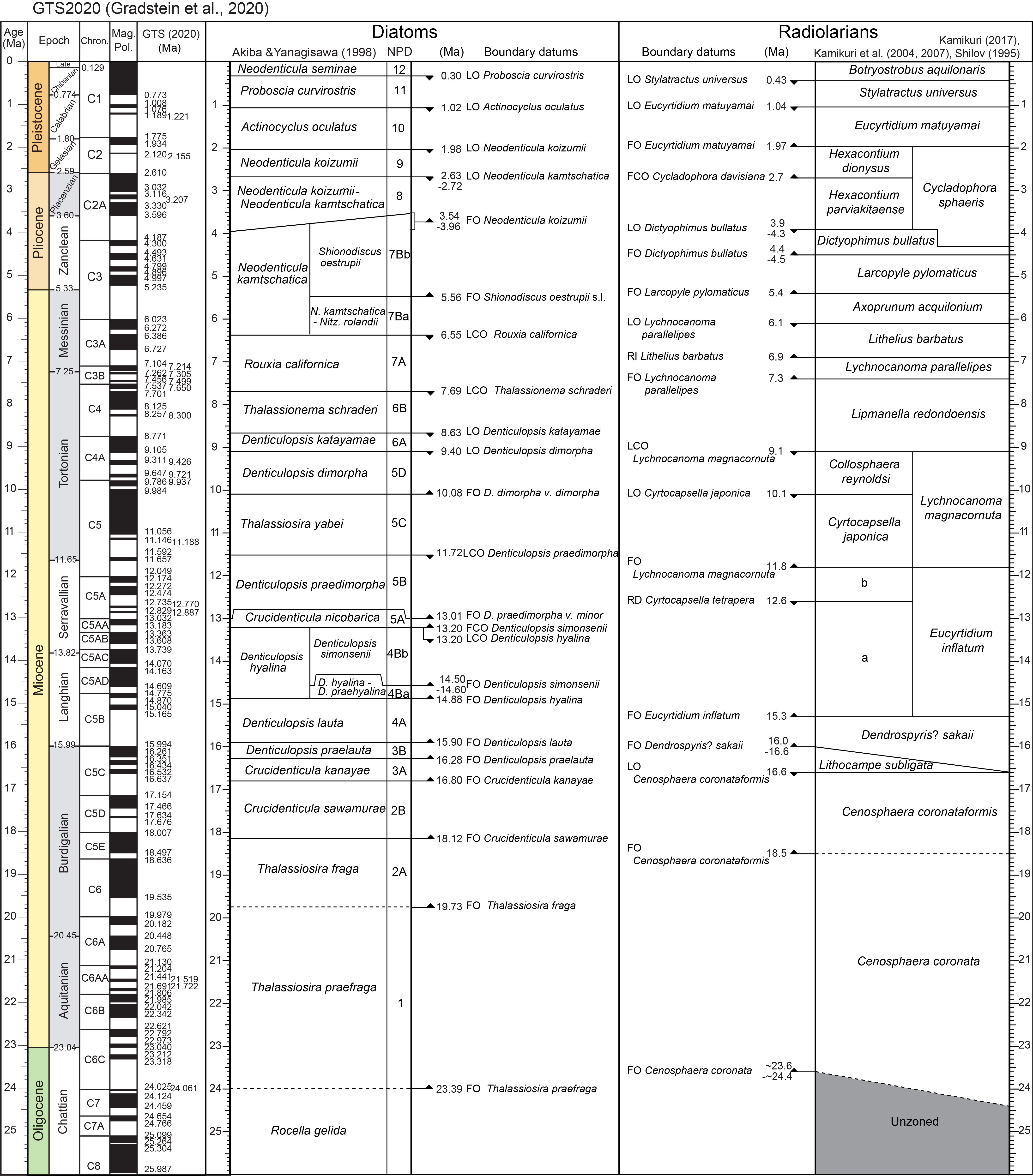
Figure F17. Neogene chronostratigraphy, diatom and radiolarian biostratigraphy, and magnetostratigraphy.
5.2. Diatoms
There are numerous studies of the diatom biostratigraphy in the North Pacific (see summaries by Barron, 1992; Yanagisawa and Akiba, 1998; Motoyama and Maruyama, 1998; Maruyama and Shiono, 2003; and Watanabe and Yanagisawa, 2005). Diatom biostratigraphy and biochronology at DSDP, ODP, and Integrated Ocean Drilling Program sites in the Japan Trench was done by Harper (1980) for DSDP Leg 56, Barron (1980) for DSDP Leg 57, Barron et al. (1980) for Legs 56 and 57, Akiba (1986) for DSDP Legs 57 and 87, Maruyama and Shiono (2003) and Motoyama et al. (2004) for ODP Leg 186, and Iwai et al. (2025) for Integrated Ocean Drilling Program Expedition 343.
The Neogene and Quaternary diatom zonal scheme and code used during Expedition 405 (Figure F17; Table T5) was based primarily on that proposed by Yanagisawa and Akiba (1998) with datum age information provided by Koizumi and Tanimura (1985), Barron (1992), Barron and Gladenkov (1995), and Watanabe and Yanagisawa (2005). Datum age information from low latitude was also referred to when it was required (Iwai et al., 2025). Several taxa names have been revised following Yanagisawa (1994), Censarek and Gersonde (2002), Alverson et al. (2006), and Williams and Kociolek (2018). All new taxa proposed by Suto (e.g., 2004a, 2004b, 2004c) for resting spores have been put into the Chaetoceros resting spores herein.
5.2.1. Methods
During Window 1 of the expedition (September–October 2024), smear slides from core catcher samples (PAL), each mounted on a 40 mm × 24 mm coverslip with optical adhesive (Nichika, Inc.), were examined routinely for stratigraphic marker species on Chikyu. Slides were examined using a Zeiss compound microscope AXIO Imager A1M at a power of 640× (objective lens of Plan-Neofluar 40×/0.9 pol with intermediate lens of 1.6 and eyepiece of 10×/23) through 1600× (objective lens of Plan-Neofluar 100×/1.3 oil pol with intermediate lens of 2.5), with the higher power being reserved mainly for taxonomic identification. A Zeiss AXIO cam 105 color, 5 megapixel microscope camera (0.5× intermediate lens) was used to capture diatom images using the microscopy software ZEN34 (ZEN lite). During Window 2 (November–December 2024), samples were sent to the KCC/Marine Core Research Institute (MaCRI), Kochi University, three times, roughly once per week. The smear slide preparation was the same as that applied during Window 1. In addition, decantation was used on shore to remove clay and sands when it was required. At KCC/MaCRI, slides were routinely examined with a Zeiss microscope Axioplan 2 image at a power of 640× or 1000× (objective lens of Plan-Neofluar 40×/0.9 pol with intermediate lens of 1.6× or 2.5× and eyepiece of 10×/23).
A JEOL scanning electron microscope (SEM)–energy dispersive spectrometer (EDS) (JCM-5700) in the Paleontology and Petrology Laboratory on Chikyu was available for higher magnification micrographs of selected specimens when deemed advantageous to taxonomic identification and determination of the fine structure of microfossils; however, it was not used during the expedition because of time limitations.
The abundance of diatoms was determined by the number of specimens observed per field of view at a magnification of 640× (diameter of a field of view is 0.355 mm with the combination of 40× objective lens, 1.25× intermediate lens, and 10×/23 eyepiece). The counting procedure followed Schrader and Gersonde (1978). These abundance estimates were recorded as follows:
- D = dominant (>5 valves per field of view).
- A = abundant (>1 valve per field of view).
- C = common (>3 valves per 5 fields and <1 per field of view).
- F = few (>3 valves per vertical traverse, 24 mm, of coverslip and <3 valves per 5 fields).
- R = rare (<3 valves per vertical traverse, 24 mm, of coverslip and >3 valves per slide).
- T= trace (<3 valves per slide observed).
- B = barren (no valve and fragment observed in slide).
At least three lines were examined before a sample was determined to be barren.
Preservation of diatoms was determined qualitatively and recorded as follows:
- G = good (slight to no fragmentation and dissolution).
- M = moderate (moderate fragmentation and dissolution).
- P = poor (severe effects of fragmentation and dissolution).
5.3. Radiolarians
Radiolarians are a group of oceanic plankton that are often well preserved as microfossils in marine sediments. In the North Pacific, radiolarian biostratigraphy has been studied extensively, mainly using deep-sea drilling cores (e.g., Reynolds, 1980; Sakai, 1980; Funayama, 1988; Shilov, 1995; Motoyama, 1996; Kamikuri et al., 2004, 2007; Kamikuri, 2017). During this expedition, we used radiolarian zones proposed by Kamikuri et al. (2004, 2007) and Kamikuri (2017) for the middle Miocene and later and zones proposed by Shilov (1995) for the early Miocene and Oligocene (Figure F17; Table T6), with numerical age information for the low-latitude radiolarians bioevents when it was required (cf. Motoyama in Iwai et al., 2025).
5.3.1. Methods
Radiolarian analyses were carried out on core catcher samples for each core. Near inferred boundaries, multiple samples were taken from the adjacent core to examine age differences across the boundary.
Sample preparation for optical microscopic examination was conducted on unconsolidated and semiconsolidated samples as follows: samples were treated with hydrogen peroxide (30% H2O2) and sodium pyrophosphate (5% Na4P2O7) and heated to boiling. A small part of the samples were only heated to 100°C with water. Disaggregated particles were sieved by washing through a 45 µm mesh sieve. The remaining residues were removed and dried. Undisaggregated sediment was treated again. Residues were then mounted with Norland Optical Adhesive 61 and covered with a 24 mm × 36 mm cover glass. The adhesive was solidified by placing the slide under ultraviolet light for approximately 15 min. Slides were examined at 125× to 250× using an optical microscope (Zeiss Imager.A1m).
Chert samples were prepared following the method of Onoue et al. (2024). First, the sample was divided into small pieces (about 1 cm3), immersed in 1 mol/L sodium hydroxide (NaOH) solution, covered, and heated at 100°C for 72 h. After 72 h, the NaOH solution was replaced. This process was repeated three times to etch the sample surface. After this, the NaOH solution was removed and washed through a 1 mm mesh sieve in which the residue was collected. The collected residue was cleaned (removal of impurities) for 60 s using an ultrasonic cleaner (KAIJO Sono Cleaner 100D CA-34800; frequency = 38 kHz) and then treated with 30% H2O2 and 5% Na4P2O7 in the same manner as the unconsolidated and semiconsolidated samples. After treatment, the remaining sample material was sieved by washing through a 45 µm mesh sieve and dried. Dried samples were examined at 30× to 100× using a stereomicroscope (Zeiss Discovery.V12).
The abundance and preservation of radiolarians were assessed qualitatively. The abundance estimates were recorded as follows:
- A = abundant (>1000 specimens).
- C = common (201–1000 specimens).
- F = few (51–200 specimens).
- R = rare (11–50 specimens).
- VR = very rare (1–10 specimens).
- B = barren (0 specimens on slide).
Only for chert samples, the following descriptors were used instead of abundance:
Preservation of radiolarians was determined qualitatively and recorded as follows:
- G = good (majority of specimens complete, with no or minor fragmentation, dissolution, and/or breakage).
- M = moderate (minor but common dissolution, with a small amount breakage).
- P = poor (strong dissolution, breakage, and more; many specimens are unidentifiable).
To accelerate the identification of radiolarians on board the ship, an artificial intelligence (AI)-based automated classification technique (Itaki et al., 2020) was implemented on a pilot basis for select samples from both Sites C0019 and C0026. The method was applied to radiolarian-bearing intervals in a discrete manner: core catcher samples from Cores 405-C0019K-1K through 10K, 405-C0026B-1K through 11K, and 405-C0026D-1H and 86 and 35 additional samples with high sampling frequency from throughout the cores from Holes C0019K and C0026E, respectively. Sample preparation was conducted in the same manner as for traditional optical microscopic examination, except for the method of spreading each sample during the preparation of the slide. A common technique is to heap the residue after washing onto a cover glass or slide glass using a pipette, but the heaped particles easily overlap. In this case, we were able to avoid the problem by using a handmade base that could keep the cover glass parallel, pouring the residue from above with the water, waiting about 5 min for the particles to settle, and then sucking out only the water.
The prepared slides were scanned using a virtual slide scanner (NanoZoomer SQ, Hamamatsu Photonics). Images were captured at 20× magnification with the focal plane centered on the middle of the slide. Additionally, 10 images with varied focal depths were captured by shifting the focal plane in 20.0 µm increments, five above and five below the central focus, resulting in a total of 11 images per field of view. A total of 11 images with varying focal depths were processed using image processing software Collection Pro customized for NanoZoomer (MITANI Corporation) to create a composite image through focus stacking. Individual particle images were then extracted from the composite image.
The extracted particle images were subjected to automated classification using the AI technique developed by Itaki et al. (2020), which is based on a convolutional neural network classification scheme. The classification model was constructed using transfer learning with a pretrained ResNet-101 architecture (He et al., 2016). The training data set was based on that described in Itaki et al. (2020), which includes particles collected from Pleistocene deep-sea sediments in the northwestern Pacific, Southern Ocean, and Japan Sea, and was further refined by the correspondence author of Ikaki et al. (2020) for the present study. Because of data privacy and storage limitations, the full training image data set is not publicly available. However, selected composite images and representative particle data can be provided upon request by the corresponding author. Of the full training data set, 90% was used for training and the remaining 10% for validation. During training, data augmentation was applied to enhance the variability and generalization of the model. The augmentation pipeline included random translation in both horizontal and vertical directions (±10 pixels), random scaling between 80% and 120%, and random rotation up to ±180°. Horizontal and vertical reflections were also enabled. Regions outside the image frame after transformation were filled with a uniform background color (RGB = 235, 235, 235). No additional modifications such as brightness, contrast, Gaussian filtering, or noise injection were applied. The training was performed using the Geological Survey of Japan Particle Analyzer (Miyakawa et al., 2024), a deep learning–based classification platform. The model was trained using stochastic gradient descent with momentum (SGDM) for 25 epochs, with a minibatch size of 16 and an initial learning rate of 0.0001. The data set was shuffled at the beginning of each epoch. The model evaluation on the test data showed a precision of 78.53%, a recall of 78.32%, and an F1 score of 78.42%. These results indicate that the trained model achieved sufficient classification performance for operational use. All classification results obtained on board during the expedition were reviewed, and only those objects identified as radiolarians were examined by the researchers for confirmation.
6. Paleomagnetism
Paleomagnetic and rock magnetic investigations during Expedition 405 were primarily designed to determine the characteristic natural remanence magnetization (NRM) on archive halves and discrete samples at room temperature and after demagnetization. In addition, AMS was measured on all discrete samples.
6.1. Laboratory instruments
The Paleomagnetism Laboratory on Chikyu is located on the starboard side of the core processing deck. Most of the equipment is housed in a large magnetically shielded room (7.3 m × 2.8 m × 1.9 m) with its long axis parallel to the ship transverse. The total magnetic field inside the room generally equals 1% of Earth’s magnetic field. The room is large enough to comfortably handle standard IODP core sections (~150 cm). The shielded room houses most of the paleomagnetic instruments. In this section, we describe the equipment used during Expedition 405.
6.1.1. Superconducting rock magnetometer
The long-core SRM (2G Enterprises, model 760) unit was upgraded from the liquid helium cooled system to the 4 K SRM liquid helium–free cooling system in June 2011. The 4 K SRM uses a Cryomech pulse tube cryocooler to achieve the required 4 K operating temperature without the use of liquid helium. The differences between the pulse tube cooled system and the liquid helium cooled magnetometers have a significant impact on the system’s ease of use, convenience, safety, and long-term reliability. The other parts of the SRM were not changed from the previous version. The SRM system is ~6 m long with an 8.1 cm diameter access bore. A 1.5 m split core liner can pass through a magnetometer, an alternating field (AF) demagnetizer, and an anhysteretic remanent magnetizer. The system includes three sets of orthogonal superconducting quantum interference devices (SQUIDs): two for transverse moment measurements (x- and y-axes) and one for axial moment measurement (z-axis). The noise level of the magnetometer is <10−7 A/m for a 10 cm3 volume rock. The magnetometer includes an automated sample handling system (2G804) consisting of aluminum and fiberglass channels designated to support and guide long-core movement. The core itself is positioned in a nonmagnetic fiberglass carriage that is pulled through the channels by a rope attached to a geared high-torque stepper motor. A 2G600 sample degaussing system is coupled to the SRM to allow automatic demagnetization of samples up to 100 mT. The system is controlled by an external computer with LabVIEW software (version 6.1) and enables programming of a complete sequence of measurements and degauss cycles without removing the long core from the holder.
6.1.2. Thermal demagnetizer
The TDS-1 thermal demagnetizer (Natsuhara Giken Co. Ltd.) has a single chamber for thermal demagnetization of dry samples over a temperature range from room temperature to 800°C. The chamber holds up to 8 or 10 cubic or cylindrical samples, depending on sample size. The oven requires a closed system of cooling water, which is placed next to the shielded room. A fan next to the µ-metal cylinder that houses the heating system is used to cool samples to room temperature. The measured magnetic field inside the chamber is <20 nT.
6.1.3. Anisotropy of magnetic susceptibility
The Kappabridge KLY 3S (AGICO Inc.) MS meter is designed for AMS measurements. Data are acquired from spinning specimens around three mutually perpendicular axes. The deviatoric susceptibility tensor can then be computed. An additional measurement for bulk susceptibility completes the sequence. The sensitivity for AMS measurements is 2 × 10⁻⁸ SI. Intensity and frequency of the applied field are 300 mA/m and 875 Hz, respectively. This system also includes a temperature control unit (CS-3/CS-L) for temperature variation of low-field MS of samples that was not used during Expedition 405.
6.2. Magnetic measurements and analysis
6.2.1. Magnetic measurements on archive-half sections
The natural remanent magnetization (NRM) of archive-half sections was measured using the SRM, and an assumed sample area of 17.1 cm2 was adopted for conversion to volume-normalized magnetization units (A/m). The interval between NRM measurement points was 1 cm for cores drilled with the HPCS and ESCS from Site C0026 and 2 cm for Site C0019 and cores retrieved with the SD-RCB coring system from Site C0026 (Table T7). Successive AF demagnetization was performed using the SRM in-line AF demagnetizer on all split archive halves. The in-line AF demagnetizer applied a field to the x-, y-, and z-axes of the SRM in this fixed order. Demagnetization fields no higher than 25 mT were used to demagnetize the sections using the following steps: 10, 15, 20, and (25). The maximum field strength of in-line AF demagnetization used on the archive-half sections was limited to 25 mT because of the destructive nature of the treatments on the NRM and the necessity to partially preserve the primary magnetizations for possible future analysis.
While measuring Section 405-C0026E-2H-2, we started experiencing drift in the z-axis of digital meters in the SQUID system. To assess if the measurements were still reliable, we performed the following tests: (1) we remeasured the NRM of Section 1H-1 (after demagnetization at 25 mT) and compared the results with the result produced before the problem arose, and (2) we measured standard samples. Both tests showed the expected results, supporting the good quality of data. However, to be cautious, we reduced the maximum demagnetization step to 20 mT and planned to eventually perform the 25 mT step during shore-based analysis. The drift on the z-axis lasted for a few days. To understand the origin of the drift, we checked the ship position and navigation data. The ship was at a heading of ~200° when the problem occurred. However, such positioning happened at other times and could not explain the drift by itself. The problem was attributed to the possible occurrence of a mild magnetic storm at the same time.
Even if flux jumps rarely occurred, some sections caused a significant shift in the SQUID values, most commonly on the y-axis, and especially at the end of measurement while the section was exiting the instrument. We attributed this phenomenon to the presence of either strong drilling overprint or particularly magnetically intense intervals (i.e., tephra layers or basalts). We visually checked the SQUID values and reset the digital meter before each step if values were not close to zero.
The sample track was magnetically cleaned every day at 80 mT to avoid magnetic contamination, and the tray background values were measured daily and/or at each change of setting. The header and trailer, which are the portions of empty track before and after each section along the tray, were measured for 20 cm to allow for future deconvolution analysis. Starting with Section 405-C0026B-15K-3, the header and trailer were reduced to 15 cm to reduce the overall measurement time.
AF demagnetization results were plotted as downhole variations with depth. The highest demagnetization step (either 20 or 25 mT) was compared to the results from discrete samples to determine whether the remanence after demagnetization reflects the characteristic remanent magnetization (ChRM).
6.2.2. Magnetic measurements on discrete samples
Oriented discrete samples were collected from working-half sections, nominally one discrete sample per section unless severe drilling disturbance (e.g., flow-in, fractures, etc.) hampered adequate sample collection or where additional samples were collected from an interval of interest. In soft sediment, discrete samples were taken with plastic Natsuhara-Giken sampling cubes (7 cm3 sample volume). Cubes were manually pushed into the working half of the core, and the up arrow on the cube pointed upsection in the core reference frame. In lithified sediments and hard rocks, 2 cm cubes (8 cm3 sample volume) were cut with a parallel saw after marking their orientation.
AMS and NRM measurements with stepwise demagnetizations were routinely performed on discrete samples. Incremental AF demagnetization used the 2G600 sample degaussing system, and NRM after each step was measured with the SRM. Stepwise AF demagnetization was performed in 13 steps between 0 and 80 mT (0, 2.5, 5, 7.5, 10, 15, 20, 25, 30, 40, 50, 60, and 80 mT). A total of 32 samples from the uppermost interval of Hole C0019J were demagnetized with a reduced sequence of 8 steps (0, 10, 20, 30, 40, 50, 60, and 80 mT). Three samples from the red sediments in Hole C0019P were subjected to a nonconventional demagnetization protocol. After the standard demagnetization at 80 mT, these samples were further thermally demagnetized with the following steps: 105°, 110°, 120°, 150°, 200°, 250°, 300°, 400°, 500°, 525°, 550°, 575°, 600°, 650°, and 700°C.
The results were plotted on orthogonal projections (Zijderveld, 1967), which represent the vector component resulting from the stepwise demagnetization. Principal component analysis (PCA; Kirschvink, 1980) was performed using the PuffinPlot 1.4.1 software (Lurcock and Wilson, 2012) to determine the ChRM direction. For PCA, we mostly applied free line fitting on more than three vector endpoints, with a few exceptions that were anchored to the origin. The ChRMs from discrete samples were used to restore the azimuth of the core in coherent intervals, thus allowing for structural data to be geographically oriented (see Structural geology). Data from sections can be used postexpedition to refine the orientation following the paleomagnetic orientation procedure in Acton et al. (2023), which includes cleaning of edge effects and drilling disturbance and visual inspection of data from archive halves.
The AMS of discrete samples was measured before demagnetization. Because of an error in saving data, 12 samples from Sections 405-C0026B-4K-3 through 8K-CC were measured for AMS after demagnetization. The AMS was analyzed with the Anisoft 6.1.02 software. The magnetic fabric is represented by an ellipsoid defined by the directions of magnetic anisotropy tensors (K1 or Kmax = maximum, K2 or Kint = intermediate, and K3 or Kmin = minimum). The directional alignment of magnetic minerals were evaluated through a Flinn diagram plotting magnetic foliation (F = K2/K3; Stacey et al., 1960) and magnetic lineation (L = K1/K2; Balsley and Buddington, 1960) similar to the fabric element characteristics conventionally used in structural geology. The corrected anisotropy degree (Pj) (Jelinek, 1981) quantifies the intensity of the preferred orientation:
Furthermore, the shape parameter (T) (Jelinek, 1981) describes the ellipsoid being prolate (T = −1), neutral (T = 0), or oblate (T = 1) based on the calculation
6.2.3. Sample coordinates
The conventional IODP core coordinate system (reference frame) was used, where +x is the vertically upward direction when the archive half is on its curved side, +y is the direction to the left along the split core surface when looking upcore, and +z is the downcore direction (Figure F18). The relationship of the SRM coordinates (X-, Y-, and Z-axes) to the data coordinates (x-, y-, and z-directions) is as follows: for archive halves, x-direction = X-axis, y-direction = Y-axis, and z-direction = Z-axis; for working halves, x-direction = −X-axis, y-direction = −Y-axis, and z-direction = Z-axis.
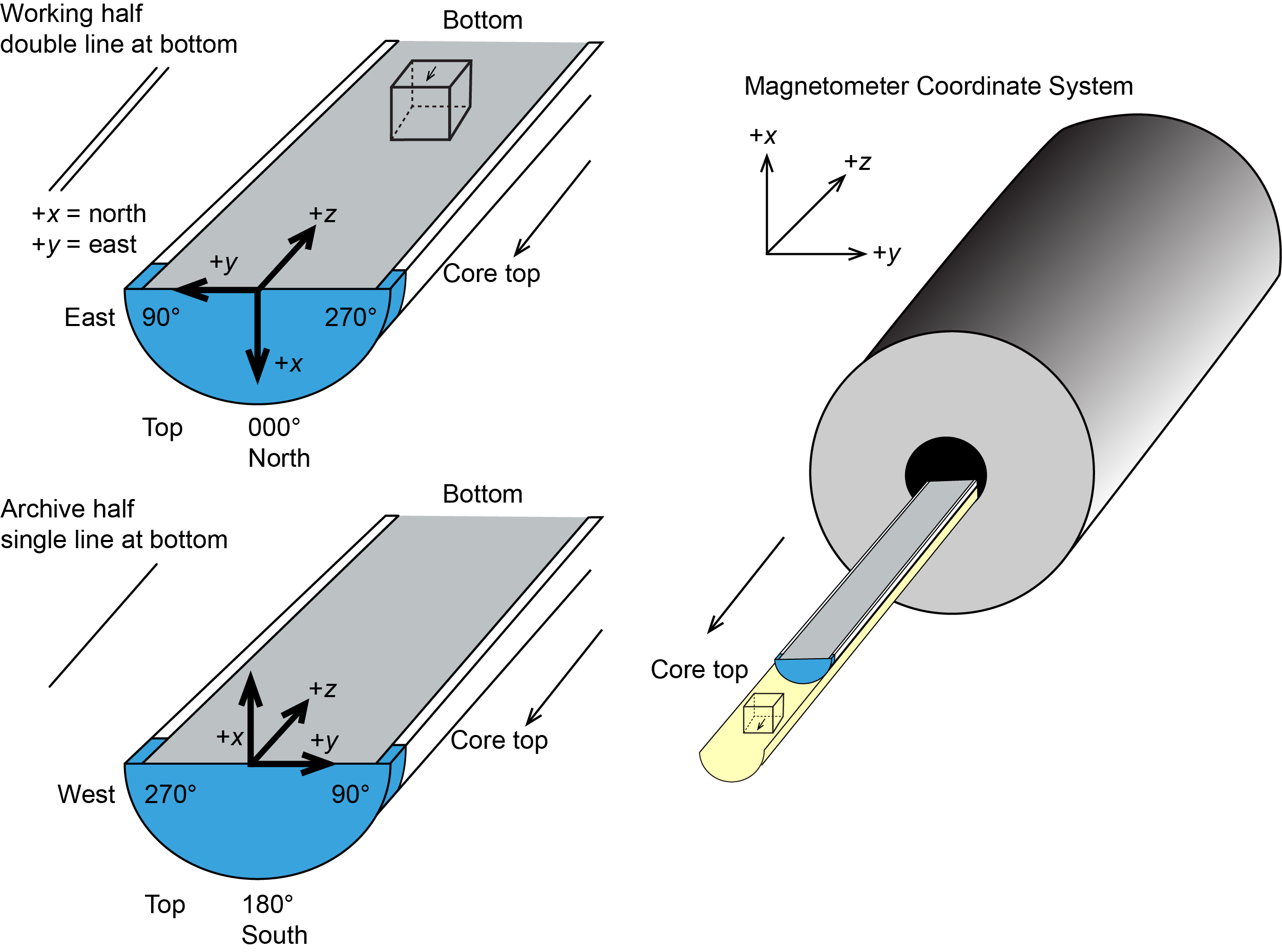
Figure F18. Paleomagnetic sample coordinate systems.
6.3. Magnetostratigraphy
The magnetostratigraphy was constructed by correlating observed polarity patterns with the reference geomagnetic polarity timescale (GPTS) and constrained by biostratigraphic datums (see Biostratigraphy). For sedimentary rocks that formed at high latitudes, no polarity ambiguity arises and inclination is needed to estimate the magnetic polarity if the bedding is horizontal. The chosen GPTS from Cenozoic through the Paleogene used for Expedition 405 is based on the geologic timescale of Gradstein et al. (2020). The chron boundary ages from table 28.1 in Speijer et al. (2020) were adopted to be consistent with the biostratigraphy datums (Figure F19; Table T8). The polarities are named with a progressive number from the top to bottom and prefixes “n” for normal polarities, “r” for reversed polarities (n1, r1, n2, etc.), and “m” for intervals showing mixed polarities or inclinations close to zero; a further prefix “K” was added for Hole C0019K to avoid confusion with other holes from the same site. For the younger ages of the timescale (Pliocene–Pleistocene), traditional names were used to refer to the various chrons and subchrons (e.g., Brunhes, Matuyama, Jaramillo, Olduvai, etc.).
Figure F19. GPTS.
7. Physical properties
Physical property measurements provide fundamental information necessary for characterizing the formation, including distinguishing lithostratigraphic units and correlating coring results with downhole logging data. A variety of tools and methods were used for measurements on Expedition 405 core samples. Prior to core splitting and sampling, XCT images were captured for all cores (see Structural geology). After the XCT scanning was completed and the whole-round cores had reached thermal equilibrium with room temperature (~20°C), GRA density, MS, NGR, and P-wave velocity were measured using the COMET. Cores were then split along the core axis: one half was designated as the archive half and the other as the working half for sampling and analyses. Cores were not geographically oriented during this expedition; therefore, all samples are oriented relative to the core reference frame (Figure F20).
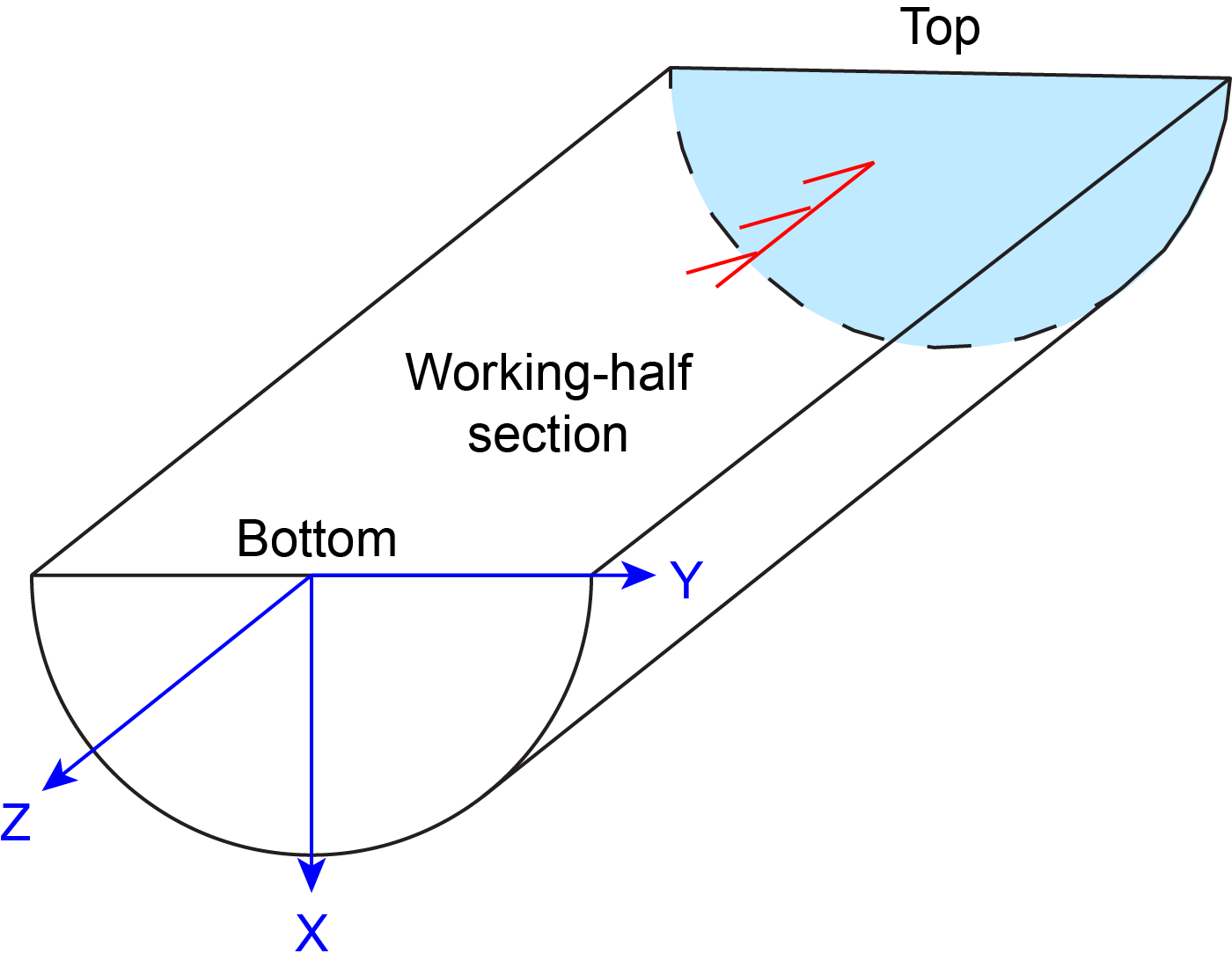
Figure F20. Core reference frame used for physical property sampling.
Thermal conductivity measurements were made using a Teka thermal conductivity meter with a full- or half-space probe on whole-round cores or the working half, respectively. Moisture and density (MAD) were determined for discrete samples collected from working halves using an Ocean High Technology Institute custom-built motion-compensated shipboard balance system and a Quantachrome pentapycnometer that utilized helium-displacement to determine sample volumes. For consolidated sediments, P-wave velocity (VP), S-wave velocity (VS), and electrical resistivity measurements were made in the x-, y-, and z-directions of the core reference frame on oriented discrete cube-shaped samples to evaluate anisotropy. For soft sediments, wave velocities were not measured, and electrical resistivity was only measured in the y- and z-directions directly on the working half. Additionally, in soft sediments, the undrained shear strength was determined using a vane shear apparatus and pocket penetrometer. Anelastic strain recovery (ASR) measurements were also conducted on a few whole-round samples, and formation temperature was determined in some holes cored with the HPCS using an advanced piston coring temperature (APCT-3) tool.
A detailed description of all the measurement methods utilized during Expedition 405, including their accuracy, is included below.
7.1. Core Measurement Track
The COMET has four measurement sensors mounted on an automated track to sequentially measure GRA density, MS, P-wave velocity and amplitude, and NGR. The quality and validity of the COMET measurements are a function of both core quality and sensor precision. Optimal results are achieved when the core liner is completely filled with a fully fluid-saturated core. If the core liner is incompletely filled or the core is partially saturated, the quality of the measurements will be compromised. Measurements were made every 4 cm along the core, except for NGR, which was typically collected every 16 cm, but occasionally a higher sample frequency of 4 cm was used.
7.1.1. Gamma ray attenuation density
GRA density is based on the attenuation of gamma rays by Compton scattering. A lead-shielded 137Cs (370 MBq) gamma ray source and 5 mm collimator produce a narrow gamma ray beam that passes through the whole-round cores and core liner. The gamma detector system includes a scintillator and an integral photomultiplier tube to record the attenuated gamma rays. The degree of attenuation is proportional to the electron density, so the GRA bulk density (ρb) is based on established calibration curves.
The gamma ray detector is calibrated with a sealed calibration core composed of nine different zones filled with material of known density inside a standard core liner (empty poly(methyl methacrylate) core liner, high-density polyethylene (HDPE), polyvinylidene fluoride, sandstone, A6063 aluminium, peridotite, titanium, SUS304 steel, and C3604 brass). A least-squares linear regression is performed to determine the relation between the measured intensity of gamma rays passing through the sample (I; counts/s) and the known density of the material, so that
where the coefficients A and B are determined from the calibration experiment.
GRA density measurements on the core samples were conducted every 4 cm for 4 s with a spatial resolution of 5 mm.
7.1.2. Magnetic susceptibility
MS quantifies the degree to which a material can be magnetized by an external magnetic field, providing information on sediment and rock composition. MS measurements were made with a Bartington loop sensor with an 8 cm diameter. An oscillator circuit in the sensor produces a low intensity (~80 A/m RMS), nonsaturating, alternating magnetic field (0.565 kHz). Bringing any material within the influence of this field will cause a change in oscillator frequency. The frequency information is returned in pulse form to the susceptometer and converted into MS. The spatial resolution of the loop sensor is 23–27 mm, and it is accurate to within 2%.
7.1.3. P-wave velocity
P-wave (compressional) velocity (VP) data can be used to evaluate small-strain moduli, correlate between log and core data, and evaluate pore volume and cementation. VP is defined as the time required for a compressional wave to travel a set distance:
where d (km) is the path length of the wave across the core and tcore (s) is the traveltime through the core.
P-wave transducers on the COMET automatically pick the total traveltime of the compressional wave, which travels horizontally across the whole core and core liner between the transducers. The picking method relies on a threshold method, with a threshold preset prior to the expedition. In many cases, these preset threshold conditions resulted in the second or third arrival being recorded for velocity estimations, which resulted in poor quality velocity picks and significant data scatter. This notwithstanding, the total traveltime observed is composed of the following:
- tdelay = time delay related to transducer faces and electronic circuitry (s).
- tpulse = delay related to the peak detection procedure (s).
- tliner = transit time through the core liner (s).
- tcore = traveltime through the sediment or rock (s).
The system is calibrated using a core liner filled with distilled water, which provides a control for tdelay, tpulse, and tliner. With these calibrations, wave velocity through the cores can be calculated on whole-round specimens in core liners as
- dcl = measured diameter of core and liner,
- eliner = liner wall thickness, and
- to = measured total traveltime.
This equation assumes that the core completely fills the core liner.
The P-wave amplitude was also measured with the COMET; however, because the gain settings may vary between measurements and the associated gain (or magnitude of the input amplitude) is unknown, the resulting amplitude is of limited use and is not examined in this report.
7.1.4. Natural gamma radiation
NGR measurements provide insights into sediment and rock composition and thus can be used to identify lithology. NGR emissions were monitored on whole-round cores on the COMET track to obtain spatial variability in radioactivity and for correlation with downhole gamma ray logs. The device utilizes a lead-shielded counter optically coupled to a photomultiplier tube and connected to a high-voltage power supply unit and a signal preamplifier. Two horizontal and two vertical sensors are mounted in a lead, cube-shaped housing. The NGR system records radioactive decay of long-period isotopes 40K, 232Th, and 238U. NGR has a spatial resolution of 120–170 mm and was measured every 16 cm with a count time of 30 s. Background radiation noise was determined by making measurements on a water-filled calibration core.
7.2. Moisture and density
Discrete samples from the working-half cores were used for the determination of index properties (e.g., bulk density, grain density, dry density, water content, porosity, and void ratio). Index properties are determined from phase relations, mass measurements on wet and dry specimens, volume measurements on dry specimens, and corrections for salinity. In general, one discrete sample for index properties was collected for every core section. Sample intervals were occasionally shifted, in consultation with the structural geology and lithostratigraphy teams, to select minimally disturbed, homogeneous samples. Each discrete index property sample was ~8 cm3 (~2 cm × 2 cm × 2 cm cubes).
In sediments, to minimize desiccation, MAD sample collection was performed as soon as feasible after core splitting and was immediately followed by measurements of wet sediment mass (Mwet). In hard rock (chert or basalt), measurement of Mwet was conducted after oriented cube samples were resaturated in seawater under vacuum for at least 24 h. These same resaturated cubes were used for wet mass, impedance, VP, VS, and discrete MS measurements (see Paleomagnetism).
Wet and dry masses were measured using a paired electronic balance system, which is designed to compensate for the ship’s heave. The sample mass was counterbalanced with a precisely known mass (40 g) that was within 20–60 g of the sample mass. The sample mass was determined to a precision of ±0.005 g. The balance system was calibrated at least once per 12 h.
After Mwet measurements, samples were dried in a convection oven at 105° ± 5°C for 24 h. After removal from the oven, dry samples were placed in a desiccator for at least 1 h to equilibrate to room temperature (~20°C), after which the dry sediment mass (Mdry) and dry sediment volume (Vdry) were measured. The dry sediment mass (Mdry) was measured using the paired electronic balance system.
The dry sediment volume (Vdry) was measured with one of two five-chamber Quantachrome pentapycnometers using a helium-displacement technique with a precision of ±0.04 cm3. Helium was chosen because it is adequate for all types of rocks and soils, including clay-rich sediments (Amoozegar et al., 2023). The five-chamber system allowed the simultaneous measurement of four sample volumes and one calibration sphere. Each reported measured volume is the average of five volume measurements. The calibration sphere was cycled between all measurement chambers to monitor for errors in each chamber. Each pycnometer chamber was calibrated at least once per 24 h.
Standard IODP practices were used to determine pore water mass and volume, salt mass and volume, and solid grain mass and volume (Blum, 1997). From these data, bulk density, dry density, grain density, porosity, and void ratio were calculated. Standard seawater density (1.024 g/cm3) and salinity (35 parts per thousand [ppt]) and a constant salt density (2.20 g/cm3) were assumed for all calculations.
7.2.1. Water content
Water content (Wc) was determined following the American Society for Testing and Materials (ASTM) standard D2216 (ASTM International, 1990). Corrections are required for salt when measuring the water content of marine samples because the salt contained in the brine filling the wet sample doesn’t evaporate and contribute to the mass and volume of the dry sample (Mdry). In addition to the water content calculation in ASTM D2216 (i.e., the ratio of pore fluid mass to dry sediment mass; Wcdry), the ratio of pore fluid mass to total sample mass (Wcwet) was also calculated. The equations for water content are
- Mwet = total wet mass of the discrete sample (g),
- Mdry = mass of the dry sample (g), and
- s = salinity of the water (assumed to be a dimensionless constant of 0.035).
7.2.2. Bulk density
Bulk density of the discrete core sample is determined as ρb (g/cm3) = Mwet/Vt. Total wet sample mass (Mwet) was measured immediately after collecting each discrete sample using the dual-balance system, as described above. Total sample volume assuming 100% saturation (Vt [cm3] = Vg + Vpw) was determined from the pycnometer measurement of grain volume (Vg) and calculated volume of pore water (Vp), which also includes the volume occupied by the salt in the seawater. Solid grain and pore water volume are determined as
- Vd = dry volume (cm3),
- ρsw = standard seawater density (g/cm3), and
- ρsalt = density of salt, assumed to be constant (2.20 g/cm3).
7.2.3. Porosity and void ratio
Porosity (ϕ) relates the volume of the pores to the total sample volume; void ratio (e) relates the pore volume to the volume of the solid grains. These are calculated as
7.2.4. Grain density
Grain density (ρg; g/cm3) was determined from measurements of dry mass made with the dual-balance system, and dry volume with the pycnometer, both with a correction for salt:
where Msalt is the mass of salt (g) and is determined from Mdry, Mwet, and s with the formula Msalt (g) = (Mwet − Mdry)(s/(1 − s)).
7.3. Electrical resistivity
Electrical resistivity was determined using a Keysight E4990A Impedance Analyzer using the bridge method with either a four-pin electrode inserted into unconsolidated sediment or two electrodes on a cubic sample for consolidated sediments.
For unconsolidated sediment, a four-pin Wenner array consisting of four 1 cm long electrodes spaced 7.5 mm apart was inserted into the working halves of split cores. During measurement, the two outer electrodes provide an alternating current into the sample and the two inner electrodes measure the resulting potential difference. In the standard test configuration, the magnitude (|Z|) and phase (θ) of the complex impedance were measured at 25 kHz across the array. On split cores, the 4-pin array can measure impedance in two orthogonal directions on the split core face (i.e., y- and z-directions) (Figure F20). Electrical resistivity in a specific direction (Ry or Rz) is computed from the complex impedance measured in the same direction:
where dr is a geometric factor specific to the electrode array determined by comparing the measured |Z| and θ of an International Association for the Physical Sciences of the Oceans (IAPSO) standard seawater solution (35 g/L NaCl, also referred to as 3.5% NaCl solution) with known electrical impedance. A new value of dr was computed every 24 h to account for changes in electrode array geometry due to corrosion or slight bending of the electrodes. The ambient air temperature was recorded for each measurement; because the cores were thermally equilibrated prior to measurement, the split core temperature is assumed to be the same as the ambient air temperature.
For consolidated sediment and hard rocks, electrical impedance measurements were performed on cubic samples (~2 cm × 2 cm × 2 cm) cut from working halves with a spatula or a diamond blade saw (depending on sample consolidation). All cubes were oriented with respect to the core reference frame (Figure F20). Carefully controlling the sample orientation during preparation allowed first-order determination of electrical resistivity, as well as anisotropy. Well-consolidated samples were immersed in a 3.5% NaCl solution, used as simulated seawater, for a few seconds prior to measurement, and hard rock samples were resaturated in seawater under vacuum for at least 24 h. Excess water was removed from the sample surface prior to measurement.
Measurements were acquired using the bridge method with a two-terminal circuit on cubic samples and the same Keysight E4990A Impedance Analyzer. For the measurement, the oriented specimen cube was placed between two stainless steel electrodes covered with seawater-saturated filter paper. The magnitude (|Z|) and phase (θ) of the complex impedance were measured at 25 kHz between opposite cube faces. The cube was rotated to measure impedance in the x-, y-, and z-directions (Figure F20). Electrical resistivity for each direction (e.g., Rx) was computed from the complex impedance measured in each direction (e.g., x) and sample dimensions defined by face length (L):
where |Zf| cos θf is the resistance of the filter paper. Face lengths were measured using the laser distance sensor on the NS Design Elastic Wave Velocity for Discrete analysis apparatus (D-EWVEL) during P-wave velocity measurements (see Discrete P-wave and S-wave velocity).
An indication of the precision of the electrical resistivity measurements can be gained from repeat measurements of a rock standard. Repeat measurements on the rock standard generally, made over a period of about 2 months, vary within 15%–20% of the average (Figure F21). The maximum deviations in the rock standard measurement were observed between 28 and 29 October 2024. These large deviations are likely due to a loose electrical connection that was discovered and repaired on 31 October 2024.
Figure F21. Electrical resistivity measurements.
From electrical resistivity measured in the x-, y-, and z-directions, anisotropy is calculated following the approach of Carlson and Christensen (1977). Horizontal anisotropies are reported only as absolute values because cores acquired during Expedition 405 were not oriented (i.e., x- and y-axes are not consistently oriented). Potential causes of anisotropy include: (1) alignment of pores during compaction, (2) fabric development, and (3) microstructures such as microfractures and microcracks. Anisotropy is calculated by comparing the horizontal (x and y) and vertical (z) components of the measurement expressed as a percentage of the mean (e.g., Shipboard Scientific Party, 2001b), for horizontal and vertical electrical resistivity anisotropy (αRhor, αRvert):
7.4. Discrete P-wave and S-wave velocity
In consolidated sediments and hard rock, discrete VP and VS measurements were performed on the same cubic samples used for electrical resistivity. Wave velocities along a given direction were measured using a D-EWVEL for discrete samples. The D-EWVEL is equipped with two sets of 1 MHz transducers, one set used for P-waves and the other for S-waves. Each set of transducers has a transmitter and a receiver. Sample length (L) was measured with a laser distance sensor. During measurement, the sample was placed between the transducers and held in place under a vertical force. A load of 20–50 N was applied, which translates to ~50–125 kPa pressure on a 2 cm cube. The transmitter was connected to a pulse generator, and the receiver was connected to an oscilloscope synchronized with the pulse generator. Total traveltime (t) for the first arrival was picked and logged from the digitally displayed oscilloscope signal. The velocity in any direction (e.g., VPx) is calculated from the sample length (e.g., Lx), total traveltime (tx), and system-calibrated delay time (tdelay):
The delay time and laser distance sensor were calibrated at least every 12 h, but recalibration was also required every time the setup was reset for either VP or VS measurements. Calibration of the delay time was determined by placing the transmitter and receiver in direct contact and measuring traveltime. Similarly, the laser distance was calibrated by measuring the distance when (1) the transmitter and the receiver were in direct contact, and (2) a reference specimen of known length (2.5 cm) was placed between the transmitter and receiver. Routine QC measurements were made by measuring velocity on glass and acrylic standards having known lengths and velocities.
As with electrical resistivity, P-wave velocity (VPx, VPy, and VPz) and S-wave velocity (VSx, VSy, and VSz) measured in the x-, y-, and z-directions were used to calculate the vertical (e.g., αVvert) and absolute horizontal anisotropy (e.g., αVhor):
7.5. Undrained shear strength
The undrained shear strength of soft sediments in the working half of the core was measured using a pocket penetrometer (Geotest E-284B) and a Wykeham Farrance vane shear device (Model No. 23544, Serial No. 119216). Measurements were made at discrete locations on the working halves of cores within undisturbed, homogeneous sediments, and, to the extent possible, ash beds were avoided. Measurements were made with the penetrometer penetration direction and the vane rotation-axis oriented perpendicular to the y-z plane of the core reference frame (Figure F20).
7.5.1. Penetration strength with pocket penetrometer
The compressive strength is calculated from the penetration resistance generated by pushing a 6.4 mm diameter cylindrical probe into the y-z plane of the split core. The average of three adjacent penetrometer tests in intact sediments was recorded as the unconfined compressive strength. The resulting measure of unconfined compressive strength (qu) can be related to undrained shear strength (Su(p)) by
where g is the acceleration due to gravity and qu is a mass per unit area. The penetrometer has a maximum measurement capacity of 6 kg/cm2.
7.5.2. Shear strength with vane shear
The vane blade is inserted into the surface of the split core so that the upper edge of the vane blade is level with the core surface. The vane is rotated at a constant rate until the sediment fails. Vane shear strength (Su[v]) can be determined from the torque (T) required to cause failure and a vane constant (Kv) as
All vane shear strength measurements were obtained using a vane with a height of 12.7 mm and a blade length of 6.35 mm rotating at an angular speed of 1.5°/s. Failure torque was determined by measuring the rotation of a torsional spring using a spring-specific relation between rotation angle and torque. Vane shear strength results were only reliable for samples with vane shear strength <100–150 kPa. When cracking or core separation occurs upon insertion of the vane blade, measurements should be discarded.
7.6. Thermal conductivity
Thermal conductivity is a bulk material property that governs the ease with which heat can be transferred through a material. It depends on the composition and porosity of the bulk material; the structure, distribution, and alignment of mineral phases; and, to a lesser extent, temperature and pressure.
The TeKa TK04 system determines thermal conductivity using a probe (Vacquier, 1985; Von Herzen and Maxwell, 1959). The system incorporates a heating wire and a temperature sensor into a line source. As the wire is heated, the temperature of the source is recorded simultaneously. The thermal conductivity of the surrounding material can be calculated from the temperature versus time measurement curve (heating curve) using the simple calculation of the thermal conductivity coefficient:
- q = input heat flux,
- (t1, t2) = time interval of the heating curve,
- T(t1), T(t2) = corresponding source temperatures,
- ka(t) = apparent thermal conductivity, depending on the time interval (t1, t2) used for calculation.
Commonly, a thermal conductivity value is calculated from the largest interval of the heating curve in which ka(t) remains constant. Therefore, sufficiently large heating durations are required to calculate the optimal thermal conductivity value. Instead of a conventional approximation method described above, the TK04 system uses a Special Approximation Method that automatically finds the optimal time interval for a thermal conductivity calculation.
Depending on the properties of the core, two different methods of measuring the thermal conductivity were used. In unconsolidated sediment, where a probe could be inserted into the core without fracturing the sediment, a full-space needle (VLQ) probe (ASTM Standard D5334-08) (Von Herzen and Maxwell, 1959) was inserted into a whole-round core through a hole drilled at the splitting line on the side of the core liner. When sediment strength precluded the use of the full-space probe, a half-space (mini-HLQ) probe (Vacquier, 1985), which approximates an infinite line source, was used on the surface of the working half of the split core. The half-space probe was placed directly on the split core so that the line source was aligned parallel to the core axis. Both the full- and half-space measurements produce a scalar thermal conductivity value in the plane perpendicular to the orientation of the probe.
All measurements were made after the cores had equilibrated to room temperature. In most cases, three repeat measurements were made at the same location. Some locations may have up to six repeat measurements if there were difficulties acquiring measurements due to contact quality or problems determining the correct heating power to use. Initial problematic measurements were excluded from the reported averages. For mini-HLQ measurements of lithified sediments, the selected samples had a flat surface, longer than 5 cm (the length of the probe), without clear cracks at the surface or inside the sample. XCT scans were often used to aid in the selection of measurement locations. To improve contact quality in hard rock (basalt), the split core surface was soaked in salt water for 1–2 h and, if the surface was rough, polished with sandpaper prior to measurement.
At the beginning of each measurement, temperature in the sediment was monitored by the system to ensure that thermal drift was less than 0.4 mK/min before generating the thermal perturbation. Because of the steps to thermally isolate and equilibrate the samples beforehand, this step typically lasted ~1–2 min. After the instrument established that the temperature was near equilibrium, a calibrated heat source was applied and the rise in temperature was recorded for 60 or 80 s for the half- and full-space probes, respectively. Values of thermal conductivity were determined based on least-squares fits of the data following the previous equation and using the known heating rate (q) applied by the system.
QC of the TK04 system was performed at least once every 24 h on Macor samples having known thermal conductivities of 1.623 W/(m·K) ± 2% and 1.652 W/(m·K) ± 2% for the full- and half-space probes, respectively. During Expedition 405, the half-space probe was the primary method for measuring thermal conductivity because even the shallowest sediments recovered did not provide good contact with the full-space probe.
7.7. Anelastic strain recovery analysis
ASR analysis is a core-based measurement technique that can evaluate both orientation and magnitude of 3D present-day principal stresses acting on earth materials at depth. The ASR approach is to measure the anelastic strain due to the stress relaxation of the core soon after its recovery from an in situ stress state to the surface. The methodology used for the ASR measurement during Expedition 405 is based on Matsuki (1991), following the guidelines described in Lin et al. (2007). We applied the same ASR measurement and analyses techniques as those successfully used during previous NanTroSEIZE expeditions and during Expedition 343 at the Japan Trench (Byrne et al., 2009; Lin et al., 2023; Yamamoto et al., 2013; Oohashi et al., 2017).
Immediately following XCT scanning, a 15 cm long undisturbed whole-round core was selected based on the XCT images and sampled. COMET measurements were not performed on these samples because the ASR measurement is time sensitive and requires instrumentation as soon as possible after core is extracted from the subsurface to capture early strain recovery. Core samples were pushed out of their core liners, and the outer surface was washed in seawater to remove drilling mud.
The anelastic strains in nine directions, including six independent directions, were measured using wire strain gauges (six 90° shear-strain gauges and six uniaxial gauges; 120 Ω) (Figure F22). Here, the z-direction represents the vertical (core-axis) direction, whereas the x- and y-directions represent arbitrary orthogonal directions that are also mutually orthogonal to the z-direction. For all directions, relaxation (or tension) represents positive strain and compaction represents negative strain. These directional strains are then converted to maximum (ε1), intermediate (ε2), and minimum (ε3) principal strains, as well as a mean strain (εm) using the methods and guidelines of Matsuki (1991) and Lin et al. (2007). Further, the vertical (z-) direction is also assumed to be a principal strain direction.
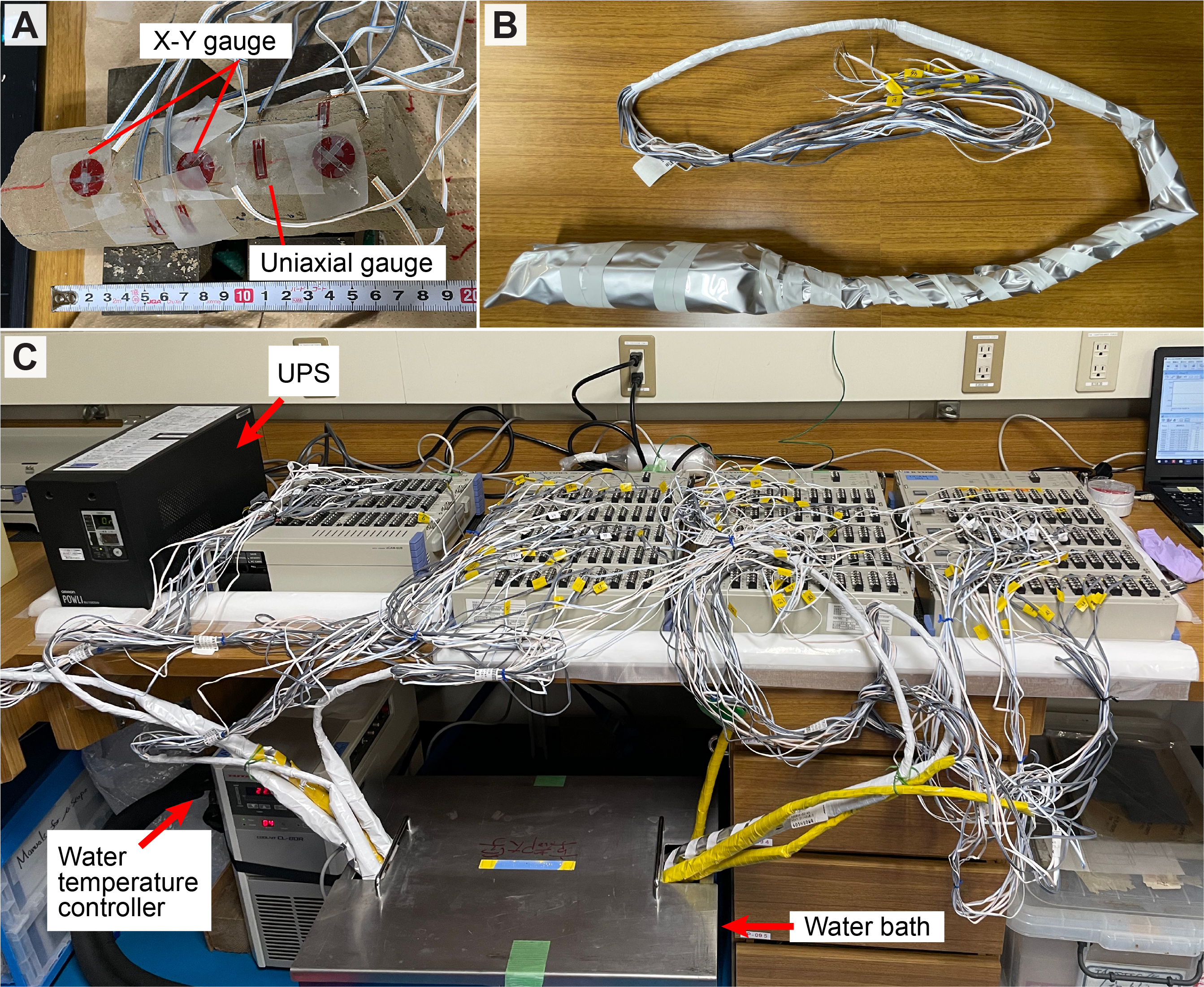
Figure F22. Equipment for ASR measurement.
In cases where a few fractures had developed in the specimen, the fractures were glued to prevent the sample from splitting into pieces. It took 1–2 h to mount 18 strain gauges, and the total elapsed time just after core on deck was 2–12 h before recording of the strain recovery commenced. The core samples were double-bagged (with plastic and aluminum) and submerged in a thermostatic water bath where temperature changes were kept controlled at 21.5° ± 0.1°C for the duration of the measurement. Strain values were collected every 10 min for a maximum of 50 days.
7.8. Formation temperature
Formation temperature measurements were carried out using the APCT-3 tool (Figure F23), which is the third-generation tool of its kind used with the HPCS to measure downhole in situ temperatures. The APCT-3 system derives from earlier versions of similar instruments developed in the 1970s and 1980s (Horai and von Herzen, 1985). The APCT tool, first deployed during DSDP Leg 86 in 1984, allows in situ formation temperature to be inferred ahead of the drill bit without the need for an additional tool run specifically for temperature measurement. The third-generation APCT-3 tool, described by Heesemann et al. (2006), was first deployed during Integrated Ocean Drilling Program Expedition 311. It consists of three components: the coring shoe hardware itself, a temperature sensor and electronics, and calculation software. The electronics fit into a special cutting shoe, which was lowered to the seafloor at the end of the HPCS core barrel. The temperature sensor was calibrated for a working range of 0°–45°C.
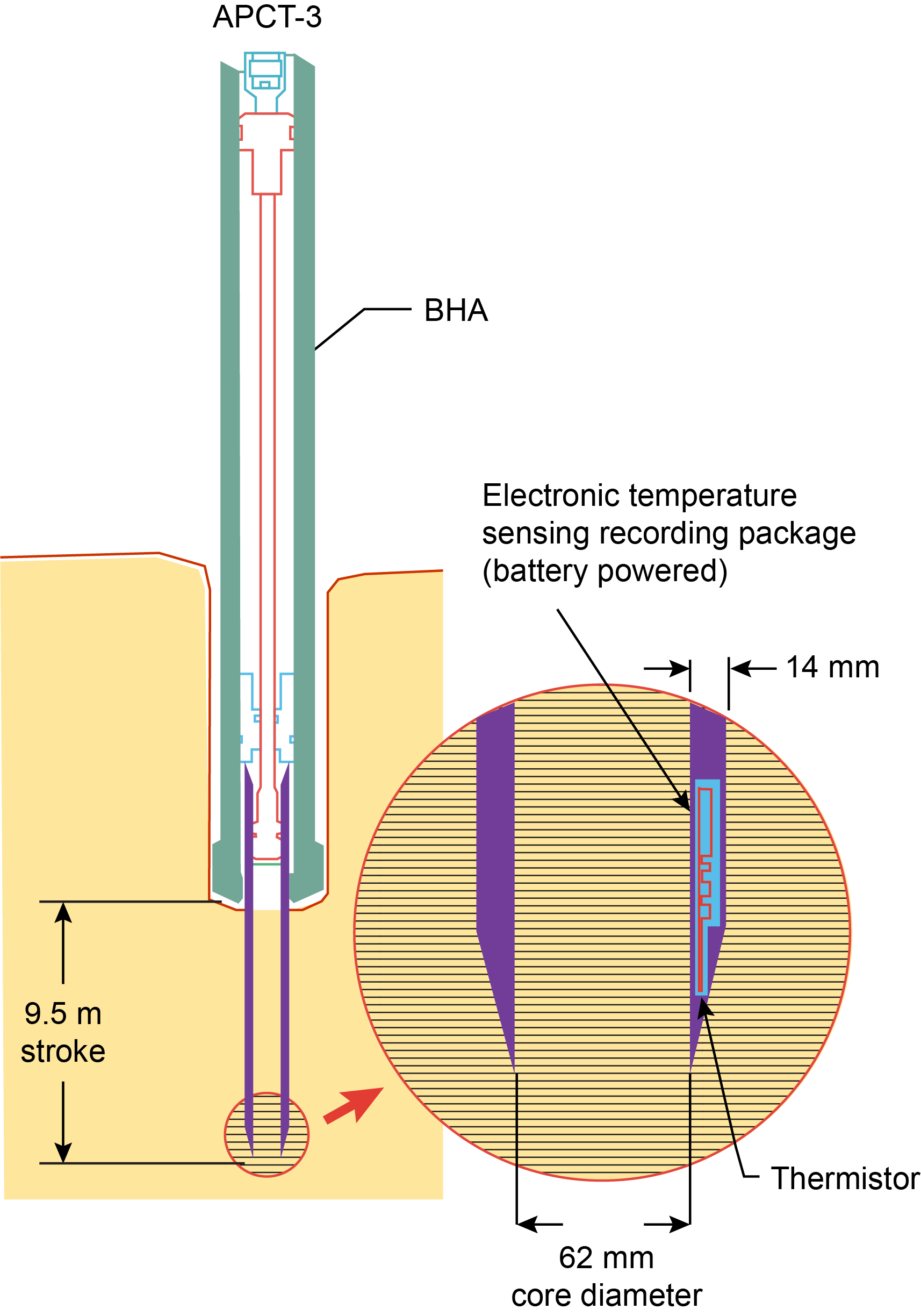
Figure F23. APCT-3 formation temperature sensor.
For operational reasons, the cutting shoe was not held at the mudline to allow equilibration with seafloor temperature. After shooting the core barrel into the sediments, the sensor was allowed to equilibrate to the in situ temperature of the formation for up to 15 min. This allowed dissipation of the rapid increase in temperature caused by frictional heating as the core barrel is fired into the formation.
Temperature was measured as a time series with a sampling rate of 1 s, and the data logged onto the microprocessor within the downhole tool were downloaded to a laboratory computer following core barrel retrieval. The time series data captures four phases of temperature evolution: (1) frictional heating as the cutting shoe is fired into the sediment, (2) the decay of temperature toward the equilibrium formation temperature, (3) further heating as the cutting shoe is extracted, and (4) cooling during return of the core barrel to the surface. The process of inferring formation temperature from the temperature time series needs to account for temperature variations arising during the deployment and retrieval of the HPCS cutting shoe containing the APCT-3 tool. The in situ temperature was calculated using the decay curve observed after core barrel penetration. Data were processed using the program TP-Fit running on a Windows PC in the Chikyu Core Processing Laboratory (https://github.com/MHee/TP-Fit).
Data processing involves isolating the portion of the temperature-time curve related to cooling toward equilibrium formation temperature and fitting the observed temperature decay to a lookup table of simulated response curves based on numerical models that consider the specific tool composition and geometry and various formation thermal properties. An advantage of this approach is that the formation temperature can be inferred without waiting until the equilibrium temperature is achieved.
The inversion scheme used by TP-Fit to extrapolate undisturbed formation temperatures from transient downhole tool data is built around reference models, Θ(t), which are normalized such that Θ(t0) = 1 and Θ(t∞) = 0. This approach is analogous to the method proposed by Bullard (1954) for analyzing marine heat flux data. Bullard used F(α, τ), an analytic solution of the conductive heat transfer equation, to describe the thermal response of an infinitely long cylindrical probe as a normalized reference model. Similarly, Θ(t) is a generalized abstraction of F(α, τ) that is precalculated numerically for a set of thermal conductivity and volumetric heat capacity values as the reference model for the APCT-3 sensors. Θ(t) also accounts for the geometry of the tool itself rather than the analytical solutions, which treat the heating signal as a line source (Heesemann, 2008). The reference model can describe the thermal response of a temperature probe while adhering to the assumptions of the governing heat transfer processes.
TP-Fit also applies an arbitrary time shift that accounts for unknowns such as incomplete knowledge of tool insertion time, incomplete thermal coupling between the sensor and the shoe, modification to sediment properties both inside and outside the tool, short-term advection immediately adjacent to the coring shoe, and nonhorizontal heat conduction (Heesemann et al. 2006). The algorithm for extrapolating undisturbed formation temperatures from transient tool responses then combines linear regression with time-window and time-shift parameters. The measured temperature data T(t) can be represented as
- Te = initial excess temperature,
- Tf = undisturbed formation temperature,
- tshift = time shift, and
- ε(t) = misfit between the observation and the forward modeling result (Heesemann, 2008).
The reference model Θ(t) is governed by thermal conductivity, volumetric heat capacity, and the time shift. Therefore, inverting these variables by minimizing the misfit ε(t) between forward model and data can provide an inversion scheme to estimate Te and Tf. The estimated undisturbed formation temperature Tf is the extrapolated T-axis intercept of a Θ(t) vs. T(t) plot.
In practice, significant uncertainties often exist in sediment thermal properties near the HPCS cutting shoe, including heterogeneity. To address this, the analysis incorporates a range of assumed thermal conductivities to evaluate the associated uncertainties. Even under ideal conditions where the tool response is unaffected by motion during temperature decay, statistical-fit criteria cannot reliably determine the effective thermal conductivity, as decay curves can be fitted to the data with varying time shifts.
For nonideal decay curves, only segments of the record may be usable, and different segments can yield different equilibrium temperature estimates. Consequently, extrapolated temperatures often exhibit a range of values, with uncertainties typically no less than 0.1°–0.2°C (Hessemann et al., 2008).
Local vertical conductive heat flow is estimated using a linear fit to vertical gradient among the measured formation temperatures deemed of good quality and the average thermal conductivity obtained from core samples over the same depth interval (see Thermal conductivity).
8. Geochemistry
8.1. Chemical analysis of interstitial water
8.1.1. Collection of interstitial water
IW samples were collected from the sediments of Sites C0019 and C0026 for a range of shipboard and shore-based analyses. The methods summarized below follow those reported by previous Chikyu IODP expeditions.
IW samples were collected from 5–25 cm long whole-round sections from cores. The whole-round core length was selected to provide enough fluid to meet the minimum needs for shipboard and personal IW analyses (ideally ≥17 mL) while maximizing the core available for the other purposes of the research.
Samples for IW extraction were selected by a shipboard structural geologist (watchdog) based on CT-scan images and visual inspection of cores. The selected samples did not contain potentially important structural features, and they were suitably free of fractures and other defects to minimize the potential for drilling fluid contamination. After selection, the sample was taken and immediately extruded from the core liner into a nitrogen-flushed glove bag.
The exterior part of the whole-round sample was thoroughly removed with a spatula or a ceramic knife to eliminate contamination from drilling fluids. The cleaned sediment was placed into a 9 cm diameter Manheim-type titanium squeezer (Manheim and Sayles, 1974) on top of filter paper rinsed with reagent-grade water (18.2 MΩ Millipore water, or Milli-Q) placed on two 40 mesh titanium screens. Sediment was squeezed at ambient temperatures and at pressures no higher than 25,000 psi (1.72 × 10⁸ Pa) to prevent the release of interlayer water from within clay minerals during the squeezing process. The IW (4–58 mL) was collected through a 24 or 60 mL acid-washed plastic syringe attached to the bottom of the squeezer assembly. The IW was then passed through a 0.2 µm disposable polytetrafluoroethylene (PTFE) filter attached to the syringe when filling sample vials for shipboard and shore-based analyses.
Aliquots of IW collected for both shipboard and shore-based analyses are presented in Table T9. HDPE sample vials for minor and trace element shipboard analyses were cleaned by immersion in 55°C 10% trace metal–grade 12 M HCl for a minimum of 24 h and were subsequently rinsed in Milli-Q water and dried in a class 100 laminar flow clean hood. Samples for minor and trace element shipboard analyses were acidified with optima-grade 6 M HNO3 before analysis by inductively coupled plasma–optical emission spectroscopy (ICP-OES) or inductively coupled plasma–mass spectrometry (ICP-MS). Unless otherwise noted, the samples were stored at 4°C after collection.
Liquid from mud water (LMW) collected from the mud tank and liquid in the core liner (LCL) were filtered through a 0.45 μm disposable PTFE filter and collected in HDPE sample vials. The LMW and LCL were used to evaluate potential contamination of the IW samples by drilling fluids.
8.1.2. Interstitial water analyses
IW samples, as well as LMW and LCL, were routinely analyzed for refractive index with a RX-5000i refractometer (ATAGO) immediately after IW extraction. The refractive index was converted to salinity based on repeated analyses of deionized water from a Millipore Milli-Q system (18.2 MΩ cm) and IAPSO standard seawater (IAPSO P-series batch 168; refractive index = 1.33945, salinity = 34.993, and chlorinity = 558.6 mM at the typical ambient laboratory temperature of 21.5°C). This batch was used throughout the analysis during this expedition. The standard deviation of the daily refractive index measurement of IAPSO standard seawater is ±0.000006, equivalent to a precision for salinity better than ±0.1‰.
If the collected IW sample volume was ≥ 4 mL, pH (pmH) and alkalinity were analyzed using Gran titration with a pH electrode and a Metrohm 888 Titrando autotitrator immediately after collection. A 0.3–1 mL IW aliquot was taken and titrated with 0.025 M HCl at 25°C using a Biotrode electrode. The electrode was calibrated every 24 h; titrant standardization was performed for each bottle of titrant or once a week, whichever was more frequent; and instrument condition checks using a 50 mM standard solution of nitric acid were carried out every 12 h. The results of the condition check throughout the expedition showed a precision (RSD%) and accuracy (percent deviation from the reference value) of 0.51% and 0.30%, respectively, for alkalinity measurements. When an interval’s collected IW volume was <4 mL, pH was analyzed by a compact pH meter (Horiba LAQUA twin) with a reproducibility of ±0.1. In this case, alkalinity was not measured.
Bromide and sulfate concentrations were analyzed using ion chromatography using a Thermo Fisher Scientific ICS-2100. IW aliquots of 0.02 mL were diluted 1:100 with Milli-Q water and left at room temperature for 2 h. Every sample batch started with measurement of blanks, followed by calibration standards, 1:100 diluted 20% standard solution for QC (0.3 mM Br−, 1.67 mM SO42−), and IW samples and finished with another 20% standard solution for QC. To be deemed acceptable, the accuracy of the QC sample was required to be Br− ±10% and SO42− ±5% from the certified value. The QC results during the expedition were used to calculate the precision (2.3% and 1.0%) and accuracy (5.3% and 0.5%) of bromide and sulfate analysis, respectively.
Chlorinity was determined using potentiometric titration with silver nitrate (AgNO3) using a Metrohm 888 Titrando autotitrator and Ag/AgCl electrode. We use the convention “chlorinity” for the titration data because it yields not only dissolved chloride but also all the other halide elements and bisulfide. A 0.1 mL aliquot of IW is used for analysis. The AgNO3 titrant was nominally 0.01 M and was standardized using IAPSO P-series standard seawater. IAPSO was also measured after every five samples as a reference, which gave a precision and accuracy of 0.49% and 0.15%, respectively, during the expedition.
Dissolved ammonium (NH4+) and phosphate (PO43−) concentrations were measured using colorimetry using an ultraviolet-visible (UV-vis) spectrophotometer (SEAL Analytical AQ2 Discrete Analyzer) within 24 h of IW sampling. The AQ2 automatically dilutes and reacts the sample to form indophenol blue for ammonium and molybdate for phosphate analysis, of which the absorption spectra are measured at 620 and 880 nm, respectively. Concentrations were calculated using standard calibration curves determined every 24 h. A drift of baseline was reset using the standard solution measurement after every five samples. Replicate analyses of QC sample solutions with 0.071 mM NH4+ and 16.19 µM PO43− showed a precision and accuracy of 7.1% and 4.5% for NH4+ and 2.4% and 0.8% for PO43−, respectively.
Concentrations of major cations, sodium (Na+), potassium (K+), magnesium (Mg2+), and calcium (Ca2+), were analyzed using a Thermo Fisher Scientific ICS-2100 ion chromatograph equipped with an IONPAC CS12 Analytical Column (4 mm × 250 mm, P/N 46073). After sitting at room temperature for 2 h, IW aliquots of 0.1 mL were acidified with concentrated nitric acid and diluted a minimum of 1:200 with Milli-Q water. Japan Calibration Service System–certified single standard solutions are used in calibration standard solutions. Every sample batch started with measurement of blanks, followed by calibration standards, 25% standard solution for QC, and IW samples (with QC every 11 analyses) and finished with another 25% standard solution for QC. The average precision and accuracy were calculated from repeated QC measurements during the expedition as follows: precision: Na+ <2%, K+ <1%, Mg2+ <6%, and Ca2+ <7%; accuracy: Na+ <1%, K+ <1%, Mg2+ <5%, and Ca2+ <1%.
The minor elements lithium (Li), boron (B), silica (SiO2, here expressed as Si), manganese (Mn), iron (Fe), strontium (Sr), and barium (Ba) were analyzed using ICP-OES (Thermo Fisher Scientific iCAP 7600 Series). The IW aliquot was acidified with concentrated nitric acid to make an acid concentration of 0.24 M (e.g., 3.2 µL concentrated HNO3 to 2 mL sample). A multielement stock solution was prepared from the ultrapure primary standards (SPC Science PlasmaCAL) to match the matrix of samples (Li = 576.29 µM; B = 3699.9 µM; Si = 1424.2 µM; Mn = 72.809 µM; Fe = 71.627 µM; Sr = 456.52 µM; Ba = 291.28 µM) and was diluted by factors of 100, 50, and 25 with 0.15 M nitric acid. An additional 50% calibration standard was made for QC. IW samples, calibration standards, and QC samples were diluted a final time 1:10 with 0.15 M nitric acid. Every sample batch started with a blank measurement, followed by calibration standards, QC standard, and IW samples (with QC every six analyses) and finished with another QC standard. The average precision and accuracy were calculated from repeated QC measurements during the expedition as follows: precision: Li <4%, B <2%, Si <3%, Mn <2%, Fe <3%, Sr <3%, Ba <2%; accuracy: Li <3%, B <3%, Si <2%, Mn <3%, Fe <3%, Sr <2%, Ba <4%.
Vanadium (V), copper (Cu), zinc (Zn), molybdenum (Mo), rubidium (Rb), cesium (Cs), lead (Pb), and uranium (U) were analyzed using ICP-MS (Agilent 7700x) equipped with an octopole reaction system to reduce polyatomic and double-charge interferences. To calibrate for interferences by the major ions Na+, K+, Ca2+, Cl−, and S on the transition metals (e.g., ClO and SOH on V, Na and CaOH on Cu, and S on Zn), standard solutions with concentrations similar to those of IAPSO standard seawater were prepared. These solutions were analyzed at the beginning of each run, and an interference correction was applied based on the average counts per second measured on the standard solutions divided by the abundance of the interfering elements. This ratio was multiplied by the known concentration of the major ions in the samples based on the previous analysis, and the result was subtracted from the measured cps of the sample. A 100 µL aliquot of 500 parts per billion (ppb) indium standard was added to the empty vials before dilution. Sample aliquots were then diluted with 1% nitric acid solution to 3% in these vials (150 µL sample with 4.85 mL of 1% HNO3 solution) based on the previously determined detection limits and the concentrations of the elements of interest. A primary standard solution matching the maximum range of predicted concentrations was made based on published results of deep-sea IW compositions in a variety of settings. Composition of the primary standard solution is as follows: V = 20 ppb; Cu, Mo, Pb, and U = 40 ppb; Zn = 140 ppb; Rb = 500 ppb; and Cs = 5 ppb. This primary standard was diluted with the 1% nitric acid solution to relative concentrations of 50%, 25%, 10%, 5%, and 1%. These standards were then diluted to 3%, similar to the standard solutions, with the addition of 150 µL of 560 mM NaCl and 4.7 mL of the 1% HNO3 solution to account for matrix suppression of the plasma ionization efficiency. After an initial batch set up of washes, blanks, standards, standards with added NaCl, then 20% standard calibration for QU (with and without NaCl), IW samples were analyzed (with QC every nine analyses). The average precision and accuracy were calculated from repeated QC measurements during the expedition were as follows: precision: V <60%, Cu <3%, Zn <4%, Mo <4%, Rb <3%, Cs <2%, Pb <5%, U <6%; accuracy: V <30%, Cu <4%, Zn <4%, Mo <3%, Rb <3%, Cs <1%, Pb <1%, U <5%.
9. Gas analysis
9.1. Sampling for headspace gas analysis
For headspace gas analysis, ~5 cm3 of sediment was sampled from every core at either the bottom of Section 1 or the top of Section 2 (or the position assigned by watchdog). For soft sediments, a cut-off disposable plastic syringe (3 cm3) was used. When sediments became too firm, a cork borer of stainless steel was used. The sediment sample was placed in a glass vial (20 cm3) sterilized by baking at 450°C for 4 h prior to use. The vial was then immediately capped by a butyl-rubber septum coated with PTFE and an aluminum cap. The butyl-rubber septa were also sterilized at 100°C for 4 h before use. The precise mass of the wet sample was determined after gas analysis was finished.
9.1.1. Sampling for void gas analysis
When a core with IW rich in dissolved gases is brought up on deck, the temperature and pressure difference from its original subseafloor setting drives gas expansion. This expansion causes sediment to move within the core liner to form voids. Gas samples were taken through the core liner from voids through a needle with a gas-tight syringe (SGE Analytical Science; 100MR-VLLMA-GT) filled with 10 mL of Milli-Q water. The enclosed gas in the syringe was transferred into a 20 cm3 vial prevacuumed by a diaphragm pump (ULVAC; DTC-22).
9.1.2. Hydrocarbon concentrations determined by GC-FID
Low-molecular weight hydrocarbons (i.e, methane, ethane, propane, and iso-/n-butane) were analyzed using a gas chromatograph with flame-ionization detection (GC-FID) (Agilent 7890B) equipped with an autosampler (Agilent Technologies 7697A Headspace Sampler). Before the analysis of headspace gas, the vial containing sample sediment was heated at 70°C for 30 min. The gas in the vial was ejected by pressurized H2 at 15 psi through a needle into a 1 mL sample loop. The ejected gas was then injected into a capillary column (HP-PLOT Q; 30 m length, 0.53 mm outer diameter, and 40 μm film) of the GC-FID. The flow rate of the H2 carrier gas was 5 mL/min. The GC oven was programmed to increase the temperature from an initial temperature of 60°C up to 150°C at a rate of 10°C/min (run time = 9 min) after the sample injection to release the different gas fractions at different temperatures. Calibration was conducted daily using 1% CH4 including N2 gas and another N2 gas including standard hydrocarbons (ethane 1.02%, propane 1.00%, propylene 1.02%, n-butane 1.02%, iso-butane 1.01%, and ethylene 1.03%). The reproducibility of the analysis was within 1.1%, 1.2%, 1.3%, 1.3%, and 1.3% for methane, ethane, propane, iso-butane, and n-butane, respectively (n = 46).
9.1.3. Hydrogen gas concentrations determined by Sensor Gas Chromatograph
Hydrogen gas (H2) concentrations were measured using a Sensor Gas Chromatograph (Semiconductor Gas Sensor; Nissha FIS, Inc., SGHA-P3-A). A 20 cm3 vial containing a ~5 cm3 sediment sample was connected to the GC using two disposable needles, which allowed the gas phase in the vial to be automatically introduced into the sample loop in the instrument. Additionally, a blank air sample collected at the core cutting area was also analyzed, and the blank value was subtracted from the measured value for the sample.
10. Chemical analysis of solid samples
10.1. Carbonate, nitrogen, carbon, and total organic carbon
Total carbon (TC), total nitrogen (TN), and total sulfur (TS) concentrations were determined on sediment. The sediment samples were dried under vacuum and ground into powder before the analysis. TC, TN, and TS concentrations were determined using a Thermo Finnigan Flash elemental analysis 1112 CHNS analyzer. Synthetic standard sulfanilamide, which contained 41.86 wt% C and 16.18 wt% N, was used for calibration. About 40 mg of sediment powder was weighed and placed in a tin container and combusted in an oxygen stream at 900°C to liberate the C and N as oxide gases from the molten sample. The combustion-produced CO2 and NO2 were transported by a constant flow of carrier gas. The NO2 was reduced to N2, which was separated from CO2 using a GC, and these gas concentrations were quantified with a thermal conductivity detector. The accuracy of the analysis was determined using a soil NCS reference material (Thermo Scientific, Milan, Italy) and a sulfanilamide standard (Thermo Scientific, Milan, Italy).
Inorganic carbon (IC) was determined from the same set of samples used for elemental analysis. Approximately 15–25 mg of sediment powder was weighed and acidified with 2 M HCl at room temperature to convert carbonate to CO2. The released CO2 was titrated, and the change in light transmittance was measured with a photodetection cell (CM5012 CO2 Coulometer; UIC Inc. Coulometrics). The weight percentage of carbonate was calculated from the IC content, assuming that all the evolved CO2 was derived from dissolution of calcium carbonate:
The presence of other carbonate minerals was not accounted for. Standard deviation of the analysis was less than ±0.05 wt%. Two standard materials (NIST-SRM 88b and JSD-2) were used to evaluate the accuracy. The detection limit of IC was assumed to be 3σ of the blank values of ~1 µg C. Concentration of total organic carbon (TOC) was determined from the difference between the concentrations of TC and IC.
11. Microbiology
11.1. Whole-round sampling
Because of the ephemeral nature of the microbial characteristics in cores, whole-round core sampling was conducted immediately after XCT scanning (Fast Track) to prevent alteration of the microbial properties of the cores, including cell abundance, community structure, and activity signatures. The CT watchdog examined the XCT imagery to select a ~10 cm long microbiology whole-round sample from an interval without significant structural or lithologic features or drilling-induced disturbance. Determination of the whole-round core location by the watchdog and Co-Chief Scientists was done by visual inspection of the cores through the plastic liner at the core cutting area for Cores 405-C0019J-5K through 29K during the malfunction and repair of the XCT instrument. Generally, the microbiology whole-round cores were located next to the IW whole-round core samples. The sampled whole-round cores were placed in ESCAL gas-barrier bags, flushed with N2 after vacuuming, sealed, and stored at 4°C until further subsampling. All subsampling and processing were done within 24 h of the core arriving on deck. Most of the whole-round core samples obtained during Window 1 of the expedition were processed as described below. Whole-round core samples obtained during Window 2, when it was not too hard to sample, were subsampled by a tip-cut syringe, sealed in ESCAL bags, and stored at 4°C. Remaining parts of the whole-round core samples and entire hard whole-round core samples were sealed in ESCAL bags, frozen in the shipboard Cells Alive System (CAS) freezer, stored at −80°C, and shipped to the onshore laboratory. Additionally, 10 cm whole-round core samples collected were immediately frozen in the CAS freezer and stored at −80°C on the ship and eventually transferred to onshore archiving at −80°C at the KCC.
11.2. Sampling for contamination check
As part of the drilling process, surface seawater was injected into the borehole; injected volumes depended on the coring method. This is the major source of microbiological contamination of the cores collected. Because the perfluorocarbon tracer, widely used for tracing contamination, was unavailable during this expedition, fluid sampling was conducted to evaluate the extent to which contaminating cells may have penetrated a sample. Contamination can be assessed by analyzing the geochemical and microbial properties of the drilling fluid (primarily composed of surface ocean water), including postexpedition analyses. Therefore, a sample of the drilling fluid (LMW) was collected every morning (at around 1100 h) during coring operations where the microbiology sampling occurred. If there was fluid between the liner and the core, it was also sampled to check the contamination (LCL).
11.3. Microbiological sampling
The workflow and QA to handle microbiology whole-round cores on Chikyu were conducted following the methods of Expedition 370 (Morono et al., 2017). To minimize the risk of drilling-induced contamination, samples for microbiological investigations were taken as whole-round cores from the most undisturbed parts of the recovered core sections, as identified by the structural geology watchdogs based on visual inspection and XCT imaging of individual core sections. In general, the first section of each hole was not sampled for microbiological investigations to avoid cross-contamination with borehole fills.
During cutting, sediment only came in contact with precleaned (with Milli-Q water) and autoclaved spatulas. Whole-round cores were packed with endcaps cleaned with ethanol, dried in a clean bench, and radiated with UV light for at least 20 min before use. For further subsampling, samples were transferred to an anaerobic chamber (95:5 [v/v] N2:H2 atmosphere; COY Laboratory Products, USA), which was installed with a KOACH T 500-F tabletop air filtration unit. The KOACH unit produces filtered laminar airflow, creating conditions that match ISO Class 1 cleanroom standards. Airborne particles in the anaerobic chamber were monitored several times during the expedition. Interior surfaces of the anaerobic chamber were routinely decontaminated by wiping with RNase AWAY. The interior surfaces of the clean bench were decontaminated by exposure to UV light. To obtain the contamination-free working surface in the anaerobic chamber, the edges of Whirl-Pak write-on sterilized bags (BA01447, Whirl-Pak, Filtration Group) were cut, and interior sterile surfaces were used for sample preparation. A fresh Whirl-Pak bag was used each time a new whole-round core was processed. All microbiological samples were collected and subsampled using precleaned (with 18 MΩ water) and sterilized tools, such as cutoff syringes, ceramic knives, and spatulas, depending on the hardness of the core material. When applicable, the indurated sediment core surface, which is assumed to be in contact with drilling fluid, was scraped off, and the interior pristine part of the cores was distributed for the following purposes.
11.4. Sample preparation for microscopic observations
Approximately 1 cm3 of sediment sample was taken from the interior part of the core by taking soft sediment using a sterilized cutoff syringe or trimming the contaminated surface part using ceramic knife. The samples were immediately fixed by transferring to a sterile 15 mL centrifuge tube containing 9 mL of 3× phosphate-buffered saline (pH = 7.5; Invitrogen 70013) with 10% (v/v) neutralized formalin as a fixative and stored at 4°C. In addition, an approximately 2 cm3 sample taken from the interior of the core with a sterilized cutoff syringe or ceramic knife was placed in a 5 mL tempered hard glass gas-chromatography vial (SVG-5, Nichiden-Rika Glass Co., LTD.). The sample was combined with 40 µL of a solution of 1 mM Cell Tracker Green 5-chloromethyl fluorescein diacetate (Thermo Fischer Scientific) that was diluted with dimethyl sulfoxide to a concentration of 25 µM. The samples were incubated at 15°C for approximately 14 days for activity staining of the microbial cells. Afterward, the incubation was stopped by adding 2.5 mL of fixing solution (1.0% glutaraldehyde and 5% formalin [~containing 2% formaldehyde] in 3× phosphate-buffered saline) and incubating overnight at 4°C, followed by freezing in the CAS freezer. Frozen samples were transferred to a −80°C freezer for storage and future analyses (e.g., Morono et al., 2019).
11.5. Sample preparation for molecular analyses
Part of the sediment samples were subsampled using a sterilized spatula or ceramic knife and placed in Whirl-Pak bags for subsequent DNA/RNA and adenosine triphosphate (ATP) analysis. The bags were frozen in the CAS freezer and stored at −80°C.
Selected samples were subjected to shipboard ATP assay. ATP has been measured in subseafloor sediments as a proxy of microbial biomass during past ODP legs (Egeberg, 2000; Kimura et al., 2003). The ATP extractions and measurements from sedimentary microbes will be performed at the onshore laboratory following methods modified from Orsi (2023).
11.6. Sample preparation for microbial activity
Part of the sediment samples were subsampled by a sterilized spatula or ceramic knife and placed in Whirl-Pak bags for subsequent microbial activity measurements. Inside the anaerobic chamber, the sample inside of the Whirl-Pak was placed in an ESCAL gas-barrier bag, heat-sealed, and stored at 4°C.
12. Observatory
Installation of instrumentation was completed for two subseafloor observatories at Site C0019 during Expedition 405: (1) redeployment of an instrument string into Hole C0019D, the Japan Trench Fast Earthquake Drilling Project (J-FAST) observatory hole that was originally drilled during Integrated Ocean Drilling Program Expedition 343/343T (Expedition 343/343T Scientists, 2013a; Fulton et al., 2013) and (2) deployment into a newly drilled and constructed observatory installed in Hole C0019Q. The location of Hole C0019Q was chosen to be along strike with the coring and LWD holes characterized during Expedition 405 and ~40 m downdip of Hole C0019D to allow comparison of signals between holes (see Figure F5 in the Expedition 405 summary chapter [Kirkpatrick et al., 2025]).
The primary objective of these observatory instrument deployments is to measure the temperature field with depth over time to characterize the hydrogeology, capture hydrologic transients, and potentially record the remaining frictional heat signal around the slip zone of the 2011 Mw 9.0 Tohoku-oki earthquake (e.g., Fulton et al., 2013; Fulton and Brodsky, 2016). Instrumentation of Hole C0019D was installed at the beginning of the expedition to allow for passive monitoring of potential cross-hole flow caused by hydrologic perturbations while subsequently drilling and circulating in many new wells at Site C0019. Drilling, completion, and instrumentation of Hole C0019Q was completed at the end of the expedition so that the total length of the instrument string and determination of instrument positions could be informed by the results from coring and logging.
12.1. General observatory design
The instrument strings for both deployments consist of an array of autonomous temperature-sensing data loggers attached to a Vectran line (rope) and suspended in cased holes with a sensor hanger resting in the wellhead at the top and a sinker bar maintaining tension in the line at the bottom.
The observatory holes are completed with 4.5 inch (11.43 cm) outer diameter steel tubing (inner diameter = 3.958 inches) that serves as uncemented casing extending from depth up through a wellhead that extends above the seafloor. At the bottom of the observatories, a one-way valve allows fluid to circulate outward during installation but prevents fluid from entering the interior of the tubing. The top opening is sealed by a miniature temperature logger (MTL) hanger, from which the Vectran line and other instrument string components, including the MTLs themselves, are suspended. The top of the MTL hanger is shaped like a core barrel, allowing installation and recovery through drill pipe with the core barrel retrieving tool (CBRT) on the core line (Figure F24).
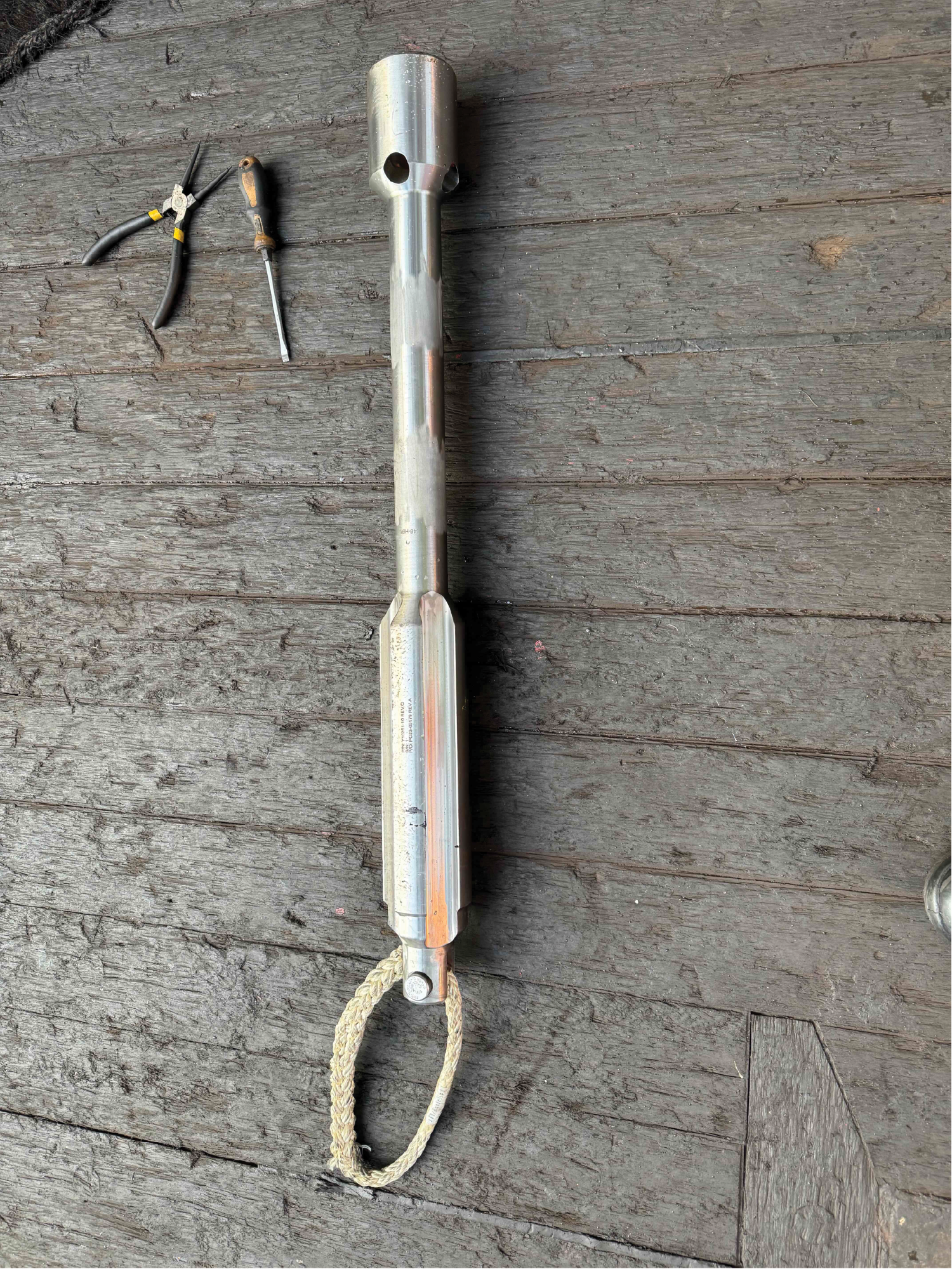
Figure F24. MTL hanger.
12.2. Sensor string components
12.2.1. Line
The instrument strings consist of several sections of 12 mm 12-strand Vectran line manufactured by Tokyo Seiko Rope Mfg. Co., Ltd. (Tokyo, Japan). Vectran is a Class 2 high-performance liquid crystal polymer fiber with high tensile strength as well as low stretch and creep properties that enable accurate placement of the sensors at designated depths (Figure F25). Each section of the Vectran line has a spliced end loop, allowing connection to the MTL hanger, the sinker bar, or other sections of line by either a carabiner hard link or a weak link (Figure F26). Attachment eyes are seized into specific locations along the line to facilitate attachment and positioning of instruments. The lines were stretched and measured under loads equivalent to those expected once installed to enable precise positioning of instruments and components.
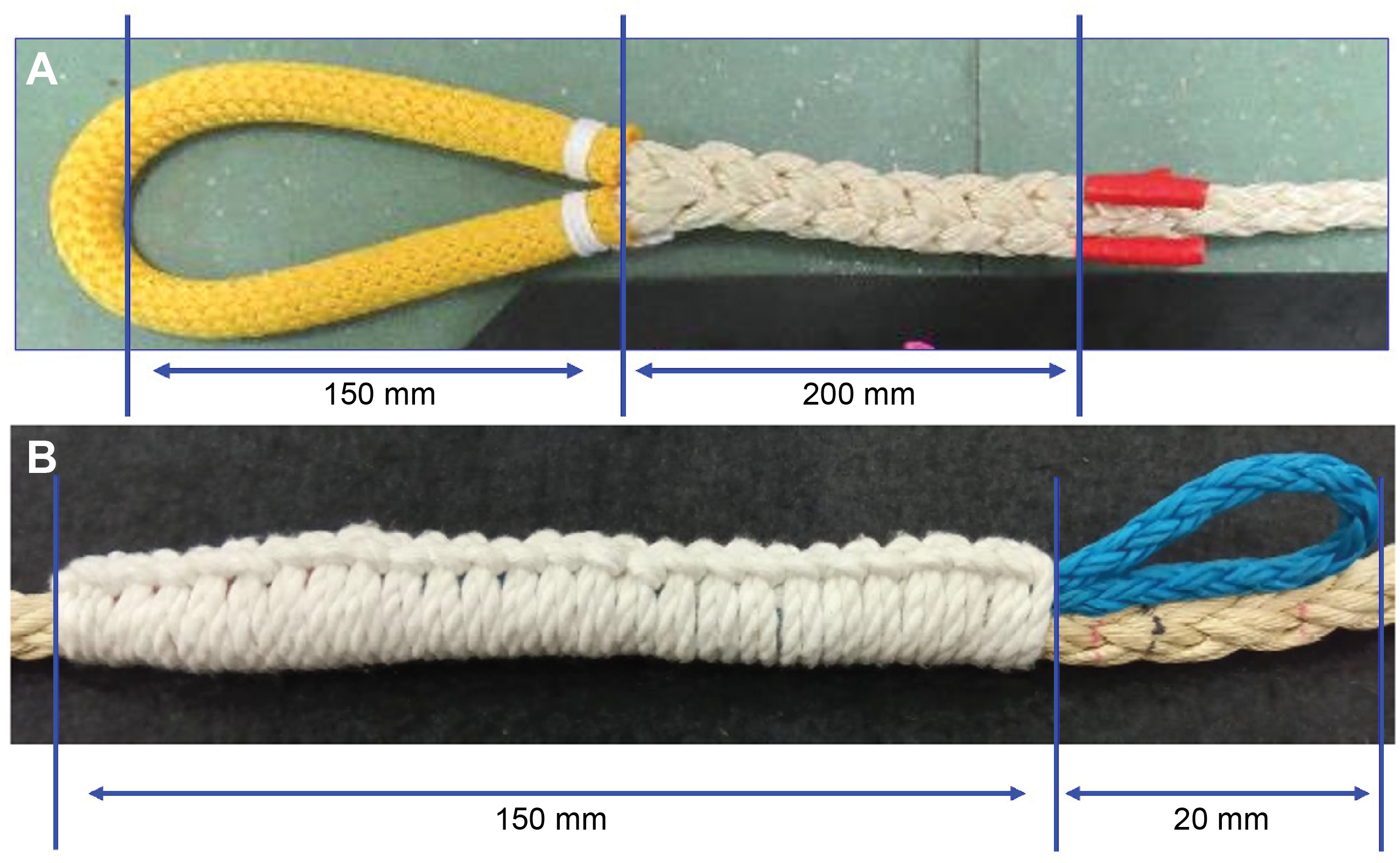
Figure F25. 12 mm Vectran line.
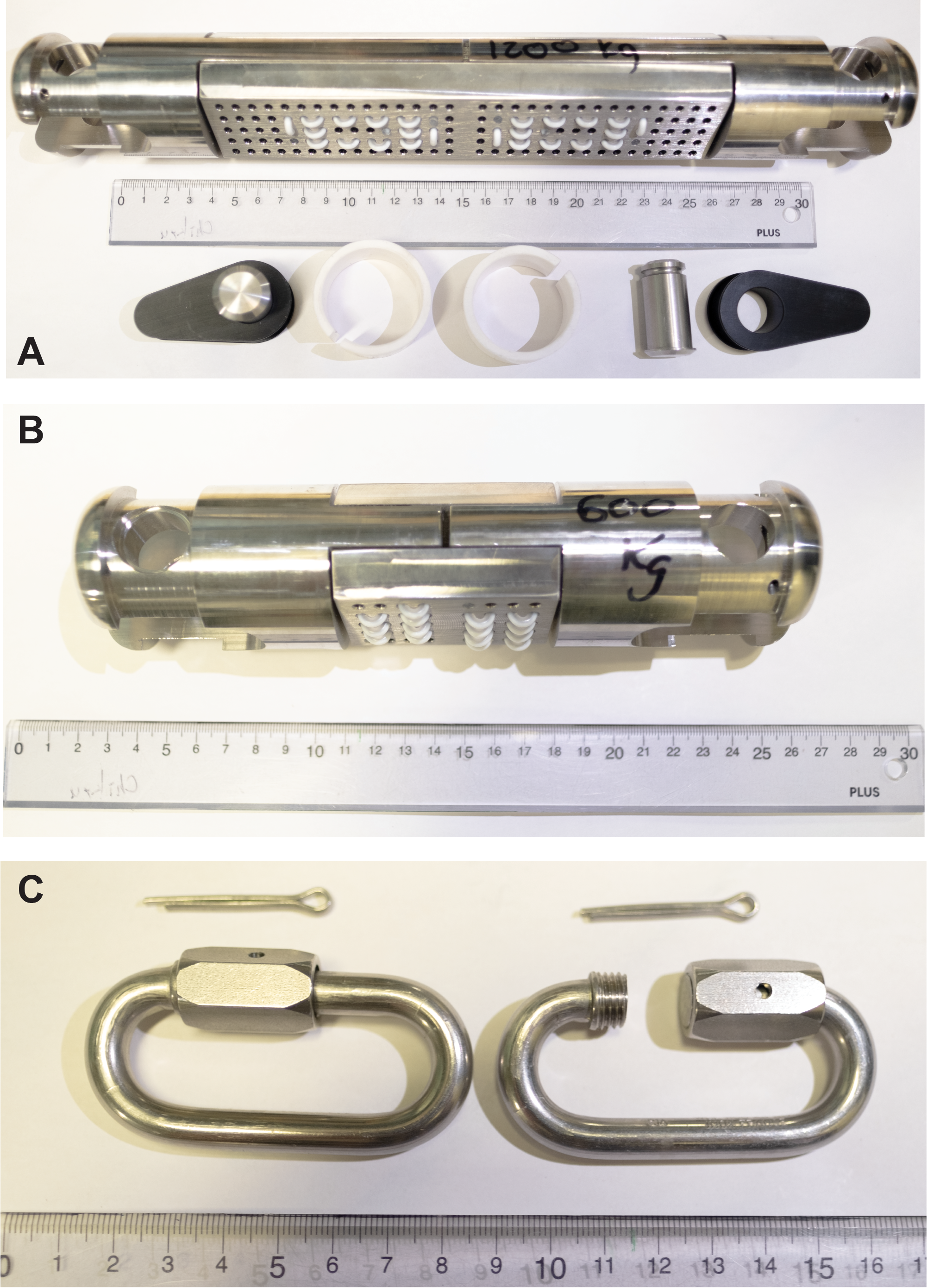
Figure F26. Weak links.
12.2.2. Weak links
Weak links are installed along the instrument string at strategically targeted locations to address the possibility that components of the instrument string could get stuck during or prior to retrieval. The two sizes of weak links used are shown in Figure F26 along with the hard link carabiners and locking pins also used to connect sections of line. The weak links were manufactured by TLR, Inc. (Carmel, California, US) and consist of metal components that include two end pieces and two connection plates. The pieces are sewn together with ⅛ inch (0.3175 cm) polypropylene cord through multiple pass-through holes that align between the pieces. The strength of each weak link is determined by the number of holes threaded; the end pieces can only be separated by shearing through the polypropylene cords. Each weak link is calibrated to be substantially stronger than those installed below it. If the instrument string is stuck upon retrieval, the weakest link above the obstruction is designed to break under tension, allowing partial recovery of the instrument string.
12.2.3. Temperature sensors/data loggers
Individual temperature-sensing data logger instruments (MTLs) are deployed to record temperature time series at prescribed depths along the instrument strings. All the temperature sensors used were manufactured by RBR, Ltd. (Ottawa, Canada). Figure F27 shows many of the instruments. A variety of different generations of instrument models are used, although they all have similar measurement capabilities (Table T10). All instruments consist of a platinum resistance temperature sensor and an independent autonomous data logger encased in a titanium housing rated for water depths up to 10 km. These sensors all have a resolution of <0.00005°C and a calibrated accuracy of <0.002°C.
Figure F27. Temperature-sensing data loggers.
The RBR TR1050 and RBR TDR2050 models use replaceable CR-123AW/4P batteries, and all other models are each powered by a single replaceable AA lithium thionyl chloride battery, enabling years-long sampling durations. The RBR TR1050 and RBR TDR2050 models have a 38 mm outer diameter, and all other models have a smaller outer diameter of 25 mm. The instruments are equipped with silica desiccant to prevent condensation in the instruments during the traversal through the cold ocean. In addition, the interior of each instrument was filled with nitrogen gas and sealed before deployment to ensure that the atmosphere inside has low moisture content.
All sensors for Hole C0019D (JFAST observatory) were programmed to start recording at 0200 h UTC on 6 September 2024, whereas those for Hole C0019Q (JTRACK observatory) were programmed to start at 0200 h Universal Time Coordinated (UTC) on 6 December 2024. Note that the RBR TR1050 and RBR TDR2050 sensors are older models and record in local Japan Standard Time (JST) (UTC + 9 h). The programmed sampling interval and the projected maximum duration, limited by battery life, for each sensor type are listed in Table T10.
12.2.4. Sinker bars
Sinker bars made of 3 inch (7.62 cm) diameter steel and various lengths and weights are used along the instrument string (Figure F28). One sinker bar is positioned at the bottom of the line to help pull the sensor string into the hole during installation and keep the line taut. Another heavier sinker bar near the top of the line is used to pull the MTL hanger into its seat and provide a resolvable indication of unloading of the core line when the MTL hanger is seated.
Figure F28. Sinker bar.
12.3. Sensor attachment
The sensors are attached to the Vectran line at predetermined positions corresponding to specific depths below seafloor within the borehole. Figure F29 illustrates the step-by-step process of attaching the sensors.
Figure F29. Process of attaching sensors.
Attachment loops are seized into the main line above these depth positions. For each sensor, an additional loop of cord is threaded through both the seized attachment loop and a hole in the instrument casing secured using a double-fisherman’s knot. The loop is adjusted to an appropriate size to position the bottom of the instrument at its assigned depth location. The attachment loop size ranges 15–658 mm depending on the specific adjustment needed based on the measured rope stretch under load. Prior to assembly, the line and attachment eye positions are measured and marked under tensions comparable to deployment conditions, ensuring precise positioning of instruments on the untensioned line with adjustment of the length of the double-fisherman’s knot attachment loop.
Once positioned on the Vectran line, the sensors are wrapped in 3 mm thick nitrile rubber sheeting that is pinned closed with zip ties and reinforced with a combination of Gorilla All Weather Outdoor Waterproof Duct Tape for strength in holding the covers closed, 3M Super 33+ Electrical Tape for overall coverage and underwater performance, and colored vinyl electrical tape for visual identification and labeling.
13. Core-log-seismic integration
13.1. Seismic-well ties
Core and downhole logging data were correlated with seismic reflection profiles intersecting the drill sites to make seismic-well ties. For this expedition, we used the P-wave velocity data from the LWD sonic logs to establish the ties and generate synthetic seismograms to compare with the seismic reflection data. The initial time-depth relationship was created for each site by a combination of a constant seawater velocity (to match the water depth with the two-way traveltime [TWT] of the seafloor reflection) to the seafloor depth, and the measured P-wave velocity curve below the seafloor. After that, the depth-domain logging data were time-converted to correlate with the seismic profiles in two-way traveltime.
We generated synthetic seismograms where good quality P-wave velocity logs (LWD memory data) were available or from real-time LWD P-wave velocity logs where the LWD memory data were not available (see Logging while drilling in the Site C0019 chapter and Logging while drilling in the Site C0026 chapter [Regalla et al., 2025; Conin et al., 2025] for QC description of the logs). Representative density logs were derived from the P-wave velocity using Gardner’s relation (Gardner et al., 1974). Acoustic impedance was calculated from the product of the P-wave and density logs, and a reflection coefficient series was generated from the acoustic impedance log. We estimated a representative seismic wavelet for each seismic reflection profile using the nearest 100 seismic traces to each site and a 400 ms length window from approximately the waterbottom depth. The estimated wavelet was quality checked by visual comparison with the waterbottom reflection and comparison with the amplitude spectrum. The wavelet was convolved with the reflection coefficient series to make a synthetic seismic trace, comparable with the nearest recorded seismic trace. The waterbottom reflection in the synthetic was tied to that on the seismic reflection data by applying a bulk shift (equivalent to modifying the seawater velocity). Major subsurface reflections were correlated between the synthetic and recorded seismic by picking dynamic tie points, which act to slightly change the subseafloor interval velocities. The final time-depth relation was used for further core-log-seismic correlation.
Where only real-time LWD P-wave velocity logs were available, the sampling interval and data quality were not sufficient to generate synthetic seismograms with comparable resolution to the seismic reflection data.
We also performed the well-seismic tie by visually correlating changes in the seismically relevant logs (e.g., gamma ray and resistivity) with the seismic section. Gamma ray should be strongly correlated with clay content, meaning that sharp changes in the measured gamma ray likely correspond to changes in bulk density. Resistivity is strongly coupled to porosity, meaning that sharp changes in the measured resistivity likely correspond to changes in both the P-wave velocity and bulk density. We used these sharp changes to correlate the logs with strong seismic reflectors by modifying the time-depth relationship as described above.
We carried out the time-depth conversion, synthetic seismogram generation, wavelet estimation, and visual log-seismic comparison using SLB’s Petrel software.
13.2. Seismic reflection data
The high-resolution seismic reflection profiles available for the seismic-log integration were acquired by the Japan Agency for Marine-Earth Science and Technology (JAMSTEC) during four cruises: KY11-E05 in October and November 2011 using the R/V Kaiyo (Lines HD33B and HS41B) (Nakamura, 2011), KR13-06 in March 2013 using the R/V Kairei (Line HDMY001) (Yamashita and Nakamura, 2013), KY14-E02 in October 2014 using Kaiyo (Line JTXC02) (Yamashita and Nakamua, 2014), and KY15-14 in September 2015 using Kaiyo (Line HD33L) (Nakamura, 2015). The seismic source was a 320 inch3 (KY11-E05) or 380 inch3 (KR13-06, KY14-E02, and KY15-14) cluster gun array, and the shot interval was 37.5 m for all cruises. The receiver array was a 1.3 km, 192 channel digital streamer cable with 6.25 m channel spacing. At these water depths (~7 km), the maximum offset was too short for reliable semblance-based velocity analysis at the target drilling depths for this expedition. We therefore adopted a constant velocity model of 1525 m/s for poststack time migration (Nakamura et al., 2013, 2023). Lines HD33B, HS41B, and HD33L intersect Site C0019, whereas Lines HDMY001 and JTXC02 intersect Site C0026.
The lower resolution seismic reflection profile used for the seismic-log integration was acquired by JAMSTEC during the KR13-01 cruise in January 2013 using Kairei (JFD1) (Kodaira, 2013). The seismic source was a 7800 inch3 tuned air gun array, and the shot interval was 50 m. The receiver array was a 5.5 km, 444 channel streamer cable with 12.5 m channel spacing. The data were processed to prestack time migration and prestack depth migration to generate time and depth sections as described in Nakamura et al. (2014). We used the prestack time-migrated section to establish the seismic-well tie. The Profile JFD1 almost intersects Site C0019 and passes approximately 1.2 km north of Site C0026. All seismic reflection data are available upon request at the JAMSTEC Seismic Survey Database (JAMSTEC, 2004).
13.3. Core-log comparison
Core-log integration is based on the correlation between the physical properties recorded by LWD and the physical properties measured on core sections and discrete samples and using the COMET. Although the holes for LWD and coring were offset by up to several tens of meters (Table T1), the logging and coring data can be compared and correlated with each other with careful consideration of the difference in the resolution. Because of partial core recovery, only significant trends or variations spanning several cores were considered. It should be noted that the scale of investigation is not the same for LWD and core samples. In addition, LWD measurements integrate both the effects of the matrix and fractures, whereas core samples provide information primarily on the matrix properties. Also, the geometry of the electrical current lines and of the seismic rays is different for the various channels, causing differences in recorded data if the formation is anisotropic.
The core-log integration is based on a comparison of NGR, electrical resistivity, and P- and S-wave velocity. Gamma ray is representative of mineralogical composition and is a robust indicator to compare cores and logs. Gamma ray is recorded for each section with the COMET (see Physical properties). For core-log integration, the points at the edges of each core section are cleared. The LWD measurements acquire resistivity data at various depths within the formation (see Logging while drilling), and the medium button resistivity data were utilized for the core-log integration. The resistivity was measured in two (y- and z-) or three (x-, y-, and z-) directions for the core section or discrete samples (see Physical properties), but for comparison with the log, the resistivity perpendicular to the drilling direction (y-direction) was used. The elastic velocities were measured in three (x-, y-, and z-) directions for the discrete samples, but for comparison with the log, the elastic velocities in parallel to the drilling direction (z-direction) were used.
The core-log integration can be confirmed by additional examination for consistency in primary and deformation structures in cores and log data. For instance, the resistivity images from the LWD tool (MicroScope) provided structural information at the borehole wall, such as dips and azimuths of bedding and fractures, which were compared with the XCT images and structural descriptions of core samples. Similarly, P- and S-wave velocities and electrical resistivity/impedance measured from core samples can be compared to corresponding logging data.
References
Acton, G.D., Satolli, S., Di Chiara, A., Friedman, S.A., Dwyer, D., Roth, A., Higley, M., Hastedt, M., Novak, B., Rudbäck, D., Blum, P., and the IODP Expedition 395 Science Party, 2023. Azimuthal orientation of piston cores collected by the International Ocean Discovery Program (IODP): an example from the North Atlantic. Presented at the 2023 American Geophysical Union Fall Meeting, San Francisco, CA, 11–15 December 2023. https://agu.confex.com/agu/fm23/meetingapp.cgi/Paper/1257800
Akiba, F., 1986. Middle Miocene to Quaternary diatom biostratigraphy in the Nankai Trough and Japan Trench, and modified lower Miocene through Quaternary diatom zones for middle-to-high latitudes of the North Pacific. In Kagami, H., Karig, D.E., Coulbourn, W.T., et al., Initial Reports of the Deep Sea Drilling Project, 87: Washington, DC (US Government Printing Office), 393–481. https://doi.org/10.2973/dsdp.proc.87.106.1986
Alford, J., Blyth, M., Tollefsen, E., Crowe, J., Loreto, J., Mohammed, S., Pistre, V., and Rodriguez-Herrera, A., 2012. Sonic logging while drilling – shear answers. Oilfield Review, 24(1):4–15.
Allouche, M., Chow, S., Dubourg, I., Ortenzi, L., and van Os, R., 2010. High-resolution images and formation evaluation in slim holes from a new logging-while-drilling azimuthal laterolog device. Presented at the SPE EUROPEC/EAGE Annual Conference and Exhibition. https://doi.org/10.2118/131513-MS
Alverson, A.J., Sung-Ho, K., and Theriot, E.C., 2006. Cell wall morphology and systematic importance of Thalassiosira ritscheri (Hustedt) Hasle, with a description of Shionodiscus gen. nov. Diatom Research, 21(2):251–262. https://doi.org/10.1080/0269249X.2006.9705667
Amoozegar, A., Heitman, J.L., and Kranz, C.N., 2023. Comparison of soil particle density determined by a gas pycnometer using helium, nitrogen, and air. Soil Science Society of America Journal, 87(1):1–12. https://doi.org/10.1002/saj2.20476
ASTM International, 1990. Standard method for laboratory determination of water (moisture) content of soil and rock (Standard D2216–90). In Annual Book of ASTM Standards for Soil and Rock. Philadelphia (American Society for Testing Materials).
Balsley, J.R., and Buddington, A.F., 1960. Magnetic susceptibility anisotropy and fabric of some Adirondack granites and orthogneisses. American Journal of Science, 258-A:6–20.
Barron, J.A., 1980. Lower Miocene to Quaternary diatom biostratigraphy of Leg 57, off northeastern Japan, Deep Sea Drilling Project. In Scientific Party, Initial Reports of the Deep Sea Drilling Project, 56, 57, Pt. 2: Washington (U.S. Govt. Printing Office), 641–685. https://doi.org/10.2973/dsdp.proc.5657.117.1980
Barron, J.A., 1992. Neogene diatom datum levels in the equatorial and North Pacific. In Ishizaki, K. and Saito, T., Centenary of Japanese Micropaleontology. Tokyo (Terra Scientific Publishing Company), 413–425.
Barron, J.A., and Gladenkov, A.Y., 1995. Early Miocene to Pleistocene diatom stratigraphy of Leg 145. In Rea, D.K., Basov, I.A., Scholl, D.W., and Allan, J.F. (Eds.), Proceedings of the Ocean Drilling Program, Scientific Results, 145: College Station, TX (Ocean Drilling Program), 3–19. https://doi.org/10.2973/odp.proc.sr.145.101.1995
Barron, J.A., Harper, H.E., Jr., Keller, G., Reynolds, R.A., Sakai, T., Shaffer, B.L., and Thompson, P.R., 1980. Biostratigraphic summary of the Japan Trench transect, Legs 56 and 57, Deep Sea Drilling Project. In Scientific Party, Initial Reports of the Deep Sea Drilling Project, 56, 57, Part 1: Washington, DC (US Government Printing Office), 505–520. https://doi.org/10.2973/dsdp.proc.5657.113.1980
Berggren, W.A., Kent, D.V., Swisher, C.C., III, Aubry, M.-P., Berggren, W.A., Kent, D.V., Aubry, M.-P., and Hardenbol, J., 1995. A revised Cenozoic geochronology and chronostratigraphy. In Berggren, W.A., Kent, D.V., Aubry, M.-P., and Hardenbol, J. (Eds.), Geochronology, Time Scales and Global Stratigraphic Correlation. SEPM Special Publication, 54. https://doi.org/10.2110/pec.95.04.0129
Blum, P., 1997. Technical Note 26: Physical properties handbook. Ocean Drilling Program. https://doi.org/10.2973/odp.tn.26.1997
Brothers, R.J., Kemp, A.E.S., and Maltman, A.J., 1996. Mechanical development of vein structures due to the passage of earthquake waves through poorly-consolidated sediments. Tectonophysics, 260(4):227–244. https://doi.org/10.1016/0040-1951(96)00088-1
Bullard, E.C., 1954. The flow of heat through the floor of the Atlantic Ocean. Proceedings of the Royal Society of London, A: Mathematical and Physical Sciences, 222(1150):408–429. https://doi.org/10.1098/rspa.1954.0085
Byrne, T.B., Lin, W., Tsutsumi, A., Yamamoto, Y., Lewis, J.C., Kanagawa, K., Kitamura, Y., Yamaguchi, A., and Kimura, G., 2009. Anelastic strain recovery reveals extension across SW Japan subduction zone. Geophysical Research Letters, 36(23):L23310. https://doi.org/10.1029/2009GL040749
Cande, S.C., and Kent, D.V., 1992. A new geomagnetic polarity time scale for the Late Cretaceous and Cenozoic. Journal of Geophysical Research: Solid Earth, 97(B10):13917–13951. https://doi.org/10.1029/92JB01202
Cande, S.C., and Kent, D.V., 1995. Revised calibration of the geomagnetic polarity timescale for the Late Cretaceous and Cenozoic. Journal of Geophysical Research: Solid Earth, 100:6093–6095. https://doi.org/10.1029/94JB03098
Carlson, R.L., and Christensen, N.I., 1977. Velocity anisotropy and physical properties of deep-sea sediments from the western South Atlantic. In Supko, P.R., Perch-Nielsen, K., et al., Initial Reports of the Deep Sea Drilling Project, 39: Washington, DC (US Government Printing Office), 555–559. https://doi.org/10.2973/dsdp.proc.39.124.1977
Carlson, W.D., 2006. Three-dimensional imaging of earth and planetary materials. Earth and Planetary Science Letters, 249(3–4):133–147. https://doi.org/10.1016/j.epsl.2006.06.020
Caulet, J.P., Nigrini, C., and Schneider, D.A., 1993. High resolution Pliocene-Pleistocene radiolarian stratigraphy of the tropical Indian Ocean. Marine Micropaleontology, 22(1–2):111–129. https://doi.org/10.1016/0377-8398(93)90006-J
Censarek, B., and Gersonde, R., 2002. Miocene diatom biostratigraphy at ODP Sites 689, 690, 1088, 1092 (Atlantic sector of the Southern Ocean). Marine Micropaleontology, 45(3–4):309–356. https://doi.org/10.1016/S0377-8398(02)00034-8
Conin, M., Bourlange, S., Henry, P., Boiselet, A., and Gaillot, P., 2014. Distribution of resistive and conductive structures in Nankai accretionary wedge reveals contrasting stress paths. Tectonophysics, 611:181–191. https://doi.org/10.1016/j.tecto.2013.11.025
Conin, M., Kirkpatrick, J., Regalla, C., Ujiie, K., Fulton, P., Kodaira, S., Okutsu, N., Maeda, L., Toczko, S., Eguchi, N., Bellanova, P., Brown, C., Brunet, M., Castillo, M., Chang, Y.-C., Doan, M.-L., Everard, J., Fintel, A., Ford, J., Fukuchi, R., Gough, A., Guo, H., Gürer, D., Hackney, R., Hagino, M., Hamada, Y., Hosono, H., Ijiri, A., Ikari, M., Ishikawa, T., Iwai, M., Jeppson, T., Jurado, M.-J., Kamiya, N., Kanamatsu, T., LaPlante, A., Lin, W., Miyakawa, A., Morono, Y., Nakamura, Y., Nicholson, U., Okuda, H., Pei, P., Pizer, C., Rasbury, T., Robertson, R.V.M., Ross, C., Satolli, S., Savage, H., Schaible, K., Shreedharan, S., Sone, H., Sun, C., Turel, C., Uchida, T., Yamaguchi, A., Yamamoto, Y., Yoshimoto, T., Zhang, J., Wspanialy, A., Le Ber, E., Rydzy, M.B., and Schuba, N., 2025. Site C0026. In Kodaira, S., Conin, M., Fulton, P., Kirkpatrick, J., Regalla, C., Ujiie, K., Okutsu, N., Maeda, L., Toczko, S., Eguchi, N., and the Expedition 405 Scientists, Tracking Tsunamigenic Slip Across the Japan Trench (JTRACK). Proceedings of the International Ocean Discovery Program, 405: College Station, TX (International Ocean Discovery Program). https://doi.org/10.14379/iodp.proc.405.104.2025
Druitt, T.H., Kutterolf, S., Ronge, T.A., Beethe, S., Bernard, A., Berthod, C., Chen, H., Chiyonobu, S., Clark, A., DeBari, S., Fernandez Perez, T.I., Gertisser, R., Hübscher, C., Johnston, R.M., Jones, C., Joshi, K.B., Kletetschka, G., Koukousioura, O., Li, X., Manga, M., McCanta, M., McIntosh, I., Morris, A., Nomikou, P., Pank, K., Peccia, A., Polymenakou, P.N., Preine, J., Tominaga, M., Woodhouse, A., and Yamamoto, Y., 2024. Site U1599. In Druitt, T.H., Kutterolf, S., Ronge, T.A., and the Expedition 398 Scientists, Hellenic Arc Volcanic Field. Proceedings of the International Ocean Discovery Program, 398: College Station, TX (International Ocean Discovery Program). https://doi.org/10.14379/iodp.proc.398.113.2024
Drury, A.J., Westerhold, T., Frederichs, T., Tian, J., Wilkens, R., Channell, J.E.T., Evans, H., John, C.M., Lyle, M., and Röhl, U., 2017. Late Miocene climate and time scale reconciliation; accurate orbital calibration from a deep-sea perspective. Earth and Planetary Science Letters, 475:254–266. https://doi.org/10.1016/j.epsl.2017.07.038
Egeberg, P.K., 2000. Adenosine 5'-triphosphate (ATP) as a proxy for bacteria numbers in deep-sea sediments and correlation with geochemical parameters (Site 994). In Paull, C.K., Matsumoto, R., Wallace, P.J., and Dillon, W.P. (Eds.), Proceedings of the Ocean Drilling Program, Scientific Results, 164: College Station, TX (Ocean Drilling Program), 393–398. https://doi.org/10.2973/odp.proc.sr.164.217.2000
Expedition 308 Scientists, 2006. Methods. In Flemings, P.B., Behrmann, J.H., John, C.M., and the Expedition 308 Scientists, Proceedings of the Integrated Ocean Drilling Program, 308: College Station, TX (Integrated Ocean Drilling Program Management International, Inc.). https://doi.org/10.2204/iodp.proc.308.102.2006
Expedition 316 Scientists, 2009a. Expedition 316 methods. In Kinoshita, M., Tobin, H., Ashi, J., Kimura, G., Lallemant, S., Screaton, E.J., Curewitz, D., Masago, H., Moe, K.T., and the Expedition 314/315/316 Scientists, Proceedings of the Integrated Ocean Drilling Program, 314/315/316: Washington, DC (Integrated Ocean Drilling Program Management International, Inc.). https://doi.org/10.2204/iodp.proc.314315316.132.2009
Expedition 316 Scientists, 2009b. Expedition 316 Site C0004. In Kinoshita, M., Tobin, H., Ashi, J., Kimura, G., Lallemant, S., Screaton, E.J., Curewitz, D., Masago, H., Moe, K.T., and the Expedition 314/315/316 Scientists, Proceedings of the Integrated Ocean Drilling Program, 314/315/316: Washington, DC (Integrated Ocean Drilling Program Management International, Inc.). https://doi.org/10.2204/iodp.proc.314315316.133.2009
Expedition 334 Scientists, 2012. Expedition 334 summary. In Vannucchi, P., Ujiie, K., Stroncik, N., and the Expedition 334 Scientists, Proceedings of the Integrated Ocean Drilling Program, 334: Tokyo (Integrated Ocean Drilling Program Management International, Inc.). https://doi.org/10.2204/iodp.proc.334.101.2012
Expedition 343/343T Scientists, 2013a. Expedition 343/343T summary. In Chester, F.M., Mori, J., Eguchi, N., Toczko, S., and the Expedition 343/343T Scientists, Proceedings of the Integrated Ocean Drilling Program, 343/343T: Tokyo (Integrated Ocean Drilling Program Management International, Inc.). https://doi.org/10.2204/iodp.proc.343343T.101.2013
Expedition 343/343T Scientists, 2013b. Methods. In Chester, F.M., Mori, J., Eguchi, N., Toczko, S., and the Expedition 343 Scientists, Proceedings of the Integrated Ocean Drilling Program, 343/343T: Tokyo (Integrated Ocean Drilling Program Management International, Inc.). https://doi.org/10.2204/iodp.proc.343343T.102.2013
Folk, R.L., 1954. The distinction between grain size and mineral composition in sedimentary rock nomenclature. The Journal of Geology, 62(4):344–359. https://www.jstor.org/stable/30065016
Fossen, H., Schultz, R.A., Shipton, Z.K., and Mair, K., 2007. Deformation bands in sandstone: a review. Journal of the Geological Society (London, UK), 164(4):755–769. https://doi.org/10.1144/0016-76492006-036
Fulton, P.M., and Brodsky, E.E., 2016. In situ observations of earthquake-driven fluid pulses within the Japan Trench plate boundary fault zone. Geology, 44(10):851–854. https://doi.org/10.1130/G38034.1
Fulton, P.M., Brodsky, E.E., Kano, Y., Mori, J.J., Chester, F.M., Ishikawa, T., Harris, R.N., Lin, W., Eguchi, N., and Toczko, S., 2013. Low coseismic friction on the Tōhoku-Oki fault determined from temperature measurements. Science, 342(6163):1214–1217. https://doi.org/10.1126/science.1243641
Funayama, M., 1988. Miocene radiolarian stratigraphy of the Suzu area, northwestern part of the Noto Peninsula, Japan. Contributions from the Institute of Geology and Paleontology, Tohoku University, 91:15–41.
Gardner, G.H.F., Gardner, L.W., and Gregory, A.R., 1974. Formation velocity and density—the diagnostic basics for stratigraphic traps. Geophysics, 39(6):770–780. https://doi.org/10.1190/1.1440465
GE Healthcare, 2013a. Discovery CT Series Service Methods (revision 15): Waukesha, Wisconsin (GE Healthcare).
GE Healthcare, 2013b. Discovery CT750 HD User Manual (Revision 1): Waukesha, Wisconsin (GE Healthcare).
GE Healthcare, 2013c. Technical Reference Manual (revision 1): Waukesha: Waukesha, Wisconsin (GE Healthcare).
Gibbard, P.L., and Head, M.J., 2020. The Quaternary period. In Gradstein, F.M., Ogg, J.G., Schmitz, M.D., and Ogg, G.M. (Eds.), Geologic Time Scale 2020. Dordrecht, Netherlands (Elsevier), 1217–1255. https://doi.org/10.1016/B978-0-12-824360-2.00030-9
Gradstein, F.M., Ogg, J.G., Schmitz, M.D., and Ogg, G.M. (Eds.), 2012. The Geologic Time Scale 2012: Amsterdam (Elsevier). https://doi.org/10.1016/C2011-1-08249-8
Gradstein, F.M., Ogg, J.G., Schmitz, M.D., and Ogg, G.M. (Eds.), 2020. Geologic Time Scale 2020: Amsterdam (Elsevier BV). https://doi.org/10.1016/C2020-1-02369-3
Gradstein, F.M., Ogg, J.G., and Smith, A.G., 2004. A Geologic Time Scale 2004: Cambridge, United Kingdom (Cambridge University Press). https://doi.org/10.1017/CBO9780511536045
Hanamura, Y., and Ogawa, Y., 1993. Layer-parallel faults, duplexes, imbricate thrusts and vein structures of the Miura Group: keys to understanding the Izu fore-arc sediment accretion to the Honshu fore arc. Island Arc, 2(3):126–141. https://doi.org/10.1111/j.1440-1738.1993.tb00081.x
Harper, H.E., Jr., 1980. Diatom biostratigraphy of Sites 434, 435, and 436, northwestern Pacific, Leg 56, Deep Sea Drilling Project. In Scientific Party, Initial Reports of the Deep Sea Drilling Project, 56, 57, Part 2: Washington DC (U.S. Government Printing Office), 633–639. https://doi.org/10.2973/dsdp.proc.5657.116.1980
He, K., Zhang, X., Ren, S., and Sun, J., 2016. Deep residual learning for image recognition. Presented at the 2016 IEEE Conference on Computer Vision and Pattern Recognition (CVPR), 27-30 June 2016. https://doi.org/10.1109/CVPR.2016.90
Heesemann, M., 2008. Advances in the acquisition and processing of subseafloor temperature and pressure data and their interpretation in the context of convergent margin processes [PhD dissertation]. University of Bremen, Germany. http://nbn-resolving.de/urn:nbn:de:gbv:46-diss000111371
Heesemann, M., Villinger, H.W., Tréhu, A.T.F.M., and White, S., 2006. Data report: testing and deployment of the new APCT-3 tool to determine in situ temperatures while piston coring. In Riedel, M., Collett, T.S., Malone, M.J., and the Expedition 311 Scientists, Proceedings of the Integrated Ocean Drilling Program, 311: Washington, DC (Integrated Ocean Drilling Program Management International, Inc.). https://doi.org/10.2204/iodp.proc.311.108.2006
Horai, K., and Von Herzen, R.P., 1985. Measurement of heat flow on Leg 86 of the Deep Sea Drilling Project. In Heath, G.R., Burckle, L. H., et al., Initial Reports of the Deep Sea Drilling Project, 86: Washington, DC (U.S. Government Printing Office), 759–777. https://doi.org/10.2973/dsdp.proc.86.135.1985
Ikehara, K., Strasser, M., Everest, J., Maeda, L., Hochmuth, K., and the Expedition 386 Scientists, 2023. Expedition 386 Preliminary Report: Japan Trench Paleoseismology. International Ocean Discovery Program. https://doi.org/10.14379/iodp.pr.386.2023
Itaki, T., Taira, Y., Kuwamori, N., Saito, H., Ikehara, M., and Hoshino, T., 2020. Innovative microfossil (radiolarian) analysis using a system for automated image collection and AI-based classification of species. Scientific Reports, 10(1):21136. https://doi.org/10.1038/s41598-020-77812-6
Iwai, M., Motoyama, I., Lin, W., Takashima, R., Yamada, Y., and Eguchi, N., 2025. Diatom and radiolarian biostratigraphy in the vicinity of the 2011 Tohoku Earthquake source fault in IODP Hole 343-C0019E of JFAST. Island Arc, 34(1):e70009. https://doi.org/10.1111/iar.70009
JAMSTEC, 2004. JAMSTEC Seismic Survey Database. JAMSTEC. https://doi.org/10.17596/0002069
Jelinek, V., 1981. Characterization of the magnetic fabric of rocks. Tectonophysics, 79(3–4):T63–T67. https://doi.org/10.1016/0040-1951(81)90110-4
Kamikuri, S.-i., 2010. New late Neogene radiolarian species from the middle to high latitudes of the North Pacific. Revue de Micropaléontologie, 53(2):85–106. https://doi.org/10.1016/j.revmic.2008.06.005
Kamikuri, S.-i., 2017. Late Neogene radiolarian biostratigraphy of the eastern North Pacific ODP Sites 1020/1021. Paleontological Research, 21(3):230–254. https://doi.org/10.2517/2016PR027
Kamikuri, S.-i., Nishi, H., and Motoyama, I., 2007. Effects of late Neogene climatic cooling on North Pacific radiolarian assemblages and oceanographic conditions. Palaeogeography, Palaeoclimatology, Palaeoecology, 249(3):370–392. https://doi.org/10.1016/j.palaeo.2007.02.008
Kamikuri, S.-i., Nishi, H., Motoyama, I., and Saito, S., 2004. Middle Miocene to Pleistocene radiolarian biostratigraphy in the Northwest Pacific Ocean, ODP Leg 186. Island Arc, 13(1):191–226. https://doi.org/10.1111/j.1440-1738.2003.00421.x
Kimura, H., Asada, R., Masta, A., and Naganuma, T., 2003. Distribution of microorganisms in the subsurface of the Manus Basin hydrothermal vent field in Papua New Guinea. Applied and Environmental Microbiology, 69(1):644–648. https://doi.org/10.1128/AEM.69.1.644-648.2003
Kirkpatrick, J., Regalla, C., Conin, M., Ujiie, K., Fulton, P., Kodaira, S., Okutsu, N., Maeda, L., Toczko, S., Eguchi, N., Bellanova, P., Brown, C., Brunet, M., Castillo, M., Chang, Y.-C., Doan, M.-L., Everard, J., Fintel, A., Ford, J., Fukuchi, R., Gough, A., Guo, H., Gürer, D., Hackney, R., Hagino, M., Hamada, Y., Hosono, H., Ijiri, A., Ikari, M., Ishikawa, T., Iwai, M., Jeppson, T., Jurado, M.-J., Kamiya, N., Kanamatsu, T., LaPlante, A., Lin, W., Miyakawa, A., Morono, Y., Nakamura, Y., Nicholson, U., Okuda, H., Pei, P., Pizer, C., Rasbury, T., Robertson, R.V.M., Ross, C., Satolli, S., Savage, H., Schaible, K., Shreedharan, S., Sone, H., Sun, C., Turel, C., Uchida, T., Yamaguchi, A., Yamamoto, Y., Yoshimoto, T., Zhang, J., Wspanialy, A., Le Ber, E., Rydzy, M.B., Bentley, C., Cooper, S., Grant, W., Kurara, Y., Letexier, D., Miura, N., Pincus, M., Schuba, N., and Smith, L., 2025. Expedition 405 summary. In Kodaira, S., Conin, M., Fulton, P., Kirkpatrick, J., Regalla, C., Ujiie, K., Okutsu, N., Maeda, L., Toczko, S., Eguchi, N., and the Expedition 405 Scientists, Tracking Tsunamigenic Slip Across the Japan Trench (JTRACK). Proceedings of the International Ocean Discovery Program, 405: College Station, TX (International Ocean Discovery Program). https://doi.org/10.14379/iodp.proc.405.101.2025
Kirkpatrick, J.D., Rowe, C.D., Ujiie, K., Moore, J.C., Regalla, C., Remitti, F., Toy, V., Wolfson-Schwehr, M., Kameda, J., Bose, S., and Chester, F.M., 2015. Structure and lithology of the Japan Trench subduction plate boundary fault. Tectonics, 34(1):53–69. https://doi.org/10.1002/2014TC003695
Kirschvink, J.L., 1980. The least-squares line and plane and the analysis of palaeomagnetic data. Geophysical Journal International, 62(3):699–718. https://doi.org/10.1111/j.1365-246X.1980.tb02601.x
Kling, S.A., 1973. Radiolaria from the eastern North Pacific Deep Sea Drilling Project, Leg 18. In Kulm, L.D., von Huene, R., et al., Initial reports of the Deep Sea Drilling Project, 18: Washington, DC (US Government Printing Office), 617–671. https://doi.org/10.2973/dsdp.proc.18.116.1973
Kodaira, S., 2013. R/V Kairei "Cruise Report" KR13-01. JAMSTEC. https://doi.org/10.17596/0002944
Koizumi, I., and Tanimura, Y., 1985. Neogene diatom biostratigraphy of the middle latitude western North Pacific, Deep Sea Drilling Project Leg 86. In Heath, G.R., Burckle, L. H., et al., Initial reports of the Deep Sea Drilling Project, 86: Washington, DC (US Government Printing Office), 269–300. https://doi.org/10.2973/dsdp.proc.86.109.1985
Lazarus, D.B., Spencer-Cervato, C., Pika-Biolzi, M., Beckmann, J.-P., von Salis, K.H., Hilbrecht, H., and Thierstein, H.R., 1995. Technical Note 24: Revised chronology of Neogene DSDP holes from the world ocean. Ocean Drilling Program. https://doi.org/10.2973/odp.tn.24.1995
Lin, W., Yamamoto, Y., and Hirose, T., 2023. Three-dimensional stress state above and below the plate boundary fault after the 2011 Mw 9.0 Tohoku earthquake. Earth and Planetary Science Letters, 601:117888. https://doi.org/10.1016/j.epsl.2022.117888
Lin, W., Yeh, E., Ito, H., Hirono, T., Soh, W., Wang, C., Ma, K., Hung, J., and Song, S.-R., 2007. Preliminary results of stress measurement using drill cores of TCDP Hole-A: an application of anelastic strain recovery method to three-dimensional in-situ stress determination. Terrestrial Atmospheric and Oceanic Sciences, 18:379–393. https://doi.org/10.3319/TAO.2007.18.2.379(TCDP)
Lurcock, P.C., and Wilson, G.S., 2012. PuffinPlot: a versatile, user-friendly program for paleomagnetic analysis. Geochemistry, Geophysics, Geosystems, 13(6):Q06Z45. https://doi.org/10.1029/2012GC004098
Maltman, A.J., 1998. Deformation structures from the toes of active accretionary prisms. Journal of the Geological Society (London, UK), 155(4):639–650. https://doi.org/10.1144/gsjgs.155.4.0639
Maltman, A.J., Byrne, T., Karig, D.E., and Lallemant, S., 1993. Deformation at the toe of an active accretionary prism: synopsis of results from ODP Leg 131, Nankai, SW Japan. Journal of Structural Geology, 15(8):949–964. https://doi.org/10.1016/0191-8141(93)90169-B
Manheim, F.T., and Sayles, F.L., 1974. Composition and origin of interstitial waters of marine sediments, based on deep sea drill cores. In Goldberg, E.D., The Sea (Volume 5): Marine Chemistry: The Sedimentary Cycle. New York (Wiley), 527–568. https://pubs.usgs.gov/publication/70207491
Maruyama, T., and Shiono, M., 2003. Middle Miocene to Pleistocene diatom biostratigraphy of the Northwest Pacific at Sites 1150 and 1151. In Suyehiro, K., Sacks, I.S., Acton, G.D., and Oda, M. (Eds.), Proceedings of the Ocean Drilling Program, Scientific Results, 186: College Station, TX (Ocean Drilling Program), 1–38. https://doi.org/10.2973/odp.proc.sr.186.106.2003
Matsuki, K., 1991. Three-dimensional in-situ stress measurement with anelastic strain recovery of a rock core. Presented at the 7th ISRM Congress. https://onepetro.org/isrmcongress/proceedings/CONGRESS91/All-CONGRESS91/ISRM-7CONGRESS-1991-110/167608
Mees, F., Swennen, R., Geet, M.V., and Jacobs, P., 2003. Applications of X-ray computed tomography in the geosciences. Geological Society Special Publication, 215(1):1–6. https://doi.org/10.1144/GSL.SP.2003.215.01.01
Miyakawa, A., Matsumoto, K., Itaki, T. and Geshi, N., 2024. Software using deep learning to support geological particle image classification. Open-File Report of the Geological Survey of Japan, AIST, 750:1–7. https://www.gsj.jp/data/openfile/no0750/gsj_openfile_report_750.pdf
Morgan, J.K., and Karig, D.E., 1995. Décollement processes at the Nankai accretionary margin, southeast Japan: Propagation, deformation, and dewatering. Journal of Geophysical Research: Solid Earth, 100(B8):15221–15231. https://doi.org/10.1029/95JB00675
Morley, J.J., and Nigrini, C., 1995. Miocene to Pleistocene radiolarian biostratigraphy of North Pacific Sites 881, 884, 885, 886, and 887. In Rea, D.K., Basov, I. A., Scholl, D.W. and Allan, J.F., (Eds.), Proceedings of the Ocean Drilling Program, Scientific Results, 145: College Station, TX (Ocean Drilling Program), 55–91. http://doi.org/10.2973/odp.proc.sr.145.107.1995
Morono, Y., Inagaki, F., Heuer, V.B., Kubo, Y., Maeda, L., Bowden, S., Cramm, M., Henkel, S., Hirose, T., Homola, K., Hoshino, T., Ijiri, A., Imachi, H., Kamiya, N., Kaneko, M., Lagostina, L., Manners, H., McClelland, H.-L., Metcalfe, K., Okutsu, N., Pan, D., Raudsepp, M.J., Sauvage, J., Schubotz, F., Spivack, A., Tonai, S., Treude, T., Tsang, M.-Y., Viehweger, B., Wang, D.T., Whitaker, E., Yamamoto, Y., and Yang, K., 2017. Expedition 370 methods. In Heuer, V.B., Inagaki, F., Morono, Y., Kubo, Y., Maeda, L., and the Expedition 370 Scientists, Temperature Limit of the Deep Biosphere off Muroto. Proceedings of the International Ocean Discovery Program, 370: College Station, TX (International Ocean Discovery Program). https://doi.org/10.14379/iodp.proc.370.102.2017
Morono, Y., Terada, T., Masui, N., and Inagaki, F., 2009. Discriminative detection and enumeration of microbial life in marine subsurface sediments. The ISME Journal, 3(5):503–511. https://doi.org/10.1038/ismej.2009.1
Motoyama, I., 1996. Late Neogene radiolarian biostratigraphy in the subarctic Northwest Pacific. Micropaleontology, 42(3):221–262. https://doi.org/10.2307/1485874
Motoyama, I., and Maruyama, T., 1998. Neogene diatom and radiolarian biochronology for the middle-to-high latitudes of the Northwest Pacific region: Calibration to the Cande and Kent's geomagnetic polarity timescales (CK92 and CK95). The Journal of the Geological Society of Japan, 104(3):171–183. https://doi.org/10.5575/geosoc.104.171
Motoyama, I., Niitsuma, N., Maruyama, T., Hayashi, H., Kamikuri, S.-i., Shiono, M., Kanamatsu, T., Aoki, K., Morishita, C., Hagino, K., Nishi, H., and Oda, M., 2004. Middle Miocene to Pleistocene magneto-biostratigraphy of ODP Sites 1150 and 1151, northwest Pacific: Sedimentation rate and updated regional geological timescale. Island Arc, 13(1):289–305. https://doi.org/10.1111/j.1440-1738.2003.00426.x
Nakamura, Y., 2011. R/V Kaiyo Cruise Report KY11-E05. JAMSTEC. https://doi.org/10.17596/0003140
Nakamura, Y., 2015. R/V Kaiyo Cruise Report KY15-14. JAMSTEC. https://doi.org/10.17596/0002832
Nakamura, Y., Kodaira, S., Cook, B.J., Jeppson, T., Kasaya, T., Yamamoto, Y., Hashimoto, Y., Yamaguchi, M., Obana, K., and Fujie, G., 2014. Seismic imaging and velocity structure around the JFAST drill site in the Japan Trench: low Vp, high Vp/Vs in the transparent frontal prism. Earth, Planets and Space, 66(1):121. https://doi.org/10.1186/1880-5981-66-121
Nakamura, Y., Kodaira, S., Fujie, G., Yamashita, M., Obana, K., and Miura, S., 2023. Incoming plate structure at the Japan Trench subduction zone revealed in densely spaced reflection seismic profiles. Progress in Earth and Planetary Science, 10:45. https://doi.org/10.1186/s40645-023-00579-7
Nakamura, Y., Kodaira, S., Miura, S., Regalla, C., and Takahashi, N., 2013. High-resolution seismic imaging in the Japan Trench axis area off Miyagi, northeastern Japan. Geophysical Research Letters, 40(9):1713–1718. https://doi.org/10.1002/grl.50364
Nakano, T., Nakajima, Y. Nakamura, K., and Ikeda, S., 2000. Observation and analysis of internal structure of rock using X-ray CT. The Journal of the Geological Society of Japan, 106:363–378. https://doi.org/10.5575/geosoc.106.363
Nigrini, C., 1977. Tropical Cenozoic Artostrobiidae (Radiolaria). Micropaleontology, 23(3):241–269. https://doi.org/10.2307/1485215
Nigrini, C.A., Sanfilippo, A., and Moore, T.J., Jr., 2006. Cenozoic radiolarian biostratigraphy: a magnetobiostratigraphic chronology of Cenozoic sequences from ODP Sites 1218, 1219, and 1220, equatorial Pacific. In Wilson, P.A., Lyle, M., and Firth, J.V., Proceedings of the Ocean Drilling Program, Scientific Results, 199: College Station, TX (Ocean Drilling Program). https://doi.org/10.2973/odp.proc.sr.199.225.2006
Ogg, J.G., 2020. Geomagnetic Polarity Time Scale. In Gradstein, F.M., Ogg, J.G., Schmitz, M., and Ogg, G. (Eds.), Geologic Time Scale 2020. Amsterdam (Elsevier), 159–192. https://doi.org/10.1016/B978-0-12-824360-2.00005-X
Ogg, J.G., Ogg, G.M., and Gradstein, F.M., 2016. A Concise Geologic Time Scale 2016: New York (Elsevier). https://doi.org/10.1016/C2009-0-64442-1
Onoue, T., Hori, S., Tomimatsu, Y., and Rigo, M., 2024. A dilute sodium hydroxide technique for radiolarian extraction from cherts. Scientific Reports, 14(1):12831. https://doi.org/10.1038/s41598-024-63755-9
Oohashi, K., Lin, W., Wu, H.-Y., Yamaguchi, A., and Yamamoto, Y., 2017. Stress state in the Kumano Basin and in slope sediment determined from anelastic strain recovery: results from IODP Expedition 338 to the Nankai Trough. Geochemistry, Geophysics, Geosystems, 18(10):3608–3616. https://doi.org/10.1002/2017GC007137
Orsi, W.D., 2023. A rapid method for measuring ATP + ADP + AMP in marine sediment. Environmental Microbiology, 25(8):1549–1558. https://doi.org/10.1111/1462-2920.16359
Plona, T., Endo, T., Wielemaker, E., Walsh, J., and Yamamoto, H., 2006. Slowness-frequency-projection logs: A QC for accurate slowness estimation and formation property identification. In SEG Technical Program Expanded Abstracts 2006. (Society of Exploration Geophysicists), 334-338. https://doi.org/10.1190/1.2370227
Raffi, I., Wade, B.S., Pälike, H., Beu, A.G., Cooper, R., Crundwell, M.P., Krijgsman, W., Moore, T., Raine, I., Sardella, R., and Vernyhorova, Y.V., 2020. The Neogene Period. In Gradstein, F.M., Ogg, J.G., Schmitz, M.D., and Ogg, G. (Eds.), Geologic Time Scale 2020. (Elsevier), 1141–1215. https://doi.org/10.1016/B978-0-12-824360-2.00029-2
Regalla, C., Ujiie, K., Fulton, P., Kirkpatrick, J., Conin, M., Kodaira, S., Okutsu, N., Maeda, L., Toczko, S., Eguchi, N., Bellanova, P., Brown, C., Brunet, M., Castillo, M., Chang, Y.-C., Doan, M.-L., Everard, J., Fintel, A., Ford, J., Fukuchi, R., Gough, A., Guo, H., Gürer, D., Hackney, R., Hagino, M., Hamada, Y., Hosono, H., Ijiri, A., Ikari, M., Ishikawa, T., Iwai, M., Jeppson, T., Jurado, M.-J., Kamiya, N., Kanamatsu, T., LaPlante, A., Lin, W., Miyakawa, A., Morono, Y., Nakamura, Y., Nicholson, U., Okuda, H., Pei, P., Pizer, C., Rasbury, T., Robertson, R.V.M., Ross, C., Satolli, S., Savage, H., Schaible, K., Shreedharan, S., Sone, H., Sun, C., Turel, C., Uchida, T., Yamaguchi, A., Yamamoto, Y., Yoshimoto, T., Zhang, J., Wspanialy, A., Le Ber, E., Rydzy, M.B., and Schuba, N., 2025. Site C0019. In Kodaira, S., Conin, M., Fulton, P., Kirkpatrick, J., Regalla, C., Ujiie, K., Okutsu, N., Maeda, L., Toczko, S., Eguchi, N., and the Expedition 405 Scientists, Tracking Tsunamigenic Slip Across the Japan Trench (JTRACK). Proceedings of the International Ocean Discovery Program, 405: College Station, TX (International Ocean Discovery Program). https://doi.org/10.14379/iodp.proc.405.103.2025
Renter, J.A.M., 1989. Applications of computerized tomography in sedimentology. Marine Geotechnology, 8(3):201–211. https://doi.org/10.1080/10641198909379868
Reynolds, R., 1980. Radiolarians from the western North Pacific, Leg 57, Deep Sea Drilling Project. In Scientific Party, Initial reports of the Deep Sea Drilling Project, 56: Washington, DC (U.S. Government Printing Office), 7350150769. https://doi.org/10.2973/dsdp.proc.5657.120.1980
Richter, C., Acton, G., Endris, C., and Radsted, M., 2007. Technical Note 34: Handbook for shipboard paleomagnetists. Ocean Drilling Program. https://doi.org/10.2973/odp.tn.34.2007
Riedel, W.R., and Sanfilippo, A., 1970. Radiolaria, Leg 4, Deep Sea Drilling Project. In Bader, R.G., et al., Initial Reports of the Deep Sea Drilling Project, 4: Washington, DC (US Government Printing Office), 503–575. https://doi.org/10.2973/dsdp.proc.4.124.1970
Rochford, E.L., Prior, D.J., Agar, S.M., and Maltman, A., 1995. Microstructural analysis of deformation bands from Site 860, Chile margin. In Lewis, S.D., Behrmann, J.H., Musgrave, R.J., and Cande, S.C. (Eds.), Proceedings of the Ocean Drilling Program, Scientific Results, 141: College Station, TX (Ocean Drilling Program). https://doi.org/10.2973/odp.proc.sr.141.017.1995
Rothwell, R.G., 1989. Minerals and mineraloids in marine sediments: an optical identification guide: (Springer Dordrecht). https://doi.org/10.1007/978-94-009-1133-8
Sakai, T., 1980. Radiolarians from Sites 434, 435, and 436, Northwest Pacific, Leg 56, Deep Sea Drilling Project. In Scientific Party (Co-Chiefs: von Huene, R., Nasu, N.), Initial Reports of the Deep Sea Drilling Project, 56: Washington, DC (US Government Printing Office), 695–733. https://doi.org/10.2973/dsdp.proc.5657.119.1980
Sanfilippo, A., and Nigrini, C., 1998. Code numbers for Cenozoic low latitude radiolarian biostratigraphic zones and GPTS conversion tables. Marine Micropaleontology, 33(1):109–156. https://doi.org/10.1016/S0377-8398(97)00030-3
Schrader, H., and Gersonde, R., 1978. Diatoms and silicoflagellates. In Zachariasse, W.J., Riedel, W.R., Sanfilippo, A., Schmidt, R.R., Brolsma, M.J., Schrader, H.J., Gersonde, R., Drooger, M.M., and Broekman, J.A. (Eds.), Micropaleontological counting methods and techniques: an exercise on an eight metres section of the Lower Pliocene of Capo Rossello, Sicily. Utrecht Micropaleontological Bulletin, 17: 129–176. https://dspace.library.uu.nl/handle/1874/205828
Shackleton, N.J., Crowhurst, S., Hagelberg, T., Pisias, N.G., and Schneider, D.A., 1995. A new late Neogene time scale: application to Leg 138 sites. In Pisias, N.G., Mayer, L.A., Janecek, T.R., Palmer-Julson, A., and van Andel, T.H. (Eds.), Proceedings of the Ocean Drilling Program, Scientific Results, 138: College Station, TX (Ocean Drilling Program), 73–101. https://doi.org/10.2973/odp.proc.sr.138.106.1995
Shilov, V.V., 1995. Miocene-Pliocene radiolarians from Leg 145, North Pacific. In Rea, D.K., Basov, I. A., Scholl, D.W. and Allan, J.F., (Eds.), Proceedings of the Ocean Drilling Program, Scientific Results, 145: College Station, TX (Ocean Drilling Program), 93–116. https://doi.org/10.2973/odp.proc.sr.145.111.1995
Shipboard Scientific Party, 1980. Site 436: Japan Trench outer rise, Leg 56. In Scientific Party, Initial Reports of the Deep Sea Drilling Program, 56: Washington, DC (US Government Printing Office), 399–446. https://doi.org/10.2973/dsdp.proc.5657.107.1980
Shipboard Scientific Party, 1991. Explanatory notes. In Taira, A., Hill, I., Firth, J.V., et al., Proceedings of the Ocean Drilling Program, Initial Reports, 131: College Station, TX (Ocean Drilling Program), 25–60. https://doi.org/10.2973/odp.proc.ir.131.104.1991
Shipboard Scientific Party, 1995a. Explanatory notes. In Curry, W.B., Shackleton, N.J., Richter, C., et al., Proceedings of the Ocean Drilling Program, Initial Reports, 154: College Station, TX (Ocean Drilling Program), 11–38. https://doi.org/10.2973/odp.proc.ir.154.102.1995
Shipboard Scientific Party, 1995b. Explanatory notes. In Shipley, T.H., Ogawa, Y., Blum, P., et al., Proceedings of the Ocean Drilling Program, Initial Reports, 156: College Station, TX (Ocean Drilling Program), 39–68. https://doi.org/10.2973/odp.proc.ir.156.104.1995
Shipboard Scientific Party, 1997. Explanatory notes. In Kimura, G., Silver, E.A., Blum, P., et al., Proceedings of the Ocean Drilling Program, Initial Reports, 170: College Station, TX (Ocean Drilling Program), 19–42. https://doi.org/10.2973/odp.proc.ir.170.102.1997
Shipboard Scientific Party, 2001a. Explanatory notes. In Moore, G.F., Taira, A., Klaus, A., et al., Proceedings of the Ocean Drilling Program, Initial Reports, 190: College Station, TX (Ocean Drilling Program), 1–51. https://doi.org/10.2973/odp.proc.ir.190.103.2001
Shipboard Scientific Party, 2001b. Leg 190 summary. In Moore, G.F., Taira, A., Klaus, A., et al., Proceedings of the Ocean Drilling Program, Initial Reports, 190: College Station, TX (Ocean Drilling Program), 1–87. https://doi.org/10.2973/odp.proc.ir.190.101.2001
Speijer, R.P., Pälike, H., Hollis, C.J., Hooker, J.J., and Ogg, J.G., 2020. The Paleogene Period. In Gradstein, F.M., Ogg, J.G., Schmitz, M., and Ogg, G. (Eds.), Geologic Time Scale 2020. (Elsevier), 1087–1140. https://doi.org/10.1016/B978-0-12-824360-2.00028-0
Stacey, F.D., Joplin, G., and Lindsay, J., 1960. Magnetic anisotropy and fabric of some foliated rocks from S.E. Australia. Geofisica pura e applicata, 47(1):30–40. https://doi.org/10.1007/BF01992481
Suto, I., 2004a. Coronodiscus gen. nov., a new diatom resting spore genus from the North Pacific and Norwegian Sea. Diatom, 20:95–104. https://doi.org/10.11464/diatom1985.20.0_95
Suto, I., 2004b. Dispinodiscus gen. nov., a new diatom resting spore genus from the North Pacific and Norwegian Sea. Diatom, 20:79–94. https://doi.org/10.11464/diatom1985.20.0_79
Suto, I., 2004c. Fossil marine diatom resting spore morpho-genus Gemellodiscus gen. nov. in the North Pacific and Norwegian Sea. Paleontological Research, 8(4):255–282. https://doi.org/10.2517/prpsj.8.255
Takahashi, M., Mita, I., Watanabe, M. and Motoyama, I., 1999. Integrated stratigraphy of the Middle Miocene marine sequence in the Boso Peninsula, central Japan: A review. Bulletin of the geological Survey of Japan, 53(3):225–243.
Ujiie, K., Maltman, A.J., and Sánchez-Gómez, M., 2004. Origin of deformation bands in argillaceous sediments at the toe of the Nankai accretionary prism, southwest Japan. Journal of Structural Geology, 26(2):221–231. https://doi.org/10.1016/j.jsg.2003.06.001
Underwood, M.B., Basu, N., Steurer, J., and Udas, S., 2003. Data report: normalization factors for semiquantitative X-ray diffraction analysis, with application to DSDP Site 297, Shikoku Basin. In Mikada, H., Moore, G.F., Taira, A., Becker, K., Moore, J.C., and Klaus, A., Proceedings of the Ocean Drilling Program, Scientific Results, 190/196: College Station, TX (Ocean Drilling Program), 1–28. https://doi.org/10.2973/odp.proc.sr.190196.203.2003
Vacquier, V., 1985. The measurement of thermal conductivity of solids with a transient linear heat source on the plane surface of a poorly conducting body. Earth and Planetary Science Letters, 74(2–3):275–279. https://doi.org/10.1016/0012-821X(85)90027-5
Vannucchi, P., Maltman, A., Bettelli, G., and Clennell, B., 2003. On the nature of scaly fabric and scaly clay. Journal of Structural Geology, 25(5):673–688. https://doi.org/10.1016/S0191-8141(02)00066-4
Vannucchi, P., and Tobin, H., 2000. Deformation structures and implications for fluid flow at the Costa Rica convergent margin, ODP Sites 1040 and 1043, Leg 170. Journal of Structural Geology, 22(8):1087–1103. https://doi.org/10.1016/S0191-8141(00)00027-4
Von Herzen, R., and Maxwell, A.E., 1959. The measurement of thermal conductivity of deep-sea sediments by a needle-probe method. Journal of Geophysical Research, 64(10):1557–1563. https://doi.org/10.1029/JZ064i010p01557
Wallace, L.M., Saffer, D.M., Barnes, P.M., Pecher, I.A., Petronotis, K.E., LeVay, L.J., Bell, R.E., Crundwell, M.P., Engelmann de Oliveira, C.H., Fagereng, A., Fulton, P.M., Greve, A., Harris, R.N., Hashimoto, Y., Hüpers, A., Ikari, M.J., Ito, Y., Kitajima, H., Kutterolf, S., Lee, H., Li, X., Luo, M., Malie, P.R., Meneghini, F., Morgan, J.K., Noda, A., Rabinowitz, H.S., Savage, H.M., Shepherd, C.L., Shreedharan, S., Solomon, E.A., Underwood, M.B., Wang, M., Woodhouse, A.D., Bourlange, S.M., Brunet, M.M.Y., Cardona, S., Clennell, M.B., Cook, A.E., Dugan, B., Elger, J., Gamboa, D., Georgiopoulou, A., Han, S., Heeschen, K.U., Hu, G., Kim, G.Y., Koge, H., Machado, K.S., McNamara, D.D., Moore, G.F., Mountjoy, J.J., Nole, M.A., Owari, S., Paganoni, M., Rose, P.S., Screaton, E.J., Shankar, U., Torres, M.E., Wang, X., and Wu, H.-Y., 2019. Expedition 372B/375 methods. In Wallace, L.M., Saffer, D.M., Barnes, P.M., Pecher, I.A., Petronotis, K.E., LeVay, L.J., and the Expedition 372/375 Scientists, Hikurangi Subduction Margin Coring, Logging, and Observatories. Proceedings of the International Ocean Discovery Program, 372B/375: College Station, TX (International Ocean Discovery Program). https://doi.org/10.14379/iodp.proc.372B375.102.2019
Wang, H., Toksöz, M.N., and Fehler, M.C., 2020. Borehole Acoustic Logging – Theory and Methods: (Springer). https://doi.org/10.1007/978-3-030-51423-5
Watanabe, M., and Yanagisawa, Y., 2005. Refined Early to Middle Miocene diatom biochronology for the middle- to high-latitude North Pacific. Island Arc, 14(2):91–101. https://doi.org/10.1111/j.1440-1738.2005.00460.x
Williams, D.M., and Kociolek, J.P., 2018. Fragilariopsis kanayae D.M. Williams & Kociolek, a new name for Nitzschia reinholdii Kanaya ex Barron & Baldauf and validation of Fragilariopsis jouseae (Bacillariophyta). Notulae Algarum, 67:1–2.
Yamamoto, Y., Lin, W., Oda, H., Byrne, T., and Yamamoto, Y., 2013. Stress states at the subduction input site, Nankai subduction zone, using anelastic strain recovery (ASR) data in the basement basalt and overlying sediments. Tectonophysics, 600:91–98. https://doi.org/10.1016/j.tecto.2013.01.028
Yamashita, M., and Nakamura, Y., 2013. R/V Kairei Cruise Report KR13-06 Leg 1 & Leg 2. JAMSTEC. https://doi.org/10.17596/0002949
Yamashita, M., and Nakamura, Y., 2014. R/V Kaiyo Cruise Report KY14-E02. JAMSTEC. https://doi.org/10.17596/0002899
Yanagisawa, Y., 1994. Koizumia Yanagisawa gen. nov., a new marine fossil araphid diatom genus. Transactions and Proceedings of the Palaeontological Society of Japan, 176:591–617. https://www.jstage.jst.go.jp/article/prpsj1951/1994/176/1994_176_591/_pdf
Yanagisawa, Y., and Akiba, F., 1998. Refined Neogene diatom biostratigraphy for the Northwest Pacific around Japan, with an introduction of code numbers for selected diatom biohorizons. The Journal of the Geological Society of Japan, 104(6):395–414. https://doi.org/10.5575/geosoc.104.395
Zijderveld, J.D.A., 1967. AC demagnetization of rocks: analysis of results. In Runcorn, S.K.C., Creer, K.M., and Collinson, D.W. (Eds.), Methods in Palaeomagnetism. Developments in Solid Earth Geophysics. J.R. Balsley (Series Ed.), 3: 254–286. https://doi.org/10.1016/B978-1-4832-2894-5.50049-5
Zoback, M.D., 2007. Reservoir Geomechanics: Cambridge (Cambridge University Press). https://doi.org/10.1017/CBO9780511586477