Kodaira, S., Conin, M., Fulton, P., Kirkpatrick, J., Regalla, C., Ujiie, K., Okutsu, N., Maeda, L., Toczko, S., Eguchi, N., and the Expedition 405 Scientists
Proceedings of the International Ocean Discovery Program Volume 405
publications.iodp.org
https://doi.org/10.14379/iodp.proc.405.104.2025
Site C00261
![]() M. Conin,
M. Conin,
![]() J. Kirkpatrick,
J. Kirkpatrick,
![]() C. Regalla,
C. Regalla,
![]() K. Ujiie,
K. Ujiie,
![]() P. Fulton,
P. Fulton,
![]() S. Kodaira,
S. Kodaira,
![]() N. Okutsu,
N. Okutsu,
![]() L. Maeda,
L. Maeda,
![]() S. Toczko,
S. Toczko,
![]() N. Eguchi,
N. Eguchi,
![]() P. Bellanova,
P. Bellanova,
![]() C. Brown,
C. Brown,
![]() M. Brunet,
M. Brunet,
![]() M. Castillo,
M. Castillo,
![]() Y.-C. Chang,
Y.-C. Chang,
![]() M.-L. Doan,
M.-L. Doan,
![]() J. Everard,
J. Everard,
![]() A. Fintel,
A. Fintel,
![]() J. Ford,
J. Ford,
![]() R. Fukuchi,
R. Fukuchi,
![]() A. Gough,
A. Gough,
![]() H. Guo,
H. Guo,
![]() D. Gürer,
D. Gürer,
![]() R. Hackney,
R. Hackney,
![]() M. Hagino,
M. Hagino,
![]() Y. Hamada,
Y. Hamada,
![]() H. Hosono,
H. Hosono,
![]() A. Ijiri,
A. Ijiri,
![]() M. Ikari,
M. Ikari,
![]() T. Ishikawa,
T. Ishikawa,
![]() M. Iwai,
M. Iwai,
![]() T. Jeppson,
T. Jeppson,
![]() M.-J. Jurado,
M.-J. Jurado,
![]() N. Kamiya,
N. Kamiya,
![]() T. Kanamatsu,
T. Kanamatsu,
![]() A. LaPlante,
A. LaPlante,
![]() W. Lin,
W. Lin,
![]() A. Miyakawa,
A. Miyakawa,
![]() Y. Morono,
Y. Morono,
![]() Y. Nakamura,
Y. Nakamura,
![]() U. Nicholson,
U. Nicholson,
![]() H. Okuda,
H. Okuda,
![]() P. Pei,
P. Pei,
![]() C. Pizer,
C. Pizer,
![]() T. Rasbury,
T. Rasbury,
![]() R.V.M. Robertson,
R.V.M. Robertson,
![]() C. Ross,
C. Ross,
![]() S. Satolli,
S. Satolli,
![]() H. Savage,
H. Savage,
![]() K. Schaible,
K. Schaible,
![]() S. Shreedharan,
S. Shreedharan,
![]() H. Sone,
H. Sone,
![]() C. Sun,
C. Turel,
C. Sun,
C. Turel,
![]() T. Uchida,
T. Uchida,
![]() A. Yamaguchi,
A. Yamaguchi,
![]() Y. Yamamoto,
Y. Yamamoto,
![]() T. Yoshimoto,
T. Yoshimoto,
![]() J. Zhang,
A. Wspanialy,
J. Zhang,
A. Wspanialy,
![]() E. Le Ber,
E. Le Ber,
![]() M.B. Rydzy, and
N. Schuba2
M.B. Rydzy, and
N. Schuba2
1 Conin, M., Kirkpatrick, J., Regalla, C., Ujiie, K., Fulton, P., Kodaira, S., Okutsu, N., Maeda, L., Toczko, S., Eguchi, N., Bellanova, P., Brown, C., Brunet, M., Castillo, M., Chang, Y.-C., Doan, M.-L., Everard, J., Fintel, A., Ford, J., Fukuchi, R., Gough, A., Guo, H., Gürer, D., Hackney, R., Hagino, M., Hamada, Y., Hosono, H., Ijiri, A., Ikari, M., Ishikawa, T., Iwai, M., Jeppson, T., Jurado, M.-J., Kamiya, N., Kanamatsu, T., LaPlante, A., Lin, W., Miyakawa, A., Morono, Y., Nakamura, Y., Nicholson, U., Okuda, H., Pei, P., Pizer, C., Rasbury, T., Robertson, R.V.M., Ross, C., Satolli, S., Savage, H., Schaible, K., Shreedharan, S., Sone, H., Sun, C., Turel, C., Uchida, T., Yamaguchi, A., Yamamoto, Y., Yoshimoto, T., Zhang, J., Wspanialy, A., Le Ber, E., Rydzy, M.B., and Schuba, N., 2025. Site C0026. In Kodaira, S., Conin, M., Fulton, P., Kirkpatrick, J., Regalla, C., Ujiie, K., Okutsu, N., Maeda, L., Toczko, S., Eguchi, N., and the Expedition 405 Scientists, Tracking Tsunamigenic Slip Across the Japan Trench (JTRACK). Proceedings of the International Ocean Discovery Program, 405: College Station, TX (International Ocean Discovery Program). https://doi.org/10.14379/iodp.proc.405.104.2025
2 Expedition 405 Scientists' affiliations.
1. Background and objectives
1.1. Objectives
The primary drilling objective at Site C0026 was to characterize the complete section of the Pacific plate sedimentary rocks and underlying uppermost basement, which are inputs to the subduction zone, using a combination of logging-while-drilling (LWD) measurements and coring. The composition, spatial distribution, and thickness of the sedimentary rocks that reside on the oceanic plate outboard of the trench at a subduction zone are thought to be key controls on the seismogenic behavior of the subduction megathrust, as well as on the long-term evolution of the subduction forearc (e.g., Underwood, 2007). For example, the composition and burial history of sedimentary rocks determines rock mechanical properties such as the frictional strength and cohesion of the rocks, hydrologic properties such as rock porosity and permeability, and the mineral-bound water content, which determines the fluid budget for dehydration reactions during diagenesis and metamorphism. These parameters dictate the overall strength of the sedimentary rocks, so they influence the propagation of the megathrust through the input section. After the input section is subducted, they also dictate the frictional stability of the fault and how it changes with depth. Identifying the input sedimentary rocks and measuring their thicknesses is therefore an important step in understanding the factors that control the magnitude of shallow earthquake slip on subduction zones.
The nearest reference drilling site on the Pacific plate is Deep Sea Drilling Project (DSDP) Leg 56 Site 436 (Shipboard Scientific Party, 1980), which is located >250 km north-northeast of Site C0026 (see Figure F1 in the Expedition 405 summary chapter [Kirkpatrick et al., 2025b]). Previous comparison of cores recovered from Site 436 provided the basis for interpreting the origin of lithostratigraphic units at Site C0019 (e.g., Rabinowitz et al., 2015). These results indicate Late Miocene to Cretaceous pelagic clay in the input section is a mechanically weak layer that localizes the plate boundary deformation (Chester et al., 2013; Kameda et al., 2015). They also provided insight into the complexity in the plate boundary fault by revealing stratigraphic age reversals in the mudstones that are intercalated within the fault zone (Rabinowitz et al., 2015). However, recovery during Leg 56 was incomplete, and there is known variation in the thickness of the layers of sedimentary rocks on the Pacific plate along the Japan Trench (Nakamura et al., 2023). Furthermore, recent results from International Ocean Discovery Program (IODP) Expedition 386 document Pleistocene to Holocene stratigraphic sequences in basins along the Japan Trench, which indicates there may be stratigraphically equivalent sediments seaward of the trench (Strasser et al., 2023). Site C0026 therefore provides a reference section closer to the location of Site C0019 that can reduce uncertainty in the initial interpretations of Site C0019, provides constraints on the regional-scale variability of the mechanical and hydrologic properties of input material, and additionally facilitates comparisons with the nearby sedimentary records from the trench-fill basins.
1.2. Background
1.2.1. Geologic setting
Site C0026 is located on the Pacific plate ~8 km east of the Japan Trench and approximately 14 km east of Site C0019 (37°55.6′N, 144°04.1′E at a water depth of 6945 m) (Figure F1). The seafloor at this location is a broadly flat plain cut by numerous fault scarps, which are interpreted to be faults accommodating extension associated with flexure at the outer rise. The site was chosen because it is situated between seismically resolvable normal faults that offset sedimentary and volcanic rocks and the seafloor (Figure F2). High-resolution multichannel seismic reflection profile data indicate that the stratigraphy at Site C0026 is not disrupted by this faulting. Based on the interpreted seismic sections, the stratigraphy at Sites C0026 and C0019 was classified into four major seismic units (SU1–SU4) (following Nakamura et al., 2013). The uppermost unit (SU1) is restricted to the landward trench slope and is absent from Site C0026. At Site C0026, the uppermost unit we expected to penetrate was Unit SU2, which is characterized by generally well stratified, parallel, and laterally continuous reflections with relatively weak seismic amplitude. Locally, Unit SU2 shows small-scale internal deformation, and it regionally shows large-scale offset by horst and graben normal faults. Unit SU2 is also intensely deformed in the vicinity of the trench axis. Unit SU2 correlates with hemipelagic/pelagic mud/mudstone and basal pelagic clay recovered at Site 436. Unit SU3 directly underlies Unit SU2 and is characterized by relatively strong reflections with one continuous reflector at the top, all of which are parallel to those of Unit SU2. The base of Unit SU3 is marked by a high-amplitude semicontinuous reflection. In comparison with the stratigraphy at Site 436, Unit SU3 is interpreted to be Cretaceous chert. The lowermost unit (SU4) is the basement, which is interpreted to be the Mesozoic mafic volcanic and igneous crust of the Pacific plate.
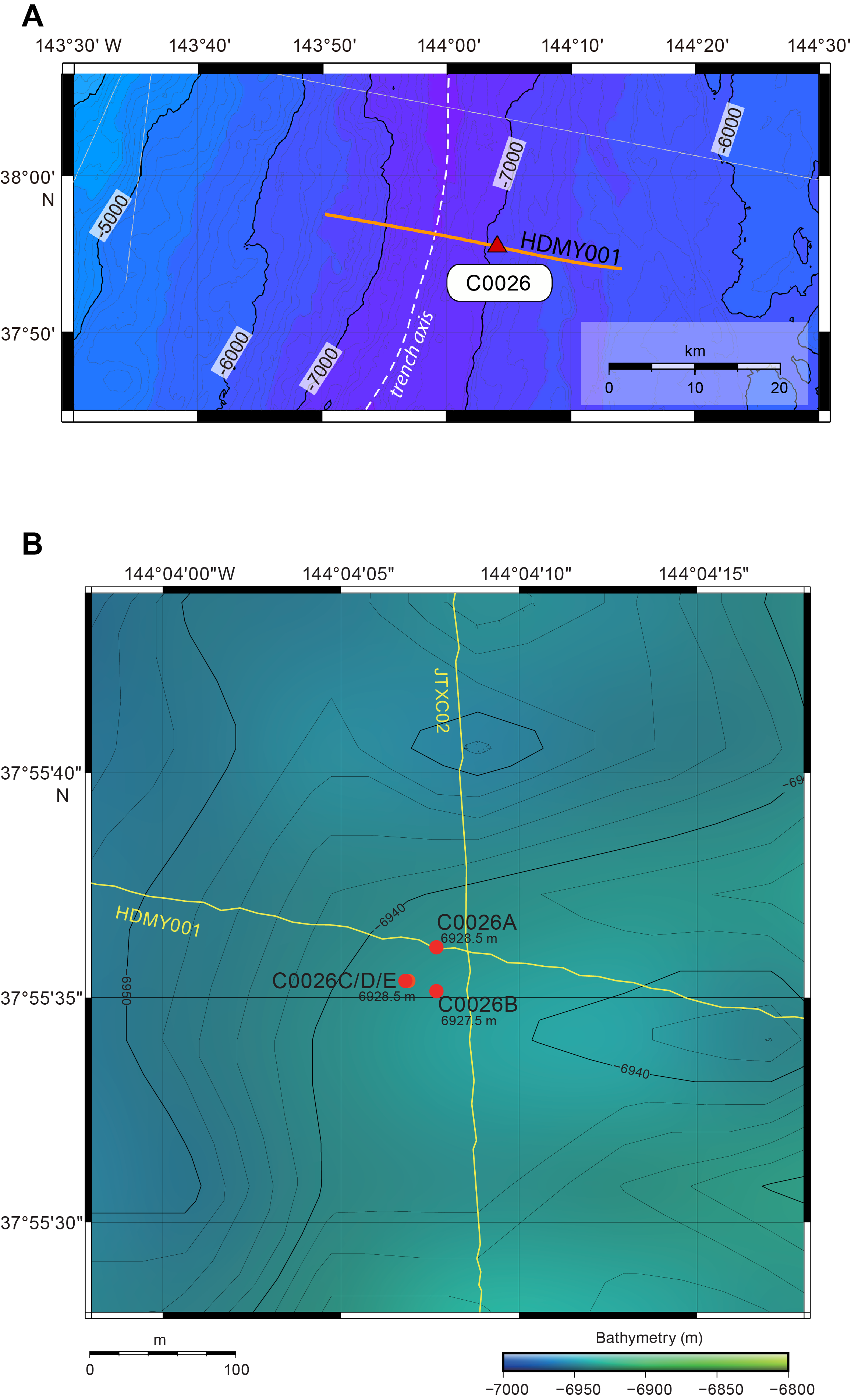
Figure F1. Bathymetric maps.
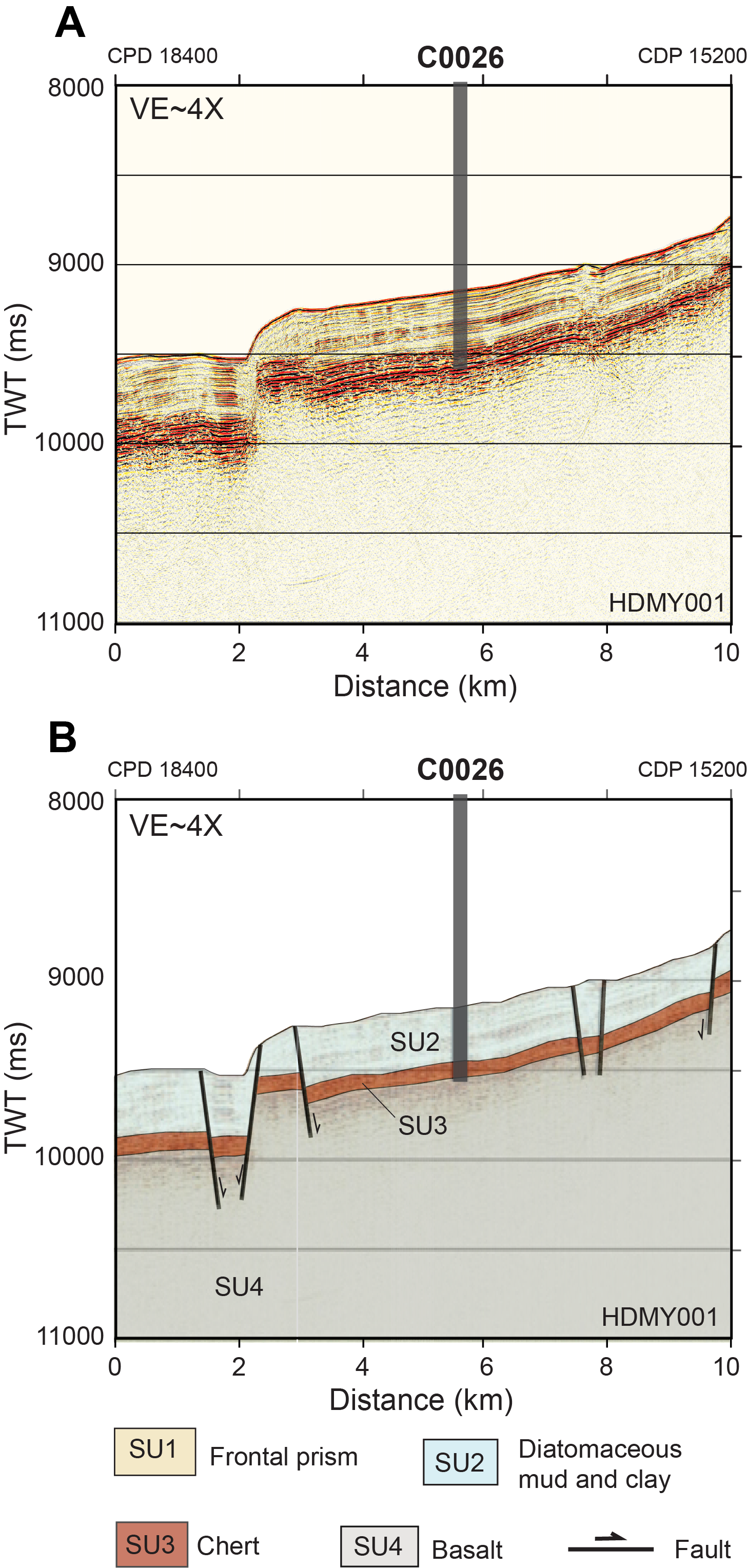
Figure F2. Location of Site C0026.
1.2.2. Motivation for hole positioning
Hole C0026A was drilled to collect LWD measurements with the goal of characterizing the entire input section from the seafloor to oceanic crust (Figure F1). The motivation for collecting LWD data from Hole C0026A was to fingerprint the lithostratigraphic units with LWD tools to derive primary formation characteristics (composition, density, etc.) and thermal and physical properties and to facilitate the interpretation of the logs at Site C0019. Because of operational problems, only real-time data could be obtained from this hole.
Hole C0026B was drilled with the small diameter rotary core barrel (SD-RCB) system to a total depth of 290.0 meters below seafloor (mbsf). Cores were collected to sample the input section, enable characterization of the lithostratigraphic units, and facilitate comparison with Sites 436 and C0019. Holes C0026C–C0026E were drilled with the hydraulic piston coring system (HPCS) to 6.5, 16.0, and 92 mbsf, respectively, which targeted the sediments at and immediately beneath the seafloor. Formation temperature measurements were taken in Hole C0026E using the advanced piston corer temperature (APCT-3) system. Priorities for postexpedition analysis of cores include but are not limited to measuring the mechanical, elastic, frictional, and hydrological properties of the incoming sedimentary units; establishing constraints on the chronology of the input stratigraphy; and evaluating the potential for sediments distal to the trench to record evidence for past earthquake activity.
2. Operations
The overall operations at Site C0026 are summarized in Table T1.
2.1. Hole C0026A
The vessel moved from Site C0019 to Hole C0026A by 2115 h on 22 September 2024 and completed preparations for dynamic positioning, such as transponder deployments, calibration, and field arrival check, at 0945 h on 23 September.
The LWD bottom-hole assembly (BHA) was made up with a new drill bit but with the same LWD tools used for Site C0019 operations. It started running at 0945 h. LWD signal tests were performed at 508.0, 2023.0, 5043.0, and 6868.0 m below rotary table (BRT) while running. The underwater TV (UWTV) camera system was run down to 8 m above the drill bit at 2100 h on 24 September for the seabed survey. The seabed survey was conducted for all planned LWD and coring holes, and it confirmed the water depth for each hole by tagging the seafloor with the drill string. The LWD BHA was spudded into Hole C0026A at 6957.0 m BRT at 0019 h on 25 September (see Table T1 in the Expedition 405 summary chapter [Kirkpatrick et al., 2005b]). We washed down from 6957.0 to 7047.0 m BRT (0–90.0 mbsf) without rotation because the first LWD hole of Site C0026 was planned as a deep hole. Drilling started at 1030 h after the UWTV was recovered to the surface and continued to 7405.0 m BRT (448.0 mbsf) at 2200 h on 27 September, with the rate of penetration (ROP) averaging 10–30 m/h.
High torque and stalled pipe were observed, and the drill string got stuck at 7401 m BRT just after connecting a new drill pipe stand. A total of 10 m3 of seawater gel (SWG) was pumped, followed by multiple attempts to free the drill string until 1000 h on 29 September:
- Overpull of 300 kN observed >45 times while pumping 590 gal/min × 22 MPa;
- Overpull of 500 kN observed >9 times while pumping 590 gal/min × 22 MPa and 20 kN while pumping 590 gal/min × 22 MPa;
- Sweeping 10 m3 of SWG with 716 gal/min × 71.9 MPa;
- Jarring down and applying slack off weight 400 kN >15 times; 900 kN overpull and attempt jarring up 15 times without pumping (fire only one time on the fifth attempt);
- 1250 kN overpull and attempt jarring up >100 times while pumping 7 m3 of kill mud with 600 gal/min × 26.5 MPa; and
- Pumping 7 and 10 m3 of SWG with 600 gal/min × 23 MPa; 1400 kN overpull and attempt jarring up >10 times without pumping.
Because all attempts failed to free the drill string, the final decision to abandon Hole C0026A and LWD operations was made at 1000 h on 29 September. The drill string was severed by a Colliding Tool at 1845 h on 30 September and recovered to the surface at 1145 h on 1 October.
The vessel sailed to an evaluation point soon after recovery of the drill string because of Typhoon 17 (JEBI).
2.2. Hole C0026B
The vessel returned to Site C0026 from Site C0019 at 1200 h on 31 October 2024. The SD-RCB BHA was run in the hole and spudded into Hole C0026B, which lies ~30 m south of Hole C0026A, at 1158 h on 1 November without the use of the UWTV. The center bit was recovered after washing down from 6956.0 to 7036.0 m BRT (0–80.0 mbsf) at 2215 h. Coring began at 2215 h and continued until 1915 h on 6 November. The coring advance was kept at 9.5 or 10 m for Cores 405-C0026B-1K through 15K and then varied between 3.0 and 7.0 m because of observed standpipe pressure increases to improve the chance of successfully coring fragile formations. In total, 32 cores (total length of initial recovery = 101.87 m) were collected from 80.0 to 290.0 mbsf (210.0 m interval) with an average recovery of 48.5% (Table T2). The SD-RCB BHA was pulled out to the surface at 1400 h on 7 November.
2.3. Hole C0026C
A HPCS BHA was made up and run in the hole at 2330 h on 7 November 2024 and spudded into Hole C0026C at 6957.0 m BRT at 1946 h without the UWTV. Core 1H was recovered on deck at 2100 h (Table T2) and successfully collected the surface sediments and mudline with some bottom water. The HPCS BHA was kept in the water while the ship moved to the next hole.
2.4. Hole C0026D
At 2159 h on 8 November 2024, Hole C0026D was spudded in from the same height and location as Hole C0026C (Table T2), again without the UWTV. Core 1H was recovered on deck at 2315 h and found to have successfully collected the surface sediment and mudline, but the bottom water flowed out and was lost when the core barrel was laid down. After cutting the second core, drilling down was required to pull the core barrel out. The sinker bar was recovered but failed to recover the core barrel because of shearing between the sinker bar and the coring line running tool. Attempts were made to recover the core barrel using the backup coring line, and the upper section of the core barrel was recovered. Hole C0026D was abandoned at 0915 h on 9 November because the lower part of the core barrel remained lost in the hole.
2.5. Hole C0026E
Spud-in of Hole C0026E was conducted at 1035 h on 9 November 2024 at the same height and location as Holes C0026C and C0026D without the UWTV. Core 405-C0026E-1H also collected the surface sediment and mudline with the bottom water. Coring continued with full stroke and required the drawworks assist to help pull the inner barrel out for all cores. In total, 10 cores (total length of initial recovery = 92.94 m) were collected from 0 to 92.0 mbsf (92.0 m interval) with an average recovery of 101.0% (Table T3).
The vessel moved back to Site C0019 after the HPCS BHA was pulled out of the hole to the surface at 1545 h on 11 November.
3. Logging while drilling
One hole was drilled and logged at Site C0026: Hole C0026A. Logging data were acquired using a LWD/measurement-while-drilling (MWD) assembly consisting of the SLB TeleScope, MicroScope, and SonicScope tools. Hole C0026A was drilled to a maximum depth of 7405.0 m BRT (448.0 mbsf). MWD data were transmitted in real time with a limited set of LWD data through the drilling fluid telemetry system. See Introduction and Logging while drilling, both in the Expedition 405 methods chapter (Kirkpatrick et al., 2025a), for a detailed description of the operations and tools. The LWD tools were not able to be recovered, so no memory data are available for Hole C0026A.
3.1. Depth shift
The mudline (seafloor) was identified from the midpoint of the first break in the gamma ray and resistivity logs (Figure F3). A mudline was picked at 6957.0 m BRT in Hole C0026A. All LWD data were converted to the LWD depth below seafloor (LSF) depth scale. In this section, LSF depths are referred to as meters below seafloor (mbsf) based on the mudline depth.
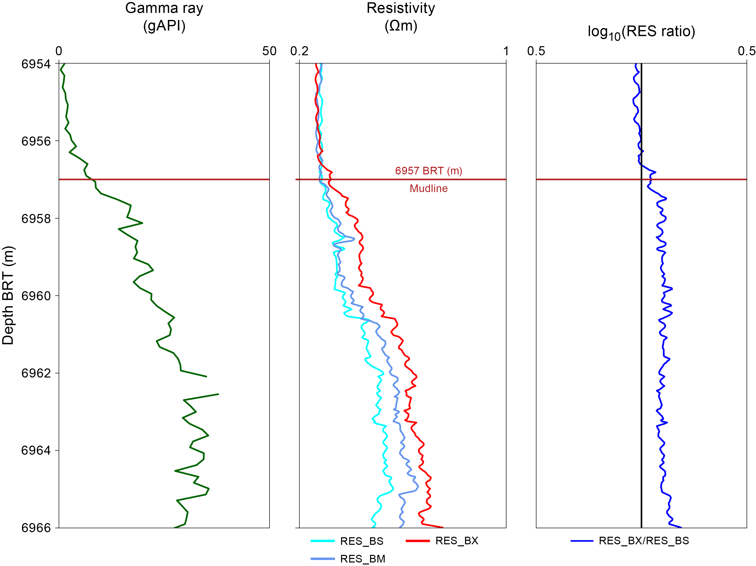
Figure F3. Mudline identification.
3.2. Data and log quality
3.2.1. Drilling parameters
Figure F4 shows the overview of the QC logs, such as drilling parameters and frequency of stick-and-slip. Caliper has been estimated from the resistivity data by the contractor. The uppermost ~275 m was drilled smoothly, with no significant drilling issues. MWD/LWD data quality was good for the upper section, with good quality real-time data from all tools. The interval from 275 mbsf to the total depth was affected by significantly more challenging drilling conditions. The average ROP was ~30 m/h to ~275 mbsf, ~10 m/h to ~350 mbsf, and <5 m/h in the deepest section of the hole. The inclination of the borehole was near vertical, with some spurious spikes in the inclination log. The real-time resistivity borehole images were of moderate to poor quality with broad drilling disturbance and intervals with missing to spotty transmission (e.g., ~246–361 mbsf) (Figure F5). The borehole is significantly enlarged at about 150 mbsf but stays in gage to 315 mbsf. Below this depth, caliper significantly degrades.
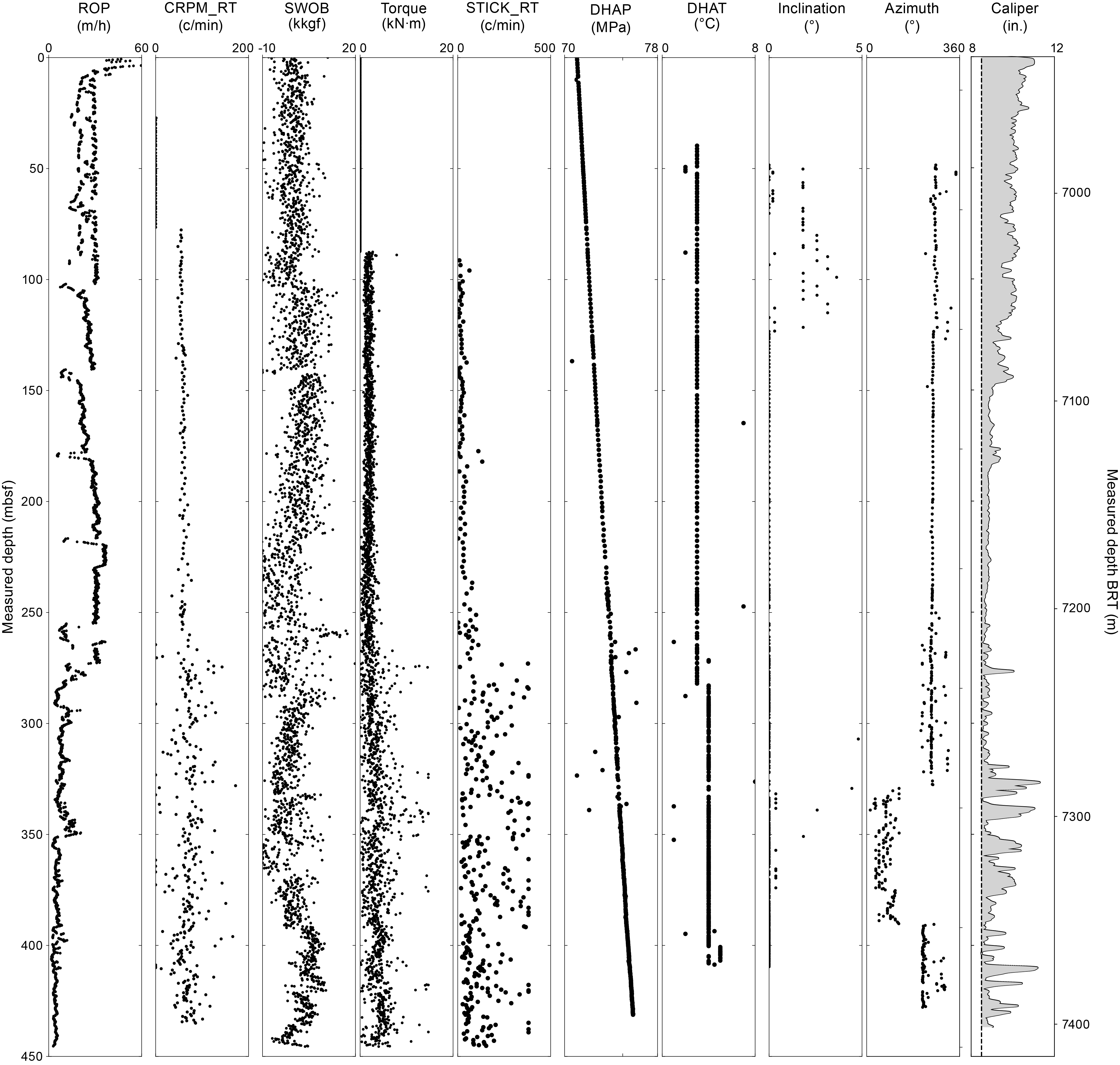
Figure F4. Log quality control log.
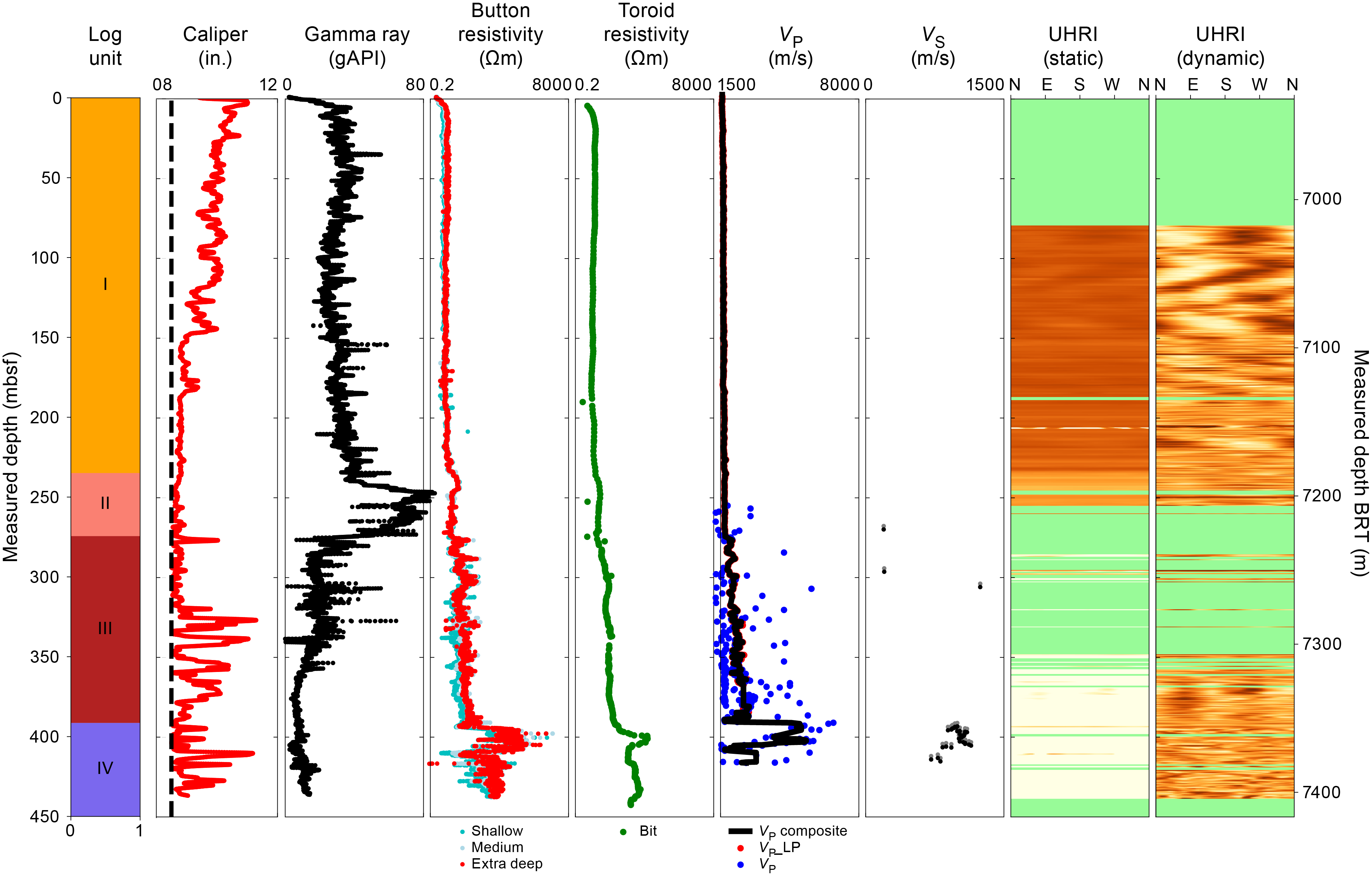
Figure F5. LWD log data.
3.2.2. Sonic data
Sonic velocities are provided through four channels in the final dataset delivered by the contractor: a leaky P-wave slowness (DT_LP_ML_DH) picked from low-frequency monopole data (using the coherence plot SPJ_LP_ML_RT), a VP slowness (DTCO_RT) determined from high-frequency monopole data (using the coherence plot SPJ_MH_RT), a shear sonic slowness (DTSH_QPI_DH in μs/ft), and synthetic VP data. Any velocity (V) in meters per second can be computed from the corresponding slowness (DT) with the formula V = 304800/DT. Figure F6 compares these sonic datasets and provides QC plots.
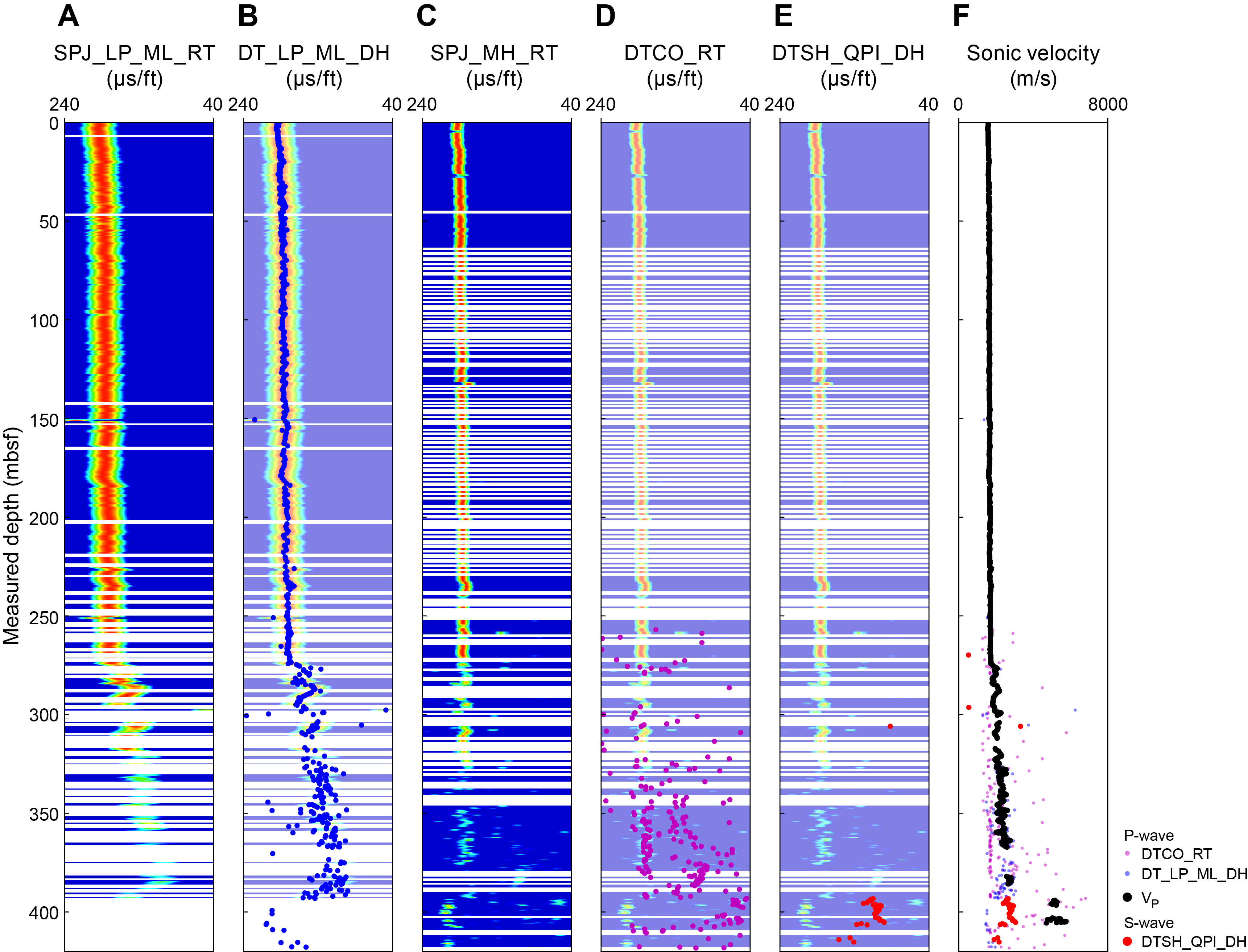
Figure F6. QC of LWD sonic data.
Two QC data are provided by the contractor: slowness-time plane projection for the high-frequency signal of the monopole (SPJ_MH_RT) and for the low-frequency signal of the monopole (SPJ_LP_ML_RT). No plots for slowness-frequency analysis was provided because of the low transmission rate of mud-pulse telemetry. The SPJ_LP_ML_RT coherence signal is strong to 315 mbsf. Below 315 mbsf, a moderate intensity coherence is observed at the same slowness that vanished below 393 mbsf. Leaky P velocity (VP_LP) is in good agreement with the SPJ_LP_ML_RT signal. High-frequency monopole data provide additional information. The SPJ_MH_RT coherency plot is strong down to 275 mbsf, but no DTCO_RT data were picked in this interval. Below this depth, a less coherent signal can be identified, but its intensity corresponds to very low velocities (~1600 m/s). SPJ_MH_RT coherency further decays below 325 mbsf, corresponding to scattered DTCO_RT pickings. Three intervals have high coherence in SPJ_MH_RT: 382–386, 394–396, and 403–405 mbsf. In these intervals, P-wave velocities are estimated at ~2720 m/s, ~5150 m/s, and ~5250 m/s, respectively. Below 405 mbsf, the coherency signal becomes strong again but corresponds to very low velocities (~1500 m/s). The final VP delivered by the contractor is based on the low-frequency monopole data down to 368 mbsf. Below that depth, the final VP data correspond to the high-frequency monopole pickings. The formation between ~276 and ~393 mbsf is interpreted to be chert, and the formation below is interpreted to be basalt based on the comparison to the seismic units defined from high-resolution seismic surveys prior to Expedition 405 (Nakamura et al., 2013). This is the same sequence as at the bottom of Site C0019 or at DSDP Site 436 (Shipboard Scientific Party, 1980).
3.3. Logging units
The combination of different MWD/LWD measurements, particularly the gamma ray, resistivity, and sonic logs, allowed us to define four logging units (I–IV) (Figure F5).
3.3.1. Logging Unit I (0–241.90 mbsf)
Unit I is characterized by moderate gamma ray values ranging ~20–45 gAPI, very low resistivity values (typically <1 Ωm), and low VP values (<1700 m/s). Gamma ray, resistivity, and sonic velocity values are relatively consistent with only minor excursions from this range, suggesting that the lithology is similar throughout. Both VP and resistivity values increase slightly downhole to 2010 m/s and 1.5 Ωm, respectively. This is consistent with a burial compaction trend for relatively unlithified sediments. The log values are consistent with those of siliceous mudstone, as observed in the equivalent shallow sequences during DSDP Leg 56 (Shipboard Scientific Party, 1980) and Integrated Ocean Drilling Program Expedition 343 (Expedition 343/343T Scientists, 2013).
3.3.2. Logging Unit II (241.90–276.30 mbsf)
Unit II is characterized by high gamma ray values with an average of ~60 gAPI and a gradual downhole decrease in resistivity values from ~2 to 1 Ωm. Gamma ray values reach a peak of 87 gAPI near the top of the sequence at 245 mbsf, and, overall, values slightly decline farther downhole. The overall pattern of gamma ray and resistivity is consistent with the pelagic clay observed in the equivalent interval from Leg 56 (Shipboard Scientific Party, 1980), Unit III in Hole C0019B from Expedition 343 (Expedition 343/343T Scientists, 2013), and cores from Hole C0026B (see Lithostratigraphy).
3.3.3. Logging Unit III (276.30–393.60 mbsf)
The top of Unit III is characterized by a sharp decrease in gamma ray values and a significant increase in resistivity log responses. Gamma ray values for this unit are consistently lower than in the units above. They have an average value of 18 gAPI between 275 and 355 mbsf. There is a notable decrease in gamma ray at 356 mbsf and average values of 8 gAPI to the base of the unit. Resistivity values are variable in this unit, from 1 to 10 Ωm, with greater separation between shallow (channel RES_BS) and extra deep resistivity (channel RES_BX) in the deeper section, but the values are higher than those of Unit I. This alternation between high and low resistivity values is compatible with chert lithology, as observed at Site C0019 (see Logging while drilling in the Site C0019 chapter [Regalla et al., 2025]). The real-time velocity data for this section are relatively scattered, particularly for high-frequency P-wave slowness, which appears to be unreliable. VP values increase within this interval from 1760 to 2830 m/s, consistent with values observed in the equivalent interval (Unit IV) at Site C0019. The resistivity borehole images in the upper section of Unit III are extremely poor between 276 and 361 mbsf.
3.3.4. Logging Unit IV (393.60–435.0 mbsf)
The top of Unit IV is characterized by a sharp increase in resistivity values from around 2 to ~100 Ωm (Figure F7). In two intervals (394–396 and 403–405 mbsf), P-wave velocity could be measured at 5150 and 5250 m/s, respectively. S-wave velocities could also be recorded in this interval at ~3030 m/s. Resistivity values vary significantly in this interval, ranging 1–100 Ωm and exhibiting varying degrees of separation between shallow and extra deep resistivity. Resistivity images (real time) are of generally poor quality but indicate nonplanar features, possibly fractures and/or cooling-related structures, similar to the images observed at the bottom of Hole C0019H in a unit interpreted to be basalt (see Logging while drilling in the Site C0019 chapter [Regalla et al., 2025]). Gamma ray values are comparable to those in Unit III, with consistent values of around 8 gAPI between ~360 and 400 mbsf but more variable (ranging 3–20 gAPI) below 400 mbsf. These values are consistent with those expected for altered basalt or interbedded basalt and sedimentary rocks.
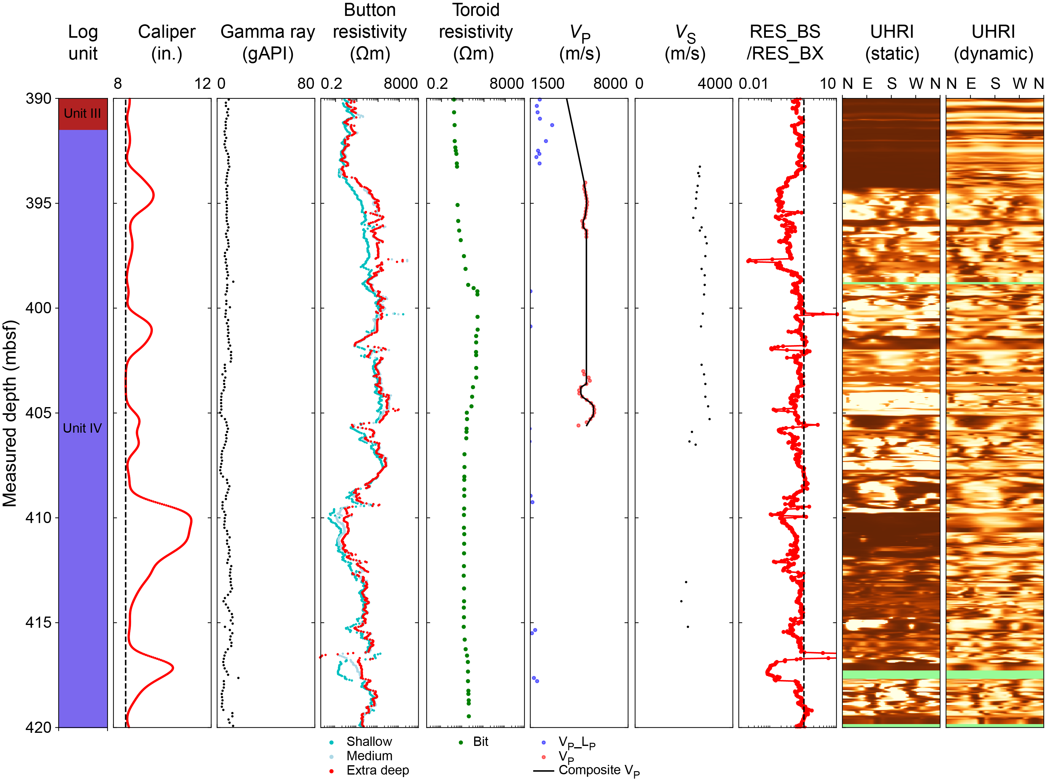
Figure F7. Unit IV logs.
3.4. Physical properties
The LWD data provide information on the natural radioactivity (gamma ray) and electrical resistivity (button and toroid velocities) and an estimate of P-wave velocity. Because only real-time data were available, the data are sparse and irregularly sampled.
3.4.1. Statistics of physical properties
Table T4 and Figure F8 summarize the variability in the main physical properties observed for Hole C0026A. There are strong petrophysical contrasts along the borehole, for which the mean and the standard deviation are reported. The extra deep resistivity (RES_BX) is considered close to the true resistivity of the formation because of the similarity between RES_BX and the medium resistivity (RES_BM).
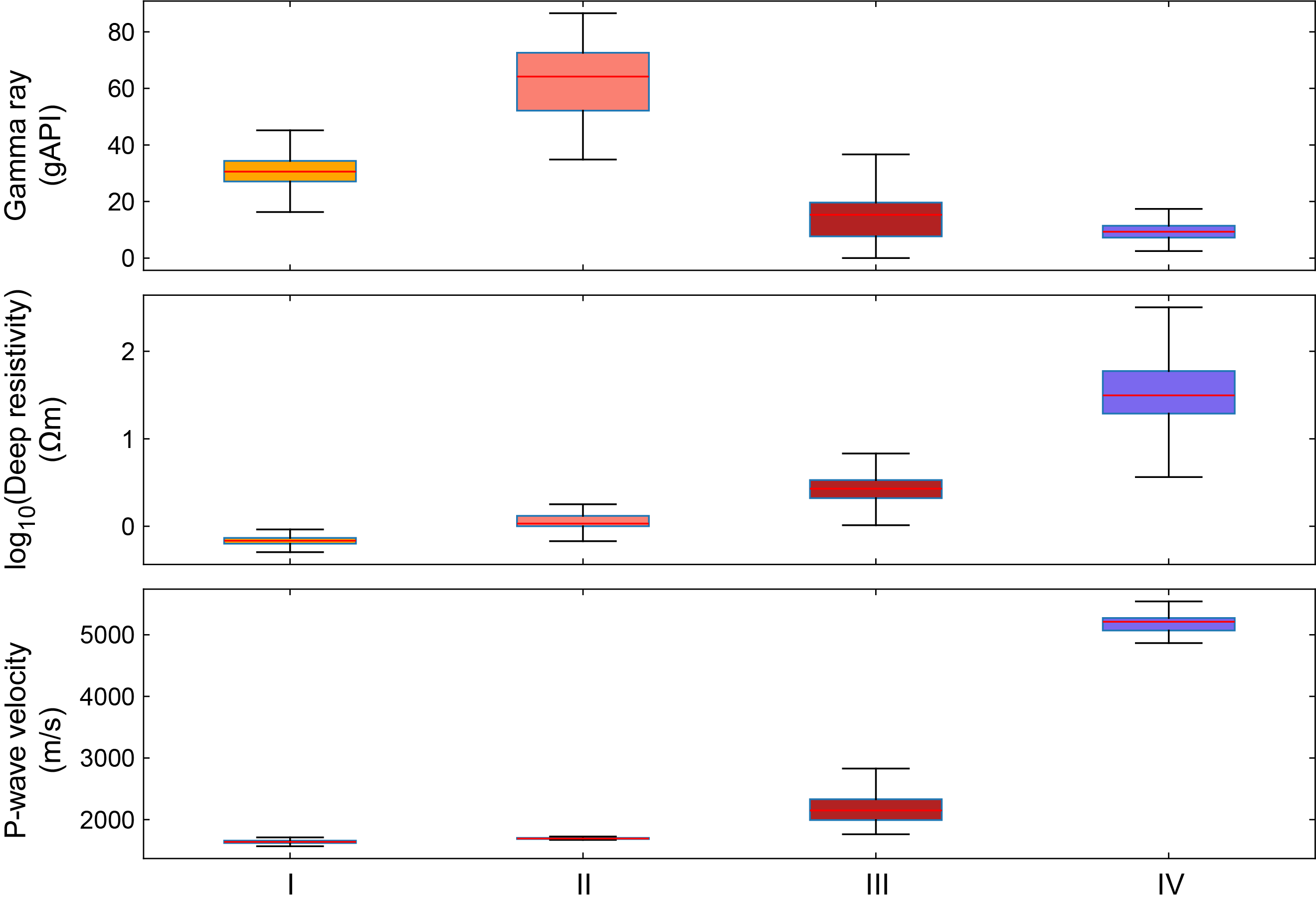
Figure F8. Gamma ray, deep resistivity, and P-wave velocity for logging units.
The gamma ray values in Unit I are moderate at 31 ± 6 gAPI, which contrasts with the larger values in Unit II (60 ± 2 gAPI) and the very low values in Units III (15 ± 8 gAPI) and IV (8 ± 3 gAPI).
The other physical parameters increase with depth. Electrical resistivity increases from very low values of 0.7 ± 0.1 Ωm in Unit I to low values in Unit II (1.1 ± 0.3 Ωm). Resistivity increases faster in Unit III (2.8 ± 1.1 Ωm) and steps up in Unit IV, where electrical resistivity increases by an order of magnitude to reach 57 ± 9 Ωm.
VP velocities follow a pattern similar to electrical resistivity with a gradual increase in Units I (1640 ± 30 m/s) and II (1700 ± 10 m/s), a faster increase in Unit III (2170 ± 230 m/s), and a step to large values in Unit IV (5030 ± 260 m/s).
3.4.2. Relations between physical properties
Figure F9 shows crossplots between the main physical properties (gamma ray, VP, and electrical resistivity).
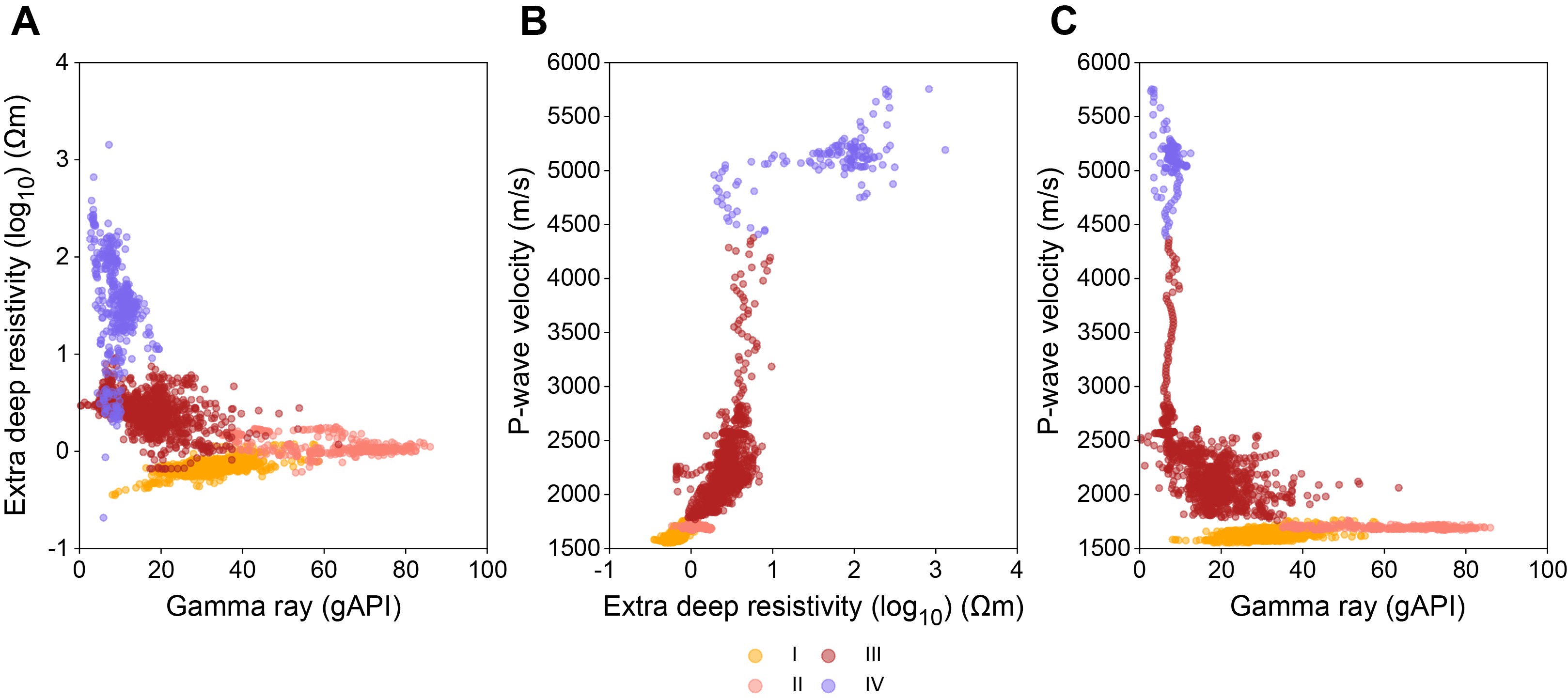
Figure F9. Physical properties for logging units.
Figure F9A compares electrical resistivity to gamma ray. In this crossplot, Unit I has a moderate gamma ray and the smallest resistivity. Unit II is distinct in its high gamma ray values. Units III and IV contain less radioactive elements, but Unit IV is distinctive in its higher resistivity.
Figure F9B shows a positive correlation between resistivity and P-wave velocity, which is particularly strong for Units I–III. Unit IV is characterized as a high-velocity zone with a positive correlation between the two properties, but the variability is larger because of the large variability in P-wave velocity (Figure F8).
The crossplot between P-wave velocity and gamma ray (Figure F9C) also shows the difference between the four units. Unit I has a moderate gamma ray and small VP. Unit II has low velocity but high gamma ray. Unit III values cluster around low gamma ray and moderate VP, whereas Unit IV has distinctive low gamma ray and in places very large VP.
3.4.3. Resistivity image interpretation
Real-time ultrahigh-resolution images (UHRIs) are available between 79 and 438 mbsf at low resolution from the real-time transmission through the drilling fluid telemetry system. The overall image quality is fair to poor for Hole C0026A. Some geologic features (bedding and fractures) and wellbore failures (breakouts) were identified from the images. However, all features identified in Hole C0026A are of fair quality only because of the low resolution of the images, which limits the possibility of identifying individual features. Image artifacts and missing sections are common throughout the image logs, which hinders interpretation. Between 79 and 145 mbsf, the image quality is poor because of artifacts that may result from tool orbiting, where the tool scrapes diagonally along the borehole wall (Lofts and Bourke, 1999). These diagonal artifacts are less pronounced between 145 and 187 mbsf, resulting in moderate image quality. Horizontal image artifacts are common throughout the entire imaged interval and are thought to be related to the stick and slip of the MicroScope tool as the buttons rotate (Lofts and Bourke, 1999). Image quality between 246 and 361 mbsf is extremely poor with significant data gaps. The interval 361–438 mbsf has improved image quality. All images were oriented to north, and the inclination of the hole was accounted for using continuous MWD data (Figure F4). Geologic features were identified and characterized, and true orientations were reported. Shallow, medium, deep, and extra deep resistivity images are unavailable for Hole C0026A because the memory data were not recovered.
3.4.4. Bedding and fractures
Structural and sedimentary features were identified and interpreted using the low-resolution real-time UHRIs (Figure F10). Each pick was critically examined by three simultaneous observers to confirm (1) sinusoids on the unwrapped images of the cylindrical borehole wall and (2) consistent criteria for structural and bedding interpretation. Our interpretation was guided by the structural picks in Hole C0019H (see Logging while drilling in the Site C0019 chapter [Regalla et al., 2025]), for which high-resolution memory images are available. Features in the logs were divided into three categories: bedding, conductive or resistive fracture, and bounding surface:
- Bedding: a series of sinusoids with consistent orientation and resistivity signatures that are visible from the static and dynamic UHRIs. The sinusoid can be traced over the full image width (see Figure F23 in the Site C0019 chapter [Regalla et al., 2025]).
- Conductive/Resistive fracture: a planar feature, visible as a sinusoid in the flattened image, that may or may not host shear displacement. Its orientation crosscuts the orientation of nearby bedding. We note whether the fracture is predominantly resistive or conductive.
- Bounding surface/feature: when a crosscutting relationship is not evident but a planar discontinuity or distinctive change in resistivity (i.e., more conductive to less conductive across a sinusoidal feature) is clear, we note the feature as a bounding surface. This may be indicative of a change in bulk rock properties (e.g., the bounding surface may be an unconformity, a fault/fracture aligned with adjacent bedding, or a fracture), especially in Unit IV, which was interpreted to be basalt.
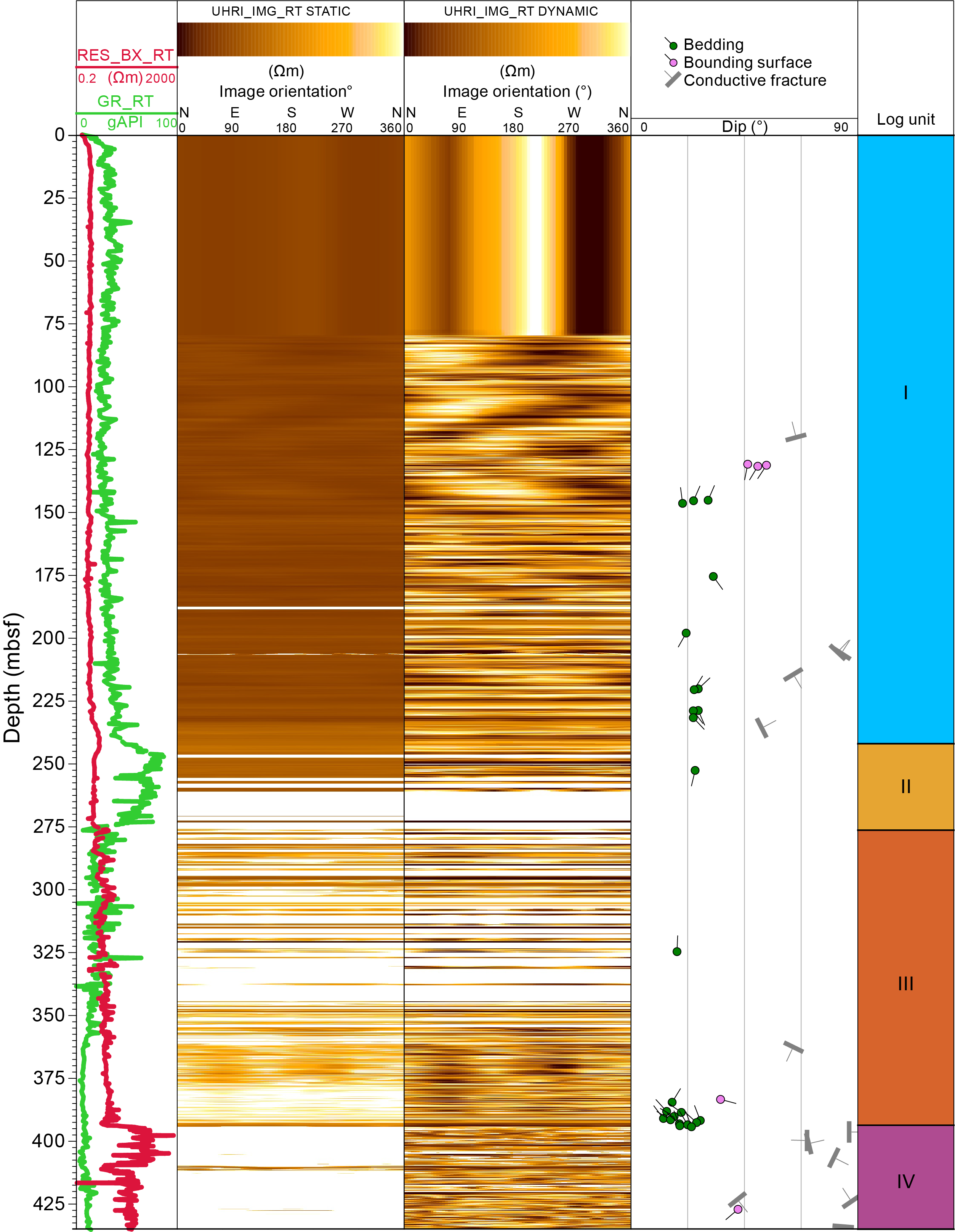
Figure F10. Preliminary interpretation of borehole images.
All bedding identified in Hole C0026A is low angle, with an average dip of 16° ± 4° (Table T5). Bedding orientation in Unit I varies in what is interpreted to be relatively unlithified sediments. However, accurately determining the orientation of subhorizontal features in the low-resolution logs is particularly challenging, which may lead to significant uncertainty in the bedding orientation measurements and, potentially, bias toward higher dip angles. High-angle conductive fractures are identified in Unit I with dips between 44° and 80°. Bedding identified in Unit III dips shallowly northwest, which is consistent with the dip of reflections in the nearby seismic data (see Core-log-seismic integration).
The five bounding surfaces identified in Hole C0026A are structures that may indicate fractures formed along weakened bedding planes or represent a change in bulk rock properties (Figure F10). However, we did not classify these features as either bedding or fractures because there were no observed crosscutting relationships with adjacent bedding planes.
The UHRIs in Unit IV, interpreted to be basalt or mixed basalt and sedimentary rocks, are highly resistive with a chaotic behavior of nonplanar conductive features that cut vertically and horizontally across the unwrapped resistivity image (Figure F10). One bounding surface and seven conductive fractures are identified in Unit IV; however, we are unable to distinguish if these features are related to tectonic deformation, cooling, or basalt characteristics. The conductive fractures are predominantly high angle and dip east, which is consistent with the orientation of conductive fractures identified in Hole C0019H in Unit V.
3.4.5. Wellbore failure
In Hole C0026A, LWD images show distinct conductive tracks approximately 180° apart that are consistent with borehole breakouts (Figure F10; Table T6) (Zoback, 2007). Breakouts occur between 365 and 385 mbsf in Unit III. Poor image quality and artifacts in the real-time images result in uncertain breakout picks. A quality code of "fair" is assigned to all breakout picks in Hole C0026A, following the criteria outlined for Site C0019 (see Logging while drilling in the Site C0019 chapter [Regalla et al., 2025]). Identified breakouts are frequently overprinted by horizontal image artifacts, and both tracks are not always visible at the depths picked. A total of 16 breakouts were identified in the images with a cumulative length of ~5 m, corresponding to ~1% of the total borehole depth (Figure F11). Breakout widths range 28°–76° with a mean value of 50° (±13° standard deviation), whereas breakout azimuth ranges 70°–90°.
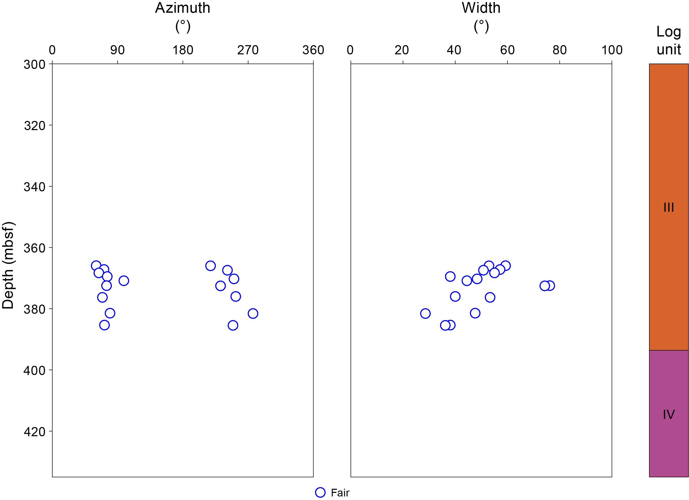
Figure F11. Breakout azimuth and width.
4. Lithostratigraphy
Site C0026 consists of four holes: C0026B–C0026E. Hole C0026B was drilled using the SD-RCB system to core from 80.00 to 290.00 mbsf (equivalent to the core depth below seafloor, Method A [CSF-A] depth scale). In contrast, Holes C0026C–C0026E were cored with the HPCS, with coring depths from the seafloor to 6.50 and 92.00 mbsf, respectively.
Three main lithostratigraphic units were identified at Site C0026 (Figure F12). Lithostratigraphic units are numbered 1–3 from the seafloor to the bottom of the cored interval (Table T7). They were distinguished based on grain size and sediment composition, supported by color variations (see Lithostratigraphy in the Expedition 405 methods chapter [Kirkpatrick et al., 2025a]). Representative intervals of each unit and unit boundaries are illustrated in Tri-Sensor Core Logger (TSCL) linescan images, modified linescan images, and X-ray computed tomography (XCT) images (Figures F14, F22, F24). Specific sedimentary features (e.g., soft-sediment deformation structures such as flame structures, load casts, and fining upward) are shown in Figure F17. Sediment compositions, derived from visual core descriptions and smear slides, are summarized in ternary diagrams (Figure F15; Table T8) and selected microscopic images (Figures F16, F20, F21, F23, F25). The grain size ranges presented for each subunit below record the range between the lowest (L) recorded and highest (H) recorded percent of each grain size fraction (displayed as L%-H%). It is noted that this smear slide analysis semiquantitative and further grain size distribution analysis is needed. Core colorimetry data from the TSCL display color variations across the units (Figure F13); however, TSCL colorimetry data is only available for Cores 405-C0026B-1K through 21K (80.00–250.42 mbsf). Variations in mineral assemblages and chemical compositions throughout the holes are documented using X-ray diffraction (XRD) analysis (Figures F18, F26; Table T9) and X-ray fluorescence (XRF) analysis (Figure F19; Table T10).
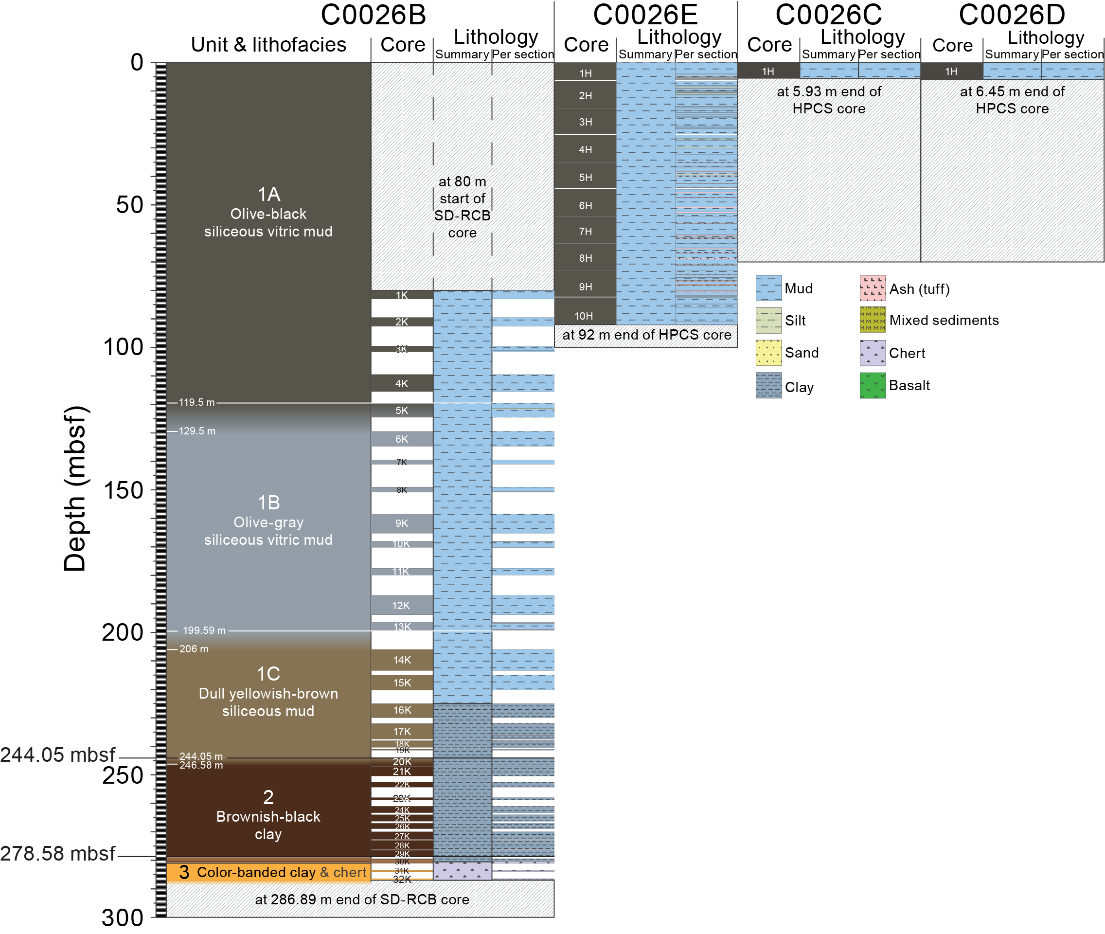
Figure F12. Lithostratigraphic units.
4.1. Unit 1
Because of the similar sediment composition and grain size of the background sedimentation throughout Unit 1, the division into Subunits 1A–1C is primarily based on color variations ascertained from visual core description and colorimetry (Figure F13), with Subunit 1C exhibiting a slightly higher proportion of siliceous biogenic material.
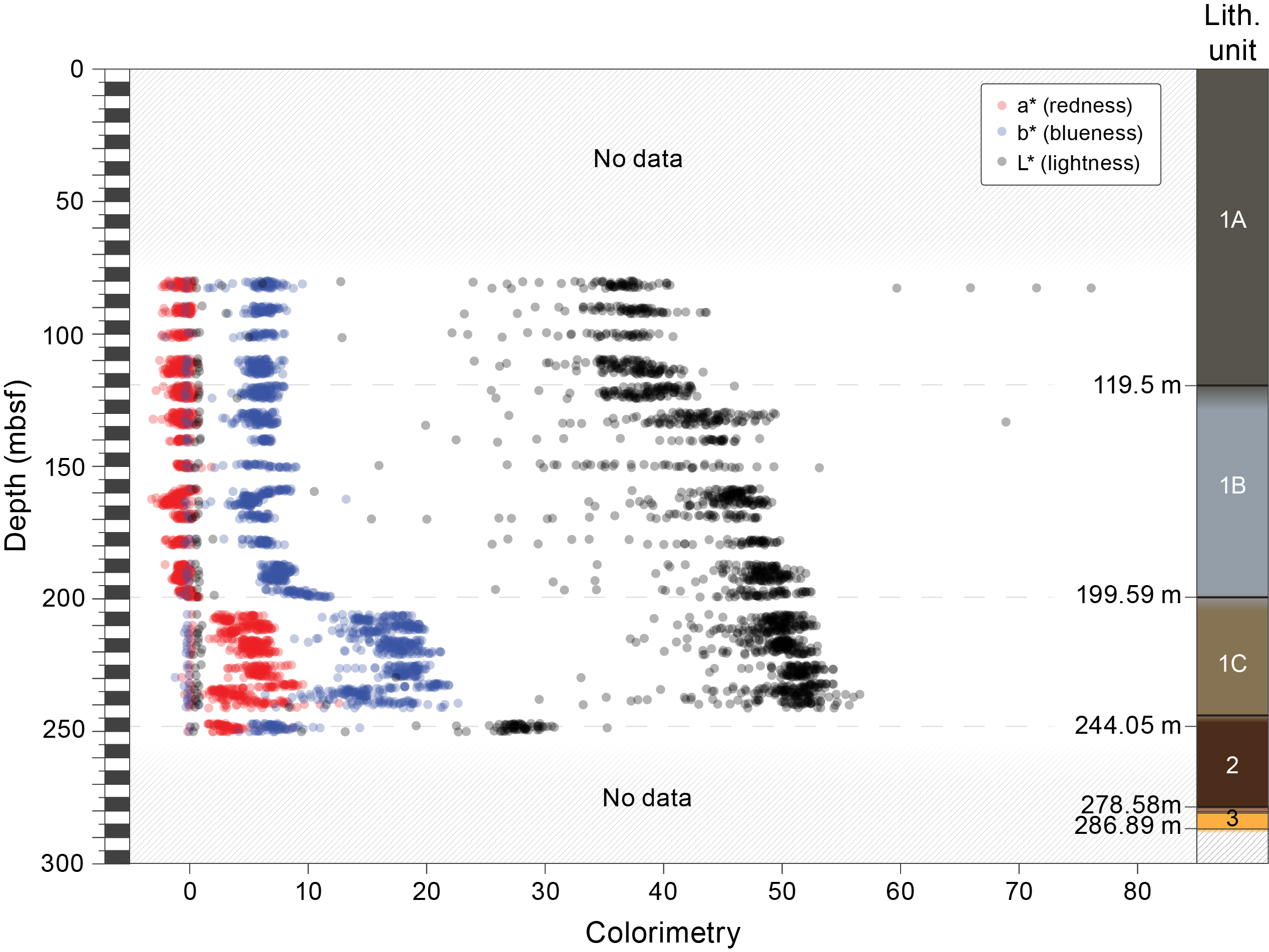
Figure F13. TSCL core colorimetry.
4.1.1. Subunit 1A
- Interval: 405-C0026B-1H-1, 0 cm, 405-C0026C-1H-1, 0 cm, 405-C0026D-1H-1, 0 cm, and 405-C0026E-1H-1, 0 cm, to 405-C0026B-5K-1, 0 cm
- Depth: 0–119.50 mbsf
- Age: 0.30–5.10 Ma (diatoms); 0.43–9.1Ma (radiolarians)
- Lithology: olive-black siliceous vitric mud
4.1.1.1. Visual core description lithology
Subunit 1A encompasses the entire cored interval of Holes C0026C–C0026E and the upper part of Hole C0026B. Based on visual core description, smear slide analysis, and XCT images, the recovered stratigraphic sequence correlates well across these cores (Figures F12, F14, F15, F16). As a result, we integrated the observations and data from the four cored intervals for Subunit 1A.
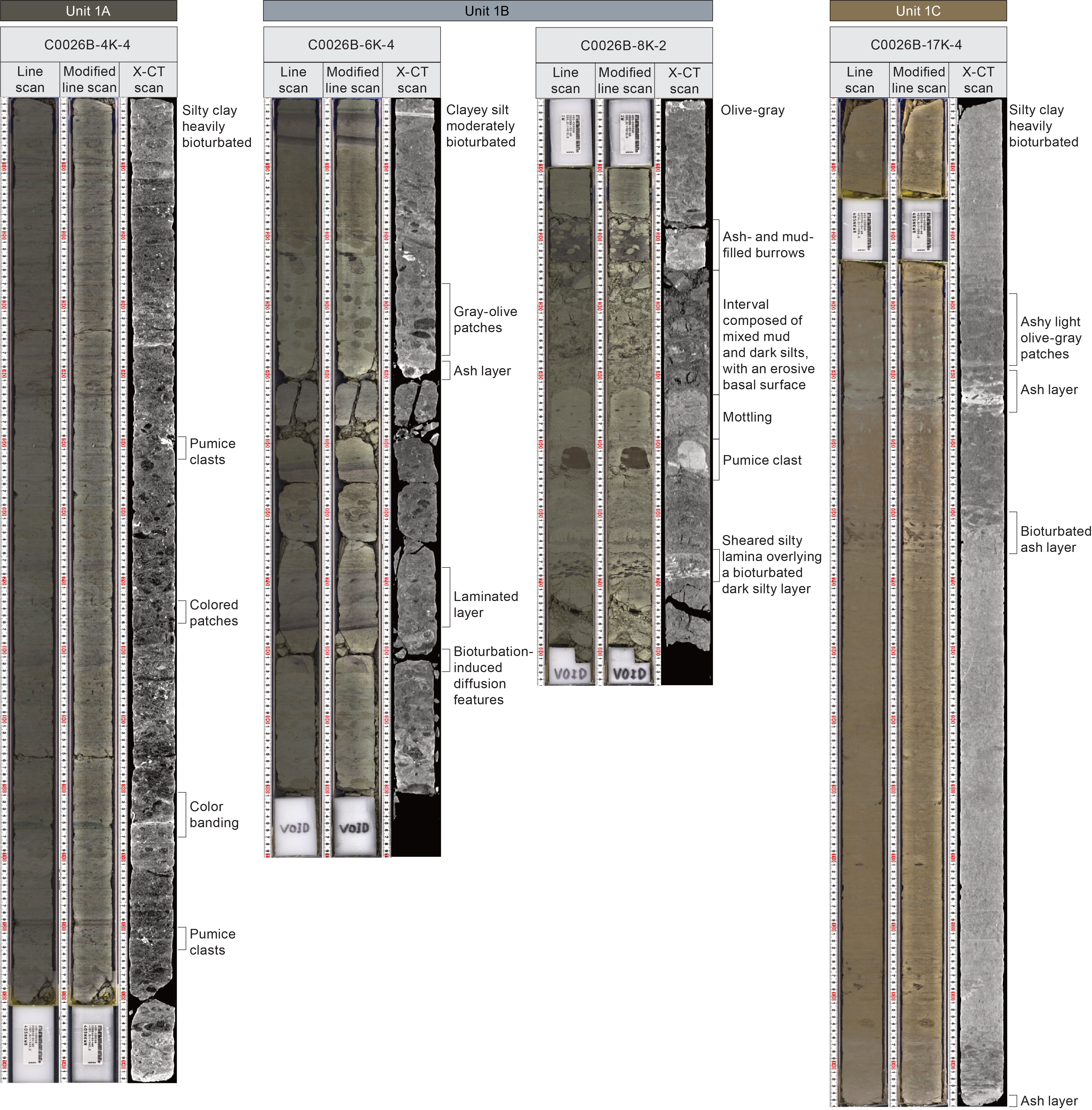
Figure F14. Subunit 1A–1C images.
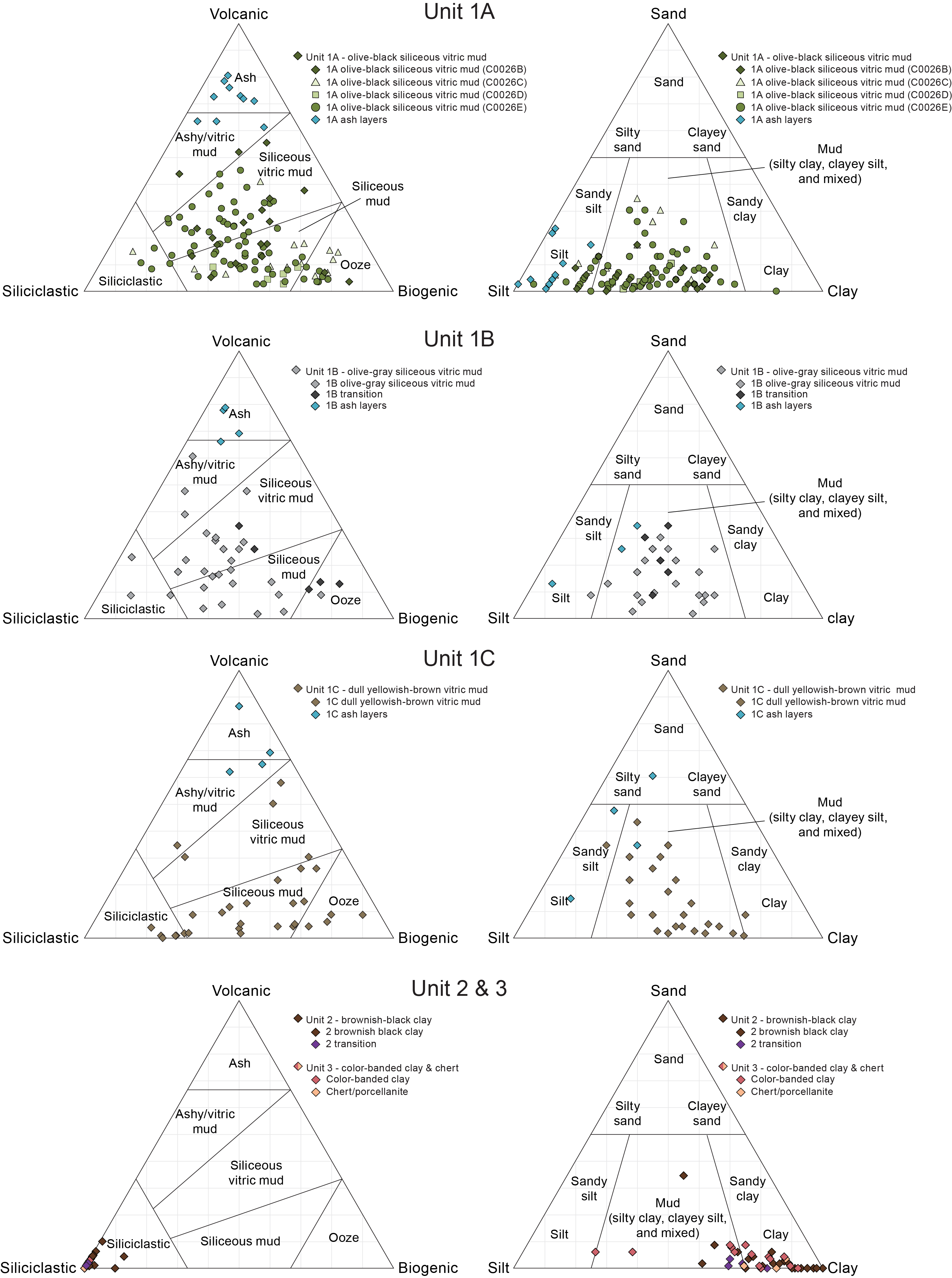
Figure F15. Sediment composition.
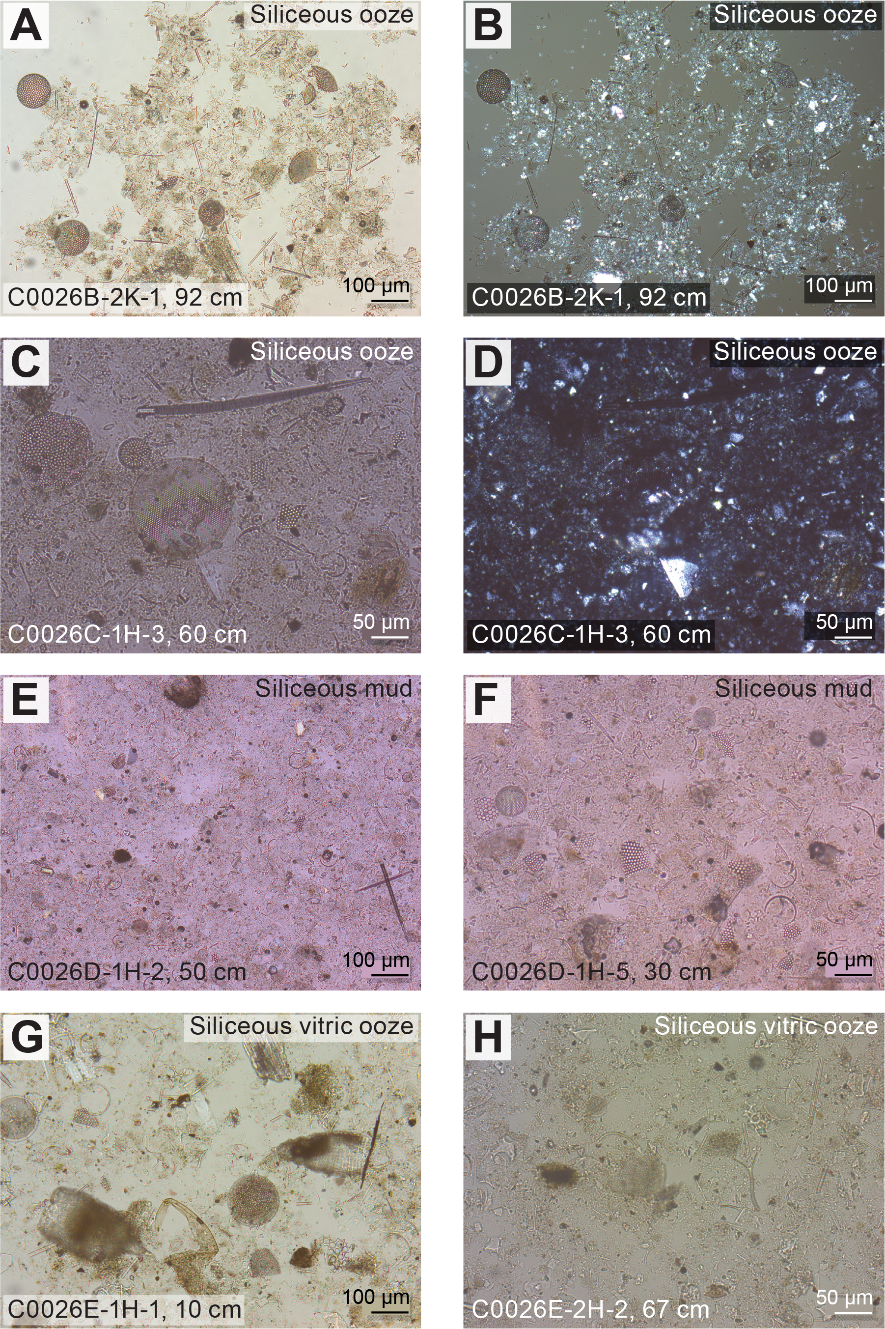
Figure F16. Subunit 1A smear slides.
Subunit 1A is composed of olive-black siliceous vitric mud with common volcanic ash-rich layers, color banding, and extensive bioturbation. Color changes between the olive-black (7.5Y 3/1) background sedimentation and grayish olive (7.5Y 5/3), olive-gray (10Y 4/2), and dark greenish gray (7.5GY 4/1) define centimeter to decimeter compositional layers that contain variations in the abundance of volcanic and siliceous biogenic material (as demonstrated by the large scatter of the datapoints in the compositional ternary diagram displayed in Figure F15). Color changes from brownish to greenish in the color bands usually correlate with a higher abundance of volcanic glass, which is typically altered. In Cores 405-C0026E-2H through 10H, more than 120 ash-rich layers were identified, with thicknesses varying from 1 to 30 cm. Fining-upward grain size trends are commonly associated with thick, ash-rich layers but can occasionally be observed in siliciclastic beds. Soft-sediment deformation, such as load and flame structures, are typically observed at the top and bottom of the ash-rich layers (Figure F17).
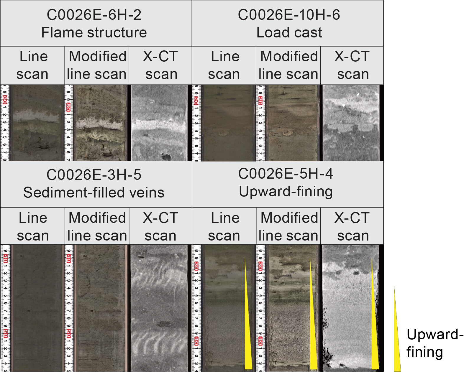
Figure F17. Sedimentary structures.
The olive-black background sedimentation of Subunit 1A is moderately to heavily bioturbated, identifiable by subhorizontal and near-vertical lighter or darker mottles (Figure F14). Some burrows show black coloration, possibly due to the presence of pyrite or iron monosulfides. Silt-filled burrows are also visible in the XCT image and appear round to ellipsoidal in cross section, with simple, unlined, and unbranched structures suggesting Planolites. In particular, bioturbation with distinct crosscutting relationships is often concentrated above, through, and under ash-rich layers.
Ash-rich layers are (1) dark green–black banded (usually <5 cm thick), (2) light gray and almost 100% glass composition (2–30 cm thick), and (3) dark gray to brown, containing pumice and heavy minerals (2–10 cm thick), as well as combinations of the above. Most thick ash-rich layers exhibit sharp basal contacts with upward grading. Soft-sediment deformation structures, particularly flame structures, are often observed where the upper boundary of an ash-rich layer is well defined. Further investigations are needed to determine whether the occasionally irregular basal boundary of ash-rich layers is created by load structures or burrows. It is noted that these features could be more evident in these layers due to the color differentiation. The abundance of ash-rich layers appears to decrease in the lower part of Subunit 1A (Hole C0026B) compared to the upper part (Hole C0026E). However, it is unclear whether this difference reflects a genuine temporal variation or is due to the lower recovery rate of the SD-RCB coring system used in Hole C0026B compared to the higher recovery rate of the HPCS used in Hole C0026E. In addition to volcanic ash-rich layers, subrounded pumice clasts are disseminated throughout Subunit 1A with sizes from several millimeters to centimeters. These clasts are usually light gray-green but are occasionally brown and sometimes black if pyritized (Figure F14).
4.1.1.1.1. Smear slide petrography
The grain size of the Subunit 1A background sedimentation is predominately mud and ranges between sand (0%–40%), silt (15%–92%), and clay (5%–85%). The sand-sized fraction usually comprises large centric diatoms and pumice (Figure F16). The composition of the background sedimentation in Subunit 1A is siliceous to siliceous vitric mud composed of a range of siliciclastic (7%–74%), volcanic (3%–64%), and biogenic (5%–82%) material (Table T8; Figure F15). Other minor components (0%–20%) include dense or opaque minerals, framboidal pyrite, mica, glauconite, and calcite. Siliciclastic grains are mostly clay minerals (0%–62%) with small amounts of quartz (1%–35%) and mud aggregates (0%–35%), as well as minor contributions of feldspar (0%–2%). The biogenic portion is a mixture of diatoms (0%–50%), radiolarians (0%–35%), silicoflagellates (0%–20%), and sponge spicules (1%–38%). The volcanic portion of Subunit 1A is mostly clear glass (0%–55%), colored glass (0%–10%), and pumice (0%–15%). The dominant grain size of ash-rich layers is silt (65%–97%) with minor sand (1%–27%) and clay (0%–15%) size fractions.
4.1.1.1.2. Mineralogy and sediment geochemistry
A total of 22 bulk samples representative of Subunit 1A were collected for XRD analysis (Figure F18; Table T9). For each sample, the semiquantitative mineral mode by weight was estimated (see Lithostratigraphy in the Expedition 405 methods chapter [Kirkpatrick et al., 2025a]). Clay mineral content dominates the composition and ranges 48–69 wt%. Plagioclase ranges 17–29 wt%, and quartz ranges 14–25 wt%. The proportion of the three components is relatively consistent throughout Subunit 1A and supports observations of mostly clay minerals in the siliciclastic component from smear slides.
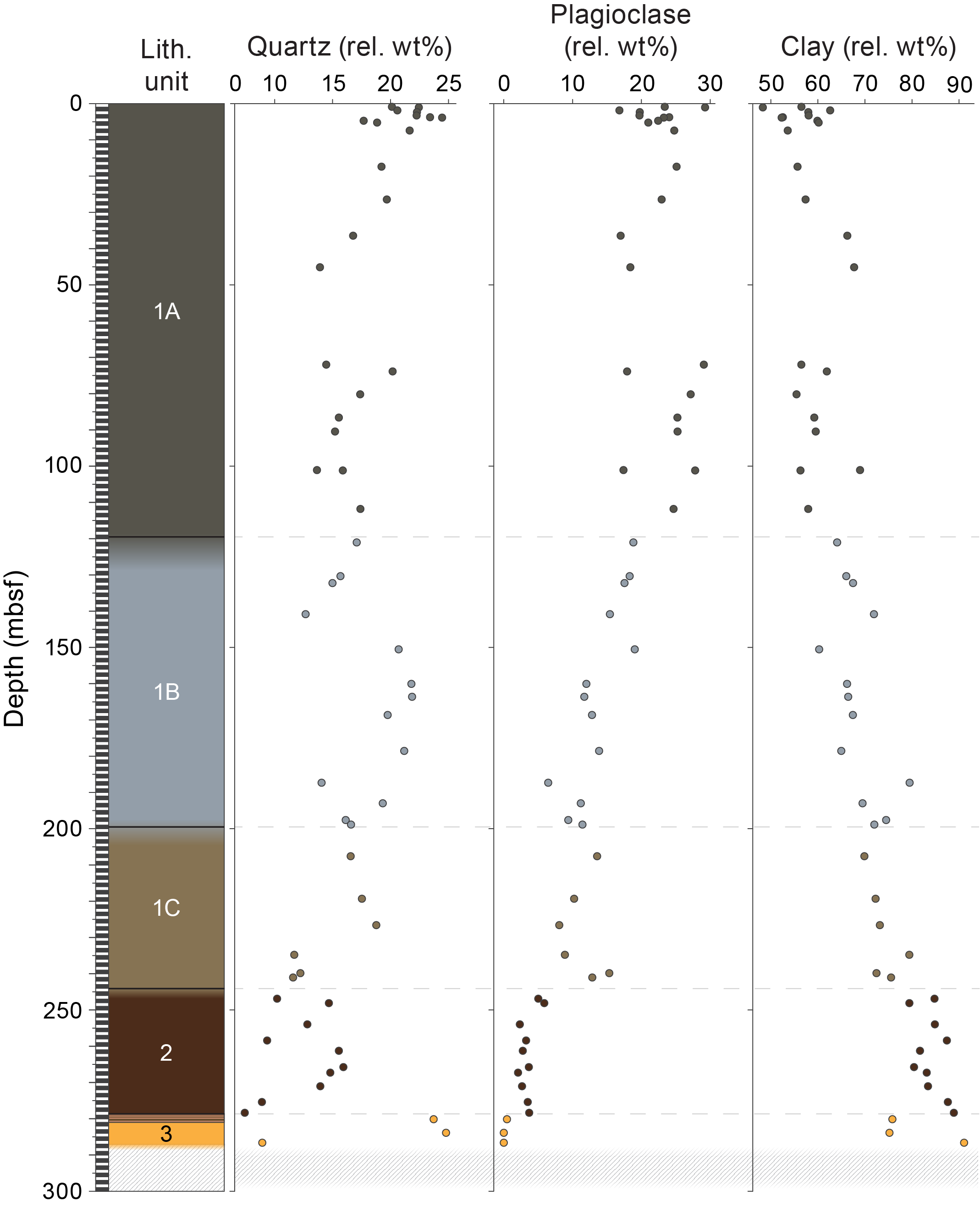
Figure F18. XRD semiquantitative mineral abundance.
XRF and loss on ignition (LOI) analyses were performed in the same intervals, yielding ranges of 3.86–4.54 wt% Na2O, 1.70–2.82 wt% MgO, 13.53–16.04 wt% Al2O3, 64.78–70.71 wt% SiO2, 0.07–0.12 wt% P2O5, 2.27–3.80 wt% K2O, 1.15–2.80 wt% CaO, 0.43–0.69 wt% TiO2, 0.06–0.14 wt% MnO, 4.15–8.51 wt% Fe2O3, and 5.38–8.69 wt% LOI (Figure F19; Table T10). The high concentration of SiO2 is consistent with the relatively high proportions of volcanic glass and siliceous biogenic components observed in smear slides throughout Subunit 1A.
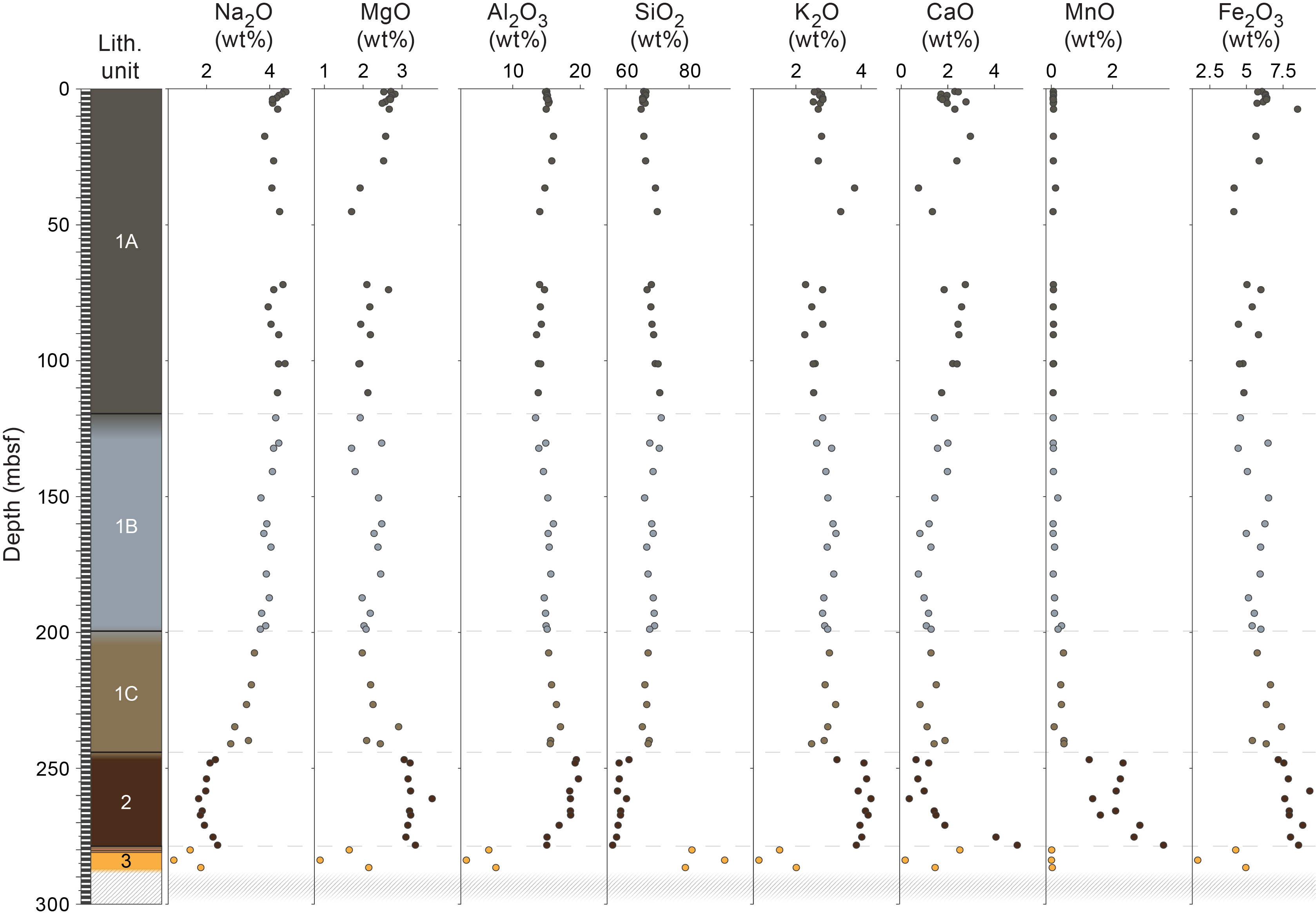
Figure F19. XRF major element compositions.
4.1.1.1.3. Summary and preliminary interpretation
The composition of Subunit 1A is dominated by siliceous biogenic material (diatoms and sponge spicules) with varying siliciclastic and volcanic components, indicating a hemipelagic depositional environment. Thick ash-rich layers have sharp contacts with concentrated bioturbation at the upper boundary and tend to display a fining-upward grain size distribution. Further work is required to distinguish the depositional mechanism for these event beds (e.g., primary volcanic ash fall or remobilization), but grain size trends and erosive basal contacts indicate higher energy compared to background sedimentation. The presence of sediment-filled veins and soft-sediment deformation structures (e.g., load and flame structures) further suggests possible links to past seismic activity.
4.1.1.2. Subunit 1B
- Interval: 405-C0026B-5K-1, 0 cm, to 13K-CC, 18.5 cm
- Depth: 119.50–199.59 mbsf
- Age: 3.5–9.1 Ma (diatoms); 2.3–16.6 Ma (radiolarians)
- Lithology: olive-gray siliceous vitric mud
4.1.1.2.1. Visual core description lithology
Subunit 1B is composed of olive-gray siliceous vitric mud characterized by a mixture of siliceous biogenic and vitric components (Figures F12, F14, F15, F20). A notable increase in the colorimetry lightness values in Core 405-C0026B-5K defines a color transition that is interpreted to represent a gradational lithologic contact between Subunits 1A and 1B (Figure F13). Features such as bioturbation, color banding, and volcanic ash-rich layers are commonly identified throughout Subunit 1B. Layering is defined by color changes between olive-gray (7.5Y 4/1), grayish olive (7.5Y 5/3), olive-gray (10Y 4/2), and dark greenish gray (7.5GY 4/1), which result from variations in the relative abundance of volcanic and biogenic material. Although soft-sediment deformation structures are less common than in Subunit 1A, graded (usually ash-rich) beds with flame structures at the top and erosive basal surfaces (e.g., Section 8K-2) (Figure F17) remain present, indicating deposition from higher energy sedimentary events was interspersed with the background sedimentation (as in Subunit 1A).
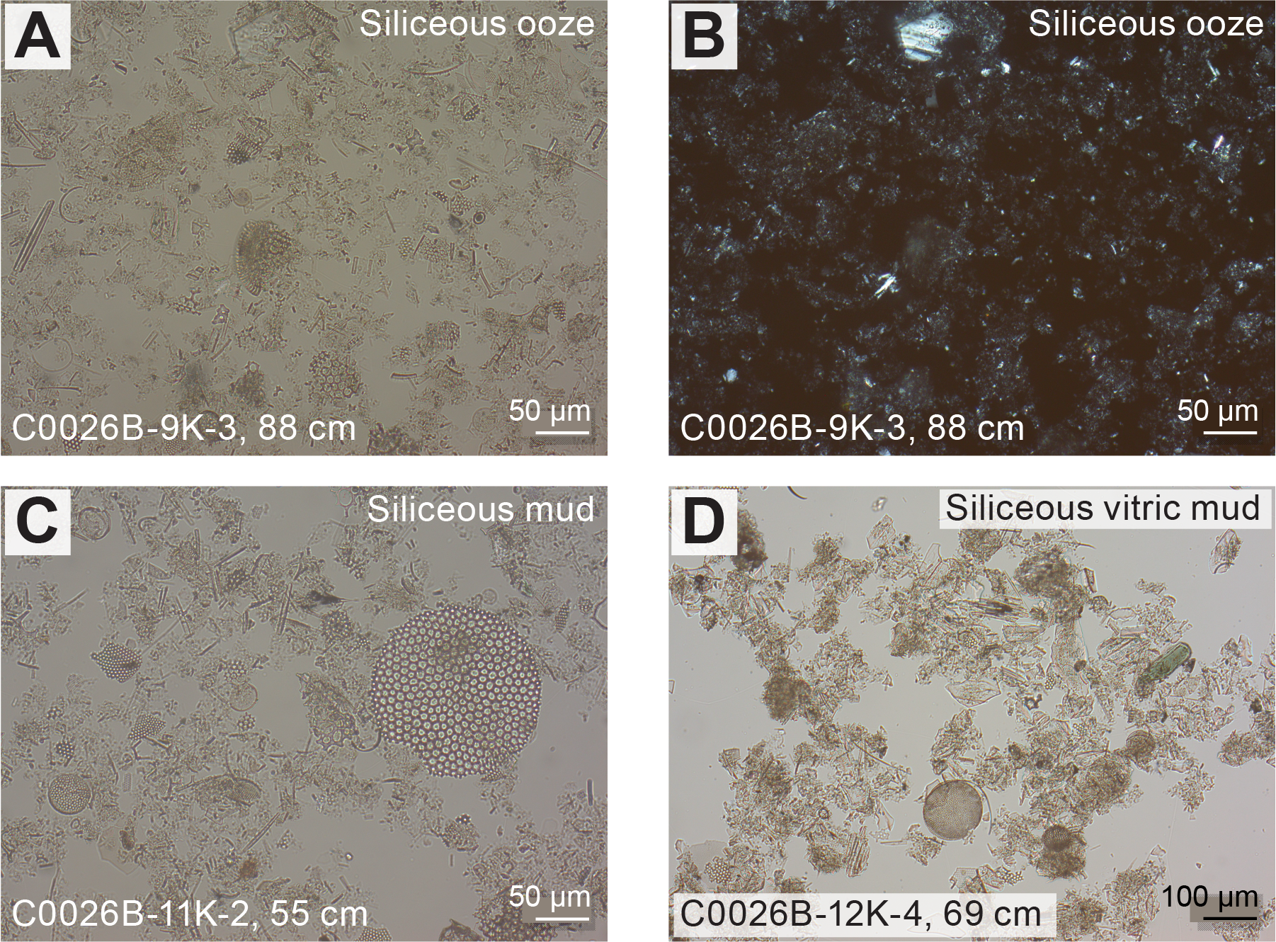
Figure F20. Subunit 1B smear slides.
The olive-gray background sediments of Subunit 1B are moderately to heavily bioturbated and identifiable by subhorizontal and subvertical lighter or darker mottles (Figure F14). Some burrows show black coloration due to the presence of pyrite or iron monosulfides. Silt-filled burrows are also visible in the XCT image and appear round to ellipsoidal in cross section, with simple, unlined, and unbranched structures suggesting Planolites. In particular, bioturbation with distinct crosscutting relationships is often concentrated above, through, and below ash-rich layers.
A total of 13 ash beds are identified in Subunit 1B, most of which are thinner (1–3 cm) and darker than the lighter and thick ash-rich layers identified in Subunit 1A.
4.1.1.2.2. Smear slide petrography
The Subunit 1B background sedimentation grain size is predominantly mud and ranges between sand (2%–35%), silt (20%–75%), and clay (15%–60%), which is overall less silty compared to Subunit 1A (Figure F15; Table T8). The sand-sized fraction usually comprises large centric diatoms or pumice (Figure F20). The average sediment composition is siliciclastic (18%–80%), volcanic (2%–70%), and biogenic (0%–70%) material, reflecting a significant variability. Siliciclastic grains are mostly clay minerals (5%–49%) and mud aggregates (0%–35%) with small amounts of quartz (0%–15%) and feldspar (0%–7%). The volcanic portion of Subunit 1B is mostly clear glass (2%–50%), colored glass (0%–20%), and pumice (0%–30%). The biogenic portion of Subunit 1B is a mixture of diatoms (1%–42%), radiolarians (0%–15%), and sponge spicules (0%–35%). Other minor components (0%–21%) consist of dense or opaque minerals and framboidal pyrite.
The dominant grain size of ash-rich layers is silt (40%–80%), with variable amounts of sand (15%–40%) and clay-sized (5%–25%) fragments. This result is less silty and slightly clayey compared to the ash-rich layers in Subunit 1A (Table T8; Figure F15). The ash layers are volcanic and contain 65%–90% volcanic components, alongside siliciclastic (8%–15%) and biogenic (0%–10%) components. The volcanic component is made up of clear glass (20%–75%), colored glass (0%–5%), and pumice clasts (10%–60%).
4.1.1.2.3. Mineralogy and sediment geochemistry
A total of 13 bulk samples representative of Subunit 1B were collected for XRD analysis (Table T9). Clay mineral content dominates the composition and ranges 60–80 wt% (Figure F18). Plagioclase ranges 8–15 wt%, and quartz ranges 12–19 wt%. Notably, the proportions of the two components gradually change throughout Subunit 1B, with plagioclase content decreasing downcore as clay content increases.
XRF analyses and LOI measurements were performed for the same intervals as XRD measurements to obtain major and minor element concentrations. The results indicate ranges of 3.72–4.31 wt% Na2O, 1.70–2.48 wt% MgO, 13.38–16.02 wt% Al2O3, 65.89–71.17 wt% SiO2, 0.07–0.10 wt% P2O5, 2.64–3.23 wt% K2O, 1.15–2.08 wt% CaO, 0.44–0.64 wt% TiO2, 0.07–0.34 wt% MnO, 4.45–6.52 wt% Fe2O3, and 5.83–7.28 wt% LOI (Figure F19; Table T10). The concentration of SiO2 is consistent with the relatively high proportions of volcanic glass and siliceous biogenic components in this unit.
4.1.1.2.4. Summary and preliminary interpretations
The olive-gray siliceous vitric mud of Subunit 1B is compositionally differentiated from Subunit 1A by reduced volcanic clasts. Approximately 13 ash beds are identified in Subunit 1B, most of which are thinner and darker compared to Subunit 1A. Bioturbation remains prominent throughout Subunit 1B, but soft-sediment deformation structures are less abundant. The age of Subunit 1B (3.54–9.10 Ma) (see Biostratigraphy) and the compositional shift between Subunits 1A and 1B suggest a similar hemipelagic depositional environment dominated by biogenic source but with decreased volcanic input, potentially resulting from either (1) increased distance from volcanic sources or (2) reduced volcanic activity.
4.1.1.3. Subunit 1C
- Interval: 405-C0026B-13K-CC, 18.5 cm, to 20K-1, 5 cm
- Depth: 199.585–244.050 mbsf
- Age: 9.30–17.50 Ma (diatoms); 2.70–20.00 Ma (radiolarians)
- Lithology: dull yellowish brown siliceous mud
4.1.1.3.1. Visual core description lithology
Subunit 1C is a siliceous mud similar in composition to Subunit 1B but differentiated by a notable change in color from the typical olive-gray siliceous mud lithology of Subunit 1B to a dull yellowish brown siliceous mud (10YR 5/4) (Figures F12, F13). The precise depth and nature of the transition from Subunit 1B to Subunit 1C are uncertain because of the lack of continuous core recovery between Cores 405-C0026B-13K (199.59 mbsf) and 14K (206.00 mbsf). However, the provisional boundary is interpreted to lie within the unrecovered 6.6 m interval between the base of Section 13K-CC and the top of Section 14K-1. The background sediment composition remains generally consistent across the color change and throughout Subunit 1C, but there is a notable downcore decrease in the proportion of volcanic material and the number of ash-rich layers compared to Subunit 1B. Based on these changes, the dull yellowish brown mud lithology was defined as Subunit 1C.
A total of 13 ash-rich layers were described throughout Subunit 1C and are identifiable by their dark color and silt-sized glass shards. Ash-rich layers in Subunit 1C contain more brown glass (17%) compared to Subunit 1B. Bioturbation often occurs throughout the ash-rich layers, with many burrows appearing black because of pyritization.
4.1.1.3.2. Smear slide petrography
The Subunit 1C background sediment grain size plots predominantly as mud and ranges between sand (1%-50%), silt (20%–57%), and clay (10%–74%). However, this unit is characterized by a downward increasing proportion of clay-sized grains with depth, accompanied by gradually increasing biogenic material through the unit that is absent in the previous two subunits (Figure F15; Table T8). Overall, Subunit 1C has a similar composition to Subunit 1B, featuring a mix of ranges of siliciclastic (3%–74%), volcanic (0%–67%), and siliceous biogenic (10%–85%) material (Figure F21). The proportion of biogenic components increases downcore in Subunit 1C (e.g., Core 405-C0026B-18K). Notably, a spike in radiolarians is observed in smear slides from Cores 16K and 17K. The volcanic component in the representative background mud (excluding ash-rich layers) decreases downcore to <5%, whereas clay minerals and mud aggregates/clasts dominate (>80%) near the base. This shift is accompanied by an increase in dense minerals, and pyrite.
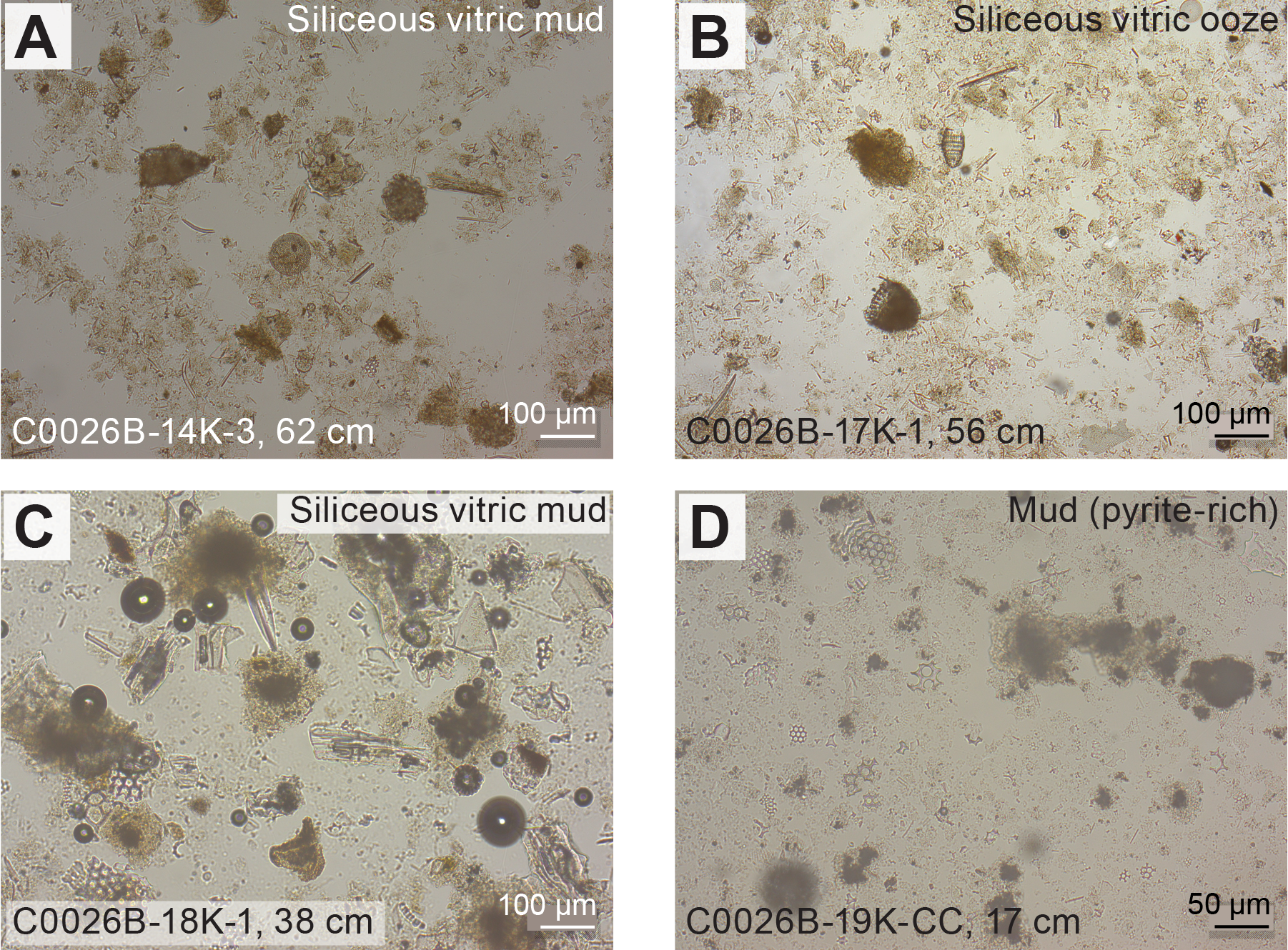
Figure F21. Subunit 1C smear slides.
4.1.1.3.3. Mineralogy and sediment geochemistry
Six bulk samples representative of Subunit 1C were collected for XRD analysis (Table T9). The trends in mineralogy noted in Subunit 1B continue to the bottom of Subunit 1C, with an increase in clay average for Subunit 1C (~74 wt%) and a decrease in average plagioclase (~11 wt%) (Figure F18). These results are in agreement with observations of increased clay from smear slide analysis.
XRF analyses conducted at the same intervals as XRD measurements for Subunit 1C reveal a decrease in SiO2 consistent with the increasing clay content observed in XRD data. The results show ranges of 2.78–3.53 wt% Na2O, 1.98–2.91 wt% MgO, 15.32–17.07 wt% Al2O3, 65.16–67.35 wt% SiO2, 0.08–0.19 wt% P2O5, 2.48–3.22 wt% K2O, 1.20–1.99 wt% CaO, 0.55–0.66 wt% TiO2, 0.10–0.42 wt% MnO, 5.42–7.41 wt% Fe2O3, and 6.44–8.33 wt% LOI (Figure F19; Table T10). Overall, the geochemical composition of the top of Subunit 1C shows a continuation of the characteristics from Subunit 1B. However, samples at the base of Subunit 1C reflect relative clay enrichment and a reduction in the biogenic component, indicated by the decrease in SiO2 and increase in Fe2O3.
4.1.1.3.4. Summary and preliminary interpretations
Subunit 1C is a dull yellowish brown siliceous mud(stone) that is marked by a further decrease in the volcanic component from Subunit 1B. Biogenic material in Subunit 1C shows a notable increase in radiolarians to ~232 mbsf, where biogenic material decreases to almost 0% at the base of the unit. The lower abundance of ash-rich/vitric components, decreased biogenic material, and lack of significant soft-sediment deformation structures indicate a low-energy depositional environment. This places Site C0026 at a location farther from the active margin than Subunits 1A and 1B (Moore et al., 2015).
4.1.2. Unit 2
- Interval: 405-C0026B-20K-1, 5 cm, to 29K-2, 65 cm
- Depth: 244.050–278.575 mbsf
- Age: TBD (the occurrence of radiolarians that lived only in the Jurassic and Cretaceous periods is noted)
- Lithology: brownish black clay
4.1.2.1. Visual core description lithology
Unit 2 is a dark brown to brownish black clay. The transition from Subunit 1C to Unit 2 is transitional and is defined by an intercalation of the yellowish brown and brownish black clay layers in Sections 405-C0026B-20K-1, 5 cm, through 20K-3, 13 cm (i.e., 2.53 m thick interval). However, the sharpest color change occurs in Section 20K-3, 13 cm (246.58 mbsf), where a ~1 cm thick concentration of pyrite marks the transition (Figure F22). Below this depth, the dull yellowish brown lithology is no longer present. The clay in Unit 2 displays a consistent brownish black color (7.5YR 2/2), with slight variations ranging from dark brown (7.5YR 2/3) to black (7.5YR 2/1). The clay is relatively structureless and occasionally contains rare thin layers and interspersed orange-brown (10YR 5/2) patches, typically less than ~2 cm in diameter. Bioturbation, mottling, and biogenic material are rare in Unit 2. No identifiable ash-rich layers were found in Unit 2. Fossilized fish teeth were found in Section 26K-1 at 3.5 and 5.6 cm.
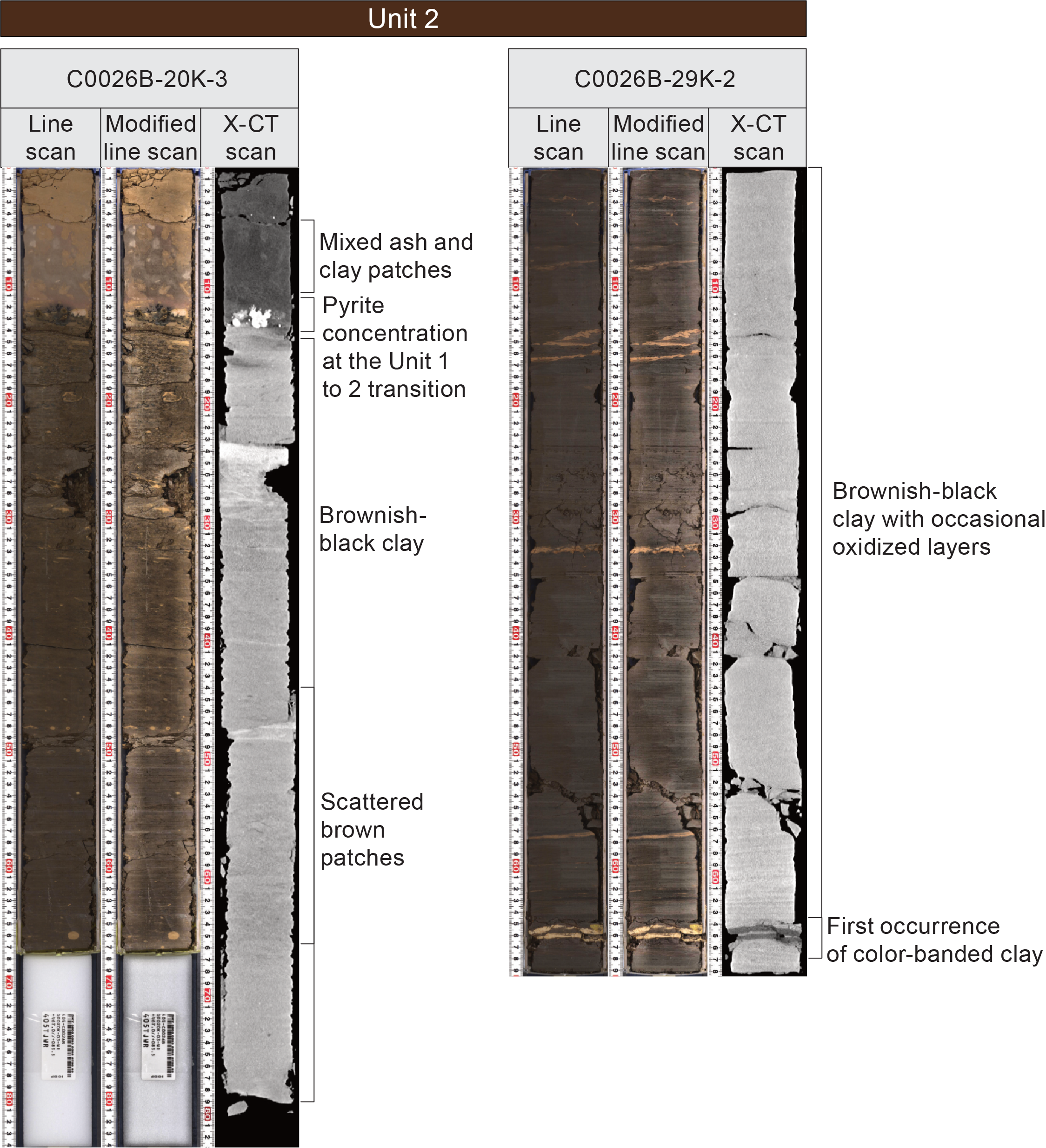
Figure F22. Unit 2 images.
4.1.2.2. Smear slide petrography
Smear slide analysis indicates that the grain size is much finer than in Unit 1 and plots as clay (Table T8). The grain size ranges between clay (68%–83%), silt (15%–30%), and sand (0%–4%) are in the color change zone at the top of Unit 2 (Cores 405-C0026B-20K and 21K), and most of the visible grains are lithic fragments and secondary pyrite growth (Figures F22, F23A). However, coarse-grained particles are nearly absent toward the bottom of the unit, where the sediment consists mostly of clay (60%–100%) with some silt (0%–38%) and sand (0%–10%). Unit 2 is predominantly composed of siliciclastic grains (67%–100%), with minimal volcanic (0%–11%) and biogenic (0%–10%) components (Figure F15). Other minor components (0%–32%) include rare occurrences of dense and opaque minerals, framboidal pyrite, and Fe oxides. Siliciclastic grains are mostly clay minerals (59%–100%), with some quartz (0%–2%) and mud aggregates/clasts (0%–7%).
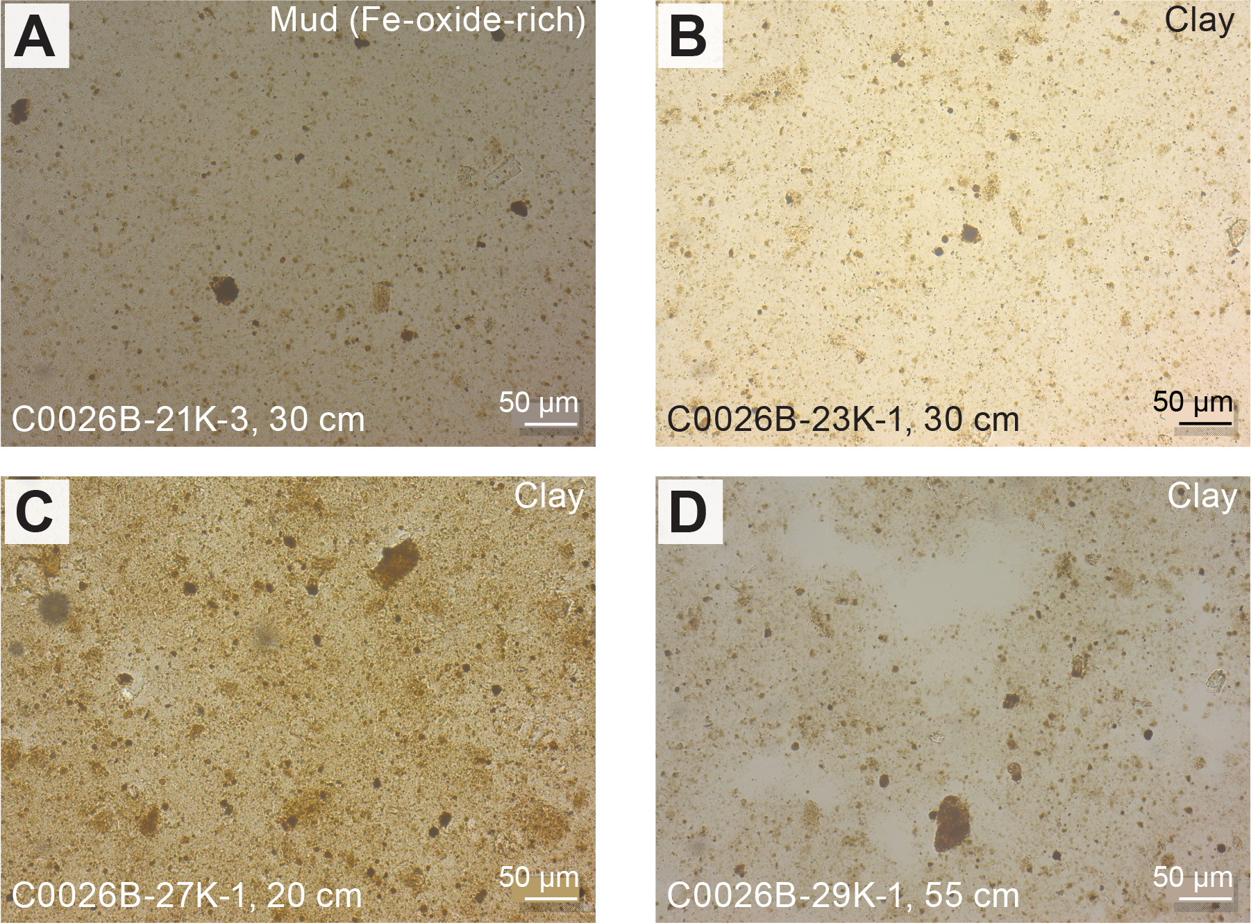
Figure F23. Unit 2 smear slides.
4.1.2.3. Mineralogy and sediment geochemistry
A total of 10 bulk samples representative of Unit 2 were collected for XRD analyses (Table T9). Unit 2 features a dominance of clay minerals (79%–89%) and a substantial reduction in quartz (7%–16%) and plagioclase (2%–6%) compared to Unit 1 (Figure F18). XRD data support the observations from smear slides that Unit 2 consists predominantly of clay.
The same samples were analyzed for major and minor element contents using XRF (Table T10). The results range 1.75–2.36 wt% Na2O, 3.05–3.77 wt% MgO, 15.04–19.73 wt% Al2O3, 55.71–60.92 wt% SiO2, 0.16–2.35 wt% P2O5, 3.26–4.30 wt% K2O, 0.86–4.29 wt% CaO, 0.68–1.08 wt% TiO2, 1.24–3.67 wt% MnO, 7.19–9.34 wt% Fe2O3, and 7.40–8.70 wt% LOI (Figure F19). Increased MgO, Al2O3, and K2O content can be related to the predominance of clay in Unit 2. The enrichment of Fe/Mn oxides and pyrite is reflected by the MnO and Fe2O3 values. Lower SiO2 is consistent with the near absence of siliceous biogenic material and reduced abundance of vitric fragments and ash-rich layers.
4.1.2.4. Summary and preliminary interpretations
Unit 2 reflects a change to a clay-dominated lithology, contrasting significantly with Unit 1. Unit 2 contains >90% siliciclastic components (mostly clay minerals), and compositions are rich in Fe oxides and pyrite. The absence of biogenic components (radiolarians and diatoms) and ash-rich layers in this unit also marks a clear shift from previous units. Occasional thin layers and orange-brown patches are likely due to localized chemical alterations or subtle depositional variations. The enrichment of Fe oxides and occasionally observed pyrite indicates both oxic and localized anoxic conditions during deposition. Because of the dominance of very fine grained clay, coupled with the near absence of biogenic material, Unit 2 is interpreted to be pelagic clay that accumulated on the Pacific plate in an area far from continental margins.
4.1.3. Unit 3
- Interval: 405-C0026B-29K-2, 65 cm, to 32K-CC, 20 cm
- Depth: 278.575–286.885 mbsf
- Age: Mesozoic (identified from the occurrence of radiolarians that lived only in the Jurassic and Cretaceous periods)
- Lithology: color-banded clays and chert
4.1.3.1. Visual core description lithology
Unit 3 consists of color-banded clays intercalated with intervals of chert, recovered as broken fragments. The top of Unit 3 is characterized by a gradual transition from the dark-brown clay of Unit 2 to a color-banded clay (Figures F12, F24). This transition is marked by the first appearance of a 1 cm thick band of dull yellowish brown clay, including a clast of greenish clay in Section 405-C0026B-29K-2, 65 cm (Figure F22). Colors in the banded clay interval include black (7.5YR 2/1), brownish black (7.5YR 2/2), brown (7.5YR 4/6), dull orange (7.5YR 3/3), and light yellow (5Y 1/3). The color bands become progressively thicker (millimeter to centimeter thick), brighter, and more lithified downcore, with millimeter-scale brown and dull orange laminations to the first chert in Section 30K-1, 105 cm. The chert fragments are lithified, and fragmentation is interpreted to result from coring. The appearance of the chert is variable. In Core 31K, the chert is light yellow and intercalated with a light yellow porcellanitic clay. In Section 30K-CC, the chert is color-banded with brownish black, brown, and light yellow bands crosscut by a silica vein. Although intervals of chert appear more often toward the base of Unit 3, color-banded clays persist to the bottom of Hole C0026B. Notably, following the recovery of chert from Sections 30K-CC through 32K-1, the deepest recovered lithology in Section 32K-CC reverts to banded clay, suggesting alternations between chert and clays in Unit 3.
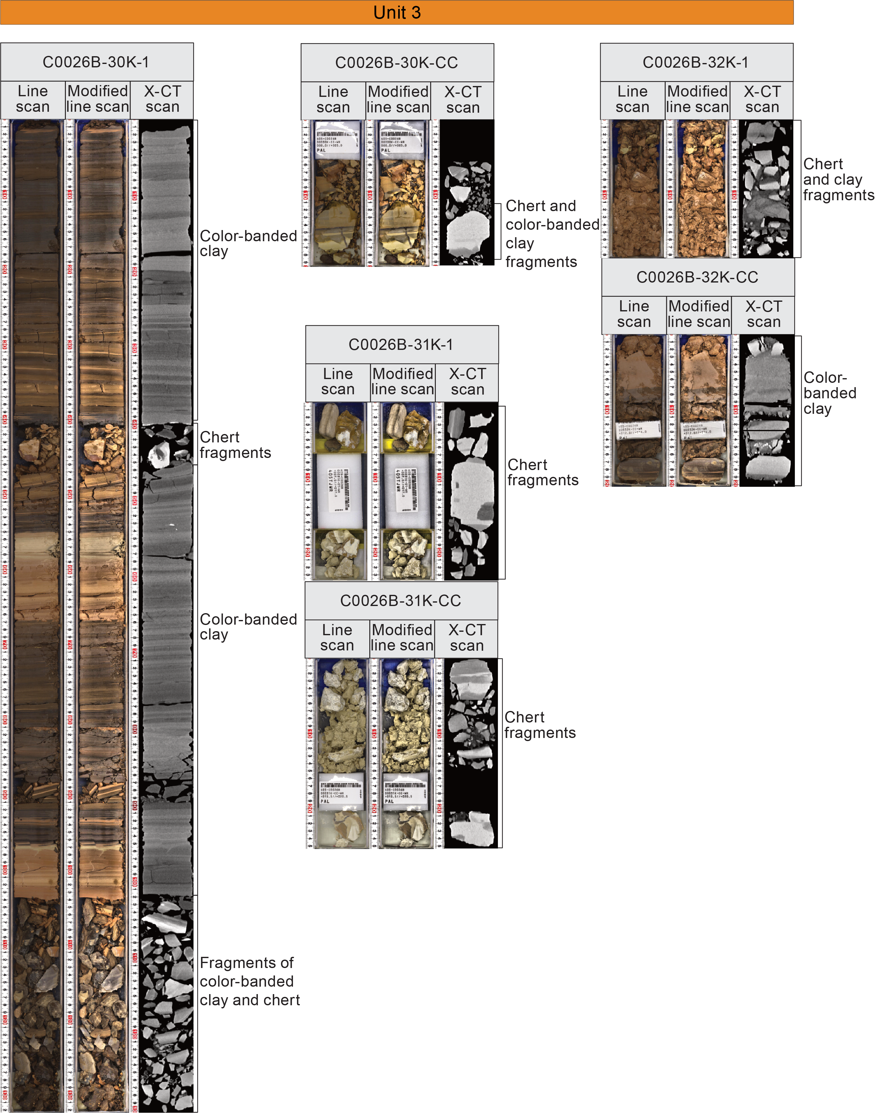
Figure F24. Unit 3 images.
4.1.3.2. Smear slide petrography
Observations from smear slides indicate that Unit 3 is largely composed of clay and SiO2 microlites (Figures F15, F25). Smear slide data suggest the proportion of clay minerals in the brownish black clay is higher than that in the light yellow porcellanitic clay. Conversely, the light yellow porcellanitic clay exhibits a slightly higher proportion of SiO2 compared to the dark brown clay. The Unit 3 background sedimentation grain size is mud and ranges between sand (0%–10%), silt (8%–70%), and clay (23%–92%). The average sediment composition is composed of siliciclastic (82%–98%) and volcanic (0%–3%) material (Table T8). Other minor components (0%–17%) consist of dense minerals and pyrite. Siliciclastic grains are mostly quartz (5%–86%) with clay minerals (0%–75%), chert (0%–12%), and mud aggregates (3%–20%).
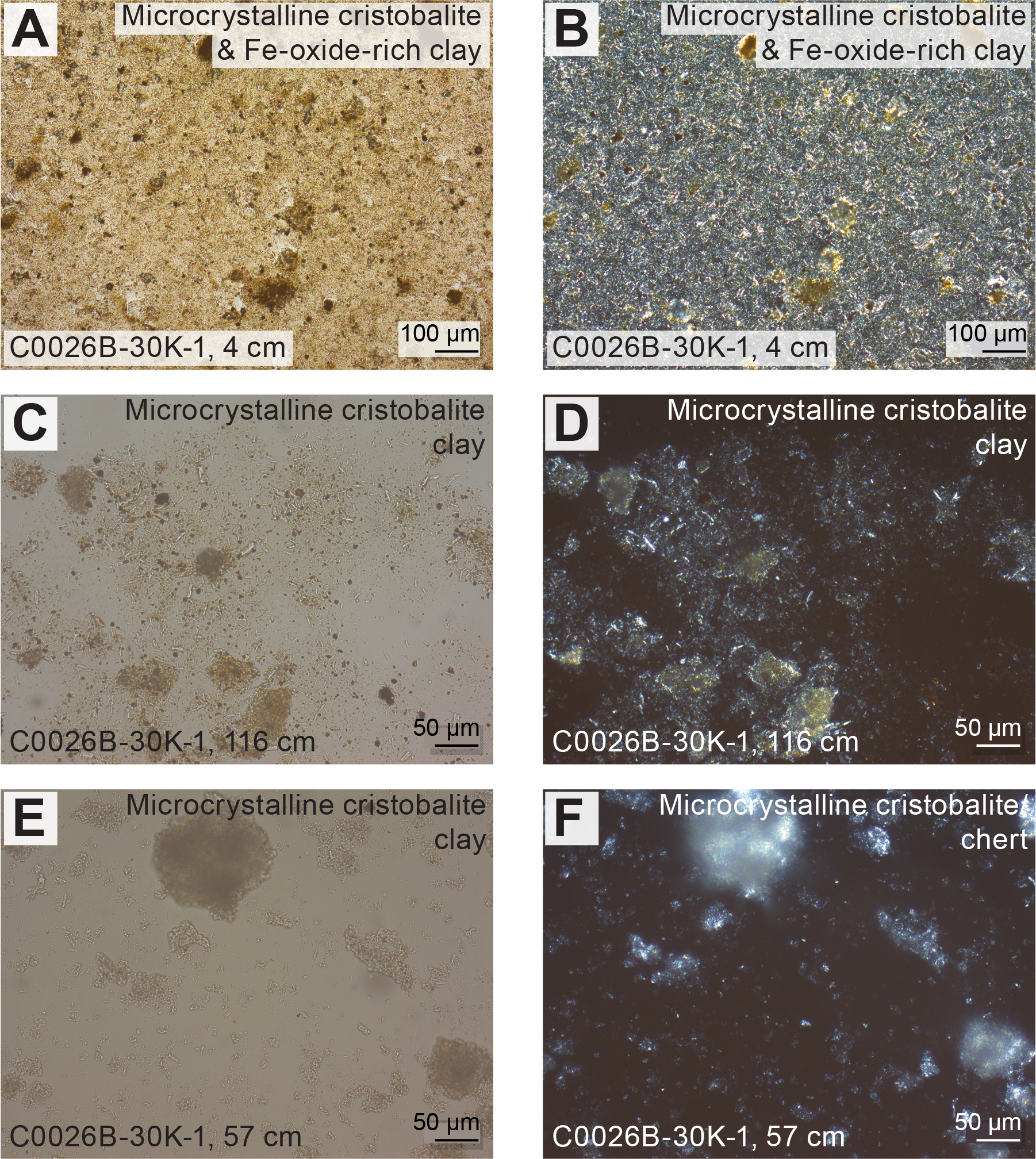
Figure F25. Unit 3 smear slides.
4.1.3.3. Mineralogy and sediment geochemistry
Three samples, one from the color-banded clay (Sample 405-C0026B-30K-1, 62–64 cm), one from the yellow porcellanite (Sample 31K-CC, 13–15 cm), and one from the dark brown clay (Sample 32K-1, 10.5–12.5 cm), were sampled for XRD analysis (Figure F26; Table T9). Results of semiquantitative mineral abundance analyses are similar between the color-banded clays and porcellanite samples with approximately 75% clay minerals, 20%–25% quartz, and <5% plagioclase (Figure F18).
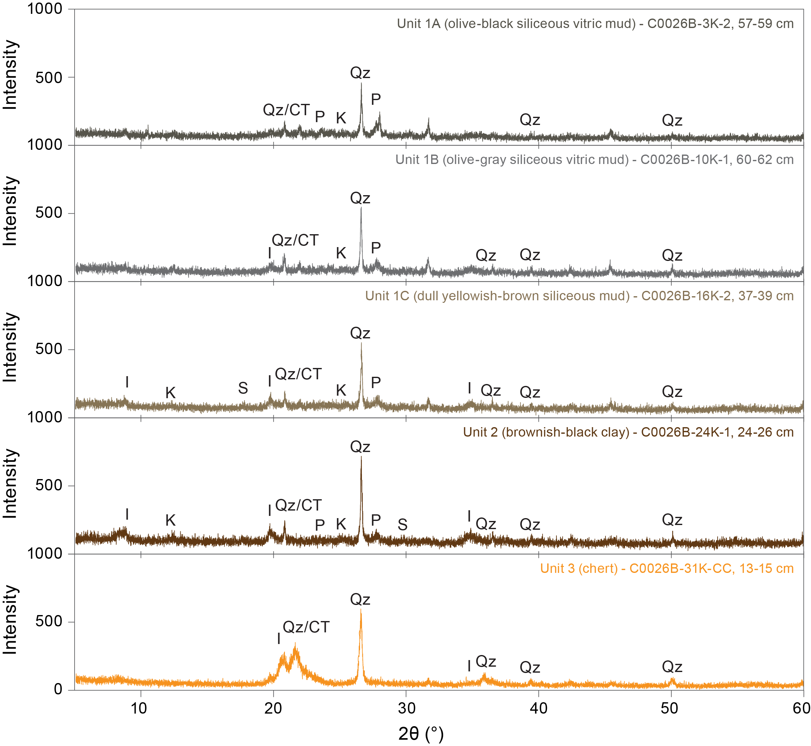
Figure F26. XRD patterns.
The same samples were analyzed for element composition using XRF (Table T10; Figure F19). The results are broadly similar between the color-banded clays and dark brown clay, ranging 1.48–1.82 wt% Na2O, 1.64–2.14 wt% MgO, 6.45–7.50 wt% Al2O3, 78.85–80.95 wt% SiO2, 0.84–1.39 wt% P2O5, 1.50–2.01 wt% K2O, 1.68–2.47 wt% CaO, 0.29–0.41 wt% TiO2, 0.02–0.04 wt% MnO, 4.28–4.97 wt% Fe2O3, and 5.88–6.09 wt% LOI. Results for the light yellow porcellanitic clay samples are quite different at 0.96 wt% Na2O, 0.89 wt% MgO, 3.12 wt% Al2O3, 91.36 wt% SiO2, 0.39 wt% P2O5, 0.87 wt% K2O, 0.73 wt% CaO, 0.16 wt% TiO2, 0.01 wt% MnO, 1.68 wt% Fe2O3, and 4.01 wt% LOI. This difference likely reflects the increased concentration of SiO2 associated with chert formation.
4.1.3.4. Summary and preliminary interpretations
Unit 3 presents a transition from the dark brown clay into color-banded clays and lithified chert. Unit 3 lacks biogenic and volcanic components. The presence of millimeter-scale laminae in the color-banded clays suggests minimal transport and/or disturbance of Unit 3. The color banding in the Unit 3 clays reflects different levels of SiO2 present in the laminae, suggesting that the degree of silicification in these clays varies over centimeter length scales. The increasing content of SiO2 microlite and transitional occurrence of color-banded clay, porcellanitic clay, and chert suggest that silicification/lithification processes that transform the clay into chert are ongoing.
4.2. Summary and preliminary assessment
Four boreholes were drilled at Site C0026 (Holes C0026B–C0026E), with overall very good recovery (>50%). Together, the cores recovered from these holes provide a relatively complete record of the entire sequence of subseafloor sediments that overlie the incoming Pacific plate at the Japan Trench from 0 to 290 mbsf. Three primary lithostratigraphic units were identified as part of the stratigraphic sequence, all of which are consistent with deposition in an open marine setting. Biostratigraphic correlations indicate the sediments range from Cretaceous to present age (see Biostratigraphy). The Cretaceous color-banded clay and chert (Unit 3) and Cretaceous to Miocene brownish black pelagic clay (Unit 2) are composed predominantly of silica and clay minerals, respectively, with a notable absence of biogenic and volcaniclastic material, suggesting they were deposited in a deepwater hemipelagic setting. The transition from the Miocene to present-day mudstone in Unit 1 is marked by an increase in the biogenic and volcaniclastic components and represents a change in depositional environment to relatively undisturbed background sedimentation in a hemipelagic environment, with an increase in sediment provided from volcanic sources. All units lack calcareous nannofossils, suggesting they were deposited below the carbonate compensation depth. This stratigraphic progression is consistent with changes in depositional environments controlled by the motion of the Pacific plate as Site C0026 was translated toward the continental margin over time (e.g., Moore et al., 2015).
The sediments recovered at Site C0026 are similar to those recovered at DSDP Site 436, the nearest drilling site that can be used as a comparison, which is located >250 km north of Site C0026 off northern Honshu (Shipboard Scientific Party, 1980). Site 436 consists of three lithostratigraphic units: Subunits 1A and 1B (vitric diatomaceous silty clay and claystone), Unit 2 (radiolarian diatomaceous claystone), and Subunits 3A and 3B (pelagic clay with chert and porcellanite). Based on the lithologies and ages of these units, the Site 436 units correspond with Site C0026 Subunits 1A and 1B, Subunit 1C, and Units 2 and 3, respectively. However, the unit thicknesses are different. For example, the interval to the base of the upper Miocene, which corresponds approximately to Subunits 1A and 1B at Site 436 is 312 m thick at Site 436 (according to the depth of the base of Site 436 Subunit 1B), whereas the equivalent interval in Subunits 1A and 1B at Site C0026 is ~200 m thick (according to the depth of the base of Site C0026 Subunit 1B). Dacite pebbles were recovered in the Pliocene to late Miocene cores at Site 436 but were absent at Site C0026.
5. Structural geology
Cores recovered from Site C0026 sampled the sedimentary inputs on the incoming Pacific plate from 0 to ~290 mbsf, outboard of the Japan Trench (note that all depths in this section are provided on the mbsf depth scale, which is equivalent to the CSF-A scale). Generally, the deformation of these incoming sedimentary input units was minimal, consisting mostly of fractures, some minor faults, sediment-filled veins, and scaly fabric in pelagic clays. For all structures, orientations were obtained on the working-half sections of cores for Holes C0026B–C0026E using visual core description and complemented by measurements using XCT. In selected coherent sections, discrete samples were analyzed paleomagnetically (see Paleomagnetism) to correct the orientation of the core to the geographic reference frame, allowing strikes of planar features to be estimated for true in situ alignment.
5.1. Hole C0026C
Hole C0026C cored the sedimentary rocks on the incoming Pacific plate from 0 to 5.90 mbsf. The sedimentary rocks in this hole consist of olive-black siliceous vitric mud (Lithostratigraphic Subunit 1A). Primary structures consisted of planar bedding. Secondary structures related to deformation were not identified in Section 1H.
5.1.1. Bedding and laminae
The orientation of one subhorizontal bed was measured (Figure F27).
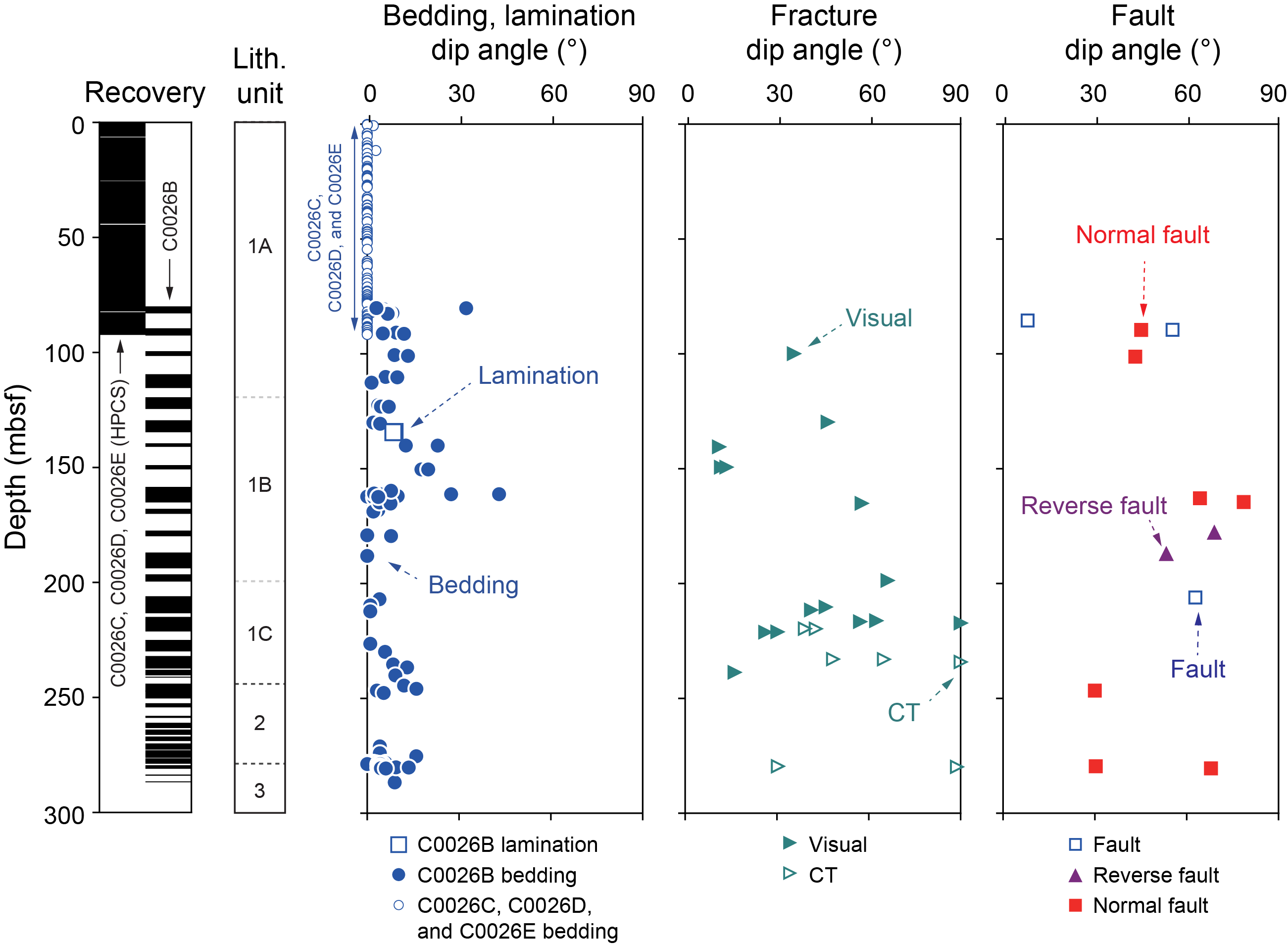
Figure F27. Orientation and density of structural features.
5.1.2. Deformation structures
No deformation structures were identified.
5.2. Hole C0026D
Hole C0026D penetrated the sedimentary rocks on the incoming Pacific plate. Hole recovery was from 0 to 6.45 mbsf. The sedimentary rocks in this hole consist of olive-black siliceous vitric mud (Lithostratigraphic Subunit 1A). Primary structures consisted of planar bedding. Secondary structures related to deformation were not identified in Section 1H.
5.2.1. Bedding and laminae
The orientations of eight horizontal to subhorizontal bedding planes were measured (Figure F27).
5.2.2. Deformation structures
No deformation structures were identified.
5.3. Hole C0026E
Hole C0026E penetrated the sedimentary rocks on the incoming Pacific plate. Hole recovery was from 0 to 92.39 mbsf. The sedimentary rocks at this site consist of olive-black siliceous vitric mud (Lithostratigraphic Subunit 1A). Two minor faults were identified in Sections 9H-8 and 10H-6, both with undetermined senses of slip. A total of 10 sediment-filled veins were identified in Cores 2H–4H. Additionally, sand injections were identified in Section 2H-5.
5.3.1. Bedding and laminae
The strike and dip of 102 beds were measured. The average orientation was subhorizontal (Figure F27).
5.3.2. Deformation structures
5.3.2.1. Fractures and minor faults
Two minor faults were visible in the core at 81.93 mbsf (Section 405-C0026E-9H-8) and 89.53 mbsf (Section 10H-6). These faults are only weakly expressed on split core faces. However, they are easily discernible on XCT images, appearing as bright, planar structures that truncate planar bedding. The higher XCT number associated with fault planes is attributed to a higher density material along the fault plane compared to the surrounding material, potentially due to compaction of the materials at the fault plane or to mineralization. The identified minor faults have an undetermined sense of motion and have true dips of 8° and 53°, respectively.
5.3.2.2. Sediment-filled veins
A total of 10 intervals of sediment-filled veins were identified in Sections 405-C0026E-2H-6, 3H-2, 3H-5, 4H-3, 4H-5, and 4H-7. These sediment-filled veins appear as parallel to subparallel, vertical to subvertical, curvilinear to sigmoidal millimeter thick bands. Traces of the veins in axial sections through the core anastomose, indicating the veins are interconnected. Their vertical length varies between 2 and 21 cm with average intervein spacings of 2–10 mm. The veins have a higher XCT number than the surrounding rocks, indicating denser material.
5.4. Hole C0026B
Core recovery in Hole C0026B was from 80.0 to 286.69 mbsf. The sedimentary rocks in this hole consist of siliceous muds (Lithostratigraphic Subunits 1A–1C), brownish-black clay (Unit 2), and color-banded clay and chert (Unit 3). The sedimentary rocks are well stratified and largely undeformed. Features observed and measured in cores (using visual core description and/or XCT) include bedding planes, minor faults, fractures, sediment-filled veins, scaly fabric, and laminae. The distribution of structures is illustrated in Figure F27.
5.4.1. Bedding and laminae
In total, 84 bedding and laminae orientations were measured. The average dip of bedding and laminae in Hole C0026B is 7° (total range = 0°–32°) (Figure F27). One normally oriented flame structure was noted inside a 7 cm long biscuit at 110.66 mbsf (Section 405-C0026B-4K-2).
5.4.2. Deformation structures
5.4.2.1. Fractures and minor faults
The strike and dip of 20 fractures and 11 minor faults were measured in Hole C0026B. We labeled cracks as "fractures" when neither opening mode nor shear sense of motion (e.g., offset features, truncated bedding, striations, and presence of gouge) could be determined. Minor faults were identified as planar structures with measurable millimeter- to centimeter-scale offsets of piercing points defined by truncation and displacement of bedding, other fractures, or bioturbation or by the presence of striations. Of the 11 minor faults, 2 had reverse offset, 8 had normal offset, and 1 did not have identifiable sense-of-slip indicators. The average dip angles for fractures and faults were ~45° and ~60°, respectively, and there was no difference in the dip of normal and reverse structures (Figure F27). Representative minor faults are shown in Figure F28. The fracture dip angle increases slightly with increasing depth in the core.
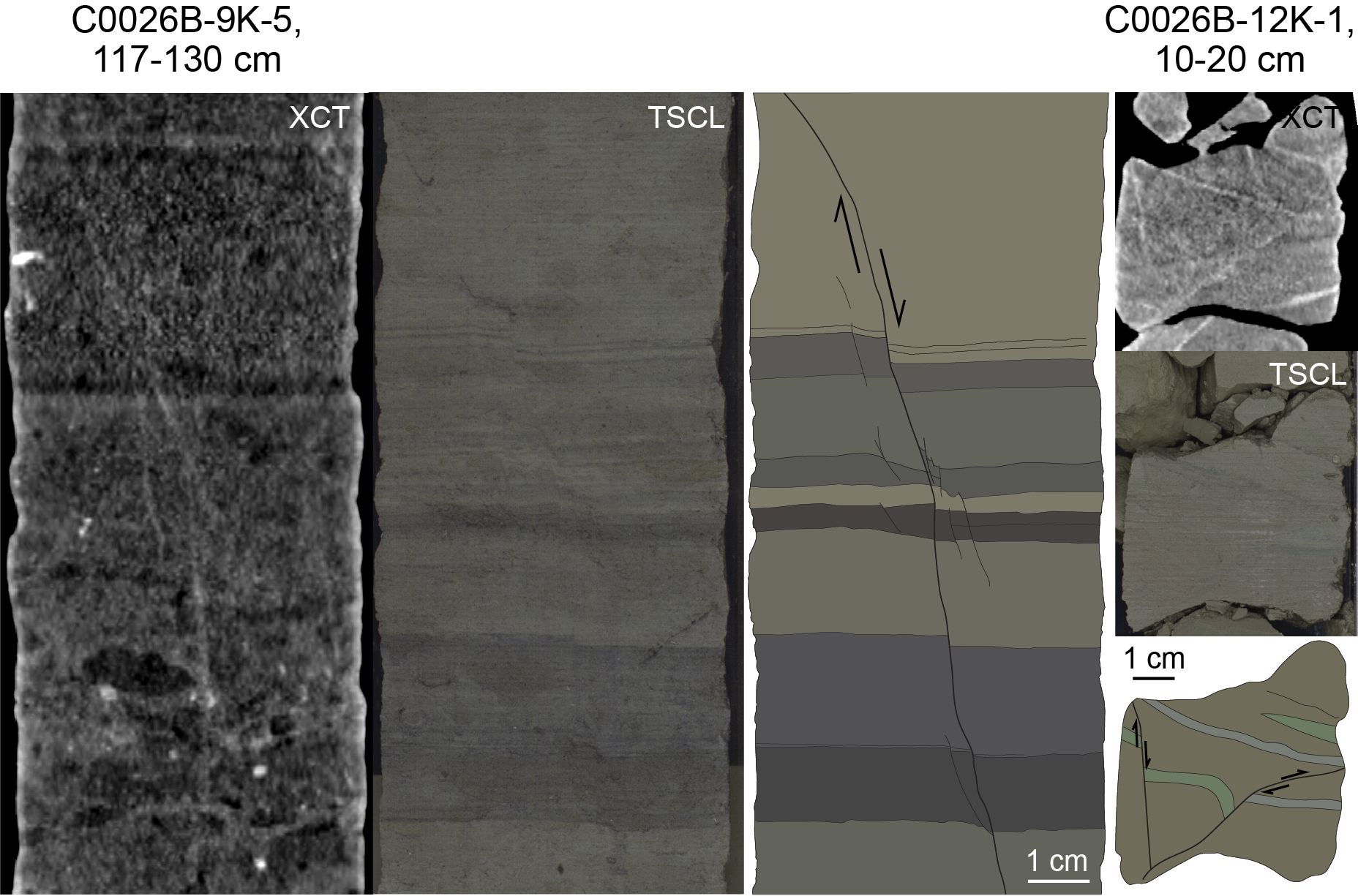
Figure F28. Characteristics of normal faults.
5.4.2.2. Scaly fabric
Between 245.74 and 246.74 mbsf (Sections 405-C0026B-20K-2 and 20K-3), scaly fabric was observed in whole-round samples in dull yellowish brown siliceous mud (Subunit 1C) and brownish black clay (Unit 2) in the transitional interval where these two lithologies are interbedded. The scaly fabric is composed of wedge- to discoidal-shaped clay phacoids. These phacoids have subangular to subrounded edges and a bimodal size distribution such that larger phacoids are generally 2–4 cm long and 1–1.5 cm wide and smaller phacoids are generally 0.4–0.6 cm long and 0.3–0.5 cm wide. Phacoid surfaces are moderately polished and frequently have parallel striations (Figure F29). Below Section 20K-3, it was difficult to assess whether the scaly fabric was present because of clay smearing when the core was split; therefore, we could not determine whether scaly fabric continues downsection.
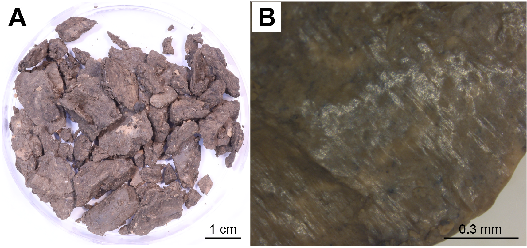
Figure F29. Phacoids.
5.4.2.3. Sediment-filled veins
Sediment-filled veins were observed in bioturbated, dull yellowish brown mud (Lithostratigraphic Subunit 1C). Five areas of sediment-filled veins were documented at 225.09–229.21 mbsf (in Sections 405-C0026B-16K-1, 16K-3, and 16K-4). The veins identified in Hole C0026B are geometrically similar to veins observed in Hole C0026E and are characterized by several parallel to subparallel, interconnected, vertical to subvertical, curviplanar to sigmoidal millimeter-scale bands (Figure F30). The vertical length of the vein arrays ranges 1–16 cm with an average intervein spacing of 1–10 mm. These veins are easily identifiable on XCT images as bright, white features related to a higher XCT number representative of the higher density of the vein-filling sediment.
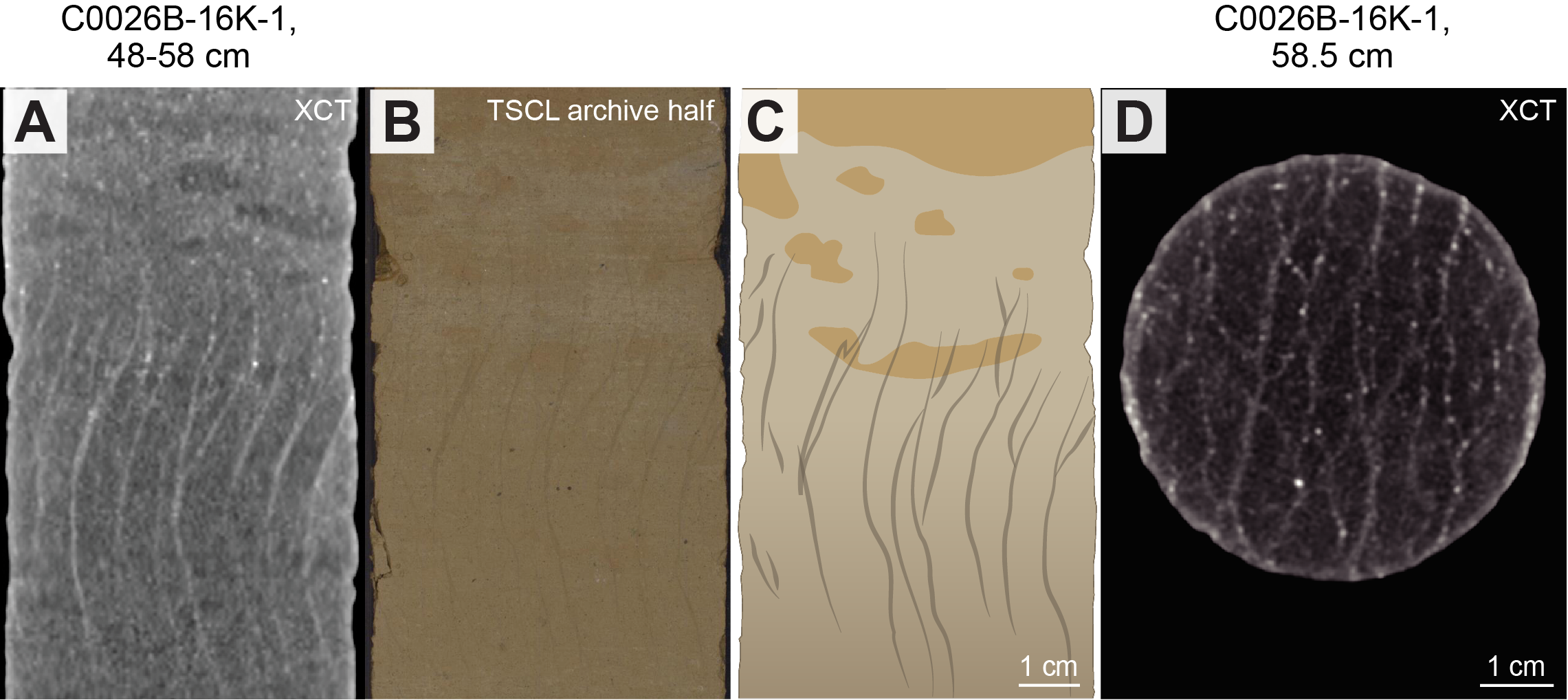
Figure F30. Sediment-filled veins.
5.4.2.4. Orientations of deformation structures
Core rotation during drilling operations produces incorrect structural orientations in recovered core. To correct for this rotation within a single coherent interval, the declination of the paleomagnetic vector was used to rotate the orientations of structural features to true in situ alignments (see Structural geology in the Expedition 405 methods chapter [Kirkpatrick et al., 2025a]). A total of 32 primary and secondary structural orientations in Hole C0026B were corrected to paleomagnetic north, and in situ strikes were calculated with respect to true north (Figure F31). The corrected orientations of the bedding are subhorizontal. Only four of the aforementioned faults were measured in sections where paleomagnetic discrete data were collected. Therefore, in situ orientations for the other deformational structures could not be determined.
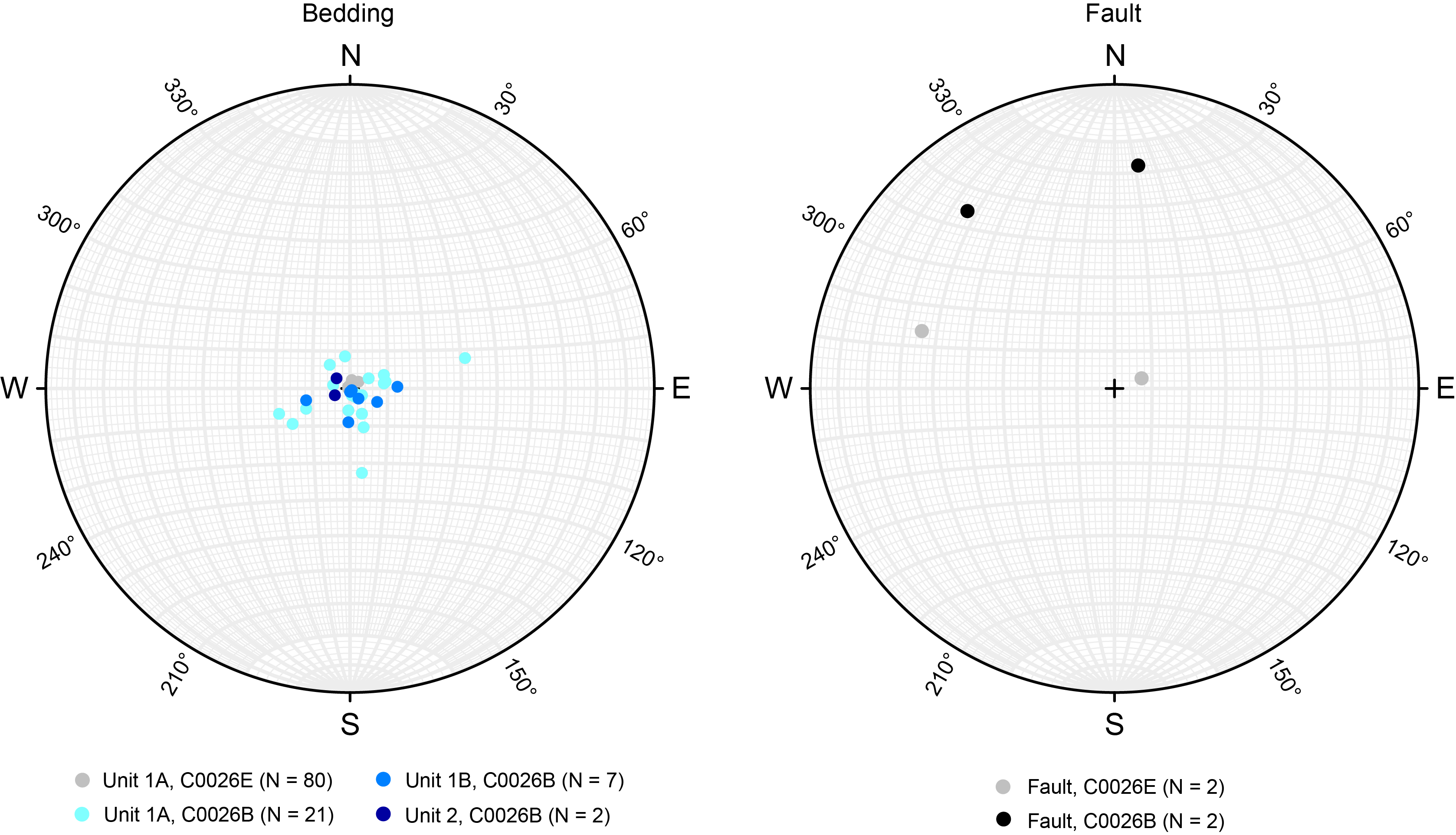
Figure F31. Structural orientations of bedding and faults.
5.5. Drilling-induced deformation
Drilling-related disturbances were commonly observed in Site C0026 cores. The disturbances to core structures and lithologies caused by piston coring primarily manifested as laminar arching of primary layering and flow-in. Flow-in was notably pronounced below a particular ash layer (56.54–56.80 mbsf) (Figure F32). In the SD-RCB coring section of Hole C0026B, biscuiting and drilling breccias were observed at intervals of several tens of centimeters. These drilling disturbances were identified on working-half and archive-half core surfaces and from CT images, and they were described as a distinct category separately from primary deformation structures.
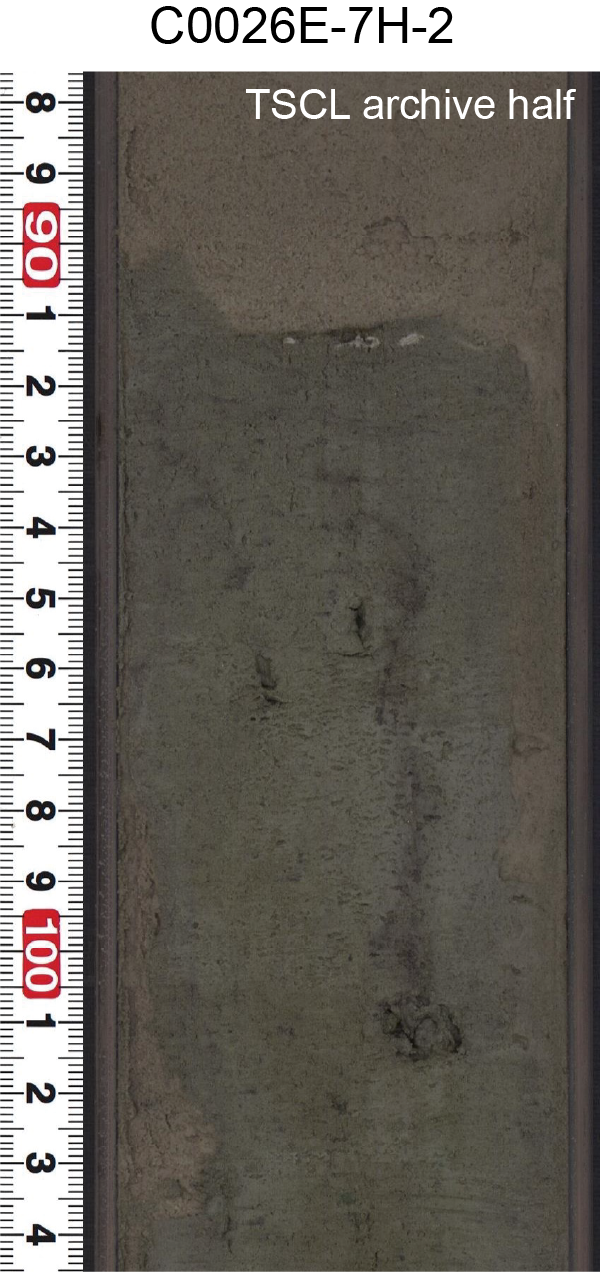
Figure F32. Drilling disturbance.
5.6. Interpretation
The three stratigraphic units that form the sedimentary part of the incoming Pacific plate stratigraphy are identified in the cored units from Holes C0026B–C0026E. Minor faults, fractures, and scaly clay most likely form because of compaction during burial, as evidenced by predominantly normal-sense faulting and subhorizontal fabric in clays. Sediment-filled veins are commonly found in sediments in subduction zones such as the Nankai Trough (Tobin et al., 2020), Miura-Boso accretionary prism (Hanamura and Ogawa, 1993; Maltman et al., 1993), and Anafi Island Basin (Druitt et al., 2024). Based on field and experimental studies, such veins are thought to form because of shaking and dewatering during earthquakes (Hanamura and Ogawa, 1993; Brothers et al., 1996). We infer that the formation of sediment-filled veins on the incoming Pacific plate outboard of the Japan Trench is analogous to sediment-filled veins identified along other seismically active subduction margins.
6. Biostratigraphy
All core catcher samples drilled with the SD-RCB system in Hole C0026B and the HPCS in Holes C0026C–C0026E were examined for radiolarian biostratigraphy. For diatom biostratigraphy, core catcher samples from all cores in Holes C0026B and C0026E were examined.
Diatoms and radiolarians were continuously observed in the Pleistocene to lower Miocene section down to Sample 405-C0026B-19K-CC (~241.2 mbsf), but samples between Samples 20K-CC (~247.5 mbsf) and 30K-CC (~280.8 mbsf) are barren of diatoms and only contain sporadic occurrences of Mesozoic radiolarians. Below Sample 31K-CC (~283.90 mbsf) to the bottom of the hole at 286.75 mbsf, no microfossils were detected at Site C0026. The results of diatom (Tables T11, T12) and radiolarian (Tables T13, T14, T15, T16) biostratigraphy from the Pleistocene through Miocene at Site C0026 is almost consistent, although some offset data may be caused by a differentiation between matrix/clast age and/or reworking of age diagnostic species (Figure F33).
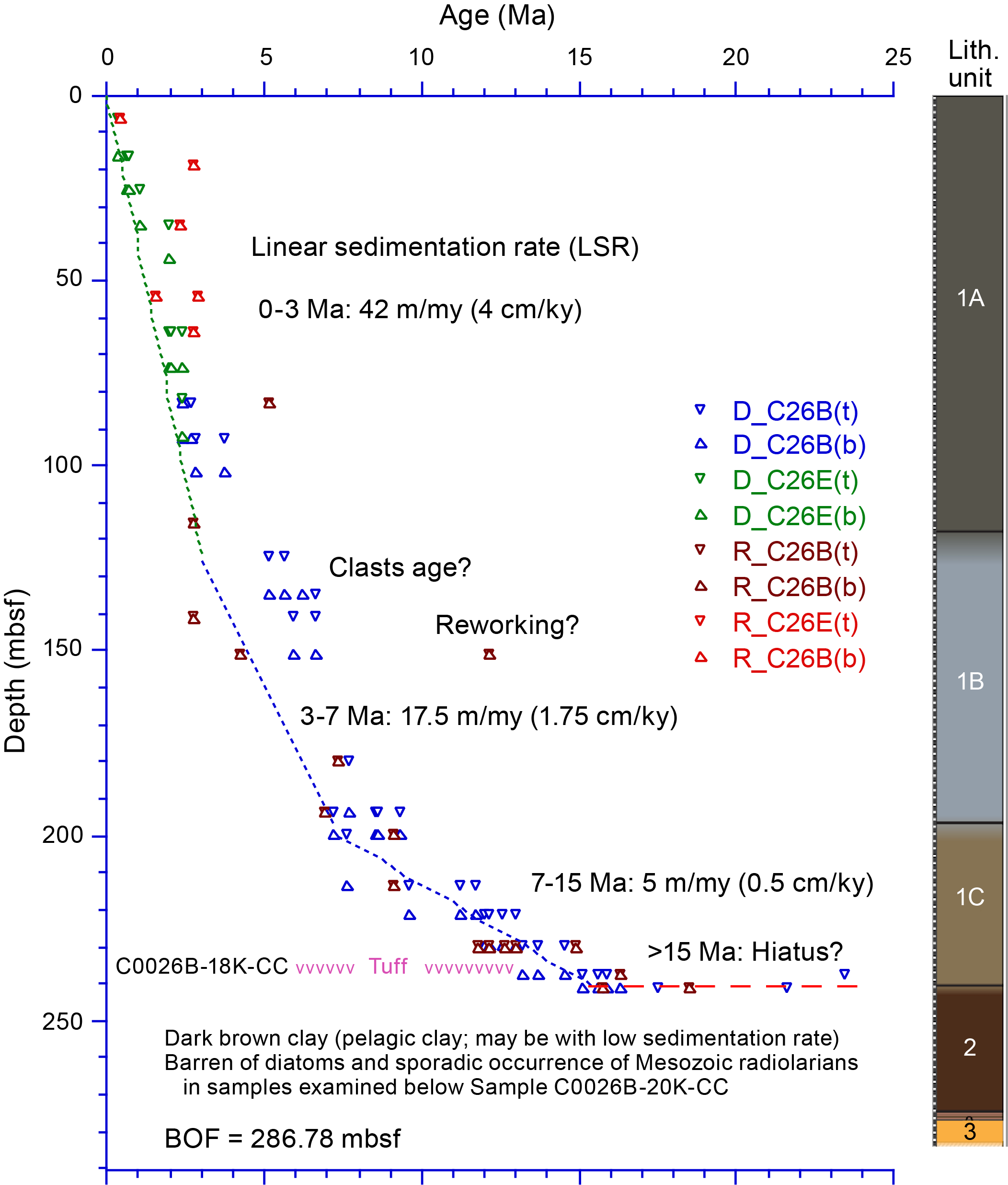
Figure F33. Age-depth profile.
DSDP Site 436 (39°55.96′N, 145°33.47′E; 5240 m water depth), drilled at the Japan Trench outer rise, is located ~240 km north-northeast from Site C0026. The site penetrated to 397.50 mbsf and collected cores that were well dated by diatom and radiolarian biostratigraphy. Barron et al. (1980) documented that Pleistocene through Miocene sediments were recovered from 0 to 360 mbsf and Miocene to Paleogene sediments from 360 to 378 mbsf above early radiolarian-rich Cretaceous chert (378–397 mbsf) containing pore microfossils. Compared to the diatom (Harper, 1980) and radiolarian biostratigraphy (Sakai, 1980) at Site 436, our observations at Site C0026 suggest that the thickness of Pleistocene–Miocene biosiliceous sediments at Site 436 is 1.5 times thicker; however, there are no significant differences detected on the timing of accumulation of siliceous microfossils between Sites 426 and C0026.
6.1. Diatoms
All core catcher samples obtained from Site C0026 in November 2024 were sent once per week to the Marine Core Research Institute (MaCRI) at Kochi University (Japan). For samples from Holes C0026B and C0026E, smear slides were made in the onshore laboratory and examined for diatom biostratigraphy (Table T11) (see Biostratigraphy in the Expedition 405 methods chapter [Kirkpatrick et al., 2025a]). Samples from Holes C0026C and C0026D will be examined during postexpedition research to reconfirm the age determination for the Pleistocene interval.
Common to abundant diatoms are found in all samples from Hole C0026E and in Samples 405-C0026B-1K-CC to 16K-CC, which corresponds to a Pleistocene through middle Miocene section. Diatoms were rare in Samples 17K-CC and 19K-CC and correspond to the deeper lower Miocene. Samples 18K-CC and 20K-CC through 32K-CC, toward the base of Hole C0026B, are barren of diatoms (Table T11). Chaetoceros resting spores, considered a seasonal upwelling indicator, are common to abundant in samples from the Pleistocene section obtained from Hole C0026B. Middle Miocene diatoms are detected as reworked diatoms in the Pliocene to Pleistocene section; however, there is no signal of Paleogene–Cretaceous diatoms in any sample examined at Site C0026 (Figure F33).
Diatom biohorizons/datums tentatively recognized during the expedition are summarized in Table T12.
6.1.1. Hole C0026E
The occurrence of Pleistocene boreal diatoms such as Thalassiosira gravida, Neodenticula seminae, and Shionodiscus oestrupii (without Neodenticula koizumii) in Sample 405-C0026E-1H-CC, 17.0–22.0 cm (6.12–6.17 mbsf), indicates this sample can be placed in North Pacific diatom (NPD) Zones NPD12–NPD10 (0–2.0 Ma). The occurrence of Fragilariopsis doliolus in this sample supports this interpretation. Reworked Miocene diatoms such as Crucidenticula punctata, Denticulopsis dimorpha var. areolata, and Fragilariopsis jouseae are observed, along with common and various neritic and freshwater diatoms such as Aulacoseira spp., Actinocyclus spp., Cocconeis spp., Cyclotella spp., Cymbella spp., Delphineis spp., Diploneis spp., Gramatophora spp., and Paralia sulcata.
The occurrence of Proboscia curvirostris without N. koizumii in Sample 405-C0026E-2H-CC, 0.0–5.0 cm (16.05–16.10 mbsf), assigns this sample to Zones NPD11–NPD10 (0.30–2.0 Ma). The last occurrence (LO) of P. curvirostris is tentatively placed between Samples 1H-CC and 2H-CC.
The co-occurrence of P. curvirostris and F. doliolus in Sample 405-C0026E-3H-CC, 4.0–9.0 cm (25.15–25.20 mbsf), allows this sample to be placed in Zones NPD11–NPD10 (0.30–2.0 Ma). One specimen of N. koizumii is observed; however, we consider it to be reworked. The occurrence of Fragilariopsis kanayae and Fragilariopsis fossilis in this sample suggests that this sample is older than the LO datums, 0.61 and 0.69 Ma in age, respectively.
The occurrence of Actinocyclus oculatus without N. koizumii in Sample 405-C0026E-4H-CC, 0.0–5.0 cm (35.20–35.25 mbsf), assigns this sample to Zone NPD10 (1.0–2.0 Ma). The LO of A. oculatus is tentatively placed between Samples 3H-CC and 4H-CC.
The occurrence of N. koizumii without or with sporadic trace occurrence of Neodenticula kamtschatica between Samples 405-C0026E-5H-CC, 24.5–29.5 cm (44.00–44.05 mbsf), and 10H-CC, 0.0–5.0 cm (91.92–91.97 mbsf), allows these samples to be placed in Zone NPD9, 2.0–2.6/2.7 Ma in age. The occurrence of Thalassiosira convexa var. aspinosa in Sample 10H-CC, which is missing from any other sample observed in this hole, allows the LO of this species to be tentatively placed between Samples 9H-CC and 10H-CC.
6.1.2. Hole C0026B
The co-occurrence of Neodenticula koizumii and N. kamtschatica in Sample 405-C0026B-1K-CC, 16.5–21.5 cm (82.95–82.00 mbsf), suggests this sample can be placed in Zone NPD8; however, N. kamtschatica only occurs in trace amounts in this sample, and it is easily reworked in Zone NPD9 (cf. Akiba, 1986). Therefore, we tentatively place this sample in Zones NPD9–NPD8, corresponding to the lineage of N. koizumii (2.0–3.5/4.0 Ma). The occurrence of T. convexa v. aspinosa in this sample further restricts it to be older than 2.4 Ma.
The co-occurrence of N. koizumii and N. kamtschatica in Sample 405-C0026B-2K-CC, 27.5–32.5 cm (92.57–92.62 mbsf), assigns this sample to Zone NPD9. We tentatively recognized the LO of N. kamtschatica between Samples 1K-CC and 2K-CC.
The co-occurrence of N. kamtschatica and Shionodiscus oestrupii s.l. without any N. koizumii in Samples 405-C0026B-3K-CC, 16.0–21.0 cm (101.49–101.54 mbsf), to 5K-CC, 16.5–21.5 cm (124.51–124.56 mbsf), allows us to place these samples in Zone NPD7Bb, the S. oestrupii Subzone of the N. kamtschatica Zone. The occurrence of Fragilariopsis jouseae in these samples also suggests they may be restricted to the Pliocene, younger than the first occurrence (FO) of the F. jouseae datum at 5.1 Ma. The occurrence of N. kamtschatica without S. oestrupii s.l. in Samples 6K-CC, 19.5–24.5 cm (134.63–134.68 mbsf), and 7K-CC, 7.5–12.5 cm (140.99–141.04 mbsf), assigns these samples to the uppermost Miocene Zone NPD7Ba between 5.6 and 6.6 Ma in age. The occurrence of Koizumia tatsunokuchiensis in Sample 7K-CC restricts this sample to above the FO of K. tatsunokuchiensis at 5.9 Ma. The FOs of F. jouseae and S. oestrupii s.l. are tentatively placed between Samples 5K-CC and 6K-CC, and the LO of K. tatsunokuchiensis occurs between Samples 6K-CC and 7K-CC.
The sporadic occurrence of N. kamtschatica and Rouxia californica, zonal marker species for the Zone NPD7A/NPD7B boundary, in Samples 405-C0026B-8K-CC, 14.0–19.0 cm (150.77–150.82 mbsf), to 11K-CC, 13.5–18.5 cm (179.85–179.90 mbsf), makes it difficult to distinguish an age determination for these samples. However, the occurrence of K. tatsunokuchiensis without S. oestrupii s.l. in Sample 8K-CC allows us to place this sample in Zone NPD7B. The sporadic occurrence of N. kamtschatica and Thalassionema schraderi in Samples 9K-CC to 11K-CC allows us to place these samples in Zone NPD7A. The occurrence of T. convexa v. aspinosa in Samples 9K-CC and 10K-CC restrict these two samples to above the FO of T. convexa v. aspinosa at 6.7 Ma. The FO of T. convexa v. aspinosa is tentatively placed between Samples 10K-CC and 11K-CC.
The occurrence of T. schraderi without any Denticulopsis in Sample 405-C0026B-12K-CC, 11.5–16.5 cm (193.77–193.82 mbsf), assigns this sample to Zone NPD6B (7.7–8.5 Ma). The occurrence of Denticulopsis simonsenii s.l., including Denticulopsis cf. katayamae, without D. dimorpha in Sample 13K-CC, 13.5–18.5 cm (199.54–199.59 mbsf), assigns this sample to Zone NPD6A (8.5–9.5 Ma). The last common occurrence (LCO) and first common occurrence (FCO) of T. schraderi are recognized between Samples 11K-CC and 12K-CC and between Samples 12K-CC and 13K-CC, respectively.
Sample 405-C0026B-14K-CC, 7.5–12.5 cm (213.36–213.41 mbsf), contains various species of the genus Denticulopsis. The occurrence of D. dimorpha v. areolata in this sample allows us to place this sample in Zone NPD5D. The occurrence of Denticulopsis praedimorpha in Sample 15K-CC, 6.5–11.5 cm (221.26–221.31 mbsf), assigns this sample to Zone NPD5B (11.7–13.0 Ma). The occurrence of Hemidiscus cuneiformis in Sample 15K-CC further restricts this sample to above the FO of H. cuneiformis at 12.0 Ma. The common occurrence of D. simonsenii without D. praedimorpha s.l. in Sample 16K-CC, 11.0–16.0 cm (229.91–229.96 mbsf), assigns this sample to Zone NPD5A (13.0–13.2 Ma). The FO of D. dimorpha and LO D. praedimorpha are recognized between Samples 14K-CC and 15K-CC, and the FO D. praedimorpha is recognized between Samples 15K-CC and 16K-CC.
The occurrence of Denticulopsis lauta without Denticulopsis hyalina in Sample 405-C0026B-17K-CC, 15.0–20.0 cm (237.37–237.42 mbsf), assigns this sample to Zone NPD4A.
The occurrence of Actinocyclus ingens v. nodus in Sample 405-C0026B-17K-CC restricts this sample to above the FO of this species at 15.4 Ma. Sample 18K-CC, 17.0–22.0 cm (240.28–240.33 mbsf), is composed of bubble wall type dominated volcanic glass and diatoms, and other fossils are completely barren in the observed slide. In Sample 19K-CC, 0.0–5.0 cm (241.16–241.21 mbsf), diatoms are rare, but the occurrence of A. ingens s.l. without any middle Miocene diatoms such as Crucidenticula and Denticulopsis allowed us to tentatively place this sample in Zones NPD3A–NPD2B with an age constraint of 16.3–17.5 Ma. The FO of D. lauta and Denticulopsis praelauta is recognized tentatively between Samples 17K-CC and 19K-CC.
Diatoms are barren in Samples 405-C0026B-20K-CC, 13.5–18.5 cm (247.42–247.47 mbsf), to 32K-CC, 4–6 cm (286.73–286.75 mbsf), which are composed of brownish black pelagic clay (Lithostratigraphic Unit 2).
6.2. Radiolarians
Slides were prepared, and radiolarians were analyzed for all core catcher samples obtained from Holes C0026B–C0026E. Radiolarian abundance of Hole C0026B ranges from abundant to barren with good to poor preservation (Figure F34; Table T13). Radiolarian abundances of cores drilled with the HPCS (Holes C0026C–C0026E) also range from abundant to common with good to moderate preservation (Table T14). For many samples, we were able to apply the Northwest Pacific Neogene radiolarian zonation in a manner similar to previous studies (Kamikuri, 2017; Kamikuri et al., 2004, 2007; Shilov, 1995). In a few samples, we were able to apply the code numbers for Cenozoic low-latitude radiolarian zonation (RN1–RN17 for the Neogene; Nigrini, 1977; Sanfilippo and Nigrini, 1998). However, zonal marker species did not occur in some samples, and we could not provide any age constraints. Radiolarian events tentatively recognized during the expedition are summarized in Table T15.
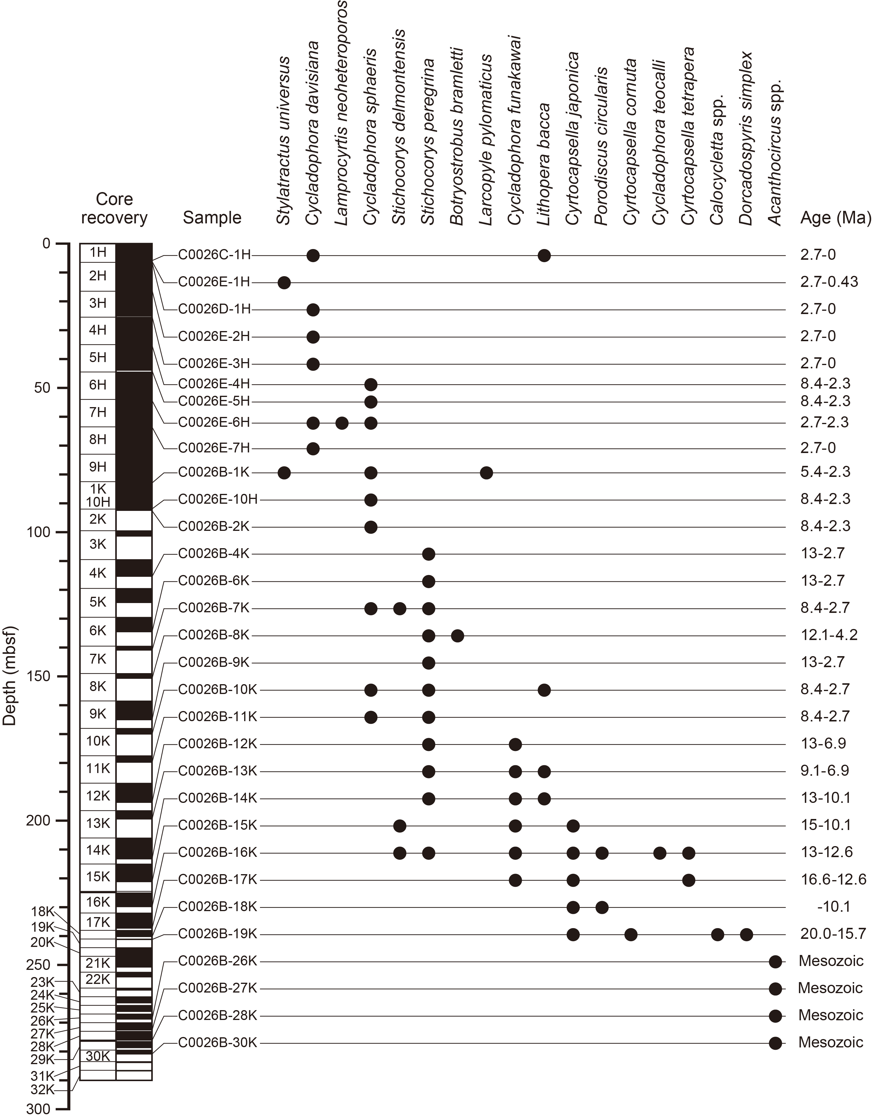
Figure F34. Radiolarians.
In addition, an automated AI-based classification system for radiolarians was performed on sediment samples that were taken one per section from Cores 405-C0026E-1H through 5H (Table T16). The results of the AI-based classification were reviewed, and the presence or absence of age constraint taxa was used as a reference for age determination in the core catcher samples. This system was also applied to Samples 405-C0026D-1H-CC and 405-C0026B-1K-CC to 11K-CC.
6.2.1. Hole C0026C
Hole C0026C was cored using the HPCS, and Core 1H (0.00–5.93 mbsf) was the only core obtained from this hole. The occurrence of Cycladophora davisiana in Sample 1H-CC (5.88–5.93 mbsf) allows this sample to be placed into the Hexacontium dionysus Subzone of the Cycladophora sphaeris Zone and Botryostrobus aquilonaris Zone, 2.7–0 Ma in age (Table T14).
6.2.2. Hole C0026D
Only one core was obtained from Hole C0026D. The occurrence of C. davisiana in Sample 1H-CC (6.40–6.45 mbsf) suggests this sample may be placed into the H. dionysus Subzone of the C. sphaeris Zone–B. aquilonaris Zone, 2.7–0 Ma in age, which is the same for Sample C0026C-1H-CC (5.88–5.93 mbsf) (Table T14).
6.2.3. Hole C0026E
A total of 10 cores were drilled with the HPCS in Hole C0026E. In this hole, radiolarian occurrences vary from abundant to common with moderate to good preservation (Figure F34; Table T14). In almost all samples, we were able to apply the Northwest Pacific Neogene radiolarian zonation based on previous studies (Kamikuri, 2010; Kamikuri et al., 2004, 2007).
The occurrence of C. davisiana in Samples 405-C0026E-1H-CC (6.12–6.17 mbsf), 2H-CC (16.05–16.10 mbsf), 3H-CC (25.15–25.20 mbsf), and 7H-CC (63.54–63.59 mbsf) show these samples are younger than the FCO of C. davisiana (i.e., 2.7 Ma in age) (Kamikuri, 2017). The occurrence of Stylatractus universus in Sample 1H-CC restricts this sample to be older than the LO of S. universus, 0.43 Ma in age. The occurrence of Cycladophora sphaeris in Samples 4H-CC (35.59–35.64 mbsf) and 5H-CC (44.00–44.05 mbsf) suggests that those samples are older than the LO of C. sphaeris, ~2.3 Ma in age (Kamikuri et al., 2004). The presence of Lamprocyrtis neoheteroporos (taxon range = 2.9–1.5 Ma; Kamikuri, 2017) in Sample 6H-CC supports this interpretation.
No age constraint radiolarians were detected on board in Samples 405-C0026E-8H-CC (73.42–73.47 mbsf) and 9H-CC (82.08–82.13 mbsf); however, the presence of C. sphaeris in Sample 10H-CC (92.34–92.39 mbsf) suggests that the bottom of Hole C0026E is still younger than the FO of C. sphaeris, ~8.4 Ma in age.
In this hole, we also use AI-based technology to detect age constraint radiolarians for one sample per section for Sections 405-C0026E-1H-1 through 5H-CC and successfully obtained consistent results with the normal analogue technique for those lithologic sections. C. davisiana was observed in most samples examined, and the fluctuation of the relative abundance of this taxa may have the potential to correlate with glacial–interglacial cycles during the late Pleistocene time interval. We also detected sporadic occurrences of C. sphaeris (?) in Samples 4H-3, 0.0–0.5 cm (28.35–28.35 mbsf), 4H-6, 0.0–0.5 cm (32.62–32.63 mbsf), 5H-5, 16.0–16.5 cm (39.51–39.52 mbsf), and 5H-7, 0.0–0.5 cm (42.18–42.18 mbsf). Those observations allow us to infer that the LO of C. sphaeris (~2.3 Ma in age based on Kamikuri et al., 2004) is placed between Samples 4H-2, 0.0–0.5 cm (26.93–26.93 mbsf), and 4H-3, 0.0–0.5 cm (28.35–28.35 mbsf). However, other maker species, such as Lamprocyrtis neoheteroporos, Lychnocanoma sakaii, and Eucyrtidium matuyamai, which may divide each zone further and provide more detailed age constraints, were not detected in this onboard analysis.
6.2.4. Hole C0026B
The co-occurrence of Cycladophora sphaeris and Larcopyle pylomaticus in Sample 405-C0026B-1K-CC (82.95–82.00 mbsf) allows us to place this sample into the L. pylomaticus–H. dionysus Zone and restricts this sample to be older than the LO of C. sphaeris (~2.3 Ma) and younger than the FO of L. pylomaticus (5.4 Ma). In addition, the detection of B. aquilonaris (?) from this sample by the AI system may restrict this sample to be younger than the FO of B. aquilonaris (?), 2.7 Ma in age. Sample 2K-CC (92.57–92.62 mbsf) also contains C. sphaeris (~2.3–8.4 Ma), and it is consistent with the above interpretation.
Samples 4045-C0026B-3K-CC (101.49–101.54 mbsf) and 5K-CC (124.51–124.56 mbsf) contain good radiolarians; however, no age constraint taxa have been detected. Stichocorys peregrina (13?–2.7? Ma) was detected in Samples 4K-CC (115.39–115.47 mbsf) and 6K-CC (134.63–134.68 mbsf) to 16K-CC (229.91–229.96 mbsf). The LO of S. peregrina (~2.7 Ma) is tentatively placed between Samples 2K-CC (92.57–92.62 mbsf) and 4K-CC (115.39–115.47 mbsf).
Cycladophora funakawai (16.6–6.9 Ma; Kamikuri, 2010) was detected in Samples 405-C0026B-12K-CC (193.77–193.82 mbsf) to 17K-CC (237.37–237.42 mbsf). The LO of C. funakawai is tentatively placed between Samples 11K-CC (179.85–179.90 mbsf) and 12K-CC (193.77–193.82 mbsf). The occurrence of Lychnocanoma cf. parallelipes (7.3–6.1 Ma) in Sample 10K-CC (170.09–170.14 mbsf) supports this interpretation, and the LO of L. cf. parallelipes (6.1 Ma) is tentatively placed between Samples 9K-CC (165.13–165.18 mbsf) and 10K-CC (170.09–170.14 mbsf). Those interpretations suggest that the occurrence of C. tetrapera (23–11.4? Ma) detected by the AI system is reworked from older sedimentary sections.
Co-occurrence of C. funakawai and Lithopera bacca in Samples 405-C0026B-13K-CC (199.54–199.59 mbsf) and 14K-CC (213.36–213.41 mbsf) suggests that those two samples are older than the LO of C. funakawai (6.9 Ma) and younger than the FO of L. bacca (9.1 Ma), which corresponds to the L. redondoensis–L. parallelipes Zone. Co-occurrence of Cyrtocapsella japonica and Stichocorys delmontensis in Sample 15K-CC (221.26–221.31 mbsf) suggests that this sample is older than the LO of C. japonica (10.5 Ma) and younger than the FO of S. delmontensis (15? Ma). Co-occurrence of S. delmontensis, C. teocalli, S. peregrina, and C. tetrapera in Sample 16K-CC (229.91–229.96 mbsf) allows us to assign this sample to the upper portion of Subzone a of the E. inflatum Zone, 13?–12.6 Ma in age. Co-occurrence of C. funakawai and C. tetrapera without Eucyrtidium inflatum, S. delmontensis, and Cenosphaera coronataformis in Sample 17K-CC (237.37–237.42 mbsf) tentatively allows us to infer that this sample corresponds to the lower portion of Subzone a of E. inflatum through L. subligata Zone, 16.6–15? Ma. Radiolarians are few in Sample 18K-CC (240.28–240.33 mbsf), and it is difficult to recognize a radiolarian zone. However, the occurrence of C. japonica and P. circularis suggest that this sample is older than the LO datum at 10.1 Ma and is consistent with previous middle Miocene radiolarians biostratigraphic interpretation. The occurrence of Dorcadospyris simplex in Sample 19K-CC (241.16–241.21 mbsf) restricts this sample within the lineage of D. simplex, 20.0–15.7 Ma in age. The absence of any other middle Miocene marker species in this sample suggests that this sample be placed somewhere between the C. coronata Zone and the lower portion of the D. sakaii Zone.
Radiolarians are rare to barren in Samples 405-C0026B-20K-CC (247.42–247.47 mbsf) to 25K-CC (266.21–266.26 mbsf), 29K-CC (278.77–278.82 mbsf), 31K-CC (283.89–283.94 mbsf), and 32K-CC (286.73–286.75 mbsf), and no age constraint taxa were detected from those samples during the expedition. However, the Mesozoic (Jurassic and Cretaceous) radiolarian Acanthocircus spp. was detected in Samples C0026B-26K-CC (268.89–268.94 mbsf) to 28K-CC (276.13–276.18 mbsf) and 30K-CC (280.83–280.88 mbsf). Additional Mesozoic radiolarians, Dictyomitra? spp. and Pseudodictyomitra? spp., were detected in Sample 30K-CC.
It is currently uncertain whether these Mesozoic radiolarians are in situ or reworked. Motoyama in Iwai et al. (2025) recognized Pseudodictyomitra paronai and Pseudodictyomitra pseudomacrocephala, indicating an Albian to Cenomanian age with some other taxa from Sample 343-C0019E-20R-2, 53.0–56.0 cm (832.85–832.88 mbsf; Expedition 343), and it would be correlatable. The preservation of siliceous microfossils is good (Figure F35), however, more detailed postexpedition analysis on taxonomy and assemblage would be required for the final decision.
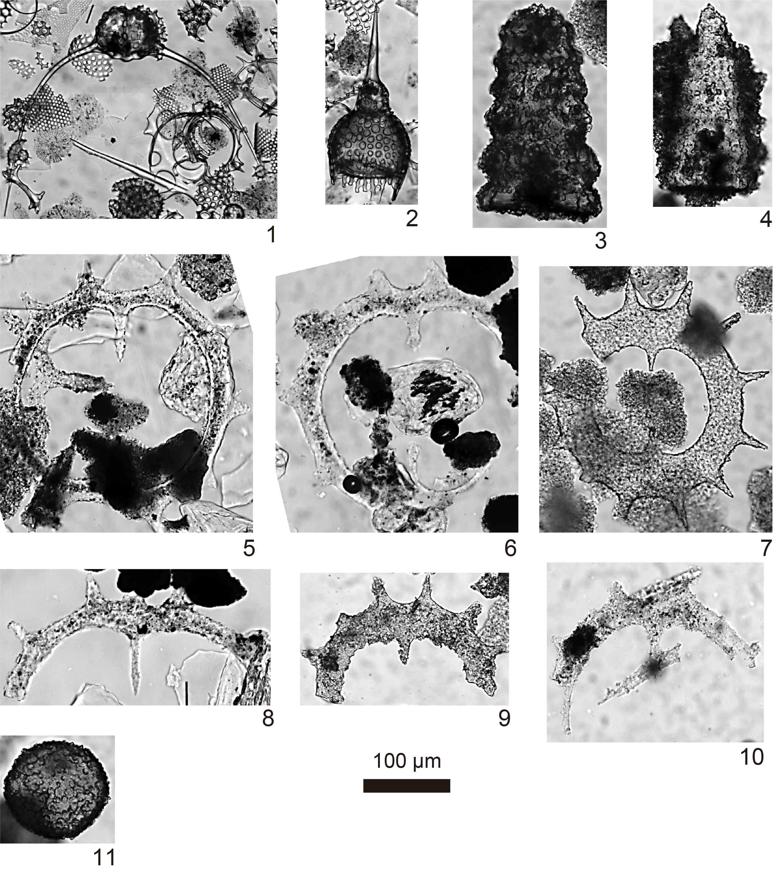
Figure F35. Mesozoic and early Miocene radiolarians.
7. Paleomagnetism
For archive halves, natural remanent magnetization (NRM) measurements with stepwise alternating field (AF) demagnetization were performed up to 25 mT peak fields for Hole C0026B and Sections 405-C0026E-1H-1 through 2H-1 and up to 20 mT for Sections 2H-2 through 10H-CC and Holes C0026C and C0026D. Remanent magnetization was measured at 2 cm intervals for Hole C0026B and at 1 cm intervals for Holes C0026C–C0026E after every demagnetization step (see Paleomagnetism in the Expedition 405 methods chapter [Kirkpatrick et al., 2025a]).
Discrete samples were all processed with the same protocol. Because of an error in saving data, 12 samples from Sections 405-C0026B-4K-3 through 8K-CC were measured for anisotropy of magnetic susceptibility (AMS) after having already been demagnetized.
7.1. Holes C0026C–C0026E
7.1.1. Demagnetization behavior
A total of 73 shipboard discrete samples were collected and analyzed: 5 samples from Hole C0026D and 68 samples from Hole C0026E. A low coercivity component, usually removed before 5 mT (Figure F36), was characterized by high intensity of magnetization. In fact, 93% of magnetization was removed between room temperature and the 20 mT step, decreasing from 4.52 × 10⁻¹ to 3.03 × 10⁻² A/m (Figure F37A). As also evidenced by archive halves, this component shows a steep downward-pointing magnetization with inclinations close to 90° and declinations biased toward 0° and 180° (Figures F37B, F37C, F38); this is a characteristic typical of a magnetization imparted by the drilling process (Acton et al., 2002). Some samples show a secondary component, usually isolated between 5 and 15 mT and usually with a normal polarity. Afterward, samples generally show stable characteristic remanent magnetization (ChRM) directions both for normal and reversed polarities. A few exceptions show an unstable demagnetization behavior; thus, their principal component analysis (PCA) was anchored to the origin.
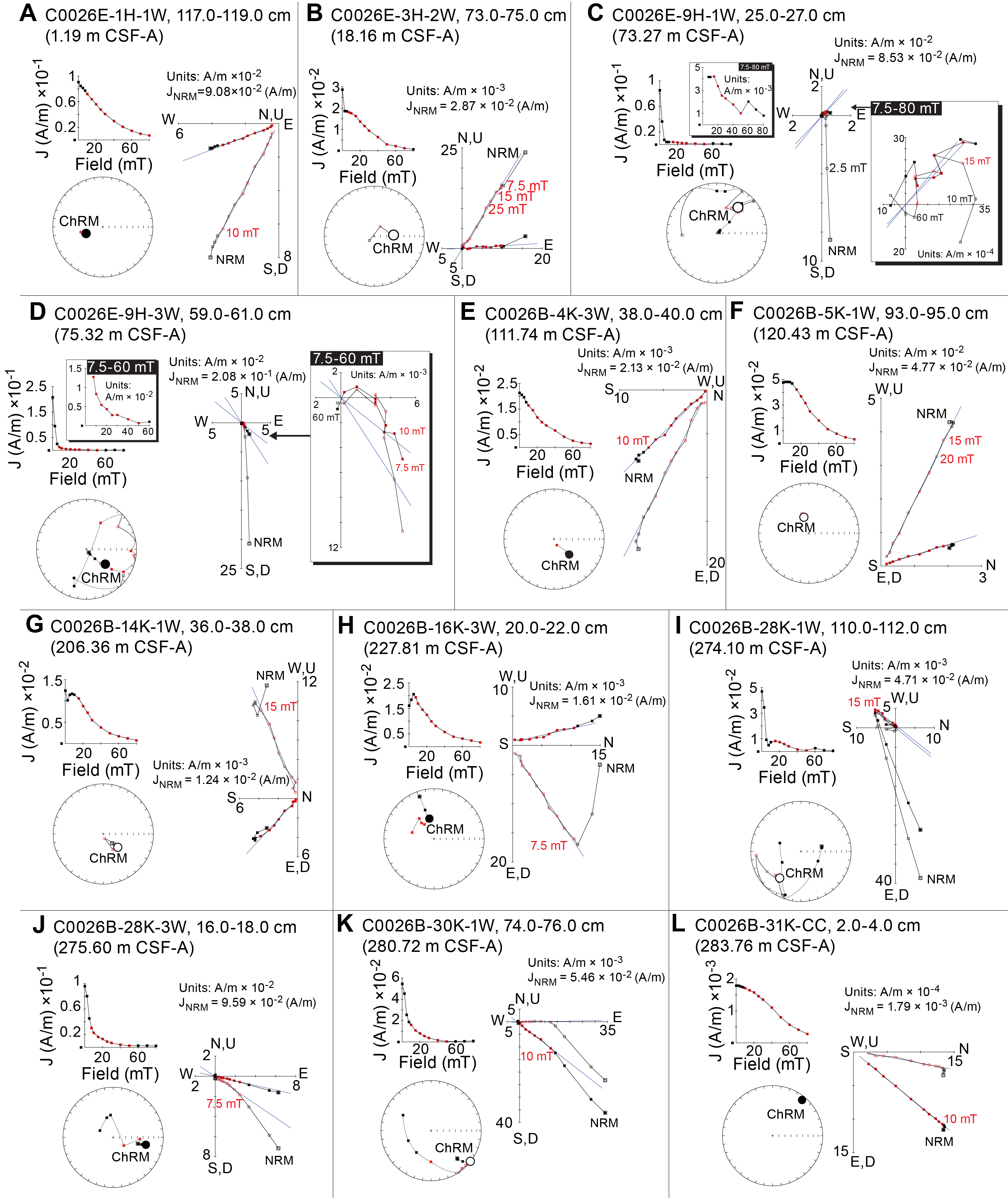
Figure F36. Demagnetization behaviors.
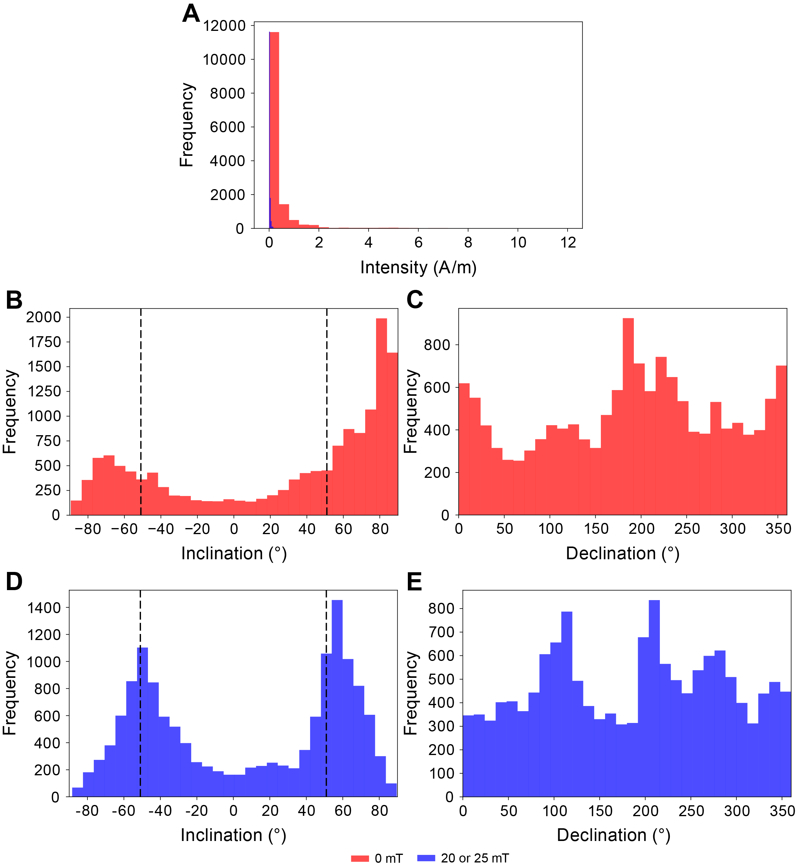
Figure F37. NRM measurements.
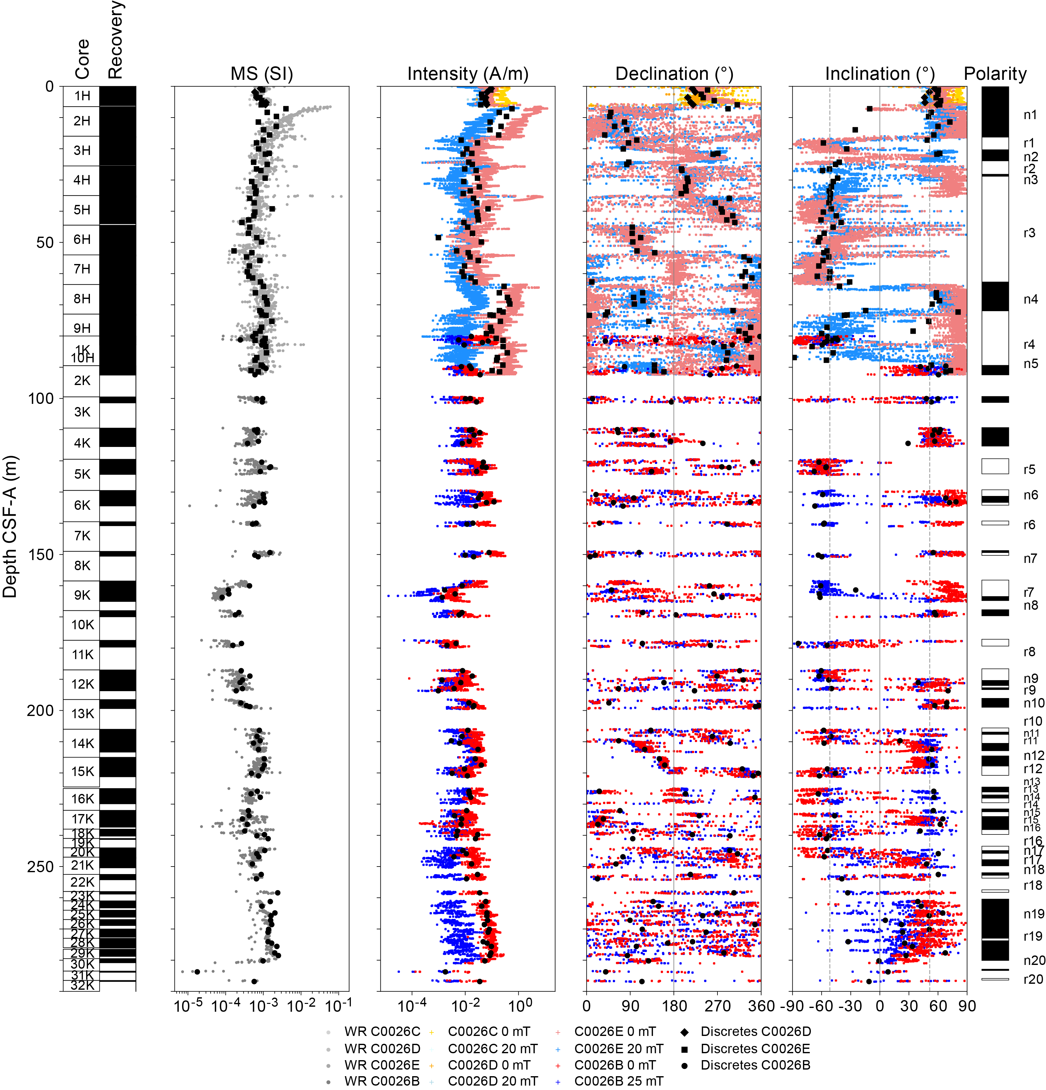
Figure F38. Paleomagnetism results.
Figure F38 shows the NRM intensity, inclination, and declination results after demagnetization at 20 mT for archive halves. The direction of discrete samples that were analyzed using PCA are also plotted, generally showing a good agreement that validates their reliability. Declinations show consistent values at the section level; however, we noticed a progressive change in magnetic declinations from the top of the core barrel to the bottom, known as core twisting (e.g., Expedition 315 Scientists, 2009), in Core 405-C0026E-1H and less evident in Core 6H. However, liners were not visibly twisted after removal from the barrel, and sediment was apparently intact. The drilling overprint is completely removed by the 10 mT step, and the inclination values at 20 mT (Figure F37D) are similar to the present-day value of 51.5° calculated at the site's coordinates using the International Geomagnetic Reference Field model (Alken et al., 2021), supporting the good quality of the signal after demagnetization.
NRM at room temperature has an average value of 4.52 × 10⁻¹ A/m, and the average magnetic susceptibility (MS) is 1.79 × 10⁻³ SI. Puzzling high values of both magnetic intensity and MS are observed in Core 405-C0026E-2H in both the archive and working halves. Here, a piece of metal was found at the top of Core 2H (Figure F38). Although the metal was removed, images from the computed tomography (CT) scan show the presence of a dense material throughout the liner. Thus, the anomalous signal was attributed to pollution from metals during drilling rather than to a real feature. A piece of metal was also found and removed from Section 5H-1A, but it does not have repercussions on the rest of the core. High intensities at room temperature in Cores 8H–10H are instead attributed to the drilling overprint.
7.2. Hole C0026B
7.2.1. Demagnetization behavior
We measured 94 discrete samples with stepwise AF demagnetization. Generally, the ChRM is isolated after the removal of a low coercivity component up to 2.5 or 5 mT, attributed to a drilling overprint (Acton et al., 2002) that is not, however, as strong as in Hole C0026E. Some samples show a secondary component with positive polarity, usually isolated between 5 and 15 mT. After that, the ChRM shows a stable direction along with a decrease in intensity during demagnetization (Figure F36).
The demagnetization behavior shows that the paleomagnetic direction is resolved well, and just a single demagnetization step of the archive halves at 25 mT is a reliable representation of the primary paleomagnetic direction. This is confirmed by the PCA isolated from discrete samples that overlaps well with the step at 25 mT measured on the archive halves (Figure F38).
Overall, the NRM intensity for Hole C0026B decreases from 3.25 × 10⁻¹ A/m at room temperature to 2.36 × 10⁻² A/m after the demagnetization step at 25 mT, with a drop of 75.9% of the magnetization intensity. Both NRM and MS show distinct average values at the unit level (see Lithostratigraphy). Lower NRM (3.22 × 10⁻² A/m) and MS (5.67 × 10⁻⁴ SI) values are documented in Subunit 1A with respect to Hole C0026E. These values are considered more representative of the lithology because they are not affected by the metal pollution documented in Core 405-C0026E-2H and Section 5H-1A. Subunit 1B shows higher average magnetic intensity (6.40 × 10⁻² A/m) and MS (6.92 × 10⁻⁴ SI) in the upper part (Cores 405-C0026B-5K through 8K) than in its lower part (1.20 × 10⁻² A/m and 1.93 × 10⁻⁴ SI, respectively). In Subunit 1C, magnetic intensity and MS are 2.35 × 10⁻² A/m and 6.20 × 10⁻⁴ SI, respectively, whereas Unit 2 is characterized by increasing values from the top to the bottom with averages of 6.64 × 10⁻² A/m and 1.09 × 10⁻³ SI, respectively. Finally, Unit 3 shows an average NRM of 4.58 × 10⁻² A/m and average MS of 7.79 × 10⁻⁴ SI. Both values noticeably decrease in the chert recovered in the lowermost part of the hole.
7.2.2. Anisotropy of magnetic susceptibility
Figure F39 shows the AMS parameters measured for discrete samples from Site C0026, and Figure F40 shows AMS parameters plotted against depth. The mean MS from discrete samples varies between 1.77 × 10⁻⁵ and 3.98 × 10⁻³. The higher value, however, is due to an outlier, and the mean MS is 8.55 × 10⁻⁴. The inclination of the minimum susceptibility axes (Kmin) ranges 4°–89° with a dominant steep inclination consistent with horizontal layers. The low anisotropy degree parameter (Pj) reveals that the three principal axes of magnetic ellipsoids have small variations. The Flinn diagram of MS ellipsoids shows relatively higher foliation (F = Kint/Kmin) than lineation (L = Kmax/Kint) value. These elements indicate the predominance of a sedimentary or compaction fabric, with horizontal bedding.
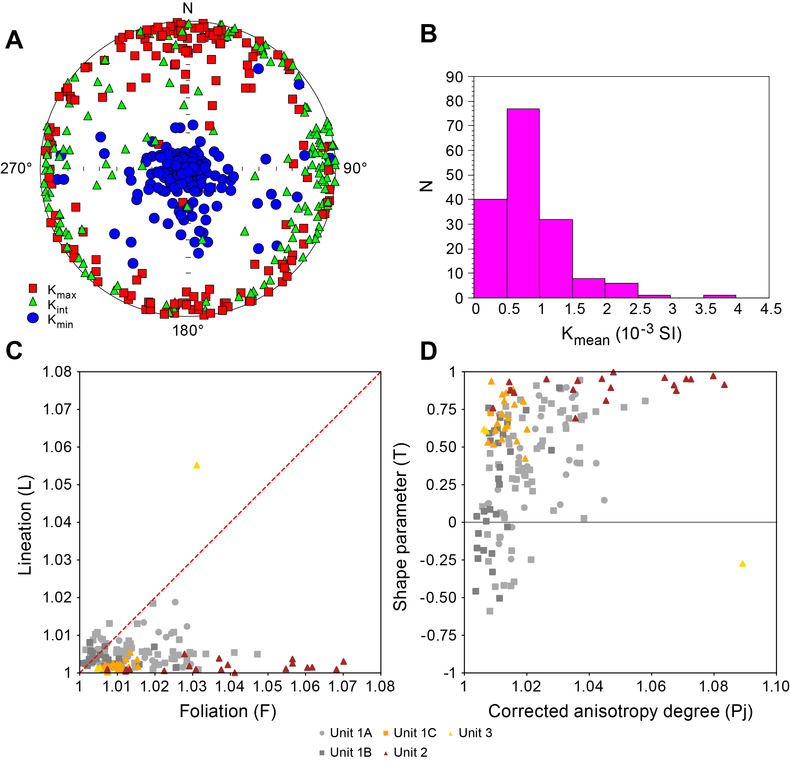
Figure F39. AMS data.
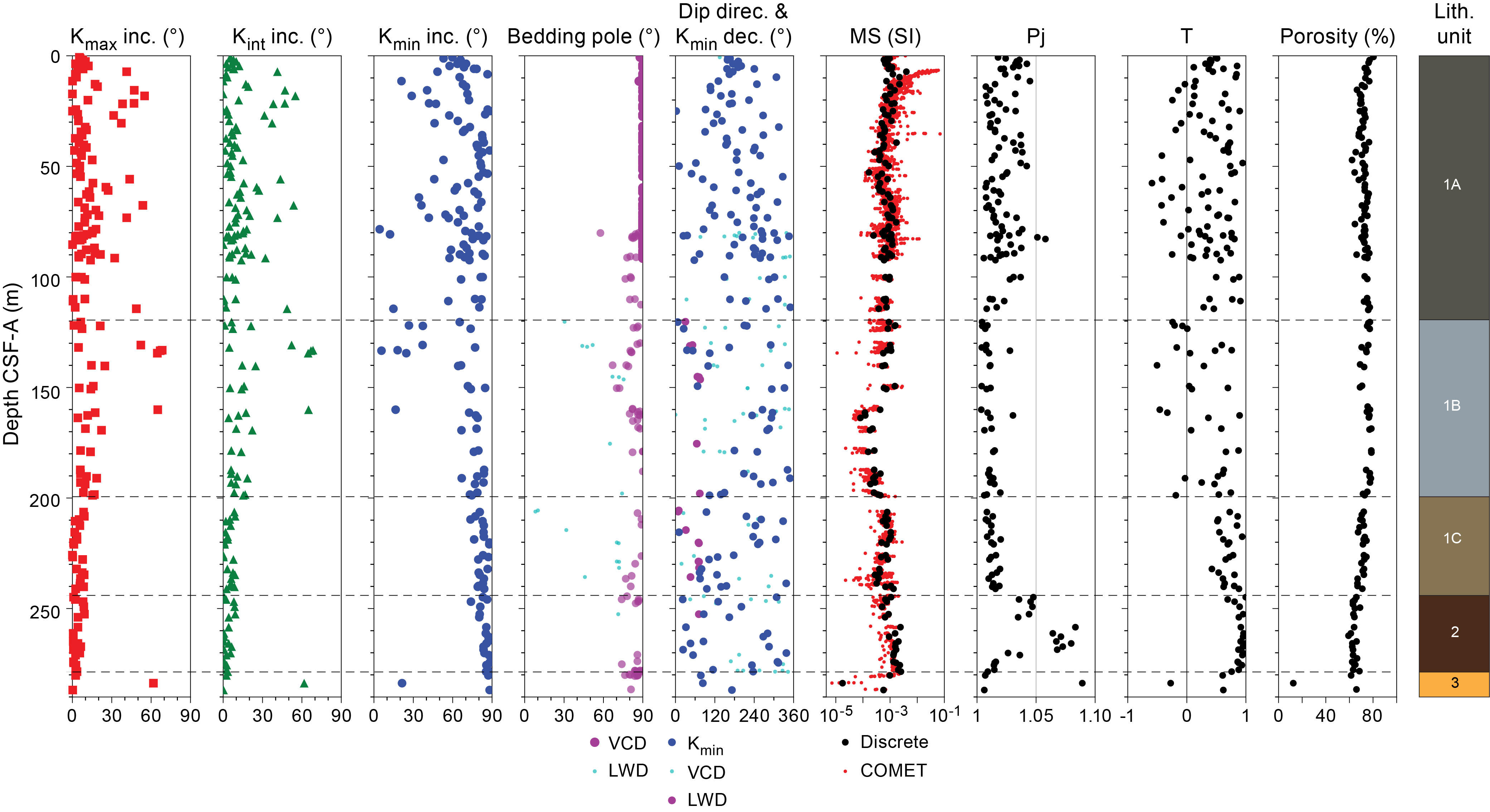
Figure F40. AMS parameters.
A plot of anisotropy parameters with depth shows distinct properties with respect to lithostratigraphic units (Figure F40). Consistent with what was documented from the whole-round sections, the excursion in MS measured around 7 m CSF-A is due to the influence of a metal chip in the core that is a contaminant from the coring process and not representative of the lithology. Both Kmin inclinations and shape parameter (T) roughly indicate a sedimentary fabric; however, their values fluctuate more in Subunits 1A and 1B than in other (sub)units. Both parameters are more stable with depth; Kmin inclination is steeper, whereas Kint inclination is shallower. In Subunit 1C, the fluctuations of K axes inclination are smaller. In addition, porosity data indicate higher compaction starting from Subunit 1C (see Physical properties). Pj shows less variability and is smaller in Subunit 1B and 1C compared to other units.
In Unit 2, Pj increases to a maximum value of 1.08 around the middle of Unit 2 and then drops with depth near its base (Figure F40). Here, the steeper Kmin inclination, higher magnetic foliation, higher Pj, and strongly oblate shape indicate a compaction fabric (Figure F39C, F39D). In Unit 3, MS and anisotropy suddenly drop, whereas the inclination of AMS axes is stable. Here, an apparent outlier is due to a nonoriented specimen.
7.3. Magnetostratigraphy
Except for variations attributed to core twisting, documented in Cores 405-C0026E-1H and 6H, declinations show consistent values at the section level in cores recovered by HPCS. In Hole C0026B, declinations show substantial scattering, which is typical of rotary coring and considered to be caused by biscuiting. The evidence for biscuiting is sometimes clearly recognized as an abrupt change in declination occurring in several to a few tens of centimeter intervals in sections. The inclination values at 20 or 25 mT (Figures F34D, F38) are consistent with what is expected at the site coordinates from the present field (~52°; Alken et al., 2021). The comparison with the demagnetization behavior of discrete samples (Figure F36) further supports the good quality of the signal after demagnetization. Therefore, variations in inclination (and declination for Hole C0026E) are interpreted to reflect changes in the magnetic polarities.
A succession of 20 normal and 20 reversed intervals was recognized (Figure F38) and used to constrain an age model based on magnetostratigraphy (Figure F41; Table T17). The overlapping parts of Holes C0026E and C0026B show consistent polarities. However, the discontinuous recovery in Hole C0026B, coupled with changes in sedimentation rates suggested by lithologic changes (see Lithostratigraphy) and supported by the paleontological data (see Biostratigraphy) hamper the reconstruction of an independent age model using data from Hole C0026B. A tentative correlation was attempted with the support of the biostratigraphic data. The lowermost part of Hole C0026B (between Cores 23K and 32K) shows shallower inclination in both archive and working halves. Here, the discrete samples show a stable demagnetization behavior, supporting the primary nature of ChRMs. Such shallower inclinations may indicate an older age for Units 2 and 3, in agreement with the biostratigraphy, suggesting Mesozoic ages for Core 21K and deeper.
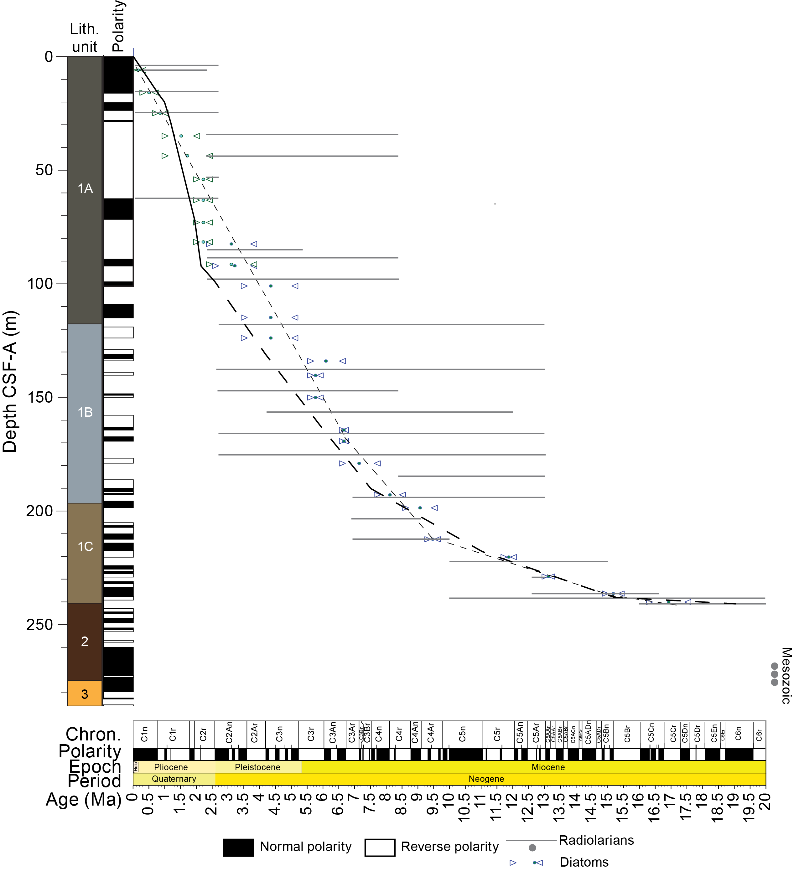
Figure F41. Age-depth model.
8. Physical properties
Shipboard physical property measurements were acquired on cores recovered from four holes at Site C0026. Three shallow holes (C0026C–C0026E) used a HPCS to recover samples from the shallow sediments that make up the upper 92 m of the sedimentary section on the incoming plate. An APCT-3 tool, installed in the HPCS cutting shoe (see Physical properties in the Expedition 405 methods chapter [Kirkpatrick et al., 2025a]), was deployed in two of these shallow holes (C0026D and C0026E) to measure the formation temperature. A SD-RCB system was used in Hole C0026B to recover core from 80 to 286.9 mbsf. All depths in this section are given on the mbsf depth scale, which is equivalent to the CSF-A scale. All of the physical properties data for this site are found in PHYSPROPS in Supplementary material.
All recovered whole-round cores were logged with the Core Measurement Track (COMET), which provided a semicontinuous record of gamma ray attenuation (GRA) density, MS, P-wave velocity, and natural gamma radiation (NGR). After splitting, measurements to characterize the physical properties, including electrical resistivity, strength, thermal conductivity, bulk density, porosity, and P- and S-wave velocity, were measured directly on the working half or on discrete samples taken from the working half. Core 1H from Holes C0026C–C0026E all represent the 0–6 mbsf depth interval. Measurements from Hole C0026E are used as representative values for this interval.
8.1. Core Measurement Track
In measurements using the COMET, the ends of the core may not yield accurate values due to the absence of core material on one side or the influence of the liner cap. Therefore, the following analysis is based on data after removing data acquired within 4 cm from both ends of each core section. COMET data for Holes C0026B–C0026E are shown in Figure F42. Figure F43 shows the COMET data taken on the core recovered from Hole C0026E with the HPCS over the depth interval that overlaps with the core recovered by SD-RCB from Hole C0026B. Over this interval, the GRA density of Hole C0026B is lower than that of Hole C0026E, but the other measurements (MS, P-wave velocity, and NGR) are similar.
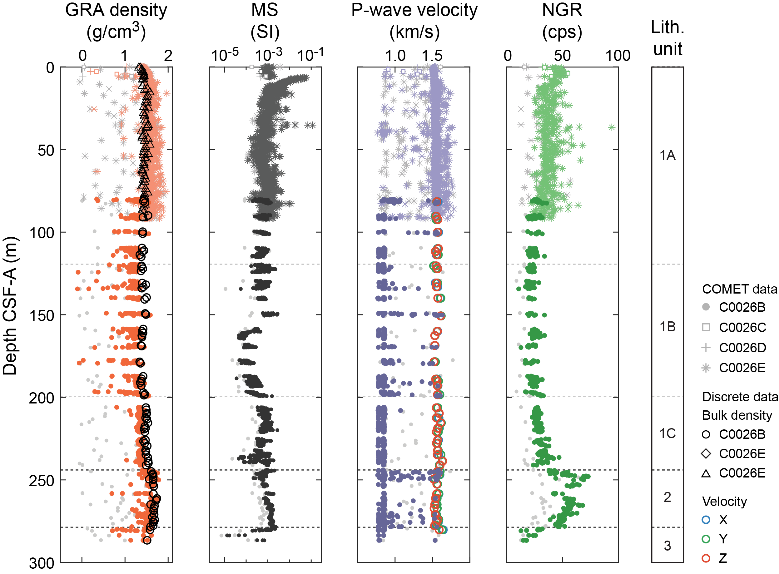
Figure F42. GRA density, MS, P-wave velocity, and NGR.
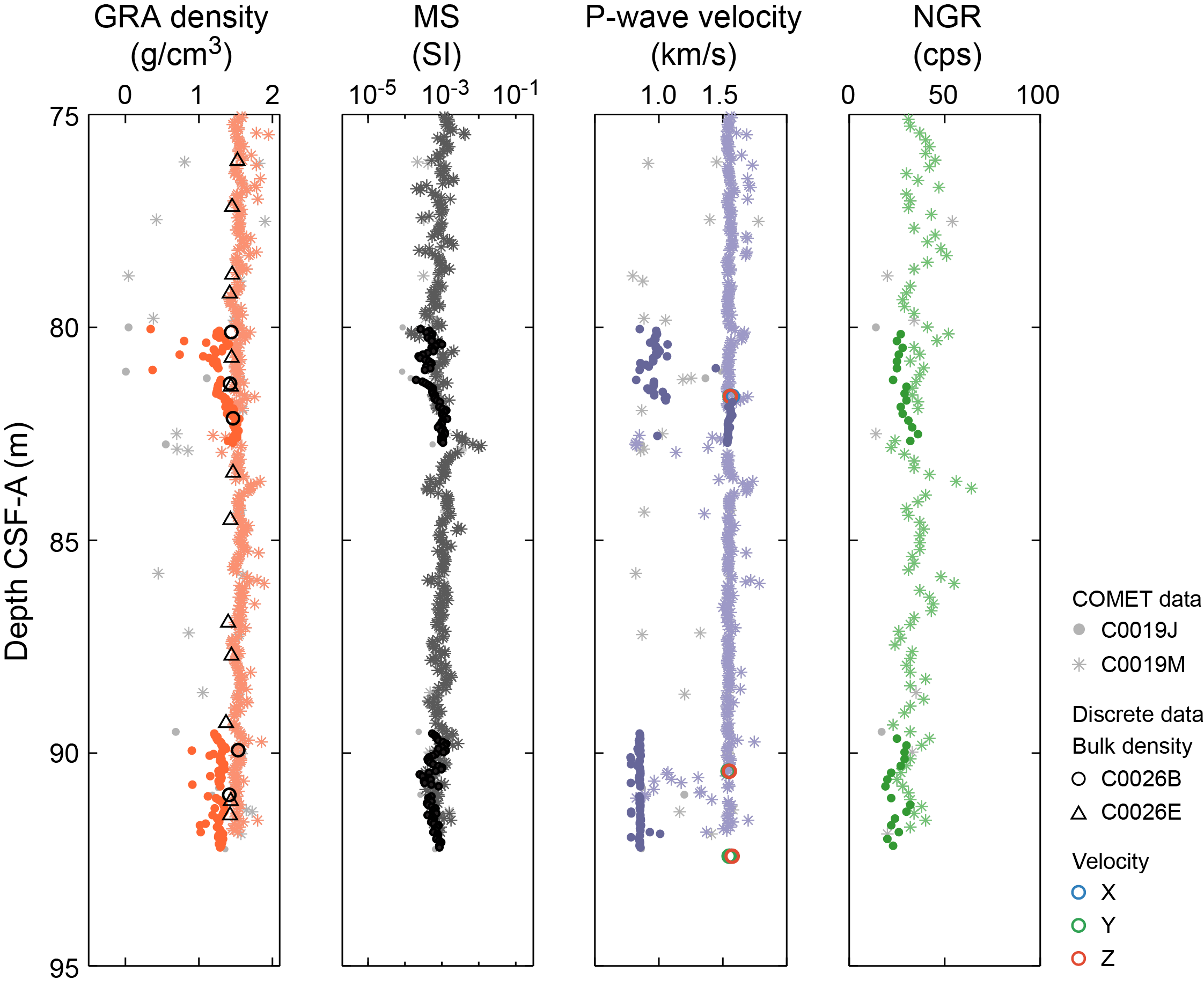
Figure F43. GRA density, MS, P-wave velocity, and NGR focusing on the overlapping section between Holes C0026B and C0026E.
8.1.1. GRA density
Bulk density determined by GRA ranges −0.10 to 2.23 g/cm3 (Figure F42). The large scatter and unrealistically low values are due to incompletely filled core liners and damaged/fractured core material, which led to an underestimation of the density. However, the higher values provide a reasonable estimate of the bulk density. In Hole C0026E, the average of the data is 1.55 g/cm3 and the data representing the upper end (or envelope) of the scatter indicate that the realistic bulk density range is 1.4–1.9 g/cm3. In Hole C0026B the average is 1.35 g/cm3 and the upper envelope ranges 1.1–1.78 g/cm3.
In Lithostratigraphic Unit 1 (see Lithostratigraphy), the GRA density increases from ~1.4 to ~1.6 g/cm3 from 0 to 9 mbsf and then remains nearly constant down to 92.0 mbsf, except for an offset in the GRA density measured on cores from Hole C0026B relative to what was measured on Hole C0026E cores. In the depth interval where cores from Holes C0026B and C0026E overlap (80–92 mbsf), GRA density values from Hole C0026B are consistently lower than those at the corresponding depths in Hole C0026E (Figure F43). This is due to the differences in the degree to which the core filled the liner. The HPCS cores tended to fill the liner, whereas significant gaps existed between core and liner in the SD-RCB cores, resulting in an underestimation of density.
In Hole C0026B, GRA density for the rest of Unit 1 (below 92 mbsf) remains nearly constant around ~1.3 g/cm3. At the boundary with Unit 2 (244 mbsf), there is a sudden step increase in GRA density to ~1.6 g/cm3. From 244 mbsf to the bottom of the hole, GRA generally varies between 1.5 and 1.8 g/cm3, decreasing slightly with depth.
The maximum GRA densities from Hole C0026B are generally consistent with discrete measurements of bulk density performed on the working half of the cores (see Moisture and density). However, GRA density from the HPCS cores tends to be slightly higher than the bulk density (Figure F42). The difference between GRA density and bulk density in the HPCS cores is likely explained by continued expansion of the cores during whole-round sampling and core splitting, resulting in a lower density for the discrete measurements of bulk density. In the HPCS intervals, the cored material generally filled the liner, and the confinement provided by the liner allowed the sediment to remain in a consolidated state. However, with subsequent whole-round sampling and splitting, the sediments expanded to occupy a larger volume, reducing the measured discrete bulk density. In the case of SD-RCB cores of materials with varying degrees of lithification, the liner was not completely filled by the cored material. Therefore, the reported GRA density included void space filled with water or air, resulting in an underestimate of density. Because these materials typically do not expand upon splitting, an overestimation of volumes is not an issue for MAD bulk density estimations in this instance.
8.1.2. Magnetic susceptibility
MS varies between 1.3 × 10⁻⁵ and 0.12 SI with no obvious difference between the HPCS and SD-RCB cores (Figures F42, F43). In Lithostratigraphic Subunit 1A, a nearly constant MS of 1.0 × 10⁻³ SI is observed except for a sudden increase to 0.060 SI at 6.5 mbsf followed by an exponential decrease. This depth corresponds to the top of Section 405-C0026E-2H-1, where an erroneous metal fragment was found and high-density particles were observed surrounding the core in the XCT images. The MS remains elevated throughout Core 2H down to 16.0 mbsf, which is also thought to be due to metal fragments mixed into the core (see Paleomagnetism). The metal is likely contamination that occurred during drilling. High-MS peaks at ~35 mbsf (Section 5H-2) are also thought to be due to metal fragments. In the following description of the MS data, these high values have been ignored.
The MS at Site C0026 does not have a consistent trend with depth but rather tends to increase or decrease over spatial scales of tens of meters. Within Lithostratigraphic Subunit 1A, MS values are nearly constant with depth with an average value of 9.6 × 10⁻⁴ SI. In Subunit 1B, there is a slight increase between 119.5 and 150.8 mbsf where MS reaches 1.8 × 10−3 SI by 150.8 mbsf. MS then decreases to ~9.4 × 10−5 SI by 160 mbsf. MS then continues to increase with depth, a trend that continues into Subunit 1C, where values reach a maximum of 1.5 × 10⁻³ SI at 215.6 mbsf. MS then decreases with depth for the rest of Subunit 1C, although there is scatter from 223.8 to 241.0 mbsf with MS values ranging from 4.6 × 10⁻⁵ to 1.8 × 10⁻³ SI. In Unit 2, MS consistently increases with depth from 6 × 10⁻⁴ SI at 244.8 mbsf to 2.1 × 10⁻³ SI at 278.4 mbsf. Unit 3 again shows significant scatter; in Cores 403-C0026E-30K through 32K (279.5–286.89 mbsf), MS decreases and ranges 1.3 × 10⁻⁵ to 2.2 × 10⁻³ SI.
8.1.3. P-wave velocity
As with the GRA measurements, P-wave velocity recorded with the COMET was adversely affected by incomplete liner filling, core damage, and fracture. This was evidenced by the fact that most of the P-wave velocity values are <1.5 km/s, lower than the velocity of seawater (Figure F42). Particularly for the data acquired below 90 mbsf using the SD-RCB system (Hole C0026B), most of the values are unrealistic for sediment. In the data acquired with the SD-RCB system, the maximum values provide an estimate of the P-wave velocity. On the other hand, in the cores obtained with the HPCS (Holes C0026C–C0026E), the velocity is generally 1.5–1.6 km/s with occasional excursions to higher values of ~1.7–1.8 km/s. Some of the higher velocities, in excess of 1.7 km/s, correspond to ash layers that show up as high density in XCT (Figure F44).
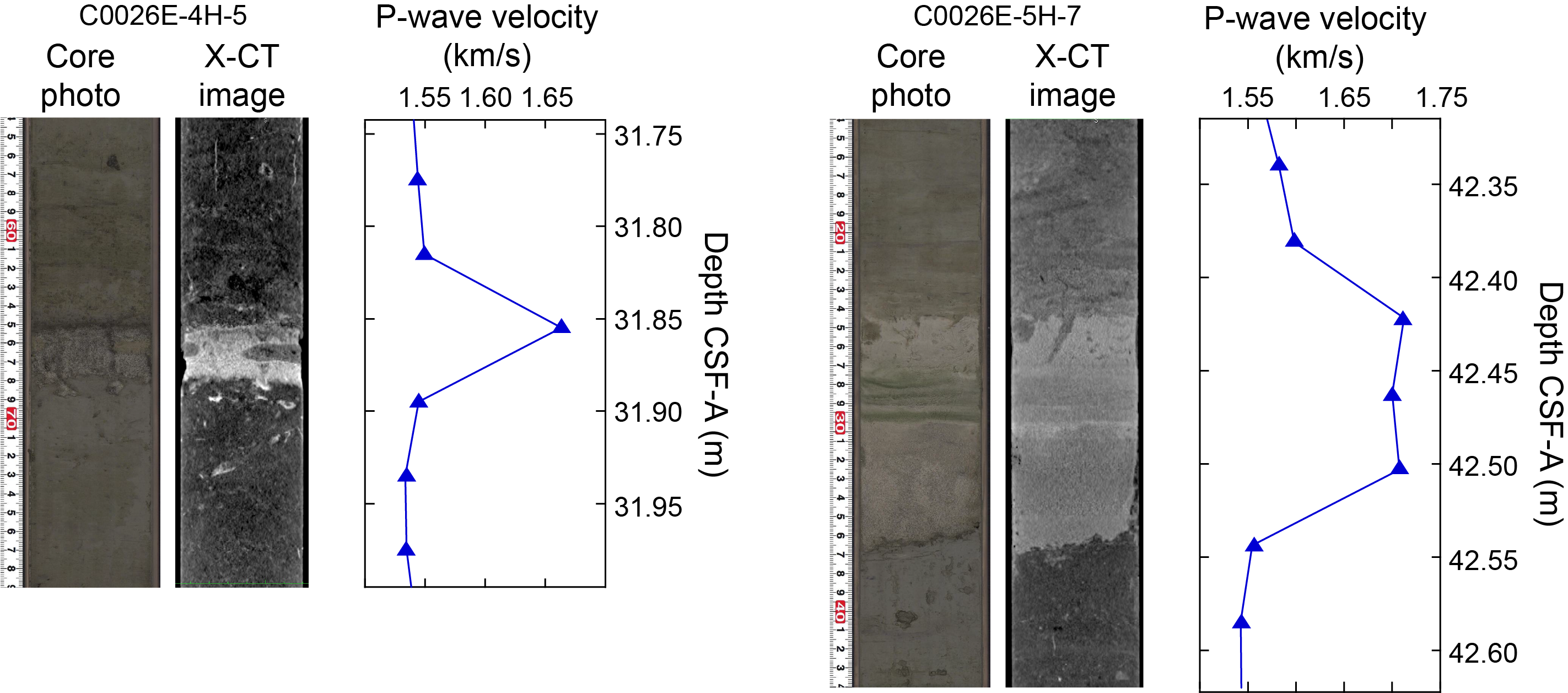
Figure F44. High P-wave velocities associated with ash layers.
At the shallowest depths (0–10 mbsf), P-wave velocity increases from 1.51 to 1.53 km/s. It then remains nearly constant through Lithostratigraphic Unit 1, increasing slightly with depth. P-wave velocity reaches 1.6 km/s at 244.5 mbsf and reduces by 0.05 km/s at the top of Lithostratigraphic Unit 2. Velocity remains low (~1.55 km/s) in Lithostratigraphic Unit 2, and no change is observed in Lithostratigraphic Unit 3. Where the COMET recorded reasonable velocities, discrete measurements of P-wave velocity performed on the core after splitting are often higher than the COMET velocity but are generally comparable.
8.1.4. Natural gamma radiation
NGR generally ranges ~11–73 counts/s with an average of ~32 counts/s (Figure F42). Data from HPCS and SD-RCB cores are generally consistent with each other at comparable depths (Figure F43). Throughout Lithostratigraphic Subunits 1A and 1B (0–199.4 mbsf), NGR values gradually decrease with depth from ~45 to ~25 counts/s. From the top of Subunit 1C, NGR gradually increases with depth, reaching ~40 counts/s at 236.6 mbsf. Lithostratigraphic Unit 2 is associated with a sudden increase in NGR, where it rapidly increases to 70 counts/s at 248 mbsf but then gradually decreases with depth, reaching ~45 counts/s at 278 mbsf. Transitioning from Lithostratigraphic Unit 2 to Unit 3, NGR sharply decreases and ranges 10–30 counts/s.
8.2. Moisture and density
Moisture and density (MAD) measurements were conducted to characterize grain density, bulk density, porosity, void ratio, and water content for Holes C0026B, C0026D, and C0026E. MAD measurements were made on a total of 161 discrete samples between Sections 405-C0026D-1H and 405-C0026B-32K (0–286.7 mbsf) at a frequency of one sample per core section where possible (approximately every 1.5 m). The variations of these parameters with depth are shown in Figure F45.
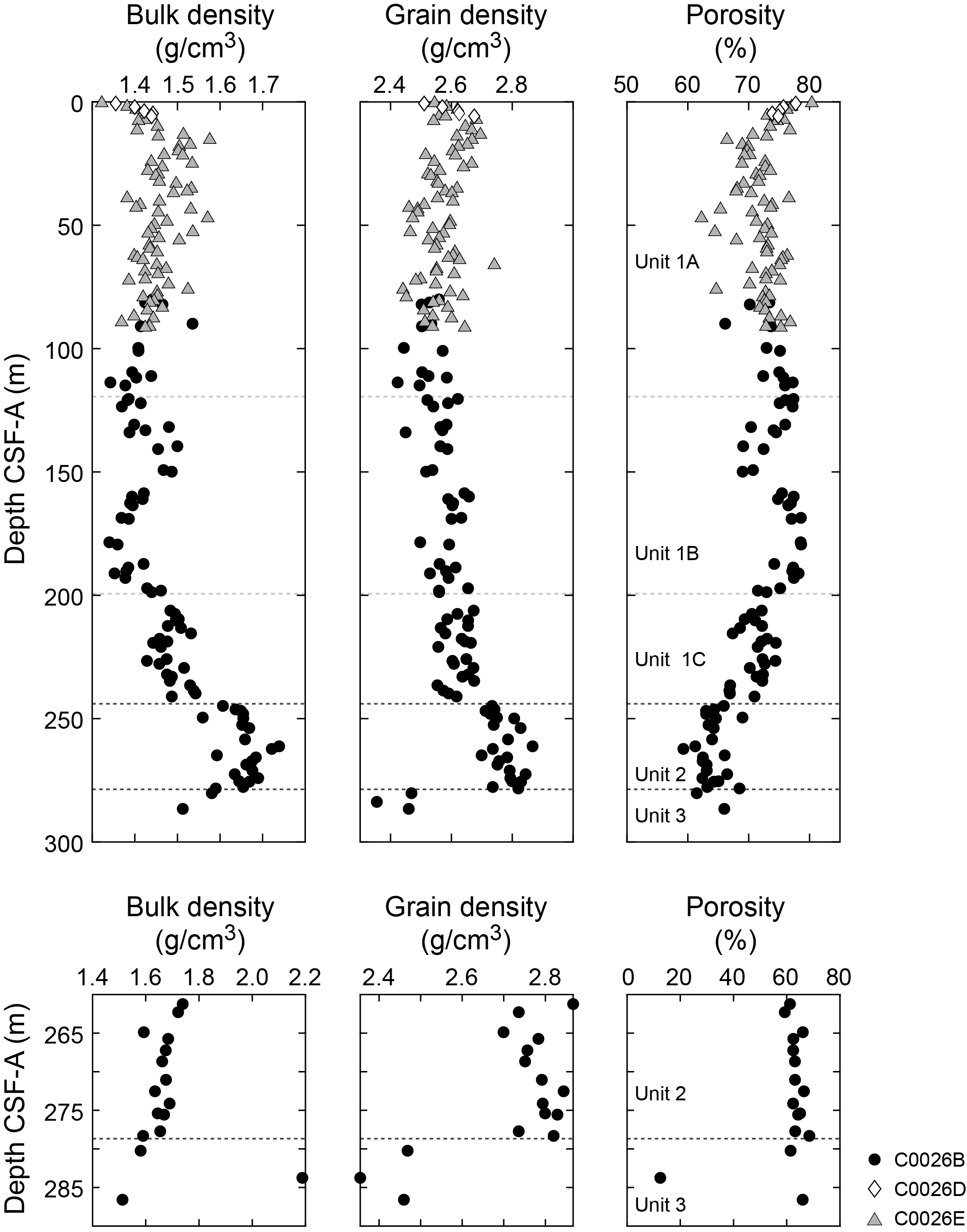
Figure F45. Bulk density, grain density, and porosity.
In general, the bulk density and porosity data exhibit increasing and decreasing trends, respectively, with depth throughout Holes C0026B, C0026D, and C0026E. In general, values of bulk density, grain density, and porosity estimated from the shallowest cores recovered from Hole C0026B and the deepest cores from Hole C0026E, in the overlapping depth interval (80.72–91.46 mbsf), are in good agreement. Below, we summarize the most important parameters: bulk density, grain density, and porosity and their variations with depth and within each lithostratigraphic unit (see Lithostratigraphy).
8.2.1. Bulk and grain density
From the seafloor to 119.5 mbsf, bulk densities in the olive-black siliceous vitric muds of Lithostratigraphic Subunit 1A range 1.32–1.58 g/cm3 (average = 1.45 g/cm3) and grain densities range 2.42–2.74 g/cm3 (average = 2.57 g/cm3). There is a sharp increase in bulk density from ~1.3 to ~1.5 g/cm3 in the shallowest 10 m. A sharp increase in bulk density and corresponding decrease in porosity close to the seafloor is typical of shallow marine sediment (Velde, 1996). Below this depth, grain densities are relatively constant throughout Subunit 1A and the bulk densities decrease slightly from ~13.29 to ~114.94 mbsf.
Bulk densities in the interval 119.5–199.4 mbsf (Cores 405-C0026B-5K through 13K; olive-gray siliceous vitric mud of Lithostratigraphic Subunit 1B) vary at 1.34–1.50 g/cm3 (average = 1.41 g/cm3) and are slightly lower than those estimated from Subunit 1A. In Lithostratigraphic Subunit 1B, there are repeated sequences of increasing and decreasing bulk density, but the grain density continues to remain relatively constant with an average value of 2.58 g/cm3.
The interval representing the dull yellowish brown mud of Lithostratigraphic Subunit 1C, 199.4–246.25 mbsf, is marked by a gradual increase in bulk density. In this interval, bulk density varies at 1.43–1.61 g/cm3 (average = 1.49 g/cm3). The grain density is constant through this interval and slightly higher than the grain density estimated for the muds of Lithostratigraphic Subunits 1A and 1B, with an average value of 2.63 g/cm3.
The interval 246.25–278.68 mbsf, consisting of brownish black clays of Lithostratigraphic Unit 2 (Cores 405-C0026B-20K through 29K), is marked by an overall increase in both bulk and grain densities when compared with shallower intervals, although their values remain relatively constant within this interval. Bulk densities range 1.56–1.74 g/cm3 (average = ~1.66 g/cm3), and grain densities range 2.7–2.87 g/cm3 (average = ~2.78 g/cm3).
The Lithostratigraphic Unit 3 interval of color-banded clay and chert (278.68–286.89 mbsf) is marked by a range of bulk densities (1.51–2.19 g/cm3) across the three MAD samples acquired from this interval (Figure F45). Similarly, grain densities in this interval vary at 2.36–2.46 g/cm3. These diverse values of bulk and grain densities are consistent with the observations of heterogeneous color variations and mineralogical compositions within this unit.
8.2.2. Porosity
Porosity and void ratios are generally anticorrelated with bulk density at Site C0026 and exhibit an overall decrease with depth (Figure F45). However, there is an almost 200 m interval of the sedimentary section that exhibits little to no dependence on depth. Initially, there is a sharp decrease in porosity from 0 to ~10 mbsf, likely reflecting mechanical compaction. Below this, from 10 to 191.15 mbsf, porosity generally ranges 70%–80%. There are repeated sequences of increasing or decreasing porosity, on the order of tens of meters of depth, but there is no clear decrease in porosity with increasing depth as is expected for vertical compaction under a lithostatic load. This zone of high depth-independent porosity is consistent with porosities estimated at Sites 436 and 1179 from DSDP Legs 56 and 57 (Carson and Bruns, 1977) and Ocean Drilling Project (ODP) Leg 191 (Shipboard Scientific Party, 2001), respectively (Figure F46). However, the porosity at Site 1179 is consistently higher than that at Sites 436 and C0026 by ~10%.
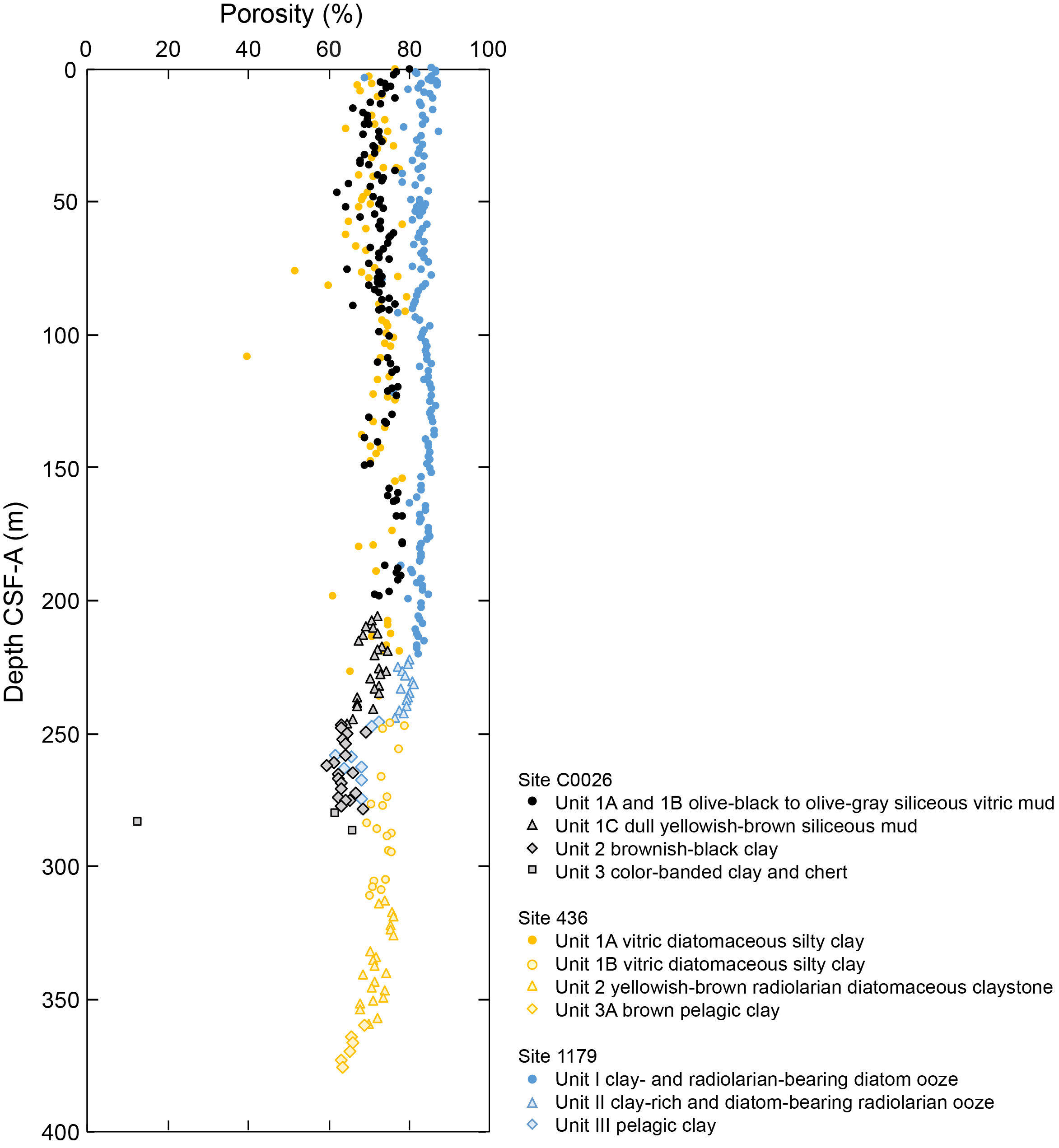
Figure F46. Porosity estimates.
There are some other common features observed at the three sites: (1) increased scatter in porosity from ~25 to 75 mbsf and (2) repeated sequences of increasing and decreasing porosity over spatial scales of tens of meters of depth from ~90 to 191 mbsf. The repeated sequences of increasing and decreasing porosity are mainly observed in Lithostratigraphic Subunit 1B at Site C0026 and are consistent with variations in bulk density (Figure F45) in this subunit. A similar pattern is also observed in MS (Figure F42). The cause of the elevated porosities and observed cyclic variations is unknown, but repeated observations at multiple sites and across measurements of different quantities indicate it is natural, relatively widespread, and not a measurement artifact.
At Site C0026, a steady decrease in porosity from 78.2% to 65.98% is observed from ~191.15 to 286.59 mbsf, likely due to consolidation associated with burial and overburden stresses. This depth range corresponds to the base of Lithostratigraphic Subunit 1B through Subunit 1C and Unit 2. This trend was also observed at Site 1179.
In the dull yellowish brown siliceous muds of Subunit 1C (199.4–246.25 mbsf), porosities range 65.9%–74.5% (average = 70.7%) and corresponding void ratios are range 1.93–2.92 (average = ~2.43). The brownish black clays of Unit 2, from Cores 405-C0026B-20K through 29K (246.25–278.7 mbsf), continue to show a trend of decreasing porosity with depth, with values ranging 59.3%–69.0% (average = 64%). Corresponding void ratios vary at 1.45–2.22 (average = 1.78).
As with bulk and grain densities, the interval between 278.7 and 286.89 mbsf (Lithostratigraphic Unit 3; color-banded clay and chert) is marked by highly variable porosity and void ratio values in the ranges of 12.5%–66.0% and 0.14–1.94, respectively, based on MAD measurements on three samples in this interval (Figure F45). This is likely due to the heterogeneous nature of the materials recovered from this interval (see Lithostratigraphy).
8.3. Electrical resistivity
Electrical resistivity measurements were made on cores from Hole C0026B, C0026D, and C0026E (Figure F47). In Holes C0026D and C0026E, 37 electrical impedance measurements were made shallower than 92 mbsf in the y- and z-directions using the 4-pin setup for soft sediments (see Physical properties in the Expedition 405 methods chapter [Kirkpatrick et al., 2025a]). For the entire cored interval in Hole C0026B, recovered material was solid enough to measure electrical resistivity on cube samples. In total, 47 cube samples were obtained from Cores 1K–31K.
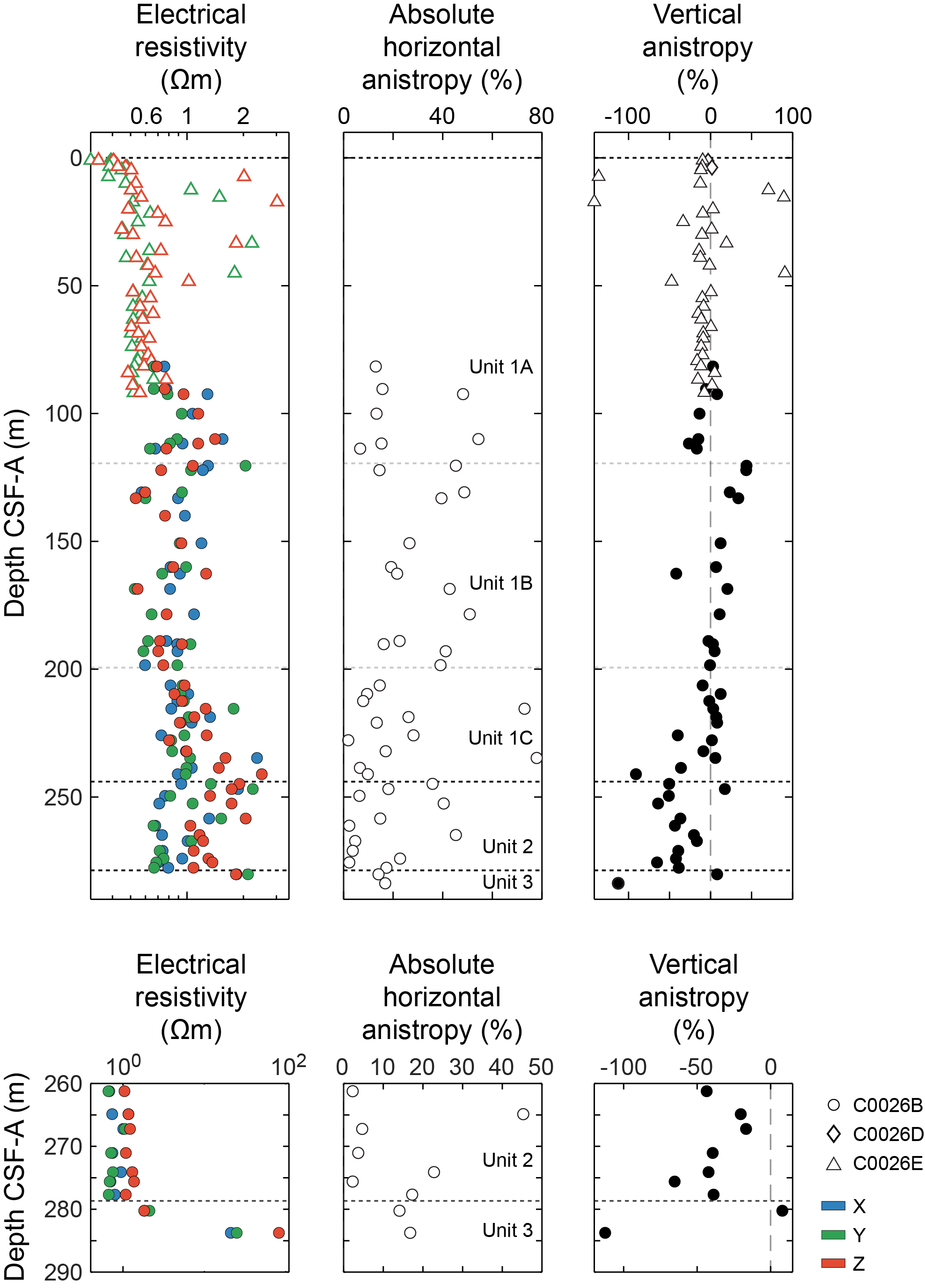
Figure F47. Electrical resistivity, absolute horizontal anisotropy, and vertical anisotropy measurements.
Throughout Lithostratigraphic Subunit 1A (0–119.5 mbsf), electrical resistivity increases slightly with depth. From 0 to 50 mbsf, there are several data outliers reaching as much as 3 Ωm. For most of these outliers only one measurement direction is high, but the high direction is not consistent (i.e., varies between y and z). The outliers are, therefore, unlikely to reflect any pervasive fabric. None of the outlier measurements coincide with a different lithology (e.g., ash layers), but an effect from core quality cannot be ruled out (e.g., voids related to fracturing). For the outlier in Section 405-C0026E-4H-6 (33.4 mbsf), measurements in both the y- and z-directions have a higher than average resistivity; this measurement was conducted several hours after the core was split and the high resistivity is likely due to reduced water content.
Excluding the outliers discussed above, the average electrical resistivities in Lithostratigraphic Subunit 1A are 0.65 Ωm in the z-direction and 0.62 Ωm in the horizontal direction (i.e., including the x- and y-directions) because the cores are not absolutely oriented in the horizontal direction (Figure F47). In Lithostratigraphic Subunit 1B, the electrical resistivity remains almost constant with depth, averaging 0.91 and 0.80 Ωm in the horizontal and z-directions, respectively. Throughout the depth interval 199.4–244.0 mbsf, coinciding with Lithostratigraphic Subunit 1C, electrical resistivities are more scattered but slightly higher, particularly in the z-direction (horizontal = 1.04 Ωm, z = 1.22 Ωm), and resistivity increases with depth.
From 244.0 to 278.7 mbsf, the electrical resistivity data remain scattered. Although the average horizontal resistivity remains similar to what was measured in Subunit 1C (1.03 Ωm), the z-direction tends to be more resistive (1.34 Ωm). This interval coincides with the brownish black clay of Lithostratigraphic Unit 2, where scaly fabric was observed (see Structural geology). The increase in resistivity in the z-direction may be related to this scaly fabric.
Below 278.7 mbsf, only two samples from Lithostratigraphic Unit 3 were measured: one from the color-banded clays and one from the underlying chert (see Lithostratigraphy). In the color-banded clays, the electrical resistivity is 1.84, 2.11, and 1.82 Ωm in the x-, y-, and z-directions, respectively, which is slightly higher than in Lithostratigraphic Unit 2. Electrical resistivity of the single sample taken from the underlying chert in Section 405-C0026B-31K-CC, however, is considerably higher: 21.17 Ωm in the x-direction, 25.05 Ωm in the y-direction, and 82.70 Ωm in the z-direction (Figure F47).
Anisotropy of electrical resistivity was calculated from the resistivity measurements on sample cubes in the x-, y-, and z-directions (see Physical properties in the Expedition 405 methods chapter [Kirkpatrick et al., 2025a]). For the soft sediments in Hole C0026E, only vertical anisotropy can be calculated because the 4-pin setup only allows resistivity to be measured in the y- and z-directions. Because the cores are not oriented, only absolute values of horizontal anisotropy (x-y plane) are presented for the measurements on cube samples from Hole C0026B.
The absolute value of horizontal anisotropy of resistivity measured from cubes is scattered within a range of 0%–50% (Figure F47). Vertical anisotropy in Lithostratigraphic Unit 1 mostly varies between ±20% but becomes dominantly negative (i.e., higher resistivity in the z-direction) and up to −100% below about 235 mbsf. This increase in vertical resistivity anisotropy is consistent with the presence of a strong fabric in this depth interval (see Structural geology).
A crossplot of electrical resistivity and porosity (Figure F48) indicates that data from individual lithostratigraphic units tend to cluster together. However, taken together, there is only a weak inverse relationship between electrical resistivity and porosity (i.e., increasing resistivity with decreasing porosity) across all holes and lithostratigraphic units at Site C0026.
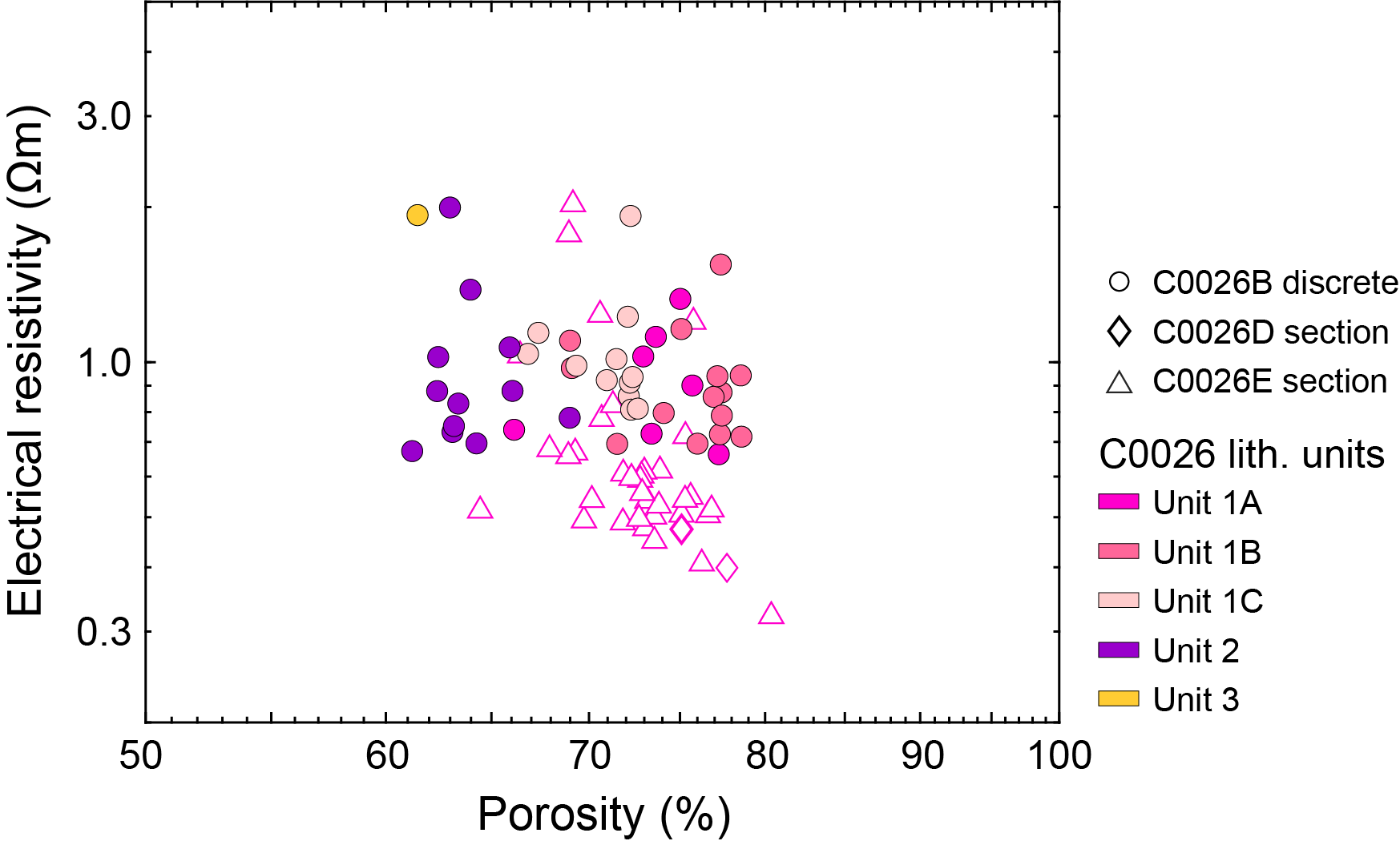
Figure F48. Electrical resistivity as a function of porosity.
8.4. Discrete P-wave velocity
P-wave velocity measured on discrete cubic samples of sediments recovered from Hole C0026B ranges 1.52 to nearly 1.64 km/s (Figure F49). The average velocity is almost constant around 1.56 km/s in Lithostratigraphic Subunit 1A. In Subunit 1B, the average is still 1.56 km/s, but there are repeated sequences of increasing and decreasing velocity as a function of depth, mirroring fluctuations observed in the porosity in this unit (Figure F45). P-wave velocity in Lithostratigraphic Subunit 1C is also generally constant with depth with an average of 1.58 km/s. In Lithostratigraphic Unit 2, there is slightly more scatter in the velocities measured in different directions, but the average velocity of 1.56 km/s is similar to that above. In Lithostratigraphic Unit 3, there is a slight increase in velocity in the color-banded clays (see Lithostratigraphy) where P-wave velocities up to 1.63 km/s were measured. The most pronounced change in velocity occurs in the chert, where a velocity of 4.15 km/s was measured at 283.8 mbsf. P-wave velocities measured on discrete cubic samples are consistent with P-wave velocities measured with the COMET shallower than 80 mbsf and with the higher range of values from the COMET below 80 mbsf (Figure F42).
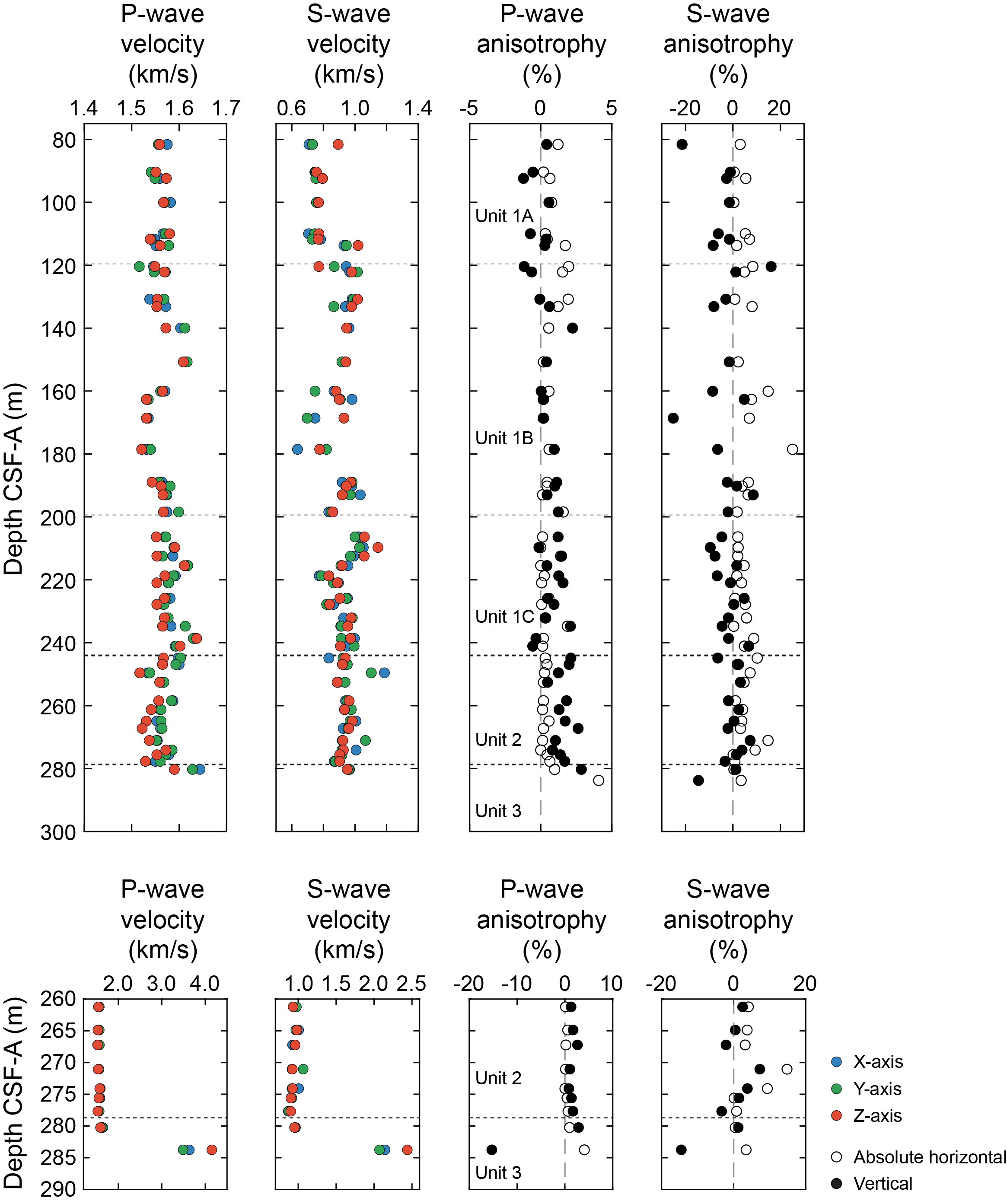
Figure F49. P- and S-wave velocity measurements.
The absolute horizontal P-wave anisotropy, measured in the plane perpendicular to the core axis (see Physical properties in the Expedition 405 methods chapter [Kirkpatrick et al., 2025a]), is scattered with values ranging between 0 and ~2% over the depth interval 80–199.4 mbsf, which corresponds to Lithostratigraphic Subunits 1A and 1B. It is almost constant with depth around ~0.2% in Lithostratigraphic Subunit 1C and Unit 2 (Figure F49). The highest values, up to 4%, are found within the chert in Lithostratigraphic Unit 3 (see Lithostratigraphy).
Vertical P-wave anisotropy (see Physical properties in the Expedition 405 methods chapter [Kirkpatrick et al., 2025a]) in Lithostratigraphic Subunits 1A and 1B is scattered mostly between ±2%. In Lithostratigraphic Subunit 1C and Unit 2, where horizontal anisotropy decreases, the vertical anisotropy increases slightly (up to 2.6%) and becomes more positive; positive vertical anisotropies indicate a relatively faster horizontal P-wave velocity than vertical. These positive values of vertical P-wave anisotropy are expected based on the orientation of the scaly fabric present in Lithostratigraphic Unit 2 (see Structural geology). The chert at 283.8 mbsf has a vertical P-wave anisotropy of −15% (Figure F49).
P-wave velocities are anticorrelated with porosity, as expected for marine sediments undergoing burial compaction with increasing depth (Erickson and Jarrard, 1998). The plot of P-wave velocity with porosity shows that the data follow this trend within two distinct clusters depending on the lithostratigraphic unit (Figure F50). One cluster is represented by data from Lithostratigraphic Unit 1, in which P-wave velocity generally increases from 1.53 to 1.63 km/s as corresponding porosities decrease from around 67% to 79%. In Lithostratigraphic Units 2 and 3, lower velocities are observed at a given porosity compared to what is observed in Unit 1; P-wave velocity increases from 1.53 to 1.62 km/s as corresponding porosities decrease from around 69% to 61%.
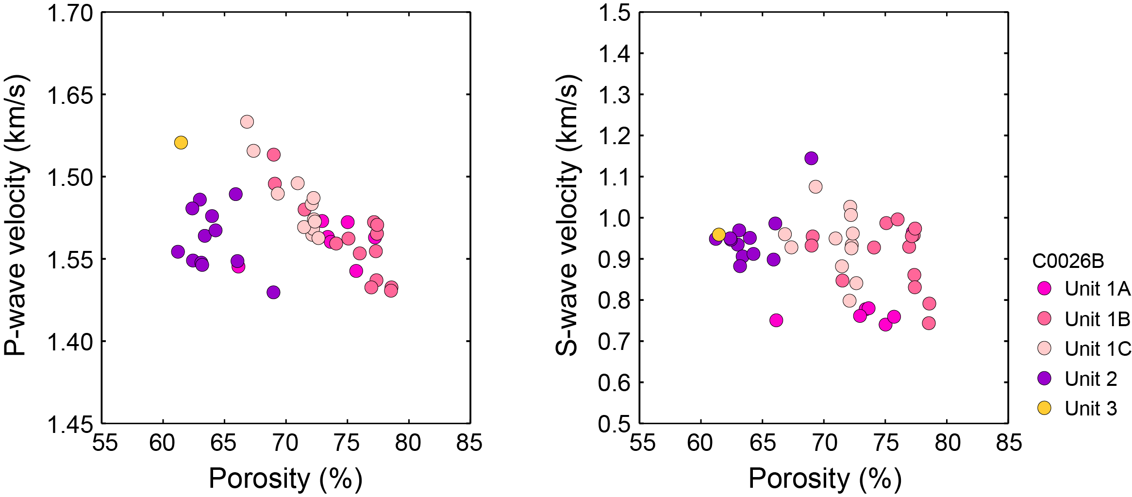
Figure F50. Average P-wave and S-wave velocity as a function of porosity.
8.5. Discrete S-wave velocity
Values of S-wave velocity measured on discrete cubic samples taken from 80 to 280 mbsf are almost constant with depth except for a sharp increase at 114 mbsf (Figure F49). In Lithostratigraphic Subunit 1A, above 114 mbsf, S-wave velocities are generally constant around 0.8 km/s. At 114 mbsf, velocity abruptly increases to ~0.96 km/s. This change occurs ~5 m above the boundary with Lithostratigraphic Subunit 1B at 119.4 mbsf. S-wave velocity in Subunit 1B decreases slightly from ~0.92 km/s at ~120 mbsf to ~0.74 km/s at 178.5 mbsf and then steps to ~0.93 km/s at 189 mbsf, reflecting variations seen in porosity and P-wave velocity. The values in Lithostratigraphic Subunit 1C decrease from 1.03 km/s at 206.4 mbsf to 0.80 km/s at 218 mbsf. S-wave velocities then begin to increase, reaching 0.95 km/s by 244.0 mbsf. In Lithostratigraphic Unit 2, S-wave velocity is generally constant around ~0.94 km/s with the exception of a single outlier sample at 249.6 mbsf. This sample was cracked, resulting in a noisy waveform, which made it difficult to pick the S-wave arrival, and an earlier arrival that is not the S-wave was likely picked. The highest values in the hole of up to ~2.5 km/s are found within the chert of Lithostratigraphic Unit 3 (see Lithostratigraphy) at ~283.8 mbsf (Figure F49).
The most obvious change in the S-wave data is seen in the anisotropy at ~199.4 mbsf (Figure F49). At the transition from Lithostratigraphic Subunit 1B to Subunit 1C, the absolute horizontal S-wave anisotropy, which is scattered between 0% and 25% shallower in the hole, reduces to 2% and remains low throughout the rest of the hole, never exceeding 15%. Vertical S-wave anisotropy also has a change at 199.4 mbsf. Shallower in the hole, it is very scattered, ranging −25%–16%, but at the transition to Subunit 1C, vertical anisotropy decreases and ranges −10%–7% throughout Lithostratigraphic Units 1C and 2. The vertical anisotropy in the chert is −15%.
A crossplot of S-wave velocity versus the corresponding porosity for the same sample (Figure F50) indicates the two properties are weakly anticorrelated. The data do not show a clear dependence on lithostratigraphic unit, as was observed for the P-wave velocity-porosity relationship.
8.6. Thermal conductivity
Thermal conductivity measurements were conducted at 156 discrete points where core conditions met the methodological standards (see Physical properties in the Expedition 405 methods chapter [Kirkpatrick et al., 2025a]). These measurements include 85 data points from Hole C0026B, 4 from Hole C0026D, and 67 (two of which were measured on whole-round cores using the needle probe) from Hole C0026E. The data set spans Sections 405-C0026D-1H-1 through 405-C0026B-31K-CC (1.1–283.745 mbsf). Data points with poor quality or where there was only one successful measurement are marked separately in Figure F51. Additionally, three measurements were taken in ash layers in Hole C0026E. The ashes have consistently low thermal conductivity with an average value of 0.241 W/(m·K) and are not representative of the larger volume of sediment that characterizes each lithostratigraphic unit. The ash thermal conductivities and poor-quality data were excluded from our general analysis at Site C0026. The remaining 133 data points are discussed below.
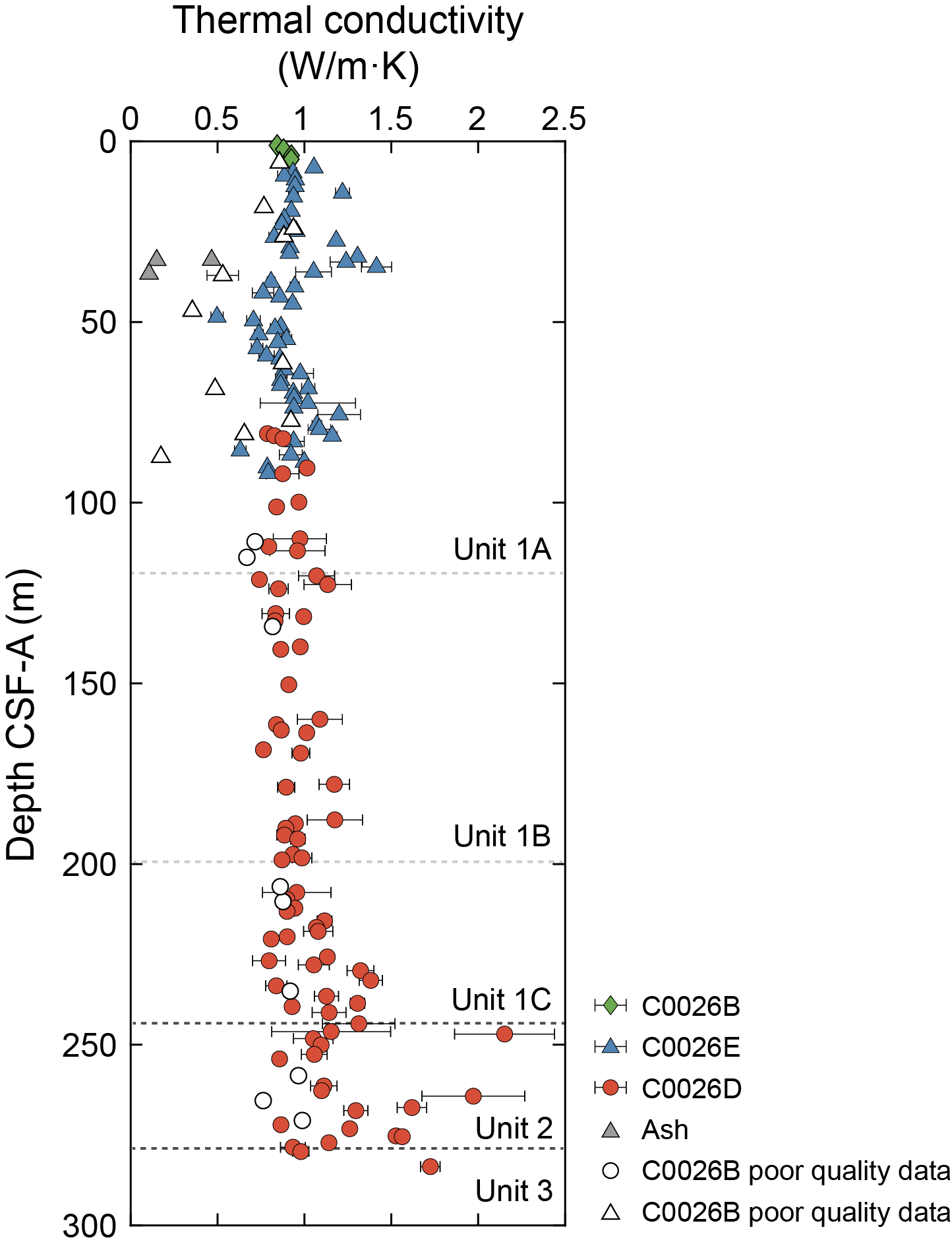
Figure F51. Thermal conductivity measurements.
Thermal conductivity values at Site C0026 range 0.497–2.152 W/(m·K) with a mean of 1.000 W/(m·K) and a standard deviation of 0.231 W/(m·K). The lowest value, 0.497 W/(m·K), was recorded for Section 405-C0026E-6H-3 (48.57 mbsf), corresponding to the olive-black siliceous vitric mud of Lithostratigraphic Subunit 1A. The low thermal conductivity suggests the sample may have dried significantly before the measurement was performed. The highest value was observed for Section 405-C0026B-20K-3 (247.06 mbsf) in the brownish black clay near the top of Lithostratigraphic Unit 2. The thermal conductivity does not vary significantly between lithostratigraphic units.
8.7. Undrained shear strength
The undrained shear strength of soft sediments in the working half of the core in Lithostratigraphic Subunit 1A (see Lithostratigraphy) was measured using an analog vane shear device and a pocket penetrometer (see Physical properties in the Expedition 405 methods chapter [Kirkpatrick et al., 2025a]). The vane shear strength is generally consistent with the strength measured by the penetrometer (Figure F52). From 0 to 22 mbsf, both measurements of undrained shear strength increase from ~7 to ~53 kPa. Below 22 mbsf, similar changes in strength are observed in both measurements, but the vane shear strength tends to be lower than the penetration strength. A decrease in strength from 22 to 30 mbsf corresponds to a slight local increase in porosity with depth (Figure F45). Below ~30 mbsf, the strengths remain nearly constant with depth, ranging 20–93 kPa for vane shear strength and 35 to ~126 kPa for penetration strength.
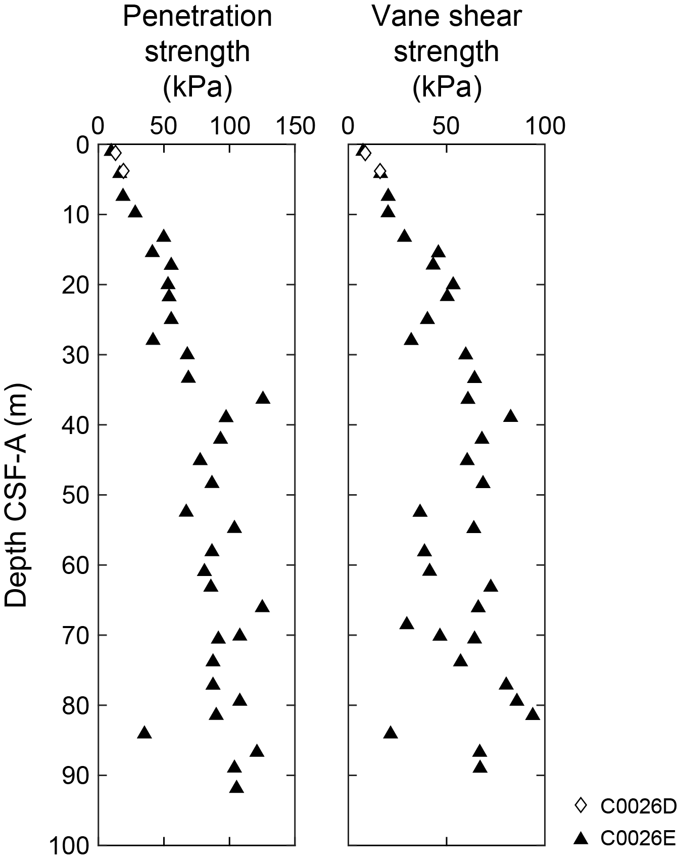
Figure F52. Penetration strength and undrained shear strength.
8.8. Anelastic strain recovery
Anelastic strain recovery (ASR) measurements to estimate the in situ stress orientation and the 3D stress regime were conducted on board using freshly acquired whole-round core samples (see Physical properties in the Expedition 405 methods chapter [Kirkpatrick et al., 2025a]). Shipboard ASR measurements were conducted for three whole-round core samples from Hole C0026B (10K-1, 76–91 cm, 16K-3, 0–18 cm, and 21K-2, 46–61 cm). Because the strain gauges needed to be attached to a smooth surface, some samples had to be cut with a rock saw. To illustrate the results of the shipboard ASR measurements, the anelastic strain data, three principal strains, and mean strains are plotted in Figure F53, which shows that the overall recovery of strain with time is evident in the data despite apparent noise. The full analysis of these data will continue as postexpedition research.
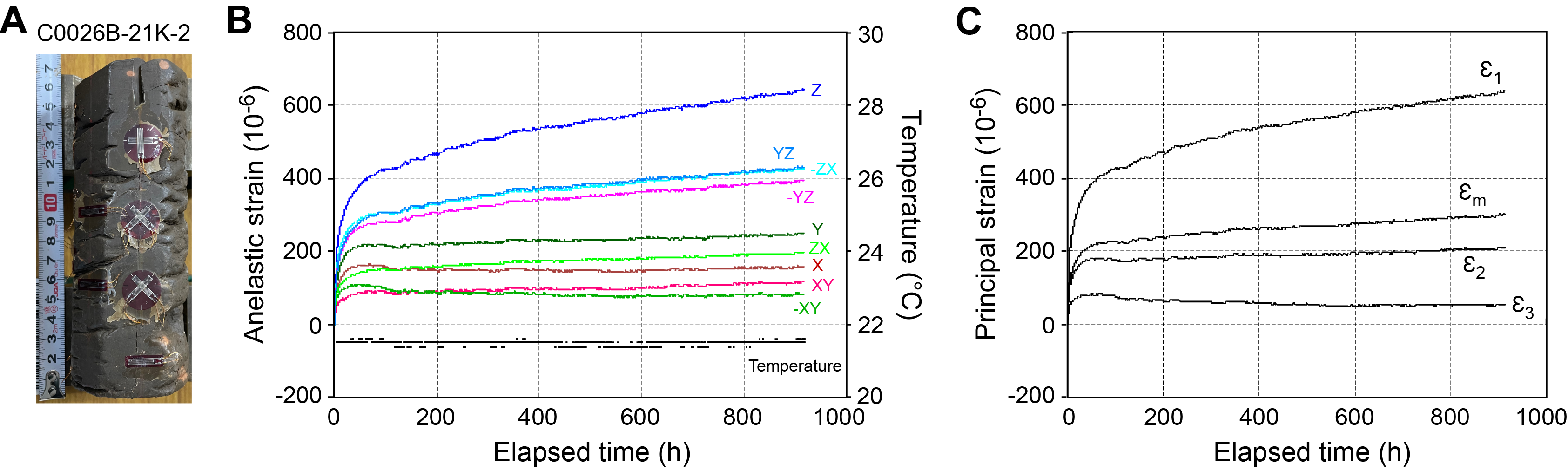
Figure F53. Anelastic strain recovery.
8.9. Formation temperature and heat flow
Formation temperature was measured in Holes C0026C–C0026E using the APCT-3 tool during HPCS coring operations (see Physical properties in the Expedition 405 methods chapter [Kirkpatrick et al., 2025a]). Four separate recording systems were prepared and cycled through for each core advance. One sensor (1858026C) was lost with the cutting shoe in Hole C0026D, a sensor failure occurred with Core 405-C0026E-6H due to water damage, and no sensor was installed for Core 9H (Table T18).
The temperature-time series recorded during the measurement for Cores 405-C0026D-1H, 405-C0026E-1H, and 2H were unstable (Figure F54). Other temperature measurements exhibit a clear frictional heating spike upon tool insertion, indicating that the tool successfully penetrated the sediment ahead of the drill bit. Data from Sensor 1858025C used for Core 6H could not be retrieved due to a water leakage issue with the cutting shoe. The exact time that this sensor began to be affected by water leakage could not be determined. Therefore, data from this sensor are excluded from all analyses, even though the time-series temperature measurements for Core 3H appear to be reliable.
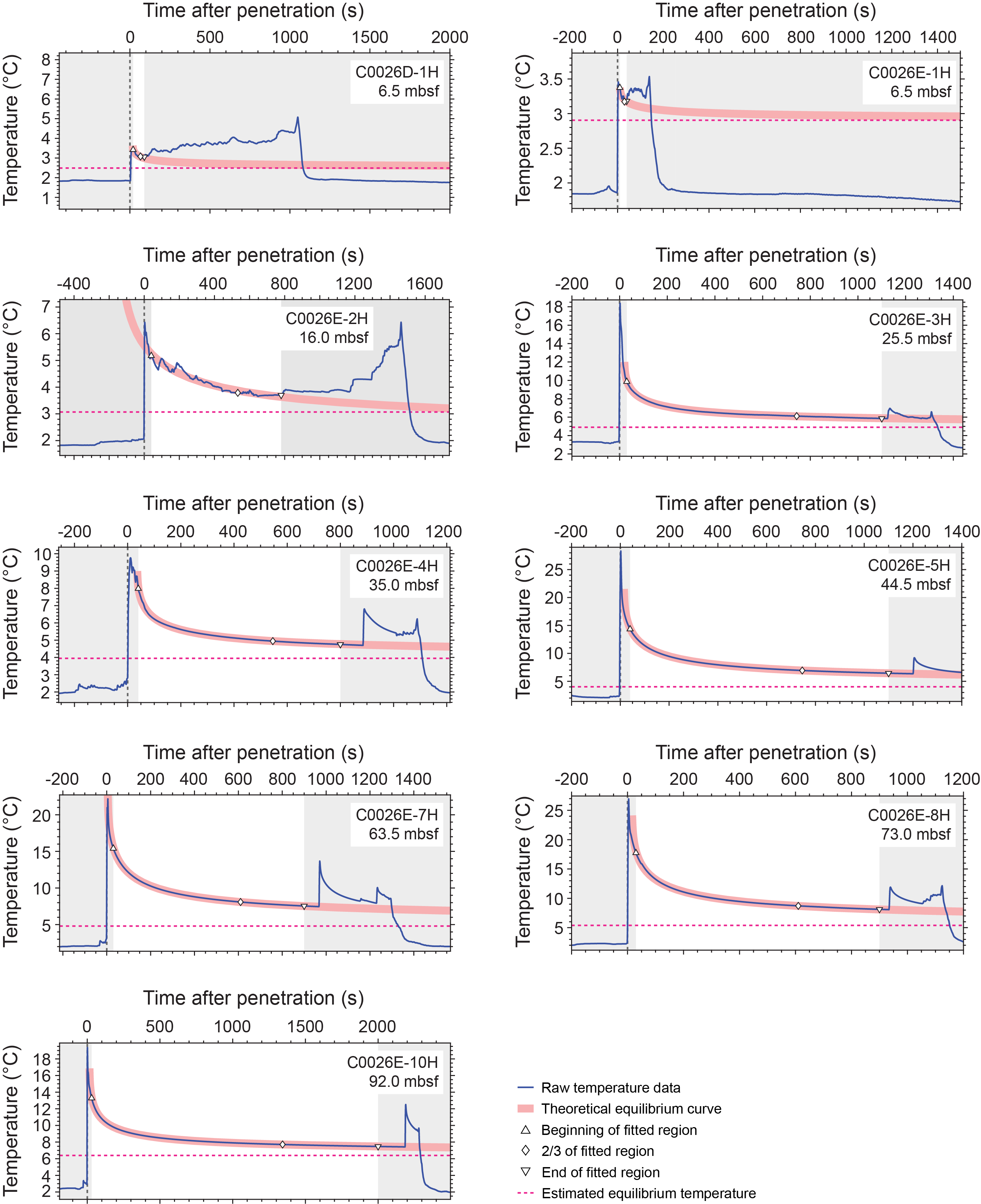
Figure F54. APCT-3 formation temperature measurements.
Equilibrium formation temperatures, estimated from the time-series temperature measurements, are plotted as a function of measurement depth in Figure F55. Inferred formation temperatures increase from about 2.5°C just below the seafloor to 6°C at about 90 mbsf. Using high-quality measurements taken during coring of Cores 405-C0026E-4H through 10H, the thermal gradient was calculated, yielding a value of 45.7°C/km for Hole C0026E. Because thermal conductivity remains relatively constant with depth (see Thermal conductivity), the average thermal conductivity of Cores 4H–10H (0.927 ± 0.179 W/[m·K]) over the depth interval (26.5–91.84 mbsf) was used to estimate the vertical conductive heat flow, resulting in a value of 42.37 ± 8.17 mW/m2.
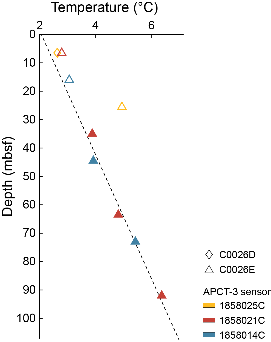
Figure F55. Estimated equilibrium formation temperatures.
9. Geochemistry
9.1. Interstitial water geochemistry
A total of 24, 32, and 6 interstitial water samples (IW) were extracted from the cores of Holes C0026B (81–278 mbsf), C0026D (0.4–5.7 mbsf), and C0026E (7.7–89 mbsf), respectively (the mbsf depth scale is equivalent to the CSF-A depth scale). Whole-round cores used for IW extraction were 5–15 cm in length, and the recovered IWs were generally 20–50 mL in volume, with a few exceptions, which is sufficient to examine detailed profiles of fluid chemistry over the length of the holes. To trace drilling fluid contamination in the collected IW, liquid from mud water (LMW) was collected while drilling (n = 7 samples), and liquid in the core liner (LCL) was also collected when available. These fluids were then analyzed along with the IW for comparison (Tables T19, T20). Methods used for IW sample analyses are described in Geochemistry in the Expedition 405 methods chapter (Kirkpatrick et al., 2025a).
9.1.1. Salinity, pH, and chlorinity
IW salinity is 34.6–36.0 near the seafloor in Hole C0026D (Table T19; Figure F56), which is consistent with, or higher than, the ambient seawater value (34.7 = LCL collected just above the mud line in Core 1H; hereafter, seawater value indicates the value for this LCL sample). With a few exceptions, the IW salinity remains at seawater-like values at greater depths, although there is a slight increase to 35.6 near the bottom of Hole C0026B. Salinities in the LMW are 34.60 ± 0.12 (1SD) in Hole C0026B and 34.56 in Hole C0026E. Salinities in the LCL are 34.09 ± 0.51, 34.67, and 34.56 ± 0.05 in Holes C0026B, C0026D, and C0026E, respectively (Table T20). The pH of the IW is 7.2 near the seafloor and increases to 7.9 at 19 mbsf. Below this depth, the pH gradually decreases to 7.0–7.4 near the bottom of the hole. The observed pH values tend to scatter below Lithostratigraphic Subunit 1C. The chlorinity of the IW is 549–552 mM near the seafloor and increases slightly to about 560 mM over the next 20 mbsf and then remains constant at about 552–563 mM to 240 mbsf. These chlorinity values are essentially consistent with the seawater value. Below 245 mbsf, where Lithostratigraphic Unit 2 dark brownish black clay dominates, IW chlorinity data scatter between 533 and 565 mM.
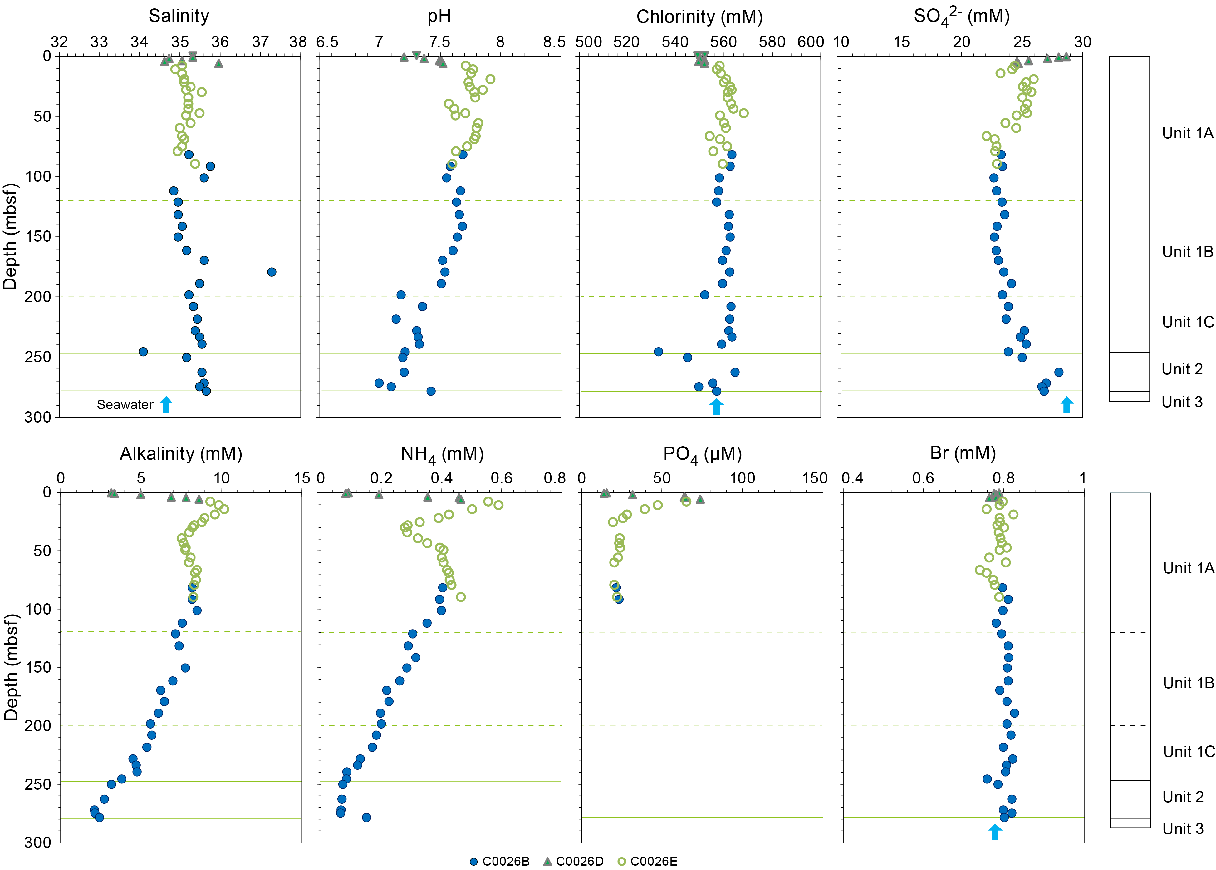
Figure F56. Dissolved chemical components in IW samples.
9.1.2. Sulfate and alkalinity
IW sulfate closest to the seafloor in Hole C0026D (0.4 mbsf) is 28.7 mM, which is consistent with the ambient seawater value of 28.8 mM. The sulfate value decreases rapidly with depth to 23 mM at 14 mbsf and then shifts to 26 mM at 19 mbsf (Figure F56). The rapid decrease in sulfate may be related to some sulfate reduction. Below this depth, the sulfate value decreases again gradually with depth to 23 mM at 70 mbsf and remains constant to 200 mbsf. Below 200 mbsf, the sulfate value increases slightly with depth, reaching seawater-like values of 26.7–28.1 near the bottom of Hole C0026B. IW alkalinity is 3.2 mM near the seafloor and increases rapidly with depth, reaching a maximum of 10.2 mM at 14 mbsf. IW alkalinity then gradually decreases toward the bottom of the hole to 2–3 mM, with a small minimum of 7.6 mM at 39 mbsf. The IW sulfate and alkalinity values observed at Site C0026 are very high and low, respectively, compared with those observed at corresponding depths at Site C0019, except for the shallowest part (Figure F57). This is presumably due to limited microbial sulfate reduction at Site C0026, as previously reported for deep-sea sediments in the open ocean with relatively low organic matter content and low sedimentation rates (Canfield, 1991).
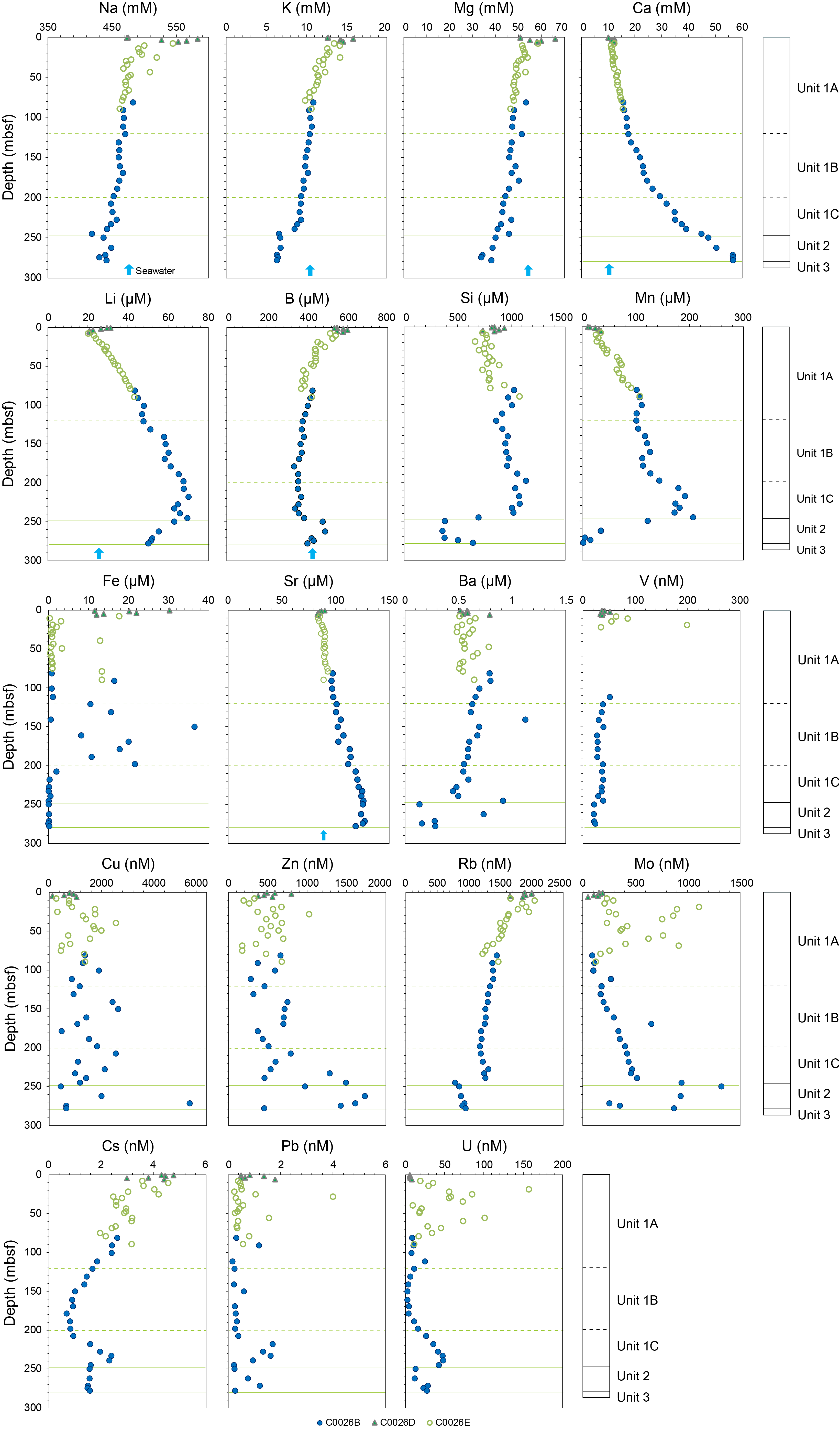
Figure F57. Major, minor, and trace element concentrations in IW samples.
9.1.3. Ammonium, phosphate, and bromide
The IW ammonium concentration closest to the seafloor in Hole C0026D is as low as 0.09 mM, increases rapidly with depth to a maximum of 0.6 mM at 11 mbsf, and then decreases rapidly to a minimum of 0.3 mM at 30 mbsf (Figure F56). Below this depth, the IW ammonium concentration gradually increases to 0.4 mM at 80 mbsf and then decreases to <0.1 mM toward the bottom of Hole C0026B. This depth profile of IW ammonium correlates well with that of alkalinity. The IW phosphate concentration closest to the seafloor is 15.7 µM, increasing rapidly to 74 µM at 6 mbsf and then decreasing to 19 mM at 25 mbsf. Below this depth, the phosphate value remains constant at 20–23 µM to 90 mbsf and decreases to below the detection limit (in this case, typically <15 µM) at greater depths. IW bromide concentrations show almost constant seawater-like values of about 0.8 mM at all depths. The IW ammonium values at site C0026 are very low compared with those at corresponding depths at Site C0019, except for the shallowest part (Figure F57), again likely due to limited microbe-induced diagenetic reactions.
9.1.4. Major cations (Na, K, Mg, and Ca)
IW sodium (Na), potassium (K), and magnesium (Mg) concentrations near the seafloor in Hole C0026D show relatively scattered values (473–583, 12.6–15.8, and 51.4–64.0 mM, respectively) from seawater-like values to higher values (Figure F57). These IW Na, K, and Mg values converge to seawater-like values at 10–30 mbsf and gradually decrease with depth. At 240 mbsf near the Subunit 1C/Unit 2 boundary, the IW K concentration decreases significantly from 8.5 to 6.6 mM, possibly reflecting K uptake into the Unit 2 dark brownish black clay during fluid-sediment interactions. The IW Na concentration also appears to vary more below this depth. The IW Mg concentration does not exhibit a sharp change at the Subunit 1C/Unit 2 boundary, showing a monotonic decrease from near-seawater values at 10 mbsf to ~34 mM toward the bottom of Hole C0026B.
IW calcium (Ca) concentrations have seawater-like values of 10.0–12.3 mM near the seafloor in Hole C0026D, which increase monotonically with depth (Figure F57). Near the bottom of Hole C0026B, the Ca concentration reaches high values of about 57 mM.
9.1.5. Minor elements (Li, B, Si, Mn, Fe, Sr, and Ba)
IW lithium (Li) and boron (B) concentrations near the seafloor in Hole C0026D are higher than those of ambient seawater: 25.8 and 428 µM, respectively (Figure F57). IW Li values decrease from 31 µM at 0.4 mbsf to 20 µM at 7.7 mbsf and then increase monotonically with depth to 70 µM at 218 mbsf. Below this depth, IW Li values decrease toward the bottom of the hole throughout Lithostratigraphic Subunit 1C and Unit 2. IW B concentrations are 548–600 µM at <5 mbsf and decrease with depth to 340 µM at 230 mbsf, although systematically low B values are present between 55 and 79 mbsf in Hole C0026E. In the deepest interval corresponding to Lithostratigraphic Unit 2 in Hole C0026B, two IWs show high B concentrations of >470 µM, which may be related to fluid-sediment interactions in the dark brownish black clays.
IW Silica (SiO2) concentrations, expressed here as Si concentrations, increase with depth with some fluctuations from 730–930 µM at <15 mbsf to 1000–1130 µM at 200–240 mbsf (Figure F57). Below this depth, IW Si concentrations decrease abruptly to 360 µM, suggesting Si uptake into solid phases during interactions with Lithostratigraphic Unit 2 sediments. Si values increase again to 640 µM in the lowermost part of Unit 2.
IW manganese (Mn) and iron (Fe) concentrations show very large variations. The IW Mn concentration near the seafloor in Hole C0026D is 10.5 µM. The Mn value increases rapidly with depth, with some fluctuations, to reach 190 µM at 218 mbsf (Figure F57). Although the IW Mn value remains relatively high at 170–210 µM in Lithostratigraphic Subunit 1C, it decreases dramatically into Unit 2 to 1.4 µM near the bottom of Hole C0026B. This marked decrease in IW Mn in Unit 2 can be explained by the uptake of Mn into the Fe-Mn oxide phases present in this unit (see Lithostratigraphy). The IW in Unit 2 is also depleted in Fe to <0.18 µM, suggesting a control by Fe-Mn oxide phases. However, IW Fe values are also very low at <2 µM in Subunit 1C, in contrast to the case of IW Mn. Below 200 mbsf (Subunits 1A and 1B), IW Fe values are highly scattered between 0.3 and 36 µM.
IW Strontium (Sr) concentrations increase nearly monotonically with depth from 83–90 µM at <5 mbsf to 120–130 µM near the bottom of Hole C0026B (Figure F57). IW barium (Ba) concentrations show relatively stable values between 0.5 and 0.8 µM throughout Lithostratigraphic Unit 1, with a few exceptions. However, IW Ba values vary between 0.1 and 0.9 µM in Unit 2.
9.1.6. Trace elements (V, Cu, Zn, Rb, Mo, Cs, Pb, and U)
IW Vanadium (V) is relatively constant between 34 and 52 nM in Hole C0026D at <6 mbsf but highly variable between 35 and 200 nM at 8–22 mbsf in Hole C0026E (Figure F57). Below that, V values are all below the detection limit to 110 mbsf. Between 111 and 278 mbsf in Hole C0026B, V values range 21–52 nM, and the lowest values are observed in Unit 2 at >246 mbsf.
IW copper (Cu) shows scattered values of 110–2600 nM but averages remain relatively constant throughout Units 1 and 2, except for a spike of 5400 nM at 271 mbsf in Unit 2 (Figure F57). Zinc (Zn) also shows scattered values, but with a relatively constant range of 170–1000 nM above 230 mbsf. Below this depth, however, high Zn values of 1300–1700 nM also occur in Subunit 1C and Unit 2.
The IW rubidium (Rb) concentration is 2,000 nM near the seafloor and gradually decreases to 1200 nM at 79 mbsf (Figure F57). The Rb value shows a positive offset to 1400 nM at 81 mbsf, followed by a gradual decrease with depth to 1200 nM at 198 mbsf and then a slight increase to 1300 nM at 239 mbsf. Near the base of Subunit 1C at 245 mbsf, the Rb value abruptly decreases to 780 nM and then increases with depth in Unit 2 to 950 nM near the bottom of Hole C0026B. A similar depth profile, but with higher amplitudes, is observed for cesium (Cs). The Cs data show a more pronounced minimum near the Subunit 1B/1C boundary compared to Rb. IW Cs remains nearly constant at 1.5–1.6 nM throughout Unit 2 after a sharp decrease near the base of Subunit 1C. The significant decrease in Rb and Cs observed in Unit 2 may reflect uptake into the brownish black clay during fluid-sediment interactions, similar to K.
IW molybdenum (Mo) ranges 48–190 nM in Hole C0026D above 6 mbsf (Figure F57). Below this depth, Mo values are highly variable from 170 to 1100 nM to 79 mbsf. Below 81 mbsf, Mo increases steadily with depth from 88 to 520 nM with a few spikes toward the base of Subunit 1C. Near the base of Subunit 1C at 245 mbsf, Mo jumps to 940 nM and then varies between 250 and 1,300 nM in Unit 2.
IW lead (Pb) concentrations range 0.2–1.8 nM throughout Units 1 and 2, except for one spike of 4.0 nM at 28 mbsf (Figure F57). Uranium (U) shows scattered values between 5.3 and 160 nM in Subunit 1A. Below this depth, a continuous trend with depth characterized by a minimum of 2.5 nM at 150 mbsf in Subunit 1B and a maximum of 48 nM at 239 mbsf in Subunit 1C is observed. U values in Unit 2 range 12–29 nM after dropping near the Subunit 1C/Unit 2 boundary.
9.2. Gas chemistry
9.2.1. Hydrocarbon gases in headspace samples
Concentrations of hydrocarbon gases in headspace samples collected from Holes C0026B–C0026E are summarized in Table T21 and Figure F58. Methane concentrations are 4–8 ppm between 6 and 230 mbsf and decrease with depth to 2 ppm near the bottom of Hole C0026B. Ethane, propane and n-butane are all below detection limits at all depths. The methane concentrations observed are two to three orders of magnitude lower than those at corresponding depths at Site C0019, except for the shallowest part, where sulfate values are still elevated (Figure F59). This is consistent with the limited microbial activity suggested by the IW data for sulfate, alkalinity, and ammonium.
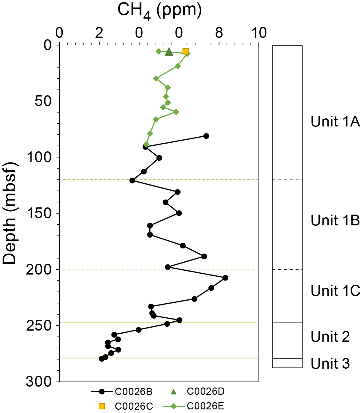
Figure F58. Methane concentration in headspace gas samples.
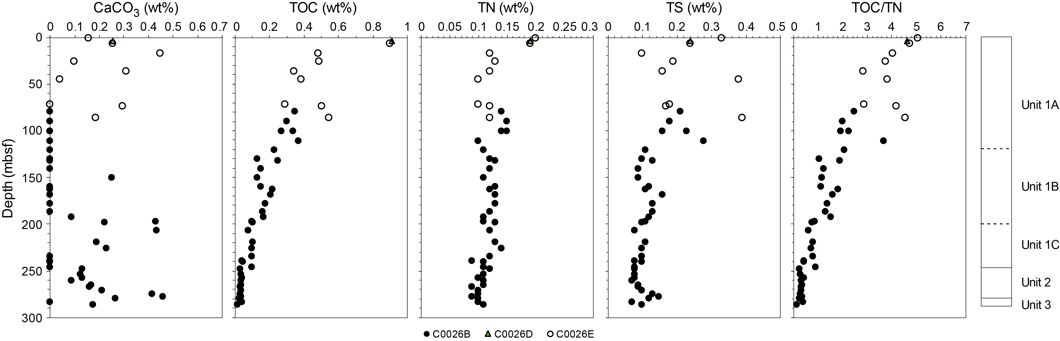
Figure F59. CaCO3, TOC, TN, and TS contents and TOC/TN ratio, Site C0026.
9.2.2. Carbon, nitrogen, and sulfur concentrations
Calcium carbonate (CaCO3), total organic carbon (TOC), total nitrogen (TN), and total sulfur (TS) contents are presented in Table T22 and Figure F59. Calcium carbonate content throughout the profile is consistently below 0.5 wt%, with samples from 72–187 mbsf and 235–246 mbsf mostly below the detection limit. TOC contents are generally low, ranging 0.02–1 wt%, and exhibit a general decreasing trend with depth. However, TOC in Lithostratigraphic Unit 2 remains relatively constant around 0.04 wt%, with a few exceptions. TN values primarily fluctuate between 0.09 and 0.15 wt%, except for the first three samples shallower than 7 mbsf, which show relatively high values of about 0.2 wt%. TS contents are all below 0.5 wt%, with greater variability observed in Subunit 1A, whereas samples from other units range 0.07–0.16 wt%. The TOC/TN ratio follows a trend similar to the TOC profile, suggesting that TOC fluctuations predominantly control the TOC/TN ratio throughout the profile. However, in Lithostratigraphic Subunit 1C, the ratio shows a slight increasing trend, reaching a peak of 0.9 at 246 mbsf before declining to 0.17 toward the bottom of the hole.
10. Microbiology
10.1. Sampling
Whole-round core samples for microbiological studies were obtained from Site C0026 using the SD-RCB coring system (Hole C0026B) and HPCS (Holes C0026D and C0026E). A total of 7 whole-round core, 24 IW squeezed cake, 5 drilling fluid (LMW), and 15 liner fluid (LCL) samples were obtained from Hole C0026B. A total of 1 whole-round core, 6 IW squeezed cake, and one LCL samples were obtained from Hole C0026D. A total of 1 whole-round core, 20 IW squeezed cake, 2 LMW, and 4 LCL samples were obtained from Hole C0026E.
10.2. Subsampling in an anaerobic chamber
Because no microbiologist was on board during the Window 2 period, the samples obtained during that period were processed using the minimized subsampling procedure described in Microbiology in the Expedition 405 methods chapter (Kirkpatrick et al., 2025a).
11. Core-log-seismic integration
11.1. Log-seismic tie
A seismic-well tie was established using the real-time Leaky-P wave velocity data obtained by LWD (see Logging while drilling) and Seismic Profile HDMY001 (high-resolution poststack time migrated profile acquired with a small source array) (Table T23). Initially, the time-domain synthetic seismogram and time-converted log data were bulk-shifted to match the mudline of the gamma ray log to the seafloor reflection of the seismic profile. After that, the reflection from the top of the chert layer and another prominent reflection in the Seismic Unit 2 sediments at ~9315 ms two-way traveltime (TWT) were used to stretch and squeeze the time-domain synthetic seismograms and log curves. Figure F60 shows the results of the seismic-well ties at Site C0026. The stretch-squeeze adjustment was quite small (e.g., <2 ms at the top of the chert). In the shallow part, between the seafloor and ~9250 ms TWT, the correspondence between the synthetic seismogram and seismic profile is poor. A series of relatively strong reflections were synthesized by the logging data between ~9175 and 9225 ms; however, those two-way traveltimes (or depths) did not coincide with the corresponding reflections in the seismic profiles. We did not adjust the reflections within the chert layer; however, most of the reflections in the synthetic seismograms were well correlated with the seismic data within this interval. The log-seismic tie was not established in the basalt layer. The LWD P-wave velocities (VP) obtained from monopole high frequency signal analysis were used to build a composite P-wave velocity curve at the bottom of Unit 3 and for all of Unit 4. However, the velocities were highly scattered in Unit 4, which could cause unrealistic synthetic reflections. Considering the P-wave velocity data in Unit 4 (basalt), we only established the log-seismic tie to near the bottom of Unit 3 (chert).
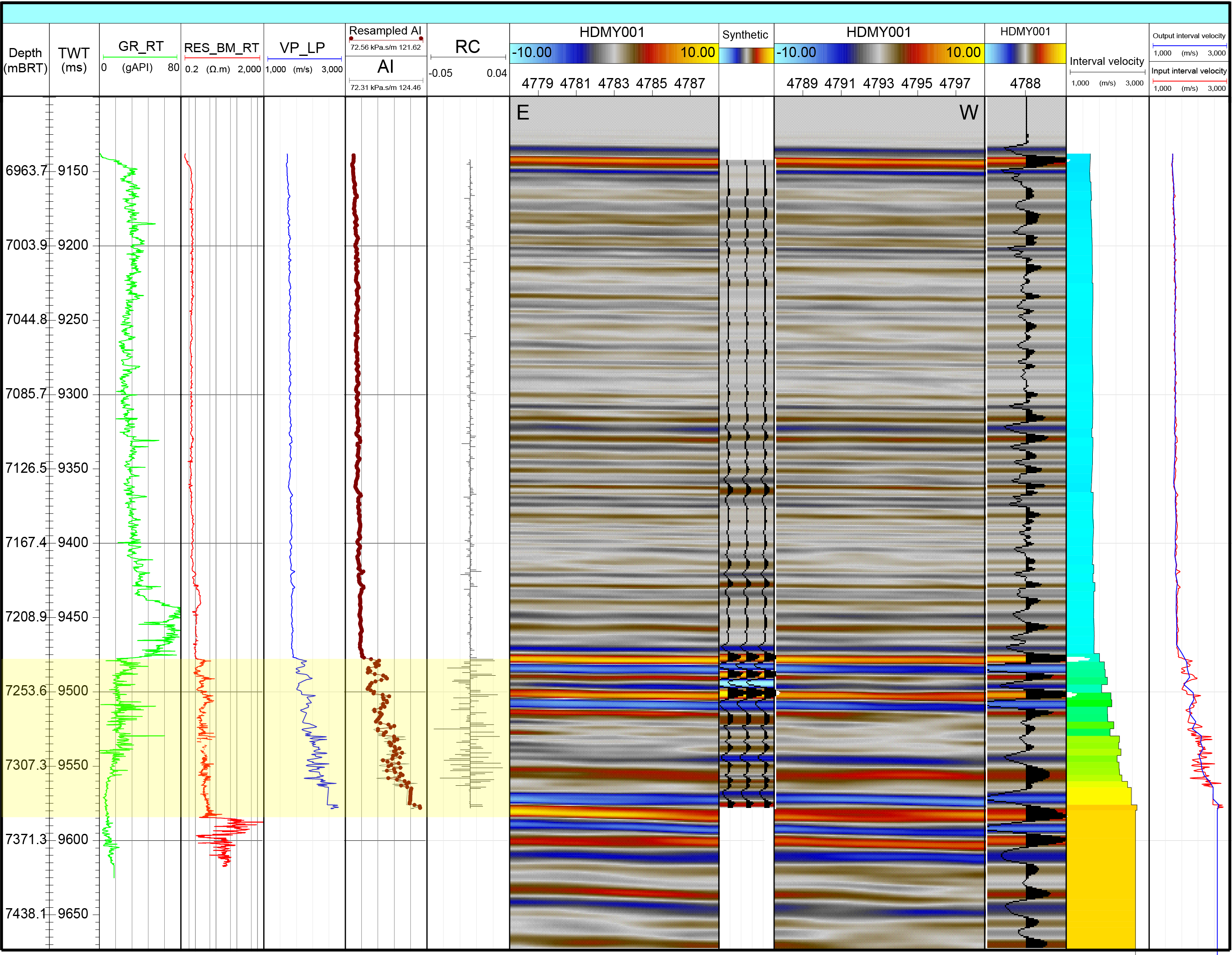
Figure F60. Seismic-well tie for high-resolution Seismic Line HDMY001.
11.2. Core-log integration and comparison
Core-log integration relies on the correlation between the physical properties recorded by LWD for Hole C0026A (see Logging while drilling in the Expedition 405 methods chapter [Kirkpatrick et al., 2025a]) and physical properties measured on the discrete samples and recorded by the COMET for Holes C0026B and C0026E (see Physical properties in the Expedition 405 methods chapter [Regalla et al., 2025a]). The correlation relied on the comparison of major NGR (Figure F61), electrical resistivity features (Figure F62), and P-wave velocity (Figure F63). Hole C0026A (LWD) was drilled to 7405.0 m BRT (448.0 mbsf), whereas Hole C0026B (coring) was only drilled to 7246 m BRT (290.0 mbsf). Therefore, data obtained from LWD and coring can only be compared to 7246 m BRT.
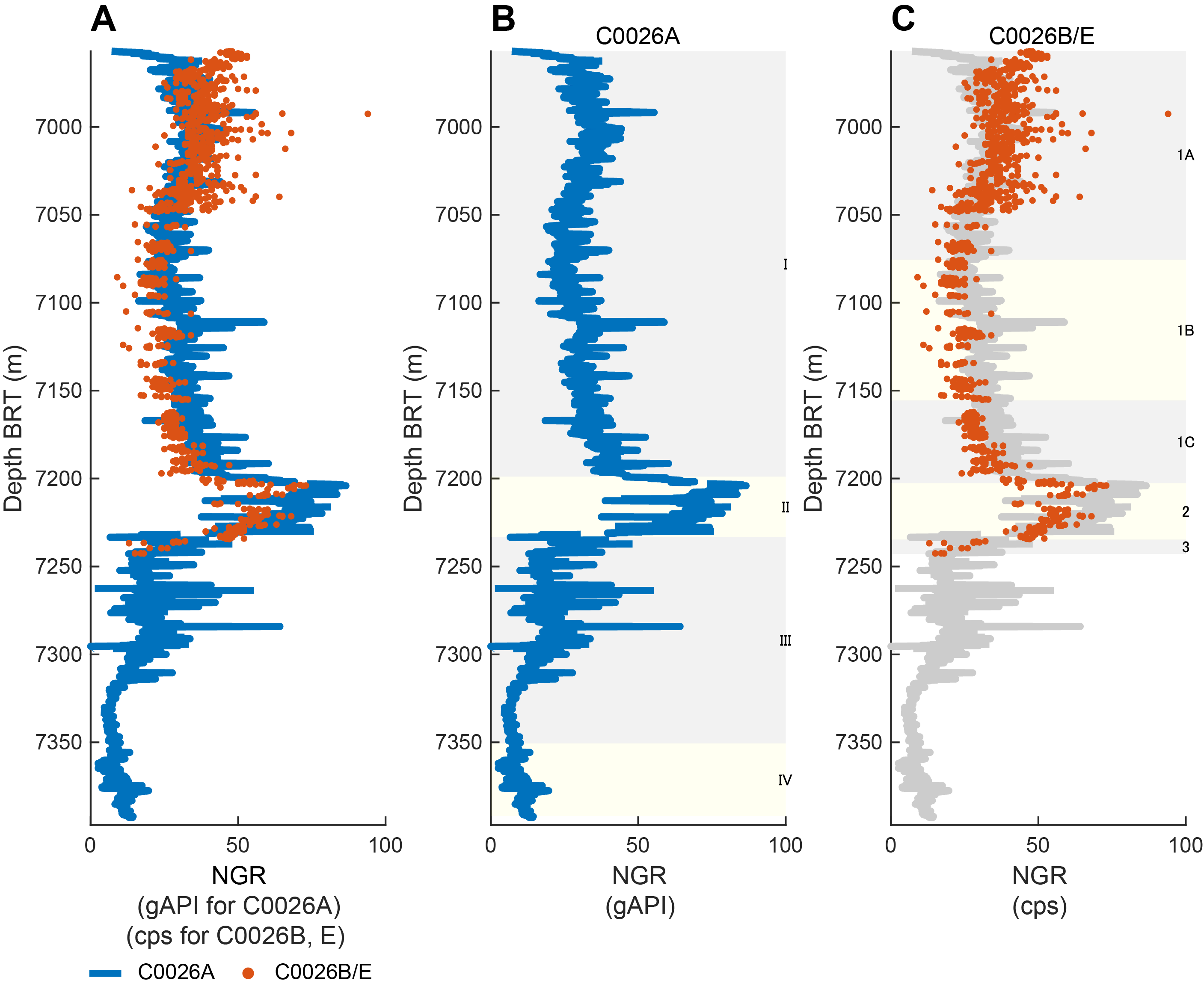
Figure F61. LWD gamma ray data and COMET gamma ray profiles.
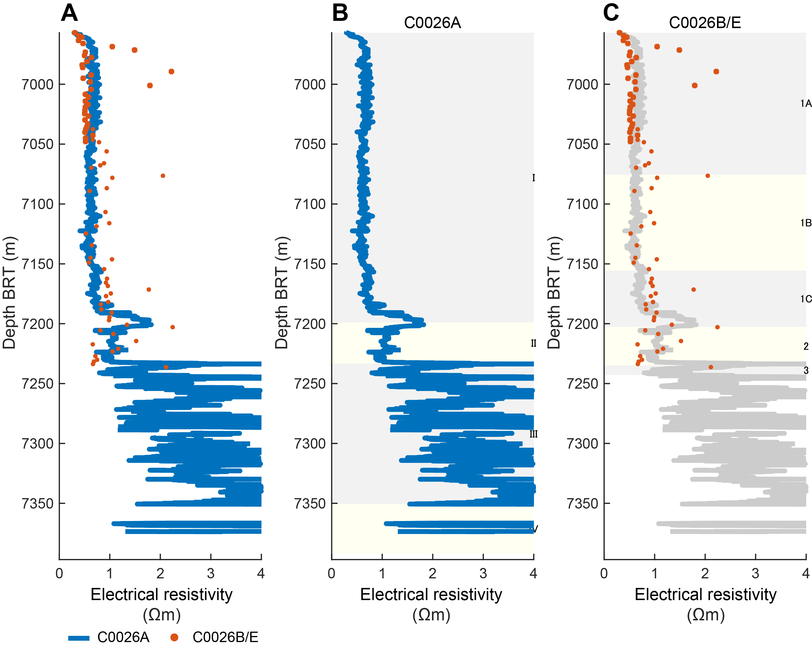
Figure F62. LWD electrical resistivity data and core and discrete sample resistivity.
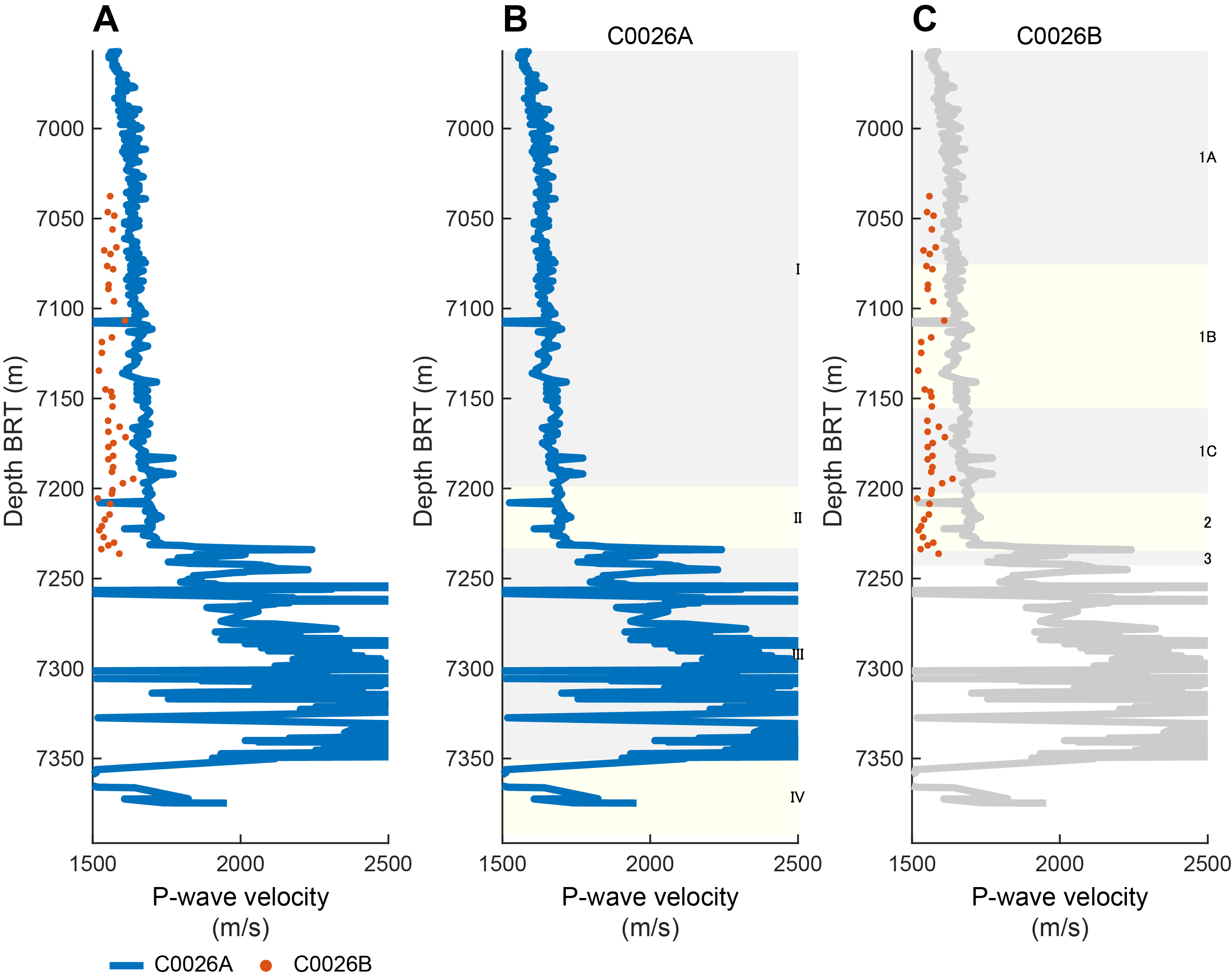
Figure F63. LWD P-wave velocity data and P-wave velocity measured on discrete core samples.
The NGR profiles for Holes C0026A, C0026B, and C0026E are very similar (Figure F61). In particular, high NGR values from around 7197 m BRT (240 mbsf) to around 7227 m BRT (270 mbsf) are observed in both LWD (Logging Unit II) and COMET measurements (Lithostratigraphic Unit 2), indicating a close correspondence. At very shallow depths (10 mbsf and shallower), the gamma ray signal strength increases with depth in Hole C0026A, whereas it decreases in Holes C0026B and C0026E. This discrepancy is likely due to the wash-down operation at the beginning of the LWD at Hole C0026A. The shallowest formation near the seafloor may have been disturbed or eroded, and the borehole may have been enlarged. As a result, the measured gamma ray values may have been smaller than the actual values of the formation. At greater depths below approximately 10 mbsf, the effect of jetting is reduced and the gamma ray values become more consistent with those measured on cores.
The electrical resistivity values are consistent for the LWD data from Hole C0026A and the discrete and section data measured from Hole C0026B and C0026E cores (Figure F62). The resistivity was measured in two (y- and z-) or three (x-, y-, and z-) directions for the core section or discrete samples, but for comparison with the log, the resistivity in the y-direction perpendicular to the drilling direction was used. The electrical resistivity values measured on the surface of the core sections in the 6957–7047 m BRT (0–90 mbsf) interval are in good agreement with the values obtained by LWD. Although there are outliers with very high values in this interval, the outliers are unlikely to reflect any significant change to the formation properties (see Physical properties). The values measured on the discrete samples in the 7047–7237 m BRT (90–280 mbsf) interval are also in good agreement with the LWD values, although the discrete sample values are larger. LWD shows high resistivity at the bottom of Logging Unit I and then steps down at the top of Logging Unit II. The discrete samples also show high values of resistivity at the boundary between Lithostratigraphic Units 1 and 2 but over a wider depth range, and the change is not as sharp as in the LWD data.
Figure F63 shows the elastic velocities obtained from Hole C0026A (LWD) and shipboard discrete sample measurements from Hole C0026B. The elastic velocities were measured in three (x-, y-, and z-) directions for the discrete samples, but for comparison with the log, only the elastic velocities in the z-direction parallel to the drilling direction was used. Detailed correlation between Holes C0026A (LWD) and C0026B (SD-RCB coring) is challenging because most of the velocities from sample measurements were systematically lower than those from LWD. This could be caused by different pressure conditions during the measurements (i.e., discrete samples were measured unconfined at atmospheric pressure) or the different frequency range used to measure the elastic velocities (the LWD tool uses waves in the kilohertz band; shipboard discrete sample measurements were made in the megahertz band). The P-wave velocity data from Leaky-P analysis (VP_LP) using LWD steadily increases with depth, whereas the P-wave velocity measured from sample cubes does not show a significant increase with depth. However, there are some areas where the P-wave velocity increases locally. The P-wave velocity increases at around 7097–7117 m BRT (140–160 mbsf) in the middle part of Lithostratigraphic Subunit 1B, 7187–7197 m BRT (230–240 mbsf) in the bottom part of Subunit 1C, and 7237 m BRT (280 mbsf) at the top of Unit 3 in both LWD data and discrete samples. The P-wave velocities obtained from a discrete sample of chert at 283.8 mbsf (7239.8 m BRT) is >4 km/s. The strong reflection at the interpreted top of the chert layer on the seismic profile is likely caused by the large acoustic impedance contrast between Lithostratigraphic Units 2 and 3.
The orientations of bedding and fractures at Site C0026 were determined through a process of data interpretation, utilizing both real-time data from the LWD resistivity images and visual observations of core samples. During LWD operations in Hole C0026A, the tool could not be recovered, resulting in the absence of memory data and the acquisition of only real-time data. Consequently, the data quality is low, and image artifacts and missing sections are prevalent throughout the image logs, impeding interpretation (see Logging while drilling). Figure F64 shows the orientations of bedding and fractures/faults obtained from the LWD resistivity images (Hole C0026A) and those measured based on the core description of the recovered cores (Holes C0026B and C0026E). Although the number of features picked in the LWD resistivity images is small, the results of structural analysis generally show similar dips at the equivalent depth intervals to the core-based measurements, with predominantly low-angle (<30°) bedding and few fractures or faults, which suggests good correlation between the logging and core-based results.
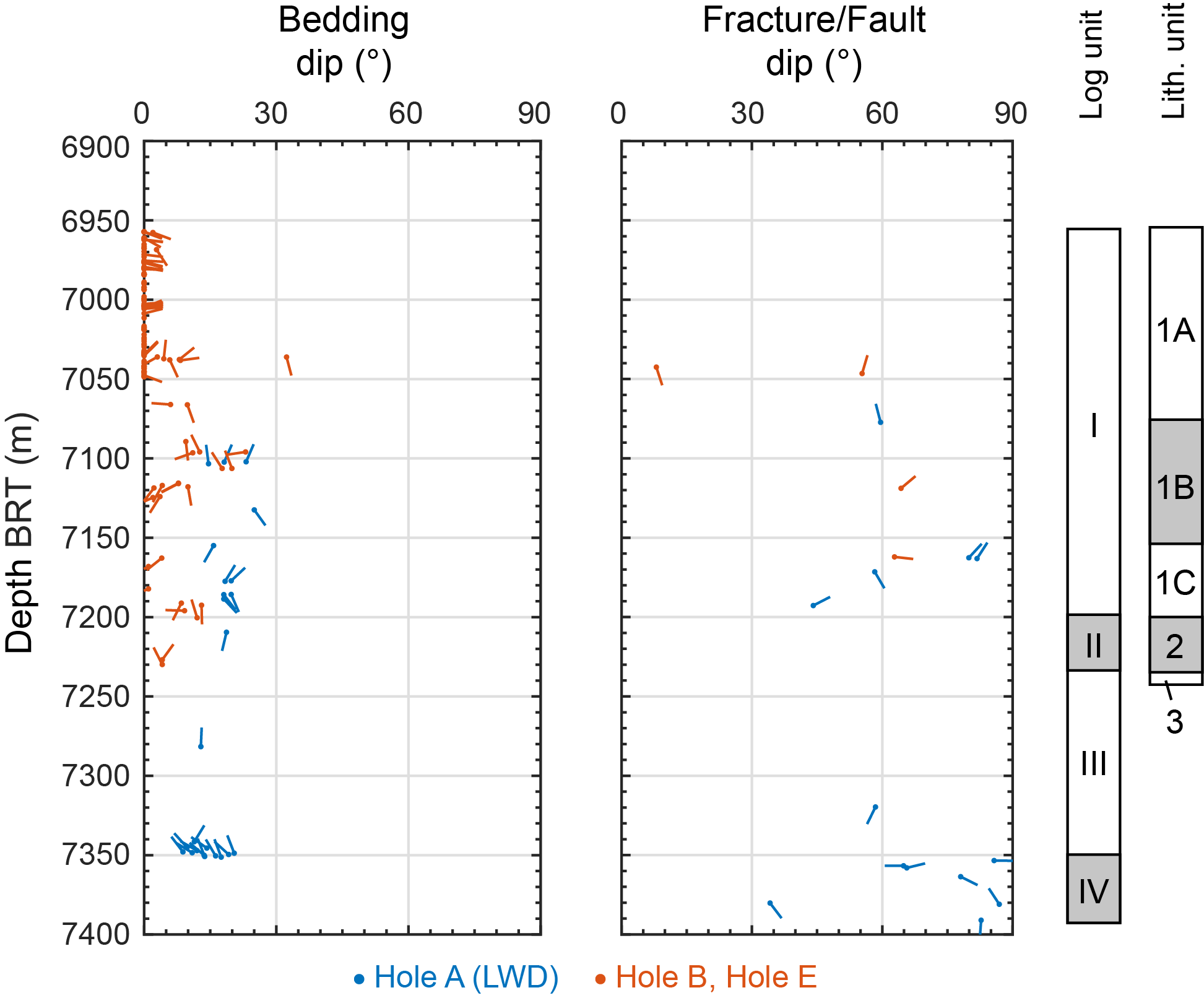
Figure F64. Dip data of planar structures, fractures, and faults (core).
11.3. Core-seismic integration and comparison
Figure F65 illustrates the time-domain seismic cross section (Seismic Profile HDMY001) and the comparison between the seismic, logging, and lithostratigraphic units, delineated based on the descriptions of the LWD real-time data and core samples. The center blue line indicated the location of Site C0026. The lithostratigraphic units are as follows: Subunit 1A (0–119.5 mbsf; 6956–7075.5 m BRT) is characterized by an olive-black siliceous vitric mud, Subunit 1B (119.5–199.585 mbsf; 7075.5–7155.59 m BRT) displays an olive-gray siliceous vitric mud, Subunit 1C is identified by transition of dull yellowish brown siliceous mud, Unit 2 (244.05–278.68 mbsf; 7155.59–7200.05 m BRT) is characterized by the presence of brownish black clay, and Unit 3 (278.68–286.89 mbsf; 7234.58–7242.89 m BRT) is distinguished by the occurrence of color-banded clay and chert (see Lithostratigraphy).
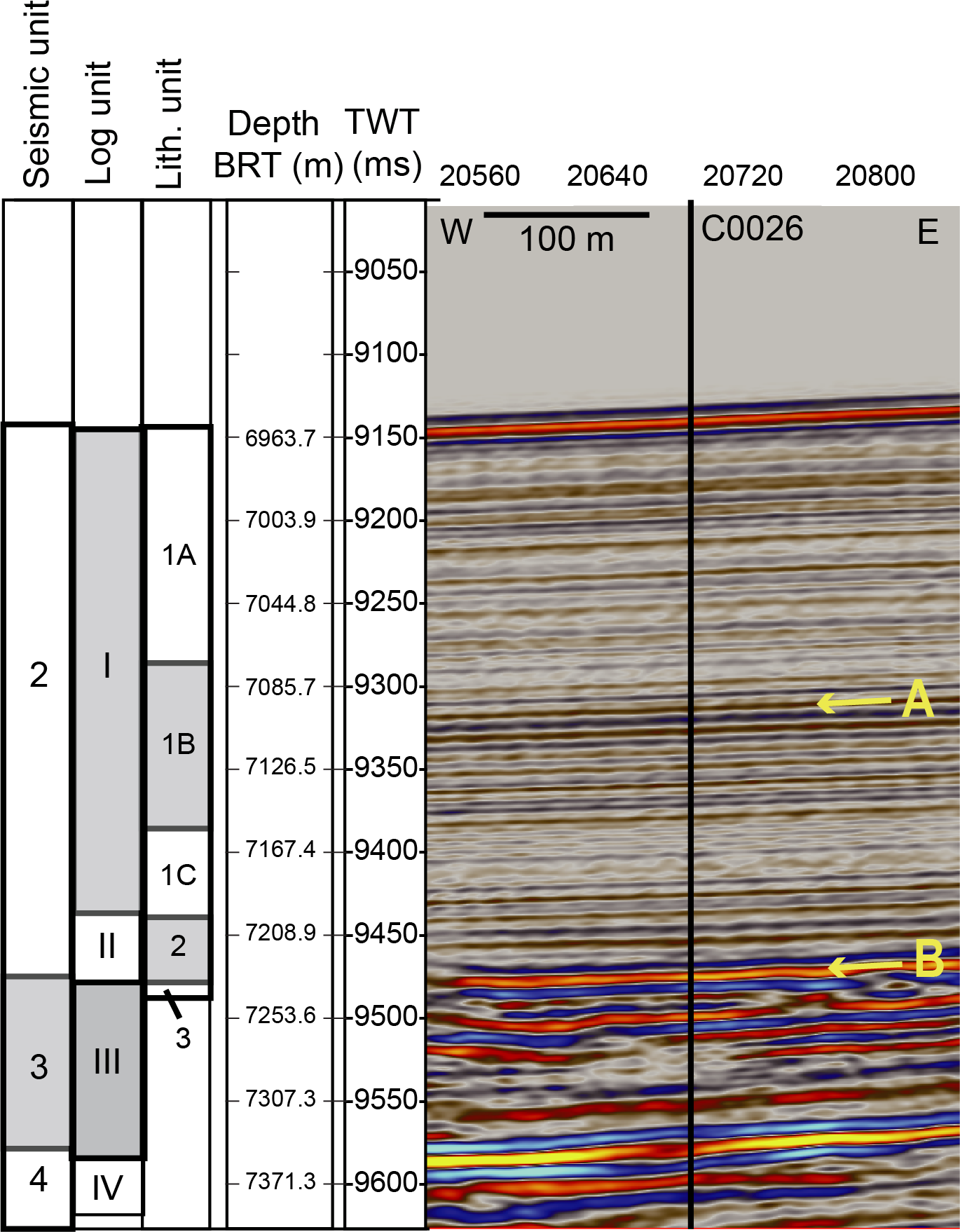
Figure F65. Seismic profile in two-way traveltime section.
The boundary between Lithostratigraphic Units 2 and 3 in the lower part of the coring interval occurs at a very similar depth to the strong reflector labeled (B), the boundary between Seismic Units 2 and 3, in Figure F65 at 275.14 mbsf (7231.14 m BRT). This reflector is considered to be a consequence of the contrasting physical properties between clay-rich sediments of Lithostratigraphic Unit 2 and chert in Lithostratigraphic Unit 3 (see Physical properties and Logging while drilling). This is demonstrated by the clear shift in the logging trend at the same depth, which defines the boundary between Logging Units II and III (276.3 mbsf; 7233.3 m BRT).
Similarly, a relatively strong reflector is also identified at the boundary between Lithostratigraphic Subunits 1B and 1C and between Subunit 1C and Unit 2. Notably, Lithostratigraphic Subunit 1B and Unit 2 display a series of relatively high-amplitude reflections in the seismic section, whereas Subunit 1C is characterized by the absence of strong reflections. However, no discernible signals are observed in the seismic structure at the boundary between Lithostratigraphic Subunits 1A and 1B. This trend is also seen in the comparison of the physical properties of LWD and physical properties measured on core samples (Figures F62, F63, F64). In contrast, the seismic reflection observed near 141 mbsf (7098 m BRT; labeled A in Figure F65) cannot be attributed to significant differences in lithology. Differences between Lithologic Subunits 1A and 1B in the core observations were subtle and based largely on color rather than pronounced changes in sediment composition (see Lithostratigraphy), which may explain the lack of a clear signal in the logging data at the boundary between them. Such discrepancies between the seismic reflection profile and core observation may also be indicative of the volume ratio of the volcanic ash layer, among other factors (see Lithostratigraphy). However, the recovery of Cores 405-C0026B-7K and 8K obtained at this depth was low, raising the possibility that the key sediments (e.g., ash layers) were not recovered.
References
Acton, G.D., Okada, M., Clement, B.M., Lund, S.P., and Williams, T., 2002. Paleomagnetic overprints in ocean sediment cores and their relationship to shear deformation caused by piston coring. Journal of Geophysical Research: Solid Earth, 107:2067–2081. https://doi.org/10.1029/2001JB000518
Akiba, F., 1986. Middle Miocene to Quaternary diatom biostratigraphy in the Nankai Trough and Japan Trench, and modified lower Miocene through Quaternary diatom zones for middle-to-high latitudes of the North Pacific. In Kagami, H., Karig, D.E., Coulbourn, W.T., et al., Initial Reports of the Deep Sea Drilling Project, 87: Washington, DC (US Government Printing Office), 393–481. https://doi.org/10.2973/dsdp.proc.87.106.1986
Alken, P., Thébault, E., Beggan, C.D., Amit, H., Aubert, J., Baerenzung, J., Bondar, T.N., Brown, W.J., Califf, S., Chambodut, A., Chulliat, A., Cox, G.A., Finlay, C.C., Fournier, A., Gillet, N., Grayver, A., Hammer, M.D., Holschneider, M., Huder, L., Hulot, G., Jager, T., Kloss, C., Korte, M., Kuang, W., Kuvshinov, A., Langlais, B., Léger, J.M., Lesur, V., Livermore, P.W., Lowes, F.J., Macmillan, S., Magnes, W., Mandea, M., Marsal, S., Matzka, J., Metman, M.C., Minami, T., Morschhauser, A., Mound, J.E., Nair, M., Nakano, S., Olsen, N., Pavón-Carrasco, F.J., Petrov, V.G., Ropp, G., Rother, M., Sabaka, T.J., Sanchez, S., Saturnino, D., Schnepf, N.R., Shen, X., Stolle, C., Tangborn, A., Tøffner-Clausen, L., Toh, H., Torta, J.M., Varner, J., Vervelidou, F., Vigneron, P., Wardinski, I., Wicht, J., Woods, A., Yang, Y., Zeren, Z., and Zhou, B., 2021. International Geomagnetic Reference Field: the thirteenth generation. Earth, Planets and Space, 73(1):49. https://doi.org/10.1186/s40623-020-01288-x
Barron, J.A., Harper, H.E., Jr., Keller, G., Reynolds, R.A., Sakai, T., Shaffer, B.L., and Thompson, P.R., 1980. Biostratigraphic summary of the Japan Trench transect, Legs 56 and 57, Deep Sea Drilling Project. In Scientific Party, Initial Reports of the Deep Sea Drilling Project, 56, 57, Part 1: Washington, DC (US Government Printing Office), 505–520. https://doi.org/10.2973/dsdp.proc.5657.113.1980
Brothers, R.J., Kemp, A.E.S., and Maltman, A.J., 1996. Mechanical development of vein structures due to the passage of earthquake waves through poorly-consolidated sediments. Tectonophysics, 260(4):227–244. https://doi.org/10.1016/0040-1951(96)00088-1
Canfield, D.E., 1991. Sulfate reduction in deep-sea sediments. American Journal of Science, 291(2):177–188. https://doi.org/10.2475/ajs.291.2.177
Carson, B., and Bruns, T.R., 1980. Physical properties of sediments from the Japan Trench margin and outer trench slope: results from Deep Sea Drilling Project Legs 56 and 57. In Scientific Party, Initial Reports of the Deep Sea Drilling Project, 56, 57, Pt. 2: Washington (U.S. Government Printing Office), 1187–1199. https://doi.org//10.2973/dsdp.proc.5657.151.1980
Chester, F.M., Rowe, C., Ujiie, K., Kirkpatrick, J., Regalla, C., Remitti, F., Moore, J.C., Toy, V., Wolfson-Schwehr, M., Bose, S., Kameda, J., Mori, J.J., Brodsky, E.E., Eguchi, N., and Toczko, S., 2013. Structure and composition of the plate-boundary slip zone for the 2011 Tohoku-Oki earthquake. Science, 342(6163):1208–1211. https://doi.org/10.1126/science.1243719
Druitt, T.H., Kutterolf, S., Ronge, T.A., Beethe, S., Bernard, A., Berthod, C., Chen, H., Chiyonobu, S., Clark, A., DeBari, S., Fernandez Perez, T.I., Gertisser, R., Hübscher, C., Johnston, R.M., Jones, C., Joshi, K.B., Kletetschka, G., Koukousioura, O., Li, X., Manga, M., McCanta, M., McIntosh, I., Morris, A., Nomikou, P., Pank, K., Peccia, A., Polymenakou, P.N., Preine, J., Tominaga, M., Woodhouse, A., and Yamamoto, Y., 2024. Expedition 398 summary. In Druitt, T.H., Kutterolf, S., Ronge, T.A., and the Expedition 398 Scientists, Hellenic Arc Volcanic Field. Proceedings of the International Ocean Discovery Program, 398: College Station, TX (International Ocean Discovery Program). https://doi.org/10.14379/iodp.proc.398.101.2024
Erickson, S.N., and Jarrard, R.D., 1998. Velocity-porosity relationships for water-saturated siliciclastic sediments. Journal of Geophysical Research: Solid Earth, 103(B12):30385–30406. https://doi.org/10.1029/98JB02128
Expedition 315 Scientists, 2009. Expedition 315 Site C0001. In Kinoshita, M., Tobin, H., Ashi, J., Kimura, G., Lallemant, S., Screaton, E.J., Curewitz, D., Masago, H., Moe, K.T., and the Expedition 314/315/316 Scientists, Proceedings of the Integrated Ocean Drilling Program, 314/315/316: Washington, DC (Integrated Ocean Drilling Program Management International, Inc.). https://doi.org/10.2204/iodp.proc.314315316.123.2009
Expedition 343/343T Scientists, 2013. Site C0019. In Chester, F.M., Mori, J., Eguchi, N., Toczko, S., and the Expedition 343 Scientists, Proceedings of the Integrated Ocean Drilling Program, 343/343T: Tokyo (Integrated Ocean Drilling Program Management International, Inc.). https://doi.org/10.2204/iodp.proc.343343T.103.2013
Gradstein, F.M., Ogg, J.G., Schmitz, M.D., and Ogg, G.M. (Eds.), 2020. Geologic Time Scale 2020: Amsterdam (Elsevier BV). https://doi.org/10.1016/C2020-1-02369-3
Hanamura, Y., and Ogawa, Y., 1993. Layer-parallel faults, duplexes, imbricate thrusts and vein structures of the Miura Group: keys to understanding the Izu fore-arc sediment accretion to the Honshu fore arc. Island Arc, 2(3):126–141. https://doi.org/10.1111/j.1440-1738.1993.tb00081.x
Harper, H.E., Jr., 1980. Diatom biostratigraphy of Sites 434, 435, and 436, northwestern Pacific, Leg 56, Deep Sea Drilling Project. In Scientific Party, Initial Reports of the Deep Sea Drilling Project, 56, 57, Part 2: Washington DC (U.S. Government Printing Office), 633–639. https://doi.org/10.2973/dsdp.proc.5657.116.1980
Iwai, M., Motoyama, I., Lin, W., Takashima, R., Yamada, Y., and Eguchi, N., 2025. Diatom and radiolarian biostratigraphy in the vicinity of the 2011 Tohoku Earthquake source fault in IODP Hole 343-C0019E of JFAST. Island Arc, 34(1):e70009. https://doi.org/10.1111/iar.70009
Kameda, J., Shimizu, M., Ujiie, K., Hirose, T., Ikari, M., Mori, J.J., Oohashi, K., and Kimura, G., 2015. Pelagic smectite as an important factor in tsunamigenic slip along the Japan Trench. Geology, 43(2):155–158. https://doi.org/10.1130/G35948.1
Kamikuri, S.-i., 2010. New late Neogene radiolarian species from the middle to high latitudes of the North Pacific. Revue de Micropaléontologie, 53(2):85–106. https://doi.org/10.1016/j.revmic.2008.06.005
Kamikuri, S.-i., 2017. Late Neogene radiolarian biostratigraphy of the eastern North Pacific ODP Sites 1020/1021. Paleontological Research, 21(3):230–254. https://doi.org/10.2517/2016PR027
Kamikuri, S.-i., Nishi, H., Motoyama, I., and Saito, S., 2004. Middle Miocene to Pleistocene radiolarian biostratigraphy in the Northwest Pacific Ocean, ODP Leg 186. Island Arc, 13(1):191–226. https://doi.org/10.1111/j.1440-1738.2003.00421.x
Kamikuri, S.-i., Nishi, H., and Motoyama, I., 2007. Effects of late Neogene climatic cooling on North Pacific radiolarian assemblages and oceanographic conditions. Palaeogeography, Palaeoclimatology, Palaeoecology, 249(3):370–392. https://doi.org/10.1016/j.palaeo.2007.02.008
Kirkpatrick, J., Fulton, P., Ujiie, K., Conin, M., Regalla, C., Kodaira, S., Okutsu, N., Maeda, L., Toczko, S., Eguchi, N., Bellanova, P., Brown, C., Brunet, M., Castillo, M., Chang, Y.-C., Doan, M.-L., Everard, J., Fintel, A., Ford, J., Fukuchi, R., Gough, A., Guo, H., Gürer, D., Hackney, R., Hagino, M., Hamada, Y., Hosono, H., Ijiri, A., Ikari, M., Ishikawa, T., Iwai, M., Jeppson, T., Jurado, M.-J., Kamiya, N., Kanamatsu, T., LaPlante, A., Lin, W., Miyakawa, A., Morono, Y., Nakamura, Y., Nicholson, U., Okuda, H., Pei, P., Pizer, C., Rasbury, T., Robertson, R.V.M., Ross, C., Satolli, S., Savage, H., Schaible, K., Shreedharan, S., Sone, H., Sun, C., Turel, C., Uchida, T., Yamaguchi, A., Yamamoto, Y., Yoshimoto, T., Zhang, J., Wspanialy, A., Le Ber, E., Rydzy, M.B., and Schuba, N., 2025a. Expedition 405 methods. In Kodaira, S., Conin, M., Fulton, P., Kirkpatrick, J., Regalla, C., Ujiie, K., Okutsu, N., Maeda, L., Toczko, S., Eguchi, N., and the Expedition 405 Scientists, Tracking Tsunamigenic Slip Across the Japan Trench (JTRACK). Proceedings of the International Ocean Discovery Program, 405: College Station, TX (International Ocean Discovery Program). https://doi.org/10.14379/iodp.proc.405.102.2025
Kirkpatrick, J., Regalla, C., Conin, M., Ujiie, K., Fulton, P., Kodaira, S., Okutsu, N., Maeda, L., Toczko, S., Eguchi, N., Bellanova, P., Brown, C., Brunet, M., Castillo, M., Chang, Y.-C., Doan, M.-L., Everard, J., Fintel, A., Ford, J., Fukuchi, R., Gough, A., Guo, H., Gürer, D., Hackney, R., Hagino, M., Hamada, Y., Hosono, H., Ijiri, A., Ikari, M., Ishikawa, T., Iwai, M., Jeppson, T., Jurado, M.-J., Kamiya, N., Kanamatsu, T., LaPlante, A., Lin, W., Miyakawa, A., Morono, Y., Nakamura, Y., Nicholson, U., Okuda, H., Pei, P., Pizer, C., Rasbury, T., Robertson, R.V.M., Ross, C., Satolli, S., Savage, H., Schaible, K., Shreedharan, S., Sone, H., Sun, C., Turel, C., Uchida, T., Yamaguchi, A., Yamamoto, Y., Yoshimoto, T., Zhang, J., Wspanialy, A., Le Ber, E., Rydzy, M.B., Bentley, C., Cooper, S., Grant, W., Kurara, Y., Letexier, D., Miura, N., Pincus, M., Schuba, N., and Smith, L., 2025b. Expedition 405 summary. In Kodaira, S., Conin, M., Fulton, P., Kirkpatrick, J., Regalla, C., Ujiie, K., Okutsu, N., Maeda, L., Toczko, S., Eguchi, N., and the Expedition 405 Scientists, Tracking Tsunamigenic Slip Across the Japan Trench (JTRACK). Proceedings of the International Ocean Discovery Program, 405: College Station, TX (International Ocean Discovery Program). https://doi.org/10.14379/iodp.proc.405.101.2025
Kodaira, S., Conin, M., Fulton, P., Kirkpatrick, J., Regalla, C., Ujiie, K., Okutsu, N., Maeda, L., Toczko, S., Eguchi, N., and the Expedition 405 Scientists, 2025. Supplementary material, https://doi.org/10.14379/iodp.proc.405supp.2025. In Kodaira, S., Conin, M., Fulton, P., Kirkpatrick, J., Regalla, C., Ujiie, K., Okutsu, N., Maeda, L., Toczko, S., Eguchi, N., and the Expedition 405 Scientists, Tracking Tsunamigenic Slip Across the Japan Trench (JTRACK). Proceedings of the International Ocean Discovery Program, 405: College Station, TX (International Ocean Discovery Program).
Lofts, J.C., and Bourke, L.T., 1999. The recognition of artefacts from acoustic and resistivity borehole imaging devices. In Lovell, M., Williamson, G., and Harvey, P. (Eds.), Borehole Imaging: Applications and Case Histories. Geological Society Special Publication, 159: 59–76. https://doi.org/10.1144/GSL.SP.1999.159.01.03
Lurcock, P.C., and Wilson, G.S., 2012. PuffinPlot: a versatile, user-friendly program for paleomagnetic analysis. Geochemistry, Geophysics, Geosystems, 13(6):Q06Z45. https://doi.org/10.1029/2012GC004098
Maltman, A.J., Byrne, T., Karig, D.E., and Lallemant, S., 1993. Deformation at the toe of an active accretionary prism: synopsis of results from ODP Leg 131, Nankai, SW Japan. Journal of Structural Geology, 15(8):949–964. https://doi.org/10.1016/0191-8141(93)90169-B
Moore, J.C., Plank, T.A., Chester, F.M., Polissar, P.J., and Savage, H.M., 2015. Sediment provenance and controls on slip propagation: lessons learned from the 2011 Tohoku and other great earthquakes of the subducting northwest Pacific plate. Geosphere, 11(3):533–541. https://doi.org/10.1130/GES01099.1
Nakamura, Y., Fujiwara, T., Kodaira, S., Miura, S., and Obana, K., 2020. Correlation of frontal prism structures and slope failures near the trench axis with shallow megathrust slip at the Japan Trench. Scientific Reports, 10(1):11607. https://doi.org/10.1038/s41598-020-68449-6
Nakamura, Y., Kodaira, S., Fujie, G., Yamashita, M., Obana, K., and Miura, S., 2023. Incoming plate structure at the Japan Trench subduction zone revealed in densely spaced reflection seismic profiles. Progress in Earth and Planetary Science, 10:45. https://doi.org/10.1186/s40645-023-00579-7
Nakamura, Y., Kodaira, S., Miura, S., Regalla, C., and Takahashi, N., 2013. High-resolution seismic imaging in the Japan Trench axis area off Miyagi, northeastern Japan. Geophysical Research Letters, 40(9):1713–1718. https://doi.org/10.1002/grl.50364
Nigrini, C., 1977. Tropical Cenozoic Artostrobiidae (radiolaria). Micropaleontology, 23(3):241–269. https://doi.org/10.2307/1485215
Rabinowitz, H.S., Savage, H.M., Plank, T., Polissar, P.J., Kirkpatrick, J.D., and Rowe, C.D., 2015. Multiple major faults at the Japan Trench: chemostratigraphy of the plate boundary at IODP Exp. 343: JFAST. Earth and Planetary Science Letters, 423:57–66. https://doi.org/10.1016/j.epsl.2015.04.010
Regalla, C., Ujiie, K., Fulton, P., Kirkpatrick, J., Conin, M., Kodaira, S., Okutsu, N., Maeda, L., Toczko, S., Eguchi, N., Bellanova, P., Brown, C., Brunet, M., Castillo, M., Chang, Y.-C., Doan, M.-L., Everard, J., Fintel, A., Ford, J., Fukuchi, R., Gough, A., Guo, H., Gürer, D., Hackney, R., Hagino, M., Hamada, Y., Hosono, H., Ijiri, A., Ikari, M., Ishikawa, T., Iwai, M., Jeppson, T., Jurado, M.-J., Kamiya, N., Kanamatsu, T., LaPlante, A., Lin, W., Miyakawa, A., Morono, Y., Nakamura, Y., Nicholson, U., Okuda, H., Pei, P., Pizer, C., Rasbury, T., Robertson, R.V.M., Ross, C., Satolli, S., Savage, H., Schaible, K., Shreedharan, S., Sone, H., Sun, C., Turel, C., Uchida, T., Yamaguchi, A., Yamamoto, Y., Yoshimoto, T., Zhang, J., Wspanialy, A., Le Ber, E., Rydzy, M.B., and Schuba, N., 2025. Site C0019. In Kodaira, S., Conin, M., Fulton, P., Kirkpatrick, J., Regalla, C., Ujiie, K., Okutsu, N., Maeda, L., Toczko, S., Eguchi, N., and the Expedition 405 Scientists, Tracking Tsunamigenic Slip Across the Japan Trench (JTRACK). Proceedings of the International Ocean Discovery Program, 405: College Station, TX (International Ocean Discovery Program). https://doi.org/10.14379/iodp.proc.405.103.2025
Sakai, T., 1980. Radiolarians from Sites 434, 435, and 436, Northwest Pacific, Leg 56, Deep Sea Drilling Project. In Scientific Party, Initial Reports of the Deep Sea Drilling Project, 56, 57, Pt. 2: Washington (U.S. Government Printing Office), 695–733. https://doi.org/10.2973/dsdp.proc.5657.119.1980
Sanfilippo, A., and Nigrini, C., 1998. Code numbers for Cenozoic low latitude radiolarian biostratigraphic zones and GPTS conversion tables. Marine Micropaleontology, 33(1):109–156. https://doi.org/10.1016/S0377-8398(97)00030-3
Shilov, V.V., 1995. Miocene-Pliocene radiolarians from Leg 145, North Pacific. In Rea, D.K., Basov, I. A., Scholl, D.W. and Allan, J.F., (Eds.), Proceedings of the Ocean Drilling Program, Scientific Results, 145: College Station, TX (Ocean Drilling Program), 93–116. https://doi.org/10.2973/odp.proc.sr.145.111.1995
Shipboard Scientific Party, 1980. Site 436: Japan Trench outer rise, Leg 56. In Scientific Party, Initial Reports of the Deep Sea Drilling Program, 56: Washington, DC (US Government Printing Office), 399–446. https://doi.org/10.2973/dsdp.proc.5657.107.1980
Shipboard Scientific Party, 2001. Site 1179. In Kanazawa, T., Sager, W.W., Escutia, C., et al., Proceedings of the Ocean Drilling Program, Initial Reports, 191: College Station, TX (Ocean Drilling Program), 1–159. https://doi.org/10.2973/odp.proc.ir.191.104.2001
Strasser, M., Ikehara, K., Everest, J., Maeda, L., Hochmuth, K., Grant, H., Stewart, M., Okutsu, N., Sakurai, N., Yokoyama, T., Bao, R., Bellanova, P., Brunet, M., Cai, Z., Cattaneo, A., Hsiung, K.-H., Huang, J.-J., Ishizawa, T., Itaki, T., Jitsuno, K., Johnson, J.E., Kanamatsu, T., Keep, M., Kioka, A., Kölling, M., Luo, M., März, C., McHugh, C., Micallef, A., Nagahashi, Y., Pandey, D.K., Proust, J.-N., Rasbury, E.T., Riedinger, N., Satoguchi, Y., Sawyer, D.E., Seibert, C., Silver, M., Straub, S.M., Virtasalo, J., Wang, Y., Wu, T.-W., and Zellers, S.D., 2023. Expedition 386 summary. In Strasser, M., Ikehara, K., Everest, J., and the Expedition 386 Scientists, Japan Trench Paleoseismology. Proceedings of the International Ocean Discovery Program, 386: College Station, TX (International Ocean Discovery Program). https://doi.org/10.14379/iodp.proc.386.101.2023
Tobin, H., Hirose, T., Ikari, M., Kanagawa, K., Kimura, G., Kinoshita, M., Kitajima, H., Saffer, D., Yamaguchi, A., Eguchi, N., Maeda, L., Toczko, S., Bedford, J., Chiyonobu, S., Colson, T.A., Conin, M., Cornard, P.H., Dielforder, A., Doan, M.-L., Dutilleul, J., Faulkner, D.R., Fukuchi, R., Guérin, G., Hamada, Y., Hamahashi, M., Hong, W.-L., Ijiri, A., Jaeger, D., Jeppson, T., Jin, Z., John, B.E., Kitamura, M., Kopf, A., Masuda, H., Matsuoka, A., Moore, G.F., Otsubo, M., Regalla, C., Sakaguchi, A., Sample, J., Schleicher, A., Sone, H., Stanislowski, K., Strasser, M., Toki, T., Tsuji, T., Ujiie, K., Underwood, M.B., Yabe, S., Yamamoto, Y., Zhang, J., Sanada, Y., Kido, Y., Le Ber, E., and Saito, S., 2020. Expedition 358 summary. With contributions by T. Kanamatsu. In Tobin, H., Hirose, T., Ikari, M., Kanagawa, K., Kimura, G., Kinoshita, M., Kitajima, H., Saffer, D., Yamaguchi, A. Eguchi, N., Maeda, L., Toczko, S., and the Expedition 358 Scientists, NanTroSEIZE Plate Boundary Deep Riser 4: Nankai Seismogenic/Slow Slip Megathrust. Proceedings of the International Ocean Discovery Program, 358: College Station, TX (International Ocean Discovery Program). https://doi.org/10.14379/iodp.proc.358.101.2020
Underwood, M.B., 2007. Sediment inputs to subduction zones: why lithostratigraphy and clay mineralogy matter. In Dixon, T.H. and Moore, C., The Seismogenic Zone of Subduction Thrust Faults. United States (Columbia University Press), 42–85. https://doi.org/10.7312/dixo13866-003
Velde, B., 1996. Compaction trends of clay-rich deep sea sediments. Marine Geology, 133(3):193–201. https://doi.org/10.1016/0025-3227(96)00020-5
Zijderveld, J.D.A., 1967. AC demagnetization of rocks: analysis of results. In Runcorn, S.K.C., Creer, K.M., and Collinson, D.W. (Eds.), Methods in Palaeomagnetism. Developments in Solid Earth Geophysics. J.R. Balsley (Series Ed.), 3: 254–286. https://doi.org/10.1016/B978-1-4832-2894-5.50049-5
Zoback, M.D., 2007. Reservoir Geomechanics: Cambridge (Cambridge University Press). https://doi.org/10.1017/CBO9780511586477