Previous   |    Next

doi:10.2204/iodp.proc.343343T.102.2013

Structural geology

X-ray computed tomography

X-ray CT imaging provided real-time constraints for the core logging and sampling strategies of Expedition 343. The following explanation of our methods was derived from the laboratory measurement manual (X-ray CT Scanner, version 3.00, 31 July 2007) prepared by CDEX/JAMSTEC for shipboard use. The laboratory measurement manual is based on GE Healthcare (2006), Mees et al. (2003), and Nakano et al. (2000).

The X-ray CT instrument on the Chikyu is a GE Yokogawa Medical Systems LightSpeed Ultra 16 capable of generating sixteen 0.625 mm thick image slices every 0.5 s, the time required for one revolution of the X-ray source around the sample (see Table T7 for operating parameters). As a result of the high scanning rate, 1.5 m sections of core were typically imaged in <3 min. Data generated for each core consist of core axis–normal planes of X-ray attenuation values with dimensions of 512 × 512 pixels, with the size of each pixel being 0.188 mm × 0.188 mm. Data were stored as Digital Imaging and Communication in Medicine (DICOM) formatted files.

Background

X-ray intensity (I) varies as a function of X-ray path length and the linear attenuation coefficient (LAC) of the target material as

where

• I = transmitted X-ray intensity,

• I₀ = initial X-ray intensity,

• µ = LAC of the target material, and

• l = X-ray path length through the material.

LAC is a function of chemical composition and density of the target material. The basic measure of attenuation, or radiodensity, is the CT number given in Hounsfield units (HU) and is defined as

where µ_t is the LAC for the target material and µ_w is the LAC for water.

The distribution of attenuation values mapped to an individual slice comprises the raw data that are used for subsequent image processing. Successive 2-D slices yield a representation of attenuation values in 3-D pixels, referred to as voxels. Visualizations are generally accomplished by varying the manner in which the distribution of CT numbers is assigned to 256 shades of gray, or a color palette. In general, high CT numbers correspond to bright colors in CT images, representing relatively high bulk density (low porosity) or increase in elements (e.g., Fe) of high atomic number. Onboard analysis of CT images was made using both the Advantage Workstation (Lightspeed Ultra 16, General Electric Medical Systems) and the OsiriX v.2.7.5 32-bit DICOM viewer running on a Macintosh (OSX 10.6).

Analytical standards used during Expedition 343 were air (CT number = –1000), water (CT number = 0), and aluminum (2477 < CT number < 2487) in an acrylic core mock-up. All three standards were run once daily after air calibration and once each week both before and after air calibration. For each standard analysis, the CT number was determined for a 24.85 mm² area at fixed coordinates near the center of the cylinder.

X-ray CT scan data usage

X-ray CT scans were used routinely during Expedition 343 to

• Provide an assessment of core recovery and liner integrity for drilling operations;

• Determine the appropriate locations for whole-round sampling;

• Provide the only data archive of core sections that were taken for whole-round samples prior to VCD;

• Identify the location of subtle features that warrant detailed study and special handling during VCD and sampling;

• Support VCD in real time through display on one of the computers in the core description lab;

• Determine 3-D geometry, cross-cutting, and other spatial relations and the orientation of primary and secondary structures; and

• Distinguish drilling-induced breccia from tectonic breccia (described later).

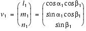
All WRC sections were screened during X-ray CT scan observation to avoid destructive testing on core samples that might contain critical structural features. Screening also ensured selection of whole-round samples with minimal drilling disturbance (essential for microbiology, inorganic geochemistry, and physical and mechanical properties) and provided an assessment of whole-round homogeneity. X-ray CT scanning was done immediately after core cutting so that time-sensitive whole-round samples (e.g., those for interstitial water and microbiological analyses) could be included in this screening process.

Fractures and other planar features that could be identified in the X-ray CT scans were oriented directly from the imagery by measuring strike in the slice view (perpendicular to the core axis) and one or more apparent dips in axial sections (e.g., coronal and sagittal) (Fig. F9). X-ray CT scanning helped reveal features that were cryptic or indistinguishable during VCD.

X-ray CT scans proved to be useful for identifying sedimentary and tectonic features prior to visual core description. 3-D structure orientation in the core reference frame could easily be determined from CT scan sections, whereas performing the same measurement on the cores generally required cutting orthogonal faces. Furthermore, structures such as shear zones could be classified by contrast in CT number, which is likely related to porosity changes or chemical alteration within shear zones. Structural and stratigraphic observations are incorporated into the structural geology and lithostratigraphy sections.

X-ray CT scan data have multiple uses, from early assessment of cores to description and synthesis. For this reason, several hundred gigabytes of scan data (~825 Mb/m) were stored on a local database at the OsiriX interpretation station. These data were later archived to tape and stored on terabyte disks.

Visual core description

Our methods for documenting the structural geology of Expedition 343 cores largely followed those given by the Expedition 316 structural geologists (Expedition 316 Scientists, 2009a). We documented the deformation observed in the split cores by classifying structures, determining the depth extent, measuring orientation, and recording kinematic information. The collected data were hand-logged at the core table and then entered into both a local spreadsheet and the J-CORES database. Where possible, the orientation data were also corrected for rotation related to drilling on the basis of paleomagnetic declination and inclination information.

Core description and orientation data collection

Each structure was recorded manually on a structural description sheet, which was modified from that used during IODP Expedition 322 (Fig. F10). We found that this modified sheet was particularly useful in recording orientation data for linear structures (e.g., striations on fault planes). Core measurement protocols followed those employed during Expedition 316, which were in turn based on previous ODP procedures developed at the Nankai accretionary margin (i.e., ODP Legs 131 and 190). We used a plastic protractor for orientation measurements (Fig. F11). Structural measurements were made on the working half of the split core, which provided greater flexibility to remove and cut (if necessary) pieces of the core for more careful study and measurement.

Orientations of planar and linear features in cored sediment were determined relative to the core axis, which was vertical in the core reference frame, and the “double line” marked on the center of the working half of the split core liner, which was 0° in the core reference frame. To determine the orientation of a plane, two apparent dips of the planar feature were measured in the core reference frame and converted to a plane orientation given as either a strike-and-dip or a dip-and-dip direction using a spreadsheet (Fig. F12). This approach had the advantage of increasing data processing efficiency and reducing errors in transferring and retyping data (e.g., by using both R. Allmendinger’s Stereonet program [www.geo.cornell.edu/geology/faculty/RWA/programs.html] and a spreadsheet). One apparent dip was typically represented by the intersection of the planar feature with the split face of the core and quantified by measuring the dip direction and angle in the core reference frame. Typical apparent dip measurements had a trend of 90° or 270° and ranged in plunge from 0° to 90°. The second apparent dip was usually represented by the intersection of the planar feature and a cut or fractured surface at a high angle to the split face of the core axis. In many cases, the cut surface was either parallel or perpendicular to the core axis. In the former case, the apparent dip lineation would trend 000° or 180° and plunge from 0° to 90°, whereas in the latter case, the trend would range from 000° to 360° and plunge 0°. Linear features observed in the cores were always associated with planar structures (typically faults or shear zones), and their orientations were determined by measuring either the trend and plunge in the core reference frame or the rake (or pitch) on the associated plane. All of these data were recorded on the log sheet with the appropriate depths and descriptive information.

Rotations were induced during RCB coring, as is common in ocean drilling. Paleomagnetic data were used routinely to correct drilling-induced rotation of the cored sediment. The new cryogenic magnetometer was not installed on the Chikyu until after Expedition 343, so paleomagnetic correction was conducted using the spinner magnetometer.

Orientation data analysis based on the spreadsheet

During Expedition 343, we adopted the modified Expedition 322 spreadsheet template for orientation data calculation in the core reference frame (e.g., Fig. F12). The core reference frame was such that the top of the core was oriented vertically upward, the core-splitting plane was 90°/270° and vertical, and the double-lined side of the working half of the core liner pointed toward 0° (Fig. F9).

Calculation of plane orientation

For planar structures (e.g., bedding or faults), two apparent dips on two different surfaces (e.g., one being the split core surface, which is 90°–270° and vertical, and the other being the 0°–180° vertical surface) were measured in the core reference frame as azimuths (measured clockwise from 0°, looking down) and plunges (Fig. F13). An xyz coordinate system was defined in such a way that the positive x-, y-, and z-directions coincided with 0°, 90°, and vertical downward, respectively (Fig. F9). If the azimuths and plunges of the two apparent dips were given as (α₁, β₁) and (α₂, β₂), respectively, as in Figure F13, then the unit vectors representing these two lines, v₁ and v₂, were

(8)

and

,

(9)

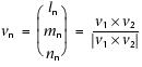
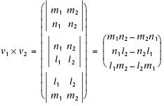
where l, m, and n represent the x-, y-, and z-components of the vectors.

The unit vector normal to this plane (v_n) (Fig. F13) was then defined as follows:

,

(10)

where

.

(11)

The azimuth (α_n) and plunge (β_n) of v_n were given by

and

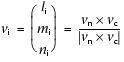
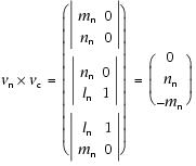
The dip direction (α_d) and dip angle (β) of this plane were α_n and 90° + β_n, respectively, when β_n < 0° (Fig. F14A). They were α_n ± 180° and 90° – β_n, respectively, when β_n ≥ 0° (Fig. F14B). The right-hand rule strike of this plane (α_s) was then given by α_d – 90° (Fig. F14).

Calculation of slickenline rake

For a fault with slickenlines, the apparent rake angle of the slickenline (ϕ_a) was measured on the fault surface from either the 90° or 270° direction of the split core surface trace (Fig. F15). Fault orientation was measured as described above. Provided that v_n and v_c were unit vectors normal to the fault and split core surfaces, respectively, the unit vector of this intersection line (v_i) was perpendicular to both v_n and v_c and therefore defined as follows:

,

(14)

where

(15)

and

.

(16)

Knowing the right-hand rule strike of the fault plane (α_s), the unit vector (v_s) toward this direction was then

.

(17)

The rake angle of the intersection line (ϕ_i) measured from the strike direction was given by

because

vs × vi = |vs||vi|cosϕi = cos ϕi, |vs| = |vi| = 1.

(19)

The rake angle of slickenline (ϕ) from the strike direction was ϕ_i ± ϕ_a, depending on which direction the apparent rake was measured from and which direction the fault plane dips toward. ϕ_a was subtracted from ϕ_i when the fault plane dipped toward 270° and ϕ_a was measured from either the top or 090° direction (Fig. F16A) or when the fault plane dipped toward 90° and ϕ_a was measured from either the bottom or 090° direction (Fig. F16B). Conversely, ϕ_a was added to ϕ_i when the fault plane dipped toward 90° and ϕ_a was measured from either the top or 270° direction (Fig. F16C) or when the fault plane dipped toward 270° and ϕ_a was measured from either the bottom or 270° direction (Fig. F16D).

Azimuth correction based on paleomagnetic data

Provided that a core was vertical, its magnetization was primary, and its bedding was horizontal, its paleomagnetic declination (α_p) represented the magnetic north direction where its inclination (β_p) was ≥0° (Fig. F17A), whereas it represented the magnetic south direction where β_p < 0° (Fig. F17B). The dip direction and strike of a plane in the geographic reference frame (α_d* and α_s*) therefore were

and

where

and were

and

where

J-CORES structural database

Structural data were entered in the J-CORES database VCD program (Fig. F18). These data include a visual (macroscopic and/or microscopic) description of core structures at a given section index and a record of planar structures in the core reference frame. We recorded the data first on paper logs and then transferred the data into the J-CORES database at a later time. Data were also entered into a spreadsheet (Fig. F12) for postacquisition processing.

Data entry through the VCD program proceeded as follows:

1. We recorded the expedition, site, hole, core, and section for which data were going to be read/written.

2. We selected the data to work with (i.e., deformation structure description), clicked on Hire, and then OK.

3. We selected a structure ID (e.g., bedding, fault, etc.) or created a new structure ID, selected the section interval in which the structure was observed, and filled in the parameters related to the particular structure (e.g., comments and planar data) (Fig. F18).

After saving, data were automatically uploaded to the Chikyu server and could be retrieved afterward as text or an Excel file for further processing.

Description and classification of structures

In general, we described and classified the structures observed using the terminology of J-CORES and Expedition 316, which in turn was based on the J-CORES VCD scheme and ODP Legs 131 (Taira, Hill, Firth et al., 1991), 156 (Shipley, Ogawa, Blum, et al., 1995), 170 (Kimura, Silver, Blum, et al., 1997), and 190 (Moore, Taira, Klaus, et al., 2001). However, for clarity we define the terminology used to describe fault-related rocks, as well as the basis for differentiating between natural and drilling-induced features and interpreting formation by gravitational or tectonic processes below.

Deformed sediment and rocks

Breccia is composed of fragments that have clearly rotated with respect to each other. The presence of a matrix may be difficult to ascertain because of pervasive intrusion of this incohesive material by drilling mud or washing away by circulating fluids near the core surface. Brecciated fragments are typically angular to subangular and commonly have polished and striated surfaces. Scaly fabric occurs in clay-rich rocks that are composed of phacoids whose surfaces make up an anastomosing network of curviplanar, striated shear surfaces. The intensity of the fabric is a function of several parameters (strain, composition, etc.) but will be described as weak, moderate, or intense.

The recognition of natural breccia and gouges in cores is of primary importance because it constitutes a straightforward way to identify fault zones and, more precisely, principal slip zones that host the maximum displacement. This recognition, easily done in the field, appears to be less trivial in cores, mainly because of frequent drilling-induced or splitting-induced brecciation and/or drilling mud injection; both processes tend to produce structures that mimic those found in nature. During Expedition 343, the distinction between natural and drilling-induced breccia was based on the following set of observations:

• Fragments observed in natural breccia commonly show polished or striated surfaces, whereas the fragments in drilling-induced breccia commonly lack such features, except for “spiral” slickenlines resulting from the coring process.

• Natural breccia is commonly bounded by, and grades into, less fractured rock, and the fracture fabrics in the bounding rocks display preferred orientations.

• Natural breccia is marked by low contrast in CT images between clasts and matrix with high CT numbers, whereas CT images of drilling-induced breccia are marked by spherical voids and bright clasts in a much darker matrix with low CT numbers (Expedition 316 Scientists, 2009b).

The distinction between natural gouge and drilling-induced mud is delicate. Drilling mud commonly occurs along biscuiting boundaries, at the periphery of cores, or as veins injected across core pieces, perpendicular to the core axis. The transition between drilling mud and surrounding rock is typically sharp. Drilling mud commonly includes small (2 mm to 1 cm) fragments of nearby rock. Natural gouge might form a gradual transition zone with surrounding rock, which consists in most cases of fault breccia or microbreccia. Fragments are either nonexistent or are of very small size (<1 mm long).

Multichannel seismic reflection data and the geologic setting of the Tohoku-oki subduction zone suggest the structural complexity in the toe region of the frontal prism could result from slumping, sliding, and faulting. Sedimentary breccia may be present. Thus, especially for this expedition, it was essential to distinguish fault-related tectonic structures from gravitational deformation structures. Natural breccia of tectonic and sedimentary origin is commonly difficult to distinguish, particularly in core samples. During Expedition 343, the origin of a breccia layer was established by integrating the textural observations (documented independently) and the stratigraphic context as follows:

• Sedimentary breccia may display erosional bases and/or depositional tops (e.g., fining-upward sequences).

• Tectonic breccia may grade from protobreccia to breccia, whereas this feature is absent in sedimentary breccia.

• Sedimentary breccia typically contains a wider range of clast compositions.

• The fragments in sedimentary breccia tend to lack polished or striated faces that are common in tectonic breccia.

Minor faults

It may be difficult to distinguish natural faults from drilling-induced faults. Helicoidal striated surfaces or polished surfaces showing striations that diverge outward most likely indicate drilling-induced fracturing resulting from the torque exerted by the bit on sediment. In contrast, faults that display more planar geometries, parallel lineations, and orientations compatible with preferred orientations displayed by multiple faults nearby are likely natural features. Deformation bands are also considered natural deformation features, even though they rarely exhibit striated surfaces. Lastly, when the orientation data are corrected for drilling-related rotations using the paleomagnetic data, natural minor faults are expected to display preferred orientations, whereas drilling-induced faults are expected to yield randomly distributed orientations.

Structural sample protocols

Structural fabrics observed in soft or partially lithified sediment often need special handling to preserve them for observation, particularly in clay-rich lithologies. One of the major scientific objectives of Expedition 343 is to clarify the characteristics of fault zones active during large earthquakes. In particular, the identification of principal slip zones from recovered cores is crucial for understanding deformation mechanisms and the role of fluid during earthquake rupture. If thin (potentially on the order of millimeters in thickness) slip zones are bounded by fragile rocks (i.e., a fault damage zone), conventional core splitting using a water-cooled saw will result in destruction of the original structures. To protect possible important structures and preserve WRC sampling for other purposes (e.g., squeezing interstitial water for geochemical and microbiological analyses), we deployed the following protocol, which was based on special handling of “critical intervals” developed by Expedition 316 scientists for treatment of thin dark gouges in the megasplay fault zone and the frontal thrust zone.

First, we checked CT images of recovered cores to find noticeably brighter or darker bands, taking the spatial resolution of the CT image into consideration (the size of each pixel is 0.188 mm × 0.188 mm). From these, we chose critical intervals that should be preserved as WRCs. In particular, we carefully examined crosscutting relationships between lithologic surfaces and fractures to select possible recent slip zones. Thereafter, critical intervals to be preserved as whole-round samples were confirmed by the Co-Chief Scientists and Expedition Project Manager. Soon after such permission was granted, the shipboard scientists developed a research and sample-processing plan. Once all whole-round samples were taken, the cores were carefully split longitudinally into archive and working halves using an ethanol-cooled saw. Visual structural description and nondestructive measurements were performed on the split cores, and then samples for structural, chemical, physical properties, and mineralogical analyses were taken from the working half.

X-ray diffraction sampling

Bulk powder samples were acquired from core smoothing or trimming activities or were independently sampled to isolate individual horizons of interest. Samples were centrifuged for clay separation as required, dried, and ball-milled to <10 µm particle size according to standard shipboard protocols.

Maintenance of moisture content for essential samples

Certain requests for samples required particular treatment to maintain moisture content as close as possible to the recovered state because dessication may affect clay-rich samples (e.g., of fault gouge). This dessication may

• Affect delicate features of microstructural interest and introduce new structures (e.g., microcracks) that could be mistaken for primary features;

• Permanently affect permeability, and possibly cohesive strength, so that subsequent rock mechanics investigations yield misrepresentative results; and

• Result in changes in the structural arrangement of clay minerals (of interest for textural studies).

Three different protocols were adopted in these cases, depending on the intended end use of the sample:

1. For samples of microstructural interest, alcohol and LR White resin impregnation was used.

2. For whole-round samples of interest for physical properties measurements, whole rounds were packed into plastic liners, sponges dampened with distilled water or seawater were placed against the sample ends, and then the ends were capped and sealed with tape. These samples were stored in a moisture-controlled refrigerator as soon as possible.

3. For clay fabric studies, samples were extracted from the cut surface (in the case of split core) or a core surface carefully scraped clean of any drilling mud (for whole rounds) before visual core description was undertaken. These samples were ~1 cm³ and were cut out with a spatula to have a V-shape with the apex pointing downhole (similar to the procedure followed by San Andreas Fault Observatory at Depth [SAFOD] and Deep Fault Drilling Project [DFDP-1]). These samples were placed in small plastic bags, which were then placed in plastic “bottles” to provide protection from crushing, and placed in a refrigerator. In an effort to preserve sample moisture, plastic wrap was used to cover and seal the split core except when temporarily removed as necessary for sample description.

Top of page   |    Previous   |    Next