Li, C.-F., Lin, J., Kulhanek, D.K., and the Expedition 349 Scientists, 2015
Proceedings of the International Ocean Discovery Program Volume 349
publications.iodp.org

doi:10.14379/iodp.proc.349.105.2015
Site U14331
C.-F. Li, J. Lin, D.K. Kulhanek, T. Williams, R. Bao, A. Briais, E.A. Brown, Y. Chen, P.D. Clift, F.S. Colwell, K.A. Dadd, W.-W. Ding, I. Hernández-Almeida, X.-L. Huang, S. Hyun, T. Jiang, A.A.P. Koppers, Q. Li, C. Liu, Q. Liu, Z. Liu, R.H. Nagai, A. Peleo-Alampay, X. Su, Z. Sun, M.L.G. Tejada, H.S. Trinh, Y.-C. Yeh, C. Zhang, F. Zhang, G.-L. Zhang, and X. Zhao2
Keywords: International Ocean Discovery Program, IODP, JOIDES Resolution, Expedition 349, Site U1433, South China Sea, pelagic red clay, Ar-Ar dating, plagioclase phenocryst, deep biosphere, carbonate turbidite, calcite compensation depth, basalt alteration, magnetic susceptibility, cooling effect, magnetic anomalies, radiolarians, nannofossils, Nereites ichnofacies, Dangerous Grounds
MS 349-105: Published 30 March 2015
Background and objectives
Because of the marked contrast in magnetic anomaly amplitude between the Southwest and East Subbasins of the South China Sea (SCS) (Yao, 1995; Jin et al., 2002; Li et al., 2007, 2008), it is justifiable to question whether rifting and drifting within these 2 subbasins were synchronous or diachronous and how these subbasins evolved in comparison to the Northwest Subbasin. Site U1433 is located in the Southwest Subbasin near the relict spreading center and magnetic Anomaly C5d identified by Briais et al. (1993) (Figures F1, F2, F3). Together with Site U1431 in the East Subbasin, coring at these sites will help to explain the sharp differences in magnetic amplitude between the East and Southwest Subbasins and test the hypothesis that in the Southwest Subbasin the transition from continental rifting to seafloor spreading occurred more recently than in the East Subbasin (Pautot et al., 1986). Coring will help determine the age of this subbasin near the end of the spreading and correlate ages from magnetic anomalies with biostratigraphic, magnetostratigraphic, and radiometric ages. The apparent weak magnetization in basement rocks suggested by the magnetic anomaly amplitudes will be examined by petrological analyses of chemical compositions and measurements of magnetic susceptibility. The specific objectives at this site are to
- Determine the termination age of spreading in the Southwest Subbasin and correlate it to ages of regional tectonic events;
- Test the rifting and subsequent seafloor spreading models of the Southwest Subbasin;
- Measure magnetization, mineralization, and geochemical compositions of basement rocks to trace how the mantle evolved through time; and
- Examine the paleoceanographic and sedimentary response to the opening of the SCS.

Figure F1. SCS regional bathymetry.
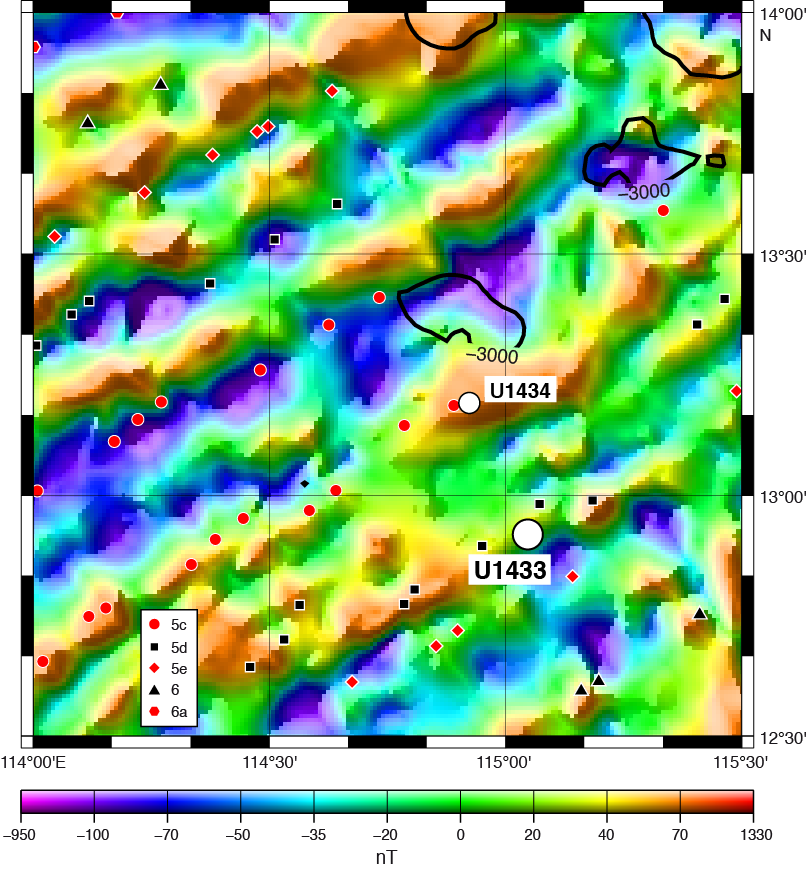
Figure F2. Magnetic anomalies.
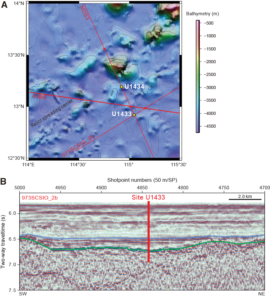
Figure F3. Regional contoured bathymetry.
Operations
The original operations plan for Site U1433 (proposed Site SCS-4B) consisted of drilling one hole to a depth of ~965 m below seafloor (mbsf), which included 100 m of basement. This plan was modified during transit in order to eliminate the use of a free-fall funnel and the extended core barrel (XCB) by coring 2 holes (Table T1). Hole U1433A was cored using the advanced piston corer (APC) to refusal at 188.3 mbsf. Hole U1433B was drilled to 186.1 mbsf and then cored using the rotary core barrel (RCB). The sediment/basement interface was encountered at ~798.5 mbsf, and we advanced the hole by rotary coring into basement to a final depth of 858.5 mbsf. After conditioning the hole for logging, we deployed the modified triple combination (triple combo) tool string and the Formation MicroScanner (FMS)-sonic tool string to 840 m wireline depth below seafloor (WSF), with multiple passes made in the basement section of the hole with the latter tool.
Table T1. Coring summary, Site U1433. Download table in .csv format.
A total of 94 cores were collected at this site. The APC was deployed 20 times, recovering 168.79 m of core over 188.3 m of penetration (89.6% recovery). The RCB system drilled one 186.1 m interval and collected 74 cores, recovering 443.04 m of core over 672.4 m of penetration (65.9% recovery). The overall recovery at Site U1433 was 71.1%. The total time spent on Site U1433 was 284.5 h (11.9 days).
Transit to Site U1433
After a 334 nmi transit lasting 29.9 h, the vessel arrived at Site U1433 (proposed Site SCS-4B) and switched to dynamic positioning mode at 0230 h (UTC + 8 h) on 8 March 2014. At 0255 h, an acoustic positioning beacon was deployed. The position reference was a combination of GPS signals and a single acoustic beacon.
Hole U1433A
After arriving on site and deploying the acoustic positioning beacon, an APC/XCB bottom-hole assembly (BHA) was assembled and run to 800.4 m below rig floor (mbrf). At 0520 h, a tool joint parted on the twenty-fourth stand of drill pipe, just after picking up the drill string and just prior to unlatching the lower set of elevators. The load cell weight at the time of the incident was recorded at ~200,000 lb. The entire weight of the drill string dropped ~18 inches and landed in the lower set of elevators, which were resting on top of the dual elevator stool. The pin on the top single of drill pipe had parted, leaving one single hanging from the upper set of elevators and 2 singles sticking up from on top of the lower set of elevators. The stand was then laid out to the V-door. The broken pipe was visually inspected and photographed. As a precaution, the twenty-third stand was also disassembled and laid out. The bottom set of elevators was removed from use and replaced with a reconditioned set of elevators. After clearing the rig floor, the trip to the seafloor resumed. When the bit was at 1147.8 mbrf, another tool joint failed when the driller was picking up the thirty-sixth stand from the pipe racker. This time, one single fell back into the trough of the pipe racker still attached to the skate, and a double remained connected to the elevators on the bales connected to the main block. After the second tool joint failure, we decided to discontinue using any of the 5 inch drill pipe that had been used in the stuck pipe incident at the previous site. Investigations continue into the root cause of the pipe failure. Documentation of the stuck pipe event was collected for analysis. The failed tool joints were prepared with care for shipment to a laboratory for detailed metallurgical analysis and were shipped from Keelung, Taiwan, at the end of the expedition. The drill string was tripped back to the BHA, and all suspect drill pipe was removed from use and stored in the port pipe racker. We picked up 201 joints of new 5 inch drill pipe from the riser hold. The new drill pipe was strapped and drifted as it was assembled and lowered toward the seafloor. After completing assembly of the new pipe, the remaining 37 stands from the starboard 5 inch pipe racker were picked up and run in the hole. The total number of 5 inch pipe stands available was then 104 stands. The remaining 101 stands of suspect drill pipe in the port pipe racker need to be inspected before they can be put back in service.
After tripping toward the seafloor with 104 stands of 5 inch drill pipe, the 5½ inch drill pipe was picked up until the bit reached 4372.9 mbrf. The trip was stopped at 3587.0 mbrf to perform a slip and cut of the drilling line. The precision depth recorder recorded an estimated depth of 4394.4 mbrf for the seafloor. The top drive was picked up and spaced out to 4390 mbrf. The nonmagnetic core barrels were dressed with liners, the FlexIT core orientation tool was inserted, and a core barrel was run down and landed. Hole U1433A was spudded at 1000 h on 9 March 2014. The mudline core recovered 8.9 m of sediment, and the seafloor was calculated to be 4390.6 mbrf (4379.4 m below sea level [mbsl]). Coring continued without issue through Core 349-U1433A-16H (151.4 mbsf). While running in the hole with a core barrel, the bridge informed the driller that a fishing boat was drifting toward the vessel’s location. At 0540 h on 10 March, the Captain ordered the driller to suspend operations. The core barrel was retrieved, and the driller began tripping out of the hole with the top drive. At 99.1 mbsf, the driller was instructed to stand by. After the threat disappeared, the drill string was tripped back to bottom, and coring continued to Core 20H (188.3 mbsf). After 4 consecutive partial strokes of the APC, refusal was called at 188.3 mbsf. Orientation was measured on all APC cores. Temperature measurements were taken with the advanced piston corer temperature tool on Cores 4H, 7H, 10H, and 13H, with good results. Perfluorocarbon tracer (PFT) fluid was used on Cores 18H through 20H. The bit was tripped to the surface and cleared the rig floor at 0325 h on 11 March, ending Hole U1433A. A total of 20 APC cores were taken over a 188.3 m interval in Hole U1433A, recovering 168.79 m of core (89.6% recovery). The total time spent on Hole U1433A was 73.0 h (3.0 days).
Hole U1433B
After offsetting the vessel 20 m east of Hole U1433A, an RCB BHA was assembled with a new RCB C-4 bit. Three additional drill collars had to be picked up from the drill collar racks to replace the ones lost in Hole U1432B. The core barrels were spaced out at the surface and the 172.07 m BHA assembled and run to 4350.3 mbrf. The top drive was then picked up and spaced out to spud Hole U1433B. A center bit was dropped and pumped to land out in the bit. Hole U1433B was spudded at 1515 h on 11 March 2014. The seafloor depth for the hole was 4390.6 mbrf (4379.4 mbsl), determined by using an offset depth from Hole U1433A. Hole U1433B was advanced by drilling without coring from the seafloor to 186.1 mbsf. The center bit was pulled from the BHA by wireline, and a core barrel was dropped to start continuous RCB coring of Cores 349-U1433B-2R through 75R to a total depth of 5249.1 mbrf (858.5 mbsf). The PFT pumps were turned on during the drilldown period, and PFT fluid was pumped through Core 26R (426.9 mbsf). Microspheres were added to the RCB core catcher sub for Cores 56R through 75R. Core 65R encountered basalt at 786.3 mbsf. Coring continued into acoustic basement from Core 65R to 75R (858.5 mbsf), with half-cores collected from Core 67R to the total depth in an attempt to improve recovery. Penetration rates varied from 0.9 to 3.9 m/h over the basement interval. The total depth of Hole U1433B was reached at 2100 h on 17 March, and the final core was pulled to the surface and laid out. At the completion of coring Hole U1433B, 74 RCB cores had been cut over a 672.4 m interval, recovering 443.04 m of core (65.9% recovery).
After pumping a 50 bbl high-viscosity mud sweep, a short wiper trip was made from total depth to just above the basement contact (786.3 mbsf) with the top drive installed. While tripping back to bottom, the hole had to be reamed from 847.4 to 858.5 mbsf. We then pumped another 50 bbl mud sweep to further clean the hole. The rotary shifting tool (RST) was then picked up and run into the hole with a coring line to release the bit for logging. An attempt was made to engage the sleeve in the mechanical bit release. After being unable to engage the shifting sleeve, the other RST was pulled back to the surface. Examination at the surface revealed the RST did not come back with the core line sinker bars. An overshot (fishing tool) was made up and run in the hole to fish for the RST. After securing the RST, the mechanical bit release sleeve was engaged and the bit was dropped from the drill string. The RST also dropped off the fishing tool on release, leaving the RST in the bottom of the hole. The core line was pulled back to surface, and the RST was deployed to shift the sleeve back into the original position. With the bit released, the drill string was raised to 5196.3 mbrf (805.7 mbsf) with the top drive. The top drive was then set back, and the drill string was raised to 5079.7 mbrf (689.1 mbsf). The circulating head was picked up, and the hole was displaced from 689.1 mbsf to the seafloor with 10.5 lb/gal high-viscosity mud designed to improve logging conditions. The drill string was then raised up and spaced out so that the end of the pipe was at 4490.7 mbrf (100.1 mbsf) for logging operations.
After holding a logging safety meeting for rig floor personnel, the triple combo tool string was rigged up and deployed. The tool string reached a total depth of 845.4 m WSF on 18 March. The hole was then logged up, and the tool string was pulled to the surface and rigged down. After rigging down the triple combo tool string, the FMS-sonic tool string was rigged up and deployed to a depth of 842.4 m WSF. The basement section of the hole was logged five times with three passes with the calipers open. On the last pass, the tool became stuck but was eventually worked free. The rest of the open hole was logged up to the end of the drill pipe and the tool string was then pulled to the surface and rigged down. All logging equipment was rigged down by 1300 h on 19 March. The drill string was pulled from the hole and the BHA set back and secured for transit at 2300 h on 19 March, ending Site U1433. Total time spent in Hole U1433B was 211.5 h (8.8 days).
Lithostratigraphy
Lithostratigraphic units
Four lithostratigraphic units are defined at Site U1433 based on a combination of visual core description and smear slide and thin section inspection as well as scanning for an array of physical properties, including magnetic susceptibility and color spectra (see Lithostratigraphy and Physical properties in the Methods chapter [Li et al., 2015b]). A composite stratigraphy was derived through a combination of material from Holes U1433A and U1433B (Figure F4). Three major sedimentary units overlie a single lithostratigraphic unit that forms the crystalline, igneous basement (Figures F4, F5). This lower unit is dominantly composed of basaltic igneous rocks and is discussed in detail in Igneous petrology and alteration. Very small volumes of thin-bedded (1.0–1.5 cm thick) sedimentary rock were found between pillow basalt and massive flows in Unit IV and are discussed along with the igneous rocks in Igneous petrology and alteration, as well as in Biostratigraphy.
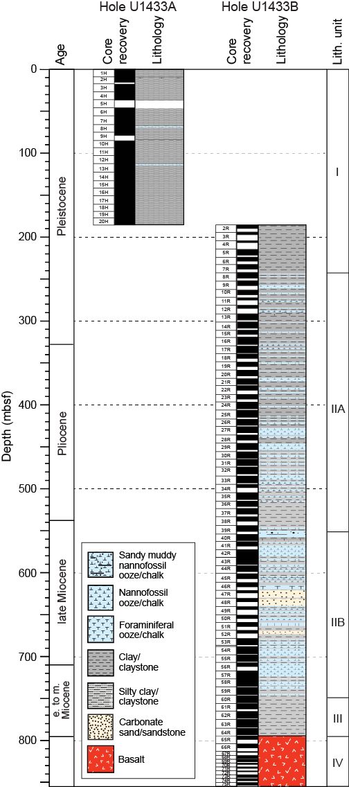
Figure F4. Lithostratigraphy summary.
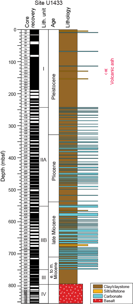
Figure F5. Synthesis sedimentary log.
Unit I is composed of dark greenish gray clay with interbedded very thin clayey silt. Unit II contains dark greenish gray clay and claystone with frequent medium to thick greenish gray nannofossil ooze and chalk interbeds. This unit is divided into upper and lower subunits based on the occurrence of thick to very thick (>1 m) greenish gray nannofossil chalk interbeds in Subunit IIB, compared to thinner beds in Subunit IIA. Unit III consists of dominantly massive reddish and yellowish brown claystone and claystone with silt, with little coarser material present, occasional thin silty turbidites, and common dark staining associated with bioturbation. This unit lies directly on the basaltic basement (Unit IV).
Unit descriptions
Unit I (0–244.15 mbsf)
- Intervals: 49-U1433A-1H through 20H; 349-U1433B-2R-1, 0 cm, through 8R-2, 5 cm
- Depths: Hole U1433A: 0–188.30 mbsf (total depth); Hole U1433B: 186.10–244.15 mbsf
- Age: Pleistocene
Unit I is composed of dark greenish gray clay with rare interbeds of thin and very thin (<5 mm) clayey silt beds. There are dark brownish clay layers in the upper parts of the unit, together with minor light greenish gray clay with nannofossils and nannofossil ooze layers throughout the section. The clay is generally massive and homogeneous, sometimes marked by faint color banding of more intense green against the background of greenish gray (Figure F6A). In some locations the green sediment is better defined and more intense in color, where it forms well-defined green bands rich in glauconite (Figure F6B). Thin clayey silt layers are usually graded and fine upward above sharp bases that at least locally show signs of erosion (Figure F7A). Silt beds in Unit I are mostly 1–2 cm thick (Figure F7B), occasionally up to 15 to 20 cm thick, but generally comprise <10% of the entire section.

Figure F6. Green layer development.
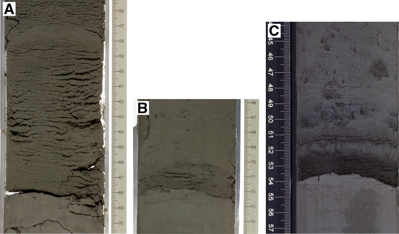
Figure F7. Silt turbidites.
We interpret both the carbonate and graded silt intervals as turbidites. In places several small turbidite silts are stacked on top of one another (Figure F7C), with up to four in succession. In these cases the lower silt is the thickest and is overlain by thinner beds, often <5 mm thick and separated by a similar thickness of clay from the next silt. Further evidence for seafloor erosion and reworking is found in some locations where 2 slightly differently colored clays are found juxtaposed with a sharp erosive contact between the two (Figure F8). These may represent areas of erosion and bypassing by turbidity currents, although very thin silts (<2 mm thick) are sometimes seen along these surfaces, which often show topography, indicating a slight angle during deposition, at least in the lee of seafloor topography.
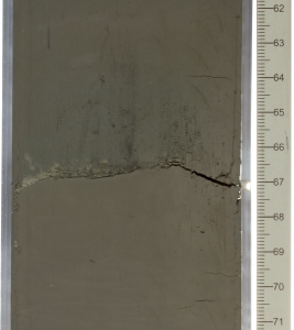
Figure F8. Erosion surface.
At the microscopic level, the apparently homogeneous clay contains common quartz silt and volcanic glass shards. In lighter colored intervals, the proportion of biogenic and redeposited calcite can be significant. Figure F9A shows the abundance of radiolarians in parts of Unit I, together with other largely siliceous microfossils including diatoms and sponge spicules. In more calcareous intervals, we also identified foraminifers, nannofossils, and calcite shelly material of undetermined origin. Foraminifers are often broken and are also found in association with quartz and volcanic glass shards (Figure F9B).

Figure F9. Radiolarians in clay.
Volcanic ash layers are rare at Site U1433, only found in Unit I from 120 to 140 mbsf (Figure F5). Figure F10 shows the thickest example of a dark-colored, graded tephra layer 6 cm thick within clay. More typically there are a number of thin (<2 cm thick) felsic ash layers in the middle part of the unit. These deposits are volumetrically insignificant, although very small amounts of volcanic glass shards are often found scattered through clay and silt beds. All identified tephras show sharp bases and normal grading from a silt-sized basal layer, typical of air fall deposits.
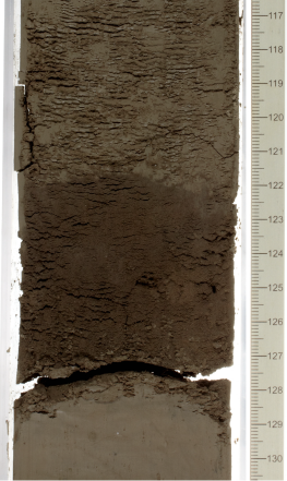
Figure F10. Mafic tephra layer.
Rare nannofossil ooze layers are found in Unit I. The beds all fine upward and have erosive bases, consistent with a turbidite origin, but these intervals are volumetrically small, resulting in Unit I being dominated by clay.
Taken together, the evidence from Unit I supports sedimentation in a distal hemipelagic muddy setting with siliceous plankton–dominated pelagic deposition and limited influxes of calcareous material. Bioturbation is presumed to be intense because of the lack of lamination, but because most of the sediment is the same color there is little chance to see burrows highlighted with contrasting lithologies. Figure F11A shows an exception to this, in which small horizontal burrows are found within a more nannofossil-rich interval. The burrows themselves are filled by coarse foraminiferal sand and are of relatively low abundance.
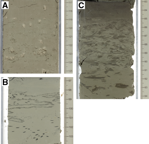
Figure F11. Burrows in sediment.
Unit II (244.15–747.93 mbsf)
- Interval: 349-U1433B-8R-2, 5 cm, through 60R-1, 93 cm
- Depth: 244.15–747.93 mbsf
- Age: Pleistocene–middle Miocene
Unit II represents the majority of the sediment recovered at this site, and is readily distinguished from overlying deposits by the presence of common calcareous turbidite beds within a dominant clay and claystone background. The unit is also unique in its physical properties (Figure F12) because it shows low magnetic susceptibility values not seen in Unit I and has much more variable color spectral proxies, especially in L* and to a lesser extent b*. Lithification increases quickly downsection from the top of this unit. Because sediment at Site U1433 was deposited below the modern calcite compensation depth, a mechanism is needed to explain the significant amount of carbonate in the core. We propose rapid redeposition from shallower water settings into the deepwater basin by turbidity currents. Unit II is divided into 2 subunits, with the lower one distinguished by much thicker carbonate turbidites but otherwise basically of the same facies as the upper subunit. The boundary between the 2 subunits is at the top of the first multimeter-thick carbonate bed encountered downsection.

Figure F12. Lithostratigraphy and magnetic susceptibility correlation.
Subunit IIA (244.15–551.32 mbsf)
- Interval: 349-U1433B-8R-2, 5 cm, through 39R-6, 100 cm
- Depth: 244.15–551.32 mbsf
- Age: Pleistocene–Pliocene
The sediments of Subunit IIA are typified by cycles of redeposited carbonate and a background of rapidly deposited, largely dark greenish gray claystone (Figure F13). The carbonate beds tend to be 15–50 cm thick and account for ~20% of the total section. Each bed is marked by a sharp, erosive base with color and grain-size gradation upward toward a more diffuse boundary with the overlying greenish gray clay. The basal few centimeters are often characterized by silt or fine sand–grade sediment with parallel laminations often observed over the basal 1–2 cm. The upper contact of each turbidite is often heavily bioturbated and contains a variety of deepwater traces of the Nereites ichnofacies. Figure F11C shows a close-up of the trace fossil assemblages in Subunit IIA. The smallest burrows are the Chondrites ichnospecies and are commonly also found in conjunction with the larger Planolites and Zoophycos. Horizontal Scolicia burrows are present but less commonly observed. This is the most typical trace fossil assemblage seen within the subunit. Typically, the intense burrowing exists in the uppermost 10 cm of the calcareous turbidite, leaving the rest of the bed undisturbed.
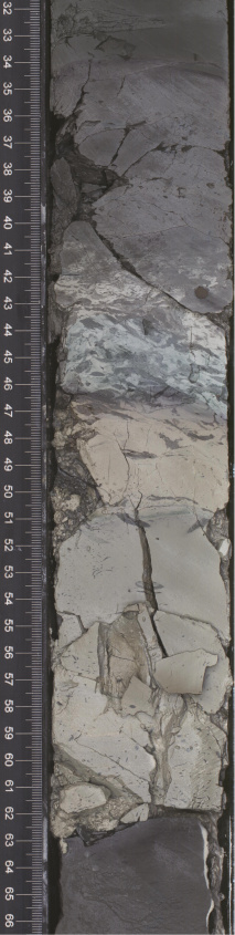
Figure F13. Typical calcareous turbidte cycle.
Figure F14 shows 2 turbidites stacked on top of one another. In this example the lower turbidite unit (interval 349-U1433B-48R-1A, 65–72 cm) is finer grained but still shows a sharp erosional base grading up into a bioturbated top. The burrows are filled with a more clay-rich, darker sediment that is in turn truncated by a second turbidite (interval 48R-1A, 57–65 cm) with parallel-laminated silt and fine sand–grade material that in turn passes up into dark greenish gray clay. This upper turbidite unit is also different in being bioturbated by large Planolites-type burrows, which have lower density than those in the lower turbidite unit. Turbidites within Subunit IIA are almost exclusively carbonate with very little siliciclastic material observed.

Figure F14. Calcareous turbidites.
At the microscopic level, the clay lithologies are composed of not only clay minerals but significant quantities of opaque material and fine silt–sized quartz, as well as some lithic grains and feldspar. Occasional fragments of angular, mafic, volcanic glass are also observed in minute quantities. The amount of biogenic material is relatively small (Figure F15A). Deeper in the subunit, diagenesis results in these mud-rich units being affected by pyrite growth. Figure F15B shows an example of very fine-grained pyrite in its earliest stage of growth within a claystone interval. With continued growth, the pyrite forms nodules and in some cases replaces burrows, although the total volume of pyrite remains relatively low. The appearance of pyrite is interpreted to reflect pervasive reducing conditions within the claystone. Microscopic analysis of the redeposited carbonate units shows that they are formed from a variety of shelly material, although foraminifers are the dominant type of clast. Figure F16C shows one of these turbidite silts higher in the section, showing the whole, unbroken character of the foraminifers, as well as a variety of less recognizable fragments of shells, together with volcanic glass and fragments of larger foraminifers. In contrast, deeper within Subunit IIA the carbonate deposits are dominated more by broken shell material (Figure F16A) and significant numbers of nannofossils. We interpret the shell breakage to have occurred during transport, not burial.
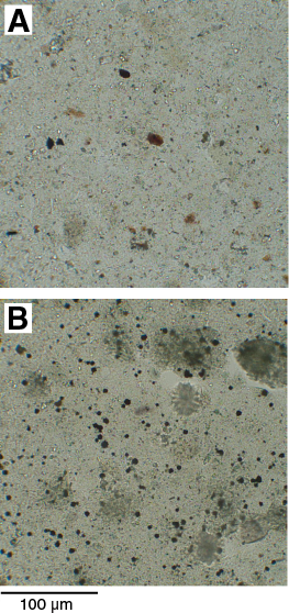
Figure F15. Typical clay/claystone lithologies.
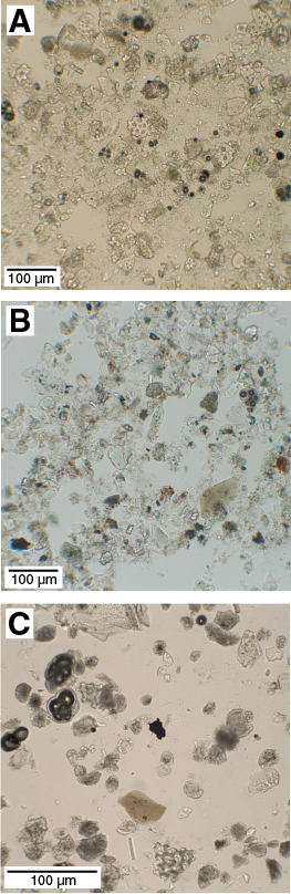
Figure F16. Coarser clastic material.
Both of these types of deposits contrast with quartz-rich silty turbidites that are mostly found within Unit I and to a lesser extent in Subunit IIA (Figure F16B). These deposits are moderately sorted and mostly composed of subangular to subrounded grains of quartz, feldspar, volcanic glass, and a lower proportion of biogenic carbonate material. Green grains of glauconite are also visible in some beds.
Subunit IIB (551.32–747.93 mbsf)
- Interval: 349-U1433B-39R-6, 100 cm, through 60R-1, 93 cm
- Depth: 551.32–747.93 mbsf
- Age: middle–late Miocene
In many respects, Subunit IIB is like Subunit IIA but is mostly distinguished by being somewhat thicker bedded and with a higher proportion of carbonate, at least over moderate lengths of the core. The Subunit IIA/IIB boundary does not stand out in most physical properties measured (Figure F12), except P-wave velocity (see Physical properties). We defined the top of this subunit to be coincident with the top of the first carbonate turbidite that is several meters thick. One consequence of the appearance of thicker redeposited carbonates is that the grain size also increases. Figure F17A shows an example in which the base of a turbidite, lying with an erosive contact on the underlying claystone, is marked by a massive to weakly laminated coarse sandstone that grades uphole over a distance of ~20 cm into medium sandstone. In this particular case, the sand consists mainly of shallow-water benthic foraminifer species, chert, feldspar, volcanic lithic fragments, and quartz grains (Figure F18), showing that the sediment is derived from a nearby shallow-water environment. In other examples, the carbonate sand is very well laminated (Figure F17B), demonstrating deposition under a high-energy laminar flow regime, which we interpret as being part of the Bouma B division (Bouma, 1962). Figure F19 shows abundant well-preserved planktonic foraminifers and occasional micro-authigenic pyrite grains within a laminated, light greenish gray foraminiferal chalk from this facies. As before, these deposits are all interpreted to be the product of sedimentation from a turbidity current with a source on some of the shallow banks mostly lying to the south of the drilling site (Figure F1), although at this stage we cannot rule out the influence of more localized sources on isolated seamounts, despite being less likely than at Site U1431.
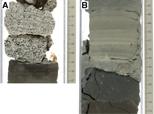
Figure F17. Erosive bases of calcareous turbidites.
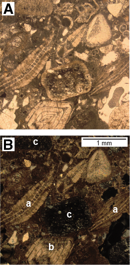
Figure F18. Coarse carbonate sandstone.
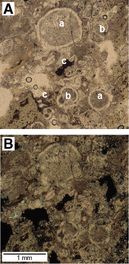
Figure F19. Parallel-laminated foraminiferal chalk.
In one unusual example (Figure F20), the coarse sand at the base of a turbidite deposit contains large amounts of fine-grained organic carbon material, which was preserved as a black substance, deformed in a plastic fashion between relatively rigid grains mostly of carbonate composition. This particular bed was quite unique in its appearance compared to the other sandstone beds within the subunit, suggesting that this was an atypical sedimentation event. As a general rule we saw little evidence for significant amounts of organic carbon in the sediment.
Figure F20. Organic carbon–bearing sandstone.
Bioturbation within Subunit IIB is generally similar to that seen in Subunit IIA with one or two exceptions in the thick carbonate beds. Figure F11B shows an example of a horizontal burrow of the Scolicia ichnospecies. This particular deposit is not heavily bioturbated but shows Chondrites and associated Scolicia burrows in the sediment immediately underlying. Sparse bioturbation within these carbonates likely reflects the relatively low amounts of organic material on which the borrowing infauna would have been able to feed.
Unit III (747.93–796.67 mbsf)
- Interval: 349-U1433B-60R-1, 93 cm, through 65R-1, 117 cm
- Depth: 747.93–796.67 mbsf
- Age: early–middle Miocene
The third major unit overlying the igneous basement is much thinner than the other 2 units (~49 m thick) and is distinguished by being entirely composed of claystone and claystone with silt with only minimal millimeter-scale silt intervals. We defined the top of this unit as being the base of the lowest significant carbonate deposit within Subunit IIB. The claystone that directly underlies this carbonate bed is very similar to much of that seen within Subunit IIB, being massive, well bioturbated, and dark greenish gray. This claystone then passes rapidly downsection through a color transition into a dominant reddish brown or yellowish brown claystone, which represents the bulk of this unit. Figure F21A shows an example of the massive-bedded reddish claystone. Sedimentary structures are not common within this unit, although there are intervals of graded, quite bioturbated clayey siltstone and silty claystone that show parallel lamination and normal grading over distances of 20–30 cm (Figure F21B). Some of the claystone intervals themselves show grading over similar distances, but more typically they are massive and occasionally bioturbated with the same type of assemblages seen in Unit II, albeit less densely developed. The unit is especially noteworthy for having a common black staining of the claystone that is sometimes, but not always, associated with burrowing (Figure F21C). In the absence of X-ray diffraction (XRD) constraints, we were unable to define causes of this black staining, although organic carbon seems the most likely, especially given the association with bioturbation.
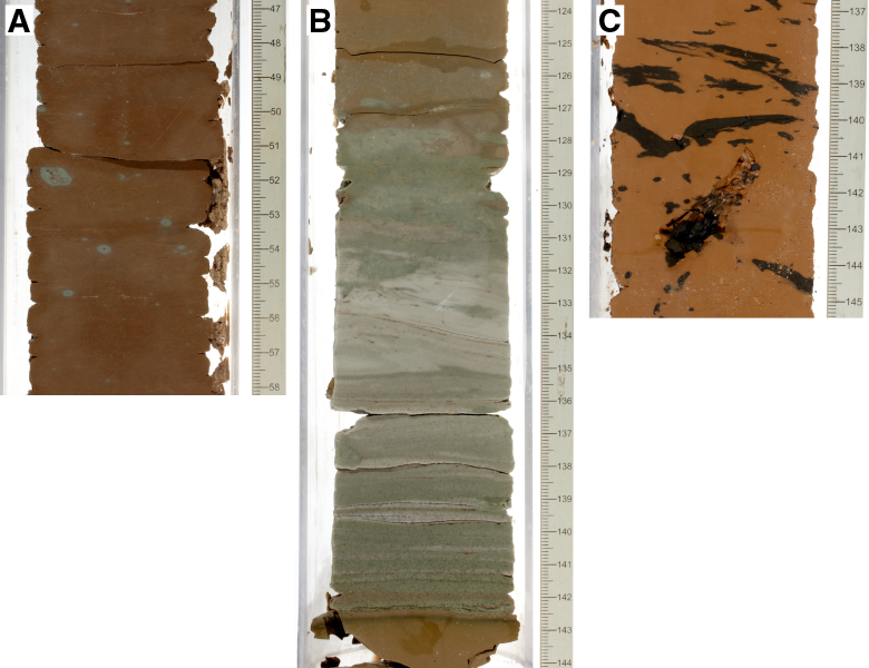
Figure F21. Claystone.
We interpreted Unit III to be deposited as a distal pelagic mudstone overlying the basaltic basement. There is no lithologic evidence for any significant hydrothermal activity during the deposition of these clays or for significant alteration after sedimentation as a result of high-temperature fluid flow. In many ways, these sediments are reminiscent of the deepwater red clays in the Central Pacific (Bryant and Bennet, 1988) and other deep abyssal plain areas, including Site U1431. Microscopic analysis shows that many or all of the carbonate microfossils that would have been deposited have dissolved as a result of sedimentation below the calcite compensation depth, leaving only siliceous microfossils such as radiolarians. Sedimentation rates are much slower in this subunit compared to the rest of the stratigraphy (see Biostratigraphy), although they are faster than those seen in the Central Pacific, reflecting the fact that our drilling location is located much closer to continental sediment sources, which are inferred to supply the silty material seen within the claystone.
Discussion
Trace fossils
Trace fossils preserved in deep-sea sediments represent the last burrows that are imposed on a sediment beneath the mixed surface layer, which spans the uppermost 5–7 cm of the seafloor (Ekdale et al., 1984). The assemblages seen in our cores are typical of very deepwater sedimentary environments in distal clastic settings and correspond to the Nereites ichnofacies. This ichnofacies is typical of the uppermost 3–7 cm in the modern subseafloor sediment of the South China Sea, where water depths exceed 4000 m (Wetzel, 2002), although after correcting for the expected thermal subsidence we anticipate that these assemblages must have been formed at shallower water depths, albeit ones at least as deep as typical seafloor spreading ridges (~2500 m). Work on deep-sea cores from the Central Pacific suggests that Zoophycos is more common in sediments with slightly higher organic carbon content (Kemp, 1995), and because this particular trace is relatively rare in our cores, we deduce that the organic carbon content is never particularly high, an observation confirmed by shipboard analysis (see Geochemistry). Conversely, we note that vertical burrows such as Skolithos are almost absent from our cores. Skolithos burrows are commonly associated with particularly low sedimentation rate environments with extremely depleted organic content (Kemp, 1995). Thus, compared to the Central Pacific, the South China Sea does not experience the types of sediment starvation and low productivity associated with these deep-sea desert regions, which is perhaps not surprising given its relative proximity to landmasses in Southeast Asia and the continental runoff associated with them. It is noteworthy that Zoophycos is only sparsely developed in Unit II but was found at least in parts of Unit III despite the relatively low sedimentation rates inferred for this part of the stratigraphy.
Provenance
Several sources may have contributed sediment to Site U1433. The location of the drill site south of the fossil mid-ocean ridge suggests that derivation of material from southern China, the Philippines, or Taiwan is unlikely, especially since these landmasses are farther away than the other possible sources in Borneo or mainland Southeast Asia (Figure F1). Modern sediment transport routes between the Sunda shelf and the drill site would presently favor sediment transport from the Mekong River, which could be the source of the clay and silt. During sea level lowstands, sediment could also flow from peninsular Malaysia or even from Sumatra via the Molengraaff River (Hanebuth and Stattegger, 2004). Seismic reflection data from offshore the Mekong Delta suggest that this system has been particularly active only since ~5 Ma (Li et al., 2013), which means that prior to that time sediment flux from Indochina must have been only from smaller rivers, such as those draining directly from the mainland into the South China Sea. These in turn would have been rejuvenated and strengthened during the uplift of the Central Highlands of Vietnam following the emplacement of flood basalts there at ~8 Ma (late Miocene; Carter et al., 2000).
In theory, clastic material could flow to the region from mainland Borneo, but in order to do this the sediment would have to cross the tectonically generated bathymetry of the Dangerous Grounds (Figure F1), which is marked by many ridges and deep basins that would act as efficient sediment traps. Although the sediment could be transported as hyperpycnal plumes, there is little evidence from satellite imagery to suggest that this is a common process today, and the proliferation of active carbonate reefs dating back into the Miocene would also indicate that substantial transport of clay across the Dangerous Grounds from Borneo is unlikely to have been significant on geological timescales (Hutchison and Vijayan, 2010). Surface currents in the South China Sea also do not favor transport from south to north across the Dangerous Grounds (Hu et al., 2000).
The source of the carbonate sediment, and the turbidites in particular, within Unit II is most likely within the Dangerous Grounds or the Reed Bank area. Local sources, such as isolated seamounts, seem less likely at Site U1433 compared to those at Site U1431 because there are fewer shallow seamounts in the region. The seismic reflection data that cross the seamount that sits on the fossil seafloor spreading axis to the north of Site U1433 do not show evidence for substantial carbonate buildup on top (see Figure F7 in the Expedition 349 summary chapter [Li et al., 2015a]). We conclude that most of the carbonate material found in the turbidite sediments is derived from the south in the Dangerous Grounds, but it is worth asking why the flow of this material is suddenly truncated during the Pleistocene at the boundary between Units I and II after several million years of quite active sedimentation. This is particularly enigmatic given the fact that over longer periods of time sea level has been falling during the Pleistocene (Haq et al., 1987). We suggest that the reduction in carbonate flux to the drill site reflects the steady subsidence and drowning of the carbonate reefs in the Dangerous Grounds despite the overall sea level fall. Although several reefs still remain and give the region its name, much of the original carbonate buildup has been drowned as a result of postrift thermal subsidence reducing the extent of shallow water within this tectonic block (Hutchison, 2004; Hutchison and Vijayan, 2010; Steuer et al., 2013).
What triggers the emplacement of individual carbonate turbidites is not entirely apparent, although they could reflect variability in sea level, as falling sea level tends to result in erosion of shallow-water regions and resedimentation into basinal areas (e.g., Vail et al., 1977). We note that falling sea level would also affect the flux of clay and silt from the southwest and would not necessarily result in more carbonate turbidites. Some of the turbidite events may have been triggered by earthquakes, especially during the Miocene after the collision of the Dangerous Grounds with Borneo starting at ~16 Ma (Hutchison, 2004). Better age control and statistical analysis will be needed if we are to understand whether the frequency of carbonate turbidites reflects some larger controlling process.
Biostratigraphy
We analyzed core catcher samples and additional samples from split cores in Holes U1433A and U1433B. Biostratigraphic datums based on calcareous nannofossils, planktonic foraminifers, and radiolarians indicate that the sedimentary succession recovered at Site U1433 spans the lower Miocene to the Pleistocene (Figure F22; Tables T2, T3, T4). Age control for the lower to middle Miocene section is difficult because of very rare occurrences of calcareous nannofossils and planktonic foraminifers in the depositional sequences, which are dominated by the reddish brown claystone of lithostratigraphic Unit III (see Lithostratigraphy). Radiolarian bioevents in Hole U1433B between 753.82 and 794.23 mbsf (Unit III) indicate sediment deposition during the early and middle Miocene (~20.6 to ~14.7 Ma). Nannofossils in carbonate infillings between basalt pillows appear to indicate an Oligocene to early Miocene age, but postexpedition studies are required to confirm this.
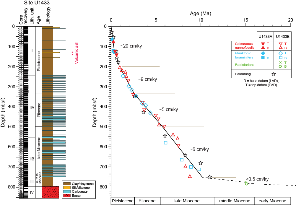
Figure F22. Age-depth model.
Table T2. Depths and ages of calcareous nannofossil events, Holes U1433A and U1433B. Download table in .csv format.
Table T3. Depths and ages of planktonic foraminifer events, Holes U1433A and U1433B. Download table in .csv format.
Table T4. Depths and ages of radiolarian events, Hole U1433B. Download table in .csv format.
Calcareous nannofossils are generally common to abundant with good preservation in samples from the Pleistocene–Pliocene section but are rare and heavily overgrown or even absent in some Pliocene and upper Miocene samples. Varying degrees of overgrowth on nannofossils, especially among discoasters, are common in nannofossil ooze and nannofossil chalk from the lower part of the sediment sequences in Hole U1433B. Planktonic foraminifers are rare to common with good to moderate preservation in most Pleistocene–Pliocene samples but decrease in abundance in some Pliocene–upper Miocene samples. Planktonic foraminifers are abundant and well preserved in silty layers, with numerous small (<150 µm) specimens probably transported by turbidity currents, but are poorly preserved and very difficult to identify in upper Miocene lithified intervals. Radiolarians are abundant and well preserved in the upper Pleistocene section in Hole U1433A, becoming rare or absent in older sediment sections downhole. In Hole U1433B, samples are barren of radiolarians until Sample 349-U1433B-60R-5, 92–94 cm (753.82 mbsf), which contains rare and poorly preserved specimens. Sponge spicules are present occasionally, whereas diatoms are absent.
The calibrated biohorizons and paleomagnetic datums indicate extremely low sedimentation rates (<0.5 cm/ky) during the early to middle Miocene when the reddish brown clay of lithostratigraphic Unit III was deposited. In the late Miocene to early Pleistocene (corresponding to lithostratigraphic Unit II), sedimentation rates varied between ~5–6 and ~9 cm/ky. The sedimentation rate during the Middle and Late Pleistocene reached ~20 cm/ky, the highest rate recorded during Expedition 349 (Figure F22).
Calcareous nannofossils
Calcareous nannofossil biostratigraphy at Site U1433 is based mainly on analysis of all core catcher samples from Holes U1433A and U1433B (Tables T5, T6). To better constrain biostratigraphic events, a number of samples from within cores were also analyzed.
Table T5. Distribution of calcareous nannofossils, Hole U1433A. Download table in .csv format.
Table T6. Distribution of calcareous nannofossils, Hole U1433B. Download table in .csv format.
Calcareous nannofossils are common to abundant with good preservation in samples from Hole U1433A. In Hole U1433B, nannofossils are generally common to abundant in samples from the Pleistocene–Pliocene section (shallower than 300 mbsf) but are rare to common in most Pliocene–upper Miocene samples (300–697 mbsf) and are absent in most samples from the reddish brown claystone of lithostratigraphic Unit III. Pleistocene nannofossils have good preservation, but nannofossils in most Pliocene to upper Miocene samples are moderately to poorly preserved. Varying degrees of overgrowth on nannofossils, especially among discoasters, are common in nannofossil ooze and nannofossil chalk from the lower part of the sediment sequences in Unit II of Hole U1433B.
Nineteen nannofossil biostratigraphic datums are recognized in the upper Miocene to Pleistocene sediment sequence at Site U1433 (Table T1; Figure F22). The oldest nannofossil event identified is the first appearance datum (FAD) of Discoaster loeblichii, which is found at 747.11 mbsf (Sample 349-U1433B-59R-CC), indicating an age younger than 8.77 Ma for much of the sedimentary sequence at Site U1433.
Pleistocene
The presence of Emiliania huxleyi in Samples 349-U1433A-1H-CC through 9H-CC (8.85–79.55 mbsf) indicates that this sediment is Middle to Upper Pleistocene (≤0.29 Ma) based on the FAD of E. huxleyi (Zone NN21). Samples 10H-CC through 12H-CC are assigned to Zone NN20 based on the absence of both E. huxleyi and Pseudoemiliania lacunosa. The top of Zone NN19 is recognized in Sample 13H-CC (122.78 mbsf), where the last appearance datum (LAD) of P. lacunosa (0.44 Ma) occurs. The LAD of Gephyrocapsa sp. 3 (0.61 Ma), which falls within Zone NN19, is found in Sample 15H-CC (141.5 mbsf). These latter 2 datums indicate a Middle Pleistocene age, which spans Samples 10H-CC through 15H-CC. The base of Hole U1433A (Sample 20H-CC; 188.69 mbsf) is assigned to mid-Zone NN19 (Middle Pleistocene).
The lower part of Zone NN19 is divided by 4 nannofossil events found in Hole U1433B:
- The FAD of Gephyrocapsa sp. 3 in Sample 4R-CC (205.74 mbsf),
- The FAD of the acme of small Gephyrocapsa spp. in Sample 5R-CC (220.52 mbsf),
- The FAD of large Gephyrocapsa spp. (>5.5 µm) in Sample 6R-CC (229.07 mbsf), and
- The FAD of medium Gephyrocapsa spp. (>4 µm) in Sample 8R-CC (249.28 mbsf).
Zone NN18 can be recognized based on the LAD of Discoaster triradiatus in Sample 10R-CC (268.89 mbsf). Similar to Site U1431, Zone NN17 cannot be recognized due to reworking of Discoaster pentaradiatus. The top of Zone NN16 is defined by the LAD of Discoaster surculus in Sample 17R-CC (338.30 mbsf). These datums indicate an early Pleistocene age for the sedimentary sequence from Samples 4R-CC through 17R-CC (205.74–338.30 mbsf).
Pliocene
Pliocene nannofossil Zones NN16–NN12 are recognized in Hole U1433B. The LAD of Sphenolithus spp. (3.54 Ma) in Sample 21R-CC (377.54 mbsf) marks the lower part of Zone NN16. The top of Zone NN15 is defined by the LAD of Reticulofenestra pseudoumbilicus (3.70 Ma), which occurs in Sample 25R-CC (415.69 mbsf). The LAD of Ceratolithus acutus (5.04 Ma) in Sample 28R-CC (441.87 mbsf) indicates lower Zone NN13. The LAD of Triquetrorhabdulus rugosus, which marks the top of Zone NN12 (5.28 Ma), occurs in Sample 29R-CC (453.36 mbsf). The Miocene/Pliocene boundary in Hole U1433B falls between Samples 29R-CC (453.36 mbsf) and 33R-CC (491.59 mbsf) based on the LAD of T. rugosus (5.28 Ma) and the FAD of C. acutus (5.35 Ma), respectively.
Miocene
Six nannofossil bioevents occur in the upper Miocene strata of Hole U1433B. The FAD of C. acutus (5.35 Ma), which marks the base of Zone NN12, occurs in Sample 33R-CC (491.59 mbsf). Three nannofossil events within Zone NN11 are identified. The FAD of Nicklithus amplificus (6.91 Ma) occurs in Sample 38R-CC (539.46 mbsf), the FADs of Amaurolithus primus and Amaurolithus spp. (7.42 Ma) occur in Sample 40R-CC (561.73 mbsf), and the LAD of Discoaster loeblichii (7.53Ma) occurs in Sample 43R-CC (590.68 mbsf). The FAD of Discoaster beggrenii (8.29 Ma) occurs in Sample 54R-CC (697.73 mbsf) and defines the Zone NN11/NN10 boundary. The FAD of D. loeblichii, which falls within Zone NN10, in Sample 59R-CC (747.11 mbsf), indicates that the overlying sedimentary sequence in Hole U1433B is younger than 8.77 Ma.
We also analyzed eight sediment samples from the uppermost surface of the igneous basement and intrapillow fillings. Six of these samples contain rare and poorly preserved calcareous nannofossils, whereas the other two (Samples 349-U1433B-65R-CC [799.62 mbsf] and 68R-2A, 8-10 cm [821.16 mbsf]) are completely barren (Table T6). Preliminary biostratigraphic ages were established based on diagnostic species found in four samples (Table T7). The presence of Triquetrorhabdulus carinatus (LAD at 18.28 Ma) and Triquetrorhabdulus challengeri (which has a very restricted geological range in the earliest Miocene spanning Zones NN1 and NN2) in Sample 65R-1A, 117 cm (796.66 mbsf), suggests an age range from 18.28 to ~23 Ma. Older species, including Zygrhablithus bijugatus, observed in this sample are considered reworked. Sample 65R-2A, 45–50 cm (797.12 mbsf), contains Helicosphaera carteri (first common appearance at 22.03 Ma) and Sphenolithus conicus (Zones NP25–NN3), which indicate an age range of ~18–22.03 Ma. Therefore, the 3 samples from the upper part of the pillow basalts in Core 349-U1433B-65R can be assigned an age range between 18.28 and 22.03 Ma. In Sample 70R-1, 88 cm (830.20 mbsf), nannofossils are poorly preserved and strongly overgrown, but some specimens of Z. bijugatus and Sphenolithus distentus can still be recognized and indicate an Oligocene age. The concurrence of Z. bijugatus (>23.74 Ma) and S. distentus (26.84–30.0 Ma), if not reworked, would indicate an age of ~27–30 Ma.
Table T7. Species composition and inferred ages of sediment found in and immediately overlying basalt, Hole U1433B. Download table in .csv format.
We note that the greenish clay and carbonate layers from the upper part of the sedimentary sequence at Site U1433 are turbidities of shallower-water origin (see Lithostratigraphy) and contain common to abundant reworked fossils of older ages. Generally, reworked microfossils are more abundant in nannofossil ooze or carbonate layers than in the greenish clay. Reworking can be distinguished when younger and older species co-occur, such as Z. bijugatus in Sample 65R-1A, 117 cm, described above; however, whether Z. bijugatus and S. distentus in Sample 70R-1, 88 cm (830.2 mbsf), from the intrapillow sediment represent an original or reworked assemblage is not clear. Postcruise studies, including micropaleontological, paleomagnetic, and 40Ar/39Ar dating of basalt sequences, may help to resolve this issue.
Planktonic foraminifers
We analyzed planktonic foraminifers in core catcher samples and selected split core samples from Holes U1433A and U1433B. In general, the abundance and preservation of planktonic foraminifers vary with lithology, which is dominated by turbidite deposits (see Lithostratigraphy). Planktonic foraminifers are rare or barren in clay-rich sediment and increase in abundance and are better preserved in coarser grained sediment. Samples from silt layers often contain abundant small (<150 µm) well-preserved planktonic foraminifers, whereas large, poorly preserved planktonic foraminifer specimens commonly occur in sandy and chalky intervals, indicating redeposition by turbidity currents.
In Hole U1433A, planktonic foraminifers vary from common to rare or absent, are poorly to well preserved, and decrease in abundance downhole (Table T8). The planktonic foraminifer assemblage is composed mainly of Globorotalia menardii, Globorotalia tumida, Globigerinoides ruber, Globigerinoides sacculifer, Pulleniatina obliquiloculata, Neogloboquadrina dutertrei, Orbulina universa, and other characteristic late Quaternary tropical Indo-Pacific species. The LAD (0.12 Ma) and FAD (0.40 Ma) of G. ruber (pink) occur in Samples 349-U1433A-7H-CC (66.3 mbsf) and 14H-CC (132.23 mbsf), respectively. Together with the FAD of Globigerinella calida (0.22 Ma) in Sample 13H-CC (122.7 mbsf), these bioevents indicate Pleistocene Subzone Pt1b (Table T3). The presence of Globigerinoides obliquus (≥1.30 Ma) and many large-sized Pleistocene species in Sample 13H-CC (122.7 mbsf), which is from within the range of G. ruber (pink) (0.40–0.12 Ma), is interpreted as a result of redeposition by turbidity currents. Planktonic foraminifers in Samples 15H-CC through 20H-CC (141.5–188.69 mbsf) from the lower part of Hole U1433A are very rare or absent, making age determination for this interval difficult; however, the absence of Globorotalia tosaensis and older species indicates that the sedimentary succession recovered in Hole U1433A represents deposition during the Middle and Late Pleistocene.
Table T8. Distribution of planktonic foraminifers, Hole U1433A. Download table in .csv format.
Planktonic foraminifers in Hole U1433B also vary from absent to abundant with variable preservation (Table T9). Our results indicate that the sediment sequence recovered in Hole U1433B spans the late Miocene (Zone M12) through the Pleistocene (Subzone Pt1a) (Table T3; Figure F22). Samples 349-U1433B-2R-CC through 15R-CC (187.79–317.66 mbsf) are Pleistocene in age. The Pliocene/Pleistocene boundary is found between Samples 15R-CC (317.66 mbsf) and 18R-CC (345.76 mbsf), as defined by the LAD of Globoturborotalita woodi (2.30 Ma) and the LAD of Globoturborotalita decoraperta (2.75 Ma), respectively. The Pliocene comprises the interval encompassing Samples 18R-CC through 27R-CC (345.76–431.91 mbsf). Three bioevents help distinguish Pliocene Zones PL5–PL2. Because sediment from Cores 349-U1433B-3R through 5R (~197–220 mbsf) contains only a few small specimens of planktonic foraminifers redeposited by turbidity currents, the uppermost occurrence of G. tosaensis in Sample 6R-CC (229.07 mbsf) is not considered to represent its LAD (0.61 Ma). The LAD of Dentoglobigerina altispira (3.47 Ma) in Sample 22R-CC (383.07 mbsf) marks the Zone PL5/PL4 boundary, which corresponds to the early/late Pliocene boundary. The Miocene/Pliocene boundary occurs between Samples 27R-CC (431.91 mbsf) and 42R-CC (580.95 mbsf), as indicated by the LAD of Globoturborotalita nepenthes (4.37 Ma) and the FAD of Globorotalia margaritae (6.08 Ma), respectively.
Table T9. Distribution of planktonic foraminifers, Hole U1433B. Download table in .csv format.
The upper Miocene includes Samples 42R-CC through 59R-CC (580.95–747.21 mbsf), with common occurrences of Globigerinoides extremus, G. obliquus, Sphaeroidinellopsis seminulina, and Neogloboquadrina acostaensis. Samples from lithostratigraphic Subunit IIB in Cores 43R through 56R are assigned to upper Miocene Zone M13 based on the presence of the FAD of Globorotalia miotumida (7.89 Ma) in Sample 51R-CC (664.3 mbsf) and the FAD of G. extremus (8.93 Ma) in Sample 54R-CC (697.73 mbsf). The Zone M13/M12 boundary occurs in Sample 56R-CC (710.98 mbsf) based on the FAD of N. acostaensis (9.83 Ma). The presence of Globorotalia limbata in Sample 59R-CC (710.98 mbsf) indicates an age younger than 10.64 Ma (late Miocene). Samples from Cores 60R through 65R (756.18–798.95 mbsf) from the reddish brown claystone of Unit III are mostly barren of planktonic foraminifers; however, sporadic specimens of Globigerina praebulloides in Sample 65R-1, 79–81 cm (796.29 mbsf), and G. woodi in Sample 65R-1, 110–112 cm (796.6 mbsf), indicate an early Miocene age (Kennett and Srinivasan, 1983; Bolli and Saunders, 1985).
Radiolarians
The radiolarians at Site U1433 vary from abundant and common with good preservation in the uppermost sections of Hole U1433A (Samples 349-U1433A-1H-CC through 3H-CC; 8.85–27.47 mbsf) to rare or absent at the bottom of Hole U1433A (Table T10). Hole U1433B is barren of radiolarians until Sample 349-U1433B-60R-5, 92–94 cm (753.82 mbsf). Radiolarians at the bottom of Hole U1433B are common to few in abundance, with moderate to poor preservation (Table T11). Sponge spicules and diatoms are only present occasionally.
Table T10. Distribution of radiolarians, Hole U1433A. Download table in .csv format.
Table T11. Distribution of radiolarians, Hole U1433B. Download table in .csv format.
The presence of Buccinosphaera invaginata in Samples 349-U1433A-1H-CC and 2H-CC (8.85 and 16.21 mbsf, respectively) indicates Zone NR1 (<0.21 Ma). Sample 3H-CC (27.47 mbsf) is estimated to be no older than Zone NR2 based on the presence of Collosphaera tuberosa (FAD at 0.42–0.46 Ma). For Samples 4H-CC through 20H-CC (37.19–188.69 mbsf), no marker species were found; therefore, age determination could not be made.
In Hole U1433B, Stichocorys delmontensis is the dominant species in all analyzed samples from below 753.82 mbsf Two radiolarian bioevents found between 753.82 and 794.23 mbsf indicate deposition during the early to middle Miocene (~20.6 to ~14.7 Ma) (Table T4; Figure F22). Radiolarian assemblages from Cores 349-U1433B-60R through 64R (lithostratigraphic Unit III) are indicative of the middle Miocene (Zones RN5–RN4). Sample 349-U1433B-60R-5, 92–94 cm (753.82 mbsf), is assigned to middle Miocene Zone RN5 based on the presence of Carpocanopsis bramlettei, Liriospyris geniculosa, and Phormospyris stabilis scaphipes. The LAD of Calocycletta costata (15 Ma) is placed between Samples 60R-5, 92–94 cm (753.82 mbsf), and 63R-3, 13–15 cm (779.22 mbsf). The Zone RN5/RN4 boundary occurs in Sample 63R-CC (785.09 mbsf), as indicated by the FAD of Dorcadospyris alata (15.03 Ma).
Sample 65R-1, 79–81 cm (796.29 mbsf), contains very few poorly preserved radiolarians. Although the early/middle Miocene boundary could not be determined because of the absence of diagnostic radiolarian species, the presence of S. delmontensis in this sample implies an age younger than 20.6 Ma (early Miocene) (Theyer et al., 1978) for the interval between Samples 64R-2, 41–45 cm, and 65R-1, 79–81 cm (787.45–796.29 mbsf).
Igneous petrology and alteration
We cored 60.81 m into igneous basement below 796.67 mbsf in Hole U1433B and recovered 29.02 m of basalt (47.7% recovery). This short basement succession is divided into 45 igneous lithologic units, which are grouped into lithostratigraphic Unit IV (Figure F23). The basement unit at Site U1433 is composed of a 37.5 m thick succession of small pillow basalt lava flows in the top followed by 23.3 m of massive basalt lava flows toward the bottom. The igneous basement is overlain by hemipelagic reddish to yellowish brown claystone (Unit III).
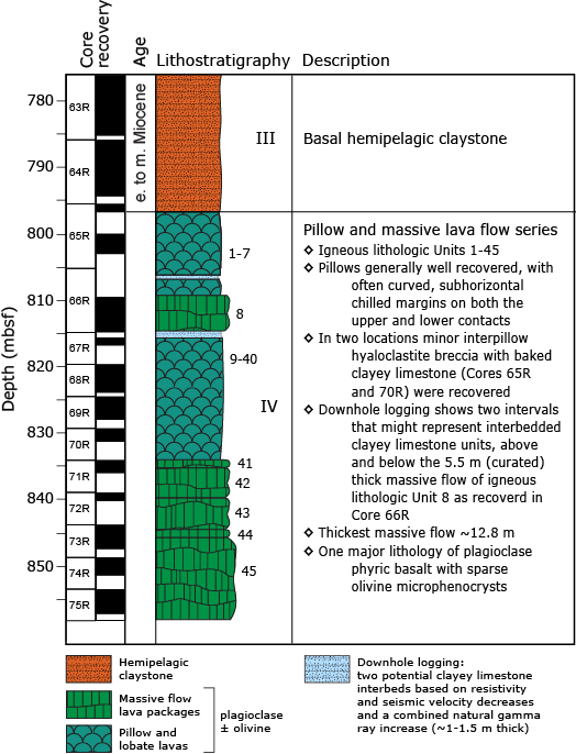
Figure F23. Igneous lithology summary.
The igneous basement begins with a sequence of sparsely to highly plagioclase-phyric pillow basalt with a trace of olivine microphenocrysts. Most of the pillow basalts are nonvesicular to sparsely vesicular, range in grain size from crypto- to microcrystalline, and in many cases have well-preserved curved glassy chilled margins along the top and bottom unit boundaries. A few larger lobate flows are present, varying in curated thicknesses up to 1.1 m. In three intervals, interpillow hyaloclastite breccias were encountered, with remnants of baked clayey limestone in which early Miocene nannofossils are preserved (see Biostratigraphy). Downhole logging provided further indications for 2 unrecovered ~1–1.5 m thick sediment (potentially clayey limestone) interbeds, based on combined increases in natural gamma radiation (NGR) measurements and decreases in the P-wave seismic velocity, electrical resistivity, and bulk density (see Downhole measurements). In between this stack of pillow basalt flows, microcrystalline to fine-grained massive flows up to 5.2 m thick were encountered that are sparsely olivine-plagioclase-phyric but have a holocrystalline groundmass with abundant plagioclase and clinopyroxene present in the interstitial spaces.
Downhole, the basement is characterized by more massive basalt lava flow units as thick as ~12.8 m. These massive flow units have similar petrologic characteristics and range from sparsely to highly plagioclase-phyric with only a trace of olivine microphenocrysts. Groundmass grain size increases to fine grained toward the interior of the thickest lava flow. All basalts have a phenocryst phase assemblage of plagioclase ± olivine, whereas the more massive lava flows have clinopyroxene in their groundmass. In conjunction with geochemical evidence, we conclude that the basement basalt at Site U1433 is typical mid-ocean-ridge basalt (MORB) (see Geochemistry).
Alteration is also typical of that of MORB and ranges from nearly absent or slightly altered to moderately altered in intensity and from gray to dark gray-green and yellow to rusty brown in color. Background alteration in the basement at Site U1433 is low, with most of it focused in halos surrounding fractures and veins. Typical secondary minerals include saponite, Fe oxide, carbonate, and celadonite, all of which represent a low-temperature alteration assemblage. Abundant basaltic glassy margins found near the quenched boundaries of pillow fragments are commonly altered to greenish palagonite, which may indicate alteration from nonoxidative fluids. Alteration veins are abundant at the top of the basement and decrease significantly downhole, indicating limited downwelling fluid flow. Vein-filling minerals include carbonate, celadonite, Fe oxide, saponite, smectite, quartz, and a blue mineral that is difficult to identify without XRD analysis, which was not available during this expedition.
Lithostratigraphic and igneous lithologic units
Unit IV (796.67–857.48 mbsf)
- Interval: 349-U1433B-65R-1, 117 cm, to 75R-4, 74 cm
- Depth: 796.67–857.48 mbsf
- Thickness: 60.81 m (29.02 m at 47.7% recovery)
- Lithology: pillow and massive basalt flows
- Igneous lithologic units: 1–45
The base of the reddish to yellowish brown hemipelagic claystone (lithostratigraphic Unit III) and the first appearance of sparsely to highly olivine-plagioclase-phyric pillow basalt fragments at the top of Section 349-U1433B-65R-2 mark the upper boundary of lithostratigraphic Unit IV at 796.67 mbsf. Throughout Unit IV, most basalt cores are moderately to highly plagioclase-phyric with traces of (pseudomorph) olivine microphenocrysts and are sparsely vesicular, with only minor occurrences of amygdaloidal basalt (Figure F24). The plagioclase phenocrysts are as large as 10 mm, often occur in subhedral short prismatic habit, and vary between 1% and 15% (with an overall average of 7%) in modal abundance in both the pillow and the massive basalt flows (Figure F25). In addition, there is abundant presence of well-preserved curved glassy margins (Figures F26, F27, F28) at the top and bottom boundaries of the pillow basalt flows. Although most of the pillow basalts are aphanitic with cryptocrystalline groundmass and contain a large proportion of mesostasis, the massive basalt flows have a high degree of groundmass crystallinity, increasing to holocrystalline in basalt varieties that are microcrystalline to fine grained (Figures F25G, F25H). Plagioclase shows a wide range of crystal habits and textures, including glomerocrysts, melt inclusions, zonation, and overgrowths (Figure F29).
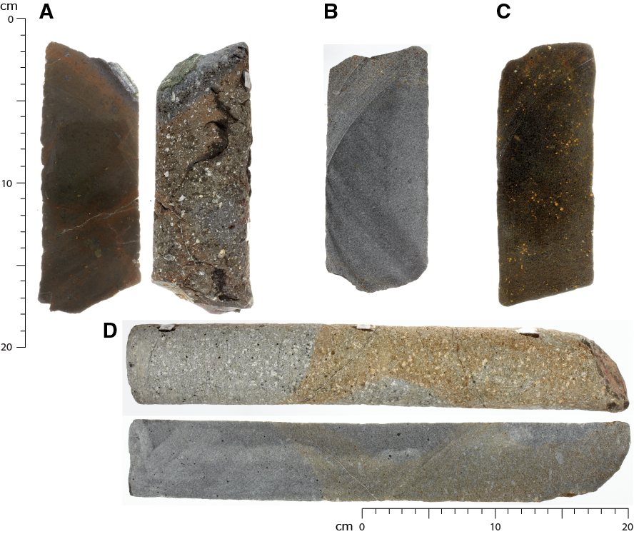
Figure F24. Basement basalt types.
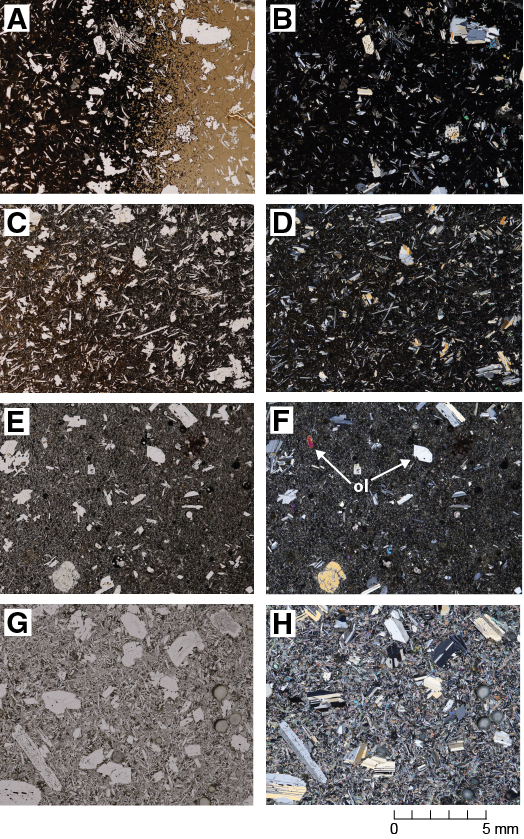
Figure F25. Basalt.
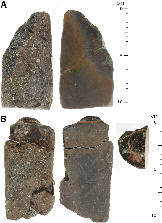
Figure F26. Pillow lava chilled margins.

Figure F27. Interpillow hyaloclastite.
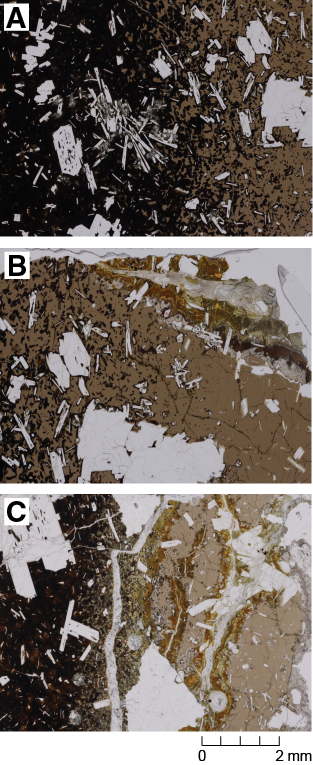
Figure F28. Chilled margins.
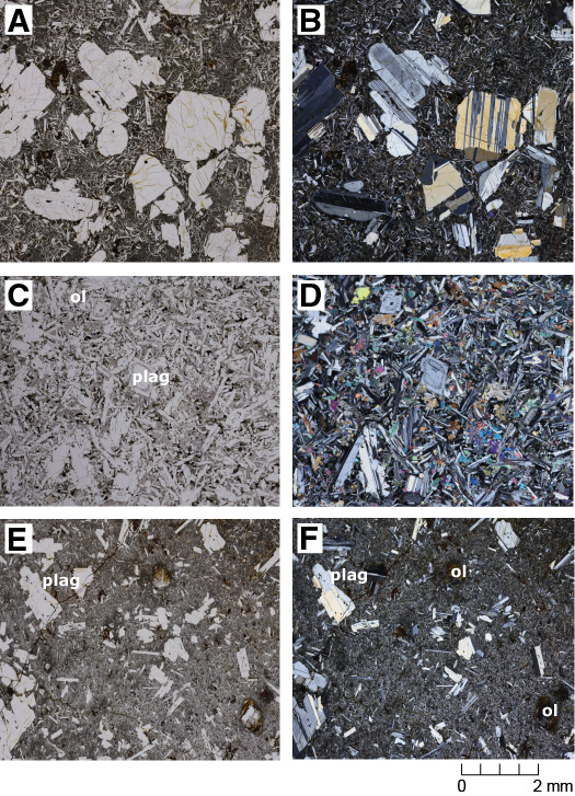
Figure F29. Plagioclase textures.
Igneous lithologic Units 1–7 (0.24–1.14 m in curated thickness) are poorly recovered; therefore, flow boundaries are inferred from the occurrence of chilled margins on separate pieces, with abundant curved glassy rinds preserved on the top or bottom of the pillows, typically 0.3–1.5 cm in thickness. These basement units are interpreted to represent pillow basalt flows composed of sparsely to highly phyric plagioclase basalt, with 0.5%–2% microphenocrysts of olivine, set in an aphanitic, cryptocrystalline groundmass (Figures F24A, F25A–F25D). These basalts are nonvesicular and are fresh to moderately altered, with most of the alteration present in halos along veins. Units with chilled margins almost all contain fresh glass showing gradations into devitrified cryptocrystalline groundmass (Figures F25A, F26A, F28A–F28C). Two occurrences of clayey limestone were recorded at Sections 349-U1433B-65R-1A, 117 cm, and 349-U1433B-65R-2A, 75 cm (Figure F23). In one case, the “baked” limestone is still attached to a glassy chilled margin. These intervals were interpreted to be interpillow hyaloclastite breccia (Figures F27, F28A, F28B). Nannofossils recovered from these intervals may indicate eruption of these pillow basalts during the early Miocene (see Biostratigraphy).
Igneous lithologic Unit 8 (5.2 m thick) is a sparsely olivine-plagioclase-phyric massive basalt flow with up to 2% plagioclase. It is also sparsely vesicular with up to 2% well-rounded, filled vesicles. Compared to the pillow basalt, the basalt in this unit has a holocrystalline groundmass ranging from microcrystalline to fine-grained and consisting of dense networks of long-prismatic plagioclase with clinopyroxene growing interstitially and, in many cases, subophitically with plagioclase. Alteration in this unit is very low and only occurs in thin halos surrounding a small number of existing veins.
Igneous lithologic Units 9–40 (0.08–1.05 m in curated thickness) comprise a second stack of pillow lava flows. The flows are mostly moderately olivine-plagioclase-phyric basalt, but some are highly phyric with plagioclase abundances up to 15% (Figures F24B, F25E, F25F). As with the pillow lavas at the top of the basement in Hole U1433B, many pillows have well-preserved glassy chilled margins (Figures F26B, F28C). At Section 70R-1W, 88 cm, another nannofossil-bearing limestone was found in contact with a chilled margin (see Biostratigraphy). Most pillow basalts are sparsely vesicular with 0.5%–2% vesicles, typically completely filled with secondary minerals, but Units 12 and 40 are strongly amygdaloidal with 7% and 12% vesicles, respectively.
The lower half of the basement unit consists of massive basalt flows of igneous lithologic Units 41–45. The basalts are nonvesicular and generally slightly to moderately altered with only a trace of olivine microphenocrysts that range from fresh to completely replaced (Figures F25G, F25H). The few equant euhedral olivine phenocrysts observed are as large as 3.6 mm, but commonly they are 1 mm or smaller, approaching the typical size of groundmass plagioclase and clinopyroxene minerals that have grown in crystal networks with long-prismatic habits and are of similar size. Groundmass grain size varies from microcrystalline to fine grained in the interiors (Figure F24D) of these massive flows, with the coarsest observed grain sizes in Core 349-U1433B-73R. Drilling at Site U1433 terminated at 857.48 mbsf after coring 12.8 m into this lowermost massive lava flow.
Interpretation of the igneous succession
The primary goal of Expedition 349 was to recover basement to help understand the opening history of the South China Sea. Site U1433 was positioned close to what is believed to be a relict spreading center (Figure F1) to obtain an age estimate for the cessation of seafloor spreading in the Southwest Subbasin. We recovered 29.02 m of basalt after penetrating 60.81 m into igneous basement at Site U1433 and identified 45 igneous lithologic units. The basement unit cored contains 2 sequences of pillow basalts alternating with 2 series of massive basalt lava flows. All basement lithologies have phase assemblages of predominantly plagioclase and sparse olivine (typically as microphenocrysts), with the coarser holocrystalline massive basalt flows also having clinopyroxene present in the groundmass. All of these phase assemblages are consistent with MORB from a petrological point of view.
In three intervals, we cored interpillow hyaloclastite breccias with remnants of clayey limestone in which early Miocene nannofossils are present (see Biostratigraphy). This provides evidence for a possible prolonged eruption age from between ~19 and 22 Ma for the upper pillow lavas to >23 Ma for the lower pillow lava series. Shore-based radiometric dating of the basement samples is required to further constrain the eruption history of the igneous basement at Site U1433. Downhole logging measurements provide evidence for 2 potentially clayey limestone interbeds ~1 to 1.5 m thick that were not recovered in Cores 349-U1433B-66R and 67R (Figure F23). The combined increase in NGR and decreases in P-wave seismic velocity, electrical resistivity, and bulk density (see Downhole measurements) are indicative of lithologies that are not basaltic but rather a clay-rich, less-resistive sedimentary layer that is compatible with downhole FMS images. If present, these 2 sedimentary interbeds may indicate some hiatus between volcanic eruptions at Site U1433, just before and shortly after the emplacement of the massive lava flow of igneous lithologic Unit 8 (Figure F23).
Alteration
Alteration intensity of the igneous basement at Site U1433 is significantly lower than at Site U1431. In addition, compared to other Integrated Ocean Drilling Program ocean crust basement sites of similar age, such as Hole U1368F (Expedition 329 Scientists, 2011), the basalts at Site U1433 seem relatively unaltered. Alteration intensity varies from slight to complete, with the majority of the recovered Site U1433 basement basalt being unaltered to slightly altered only. The highest extent of alteration occurs in the halos flanking the veins (Figures F24D, F30A). According to our macroscopic shipboard description, background alteration accounts for ~71% of the recovered cores at Site U1433, whereas the highly altered halos and veins account for ~28% and ~1%, respectively.
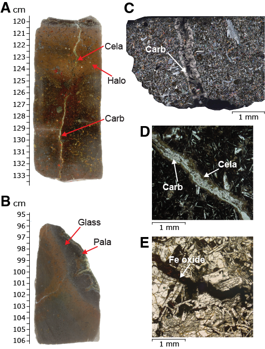
Figure F30. Alteration halo types.
Alteration veins and associated halos are abundant in the top of the basement cores and decrease downhole (Figure F31), indicating more limited interaction with seawater with depth. Background alteration colors in the basalt cores range from gray to gray-green and yellow-brown. Alteration halos vary in color from green to red-brown. In intervals away from veins and halos, plagioclase phenocrysts, olivine microphenocrysts, and the basaltic groundmass are all remarkably unaltered, and large proportions of well-preserved glassy rinds remain in the chilled margins. Based on macroscopic and thin section observations, the overall alteration style is characterized by the following categories:
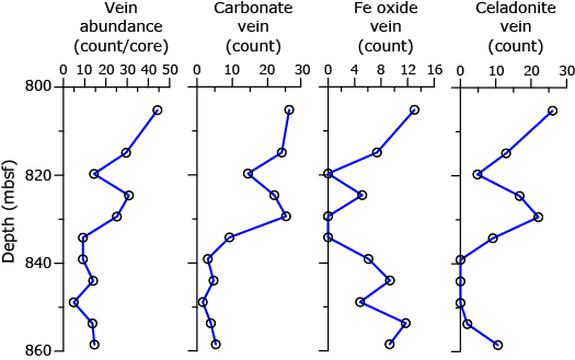
Figure F31. Downhole vein abundance.
- Green to red-brown alteration halos, typically associated with veins;
- Partial to complete vesicle fillings (Figure F32) by secondary minerals, typically celadonite, carbonate, Fe oxide, smectite, and saponite (in decreasing order);
- Minor vein fillings by celadonite, carbonate, Fe oxide, smectite, quartz, and some other (unidentifiable) secondary minerals; and
- Background alteration occurring in slightly altered basalt, typically represented by alteration of olivine, plagioclase, clinopyroxene, and mesostasis in the groundmass.
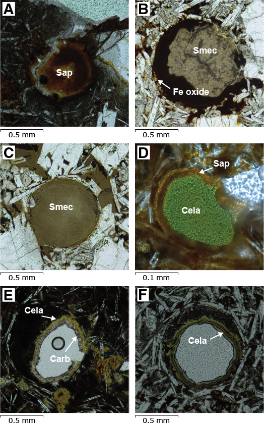
Figure F32. Vesicle fillings.
Alteration phases
Alteration in the Site U1433 basement is characterized by halo alteration caused by fluid/seawater flow through fractures and veins (Figures F24D, F30A). Oxidative and nonoxidative alteration appear to both exist in the basalt cores. Oxidative alteration is indicated by the occurrence of abundant Fe oxide in veins and as mineral fillings in vesicles. Nonoxidative alteration is marked by the occurrence of greenish palagonite in volcanic glass rinds and smectite. The major alteration minerals include celadonite, saponite, carbonate, palagonite, and Fe oxide.
Celadonite is distinctively bright green and is observed throughout the basement cores in Hole U1433B. It is the most abundant secondary mineral in vein fillings, vein-surrounding halos, and vesicles. Saponite is also a widespread alteration mineral at Site U1433 and occurs as one of the major vesicle-filling minerals. It has a color that ranges from yellow to light brown. Carbonate appears throughout the recovered basement cores and in vein fillings (Figures F30A, F30C, F30D). In some places, it also replaces the groundmass mesostasis. Palagonite is present as a green alteration product of basaltic glass and typically is observed in the chilled margins of pillow basalt and thin sheet flows (Figure F30B). Fe oxide mainly exists as a vein-filling mineral (Figure F30E), but it also replaces primary minerals such as olivine. Colors of Fe oxide vary from yellow-brown to dark brown. Other alteration phases, such as quartz (in veins in Section 349-U1433B-71R-1) and unidentified light blue and red minerals, are also observed, particularly as minor vein-filling minerals.
Alteration of primary minerals
Olivine microphenocrysts are usually completely altered to secondary minerals in halos and highly altered basalt, where they can only be recognized by their pseudomorphs. They are mostly fresh (1%–10% alteration) in most of the unaltered and slightly altered basalt cores; entirely fresh olivine crystals are rare in Hole U1433B. Similar to Site U1431, replacement of olivine by various secondary mineral phases (e.g., saponite, Fe oxide, and celadonite) ranges from 1% to 100%. Clinopyroxene is only observed in the interstitial spaces in groundmass and is often replaced by saponite, smectite, and Fe oxide. Plagioclase accounts for the majority of the phenocrysts and groundmass minerals but is the least altered mineral. Unaltered plagioclase can be found even in the most strongly altered basalt cores, and its alteration intensities range from 0% to 20% only. Plagioclase is replaced by clay minerals, such as saponite, smectite, and Fe oxide in these highly altered intervals.
Background alteration
The background alteration at Site U1433 has low intensity overall. The strongest background alteration occurs in the upper part of the basement section and in the upper (Section 349-U1433B-68R-1) and lower part of the massive flow of igneous lithologic Unit 8. The background alteration in these intervals is characterized by the formation of Fe oxide, saponite, and celadonite. Even in the least altered basalt, olivine is mostly altered.
Veins and alteration halos
Based on macroscopic observation of archive sections, we identified 106 veins in the 29.02 m of recovered basement basalt, with an average vein abundance of 3.7 per meter, which is higher than that at Site U1431 (2.8 veins per meter). Vein thickness varies from <0.2 to 2.5 mm, with an average thickness of 0.96 mm. Veins observed in the basement at Site U1433 exhibit curved, planar, irregular, and (complex) anastomosing shapes, and they are mostly isolated, with a few branched veins or vein networks. Vein fillings have colors varying from white to dirty white, light green to green, and in some cases they are pink or light blue. Fillings consist of celadonite, saponite, Fe oxide, carbonate, quartz, and other secondary minerals (Figures F30C, F30D). Veins range from slightly to completely filled. Most have 1 mineral filling, but some have more than 1 mineral filling and are banded. Veins filled with carbonate are most abundant (63%), followed by veins filled with celadonite (55%), Fe oxide (31%), and quartz (3%). The distribution of vein-filling minerals, from the vein walls inward, indicates that their formation sequence progressed from Fe oxide to saponite to smectite to celadonite to carbonate. Quartz occurs only near the highly altered basaltic glass remnants. Most of the veins (85%) observed at Site U1433 have halos that vary in width from <0.1 to 3 cm.
Vesicle fillings
Vesicles make up (on average) only 1% of the recovered basement basalt in Hole U1433B, with individual core sections having vesicle abundances up to 12%. According to thin section observations, vesicle fillings range from none to 100% and include saponite, Fe oxide, carbonate, celadonite, and smectite. The general filling order is Fe oxide or saponite, smectite, celadonite, and carbonate (Figure F32).
Basalt glass alteration
Basaltic glass was recovered from most of the lobate flow and pillow lava flow boundaries. These glasses are partly altered to greenish palagonite (Figure F30B), but overall they are well preserved.
Interpretation of alteration
Evidence for both oxidative and nonoxidative alteration exists at Site U1433, which is typical of previous sites with a thick (clay-rich) sediment cover, such as Ocean Drilling Program (ODP) Holes 801C and 504B (Alt et al., 1992). The abundant basaltic glass altered to green palagonite indicates that alteration occurred in nonoxidative conditions, whereas the secondary mineral assemblage of Fe oxide and saponite suggests low-temperature and oxidative alteration. Alteration at Site U1433 is controlled by the formation of vein halos, where the background alteration is less intense compared to Site U1431 where it occurs pervasively throughout the cores. In fact, most of the basaltic cores at Site U1433 are quite fresh or only slightly altered. The strongest alteration occurs in halos flanking veins, which mostly are concentrated in the top part of the basement section.
The total abundance of veins at Site U1433 and the abundance of each specific vein type, such as Fe oxide- or celadonite-dominated veins, show downhole variations. The number of total veins, carbonate veins, and celadonite veins appears to be highest toward the top of the basement and decreases with depth (Figure F31). Such a vein distribution could be the result of a limited downwelling fluid flow and/or presence of fewer fractures with increasing depth. This vein distribution is consistent with the downhole decrease in overall alteration extent based on macroscopic observations.
Structural geology
Site U1433 is located in a seafloor depression bordered by 2 abyssal highs and is ~50 km southeast of the relict spreading ridge (Figure F1). Seismic reflectors show quite continuous sedimentation around the site with no obvious faulting activity at shallow depth (Figure F3). We cored ~60 m of basalt and successfully recovered ~29 m of basement cores. The basalt sequence consists of 9.7 m of thick pillow basalts, ~5 m of thick massive flows, ~20 m of thick pillow basalts, and ~23 m of thick massive flow at the bottom (see Igneous petrology and alteration). Pieces of mudstone and limestone were also present above and below the 5 m thick massive flow.
Shape and connectivity of fractures and veins
We observed >300 fractures and veins at this site and measured roughly 240 of them. Many of the structural features are either irregular or in small branches and thus could not be measured easily. The veins generally reflect later stages of cracking, fluid circulation, and fluid-rock reaction, whereas many fractures are reactivated along existing veins during drilling or by local stress perturbation. Most of the fractures or veins observed have no obvious lateral offset or striations on the fractured surface. These structures can be used as an indicator of the degree of rock fragmentation.
Veins are filled with different minerals, including dark green celadonite, white smectite, white carbonate, and brownish Fe oxide. In general, the veins (including reactivated fractures along existing veins) can be categorized into six types of distinctive shapes:
- Single straight or curved veins (Figure F33),
- Irregular sinuous veins (Figure F34),
- Triple-junction veins (Figure F35),
- Branched veins (Figure F36),
- Crosscutting veins (Figure F37), and
- Radiate veins (Figure F38).
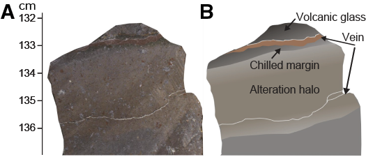
Figure F33. Single curved veins.

Figure F34. Irregular sinuous veins.
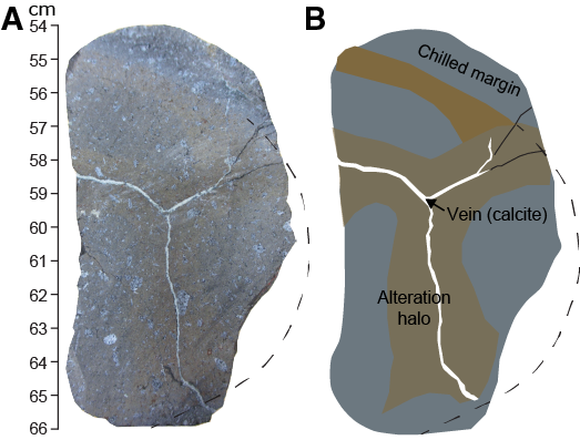
Figure F35. Triple-junction veins.
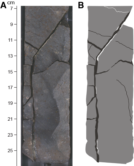
Figure F36. Branched veins.
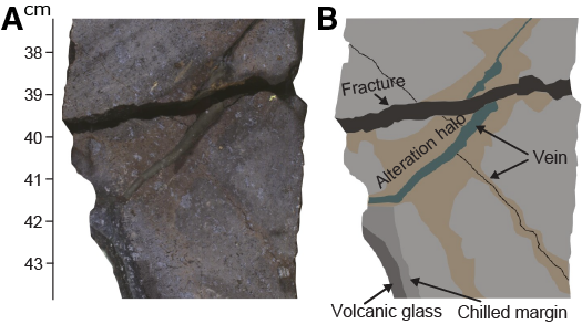
Figure F37. Crosscutting veins.

Figure F38. Radiate veins.
Curved, crosscutting, irregular sinuous, radiate, and triple-junction veins are usually distributed in pillow basalt units, whereas single straight and branched veins are usually found in the massive flow units. In many cases, curved veins appear subparallel to the chilled margins of pillow basalt units, whereas radiate veins point away from the flow center toward the chilled margins. Triple-junction veins appear as a part of the radiate structure with three arms pointing to different directions toward the chilled margin. Alteration along the fractures or veins often generates 1–2 cm wide yellow to brown vein halos. These kinds of veins are either parallel or perpendicular to the chilled margin and are thought to form during cooling of the pillow lava. Single straight or branched veins are sparse and usually observed in massive flow basalts with random orientations.
Frequency of fractures and veins
In order to evaluate the rock fragmentation, the frequency of fractures and veins was calculated (Figure F39). First, the total number of fractures and veins in each section was counted. Frequency was obtained by dividing the total number of fractures and veins by the length of the section. For pillow basalt units, the calculated frequency may underestimate the degree of fragmentation because the pillows were broken into small pieces that were not counted; however, the results remain informative.
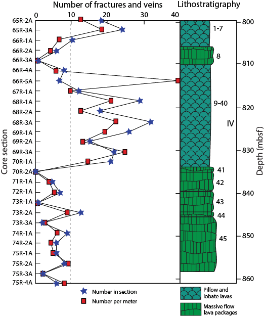
Figure F39. Fracture and vein frequency.
The average frequency of fractures and veins in the basalt is ~10 per meter, which is about 57% of the average frequency of fractures and veins observed at the basalt units of Site U1431. The frequency of fractures and veins changes in different basalt segments. High frequencies occur in the pillow basalt units, whereas massive flow basalts have lower frequencies. During the magma cooling process, pillow basalts generally break much more easily along well-developed fractures and veins. Massive flow basalts are much thicker or larger, so most of the fractures or veins occur on the margins with their occurrence decreasing toward the center of the basalt flow unit.
Orientation statistics
In order to evaluate the causes of the fractures and veins, we created orientation rose diagrams (Figure F40). Usually, fractures align in particular dipping directions if they were caused by a relatively uniform regional stress field. The rose diagram for the total population of fractures and veins shows a very scattered dipping distribution. We hypothesize that the fractures and veins resulted mainly from cooling. The regional stress field might have a weak effect on fracture or vein formation, but this effect is difficult to evaluate because of the scattered orientations.
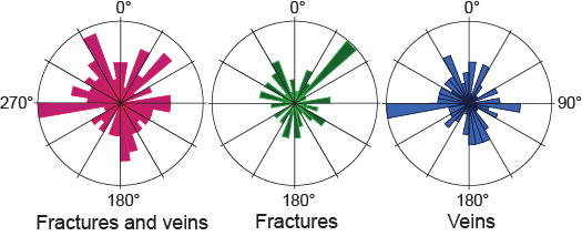
Figure F40. Vein and fracture dipping angles.
Geochemistry
Interstitial water chemistry
We collected 25 whole-round samples (5 cm long) for interstitial water measurements between 0 and 186.8 mbsf in Hole U1433A at a frequency of 2 samples per core. In Hole U1433B, which is ~20 m away from Hole U1433A, 39 interstitial water samples were taken from 196 to 604.5 mbsf at a frequency of one sample per core. Interstitial water chemistry data are given in Tables T12 and T13 and shown in Figures F41, F42, F43, F44, and F45.
Table T12. Interstitial water major element concentrations, Holes U1433A and U1433B. Download table in .csv format.
Table T13. Interstitial water minor element concentrations, Holes U1433A and U1433B. Download table in .csv format.
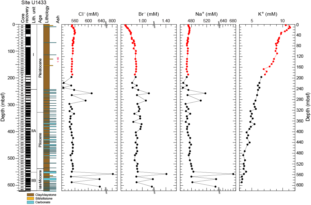
Figure F41. Chloride, bromide, sodium, and potassium.
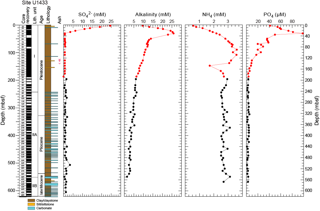
Figure F42. Sulfate, alkalinity, ammonium, and phosphate.
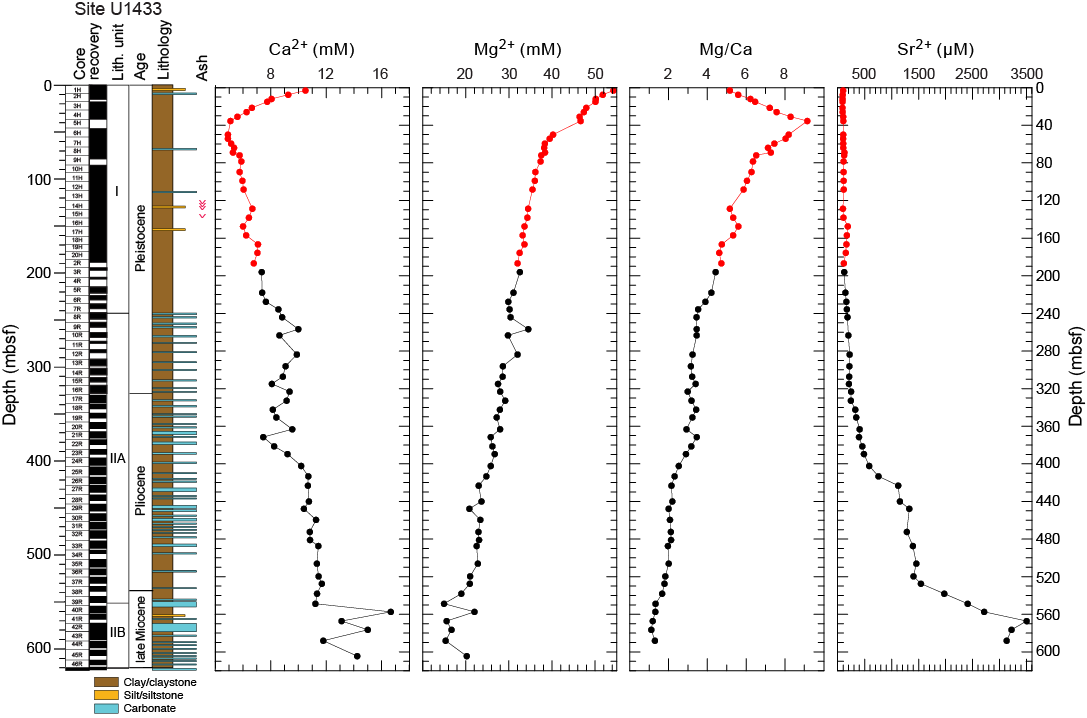
Figure F43. Calcium, magnesium, and strontium.
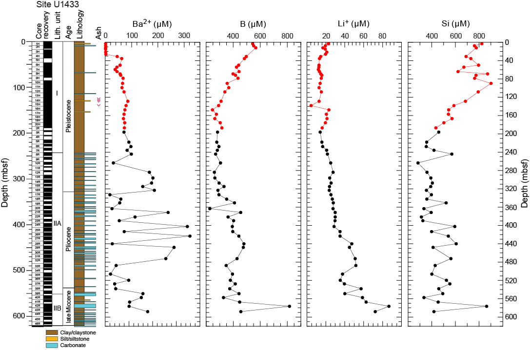
Figure F44. Barium, boron, lithium, and silica.
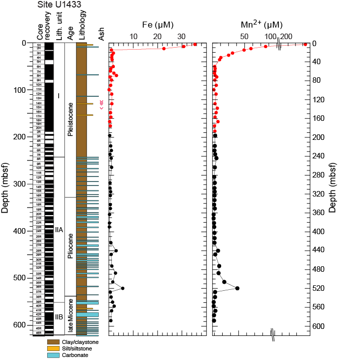
Figure F45. Iron and manganese.
Chloride, bromide, sodium, and potassium
Downhole profiles of chloride, bromide, sodium, and potassium at Site U1433 are shown in Figure F41. Chloride, sodium, and bromide show similar profiles with depth. Chloride and sodium concentrations are relatively constant downhole to ~200 mbsf, ranging from 543 to 560 mM and from 468 to 485 mM, respectively. Bromide concentrations increase from 0.84 mM close to the seafloor to 0.94 mM at ~200 mbsf; however, chloride, bromide, and sodium vary significantly between 217 and 284 mbsf, which corresponds to the transition from the clay of lithostratigraphic Unit I to interbedded clay and carbonate turbidite deposits in Subunit IIA (see Lithostratigraphy). Shore-based oxygen and hydrogen isotopic analysis will delineate possible causes for interstitial water variations in this interval. Chloride and sodium concentrations from ~300 to 550 mbsf are similar to those in the uppermost 200 m of the site, whereas bromide concentrations are somewhat more variable over this interval but average ~0.95 mM. Concentrations of chloride, bromide, and sodium vary widely at the top of lithostratigraphic Subunit IIB (550–605 mbsf), which is characterized by thicker carbonate turbidite deposits (see Lithostratigraphy). Over this interval, chloride concentrations range from 550 mM (similar to seawater) to a hypersaline value of 801 mM, with other peaks of ~640 mM. Throughout the depth profile, most bromide concentrations are higher than that of modern seawater (0.87 mM), most likely caused by organic matter diagenesis in the sediment, as indicated by sulfate reduction and high methane concentrations (Figures F41, F42, F46).
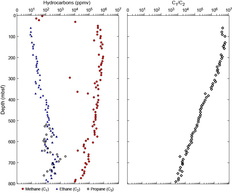
Figure F46. Hydrocarbon gases and methane/ethane ratios.
Potassium concentrations increase from 10.5 mM (similar to modern seawater) close to the seafloor to 11.2 mM at 12 mbsf. Below 12 mbsf, K+ decreases with depth throughout the hole, with a minimum value of 3.4 mM at 605 mbsf. Concentrations higher than the modern seawater value occur in the uppermost 26 m of sediment. This phenomenon is also observed at Sites U1431 and U1432 and is attributed to ion exchange with clay minerals (see Geochemistry in the Site U1431 chapter and Geochemistry in the Site U1432 chapter [Li et al., 2015c, 2015d]).
Alkalinity, sulfate, ammonium, and phosphate
Alkalinity, sulfate, ammonium, and phosphate profiles are shown in Figure F42. Alkalinity increases from 9.7 mM close to the seafloor to a maximum of 25.8 mM at ~30 mbsf, where sulfate is completely consumed. Below 40 mbsf, alkalinity decreases with depth to 1.4 mM at 549 mbsf. The increase in alkalinity promotes carbonate precipitation in the uppermost 40 m, as suggested by the calcium and magnesium concentrations (Figure F43). The low alkalinity below 200 mbsf is probably caused by low amounts of organic matter diagenesis due to the relatively low sedimentation rates of 5–9 cm/ky estimated for this interval (Figure F22; see also Biostratigraphy).
Sulfate concentrations decrease with depth and sulfate is almost completely depleted at ~30 mbsf (Figure F42). This is consistent with the increase of methane concentration to 1100 ppmv at 30 mbsf, reaching a maximum of 93 × 103 ppmv at ~200 mbsf (Figure F46). Based on sulfate and methane concentrations, the sulfate–methane transition zone (SMTZ) occurs at ~30 mbsf.
Ammonium concentrations increase from 0.6 mM near the seafloor to a maximum 3.6 mM at ~100 mbsf, 70 m below the SMTZ. This suggests organic matter fermentation producing ammonium continues below the sulfate reduction zone. From 200 to 570 mbsf, ammonium averages around 2.8 mM. Phosphate behaves differently from ammonium; phosphate concentrations increase from 40 µM at the top to a maximum 98 µM at the SMTZ and then decrease with depth to 1.7 µM at ~235 mbsf. Below that depth, phosphate concentrations remain approximately constant at ~2 µM down to 570 mbsf. The low phosphate concentrations below 200 mbsf are likely caused by less reactive organic matter due to the low sedimentation rates of 5–9 cm/ky (see Biostratigraphy).
Calcium, magnesium, and strontium
Downhole distributions of Ca2+, Mg2+, Mg/Ca ratio, and Sr2+ are shown in Figure F43. Calcium concentrations decrease from 10.5 mM near the seafloor to a minimum of 5.1 mM at 35.4 mbsf, approximately at the SMTZ, where the alkalinity reaches a maximum and could trigger diagenetic carbonate precipitation, taking up Ca2+ and some of the other alkaline earth elements, particularly Mg2+ and Sr2+. The Mg/Ca ratio increases from ~5 (modern seawater value) near the seafloor to a maximum of 9 (almost twice that of modern seawater) at ~35 mbsf, indicating that carbonate precipitation is dominated by preferential uptake of Ca2+ compared to Mg2+ in the uppermost part of the hole. Below 35 mbsf, calcium concentrations gradually increase to 11.5 mM, corresponding to a gradual Mg2+ decrease to a minimum 14.9 mM and a gradual Mg/Ca ratio decrease to ~2 at ~548 mbsf. These distributions could indicate dolomitization of calcite occurring in the sediment. Below 550 mbsf, calcium concentrations increase significantly to a maximum 16.7 mM at ~557 mbsf and then vary from 11.8 to 16.7 mM downhole to 605 mbsf. Magnesium concentrations also show more variability below 550 mbsf, varying from 15.3 to 22.0 mM.
Sr2+ behaves differently from Ca2+ and Mg2+ because carbonate precipitation and recrystallization does not affect Sr2+ concentrations at low temperatures. Sr2+ concentrations are low and relatively constant (<200 µM) in the uppermost 200 mbsf. Below that depth, Sr2+ concentrations increase slowly to 500 µm at 400 mbsf, before reaching a maximum of ~3500 µM at ~567 mbsf and then slightly decreasing to 3100 µM at 588 mbsf.
Higher Sr2+ and Ca2+ concentrations deeper than 550 mbsf may derive from a deep fluid source. This is supported by the high concentrations of boron, lithium, and silica in the same horizon (Figure F44). Shore-based isotopic analysis of interstitial water should provide better constraint for the fluid source.
Barium, boron, lithium, silica, iron, and manganese
Downhole distributions of barium, boron, lithium, silica, iron, and manganese are shown in Figures F44 and F45. Barium concentrations are elevated with respect to modern seawater (0.032–0.15 µM), ranging from 1.0 to 322 µM. Barium reaches a first peak of 62.4 µM at ~35 mbsf, corresponding to the SMTZ. Deeper than 35 mbsf, barium increases slightly to ~100 µM down to ~250 mbsf and then varies significantly between 10 and 300 µM, showing lower values in clay and higher values in carbonate turbidites. The Ba2+ profile is likely related to the stability of barite (BaSO4) in sediment. The Ba2+ concentration increase may result from in situ barite dissolution due to sulfate reduction or the migration of Ba2+ in the low-sulfate fluid. Shore-based solid-phase barium analyses will be critical for determining the origin of the elevated barium and the history of the fluid flow.
In the uppermost 200 mbsf, boron concentrations decrease from ~550 µM close to the seafloor to a minimum ~246 µM at 147 mbsf. Deeper than 200 mbsf, boron concentrations show a very gradual increase to ~500 µm at 450 mbsf. Below this depth, boron concentrations vary around 400 µM, with a single peak of 801 µM at 565 mbsf
Lithium concentrations decrease from 22.7 µM close to the seafloor, which is slightly lower than the modern seawater value (25 µM), to 4.5 µM at ~138 mbsf. Deeper than 140 mbsf, lithium concentrations gradually increase to a maximum of 86.7 µM at ~580 mbsf before decreasing to 72.3 µM at 590 mbsf.
In the uppermost 140 mbsf, silica concentrations are elevated compared to modern seawater (0–180 µM), ranging from 600 to 901 µM (Figure F44), possibly due to dissolution of siliceous microfossils, including diatoms, radiolarians, and sponge spicules, that occurs in the uppermost part of Hole U1433A (see Lithostratigraphy and Biostratigraphy). Deeper than 140 mbsf, silica concentrations are much lower, mostly fluctuating between 400 and 600 µM with a single peak of 864 µM at ~576 mbsf. This is consistent with the lithology change from predominantly clay in lithostratigraphic Unit I to interbedded clay and carbonate turbidite deposits in Unit II (see Lithostratigraphy).
Both dissolved iron and manganese concentrations decrease in the uppermost ~40 mbsf (Figure F45), corresponding to the zone of active sulfate reduction. Usually in this zone, iron and manganese concentrations increase with increasing sulfate reduction; oxidized iron and manganese are being reduced and released into the interstitial fluid as Fe2+ and Mn2+, which are more soluble than the oxidized species. The decrease in iron and manganese concentrations likely suggests that Fe2+ and Mn2+ are taken up by diagenetic precipitation of sulfides and carbonates. From 40 to 423 mbsf, both Fe2+ and Mn2+ concentrations are very low, ranging from 0.2 to 3.1 µM and 2.7 to 4.1 µM, respectively. Below 430 mbsf, Fe2+ and Mn2+ concentrations increase to 5.7 and 38.7 µM, respectively, at ~520 mbsf before decreasing again to very low values from 520 to 580 mbsf.
Headspace gas geochemistry
Sediments recovered from Holes U1433A and U1433B were monitored for hydrocarbon gases as part of the shipboard safety and pollution prevention program (Figure F46; Table T14). Headspace methane content increases from 2–5 ppmv close to the seafloor to 1101 ppmv at 30 mbsf corresponding to the SMTZ. Methane content reaches a maximum 93,595 ppmv at 196 mbsf before decreasing slowly with depth. Ethane is present at low concentrations below 59 mbsf, ranging from 0.9 to 681 ppmv. Propane is present between 519 and 774 mbsf, ranging from 7 to 287 ppmv. The C1/C2 ratio gradually decreases from >50,000 at ~150 mbsf to ~1000 at 800 mbsf at the base of the sediment section in Hole U1433B. These values are well within the normal range based on the relatively high thermal gradient of ~78°C/km at this site (see Downhole measurements) (Pimmel and Claypool, 2001). Shore-based carbon isotopic analysis of methane in the headspace gas samples will provide more insights on the origin of hydrocarbon gases.
Table T14. Headspace sample hydrocarbon concentrations, methane, ethene, ethane, propene, and propane, Holes U1433A and U1433B. Download table in .csv format.
Bulk carbon and nitrogen analysis
Organic and inorganic carbon distributions for Site U1433 are illustrated in Figure F47 and listed in Table T15. In the uppermost 300 mbsf, CaCO3 content is <15 wt%, except for one peak of 40 wt% at ~70 mbsf that corresponds to a nannofossil ooze turbidite layer. Below 300 mbsf, CaCO3 is more variable, with values >40 wt% corresponding to carbonate horizons, whereas clay intervals have CaCO3 content of <15 wt%. Total organic carbon (TOC) content decreases slightly in the upper 200 mbsf, suggesting organic matter diagenesis. From 200 to 300 mbsf, TOC is relatively constant at ~0.5 wt%. Below 300 mbsf, TOC is more variable, with a peak of 8.5 wt% at 371 mbsf (measured twice to confirm the high value). The TOC to total nitrogen (C/N) ratio at this depth is also abnormally high (250). There are several other intervals of higher TOC and C/N ratios at 440–460, 550–570, and 700–750 mbsf. Samples from these intervals are from carbonate turbidite deposits thought to have been derived from shallow-water locations south of Site U1433 (see Lithostratigraphy). The C/N ratio also increases in these intervals with higher TOC, reaching >20, which suggests a terrestrial source for the organic carbon. This is consistent with organic carbon-rich sandstone in lithostratigraphic Unit IIB (Figure F20; see also Lithostratigraphy).
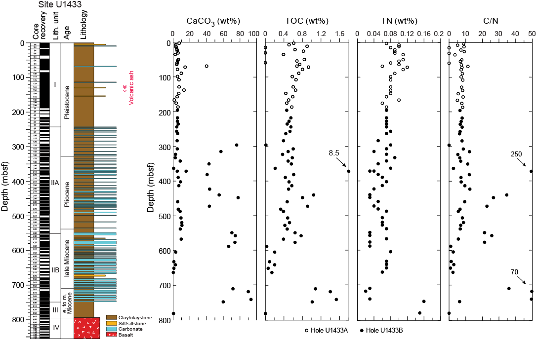
Figure F47. Calcium carbonate, TOC, TN, and C/N ratios.
Table T15. Carbon and nitrogen content, Holes U1433A and U1433B. Download table in .csv format.
Igneous rock geochemistry
Eighteen igneous rock samples from Cores 349-U1433B-65R through 75R were analyzed for concentrations of major and minor elements by inductively coupled plasma–atomic emission spectroscopy (ICP-AES) (Table T16).
Table T16. Major element oxide and trace element concentrations in igneous rock samples, Hole U1433B. Download table in .csv format.
Total weight percentage for the major element oxides varies from 98.0 to 103.8 wt%. For comparison with data from other sites, measured major element total values were normalized to 100 wt%. The loss on ignition (LOI) values, which serve as a rough indicator of the overall level of alteration in the rocks, are low, ranging from 0.52 to 2.06 wt%. The samples have extremely low K2O (0.11–0.29 wt%), moderate TiO2 (1.32–1.63 wt%), MgO (5.01–8.22 wt%), Fe2O3 (9.20–11.39 wt%), Na2O (2.63–3.02 wt%), and SiO2 (48.5–51.1 wt%), and high Al2O3 (16.37–18.55 wt%) and CaO (10.89–12.13 wt%) compared to an average basalt. In general, concentrations of major elements vary within a narrow range (Figure F48).

Figure F48. LOI and major elements.
When plotted on the alkali vs. silica diagram of volcanic rock types (Le Maitre et al., 1989) (Figure F49), the samples plot as tholeiitic basalt. As shown in Figure F50, these rocks are similar to both Indian and Pacific MORB but are distinct from the Hainan Island ocean-island basalt (OIB) and the seamount basalts in the South China Sea. Thus, the basalt samples from Hole U1433B are tholeiitic basalt and are considered representative of South China Sea MORB.
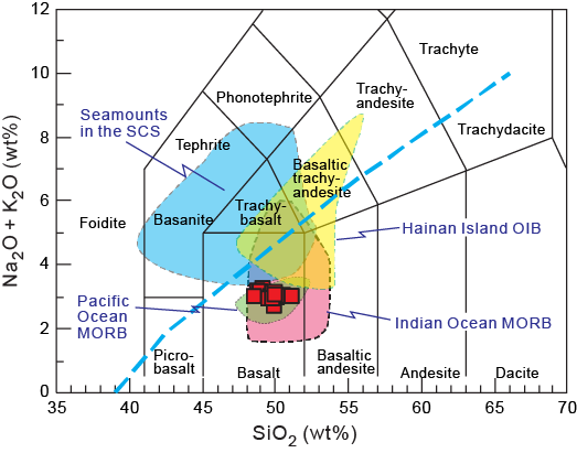
Figure F49. Total alkalis vs. silica.
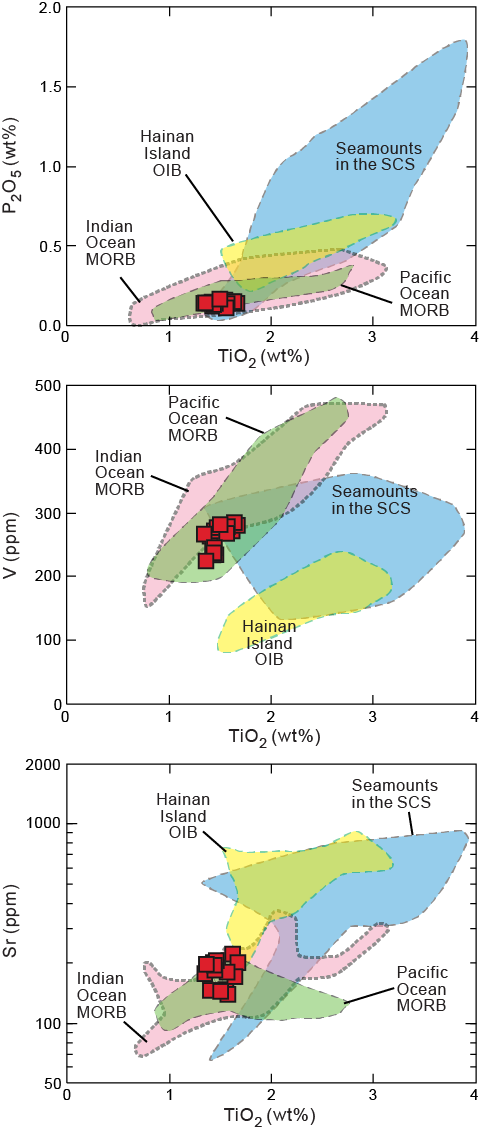
Figure F50. Titanium oxide vs. phosphate.
Microbiology
Our goal for microbiological research conducted at Site U1433 was to collect and preserve samples for shore-based characterization of microbial communities. We collected samples on a routine basis throughout the cored intervals and on a case-by-case basis according to features in the cores that suggested the presence of important geological interfaces. A number of samples were used to start microbial cultivations aboard the ship. In addition, we collected samples for measuring contamination, including perfluorocarbons, microspheres, and fluid community tracers (FCT).
Specific depths sampled for microbiology at Site U1433 are shown in Figure F51. Coring at Site U1433 yielded 50 routine, 5–10 cm whole-round samples to be used for microbiological analysis from the seafloor to 790 mbsf from Holes U1433A and U1433B. We collected whole-round samples for microbiology adjacent to samples for interstitial water measurements (see Geochemistry) in order to understand proximal interstitial water chemistry.
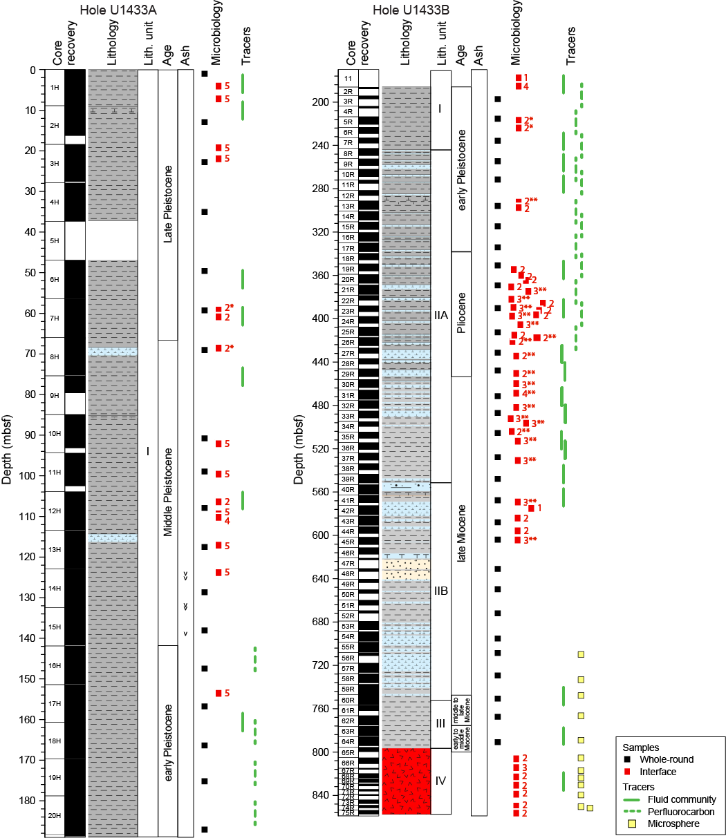
Figure F51. Microbiology and contamination testing samples.
We collected and preserved 164 samples from the split cores for investigating the microbiology of interfaces or coring-induced disturbance using lipid and nucleic acid analyses. We obtained these samples between 4 and 154 mbsf in Hole U1433A and between 187 and 854 mbsf in Hole U1433B. Two sets of interface samples were obtained from volcanic ash/clay interfaces and four sets were obtained from turbidite/clay interfaces. From the split cores, we also sampled four horizons (2 from Hole U1433A and 2 from Hole U1433B) that were within 1 cm of the depth where a whole-round sample was taken on the catwalk several hours previously. We will measure lipids and DNA in these samples to estimate the effect of storage in the core laboratory during the period between when the core arrives at the surface and when the samples are obtained from the split cores on the sampling table. Samples from the split cores from Hole U1433B will be used to compare the microbial communities that are present within intact core biscuits and those that are present in the proximal sediment that has been severely altered during drilling. Twenty sample sets were collected to make this comparison. We selected all interface samples by recognition of key intervals and through consultation with sedimentologists or petrologists.
Microbiological analyses
Most of the samples collected at Site U1433 were preserved for shore-based analysis. Samples to be used for DNA and RNA extractions and sequencing were frozen at −80°C, and samples to be used for lipid extraction and analysis were frozen at −80°C or −20°C. Portions of the whole-round samples were selected for cultivation-based studies to enrich for anaerobic autotrophs and heterotrophs.
Contamination testing
We used three different methods of contamination testing during coring at Site U1433. The PFT perfluoromethylcyclohexane was introduced into the drilling fluid during coring of Holes U1433A and U1433B to trace potential drilling fluid contamination of the cores. PFT samples were acquired from the outside and inside of 16 cores during the coring of these holes (Figure F51). The concentration of PFTs measured on samples from the outside of Sections 349-U1433B-3R-2 (195.9 mbsf) and 13R-4 (296.1 mbsf) were higher than those measured on the inside of these same sections, which indicates no apparent drilling fluid contamination of the interiors of these cores. However, PFTs were not detected in most of the samples collected, regardless of whether the samples were taken from the outside or the inside of the core. The PFT pump was operating during these coring events. One possible explanation for the lack of detectable PFTs in most of the samples from Site U1433 is a leak in the system between the PFT pumps and where the PFT enters the drilling fluid.
Microsphere tracers were used with the RCB coring system in Hole U1433B by adding them to the core catcher sub in Cores 349-U1433B-56R through 75R (709–854 mbsf). Two microsphere samples were collected from each of these cores: one from scrapings of the core surface and one as a subsample from the interior of each whole-round sample. Microscopic counts of the microspheres in these samples will be performed in shore-based laboratories using the Procedure for Curation of DeepBIOS (www.kochi-core.jp/DeepBIOS).
Twenty-four FCT samples were collected either from the drilling fluids that drained from the core liners when cores arrived on the catwalk or from a sampling port near the mud pumps on the rig floor during active coring. The fluids collected for FCT samples correspond to cores obtained between 6 and 824 mbsf. Microbial community DNA and lipids from FCT samples will be compared to the same measurements made on the core samples to determine if the drilling fluids contain microbes that can be regularly tracked as recognizable contaminant taxa.
Paleomagnetism
Shipboard paleomagnetic study at Site U1433 consisted of pass-through magnetometer measurements on all archive-half cores and on representative discrete samples taken from the working halves. At Site U1433, Cores 349-U1433A-1H through 20H were cored with the APC using nonmagnetic core barrels equipped with the FlexIT orientation tool. Thus, both paleomagnetic inclinations and corrected declinations are available for Hole U1433A to construct magnetostratigraphy. Cores 349-U1433B-2R through 75R were cored using the RCB with nonmagnetic core barrels.
In order to isolate characteristic remanent magnetization (ChRM), sedimentary archive-half cores were demagnetized in an alternating field (AF) using steps of 5, 10, 15, and 20 mT and then were measured with the pass-through superconducting rock magnetometer (SRM) at a 2.5 cm interval. Selected discrete samples were AF demagnetized with an ASC Scientific D-2000 AF demagnetizer using 5, 10, 15, 20, 30, 40, 60, 80, and 100 mT steps. The results were analyzed using Zijderveld diagrams (Zijderveld, 1967), and ChRM directions were obtained using principal component analysis (Kirschvink, 1980).
Natural remanent magnetization of sedimentary cores
Downhole variation in natural remanent magnetization (NRM) properties is illustrated in Figures F52 and F53. In Hole U1433A, NRM inclinations are strongly biased toward vertical (mostly toward +90°). Upon 20 mT AF demagnetization, a significant decrease in intensity and a shift of inclination toward shallower or negative values were observed for intervals with normal or reversed polarity, respectively, suggesting the presence of drilling-induced remagnetization.
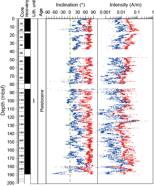
Figure F52. Paleomagnetism, Hole U1433A.
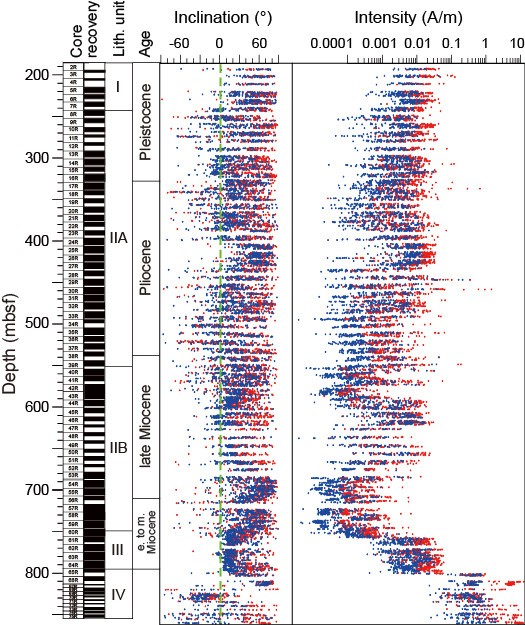
Figure F53. Paleomagnetism, Hole U1433B.
Although this drilling-induced remagnetization is not a welcome feature in isolating the characteristic component of magnetization, its steep positive inclinations do serve as a useful check for whether or not core sections and shipboard paleomagnetic samples were inverted by human error during either collection or measurement processes. Using this information, we successfully identified and corrected several such errors for core sections from Hole U1433A. An example is for Sections 349-U1433A-10H-1 through 10H-3, in which the correct orientation was not known after curation on the catwalk, but their steep negative NRM inclinations served as useful confirmation that the up/down directions of these sections were inverted.
Hole U1433B was drilled by RCB, which resulted in stronger drilling-induced remagnetization (Figure F53). Nevertheless, for most cores, 10–20 mT AF demagnetizations significantly removed the drilling-induced remagnetization. To the first order, the variation of NRM intensity is highly tied to lithology. For sediment shallower than 800 mbsf, NRM intensity is less than ~0.025 A/m but sharply increases by about 2 orders of magnitude in the underlying basalt units. This increase indicates that the basalt contains more strongly magnetic iron oxide than the sediment. Variations in magnetic susceptibility are consistent with variations in NRM intensity (see Physical properties).
As with Sections 349-U1433A-10H-1 through 10H-3 mentioned above, Section 349-U1433B-54R-CC was thought by shipboard sedimentologists to have been inverted based on the observed turbidite sequence in the core. We were able to use the polarity of magnetization of the overlying section to confirm that the core catcher section was indeed inverted.
Paleomagnetic demagnetization results
Representative vector plots (Zijderveld, 1967) showing magnetic behavior during AF demagnetization are given in Figure F54. The vertical overprint affects magnetic minerals with lower remanence coercivity (Bcr < 10 mT). Generally, Bcr is affected by the type and grain size of magnetic minerals. Therefore, downhole variations in magnetic minerals result in changes in Bcr. Theoretically, the effects of vertical overprint are significant for samples containing more low-coercivity minerals (e.g., pseudosingle-domain and multiple-domain magnetite particles in sediment). In contrast, basalt usually contains much finer grained magnetite particles in pseudosingle- and single-domain grain size with higher Bcr values and in turn is less affected by the vertical overprint. Such a phenomenon can be seen in Figure F54. For example, Sample 349-U1433A-1H-6A, 107.5 cm, exhibits a strong vertical overprint that can be removed by 10 mT AF demagnetization. In contrast, for basalt samples such as Sample 349-U1433B-73R-2A, 80.0 cm, the overprint effects are insignificant.

Figure F54. Demagnetization.
The ChRM of Sample 349-U1433A-3R-1A, 42.5 cm, is well defined by a linear trend toward the origin of the vector plot. For other samples (Figure F54B, F54D, F54F), the inclination changes from positive to negative values. This change indicates that the overprint and viscous remanent magnetization effects have been largely removed. For such cases, the remanent magnetization after 20 mT AF demagnetization can be used to represent ChRM for constructing magnetostratigraphy.
At Site U1433, we also obtained representative paleomagnetism directions from several intervals for structural analysis and core orientation. Paleomagnetic core reorientation methods have been successfully used for both continental and oceanic rocks from outcrops or drill cores (e.g., Fuller, 1969; Kodama, 1984; Shibuya et al., 1991). Assuming that the direction of stable remanent magnetization (either viscous remanent magnetization or primary magnetization) represents the expected magnetic direction at the site, the orientation of the paleomagnetic ChRM, which specifies the rotation of the core relative to the geographic coordinates, is then used to restore the azimuth of the core. For intervals of particular interest for structural geology at Site U1433, we either used the stable ChRM isolated from progressive demagnetization of small homogeneous segments (that contain structural features) or an average declination from 3–4 consecutive measurement intervals with the same inclination sign from the archive-half core data. The preliminary results suggest that, overall, paleomagnetic data are reasonably robust and can provide information to serve as the reference direction for structural studies.
Magnetostratigraphy
Constrained by biostratigraphic data, the basal age for Core 349-U1433A-20H (~188 mbsf) is <0.91 Ma, which indicates a rather high sedimentation rate compared to both Sites U1431 and U1432. The major shift in both declination and inclination at ~180 mbsf is therefore assigned to the Matuyama/Brunhes reversal boundary (0.781 Ma) (Figure F55). This correlates to a sedimentation rate of ~23.7 cm/ky. Such a high sedimentation rate facilitates preservation of short-lived paleomagnetic features (e.g., paleomagnetic excursions; Roberts, 2008).
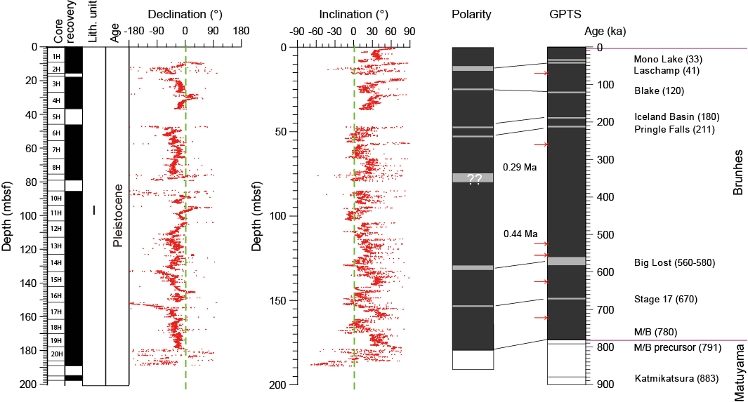
Figure F55. Magnetostratigraphy, Hole U1433A.
Within the Brunhes Chron, 8 polarity shifts are observed. These short-lived events most likely represent geomagnetic excursions as evidenced by both declination and inclination changes. The polarity shifts at ~12, 18, 28, 48, 53, 132, and 152 mbsf match well with known excursion events: Mono Lake (33 ka), Laschamp (41 ka), Blake (120 ka), Iceland Basin (180 ka), Pringle Falls (211 ka), Big Lost (560–580 ka), and Stage 17 (670 ka), respectively. For the other 2 directional anomalies at ~78 and 88 mbsf, there are no counterparts from previous studies. In addition, these 2 anomalies bracket an interval without core recovery. Therefore, further studies are needed to confirm the origin of these 2 anomalies.
Only inclinations in Hole U1433B can be used to construct magnetostratigraphy. Because of the more severe overprint effects of the RCB than the APC, the overall paleomagnetic pattern of cores from Hole U1433B is less obvious (Figure F56). Therefore, we define the positive chrons on the basis of the first-order pattern as constrained by biostratigraphy. Altogether, 6 major positive chrons are recognized. The basal boundaries for the Matuyama (2.581 Ma), Gauss (3.596 Ma), and Gilbert (6.066 Ma) Chrons are therefore defined at ~350, 420, and 550 mbsf, respectively. The basal age for sediment (Core 349-U1433B-60R) is ~11 Ma (see Biostratigraphy). On the basis of this age model, the sedimentation rate changes at ~660 mbsf (between ~9 and 10 Ma).
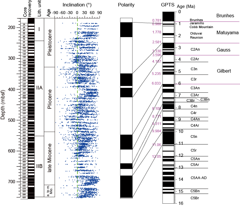
Figure F56. Magnetostratigraphy, Hole U1433B.
Paleomagnetic results for the basement show that the upper part of the unit (805–817 mbsf) is dominated by positive polarity (Figure F57). Between ~817 and 830 mbsf, a reversed polarity zone is observed. Below this depth range, paleomagnetic inclinations display both normal and reversed polarities. Overall, remanent magnetization of rock deeper than ~817 mbsf is dominated by reversed polarity. The variation of remanent magnetization intensity after 20 mT AF demagnetization shows a downhole increasing trend. Magnetization values of the upper units are less than ~1 A/m and increase to 2–2.5 A/m at the bottom. For comparison, the magnetic signature of the basalt units recovered at Site U1431 is also plotted in Figure F57.
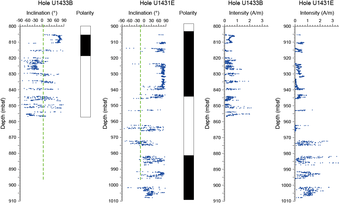
Figure F57. Paleomagnetism comparison.
Physical properties
Cores from Holes U1433A and U1433B were measured for physical properties on whole-round cores (P-wave velocity, bulk density, magnetic susceptibility, and NGR), as well as on split cores (point magnetic susceptibility and x-caliper and z-bayonet P-wave velocity) and discrete samples (moisture and density). Thermal conductivity was measured with a needle probe in soft sediment and then with a contact probe in the lithified sediment and igneous rock. Most P-wave velocities measured on whole-round cores from Hole U1433A are orders of magnitude out of range and not shown in the figures, probably because of the relatively high gas content in the sediment. P-wave measurements were not made on the RCB whole-round cores from Hole U1433B because the space between the core and the liner prevented reliable measurements.
Whole-Round Multisensor Logger measurements
Measurement points that were orders of magnitude out of range were removed from the whole-round core data, which were then smoothed using a five-point average moving window for gamma ray attenuation (GRA) density and a ten-point average moving window for magnetic susceptibility and NGR. The measurements of physical properties in Holes U1433A and U1433B are compiled in Figure F58. Measurements in sediment and basalt are presented in Figures F59 and F60, respectively, to enhance the observations in the corresponding lithostratigraphic units.
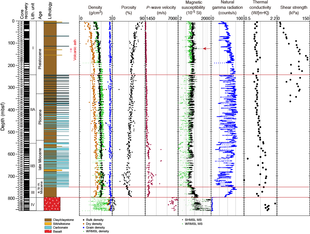
Figure F58. Combined physical property measurements.
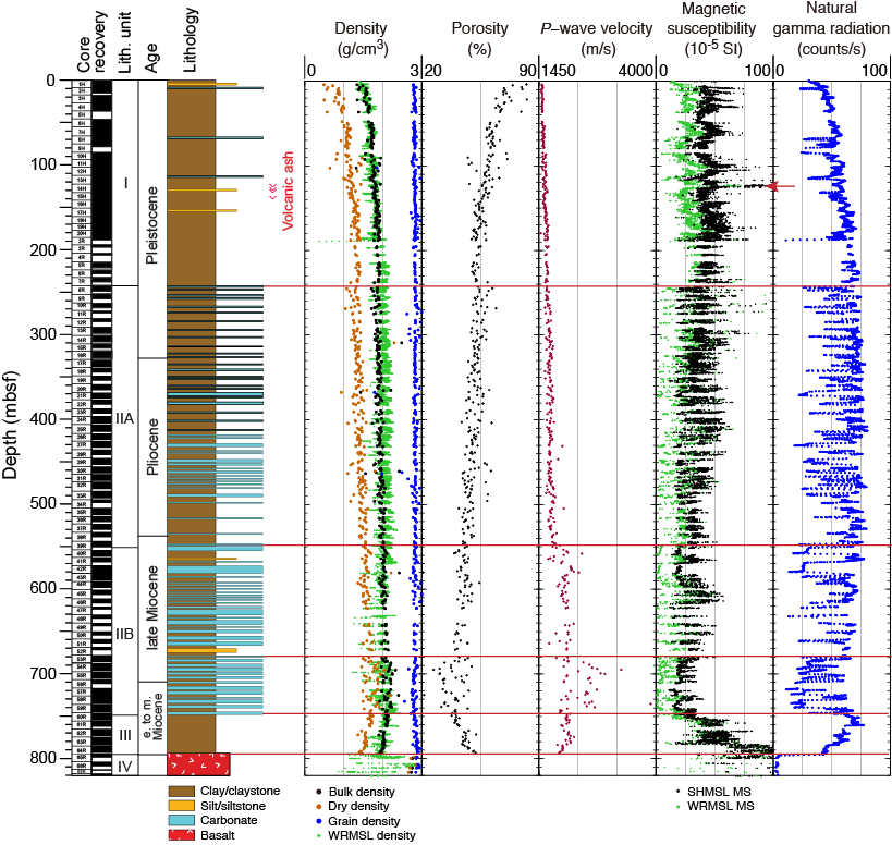
Figure F59. Physical property measurements for sediment.
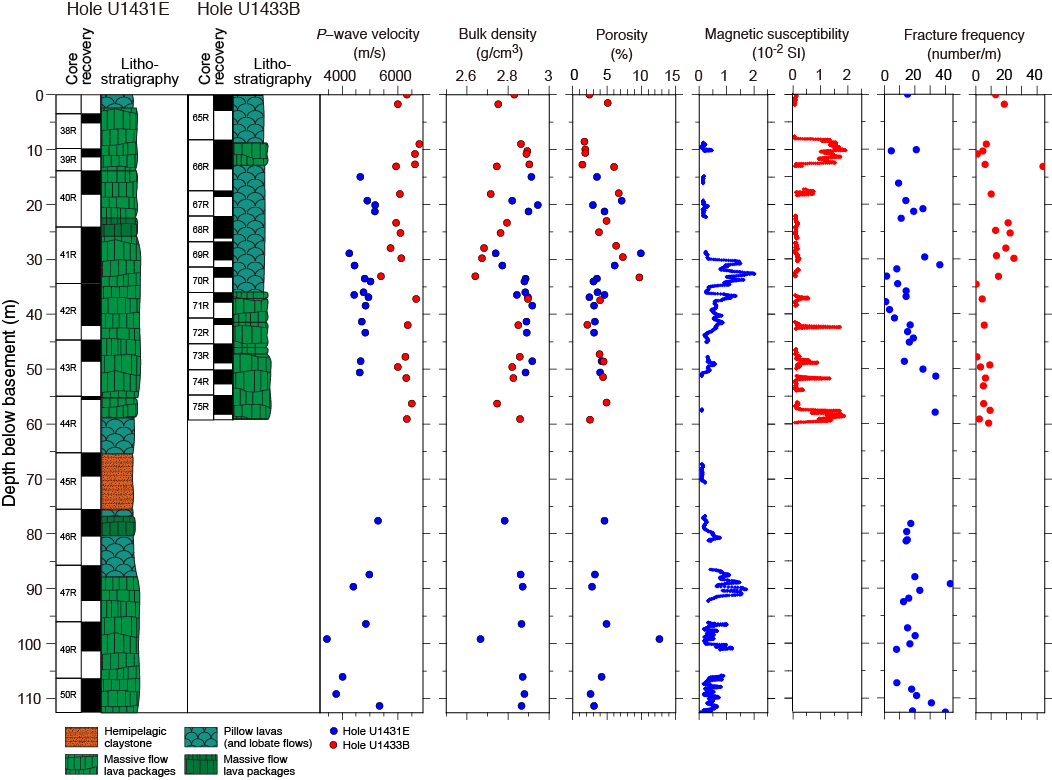
Figure F60. Physical property measurements for basalt.
Gamma ray attenuation bulk density
Bulk density measured from GRA on the Whole-Round Multisensor Logger (WRMSL) increases with depth from 1.4 to nearly 2 g/cm3 in the uppermost 150 m and remains constant near 2 g/cm3 downhole to ~600 mbsf in the clay and carbonate of lithostratigraphic Units I and II. Density gradually decreases with depth from 2.0 to 1.8 g/cm3 in the clay of Unit III, whereas porosity increases with depth in this unit. Density shows large variations from 1.7 to 2.8 g/cm3 in the basalt of Unit IV.
Magnetic susceptibility
Large variations in Site U1433 magnetic susceptibility data with lithology are shown on the log-scale plot in Figure F58. Values increase with depth from 30 × 10−5 to 40 × 10−5 SI in the uppermost 150 m. A peak reaching 100 × 10−5 SI near 125 mbsf corresponds to an ash layer (red arrows in Figures F58, F59). Values are relatively constant at ~40 × 10−5 SI in the clays of Unit I. Magnetic susceptibility values generally decrease with depth in Unit II, from values of 30 × 10−5 to 50 × 10−5 near 240 mbsf to 0−30 × 10−5 SI near 750 mbsf, but the values also show large variability corresponding to changes in lithology in the interbedded clay and carbonate. Magnetic susceptibility values increase with depth in the clays of Unit III and show a large variability in the basalt of Unit IV, from 0 to 2000 × 10−5 SI.
Natural gamma radiation
In Holes U1433A and U1433B, NGR values display trends and variability similar to the magnetic susceptibility values within the different lithostratigraphic units. NGR counts increase with depth from 30 to 70 counts/s over the uppermost 240 m. Below this depth, values alternate between 70 and 30–40 counts/s throughout Unit II downhole to 750 mbsf. NGR counts decrease with depth from 70 to 40 counts/s in Unit III, between ~750 and 800 mbsf, and then are very low in the basalt of Unit IV.
Thermal conductivity
Thermal conductivity increases from 1 to 1.2 W/(m·K) in the uppermost 150 m and then gradually increases to ~1.4 W/(m·K) downhole to ~540 mbsf (Subunit IIA/IIB boundary). Thermal conductivity shows large variations and relatively high values between 1.2 and 1.7 W/(m·K) in the interbedded clay and carbonate of Subunit IIB and the clay of Unit III and is very high in the basalt of Unit IV, from 1.8 to 2.2 W/(m·K). The contact probe requires that measurements in lithified sediment and basalt cores be made on large pieces with smooth splitting surfaces, so the measured values likely overestimate the average in situ thermal conductivity.
Point magnetic susceptibility
Point magnetic susceptibility measurements from the Section Half Multisensor Logger (SHMSL) agree well with WRMSL results. A small offset observed between the 2 types of measurements results from the difference in instrument resolution (see Physical properties in the Methods chapter [Li et al., 2015b]). On average, point magnetic susceptibility is 20 × 10−5 SI greater than WRMSL magnetic susceptibility. Point magnetic susceptibility peaks in lithostratigraphic Unit I reflect the presence of ash layers (red arrow in Figures F58, F59). Magnetic susceptibility values for the basalt of Unit IV range between 0 and 2000 × 10−5 SI, with the highest values in the thick lava flows (Figure F60).
Compressional wave (P-wave) velocity
In Holes U1433A and U1433B, P-wave velocity gradually increases from near seawater velocity at the seafloor (1480 m/s) to ~1700 m/s at 540 mbsf in the soft sediment of lithostratigraphic Units I and II and increases again to ~2000 m/s in the more indurated sediment of Subunit IIB downhole to ~680 mbsf. Below this depth, P-wave velocity shows very variable values from 1800 to 4000 m/s at the bottom of Subunit IIB, with the highest values in the more indurated carbonate layers. P-wave velocity shows lower values near 1900–2000 m/s in the clay of Unit III, with slightly lower values near the sediment/basement interface. P-wave velocity increases to very high values between 5000 and 7000 m/s in the basalt of Unit IV.
Shear strength
Shear strength increases with depth from 20 to 150 kPa in the uppermost 150 m. Below 150 mbsf, shear strength decreases with depth, with more variability in the measurements, between 150 and 60 kPa (Figure F58). Because of sediment compaction, vane shear strength was not measured below 370 mbsf, as many cracks started to develop during measurement.
Moisture and density
Bulk and dry density measured on individual samples show the same variations as bulk density measured on whole-round cores. Grain density is almost constant (~2.8 g/cm3) in sediment (lithostratigraphic Units I–III). Basalt grain densities are close to 2.9 g/cm3. Porosity shows a large decrease with depth in the uppermost 150 m, from 90% to 50%, decreases more slowly with depth from 60% to 40% downhole to 750 mbsf, and increases again in the clay of Unit III, up to 60%. Porosity drops to 1%–10% in basalt.
Data interpretation and lithologic correlation
In Holes U1433A and U1433B, physical properties correlate both with lithology and observed lithification. The variations near the seafloor of some physical properties reflect compaction of sediment. Large variations are observed in the basalt layers that result from a combination of factors discussed below.
Surface sediment compaction
In Hole U1433A, bulk density, P-wave velocity, shear strength, NGR, and thermal conductivity increase gradually with depth over the uppermost 150 m, whereas porosity measured on discrete samples decreases from 90% to 50% over the same depth range. This indicates that sediment compaction dominates some of the physical property variations above 150 mbsf. Below that depth, bulk and dry densities, P-wave velocity, and thermal conductivity continue to increase at a slower rate downhole to ~540 mbsf, showing that compaction is still significant in the soft sediment.
Interbedding of clays and carbonates and lithification
Between 240 and 750 mbsf (lithostratigraphic Unit II), variability in porosity, magnetic susceptibility, and NGR values reflects the interbedding of carbonate and clay layers. The carbonates have low magnetic susceptibility and NGR compared to the clays. An increase in P-wave velocity from ~1700 to ~2000 m/s near 540 mbsf coincides with stronger lithification of the more deeply buried sediment between Subunits IIA and IIB. From 680 to 750 mbsf, P-wave velocities measured in the lithified carbonates reach ~2600 m/s, showing a strong contrast with those measured in clay (~2000 m/s). The strong reflectors observed in the seismic profile (Figure F3) probably result from this contrast in velocity in Subunit IIB, which is also supported by downhole sonic velocities and conversion to two-way traveltimes, which indicate that the top of Subunit IIB appears to coincide with the strong reflector above basement (see Downhole measurements).
Basalt and basalt alteration
The basalt below 800 mbsf in Hole U1433B (Unit IV) displays very low NGR (<6 counts/s) and highly variable magnetic susceptibility (0 to 2000 × 10−5 SI) and porosity (1%–10%) (Figures F58, F60). Some of the relatively unaltered, phenocryst-rich basalt has very high magnetic susceptibility and P-wave velocity (up to 7000 m/s). Variations in physical properties in the basalt may result from different factors, including degree of alteration and fracture, size of phenocrysts, and composition. To better analyze the physical properties of the basalt layers, we compare their variations between basalt units from Sites U1431 and U1433 and with other basalt collected during 2 previous drilling expeditions. We plot physical property data as a function of depth below the top of the basement instead of depth below seafloor for both holes. P-wave velocity in the basalt of Hole U1431E is on average 30% (~1500 m/s) lower than in the basalt of Hole U1433B, but bulk densities do not show significant differences, with variations between 2.6 and 2.9 g/cm3 in both holes. In addition, basalt from Hole U1431E exhibits smaller P-wave velocity variations compared to that of Hole U1433B but relatively higher frequency of rock fractures and vein injection (Figure F61), reflecting higher alteration (see Igneous petrology and alteration). The relatively low P-wave velocity measured for the basalt of Holes U1431E and U1433B may be associated with higher porosity, from 1% to 14%, which may itself result from fractures and vein injection (Busch et al., 1992). Variations in P-wave velocity in Hole U1433B (5400–6770 m/s) compared to bulk density show the same linear trend observed on typical aphyric to olivine-plagioclase-phyric basalt recovered during previous drilling expeditions (ODP Sites 801 and 802 in the western Pacific and Integrated Ocean Drilling Program Sites U1373 and U1376 along the Louisville Seamount chain [Busch et al., 1992; Expedition 330 Scientists, 2012a, 20012b]) (Figure F62). In addition, magnetic susceptibility values display a good relationship to fracture frequency in both Holes U1431E and U1433B. These comparisons between parameters and basalt characteristics suggest that P-wave velocity variation may be dominated by rock fractures, vein injection, and alteration (Figure F61), rather than phenocryst size.
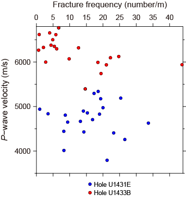
Figure F61. Velocity and rock fracture frequency.

Figure F62. Velocity and bulk density.
Downhole measurements
Logging operations
The last core from Hole U1433B arrived on deck at 2145 h on 17 March 2014. Hole preparation for the logging program included a 50 bbl sepiolite mud sweep, a wiper trip from 858.5 to 786.3 mbsf, a further 50 bbl sepiolite mud sweep, release of the RCB drill bit, and displacement with 225 bbl of heavy (10.5 lb/gal; barite weighted) mud from 689.1 mbsf. The pipe was raised to a logging depth of 100.4 m drilling depth below seafloor (DSF) (4491 m drilling depth below rig floor). The heavy mud aimed to prevent cave-ins in a potentially suspect interval of low core recovery. Rig-up for downhole logging started at 1100 h on 18 March. Seas were calm, with heave at ~30 cm peak-to-peak, so the wireline heave compensator was not used.
The modified triple combo tool string started downhole at 1345 h on 18 March and reached 830 m WSF, ~18 m short of the bottom of the hole (Figure F63). The tool string included the Hostile Environment Natural Gamma Ray Sonde, Hostile Environment Litho-Density Sonde, and High-Resolution Laterolog Array. The FMS-sonic tool string was run into the pipe at 0145 h on 19 March and, after passing an obstruction in the upper part of the basement section, reached the same depth as the triple combo tool string. Two short passes were taken in the basement below the obstruction. During the main upward log, the FMS caliper arms were closed while the obstruction was passed.
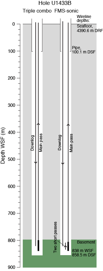
Figure F63. Logging operation summary.
Log data quality
Between 100 and 550 m WSF, rapid variations in borehole diameter from 25 cm (9.84 inches) to wider than 43 cm (16.9 inches) caused density values to be underestimated (Figure F64). The NGR log was affected to a lesser extent. Deeper than 550 m WSF, the hole diameter tended to be in gauge with fewer washed out zones. In general, there were fewer bridged (narrow borehole) zones than at Site U1431. However, high cable tension had to be employed to pull the tool string up through an obstruction just above the basement on the FMS-sonic main pass, which caused some depth discrepancies in the FMS-sonic logs around the sediment/basement interface. FMS resistivity images are generally of good quality, although washed-out zones are characterized by conductive (dark) images.
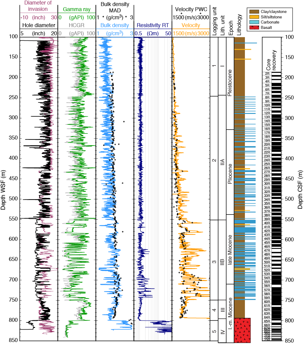
Figure F64. Downhole logs.
The barite-weighted mud that was pumped uphole from 689 m DSF appears not to have had a large effect on the photoelectric effect factor (PEF) log, perhaps only slightly raising the lower envelope of this log at ~570–700 m WSF. This pumping also appears to have caused a deviation to colder temperatures in the borehole fluid temperature log (not plotted).
The triple combo main upward pass was taken as the depth reference, and the other logging runs were depth matched to it by means of the NGR logs.
Logging units
Logging Unit 1: base of drill pipe (100 m WSF) to 245 m WSF
Logging Unit 1 is characterized by relative homogeneity in the sonic velocity log, without major excursions to higher velocity values (Figure F64). NGR values are relatively high, averaging ~65 gAPI, with a 10 m interval at the base of the unit with NGR values at ~85 gAPI. This logging unit corresponds to lithostratigraphic Unit I (see Lithostratigraphy).
Logging Unit 2: 245–550 m WSF
At the top of logging Unit 2, NGR values drop to levels averaging ~55 gAPI. This unit is characterized by the appearance of meter-scale beds with higher sonic velocity and PEF values (Figure F65). A steady downhole increase in background density and sonic velocity reflects compaction with depth. This logging unit corresponds to lithostratigraphic Subunit IIA (see Lithostratigraphy), which includes carbonate turbidites.
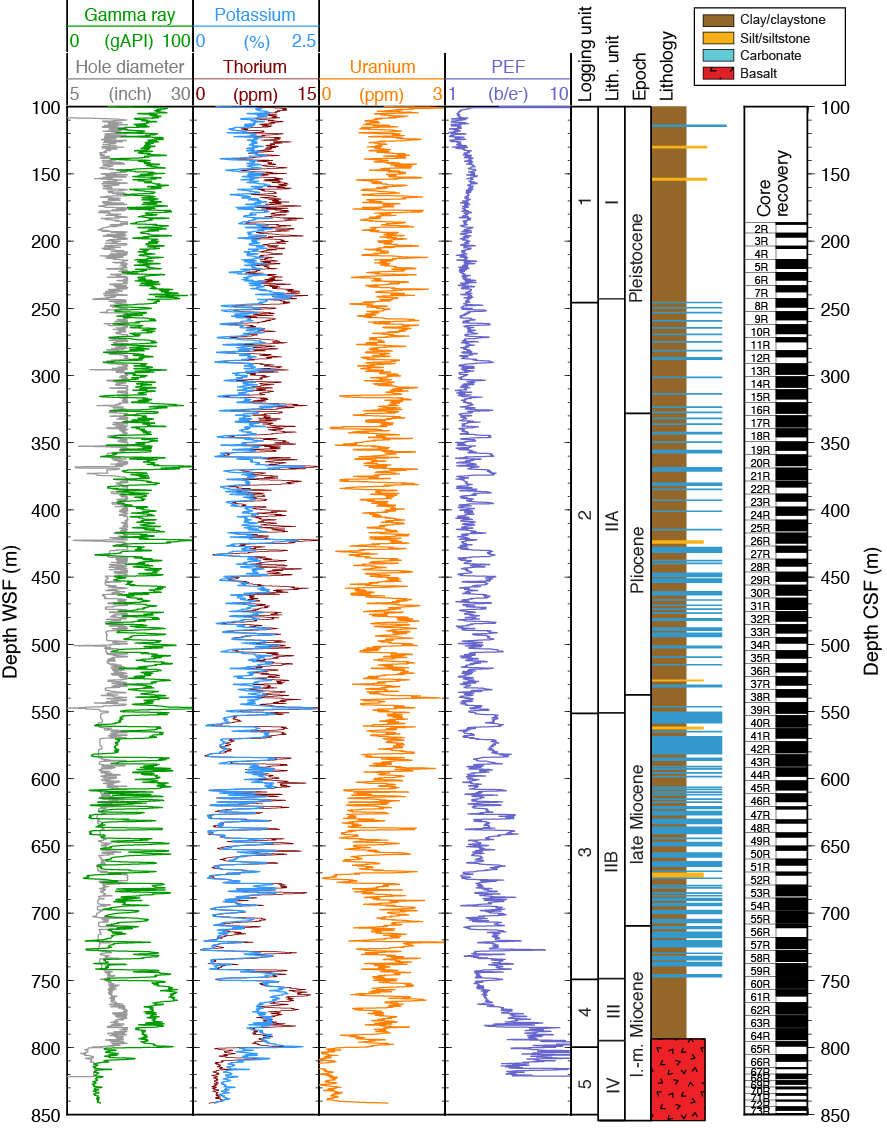
Figure F65. Geochemistry-dependent downhole logs.
Logging Unit 3: 550–750 m WSF
The top of logging Unit3 corresponds to the first appearance of sonic velocity values >2300 m/s and also to high velocity and low NGR layers >5 m thick. The downhole compaction and lithification trend continues in this unit. This logging unit corresponds to lithostratigraphic Subunit IIB (see Lithostratigraphy), which includes thick carbonate turbidites.
Logging Unit 4: 750–800 m WSF
The top of logging Unit 4 is marked by an increase in NGR values to ~85 gAPI and a drop in sonic velocity values. There is an absence of excursions to higher velocities and lower NGR values, and the downhole trend in this ~50 m thick unit is to lower densities and sonic velocities. This logging unit corresponds to lithostratigraphic Unit III, which is composed of reddish to yellowish brown clay (see Lithostratigraphy).
Logging Unit 5: 800–840 m WSF (base of logging data)
A step increase to higher sonic velocity, density, and resistivity values marks the top of basaltic basement. NGR drops to lower values (Figures F64, F66). Logging Unit 5 is not homogeneous; it contains resistivity changes varying over 2 orders of magnitude. Two thin intervals at 808 and 816 m WSF have higher NGR values and low sonic velocity and resistivity.
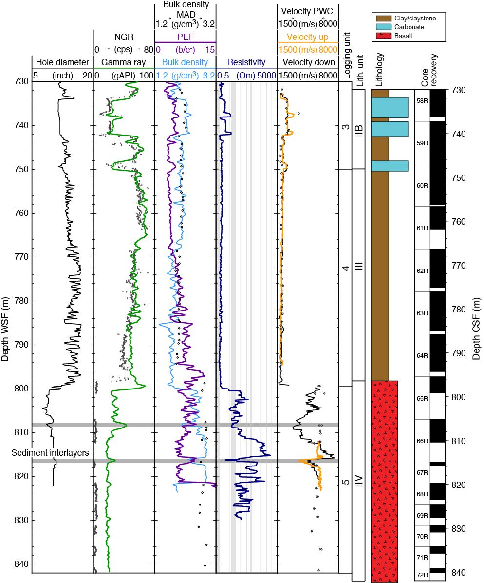
Figure F66. Downhole logs and core physical properties.
Downhole logs and lithology
Downhole logs and FMS images reflect lithology at Site U1433. The clay-dominated sediment of logging Unit 1 has high NGR because of K and Th in the clay minerals. Clay-rich lithologies form the background sediment in logging Units 2 and 3, but carbonate turbidites appear at the top of Unit 2 and become more common downhole, becoming the dominant lithology in Unit 3. The carbonates are apparent by their low NGR values, due to the lack of clay minerals, and high PEF, due to the relatively high concentration of calcium. The carbonates are also more cemented than the background sediment, as seen in the high velocity log values. Sharp bases in the FMS images support the interpretation of these beds as turbidites (Figures F67, F68A, F68B). The higher resistivity and higher velocity values in the lower part of these beds implies more cementation in the coarser part of the turbidites (Figure F67). The presence of thin, highly resistive laminations is observed in the lower part of some of the turbidites, particularly in Unit 3, perhaps indicating that the Unit 3 turbidites come from a more proximal source than the more distal turbidites of Unit 2.
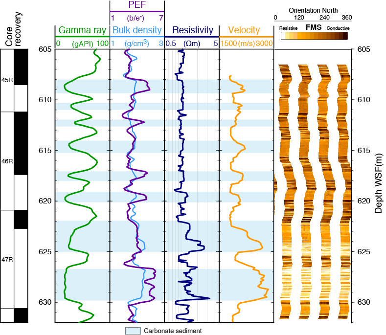
Figure F67. Downhole logs and FMS images.
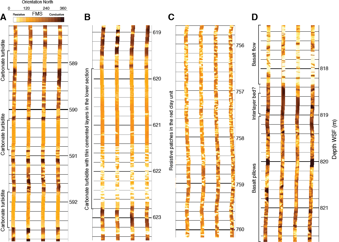
Figure F68. FMS images.
Logging Unit 4 is composed of yellowish to reddish brown clay (see Lithostratigraphy) and accordingly has relatively high NGR, reaching 85 gAPI at the top of the unit. NGR values decrease and PEF increases with depth downhole in the unit. This potentially reflects an increasing abundance of hematite and other oxides in the sediment, because a greater concentration of heavy elements would be required to produce the observed PEF values. The concentration of such oxides could result from hydrothermal processes and/or the removal of other sediment components in this interval overlying the basaltic basement. FMS images from this unit have distinct centimeter–scale resistive patches (Figure F68C) whose origin is uncertain at this time.
As expected, the step in physical and chemical properties at the basalt interface is clearly seen in nearly all of the downhole logs. However, NGR does not fall to values as low as those seen in the core measurements or as low as is expected of basalt, so the NGR log measurements in the basalt unit should be regarded with caution. A massive flow and pillow basalt can be distinguished in the FMS images (Figure F68B), as well as veins and 2 possible sediment interlayers (Figures F66, F68D).
Sonic velocity and two-way traveltime
In general, the sonic velocity log repeated reasonably well between the upward and downward passes of the logging tool, so the data are considered to be robust, a conclusion that is supported by the general similarity to the P-wave velocities measured on core samples (Figures F64, F66, F69A). The laboratory measurement sometimes underestimates in situ velocity because of the removal of high-pressure conditions when the sediment is raised to the ship (e.g., from 470 to 550 m CSF in Figure F64). The upward sonic velocity log was recorded using a medium sonic source frequency, and the downward log was recorded using a high sonic source frequency. The high frequency is the standard Schlumberger setting, but in the mostly slow formations logged here (and in general during the Integrated Ocean Drilling Program), the medium sonic frequency source proved to be more reliable because of lower signal attenuation. An example is seen in the turbidites at 738 and 742 m WSF (Figure F66); the medium-frequency upward pass records the higher velocities at the base of the turbidites, whereas the high-frequency downward pass does not.
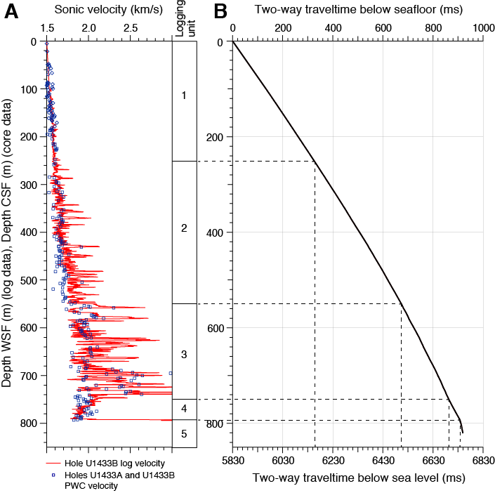
Figure F69. Sonic velocity and two-way traveltime.
Sonic velocities increase with depth to 750 m WSF, decrease to lower values in the reddish brown clay (750–800 m WSF), and exceed 6000 m/s in the basaltic basement. This data set was used to calculate interval velocities between measurement points, and then these interval velocities were summed and doubled to yield two-way traveltime for Site U1433 (Figure F69B). From these data, the boundary between logging Units 2 and 3 at 550 m WSF lies at the top of the set of high-amplitude reflectors in the seismic section at ~6.5 s two-way traveltime (Figure F3). The basement two-way traveltime is predicted to be at 6.74 s.
Downhole temperature and heat flow
Four downhole temperature measurements were made using the advanced piston corer temperature tool (APCT-3) in Hole U1433A, yielding values from 6.0°C at 37.4 m DSF to 12.2°C at 122.9 m DSF (Table T17; Figures F70, F71A) and giving a geothermal gradient of 78°C/km. These measurements, together with the seafloor temperature of 2.5°C, indicate that temperature increases approximately linearly with depth.
Table T17. APCT-3 temperature measurements, Hole U1433A. Download table in .csv format.
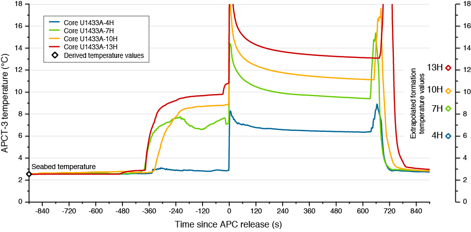
Figure F70. APCT-3 temperature-time series.
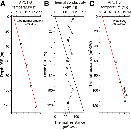
Figure F71. Heat flow calculations.
Thermal conductivity under in situ conditions was estimated from laboratory-determined thermal conductivity from Hole U1433A using the method of Hyndman et al. (1974) (see Physical properties in the Methods chapter [Li et al., 2015b]). The calculated in situ values average 1.1% lower than the measured laboratory values. Thermal resistance was then calculated by integrating the inverse of the in situ thermal conductivity over depth (Figure F71B). A heat flow of 83 mW/m2 was obtained from the linear fit between temperature and thermal resistance (Figure F71C) (Pribnow et al., 2000). This geothermal gradient and heat flow at Site U1433 are similar to the closest values for this part of the deep South China Sea Basin (Li et al., 2010).
References
Alt, J.C., France-Lanord, C., Floyd, P.A., Castillo, P., and Galy, A., 1992. Low-temperature hydrothermal alteration of Jurassic ocean crust, Site 801. In Larson, R.L., Lancelot, Y., et al., Proceedings of the Ocean Drilling Program, Scientific Results, 129: College Station, TX (Ocean Drilling Program), 415–427. http://dx.doi.org/10.2973/odp.proc.sr.129.132.1992
Berggren, W.A., Kent, D.V., Swisher, C.C., III, and Aubry, M.-P., 1995. A revised Cenozoic geochronology and chronostratigraphy. In Berggren, W.A., Kent, D.V., Aubry, M.-P., and Hardenbol, J. (Eds.), Geochronology, Time Scales and Global Stratigraphic Correlation. Special Publication - SEPM (Society for Sedimentary Geology), 54:129–212. http://dx.doi.org/10.2110/pec.95.04.0129
Bolli, H.M., and Saunders, J.B., 1985. Oligocene to Holocene low latitude planktic foraminifera. In Bolli, H.M., Saunders, J.B., and Perch-Nielsen, K. (Eds.), Plankton Stratigraphy (Vol. 1): Planktic Foraminifera, Calcareous Nannofossils and Calpionellids: Cambridge, UK (Cambridge University Press), 155–262.
Bouma, A.H., 1962. Sedimentology of Some Flysch Deposits: A Graphic Approach to Facies Interpretation: Amsterdam (Elsevier).
Briais, A., Patriat, P., and Tapponnier, P., 1993. Updated interpretation of magnetic anomalies and seafloor spreading stages in the South China Sea: implications for the Tertiary tectonics of Southeast Asia. Journal of Geophysical Research: Solid Earth, 98(B4):6299–6328. http://dx.doi.org/10.1029/92JB02280
Bryant, W.R., and Bennett, R.H., 1988. Origin, physical, and mineralogical nature of red clays: the Pacific Ocean Basin as a model. Geo-Marine Letters, 8(4):189–249. http://dx.doi.org/10.1007/BF02281640
Busch, W.H., Castillo, P.R., Floyd, P.A., and Cameron, G., 1992. Effects of alteration on physical properties of basalts from the Pigafetta and East Mariana Basins. In Larson, R.L., Lancelot, Y., et al., Proceedings of the Ocean Drilling Program, Scientific Results, 129: College Station, TX (Ocean Drilling Program), 485–499. http://dx.doi.org/10.2973/odp.proc.sr.129.139.1992
Carter, A., Roques, D., and Bristow, C.S., 2000. Denudation history of onshore central Vietnam: constraints on the Cenozoic evolution of the western margin of the South China Sea. Tectonophysics, 322(3–4):265–277. http://dx.doi.org/10.1016/S0040-1951(00)00091-3
Ekdale, A.A., Bromley, R.G., and Pemberton, S.G. (Eds.), 1984. Ichnology: The Use of Trace Fossils in Sedimentology and Stratigraphy. SEPM Short Course, 15.
Expedition 329 Scientists, 2011. Site U1368. In D’Hondt, S., Inagaki, F., Alvarez Zarikian, C.A., and the Expedition 329 Scientists, Proceedings of the Integrated Ocean Drilling Program, 329: Tokyo (Integrated Ocean Drilling Program Management International, Inc.). http://dx.doi.org/10.2204/iodp.proc.329.106.2011
Expedition 330 Scientists, 2012a. Site U1373. In Koppers, A.A.P., Yamazaki, T., Geldmacher, J., and the Expedition 330 Scientists, Proceedings of the Integrated Ocean Drilling Program, 330: Tokyo (Integrated Ocean Drilling Program Management International, Inc.). http://dx.doi.org/10.2204/iodp.proc.330.104.2012
Expedition 330 Scientists, 2012b. Site U1376. In Koppers, A.A.P., Yamazaki, T., Geldmacher, J., and the Expedition 330 Scientists, Proceedings of the Integrated Ocean Drilling Program, 330: Tokyo (Integrated Ocean Drilling Program Management International, Inc.). http://dx.doi.org/10.2204/iodp.proc.330.107.2012
Fuller, M., 1969. Magnetic orientation of borehole cores. Geophysics, 34(5):772–774. http://dx.doi.org/10.1190/1.1440047
Gradstein, F.M., Ogg, J.G., Schmitz, M.D., and Ogg, G.M. (Eds.)., 2012. The Geological Time Scale 2012: Oxford, UK (Elsevier).
Hanebuth, T.J.J., and Stattegger, K., 2004. Depositional sequences on a late Pleistocene–Holocene tropical siliciclastic shelf (Sunda Shelf, southeast Asia). Journal of Asian Earth Sciences, 23(1):113–126. http://dx.doi.org/10.1016/S1367-9120(03)00100-7
Haq, B.U., Hardenbol, J., and Vail, P.R., 1987. Chronology of fluctuating sea levels since the Triassic. Science, 235(4793):1156–1167. http://dx.doi.org/10.1126/science.235.4793.1156
Hékinian, R., Bonté, P., Pautot, G., Jacques, D., Labeyrie, L.D., Mikkelsen, N., and Reyss, J.-L., 1989. Volcanics from the South China Sea ridge system. Oceanologica Acta, 12(2):101–115.
Hu, J., Kawamura, H., Hong, H., and Qi, Y., 2000. A review on the currents in the South China Sea: seasonal circulation, South China Sea Warm Current and Kuroshio Intrusion. Journal of Oceanography, 56(6):607–624. http://dx.doi.org/10.1023/A:1011117531252
Hutchison, C.S., 2004. Marginal basin evolution: the southern South China Sea. Marine and Petroleum Geology, 21(9):1129–1148. http://dx.doi.org/10.1016/j.marpetgeo.2004.07.002
Hutchison, C.S., and Vijayan, V.R., 2010. What are the Spratly Islands? Journal of Asian Earth Sciences, 39(5):371–385. http://dx.doi.org/10.1016/j.jseaes.2010.04.013
Hyndman, R.D., Erickson, A.J., and Von Herzen, R.P., 1974. Geothermal measurements on DSDP Leg 26. In Davies, T.A., Luyendyk, B.P., et al., Initial Reports of the Deep Sea Drilling Project, 26: Washington, DC (U.S. Government Printing Office), 451–463. http://dx.doi.org/10.2973/dsdp.proc.26.113.1974
Ishihara, T., and Kisimoto, K., 1996. Magnetic anomaly map of East Asia, 1:4,000,000 (CD-ROM version). Geological Survey of Japan, Coordinating Committee for Coastal and Offshore Geoscience Programs in East and Southeast Asia (CCOP).
Jin, Z., Xu, S., and Li, Z., 2002. Inversion of heterogeneous magnetism for seamounts in the South China Sea. Journal of Ocean University of Qingdao (English Edition), 32:926–934. (in Chinese)
Kemp, A.E.S., 1995. Variation of trace fossils and ichnofacies in Neogene and Quaternary pelagic sediments from the eastern equatorial Pacific Ocean (Leg 138). In Pisias, N.G., Mayer, L.A., Janecek, T.R., Palmer-Julson, A., and van Andel, T.H. (Eds.), Proceedings of the Ocean Drilling Program, Scientific Results, 138: College Station, TX (Ocean Drilling Program), 177–190. http://dx.doi.org/10.2973/odp.proc.sr.138.110.1995
Kennett, J.P., and Srinivasan, M.S., 1983. Neogene Planktonic Foraminifera: A Phylogenetic Atlas: Stroudsburg, PA (Hutchinson Ross).
Kirschvink, J.L., 1980. The least-squares line and plane and the analysis of palaeomagnetic data. Geophysical Journal of the Royal Astronomical Society, 62(3):699–718. http://dx.doi.org/10.1111/j.1365-246X.1980.tb02601.x
Kodama, K.P., 1984. Palaeomagnetism of granitic intrusives from the Precambrian basement under eastern Kansas: orienting drill cores using secondary magnetization components. Geophysical Journal International, 76(2):273–287. http://dx.doi.org/10.1111/j.1365-246X.1984.tb05045.x
Le Maitre, R.W., Bateman, P., Dudek, A., Keller, J., Lameyre, J., Le Bas, M.J., Sabine, P.A., Schmid, R., Sorensen, H., Streckeisen, A., Woolley, A.R., and Zanettin, B., 1989. A Classification of Igneous Rocks and Glossary of Terms: Oxford, UK (Blackwell Science Publishing).
Li, C.-F., Lin, J., Kulhanek, D.K., Williams, T., Bao, R., Briais, A., Brown, E.A., Chen, Y., Clift, P.D., Colwell, F.S., Dadd, K.A., Ding, W., Almeida, I.H., Huang, X.-L., Hyun, S., Jiang, T., Koppers, A.A.P., Li, Q., Liu, C., Liu, Q., Liu, Z., Nagai, R.H., Peleo-Alampay, A., Su, X., Sun, Z., Tejada, M.L.G., Trinh, H.S., Yeh, Y.-C., Zhang, C., Zhang, F., Zhang, G.-L., and Zhao, X., 2015a. Expedition 349 summary. In Li, C.-F., Lin, J., Kulhanek, D.K., and the Expedition 349 Scientists, Proceedings of the Integrated Ocean Drilling Program, 349: South China Sea Tectonics: College Station, TX (International Ocean Discovery Program). http://dx.doi.org/10.14379/iodp.proc.349.101.2015
Li, C.-F., Lin, J., Kulhanek, D.K., Williams, T., Bao, R., Briais, A., Brown, E.A., Chen, Y., Clift, P.D., Colwell, F.S., Dadd, K.A., Ding, W., Almeida, I.H., Huang, X.-L., Hyun, S., Jiang, T., Koppers, A.A.P., Li, Q., Liu, C., Liu, Q., Liu, Z., Nagai, R.H., Peleo-Alampay, A., Su, X., Sun, Z., Tejada, M.L.G., Trinh, H.S., Yeh, Y.-C., Zhang, C., Zhang, F., Zhang, G.-L., and Zhao, X., 2015b. Methods. In Li, C.-F., Lin, J., Kulhanek, D.K., and the Expedition 349 Scientists, Proceedings of the Integrated Ocean Drilling Program, 349: South China Sea Tectonics: College Station, TX (International Ocean Discovery Program). http://dx.doi.org/10.14379/iodp.proc.349.102.2015
Li, C.-F., Lin, J., Kulhanek, D.K., Williams, T., Bao, R., Briais, A., Brown, E.A., Chen, Y., Clift, P.D., Colwell, F.S., Dadd, K.A., Ding, W., Almeida, I.H., Huang, X.-L., Hyun, S., Jiang, T., Koppers, A.A.P., Li, Q., Liu, C., Liu, Q., Liu, Z., Nagai, R.H., Peleo-Alampay, A., Su, X., Sun, Z., Tejada, M.L.G., Trinh, H.S., Yeh, Y.-C., Zhang, C., Zhang, F., Zhang, G.-L., and Zhao, X., 2015c. Site U1431. In Li, C.-F., Lin, J., Kulhanek, D.K., and the Expedition 349 Scientists, Proceedings of the Integrated Ocean Drilling Program, 349: South China Sea Tectonics: College Station, TX (International Ocean Discovery Program). http://dx.doi.org/10.14379/iodp.proc.349.103.2015
Li, C.-F., Lin, J., Kulhanek, D.K., Williams, T., Bao, R., Briais, A., Brown, E.A., Chen, Y., Clift, P.D., Colwell, F.S., Dadd, K.A., Ding, W., Almeida, I.H., Huang, X.-L., Hyun, S., Jiang, T., Koppers, A.A.P., Li, Q., Liu, C., Liu, Q., Liu, Z., Nagai, R.H., Peleo-Alampay, A., Su, X., Sun, Z., Tejada, M.L.G., Trinh, H.S., Yeh, Y.-C., Zhang, C., Zhang, F., Zhang, G.-L., and Zhao, X., 2015d. Site U1432. In Li, C.-F., Lin, J., Kulhanek, D.K., and the Expedition 349 Scientists, Proceedings of the Integrated Ocean Drilling Program, 349: South China Sea Tectonics: College Station, TX (International Ocean Discovery Program). http://dx.doi.org/10.14379/iodp.proc.349.104.2015
Li, C.-F., Shi, X., Zhou, Z., Li, J., Geng, J., and Chen, B., 2010. Depths to the magnetic layer bottom in the South China Sea area and their tectonic implications. Geophysical Journal International, 182(3):1229–1247. http://dx.doi.org/10.1111/j.1365-246X.2010.04702.x
Li, C.-F., Zhou, Z., Li, J., Chen, B., and Geng, J., 2008. Magnetic zoning and seismic structure of the South China Sea ocean basin. Marine Geophysical Research, 29(4):223–238. http://dx.doi.org/10.1007/s11001-008-9059-4
Li, C.-F., Zhou, Z., Li, J., Hao, H., and Geng, J., 2007. Structures of the northeasternmost South China Sea continental margin and ocean basin: geophysical constraints and tectonic implications. Marine Geophysical Research, 28(1):59–79. http://dx.doi.org/10.1007/s11001-007-9014-9
Li, L., Clift, P.D., and Nguyen, H.T., 2013. The sedimentary, magmatic and tectonic evolution of the southwestern South China Sea revealed by seismic stratigraphic analysis. Marine Geophysical Research, 34(3–4):341–365. http://dx.doi.org/10.1007/s11001-013-9171-y
Macdonald, G.A., 1968. Composition and origin of Hawaiian lavas. In Coats, R.R., Hay, R.L., and Anderson, C.A. (Eds.), Studies in Volcanology—A Memoir in Honor of Howel Williams. Memoir - Geological Society of America, 116:477–522. http://dx.doi.org/10.1130/MEM116-p477
Macdonald, G.A., and Katsura, T., 1964. Chemical composition of Hawaiian lavas. Journal of Petrology, 5(1):82–133. http://petrology.oxfordjournals.org/content/5/1/82.abstract
Martini, E., 1971. Standard Tertiary and Quaternary calcareous nannoplankton zonation. In Farinacci, A. (Ed.), Proceedings of the Second Planktonic Conference, Roma 1970: Rome (Edizioni Tecnoscienza), 2:739–785.
Pautot, G., Rangin, C., Briais, A., Tapponnier, P., Beuzart, P., Lericolais, G., Mathieu, X., Wu, J., Han, S., Li, H., Lu, Y., and Zhao, J., 1986. Spreading direction in the central South China Sea. Nature, 321(6066):150–154. http://dx.doi.org/10.1038/321150a0
Pimmel, A., and Claypool, G., 2001. Introduction to shipboard organic geochemistry on the JOIDES Resolution. ODP Technical Note, 30. http://dx.doi.org/10.2973/odp.tn.30.2001
Pribnow, D., Kinoshita, M., and Stein, C., 2000. Thermal Data Collection and Heat Flow Recalculations for Ocean Drilling Program Legs 101–180: Hanover, Germany (Institute for Joint Geoscientific Research, Institut für Geowissenschaftliche Gemeinschaftsaufgaben [GGA]). http://www-odp.tamu.edu/publications/heatflow/ODPReprt.pdf
Roberts, A.P., 2008. Geomagnetic excursions: knowns and unknowns. Geophysical Research Letters, 35(17):L17307. http://dx.doi.org/10.1029/2008GL034719
Sanfilippo, A., and Nigrini, C., 1998. Code numbers for Cenozoic low latitude radiolarian biostratigraphic zones and GPTS conversion tables. Marine Micropaleontology, 33(1–2):109–117, 121–156. http://dx.doi.org/10.1016/S0377-8398(97)00030-3
Shibuya, H., Merrill, D.L., Hsu, V., and Leg 124 Shipboard Scientific Party, 1991. Paleogene counterclockwise rotation of the Celebes Sea—orientation of ODP cores utilizing the secondary magnetization. In Silver, E.A., Rangin, C., von Breymann, M.T., et al., Proceedings of the Ocean Drilling Program, Scientific Results, 124: College Station, TX (Ocean Drilling Program), 519–523. http://dx.doi.org/10.2973/odp.proc.sr.124.169.1991
Steuer, S., Franke, D., Meresse, F., Savva, D., Pubellier, M., and Auxietre, J.-L., in press. Oligocene–Miocene carbonates and their role for constraining the rifting and collision history of the Dangerous Grounds, South China Sea. Marine and Petroleum Geology. http://dx.doi.org/10.1016/j.marpetgeo.2013.12.010
Theyer, F., Mato, C.Y., and Hammond, S.R., 1978. Paleomagnetic and geochronologic calibration of latest Oligocene to Pliocene radiolarian events, equatorial Pacific. Marine Micropaleontology, 3(4):377–395. http://dx.doi.org/10.1016/0377-8398(78)90019-1
Tu, K., Flower, M.F.J., Carlson, R.W., Xie, G., Chen, C.-Y., and Zhang, M., 1992. Magmatism in the South China Basin: 1. Isotopic and trace-element evidence for an endogenous Dupal mantle component. Chemical Geology, 97(1–2):47–63. http://dx.doi.org/10.1016/0009-2541(92)90135-R
Vail, P.R., Mitchum, R.M., Jr., Todd, R.G., Widmier, J.M., Thompson, S.I., Sangree, J.B., Bubb, J.N., and Hatlelid, W.G., 1977. Seismic stratigraphy and global changes of sea level, Parts 1–11. In Payton, C.E. (Ed.), Seismic Stratigraphy: Applications to Hydrocarbon Exploration. AAPG Memoir, 26:51–212.
Wade, B.S., Pearson, P.N., Berggren, W.A., and Pälike, H., 2011. Review and revision of Cenozoic tropical planktonic foraminiferal biostratigraphy and calibration to the geomagnetic polarity and astronomical time scale. Earth-Science Reviews, 104(1–3):111–142. http://dx.doi.org/10.1016/j.earscirev.2010.09.003
Wang, R., and Abelmann, A., 1999. Pleistocene radiolarian biostratigraphy in the South China Sea. Science in China (Series D), 42(5):537–543.
Wang, X.-C., Li, Z.-X., Li, X.-H., Li, J., Liu, Y., Long, W.-G., Zhou, J.-B., and Wang, F., 2012. Temperature, pressure, and composition of the mantle source region of late Cenozoic basalts in Hainan Island, SE Asia: a consequence of a young thermal mantle plume close to subduction zones? Journal of Petrology, 53(1):177–233. http://dx.doi.org/10.1093/petrology/egr061
Wetzel, A., 2002. Modern Nereites in the South China Sea—ecological association with redox conditions in the sediment. Palaios, 17(5):507–515. http://dx.doi.org/10.1669/0883-1351(2002)017<0507:MNITSC>2.0.CO;2
Yao, B., 1995. Characteristics and tectonic significance of the Zhongnan-Lile fault. Geological Research of South China Sea, Memoir, 7:1–14. (in Chinese)
Zhang, G., Smith-Duque, C., Tang, S., Li, H., Zarikian, C., D’Hondt, S., Inagaki, F., and IODP Expedition 329 Scientists, 2012. Geochemistry of basalts from IODP Site U1365: implications for magmatism and mantle source signatures of the mid-Cretaceous Osbourn Trough. Lithos, 144–145:73–87. http://dx.doi.org/10.1016/j.lithos.2012.04.014
Zhang, G., Zeng, Z., Yin, X., Wang, X., and Chen, D., 2009. Deep fractionation of clinopyroxene in the East Pacific Rise 13°N: evidence from high MgO MORB and melt inclusions. Acta Geologica Sinica, 83(2):266–277. http://dx.doi.org/10.1111/j.1755-6724.2009.00030.x
Zhang, G.-L., Chen, L.-H., and Li, S.-Z., 2013. Mantle dynamics and generation of a geochemical mantle boundary along the East Pacific Rise—Pacific/Antarctic Ridge. Earth and Planetary Science Letters, 383:153–163. http://dx.doi.org/10.1016/j.epsl.2013.09.045
Zhang, G.-L., Zong, C.-L., Yin, X.-B., and Li, H., 2012. Geochemical constraints on a mixed pyroxenite–peridotite source for East Pacific Rise basalts. Chemical Geology, 330–331:176–187. http://dx.doi.org/10.1016/j.chemgeo.2012.08.033
Zijderveld, J.D.A., 1967. AC demagnetization of rocks: analysis of results. In Collinson, D.W., Creer, K.M., and Runcorn, S.K. (Eds.), Methods in Palaeomagnetism: Amsterdam (Elsevier), 254–286.
1Li, C.-F., Lin, J., Kulhanek, D.K., Williams, T., Bao, R., Briais, A., Brown, E.A., Chen, Y., Clift, P.D., Colwell, F.S., Dadd, K.A., Ding, W.-W., Hernández-Almeida, I., Huang, X.-L., Hyun, S., Jiang, T., Koppers, A.A.P., Li, Q., Liu, C., Liu, Q., Liu, Z., Nagai, R.H., Peleo-Alampay, A., Su, X., Sun, Z., Tejada, M.L.G., Trinh, H.S., Yeh, Y.-C., Zhang, C., Zhang, F., Zhang, G.-L., and Zhao, X., 2015. Site U1433. In Li, C.-F., Lin, J., Kulhanek, D.K., and the Expedition 349 Scientists, Proceedings of the International Ocean Discovery Program, 349: South China Sea Tectonics: College Station, TX (International Ocean Discovery Program). http://dx.doi.org/10.14379/iodp.proc.349.105.2015
2Expedition 349 Scientists’ addresses.
Figure F1. A. Bathymetric map of the South China Sea region. Solid yellow circles = Expedition 349 sites. Solid pink circles = ODP Leg 184 sites. Yellow dashed line = inferred continent/ocean boundary, blue lines = fossil South China Sea spreading center, white-flagged line = Manila Trench. B. Detailed bathymetry around Sites U1433 and U1434 (red box in A) showing nearby seamounts and the Dangerous Grounds and Reed Bank to the south.
Figure F2. Shaded map of magnetic anomalies near Sites U1433 and U1434 (data from Ishihara and Kisimoto, 1996). Bold black lines mark 3000 m isobaths outlining the seamounts. Symbols are magnetic anomaly picks from Briais et al. (1993).
Figure F3. A. Regional contoured bathymetric map showing seismic reflection profiles (red lines) and the location of Sites U1433 and U1434. Contour interval = 100 m. B. Seismic profile Line 973SCSIO_2b with location of Site U1433. SP = shotpoint. Green line = interpreted top of basement, blue line = approximate uppermost Miocene sediment.
Figure F4. Lithostratigraphy summary, Site U1433.
Figure F5. Synthesis sedimentary log for Site U1433 showing combined recovery in Holes U1433A and U1433B. Interpretation of poorly recovered areas was enhanced by reference to downhole logging results.
Figure F6. Green layer development, Hole U1433A, Unit I. A. Massive clay with faintly developed green layering typical of the unit (14H-3A, 76–83 cm). B. Green layer in clay (2H-2A, 29–36 cm).
Figure F7. Silt turbidites, Hole U1433A, Unit I. A. Rare thick-bedded silt turbidite (16H-2, 55–71 cm). B. More typical thin-bedded graded silt turbidite (7H-3A, 66–75 cm). C. Thin, stacked silt turbidites in clay (4H-4, 44–57 cm).
Figure F8. Erosion surface between 2 clay units, Hole U1433A, Unit I (16H-6A, 62–71 cm). Note the thin silt developed on the left side of the core along the contact.
Figure F9. Hole U1433A, Unit I (plane-polarized light [PPL]). (A) Radiolarians in clay (2H-1, 89 cm) and (B) clay with foraminifers, sponge spicules, and radiolarians, as well as quartz silt (6H-5, 73 cm).
Figure F10. Dark-colored mafic tephra layer, Hole U1433A, Unit I (14H-1A, 117–130 cm).
Figure F11. Burrows in sediment. A. Simple burrows (Planolites) in ooze infilled by foraminifer sands, Hole U1433A, Unit I (8H-3A, 117–125 cm). B. Horizontal burrows in ooze, likely Scolicia, Hole U1433B (29R-1A, 97–104 cm). C. Bioturbated top of a typical calcareous turbidite within Unit II, Hole U1433B. Burrows are dominated by Planolites, Chondrites, and Zoophycos (19R-1A, 83–94 cm).
Figure F12. Correlation of lithostratigraphic units with magnetic susceptibility and reflectance spectroscopy (after 30-point running average), Site U1433.
Figure F13. Typical calcareous turbidite cycle showing grading from the erosive base to the bioturbated top (349-U1433B-17R-3A, 32–66 cm).
Figure F14. Two calcareous turbidites stacked on top of one another, Hole U1433B (48R-1A, 56–73 cm). The lower turbidite is finer grained claystone to siltstone with a Chondrites-burrowed top. The upper turbidite is silty and laminated with larger Planolites burrows, grading upward into claystone.
Figure F15. Typical clay/claystone lithologies, Hole U1433B (PPL). A. Clay with minor quartz silt and brown mafic volcanic glass shards (9R-3, 43 cm). B. Common pyrite crystals scattered through the matrix (15R-5, 52 cm).
Figure F16. Coarser clastic material (PPL). A. Broken, mostly calcareous fine sand with foraminifer fragments (U1433B-25R-1, 41 cm). B. Siliciclastic silt with minor glass shards and foraminifers (U1433B-6R-4, 115 cm). C. Carbonate sand dominated by whole and fragmented foraminifers (U1433A-8H-3, 39 cm).
Figure F17. Erosive bases of calcareous turbidites, Hole U1433B. A. Coarse sand–grade base with carbonate and volcanic rock fragments (47R-1A, 28–37 cm). B. Laminated medium sand of foraminifer-rich carbonate material overlying claystone (26R-5A, 68–79 cm).
Figure F18. Coarse carbonate sandstone, Hole U1433B, Subunit IIB (47R-1, 30–32 cm). A. PPL. B. Well-preserved benthic foraminifers (a) Lepidocyclina and (b) Amphistegina that live in water depths shallower than 100 m. Subrounded to rounded (c) chert, feldspar, and quartz grains also occur (cross-polarized light [XPL]).
Figure F19. Parallel-laminated foraminiferal chalk, Hole U1433B, Subunit IIB (40R-5, 38–40 cm). A. Planktonic foraminifers including (a) Orbulina and (b) Globigerinoides are major components of the chalk. Microauthigenic (c) pyrite grains occur as black spots or aggregates (PPL). B. XPL.
Figure F20. Organic carbon–bearing sandstone at the base of a turbidite, Hole U1433B (53R-1A, 65–72 cm).
Figure F21. Claystone, Hole U1433B, Unit III. A. Massive reddish brown claystone typical of the deposits immediately overlying basement (61R-1A, 47–58 cm). B. Redeposited clayey siltstone and silty claystone beds within the dominant claystone (63R-3A, 124–144 cm). C. Black-stained burrows in claystone (64R-4A, 137–145 cm).
Figure F22. Age-depth model, Site U1433. FAD = first appearance datum, LAD = last appearance datum.
Figure F23. Lithostratigraphic summary of igneous rocks and their lithologic features with integrated downhole logging observations, Hole U1433B. Lithostratigraphy column includes lithology, igneous lithologic units (1–45), and lithostratigraphic units (III and IV).
Figure F24. Basement basalt types, Hole U1433B, Unit IV. A. Highly olivine-plagioclase phyric basalt with glassy rim (65R-2A, 0–19 cm; Unit 1). B. Amygdaloidal, sparsely olivine-plagioclase-phyric basalt (70R-2A, 16–33 cm; Unit 40). C. Fine-grained, sparsely olivine-plagioclase-phyric basalt (71R-1A, 59–71 cm; Unit 41). D. Highly plagioclase-phyric microcrystalline basalt with sparse olivine (73R-2A, 115–145 cm; Unit 45).
Figure F25. Basalt, Hole U1433B, Unit IV. A, B. Moderately olivine-plagioclase-phyric pillow flow with glassy margins and pseudomorphs of equant olivine and fresh plagioclase phenocrysts set in hypocrystalline groundmass (65R-3, 93–96 cm; TS71); (A) PPL, (B) XPL. C, D. Moderately olivine-plagioclase-phyric basalt containing olivine and plagioclase phenocrysts in cryptocrystalline groundmass with plagioclase microlites (65R-3, 104–107 cm; TS72); (C) PPL, (D) XPL. E, F. Moderately olivine-plagioclase-phyric fine-grained basalt with large euhedral to subhedral olivine and plagioclase phenocrysts in microcrystalline intersertal groundmass of plagioclase and clinopyroxene (70R-1, 55–58 cm; TS90); (E) PPL, (F) XPL. G, H. Moderately plagioclase-phyric basalt with a trace of olivine microphenocrysts in medium-grained groundmass showing variolitic growth texture of plagioclase around clinopyroxene (72R-1, 112–115 cm; TS93); (G) PPL, (H) XPL.
Figure F26. Pillow lava chilled margins, Hole U1433B, Unit IV. A. 2 cm wide glassy margin (65R-3, 93–109 cm). B. Top and side views of chert sandwiched between 2 chilled margins (68R-3, 133–135 cm).
Figure F27. Interpillow hyaloclastite and baked clayey limestone containing inclusions of green claystone and chert fragments, Hole U1433B, Unit IV (65R-2, 40–55 cm).
Figure F28. Chilled margins in thin section, Hole U1433B, Unit IV (PPL). A. Fresh glass grading into palagonitized glass toward pillow interior (65R-3, 93–96 cm; TS71). B. Same as A showing contact with hyaloclastite containing a limestone fragment. C. Several layers of glassy margins showing palagonitized boundaries (70R-1, 88–90 cm; TS91).
Figure F29. Plagioclase (plag) textures and olivine (ol) phenocrysts, Hole U1433B, Unit IV. A, B. Overgrowth zoning and fractured and sieved texture in plagioclase with infill of melt along cleavage and cracks (74R-2, 6–8 cm; TS99); (A) PPL, (B) XPL. C, D. Melt inclusions along overgrowth boundaries in plagioclase and partially replaced euhedral olivine (66R-2, 104–107 cm; TS77); (C) PPL, (D) XPL. E, F. Euhedral to subhedral pseudomorphs of olivine (66R-4, 128–132 cm; TS78); (E) PPL, (F) XPL.
Figure F30. Types of alteration halos, basalt glass alteration, and alteration veins, Hole U1433B. Images in A and B are of a wet surface with fill-in lightening to enhance alteration features. A. Alteration halo flanking a composite vein filled with carbonate (Carb) and celadonite (Cela) (69R-1A, 120–134 cm). B. Greenish palagonite (Pala) from altered basalt glass (65R-3A, 93–109 cm). C. Carbonate vein (~3 mm thick) across the fine-grained basalt groundmass (66R-1, 63–66 cm; TS76; XPL). D. Composite vein filled with celadonite and carbonate (69R-1, 111–114 cm; TS 88; XPL). E. Vein filled with Fe oxide (74R-1, 83–86 cm; TS97; PPL).
Figure F31. Downhole abundance (number of veins per 9.7 m length of core) variation of all veins, as well as individual plots for veins filled with carbonate, Fe oxide, and celadonite. The total abundance of veins and the abundance of specific veins were calculated and corrected for percent recovery in each core.
Figure F32. Vesicle fillings, Hole U1433B (PPL). A. Saponite (Sap) (66R-4, 128–132 cm; TS78). B. Fe oxide and smectite (Smec) (67R-1, 59–62 cm; TS81). C. Smectite (67R-1, 98–100 cm; TS82). D. Saponite and celadonite (Cela) (69R-1, 34–38 cm; TS87). E. Celadonite and carbonate (Carb) (69R-1, 111–114 cm; TS88). F. Celadonite (73R-1, 11–14 cm; TS94).
Figure F33. Single curved veins subparallel to the chilled margin in pillow basalt, Hole U1433B (68R-3A, 132–137 cm). A. Original photo. B. Interpretation.
Figure F34. Irregular sinuous veins in pillow basalt, Hole U1433B (69R-3A, 78–89 cm). A. Original photo. B. Interpretation.
Figure F35. Triple-junction veins, Hole U1433B (69R-3A, 54–66 cm). A. Original photo. B. Interpretation.
Figure F36. Branched veins, Hole U1433B (68R-3A, 7–26 cm). A. Original photo. B. Interpretation.
Figure F37. Crosscutting veins, Hole U1433B (65R-2A, 37–44 cm). A. Original photo. B. Interpretation.
Figure F38. Radiate veins developed in pillow basalt, Hole U1433B (65R-2A, 0–17 cm). A. Original photo. B. Interpretation.
Figure F39. Frequency of fractures and veins in basalt, Site U1433. Lithostratigraphy column includes lithology, igneous lithologic units (1–45) and lithostratigraphic unit (IV).
Figure F40. Rose diagrams showing dipping angles of total fractures and veins, fractures, and veins in basalt units, Site U1433.
Figure F41. Interstitial water chloride, bromide, sodium, and potassium, Holes U1433A (red) and U1433B (black).
Figure F42. Interstitial water sulfate, alkalinity, ammonium, and phosphate, Holes U1433A (red) and U1433B (black).
Figure F43. Interstitial water calcium, magnesium, and strontium, Holes U1433A (red) and U1433B (black).
Figure F44. Interstitial water barium, boron, lithium, and silica, Holes U1433A (red) and U1433B (black).
Figure F45. Interstitial water iron and manganese, Holes U1433A (red) and U1433B (black).
Figure F46. Hydrocarbon gases and methane/ethane ratios, Site U1433.
Figure F47. Calcium carbonate, TOC, TN, and C/N ratio, Site U1433.
Figure F48. LOI and major element composition of igneous rock samples, Hole U1433B. EOH = end of hole. Lithostratigraphy column includes lithology, igneous lithologic units (1–45), and lithostratigraphic units (III and IV).
Figure F49. Total alkalis vs. silica for igneous rocks, Hole U1433B. Classification of volcanic rock types from Le Maitre et al. (1989). The dashed blue line divides data between tholeiitic and alkalic lavas of Hawaii (Macdonald and Katsura, 1964; Macdonald, 1968). Shown for comparison are data for Indian Ocean MORB from the Geochemical Rock Database (georoc.mpch-mainz.gwdg.de), seamounts in the SCS (Tu et al., 1992; Hékinian et al., 1989), OIB in the Hainan Island (Wang et al., 2012), and Pacific Ocean MORB (Zhang et al., 2009, 2012a, 2012b, 2013).
Figure F50. TiO2 vs. P2O5, V, and Sr, Hole U1433B. Shown for comparison are data for Indian Ocean MORB from the Geochemical Rock Database (georoc.mpch-mainz.gwdg.de), seamounts in the SCS (Tu et al., 1992; Hékinian et al., 1989), OIB in the Hainan Island (Wang et al., 2012), and Pacific Ocean MORB (Zhang et al., 2009, 2012a, 2012b, 2013).
Figure F51. Microbiology whole-round and interface samples and contamination testing samples, Site U1433. Numbers next to red squares indicate number of samples taken from those depths. * = sample collected within a centimeter of previously collected whole-round samples, ** = sample collected to determine how microbial communities change as a result of severe sample disturbance that can occur during coring.
Figure F52. Paleomagnetic measurements of NRM inclination and intensity on archive sections of sediment after 0 mT (red) and 20 mT (blue) AF demagnetization, Hole U1433A.
Figure F53. Paleomagnetic measurements of NRM inclination and intensity on archive sections of sediment and basalt after 0 mT (red) and 20 mT (blue) AF demagnetization, Hole U1433B.
Figure F54. A–F. Representative vector endpoint diagrams (Zijderveld, 1967) for sediment and basalt samples through stepwise AF demagnetizations. The characteristic remanent magnetization of most samples can be separated after 10 mT AF demagnetization.
Figure F55. Magnetostratigraphic results, Hole U1433A. Paleomagnetic declination and inclination after 20 mT AF demagnetization. For polarity and GPTS (Gradstein et al., 2012), black = normal polarity and white = reversed polarity. Red arrows indicate possible paleomagnetic excursions (Roberts, 2008). M/B = Matuyama/Brunhes boundary.
Figure F56. Magnetostratigraphic results, Hole U1433B. Paleomagnetic inclination after 20 mT AF demagnetization. For polarity and GPTS (Gradstein et al., 2012), black = normal polarity and white = reversed polarity.
Figure F57. Comparison of paleomagnetic results from the basalt units in Holes U1433B and U1431E. For polarity, black = normal polarity and white = reversed polarity.
Figure F58. Combined results of physical property measurements, Holes U1433A and U1433B. Note log scale for magnetic susceptibility plot. Red arrow denotes magnetic susceptibility peak associated with ash layer. Red lines delineate correlation between changes in physical properties and lithostratigraphic boundaries. MS = magnetic susceptibility. WRMSL = Whole Round Multisensor Logger, SHMSL = Section-Half Multisensor Logger.
Figure F59. Combined results of physical property measurements of sediment, Holes U1433A and U1433B. Scales have been adjusted to the values in the sediment. Some values from basalt do not appear on the plots. Red arrow denotes magnetic susceptibility peak associated with ash layer. MS = magnetic susceptibility.
Figure F60. Comparison of physical property measurements of basalt, Holes U1431E and U1433B. Note that the highest P-wave velocities and magnetic susceptibility values correspond to the lowest rock fracture frequency, reflecting the role of alteration in basalt physical properties.
Figure F61. Correlation between P-wave velocity and rock fracture frequency, Holes U1431E and U1433B (see Igneous petrology and alteration).
Figure F62. Correlation between P-wave velocity and bulk density in SCS basalt in Holes U1431E and U1433B and Pacific basalt from Integrated Ocean Drilling Program Expedition 330 Sites U1373 and U1376 and ODP Leg 129 Sites 801 and 802. Basalt in Hole U1433B follows the general correlation, whereas basalt in Hole U1431E does not; the difference probably results from basalt alteration (Bush et al., 1992; Expedition 330 Scientists, 2012a, 2012b).
Figure F63. Logging operations summary diagram, Hole U1433B.
Figure F64. Downhole logs with lithostratigraphic and logging units, Hole U1433B. Note that the downhole logs are on the logging depth scale, whereas the moisture and density discrete sample (MAD), P-wave caliper (PWC), and core recovery data are on the core depth scale. There are small depth shifts between the 2 depth scales, usually <2 m in amplitude. Lithology was interpreted jointly from core and log data. HCGR = computed (U-free) gamma radiation, RT = “true” resistivity.
Figure F65. Downhole logs from Hole U1433B that are dependent on the geochemistry and mineralogy of the formation. Note that the downhole logs are on the logging depth scale, whereas core recovery data are on the core depth scale. Lithology was interpreted jointly from core and log data.
Figure F66. Detail of downhole logs and comparison to core physical properties and lithology between 730 and 842 m WSF, Hole U1433B. Gray rectangles indicate presumed sediment interlayers interpreted based on the downhole logs.
Figure F67. Detail of downhole logs and FMS images between 605 and 632 m WSF, Hole U1433B. Inferred carbonate sediment layers (blue shaded areas) are characterized by low NGR, high PEF, and high velocity. In the FMS images, some layers appear massive and homogeneous, whereas others have thin resistive layers at their base.
Figure F68. Examples of FMS images, Hole U1433B. A. Carbonate turbidites with sharp resistive bases and homogeneous appearance, with some mottling probably due to bioturbation (logging Unit 3, 588–593 m WSF). B. A 3 m thick carbonate turbidite, the lower half of which has few-centimeter thick high-resistivity bands (logging Unit 3, 619–623 m WSF). C. Centimeter-scale mottling in the reddish brown clay interval; origin unknown but likely due to alteration (logging Unit 4, 756–760 m WSF). D. Highly resistive basalt flow overlying slightly less resistive pillow basalts, with veins and fractures apparent as more conductive linear features (logging Unit 5, 817–822 m WSF).
Figure F69. Plots of (A) sonic velocity and (B) two-way traveltime data. Two-way traveltime was calculated from the main pass of sonic velocity log data between 155 and 430 m WSF. The top part of the hole was estimated to be a linear increase of velocity from 1500 to 1535 m/s at 100 m WSF.
Figure F70. APCT-3 temperature-time series with extrapolated formation temperature estimates, Hole U1433A.
Figure F71. Plots of heat flow calculations, Hole U1433A. A. Sediment temperature. B. Thermal conductivity data from Hole U1433A (circles and dashed line) with calculated thermal resistance (solid line). C. Bullard plot of heat flow calculated from a linear fit of the temperature data.
Table T1. Coring summary, Site U1433. Download table in .csv format.
Table T2. Depths and ages of calcareous nannofossil events, Holes U1433A and U1433B. Download table in .csv format.
Table T3. Depths and ages of planktonic foraminifer events, Holes U1433A and U1433B. Download table in .csv format.
Table T4. Depths and ages of radiolarian events, Hole U1433B. Download table in .csv format.
Table T5. Distribution of calcareous nannofossils, Hole U1433A. Download table in .csv format.
Table T6. Distribution of calcareous nannofossils, Hole U1433B. Download table in .csv format.
Table T7. Species composition and inferred ages of sediment found in and immediately overlying basalt, Hole U1433B. Download table in .csv format.
Table T8. Distribution of planktonic foraminifers, Hole U1433A. Download table in .csv format.
Table T9. Distribution of planktonic foraminifers, Hole U1433B. Download table in .csv format.
Table T10. Distribution of radiolarians, Hole U1433A. Download table in .csv format.
Table T11. Distribution of radiolarians, Hole U1433B. Download table in .csv format.
Table T12. Interstitial water major element concentrations, salinity, pH, alkalinity, SO4, NH4, PO4, Cl, Br, Ca, Mg, Na, and K, Holes U1433A and U1433B. Download table in .csv format.
Table T13. Interstitial water minor element concentrations, B, Ba, Fe, Li, Mn, Si, and Sr, Holes U1433A and U1433B. Download table in .csv format.
Table T14. Headspace sample hydrocarbon concentrations, methane, ethene, ethane, propene, and propane, Holes U1433A and U1433B. Download table in .csv format.
Table T15. Carbon and nitrogen content, Holes U1433A and U1433B. Download table in .csv format.
Table T16. Major and minor element compositions of igneous rock samples, SiO2, TiO2, Al2O3, Fe2O3T, MgO, MnO, CaO, Na2O, K2O, P2O5, total element oxides, LOI, Ba, Co, Cr, Sc, Sr, V, Zn, and Zr, Hole U1433B. Download table in .csv format.
Table T17. APCT-3 temperature measurements, Hole U1433A. Download table in .csv format.