Arculus, R.J., Ishizuka, O., Bogus, K., and the Expedition 351 Scientists, 2015
Proceedings of the International Ocean Discovery Program Volume 351
publications.iodp.org

doi:10.14379/iodp.proc.351.102.2015
Expedition 351 methods1
R.J. Arculus, O. Ishizuka, K. Bogus, M.H. Aljahdali, A.N. Bandini-Maeder, A.P. Barth, P.A. Brandl, R. do Monte Guerra, L. Drab, M.C. Gurnis, M. Hamada, R.L. Hickey-Vargas, F. Jiang, K. Kanayama, S. Kender, Y. Kusano, H. Li, L.C. Loudin, M. Maffione, K.M. Marsaglia, A. McCarthy, S. Meffre, A. Morris, M. Neuhaus, I.P. Savov, C.A. Sena Da Silva, F.J. Tepley III, C. van der Land, G.M. Yogodzinski, and Z. Zhang2
Keywords: International Ocean Discovery Program, IODP, JOIDES Resolution, Expedition 351, Site U1438, Izu Bonin Mariana, arc origins, subduction initiation, Earth connections, Amami Sankaku Basin, Kyushu-Palau Ridge, basalt, volcanic ash, breccia-conglomerate, biostratigraphy, magnetostratigraphy, oceanic crust, arc basement, Neogene, Paleogene, foraminifers, radiolarians, volcaniclastic, back arc, tuffaceous mud, hemipelagic, East Asian Monsoon, subduction factory
MS 351-102: Published 25 August 2015
Introduction
This chapter documents the procedures and methods used in the shipboard laboratories during International Ocean Discovery Program (IODP) Expedition 351. This introductory section provides a rationale for the site location and an overview of IODP depth conventions, curatorial procedures, and general core handling/analyses. This information only applies to shipboard work described in this Proceedings volume; methods used in shore-based analyses of Expedition 351 samples and/or data will be described in various scientific contributions in the open peer-reviewed literature and the Expedition research results section of the volume.
Site location
Site U1438 was chosen because we expected (1) remnants of drillable oceanic crust that existed in the region immediately before arc inception, (2) preservation of the initial Izu-Bonin-Mariana (IBM) magmatic record, including geological evidence for inferring the tectonic setting at subduction initiation, and (3) preservation of the temporal variations of magmatism in the rear IBM arc as a sequence of volcaniclastic sediments and tephra.
Once arriving at the site, the ship’s thrusters were lowered and a positioning beacon was dropped to the seafloor. The vessel used a Neutronics 5002 dynamic positioning system with input from the GPS system and triangulation to the seafloor beacon to remain on site. Final hole positions were averages calculated from GPS data collected over a significant period of time while the hole was occupied. Full operational details from Site U1438 can be found in Operations in the Site U1438 chapter (Arculus et al., 2015).
Site, hole, core, and sample numbering
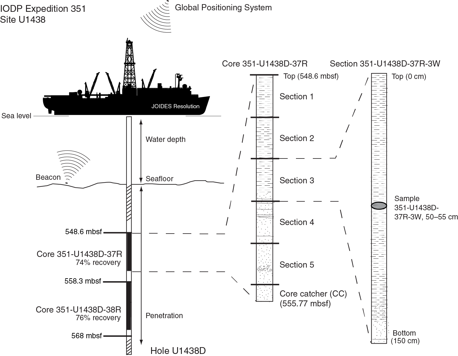
Numbering of the site, holes, cores, and samples followed standard IODP protocol (Figure F1). Drilling sites have been numbered consecutively from the first site drilled by the Glomar Challenger in 1968, and since Expedition 301 the prefix “U” has been used to designate sites cored by the U.S. research vessel JOIDES Resolution. At a site, multiple holes are often drilled, and a letter suffix distinguishes the holes drilled at one site. For example, the first hole would be given the suffix “A,” the second “B,” and so on. During Expedition 351, a letter designation applied to each cored hole (including one jet-in test) and a dedicated logging hole.
Following the hole designation, each recovered core was numbered sequentially. A cored interval is generally ~9.5 m maximum, which is the length of a standard core barrel. However, the half-length advanced piston corer (APC) system employs a core barrel of ~4.7 m. The specific coring system used to recover a core is designated by a letter representing the core type and is a suffix to the core number: H = APC, F = half-length APC, X = extended core barrel (XCB), and R = rotary core barrel (RCB). All of these systems were utilized during Expedition 351.
Each recovered core was cut into ~1.5 m sections. The number of sections is determined by core recovery, and sections are numbered sequentially starting with “1” at the top of the core. Each core is eventually split lengthwise into working- and archive-half sections (described below) designated by either the letter “W” or “A” succeeding the core number. For depth calculations (see below), the top depth of the core is equated with the top depth of the cored interval (in meters below seafloor [mbsf]) to achieve consistency in handling analytical data derived from the cores. Sample intervals are described in centimeters within a core section (typically between 0 and 150 cm) beginning from the top of the core section.
Thus, the full curatorial identifier of a sample consists of the following: expedition, site, hole, core number, core type, section number, section half, piece number (hard rocks only), and interval in centimeters measured from the top of the core section (Figure F1). For example, a sample identified as “351-U1438D-37R-4W, 50–55 cm” represents a 5 cm interval from the fourth section (working half) of Core 37R (cored with the RCB system) from Hole D of Site U1438 during Expedition 351.
Sample depth calculation
During Expedition 351, the cored interval was measured in meters below seafloor as determined by core depth below seafloor, method A (CSF-A). The calculation of this depth scale is defined by protocol (see IODP Depth Scales Terminology at www.iodp.org/program-policies). In general, the depth below seafloor is determined by subtracting the initial drill pipe measurement to the seafloor from the total drill pipe measurement. The core depth interval begins with the depth below seafloor where coring began and extends to the depth that coring advanced. However, if a core has incomplete recovery (<100%), all material is assumed to originate from the top of the cored interval as a continuous section for curation purposes (Figure F1); thus, the true depth interval within the cored interval is unknown and represents a sampling uncertainty in age-depth analysis or correlation with downhole logging data.
Additionally, wireline log depths were calculated from the wireline log depth below seafloor (WSF) and are also reported in meters below seafloor. When multiple logging passes were made (see Downhole measurements), the wireline log depths are matched to one reference pass, creating the wireline log matched depth below seafloor (WMSF). These distinctions in nomenclature between core (curated) and wireline log depth should be noted because the same depth value from different scales does not necessarily refer to the same stratigraphic interval.
Core handling and analysis
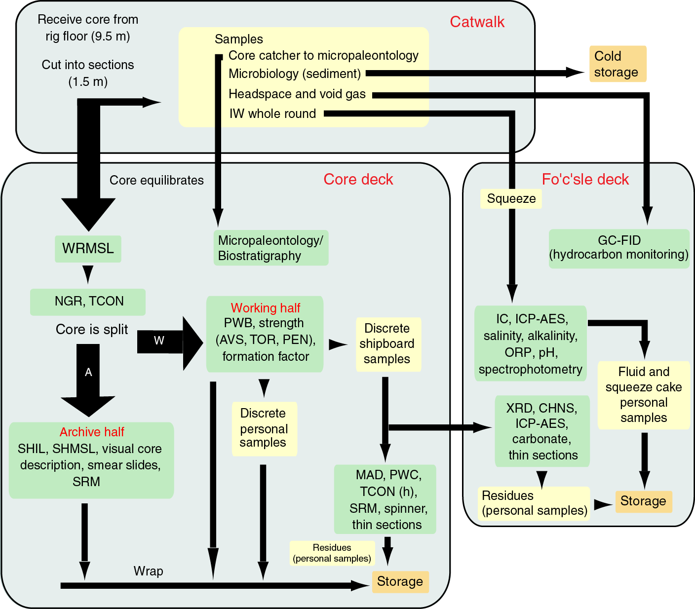
Core handling and flow are depicted in Figure F2.
Sediment
Immediately upon arriving on deck, core catcher samples were taken for biostratigraphic analyses. The cores were then cut into 1.5 m sections, after which whole-round samples were taken for shipboard interstitial water measurements and noted by the use of a yellow end cap. Additional samples taken on the catwalk include syringe samples for routine hydrocarbon gas safety monitoring, samples for postcruise microbiological studies, and samples for postcruise redox-sensitive element analyses (see Geochemistry). After the cores equilibrated to laboratory temperature (~4 h), they were run through the Whole-Round Multisensor Logger (WRMSL) for P-wave velocity, magnetic susceptibility, and bulk density measurements, as well as the Natural Gamma Radiation Logger (NGRL). Thermal conductivity measurements were also made when the samples were unconsolidated sediments (see Physical properties).
The core sections were then split lengthwise into archive- and working-half sections. Oriented pieces of more indurated sediments were marked on the bottom with a red wax pencil.
Hard rock
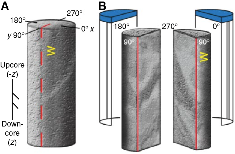
During Expedition 351, cores from the igneous basement were curated as hard rock. On the catwalk, pieces were pushed to the bottom of the sections and the total length was measured as “recovered length,” which was used to calculate recovery. The sections were then brought into the core splitting room, where oriented pieces of core were marked with a wax pencil. In several cases, pieces were too small to be oriented with certainty. Pieces in a section were placed into sample bins separated by plastic core spacers. The plastic spacers were also used to indicate areas of no recovery. Adjacent pieces that could be fit back together were curated as single pieces. Once completed, a designated scientist (usually the paleomagnetist on shift) confirmed the piece matches and drew split lines indicating where/how the pieces should be cut into archive and working halves. The split lines ideally maximized the expression of dipping surfaces on the cut face of the core while preserving representative features in the archive and working halves (Figure F3).
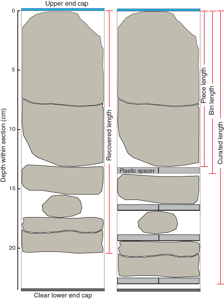
Once the split lines were drawn, the spacers were secured in place with acetone in both archive- and working-half core liners with the angle brace facing uphole. This ensured that the curated interval for each bin matched the top of each piece. The length of each bin was entered into SampleMaster as “bin length,” and the sum of a section’s bin lengths was entered as “curated length.” Additionally, the length of each piece was measured along the longest vertical dimension and entered as “piece length” (Figure F4). Following this, the empty core liner half was placed over the full half and taped together in several places. The cores were allowed to dry and equilibrate to laboratory conditions (~3 h).
The sections were then run through the WRMSL and NGRL before being carefully split into archive and working halves. Piece halves were numbered sequentially from the top of each section, and reconstructed groups of pieces in the same bin were assigned the same number but lettered sequentially. If a piece was oriented with respect to vertical, an arrow pointing to the top of the section was added to the label.
For both sediment and hard rock cores, the working-half sections were used for taking discrete shipboard samples for paleomagnetic, physical properties, geochemical, and thin section analyses (for details, see the individual laboratory group methods in this chapter), as well as science party personal samples for postcruise research. Sampling for postcruise research was based on the sampling plan agreed upon by the science party and the Sample Allocation Committee.
The archive-half core sections were run through the Section Half Imaging Logger (SHIL) and the Section Half Multisensor Logger (SHMSL) for color reflectance and point magnetic susceptibility measurements. The archive halves were described by expedition scientists visually and by smear slide and thin section analyses. Finally, they were measured with the cryogenic magnetometer.
All instrument data from Expedition 351 were uploaded into the IODP Laboratory Information Management System (LIMS), and core description observations were entered using the DESClogik application. DESClogik is an interface used to input visual (macro- and/or microscopic) core descriptions on a core (sediment) or section (igneous basement) scale to be stored in LIMS.
When all shipboard measurements were completed, data uploaded, and samples taken, the cores were wrapped, sealed in plastic, and transferred to cold storage on the ship. At the end of the expedition, the cores were transferred into refrigerated trucks and transported to cold storage at the IODP Kochi Core Center in Kochi, Japan.
Core sample disturbance
Core material has the potential to be disturbed and/or contain extraneous material as a result of the coring process or core handling and analysis. In less consolidated sections, material from intervals shallower in the hole may be washed down by drilling circulation and accumulate at the bottom of the hole; they then are sampled with the recovery of the next core. This is referred to as “fall-in.” In most Expedition 351 cores, there was very little evidence of fall-in, but when present, it affected the upper ~10–20 cm of the cores. Additionally, common coring deformation includes concave appearance of originally horizontal bedding. In more consolidated material, biscuiting is a common core disturbance, where fractured material (“biscuits”) spin within the core barrel. In many cases, drilling slurry can be interjected between the biscuits. Finally, fracturing, fragmentation, and brecciation as a result of the drilling process are also common drilling-induced disturbances. The occurrences of these disturbance types are described in Lithostratigraphy in the Site U1438 chapter (Arculus et al., 2015) and graphically represented on the visual core descriptions (VCDs) (see Core descriptions).
Authorship of methods and site chapters
The sections of the methods and site chapters were written by the following scientists (in alphabetical order):
- Background and objectives: Arculus, Ishizuka
- Operations: Bogus
- Lithostratigraphy: Barth, Brandl, Hickey-Vargas, Jiang, Kanayama, Kusano, Li, Marsaglia, McCarthy, Meffre, Savov, Tepley, Yogodzinski
- Biostratigraphy and paleontology: Aljahdali, Bandini, Guerra, Kender
- Geochemistry: Loudin, Sena, van der Land, Zhang
- Paleomagnetism: Maffione, Morris
- Physical properties: Drab, Gurnis, Hamada
- Downhole measurements: Drab, Gurnis, Hamada, Neuhaus
Lithostratigraphy
Core description process
During Expedition 351, sediments and rocks were described by a team with diverse backgrounds in igneous petrology, volcanology, and volcaniclastic and nonvolcanic sedimentology. Macroscopic descriptions of the core were made on the archive halves of split cores. Observations were tabulated on printouts of high-resolution images from the Section Half Imaging Logger (SHIL) and entered into the LIMS database using DESClogik software. Smear slides and petrographic thin sections were made for selected intervals and described using polarized light microscopy (transmitted and reflected light). Petrographic observations were entered into the LIMS database using DESClogik. Microscopic observations apply rigorously only to the intervals where a smear slide or thin section was made, which is indicated on the visual core descriptions (VCDs).
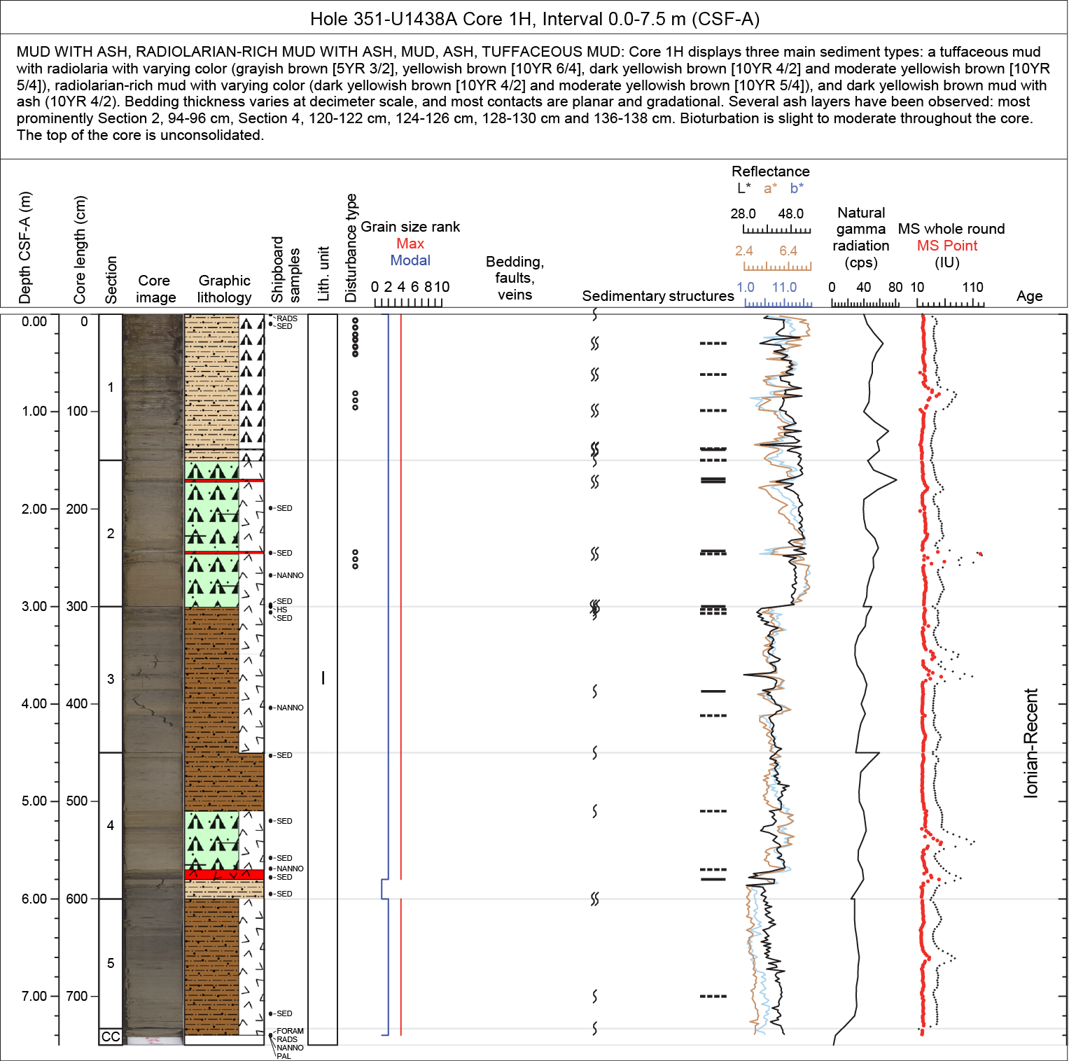
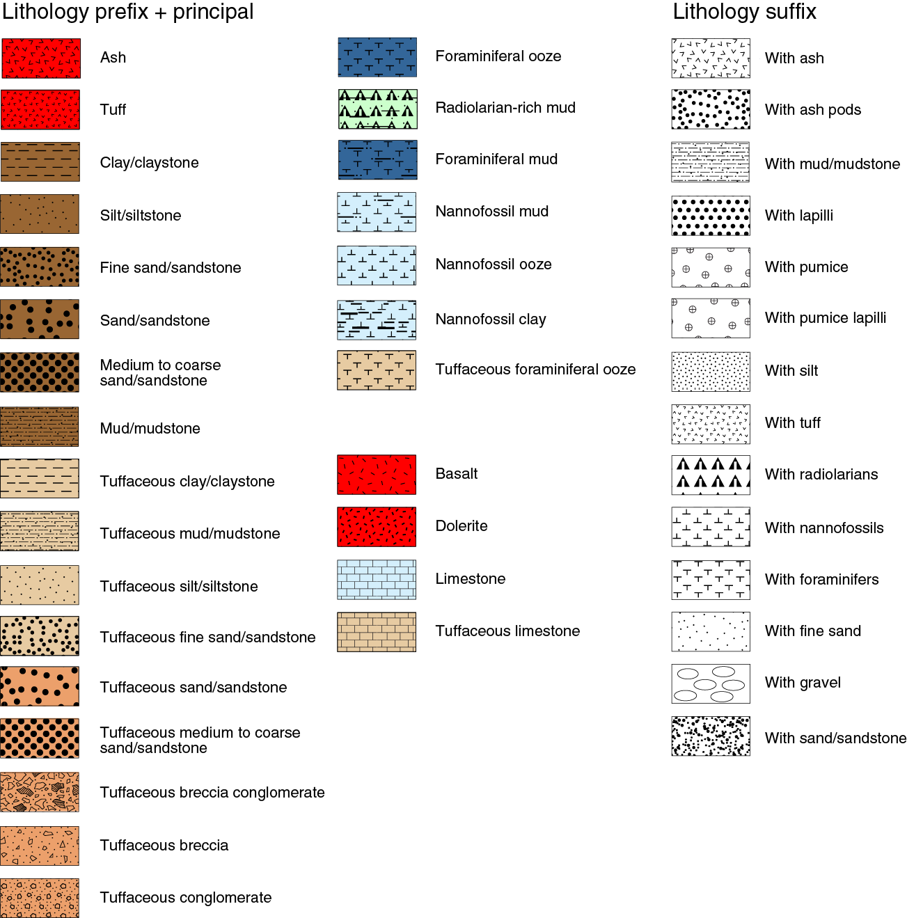
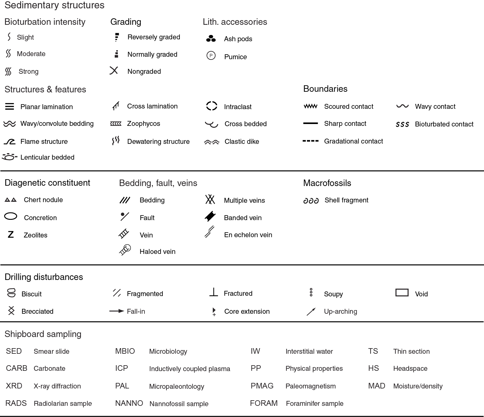
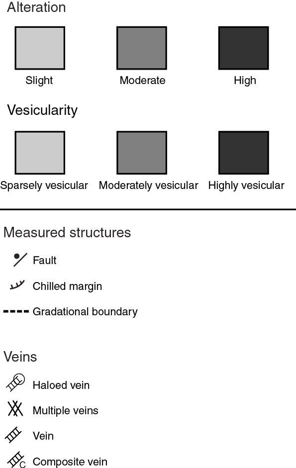
Core description data are available through the “Descriptive Information” LIMS report (web.iodp.tamu.edu/DESCReport). Standard graphic reports were generated from data downloaded from the LIMS database to summarize each core (typical for sediments) or section half (typical for igneous rocks). A sample VCD is shown in Figure F5. Legends for symbols used on the VCDs are shown in Figures F6, F7, and F8.
Sediment and sedimentary rock classification scheme
Pelagic/hemipelagic and volcaniclastic sediments and sedimentary rocks were the principal sedimentary materials recovered during Expedition 351. The sedimentary classification scheme that was employed emphasizes important descriptors for those sediments and rocks, particularly descriptors that can be quantified and recorded in DESClogik in the same time frame as shipboard core description (“Macroscopic” template, “Sediment” tab). A schematic of the description parameters and scheme is shown in Figure F9.
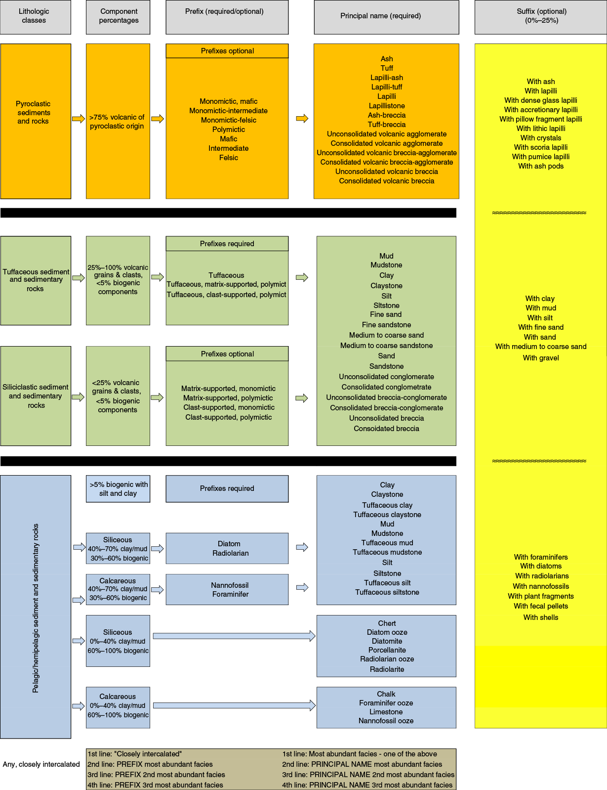
Sediments and sedimentary rocks were classified using an approach that integrates volcanic particles into the sedimentary descriptive scheme typically used by IODP. In our scheme, sediments and sedimentary rocks are divided into four lithologic classes, based on composition (types of particles):
- Volcaniclastic sediment and rocks of pyroclastic origin, containing >75% volcanic particles;
- Tuffaceous volcaniclastic sediment and rocks of sedimentary origin, containing 25%–75% volcanic-derived particles;
- Siliciclastic sediment and sedimentary rocks, containing <25% volcanic siliciclastic particles and <5% biogenic particles; and
- Pelagic to hemipelagic sediment (rock), containing <25% volcanic particles and >5% biogenic particles.
Examples from each of these four lithologic classes were encountered during this expedition. Within each class, the principal lithology name is based on particle size. In addition, appropriate prefixes and suffixes were chosen; for example, the prefix “tuffaceous” was used for the tuffaceous lithologic classes, and prefixes that indicate the dominant biogenic component, determined by microscopic examination, were used for pelagic/hemipelagic sediment and sedimentary rocks. Suffixes were also chosen to indicate minor components within a principal lithologic type.
Principal lithology names
Principal names for sediments and sedimentary rocks of the tuffaceous, nonvolcanic siliciclastic, and pelagic/hemipelagic lithologic classes are adapted from the grain size classes of Wentworth (1922). Principal lithology names for sediment and sedimentary rocks of the pyroclastic lithologic class were adapted from the grain size classes of Fisher and Schmincke (1984) (Table T1). For each grain size class, both a consolidated (semilithified to lithified) and a nonconsolidated term exists; they are mutually exclusive (e.g., mud or mudstone; ash or tuff). For simplicity, Wentworth’s clay and fine silt sizes are combined in a “mud” class; similarly, very fine, fine, medium coarse, and very coarse sand are combined in “fine sand,” “sand,” and “medium to coarse sand” (stone) classes. Silt/siltstone is also used independently.
Table T1. Particle size nomenclature and classifications. Download table in .csv format.
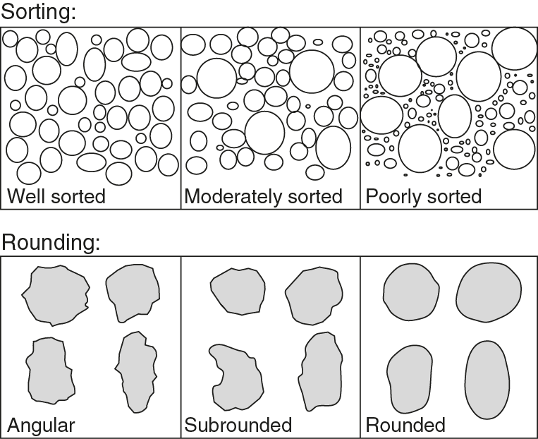
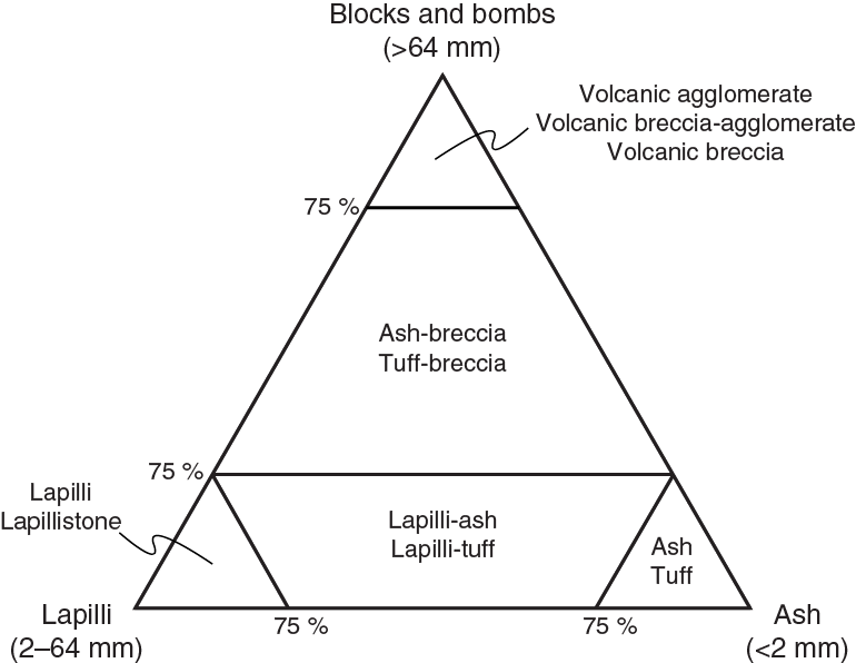
The grain size terms granule, pebble, and cobble (Wentworth, 1922) in lithified sediments are replaced by breccia, conglomerate, and breccia-conglomerate (Table T1). A conglomerate is defined as a rock where the fragments are >2 mm and are exclusively (>95 vol%) rounded and subrounded (Figure F10). A breccia-conglomerate is composed of predominantly rounded and/or subrounded clasts (>50 vol%) and subordinate angular clasts. A breccia is predominantly composed of angular clasts (>50 vol%). For the equivalent pyroclastic lithologic class, the term “agglomerate” would be used in place of conglomerate (Fisher and Schmincke, 1984) (Figure F11). Irrespective of the sediment or rock lithologic class, the average and maximum grain size reported in the VCDs follow Wentworth (1922). For example, an ash can be further described as sand-sized ash or silt-sized ash, whereas a lapilli-tuff can be described as coarse sand sized or pebble sized.
For pelagic and hemipelagic sediments (the nonvolcanic siliciclastic and biogenic classes, 3 and 4 above), a modified version of the Ocean Drilling Program (ODP) Leg 126 sediment classification scheme was used (Figure F12; Table T1) (Taylor, Fujioka, et al., 1990). Our modified classification uses composition and grain size as the only criteria to define sediment and rock types. The principal lithology name is based on induration and on average grain size as determined macroscopically, supplemented at selected intervals with smear slide observations of the identity and abundances of biogenic particles. For sediments and rocks with <60% biogenic material, the principal name is determined by the relative proportions of nonbiogenic sand-, silt-, and clay-sized particles. If the biogenic component exceeds 60%, the principal name is ooze or an appropriate term that denotes the sediment induration, for example, chert and chalk or limestone.
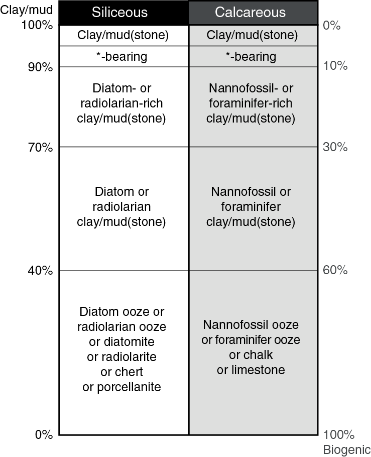
Prefixes
Prefixes were used to indicate the lithologic class of sediment or sedimentary rocks. For pelagic/hemipelagic sediments and sedimentary rocks with 25%–60% biogenic material, prefixes were added to indicate the type and quantity of fossil material, using the classification scheme shown in Figure F12. In this case, prefix categories were based on the percentage of microfossils seen in smear slides taken at selected intervals. For sediments and rocks with 5%–25% biogenic material, either a prefix or suffix was added (see below) to indicate the presence of microfossils as a minor component. Other prefixes may be selected in combination with those for the pyroclastic and tuffaceous lithologic classes. These prefixes are primarily used for sedimentary rocks having clasts (i.e., particles >2 mm) that can be examined by macroscopic observation. The term “monomict” applies to clast compositions of a single type, and “polymict” applies to clast compositions of multiple types. The term “matrix-supported” was used where smaller particles visibly envelop each of the larger particles. In this usage, the word “matrix” is not defined by a specific grain size (e.g., conglomerate may have a sandstone matrix, and sandstone may have a mudstone matrix). The term “clast-supported” was used where clasts form a sediment framework.
Suffixes
A suffix was used for a subordinate but important component that deserved to be highlighted. Suffixes are restricted to a single phrase to maintain a short and effective lithology name containing the most important information only. They are in the form “with ash,” “with clay,” or “with foraminifers” in cases where abundance is between 5% and 25%.
Thin section description of sedimentary rocks
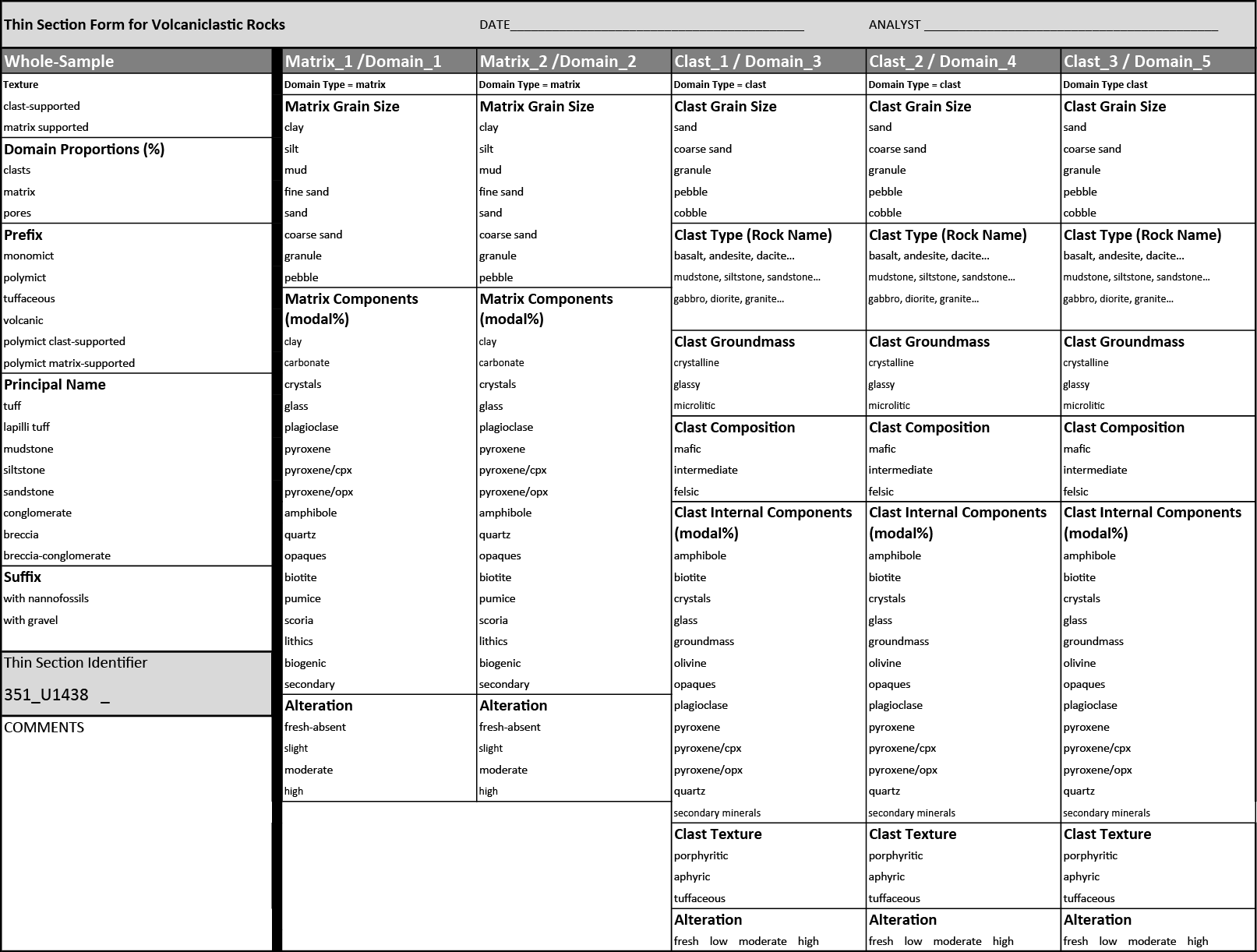
Because of their importance in Expedition 351 cores, a systematic approach was implemented in DESClogik to record microscopic characteristics of volcaniclastic sedimentary rocks (“Microscopic” template, “Sediment TS” tab). The system provides a framework for recording data for both texturally complex (clast-bearing) coarse-grained rocks and less complex lithologies dominated by finer grain sizes (sand, silt, and mud). For tuffaceous breccia-conglomerates and other clast-bearing lithologies, the system provides the opportunity to record modal data for two types of whole-rock matrix and up to five separate clast types. Each matrix or clast type is assigned a domain type and number and is entered on a separate row in DESClogik. Modal components available under the matrix category are minerals, which occur as matrix grains, with additional options such as ash, clay, pumice, scoria, lithics, carbonate, and authigenic mineral (secondary) components. Modal components available under the clast category include the same list of minerals, which occur as phenocrysts, plus groundmass, vesicles, and secondary minerals, which make up the remaining portion of the mode for most volcanic clasts.
Each clast is also assigned the following:
- Grain size category (e.g., granule, pebble, or cobble),
- Clast type, selected from a list of rock names,
- Texture (porphyritic, aphyric, or tuffaceous), and
- Alteration category (absent/fresh, slight, moderate, or high).
The modes for each matrix and clast should total 100%. For texturally simple rock types of more uniform grain size, such as tuffaceous sandstone, siltstone, and mudstone, the pertinent microscopic information is entered into DESClogik as a single matrix domain. An Excel spreadsheet form was developed to facilitate recording of thin section observations by hand (Figure F13). The data on this form was then entered into DESClogik.
Other parameters
Average and maximum particle size, sediment sorting and grading, the characteristics of bedding planes, the extent of bioturbation, and the presence of sedimentary structures are additional elements that were recorded in macroscopic core descriptions (Figures F10, F14; Table T2). Coring disturbances were also noted and recorded. Disturbance types are primarily brecciation, fracturing, and biscuiting, with some other types as summarized in Figure F15.
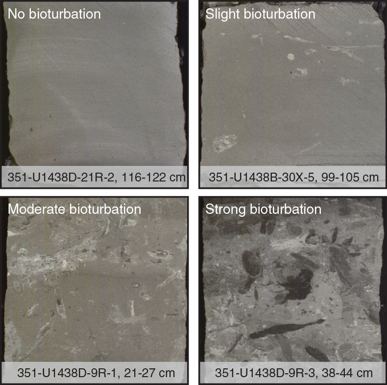
Table T2. Bed thickness classifications. Download table in .csv format.

Secondary minerals in sediments and sedimentary rocks
Secondary mineral development in Site U1438 sediments and sedimentary rocks was documented through smear slide, thin section, and X-ray diffraction (XRD) observations. Smear slide and thin section sample preparation steps followed standard and widely accepted practices. Smear slide and petrographic observations of secondary minerals are recorded in both the macroscopic and microscopic areas of DESClogik.
Samples for XRD analysis were freeze-dried for 12 h and then crushed using an agate mortar and pestle. No additional sample preparation steps were taken to aid identification of clay or zeolite mineral species. Diffraction data were generated on the JOIDES Resolution shipboard Bruker D4Endeavor X-ray diffractometer using a generator voltage of 35 kV and current of 40 mA. We collected continuous scans from 4° to 75°2θ for 4276 steps at a rate of 1 s/step. We evaluated diffraction data against the International Center for Diffraction Data database for minerals using the Search/Match component of Bruker’s EVA Diffraction Evaluation software. The diffractogram of a typical sample was usually accounted for by the presence of three to six common minerals or minerals known to be present or considered likely to be present in the samples, based on geologic context and thin section or smear slide observations.
Unit determinations
Sediments and sedimentary rocks, including volcaniclastic, siliciclastic, and biogenic types, were described at the level of (1) the descriptive interval (a single descriptive line in the DESClogik spreadsheet) and (2) the lithostratigraphic unit. A descriptive interval (Table T3) is unique to a specific depth interval and typically consists of a single sediment or rock type distinct from those immediately above and below it, for example, a tuff interval intercalated between mudstone intervals. Less commonly, the same sediment or rock type may be repeated in consecutive descriptive intervals if one or more characteristics differ between them, for example, a planar laminated tuffaceous siltstone below or above cross-laminated tuffaceous sandstone.
Table T3. Definition of lithostratigraphic units, descriptive intervals, and domains. Download table in .csv format.
Lithostratigraphic units are meter-thick to hundreds of meters–thick assemblages of multiple descriptive intervals containing similar sediment or rock types (Table T3). They are numbered sequentially (Unit I, Unit II, etc.) from top to bottom. Lithostratigraphic units are clearly distinguishable from each other by several characteristics, such as composition, bed thickness, grain size class, and internal homogeneity. Lithostratigraphic units are, therefore, informal formations that are not defined by age, geochemistry, or paleontology, although changes in these parameters may coincide with boundaries between lithostratigraphic units.
Sedimentary rock structure and measurement
The methods used during Expedition 351 for documenting the structural geology were simplified from those used during Integrated Ocean Drilling Program Expedition 344 (Harris et al., 2013). We documented deformation that was observed on the archive half of the split cores by classifying structures, measuring orientation data, and recording the sense of displacement. These data were logged at the core table and entered into DESClogik under the “Structure” tab or as comments for the interval (for millimeter- to centimeter-scale structures within the interval).
Igneous rocks
Igneous rock description procedures during Expedition 351 generally followed those of IODP Expedition 350, Expedition 344, and other Integrated Ocean Drilling Program and IODP expeditions that encountered volcanic units (e.g., Expedition 350 Scientists, 2014; Expedition 330 Scientists, 2012; Expedition 336 Scientists, 2012; Expedition 340 Scientists, 2013; Harris et al., 2013). Macroscopic observations were coordinated where possible with thin section or smear slide petrographic observations and bulk-rock chemical analyses of representative samples. Data for the macroscopic and microscopic descriptions of recovered cores were entered into the LIMS database using DESClogik. Volcanic rock characteristics were entered through the “Extrusive hypabyssal” tab, and plutonic rocks were entered through the “Intrusive mantle” tab.
Macroscopic descriptions of volcanic rocks recovered during Expedition 351 were entered into the “Macroscopic” template’s “Extrusive hypabyssal” tab. Volcaniclastic sediments that contain igneous particles of various sizes were recovered, for the most part with grain sizes <2 cm; for these sediments, microscopic clast descriptions were entered using the “Microscopic” template’s “Sediment TS” tab, as described in Thin section description of sedimentary rocks. Igneous clasts >2 cm in size and basement volcanic rocks were described using the “Microscopic” template’s “Extrusive hypabyssal” tab.
Volcanic (extrusive hypabyssal) rocks: principal lithology name and descriptive parameters
For macroscopic description of volcanic rocks, we use a simplified classification scheme based on visual characteristics. The lithology name consists of a principal name and optional suffix (Table T4). The principal name depends on the nature of phenocrysts, when present, and/or the color of the groundmass. Three rock categories are defined:
- Basalt: black to dark gray rock containing plagioclase and pyroxene.
- Andesite: dark to light gray rock containing pyroxenes and/or feldspar and/or amphibole and typically devoid of olivine and quartz.
- Rhyolite/dacite: light gray to pale white rocks, usually plagioclase-phyric, and sometimes containing quartz ± biotite.
Table T4. Nomenclature for macroscopic and microscopic description of extrusive and hypabyssal volcanic rocks. Download table in .csv format.
The suffix indicates the nature of the volcanic body: lava, pillow lava, intrusive sheet, or clast. The suffix “hyaloclastite” or “breccia” is used if the rock occurs in direct association with related in situ lava (Table T4). Prefixes are not used for macroscopic description.
Other descriptive parameters that are recorded are rock texture (see below), grain size, phenocryst type and abundance, vesicularity and vesicle shape, secondary minerals, and the nature of contacts between volcanic rock intervals.
Microscopic descriptions are similar to macroscopic observations but are more detailed. Seven primary rock types are defined (basalt, boninite, dolerite, basaltic andesite, andesite, dacite, and rhyolite) (Table T4). Optional suffixes indicate the nature of the volcanic rock body. Phenocryst type, modal abundance, and modal grain size are recorded, together with other parameters used for macroscopic description.
Plutonic (intrusive mantle) rocks: principal lithology name and descriptive parameters
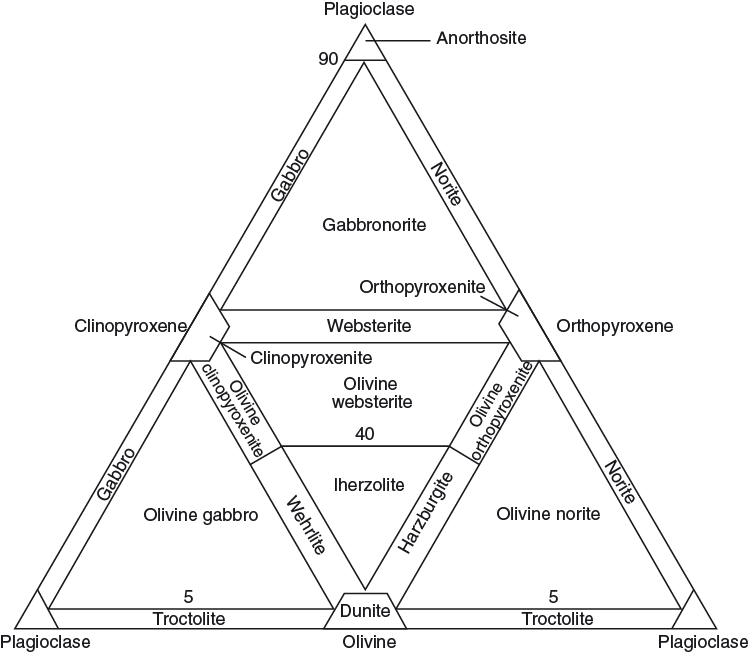
Plutonic rocks are classified according to the International Union of Geological Sciences classification scheme of Le Maitre et al. (2002). The nature and proportion of minerals are used to give a principal lithology name to the sample. Leucocratic rocks dominated by quartz and feldspar are named using the quartz-alkali feldspar-plagioclase (QAP) diagram (Figure F16). For melanocratic plutonic rocks, we used the plagioclase-clinopyroxene-orthopyroxene and olivine-pyroxene-plagioclase triangular plots (Figure F17). In all, 22 principal lithology names are used. Three suffixes, banded, layered, and foliated, may be used to identify macroscopic rock features. Rock texture, overall grain size, modal abundance, and modal grain size of mineral types and intrusive rock contact types are recorded.

Microscopic descriptions are similar to macroscopic observations but are more detailed. A larger list of descriptive suffixes is used, and more options are used for definition of rock texture; maximum grain size and grain size distribution are added characteristics. Constituent minerals are described with modal abundance and modal and maximum grain size.
Igneous texture definitions
Textures are described macroscopically for all igneous rock core sections and microscopically for the subset of intervals having thin sections. Macroscopic textural descriptions applied to volcanic/hypabyssal rocks are holocrystalline, porphyritic, trachytic, flow banding, perlite, glassy matrix, glassy, quench margin, and glomeroporphyritic.
For intrusive/mantle rocks, textural descriptors are
- Equigranular (principal minerals are in the same size range),
- Inequigranular (principal minerals have different grain sizes),
- Porphyritic,
- Poikilitic (larger crystals enclose smaller grains),
- Ophitic (pyroxene encloses plagioclase laths), and
- Subophitic (pyroxene partially encloses plagioclase laths).
In addition, for microscopic descriptions, cryptocrystalline (<0.1 mm) is used.
Prefixes used in microscopic textural descriptions are (Wilcox, 1954)
Glomeroporphyritic texture refers to clusters of phenocrysts.
Magmatic flow textures are described as trachytic when plagioclase laths are subparallel.
Perlite describes rounded hydration fractures in glass.
Quenched margin texture describes a glassy or microcrystalline margin to an otherwise coarser grained interior.
Vesicularity is described according to proportions:
For microscopic observations, the modal size and sphericity of vesicle populations are estimated using appropriate comparison charts, following Expedition 330 Scientists (2012) (Figure F18).

Secondary minerals in igneous rocks
Alteration features in igneous rocks from Expedition 351 are based on macroscopic observations of core, aided by shipboard smear slide, thin section, and XRD and inductively coupled plasma–atomic emission spectroscopy (ICP-AES) investigations. Secondary minerals in cores were recorded in DESClogik in the macroscopic template under separate tabs for alteration, veins, and halos.
Levels of alteration in groundmass were recorded as
Textures used to define groundmass alteration were patchy, corona, pseudomorphic, and recrystallized.
Colors used to define alteration are black, brown, gray, green, white, and yellow.
Groundmass, glass, and mineral replacement minerals and vesicle filling minerals are classified as dominant, second order, and third order.
Alteration of groundmass includes major mineral products amphibole, biotite, carbonate, chalcedony, chlorite, clay, epidote, feldspar (albite), glauconite, oxide, quartz, sulfide, zeolite, or unknown when the mineral cannot be identified.
Alteration of phenocryst minerals includes iddingsite, prehnite, sericite, serpentine, and talc.
Vesicle-filling minerals include calcite, carbonate, chalcedony, zeolite, clay, chalcopyrite, sulfide, chlorite, prehnite, and unknown and undefined mineral.
Microscopic observations of alteration minerals in igneous rocks are similar but more detailed. Percentages of individual replacement minerals are estimated for each phenocryst mineral, groundmass, and glass.
Descriptions of veins and halos record their mineralogy, geometry, contacts, and crosscutting relationships with the host rock(s).
Vein texture selections are vuggy, cataclastic, saccharoidal, sutures, patchy, banded, comb-structured, overgrowths, fibrous, and brecciated.
Vein geometry selections are splayed, sinuous, irregular, planar, and curved.
Vein contacts may be gradational, sharp-to-gradational, sharp, sutured, and diffuse.
Vein connectivity is described as networked, anastomosing, branched, and isolated.
Vein and halo minerals are described as dominant, second order, and third order.
Unit designations
Igneous rocks are described at the level of the descriptive interval (the individual descriptive line in DESClogik), which ultimately is the lithostratigraphic unit level. A descriptive interval consists of variations in rock characteristics, such as vesicle distribution, igneous textures, mineral modes, and chilled margins. Samples within the volcanic category are massive lavas, pillow lavas, intrusive sheets (i.e., dikes and sills), and volcanic breccias intimately associated with lava flows. Breccias not associated with lava flows and hyaloclastites not associated with pillow lavas are described on the sediment form in DESClogik.
Massive lava is defined as a coherent volcanic body with a massive core and vesiculated (sometimes brecciated or glassy) flow top and/or bottom. Intrusive sheets are defined as dikes or sills cutting across other volcanic bodies. They frequently have holocrystalline groundmass and nonvesiculated chilled margins along their boundaries. Their size varies from several millimeters to several meters in thickness.
Description of workflow
The core description workflow included the following steps:
- Initial determination of intervals in a core section based on macroscopic observation of particle/grain sizes, compositional changes and heterogeneity, igneous and sedimentary structures, and characteristics of contacts.
- Microscopic analyses performed on selected intervals using (a) sediment smear slides or (b) petrographic thin sections.
- Classification of the rock intervals based on macroscopic parameters and microscopic analyses, when available.
- Descriptive summary of the core.
- Integration with XRD and carbonate analyses to verify or correct mineralogical identification.
Biostratigraphy
Paleontological investigations and biostratigraphic determinations during Expedition 351 were carried out on calcareous nannofossils, planktonic and benthic foraminifers, and radiolarians. We followed the Cenozoic planktonic foraminifer biozonation scheme of Wade et al. (2011). Species identification was primarily based on Kennett and Srinivasan (1983), Pearson et al. (2006), and Bolli and Saunders (1985). Benthic foraminifer species determination was largely carried out with reference to Kaiho (1992), van Morkhoven et al. (1986), and Holbourn et al. (2013). The standard zonations of Martini (1971) and Okada and Bukry (1980) were used for Cenozoic nannofossil biostratigraphy. The identification of calcareous nannofossils during this expedition followed the taxonomy of Perch-Nielsen (1985), Varol (1998), and Young (1998). The radiolarian low-latitude zonation used during the expedition was based on Sanfilippo et al. (1985) and Sanfilippo and Nigrini (1998). For radiolarians, the primary references for taxonomic identification were Sanfilippo et al. (1985), Hollis (2006), and Jackett et al. (2008). All ages cited in the text and figures for each of the microfossil groups are based on calibration with the timescale of Gradstein et al. (2012). All data were recorded in DESClogik and uploaded to the LIMS database.
Core catcher (CC) samples from all cores were examined. Additional samples were taken from the working-half section as necessary to refine the biostratigraphy, preferentially sampling hemipelagic intervals.
Foraminifers
Sediment volumes of approximately 20 cm3 were collected for analysis of both benthic and planktonic foraminifers. All samples were washed with water over a 63 µm mesh sieve and dried in an oven at ~70°C. Samples that were more lithified were soaked in warm (70°C) water with sodium borate (Borax) for several hours prior to wet sieving. For the most lithified samples, a freeze-thaw method with kerosene was used (adapted from Hermann [1992] and Kennedy and Coe [2014]). The samples were placed in sample bags and broken with a plastic hammer, soaked in water for more than 1 h, and then placed in a freezer at –80°C for several hours. Boiling water was poured over the residue, which was then washed with water over a 63 µm sieve. The residue was placed in a freeze-drier for approximately 24 h to clear the pore spaces and then soaked in kerosene for 24 h. The kerosene was decanted, and the sample was left to soak in deionized water for several minutes before sieving. The water replacement of the kerosene in pore spaces creates pressure that helps disaggregate the clay (Hermann, 1992). All dry coarse fractions were placed in a labeled vial ready for micropaleontological examination.
Examination of foraminifers was carried out on the >150 µm size fraction following dry sieving. The sample was spread over a sample tray and examined for planktonic and benthic foraminifers. The size fraction <150 µm was examined in parts of the record when datum species of smaller sizes were expected. A visual assessment of group and species relative abundances was made, along with their preservation according to the categories defined below. Photomicrographs were taken using a Spot RTS system with IODP Image Capture and commercial Spot software and using a Hitachi TM3000 tabletop scanning electron microscope (SEM).
The relative abundance of both planktonic and benthic foraminiferal species in the biogenic fraction >150 µm was estimated as follows:
The proportion of either planktonic or benthic foraminifer specimens in each slide (>150 µm) was estimated as follows:
- Barren = no foraminifers present.
- Present = <1%.
- Rare = 1%–5%.
- Few = 5%–10%.
- Common = 10%–30%.
- Abundant = >30%.
Preservation of planktonic and benthic foraminiferal assemblages was estimated using the following categories:
- G = good (>90% of specimens unbroken with only minor evidence of diagenetic alteration; diagnostic characteristics fully preserved).
- M = medium (30%–90% of specimens are unbroken; dissolution and/or secondary overgrowth present).
- P = poor (strongly recrystallized or dominated by fragments and broken or corroded specimens).
Calcareous nannofossils
Calcareous nannofossils were examined in smear slides prepared directly from unprocessed samples using standard techniques. The slides were analyzed between crossed polars (PPL), phase contrast, and between crossed polars (XPL) using a Zeiss Axiophot light microscope at a magnification of 1000×. One traverse (~100 fields of view) was used to estimate relative abundance and to ensure rare species were recorded. For coarse material, the fine fraction was separated from the coarse fraction by settling through water before the smear slide was prepared. Photomicrographs were taken using a Spot RTS system with the IODP Image Capture and Spot commercial software.
The overall and individual nannofossil abundances were determined using the following criteria:
- B = barren (no nannofossils).
- R = rare (1 specimen per >10 fields of view).
- VF = very few (1 specimen per 2–10 fields of view).
- F = few (2–10 specimens per 2–10 fields of view).
- C = common (1–10 specimens per field of view).
- A = abundant (11–100 specimens per field of view).
- V = very abundant (>100 specimens per field of view).
- * = reworked occurrence.
The following basic criteria were used to qualitatively provide a measure of preservation of the nannofossil assemblage:
- E = excellent (no dissolution is seen; all specimens can be identified).
- G = good (little dissolution and/or overgrowth is observed; diagnostic characteristics are preserved and all specimens can be identified).
- M = moderate (dissolution and/or overgrowth are evident; a significant proportion [up to 25%] of the specimens cannot be identified to species level with absolute certainty).
- P = poor (severe dissolution, fragmentation, and/or overgrowth has occurred, most primary features have been destroyed, and many specimens cannot be identified at the species level).
Radiolarians
Radiolarian assemblages were examined and described from all core catcher samples and from selected additional samples. Lithified samples were initially crushed with a hammer into millimeter-sized fragments. All samples were then disaggregated in a warm (70°C) solution of 10% hydrogen peroxide (H2O2) to remove any organic material, with the addition of a squirt of Borax, which acts as a clay dispersant. After effervescence, samples were sieved and washed through a 63 µm mesh. Residues of more lithified samples were returned into a beaker with a similar solution, sieved, and washed a second time. If calcium carbonate was evident, a 10% solution of hydrochloric acid (HCl) was added after effervescence decreased to dissolve the calcareous fraction. A portion of the residue was placed with a pipette directly onto a glass microscope coverslip. The coverslip was then dried on a hot plate. After drying but while still warm, the coverslip was gently mounted onto a glass microscope slide with Norland optical adhesive (Number 61) and placed under an ultraviolet lamp for about 10 min. Strewn slides were examined using a Zeiss Microscope (Model AX 10) coupled with a Diagnostic Instruments (Model 15.2 64 Mp Shifting Pixel) photomicrograph camera system.
When radiolarian skeletons were recrystallized as quartz, clay minerals, or zeolites filled by matrix or cement, they could not be examined using standard transmitted-light techniques. These residues were sieved, dried, and examined using reflected-light methods and a Hitachi TM3000 tabletop scanning electron microscope (SEM).
Total abundances of radiolarian assemblages on a slide were estimated using the following categories:
- B = barren (absent).
- R = rare (>0–500 specimens per slide).
- F = few (>500–2,000 specimens per slide).
- C = common (>2,000–10,000 specimens per slide).
- A = abundant (>10,000 specimens per slide).
Abundances of individual taxa per sample were estimated using the following categories:
- ?r = possibly reworked.
- R = rare (1% or less of slide).
- F = few (>1%–5% of slide).
- C = common (>5%–15% of slide).
- A = abundant (>15%–30% of slide).
- D = dominant (>30% of slide).
Preservation of the radiolarian assemblage was estimated using the following categories:
- G = good (most specimens complete; fine structures preserved).
- M = moderate (minor evidence of dissolution and/or breakage).
- P = poor (common crystal overgrowth, dissolution, and/or breakage).
Geochemistry
Shipboard geochemical analyses were performed on samples from Holes U1438A, U1438B, U1438D, and U1438E. These analyses included inorganic chemical analysis of the interstitial water present in the pores and fractures of the cored sediments and rocks, hydrocarbon analysis of headspace gas, and organic and inorganic chemical analysis of the solid matrix.
Headspace analysis of hydrocarbon gases
One sample per sediment core was routinely taken for headspace hydrocarbon gas analysis as part of the standard shipboard safety monitoring procedure as described in Kvenvolden and McDonald (1986) and updated by Pimmel and Claypool (2001). Regular shipboard monitoring of the hydrocarbon content of the cores ensured an assessment of the probable risks of an uncontrolled release of hydrocarbons while drilling.
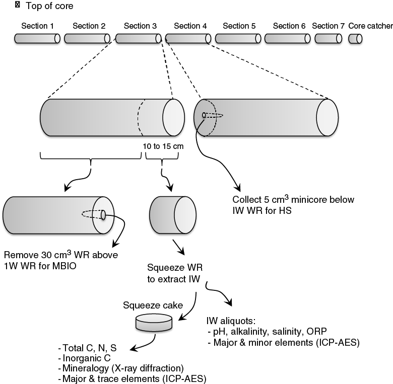
A 5 cm3 sediment sample was collected from the core immediately after sectioning on deck, placed in a 20 cm3 glass vial, and sealed with a Teflon/silicon septum and a crimped aluminum cap. During Expedition 351, the location of the headspace sample was typically taken at the top of Section 4 (Figure F19). A 5 cm3 aliquot of the evolved hydrocarbon gases was extracted from the headspace vial with a standard gas syringe and then manually injected into an Agilent/Hewlett Packard 6890 Series II gas chromatograph equipped with a flame ionization detector set at 250°C. The column (2 mm inner diameter; 6.3 mm outer diameter) was packed with 80/100 mesh HayeSep (Restek). The gas chromatograph oven program remained at 80°C for 8.25 min, was taken to 150°C at 40°C/min, and then was kept isothermal for 5 min, resulting in a total run time of 15 min.
Results were collected using the Hewlett Packard 3365 ChemStation data processing software. The chromatographic response was calibrated with nine different gas standard analyses and checked daily. The concentration of the analyzed hydrocarbon gases was reported as parts per million volume (ppmv).
Interstitial water analyses
Sampling
A whole-round core sample was taken immediately after core sectioning on deck, typically at the bottom of Section 3, for the subsequent extraction of interstitial water (IW) in the Geochemistry laboratory (Figure F19). The length of the whole-round core taken for IW analysis varied from 5 cm in the upper sediments, where the extracted volume of IW was enough for performing the shipboard analyses, to 20 cm in the deeper sediments and rocks, where the volume of extracted IW was more limited.
The whole-round samples collected were processed under atmospheric conditions. After extrusion from the core liner, contamination from seawater and sediment smearing was removed by scraping the core surface with a spatula. In APC cores, ~0.5 cm of material from the outer diameter and the top and bottom faces was removed, whereas in XCB and RCB cores, where borehole contamination is higher, as much as two-thirds of the sediment was removed from each whole round. The remaining inner core (~150–300 cm3) was placed into a titanium squeezer (modified after Manheim and Sayles, 1974) and compressed using a laboratory hydraulic press to extract the interstitial pore water, using a total pressure <20 MPa.
The IW extracted from the compressed sediment sample was filtered through a prewashed Whatman No. 1 filter situated above a titanium mesh screen. Approximately 20 mL of IW was collected in precleaned plastic syringes attached to the squeezing assembly and then filtered through a Gelman polysulfone disposable filter (0.45 µm). In deeper sections, IW recovery was as low as 5 mL after squeezing the sediment for as long as ~2 h. After extraction, the squeezer parts were cleaned with shipboard water, rinsed with deionized water, and dried thoroughly prior to the next use. Sample allocation was determined based on the IW volume recovered and analytical priorities based on the expedition objectives.
Shipboard IW analyses
IW samples were analyzed on board following the protocols in Gieskes et al. (1991), Murray et al. (2000), and the IODP user manuals for shipboard instrumentation. Precision and accuracy were tested using International Association for the Physical Sciences of the Oceans (IAPSO) standard seawater with the following composition: alkalinity (2.353 mM), Ca (10.54 mM), Mg (54.1 mM), K (10.46 mM), Sr (93.0 µM), sulfate (28.94 mM), Cl (559.6 mM), Na (480.7 mM), and Li (26.4 µM) (Leeman Prodigy ICP-AES: User Guide).
The IW extracted from the compressed sediment sample was split into aliquots for the following analyses: (1) ~50 µL for salinity measurement with a refractometer, (2) 3 mL for pH and alkalinity, (3) 2 mL for the analysis of major, minor, and trace elements by inductively coupled plasma–atomic emission spectroscopy (ICP-AES), 100 µL for ion chromatographic (IC) analysis of major anions and cations, (4) 500 µL for chloride titration, (5) 10–15 mL for oxidation-reduction potential (ORP) measurement, (6) 100 µL for ammonium analysis, and (7) 300 µL for phosphate analysis by spectrophotometry.
Salinity, alkalinity, and pH
Salinity, alkalinity, and pH were measured immediately after IW extraction, following the procedures in Gieskes et al. (1991). Salinity was measured using a Fisher temperature-compensated handheld refractometer (Fisher Model S66366). A transfer pipette was used to transfer two drops of IW to the salinity refractometer, and the corresponding salinity was recorded in the log book.
The pH was measured with a combination glass electrode, and alkalinity was determined by Gran titration with an autotitrator (Metrohm 794 basic Titrino) using 0.1 M HCl at 20°C. Certified Reference Material 104 was used for calibration of the acid. IAPSO standard seawater was used for calibration and was analyzed at the beginning and end of the sample set for each site and after every 10 samples. Repeated measurements of IAPSO standard seawater alkalinity yielded a precision <0.8%.
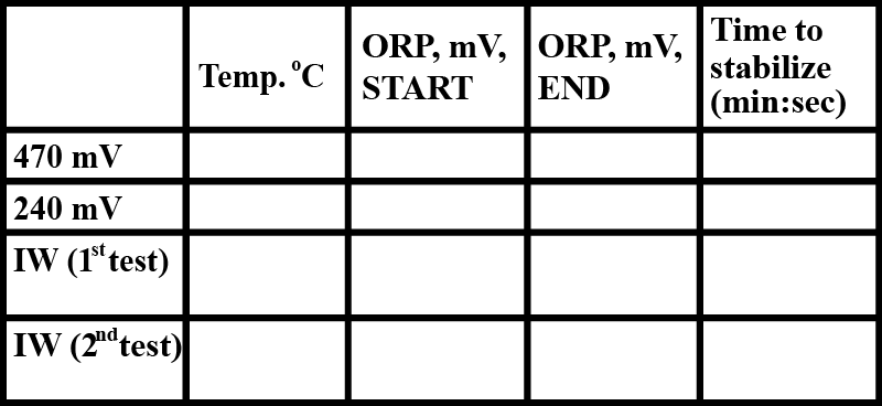
Oxidation-reduction potential
ORP was measured immediately after IW extraction from sediment in order to avoid oxidation of the IW by air. The ORP meter used during Expedition 351 comprised a glass electrode with a platinum pointer filled with an electrolyte of 3.5 M KCl + AgCl. The HANNA Instruments reference for this electrode is HI3131B, and it is coupled to the pH/ORP meter (reference HI9025). A temperature probe with a metallic pointer was coupled to the pH/ORP meter. The ORP electrode operates from –100° to +100°C, and the output ranges from –399.9 to +399.9 mV. Both ORP and temperature readings were recorded.
Standard solutions of 470 mV (reference HI7022) and 240 mV (reference HI7021) were measured before each IW sample analysis (Figure F20). If the ORP reading was more than 20 mV above the high standard value, the electrode was inserted into the reducing pretreatment solution (reference HI7091) for approximately 1 min, followed by rinsing with deionized water. Similarly, if the ORP reading was more than 20 mV below the low standard value, the electrode was inserted into the oxidizing pretreatment solution (reference HI7092) for 1 min, followed by rinsing with deionized water. When not in use, the ORP electrode was kept in a storage solution (reference HI703000).
Each IW sample was measured twice for ORP. Between measurements, the ORP and temperature electrodes were thoroughly rinsed with deionized water and dried carefully with clean, soft paper. As ORP is the measured oxidation-reduction potential in millivolts referred to the platinum electrode with an electrolyte of 3.5 M KCl + AgCl, it was converted to Eh values referred to the standard hydrogen electrode (SHE), using the following equation (Nordstorm and Wilde, 2005):
where EhSHE is the redox potential (mV) referred to the standard hydrogen electrode and Ehref is the reference electrode potential (mV) corrected for the sample temperature. Whenever the sample temperature was between the listed values, a linear interpolation between two consecutive values of Table T5 was applied to calculate the corresponding Ehref value.
Table T5. Reference redox potentials for a platinum electrode with the electrolyte 3.5 M KCl + AgCl, as a function of temperature. Download table in .csv format.
Chloride
Chloride concentrations in IW samples were measured through titration using a Metrohm 785 DMP autotitrator and silver nitrate (AgNO3) solutions calibrated against repeated titrations of an IAPSO standard. Where fluid recovery was ample, a 0.5 mL sample aliquot was diluted with 30 mL of nitric acid (HNO3) solution (92 ± 2 mM) and titrated with 0.1015 M AgNO3. In all other cases, a 0.1 mL aliquot was diluted with 10 mL of 90 ± 2 mM HNO3 and titrated with 0.1778 M AgNO3. IAPSO standard solutions analyzed interspersed with the unknowns yielded a precision <0.5%.
Ion chromatography: chloride, sulfate, bromide, sodium, magnesium, potassium, and calcium
Major ions in IW samples were analyzed on a Metrohm 850 Professional II ion chromatograph equipped with a Metrohm 858 Professional sample processor, an MSM CO2 suppressor, and a thermal conductivity detector (TCD). For anion (Cl, SO42–, and Br) analyses, a Metrosep C6 column (100 mm length × 4 mm inner diameter) was used, and 3.2 mM Na2CO3 and 1.0 mM NaHCO3 solutions were used as the eluent. For cation (Na, Mg, K, and Ca) analyses, a Metrosep A supp 7 column (150 mm length × 4 mm inner diameter) was used, and 1.7 mM HNO3 and 1.7 mM PDCA (pyridine-2,6-dicarboxylic acid, CAS# 499-83-2) solutions were used as the eluent.
The calibration curve was established by diluting the IAPSO standard by 100×, 150×, 200×, 350×, and 500×. An aliquot of 100 µL IW sample was diluted 1:100 with deionized water. For every 10 samples, an IAPSO standard with specific dilution was run as unknown to ensure accuracy. Repeated measurement of anion and cation concentrations in IAPSO standard seawater yielded the following precision for each ion: Cl < 0.5%, SO42– < 0.48%, Br < 2.94%, Na < 0.36%, Mg < 0.61%, K < 14.57%, and Ca < 4.62%. The poor precision of K was due to a software integration problem, and K data obtained from ion chromatographic measurements were discarded.
Ammonium and phosphate
Concentrations of ammonium and phosphate in IW were determined on an Agilent Technologies Cary Series 100 UV-Vis spectrophotometer equipped with a sipper sample introduction system, following the protocol in Gieskes et al. (1991). The determination of ammonium in 100 μL of IW was based on diazotization of phenol and subsequent oxidation of the diazo compound by Clorox to yield a blue color, measured spectrophotometrically at 640 nm.
The determination of phosphate concentration was based on the reaction of orthophosphate with Mo(VI) and Sb(III) in an acidic solution that forms an antimony-phosphomolybdate complex, which is subsequently reduced by ascorbic acid to form a blue color. The absorbance is measured spectrophotometrically at 885 nm (Gieskes et al., 1991). For phosphate analysis, 300 µL of IW was diluted prior to color development so that the highest concentration was <1000 µM.
ICP-AES: major and minor elements
A 2 mL aliquot of IW from each sample was acidified immediately with two drops of ultrapure HNO3 after sampling and analyzed on a Teledyne Leeman Labs Prodigy high-dispersion ICP-AES for major and minor elements. The general method for shipboard ICP-AES analysis is described in ODP Technical Note 29 (Murray et al., 2000) and the user manuals for shipboard instrumentation, with modifications as indicated.
Blanks and standard solutions of known concentrations were added to each analytical run. The raw-intensity values were corrected for instrument drift and blank values. Drift correction was applied to each element by linear interpolation between the drift-monitoring solutions, except sodium, for which a second-order regression was used to accurately account for instrument response. Whenever possible, multiple wavelength analyses of an element were performed, and wavelengths generating the least scatter and smallest deviations from the certified standard values were selected. The wavelengths performed for each major and minor element in the IW samples and the wavelength selected for reporting the analytical data of each element are shown in Table T6. Major and minor elements were run in triplicate for both unknowns and standards.
Table T6. List of wavelengths performed for major and minor element analysis of the IW samples by ICP-AES. Download table in .csv format.
IW samples and IAPSO seawater standards were diluted 1:100 in a matrix solution with 2% HNO3 spiked with 10 ppm Y for major element analyses (Na, K, Mg, and Ca). For minor element analyses (Li, B, Al, Mn, Fe, Sr, Ba, and Si) IAPSO seawater standards were diluted 1:20 using the same matrix solution. Major element standards were produced by diluting IAPSO standard seawater to 120%, 100%, 75%, 50%, 25%, 10%, 5%, and 2.5% relative to the 1:100 primary dilution ratio (for more details, see Harris et al., 2013). Each IAPSO seawater dilution was run four times as unknowns throughout each analytical batch to determine the precision and accuracy. The precisions for major elements were Ca < 0.7%, K < 1.1%, Mg < 0.7%, and Na < 0.8%, and the relative deviations were Ca ± 1.0%, K ± 0.1%, Mg ± 0.6%, and Na ± 1.5%.
For minor element analysis, a stock solution was prepared by diluting ultrapure primary standards (SPC Science PlasmaCAL) of the selected minor elements (Li, B, Al, Mn, Fe, Sr, Ba, and Si) in acidified synthetic seawater from which serial dilutions of 100%, 75%, 50%, 25%, 10%, 5%, 2.5%, and 1% were prepared. IAPSO standards were analyzed as unknowns interspersed with IW samples in a batch to ensure the precision and accuracy. Calibration standards were analyzed in triplicate and yielded an average precision of B < 2.1%, Ba < 1.8%, Li < 8.2%, Si < 2.5%, Mn < 0.8%, and Sr < 1.3%. Relative deviations were B ± 2.9%, Ba ± 16.1%, Li ± 0.4%, Si ± 0.6%, Mn ± 0.7%, and Sr ± 2.0%.
The calibration standards analyzed in triplicate for Fe and Al yielded a precision of Fe < 1.3% and Al < 2.2%, whereas the accuracy was Fe < 1.0% and Al < 1.2%. The detection limits for Fe and Al were 2.08 and 0.38 µM, respectively. Given the fact that all the IW samples analyzed were below the detection limit for both Fe and Al, data for these elements are not reported.
When preparing the IW for a second set of analyses, white and translucent crystals were observed in 15 of the 67 IW samples acidified after sampling. These crystals were photographed and identified by smear slide and X-ray diffraction (for more details, see Geochemistry in the Site U1438 chapter [Arculus et al., 2015]). However, no crystals formed in the untreated ion chromatography splits for these samples. The splits were acidified and prepared for ICP-AES as described above.
Sediment bulk geochemistry
An aliquot of the “squeeze cake” produced when compressing the sediments for IW extraction was freeze-dried for ~24 h to remove water and then ground to powder to ensure homogenization. This aliquot was used for sediment bulk geochemical analyses.
Carbonate content
Inorganic carbon content was determined by acidifying approximately 11 mg of the bulk powder with 5 mL of 2 M HCl at 40°C and measuring the amount of CO2 generated on a UIC 5015 CO2 coulometer. Its volume was determined by trapping the CO2 with ethanolamine and titrating coulometrically with the hydroxy-ethylcarbamic acid. The end-point of the titration was determined by a photodetector, where the change in light transmittance is proportional to the inorganic carbon (IC) content of the sample. The weight percent of carbonate was calculated from total inorganic carbon by:
CaCO3 (wt%) = IC (wt%) × 8.33.
All CO2 was assumed to derive from dissolution of CaCO3. No corrections were made for other carbonate minerals.
Total carbon, total organic carbon, and total nitrogen
Approximately 10 mg of bulk powder was weighed into a tin capsule to determine the total carbon (TC) and total nitrogen (TN) content. The powder was combusted in an oxygen gas stream at 900°C on a Flash EA-1112 Series Thermo Electron Corporation carbon-hydrogen-nitrogen-sulfur (CHNS) analyzer equipped with a Thermo Electron packed column CHNS/NCS and a TCD for TC and TN. Reaction gases were passed through a reduction chamber to reduce nitrogen oxides to N2, and the mixture of CO2 and N2 was separated by gas chromatography and detected by the TCD. Calibration was based on the Thermo Fisher Scientific NC Soil Reference Material standard that contains 2.29 wt% C and 0.21 wt% N. This standard was chosen because the elemental C and N compositions in the standard are close to those expected at Site U1438. Total organic carbon was calculated by subtracting weight percent of inorganic carbon from TC obtained with the CHNS analyzer.
Sampling and analysis of igneous and volcaniclastic rocks with ICP-AES
The ICP-AES protocols for sample digestion and analysis used during Expedition 351 are outlined in Murray et al. (2000). Representative samples of igneous, volcaniclastic rocks and volcaniclastic sediments were selected in collaboration with shipboard igneous petrologists/core describers and analyzed for major and trace element contents using ICP-AES.
Sample preparation
Igneous rocks (~2–8 cm3) were cut from the core with a diamond saw blade. A thin section billet was taken from the same or adjacent interval. To remove altered rinds and surface contamination, all cutting surfaces were ground on a diamond-impregnated disk. Igneous rock blocks were placed in a beaker containing trace-metal-grade methanol and washed in an ultrasonic bath for 15 min. The methanol was decanted, and the samples were washed in deionized water for 10 min. Subsequently, the samples were placed in an ultrasonic bath of Barnstead deionized water (~18 MΩ·cm) for 10 min. The cleaned pieces were dried for 10–12 h at 110°C.
After drying, the igneous samples were crushed to <1 cm between two Delrin plastic disks in a hydraulic press. The chips were ground to a fine powder in a SPEX 8515 Shatterbox with a tungsten carbide lining. An aliquot of sample powder was weighed to 1000.0 ± 0.5 mg and then ignited at 700°C for 4 h to determine weight loss on ignition.
Volcaniclastic sediments and ash layers were sampled by scooping, whereas lapilli-sized pumice clasts were hand-picked, targeting a total sample volume of ~5 cm3. Volcaniclastic sediments and ashes were freeze-dried (10–12 h). The samples were ground to a fine powder in the SPEX 8515 Shatterbox, and an aliquot of sample powder weighing 1000.0 ± 0.5 mg was ignited at 700°C for 4 h to determine loss on ignition.
Each sample and standard was weighed on a Cahn C-31 microbalance to make 100.0 ± 0.2 mg splits; weighing errors were estimated to be ±0.05 mg under relatively smooth sea-surface conditions. Splits of ignited whole-rock powders were mixed with 400.0 ± 0.5 mg of LiBO2 flux (preweighed on shore). During each ICP-AES analysis, standard rock powders and full procedural blanks were interspersed with unknowns (among the elements reported, contamination from the tungsten carbide mills is negligible) (Shipboard Scientific Party, 2003).
Aqueous LiBr solution (10 mL of 0.172 mM) was added to the flux and rock powder mixture as a nonwetting agent prior to sample fusion to prevent the fused bead sticking to the crucible during cooling. Samples were fused individually in Pt-Au (95:5) crucibles for ~12 min at a maximum temperature of 1050°C in an internally rotating induction furnace (Bead Sampler NT-2100).
The beads were transferred into 125 mL high-density polypropylene (HDPE) bottles and dissolved in a 50 mL solution containing 10% HNO3 and 10 ppm Ge. The solution bottle was placed in a Burrell wrist-action shaker for 1 h to aid dissolution. Next, 20 mL increments of the solution were passed through a 0.45 µm filter into a clean 60 mL wide-mouth HDPE bottle. From the filtered solution, 1.25 mL was pipetted into a scintillation vial and diluted with 8.75 mL of dissolution solution containing 10% HNO3. The final solution-to-sample dilution factor was 4000; this solution was used to analyze both major and trace elements. For standards, stock standard solutions were placed in an ultrasonic bath for 1 h prior to final dilution to ensure a homogeneous solution.
Analysis and data reduction
Major (Si, Ti, Al, Fe, Mn, Mg, Ca, Na, K, and P) and trace (Sc, V, Cr, Co, Ni, Cu, Zn, Rb, Sr, Y, Zr, Nb, Ba, Ce, and Nd) element concentrations of samples and standards were measured on a Teledyne Leeman Labs Prodigy ICP-AES instrument.
Whenever possible, multiple wavelength analyses of an element were performed (e.g., Si at 250.690 and 251.611 nm), and the wavelength with the least scatter and smallest deviations from the certified standard concentration was selected (Table T7).
Table T7. Wavelengths performed for major and trace element analysis of rock samples by ICP-AES. Download table in .csv format.
To allow the instrument to stabilize, the plasma was ignited at least 30 min before each ICP-AES run. A zero-order search was performed to check the mechanical zero of the diffraction grating, and then the mechanical step positions of emission lines were tuned by automatically searching with a 0.002 nm window across each emission peak using single-element solutions. No alignment solutions were available for Ce and Nd; therefore, each wavelength corresponding to the element was scanned manually while analyzing a standard, and the closest reproducible value was chosen. The ICP-AES data were acquired using the Gaussian mode of the instrument software. Each sample was analyzed in quadruplicate within a given sample run. Between analyses, a 10% HNO3 solution was introduced for 90 s. Blank solutions aspired during each run were below the detection limit.
A typical ICP-AES run included a subset from 13 certified rock standards (AGV, BCR-2, BHVO-2, GSP-2, JB-2, JG-2, JG-3, JP-1, JR-1, JR-2, Nod-A-1, STM-1, and VS-N) interspersed with the samples in quadruplicate. The criteria for standard selection were to best cover the range of chemical compositions and matrixes for Expedition 351 samples. Standard JB-2 is from the Izu-Bonin arc, so it was analyzed as an unknown because its composition could potentially match the Expedition 351 samples (Table T8).
Table T8. JB-2 check standard data for ICP-AES analysis. Download table in .csv format.
For drift correction, a solution containing Standard JR-2 was analyzed at the beginning and end of each run and interspersed in the sequence. Measured raw intensities were corrected offline for instrument drift using the shipboard ICP Analyzer software. A linear calibration line for each element was calculated using the results for the certified rock standards. Element concentrations in the samples were then calculated from the relevant calibration lines. Data were rejected if volatile-free major element weight percentages were outside 100 ± 5 wt%. Sources of error included weighing (particularly in rougher seas), sample and standard dilution, and instrumental instabilities. Major element data were reported normalized to 100 wt% total. Total iron was stated as Fe2O3t.
Major element standards were analyzed as unknowns in the batch of sediment and rock samples to check the precision of the method. Calibration standards were analyzed in quadruplicate and yielded a precision of Al < 0.4%, Ca < 0.6%, Fe < 0.5%, K < 0.6%, Mg < 0.5%, Mn < 0.6%, Na < 1.5%, Si < 0.4%, Ti < 0.5%, Ba < 1.5%, Cr < 6.6%, Sr < 0.9%, Sc < 1.6%, V < 9.7%, Y < 1.0%, and Zr < 1.7%.
Processing samples for onshore analysis
Interstitial water splits for onshore analysis
From the volume of IW remaining after shipboard analysis splits, additional splits were made for onshore analyses. These included
- 2 mL for onshore metal trace element analysis,
- 1 mL for oxygen isotopes (18O/16O) of water,
- 1 mL for hydrogen isotopes (2H/1H) of water, and
- 3 mL for carbon isotopes (13C/12C) of dissolved inorganic carbon.
In addition, the IW residue generated after titration with HCl for alkalinity determination and the residue generated from the ORP measurements (which is a nondestructive method) were subsequently processed for onshore analysis of 34S/32S isotopes from dissolved sulfate and sulfide.
Processing IW samples for onshore stable isotope analyses
IW samples were processed onboard for postexpedition stable isotope analyses. Following the methods proposed in Clark and Fritz (1997) for the determination of 13C/12C in dissolved inorganic carbon, 3 mL of IW was stored in a glass vial covered with opaque tape (to keep the IW sample dark) and spiked with a minor amount of Na-azide (NaN2, less than the tip of a spatula) to prevent biological activity inside the vial. For the determination of 34S/32S in dissolved sulfate and sulfide, the residue from ORP measurements was used, and whenever the recovery of IW volume was too low, the residue from alkalinity measurements was used. In order to fix aqueous sulfide, IW left from ORP measurements was spiked with zinc acetate (1–2 g) to precipitate ZnS. This precipitate was filtered through a 0.45 µm filter, dried, and stored in a polypropylene bottle. In order to fix aqueous sulfate, the filtered solution was acidified by adding 1 M HCl until a pH of 4–5 was reached, and then BaCl2·2H2O was added to prevent BaCO3 precipitation. The BaSO4 precipitate was allowed to settle for 4 h, after which it was decanted and filtered through a 0.45 µm filter. After drying, the BaSO4 precipitate was stored in a polypropylene bottle.
Sediment and IW sampling for postexpedition dissolved trace metal analysis
For the onshore analyses of dissolved trace metals (e.g., Mo, Co, Re, and U), two 10 mL syringe samples per core were taken from undisturbed sediments at the bottom of Sections 1 and 5 of each core immediately upon retrieval. When later core splitting revealed that the sediments at these depths were disturbed, they were replaced by 10 cm3 scoop samples from the split core. To minimize oxidation, wet samples were frozen and freeze-dried on board.
A 2 mL aliquot of IW was acidified by adding 10 µL of concentrated HNO3 and stored at room temperature. A quarter of the sediment residue after IW extraction was freeze-dried for later postexpedition trace metal analysis.
Processing of sediments for onshore microbiological analyses
For onshore microbiological analyses of sediments and rocks collected during Expedition 351, approximately 30 cm3 of sediment was collected with a minicorer (sterilized syringe with its pointer cut off), normally from the lower part of Section 3, immediately above the whole round that was taken for IW (Figure F19). A total of 21 samples were collected in Hole U1438B, three samples in Hole U1438D, and three samples in Hole U1438E.
Immediately after sampling on the catwalk, the samples were taken to the Geochemistry laboratory and were split into two subsamples: 20 cm3 for pyrosequencing of DNA and 10 cm3 for fluorescence in situ hybridization (FISH).
From the subsample taken for pyrosequencing, approximately 0.5 g of sediment was stored in a sterilized Eppendorf tube filled with glycerol at 40%. The remaining amount of sediment collected for pyrosequencing was stored in a sterilized Falcon tube. The two subsamples for pyrosequencing were stored and shipped frozen at −80°C.
The 10 cm3 of sediment and/or rock collected for FISH was fixed shipboard using three solutions:
- D17 water, filtered with a membrane filter with pore size of 0.22 µm and sterilized (i.e., autoclaved) with formaldehyde, at a final concentration of 2%;
- 1× phosphate buffered saline (PBS) solution (CAS 7647-14-5); and
- 1× PBS with 80% ethanol at a ratio of 1:1.
Fixation of the sediment samples for FISH was done by splitting each sample into 10 subsamples of 1.0 g, each weighed in a 4 mL Eppendorf tube, and then following the steps below:
- 3.0 mL of D17 water with formaldehyde was added to each Eppendorf tube.
- The sediment with D17 water with formaldehyde was stored for 4 h, shaking the samples every hour (manually or with the aid of a shaker).
- After completing the 4 h period of fixation, the Eppendorf tubes were centrifuged for 2 min at a relatively high rotation rate (2600 rpm). The objective of this step was to separate the aqueous solution from the solid particles. In this context, after centrifuging the Eppendorf tubes, the aqueous solution was discarded, leaving only the solid phase at the bottom.
- 3.0 mL of the solution 1× PBS was added to each Eppendorf tube. In order to suspend the sediment and mix it well with the 1× PBS solution, each Eppendorf tube was shaken in the shaker.
- The Eppendorf tubes were then centrifuged again for 2 min (2600 rpm) in order to separate the solution from the sediment. After centrifugation, the aqueous solution was discarded, leaving only the solid phase at the bottom.
- Steps 4 and 5 were repeated.
- After repeating Steps 4 and 5, the aqueous solution (i.e., supernatant) was discarded and 3.0 mL of the solution 1× PBS with 80% ethanol at 1:1 was added to each Eppendorf tube.
- The mixture of the sediment with the solution 1× PBS with ethanol (80%) at 1:1 was suspended in the shaker, and the Eppendorf tubes were stored at –80°C.
Paleomagnetism
During Expedition 351, routine shipboard paleomagnetic and magnetic anisotropy experiments were carried out. Remanent magnetization was measured on archive section halves and on discrete cube samples taken from the working halves. Continuous archive section halves were demagnetized in an alternating field (AF), whereas discrete samples were subjected to stepwise AF demagnetization or low-temperature demagnetization followed by thermal treatment. Because the azimuthal orientations of core samples recovered by rotary drilling are not constrained, all magnetic data are reported relative to the sample core coordinate system (Fig. F3). In this system, +x points into the working section half (i.e., toward the double line), +z is downcore, and +y is orthogonal to x and z in a right-hand sense.
Archive section-half remanent magnetization data
Measurement
The remanent magnetization of archive section halves was measured at 2 cm intervals using the automated pass-through direct-current superconducting quantum interference device (DC-SQUID) cryogenic rock magnetometer (2G Enterprises model 760R). An integrated inline AF demagnetizer (2G model 600) capable of applying peak fields up to 80 mT was used to progressively demagnetize the core. Variable demagnetization step intervals from 2 to 40 mT were adopted, based on the type of material being analyzed: steps of 25, 35, and 40 mT were used on sediment sections (after pilot experiments demonstrated that only a drilling-induced remanence was present up to 25 mT), but more detailed experiments using 2 and 5 mT steps were performed on basement samples (made possible by the slow rate of hard rock core recovery). Demagnetization in AFs > 40 mT was not attempted because of a well-documented problem with the SRM demagnetization coils that has been a characteristic of the SRM system observed on several Integrated Ocean Drilling Program expeditions (e.g., see Expedition 335 Scientists, 2012), which results in acquisition of spurious, laboratory-imparted anhysteretic remanent magnetizations (ARMs) along the z-axis of the SRM system at higher applied fields (and which was found to still persist during Expedition 351).
For sedimentary sections, a magnetometer track velocity of 10 cm/s was used to optimize the rate at which core could be processed. With more strongly magnetized materials, the maximum intensity that can be reliably measured (i.e., with no residual flux counts) is limited by the slew rate of the sensors. At a track velocity of 2 cm/s, it is possible to measure archive section halves with a magnetization as high as ~10 A/m (Expedition 304/305 Scientists, 2006; Expedition 330 Scientists, 2012), and so the track velocity was reduced to 2 cm/s in the more intensely magnetized igneous basement rocks.
The compiled version of the LabView software (SRM section) used during Expedition 351 was SRM version 318. In this version (Expedition 330 Scientists, 2012), the speed at which the archive section is moved when not measuring is set at 20 cm/s, and simultaneous sampling of the magnetometer axes is incorporated.
The response functions of the pick-up coils of the SQUID sensors have a full width of 7–8 cm at half height (Parker and Gee, 2002). Therefore, data collected within ~4 cm of piece boundaries (or voids) are significantly affected by edge effects. Consequently, data points within 4.5 cm of piece edges were filtered out prior to further processing. Sedimentary core sections characterized by very coarse grained lithologies (i.e., conglomerates with clasts larger than 2 cm) or significant disturbance were not measured, and, where such intervals were present in part of a section, they were filtered out from the measured data prior to interpretation. To further reduce artifacts in hard rock sections recovered by RCB drilling, any pieces smaller than 10 cm were removed from section trays prior to measuring/demagnetizing and replaced afterward.
Filtering and processing
Downhole data plots from each AF treatment level were augmented by plots of the inclination of remanence directions determined using principal component analysis (PCA; Kirschvink, 1980). To achieve this, data files with a standard (Lamont Doherty Geomagnetic Observatory) format were constructed using Microsoft Excel functionality to assign demagnetization data from individual raw SRM output files to their common measurement points. The MacPaleomag analysis software written by Jeff Gee (Expedition 330 Scientists, 2012) was then used for PCA analysis. With more than 33,500 individual measurement points downhole, it was impossible to examine all of the resulting orthogonal vector plots manually, so PCA directions were calculated automatically from the 25, 35, and 40 mT demagnetization steps using the MacPaleomag software. PCA picks with maximum angular deviations >10° were rejected as unreliable and filtered out prior to interpretation. With a maximum applied field of 40 mT, many intervals were marked by linear demagnetization components that were not directed to the origin on orthogonal vector plots. This means that PCA picks could have a positive inclination even though the individual remanence determinations had crossed onto the upper hemisphere (suggesting that the characteristic remanence would eventually have a negative inclination if demagnetization had continued to higher field levels). To overcome such problems, PCA data were further filtered in two alternative ways. First, the sign of the PCA inclination was compared with that of the 40 mT demagnetization step data. This allowed identification of intervals with mismatches between the inclination signs of the PCA picks and the final demagnetization steps. Second, the angular difference between the full PCA direction (declination and inclination) and that of the 25 mT demagnetization step was calculated. Intervals where this angular difference was <15° are characterized by PCA directions consistent with the sign of the inclination after removal of the drilling-induced magnetization and are directed broadly toward the origin (representing the autopicked PCAs with the highest level of confidence). Finally, in core sections recovered by RCB drilling, Fisherian mean directions of magnetization were calculated for individual core pieces in order to provide more effective time-averaging of secular variation. Piece averages were calculated for data from each of the individual demagnetization steps and for the PCA directions. Downhole plots of all available data were then used to identify reversal boundaries for magnetostratigraphic purposes.
Discrete sample data
Measurement and instrumentation
All discrete samples taken from working-half core sections for shipboard magnetic analysis were 8 cm3 cubes. Although standard 2.5 cm diameter minicores are more commonly used, cubic samples were preferred, as they should have a more precisely determined vertical reference (based on a saw cut perpendicular to the core length) than minicores, where the arrow on the split-core face must be transferred to the long axis of the sample.
Remanent magnetization of discrete samples was measured exclusively with the AGICO JR-6A spinner magnetometer, following tests of the reliability of discrete measurements on the 2G superconducting rock magnetometer conducted during Integrated Ocean Drilling Program Expedition 335 that showed significant scatter in remanence directions measured in different sample orientations (Expedition 335 Scientists, 2012). For samples measured on the spinner magnetometer, the automated sample holder was used, providing the most accurate discrete sample remanent magnetization directions and intensities. Measurements of the empty automatic sample holder after subtracting the stored holder magnetization yielded intensities on the order of 4.0 × 10⁻⁶ A/m, representing the practical noise limit of the system.
Discrete samples were subjected to stepwise AF demagnetization using the DTech AF demagnetizer (model D-2000), capable of peak fields up to 200 mT. Up to 15 AF demagnetization steps were used, with 5 mT steps up to 50 mT and 10 mT steps up to a maximum peak field of 100 mT. The residual magnetic field at the demagnetizing position in this equipment was ~25 mT. Only limited samples could be treated by AF demagnetization, however, as an intermittent electrical fault with the D-2000 unit made extensive use of this equipment impractical.
The majority of discrete samples were, therefore, thermally demagnetized using an ASC Scientific Thermal Demagnetizer (model TD-48 SC) capable of demagnetizing samples up to 700°C. The total magnetic field along the length of the TD-48 SC access tube has a maximum field in the sample chamber region of <50 mT from 30 cm onward (measured from the edge of the access opening). Within this zone, each sample boat could accommodate up to 50 samples, and sample orientations were varied at alternative steps to allow any interaction between adjacent samples to be identified. Samples were held at the desired temperature for 60 min prior to cooling in the low-field chamber. Magnetic susceptibility was measured (using a Bartington MS2C magnetic susceptibility sensor) after every heating step to monitor thermal alteration of magnetic minerals during heating.
Discrete samples were subjected to low-temperature demagnetization (LTD) (Merrill, 1970; Dunlop, 2003; Yu et al., 2003) prior to thermal demagnetization in order to remove substantial secondary drilling-related magnetizations. LTD involves cooling samples in a liquid nitrogen bath (T = 77 K) and allowing them to warm back up to room temperature in a very low field environment. This cools the samples to below the Verwey transition of magnetite (Dunlop, 2003), resulting in a loss of magnetic remanence by multidomain grains upon subsequent warming to ambient temperature. This technique was employed in shore-based paleomagnetic analysis of discrete samples from gabbroic rocks recovered from Atlantis Massif in Integrated Ocean Drilling Program Hole U1309D (Morris et al., 2009) and successfully removed a large proportion of the drilling-related magnetization that is presumed to be carried by coarse, multidomain magnetite grains. During shipboard experiments, a suitable low-field environment was provided by nesting the two available sets of cylindrical mu-metal shields to produce a six-layer shield with an internal field <10 mT. This was sufficiently low to allow LTD treatment to be performed successfully.
Anisotropy of low-field magnetic susceptibility
The anisotropy of low-field magnetic susceptibility was determined for representative discrete samples using the AGICO KLY 4S Kappabridge with the software AMSSpin (Gee et al., 2008). A default field of 300 A/m was kept for our measurements. The susceptibility tensor and associated eigenvectors and eigenvalues were calculated offline following the method of Hext (1963). All bulk susceptibility values reported for discrete samples are based on a sample volume of 8 cm3.
Magnetostratigraphy
Site U1438 is located at 27.4°N, and hence reversals of the Earth’s magnetic field in more recent parts of the stratigraphy can be identified easily by distinct changes in inclination. Assuming a geocentric axial dipole (GAD) geometry for the field, the expected time-averaged, present-day field inclination at the position of Site U1438 is 45.7°. For older parts of the stratigraphy (and underlying basement rocks) believed to have formed closer to the Equator (Salisbury et al., 2002), magnetic polarities are more difficult to determine using inclination data alone. Magnetozones identified from the shipboard data were correlated to the geomagnetic polarity timescale (GPTS; Gradstein et al., 2012) with the aid of biostratigraphic datums. In this updated GPTS version, the Late Cretaceous through Neogene time has been calibrated with magnetostratigraphic, biostratigraphic, and cyclostratigraphic studies, as well as selected radioisotopically dated levels. The chron terminology is from Cande and Kent (1995).
Physical properties
Shipboard measurements of physical properties were undertaken to characterize recovered core material. These data are used to link geological observations made on the core to downhole logging and regional geophysical survey results.
Prior to physical property measurements, whole-round cores were allowed to thermally equilibrate to ambient room temperature (~4 h). During hard rock curation, the cores were run through the whole-round track as soon as possible following curation, which in general was a few hours. After equilibration, whole-round cores were run on the Whole-Round Multisensor Logger (WRMSL). Following whole-round measurements and core splitting, the archive half of the core was passed through the Section Half Multisensor Logger (SHMSL).
Shipboard samples were preferentially taken to avoid unique units, such as ash beds critical for geological and geochemical analysis, that were judged to be of insufficient size to contribute to the average physical properties of a section. For Holes U1438B and U1438D, we did not attempt to collocate measurements of shear strength and P-wave velocity on the gantry with those discrete samples for moisture and density (MAD) or thermal conductivity. For Hole U1438E, discrete cube samples (2 cm × 2 cm × 2 cm) were taken from the working halves and used for P-wave velocity measurements in three orthogonal directions following IODP convention and in MAD measurements (IODP shipboard Method C) used to determine bulk density, grain density, and porosity. Throughout Expedition 351, all raw data were uploaded to the LIMS database. A comprehensive discussion of methodologies and calculations used in the JOIDES Resolution Physical Properties Laboratory is presented in Blum (1997).
Whole-Round Multisensor Logger measurements
The WRMSL was used to measure gamma ray attenuation (GRA) bulk density and magnetic susceptibility nondestructively. The sampling interval for WRMSL measurements was first set at 2.5 cm. Calibration was verified after each core measurement by passing a freshwater-filled calibration core through the WRSML. The nominal accuracy of the calibrated instruments is between 1% and 2%. The WRMSL was only used for all sections that filled the core liner to capacity (i.e., material cored with the APC system from Holes U1438A and U1438B).
Gamma ray attenuation bulk density
The GRA densitometer on the WRMSL operates by passing gamma rays from a 137Cs source through a whole-round core into a 75 mm × 75 mm sodium iodide (NaI) detector located directly below the core. The input gamma ray peak has a principal energy of 0.662 MeV and is attenuated as it passes through the core. Attenuation of gamma rays, mainly by Compton scattering, is related to electron density and thereby related to material bulk density as follows:
- ρb = bulk density,
- ρe = electron density,
- w = molecular weight, and
- N = atomic number of elements in the material.
For the majority of elements and for rock-forming minerals, 2ΣN/w is ~1, whereas for hydrogen it is 1.9841. Therefore, for a known sample thickness, the gamma ray count is proportional to density. Calibration of the GRA densitometer was performed using a core liner filled with freshwater and aluminum density standards. A freshwater-filled liner was measured at the end of each core measurement; recalibration was performed if the measured density of the freshwater standard was not within 1.00 ± 0.02 g/cm3.
Magnetic susceptibility
Magnetic susceptibility (κ) is a dimensionless measure of the degree to which a material can be magnetized by an external magnetic field:
where M is the magnetization induced in the material and H is strength of an external field (very low field = ≤0.5 mT). Magnetic susceptibility varies in response to the type and concentration of magnetic grains, making it useful for identification of compositional variations.
The WRMSL measures volume magnetic susceptibility using a Bartington Instruments MS2 meter coupled to a MS2C sensor coil (88 mm diameter) and operates at a 0.513 kHz frequency. During Expedition 351, the instrument was set to record SI units with an integration period of ~1 s to give a sensitivity of 1 × 10⁻⁵ SI. The core diameter is smaller than the sensor coil aperture. The instrument output (κMEAS) depends on the diameter of the core (d) passing through the coil diameter (D), so a correction factor (κREL) is necessary to convert the instrument output to true volume susceptibility (κ in SI), where κREL = 3.45(d/D)3 (Bartington Instruments, Ltd., 2011). κREL is 1 for d = 58 mm and D = 88 mm; d is typically 57 ± 1 mm for well-cut RCB hard rock cores, and the size of small pieces and rollers varies in an unpredictable manner. Hence, a single correction factor was not justified; therefore, no correction was applied to WRSML magnetic susceptibility measurements, and raw data are reported in instrument units (10–5 SI).
The along-core response curve of the MS2C coil has a full width at half maximum of ~4 cm (Blum, 1997) and is consistent with the decay in magnetic intensity with distance from a dipole. Therefore, measurements of susceptibility from core pieces <8 cm long will significantly underestimate magnetic susceptibility by more than 10%.
Natural Gamma Radiation Logger measurements
Gamma radiation is emitted from rock primarily as a result of the radioactive decay of 40K and the decay of isotopes in the 238U and 232Th series. Measurement of natural gamma radiation from the recovered core provides an indication of the concentration of these elements and can also be used to correlate the core with the downhole gamma ray logs (e.g., Révillon et al., 2002). The Natural Gamma Radiation Logger (NGRL) installed on the JOIDES Resolution was designed and built by IODP at Texas A&M University (Vasilyev et al., 2011). The main NGR detector unit comprises 8 sodium iodide (NaI) scintillator detectors (~500 in3 each), 7 plastic scintillation detectors, 22 photomultipliers, and passive lead shielding. The 8 NaI detectors are spaced every 20 cm in the detector; the detectors themselves are semicylindrical annuli around the lower half of the core (each crystal is ~13 cm wide along the core). Detectors are shielded by lead to reduce the measurement of external gamma radiation, and the NGRL also employs seven plastic scintillation detectors that detect and actively suppress the effect of high-energy gamma and muon components of cosmic radiation.
The NGRL was calibrated using 137Cs and 60Co sources to identify peaks at 662 and 1330 keV, respectively. Background measurements of an empty core liner counted for 40,000 s (>12 h) were made upon arrival at Site U1438 and then every month. Over the 100–4000 keV integration range, background counts averaged ~4–8 counts/s during Expedition 351.
A single measurement run with the NGRL provides 16 data points at 10 cm intervals over a 150 cm section of core. To achieve a 10 cm interval using the NGRL’s 8 sensors spaced every 20 cm, the NGRL records two sets of measurements offset by 10 cm. Total counts are routinely summed over the range of 100–3000 keV. The quality of the energy spectrum measured depends on the concentration of radionuclides in the sample and on the counting time, with longer counting times providing better counting statistics. A live counting time of 5 min was set in each position (for a total live count time of about 1 h per core for the rather complete cores from Holes U1438A, U1438B, and U1438D but only about 10–20 min for Hole U1438E).
Section Half Multisensor Logger measurements
The SHMSL was used to measure spectral reflectance and magnetic susceptibility on archive section halves. An electronic platform moves along a track above the section half, recording the sample height using a laser sensor. The laser establishes the location of the bottom of the section and the presence of samples to measure by locating gaps and cracks between pieces. The platform then reverses the direction of movement, moving from bottom to top, taking measurements of point magnetic susceptibility at 2 cm intervals.
The SHMSL also takes measurements on empty intervals and in places where the core surface is well below the level of the core liner. Such measurements could cause spurious data. Spurious measurements can also result from small cracks, sediment disturbance caused by the drilling process, or plastic spacers.
Reflectance spectrophotometry and colorimetry
Reflectance of visible light from the archive halves of cores was measured using an Ocean Optics USB4000 spectrophotometer mounted on the automated SHMSL. For sediments and sedimentary rocks, freshly split cores were covered with clear plastic wrap and placed on the SHMSL. Spectral data are routinely reduced to the L*a*b* color space for output and presentation, in which L* is luminescence, a* is the red–green value, and b* is the blue–yellow value. The color reflectance spectrometer calibrates on two spectra, pure white (reference) and pure black (dark). Each measurement was recorded in wide spectral bands from 400 to 900 nm in 2 nm steps. Each measurement takes ~5 s.
Point magnetic susceptibility
Point magnetic susceptibility was measured on the SHMSL using a Bartington MS2K point sensor (high-resolution surface scanning sensor) operating at a frequency of 0.580 kHz, as with the Bartington sensor for magnetic susceptibility on the WRMSL. The sensor takes and averages three measurements at 1 s intervals to an accuracy of 5%. Because the SHMSL demands flush contact between the magnetic susceptibility point sensor and the split core, measurements were made on the archive halves of split cores that were covered with clear plastic wrap. Measurements were taken at 2 cm spacing, integrating over a volume of 10.5 mm × 3.8 mm × 4 mm, where 10.5 mm is the length perpendicular to the core axis, 3.8 mm is the width in the core axis, and 4 mm is the depth. The probe was zeroed in air before each measurement point, and a background magnetic field was measured and removed from the data before being output.
Discrete measurements
P-wave velocity
The P-wave velocity gantry measures the ultrasonic sound speed of samples placed between the transducers on the working half of split cores or discrete cubes (2 cm × 2 cm × 2 cm). Discrete cubes from each core were taken only from Hole U1438E. For the discrete cubes, we used a vacuum pump system to ensure complete saturation. The system consists of a vacuum pump and a plastic chamber containing the cubes submerged in seawater in small vials. A vacuum pump then removes air from the chamber once an hour, essentially sucking air from pore spaces in the sample cubes. Samples were kept under vacuum for at least 24 h. During this time, a gauge attached to the vacuum pump monitored the pressure in the chamber periodically to ensure a stable vacuum. After removal from the saturator, cubes were stored in sample containers to maintain saturation. We increased the number of samples measured from the basement (about 1 sample per core) by using the samples taken for paleomagnetic analysis; these samples were saturated but were not processed through the entire MAD workflow to avoid heating the samples.
The cubes were oriented following standard IODP conventions, and the gantry measures P-wave velocity in all three directions (x-, y-, and z-directions). P-wave anisotropy between the average horizontal and vertical velocities and horizontal anisotropy was calculated using
[mean(Vx, Vy) – Vz)]/mean(Vx, Vy, Vz)
respectively, where x, y, and z are the standard core coordinate axes, Vx and Vy are the transverse core velocities, and Vz is the longitudinal core velocity.
The measurement system uses Panametrics-NDT Microscan delay line transducers (transmitting at 0.5 MHz). The IODP software Velocity Gantry (version 2.0.5.0) identifies the peak of the first arrival of P-wave automatically and/or manually. The complete waveform is stored with the data in case reanalysis is deemed necessary. Shipboard visual checks of the picks appeared satisfactory. The distance between transducers was measured with a built-in linear voltage displacement transformer. Measurements on standards were conducted as frequently as necessary. A calibration was made daily with acrylic cylinders of different thicknesses (in which the standard with a 45 mm thickness was usually used) and a known P-wave velocity (2750 ± 20 m/s). We found that measured values are more consistent and closer to the certified acrylic velocity (2750 ± 20 m/s) when a drop of water is added between the acrylic cylinder surfaces and the transducers to improve contact.
Moisture and density
On average, one discrete sample was taken per section of core, but the type of sample varied depending on the strength and the consolidation of the core. Before the sediment became lithified (as in Hole U1438B and the upper part of Hole U1438D), cylindrical samples (~10 mL) were taken and placed in preweighed labeled glass specimen jars. For the lower part of Hole U1438D, samples were cut—but not oriented—and placed in the glass jars. For Hole U1438E, when the sediments were nearly fully lithified, the samples were cut into cubes, oriented, and saturated in seawater, as described above. Additionally in Hole U1438E, the discrete cubes that were used for P-wave velocity measurements were also used for MAD measurements. Mass and volume measurements on discrete cubes were made to determine bulk, dry, and grain density and porosity. The shipboard MAD facility consists of a dual balance system and a hexapycnometer.
Dual balance system
A dual balance system was used to measure both wet and dry masses. Two analytical balances (Mettler-Toledo XS204) compensate for ship motion; one acts as a reference, and the other measures the sample. A standard mass of similar value to that of the sample was placed on the reference balance to increase accuracy. Using a reference mass within ~10% of the sample mass, an accuracy of 0.005 g is readily attainable. After wet mass determinations and P-wave measurements (for Hole U1438E samples), samples were placed in an oven at 105° ± 5°C for at least 24 h and then allowed to cool in a desiccator for a minimum of 1 h prior to the determination of dry masses.
Hexapycnometer system
The hexapycnometer is an IODP custom-built system that uses six Micromeritics pycnometer cell units, custom electronics, and custom control programs. The system measures dry sample volume using pressurized He-filled chambers with a precision of 0.02 cm3. At the start of the expedition, and whenever the helium gas tank was changed, shipboard technicians performed a calibration using stainless steel spheres of known volume. For each measurement, five unknown cells and one cell that contains two stainless steel calibration spheres (3 and 7 cm3) with a total volume of ~10 cm3 were run. Calibration spheres were cycled through the cells to identify any systematic error and/or instrument drift. Spheres are assumed to be known to within 1% of their total volume. If the volumes of the calibration spheres deviated by 1% from their known volume, then that pycnometer cell was recalibrated.
Moisture and density calculations
For density calculations, both mass and volume are first corrected for the salt content of the pore fluid:
Grain density (ρg) is determined from the dry mass (Md) and dry volume (Vd) measurements:
ρg = (Md – Ms)/[Vd – (Ms/ρs)],
where ρs is the density of salt (2.20 g/cm3; Blum, 1997) and Mw is the wet mass of the sample.
The salt-corrected mass of pore water (Mpw) is calculated as
Then, the volume of pore water (Vpw) is
Vpw = Mpw/ρpw = (Mw – Md)/[(1 – s)ρpw],
where we assume the density of the pore fluid (ρpw) is 1.024 g/cm3 (seawater with salinity of 35 g/L; Blum, 1997). To calculate sample bulk density (ρb), we first compute bulk volume:
Porosity (φ) is calculated from the two volume parameters above:
Automated vane shear measurement
The shear strength of the cores was measured using a shipboard automated vane shear (AVS) instrument. A 4-bladed vane was manually inserted into working-half core sections using the crank handle, with the rotation axis parallel to the bedding plane (x-axis). The vane was automatically rotated at constant rate (1°/s) to determine the torque required to cause a cylindrical surface to shear. This destructive measurement was only possible for less stiff (<100 kN/m2) undrained cores, such as clays containing pore water. If the cores contain sand or are composed of hard rocks, this measurement is not possible and not applied.
Thermal conductivity
Thermal conductivity (k, in watts per meter degree Kelvin; W/[m·K]) is a measure of the rate at which heat is transported through a material that depends on temperature, pressure, types of saturating fluid, and the composition, distribution, and alignment of mineral phases. Thermal conductivity was measured on pieces from the working-half core sections, depending on the availability of suitable material. At steady state, thermal conductivity is the coefficient of heat transfer (q) across a steady-state temperature difference (dT) over a distance (dx):
Thermal conductivity was measured on working-half section pieces using the Teka TK04 system described in Blum (1997).
The TK04 system measures thermal conductivity by transient heating of the sample with a known heating power and geometry. Changes in temperature with time during heating are recorded and used to calculate thermal conductivity. Heating power can be adjusted for each sample; as a rule of thumb, heating power (in watts per meter [W/m]) is set to be approximately two times the expected thermal conductivity. The TK04 device uses an approximation method to calculate conductivity and to assess the fit of the heating curve. This method fits discrete windows of the heating curve to the theoretical temperature (T) with time (t) function:
T(t) = A1 + A2 ln(t) + A3[ln(t)/t] + (A4/t),
where A1–4 are constants that are calculated by linear regression. A1 is the initial temperature, and A2, A3, and A4 are related to geometry and material properties surrounding the needle probe. Having defined these constants (and how well they fit the data), the apparent conductivity (ka) for the fitted curve is time-dependent and given by
ka(t) = q/4π{A2 + A3[1 – ln(t)/t] – (A4/t)},
where q is the input heat flux. The maximum value of ka and the time (tmax) at which it occurs on the fitted curve are used to assess the validity of that time window for calculating the thermal conductivity. The best solutions are those where tmax is greatest, and these solutions were selected for output. Fits are considered good if ka has a maximum value, tmax is large, and the standard deviation of the least-squares fit is low. For each heating cycle, several output values can be used to assess the quality of the data, including natural logarithm of extreme time (LET) tmax, which should be large, the number of solutions, which should also be large, and the contact value, which assesses contact resistance between the probe and the sample and should be small and uniform for repeat measurements.
Two heating probes were used depending on the consolidation of the sediment. For the less consolidated material in Holes U1438A and U1438B, a needle probe was inserted into the sediment where a 2 mm hole had been drilled into the plastic core liner. The temperature of the superconductive needle probe has a quasilinear relationship with the natural logarithm of the time after the initiation of heating (Blum, 1997).
For the more consolidated cores from Holes U1438D and U1438E, half-space determinations of thermal conductivity were made with a needle probe embedded in the bottom of a Plexiglas block with a thermal conductivity of 0.184 W/(m·K). The Plexiglas block was placed against samples from the half rounds. Heat is assumed as transferred through the sample, and the TK04 documentation indicates that heat flow through the Plexiglas block itself is only significant for sample thermal conductivities <1 W/(m·K). Samples and sensor needle were placed in an isolated Styrofoam-covered seawater bath (k = ~0.6 W/[m·K]) during measurement. Seawater was preferred to improve the needle/sample contact compared to silicone thermal contact gel in order to avoid contamination of the samples. Isolation of the seawater bath with the sample and sensor needle eliminated the effect of small but rapid temperature changes introduced by air currents in the laboratory and the ship’s motion.
The instrument internally measures temperature drift and does not begin a heating run until sufficient thermal equilibrium is attained. Working-half section pieces were measured at irregular intervals downhole depending on the availability of homogeneous and relatively vein/crack-free pieces long enough to be measured without edge effects (pieces >7 cm long; i.e., longer than the instrument needle). Three measurements were performed on each sample to verify the consistency of the results and provide an average value. The probe was periodically checked using the MACOR ceramic standard.
All measurements were subsequently corrected for in situ conditions using the relation in Hyndman et al. (1974) in which the temperatures were determined from the APCT-3 measures (see Downhole measurements) and extrapolation of the APCT-3 to deeper depths. Spurious values with k < 0.85 W/(m·K) from each set of three individual measurements were removed and the mean and standard deviation determined.
Downhole measurements
Downhole logs are in situ measurements of the physical, chemical, and structural properties of a formation surrounding a borehole. The data are collected after completion of drilling and are continuous with depth. Downhole logs measure formation properties on a scale that is intermediate between those obtained from laboratory measurements on core samples and those from geophysical surveys. They are useful in calibrating the interpretation of geophysical survey data and provide a necessary link for the integrated understanding of physical and chemical properties on all scales. Logs can be interpreted in terms of the stratigraphy, lithology, mineralogy, magnetic characteristics, and geochemical composition of the penetrated formation. They also provide information on the status and size of the borehole. Where core recovery is incomplete or disturbed, log data may provide the only way to characterize the formation in some intervals. Where core recovery is good, log and core data complement each other and may be interpreted jointly.
During Expedition 351, downhole measurements were completed in Holes U1438D–U1438F.
Logging operations
During logging operations, logs were recorded with a variety of Schlumberger tools combined into several tool strings and with the third-party Göttingen Borehole Magnetometer (GBM) (Steveling et al., 1991, 2003). Four tool strings were used during Expedition 351 (Figure F21; Table T9): (1) the triple combination (triple combo; spectral gamma ray, porosity, density, resistivity, and magnetic susceptibility), (2) the Formation MicroScanner (FMS)-sonic (spectral gamma ray, sonic velocity, and electrical resistivity images), (3) the Versatile Seismic Imager (VSI; gamma ray and seismic transit times), and (4) the GBM (measuring three-component magnetic fields). Each tool string also contained an Enhanced Digital Telemetry Cartridge (EDTC) for communicating through the wireline to the Schlumberger data acquisition system on the drillship. The GBM communicated with its own dedicated acquisition unit on the drillship through the standard logging wireline.
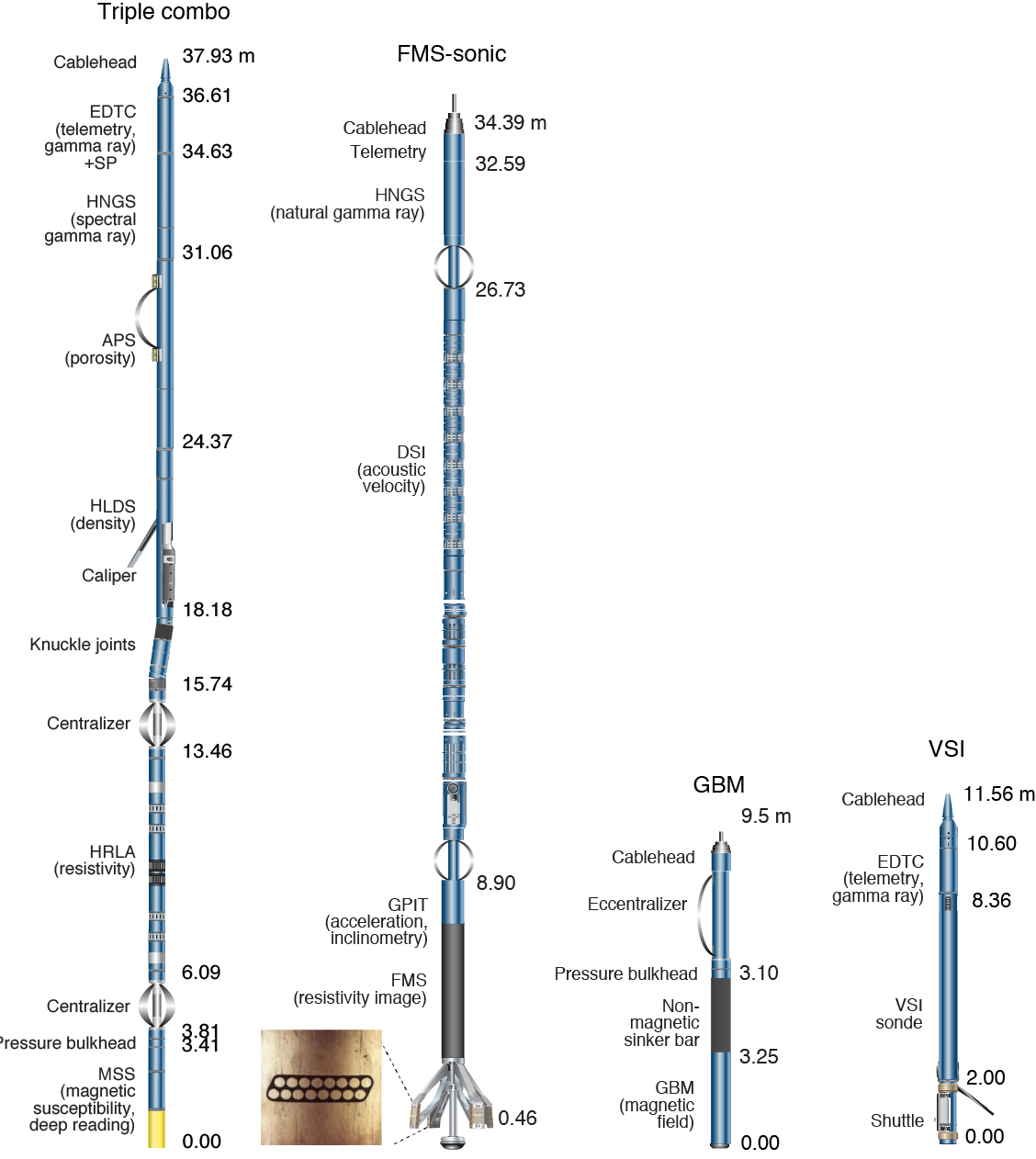
Table T9. Downhole measurements made by wireline tool strings, Expedition 351. Download table in .csv format.
In preparation for logging, the boreholes were flushed of debris by circulating seawater and filled with heavy mud or seawater (see Physical properties and downhole measurements in the Site U1438 chapter [Arculus et al., 2015]). The bottom-hole assembly (BHA) was set at some depth inside the hole (as deep as ~100 m from the surface) to prevent the collapse of unstable shallow sediment. For the cased hole (U1438E), the bottom of the drill string was set high enough above the bottom of the casing for the longest tool string to fit inside the casing. Data were recorded in the open hole; however, gamma ray logs can provide qualitative measurements inside the pipe, such as the identification of the seafloor. Each deployment of a tool string was a logging run and started with the assembly of the tools and the necessary calibrations. The tool string was then lowered to the bottom of the hole while recording a partial set of data and pulled back up at a constant speed (typically 500–550 m/h for the Schlumberger tools) to record the main data. The GBM was retrieved at a speed of 360 m/h. During each run, the tool strings were lowered down and pulled up the hole several times to assess reproducibility and/or to improve the quality of the data. Each lowering or hauling-up of the tool string while collecting data constitutes a pass. During each pass, the incoming data were recorded and monitored in real time. A logging run was complete once the tool string was brought to the rig floor and disassembled.
Logged sediment properties and tool measurement principles
Logged sediment properties and the methods used to measure them are described below. The main logs recorded during Expedition 351 are listed in Table T9. More detailed information on individual tools and their geological applications may be found in Serra (1984, 1986, 1989), Schlumberger (1989, 1994), Rider (1996), Goldberg (1997), Lovell et al. (1998), and Ellis and Singer (2007). A complete online list of acronyms and details for the Schlumberger tools can be found at iodp.tamu.edu/tools/logging/index.html.
Natural radioactivity
The Hostile Environment Natural Gamma Ray Sonde (HNGS), a spectral gamma ray tool, was used on both the triple combo and the FMS-sonic tool strings to measure natural radioactivity of the various lithologies encountered downhole. The HNGS uses two bismuth germinate scintillation detectors and five-window spectroscopy to determine the concentration of potassium (K in wt%), thorium (Th in parts per million [ppm]), and uranium (U in ppm) from the characteristic gamma ray energies of isotopes in the 40K, 232Th, and 238U radioactive decay series. The radioactive isotopes of these three elements dominate the natural radiation spectrum. The HNGS filters out gamma ray energies below 500 keV, eliminating sensitivity to bentonite or KCl in the drilling mud, improving measurement accuracy. The HNGS also provides a measure of the total gamma ray emission (HSGR) and uranium-free or computed gamma ray emission (HCGR) measured in American Petroleum Institute units (gAPI). The HNGS response is influenced by the borehole diameter; therefore, HNGS data are corrected for borehole diameter variations during acquisition.
An additional natural gamma radiation sensor is present in the EDTC, which was used primarily to communicate data to the surface. It includes a sodium iodide scintillation detector that also measures the total natural gamma ray emission of the formation. It is not a spectral tool but it provides high-resolution total gamma ray for each pass.
The inclusion of a HNGS sonde in a tool string allows for precise depth-match processing between logging tool strings and passes and for core-log integration.
Self-potential
The self-potential (or spontaneous potential) tool was used to measure the natural electrical potential that occurs in a borehole between the drilling mud and the formation water placed in contact with a bed. The tool records the voltage difference between an electrode moving inside the borehole and a reference electrode positioned at the surface; it is measured in millivolts (mV). This measurement is not affected by the porosity of the formation or by the borehole diameter. Self-potential data can help (1) distinguish permeable (sandstone) from impermeable rocks (clay and shale), (2) determine bed boundaries, (3) identify some minerals (pyrite and oxidized beds, for example), and (4) estimate formation water resistivity and permeability.
Porosity
The Accelerator Porosity Sonde (APS) was used to measure formation porosity. The APS incorporates a minitron neutron generator that produces fast neutrons and five detectors positioned at different spacing from the minitron. The detectors count neutrons that arrive after being scattered and slowed by atomic nuclei in the formation. Because hydrogen nuclei have almost the same mass as neutrons, the highest energy loss occurs when both collide. Therefore, the tool provides a measure of the hydrogen content of the formation, which is most commonly found in water in the pore fluid and can be directly related to porosity. However, in igneous and altered rocks, hydrogen may be present, which can result in overestimation of porosity in these rocks.
Upon reaching thermal energies (0.025 eV), neutrons are captured by the nuclei of Cl, Si, B, and other elements, resulting in gamma ray emission. This neutron capture cross section (Σf) is also measured by the tool and can be used to identify such elements (Broglia and Ellis, 1990; Brewer et al., 1996).
Density
The Hostile Environment Litho-Density Sonde (HLDS) measures formation density. This tool contains a radioactive 137Cs gamma ray source and far and near gamma ray detectors mounted on a shielded skid; the latter is pressed against the borehole wall by a hydraulically activated centralizing arm that measures the hole diameter. Gamma rays emitted by the source undergo Compton scattering, in which gamma rays are scattered by electrons in the formation. The number of scattered gamma rays that reach the detectors is proportional to the density of electrons in the formation, which in turn is related to the bulk density. Porosity may also be derived from this bulk density if the matrix density is known.
The HLDS also measures a photoelectric factor caused by photoelectric absorption of low-energy gamma rays. This absorption occurs when gamma ray energies are reduced below 150 keV after being repeatedly scattered by electrons in the formation. Because the photoelectric factor depends on the atomic number of the elements in the formation, it also varies according to the chemical composition of the minerals present and can be used to identify some minerals (Bartetzko et al., 2003; Expedition 304/305 Scientists, 2006). This measurement might be affected or unreliable when heavy mud with barite is used to prepare the hole and should thus be used with caution.
Good contact between the tool and the borehole is essential for good HLDS logs; poor contact results in underestimation of density values.
Resistivity
The High-Resolution Laterolog Array (HRLA) provided six resistivity measurements with different depths of investigation (including the borehole fluid or mud resistivity and five measurements of formation resistivity with increasing depth of penetration into the formation). The HRLA sends a focused current into the borehole wall and measures the intensity necessary to maintain a constant drop in voltage across a fixed interval, providing a direct measurement of resistivity. The array has one central source electrode and six electrodes above and below it. By rapidly changing the role of these electrodes, a simultaneous resistivity measurement is obtained at six penetration depths. The HRLA needs to be centralized in the borehole for optimal results, so knuckle joints were used.
Most minerals present in sediment and crystalline rocks are electrical insulators, whereas ionic solutions like pore water are conductors. In most rocks, electrical conduction occurs primarily by ion transport through pore fluids and thus is strongly dependent on porosity. Therefore, electrical resistivity can be used to estimate porosity for a given salinity and resistivity of the pore water.
Magnetic susceptibility
The Magnetic Susceptibility Sonde (MSS) is a nonstandard tool designed by Lamont Doherty Earth Observatory (LDEO) that measures the ease with which formations are magnetized when subjected to the Earth’s magnetic field. The ease of magnetization is related to the concentration and composition of magnetizable material within the formation. These measurements provide one of the best methods for investigating stratigraphic changes in mineralogy and lithology because the measurement is quick, repeatable, and nondestructive and because different lithologies often have strongly contrasting susceptibilities. A dual-coil sensor was used during Expedition 351, providing a deep-reading measurement (~20 cm of horizontal investigation) with a vertical resolution of ~40 cm. The MSS was run as an addition to the triple combo tool string, using a specially developed data translation cartridge.
Magnetic susceptibility data are plotted in uncalibrated units and are affected by borehole size. The electronics of the sensor are also affected by temperature: a higher temperature leads to higher susceptibility values. The acquired data tend to be affected by a nonlinear temperature-related drift superposed on signal variability. Preliminary processing was performed onboard to remove the temperature drift from the data set. The residual components from the deep-reading sensor should be an indication of the magnetic signal variability in the formation. When the magnetic susceptibility signal in the sediments is very low, the detection limits of the tool are sensitive enough to record values. For quality control and environmental correction, the MSS also measures internal tool temperature, z-axis acceleration, and low-resolution borehole conductivity.
Acoustic velocity
The Dipole Shear Sonic Imager (DSI) was used to measure transit times between sonic transmitters and an array of eight receivers. It combines replicate measurements, providing a direct measurement of sound velocity through formations that is relatively free from the effects of formation damage and an enlarged borehole (Schlumberger, 1989). The omnidirectional monopole transmitter emits high-frequency pulses (5–15 kHz) to extract the compressional velocity (VP). The DSI also has two cross-dipole transmitters that allow measurement of shear velocity (VS) in “slow” formations where VS is slower than the velocity in the borehole fluid. Such formations are generally encountered in deep ocean drilling.
Formation MicroScanner (electrical images)
The FMS provided high-resolution electrical resistivity images of the borehole walls. The FMS has four orthogonal arms and pads, each containing 16 button electrodes that are pressed against the walls of the borehole. The electrodes are arranged in two diagonally offset rows of eight electrodes each. A focused current is emitted from the button electrodes into the formation with a return electrode near the top of the tool. Resistivity of the formation at the button electrodes is derived from the intensity of current passing through the button electrodes. Processing transforms these measurements into oriented high-resolution images that reveal the structures of the borehole wall. Features such as flows, clast, breccias, fractures, folding, or alteration can be resolved. The images are oriented to magnetic north, so the dip and direction (azimuth) of planar features in the formation can be measured.
Approximately 30% of the borehole (25 cm diameter) is covered during a single pass. The standard procedure is to make two full passes uphole to maximize the chance of getting greater borehole coverage. The maximum extension of the arms is 40.6 cm. In holes with a diameter greater than this extension maximum, the pad contact at the end of the caliper arms is inconsistent and the FMS images may appear out of focus and too conductive. Irregular borehole walls will also affect the images if contact with the wall is poor.
Magnetic parameters (borehole inclination and magnetic field measurement)
The General Purpose Inclinometery Tool (GPIT), included in the FMS-sonic tool string, calculates acceleration and magnetic field during logging. The primary purpose of the tool is to determine the acceleration and orientation of the FMS-sonic tool string during logging.
Tool orientation is defined by three parameters: tool deviation, tool direction (azimuth), and relative bearing. The GPIT utilizes a three-axis inclinometer and a three-axis fluxgate magnetometer to record the orientation of the FMS as the magnetometer records the magnetic field components (Fx, Fy, and Fz). Thus, FMS images can be corrected for irregular tool motion, and the dip and azimuth of features can be determined.
The GPIT is run with other tools that can carry remanent and/or induced magnetization on the tool string; therefore, its magnetic measurements can be affected. However, on the FMS-sonic tool string, the GPIT has greater nonmagnetic insulation from the other tools, and the effects on its magnetic measurements are greatly reduced.
The Göttigen Borehole Magnetometer
The GBM was designed and developed in 1989 by the Geophysical Institute of the University of Göttigen (Germany). It was originally built for vertical magnetic gradient sounding and comprises two inclinometers and a three-component fluxgate magnetometer (Steveling et al., 1991). The tool is also equipped with three fiber-optic gyros that measure the rotation of the GBM around the vertical axis of the tool with a small drift (1.5°/h) and high resolution (9 × 10⁻⁵ degrees) (Virgil et al., 2010) that allows for reorientation of the magnetic field vector to the geographic reference frame. The GBM housing is made of low-magnetic Inconel and connects directly to the Schlumberger cable head. The tool was deployed as a separate logging run.
The fiber-optic gyros on the GBM allow independent determination of both inclination and declination of the magnetic field in the borehole. The fluxgate data from the GBM can be checked against GPIT magnetic data (even if the resolution of the GPIT is lower) to assess the quality of the data set.
GBM angular rate sensors
Miniature fiber-optic rate sensors (µFORS) manufactured by Northrup Grumman LITEF were used to provide angular rate output during the entire run (downlog and uplog) of the GBM. The sensors detect and measure angular rates through the frequency difference between two contra-rotating light beams. A beam is polarized, split, and phase modulated. When one of the gyros is at rest, the two beams have identical frequencies. When the gyro is subjected to an angular turning rate around an axis perpendicular to the plane of the two beams, one beam has a greater optical path length. Therefore, the two resonant frequencies change and the frequency differential is optically measured, resulting in a digital output.
The angular rate measured by the sensor is influenced by the Earth’s rotation, which depends on latitude (ø) and varies from 15.04°/h at the poles to 0°/h at the Equator. From Equator to pole, Earth’s measured rotation increases by sin(ø). To obtain the rotation rate about an inertial system, the effect of Earth’s rotation must be eliminated through the orientation of the tool relative to the Earth’s reference frame at the beginning of a measurement (which can be measured well). The x-gyro of the GBM is aligned with the axis of the ship, using a scope mounted to the tool and a sighting plate positioned in the center of the helideck. Knowing that the tool is now similarly oriented as the ship, information from the ship’s gyro and two GPS antennas are then used to determine the heading of the ship (at the time of sighting) and thus the orientation of the tool at the start of logging. This procedure is repeated at the end of each logging run to compare the true heading of the gyro with the heading calculated by the data processing algorithm. If the corrected rotation rate around each axis is known, the orientation of the tool can be derived as a function of depth from the rotation history, and thus the three components of the magnetic field can be calculated for every data point collected by the GBM.
The maximum operating temperature for the fiber-optic gyros is 70°C. Data are acquired from the tool using GBMlog software (written by Erich Steveling, University of Göttingen) and processed with software developed by Sebastian Ehmann (University of Braunschweig).
Vertical seismic profile
The VSI is used to provide a direct measurement of the time for seismic waves to travel from the surface to a given depth. A link is thus possible between seismic profiles (in two-way traveltimes) and observations into the borehole (in depth).
The tool comprises a three-axis geophone accelerometer and a caliper arm anchoring the geophone against the hole wall. During Expedition 351, measurements were obtained every ~50 m, and about five recordings were made at each station. The waveforms were then stacked, and the one-way traveltime determined from the first arrival at each station.
The seismic source is a Sercel G. Gun parallel cluster composed of two 250 in3 air guns separated by 1 m. The source was positioned ~7 m below sea surface by one of the ship’s cranes off the port side of the ship for a total offset from the top of the wellhead of ~30 m.
In accordance with requirements of the National Environmental Policy Act and the Endangered Species Act, all seismic activities were conducted during daylight hours and Protected Species Observers kept watch for protected species for the duration of the zero-offset VSP. Any sighting of protected species within the exclusion zone of 940 m for deep water (>1000 m) would require interruption of the survey for 1 h after the last sighting or until the protected species was seen to leave the area. The same ramp-up procedure was followed upon resumption of the VSP after any interruption (sighting of protected species or not firing the gun for more than 30 min).
Logging data quality
The condition of the borehole wall is the main factor contributing to the quality of log data. If the borehole diameter changes over short intervals (because of washouts or ledges made of layers of harder material), the logs from tools that require good contact with the borehole may be degraded. Measurements made at depth, such as gamma ray, resistivity, and sonic velocity, which do not require contact with the borehole wall, are generally less sensitive to borehole conditions. Narrow sections will also cause irregular log results. The quality of the borehole is improved by (1) minimizing circulation of drilling fluid while drilling, (2) flushing the borehole to remove debris, and (3) logging as soon as possible after drilling and hole conditioning operations are completed.
The accuracy of the logging depth depends on series of factors. The depth of the logging measurements is determined from the length of the cable deployed from the ship’s winch. Uncertainties in logging depth occur because of ship heave, cable stretch, cable slip, or even tidal changes. Similarly, uncertainties in the depth of the core samples occur because of incomplete core recovery or incomplete heave compensation. All these factors generate some discrepancy between core sample depths, logs, and individual logging passes. To minimize the effect of ship heave, a hydraulic wireline heave compensator was used to adjust the wireline length for rig motion during wireline logging operations.
Wireline heave compensator
The wireline heave compensator is dedicated to compensate for the vertical motion of the ship and maintain steady motion of the logging tool to ensure high-quality logging acquisition (Liu et al., 2013; Iturrino et al., 2013). It uses vertical acceleration measurements made by a motion reference unit (MRU) located under the rig floor near the ship’s center of gravity to calculate the vertical motion of the ship. It then adjusts the length of the wireline by varying the distance between two sets of pulleys through which the wireline passes. An LDEO-developed software package allows these data to be analyzed and compared in real time, displaying the actual motion of the logging tool string and enabling monitoring of the efficiency of the compensator.
Logging data flow and log depth scales
Data for each logging run were monitored in real time and recorded using the Schlumberger MAXIS 500 system. Data were then copied to the shipboard workstations for processing. The main pass of the triple combo was commonly used as a reference to which other passes were interactively depth matched. After depth matching, all logging depths were shifted to the seafloor (WMSF) after identifying the seafloor from a step in the gamma ray profile. The meters below seafloor (mbsf) reference depth was then used (see Operations in the Site U1438 chapter [Arculus et al., 2015]). The electrical images were processed by using the data from the GPIT to correct for irregular tool motion, and the image gains were equalized to enhance the representation of the borehole wall. All processed data were made available to the science party within one day of their acquisition as ASCII files for most logs and as GIF files for the images.
Data were also transferred onshore to LDEO for a standardized implementation of the same data processing, formatting for the online logging database, and archiving.
In situ temperature measurements
In situ temperature measurements were made in Hole U1438B using the advanced piston corer temperature tool (APCT-3). The APCT-3 fits directly into the coring shoe of the APC system and consists of a battery pack, a data logger, and a platinum resistance-temperature device calibrated over a temperature range from 0° to 30°C. Before entering the borehole, the tool was allowed to thermally equilibrate with bottom water at the seafloor for five minutes. However, the lowest temperature recorded during the run down was expected to represent the average temperature at the seafloor, because it was more repeatable, and the bottom water was expected to have the lowest temperature in the profile. After the APC system penetrated the sediment, the APCT-3 recorded the temperature of the cutting shoe every second for 10 min. Shooting the APC system into the formation generates an instantaneous temperature rise from frictional heating. This heat gradually dissipates into the surrounding sediments as the temperature immediately adjacent to the APCT-3 equilibrates toward the sediment temperature.
The equilibrium temperature of the sediments was estimated by applying a heat-conduction model to the temperature decay record (Horai and Von Herzen, 1985). The synthetic thermal decay curve for the APCT-3 is a function of the geometry and thermal properties of the probe and the sediments (Bullard, 1954; Horai and von Herzen, 1985). The equilibrium temperature is estimated by applying an appropriate curve fitting procedure (Pribnow et al., 2000). However, when the APC system does not achieve a full stroke, or when the ship’s heave prevents the APC system from full penetration, the temperature equilibration curve is disturbed and temperature determination is more difficult. The nominal accuracy of the APCT-3 temperature measurement is ±0.1°C.
Seven temperature readings were made, including the seafloor and down to 83 mbsf. APCT-3 temperature data were combined with measurements of thermal conductivity (see Physical properties) obtained from core samples to obtain heat flow values using the method designed by Bullard (1954).
Core-log-seismic integration
During Expedition 351, shipboard physical properties and logging data were used to define tie points between the cores, logs, and seismic data sets. These data sets were used to (1) evaluate how representative the recovered cores are relative to the logs, (2) determine the nature and extent of sediment not recovered during coring operations, particularly when the RCB system was used, and (3) examine if observed facies can be linked to borehole data.
In order to integrate the cores and the logs with seismic data, core and log data were converted to two-way traveltime. Whenever possible, velocity information from the logging tools was used. When wireline logging velocities were unavailable, a combination of the velocities measured on the cores was used.
Velocity and density logs, together with the equivalent measurements made on cores in the physical properties laboratory, can be used to create synthetic seismograms. The depth-traveltime relation must be adjusted until the features in the synthetic seismogram match the features in the seismic section. In this way, lithostratigraphic units in the core were correlated with reflectors and sequences in the seismic section.
Processing of GBM data
The GBM raw data stream consists of a 24-bit string containing three components: the magnetic flux density, the rotational rate of the GBM around the z-axis, and the inclination of the tool along the x- and y-axis. The rotational rate around the x- and y-axis was recorded in an alternating order. The temperature was updated every minute (Leven, 1998).
The data stream was first deconvolved into separate data streams and converted to SI units. A Wiener filter was then applied to the magnetic flux density data to reduce the influence of the digitizing low-pass filter (Virgil, 2012).
The orientation of the GBM was found by using both the inclinometer data and the integrated fiber-optic gyros data. However, because the fiber-optic gyros record the time derivative of the rotation, its integration, and thus the absolute orientation, is distorted by the temperature-dependent gyro noise. This results in a random walk and an additional drift in angular means. To reduce the drift, a temperature-dependent correction was applied. Further improvements were made by (1) applying an additional drift correction found by comparing inclinometer and integrated gyro data and (2) using a Kalman filtering approach.
The corrected orientation was finally used to transfer the vector of the magnetic flux density into the geographic coordinate system.
Because the functional relationship between the magnetic flux density and the magnetization has infinite solutions, the calculation of the magnetization leads to a nonunique inverse problem. In order to reduce the ambiguity in the estimation of the magnetization, the geometric distribution of the magnetization was assumed (Bosum et al., 1988; Li and Oldenburg, 1996).
References
Arculus, R.J., Ishizuka, O., Bogus, K., Drab, L., Aljahdali, M.H., Bandini-Maeder, A.N., Barth, A.P., Brandl, P.A., do Monte Guerra, R., Gurnis, M.C., Hamada, M., Hickey-Vargas, R.L., Jiang, F., Kanayama, K., Kender, S., Kusano, Y., Li, H., Loudin, L.C., Maffione, M., Marsaglia, K.M., McCarthy, A., Meffre, S., Morris, A., Neuhaus, M., Savov, I.P., Sena Da Silva, C.A., Tepley, F.J., III, van der Land, C., Yogodzinski, G.M., and Zhang, Z., 2015. Site U1438. In Arculus, R.J., Ishizuka, O., Bogus, K., and the Expedition 351 Scientists, Proceedings of the International Ocean Discovery Program, Expedition 351: Izu-Bonin-Mariana Arc Origins: College Station, TX (International Ocean Discovery Program). http://dx.doi.org/10.14379/iodp.proc.351.103.2015
Bartetzko, A., Paulick, H., Iturrino, G., and Arnold, J., 2003. Facies reconstruction of a hydrothermally altered dacite extrusive sequence: evidence from geophysical downhole logging data (ODP Leg 193). Geochemistry, Geophysics, Geosystems, 4(10):1087. http://dx.doi.org/10.1029/2003GC000575
Bartington Instruments, Ltd., 2011. Operation Manual for MS2 Magnetic Susceptibility System: Oxford, UK (Bartington Instruments, Ltd.). http://www.bartington.com/Literaturepdf/Operation%20Manuals/om0408%20MS2.pdf
Blum, P., 1997. Physical properties handbook: a guide to the shipboard measurement of physical properties of deep-sea cores. Ocean Drilling Program Technical Note, 26. http://dx.doi.org/10.2973/odp.tn.26.1997
Bolli, H.M., and Saunders, J.B., 1985. Oligocene to Holocene low latitude planktic foraminifera. In Bolli, H.M., Saunders, J.B., and Perch-Nielsen, K. (Eds.), Plankton Stratigraphy (Vol. 1): Planktic Foraminifera, Calcareous Nannofossils and Calpionellids: Cambridge, UK (Cambridge University Press), 155–262.
Bosum, W., Eberle, D., and Rehli, H.-J., 1988. A gyro-oriented 3-component borehole magnetometer for mineral prospecting, with examples of its application. Geophysical Prospecting, 36(8):933–961. http://dx.doi.org/10.1111/j.1365-2478.1988.tb02201.x
Brewer, T.S., Harvey, P.K., Locke, J., and Lovell, M.A., 1996. Neutron absorption cross section (Σ) of basaltic basement samples from Hole 896A, Costa Rica rift. In Alt, J.C., Kinoshita, H., Stokking, L.B., and Michael, P.J. (Eds.), Proceedings of the Ocean Drilling Program, Scientific Results, 148: College Station, TX (Ocean Drilling Program), 389–394. http://dx.doi.org/10.2973/odp.proc.sr.148.154.1996
Broglia, C., and Ellis, D., 1990. Effect of alteration, formation absorption, and standoff on the response of the thermal neutron porosity log in gabbros and basalts: examples from Deep Sea Drilling Project-Ocean Drilling Program sites. Journal of Geophysical Research: Solid Earth, 95(B6):9171–9188. http://dx.doi.org/10.1029/JB095iB06p09171
Bullard, E.C., 1954. The flow of heat through the floor of the Atlantic Ocean. Proceedings of the Royal Society of London, Series A: Mathematical, Physical and Engineering Sciences, 222(1150):408–429. http://dx.doi.org/10.1098/rspa.1954.0085
Cande, S.C., and Kent, D.V., 1995. Revised calibration of the geomagnetic polarity timescale for the Late Cretaceous and Cenozoic. Journal of Geophysical Research: Solid Earth, 100(B4):6093–6095. http://dx.doi.org/10.1029/94JB03098
Clark, I.D., and Fritz, P., 1997. Environmental Isotopes in Hydrogeology: Boca Raton, FL (CRC Press/Lewis Publishers)
Droser, M.L., and Bottjer, D.J., 1986. A semiquantitative field classification of ichnofabric. Journal of Sedimentary Research, 56(4):558–559. http://dx.doi.org/10.1306/212F89C2-2B24-11D7-8648000102C1865D
Dunlop, D.J., 2003. Stepwise and continuous low-temperature demagnetization. Geophysical Research Letters, 30(11):1582. http://dx.doi.org/10.1029/2003GL017268
Ellis, D.V., and Singer, J.M., 2007. Well Logging for Earth Scientists (2nd ed.): New York (Elsevier).
Expedition 304/305 Scientists, 2006. Methods. In Blackman, D.K., Ildefonse, B., John, B.E., Ohara, Y., Miller, D.J., MacLeod, C.J., and the Expedition 304/305 Scientists, Proceedings of the Integrated Ocean Drilling Program, 304/305: College Station, TX (Integrated Ocean Drilling Program Management International, Inc.). http://dx.doi.org/10.2204/iodp.proc.304305.102.2006
Expedition 317 Scientists, 2011. Methods. In Fulthorpe, C.S., Hoyanagi, K., Blum, P., and the Expedition 317 Scientists, Proceedings of the Integrated Ocean Drilling Program, 317: Tokyo (Integrated Ocean Drilling Program Management International, Inc.). http://dx.doi.org/10.2204/iodp.proc.317.102.2011
Expedition 330 Scientists, 2012. Methods. In Koppers, A.A.P., Yamazaki, T., Geldmacher, J., and the Expedition 330 Scientists, Proceedings of the Integrated Ocean Drilling Program, 330: Tokyo (Integrated Ocean Drilling Program Management International, Inc.). http://dx.doi.org/10.2204/iodp.proc.330.102.2012
Expedition 335 Scientists, 2012. Methods. In Teagle, D.A.H., Ildefonse, B., Blum, P., and the Expedition 335 Scientists, Proceedings of the Integrated Ocean Drilling Program, 335: Tokyo (Integrated Ocean Drilling Program Management International, Inc.). http://dx.doi.org/10.2204/iodp.proc.335.102.2012
Expedition 336 Scientists, 2012. Methods. In Edwards, K.J., Bach, W., Klaus, A., and the Expedition 336 Scientists, Proceedings of the Integrated Ocean Drilling Program, 336: Tokyo (Integrated Ocean Drilling Program Management International, Inc.). http://dx.doi.org/10.2204/iodp.proc.336.102.2012
Expedition 340 Scientists, 2013. Methods. In Le Friant, A., Ishizuka, O., Stroncik, N.A., and the Expedition 340 Scientists, Proceedings of the Integrated Ocean Drilling Program, 340: Tokyo (Integrated Ocean Drilling Program Management International, Inc.). http://dx.doi.org/10.2204/iodp.proc.340.102.2013
Expedition 350 Scientists, 2014. Izu-Bonin-Mariana rear arc: the missing half of the subduction factory. International Ocean Discovery Program Preliminary Report, 350. http://dx.doi.org/10.14379/iodp.pr.350.2014
Fisher, R.V., and Schmincke, H.-U., 1984. Pyroclastic Rocks: Berlin (Springer-Verlag). http://dx.doi.org/10.1007/978-3-642-74864-6
Gee, J.S., Tauxe, L., and Constable, C., 2008. AMSSpin: a LabVIEW program for measuring the anisotropy of magnetic susceptibility with the Kappabridge KLY-4S. Geochemistry, Geophysics, Geosystems, 9(8):Q08Y02. http://dx.doi.org/10.1029/2008GC001976
Gieskes, J.M., Gamo, T., and Brumsack, H., 1991. Chemical methods for interstitial water analysis aboard JOIDES Resolution. Ocean Drilling Program Technical Note, 15. http://dx.doi.org/10.2973/odp.tn.15.1991
Goldberg, D., 1997. The role of downhole measurements in marine geology and geophysics. Reviews of Geophysics, 35(3):315–342. http://dx.doi.org/10.1029/97RG00221
Govindaraju, K., 1994. 1994 compilation of working values and sample description for 383 geostandards. Geostandards Newsletter, 18(1). http://dx.doi.org/10.1111/j.1751-908X.1994.tb00502.x
Gradstein, F.M., Ogg, J.G., Schmitz, M.D., and Ogg, G.M. (Eds.)., 2012. The Geological Time Scale 2012: Amsterdam (Elsevier).
Harris, R.N., Sakaguchi, A., Petronotis, K., Baxter, A.T., Berg, R., Burkett, A., Charpentier, D., Choi, J., Diz Ferreiro, P., Hamahashi, M., Hashimoto, Y., Heydolph, K., Jovane, L., Kastner, M., Kurz, W., Kutterolf, S.O., Li, Y., Malinverno, A., Martin, K.M., Millan, C., Nascimento, D.B., Saito, S., Sandoval Gutierrez, M.I., Screaton, E.J., Smith-Duque, C.E., Solomon, E.A., Straub, S.M., Tanikawa, W., Torres, M.E., Uchimura, H., Vannucchi, P., Yamamoto, Y., Yan, Q., and Zhao, X., 2013. Methods. In Harris, R.N., Sakaguchi, A., Petronotis, K., and the Expedition 344 Scientists, Proceedings of the Integrated Ocean Drilling Program, 344: College Station, TX (Integrated Ocean Drilling Program). http://dx.doi.org/10.2204/iodp.proc.344.102.2013
Hermann, Y., 1992. Eocene through Quaternary planktonic foraminifers from the northwest Pacific, Leg 126. In Taylor, B., Fujioka, K., et al., Proceedings of the Ocean Drilling Program, Scientific Results, 126: College Station, TX (Ocean Drilling Program), 271–284. http://dx.doi.org/10.2973/odp.proc.sr.126.133.1992
Hext, G.R., 1963. The estimation of second-order tensors, with related tests and designs. Biometrika, 50(3–4):353–373. http://dx.doi.org/10.1093/biomet/50.3-4.353
Holbourn, A., Henderson, A.S., and MacLeod, N., 2013. Atlas of Benthic Foraminifera: Chichester (John Wiley & Sons, Ltd.). http://dx.doi.org/10.1002/9781118452493
Hollis, C.J., 2006. Radiolarian faunal turnover through the Paleocene–Eocene transition, Mead Stream, New Zealand. Eclogae Geologicae Helvetiae, 99(1):S79–S99. http://dx.doi.org/10.1007/s00015-006-0604-3
Horai, K., and Von Herzen, R.P., 1985. Measurement of heat flow on Leg 86 of the Deep Sea Drilling Project. In Heath, G.R., Burckle, L.H., et al., Initial Reports of the Deep Sea Drilling Project, 86: Washington, DC (U.S. Government Printing Office), 759–777. http://dx.doi.org/10.2973/dsdp.proc.86.135.1985
Hyndman, R.D., Erickson, A.J., and Von Herzen, R.P., 1974. Geothermal measurements on DSDP Leg 26. In Davies, T.A., Luyendyk, B.P., et al., Initial Reports of the Deep Sea Drilling Project, 26: Washington, DC (U.S. Government Printing Office), 451–463. http://dx.doi.org/10.2973/dsdp.proc.26.113.1974
Ingram, R.L., 1954. Terminology for the thickness of stratification and parting units in sedimentary rocks. Geological Society of America Bulletin, 65(9):937–938. http://dx.doi.org/10.1130/0016-7606(1954)65[937:TFTTOS]2.0.CO;2
Iturrino, G., Liu, T., Goldberg, D., Anderson, L., Evans, H., Fehr, A., Guerin, G., Inwood, J., Lofi, J., Malinverno, A., Morgan, S., Mrozewski, S., Slagle, A., and Williams, T., 2013. Performance of the wireline heave compensation system onboard D/V JOIDES Resolution. Scientific Drilling, 15:46–50. http://dx.doi.org/10.2204/iodp.sd.15.08.2013
Jackett, S.-J., Baumgartner, P.O., and Bandini, A.N., 2008. A new low-latitude late Paleocene–early Eocene radiolarian biozonation based on unitary associations: applications for accreted terranes. Stratigraphy, 54(1):39–62.
Kaiho, K., 1992. Eocene to Quaternary benthic foraminifers and paleobathymetry of the Izu-Bonin arc, Legs 125 and 126. In Taylor, B., Fujioka, K., et al., Proceedings of the Ocean Drilling Program, Scientific Results, 126: College Station, TX (Ocean Drilling Program), 285–310. http://dx.doi.org/10.2973/odp.proc.sr.126.137.1992
Kennedy, A.E., and Coe, A.L., 2014. Development of the freeze–thaw processing technique for disaggregation of indurated mudrocks and enhanced recovery of calcareous microfossils. Journal of Micropalaeontology, 33(2):193–203. http://dx.doi.org/10.1144/jmpaleo2013-020
Kennett, J.P., and Srinivasan, M.S., 1983. Neogene Planktonic Foraminifera: A Phylogenetic Atlas: Stroudsburg, PA (Hutchinson Ross).
Kirschvink, J.L., 1980. The least-squares line and plane and the analysis of palaeomagnetic data. Geophysical Journal of the Royal Astronomical Society, 62(3):699–718. http://dx.doi.org/10.1111/j.1365-246X.1980.tb02601.x
Kvenvolden, K.A., and McDonald, T.J., 1986. Organic geochemistry on the JOIDES Resolution—an assay. Ocean Drilling Program Technical Note, 6: College Station, TX (Ocean Drilling Program). http://dx.doi.org/10.2973/odp.tn.6.1986
Le Maitre, R.W., Steckeisen, A., Zanettin, B., Le Bas, M.J., Bonin, B., and Bateman, P. (Eds.), 2002. Igneous rocks: A Classification and Glossary of Terms (2nd ed.): Cambridge, UK (Cambridge University Press).
Leven, M.,1998. Entwicklung und Aufbau eines triaxialen Bohrlochmagnetometers für den Einsatz in tiefen Bohrungen zu vertikalen Gradientensondierung [Dissertation]. Georg-August-Universität Göttingen.
Li, Y., and Oldenburg, D.W, 1996. 3-D inversion of magnetic data. Geophysics, 61(2):394–408. http://dx.doi.org/10.1190/1.1443968
Liu, T., Iturrino, G., Goldberg, D., Meissner, E., Swain, K., Furman, C., Fitzgerald, P., Frisbee, N., Chlimoun, J., Van Hyfte, J., and Beyer, R., 2013. Performance evaluation of active wireline heave compensation systems in marine well logging environments. Geo-Marine Letters, 33(1):83–93. http://dx.doi.org/10.1007/s00367-012-0309-8
Lovell, M.A., Harvey, P.K., Brewer, T.S., Williams, C., Jackson, P.D., and Williamson, G., 1998. Application of FMS images in the Ocean Drilling Program: an overview. In Cramp, A., MacLeod, C.J., Lee, S.V., and Jones, E.J.W. (Eds.), Geological Evolution of Ocean Basins: Results from the Ocean Drilling Program. Geological Society Special Publication, 131(1):287–303. http://dx.doi.org/10.1144/GSL.SP.1998.131.01.18
Manheim, F.T., and Sayles, F.L., 1974. Composition and origin of interstitial waters of marine sediments, based on deep sea drill cores. In Goldberg, E.D. (Ed.), The Sea (Vol. 5): Marine Chemistry: The Sedimentary Cycle: New York (Wiley), 527–568.
Martini, E., 1971. Standard Tertiary and Quaternary calcareous nannoplankton zonation. In Farinacci, A. (Ed.), Proceedings of the Second Planktonic Conference, Roma 1970: Rome (Edizioni Tecnoscienza), 2:739–785.
Merrill, R.T., 1970. Low-temperature treatments of magnetite and magnetite-bearing rocks. Journal of Geophysical Research: Solid Earth, 75(17):3343–3349. http://dx.doi.org/10.1029/JB075i017p03343
Morris, A., Gee, J.S., Pressling, N., John, B.E., MacLeod, C.J., Grimes, C.B., and Searle, R.C., 2009. Footwall rotation in an oceanic core complex quantified using reoriented Integrated Ocean Drilling Program core samples. Earth and Planetary Science Letters, 287(1–2):217–228. http://dx.doi.org/10.1016/j.epsl.2009.08.007
Murray, R.W., Miller, D.J., and Kryc, K.A., 2000. Analysis of major and trace elements in rocks, sediments, and interstitial waters by inductively coupled plasma–atomic emission spectrometry (ICP-AES). Ocean Drilling Program Technical Note, 29. http://dx.doi.org/10.2973/odp.tn.29.2000
Nordstrom, D.K., and Wilde, F.D., 2005. Reduction oxidation potential (electrode method) (version 1.2). U.S. Geological Survey Techniques of Water-Resources Investigations, Book 9. http://water.usgs.gov/owq/FieldManual/Chapter6/6.5_contents.html
Okada, H., and Bukry, D., 1980. Supplementary modification and introduction of code numbers to the low-latitude coccolith biostratigraphic zonation (Bukry, 1973; 1975). Marine Micropaleontology, 5:321–325. http://dx.doi.org/10.1016/0377-8398(80)90016-X
Parker, R.L., and Gee, J.S., 2002. Calibration of the pass-through magnetometer—II. Application. Geophysical Journal International, 150:140–152. http://dx.doi.org/10.1046/j.1365-246X.2002.01692.x
Pearson, P.N., Olsson, R.K., Hemleben, C., Huber, B.T., and Berggren, W.A., 2006. Atlas of Eocene planktonic foraminifera. Special Publication— Cushman Foundation for Foraminiferal Research, 41.
Perch-Nielsen, K., 1985. Cenozoic calcareous nannofossils. In Bolli, H.M., Saunders, J.B., and Perch-Nielsen, K. (Eds.), Plankton Stratigraphy: Cambridge, UK (Cambridge University Press), 427–554.
Pimmel, A., and Claypool, G., 2001. Introduction to shipboard organic geochemistry on the JOIDES Resolution. Ocean Drilling Program Technical Note, 30. http://dx.doi.org/10.2973/odp.tn.30.2001
Pribnow, D., Kinoshita, M., and Stein, C., 2000. Thermal Data Collection and Heat Flow Recalculations for Ocean Drilling Program Legs 101–180: Hanover, Germany (Institute for Joint Geoscientific Research, Institut für Geowissenschaftliche Gemeinschaftsaufgaben [GGA]). http://www-odp.tamu.edu/publications/heatflow/ODPReprt.pdf
Révillon, S., Barr, S.R., Brewer, T.S., Harvey, P.K., and Tarney, J., 2002. An alternative approach using integrated gamma-ray and geochemical data to estimate the inputs to subduction zones from ODP Leg 185, Site 801. Geochemistry, Geophysics, Geosystems, 3(12):8902. http://dx.doi.org/10.1029/2002GC000344
Rider, M.H., 1996. The Geological Interpretation of Well Logs (2nd ed.): Caithness, Scotland (Whittles Publishing).
Salisbury, M.H., Shinohara, M., Suetsugu, D., Arisaka, M., Diekmann, B., Januszczak, N., and Savov, I.P., 2006. Leg 195 synthesis: Site 1201—a geological and geophysical section in the West Philippine Basin from the 660-km discontinuity to the mudline. In Shinohara, M., Salisbury, M.H., and Richter, C. (Eds.), Proceedings of the Ocean Drilling Program, Scientific Results, 195: College Station, TX (Ocean Drilling Program), 1–27. http://dx.doi.org/10.2973/odp.proc.sr.195.113.2006
Sanfilippo, A., and Nigrini, C., 1998. Code numbers for Cenozoic low latitude radiolarian biostratigraphic zones and GPTS conversion tables. Marine Micropaleontology, 33(1–2):109–117, 121–156. http://dx.doi.org/10.1016/S0377-8398(97)00030-3
Sanfilippo, A., Westberg-Smith, M.J., and Riedel, W.R., 1985. Cenozoic Radiolaria. In Bolli, H.M., Saunders, J.B., and Perch-Nielsen, K. (Eds.), Plankton Stratigraphy (Vol. 2): Radiolaria, Diatoms, Silicoflagellates, Dinoflagellates, and Ichthyoliths: Cambridge, UK (Cambridge University Press), 631–712.
Schlumberger, 1989. Log Interpretation Principles/Applications: Houston (Schlumberger Education Services), SMP–7017.
Schlumberger, 1994. IPL Integrated Porosity Lithology: Houston (Schlumberger Wireline Testing), SMP-9270.
Serra, O., 1984. Fundamentals of Well-Log Interpretation (Vol. 1): The Acquisition of Logging Data: Amsterdam (Elsevier).
Serra, O., 1986. Fundamentals of Well-Log Interpretation (Vol. 2): The Interpretation of Logging Data. Amsterdam (Elsevier).
Serra, O., 1989. Formation MicroScanner Image Interpretation: Houston (Schlumberger Education Services), SMP-7028.
Shipboard Scientific Party, 2003. Explanatory notes. In Wilson, D.S., Teagle, D.A.H., Acton, G.D. et al., Proceedings of the Ocean Drilling Program, Initial Reports, 206: College Station, TX (Ocean Drilling Program), 1–94. http://dx.doi.org/10.2973/odp.proc.ir.206.102.2003
Steveling, E., Spitzer, K., and Leven, M., 1991. Vertical gradient of horizontal geomagnetic variations—first results with the new Goettingen borehole magnetometer in the KTB-VB pilot hole. Scientific Drilling, 2:180–187.
Steveling, E., Stoll, J.B., and Leven, M., 2003. Quasi-continuous depth profiles of rock magnetization from magnetic logs in the HSDP-2 borehole, Island of Hawaii. Geochemistry, Geophysics, Geosystems, 4(4):8708–8734. http://dx.doi.org/10.1029/2002GC000330
Tamura, Y., Busby, C.J., Blum, P., Guèrin, G., Andrews, G.D.M., Barker, A.K., Berger, J.L.R., Bongiolo, E.M., Bordiga, M., DeBari, S.M., Gill, J.B., Hamelin, C., Jia, J., John, E.H., Jonas, A.-S., Jutzeler, M., Kars, M.A.C., Kita, Z.A., Konrad, K., Mahoney, S.H., Martini, M., Miyazaki, T., Musgrave, R.J., Nascimento, D.B., Nichols, A.R.L., Ribeiro, J.M., Sato, T., Schindlbeck, J.C., Schmitt, A.K., Straub, S.M., Vautravers, M.J., and Yang, Y., 2015. Expedition 350 methods. In Tamura, Y., Busby, C.J., Blum, P., and the Expedition 350 Scientists, Proceedings of the International Ocean Discovery Program, Expedition 350: Izu-Bonin-Mariana Rear Arc: College Station, TX (International Ocean Discovery Program). http://dx.doi.org/10.14379/iodp.proc.350.102.2015
Taylor, B., Fujioka, K., et al., 1990. Proceedings of the Ocean Drilling Program, Initial Reports, 126: College Station, TX (Ocean Drilling Program). http://dx.doi.org/10.2973/odp.proc.ir.126.1990
van Morkhoven, F.P.C.M., Berggren, W.A., Edwards, A.S.,and Oertli, H.J., 1986. Cenozoic cosmopolitan deep-water benthic foraminifera. Bulletin des Centres de Recherches Exploration-Production Elf-Aquitaine, 11.
Varol, O., 1998. Paleogene. In Bown, P.R. (Ed.), Calcareous Nannofossil Biostratigraphy: London (Kluwer Academic Publishing), 201–224.
Vasiliev, M.A., Blum, P., Chubarian, G., Olsen, R., Bennight, C., Cobine, T., Fackler, D., Hastedt, M., Houpt, D., Mateo, Z., and Vasilieva, Y.B., 2011. A new natural gamma radiation measurement system for marine sediment and rock analysis. Journal of Applied Geophysics, 75:455–463. http://dx.doi.org/10.1016/j.jappgeo.2011.08.008
Virgil, C., 2012. Vorbereitung und Durchführung von dreikomponentigen Magnetfeldmessungen mit dem Göttingen Bohrlochmagnetometer [Dissertation]. Technische Universität Braunschweig.
Virgil, C., Hördt, A., Klein, T., Kück, J., Leven, M., and Steveling, E., 2010. High-precision orientation of three-component magnetic downhole logs. Scientific Drilling, 9:37–40. http://dx.doi.org/10.2204/iodp.sd.9.07.2010
Wade, B.S., Pearson, P.N., Berggren, W.A., and Pälike, H., 2011. Review and revision of Cenozoic tropical planktonic foraminiferal biostratigraphy and calibration to the geomagnetic polarity and astronomical time scale. Earth-Science Reviews, 104(1–3):111–142. http://dx.doi.org/10.1016/j.earscirev.2010.09.003
Wentworth, C.K., 1922. A scale of grade and class terms for clastic sediments. Journal of Geology, 30(5):377–392. http://dx.doi.org/10.1086/622910
Wilcox, R.E., 1954. Petrology of Parícutin Volcano, Mexico. U.S. Geological Survey Bulletin, 965-C. http://pubs.usgs.gov/bul/0965c/report.pdf
Young, J.R., 1998. Neogene. In Bown, P.R. (Ed.), Calcareous Nannofossil Biostratigraphy: Dordrecht, The Netherlands (Kluwer Academic Publishing), 225–265.
Yu, Y., Dunlop, D.J., and Özdemir, Ö., 2003. On the resolution of multivectorial remanences. Earth and Planetary Science Letters, 208(1–2):13–26. http://dx.doi.org/10.1016/S0012-821X(02)01149-4
1 Arculus, R.J., Ishizuka, O., Bogus, K., Aljahdali, M.H., Bandini-Maeder, A.N., Barth, A.P., Brandl, P.A., do Monte Guerra, R., Drab, L., Gurnis, M.C., Hamada, M., Hickey-Vargas, R.L., Jiang, F., Kanayama, K., Kender, S., Kusano, Y., Li, H., Loudin, L.C., Maffione, M., Marsaglia, K.M., McCarthy, A., Meffre, S., Morris, A., Neuhaus, M., Savov, I.P., Sena Da Silva, C.A., Tepley, F.J., III, van der Land, C., Yogodzinski, G.M., and Zhang, Z., 2015. Expedition 351 methods. In Arculus, R.J., Ishizuka, O., Bogus, K., and the Expedition 351 Scientists, Proceedings of the International Ocean Discovery Program, Expedition 351: Izu-Bonin-Mariana Arc Origins: College Station, TX (International Ocean Discovery Program). http://dx.doi.org/10.14379/iodp.proc.351.102.2015