MacLeod, C.J., Dick, H.J.B., Blum, P., and the Expedition 360 Scientists
Proceedings of the International Ocean Discovery Program Volume 360
publications.iodp.org
doi:10.14379/iodp.proc.360.102.2017

Expedition 360 methods1
C.J. MacLeod, H.J.B. Dick, P. Blum, N. Abe, D.K. Blackman, J.A. Bowles, M.J. Cheadle, K. Cho, J. Ciążela, J.R. Deans, V.P. Edgcomb, C. Ferrando, L. France, B. Ghosh, B.M. Ildefonse, M.A. Kendrick, J.H. Koepke, J.A.M. Leong, C. Liu, Q. Ma, T. Morishita, A. Morris, J.H. Natland, T. Nozaka, O. Pluemper, A. Sanfilippo, J.B. Sylvan, M.A. Tivey, R. Tribuzio, and L.G.F. Viegas2
Keywords: International Ocean Discovery Program, IODP, JOIDES Resolution, Expedition 360, Site U1473, Hole 1105A, Moho, Mohorovičić discontinuity, Southwest Indian Ridge, SloMo, Atlantis Bank, mid-ocean ridge, slow spreading rate, Atlantis II Transform, Hole 735B, Site U1309
MS 360-102: Published 30 January 2017
Introduction
This chapter documents the procedures and methods employed in the various shipboard laboratories of the R/V JOIDES Resolution during International Ocean Discovery Program (IODP) Expedition 360. This information applies only to shipboard work described in the Expedition Reports section of the Expedition 360 Proceedings volume, which used the shipboard sample registry, imaging and analytical instruments, core description tools, and the Laboratory Information Management System (LIMS) database. Methods for shore-based analysis of Expedition 360 samples and data will be described in the individual peer-reviewed scientific contributions to be published in the Research Results section of the Expedition 360 Proceedings volume and in international scientific journals and books.
All shipboard scientists contributed in various ways to this volume with the following primary responsibilities:
- Expedition 360 summary chapter: Expedition 360 Scientists
- Methods and Site U1473 chapter:
- Background and objectives: Dick and MacLeod
- Introduction/operations: Blum, Dick, MacLeod, and Midgley
- Igneous petrology and geochemistry: France, Ghosh, Liu, Morishita, Natland, and Sanfilippo
- Alteration and metamorphism: Koepke, Leong, Ma, Nozaka, and Tribuzio
- Geochemistry: Cho, Ciążela, and Kendrick
- Structural geology: Cheadle, Deans, Ferrando, Pluemper, and Viegas
- Petrophysics (core and downhole): Abe, Blackman, Blum, and Ildefonse
- Paleomagnetism: Bowles, Morris, and Tivey
- Microbiology: Edgcomb and Sylvan
This introductory section of the methods chapter covers methods and procedures that apply to most or all of the shipboard laboratory groups. Subsequent sections describe detailed methods used by each laboratory group.
Sites and holes
GPS coordinates from precruise site surveys were used for the general position of the vessel at the Expedition 360 site. A SyQuest Bathy 2010 CHIRP subbottom profiler was used to monitor the seafloor depth during the approach to the site to reconfirm the depth profiles from precruise surveys. Once the vessel was positioned at the site, a camera survey was conducted to confirm suitable flat bedrock for spudding the hole (Figure F1). Two positioning beacons were deployed on the seafloor. While on site, ship location over the hole was maintained using the Neutronics 5002 dynamic positioning (DP) system on the JOIDES Resolution. DP control of the vessel used navigational input from the GPS and triangulation to the seafloor beacon, weighted by the estimated positional accuracy. The final hole position was the mean position calculated from the GPS data collected over a significant portion of the time the hole was occupied.
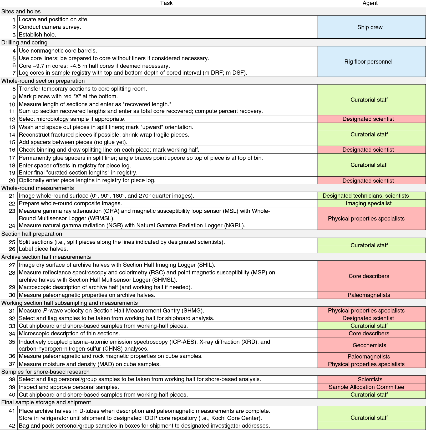
Figure F1. Overview of general shipboard workflow, Expedition 360.
The drilling site was numbered according to the series that began with the first site drilled by the Glomar Challenger in 1968. Starting with Integrated Ocean Drilling Program Expedition 301, the prefix “U” designates sites occupied by the JOIDES Resolution. For all IODP drill sites, a letter suffix distinguishes each hole drilled at the same site. The first hole drilled is assigned the site number modified by the suffix “A,” the second hole takes the site number and the suffix “B,” and so forth. During Expedition 360, Hole U1473A was the only hole drilled.
Drilling and coring operations
The coring strategy for Expedition 360 was to obtain as deep a penetration as possible at the primary site. Operations began with the deployment of a 14 m long, 13⅜ inch conductor casing drilled in using a mud motor and underreamer and included a free-fall funnel type reentry cone, as described in detail in Operations in the Site U1473 chapter (MacLeod et al., 2017b).
We used the rotary core barrel (RCB) system exclusively for all drilling and coring operations during Expedition 360. The RCB is the most conventional rotary coring system and suitable for lithified rock material. It cuts a core of up to 9.5 m length with nominal diameter of 5.87 cm. RCB coring can be conducted with or without core liners. Liners are sometimes omitted with the RCB system in an attempt to prevent core pieces from getting caught at the edge of the liner, which could lead to a jam and lack of recovery. During Expedition 360, liners were used for all cores except Core 360-U1473A-12R. Nonmagnetic core barrels were used throughout.
The bottom-hole assembly (BHA) is the lowermost part of the drill string, configured to provide appropriate strength and tension in the drill string. A typical RCB BHA consists of a drill bit, a bit sub, an outer core barrel, a top sub, a head sub, eight joints of 8¼ inch drill collars, a tapered drill collar, two joints of standard 5½ inch drill pipe, and a crossover sub to the regular 5 inch drill pipe.
During most IODP expeditions, cored intervals are 9.6–9.8 m long, which is the length of a core barrel. The length of the recovered core varies based on a number of factors. In igneous rock, the length of the recovered core is typically less than the cored interval. A common cause of poor recovery is core jamming in the bit or in the throat of the core barrel, which prevents core from entering the core barrel. This problem can be partly mitigated by extracting cores at shorter coring intervals (not done during Expedition 360 because maximizing penetration rate was more important) or by coring without a core liner (done only for one core, but the disadvantages for core handling were significant).
Cored intervals may not be contiguous if separated by intervals drilled but not cored. Drilling ahead may be necessary or desired because (1) certain intervals are hard or impossible to recover or need to be reamed to the diameter required for coring, (2) the cored interval is set to target a specific stratigraphic interval, or (3) accelerated penetration is sought in a stratigraphic section that was recovered in a nearby hole (such as Ocean Drilling Program [ODP] Hole 735B in the case of Expedition 360). During Expedition 360, we drilled ahead without coring using a tricone bit for a 37.5 m interval (481.7–519.2 m drilling depth below seafloor [DSF]) for the first and third reasons listed above, as further detailed in Operations in the Site U1473 chapter (MacLeod et al., 2017b).
Holes thus consist of a sequence of cored and drilled intervals, or “advancements.” These advancements are numbered sequentially from the top of the hole downward. Numbers assigned to physical cores recovered correspond to advancements and may not be consecutive.
Recovery rates for each core were calculated based on the total length of a core recovered (see Core curatorial procedures and sampling) divided by the length of the cored interval. In rocks, recovery rates are typically <100%. However, recovery rates of >100% do occur and since the rocks do not expand (significantly) upon recovery, the following two possibilities must be considered:
- The cored interval is underestimated, perhaps because it was largely drilled during a rising tide (maximum ~2 m). Monitoring tides using tide tables for the area could provide evidence.
- Part of the previous core was left behind as a stub or piston and recovered in the top of the subsequent core barrel. One supporting (but not conclusive) indication for this phenomenon would be a lower recovery in the previous core by at least the excessive amount in the next core. Also, when a stub is “re-cored” it tends to have a smaller diameter than a freshly cut core.
Core curatorial procedures and sampling
Whole-round section preparation
To minimize contamination of the core with platinum group elements and gold, all personnel handling and describing the cores or other sample material removed jewelry from their hands and wrists before handling. For cores where the selection of microbiological samples was planned, all personnel handling the cores wore nitrile gloves to reduce contamination.
Cores recovered in core liners were extracted from the core barrel by rig personnel and carried to the catwalk by JOIDES Resolution Science Operator (JRSO) technicians. Technicians cut the liner, and core if necessary, into ~1.4 m long sections. The sections were temporarily secured with blue and colorless liner end caps to denote top and bottom, respectively, a convention that was used throughout the curation process. The sections were transferred to the core splitting room, where the core liners were emptied and the pieces transferred into split core liners for processing.
In the one case where we cored without a core liner, JRSO technicians waited with 1.5 m long presplit core liners at the end of the catwalk. Once the core barrel was lowered horizontally, each rock piece was removed from the core barrel one by one and placed in consecutive order in the split plastic liners labeled “A” through “F,” with “A” being the lowermost split liner section (Figure F2). Before each piece was removed from the core barrel, JRSO personnel marked the bottom of all “oriented” pieces (pieces with greater length than diameter) with a red wax pencil. The core catcher sample was added to the bottom of split Section A. Once all core material was removed from the core barrel, the split liner sections were transferred to the core splitting area, where the pieces were transferred into split core liners, this time from top to bottom, for Sections 1, 2, 3, and so forth, for processing.
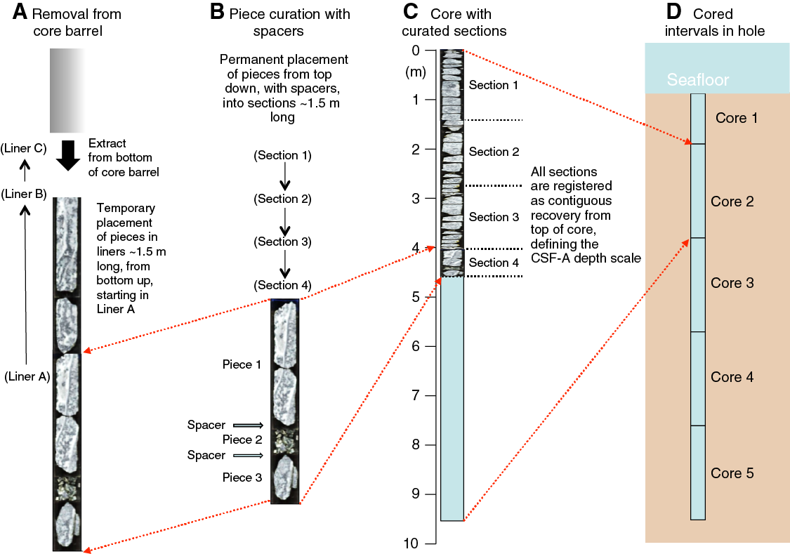
Figure F2. Core handling, Expedition 360.
The total length of all rock material in each section was measured and entered into the Sample Master registry as recovered length. The sum of all recovered lengths in a core was used to compute core recovery as a percentage of the cored interval.
Microbiology samples were taken from selected pieces, according to the cruise sampling plan, under supervision of the assigned Sample Allocation Committee (SAC) representative. Only the necessary 2–3 people were in the room for microbiology sampling to minimize contamination, wearing face masks and nitrile gloves, and the samples were immediately transferred to the microbiology sample preparation laboratory (see Microbiology for information on microbiology sample handling and preparation). JRSO personnel then washed the whole-round pieces, one piece at a time, and allowed them to dry.
Next, plastic dividers made from core liner caps were inserted between core pieces to keep them in place for curation. The spacers may represent substantial intervals of no recovery, to the point of creating a curated core that is longer than the cored interval (see Depth computations). Adjacent core pieces that could be fitted together along fractures were curated as single pieces. Core pieces that appeared susceptible to crumbling were encased in shrink-wrap.
A designated scientist was then called to the splitting room to check and approve the binning and reconstruction of fractured pieces. The scientist marked a splitting line on each piece with a red wax pencil so that the piece could be split into representative working and archive halves, ideally maximizing the expression of dipping structures on the cut face of the core while maintaining representative features in both archive and working halves. To ensure a consistent protocol for whole-core imaging, the splitting line was drawn so that the working half was on the right side of the line with the core upright. The working half of each piece was marked with a “W” to the right of the splitting line (Figure F3). Where magmatic fabrics or crystal-plastic fabrics (CPFs) were present, cores were marked for splitting with the fabric dipping to the east (090°) in the IODP core reference frame (CRF) (see Core reference frame for sample orientation; Figure F3). This protocol was sometimes overridden by the presence of specific features (e.g., mineralized patches or dike margins) that were divided between the archive and working halves to ensure preservation and/or allow shipboard or postcruise sampling.

Figure F3. Core reference frame for structural and paleomagnetic orientation measurements, Expedition 360.
Once the split line was drawn, JRSO technical personnel secured the plastic spacers permanently with acetone between individual pieces into matching working and archive half split core liners. Spacers were mounted into the liners with the angle brace facing uphole. This ensured that the top of each piece had the same depth as the top of the curated interval for each bin. The top and bottom offsets of each bin were entered into Sample Master. Based on the calculated bin lengths, the cumulative length of all bins, including spacers, was computed as the curated length of the section (Figure F2). The empty split liner with spacers glued in was then placed over the split liner containing the pieces and the two halves were taped together in a few places for temporary storage, until core pieces were dry and equilibrated to laboratory conditions (usually <1 h from arrival from the catwalk).
Whole-round section measurements
Once the core sections were deemed thermally equilibrated, the following whole-round measurements were taken:
- Whole-round surface imaging (i.e., four surface “quarter image” scans orthogonal to angles of 0°, 90°, 180°, and 270° relative to the CRF) (Figure F3) using the Section Half Imaging Logger (SHIL) configured for whole-round sections.
- Logging using the Whole-Round Multisensor Logger (WRMSL) with the magnetic susceptibility loop sensor (MSL) and the gamma ray attenuation (GRA) detector (see Petrophysics).
- Logging using the Natural Gamma Radiation Logger (NGRL) (see Petrophysics).
Section half preparation
After the completion of whole-round measurements, each piece of core was split into archive and working halves, with the positions of plastic spacers between pieces maintained in both halves. Piece halves were labeled sequentially from the top of each section, beginning with number 1 (Figure F2). Pieces were labeled only on the outer cylindrical surfaces of the core.
Archive section half measurements
The following archive section half measurements were taken:
- Imaging of the dry faces of archive halves using the SHIL (see Igneous petrology).
- Automated compilation of a core composite image, whereby all sections of a core are displayed next to each other in a one-page layout.
- Logging using the Section Half Multisensor Logger (SHMSL) with reflectance spectroscopy and colorimetry (RSC) and point magnetic susceptibility (MSP) contact probe (see Petrophysics).
- Macroscopic core description using the DESClogik data capture program (see Igneous petrology).
- Remanent magnetization logging using the superconducting rock magnetometer (SRM) (see Paleomagnetism).
- Close-up images of particular features for illustrations in the summary of each site, as requested by individual scientists.
Working section half sampling and measurements
The following working section half samples and measurements were taken:
- Thin section billets (TSBs) were sampled to prepare thin sections and collect microscopic observations on thin sections (see Igneous petrology).
- Cube samples (~8 cm3) were taken for moisture and density (MAD) tests and for P-wave velocity measurements using the P-wave caliper (PWC) mounted on the Section Half Measurement Gantry (see Petrophysics).
- Cube samples (~8 cm3) were taken for paleomagnetic and rock magnetism tests (PMAG) (see Paleomagnetism).
- Slabs or chips were taken and powdered for inductively coupled plasma–atomic emission spectroscopy (ICP-AES) and carbon-hydrogen-nitrogen-sulfur (CHNS) elemental tests (see Geochemistry).
- Fragments were scraped off for X-ray diffraction (XRD) measurements (see Metamorphic petrology).
Samples for shore-based research
Samples for postcruise analyses were taken from the working half for individual investigators, based on requests approved by the SAC. For the first sampling party, 44 cores were laid out across the entire core deck and sampled during a medical evacuation transit. Toward the end of the cruise, up to 8 cores were laid out in 6 consecutive sampling parties lasting 2–3 days each, from planning to execution. Scientists viewed the cores, flagged sampling locations, and submitted detailed lists of requested samples. The SAC reviewed the flagged samples and resolved very rare conflicts as needed. Shipboard staff cut, registered, and packed the samples. A total of 3045 samples were taken for shore-based analyses, in addition to the 1454 samples taken for shipboard analysis.
Extracted samples were sealed in plastic vials or bags and were labeled. Each sample cut from the working section half was logged into the LIMS database using the Sample Master program, including the sample type and either the shipboard analysis (test) conducted on the sample or the name of the investigator receiving the sample for postcruise analysis. Records of all samples taken from the cores are accessible online in the Curation and Samples > Sample Report (http://web.iodp.tamu.edu/LORE/).
Final sample storage
Following shipboard initial scientific observations, measurements, and sampling, both core halves were shrink-wrapped in plastic to prevent rock pieces from moving out of sequence during transit. Working and archive halves were then put into labeled plastic tubes, sealed, and transferred to cold-storage space aboard the drilling vessel. At the end of Expedition 360, cores were transferred from the ship to the Kochi Core Center, Japan, for permanent storage.
Sample names
Three concepts
Sample names are computer-generated constructs of multiple pieces of information registered in the LIMS database during the course of the various sampling and curation processes, following specific rules. Understanding the three concepts (text ID, label ID, and printed labels) in use may help users enter the correct information in the Sample Master registry and find the samples of interest using the available filters in the LIMS Reports applications.
Text ID
Samples taken on the JOIDES Resolution are uniquely identified for use by software applications using the text ID, which combines two elements:
- Sample type designation (e.g., SHLF for section half).
- A unique sequential number for any sample and sample type, added to the sample type code (e.g., SHLF30495837).
The text ID is not particularly helpful to most users. For a more process-oriented human-readable sample naming convention, the label ID concatenates a number of parameters, according to specific rules.
Label ID
The label ID is used throughout the JOIDES Resolution workflows as a convenient, human readable sample identification and nomenclature. The user may think of the label ID as being made up of two parts: primary sample identifier and sample name. The label IDs are not necessarily unique.
Primary sample identifier
The primary sample identifier is composed of a concatenation of the following parameters, per decades-long convention:
- Expedition during which the core was taken (e.g., 360).
- Site at which one or more holes were drilled (e.g., U1499).
- Hole at the designated site (e.g., A, although the hole is really determined by the combination of site and hole [i.e., U1499A]).
- Core and its type retrieved in one wireline run (e.g., 35R [R = RCB]).
- Section cut from the core (e.g., 2).
- Section half after splitting, working or archive (i.e., W or A, respectively).
- The sample top and bottom offset, relative to the parent sample (e.g., 35/37); also see the label ID offset rules below.
The complete label for the primary sample thus has 2–5 dash-delimited terms, followed by the space-delimited offset/offset element (e.g., 360-U1499A-35R-2-W 35/37).
IMPORTANT: Specific rules were set for printing the offset/offset at the end of the primary sample identifier:
- For samples taken out of the hole, core, or section, offset/offset is NOT added to the label ID. This has implications for the common process of taking samples out of the core catcher (CC), which technically is a section (for microbiology and paleontology samples).
- For samples taken out of the section half, offset/offset is always added to the label ID. The rule is triggered when an update to the sample name, offset, or length occurs.
- The offsets are always rounded to the nearest centimeter before insertion into the label ID (even though the database stores higher precisions and reports offsets to millimeter precision).
Sample name
The sample name is a free text parameter for subsamples taken from a primary sample, or from subsamples thereof. It is always added to the primary sample identifier following a dash (-NAME) and populated from one of the following prioritized user entries in the Sample Master application:
- Entering a sample type (-TYPE) is mandatory (same sample type code used as part of the text ID; see above). By default, -NAME = -TYPE (examples include SHLF, CUBE, CYL, PWDR, and so on).
- If the user selects a test code (-TEST), the test code replaces the sample type and -NAME = -TEST. The test code indicates what the purpose of taking the sample was, which does not guarantee that the test was actually completed on the sample (examples include TSB, ICP, PMAG, MAD, and so on).
- If the user selects a requester code (-REQ), it replaces -TYPE or -TEST and -NAME = -REQ. The requester code represents the name of the requester of the sample who will conduct postcruise analysis (examples include HANK, MACL, ILD, CHEA, and so on).
- If the user types a value (-VALUE) in the -NAME field, perhaps to add critical sample information for postcruise handling, the value replaces -TYPE, -TEST or -REQ and -NAME = -VALUE (examples include SYL-80deg, MORR-40mT, and so on).
In summary, and given the examples above, the same subsample may have the following label IDs based on the priority rule -VALUE > -REQ > -TEST > -TYPE:
- 360-U1499A-35R-2-W 35/37-CYL
- 360-U1499A-35R-2-W 35/37-PMAG
- 360-U1499A-35R-2-W 35/37-MORR
- 360-U1499A-35R-2-W 35/37-MORR-40mT
When subsamples are taken out of subsamples, the -NAME of the first subsample becomes part of the parent sample ID, and another -NAME is added to that parent sample label ID:
For example, a thin section billet (sample type = TSB) was taken from the working half at 40–42 cm offset from the section top, resulting in the label ID 360-U1473A-3R-4-W 40/42-TSB. After the thin section was prepared (~48 h later), the technician entered it as a subsample of the billet (because additional thin sections could be prepared from the same billet) and entered the value TS05 (because this was the fifth thin section made during the expedition). The resulting thin section label ID was 360-U1473A-3R-4-W 40/42-TSB-TS_5.
Printed labels
The requirements for printed labels have no relationship to the rules applied to create the label ID. A printed label may look like it carries a label ID, and the label ID is encoded in the barcode field, but the rules for what is printed on the label are subject to the label format definition, which emphasizes requester and routing information. Printed labels are not further discussed here.
Depth computations
The bit depths in a hole during deployment of a reentry system and during drilling and coring are based on the length of drill pipe added at, and deployed beneath, the rig floor (to the nearest 0.1 m). They are expressed as drilling depth below rig floor (DRF) (in meters) (Figure F4). When applicable, these depths are converted to DSF by subtracting the seafloor depth determined by tagging the seafloor (or some other method) from the current bit depths (both at DRF scale). The bit depths (DRF and DSF) at which a coring advance begins and ends define the cored interval.
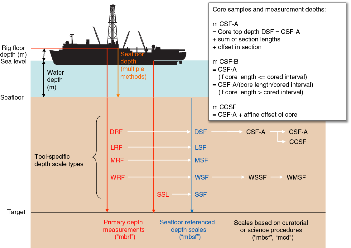
Figure F4. Overview of depth scale types.
Once the recovered core is subjected to curatorial procedures (see Core curatorial procedures and sampling; Figure F2), the core depth below seafloor, method A (CSF-A) depth scale is used for assigning depths to samples and measurements. The top depth of a core in CSF-A is equal to the top of the cored interval in DSF. However, the bottom depth of the core at the CSF-A scale and the depths of samples and measurements within the core are based on the curatorial procedures and rules applied on the catwalk and in the shipboard laboratory and have no defined relation to the bottom depth of the cored interval at the DSF scale. Depths of samples and associated measurements at the CSF-A scale were calculated by adding the offset of the sample or measurement from the top of its section, and the lengths of all higher sections in the core, to the top depth of the cored interval. This computation assumes that the recovered material represents a contiguous interval, starting at the top depth of the cored interval, even if core pieces are separated by nonrecovered stratigraphic intervals. If a core is shorter than the full barrel length and/or consists of more than one piece, the true depth of a sample or measurement in the core is unknown and should be considered a sample depth uncertainty when analyzing data associated with the core material.
If cores must be depth-shifted to create a modified depth scale that better represents the stratigraphy at a site or simply to remove artificial overlaps between cores related to natural, drilling, or curatorial processes, a core composite depth below seafloor (CCSF) is constructed. A simple, single depth offset is defined for each core and the transform from the CSF-A scale to the CCSF scale for all cores in a hole is given by the affine table. CCSF (or “alternate depth”) database tools were primarily designed to meet the needs of paleoceanographic projects where cores from multiple adjacent holes are depth shifted to correlate stratigraphic features and create stratigraphic splices. During Expedition 360, we used the alternate depth database tools to remove artificial core overlaps resulting from the curated length (including the spacers and gaps between pieces) of many cores being greater than the cored interval. We shifted cores with excessive length upward (negative offset) by the amount of its excessive length, and into the “empty space” at the bottom of the next higher core. If the necessary space did not exist in the next higher core, that core was also shifted up, and so on, until all core lengths were accommodated. Fortunately, we did not run out of space, which would have required a shift downward and extending the total depth of the hole. All site reports and figures except those relating to logging use the CCSF depth scale (see DEPTH in Supplementary material and the LIMS database for offset values used during Expedition 360).
Additional depth scales are defined for downhole logging operations because those measurements are based on the length of the logging cable deployed beneath the rig floor, with their specific sources of uncertainly and correction procedures.
In summary, the depth scales used (Figure F4; IODP Depth Scales Terminology version 2 [http://www.iodp.org/top-resources/program-documents/policies-and-guidelines/142-iodp-depth-scales-terminology-april-2011/file]) and the corresponding pre-IODP references, are as follows.
Drilling and coring depth scales:
- DRF = meters below rig floor (mbrf).
- DSF = meters below seafloor (mbsf).
- CSF-A = mbsf.
- CCSF = meters composite depth (mcd).
- Wireline log depth below rig floor (WRF) = mbrf.
- Wireline log depth below seafloor (WSF) = mbsf.
- Wireline log speed-corrected depth below seafloor (WSSF) = mbsf.
- Wireline log matched depth below seafloor (WMSF) = mbsf.
Core reference frame for sample orientation
Each core piece that has a length exceeding that of the core liner diameter is associated with its own CRF (Figure F3). The primary reference is the axial orientation (i.e., the top and bottom of the piece) based on piece orientation when extracted from the core barrel. The core axis defines the z-direction, where positive is downcore. The secondary reference is an arbitrarily marked axis-parallel line on the whole-round surface of the piece. This is the cut line, which marks the plane through the cut line and the core axis where the piece will be split. The cut line was selected by Expedition 360 Scientists to maximize the dip angle of planar features on the split surface, which facilitates accurate structural measurements. The x-axis of the CRF is defined orthogonally to the cut plane, positive (000°) into the working half and negative (180°) into the archive half. The y-axis is orthogonal to the x-z plane and, using the right-hand cork-screw rule, is positive (090°) to the right and negative (270°) to the left when looking upcore onto the working half (Figure F3).
Cube samples taken from the working half were marked with an arrow in the −z-direction (upcore) on the working half surface (y-z plane), which defines the cube’s orientation unequivocally within the CRF. TSBs and thin sections made from billets were also marked with an upcore arrow in the most common case where the thin section was cut from the y-z plane of the working half sample. If thin sections were cut in the x-y or x-z plane, these directions were marked on the thin sections (Figure F3).
Section graphic summary (visual core descriptions)
For each core section, the most pertinent instrument measurement parameters and core description observables were plotted on a section graphic summary (also traditionally referred to as visual core description [VCD]). An existing template was reviewed by the science party, and JRSO personnel implemented modifications as needed during the course of the expedition to arrive at the final template (Figure F5). JRSO personnel plotted all graphic summaries using the final template and data retrieved from the LIMS database or directly from DESClogik, using symbols, patterns, and line plots with depth, using the commercial plotting program Strater (Figure F6). A key to symbols used on the graphic summaries is given in Figure F7.
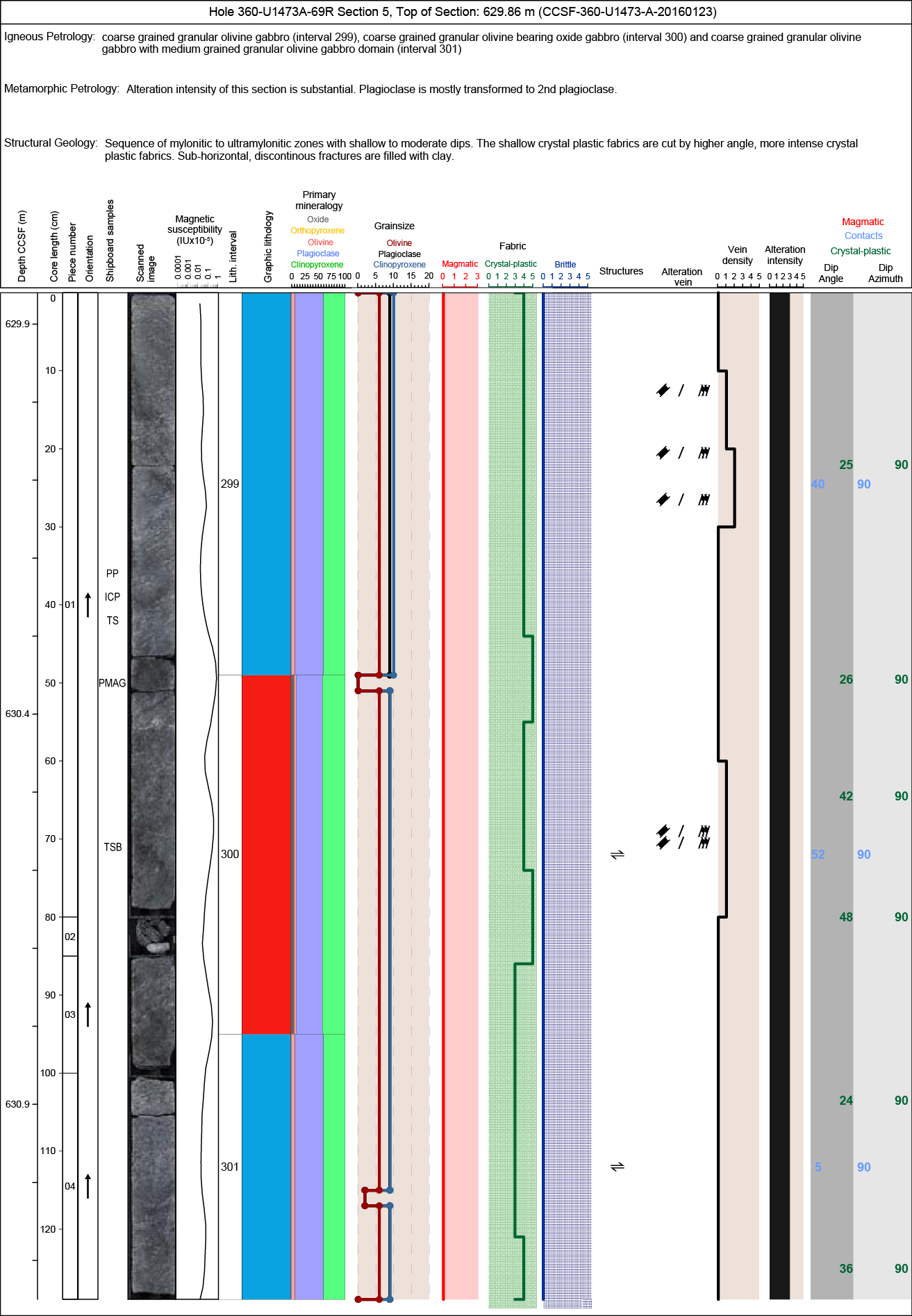
Figure F5. Example of a graphic summary, Expedition 360.
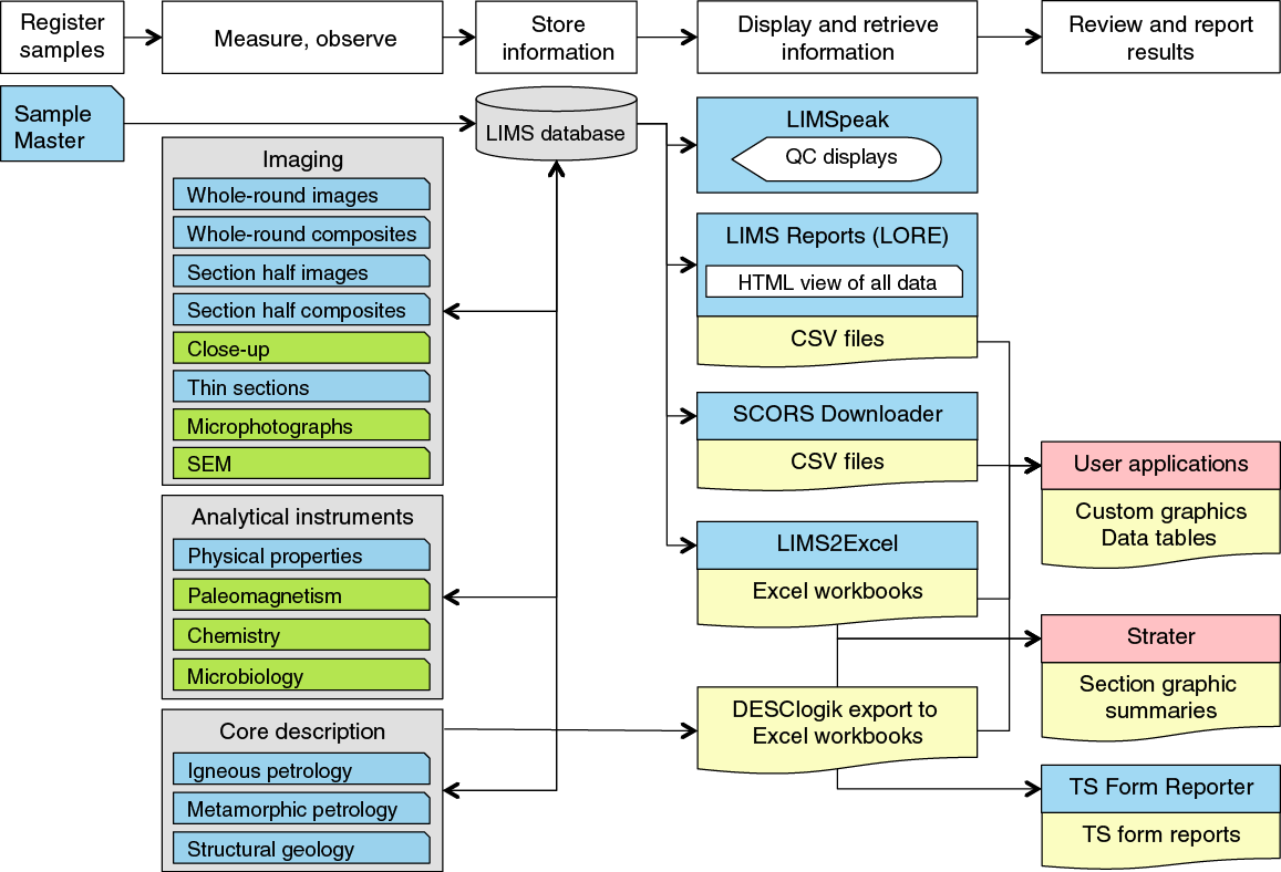
Figure F6. Overview of general data flow and software tools, Expedition 360.

Figure F7. Colors, patterns, abbreviations, and symbols used on graphic summaries, Expedition 360.
The section graphic summary forms summarize the shipboard observations for the section starting with a text summary from each description team (igneous petrology, metamorphic petrology, and structural geology) across the top. All other information is plotted by depth in the main report area, starting with an image of the archive section half and followed by the identification of pieces recovered, lithologic units defined, shipboard samples analyzed, magnetic susceptibility measurements, and the most significant observed igneous, metamorphic, and structural parameters (Figure F5).
Thin section reports were created to summarize the most significant information for each thin section, extracted with a program from the extensive observation workbooks exported from the DESClogik spreadsheet application, in a 1–3 page PDF form (Figure F8). JRSO personnel created the report definition in the report Builder custom tool, updated the definition with input from scientists during the course of the cruise, and generated batches of PDF reports on request using the report writer tool.
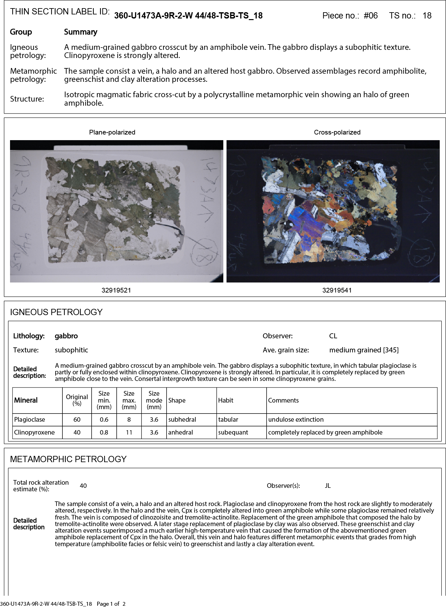
Figure F8. Example of a thin section report, Expedition 360.
Software tools and databases
LIMS database
The JRSO LIMS database is an infrastructure to store all operational, sample, and analytical data produced during a drilling expedition (Figure F6). The LIMS database comprises an Oracle database and a custom-built asset management system, along with numerous web services to exchange data with information capture and reporting applications.
Sample registry tool
All samples collected during Expedition 360 were registered in the LIMS database using the Sample Master application. The program has workflow-specific interfaces to meet the needs of different users. Sample registration begins with the driller entering information about the hole and then the cores retrieved from the hole. IODP personnel entered additional core information, sections, pieces, and any other subsamples taken from these, such as cubes or TSBs. One interface is designed for visiting scientists so they can autonomously enter subsample information according to the sampling plan.
Imaging systems
The following highly integrated and workflow-customized imaging systems were used during Expedition 360:
- Section half surface images using the SHIL; also used to capture whole-round section surface (360°) images using a special configuration that takes four swaths at 90° angles and covering ~90% of the surface.
- A manual compositing process for the whole-round section images to produce a quasi-360° presentation of features on the core surface.
- An automated compositing process for all section half images of a core to produce a “virtual core table” view.
- Close-up images taken to meet special imaging needs not covered with routine line scan images.
- Whole-area high-resolution thin section images using a custom-built imaging system.
- Photomicrographs using commercial cameras mounted on all microscopes.
- High-resolution images using the scanning electron microscopy (SEM) system.
All images were uploaded to the LIMS database immediately after capture and were accessible via browser-based reports. Images were provided in at least one generally usable format (JPG, TIFF, or PDF) and in multiple formats if appropriate (also see GALLERIES in Supplementary material).
Core description
Descriptive and interpretive information was entered and stored using the DESClogik custom software application, and all information was stored in the LIMS database. The main DESClogik interface is a spreadsheet with extensive data entry and data validation support. The columns (observables), worksheets (sets of observables logged in context), and workbooks (sets of worksheets used in conjunction with each other) are entirely configurable by JRSO personnel based on experience from past expeditions and specific requirements defined by Expedition 360 Scientists.
Three teams were formed to describe igneous petrology, metamorphic petrology, and structural geology in all core sections and thin sections prepared on board (see Igneous petrology, Metamorphic petrology, and Structural geology). This disciplinary team approach ensured that all members of a specialty group were able to work collaboratively on all recovered material and work in a coordinated fashion to produce consistent data sets. The teams were assigned overlapping 12 h shifts, whereby each team had priority access to laboratory infrastructure, particularly microscopes, for 8 h. Plenty of overlap time ensured information exchange among the teams.
At the beginning of the expedition, each group reviewed existing workbook templates for gabbroic rocks and specified expedition-specific modifications, which were implemented in the DESClogik application by JRSO personnel. Observable parameters were of three types: controlled values, free text, and numbers. For the controlled value columns, subject matter experts defined specific value lists that were configured in DESClogik as drop-down lists to facilitate consistent data entry. These values are defined in each description team’s section of this chapter. Free text fields had no constraints and were used for comments and summaries. Number columns were used to log abundance percentage, size, intensity, and rank (for plotting) of physical constituents, texture, and structures. The three teams selected a total of 268 observables for macroscopic description and 180 observables for microscopic descriptions.
Instrumented measurement systems
Physical properties, paleomagnetic, and geochemistry analytical systems in the shipboard laboratories were used to capture instrumental data, as described in the corresponding sections below, using dozens of commercial and custom-built software applications. In cases where no user interaction was required after data capture, data upload to the LIMS database was triggered automatically. In cases where quality control or data processing was needed before upload, the user triggered the upload to the LIMS database when the data were ready.
Data retrieval
All data used for analysis, interpretation, and report preparation were downloaded using the latest version of LIMS Reports (Figure F6), where the user selects the type of desired information from ~50 available reports, selects a hole (and optionally, cores, sections, or samples), and uses additional report-specific filters, if desired, to view a report online or download information in a standard comma-separated value (CSV) file.
Alternatively, data could also be retrieved using applications built for more specific purposes, with various filtering and configuration options:
- LIMS2Excel, a highly configurable Java-based data extractor where users can save a specific configuration for any combination of data parameters and export it into a Microsoft Excel workbook; and
- SCORS Downloader, designed to download certain data sets iteratively for stratigraphic analysis programs and can be used for any data and purpose.
Many data sets could also be viewed on LIMSpeak, a browser-based application that plots cores, sections, and samples along with a user-selected data set, including images, against depth. The application is particularly useful for monitoring core logging data acquisition, real-time quality control, and browsing images.
Igneous petrology
Rock description procedures during Expedition 360 closely followed those used during Integrated Ocean Drilling Program Expeditions 304/305 (Expedition 304/305 Scientists, 2006), 309/312 (Expedition 309/312 Scientists, 2006), and 335 (Expedition 335 Scientists, 2012). These, in turn, were based on ODP Leg 209 and earlier “gabbro” legs (ODP Legs 118, 147, 153, and 176) to maintain as high a degree of uniformity as practicably possible. As during Legs 176, 206, and 209 and Expeditions 304/305, 309/312, and 335, core descriptions were performed by the entire igneous petrology team working together on the same shift. Each member was responsible for one or more aspects of the description (e.g., igneous contacts, textures, mineral modes, and habits) to ensure consistency of recorded observations throughout the core; however, the entire team worked together as much as possible, particularly when defining intervals and contacts.
Cores were described both macroscopically and microscopically, and their characteristics were entered into the LIMS database through the DESClogik application. Key information was entered into the section_summary worksheet in DESClogik. This information was then used to produce graphic section summaries (VCDs). An example and the key to symbols used on the graphic summaries are given in Figures F5 and F7.
Igneous intervals, grain size intervals, and contact logs
The first step in describing core was identification of interval boundaries on the basis of the presence of contacts, chilled margins, changes in primary mineralogy, color, grain size, and textural variations. Igneous intervals in Hole U1473A were numbered sequentially from top to bottom. Lithologically and texturally similar pieces from consecutive core sections were described as belonging to the same interval. Further, heterogeneities within a given interval that cannot be attributed to a new interval were described as different domains, one domain per row in the plutonic_mantle worksheet in DESClogik. Two different domains were identified when patches or areas with a variation in grain size, modal composition, or texture were recognized within an interval. In order not to define an excessive number of intervals, magmatic veins were considered as crosscutting features of a given interval and not as separating two different intervals; those veins are numbered (MV01, MV02 and so on). Crosscutting dikes are considered as separate intervals. Magmatic veins and crosscutting dikes are identified in the plutonic_mantle worksheet but are described in the veins_halos worksheet in DESClogik.
The maximum and mean grain sizes of each of the major constituent minerals (olivine, plagioclase, clinopyroxene, and orthopyroxene) in each core section are measured in hand specimen along the long axis of each mineral. We define “grain size interval” independently from lithologic intervals only based on the differences in grain size.
Where contacts deviated from horizontal within the CRF, their depth was logged at their midpoint. The igneous interval and contact log (see Table T2 in the Hole 1105A redescription chapter and Table T3 in the Site U1473 chapter [MacLeod et al., 2017a, 2017b]) provides information about interval boundaries and a brief description of each interval. For each interval, the table lists interval number, top depth (in CSF-A); core, section, interval, and piece number of the top of the unit; unit thickness; lithology; a description of the upper and lower boundaries; average grain size; texture; and modal composition. If the contact between two intervals was recovered, its location is recorded by the core, section, position (cm), and piece number. If the contact was not recovered, but a significant change in grain size is observed, the contact is placed at the bottom of the lowest piece of the upper interval.
Macroscopic core description
Macroscopic descriptions were divided into the following categories.
Lithology
Plutonic rocks
Plutonic rocks were classified on the basis of abundance, grain size, and texture of their primary minerals (as inferred prior to alteration), based on the International Union of Geological Sciences (IUGS) system (Streckeisen, 1974; Le Maitre, 1989; Le Maitre et al., 2002). This classification defines the following rocks (Figure F9):
- Troctolite: olivine + plagioclase >95%, with both olivine and plagioclase >10%.
- Olivine gabbro: olivine + plagioclase + clinopyroxene, none of which is <5%.
- Gabbro or diorite: plagioclase + clinopyroxene >95%, plagioclase >10%, clinopyroxene >10%, and quartz <5%.
- Gabbronorite: plagioclase + clinopyroxene + orthopyroxene, none of which is <5%.
- Quartz diorite: quartz 5%–20% of quartz + alkali feldspar + plagioclase (QAP), with alkali feldspar <10% of QAP.
- Tonalite: quartz 20%–60% of QAP, with alkali feldspar <10% of QAP.
- Trondhjemite: tonalite with total mafic mineral content <10%.
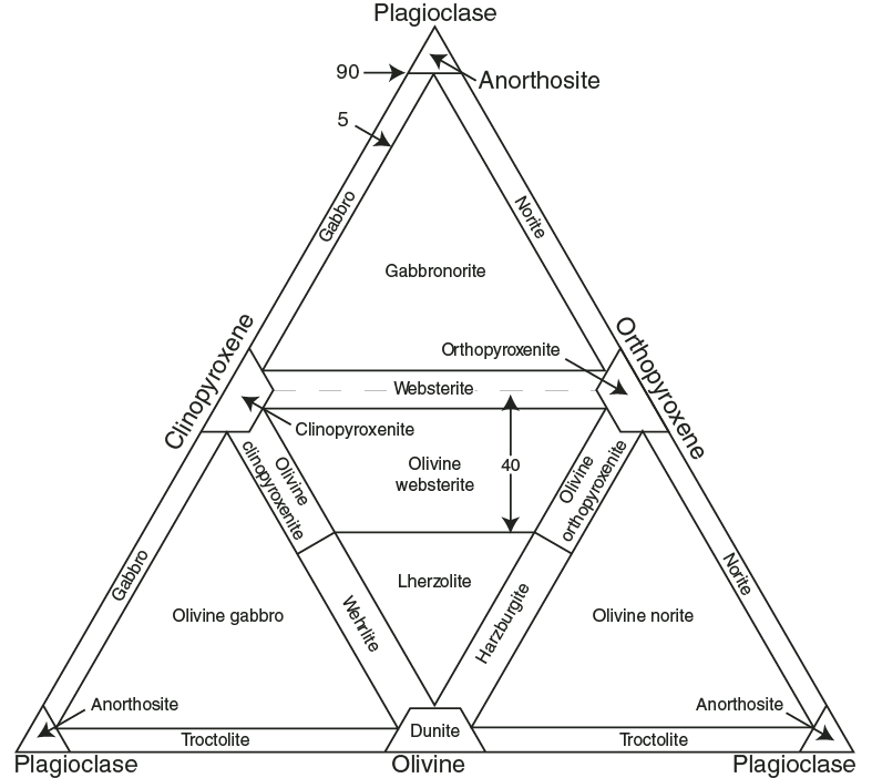
Figure F9. Rock classification, Expedition 360.
In the IUGS classification, diorite is distinguished from gabbro by the anorthite content of plagioclase, with diorite having plagioclase containing <50 mol% An and gabbro having plagioclase containing >50 mol% An. Because this cannot be characterized during macroscopic description, we used the following convention: if a gabbroic rock contained quartz (<5%) or primary amphibole, indicating a relatively high degree of fractionation, the rock was classified as diorite. If no quartz or primary amphibole was observed, the rock was classified as gabbro.
Minor modifications to the IUGS system were made to divide the rock types more accurately on the basis of significant differences rather than arbitrary cutoffs based on the abundance of a single mineral. We have attempted to follow as closely as possible the descriptions from Leg 209 (Shipboard Scientific Party, 2004) and Expeditions 304/305 (Expedition 304/305 Scientists, 2006), 309/312 (Expedition 309/312 Scientists, 2006), and 335 (Expedition 335 Scientists, 2012) to facilitate intersite comparison.
Vein and rock names included a modifier based on modal mineralogy (Figures F9, F10). For gabbroic rocks, the following rock name modifiers were used:
- Disseminated oxide = 1%–2% Fe-Ti oxide.
- Oxide bearing= >2%–5% Fe-Ti oxide.
- Oxide = >5%–50% Fe-Ti oxide.
- Olivine bearing = 1%–5% olivine.
- Orthopyroxene bearing = 1%–5% orthopyroxene.
- Clinopyroxene-rich troctolite = 5%–15% clinopyroxene; >20% olivine.
- Olivine rich = >70% olivine.
- Anorthositic = >90% plagioclase.
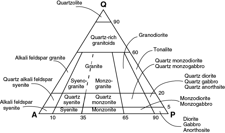
Figure F10. Rock name modifiers based on modal mineralogy, Expedition 360.
Following Streckeisen (1974) classification (Figures F9, F10), any mineral >5% should be added as a suffix without any hyphen.
Additional rock name modifiers were defined as follows:
- Leucocratic = light colored, high proportions of plagioclase.
- Micro = dominant grain size <1 mm.
- Diabasic = fine- or medium-grained gabbroic rocks with dominant ophitic or subophitic textures.
Felsic veins are described in collaboration with metamorphic petrology and structural geology teams in the veins_halos worksheet in DESClogik.
Volcanic rocks
For volcanic and hypabyssal rocks, we used the following definitions:
- Basalt: all igneous rocks of basaltic composition not clearly intrusive, in the grain size range glassy to medium grained.
- Diabase: holocrystalline, very fine to medium-grained intrusive rocks of basaltic composition often with well-developed subophitic or ophitic textures (dolerite in European nomenclature).
Basalt was divided according to phenocryst content, using the following convention:
- Aphyric = <1% phenocrysts.
- Sparsely phyric = 1%–5% phenocrysts.
- Moderately phyric = >5%–10% phenocrysts.
- Highly phyric = >10% phenocrysts.
If present and >5%, phenocryst phases were placed as modifiers in front of the rock name without any hyphen in between. If <1% phenocryst is present, the rock was given the modifier “aphyric.”
Mineralogy
Plutonic rocks
In oceanic plutonic rocks, the primary rock-forming minerals are spinel, olivine, plagioclase, clinopyroxene, orthopyroxene, amphibole, Fe-Ti oxide, sulfide, and quartz. The following data were recorded in the plutonic_mantle worksheet (if not otherwise mentioned) in DESClogik for each primary silicate:
- Visually estimated modal percent: in fresh rocks this represents the modal mineralogy as observed; in (partially) altered rocks this represents the estimated igneous modes prior to alteration. Where a mineral occurs in trace quantities (i.e., too low to assign a meaningful percentage), 0.1% is recorded. Accessory phases are also noted where observed. Modal estimates were estimated visually by three different team members and normalized to 100%.
- Grain size:
- General (based on average grain size): fine grained = <1 mm, medium grained = 1–5 mm, coarse grained = >5–30 mm, or pegmatitic = >30 mm.
- Detailed (absolute grain sizes of each mineral phase): minimum, median, and maximum.
- Mineral shape:
- General: euhedral, subhedral, and anhedral.
- Where oxides and sulfides form aggregates: angular aggregates, amoeboid aggregates, and interstitial aggregates.
- Mineral habit:
The first four mineral habit terms apply predominantly to subhedral or euhedral grains, the latter generally to anhedral grains. Another term (poikilitic) was used for an anhedral mineral containing several inclusions of a different mineral phase.
Volcanic rocks
In volcanic and hypabyssal rocks, the groundmass, phenocrysts (if any), and vesicles were described:
- Groundmass grain size (the first four terms apply predominantly to the matrix; the latter two generally apply to the phenocrysts):
- Glassy.
- Cryptocrystalline = <0.1 mm.
- Microcrystalline = 0.1–0.2 mm.
- Fine grained = >0.2–1 mm.
- Medium grained = >1–5 mm.
- Coarse grained = >5–30 mm.
- Phenocryst phases:
- Vesicles:
- Abundance (in percent).
- Vesicularity.
- Size distribution: minimum, maximum, and modal size (in millimeters).
- Roundness (rounded, subrounded, or well rounded).
- Sphericity (highly spherical, moderately spherical, or slightly spherical; or elongate [direction was noted]).
- Filling (in percent).
- Fill composition.
Contacts
For contacts between intervals, the type, definition, geometry, and interpretation were described. Where the contact was not recovered this was noted.
We used the following definitions for contact types:
- Grain size: units on either side have markedly different grain sizes, such as coarse- and fine-grained gabbro on each side, or a chilled margin of a vein/dike.
- Modal: units on either side have markedly different mineral proportions.
- Intrusive: sharp contact that cuts across grain boundaries of the minerals composing the country rock.
- Sutured: specific form of igneous contact showing interpenetrating grains.
If contacts were characterized by combinations of the first two parameters, the terms were combined (e.g., “grain size and modal contact”).
Where contacts are obscured by deformation and metamorphism, these were noted using the following definitions:
- Sheared: an interval with deformation fabric is in contact with an undeformed interval.
- Foliated: both intervals have deformation fabrics.
- Tectonic: the contact appears to be the result of faulting.
Following description, contacts were interpreted as being extrusive, intrusive, or igneous. The latter term was used for contacts in plutonic rocks where the units on either side of the contact were interpreted to form part of the same igneous package (e.g., a modal contact between cumulate layers or a grain size contact in a graded sequence).
The term dike refers to any sharp, well-defined, and relatively thick (>1 cm) crosscutting feature formed by injection of magma. This contrasts with igneous vein, which describes a thin (<1 cm) crosscutting feature formed by injection of magma with generally less well-defined contacts. Dikes and veins are generally designated as separate intervals, as described above in Igneous intervals, grain size intervals, and contact logs.
If present, grain size variations toward the contact were documented:
Also, if present, the grain fabric at the boundary contact was documented:
Other information with reference to the interval contacts was added to the plutonic_mantle worksheet in DESClogik by the structural geology team.
Texture
Textures were defined on the basis of three categories: grain size, grain size distribution, and the relationships between different grains.
For plutonic rocks, grain size distributions were classed as follows:
For volcanic rocks, grain size distribution applied to phenocrysts only:
- Unimodal: all phenocrysts are of similar size.
- Bimodal: phenocrysts define two size populations.
- Seriate: phenocrysts form a continuous range of sizes.
The following terms were used to describe the textural relationships between different silicate grains (Figure F11):
- Granular: aggregation of grains of approximately equal size.
- Intergranular: coarser grains (typically plagioclase) form a touching framework in the rock with interstices filled by crystalline material.
- Intersertal: coarser touching grains form a framework in the rock with interstices filled by glass.
- Subophitic: partial inclusion of plagioclase in clinopyroxene.
- Ophitic: total inclusion of plagioclase chadacrysts in clinopyroxene oikocrysts.
- Poikilitic: large oikocrysts containing numerous chadacrysts of any type.
- Porphyritic: texture containing large grains within a finer-grained matrix.
- Comb structure: comblike arrangement of crystals growing inward from a contact.
- Skeletal: either hopper crystals or with hourglass shape.
- Dendritic: branching arrangement of elongate crystals.
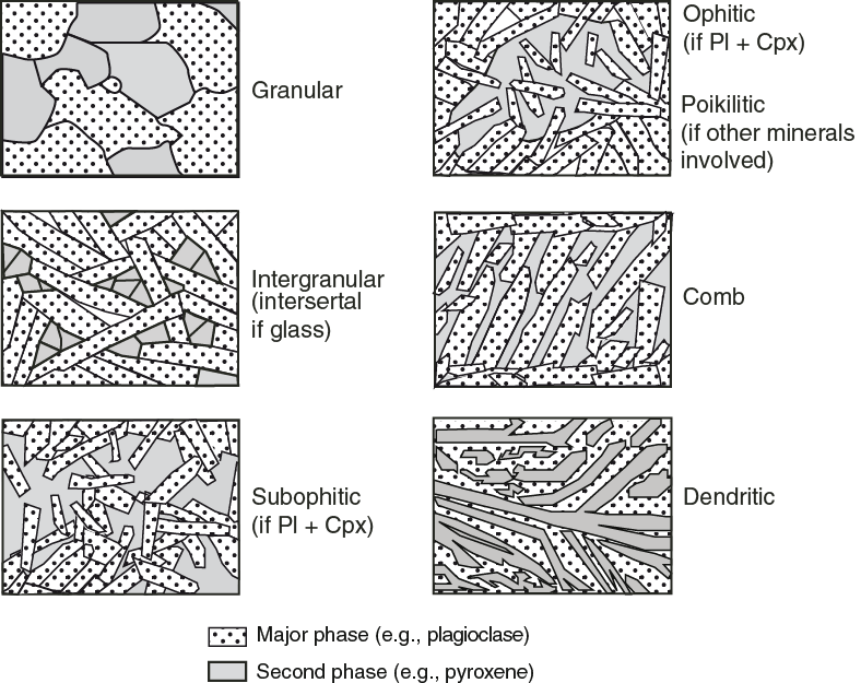
Figure F11. Terms used to describe textural relationships between silicate grains, Expedition 360.
As with the silicate minerals, textures of oxide and sulfide minerals were described in terms of grain size and their relationship to adjacent minerals. In plutonic rocks, oxides commonly occur as aggregates of ilmenite and magnetite; for grain size determination, an aggregate is counted as a single grain.
Layering or foliation are identified here but are described in detail in Structural geology.
Thin section descriptions
Each thin section was photographed in both plane-polarized light (PPL) and cross-polarized light (XPL). All images are available from the LIMS database, and thumbnail versions are printed on the thin section form reports (see Core descriptions). Thin section descriptions closely follow the procedure for macroscopic core descriptions. Where a thin section contained areas with different primary lithology, mineralogy, and/or texture (not alteration related), these were defined as domains (e.g., Domain 1, Domain 2, and so on). Domains were described separately and their relative abundance was noted.
The following data were recorded and entered into the thin_sections and ts_plutonic_mantle worksheets of the microscopic workbook in DESClogik.
Lithology and texture
Plutonic rock
The following definitions were used for plutonic rocks:
- Rock name (based on thin section observations), using the same definitions as those for macroscopic descriptions.
- Number of igneous domains within the thin section.
- Igneous domain lithology name. If only one domain is present, this is identical to the rock name. A prefix is added to describe the minor minerals (e.g., amphibole-bearing gabbro), and a suffix is added to describe the structure of domain (e.g., amphibole-bearing gabbro mylonite). A complete lithology will be generated together with both prefix and suffix.
- Igneous domain relative abundance (in percent).
- Igneous domain texture (granular, intergranular, intersertal, subophitic, ophitic, comb structure, skeletal, dendritic, porphyritic, or poikilitic).
- Texture comment, emphasizing some special textures in thin section. In a poikilitic gabbro, for example, plagioclase chadacrysts within clinopyroxene oikocrysts.
- Igneous domain grain size modal name (glassy, cryptocrystalline, microcrystalline, fine grained, medium grained, coarse grained, or pegmatitic).
- Total rock alteration estimate. This parameter describes the alteration degree estimated for each domain.
For the domain grain size distribution in plutonic rock, we used the terms equigranular and seriate. For the description of the texture of each domain, the terms granular, subophitic, ophitic, granoblastic, and poikilitic were used.
Volcanic rock
For the textures in volcanic rock, we followed the definitions from Expedition 309/312 (Expedition 309/312 Scientists, 2006):
Holohyaline (100% glass) to holocrystalline (100% crystals) rock was described as follows:
- The terms “phyric” and “glomeroporphyritic” indicate the presence of phenocrysts and clusters of phenocrysts, respectively.
- For a continuous range in grain size, the texture is seriate. In cases where there is no significant grain size difference between groundmass crystals and somewhat larger and more euhedral crystals, which do not adhere to the definition of phenocrysts, the term “microphenocryst” is used.
In holohyaline to hypohyaline rock, glass was divided into four distinct types:
- Fresh glass (amber in PPL and isotropic under XPL), commonly found in the outermost parts of preserved chilled margins.
- Dark (because of abundant crystallites) interstitial volcanic glass of basaltic composition termed “tachylitic.”
- Glass that contains abundant fibrous spherulites.
- Glass that has been altered to clay minerals.
As for plutonic rock grain size distribution, the terms equigranular or seriate were used for volcanic rock. For groundmass, the following terms were used to describe textures:
- Intergranular: olivine and pyroxene grains between plagioclase laths.
- Intersertal: glass between plagioclase laths.
- Variolitic: fanlike arrangement of divergent microlites.
- Subophitic: partial inclusion of plagioclase in clinopyroxene.
- Ophitic: total inclusion of plagioclase in clinopyroxene.
The following terms were used to describe flow textures:
- Trachytic: subparallel arrangement of plagioclase laths in the groundmass.
- Pilotaxitic: aligned plagioclase microlites embedded in a matrix of granular and usually smaller clinopyroxene grains.
- Hyalopilitic: aligned plagioclase microlites with glassy matrix.
Mineralogy
Igneous domain mineralogy was described using abundance (in percent) of primary minerals preserved; estimated abundance (in percent) of primary minerals prior to alteration; computed value of mineral replacement by alteration; minimum size, maximum size, median size, shape, habit, and special features of primary minerals, using the same conventions as during macroscopic description; individual comments for primary minerals; and absorption colors/pleochroism for clinopyroxene, orthopyroxene, and amphibole.
For plagioclase, a qualifier for zoning was recorded using the following convention:
- 0 = none.
- 1 = zoning is rare and weakly developed.
- 2 = abundant zoning that can range from weak to strong.
- 3 = nearly ubiquitous, generally strong zoning.
The type of zoning in plagioclase was also documented:
- Continuous: zoning is optically continuous from core to rim.
- Discontinuous: zoning occurs from core to rim but with distinct break(s).
- Patchy: zoning occurs in patches randomly throughout the grain.
- Oscillatory.
The crystallization order of minerals, when possible, was also documented:
The crystallization order of ilmenite, magnetite, amphibole, and sulfide is treated together as IMAS.
A summary of each thin section is given in the order of unit/subunit, which describes the first-order characteristics of the thin section.
Metamorphic petrology
General work organization
The terms “alteration” and “metamorphism” in this report are used interchangeably without implication as to spatial scale or open- versus closed-system processes. The characteristics of hydrothermal alteration or metamorphism of rocks recovered from Hole U1473A and ODP Hole 1105A were observed macroscopically aided by hand lens and in thin sections under a microscope. The macroscopic identification of minerals was confirmed by microscopic observations of thin sections of representative intervals and in some cases by XRD analyses. The shipboard macroscopic and microscopic observations were recorded using the alteration worksheets in DESClogik and uploaded to the LIMS database. The data were then used for the production of graphic section summaries (VCDs), which report the metamorphic description of each section and present downhole variation of alteration characteristics. Microscopic observations were summarized in thin section form reports. The terminology and mineral abbreviations used for alteration descriptions are summarized in Tables T1 and T2 (Expedition 304/305 Scientists, 2006; Siivola and Schmid, 2007). Core descriptions were completed in a collaborative fashion where each member of the metamorphic petrology team was responsible for one or more aspects of observation and description.
Table T1. Glossary of metamorphic petrology terms, Expedition 360. Download table in .csv format.
Table T2. Mineral abbreviations used for metamorphic petrology descriptions, Expedition 360. Download table in .csv format.
Macroscopic core description
Alteration log
All macroscopic observations were carried out on the archive section halves of cores and logged as description intervals. The first step of descriptions was estimation of intervals with different alteration characteristics. Three distinct types of alteration were observed: (1) static hydrothermal alteration, (2) alteration associated with crystal-plastic deformation, and (3) alteration associated with cataclastic deformation. For rocks that experienced crystal-plastic deformation, porphyroclastic and neoblastic minerals were distinguished only where they could be identified macroscopically; therefore, estimation of the total alteration intensity can be significantly biased. Definite identification of neoblastic minerals was generally possible only by microscopic observation. Static alteration was categorized into three groups: (a) pervasive background alteration, (b) halo alteration in proximity to veins, and (c) localized patch alteration without apparent relationship to veining. Where a primary phase was completely decomposed to form a polycrystalline pseudomorph, it was categorized as background alteration with pseudomorphic texture. The approximate proportions of each group of static alteration style were estimated in each descriptive interval.
Particular caution was required for volume estimation of alteration minerals in mylonitic rocks. Neoblasts of olivine, pyroxene, and plagioclase formed by dynamic recrystallization were not counted in alteration products because it was difficult to distinguish a monomineralic aggregate of recrystallized neoblasts from a porphyroclast and to identify individual neoblastic minerals within multiphase aggregates. Secondary clinopyroxene was not distinguished from primary clinopyroxene in macroscopic descriptions because its identification was possible only under the microscope. Plagioclase that exhibited milky white appearance was counted as an alteration product.
The static alteration intensities of rocks and individual igneous minerals were recorded in DESClogik worksheets using a rank scale for their volume proportions, rather than assigning a percentage to these proportions, in order to encompass the uncertainty associated with macroscopic estimation. The main causes of the uncertainty in volume proportion estimation are the small grain size, inhomogeneous distribution, and complicated microscopic- or submicroscopic-scale textures of alteration minerals. The variation of alteration intensity plotted on the graphic section summaries corresponds to the rank of background alteration intensity. The graphic section summaries also contain a summary statement of the alteration characteristics for each section of cores.
Descriptive intervals and alteration mineral logs were different between Holes U1473A and 1105A. Cores from Hole 1105A were described on a piece-by-piece basis, and metamorphic domains were defined as regions with significantly different alteration characteristics within a piece. Examples of domain types include igneous lithologic intervals, wide alteration halos, and mylonitic and cataclastic zones. Each secondary mineral replacing individual igneous minerals was recorded using a rank scale for its volume proportion.
Cores from Hole U1473A were described on the basis of alteration intervals, which were defined on the basis of major changes in alteration mineralogy and/or intensity, regardless of igneous lithology, intensity of deformation, and the sizes of pieces. Minimum length of the alteration interval was defined to be 10 cm. Local alteration variations within a length <10 cm were averaged to describe the interval, and the heterogeneities were referred to in a comment column of the DESClogik worksheets. Intervals that were sampled for microbiological analyses were omitted from descriptions. Metamorphic domains adopted for the descriptions of Hole 1105A were not used for the descriptions of Hole U1473A. Alteration minerals replacing each igneous mineral were logged in separated columns of the worksheets in the order of relative abundance without applying the rank scale for potentially high uncertainty.
The procedures adopted for macroscopic observation and description of cores using the alteration worksheets in DESClogik are summarized as follows; the description procedures for Hole U1473A were improved from those for Hole 1105A, and those points relevant for Hole 1105A are noted in brackets:
- Determine the number of different alteration intervals in each section [domains in each piece for Hole 1105A] and assign each interval [domain] to a row in the DESClogik worksheet.
- Estimate the proportion of mylonitic areas in each alteration interval and identify the minerals that form dynamically recrystallized neoblasts.
- Estimate the proportion by area of the three groups of static alteration, namely, background, halo, and patch.
- Estimate the alteration intensity and assign a rank scale to each primary mineral, namely, olivine, pyroxene, and plagioclase for gabbroic rocks:
- 0 = fresh (<3%).
- 1 = slight (3%–9%).
- 2 = moderate (10%–29%).
- 3 = substantial (30%–59%).
- 4 = extensive (60%–89%).
- 5 = complete (≥90%).
- [Rank 0 was not used, and Rank 1 is used for values <10% for Hole 1105A.]
- Identify the secondary minerals that replace each primary mineral and assign each secondary mineral to a column (i.e., min 1, min 2, min 3, min 4, and other minerals, in the order of abundance) [assign a rank scale of each secondary mineral for Hole 1105A].
- Estimate the total static alteration intensity and assign a rank scale (see Step 4 above) to each alteration interval. A weighted average of alteration intensity of each primary mineral gives the total alteration intensity of the interval.
- Record characteristic features of alteration in the interval in the “General comments” column.
- Create a section summary description, which appears near the top of the graphic section summaries. Use the classification terms for alteration intensity (see Step 4 above).
Vein and halo log
Veins were defined as linear cracks partially or completely filled by secondary minerals. Fractures were defined as linear cracks with no mineral fill. The term halo was used to describe alteration in the original rock spatially related to veins and fractures.
Veins and halos were described collaboratively by representatives from the structural geology, igneous petrology, and metamorphic petrology teams and collected in the veins_halos worksheet in DESClogik. The metamorphic petrology team recorded vein color and vein fillings with respect to the phases using the following rank system:
Specific phases logged are clays, carbonate, sulfide, Fe oxide, quartz, secondary plagioclase, chlorite, amphibole, epidote, and other minerals. These individual estimates of the different vein minerals allow formulation of vein types. Alteration halos representing zones of increased alteration adjacent to veins were described by width, percentage of secondary minerals, and a general comment in the veins_halos worksheet. The halo alteration mineralogy was described in the alteration worksheet, if possible. Other vein data, such as abundance, width, orientation, texture, connectivity, and other structural features were described by the structural geology team in the veins_halos worksheet. Details of their particular methods are described in the corresponding sections in this chapter.
Data were recorded for each piece containing one or more veins. In pieces with more than one vein, veins were numbered sequentially from the top of the piece. All three description teams used the same vein numbering scheme. Veins were measured on the archive half unless otherwise noted. The classification used for vein geometry, texture, and connectivity is shown in Figure F16 (see Structural geology). The orientations of veins in oriented core pieces were systematically measured by the structural geology team (see Structural geology) in close liaison with the metamorphic petrology group to ensure consistency of vein classification.
For the magmatic veins of Hole U1473A, both magmatic and alteration features were logged by the metamorphic petrology team in order to ensure a high grade of consistency. Observations for the following magmatic vein features were entered in the veins_halos worksheet: texture; texture comment; modal grain size; grain size comment; proportion (percentage) of plagioclase, amphibole, oxide, and quartz; and rock name. Observations for the following alteration features of the magmatic veins were entered in the veins_halos worksheet: percentage of secondary minerals and presence of altered minerals within the magmatic veins (explicitly: secondary plagioclase, amphibole, chlorite, secondary oxide, sulfide, clay, and other minerals).
The procedures for describing magmatic veins in Hole 1105A were slightly different from those for Hole U1473A. For Hole 1105A, all magmatic features of magmatic veins were recorded by the igneous petrology team only. Details of their particular methods are described in the corresponding sections in this chapter.
Thin section description
Thin sections of rocks were examined to confirm macroscopic identifications of secondary minerals and to establish their abundance, distribution, and relative timing of formation. Whole images of each thin section in PPL and XPL were taken and uploaded to the LIMS database by technical support personnel. Photomicrographs at variable magnifications were taken by core describers and uploaded when a notable occurrence of alteration minerals and textures was observed. Thin section observations were recorded in the alteration worksheet of the “microscopic” workbook in DESClogik. Where a thin section contains distinguishable areas with different alteration intensity, mineralogy, texture, deformation style, and/or igneous lithology, a different domain number was assigned to each area (e.g., Domain 1, Domain 2, etc.). The different domains were described separately, and the relative abundance of each domain was noted.
For consistency, the mineral nomenclature used for microscopic descriptions is the same as that for macroscopic descriptions. Different amphiboles were distinguished on the basis of their color and pleochroism. In rocks subjected to crystal-plastic deformation, the recrystallized anhydrous neoblasts of olivine, pyroxene, and plagioclase were not counted in the estimation of modal proportion of alteration products for consistency with macroscopic descriptions. Conversely, all amphiboles were described as alteration minerals by the metamorphic petrology team, although some of the brown amphibole crystals could be late-stage magmatic products or could be crystallized together with clinopyroxene neoblasts. Clinopyroxene replacing primary or porphyroclastic clinopyroxene was counted as a secondary phase because replacement texture is obvious. The secondary clinopyroxene was not logged in macroscopic descriptions, thereby producing a slight discrepancy of modal estimations between microscopic and macroscopic data. Note that “secondary plagioclase” in this report includes only statically formed plagioclase, unlike the Leg 176 Hole 735B report, in which dynamically recrystallized plagioclase was included in the secondary plagioclase (Dick, Natland, Miller, et al., 1999). Primary plagioclase crystals commonly have a faint brownish color in PPL, whereas secondary plagioclase is colorless. In most cases, the colorless plagioclase in thin section has a milky white appearance in hand specimen, ensuring consistency between macroscopic and microscopic descriptions. In some mylonitic rocks, however, the brownish color of plagioclase neoblasts is not as obvious as that of porphyroclasts. In such cases, attempts were needed to distinguish statically formed secondary plagioclase from the dynamically recrystallized neoblasts unaffected by static alteration using a whole thin section image that was subjected to contrast enhancement using Adobe Photoshop. However, estimation of modal proportion of secondary plagioclase in mylonitic rocks was problematic and not entirely reliable.
The procedures adopted for microscopic observation and description of each thin section were as follows; differences in description of Hole 1105A from that of Hole U1473A are noted in brackets:
- Determine the number of different alteration domains and their relative abundance, and assign each domain to a row in the spreadsheet.
- Describe comments for alteration associated with mylonitic and cataclastic features, if any.
- Determine the number of veins of different mineralogy, assign each vein type to a column (i.e., Vein 1, Vein 2, Vein 3, in the order of abundance, if possible), and describe constituent minerals of each vein.
- For each alteration domain [row], enter observations in the appropriate columns. Observations include identification of primary minerals that have secondary minerals replacing them and estimation of the alteration intensity [percent] and proportion of alteration minerals [percent] for each. Describe the textural relationships between the secondary and primary minerals.
- Estimate the total alteration intensity [percent] of each domain. A weighted average of each domain gives the total alteration of the rock in thin section.
- Establish chronological relationships, where discernible, between different secondary minerals or paragenesis and record them in the “Detailed comments” column [“General comments” column for Hole 1105A]. Also included in these columns were characteristic textures (e.g., corona, mesh texture, halos, etc.) and modes of occurrence of alteration minerals.
- Create a brief summary description worksheet for the alteration characteristics in the thin_sections worksheet. The summary appears in the thin section form report along with summaries from the igneous petrology and structural geology teams.
X-ray diffraction
Vein materials and, when necessary, powders for whole rocks, vein halos, or patches were analyzed for mineral identification by XRD using a Bruker D-4 Endeavor diffractometer with Vantec-1 detector and using nickel-filtered CuKα radiation. Small amounts of powder (usually ~20 mg) were prepared for XRD analysis by freeze-drying, crushing, and either mounting as smear slides or pressing onto depressions in sample holders. Mineral identification based on multiple peak matches was carried out using the interactive software package Diffrac Suite Eva V1.4 (2010 release) and associated powder diffraction file database. Instrument conditions were as follows:
- Voltage = 40 kV.
- Current = 40 mA.
- Goniometer scan (bulk samples) 2θ = 2°–70°.
- Step size = 0.0087°.
- Scan speed = 0.2 s/step.
- Divergence slit = 0.3°, 0.6 mm.
Structural geology
Atlantis Bank, the setting of the site drilled during Expedition 360, is an oceanic core complex that exposes gabbroic rocks exhumed in the footwall of a detachment fault. These rocks may be expected to retain a record of both magmatic accretion and superposed, or coincident, deformation events during their cooling and exhumation. The continuum of these superposed events is likely to span the transition from hypersolidus to subsolidus and from ductile to brittle, decreasing in temperature with time. Based on this premise, the methods described here are organized following the down-temperature pattern of the deformation.
Conventions for structural studies established during previous “hard rock” drilling projects (e.g., ODP Legs 118, 131, 140, 147, 153, 176, 179, 206, and 209 and Integrated Ocean Drilling Program Expeditions 304/305, 309/312, 335, and 345 [Shipboard Scientific Party 1989, 1991, 1992a, 1992b, 1992c, 1993a, 1993b, 1995, 1999a, 2003, 2004; Expedition 304/305 Scientists, 2006; Expedition 309/312 Scientists, 2006; Expedition 335 Scientists, 2012; Gillis et al., 2014) were generally followed during Expedition 360. Definitions of structural measurements and descriptive parameters were further refined during Expedition 345 and IODP Expedition 352 to configure the core description software application DESClogik for hard rock descriptions. DESClogik was used to enter and upload the information into the LIMS database (see Introduction). Legacy Cores 118-735B-1D through 22R (0–100 mbsf; not present) and the complete drilled section from Leg 179 (Cores 179-1105A-1R through 30R; 0–158 mbsf) were redescribed using the techniques and methods outlined below to ensure consistency in descriptions between holes in plutonic crust at Atlantis Bank and other hard rock expeditions.
Structural orientations
Measurements
Structural features categorized as magmatic, crystal plastic, or brittle, together with alteration and magmatic veins and igneous contacts, were logged by interval in centimeters from the top of each section. Depth intervals of structures were recorded as the distance from the top of the section to the top and bottom of the feature, where the feature intersects the center of the section half surface (Figure F12). We measured structures on the archive half relative to the standard IODP CRF (see Figure F3). The plane normal to the axis of the borehole is referred to as the horizontal plane. On this plane, a 360° net is used with pseudosouth (180°; −x-direction) pointing into the archive half and pseudonorth (000°; x-direction) pointing from the split surface out of the archive half. The cut surface of the section half, therefore, is a vertical plane striking 090°–270°.
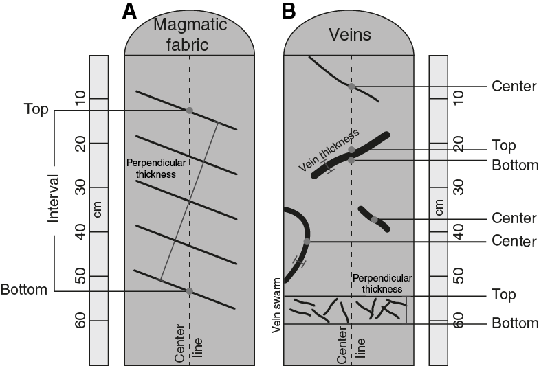
Figure F12. Schematic illustration of structure logging, Expedition 360.
Apparent dip angles of planar features were measured on the split face of the archive half of the core. To obtain a true dip value, a second apparent dip was measured, where possible, in a section perpendicular to the split face (second apparent orientation, in Figure F13B). The two apparent dips and dip azimuths (or one apparent direction combined with the strike) measured for each planar feature were used to calculate the dip (between 0° and 90°) and dip azimuth (between 0° and 360°) (i.e., the bearing of maximum dip in the CRF). If the feature intersected the upper or lower surface of the core piece, measurements of the strike could be made directly in the CRF, recorded as the trend of a line with zero dip angle (i.e., strike), and combined with an apparent dip measurement, measured on the cut surface of the core, to calculate the true dip and dip azimuth in the CRF (Figure F13C). If a feature was exposed on the surface of the core (i.e., a fracture defining the top or bottom of a piece), the true dip and dip azimuth were measured directly on the feature with no need for another measurement or a calculation. All structural measurements made on the core were reported in DESClogik. True dip and dip azimuth in the CRF were calculated using a macro in Microsoft Excel written by Michael Cheadle for Leg 209 or the Stereonet 9.04 program developed by Allmendinger et al. (2011) and Cardozo and Allmendinger (2013) and imported into the various Structure worksheets within the macroscopic workbook in DESClogik. Where linear structural elements were observed (i.e., such as slickenlines on a fault), the trend and plunge of the lineation were measured directly, relative to the CRF. The sense of shear on fault surfaces is determined by structures such as groove marks or steps in the slickensides. Senses of shear for magmatic fabrics and CPFs were determined using the asymmetry of rotated crystals, porphyroclast-tail systems, or foliation deflection morphologies (e.g., Ramsay and Huber, 1987).
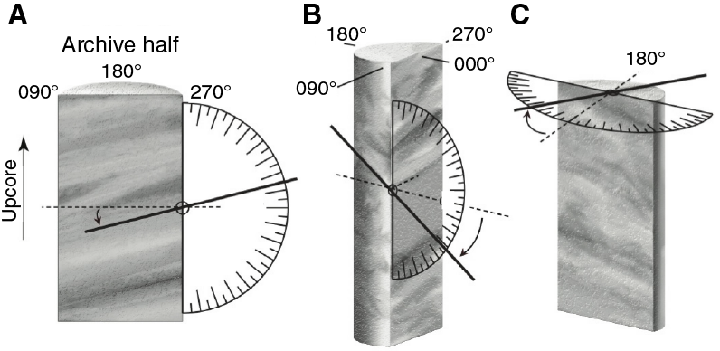
Figure F13. Reference frame and measuring the orientation of planar features, Expedition 360.
Statistical analysis of true-dip vein and fracture data
Statistical analysis of the true dip of discrete planar features, with small lengths compared to the length of the borehole, such as veins and fractures, requires an understanding of two geometrical effects classified as follows and defined below:
- The length-scale or spherical effect, which leads to overrepresentation of steeply dipping planar structures.
- The so-called borehole effect, which leads to preferential sampling of shallow-dipping planar structures compared to more steeply dipping structures.
The length-scale or spherical effect
A purely random distribution of planes represented by poles within any given area on a unit hemisphere will, on average, contain the same number of poles, irrespective of the position on the unit sphere. Within any given dip interval, the number of poles is a function of the number of poles intercepting the corresponding arc on the unit sphere. By integration it can be shown that the number of planes (n) with a given dip (α) is obtained by
where C is a constant. The resultant distribution for a theoretical random data set is shown in Figure F14. The dip data are biased such that there is an overrepresentation of steeper dips as a result of the spherical geometry effect on the true dip data.
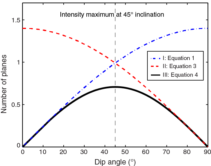
Figure F14. Predicted distribution of a random set of planar features, Expedition 360.
The borehole effect
A further consideration is the effect of sampling bias introduced by the vertical nature of the borehole (see Newmark et al., 1985). If we consider an equally spaced set of horizontal planes, then the number (n) encountered within a unit borehole length (l) is given by
where s is the spacing of the planes. For vertical planes, either 1 or 0 planes are encountered within the borehole. Thus, for the general case of dipping planes:
Thus, this effect tends to bias the data in favor of shallow dips (Figure F14).
Combining the two aforementioned effects results in the following relationship:
where K is a constant (i.e., scaling factor) and the distribution derived from Equation 4 results in a frequency maximum at 45° inclination (Figure F14). Consequently, we present a random distribution curve derived from Equation 4 on all appropriate frequency distribution plots for fracture and vein dips to help assess whether dip distributions are random or nonrandom.
If the length scale of structures such as magmatic contacts, layering, or CPFs considerably exceeds the width of the core, then the length scale or spherical effect does not apply. However, these features are still subject to the borehole effect, so steeply dipping features will be undersampled relative to gently dipping features.
To correct for the aforementioned effects we follow the methodology proposed in Shipboard Scientific Party (1992c). For a more in depth discussion the reader is referred to Martel (1999). Moreover, to allow for a first-order comparison between different dip distributions for different data sets, such as amphibole and carbonate vein dips, we also calculated the Gaussian mean, standard deviation, and skewness for each distribution. In particular, we used the Gaussian standard deviation to quantify the range or width of any dip distribution and not as an estimate on the uncertainty of the mean dip.
Macroscopic core description and terminology
Workflow organization
All descriptions and structural measurements during Expedition 360 were made on the archive halves unless otherwise noted. Whole-round pieces were oriented for splitting prior to curation by a member of the science party, either a Co-Chief Scientist or a member of the structural geology team. Cores were marked and split to maximize the dip of planar structures so that the dominant structure dips toward 090° in the CRF (see Figure F3). Where no obvious structures were present, cores were marked to maximize contiguity and/or to ensure that representative material is present in both working and archive halves of the core. This convention was adopted primarily for ease of structural feature measurement and allows some impression to be gained as to the relative orientation of other structural features, such as amphibole veins and CPFs.
During Expedition 360, the structural geologists worked together on the same shift with each member of the team responsible for making a specific set of observations throughout the entire expedition (e.g., one team member responsible for characterization of CPF intensity). Measurements were made and logged in exactly the same fashion as during Leg 176 so as to be able to compare directly with Hole 735B. For the same reason, structures in Hole 1105A were relogged by Expedition 360 scientists, as conventions adopted for structural measurements during Leg 179 did not always conform directly to those used during Leg 176 or during Expedition 360.
Each core section was described and logged with detailed structural information. This information was then entered into the DESClogik framework. The DESClogik worksheets, listed below, contain data on the interval, type of structure, intensity, orientation, certainty of observation, crosscutting relationships, and comments:
- Plutonic/mantle worksheet: magmatic contact characterization in conjunction with the igneous petrology team, including contact nature and geometry.
- Magmatic fabric worksheet: compositional or grain size layering and magmatic fabrics.
- Crystal-plastic fabrics worksheet: solid-state foliation morphologies, CPF intensity, and shear sense.
- Veins worksheet: alteration and magmatic vein data in conjunction with the metamorphic and igneous petrology teams; includes vein label, morphology, connectivity, texture, structure, vein-wall relationship, and vein crosscutting relationships with other veins and other structural elements.
- Vein and fracture density worksheet.
- Brittle deformation worksheet: fault rock type and intensity, apparent fault offset, and fracture morphology.
The parameter “Certainty of the observed feature” was included to qualify the degree of confidence related to the identification of the logged structure. Uncertain refers to weakly characterized features; likely and certain are related to moderate and well-defined structures, respectively.
The most representative and/or prominent structural features in the cores from Expedition 360 are plotted on the VCD graphic reports (e.g., Figure F5). Prominent structural features include intensity of magmatic fabric and CPF alignment, brittle deformation intensity (fault rock intensity and fracture density), and precise locations of observed prominent structures, such as igneous contacts, magmatic layering and magmatic veins/dikes, alteration veins, vein networks, hydrothermal breccia, fault rocks, and shear veins. The dip and dip azimuth of the magmatic contacts, magmatic fabrics, and CPFs are also plotted on the VCDs.
Short explanations for terms and abbreviations used in the respective structural categories are given below, based on definitions given in Ramsay and Huber (1987), Twiss and Moores (1992), Passchier and Trouw (2005), and Davis et al. (2011).
Magmatic structures
Intrusive and structural contacts were measured and described in accordance with the igneous petrology worksheet (plutonic_mantle) (see Igneous petrology). Descriptions include the following:
- Contact relationship: sharp, gradational, or sutured (contacts where individual mineral grains interlock across the contact).
- Contact geometry: planar, curved, or irregular.
- Orientation: dip and dip azimuth in the CRF.
Magmatic layering, where present, was measured and described in accordance with the magmatic_fabric worksheet in the macroscopic workbook. Descriptions include the following:
- Nature of layering: modal layering, grain size layering, or grain size and modal boundary or contact; when neither term describes the observations well, the nature of layering is described in the comments.
- Layering boundary: sharp, gradational, irregular, planar, curved, or anastomosing.
- Layering intensity rank:
- Perpendicular thickness of the layers.
- Orientation: dip and dip azimuth, where measurable in the CRF.
- Certainty of the observed feature:
Magmatic fabrics were defined by the presence and intensity of any shape-preferred orientation (SPO) of magmatic phases. A magmatic fabric intensity of 0 was attributed to intervals characterized by isotropic texture and/or where no igneous textures are preserved due to crystal-plastic overprint. Descriptions of magmatic fabric were captured in the magmatic_fabric worksheet in the macroscopic workbook and include the following:
- Geometry of magmatic fabric: linear, planar, planar-linear, or anastomosing/irregular.
- Magmatic fabric intensity accompanied by intensity rank (Figure F15):
- Certainty of the observed feature:
- Sense of shear: normal (n), reversed (r), dextral (d), sinistral (s), a combination of these (nd, ns, rd, or rs), or unknown.
- Magmatic phase(s) defining the SPO:
- 1 = olivine.
- 2 = plagioclase.
- 3 = pyroxene.
- 4 = oxide.
- Combinations of two phases (e.g., plagioclase-pyroxene)
- Orientation of the magmatic fabric: dip and dip azimuth as well as trend and plunge of lineation, where measurable in the CRF.
Figure F15. Intensity ranks for macroscopic and microscopic observations, Expedition 360.
Crystal-plastic fabrics
CPFs include planar or linear fabrics defined by crystals exhibiting plastic strain. Descriptions for CPFs were captured in the c_p_fabrics worksheet of the macroscopic workbook and include the following:
- Geometry of CPF: linear (L), planar (S), planar-linear (L-S), gradational, or anastomosing/irregular.
- Six levels of deformation intensity, ranging from undeformed (0), through two stages of foliation and porphyroclast development (1–2), to protomylonitic, mylonitic, and ultramylonitic fabrics (3–5, respectively) (Figure F15). The final characterization of the structure was performed after petrographic inspection, when possible.
- CPF boundary sharpness: sharp or diffuse.
- Sense of shear: normal (n), reversed (r), dextral (d), sinistral (s), a combination of these (nd, ns, rd, or rs), or unknown.
- CPF perpendicular thickness (in centimeters).
- Orientation of the CPF (dip and dip azimuth, where measurable in the CRF; in practice almost exclusively foliation planes).
- Certainty of the observed feature (CPF, peridotite fabric, or sense of shear):
Alteration and magmatic veins
Alteration and magmatic vein descriptions during Expedition 360 were captured in the veins_halos worksheet in the macroscopic workbook. The descriptions include characterization of the vein margin, structure of the vein fill, relative chronology of vein formation, relations with other veins, and crosscutting relationships between veins and other structures. The nature of the alteration vein fill material was identified in cooperation with the metamorphic petrology team. The igneous petrology team determined the vein fill material of magmatic veins. Descriptions of veins include the following:
- Vein type: magmatic, metamorphic, or hybrid (i.e., late magmatic fluid/hybrid metamorphic).
- Vein attitude: horizontal, random, subhorizontal, inclined, steeply dipping, subvertical, or vertical.
- Vein morphology: planar, curved, irregular, vein tip, pull-apart, or fault vein (Figure F16).
- Vein connectivity: isolated, single, branched, network, en echelon, crosscutting, ribbon, parallel, anastomosing, or overlapping (Figure F16).
- Vein texture: massive, cross fiber, slip fiber, vuggy, polycrystalline, crack-seal, sheared, patchy, overgrowth, or brecciated (Figure F16).
- Vein structure: uniform, banded, composite, haloed, or intraveinous (Figure F16).
- Vein-wall rock relationship: gradational, halo, diffuse, or clear cut.
- Vein crosscutting relationships (e.g., V1 > V2).
- Sense of shear: normal (n), reversed (r), dextral (d), sinistral (s), a combination of these (nd, ns, rd, or rs), or unknown.
- Crosscutting relationships with other structural elements, such as shear zones, breccias, and relationships of the magmatic veins and dikes.
- Mean vein perpendicular thickness (in centimeters).
- Vein offset (in millimeters), if present and where measurable.
- Orientation of the vein given by dip and dip azimuth and trend and plunge of associated lineation in the CRF.
- Certainty of the observed veins:
- Vein density (Figure F15):
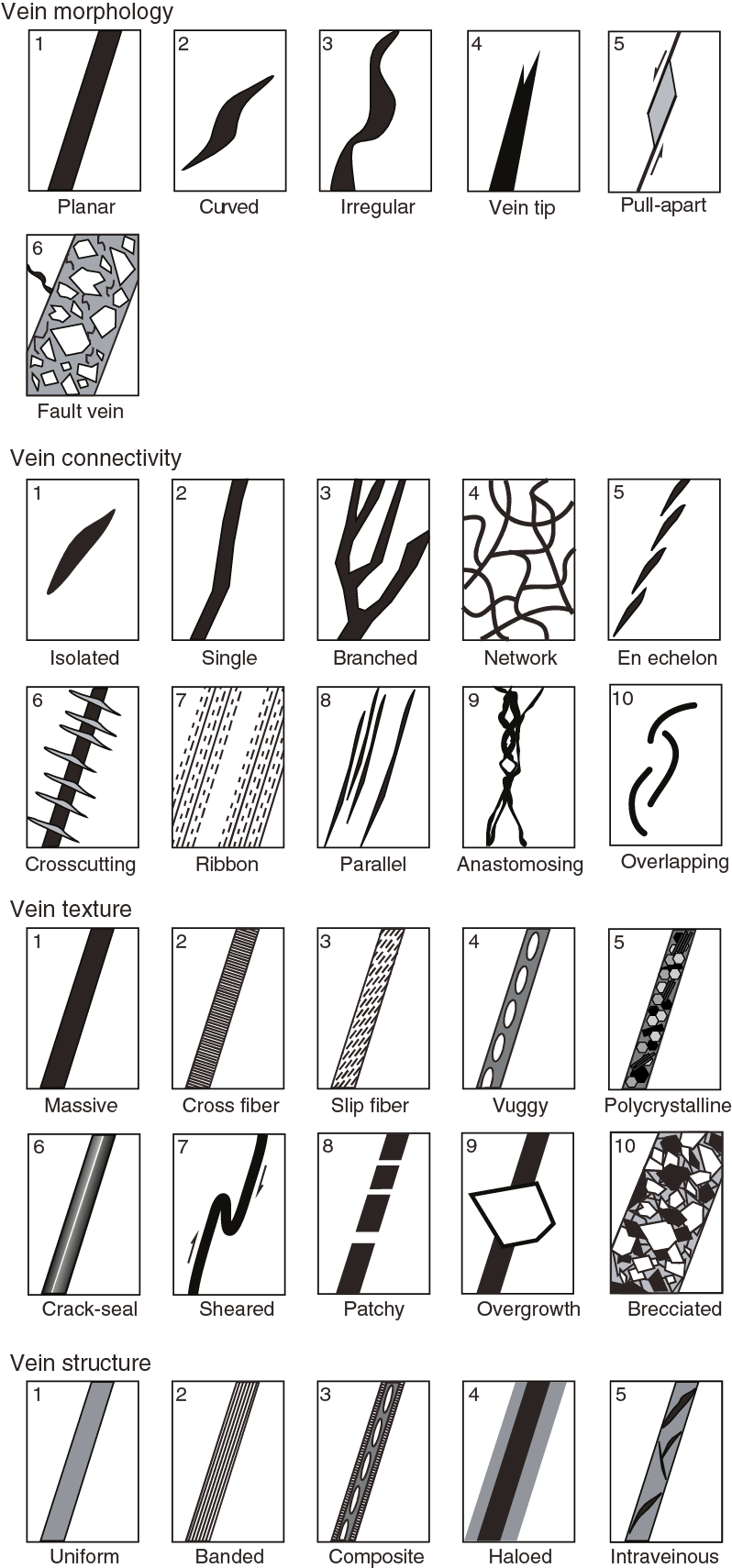
Figure F16. Characteristics of veins and vein network classifications, Expedition 360.
Density of veins (with a density scale across a 10 cm depth interval along the long axis of the core) was recorded in the vein_fracture_density worksheet of the macroscopic workbook.
Brittle deformation
Brittle fabrics described during Expedition 360 include breccias, faults (defined as fractures with shear displacement), and fractures (including open and drilling induced). Drilling-induced fractures are those defined by subhorizontal fractures with rounded edges and no mineralization. The orientation of drilling-induced fractures was not measured; however, their density (number of fractures per 10 cm) was measured. Descriptions are captured in the brittle_deformation worksheet of the macroscopic workbook and include the following:
- Fault rock type: fault gouge, fault breccia, cataclasite, hydrothermal breccia, or pseudotachylite.
- Fault rock cohesion:
- Apparent fault offset (in centimeters), where measurable.
- Sense of shear: normal (n), reversed (r), dextral (d), sinistral (s), a combination of these (nd, ns, rd, or rs), or unknown.
- Deformation intensity for fabrics, based on the percentage of matrix present in each fault rock (Figure F15); thin section descriptions, wherever available, aided this categorization:
- 0 = undeformed.
- 1 = minor fracturing.
- 2 = moderate fracturing.
- 3 = dense anastomosing fracturing and no significant clast rotation, incipient breccia.
- 4 = well-developed fault, breccia, and clast rotation.
- 5 = cataclasite.
- Certainty of the observed fault rock:
- Clast in fault rock (in percent).
- Matrix in fault rock (in percent).
- Average size of clast in fault rock (in millimeters).
- Fracture morphology: planar, curved, irregular, or no open fractures if none were recorded (Figure F17).
- Fracture network morphology: stepped, splayed, or anastomosing (Figure F17).
- Fracture perpendicular thickness (in centimeters).
- Orientation (dip and dip azimuth) of fracture and trend and plunge of associated lineation (e.g., slickensides/slickenlines/slickenfibers).
- Fracture density:
- 0 = no open fracture.
- 1 = <1 fracture/10 cm.
- 2 = 1–5 fractures/10 cm.
- 3 = >5 fractures/10 cm (Figure F15).

Figure F17. Classification of fracture and fracture network morphologies, Expedition 360.
Density of fractures and density of drilling-induced fractures were recorded in the vein_fracture_density worksheet of the macroscopic workbook.
Microstructures
Workflow organization
To better characterize different types of deformation, we studied the microstructural features of interesting and/or prominent mesoscopic structures. Thin sections were examined in order to
- Characterize the microstructure of the rocks,
- Confirm macroscopic descriptions of structures,
- Document crystal-plastic and brittle overprinting of magmatic fabrics,
- Provide information on the kinematics of deformation,
- Identify crosscutting relationships between magmatic and crystal-plastic deformation and alteration processes, and
- Document downhole strain variations.
Shipboard thin sections were systematically oriented relative to the CRF, as marked on each thin section (see Figure F3). Marking two directions is necessary to achieve unambiguous orientation of the thin sections cut parallel to the cut surface of the core. Only one thin section was cut perpendicular to the cut face of the core (Sample 360-U1473A-69R-5, 41–43 cm; TS 240). In this case, the orientation of the y-axis, parallel to 090°, is inscribed on the thin section. Macroscopic observations were refined by the microscopic description. Digital photomicrographs were taken to document microstructures that best illustrate different deformation styles, crosscutting relationships, and intensity recorded in the LIMS database. Microstructural notes were entered into the ts_structures worksheet in the thin section workbook.
Microstructure terminology
We followed the terminology used during Legs 153, 176, and 209 and Expeditions 304/305 (Expedition 304/305 Scientists, 2006) and 345 (Gillis et al., 2014), which broadly follows the terminology of Passchier and Trouw (2005). In the ts_structures worksheet of the thin section workbook, we described the following microscopic features for each thin section:
- Type of microstructure: magmatic, submagmatic/transitional, crystal-plastic, fault rock, or metamorphic.
- Recrystallized grain size: fine (<100 µm), medium (100–300 µm), or coarse (>300 µm).
- Recrystallized grain shape: anhedral, subhedral, euhedral, equigranular, or inequigranular.
- Intensity of static recrystallization: absent, weak, strong, partial, or complete.
- Intensity of magmatic fabric and rank:
- Crystal-plastic subgrain boundaries: straight, curved, serrate, or polygonal.
- Intensity of dynamic recrystallization: absent, weak, strong, or complete.
- Intensity of overall CPF with intensity rank (Figure F15):
- 0 = undeformed.
- 1 = weakly foliated/lineated.
- 2 = strongly foliated/lineated.
- 3 = porphyroclastic/protomylonitic.
- 4 = mylonitic.
- 5 = ultramylonitic.
- Fractures: absent, rare, or common.
- Fault rock clast percent of cataclasite/brittle fracture.
- Size (in millimeters) of clasts in cataclasite/brittle fracture.
- Fault rock intensity and rank (Figure F15):
- 0 = undeformed.
- 1 = minor fracturing.
- 2 = moderate fracturing.
- 3 = dense anastomosing fracturing with incipient breccia.
- 4 = well-developed fault breccia.
- 5 = cataclasite.
- Sense of shear: normal (n), reversed (r), dextral (d), sinistral (s), a combination of these (nd, ns, rd, or rs), or unknown.
- Olivine: grain size, grain shape, grain boundaries, undulose extinction, degree of subgrain development, fracture density, and textural relationships.
- Plagioclase: grain size, grain shape, grain boundaries, twinning, undulose extinction, degree of subgrain development, and textural relationships.
- Clinopyroxene: grain size, grain shape, grain boundaries, undulose extinction, fracture density, and textural relationships.
- Fe-Ti oxides: band/pod geometry, fracture density, and textural relationships.
- Comments: including any minerals and or textures not explained above.
Geochemistry
Shipboard chemical analyses performed on rock samples recovered during Expedition 360 to Atlantis Bank included measurement of major (Si, Al, Ti, Fe, Mg, Mn, Ca, Na, and K) and trace elements (Ni, Cr, Co, Sc, Sr, V, Y, Zr, Zn, and Cu) by ICP-AES. In addition, volatiles in all geochemistry samples were measured by weight loss on ignition (LOI) and by gas chromatography (GC) (H2O, CO2, and S), and CO2 was measured in a subset of 10 geochemistry samples and 9 microbiology samples by coulometry. The geochemistry samples selected for ICP-AES were chosen as representative of the rock recovered from Hole U1473A by the shipboard scientific party and included both fresh igneous lithologies and their altered equivalents. The rock types recovered from Hole U1473A are dominated by olivine gabbro but include oxide gabbros, diabase dikes, and felsic veins with variable degrees of alteration (see Igneous petrology and Metamorphic petrology). A thin section was taken in the vicinity of each geochemistry sample whenever possible in order to precisely determine the modal mineralogy and degree of alteration. The rock names in Table T11 in the Site U1473 chapter (MacLeod et al., 2017b) are therefore based on the thin section descriptions (see Igneous petrology) and are identical to those used elsewhere in this report.
Sample preparation and LOI
Samples were prepared from volumes of 2–10 cm3 of fine-grained basalt and felsic veins and 10–40 cm3 of coarse-grained gabbroic rock. A diamond rock saw was used to carefully cut rock samples from the center of the working-half cores to remove altered rinds resulting from drilling. The samples were then ground on a diamond-impregnated disk to remove saw marks. The resulting sample cuboid was photographed and its approximate weight recorded. It was then cleaned in an ultrasonic bath with nanopure deionized water (18 MΩ·cm) with three consecutive rounds of 15 min. The cleaned pieces were dried for 10–12 h at 110°C.
The dried rock samples were crushed between clean Delrin plastic discs in a SPEX X-press crusher, and the crushed pieces were then ground to a fine powder in a tungsten carbide mill in a SPEX 8510 shatterbox. A check on grinding contamination contributed by the tungsten carbide mills was performed during Leg 206, and contamination was found to be negligible for the elements measured (Shipboard Scientific Party, 2003). However, a systematic analysis of the shipboard powders from Expeditions 304/305 found that a few samples were affected by Co contamination during those expeditions (Godard et al., 2009).
After milling, the powdered sample was split into three portions. An aliquot of 5.00 ± 0.05 g was used to determine LOI, with a 100.0 ± 0.1 mg portion of the devolatilized powder then used for major and trace element analysis by ICP-AES. An aliquot of ~50 mg was used for volatile analysis by GC. The remaining sample powder was retained for shore-based analysis. In addition, ~100 mg aliquots of 10 geochemistry samples and 9 microbiology samples were used for inorganic CO2 analysis by coulometry.
LOI was performed on a 5.00 ± 0.05 g aliquot placed in a quartz glass crucible and weighed on a Mettler Toledo dual balance system immediately after grinding. The sample was heated in a Fisher ashing furnace for 12 h and held at 1025°C for either 4 or 6 h before being weighed a second time. The duration at 1025°C was increased from 4 to 6 h after analysis of the first 72 samples in order to evaluate whether incomplete sample ignition contributed to a poor coherence between LOI and CHNS H2O data. This experiment, considered together with ICP oxide totals routinely close to ~100%, demonstrated that incomplete sample ignition was not responsible for the limited agreement between these techniques (see Comparison of LOI, CHNS, and coulometry).
ICP-AES analysis necessitates digestion of rock powders, which was accomplished using standard shipboard procedures (Murray et al., 2000). Following LOI, 100.0 ± 0.1 mg aliquots of the ignited whole-rock powder were weighed and mixed with 400.0 ± 0.5 mg of preweighed lithium metaborate (LiBO2) flux. Samples and standards were weighed on the Cahn C-29 microbalance (designed to measure on a moving platform). Weighing errors are conservatively estimated to be ±0.02 mg. A 10 µL aliquot of 0.172 mM aqueous LiBr solution was added as a nonwetting agent to the flux and rock powder mixture. Samples were then individually fused in Pt-Au (95:5) crucibles for ~12 min at a maximum temperature of 1050°C in a Tokyo Kagaku Bead Sampler TK-4100 internally rotating induction furnace. After cooling, beads were transferred to 125 mL high-density polypropylene bottles and dissolved in 50 mL of 10% dilution of concentrated trace-metal grade HNO3 (hereafter referred to as 10% HNO3), aided by shaking with a Burrell wrist-action bottle shaker for 1 h. After digestion of the glass bead, the solution was passed through a 0.45 µm filter into a clean 60 mL wide-mouth high-density polypropylene bottle. Next, 1.25 mL of this solution was pipetted into a plastic vial and diluted with 8.75 mL of 10% HNO3 to bring the total volume to 10 mL. The final solution-to-sample dilution factor for this procedure was ~4000. Dilutions were conducted using a Brinkman Dispensette.
ICP-AES
Major and trace element concentrations of standards and samples were determined using a Teledyne Leeman Labs Prodigy ICP-AES instrument. The wavelengths used for the elements analyzed during Expedition 360 and estimated detection limits are provided in Table T3. The ICP-AES plasma was ignited at least 30 min before each analytical run to allow the instrument to warm up and stabilize. After the warm-up period, a zero-order search was performed to check the mechanical zero of the diffraction grating, and solutions containing 10 ppm concentrations of set elements were used to optimize the step positions and emission line backgrounds. The intensity curve for each emission line is defined by 15 measurements, and the Prodigy Salsa software integrates the area delineated by the intensity curve and background. For several elements, measurements were made at two wavelengths (e.g., Si at 250.690 and 251.611 nm; Table T3). For each run, the wavelength yielding the best calibration line was identified and used for determining elemental concentrations (e.g., Figure F18).
Table T3. ICP-AES wavelengths and limits of detection, Expedition 360. Download table in .csv format.
Figure F18. ICP-AES calibration curves determined from rock standards, Expedition 360.
Following instrument set up, solutions prepared from a Li metaborate bead (procedural blank) and seven certified rock standards were analyzed and used for calibration. The selected standards include a peridotite (DTS-1), a gabbro (JGb-1), four basalts (BHVO-2, BCR-2, BIR-1, and JB-2), and a granite (JG-2). Solutions prepared from ~12 to 20 unknown samples and additional standards analyzed as unknowns (DTS-1, MRG-1, and BAS-206) were then analyzed, with BHVO-2 or BCR-2 analyzed after every third or fourth unknown to check for instrumental drift. A 10% HNO3 wash solution was run for 90–120 s between each sample analysis, and every solution was analyzed in either quadruplicate or triplicate. The number of repeat analyses and duplicate emission lines measured (Table T3) was reduced during the expedition to shorten run times and thereby limit instrumental drift and wear on the instrument’s nebulizer. The SeaSpray nebulizer available on the ship during Expedition 360 was prone to blocking after extended use and required frequent replacement, ultimately limiting the number of samples that could be analyzed during the expedition. Leeman Labs recommended a Hildebrand Grid nebulizer as a more robust alternative for future hard rock expeditions.
Data reduction for ICP-AES
The data produced in each sample run was reduced using the Prodigy Salsa software. Raw emission line intensities corrected for background were transferred to a data file and corrected for drift by linear interpolation between drift-monitoring solutions. Calibration lines were obtained between the drift-corrected wavelength intensity and reference concentrations of each element (Figure F18). Concentrations used for the calibrations were compiled from the literature and are on a volatile-free basis (Govindaraju, 1994; Jochum et al., 2005; http://georem.mpch-mainz.gwdg.de; December 2012) (Table T4). At the time of Expedition 360, the Salsa software was not implementing a blank correction. However, data quality evaluated on the basis of oxide totals and the analysis of rock standards analyzed as unknowns in the first analytical run was not improved by manual implementation of a blank correction in Microsoft Excel spreadsheets. Analyses were rejected if volatile-free major element oxide totals were outside the range 100 ± 5 wt%, and an effort was made to repeat analyses with oxide totals outside the range 100 ± 2 wt%. Samples were reanalyzed until they gave oxide totals better than 100 ± 5 or 100 ± 2 wt%. Occasionally poor analyses are expected to result from movement of the ship during analysis; however, weighing or dilution errors could account for repeats with reproducibly bad totals 2–5 wt% from 100 wt%, and some data in this range were accepted and renormalized to 100. These analyses are identified as renormalized and have the original oxide total included in the data sheet.
Table T4. International Rock Geostandards used for ICP-AES measurement calibration, Expedition 360. Download table in .csv format.
ICP-AES detection limits varied between analytical sessions during Expedition 360, with typical values for major element oxides ranging from better than 0.05 to ~0.4 wt% and typical values for trace elements ranging from several tens of ppm to >10 ppm under the most favorable conditions (Table T3). Estimates of accuracy and precision are based on replicate analyses of JP-1, MRG-1, and BAS-206 included in each analytical run (Table T5; Figure F19). For concentrations of more than four times the detection limit, the analytical precision based on the relative standard deviation of all JP-1, MRG-1, and BAS-206 analyses was ±1%–2% for most major elements and ±5% for most trace elements. Accuracy, based on comparison of measured values to recommended values (e.g., Govindaraju, 1994), was better than ~2% for most major elements and 5%–10% for most trace elements. However, accuracy and precision deteriorate for all elements as detection limits are approached, and typical uncertainties for some of the trace elements analyzed are significantly higher than 10% when present at the concentrations typical of gabbro (Table T5). Notably, minimum uncertainties are estimated as 15%–20% for concentrations of <100 ppm Ni and >40% for concentrations of <50 ppm Ni (Table T4; Figure F19). Co and Zn gave good reproducibility of ~5% when present in concentrations well above detection limits but are calibrated relative to standards with systematic discrepancies in their reference values (e.g., Co in Figure F18). Consequently, the concentrations of these elements measured in the three standards analyzed as unknowns also show variable agreement with the recommended reference values (Table T5).
Table T5. Summary of ICP-AES standards analyzed as unknowns during Expedition 360. Download table in .csv format.
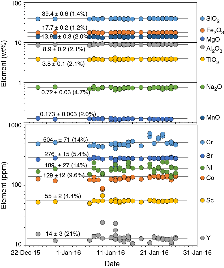
Figure F19. Major and trace element reproducibility in the MRG-1 standard, Expedition 360.
Volatile measurements
The Thermo Electron Corporation CHNS analyzer (Flash EA 1112 Series) gas chromatograph was used to quantify H2O, total C (assumed in most of this report to have been present in the form of CO2 and therefore used to calculate concentrations of the latter), and S in powdered aliquots of almost all shipboard samples during Expedition 360. The instrument was initially tested using a combination of rock standards (MRG-1, BCR-2, and BHVO-2) and sulfanilamide (C6H8N2O2S; 18.6% S). The test run demonstrated that MRG-1 and sulfanilamide lie on common calibration curves for H2O, CO2, and S, and, as the concentrations of H, C, and S in sulfanilamide are stoichiometric, these standards were adopted as reliable calibrants. In contrast to MRG-1, BHVO-2 contains too little CO2 (0.07 wt%) and H2O (0.2 wt%) to be a reliable calibrant, and BCR-2 lies on a significantly different calibration curve for H2O, suggesting its reported H2O content of 1.56 wt% may be unreliable. The instrument was therefore calibrated for all analytical sessions using different sized aliquots of only the MRG-1 and sulfanilamide standards (e.g., Figure F20).

Figure F20. Calibration curves for CHNS analyzer sulfanilamide and MRG-1 standards.
Analytical method
Shipboard powders were placed in a freeze dryer for 12 h and then ~50 mg aliquots were weighed on the Cahn C-29 microbalance, with weighing errors conservatively estimated to be ±0.02 mg. The sample was packed into CHNS tin containers (Universal Tin Container “light”; Thermo Electron P/N 240-06400) and mixed with a spatula full of vanadium pentoxide (V2O5) estimated as 10 ± 3 mg. The samples were placed in a revolving autosampler with 31 spaces and dropped into a 950°C resistance furnace where they were combusted in a reactor. The tin capsule creates a violent flash combustion (Sn has a melting point of only 230°C) and the V2O5 generates an oxygen-enriched atmosphere. The liberated volatiles were entrained by helium gas and carried through a commercial glass column (Costech P/N 061110) packed with a tungsten trioxide (WO3) oxidation catalyst and a copper reducer. The gases were then separated by a 2 m packed GC column (Costech P/N 0581080). During the measuring time of 1000 s, the millivoltage at the thermal conductivity detector was continuously recorded, with CO2, H2O, and S arriving at approximately 94 s (CO2), 250 s (H2O), and 781 s (S).
Analytical runs typically began with a blank consisting of a tin capsule with ~10 mg of V2O5 and five variably sized aliquots of the MRG-1 standard. Thereafter, approximately 20 ~50 mg samples were analyzed, interspersed with additional standards (MRG-1 and sulfanilamide) and blanks. It was found that blanks were minimized and sample carry-over avoided by running bypasses after all samples and standards (a bypass represents an empty space in the autosampler). The blank imposes a strong control on the detection limit of the instrument, which is significant for measurement of CO2 in gabbro. An investigation of six consecutive blanks alternating between 5 and 15 mg sized aliquots of V2O5 demonstrated that CO2 blanks resulting from ~15 mg of V2O5 were on average ~35% higher than those resulting from ~5 mg of V2O5. This compares to typical variation in the blank of 30%–50% in any single analytical session and variations of >100% in the blank between analytical sessions. These results suggests that V2O5 is not the only factor controlling the procedural blank but that CO2 detection limits could be improved by establishing the minimum quantity of V2O5 required to reliably oxidize S in the samples and by weighing uniform quantities of the minimum required into the tin capsule.
The scatter of the standards around the calibration lines for each session represents the maximum attainable precision for any given session. Calculated precision was better than 3%–12% for the calibrated range of H2O and CO2 in all analytical runs but varied from ~20% to as high as 60% for S (e.g., Figure F20). Similar levels of precision of ~5%–10% for H2O and 5%–60% for S were demonstrated by analyzing sample duplicates in multiple analytical runs, whereas the repeatability of CO2 measurements between runs was limited by the instrumental detection limit rather than the calibration (Figures F20, F21). Detection limits are related to the procedural blank and signal-to-background ratio, and as already discussed, instrument blanks varied between analytical sessions. Typical detection limits were ~0.05–0.1 wt% for H2O and CO2 and ~0.02–0.06 wt% for S, but slightly lower detection limits of ~130 ppm C (or 400 ppm CO2) were attained under optimal conditions.
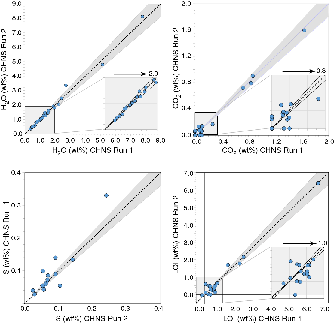
Figure F21. Reproducibility of samples analyzed by CHNS and for LOI, Expedition 360.
Inorganic carbon by coulometry
A UIC CM5015 coulometer was used to quantify CO2 in 9 samples collected by the shipboard microbiologists and 10 samples collected for ICP analyses. This was undertaken to test the feasibility of shipboard organic carbon (OC) analysis in basement rocks and to compare the sensitivity of two different techniques for C measurement. OC can theoretically be determined as the difference between the total carbon (TC) measured by CHNS and total inorganic carbon (IC) measured by coulometry (OC = TC − IC). Alternatively, in cases where precision is too low to distinguish the different types of C with confidence, the techniques can be interpreted as providing independent constraints on CO2, which is likely to be the dominant form of C present in basement rocks.
Sample powders designated for coulometry were dried for 12 h in either a furnace at 110°C or a freeze dryer at ~0.5 mbar, and after drying they were stored in a desiccator until analysis. Aliquots of ~100 mg rock powder were weighed using the Cahn C-29 microbalance, with weighing errors estimated to be ±0.02 mg. The rock powder was then placed in a sealed glass vessel and reacted with 5 mL 2 M HCl to liberate CO2. The evolved CO2 is entrained by N2 carrier gas and carried into a coulometer cell where it forms a titratable acid by reaction with a proprietary solution containing a coulometric pH indicator. A silver anode supplies a titration current to neutralize the acid, and the end point of the titration is determined by the transmittance of light through the coulometric cell measured via a photodetector. The electronics are calibrated to provide an output of C in micrograms that was recalibrated with 0.2–0.3 mg aliquots of NHCO3 or CaCO3 standards at the beginning of each analytical run (Figure F22). The regression of the calibration data determines the maximum precision attainable by this technique. Typically, standards run throughout the session lie on slopes within 2%–4% of the calibration line and samples can be reproduced at this level. However, the standard data can be regressed using either a polynomial or linear regression and the intercept is poorly defined, implying much higher external uncertainty for low concentrations of carbon. As a result, although the instrument can theoretically detect 1 ± 1 µg of C (equivalent to 10 ± 10 ppm C in a 100 mg sample), the external 1σ uncertainty that is relevant for comparing coulometry and CHNS was ~60%–80% for concentrations of <100 ppm C (350 ppm CO2).
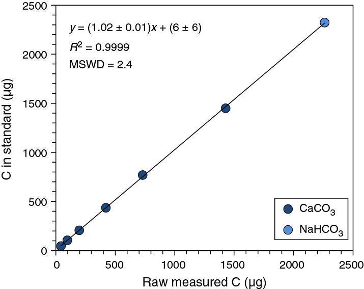
Figure F22. Calibration curve for coulometric C measurement, Expedition 360.
Comparison of LOI, CHNS, and coulometry
Initial results indicated a poor coherence between the total volatiles measured by CHNS and LOI. However, although there is considerable scatter in the data, these parameters are approximately related to one another by the formula H2O wt% ≈ LOI wt% + 0.56 wt% (see Figure F153 in the Site U1473 chapter [MacLeod et al., 2017b]). This relationship indicates that oxidation of Fe2+ to Fe3+ during ignition, which causes a weight gain of 11.1% of the FeO initially present, caused an average weight gain of 0.56 wt% in the sample analyzed. The scatter around the LOI versus H2O correlation line is explained by the low reproducibility of low LOI measurements (Figure F21), the variable Fe content of the samples analyzed (7.9 ± 3.6 wt% Fe2O3T), and variation in Fe2+/Fe3+ of the samples, which must have averaged >0.7 based on the average weight gain and Fe2O3 content of the samples analyzed and the presence of carbonate (see Figure F153 in the Site U1473 chapter [MacLeod et al., 2017b]). Alternative causes for the offset between LOI and CHNS H2O concentrations are not favored because (1) ignited powders analyzed by ICP gave oxide totals close to 100%, demonstrating that the samples were completely dehydrated during all LOI experiments; (2) H2O concentration determined by CHNS was accurately calibrated and had an average reproducibility of ~5% between analytical sessions (Figures F20, F21); and (3) SO2 interference with CHNS H2O measurements, the possibility suggested by Expedition 335 scientists, is very unlikely in typical silicate rocks. The tail of a large H2O peak can mask a small S peak from detection, but the small S peak does not significantly impact the measurement of H2O because more than 95% of the sample’s H2O comes through the chromatographic column before S.
The CHNS CO2 measurements are demonstrated to have a precision comparable to H2O at high CO2 concentrations (Figures F20, F21), but they have much lower reproducibility at concentrations of less than ~0.3 wt% CO2, which is typical of most of the gabbros investigated (Figure F21). These data indicate that reliable determination of OC by combining shipboard CHNS and coulometric data can only be expected in samples with more than ~0.5 wt% CO2 (equivalent to ~1300 ppm C), which is compatible with experience on sediment projects. However, OC can potentially be determined at lower concentrations under favorable conditions if the CHNS procedural blank is minimized and measurements are duplicated. Coulometry can be used to measure CO2 in samples with TC equivalent to less than the CHNS detection limit of ~500 ppm CO2. However, new standards with low C concentrations in the same range as typical low C samples analyzed from these gabbros and other sample types cored by the JOIDES Resolution (e.g., hundreds of ppm) are required to improve the external precision of this technique at low C concentrations.
Microbiology
Rock sampling
For microbiological studies, whole-round core samples are required in order to have enough material to work with while avoiding contamination introduced by sample handling before and during the core splitting process. Whole rounds were sampled in the splitting room after the core was brought in from the catwalk. Technicians wore gloves and shook the core into a split core liner that had been sprayed with ethanol to reduce the chances of contamination. The microbiologist then selected a whole-round section for sampling with the Co-Chief Scientist on shift or a member of the petrophysics team. An ideal sample was one that had some indication of fracturing (such as visible veins) but that had not split apart during the dislocation, nor was it a unique lithology that would be critical to the core description team. Both the microbiologist and the geologist taking part in sample selection wore gloves sprayed with ethanol and a facemask to limit possible contamination of the sample from human contact. The microbiologist wore either a closed-sleeve laboratory coat or a Tyvek suit. The whole-round rock sample chosen for dedicated microbiology investigation was then transferred into a sterile Whirlpak bag and transported to the microbiology laboratory for processing.
Once in the microbiology laboratory, the whole-round sample was rinsed four times in sterile water (changing the Whirlpak bag once after the second rinse) to reduce contamination from drilling fluid. The sample was then transferred to an ethanol-sterilized metal rock box placed within a positive pressure clean area constructed of Plexiglas with a vinyl entrance curtain and skirt and incorporating a HEPA air filter (Figure F23). The outside of each core was sprayed with 75%–95% ethanol, wiped with Kimwipes, and then sprayed one final time with ethanol and left to air dry (~5 min). During the drying time, photographs of each side of the whole-round sample were taken while it was sitting in the rock box. At all stages of the process, samples were handled as little as possible and with gloved hands only. Masks, gloves, and a laboratory coat or Tyvek suit were worn by those handling the sample during whole-round cleaning and all subsequent steps.
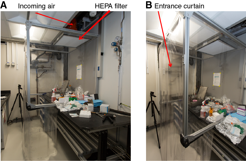
Figure F23. Clean area designed for microbiology sampling, Expedition 360.
Prior work has shown that the interior of rock cores is generally free from contamination (Lever et al., 2006). Therefore, efforts were taken to sample only the interior of the cores. Sections that showed some sign of alteration or fluid flow conduits were specifically chosen because these are the most likely locations for microbial life.
Microbiology samples on average were 10–20 cm long. Sample material was divided into subsamples for a variety of tests. All inclusive, these tests include shore-based cell counts, molecular biology (DNA, RNA, and lipid extraction), thin section analysis, SEM, Raman analyses, stable isotope analysis (δ13C), shipboard initiation of fungal and prokaryotic enrichment cultures, shipboard initiation of nutrient addition bioassays, shipboard measurements of total inorganic carbon (TIC) and TC, adenosine triphosphate (ATP) quantification, and shipboard initiation of exoenzyme assays. For every sample, subsamples were collected for cell counts; TIC, TC, and DNA analyses; thin section preparation; and ATP quantification. Subsamples were collected for other analyses depending on material available.
After cleaning the exterior of whole-round core samples, the rock was split with a sterile chisel and core interiors were subsampled for the above-mentioned tests. An ethanol-sterilized titanium chisel was used to separate the core exterior from the interior of large pieces. Samples for RNA analysis were taken first and immediately frozen at −80°C. Whenever pieces of the whole-round core remained after collection of material for analyses, those and the outer portions of the core that were removed were returned to the curator to be placed back into the working and archive halves. Following completion of sample processing, all tools and the rock box were cleaned with water. They were then brought back into the sampling enclosure and sprayed with 75% ethanol, wiped with Kimwipes, then sprayed with 75% ethanol again, and allowed to air dry. The bench top was also sprayed with 75% ethanol, wiped with Kimwipes, sprayed once more, and allowed to air dry. Periodically, the inside walls of the enclosure were sprayed with 75% ethanol and wiped down; although a film was observed when this was done to the outside of the enclosure, this was never observed on the inside of the enclosure.
Contamination testing of drilling fluid
As part of the drilling process, a huge amount of surface seawater is injected into the borehole. This is the major potential source of microorganism contamination of the cores. As a check for intrusion of drilling fluid into core samples, the microbial composition of drilling fluid (primarily composed of surface ocean water) will be assessed postcruise via DNA sequencing approaches. We collected samples of the drilling fluid for microbial community iTAG small subunit ribosomal RNA gene diversity analysis at the start of drilling during Expedition 360 and then again at periodic intervals. These samples were collected directly from the injection pipe on the rig floor into sterile bottles with screw caps and handled using sterile equipment. Organisms found to be present in both the drilling fluid and rock samples will be considered a sign of contamination. Although it is possible that some taxa found in surface ocean water may also survive in the deep subsurface biosphere, these organisms will be conservatively interpreted as contaminants, not subsurface residents. Any samples where all of the organisms detected during postcruise analyses are also detected in the drilling fluid will be excluded from further analysis. Consistent with a recent study of deep subsurface sediments (Inagaki et al., 2015), we feel a conservative approach is most appropriate. Our 1 L samples of drilling fluid were filtered onto 45 mm 0.20 µm pore-size Millipore Express Plus polycarbonate filters and frozen at −80°C for shore-based DNA extraction and analysis. Samples of drilling mud, or sepiolite, were collected twice during drilling. Samples were collected on the rig floor prior to injection into the drill pipe into two sterile 50 mL polypropylene Falcon tubes (Corning, Inc., USA) and frozen at −80°C for shore-based DNA extraction.
Previous cruises have used perfluoromethylcyclohexane (PMCH) injected into drilling fluid to try to quantify intrusion of drilling fluid into the interior of samples (Smith et al., 2000; Lever et al., 2006; Inagaki et al., 2015). After flaming the sample upon recovery to volatilize the PMCH and release it into the air, PMCH is typically rendered undetectable in the sample. A piece of the interior of the rock is then placed in a serum vial and crimped. The vial is heated to volatilize any PMCH present and the quantity of PMCH that may be present in the interior sample is detected using GC. Any PMCH detected on the interior of a whole-round sample is interpreted to mean drilling fluid was able to penetrate into the sample, and the sample is thus contaminated.
Although good in theory, PMCH is extremely volatile, and once a few samples have been processed in the laboratory, the tracer is subsequently detected in most samples tested because it remains in the air in the laboratory. Working inside the new positive pressure, filtered air enclosure does not prevent the clean interior sample from being contaminated by any remaining volatile tracer on core exteriors during the processes of removing the exterior core material and sample collection. Therefore, while working inside the “clean room space” prevents contamination from nonin situ microbes, it does not prevent contamination from volatile tracer, which can be released from the exterior rock while processing and remain in the airspace within the enclosure. We tested a new, less volatile tracer, perfluoromethyldecaline (PFMD) during Expedition 360 in the hopes that it would be less likely to be detected in background samples due to its lower volatility and the lower likelihood that it would escape into the laboratory air and remain there during future sampling. PFMD is produced in Russia and was difficult to secure in sufficient quantities prior to the expedition to run with every core. Enough tracer was therefore only available to run during drilling of 8–10 cores (i.e., enough for approximately one sample for every 100 m cored). Because of the volatility of PMCH and because new calibrations of the gas chromatograph were necessary for quantifying the PFMD vs. PMCH, we only ran PMCH during the drilling of three cores toward the end of Expedition 360, after we had used all the PFMD available.
PFMD was added to the drilling fluid at a rate of 1–2 mL/min. For contamination tests of whole-round samples, a fragment of the exterior of each core sample prior to cleaning was transferred to a 20 mL headspace glass vial with metal caps and Teflon seals for detection of PFMD. This sample provided a baseline for the level of contamination present prior to cleaning. When possible, we collected pebbles from the core liner in the splitting room instead of generating fragments of the core exterior from the microbiology whole round. This ensured that the rock samples measured for PFMD were completely exposed to the PFMD, whereas when sampling from the whole round, one inevitably includes portions of the rock interior just behind the outside wall that were not exposed. Sampling of the exterior of the whole round was also conducted following cleaning of the core sample exterior and then again for an interior sample. For several core samples, we ran each analysis (interior, exterior before cleaning, and exterior after cleaning) in triplicate, and we additionally tested the concentrations of tracer in drilling fluid several times. Detection of the tracer in rock chips was measured after heating at 70°C for 5–10 min in an oven to evaporate and release the tracer. Headspace samples were injected into a Hewlett Packard 5890 gas chromatograph for measurement after preparing and running calibration standards using 10−4, 10−6, 10−8, and 10−10 dilutions of the tracer.
ATP quantification
For quantification of ATP in rock samples, we collected 0.1 cm3 of powderized rock into a 1.5 mL centrifuge tube, which was stored at 4°C until performing the ATP assay. We ran samples in batches to preserve assay reagent (since standards are run with every batch, running fewer batches reduced the overall number of standards run during the expedition), which meant that samples were stored at 4°C for up to a few days (never more than 4 days) prior to reading. However, no difference in quantification was noted for samples read immediately and those run days later. To the 0.1 cm3 powderized rock, we added 200 µL of autoclaved Milli-Q water, vortexed for 60 s, and then spun the tube at 2000 rotations/min for 1 min in a benchtop microcentrifuge. The commercial kit Adenosine 5′-triphosphate (ATP) Bioluminescent Assay Kit (Sigma-Aldrich, St. Louis, MO) was used for quantification in a Turner TD20/20 Luminometer, which was available in the JOIDES Resolution microbiology laboratory. Acid-cleaned (10% HCl) glass vials were used for measurement. As per the manufacturer’s suggestions, 0.1 mL of ATP assay mix was added to the glass vials and allowed to sit for 3 min prior to adding sample. During this period, any ATP present in the vial would be hydrolyzed and therefore not quantified; luminescence fades quickly for the ATP assay, so 3 min is adequate to remove any existing ATP signal in the tube prior to adding sample. After 3 min, 0.1 mL of the supernatant from the 1.5 mL centrifuge tube was added to the assay vial, the vial was swirled briefly and then immediately placed in the luminometer, and the sample was read. The raw signal reported in Table T14 in the Site U1473 chapter (MacLeod et al., 2017b) includes a correction factor of 3× the instrument reading to account for the dilution of the sample with Milli-Q water during processing. Occasionally, rock powder absorbed the water so much that <0.1 mL of supernatant was available for the reading. In these cases, an additional 0.1 mL of Milli-Q water was added to the tube, it was respun, 0.1 mL was used for the assay, and the correction factor changed to 4×. Raw luminescence was converted to pg/mL ATP by running 0, 1, and 10 pg/mL standards, diluted from the ATP standard included in the kit, with each batch of samples. To preserve ATP assay mix for use during the duration of the cruise (it is light sensitive and breaks down over time), we split aliquots of the ATP assay mix into 1.5 mL centrifuge tubes after thawing it initially and froze all the tubes save for one, which was used as the working mix until no more remained and then another tube was removed from the freezer and used. The working mix was stored at 4°C in the dark.
Molecular biology
DNA
For DNA analyses, we collected 15–50 g samples and froze them at −80°C. These samples will be analyzed during postcruise research.
RNA
Samples (rock chips) were placed in sterile 50 mL Falcon tubes and immediately stored at −80°C. We added LifeGuard Soil Preservation Solution (MoBio Laboratories, Inc., Carlsbad, CA) to some of the RNA samples prior to freezing. For RNA analyses, we collected ~50 g of sample. LifeGuard protects the viability of microbial cells while keeping them in stasis, allowing for efficient DNA and RNA extractions from samples collected in the field. These samples will be analyzed during postcruise research.
Lipids
For analyses of lipid biomarkers, ~50 g samples were placed in sterile 50 mL Falcon tubes and frozen at −80°C for postcruise analysis.
Cultivation experiments
Based on prior work with both subsurface and surface exposed basalts, the functional groups of microbes likely to be found in the subsurface at Atlantis Bank include sulfur oxidizers, sulfate reducers, methanogens, iron reducers, and fungi (Cowen et al., 2003; Mason et al., 2009, 2010; Santelli et al., 2009). Media were prepared targeting enrichment of these groups during the cruise and used to culture subsurface microbes. Details of the media recipes can be found in Tables T6 and T7.
Table T6. Media used for culturing fungi, Expedition 360. Download table in .csv format.
Table T7. Media used for culturing prokaryotes, enzyme assays, and enrichment incubations, Expedition 360. Download table in .csv format.
Fungi cultivation experiments
For fungal enrichments, ~2 g of crushed (powdered) rock were mixed 1:5 with anaerobic sterile artificial seawater (ASW) in a sterile 15 mL Falcon tube, and 100 µL of this slurry was removed using a sterile pipette tip and spread aseptically on the surface of media plates with autoclaved glass spreaders. Three different media were prepared (Table T6), with and without addition of antibiotics. Three plates of each type (n = 6) were inoculated; one plate was placed at 4°C, one at 10°C, and one at 20°C. A control plate of each medium type (n = 6) was left exposed (lid off) within the positive pressure, filtered air enclosure during inoculation of media. These plates were then covered, sealed with Parafilm, and stored at room temperature for the remainder of the cruise to monitor for contamination. The remaining slurry was transferred to a 30 mL glass Hungate bottle with a rubber septum and topped up with ASW, leaving a ~30% headspace that was gassed with biomix gas (a 90%:5%:5% N2:CO2:H2). Bottles were stored at room temperature for continuation of shore-based fungal culturing.
Prokaryotes cultivation experiments
Prokaryote enrichment cultures were initiated from the same starting inoculum as used for the fungal cultures; 100 µL of ASW/powdered rock slurry was transferred to a glass vial and 3 mL of ASW was added. Duplicate vials were established for each targeted group according to the media recipes in Table T7: autotrophic sulfur-oxidizing bacteria, heterotrophic sulfate-reducing bacteria, heterotrophic methanogens, and heterotrophic Fe-reducers. After addition of each medium to the slurry (leaving ⅓ volume headspace), each vial was sealed with a thick butyl stopper and crimped. Headspaces were flushed with nitrogen gas or with a 90%:5%:5% N2:CO2:H2 gas mix according to Table T7. All enrichment cultures were stored at 10°C and shipped to labs on shore for postcruise analysis. Growth is expected to be slow, and therefore several months will be allowed before checking for the presence of cells via microscopy. For all enrichments that prove successful, further steps will be taken to isolate and characterize pure cultures of microorganisms during postcruise research.
Nutrient addition experiments
Little is known about limiting factors for growth in subseafloor plutonic basement because of the difficulty of sampling this environment and the typically low biomass. We used a nutrient addition bioassay approach to assess whether added inorganic nutrients and/or organic carbon can stimulate growth of in situ microbial communities. Microcosm experiments in 30 mL serum vials were used for this purpose, with anaerobic ASW as the basal media for all enrichments. Four conditions were tested:
- No added nutrients (control).
- Added 750 µM NH4Cl.
- Added 750 µM NH4Cl and 50 µM K2HPO4.
- Added 200 µM each of acetate, formate, and lactate.
Concentrations of NH4Cl and K2HPO4 were chosen to be roughly 10–15 times the predicted in situ concentrations. To initiate enrichments, 1–5 mL of crushed rock chips, depending on sample availability, was transferred to 30 mL serum vials and submerged in anaerobic ASW to a level equivalent to 27 mL total volume (crushed rock plus media). After the appropriate additions were made to the vials, they were sealed with butyl stoppers and gassed with a mixture of 90%:5%:5% N2:CO2:H2. This procedure will allow for quantitative analysis of methane during postcruise research. Enrichments were stored at 10°C for the remainder of the cruise and will be analyzed 6 months or more postcruise to allow for sufficient growth.
Cell counts
A total of 4 mL of paraformaldehyde (4% solution in 100 mM phosphate-buffered saline [PBS]) was added to autoclaved 7 mL plastic tubes, and 1 mL of powdered rock material was added to each tube, bringing the total volume to 5 mL. Two replicate tubes were prepared for cell counts from each sample, and, when possible, vein material only was aliquoted into one sample and whole-rock powder into the other. Preserved samples were stored at 4°C for onshore analysis using a density gradient separation of cells from rocks. The protocol is adapted from Morono et al. (2013).
Exoenzyme measurements
Hydrolytic exoenzymes are indicators of metabolically active microbes and have been used to measure community metabolic rates in subsurface environments (Coolen and Overmann 2000; Engelen et al., 2008) and on marine basalts (Jacobson Meyers et al., 2014). Data exist from multiple environments for comparison, making exoenzyme activity a valuable form of data for cross comparison between multiple environments and data sets (Jacobson Meyers et al., 2014). During Expedition 360, we measured the activities of the following exoenzymes:
- Alkaline phosphatase, which cleaves inorganic phosphate from organic phosphate esters (C-O-P bond);
- Leucine-aminopeptidase, which cleaves proteins and peptides into smaller fragments with a preference for cleavage at leucine residues;
- Arginine-aminopeptidase, which cleaves proteins and peptides into smaller fragments with a preference for cleavage at arginine residues; and
- Esterase, which cleaves small esters from glycerides.
All exoenzymes were assayed using fluorogenic substrates, which are nonfluorescent until the specific functional group is cleaved from the fluorescent moiety. For example, 4-methylumbelliferyl phosphate (MUF-P) is nonfluorescent until the phosphate molecule is cleaved, creating the fluorescent molecule 4-methylumbelliferone (MUF). Exoenzyme activity is linear when measured at saturating substrate conditions. To determine an activity rate, two to three time points are analyzed in order to measure the increase in fluorescence over time. A standard curve is run at the time of every reading to determine the absolute amount of substrate cleaved. The slope of the curve is therefore a rate in nanomoles per gram of rock per hour (nmol/[g·h]). After the last time point, the rock chips used in the assay are dried in a drying oven and weighed to allow for normalizing activity rate to grams of rock.
During Expedition 360, assays for exoenzymes were performed using the following substrates at the following concentrations:
- Alkaline phosphatase-4-methylumbelliferyl phosphate: 50 µM
- Leucine-aminopeptidase-L-leucine-7-amido-4-methylcoumarin hydrochloride: 100 µM
- Arginine-aminopeptidase-L-arginine-7-amido-4-methylcoumarin hydrochloride: 100 µM
- Esterase-4-methylumbelliferyl acetate: 100 µM
These concentrations were chosen according to information provided by a literature review of exoenzyme studies performed on sediments and basalts and represents best available estimates of saturating conditions. To quantify enzyme activity, standard curves of the fluorophores MUF and 7-amino-4-methylcoumarin (AMC) were run for the methylumbelliferyl substrates and the peptidase substrates, respectively.
Assays were initiated by adding 1 cm3 of powdered rock chips to an 8 mL serum vial, and the sample was submerged in 5 mL of anaerobic ASW (6 mL final volume) (Table T7). Substrate was added to the final concentrations indicated above, and the serum vial was then sealed with a butyl stopper and crimped. Vials were gassed with a 90%:5%:5% N2:CO2:H2 gas mixture for 3–5 min after crimping to ensure that incubations were anaerobic. A subsample of 700 µL of each slurried sample was withdrawn with a sterile syringe to a 1.5 mL Eppendorf tube after setup but before sealing the vial; this sample served as T0, with triplicate 200 µL technical replicates. These 700 µL samples were briefly centrifuged (120 s at 2500 rpm) and the supernatant used for the T0 analyses. Two additional samples were taken after at least 2 weeks and then again after 4–6 weeks to generate a slope of activity.
Fluorescence of MUF and AMC is greatest at pH 10, so 25 µL of 400 mM NaOH (final concentration 40 mM) was added to the wells to be read; 25 µL of 1 M ethylene diamine tetraacetic acid (EDTA) was added as well (100 mM final concentration) to prevent precipitation of carbonate from sampled veins (Coolen and Overmann, 2000). Fluorescence was measured in triplicate for each vial on a Tecan Spark 10M Fluorescence microplate reader with an excitation wavelength of 380 nm and emission of 454 nm for all substrates and standards.
Paleomagnetism
During Expedition 360, routine shipboard paleomagnetic and magnetic anisotropy experiments were carried out. Remanent magnetization was measured on archive section halves and on discrete cube samples taken from the working halves. Continuous archive section halves were demagnetized in an alternating field (AF), whereas discrete samples were subjected to stepwise AF demagnetization, thermal demagnetization, or a combination of low-temperature demagnetization followed by either AF or thermal treatment. Because the azimuthal orientations of core samples recovered by rotary drilling are not constrained, all magnetic data are reported relative to the CRF (Figure F3). In this system, +x points into the working section half (i.e., toward the double line), +z is downcore, and +y is orthogonal to x and z in a right-hand sense. Therefore, +x corresponds to 000° and +y to 090° in the CRF, as also used by the structural geology team. Magnetization directions of samples were determined using principal component analysis (PCA) (Kirschvink, 1980) and analyzed using inclination-only statistics (McFadden and Reid, 1982).
Archive section half remanent magnetization data
The remanent magnetization of archive section halves was measured at 2 cm intervals using the automated pass-through direct-current superconducting quantum interference device (DC-SQUID) cryogenic rock magnetometer (2G Enterprises model 760R). An integrated inline AF demagnetizer (2G model 600), capable of applying peak fields up to 80 mT, was used to progressively demagnetize the core. For measurements on legacy archive section half samples from Hole 1105A, which had been previously demagnetized to 20 mT during Leg 179 shipboard operations, initial magnetizations were measured and samples subsequently demagnetized at 20, 25, 30, 35, 40, and 50 mT. A limited set of archive section halves were treated at higher fields (60 and 80 mT), but this resulted in no increase in data quality and was discontinued to reduce measurement times and increase core flow through the SRM. For archive section halves from Hole U1473A, natural remanent magnetization (NRM) was measured and then demagnetized in 5 mT steps up to 40 mT and at 50 mT.
For strongly magnetized igneous rocks, the maximum intensity that can be reliably measured (i.e., with no residual flux counts) is limited by the slew rate of the sensors. Previous expeditions have established that with a track velocity of 2 cm/s it is possible to measure archive section halves with a magnetization as high as ~10 A/m (Expedition 304/305 Scientists, 2006; Expedition 330 Scientists, 2012), so this track velocity was used during Expedition 360. The compiled version of the LabView software (SRM Section) used during Expedition 360 is SRM version 354.
The response functions of the pick-up coils of the SQUID sensors have a full width of 7–8 cm at half height (Parker and Gee, 2002). Therefore, for core samples collected by RCB drilling, data collected within ~4 cm of piece boundaries (or voids) are significantly affected by edge effects. Consequently, data points within 4 cm of piece boundaries were filtered out prior to further processing. To further reduce artifacts, any pieces smaller than 8 cm were removed from section trays prior to measuring/demagnetizing and replaced afterward.
During measurement of Sections 360-U1473A-2R-1 through 6R-1 it was noted that peak magnetization intensities for isolated, short (~10 cm) pieces, measured with adjacent smaller pieces removed, appeared to be offset by 2.0 cm from the piece center. In checking data measured prior to this from isolated archive-half samples from Hole 1105A, it was found that ~50% of such pieces had peak intensities located at offset depths 2.0 cm lower than the piece center offset, suggesting a systematic effect that cannot be entirely attributed to sample heterogeneity. An experiment was conducted by measuring a point magnetic source with the dipole aligned parallel to each of the SRM SQUID sensor axes in turn. Results demonstrated a consistent offset of the SQUID sensor response by 1.0 cm relative to the known position of the point source (Figure F24A), indicating an incorrect value for the offset of the SQUID sensors in the SRM initialization parameters. Adjusting this value by 1.0 cm (from a SQUID offset of 255.2 cm to 256.2 cm) resulted in peak responses at the correct location (Figure F24B). Importantly, before this correction, the software returned an inclination of the dipole sample that was ~9° too shallow (Figure F24C) but returned an inclination exactly equal to the known value after adjustment (Figure F24D). We suggest that testing the SRM configuration in this way be performed at the start of all IODP expeditions, using an appropriate standard sample. We chose not to apply this 1.0 cm correction to the entire Hole 1105A SRM data set as the data had already been collected, processed, and statistically analyzed. This SQUID offset should have no significant effect on the inclination data results given in Figure F50 and Tables T4 and T5, all in the Hole 1105A redescription chapter (MacLeod et al., 2017a).
Figure F24. Adjustment of SQUID location in SRM software located at an offset of 13 cm in the tray, Expedition 360.
Remanent magnetization directions were calculated for each 2 cm measurement using PCA (Kirschvink, 1980). From a time perspective, it was impractical to achieve this by manually inspecting each individual orthogonal vector plot to identify linear components. Instead, an automated approach was used, as follows:
- A modified version of the MacPaleomag software (written by Jeff Gee, Scripps Institution of Oceanography) was used to automatically pick components using either the 25–40 mT (Hole 1105A) or 25–50 mT (Hole U1473A) AF demagnetization data (not anchored to origin). The modified software also allowed calculation of median destructive field (MDF) and the deviation angle (Dang) (Tanaka and Kobayashi, 2003; Tauxe and Staudigel, 2004) between the PCA and a line connecting the center of mass of the data and the origin, in addition to the maximum angular deviation (Kirschvink, 1980) of the PCA vector.
- All PCA picks with maximum angular deviation values >10° were rejected to ensure statistically acceptable linearity of components.
- Picks with Dang > 10° were also rejected to ensure the PCA is directed toward the origin and represents a stable remanence direction.
In the case of Hole 1105A, final quality filtering was achieved by rejecting components from samples with the lowest coercivities (MDF < 25 mT), to ensure that samples with a strong viscous overprint were removed. Note that all Hole 1105A samples had been previously demagnetized to 20 mT during Leg 179; hence, initial magnetization measurements of these archive section halves during Expedition 360 do not represent NRM values and the calculated MDF values are likely overestimates.
The intensity reported for such PCA directions represents the length of the projection of the lowest and highest treatment vectors used in the PCA calculation onto the best-fit direction. Because the origin is not included in the PCA calculation and the remanence remaining after the highest treatment may potentially be significant, resulting characteristic remanent magnetization intensity values will be systematically lower than those derived from the remanence at the lowest demagnetization step adopted for the PCA calculation.
Discrete sample remanent magnetization data
All discrete samples taken from working section halves for shipboard magnetic analysis were 8 cm3 cubes. Although standard 2.5 cm diameter minicores are more commonly used, cubic samples were preferred, as they should have a more precisely determined vertical reference (based on a saw cut perpendicular to the core length) than minicores, where the arrow on the split-core face must then be transferred to the long axis of the sample.
Remanent magnetization of discrete samples was measured exclusively with the JR-6A spinner magnetometer. This approach was adopted following tests of the reliability of discrete measurements on the 2G SRM conducted during Expedition 335 that showed significant scatter in remanence directions measured in different sample orientations (Expedition 335 Scientists, 2012). For samples measured on the spinner magnetometer, the automated sample holder was used, providing the most accurate discrete sample remanent magnetization directions and intensities. Measurements of the empty automatic sample holder after subtracting the stored holder magnetization yielded intensities on the order of 10.0 × 10⁻⁶ A/m, representing the practical noise limit of the system.
Stepwise AF demagnetization of discrete samples was performed using the DTech AF demagnetizer (model D-2000), capable of peak fields up to 200 mT. The residual magnetic field at the demagnetizing position in this equipment was ~40–75 nT. Samples were AF demagnetized at peak fields of 2.5, 5, 7.5, 10, 15, 20, 25, 30, 35, 40, 50, 60, 80, and 100 mT. Additional steps up to 200 mT were applied as needed. The orientation of sample axes was alternated with each successive step from +x, +y, +z to −x, −y, −z in order to detect any anhysteretic remanent magnetization acquired during the demagnetization process.
Thermal demagnetization of discrete samples was performed using an ASC Scientific thermal demagnetizer (model TD-48 SC), capable of demagnetizing samples up to 700°C. The total magnetic field along the length of the TD-48 SC access tube is illustrated in Figure F25, demonstrating that the sample chamber from 33 cm onward (measured from the edge of the access opening) has a maximum field of <50 nT. Each sample boat for thermal demagnetization included as many as 36 samples, and sample orientations were changed between each successive step to allow any magnetic interaction between adjacent samples to be identified. Samples were heated in 50°C steps from 150°C to 450°C, in 25°C steps to 500°C, and then in 10°C steps to 580°C. Samples were held at the desired temperature for 40 min prior to cooling in the low-field chamber. Magnetic susceptibility was measured (using a Bartington MS2C magnetic susceptibility sensor) after every heating step to monitor thermal alteration of magnetic minerals during heating.
Figure F25. Total magnetic field profile through thermal demagnetizer, Expedition 360.
The majority of discrete samples were also subjected to low-temperature demagnetization (LTD) (Merrill, 1970; Dunlop, 2003; Yu et al., 2003) prior to subsequent AF or thermal demagnetization in order to remove secondary drilling-related magnetizations. LTD involves cooling samples in a liquid nitrogen bath (T = 77K) and allowing them to warm back up to room temperature in a very low field environment. This cools the samples to below the Verwey transition of magnetite (Dunlop, 2003), resulting in a loss of magnetic remanence by multidomain magnetite grains upon subsequent warming to ambient temperature. This technique was employed in shore-based paleomagnetic analysis of discrete samples from gabbroic rocks recovered from Atlantis Massif in Integrated Ocean Drilling Program Hole U1309D (Morris et al., 2009) and successfully removed a large proportion of the drilling-related magnetization that is presumed to be carried by coarse multidomain magnetite grains. During shipboard experiments, a suitable low-field environment was provided by nesting the two available cylindrical mu-metal shields to produce a six-layer shield with an internal field <20 nT (with shields aligned approximately perpendicular to the ambient magnetic field). This was sufficiently low to allow LTD treatment to be performed successfully.
Anisotropy of low-field magnetic susceptibility
In addition to standard paleomagnetic measurements, the anisotropy of low-field magnetic susceptibility was determined for all discrete samples using the KLY 4S Kappabridge with the software AMSSpin (Gee et al., 2008). The susceptibility tensor and associated eigenvectors and eigenvalues were calculated offline following the method of Hext (1963). All bulk susceptibility values reported for discrete samples are based on a sample volume of 8 cm3.
Petrophysics
Shipboard measurements of physical properties were undertaken to characterize the cores. These data are used to link the geological observations made on the core to the results of downhole logging and regional geophysical survey results. Downhole logs can be obtained after drilling to measure physical, chemical, and structural properties of the formation surrounding a borehole. These data are continuous with depth, and in situ recording intervals downhole range from 2.5 mm to 15 cm. The sensitivity to lateral and depth variations of properties that logging investigation allows are intermediate between laboratory measurements on core samples and geophysical surveys, thereby providing a necessary link for the integrated understanding of petrophysical properties on multiple scales. The logs also provide information on the status and size of the borehole and on possible deformations induced by drilling or formation stress. When core recovery is incomplete or disturbed, log data may provide the only way to characterize the formation. Logs can be used to determine the actual thickness of individual units or lithologies when contacts are not recovered, to pinpoint the actual depth of features in cores with incomplete recovery, or to identify intervals that were not recovered. Finally, in complex settings such as Atlantis Bank, imaging logs may provide a link for understanding the structure surrounding the borehole as well as being crucial for determining orientation for some of the core.
For each of the three main sections on core, discrete sample, and downhole measurements, a general procedures section is followed by sections that describe measurement parameters for each petrophysical property investigated during Expedition 360.
Core whole-round and section half measurements
Laboratory core flow
Prior to physical properties measurements, whole-round core sections were allowed to thermally equilibrate for about 1–2 h to ambient room temperature. Most sections were run through the WRMSL to measure density and magnetic susceptibility. The NGRL was used to measure natural gamma radiation (NGR) for whole-round sections. We did not use the P-wave logger on the WRMSL, as these measurements require full-diameter core and good coupling to the liner. This is generally not the case for hard rock cores. Following whole-round measurements and core splitting, the archive section halves were passed through the SHMSL for measurements of magnetic susceptibility with a contact sensor probe and determination of color reflectance.
Filtering of core section data
WRMSL and SHMSL data contain spurious values measured at gaps in the core section (empty intervals), cracks in core pieces, and, for bulk volumetric measurements (WRMSL), reduced volume of material (departure from a continuous cylindrical core) in the vicinity of the sensor. Filtering out these data points provides a data set suitable for quantitative analysis. In the case of full-diameter, continuous core recovery, only a minor amount of filtering is required. A Matlab routine (see filtMSLd.m in METHODS in PETROPHYS in Supplementary material) identified valid measurement intervals based on SHMSL laser profile data, and the SHMSL and WRMSL MS data were filtered according to the procedure described below.
The SHMSL includes a platform moving along a track above the section half that first records the sample height using a laser sensor. The laser profile establishes the location of the bottom of the core section and the distribution of rock to measure by locating gaps and cracks between pieces based on a laser distance exceeding a set value; 20 mm was used for this instrument parameter during Expedition 360. The SHMSL laser profiler initially detects almost all of the gaps between pieces; however, a significant number of small gaps are not recorded because of an internal 8-point averaging step in the system. In these cases, the height gradient of the profile data was used to detect piece edges. Where the profile data indicate a gap or break in core, values obtained less than half the width of each tool’s sensitivity area from the edge of the core pieces were set to “NaN” (not a number) in the filtered data (Figure F26A). Additional manual editing was required in specific intervals where the geometry of gaps/breaks was sufficiently complex that the algorithm logic broke down (Figure F26B). The algorithm was tested on Hole 1105A using different specified edge offsets for each instrument (Table T8; parameters eoff or peoff set in filtMSLd). A SHMSL offset criterion of 2 cm and WRMSL offset criterion of 5 cm required less manual editing than did 1 and 4 cm, respectively, with modest loss of data (Figure F26C); accordingly, these values were adopted for filtering data from the upper section of Hole U1473A. As core quality improved in the lower part of the hole, these parameters became overly restrictive. For Section 360-U1473A-82R-1 downhole, SHMSL offset (eoff) and WRMSL offset (peoff) were dropped back down to 4 cm and 1 cm, respectively. Raw data for Expedition 360 were retained in the LIMS database. Filtered WRMSL and SHMSL data are available in U1473 in PETROPHYS in Supplementary material; they are not available in the LIMS database.

Figure F26. Filtering of MS data measured on whole-round sections and section halves, Expedition 360.
Table T8. Edge offsets used in filtering core section physical properties data, Expedition 360. Download table in .csv format.
Magnetic susceptibility
Magnetic susceptibility (κ) is a volume-specific measure of the degree to which a material can be magnetized by an external magnetic field:
where M is the magnetization induced in the material by an external field with strength H (very low field, ≤0.5 mT). Magnetic susceptibility varies in response to the type and concentration of magnetic grains, making it useful for the identification of compositional variations.
Whole-round magnetic susceptibility
WRMSL volume magnetic susceptibility was measured using a Bartington Instruments MS2 meter coupled to a MS2C sensor coil with a diameter of 88 mm. This instrument has an operating frequency of 0.513 kHz. During Expedition 360, the instrument was set to record with an integration period of ~1 s to give a sensitivity of 1 × 10⁻⁵ instrument units (IU); the measured value was the average of three 1 s acquisitions. The core diameter is smaller than the sensor coil aperture. Instrument output (κMEAS) depends on the diameter of the core (d) passing through the coil diameter (D), so a correction factor (κREL) is necessary to convert instrument output to true volume susceptibility (in SI), where κREL = 3.45(d/D)3 (Bartington Instruments Ltd., 2011). κREL is 1 for d = 58 mm and D = 88 mm; d is typically 57 mm ± 1 mm for well-cut RCB hard rock cores, and the size of small pieces and rollers varies in an unpredictable manner. A single correction factor was therefore not justified; hence, no correction was applied to WRSML magnetic susceptibility measurements. Raw data are reported in instrument units, which could be multiplied by κREL × 10−5 to obtain SI units where sufficiently long (>15 cm), full diameter (58 mm) core intervals were measured.
Magnetic susceptibility data were obtained on whole-round core sections every 2 cm. The along-core response curve of the MS2C coil has a full width at half maximum of ~4 cm (Blum, 1997) and is consistent with the decay in magnetic intensity with distance from a dipole (Figure F27). Therefore, susceptibility measurements from core pieces <8 cm long will underestimate magnetic susceptibility by more than 10%. Data from these pieces are filtered out prior to data analysis (filtered data are available in PETROPHYS in Supplementary material).
Figure F27. Normalized response curve of MS meter on the WRMSL, Expedition 360.
The Bartington sensor has a maximum output threshold of 9,999 IU, so any reading ≥10,000 IU loses the most significant digit and recorded values “wrap” around to lower values. Measurements that were judged to be wrong, based on neighboring high susceptibility values and examination of the core, were corrected by adding 10,000 to the raw value. Figure F28 illustrates how data were corrected for this record offset when measuring high-susceptibility rocks.
Figure F28. Corrected whole-round/pass-through MS data when signal is higher than maximum value recorded by instrument.
Point magnetic susceptibility
MSP is measured using a Bartington MS2E contact probe with a flat 15 mm diameter sensor operating at a frequency of 0.580 kHz. The sensor takes and averages three measurements at 1 s intervals to an accuracy of 5%. The area of response of the MS2E sensor is 3.8 mm × 10.5 mm, with a depth response of 50% at 1 mm and 10% at 3.5 mm, providing higher resolution measurements than the whole-round magnetic susceptibility instrument on the WRMSL (Bartington Instruments, 2011). Measurements are reported in instrument units. The MSP meter was calibrated by the manufacturer before installation on the ship. The probe is zeroed in air before each measurement point, and a background magnetic field is measured and removed from the data before being output. MSP measurements were taken at 1 cm intervals.
As with the Bartington MS2C meter for the pass-through coil on the WRMSL, the MS2 recorder attached to the contact probe on the SHMSL has an output threshold of 9,999 IU and truncates the most significant digit for measurements >9,999 IU. Unlike whole-round magnetic susceptibility data, no attempt was made to correct MSP data for values >9,999 IU during Expedition 360. Series of point measurements on section half pieces do not necessarily produce smooth curves over depth, in contrast to the whole-round measurements, so it is generally impossible to recognize clipped data.
Natural gamma radiation
Gamma rays are emitted from rocks primarily as a result of the radioactive decay of 40K and the decay of isotopes in the decay series of 238U and 232Th. NGR measurements from the core provide an indication of the concentration of these elements and can also be used to correlate core with the downhole gamma ray logs (e.g., Révillon et al., 2002).
The NGRL installed on the JOIDES Resolution was designed and built at Integrated Ocean Drilling Program-U.S. Implementing Organization at Texas A&M University in College Station, Texas (Vasiliev et al., 2011). The main NGR detector unit consists of 8 sodium iodide (NaI) scintillator detectors (~500 in3 each), 7 plastic scintillation detectors, 22 photomultipliers, and passive lead shielding. The eight NaI detectors are spaced every 20 cm in the detector (Figure F29); the detectors themselves are semicylindrical annuli around the lower half of the core (each crystal is ~13 cm wide along the core). The detectors are shielded by lead to reduce external gamma radiation measurement, and the NGRL also employs seven plastic scintillation detectors that detect and actively suppress the effect of high-energy gamma and muon components of cosmic radiation. The NGRL was calibrated using 137Cs and 60Co sources to identify peaks at 662 and 1330 keV, respectively.
Figure F29. NGRL detector space resolution and position, Expedition 360.
Background measurements of an empty (two-sided) core liner counted for 44,000 s (>12 h) were made upon arrival at Site U1473. Over the 100–3000 keV integration range, background counts averaged ~6 counts/s.
A single measurement run with the NGRL provides a total of 16 measurements at 10 cm intervals over a 150 cm section of core. To achieve a 10 cm interval using the NGRL’s eight sensors spaced every 20 cm (Figure F29B), the NGRL records two sets of measurements offset by 10 cm. Total counts are routinely summed over the range of 100–3000 keV and depend on the concentration of radionuclides in the sample and the counting time, with longer counting times providing better counting statistics. A live counting time of 900 s (15 min) was set in each position (total live count time of 30 min per section). No piece/gap filtering was applied to the NGRL data because they were not a focus of petrophysical analysis during this expedition.
Reflectance spectrophotometry and colorimetry
An Ocean Optics Inc. system for UV through visible to near-infrared light (171–1100 nm wavelength at 2 nm increments) mounted on the SHMSL was used to measure spectral reflectance. Each full-band measurement takes ~5 s to acquire. Spectral data are routinely reduced to the L*a*b* (CIELAB) color space for output and presentation, in which L* is luminescence, a* is the red–green value, and b* is the blue–yellow value. The color reflectance spectrometer calibrates on two spectra: pure white (reference) and pure black (dark).
Test measurements made during Expedition 345 (Gillis et al., 2014) demonstrated that these data have little significance for gabbroic rocks with variable grain sizes. Hence, measurements were taken at 1 cm spacing together with MSP measurements and uploaded to the database but were not analyzed during Expedition 360.
Gamma ray attenuation density
GRA bulk density was measured nondestructively with the WRMSL at 2 cm intervals with an integration time of 5 s for each data point. GRA data were obtained at the same points that whole-round magnetic susceptibility was measured. Calibration was verified after each core measurement by passing a freshwater-filled calibration core through the WRMSL. The nominal accuracy of the calibrated instrument is 1%–2% assuming a perfectly cylindrical core.
The GRA densitometer on the WRMSL operates by passing gamma rays from a 137Cs source through a whole-round core into a 75 mm × 75 mm sodium iodide detector located directly below the core. The input gamma ray peak has a principal energy of 0.662 MeV and is attenuated as it passes through the core. Attenuation of gamma rays, mainly by Compton scattering, is related to electron density, which is related to material bulk density (Blum, 1997).
For the majority of elements, and for rock-forming minerals, the mass attenuation coefficient is ~1, whereas for hydrogen it is 1.9841. Therefore, for a known thickness of sample and a simple two-phase system consisting of minerals and water, the gamma ray count is proportional to bulk density. Calibration of the GRA densitometer was performed using a core liner filled with freshwater and aluminum density standards. Recalibration was performed if the measured density of the freshwater standard was not 1.00 ± 0.02 g/cm3. The spatial resolution of the GRA densitometer is <1 cm. Data were filtered to remove biased measurements near piece edges using the filtMSLd Matlab routine (see Filtering of core section data) and were further filtered by (i) removing all values <1 g/cm3 and (ii) removing values that show density gradients too high to correspond to realistic density variations in the core pieces (i.e., >0.2 g/cm3 per cm). Comparison of the filtered data curves with core scan images confirmed that this procedure efficiently removed spurious data that correspond to empty intervals, small or irregularly shaped pieces, and cracks in large pieces.
Discrete sample measurements
Thermal conductivity was measured on pieces from the archive section halves, where suitable material was available. Discrete samples (2 cm × 2 cm × 2 cm cubes) were taken from working section halves for MAD and P-wave velocity measurements. During the first part of the expedition (Cores 360-U1473A-2R through 44R), these samples were the same as those used for paleomagnetic measurements. Starting with Core 46R and for the remainder of the expedition, petrophysics samples were not used for paleomagnetic measurements, as the drying procedure described below (24 h at ~105°C) proved to add a measurable thermoviscous magnetization to the sample. Shipboard samples were preferentially located close to where shipboard geochemistry and thin section samples were taken whenever possible. A comprehensive discussion of the MAD and P-wave velocity methodologies and calculations used in the JOIDES Resolution physical properties laboratory is presented in Blum (1997).
Moisture and density
Mass and volume measurements on discrete samples were made to determine bulk, dry, and grain density as well as porosity. IODP shipboard Method C was used with the MAD facility for hard rock samples, which consists of a vacuum water saturator, a dual balance system, and a hexapycnometer.
Vacuum water saturator
A vacuum pump system is used to ensure seawater saturation of discrete samples. The system consists of a plastic chamber filled with seawater. The vacuum pump removes air from the chamber, essentially sucking air from connected pore spaces. Samples were kept under vacuum for at least 24 h. During this time, pressure in the chamber is monitored periodically via a gauge attached to the vacuum pump to ensure a stable vacuum. After removal from the saturator, cubes were stored in sample containers filled with seawater to maintain saturation.
Dual balance system
A dual balance system was used to measure both wet and dry masses. Two analytical balances (Mettler-Toledo XS204) compensate for ship motion; one acts as reference and the other measures the sample. A standard mass of similar value to that of the sample was placed on the reference balance to increase accuracy. Using a reference mass within ~10% of the sample mass, an accuracy of 0.005 g is readily attainable. After wet mass determinations and P-wave measurements (see P-wave velocity) and prior to the determination of dry mass and volume, samples were placed in an oven at 105° ± 5°C for 24 h and then allowed to cool in a desiccator for a minimum of 1 h.
Hexapycnometer system
The hexapycnometer is an IODP custom-built system, using six Micromeritics cell units, custom electronics, and custom control programs. The system measures dry sample volume using pressurized helium-filled chambers with a precision of 0.02 cm3. At the start of the expedition, and whenever the helium gas tank was changed, shipboard technicians performed a calibration using stainless steel spheres of known volume. For each measurement series, we ran five cells that contained unknowns and one cell that contained two stainless steel calibration spheres (3 and 7 cm3) with a total volume of ~10 cm3. Calibration spheres were cycled through the cells to identify any systematic error and/or instrument drift. Spheres are assumed to be known to within 1% of their total volume. Individual volume measurements were preceded by three purges of the sample chambers with research grade (99.995% or better) helium heated to 28°C, followed by three data acquisition cycles.
Moisture and density calculations
For density calculations, both mass and volume are first corrected for the salt content of the pore fluid:
Ms = [S(Mw − Md)]/(1 − S), (6)
- Ms = mass of salt,
- S = pore water salinity,
- Mw = wet mass of the sample, and
- Md = dry mass of the sample.
Grain density (ρg) is determined from the dry mass (Md) and dry volume (Vd) measurements:
ρg = (Md − Ms)/[Vd − Ms/ρs)], (7)
where ρs is the density of salt (2.20 g/cm3; Blum, 1997).
The salt-corrected mass of pore water (Mpw) is calculated as
Then, the volume of pore water (Vpw) is
Vpw = Mpw/ρpw = (Mw − Md)/[(1 − S)ρpw], (9)
where we assume the density of the pore fluid (ρpw) = 1.024 g/cm3 (seawater with salinity of 35 g/L; Blum, 1997).
To calculate sample bulk density (ρb), bulk volume (Vb) is first computed:
Porosity calculation
Porosity (φ) is calculated from the two volume parameters obtained from the MAD measurements and resulting bulk and pore water volume calculations:
P-wave velocity
P-wave velocity measurements were performed on the same discrete cube samples that were used for MAD determinations. Measurements were taken on seawater-saturated samples immediately before wet mass determinations were made. The P-wave velocity gantry has caliper contact transducers, and the delay line transducers are Panametrics-NDT Microscan, which transmit at 0.5 MHz. The distance between the stainless steel capped transducers was measured with a built-in linear voltage displacement transformer and pressure was maintained constant using the AutoClose option. The peak of the first arrival is identified automatically by the IODP software (Seismic Velocity Gantry, Version 5). The waveform is stored with the data. Regular shipboard visual checks confirmed that the automatic picks were satisfactory. System calibration runs with standards were conducted every day using a series of acrylic cylinders (VP = 2750 ± 20 m/s) of different thicknesses so that system and transducer delay time settings were current.
The measurement protocol used for Expedition 360 was similar to that used during prior hard rock expeditions. Ten successive measurements were obtained in each of the three directions for each cube sample (x, y, and z in the CRF, Figure F3). Although the acquisition system no longer shows the bias in the first few measurements that occurred during past hard rock expeditions, variability between individual measurements was sufficiently high that documenting the average and associated standard deviation was warranted. These average values are available in Petrophysics in the Site U1473 chapter (MacLeod et al., 2017b); they are not stored in the LIMS database. The 10-part series averages typically provided low standard deviations, ≤1% of the determined acoustic velocity. The apparent anisotropy was approximated from the three measurements along x, y, and z as
VP anisotropy = (VPmax − VPmin)/VPmean, (13)
where VPmax and VPmin were the largest and smallest velocity, respectively, measured in one of the x, y, or z sample directions.
Thermal conductivity
Thermal conductivity (k, in W/[m·K]) is a measure of the rate at which heat is transported through a material. At steady state, it is the coefficient of heat transfer (q) across a steady-state temperature (T) difference over a distance (x):
Thermal conductivity of rock depends on many factors, including temperature, pressure, porosity, type of saturating fluid, and the composition, distribution, and alignment of mineral phases.
Thermal conductivity was measured on split core pieces under ambient conditions using the TeKa TK04 system described in Blum (1997). All measurements were made at room temperature and pressure and were not corrected for in situ conditions. This system measures thermal conductivity by transient heating of the sample with a known heating power and geometry. Changes in temperature with time during heating are recorded and used to calculate thermal conductivity. Heating power can be adjusted for each sample; as a rule of thumb, heating power (in W/m) is set to be approximately two times the expected thermal conductivity (in W/[m·K]). The temperature of the superconductive needle probe has a quasilinear relationship with the natural logarithm of the time after the initiation of heating (Blum, 1997). The TeKa TK04 device uses a special approximation method to calculate conductivity and to assess the fit of the heating curve. This method fits discrete windows of the heating curve to the theoretical temperature (T) with time (t) function:
T(t) = A1 + A2 ln(t) + A3 [ln(t)/t] + (A4/t), (15)
where A1–A4 are constants that are calculated by linear regression. A1 is the initial temperature, whereas A2, A3, and A4 are related to geometry and material properties surrounding the needle probe. Having defined these constants (and how well they fit the data), the apparent conductivity (ka) for the fitted curve is time-dependent and given by
ka(t) = q/4π{A2 + A3[l − ln(t)/t] − (A4/t)}, (16)
where q is the input heat flux. The maximum value of ka and the time (tmax) at which it occurs on the fitted curve are used to assess the validity of that time window for calculating the thermal conductivity. The best solutions are those where tmax is greatest, and these solutions are selected for output. Fits are considered good if ka has a maximum value, tmax is large, and the standard deviation of the least-squares fit is low. For each heating cycle, several output values can be used to assess the quality of the data, including natural logarithm of extreme time (LET) tmax, which should be large; the number of solutions (N), which should also be large; and the contact value, which assesses contact resistance between the probe and the sample and should be small and uniform for repeated measurements.
Half-space determinations of thermal conductivity were made with a needle probe embedded in the bottom of a Plexiglas block with a thermal conductivity of 0.184 W/(m·K). Heat is assumed to be transferred through the sample, and the TK04 documentation indicates that heat flow through the Plexiglas block itself is only significant for sample thermal conductivities <1 W/(m·K). Good thermal contact with the heating needle is required, so the split face of the samples was polished with 240 gauge silicon carbide powder.
During transit to Site U1473, measurements were conducted with both a certified MACOR ceramic standard (k = 1.626 W/[m·K] ± 2%) and gabbroic samples from Hole 1105A to evaluate the reproducibility of results. The 7.3 cm long needle was used for measurements with the needle aligned with the axis core pieces. The quality of measurements done with the large needle probe was assessed using LET and N (number of solutions); only a few measured values were rejected. Our measurement protocol (with a series of 6 measurements) provided consistent analyses within analytical error <2%.
Core pieces were left to equilibrate to room temperature in a seawater vacuum saturator for ≥12 h, and then the piece and sensor needle were kept equilibrated at room temperature in an isolated seawater bath (k = ~0.6 W/[m·K]) for at least 15 min prior to measurement. Seawater was used to improve the needle/sample contact; silicone thermal contact gel was avoided in light of potential contamination of the core. Isolation of the piece and sensor needle eliminated the effect of small but rapid temperature changes introduced by air currents in the laboratory. The instrument internally measures temperature drift and does not begin a heating run until sufficient thermal equilibrium is attained.
Archive section half pieces were measured at irregular intervals downhole depending on the availability of homogeneous and relatively vein/crack free pieces long enough to be measured without edge effects (pieces >7 cm long; i.e., longer than the instrument needle). The probe was regularly checked using the MACOR ceramic standard.
Downhole logging
Downhole logging operations
Downhole logs were acquired after drilling during Expedition 360 using a variety of sensors combined into several different tool strings. Three tool strings were used (Figure F30; Table T9):
- Modified triple combo (measuring radioactivity, density, resistivity, and magnetic susceptibility),
- Formation MicroScanner (FMS)-sonic (measuring electrical imaging and seismic velocity), and
- Ultrasonic Borehole Imager (UBI) (acoustic imaging).

Figure F30. Wireline tool strings used during Expedition 360.
Table T9. Wireline tools, acronyms, and units used for downhole wireline measurements, Expedition 360. Download table in .csv format.
Detailed information on the physical properties measured by individual logging tools and their geological applications may be found in Ellis and Singer (2007), Goldberg (1997), Lovell et al. (1998), Rider (1996), Schlumberger (1989), and Serra (1984, 1986, 1989). Acronyms and units used for downhole wireline tools and measurements are listed in Table T9.
After completion of coring for the interval to be logged, the fluid in the hole was displaced with freshwater. Freshwater (i.e., resistive water) was used, as it had previously been found to reduce the contrast in resistivity between the highly resistive gabbroic rocks and the borehole fluid and hence to enhance the quality of electrical resistivity logs and FMS images (Blackman, Ildefonse, John, Ohara, Miller, and the Expedition 304/305 Scientists, 2006; Shipboard Scientific Party, 1999b). The bottom of the drill string is set at some depth inside the hole (typically a few tens of meters below seafloor) to prevent unstable shallow material from collapsing onto the tools. Logging data are recorded in the open hole section below this depth.
Each tool string deployment is a logging “run,” starting with assembly of the tool string and the necessary calibrations. The tool string is then sent to the bottom of the hole while recording a partial set of data and is then pulled up at a constant speed (typically 250–500 m/h) to acquire the “main run” data. During each run, a tool string can be lowered down and pulled up the hole several times for control of repeatability or to try to improve the quality or coverage of the data. Each lowering or hauling-up of the tool string while collecting data constitutes a “pass.” During each pass, the incoming data are recorded and monitored in real time using the Schlumberger MAXIS 500 system. A logging run is complete once the tool string has been brought to the rig floor and disassembled.
The Schlumberger logging equipment head (or cablehead) measures tension at the very top of the wireline tool string, which detects and can diagnose difficulties in running the tool string up or down the borehole or when exiting or entering the drill string or casing.
Telemetry cartridges are used in each tool string to transmit in real time the data from the tools to the surface via the Enhanced Digital Telemetry Cartridge (EDTC). The EDTC includes an accelerometer, whose data are used to evaluate the efficiency of the wireline heave compensator (WHC) (see below). The EDTC also includes a scintillation gamma ray detector, which aids detection of when the tool passes the seafloor (see Log data processing). A clearer indication of seafloor is provided by the Hostile Environment Natural Gamma Ray Sonde (HNGS), which was included on the FMS-sonic and UBI runs as well as the triple combo.
Because the tool strings combine tools of different generations and with various designs, they include several adapters and joints between individual tools to allow communication, provide isolation, avoid interferences (mechanical or acoustic), terminate wirings, or position the tool properly in the borehole. Knuckle joints in particular were used to allow some of the tools such as the High-Resolution Laterolog Array (HRLA) resistivity tool to remain centralized in the borehole, whereas the overlying Hostile Environment Litho-Density Sonde (HLDS) was pressed against the borehole wall. All these additions are included and contribute to the total length of the tool strings in Figure F30.
The logging WHC system is designed to compensate for the ship’s vertical motion and maintain steady motion of the logging tools. It uses vertical acceleration measurements made by a motion reference unit (MRU), located under the rig floor near the ship’s center of gravity, to calculate the vertical motion of the ship. The WHC then adjusts the length of the wireline by varying the distance between two sets of pulleys through which the cable passes. Real-time measurements of uphole (surface) and downhole acceleration are made simultaneously by the MRU and by the EDTC tool, respectively. A software package developed by Lamont-Doherty Earth Observatory (LDEO) allows these data to be analyzed and compared in real time, displaying the actual motion of the logging tool string and enabling evaluation of the efficacy of the compensator.
Log data processing
The depth of the logging measurements is determined from the length of the cable played out from the winch on the ship. Logging depth accuracy depends on several factors with uncertainties due to incomplete ship heave compensation, cable stretch or slip, tool stick-slip along the borehole wall, and/or tides. When performing core-log integration, uncertainties in both the depths of core samples (mostly because of incomplete core recovery) and in logging depth (due to the aforementioned factors) need to be documented and accounted for.
Upon completion of the logging runs, basic data processing was carried out at LDEO, following transfer of the data onshore. The main pass of the triple combo was commonly used as the reference to which other passes were depth matched interactively. After depth matching, all the logging depths were corrected to depths below seafloor based on identifying the seafloor from a step in gamma ray value. Electrical images were processed by using the data from the General Purpose Inclinometry Tool (GPIT) to correct for irregular tool motion, and the image gains were equalized to enhance the representation of the borehole wall. Logs with documentation, including a separate assessment of log quality, were prepared, and the data were formatted and entered in the archive database onshore. All the processed data were then returned to the ship and made available to the science party in ASCII format for the standard logs and in GIF format for the images.
The principal factor that influences log data quality is the condition of the borehole wall. If the borehole diameter varies over short intervals because of washouts or ledges, logs from tools that require good contact with the borehole wall may be degraded. Deep investigation measurements such as gamma ray, resistivity, and sonic velocity, which do not require contact with the borehole wall, are generally less sensitive to borehole conditions. Very narrow (“bridged”) sections will also cause irregular log results.
Formation density
In situ formation density was measured with the HLDS. The sonde contains a radioactive cesium (137Cs) gamma ray source and far and near gamma ray detectors mounted on a shielded skid, which is pressed against the borehole wall by an eccentralizing arm (Figure F30). Gamma rays emitted by the source undergo Compton scattering, by which gamma rays are scattered by electrons in the formation. The number of scattered gamma rays that reach the detectors is proportional to the density of electrons in the formation, which is in turn related to bulk density. Porosity may be derived from this bulk density if the matrix (grain) density is known.
The HLDS also measures photoelectric absorption as the photoelectric effect (PEF). Photoelectric absorption of the gamma rays occurs when their energy is reduced below 150 keV after being repeatedly scattered by electrons in the formation. Because PEF depends on the atomic number of the elements encountered, it varies with the chemical composition of the minerals present and can be used for the identification of some minerals such as sulfides (e.g., Bartetzko et al., 2003), or some specific lithologic intervals such as diabase or oxide gabbro (e.g., Blackman, Ildefonse, John, Ohara, Miller, and the Expedition 304/305 Scientists, 2006).
Formation radiation
The HNGS measures natural radioactivity in the borehole wall using two bismuth germanate scintillation detectors. Concentrations of K, Th, and U, whose radioactive isotopes dominate the natural radiation spectrum, were computed by Schlumberger’s proprietary spectroscopy method. Considering the low levels of natural radioactivity in the formation logged in Atlantis Bank, these gamma ray tools were used mainly to improve the reliability of the depth matching between logging passes and runs.
Formation magnetic susceptibility
The Magnetic Susceptibility Sonde measures formation magnetic susceptibility in the borehole. These measurements provide a means to investigate downhole changes in mineralogy and lithology, being most sensitive to Fe-Ti oxide intervals and serpentinized zones where magnetite has been concentrated. The sensor used during Expedition 360 was a dual-coil sensor providing deep-reading measurements, with a vertical resolution of ~36 cm.
Formation seismic velocity sonic log
The Dipole Sonic Imager (DSI) generates acoustic pulses from various sonic transmitters and records the waveforms with an array of eight receivers. The waveforms are then used to calculate the velocity of the formation. The omnidirectional monopole transmitter emits high-frequency (5–15 kHz) pulses to extract the compressional velocity (VP) of the formation, as well as the shear velocity (VS) when it is faster than the sound velocity in the borehole fluid. The same transmitter can be fired in sequence at a lower frequency (0.5–1 kHz) to generate Stoneley waves that are sensitive to fractures and variations in permeability. The DSI also has two crossed-dipole transmitters, which allow an additional measurement of shear wave velocity in “slow” formations, where VS is slower than the velocity in the borehole fluid. However, in igneous formations, VS is primarily measured from the monopole waveforms that produce sharper shear arrival. The waveforms produced by the two orthogonal dipole transducers can be used to identify the degree and orientation of seismic anisotropy in the formation.
The DSI measures the transit times between sonic transmitters and an array of eight receiver groups with 15 cm spacing along the tool. During acquisition, VP and VS are determined from the recorded waveforms using a slowness/time coherence processing algorithm (Kimball and Marzetta, 1984). In the process, a semblance function is calculated for a fixed time window across the receiver array, varying traveltimes and velocity within a predefined range to identify peaks in semblance corresponding to individual mode arrivals. Acquisition parameters were configured for the velocity range expected in the deepest part of Hole U1473A (VP = 6–7 km/s). The average repeatability of the seismic velocity measurements is 2%, 3%, 5%, and 3% for compressional, shear, dipole shear, and Stoneley waves, respectively.
Electrical resistivity
Electrical resistivity of Site U1473 rock was measured only in the borehole, not on core or discrete samples. The HRLA tool provides six resistivity measurements at different depths of investigation into the formation (including the borehole fluid, or mud resistivity, and five measurements of formation resistivity with increasing penetration into the formation). The sonde sends a focused current beam into the formation and measures the intensity necessary to maintain a constant drop in voltage across a fixed interval, providing direct resistivity measurement. The array has one central source electrode and six electrodes above and below it, which serve alternately as focusing and returning current electrodes. By rapidly changing the role of these electrodes, a simultaneous resistivity measurement is achieved at six penetration depths.
Typically, igneous minerals found in crustal rocks are electrical insulators, whereas sulfide and oxide minerals as well as ionic solutions like pore water are conductors. In most rocks, electrical conduction occurs primarily by ion transport through pore fluids, and thus is strongly dependent on porosity. Electrical resistivity can hence be used to estimate porosity, alteration, and fluid salinity. In gabbroic rocks such as those encountered at Atlantis Bank, electrical resistivity will be sensitive most of all to fractured formations and to a lesser extent to oxide-rich lithologies (e.g., Haggas et al., 2005; Tominaga et al., 2009).
Borehole wall imaging
Imaging tool orientation
The GPIT incorporates a three-component accelerometer and a three-component magnetometer, with which it determines the acceleration and orientation of the FMS-sonic tool string during logging. Thus, the FMS images can be corrected for irregular tool motion, and the dip and direction (azimuth) of features in the FMS image can be determined.
Formation MicroScanner
The FMS provides high-resolution electrical resistivity images of borehole walls. The tool has four orthogonal arms and pads, each containing 16 button electrodes that are pressed against the borehole wall during recording. The electrodes are arranged in two diagonally offset rows of eight electrodes each. A focused current is emitted from the button electrodes into the formation, with a return electrode near the top of the tool. Resistivity of the formation at each pad is derived from the intensity of current passing through the button electrodes. Processing transforms these measurements into oriented high-resolution (millimeter to centimeter scale) images that reveal the structures of the borehole wall. Features such as flows, breccias, fracturing, folding, or alteration can be resolved. The images are oriented to magnetic north so that the dip and direction (azimuth) of planar features in the formation can be measured.
Ultrasonic Borehole Imager
The UBI features a high-resolution transducer that provides acoustic images of the borehole wall. The transducer emits ultrasonic pulses at a frequency of 250 or 500 kHz (low and high resolution, respectively), which are reflected at the borehole wall and then received by the same transducer. The amplitude and traveltime of the reflected signal are determined. Continuous rotation of the transducer and the upward motion of the tool produce a complete map of the borehole wall. The amplitude depends on the reflection coefficient of the borehole fluid/rock interface, the position of the UBI tool in the borehole, the shape of the borehole, and the roughness of the borehole wall. Changes in the borehole wall roughness (e.g., at fractures intersecting the borehole) modulate the reflected signal; therefore, fractures or other variations in the character of the drilled rocks can be recognized in the amplitude image. The recorded traveltime image gives detailed information about the shape of the borehole, which allows calculation of one caliper value of the borehole from each recorded traveltime. Amplitude and traveltime are recorded together with a reference to magnetic north by means of a magnetometer (GPIT), permitting the orientation of images.
Core reorientation
If structural features (e.g., fractures, oxide seams, or veins) recognized in the core are observed in the FMS and/or UBI images, orientation of the core is possible (e.g., MacLeod et al., 1992, 1994; Morris et al., 2009). The FMS/UBI-oriented images can also be used to measure stress in the borehole through identification of borehole breakouts and slip along fault surfaces penetrated by the borehole (i.e., Paillet and Kim, 1987). In an isotropic linearly elastic rock subjected to an anisotropic stress field, drilling a subvertical borehole causes breakouts in the direction of the minimum principal horizontal stress (Bell and Gough, 1983).
References
Allmendinger, R.W., Cardozo, N., and Fisher, D.M., 2011. Structural Geology Algorithms: Vectors and Tensors: Cambridge, United Kingdom (Cambridge University Press). http://dx.doi.org/10.1017/CBO9780511920202
Bartetzko, A., Paulick, H., Iturrino, G., and Arnold, J., 2003. Facies reconstruction of a hydrothermally altered dacite extrusive sequence: evidence from geophysical downhole logging data (ODP Leg 193). Geochemistry, Geophysics, Geosystems, 4(10):1087. http://dx.doi.org/10.1029/2003GC000575
Bartington Instruments, Ltd., 2011. Operation Manual for MS2 Magnetic Susceptibility System: Oxford, United Kingdom (Bartington Instruments, Ltd.). http://www.bartington.com/Literaturepdf/Operation%20Manuals/om0408%20MS2.pdf
Bell, J.S., and Gough, D.I., 1983. The use of borehole breakouts in the study of crustal stress. In Zoback, M.D., and Haimson, B.C. (Eds.), Hydraulic Fracturing Stress Measurements: Washington, DC (National Academic Press), 201–209.
Blackman, D.K., Ildefonse, B., John, B.E., Ohara, Y., Miller, D.J., MacLeod, C.J., and the Expedition 304/305 Scientists, 2006. Proceedings of the Integrated Ocean Drilling Program, 304/305: College Station, TX (Integrated Ocean Drilling Program Management International, Inc.). http://dx.doi.org/10.2204/iodp.proc.304305.2006
Blum, P., 1997. Technical Note 26: Physical Properties Handbook—A Guide to the Shipboard Measurement of Physical Properties of Deep-Sea Cores. Ocean Drilling Program. http://dx.doi.org/10.2973/odp.tn.26.1997
Cardozo, N., and Allmendinger, R.W., 2013. Spherical projections with OSXStereonet. Computers & Geosciences, 51:193–205. http://dx.doi.org/10.1016/j.cageo.2012.07.021
Coolen, M.J.L., and Overmann, J., 2000. Functional exoenzymes as indicators of metabolically active bacteria in 124,000-year-old sapropel layers of the eastern Mediterranean Sea. Applied and Environmental Microbiology, 66(6):2589–2598. http://dx.doi.org/10.1128/AEM.66.6.2589-2598.2000
Cowen, J.P., Giovannoni, S.J., Kenig, F., Johnson, H.P., Butterfield, D., Rappé, M.S., Hutnak, M., and Lam, P., 2003. Fluids from aging ocean crust that support microbial life. Science, 299(5603):120–123. http://dx.doi.org/10.1126/science.1075653
Davis, G.H., Reynolds, S.J., and Kluth, C., 2011. Structural Geology of Rocks and Regions (3rd edition): New York (John Wiley & Sons).
Dick, H.J.B., Natland, J.H., Miller, D.J., et al., 1999. Proceedings of the Ocean Drilling Program, Initial Reports, 176: College Station, TX (Ocean Drilling Program). http://dx.doi.org/10.2973/odp.proc.ir.176.1999
Dunlop, D.J., 2003. Stepwise and continuous low-temperature demagnetization. Geophysical Research Letters, 30(11):1582. http://dx.doi.org/10.1029/2003GL017268
Ellis, D.V., and Singer, J.M., 2007. Well Logging for Earth Scientists (2nd edition): New York (Elsevier).
Engelen, B., Ziegelmüller, K., Wolf, L., Köpke, B., Gittel, A., Cypionka, H., Treude, T., Nakagawa, S., Inagaki, F., Lever, M.A., and Steinsbu, B.O., 2008. Fluids from the ocean crust support microbial activities within the deep biosphere. Geomicrobiology Journal, 25(1):56–66. http://dx.doi.org/10.1080/01490450701829006
Expedition 304/305 Scientists, 2006. Methods. In Blackman, D.K., Ildefonse, B., John, B.E., Ohara, Y., Miller, D.J., MacLeod, C.J., and the Expedition 304/305 Scientists, Proceedings of the Integrated Ocean Drilling Program, 304/305: College Station, TX (Integrated Ocean Drilling Program Management International, Inc.). http://dx.doi.org/10.2204/iodp.proc.304305.102.2006
Expedition 309/312 Scientists, 2006. Methods. In Teagle, D.A.H., Alt, J.C., Umino, S., Miyashita, S., Banerjee, N.R., Wilson, D.S., and the Expedition 309/312 Scientists. Proceedings of the Integrated Ocean Drilling Program, 309/312: Washington, DC (Integrated Ocean Drilling Program Management International, Inc.). http://dx.doi.org/10.2204/iodp.proc.309312.102.2006
Expedition 330 Scientists, 2012. Methods. In Koppers, A.A.P., Yamazaki, T., Geldmacher, J., and the Expedition 330 Scientists, Proceedings of the Integrated Ocean Drilling Program, 330: Tokyo (Integrated Ocean Drilling Program Management International, Inc.). http://dx.doi.org/10.2204/iodp.proc.330.102.2012
Expedition 335 Scientists, 2012. Methods. In Teagle, D.A.H., Ildefonse, B., Blum, P., and the Expedition 335 Scientists, Proceedings of the Integrated Ocean Drilling Program, 335: Tokyo (Integrated Ocean Drilling Program Management International, Inc.). http://dx.doi.org/10.2204/iodp.proc.335.102.2012
Gee, J.S., Tauxe, L., and Constable, C., 2008. AMSSpin: a LabVIEW program for measuring the anisotropy of magnetic susceptibility with the Kappabridge KLY-4S. Geochemistry, Geophysics, Geosystems, 9(8):Q08Y02. http://dx.doi.org/10.1029/2008GC001976
Gillis, K.M., Snow, J.E., Klaus, A., Guerin, G., Abe, N., Akizawa, N., Ceuleneer, G., Cheadle, M.J., Adrião, Á., Faak, K., Falloon, T.J., Friedman, S.A., Godard, M.M., Harigane, Y., Horst, A.J., Hoshide, T., Ildefonse, B., Jean, M.M., John, B.E., Koepke, J.H., Machi, S., Maeda, J., Marks, N.E., McCaig, A.M., Meyer, R., Morris, A., Nozaka, T., Python, M., Saha, A., and Wintsch, R.P., 2014. Methods. In Gillis, K.M., Snow, J.E., Klaus, A., and the Expedition 345 Scientists, Proceedings of the Integrated Ocean Drilling Program, 345: College Station, TX (Integrated Ocean Drilling Program). http://dx.doi.org/10.2204/iodp.proc.345.102.2014
Godard, M., Awaji, S., Hansen, H., Hellebrand, E., Brunelli, D., Johnson, K., Yamasaki, T., Maeda, J., Abratis, M., Christie, D., Kato, Y., Mariet, C., and Rosner, M., 2009. Geochemistry of a long in-situ section of intrusive slow-spread oceanic lithosphere: results from IODP Site U1309 (Atlantis Massif, 30°N Mid-Atlantic-Ridge). Earth and Planetary Science Letters, 279(1–2):110–122. http://dx.doi.org/10.1016/j.epsl.2008.12.034
Goldberg, D., 1997. The role of downhole measurements in marine geology and geophysics. Reviews of Geophysics, 35(3):315–342. http://dx.doi.org/10.1029/97RG00221
Govindaraju, K., 1994. 1994 compilation of working values and sample description for 383 geostandards. Geostandards Newsletter, 18(1). http://dx.doi.org/10.1111/j.1751-908X.1994.tb00502.x
Haggas, S.L., Brewer, T.S., Harvey, P.K., and MacLeod, C.J., 2005. Integration of electrical and optical images for structural analysis: a case study from ODP Hole 1105A. In Harvey, P.K., Brewer, T.S., Pezard, P.A., and Petrov, V.A. (Eds.), Petrophysical Properties of Crystalline Rocks. Geological Society Special Publication, 240:165–177. http://dx.doi.org/10.1144/GSL.SP.2005.240.01.13
Hext, G.R., 1963. The estimation of second-order tensors, with related tests and designs. Biometrika, 50(3–4):353–373. http://dx.doi.org/10.1093/biomet/50.3-4.353
Inagaki, F., Hinrichs, K.-U., Kubo, Y., Bowles, M.W., Heuer, V.B., Long, W.-L., Hoshino, T., Ijiri, A., Imachi, H., Ito, M., Kaneko, M., Lever, M.A., Lin, Y.-S., Methé, B.A., Morita, S., Morono, Y., Tanikawa, W., Bihan, M., Bowden, S.A., Elvert, M., Glombitza, C., Gross, D., Harrington, G.J., Hori, T., Li, K., Limmer, D., Liu, C.-H., Murayama, M., Ohkouchi, N., Ono, S., Park, Y.-S., Phillips, S.C., Prieto-Mollar, X., Purkey, M., Riedinger, N., Sanada, Y., Sauvage, J., Snyder, G., Susilawati, R., Takano, Y., Tasumi, E., Terada, T., Tomaru, H., Trembath-Reichert, E., Wang, D.T., and Yamada, Y., 2015. Exploring deep microbial life in coal-bearing sediment down to ~2.5 km below the ocean floor. Science, 349(6246):420–424. http://dx.doi.org/10.1126/science.aaa6882
Jacobson Meyers, M.E., Sylvan, J.B., and Edwards, K.J., 2014. Extracellular enzyme activity and microbial diversity measured on seafloor exposed basalts from Loihi Seamount indicate the importance of basalts to global biogeochemical cycling. Applied and Environmental Microbiology, 80(16):4854–4864. http://dx.doi.org/10.1128/AEM.01038-14
Jochum, K.P., Willbold, M., Raczek, I., Stoll, B., and Herwig, K., 2005. Chemical characterisation of the USGS reference glasses GSA-1G, GSC-1G, GSD-1G, GSE-1G, BCR-2G, BHVO-2G and BIR-1G using EPMA, ID-TIMS, ID-ICP-MS and LA-ICP-MS. Geostandards and Geoanalytical Research, 29(3):285–302. http://dx.doi.org/10.1111/j.1751-908X.2005.tb00901.x
Kimball, C.V., and Marzetta, T.L., 1984. Semblance processing of borehole acoustic array data. Geophysics, 49(3):274–281. http://dx.doi.org/10.1190/1.1441659
Kirschvink, J.L., 1980. The least-squares line and plane and the analysis of palaeomagnetic data. Geophysical Journal of the Royal Astronomical Society, 62(3):699–718. http://dx.doi.org/10.1111/j.1365-246X.1980.tb02601.x
Le Maitre, R.W., 1989. A Classification of Igneous Rocks and Glossary of Terms: Oxford, United Kingdom (Blackwell Science Publishing).
Le Maitre, R.W. (Ed.), Streckeisen, A., Zanettin, B., Le Bas, M.J., Bonin, B., Bateman, P., Bellieni, G., Dudek, A., Efremova, S., Keller, J., Lameyre, J., Sabine, P.A., Schmid, R., Sørensen, H., and Woolley, A.R., 2002. Igneous Rocks: A Classification and Glossary of Terms (2nd edition)—Recommendations of the International Union of Geological Sciences Subcommission on the Systematics of Igneous Rocks: Cambridge, United Kingdom (Cambridge University Press). http://dx.doi.org/10.1017/CBO9780511535581
Lever, M.A., Alperin, M., Engelen, B., Inagaki, F., Nakagawa, S., Steinsbu, B.O., Teske A., and IODP Expedition 301 Scientists, 2006. Trends in basalt and sediment core contamination during IODP Expedition 301. Geomicrobiology Journal, 23(7):517–530. http://dx.doi.org/10.1080/01490450600897245
Lovell, M.A., Harvey, P.K., Brewer, T.S., Williams, C., Jackson, P.D., and Williamson, G., 1998. Application of FMS images in the Ocean Drilling Program: an overview. In Cramp, A., MacLeod, C.J., Lee, S.V., and Jones, E.J.W. (Eds.), Geological Evolution of Ocean Basins: Results from the Ocean Drilling Program. Geological Society Special Publication, 131(1):287–303. http://dx.doi.org/10.1144/GSL.SP.1998.131.01.18
Ludwig, K.R., 2009. User's manual for Isoplot/Ex version 3.70. Berkeley Geochronology Center Special Publication, 4.
MacLeod, C.J., Dick, H.J.B., Blum, P., Abe, N., Blackman, D.K., Bowles, J.A., Cheadle, M.J., Cho, K., Ciążela, J., Deans, J.R., Edgcomb, V.P., Ferrando, C., France, L., Ghosh, B., Ildefonse, B.M., Kendrick, M.A., Koepke, J.H., Leong, J.A.M., Liu, C., Ma, Q., Morishita, T., Morris, A., Natland, J.H., Nozaka, T., Pluemper, O., Sanfilippo, A., Sylvan, J.B., Tivey, M.A., Tribuzio, R., and Viegas, L.G.F., 2017a. Hole 1105A redescription. In MacLeod, C.J., Dick, H.J.B., Blum, P., and the Expedition 360 Scientists, Southwest Indian Ridge Lower Crust and Moho. Proceedings of the International Ocean Discovery Program, 360: College Station, TX (International Ocean Discovery Program). http://dx.doi.org/10.14379/iodp.proc.360.104.2017
MacLeod, C.J., Dick, H.J.B., Blum, P., Abe, N., Blackman, D.K., Bowles, J.A., Cheadle, M.J., Cho, K., Ciążela, J., Deans, J.R., Edgcomb, V.P., Ferrando, C., France, L., Ghosh, B., Ildefonse, B.M., Kendrick, M.A., Koepke, J.H., Leong, J.A.M., Liu, C., Ma, Q., Morishita, T., Morris, A., Natland, J.H., Nozaka, T., Pluemper, O., Sanfilippo, A., Sylvan, J.B., Tivey, M.A., Tribuzio, R., and Viegas, L.G.F., 2017b. Site U1473. In MacLeod, C.J., Dick, H.J.B., Blum, P., and the Expedition 360 Scientists, Southwest Indian Ridge Lower Crust and Moho. Proceedings of the International Ocean Discovery Program, 360: College Station, TX (International Ocean Discovery Program). http://dx.doi.org/10.14379/iodp.proc.360.103.2017
MacLeod, C.J., Parson, L.M., Sager, W.W., and the ODP Leg 135 Scientific Party, 1992. Identification of tectonic rotations in boreholes by the integration of core information with Formation MicroScanner and borehole televiewer images. In Hurst, A., Griffiths, C.M., and Worthington, P.F. (Eds.), Geological Applications of Wireline Logs, II. Geological Society Special Publication, 65:235–246. http://dx.doi.org/10.1144/GSL.SP.1992.065.01.18
MacLeod, C.J., Parson, L.M., and Sager, W.W., 1994. Reorientation of cores using the Formation MicroScanner and borehole televiewer: application to structural and paleomagnetic studies with the Ocean Drilling Program. In Hawkins, J., Parson, L., Allan, J., et al., Proceedings of the Ocean Drilling Program, Scientific Results, 135: College Station, TX (Ocean Drilling Program), 301–311. http://dx.doi.org/10.2973/odp.proc.sr.135.160.1994
Martel, S.J., 1999. Analysis of fracture orientation data from boreholes. Environmental & Engineering Geoscience, 5(2):213–233. http://dx.doi.org/10.2113/gseegeosci.V.2.213
Mason O.U., Di Meo-Savoie, C.A., Van Nostrand, J.D., Zhou, J., Fisk, M.R., and Giovannoni, S.J., 2009. Prokaryotic diversity, distribution, and insights into their role in biogeochemical cycling in marine basalts. ISME Journal, 3:231–242. http://dx.doi.org/10.1038/ismej.2008.92
Mason, O.U., Nakagawa, T., Rosner, M., Van Nostrand, J.D., Zhou, J., Maruyama, A., Fisk, M.R., and Giovannoni, S.J., 2010. First investigation of the microbiology of the deepest layer of ocean crust. PLoS One, 5(11):e15399. http://dx.doi.org/10.1371/journal.pone.0015399
McFadden, P.L., and Reid, A.B., 1982. Analysis of paleomagnetic inclination data. Geophysical Journal of the Royal Astronomical Society, 69(2):307–319. http://dx.doi.org/10.1111/j.1365-246X.1982.tb04950.x
Merrill, R.T., 1970. Low-temperature treatments of magnetite and magnetite-bearing rocks. Journal of Geophysical Research: Solid Earth, 75(17):3343–3349. http://dx.doi.org/10.1029/JB075i017p03343
Morono, Y., Terada, T., Kallmeyer, J., and Inagaki, F., 2013. An improved cell separation technique for marine subsurface sediments: applications for high-throughput analysis using flow cytometry and cell sorting. Environmental Microbiology, 15(10):2841–2849. http://dx.doi.org/10.1111/1462-2920.12153
Morris, A., Gee, J.S., Pressling, N., John, B.E., MacLeod, C.J., Grimes, C.B., and Searle, R.C., 2009. Footwall rotation in an oceanic core complex quantified using reoriented Integrated Ocean Drilling Program core samples. Earth and Planetary Science Letters, 287(1–2):217–228. http://dx.doi.org/10.1016/j.epsl.2009.08.007
Murray, R.W., Miller, D.J., and Kryc, K.A., 2000. Technical Note 29: Analysis of Major and Trace Elements in Rocks, Sediments, and Interstitial Waters by Inductively Coupled Plasma–Atomic Emission Spectrometry (ICP-AES). Ocean Drilling Program. http://dx.doi.org/10.2973/odp.tn.29.2000
Newmark, R.L., Anderson, R.N., Moos, D., and Zoback, M.D., 1985. Sonic and ultrasonic logging of Hole 504B and its implications for the structure, porosity, and stress regime of the upper 1 km of the oceanic crust. In Anderson, R.N., Honnorez, J., Becker, K., et al., Initial Reports of the Deep Sea Drilling Project, 83: Washington, DC (U.S. Government Printing Office), 479–510. http://dx.doi.org/10.2973/dsdp.proc.83.127.1985
Paillet, F.L., and Kim, K., 1987. Character and distribution of borehole breakouts and their relationship to in situ stresses in deep Columbia River basalts. Journal of Geophysical Research: Solid Earth, 92(B7):6223–6234. http://dx.doi.org/10.1029/JB092iB07p06223
Parker, R.L., and Gee, J.S., 2002. Calibration of the pass-through magnetometer—II. Application. Geophysical Journal International, 150:140–152. http://dx.doi.org/10.1046/j.1365-246X.2002.01692.x
Passchier, C.W., and Trouw, R.A.J., 2005. Microtectonics (2nd edition): Berlin (Springer).
Ramsay, J.G., and Huber, M.I., 1987. The Techniques of Modern Structural Geology (Volume 2): Folds and Fractures: New York (Academic Press).
Révillon, S., Barr, S.R., Brewer, T.S., Harvey, P.K., and Tarney, J., 2002. An alternative approach using integrated gamma-ray and geochemical data to estimate the inputs to subduction zones from ODP Leg 185, Site 801. Geochemistry, Geophysics, Geosystems, 3(12):8902. http://dx.doi.org10.1029/2002GC000344
Rider, M.H., 1996. The Geological Interpretation of Well Logs (2nd edition): Caithness, Scotland (Whittles Publishing).
Santelli, C.M., Edgcomb, V.P., Bach, W., and Edwards, K.J., 2009. The diversity and abundance of bacteria inhabiting seafloor lavas positively correlate with rock alteration. Environmental Microbiology, 11(1):86–98. http://dx.doi.org/10.1111/j.1462-2920.2008.01743.x
Schlumberger, 1989. Log Interpretation Principles/Applications: Houston (Schlumberger Education Services), SMP–7017.
Serra, O., 1984. Fundamentals of Well-Log Interpretation (Volume 1): The Acquisition of Logging Data: Amsterdam (Elsevier).
Serra, O., 1986. Fundamentals of Well-Log Interpretation (Volume 2): The Interpretation of Logging Data: Amsterdam (Elsevier).
Serra, O., 1989. Formation MicroScanner Image Interpretation: Houston (Schlumberger Education Services), SMP-7028.
Shipboard Scientific Party, 1989. Introduction and explanatory notes. In Robinson, P.T., Von Herzen, R., et al., Proceedings of the Ocean Drilling Program, Initial Reports, 118: College Station, TX (Ocean Drilling Program), 3–23. http://dx.doi.org/10.2973/odp.proc.ir.118.101.1989
Shipboard Scientific Party, 1991. Explanatory notes. In Taira, A., Hill, I., Firth, J.V., et al., Proceedings of the Ocean Drilling Program, Initial Reports, 131: College Station, TX (Ocean Drilling Program), 25–60. http://dx.doi.org/10.2973/odp.proc.ir.131.104.1991
Shipboard Scientific Party, 1992a. Explanatory notes. In Dick, H.J.B., Erzinger, J., Stokking, L.B., et al., Proceedings of the Ocean Drilling Program, Initial Reports, 140: College Station, TX (Ocean Drilling Program), 5–33. http://dx.doi.org/10.2973/odp.proc.ir.140.101.1992
Shipboard Scientific Party, 1992b. Explanatory notes. In Parson, L., Hawkins, J., Allan, J., et al., Proceedings of the Ocean Drilling Program, Initial Reports, 135: College Station, TX (Ocean Drilling Program), 49–79. http://dx.doi.org/10.2973/odp.proc.ir.135.102.1992
Shipboard Scientific Party, 1992c. Site 504. In Dick, H.J.B., Erzinger, J., Stokking, L.B., et al., Proceedings of the Ocean Drilling Program, Initial Reports, 140: College Station, TX (Ocean Drilling Program), 37–200. http://dx.doi.org/10.2973/odp.proc.ir.140.102.1992
Shipboard Scientific Party, 1993a. Explanatory notes. In Alt, J.C., Kinoshita, H., Stokking, L.B., et al., Proceedings of the Ocean Drilling Program, Initial Reports, 148: College Station, TX (Ocean Drilling Program), 5–24. http://dx.doi.org/10.2973/odp.proc.ir.148.101.1993
Shipboard Scientific Party, 1993b. Explanatory notes. In Gillis, K., Mével, C, Allan, J., et al., Proceedings of the Ocean Drilling Program, Initial Reports, 147: College Station, TX (Ocean Drilling Program), 15–42. http://dx.doi.org/10.2973/odp.proc.ir.147.102.1993
Shipboard Scientific Party, 1995. Explanatory notes. In Cannat, M., Karson, J.A., Miller, D.J., et al., Proceedings of the Ocean Drilling Program, Initial Reports, 153: College Station, TX (Ocean Drilling Program), 15–42. http://dx.doi.org/10.2973/odp.proc.ir.153.10X.1995
Shipboard Scientific Party, 1999a. Explanatory notes. In Dick, H.J.B., Natland, J.H., Miller, D.J., et al., Proceedings of the Ocean Drilling Program, Initial Reports, 176: College Station, TX (Ocean Drilling Program), 1–42. http://dx.doi.org/10.2973/odp.proc.ir.176.102.1999
Shipboard Scientific Party, 1999b. Site 735. In Dick, H.J.B., Natland, J.H., Miller, D.J., et al., Proceedings of the Ocean Drilling Program, Initial Reports, 176: College Station, TX (Ocean Drilling Program), 1–314. http://dx.doi.org/10.2973/odp.proc.ir.176.103.1999
Shipboard Scientific Party, 2003. Explanatory notes. In Wilson, D.S., Teagle, D.A.H., Acton, G.D. et al., Proceedings of the Ocean Drilling Program, Initial Reports, 206: College Station, TX (Ocean Drilling Program), 1–94. http://dx.doi.org/10.2973/odp.proc.ir.206.102.2003
Shipboard Scientific Party, 2004. Explanatory notes. In Kelemen, P.B., Kikawa, E., Miller, D.J., et al., Proceedings of the Ocean Drilling Program, Initial Reports, 209: College Station, TX (Ocean Drilling Program), 1–75. http://dx.doi.org/10.2973/odp.proc.ir.209.102.2004
Siivola, J., and Schmid, R., 2007. Classification and nomenclature scheme: list of mineral abbreviations. In Fettes, D., and Desmons, J. (Eds.), Metamorphic Rocks: A Classification and Glossary of Terms: Cambridge, United Kingdom (Cambridge University Press), 93–110.
Smith, D.C., Spivack, A.J., Fisk, M.R., Haveman, S.A., Staudigel, H., and the Leg 185 Shipboard Scientific Party, 2000. Technical Note 28: Methods for Quantifying Potential Microbial Contamination during Deep Ocean Coring. Ocean Drilling Program. http://dx.doi.org/10.2973/odp.tn.28.2000
Streckeisen, A., 1974. Classification and nomenclature of plutonic rocks recommendations of the IUGS subcommission on the systematics of igneous rocks. Geologische Rundschau, 63(2):773–786. http://dx.doi.org/10.1007/BF01820841
Tanaka, H., and Kobayashi, T., 2003. Paleomagnetism of the late Quaternary Ontake Volcano, Japan: directions, intensities, and excursions. Earth, Planets and Space, 55(4):189–202. http://dx.doi.org/10.1186/BF03351748
Tauxe, L., and Staudigel, H., 2004. Strength of the geomagnetic field in the Cretaceous normal superchron: new data from submarine basaltic glass of the Troodos ophiolite. Geochemistry, Geophysics, Geosystems, 5:Q02H06. http://dx.doi.org/10.1029/2003GC000635
Tominaga, M., Teagle, D.A.H., Alt, J.C., and Umino, S., 2009. Determination of the volcanostratigraphy of the oceanic crust formed at superfast spreading ridge: electrofacies analyses of ODP/IODP Hole 1256D. Geochemistry, Geophysics, Geosystems, 10(1):Q01003. http://dx.doi.org/10.1029/2008GC002143
Twiss, R.J., and Moores, E.M., 1992. Structural Geology: New York (Freeman).
Vasiliev, M.A., Blum, P., Chubarian, G., Olsen, R., Bennight, C., Cobine, T., Fackler, D., Hastedt, M., Houpt, D., Mateo, Z., and Vasilieva, Y.B., 2011. A new natural gamma radiation measurement system for marine sediment and rock analysis. Journal of Applied Geophysics, 75:455–463. http://dx.doi.org/10.1016/j.jappgeo.2011.08.008
Yu, Y., Dunlop, D.J., and Özdemir, Ö., 2003. On the resolution of multivectorial remanences. Earth and Planetary Science Letters, 208(1–2):13–26. http://dx.doi.org/10.1016/S0012-821X(02)01149-4
1 MacLeod, C.J., Dick, H.J.B., Blum, P., Abe, N., Blackman, D.K., Bowles, J.A., Cheadle, M.J., Cho, K., Ciążela, J., Deans, J.R., Edgcomb, V.P., Ferrando, C., France, L., Ghosh, B., Ildefonse, B.M., Kendrick, M.A., Koepke, J.H., Leong, J.A.M., Liu, C., Ma, Q., Morishita, T., Morris, A., Natland, J.H., Nozaka, T., Pluemper, O., Sanfilippo, A., Sylvan, J.B., Tivey, M.A., Tribuzio, R., and Viegas, L.G.F., 2017. Expedition 360 methods. In MacLeod, C.J., Dick, H.J.B., Blum, P., and the Expedition 360 Scientists, Southwest Indian Ridge Lower Crust and Moho. Proceedings of the International Ocean Discovery Program, 360: College Station, TX (International Ocean Discovery Program). http://dx.doi.org/10.14379/iodp.proc.360.102.2017
- F1. Overview of general shipboard workflow, Expedition 360.
- F2. Core handling, Expedition 360.
- F3. Core reference frame for structural and paleomagnetic orientation measurements, Expedition 360.
- F4. Overview of depth scale types.
- F5. Example of a graphic summary, Expedition 360.
- F6. Overview of general data flow and software tools, Expedition 360.
- F7. Colors, patterns, abbreviations, and symbols used on graphic summaries, Expedition 360.
- F8. Example of a thin section report, Expedition 360.
- F9. Rock classification, Expedition 360.
- F10. Rock name modifiers based on modal mineralogy, Expedition 360.
- F11. Terms used to describe textural relationships between silicate grains, Expedition 360.
- F12. Schematic illustration of structure logging, Expedition 360.
- F13. Reference frame and measuring the orientation of planar features, Expedition 360.
- F14. Predicted distribution of a random set of planar features, Expedition 360.
- F15. Intensity ranks for macroscopic and microscopic observations, Expedition 360.
- F16. Characteristics of veins and vein network classifications, Expedition 360.
- F17. Classification of fracture and fracture network morphologies, Expedition 360.
- F18. ICP-AES calibration curves determined from rock standards, Expedition 360.
- F19. Major and trace element reproducibility in the MRG-1 standard, Expedition 360.
- F20. Calibration curves for CHNS analyzer sulfanilamide and MRG-1 standards.
- F21. Reproducibility of samples analyzed by CHNS and for LOI, Expedition 360.
- F22. Calibration curve for coulometric C measurement, Expedition 360.
- F23. Clean area designed for microbiology sampling, Expedition 360.
- F24. Adjustment of SQUID location in SRM software located at an offset of 13 cm in the tray, Expedition 360.
- F25. Total magnetic field profile through thermal demagnetizer, Expedition 360.
- F26. Filtering of MS data measured on whole-round sections and section halves, Expedition 360.
- F27. Normalized response curve of MS meter on the WRMSL, Expedition 360.
- F28. Corrected whole-round/pass-through MS data when signal is higher than maximum value recorded by instrument.
- F29. NGRL detector space resolution and position, Expedition 360.
- F30. Wireline tool strings used during Expedition 360.
- T1. Glossary of metamorphic petrology terms, Expedition 360.
- T2. Mineral abbreviations used for metamorphic petrology descriptions, Expedition 360.
- T3. ICP-AES wavelengths and limits of detection, Expedition 360.
- T4. International Rock Geostandards used for ICP-AES measurement calibration, Expedition 360.
- T5. Summary of ICP-AES standards analyzed as unknowns during Expedition 360.
- T6. Media used for culturing fungi, Expedition 360.
- T7. Media used for culturing prokaryotes, enzyme assays, and enrichment incubations, Expedition 360.
- T8. Edge offsets used in filtering core section physical properties data, Expedition 360.
- T9. Wireline tools, acronyms, and units used for downhole wireline measurements, Expedition 360.