Sun, Z., Jian, Z., Stock, J.M., Larsen, H.C., Klaus, A., Alvarez Zarikian, C.A., and the Expedition 367/368 Scientists
Proceedings of the International Ocean Discovery Program Volume 367/368
publications.iodp.org
https://doi.org/10.14379/iodp.proc.367368.102.2018

Expedition 367/368 methods1
Zhen Sun, Zhimin Jian, Joann M. Stock, Hans Christian Larsen, Adam Klaus, Carlos A. Alvarez Zarikian, Jacopo Boaga, Stephen A. Bowden, Anne Briais, Yifeng Chen, Deniz Cukur, Kelsie A. Dadd, Weiwei Ding, Michael J. Dorais, Eric C. Ferré, Fabricio Ferreira, Akira Furusawa, Aaron J. Gewecke, Jessica L. Hinojosa, Tobias W. Höfig, Kan-Hsi Hsiung, Baoqi Huang, Enqing Huang, Xiao-Long Huang, Shijun Jiang, Haiyan Jin, Benjamin G. Johnson, Robert M. Kurzawski, Chao Lei, Baohua Li, Li Li, Yanping Li, Jian Lin, Chang Liu, Chuanlian Liu, Zhifei Liu, Antonio Luna, Claudia Lupi, Anders J. McCarthy, Geoffroy Mohn, Lachit Singh Ningthoujam, Michael Nirrengarten, Nobuaki Osono, David W. Peate, Patricia Persaud, Ning Qiu, Caroline M. Robinson, Sara Satolli, Isabel Sauermilch, Julie C. Schindlbeck, Steven M. Skinner, Susanne M. Straub, Xiang Su, Liyan Tian, Froukje M. van der Zwan, Shiming Wan, Huaichun Wu, Rong Xiang, Rajeev Yadav, Lang Yi, Cuimei Zhang, Jinchang Zhang, Yang Zhang, Ning Zhao, Guangfa Zhong, and Lifeng Zhong2
Keywords: International Ocean Discovery Program, IODP, JOIDES Resolution, Expedition 367, Expedition 368, Site U1499, Site U1500, Site U1501, Site U1502, Site U1503, Site U1504, Site U1505, northern South China Sea, rifted margin, continent–ocean transition zone, hyperextension, continental breakup, lithosphere thinning, outer margin high, embryonic ocean
MS 367368-102: Published 28 September 2018
Introduction
This introduction provides an overview of operations, depth conventions, core handling, curatorial procedures, and analyses performed on the R/V JOIDES Resolution during International Ocean Discovery Program (IODP) Expeditions 367 and 368. These two expeditions were implemented as a single science program; the methods used were intended to be the same for both expeditions. Any differences are clearly noted in this chapter. The information applies only to shipboard work described in the Expedition reports section of the Expedition 367/368 Proceedings of the International Ocean Discovery Program volume. Methods used by investigators for shore-based analyses of Expedition 367 and 368 data will be described in separate individual publications.
Site locations
GPS coordinates (WGS84 datum) from precruise site surveys were used to position the vessel at the Expedition 367 and 368 sites. A SyQwest Bathy 2010 CHIRP subbottom profiler was used to monitor seafloor depth on the approach to each site to confirm the depth profiles from precruise surveys. Once the vessel was positioned at a site, the thrusters were lowered and a positioning beacon was dropped to the seafloor. Dynamic positioning control of the vessel uses navigational input from the GPS system and triangulation to the seafloor beacon (Figure F1) weighted by the estimated positional accuracy. The final hole position was the mean position calculated from the GPS data collected over a significant portion of the time during which the hole was occupied.
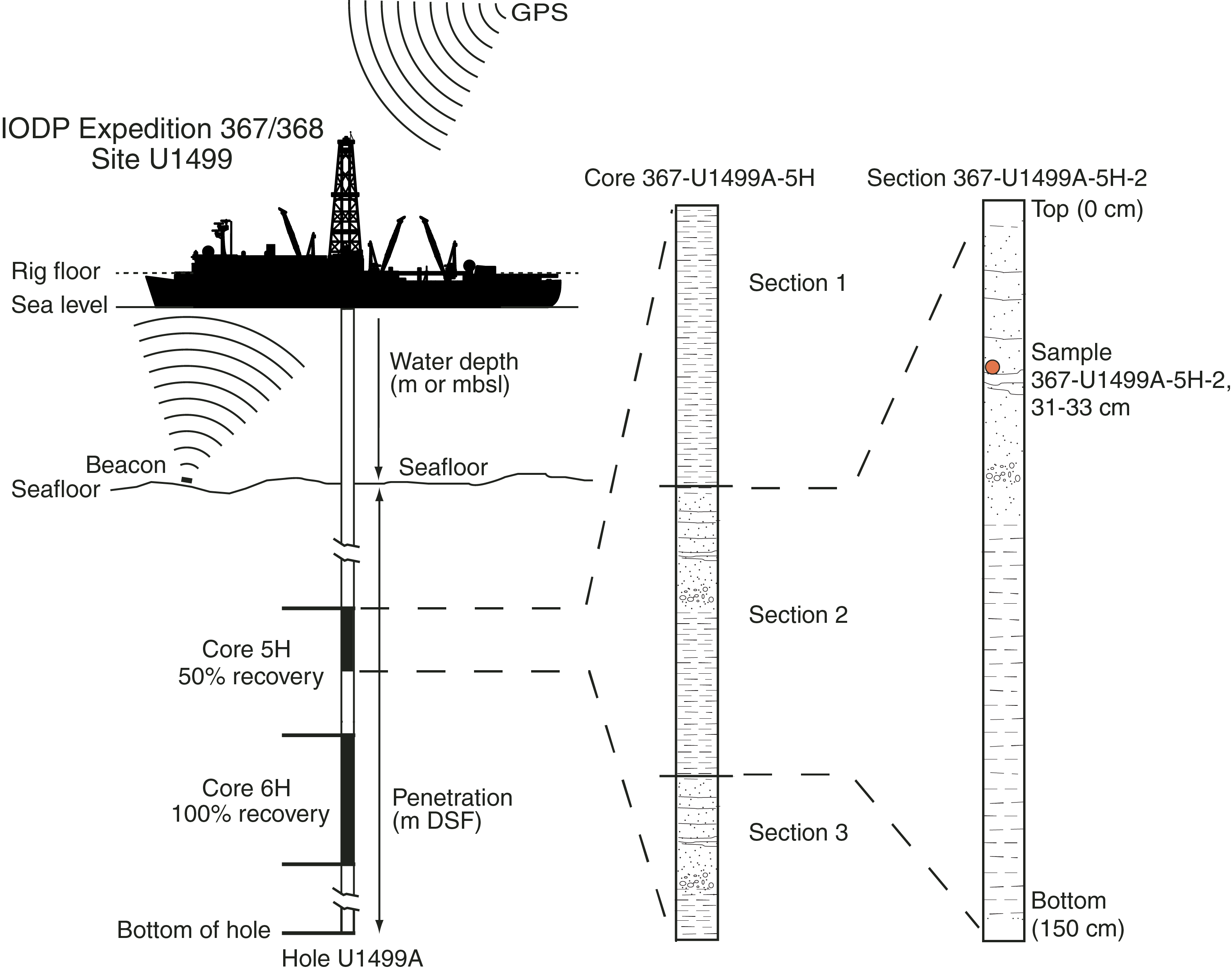
Figure F1. IODP conventions for naming sites, holes, cores, sections, and samples.
Drilling operations
The advanced piston corer (APC), half-length APC (HLAPC), extended core barrel (XCB), and rotary core barrel (RCB) systems were available during Expeditions 367 and 368. Because sampling and logging the lowermost sediments and basement were our highest priority objectives, we used the HLAPC during Expedition 368 but not during Expedition 367.
The APC and HLAPC systems cut soft-sediment cores with minimal coring disturbance relative to other IODP coring systems. After the APC/HLAPC core barrel is lowered through the drill pipe and lands above the bit, the drill pipe is pressured up until the two shear pins that hold the inner barrel attached to the outer barrel fail. The inner barrel then advances into the formation and cuts the core (Figure F2A). The driller can detect a successful cut, or “full stroke,” by observing the pressure gauge on the rig floor because the excess pressure accumulated prior to the stroke drops rapidly. Cores collected with the APC system are denoted by the letter “H,” and those collected with the HLAPC system are denoted by the letter “F.”
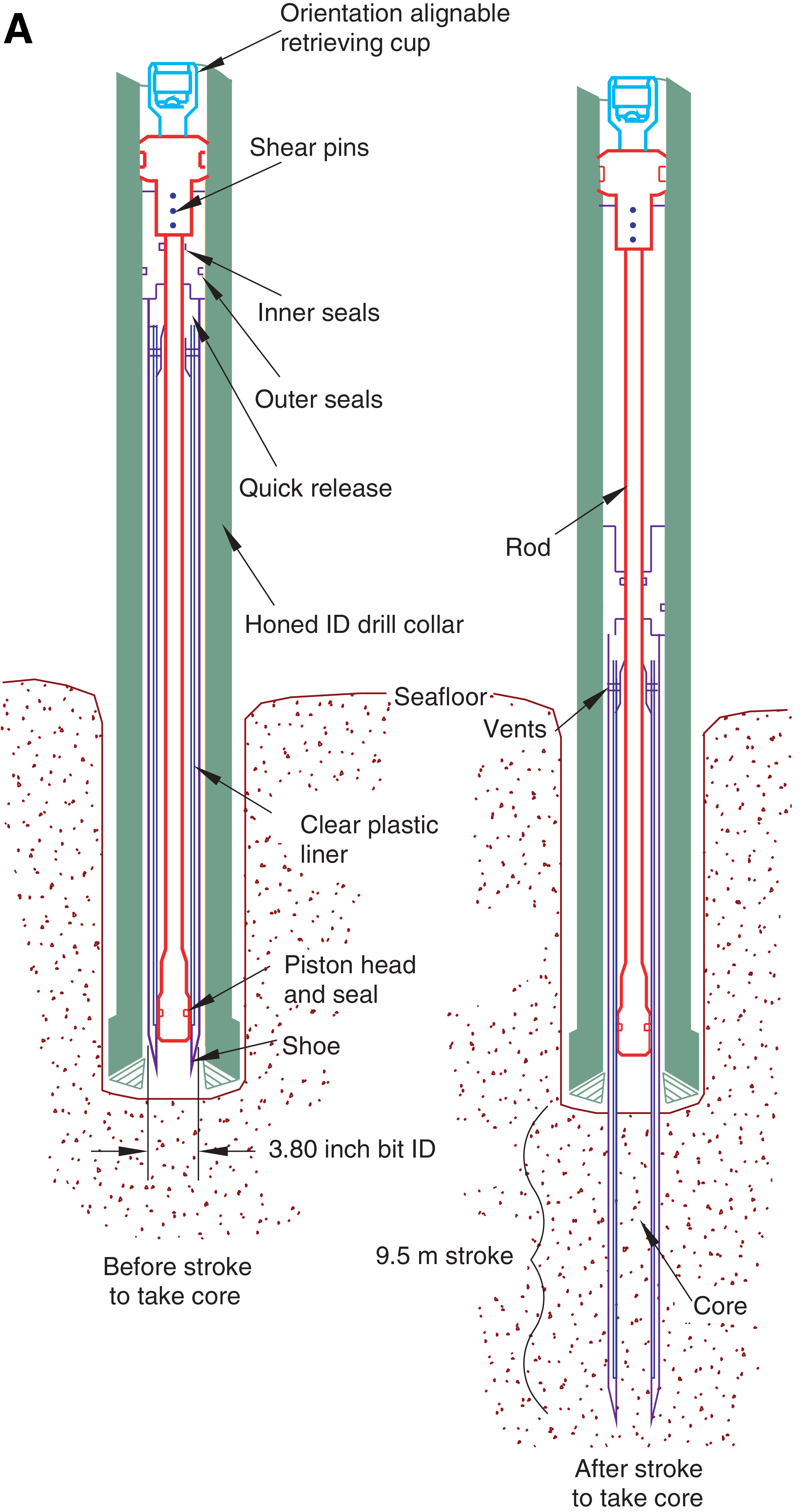
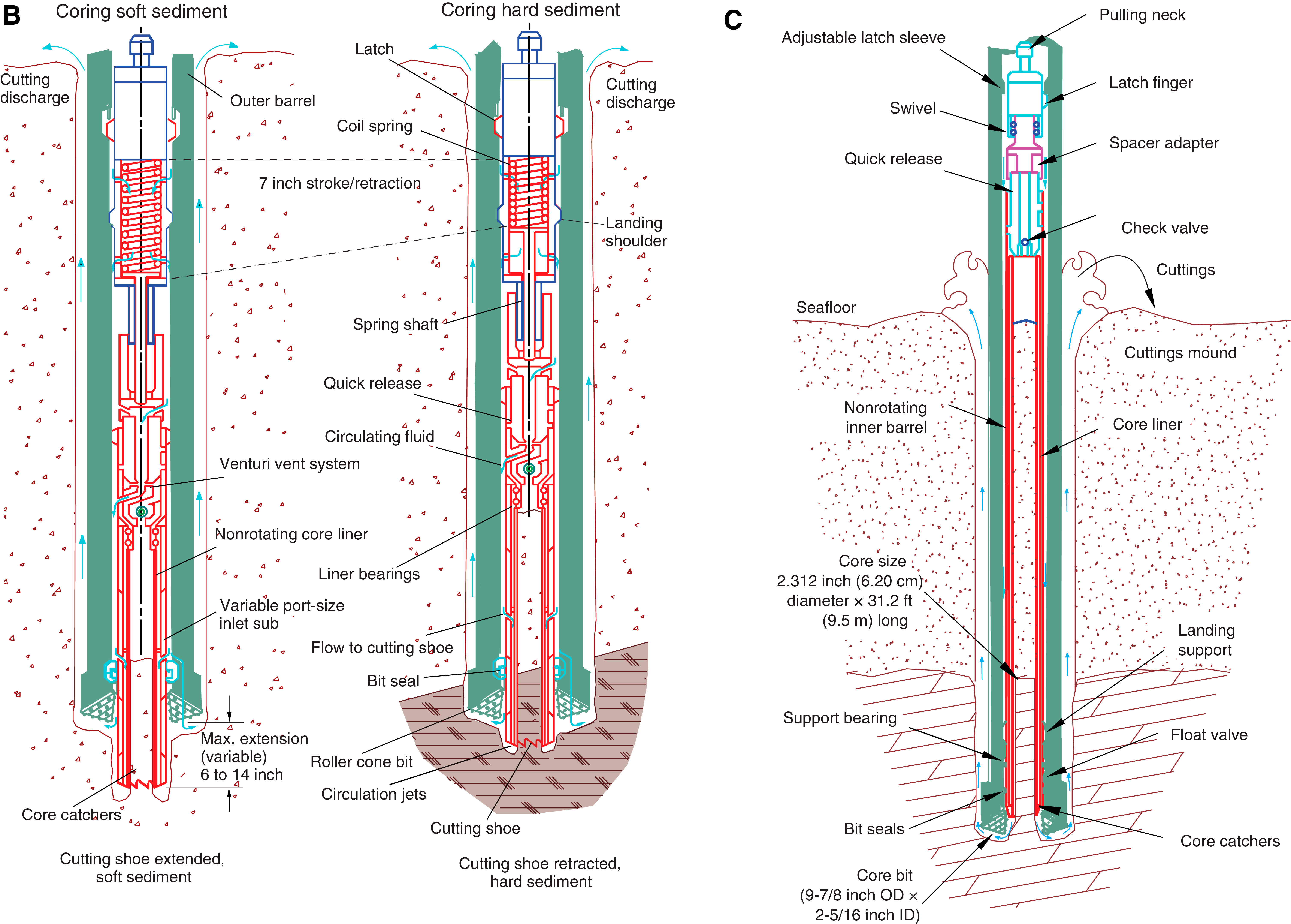
Figure F2. Coring systems.
APC refusal is conventionally defined in one of two ways: (1) the piston fails to achieve a complete stroke (as determined from the pump pressure and recovery reading) because the formation is too hard or (2) excessive force (>60,000 lb) is required to pull the core barrel out of the formation. When a full stroke could not be achieved, one or more additional attempts were typically made, and with each attempt the bit was advanced by the length of the core barrel. Note that these attempts resulted in a nominal recovery of ~100% based on the assumption that the barrel penetrated the formation by the length of core recovered. If an APC core does not achieve a full stroke, the next core can be taken after advancing to a depth determined by the recovery of the previous core (advance by recovery) or to a depth of a full APC core (typically 9.7 m). When a full or partial stroke was achieved but excessive force could not retrieve the barrel, the core barrel could be “drilled over,” meaning that after the inner core barrel was successfully shot into the formation, the drill bit was advanced to total depth to free the APC barrel.
The standard APC system uses a 9.5 m long core barrel, whereas the HLAPC system uses a 4.7 m long core barrel. In most instances, the HLAPC system was deployed after the standard APC consistently had <50% recovery. During use of the HLAPC system, the same criteria were applied in terms of refusal as for the APC system. Use of the HLAPC system allowed for significantly greater APC sampling depths to be attained than would have otherwise been possible.
The XCB system is typically used when the APC/HLAPC system has insufficient recovery. Cores collected with the XCB system are denoted by the letter “X.” In our case, however, the XCB system was not able to recover the unconsolidated sands encountered at depths where the APC/HLAPC system could not be used. The XCB system was used to advance the hole when HLAPC refusal occurred before the target depth was reached or when drilling conditions required it. The XCB system has a small cutting shoe that extends below the large rotary APC/XCB bit (Figure F2B). The smaller bit can cut a semi-indurated core with less torque and fluid circulation than the main bit, potentially improving recovery. The XCB cutting shoe typically extends ~30.5 cm ahead of the main bit in soft sediments but is allowed to retract into the main bit when hard formations are encountered. Shorter XCB cutting shoes can also be used. The XCB system could not recover the poorly consolidated and loose sand lithologies penetrated during Expedition 367.
The bottom-hole assembly (BHA) used for APC and XCB coring is typically composed of an 11⁷⁄₁₆ inch (~29.05 cm) drill bit, a bit sub, a seal bore drill collar, a landing saver sub, a modified top sub, a modified head sub, five 8¼ inch control length drill collars, a tapered drill collar, two stands of 5½ inch transition drill pipe, and a crossover sub to the drill pipe that extends to the surface.
The RCB system is a rotary system designed to recover firm to hard sediments and igneous basement. The BHA, including the bit and outer core barrel, is rotated with the drill string while bearings allow the inner core barrel to remain stationary (Figure F2C).
A typical RCB BHA includes a 9⅞ inch drill bit, a bit sub, an outer core barrel, a modified top sub, a modified head sub, a variable number of 8¼ inch control length drill collars, a tapered drill collar, two stands of 5½ inch drill pipe, and a crossover sub to the drill pipe that extends to the surface. Cores collected with the RCB system are denoted by the letter “R.”
Nonmagnetic core barrels were used for all APC, HLAPC, and RCB deployments. APC cores were oriented with the Icefield MI-5 core orientation tool when coring conditions allowed. Formation temperature measurements were taken with the advanced piston corer temperature tool (APCT-3; see Downhole measurements). Information on recovered cores, drilled intervals, downhole tool deployments, and related information are provided in the Operations, Paleomagnetism, and Downhole measurements sections of each site chapter.
IODP depth conventions
The primary depth scales used are based on the length of the drill string deployed (e.g., drilling depth below rig floor [DRF] and drilling depth below seafloor [DSF]), the length of core recovered (e.g., core depth below seafloor [CSF] and core composite depth below seafloor [CCSF]), and the length of logging wireline deployed (e.g., wireline log depth below rig floor [WRF] and wireline log depth below seafloor [WSF]) (see IODP Depth Scales Terminology at http://www.iodp.org/policies-and-guidelines/142-iodp-depth-scales-terminology-april-2011/file). In cases where multiple logging passes are made, wireline log depths are mapped to one reference pass, creating the wireline log matched depth below seafloor (WMSF) scale. All units are in meters. The relationship between scales is defined either by protocol, such as the rules for computation of CSF depth from DSF depth, or by user-defined correlations, such as core-to-log correlation. The distinction in nomenclature should keep the reader aware that a nominal depth value in different depth scales usually does not refer to the exact same stratigraphic interval.
Depths of cored intervals are measured from the drill floor based on the length of drill pipe deployed beneath the rig floor (DRF scale; Figure F1). The depth of the cored interval is referenced to the seafloor (DSF scale) by subtracting the seafloor depth of the hole from the DRF depth of the interval. Standard depths of cores in meters below seafloor (CSF-A scale) are determined based on the assumption that (1) the top depth of a recovered core corresponds to the top depth of its cored interval (at the DSF scale) and (2) the recovered material is a contiguous section even if core segments are separated by voids when recovered. Standard depths of samples and associated measurements (CSF-A scale) are calculated by adding the offset of the sample or measurement from the top of its section and the lengths of all higher sections in the core to the top depth of the core.
If a core has <100% recovery, for curation purposes all cored material is assumed to originate from the top of the drilled interval as a continuous section. In addition, voids in the core are closed by pushing core segments together, if possible, during core handling. Therefore, the true depth interval within the cored interval is unknown. This result should be considered a sampling uncertainty in age-depth analysis or in correlation of core data with downhole logging data.
When core recovery is >100% (the length of the recovered core exceeds that of the cored interval), the CSF depth of a sample or measurement taken from the bottom of a core will be deeper than that of a sample or measurement taken from the top of the subsequent core (i.e., the data associated with the two core intervals overlap at the CSF-A scale). This overlap can happen when a soft to semisoft sediment core recovered from a few hundred meters below the seafloor expands upon recovery (typically by a few percent to as much as 15%). Therefore, a stratigraphic interval may not have the same nominal depth on the DSF and CSF scales in the same hole.
During Expeditions 367 and 368, all core depths below seafloor were initially calculated according to the CSF-A depth scale. Unless otherwise noted, all depths presented are calculated on the CSF-A scale and reported simply in meters (m).
Curatorial procedures and sample depth calculations
Numbering of sites, holes, cores, and samples follows standard IODP procedure. A full curatorial identifier for a sample consists of the following information: expedition, site, hole, core number, core type, section number, section half, piece number (hard rocks only), and interval in centimeters measured from the top of the core section. For example, a sample identification of “367-U1499A-5H-2W, 31–33 cm” indicates a 2 cm sample removed from the interval between 31 and 33 cm below the top of Section 2 (working half) of Core 5 (“H” designates that this core was taken with the APC system) of Hole A at Site U1499 during Expedition 367 (Figure F1). The “U” preceding the hole number indicates the hole was drilled by the US platform, the JOIDES Resolution. The drilling system used to obtain a core is designated in the sample identifiers as follows: H = APC, F = HLAPC, R = RCB, and X = XCB. Integers are used to denote the “core” type of drilled intervals (e.g., a drilled interval between Cores 2H and 4H would be denoted by Core 31).
Core handling and analysis
Sediment
When the core barrel reached the rig floor, the core catcher from the bottom of the core barrel was removed and a sample was extracted for paleontological (PAL) analysis. Next, the sediment core was extracted from the core barrel in its plastic liner. The liner was carried from the rig floor to the core processing area on the catwalk outside the core laboratory, where it was split into ~1.5 m sections. Blue (uphole direction) and clear (downhole direction) liner caps were glued with acetone onto the cut liner sections.
Once the core was cut into sections, whole-round samples were taken for interstitial water chemical analyses. When a whole-round sample was removed, a yellow cap was used to denote the missing interval. Syringe samples were taken for headspace gas analyses according to the IODP hydrocarbon safety monitoring protocol.
Core sections were placed in a core rack in the laboratory. When the core sections reached equilibrium with laboratory temperature (typically after 2 h), they were run through the Whole-Round Multisensor Logger (WRMSL) for P-wave velocity on the P-wave logger (PWL), magnetic susceptibility, and gamma ray attenuation (GRA) bulk density (see Physical properties). The core sections were also run through the Natural Gamma Radiation Logger (NGRL), and thermal conductivity measurements were taken once per core when the material was suitable.
The core sections were then split lengthwise from bottom to top into working and archive halves. Investigators should note that older material can be transported upward on the split face of each section during splitting.
The working half of each core was described by the sedimentologists and structural geologists. Discrete samples were then taken for moisture and density (MAD) and paleomagnetic (PMAG) analyses and for remaining shipboard analyses such as X-ray diffraction (XRD) and carbonate (CARB). Samples were not collected when the lithology was a high-priority interval for expedition or postexpedition research (e.g., ash layers, etc.), there was unsuitable core material, or the core was severely deformed. During the expeditions, no samples were taken for personal postexpedition research (except for ephemeral pore water samples and five reconnaissance samples for lipids necessary to determine the appropriate sample volume/number to prepare for sensible postexpedition sampling).
The archive half of each core was scanned on the Section Half Imaging Logger (SHIL) and measured for point magnetic susceptibility (MSP), and reflectance spectroscopy and colorimetry (RSC) were measured on the Section Half Multisensor Logger (SHMSL). Labeled foam pieces were used to denote missing whole-round (WR) intervals in the SHIL images. The archive-half sections were then described visually and by means of smear slides for sedimentology. Finally, the magnetization of archive-half sections and working-half discrete pieces was measured with the cryogenic magnetometer and spinner magnetometer.
Hard rock
Pieces were extracted from the core liner on the catwalk or directly from the core barrel on the rig floor. The pieces were pushed to the bottom of 1.5 m liner sections, and the total rock length was measured. The length was entered into the database using the SampleMaster application as “created length.” This number was used to calculate recovery. The liner sections were then transferred to the core splitting room.
Oriented pieces of core were marked on the bottom with a wax pencil to preserve orientation. Adjacent but broken pieces that could be fit together along fractures were curated as single pieces. The petrologists and structural geologists confirmed piece matches and marked the split line on the pieces, which defined how the pieces were to be cut into two equal halves. The aim was to maximize the expression of dipping structures on the cut face of the core while maintaining representative features in both archive and working halves. A plastic spacer was secured with acetone to the split core liner between individual pieces or reconstructed contiguous groups of subpieces. These spacers can represent substantial intervals of no recovery. The length of each section of core, including spacers, was entered into the database as “curated length,” which commonly differs by several centimeters from the length measured on the catwalk. Finally, the depth of each piece in the database was recalculated based on the curated length.
Core pieces were imaged around the full 360° circumference and then placed in a core rack in the laboratory. When the core sections reached equilibrium with laboratory temperature (typically after 2 h), the whole-round core sections were run through the WRMSL (GRA and magnetic susceptibility only) and NGRL (see Physical properties).
Each piece of core was split with a diamond-impregnated saw into an archive half and a working half, with the positions of plastic spacers between pieces maintained in both halves. Pieces were numbered sequentially from the top of each section, beginning with 1. Separate subpieces within a single piece were assigned the same number but lettered consecutively (e.g., 1A, 1B, etc.). Pieces were labeled only on the outer cylindrical surfaces of the core. If it was evident that an individual piece had not rotated around a horizontal axis during drilling, an arrow pointing to the top of the section was added to the label. The piece’s oriented character was recorded in the database using the SampleMaster application.
The working half of each core was first described by the petrologists and structural geologists. Samples were then taken for thin section preparation and shipboard paleomagnetic and physical properties analyses. The archive half of each core was scanned on the SHIL and measured for MSP and RSC on the SHMSL. Thermal conductivity measurements were made on selected archive-half samples (see Physical properties). After the archive halves were fully described, samples were taken for shipboard analyses (thin sections, inductively coupled plasma spectroscopy [ICP], XRD, MAD, etc). Finally, the magnetizations of archive-half sections, archive-half pieces, and discrete samples taken from the working half were measured with the cryogenic magnetometer and spinner magnetometer.
When all steps were completed, cores were wrapped, sealed in plastic tubes, and transferred to cold storage space aboard the ship. At the end of the expedition, the cores were sent to the IODP Gulf Coast Repository (Texas A&M University, College Station, Texas [USA]), where samples for postexpedition research were taken.
Drilling and handling core disturbance
Cores may be significantly disturbed and contain extraneous material as a result of the coring and core handling process (Jutzeler et al., 2014). In formations with loose sand layers, sand from intervals higher in the hole may be washed down by drilling circulation, accumulate at the bottom of the hole, and be sampled with the next core. The uppermost 10–50 cm of each core must therefore be examined critically during description for potential “fall-in.” Common coring-induced deformation includes the concave-downward appearance of originally horizontal bedding. Piston action can result in fluidization (“flow-in”) at the bottom of APC cores. Retrieval from depth to the surface can result in elastic rebound. Gas that is in solution at depth may become free and drive apart core segments within the liner. When gas content is high, pressure must be relieved for safety reasons before the cores are cut into segments. Holes are drilled into the liner, which forces some sediment as well as gas out of the liner. These disturbances are described in each site chapter and graphically indicated on the visual core descriptions (VCDs).
Authorship of chapters
The separate sections of the methods and site chapters were written by the following scientists (authors are listed in alphabetical order; see Expedition 367/368 participants for affiliation information):
Expedition 367 (Sites U1499 and U1500)
- Background and objectives: J.M. Stock and Z. Sun
- Operations: A. Klaus and S. Midgley
- Lithostratigraphy: J.L. Hinojosa, K.-H. Hsiung, B.G. Johnson, Z. Liu, C. Robinson, C. Su, and N. Zhao
- Igneous and metamorphic petrology: T.W. Höfig, X.-L. Huang, A. Luna, A.J. McCarthy, and L. Zhong
- Structural geology: M.F.R. Nirrengarten and C. Zhang
- Biostratigraphy: A. Furusawa, B. Huang, C. Lupi, X. Su, and R. Xiang
- Paleomagnetism: S.M. Skinner, L. Yi, and Y. Zhang
- Geochemistry: Y. Chen, M.J. Dorais, and L. Li
- Physical properties: J. Boaga, A. Briais, C. Lei, I. Sauermilch, R. Yadav, and J. Zhang
- Downhole measurements: J. Boaga, A. Briais, C. Lei, I. Sauermilch, R. Yadav, and J. Zhang
- Core-log-seismic integration: J. Boaga, A. Briais, C. Lei, I. Sauermilch, R. Yadav, and J. Zhang
Expedition 368 (Sites U1501–U1505)
- Background and objectives: Z. Jian and H.-C. Larsen
- Operations: C.A. Alvarez Zarikian and K. Grigar
- Lithostratigraphy: K.A. Dadd, C. Liu, J.C. Schindlbeck, S.M. Straub, S. Wan, and G. Zhong
- Igneous and metamorphic petrology: D.W. Peate, S.M. Straub, and F.M. Van der Zwan
- Structural geology: W. Ding, R.M. Kurzawski, and G.T.F. Mohn
- Biostratigraphy: F. Ferreira, A.J. Gewecke, S. Jiang, H. Jin, B. Li, C. Liu, and P.-S. Yu
- Paleomagnetism: E.C. Ferré, S. Satolli, and H. Wu
- Geochemistry: S.A. Bowden, Y. Li, and L. Tian
- Physical properties: D. Cukur, E. Huang, J. Lin, L.S. Ningthoujam, N. Osono, P. Persaud, and N. Qiu
- Downhole measurements: D. Cukur, J. Lin, P. Persaud, and N. Qiu
- Core-log-seismic integration: J. Lin and H.-C. Larsen
Lithostratigraphy
The lithologies of sediment and sedimentary rocks recovered during Expeditions 367 and 368 were determined using visual (macroscopic) core description, smear slides, and thin sections. Integration of data from digital core images, color reflectance spectrophotometry, magnetic susceptibility, XRD, and geochemistry provided complementary information. The methods employed during the expeditions were adapted from those used during IODP Expedition 349 (Li et al., 2015), along with those from other IODP expeditions (e.g., Expedition 339 Scientists, 2013). We used the DESClogik application to record and upload descriptive data into the Laboratory Information Management System (LIMS) database (see the DESClogik user guide at http://iodp.tamu.edu/labs/documentation). Spreadsheet templates were set up in DESClogik and customized for Expeditions 367 and 368 before the first core was brought on deck. The templates were used to record macroscopic core descriptions and microscopic data from smear slides and thin sections. The location of all smear slide and thin section samples taken from the core were recorded in the SampleMaster application, and descriptive data uploaded to the LIMS database were used to produce VCD standard graphic reports.
Core preparation
Standard methods for splitting core were performed either by pulling a wire lengthwise through the center of the core or by cutting the core with a rock saw. Each piece of core was split into archive and working halves, with the archive half used for visual description. When splitting the cores with a wire, we sometimes gently scraped across the cut surface of the core section using a stainless steel or glass scraper to prepare the surface for unobscured description and digital imaging, especially in the upper, poorly consolidated intervals. Most cores were imaged after they had dried; however, some cores were imaged still damp from the water used during cutting if this enhanced the features. If these cores had partially dried before they were imaged, we applied a light spray of deionized water to dampen the surface.
Visual core description
VCDs include a simplified graphical representation of each site on a core-by-core basis (Figure F3). The principal function of the graphic VCD is to present the physical observations of the core in a columnar format. Site, hole, core, and depth in meters CSF-A are given at the top of each VCD, with the depth and core section numbers plotted along the left margin. Next to the depth and section columns, we plotted the lithostratigraphic unit and the biostratigraphic age (see Biostratigraphy). The lithostratigraphic units were assigned by grouping intervals based on their lithologic similarities (see Definition of lithostratigraphic units). Further definition of the lithostratigraphic units and their boundaries is described in each site chapter. Additional columns correspond to either core images, physical properties (e.g., natural gamma radiation [NGR]), entries made in DESClogik, or shipboard sample locations. Data taken from DESClogik entries include core summary, principal lithology, sedimentary structures, bioturbation intensity, and drilling disturbances. The VCDs also include descriptive and lithostratigraphic information from the metamorphic and igneous rocks recovered at each site. Each VCD column is described in more detail below.
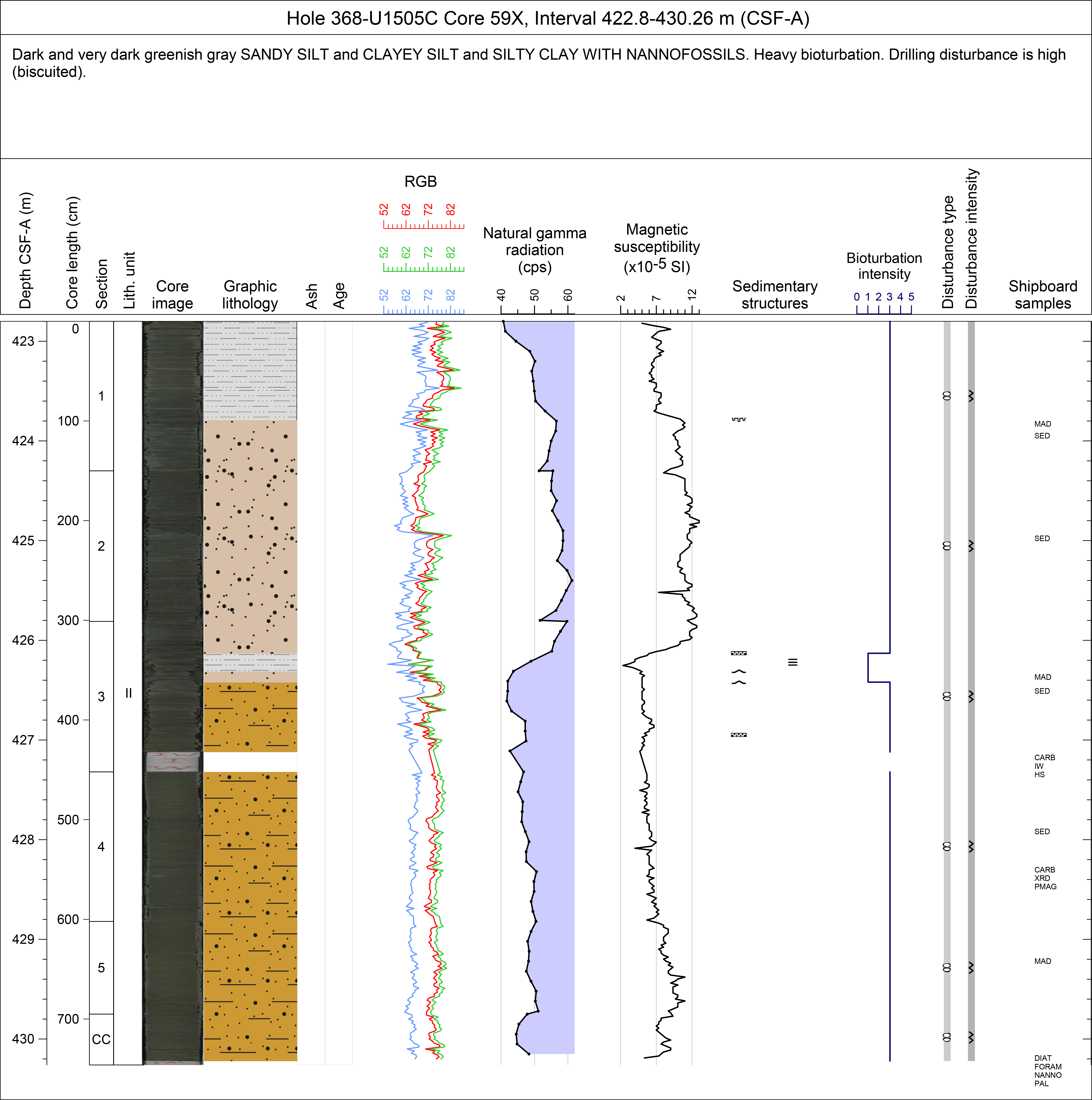
Figure F3. Example graphic description form.
Core summary
The core summary provides a brief overview of major and minor lithologies present in the core, as well as notable features (e.g., sedimentary structures). The summary is presented at the top of the VCDs and includes sediment color determined qualitatively using Munsell soil color charts. Because sediment color may evolve during drying and subsequent oxidization, color was described shortly after the cores were split and imaged or measured by the SHIL and SHMSL. Deionized water was applied to the cut surface of lithified sedimentary rocks before determining color.
Core images
High-resolution color images were produced by scanning the flat surface of the archive-half sections with the SHIL. The cores were scanned as soon as possible after splitting and scraping to avoid color changes caused by sediment oxidation and drying. In some cases involving lithified rock, we photographed the cores both wet and dry and selected the image that best represented the lithology.
The SHIL uses three pairs of advanced illumination, high-current-focused, LED line lights to illuminate large cracks and blocks in the core surface and sidewalls. Each LED pair has a color temperature of 6500 K and emits 90,000 lx at 76.2 mm. A line-scan camera images 10 lines/mm to create a high-resolution TIFF file. The camera height is adjusted so that each pixel images a 0.1 mm2 section of the core. However, actual core width per pixel varies because of differences in section-half surface height. High- and low-resolution JPEG files are subsequently created from the high-resolution TIFF file. Two different image types were uploaded to the LIMS database: one that includes a grayscale and ruler and one that is cropped to exclude the grayscale and ruler.
Graphic lithology
The graphic lithology column illustrates an interval-by-interval record of the primary lithologies contained within each core. The column was constructed by pairing the principal lithology name assigned to each interval in DESClogik with a predetermined set of lithology patterns (Figure F4). The column plots to scale all intervals that are at least 2 cm thick. Principal lithology names were not assigned to intervals thinner than 2 cm unless they were of special significance (e.g., ash layers).
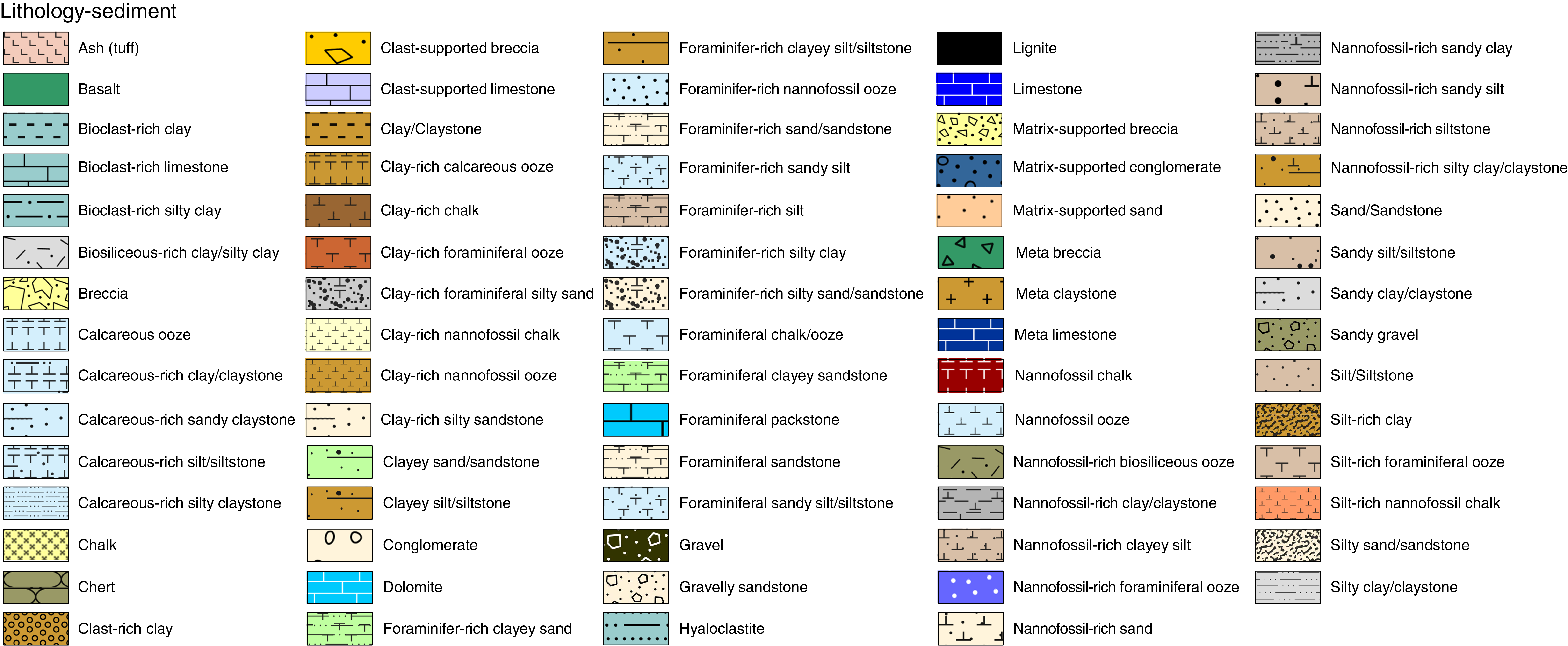
Figure F4. Lithology patterns used for visual core description.
Reflectance
Reflectance of visible light from the archive halves of sediment cores was measured using an Ocean Optics USB4000 spectrophotometer mounted on the automated SHMSL. Freshly split cores were covered with clear plastic wrap and placed on the SHMSL, and measurements were taken at 1, 2, or 2.5 cm spacing to provide a high-resolution stratigraphic record of color variation for visible wavelengths. Each measurement was recorded in 2 nm wide spectral bands from 400 to 900 nm. Reflectance parameters L*, a*, and b* were recorded (Balsam et al., 1997, 1998).
The SHMSL takes measurements in empty intervals and over intervals where the core surface is well below the level of the core liner, but it cannot recognize relatively small cracks, disturbed areas of core, or plastic section dividers. Thus, SHMSL data may contain spurious measurements that must be edited out of the data set by the user. When significant fragmentation and/or brecciation from drilling disturbances was evident, the SHMSL spacing was adjusted manually to avoid taking measurements in the wide spaces caused by drilling fractures. Additional detailed information about measurement and interpretation of reflectance data can be found in Balsam et al. (1997, 1998) and Balsam and Damuth (2000).
Natural gamma radiation
NGR occurs primarily by decay of 238U, 232Th, and 40K isotopes. This radiation is measured using the NGRL (see Physical properties). Data generated from this instrument were used to augment geologic interpretations.
Magnetic susceptibility
We measured magnetic susceptibility with a Bartington Instruments MS2E point sensor (high-resolution surface-scanning sensor) on the SHMSL. Because the SHMSL demands direct contact between the point magnetic susceptibility sensor and the split core, measurements were made on the archive halves of split cores that were covered with clear plastic wrap. Measurements were taken at 1.0, 2.0, or 2.5 cm spacing. Measurement resolution was 1.0 SI, and each measurement integrated a volume of 10.5 mm × 3.8 mm × 4 mm, where 10.5 mm is the length perpendicular to the core axis, 3.8 mm is the width along the core axis, and 4 mm is the depth into the core.
Sedimentary structures
The location and type of stratification and sedimentary structures visible on the surface of the split cores are shown in the sedimentary structures column of the VCDs. Symbols in this column indicate the location, scale, and frequency of stratification and other sedimentary features, such as sole marks, cross-lamination, and fining-upward intervals (Figure F5).
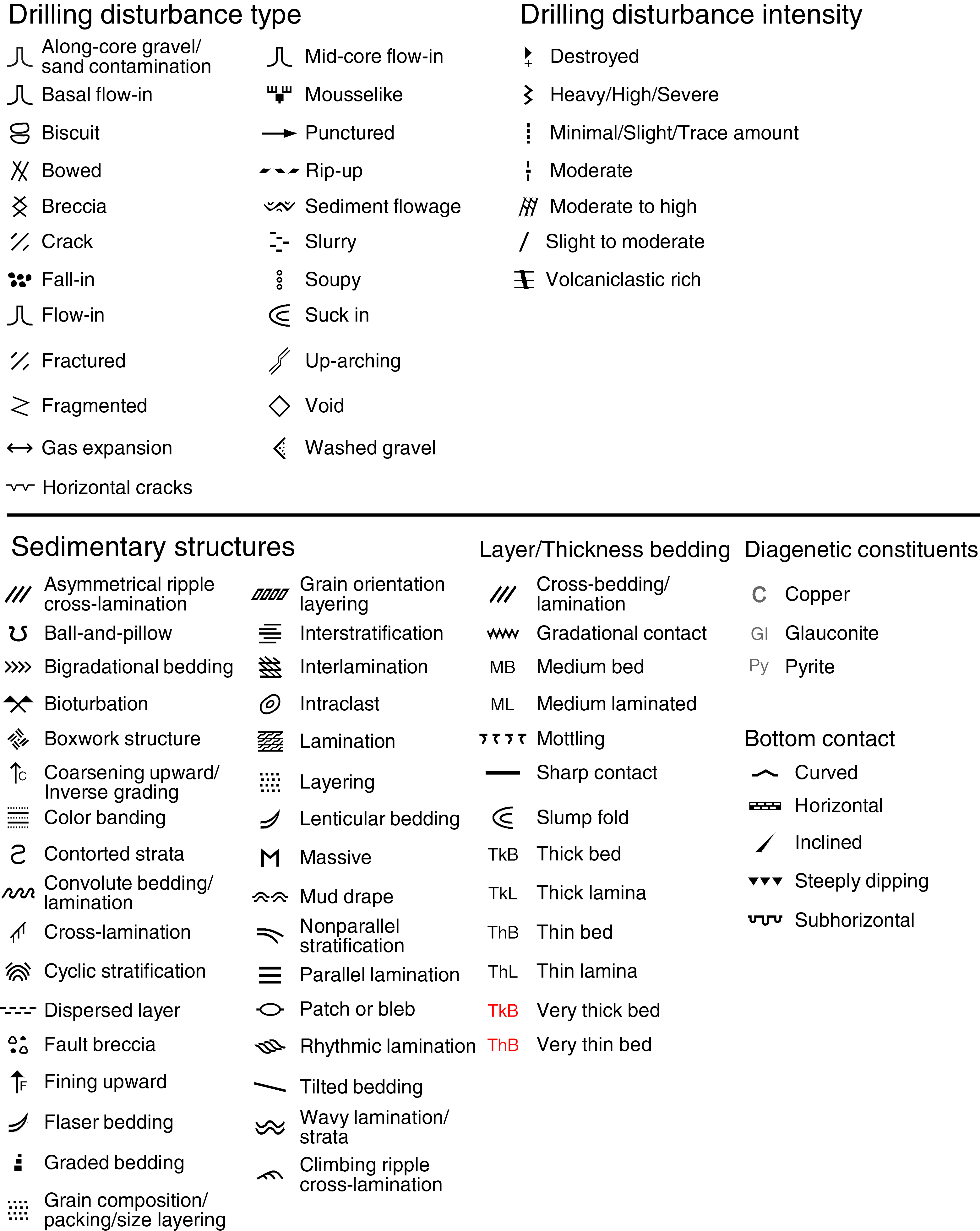
Figure F5. Symbols and nomenclature used for visual core description.
For Expeditions 367 and 368, the following terminology (based on Stow, 2005) was used to describe the scale of stratification:
- Thin lamination = <0.3 cm thick.
- Medium lamination = 0.3–0.6 cm thick.
- Thick lamination = 0.6–1 cm thick.
- Very thin bed = 1–3 cm thick.
- Thin bed = 3–10 cm thick.
- Medium bed = 10–30 cm thick.
- Thick bed = 30–100 cm thick.
- Very thick bed = >100 cm thick.
Bioturbation intensity
Five levels of bioturbation are recognized using a scheme like that of Droser and Bottjer (1986). These levels are illustrated with a numeric scale in the bioturbation intensity column. Any identifiable trace fossils (ichnofossils) are identified in the general interval comment field in DESClogik and in the core summary.
- 1 = No bioturbation.
- 2 = Slight bioturbation (<10%–30%).
- 3 = Moderate bioturbation (30%–60%).
- 4 = Heavy bioturbation (60%–90%).
- 5 = Complete bioturbation (>90%).
Drilling disturbance
Drilling-related sediment disturbance is recorded in the disturbance type and intensity columns. The disturbance intensity, where present, is ranked on a five-point scale: slight, slight to moderate, moderate, moderate to high, and high. The type of drilling disturbance is classified using the symbols shown in Figure F5. Each symbol corresponds to the following terms:
- Soupy: intervals are water-saturated and have lost all aspects of original bedding.
- Fall-in: characteristically occurs at the top of individual cores when out-of-place material from the shallower cored interval has fallen downhole onto the cored surface.
- Up-arching: bedding planes are slightly to moderately deformed but still subhorizontal and continuous across the core surface. The edges of the bedding planes typically show a concave downward shape caused by shear along the wall of the core liner.
- Flow-in: occurs in unconsolidated, sandy, or gravelly sediment, leaving a soupy texture at the base of the core. It typically occurs during APC drilling, following a partial stroke of the piston core.
- Biscuit: sediments of intermediate stiffness show vertical variations in the degree of disturbance. Softer intervals are washed and/or soupy, whereas firmer intervals are relatively undisturbed.
- Fractured: common in consolidated and lithified sediments. The core pieces are broken in places and may have been partly displaced or moved, but the correct stratigraphic sequence is maintained.
- Fragmented: complete fracturing of the core into large (>2 cm thick) pieces, where the stratigraphic order of the pieces is retained but their orientation is lost.
- Drilling breccia: core is crushed and broken into many small and angular pieces, with original orientation and stratigraphic position lost.
Samples
The shipboard samples column records the position of samples used for microscopic descriptions (i.e., smear slides and thin sections), biochronological determinations, and shipboard analyses of chemical and physical properties.
Classification of principal lithology
Types of sediment
The sediment recovered during Expeditions 367 and 368 was described and classified by measuring the relative proportions of biosiliceous, calcareous, and siliciclastic material (Figure F6). This classification scheme was adapted from Integrated Ocean Drilling Program Expedition 339 (Expedition 339 Scientists, 2013), Expedition 349 (Li et al., 2015) and Stow (2005). Biosiliceous sediment is restricted to only include siliceous skeletal remains of microorganisms (e.g., radiolarians and diatoms), whereas calcareous sediment includes a wide range of grain types, such as the skeletal remains of microfauna (e.g., foraminifers) and microflora (e.g., nannofossils), macrofossil shell fragments, and fine-grained detrital carbonate. Siliciclastic sediment includes mineral and rock fragments eroded from igneous, sedimentary, and metamorphic rocks. In rare cases, sediment recovered during Expeditions 367 and 368 included grains that were directly derived from a volcanic eruption, mainly in the form of vitric material (e.g., ash and lapilli), so a separate classification scheme was applied to their description.
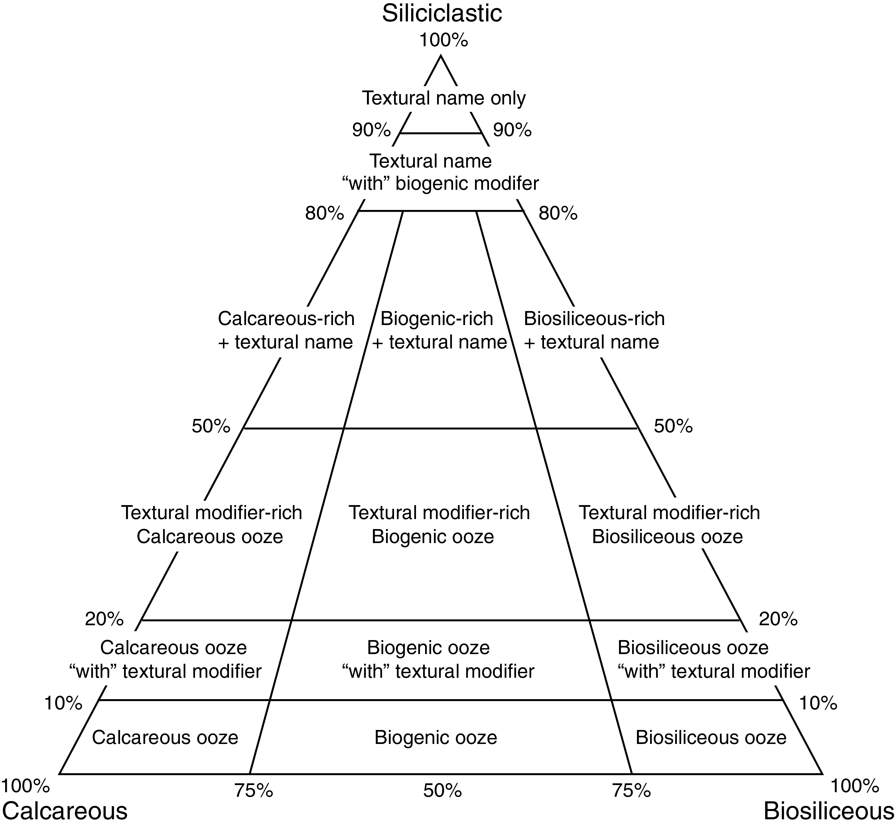
Figure F6. Siliciclastic-calcareous-biosiliceous ternary diagram.
Naming conventions for Expeditions 367 and 368 follow the general guidelines of the Ocean Drilling Program (ODP) sediment classification scheme (Mazzullo et al., 1988), except that during Expeditions 367 and 368 a separate “mixed sediment” category was not distinguished and detrital biogenic sediment with evidence of being reworked and transported by sedimentary processes was described using the terminology for siliciclastic rocks with a prefix that describes the main biogenic component. For example, the term “foraminifer sand” defines sediment composed of >50% foraminifer tests that are >63 µm in size. A principal lithology name is assigned to each interval, and when the sediment comprises a mixture of different sediment types, modifying prefixes and suffixes are added to the principal name.
We followed the naming scheme of Shepard (1954) for the classification of siliciclastic sediment and sedimentary rock that reflects the relative proportion of sediments of different grain size (Figure F7). Sediment grain size divisions for siliciclastic and redeposited biogenic components are based on Wentworth (1922), with categories based on the relative proportions of gravel and sand-, silt-, and clay-sized particles (Figure F8). Distinguishing between some of these categories can be difficult at the macroscopic level, especially considering the relative abundance of the fine-grained fraction (e.g., silty clay versus clayey silt); therefore, smear slides and thin sections were used in classifying fine-grained sediment abundances.
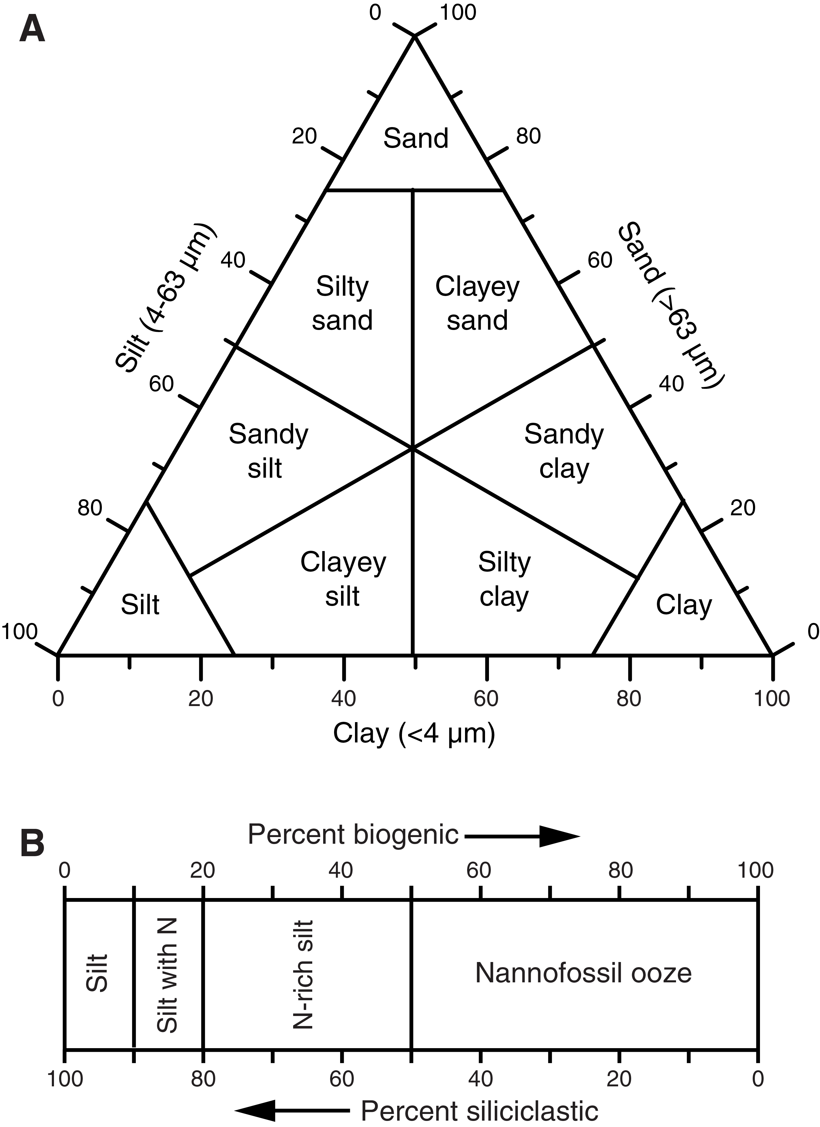
Figure F7. Lithologic classification for textural names.
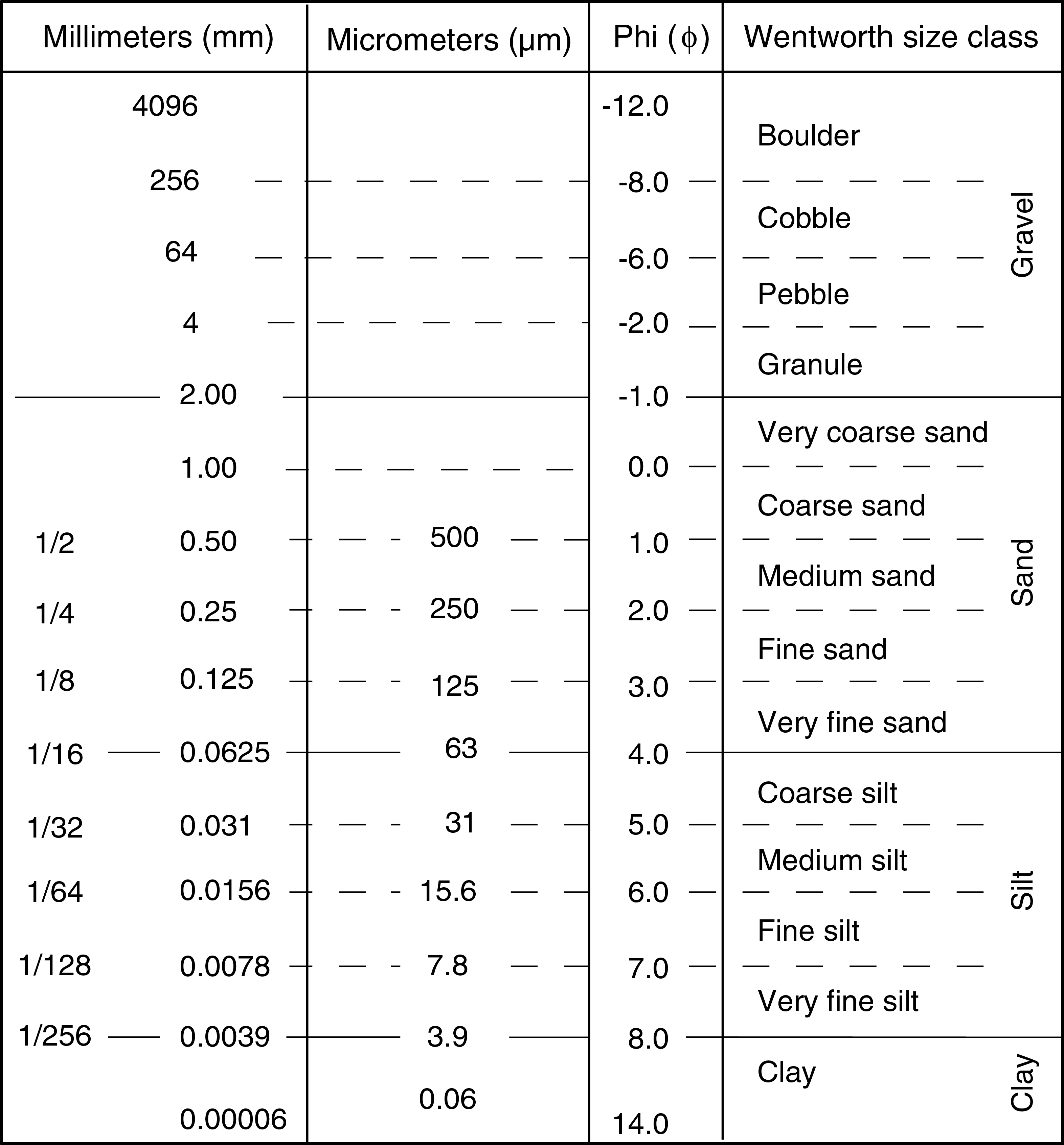
Figure F8. Udden-Wentworth grain-size classification.
The proportions of biogenic material, both siliceous and calcareous sediment, were first macroscopically determined by observing changes in color. We used Munsell soil color charts to assign a color to different intervals within a core. Sediments that contained significant amounts of calcareous material typically had a lighter color value. Biogenic material was also determined by observing physical property changes in NGR, magnetic susceptibility, and reflectance values. Low magnetic susceptibility and high color reflectance values were two defining patterns associated with significant amounts of calcareous material. We then used smear slides and thin sections to identify and estimate the relative abundance of the different microfossils, such as nannofossils, foraminifers, and radiolarians, within unique lithologic intervals. However, smear slide observations tend to overestimate the relative proportions of calcareous microorganisms with respect to the clay-sized fraction of siliciclastic material, so we used the shipboard calcium carbonate data as a quality control. Sediment with >40 wt% calcium carbonate was classified using a calcareous principal lithology.
The lithologic names assigned to a given interval of sediment consist of a principal name and in some cases a modifying prefix and/or suffix. The assigned names are based on abundance and composition of grains determined from visual description of the core and from smear slide/thin section observations. For sediment that contains >90% of one component (either the siliciclastic or biogenic component), only the principal name was used. For sediment that contains >90% biogenic components and is not clearly reworked, the name applied indicates the most common type of biogenic grain. For example, sediment composed of >90% calcareous nannofossils was named nannofossil ooze, and sediment composed of subequal amounts of foraminifers and nannofossils was named calcareous ooze.
For sediment with >90% siliciclastic grains, the principal name is based on the textural characteristics of siliciclastic sediment particles (Figure F7). For sediment that contains a significant mixture of siliciclastic and biogenic components (between 10% and 90% of both siliciclastic and biogenic components), the principal name is determined by the more abundant component. If the siliciclastic component is more abundant, the principal name is based on the textural characteristics of siliciclastic fraction. If the biogenic component is more abundant, the principal name is based on the predominant microfossil group.
If a microfossil group composes 10%–50% of the sediment and this group is not included as part of the principal name, modifiers are used instead. When a microfossil group (e.g., diatom, nannofossil, or foraminifer) comprises 20%–50% of the sediment, a major modifier consisting of the component name hyphenated with the suffix “-rich” (e.g., nannofossil-rich clay) is used. When the calcareous or biosiliceous material comprises a mixture of different microfossil grain types, the major modifier “calcareous-rich” or “biosiliceous-rich” is used instead.
If the principal component forms 80%–90% of the sediment, the principal name is followed by a minor modifier (e.g., “with nannofossils”), with the minor modifier based on the most abundant component that forms 10%–20% of the sediment. If the minor component is biogenic, the modifier describes the most limited group of grains that exceeds the 10% abundance threshold. If the minor component is siliciclastic, the minor modifier is based on the texture of the siliciclastic fraction.
If the primary lithology for an interval of core has a major modifier, that major modifier is indicated in the Graphic lithology column of the VCDs using a modified version of the lithologic pattern for the primary lithology (Figure F3). The modified lithologic patterns are shown in Figure F4. The minor modifiers of sediment lithologies are not included in the graphic lithology column. Although size-texture qualifiers were used to describe siliciclastic sediment (using prefixes such as clayey or sandy), size-texture qualifiers were not typically used in the principal name for biogenic sediment.
Lithification
The degree of lithification was determined by observing the amount of deformation the sediment can accommodate and the level of sediment consolidation. Sediment was considered lithified when the sediment could not be deformed easily with a finger, toothpick, or metal scraper. Lithification was ranked using a qualitative scale with the terms slightly consolidated, moderately consolidated, well consolidated, and lithified.
Depending on the principal lithology, different lithification terms were used. For example, the name “ooze” was applied to unlithified biogenic sediment predominantly composed of calcareous or siliceous microorganisms (e.g., nannofossil ooze). The term “ooze” indicates that the sediment can be deformed by a finger. Chalk is the lithified variant of calcareous ooze that is fine grained and more compact although it can be scratched by a fingernail. Lithified sediment composed of siliceous microfossils (diatoms and radiolarians) is called “radiolarite/diatomite.” Well-lithified calcareous sediment that contains evidence of shallow water deposition (e.g., skeletal macrofossils such as coral) was called “limestone” with supporting prefixes such as “bioclast-rich,” “clast-supported,” and “dolomitic.”
For unlithified siliciclastic sediment, no lithification term was added, and the sediment was named for the dominant grain size (i.e., gravel, sand, silt, or clay). For more lithified siliciclastic material, the suffix “-stone” was appended to the dominant size classification (e.g., claystone), except for sediment of gravel size where the terms “conglomerate” or “breccia” were used for well-rounded and angular clasts, respectively. The principal names “conglomerate” and “breccia” were modified using the terms “matrix-supported” and “clast-supported,” depending on the matrix to clast ratio.
When the mineralogical, chemical, or structural compositions of the sediments or sedimentary rocks have been altered or changed from their original form, the prefix “meta” is used in conjunction with principal lithology (e.g., metasandstone). These rocks are described under the Metamorphic tab in DESClogik. In many cases, however, no clear distinction of boundary between well-lithified sediments and metasedimentary rock exists. Furthermore, extensive alteration by veins, fractures, and other structural features requires special treatment, particularly when a sedimentary rock is crosscut by a mesh network of veins. For this reason, the name “breccia” is applied in several different ways (see Igneous and metamorphic petrology).
Ash layers (volcaniclastic sediment)
The classification of volcanic sediments followed here differs from the standard ODP and IODP classification (Mazzullo et al., 1988) in that we adopted a descriptive (nongenetic) terminology like that employed during ODP Leg 197 and Integrated Ocean Drilling Program Expedition 324 (Shipboard Scientific Party, 2002; Expedition 324 Scientists, 2010). Unless an unequivocally pyroclastic origin for volcanogenic particles could be determined, we simply described these deposits as we did for siliciclastic sediment (i.e., sand, silt, etc.).
Where evidence for a pyroclastic origin is compelling and the sediment has >50% vitric and other primary volcanic material, we adopted the classification scheme of Fisher and Schmincke (1984). In these instances, we used the grain size terms “volcanic block or bomb” (>64 mm), “lapilli” (2–64 mm), and “ash” (<2 mm) for unconsolidated sediment and “volcanic breccia” (>64 mm), “lapillistone” (2–64 mm), and “tuff” (<2 mm) for lithified material. When the volcanic particles compose between 25% and 50% of the sediment fraction, the modifier “tuffaceous” was used as the prefix for the siliciclastic sediment (e.g., tuffaceous sandstone). The term “hyaloclastite” is used for vitroclastic (i.e., glassy) materials produced by the interaction of water and hot magma or lava.
Smear slide and thin section observation
Two or more smear slide samples of the main lithologies were typically collected from the archive half of each core. Additional samples were collected from areas of interest (e.g., laminations, ash layers, and nodules). A small amount of sediment was taken with a wooden toothpick and put on a 2.5 cm × 7.5 cm glass slide. The sediment sample was homogenized with a drop of deionized water and evenly spread across the slide to create a very thin (about <50 µm) uniform layer of sediment grains for quantification. The dispersed sample was dried on a hot plate. A drop of Norland optical adhesive was added as a mounting medium to a coverslip, which was carefully placed on the dried sample to prevent air bubbles from being trapped in the adhesive. The smear slide was then cured in an ultraviolet light box.
Thin sections were prepared by cutting 3–5 cm3 billets of lithified sediment from the working half of the core. In some cases, the cut billet was impregnated with a clear epoxy to further consolidate the grains. They were then mounted on 2.5 cm × 4.5 cm glass slides and ground down to a thickness of ~30 µm.
Smear slides and thin sections were examined with a transmitted-light petrographic microscope equipped with a standard eyepiece micrometer. The texture of siliciclastic grains (relative abundance of sand-, silt-, and clay-sized grains) and the proportions and presence of biogenic and mineral components observed in thin sections or smear slides were recorded in DESClogik. Biogenic and mineral components were identified using IODP Technical Notes 1 and 2 (Marsaglia et al., 2013, 2015) for smear slides, and their percentage abundances were visually estimated using Rothwell (1989). The mineralogy of clay-sized grains could not be determined from smear slides. Note that smear slide analyses tend to underestimate the amount of sand-sized and larger grains because these grains are difficult to incorporate onto the slide.
Relative abundances of identified components such as mineral grains, microfossils, and biogenic fragments were assigned on a semiquantitative basis using the following abbreviations:
- Tr = trace (<1% in field of view [FOV]).
- R = rare (1%–5% in FOV).
- C = common (>5%–25% in FOV).
- A = abundant (>25%–75% in FOV).
- D = dominant (>75% in FOV).
X-ray diffraction analysis
Samples for XRD analyses were selected from the working half, generally at the same depth as sampling for solid-phase geochemistry and smear slide analyses. Approximately one 5 cm3 sample was taken of a representative lithology per core. Samples analyzed for bulk mineralogy were freeze-dried and homogenized by grinding in the metal ball mill. Prepared samples were top-mounted onto a sample holder and analyzed using a Bruker D-4 Endeavor diffractometer mounted with a Vantec-1 detector using nickel-filtered CuKα radiation. Settings for the standard locked coupled scan were as follows:
- Voltage = 37 kV.
- Current = 40 mA.
- Goniometer scan = 4°–70°.
- Step size = 0.0166°.
- Scan speed = 1 s/step.
- Divergence slit = 0.3 mm.
Diffractograms of bulk samples were evaluated with the aid of the Jade6 or EVA software package, which allowed for mineral identification and basic peak characterization (e.g., baseline removal and characteristic peak intensity). Files were created that contained d-spacing values, diffraction angles, and peak intensities with and without the background removed. These files were scanned by the Jade6 or EVA software to find d-spacing values characteristic of a limited range of minerals. Peak areas were further quantitatively estimated by the TOPAS software. Shipboard evaluation yielded semiquantitative results of the presence and relative abundances of the most common mineralogical components by applying correction factors (Cook et al., 1975) to the measured intensity of the characteristic reflections of minerals.
Definition of lithostratigraphic units
Sediments and sedimentary rocks were described at two levels: (1) the descriptive interval (a single descriptive line in DESClogik) and (2) the lithostratigraphic unit. Lithostratigraphic units are defined as assemblages of multiple descriptive intervals containing similar principal lithologies that are typically tens to hundreds of meters thick (e.g., Tamura et al., 2015). Lithostratigraphic units should be clearly distinguishable from each other by several characteristics, such as composition, bed thickness, grain-size class, and internal homogeneity. Following IODP tradition, they are numbered sequentially as Unit I, Unit II, and so on from the top of the core to the bottom. Subunits were defined within units that showed distinct changes in minor lithology types or bed forms but maintained continuity in the principal lithology. For instance, a unit primarily composed of clay and interbedded silt would be divided into two subunits if the interbedded lithology changed to sand and silt in the lower half of the unit’s interval. Note that this distinction was interpreted differently during Expeditions 367 and 368, so a greater number of subunits were defined during Expedition 367 than during Expedition 368.
Igneous and metamorphic petrology
Expedition 367 and 368 core description procedures for igneous and metamorphic rocks are based on those from IODP Expeditions 349 and 351 (Li et al., 2015; Arculus et al., 2015) and ODP Legs 209 and 210 (Shipboard Scientific Party, 2004a, 2004b).
Core description workflow
Prior to splitting the core into working and archive halves, each core was subjected to nondestructive physical property measurements (see Physical properties) and imaged using the SHIL (see Lithostratigraphy) on a wet outside surface at four different angles (0°, 90°, 180°, and 270°) that were combined to form a 360° whole-round image. The coherent hard rock sections and/or hard rock pieces were then split by a diamond-impregnated saw along lines drawn by a petrologist and/or a structural geologist in order to preserve significant compositional and structural features in both the archive and working halves. Afterward, fragmented pieces of hard rock that fit together were assigned a joint number and labeled with a letter in consecutive order downsection (e.g., 1A, 1B, 1C). Plastic spacers separate pieces with different numbers. An arrow added to the labels of single pieces that showed no evidence of rotation indicates the orientation by pointing to the top of the section. Scanning of the cut, dry archive-half surfaces by the SHIL produced high-resolution color images. Then the archive halves were analyzed for color reflectance and magnetic susceptibility at 1–2.5 cm increments by deploying the SHMSL (see Lithostratigraphy). Shipboard samples were taken from working halves for carrying out destructive physical properties and paleomagnetic measurements, as well as thin section, XRD, and inductively coupled plasma–atomic emission spectroscopy (ICP-AES) analysis. Because of the presence of hyaloclastic lava-sediment mixtures and sedimentary veins, working halves of igneous rock cores were also sampled for paleontological and sedimentary studies.
Initial macroscopic examination of each core section focused on petrologic and alteration features, followed by characterization of structures (see Structural geology). Subsequently, the texture and composition of any veins were recorded. Apart from thin sections, all descriptions were made on the archive half of each core. The DESClogik software was used to record the macroscopic and microscopic observations of primary (igneous) and secondary (alteration/metamorphic) characteristics, forming the basis of all descriptions. The use of a hand lens and binocular microscope aided the estimation of mineral modes and sizes.
Macroscopic visual core description
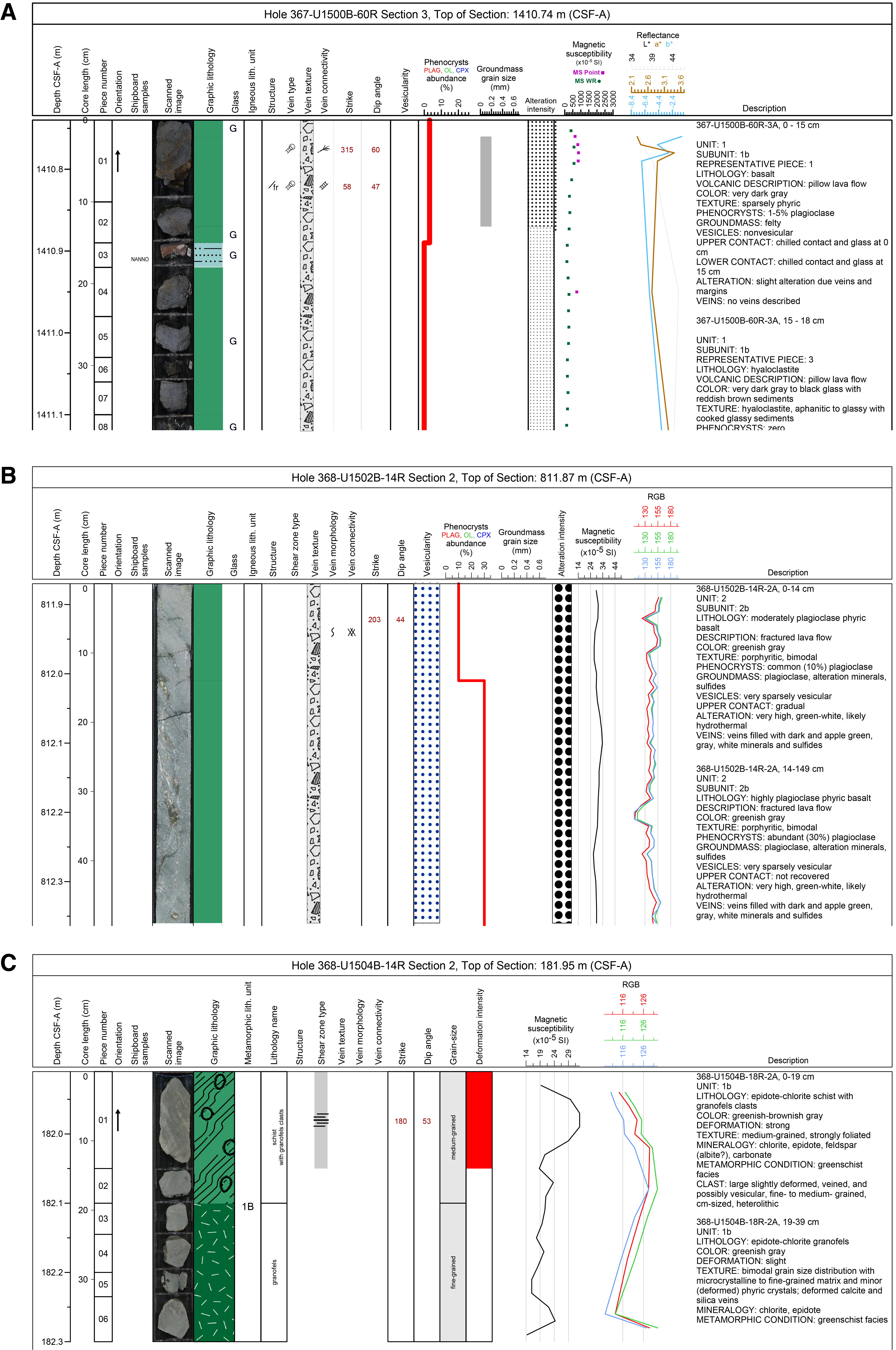
VCDs present and summarize macroscopic features observed in the cores. Expedition 349 VCDs were used as the basis for macroscopic descriptions for this study so they would remain as closely comparable as possible. The slightly modified VCDs display the following entries (from left to right) in terms of igneous, alteration, and metamorphic features for each core section (Figure F9; see Figure F10 for VCD legend):
- CSF-A depth scale (meters below seafloor);
- Core length scale from 0 to 150 cm;
- Number and orientation of hard rock pieces;
- Interval of shipboard samples;
- Scanned digital image of the archive half;
- Graphic representation of lithology;
- Symbol “G” (for igneous rocks, next to the graphic lithology), which indicates the presence of volcanic glass either in the glassy rind of chilled margins or in hyaloclastite, if encountered; thin horizontal lines in the graphic lithology constrain the section interval containing the volcanic glass and mark the location of chilled margins/contacts;
- Igneous or metamorphic lithologic unit number;
- Vein texture, type, and connectivity;
- Line chart displaying vesicularity percentage;
- Stacked line chart displaying percent phenocryst abundance for plagioclase (PLAG; red line), olivine (OL; green line), and clinopyroxene (CPX; blue line), if present;
- Chart displaying variation in crystal size of modal groundmass (in millimeters);
- Column with variable patterns depicting alteration intensity;
- Overall grain size of the corresponding lithology and deformation intensity for metamorphic rocks, for which vesicularity, percent phenocryst abundance, groundmass grain size, and alteration intensity are not applicable;
- Plot showing whole-round magnetic susceptibility measurements (and point source for Site U1500);
- Diagram displaying color reflectance, with total reflectance (L*), red (a*), and blue (b*) (Site U1500) or individual red-green-blue color space (RGB) values (Sites U1502 and U1504); and
- Description summary of each igneous/metamorphic lithologic unit identified in the corresponding section (see below for details).

Figure F9. Example VCDs for igneous and metamorphic rocks.
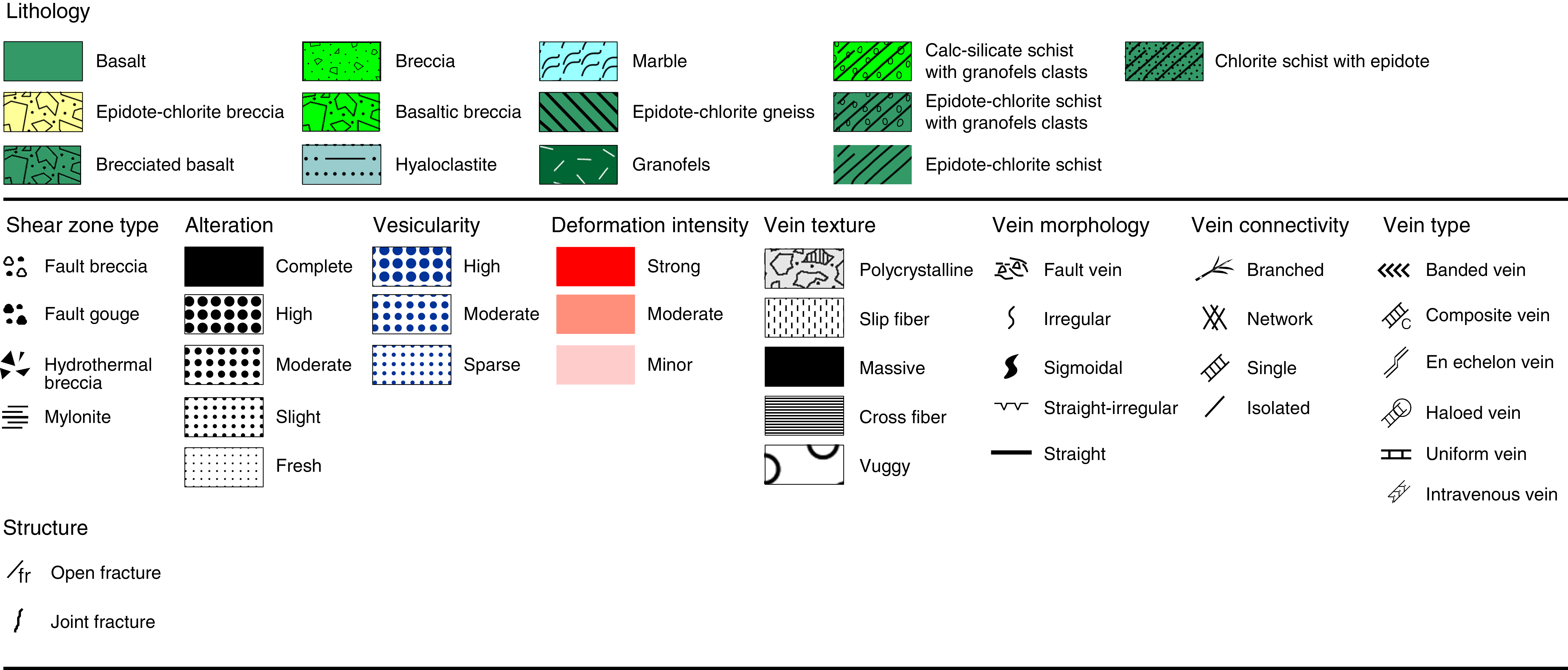
Figure F10. Symbols and nomenclature used in igneous VCDs.
The section unit summary (presented on the right side of the VCD) for each igneous lithologic unit contains the following details:
- Expedition, site, hole, core, core type (archive or working half), section number, and interval;
- Igneous lithologic unit/subunit number(s) and representative piece (Site U1500);
- Lithology and volcanic description (e.g., massive flow);
- Color of the bulk rock determined on dry rock surfaces using standard Munsell soil color charts (Munsell Color Company, Inc., 2000);
- Texture (microstructure) based on total percentage of phenocrysts and microphenocrysts by volume;
- Percent phenocryst abundance and type based on minerals identifiable by the unaided eye, hand lens, or binocular microscope;
- Groundmass texture or mineralogy;
- Percent vesicle abundance;
- Upper and lower unit contact relations and boundaries based on physical changes observed in retrieved core material (e.g., presence of chilled margins, changes in vesicularity, and alteration), including information regarding their position within the section; the term “not recovered” was entered where no direct contact was recovered (Expedition 349 Scientists, 2015);
- Alteration intensity and vein mineralogy; and
- Comment, if applicable.
The section unit summary (presented on the right side of the VCD) for each metamorphic lithologic unit contains the following details:
- Expedition, site, hole, core, core type (archive or working half), section number, and interval;
- Metamorphic lithologic unit/subunit number(s);
- Lithology;
- Color of the bulk rock determined on dry rock surfaces using standard Munsell soil color charts (Munsell Color Company, Inc., 2000);
- Deformation intensity;
- Texture based on appearance, grain size distribution and presence of foliations, lineations, or shears;
- Mineralogy;
- Metamorphic condition, applying the metamorphic facies;
- Clast description, if applicable; and
- Comment, if applicable.
Igneous and metamorphic lithologic units and lithostratigraphic units
A hard rock lithologic unit is defined by rock type or the similarity of phenocryst/mineral assemblages within each rock type. Boundaries are defined by major changes in rock type, in phenocryst/mineral assemblages, or in the presence of a significant thickness of intervening sedimentary rocks. All igneous and metamorphic lithologic units are given consecutive downhole Arabic numerals (e.g., igneous or metamorphic lithologic Units 1, 2, 3, etc.).
To aid description of igneous and metamorphic units, it is often convenient to divide them into subunits that are named igneous or metamorphic lithologic Subunits 1a, 1b, 1c, and so on. For igneous sequences, lithologic subunits are typically used in cases where a given lithologic unit changed deposition type (e.g., massive flows changed to pillow lavas or basaltic breccia and brecciated basalt changed to massive flows). For metamorphic rocks, lithologic subunits are used when different lithologies occur intercalated with the main rock type that defines the lithologic unit, (e.g., appearance of calc-silicate schists and marble within a unit of chlorite-epidote schists). Closely intercalated intervals may be grouped as subunits to avoid repetitive entry at the small-scale level. Because of the diversity of basement rock types encountered during Expeditions 367 and 368 (fresh basalt lavas, highly altered basalt lavas, and metamorphic schists), different criteria had to be developed by the shipboard scientists to define lithologic subunits at each site. These criteria are described in detail in the relevant site chapters.
Lithostratigraphic units (as used in Lithostratigraphy) are defined for (1) igneous rocks in which successions of consecutive cooling or depositional units with similar volcanic characteristics could be identified based on modal compositions and matrix fabric and (2) metamorphic rocks in which successions of similar metamorphic conditions and fabric could be determined. For Expeditions 367 and 368, the lithostratigraphic units are equivalent to the igneous and metamorphic lithologic units described above. These successions are given consecutive downhole Roman numerals (e.g., lithostratigraphic Units III, IV, and V) that follow directly from the overlying sedimentary units (lithostratigraphic Units I and II, in this example).
Magmatic rock classification
Igneous rocks were classified on the basis of abundance, grain size, and texture of their primary minerals based on the International Union of Geological Sciences (IUGS) system (Le Maitre et al., 2005). This approach also applies to igneous clasts found in sedimentary lithostratigraphic units.
Grain size classification
The classification of Neuendorf et al. (2005) was used for grain size division:
- Coarse-grained (crystal diameters = 5 to ≤30 mm),
- Medium-grained (crystal diameters = 1 to <5 mm), and
- Fine-grained (crystal diameters = 0.2 to <1 mm).
Grain size distribution
Terms used to describe the grain size distribution are bimodal (two dominant mineral sizes), equigranular (principal minerals are in the same size range), inequigranular (principal minerals have different grain sizes), and seriate (continuous range in grain size).
Texture
Textures (microstructures) were described macroscopically for all igneous rock core sections and microscopically for a subset of intervals having thin sections.
Textural descriptors applied to volcanic rocks are aphyric, holocrystalline, hypocrystalline (comprising both crystals [major component] and glass), hypohyaline (comprising both crystals [minor component] and glass), holohyaline (vitric; only glass), poikilitic (larger crystals enclose smaller grains), ophitic (pyroxene encloses plagioclase laths), subophitic (pyroxene partially encloses plagioclase laths), porphyritic, phaneritic, aphanitic, trachytic, flow banding, perlite (rounded hydration fractures in glass), glomeroporphyritic (clusters of phenocrysts), “chilled” margin (a glassy or micro to cryptocrystalline margin), and layered.
Mineral shape and habit
Descriptions of mineral habits were based on Leg 209 (Shipboard Scientific Party, 2004a). The terms euhedral, subhedral, anhedral, and interstitial were used to describe the shapes of crystals interpreted to preserve their igneous morphology. The aspect ratio of the grains was used to describe the euhedral to subhedral habit of a crystal. The aspect ratio is the ratio of the short to the long dimension of the crystal:
- Equant: aspect ratio = less than 1:2,
- Subequant: aspect ratio = 1:2 to 1:3,
- Tabular: aspect ratio = 1:3 to 1:5, and
- Elongate: aspect ratio = more than 1:5.
The description of habits for plagioclase and clinopyroxene groundmass crystals was adapted from ODP Legs 148 and 206 (Shipboard Scientific Party, 1993, 2003):
- Cryptocrystalline aggregates of fibrous crystals (fibrous),
- Comb-shaped or sheaf-like plumose crystals (fibrous),
- Granular-acicular subhedral to anhedral crystals, and
- Prismatic-stubby euhedral to subhedral crystals.
Primary lithology names of volcanic (extrusive and hypabyssal) rocks
Units and subunits were classified on the basis of groundmass texture and primary modal composition. The combined color and texture of the groundmass and the major phenocryst(s) found in hand specimens were used to give a principal lithology name to a given igneous lithologic unit. Three rock categories were defined according to Expedition 351 (Arculus et al., 2015):
- Basalt: a black to dark gray rock with a microcrystalline to cryptocrystalline groundmass that contains plagioclase and pyroxene and/or olivine,
- Andesite: a dark to light gray rock with a microcrystalline groundmass that contains pyroxenes and/or feldspar and/or amphibole but is typically devoid of olivine and quartz, and
- Rhyolite/dacite: a light gray to pale white rock with glassy to cryptocrystalline groundmass that is usually plagioclase to potassium feldspar phyric and sometimes contains quartz ± biotite.
A prefix was applied as a modifier to the primary lithology names to indicate the abundance of phenocrysts:
- Aphyric (<1% phenocrysts),
- Sparsely phyric (1%–5% phenocrysts),
- Moderately phyric (>5%–10% phenocrysts), and
- Highly phyric (>10% phenocrysts).
Moreover, the most abundant phenocryst phase was used as a mineralogical modifier for the primary lithology name of porphyritic rocks, whereas aphyric rocks were not assigned any mineralogical modifier. If present in a given sample, multiple phenocryst minerals were used as modifiers appearing in the order of increasing abundance. For example, in plagioclase-olivine phyric basalt, olivine is the more abundant phenocryst mineral.
Other volcanic rock types distinguished are fragmented rocks made up of either (1) lithic clasts associated with basaltic lava flows (basaltic breccias are defined as matrix-supported breccias with basalt clasts, whereas brecciated basalts are clast supported) or (2) hyaloclastites defined as glass-rich volcanic rocks formed by lava–water/sediment interaction where the lava is shattered into small angular glassy fragments that may be suspended in any sediment present. Breccias not related to flows are described in the Sedimentary tab in DESClogik (see DESC_WKB in Supplementary material). Large (>2 cm) volcanic clasts in sediments and sedimentary rocks were classified in the Volcanic tab in DESClogik.
Groundmass
For the textural description of the groundmass of volcanic rocks, we used terms and definitions modified from Expedition 349 (Li et al., 2015). The groundmass of extrusive lithologies was defined as the finer grained matrix enclosing phenocrysts.
For grain size descriptions of the groundmass, we used the following terms:
- G = glassy.
- cx = cryptocrystalline (<0.1 mm).
- µx = microcrystalline (0.1–0.2 mm).
- fg = fine grained (>0.2–1 mm).
The following nomenclature was applied to describe the groundmass, predominantly at the microscopic level (MacKenzie et al., 1982; Neuendorf et al., 2005):
- Aphanitic (crystalline but individual grains not discernable with a hand lens),
- Equigranular (similar crystal sizes),
- Glomeroporphyritic (containing clusters of phenocrysts),
- Felty (tightly irregularly interwoven feldspar microlites),
- Holohyaline (100% glass),
- Holocrystalline (100% crystals),
- Hypohyaline (glass is a major component, and crystals are a minor component),
- Inequigranular (different crystal sizes),
- Intergranular (plagioclase crystals surrounded by interstitial granular pyroxene, olivine, and/or oxide minerals),
- Intersertal (plagioclase laths surrounded by interstitial glass or cryptocrystalline material),
- Interstitial (glass, crypto-, or microcrystalline material between coarser grained crystals),
- Ophitic (total inclusion of plagioclase in clinopyroxene),
- Porphyritic (increasing presence of phenocrysts),
- Seriate (continuous range in grain size),
- Spherulitic (fan-like arrangement of divergent microlites),
- Subophitic (partial inclusion of plagioclase in clinopyroxene), and
- Vitrophyric (phenocrysts in a glassy groundmass).
Flow textures are defined below.
Glass groundmass was recorded in terms of the percentage of fresh material:
- Fresh glass (amber in transmitted plane-polarized light and isotropic in transmitted cross-polarized light [XPL]),
- Dark glass (darkness is caused by abundant crystallites; interstitial volcanic glass of basaltic composition is termed tachylite),
- Glass with spherulites (spheroid aggregates of acicular crystals forming a nucleus), and
- Altered glass (partially or completely altered to clay minerals).
Vesicularity
Vesicularity is characterized by the abundance of vesicles:
- Nonvesicular = <1% vesicles.
- Sparsely vesicular = 1%–5% vesicles.
- Moderately vesicular = >5%–20% vesicles.
- Highly vesicular = >20% vesicles.
The description of the size, shape, and roundness of vesicles is based on the classification charts from Integrated Ocean Drilling Program Expedition 330 and Expedition 349 (Expedition 330 Scientists, 2012; Li et al., 2015), modified from Wentworth (1922) (Figure F11). An estimate of the percentage abundance of vesicles is included in the VCDs (Figure F9).
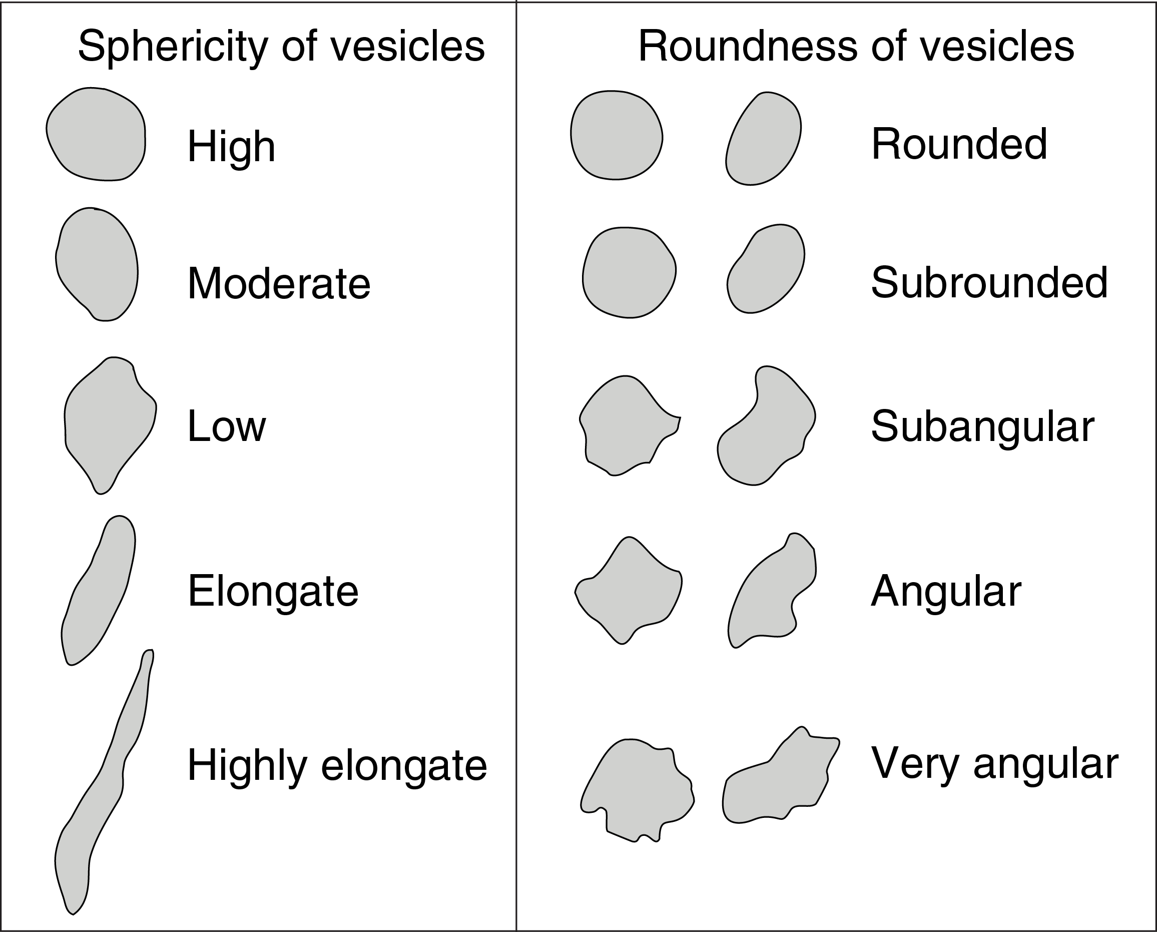
Figure F11. Comparison chart for describing vesicle sphericity and roundness in volcanic rocks.
Lava flow types
The suffix of the principal lithology name indicates the nature of the volcanic body. We applied the classification scheme used for Expedition 349 (Li et al., 2015), which includes the following types:
- Pillow lava flows: 0.1–1 m in thickness and defined by curved chilled margins, spherulitic textures, glassy margins and/or hyaloclastites, and microcrystalline to cryptocrystalline groundmass grain size, as well as decreasing crystal abundances and sizes (phenocrysts, groundmass) toward the glassy rims.
- Lobate lava flows: 1–2 m thick and formed by the same inflationary process as pillow lavas. In contrast to pillow lavas, they have massive, coarser grained, and sparsely vesicular flow interiors, often with pipe vesicle domains. Vesicle zoning occurs in the upper zones of the inflation unit as a series of vesicle bands, whereas the lower zones contain sparse, poorly defined vesicle banding and/or teardrop-shaped vesicles at the basal chilled zone.
- Sheet lava flows and massive lava flows: defined as more texturally uniform, sparsely vesicular, and characterized by a gradual increase in grain size toward the center of the flow, with sheet lava flows being <3 m thick and massive lava flows being >3 m thick.
For purposes of clarity, pillow lava flows and lobate lava flows are considered to be the same subunit when they occurred together. When pillow lava and lobate lava flows occurred in succession of each other, the igneous lithologic subunit was called a “pillow lava flow.” However, if a lobate lava flow had no pillow lava flow components and occurred as a separate flow either within or between massive and sheet flows, the igneous lithologic subunit was considered a “lobate lava flow” and given its own designation. Individual lobate and pillow lava flows were still recorded in DESClogik, but the lithologic subunit was not affected.
Contact types
Margins and contacts of flows were described by observing the features of the chilled sections that indicate a possible hiatus between two flows/pillows. A chilled contact, with or without glass, was recognized by observing the terminal end of the margin for sediment that was not entrenched into the rock but rather baked or cooked onto the rock, indicating a baked or chilled contact with the rock. A chilled margin was recognized through identification of a sudden change in groundmass over a very short distance. Unlike a chilled contact, sediment at the terminal end of the lobe or pillow was not required to determine its nomenclature. Several sections were described as having a chilled contact (typically with glass) in direct contact with sediments with an adjacent (or grading into) chilled margin (typically without glass) where the groundmass was determined to be cryptocrystalline and graded into a microcrystalline texture further up- or downhole. Glassy margins, chilled margins, and contact boundaries were inserted individually for the top and bottom of each section where they could be determined to discriminate individual flows and allow for a greater level of precision in the descriptions.
The following contact types were defined:
- Baked contact: contact with sediments that were baked by proximity of lava.
- Bottom (or top) chilled contact: chilled contact with sediments, with or without glass, in direct contact with sediments.
- Bottom (or top) chilled margin: chilled contact without sediments, without glass, determined by cryptocrystalline groundmass, typically found quenched adjacent to the chilled contact.
- Chilled contact: a contact that cannot be determined to be top or bottom of a flow that has sediment attached, such as a “roller.”
- Chilled margin: a chilled contact without sediment or obvious glass that cannot be determined to be top or bottom of a flow.
- Glassy margin: a margin between two pillows that has no sediment and the pillows have fused together. There is no clear indication of the boundary between the pillows as originally deposited.
Alteration
Alteration minerals
Alteration minerals were recorded in DESClogik in the macroscopic template under separate tabs for alteration, veins, and halos. Primary minerals are rock-forming minerals present prior to alteration (e.g., igneous minerals), whereas secondary minerals are related to alteration (e.g., metasomatism and hydrothermal circulation). Secondary minerals found replacing primary minerals and composing vesicle fillings and veins were classified as dominant, second order, and third order.
Identified alteration minerals or mineral mixtures include carbonate (calcite, dolomite, or siderite), chlorite, clay minerals (green clay), epidote (clinozoisite), secondary feldspar (albite), iddingsite, iron hydroxides, iron oxide, mica (sericite), neptunite, silica (jasper, quartz, opal, or hydrated quartz), spinel (magnetite), sulfides (chalcopyrite, covellite, pyrite, or sphalerite), zeolites, or unknown when the mineral could not be identified.
Alteration intensity
Low-temperature and low-pressure (i.e., seafloor) mineralization, veins, and background alteration were defined as alteration. Alteration description includes primary mineralogy, groundmass, phenocryst alteration, and infilling of vesicles and halos. Textures used to define groundmass alteration are patchy, corona, pseudomorphic, and recrystallized.
Levels of background alteration were recorded as follows:
- Fresh = <2 vol%.
- Slight = 2–10 vol%.
- Moderate = >10–50 vol%.
- High = >50–95 vol%.
- Complete = >95 vol%.
Veins and halos
We used the term “vein” to refer to any later crosscutting feature formed by sediment injection or precipitation from hydrothermal fluids and reserved the word “dike” to describe any later crosscutting feature that formed by introduction of magma. The term “halo” refers to alteration zones around veins or minerals identified by discoloration through change of the primary mineral assemblage. The density (i.e., the percentage of veins within a piece or an interval estimated visually), mineralogy, width, color, vein type (banded, composite, en echelon, haloed, intravenous, and uniform), connectivity (isolated, single, branched, and network), texture (cross-fiber, slip-fiber, massive, polycrystalline, and vuggy), and contacts with host rocks (diffuse, irregular, and sharp) were described, modified from the criteria from Leg 209 (Shipboard Scientific Party, 2004a) (Figures F11, F12). The length, width, and orientation of representative veins in a section were measured.
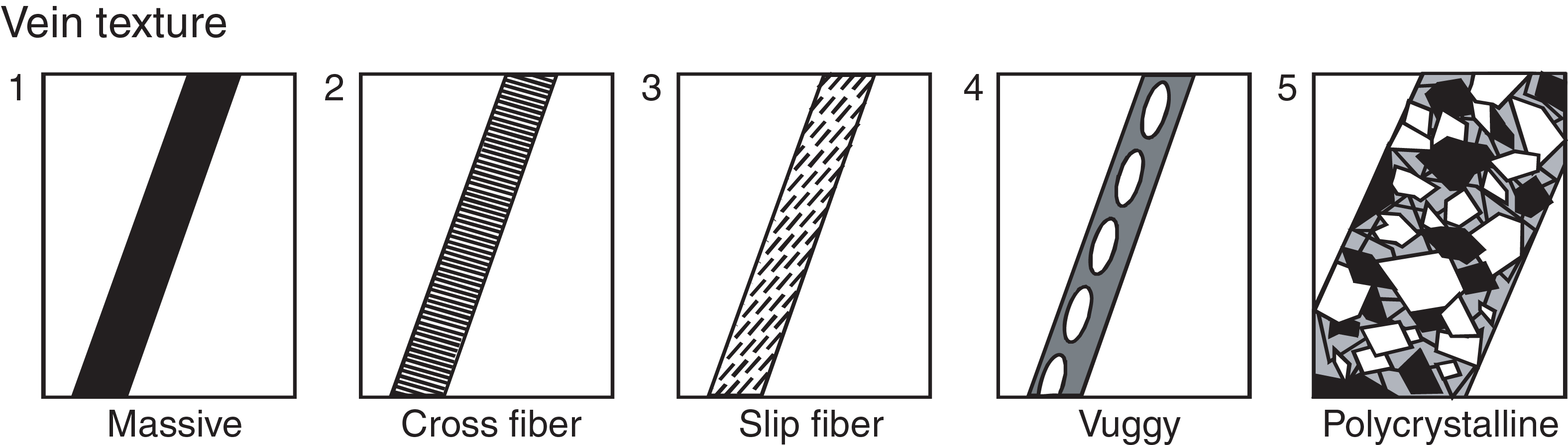
Figure F12. Textures used to describe veins.
Metamorphic petrology
Primary metamorphic lithology names
The nomenclature for metamorphic rocks applied here follows the recommendations of the IUGS Subcommission on the Systematics of Metamorphic Rocks (Schmid et al., 2004). A simple but comprehensive terminology for common metamorphic rocks follows their division into three major groups on the basis of their structure (as seen in hand specimen), giving the rock its principal lithology name: schist, gneiss, or granofels. The terms essentially reflect the degree of fissility or schistosity (i.e., a preferred orientation of tabular to elongate mineral grains or grain aggregates produced by metamorphic processes) shown by the rock. If the schistosity in a metamorphic rock is well developed, the rock has a schistose texture and is termed “schist.” If it is poorly developed, the rock has a gneissose texture and is termed “gneiss,” and if schistosity is effectively absent, the rock has a granofelsic texture and is termed “granofels.” Identified characteristic rock-forming minerals were added as a prefix. One exception to this general terminology was introduced for the specific case of mylonitic metabreccias (i.e., rocks showing an overprinted inherited fabric consisting of clasts within a matrix). To emphasize that the clasts are clearly prekinematic with respect to the mylonitic foliation, they were termed “granofels clasts.”
Other standard rock names used to describe metamorphic rocks as a function of mineralogy and texture are as follows:
- Marble: dominated by carbonates (>50% calcite ± Ca-bearing silicate, such as epidote and wollastonite). If the carbonates consist of dolomite, the prefix “dolomite” was added.
- Calc-silicate schist: schistose rock consisting of silicates and carbonates (<50% calcite ± Ca-bearing silicate, such as epidote and wollastonite).
Metamorphic textures
For metamorphic rocks, textural descriptions such as ductile (pervasive, weak, strong, or mylonitic) and brittle deformation (cataclasite or fractures) were used, as well as porphyroblasts, neoblasts, and porphyroclasts. Reaction textures were categorized, including prograde and retrograde metamorphism, coronas, symplectites, and intergrowths.
For deformed rocks, characteristics include (1) fault breccia, defined as any rock composed of angular broken rock fragments held together by mineral cement or a fine-grained matrix; (2) cataclasite, defined as a rock whose mineral grains or aggregates are fractured, rotated, bent, and granulated without accompanying recrystallization; and (3) mylonites, defined as a rock from a shear zone where the dominant deformation mechanism is ductile as solid-state flow and whose mineral grain sizes are often reduced in size by dynamic recrystallization.
Microscopic (thin section) description
The characterization of thin sections was used to complement and refine macroscopic core observations for igneous and metamorphic rocks (Figure F13). All thin section observations were entered into the LIMS database through a special DESClogik thin section template (see DESC_WKB in Supplementary material). Thin section descriptions include both primary (igneous) rock-forming minerals (including phenocrysts, groundmass, etc.) and secondary (alteration/metamorphism) mineral phases (in veins, vesicles, groundmass, etc.). Their mineralogy, abundance (modal volume percentages), sizes, shapes, habits, textural relationships, inclusions, alteration color, intensity and style, veins (type and number), and vesicles (type and fillings) were determined, enabling verification of macroscopic observations. The percentages of the original, primary mineral phases, groundmass, and vesicles (Original [%] = Present [%] + Replaced [%]) and the proportion of unaltered primary minerals were recorded when entering mineral abundances in DESClogik. Moreover, the presence of inclusions, overgrowths, zonations, and accessory minerals were documented.
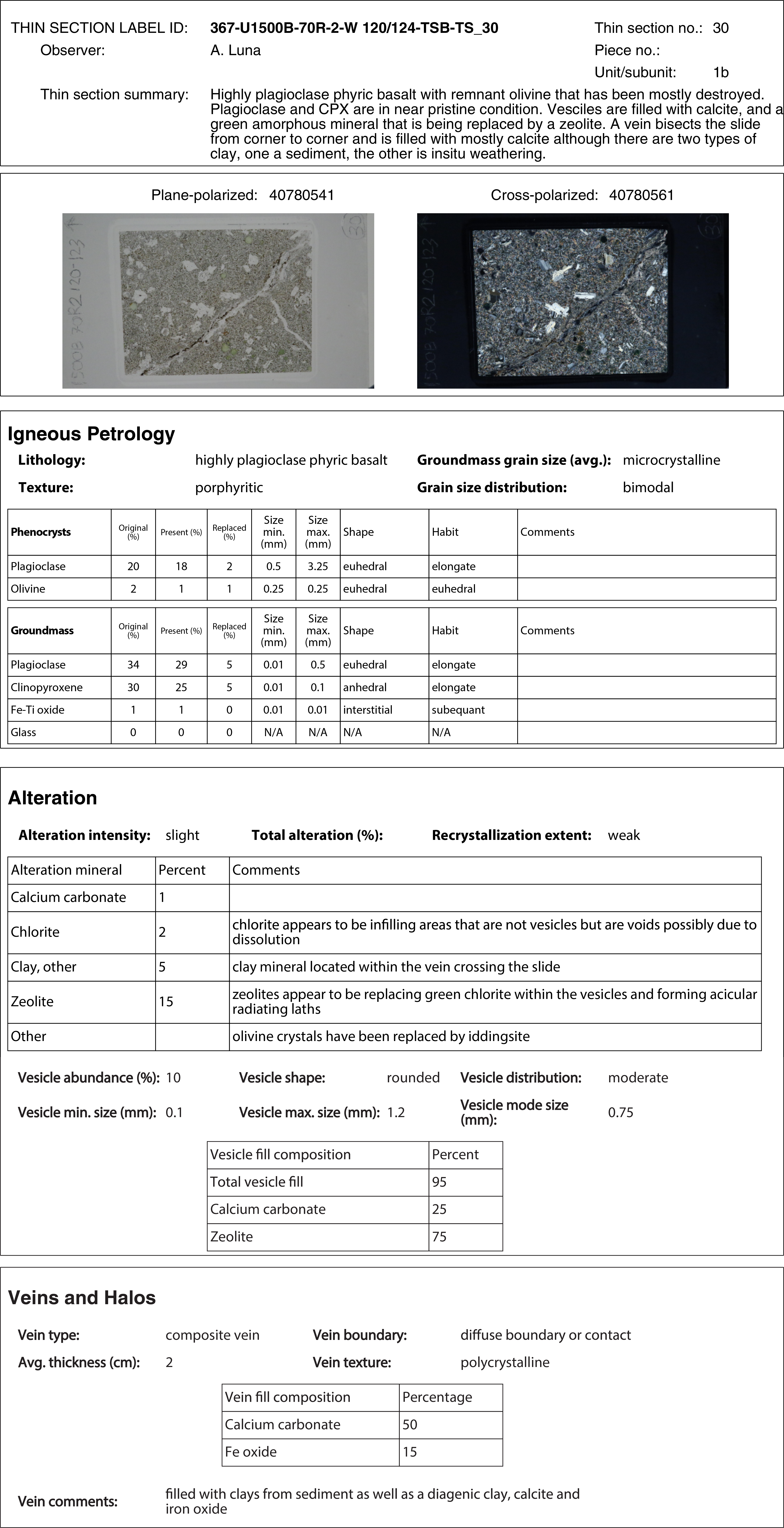
Figure F13. Example of a thin section report for igneous rocks.
Extrusive and hypabyssal thin section descriptions in the LIMS database
Thin section descriptions include the following terms:
- Sample domain: if there is more than one domain on the slide, each domain is described separately. For example, a slide that shows a large sedimentary vein (25% of the slide) in a basaltic matrix (75% of the slide) is described as two slides (samples): the first sample domain as “vein” and the second one as “host rock”. Other possible domains include clast, glass, halo, lithology, and xenolith.
- Lithology prefix: lithology prefix for the described sample domain.
- Principal lithology: refers only to the lithology of the described sample domain, which includes basalt, brecciated basalt, breccia, and hyaloclastite.
- Average groundmass grain size modal name: grain sizes follow Neuendorf et al. (2005) using the divisions glass, cryptocrystalline, microcrystalline, fine-, medium-, and coarse-grained (as defined in Primary lithology names of volcanic (extrusive and hypabyssal) rocks).
- Maximum grain size modal name: analogous to “average groundmass grain size modal name.”
- Grain size distribution: bimodal, equigranular, granular, inequigranular, poikilitic, and seriate (see Texture).
- Texture: aphanitic, aphyric, granular, glomeroporphyritic, holocrystalline, holohyaline, hypocrystalline, hypohyaline, intergranular, intersertal, interstitial, ophitic, porphyritic, seriate, spherulitic, subophitic, trachytic, and vitrophyric (see definitions above).
- Mineral phenocryst shape: the dominant (>50% of crystals) shape of the olivine (ol), plagioclase (plag), clinopyroxene (cpx), orthopyroxene (opx), and spinel (sp) crystals in euhedral, subhedral, and anhedral shapes.
- Mineral phenocryst habit: the dominant (>50% of crystals) habit of ol, plag, cpx, opx, and sp crystals in elongate, equant, subequant, and tabular habits (see definitions below).
- Plag phenocryst zoning type: continuous, discontinuous, oscillatory, and patchy zonation of the plagioclase crystals.
- Plag phenocryst zoning extent: none, scarce, abundant, and very abundant.
- Cpx and opx phenocryst exsolution: blebs and lamellae.
- Vesicle shape: see Figure F11.
- Mineral groundmass shape: for ol, plag, cpx, opx, sp, Fe-Ti oxides and sulfides—euhedral, subhedral, and anhedral.
- Mineral groundmass habit: for ol, plag, cpx, opx, sp, Fe-Ti oxides and sulfides—elongate, equant, subequant, and tabular.
Additional features such as dissolution/resorption textures, sieve textures, and inclusions are noted in the comments section.
Domains in DESClogik define different lithologies or textural domains inside a single lithologic unit (see Igneous and metamorphic lithologic units and lithostratigraphic units) within a thin section, including a diverse population of clasts, xenoliths, alteration, mingled magma, vesicular banding, and so on. Thus, thin sections encompassing a single lithologic unit might have multiple domains defined as Domain 1, Domain 2, and so on.
Metamorphic thin section description
Thin section descriptions include stable mineral parageneses, grain sizes, texture, minerals overprinting events (e.g., coronas, overgrowths, and pseudomorphs), secondary mineral assemblages, and estimation of the metamorphic facies. Such information is provided in the thin section summary in DESClogik.
Thin section descriptions include the following terms:
- Sample domain: if there is more than one domain on the slide, each domain is described separately. For example, a slide that shows a large granofels clast (25% of the slide) in an epidote-chlorite schist (75% of the slide) is described as two slides (samples): the first sample domain as “clast” and the second one as “groundmass.”
- Lithology prefix: lithology prefix for the described sample domain that includes epidote-chlorite, calc-silicate, and epidote.
- Principal lithology: refers only to the lithology of the described sample domain, which includes schist and granofels.
- Average grain size modal name: grain sizes follow Neuendorf et al. (2005) using the divisions cryptocrystalline, microcrystalline, fine grained, medium grained, and coarse grained.
- Maximum grain size class: maximum grain size encountered in the thin section, which includes fine grained, medium grained, and coarse grained.
- Grain size distribution: bimodal, equigranular, granular, inequigranular.
- Texture: isotropic and foliated.
Chemical analysis
During Expedition 368, a handheld portable X-ray fluorescence spectrometer (pXRF) (Olympus Delta) was used to conduct rapid in situ chemical analysis of solid rock samples (surfaces of the archive core sections and thin section billets). Previous IODP expeditions (e.g., Reagan et al., 2015; Ryan et al., 2017) demonstrated the utility of the pXRF to provide quick chemical characterization of igneous rocks encountered in the core. Such data are invaluable in initial assessments of broad chemical variations and the nature of the igneous rocks and, in conjunction with petrographic observations, in determining unit boundaries. These compositional data also help to target sample selection for postexpedition research.
The Olympus Delta pXRF is a self-contained, energy-dispersive XRF survey instrument. The instrument setup includes several modes (e.g., Geochem and Soils) that apply different correction protocols depending on sample type and geometry. During Expedition 368, we only applied the Geochem mode, which uses two sequential beams of different energy to determine a wide range of elements. The Olympus Delta pXRF cannot determine elements lighter than Mg (such as Na). For quantitative analyses, it is important to have the sample surface parallel to and in direct contact with the face of the instrument analyzer. To ensure a consistent geometry, two different holders were used, depending on the type of sample. Long core pieces (>5 cm) were analyzed directly in the core liner using a specially made, shielded XRF holder that holds the pXRF pointed vertically downward and resting in direct contact with the flat core surface. For smaller rock pieces (<5 cm) and calibration standard powders, the pXRF was pointed vertically upward and supported in a stand, and a special shielded chamber was attached to the front of the instrument. This allowed samples to be placed directly on the face of the analyzer. Analyses were made directly on the archive half of the core. Each measurement took 60 s, and three measurements were implemented on each sample point and averaged for an individual analysis (following the protocol in Reagan et al., 2015). A basaltic powder standard reference material (BHVO-2) was analyzed approximately every 12 samples to monitor data quality and instrument performance. Raw data were exported regularly and saved to the shipboard file directory for easy access. All data processing was done using Microsoft Excel spreadsheets.
To assess how well the correction protocols of the Geochem analysis mode recovered accurate concentration data in igneous rocks, calibration curves were produced on powder mounts of a suite of international standard reference materials (JP-1, BIR-1, BE-N, BCR-2, JB-2, AGV-1, and JA-2). These standards were chosen to cover the range of compositions that were initially anticipated for Expedition 368 (basalts, andesites, and peridotites). The accepted values for these standards were taken from the GEOREM database (http://georem.mpch-mainz.gwdg.de). These calibration standards were analyzed at the start (11 May 2017) and end (7 June 2017) of the analysis period (Table T1). Drift over this time period is limited (Figure F14), so the data from both calibration runs were combined to calculate a single calibration curve for each element. These calibrations were used to correct the raw concentration data output from the pXRF to improve the accuracy relative to the accepted values for the mafic igneous rock standards. Although these secondary calibrations were made on powders of standard materials and expedition data were measured on solid core material, previous studies have shown that this difference in method does not introduce any significant bias within the precision of the pXRF data (e.g., Ryan et al., 2017). Calibration data for 21 elements (Si, Ti, Al, Fe, Mn, Mg, Ca, K, P, V, Cr, Ni, Cu, Zn, Rb, Sr, Y, Zr, Nb, Mo, and Pb) are shown in Figure F14. For the remaining 13 elements measured by the pXRF (S, Co, As, Se, Ag, Cd, Sn, Sb, W, Hg, Bi, Th, and U), concentrations in the suite of standards were mostly below the instrument detection limits, so these elements were not considered further and are not reported in data tables. Although S is below detection limits in the calibration standards, it is semiquantifiable in rocks containing sulfide minerals, so raw S concentration data are reported when detected in samples. The correlation curves in Figure F14 are of varying quality, but most give high correlation coefficient values (R2 > 0.95). In a few cases, the high R2 values are influenced by one standard with a significantly higher (Mg, Cr, Ni, Nb, and Mo) or lower (Al) concentration. Several elements, such as Fe and Ca, show excellent correlations but with slopes that are significantly different to 1, and for these particular elements, making the secondary calibration correction is critical to get accurate data. Although V is above the instrument detection limits in most samples, a secondary calibration could not be applied because the calibration curve is extremely poor, and V results are presented as raw data only for information.
Table T1. Major element oxides and minor elements in reference solids. Download table in CSV format.
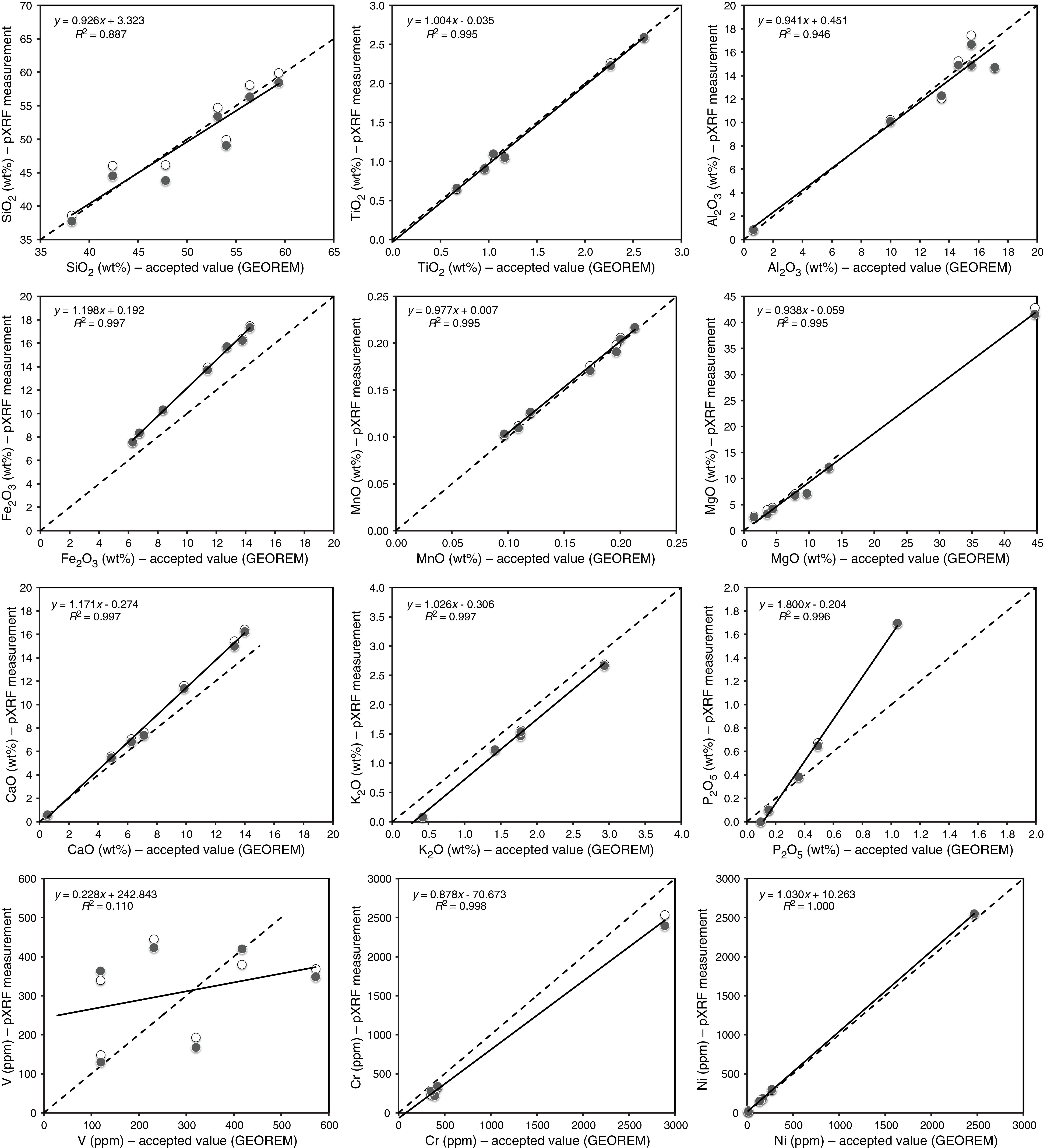
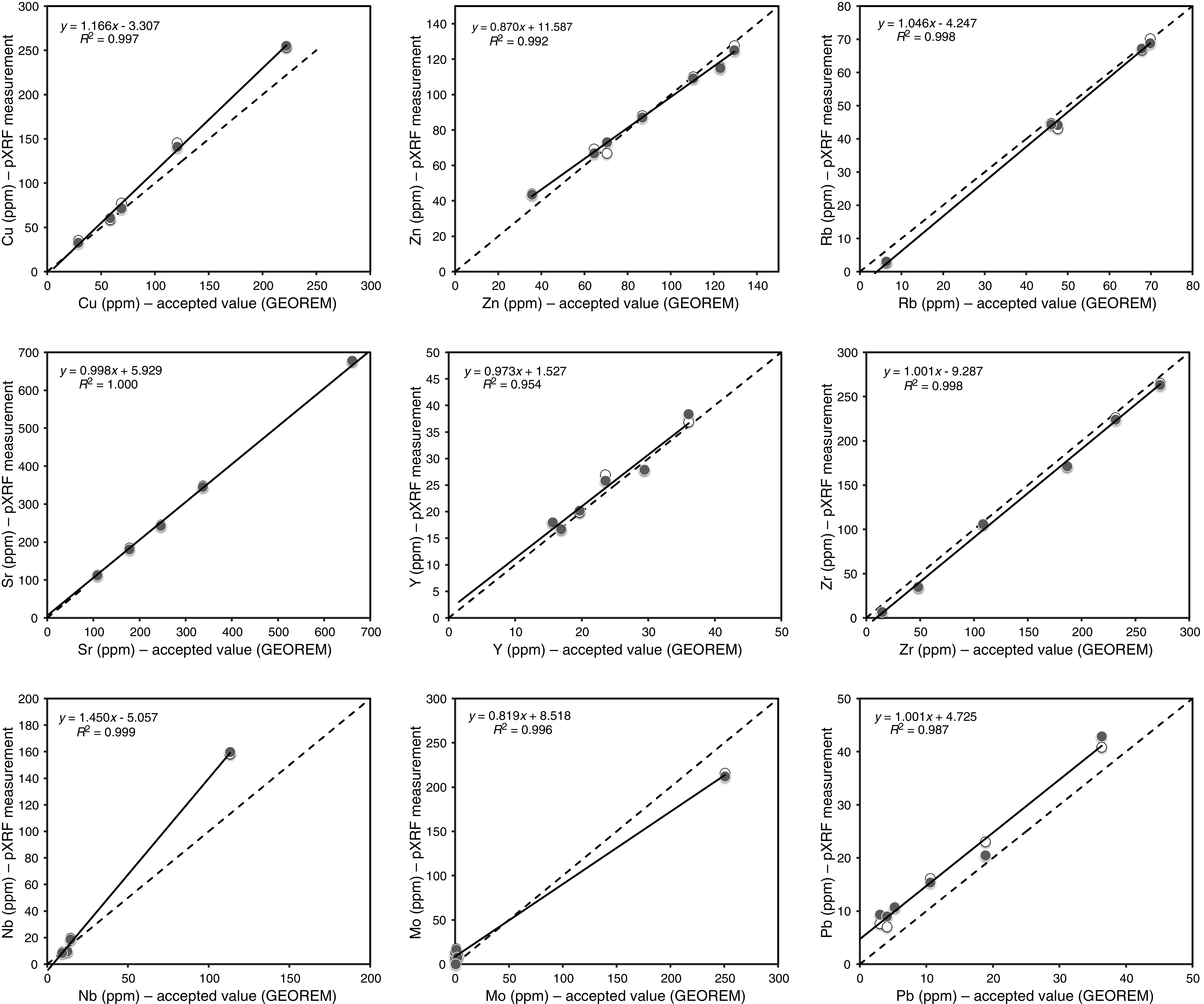
Figure F14. Comparison plots of measured pXRF data.
Results for the 42 replicate analyses of the data quality standard reference material (BHVO-2) are given in Table T1. Two of the 42 analyses had anomalously low values (SiO2 and Al2O3), perhaps indicating that the powder mount was not properly centered over the analysis window, and are thus excluded from the data analysis. Reproducibility over the course of analytical work during Expedition 368 was better than ±3% (relative standard deviation) for many elements (Si, Ti, Al, Fe, Mn, Ca, K, Ni, Cu, Zn, Sr, Y, and Zr) and better than ±10% for the remaining elements (Mg, P, Cr, Rb, Nb, and Mo), except for V (11%) and Pb (which is close to the instrument detection limit in BHVO-2). In terms of accuracy, the corrected concentrations of Si, Fe, Mn, Ca, Zn, Sr, Zr, and Nb are within 3% of the accepted values for BHVO-2 and Ti, Mg, K, Cu, and Y are within 5% of the accepted values.
To complement and considerably extend the chemical analysis made by the shipboard pXRF data set, a third-generation, energy-dispersive Avaatech XRF core scanner was used postexpedition. Onshore in situ XRF measurements were implemented for major (beyond the atomic number of Mg) and selected trace elements on Site U1500 and U1502 volcanic rock sections at the JRSO XRF Core Scanning Facility at the Gulf Coast Repository at Texas A&M University. A high standard resolution of 2 cm was applied (partially down to 0.1 cm), whereas a lower resolution had to be chosen in sections with cracks, rubble, and plastic spacers. Three runs with irradiated sample dimensions of 1.2 cm cross-core and 1 cm downcore were performed on each core section along its centerline under different X-ray excitation conditions (defined by appropriate kV, mA, and filter settings). Several repeated runs were carried out across the entire depth range of the volcanic rock section to monitor data reproducibility. Rock standard mounts were run parallel on a regular basis for quality assurance. As part of the shipboard data set, the produced XRF core scanning data can be retrieved from the LIMS database (http://web.iodp.tamu.edu/LORE).
Structural geology
This section outlines the tectonic terminology used in this volume to describe the general architecture of the northern South China Sea margin and the methods and nomenclature applied to document the structural features observed in the sediments and basement rocks recovered during Expeditions 367 and 368. Such features encompass bedding dips, fractures and veins, faults and folds, and fault rocks and shear zones.
Tectonic terminology
Numerous classifications and terminologies have been proposed to describe the nature of hyperextended margins (see Peron-Pinvidic et al. [2013] and Tugend et al. [2015] for recent summaries and discussion). Although hyperextended margins are often equated with magma-poor rifted margins (e.g., Doré and Lundin, 2015), in this volume we simply refer to hyperextension as a process of profound extension (crustal stretching factor ~3 or higher) of the continental crust by normal faulting and low-angle detachments. This tectonic episode may or may not include several generations of faulting. We note that hyperextension of the continental crust and mantle lithosphere may involve different structural domains across the rifted margin. We refer in our study to the continent–ocean transition as the hyperextended domain (also referred to as distal domain) linking moderately thinned continental crust (~15 km thick) to oceanic crust. Oceanic crust in our study is 5–6 km thick crust that accretes in a steady state along a focused spreading ridge. The source of new crust can range from mantle undergoing serpentinization to form a crustal layer to upwelling of asthenospheric mantle that melts by decompression and produces new, “Penrose-type” igneous crust.
Methods
After a core was split and described by sedimentologists or petrologists, we documented structural features observed on the archive half by
- Identifying structural features and classifying their structural types,
- Determining the top and bottom location of structural features in the core,
- Measuring the orientation of a structural feature where applicable,
- Determining the sense of displacement on a structural feature where applicable,
- Determining the temporal relation between structures (especially for crosscutting structures and shear zones), and
- Assessing the role of fluids in deformation processes.
Our methods largely followed those used by structural geologists from Integrated Ocean Drilling Program Expedition 344 and Expedition 349 (Harris et al., 2013; Li et al., 2015). The types of structural measurements and key parameters (either observed or calculated) were recorded on a spreadsheet (Figure F15). These data were then input into the LIMS database using DESClogik. Where possible, orientation data were corrected for rotation related to drilling using paleomagnetic declination and inclination information (see Paleomagnetism) or by comparison to observed features in the Formation MicroScanner (FMS) log (see Azimuth correction based on FMS log).
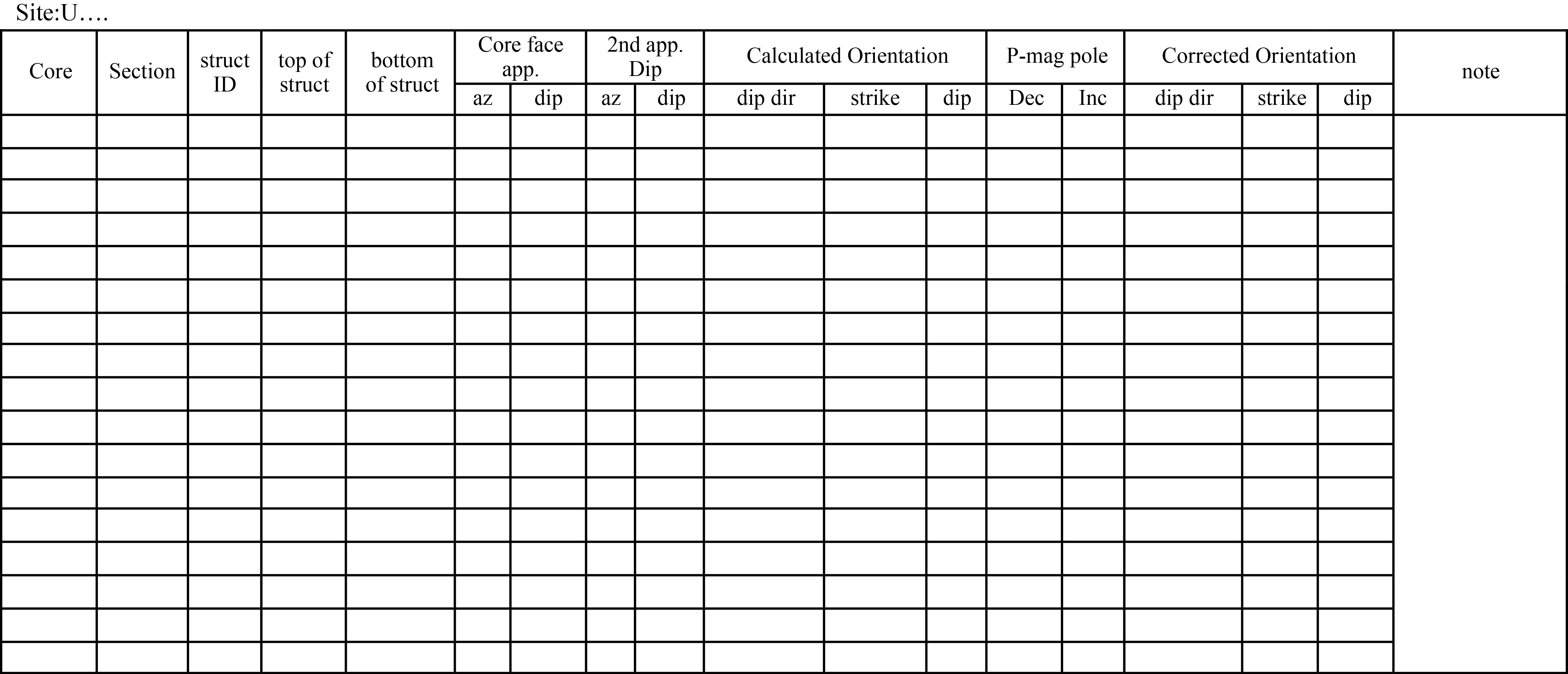
Figure F15. Example structural geology observation sheet.
Graphic symbols and terminology
A predefined set of commonly observed structural features was used in the structural description of cores. The terminology and graphic symbols used are presented in Figures F16 and F17. We identified the following major structural features:
- Joints and fractures: brittle failure with no displacement and no secondary infill minerals. Breaks clearly resulting from drilling were logged separately as drilling-induced fractures in the Drilling disturbance spreadsheet in DESClogik.
- Veins: fractures filled with secondary minerals. Veins were described in both the Structure and Veins/halos tabs in DESClogik.
- Fault rocks: brittlely deformed rocks such as fault breccia and fault gouge. For sake of simplicity in this volume, the term “fault breccia” is defined as a clast-supported fault rock with angular clasts, and the term “fault gouge” is defined as a matrix-supported fault rock with rounded clasts.
- Hydrothermal breccia: fluid-assisted deformation leading to the fragmentation and brecciation of the rocks.
- Shear zones: zones affected by ductile crystal-plastic deformation and surrounded by less deformed rocks.
- Sedimentary bedding: layering of sediments and sedimentary rocks.
- Folds: folded sedimentary or basement rock layers.
- Igneous contacts: material contacts of extrusive or intrusive igneous rocks.
- Magmatic fabrics: magmatic foliations defined by the preferred orientations of primary minerals with no evidence of crystal-plastic deformation.
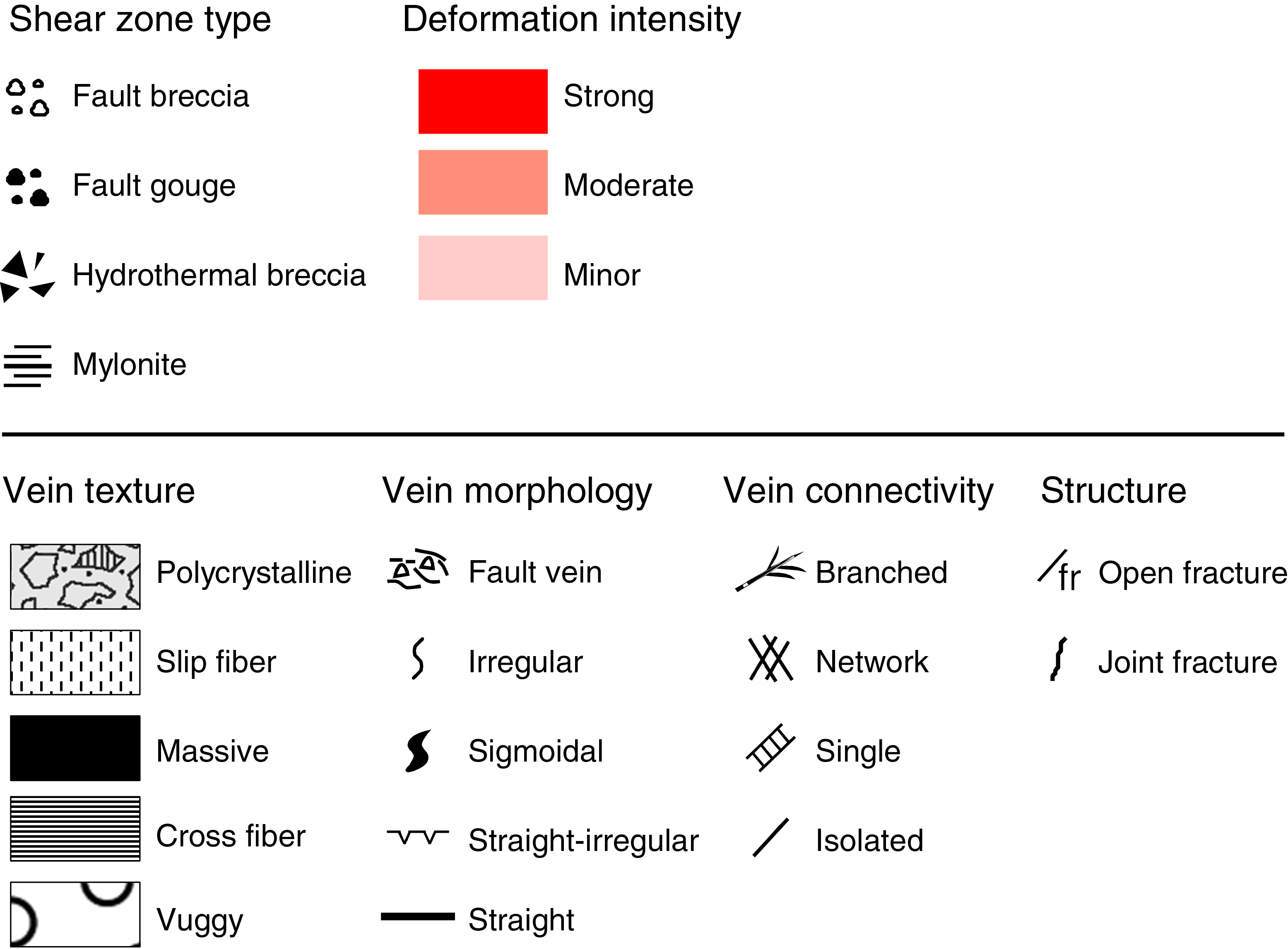
Figure F16. Symbols and nomenclature used for visual core description.
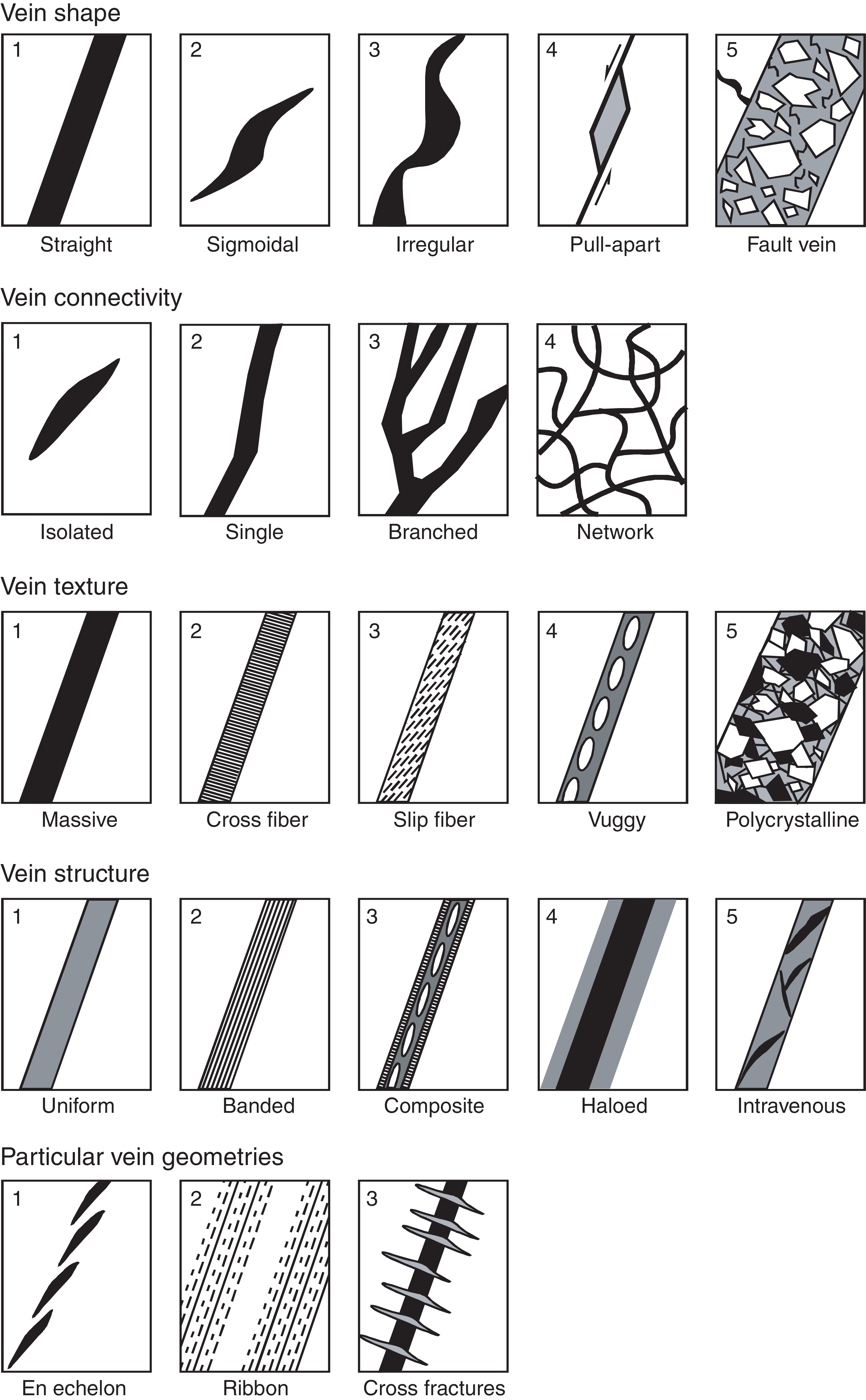
Figure F17. Vein description scheme.
Structural observation and description
Structural features were described from the top to the bottom of each section of the core. For fractures, we examined and measured the following parameters:
- Location: where a fracture occurs in a core, measured in centimeters from the top of the section.
- Morphology and structure: morphological shape of a fracture (e.g., straight, curved, banded, irregular, composite, isolated, single or branched).
- Displacement: lateral offset and/or opening of a fracture measured in centimeters; a closed fracture with no lateral offset is recorded as 0 cm of displacement.
- Orientation: dip angle, strike, and dip direction of a fracture measured in degrees; where applicable, reorientation of a fracture to geographic coordinates (i.e., relative to true north) was done to determine the real dip direction (see Orientation measurements and correction).
- Frequency: occurrence frequency of fractures per section.
- Types: type of deformation of a fracture (e.g., normal, reverse, dextral, sinistral displacement, or a combination of the above).
For veins, we examined and measured several parameters:
- Location: where a vein occurs in a core, measured in centimeters from the top of the section.
- Morphology: main morphological characteristics of a vein such as shape, connectivity, texture, structure, and particular vein geometries (Figure F17).
- Orientation: dip angle and dipping direction of a vein.
- Frequency: occurrence frequency of veins per section.
- Mineral infill and alteration: these features are recorded as described by petrologists.
For fault rocks, hydrothermal breccias, and shear zones, we examined and measured the following parameters:
- Location: interval where a shear zone occurs in a core, measured in centimeters from the top of the section.
- Nature: type of fault rock, hydrothermal breccia, or shear zone, including fault gouge, fault breccia, cataclasite and mylonite.
- Morphology: morphological shape of the deformed zone and of the clasts.
- Orientation: dip angle and dip direction of the preferred orientation of the clasts, where applicable.
- Deformation intensity: characterization of the deformation intensity including foliation development.
- Frequency: occurrence frequency of shear zones per section.
- Mineral and alteration: matrix and clasts described by petrologists.
For sedimentary bedding, we described the following parameters:
- Location: where a nonsubhorizontal bedding occurs in a core (dip > 5°), measured in centimeters from the top of the section.
- Type of contacts: type of sedimentary contact boundary.
- Orientation: dip angle, strike, and dip direction of sedimentary bedding.
For folds, we described the following parameters:
- Location: where a fold contact occurs in a core, measured in centimeters from the top of the section.
- Type: type of fold.
- Frequency: occurrence frequency of fold axis per section.
For igneous contacts, we described the following parameters:
- Location: where an igneous contact occurs in a core, measured in centimeters from the top of the section.
- Type of contacts: type of igneous contact boundary.
- Orientation: dip angle and dip direction of an igneous contact.
- Frequency: occurrence frequency of igneous contacts per section.
- Mineral infill and alteration: as described by petrologists.
For magmatic fabrics, we measured the following parameters:
- Location: where a magmatic fabric feature occurs in a core, measured in centimeters from the top of the section.
- Morphology: morphological shape of a magmatic fabric feature.
- Orientation: dip angle, strike and dip direction of a magmatic fabric feature.
- Frequency: occurrence frequency of magmatic fabrics per section. The occurrence frequency of a structure per section is normalized on a 10 cm section.
Orientation measurements and correction
Orientation measurements
We used a plastic goniometer for orientation measurements. For sealed structures, we wrapped a transparent plastic protractor template around the core to determine the true dip (Figure F18). Orientations of planar and linear features in a core section were determined relative to the core reference frame (Figure F19). The vertical axis of the core reference frame is aligned with the upcore direction of the core section, whereas the double line marked on the core liner is defined as 180° in the cross-sectional plane perpendicular to the core vertical axis.
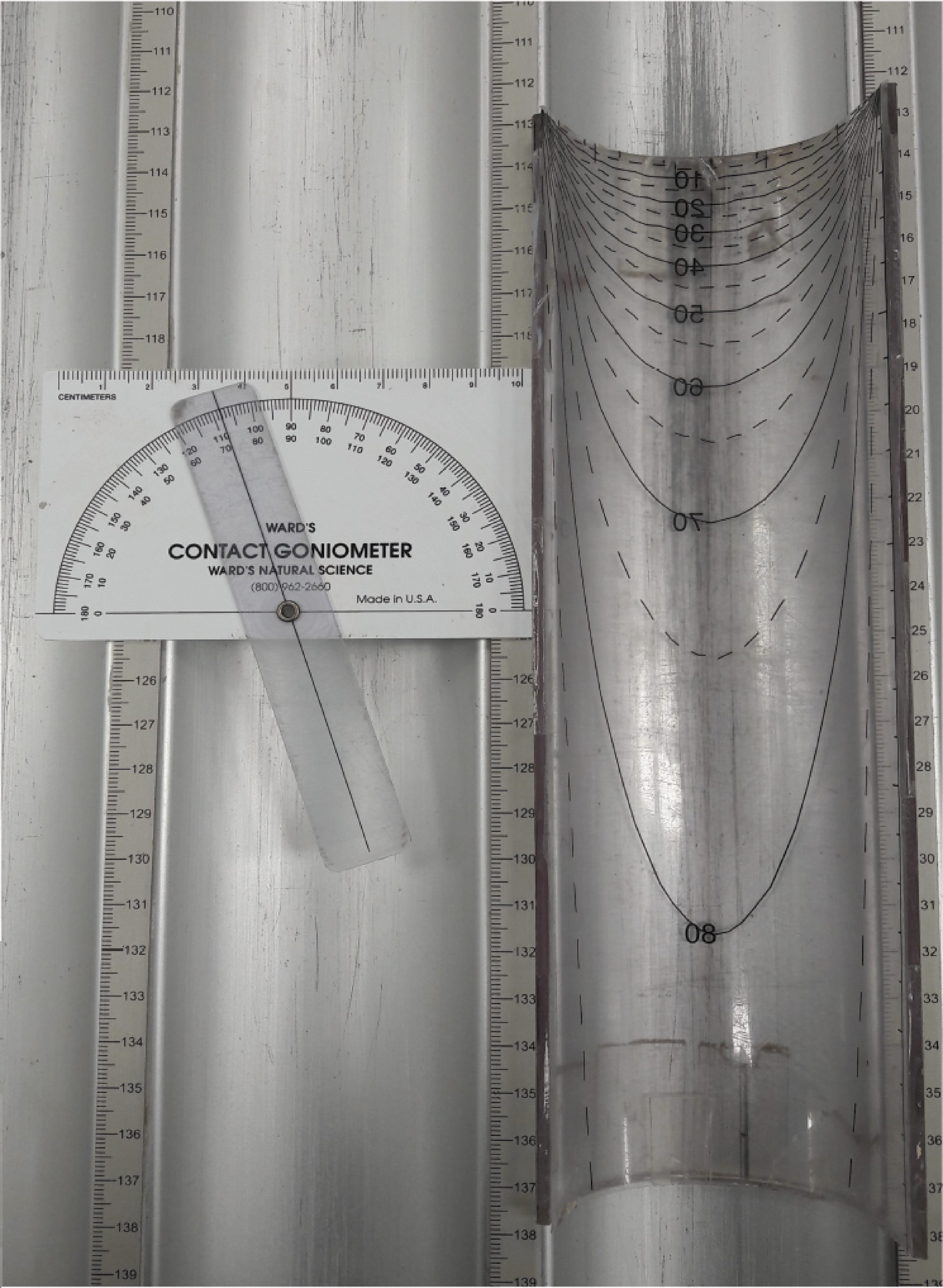
Figure F18. Goniometer and plastic protractor template.
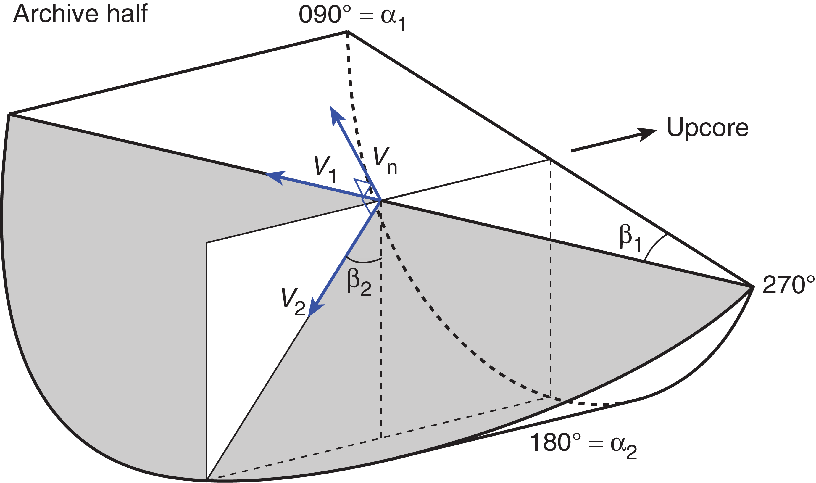
Figure F19. Core reference frame and coordinates used in orientation data calculation.
To determine the orientation of a planar structural element (shaded plane in Figure F19), two apparent dips of the element were measured in the core reference frame. The first apparent dip measures the intersection angle between the planar structural element and the split face of the core (β1 in Figure F19); it is determined by measuring the dip direction and angle of the planar structural element in the core reference frame. A planar structural element could have a trend of 90° or 270° and a plunge angle ranging from 0° to 90°. The second apparent dip measures the intersection angle between the central line of the planar structural element and the split face of the core (β2 in Figure F19). In most cases, this was a plane either parallel or perpendicular to the core axis. In the former case, the apparent dip would trend 0° or 180° with a plunge angle ranging from 0° to 90°; in the latter case, the trend would range from 0° to 360° with a plunge angle of 0°.
A linear feature observed in the surface of a split core is often associated with a planar structural element (e.g., a fault plane) in the core; the orientation of the planar structural element is determined by measuring either the rake (or pitch) of the associated plane or the trend and plunge of the planar element in the core reference frame. All measured data were manually typed into the log sheet together with the measured depths in the core section and descriptive information (Figure F15).
Plane orientation calculation
For a planar structural element (e.g., a bedding or fault plane), two apparent dips on two different surfaces (e.g., one being the split core surface, which is east–west vertical, and the other being a horizontal or north–south vertical surface) were measured in the core reference frame. The two apparent dips are the azimuth (measured clockwise from north, looking down) and plunge. An x, y, z coordinate system was defined in such a way that the positive x-, y-, and z-directions coincide with north, east, and vertical downward, respectively. If the azimuths and plunges of the two apparent dips are given as (α1, β1) and (α2, β2), respectively, as in Figure F19, the unit vectors representing these two lines, v1 and v2, are given by the following expression:
For any plane, the direction of the normal to the plane can be found by taking the cross product of two (nonparallel) vectors that lie within the plane. Using the above equations for v1 and v2, therefore, the unit vector normal to plane vn (Figure F20) is defined as follows:
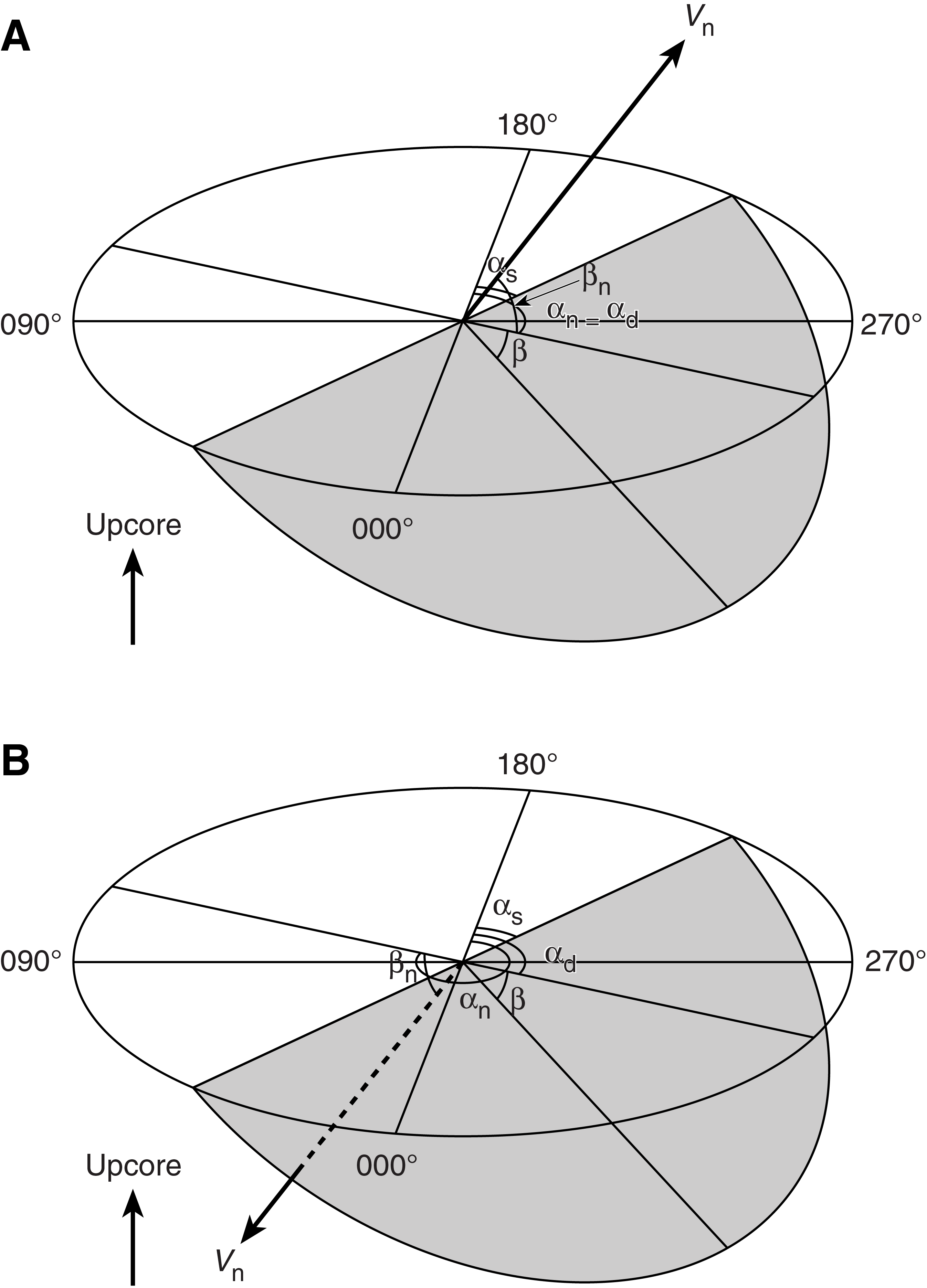
Figure F20. Dip direction, right-hand rule strike, and dip.
The azimuth αn and plunge βn of the vector vn are given by
The dip direction αd and dip angle β of this plane are αd = αn and β = 90°+ βn, respectively, when βn < 0° and αd = αn ± 180° and β = 90° − βn, respectively, when βn ≥ 0°. The strike of this plane, αs, according to the right-hand rule is then given by αs = αd − 90° (Figure F20).
Azimuth correction based on paleomagnetic data
Provided that a core is vertical, its magnetization is primary, the core was magnetized in the Northern Hemisphere, and its bedding is horizontal, its paleomagnetic declination αp indicates the magnetic north direction when its inclination βp ≥ 0° (Figure F21); in contrast, the angle αp indicates the magnetic south direction when βp < 0°. The dip direction and strike of a planar structural element in the geographic reference frame, αd* and αs*, are therefore αd* = αp − αd and αs* = αp − αs when βp ≥ 0° or αd* = 180° + αp − αd and αs* = 180° + αp − αs when βp < 0°.

Figure F21. Azimuth correction based on paleomagnetic data.
If a core section was complete and continuous, one paleomagnetism sample per section (1.5 m) was deemed sufficient to determine the paleomagnetic orientation of the core section. If the core was discontinuous, one paleomagnetism sample for each subsection of the core that was continuous and structurally important was required. Paleomagnetism samples were taken as cubic or cylindrical samples close to a planar structural element of interest (usually within 5 cm) and from a coherent core interval that included the structural element of interest. In general, we avoided core fragments that were so small that potential spinning during drilling might cause significant deviation from the core axis (e.g., fragments of brecciated segments). This procedure was carefully followed, but for different reasons at each site we failed to reorient our structural measurements with respect to the paleomagnetic data.
Azimuth correction based on FMS log
If an FMS log is available for the section of the drill hole that contains the core, there may be distinctive features that can be correlated from the FMS log to the core, such as bedding, fractures, folds, veins, stratification, and bioturbation. In this case, the core can be oriented with respect to geographic north. However, this orientation has to be done after the FMS log is obtained after all the cores in the hole have been collected.
Thin section description
Following ODP Leg 210 (the most recent expedition to sample basement rocks similar to those of the current expeditions), thin sections of sedimentary, igneous, and metamorphic rocks recovered were examined to
- Document each type of macroscopic deformation structure in a systematic and quantitative way,
- Characterize the microstructure of the rocks,
- Provide information on the kinematics of ductile and brittle deformation,
- Assess the role of fluids in contributing to deformation, and
- Document major structural zones and downhole variations.
For the description of microstructures, we applied the terminology of Passchier and Trouw (2005). Shipboard thin sections were oriented, except when they were made from small pieces whose orientation with respect to the rest of the core was unknown. Orientation was in the core reference frame and was marked on each thin section by an arrow pointing upward and a short tick pointing west from the base of the arrow. Marking two directions is necessary to achieve complete orientation of thin sections, which are cut parallel to the split surface of the core.
Biostratigraphy
During Expeditions 367 and 368, calcareous nannofossils, planktonic and benthic foraminifers, diatoms, and ostracods were studied in core catcher samples. Samples from core sections were examined when a more refined age determination was necessary and when time permitted. Biostratigraphic events, mainly the first appearance datum (FAD or base) and last appearance datum (LAD or top) of the age-diagnostic species are tied to the geomagnetic polarity timescale (GPTS) of Gradstein et al. (2012) (Figure F22).
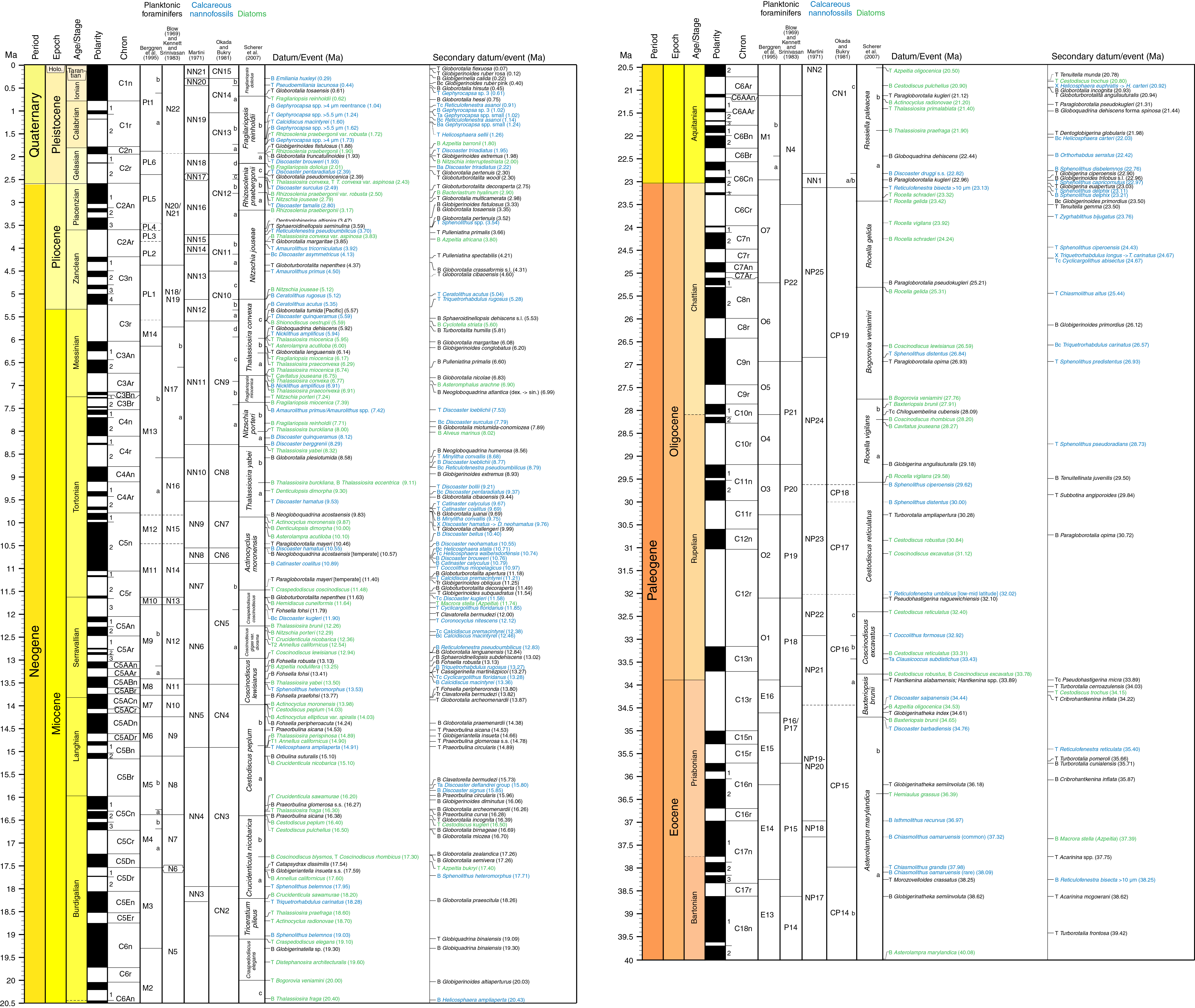
Figure F22. Calcareous nannofossil, diatom, and planktonic foraminiferal events and scaled ages.
Calcareous nannofossils
Calcareous nannofossil zonation was based on the schemes of Okada and Bukry (1980) and Martini (1971). Calibrated ages for bioevents are from Gradstein et al. (2012) and given in Table T2. The timescale of Gradstein et al. (2012) assigns the Pleistocene/Pliocene boundary between the Gelasian and Piacenzian stages (2.59 Ma), the Pliocene/Miocene boundary between the Zanclean and Messinian stages (5.33 Ma), the late/middle Miocene boundary between the Tortonian and Serravalian stages (11.63 Ma), the middle/early Miocene boundary between the Langhian and Burdigalian stages (15.97 Ma), the Miocene/Oligocene boundary between the Aquitanian and Chattian stages (23.03 Ma), and the Oligocene/Eocene boundary between the Rupelian and Priabonian stages (33.89 Ma). For calcareous nannofossil biostratigraphy, the Pleistocene/Pliocene boundary now falls within Zone NN16 (Martini, 1971) between the LADs of Discoaster surculus (2.49 Ma) and Discoaster tamalis (2.8 Ma). The Pliocene/Miocene boundary falls within Zone NN12 between the LAD of Triquetrorhabdulus rugosus (5.28 Ma) and the FAD of Ceratolithus larrymayeri (5.34 Ma); however, C. larrymayeri was not noted in our samples, so we used the FAD of Ceratolithus acutus (5.35 Ma) as an alternative event. The late/middle Miocene boundary is placed within Zone NN7 between the LAD of common Discoaster kugleri (11.58 Ma) and the FAD of common D. kugleri (11.90 Ma). The middle/early Miocene boundary falls within Zone NN4 between the LADs of Helicosphaera ampliaperta (14.91 Ma) and Sphenolithus belemnos (17.95 Ma). The Miocene/Oligocene boundary is placed within Zone NN1 between the FAD of Discoaster druggii (22.82 Ma) and the LAD of Reticulofenestra bisecta (>10 µm; 23.13 Ma). The Oligocene/Eocene boundary is placed within Zone NP21 between the LADs of Coccolithus formosus (32.92 Ma) and Discoaster saipanensis (34.44 Ma). In this study, the subdivision of these geologic time boundaries was mostly based on recognition of these nannofossil bioevents.
Table T2. Calcareous nannofossil events and scaled ages. Download table in CSV format.
Several species of the genus Gephyrocapsa, which are commonly used as Pleistocene biostratigraphic markers, often show a great range of variation in sizes and other morphological features, causing problems in identification (e.g., Samtleben, 1980; Su, 1996; Bollmann, 1997). Size-defined morphological groups of this genus (Young, 1998; Maiorano and Marino, 2004; Lourens et al., 2004; Raffi et al., 2006) were used as event markers during shipboard study, including Gephyrocapsa sp. 3, Gephyrocapsa spp. medium I (≥4 µm), large Gephyrocapsa spp. (≥5.5 µm), Gephyrocapsa spp. medium II (≥4 µm; bmG event), and small Gephyrocapsa spp. (<3.5 µm).
Several Reticulofenestra species with different coccolith and central opening sizes have been used as Neogene and Quaternary biostratigraphic markers; however, these parameters show considerable variations within and between “species,” making species differentiation difficult (e.g., Su, 1996; Young, 1998). In this study, we followed the definition of Reticulofenestra pseudoumbilicus by Young (1998) as having a coccolith length >7 µm (similar to the size of its holotype), especially for specimens from its uppermost range in the early Pliocene. We distinguished Reticulofenestra asanoi from the similarly sized Pseudoemiliania lacunosa by the absence of slits on the shield (Su, 1996). In addition, we further distinguished three Reticulofenestra morphotypes including Reticulofenestra ampla (5~7 µm, with central opening), R. bisecta (5~10 µm, with a solid central plug), and R. bisecta (>10 µm, with a solid central plug) following Young et al. (2014).
The LAD of Sphenolithus spp. (3.54 Ma) in Pliocene Zone NN16 was based on the LADs of Sphenolithus abies and Sphenolithus neoabies according to Raffi et al. (2006). Species concepts for other taxa mainly follow those of Perch-Nielsen (1985) and Bown (1998).
Methods
Calcareous nannofossil samples were prepared using standard smear slide techniques. For samples from sandy sediments, suspended aliquots of the raw sample were analyzed. Samples were examined with a Zeiss microscope under XPL and plane-transmitted or phase contrast light at 1000× to 2000× magnification. A Hitachi TM3000 tabletop scanning electron microscope (SEM) was used to confirm the presence of small forms such as Emiliania huxleyi, an important marker for the latest Pleistocene–Holocene. Preservation of nannofossils was defined as follows:
- VG = very good (no evidence of dissolution and/or overgrowth).
- G = good (slight dissolution and/or overgrowth; specimens are identifiable to the species level).
- M = moderate (some etching and/or overgrowth; most specimens are identifiable to the species level).
- P = poor (severely etched or overgrowth; most specimens cannot be identified at the species and/or generic level).
The relative abundance of calcareous nannofossils within the sediment was visually estimated at 1000× magnification by referring to the particle abundance charts in Rothwell (1989) and reported using the following abundance categories:
- D = dominant (>90% of sediment particles).
- A = abundant (>50%−90% of sediment particles).
- C = common (>10%−50% of sediment particles).
- F = few (1%–10% of sediment particles).
- R = rare (<1% of sediment particles).
- B = barren (no nannofossils present in 100 FOV).
The relative abundance of individual calcareous nannofossil species or taxa groups was estimated at 1000× magnification and defined as follows:
- D = dominant (>50%, or 100 specimens/FOV).
- A = abundant (10%−50%, or 10–100 specimens/FOV).
- C = common (1%−10%, or 1–10 specimens/FOV).
- F = few (0.1%−1%, or 1 specimen/1–10 FOV).
- R = rare (<0.1%, or <1 specimen/10 FOV).
Foraminifers
Planktonic foraminifers
The planktonic foraminiferal zonation schemes of Blow (1969, 1979) and Berggren et al. (1995) as modified by Wade et al. (2011) were used in this study. Calibrated ages for bioevents are from Gradstein et al. (2012) (Table T3). We also adopted the use of the LAD (0.12 Ma; Thompson et al., 1979) and FAD (1.16 Ma; Li et al., 2005) of Globigerinoides ruber (pink) as biostratigraphic indicators. The FAD of G. ruber (pink) acme (0.40 Ma; Li et al., 2005) was also adopted. The age for the LAD of Globorotalia mutlicamerata (2.18 Ma) was adjusted based on regional stratigraphic work (Li et al., 2005).
Table T3. Planktonic foraminiferal events and scaled ages. Download table in CSV format.
Taxonomic concepts for Neogene and Paleogene taxa mainly follow those of Kennett and Srinivasan (1983) and Bolli and Saunders (1985).
Planktonic foraminifer species distribution and range charts are presented in each site chapter.
Benthic foraminifers
Taxonomic assignments for benthic foraminifers follow Loeblich and Tappan (1988), Kaminski and Gradstein (2005), and Holbourn et al. (2013). Paleodepth estimates were based on selected benthic foraminiferal taxa noted and described by van Morkhoven et al. (1986) using the following categories:
- Neritic = <200 m.
- Bathyal = 200–2000 m.
- Upper bathyal = 200–600 m.
- Middle bathyal = 600–1000 m.
- Lower bathyal = 1000–2000 m.
- Abyssal = >2000 m.
- Upper abyssal = 2000–3000 m.
- Lower abyssal = >3000 m.
Benthic foraminiferal assemblage composition and paleodepth estimates were based on counts of at least 100 specimens from the >150 µm size fractions, where possible.
Preparation and examination techniques
Sample preparation for foraminifer identification uses the same techniques for both planktonic and benthic foraminifers. Core catcher samples (and additional core samples as needed) were soaked in distilled water and washed over a 63 µm mesh sieve. Consolidated or lithified samples were cut in pieces and crushed to pea size, to which a hydrogen peroxide solution was added. This mixture was heated in the oven below 50°C for several hours and then sieved as above. Some samples were rewashed by additional disaggregation with the hydrogen peroxide solution. All samples were dried in a low temperature oven at ~50°C. The dried samples were sieved over a 150 µm sieve, retaining the <150 µm size fraction in a separate vial. To avoid contamination of foraminifers between samples, the sieves were thoroughly cleaned between samples, placed into a sonicator for at least 15 min, and then carefully checked. Species identifications for planktonic and benthic foraminifers were generally made on the >150 µm size fractions. The 63–150 µm size fraction was observed for distinctive taxa.
In addition, mudline (or hole top) samples were taken from selected sites and analyzed for planktonic and benthic foraminifers and ostracods. Mudline samples were collected by emptying the sediment/water material from the top core liner of a hole into a bucket and then washing it with tap water over a 63 μm sieve. Sample staining using Rose Bengal (1 g/L) was performed to confirm the presence of living foraminifers and ostracods in the mudline sample. For this, a portion of the sample was incubated for 12 h with Rose Bengal stain before being washed through a 63 μm sieve. All samples were then dried at ~50°C and subsequently examined under a binocular light microscope. Selected microfossil specimens were also examined and imaged using the shipboard SEM.
The total abundance of planktonic foraminifers was reported using the following categories:
- A = abundant (>30% planktonic foraminifer specimens in total residue).
- C = common (10%−30% planktonic foraminifer specimens in total residue).
- R = rare (%1−10% planktonic foraminifer specimens in total residue).
- P = present (<1% planktonic foraminifer specimens in total residue).
- B = barren (no planktonic foraminifer specimens in total residue).
Individual planktonic foraminifers were recorded in qualitative terms based on an assessment of forms observed in a random sample of ~400 specimens from the >150 µm size fraction. Relative abundances were reported using the following categories:
- D = dominant (>30% of the assemblage).
- A = abundant (>10%−30%).
- F = few (>5%−10%).
- R = rare (1%−5%).
- P = present (<1%).
Preservation of planktonic foraminifer assemblages was recorded using the following categories:
- VG = very good (no evidence of breakage or dissolution).
- G = good (>80% of specimens unbroken with only minor evidence of diagenetic alteration).
- M = moderate (30%−80% of the specimens unbroken).
- P = poor (strongly recrystallized or dominated by fragments and broken or corroded specimens).
Ostracods
Ostracods were studied at selected sites when time was available. Sample preparation for ostracod examination and illustration followed the same techniques as for foraminifers. Ostracod taxonomic assignments follow Yang et al. (1990), Zhao et al. (2000), Zhao (2005), Hu and Tao (2008), and Alvarez Zarikian (2015).
Abundance of ostracods was noted using the following definitions:
Ostracod preservation was estimated using the following definitions:
- VG = very good (valves translucent; no evidence of overgrowth, dissolution, or abrasion).
- G = good (valves semitranslucent; little evidence of overgrowth, dissolution, or abrasion).
- M = moderate (common but minor calcite overgrowth, dissolution, or abrasion).
- P = poor (substantial overgrowth, dissolution, or fragmentation of the valves).
Diatoms
Diatom zonal scheme and taxonomy
The taxonomy for diatoms studied during Expeditions 367 and 368 is taken largely from Burckle (1972), Akiba (1986), Akiba and Yanagisawa (1986), Baldauf and Iwai (1995), Barron (1981, 1985, 2005), and Barron et al. (2004). The diatom datum sequence follows Lazarus et al. (2014) with adjustments based on updates (J.A. Barron, pers. comm., 2017) and calibration to the GPTS of Gradstein et al. (2012) (Table T4). The diatom zonal scheme used follows the biostratigraphic study by Scherer et al. (2007). A taxonomic list of relevant diatom species is given in Table T5.
Table T4. Diatom events and scaled ages. Download table in CSV format.
Table T5. Taxonomic list of relevant diatom species. Download table in CSV format.
Methods
Strewn slides were prepared for samples examined from Expedition 368 by placing a small amount of raw sediment onto a slide and allowing the water to evaporate by heating on a hot plate for ~5 min. About 1–2 drops of optical adhesive were applied to the dry slide, which was then covered with a 22 mm × 40 mm glass coverslip. The adhesive was solidified by placing the slide under ultraviolet light for ~10 min. Strewn slides were scanned at a maximum magnification of 1250× for stratigraphic markers and other common taxa.
Abundance estimates of the diatom assemblage are qualitative estimates of the concentration of diatoms in individual sediment samples as defined by the following categories:
- D = dominant (>90% of sediment particles).
- A = abundant (>50%–90% of sediment particles).
- C = common (>10%–50% of sediment particles).
- F = few (1%–10% of sediment particles).
- R = rare (<1% of sediments particles).
- B = barren (none present).
Abundance of individual diatom species was recorded using the following categories:
- D = dominant (>50 valves per counted transect).
- A = abundant (>20–50 valves per counted transect).
- C = common (>10–20 valves per counted transect).
- F = few (>1–10 valves per counted transect).
- R = rare (≤1 valve per counted transect).
Preservation of the diatom assemblage was recorded using the following categories:
- G = good (majority of specimens complete with minor dissolution and/or breakage and no significant enlargement of the areolae or dissolution of the frustules rim detected; the sample generally has a high diatoms per gram concentration).
- M = moderate (minor but common areolae enlargement and dissolution of the frustule rim with a considerable amount of breakage of specimens).
- P = poor (strong dissolution or breakage, some specimens unidentifiable, strong dissolution of the frustule rim and areolae enlargement; the sample generally has lower diatoms per gram concentration).
Other microfossils
The presence of other microfossils such as pteropods, fish teeth, sponge spicules, corals, radiolarians, and other bioclasts found in the >150 μm size fractions was noted.
Paleomagnetism
Shipboard paleomagnetic investigations were conducted on both the archive and working halves of cores recovered during Expeditions 367 and 368. The primary objectives were to determine directions of natural remanent magnetization (NRM) components, including magnetic polarity, and downhole variation of magnetic properties.
Shipboard paleomagnetic investigations combined three complementary approaches: (1) measurement and in-line alternating field (AF) demagnetization of archive-half sections on the pass-through 2G Enterprises (model 760R-4K) superconducting rock magnetometer (SRM), (2) measurement and thermal demagnetization of oriented discrete samples on the SRM, and (3) measurement and AF demagnetization of oriented discrete samples on the spinner magnetometer (AGICO model JR6). Additionally, the anisotropy of magnetic susceptibility (AMS) was measured on discrete samples with the AGICO KLY 4 Kappabridge.
Discrete cube samples were collected from the central part of working-half sections to reduce the effect of drilling disturbance. The discrete sampling strategy was modified depending upon lithology (sediments versus basement), type of drilling used (e.g., soft sediments can be disturbed by RCB coring to the point of not being usable for magnetic inclination), and recovery rate. For basement rocks, at least one cube was collected per major lithologic unit (as defined by petrologists) to characterize the magnetic response of major units, different grain-size distributions, and deformation. These data were to be used by shipboard paleomagnetists to construct the magnetostratigraphy and by structural geologists to orient cores. Due to the low recovery in basement (<20%), samples were shared with the petrophysics team to measure porosity and moisture during Expedition 367 and until Hole U1501D of Expedition 368. The sample sharing significantly slowed down data acquisition for both teams (old protocol in Table T6). Furthermore, heating samples to 105°C in a magnetically unshielded oven imparts an undesirable artificial magnetization on samples. The only way to remove this artificial magnetization is to thermally demagnetize the sample to 250°/350°C, which results in the loss of all demagnetization steps between 95° and 350°C. Considering that a cube is not necessary to perform a density and porosity measurement, a new protocol was suggested that includes the use of residuals (Table T6). Moreover, for shared samples (cubes of hard rock) we proposed to use the magnetically shielded oven (ASC Scientific model TD-48SC), which can accommodate up to 48 samples at a time. Both teams agreed to follow this protocol and to apply it for the rest of Expedition 368.
Table T6. Sampling protocols. Download table in CSV format.
Previous paleomagnetic studies documented a coring-induced, isothermal remanent magnetization (IRM) imparted on the core (e.g., Pinto and McWilliams, 1990; Fuller et al., 1998; de Wall and Worm, 2001).
Both section-half and discrete data, collected on the pass-through SRM and spinner magnetometer, respectively, were uploaded to the LIMS database. We then analyzed the stepwise demagnetization data of the discrete samples by principal component analysis (PCA) to define the characteristic remanent magnetization (ChRM) (Kirschvink, 1980). Data visualization (Zijderveld demagnetization plots and equal area projections) and PCA were conducted using the PuffinPlot software (version 1.03, 23 April 2015) (Lurcock and Wilson, 2012).
Magnetic measurements on archive-half sections
The remanent magnetization of archive-half sections was measured using a pass-through SRM equipped with direct-current superconducting quantum interference devices (SQUIDs) and an in-line, automated three-axis AF demagnetizer capable of reaching a peak field of 80 mT.
Measurement of archive halves was conducted using the SRM software (IMS-SRM version 9.2) assuming a sample area of 17.5 cm2 for conversion to volume-normalized magnetization units (A/m). The interval between NRM measurement points was typically at 2.5 to 5 cm spacing for sedimentary material (depending on the expected sedimentation rate) and 2.0 cm for igneous rocks at the speed of 10 cm/s. The response functions of the pick-up coils of the SQUID sensors have a full width of 7.25–8.8 cm at half height. Therefore, data collected within ~4 cm of piece boundaries (or voids) can be significantly affected by edge effects and have to be treated with caution.
We performed successive AF demagnetizations using the SRM in-line AF demagnetizer on all split-core archive sections. The in-line AF demagnetizer applies a field to the x-, y-, and z-axes of the SRM in this fixed order (Figure F23A, F23D). Previous reports suggest that higher AF demagnetization fields have produced significant anhysteretic remanent magnetization (ARM) along the z-axis of the SRM (e.g., Harris et al., 2013b). Considering this limitation, we only used demagnetization steps up to 25 mT to demagnetize the sections. Depending on time constraints imposed by the rate of core recovery, for most of the sediment sections we performed 3–6 steps from NRM up to 15 or 25 mT. For basement rocks during Expedition 367, we adopted a set of narrower AF steps of 2 mT from NRM to 10 mT and steps of 5 mT from 10 to 25 mT. For Hole U1505C (starting from Section 3H-2) and for Holes U1504A, U1504B, and U1505C, only NRM was measured. This decision was made after a comparison of magnetization intensities between discrete samples and sections led us to suspect that the SRM was not properly calibrated (geometrically) for core sections. AF demagnetization results were plotted individually as vector plots (Zijderveld, 1967)and as downhole variations with depth. We inspected the plots visually to evaluate whether the remanence after demagnetization at the highest AF step reflects the ChRM and geomagnetic polarity sequence.
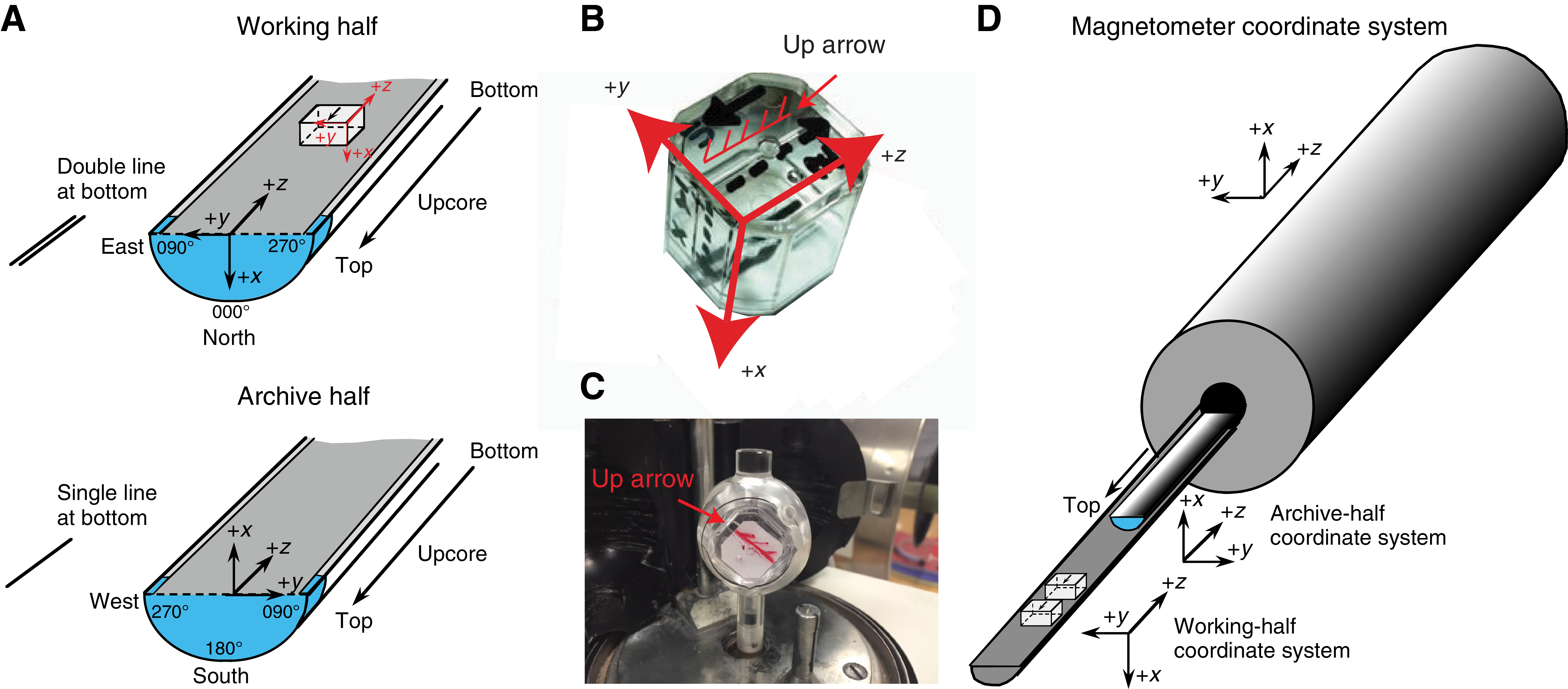
Figure F23. IODP coordinates of paleomagnetic samples.
Low-field magnetic susceptibility (κ), measured on whole-round core sections using the WRMSL and archive-half core sections using the SHMSL (see Physical properties), was used to assess the concentration of magnetic minerals and to determine the downhole relative paleointensity (NRM/κ). These whole-round records of magnetic susceptibility were compared to visual features in the split cores to flag possible artifacts.
Magnetic measurements on discrete samples
Discrete samples were initially measured on both the SRM and a spinner magnetometer. These samples were subjected to AF demagnetization treatments using both the 2G in-line AF demagnetizer (as described above) and the DTECH (model D-2000) AF demagnetizer. But the resultant demagnetization behavior of the discrete samples becomes noisy at higher AF treatments, and thus measurement on the SRM is not recommended for discrete samples. This recommendation is also confirmed by shipboard tests of the reliability of discrete measurements on the 2G SRM. The routine AF demagnetization treatment was performed using the DTECH (model D-2000) AF demagnetizer. In addition, to avoid contamination by the ambient magnetic field during shipboard measurements, two cylindrical mu-metal shields provided a suitable low-field environment for temporary sample storage.
Oriented discrete samples were taken preferentially in fine-grained intervals where drilling deformation was minimal. In soft sediment, discrete samples were taken in plastic “Japanese” Natsuhara-Giken sampling cubes (7 cm3 sample volume; Figure F23B). Cubes were pushed into the working half of the core with the “up” arrow on the cube pointing upsection in the core. In lithified sediments and hard rocks, 2 cm cubes (8 cm3 sample volume) were cut with the parallel saw.
Incremental AF demagnetization of discrete samples was performed with the DTECH AF demagnetizer (model D-2000) at fields up to 45 or 50 mT for lower coercivity samples and 120 or 200 mT for high-coercivity samples. We also applied progressive thermal demagnetization using a thermal specimen demagnetizer (ASC Scientific model TD-48SC) up to 700°C at steps of 25° to 50°C depending on the magnetic minerals present in the sample. During Expedition 367, a combination of stepwise AF and thermal demagnetization was applied.
AMS was measured on an AGICO KLY 4S Kappabridge instrument at a field of 300 A/m using the AMSSpin LabVIEW program designed by Gee et al. (2008) or the SUFAR (AGICO) program. The KLY 4S Kappabridge measures AMS by rotating the sample along three axes, stacking the data, and calculating the best-fit second-order tensor. It also measures the volume-normalized calibrated bulk susceptibility (χ).
Coordinates
All magnetic data are reported relative to the IODP orientation conventions: +x is into the face of the working half, +y points toward the left side of the face of the working half, and +z points downsection. The relationship of the SRM coordinates (X-, Y-, and Z-axes) to the data coordinates (x-, y-, and z-directions) is as follows: for archive halves, x-direction = X-axis, y-direction = −Y-axis, and z-direction = Z-axis; for working halves, x-direction = −X-axis, y-direction = Y-axis, and z-direction = Z-axis (Figure F23). The coordinate systems for the spinner magnetometer and Natsuhara-Giken sampling cubes are also shown in Figure F23.
Core orientation
Paleomagnetic study of marine sediment cores is greatly enhanced if the angle between magnetic north and the double line marked on the core liner can be determined. Core orientation of APC cores was achieved with the orientation tool (Icefield MI-5 core orientation tool) mounted on the core barrel. The Icefield MI-5 core orientation tool consists of triaxial magnetometers and accelerometers. These sensors provide an azimuthal correction for the core barrel that, combined with the local magnetic declinations, allows the measured NRM declinations to be transformed into true geographic coordinates. In the orientation deployment, the tool is connected to the core barrel with the double lines on the core liner at a fixed and known angle relative to its sensors. Previous expeditions have reported that in general these orientation tools have an accuracy of 20°–30°. Unlike earlier expeditions that reported reversed directions (i.e., 180° instead of 0°) during a period of normal polarity, the declinations (above ~160 m from the APC cores) corrected based on the Icefield data are consistent with the inclinations.
The ChRMs can also provide a reference frame to orient cores (see Structural geology). Provided that the reference magnetic pole is known, the orientation of the paleomagnetic vector is then used to restore the azimuth of the +x core axis (e.g., Fuller, 1969).
Magnetostratigraphy reference scale and interpretations
The magnetostratigraphy at each site was constructed by correlating observed polarity sequences with a reference GPTS in combination with biostratigraphic biohorizons. The GPTS used for Expeditions 367 and 368 (Table T7) is the GPTS2016 synthesis of astronomical tuning of Cenozoic through latest Cretaceous polarity zones updated in Ogg et al. (2016). The Cenozoic portion of GPTS2016, together with microfossil and nannofossil biozones, is plotted in Figure F24.
Table T7. Geomagnetic polarity timescale. Download table in CSV format.
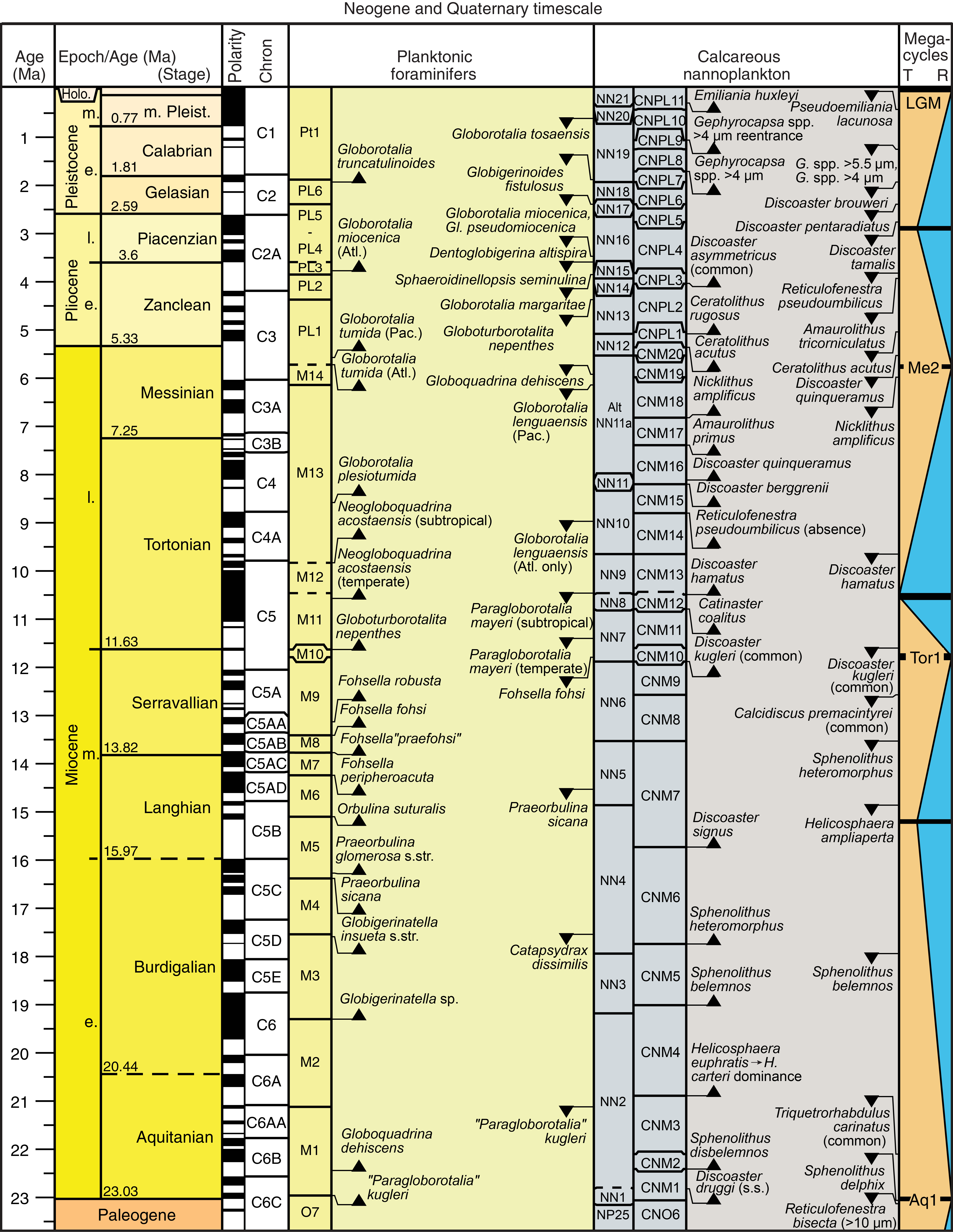
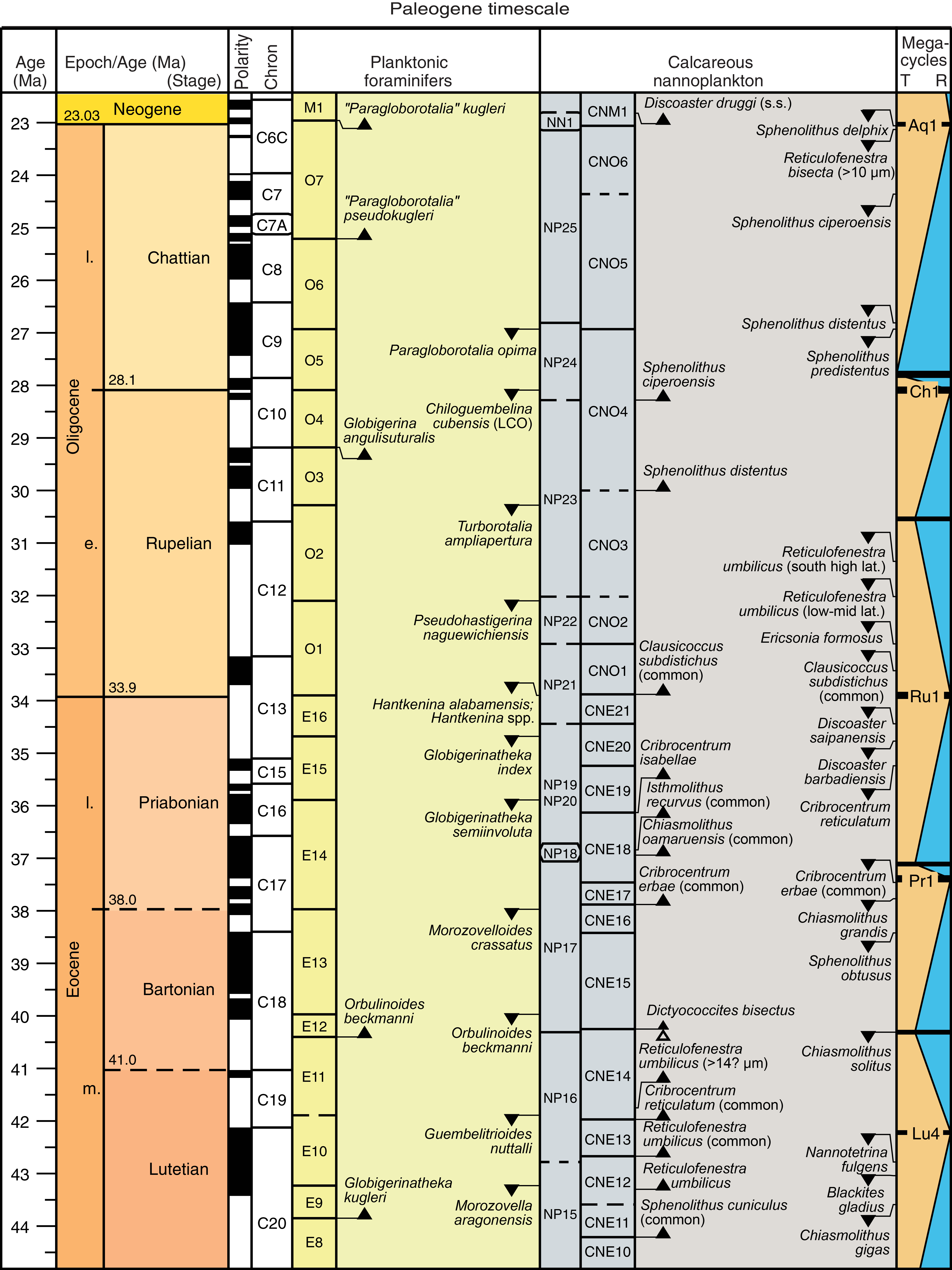
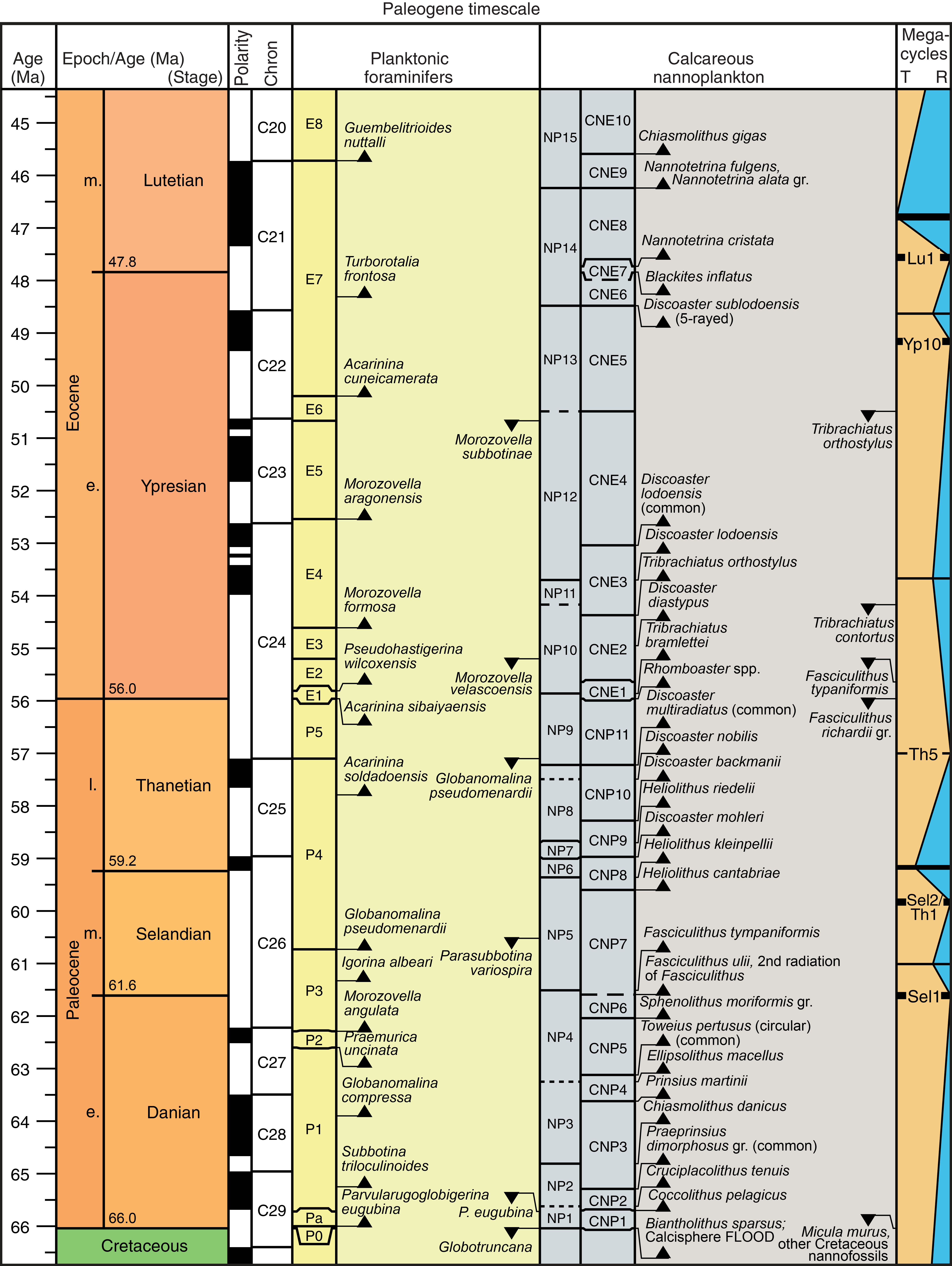
Figure F24. Selected Cenozoic marine and terrestrial biostratigraphic zonations.
For azimuthally unoriented samples from sedimentary rocks that formed at low latitudes, such as those at the Expedition 367 and 368 drill sites, determining the polarity of sedimentary units can be difficult. The polarity ambiguity arises when the samples are azimuthally unoriented and the inclination is very shallow near the Equator (the angular distance between reversed and normal polarity inclinations is small). Because paleomagnetic inclinations from any samples will have some degree of dispersion about their mean inclination, it is likely that when the mean inclination is shallow (near zero), the sign of the inclination will not be indicative of the polarity (e.g., McFadden and Reid, 1982; Cox and Gordon, 1984). The sign of the inclination of these samples should be used carefully as a definitive estimate of magnetic polarity.
We applied the following methods to establish magnetozones:
- Observing near-180° shift in declinations and significant changes in inclinations from pass-through measurements on long coherent core sections after AF demagnetization. The observed magnetozones are then checked with the ChRM directions of the discrete samples from the corresponding intervals.
- Comparison of inclination trends with predicted paleolatitudes of the drill sites according to the absolute plate motion of the South China plate on global plate circuit reconstructions (e.g., Scotese, 2014a, 2014b). However, the reconstructed position of the drill holes through the Cenozoic has negligible displacement in paleolatitude because that plate and the adjoining main Asian landmass underwent clockwise rotation.
Whenever possible, we provide an interpretation of the magnetic polarity, with the naming convention following that of correlative chron and anomaly numbers prefaced by the letter C (e.g., Ogg et al., 2016). Normal polarity subchrons are referred to by adding suffixes (n1, n2, etc.) that increase with age. For the younger part of the timescale (Pliocene–Pleistocene), we use the traditional names to refer to the various chrons and subchrons (e.g., Brunhes, Jaramillo, Olduvai, etc.). In general, polarity reversals occurring at the end of core sections have been treated with extreme caution.
Geochemistry
The shipboard geochemistry program for Expeditions 367 and 368 included the following measurements:
- Headspace gas content;
- Interstitial water composition;
- Sedimentary geochemistry, including total inorganic carbon, total carbon, total nitrogen, and major and minor element content; and
- Igneous and metamorphic rock geochemistry (major and minor element content).
Our analytical procedures follow those described by Integrated Ocean Drilling Program Expedition 345 and IODP Expeditions 349, and 352 (Gillis et al., 2014; Li et al., 2015; Reagan et al., 2015). Our analyses were conducted to satisfy routine shipboard safety and pollution prevention requirements; characterize interstitial water, sediment, and rock geochemistry for shipboard interpretation; and provide a basis for sampling for subsequent shore-based research.
Headspace gas analysis
For headspace gas analysis, 5 cm3 samples were collected immediately after core retrieval on deck, placed in a 20 cm3 glass vial, sealed with a septum, and crimped with a metal cap. When consolidated or lithified samples were encountered, chips of material were placed in the vial and sealed and soft-sediment samples were collected with a sawn-off syringe or with a scoop. If an interstitial water sample was obtained, the headspace sample was taken from the top of the section immediately next to the interstitial water sample whenever possible. Otherwise, the headspace sample was taken from the top of the third section. The vial was labeled with the core, section, and interval from which the sample was taken and then placed in an oven at 70°C for 30 min. A 5 cm3 aliquot of gas was extracted through the septum with a gas-tight glass syringe and then injected into a gas chromatograph (GC).
An Agilent 6890 GC equipped with a flame ionization detector (FID) was used to measure the concentrations of methane (C1), ethane (C2), ethylene (C2=), propane (C3), and propylene (C3=). A 2.4 m × 2.0 mm stainless steel column packed with 80/100 mesh HayeSep “R” was installed in the GC oven. The injector consists of a ¹⁄₁₆ inch Valco union with a 7 μm screen connected to a Valco-to-Luer lock syringe adapter. This injector connects to a 10-port Valco valve that is switched pneumatically by a digital valve interface. The injector temperature was set at 120°C throughout each run. Samples were introduced into the GC through a 0.25 cm3 sample loop connected to the Valco valve. The valve can be switched automatically to backflush the column. The oven temperature was programmed to start at 80°C for 8.25 min and then increase to 150°C at a rate of 40°C/min and hold for 5 min. Helium was used as the carrier gas. Initial helium flow in the column was 30 mL/min. Flow was then ramped up to 60 mL/min after 8.25 min to accelerate elution of C3 and C3=. The run time was 15 min. The GC was also equipped with an electronic pressure control module to control the overall gas flow. The FID was set at 250°C. Data were collected and evaluated with an Agilent Chemstation data handling program. Chromatographic response was calibrated against known standards provided by Scott Specialty Gases.
No accurate measurement of the sediment mass was carried out. As such, measured concentrations are semiquantitative (likely carrying a ±25% relative uncertainty, mainly reflecting variations in the sediment mass around the target mass) and are only indicative for safety monitoring. However, gas ratios (e.g., C1/C2) are not affected by the uncertainty on the sediment mass.
Interstitial water chemistry
Interstitial water collection
Routine interstitial water samples were obtained by squeezing whole-round sections cut from cores. Standard whole-round samples were 5 cm long, but as water content decreased downhole, the size of the whole-round samples was increased to 15 cm to enable extraction of ~30 mL of water needed for shipboard and shore-based analyses. Interstitial water collection stopped when it was no longer possible to obtain ~10 mL for shipboard analyses by squeezing 15–20 cm long whole-round sediments. Whole-round samples were cut and capped as quickly as possible after the core arrived on deck and immediately moved to the chemistry laboratory for squeezing. Whole-round samples were typically collected at a frequency of ~3 samples per core in the first 5 cores, 2 samples per core for cores 5–10, and subsequently 1 sample per core. Samples of basement were not collected for squeezing interstitial water.
The exterior of the whole-round sample was carefully scraped with a spatula to remove potential contamination from drilling fluid and sediment smearing in the borehole. In APC cores, ~0.5 cm of material from outside of the whole round was removed, whereas in XCB and RCB cores, where borehole contamination is higher, as much as two-thirds of the sediment was removed from each whole round. The cleaned sediment was placed into a 9 cm diameter titanium squeezer that was then placed in a Carver hydraulic press (Manheim and Sayles, 1974) and squeezed at pressures no higher than 30,000 lb (~20.3 MPa) to extract interstitial water. The squeezed interstitial water was collected in precleaned high-density polyethylene syringes attached to the squeezing assembly. Subsequently, the interstitial water was filtered through a 0.45 µm polyethersulfone membrane disc filter into various sample containers, except for aliquots taken for dissolved organic carbon (DOC) analysis, which were filtered through a 0.2 µm polyethersulfone membrane disc filter.
Sample allocation was determined based on the pore fluid volume obtained and analytical priorities based on the objectives of the expedition. Aliquots for major and minor elements by ICP-AES were acidified by adding ~10 µL of trace metal–grade concentrated HNO3 and placed in 2 mL cryovials. Aliquots for chloride and alkalinity titration, ammonium and phosphate spectrophotometry analyses, and ion chromatography analyses were put in 8 mL glass vials. Aliquots for isotopic analyses of oxygen and hydrogen were placed in zero-headspace 2 mL septum screw-lid glass vials. Aliquots for Sr, B, and Li isotopes were acidified by adding ~10 μL of trace metal–grade concentrated HNO3 and placed in two 5 mL cryovials. Aliquots for dissolved inorganic carbon (DIC) and DOC and their δ13C were treated with 10 µL of a saturated HgCl2 solution and placed in zero-headspace 2 mL and 5 mL septum screw-lid glass vials, respectively. Aliquots for TH2S were placed in 2 mL septum screw-lid glass vials with 0.5 mL of ~50 mM zinc acetate solution. The samples were stored at 4°C after collection.
Alkalinity, pH, and salinity were analyzed immediately after interstitial water was obtained. Other shipboard analyses were carried out in batches. Dissolved sodium, calcium, magnesium, chloride, bromide, and sulfate were analyzed by ion chromatography. Ammonium and phosphate were analyzed by UV-VIS spectrophotometry. Minor element concentrations were analyzed by ICP-AES.
After interstitial water extraction was complete, sediment squeeze cakes were divided and sealed in plastic bags for shipboard and shore-based analyses. Squeeze cake samples for shore-based organic analysis were stored at −20°C. All other squeeze cake samples were refrigerated at 4°C.
Shipboard interstitial water analysis
Interstitial water samples were analyzed on board following the protocols in Gieskes et al. (1991), Murray et al. (2000), and the Integrated Ocean Drilling Program user manual for shipboard instrumentation, which was updated during Expedition 344 (Harris et al., 2013).
Salinity, alkalinity, and pH
Salinity, alkalinity, and pH were measured immediately after squeezing, following the procedures in Gieskes et al. (1991). Salinity was measured using a Fisher temperature-compensated handheld refractometer. The pH was measured with a combined glass electrode, and alkalinity was determined by Gran titration with an autotitrator (Metrohm 794 basic Titrino). Three milliliters of interstitial water sample was titrated against 0.1 M HCl at 25°C. International Association for the Physical Sciences of the Oceans (IAPSO) standard seawater was used for calibration and was analyzed at the beginning and end of a set of samples for each site and also every 5–10 samples. Both the analytical precision and accuracy of alkalinity titrations were better than 3% based on repeated analysis of IAPSO standard seawater.
Chloride by titration
High-precision chloride concentrations were acquired using a Metrohm 785 DMP autotitrator and silver nitrate (AgNO3) solution calibrated against repeated titrations of IAPSO standard. A 0.5 mL aliquot of sample was diluted with 30 mL of 0.32 M HNO3 solution and titrated with 0.1 M AgNO3. Repeated analyses of an IAPSO standard yielded a precision better than 0.06%; however, the chloride concentrations yielded by titration includes not only dissolved chloride but also all of the other halide elements and bisulfide. The JOIDES Resolution is equipped with a Metrohm 850 Professional ion chromatograph that can analyze anions and cations simultaneously. The chloride concentration was analyzed by both titration and ion chromatography for Holes U1499A, U1501C, U1501D, U1502A, U1504A, and U1505C. Chloride concentrations analyzed by ion chromatography were not greater than those by titration, indicating that ion chromatography can provide mostly reliable chloride data. As a result, chloride concentration was analyzed by both titration and ion chromatography only for the upper 50 m section for all sites during Expeditions 367 and 368.
Sulfate, chloride, bromide, calcium, magnesium, potassium, and sodium
Sulfate, chloride, bromide, calcium, magnesium, and sodium concentrations were analyzed by ion chromatography (Metrohm 850 Professional IC) using aliquots of 100 µL that were diluted 1:100 with deionized water (18 MΩ/cm). At the beginning and end of each run, different dilutions (1:80 to 1:500) of IAPSO standard seawater were analyzed to create a six point calibration curve. The r2 for the calibration curve was always >0.99, and relative standard deviation varied from 0.8% to 3.4%. The 1:100 diluted IAPSO standard seawater was also analyzed every ~10 samples for quality control and to determine accuracy and precision. A new calibration curve was run if measured concentrations deviated from the expected values (28.9 mM for SO42− and 0.865 mM for Br−). Based on measurements of IAPSO standard seawater, analytical precision (2σ) was within 1% for chloride, 5% for bromide, 2% for sulfate, 5% for calcium, 3% for magnesium, and 1% for sodium.
Ammonium and phosphate
Ammonium and phosphate concentrations were determined using an Agilent Technologies Cary Series SPS3 spectrophotometer with a sipper sample introduction system following the protocol in Gieskes et al. (1991). For ammonium concentration analysis, a 0.2 mL sample aliquot was diluted with 2 mL reagent water to which 1 mL phenol ethanol, 1 mL sodium nitroprusside, and 2 mL oxidizing solution of sodium hypochlorite were added in a 15 mL capped plastic tube (Gieskes et al., 1991). The solution was kept at room temperature for ~6.5 h to develop color. Ammonium concentrations were determined at an absorbance of 640 nm. Precision and accuracy of the ammonium analyses of a standard were within 4% and 10%, respectively.
For phosphate analysis, a 0.6 mL sample was diluted with 2 mL deionized water (18 MΩ/cm) and 4 mL mixed reagent solution of ammonium molybdate, sulfuric acid, ascorbic acid, and antimony potassium tartrate in a 15 mL plastic tube. Then 2 mL of mixed reagent (ammonium molybdate, sulfuric acid, ascorbic acid, and potassium antimonyl tartrate) was added to the vial (Gieskes et al., 1991), which was capped and kept at room temperature for at least several minutes to develop color. The phosphate concentration was determined at an absorbance of 885 nm ~30 min after adding the mixed reagent solution. At beginning of each run, different concentrations (0–300 μM) of phosphorus standards were analyzed to create an 11-point calibration curve. Based on the measurements of 100 μM phosphorus standard during the expedition, precision (1σ) and accuracy of the phosphate analyses were better than 2% and 0.3%, respectively.
Minor elements
Dissolved minor elements were determined by Teledyne Leeman Prodigy ICP-AES. The general method for shipboard ICP-AES analysis of samples is described in Murray et al. (2000) and the user manuals for shipboard instrumentation.
For minor element (B, Ba2+, Fe2+, Mn2+, Li+, Si, and Sr2+) analyses, interstitial water samples were diluted 1:20 (v/v) using 2% HNO3 solution with 10 ppm Y (the interstitial water matrix solution) as an internal standard. Because the high concentration of salt in interstitial water samples at the 1:20 dilution demands matrix matching of standards and samples, standards were prepared with an acidified synthetic seawater of 35‰ NaCl with 2% HNO3 to have an ionic strength similar to seawater. A stock multielement synthetic standard solution was gravimetrically prepared from ultrapure primary standards (SPC Science PlasmaCAL) diluted in the acidified synthetic seawater. An eight-point calibration curve was created through diluting the stock multielement standard in the acidified synthetic seawater at various degrees. Drift correction was made using the factor from a drift monitor solution of 100% stock standard solution, which was analyzed every 8–10 samples. The ICP-AES autosampler and analysis chamber were rinsed with a 3% (by volume) HNO3 solution between samples. Multiple wavelengths were measured for each element, and the best were selected for reporting element concentrations. Wavelengths were selected based on possible interferences, the linearity of calibration curves, and the precision and accuracy of measurements of several standards. The selected wavelengths were Ba = 493.409 nm, B = 249.772 nm, Li = 670.784 nm, Fe = 259.940 nm, Si = 288.158 nm, Mn = 257.610 nm, and Sr = 460.733 nm.
Sediment geochemistry
Sediment nitrogen and inorganic and organic carbon content
Samples (~50 mg) for carbon, sulfur and nitrogen analyses were collected from squeeze cakes from interstitial water analyses and taken from intervals of distinct lithologic importance for expedition aims. Samples were freeze-dried for ~24 h, crushed using an agate pestle and mortar, and then analyzed for total carbon (TC), total inorganic carbon (TIC), total sulfur (TS) and total nitrogen (TN).
TC, TS, and TN of the bulk sediment samples were determined with a ThermoElectron Corporation Flash EA 1112 CHNS elemental analyzer equipped with a ThermoElectron packed column CHNS/NCS GC and a thermal conductivity detector (TCD). Approximately 12–13 mg of dry sediment was weighed into a tin cup, and 5–10 mg of vanadium pentoxide was added. Samples were then combusted at 950°C in a stream of oxygen. The reaction gases were passed through a reduction chamber to reduce nitrogen oxides to N2, and then the evolved N2, CO2, and SO2 were separated by the GC column before detection by the TCD. All measurements were calibrated to a set of reference standards covering the range in expected TC, TS, and TN values (Soil Reference Material: Buffalo River Sediments PWDR7837591) that was run every 9 samples. Peak areas from the TCD were calculated to determine the TC, TS, and TN of the samples. Blank levels were determined by analyzing empty tin cups and were subtracted from each measurement. Blank contributions for C is on the order of 1 µg. Given the typical sample mass used (12.5 mg on average) and using a signal/blank threshold of 10, this translates into a detection limit of ~0.04 wt%. For N, blanks were also estimated from the intercept of the calibration curve, which gave results similar to direct blank determination (i.e., empty tin cup blank). Blank contribution for N is on the order of 12 µg, unsurprisingly high considering the use of a sampler open to the atmosphere. This translates into a detection limit of ~0.06 wt%. Accuracy of TC determination was estimated using repeated measurements of reference material and was found to be better than 5% of the TC value (i.e., <0.05 wt% for the vast majority of samples analyzed). Precision of TC determination was estimated from limited duplicate measurements and was systematically within estimated accuracy. TS determination was less accurate than for nitrogen or carbon, and based on the analysis of both blank cups and minimum detection limits obtained from calibration curves, this equates to a TS of 0.1 wt%.
Sulfur analyses were only carried out for Expedition 368. TIC was determined using a Coulometrics 5015 CO2 coulometer. Approximately 13 mg (10 mg for lithologies dominated by carbonates) of sediment was weighed into a glass vial and acidified with 2 M HCl. The liberated CO2 was titrated, and the corresponding change in light transmittance in the coulometric cell was monitored using a photodetection cell. The weight percent of calcium carbonate was calculated from the inorganic carbon content using the following equation:
CaCO3 (wt%) = TIC (wt%) × 100/12.
Blank levels were determined by analyzing empty reactors, were found to vary between 3 and 7 µg C, and were subtracted from each measurement. Repeated measurements of pure CaCO3 (several times at the beginning and every 10 samples) were used to estimate accuracy, which was <2% of the TIC. TOC content was calculated by subtraction of TIC from TC.
Surface-enhanced Raman spectroscopy of solvent extractable sedimentary organic matter
Samples for surface-enhanced Raman spectroscopy (SERS) of solvent extractable organic matter were only collected during Expedition 368. They were obtained from freeze-dried residues used for TC analysis or collected from locations of lithologic interest to expedition goals. Powdered samples were placed in 10 mL extraction vials and sonicated for 15 min in 3:1 DCM/MeOH (dichloromethane/methanol) to obtain a solvent extract. The extract was decanted into a separate vial; more DCM was added to the sediment-residue before sonication was repeated for another 15 min. The solvent was again decanted, and the process was repeated to produce three extraction stages. The combined extract was reduced to dryness.
The extract was dissolved in DCM, and 4 μL of it was introduced in small increments to the sample wells of a gold-coated SERS-substrate. Introducing samples as small increments allowed the solvent to evaporate under ambient conditions until the entire volume had been loaded. When the solvent had evaporated, 4 μL of dilute nitric acid (1 M concentration) was dispensed into the pit and allowed to stand for ~2–3 min. The aqueous phase remaining within the pit was then removed to aid focusing of the microscope on the base of the pit. Raman spectroscopic measurements were performed using a BWTek i-Raman Pro fitted with a 532 nm light source and mounted on 20× video-microscope. Spectra were collected by accumulating 20 spectra over 20 s; spectral acquisition was in the range 200–2000 per centimeter. Laser spot size was approximately 1–2 μm, and laser power was 50% (<13 mW delivered to the sample). Identification of key bands was made with reference spectra presented in Alabi et al., 2015.
Elemental analysis of bulk sediment/sedimentary rock by ICP-AES
Elemental composition of bulk sediment was determined using a Leeman ICP-AES. Our analytical approach followed the general procedure outlined by Murray et al. (2000) and the constraints indicated by Quintin et al. (2002). Analytical blanks were prepared using 400 mg of lithium metaborate (LiBO2) flux to ensure matrix matching. Samples analyzed by ICP-AES were ignited before dissolution by heating 5 g of oven-dried (600°C for 12 h) ground sediment at 1025°C for 5 h to determine weight loss on ignition (LOI), release volatile phases (H2O, CO2, and S), and fully oxidize all iron to ferric iron.
Aliquots of 100 mg of ignited sediment and standards were mixed with 400 mg of LiBO2 flux. Subsequently, 10 µL of a wetting agent, 0.172 mM lithium bromide (LiBr), was added to the samples, standards, and blanks. This mixture was fused at 1050°C for 5 min in a Bead Sampler NT-4100 prior to dissolution in 50 mL of 10% HNO3. For complete dissolution, 1 h of shaking with a Burrell wrist-action shaker was required. Aliquots of 5 mL of the resulting solutions were filtered (0.45 µm) and diluted with 35 mL of 10% HNO3, resulting in a 4000× dilution of the original sediment.
A range of standards was selected to cover the entire range of expected sediment compositions, with their suitability monitored during the expedition. These standards were: STSD1, STSD2, STSD4, SO-1, SO-2, SO-3, SO-4, NBS-1c, JR-2, and BCR-2. BHVO-2 was also selected as both the drift and consistency standard. A range of major and trace elements was analyzed. Major elements included Al, Ca, Fe, K, Mg, Mn, Na, Si, and Ti, and trace elements included Ba, Co, Cr, Cu, Sc, Sr, V, Zn, and Zr. Major elements were expressed as weight percent oxide, and trace elements were expressed as parts per million. LOI values were determined routinely. Samples were analyzed in duplicate. The procedures used to process the data are outlined in Data reduction, below.
The elemental compositions of sediment/sedimentary rock were only determined during Expedition 368 because the bead maker for the ICP did not work during Expedition 367.
Igneous and metamorphic rock geochemistry
Sample preparation
Representative samples of igneous and metamorphic rocks were analyzed for major and trace element concentrations during Expeditions 367 and 368 using the Leeman ICP-AES.
Samples ranging in size from ~2 to ~8 cm3 were cut from the core with a diamond saw blade. A thin section billet was taken from the same or adjacent interval for petrographic analysis and alteration determination (see Igneous and metamorphic petrology and Alteration). All outer surfaces were ground on a diamond-impregnated disk to remove altered rinds and surface contamination derived from the drill or saw. Each sample was then placed in a beaker containing acetone and washed ultrasonically for 15 min. The acetone was decanted, and the samples were sonicated in deionized water (18 MΩ/cm) twice for 10 min. The cleaned pieces were dried for 10–12 h at 110°C.
The cleaned, dried samples were crushed to <1 cm chips between two disks of Delrin plastic in a hydraulic press. The rock chips were then ground to a fine powder in tungsten carbide in a SPEX 8515 Shatterbox. After grinding, a 5.0 ± 0.5 g aliquot of the sample powder was weighed on a Mettler Toledo balance and ignited at 1025°C for 4 h to determine LOI.
Murray et al. (2000) describes in detail the shipboard procedure for digestion of rocks and ICP-AES analysis of samples. The following protocol is an abbreviated form of this procedure with minor modifications. After determination of LOI, 100.0 ± 0.2 mg splits of the ignited whole-rock powders were weighed and mixed with 400.0 ± 0.5 mg of LiBO2 flux that had been preweighed on shore. Standard rock powders and full procedural blanks were included with unknowns in each ICP-AES run (note that among the elements analyzed, contamination from the tungsten carbide mills is negligible; Shipboard Scientific Party, 2003). All samples and standards were weighed on a microbalance with weighing errors estimated to be ±0.05 mg under relatively smooth sea-surface conditions.
To prevent the cooled bead from sticking to the crucible, 10 mL of 0.172 mM aqueous LiBr solution was added to the mixture of flux and rock powder as a nonwetting agent. Samples were then fused individually in Pt-Au (95:5) crucibles for ~12 min at a maximum temperature of 1050°C in an internally rotating induction furnace (Bead Sampler NT-4100).
After cooling, beads were transferred to high-density polypropylene bottles and dissolved in 50 mL of 10% (by volume) HNO3, aided by shaking with a Burrell wrist-action bottle shaker for 1 h. Following digestion of the bead, the solution was passed through a 0.45 µm filter into a clean 60 mL wide-mouth high-density polypropylene bottle. Next, 1.25 mL of this solution was transferred to a plastic vial and diluted with 10% HNO3 to a total volume of 10 mL. The final solution-to-sample dilution factor was ~4000×.
Analyses of igneous and metamorphic rocks
Major (Al, Ca, Fe, K, Mg, Mn, Na, Si, and Ti) and trace (Ba, Co, Cr, Cu, Sc, Sr, V, Zn, and Zr) element concentrations of standards and samples were determined with a Leeman ICP-AES instrument. The plasma was ignited at least 30 min before each run of samples to allow the instrument to warm up and stabilize.
The ICP-AES data presented in the Geochemistry section of each site chapter were acquired using the Gaussian mode of the Prodigy software. This mode fits a curve to points across a peak and integrates the area under the curve for each element measured. Each sample was analyzed four times from the same dilute solution (i.e., in quadruplicate) within a given sample run. For elements measured at more than one wavelength, we either used the wavelength giving the best calibration line in a given run or, if the calibration lines for more than one wavelength were of similar quality, used the data from all wavelengths and reported the average concentration.
The ICP-AES run included the following:
- Certified rock standards, analyzed twice during each run, chosen to cover a wide range of compositions in order to calibrate the analyses (peridotite: JP-1; basalt: BIR-1, BHVO-2, and BCR-2; gabbro: MRG-1; andesite: AGV-1; and granodiorite: JG-1A);
- Samples (unknowns) analyzed in quadruplicate;
- A drift-correcting standard (BHVO-2) analyzed in every eighth sample position and at the beginning and end of each run;
- A blank solution analyzed near the beginning;
- Two or three “check” standards run as unknowns, each also analyzed in quadruplicate; check standards were chosen for their compositions similar to that of the analyzed material (ultramafic: DTS-1, basalt: JB-1a, JB-2, felsic rocks: JG-2, JG-3, etc.); and
- A 10% HNO3 wash solution run for 60 s between each analysis.
Data reduction
Following each run of the instrument, the measured raw intensity values were transferred to a data file, corrected for instrument drift, and then corrected for the procedural blank. Drift correction was applied to each element by linear interpolation between the drift-monitoring solutions run in every eighth sample position.
After drift correction and blank subtraction, a calibration line for each element was calculated using the results for the certified rock standards. Element concentrations in the samples were then calculated from the relevant calibration lines.
Individual analyses of both standards and samples produced total volatile-free major element weight percentages that vary from 100 wt% by as much as several percent. Possible causes include some combination of errors in weighing the sample (particularly in rougher seas) and/or flux powders (although even when weighed on land, weighing errors are possible), variability in the dilutions (which were done volumetrically), and the duration and relatively low temperature of ignition. To facilitate comparison of Expedition 367 and 368 results with each other and with data from the literature, the measured major element values were normalized to 100 wt% totals.
Estimates of accuracy and precision of major and trace element analyses were based on replicate analyses of check standards compared to values published in Govindaraju (1994) and the GeoReM database (http://georem.mpch-mainz.gwdg.de) for international rock standards and to values published in Puchelt et al. (1996). Results are presented in Table T1. During Expeditions 367 and 368, run-to-run relative standard deviation by ICP-AES was generally ±1% for major elements except for MgO (±5%) and ±10% for trace elements. Accuracy was better than 2% for major elements and better than 5% for most trace elements, with the exception of low-concentration data for Cr and Zr.
Physical properties
High-resolution physical property measurements were made during Expeditions 367 and 368 mainly to aid lithostratigraphic characterization and to tie core descriptions to borehole data and seismic profiles. In particular, physical property data play a major role in hole-to-hole and site-to-site stratigraphic correlation, detection of discontinuities and inhomogeneities, collection of information about differences in the composition and texture of sediment, identification of major seismic reflectors, and construction of synthetic seismic profiles. A variety of techniques and methods were used to characterize Expedition 367 and 368 cores on whole-round, split section-half, and discrete samples. Core sections are generally 1.5 m in length, so a typical coring length (stroke) of 9.5 m yields six sections plus a shorter seventh section. Procedures for measuring sediment or hard rock cores differed slightly.
Sedimentary cores
Recovered whole-round sections were first allowed to equilibrate to ambient room temperature (~20°C) and pressure for ~4 h. After thermally equilibrating, core sections were run through the WRMSL for measurement of density by GRA, magnetic susceptibility, and compressional wave velocity on the PWL. Cores recovered with the XCB or the RCB coring systems are slightly smaller in diameter than those cored with the APC system. As a result, sections cored with the XCB or RCB systems typically have gaps between the liner and the core, so P-wave velocity was not measured with he WRMSL. Sections were then measured with the NGRL. Thermal conductivity was measured on one whole-round section per sediment core (typically Section 3) by a needle probe inserted into the section through a small hole drilled through the plastic core liner close to the middle of the section. When the sediment cores were too hard to insert the needle probe, a contact probe was used instead to measure the thermal conductivity later on the section half after core splitting. Cores were split longitudinally, with one half designated as archive and one as working half for sampling and analysis. The archive half of the core was passed through the SHMSL for measurement of point magnetic susceptibility and color reflectance. P-wave velocity measurements on split cores were made on the working halves at least for every section that had been sampled for MAD, or on other sections according to the lithology, employing the transducers oriented in x- and z-axis directions (see directions defined in Figure F23). Discrete samples were collected from the working halves (every other section) to measure wet bulk density, dry bulk density, water content, porosity, and grain density with MAD procedures.
Hard rock cores
Recovered hard rock sections were shaken onto sterile liners in the core splitting room for examination by a petrologist and/or a structural geologist, who decided where the pieces should be split between working and archive halves. The pieces were then put back into liners and run through the WRMSL and NGRL. P-wave velocity was not measured because the spaces between the liner and the rock core pieces make these measurements meaningless. After physical property measurements on whole-round cores, the core sections were split into working and archive halves and all rock pieces were labeled. The archive half of the core was passed through the SHMSL for measurement of point magnetic susceptibility and color reflectance. Thermal conductivity was measured once per core using a contact probe on a piece of section half in a bath of seawater for igneous rock pieces. Samples were taken from the working half of the core at a sampling interval of ~1 m depending on lithologic variability. Samples from igneous basement were shared for both paleomagnetic and MAD measurements. P-wave velocity measurements were made on these discrete samples.
A full discussion of all methodologies and calculations used aboard the JOIDES Resolution in the Physical Properties Laboratory is available in Blum (1997). Details and procedures for each physical property measurement are described below.
Whole-Round Multisensor Logger measurements
GRA-derived bulk density, P-wave velocity, and magnetic susceptibility were measured nondestructively with the WRMSL (Figure F25). To optimize the measurement process, sampling intervals and measurement integration times were set to be uniform for all sensors. Sampling intervals were set at 2 cm with an integration time of 5 s for each measurement. These sampling intervals are common denominators of the distances between the sensors installed on the WRMSL (30–50 cm), which allows sequential and simultaneous measurements. After every core, quality assurance/quality control (QA/QC) was monitored by passing a single core liner filled with deionized water through the WRMSL; if deviations from expected values were observed, recalibrations could be conducted if needed.
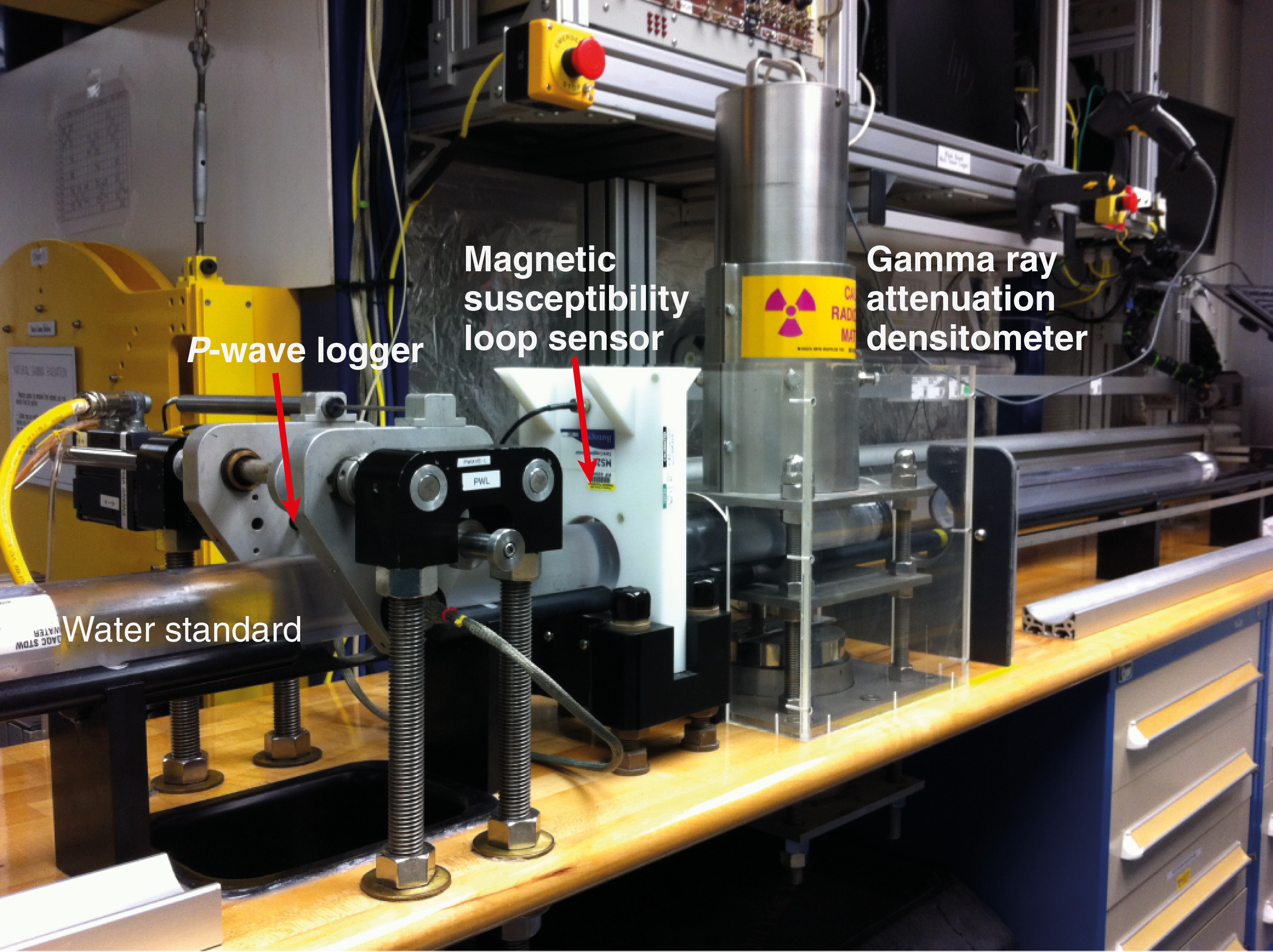
Figure F25. Whole-Round Multisensor Logger.
GRA bulk density
Bulk density can be used to estimate the pore volume in sediment and evaluate the consolidation state of sediment. GRA density is an estimate of bulk density based on the attenuation of a gamma ray beam. The beam is produced by a 137Cs gamma ray source at a radiation level of 370 MBq within a lead shield with a 5 mm collimator that is directed through the whole-round core. The gamma ray detector on the opposite side of the core from the source includes a scintillation detector and an integral photomultiplier tube to record the gamma radiation that passes through the core. The attenuation of gamma rays occurs primarily by Compton scattering, in which gamma rays are scattered by electrons in the formation; the degree of scattering is related to the material bulk density. Therefore, for a known thickness of sample, the density (ρ) is related to the intensity of the attenuated gamma rays and can be expressed as follows:
- I = the measured intensity of gamma rays passing through the sample,
- I0 = gamma ray source intensity,
- μ = Compton attenuation coefficient, and
- d = sample diameter.
The μ and I0 are treated as constants, such that ρ can be calculated from I. Note that this equation differs from the equation (5) in Blum (1997) in order to correct a typo.
In general, WRMSL measurements are most accurate when taken on a completely filled core liner with minimal drilling disturbance; otherwise, measurements tend to underestimate true values. By default, the instrument reports measurements using the internal diameter of the core liner (66 mm) as the assumed sample diameter. This assumption is suitable for most sediment cores obtained by the APC system; however, for sediment and/or hard rock cored by the XCB or RCB systems, core diameter is usually about 58 mm or less. Following Jarrard and Kerneklian (2007), the density measurements of cores obtained by XCB or RCB may be corrected by multiplying the density values by ⁶⁶⁄₅₈ = 1.138 to account for this bias. We chose not to correct the raw values but to mention the offset in the description of the measurements. The spatial resolution of the GRA densitometer is less than ±1 cm. The gamma ray detector is calibrated with sealed calibration cores (one standard core liner filled with distilled water and aluminum cylinders of various diameters). To establish the calibration curves, gamma ray counts were taken through each aluminum cylinder for 60 s. Each aluminum cylinder has a density of 2.7 g/cm3, and d is 1, 2, 3, 4, 5, or 6 cm. The relationship between I and µd is
where A, B, and C are coefficients determined from the calibration.
Recalibration was performed as needed when the deionized water QA/QC standard density deviated significantly (more than a few percent) from 1 g/cm3.
Magnetic susceptibility
Magnetic susceptibility (χ) is a dimensionless measure of the degree to which a material can be magnetized by an external magnetic field:
where M is the magnetization induced in the material by an external field of strength H. Magnetic susceptibility is primarily sensitive to the concentration of ferrimagnetic minerals (e.g., magnetite and maghemite). It is also sensitive to magnetic mineralogy and can be related to the origin of the materials in the core and their subsequent diagenesis. Igneous materials typically have magnetic susceptibility a couple of orders of magnitude greater than their alteration products, such as clay.
The measurements were made using a Bartington MS2C loop sensor with a 9 cm diameter. An oscillator circuit in the sensor, which operates at a frequency of 0.565 kHz and an AF of ~140 A/m, produces a low-intensity, nonsaturating alternating magnetic field. Sediment or hard rock core sections passing through the influence of this field cause a change in oscillator frequency. Frequency information returned in pulse form to the susceptibility meter is converted into magnetic susceptibility. The loop sensor has a spatial resolution of 23–27 mm, and it is accurate to within 2%.
P-wave velocity
P-wave velocity data can be used to evaluate small-strain moduli, correlate downhole logging and core data, and evaluate porosity and cementation. P-wave (compressional) velocity (VP) is defined by the time required for a compressional wave to travel a specific distance:
where d is the path length of the wave across the core and tcore is the traveltime through the core.
The PWL measures the traveltime of 500 kHz ultrasonic waves horizontally across the core at 2 cm intervals while it remains in the core liner. Waves are transmitted to the core by plastic transducer contacts connected to linear actuators. Pressure is applied to the actuators to ensure coupling between the transducers and the core liner. P-wave velocity transducers measure total traveltime of the compressional wave between transducers. The wave travels horizontally across the whole core and core liner. The total observed traveltime, tcore, is composed of
- tdelay = time delay related to transducer faces and electronic circuitry,
- tpulse = delay related to the peak detection procedure,
- tliner = transit time through the core liner, and
- tcore = traveltime through the sediment.
The system is calibrated using a core liner filled with distilled water, which provides control for tdelay, tpulse, and tliner. From these calibrations, VP can be calculated for the whole-round specimens in core liners as
VP = (dcl − 2dliner)/(to − tpulse − tdelay − 2tliner),
- dcl = measured diameter of core and liner,
- dliner = liner wall thickness, and
- to = measured total traveltime.
The above equation assumes that the core completely fills the core liner. The PWL of the WRMSL was turned off for cores recovered with the XCB and RCB systems, which often do not fill the core liner.
Natural Gamma Radiation Logger measurements
Gamma radiation is emitted from the decay of mineral-hosted 238U, 232Th, and 40K. The NGRL measures this natural emission on whole-round cores using a system designed and built at the Integrated Ocean Drilling Program US Implementing Organization (USIO) (Texas A&M University) (Vasiliev et al., 2011; Dunlea et al., 2013) (Figure F26). When 238U, 232Th, and 40K radioisotopes decay, they and their daughter products emit gamma radiation at specific energy levels unique to each isotope. NGR spectroscopy measures a wide energy spectrum that can be used to estimate the abundance of each isotope based on the strength of the signal at characteristic energies (Blum, 1997; Gilmore, 2008). Spectral data were collected and can be used for postcruise processing for U, Th, and K abundance. We estimated concentrations of K, U, and Th using NGR and bulk density measurements (see Figure F26), based on a study and Matlab scripts from De Vleeschouwer et al. (2017). High total counts usually identify fine-grained deposits containing K-rich clay minerals and their absorbed U and Th isotopes. NGR data thus reveal stratigraphic details that aid in core-to-core correlations. The system was initially installed on the renovated JOIDES Resolution in 2009 and has been used during every Integrated Ocean Drilling Program USIO and IODP JOIDES Resolution Science Operator (JRSO) expedition starting with Expedition 320. The main NGR detector unit consists of 8 sodium iodide (NaI) detectors arranged along the core measurement axis at 20 cm intervals surrounding the lower half of the section (Figure F27). During Expedition 367, scintillation Detector 7 was deficient, which led to a small gap in the measurements. Before Expedition 368, the deficient scintillation detector was fixed by the IODP technicians, and all detectors performed well during Expedition 368. The detector array has passive (layers of lead) and active (plastic scintillometers) shielding to reduce the background environmental and cosmic radiation. The overlying plastic scintillometers detect incoming high-energy gamma and muon cosmic radiation and cancel this signal from the total counted by the NaI detectors.
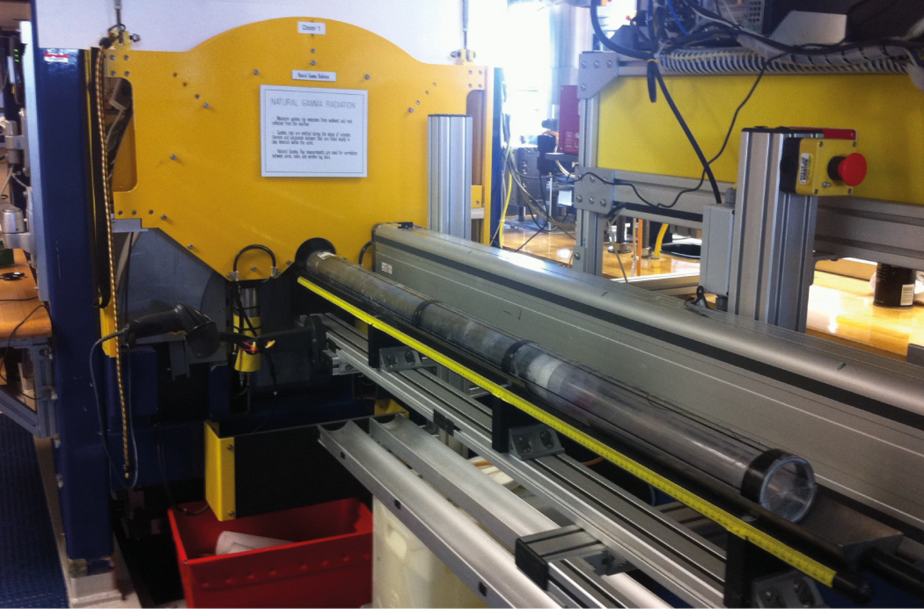
Figure F26. Natural Gamma Ray Logger.
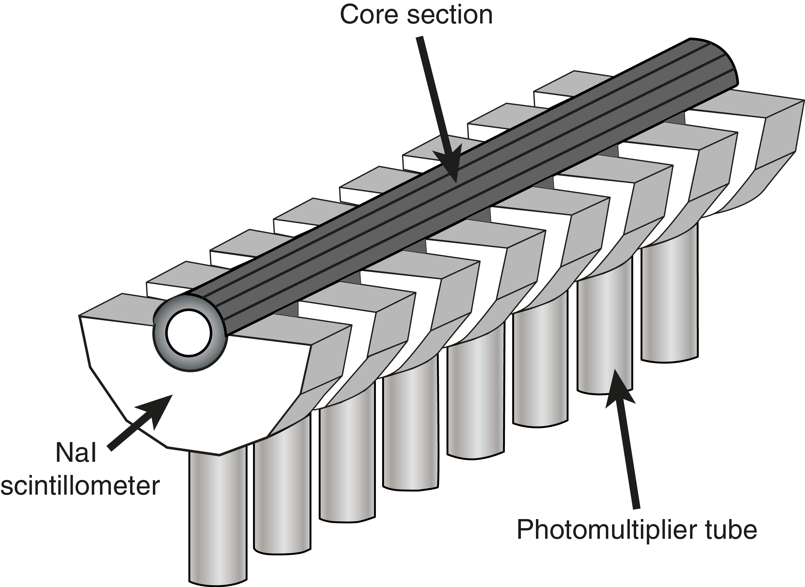
Figure F27. NGRL detectors.
A measurement run consisted of two sample positions, 10 cm apart, for a total of 16 (14 during Expedition 367) measurements per 150 cm section. During Expedition 367, measurements at distances of 20 and 30 cm in each section have no measured values because of the scintillation detector failure. The quality of the energy spectrum measured in a core depends on the concentration of radionuclides in the sample but also on the counting time, with higher times yielding better spectra. Counting times were chosen as 5 min per position, or ~10 min per core, yielding statistically significant energy spectra (Vasiliev et al., 2011).
Thermal conductivity measurements
After NGR measurements were completed, thermal conductivity was measured with the TK-04 (Teka Bolin) system using a needle-probe method in full-space configuration for whole-round sediment cores (Von Herzen and Maxwell, 1959) or a contact-probe method in half-space configuration on split cores for hard rock. The probes contain a heater wire and calibrated thermistor.
For soft sediment, the needle probe was inserted into a 2 mm diameter hole drilled through the liner along one of the lines that later guided core splitting. To avoid interference from air flow in the laboratory, the core was placed into an enclosed box outfitted with foam.
For hard rock cores, samples were selected from the working half and returned unaltered to the core liner upon completion of the measurements. The contact probe embedded in the surface of an epoxy block with a low thermal conductivity (Vacquier, 1985) was maintained in contact with the sample. For igneous rock pieces, both rock and probe were equilibrated together in a bath of seawater at room temperature in a cooler insulated with extruded polystyrene foam. The calibrated heat source of the probe was then turned on, and the increase in temperature was recorded over 80 s. A heating power of 1.5 to 1.8 W/m was typically used in soft sediment and for indurated material. In cases when this heating power did not lead to reliable measurements, we used a higher value, up to 2.0 W/m. The solution to the heat conduction equation with a line source of heat was then fit to the temperature measurements to obtain the thermal conductivity. Because the probe is much more conductive than sediment or hard rock, the probe is assumed to be a perfect conductor. Under this assumption, the temperature of the superconductive probe has a linear relationship with the natural logarithm of the time after the initiation of the heat:
- T = temperature (K),
- q = heat input per unit length per unit time (J/m/s),
- k = thermal conductivity (W/[m·K]),
- t = time after the initiation of the heat (s), and
- C = instrumental constant.
Three measuring cycles were automatically performed to calculate average conductivity. A self-test, which included a drift study, was conducted at the beginning of each measurement cycle. Once the probe temperature stabilized, the heater circuit was closed and the temperature rise in the probe was recorded. Thermal conductivity was calculated from the rate of temperature rise while the heater current was flowing. Temperatures measured during the first 80 s of the heating cycle were fitted to an approximate solution of a constantly heated line source (for details, see Kristiansen, 1982; Blum, 1997). Measurement errors were 5%–10%. Thermal conductivity measurements were routinely taken in one section per core (usually the third section of each core). Some cores retrieved by the XCB system did not yield results for thermal conductivity because cracks in the hard sediment caused bad coupling of the probe to the sediment.
Section Half Multisensor Logger measurements
We measured color reflectance and magnetic susceptibility on archive section halves using the SHMSL. The archive half of the split core was placed on the core holder, above which an electronic platform moves along a track, recording the height of the split-core surface with a laser sensor. The laser establishes the location of the bottom of the section, and then the platform reverses the direction of movement, moving from bottom to top making measurements of point magnetic susceptibility and color reflectance. All foam inserts were removed from the section-half cores before measurement, so the measured range of values represents that of the core material only. During Expeditions 367 and 368, point magnetic susceptibility and color reflectance data were collected at constant intervals for each core but varied between 0.5 and 2.0 cm for different cores, depending on the available time for processing and the type of rock recovered. These measurements have a sufficient resolution for comparing with the results obtained from the magnetic susceptibility loop of the WRMSL.
Color reflectance spectrometry
The color reflectance spectrometer uses an Ocean Optics 30 mm integrating sphere and both halogen and LED light sources, which cover wavelengths from ultraviolet through visible to near infrared. The measurements were taken from 380 to 900 nm wavelengths at 2 nm intervals. The approximate 3 s data acquisition offset was applied for the entire scan of the archive section half. The data are reported using the L*a*b* color system, in which L* is lightness, a* is redness (positive) versus greenness (negative), and b* is yellowness (positive) versus blueness (negative) of the rock. The color reflectance spectrometer calibrates on two spectra, pure white (reference) and pure black (dark). Color calibration was conducted automatically approximately once every 6 h (twice per shift).
Point magnetic susceptibility
Point magnetic susceptibility was measured with a Bartington MS2 meter and an MS2K contact probe with a flat 15 mm diameter round sensor with a field of influence of 25 mm and an operation frequency of 930 Hz. The instrument averages three measurements from the sensor for each offset, leading to an accuracy of ~5%. The spatial resolution of the point magnetic susceptibility instrument is ~3.8 mm, higher than that of the whole-round magnetic susceptibility (23–27 mm), making it especially useful for sections containing broken pieces <4 cm in length. As with whole-round measurements, the output displayed by the point magnetic susceptibility sensor must be converted to dimensionless SI units by multiplying by 10−5. The probe is zeroed in air before each measurement location to avoid influence from the metal track. The point magnetic susceptibility meter was calibrated by the manufacturer before installation on the ship and is quality checked every ~6 h at the same time as color reflectance sensor calibration.
Section Half Measurement Gantry measurements
For soft-sediment cores, P-wave velocity measurements were performed on the working half of split cores before any samples were taken. P-wave velocity measurements used the x-axis caliper and z-axis bayonet contact probe transducers on the Section Half Measurement Gantry (SHMG) (Figure F28) with one analysis completed every other section. Measurements were usually taken at ~75 cm in the section; however, if this interval lacked good sediment/transducer coupling (e.g., caused by high amounts of sand or cracks), different positions were chosen to generate viable data. Cores drilled with the XCB sometimes did not provide usable data because of bad sediment/liner contact and disturbed sediment. For hard rock cores, P-wave velocity was measured on the discrete samples chosen for both physical property and paleomagnetic measurements.
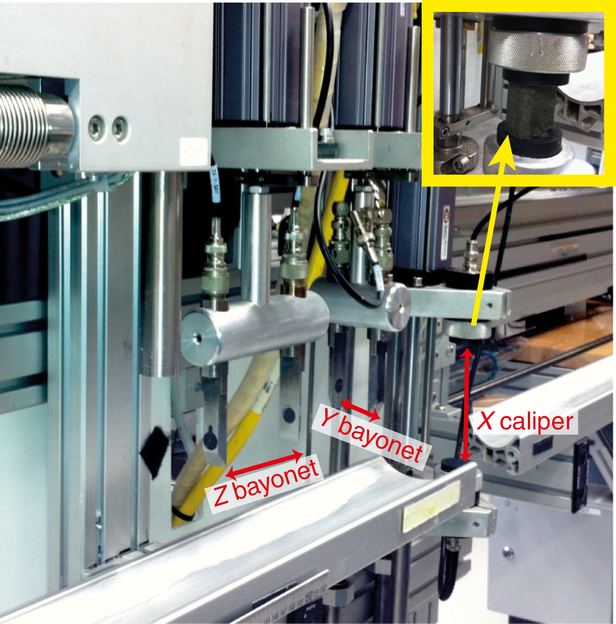
Figure F28. Section Half Measurement Gantry.
P-wave velocity
The P-wave velocity system uses Panametrics-NDT Microscan delay line transducers, which transmit at 0.5 MHz. The signal received through the section half or the discrete sample was recorded by the computer attached to the system, with the peak (P-wave arrival) usually chosen by autopicking software. In case of a weak signal, the first arrival was manually picked. The distance between transducers was measured with a built-in linear voltage displacement transformer. Calibration was performed with a series of acrylic cylinders of differing thicknesses and a known P-wave velocity of 2750 ± 20 m/s. The determined system time delay from calibration was subtracted from the picked arrival time to give a traveltime of the P-wave through the sample. The thickness of the sample (calculated by the linear voltage displacement transformer, in meters) was divided by the traveltime (in seconds) to calculate P-wave velocity in meters per second.
Discrete sample MAD measurements
Discrete samples were collected from the working halves to determine wet and dry bulk density, grain density, water content, and porosity. In soft sediment, samples of ~10 cm3 volume were collected with a plastic syringe, the diameter of which fits that of the glass vials. We sampled every other section of core (usually Sections 1, 3, and 5). In indurated sediment and hard rock, minicores or pieces were extracted from the working halves for physical property measurements. Samples from igneous basement were shared for paleomagnetic measurements.
Sample preparation
Soft-sediment samples were placed in numbered, preweighed ~16 mL Wheaton glass vials for wet and dry sediment weighing, drying, and dry volume measurements. Determination of an accurate wet mass of the minicore samples of indurated sediment and hard rock first required that the pore space of the samples be completely saturated with seawater. To do this, we placed the samples in individual plastic vials filled with seawater and used a vacuum chamber. A vacuum pump removed the air from the chamber to a pressure of ~40–50 kPa below the atmospheric pressure, forcing seawater into the samples. The samples were kept under saturation for at least 24 h, with the vacuum maintained in the chamber by turning the pump on for 30 min every 5 h. After removal from the saturator, the minicores were patted dry with a paper towel, and wet mass was immediately determined using the dual balance system. P-wave velocities were then measured on the wet samples. Following the velocity measurements, the samples were dried in a convection oven for at least 24 h at 105° ± 5°C. Dried samples were then cooled in a desiccator for at least 4 h before the dry mass and the volume were measured.
Dual balance mass measurement
The weights of wet and dry sample masses were determined to a precision of 0.005 g using two Mettler Toledo electronic balances, with one acting as a reference. A standard weight of similar value to the sample was placed upon the reference balance to increase accuracy. A computer averaging system was used to compensate for the ship’s motion. The default setting of the balances is 300 measurements (taking ~1.5 min).
Pycnometer volume measurement
Dry sample volume was determined using a hexapycnometer system of a six-celled, custom-configured Micrometrics AccuPyc 1330TC helium-displacement pycnometer (Figure F29). The precision of each cell is 1% of the full-scale volume. Volume measurement was preceded by three purges of the sample chamber with helium warmed to ~28°C. Three measurement cycles were run for each sample. A reference volume (a set of two calibration spheres) was placed sequentially in one of the chambers to check for instrument drift and systematic error. The volumes occupied by the numbered Wheaton vials were calculated before the cruise by multiplying each vial’s weight against the average density of the vial glass. The procedures for the determination of these physical properties comply with the American Society for Testing and Materials (ASTM) designation (D) 2216 (ASTM International, 1990). The fundamental relation and assumptions for the calculations of all physical property parameters are discussed by Blum (1997) and summarized below.
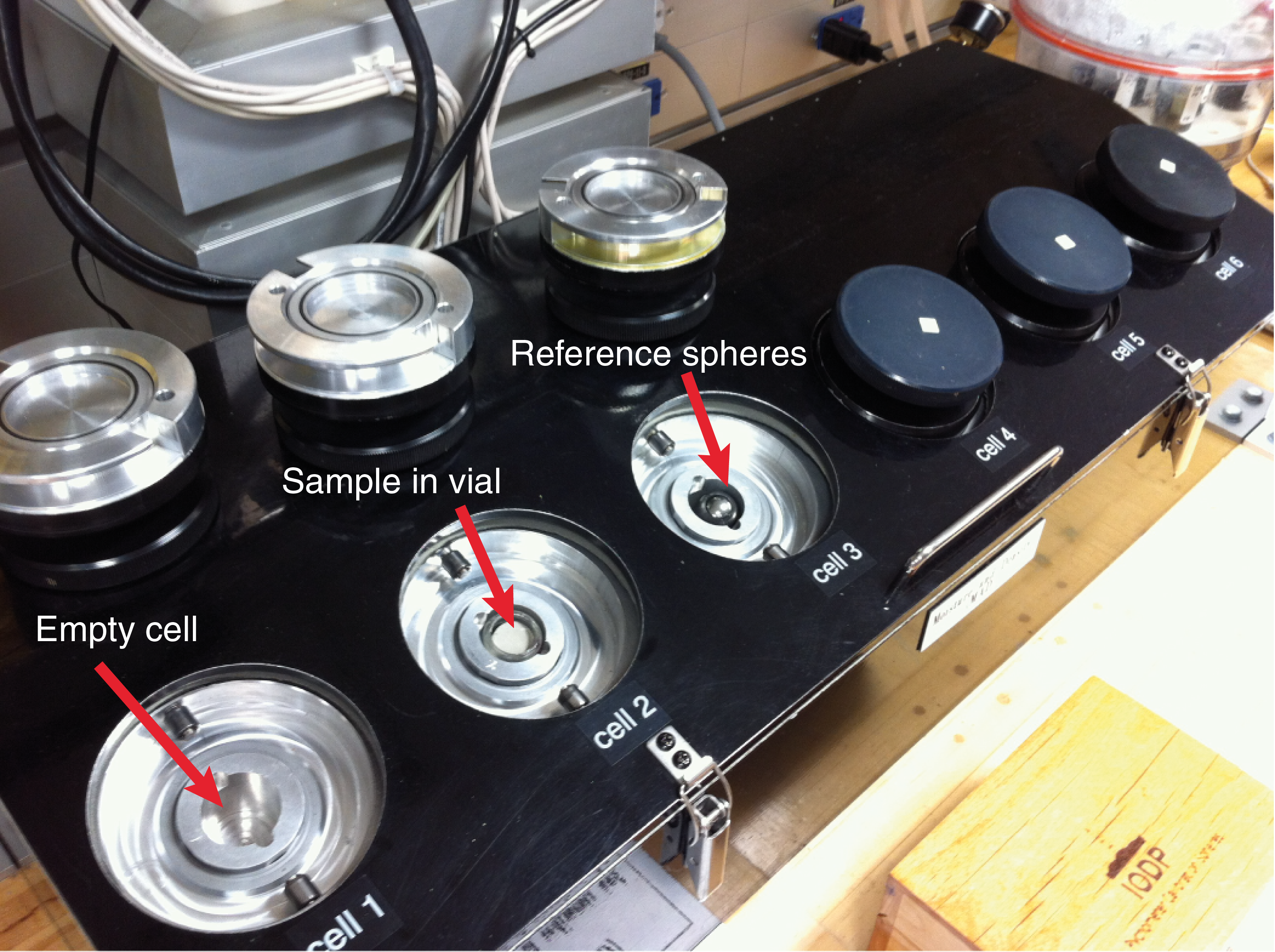
Figure F29. Pycnometer.
Mass and volume calculation
We measured wet mass (Mwet), dry mass (Mdry), and dry volume (Vdry). The ratio of mass (rm) is a computational constant of 0.965 (i.e., 0.965 g of freshwater per 1 g of seawater). Salt precipitated in sediment pores during the drying process is included in the Mdry and Vdry values. The mass of the evaporated water (Mwater) and salt (Msalt) in the sample are given by
where s is the assumed saltwater salinity (0.035%) corresponding to a pore water density (ρpw) of 1.024 g/cm3 and a salt density (ρsalt) of 2.22 g/cm3. The corrected mass of pore water (Mpw), volume of pore water (Vpw), mass of solids excluding salt (Msolid), volume of salt (Vsalt), volume of solids excluding salt (Vsolid), and wet volume (Vwet) are
Vwet = Vdry − Vsalt + Vpw, and
Calculation of bulk properties
For all sediment samples, water content (w) is expressed as the ratio of mass of pore water to wet sediment (total) mass:
Wet bulk density (ρwet), dry bulk density (ρdry), sediment grain density (ρsolid), porosity (φ), and void ratio (VR) are calculated as follows:
MAD properties reported and plotted in the Physical properties sections of all site chapters were calculated with the MADMax shipboard program set with the “method C” calculation process.
Downhole measurements
Downhole logs are used to determine physical, chemical, and structural properties of the formation penetrated by a borehole. The data are rapidly collected, continuous with depth, and measured in situ; they can be interpreted in terms of the stratigraphy, lithology, mineralogy, magnetic characteristics, and geochemical composition of the penetrated formation. Where core recovery is incomplete or disturbed, log data may provide the only way to characterize the borehole section. Where core recovery is good, log and core data complement one another and may be interpreted jointly.
Downhole logs measure formation properties on a scale that is intermediate between those obtained from laboratory measurements on core samples and those from geophysical surveys. They are useful in calibrating the interpretation of geophysical survey data (e.g., through the use of synthetic seismograms) and provide a necessary link for the integrated understanding of physical and chemical properties on different scales.
During Expeditions 367 and 368, downhole wireline log data was collected at Sites U1499–U1501, and U1503. In addition, a total of 14 downhole temperature measurements were acquired using the APCT-3 in Holes U1499A (6), U1501C (4), and U1505C (4).
Wireline logging
During wireline logging operations, logs were recorded with Schlumberger logging tools combined into several tool strings that were lowered into the hole after completion of coring operations. Three standard IODP tool string configurations were used during Expeditions 367 and 368 (Figure F30; Table T8). The first was a variant of the triple combo tool string, which measures borehole fluid temperature, NGR, porosity, density, electrical resistivity, and magnetic susceptibility. The second was the FMS-sonic tool string, which measures NGR, sonic velocity, and FMS resistivity images of the borehole wall. The third was the Versatile Seismic Imager (VSI) tool string, which measures a vertical seismic profile in order to integrate well and seismic data. Each tool string also contains an Enhanced Digital Telemetry Cartridge (EDTC) for communicating through the wireline to the Schlumberger data acquisition system (i.e., multitasking acquisition and imaging system [MAXIS]) on the drillship. See the site chapters for detailed lists of which tools were run in which combinations in each hole.
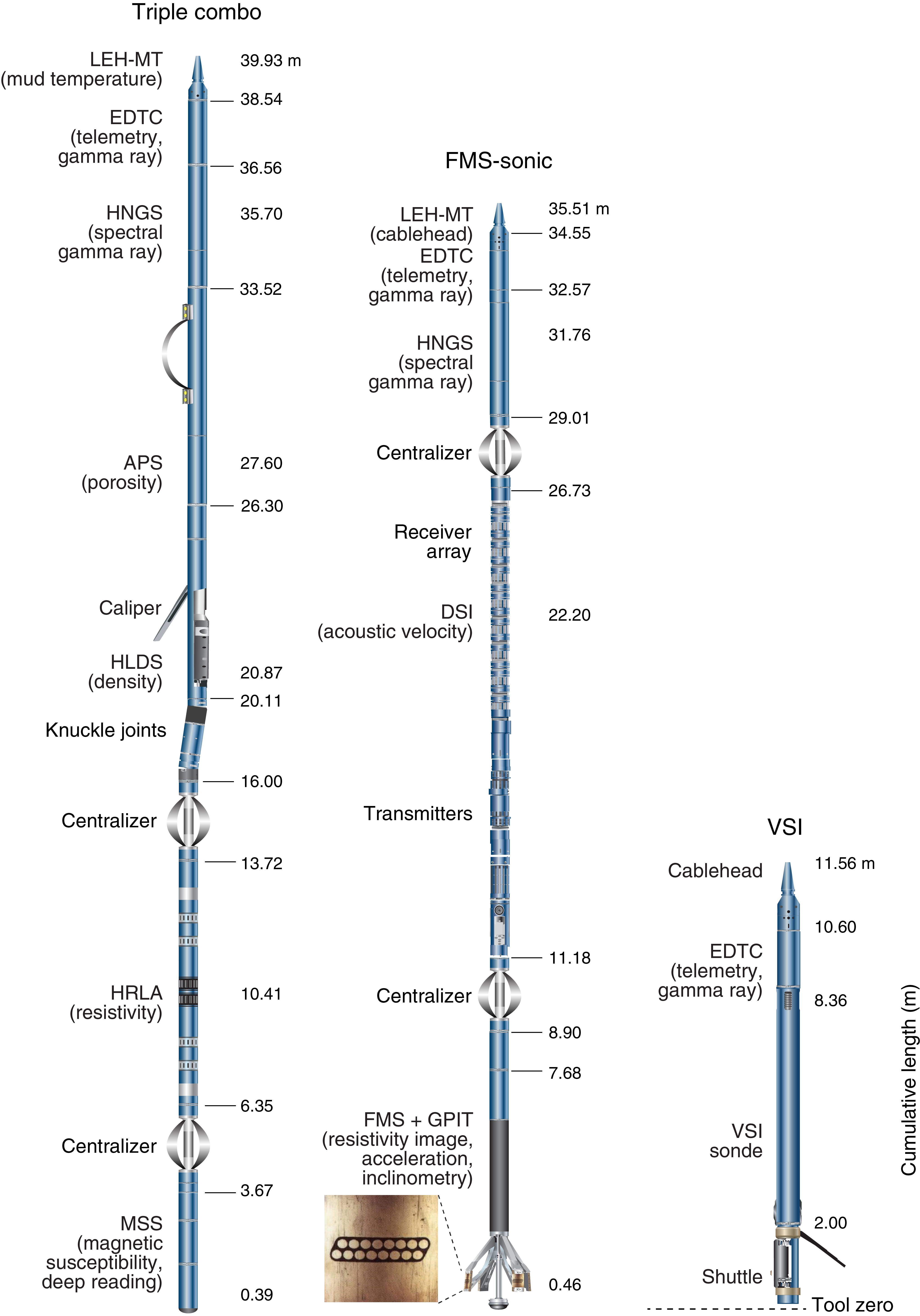
Figure F30. Wireline tool strings.
Table T8. Downhole measurements made by wireline tool strings. Download table in CSV format.
In preparation for logging, the boreholes were reamed in their lower sections, flushed of debris by circulating drilling fluid, and filled with seawater-based logging gel (i.e., sepiolite mud mixed with seawater and weighted with barite; approximate density = 10.5 lb/gal) to help stabilize the borehole walls in sections where instability would be expected based on drilling and coring results. The BHA was pulled up to a logging depth determined by the borehole conditions. Although log data can be collected while lowering the tool string to the bottom of the hole, the primary data set is collected while raising the tool strings upward at a constant speed, typically ~300 m/h for the triple combo and 600 m/h for the FMS-sonic.
Each tool string deployment is termed a logging “run.” During each run, tool strings can be lowered and pulled up in the hole several times to check repeatability and increase coverage of the FMS borehole images. Each lowering or hauling-up of the tool string while collecting data constitutes a “pass.” Incoming data were recorded and monitored in real time on the Schlumberger Minimum Configuration MAXIS logging computer. A wireline heave compensator (WHC) was typically used to minimize the effect of ship’s heave on the tool position in the borehole (see below).
Logged sediment properties and tool measurement principles
The logged properties and the principles used with the tools that measure them are briefly described below. The main tools are listed in Tables T8 and T9. More detailed information on individual tools and their geological applications may be found in Serra (1984, 1986, 1989), Schlumberger (1989, 1994), Rider (1996), Goldberg (1997), Lovell et al. (1998), and Ellis and Singer (2007). A complete list of acronyms for the Schlumberger tools and measurement curves is available at http://www.apps.slb.com/cmd. The complete list of downhole logging tools used during Integrated Ocean Drilling Program and IODP expeditions and additional information about tool physics are available at http://iodp.ldeo.columbia.edu/TOOLS_LABS/tools.html and http://iodp.tamu.edu/tools/logging/index.html.
Table T9. Acronyms and units used for downhole wireline tools and measurements. Download table in CSV format.
Natural gamma radiation
The Hostile Environment Natural Gamma Ray Sonde (HNGS) was used on both the triple combo and FMS-sonic tool strings to measure NGR in the formation. The HNGS uses two bismuth germanate scintillation detectors and five-window spectroscopy to determine concentrations of potassium (in weight percent), thorium (in parts per million), and uranium (in parts per million) from the characteristic gamma ray energies of isotopes in the 40K, 232Th, and 238U radioactive decay series, which dominate the natural radiation spectrum. The computation of the elemental abundances uses a least-squares method of extracting U, Th, and K elemental concentrations from the spectral measurements. The HNGS filters out gamma ray energies below 500 keV, eliminating sensitivity to bentonite or KCl in the drilling mud and improving measurement accuracy. The HNGS also provides a measure of the total spectral gamma ray (HSGR) and computed gamma ray (HCGR) that are measured in American Petroleum Institute gamma radiation units (gAPI). The HNGS response is influenced by the borehole diameter; therefore, the HNGS data are corrected for borehole diameter variations during acquisition.
An additional NGR sensor was housed in the EDTC to communicate data to the surface. The sensor includes a sodium iodide scintillation detector that also measures the total NGR emission of the formation. It is not a spectral tool (i.e., it does not provide U, Th, and K concentrations), but it provides total gamma radiation for each pass.
The inclusion of the HNGS in every tool string allows use of the gamma ray data for precise depth match processing between logging strings and passes and for core-log integration.
Density and photoelectric factor
Formation density was measured with the Hostile Environment Litho-Density Sonde (HLDS). The sonde contains a radioactive cesium (137Cs) gamma ray source (622 keV) and far and near gamma ray detectors mounted on a shielded skid that is pressed against the borehole wall by a hydraulically activated decentralizing arm. Gamma radiation emitted by the source undergoes Compton scattering, in which gamma rays are scattered by electrons in the formation. The number of scattered gamma rays that reach the detectors is proportional to the density of electrons in the formation, which is in turn related to bulk density. Porosity may also be derived from this bulk density if the matrix (grain) density is known.
The HLDS also measures the photoelectric effect factor (PEF), a measure of the photoelectric absorption of low-energy gamma radiation. Photoelectric absorption occurs when the energy of the gamma rays falls below 150 keV as a result of being repeatedly scattered by electrons in the formation. PEF is determined by comparing the counts from the far detector in the high-energy region, where only Compton scattering occurs, to those in the low-energy region, where count rates depend on both reactions. Because PEF depends on the atomic number of the elements in the formation (heavier elements have higher PEF), it also varies according to the chemical composition of the minerals present and can be used for the identification of the overall mineral makeup of the formation. For example, the PEF of calcite is 5.08 barn/e−, illite is 3.03 barn/e−, quartz is 1.81 barn/e−, and hematite is 21 barn/e−. Good contact between the tool and the borehole wall is essential for good HLDS logs; poor contact results in underestimation of density values. Both the density correction and caliper measurement of the hole are used to check the contact quality. In the deeper parts of the hole, the PEF log should be used with caution, especially in washouts, because barium in the logging mud swamps the signal despite correction for mud effect.
Electrical resistivity
The High-Resolution Laterolog Array (HRLA) provides six resistivity measurements with different depths of investigation (including the borehole or mud resistivity and five measurements of formation resistivity with increasing penetration into the formation). The tool sends a focused current into the formation and measures the intensity necessary to maintain a constant drop in voltage across a fixed interval, providing direct resistivity measurements. The array has one central (source) electrode and six electrodes above and below it, which serve alternatively as focusing and returning current electrodes. By rapidly changing the role of these electrodes, a simultaneous resistivity measurement at six penetration depths is achieved. The tool is designed to ensure that all signals are measured at exactly the same time and tool position and to reduce the sensitivity to “shoulder bed” effects when crossing sharp beds thinner than the electrode spacing. The design of the HRLA, which eliminates the need for a surface reference electrode, improves formation resistivity evaluation compared to traditional dual induction and allows the full range of resistivity to be measured from low (e.g., in high-porosity sediments) to high (e.g., in basalt). The HRLA needs to be run centralized in the borehole for optimal results, so knuckle joints were used to centralize the HRLA while allowing the density and porosity tools to maintain good contact with the borehole wall (Figure F30).
Calcite, silica, and hydrocarbons are electrical insulators, whereas ionic solutions like interstitial water are conductors. Electrical resistivity, therefore, can be used to evaluate porosity for a given salinity and resistivity of the interstitial water. Clay surface conduction also contributes to the resistivity values, but at high porosities, this effect is relatively minor.
Acoustic velocity
The Dipole Shear Sonic Imager (DSI) measures the transit times between sonic transmitters and an array of eight receivers. It combines replicate measurements, thus providing a direct measurement of sound velocity through formations that is relatively free from the effects of formation damage and an enlarged borehole (Schlumberger, 1989). Along with the monopole transmitters found on most sonic tools, it also has two crossed-dipole transmitters that allow the measurement of shear wave velocity in addition to compressional wave velocity. Dipole measurements are necessary to measure shear velocities in slow formations with shear velocity less than the velocity of sound in the borehole fluid. Such slow formations are typically encountered in deep-ocean drilling.
Formation MicroScanner
The FMS provides high-resolution electrical resistivity–based images of borehole walls. The tool has four orthogonal arms and pads, each containing 16 button electrodes that are pressed against the borehole wall during logging (Figure F30). The electrodes are arranged in two diagonally offset rows of 8 electrodes each. A focused current is emitted from the button electrodes into the formation, with a return electrode near the top of the tool. Resistivity of the formation at the button electrodes is derived from the intensity of current passing through the button electrodes.
Processing transforms the resistivity measurements into oriented high-resolution images that reveal geologic structures of the borehole wall. Features such as bedding, stratification, fracturing, slump folding, and bioturbation can be resolved (Luthi, 1990; Salimullah and Stow, 1992; Lovell et al., 1998). Because the images are oriented to magnetic north, further analysis can provide measurement of the dip and direction (azimuth) of planar features in the formation. In addition, when the corresponding planar features can be identified in the recovered core samples, individual core pieces can be reoriented with respect to true north.
Approximately 30% of a borehole with a diameter of 25 cm (9⅞ inches) is imaged during a single pass. Standard procedure is to make two full upward passes with the FMS to maximize the chance of getting full borehole coverage with the pads. The maximum extension of the caliper arms is 40.6 cm (16 inches). In holes with a diameter greater than this maximum, the pad contact at the end of the caliper arms is inconsistent, and the FMS images may appear out of focus and too conductive. Irregular (rough) borehole walls will also adversely affect the images if contact with the wall is poor.
Magnetic susceptibility
The magnetic susceptibility sonde (MSS) is a nonstandard wireline tool designed by the Lamont-Doherty Earth Observatory (LDEO). It measures the ease with which formations are magnetized when subjected to a magnetic field. The ease of magnetization is ultimately related to the concentration and composition (size, shape, and mineralogy) of magnetic minerals (principally magnetite) in the formation. These measurements provide one of the best methods for investigating stratigraphic changes in mineralogy and lithology because the measurement is quick, repeatable, and nondestructive and because different lithologies often have strongly contrasting susceptibilities.
The MSS dual-coil sensor provides ~40 cm resolution measurements, with ~20 cm depth of horizontal investigation. The MSS was run as the lowermost tool in the triple combo tool string using a specially developed data translation cartridge to enable the MSS to be run in combination with the Schlumberger tools. The MSS also has an optional single-coil sensor to provide high-resolution measurements (~10 cm), but this sensor was not used during Expeditions 367 and 368 because it has a large bowspring that requires the MSS to be run higher up in the tool string and because it is very sensitive to separation from the borehole wall.
Magnetic susceptibility data from both the high-resolution and deep-reading sensors are plotted as uncalibrated units. The MSS reading responses are affected by temperature and borehole size (higher temperatures lead to higher susceptibility measurements). Preliminary processing was performed offshore to remove the temperature drift by calculating a least-squares polynomial fit to the data and subtracting the calculated trend from the data set. When the magnetic susceptibility signal in sediment is very low, the detection limits of the tool may be reached. For quality control and environmental correction, the MSS also measures internal tool temperature, z-axis acceleration, and low-resolution borehole conductivity.
Acceleration and inclinometry
The General Purpose Inclinometry Tool (GPIT) was included in the FMS-sonic tool string to calculate tool acceleration and orientation during logging. Tool orientation is defined by three parameters: tool deviation, tool azimuth, and relative bearing. The GPIT utilizes a three-axis inclinometer and a three-axis fluxgate magnetometer to record the orientation of the FMS as the magnetometer records the magnetic field components (Fx, Fy, and Fz). Thus, the FMS images can be corrected for irregular tool motion, and the dip and direction (azimuth) of features in the FMS image can be determined.
Versatile Seismic Imager
Borehole seismic tools are used in wells to detect the acoustic signal generated at the surface. The VSI is used to determine the time–depth relation and to produce a zero-offset vertical seismic profile and/or check shots in the borehole. The VSI (Figure F30) uses three-axis single sensor seismic hardware and software and advanced wireline telemetry for efficient data delivery from the borehole to the surface. Each sensor package delivers high-fidelity wave fields through the use of a three-axis geophone accelerometer that is acoustically isolated from the main body of the tool (Figure F30). The geophone accelerometer detects particle motion and provides a linear and flat response from 3 to 200 Hz. The VSI maximal operational temperature is 177°C, or 350°F.
During Expeditions 367 and 368, the VSI was anchored against the borehole wall or the casing at ~50 m intervals, and 5–10 recordings were typically taken at each station. The recorded waveforms were stacked, and a one-way traveltime was determined from the first breaks for each station. The seismic source was a Sercel G-gun parallel cluster composed of two 250 inch3 air guns separated by 1 m. It was positioned by one of the ship cranes off the port side of the ship at a total horizontal offset of ~30 m from the top of the wellhead and was maintained at a fixed water depth (typically between 2 and 7 m; see Figure F50 in the Site U1500 chapter [Stock et al., 2018]).
Log data quality
The main influence on log data quality is the condition of the borehole wall. Where the borehole diameter varies over short intervals because of washouts of softer material or ledges of harder material, the logs from tools that require good contact with the borehole wall (i.e., FMS, density, and porosity) may be degraded. Deep investigation measurements such as gamma radiation, resistivity, and sonic velocity, which do not require contact with the borehole wall, are generally less sensitive to borehole conditions. “Bridged” sections, where borehole diameter is much below the bit size, also cause irregular log results. The quality of the borehole is improved by minimizing the circulation of drilling fluid while drilling, flushing the borehole to remove debris, and logging as soon as possible after drilling and conditioning are completed. During Expeditions 367 and 368, the necessity of flushing loose material from sandy formations up and out of the borehole required heavy circulation.
The quality of the wireline depth determination depends on several factors. The depth of the logging measurements is determined from the length of the cable payed out from the winch on the ship. The seafloor is identified on the NGR log by the abrupt reduction in gamma ray count at the water/sediment interface (mudline). Discrepancies between the drilling depth and the wireline log depth may occur. In the case of drilling depth, discrepancies are due to core expansion, incomplete core recovery, or incomplete heave compensation. In the case of log depth, discrepancies between successive runs occur because of incomplete heave compensation, incomplete correction for cable stretch, and cable slip. Tidal changes in sea level affect both drilling and logging depths, although these were <1 m in the South China Sea.
Wireline heave compensator
During wireline logging operations, the up-and-down motion of the ship (heave) causes a similar motion of the downhole logging tools. If the amplitude of this motion is large, depth discrepancies can be introduced into the logging data. The risk of damaging downhole instruments is also increased. A WHC system was thus designed to compensate for the vertical motion of the ship and maintain a steady motion of the logging tools to ensure high-quality logging data acquisition (Liu et al., 2013; Iturrino et al., 2013). The WHC uses a vertical accelerometer (motion reference unit [MRU]) positioned under the rig floor near the ship’s center of gravity to calculate the vertical motion of the ship with respect to the seafloor. It then adjusts the length of the wireline by varying the distance between two sets of pulleys through which the cable passes in order to minimize downhole tool motion. Real-time measurements of uphole (surface) and downhole acceleration are made simultaneously by the MRU and the EDTC, respectively. An LDEO-developed software package allows these data to be analyzed and compared in real time, displaying the actual motion of the logging tool string and enabling monitoring of the efficiency of the compensator.
Logging data flow and log depth scales
Data for each wireline logging run were monitored in real time and recorded using the Schlumberger MAXIS 500 system. Initial logging data were referenced to the rig floor (wireline depth below rig floor [WRF]). After logging was completed, the data were shifted to a seafloor reference (WSF) that is based on the step in gamma radiation at the sediment/water interface.
Data were transferred onshore to LDEO, where standardized data processing takes place. The main part of the processing is depth matching to remove depth offsets between logs from different logging runs, which results in a new depth scale: wireline log matched depth below seafloor (WMSF). Also, corrections are made to certain tools and logs (e.g., FMS imagery is corrected for tool acceleration, including “stick and slip”), documentation for the logs (with an assessment of log quality) is prepared, and the data are converted to ASCII for the conventional logs and GIF for the FMS images. The Schlumberger Geo-Quest GeoFrame software package is used for most of the processing of the collected wireline logging data. The data were transferred back to the ship within a few days after logging, and this processed data set was made available to the science party (in ASCII and DLIS formats) through the shipboard IODP logging database and shipboard servers.
In situ temperature measurements and heat flow calculation
During Expeditions 367 and 368, in situ temperature measurements were made with the APCT-3 (Figure F31) at each site when the APC was deployed. The APCT-3 fits directly into the coring shoe of the APC and consists of a battery pack, data logger, and platinum resistance-temperature device calibrated over a temperature range from 0° to 30°C. Before entering the borehole, the tool is first stopped at the mudline for 5 min to thermally equilibrate with bottom water. However, the lowest temperature recorded during the run is occasionally used instead of the average temperature at the mudline as an estimate of the bottom water temperature because (1) it is more repeatable and (2) the bottom water is expected to have the lowest temperature in the profile. When the APC is plunged into the formation, there is an instantaneous temperature rise from frictional heating. This heat gradually dissipates into the surrounding sediment as the temperature at the APCT-3 equilibrates toward the temperature of the sediment. After the APC penetrates the sediment, it is held in place for 5 min while the APCT-3 records the temperature of the cutting shoe every second.
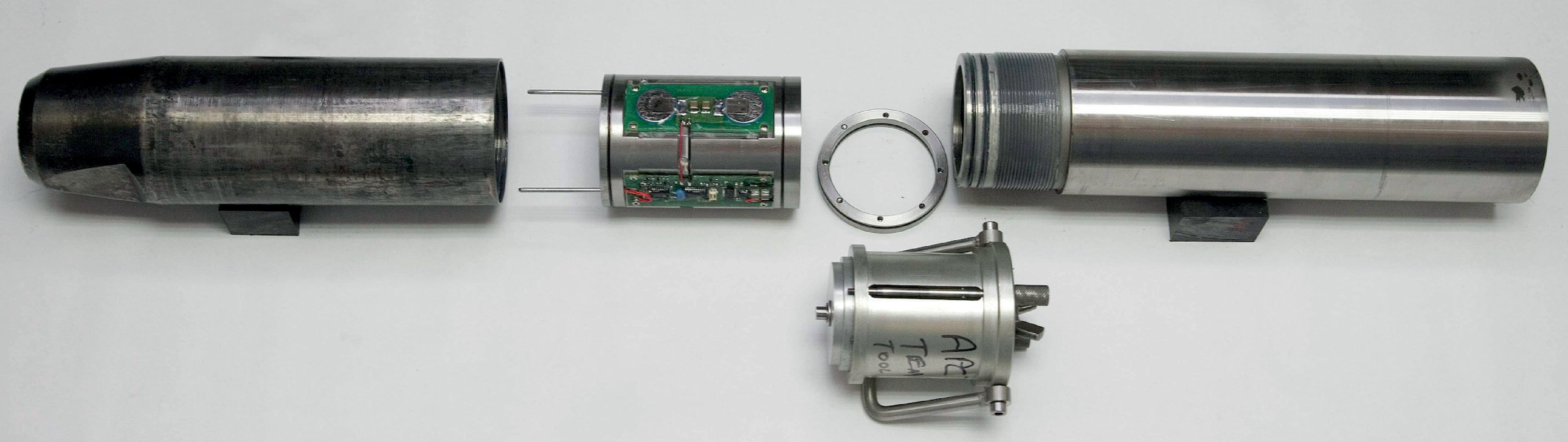
Figure F31. APCT-3 for in situ temperature measurements.
The equilibrium temperature of the sediment is estimated by applying a mathematical heat-conduction model to the temperature decay record (Horai and Von Herzen, 1985). The synthetic thermal decay curve for the APCT-3 is a function of the geometry and thermal properties of the probe and the sediment (Bullard, 1954; Horai and Von Herzen, 1985). Equilibrium temperature is estimated by applying a fitting procedure (Pribnow et al., 2000). However, where the APC does not achieve a full stroke or where ship heave pulls the APC up from full penetration, the temperature equilibration curve is disturbed and temperature determination is less accurate. The nominal accuracy of the APCT-3 temperature measurements is ±0.05°C.
APCT-3 temperature data is combined with thermal conductivity measurements obtained from whole-round core sections to retrieve heat flow values. Heat flow and geothermal gradient are calculated according to the Bullard (1939) method to be consistent with the synthesis of ODP heat flow data by Pribnow et al. (2000). This method assumes a linear relation between temperature T and thermal resistance of the sediments:
- T = temperature,
- z = depth,
- T0 = surface temperature (z = 0),
- Q = is heat flow, and
- Ω(z) = thermal resistance, expressed as
with zi and zi−1 as bottom and top depths, respectively, of a horizontal layer with thermal conductivity λi. I is the number of layers between the surface and depth z.
Plotting Ω(z) as a function of T(z), the Bullard plot allows estimation of the surface temperature (T0) from the intercept with z = 0 and of the heat flow (Q) from the slope. The conditions for the linearity of the plot are affected by conductive conditions, steady state, and absence of internal heat source.
To obtain the thermal conductivity at the depth of the temperature measurements, we estimated a continuous profile of λ(z), assuming that there is a linear variation of thermal conductivity with depth (Pribnow et al., 2000):
The linear trend was confirmed at each site. The thermal resistance ΩLIN,j for the depth zT,j of the jth temperature value Tj was calculated using the results of the linear regression, λ0 and Г (slope) with
ΩLIN,j = [ln(λ0 + Γ × zT,j) − ln(λ0)]/Г,
which allows the calculation of the heat flow.
Correlation to seismic data
The Chinese National Offshore Oil and Gas Company (CNOOC) holds an extensive database of 2-D and 3-D reflection seismic data covering the northern South China Sea margin. Interpretations of these data by CNOOC allow a suite of regional seismic unconformities to be identified. These are named by CNOOC with the capital letter T followed by a number (e.g., T30, T50, etc.). The ages of these seismic stratigraphic unconformities are constrained by industry wells located significantly landward of our study area.
During this expedition, we tried to extend the regional seismic unconformities mapped by CNOOC within the northern SCS continental slope (e.g., Dai et al., 2015) into our more southerly located study area of the slope and deep SCS basin. We applied the principle of seismic stratigraphy established by Vail et al. (1977) in the mapping of these horizons. That is, each unconformity and its correlative conformity are determined by recognizing systematic reflection terminations (including onlap, downlap, truncation, etc.). We expect there to be ten horizons tied to the CNOOC scheme in our area (Table T10), although at some of our sites one or more of these could not be identified due to lack of age control and/or disruption by faulting. Following the seismic stratigraphic principle, these can all be considered time markers, but only where they have a true conformal relationship to strata above and below will they represent a specific age. In all other settings, they represent a hiatus of a shorter or longer time interval.
Table T10. CNOOC seismic horizon and lithostratigraphy correlation scheme. Download table in CSV format.
We follow the convention established by CNOOC to name the base of the Cenozoic sedimentary succession Reflector Tg. This horizon is also often referred to as the “acoustic basement.” By this we mean a strong reflector that to a large but variable degree masks the underlying reflectors and does not allow any regional seismic stratigraphic mapping below it. Importantly, Tg is not a seismic stratigraphically defined horizon, nor does it represent any particular age or lithology. In our study area, it can represent the top of anything from volcanic basement of Neogene age to Mesozoic sediments or continental crystalline crust.
References
Agnini, C., Fornaciari, E., Raffi, I., Catanzariti., R., Pälike, H., Backman, J., and Rio, D., 2014. Biozonation and biochronology of Paleogene calcareous nannofossils from low and middle latitudes. Newsletters on Stratigraphy, 47(2):131–181. https://doi.org/10.1127/0078-0421/2014/0042
Akiba, F., 1986. Middle Miocene to Quaternary diatom biostratigraphy in the Nankai Trough and Japan Trench, and modified lower Miocene through Quaternary diatom zones for middle-to-high latitudes of the north Pacific. In Kagami, H., Karig, D.E., Coulbourn, W.T., et al., Initial Reports of the Deep Sea Drilling Project, 87: Washington, DC (U.S. Government Printing Office), 393–481. https://doi.org/10.2973/dsdp.proc.87.106.1986
Akiba, F., and Yanagisawa, Y., 1986. Taxonomy, morphology and phylogeny of the Neogene diatom zonal marker species in the middle-to-high latitudes of the North Pacific. In Kagami, H., Karig, D.E., Coulbourn, W.T., et al., Initial Reports of the Deep Sea Drilling Project, 87: Washington, DC (U.S. Government Printing Office), 483–554. https://doi.org/10.2973/dsdp.proc.87.107.1986
Alabi, O.O., Edilbi, A.N.F., Brolly, C., Muirhead, D., Parnell, J., Stacey, R., and Bowden, S.A., 2015. Asphaltene detection using surface enhanced Raman scattering (SERS). Chemical Communications, 51(33):7152–7155. http://pubs.rsc.org/en/content/articlehtml/2015/cc/c5cc00676g
Alvarez Zarikian, C.A., 2015. Cenozoic bathyal and abyssal ostracods beneath the South Pacific Gyre (IODP Expedition 329 Sites U1367, U1368 and U1370). Palaeogeography, Palaeoclimatology, Palaeoecology, 419:115–142. https://doi.org/10.1016/j.palaeo.2014.07.024
Anthonissen, D.E., and Ogg, J.G., 2012. Appendix 3—Cenozoic and Cretaceous biochronology of planktonic foraminifera and calcareous nannofossils. In Gradstein, F.M., Ogg, J.G., Schmitz, M.D., and Ogg, G.M., (Eds.), The Geologic Time Scale 2012: Amsterdam (Elsevier), 1083–1127. https://doi.org/10.1016/B978-0-444-59425-9.15003-6
Arculus, R.J., Ishizuka, O., Bogus, K., Aljahdali, M.H., Bandini-Maeder, A.N., Barth, A.P., Brandl, P.A., do Monte Guerra, R., Drab, L., Gurnis, M.C., Hamada, M., Hickey-Vargas, R.L., Jiang, F., Kanayama, K., Kender, S., Kusano, Y., Li, H., Loudin, L.C., Maffione, M., Marsaglia, K.M., McCarthy, A., Meffre, S., Morris, A., Neuhaus, M., Savov, I.P., Sena Da Silva, C.A., Tepley, F.J., III, van der Land, C., Yogodzinski, G.M., and Zhang, Z., 2015. Expedition 351 methods. In Arculus, R.J., Ishizuka, O., Bogus, K., and the Expedition 351 Scientists, Izu-Bonin-Mariana Arc Origins. Proceedings of the International Ocean Discovery Program, 351: College Station, TX (International Ocean Discovery Program). https://doi.org/10.14379/iodp.proc.351.102.2015
ASTM International, 1990. Standard method for laboratory determination of water (moisture) content of soil and rock (Standard D2216–90). In Annual Book of ASTM Standards for Soil and Rock (Volume 04.08): Philadelphia (American Society for Testing Materials). [revision of D2216-63, D2216-80]
Backman, J., Raffi, I., Rio, D., Fornaciari, E., and Pälike, H., 2012. Biozonation and biochronology of Miocene through Pleistocene calcareous nannofossils from low and middle latitudes. Newsletters on Stratigraphy, 45(3):221–244. https://doi.org/10.1127/0078-0421/2012/0022
Baldauf, J.G., and Iwai, M., 1995. Neogene diatom biostratigraphy for the eastern equatorial Pacific Ocean, Leg 138. In Pisias, N.G., Mayer, L.A., Janecek, T.R., Palmer-Julson, A., and van Andel, T.H. (Eds.), Proceedings of the Ocean Drilling Program, Scientific Results, 138: College Station, TX (Ocean Drilling Program), 105–128. https://doi.org/10.2973/odp.proc.sr.138.107.1995
Balsam, W.L., and Damuth, J.E., 2000. Further investigations of shipboard vs. shore-based spectral data: implications for interpreting Leg 164 sediment composition. In Paull, C.K., Matsumoto, R., Wallace, P., and Dillon, W.P. (Eds.), Proceedings of the Ocean Drilling Program, Scientific Results, 164: College Station, TX (Ocean Drilling Program), 313–324. https://doi.org/10.2973/odp.proc.sr.164.222.2000
Balsam, W.L., Damuth, J.E., and Schneider, R.R., 1997. Comparison of shipboard vs. shore-based spectral data from Amazon Fan cores: implications for interpreting sediment composition. In Flood, R.D., Piper, D.J.W., Klaus, A., and Peterson, L.C. (Eds.), Proceedings of the Ocean Drilling Program, Scientific Results, 155: College Station, TX (Ocean Drilling Program), 193–215. https://doi.org/10.2973/odp.proc.sr.155.210.1997
Balsam, W.L., Deaton, B.C., and Damuth, J.E., 1998. The effects of water content on diffuse reflectance spectrophotometry studies of deep-sea sediment cores. Marine Geology, 149(1–4):177–189. https://doi.org/10.1016/S0025-3227(98)00033-4
Barron, J.A., 1981. Late Cenozoic diatom biostratigraphy and paleoceanography of the middle-latitude eastern North Pacific, Deep Sea Drilling Project Leg 63. In Yeats, R.S., Haq, B.U., et al., Initial Reports of the Deep Sea Drilling Project, 63: Washington, DC (U.S. Government Printing Office), 507–538. https://doi.org/10.2973/dsdp.proc.63.113.1981
Barron, J.A., 1985. Late Eocene to Holocene diatom biostratigraphy of the equatorial Pacific Ocean, Deep Sea Drilling Project Leg 85. In Mayer, L., Theyer, F., Thomas, E., et al., Initial Reports of the Deep Sea Drilling Project, 85: Washington, DC (U.S. Government Printing Office), 413–456. https://doi.org/10.2973/dsdp.proc.85.108.1985
Barron, J.A., 2003. Planktonic marine diatom record of the past 18 m.y.: appearances and extinctions in the Pacific and Southern Oceans. Diatom Research, 18(2):203–224. https://doi.org/10.1080/0269249X.2003.9705588
Barron, J.A., 2006. Diatom biochronology for the early Miocene of the equatorial Pacific. Stratigraphy, 2(4):281–309. http://www.micropress.org/micropen2/articles/1/4/3987_articles_article_file_1443.pdf
Barron, J.A., Fourtanier, E., and Bohaty, S.M., 2004. Oligocene and earliest Miocene diatom biostratigraphy of ODP Leg 199 Site 1220, equatorial Pacific. In Wilson, P.A., Lyle, M., Janecek, T.R., and Firth, J.V. (Eds.), Proceedings of the Ocean Drilling Program, Scientific Results, 199: College Station, TX (Ocean Drilling Program), 1–25. https://doi.org/10.2973/odp.proc.sr.199.204.2004
Berggren, W.A., Kent, D.V., Swisher, C.C., III, and Aubry, M.-P., 1995. A revised Cenozoic geochronology and chronostratigraphy. In Berggren, W.A., Kent, D.V., Aubry, M.-P., and Hardenbol, J. (Eds.), Geochronology, Time Scales and Global Stratigraphic Correlation. Special Publication - SEPM (Society for Sedimentary Geology), 54:129–212. https://doi.org/10.7916/D8XD1B1H
Blow, W.H., 1969. Late middle Eocene to recent planktonic foraminiferal biostratigraphy. Proceedings of the International Conference on Planktonic Microfossils, 1:199–422.
Blow, W.H., 1979. The Cainozoic Foraminifera (Volumes 1−3): Leiden, The Netherlands (E.J. Brill).
Blum, P., 1997. Technical Note 26: Physical Properties Handbook—A Guide to the Shipboard Measurement of Physical Properties of Deep-Sea Cores. Ocean Drilling Program. https://doi.org/10.2973/odp.tn.26.1997
Bolli, H.M., and Saunders, J.B., 1985. Oligocene to Holocene low latitude planktic foraminifera. In Bolli, H.M., Saunders, J.B., and Perch-Nielsen, K. (Eds.), Plankton Stratigraphy (Volume 1): Planktic Foraminifera, Calcareous Nannofossils and Calpionellids: Cambridge, United Kingdom (Cambridge University Press), 155–262.
Bollmann, J., 1997. Morphology and biogeography of Gephyrocapsa coccoliths in Holocene sediments. Marine Micropaleontology, 29(3–4):319–350. https://doi.org/10.1016/S0377-8398(96)00028-X
Bown, P.R. (Ed.), 1998. Calcareous Nannofossil Biostratigraphy: Dordrecht, The Netherlands (Kluwer Academic Publishing).
Bullard, E.C., 1939. Heat flow in South Africa. Proceedings of the Royal Society of London, Series A, 173(955):474–502. https://doi.org/10.1098/rspa.1939.0159
Bullard, E.C., 1954. The flow of heat through the floor of the Atlantic Ocean. Proceedings of the Royal Society of London, Series A: Mathematical, Physical and Engineering Sciences, 222(1150):408–429. https://doi.org/10.1098/rspa.1954.0085
Burckle, L.H., 1972. Late Cenozoic planktonic diatom zones from the eastern equatorial Pacific. In Simonsen, R. (Ed.), First Symposium on Recent and Fossil Marine Diatoms (Bremenhaven, Germany, 21–26 September 1970). Beihefte zur Nova Hedwigia, 39:217–249.
Cervato, C., and Burckle, L., 2003. Pattern of first and last appearance in diatoms: Oceanic circulation and the position of polar fronts during the Cenozoic. Paleoceanography, 18(2). https://doi.org/10.1029/2002PA000805
Coccioni, R., Marsili, A., Montanari, A., Bellanca, A., Neri, R., Bice, D.M., Brinkhuis, H., Church, N., Macalady, A., McDaniel, A., Deino, A., Lirer, F., Sprovieri, M., Maiorano, P., Monechi, S., Nini, C., Nocchi, M., Pross, J., Rochette, P., Sagnotti, L., Tateo, F., Touchard, Y., Van Simaeys, S., and Williams, G.L., 2008. Integrated stratigraphy of the Oligocene pelagic sequence in the Umbria-Marche Basin (northeastern Apennines, Italy): a potential Global Stratotype Section and Point (GSSP) for the Rupelian/Chattian boundary. Geological Society of America Bulletin, 120(3–4):487–511. https://doi.org/10.1130/B25988.1
Cook, H.E., Johnson, P.D., Matti, J.C., and Zemmels, I., 1975. Methods of sample preparation and X-ray diffraction data analysis, X-ray Mineralogy Laboratory, Deep Sea Drilling Project, University of California, Riverside. In Hayes, D.E., Frakes, L.A., et al., Initial Reports of the Deep Sea Drilling Project, 28: Washington (U.S. Government Printing Office), 999–1007. http://dx.doi.org/10.2973/dsdp.proc.28.app4.1975
Cox, A., and Gordon, R.G., 1984. Paleolatitudes determined from paleomagnetic data from vertical cores. Reviews of Geophysics and Space Physics, 22(1):47–71. https://doi.org/10.1029/RG022i001p00047
Dai, Y., Yu, Q., Li, H., Wang, Z., Bai, J., and Peng, H., 2015. Threshold conditions and reservoir-controlling characteristics of source kitchen in Zhu I depression, Pearl River Mouth Basin. Acta Petrolei Sinica, 36(S2):145–155. (in Chinese with English abstract) https://doi.org/10.7623/syxb2015S2013
De Vleeschouwer, D., Dunlea, A.G., Auer, G., Anderson, C.H., Brumsack, H., de Loach, A., Gurnis, M., Huh, Y., Ishiwa, T., Jang, K., Kominz, M.A., März, C., Schnetger, B., Murray, R.W., Pälike, H., and Expedition 356 Shipboard Scientists, 2017. Quantifying K, U, and Th contents of marine sediments using shipboard natural gamma radiation spectra measured on DV JOIDES Resolution. Geochemistry, Geophysics, Geosystems, 18(3):1053–1064. https://doi.org/10.1002/2016GC006715
de Wall, H., and Worm, H.-U., 2001. Recognition of drilling-induced remanent magnetization by Q-factor analysis: a case study from the KTB-drillholes. Journal of Applied Geophysics, 46(1):55–64. https://doi.org/10.1016/S0926-9851(00)00039-2
Doré, T., and Lundin, E., 2015. Research focus: hyperextended continental margins—knowns and unknowns. Geology, 43(1):95–96. https://doi.org/10.1130/focus012015.1
Droser, M.L., and Bottjer, D.J., 1986. A semiquantitative field classification of ichnofabric. Journal of Sedimentary Research, 56(4):558–559. https://doi.org/10.1306/212F89C2-2B24-11D7-8648000102C1865D
Dunlea, A.G., Murray, R.W., Harris, R.N., Vasiliev, M.A., Evans, H., Spivack, A.J., and D’Hondt, S., 2013. Assessment and use of NGR instrumentation on the JOIDES Resolution to quantify U, Th, and K concentrations in marine sediment. Scientific Drilling, 15:57–63. https://doi.org/10.2204/iodp.sd.15.05.2013
Edwards, A.R., 1991. The Oamaru diatomite. New Zealand Geological Survey Paleontological Bulletin, 64.
Ellis, D.V., and Singer, J.M., 2007. Well Logging for Earth Scientists (2nd edition): New York (Elsevier).
Expedition 324 Scientists, 2010. Methods. In Sager, W.W., Sano, T., Geldmacher, J., and the Expedition 324 Scientists, Proceedings of the Integrated Ocean Drilling Program, 324: Tokyo (Integrated Ocean Drilling Program Management International, Inc.). https://doi.org/10.2204/iodp.proc.324.102.2010
Expedition 330 Scientists, 2012. Methods. In Koppers, A.A.P., Yamazaki, T., Geldmacher, J., and the Expedition 330 Scientists, Proceedings of the Integrated Ocean Drilling Program, 330: Tokyo (Integrated Ocean Drilling Program Management International, Inc.). https://doi.org/10.2204/iodp.proc.330.102.2012
Expedition 339 Scientists, 2013. Methods. In Stow, D.A.V., Hernández-Molina, F.J., Alvarez Zarikian, C.A., and the Expedition 339 Scientists, Proceedings of the Integrated Ocean Drilling Program, 339: Tokyo (Integrated Ocean Drilling Program Management International, Inc.). https://doi.org/10.2204/iodp.proc.339.102.2013
Fenner, J., 1978. Cenozoic diatom biostratigraphy of the equatorial and southern Atlantic Ocean. In Perch-Nielsen, K., Supko, P.R., et al., Initial Reports of the Deep Sea Drilling Project, 38, 39, 40, 41 (Suppl.): Washington, DC (U.S. Government Printing Office), 491–624. https://doi.org/10.2973/dsdp.proc.38394041s.201.1978
Fenner, J., 1985. Late Cretaceous to Oligocene planktic diatoms. In Bolli, H.M., Saunders, J.B., and Perch-Nielsen, K. (Eds.), Plankton Stratigraphy: Cambridge, United Kingdom (Cambridge University Press), 713–762.
Fenner, J., 1994. Diatoms of the Fur Formation, their taxonomy and biostratigraphic interpretation: results from the Harre borehole, Denmark. Aarhus Geoscience, 1:99–163.
Fisher, R.V., and Schmincke, H.-U., 1984. Pyroclastic Rocks: Berlin (Springer-Verlag). https://doi.org/10.1007/978-3-642-74864-6
Fuller, M., 1969. Magnetic orientation of borehole cores. Geophysics, 34(5):772–774. https://doi.org/10.1190/1.1440047
Fuller, M., Hastedt, M., and Herr, B., 1998. Coring-induced magnetization of recovered sediment. In Weaver, P.P.E., Schmincke, H.-U., Firth, J.V., and Duffield, W. (Eds.), Proceedings of the Ocean Drilling Program, Scientific Results, 157: College Station, TX (Ocean Drilling Program), 47–56. https://doi.org/10.2973/odp.proc.sr.157.103.1998
Gee, J.S., Tauxe, L., and Constable, C., 2008. AMSSpin: a LabVIEW program for measuring the anisotropy of magnetic susceptibility with the Kappabridge KLY-4S. Geochemistry, Geophysics, Geosystems, 9(8):Q08Y02. https://doi.org/10.1029/2008GC001976
Gieskes, J.M., Gamo, T., and Brumsack, H., 1991. Technical Note 15: Chemical Methods for Interstitial Water Analysis Aboard JOIDES Resolution. Ocean Drilling Program. https://doi.org/10.2973/odp.tn.15.1991
Gillis, K.M., Snow, J.E., Klaus, A., Guerin, G., Abe, N., Akizawa, N., Ceuleneer, G., Cheadle, M.J., Adrião, Á., Faak, K., Falloon, T.J., Friedman, S.A., Godard, M.M., Harigane, Y., Horst, A.J., Hoshide, T., Ildefonse, B., Jean, M.M., John, B.E., Koepke, J.H., Machi, S., Maeda, J., Marks, N.E., McCaig, A.M., Meyer, R., Morris, A., Nozaka, T., Python, M., Saha, A., and Wintsch, R.P., 2014. Methods. In Gillis, K.M., Snow, J.E., Klaus, A., and the Expedition 345 Scientists, Proceedings of the Integrated Ocean Drilling Program, 345: College Station, TX (Integrated Ocean Drilling Program). https://doi.org/10.2204/iodp.proc.345.102.2014
Gilmore, G.R., 2008. Practical Gamma-ray Spectrometry (2nd edition): Hoboken, NJ (John Wiley & Sons). https://doi.org/10.1002/9780470861981
Goldberg, D., 1997. The role of downhole measurements in marine geology and geophysics. Reviews of Geophysics, 35(3):315–342. https://doi.org/10.1029/97RG00221
Gombos, A.M., Jr., 1982. Early and middle Eocene diatom evolutionary events. Bacillaria, 5:225–242.
Govindaraju, K., 1994. 1994 compilation of working values and sample description for 383 geostandards. Geostandards Newsletter, 18(1). https://doi.org/10.1111/j.1751-908X.1994.tb00502.x
Gradstein, F.M., Ogg, J.G., Schmitz, M.D., and Ogg, G.M. (Eds.), 2012. The Geological Time Scale 2012: Oxford, United Kingdom (Elsevier).
Hajós, M., 1976. Upper Eocene and lower Oligocene diatomaceae, archaeomonadaceae, and silicoflagellatae in southwestern Pacific sediments, DSDP Leg 29. In Hollister, C.D., Craddock, C., et al., Initial Reports of the Deep Sea Drilling Project, 35: Washington, DC (U.S. Government Printing Office), 817–883. https://doi.org/10.2973/dsdp.proc.35.29chap1.1976
Hardenbol, J., Thierry, J., Farley, M.B., Jacquin, T., de Graciansky, P.-C., and Vail, P.R., 1998. Mesozoic and Cenozoic sequence chronostratigraphic framework of European basins. In de Graciansky, P.-C., Hardenbol, J., Jacquin, T., and Vail, P.R. (Eds.), Mesozoic and Cenozoic Sequence Stratigraphy of European Basins. Special Publication - SEPM (Society for Sedimentary Geology), 60:3–13. http://archives.datapages.com/data/sepm_sp/SP60/Mesozoic_and_Cenozoic_Sequence_Chronostratigraphic.pdf
Harris, R.N., Sakaguchi, A., Petronotis, K., Baxter, A.T., Berg, R., Burkett, A., Charpentier, D., Choi, J., Diz Ferreiro, P., Hamahashi, M., Hashimoto, Y., Heydolph, K., Jovane, L., Kastner, M., Kurz, W., Kutterolf, S.O., Li, Y., Malinverno, A., Martin, K.M., Millan, C., Nascimento, D.B., Saito, S., Sandoval Gutierrez, M.I., Screaton, E.J., Smith-Duque, C.E., Solomon, E.A., Straub, S.M., Tanikawa, W., Torres, M.E., Uchimura, H., Vannucchi, P., Yamamoto, Y., Yan, Q., and Zhao, X., 2013. Methods. In Harris, R.N., Sakaguchi, A., Petronotis, K., and the Expedition 344 Scientists, Proceedings of the Integrated Ocean Drilling Program, 344: College Station, TX (Integrated Ocean Drilling Program). https://doi.org/10.2204/iodp.proc.344.102.2013
Hilgen, F.J., Lourens, L.J., and Van Dam, J.A., 2012. The Neogene period. With contributions by A.G. Beu, A.F. Boyes, R.A. Cooper, W. Krijgsman, J.G. Ogg, W.E. Piller, and D.S. Wilson. In Gradstein, F.M., Ogg, J.G., Schmitz, M.D., and Ogg, G.M. (Eds.), The Geologic Time Scale: Oxford, United Kingdom (Elsevier), 923–978. https://doi.org/10.1016/B978-0-444-59425-9.00029-9
Holbourn, A., Henderson, A.S., and MacLeod, N., 2013. Atlas of Benthic Foraminifera: Chichester, United Kingdom (John Wiley & Sons, Ltd.). https://doi.org/10.1002/9781118452493
Horai, K., and Von Herzen, R.P., 1985. Measurement of heat flow on Leg 86 of the Deep Sea Drilling Project. In Heath, G.R., Burckle, L.H., et al., Initial Reports of the Deep Sea Drilling Project, 86: Washington, DC (U.S. Government Printing Office), 759–777. https://doi.org/10.2973/dsdp.proc.86.135.1985
Hu, C.-H., and Tao, H.-J., 2008. Studies on the ostracod fauna of Taiwan and it adjacent seas, Part 1 and 2. Journal of the National Taiwan Museum, Special Publication Series, 13. (in Chinese)
Husson, D., Galbrun, B., Laskar, J., Hinnov, L.A., Thibault, N., Gardin, S., and Lockair, R.E., 2011. Astronomical calibration of the Maastrichtian (Late Cretaceous). Earth and Planetary Science Letters, 305(3–4):328–340. https://doi.org/10.1016/j.epsl.2011.03.008
Iturrino, G., Liu, T., Goldberg, D., Anderson, L., Evans, H., Fehr, A., Guerin, G., Inwood, J., Lofi, J., Malinverno, A., Morgan, S., Mrozewski, S., Slagle, A., and Williams, T., 2013. Performance of the wireline heave compensation system onboard D/V JOIDES Resolution. Scientific Drilling, 15:46–50. https://doi.org/10.2204/iodp.sd.15.08.2013
Jarrard, R.D., and Kerneklian, M.J., 2007. Data report: physical properties of the upper oceanic crust of ODP Site 1256: multisensor track and moisture and density measurements. In Teagle, D.A.H., Wilson, D.S., Acton, G.D., and Vanko, D.A. (Eds.), Proceedings of the Ocean Drilling Program, Scientific Results, 206: College Station, TX (Ocean Drilling Program), 1–11. https://doi.org/10.2973/odp.proc.sr.206.011.2007
Jutzeler, M., White, J.D.L., Talling, P.J., McCanta, M., Morgan, S., Le Friant, A., and Ishizuka, O., 2014. Coring disturbances in IODP piston cores with implications for offshore record of volcanic events and the Missoula megafloods. Geochemistry, Geophysics, Geosystems, 15(9):3572–3590. https://doi.org/10.1002/2014GC005447
Kaminski, M.A., and Gradstein, F.M., 2005. Atlas of Paleogene cosmopolitan deep-water agglutinated foraminifera. Grzybowski Foundation Special Publication, 10. http://www.foraminifera.eu/atlas.html
Kennett, J.P., and Srinivasan, M.S., 1983. Neogene Planktonic Foraminifera: A Phylogenetic Atlas: Stroudsburg, PA (Hutchinson Ross).
Kirschvink, J.L., 1980. The least-squares line and plane and the analysis of palaeomagnetic data. Geophysical Journal of the Royal Astronomical Society, 62(3):699–718. https://doi.org/10.1111/j.1365-246X.1980.tb02601.x
Koizumi, I., and Tanimura, Y., 1985. Neogene diatom biostratigraphy of the middle latitude western North Pacific, Deep Sea Drilling Project Leg 86. In Heath, G.R., Burckle, L.H., et al., Initial Reports of the Deep Sea Drilling Project, 86: Washington, DC (U.S. Government Printing Office), 269–300. https://doi.org/10.2973/dsdp.proc.86.109.1985
Kristiansen, J.I., 1982. The transient cylindrical probe method for determination of thermal parameters of earth materials [Ph.D. dissertation]. Åarhus University, Åarhus, Denmark.
Lazarus, D., Barron, J., Renaudie, J., Diver, P., and Türke, A., 2014. Cenozoic planktonic marine diatom diversity and correlation to climate change. PLoS ONE, 9(1):e84857. https://doi.org/10.1371/journal.pone.0084857
Le Maitre, R.W., Steckeisen, A., Zanettin, B., Le Bas, M.J., Bonin, B., and Bateman, P. (Eds.), 2002. Igneous rocks: A Classification and Glossary of Terms (2nd edition.): Cambridge, United Kingdom (Cambridge University Press).
Li, B., Jian, Z., Li, Q., Tian, J., and Wang, P., 2005. Paleoceanography of the South China Sea since the middle Miocene: evidence from planktonic foraminifera. In Wang, P., and Lipps, J. (Eds.), Marine Micropaleonotology of the South China Sea. Marine Micropaleontology, 54(1–2):49–62. https://doi.org/10.1016/j.marmicro.2004.09.003
Li, C.-F., Lin, J., Kulhanek, D.K., Williams, T., Bao, R., Briais, A., Brown, E.A., Chen, Y., Clift, P.D., Colwell, F.S., Dadd, K.A., Ding, W., Hernández-Almeida, I., Huang, X.-L., Hyun, S., Jiang, T., Koppers, A.A.P., Li, Q., Liu, C., Liu, Q., Liu, Z., Nagai, R.H., Peleo-Alampay, A., Su, X., Sun, Z., Tejada, M.L.G., Trinh, H.S., Yeh, Y.-C., Zhang, C., Zhang, F., Zhang, G.-L., and Zhao, X., 2015. Methods. In Li, C.-F., Lin, J., Kulhanek, D.K., and the Expedition 349 Scientists, South China Sea Tectonics. Proceedings of the International Ocean Discovery Program, 349: College Station, TX (International Ocean Discovery Program). https://doi.org/10.14379/iodp.proc.349.102.2015
Liu, T., Iturrino, G., Goldberg, D., Meissner, E., Swain, K., Furman, C., Fitzgerald, P., Frisbee, N., Chlimoun, J., Van Hyfte, J., and Beyer, R., 2013. Performance evaluation of active wireline heave compensation systems in marine well logging environments. Geo-Marine Letters, 33(1):83–93. https://doi.org/10.1007/s00367-012-0309-8
Loeblich, A.R., Jr., and Tappan, H., 1988. Foraminiferal Genera and Their Classification:New York (Van Nostrand Reinhold). https://doi.org/1007/978-1-4899-5760-3
Lourens, L., Hilgen, F., Shackleton, N.J., Laskar, J., and Wilson, D., 2004. The Neogene period. In Gradstein, F.M., Ogg, J.G., and Smith, A. (Eds.), A Geologic Time Scale 2004: Cambridge, United Kingdom (Cambridge University Press), 409–440. https://doi.org/10.1017/CBO9780511536045.022
Lovell, M.A., Harvey, P.K., Brewer, T.S., Williams, C., Jackson, P.D., and Williamson, G., 1998. Application of FMS images in the Ocean Drilling Program: an overview. In Cramp, A., MacLeod, C.J., Lee, S.V., and Jones, E.J.W. (Eds.), Geological Evolution of Ocean Basins: Results from the Ocean Drilling Program. Geological Society Special Publication, 131(1):287–303. https://doi.org/10.1144/GSL.SP.1998.131.01.18
Lurcock, P.C., and Wilson, G.S., 2012. PuffinPlot: a versatile, user-friendly program for paleomagnetic analysis. Geochemistry, Geophysics, Geosystems, 13(6):Q06Z45. https://doi.org/10.1029/2012GC004098
Luthi, S.M., 1990. Sedimentary structures of clastic rocks identified from electrical borehole images. In Hurst, A., Lovell, M.A., and Morton, A.C. (Eds.), Geological Applications of Wireline Logs. Geological Society Special Publication, 48:3–10. https://doi.org/10.1144/GSL.SP.1990.048.01.02
MacKenzie, W.S., Donaldson, C.H., and Guilford, C., 1982. Atlas of Igneous Rocks and Their Textures: Essex, United Kingdom (Longman Group UK Limited).
Maiorano, P., and Marino, M., 2004. Calcareous nannofossil bioevents and environmental control on temporal and spatial patterns at the early–middle Pleistocene. Marine Micropaleontology, 53(3–4):405–422. https://doi.org/10.1016/j.marmicro.2004.08.003
Manheim, F.T., and Sayles, F.L., 1974. Composition and origin of interstitial waters of marine sediments, based on deep sea drill cores. In Goldberg, E.D. (Ed.), The Sea (Volume 5): Marine Chemistry: The Sedimentary Cycle: New York (Wiley), 527–568.
Marsaglia, K., Milliken, K., and Doran, L., 2013. Technical Note 1: IODP digital reference for smear slide analysis of marine mud—Part 1: Methodology and atlas of siliciclastic and volcanogenic components. Integrated Ocean Drilling Program. https://doi.org/10.2204/iodp.tn.1.2013
Marsaglia, K., Milliken, K., Leckie, R.M., Tentori, D., and Doran, L., 2015. Technical Note 2: IODP smear slide digital reference for sediment analysis of marine mud, Part 2: Methodology and atlas of biogenic components. International Ocean Discovery Program. https://doi.org/10.2204/iodp.tn.2.2015
Martini, E., 1971. Standard Tertiary and Quaternary calcareous nannoplankton zonation. In Farinacci, A. (Ed.), Proceedings of the Second Planktonic Conference, Roma 1970: Rome (Edizioni Tecnoscienza), 2:739–785.
Mazzullo, J.M., Meyer, A., and Kidd, R.B., 1988. New sediment classification scheme for the Ocean Drilling Program. In Mazzullo, J., and Graham, A.G. (Eds.), Technical Note 8: Handbook for Shipboard Sedimentologists. Ocean Drilling Program, 44–67. https://doi.org/10.2973/odp.tn.8.1988
McFadden, P.L., and Reid, A.B., 1982. Analysis of paleomagnetic inclination data. Geophysical Journal of the Royal Astronomical Society, 69(2):307–319. https://doi.org/10.1111/j.1365-246X.1982.tb04950.x
Munsell Color Company, Inc., 2000. Munsell Soil Color Charts: Year 2000 Revised Washable Edition: Grand Rapids, MI (GretagMacbeth).
Murray, R.W., Miller, D.J., and Kryc, K.A., 2000. Technical Note 29: Analysis of Major and Trace Elements in Rocks, Sediments, and Interstitial Waters by Inductively Coupled Plasma–Atomic Emission Spectrometry (ICP-AES). Ocean Drilling Program. https://doi.org/10.2973/odp.tn.29.2000
Neuendorf, K.K.E., Mehl, J.P., Jr., and Jackson, J.A., 2005. Glossary of Geology (5th edition, revised): Alexandria, VA (American Geological Institute).
Ogg, J.G., Ogg, G., and Gradstein, F.M., 2016. A Concise Geologic Time Scale 2016: Boston (Elsevier).
Okada, H., and Bukry, D., 1980. Supplementary modification and introduction of code numbers to the low-latitude coccolith biostratigraphic zonation (Bukry, 1973; 1975). Marine Micropaleontology, 5:321–325. https://doi.org/10.1016/0377-8398(80)90016-X
Passchier, C.W., and Trouw, R.A.J., 2005. Microtectonics (2nd edition): Berlin (Springer).
Perch-Nielsen, K., 1985. Cenozoic calcareous nannofossils. In Bolli, H.M., Saunders, J.B., and Perch-Nielsen, K. (Eds.), Plankton Stratigraphy: Cambridge, United Kingdom (Cambridge University Press), 427–554.
Peron-Pinvidic, G., Manatschal, G., and Osmundsen, P.T., 2013. Structural comparison of archetypal Atlantic rifted margins: a review of observations and concepts. Marine and Petroleum Geology, 43:21–47. https://doi.org/10.1016/j.marpetgeo.2013.02.002
Pinto, M.J., and McWilliams, M., 1990. Drilling-induced isothermal remanent magnetization. Geophysics, 55(1):111–115. https://doi.org/10.1190/1.1442765
Pribnow, D., Kinoshita, M., and Stein, C., 2000. Thermal Data Collection and Heat Flow Recalculations for Ocean Drilling Program Legs 101–180: Hanover, Germany (Institute for Joint Geoscientific Research, Institut für Geowissenschaftliche Gemeinschaftsaufgaben [GGA]). http://www-odp.tamu.edu/publications/heatflow/ODPReprt.pdf
Puchelt, H., Prichard, H.M., Berner, Z., and Maynard, J., 1996. Sulfide mineralogy, sulfur content, and sulfur isotope composition of mafic and ultramafic rocks from Leg 147. In Mével, C., Gillis, K.M., Allan, J.F., and Meyer, P.S. (Eds.), Proceedings of the Ocean Drilling Program, Scientific Results, 147: College Station, TX (Ocean Drilling Program), 91–101. https://doi.org/10.2973/odp.proc.sr.147.005.1996
Quintin, L.L., Faul, K.L., Lear, C., Graham, D., Peng, C., Murray, R.W., and Shipboard Scientific Party, 2002. Geochemical analysis of bulk marine sediment by inductively coupled plasma–atomic emission spectroscopy on board the JOIDES Resolution. In Lyle, M., Wilson, P.A., Janecek, T.R., et al., Proceedings of the Ocean Drilling Program, Initial Reports, 199: College Station, TX (Ocean Drilling Program), 1–14. https://doi.org/10.2973/odp.proc.ir.199.107.2002
Raffi, I., Backman, J., Fornaciari, E., Pälike, H., Rio, D., Lourens, L., and Hilgen, F., 2006. A review of calcareous nannofossil astrobiochronology encompassing the past 25 million years. Quaternary Science Reviews, 25(23–24):3113–3137. https://doi.org/10.1016/j.quascirev.2006.07.007
Reagan, M.K., Pearce, J.A., Petronotis, K., Almeev, R., Avery, A.A., Carvallo, C., Chapman, T., Christeson, G.L., Ferré, E.C., Godard, M., Heaton, D.E., Kirchenbaur, M., Kurz, W., Kutterolf, S., Li, H.Y., Li, Y., Michibayashi, K., Morgan, S., Nelson, W.R., Prytulak, J., Python, M., Robertson, A.H.F., Ryan, J.G., Sager, W.W., Sakuyama, T., Shervais, J.W., Shimizu, K., and Whattam, S.A., 2015. Expedition 352 methods. In Reagan, M.K., Pearce, J.A., Petronotis, K., and the Expedition 352 Scientists, Izu-Bonin-Mariana Fore Arc. Proceedings of the International Ocean Discovery Program, 352: College Station, TX (International Ocean Discovery Program). https://doi.org/10.14379/iodp.proc.352.102.2015
Richter, C., Acton, G., Endris, C., and Radsted, M., 2007. Technical Note 34: Handbook for Shipboard Paleomagnetists. Ocean Drilling Program. https://doi.org/10.2973/odp.tn.34.2007
Rider, M.H., 1996. The Geological Interpretation of Well Logs (2nd edition): Caithness, Scotland (Whittles Publishing).
Rothwell, R.G., 1989. Minerals and Mineraloids in Marine Sediments: An Optical Identification Guide: London (Elsevier). https://doi.org/10.1007/978-94-009-1133-8
Ryan, J.G., Shervais, J.W., Li, Y., Reagan, M.K., Li, H.Y., Heaton, D., Godard, M., Kirchenbauer, M., Whattam, S.A., Pearce, J.A., Chapman, T., Nelson, W., Prytulak, J., Shimizu, K., Petronotis, K., and the IODP Expedition 352 Scientific Team, 2017. Application of a handheld X-ray fluorescence spectrometer for real-time, high-density quantitative analysis of drilled igneous rocks and sediments during IODP Expedition 352. Chemical Geology, 451:55–66. https://doi.org/10.1016/j.chemgeo.2017.01.007
Salimullah, A.R.M., and Stow, D.A.V., 1992. Application of FMS images in poorly recovered coring intervals: examples from ODP Leg 129. In Hurst, A., Griffiths, C.M., and Worthington, P.F. (Eds.), Geological Application of Wireline Logs II. Geological Society Special Publication, 65(1):71–86. https://doi.org/10.1144/GSL.SP.1992.065.01.06
Samtleben, C., 1980. Die Evolution der Coccolithophoriden-Gattung Gephyrocapsa nach Befunden im Atlantik. Paläontologische Zeitschrift, 54(1–2):91–127. https://doi.org/10.1007/BF02985885
Scherer, R.P., Bohaty, S.M., and Harwood, D.M., 2000. Oligocene and lower Miocene siliceous microfossil biostratigraphy of Cape Roberts Project core CRP-2/2A, Victoria Land Basin, Antarctica. Terra Antartica, 7(4):417–442.
Scherer, R.P., Gladenkov, A.Y., and Barron, J.A., 2007. Methods and applications of Cenozoic marine diatom biostratigraphy. In Starratt, S.W. (Ed.), Pond Scum to Carbon Sink: Geological and Environmental Applications of the Diatoms. Paleontological Society Papers, 13:61–83.
Schlumberger, 1989. Log Interpretation Principles/Applications: Houston (Schlumberger Education Services), SMP–7017.
Scherer, R.P., and Koç, N., 1996. Late Paleogene diatom biostratigraphy and paleoenvironments of the northern Norwegian-Greenland Sea. In Thiede, J., Myhre, A.M., Firth, J.V., Johnson, G.L., and Ruddiman, W.F. (Eds.), Proceedings of the Ocean Drilling Program, Scientific Results, 151: College Station, TX (Ocean Drilling Program), 75–99. https://doi.org/10.2973/odp.proc.sr.151.155.1996
Schlumberger, 1994. IPL Integrated Porosity Lithology: Houston (Schlumberger Education Services), SMP-9270.
Schmid, R., Fettes, D., Harte, B., Davis, E., Desmons, J., Meyer-Marsilius, H.J., and Siivola, J., 2004. A systematic nomenclature for metamorphic rocks: 1. How to name a metamorphic rock. Recommendations by the IUGS Subcommission on the Systematics of Metamorphic Rocks. Recommendations, web version of 2004.
Schrader, H.-J., 1974. Cenozoic marine planktonic diatom stratigraphy of the tropical Indian Ocean. In Fisher, R.L., Bunce, E.T., et al., Initial Reports of the Deep Sea Drilling Project, 24: Washington, DC (U.S. Government Printing Office), 887–967. https://doi.org/10.2973/dsdp.proc.24.122.1974
Scotese, C.R., 2014a. Atlas of Neogene Paleogeographic Maps (Mollweide Projection), Maps 1–7, Volume 1, The Cenozoic, PALEOMAP Atlas for ArcGIS, PALEOMAP Project, Evanston, IL. https://www.academia.edu/11082185/Atlas_of_Neogene_Paleogeographic_Maps
Scotese, C.R., 2014b. Atlas of Paleogene Paleogeographic Maps (Mollweide Projection), Maps 8–15, Volume 1, The Cenozoic, PALEOMAP Atlas for ArcGIS, PALEOMAP Project, Evanston, IL. https://www.academia.edu/11099001/Atlas_of_Paleogene_Paleogeographic_Maps
Serra, O., 1984. Fundamentals of Well-Log Interpretation (Volume 1): The Acquisition of Logging Data: Amsterdam (Elsevier).
Serra, O., 1986. Fundamentals of Well-Log Interpretation (Volume 2): The Interpretation of Logging Data: Amsterdam (Elsevier).
Serra, O., 1989. Formation MicroScanner Image Interpretation: Houston (Schlumberger Education Services), SMP-7028.
Shepard, F.P., 1954. Nomenclature based on sand-silt-clay ratios. Journal of Sedimentary Research, 24(3):151–158. https://doi.org/10.1306/D4269774-2B26-11D7-8648000102C1865D
Shi, H., He, M., and Zhang, L., 2014. Hydrocarbon geology, accumulation pattern and the next exploration strategy in the eastern Pearl River Mouth basin. China Offshore Oil and Gas, 26(3):11–22. (in Chinese with English abstracts)
Shipboard Scientific Party, 1993. Explanatory notes. In Alt, J.C., Kinoshita, H., Stokking, L.B., et al., Proceedings of the Ocean Drilling Program, Initial Reports, 148: College Station, TX (Ocean Drilling Program), 5–24. https://doi.org/10.2973/odp.proc.ir.148.101.1993
Shipboard Scientific Party, 2002. Explanatory notes. In Tarduno, J.A., Duncan, R.A., Scholl, D.W., et al., Proceedings of the Ocean Drilling Program, Initial Reports, 197: College Station, TX (Ocean Drilling Program), 1–89. https://doi.org/10.2973/odp.proc.ir.197.102.2002
Shipboard Scientific Party, 2003. Explanatory notes. In Wilson, D.S., Teagle, D.A.H., Acton, G.D. et al., Proceedings of the Ocean Drilling Program, Initial Reports, 206: College Station, TX (Ocean Drilling Program), 1–94. https://doi.org/10.2973/odp.proc.ir.206.102.2003
Shipboard Scientific Party, 2004a. Explanatory notes. In Kelemen, P.B., Kikawa, E., Miller, D.J., et al., Proceedings of the Ocean Drilling Program, Initial Reports, 209: College Station, TX (Ocean Drilling Program), 1–75. https://doi.org/10.2973/odp.proc.ir.209.102.2004
Shipboard Scientific Party, 2004b. Explanatory notes. In Tucholke, B.E., Sibuet, J.-C., Klaus, A., et al., Proceedings of the Ocean Drilling Program, Initial Reports, 210: College Station, TX (Ocean Drilling Program), 1–69. https://doi.org/10.2973/odp.proc.ir.210.102.2004
Stock, J.M., Sun, Z., Klaus, A., Larsen, H.C., Jian, Z., Alvarez Zarikian, C.A., Boaga, J., Bowden, S.A., Briais, A., Chen, Y., Cukur, D., Dadd, K.A., Ding, W., Dorais, M.J., Ferré, E.C., Ferreira, F., Furusawa, A., Gewecke, A.J., Hinojosa, J.L., Höfig, T.W., Hsiung, K.-H., Huang, B., Huang, E., Huang, X.-L., Jiang, S., Jin, H., Johnson, B.G., Kurzawski, R.M., Lei, C., Li, B., Li, L., Li, Y., Lin, J., Liu, C., Liu, Z., Luna, A., Lupi, C., McCarthy, A.J., Mohn, G., Ningthoujam, L.S., Nirrengarten, M., Osono, N., Peate, D.W., Persaud, P., Qui, N., Robinson, C.M., Satolli, S., Sauermilch, I., Schindlbeck, J.C., Skinner, S.M., Straub, S.M., Su, X., Tian, L., van der Zwan, F.M., Wan, S., Wu, H., Xiang, R., Yadav, R., Yi, L., Zhang, C., Zhang, J., Zhang, Y., Zhao, N., Zhong, G., and Zhong, L., 2018. Site U1500. In Sun, Z., Jian, Z. Stock, J.M., Larsen, H.C., Klaus, A., Alvarez Zarikian, C.A., and the Expedition 367/368 Scientists, 2018. South China Sea Rifted Margin. Proceedings of the International Ocean Discovery Program, 367/368: College Station, TX (International Ocean Discovery Program). https://doi.org/10.14379/iodp.proc.367368.104.2018
Stow, D.A.V., 2005. Sedimentary Rocks in the Field: A Colour Guide: London (Manson Publishing)
Su, X., 1996. Development of late Tertiary and Quaternary coccolith assemblages in the northeast Atlantic. GEOMAR Report, 48. https://doi.org/10.3289/GEOMAR_Report_48_1996
Tamura, Y., Busby, C.J., Blum, P., Guèrin, G., Andrews, G.D.M., Barker, A.K., Berger, J.L.R., Bongiolo, E.M., Bordiga, M., DeBari, S.M., Gill, J.B., Hamelin, C., Jia, J., John, E.H., Jonas, A.-S., Jutzeler, M., Kars, M.A.C., Kita, Z.A., Konrad, K., Mahony, S.H., Martini, M., Miyazaki, T., Musgrave, R.J., Nascimento, D.B., Nichols, A.R.L., Ribeiro, J.M., Sato, T., Schindlbeck, J.C., Schmitt, A.K., Straub, S.M., Vautravers, M.J., and Yang, Y., 2015. Expedition 350 summary. In Tamura, Y., Busby, C.J., Blum, P., and the Expedition 350 Scientists, Izu-Bonin-Mariana Rear Arc. Proceedings of the International Ocean Discovery Program, 350: College Station, TX (International Ocean Discovery Program). https://doi.org/10.14379/iodp.proc.350.101.2015
Thompson, P.R., Bé, A.W.H., Duplessy, J.-C., and Shackleton, N.J., 1979. Disappearance of pink-pigmented Globigerinoides ruber at 120,000 yr BP in the Indian and Pacific Oceans. Nature, 280(5723):554–558. https://doi.org/10.1038/280554a0
Tugend, J., Manatschal, G., Kusznir, N.J., and Masini, E., 2015. Characterizing and identifying structural domains at rifted continental margins: application to the Bay of Biscay margins and its Western Pyrenean fossil remnants. In Gibson, G.M., Roure, F., and Manatschal, G. (Eds.), Sedimentary Basins and Crustal Processes at Continental Margins: From Modern Hyper-extended Margins to Deformed Ancient Analogues. Geological Society Special Publication, 413:171–203. https://doi.org/10.1144/SP413.3
Vacquier, V., 1985. The measurement of thermal conductivity of solids with a transient linear heat source on the plane surface of a poorly conducting body. Earth and Planetary Science Letters, 74(2–3):275–279. https://doi.org/10.1016/0012-821X(85)90027-5
Vail, P.R., Mitchum, R.M., Jr., Todd, R.G., Widmier, J.M., Thompson, S.I., Sangree, J.B., Bubb, J.N., and Hatlelid, W.G., 1977. Seismic stratigraphy and global changes of sea level, Parts 1–11. In Payton, C.E. (Ed.), Seismic Stratigraphy: Applications to Hydrocarbon Exploration. AAPG Memoir, 26:51–212.
van Morkhoven, F.P.C.M., Berggren, W.A., Edwards, A.S.,and Oertli, H.J., 1986. Cenozoic cosmopolitan deep-water benthic foraminifera. Bulletin des Centres de Recherches Exploration-Production Elf-Aquitaine, 11.
Vandenberghe, N., Hilgen, F.J., and Speijer, R.P., 2012. The Paleogene period. With contributions by J.G. Ogg, F.M. Gradstein, O. Hammer, C.J. Hollis, and J.J. Hooker. In Gradstein, F.M., Ogg, J.G., Schmitz, M.D., and Ogg, G.M. (Eds.), The Geological Time Scale 2012: Amsterdam (Elsevier), 855−921. https://doi.org/10.1016/B978-0-444-59425-9.00028-7
Vasiliev, M.A., Blum, P., Chubarian, G., Olsen, R., Bennight, C., Cobine, T., Fackler, D., Hastedt, M., Houpt, D., Mateo, Z., and Vasilieva, Y.B., 2011. A new natural gamma radiation measurement system for marine sediment and rock analysis. Journal of Applied Geophysics, 75:455–463. https://doi.org/10.1016/j.jappgeo.2011.08.008
Von Herzen, R., and Maxwell, A.E., 1959. The measurement of thermal conductivity of deep-sea sediments by a needle-probe method. Journal of Geophysical Research, 64(10):1557–1563. https://doi.org/10.1029/JZ064i010p01557
Wade, B.S., Pearson, P.N., Berggren, W.A., and Pälike, H., 2011. Review and revision of Cenozoic tropical planktonic foraminiferal biostratigraphy and calibration to the geomagnetic polarity and astronomical time scale. Earth-Science Reviews, 104(1–3):111–142. https://doi.org/10.1016/j.earscirev.2010.09.003
Wentworth, C.K., 1922. A scale of grade and class terms for clastic sediments. Journal of Geology, 30(5):377–392. https://doi.org/10.1086/622910
Westerhold, T., Röhl, U., Frederichs, T., Bohaty, S.M., and Zachos, J.C., 2015. Astronomical calibration of the geological timescale: closing the middle Eocene gap. Climate of the Past, 11:1181–1195. https://doi.org/10.5194/cp-11-1181-2015
Yanagisawa, Y., and Akiba, F., 1998. Refined Neogene diatom biostratigraphy for the northwest Pacific around Japan, with an introduction of code numbers for selected diatom biohorizons. Chishitsugaku Zasshi, 104(6):395–414. http://dx.doi.org/10.5575/geosoc.104.395
Yang, H., Chen, D., and Wang, J., 1990. Eocene ostracoda from the southwestern continental shelf basin of the East China Sea. Acta Micropaleontologica Sinica, 7(4):367–388. http://caod.oriprobe.com/articles/35018830/dong_hai_lu_jia_pen_di_xi_nan_bu_shi_xin_shi_hai_xiang_jie_xing_lei_.html
Young, J.R., 1998. Neogene. In Bown, P.R. (Ed.), Calcareous Nannofossil Biostratigraphy: Dordrecht, The Netherlands (Kluwer Academic Publishing), 225–265.
Young, J.R., Bown, P.R., and Lees, J.A. (Eds.). Nannotax3. http://ina.tmsoc.org/Nannotax3 (accessed 24 September 2014).
Zhao, Q., Whatley, R., and Zhou, B., 2000. The taxonomy and distribution of recent species of the ostracod genus Cytheropteron in the South China Sea. Revista Espanola de Micropaleontologia, 32(2):259–281.
Zhao, Q., 2005. Late Cainozoic ostracod faunas and paleoenvironmental changes at ODP Site 1148, South China Sea. In Wang, P., and Lipps, J. (Eds.), Marine Micropaleonotology of the South China Sea. Marine Micropaleontology, 54(1–2):27–47. https://doi.org/10.1016/j.marmicro.2004.09.002
Zijderveld, J.D.A., 1967. AC demagnetization of rocks: analysis of results. In Collinson, D.W., Creer, K.M., and Runcorn, S.K. (Eds.), Methods in Palaeomagnetism: Amsterdam (Elsevier), 254–286.
1 Sun, Z., Jian, Z., Stock, J.M., Larsen, H.C., Klaus, A., Alvarez Zarikian, C.A., Boaga, J., Bowden, S.A., Briais, A., Chen, Y., Cukur, D., Dadd, K.A., Ding, W., Dorais, M.J., Ferré, E.C., Ferreira, F., Furusawa, A., Gewecke, A.J., Hinojosa, J.L., Höfig, T.W., Hsiung, K.-H., Huang, B., Huang, E., Huang, X.-L., Jiang, S., Jin, H., Johnson, B.G., Kurzawski, R.M., Lei, C., Li, B., Li, L., Li, Y., Lin, J., Liu, C., Liu, C., Liu, Z., Luna, A., Lupi, C., McCarthy, A.J., Mohn, G., Ningthoujam, L.S., Nirrengarten, M., Osono, N., Peate, D.W., Persaud, P., Qui, N., Robinson, C.M., Satolli, S., Sauermilch, I., Schindlbeck, J.C., Skinner, S.M., Straub, S.M., Su, X., Tian, L., van der Zwan, F.M., Wan, S., Wu, H., Xiang, R., Yadav, R., Yi, L., Zhang, C., Zhang, J., Zhang, Y., Zhao, N., Zhong, G., and Zhong, L., 2018. Expedition 367/368 methods. In Sun, Z., Jian, Z., Stock, J.M., Larsen, H.C., Klaus, A., Alvarez Zarikian, C.A., and the Expedition 367/368 Scientists, 2018. South China Sea Rifted Margin. Proceedings of the International Ocean Discovery Program, 367/368: College Station, TX (International Ocean Discovery Program). https://doi.org/10.14379/iodp.proc.367368.102.2018
2 Expedition 367/368 Scientists’ addresses.
This work is distributed under the Creative Commons Attribution 4.0 International (CC BY 4.0) license. 