Sun, Z., Jian, Z., Stock, J.M., Larsen, H.C., Klaus, A., Alvarez Zarikian, C.A., and the Expedition 367/368 Scientists
Proceedings of the International Ocean Discovery Program Volume 367/368
publications.iodp.org

https://doi.org/10.14379/iodp.proc.368X.102.2020
Expedition 368X methods supplement1
L.B. Childress, C.A. Alvarez Zarikian, A. Briais, K.A. Dadd, J.-M. Deng, T.W. Höfig, X.-L. Huang, B. Li, J. Lin, C. Liu, Z. Liu, M.F.R. Nirrengarten, D.W. Peate, N. Qiu, S. Satolli, J.M. Stock, Z. Sun, F.M. van der Zwan, R. Xiang, L. Yi, and L. Zhong2
Keywords: International Ocean Discovery Program, IODP, JOIDES Resolution, Expedition 367, Expedition 368, Expedition 368X, South China Sea Rifted Margin, Site U1503, northern South China Sea, rifted margin, continent–ocean transition zone, hyperextension, continental breakup, lithosphere thinning, outer margin high, embryonic ocean
MS 368X-102: Published 23 April 2020
Introduction
Site location
An acoustic positioning beacon was not deployed during International Ocean Discovery Program (IODP) Expedition 368X, but one was prepared for immediate deployment if required.
Core handling and analysis
Sediment
During Expedition 368X, a 5 cm whole-round sample for paleontological (PAL) analysis was collected from the core catcher of most sediment cores by the IODP JOIDES Resolution Science Operator (JRSO) technical staff. The sample was vacuum sealed and placed in cold storage for postcruise analysis. Paleontological samples were not collected from cores with exceptionally low recovery or from sediments that were not soft or semilithified. Paleontological samples were distributed postcruise to micropaleontologists of Expeditions 367 and 368. Postcruise processing of paleontological samples is described in Biostratigraphy.
The archive half of each core was preliminarily described on board by two structural geologists and a petrologist. Shipboard descriptions were primarily macroscopic except for seven smear slides and six thin sections. Descriptions of each core were completed during the subsequent description party at the IODP Gulf Coast Repository (GCR; Texas A&M University, College Station, Texas [USA]).
Authorship of chapters
The separate sections of the methods and site chapters were written during Expedition 368X, and the subsequent core description and editorial meeting was held at the GCR on 16–24 April 2019. Content was contributed by the following scientists (authors are listed in alphabetical order; see Expedition 368X participants for affiliation information):
- Operations: Childress and Midgley
- Lithostratigraphy, igneous and metamorphic petrology, and structural geology: Dadd, Huang, Nirrengarten, Peate, Sun, van der Zwan, and Zhong
- Biostratigraphy: Alvarez Zarikian, Li, C. Liu, and Xiang
- Paleomagnetism: Satolli and Yi
- Geochemistry: Childress
- Physical properties: Briais, Deng, Lin, Qiu, and Stock
- Downhole measurements and seismic correlation: Briais, Deng, Lin, and Qiu
Core description (lithostratigraphy, igneous and metamorphic petrology, and structural geology)
The lithostratigraphy, structural geology, and igneous petrology methods from Expedition 367/368 (see the Expedition 367/368 methods chapter [Sun et al., 2018]) were consistently followed by the core description group during Expedition 368X and the subsequent postcruise core description meeting at the GCR.
Visual core description
Expedition 368X graphic visual core descriptions (VCDs) include a simplified graphical representation of Site U1503 on a core-by-core basis. VCDs illustrate an interval-by-interval record of the primary lithologies contained within each core by pairing the principal lithology name assigned to each interval in DESClogik with a predetermined set of lithology patterns for sedimentary (Figure F1) and igneous (Figure F2) core material. See the Expedition 367/368 methods chapter (Sun et al., 2018) for detailed information.
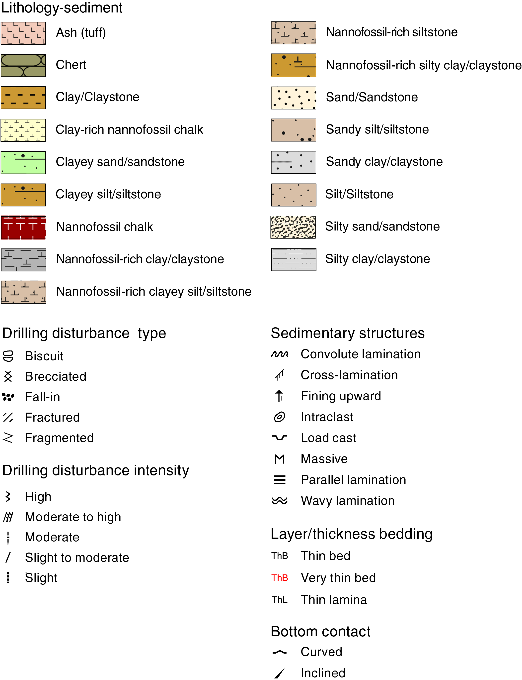
Figure F1. Sedimentary lithology patterns and symbols.
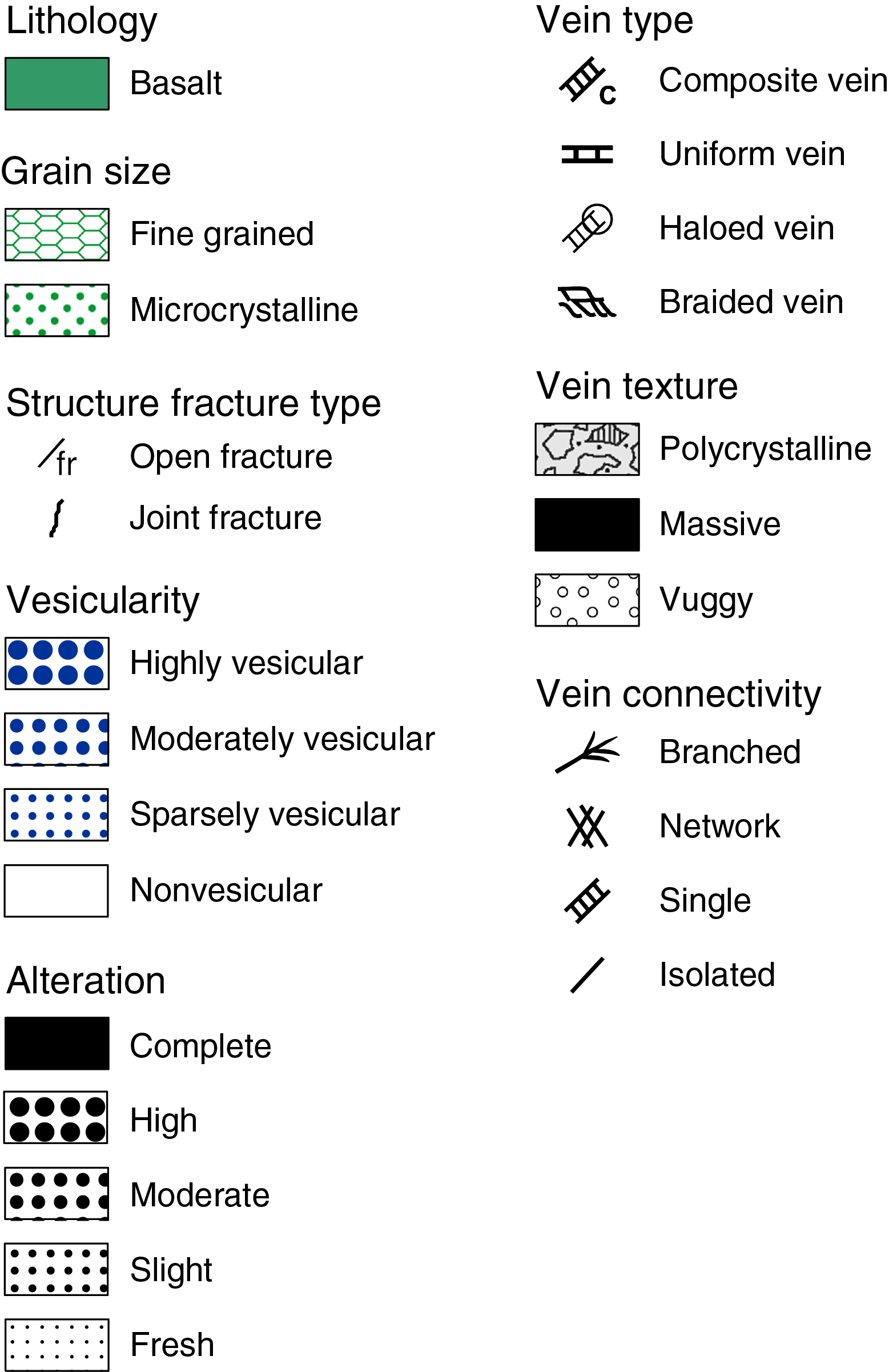
Figure F2. Igneous lithology patterns and symbols.
Chemical analysis
X-ray fluorescence
During Expedition 368X, we expanded the use of the handheld portable X-ray fluorescence spectrometer (pXRF; Olympus Delta) to include sediment section halves. Although many factors can impact the accuracy of section-half pXRF measurements, the presence of pore water results in large relative standard deviation (RSD) values (5%–20%) that increase with increasing pore water content. This makes quantitative results from section-half measurements less reliable for sediment. However, pXRF measurements of section halves can provide qualitative data on the elemental composition of sediment, including relative percent abundances. pXRF measurements of sediment section halves provide complementary results to smear slide and X-ray diffraction (XRD) analyses.
By comparing the results of shipboard pXRF data and published values of United States Geological Society (USGS) rock standard basalt (BHVO-2; e.g., Wei et al., 2014), we determined that discrete-powder pXRF results are reliable for elements with a content >10 ppm (Figure F3). Comparisons were then made between measurements of section-half surfaces, quarter-core wedges, and powder samples of material from Hole U1503A to better estimate error. Quarter-core wedges show a 1%–20% discrepancy with powders of the same material, especially for Ti, K, Sr, Zr, Ni, and Cu, whereas measurements of section-half surfaces usually show an even greater discrepancy with powder samples, especially for Mg, Mo, Ca, Si, Al, and Zn (Figure F4A). To produce the best-quality data, section halves were measured after their surfaces were dried for imaging. Surfaces that were flat and large enough for the detector (roughly 2–4 cm long) were selected to assure consistent measurements between each data point. Fractures, nonplanar surfaces, and areas of drilling disturbance were avoided. Measurements along sediment section halves were made every 20–40 cm, depending on the lithologic variation. Basalt rock measurements were done on centimeter-scale broken pieces. In contrast to the sediment section halves, there is a closer correspondence for most elements between measurements of basalt pieces and basalt powder (much closer to the diagonal line) than sediment section halves (Figure F4).
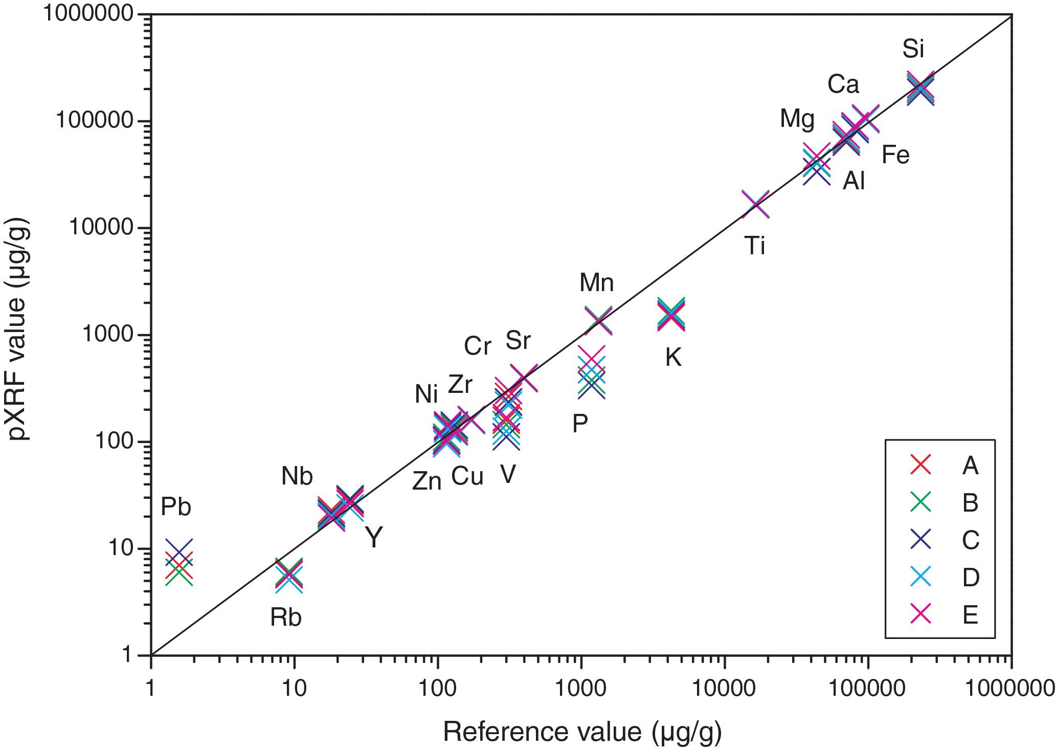
Figure F3. pXRF vs. published rock standard measurements.
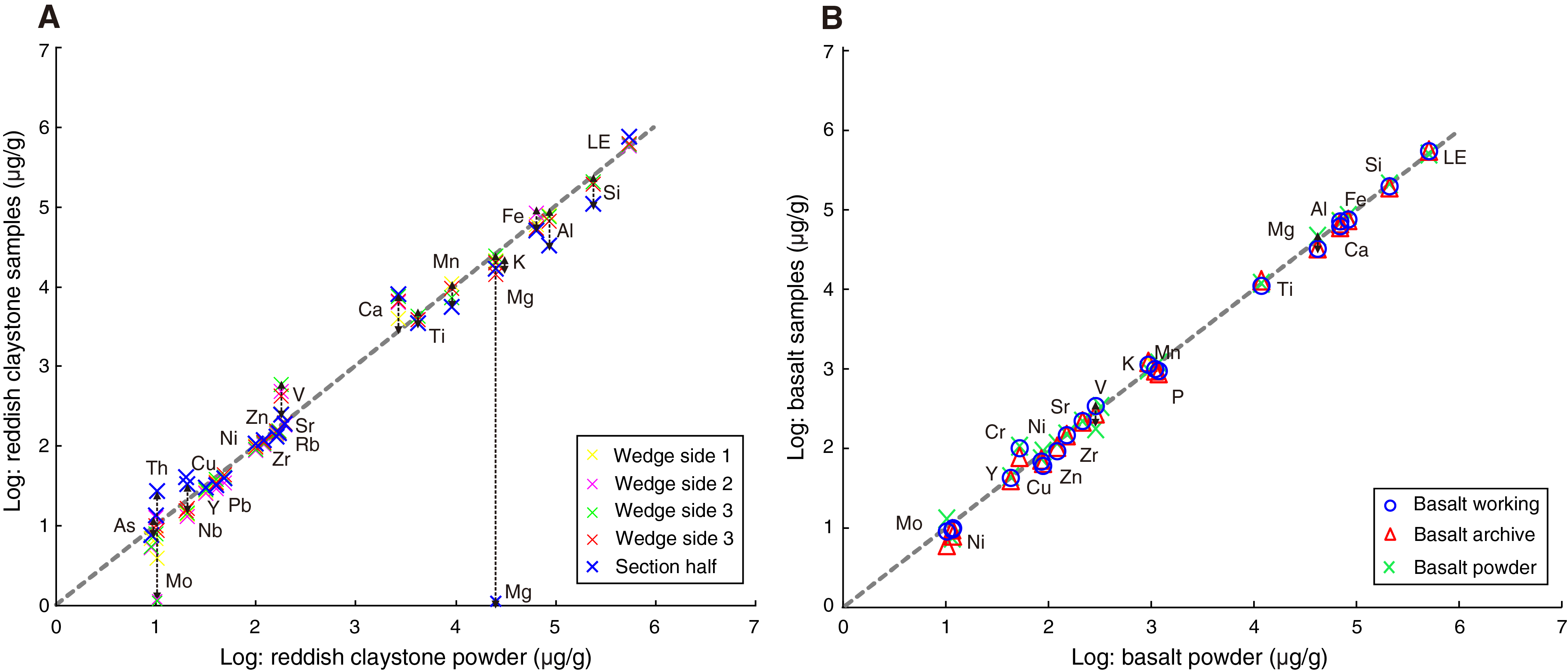
Figure F4. pXRF quarter-core wedges or core pieces vs. powders.
Biostratigraphy
Calcareous nannofossils and planktonic foraminifers were studied from core catcher samples after Expedition 368X to build a biostratigraphic framework for Hole U1503A. Twenty-seven core catcher samples from Cores 368X-U1503A-2R through 48R were split at the GCR after Expedition 368X and distributed to members of the Expedition 367 and 368 micropaleontology team for examination at their home institutions. Additional samples from the core sections were examined during the Expedition 368X onshore core description and editorial meeting to refine age determinations at selected intervals. Biostratigraphic events, mainly the first appearance datum (FAD; or base) and last appearance datum (LAD; or top) of the diagnostic species are tied to the geomagnetic polarity timescale of Gradstein et al. (2012) (Figure F5).
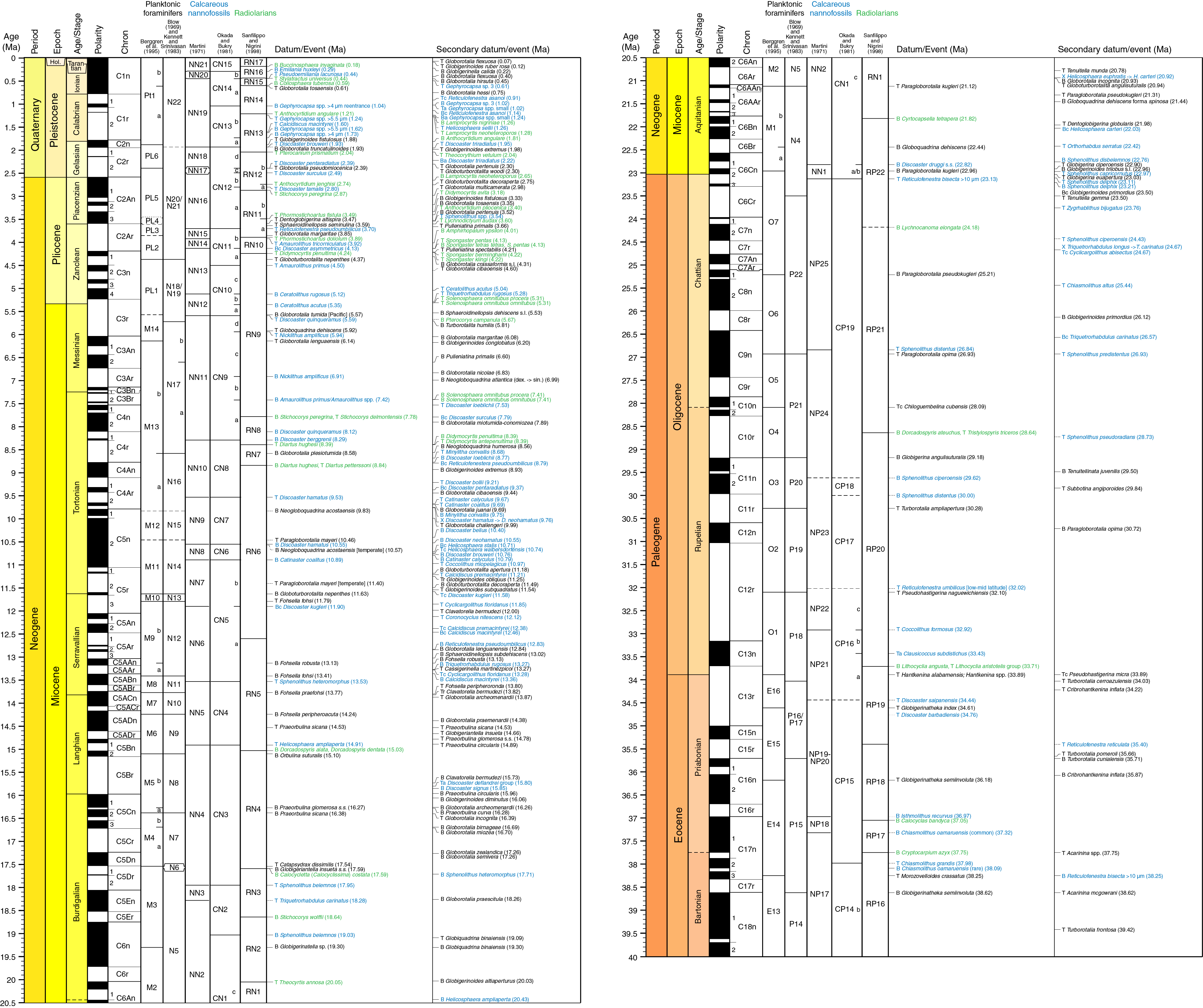
Figure F5. Nannofossil and foraminiferal events and scaled ages. (This figure is also available in an oversized format.)
Calcareous nannofossils
The calcareous nannofossil zonation is based on the schemes of Okada and Bukry (1980) and Martini (1971). Calibrated ages for bioevents are from Gradstein et al. (2012) and given in Table T1. The Gradstein et al. (2012) timescale assigns the Pleistocene/Pliocene boundary between the Gelasian and Piacenzian stages (2.59 Ma), the Pliocene/Miocene boundary between the Zanclean and Messinian stages (5.33 Ma), the late/middle Miocene boundary between the Tortonian and Serravallian stages (11.63 Ma), the middle/early Miocene boundary between the Langhian and Burdigalian stages (15.97 Ma), and the Miocene/Oligocene boundary between the Aquitanian and Chattian stages (23.03 Ma). For calcareous nannofossil biostratigraphy, the Pleistocene/Pliocene boundary now falls in Zone NN16 (Martini, 1971) between the LAD of Discoaster surculus (2.49 Ma) and Discoaster tamalis (2.8 Ma). The Pliocene/Miocene boundary lies in Zone NN12 between the LAD of Triquetrorhabdulus rugosus (5.28 Ma) and the FAD of Ceratolithus larrymayeri (5.34 Ma); however, C. larrymayeri was not noted in our samples, so we use the FAD of Ceratolithus acutus (5.35 Ma) as an alternative event. The late/middle Miocene boundary is placed in Zone NN7 between the LAD of common Discoaster kugleri (11.58 Ma) and the FAD of common D. kugleri (11.90 Ma). The middle/early Miocene boundary falls in Zone NN4 between the LAD of Helicosphaera ampliaperta (14.91 Ma) and the LAD of Sphenolithus belemons (17.95 Ma). The Miocene/Oligocene boundary is placed in Zone NN1 between the FAD of Discoaster druggi (22.82 Ma) and the LAD of Reticulofenestra bisecta >10 µm (23.13 Ma). In this study, the division of these geologic time boundaries is mostly based on recognition of these nannofossil bioevents.
Several species of the genus Gephyrocapsa, which are commonly used as Pleistocene biostratigraphic markers, often show a great range of variation in sizes and other morphological features, which causes problems in identification (e.g., Samtleben, 1980; Su, 1996; Bollmann, 1997). Size-defined morphological groups of this genus (Young, 1998; Maiorano and Marino, 2004; Lourens et al., 2004; Raffi et al., 2006) were used as event markers during shipboard study, including the groups Gephyrocapsa sp. 3, Gephyrocapsa spp. medium I (=4 µm), large Gephyrocapsa spp. (=5.5 µm), Gephyrocapsa spp. medium II (=4 µm; =bmG event), and small Gephyrocapsa spp. (<3.5 µm).
Several Reticulofenestra species with different coccolith and central opening sizes have been used as Neogene and Quaternary biostratigraphic markers; however, these parameters show considerable variations within and between "species," making species differentiation difficult (e.g., Su, 1996; Young, 1998). In this study, we followed the definition of Reticulofenestra pseudoumbilicus by Young (1998) as having a maximum coccolith length >7 µm (similar to the size of its holotype), especially for specimens from its uppermost range in the early Pliocene. We distinguished Reticulofenestra asanoi from the similarly sized Pseudoemiliania lacunosa by the absence of slits on the shield (Su, 1996). In addition, we further distinguished three Reticulofenestra morphotypes, Reticulofenestra ampla (5~7 µm, with central opening), R. bisecta (5~10 µm, with a solid central plug), and Reticulofenestra stavensis (>10 µm, with a solid central plug), following Sato et al. (1991) and Young et al. (2014).
The LAD of Sphenolithus spp. (3.54 Ma) in Pliocene Zone NN16 was based on the LAD of Sphenolithus abies and Sphenolithus neoabies according to Raffi et al. (2006). Species concepts for other taxa mainly follow those of Perch-Nielsen (1985) and Bown (1998).
Methods
Calcareous nannofossil samples were prepared using standard smear slide techniques. In cases with sandy sediments, suspended aliquots of the raw sample were utilized for analysis. Samples were examined with a Zeiss microscope under crossed polarized and plane-transmitted or phase contrast light at 1000× to 2000× magnification. Preservation of nannofossils was noted as follows:
- VG = very good (no evidence of dissolution and/or overgrowth).
- G = good (slight dissolution and/or overgrowth; specimens are identifiable to the species level).
- M = moderate (some etching and/or overgrowth; most specimens are identifiable to the species level).
- P = poor (severely etched or with overgrowth; most specimens cannot be identified at the species and/or generic level).
The relative abundance of calcareous nannofossils in the sediment was visually estimated at 1000× magnification by referring to the particle abundance charts in Rothwell (1989) and reported using the following abundance categories:
- D = dominant (>90% of sediment particles).
- A = abundant (>50%–90% of sediment particles).
- C = common (>10%–50% of sediment particles).
- F = few (1%–10% of sediment particles).
- R = rare (<1% of sediment particles).
- B = barren (no nannofossils present in 100 fields of view [FOVs]).
The relative abundance of individual calcareous nannofossil species or taxa groups was estimated at 1000× magnification as follows:
- D = dominant (>50%, or 100 specimens per FOV).
- A = abundant (10%–50%, or 10,100 specimens per FOV).
- C = common (1%–10%, or 110 specimens per FOV).
- F = few (0.1%–1%, or 1 specimen per 110 FOVs).
- R = rare (<0.1%, or <1 specimen per 10 FOVs).
Planktonic foraminifers
The planktonic foraminiferal zonation schemes of Blow (1969, 1979) and Berggren et al. (1995), as modified by Wade et al. (2011), were used in this study. Calibrated ages for bioevents are from Gradstein et al. (2012), as given in Table T2. We adopted the use of the LAD of Paragloborotalia nana as an early Miocene (19.30–21.12 Ma; Leckie et al., 2018) biostratigraphic indicator. Taxonomic concepts for Neogene and Paleogene taxa mainly follow those of Kennett and Srinivasan (1983) and Bolli and Saunders (1985).
Core catcher samples were soaked in distilled water and washed over a 63 µm mesh sieve. Consolidated or lithified samples were cut into pieces and crushed to pea size, added to a hydrogen peroxide solution, heated in the oven at <50°C for several hours, and then sieved as above. All samples were dried in a low-temperature oven at ~50°C. The dried samples were sieved over a 150 µm sieve, retaining the <150 µm size fraction in a separate vial. To avoid contamination of foraminifers between samples, the sieves were thoroughly cleaned between samples, placed in a sonicator for at least 15 min, and then carefully checked for the presence of sediment particles. Species identifications for planktonic and benthic foraminifers were generally made on the >150 µm size fraction.
The total abundance of planktonic foraminifers was defined as follows:
- A = abundant (>30% planktonic foraminifer specimens in total residue).
- C = common (10%–30% planktonic foraminifer specimens in total residue).
- R = rare (1%–10% planktonic foraminifer specimens in total residue).
- P = present (<1% planktonic foraminifer specimens in total residue).
- B = barren (no planktonic foraminifer specimens in total residue).
Individual planktonic foraminifers were recorded in qualitative terms based on an assessment of forms observed in a random sample of ~400 specimens from the >150 µm size fraction. Relative abundances were reported using the following categories:
- D = dominant (>30% of the assemblage).
- A = abundant (10%–30%).
- F = few (5%–10%).
- R = rare (1%–5%).
- P = present (<1%).
Preservation of planktonic foraminifer assemblages was recorded using the following categories:
- VG = very good (no evidence of breakage or dissolution).
- G = good (>80% of specimens are unbroken with only minor evidence of diagenetic alteration).
- M = moderate (30%–80% of the specimens are unbroken).
- P = poor (strongly recrystallized or dominated by fragments and broken or corroded specimens).
Paleomagnetism
Shipboard paleomagnetic investigations were conducted following the same methods applied during Expeditions 367 and 368 (see the Expedition 367/368 methods chapter [Sun et al., 2018]). During Expedition 368X, some differences in methods for discrete samples, including the sampling space and the demagnetization steps, were used and are therefore described here.
Usually, only one discrete cube sample was collected from each core to perform alternating field (AF) demagnetization, depending on recovery rate and lithology. No samples were collected for thermal demagnetization because of the time necessary to complete those measurements and the limited duration of Expedition 368X.
Basalt samples were shared with the petrophysics and core description teams to minimize the number of samples collected, optimize data processing time, and maximize the number of residuals (e.g., not heating residuals for rock magnetic analysis). A protocol modified after Expeditions 367 and 368 (see the Expedition 367/368 methods chapter [Sun et al., 2018]) was adopted (Table T3).
The characteristic remanent magnetization (ChRM) directions were calculated by principal component analysis (PCA; Kirschvink, 1980) using the Remasoft 3.0 software. Data visualizations (demagnetization plots; Zijderveld, 1967) and equal area projections were plotted using the PuffinPlot software (version 1.03; 23 April 2015; Lurcock and Wilson, 2012).
Magnetic measurements on archive section halves
Measurement of archive section halves was conducted using the superconducting rock magnetometer (SRM) and IMS-SRM software (version 10.2). A reduced sample area of 13.4 cm2 was assumed for conversion to volume-normalized magnetization units (A/m) of cores sampled with the rotary core barrel (RCB) system. We performed successive AF demagnetization using the SRM in-line AF demagnetizer on all archive section halves except for cores with <2% recovery (only the core catcher) and intervals that were too highly fractured to collect accurate measurements.
Natural remanent magnetization (NRM) measurements were made every 2.5 cm for sedimentary material and every 2.0 cm for igneous rocks. After NRM measurements, sediment cores were subjected to stepwise in-line AF demagnetization at 5, 10, 15, 20, and 25 mT. For igneous rocks, we adopted the same set of AF demagnetization steps used during Expeditions 367 and 368, which includes using narrower AF steps at an incremental rate of 2 mT for NRM up to 10 mT and at a rate of 5 mT from 10 to 25 mT.
Magnetic measurements on discrete samples
Incremental AF demagnetization was performed with the DTech AF demagnetizer (model D-2000) for the JR-6A spinner magnetometer (steps at 2.5, 5, 7.5, 10, 15, 20, 25, 30, 35, 40, 50, 60, 70, and 80 mT). The demagnetization axes were inverted at each step to avoid the gyroremanent magnetization documented during Expeditions 367 and 368 (see the Expedition 367/368 summary chapter [Larsen et al., 2018]). For basalts, the same set of AF demagnetization steps used for archive section halves was adopted, with further steps at an incremental rate of 5 mT up to 40 mT until the demagnetization was completed.
Geochemistry
The shipboard geochemistry program for Expedition 368X included measurements of headspace gas content; sedimentary geochemistry, including total inorganic carbon, total carbon, total nitrogen, and major and minor element content; and igneous and metamorphic rock geochemistry (major and minor element content).
Our analytical procedures followed those described in the Expeditions 367/368 methods chapter (Sun et al., 2018). Our analyses were conducted to satisfy routine shipboard safety and pollution prevention requirements, characterize sediment and rock geochemistry for shipboard interpretation, and provide a basis for sampling for subsequent shore-based research.
Headspace gas analysis
During Expedition 368X, headspace gas samples were frequently taken from the first or second section of cores because of low recovery or lack of a third section.
Interstitial water chemistry
No interstitial water samples were obtained during Expedition 368X.
Sediment geochemistry
Sediment sulfur, nitrogen, and inorganic and organic carbon contents
Sulfur analyses were carried out during Expeditions 368 and 368X. Total organic and inorganic carbon, total nitrogen, and total sulfur were measured during Expedition 368X.
Elemental analysis of bulk sediment/sedimentary rock by ICP-AES
The elemental compositions of sediment/sedimentary rock were only determined during Expedition 368 because the bead maker used for preparing inductively coupled plasma–atomic emission spectroscopy (ICP-AES) samples did not work during Expedition 367. During Expedition 368X, discrete samples were collected for shipboard XRD analysis and collocated samples were retained for shore-based analysis for concentrations of major elements and several trace elements by ICP-AES.
Source rock analysis
During Expedition 368X, source rock analyses were conducted to identify the type and stage of maturation of organic matter, estimate total organic carbon (TOC), and detect petroleum potential in sediments. Using source rock pyrolysis, free and adsorbed hydrocarbons released during programmed heating of a sample are recorded in a pyrogram as the first peak (S1) under low temperature. The second peak (S2) represents hydrocarbons released by kerogen cracking. The temperature at the maximum of the S2 peak (Tmax) is an indicator of rock maturity. CO2 (third peak; S3) is also generated by kerogen degradation. When these components are normalized to the TOC content, the S2 peak becomes the hydrogen index (HI = S2 × 100/TOC) and S3 becomes the oxygen index (OI = S3 × 100/TOC) (Tissot and Welte, 1984).
Source rock pyrolysis and TOC were determined by a Weatherford source rock analyzer. A crucible sample containing no material was included as the first sample of any sequence. After this calibration blank, 90–100 mg of standard material was used to calibrate the instrument signals and allow us to monitor instrument accuracy and precision. A pyrolysis program starting at 300°C with a heating rate of 25°C/min was used as a standard mode for the analysis of sediment with low maturity.
Physical properties
Measurements of physical properties in the Expedition 368X cores followed the same methodology as for Expeditions 367 and 368 (see the Expedition 367/368 methods chapter [Sun et al., 2018]). Only a few procedures were adjusted during Expedition 368X, and they are described below.
Hard rock cores
Recovered hard rock sections were run through the Whole-Round Multisensor Logger (WRMSL) and Natural Gamma Radiation Logger (NGRL) after the core sections reached equilibrium with laboratory temperature, which typically took 2 h during Expedition 368X because of the great depth of the cores below seafloor.
Samples from igneous basement were shared for both paleomagnetic and moisture and density measurements. The flow of sample sharing from Expeditions 367 and 368 was optimized for Expedition 368X (see Paleomagnetism; Table T3).
Thermal conductivity measurements
During Expedition 368X, we measured thermal conductivity on samples from working section halves using contact probes of different sizes to optimize the measurements according to the size of the piece of rock. After the rock and probe were equilibrated together in a bath of seawater at room temperature in a cooler insulated with extruded polystyrene foam, the calibrated heat source of the probe was turned on and the increase in temperature was recorded over 80 s for the standard probe and 60 s for the small probe.
Thermal conductivity was calculated from the rate of temperature rise while the heater current was flowing. Temperatures measured during the first 80 or 60 s of the heating cycle were fitted to an approximate solution of a constantly heated line source (for details, see Kristiansen, 1982, and Blum, 1997). Measurement errors were 5%–10%. Thermal conductivity measurements were routinely taken in one section per core (usually the third).
Discrete sample moisture and density measurements
Discrete samples were collected from the working section halves to determine wet and dry bulk density, grain density, water content, and porosity. In hard rock, cubes were extracted from the working section halves for physical property measurements. Samples from igneous basement were shared for paleomagnetic measurements.
References
Berggren, W.A., Kent, D.V., Swisher, C.C., III, and Aubry, M.-P., 1995. A revised Cenozoic geochronology and chronostratigraphy. In Berggren, W.A., Kent, D.V., Aubry, M.-P., and Hardenbol, J. (Eds.), Geochronology, Time Scales and Global Stratigraphic Correlation. Special Publication - SEPM (Society for Sedimentary Geology), 54:129–212. https://doi.org/10.2110/pec.95.04.0129
Blow, W.H., 1969. Late middle Eocene to recent planktonic foraminiferal biostratigraphy. In Bronnimann, P. and Renz, H.H. (Eds.), Proceedings of the 1st International Conference on Planktonic Microfossils, 1:199–422.
Blow, W.H., 1979. The Cainozoic Foraminifera (Volumes 1-3): Leiden, The Netherlands (E.J. Brill).
Blum, P., 1997. Technical Note 26: Physical Properties Handbook—A Guide to the Shipboard Measurement of Physical Properties of Deep-Sea Cores. Ocean Drilling Program. https://doi.org/10.2973/odp.tn.26.1997
Bolli, H.M., and Saunders, J.B., 1985. Oligocene to Holocene low latitude planktic foraminifera. In Bolli, H.M., Saunders, J.B., and Perch-Nielsen, K. (Eds.), Plankton Stratigraphy (Volume 1): Planktic Foraminifera, Calcareous Nannofossils and Calpionellids: Cambridge, United Kingdom (Cambridge University Press), 155–262.
Bollmann, J., 1997. Morphology and biogeography of Gephyrocapsa coccoliths in Holocene sediments. Marine Micropaleontology, 29(3–4):319–350. https://doi.org/10.1016/S0377-8398(96)00028-X
Bown, P.R. (Ed.), 1998. Calcareous Nannofossil Biostratigraphy: Dordrecht, The Netherlands (Kluwer Academic Publishing).
Gradstein, F.M., Ogg, J.G., Schmitz, M.D., and Ogg, G.M. (Eds.), 2012. The Geological Time Scale 2012: Amsterdam (Elsevier). https://doi.org/10.1016/C2011-1-08249-8
Kennett, J.P., and Srinivasan, M.S., 1983. Neogene Planktonic Foraminifera: A Phylogenetic Atlas: Stroudsburg, PA (Hutchinson Ross).
Kirschvink, J.L., 1980. The least-squares line and plane and the analysis of palaeomagnetic data. Geophysical Journal of the Royal Astronomical Society, 62(3):699–718. https://doi.org/10.1111/j.1365-246X.1980.tb02601.x
Kristiansen, J.I., 1982. The transient cylindrical probe method for determination of thermal parameters of earth materials [Ph.D. dissertation]. Åarhus University, Åarhus, Denmark.
Larsen, H.C., Sun, Z., Stock, J.M., Jian, Z., Alvarez Zarikian, C.A., Klaus, A., Boaga, J., Bowden, S.A., Briais, A., Chen, Y., Cukur, D., Dadd, K.A., Ding, W., Dorais, M.J., Ferré, E.C., Ferreira, F., Furusawa, A., Gewecke, A.J., Hinojosa, J.L., Höfig, T.W., Hsiung, K.-H., Huang, B., Huang, E., Huang, X.-L., Jiang, S., Jin, H., Johnson, B.G., Kurzawski, R.M., Lei, C., Li, B., Li, L., Li, Y., Lin, J., Liu, C., Liu, C., Liu, Z., Luna, A., Lupi, C., McCarthy, A.J., Mohn, G., Ningthoujam, L.S., Nirrengarten, M., Osono, N., Peate, D.W., Persaud, P., Qiu, N., Robinson, C.M., Satolli, S., Sauermilch, I., Schindlbeck, J.C., Skinner, S.M., Straub, S.M., Zu, X., Tian, L., van der Zwan, F.M., Wan, S., Wu, H., Xiang, R., Yadav, R., Yi, L., Zhang, C., Zhang, J., Zhang, Y., Zhao, N., Zhong, G., and Zhong, L., 2018. Expedition 367/368 summary. In Sun, Z., Jian, Z., Stock, J.M., Larsen, H.C., Klaus, A., Alvarez Zarikian, C.A., and the Expedition 367/368 Scientists, South China Sea Rifted Margin. Proceedings of the International Ocean Discovery Program, 367/368: College Station, TX (International Ocean Discovery Program). https://doi.org/10.14379/iodp.proc.367368.101.2018
Leckie, R.M., Wade, B.S., Pearson, P.N. Fraass, A.J., King, D.J., Olsson, R.K., Premoli Silva, I., Spezzaferri, S., and Berggren, W.A. 2018. Taxonomy, biostratigraphy, and phylogeny of Oligocene and early Miocene Paragloborotalia and Parasubbotina. In Wade, B.S., Olsson, R.K., Huber, B.T., and Berggren, W.A. (Eds.), Atlas of Oligocene Planktonic Foraminifera. Cushman Foundation Special Publication, 46:125–178. https://www.ucl.ac.uk/earth-sciences/sites/earth-sciences/files/Chapter_5.pdf
Lourens, L.J., Hilgen, F.J., Laskar, J., Shackleton, N.J., and Wilson, D., 2004. The Neogene period. In Gradstein, F.M., Ogg, J., et al. (Eds.), A Geologic Time Scale 2004: Cambridge, United Kingdom (Cambridge University Press), 409–440. https://doi.org/10.1017/CBO9780511536045.022
Lurcock, P.C., and Wilson, G.S., 2012. PuffinPlot: a versatile, user-friendly program for paleomagnetic analysis. Geochemistry, Geophysics, Geosystems, 13(6):Q06Z45. https://doi.org/10.1029/2012GC004098
Maiorano, P., and Marino, M., 2004. Calcareous nannofossil bioevents and environmental control on temporal and spatial patterns at the early–middle Pleistocene. Marine Micropaleontology, 53(3–4):405–422. https://doi.org/10.1016/j.marmicro.2004.08.003
Martini, E., 1971. Standard Tertiary and Quaternary calcareous nannoplankton zonation. In Farinacci, A. (Ed.), Proceedings of the Second Planktonic Conference, Roma 1970: Rome (Edizioni Tecnoscienza), 2:739–785.
Okada, H., and Bukry, D., 1980. Supplementary modification and introduction of code numbers to the low-latitude coccolith biostratigraphic zonation (Bukry, 1973; 1975). Marine Micropaleontology, 5:321–325. https://doi.org/10.1016/0377-8398(80)90016-X
Perch-Nielsen, K., 1985. Cenozoic calcareous nannofossils. In Bolli, H.M., Saunders, J.B., and Perch-Nielsen, K. (Eds.), Plankton Stratigraphy: Cambridge, United Kingdom (Cambridge University Press), 427–554.
Raffi, I., Backman, J., Fornaciari, E., Pälike, H., Rio, D., Lourens, L., and Hilgen, F., 2006. A review of calcareous nannofossil astrobiochronology encompassing the past 25 million years. Quaternary Science Reviews, 25(23–24):3113–3137. https://doi.org/10.1016/j.quascirev.2006.07.007
Rothwell, R.G., 1989. Minerals and Mineraloids in Marine Sediments: An Optical Identification Guide: London (Elsevier). https://doi.org/10.1007/978-94-009-1133-8
Samtleben, C., 1980. Die Evolution der Coccolithophoriden-Gattung Gephyrocapsa nach Befunden im Atlantik. Paläontologische Zeitschrift, 54(1–2):91–127. https://doi.org/10.1007/BF02985885
Sato, T., Kameo, K., and Takayama, T., 1991. Coccolith biostratigraphy of the Arabian Sea. In Prell, W.L., Niitsuma, N., et al., Proceedings of the Ocean Drilling Program, Scientific Results, 117: College Station, TX (Ocean Drilling Program), 37–54. http://doi.org/10.2973/odp.proc.sr.117.133.1991
Su, X., 1996. Development of late Tertiary and Quaternary coccolith assemblages in the northeast Atlantic. GEOMAR Report, 48. https://doi.org/10.3289/GEOMAR_Report_48_1996
Sun, Z., Jian, Z., Stock, J.M., Larsen, H.C., Klaus, A., Alvarez Zarikian, C.A., Boaga, J., Bowden, S.A., Briais, A., Chen, Y., Cukur, D., Dadd, K.A., Ding, W., Dorais, M.J., Ferré, E.C., Ferreira, F., Furusawa, A., Gewecke, A.J., Hinojosa, J.L., Höfig, T.W., Hsiung, K.-H., Huang, B., Huang, E., Huang, X.-L., Jiang, S., Jin, H., Johnson, B.G., Kurzawski, R.M., Lei, C., Li, B., Li, L., Li, Y., Lin, J., Liu, C., Liu, C., Liu, Z., Luna, A., Lupi, C., McCarthy, A.J., Mohn, G., Ningthoujam, L.S., Nirrengarten, M., Osono, N., Peate, D.W., Persaud, P., Qiu, N., Robinson, C.M., Satolli, S., Sauermilch, I., Schindlbeck, J.C., Skinner, S.M., Straub, S.M., Zu, X., Tian, L., van der Zwan, F.M., Wan, S., Wu, H., Xiang, R., Yadav, R., Yi, L., Zhang, C., Zhang, J., Zhang, Y., Zhao, N., Zhong, G., and Zhong, L., 2018. Expedition 367/368 methods. In Sun, Z., Jian, Z., Stock, J.M., Larsen, H.C., Klaus, A., Alvarez Zarikian, C.A., and the Expedition 367/368 Scientists, South China Sea Rifted Margin. Proceedings of the International Ocean Discovery Program, 367/368: College Station, TX (International Ocean Discovery Program). https://doi.org/10.14379/iodp.proc.367368.102.2018
Tissot, B.P., and Welte, D.H., 1984. Petroleum Formation and Occurrence (2nd edition): Heidelberg (Springer-Verlag). https://doi.org/10.1007/978-3-642-87813-8
Wade, B.S., Pearson, P.N., Berggren, W.A., and Pälike, H., 2011. Review and revision of Cenozoic tropical planktonic foraminiferal biostratigraphy and calibration to the geomagnetic polarity and astronomical time scale. Earth-Science Reviews, 104(1–3):111–142. https://doi.org/10.1016/j.earscirev.2010.09.003
Wei, X., Xu, Y.-G., Feng, Y.-X., and Zhao, J.X., 2014. Plume-lithosphere interaction in the generation of the Tarim large igneous province, NW China: geochronological and geochemical constraints. American Journal of Science, 314(1): 314–356. https://doi.org/10.2475/01.2014.09
Young, J.R., 1998. Neogene. In Bown, P.R. (Ed.), Calcareous Nannofossil Biostratigraphy: Dordrecht, The Netherlands (Kluwer Academic Publishing), 225–265.
Young, J.R., Bown, P.R., and Lees, J.A. (Eds.). Nannotax3. http://ina.tmsoc.org/Nannotax3
Zijderveld, J.D.A., 1967. AC demagnetization of rocks: analysis of results. In Collinson, D.W., Creer, K.M., and Runcorn, S.K. (Eds.), Developments in Solid Earth Geophysics (Volume 3): Methods in Palaeomagnetism: Amsterdam (Elsevier), 254–286. https://doi.org/10.1016/B978-1-4832-2894-5.50049-5
1 Childress, L.B., Alvarez Zarikian, C.A., Briais, A., Dadd, K.A., Deng, J.-M., Höfig, T.W., Huang, X.-L., Li, B., Lin, J., Liu, C., Liu, Z., Nirrengarten, M.F.R., Peate, D.W., Qiu, N., Satolli, S., Stock, J.M., Sun, Z., van der Zwan, F.M., Xiang, R., Yi, L., and Zhong, L., 2020. Expedition 368X methods supplement. In Sun, Z., Jian, Z., Stock, J.M., Larsen, H.C., Klaus, A., Alvarez Zarikian, C.A., and the Expedition 367/368 Scientists, South China Sea Rifted Margin. Proceedings of the International Ocean Discovery Program, 367/368: College Station, TX (International Ocean Discovery Program). https://doi.org/10.14379/iodp.proc.368X.102.2020
2 Expedition 367/368 Scientists' affiliations.
This work is distributed under the Creative Commons Attribution 4.0 International (CC BY 4.0) license. 