Hobbs, R.W., Huber, B.T., Bogus, K.A., and the Expedition 369 Scientists
Proceedings of the International Ocean Discovery Program Volume 369
publications.iodp.org

https://doi.org/10.14379/iodp.proc.369.105.2019
Site U15141
B.T. Huber, R.W. Hobbs, K.A. Bogus, S.J. Batenburg, H.-J. Brumsack, R. do Monte Guerra, K.M. Edgar, T. Edvardsen, M.L. Garcia Tejada, D.L. Harry, T. Hasegawa, S.J. Haynes, T. Jiang, M.M. Jones, J. Kuroda, E.Y. Lee, Y.-X. Li, K.G. MacLeod, A. Maritati, M. Martinez, L.K. O’Connor, M.R. Petrizzo, T.M. Quan, C. Richter, L. Riquier, G.T. Tagliaro, C.C. Wainman, D.K. Watkins, L.T. White, E. Wolfgring, and Z. Xu2
Keywords: International Ocean Discovery Program, IODP, JOIDES Resolution, Expedition 369, Site U1514, Hot Cretaceous Greenhouse, oceanic anoxic events, Mentelle Basin, Naturaliste Plateau, Great Australian Bight, Gondwana breakup, Tasman Gateway, Indonesian Gateway, cyclostratigraphy, carbon isotope excursions, Paleocene/Eocene Thermal Maximum, Eocene greenhouse, Miocene, volcanic rifted margin, nonvolcanic rifted margin
MS 369-105: Published 25 May 2019
Background and objectives
International Ocean Discovery Program (IODP) Site U1514 is the northernmost (33°7.2327′S, 113°5.4672′E; Figures F1, F2) and deepest (3850 m water depth) site cored during Expedition 369. The greater paleodepth of the site relative to other sites cored in the Mentelle Basin provides the opportunity to characterize the evolution of deep water masses and deep ocean circulation during the final phase of breakup of the Gondwana continents. Because Site U1514 is located at a high paleolatitude (~60°S), the sediments preserve a paleoclimate record that serves as a sensitive monitor of global climatic changes. Coring at this site sampled Cenozoic and Late Cretaceous deposits that enable new insights into the early and later phases of the opening of the Tasman Gateway and the restriction of the Indonesian Gateway. The Cretaceous sedimentary basin is probably underlain by synrift Permian to Jurassic sediments that are part of an earlier rifting event extending along the western margin of Australia (Borissova et al., 2002). Following the separation of India from Australia/Antarctica in the Early Cretaceous, the basin underwent a period of rapid thermal subsidence with deposition of deltaic sediments, shale and claystone sequences, and then deep-water chalks and limestones. The current seabed is composed of Paleogene/Neogene/Quaternary oozes that sit unconformably on the Cretaceous (Maloney et al., 2011).
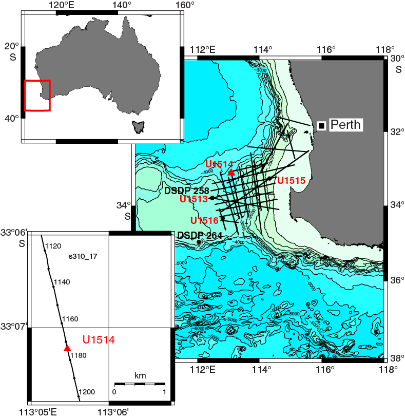
Figure F1. Site U1514 location.
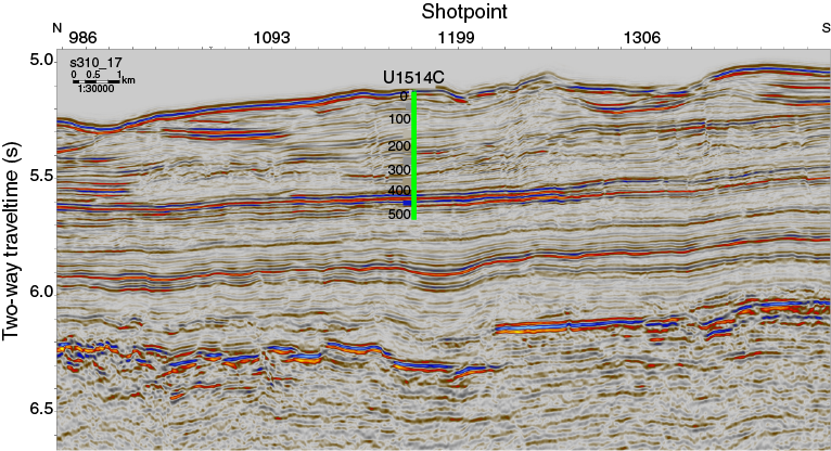
Figure F2. Seismic Profile s310_17.
The primary objectives for coring Site U1514 were as follows:
- Obtain a continuous Cenozoic sediment record in the Mentelle Basin to characterize how oceanographic conditions changed during the Cenozoic opening of the Tasman Gateway and the restriction of the Indonesian Gateway;
- Reconstruct middle through Late Cretaceous paleotemperature changes to document when the Cretaceous hot greenhouse climate initiated, how long the extreme warmth persisted, and when a switch to a cooler climate occurred; and
- Obtain a complete and well-preserved sediment record across mid-Cretaceous oceanic anoxic events (OAEs) to better understand their cause and accompanying changes in the climate-ocean system and in the marine biota.
The Site U1514 sequence will be compared with coeval Expedition 369 sections cored elsewhere in the Mentelle Basin and Site U1512 from the Great Australian Bight. Other IODP and industry data from the Western Australia margin and the Great Australian Bight will be used to identify any regional differences in the geochemical and/or biological responses to the OAEs and Cretaceous and Neogene ocean circulation history.
Operations
Site U1514 consisted of coring and logging operations in three holes (Table T1). All four coring systems were used. The advanced piston corer (APC), half-length APC (HLAPC), and extended core barrel (XCB) systems were used in Hole U1514A; Hole U1514B was cored with the APC system only; and the rotary core barrel (RCB) system was used in Hole U1514C. Hole U1514A extended to 255.6 m drilling depth below seafloor (DSF), at which point the XCB system was unable to penetrate deeper. Cores recovered from Hole U1514B were sectioned on the catwalk into whole rounds for postexpedition analyses. Hole U1514C penetrated to 516.8 m DSF and was successfully logged with the modified triple combination tool string (Quambo; see Petrophysics in the Expedition 369 methods chapter [Huber et al., 2019a]).
Overall, 7.4 days (2–9 November 2017) were spent at Site U1514. A total of 21 APC, 5 HLAPC, 7 XCB, and 34 RCB cores were recorded for the site, penetrating to 516.8 m DSF total depth. Of the 591.9 m cored, 518.12 m of material was recovered (87.5%).
Transit to Site U1514
The ship arrived at the site after a 51 nmi voyage at an average speed of 8.1 kt (6.25 h), lowered the thrusters, and entered dynamic positioning mode at 0800 h (UTC + 11 h) on 2 November 2017. The acoustic positioning beacon was deployed at 0830 h.
Hole U1514A
After offsetting from the beacon, preparations for coring in Hole U1514A (33°7.2327′S, 113°5.4672′E) commenced. The APC/XCB system was assembled, and the bottom-hole assembly (BHA) was lowered. The Icefield MI-5 and FlexIT core orientation tools and nonmagnetic drill collars, core barrels, and sinker bars were used when coring with the APC system. We started Hole U1514A at 2220 h on 2 November 2017. An 8.15 m mudline core was recovered, and the water depth was calculated to be 3838.2 meters below sea level (mbsl). We continued APC coring with orientation through Core 19H to 178.1 m DSF. Successful in situ formation temperature measurements were taken with the advanced piston corer temperature tool (APCT-3) on Cores 4H, 6H, and 8H. Coring switched to the HLAPC system and recovered Cores 21F through 24F to 202.1 m DSF, where piston coring refusal was reached. We switched to the XCB system and cut Cores 25X through 31X to 255.6 m DSF. At this point, the rate of penetration had slowed to <5 m/h and pump pressure was 2950 psi (XCB maximum pressure is ~3000 psi). These conditions were considered XCB refusal, and coring was stopped. The drill string cleared the seafloor at 2015 h on 4 November, ending Hole U1514A. In total, we recovered 255.2 m of 255.6 m cored (99.8%). The APC system recovered 185.96 m of 178.1 m cored (104.4%), the HLAPC system recovered 24.88 m of 24.0 m cored (103.7%), and the XCB system recovered 44.36 m of 53.5 m cored (82.9%). The total time spent in Hole U1514A was 2.5 days.
Hole U1514B
The vessel was offset 20 m east, and Hole U1514B (33°7.2335′S, 113°5.4798′E) was started at 2200 h on 4 November 2017. The seafloor was calculated at 3838.72 mbsl. Only two APC cores were taken to 15.1 m DSF, and they were completely sectioned into 30 cm whole rounds (stored in light-proof bags) on the catwalk for postexpedition optically stimulated luminescence (OSL) analyses. Coring in Hole U1514B recovered 15.45 m of 15.1 m cored (102.3%). The drill string was pulled up, clearing the seafloor at 2355 h. The bit cleared the rotary table at 0930 h on 5 November, ending Hole U1514B. The total time spent in the Hole U1514B was 0.6 days.
Hole U1514C
Preparations were made to core with the RCB system. While lowering the drill string to the seafloor, the vessel was offset 20 m south. Hole U1514C (33°7.2443′S, 113°5.4799′E) was started at 1940 h on 5 November 2017 at a water depth of 3838.8 mbsl, which was determined by offset. A center bit was dropped, and the hole was drilled to 195.6 m DSF without coring by 0115 h on 6 November. The center bit was pulled at 0200 h, and coring commenced with cutting Core 2R. We recovered Cores 2R through 35R to 516.8 m DSF. The last core was recovered at 1605 h on 8 November. In total, 247.47 m was recovered of 321.2 m cored (77%).
After coring, the hole was circulated twice with high-viscosity mud and displaced with heavy mud. The RCB bit was then released to the bottom of the hole at 1635 h. The top drive was racked back, and the drill string was pulled up to 82.2 m DSF for logging. The Quambo was assembled with the following tools:
- Hostile Environment Natural Gamma Ray Sonde (HNGS),
- High-Resolution Laterolog Array (HRLA),
- Dipole Sonic Imager (DSI),
- Hostile Environment Litho-Density Sonde (HLDS) with source,
- Enhanced Digital Telemetry Cartridge (EDTC),
- Logging equipment head-Q tension (LEH-QT),
- Centralizer for centralizing the DSI and HRLA, and
- Magnetic susceptibility sonde (MSS) added to the bottom of the tool string.
The tool string was deployed at 0015 h on 9 November. The entire length of the open borehole (82.2–514.0 m DSF) was logged. The logging tools were recovered at 0630 h on 9 November and disassembled by 0815 h. The drill string was then brought up, clearing the seafloor at 0855 h. While raising the drill string, the beacon was released at 1330 h and then recovered at 1415 h. The drill string was on the rig floor at 1735 h on 9 November, ending Hole U1514C. The total time spent in Hole U1514C was 4.3 days. The rig floor was then secured for the transit to Site U1515.
Lithostratigraphy
The sedimentary sequence recovered at Site U1514 is divided into three main lithostratigraphic units based on a combination of data from Holes U1514A and U1514C (Figure F3; Table T2). The cores from Hole U1514B are dedicated for postexpedition OSL measurements; they were not described onboard (see Operations). Lithostratigraphic units and boundaries are defined by changes in lithology and sedimentary characteristics as identified by macroscopic core description, smear slide examination, and X-ray diffraction (XRD) and handheld portable X-ray fluorescence (pXRF) measurements. Unit I is an 81.20 m thick Pleistocene to Eocene sequence of very pale brown to pale yellow nannofossil ooze, foraminiferal ooze, sponge spicule-rich nannofossil ooze, and biosiliceous ooze. Unit II is a 308.01 m thick Eocene to Paleocene sequence of light greenish gray clayey nannofossil ooze, sponge spicule-rich clay, nannofossil-rich clay that gradationally transitions into clayey nannofossil chalk, and nannofossil-rich claystone. Unit III is an at least 126.43 m thick Paleocene to Albian sequence of greenish gray, brown, and black claystone.
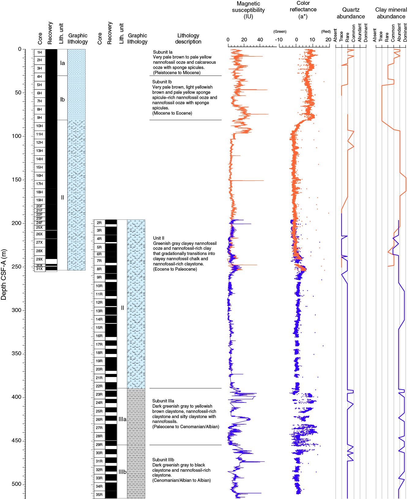
Figure F3. Lithostratigraphic summary.
Unit I
- Interval: 369-U1514A-1H-1, 0 cm, to 9H-5, 58 cm
- Depth: 0–81.20 m CSF-A
- Age: Pleistocene to Eocene
- Lithology: nannofossil ooze, calcareous ooze, foraminiferal ooze, and biosiliceous ooze with clay
- Drilling disturbance type and intensity: various (soupy, bowed, and flow-in); none to slight
- Nature of top contact: seafloor
- Nature of bottom contact: sharp
Lithostratigraphic Unit I is an 81.20 m thick sequence of nannofossil ooze that gradationally transitions into nannofossil-rich clay (Figures F3, F4; Table T2). This unit has medium and thick beds that are massive and structureless. The color of this unit progressively changes downhole from very pale brown, pale yellow, and light yellowish brown in the upper intervals (top of Core 369-U1534A-1H through Section 4H-2) to pale yellow in the lower intervals (Sections 4H-2 through 9H-5). Disseminated dark oxide mineral/irregularly shaped manganese nodules are common in Cores 8H through 9H and are concentrated above a sharp boundary in Section 9H-5 at 58 cm. In smear slides, biogenic grains in this unit include dominant nannofossils, common to abundant sponge spicules, and rare to common foraminifers (Figure F5A, F5C; see Site U1514 smear slides in Core descriptions). Unit I is divided into Subunits Ia (nannofossil ooze) and Ib (sponge spicule–rich nannofossil ooze and biosiliceous ooze) based on the relative abundance of biosiliceous and calcareous microfossils (Figures F3, F4A).
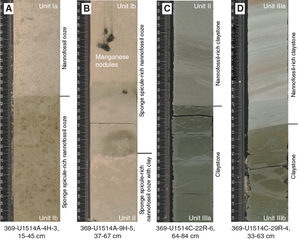
Figure F4. Unit boundaries and dominant lithologies.
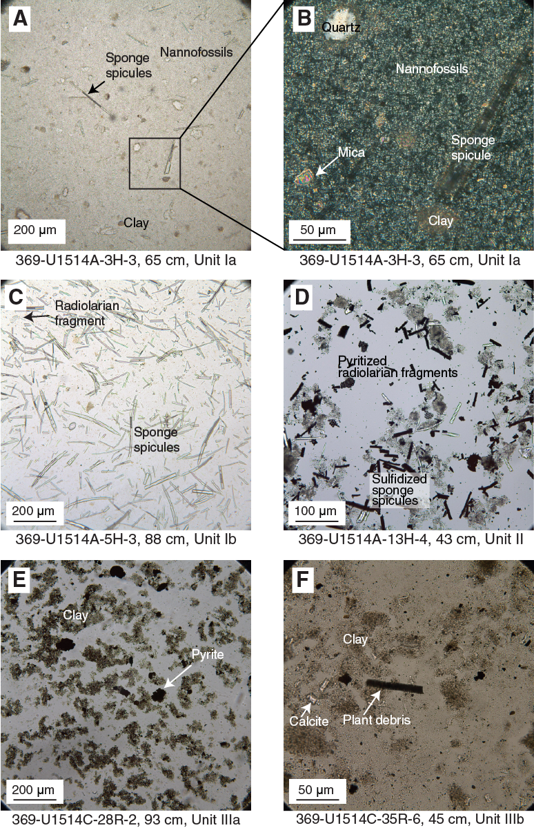
Figure F5. Sediment constituents.
Subunit Ia
- Interval: 369-U1514A-1H-1, 0 cm, to 4H-3, 28 cm
- Depth: 0–30.38 m CSF-A
- Age: Pleistocene to Miocene
- Lithology: nannofossil ooze, nannofossil ooze with sponge spicules, foraminiferal ooze, foraminiferal ooze with sponge spicules, calcareous ooze, and sandy calcareous ooze
- Drilling disturbance type and intensity: various (soupy, bowed, and flow-in); none to slight
- Nature of top contact: seafloor
- Nature of bottom contact: sharp
Lithostratigraphic Subunit Ia is a 30.38 m thick sequence of very pale brown to pale yellow nannofossil ooze and nannofossil ooze with sponge spicules, foraminiferal ooze, foraminiferal ooze with sponge spicules, calcareous ooze, and sandy calcareous ooze (Figure F4A). This subunit is massive and structureless. Color varies from very pale brown to pale yellow. Some of the thin to very thin beds of light gray, white to light greenish foraminiferal ooze, and foraminiferal ooze with sponge spicules in Cores 369-U1514A-1H and 3H have sharp bottom contacts. Black, irregularly shaped oxide minerals are present in trace amounts throughout Subunit Ia. Coarse to medium sand–sized radiolarians are also present in trace and common amounts between Sections 3H-2 and 3H-CC. Sections 4H-1 through 4H-4 are characterized by small burrows infilled with sponge spicules and radiolarians. In smear slides, biogenic grains are largely composed of common to dominant nannofossils, trace to common sponge spicules, trace to common foraminifers, and trace to rare radiolarians (Figure F5A, F5B; see Site U1514 smear slides in Core descriptions). XRD analyses confirm that calcite is the dominant mineral in this unit (Figure F6A), which is consistent with a pXRF Ca content of >37 wt% (Table T3) and carbonate content of >72 wt% (see Geochemistry). Other minerals present in trace amounts include quartz, chlorite/kaolinite, illite, and interstratified clays.
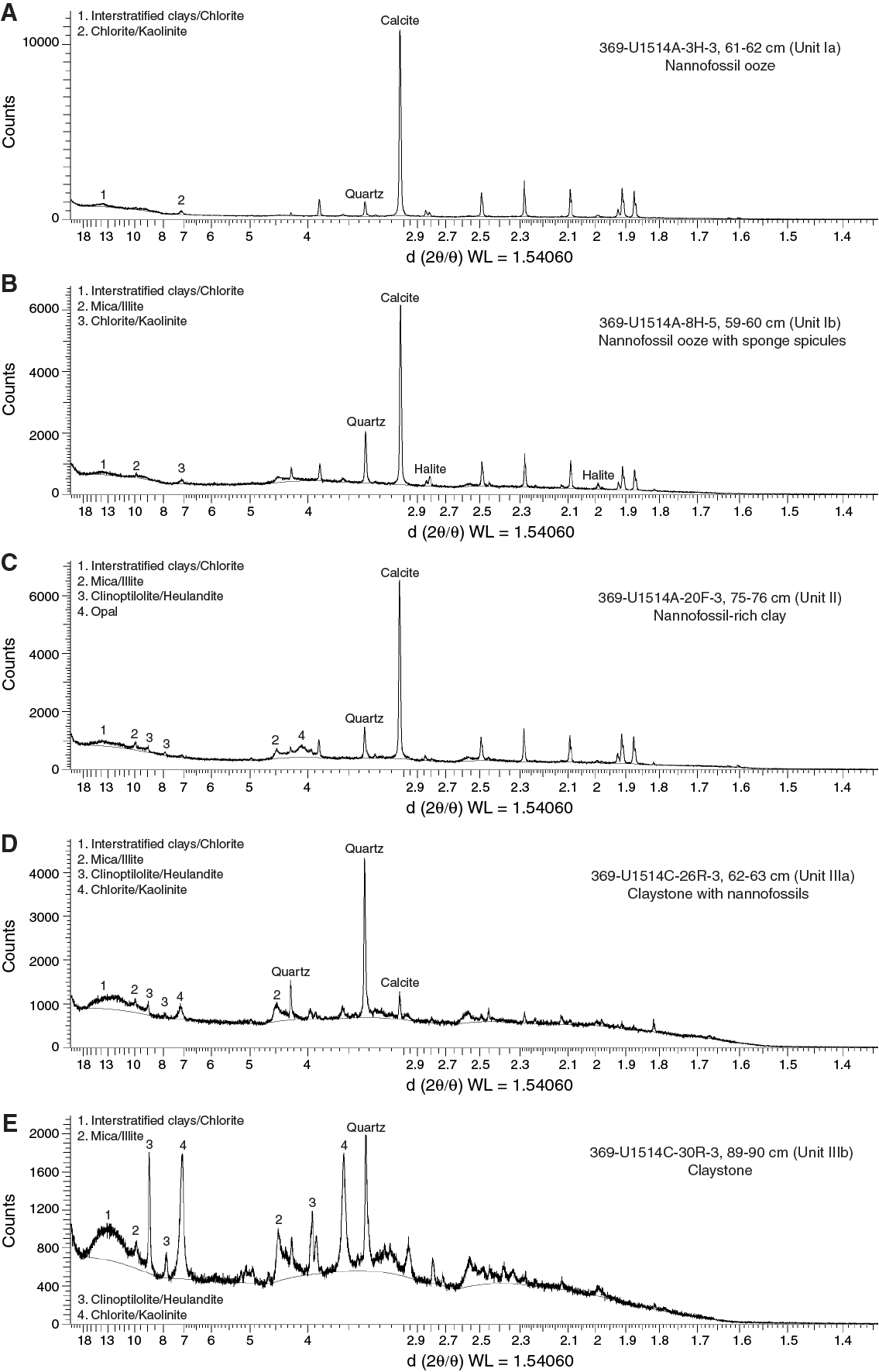
Figure F6. XRD results.
Subunit Ib
- Interval: 369-U1514A-4H-3, 28 cm, to 9H-5, 58 cm
- Depth: 30.38–81.20 m CSF-A
- Age: Miocene to Eocene
- Lithology: nannofossil ooze, nannofossil ooze with sponge spicules, sponge spicule–rich nannofossil ooze, sponge spicule–rich nannofossil ooze with radiolarians, biosiliceous nannofossil ooze, and biosiliceous ooze with clay
- Drilling disturbance type and intensity: various (soupy, bowed, and flow-in); low to moderate
- Nature of top contact: sharp
- Nature of bottom contact: sharp
Lithostratigraphic Subunit Ib is a 50.82 m sequence of brown, very pale brown, and light yellowish brown nannofossil ooze, nannofossil ooze with sponge spicules, sponge spicule–rich nannofossil ooze, sponge spicule–rich nannofossil ooze with radiolarians, biosiliceous nannofossil ooze, and biosiliceous ooze with clay (Figure F3, F4B). This unit is massive and structureless. Compared with Subunit Ia, Subunit Ib is characterized by an increase in the abundance of siliceous sponge spicules and radiolarians. Bioturbation intensity in this subunit ranges from low to moderate. The upper portion of this subunit (Sections 369-U1514A-4H-3 through 5H-CC; 31.60–46.69 m CSF-A) is distinctive in that it is darker than the under- and overlying intervals. Overall, this interval ranges in color from pale/light yellowish brown to brown. Black, irregular manganese nodules are common in the lower interval (Cores 8H and 9H) (Figure F4B). In smear slides, biogenic grains largely consist of common to dominant calcareous nannofossils and sponge spicules, trace to common radiolarians, and trace foraminifers (Figure F4C). XRD analyses confirm that the mineral assemblage is dominated by calcite and reveals the presence of quartz, halite, and some traces of illite/mica, chlorite/kaolinite, and clinoptilolite/heulandite (Figure F6B). Bulk sediment pXRF data (Table T3) reveals higher Mn content (460–3150 ppm) in this subunit relative to Subunit Ia and Unit II.
Unit II
- Intervals: 369-U1514A-9H-5, 58 cm, to 31X-CC, 38 cm (bottom of hole [BOH]); 369-U1514C-2R-1, 0 cm (top of hole [TOH]), to 22R-6, 78 cm
- Depths: Hole U1514A = 81.20–253.82 m CSF-A; Hole U1514C = 195.60–389.21 m CSF-A
- Age: Eocene to Paleocene
- Lithology: nannofossil chalk with clay, clayey nannofossil chalk, biosiliceous nannofossil chalk with clay, silicified nannofossil chalk with clay, clayey nannofossil chalk with biosilica, nannofossil-rich claystone, and claystone
- Drilling disturbance type and intensity: various (bowed, flow-in, and biscuit); none to severe
- Nature of top contact: sharp
- Nature of bottom contact: sharp
Lithostratigraphic Unit II is a 308.01 m thick sequence of nannofossil chalk with clay, clayey nannofossil chalk, biosiliceous nannofossil chalk with clay, silicified nannofossil chalk with clay, clayey nannofossil chalk with biosilica, nannofossil-rich claystone, and claystone (Figures F3, F4C; Table T2). Compared with Unit I, Unit II is characterized by a higher abundance of clay minerals (5%–80% by smear slide description), which are light greenish gray. Sediment color changes to pale yellow/light yellowish brown between 250 and 260 m CSF-A (Cores 369-U1514A-31X and 369-U1514C-8R). Chert nodules and several very thin claystone beds are present in Cores 369-U1514A-11H, 12H, 26X, 28X, and 30X and 369-U1514C-2R (Figure F7A, F7B). Unit II has a sharp basal contact with a very thick (>4 m) bed of dark greenish gray claystone at the top of Unit III (Figure F4C). Several ~10 cm thick intervals with inclined erosive bases and soft-sediment deformation structures are present in Section 369-U1514C-11R-2 (Figure F7C). Parallel lamination is common in Cores 369-U1514A-28X and 369-U1514C-16R and 17R and rare in Cores 369-U1514A-27X and 369-U1514C-2R, 4R, 5R, 19R, 21R, and 22R. Bioturbation intensity ranges from absent to high. The ichnofacies in this unit include Planolites, Chondrites, and Zoophycos (Figure F7D).
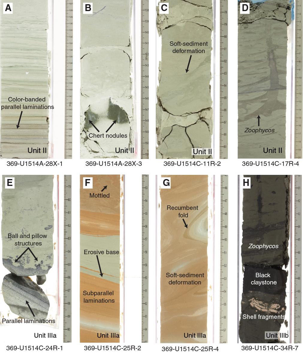
Figure F7. Sedimentary characteristics.
Smear slide observations reveal that clay minerals and calcareous nannofossils are the dominant lithologic components in Unit II. Biogenic constituents include rare to dominant nannofossils, trace to common radiolarians, rare to common sponge spicules, and occasional trace foraminifers (Figure F5D; see Site U1514 smear slides in Core descriptions). Siliciclastic grains observed in smear slides are dominated by clay minerals and include rare quartz.
XRD analyses conducted on discrete samples confirm that calcite is the dominant mineral in this unit. In addition, quartz and opal are present, as well as some traces of heulandite/clinoptilolite, illite/mica, chlorite/kaolinite, montmorillonite, and probable interstratified clays (Figure F6C). Ca content measured by pXRF ranges from 12 to 35 wt% (Table T3).
Unit III
- Interval: 369-U1514C-22R-6, 78 cm, to 35R-CC, 7 cm (BOH)
- Depth: 389.21–515.64 m CSF-A
- Age: Paleocene to Albian
- Lithology: claystone with nannofossils, silty claystone with nannofossils, nannofossil-rich claystone, silicified claystone, claystone, and chert
- Drilling disturbance type and intensity: various (biscuit, fractured, fragmented); none to severe
- Nature of top contact: sharp
- Nature of bottom contact: BOH
Lithostratigraphic Unit III is an at least 126.43 m thick sequence of greenish gray, brown, and black claystone, nannofossil-rich claystone, and claystone with nannofossils, with low to intense bioturbation. The top of this unit is defined by a distinctive, very thick bed of dark greenish gray claystone extending from Section 369-U1514C-22R-6, 78 cm, to Section 23R-2, 4 cm (389.21–393.54 m CSF-A). The contact between Units II and III is sharp (Figure F4C). Unit III is divided into Subunits IIIa and IIIb based on sedimentary characteristics (Figures F3, F4D; Table T2).
Subunit IIIa
- Interval: 369-U1514C-22R-6, 78 cm, to 29R-4, 50 cm
- Depth: 389.21–454.33 m CSF-A
- Age: Paleocene to Cenomanian/Albian
- Lithology: claystone, nannofossil-rich claystone, claystone with nannofossils, silty claystone with nannofossils, silicified claystone, and chert.
- Drilling disturbance type and intensity: various (biscuit, fractured, fragmented); none to severe
- Nature of top contact: sharp
- Nature of bottom contact: sharp
Lithostratigraphic Subunit IIIa is a 65.12 m thick sequence of greenish gray to yellowish brown claystone, nannofossil-rich claystone, claystone with nannofossils, silty claystone with nannofossils, silicified claystone, and chert (Figure F4D; Table T2). Bioturbation varies from absent to intense. Sedimentary structures in this subunit include soft-sediment deformation structures (notably convolute and overturned bedding), microfaults, and parallel lamination. Beds with normal grading and erosive bases are also common (Figure F7E, F7G). Several occurrences of chert (in bedded and nodular forms) are present in Cores 369-U1514C-27R through 29R. Smear slide descriptions indicate that calcareous nannofossils are rare to dominant in this unit (Figure F5E). Trace to rare foraminifers and radiolarians were occasionally observed. Siliciclastic constituents include abundant to dominant clay, rare to common quartz, trace to common zeolite, trace to rare glauconite, and trace chlorite.
Whole-rock XRD analyses on discrete samples indicate that calcite is progressively replaced by quartz as the dominant mineral in Subunit IIIa. Other minerals present in this subunit include clinoptilolite/heulandite, opal, illite/mica, kaolinite/chlorite, montmorillonite, and interstratified clay (Figure F6D). Bulk-rock pXRF analyses in Subunit IIIa (Table T3) reveal the highest Si content (43 wt%) in interval 369-U1514C-27R-4, 95–96 cm (435.57 m CSF-A).
Subunit IIIb
- Interval: 369-U1514C-29R-4, 50 cm, to 35R-CC, 7 cm (BOH)
- Depth: 454.33–515.64 m CSF-A
- Age: Cenomanian/Albian to Albian
- Lithology: claystone, nannofossil-rich claystone, and claystone with nannofossils
- Drilling disturbance type and intensity: various (biscuit, fractured, fragmented); none to severe
- Nature of top contact: sharp
- Nature of bottom contact: BOH
Lithostratigraphic Subunit IIIb is an at least 61.31 m thick sequence of massive to mottled dark greenish gray to black claystone, nannofossil-rich claystone, and claystone with nannofossils (Figures F3, F4D; Table T2). Bioturbation intensity varies from entirely absent to intense. Trace to common shell fragments (including inoceramid prisms) are present in Cores 369-U1514C-34R and 35R. Several very thin to thin beds (1–10 cm) of black claystone are present below Core 32R. Smear slide observations show that this unit is dominated by clay minerals (abundant to dominant) with rare to abundant nannofossils, rare to common quartz, trace to rare chlorite and glauconite, and occasional trace plant debris (Figure F6F; see Site U1514 smear slides in Core descriptions). Several normal microfaults (~40°–60° dip) are also present in Section 32R-4.
Whole-rock XRD analyses of discrete samples confirm that the mineral assemblage in Subunit IIIb is dominated by quartz, clinoptilolite/heulandite, chlorite/kaolinite, and montmorillonite (Figure F6E). Other minerals in this unit include interstratified clays, mica/illite, and calcite. Bulk-rock pXRF analyses (Table T3) reveal high contents of Al (3.3–9.3 wt%) and Mn (310–19,700 ppm) in Subunit IIIb compared with those in the overlying units.
Biostratigraphy and micropaleontology
Samples from Hole U1514A and U1514C core catchers and selected samples from split-core sections were analyzed for calcareous nannofossils, planktonic foraminifers, and benthic foraminifers. The presence of planktonic and benthic foraminifers and calcareous nannofossils and observations of other distinctive and potentially age- or environmentally diagnostic microfossil groups, including calcispheres, diatoms, radiolarians, fish debris, sponge spicules, and inoceramid prisms, are documented in Table T4. Siliceous microfossils are particularly abundant at this site. Sponge spicules and, to a lesser extent, radiolarians are very abundant in the Pleistocene through mid-Eocene material (Cores 369-U1514A-3H through 17H), and radiolarians are the dominant siliceous microfossil in the lower middle Eocene. Diatoms are present, albeit rare, throughout the Oligocene to mid-Eocene (Cores 6H through 17H). Calcispheres are abundant throughout Cretaceous sediments in Hole U1514C.
Calcareous nannofossil and foraminiferal datums form the chronologic framework for Site U1514 (Tables T5, T6). In addition, paleomagnetic reversal stratigraphy (Table T15) provides additional temporal control. These data define the age-depth plot for this site (Figure F8) and illustrate the general trend of sediment accumulation. The middle Oligocene to Holocene record indicates a slow (<10 m/My) and sporadic pattern of sediment accumulation during the Pliocene to Pleistocene, early and late Miocene, and early and middle Oligocene. These accumulation periods were separated by hiatuses with no net sediment accumulation. The more substantial hiatuses during the middle Miocene and spanning the Oligocene/Miocene boundary are approximately as long in duration as the sediment accumulation periods. The late Maastrichtian through early Oligocene is recorded by a nearly continuous sediment accumulation rate of ~14 m/My. The inflection point in the age-depth plot at ~49 Ma is an artifact caused by the combination of the biostratigraphic and paleomagnetic records from Holes U1514A and U1514C and does not necessarily indicate a hiatus in sediment accumulation.
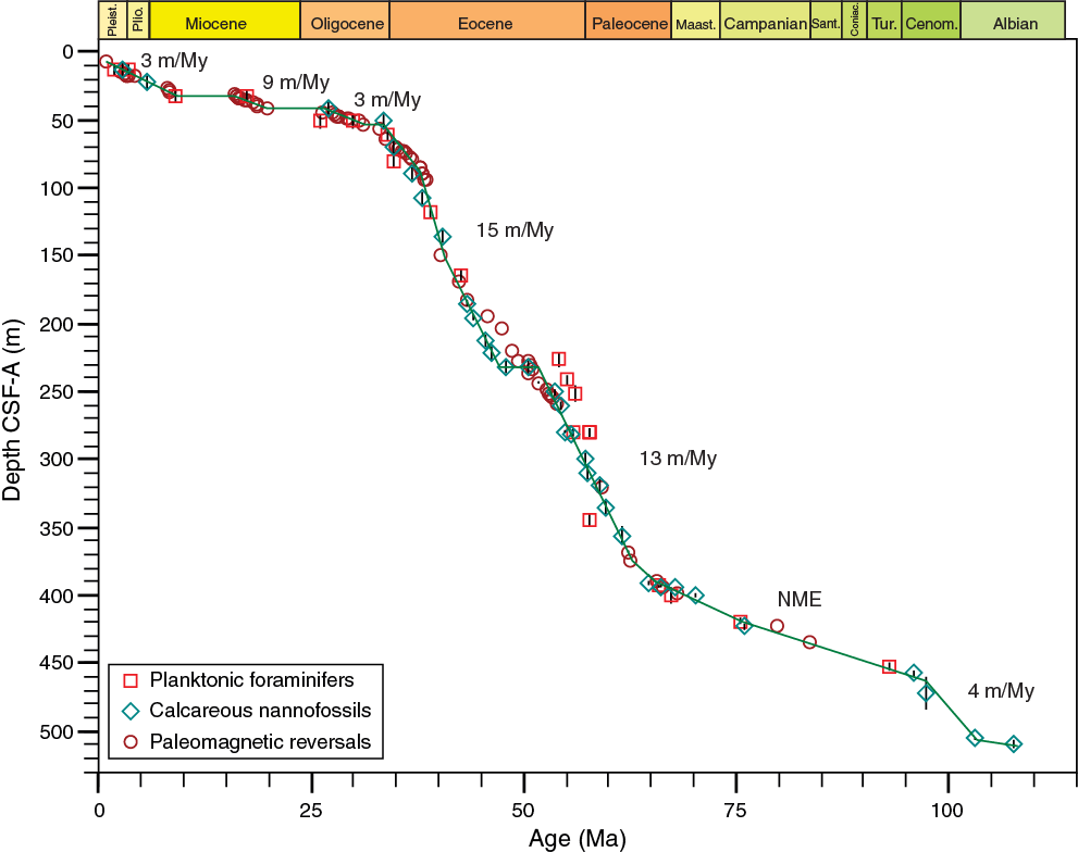
Figure F8. Age-depth plot.
The ~400–460 m CSF-A interval is structurally disturbed. Although the rocks in this interval have a variety of Late Cretaceous ages, they are not always in stratigraphic order; therefore, no meaningful estimate (NME in Figure F8) of sediment accumulation rate for this interval can be made. Sediment accumulation rates in the middle Cenomanian to upper Albian section average ~4 m/My; however, the number of control points is too few for reliable determination.
Calcareous nannofossils
Calcareous nannofossils occur throughout the succession recovered at Site U1514; only ~3% of the samples are barren. Table T5 contains the calcareous nannofossil datums used to establish the temporal framework (Figure F8). The distribution of biostratigraphically important calcareous nannofossils is given in Tables T7 and T8.
Sample 369-U1514A-2H-CC, 14–19 cm, contains abundant, well-preserved calcareous nannofossils, including Discoaster tamalis, Discoaster surculus, Discoaster pentaradiatus, and Pseudoemiliania lacunosa, which indicate upper Pliocene Subzone CN12a. Rare specimens of reworked forms including Reticulofenestra perplexa, Reticulofenestra pseudoumbilica, and Discoaster quintatus, suggest a lower Pliocene to upper Miocene provenance.
Sample 369-U1514A-3H-CC, 29–34 cm, contains abundant, well-preserved calcareous nannofossils, including Amaurolithus tricorniculatus, Discoaster quinqueramus (late form), D. quintatus, and Discoaster mendomobensis, which indicate upper Miocene Subzone CN9b. Rare reworked species include Discoaster berggrennii, Discoaster loeblichii, and R. perplexa. Sponge spicules are common constituents of the sediment.
Sample 369-U1514A-4H-CC, 33–38 cm, is dominated by sponge spicules and, to a lesser extent, radiolarian debris. Calcareous nannofossils are common and exhibit moderate preservation; etching is the most pervasive diagenetic alteration. The assemblage is relatively restricted and strongly dominated by Cyclicargolithus floridanus and Discoaster deflandrei. The presence of Discoaster moorei, Discoaster challengerii, and forms similar to, but smaller than, Discoaster druggii suggest placement in the lower Miocene part of Zones CN3–CN4.
Sample 369-U1514A-5-CC, 21–26 cm, contains common but generally poorly preserved calcareous nannofossils, including Dictyococcites bisectus and D. deflandrei, and a relatively diverse assemblage of sphenoliths, including Sphenolithus ciperoensis, Sphenolithus distentus, and Sphenolithus predistentus. This association of species is diagnostic of upper Oligocene Subzone CP19a. Reticulofenestra umbilica occurs as rare, reworked specimens among the abundant sponge spicules dominating the sediment.
The interval from Sample 369-U1514A-6H-CC, 27–32 cm, through Core 7H contains assemblages that are characteristic of lowest Oligocene Subzone CP16a, including common Isthmolithus recurvus and Clausicoccus subdistichus, frequent Chiasmolithus oamaruensis and Chiasmolithus altus, and rare Sphenolithus akropodus. Nannofossil preservation is moderate in Sample 6H-CC, 27–32 cm, but deteriorates significantly by Sample 7H-CC, 19–24 cm, rendering identification of the chiasmolithids in the latter sample nearly impossible because of the loss of the central cross structure. The sediment is dominated by abundant siliceous debris, including sponge spicules and, to a lesser extent, radiolarian debris.
The presence of Discoaster saipanensis, Discoaster barbadiensis, and I. recurvus in Sample 369-U1514A-8H-CC, 44–49 cm, indicates that the Eocene/Oligocene boundary lies within Core 8H. This assemblage indicates uppermost Eocene Subzone CP15b and continues downhole through Core 9H. The placement of this interval is corroborated by the absence of Cribrocentrum species, including Cribrocentrum reticulatum. Nannofossil abundance and preservation deteriorates in the interval from Sample 10H-CC, 20–25 cm, through Core 11H, and the quantity of siliceous material, especially sponge spicules, increases. Isthmolithus recurvus is absent in this interval, and C. reticulatum appears as a rare component in Sample 10H-CC, 20–25 cm, indicating upper Eocene Subzone CP15a. Preservation in the lower samples (11H-2, 146–150 cm, and 11H-CC, 29–34 cm) is so poor, only a few taxa can be identified with confidence. These include D. saipanensis, D. barbadiensis, and D. bisectus. This dissolution assemblage indicates a generalized late Eocene age.
The interval from Sample 369-U1514A-12H-4, 82–86 cm, through Core 14H is characterized by the presence of rare to common Chiasmolithus grandis and absence of Chiasmolithus solitus, indicating upper Eocene Subzone CP14b. Sample 12H-4, 82–86 cm, contains a diverse assemblage of well-preserved Upper Cretaceous taxa including Micula staurophora, Eiffellithus eximius (s.s.), Ahmuellerella octoradiata, and Gartnerago obliquum. These reworked forms collectively occur as frequent specimens. The presence of C. solitus and the common to few occurrences of R. umbilica in the interval between Samples 15H-CC, 0–8 cm, and 20F-CC, 14–19 cm, are diagnostic of upper Eocene Subzone CP14a.
Samples 369-U1514A-21F-CC, 17–22 cm, and 22F-CC, 21–26 cm, contain a well-preserved calcareous nannofossil assemblage, including Nannotetrina pappii, Nannotetrina cristata, Sphenolithus furcatolithoides, and Pseudotriquetrorhabdulus inversus without common, large (>14 µm) R. umbilica. This assemblage indicates middle Eocene Subzone CP13c and is joined by Coccolithus gigas in the interval from Sample 23F-CC, 16–21 cm, through Core 25X, indicating middle Eocene Subzone CP13b. Sample 26X-CC, 51–56 cm, contains N. cristata, Nannotetrina fulgens, and Discoaster kuepperii without C. gigas, suggesting middle Eocene Subzone CP13a. Preservation is moderate to good in this interval, with abundant nannofossils throughout Zone CP13.
The calcareous nannofossil assemblage in Sample 369-U1514A-27X-CC, 34–39 cm, is placed in lower middle Eocene Subzone CP12b based on the absence of N. fulgens and the presence of rare Blackites inflatus and frequent Discoaster sublodoensis. Calcareous nannofossils are abundant and moderately preserved in this sample.
The presence of few to common Tribrachiatus orthostylus and Discoaster lodoensis from Sample 369-U1514A-28X-CC, 20–25 cm, through Core 30X indicates lower Eocene Zone CP10. The absence of D. lodoensis in Sample 31X-CC, 13–18 cm, indicates lower Eocene Subzone CP9b. Hole U1514A was terminated at this depth.
Sample 369-U1514C-2R-CC, 16–21 cm, contains abundant, moderately preserved calcareous nannofossils with frequent N. cristata and C. gigas and rare Coccolithus staurion and Sphenolithus furcatulithoides, indicating middle Eocene Subzone CP13b. Sample 2R-CC, 16–21 cm, contains N. cristata and C. staurion but lacks C. gigas and S. furcatolithoides, indicating middle Eocene Subzone CP13a. The assemblage in Sample 4R-CC, 18–23 cm, contains common D. sublodoensis and rare B. inflatus but lacks N. fulgens and N. cristata. This association indicates middle Eocene Subzone CP12b. Rare specimens of T. orthostylus are reworked in this sample.
Sample 369-U1514C-5R-CC, 18–23 cm, through Core 7R contains common D. lodoensis and D. kuepperii and frequent T. orthostylus without any Reticulofenestra or Dictyococcites. This association is diagnostic for lower Eocene Zone CP10. Calcareous nannofossils are abundant but poorly preserved, and siliceous debris and siliceous sponge spicules contribute a substantial portion to the sediment.
Sample 369-U1514C-8R-CC, 13–18 cm, contains abundant and well-preserved nannofossils including T. orthostylus but lacks D. lodoensis and D. kuepperii, indicating lower Eocene Subzone CP9b. Samples 9R-CC, 16–21 cm, to 11R-2, 99–100 cm, contain a generally abundant and well-preserved nannofossil assemblage containing Discoaster salisburgensis, Discoaster diastypus, and Discoaster multiradiatus but lacking T. orthostylus. This association is diagnostic for oceanic sections of lower Eocene Subzone CP9a. Two points are noteworthy about this interval. First, the progression of forms ancestral to T. orthostylus (including the Subzone CP9a indicator Tribrachiatus contortus) was not present in these assemblages. Second, Sample 10R-CC, 8–13 cm, contains several taxa, including Heliolithus kleinpellii and Fasciculithus tympaniformis, indicative of reworking from the middle Paleocene. This reworking concurs with similar reworking of the Paleocene planktonic foraminifer Globanomalina pseudomenardii in this sample (see Planktonic foraminifers).
Sample 369-U1514C-11R-3, 90–91 cm, contains an abundant, well-preserved calcareous nannofossil assemblage assigned to upper Paleocene Subzone CP8b by the presence of D. multiradiatus and Camplyosphaera eodela without D. diastypus. As noted previously, the absence of the Tribrachiatus species plexus cannot be used for biostratigraphy at this site. This sample marks the highest consistent occurrence of Fasciculithus. Samples 11R-CC, 21–26 cm, to 12R-CC, 13–18 cm, contain common D. multiradiatus and abundant F. tympaniformis but lack C. eodela, suggesting upper Paleocene Subzone CP8a. The presence of Discoaster nobilis and the absence of D. multiradiatus in Sample 13R-CC, 23–28 cm, indicate upper Paleocene Zone CP7. In Sample 14R-CC, 0–5 cm, Zone CP6 is characterized by the lack of D. nobilis and presence of Discoaster mohleri. Samples 15R-CC, 17–22 cm, and 16R-CC, 0–8 cm, contain frequent H. kleinpellii and Heliolithus cantabriae but lack D. mohleri, indicating upper Paleocene Zone CP5.
The interval from Sample 369-U1514C-17R-5, 94–99 cm, through Core 18R contains common, moderately preserved calcareous nannofossil assemblages with F. tympaniformis, Lithoptychius ullii, Sphenolithus primus, and Bomolithus elegans and without H. kleinpellii, indicating middle Paleocene Zone CP4. The presence of B. elegans throughout this interval suggests the upper part of Zone CP4, following Perch-Nielsen (1985).
Samples 369-U1514C-19R-CC, 13–18 cm, to 22R-CC, 0–1 cm, are assigned to the interval between lower Paleocene Zones CC3 and CC2 based on the occurrence of Chiasmolithus danicus and the lack of F. tympaniformis.
Sample 369-U1514C-22R-CC, 16–21 cm, contains rare, poorly preserved calcareous nannofossil assemblages characterized by the occurrence of Cruciplacolithus tenuis and absence of C. danicus, indicating lower Paleocene Subzone CP1b.
Samples 369-U1514C-23R-1, 17–18 cm, and 23R-1, 98–99 cm, are assigned to lowermost Paleocene Subzone CP1a based on an assemblage composed of common to few Biantholithus sparsus, Cyclagelosphaera reinhardtii, Neocrepidolithus cruciatus, and Thoracosphaera spp. with reworking of some Upper Cretaceous taxa. The Cretaceous/Paleogene boundary is located at the top of Section 23R-2 between Samples 23R-2, 0–1 cm, and 23R-2, 4 cm. The former sample is placed in lowermost Paleocene Subzone CP1a based on the occurrence of rare B. sparsus, and the latter is assigned to uppermost Maastrichtian Subzone CC26b by the absence of B. sparsus and occurrence of Nephrolithus frequens, Lithraphidites quadratus, Micula murus, and Micula prinsii. Uppermost Maastrichtian Subzone CC26b extends to Sample 23R-2, 40–41 cm.
Sample 369-U1514C-23R-2, 67 cm, contains few M. murus but lacks M. prinsii and N. frequens, indicating upper Maastrichtian Subzone CC25c. Samples 23R-3, 29 cm, to 23R-CC, 6–11 cm, contain moderately preserved calcareous nannofossil assemblages and low species richness. The absence of L. quadratus and Reinhardtites levis suggests upper Maastrichtian Subzone CC25a.
Sample 369-U1514C-24R-1, 28 cm, contains abundant calcareous nannofossils. The few occurrences of R. levis indicate lower Maastrichtian Subzone CC24c. The absence of Uniplanarius trifidus in the section prevents recognition of the following Subzone CC24b. Upper Campanian Subzone CC24a occurs between Samples 24R-3, 79 cm, and 26R-1, 67–68 cm. Abundant and moderately to well-preserved assemblages, including Broinsonia parca constricta and Broinsonia parca parca, characterize this subzone. Calcareous nannofossil assemblages in Sample 26R-CC, 0–5 cm, are poorly preserved. The presence of E. eximius and Tranolithus orionatus with R. levis indicates an upper Campanian placement in Zones CC20–CC22. The absence of temperate taxa such as Ceratolithoides spp. and Uniplanarius spp. makes it impossible to place this sample more precisely.
The rocks recovered from Samples 369-U1514C-27R-CC to 29R-CC exhibit unmistakable evidence of structural complexity. Many of the samples in this interval are barren of calcareous nannofossils, whereas others contain unusual assemblages of dissolution-resistant taxa. Faulting and folding (see Lithostratigraphy) have distorted the normal stratigraphic order of this interval, which is indicated by the following series of samples: Sample 27R-CC, 17–24 cm (lower Coniacian Zone CC14), overlies Sample 28R-3, 92–95 cm (lower Turonian Zone CC11), which overlies Sample 28R-CC, 14–19 cm (middle Turonian Zone CC12).
Sample 369-U1514C-30R-1, 51–52 cm, contains a diverse and moderately preserved middle Cenomanian assemblage, including Corollithion kennedyi, Gartnerago theta, Helenea chiastia, Ceratolithina naturalisteplateauensis, Ceratolithina copis, and Cylindralithus sculptus, which indicate the upper part of Subzone CC9c. The presence of Ceratolithina, frequent Seribiscutum primitivum, and Repagulum parvidentatum indicates this assemblage’s cooler water austral affinities. Based on core catcher samples and sedimentology smear slides, Section 30R-2 through Core 31R contains brown to greenish zeolitic claystones barren of calcareous nannofossils.
The interval from Sample 369-U1514C-32R-CC, 45–50 cm, through Core 34R contains a section of upper Albian nannofossil-rich claystones with common, well-preserved assemblages associated in age with OAE 1d. Sample 32R-CC, 45–50 cm, contains few, poorly preserved nannofossils, whereas the rest of the interval has common, well-preserved specimens. Samples 34R-CC, 14–19 cm, to 34R-6, 50–51 cm, contain Watznaueria britannica, G. theta, Eiffellithus casulus, and a variety of other eiffellithids without Hayesites albiensis, indicating the upper Albian portion of Subzone CC9a. Eiffellithus turriseifellii (s.s.; >8 μm) occurs in the upper part of the interval (Sample 32R-CC, 45–50 cm, through Section 33R-CC), and its smaller ancestral species, E. casulus, occurs downhole to Sample 34R-6, 50–51 cm, marking the base of Subzone CC9a. Sample 34R-CC, 14–19 cm, contains Eiffellithus monechiae without E. casulus, indicating upper Albian Subzone CC8d. The presence of Eiffellithus equibiramus and Eiffellithus praestigium throughout this succession indicates an interval correlative to OAE 1d.
The interval from Sample 369-U1514C-35R-5, 88–89 cm, through Section 35R-CC contains Prediscosphaera columnata and T. orionatus without E. monechiae or other eiffellithids, indicating Subzones CC8b–CC8c. Axopodorhabdus biramiculatus (= Axopodorhabdus albianus of some authors) occurs too sporadically in this area to be used as a biostratigraphic criterion to divide Subzone CC8c from CC8b; therefore, it is necessary to use the combined subzone.
Planktonic foraminifers
Holes U1514A and U1514C core catcher samples were analyzed for planktonic foraminiferal biostratigraphy. Bioevents are presented in Table T6, and planktonic foraminiferal occurrences are presented in Tables T9 and T10. Several thousand particles (multiple picking trays) were routinely scanned for each sample. Planktonic foraminiferal assemblages in Hole U1514A span the Pleistocene through lower Eocene in a discontinuous sequence characterized by major unconformities in the lower Pleistocene, Pliocene, Miocene, and Oligocene. In contrast, the Eocene sequence appears to be stratigraphically complete. Hole U1514C ranges from the mid-Eocene to upper Albian. Preservation is generally poor to moderate throughout the sequence in both holes, but discrete samples in the Pleistocene, Paleocene, Turonian, and Albian contain seemingly unrecrystallized specimens. Planktonic foraminifers are, for the most part, rare (<5% of scanned particles) at this site, making biostratigraphy difficult (Tables T9, T10). However, low-latitude marker species are present in the Neogene and Paleogene, although at very low abundances; therefore, the low-latitude biozonation scheme of Wade et al. (2011) can be applied to these sediments. Eocene and Cretaceous assemblages, however, are largely dominated by smaller taxa (<200 µm). Thus, ages for these intervals are primarily based on evaluation of whole assemblages and co-occurrence of species according to their stratigraphic distribution presented in Pearson et al. (2006), Premoli Silva and Sliter (1995), Robaszynski and Caron (1995), Robaszynski et al. (2000), Petrizzo (2000, 2001, 2003), Huber et al. (2008), and the geomagnetic polarity timescale of Gradstein et al. (2012).
Lower Pleistocene planktonic foraminiferal Subzone PT1a occurs in Sample 369-U1514A-1H-CC and is defined by the overlapping occurrences of Truncorotalia truncatulinoides and Truncorotalia tosaensis. Zone PL4 in the upper Pliocene occurs in Sample 2H-CC and is defined by the overlapping occurrences of Dentoglobigerina altispira, Globigerinoides extremus, Globorotalia inflata, and Globorotalia puncticulata and absence of Sphaeroidinellopsis seminulina. Samples 3H-CC to 17H-CC are dominated by sponge spicules, radiolarians, and diatoms; foraminifers are only a minor component. Nevertheless, the co-occurrence of relatively short ranging planktonic foraminiferal species allows the identification of stratigraphic intervals corresponding to precise biozones. Sample 3H-CC is assigned to upper Miocene planktonic foraminiferal Zones M14–M13 based on the overlapping occurrences of D. altispira, Globoturborotalita nepenthes, Globoconella miozea, and G. extremus. The presence of Catapsydrax dissimilis and Trilobatus trilobus may indicate lower Miocene Zone M3 in Sample 4H-CC. The co-occurrence of Globigerinoides primordius, Dentoglobigerina rohri, and Dentoglobigerina tripartita in Sample 5H-CC allows the identification of upper Oligocene Zones O5–O6. The presence of few Subbotina angiporoides, Subbotina linaperta, and Paragloborotalia nana likely indicates lower Oligocene Zones O1–O2 in the underlying Sample 6H-CC. The overlapping occurrences of Chiloguembelina cubensis and Pseudohastigerina micra in Sample 7H-CC correspond to the Oligocene–Eocene stratigraphic interval and are assigned to Zones O1–E16. The underlying stratigraphic sequence from Samples 8H-CC to 10H-CC only contains fragments of Globigerinatheka spp. and Globigerinatheka index but clearly indicates an Eocene age and likely Zones E13–E16. Sample 11H-CC is barren of planktonic foraminifers. The co-occurrence of Acarinina primitiva, Subbotina gortanii, and G. index in Sample 13H-CC allows assignment to Zone E13; therefore, overlying Sample 12H-CC spans the intervening interval of Zones E13–E15. Samples 14H-CC to 17H-CC correspond to Zones E13–E11 based on the overlapping occurrences of G. index and S. angiporoides, and underlying Cores 18H through 21X are assigned to Zones E11–E10 in the absence of G. index. Sample 22F-CC is assigned to Zone E9 based on the co-occurrence of Globanomalina australiformis and A. primitiva, and Sample 23F-CC may indicate Zone E8 based on the co-occurrence of P. micra, A. primitiva, and Subbotina corpulenta. Samples 21F-CC and 24F-CC are barren of planktonic foraminifers. The presence of Acarinina coalingensis, A. primitiva, and G. australiformis in Samples 25X-CC to 28X-CC suggests Zones E6–E7. Samples 29X-CC to 30X-CC are designated as Zone E5 based on the absence of A. primitiva from the assemblage. Samples from Core 31X contain Subbotina hornibrooki, indicating early Eocene Zone E4 or older.
The top of Hole U1514C overlaps the base of Hole U1514A. Specifically, Sample 369-U1514C-2R-CC corresponds to undifferentiated Zones E8–E9 based on the co-occurrence of A. primitiva and G. australiformis and the absence of Acarinina soldadoensis and A. coalingensis. The overlapping ranges of A. primitiva, A. coalingensis, and Subbotina eoceana in Samples 3R-CC and 4R-CC is indicative of Zones E6–E7. Sample 5R-CC contains Morozovella aequa and Acarinina esnaensis but not S. hornibrooki, so it is assigned to Zone E5. The overlapping ranges of S. hornibrooki and Acarinina alticonica in Samples 6R-CC and 7R-CC indicate Zone E4. Samples 8R-CC to 9R-CC contain Subbotina velascoensis, Acarinina pseudotopilensis, and Acarinina subsphaerica, indicating Zones E2–E3. Samples 10R-5, 139–140 cm, and 10R-CC contain reworked G. pseudomenardii, the marker taxon of Paleocene Zone P4, and a diverse late Paleocene to early Eocene assemblage indicative of Zones P5–E2. Samples 11R-CC and 13R-CC are barren of planktonic foraminifers, and Sample 12R-CC is almost barren, containing only Globanomalina fragments, and thus remains unzoned at present. The overlapping ranges of Subbotina cancellata, S. velascoensis, and G. pseudomenardii indicate upper Paleocene Zone P4 in Samples 14R-CC to 17R-5, 94–99 cm. Sample 19R-CC is assigned to lower Paleocene Zone P1 based on the presence of Globanomalina planocompressa, Chiloguembelina morsei, Rectoguembelina cretacea, and Subbotina triloculinoides. Samples 20R-CC to 23R-CC are barren of planktonic foraminifers. However, Sample 23R-1, 101–103 cm, contains an early Paleocene assemblage (Zone Pα) characteristic of the Cretaceous to Paleogene interval in Chron C29R based on the presence of Eoglobigerina eobulloides, Praemurica nikolasi, Chiloguembelina midwayensis, Woodringina hornerstownensis, Guembelina cretacea, and Antarcticella pauciloculata (Figure F9).

Figure F9. Selected planktonic foraminifers.
The upper Maastrichtian Pseudoguembelina hariensis Zone is present in Sample 369-U1514C-23R-2, 38–41 cm, and is defined by the presence of the nominate taxon. Sample 23R-CC is barren of planktonic foraminifers. Samples 24R-CC and 25R-CC contain Gublerina rajagopalani, indicating a late Campanian age for the older sediments (Table T6) according to the calibration of the lowest occurrence of G. rajagopalani at Exmouth Plateau (Petrizzo et al., 2011). The underlying stratigraphic interval from Sample 26R-1, 67–70 cm, to Sample 26R-CC is barren of planktonic foraminifers, and washed residues contain only abundant calcispheres and benthic foraminifers. Sample 27R-CC contains Globigerinelloides prairiehillensis, Globigerinelloides bollii, Marginotruncana pseudolinneiana, and Marginotruncana imbricata and is tentatively considered equivalent to the lower Santonian to upper Turonian Dicarinella concavata Zone in the tropical zonation scheme (Premoli Silva and Sliter, 1995; Robaszynski and Caron, 1995; Gradstein et al., 2012). Sample 28R-CC contains the distinctive Falsotruncana maslakovae and constrains the F. maslakovae Zone, which is equivalent to the lower portion of the D. concavata Zone and to the Marginotruncana schneegansi Zone in tropical biozonation schemes (Premoli Silva and Sliter, 1995; Robaszynski and Caron, 1995; Gradstein et al., 2012) and spans the lower Coniacian through upper Turonian (Petrizzo, 2003; Huber et al., 2017). The base of Core 29R is not zoned but contains G. bentonensis, indicating a Cenomanian to late Albian age (Gale et al., 2011). Samples 30R-CC to 32R-CC are barren of planktonic foraminifers. Planktonic foraminiferal preservation and abundance improves in the upper Albian, and glassy specimens were observed in Sample 369-U1514C-34R-CC. Samples 33R-CC through 35R-CC are assigned to the Thalmanninella appenninica and Pseudothalmanninella ticinensis Zones of the upper Albian based on the overlapping presence of rare ticinellids and G. bentonensis (Petrizzo and Huber, 2006; Gale et al., 2011).
Benthic foraminifers
A total of 66 samples (all of Hole U1514A and U1514C core catcher samples, except for 369-U1514A-8H-CC, 19H-CC, and 21F-CC) were analyzed for benthic foraminifers. Benthic foraminifers are present in most samples (Tables T11, T12). There are three samples in which benthic foraminifers are dominant, 29 samples in which they are abundant, 7 samples in which they are present, and 7 samples in which they are rare. In 14 samples, the frequent occurrence of benthic foraminifers was noted, and only 3 samples were barren.
Pleistocene to Oligocene benthic foraminiferal communities recovered from Hole U1514A (Samples 1H-CC to 7H-CC) are characteristic of well-connected, lower bathyal to midbathyal paleoenvironments. Calcareous-walled taxa dominate the assemblages, and only few agglutinated taxa were recorded in this interval. The percentage of planktonic foraminifers relative to benthic forms in this interval is generally >90%. The assemblages are dominated by epifaunal taxa such as Pyrgo murrhina, Melonis pacificum, and Cibicidoides spp., accompanied by Nodosaria spp.
The Eocene sequence, spanning Samples 369-U1514A-9H-CC to 31X-CC and Samples 369-U1514C-2R-CC to 10R-CC, records a distinct benthic foraminiferal assemblage characterized by a dominance of calcareous-walled forms. Representative taxa include Nuttallides truempyi, Cibicidoides eoceanus, Cibicidoides grimsdalei, Oridorsalis sp., Dentalina spp., and abundant Psammosiphonella sp.
The Paleocene benthic foraminiferal assemblage is characterized by the frequent occurrence of the benthic foraminiferal marker Stensioeina beccariiformis, the extinction of which helps identify the Paleocene/Eocene boundary (Alegret and Thomas, 2013; Tjalsma and Lohmann, 1983; van Morkhoven et al., 1986). The highest occurrence of this species, dated to 55.81 Ma (Alegret et al., 2009), is recorded in Sample 369-U1514C-11R-CC (Table T6). Other common components of the assemblage are Tappanina spp., Aragonia ouezzanensis, and Aragonia velascoensis and agglutinated foraminifers such as Tritaxia sp., Glomospira sp., and Ammodiscus sp. Lower to middle bathyal paleowater depths are inferred for the Paleocene interval based on the observed assemblage (van Morkhoven et al., 1986).
Sample 369-U1514C-22R-CC yields a lowermost Danian agglutinated foraminiferal assemblage with the frequent occurrence of Caudammina ovula, Subreophax sp., Psammosiphonella sp., and Hormosina velascoensis. The assemblage composition indicates bathyal to abyssal water depths (Kaminski and Gradstein, 2005).
The frequent occurrence of Dorothia oxycona associated with Planulina sp., Notoplanulina sp. aff. N. rakauroana, and Spiroplectammina sp. characterizes the Upper Cretaceous benthic foraminiferal assemblages in Samples 369-U1514C-23R-CC through 29R-CC. In Maastrichtian to Campanian age sediments (Samples 23R-CC, 25R-CC, and 26R-CC), N. truempyi and S. beccariiformis were observed. The taxonomic composition suggests bathyal water depths. Samples 24R-CC, 30R-CC, and 31R-CC are barren of benthic foraminifers. Agglutinated foraminifers dominate Samples 32R-1, 11–14 cm, to 35-CC. The frequent appearances of Glomospira sp. and Ammodiscus sp. in these samples indicate bathyal water depths (Kaminski and Gradstein, 2005).
Paleomagnetism
We measured the natural remanent magnetization (NRM) of all archive-half sections from Holes U1514A (369-U1514A-1H through 31X) and U1514C (369-U1514C-2R through 35R) and 82 discrete samples collected from the working-half sections from Holes U1514A and U1514C. The archive-half sections were subjected to either 5, 10, 15, and 20 mT alternating field (AF) demagnetization (Cores 369-U1514A-1H through 13H); 10 and 20 mT AF demagnetization (Cores 369-U1514A-13H through 31X); or 10, 20, and 30 mT AF demagnetization (Cores 369-U1514C-2R through 35R) and measured with the pass-through superconducting rock magnetometer (SRM) at 5 cm intervals. Discrete samples were subjected to progressive AF demagnetization up to 60 mT using the in-line automated degausser and measured with the SRM to isolate the characteristic remanent magnetization (ChRM).
Natural remanent magnetization of sedimentary cores
Hole U1514A
Downhole paleomagnetic variations in Hole U1514A are shown in Figure F10. Sediments recovered from Hole U1514A (Cores 369-U1514A-1H through 31X) were cored with a combination of the APC, HLAPC, and XCB systems. APC Cores 1H through 19H were oriented with the Icefield MI-5 and FlexIT core orientation tools, enabling magnetic declination correction for these cores (Table T13). Core orientation was not possible with the HLAPC and XCB coring methods deployed in the deeper part of Hole U1514A. APC and HLAPC core recovery is generally good except for Core 11H, in which four sections (11H-4 through 11H-7) were significantly affected by “flow-in” and were therefore excluded from the measurement program. In the XCB cores, recovery is good except for the lowermost three cores, but coring-induced disturbance is significant (29X through 31X).
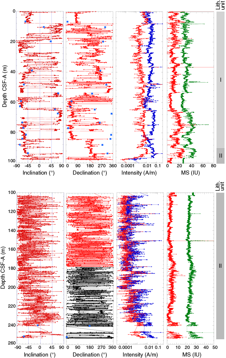
Figure F10. Paleomagnetic data, Hole U1514A.
The NRM of the majority of the recovered sedimentary cores shows generally downward-pointing moderate to steep inclinations, indicating a drilling-induced viscous overprint (e.g., Richter et al., 2007). This overprint was generally removed by AF demagnetization (Figure F10). The NRM of the uppermost ~96 m displays predominantly northward-pointing declinations. The NRM of the cores from deeper than ~96 m CSF-A exhibits a generally scattered distribution of declinations. Except for the 210–230 m CSF-A interval, AF demagnetization is generally effective in removing the overprint. Hole U1514A recovered sedimentary core NRM intensity varies from 6.84 × 10⁻⁶ to 1.10 A/m with a mean of 1.53 × 10⁻² A/m. Overall, the uppermost ~96 m and basal ~8 m of the hole (246.6–254 m CSF-A) display elevated NRM intensity.
The whole-round low-field magnetic susceptibility of recovered Hole U1514A sedimentary cores (Figure F10; see Petrophysics) shows distinctively different variations between cores from shallower than ~96 m CSF-A and those from deeper than this level. Magnetic susceptibility shallower than ~96 m CSF-A typically varies from ~5 to ~25 instrument units (IU) with an overall mean of ~15 IU, whereas magnetic susceptibility deeper than ~96 m CSF-A mostly varies around 5 IU. Magnetic susceptibility slightly increases in the basal 10 m of the hole. Downhole magnetic susceptibility variations broadly mimic lithologic changes from calcareous oozes (Unit I) to clay/claystone (Unit II) (see Lithostratigraphy). Striking magnetic susceptibility spikes >50 IU occur at ~46, 75, 150, and 247.6 m CSF-A. The first three spikes correspond to the tops of Cores 369-U1514A-6H, 9H, and 17H, suggesting possible drilling-related magnetic contamination. The magnetic susceptibility spike at 247.6 m CSF-A corresponds to the basal part of Section 30X-1, where an interstitial water sample was taken.
Hole U1514C
Downhole paleomagnetic variations in Hole U1514C are shown in Figure F11. All sediments from Hole U1514C were cored with the RCB. The uppermost ~195 m, overlapping with Hole U1514A, was not cored (see Operations). Recovery is generally good to moderate except for Cores 369-U1514C-21R and 24R. The recovered cores consist of lithostratigraphic Units II (lower part) and III (see Lithostratigraphy).

Figure F11. Paleomagnetic data. Hole U1514C.
Magnetic inclinations are well preserved and display upward (normal) and downward (reversed?) values, whereas magnetic declinations in the rotary-cored section are highly scattered (Figure F11). Mean NRM intensity decreases by an order of magnitude from 0.015 to 0.0025 A/m after 30 mT AF demagnetization. Inclinations and declinations remain scattered after 30 mT AF demagnetization treatment. The NRM intensity of lithostratigraphic Units II and III varies from 6.44 × 10⁻⁶ to 1.09 A/m with a mean of 1.53 × 10⁻² A/m. NRM intensity is elevated in Cores 369-U1514C-6R through 8R, 18R, 23R through 27R, and 30R.
Downhole variations in magnetic susceptibility range from a few instrument units to ~50 IU (Figure F11). Magnetic susceptibility in lithostratigraphic Unit II is mostly <10 IU with generally subtle variations. Compared with the magnetic susceptibility in lithostratigraphic Unit II, magnetic susceptibility in Unit III displays a larger magnitude of variations, ranging from a few instrument units to ~50 IU although values mainly fluctuate around ~10 IU. Magnetic susceptibility in Unit III is elevated at ~395, ~474, and ~510 m CSF-A, corresponding to changes in lithology (see Lithostratigraphy).
Paleomagnetic demagnetization results
Archive-half sections from Cores 369-U1514A-1H through 31X were subjected to stepwise AF demagnetization up to 20 mT. Archive-half sections from Cores 369-U1514C-2R through 35R were subjected to stepwise AF demagnetization up to 30 mT. AF demagnetization for Cores 369-U1514A-1H through 13H-5 employed 5 mT steps; 10 mT steps were used for the rest of the core sections. Declinations of section halves and discrete samples from fully oriented cores were corrected using the core orientation data (Table T13).
Demagnetization results were visually inspected using the Laboratory Information Management System Information Viewer (LIVE), PuffinPlot (Lurcock and Wilson, 2012), and ZPlotit (http://paleomag.ucdavis.edu/software-Zplotit.html) software packages. Principal component analysis (PCA) was performed only for selected intervals using these software packages to aid in defining ChRMs and assigning polarity. Given the amount of demagnetization data collected, it was not possible to perform complete PCA on board because of time constraints. Nevertheless, shipboard analysis permits the determination of first-order features of the paleomagnetic demagnetization results. The demagnetization data show that the drilling-induced magnetic overprint (Richter et al., 2007) can generally be removed by AF demagnetization at 5 or 10 mT, as indicated by a large drop in magnetic intensity (Figures F10, F11) and significant changes in demagnetization trajectories (Figures F12, F13, F14). AF demagnetization up to 20 or 30 mT mostly resulted in a decrease in magnetic intensity by >50%. In many cases, ChRMs can be defined from the paleomagnetic data acquired from the pass-through measurements. ChRMs can be determined by PCA (Kirschvink, 1980) using either two or three demagnetization steps (Figures F12, F13, F14) that display a vector trajectory decaying toward the origin. When some samples have been demagnetized, magnetic intensity either gradually increases or rapidly decreases and/or shows erratic directions. In these cases, the ChRMs cannot be isolated.
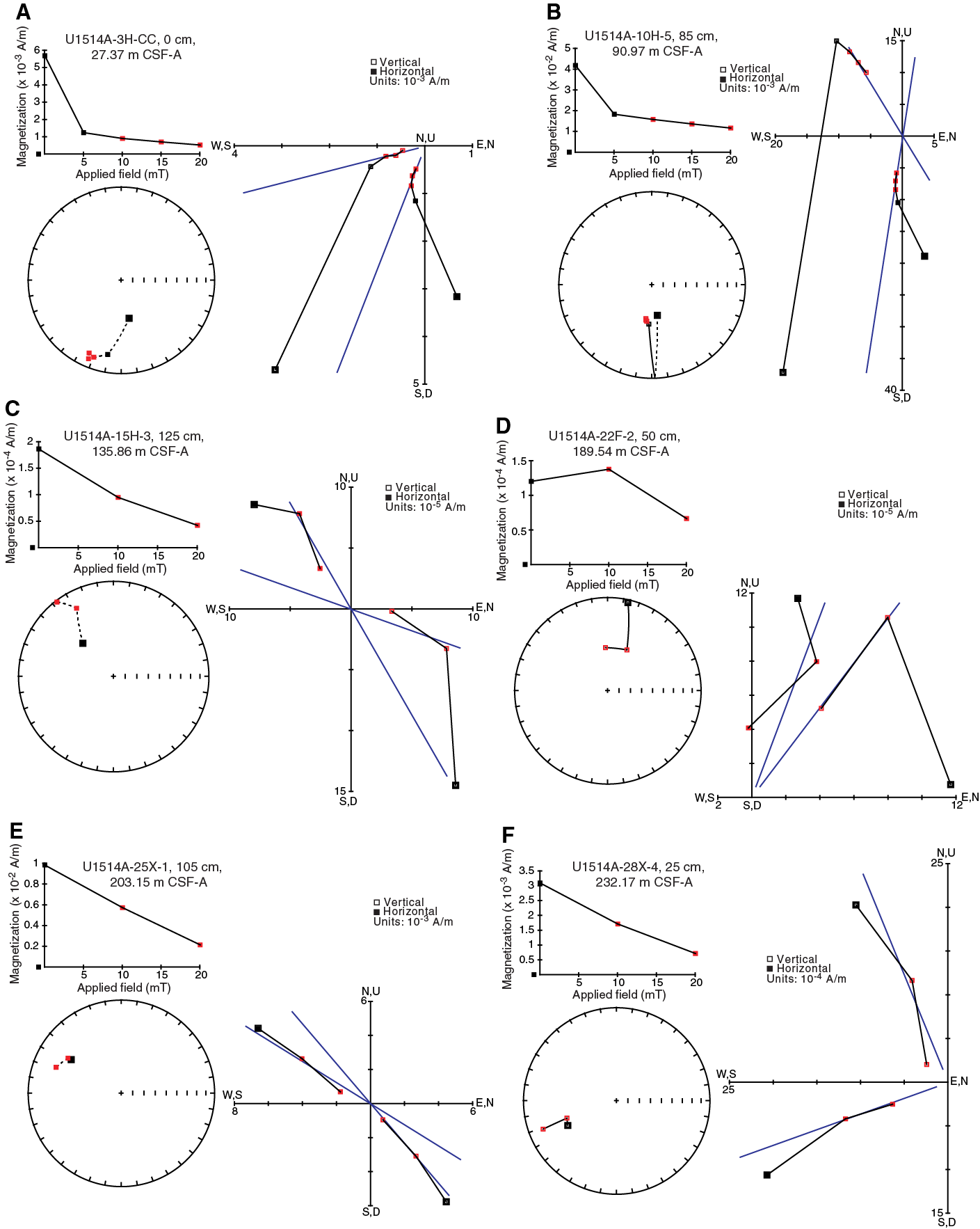
Figure F12. Vector endpoint diagrams for section halves, Hole U1514A.
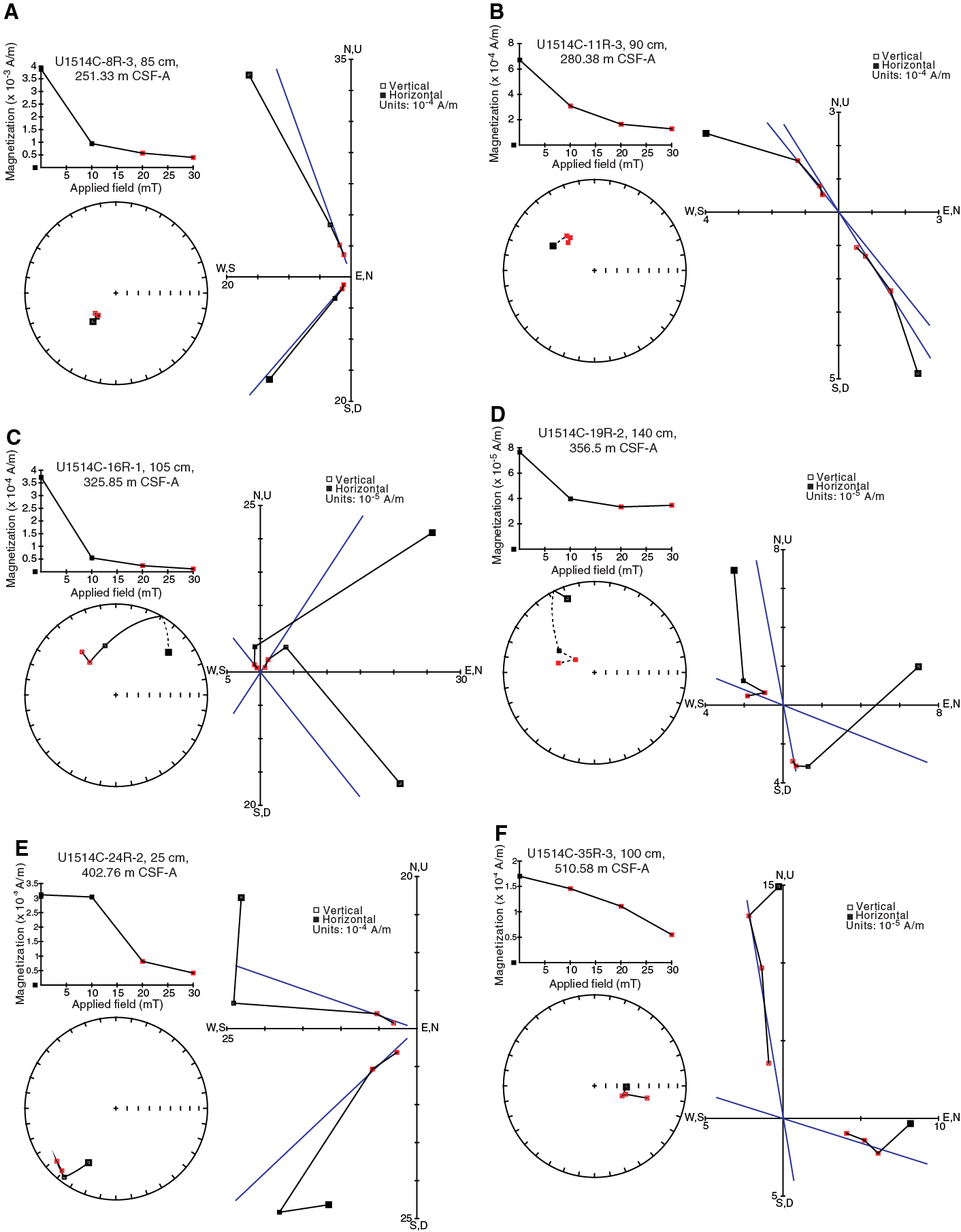
Figure F13. Vector endpoint diagrams for section halves, Hole U1514C.
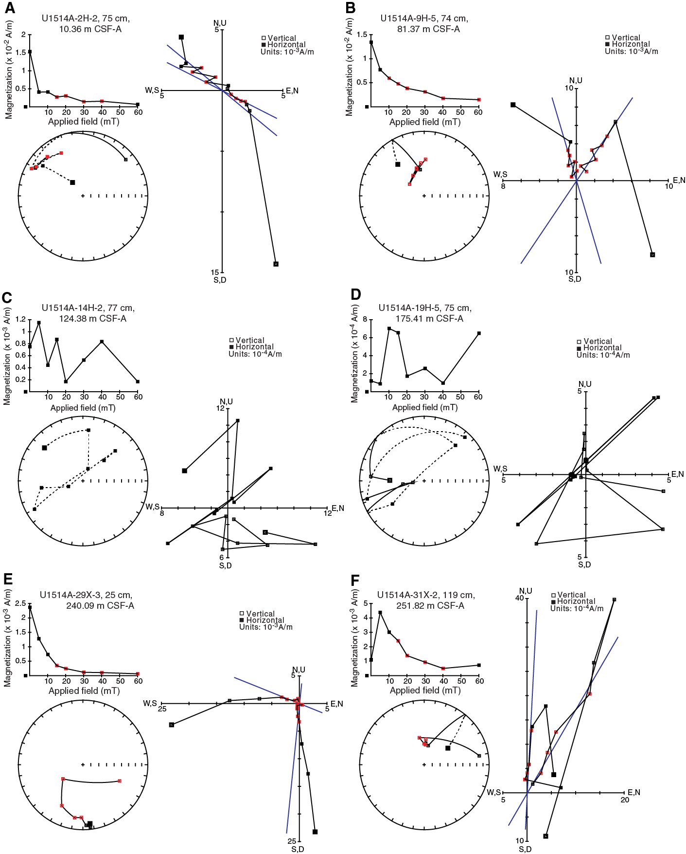
Figure F14. Vector endpoint diagrams for representative discrete samples.
The remanent magnetization of 82 discrete samples from Holes U1514A and U1514C was investigated using detailed stepwise AF demagnetization up to 60 mT measured with the SRM. A total of 50 discrete samples were collected from Hole U1514A sedimentary cores. Discrete samples from the pale brown to pale yellow calcareous oozes (lithostratigraphic Unit I; see Lithostratigraphy) have a typical NRM intensity of 10−2 A/m. These samples display overall stable trajectories decaying toward the origin upon progressive demagnetization, and ChRMs can be well defined (Figure F14A, F14B). The NRM intensity of light greenish ooze/chalk and clay (Unit II) is low, typically 10−3 to 10−4A/m. Discrete samples from this unit display variable demagnetization behaviors. Many show erratic directions (Figure F14C, F14D), but some display relatively stable trajectories (Figure F14E, F14F). PCA results of well-resolved samples from Hole U1514A are presented in Table T14. Hole U1514C sedimentary cores consist of the lower part of lithostratigraphic Unit II and Unit III. The 32 discrete samples from Hole U1514C have a NRM intensity of 10−3 to 10−4A/m. Most of these samples show unstable trajectories upon stepwise AF demagnetization, and their ChRMs cannot be resolved.
Magnetostratigraphy
We mainly used the inclinations from the section-half measurements after the highest AF demagnetization treatment (20 or 30 mT) to define magnetic polarity. ChRM inclinations of discrete samples and declinations of oriented APC cores from Hole U1514A were used as additional constraints to aid in magnetic polarity assignment. Age information from shipboard biostratigraphic analyses (see Biostratigraphy and micropaleontology) were used as the major constraints for making tentative correlations of the established magnetic polarity zones with the geomagnetic polarity timescale (GPTS) (Ogg et al., 2012).
Hole U1514A penetrated to ~254 m CSF-A with overall excellent recovery except for Cores 369-U1514A-29X through 31X. Hole U1514A sedimentary cores consist of lithostratigraphic Unit I and the upper part of Unit II. Coring in Hole U1514C started at ~196 m CSF-A and recovered material to ~516 m CSF-A. Therefore, the ~196 to ~254 m CSF-A interval overlaps in Holes U1514A and U1514C. Hole U1514C sedimentary cores consist of the lower part of Unit II and Unit III. For clarity, magnetostratigraphies from Holes U1514A and U1514C are presented separately (Figure F15), and the overlapped interval is used to bridge the magnetostratigraphies from Hole U1514A and U1514C and generate a composite section for Site U1514.
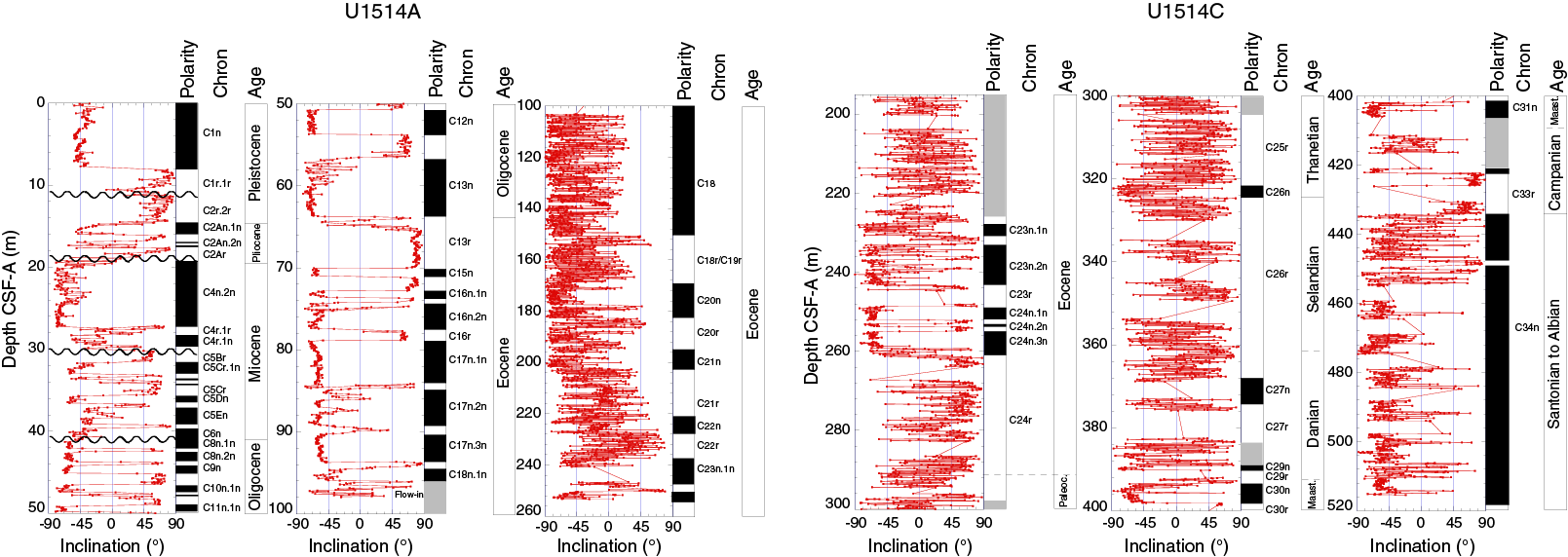
Figure F15. Magnetostratigraphic results.
In Hole U1514A, paleomagnetic inclinations and corrected declinations in lithostratigraphic Unit I (uppermost ~96 m) show a distinct variation pattern characterized by negative and positive inclination zones (Figure F15). Discrete sample ChRM inclinations and declinations are consistent with data from the section-half measurements. Magnetic polarity zones are very well defined, with negative values indicating normal polarity and positive values indicating reversed polarity. Paleomagnetic inclinations and declinations measured in Unit II, recovered with the XCB system, are generally noisy but become only somewhat less scattered toward the base of Hole U1514A. Nevertheless, polarities can be tentatively assigned for the generally noisy interval from 105 to 220 m CSF-A based on the overall inclination distribution. The magnetic polarity zones are well defined for the basal 30 m (220–250 m CSF-A).
Almost 30 pairs of normal and reversed polarity zones were identified in Hole U1514A sedimentary cores. Core by core, these polarity zones were correlated with the GPTS (Gradstein et al., 2012) using the biostratigraphic constraints from the base of each core (core catcher samples). Four hiatuses had to be introduced in the uppermost 50 m to match the magnetostratigraphy with the biostratigraphic ages. Images of Cores 369-U1514A-1H through 6H reveal sharp lithologic boundaries at corresponding levels. These sharp boundaries are likely erosive in nature, and thus are consistent with the presence of a sedimentary hiatus inferred from the chronostratigraphic results. Combined paleomagnetic, lithostratigraphic and biostratigraphic observations indicate hiatal surfaces are present at ~11 m CSF-A in Section 2H-2, ~18 m CSF-A in Section 3H-1, ~30 m CSF-A in Section 4H-3, and ~41 m CSF-A in Section 5H-4. In turn, the magnetic polarity sequence in lithostratigraphic Unit I is correlated with Chrons C1n through C18n.1n. The magnetic polarity sequence in Unit II is correlated with Chrons C18n through C23n.1n (Figure F15).
In Hole U1514C, paleomagnetic inclinations from 196 to 225 m CSF-A are randomly distributed, and magnetic polarity cannot be assigned (Figure F15). For the rest of the Hole U1514C sedimentary cores, paleomagnetic inclinations display either a distinct positive and negative zone pattern or discernible zones of predominantly positive and negative values. For instance, the magnetic polarity zones between ~220 and ~260 m CSF-A are very well defined. Similarly, despite the relatively noisy paleomagnetic inclinations and moderate recovery from ~260 to ~370 m CSF-A, the occurrence of predominantly positive inclinations allow us to assign reversed polarity zones, except for the ~320 to ~325 m CSF-A interval. Inclinations are dominantly negative in this interval; therefore, it is assigned to a normal polarity zone. Likewise, paleomagnetic inclinations deeper than ~440 m CSF-A are predominantly negative, despite the moderate core recovery, and indicate a normal polarity zone. With the biostratigraphic constraints, the magnetic polarity sequence in Hole U1514C can be tentatively correlated with Chrons C23n.1n through C34n, the latter of which is the Cretaceous Normal Superchron (Ogg et al., 2012). A summary of magnetostratigraphic data with age and depth information is provided in Table T15, and an age-depth model based on magnetostratigraphic events is shown in Figure F16.
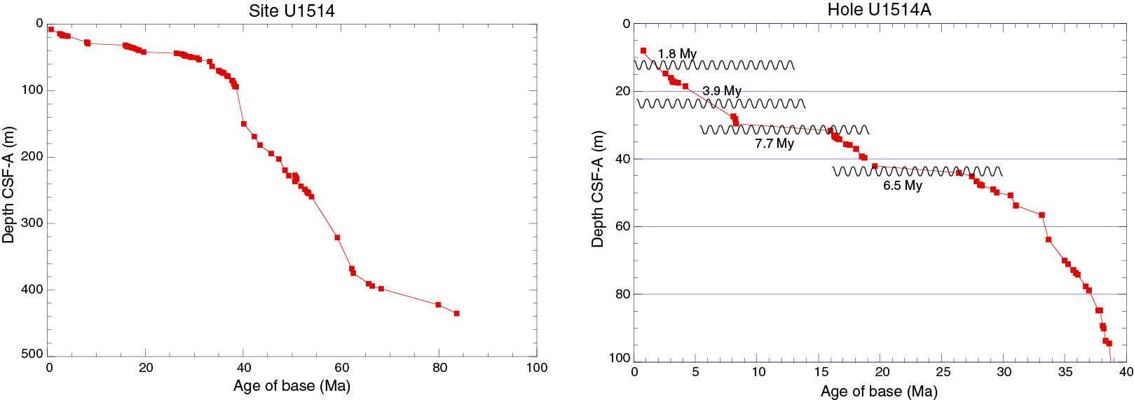
Figure F16. Age-depth plot.
Petrophysics
Physical properties
Physical property data were collected from Holes U1514A and U1514C. The holes overlap from ~200 to 250 m CSF-A, filling several gaps in this interval where core recovery was poor. Additional partial data gaps exist from 330 to 430 m CSF-A and 455 to 500 m CSF-A in Hole U1514C, due to occasional poor recovery in deeper cores. The discussion below is based on integrated results from Holes U1514A and U1514C.
Natural gamma radiation
Natural gamma radiation (NGR) ranges from undetectable to 105 counts/s, and several features are noted. In the uppermost 2.5 m, NGR decreases downcore from ~40 to <10 counts/s (Figure F17), which corresponds to a decrease in U and K content but no change in Th content (Figure F18). NGR then remains relatively stable from 2.5 to 65 m CSF-A, with all values <20 counts/s. NGR progressively increases to 30 counts/s from 65 to 103 m CSF-A. This increase corresponds to an interval where sediment color transitions from light brown in lithostratigraphic Subunit Ib to dark green in Unit II (see Lithostratigraphy). An abrupt decrease in NGR at 103 m CSF-A corresponds to a change in sediment color from dark to light green. NGR then fluctuates with low amplitudes around mean values of 10–15 counts/s downhole to 382 m CSF-A (Figures F17, F19). This interval of low NGR contains three spikes, one at 228–229 m CSF-A in Hole U1514A (Figure F17) and two in Hole U1514C at 279 m and 375 m CSF-A (Figure F19), corresponding to enrichments in U and U/Th ratios >1 (Figures F18, F20). The second spike notably occurs around the transition between the Paleocene and Eocene and may be related to the Paleocene/Eocene Thermal Maximum (PETM; see Biostratigraphy and micropaleontology).

Figure F17. Physical properties, Hole U1514A.
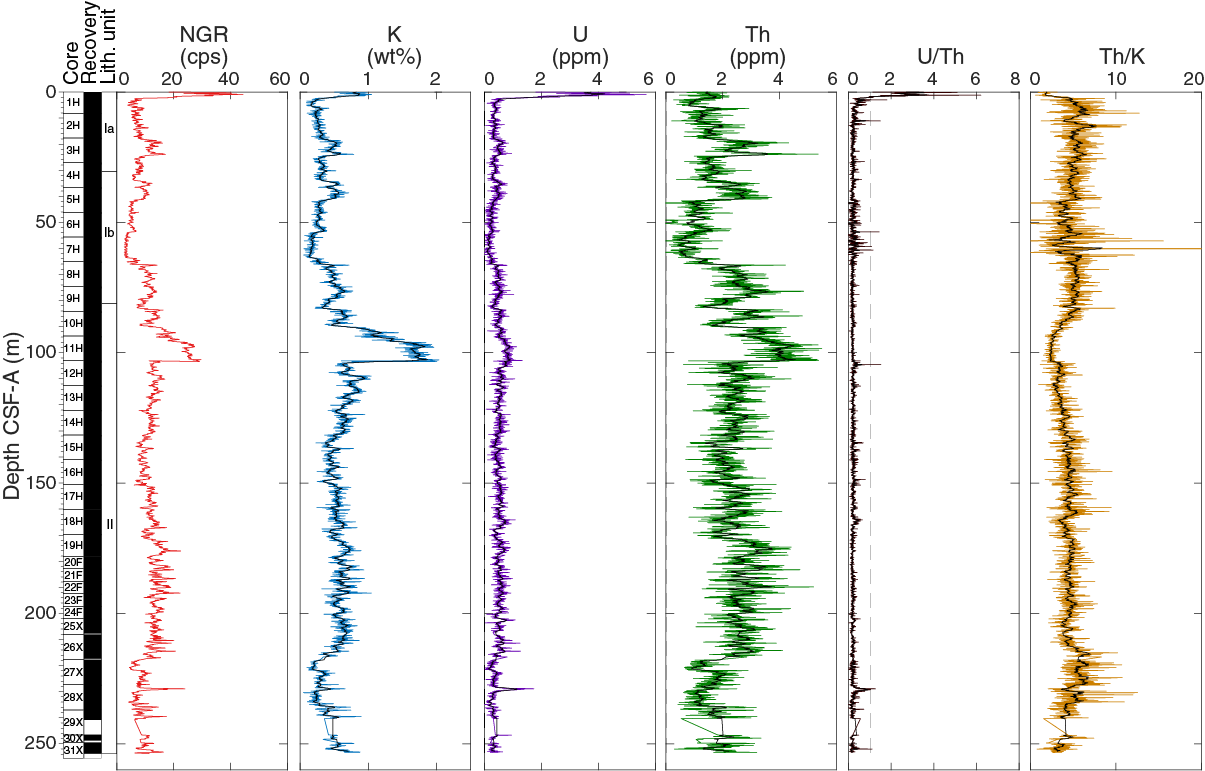
Figure F18. NGR data, Hole U1514A.

Figure F19. Physical properties, Hole U1514C.

Figure F20. NGR data, Hole U1514C.
NGR exhibits four sequences of high-amplitude fluctuations in the lower portion of Hole U1514C (e.g., 382–406, 421–433, 441–447, and 455–485 m CSF-A) and then decreases to a mean of 30 counts/s below (Figure F19). The shallowest of the sequences encompasses the Cretaceous/Paleogene (K/Pg) boundary interval (see Biostratigraphy and micropaleontology and Paleomagnetism). This section represents the highest NGR (105 counts/s) and U content (10 ppm) at the site, with the peak recorded at 395.6 m CSF-A, roughly 2 m below the K/Pg boundary and within magnetic polarity Chron C30n (see Paleomagnetism) (Figures F19, F20). The third NGR sequence (441–447 m CSF-A) corresponds to a slight enrichment in U to 3 ppm and an increase in U/Th ratio at 444 m CSF-A (Figure F20).
Magnetic susceptibility
Magnetic susceptibility was measured on all whole-round sections with the Whole-Round Multisensor Logger (WRMSL), and magnetic susceptibility point measurements were made on archive-half sections with the Section Half Multisensor Logger (SHMSL). The magnetic susceptibility data and overall trends from the WRMSL and SHMSL are comparable (Figures F17, F19).
Magnetic susceptibility ranges from −1.76 to 50.48 IU and fluctuates with high amplitudes from 0 to 97 m CSF-A around a mean of 27 IU (Figure F17). A sharp decrease in magnetic susceptibility at 97 m CSF-A followed by a smaller decrease at 103 m CSF-A correspond to changes in sediment color (see Lithostratigraphy). The first of these decreases in magnetic susceptibility corresponds with an increase in NGR, whereas the second decrease corresponds to a decrease in NGR.
At greater depths (103–382 m CSF-A), magnetic susceptibility is low with values around 4 IU except for an isolated spike at 150.9 m CSF-A and a sequence of increased values from 232 to 260 m CSF-A (Figures F17, F19). The spike at 150.9 m potentially corresponds to the Chron C19r event (see Paleomagnetism), a dissolution event marked by a peak in Fe content in Atlantic sites (Edgar et al., 2007) (Figure F17). Several additional changes in magnetic susceptibility occur below 382 m CSF-A, with three elevated intervals between 382 and 485 m CSF-A (Figure F19). Magnetic susceptibility exhibits much less variability below 485 m CSF-A, generally with a mean of 10 IU. Magnetic susceptibility is broadly correlated to NGR, with noticeable exceptions where magnetic susceptibility decreases while NGR peaks (e.g., at 97 m CSF-A and from 437 to 450 m CSF-A).
GRA bulk density
Gamma ray attenuation (GRA) density was measured on all whole-round sections with the WRMSL. Excluding sparse outliers, the highest values within a given core section are deemed to be the most reliable. For sections cored in Hole U1514A with the APC system (0–202 m CSF-A), GRA density is generally in agreement with that obtained from moisture and density (MAD) measurements (Figure F21). For cores recovered with the XCB (202–255 m CSF-A) and RCB systems (Hole U1514C), the GRA density magnitude is consistently lower than that obtained from MAD measurements (Figures F21, F22), but the downhole trends (slope, discontinuities, and inflections) are comparable. The relatively low GRA density magnitude in XCB and RCB cores is related to the core diameter being less than the diameter of the core liner; the GRA detector is calibrated to the standard core liner diameter.

Figure F21. Density, porosity, thermal conductivity, and P-wave velocity, Hole U1514A.
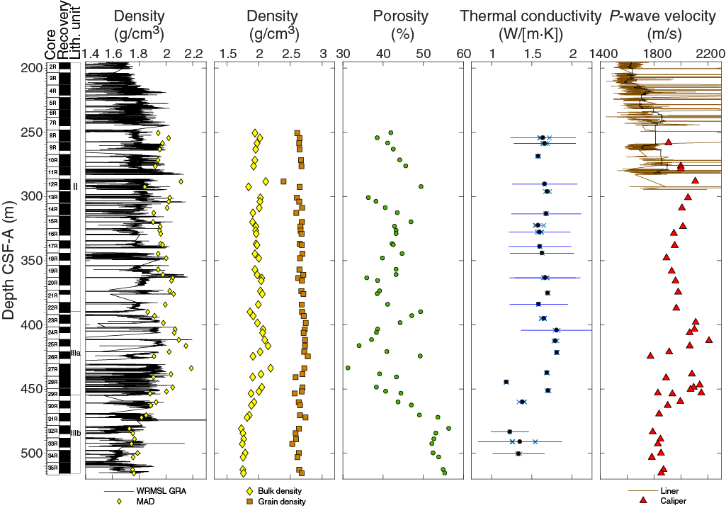
Figure F22. Density, porosity, thermal conductivity, and P-wave velocity, Hole U1514C.
Changes in GRA density are noticeable through the core. GRA density increases downhole from 1.57 to 1.72 g/cm3 between 0 and 8 m CSF-A (Figure F21). The density is then nearly constant (1.75 ± 0.03 g/cm3) between 8 m and 30 m CSF-A and then decreases to 1.57 g/cm3 at 32 m CSF-A. This decrease in GRA density occurs at the transition between lithostratigraphic Subunits Ia and Ib. An increase in GRA density from 76 to 82 m CSF-A occurs at the transition from Subunit Ib to Unit II (see Lithostratigraphy). A decrease in GRA density at ~380 m CSF-A occurs near the K/Pg boundary and the contact of Unit II and Subunit IIIa (see Lithostratigraphy) below an interval of relatively uniform GRA density (Figure F22).
Other changes in GRA density appear not to be caused by geologic changes. For example, the sharp decrease noted at ~200 m CSF-A (Figure F22) corresponds to the change from APC to XCB coring. This change simply reflects the way GRA density is measured using the WRMSL.
Color reflectance
High-resolution (2.5 cm) reflectance spectroscopy and colorimetry (RSC) and RGB data such as reflectance (L*), red versus green (a*), and blue versus yellow (b*) from archive-half sections measured on the SHMSL display significant amounts of instrumental noise (Figures F17, F19); however, some general trends exist. L*, a*, and b* values vary between the seafloor and 80 m CSF-A, and a decrease around 30 m CSF-A notably corresponds to a change in sediment color from beige to brown and the contact of lithostratigraphic Subunits Ia and Ib (see Lithostratigraphy).
L* and RGB data show a local minimum at ~80 m CSF-A, which corresponds to a change from the brownish nannofossil ooze of lithostratigraphic Subunit Ib to the light greenish gray nannofossil chalk and claystone of Unit II (Figure F17) (see Lithostratigraphy). From 95 to ~390 m CSF-A, L*, a*, and b* are relatively constant, aside from an increase in a* and b* between ~240 and ~270 m CSF-A. This increase corresponds to an interval of pale yellow and light yellowish brown sediment (see Lithostratigraphy). Between 390 and 460 m CSF-A, RSC values are variable, and a* and b* are widely scattered due to highly variable sediment color (Figure F19). This interval corresponds to Subunit IIIa, which is characterized by greenish gray to yellowish brown claystone, bioturbation, and numerous likely gravity flow deposits (see Lithostratigraphy). Below 460 m CSF-A, RSC values are stable and constant to the bottom of Hole U1514C; the minimal L* values are a result of dark greenish-gray to black claystones in Subunit IIIb.
Bulk density, grain density, and porosity
The bulk density, grain density, and porosity of core material were measured on discrete samples using MAD measurements (Figures F21, F22). These were typically taken from two samples per core that are representative of the overall lithology. In general, MAD measurements indicate that bulk density decreases from 1.6–1.7 g/cm3 near the top of Hole U1514A to ~1.5 g/cm3 at ~35 m CSF-A. Bulk density remains at ~1.5 g/cm3 between 35 and 150 m CSF-A and increases from 1.5 to 2.05 g/cm3 to the base of the Hole U1514A (252 m CSF-A). Bulk density values are more scattered between 250 and 420 m CSF-A and decrease from ~400 to 475 m CSF-A then remain constant to the base of Hole U1514C (518 m CSF-A) (Figure F22).
Porosity follows a similar but inverse pattern to bulk density, with ~58%–65% porosity in the uppermost 20 m of Hole U1514A and 60%–72% between 25 and 100 m CSF-A. A steady decrease in porosity occurs from ~65.5% at ~150 m CSF-A to 30%–40% at the base of Hole U1514A (~250 m CSF-A) (Figure F21). Porosity values are more variable between ~250 and ~430 m CSF-A, including an apparent discontinuity at ~290 m CSF-A. Porosity increases between ~400 to 475 m CSF-A and then remains relatively constant to the base of Hole U1514C (~520 m CSF-A), especially below a lithologic transition to claystones in lithostratigraphic Subunit IIIb (Figure F22).
Grain density in Hole U1514A combined with that in Hole U1514C shows some similarity with bulk density downhole, but grain density overall is more variable, particularly shallower than 300 m CSF-A. Several lower grain density values in the upper part of lithostratigraphic Subunit Ib (2.3–2.4 g/cm3) and higher values (~3.0 g/cm3) near the base of Hole U1514A diverge from the general trend (Figure F22). In the deeper interval of Hole U1514C, grain density subtly decreases from ~2.75 g/cm3 at ~420 m CSF-A to ~2.6 g/cm3 at the base of Hole U1514C (~520 m CSF-A).
Thermal conductivity, downhole temperature, and heat flow
Thermal conductivity was measured on less-disturbed cores; however, null results were obtained from multiple sections. Nonetheless, enough data were obtained to resolve four general trends in the downhole thermal conductivity data at Site U1514 (Figures F21, F22). Thermal conductivity is variable from the seafloor to ~115 m CSF-A but gradually decreases downhole from 1.16 to 0.8 W/(m·K). From 115 to 260 m CSF-A, thermal conductivity values increase downcore to ~1.7 W/(m·K). Between 260 and 440 m CSF-A, thermal conductivity is generally constant, ranging from 1.55 to 1.83 W/(m·K). Below ~445 m CSF-A, thermal conductivity decreases in the claystones of lithostratigraphic Subunit IIIb and is generally less than 1.4 W/(m·K) to the bottom of Hole U1514C.
Downhole temperatures were obtained with the APCT-3 (see Operations). A formation temperature was calculated from each APCT-3 record using the TP-Fit MATLAB script, involving the identification of the characteristic peak in temperature during penetration of the core barrel and removing the thermal spikes associated with the friction of the core barrel when it punctures and is extracted from the sediment. Equilibrium in situ temperature estimates were obtained in Cores 369-U1514A-4H, 6H, and 8H (Table T16). Linear regression results in an estimated bottom water temperature of 1.18°C and a geothermal gradient of 49.2°C/km.
Heat flow was calculated to be 51 ± 5 mW/m2 based on downhole temperatures (Table T16) and assumed a constant average geothermal gradient and thermal conductivity above the deepest downhole temperature measurement. Similar heat flow values are obtained using Bullard’s method as described by Pribnow et al. (2000) with discrete downhole temperatures, a constant average thermal conductivity, and a best-fit linear increase in thermal conductivity with depth. This method yielded heat flow estimates of 48 ± 1 and 46 ± 1 mW/m2.
P-wave velocity
The WRMSL P-wave logger (PWL) measured whole-round core P-wave velocity and the Section Half Measurement Gantry P-wave caliper (PWC) measured working-half section and discrete sample velocity. Whole-round P-wave velocity was not measured in some intervals (e.g., Core 369-U1514A-30X and most of Hole U1514C) because of scattered data and poor contact between the core and liner. One or two PWC measurements were taken per core, often near the location where MAD samples were collected. Reported values are the automatically picked first arrival time velocities measured using the PWC computer system.
Velocity values obtained using the PWL and PWC range between 1500 and 1600 m/s from the seafloor to 165 m CSF-A (Figure F21). PWL values are more scattered between 165 and 290 m CSF-A and increase with depth. PWC velocity increases to ~2107 m/s at 288 m CSF-A (Figures F21, F22). Deeper than 288 m CSF-A, PWC velocity is relatively constant, ranging between 1900 and 2050 m/s downhole to 390 m CSF-A. Between 390 and 460 m CSF-A, PWC velocity is variable (Figure F22), corresponding to an interval of soft-sediment deformation caused by a probable large-scale slump referred to as lithostratigraphic Subunit IIIa (see Lithostratigraphy). Below the transition to claystones of Subunit IIIb at ~460 m CSF-A, velocity decreases and is relatively constant around 1830 m/s.
Downhole logging
Downhole wireline logging operations were completed in Hole U1514C from the end of the drill pipe at 82.2 m DSF to the bottom of the hole at 514.7 m DSF with the Quambo tool string (see Operations; Figure F23). The offset between the processed wireline logging depth and core depth scales is estimated to be <0.8 m.
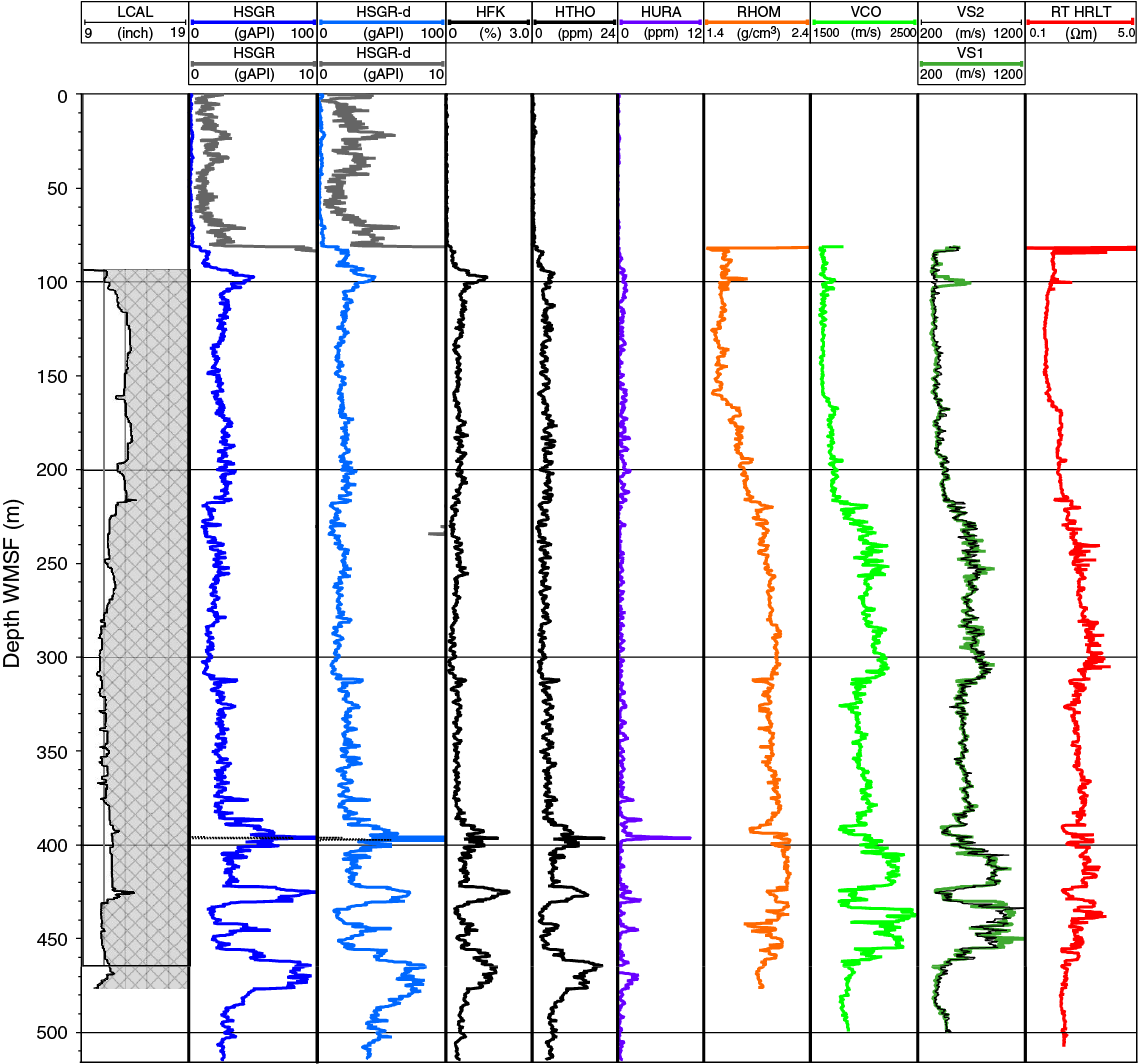
Figure F23. Downhole logging main pass results.
An inclinometer housed in the EDTC recorded a deviation of less than ~4° from vertical in Hole U1514C. Caliper measurements ranged between 10.5 and 14 inches, indicating excellent borehole stability.
Natural gamma radiation
The HNGS measured relatively similar and consistent NGR values (10–35 gAPI) in Hole U1514C from ~105 to ~380 m wireline log matched depth below seafloor (WMSF). Some minor variations in NGR were observed over this depth interval, generally corresponding with minor changes in borehole shape and therefore likely reflecting minor changes in the clay content of lithologies. NGR increases below the contact of lithostratigraphic Units II and III at ~385 m WMSF, reaching a narrow peak of ~190 gAPI at ~396 m WMSF followed by a decrease between ~400 and 410 m WMSF. Additional peaks in NGR occur between ~422 and 430, 442 and 448, and 455 and 480 m WMSF in the claystone interval corresponding to lithostratigraphic Unit III (see Lithostratigraphy). The peaks at 390–400 and 420–430 m WMSF correspond to decreases in bulk density, sonic velocity, and resistivity.
The five-window spectroscopy of the HNGS tool also allows determination of approximate U, Th, and K contents. Downhole trends in these elements’ contents largely mimic the NGR spectra, with Th, K, and U contents increasing through each of the four NGR peaks deeper than ~390 m WMSF. Notably, U contents spike to >10 ppm at 396 m WMSF, roughly 20 times the mean value for the hole. This horizon occurs near the K/Pg boundary (see Biostratigraphy and micropaleontology). U, Th, and K contents from downhole logging in Hole U1514A are also similar to those deconvolved from core-based NGR data using the methodology specified in De Vleeschouwer et al. (2017) (Figures F18, F20).
Resistivity
Relatively low computed true resistivity (HRLT) between 1.0 and 3.5 Ωm is recorded in Hole U1514C (Figure F23). Resistivity is stable at ~1 Ωm from ~80 to 160 m WMSF. Resistivity gradually increases downhole from ~160 m WMSF to the highest value in this hole (~3.5 Ωm) at ~305 m WMSF followed by a gradual decrease downhole between 305 and 340 m WMSF. Two intervals with further decreased resistivity (<2.0 Ωm) occur between 390 and 394 and 423 and 429 m WMSF. These intervals also correspond to increased NGR, decreased sonic velocity, and the clay-rich lithologies of lithostratigraphic Unit III (see Lithostratigraphy). No apparent correlation is evident between resistivity and caliper measurements (i.e., borehole shape).
P-wave velocity
P-wave velocity ranges from ~1600 to 2500 m/s in Hole U1514C (Figure F23). The compressional and shear wave velocity measurements mimic one another and the resistivity and density curves. Compressional P-wave velocities are relatively constant and average 1600 m/s from 80 to 160 m WMSF. Velocity subtly increases at 160 m WMSF to ~1700 m/s followed by a greater increase at ~220 m WMSF to ~1950 m/s. Velocity trends track resistivity values to the bottom of the hole; however, more distinct changes in velocities occur between ~400 and 460 m WMSF. Intervals of slower compressional and shear sonic velocities (e.g., 422–433 m WMSF) correspond to increased NGR log values, representing more clay rich lithologies. Compressional and shear velocities also decrease below ~455 m WMSF by ~400 and 600 m/s, respectively. This occurs below the base of a wide zone of soft-sediment deformation associated with a gravity flow between ~420 and 440 m WMSF and at the contact with underlying fractured green siltstones of Subunit IIIb beneath the deformed unit (see Lithostratigraphy).
Density
Density measurements in Hole U1514C range from 1.5 to ~2.2 g/cm3 (Figure F23). The density curve has a similar shape to the recorded P-wave velocity and resistivity curves. Density exhibits very little variation between 80 and 160 m WMSF with an average of 1.5 g/cm3. Density increases downhole between 160 and 290 m WMSF to ~2.1 g/cm3 and is underlain by relatively similar values between 310 and 380 m WMSF. Density decreases by 0.25 g/cm3 downhole from 380 to 393 m WMSF, at which point density increases sharply within 1 m of the K/Pg boundary, which is placed at ~390 m CSF-A. This decrease in density is similar to decreases in P-wave velocity and resistivity at the same depths and a sharp increase in NGR at ~400 m WMSF, indicating potential logging markers of the K/Pg boundary at Site U1514. Other clay-rich intervals downhole preserve similar decreases in density of 0.1 to 0.2 g/cm3, such as from 422 to 429 m WMSF. This decreased density and P-wave velocity, has the potential to generate seismic reflectors. Velocity and density log data correlate well in the uppermost 390 m WMSF of the hole (r2 = 0.89), whereas these properties do not correlate well deeper than 390 m WMSF (r2 = 0.20).
Magnetic susceptibility
Magnetic susceptibility values obtained from the MSS log and the WRMSL measurements on core sections (see Physical properties) are not similar. This discrepancy suggests that the log did not accurately characterized the magnetic susceptibility of the borehole wall and that downhole environmental or technical issues interfered with the measurement.
Geochemistry
The geochemistry program at Site U1514 was designed to characterize the composition of interstitial water and solid sediments and to assess the potential presence of volatile hydrocarbons. Samples discussed here were taken from Holes U1514A (0–253.82 m CSF-A) and U1514C (195.60–515.66 m CSF-A) unless otherwise specified. In addition to routine analyses, additional horizons (Cores 369-U1514C-27R, 32R, and 34R) were analyzed at a higher resolution to characterize bulk sediment and organic matter.
Headspace hydrocarbon gases
A total of 56 headspace gas samples were taken for routine safety monitoring downhole to ~513 m CSF-A (Table T17; Figure F24). Although only trace amounts of methane (≤90 ppmv) were detected, values gradually increased with depth and peaked at 81.73 ppmv around 494 m CSF-A (Core 369-U1514C-33R) near the bottom of the hole. Trace amounts of ethane were detected in Core 33R.
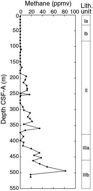
Figure F24. Headspace gas methane concentration.
Interstitial water analyses
For analysis of water chemistry, 54 interstitial water samples were taken from whole-round squeezing of sediment intervals in Holes U1514A (black circles and red triangles in Figure F25) and U1514C (green circles and blue triangles in Figure F25), and an additional sample was taken from the mudline. Ion chromatography was used to measure chloride (Cl−) and bromide (Br−), and inductively coupled plasma–atomic emission spectroscopy (ICP-AES) was used to analyze barium (Ba), boron (B), lithium (Li), manganese (Mn), silicon (Si), iron (Fe), calcium (Ca), phosphorus (P), potassium (K), magnesium (Mg), sodium (Na), sulfur (S), and strontium (Sr). All ICP-AES measurements were converted to molar concentrations, and we assumed all sulfur was present as sulfate (SO42−). Sulfate, Na, Ca, Mg, and K were also measured by ion chromatography, but the ICP-AES concentration data were determined to be of higher quality (see Geochemistry in the Expedition 369 methods chapter [Huber et al., 2019a]). Ammonium (NH4+) was measured by spectrophotometry (Gieskes et al., 1991).

Figure F25. Interstitial water geochemistry.
The preliminary plan for whole-round sampling was one sample per full-length core or every other half-length core. A mudline water sample was taken from the top of Core 369-U1514A-1H. In Hole U1514A, interstitial water samples were taken downhole to 247.75 m CSF-A; no sample was taken from Core 31X, the final core of Hole U1514A. Interstitial water sampling in Hole U1514C began at 254.96 m CSF-A (Sample 369-U1514C-8R-6, 57–67 cm) and continued to the bottom of the hole (Sample 35R-5, 122–132 cm). The small volumes of interstitial water extracted from some samples meant that some analyses could not be performed for many samples. Preference was given to ICP-AES and ion chromatography analyses because of the quantity of information generated using these techniques.
Salinity, pH, and alkalinity
The salinity of interstitial water samples is generally constant, ranging between 35.5 and 38.0 with the exception of samples from lithostratigraphic Subunit IIIb, in which salinity decreases to 26.5–34.0 (Table T18; Figure F25). This drawdown in salinity is reflected in Cl− depletions (~22%) compared to seawater concentration in Subunit IIIa. Na, K, Mn, Si, Ca, SO42−, Sr, and Mg show synchronous drawdown in Subunit IIIb. The changes in salinity in Subunit IIIb are not reflected in Na/Cl− ratios, which steadily decrease downhole. Because the presence and decomposition of gas hydrate can be excluded as a source for low-salinity water, input of a freshwater component through pathways at greater depth (likely along faults) is suggested.
Alkalinity and pH measurements were generally limited to depths shallower than ~270 m CSF-A (Cores 369-U1514A-1H through 30X and 369-U1514C-8R through 10R), although these metrics were measured on single sample from 403.91 m CSF-A (Section 369-U1514C-24R-2). Measurements were not made on the remaining samples because of the small volumes of interstitial water obtained. Alkalinity generally increases from 2.51 mM in the mudline sample to 7.41 mM at 193.9 m CSF-A, followed by a slight decrease downhole (Table T18; Figure F25). The pH values decrease from 7.76 at the mudline to 6.90 in the deepest sample (403.91 m CSF-A).
Sulfate and ammonium
SO42− linearly decreases with depth from 27.8 mM at the mudline to 7.2 mM in the deepest sample at 513.36 m CSF-A (Table T18; Figure F25). NH4+ concentration exhibits an opposite trend, with the lowest values in the shallowest core samples and increasing to ~0.62 mM at the base of lithostratigraphic Subunit IIIa (452.47 m CSF-A; Sample 369-U1514C-29R-2, 140–150 cm). Changes in SO42− and NH4+ reflect organic matter metabolization with depth; trends deviate from linearity in the low-salinity interval in Subunit IIIb but the deviations disappear when elemental concentrations are normalized to Cl− (not shown), indicating they result from dilution effects.
Magnesium and potassium
Dissolved Mg and K decrease almost linearly with depth (Table T18; Figure F25). Mg concentration decreases from 50.8 mM at the mudline to 26.0 mM in the deepest sample (513.36 m CSF-A). K concentration is relatively constant (9.8–11.1mM) in lithostratigraphic Subunits Ia and Ib and then decreases from 11.1 mM at 99.54 CSF-A (Sample 369-U1514A-11R-4, 142–152 cm) to 2.2 mM at the base of Hole U1514C (513.36 m CSF-A). Both elements are diluted by low-salinity interstitial water present in Subunit IIIb. When Mg and K concentrations are normalized to Cl−, the gradients with depth are consistently linear. The coupled changes in K and Mg reflect alteration reactions of volcanic material likely present in the sediment record below the cored depths at this site (e.g., Gieskes and Lawrence 1981).
Calcium and strontium
Dissolved Ca concentration linearly increases downhole, reaching a maximum of 44.2 mM at the base of lithostratigraphic Subunit IIIa (452.47 m CSF-A; Sample 369-U1514C-29R-2, 140–150 cm) (Table T18; Figure F25). This increase may be due to the release of Ca during alteration reactions of volcanic material (e.g., Bischoff and Dickson 1975) hypothesized to occur deeper in the section at this site. Ca concentration decreases slightly in the low-salinity interval of Subunit IIIb. The dissolved Sr profile parallels the Ca profile (r2 = 0.989), suggesting that alteration reactions of volcanogenic material lead to the synchronous release of Ca and Sr.
Chloride, bromide, sodium, and lithium
Interstitial water Cl− and Br− concentration profiles are similar. Cl− concentration is essentially constant with minimal variations (551–565 mM) from the mudline to 414.48 m CSF-A (Sample 369-U1514C-25R-1, 130–140 cm). Cl− concentration then decreases drastically to 389–568 mM in lithostratigraphic Subunit IIIb, coincident with the decrease in salinity (Table T18; Figure F25). The Br− profile is similar to that of Cl− with a constant concentration (0.83–0.87 mM) throughout most of the hole (0–414.48 m CSF-A) followed by a sharp decrease (0.57–0.88 mM) caused by the lower-salinity water in Subunit IIIb. For both Cl− and Br−, the decrease in concentration in Subunit IIIb (461.68 m CSF-A to bottom of hole) corresponds to the negative excursion in the salinity profile. The Br−/Cl− ratio is fairly constant at a seawater-like value throughout the cored section, indicating that organic matter degradation is less important than freshwater dilution in causing the decrease in concentration of both anions.
Na concentration is relatively constant with depth (403–459 mM), with the exception of a decrease to 295–389 mM associated with the low-salinity water in lithostratigraphic Subunit IIIb (Table T18; Figure F25). The Na/Cl ratio decreases slightly but consistently downhole from a seawater-like value around 0.82 to 0.70 throughout the cored interval, including the low-salinity interval in Subunit IIIb. This pattern indicates that changes in Na are influenced by alteration reactions, as seen at Site U1513 (see Geochemistry in the Site U1513 chapter [Huber et al., 2019b]), as well as freshwater dilution.
Li concentration increases from a seawater-like value (0.02 mM in the mudline sample of Core 639-U1514A-1H) to a maximum of 0.25 mM at 452.47 m CSF-A (Section 369-U1514C-29R-2; base of lithostratigraphic Subunit IIIa) (Table T18; Figure F25). As with other ion concentrations at this site, Li decreases slightly to 0.21–0.25 mM under the influence of the freshwater input in Subunit IIIb. Li correlates well with Sr (r2 = 0.980), suggesting that alteration reactions at depth are governing the profile of both elements.
Barium, boron, and silicon
Ba concentration is strongly related to the presence or absence of SO42− in interstitial water (Torres et al., 1996). Because SO42− is present throughout Site U1514, Ba concentrations are barely above detection limit, primarily <1 µM, following the solubility product of barite (Church and Wolgemuth, 1972) (Table T18).
Dissolved Si concentration gradually increases from 0.62 to 0.89 mM from the mudline to 156.53 m CSF-A (Sample 369-U1514A-17H-4, 141–151 cm) (Table T18; Figure F25). Si concentration decreases to 0.55 mM by 452.47 m CSF-A (Sample 369-U1514C-29R-2, 140–150 cm). Dissolved Si concentration further decreases in lithostratigraphic Subunit IIIb, due to the influence of freshwater through this interval. High Si values are consistent with the presence of biogenic Si tests, and Si concentrations seem to generally follow the abundance of siliceous tests throughout the hole.
B concentration increases gradually from a seawater-like value of 0.46 mM at 4.45 m CSF-A (Sample 369-U1514A-1H-3, 145–150 cm) to a maximum of 0.78 mM at 214.10 m CSF-A (Sample 26X-4, 140–150 cm) followed by a constant but highly variable interval between 214.1 and 452.47 m CSF-A (Table T18; Figure F25). Adsorption/desorption and alteration reactions within the sedimentary column are likely responsible for this increase and variability (Brumsack and Zuleger, 1992). B concentrations are distinctly lower in lithostratigraphic Subunit IIIb than higher in the section, but the magnitude of the change indicates removal at depth in addition to dilution due to the presence of lower-salinity water in that interval.
Manganese and iron
Two high concentration peaks occur in the Mn profile (Table T18; Figure F25), one at the base of lithostratigraphic Subunit Ib (21.9 µM; Sample 369-U1514A-9H-4, 141–151 cm) and the other at the base of Subunit IIIa (46.9 µM; Sample 369-U1514C-29R-2, 140–150 cm). The lower peak’s shape is likely modified by the presence of low-salinity water in Subunit IIIb. High Mn concentrations reflect the reducing character of the sedimentary column in Subunits Ia, Ib, IIIa, and IIIb, an idea supported by the presence of green and/or black sediment intervals. The upper Mn peak is centered in Cores 369-U1514A-8H through 10H, at or close to the Eocene/Oligocene boundary (Core 8H),which is characterized by the presence of buried Mn nodules (see Lithostratigraphy). These nodules seem to be slowly dissolving under the current suboxic nonsulfidic conditions.
Only a partial profile for Fe could be generated because of the rapid oxidation of this element during the squeezing process (Table T18). Noticeably high Fe concentrations are mostly detected in the upper part of lithostratigraphic Unit II (90.02–214.1 m CSF-A; Sections 369-U1514A-10H-4 through 26X-4) and between 328.30 and 356.18 m CSF-A (Sections 369-U1514C-16R-3 through 18R-2). The reducing character of the sedimentary column and high Mn concentration in combination with low bacterial SO42− reduction rates suggest that Fe concentrations were higher in situ. Whether the sharp decrease in Fe at 137.54 m CSF-A is due to iron sulfide formation or represents a squeezing artifact cannot be determined.
Bulk sediment geochemistry
A total of 64 bulk sediment samples were collected downhole to ~513 m CSF-A (Core 369-U1514C-35R). For standard low-resolution analyses, these samples were taken from the interstitial water squeeze cake when an interstitial water sample was taken; otherwise, a small sample was taken from the working-half section. Further samples were taken in the possible OAE intervals (Cores 27R, 32R, and 34R).
Carbonate content at this site ranges from 0 to ~90 wt% (Table T19; Figure F26). Carbonate content fluctuated widely in lithostratigraphic Subunit IIIa, where lithologic features suggest the presence of allochthonous blocks (see Lithostratigraphy). Carbonate content also decreases to nearly 0 wt% between ~462 and ~481 m CSF-A in Subunit IIIb and then increases to ~10 wt% near the deepest part of the site (~500 m CSF-A). Two black layers in Section 369-U1514C-27R-1 (~431 m CSF-A) contain 0 wt% carbonate. Two conspicuous black and green couplets of sediment from Core 32R also contain ~0% carbonate, whereas similar lithologies in Section 34R-7 contain 5–7 wt% carbonate.
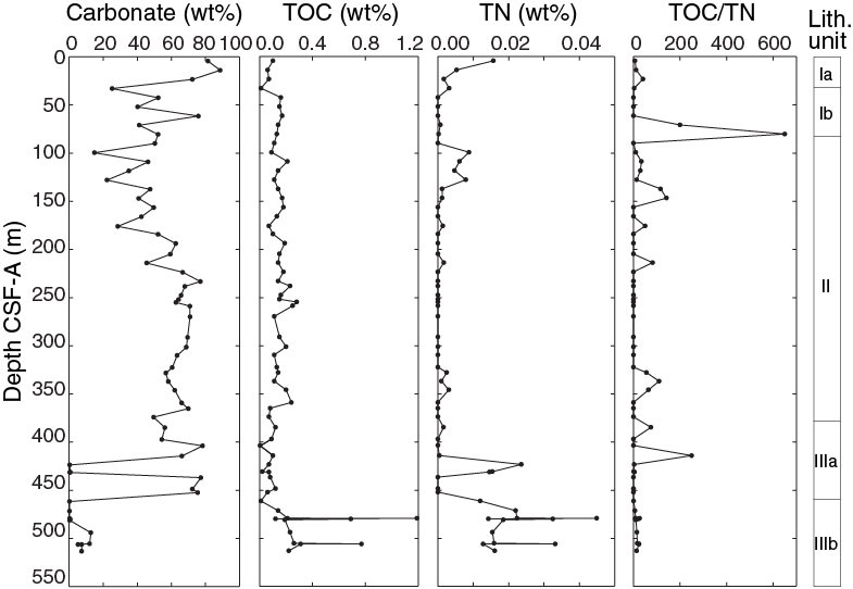
Figure F26. Carbon, nitrogen, and TOC/TN.
Total organic carbon (TOC) content at this site is generally very low (≤0.2 wt%) (Table T19; Figure F26). Black layers that were initially considered candidates for OAE 2–related deposits in Core 369-U1514C-27R (~431 m CSF-A) are remarkably low in TOC (<0.1 wt%). Three sedimentary black and green couplets from the depth and age (see Biostratigraphy and micropaleontology) expected for OAE 1d in Cores 32R and 34R are enriched in TOC in the black layers relative to each green layer; however, maximum TOC never exceeds 1.2 wt%.
Total nitrogen (TN) content was below detection level for approximately half of the samples. In samples with quantifiable TN content, values are all below 0.05 wt%. As TOC and TN contents are near detection limits, the calculated TOC/TN ratio has large uncertainties.
Organic matter source analysis
As no samples taken for routine analysis contained ≥0.8 wt% TOC based on bulk rock analyses, eight additional samples were taken from potential OAE 2 and 1d horizons and analyzed using source rock analysis (SRA). Two samples were taken from the thin black layers observed in Section 369-U1514C-27R-1. From the depth expected for OAE 1d, a small rock chip was taken from each lithology of three selected black and green couplets in Cores 32R and 34R (Table T20; Figure F27).
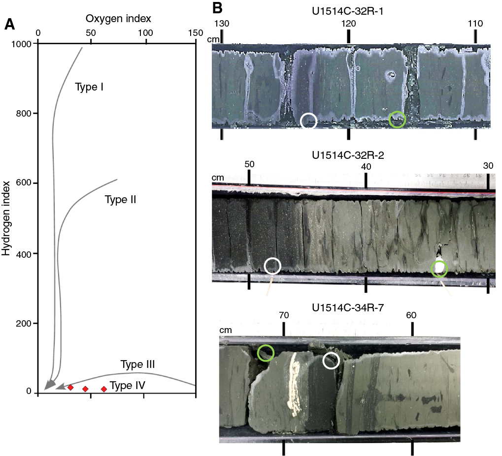
Figure F27. Source rock analysis.
TOC content was independently evaluated during SRA based on detection of pyrolyzed organic matter. Because this calculation of TOC employs a different analytical method, these TOC values do not necessarily correspond to TOC values reported from bulk sediment analysis (see Bulk sediment geochemistry). To discriminate TOC content derived from regular bulk sediment analysis, we designate values evaluated during source rock analysis as TOCSRA. Measurements of low TOCSRA values (<0.8 wt%) have large uncertainties and potentially overestimate hydrogen index (HI) and oxygen index (OI) values. The nominal temperature of the maximum rate of hydrocarbon yield (Tmax) from these low-TOCSRA samples show significant scatter and are likely not useful for estimating the thermal maturity of organic matter.
Samples from Core 369-U1514C-27R do not have a high TOCSRA content or a large S2 peak, indicating the that sediment is more likely to be pelagic clays. From the OAE 1d interval, the black layers (white circles in Figure F27B) of the black-green couplets have higher TOCSRA content (>1 wt%) and low S2 and moderate S3 values. This result indicates that the major kerogen is Type IV (Peters et al., 2005). Tmax values obtained from three samples containing ≥1 wt% TOCSRA through the putative OAE 1d interval range widely from 420° to 450°C, suggesting moderate to high thermal maturity.
Stratigraphic correlation
At Site U1514, Hole U1514A was cored with the APC and HLAPC systems to 197.47 m CSF-A, and 24 cores were recovered. Coring continued with the XCB system to 253.82 m CSF-A (Cores 369-U1514A-25X through 31X). In Hole U1514C, coring with the RCB system started at 195.60 m CSF-A and continued to 515.66 m DSF (Cores 369-U1514C-2R through 35R). A splice was created for the lower Eocene interval in Cores 369-U1514A-26X through 31X (208.2–253.82 m CSF-A) and Cores 369-U1514C-2R through 9R (195.6–264.31 m CSF-A).
Guidance for coring
A suitable depth to start coring in Hole U1514C was chosen based on physical property data from Hole U1514A. We looked for intervals where physical property measurements showed sufficient coherence and variability in amplitude within one or more of the data sets with the hope that if the same interval were recovered in Hole U1514C the correspondence between measurements would be convincing and increase confidence in correlation. A strong peak in NGR at 229 m CSF-A, coinciding with a laminated interval in Core 369-U1514A-28X, was identified as a primary correlation target. Two additional intervals, each containing a series of four NGR peaks in Cores 26X (210–215 m CSF-A) and 28X through 29X (234–240 m CSF-A), were identified as secondary targets. To provide samples that could be useful in verifying the level of biostratigraphic events observed in Hole U1514A and to attempt recovery of less-disturbed intervals in Hole U1514A, a target starting depth of 200 m CSF-A was recommended for Hole U1514C.
For Cores 369-U1514C-2R through 8R, magnetic susceptibility, GRA bulk density, and P-wave velocity were measured immediately after recovery on the Special Task Multisensor Logger at 10 cm resolution. The GRA bulk density and P-wave velocity data do not show coherent patterns between holes, but the magnetic susceptibility data do show coherent patterns that match those observed in Hole U1514A (Figures F24, F26). Magnetic susceptibility and NGR data in Hole U1514A also correlate with each other (Figure F24), and the variation in magnetic susceptibility values in Hole U1514C closely follows lithologic variations seen through the core liner. Thus, cores could be confidently aligned during coring. Depths below seafloor and patterns in magnetic susceptibility data suggested points of correlation between Holes U1514A and U1514C and were used to choose target depths for core breaks so that Hole U1514C cores would bridge coring gaps in Hole U1514A. Specifically, the depth to begin cutting Core 369-U1514C-7R was chosen so that it would span as much as possible of the poorly recovered interval between Cores 369-U1514A-29X and 30X (240.82–246.6 m CSF-A); this was the reason for the short advance (6 m) on Core 369-U1514C-6R.
Correlation of cores
Comparison of the physical property records from Holes U1514A and U1514C allowed for the construction of a splice plotted in m core composite depth below seafloor (CCSF) for Cores 369-U1514A-26X through 31X (208.2–253.82 m CSF-A) and 369-U1514C-2R through 9R (195.6–264.31 m CSF-A). Initially, cores were aligned using broad trends and sharp peaks in NGR, magnetic susceptibility (both point sensor and whole-round magnetic susceptibility; see Petrophysics), and color reflectance (L*; see Petrophysics). Where possible, correlation was refined preferentially using comparable variations in magnetic susceptibility, where present, because magnetic susceptibility data allow for higher resolution comparison (one measurement every 2.5 cm) than the NGR data sets (one measurement every 10 cm). One tie point between Cores 369-U1514A-28X and 369-U1514C-5R was selected based on L* because the color variation pattern over the laminated interval centered at 229 m CSF-A in Hole U1514A is very distinctive and corresponds closely to a laminated interval at 228 m CSF-A in Hole U1514C. Remaining tie points were chosen based on NGR variations, especially where overlap between cores was limited. The broad trends in NGR consistently show coherent patterns between the holes, and these similarities best demonstrate the accuracy of the splice. After correlation, the most continuous and representative intervals of both holes were incorporated in the splice.
Core-log integration
Recognition of sharp peaks in NGR data at 18 depths present in both core-based measurements and wireline logging data in Hole U1513C permitted translation of the CSF-A scale to the WMSF scale (see Petrophysics) (Figure F28; Table T21). Tie points were chosen at peak values in NGR within broad trends in both the core data and wireline logging results.
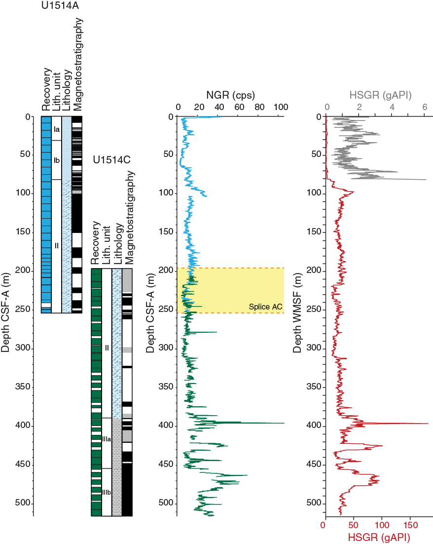
Figure F28. Correlation between core-based data and wireline log NGR data.
Summary
The cored interval at Site U1514 includes seemingly complete stratigraphic records of the Eocene/Oligocene and K/Pg boundaries and a relatively expanded record of most of the Eocene and Paleogene. A multicolor interval of Turonian to Campanian rocks spanning Cores 369-U1514C-27R through 29R separates the younger units from Albian and Cenomanian claystone and correlates with a zone of low salinity. The interval is interpreted as a zone of deformation possibly associated with downslope motion of most of the Late Cretaceous and Cenozoic section. Carbonate content is moderate to high through the Cenozoic section where good biostratigraphic and paleomagnetic data provide excellent age control (Figure F29). The Oligocene and Miocene interval was interrupted by hiatuses, and sediment accumulation rates between these breaks was quite low (3–9 m/My). Accumulation rates were moderate for the Eocene and Paleocene (~1.5 cm/ky). Sedimentation rates are not calculated for the Cretaceous as structural complications are large in this interval (see Biostratigraphy and micropaleontology).

Figure F29. Site U1514 summary.
References
Alegret, L., Ortiz, S., Orue-Extebarria, X., Bernaola, G., Baceta, J.I., Monechi, S., Apellaniz, E., and Pujalte, V., 2009. The Paleocene–Eocene Thermal Maximum: new data on microfossil turnover at the Zumaia section, Spain. Palaios, 24(5):318–328. https://doi.org/10.2110/palo.2008.p08-057r
Alegret, L., and Thomas, E., 2013. Benthic foraminifera across the Cretaceous/Paleogene boundary in the Southern Ocean (ODP Site 690): diversity, food and carbonate saturation. Marine Micropaleontology, 105:40–51. https://doi.org/10.1016/j.marmicro.2013.10.003
Bischoff, J.L., and Dickson, F.W., 1975. Seawater-basalt interaction at 200°C and 500 bars: implications for origin of sea-floor heavy-metal deposits and regulation of seawater chemistry. Earth and Planetary Science Letters, 25(3):385–397. https://doi.org/10.1016/0012-821X(75)90257-5
Borissova, I., 2002. Geological Framework of the Naturaliste Plateau. Geoscience Australia, 2002/20. http://www.ga.gov.au/metadata-gateway/metadata/record/40535/
Brumsack, H.-J., and Zuleger, E., 1992. Boron and boron isotopes in pore waters from ODP Leg 127, Sea of Japan. Earth and Planetary Science Letters, 113(3):427–433. https://doi.org/10.1016/0012-821X(92)90143-J
Church, T.M., and Wolgemuth, K., 1972. Marine barite saturation. Earth and Planetary Science Letters, 15(1):35–44. https://doi.org/10.1016/0012-821X(72)90026-X
De Vleeschouwer, D., Dunlea, A.G., Auer, G., Anderson, C.H., Brumsack, H., de Loach, A., Gurnis, M., et al., 2017. Quantifying K, U, and Th contents of marine sediments using shipboard natural gamma radiation spectra measured on DV JOIDES Resolution. Geochemistry, Geophysics, Geosystems, 18(3):1053–1064. https://doi.org/10.1002/2016GC006715
Edgar, K.M., Wilson, P.A., Sexton, P.F., and Suganuma, Y., 2007. No extreme bipolar glaciation during the main Eocene calcite compensation shift. Nature, 448(7156):908–911. https://doi.org/10.1038/nature06053
Gale, A.S., Bown, P., Caron, M., Crampton, J., Crowhurst, S.J., Kennedy, W.J., Petrizzo, M.R., and Wray, D.S., 2011. The uppermost middle and upper Albian succession at the Col de Palluel, Hautes-Alpes, France: an integrated study (ammonites, inoceramid bivalves, planktonic foraminifera, nannofossils, geochemistry, stable oxygen and carbon isotopes, cyclostratigraphy). Cretaceous Research, 32(2):59–130. https://doi.org/10.1016/j.cretres.2010.10.004
Gieskes, J.M., Gamo, T., and Brumsack, H., 1991. Technical Note 15: Chemical Methods for Interstitial Water Analysis Aboard JOIDES Resolution. Ocean Drilling Program. https://doi.org/10.2973/odp.tn.15.1991
Gieskes, J.M., and Lawrence, J.R., 1981. Alteration of volcanic matter in deep-sea sediments: evidence from the chemical composition of interstitial waters from deep sea drilling cores. Geochimica Cosmochimica Acta, 45(10):1687–1703. https://doi.org/10.1016/0016-7037(81)90004-1
Gradstein, F.M., Ogg, J.G., Schmitz, M.D., and Ogg, G.M. (Eds.), 2012. The Geological Time Scale 2012: Amsterdam (Elsevier).
Huber, B.T., Hobbs, R.W., Bogus, K.A., Batenburg, S.J., Brumsack, H.-J., do Monte Guerra, R., Edgar, K.M., Edvardsen, T., Garcia Tejada, M.L., Harry, D.L., Hasegawa, T., Haynes, S.J., Jiang, T., Jones, M.M., Kuroda, J., Lee, E.Y., Li, Y.-X., MacLeod, K.G., Maritati, A., Martinez, M., O’Connor, L.K., Petrizzo, M.R., Quan, T.M., Richter, C., Riquier, L., Tagliaro, G.T., Wainman, C.C., Watkins, D.K., White, L.T., Wolfgring, E., and Xu, Z., 2019a. Expedition 369 methods. In Hobbs, R.W., Huber, B.T., Bogus, K.A., and the Expedition 369 Scientists, Australia Cretaceous Climate and Tectonics. Proceedings of the International Ocean Discovery Program, 369: College Station, TX (International Ocean Discovery Program). https://doi.org/10.14379/iodp.proc.369.102.2019
Huber, B.T., Hobbs, R.W., Bogus, K.A., Batenburg, S.J., Brumsack, H.-J., do Monte Guerra, R., Edgar, K.M., Edvardsen, T., Garcia Tejada, M.L., Harry, D.L., Hasegawa, T., Haynes, S.J., Jiang, T., Jones, M.M., Kuroda, J., Lee, E.Y., Li, Y.-X., MacLeod, K.G., Maritati, A., Martinez, M., O’Connor, L.K., Petrizzo, M.R., Quan, T.M., Richter, C., Riquier, L., Tagliaro, G.T., Wainman, C.C., Watkins, D.K., White, L.T., Wolfgring, E., and Xu, Z., 2019b. Site U1513. In Hobbs, R.W., Huber, B.T., Bogus, K.A., and the Expedition 369 Scientists, Australia Cretaceous Climate and Tectonics. Proceedings of the International Ocean Discovery Program, 369: College Station, TX (International Ocean Discovery Program). https://doi.org/10.14379/iodp.proc.369.104.2019
Huber, B.T., MacLeod, K.G., and Tur, N.A., 2008. Chronostratigraphic framework for upper Campanian–Maastrichtian sediments on the Blake Nose (subtropical North Atlantic). Journal of Foraminiferal Research, 38(2):162–182. https://doi.org/10.2113/gsjfr.38.2.162
Huber, B.T., Petrizzo, M.R., Watkins, D.K., Haynes, S.J., and MacLeod, K.G., 2017. Correlation of Turonian continental margin and deep-sea sequences in the subtropical Indian Ocean sediments by integrated planktonic foraminiferal and calcareous nannofossil biostratigraphy. Newsletters on Stratigraphy, 50(2):141–185. https://doi.org/10.1127/nos/2017/0373
Kaminski, M.A., and Gradstein, F.M., 2005. Atlas of Paleogene cosmopolitan deep-water agglutinated foraminifera. Grzybowski Foundation Special Publication, 10. http://www.foraminifera.eu/atlas.html
Kirschvink, J.L., 1980. The least-squares line and plane and the analysis of palaeomagnetic data. Geophysical Journal of the Royal Astronomical Society, 62(3):699–718. https://doi.org/10.1111/j.1365-246X.1980.tb02601.x
Lurcock, P.C., and Wilson, G.S., 2012. PuffinPlot: a versatile, user-friendly program for paleomagnetic analysis. Geochemistry, Geophysics, Geosystems, 13(6):Q06Z45. https://doi.org/10.1029/2012GC004098
Maloney, D., Sargent, C., Direen, N.G., Hobbs, R.W., and Gröcke, D.R., 2011. Re-evaluation of the Mentelle Basin, a polyphase rifted margin basin, offshore southwest Australia: new insights from integrated regional seismic datasets. Solid Earth, 2(2):107–123. https://doi.org/10.5194/se-2-107-2011
Ogg, J.G., 2012. Geomagnetic polarity time scale. In Gradstein, F.M., Ogg, J.G., Schmitz, M.D., and Ogg, G.M. (Eds.), The Geologic Time Scale 2012: Amsterdam (Elsevier), 85–113. https://doi.org/10.1016/B978-0-444-59425-9.00005-6
Pearson, P.N., Olsson, R.K., Hemleben, C., Huber, B.T., and Berggren, W.A., 2006. Atlas of Eocene planktonic foraminifera. Special Publication - Cushman Foundation for Foraminiferal Research, 41.
Perch-Nielsen, K., 1985. Mesozoic calcareous nannofossils. In Bolli, H.M., Saunders, J.B., and Perch-Nielsen, K. (Eds.), Plankton Stratigraphy: Cambridge, United Kingdom (Cambridge University Press), 329–426.
Peters, K.E., Walters, C.C., and Moldowan, J.M., 2004. The Biomarker Guide (Volume 2): Biomarkers and Isotopes in Petroleum Systems and Earth History: Cambridge, United Kingdom (Cambridge University Press). https://doi.org/10.1017/CBO9781107326040
Petrizzo, M.R., 2000. Upper Turonian–lower Campanian planktonic foraminifera from southern mid–high latitudes (Exmouth Plateau, NW Australia): biostratigraphy and taxonomic notes. Cretaceous Research, 21(4):479–505. https://doi.org/10.1006/cres.2000.0218
Petrizzo, M.R., 2001. Late Cretaceous planktonic foraminifera from the Kerguelen Plateau (ODP Leg 183): new data to improve the Southern Oceans biozonation. Cretaceous Research, 22(6):829–855. https://doi.org/10.1006/cres.2001.0290
Petrizzo, M.R., 2003. Late Cretaceous planktonic foraminiferal bioevents in the Tethys and in the Southern Ocean record: an overview. Journal of Foraminiferal Research, 33(4):330–337. https://doi.org/10.2113/0330330
Petrizzo, M.R., Falzoni, F., and Premoli Silva, I., 2011. Identification of the base of the lower-to-middle Campanian Globotruncana ventricosa Zone: comments on reliability and global correlations. Cretaceous Research, 32(3):387–405. https://doi.org/10.1016/j.cretres.2011.01.010
Petrizzo, M.R., and Huber, B.T., 2006. On the phylogeny of the late Albian genus Planomalina. Journal of Foraminiferal Research, 36(3):233–240. https://doi.org/10.2113/gsjfr.36.3.233
Premoli Silva, I., and Sliter, W.V., 1995. Cretaceous planktonic foraminiferal biostratigraphy and evolutionary trends from the Bottaccione section, Gubbio, Italy. Palaeontographia Italica, 82:2–90.
Pribnow, D., Kinoshita, M., and Stein, C., 2000. Thermal Data Collection and Heat Flow Recalculations for Ocean Drilling Program Legs 101–180: Hanover, Germany (Institute for Joint Geoscientific Research, Institut für Geowissenschaftliche Gemeinschaftsaufgaben [GGA]). http://www-odp.tamu.edu/publications/heatflow/ODPReprt.pdf
Richter, C., Acton, G., Endris, C., and Radsted, M., 2007. Technical Note 34: Handbook for Shipboard Paleomagnetists. Ocean Drilling Program. https://doi.org/10.2973/odp.tn.34.2007
Robaszynski, F., and Caron, M., 1995. Foraminifères planctoniques du Crétacé: commentaire de la zonation Europe-Méditerranée. Bulletin De La Societe Geologique De France, 166:681–692.
Robaszynski, F., González Donoso, J.M., Linares, D., Amédro, F., Caron, M., Dupuis, C., Dhondt, A.V., and Gartner, S., 2000. Le Crétacé Supérieur de la région de Kalaat Senan, Tunisie Centrale. Lithobiostratigraphie intégrée: zones d’ammonites, de foraminifères planctoniques et de nannofossiles du Turonien supérieur au Maastrichtien. Bulletin des Centres de Recherche Exploration-Production Elf-Aquitaine, 22:359–490.
Tjalsma, R.C., and Lohmann, G.P., 1983. Paleocene–Eocene bathyal and abyssal benthic foraminifera from the Atlantic Ocean. Micropaleontology, Special Publication, 4.
Torres, M.E., Brumsack, H.-J., Bohrmann, G., and Emeis, K.C., 1996. Barite fronts in continental margin sediments: a new look at barium remobilization in the zone of sulfate reduction and formation of heavy barites in diagenetic fronts. Chemical Geology, 127(1–3):125–139. https://doi.org/10.1016/0009-2541(95)00090-9
van Morkhoven, F.P.C.M., Berggren, W.A., Edwards, A.S.,and Oertli, H.J., 1986. Cenozoic cosmopolitan deep-water benthic foraminifera. Bulletin des Centres de Recherches Exploration-Production Elf-Aquitaine: Mémoire, 11.
Wade, B.S., Pearson, P.N., Berggren, W.A., and Pälike, H., 2011. Review and revision of Cenozoic tropical planktonic foraminiferal biostratigraphy and calibration to the geomagnetic polarity and astronomical time scale. Earth-Science Reviews, 104(1–3):111–142. https://doi.org/10.1016/j.earscirev.2010.09.003
Zijderveld, J.D.A., 1967. AC demagnetization of rocks: analysis of results. In Collinson, D.W., Creer, K.M., and Runcorn, S.K. (Eds.), Developments in Solid Earth Geophysics (Volume 3): Methods in Palaeomagnetism: Amsterdam (Elsevier), 254–286. https://doi.org/10.1016/B978-1-4832-2894-5.50049-5
1 Huber, B.T., Hobbs, R.W., Bogus, K.A., Batenburg, S.J., Brumsack, H.-J., do Monte Guerra, R., Edgar, K.M., Edvardsen, T., Garcia Tejada, M.L., Harry, D.L., Hasegawa, T., Haynes, S.J., Jiang, T., Jones, M.M., Kuroda, J., Lee, E.Y., Li, Y.-X., MacLeod, K.G., Maritati, A., Martinez, M., O’Connor, L.K., Petrizzo, M.R., Quan, T.M., Richter, C., Riquier, L., Tagliaro, G.T., Wainman, C.C., Watkins, D.K., White, L.T., Wolfgring, E., Xu, Z., 2019. Site U1514. In Hobbs, R.W., Huber, B.T., Bogus, K.A., and the Expedition 369 Scientists, Australia Cretaceous Climate and Tectonics. Proceedings of the International Ocean Discovery Program, 369: College Station, TX (International Ocean Discovery Program). https://doi.org/10.14379/iodp.proc.369.105.2019
2 Expedition 369 Scientists’ affiliations.
This work is distributed under the Creative Commons Attribution 4.0 International (CC BY 4.0) license. 
- F1. Site U1514 location.
- F2. Seismic Profile s310_17.
- F3. Lithostratigraphic summary.
- F4. Unit boundaries and dominant lithologies.
- F5. Sediment constituents.
- F6. XRD results.
- F7. Sedimentary characteristics.
- F8. Age-depth plot.
- F9. Selected planktonic foraminifers.
- F10. Paleomagnetic data, Hole U1514A.
- F11. Paleomagnetic data. Hole U1514C.
- F12. Vector endpoint diagrams for section halves, Hole U1514A.
- F13. Vector endpoint diagrams for section halves, Hole U1514C.
- F14. Vector endpoint diagrams for representative discrete samples.
- F15. Magnetostratigraphic results.
- F16. Age-depth plot.
- F17. Physical properties, Hole U1514A.
- F18. NGR data, Hole U1514A.
- F19. Physical properties, Hole U1514C.
- F20. NGR data, Hole U1514C.
- F21. Density, porosity, thermal conductivity, and P-wave velocity, Hole U1514A.
- F22. Density, porosity, thermal conductivity, and P-wave velocity, Hole U1514C.
- F23. Downhole logging main pass results.
- F24. Headspace gas methane concentration.
- F25. Interstitial water geochemistry.
- F26. Carbon, nitrogen, and TOC/TN.
- F27. Source rock analysis.
- F28. Correlation between core-based data and wireline log NGR data.
- F29. Site U1514 summary.
- T1. Core summary.
- T2. Lithostratigraphic units.
- T3. XRF results.
- T4. Selected microfossil groups and minerals.
- T5. Calcareous nannofossil bioevents.
- T6. Foraminifer datums.
- T7. Calcareous nannofossil distribution, Hole U1514A.
- T8. Calcareous nannofossil distribution, Hole U1514C.
- T9. Planktonic foraminifer distribution, Hole U1514A.
- T10. Planktonic foraminifer distribution, Hole U1514C.
- T11. Benthic foraminifer distribution, Hole U1514A.
- T12. Benthic foraminifer distribution, Hole U1514C.
- T13. Core orientation data.
- T14. Paleomagnetic data.
- T15. Magnetic reversal depths and ages.
- T16. Downhole temperatures.
- T17. Gas element data.
- T18. Interstitial water geochemistry.
- T19. Bulk sediment geochemistry.
- T20. Source rock analysis data.
- T21. Core and wireline NGR data correlation.