Hobbs, R.W., Huber, B.T., Bogus, K.A., and the Expedition 369 Scientists
Proceedings of the International Ocean Discovery Program Volume 369
publications.iodp.org

https://doi.org/10.14379/iodp.proc.369.102.2019
Expedition 369 methods1
B.T. Huber, R.W. Hobbs, K.A. Bogus, S.J. Batenburg, H.-J. Brumsack, R. do Monte Guerra, K.M. Edgar, T. Edvardsen, M.L. Garcia Tejada, D.L. Harry, T. Hasegawa, S.J. Haynes, T. Jiang, M.M. Jones, J. Kuroda, E.Y. Lee, Y.-X. Li, K.G. MacLeod, A. Maritati, M. Martinez, L.K. O’Connor, M.R. Petrizzo, T.M. Quan, C. Richter, L. Riquier, G.T. Tagliaro, C.C. Wainman, D.K. Watkins, L.T. White, E. Wolfgring, and Z. Xu2
Keywords: International Ocean Discovery Program, IODP, JOIDES Resolution, Expedition 369, Site U1512, Site U1513, Site U1514, Site U1515, Site U1516, Hot Cretaceous Greenhouse, oceanic anoxic events, Mentelle Basin, Naturaliste Plateau, Great Australian Bight, Gondwana breakup, Tasman Gateway, Indonesian Gateway, cyclostratigraphy, carbon isotope excursions, Paleocene/Eocene Thermal Maximum, Eocene greenhouse, Miocene, volcanic rifted margin, nonvolcanic rifted margin
MS 369-102: Published 25 May 2019
Introduction
This chapter documents the procedures and methods used in the shipboard laboratories during International Ocean Discovery Program (IODP) Expedition 369. This introductory section in particular provides a rationale for the site locations and an overview of IODP depth conventions, curatorial procedures, and general core handling/analyses during Expedition 369. Subsequent sections describe specific laboratory procedures and instruments in more detail. This information only applies to shipboard work described in the Proceedings volume; methods used in shore-based analyses of Expedition 369 samples and/or data will be described in various scientific contributions in the open peer-reviewed literature and the Expedition Research Results chapters of this Proceedings volume.
Site locations
The five sites (U1512–U1516) drilled during Expedition 369 are situated in the Great Australian Bight (Site U1512) and off southwestern Western Australia in the Mentelle Basin (Sites U1513–U1516). These sites were targeted because coring the Cretaceous sequence at different paleodepths will allow recovery of material suitable for generating records that span the rise and collapse of the Cretaceous hot greenhouse (including Oceanic Anoxic Events [OAEs] 1d and 2), providing insight to resultant changes to deep- and surface-water circulation that can be used to test predictions from Earth system models. The sites are also well positioned to monitor the mid-Eocene to early Oligocene opening of the Tasman Gateway and the Miocene to Pliocene restriction of the Indonesian Gateway; both passages have important effects on global oceanography and climate. Coring Early Cretaceous volcanic rocks and underlying Jurassic(?) sediments in different parts of the Mentelle Basin provides information on the timing of different stages of the Gondwana breakup and the nature of the various phases of volcanism that will lead to an improved understanding of the evolution of the Naturaliste Plateau and Mentelle Basin. Previous work by both academia and industry provided site data, including seismic data acquired in 1986, 2004, and 2009 by Geoscience Australia and limited physical material (e.g., Deep Sea Drilling Project [DSDP] Site 258 and dredge samples adjacent to Site U1512 and on the margins of the Naturaliste Plateau), that were used to guide the initial operations plan for each site.
GPS coordinates from precruise site surveys were used to position the vessel at all Expedition 369 sites. A SyQuest Bathy 2010 CHIRP subbottom profiler was used to monitor the seafloor depth on the approach to each site to reconfirm the depth profiles from precruise surveys. Once the vessel was positioned at the site coordinates, the thrusters were lowered and an acoustic positioning beacon was dropped to the seafloor. The dynamic positioning control of the vessel used navigational input from the GPS and triangulation to the seafloor beacon, weighted by the estimated positional accuracy. The final hole position was the mean position calculated from the GPS data collected over a significant portion of the time the hole was occupied.
Coring and drilling operations
All four standard coring systems, the advanced piston corer (APC), half-length APC (HLAPC), extended core barrel (XCB), and rotary core barrel (RCB), were used during Expedition 369 (see Operations in the individual site chapters).
The APC system was generally used in the upper portion of a hole to obtain high-quality core. The APC system cuts soft-sediment cores with minimal visual coring disturbance relative to other IODP coring systems. After the APC core barrel is lowered through the drill pipe and lands near the bit, the drill pipe is pressured up until the shear pins that hold the inner barrel attached to the outer barrel fail. The inner barrel then advances into the formation and cuts the core. The driller can detect a successful cut, or “full stroke,” from the pressure gauge on the rig floor.
APC refusal is conventionally defined in two ways: (1) the piston fails to achieve a complete stroke (as determined from the pump pressure reading) because the formation is too hard, or (2) excessive force (>60,000 lb; ~267 kN) is required to pull the core barrel out of the formation. When a full stroke cannot be achieved, additional attempts are typically made, and after each attempt the bit is advanced by the core recovery (in meters). The number of additional attempts is generally dictated by the length of recovery of the partial stroke core and the time available to advance the hole by piston coring. Note that this process results in a nominal recovery of ~100% based on the assumption that the barrel penetrates the formation by the equivalent of the length of core recovered. When a full or partial stroke is achieved but excessive force cannot retrieve the barrel, the core barrel is sometimes “drilled over,” meaning after the inner core barrel is successfully shot into the formation, the drill bit is advanced to the full stroke depth to free the APC barrel.
Nonmagnetic core barrels were used during all APC coring to a pull force of ~40,000 lb. In all Expedition 369 APC holes, orientation was attempted with either the Icefield MI-5 or Minex FlexIT core orientation tool (see Paleomagnetism). Formation temperature measurements were taken in many of the second APC holes to obtain temperature gradients and heat flow estimates (see Petrophysics).
Once APC refusal was reached, the HLAPC system was used. The standard APC system contains a 9.5 m long core barrel; the HLAPC system uses a 4.7 m long core barrel. In most instances, the HLAPC system was deployed after the APC system reached refusal to extend the total piston coring depth or when a more indurated interval was anticipated (e.g., silicified limestones/cherts at Site U1513). While using the HLAPC system, the same criteria as for the APC system were applied in terms of refusal. The HLAPC system allowed us to reach greater piston sampling depths and recover more indurated material in the upper sections than would have been possible with the APC or XCB systems.
The XCB coring system was used to advance the hole when the formation became too stiff for HLAPC coring (e.g., Site U1514) or hard substrate was encountered in the upper sections of a hole (e.g., Site U1513). The XCB rotary system has a small cutting shoe (bit) that extends below the large APC/XCB bit. The smaller bit can cut a semi-indurated core with less torque and fluid circulation than the main bit, thereby optimizing recovery. The XCB cutting shoe extends ~30.5 cm ahead of the main bit in soft sediment but retracts into the main bit when hard formations are encountered. Use of this system resulted in the greatest loss of core quality; the majority of XCB cores collected during Expedition 369 were highly biscuited. However, the APC and XCB systems use the same bit, so it is possible to switch between the two coring systems in the same hole.
The bottom-hole assembly (BHA) is the lowermost part of the drill string. A typical APC/XCB BHA consists of a drill bit (outer diameter = 11⁷⁄₁₆ inches; ~20.05 cm), a bit subassembly, a seal bore drill collar, a landing saver subassembly, a modified top subassembly, a modified head subassembly, a nonmagnetic drill collar, a number of 8 inch (~20.32 cm) drill collars, a tapered drill collar, six joints (two stands) of 5½ inch (~13.97 cm) drill pipe, and one crossover subassembly. A lockable float valve was used when downhole logging was planned so that downhole logs could be collected through the bit (e.g., Hole U1513A).
The RCB system is generally deployed when XCB coring reaches refusal (generally when the time to cut a core is >90 min), but it was also used during Expedition 369 as an alternative to the XCB system and to duplicate XCB-cored intervals to recover cores with reduced disturbance (biscuiting). The RCB system was also the only coring system used at two sites (U1512 and U1515).
The RCB system is a conventional rotary drilling system. The RCB system requires a dedicated RCB BHA and a dedicated RCB drilling bit. The BHA used for RCB coring included a 9⅞ inch (~20.08 cm) RCB drill bit, a mechanical bit release (if logging was considered), a modified head subassembly, an outer core barrel, a modified top subassembly, a modified head subassembly, and 7–10 control-length drill collars followed by a tapered drill collar to the two stands of 5½ inch drill pipe. Most cored intervals were ~9.6 m long, which is the length of a standard rotary core and approximately the length of a joint of drill pipe. In some cases, the drill string was drilled or “washed” ahead without recovering sediment to advance the drill bit to a target depth to resume core recovery. Such intervals were typically drilled using a center bit installed within the RCB bit. When coring, half cores were occasionally collected with both the XCB and RCB systems (e.g., Site U1513) to improve recovery over critical intervals (e.g., Cenomanian/Turonian boundary) and when rates of penetration decreased significantly.
Coring disturbance
Core material has the potential to be disturbed and/or contain extraneous material as a result of the drilling process, core handling, and analysis. In formations with loose granular layers (e.g., sand), material from intervals higher in the hole may be washed down by drilling circulation, accumulate at the bottom of the hole, and then be sampled with the recovery of the next core. This is referred to as “fall-in.” Expedition 369 cores showed evidence of fall-in, and when present it affects the upper ~10–40 cm of the cores. Common coring deformation includes the concave appearance of originally horizontal bedding. Another disturbance type is “flow-in,” in which the piston coring action results in fluidization at the bottom of the core; this disturbance was seen in several cores from Sites U1513 and U1514. Retrieval of the core from depth to the surface may result in elastic rebound. Gas that is in solution at depth may become free and drive core segments within the liner apart. Both elastic rebound and gas pressure can result in a total length for each core that is longer than the interval that was cored and thus a calculated recovery of >100%. If gas expansion or other coring disturbance results in a void in any particular core section, the void can be closed by moving material if it is very large, stabilized by a foam insert if it is moderately large, or left as is. When gas content is high, pressure must be relieved for safety reasons before the cores are cut into segments. Drilling holes into the liner releases this gas but also results in some sediment being extruded out of the liner. In more consolidated material, a common core disturbance is biscuiting, in which fractured material (biscuits) spin within the core barrel. In many cases, drilling slurry is injected between them. Finally, fracturing, fragmentation, and brecciation as a result of the drilling process are also common drilling-induced disturbance types.
The occurrence of these disturbance types is reported in the Lithostratigraphy sections of the site chapters and graphically represented on the visual core descriptions (VCDs).
Site, hole, core, and sample numbering
Numbering of the sites, holes, cores, and samples followed standard IODP protocol. Drilling sites have been numbered consecutively from the first site drilled by the Glomar Challenger in 1968, and since Expedition 301 the prefix “U” has been used to designate sites cored by the R/V JOIDES Resolution. At a site, multiple holes are often drilled, and a letter suffix distinguishes the holes drilled at one site. For example, the first hole would be given the suffix “A,” the second “B,” and so on.
Following the hole designation, each recovered core is numbered sequentially. A cored interval is generally ~9.5 m, the length of a standard core barrel, with the exception of the 4.7 m core barrel of the HLAPC system. The specific coring system used to recover a core is designated by a letter representing the core type and is a suffix to the core number. The coring system letters are H = APC, F = HLAPC, X = XCB, and R = RCB.
Each recovered core is cut into ~1.5 m sections. The number of sections is determined by the core recovery, and sections are numbered sequentially starting with “1” at the top of the core. Each core is eventually split lengthwise into working- and archive-half sections (see below) designated by either the letter “W” or “A” succeeding the core number. For depth calculation purposes (see below), the top depth of the core is equated with the top depth of the cored interval (usually in meters drilling depth below seafloor [m DSF]) to achieve consistency in handling analytical data derived from the cores. Sample intervals are described in centimeters within a core section (typically between 0 and 150 cm) beginning from the top of the core section.
Thus, the full curatorial identifier of a sample consists of the following: expedition, site, hole, core number, core type, section number, section half, and interval in centimeters measured from the top of the core section. For example, a sample identified as “369-U1512A-24R-3W, 50–55 cm” represents a 5 cm interval from the third section (working half) of Core 24R (cored with the RCB system) from Hole A of Site U1512 during Expedition 369 (Figure F1).
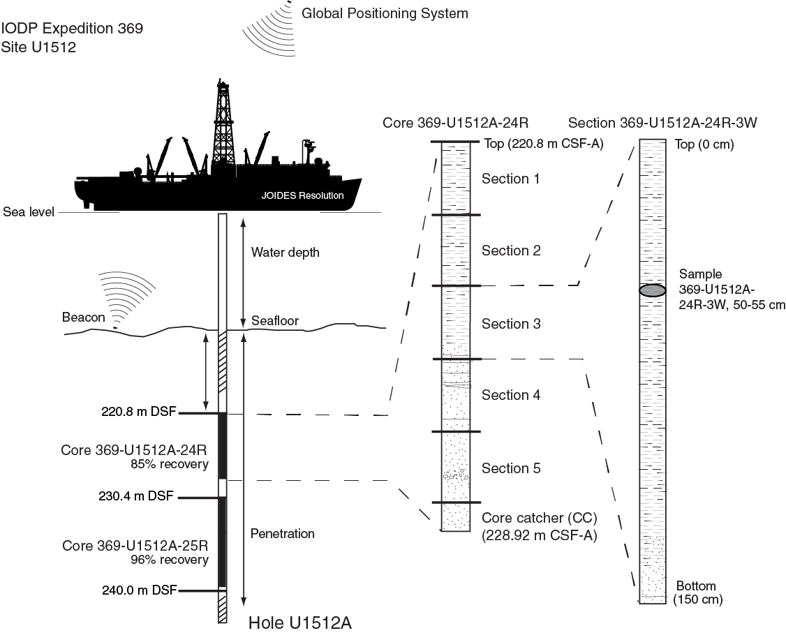
Figure F1. IODP naming conventions.
Sample depth calculation
During Expedition 369, the cored interval was measured in meters as determined by core depth below seafloor, method A (CSF-A). This calculation is defined by protocol (see “IODP Depth Scales Terminology” at http://www.iodp.org/policies-and-guidelines). In general, the depth below seafloor is determined by subtracting the initial drill pipe measurement to the seafloor from the total drill pipe measurement (DSF; Figure F1). The core depth interval begins with the depth below seafloor where coring began and extends to the depth that coring advanced. However, if a core has incomplete recovery (<100%), all material is assumed to originate from the top of the cored interval as a continuous section for curation purposes; thus, the true depth interval within the cored interval is unknown and represents a sampling uncertainty in age-depth analysis or correlation with downhole logging data. Three sites (U1513, U1514, and U1516) had sections that were correlated when multiple holes were cored to produce a splice based on a core composite depth below seafloor (CCSF) scale. The calculation of this depth scale is discussed in Stratigraphic correlation.
Additionally, wireline log depths were calculated from the wireline log depth below seafloor (WSF). When multiple logging passes were made (see Petrophysics), the wireline log depths are matched to one reference pass, creating the wireline log matched depth below seafloor (WMSF). These distinctions in nomenclature between core (curated) and wireline log depth should be noted because the same depth value from different scales does not necessarily refer to the same stratigraphic interval. In several cases, however, core to log tie points were provided by the stratigraphic correlators (see Stratigraphic correlation in the Site U1512, Site U1513, Site U1514, Site U1515, and Site U1516 chapters (Huber et al., 2019a–2019e).
Core handling and analysis
For sediment cores, core catcher samples were taken for biostratigraphic analyses immediately upon arriving on deck. The cores were then cut into ~1.5 m sections, after which whole-round samples were taken for shipboard interstitial water and noted by the use of a yellow end cap. Additional samples taken on the catwalk include syringe samples for routine hydrocarbon gas safety monitoring (see Geochemistry). At sites where piston coring occurred (Sites U1513, U1514, and U1516), a separate, short hole was cored to obtain samples for postcruise optically stimulated luminescence analyses (see Operations in the Site U1513, Site U1514, and Site U1516 chapters [Huber et al., 2019b, 2019c, 2019e] and core summary tables therein). In this case, all of the recovered material was cut into 30 cm whole rounds on the catwalk and immediately placed into light-proof bags.
Once the core sections were brought inside, they were immediately run through the Special Task Multisensor Logger (STMSL) by the stratigraphic correlators to aid in drilling guidance (see Stratigraphic correlation) before being placed in the core racks and allowed to thermally equilibrate.
For hard rock cores on the catwalk, pieces were pushed to the bottom of the sections and the total length was measured as “recovered length,” which was used to calculate recovery. The sections were then brought into the core splitting room, where, if possible, the pieces of core were oriented with respect to each other; these relationships were marked with a wax pencil. In several cases, pieces were too small to be oriented with certainty. Pieces in a section were placed into sample bins separated by plastic core spacers. The plastic spacers were also used to indicate areas of no recovery. Adjacent pieces that could be fitted back together were curated as single pieces. Once completed, a designated scientist, usually the petrologist, confirmed the piece matches and drew split lines indicating where/how the pieces should be cut into archive and working halves. The split lines ideally maximized the expression of dipping surfaces on the cut face of the core while preserving representative features in the archive and working halves.
Once the split lines were drawn, the spacers were secured in place with acetone in both archive- and working-half core liners with the angle brace facing uphole, ensuring that the curated interval for each bin matched the top of each piece. The length of each bin was entered into SampleMaster as “bin length,” and the sum of bin lengths of a section was entered as the “curated length.” Additionally, the length of each piece was measured along the longest vertical dimension and entered as “piece length” (Figure F2). Following this process, the empty core liner half was placed over the full half and taped together in several places. The cores were allowed to dry and equilibrate.

Figure F2. Hard rock core curation labeling.
After all of the cores (sediment and hard rock) equilibrated to laboratory temperature (~4 h), they were run through the Whole-Round Multisensor Logger (WRMSL) for P-wave velocity, magnetic susceptibility, and gamma ray attenuation (GRA) bulk density measurements and through the Natural Gamma Radiation Logger (NGRL). Thermal conductivity measurements were also taken (see Petrophysics).
For sediments, core sections were split lengthwise into archive- and working-half sections. Oriented pieces of more indurated sediments were marked on the bottom with a red wax pencil. For hard rock, the pieces were halved on the saw following the split lines and placed into the respective working- and archive-half bin.
The working-half sections were used for taking discrete shipboard samples for paleomagnetic, physical property, geochemical, and thin section analyses (for details see the individual laboratory group methods in this chapter) and, in some limited cases, science party personal samples for postcruise research. Sampling for postcruise research was based on the sampling plan agreed on by the science party and the Sample Allocation Committee. The majority of samples for personal postcruise research were taken at a sampling party at the Gulf Coast Repository (College Station, Texas, USA) on 18–22 May 2018.
The archive-half core sections were run through the Section Half Imaging Logger (SHIL), as well as the Section Half Multisensor Logger (SHMSL) for color reflectance and point magnetic susceptibility measurements. The archive halves were described by expedition scientists visually and by smear slide analyses. Finally, most of the sections were measured with the cryogenic magnetometer (see Paleomagnetism).
All instrument data collected during Expedition 369 were uploaded to the IODP Laboratory Information Management System (LIMS) database (http://web.iodp.tamu.edu/LORE), and core descriptions were entered using the DESClogik application, a program used to input visual (macroscopic and/or microscopic) core descriptions (see the DESClogik user guide at http://iodp.tamu.edu/labs/documentation).
When all shipboard measurements were completed, data were uploaded, and samples were taken, the cores were wrapped in clear plastic film, sealed in plastic D-tubes, and transferred to cold storage on the ship. For core sections containing OAEs, which are characterized by high–organic carbon black shales, special handling was required. These OAE core sections were flushed with argon gas, wrapped in special plastic, and heat sealed with oxygen scrubbers inside. At the end of the expedition, the cores were transported to the Gulf Coast Repository until the sampling party, after which they were transported to long term cold storage at the Kochi Core Center (Kochi, Japan).
Authorship of methods and site chapters
The separate sections of the methods and site chapters were written by the following scientists (in alphabetical order):
- Background and objectives: Hobbs and Huber
- Operations: Bogus
- Lithostratigraphy: Haynes, Jiang, Kuroda, Maritati, Riquier, Tagliaro, Tejada, Wainman, and Xu
- Biostratigraphy and micropaleontology: do Monte Guerra, Edgar, Edvardsen, Petrizzo, Watkins, and Wolfgring
- Geochemistry: Brumsack, Hasegawa, O’Connor, and Quan
- Paleomagnetism: Li and Richter
- Petrophysics: Harry, Jones, Lee, Martinez, and White
- Stratigraphic correlation: Batenburg and MacLeod
Lithostratigraphy
The lithology of material recovered during Expedition 369 was primarily determined using macroscopic core descriptions and smear slide and thin section observations. Where necessary, digital core imaging, color reflectance spectrophotometry, X-ray diffraction (XRD), handheld portable X-ray fluorescence (pXRF), and magnetic susceptibility analyses were used to provide complementary description criteria. The methods employed during this expedition were modified from those used during IODP Expeditions 349 (Li et al., 2015) and 355 (Pandey et al., 2016). The DESClogik application was used to record and upload descriptive data into the LIMS database. Spreadsheet templates were set up in DESClogik and customized for Expedition 369 before the first core was recovered. These templates were used to generate VCDs and incorporated microscopic data from smear slides and thin sections. These additional data sets were used to quantify the texture and relative abundance of biogenic and nonbiogenic components. The sampling positions of each smear slide and thin section were recorded in Sample Master. Descriptive data were uploaded to the LIMS database and were used to produce the VCDs.
The standard method of splitting cores into working and archive halves, using a piano wire or a saw, can affect the appearance of the split-core surface and obscure fine details of the lithology and sedimentary structure. When necessary, core archive halves were scraped with a stainless steel or glass slide parallel to bedding for improved results during digital imaging and to prevent cross-stratigraphic contamination during sedimentological analysis. Cleaned section halves were first scanned using the SHIL and SHMSL (see Petrophysics). Sediment/rock color was determined qualitatively using Munsell soil color charts and quantitatively using the SHMSL. Because sediment color may change during drying and subsequent oxidization, color was described shortly after the cores were split. When necessary, dry and wet digital images were acquired for hard rocks to highlight fine details not visible using only one of the methods.
Visual core descriptions
VCDs were generated after descriptions were uploaded to the LIMS database with the DESClogik software. VCDs are simplified graphical representations of each core in the case of sediments/sedimentary rocks (Figure F3) and of each section for igneous and basement rocks (Figure F4). Depending on the type of material recovered, one of two VCD outputs was produced in a given core: one to describe sediments or sedimentary rocks and the other to describe igneous rocks. Where both rock types were encountered in a given section, two VCDs were produced to optimize the descriptive output.
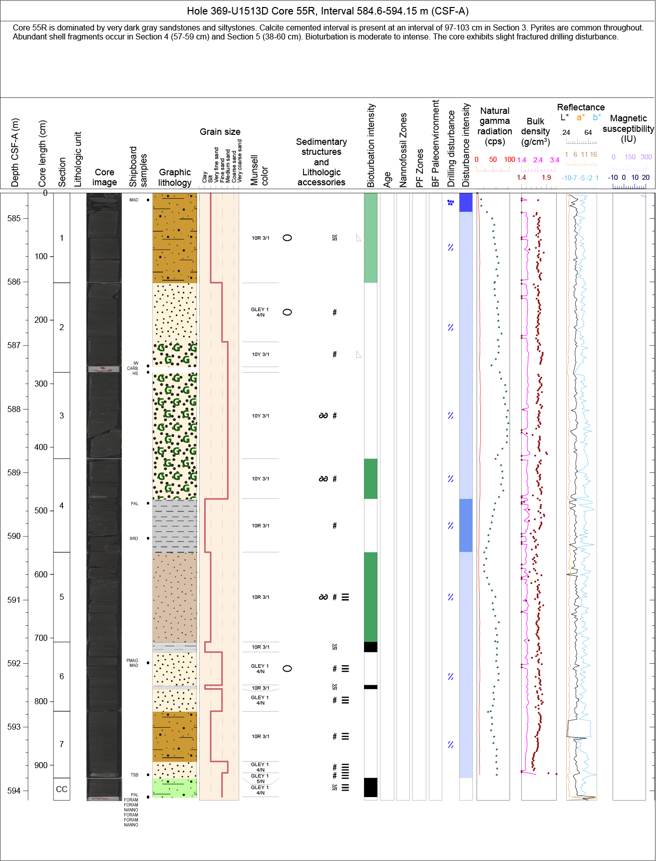
Figure F3. Sediment and sedimentary rock VCD.
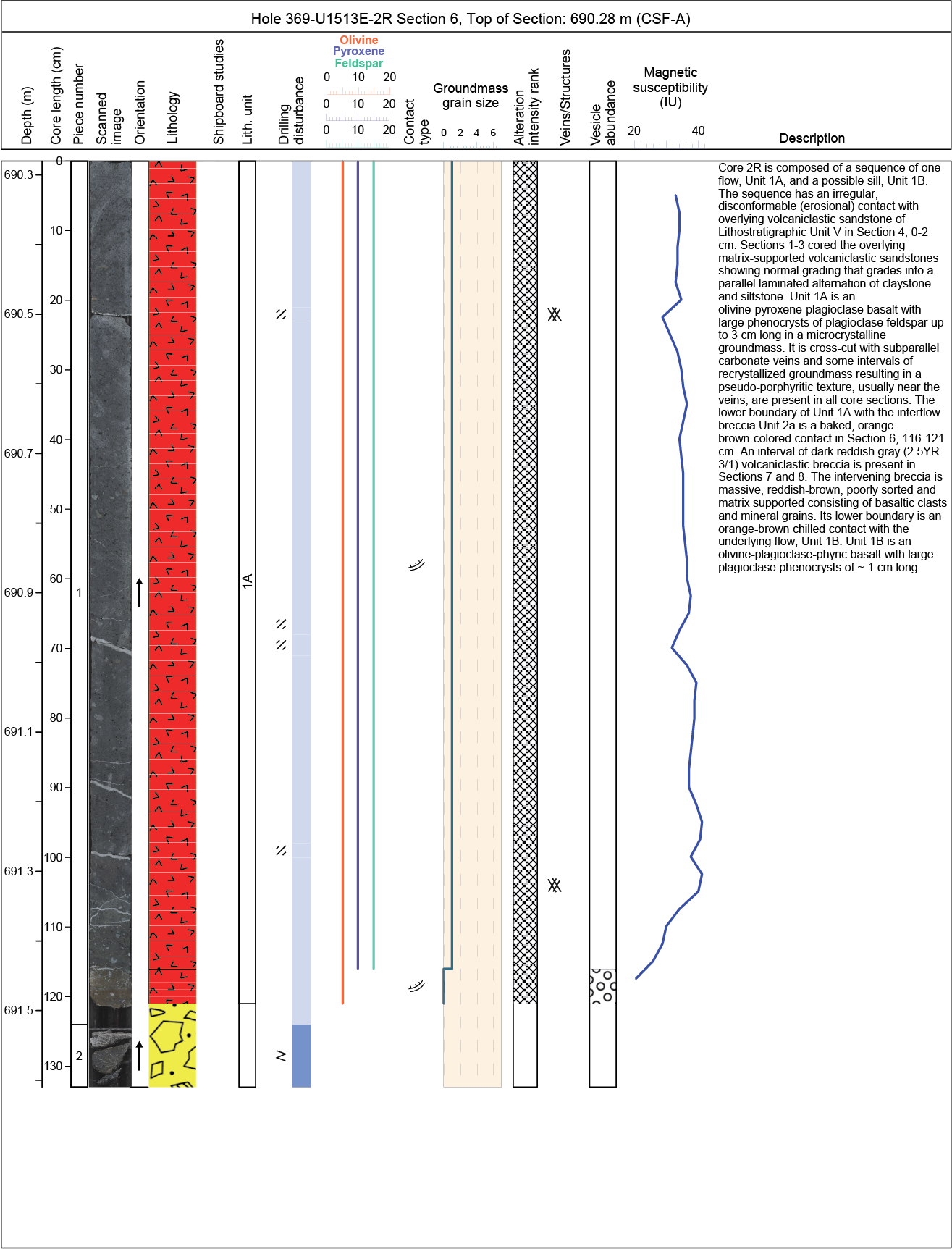
Figure F4. Igneous rock VCD.
A summarized lithologic description is provided at the top of each VCD. Depth and length of core sections are indicated along the left margin in the CSF-A depth scale. The graphic lithology is displayed with physical descriptions of the core that include grain size, Munsell color, sedimentary structures and lithologic accessories, bioturbation intensity, and drilling disturbance (type and intensity). Graphic patterns and symbols used in the VCDs are shown in Figures F5 and F6. In addition, VCDs display micropaleontological data, shipboard sampling locations and type, and physical property data (natural gamma radiation [NGR], bulk density, color reflectance [L*, a*, and b*], and magnetic susceptibility).

Figure F5. VCD graphic patterns.
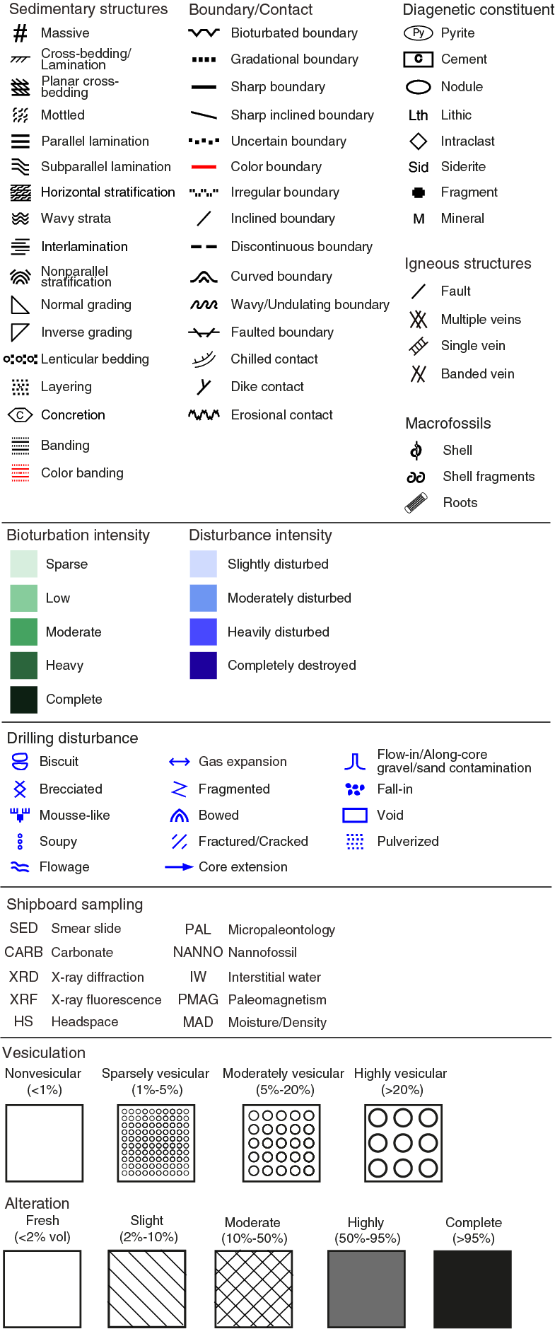
Figure F6. VCD symbols and nomenclature.
Core summary
A brief overview of major and minor lithologies present in the core, including sedimentary structures, lithologic accessories, and sediment/rock color, is presented in the core summary text field at the top of the VCD report. A summary of drilling disturbance is also given.
Section-half image
The flat faces of the archive halves were scanned on the SHIL after splitting and scraping to avoid color changes caused by sediment oxidation and drying. The SHIL uses three pairs of advanced illumination high-current-focused LED line lights to illuminate the features of the core. A line-scan camera made by JAI imaged 20 lines/mm to create a high-resolution TIFF file, high- and low-resolution JPEG files were subsequently created. The full-size images are 508 ppi (dpi). The camera height was adjusted so that the size of each pixel was 50 µm. However, actual core width per pixel varied because of differences in surface height of each section half. All section-half image files include a grayscale and ruler. Section-half depths were automatically included with images and stored in the LIMS database.
Graphic lithology
Lithologies of the core intervals recovered are represented on the VCD sheets by graphic patterns in the Graphic lithology column using the symbols illustrated in Figure F5. All sedimentary beds thicker than 2 cm are represented in the Graphic lithology column on each VCD. The major modifier of a principal lithology is shown using a modified version of the principal lithology pattern. Lithologic abundances are rounded to the nearest 5%; minor lithologies that constitute <5% of the core are generally not shown but are listed in the Core summary at the top of the VCDs. Relative abundances of lithologic constituents reported in this way are useful for general characterization of the sediment but do not constitute precise quantitative observations.
Sedimentary structures
The locations and types of stratification and sedimentary structures visible on the prepared surfaces of the split cores are shown in the Sedimentary structures and lithologic accessories column of the VCD. Symbols in this column indicate the locations of interstratification, bedding structures, and any other sedimentary features, such as mottled bedding and parallel lamination (Figure F6). Terminology outlined in Stow (2005) was used to describe stratification thickness (Table T1). Descriptive terms for bed boundaries, such as sharp, erosive, gradational, and bioturbated, were noted in DESClogik.
Lithologic accessories
Lithologic, diagenetic, and paleontologic accessories, such as nodules, alteration halos, shell fragments, and lithic clasts >2 mm, are indicated in the Sedimentary structures and Lithologic accessories columns on the VCDs and are also noted in the General interval comments column in DESClogik. Lithologic accessory abundances are outlined in Table T2. Descriptions are based on the archive halves, but if holes or depressions caused by clasts or core splitting were present, the working half was also examined. The symbols used to designate these features are shown in Figure F6.
Bioturbation intensity
Description and intensity of bioturbation were classified using the scheme of Stow (2005) and are denoted with a color scale in the Bioturbation intensity column (Table T3; Figure F6). Any identifiable ichnofossils were described in the core summary on the VCDs.
Drilling disturbance
Drilling disturbance was recorded in the Disturbance type column of the VCD using the symbols shown in Figure F6. The type of drilling disturbance is described for soft and firm sediments using the terms described in Table T4. The intensity of drilling disturbances (slight, moderate, heavy, and completely destroyed) is also described on the VCD sheet using a color scale.
Lithostratigraphic unit and age
Lithostratigraphic units are numbered sequentially starting from the top of the hole using Roman numerals and are shown in the Lithostratigraphic unit column of the VCD (Figure F3). Sediment age was based on the shipboard biostratigraphy (see Biostratigraphy and micropaleontology) and magnetostratigraphy (see Paleomagnetism) and is listed in the Age column. Calcareous nannofossil and planktonic foraminifer biozones and paleodepth estimates based on benthic foraminifers are also included in columns on the VCDs.
Shipboard samples
Positions of shipboard samples used for microscopic descriptions (i.e., smear slides and thin sections; SED), mineralogical analyses (XRD), shipboard chemical analyses (IW, HS, and CARB; see Geochemistry), micropaleontological (PAL, NANNO, and FORAM; see Biostratigraphy and micropaleontology), paleomagnetic (PMAG; see Paleomagnetism) and physical property analyses (MAD; see Petrophysics) are recorded in the Shipboard samples column (refer to key in Figure F6).
Sediment classification
Sediments recovered during Expedition 369 are composed of biogenic, siliciclastic, and volcaniclastic components and were described using a classification scheme derived from Expedition 349 (Li et al., 2015) and Stow (2005), DSDP Leg 26 in the Indian Ocean, which covered part of the Naturaliste Plateau, and ODP Leg 182 in the Great Australian Bight. The biogenic component includes open-marine calcareous and siliceous microfossils (e.g., foraminifers, calcareous nannofossils, diatoms, and radiolarians) and macrofossils (e.g., shell fragments). The siliciclastic component consists of mineral and rock fragments derived from igneous, sedimentary, and metamorphic rocks. The relative proportion of these two components are used to define the major classes of sediment in this scheme.
Lithologic naming conventions used during Expedition 369 follow the general guidelines of the Ocean Drilling Program (ODP) sediment classification scheme (Mazzullo et al., 1988), but a separate “mixed sediment” category was not distinguished during Expedition 369. As a result, biogenic sediments are those that contain >50% biogenic grains and <50% siliciclastic grains, whereas siliciclastic sediments are those that contain >50% siliciclastic grains and <50% biogenic grains (Figures F7, F8). We follow the naming schemes of Shepard (1954), Pettijohn et al. (1987), Folk (1962), Dunham (1962), and Stow (2005) for the detailed classification of sediments and sedimentary rocks (Table T5). Sediment grain size divisions for both biogenic and siliciclastic components are based on the nine major textural categories of Wentworth (1922) (Figure F9). These categories are defined using the relative proportions of sand-, silt-, and clay-sized particles (Figure F10, modified after Shepard, 1954), which can be difficult (e.g., silty clay versus sandy clay) without quantitative grain size measurements. The term “clay” is only used to describe particle size and is applied to both clay minerals and all other grains <4 µm in size.
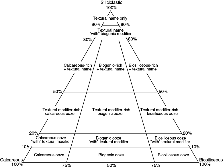
Figure F7. Siliciclastic-calcareous-biosiliceous ternary diagram.
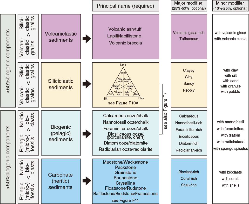
Figure F8. Sediment classification summary.
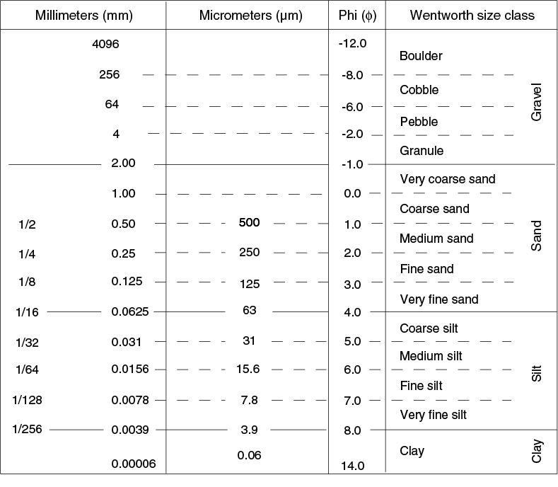
Figure F9. Udden-Wentworth grain size classification of terrigenous sediments.
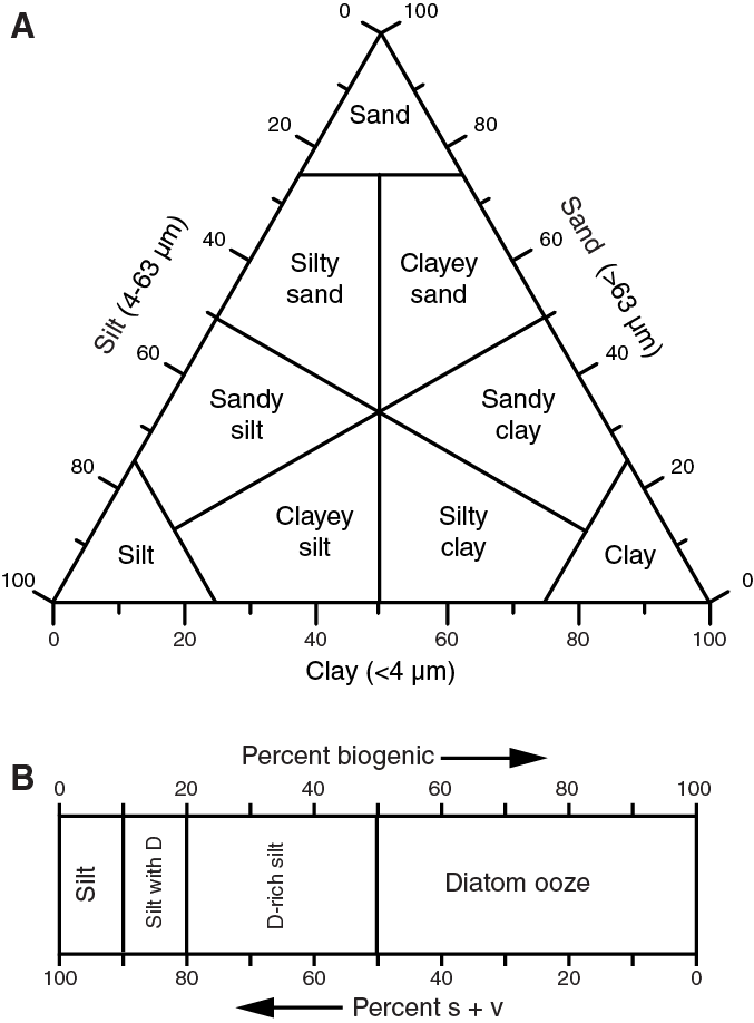
Figure F10. Lithologic textural name classification.
Lithologic names assigned to these sediments consist of a principal name with major and minor modifiers that are based on composition and degree of lithification and/or texture as determined from visual description of the cores and from smear slide observations (Figure F8).
Naming of siliciclastic and biogenic sediments
Principal names
For sediments with >90% biogenic components, the name applied indicates the most common type of biogenic grain. For example, sediment composed of >90% calcareous nannofossils is called nannofossil ooze/chalk, and sediment composed of 50% foraminifers and 45% calcareous nannofossils is called calcareous ooze/chalk. For sediment with >90% siliciclastic grains, the principal name is based on the textural characteristics (Figure F10) of all sediment particles (both siliciclastic and biogenic).
For a sediment sample that contains a significant mixture of siliciclastic and biogenic components (between 10% and 90% of both siliciclastic and biogenic components), the principal name is determined by the more abundant component (Figures F7, F8). If the siliciclastic component is more abundant (i.e., >50% siliciclastic component in Figure F7), the principal name is based on the textural characteristics such as silty clay or sandy silt (Figure F10). If the biogenic component is more abundant (i.e., <50% siliciclastic component in Figure F7), the principal name is based on the predominant biogenic component, such as calcareous ooze.
Major and minor modifiers
If a biogenic (or siliciclastic/volcaniclastic) group makes up 5%–50% of the sediment and this group is not included as part of the principal name, major/minor modifiers are generally used. When a microfossil group (e.g., diatoms, nannofossils, or foraminifers) comprises 20%–50% of the sediment, a major modifier consisting of the component name hyphenated with the suffix “-rich” (e.g., diatom-rich clay) is used. The principal name is followed by a minor modifier (e.g., with diatoms), which is the most abundant component among those making up 5%–20% of the sediment. If the minor component is biogenic, then the modifier describes the group of biogenic grains that exceeds the 5% abundance threshold (e.g., silty clay with radiolarians). If the minor component is siliciclastic, the minor modifier is based on the texture of the siliciclastic fraction (e.g., diatom ooze with clay).
If the primary lithology for an interval of core has a major modifier, then that major modifier is indicated in the Graphic lithology column of the VCD sheets using a modified version of the lithologic pattern for the primary lithology. The minor modifiers of sediment lithologies are not included in the Graphic lithology column.
Naming by different lithification grades
The following terms describe lithification that varies depending on the dominant composition, and the degree of lithification is specified on the VCD:
- Sediment samples that are composed predominantly of calcareous, pelagic organisms (e.g., calcareous nannofossils and foraminifers): the lithification terms “ooze” and “chalk” reflect whether the sediment sample can be deformed with a finger (ooze) or scratched easily by a fingernail (chalk).
- Sediment samples that are composed predominantly of siliceous microfossils (diatoms, radiolarians, and siliceous sponge spicules): the lithification terms “ooze” and “radiolarite/diatomite” reflect whether the sediment can be deformed with a finger (ooze) or cannot be easily deformed manually (radiolarite/diatomite).
- Sediment samples that are composed of a mixture of calcareous and siliceous microfossils: the lithification terms “ooze” and “indurated sediment” reflect whether the sediment can be deformed with a finger (ooze) or cannot be easily deformed manually (indurated sediment).
- Sediment samples that are composed predominantly of siliciclastic material: if the sediment can be deformed easily with a finger, no lithification term is added and the sediment is named for the dominant grain size (i.e., sand, silt, or clay). For more consolidated material, the lithification suffix “-stone” is appended to the dominant size classification (e.g., claystone), except for gravel-sized sediment, when the terms “conglomerate” or “breccia” are used.
Classification of carbonate sediments
The principal names of carbonate sediments were decided based on the classification by Dunham (1962) and Embry and Klovan (1971) (Figure F11). Consistent with the terminology used for Site 258 (Luyendyk and Davies, 1974), the term “silicified limestone” was used for samples characterized by fine-grained calcareous biogenic sediments that were partially or fully replaced by silica.

Figure F11. Limestone classification.
Naming of volcaniclastic sediments
The subclassification of volcaniclastic sediments followed here differs from the standard ODP classification (Mazzullo et al., 1988) in that we adopted the same descriptive, nongenetic terminology based on particle size classification that was employed during Leg 26 (Shipboard Scientific Party, 1974). Unless an unequivocally pyroclastic origin for volcanogenic particles could be determined, volcaniclastic sediments were described as siliciclastic sediments (i.e., sand, silt, etc.).
Where pyroclastic rocks were observed, we adopted the classification scheme of Fisher and Schmincke (1984). In this instance, we used the grain size terms “volcanic breccia” (>64 mm), “lapilli/lapillistone” (2–64 mm), and “ash/tuff” (<2 mm). The term “hyaloclastite” was used for vitroclastic (i.e., glassy) materials produced by the interaction of water and magma or lava (Fisher and Schmincke, 1984).
Igneous rocks
Systematic descriptions of the primary petrology of recovered igneous rocks and their alteration were made on each archive half, except for those made on thin sections, which are derived from the working halves. First, lithologic unit boundaries were defined by visual identification of lithologic contacts or by inference using observed changes in mineralogical and textural characteristics. Second, lithologic characteristics such as mineralogical assemblage, igneous textures, and vesicle distribution were described. Third, any alterations, together with vein and vesicle infillings and alteration halos, were recorded. Finally, these macroscopic observations were combined with those from detailed thin section petrographic studies of key igneous units and alteration intervals. Macroscopic and microscopic observations and descriptions were recorded in DESClogik and were noted on the VCDs (Figures F4, F6).
Descriptive features and nomenclature
Phenocryst-based lithology names
Porphyritic basalts were named according to phenocryst phases, but only where the total abundance of phenocrysts was >1%. The most abundant phenocryst type was named last. For example, olivine is the most abundant mineral in a plagioclase-olivine-phyric basalt. The term “phenocryst” was used for any crystal that was (1) significantly (typically five times) larger than the average size of the groundmass crystals, (2) >1 mm, and (3) euhedral or subhedral. The term “microphenocryst” was used for crystals larger than the modal groundmass grain size but <1 mm. When macroscopic observations were possible, these microphenocrysts were also described in the DESClogik “microscopic” section in the phenocryst columns and were used to establish the primary lithology name. A prefix was applied as a modifier to the primary lithology names to indicate the abundance of phenocrysts in the hand samples (Table T6).
Aphyric rocks were not assigned any mineralogical modifier. Likewise, in coarse-grained rocks with seriate to equigranular textures, we did not use modifiers unless there was a clear distinction between phenocrysts and groundmass crystals.
Groundmass
Groundmass is characterized by its grain size with standard notation (Table T7).
Igneous textures
For volcanic rocks, the following terms were used to describe textures when microlites (very small crystals in glassy matrix visible only in thin section) are present:
- Variolitic (fanlike arrangement of divergent microlites),
- Intergranular (olivine and pyroxene grains between plagioclase laths),
- Intersertal (glass between plagioclase laths),
- Subophitic (partial inclusion of plagioclase in clinopyroxene), and
- Ophitic (total inclusion of plagioclase in clinopyroxene).
The following terms were used to describe flow textures:
- Trachytic (subparallel arrangement of plagioclase laths in the groundmass),
- Pilotaxitic (aligned plagioclase microlites embedded in a matrix of granular and usually smaller clinopyroxene grains), and
- Hyalopilitic (aligned plagioclase microlites with glassy matrix).
Vesicles
An estimate of the percentage of vesicles, their shape, and their average size are included on the VCDs. The division, based on the occurrence of vesicles, was made according to the descriptions recorded in Table T8.
Alteration
Vesicle and vein fillings, as well as replacement of phenocrysts and groundmass by secondary minerals, were recorded on the DESClogik microscopic description templates. Alteration minerals were identified by color, crystal habit, shape, and association with primary minerals (if recognizable). Difficulties arise in the identification of alteration minerals because many are visually similar and are often microcrystalline or amorphous. Thus, their identification remains preliminary, pending detailed shore-based studies. The degree of the overall alteration was reported graphically on the VCDs. Different patterns are used to indicate the degree of alteration (Table T9): fresh, slight, moderate, highly, and complete.
Lithostratigraphic units
Sediments and sedimentary rocks
Lithostratigraphic units were defined at each site where successions of conformable units with similar sedimentary characteristics or phases were recognized. These successions were given consecutive downhole Roman numbers (Units I, II, etc.). When necessary, lithostratigraphic subunits were also defined (Subunits Ia, Ib, etc.).
Igneous rocks
The succession of igneous rocks and associated breccias was defined as one igneous lithostratigraphic unit and was assigned a successive Roman number following the sedimentary lithostratigraphic units in the hole. Within the igneous lithostratigraphic unit, the boundaries of volcanic rocks were generally defined to reflect different volcanic cooling or lithologic units and assigned an Arabic number (Units 1, 2, etc.). The definition of an igneous lithologic unit is usually based on the presence of lava flow contacts, which are typically marked by chilled or glassy margins on the upper and lower boundaries, or the presence of intercalated volcaniclastic or sedimentary horizons. If no such boundaries were recovered, the lithologic unit boundaries were defined according to changes in primary mineralogy (based on the abundance of visible phenocryst and groundmass mineral phases), grain size, color, and structural or textural variations.
Microscopic description
Smear slide
For unlithified sediments, at least one smear slide was made from the archive half of each core to determine the lithology. Additional samples were collected from intervals of interest (e.g., laminations and suspected ash layers). Specific sampling locations were noted on the VCDs. A small amount of sediment was taken with a wooden toothpick and put on a 2.5 cm × 7.5 cm glass slide. The sediment sample was homogenized with a drop of deionized water and evenly spread across the slide to create a very thin (about <50 µm) uniform layer of sediment grains for qualitative estimation of relative abundance. The dispersed sample was dried on a hot plate. A drop of Norland optical adhesive was added as a mounting medium to a coverslip, which was carefully placed on the dried sample to prevent air bubbles from being trapped in the adhesive. The smear slide was then fixed in an ultraviolet light box.
Smear slides were examined with a transmitted light petrographic microscope equipped with a standard eyepiece micrometer. The texture of siliciclastic grains (relative abundance of sand-, silt-, and clay-sized grains) and the proportions and presence of biogenic and mineral components were visually estimated using Rothwell (1989) and recorded in DESClogik. The mineralogy of clay-sized grains could not be determined from smear slides. Note that smear slide analyses tend to underestimate the amount of sand-sized and larger grains because these grains are difficult to incorporate onto the slide.
Thin sections
Thin section analyses were used to complement and refine macroscopic core observations for lithified sedimentary rocks and igneous rocks. At least one thin section was examined and logged per defined lithologic unit, except for volcaniclastic units with frequent alternations of massive and brecciated units where additional thin-sections were made to confirm the mineralogical composition and lithology of samples. Terminology and nomenclature hierarchy for thin section descriptions followed Dunham (1962) (Figure F11). For sedimentary rocks, the framework of grains (modal abundance of sand-, silt-, and clay-sized grains; grain sorting; and roundness) and the proportions and presence of matrix were visually estimated and recorded in DESClogik. The modal proportions of siliciclastic, calcareous, biosiliceous, or other components were also estimated in both mineral grains and cementing material. The occurrence of identified single mineral grains was also reported in DESClogik. For igneous rocks, phenocryst assemblages (and their modal percentages and sizes), groundmass, textures, and alteration phases were determined. Downloaded tabular reports of all igneous and sedimentary thin section descriptions can be found in Core descriptions.
X-ray diffraction analyses
Samples were prepared for XRD analysis to identify the main mineral phases in bulk samples. In general, one or two samples (~5 cm3 in volume) were taken from each core. Sampling locations are noted on the VCDs. In preparation for bulk mineralogy analysis, samples were freeze-dried and then ground in a shatter-box for 30 s. Prepared samples were top-mounted onto a sample holder and analyzed using a Bruker D-4 Endeavor diffractometer mounted with a Vantec-1 detector using nickel-filtered CuKα radiation. The standard locked coupled scan was as follows:
- Voltage = 40 kV.
- Current = 40 mA.
- Goniometer scan = 4°–70°2θ.
- Step size = 0.0087°2θ.
- Scan speed = 0.2 s/step.
- Divergence slit = 0.3 mm.
Shipboard results yielded only qualitative information for the presence of the most common mineral components. Diffractograms of bulk samples were processed (e.g., baseline removal and maximum peak intensity) with the software package EVA, which allowed peak characterization and mineral identification. Processed files include d-spacing values, diffraction angles, and peak intensities with background removed. D-spacing results were compared to expected values of d-spacing for minerals in the EVA database using aluminum oxide as a standard to monitor data quality. Muscovite/illite/glauconite and kaolinite/chlorite have similar diffraction patterns and could not be distinguished with shipboard results. Digital files with the diffraction patterns are available from the LIMS database.
X-ray fluorescence analyses
An Olympus Delta handheld pXRF spectrometer was used to conduct rapid reconnaissance analysis of element compositions for both sediment and igneous rock samples (split surfaces of the archive halves or thin section billets) and rock powders prepared for XRD analysis. We primarily utilized the “geochemistry” correction protocol within the “geochemistry and soil” submenu, which analyzes for elements in three energy ranges (low = Al, Si, K, Ca, Ti, Mn, Fe, Cr, P, S, and Mg; main = Ca, Ti, Mn, Fe, Ni, Sr, Rb, Zr, Zn, and others; and high = Sr, Rb, Zr, Ba, La, and Ce). In general, the high-energy elements did not provide reliable results, but the main and low-range groupings yielded results that were sufficiently precise when concentrations were above instrument detection limits.
Biostratigraphy and micropaleontology
Calcareous nannofossils, planktonic foraminifers, and benthic foraminifers were studied from core catcher samples at all sites. At most sites, samples from split core sections were also examined for both calcareous nannofossils and planktonic foraminifers, as time allowed, to provide more-refined age determinations or to investigate where significant changes in lithology occurred. Nannofossils and planktonic foraminifers were used for biostratigraphy, and benthic foraminifers were used mainly to acquire estimates of paleobathymetry. Biostratigraphic studies focused primarily on the identification of biostratigraphic horizons (biohorizons) in the cores, generally the top or base of the stratigraphic range of a species. Expedition 369 used the Gradstein et al. (2012) timescale with the modifications discussed below.
Identification of a sequence of biohorizons in stratigraphic order allowed the recognition of biostratigraphic zones and subzones using standard schemes. These zones have been assigned absolute ages based on calibrations from other areas, mainly referenced to the paleomagnetic reversal sequence.
All paleontological data gathered during shipboard investigations are available from the LIMS database in accordance with IODP policy. Species distribution data are included for every sample studied for each hole and each taxonomic group (calcareous nannofossils, planktonic foraminifers, and benthic foraminifers). Calcareous nannofossil and planktonic foraminifer data are provisional and focus mainly on biostratigraphic marker species, whereas common species of little stratigraphic value are generally omitted. The tables also record suspected reworking or otherwise out-of-place species (e.g., through downhole contamination).
Calcareous nannofossils
Calcareous nannofossil assemblages were examined and described from smear slides made from core catcher samples (at ~10 m intervals). Additional toothpick samples were taken between core catcher samples from split core sections when necessary to refine the stratigraphic position of bioevents. Slides were fixed with Norland optical adhesive and cured under UV light for examination using a Zeiss Axioscope microscope at 1000× magnification. All photomicrographs were taken using a SPOT RTS system with the IODP Image Capture and commercial SPOT software. Additional observations with a Hitachi TM3000 tabletop scanning electron microscope (SEM) were made to verify the preservation state of calcareous nannofossils.
Nannofossil taxonomy follows the online Nannotax 3 database (http://ina.tmsoc.org/Nannotax3). The zonal scheme of Okada and Bukry (1980; CN–CP codes) was used for Cenozoic calcareous nannofossil biostratigraphy (Figures F12, F13). For the Mesozoic, the zonal scheme of Perch-Nielsen (1985; CC code) was used (Figures F14, F15).
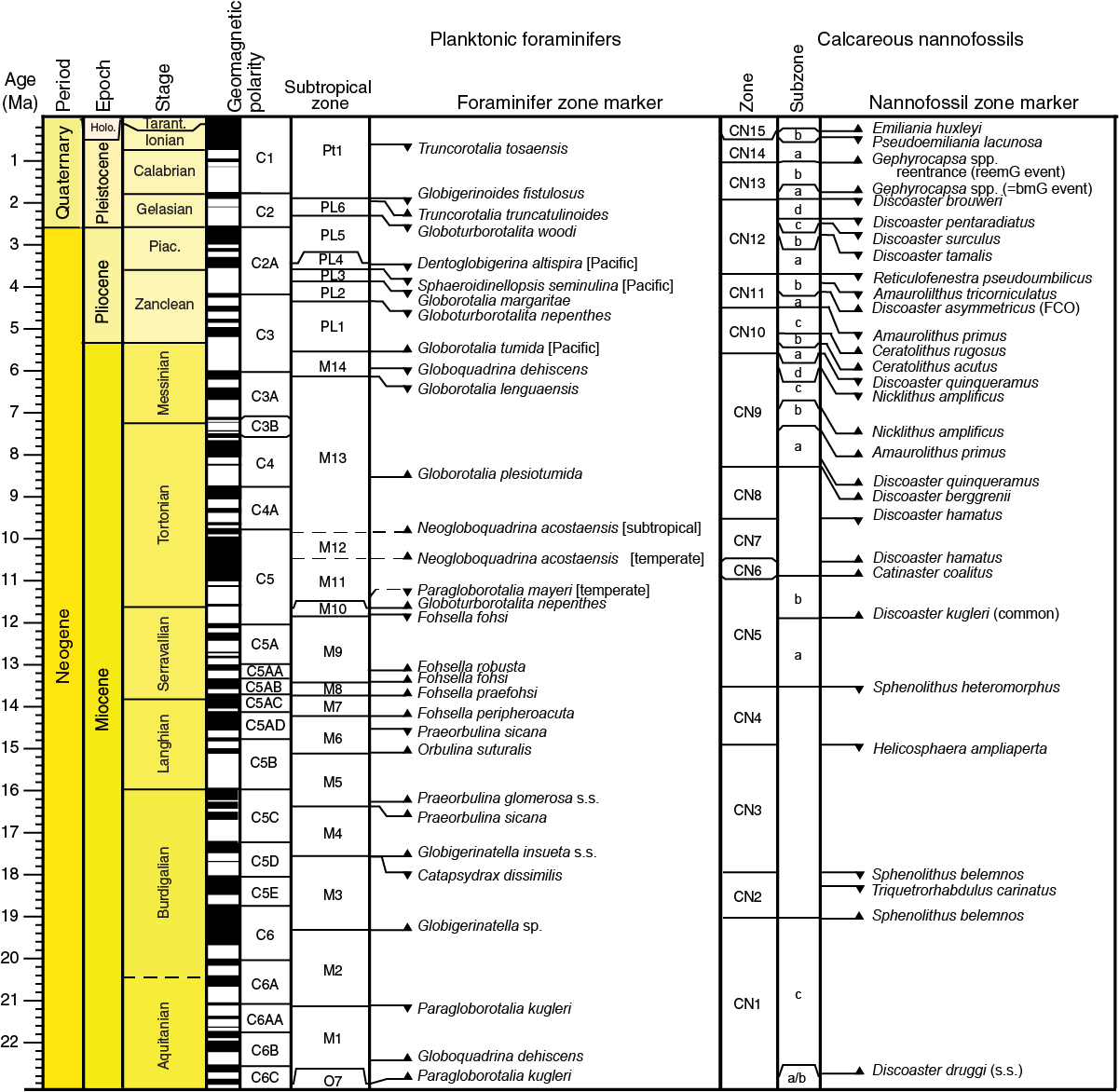
Figure F12. Neogene timescale.
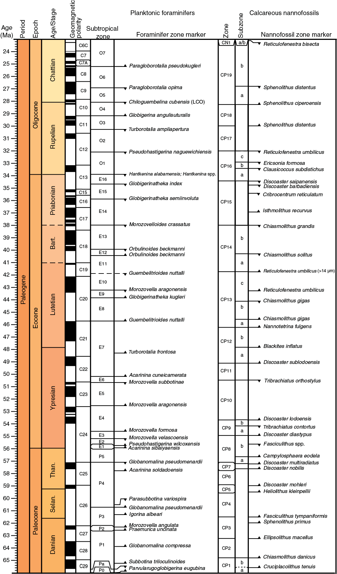
Figure F13. Paleogene timescale.
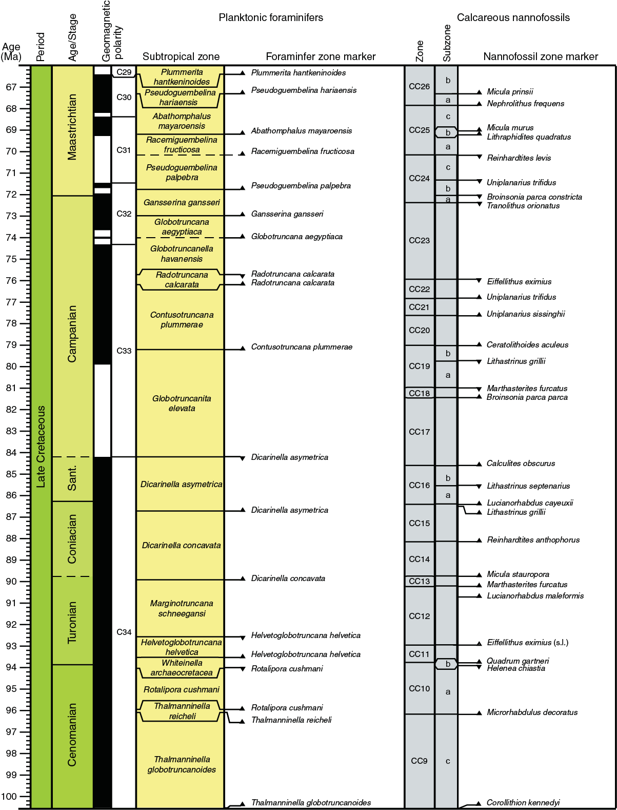
Figure F14. Late Cretaceous timescale.

Figure F15. Early Cretaceous timescale.
The following qualitative abundance codes were used in the DESClogik data entry program and uploaded to the LIMS database.
Total calcareous nannofossil abundance in the sediment was recorded as follows:
- A = abundant (>50% of sediment particles).
- C = common (>10%–50% of sediment particles).
- F = few (1%–10% of sediment particles).
- R = rare (<1% of sediment particles).
- B = barren (none present).
Abundance of individual calcareous nannofossil taxa is based on specimens per field of view (FOV) at 1000× magnification:
- V = very abundant (>100 specimens per FOV).
- A = abundant (10–100 specimens per FOV).
- C = common (1–9 specimens per FOV).
- F = few (1 specimen per 2–10 FOV).
- R = rare (1 specimen per 11–100 FOV).
- P = present (1 specimen per >100 FOV).
Preservation of calcareous nannofossils was recorded as follows:
- E = excellent (no evidence of dissolution and/or recrystallization, no alteration of primary morphological characteristics, and specimens identifiable to the species level).
- G = good (little or no evidence of dissolution and/or recrystallization, primary morphological characteristics unaltered or only slightly altered, and specimens identifiable to the species level).
- M = moderate (specimens exhibit some etching and/or recrystallization; primary morphological characteristics somewhat altered; most specimens, however, are identifiable to the species level).
- P = poor (specimens are severely etched or overgrown, primary morphological characteristics are largely destroyed, fragmentation has occurred, and specimens often could not be identified at the species and/or generic level).
Planktonic foraminifers
Planktonic foraminifers were examined from core catcher samples, and additional samples per core were examined as necessary. Sample volumes of ~20 cm3 were washed over 45 μm sieves and then dried on a hot plate. Empty sieves were cleaned in an ultrasonic bath to minimize cross-contamination between samples, rinsed in water dyed with methylene blue to stain any remaining foraminifers still caught in the sieve mesh to avoid contaminating subsequent samples, and then rinsed again with water. Dried residues (>45 μm fraction) were transferred to labeled glass vials from which subsamples were examined on metal trays using binocular Zeiss Discovery V8 stereomicroscopes. Specimens of special interest were transferred to stubs for SEM study.
Most shipboard work focused on the >150 μm size fraction for biostratigraphic purposes, but the 45–150 μm fraction was also examined for marker species and to scan for smaller species. Selected specimens were imaged using a SPOT RTS system with IODP Image Capture and commercial SPOT software for photomicrographs. Selected specimens of planktonic foraminifers were imaged using a Hitachi TM3000 tabletop SEM after coating with conductive gold-palladium. All images are available in the LIMS database.
The taxonomic concepts for planktonic foraminiferal genera and species follow the original descriptions by the author (with any amendments to original species descriptions noted) and/or the Mikrotax online taxonomic atlas (http://www.mikrotax.org) of planktonic foraminifers.
The Cenozoic biohorizons, their age assignments, and their zonal scheme follow Gradstein et al. (2012) and include additional Cenozoic datums recognized by Wade et al. (2011) with two modifications: (1) Zone PL6 is retained despite the fact that it now falls wholly within the Pleistocene series following the definition of the Pliocene/Pleistocene boundary at 2.59 Ma (Gibbard et al., 2010), and (2) the list was edited to be relevant to the subtropical Indo-Pacific (Figures F12, F13).
The Cretaceous biohorizons, their age assignments, and their zonal scheme are according to Gradstein et al. (2012) with the following modifications (Figures F14, F15):
- The generic assignment of the species Parathalmanninella appenninica was changed to Thalmanninella appenninica (see discussion in Petrizzo et al., 2015), and the species Paraticinella eubejaouaensis was updated to Paraticinella rohri according to Ando et al. (2013).
- The Hedbergella infracretacea Zone was changed to the Hedbergella trocoidea Zone (Sigal, 1977).
- The Lower Cretaceous biohorizons from the Leupoldina cabri Zone to the Favusella (= Globuligerina) hoterivica Zone are after Coccioni et al. (2007).
The following planktonic foraminiferal abundance categories relative to total sediment particles were estimated from visual examination of the dried sample in the >150 µm fraction:
- A = abundant (>30% of sediment particles).
- C = common (10%–30% of sediment particles).
- F = few (5% to <10% of sediment particles).
- R = rare (<5% of sediment particles).
- B = barren (none present).
Abundances of planktonic foraminifer species were estimated using the following scheme:
- A = abundant (>20% of the planktonic foraminiferal assemblage).
- C = common (>10%–20% of the planktonic foraminiferal assemblage).
- F = few (>5%–10% of the planktonic foraminiferal assemblage).
- R = rare (1%–5% of the planktonic foraminiferal assemblage).
- P = present (<1% of the planktonic foraminiferal assemblage).
Planktonic foraminiferal preservation as viewed under the light microscope was recorded as follows:
- E = excellent (most specimens have a “glassy” appearance indicating little recrystallization or evidence of overgrowth, dissolution, or infilling and abrasion).
- G = good (some specimens show minor evidence of diagenetic overgrowth, dissolution, or abrasion; recrystallization may or may not have occurred).
- M = moderate (most specimens show evidence of overgrowth, dissolution, and abrasion; tests infilled with cement or indurated sediment obscuring apertures).
- P = poor (specimens with substantial diagenetic overgrowth (including infilling), dissolution, and abrasion; foraminifers can be fragmentary and difficult to identify because of major overgrowth and/or dissolution).
Benthic foraminifers
For sampling, preparation, and imaging methods, refer to Planktonic foraminifers. Taxonomic assignments predominantly follow van Morkhoven et al. (1986), Jones (1994), Kaminski and Gradstein (2005), Holbourn et al. (2013), and Hanagata and Nobuhara (2015). The generic classification of Loeblich and Tappan (1988) was used and updated in some instances, in particular for uniserial taxa (Hayward, 2002). The identifications of benthic foraminiferal taxa were generally made on the >150 µm size fraction. The 45–150 µm size fractions were searched for stratigraphically and/or paleoecologically important taxa.
The following benthic foraminiferal abundance categories are relative to total estimated sediment particles:
- D = dominant (>30% of sediment particles).
- A = abundant (>10%–30% of sediment particles).
- F = few (>5% to <10% of sediment particles).
- R = rare (>1% to <5% of sediment particles).
- P = present (<1% of sediment particles).
- B = barren (none present).
Paleodepth range estimates from benthic foraminiferal taxa were based on van Morkhoven et al. (1986), Kaminski and Gradstein (2005), and Holbourn et al. (2013). Paleobathymetry was assigned using the following categories:
- Neritic = <200 m below sea level (mbsl).
- Bathyal = 200–2000 mbsl; where possible, upper (200–1000 mbsl) and lower (1000–2000 mbsl) bathyal intervals were determined.
- Abyssal = >2000 mbsl.
Sediment accumulation history
Biostratigraphic and additional age determinations (such as paleomagnetic reversals) and sediment depth below seafloor (provided by the drillers) were used to estimate the history of sediment accumulation for each site. Tables of estimated age versus depth are included for each site, as well as a graphic representation of the sediment accumulation history, except for Site U1515, which contains extensive reworking of assemblages.
Paleomagnetism
Paleomagnetic investigations during Expedition 369 focused mainly on measuring the natural remanent magnetization of archive-half sections before and after alternating field (AF) demagnetization for magnetostratigraphic dating. In addition, discrete samples were collected from selected working-half sections for use in AF demagnetization and rock magnetic experiments.
Coordinate systems
All magnetic data are reported relative to IODP orientation conventions: +x points into the face of the working-half section, +y points toward the left side of the face of the working-half section, and +z points downcore. The relationship between the superconducting rock magnetometer (SRM) coordinates (X, Y, and Z) and the data coordinates (x, y, and z) is x = X, y = −Y, and z = Z for archive-half sections and x = −X, y = Y, and z = Z for working-half sections. The coordinate systems for the spinner magnetometer (AGICO Model JR-6A) and Natsuhara-Giken sampling cubes are indicated in Figure F16.
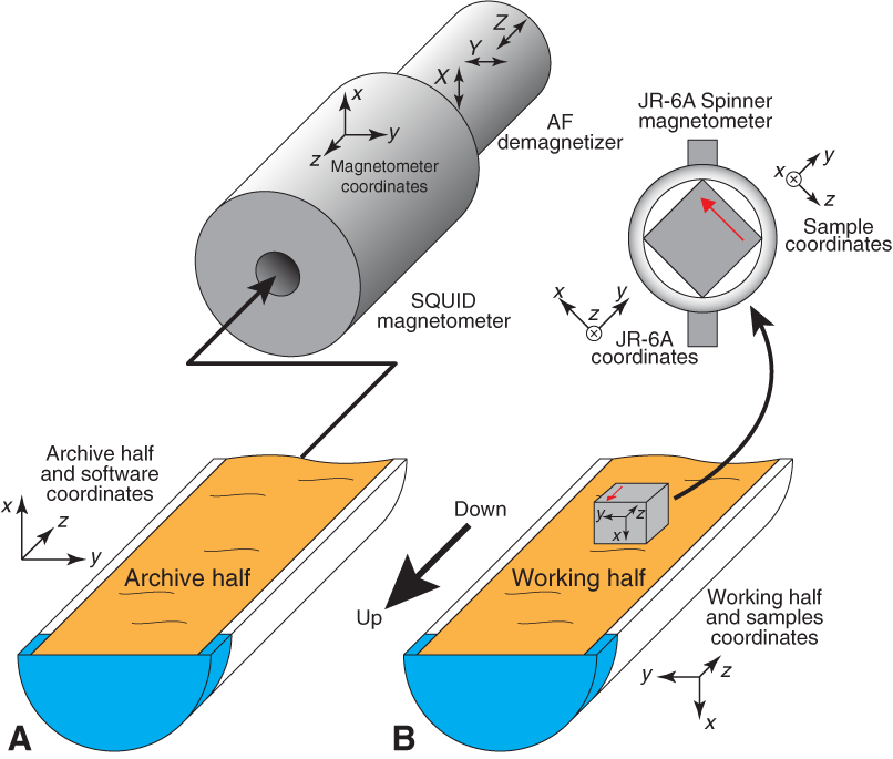
Figure F16. SRM and magnetometer coordinate systems.
Core orientation
APC core orientation was achieved with one of two core orientation tools (FlexIT and Icefield MI-5) mounted on the core barrel. These tools use three mutually perpendicular fluxgate magnetic sensors and three orthogonally mounted accelerometers to monitor the movement of the drill assembly and to help determine when the most stable and thus useful core orientation data were gathered. The information from both sets of sensors allows the azimuth and dip of the hole to be measured, as well as the azimuth of the APC core orientation. The orientation information contributed to paleomagnetic polarity determinations and magnetostratigraphic interpretations.
Magnetic measurements
Remanent magnetization was measured using the SRM (2G Enterprises Model 760R-4K) on the JOIDES Resolution equipped with direct-current superconducting quantum interference devices (SQUIDs) and an in-line, automated AF demagnetizer capable of reaching a peak field of 80 mT. Ocean drilling cores generally carry secondary remanence components (overprints), including natural viscous remanence and a steep downward-pointing component attributed to the drill string (e.g., Richter et al., 2007). To separate the overprints from the characteristic remanence (ChRM), stepwise demagnetization experiments were performed, as described below.
Archive-half sections
Measurements of archive-half sections were conducted using the Integrated Measurement System (version IMS 9.2) software with a nominal sample area parameter of 17.5 cm2. The measurement interval and speed were 5 cm and 5 cm/s, respectively. The response functions of the pick-up coils of the SQUID sensors have a full width of 7.2–9.1 cm at half height (Acton et al., 2017). Therefore, data collected within ~4.5 cm of piece boundaries (or voids) are significantly affected by edge effects. Consequently, all data points within 5 cm of piece boundaries (as documented in the curatorial record) were filtered out prior to further processing. Edge effects may also occur in a contiguous core piece if substantial heterogeneity (in intensity or direction) is present in the piece. It is more difficult to filter out such artifacts, but calculating the average direction (using Fisher statistics) for each core piece could provide a means of identifying these problems (Expedition 330 Scientists, 2012).
For most of the section halves, we performed demagnetization steps of 0, 10, and 20 mT. When time permitted, a higher AF demagnetization field of 30 mT (RCB cores) or more detailed demagnetization steps of 0, 5, 10, 15, and 20 mT were used. The AF demagnetization results were plotted individually as vector plots (Zijderveld, 1967) and as downhole variations with depth. We inspected the plots visually to judge whether the remanence after demagnetization at the highest AF step reflects the ChRM and geomagnetic polarity sequence.
Discrete samples from working-half sections
Oriented discrete samples representative of lithology were collected from selected working-half sections at a rate of one or two samples per core. In soft sediments, discrete samples were taken in plastic “Japanese” Natsuhara-Giken sampling cubes (or J-cube; 7 cm3 sample volume). Cubes were pushed by hand into the working half of the core with the “up” arrow on the cube pointing upsection. For more indurated intervals, an extruder was pushed into the sediment, and the sample was then placed into the plastic cubes. In lithified sediment and hard rock, oriented cubes (~8 cm3) were cut and trimmed using a dual-blade saw. Measurements of discrete samples were conducted with a spinner magnetometer (AGICO Model JR-6A) using the Rema (version 6.0) software or the SRM using the discrete measurement mode.
For discrete samples, we performed successive AF demagnetization with the DTech AF demagnetizer (Model D-2000) for spinner measurements up to 80 mT (majority of the samples) or the in-line, automated AF demagnetizer equipped with the SRM up to 80 mT. We analyzed the stepwise demagnetization data of the discrete samples by principal component analysis (Kirschvink, 1980) to define the ChRM. Demagnetization data analysis was performed using the PuffinPlot (Lurcock and Wilson, 2012) and Zplotit (http://paleomag.ucdavis.edu/software-Zplotit.html) software packages. Both the section-half data collected on the SRM and the discrete sample data acquired on the spinner magnetometer and the SRM were uploaded to the LIMS database.
Low-field magnetic susceptibility of both whole rounds (see Petrophysics) and split sections (see Lithostratigraphy) was routinely measured as a proxy for the concentration of magnetic minerals.
Magnetostratigraphy
Magnetostratigraphic interpretations for each site were constructed by correlating observed polarity sequences with the geomagnetic polarity timescale (GPTS) (Ogg et al., 2012) in combination with biostratigraphic observations where available and age diagnostic. We used the GPTS of Gradstein et al. (2012) (Table T10), in which boundary ages for Chrons C1n–C13n and C24n.1n–C34n are orbitally tuned but those for Chrons C13r–C23r are spline fitted.
Expedition 369 sites are located at ~34°S. For azimuthally unoriented samples of sedimentary rocks at these sites, the polarity of sedimentary units can be constrained with paleomagnetic inclinations only. Despite the fact that paleomagnetic inclinations will exhibit some degree of dispersion of their mean inclination, it is steep enough to allow the sign of the inclination to be used to indicate geomagnetic polarity.
Whenever possible, we offer an interpretation of the magnetic polarity following the naming convention of correlative anomaly numbers prefaced by the letter C (Tauxe et al., 1984). For the younger part of the timescale (Pliocene to Pleistocene), we also use traditional names to refer to the various chrons and subchrons (e.g., Brunhes, Jaramillo, Olduvai, etc.). In general, polarity reversals occurring at core section ends have been treated with extreme caution.
Petrophysics
During Expedition 369, high-resolution petrophysical measurements were made on the physical properties of cores in the shipboard laboratory and using downhole (in situ) logging tools. These data play a major role in determining hole-to-hole and site-to-site stratigraphic correlation, detecting stratal discontinuities and inhomogeneities, obtaining information about differences in the composition and texture of sediment, identifying major seismic reflectors, and constructing synthetic seismograms. A variety of techniques and methods were used to characterize the physical properties of whole-round, section-half, and discrete samples. Core sections are generally 1.5 m in length, so a typical coring length (stroke) of 9.5 m yields six sections plus a shorter seventh section. Procedures for measuring soft sediment, indurated sediment, and hard rock (e.g., igneous rock) cores differ slightly.
When acquired, downhole logs are used to obtain in situ measurements of physical, chemical, and structural properties of the formation penetrated by a borehole. The data are rapidly collected and continuous with depth and can be interpreted in terms of the stratigraphy, lithology, mineralogy, magnetic characteristics, and geochemical composition of the penetrated formation. Where core recovery is incomplete or disturbed, log data may provide the only way to characterize the borehole section. Where core recovery is good, log and core data complement one another and may be interpreted jointly.
Downhole logs measure formation properties on a scale intermediate between those obtained from laboratory measurements on core samples and those from geophysical surveys. Downhole logs are also useful in calibrating the interpretation of geophysical survey data (e.g., through the use of synthetic seismograms) and provide a necessary link for the integrated understanding of physical and chemical properties on different scales.
General physical properties sampling and measurement sequence
Measurements of sediment core sections
Whole-round core sections were first allowed to equilibrate to ambient room temperature (~20°C) and pressure for ~4 h. After thermally equilibrating, sections were run through the WRMSL to measure GRA bulk density, magnetic susceptibility, and compressional wave (P-wave) velocity with the P-wave logger (PWL) (Figure F17). WRMSL data were collected at a nominal measurement interval of 2.5 cm. Cores recovered with the XCB or RCB systems are slightly smaller in diameter than those cored with the APC or HLAPC systems, resulting in gaps between the core liner and core that can produce erroneous velocity measurements. P-wave velocity was therefore not always measured with the WRMSL on sections cored with the XCB or RCB systems.
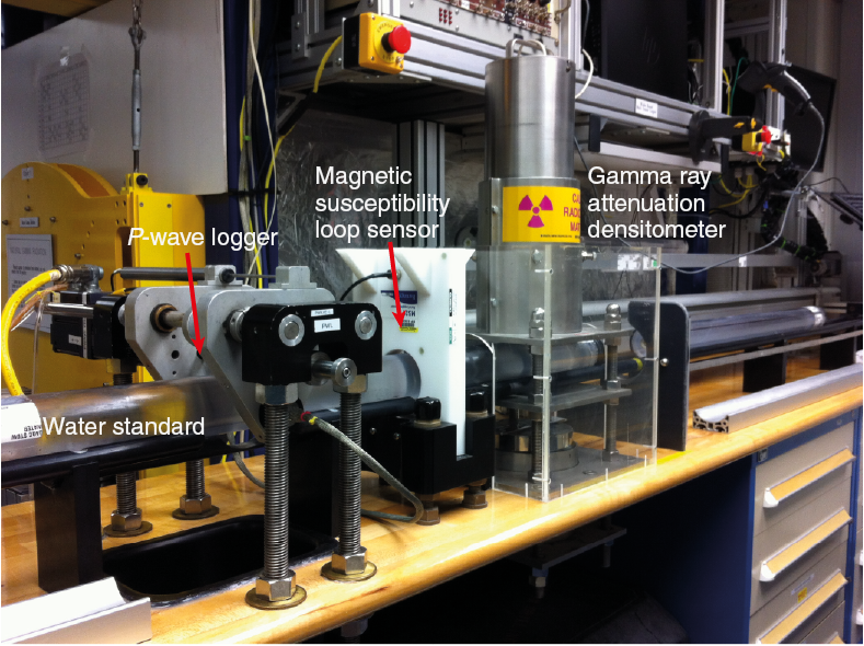
Figure F17. WRMSL system.
Following WRMSL measurements, core sections were measured with the spectral NGRL (Figure F18) at a nominal interval of 10 cm and a gamma ray counting time of 5 min (i.e., 10 min per core section; each analysis consists of two measurement cycles).
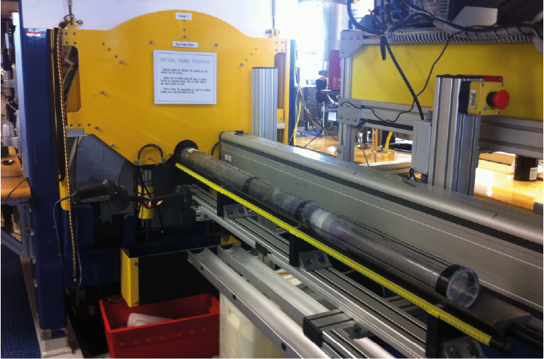
Figure F18. NGRL system.
Thermal conductivity was measured on approximately one section per core (typically Section 3) by a needle probe inserted into the soft-sediment core through a small hole drilled in the plastic core liner near the middle of the whole-round section or by the contact probe method in half-space configuration on split cores for indurated sediment cores. After completing measurements on whole-round sections, the cores were split longitudinally, with one half for archiving (the archive half) and the other half (the working half) for sampling and analysis. The archive half was passed through the SHMSL to measure point magnetic susceptibility and color reflectance at a nominal sample interval of 2.5 cm.
Discrete samples were collected from 1–3 sections of the working half (typically Sections 2, 4, and 6) to measure wet bulk density, dry bulk density, water content, porosity, and grain density using moisture and density (MAD) procedures. Where possible, samples were taken as close to the middle of the core sections as core conditions permitted. However, because of poor core recovery or cores consisting of numerous small biscuits, discrete samples were taken from what were deemed the most suitable and representative components of the cores. At sites where multiple holes provided overlapping intervals, the duplicate cores were not sampled and only nondestructive analyses (WRMSL, SHMSL, and/or downhole logs) were collected to fill gaps at sites with poor core recovery in earlier boreholes. P-wave velocity was typically measured on 1–3 sections per split core using the Section Half Measurement Gantry (SHMG).
Measurements of hard rock core sections
Hard rock (e.g., igneous) cores were run through the WRMSL and NGRL using the method described for sedimentary cores (Figures F17, F18). Hard rock core sections containing fragments were loaded into sterile liners in the core splitting room for examination by a petrologist who decided where the pieces should be split between working and archive halves (see Core handling and analysis). The pieces were then put back into liners before measurement with the WRMSL and NGRL. P-wave velocity was not measured with the WRMSL on hard rock samples because the spaces between the liner and the core or rock pieces would have caused an erroneous result. After physical property measurements on whole-round cores, the cores were split into working and archive halves and all rock pieces were labeled. The archive half was passed through the SHMSL to measure point magnetic susceptibility and color reflectance at a nominal sample interval of 2.5 cm. Thermal conductivity was measured approximately once per core using a contact probe on a piece of the section half. P-wave velocity was measured on 1–3 sections per core using the SHMG for discrete hard rock samples and on XCB and RCB section halves. MAD measurements were also taken on these samples or on discrete samples or core fragments from the same lithology at a position near the P-wave velocity samples. In some cases, core recovery was poor or the cores consisted of numerous small biscuits. In such cases, discrete samples were taken from the most suitable and representative components of these cores.
A full discussion of all methodologies and calculations used on board the JOIDES Resolution in the Physical Properties Laboratory is available in Blum (1997). Details and procedures for each physical property measurement are described below.
Whole-Round Multisensor Logger measurements
GRA bulk density, P-wave velocity, and magnetic susceptibility were measured nondestructively with the WRMSL (Figure F17). To optimize the process, sampling interval and measurement integration time (2.5 cm and 5 s, respectively) were the same for all sensors. These sampling intervals are common denominators of the distances between the sensors installed on the WRMSL (30 cm), which allows for efficient sequential and simultaneous measurements. Such relatively high resolution measurements are a prerequisite to ensure the potential detection of Milankovitch cycles. After measuring every core, the fidelity of the measurements was monitored by passing a single core liner filled with deionized water through the WRMSL. When required, the STMSL was operated for fast-tracked measurement of the whole-round cores with 10 cm spacing, measuring GRA bulk density and magnetic susceptibility before the cores had thermally equilibrated. This allowed us to provide preliminary information on the cores to be used for stratigraphic correlation of overlapping holes at a given site (see Stratigraphic correlation).
GRA bulk density
GRA density provides an estimate of bulk density of the core based on attenuation of a gamma ray beam. The beam is produced by a 137Cs gamma ray source at a radiation level of 370 MBq within a lead shield with a 5 mm collimator and directed through the whole-round core. The gamma ray detector on the opposite side of the core from the source includes a scintillator and an integral photomultiplier tube to record the gamma radiation that passes through the core. The attenuation of the gamma rays occurs primarily by Compton scattering, in which the gamma rays are scattered by electrons in the formation. The degree of scattering is related to the material bulk density. The density (ρ) is proportional to the intensity of the attenuated gamma rays and can be expressed as
- I = measured intensity of gamma rays passing through the sample,
- I0 = gamma ray source intensity,
- μ = Compton attenuation coefficient, and
- d = sample diameter.
The μ, I0, and d are treated as constants so that ρ can be calculated from I.
In general, WRMSL GRA density measurements are most accurate when taken on a completely filled core liner with minimal drilling disturbance; otherwise, measurements tend to underestimate true values. By default, the instrument reports measurements using the internal diameter of the core liner (66 mm) as the assumed sample diameter. This assumption is suitable for most sediment cores obtained with the APC system. For sediment and/or hard rock cored by the XCB or RCB systems, core diameter is usually ~58 mm or less, resulting in an underestimated density for these cores. The spatial resolution of the GRA densitometer is less than ±1 cm. The gamma ray detector is calibrated with sealed calibration cores (one standard core liner filled with distilled water and aluminum cylinders of various diameters). To establish the calibration curves, gamma ray counts were taken through each aluminum cylinder for 60 s. Each aluminum cylinder has a density of 2.7 g/cm3, and d is 1, 2, 3, 4, 5, or 6 cm. The relationship between I and µd is
where the coefficients A, B, and C are instrument constants determined from the calibration. Recalibration was performed as needed when the estimated deionized water standard deviated significantly (more than a few percent) from 1 g/cm3.
Magnetic susceptibility
Magnetic susceptibility (χ) is a dimensionless measure of the degree to which a material can be magnetized by an external magnetic field:
where M is the magnetization induced in the material by an external field of strength H. The bulk magnetic susceptibility depends on its mineralogical composition, the magnetic susceptibility of the minerals, and sometimes the size of the particles. Ferrimagnetic minerals (e.g., magnetite and maghemite) have relatively high positive magnetic susceptibility and can produce large bulk magnetic susceptibility in a rock even when present at low concentrations. Antiferromagnetic (hematite and goethite) and paramagnetic (smectite, illite, and chlorite) minerals have lower positive magnetic susceptibility and can produce weak bulk rock magnetic susceptibility in the absence or near absence of ferromagnetic minerals. Diamagnetic minerals (calcite, quartz, and kaolinite) have very low negative magnetic susceptibility and produce null or slightly negative bulk rock magnetic susceptibility in the absence of other magnetic minerals. Igneous materials typically have a magnetic susceptibility that is two orders of magnitude greater than their alteration products, such as clay minerals.
Magnetic susceptibility core measurements on the WRMSL were made using a 9 cm diameter Bartington MS2C loop sensor (Figure F17). An oscillator circuit in the sensor, which operates at a frequency of 0.565 kHz and an alternating field of ~140 A/m, produces a low-intensity, nonsaturating alternating magnetic field. Sediment and hard rock core sections going through the influence of this field cause a change in oscillator frequency. Frequency information returned in pulse form to the susceptometer is converted into magnetic susceptibility. The loop sensor has a spatial resolution of 23–27 mm and is accurate to within 2%. Converting from instrument units (IU) to dimensionless SI units for magnetic susceptibility requires standards with known magnetic susceptibility values. None were available on the ship, and magnetic susceptibility measurements are therefore reported in IU.
P-wave velocity
P-wave (compressional) velocity (VP) data can be used to evaluate small-strain moduli, correlate between downhole logging and core data, and evaluate porosity and cementation. P-wave velocity is determined by measuring the time required for a compressional wave to travel a specific distance through the core:
where d is the path length and tcore is the traveltime through the core.
The PWL measures the traveltime of 500 kHz ultrasonic waves traveling horizontally across the core while it remains in the core liner. Waves are transmitted to the core by plastic transducer contacts connected to linear actuators. Pressure is applied to the actuators to ensure coupling between the transducers and the core liner. The total traveltime, t0, is the sum of
- tdelay = time delay related to transducer faces and electronic circuitry,
- tpulse = delay related to the peak detection procedure,
- tliner = transit time through the core liner, and
- tcore = traveltime through the core.
The system is calibrated using a core liner filled with distilled water, which provides control for tdelay, tpulse, and tliner. From these calibrations, VP can be calculated for the whole-round specimens in core liners as
VP = (dcl − 2dliner)/(t0 − tpulse − tdelay − 2tliner),
This equation assumes that the core completely fills the core liner. The WRMSL PWL was usually turned off for XCB and RCB core segments that did not fill the core liner.
Natural Gamma Radiation Logger measurements
Gamma radiation is emitted from the decay of mineral-hosted 238U, 232Th, and 40K. The NGRL measures this natural emission on whole-round cores using a system designed and built at Texas A&M University (USA) by the IODP JOIDES Resolution Science Operator (Figure F18) (Vasiliev et al., 2011; Dunlea et al., 2013). When 238U, 232Th, and 40K radioisotopes decay, they and their daughter products emit gamma radiation at specific energy levels unique to each isotope. NGR spectroscopy measures a wide energy spectrum that can be used to estimate the abundance of each isotope based on the strength of the signal at characteristic energies (Blum, 1997; Gilmore, 2008). In sediments and sedimentary rocks, Th and K are usually associated with particular clay minerals, whereas U is often encountered in either clay minerals or organic-rich material. Because minor changes in the abundance of clay minerals produce a relatively large variation in gamma radiation, NGR data are useful as a lithologic indicator, aiding in core-to-core correlation. These spectral data were then processed to estimate U, Th, and K abundance (e.g., De Vleeschouwer et al., 2017).
The NGRL system was installed on the renovated JOIDES Resolution in 2009 and has been used on every JOIDES Resolution expedition starting with Expedition 320. The NGRL system consists of eight sodium iodide-thallium (NaI[Tl]) detectors arranged at 20 cm intervals under the lower half of the core section (Figure F19). Data are collected in two measurement cycles, each of which produce NGRL measurements at eight positions within the core section per 150 cm section. During the first measurement cycle, the first detector is located 10 cm from the top of the core section, thus producing eight measurements at odd multiples of 10 cm from the top of the core. The core is then advanced 10 cm, producing another eight measurements at even multiples of 10 cm from the top of the core. The detector array has both passive (layers of lead) and active (plastic scintillators) shielding to reduce the background environmental and cosmic radiation. The plastic scintillators are positioned above the core section and detect incoming high-energy gamma and muon cosmic radiation, which is removed from the total counted by the NaI(Tl) detectors. The passive (lead) layers separate the NaI(Tl) detectors, isolating the portion of core being measured. The quality of the energy spectrum measured in a core depends on the concentration of radionuclides in the sample and on the measurement time, with longer duration measurements yielding better spectra. Measurement times were chosen to be 5 min per measurement cycle, or ~10 min per core section, or 60 min per core. This yields statistically significant energy spectra for most lithologies (Vasiliev et al., 2011).
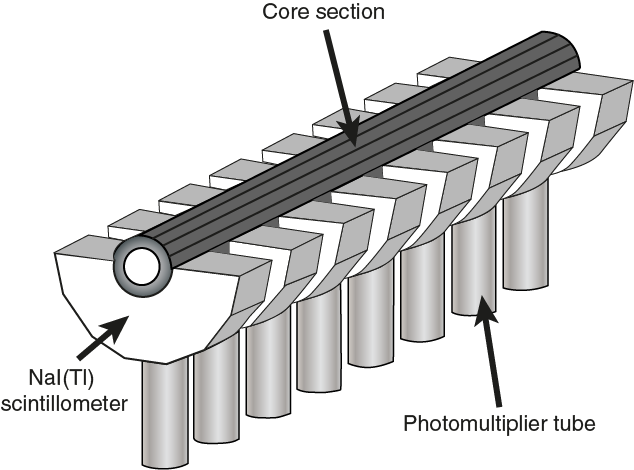
Figure F19. Main elements of the NGRL.
Thermal conductivity core measurements
Thermal conductivity was measured on approximately one section per core (usually Section 3) with the TK04 (TeKa Berlin) system using the needle probe method in full-space configuration for whole-round soft-sediment cores (Von Herzen and Maxwell, 1959) or the contact probe method in half-space configuration on split cores for indurated sediment and hard rock. The probes contain a heater wire and calibrated thermistor.
For soft sediment, the needle probe was inserted into a 2 mm diameter hole drilled through the liner along one of the lines marking where the core was later to be split into working and archive halves. For indurated sediment and hard rock cores, samples were selected from the working half and returned unaltered to the core liner upon completion of the tests. Measurements were taken with a contact probe embedded in the surface of an epoxy block with a low thermal conductivity (Vacquier, 1985). To avoid interference from air flow in the laboratory during the thermal conductivity measurement, the core section was placed into an enclosed box insulated with foam (Figure F20).
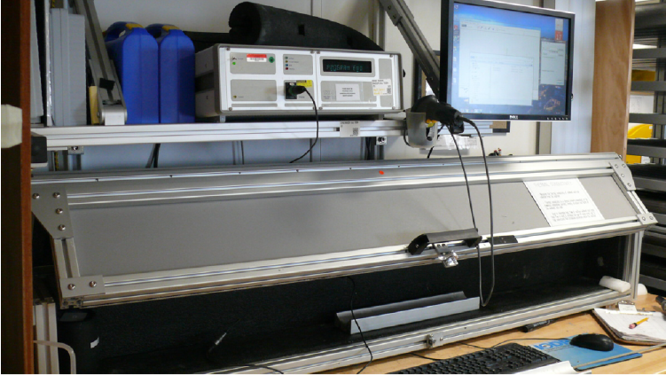
Figure F20. Thermal conductivity system.
To measure thermal conductivity, the probe heat source was turned on and the increase in temperature was recorded over 80 s. A heating power of 0.7–1.7 W/m was typically used in soft sediment, and 1.2–1.9 W/m was used for indurated material. The solution to the heat conduction equation with a line source of heat was then fitted to the temperature measurements to obtain the thermal conductivity. Because the probe is much more conductive than sediment or hard rock, the probe is assumed to be a perfect conductor. Under this assumption, the temperature of the probe has a linear relationship with the natural logarithm of the time after heating was initiated:
- T = temperature (K),
- q = heat input per unit length per unit time (J/m/s),
- k = thermal conductivity (W/[m·K]),
- t = time after the initiation of the heat (s), and
- C = instrumental constant.
Three measuring cycles were automatically performed, and the probe and sample were allowed to reequilibrate for 10 min between each cycle. The conductivity was taken to be the average of the conductivity determined from each cycle. A self-test, which included a drift study, was conducted at the beginning of each measurement cycle. Once the probe temperature stabilized, the heater circuit was closed and the temperature rise in the probe was recorded. Thermal conductivity was calculated from the rate of temperature rise while the heater current was flowing. Temperatures measured during the first 80 s of the heating cycle were fitted to an approximate solution of a constantly heated line source (for details, see Kristiansen, 1982; Blum, 1997). Measurement errors were 5%–10%.
Section Half Multisensor Logger measurements
Color reflectance and point magnetic susceptibility were measured by the core description team on archive halves using the SHMSL (Figure F21). The archive half of the split core was placed on the core track, above which an electronic platform moves along a track, recording the height of the split-core surface with a laser sensor. The laser establishes the surface topography of the section, and then the platform reverses the direction of movement, moving from the core section end (lower in the borehole) to top (higher in the borehole) while making measurements of point magnetic susceptibility and color reflectance. Also, because the SHMSL requires flush contact between the magnetic susceptibility point sensor and the split core, measurements were made on the archive halves of split cores, which were covered with clear plastic wrap. Any foam inserts were removed from the section-half cores before measurement, so the measured range of values represents that of the core material only. During Expedition 369, point magnetic susceptibility and color reflectance data were collected at a nominal interval of 2.5 cm for each core.
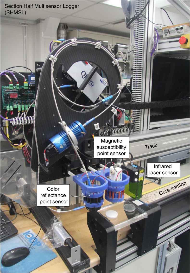
Figure F21. SHMSL system.
Color reflectance spectrophotometry
The color reflectance spectrometer uses an Ocean Optics QEPro Peltier-cooled spectrophotometer mounted on the automated SHMSL that uses both halogen and LED light sources, which covers wavelengths from ultraviolet through visible to near infrared. Measurements were taken from 380 to 900 nm wavelengths at a 2 nm interval every 3 cm along the archive-half section. The data are reported using the L*a*b* color system, in which L* is lightness, a* is redness (positive) versus greenness (negative), and b* is yellowness (positive) versus blueness (negative). The color reflectance spectrometer calibrates on two spectra, pure white (reference) and pure black (dark). Color calibration was conducted approximately once every 6 h (twice per shift). Clear plastic film was used to cover all sections to keep the material from collecting on the detectors and to avoid any discrepancies from the use of the plastic wrap.
Point magnetic susceptibility
Point measurements of magnetic susceptibility were taken with a Bartington Instruments MS2K contact probe with a flat 15 mm diameter circular sensor, a 25 mm field of influence, and an operational frequency of 930 Hz. The instrument averages three measurements from the sensor at each position on the core, leading to an accuracy of ~5%. The spatial resolution of the point magnetic susceptibility instrument is ~25.4 mm diameter full-width-half-maximum, which is higher than the 100 mm resolution of the MS2C sensors on the WRMSL. The probe is zeroed in air slightly above the core before each measurement to compensate for the influence of the metal track. The point magnetic susceptibility meter was calibrated by the manufacturer before installation on the ship and is quality checked every 6 h at the same time as color reflectance sensor calibration.
Section Half Measurement Gantry measurements of P-wave velocity
For sediment and hard rock cores, P-wave velocity was performed on the working halves using the x-axis caliper contact probe transducer on the SHMG, with at least one analysis per core. P-wave velocity measurements were taken on intact core sections at positions coinciding as much as possible with the MAD sample locations (see Discrete sample measurements of moisture and density). For cores that did not have intact sections, P-wave velocity measurements were taken on either the MAD samples or on larger pieces obtained from the same core section with the same lithology and as nearby a position in the core as possible. The P-wave velocity system on the SHMG uses Panametrics-NDT Microscan delay line transducers (Figure F22) transmitting at 0.5 MHz. The signal received through the section half or discrete sample was digitally recorded, and the first arrival was picked automatically. The distance between transducers was measured with a built-in linear voltage displacement transformer. Calibration was performed with a series of acrylic cylinders of differing thicknesses and a known P-wave velocity of 2750 ± 20 m/s. The system time delay determined from calibration was subtracted from the picked arrival time to estimate the P-wave traveltime through the sample. The thickness of the sample (calculated by the linear voltage displacement transformer) was divided by the traveltime to calculate P-wave velocity in meters per second.
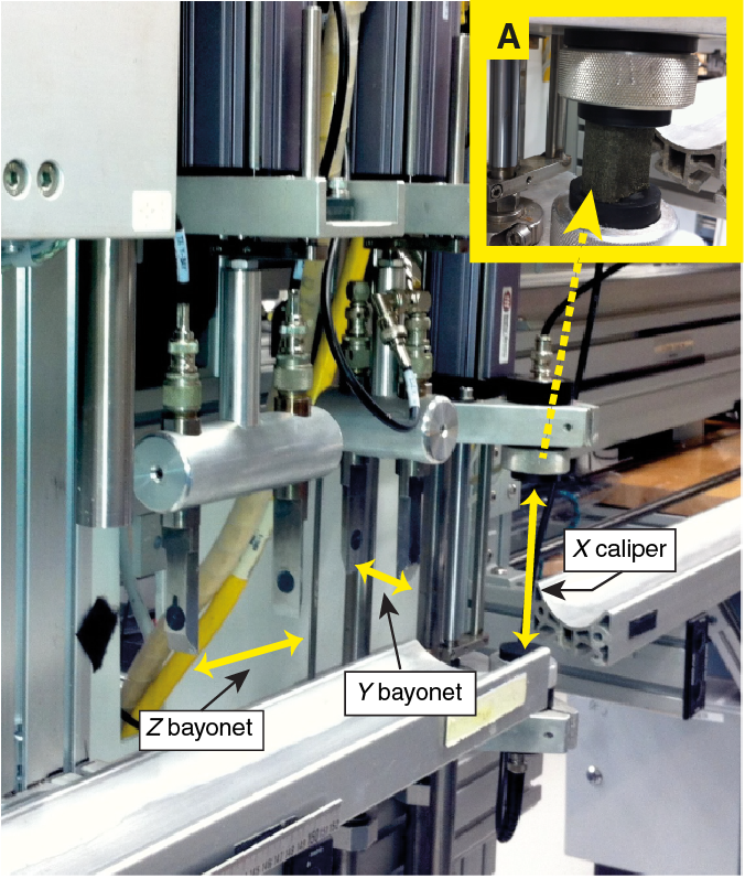
Figure F22. SHMG x-axis caliper and y- and z-axis bayonets.
Discrete sample measurements of moisture and density
Discrete samples were collected from the working halves of the core to determine wet and dry bulk density, grain density, water content, and porosity using MAD analysis techniques. Samples were taken from 1–3 sections per core, and additional samples were taken as warranted by lithology changes. At sites where multiple holes provided overlapping intervals, the duplicate cores were not sampled. In soft sediment, ~10 cm3 samples were collected with a plastic syringe and placed in glass vials for measurements. In indurated sediment and hard rock, samples were cut with a saw from the working halves; more often than not, these samples correspond with the same interval collected for discrete paleomagnetic analyses.
Sample preparation
Soft-sediment samples were placed in numbered, preweighed ~16 mL Wheaton glass vials for wet and dry sediment weighing, drying, and dry volume measurements. To determine the wet mass of well-indurated samples (typically basalt, cemented breccia, and sandstone), we placed the samples in individual plastic vials filled with seawater and used a vacuum chamber to force saturation in the pore spaces. The vacuum pump removed the air from the chamber to a pressure of ~40–50 kPa below atmospheric pressure, thereby, in theory, forcing seawater into the samples. These samples were kept under saturation for at least 24 h with the vacuum maintained in the chamber by turning the pump on for 30 min every 5 h. After removal from the saturator, the cubes were patted dry with a paper towel, and wet mass was immediately determined using the dual balance system. The samples were then dried and measured for dry mass and the volume.
Dual balance mass measurement
The weights of wet and dry samples were determined to a precision of 0.005 g using two Mettler-Toledo XS204 electronic balances, with one acting as a reference. A standard weight of similar value to the sample was placed upon the reference balance to increase accuracy. A computer averaging system was used to compensate for the ship’s motion. The default setting of the balances is 300 measurements (taking ~90 s).
Pycnometer volume measurement
Dry sample volume was determined using a six-celled, custom-configured Micrometrics AccuPyc 1330TC helium-displacement pycnometer (Figure F23). The precision of each cell is 1% of the full-scale volume. Volume measurement was preceded by three purges of the sample chamber with helium warmed to ~28°C. Three measurement cycles were run for each sample. A reference volume (set of two calibration spheres) was placed in one of the chambers during each set of measurements to check for instrument drift and systematic error. The reference volume was moved sequentially between chambers such that each chamber was calibrated in turn every five sets of measurements. The volumes occupied by the Wheaton vials used for soft-sediment samples were calculated before the expedition by dividing each vial’s weight by the average density of the vial glass. Dry mass and volume were measured after samples were heated in an oven at 105°C ± 5°C for 24 h and allowed to cool in a desiccator. The procedures for the determination of these physical properties comply with the American Society for Testing and Materials (ASTM) designation (D) 2216 (ASTM International, 1990). The fundamental relation and assumptions for the calculations of all physical property parameters are discussed by Blum (1997) and summarized below.
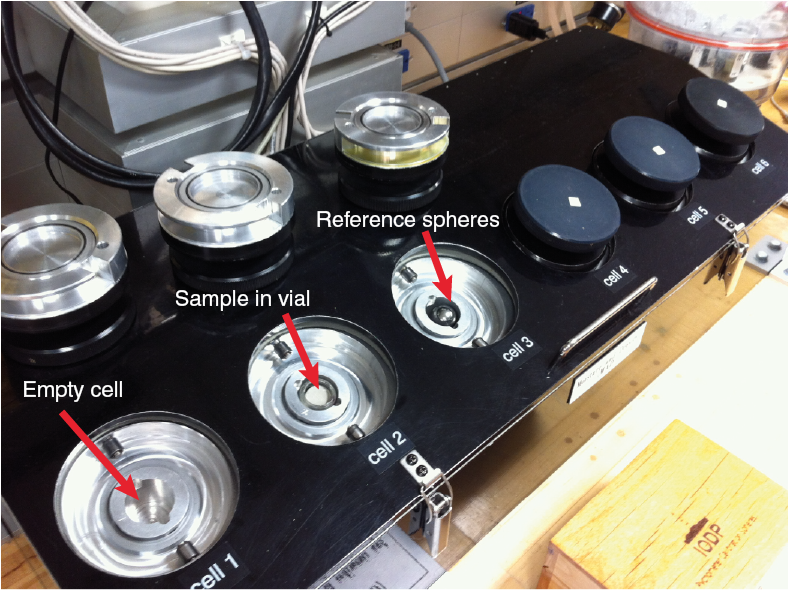
Figure F23. Pycnometer cells for MAD measurements.
Mass and volume calculation
We measured wet mass (Mwet), dry mass (Mdry), and dry volume (Vdry). Salt precipitated in sediment pores during the drying process is included in the Mdry and Vdry values. The mass of the evaporated water (Mwater) and salt (Msalt) in the sample are given by
where s is the assumed saltwater salinity (0.035) corresponding to a pore water density (ρpw) of 1.024 g/cm3 and a salt density (ρsalt) of 2.22 g/cm3. The corrected mass of pore water (Mpw), volume of pore water (Vpw), mass of solids excluding salt (Msolid), volume of salt (Vsalt), volume of solids excluding salt (Vsolid), and wet volume (Vwet) are
Vwet = Vdry − Vsalt + Vpw , and
where rm is the ratio of mass between equal volumes of freshwater and seawater (a computational constant of 0.965).
Calculation of bulk properties
For all sediment samples, water content (w) is expressed as the ratio of mass of interstitial water to wet sediment (total) mass:
Wet bulk density (ρwet), dry bulk density (ρdry), sediment grain density (ρsolid), porosity (φ), and void ratio (VR) are calculated as
Moisture and density properties reported in the physical properties sections of all site chapters were calculated with the MADMax shipboard program using the program’s predefined “Method C.” In Method C, the wet and dry mass and dry volume are measured, and the other physical properties are derived using the above equations.
Downhole logging
Wireline logging
During wireline logging operations, the logs were recorded with Schlumberger logging tools combined into tool strings lowered into the hole after coring operations are completed. Different tool string configurations were used during Expedition 369. These tool strings included the triple combination (triple combo) tool string, which measures NGR, porosity, density, and resistivity, and the Formation MicroScanner (FMS)-sonic tool string, which provides FMS resistivity images of the borehole wall and sonic velocities. An alternate configuration was selected for logging most holes (Figure F24); this tool configuration is herein referred to as the Quambo because it incorporates the sonic tool onto the traditional triple combo at the expense of the porosity tool, which was removed to stay below the maximum tool power consumption limit. The standard triple combo tool string (minus magnetic susceptibility) and FMS/porosity tools were also used to log segments of Hole U1513E. Additionally, the Vertical Seismic Imager (VSI) was used to create a vertical seismic profile (VSP) in Hole U1513E.
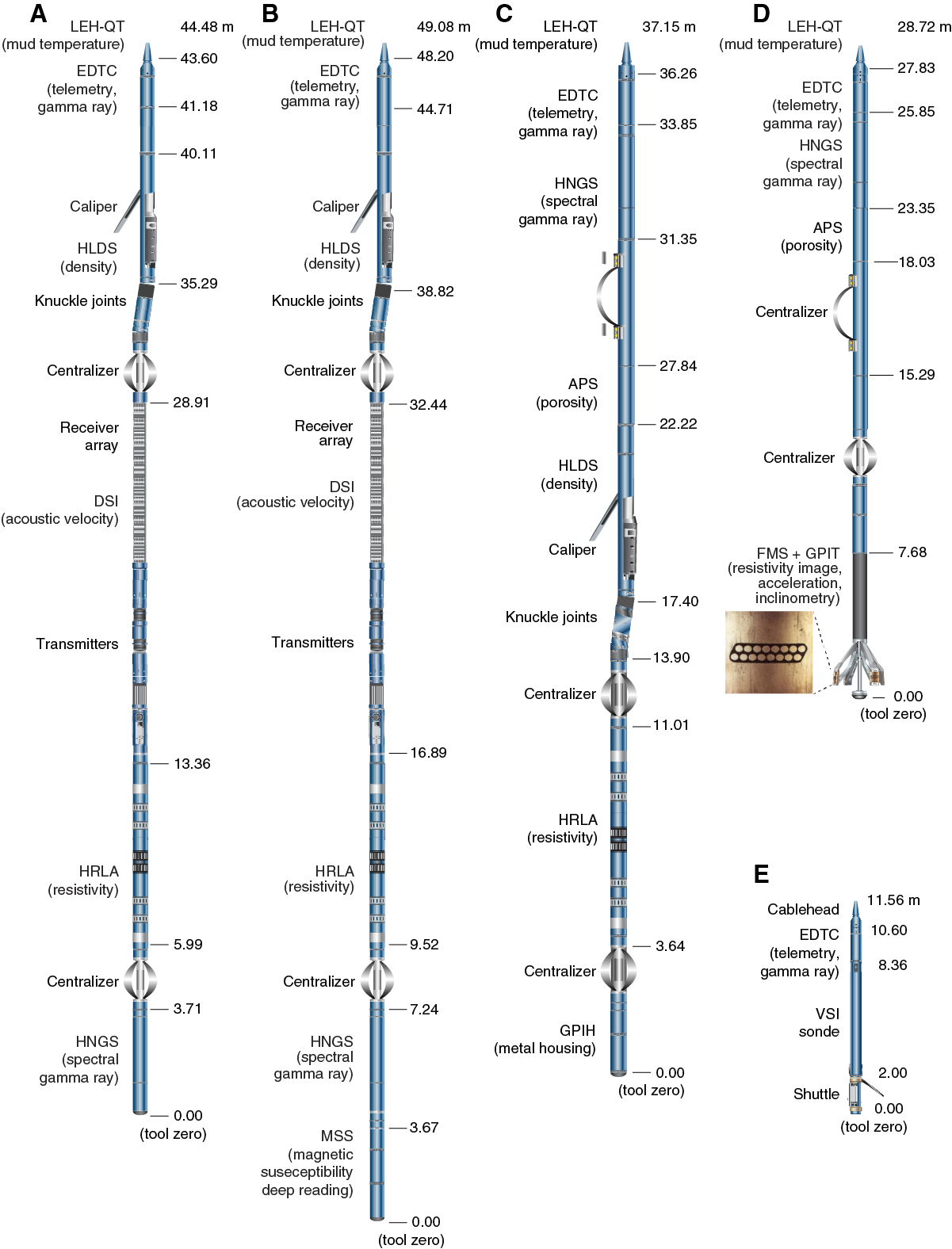
Figure F24. Downhole logging tool strings.
Each tool string contains a telemetry cartridge for communicating through the wireline to the Schlumberger data acquisition system (MAXIS unit) on the drillship. In preparation for logging, the boreholes were cleaned, flushed of debris using drilling fluid, and filled with seawater-based logging gel (sepiolite mud mixed with seawater and weighted with barite; approximate density = 10.5 lb/gal, ~1258 kg/m3) to help stabilize the borehole walls. The BHA was typically pulled up to ~70–150 m WMSF to expose the deeper borehole wall for wireline measurement while also stabilizing the upper portion of the hole. The tool strings were then lowered downhole on a seven-conductor wireline cable before being pulled up at constant speed to provide continuous log measurements of several properties simultaneously.
Each tool string deployment is termed a logging “run.” During each run, tool strings can be lowered and pulled up in the hole several times to check repeatability and to increase coverage of the FMS borehole images. Each lowering or hauling-up of the tool string while collecting data constitutes a “pass.” Incoming data were recorded and monitored in real time on the MCM MAXIS logging computer. An active wireline heave compensator (WHC) was used to minimize the effect of ship’s heave on the tool position in the borehole (see below).
Wireline logged sediment properties and tool measurement principles
The logged properties and the principles used in the tools that measure them are briefly described below. More detailed information on individual tools and their geological applications may be found in Serra (1984, 1986, 1989), Schlumberger (1989, 1994), Rider (1996), Goldberg (1997), Lovell et al. (1998), and Ellis and Singer (2007). A complete online list of acronyms for the Schlumberger tools and measurement curves is at http://www.apps.slb.com/cmd and http://iodp.tamu.edu/tools/logging/index.html.
Downhole natural gamma radiation
The Hostile Environment Natural Gamma Ray Sonde (HNGS) measured the NGR of the borehole when the standard triple combo, modified Quambo, or FMS-sonic tool strings were deployed downhole (Figure F24). The HNGS uses two bismuth germanate scintillation detectors and five-window spectroscopy to determine concentrations of K (in weight percent), Th (in parts per million), and U (in parts per million) from the characteristic gamma ray energies of isotopes in the 40K, 232Th, and 238U radioactive decay series that dominate the natural radiation spectrum. The computation of the elemental abundances uses a least-squares method of extracting U, Th, and K elemental concentrations from the spectral measurements. The HNGS filters out gamma ray energies <500 keV, eliminating sensitivity to bentonite or KCl in the drilling mud and improving measurement accuracy. The HNGS also provides a measure of the total gamma ray emission (HSGR) and uranium-free or computed gamma ray emission (HCGR), which are measured in American Petroleum Institute units (gAPI). The HNGS response is influenced by the borehole diameter; therefore, the HNGS data are corrected for borehole diameter variations during acquisition.
An additional NGR sensor was housed in the Enhanced Digital Telemetry Cartridge (EDTC) at the top of each tool string (Figure F24). The EDTC is primarily used to communicate data to the surface. The sensor includes a sodium iodide scintillation detector that also measures the total NGR emission of the formation. The EDTC is not a spectral tool (it does not provide U, Th, and K concentrations), but it provides total gamma radiation for each pass. The inclusion of the HNGS in the triple combo, Quambo, and FMS-sonic tool strings means that the gamma ray data can be used to match depths between logging strings and passes and for core-log integration.
Density and photoelectric factor
Formation density was measured downhole with the Hostile Environment Litho-Density Sonde (HLDS) (Figure F24). The sonde contains a radioactive cesium (137Cs) gamma ray source (622 keV) and far and near gamma ray detectors mounted on a shielded skid, which is pressed against the borehole wall by a hydraulically activated decentralizing arm. Gamma rays emitted by the source undergo Compton scattering, in which gamma rays are scattered by electrons in the formation. The number of scattered gamma rays that reach the detectors is proportional to the density of electrons in the formation, which is in turn related to bulk density. Porosity may also be derived from this bulk density if the matrix (grain) density is known.
The HLDS also measures the photoelectric effect factor (PEF), a measure of the photoelectric absorption of low-energy gamma radiation. Photoelectric absorption occurs when the energy falls below 150 keV as a result of being repeatedly scattered by electrons in the formation. PEF is determined by comparing the counts from the far detector in the high-energy region, where only Compton scattering occurs, with those in the low-energy region, where count rates depend on both reactions. Because PEF depends on the atomic number of the elements in the formation (heavier elements have higher PEF), it also varies according to the chemical composition of the minerals present and can be used to identify the overall mineral make-up of the formation. For example, the PEF of calcite is 5.08 barn/e−, illite is 3.03 barn/e−, quartz is 1.81 barn/e−, K-feldspar is 2.86 barn/e−, and pure pyrite is 16.97 barn/e− (where barn = 10−24 cm2). Contact between the tool and borehole wall is essential for good-quality HLDS logs; poor contact results in underestimation of density values. Both the density correction and caliper measurement of the hole are used to check the contact quality. In the deeper parts of the hole, the PEF log should be used with caution, especially in washouts, because barium in the logging mud swamps the signal, despite correction for mud effect.
Porosity
Formation porosity was measured downhole with the Accelerator Porosity Sonde (APS) (Figure F24). The APS was not part of the Quambo tool string (it was only deployed at Site U1513E) because of time constraints and borehole stability concerns and the potential for washed out intervals that interfere with the APS measurements. The sonde includes a minitron neutron generator that produces fast (14.4 MeV) neutrons and five neutron detectors (four epithermal and one thermal) positioned at different distances from the minitron. The tool’s detectors count neutrons that arrive at the detectors after being scattered and slowed by collisions with atomic nuclei in the formation.
The highest energy loss occurs when neutrons collide with hydrogen nuclei, which have practically the same mass as the neutron (the neutrons bounce off of heavier elements without losing much energy). If the hydrogen (i.e., water) concentration is low, as in low-porosity formations, neutrons can travel farther before being captured and the count rates increase at the detector. The opposite effect occurs in high-porosity formations where the water content is high. However, because hydrogen bound in minerals such as clays or in hydrocarbons also contributes to the measurement, the raw porosity value is often an overestimate.
Upon reaching thermal energies (0.025 eV), the neutrons are captured by the nuclei of chlorine, silicon, boron, and other elements, resulting in a gamma ray emission. This neutron-capture cross section (Σf) is also measured by the tool.
Electrical resistivity
The High-Resolution Laterolog Array (HRLA) tool provides six resistivity measurements (including the borehole or mud resistivity and five measurements of formation resistivity with increasing penetration into the formation) with different depths of investigation (Figure F24). The tool sends a focused current into the formation and measures the intensity necessary to maintain a constant drop in voltage across a fixed interval, providing direct resistivity measurements. The array has one central (source) electrode and six electrodes above and below it that serve alternatively as focusing and returning current electrodes. By rapidly changing the role of these electrodes, a simultaneous resistivity measurement at six penetration depths is achieved. The tool is designed to ensure that all signals are measured at exactly the same time and tool position and to reduce the sensitivity to “shoulder bed” effects when crossing sharp beds thinner than the electrode spacing. The design of the HRLA, which eliminates the need for a surface reference electrode, improves formation resistivity evaluation compared to traditional dual induction and allows the full range of resistivity to be measured, from low (e.g., in high-porosity sediments) to high (e.g., in basalt). The HRLA needs to be centralized in the borehole during the run for optimal results, so knuckle joints were used to centralize the HRLA while allowing the density and porosity tools to maintain good contact with the borehole wall.
Calcite, silica, and hydrocarbons are electrical insulators, whereas ionic solutions like interstitial water are conductors. Electrical resistivity, therefore, can be used to evaluate porosity for a given salinity and resistivity of the interstitial water. Clay surface conduction also contributes to the resistivity values, but at high porosities, this is a relatively minor effect.
Acoustic velocity
The Dipole Sonic Imager (DSI) measures the transit times between sonic transmitters and an array of eight receivers and combines replicate measurements, thus providing a direct measurement of sound velocity through formations that is relatively free from the effects of formation damage and an enlarged borehole (Schlumberger, 1989) (Figure F24). Along with the monopole transmitters found on most sonic tools, the DSI also has two crossed-dipole transmitters that allow the measurement of shear wave velocity in addition to compressional wave velocity. Dipole measurements are necessary to measure shear velocities in slow formations with shear velocity less than the velocity of sound in the borehole fluid. Such slow formations are typically encountered in deep-ocean drilling.
Formation MicroScanner
The FMS provides oriented, high-resolution electrical resistivity–based images of borehole walls (Figure F24). The tool has four orthogonal arms and pads, each containing 16 button electrodes that are pressed against the borehole wall during logging. The electrodes are arranged in two diagonally offset rows of eight electrodes each. A focused current is emitted from the button electrodes into the formation, and a return electrode is located near the top of the tool. Resistivity of the formation at the button electrodes is derived from the intensity of current passing through the button electrodes.
Processing of the resistivity measurements offshore at Lamont-Doherty Earth Observatory (LDEO) generates oriented high-resolution images that reveal geologic structures of the borehole wall. Features such as bedding, stratification, fracturing, slump folding, and bioturbation can be resolved (Luthi, 1990; Salimullah and Stow, 1992; Lovell et al., 1998). Because the images are oriented to magnetic north, further analysis can provide measurement of the dip and direction (azimuth) of planar features in the formation. In addition, when the corresponding planar features can be identified in the recovered core samples, individual core pieces can be reoriented with respect to true north.
The maximum extension of the caliper arms is 40.6 cm (16 inches). In holes or in sections of holes with a diameter greater than this maximum, the pad contact at the end of the caliper arms will be inconsistent, and the FMS images may appear out of focus and too conductive. For example, irregular (rough) borehole walls will also adversely affect the images if contact with the wall is poor. The standard procedure is therefore to make two full uphole passes with the FMS to maximize the chance of getting full borehole coverage with the pads. This method also helps to ensure that adequate data coverage is obtained because only ~30% of a borehole with a diameter of 25 cm is imaged during a single pass.
Magnetic susceptibility sonde
The magnetic susceptibility sonde (MSS) is a nonstandard wireline tool designed by LDEO (Figure F24). It measures the ease with which formations are magnetized when subjected to a magnetic field. The ease of magnetization is ultimately related to the concentration and composition (size, shape, and mineralogy) of magnetic minerals (principally magnetite) in the formation. These measurements provide one of the best methods for investigating stratigraphic changes in mineralogy and lithology because the measurement is quick, repeatable, and nondestructive and because different lithologies often have strongly contrasting susceptibilities.
The MSS dual-coil sensor provides ~40 cm resolution measurements with ~20 cm depth of horizontal investigation. The MSS was run as the lowermost tool in the triple combo tool string in Hole U1514C, using a specially developed data translation cartridge to enable the MSS to be run in combination with the Schlumberger tools. However, the MSS tool was not included in the Quambo tool string at all sites—particularly where there were concerns about ledges or partial borehole collapse and therefore too much risk of damaging the MSS tool (Figure F24). The MSS also has an optional single-coil sensor to provide high-resolution measurements (~10 cm), but it was not used during Expedition 369 because it has a large bowspring that would require the MSS to be run higher up in the tool string and because it is very sensitive to separation from the borehole wall.
Magnetic susceptibility data from both the high-resolution and deep-reading sensors are plotted as uncalibrated units. The MSS reading responses are affected by temperature and borehole size (higher temperatures lead to higher susceptibility measurements). Preliminary processing was performed offshore to remove the temperature drift by calculating a least-squares polynomial fit to the data and subtracting the calculated trend from the data set. When the magnetic susceptibility signal in sediment is very low, the detection limits of the tool may be reached. For quality control and environmental correction, the MSS also measures internal tool temperature, z-axis acceleration, and low-resolution borehole conductivity.
Acceleration and inclinometry
Three-component acceleration and magnetic field measurements were made with the General Purpose Inclinometry Tool (GPIT) during logging (Figure F24). The primary purpose of this tool, which incorporates a three-component accelerometer and a three-component magnetometer, is to determine the acceleration and orientation of the FMS-sonic string. This information allows the FMS image to be corrected for irregular tool motion to determine the dip and direction (azimuth) of features in the images. The GPIT was also run on the triple combo tool string to provide data to optimize the WHC before logging began and to acquire the best possible downhole data. The GPIT is run with other tools on both the triple combo and FMS-sonic tool strings. These other tools may carry remnant or induced magnetization; therefore, the GPIT magnetic measurements can be affected. However, on the FMS-sonic tool string the GPIT has greater nonmagnetic insulation from the other tools, which greatly reduces the effects on its magnetic measurements.
Vertical seismic profile
In a VSP experiment, a borehole VSI tool is anchored against the borehole wall at regularly spaced intervals and records the full waveform of elastic waves generated by a seismic source positioned just below the sea surface (Figure F24). These check shot measurements relate depth in the hole to traveltime in reflection seismic profiles. The VSI used here contains a three-axis geophone. During the VSP survey conducted in Hole U1513E, the VSI was anchored against the borehole wall at approximately 25 m station intervals (where possible), and 5–10 air gun shots were typically taken at each station. The recorded waveforms were stacked, and a one-way traveltime was determined from the median of the first breaks for each station. The acoustic source used was a two 250 cubic inch G-gun cluster fired at 2000 psi. This source was positioned on the port side of the JOIDES Resolution in ~7–9 m water depth with a horizontal borehole offset of ~47 m (Figure F25).

Figure F25. VSI source deployment plan.
Precautions were taken to protect marine mammals, sea turtles, and diving birds per the restrictions placed on seismic surveys in Australian waters that are enforced by the Australian Government. If there were no such fauna in or approaching the safety radius (940 m for water depths >1000 m; 1850 m for water depths between 100 m and 1000 m), air gun operations commenced using a ramp-up or “soft start” procedure (gradually increasing the operational pressure and decreasing the air gun firing interval) to provide time for undetected fauna to respond to the sounds and vacate the area. Once the air guns were at full power, the check shot survey proceeded. Observations for relevant wildlife continued during the survey. If marine mammals, sea turtles, or diving birds had entered the designated safety radius, the survey would have been suspended.
Log data quality
The main influence on log data quality is the condition of the borehole wall. Where the borehole diameter varies over short intervals because of washouts of softer material or ledges of harder material, the logs from tools that require good contact with the borehole wall (i.e., FMS, density, and porosity) may be degraded. Deep investigation measurements such as gamma radiation, resistivity, magnetic susceptibility, and sonic velocity, which do not require contact with the borehole wall, are generally less sensitive to borehole conditions. “Bridged” sections, where borehole diameter is significantly below the bit size, also cause irregular log results. The quality of the borehole is improved by minimizing the circulation of drilling fluid while drilling, flushing the borehole to remove debris, and logging as soon as possible after drilling and conditioning are completed. During this expedition, the necessity of flushing dense hard rocks up and out of the borehole required heavy-fluid circulation.
The quality of the wireline depth determination depends on several factors. The depth of the logging measurements is determined from the length of the cable payed out from the winch on the ship. The seafloor is identified on the NGR log by the abrupt reduction in gamma ray count at the water/sediment interface (mudline). Discrepancies between the drilling depth and the wireline log depth may occur. In the case of drilling depth, discrepancies are due to core expansion, incomplete core recovery, or incomplete heave compensation. In the case of log depth, discrepancies between successive runs occur because of incomplete heave compensation, incomplete correction for cable stretch, and cable slip. Tidal changes in sea level affect both drilling and logging depths. They were predicted to be ~0.8 m in the Great Australian Bight while logging Site U1512 and between 0.2 and 0.4 m while logging Sites U1512, U1513, and U1514 in the Mentelle Basin and Naturaliste Plateau, based on nearby coastal tidal gauges (Australian Government, Bureau of Meteorology).
Wireline heave compensator
During wireline logging operations, the up-and-down motion of the ship (heave) causes a similar motion of the downhole logging tools. If the amplitude of this motion is large, depth discrepancies can be introduced into the logging data. The risk of damaging downhole instruments is also increased. A WHC system was thus designed to compensate for the vertical motion of the ship and maintain a steady motion of the logging tools to ensure high-quality logging data acquisition (Liu et al., 2013; Iturrino et al., 2013). The WHC uses a vertical accelerometer (motion reference unit [MRU]) positioned under the rig floor near the ship’s center of gravity to calculate the vertical motion of the ship with respect to the seafloor. It then adjusts the length of the wireline by varying the distance between two sets of pulleys through which the cable passes to minimize downhole tool motion. Real-time measurements of uphole (surface) and downhole acceleration are made simultaneously by the MRU and the EDTC, respectively. A LDEO-developed software package allows these data to be analyzed and compared in real time, displaying the actual motion of the logging tool string and enabling monitoring of the efficiency of the compensator.
Logging data flow and log depth scales
Data for each wireline logging run were monitored in real time and recorded using the Schlumberger MAXIS 500 system. Initial logging data were referenced to the rig floor (wireline log depth below rig floor [WRF]). After logging was completed, the data were shifted to a seafloor reference (WSF) based on the step in gamma radiation at the sediment/water interface.
Data were transferred onshore to LDEO, where standardized data processing took place. The main part of the processing is depth matching to remove depth offsets between logs from different logging runs, which results in a new depth scale: WMSF. Also, corrections are made to certain tools and logs (e.g., FMS imagery is corrected for tool acceleration, including “stick and slip”), documentation for the logs (with an assessment of log quality) is prepared, and the data are converted to ASCII format for the conventional logs and GIF for the FMS images. The data were transferred back to the ship within a few days, and this processed data set was made available to the science party (in ASCII and DLIS formats) through the shipboard IODP logging database and shipboard servers. The Schlumberger Petrel/Techlog software packages were used to visualize and interpret the collected wireline logging data.
In situ temperature measurements
During Expedition 369, in situ temperature measurements were made with the advanced piston corer temperature tool (APCT-3) in Holes U1513B, U1514A, and U1516A in the Mentelle Basin and Naturaliste Plateau, where the APC system was deployed. The APCT-3 fits directly into the APC coring shoe and consists of a battery pack, a data logger, and a platinum resistance-temperature device calibrated over a temperature range from 0° to 30°C. The nominal accuracy of the APCT-3 temperature measurements is ±0.05°C.
Before entering the borehole, the tool is first stopped at the mudline for 5 min to thermally equilibrate with bottom water. However, the lowest temperature recorded during the run was occasionally used as an estimate of the bottom water temperature instead of the average temperature at the mudline because (1) the lowest temperature was more repeatable and (2) bottom water is expected to have the lowest temperature in the profile. When the APC system is plunged into the formation, the temperature instantaneously rises from frictional heating. This heat gradually dissipates into the surrounding sediment as the temperature at the APCT-3 equilibrates toward the temperature of the sediment. After the APC penetrated the sediment, it was held in place for 5 min while the APCT-3 recorded the temperature of the cutting shoe every second.
The equilibrium temperature of the sediment was estimated by applying a mathematical heat-conduction model to the temperature decay record (Horai and Von Herzen, 1985). The synthetic thermal decay curve for the APCT-3 is a function of the geometry and thermal properties of the probe and the sediment (Bullard, 1954; Horai and Von Herzen, 1985). Equilibrium temperature was estimated by applying a fitting procedure (Pribnow et al., 2000). However, where the APC did not achieve a full stroke or where ship heave pulled the APC up from full penetration, the temperature equilibration curve is disturbed and temperature determination is less accurate.
Geochemistry
The shipboard geochemistry program for Expedition 369 included the following measurements:
- Headspace gas content;
- Interstitial water composition;
- Bulk geochemical parameters, including total inorganic carbon (TIC), total carbon, total nitrogen, and organic matter source rock analyses; and
- Bulk elemental composition of igneous rocks.
These analyses were carried out to satisfy routine shipboard safety and pollution prevention requirements, characterize the diagenetic regime by interstitial water analysis, and provide bulk sediment geochemistry data for shipboard interpretation, providing a basis for sampling for shore-based research.
Interstitial water chemistry
Sample collection
Routine interstitial water samples were obtained by squeezing whole-round sections cut from cores immediately after core retrieval. Standard whole-round samples were 10 cm long, but as water content decreased downhole at each site, the size of the whole-round samples was increased to 15 cm to enable extraction of the ~40 mL of water needed for shipboard and shore-based analyses. Whole-round samples were cut and capped as quickly as possible after the core arrived on deck and were immediately moved to the chemistry laboratory for squeezing. Whole-round samples were typically collected at a frequency of one sample per core or one per every other half-core to basement, to the end of the hole, or until interstitial water extraction was no longer possible. The exterior of the whole-round sample was carefully cleaned with a spatula to remove potential contamination from drilling fluid. For XCB and RCB cores, the intruded drilling mud between biscuits was also removed to eliminate contamination from drilling fluid. The cleaned sediment was transferred into an 8 cm inner diameter titanium squeezer that was placed in a Carver hydraulic press (Manheim and Sayles, 1974) and squeezed with slowly increasing pressure to 30,000 lb (~21 MPa) to prevent the release of interlayer water from clay minerals during squeezing. For samples that remained “dry” after several hours of squeezing, the small squeezing device (4 cm inner diameter pressure to 106 MPa) was used. In these cases, only small volumes of interstitial water (usually <2.5 mL) were retrieved. After discarding the initial drops to prevent contamination, the squeezed interstitial water was collected in a 60, 24, or 12 mL deionized water–washed (18 MΩ/cm) high-density polyethylene syringes attached to the squeezing assembly and subsequently filtered through a 0.45 μm polyethersulfone membrane filter into various sample containers.
Sample allocation was determined based on the obtained pore fluid volume and analytical priorities. Aliquots for shipboard analysis by inductively coupled plasma–atomic emission spectroscopy (ICP-AES) were acidified by adding ~10 μL of trace metal–grade concentrated HNO3 and placed in 4 mL cryovials. Aliquots for shore-based ICP-AES and high-resolution inductively coupled plasma–mass spectrometer (H-ICP-MS) analysis were stored in precleaned 12 mL screw-top polyethylene vials and acidified by adding 100 µL of trace metal–grade concentrated HNO3. Aliquots for titration and ion chromatography analyses were put in 10 mL high-density polyethylene vials. Aliquots for shore-based dissolved inorganic carbon (DIC) and δ13C-DIC were treated with 5 μL of a saturated HgCl2 solution and placed in 4 mL septum screw-top glass vials. Aliquots for shore-based isotopic analysis of oxygen and hydrogen were sealed in 2 mL glass ampoules. Aliquots for shore-based δ34S and sulfate δ18O were placed in 12 mL septum screw-lid glass vials with 0.7 mL of 5% zinc acetate solution. All samples were stored at 4°C after collection. For samples with low interstitial water yield, priority was given to ICP-AES and ion chromatography analyses.
Alkalinity, pH, and salinity were analyzed immediately after interstitial water was obtained. Other shipboard analyses were carried out in batches. Dissolved sodium, calcium, magnesium, chloride, bromide, and sulfate were analyzed by ion chromatography. Ammonium was analyzed by spectrophotometry. Major and minor element concentrations were analyzed by ICP-AES.
After interstitial water extraction was complete, a sample was taken from the sediment squeeze cake for onboard bulk parameter analyses, and the remainder was divided up and kept for various shore-based analyses by the shipboard science party.
Shipboard analysis
Interstitial water samples were analyzed on board following protocols in Gieskes et al. (1991), Murray et al. (2000), and the IODP user manuals for shipboard instrumentation.
Salinity, alkalinity, and pH
Salinity, alkalinity, and pH were measured immediately after squeezing, following the procedures in Gieskes et al. (1991). Salinity was measured using a Fisher temperature-compensated handheld refractometer, pH was measured with a combined glass electrode, and alkalinity was determined by Gran titration with an autotitrator (Metrohm 794 basic Titrino) using 0.1 M HCl at 25°C. International Association for the Physical Sciences of the Oceans (IAPSO) standard seawater was used for calibration and was analyzed at the beginning and end of a batch of samples for each site and after every 10 samples. Alkalinity titrations had precision better than 2% based on repeated analysis of IAPSO standard seawater. For sample volumes of ≤14 mL, alkalinity and pH were not measured because each alkalinity and pH analysis required 3 mL of interstitial water.
Sulfate, chloride, bromide, calcium, magnesium, and sodium
Sulfate, chloride, bromide, calcium, magnesium, potassium, and sodium concentrations were analyzed by ion chromatography (Metrohm 850 Professional IC) using aliquots of 100 μL that were diluted 1:100 with deionized water (18 MΩ/cm). At the beginning and end of each run, different dilutions of IAPSO standard seawater were analyzed for quality control and to determine accuracy and precision. Analytical precision was generally better than 3% for chloride, bromide, sulfate, calcium, magnesium, potassium, and sodium concentrations. See Preference for multiple data sets for a discussion on potassium data preference.
Ammonium
Ammonium, phosphate, and silicon concentrations were determined using an Agilent Technologies Cary Series 100 UV-Vis spectrophotometer with a sipper sample introduction system, following the protocol in Gieskes et al. (1991). Even though data for phosphate and silicon were generated, they were not used; thus, concentrations for these elements reported in this volume were derived only from the ICP-AES (see Preference for multiple data sets). For ammonium concentration analysis, a 0.1 mL sample aliquot was diluted with 1 mL reagent water to which 0.5 mL phenol ethanol, 0.5 mL sodium nitroprusside, and 1 mL oxidizing solution (trisodium citrate and sodium hydroxide) were added in a 5 mL capped glass vial (Gieskes et al., 1991). The solution was kept at room temperature for ~6.5 h to develop color. Ammonium concentrations were determined at an absorbance of 640 nm. Precision and accuracy of the ammonium analyses were within 2.5% and 3%, respectively.
Major and minor elements
Dissolved major (Na+, K+, Ca2+, SO42−, and Mg2+) and minor (Li, Sr, B, Si, Mn, Fe, P, and Ba) element concentrations were determined by an Agilent 5110 ICP-AES with a SPS4 autosampler. This instrument was installed at the start of IODP Expedition 371 in July 2017. The shipboard ICP-AES analyses of interstitial water samples followed an analytical protocol originally developed at the Institute for Chemistry and Biology of the Marine Environment (ICBM; Oldenburg University, Germany). Each acidified interstitial water sample was diluted 1:10 by adding 500 µL interstitial water and 100 µL spike solution containing 100 ppm each of beryllium (Be), indium (In), and scandium (Sc) internal standards and 200 ppm antimony (Sb) to 4.4 mL 2% HNO3 in 18 MΩ deionized water. The multielement spike was used to cover both atomic and ionic interferences (B. Schnetger, ICBM Oldenburg University, pers. comm., 2017). For calibration, serial dilutions of IAPSO standard seawater (10%, 30%, 50%, 70%, 90%, and 110%) were prepared to cover interstitial water concentrations smaller than or equal to normal seawater. Additional calibration solutions for major and minor element concentrations exceeding seawater (Ca, B, Ba, Fe, Li, Mn, P, Si, and Sr) were prepared with 3.5% NaCl as a matrix. Calibration solutions were spiked in the same way as the interstitial water samples. Calibration solutions were made up from certified stock solutions for minor elements (B, Ba, Fe, Li, Mn, P, Si, and Sr).
During each ICP-AES run, a complete set of all in-house and IAPSO dilutions were analyzed at the beginning and end of each batch. Furthermore, 100% concentration solutions of in-house and IAPSO standards were run every 8–10 samples to monitor instrumental drift. Elemental concentrations reported for each sample were average values from three replicate integrations of each sample measured consecutively by continuous flow, as set by instrumental parameters; the standard error in the average was also calculated by the instrument software.
Following each ICP-AES run, measured concentrations were recalculated after setting background correction parameters and adjusting peak centers using the software that accompanies the ICP-AES instrument. Replicate analyses of IAPSO standard seawater between every 10 interstitial water samples were used to estimate the accuracy of the measurements for all elements, which typically was lower than 5%. Precision was determined by the instrument from threefold runs of each sample.
Preference for multiple data sets
Often, more than one data set was produced for the concentration of a dissolved species. For example, Ca, Mg, K, Na, Sr, Si, B, Ba, Fe, P, and Mn were measured using two or more wavelengths by ICP-AES. In addition, Ca, Mg, K, and Na were measured by ion chromatography, and Si and P were measured by spectrophotometry. Concentrations of Cl− and Br− were analyzed by ion chromatography. Data generated from two different wavelengths on the ICP-AES instrument were usually similar. For Na, data from ion chromatography were consistently slightly higher than those from ICP-AES. In general, ICP-AES values were preferred unless instrument errors were evident, which was the case for Na analyses from Sites U1515 and U1516, for which the sample inlet system led to larger variability of Na data. In this case, ion chromatography data were chosen. For Ca, Mg, K, Si, and P, however, the data obtained by ICP-AES using one of the wavelengths were adopted because of better accuracy and precision than the data from ion chromatography. The adoption of each wavelength was based on the availability of data and on previous ICP-AES tests in other labs (Morishige and Kimura, 2008; Rüdel et al., 2007; van de Wiel, 2003). For Cl− and Br−, data from ion chromatography were used.
Headspace gas geochemistry
One sediment sample (5 cm3) from each core, collected immediately after retrieval on deck, was placed in a 20 cm3 glass vial and then sealed with a septum and crimped metal cap. When consolidated or lithified samples were encountered, chips of material were placed in the vial and sealed. If an interstitial water sample was obtained, the headspace sample was taken from the top of the section immediately next to the interstitial water sample whenever possible. The vial was labeled with the core, section, and interval from which the sample was taken and then placed in an oven at 70°C for 30 min. A 5 cm3 volume of gas extracted through the septum was then injected with a gas-tight glass syringe into a gas chromatograph.
The gas chromatograph (Agilent 6890 equipped with a flame ionization detector) was set at 250°C and used to accurately and rapidly measure the concentrations of methane (C1), ethane (C2), ethylene (C2=), propane (C3), and propylene (C3=). A 2.4 m × 2.0 mm stainless steel column packed with 80/100 mesh HayeSep R is installed in the oven. The injector consists of a ¹⁄₁₆ inch Valco union with a 7 μm screen connected to a Valco-to-Luer lock syringe adaptor. This injector connects to a 10-port Valco valve that was switched pneumatically by a digital valve interface. The injector temperature was set at 120°C. Samples were introduced into the gas chromatograph through a 0.25 cm3 sample loop connected to the Valco valve. The valve can be switched automatically to back flush the column. The oven temperature was programmed to start at 80°C for 8.25 min and then increase to 150°C for 5 min at a rate of 40°C/min. Helium was used as the carrier gas. Initial helium flow in the column was 30 mL/min. Flow was then ramped to 60 mL/min after 8.25 min to accelerate elution of C3 and C3=. The run time was 15 min. The gas chromatograph was also equipped with an electronic pressure control module to control the overall flow into the instrument.
Sediment geochemistry
Sedimentary inorganic and organic carbon content
Sediment samples were collected from the interstitial water squeeze cakes, and additional samples were taken from intervals of distinct lithology. Samples were freeze-dried for ~12 h, crushed using an agate pestle and mortar, and then analyzed for total carbon, TIC, and total nitrogen.
Total carbon and total nitrogen of the sediment samples were determined with a ThermoElectron Corporation FlashEA 1112 CHNS elemental analyzer equipped with a ThermoElectron packed column CHNS/NCS gas chromatograph and a thermal conductivity detector (TCD). Approximately 10–15 mg of sediment was weighed into a tin cup and then combusted at 950°C under a stream of oxygen. The reaction gases were passed through a reduction chamber to reduce nitrogen oxides to nitrogen and then were separated by the gas chromatograph before detection by the TCD. All measurements were calibrated to a standard (Soil Reference Material [NIST2704]), which was run every 10 samples. The peak areas from the TCD were calculated to determine the total carbon and total nitrogen of the samples.
TIC was determined using a Coulometrics 5015 CO2 coulometer. Approximately 10 mg of sediment was weighed into a glass vial and acidified with 2 M HCl. The liberated CO2 was titrated, and the corresponding change in light transmittance in the coulometric cell was monitored using a photodetection cell. The weight percent of calcium carbonate (CaCO3) was calculated from the inorganic carbon content using the following equation:
CaCO3 (wt%) = TIC (wt%) × 100/12.
Standard CaCO3 (>99.9%; Fisher Scientific) was used to confirm accuracy. Total organic carbon (TOC) content was calculated by subtraction of inorganic carbon from the total carbon.
Elemental analysis of igneous samples
Major (Si, Ti, Al, Fe, M, Mg, Ca, Na, K, and P) and selected minor (Ba, Co, Cr, Cu, La, Nb, Ni, Rb, Sc, Sr, V, Y, Zn, and Zr) element concentrations were determined by an Agilent 5110 ICP-AES with a SPS4 autosampler. The shipboard ICP-AES analyses of samples closely followed the methods described by Murray et al. (2000). Each igneous rock and reference material sample was treated according to the IODP Hard Rock Preparation for ICP User Guide, made into a sample bead by lithium metaborate fusion, and then dissolved in 50 mL 10% HNO3 (dilution factor = 500). From these digestions, 500 µL of sample was mixed with 4.4 mL deionized water and 100 µL of a spike solution containing 100 ppm Be, In, and Sc and 200 ppm Sb (final sample dilution = 1:2500; final spike concentrations in solution were 10 and 20 ppm, respectively). The AGV-1, BCR-2, BHVO-2, BIR-1, JA-3, JGB-1, JP-1, and JR-2 reference materials were used for establishing calibration curves. Elemental concentrations for reference materials are given in Imai et al. (1995) and Jochum et al. (2015). Agilent software was used for establishing calibration curves for the elements mentioned above. Sample results are reported as weight percent for major element oxides and parts per million (mg/kg) for trace elements. Additional reference materials were not analyzed. The wavelengths used for ICP-AES analyses are reported in Table T11.
Organic matter characterization with pyrolysis
The type and quantity of organic matter in sediment with ≥0.8 wt% TOC or in samples taken from intervals of specific interest were evaluated by pyrolysis assay using a source rock analyzer (SRA; Weatherford Laboratories). Between 60 and 180 mg of freeze-dried, ground sediment was weighed into SRA crucibles. The sample was heated at 340°C for 3 min, releasing volatile hydrocarbon (HC) as the S1 peak (mg HC/g rock). The temperature was increased from 340° to 640°C at 25°C/min, leading to hydrocarbon release from the pyrolysis of kerogen (S2 peak; mg HC/g rock). The nominal temperature of the maximum rate of hydrocarbon yield during the S2 analysis is Tmax. The S3 peak constitutes CO2 (as mg C/g rock) released during pyrolysis between 340° and 390°C. CO2 (as mg C/g rock) produced by oxidizing the pyrolysis residue at 580°C is the S4 peak, but this is not directly reported. TOCSRA (to distinguish SRA-based TOC from calculated TOC derived from the elemental analyzer) was calculated from S1, S2, and S4, assuming that S1 and S2 are 83% carbon:
wt% TOCSRA = (0.83 × [S1 + S2] + S4)/10.
The carbon-normalized hydrogen index (HI) (mg HC/g TOC) and the oxygen index (OI) (mg CO2/g TOC) were calculated from pyrolysis values:
Production index (PI) was calculated with the following equation:
All measurements were preceded by a blank and then calibrated to a rock standard from Weatherford Laboratories (533; PN:810-141-B). The same standard was used for quality control every 10 samples.
Stratigraphic correlation
Complete records of drilled sedimentary sections cannot be collected from a single IODP borehole because gaps and disturbances occur between successive cores even when nominal recovery is 100% or greater (Ruddiman, Kidd, Thomas, et al., 1987; Hagelberg et al., 1995). To bridge gaps and avoid disturbed intervals, we correlated at as fine a scale as possible between all holes drilled at any site and assembled a composite section (the “splice”) for overlapping intervals. The goal in constructing a splice is to determine and report which intervals in which cores represent the most complete and continuous sedimentary sequence recovered at each site.
Sampling in a well-constrained stratigraphic framework will be critical to meeting the scientific objectives of Expedition 369. The spliced section represents our attempt to provide this framework in intervals of overlap. Intervals not included in the splice interval can also be referenced to the depth scale for the splice, although differential degrees of core expansion, compression, or local sedimentological differences among holes can introduce variation in the reported depth of correlative features in adjacent holes (see below).
Maximizing the likelihood of recovering a complete record of the drilled interval and constructing a spliced section follows two similar but separate activities. The first activity is tracking the downward coring progress of each subsequent hole after the first hole is completed at a given site. While the hole is being deepened, the stratigraphic correlator identifies and links features in newly recovered cores to features in previously drilled cores from the same site. The stratigraphic correlator advises the driller if and when adjustments should be made in coring to reduce or eliminate the alignment of intercore gaps among holes based on the position of core breaks in previously drilled cores relative to the predicted position of upcoming core breaks for ongoing drilling. To do this well while the drill bit is advancing obviously requires measurements to be obtained as quickly as possible at the time cores reach the Core Laboratory and are curated. During Expedition 369, we found that magnetic susceptibility obtained on the STMSL, notes of features visible through the core liner on the catwalk, and comparisons of reported drilling depth below seafloor to core depth below seafloor generally gave the most useful information to guide drilling decisions.
The second activity involved in stratigraphic correlation is refining correlation tie points between holes and identifying intervals in each hole with the best recovery that can be joined to assemble a continuous, spliced record. The goal is to construct a downhole “map” that will guide samplers to the most continuous stratigraphic section available for the cores recovered at that site as estimated from shipboard data.
The process begins by identifying a tie point in each core of each hole that places that feature in a stratigraphic position most in agreement with cores in neighboring holes. This step is referred to as “compositing.” To composite, the correlator scans multiple data types and tries to identify features in common among cores from multiple holes that are useful for correlation. The hole in which that feature occurs at a deeper drilling depth is generally used as the fixed end of the tie point, and the core being composited is shifted downward to match that level. This practice avoids forcing overlaps in offsets in higher cores. Total offsets do not always increase downhole. During Expedition 369, we found relatively large offsets needed to align one core often decreased in subsequent cores, and offsets in any one core did not generally exceed the depth of the bottom of the interval drilled as reported by the drillers.
When all cores at a site are composited, the stratigraphic correlator begins to construct a splice section. The splice starts with the core that contains the most reliable level of the seafloor (the “mudline” core) or the highest core in the interval of overlap between holes if it is some distance below the seafloor. Splicing continues downhole through the collection of composited cores with the goal of constructing an unbroken splice of the most favorable intervals. The “splice section” is complete at the deepest level where overlapping cores exists in different holes at the same site. The splice is one of the major products generated by the stratigraphic correlators.
Many criteria are used in selecting which intervals, when joined by tie points, provide the most complete stratigraphic succession. In addition, downhole log measurements can be incorporated to establish the proper stratigraphic position of core data that may be impossible to place accurately due to incomplete core recovery. During Expedition 369, we found correlation to downhole logs to be extremely useful in verifying that a splice across the Cenomanian/Turonian boundary interval at Site U1513 was reasonable, a real concern given large coring gaps present between multiple cores in both holes in the splice interval. NGR was the most useful metric in core-log integration, and NGR, color reflectance, core observations, and core photographs were most important in core-to-core correlation. Discussion of decisions made and criteria used are provided in the stratigraphic correlation section in each site chapter.
Constructing composite and splice intervals during Expedition 369 followed the basic strategy first developed during ODP Leg 138 (e.g., Hagelberg et al., 1995) and refined during subsequent legs. This same approach is now common practice during all high-resolution paleoceanographic expeditions. Differences between expeditions and users are conceptually small and concern the specifics of the measurements used as the basis for correlation and the computer software used to match and manipulate data.
Constructing a spliced section entails a progression through a series of different depth scales from reported drilling depth to a final composite depth (Figure F26). The naming conventions used for the depth scales followed IODP convention (http://www.iodp.org/policies-and-guidelines) and are described below.
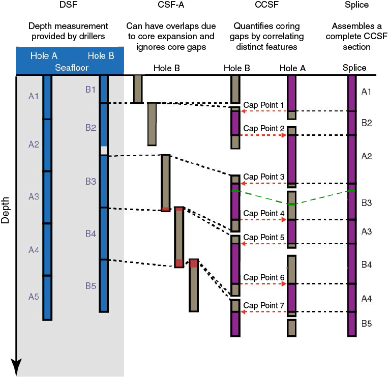
Figure F26. Cored material and depth scale interrelationships.
Core depth below seafloor (CSF) scale
The process of building a composite section begins by assigning a depth to the top of each core initially using the DSF scale. DSF is a drill string measurement based on the length of drill string from the seafloor to the cored top of each core. It is calculated by subtracting the length of the drill string between the rig floor and the mudline (the estimated level of the seafloor) from the length of the drill string from the rig floor to the top of the cored interval. Sources of error in DSF are numerous and include pipe and BHA stretch and compression, tidal variations, wind induced differences in the height of the sea surface, currents and wind affecting the bend of the drill string, and uncompensated heave. Tidal influence on DSF measurement can be significant (Hagelberg et al., 1995), and the prediction of tides may be useful for guiding drilling to avoid initial gap alignment (Mix, Tiedemann, Blum, et al., 2003), but during Expedition 369 we did not try to adjust for this factor due to the small tidal range in the regions cored.
A second depth scale, CSF-A, is used to characterize the depth to a given position within any core. CSF-A combines the DSF core-top depth with the curated length of the core after retrieval. CSF-A is equivalent to the meters below seafloor (mbsf) scale used during DSDP, ODP, and the early phase of the Integrated Ocean Drilling Program, but naming conventions were changed to increase precision and avoid confusion for IODP. CSF-A depths are specific to each hole, and CSF-A is the depth scale used for presenting most primary observations, including information summarized on the VCDs and presented in the site chapters. However, it is important to note that the “within-core” position of any given sedimentary feature may change during and after recovery as a result of drilling disturbance, the relief of overburden, gas-induced expansion, or water loss. Thus, error in the CSF-A scale includes both drilling effects and core aging effects. The CSF-A scale also permits stratigraphically impossible overlaps between successive cores, a situation that is relatively common due to core expansion resulting in >100% recovery.
To address this problem, a third depth scale, CSF, Method B (CSF-B), was also calculated for all cores. When recovery is ≤100% (i.e., when the length of core recovered does not exceed the length drilled), the CSF-A and CSF-B scales have the same value. However, when recovery is >100%, linear interpolation can be used to compress the recovered interval into the length drilled, thereby eliminating apparent overlaps. Factors that lead to >100% recovery include elastic, thermal, and gas-induced core expansion, as well as flow in, recovery of downhole contaminants, and gaps caused by rotation and misalignment of breaks during sectioning. CSF-B values are available for all holes drilled during Expedition 369 but were not used in any of the reports for the expedition.
The CCSF scale, described below, is the scale generated when compositing. Like the CSF-B scale, the CCSF scale should eliminate artifacts such as overlap between cores within a hole, and it is the scale on which the splice section is plotted. Composite depths may exceed the total depth drilled for the interval covered by the splice.
Core composite depth below seafloor (CCSF) scale
The construction of a common composite depth scale for a given IODP site involves identification of coeval, laterally continuous features in all drilled holes. Despite being correlative, the features will commonly occur at different depths on the CSF-A depth scale for each hole. Once correlative features are identified, the depth of individual cores is offset relative to the CSF-A depth in that hole such that the features are aligned on a common depth scale, CCSF. The CCSF scale is equivalent to the meters composite depth (mcd) scale used during ODP and Integrated Ocean Drilling Program expeditions.
In constructing the CCSF scale, the depths of all material in each individual core are offset from the CSF-A scale by a constant amount (i.e., without stretching or squeezing within individual cores). The size of the offset is determined by aligning the tie points used in compositing. Plotting cores relative to composite depth provides good estimates of the length of coring gaps and forms the basis for developing the spliced record. In cores where expansion has occurred, the size of the offsets generally increases downcore, but this pattern was not prevalent in Expedition 369 cores. Offsets for every core in every hole at each site are tabulated in an affine table. The affine table and the splice (see below) are the primary products generated by the stratigraphic correlators.
The CCSF scale is built during compositing by correlating features downhole starting from the mudline or at the highest core within an interval of overlap. The top of the highest core or the mudline establishes the top of the composited stratigraphic section, anchoring the composite depth scale for all cores from all holes at each site. Compositing proceeds sequentially downcore through the establishment of specific tie points among the various holes. Tie points are often refined and updated as additional data become available as core is processed. The CCSF scale rarely (if ever) results in precise alignment of all coeval features between holes because of the contrasting effects of coring-induced stretching and squeezing among cores and stratigraphic differences between holes. This variation means care should be taken when comparing results from samples collected from within the splice to those for the same CCSF interval in intervals not included in the splice.
In principle, drilling could proceed such that there are no aligned coring gaps among the holes at a given site. If so, and if recovery was sufficiently high, it should then be possible to correlate each successive core in one hole to a core from an adjacent hole all the way to the bottom of a drilled section. The result in this case would be a complete, anchored splice. In practice, at most sites at least some coring gaps align. Downhole logging data can be used to estimate the length of the gap, maintaining an observational connection to the anchor core. When there is an aligned core gap across all holes at a site without downhole data suitable to fill the gap, though, cores below the gap are no longer tied to the anchor core. These cores can still be tied to one another, but the correlated sections are considered “floating” on the CCSF scale.
Choosing a CCSF depth for floating sections is subjective. During Expedition 369, either of two methods were used to tie floating sections into the splice as noted in the affine table. When a core is “APPENDED,” the core being appended uses the inherited absolute offset of the core above the coring gap. When a core is “SET,” the stratigraphic correlator sets a user-defined offset that results in the best qualitative alignment. In cases where large aligned core gaps exist within a splice, the CCSF scale for the uppermost core below the gap is assigned the same value as the CSF-A offset of that core. Alternative methods for defining a SET offset are available, but these were not used during Expedition 369.
During the process of constructing the composite section, a CCSF depth may become greater than the CSF-A depth for equivalent horizons. This expansion of the depth scale may be an artifact of the selection of tie points or can be related to physical processes, including decompression and expansion of the sediment as it is brought to atmospheric pressure, pore-space gases coming out of solution, warming, stretching that occurs as part of the coring process, and recovery of additional material, likely from borehole-wall sediment that fell downhole and entered the core barrel (e.g., Hagelberg et al., 1995; Acton et al., 2001). Expansion of depth scales during Expedition 369 was limited, and offsets did not generally exceed the depth of the bottom of the drilled interval.
The splice
Once the CCSF scale is developed and the between-core gaps identified, a complete stratigraphic section (splice) is constructed by combining selected intervals between the previously established tie points. In the case of core gaps aligned across all holes, any spliced sections below the gap are designated as floating splice sections and plotted against CCSF as described above.
Measurements and methods for correlation
Given that during Expedition 369 few long sections of overlap were cored at any site and the drilling technique often differed between holes, we adjusted our approach to correlation based on the specifics of the situation. Observations of features in the recovered core seen through the core liner, comparison of DSF/CSF-A measurements between holes, and magnetic susceptibility measurements acquired as soon after core retrieval as possible using the STMSL were most useful for guiding drilling decisions in near real time. The success rate of these decisions in bridging coring gaps and areas of disturbed sediment was high.
The initial correlation between holes used for guiding drilling was refined as additional information became available from subsequent analyses, including biostratigraphic and magnetostratigraphic information, higher resolution physical property records measured on the WRMSL, sedimentological observations, photos, and color data. In addition, comparison between core measurements and downhole logs was used to test and refine correlations. NGR arguably gave the most consistently useful means of correlation between holes beyond aligning drilling depths. In specific instances, however, other data were important (e.g., digitized color data [both RGB and L*, a*, b* measurements], magnetic susceptibility, GRA bulk density, lithologic observations, and paleomagnetic data). These data have different resolutions, and details on instrument calibrations, settings, and measurement intervals for Expedition 369 are given in Petrophysics and Paleomagnetism.
Compositing and splicing were accomplished using Correlator software (version 2.1). The software generated standard affine tables (listings of the vertical offset in meters added to each core to generate the CCSF scale) and splice interval tables (listings of the specific core intervals used to construct the splice). These tables were uploaded to the LIMS database, which then linked the appropriate depth scale to any associated data set.
References
Acton, G.D., Borton, C.J., and the Leg 178 Shipboard Scientific Party, 2001. Palmer Deep composite depth scales for Leg 178 Sites 1098 and 1099. In Barker, P.F., Camerlenghi, A., Acton, G.D., and Ramsay, A.T.S. (Eds.), Proceedings of the Ocean Drilling Program, Scientific Results, 178: College Station, TX (Ocean Drilling Program), 1–35. https://doi.org/10.2973/odp.proc.sr.178.202.2001
Acton, G., Morris, A., Musgrave, R., Zhao, X., and IODP SRM Personnel, 2017. Assessment of the new superconducting rock magnetometer (SRM) on the JOIDES Resolution. Retrieved from International Ocean Discovery Program Website: http://iodp.tamu.edu/publications/JRSO/SRM_Workshop_2017.pdf
Ando, A., Huber, B.T., and Premoli Silva, I., 2013. Paraticinella rohri (Bolli, 1959) as the valid name for the latest Aptian zonal marker species of planktonic foraminifera traditionally called bejaouaensis or eubejaouaensis. Cretaceous Research, 45:275–287. https://doi.org/10.1016/j.cretres.2013.05.002
ASTM International, 1990. Standard method for laboratory determination of water (moisture) content of soil and rock (Standard D2216–90). In Annual Book of ASTM Standards for Soil and Rock (Volume 04.08): Philadelphia (American Society for Testing Materials). [revision of D2216-63, D2216-80]
Blum, P., 1997. Technical Note 26: Physical Properties Handbook—A Guide to the Shipboard Measurement of Physical Properties of Deep-Sea Cores. Ocean Drilling Program. https://doi.org/10.2973/odp.tn.26.1997
Bullard, E.C., 1954. The flow of heat through the floor of the Atlantic Ocean. Proceedings of the Royal Society of London, Series A: Mathematical, Physical and Engineering Sciences, 222(1150):408–429. https://doi.org/10.1098/rspa.1954.0085
Coccioni, R., Premoli Silva, I., Marsili, A., and Verga, D., 2007. First radiation of Cretaceous planktonic foraminifera with radially elongate chambers at Angles (southeastern France) and biostratigraphic implications. Revue de Micropaléontologie, 50(3):215–224. https://doi.org/10.1016/j.revmic.2007.06.005
De Vleeschouwer, D., Dunlea, A.G., Auer, G., Anderson, C.H., Brumsack, H., de Loach, A., Gurnis, M., et al., 2017. Quantifying K, U, and Th contents of marine sediments using shipboard natural gamma radiation spectra measured on DV JOIDES Resolution. Geochemistry, Geophysics, Geosystems, 18(3):1053–1064. https://doi.org/10.1002/2016GC006715
Dunham, R.J., 1962. Classification of carbonate rocks according to depositional texture. In Ham, W.E. (Ed.), Classification of Carbonate Rocks. AAPG Memoir, 1:108–121. http://archives.datapages.com/data/specpubs/carbona2/data/a038/a038/0001/0100/0108.html
Dunlea, A.G., Murray, R.W., Harris, R.N., Vasiliev, M.A., Evans, H., Spivack, A.J., and D’Hondt, S., 2013. Assessment and use of NGR instrumentation on the JOIDES Resolution to quantify U, Th, and K concentrations in marine sediment. Scientific Drilling, 15:57–63. https://doi.org/10.2204/iodp.sd.15.05.2013
Ellis, D.V., and Singer, J.M., 2007. Well Logging for Earth Scientists (2nd edition): New York (Elsevier).
Embry, A.F., III, and Klovan, J.E., 1971. A late Devonian reef tract on northeastern Banks Island, Northwest Territories. Bulletin of Canadian Petroleum Geology, 19(4):730–781. http://archives.datapages.com/data/cspg/data/019/019004/0730.html
Expedition 330 Scientists, 2012. Expedition 330 summary. In Koppers, A.A.P., Yamazaki, T., Geldmacher, J., and the Expedition 330 Scientists, Proceedings of the Integrated Ocean Drilling Program, 330: Tokyo (Integrated Ocean Drilling Program Management International, Inc.). https://doi.org/10.2204/iodp.proc.330.101.2012
Fisher, R.V., and Schmincke, H.-U., 1984. Pyroclastic Rocks: Berlin (Springer-Verlag). https://doi.org/10.1007/978-3-642-74864-6
Folk, R.L., 1962. Spectral subdivision of limestone types. In Ham, W.E. (Ed.), Classification of Carbonate Rocks. AAPG Memoir, 1:62–84. http://archives.datapages.com/data/specpubs/carbona2/data/a038/a038/0001/0050/0062.html
Gieskes, J.M., Gamo, T., and Brumsack, H., 1991. Technical Note 15: Chemical Methods for Interstitial Water Analysis Aboard JOIDES Resolution. Ocean Drilling Program. https://doi.org/10.2973/odp.tn.15.1991
Gibbard, P.L., Head, M.J., and Walker, M.J.C., 2010. Formal ratification of the Quaternary system/period and the Pleistocene series/epoch with a base at 2.58 Ma. Journal of Quaternary Science, 25(2):96–102. https://doi.org/10.1002/jqs.1338
Gilmore, G.R., 2008. Practical Gamma-ray Spectrometry (2nd edition): Hoboken, NJ (John Wiley & Sons). https://doi.org/10.1002/9780470861981
Goldberg, D., 1997. The role of downhole measurements in marine geology and geophysics. Reviews of Geophysics, 35(3):315–342. https://doi.org/10.1029/97RG00221
Gradstein, F.M., Ogg, J.G., Schmitz, M.D., and Ogg, G.M. (Eds.), 2012. The Geological Time Scale 2012: Amsterdam (Elsevier).
Hagelberg, T.K., Pisias, N.G., Shackleton, N.J., Mix, A.C., and Harris, S., 1995. Refinement of a high-resolution, continuous sedimentary section for studying equatorial Pacific Ocean paleoceanography, Leg 138. In Pisias, N.G., Mayer, L.A., Janecek, T.R., Palmer-Julson, A., and van Andel, T.H. (Eds.), Proceedings of the Ocean Drilling Program, Scientific Results, 138: College Station, TX (Ocean Drilling Program), 31–46. https://doi.org/10.2973/odp.proc.sr.138.103.1995
Hanagata, S., and Nobuhara, T., 2015. Illustrated guide to Pliocene foraminifera from Miyakojima, Ryukyu Island Arc, with comments on biostratigraphy. Palaeontologia Electronica,18.1.3A. https://doi.org/10.26879/444
Hayward, B.W., 2002. Late Pliocene to Middle Pleistocene extinctions of deep-sea benthic foraminifera (“Stilostomella extinction”) in the southwest Pacific. Journal of Foraminiferal Research, 32(3):274–307. https://doi.org/10.2113/32.3.274
Holbourn, A., Henderson, A.S., and MacLeod, N., 2013. Atlas of Benthic Foraminifera: Chichester, United Kingdom (John Wiley & Sons, Ltd.). https://doi.org/10.1002/9781118452493
Horai, K., and Von Herzen, R.P., 1985. Measurement of heat flow on Leg 86 of the Deep Sea Drilling Project. In Heath, G.R., Burckle, L.H., et al., Initial Reports of the Deep Sea Drilling Project, 86: Washington, DC (U.S. Government Printing Office), 759–777. https://doi.org/10.2973/dsdp.proc.86.135.1985
Huber, B.T., Hobbs, R.W., Bogus, K.A., Batenburg, S.J., Brumsack, H.-J., do Monte Guerra, R., Edgar, K.M., Edvardsen, T., Garcia Tejada, M.L., Harry, D.L., Hasegawa, T., Haynes, S.J., Jiang, T., Jones, M.M., Kuroda, J., Lee, E.Y., Li, Y.-X., MacLeod, K.G., Maritati, A., Martinez, M., O’Connor, L.K., Petrizzo, M.R., Quan, T.M., Richter, C., Riquier, L., Tagliaro, G.T., Wainman, C.C., Watkins, D.K., White, L.T., Wolfgring, E., and Xu, Z., 2019a. Site U1512. In Hobbs, R.W., Huber, B.T., Bogus, K.A., and the Expedition 369 Scientists, Australia Cretaceous Climate and Tectonics. Proceedings of the International Ocean Discovery Program, 369: College Station, TX (International Ocean Discovery Program). https://doi.org/10.14379/iodp.proc.369.103.2019
Huber, B.T., Hobbs, R.W., Bogus, K.A., Batenburg, S.J., Brumsack, H.-J., do Monte Guerra, R., Edgar, K.M., Edvardsen, T., Garcia Tejada, M.L., Harry, D.L., Hasegawa, T., Haynes, S.J., Jiang, T., Jones, M.M., Kuroda, J., Lee, E.Y., Li, Y.-X., MacLeod, K.G., Maritati, A., Martinez, M., O’Connor, L.K., Petrizzo, M.R., Quan, T.M., Richter, C., Riquier, L., Tagliaro, G.T., Wainman, C.C., Watkins, D.K., White, L.T., Wolfgring, E., and Xu, Z., 2019b. Site U1513. In Hobbs, R.W., Huber, B.T., Bogus, K.A., and the Expedition 369 Scientists, Australia Cretaceous Climate and Tectonics. Proceedings of the International Ocean Discovery Program, 369: College Station, TX (International Ocean Discovery Program). https://doi.org/10.14379/iodp.proc.369.104.2019
Huber, B.T., Hobbs, R.W., Bogus, K.A., Batenburg, S.J., Brumsack, H.-J., do Monte Guerra, R., Edgar, K.M., Edvardsen, T., Garcia Tejada, M.L., Harry, D.L., Hasegawa, T., Haynes, S.J., Jiang, T., Jones, M.M., Kuroda, J., Lee, E.Y., Li, Y.-X., MacLeod, K.G., Maritati, A., Martinez, M., O’Connor, L.K., Petrizzo, M.R., Quan, T.M., Richter, C., Riquier, L., Tagliaro, G.T., Wainman, C.C., Watkins, D.K., White, L.T., Wolfgring, E., and Xu, Z., 2019c. Site U1514. In Hobbs, R.W., Huber, B.T., Bogus, K.A., and the Expedition 369 Scientists, Australia Cretaceous Climate and Tectonics. Proceedings of the International Ocean Discovery Program, 369: College Station, TX (International Ocean Discovery Program). https://doi.org/10.14379/iodp.proc.369.105.2019
Huber, B.T., Hobbs, R.W., Bogus, K.A., Batenburg, S.J., Brumsack, H.-J., do Monte Guerra, R., Edgar, K.M., Edvardsen, T., Garcia Tejada, M.L., Harry, D.L., Hasegawa, T., Haynes, S.J., Jiang, T., Jones, M.M., Kuroda, J., Lee, E.Y., Li, Y.-X., MacLeod, K.G., Maritati, A., Martinez, M., O’Connor, L.K., Petrizzo, M.R., Quan, T.M., Richter, C., Riquier, L., Tagliaro, G.T., Wainman, C.C., Watkins, D.K., White, L.T., Wolfgring, E., and Xu, Z., 2019d. Site U1515. In Hobbs, R.W., Huber, B.T., Bogus, K.A., and the Expedition 369 Scientists, Australia Cretaceous Climate and Tectonics. Proceedings of the International Ocean Discovery Program, 369: College Station, TX (International Ocean Discovery Program). https://doi.org/10.14379/iodp.proc.369.106.2019
Huber, B.T., Hobbs, R.W., Bogus, K.A., Batenburg, S.J., Brumsack, H.-J., do Monte Guerra, R., Edgar, K.M., Edvardsen, T., Garcia Tejada, M.L., Harry, D.L., Hasegawa, T., Haynes, S.J., Jiang, T., Jones, M.M., Kuroda, J., Lee, E.Y., Li, Y.-X., MacLeod, K.G., Maritati, A., Martinez, M., O’Connor, L.K., Petrizzo, M.R., Quan, T.M., Richter, C., Riquier, L., Tagliaro, G.T., Wainman, C.C., Watkins, D.K., White, L.T., Wolfgring, E., and Xu, Z., 2019e. Site U1516. In Hobbs, R.W., Huber, B.T., Bogus, K.A., and the Expedition 369 Scientists, Australia Cretaceous Climate and Tectonics. Proceedings of the International Ocean Discovery Program, 369: College Station, TX (International Ocean Discovery Program). https://doi.org/10.14379/iodp.proc.369.107.2019
Imai, N., Terashima, S., Itoh, S., and Ando, A., 1995. 1994 compilation of analytical data for minor and trace elements in seventeen GSJ geochemical reference samples, “igneous rock series.” Geostandards and Geoanalytical Research, 19(2):135–213. https://doi.org/10.1111/j.1751-908X.1995.tb00158.x
Iturrino, G., Liu, T., Goldberg, D., Anderson, L., Evans, H., Fehr, A., Guerin, G., Inwood, J., Lofi, J., Malinverno, A., Morgan, S., Mrozewski, S., Slagle, A., and Williams, T., 2013. Performance of the wireline heave compensation system onboard D/V JOIDES Resolution. Scientific Drilling, 15:46–50. https://doi.org/10.2204/iodp.sd.15.08.2013
Jochum, K.P., Weis, U., Schwager, B., Stoll, B., Wilson, S.A., Haug, G.H., Andreae, M.O., and Enzweiler, J., 2015. Reference values following ISO guidelines for frequently requested rock reference materials. Geostandards and Geoanalytical Research, 40(3):333–350. https://doi.org/10.1111/j.1751-908X.2015.00392.x
Jones, R.W., 1994. The Challenger Foraminifera: New York (Oxford University Press USA).
Kaminski, M.A., and Gradstein, F.M., 2005. Atlas of Paleogene cosmopolitan deep-water agglutinated foraminifera. Grzybowski Foundation Special Publication, 10. http://www.foraminifera.eu/atlas.html
Kirschvink, J.L., 1980. The least-squares line and plane and the analysis of palaeomagnetic data. Geophysical Journal of the Royal Astronomical Society, 62(3):699–718. https://doi.org/10.1111/j.1365-246X.1980.tb02601.x
Kristiansen, J.I., 1982. The transient cylindrical probe method for determination of thermal parameters of earth materials [Ph.D. dissertation]. Åarhus University, Åarhus, Denmark.
Li, C.-F., Lin, J., Kulhanek, D.K., Williams, T., Bao, R., Briais, A., Brown, E.A., Chen, Y., Clift, P.D., Colwell, F.S., Dadd, K.A., Ding, W., Hernández-Almeida, I., Huang, X.-L., Hyun, S., Jiang, T., Koppers, A.A.P., Li, Q., Liu, C., Liu, Q., Liu, Z., Nagai, R.H., Peleo-Alampay, A., Su, X., Sun, Z., Tejada, M.L.G., Trinh, H.S., Yeh, Y.-C., Zhang, C., Zhang, F., Zhang, G.-L., and Zhao, X., 2015. Methods. In Li, C.-F., Lin, J., Kulhanek, D.K., and the Expedition 349 Scientists, South China Sea Tectonics. Proceedings of the International Ocean Discovery Program, 349: College Station, TX (International Ocean Discovery Program). https://doi.org/10.14379/iodp.proc.349.102.2015
Liu, T., Iturrino, G., Goldberg, D., Meissner, E., Swain, K., Furman, C., Fitzgerald, P., Frisbee, N., Chlimoun, J., Van Hyfte, J., and Beyer, R., 2013. Performance evaluation of active wireline heave compensation systems in marine well logging environments. Geo-Marine Letters, 33(1):83–93. https://doi.org/10.1007/s00367-012-0309-8
Loeblich, A.R., Jr., and Tappan, H., 1988. Foraminiferal Genera and Their Classification: New York (Van Nostrand Reinhold).
Lovell, M.A., Harvey, P.K., Brewer, T.S., Williams, C., Jackson, P.D., and Williamson, G., 1998. Application of FMS images in the Ocean Drilling Program: an overview. In Cramp, A., MacLeod, C.J., Lee, S.V., and Jones, E.J.W. (Eds.), Geological Evolution of Ocean Basins: Results from the Ocean Drilling Program. Geological Society Special Publication, 131(1):287–303. https://doi.org/10.1144/GSL.SP.1998.131.01.18
Lurcock, P.C., and Wilson, G.S., 2012. PuffinPlot: a versatile, user-friendly program for paleomagnetic analysis. Geochemistry, Geophysics, Geosystems, 13(6):Q06Z45. https://doi.org/10.1029/2012GC004098
Luthi, S.M., 1990. Sedimentary structures of clastic rocks identified from electrical borehole images. In Hurst, A., Lovell, M.A., and Morton, A.C. (Eds.), Geological Applications of Wireline Logs. Geological Society Special Publication, 48:3–10. https://doi.org/10.1144/GSL.SP.1990.048.01.02
Luyendyk, B.P., and Davies, T.A., 1974. Results of DSDP Leg 26 and the geologic history of the Southern Indian Ocean. In Davies, T.A., Luyendyk, B.P., et al., Initial Reports of the Deep Sea Drilling Project, 26: Washington, DC (U.S. Government Printing Office), 909–943. https://doi.org/10.2973/dsdp.proc.26.136.1974
Manheim, F.T., and Sayles, F.L., 1974. Composition and origin of interstitial waters of marine sediments, based on deep sea drill cores. In Goldberg, E.D. (Ed.), The Sea (Volume 5): Marine Chemistry: The Sedimentary Cycle: New York (Wiley), 527–568.
Mazzullo, J.M., Meyer, A., and Kidd, R.B., 1988. New sediment classification scheme for the Ocean Drilling Program. In Mazzullo, J., and Graham, A.G. (Eds.), Technical Note 8: Handbook for Shipboard Sedimentologists. Ocean Drilling Program, 44–67. https://doi.org/10.2973/odp.tn.8.1988
Mix, A.C., Tiedemann, R., Blum, P., et al., 2003. Proceedings of the Ocean Drilling Program, Initial Reports, 202: College Station, TX (Ocean Drilling Program). https://doi.org/10.2973/odp.proc.ir.202.2003
Morishige, Y., and Kimura, A., 2008. Ionization interference in inductively coupled plasma-optical emission spectroscopy. SEI Technical Review, 66:106–111. http://global-sei.com/technology/tr/bn66/pdf/66-14.pdf
Murray, R.W., Miller, D.J., and Kryc, K.A., 2000. Technical Note 29: Analysis of Major and Trace Elements in Rocks, Sediments, and Interstitial Waters by Inductively Coupled Plasma–Atomic Emission Spectrometry (ICP-AES). Ocean Drilling Program. https://doi.org/10.2973/odp.tn.29.2000
Ogg, J.G., 2012. Geomagnetic polarity time scale. In Gradstein, F.M., Ogg, J.G., Schmitz, M.D., and Ogg, G.M. (Eds.), The Geologic Time Scale 2012: Amsterdam (Elsevier), 85–113. https://doi.org/10.1016/B978-0-444-59425-9.00005-6
Okada, H., and Bukry, D., 1980. Supplementary modification and introduction of code numbers to the low-latitude coccolith biostratigraphic zonation (Bukry, 1973; 1975). Marine Micropaleontology, 5:321–325. https://doi.org/10.1016/0377-8398(80)90016-X
Pandey, D.K., Clift, P.D., Kulhanek, D.K., Andò, S., Bendle, J.A.P., Bratenkov, S., Griffith, E.M., Gurumurthy, G.P., Hahn, A., Iwai, M., Khim, B.-K., Kumar, A., Kumar, A.G., Liddy, H.M., Lu, H., Lyle, M.W., Mishra, R., Radhakrishna, T., Routledge, C.M., Saraswat, R., Saxena, R., Scardia, G., Sharma, G.K., Singh, A.D., Steinke, S., Suzuki, K., Tauxe, L., Tiwari, M., Xu, Z., and Yu, Z., 2016. Expedition 355 methods. In Pandey, D.K., Clift, P.D., Kulhanek, D.K., and the Expedition 355 Scientists, Arabian Sea Monsoon. Proceedings of the International Ocean Discovery Program, 355: College Station, TX (International Ocean Discovery Program). https://doi.org/10.14379/iodp.proc.355.102.2016
Perch-Nielsen, K., 1985. Mesozoic calcareous nannofossils. In Bolli, H.M., Saunders, J.B., and Perch-Nielsen, K. (Eds.), Plankton Stratigraphy: Cambridge, United Kingdom (Cambridge University Press), 329–426.
Petrizzo, M.R., Caron, M., and Premoli Silva, I., 2015. Remarks on the identification of the Albian/Cenomanian boundary and taxonomic clarification of the planktonic foraminifera index species globotruncanoides, brotzeni and tehamaensis. Geological Magazine, 152(3):521–536. https://doi.org/10.1017/S0016756814000478
Pettijohn, F.J., Potter, P.E., and Siever, R., 1987. Sand and Sandstones (2nd edition): New York (Springer-Verlag).
Pribnow, D., Kinoshita, M., and Stein, C., 2000. Thermal Data Collection and Heat Flow Recalculations for Ocean Drilling Program Legs 101–180: Hanover, Germany (Institute for Joint Geoscientific Research, Institut für Geowissenschaftliche Gemeinschaftsaufgaben [GGA]). http://www-odp.tamu.edu/publications/heatflow/ODPReprt.pdf
Richter, C., Acton, G., Endris, C., and Radsted, M., 2007. Technical Note 34: Handbook for Shipboard Paleomagnetists. Ocean Drilling Program. https://doi.org/10.2973/odp.tn.34.2007
Rider, M.H., 1996. The Geological Interpretation of Well Logs (2nd edition): Caithness, Scotland (Whittles Publishing).
Rothwell, R.G., 1989. Minerals and Mineraloids in Marine Sediments: An Optical Identification Guide: London (Elsevier). https://doi.org/10.1007/978-94-009-1133-8
Ruddiman, W.F., Kidd, R.B., Thomas, E., et al., 1987. Initial Reports of the Deep Sea Drilling Project, 94: Washington, DC (U.S. Government Printing Office). https://doi.org/10.2973/dsdp.proc.94.1987
Rüdel, H., Kösters, J., and Schörmann, J., 2007. Guidelines for Chemical Analysis: Determination of the Elemental Content of Environment Samples using ICP-OES. Schmallenberg, Germany (Fraunhofer Institute for Molecular Biology and Applied Ecology). https://www.ime.fraunhofer.de/content/dam/ime/en/documents/AE/SOP_ICP-OES_en.pdf
Salimullah, A.R.M., and Stow, D.A.V., 1992. Application of FMS images in poorly recovered coring intervals: examples from ODP Leg 129. In Hurst, A., Griffiths, C.M., and Worthington, P.F. (Eds.), Geological Application of Wireline Logs II. Geological Society Special Publication, 65(1):71–86. https://doi.org/10.1144/GSL.SP.1992.065.01.06
Schlumberger, 1989. Log Interpretation Principles/Applications: Houston (Schlumberger Education Services), SMP–7017.
Schlumberger, 1994. IPL Integrated Porosity Lithology: Houston (Schlumberger Education Services), SMP-9270.
Serra, O., 1984. Fundamentals of Well-Log Interpretation (Volume 1): The Acquisition of Logging Data: Amsterdam (Elsevier).
Serra, O., 1986. Fundamentals of Well-Log Interpretation (Volume 2): The Interpretation of Logging Data: Amsterdam (Elsevier).
Serra, O., 1989. Formation MicroScanner Image Interpretation: Houston (Schlumberger Education Services), SMP-7028.
Shepard, F.P., 1954. Nomenclature based on sand-silt-clay ratios. Journal of Sedimentary Research, 24(3):151–158. https://doi.org/10.1306/D4269774-2B26-11D7-8648000102C1865D
Shipboard Scientific Party, 1974. Explanatory notes. In Davies, T.A., Luyendyk, B.P., et al., Initial Reports of the Deep Sea Drilling Project, 26: Washington, DC (U.S. Government Printing Office), 11–19. https://doi.org/10.2973/dsdp.proc.26.102.1974
Sigal, J., 1977. Essai de zonation du Crétacé méditerranéen à l’aide des foraminifères planctoniques. Géologie Méditerranéene, 4:99–108.
Stow, D.A.V., 2005. Sedimentary Rocks in the Field: A Colour Guide: London (Manson Publishing)
Tauxe, L., Tucker, P., Peterson, N.P., and LaBrecque, J.L., 1984. Magnetostratigraphy of Leg 73 sediments. In Hsü, K.J., LaBrecque, J.L., et al., Initial Reports of the Deep Sea Drilling Project, 73: Washington, DC (U.S. Government Printing Office), 609–621. https://doi.org/10.2973/dsdp.proc.73.123.1984
Vacquier, V., 1985. The measurement of thermal conductivity of solids with a transient linear heat source on the plane surface of a poorly conducting body. Earth and Planetary Science Letters, 74(2–3):275–279. https://doi.org/10.1016/0012-821X(85)90027-5
van de Wiel, H.J., 2003. Determination of Elements by ICP-AES and ICP-MS: Bilthoven, The Netherlands (National Institute of Public Health and the Environment [RIVM]). https://www.ecn.nl/docs/society/horizontal/hor_desk_19_icp.pdf
van Morkhoven, F.P.C.M., Berggren, W.A., Edwards, A.S.,and Oertli, H.J., 1986. Cenozoic cosmopolitan deep-water benthic foraminifera. Bulletin des centres de recherches Exploration-production Elf-Aquitaine: Mémoire, 11.
Vasiliev, M.A., Blum, P., Chubarian, G., Olsen, R., Bennight, C., Cobine, T., Fackler, D., Hastedt, M., Houpt, D., Mateo, Z., and Vasilieva, Y.B., 2011. A new natural gamma radiation measurement system for marine sediment and rock analysis. Journal of Applied Geophysics, 75:455–463. https://doi.org/10.1016/j.jappgeo.2011.08.008
Von Herzen, R., and Maxwell, A.E., 1959. The measurement of thermal conductivity of deep-sea sediments by a needle-probe method. Journal of Geophysical Research, 64(10):1557–1563. https://doi.org/10.1029/JZ064i010p01557
Wade, B.S., Pearson, P.N., Berggren, W.A., and Pälike, H., 2011. Review and revision of Cenozoic tropical planktonic foraminiferal biostratigraphy and calibration to the geomagnetic polarity and astronomical time scale. Earth-Science Reviews, 104(1–3):111–142. https://doi.org/10.1016/j.earscirev.2010.09.003
Wentworth, C.K., 1922. A scale of grade and class terms for clastic sediments. Journal of Geology, 30(5):377–392. https://doi.org/10.1086/622910
Zijderveld, J.D.A., 1967. AC demagnetization of rocks: analysis of results. In Collinson, D.W., Creer, K.M., and Runcorn, S.K. (Eds.), Developments in Solid Earth Geophysics (Volume 3): Methods in Palaeomagnetism: Amsterdam (Elsevier), 254–286. https://doi.org/10.1016/B978-1-4832-2894-5.50049-5
1 Huber, B.T., Hobbs, R.W., Bogus, K.A., Batenburg, S.J., Brumsack, H.-J., do Monte Guerra, R., Edgar, K.M., Edvardsen, T., Garcia Tejada, M.L., Harry, D.L., Hasegawa, T., Haynes, S.J., Jiang, T., Jones, M.M., Kuroda, J., Lee, E.Y., Li, Y.-X., MacLeod, K.G., Maritati, A., Martinez, M., O’Connor, L.K., Petrizzo, M.R., Quan, T.M., Richter, C., Riquier, L., Tagliaro, G.T., Wainman, C.C., Watkins, D.K., White, L.T., Wolfgring, E., Xu, Z., 2019. Expedition 369 methods. In Hobbs, R.W., Huber, B.T., Bogus, K.A., and the Expedition 369 Scientists, Australia Cretaceous Climate and Tectonics. Proceedings of the International Ocean Discovery Program, 369: College Station, TX (International Ocean Discovery Program). https://doi.org/10.14379/iodp.proc.369.102.2019
2 Expedition 369 Scientists’ affiliations.
This work is distributed under the Creative Commons Attribution 4.0 International (CC BY 4.0) license. 
- F1. IODP naming conventions.
- F2. Hard rock core curation labeling.
- F3. Sediment and sedimentary rock VCD.
- F4. Igneous rock VCD.
- F5. VCD graphic patterns.
- F6. VCD symbols and nomenclature.
- F7. Siliciclastic-calcareous-biosiliceous ternary diagram.
- F8. Sediment classification summary.
- F9. Udden-Wentworth grain size classification of terrigenous sediments.
- F10. Lithologic textural name classification.
- F11. Limestone classification.
- F12. Neogene timescale.
- F13. Paleogene timescale.
- F14. Late Cretaceous timescale.
- F15. Early Cretaceous timescale.
- F16. SRM and magnetometer coordinate systems.
- F17. WRMSL system.
- F18. NGRL system.
- F19. Main elements of the NGRL.
- F20. Thermal conductivity system.
- F21. SHMSL system.
- F22. SHMG x-axis caliper and y- and z-axis bayonets.
- F23. Pycnometer cells for MAD measurements.
- F24. Downhole logging tool strings.
- F25. VSI source deployment plan.
- F26. Cored material and depth scale interrelationships.
- T1. Stratification thickness terminology.
- T2. Lithologic accessory abundance classifications.
- T3. Bioturbation intensity index.
- T4. Drilling disturbance classifications.
- T5. Sediment and rock classification scheme.
- T6. Phenocryst-based lithology names.
- T7. Groundmass description.
- T8. Vesicle-based description.
- T9. Degree of alteration.
- T10. Geomagnetic polarity timescale.
- T11. ICP-AES wavelengths.