Teske, A., Lizarralde, D., Höfig, T.W., and the Expedition 385 Scientists
Proceedings of the International Ocean Discovery Program Volume 385
publications.iodp.org

https://doi.org/10.14379/iodp.proc.385.102.2021

Expedition 385 methods¹

 A. Teske,  D. Lizarralde,  T.W. Höfig,  I.W. Aiello,  J.L. Ash,  D.P. Bojanova,  M.D. Buatier,  V.P. Edgcomb,  C.Y. Galerne,  S. Gontharet,  V.B. Heuer,  S. Jiang,  M.A.C. Kars,  S. Khogenkumar Singh,  J.-H. Kim,  L.M.T. Koornneef,  K.M. Marsaglia,  N.R. Meyer,  Y. Morono,  R. Negrete-Aranda,  F. Neumann,  L.C. Pastor,  M.E. Peña-Salinas,  L.L. Pérez-Cruz,  L. Ran,  A. Riboulleau,  J.A. Sarao,  F. Schubert,  J.M. Stock,  L.M.A.A. Toffin,  W. Xie,  T. Yamanaka,  G. Zhuang ²

¹Teske, A., Lizarralde, D., Höfig, T.W., Aiello, I.W., Ash, J.L., Bojanova, D.P., Buatier, M.D., Edgcomb, V.P., Galerne, C.Y., Gontharet, S., Heuer, V.B., Jiang, S., Kars, M.A.C., Khogenkumar Singh, S., Kim, J.-H., Koornneef, L.M.T., Marsaglia, K.M., Meyer, N.R., Morono, Y., Negrete-Aranda, R., Neumann, F., Pastor, L.C., Peña-Salinas, M.E., Pérez Cruz, L.L., Ran, L., Riboulleau, A., Sarao, J.A., Schubert, F., Stock, J.M., Toffin, L.M.A.A., Xie, W., Yamanaka, T., and Zhuang, G., 2021. Expedition 385 methods. In Teske, A., Lizarralde, D., Höfig, T.W., and the Expedition 385 Scientists, Guaymas Basin Tectonics and Biosphere. Proceedings of the International Ocean Discovery Program, 385: College Station, TX (International Ocean Discovery Program). https://doi.org/10.14379/iodp.proc.385.102.2021

²Expedition 385 Scientists’ affiliations.

1. Introduction

This chapter outlines the procedures and methods employed for coring and drilling operations as well as in the various shipboard laboratories of the research vessel (R/V) JOIDES Resolution during International Ocean Discovery Program (IODP) Expedition 385. The laboratory information applies only to shipboard work described in the Expedition Reports section of the Expedition 385 Proceedings of the International Ocean Discovery Program volume, using the shipboard sample registry, imaging and analytical instruments, core description tools, and the Laboratory Information Management System (LIMS) database. Methods used by investigators for shore-based analyses of Expedition 385 samples and data will be described in separate individual peer-reviewed scientific publications.

All shipboard scientists contributed in various ways to this volume with the following primary responsibilities (authors are listed in alphabetical order; see Expedition 385 scientists for contact information):

Summary chapter: Expedition 385 Scientists

Methods and site chapters:

• Background and objectives: D. Lizarralde, A.P. Teske
• Operations: K. Grigar, T.W. Höfig
• Lithostratigraphy: I.W. Aiello, M.D. Buatier, S. Gontharet, K.M. Marsaglia
• Igneous petrology and alteration: S. Khogenkumar Singh, W. Xie
• Structural geology: J.M. Stock
• Biostratigraphy: S. Jiang, L.L. Pérez Cruz, L. Ran, J.A. Sarao
• Paleomagnetism: M.A.C. Kars, L.M.T. Koornneef
• Inorganic geochemistry: J.-H. Kim, L.C. Pastor, T. Yamanaka
• Organic geochemistry: J.L. Ash, V.B. Heuer, A. Riboulleau, G. Zhuang
• Microbiology: D.P. Bojanova, V.P. Edgcomb, N.R. Meyer, Y. Morono, F. Schubert
• Petrophysics (physical properties and downhole measurements): C.Y. Galerne, R. Negrete-Aranda, F. Neumann, M.E. Peña-Salinas

The present introductory section provides an overview of drilling and coring operations, core handling, curatorial conventions, depth scale terminology, and the sequence of shipboard analyses. Subsequent sections of this chapter document specific laboratory instruments and methods in detail.

1.1. Locations of sites and holes

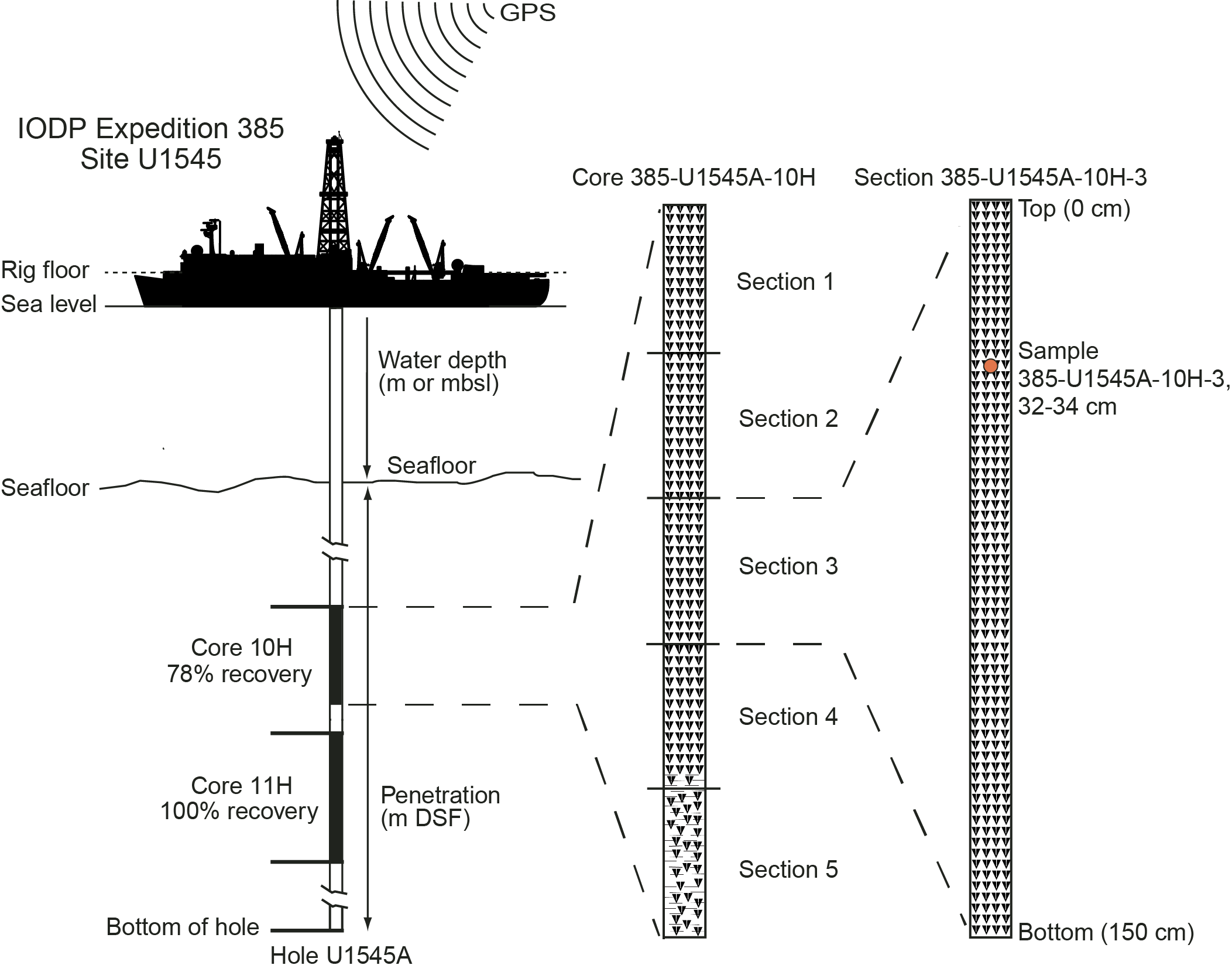
GPS coordinates (World Geodetic System 84 datum) obtained from preexpedition site surveys were used to position the vessel at the Expedition 385 sites. A SyQwest Bathy 2010 compressed high-intensity radar pulse (CHIRP) subbottom profiler was deployed to monitor the seafloor depth on the approach to the site to reconfirm the depth profiles from preexpedition surveys. Once positioned at a site, the thrusters were lowered, and the location of the ship was maintained over each hole of a site by means of the Neutronics 5002 dynamic positioning (DP) system on JOIDES Resolution. DP control of the vessel used navigational input from the GPS (Figure F1). The final hole position was the calculated mean position derived from the GPS data collected over a significant portion of the time the hole was occupied. In hydrothermally active areas, a deep-sea camera survey of the seafloor was implemented prior to drilling to ensure no proximal animal communities were present and to confirm suitable locations for spudding boreholes.

The drilling sites were numbered according to the series that began with the first site drilled by the Glomar Challenger in 1968. Starting with Integrated Ocean Drilling Program Expedition 301, the prefix “U” defines sites occupied by JOIDES Resolution. For all IODP drill sites, a letter suffix distinguishes each hole drilled at the same site. The first hole drilled is assigned the site number modified by the suffix “A,” the second hole takes the site number and the suffix “B,” and so forth. During Expedition 385, eight sites were drilled in Guaymas Basin in the central Gulf of California: Site U1545 (Holes U1545A–U1545C), Site U1546 (Holes U1546A–U1546D), Site U1547 (Holes U1547A–U1547E), Site U1548 (Holes U1548A–U1548E), Site U1549 (Holes U1549A and U1549B), Site U1550 (Holes U1550A and U1550B), Site U1551 (Holes U1551A and U1551B), and Site U1552 (Holes U1552A–U1552C).

1.2. Drilling and logging operations

To successfully drill both soft and indurated sediments as well as intruded sills, all four standard coring tools available on JOIDES Resolution were deployed during Expedition 385: the advanced piston corer (APC), half-length APC (HLAPC), extended core barrel (XCB), and rotary core barrel (RCB) systems. Operations took place in Mexican territorial waters in water depths of ~1600–2000 m.

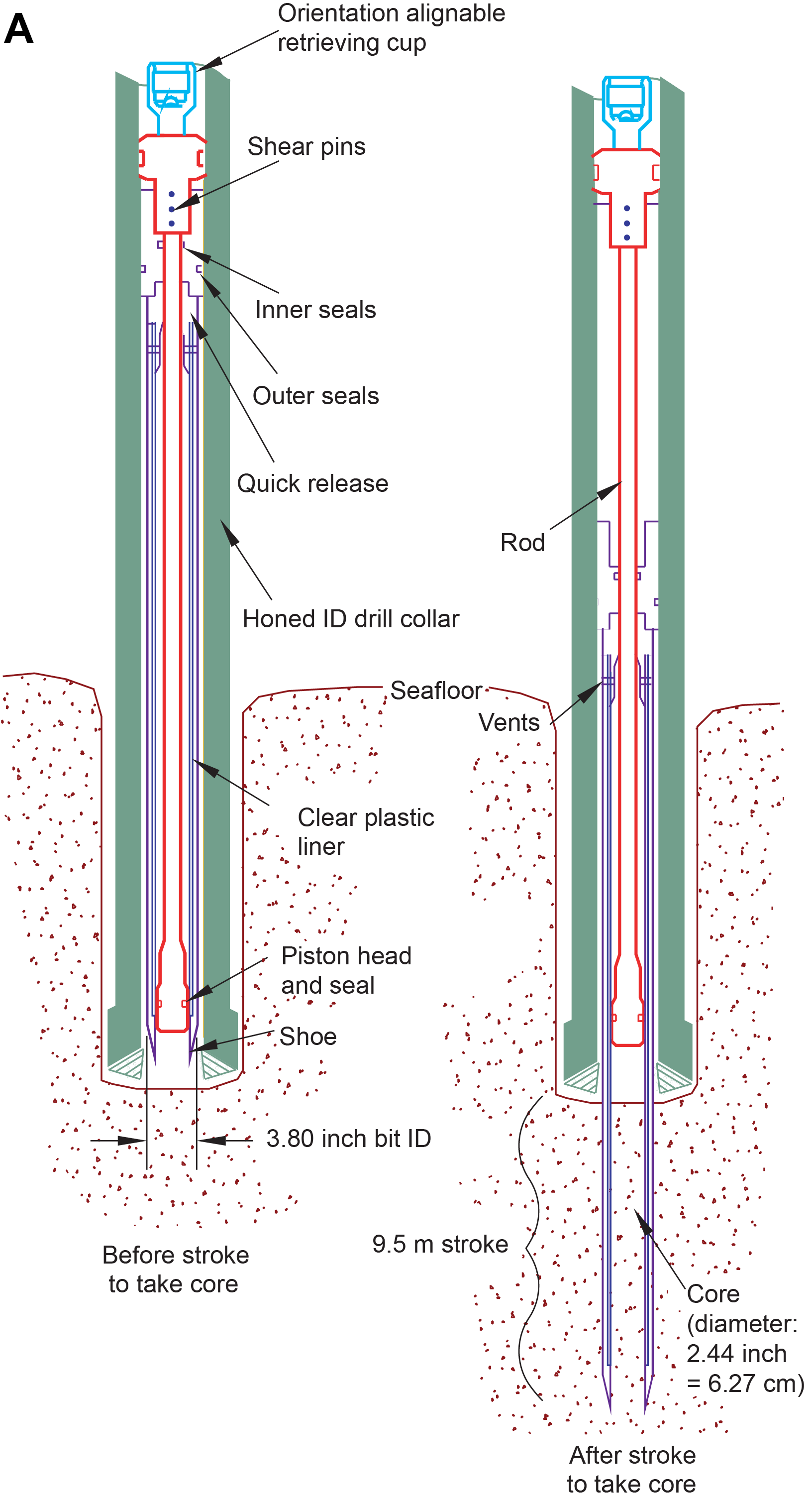
The APC and HLAPC systems cut soft-sediment cores with negligible coring disturbance relative to other IODP coring tools. Upon lowering the APC/HLAPC core barrel through the drill pipe, it lands above the bit. Subsequently, the drill pipe is hydraulically pressured up until the two shear pins that hold the inner barrel and are attached to the outer barrel fail. The inner barrel then advances into the formation and cuts the core (Figure F2A). The driller can identify a successful cut, or full stroke, by observing the pressure gauge on the rig floor because the excess pressure built up prior to the stroke drops promptly. Cores collected with the APC system are denoted by the letter “H” (for hydraulic piston coring), and those collected with the HLAPC system are indicated by the letter “F.”

APC refusal is conventionally defined in one of two ways: (1) the piston fails to accomplish a full stroke (as determined by the pump pressure and recovery reading) because the formation is too hard or (2) excessive force (>60,000 lbf or >266.9 kN) is required to pull the core barrel out of the formation. When a complete APC stroke could not be achieved, either the HLAPC system or the XCB system was deployed, depending on the severity of deterioration of the preceding APC coring progress and overall formation conditions. With each APC attempt, the bit was advanced by the length of the core barrel. Note that failed APC attempts resulted in a nominal recovery of ~100% based on the assumption that the barrel penetrated the formation by the length of the recovered core. If an APC core does not achieve a full stroke, the next core can be taken after advancing to a depth calculated from the recovery of the previous core (advance by recovery) or to a depth of a full APC core (typically 9.5–9.7 m). When a full or partial stroke was achieved but excessive force could not retrieve the barrel, the core barrel could be drilled over (i.e., after the inner core barrel was successfully shot into the formation, the drill bit was advanced to total depth to free the APC barrel).

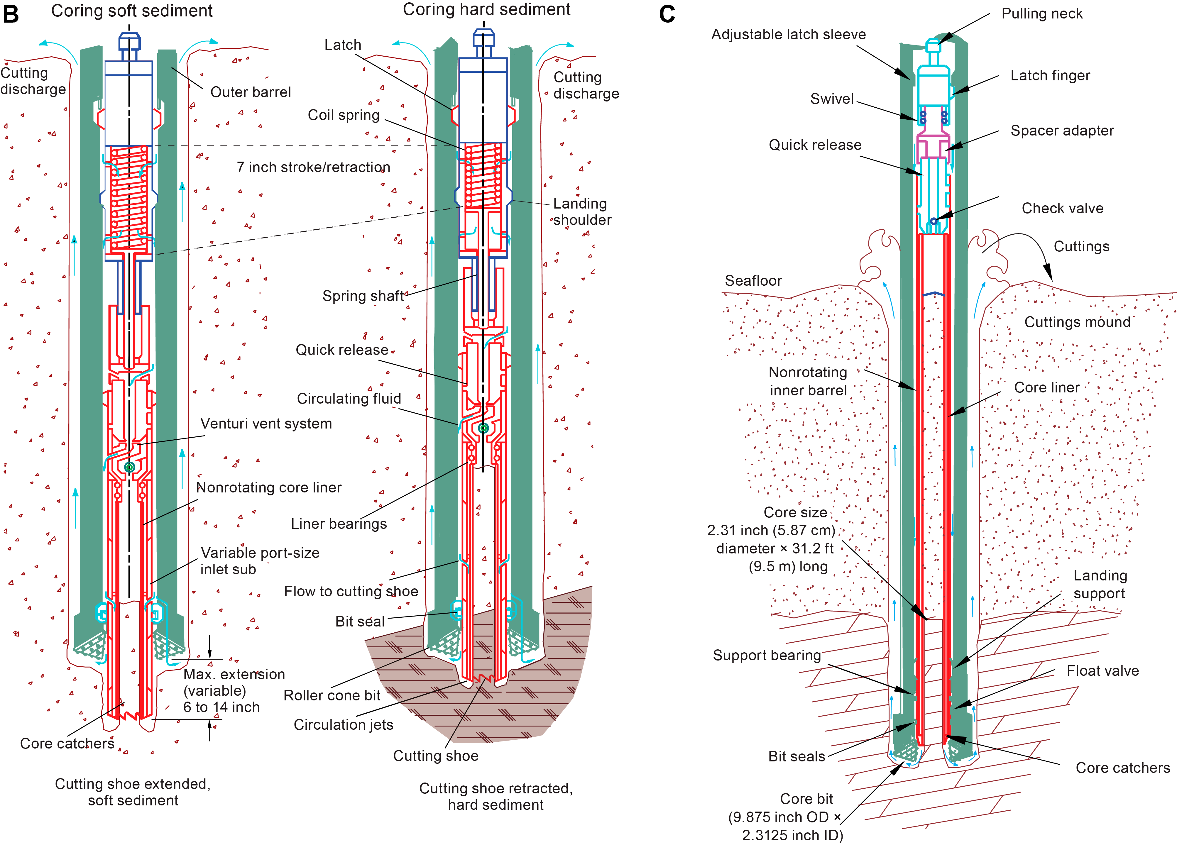
The standard APC system employs a 9.5 m long core barrel, whereas the HLAPC system uses a 4.7 m long core barrel. Both systems cut cores with a nominal diameter of 6.27 cm. The HLAPC system was deployed after the standard APC had <50% recovery or once the deployment of the XCB system emerged as a regular approach due to high abundance of infrequently occurring hard carbonate layers intercalated with soft clay- and ooze-rich sediments. While using the HLAPC system, the same criteria were applied in terms of refusal as for the APC system. Deployment of the HLAPC system allowed for considerably greater APC sampling depths to be attained than would have otherwise been possible.

The XCB system is typically used when the APC/HLAPC system has insufficient recovery. Cores collected with the XCB system are denoted by the letter “X” (for extended). The XCB system was utilized to advance the hole when APC or HLAPC refusal occurred before the target depth was reached or when drilling/formation conditions required it. The latter case applied once the APC/XCB drill bit encountered infrequently occurring hard carbonate layers or sediment/sill contact zones. The XCB system is equipped with a small coring shoe that extends below the large rotary APC/XCB drill bit (Figure F2B), cutting cores with a nominal diameter of 5.87 cm. The smaller XCB coring shoe is able to cut a semi-indurated core with less torque and fluid circulation than the main drill bit, possibly improving core recovery. The XCB cutting shoe typically extends ~30.5 cm ahead of the main bit in soft sediments but is allowed to retract into the main bit when hard formations are encountered (Figure F2B). Shorter XCB cutting shoes can be used as well.

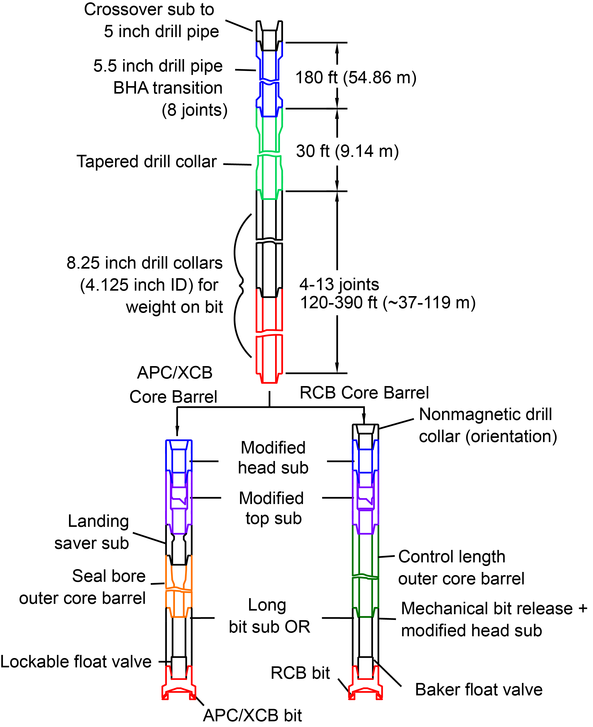
The joint bottom-hole assembly (BHA) used for APC and XCB coring is typically composed of an 11.4375 inch (~29.05 cm) drill bit, a bit sub, a seal bore drill collar, a landing saver sub, a modified top sub, a modified head sub, five 8.25 inch (20.96 cm) control-length drill collars, a tapered drill collar, two stands of 5.5 inch (13.97 cm) transition drill pipe, and a crossover sub to the drill pipe that extends to the surface (Figure F3).

The RCB system is a rotary system designed to recover sedimentary rocks and crystalline basement, such as igneous rocks. Its BHA, including the bit and outer core barrel, is rotated with the drill string while bearings allow the inner core barrel to remain stationary (Figure F2C).

A typical RCB BHA consists of, from bottom to top, a coring bit (typically 9.875 inch in diameter), a bit sub, an outer core barrel, a modified top sub, a modified head sub, a variable number of 8.25 inch control-length drill collars, one tapered drill collar, two stands of 5.5 inch drill pipe, and a crossover sub to the drill pipe that extends to the surface (Figure F3). Cores collected with the RCB system are denoted by the letter “R” (for rotary) and have a nominal diameter of 5.87 cm.

The recovery rate for each core was derived from the total length of a core recovered divided by the length of the cored interval (see Curatorial core procedures and sampling depth calculations). In soft sediments, recovery rates are typically ~100%, unless unconsolidated granular (e.g., loose sand) formation is cored (as happened at Site U1551). In firm sediments and igneous rocks, recovery rates are <100%, with the XCB system usually ranging from 50% to 90% and the RCB system generally ranging from 20% to 60% (rarely up to 80%).

Nonmagnetic core barrels were used for all APC, HLAPC, and RCB deployments during Expedition 385. APC cores were oriented with the Icefield MI-5 core orientation tool upon request when coring conditions allowed. Numerous in situ formation temperature measurements were taken with the advanced piston corer temperature (APCT-3) and sediment temperature (SET2) tools (see Petrophysics). Additionally, there was one single deployment of the Elevated Temperature Borehole Sensor (ETBS) (upon completion of drilling in Hole U1547D). We deployed the two routine downhole logging tool strings, the triple combination (triple combo) and the Formation MicroScanner (FMS)-sonic tool suites, at two sites. Furthermore, we sampled borehole fluid by deploying the Kuster Flow Through Sampler (Kuster FTS) tool in several holes. Detailed information on recovered cores, drilled intervals, downhole tool deployments, and related information are provided in the Operations, Paleomagnetism, and Petrophysics sections of each site chapter.

1.3. IODP depth conventions

The primary depth scales used are defined by the length of the drill string deployed (e.g., drilling depth below rig floor [DRF] and drilling depth below seafloor [DSF]), the length of core recovered (e.g., core depth below seafloor [CSF] and core composite depth below seafloor [CCSF]), and the length of logging wireline deployed (e.g., wireline log depth below rig floor [WRF] and wireline log depth below seafloor [WSF]) (see IODP Depth Scales Terminology at http://www.iodp.org/policies-and-guidelines/142-iodp-depth-scales-terminology-april-2011/file). In cases where multiple logging passes are made, wireline log depths are mapped to one reference pass, creating the wireline log matched depth below seafloor (WMSF) scale. All units are always expressed in meters. The relationship between scales is defined either by protocol, such as the rules for computation of CSF depth from DSF depth, or by user-defined correlations, such as core-to-log correlation. The distinction in nomenclature should keep the reader aware that a nominal depth value in different depth scales usually does not refer to the exact same stratigraphic interval.

Depths of cored intervals are measured from the drill floor based on the length of drill pipe deployed beneath the rig floor (DRF scale). The depth of the cored interval is referenced to the seafloor (DSF scale; Figure F1) by subtracting the seafloor depth of the hole (i.e., water depth) from the DRF depth of the interval. Standard depths of cores in meters below seafloor (CSF-A scale) are determined based on the assumption that (1) the top depth of a recovered core corresponds to the top depth of its cored interval (on the DSF scale) and (2) the recovered material is a contiguous section even if core segments are separated by voids when recovered. Standard depths of samples and associated measurements (CSF-A scale) are calculated by adding the offset of the sample or measurement from the top of its section and the lengths of all higher sections in the core to the top depth of the core.

If a core has <100% recovery, for curation purposes all cored material is assumed to originate from the top of the drilled interval as a continuous section. In addition, voids in the core are closed by pushing core segments together, if possible, during core handling. Therefore, the true depth interval within the cored interval is unknown. This result should be considered a sampling uncertainty in age-depth analysis or in correlation of core data with downhole logging data.

When core recovery is >100% (the length of the recovered core exceeds that of the cored interval), the CSF depth of a sample or measurement taken from the bottom of a core will be deeper than that of a sample or measurement taken from the top of the subsequent core (i.e., the data associated with the two core intervals overlap on the CSF-A scale). This overlap can happen when a soft to semi-soft sediment core recovered from a few hundred meters below the seafloor expands upon recovery (typically by a few percent to as much as 15%). Therefore, a stratigraphic interval may not have the same nominal depth on the DSF and CSF scales in the same hole.

During Expedition 385, all core depths below seafloor were initially calculated according to the CSF-A depth scale. Unless otherwise noted, all depths presented are calculated on the CSF-A scale and reported as meters below seafloor (mbsf).

1.4. Curatorial core procedures and sampling depth calculations

Numbering of sites, holes, cores, and samples follows standard IODP procedures. A full curatorial identifier for a sample consists of the following information: expedition, site, hole, core number, core type, section number, section half, piece number (for cores/sections of igneous/metamorphic rocks only), and interval in centimeters measured from the top of the core section. For example, a sample identification of “385-U1545A-5H-2W, 23–25 cm” indicates a 2 cm long sample taken from the interval between 23 and 25 cm below the top of Section 2 (working half) of Core 5 (“H” designates that this core was taken with the APC system) of Hole A at Site U1545 (Figure F1). The “U” preceding the hole number indicates the hole was drilled by a US platform (i.e., JOIDES Resolution). The coring system used to obtain a core is designated in the sample identifiers as follows: H = APC, F = HLAPC, R = RCB, and X = XCB. Integers are used to denote the “core” type of drilled intervals (e.g., a drilled interval before Core 2R would be denoted by Core 11 [i.e., “Core 1” and “Type 1”]).

2. Core handling and analysis

2.1. Sediment

When the core barrel reached the rig floor, the core catcher from the bottom of the core barrel was removed and a sample was extracted for paleontological (PAL) analysis. Next, the sediment core was extracted from the core barrel in its plastic liner. The liner was carried from the rig floor to the core processing area on the core receiving platform outside the core laboratory, where it was split into ~1.5 m sections. Blue (uphole direction) and clear (downhole direction) liner end caps were glued with acetone onto the cut liner sections. Prior to cutting the whole-round sections of sediment cores, the length of gas expansion–derived voids was measured when observed and void gas samples were taken (see Organic geochemistry).

Once the core was cut into sections, whole-round samples were taken for interstitial water (IW) chemical analyses. Additional whole-round samples were taken from cores recovered in holes dedicated to extensive personal sampling for microbiology and biogeochemistry studies based on a complex sampling protocol (see Microbiology). When a whole-round sample was removed, a yellow liner end cap was used to denote the missing interval. Syringe samples were taken for headspace gas analyses according to the IODP hydrocarbon safety monitoring protocol. Selected whole-round core sections were subjected to IW extraction using Rhizon samplers within minutes of recovery at three different sites (see Inorganic geochemistry).

Core sections were placed in a core rack in the core laboratory. When they reached equilibrium with laboratory temperature (typically after 3 h), they were run through the Whole-Round Multisensor Logger (WRMSL) for P-wave velocity on the P-wave logger (PWL), magnetic susceptibility (MS), and gamma ray attenuation (GRA) bulk density (see Petrophysics). The core sections were also run through the Natural Gamma Radiation Logger (NGRL) for natural gamma radiation (NGR), and thermal conductivity measurements were made once per core when the material was suitable.

The core sections were then split lengthwise from bottom to top into working and archive halves. Investigators should note that older material can be transported upward on the split face of each section during splitting.

The working half of each sediment core was described by the sedimentologists and structural geologists. Discrete samples were then taken for moisture and density (MAD) and paleomagnetic (PMAG) analyses and for remaining shipboard analyses such as X-ray diffraction (XRD), carbonate (CARB), and source rock analyzer (SRA) measurements. Samples were not collected or sampling was restricted when (1) the lithology was a high-priority interval for expedition or postexpedition research (e.g., ash layers, most of sediment/sill contact zone, etc.), (2) there was unsuitable core material, or (3) the core was severely deformed. During the expedition, samples were taken for personal expedition (e.g., in the radiation van) and postexpedition research when studies focused on examining ephemeral properties, such as microbiology and biogeochemistry research.

The archive half of each core was scanned on the Section Half Imaging Logger (SHIL). It was also measured for point magnetic susceptibility (MSP), as well as reflectance spectroscopy and colorimetry (RSC) on the Section Half Multisensor Logger (SHMSL). Occasionally, X-ray images of archive-half sections were taken as well. Labeled foam pieces were used to denote missing whole-round (WR) intervals in the SHIL images. The archive-half sections were then described visually and by means of smear slides for sedimentology. Finally, magnetization of archive-half sections and working-half discrete pieces was measured with the cryogenic magnetometer and spinner magnetometer.

2.2. Igneous rock

Pieces were extracted from the core liner on the core receiving platform or directly from the core barrel on the rig floor and subsequently put into split plastic liners in consecutive order. The pieces were then pushed to the bottom of the 1.5 m liner sections, and the total rock length was measured. The length was entered into the database using the SampleMaster application as “recovered length.” This number was used to calculate recovery. The liner sections were then transferred to the core splitting room. If a core catcher sample was present, it was taken to the core splitting room separately and added to the bottom section of the recovered core.

In drilled depth intervals dedicated to microbiology sampling in sill intrusions, selected whole-round igneous rock pieces or sections were taken from certain cores for further microbiology subsampling according to an established sampling plan. Only the necessary five scientists (petrologist, structural geologist, and microbiologists on shift) and an assigned representative of the Sample Allocation Committee (SAC), wearing face masks and nitrile gloves, were present in the core splitting room for microbiology sampling to minimize contamination, and the samples/sections were immediately transferred to the microbiology laboratory for further processing (see Microbiology).

Oriented pieces of core were marked on the bottom with a blue- or red-colored wax pencil to preserve orientation. Adjacent but broken pieces that could be fit together along fractures were curated as single pieces. The petrologists and structural geologists confirmed piece matches and marked the split line on the pieces and denoted the working half with the letter “W,” which defined how the pieces were to be cut into two equal halves. The aim was to maximize the expression of dipping structures on the cut face of the core while maintaining representative lithologic and mineralogic features in both archive and working halves. Any present dipping structures were then measured on the whole-round core pieces by the structural geologist on shift (see Structural geology). A plastic spacer was secured with acetone to the split core liner between individual pieces or reconstructed contiguous groups of subpieces. These spacers can represent substantial intervals of no recovery. The length of each section of core, including spacers, was entered into the database as “curated length,” which commonly differs by several centimeters from the length measured on the core receiving platform. Ultimately, the eventual depth of each piece in the database was recalculated based on the curated length.

Core pieces were imaged around the full 360° circumference (at four different angles of 000°, 090°, 180°, and 270°) using the SHIL configured for whole-round sections and then placed in a core rack in the laboratory. When the core sections reached equilibrium with laboratory temperature (typically after 2 h), the whole-round core sections were run through the WRMSL (GRA and MS only) and NGRL (see Petrophysics).

Each piece of core was split with a diamond-impregnated saw into an archive half and a working half, with the positions of plastic spacers between pieces maintained in both halves. Pieces were numbered sequentially from the top of each section, beginning with 1. Separate subpieces within a single piece were assigned the same number but lettered consecutively (e.g., 1A, 1B, etc.). Pieces were labeled only on the outer cylindrical surfaces of the core. If it was evident that an individual piece had not rotated around a horizontal axis during drilling, an arrow pointing to the top of the section was added to the label. The oriented character of each piece was recorded in the database using the SampleMaster application.

The archive half of each core was scanned on the SHIL (with both a dry and wet surface) and measured for MSP and RSC on the SHMSL. Thermal conductivity measurements were made on selected archive-half pieces (see Petrophysics). After the archive-half sections of each core were fully described by the petrologist and structural geologist on shift, samples were taken from the working-half sections for shipboard analyses (billets for thin sections; chips for inductively coupled plasma–atomic emission spectroscopy [ICP-AES]; and cube samples (~8 cm³) for paleomagnetism analyses, MAD, and discrete P-wave velocity measurements; see Igneous petrology and alteration, Inorganic geochemistry, Paleomagnetism, Petrophysics). The magnetizations of archive-half sections and pieces, as well as discrete cube samples taken from the working-half sections, were measured with the cryogenic magnetometer and spinner magnetometer, respectively (see Paleomagnetism).

When all laboratory processing steps were completed, cores were wrapped, sealed in plastic tubes, and transferred to cold storage space aboard the ship. At the end of the expedition, the cores were sent to the IODP Gulf Coast Repository (Texas A&M University, College Station, Texas [USA]), where personal nonephemeral samples for postexpedition research were taken and the cores are permanently stored.

2.3. Handling drilling and core disturbance

Cores may be significantly disturbed and contain extraneous material as a result of the coring and core handling process (Jutzeler et al., 2014). In formations with loose sand layers, sand from intervals higher in the hole may be washed down by drilling circulation, accumulate at the bottom of the hole, and be sampled with the next core. The uppermost 10–50 cm of each core must therefore be examined critically during description for potential “fall-in” material. Common coring-induced deformation includes the concave-downward appearance of originally horizontal bedding. Piston action can result in fluidization (“flow-in”) at the bottom of APC/HLAPC cores. Retrieval from depth to the surface can result in elastic rebound. Gas that is in solution at depth may become free and drive apart core segments within the liner. When gas content is high, pressure must be relieved for safety reasons by drilling holes into the plastic liner before the cores are cut into segments. These holes force some sediment as well as gas out of the liner. Such observed disturbances are described in each site chapter and graphically indicated on the visual core descriptions (VCDs).

3. Lithostratigraphy

Descriptions of sediment cores recovered during Expedition 385 are based on a combination of digital color imagery, visual core description (e.g., visual color determination of core disturbance, sediment structures, and color using a Munsell chart), microscopy, and various X-ray techniques. Lithologies were determined by (1) macroscopic description of the archive halves of split cores and/or (2) microscopic assessment of smear slides and thin sections using a petrographic microscope. All of these observations were saved to the LIMS database through data capture by the in-house core description software DESClogik. Additional X-ray techniques that were used to assist core material description and determination include X-ray imagery and XRD. A selection of data sets was combined to inform a VCD sheet for each core.

The methods employed are adapted from those used during Integrated Ocean Drilling Program Expedition 323 (Expedition 323 Scientists, 2011). The timescale used for Expedition 385 is that of Gradstein et al. (2012) and updated to the latest division of the formal series for the Pliocene and Pleistocene (version 2019/05 of the International Chronostratigraphic Chart available at http://www.stratigraphy.org). Note that because of both the drilling technique used to retrieve the cores (i.e., missing mudline) and/or possible hiatuses in the uppermost and most recent part of the sedimentary record (e.g., Barron et al., 2005), the first core collected in each hole at all sites could be missing the Holocene strata.

3.1. Digital color image and core description sheets

The SHIL captures an image of the flat face of the archive half of the split cores using a line-scan camera. Sediment cores are split, and the archive half is scraped with the edge of a glass slide or stainless steel rectangular plate to provide a “clean” surface for imaging. Note that this approach occasionally resulted in faint linear scratches on the flat surface of the archive half that made scrape markings appear on some core section images. The cleaned, flat face of the archive half was imaged as soon as possible after splitting and surface scraping to minimize color changes that may occur through oxidation and drying. Images were taken at an interval of 10 lines/mm. Camera height was adjusted so that image pixels are square. Light is provided by three pairs of Advanced Illumination high-current focused LED line lights with fully adjustable angles to the lens axis. We noted that compression of line-scanned images into compiled stacks (like the core image shown in the VCDs) may result in visual artifacts (e.g., the false appearance of lamination). The stacked images were integrated into core description sheets that were printed before making observations to facilitate the implementation of core description through handwritten notes (Figure F4). These sheets contain field notes used to help organize whole-core observations prior to itemized entry into the DESClogik software, ensuring consistency between core describers and preserving information needed for later shore-based sampling in a format used in sedimentological studies.

3.1.1. Visual color determination and spectrophotometry

Descriptions of sediment color and the corresponding hue, value, and chroma data were determined qualitatively using Munsell soil color charts for each major and minor lithology (Munsell Color Company, 2000, 2009). Color reflectance spectrophotometry and MSP of the archive-half sections were measured on the SHMSL. Reflectance of visible light from the archive halves of sediment cores was measured using an Ocean Optics USB4000 spectrophotometer mounted on the automated SHMSL. Additional detailed information about measurement and interpretation of spectral data and MSP can be found in Petrophysics, Balsam et al. (1997, 1998), and Balsam and Damuth (2000). The Munsell color data were added to the core description sheet and the VCDs (see Visual core description summaries).

3.1.2. Sedimentary structures

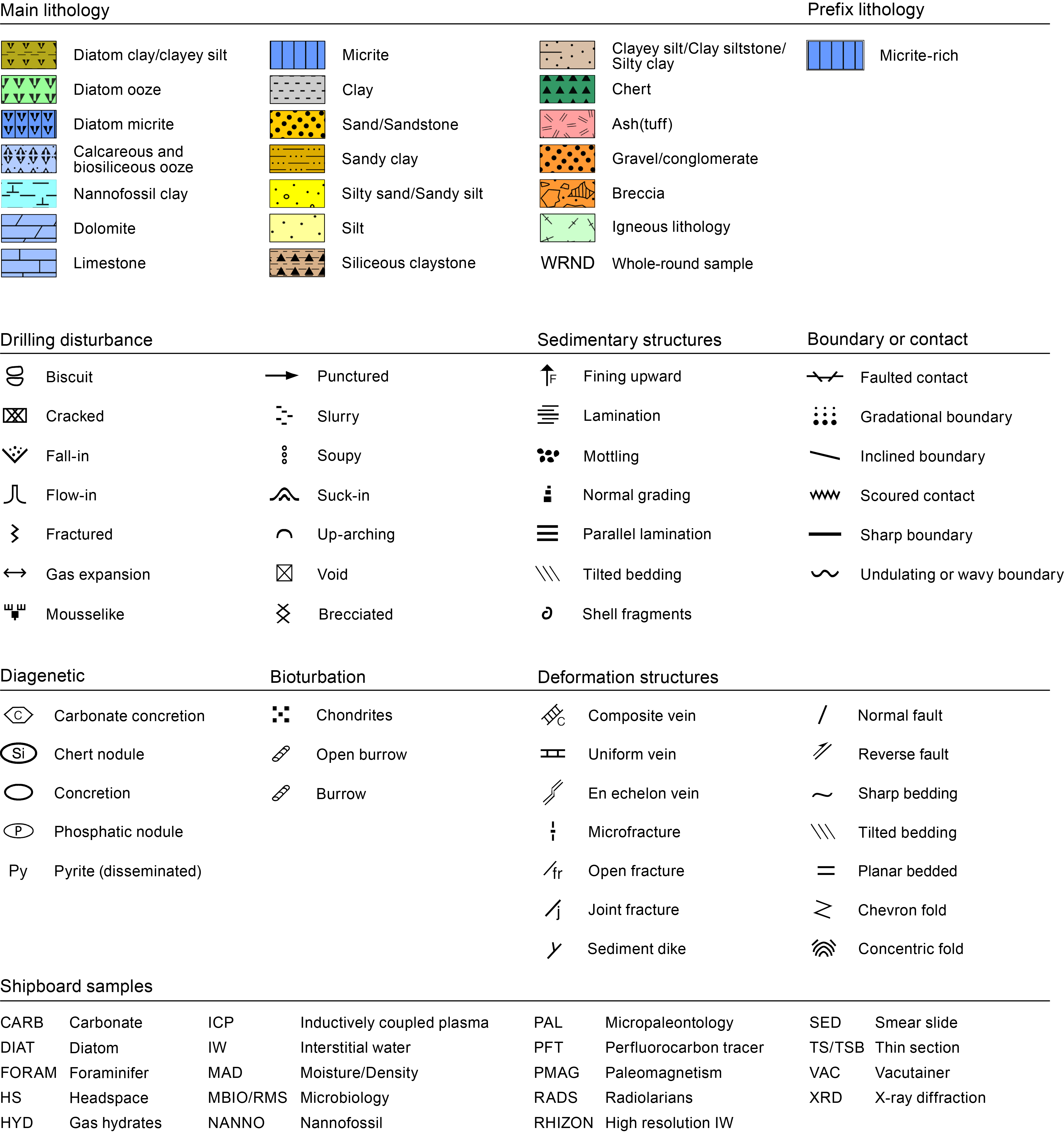
Sedimentary structures, bedding planes, and diagenetic features formed by natural processes (i.e., not as a result of drilling disturbance) were noted on the core description sheets (Figure F4) and are also represented on the VCDs with symbols in the Sedimentary structures column (Figure F5). Structures formed by both biogenic and physical processes are included.

Bed thickness in the core was defined according to McKee and Weir (1953):

• Very thick bedded = >100 cm.
• Thick bedded = >30–100 cm.
• Medium bedded = >10–30 cm.
• Thin bedded = >3–10 cm.
• Very thin bedded = 1–3 cm.
• Laminae = <1 cm.

3.1.3. Sediment diagenesis, hydrothermal alteration, and contact metamorphism

The recovered sedimentary units have undergone various stages of postburial modification over a vast temperature range, spanning the realms of bottom seawater temperature at the seafloor (~4°C), burial diagenesis (<200°C), and hydrothermal alteration and thermal metamorphism resulting from heating and dewatering of sediments in contact with sill intrusions, which are abundant in the Expedition 385 study area. Temperatures of 200°–800°C can be expected in the contact aureoles of major sill intrusions in sedimentary basins (Aarnes et al., 2010, and references therein). Low-temperature alteration (diagenetic) features were documented through descriptions of degree of lithification, cementation, new mineral growth in pore spaces, and formation of concretions. Intervals of contact metamorphism or hydrothermal overprint were noted but not described in detail because of time and analytical constraints. The initial mineral identification and degree of alteration estimates were later refined by incorporating the results from thin section descriptions (using both transmitted and reflected light modes), scanning electron microscope (SEM) images, and XRD analyses.

3.1.4. Drilling disturbance

Sediment disturbance resulting from the coring process was recorded in the VCDs.

Types of drilling disturbances observed in soft and firm sediments include the following:

• Biscuits: sediment of intermediate stiffness that has vertical variations in the degree of disturbance. Softer intervals are washed and/or soupy, whereas firmer intervals are relatively undisturbed (this type of disturbance is considered moderate–high).
• Brecciated: sediment is broken up in a chaotic framework of pieces produced by the coring process.
• Cracked: firm sediments are broken during drilling but not displaced or rotated significantly.
• Fall-in: out-of-place material that has fallen downhole onto the cored surface after core barrel retrieval. This material is recovered in the top of the following core.
• Flow-in: out-of-place material is displaced along the sides of a core, often with a streaky appearance.
• Gas expansion: expansion of gas disrupts the stratigraphic sequence. It is described as slight if it does not disrupt the stratigraphic sequence or moderate–severe if the sequence is partially or completely disrupted, respectively.
• Punctured: sediment is displaced from puncturing the core liner.
• Soupy: water-rich sediments are liquefied to some degree.
• Suck-in: sediment is introduced (sucked in) at the bottom of the core barrel due to motion when drilling.
• Void: empty space occurs within the cored material. These may be products of gas expansion during core retrieval, partial strokes during the coring process, or partial recovery.

Additional types of drilling disturbance in more lithified sections include fracture and drilling breccia. Drilling disturbance is also displayed on the VCDs (e.g., fall-in, flow-in, void, and soupy).

3.2. Sediment classification

Sedimentary materials recovered during Expedition 385 are largely composed of biogenic sediments mixed with a minor siliciclastic component. Occasionally, pyroclastic deposits of ash to lapilli grain size occur.

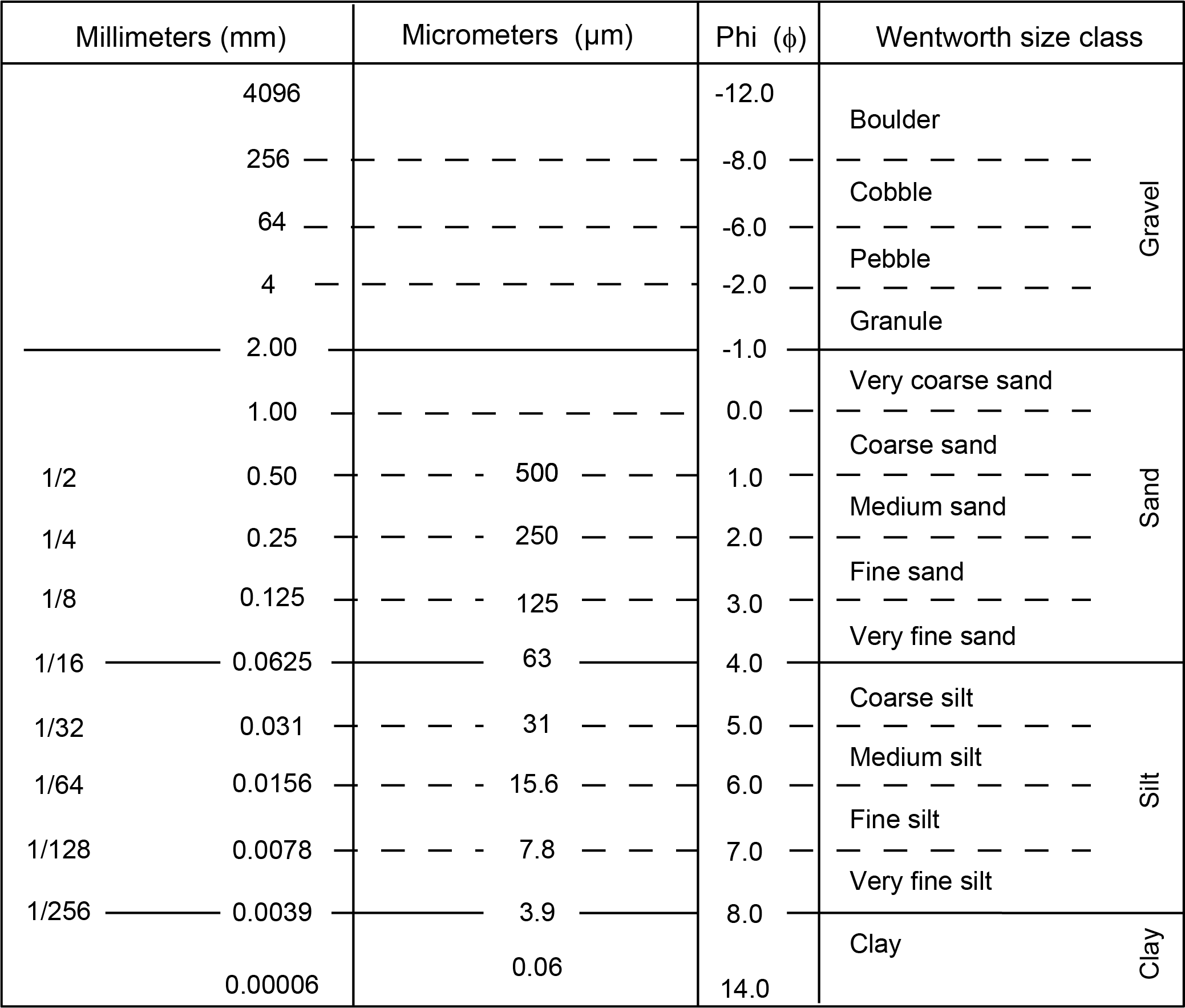
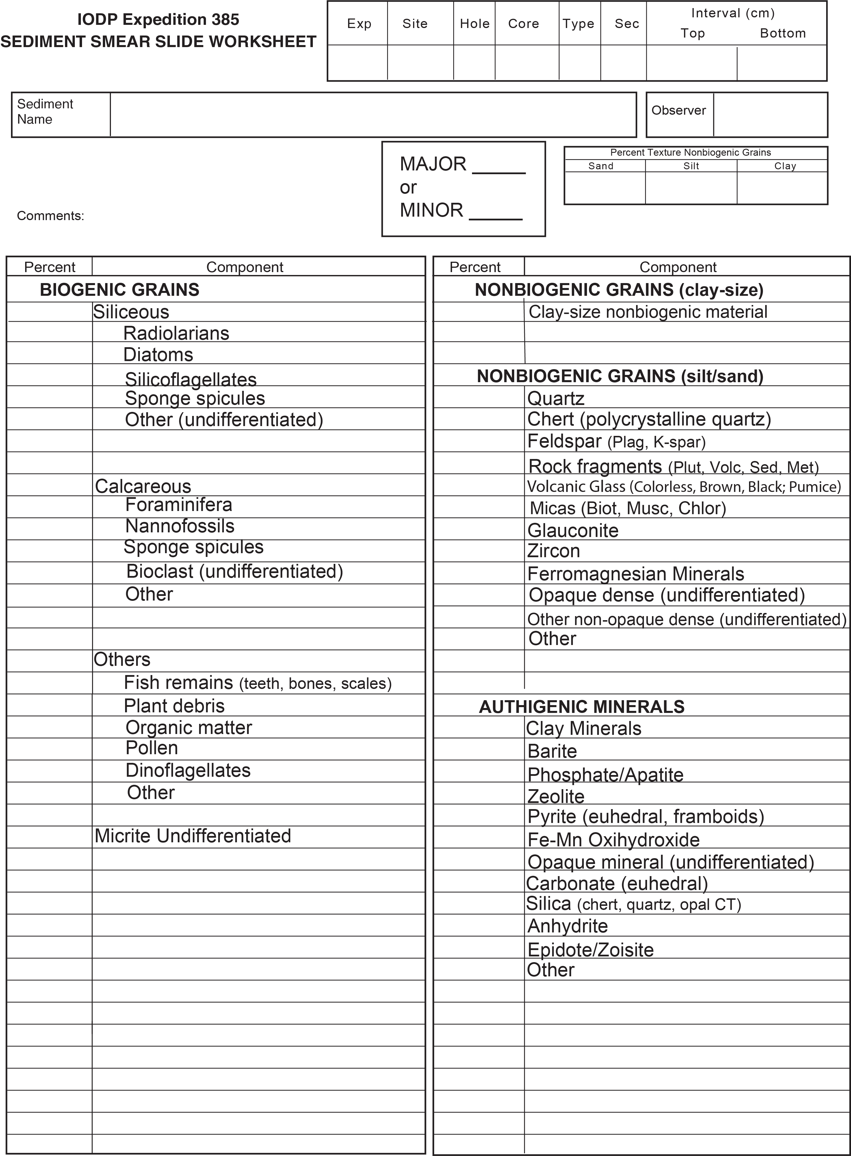
Our approach for sediment classification consists of two parts: a principal name (e.g., silt or ooze) and a prefix (e.g., foraminifer-rich). The principal name applied to a sediment is determined by the component or group of components making up >60% of the sediment, and, in case of the main lithology being siliciclastic, the main particle size according to the Udden-Wentworth scale (Wentworth, 1922; Figure F6). For example, sediment composed of 70% silt-sized siliciclastic material and 30% foraminifers is classified as foraminifer-rich silt. When the biogenic components make up more than 60%, the principal name of the sediment contains the word ooze. For instance, a sediment composed of 20% clay, 40% foraminifers, and 40% diatoms is called clay-rich foraminifer and diatom ooze. Prefixes such as clay-rich or clay-bearing are used for components ranging from 5% to 40% of the sediment, as defined below. The naming scheme for sediments with subequal mixtures of biogenic and siliciclastic and/or volcanogenic material is described below (see Mixed sediments). Visual percentage estimates and textural attributes of biogenic and nonbiogenic components are made from smear slides (see Smear slide and thin section description) (Figure F7) or macroscopic observation of the core with a hand lens.

3.2.1. Siliciclastic and volcaniclastic sediments

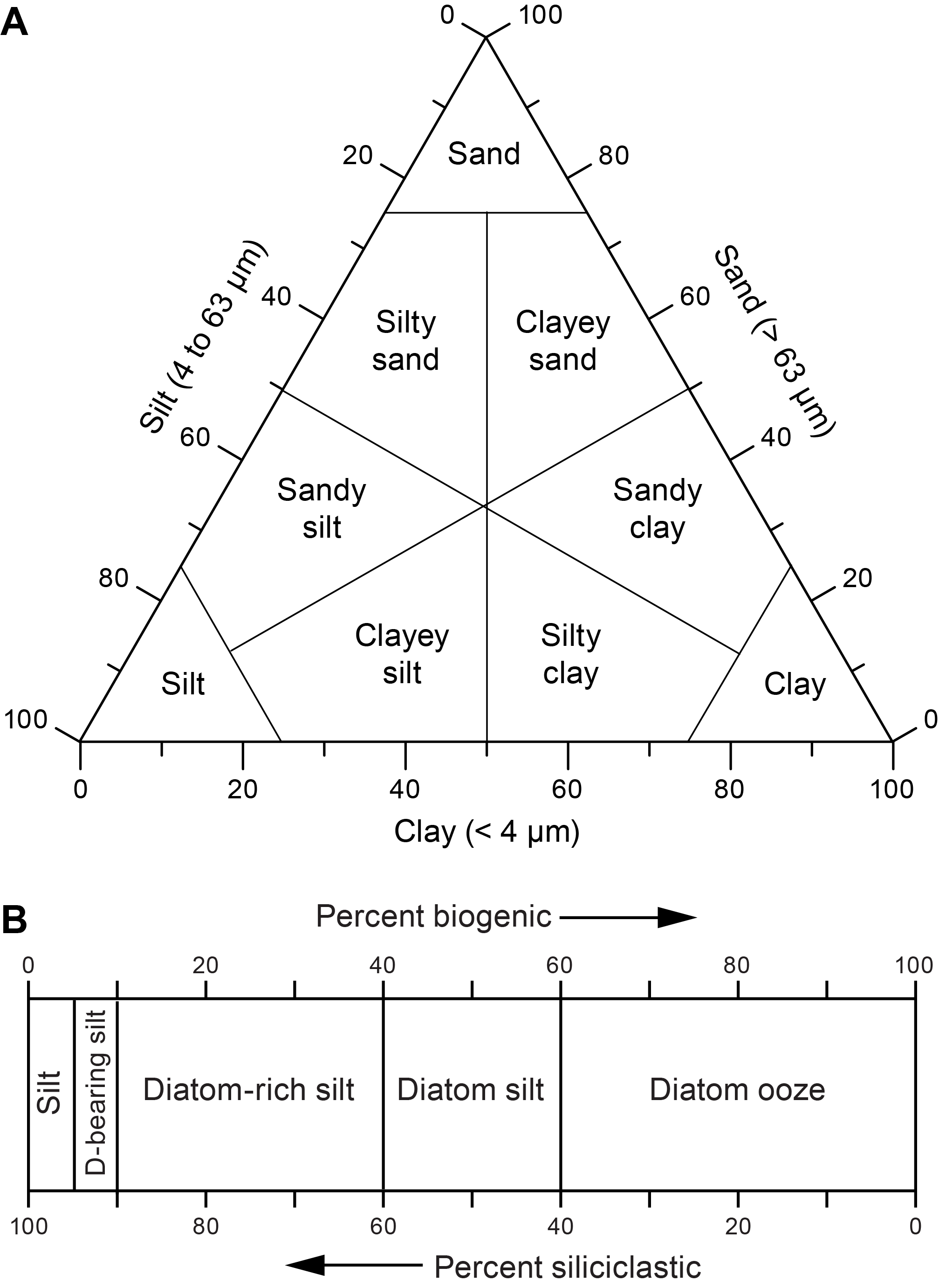
If total siliciclastic content is >60%, the principal name is determined by the texture of the siliciclastic grains (i.e., the relative proportions of sand-, silt-, and clay-grade components when plotted on a modified Shepard [1954] ternary classification diagram) (Figure F8A). The siliciclastic principal names are clay (<4 µm), silt (4–63 µm), sand (63–2000 µm), and combinations of the three end-members using a modifier (e.g., silty clay, sandy clay, clayey silt, sandy silt, clayey sand, and silty sand). Siliciclastic particles include terrigenous epiclasts produced by erosion of onshore volcanic units. If a sediment is entirely composed of pyroclastic particles (e.g., vitric/glass shards, pumice, or mineral fragments) and exhibits no evidence of reworking, then it is identified as unconsolidated tephra (e.g., ash or lapilli) or lithified/consolidated tephra (e.g., tuff or lapillistone) using the descriptive terminology of Fisher and Schmincke (1984).

3.2.2. Mixed sediments

Mixed sediments include sediment in which no single type of sedimentary component, either siliciclastic, biogenic, or pyroclastic, is dominant (i.e., >60%). If siliciclastic grains compose 40%–60% of the sediment, the principal name is determined by the texture/main particle size of the siliciclastic grains. For example, the principal name of a sample containing 10% ash, 40% diatoms, and 50% siliciclastic grains that are >75% silt sized is diatom silt. If the abundances of diatoms and siliciclastic grains are reversed (i.e., 50% diatoms and 40% siliciclastic grains), the principal name is still diatom silt, as neither composes >60% of the sediment.

3.2.3. Modifiers

Minor modifiers are used if a sediment type composes 5%–40% of the sediment and this group is not included as part of the principal name. When a microfossil group, a siliciclastic group, or pyroclastic group composes 10%–40% of the sediment, a minor modifier consisting of the component name hyphenated with the suffix “-rich” (e.g., diatom-rich clay or silt-rich foraminifer ooze) is applied. When a microfossil group, siliciclastic group, or ash composes 5%–10% of the sediment, a minor modifier consisting of the component name hyphenated with the suffix “-bearing” (e.g., diatom-bearing clay or ash-bearing clayey silt) is used. When two minor components are present, minor modifiers are listed before the principal name in order of increasing abundance. For example, sediment with 15% foraminifers, 40% nannofossils, and 45% clay is foraminifer-rich nannofossil clay; and a sediment with 5% diatoms, 15% radiolarians, and 80% clay is diatom-bearing radiolarian-rich clay (Figure F8B). It should be noted that although the suffix “-bearing” was used to classify the sediment during smear slide description (see Smear slide and thin section description), it was not used in the lithologic representation of the cores included in the VCDs. This choice was made to reduce the number of lithologic patterns, thus making the VCDs more readable.

3.2.4. Lithification

Sediments that range from unconsolidated to variably indurated have the suffix “-stone” added to the principal names sand, silt, and clay when a spatula and mallet, hammer and chisel, or saw was needed to take samples from the working half of the split core. For other biogenic-dominated lithologies, a different term was used (e.g., limestone) when they reached that level of induration.

Induration is separated into four classes:

• Soupy: water-saturated sediment with very little strength.
• Soft: sediment with little strength that is readily deformed under the pressure of a finger or broad-blade spatula.
• Stiff: partly lithified sediment that is readily scratched with a fingernail or edge of a spatula.
• Hard: well-lithified, compacted, and/or cemented sediment that is resistant or impossible to scratch with a fingernail or edge of a spatula or core that must be cut with a band saw or diamond saw.

3.3. Smear slide and thin section description

One or more smear slide samples of the main lithologies were collected from the archive half of most Hole A sediment cores to define the lithologies. These were used as guides for assigning lithologies in other nearby (in most cases ~20 m) holes at a given drill site owing to time constraints posed by high recovery rates. Additional samples were locally collected to characterize small-scale lithologic variations across laminations and tephra layers. A small amount of sediment was taken by toothpick from the cores and dispersed evenly in deionized water on a 2.5 cm × 7.5 cm glass slide to create a very thin (less than ~50 µm) uniform layer of sediment grains for quantification. The dispersed sample was then dried on a hot plate. A drop of mounting medium (Norland optical adhesive Number 61) and a cover glass were added. The slide was then placed in an ultraviolet light box for 10–15 min to cure.

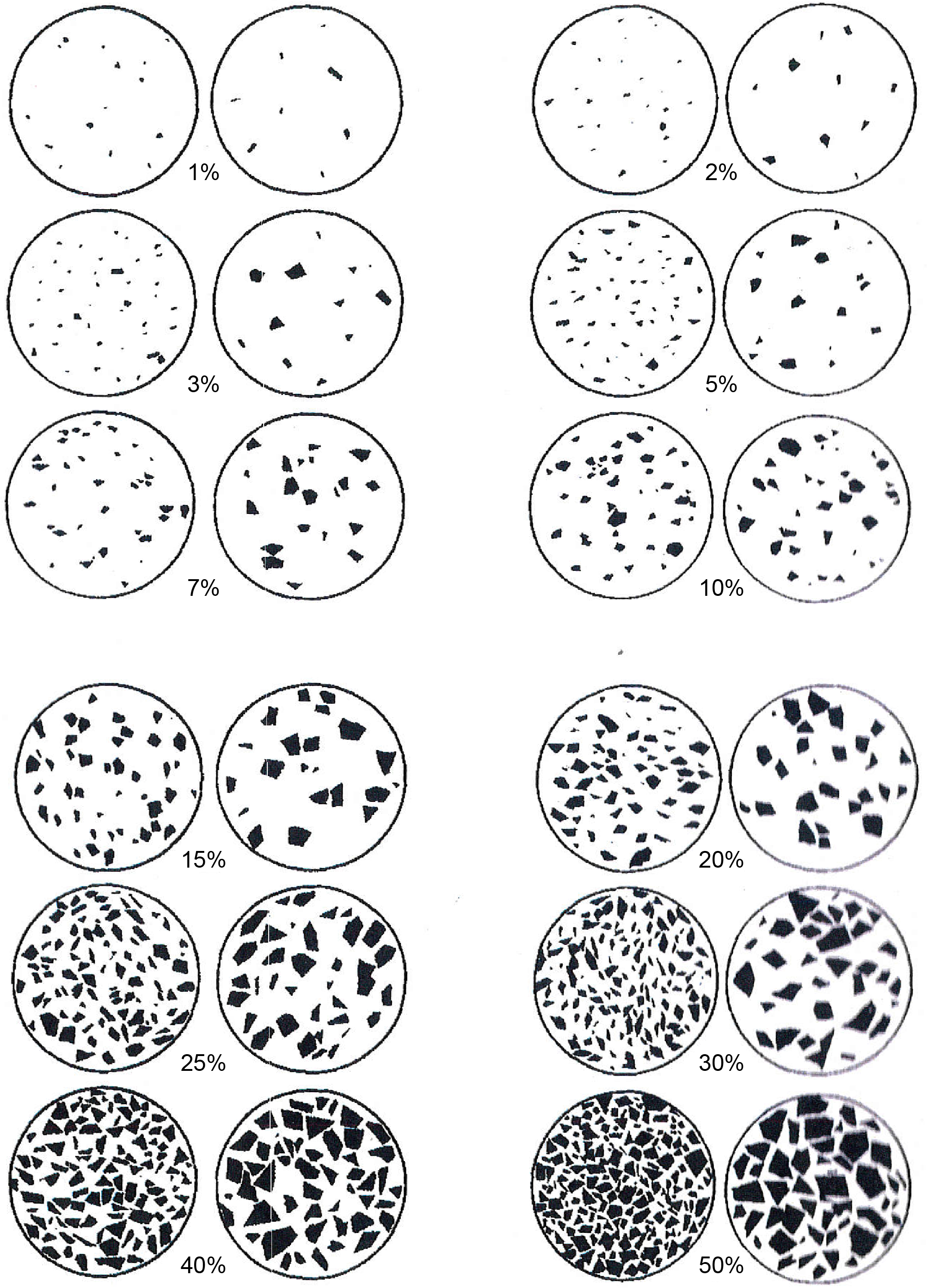
Smear slides were examined through a Zeiss transmitted-light binocular petrographic microscope (AXIO10207) equipped with a standard eyepiece micrometer and photographed with an attached SPOT Insight camera built by Diagnostic Instruments, Inc. Visual percentage estimates of biogenic, nonbiogenic, and textural features were made from each slide using a 40× objective. Biogenic and mineral component percentage abundances were visually estimated following Rothwell (1989) (Figure F9). Clay-sized (3–4 µm) particles are visible at higher magnifications (40×), but clay minerals are often not visible as single particles using a petrographic microscope given their fine-grained nature (≤2 µm); the latter were identified based on the presence of cloudiness and slight pleochroism in plane-polarized light often accompanied by diffuse birefringence in cross-polarized light (Rothwell, 1989). Grain size distributions of the coarser silt (4–63 µm) and sand (63–2000 µm) siliciclastic fractions were estimated using an eyepiece micrometer calibrated by means of a stage micrometer (microscope slide with an inscribed micrometer scale). The texture/main particle size of siliciclastic grains (i.e., relative abundance of sand-, silt-, and clay-sized grains) and the proportions and presence of biogenic and mineral components were recorded on a smear slide sample sheet (Figure F7), and data were entered into DESClogik. It should be noted that because sand-sized and larger grains are difficult to incorporate into a smear slide, such petrographic analyses may underestimate their abundance and estimates are best made macroscopically using a hand lens.

Thin sections of lithified core material were made to enable a more accurate definition of lithologies. These were ground to a thickness of 30 µm and polished for examination using the petrographic microscope described above. Observations include the nature of components and their relative proportions, including grain types, porosity, and cementation. They were tallied on a thin section description sheet similar to that used for smear slides and data were entered into DESClogik.

3.4. Visual core description summaries

Core description was initially carried out visually, and observations were logged on paper forms (Figure F4) based on figure 7 in Mazzullo et al. (1988). Reporting included notes and observations, drawings of sedimentary structures, Munsell colors, and the location of samples collected for smear slides, thin sections, and XRD. The handwritten notes were then transferred into DESClogik, from which VCDs were created.

VCDs of the archive half of the split cores provide a summary of the lithologic composition, age (based on biostratigraphy and magnetostratigraphy), and physical properties data obtained from shipboard analyses (Figure F10). IODP VCDs are equivalent to the barrel sheets used during the Deep Sea Drilling Project (DSDP), Ocean Drilling Program (ODP), and, partially, the Integrated Ocean Drilling Program. Lithologic data for VCDs were digitally recorded shipboard using the customized core description software DESClogik (version 16.1.0.22), which generates a spreadsheet for data entry, providing extensive data validation support. Prior to drilling operations, a spreadsheet template with specific tabs was constructed in Tabular Data Capture mode and customized for Expedition 385. Spreadsheet tabs were used to record the following information:

• Drilling disturbance,
• General (lithologic core description and sedimentary structures),
• Core summary (written description of major lithologic findings by core, sedimentary structures, lithostratigraphic unit, and age), and
• Hole summary (lithostratigraphic unit and age).

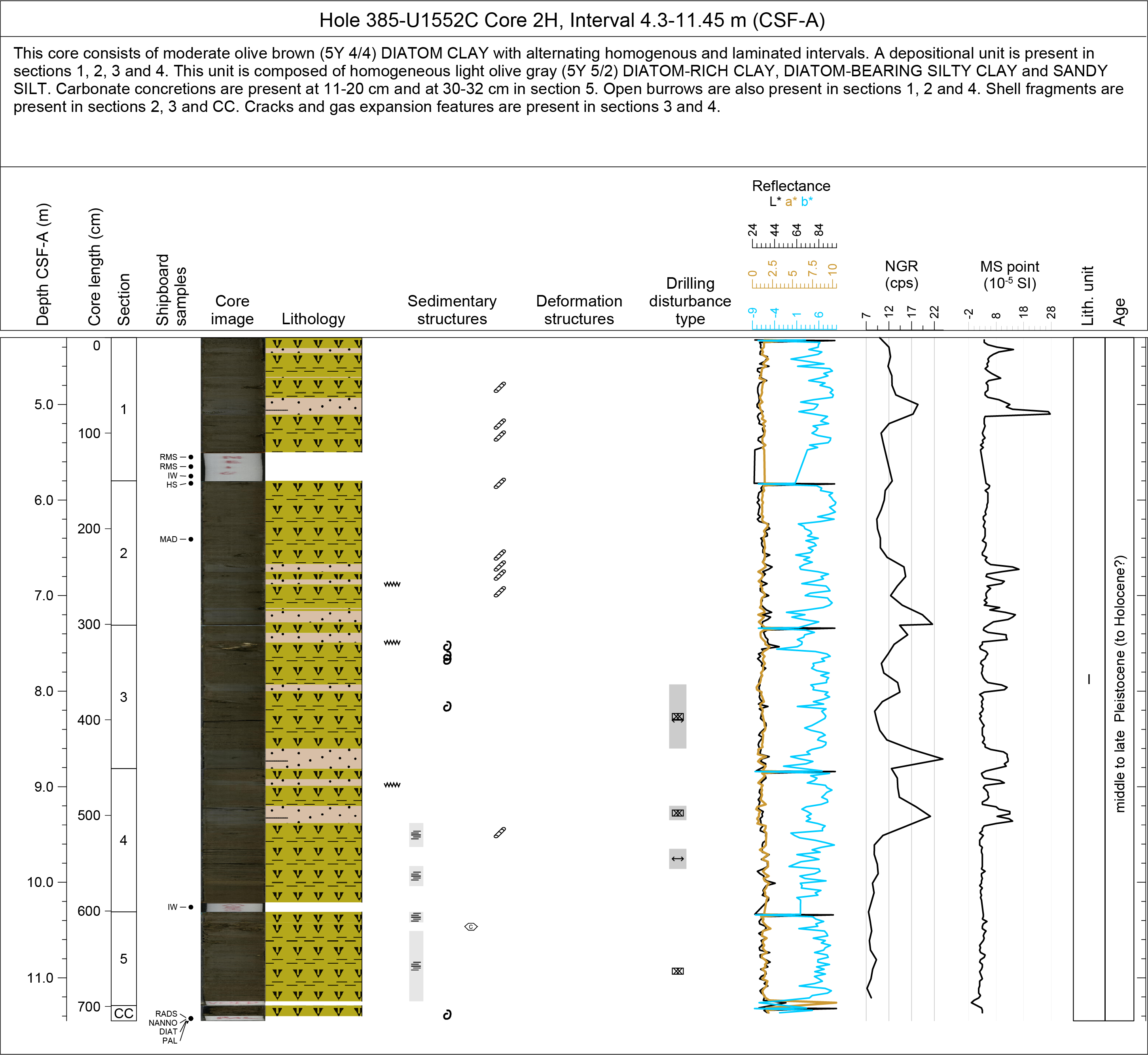
To aid core description, core data are displayed graphically in LIMS Information Viewer (LIVE, version 4.0), a separate browser-based application that displays core images alongside physical properties and geochemical data. The commercial plotting software Strater was deployed by JRSO personnel to compile the digital VCDs for each core using the data retrieved from the LIMS database or DESClogik. Site, hole, core number, and depth intervals in core depth below seafloor, Method A (CSF-A), are given at the top of the VCD together with a summary core description. The written description for each core contains a succinct overview of major lithologies, their Munsell colors, and notable features such as sedimentary structures, boundary contacts, diagenetic features (e.g., authigenic precipitates), extent of lithification, and major disturbances resulting from the coring process (Figure F10). Core depth below seafloor (recorded on the CSF-A scale in meters; represented in text, tables, and figures on the equivalent mbsf scale), core length (in centimeters), section breaks, lithostratigraphic unit, and age are indicated along the left side of the digital color image of the core. The two columns between the color image and the graphic lithology columns show the locations of shipboard samples. Columns to the right of the graphic lithology column show drilling disturbance, extent of bioturbation, lithologic accessories, sedimentary structures, and physical properties data collected using the WRMSL and SHMSL (see Petrophysics). Data collected include NGR, GRA bulk density, MS, lightness (L*), and color reflectance (a* and b*). Symbols used in the VCDs are given in Figure F5.

3.5. Lithostratigraphic units

Lithostratigraphic units are stratigraphic intervals (between tens and hundreds of meters thick) containing similar sediment or rock types. They are numbered sequentially (Unit I, Unit II, etc.) from top to bottom of the cored interval. Lithostratigraphic units are clearly distinguishable from each other by several characteristics such as composition, bed thickness, grain size class, sedimentary structures, and internal homogeneity. Lithostratigraphic units are informal “formations” that are not defined by age, geochemistry, or paleontology, although changes in these parameters may coincide with boundaries between lithostratigraphic units. When downhole changes in the lithologic characteristics of sediments are distinctive but not significant enough to require a unit division, more informal subunit designators (Subunit IA, Subunit IB, etc.) are used. This occurred at several Expedition 385 sites where only one unit but several subunits were designated when using diagenetic boundaries.

3.6. X-ray imaging

X-radiograph images were produced at all sites to evaluate bioturbation intensity, drilling disturbance, sedimentary structures, and clast abundance. Images were obtained from archive-half sections after splitting. The onboard X-Ray Imager (XRI) is composed of a Teledyne ICM CP120B portable X-ray generator and a detector unit. The generator works with a maximum voltage of 120 kV and a tube current of 1 A and has a 0.8 mm × 0.5 mm focal spot. The generator produces a directional cone at a beam angle of 50° × 50°. The detector unit is located 65 cm from the source and consists of a Go-Scan 1510 H system composed of an array of CMOS sensors arranged to offer an active area of 102 mm × 153 mm and a resolution of 99 µm. Core sections were run through the imaging area at 12 cm intervals, providing 15 cm images onto the detector and allowing overlap of 3 cm. The X-ray source and detector are housed in the source shield constructed with 6 mm of lead with an internal baffle on the unload side. The exterior corners are covered with 6 mm lead strips and lead vinyl (0.5 mm) overspreading the sides. The GRA-MS shield section is constructed with 2 mm of lead with an internal baffle on the load side, and both the load and unload ends of the track are shielded by lead vinyl (0.5 mm).

During Expedition 385, tests were conducted on archive halves to obtain the best image resolution for determining the internal structure of cores. The XRI settings were then tailored to the varying lithologies of the cores. The number of images stacked was 20, taken at exposure times of 300–400 ms. The voltage ranged between 60 and 70 kV, and the current varied between 0.7 and 1.0 A.

The raw images were collected as 16 bit images and processed with the IODP in-house processing utility in the Integrated Measurement System (IMS) software (version 1.2). The software applies gain and offset corrections for the detector, compensates for core shape and thickness, and adjusts the image contrast. The Savitzky-Golay finite impulse response (FIR) filter was chosen to smooth images. The resulting processed images include a masked background, the depth scale within the section, and the acquisition parameters. X-ray images taken during Expedition 385 can be retrieved from the Zenodo database (https://zenodo.org; search the International Ocean Discovery Program community for Expedition 385 data).

3.7. Scanning electron microscopy and X-ray diffraction analysis

SEM imaging of the bulk sediment and lithologic accessories (i.e., concretions) was performed to confirm smear slide identification of major, minor, and trace lithologic components using a Hitachi TM3000 tabletop SEM. The sample was mounted on a stub and secured on an exchange rod inside a vacuum chamber. If image quality was low, the sample was sputter coated with an ultrathin coating of gold-palladium. Sputter coating reduces sample charging and improves emission of secondary electrons, which enhances the signal-to-noise ratio.

Bulk sample XRD analyses were performed to assess lithologic components using two instruments: a Bruker D4 Endeavor X-ray diffractometer with a Vantec detector and an AERIS Malvern PANalytical with a PIXcel1D-Medipix3 detector, both using Ni-filtered CuKα radiation. The number of XRD analyses depended on the degree of lithologic complexity in various parts of the core. Generally, we analyzed approximately 5–10 samples per site to assess the mineralogy of the bulk sediment and lithologic accessories. Samples were freeze-dried, ground in a metal ball mill, and top-mounted onto a sample holder prior to analysis. The instrument settings used were

• Voltage = 40 kV.
• Current = 40 mA.
• Goniometer scan = 2°–70°2θ (freeze-dried bulk samples).
• Step size = 0.01°2θ.
• Scan speed = 1.2°2θ/min.
• Count time = 0.5 s.

The samples analyzed for clay minerals were prepared as follows:

1. ~2 g of the sample was placed in a 50 mL centrifuge tube with 10% acetic acid, sonicated for 15 min, and allowed to stand overnight to remove organic carbon and carbonates.
2. After centrifuging for 15 min at 1500 rpm, the acetic acid was decanted, 25 mL of distilled water was added, the sample was centrifuged again, and the water was decanted.
3. The washing procedure in Step 2 was repeated two more times to remove both the acid and salts from the sample.
4. After decanting the final wash, 25 mL of borate solution was added to the sample in a 50 mL beaker.
5. The sample was placed in an ultrasonic bath for 5 min to suspend the clays by ultrasonic disaggregation and then centrifuged for 5 min at 1000 rpm to settle the >2 μm particles.
6. The clays that remained in suspension were removed from the top ~1 cm of the centrifuge tube and pipetted onto three amorphous quartz sample discs.
7. The sample discs were then left to air dry in a desiccator.
8. After drying, the first disc was analyzed, the second disc was solvated with ethylene glycol for ~8 h at 65°C and reanalyzed to determine the presence of expandable clays, and the third disc was baked in the oven at 400°C and 550°C for at least 30 min.

Diffractograms were interpreted using the EVA (Bruker) software package, which enabled mineral identification, basic peak characterization, and the estimation of the relative abundance of each mineral (e.g., baseline removal and maximum peak intensity).

3.8. Shipboard sampling

VCDs (Figure F10) display the interval where sample material was taken for shipboard analysis (whole-round and discrete samples taken to aid core description). Whole-round samples consist of material taken for IW and paleontological analyses (see Inorganic geochemistry, Organic geochemistry, Biostratigraphy, and Microbiology). Samples taken to aid core description include toothpick samples for microscopic analyses using both transmitted light and SEM, as well as 5–10 cm² samples for mineralogic XRD analysis, MAD, inorganic and organic carbon, total nitrogen content, and paleomagnetic properties. Typically, one smear slide was prepared and examined per core for Hole A at each site; however, the number of smear slides analyzed was adjusted to the degree of lithologic variability in various parts of the core.

4. Igneous petrology and alteration

4.1. Lithology

Description procedures used for unaltered and altered igneous rocks of Expedition 385 were adapted from IODP Expeditions 367/368 and 376 (Sun et al., 2018; de Ronde et al., 2019). Data for the macroscopic and microscopic descriptions of recovered cores were entered into the LIMS database by means of the customized DESClogik core description software application. Our shipboard studies sought to systematically describe the physical appearance, petrology, mineralogy, and alteration of the recovered igneous rock material. Phenocryst abundance and appearance, vesicularity, alteration, characteristic igneous textures, and presence/absence of veins were described at a macroscopic level and investigated in more detail through the study of thin sections.

4.2. Core description work flow

The procedures applied to description and documentation of the igneous rocks recovered included visual core description, thin section assessment under a petrographic microscope, digital color imagery, color reflectance spectrophotometry, XRD analysis, and ICP-AES (see Inorganic geochemistry). Prior to splitting the cores into working- and archive-half sections, each whole-round section was subjected to nondestructive physical properties measurements (see Petrophysics) and imaged using the SHIL (see Lithostratigraphy) on a wet surface at four different angles (0°, 90°, 180°, and 270°). These images were then combined to create a 360° whole-round image for each core section. All cores were processed following the established shipboard procedure for igneous rocks. Accordingly, fragmented pieces of igneous rock were oriented prior to splitting. From those igneous rock sections that were considered for microbiology screening and partial sampling, a photograph of each selected core section and corresponding interval was taken using a high-resolution digital single-lens reflex (DSLR) camera. This step was necessary because the microbiology laboratory group removed some of the whole-round sections before the cores were split (see Microbiology for sampling procedure). Also, the image was used to reconstruct the sampled section interval for the leftover material that was returned from subsampling of the microbiology whole-round core pieces. These were generally a few centimeters to ~30 cm in length, depending on the presence and abundance of veins and amygdules. After the microbiology sampling, structural geology measurements were made on the remaining igneous rock sections and/or pieces (see Structural geology) and splitting lines were drawn by a petrologist and/or a structural geologist to preserve significant compositional and structural features in both the archive- and working-half sections. The cores were then split using a diamond-impregnated saw along the splitting lines. Afterward, fragmented pieces of igneous rock that fit together were assigned a joint number and labeled with a letter in consecutive order downsection (e.g., 1A, 1B, and 1C). Plastic spacers were mounted to separate pieces with different numbers. An arrow added to the labels of single pieces that showed no evidence of rotation indicates the orientation by pointing to the top of the section. Upon splitting and labeling, the archive-half section was used for macroscopic investigation and the working-half section was subjected to shipboard sampling as needed. Scanning the cut dry and wet archive-half surfaces using the SHIL produced high-resolution color images. Then, color reflectance and MSP were measured at a step size of 1–2.5 cm on the archive-half section surfaces using the SHMSL (see Lithostratigraphy and Petrophysics). The working halves were sampled for destructive shipboard analyses such as physical properties measurements, paleomagnetic measurements, thin section preparation, XRD analysis, and geochemical analysis by ICP-AES. Most of the samples chosen for XRD and ICP-AES analyses were also from the same piece taken for thin section petrography. The presence of precious metals that could be utilized for postexpedition geochemical analysis was expected in samples recovered during this expedition, so no jewelry was allowed near the core and gloves were used for handling the samples at all times.

All archive-half sections of each core were first macroscopically examined and described for primary (igneous) and secondary (alteration) petrologic characteristics (aided by a 10× magnification field hand lens and a binocular microscope). Lithologic descriptions and most structural observations (see Structural geology) were made on the archive halves. For both macroscopic and microscopic observations, DESClogik was used to record igneous characteristics (e.g., groundmass and phenocryst mineralogy as well as vesicle shape and abundance) and alteration features (e.g., color, vesicle filling, secondary minerals, and vein/fracture fillings).

4.3. Macroscopic visual core description

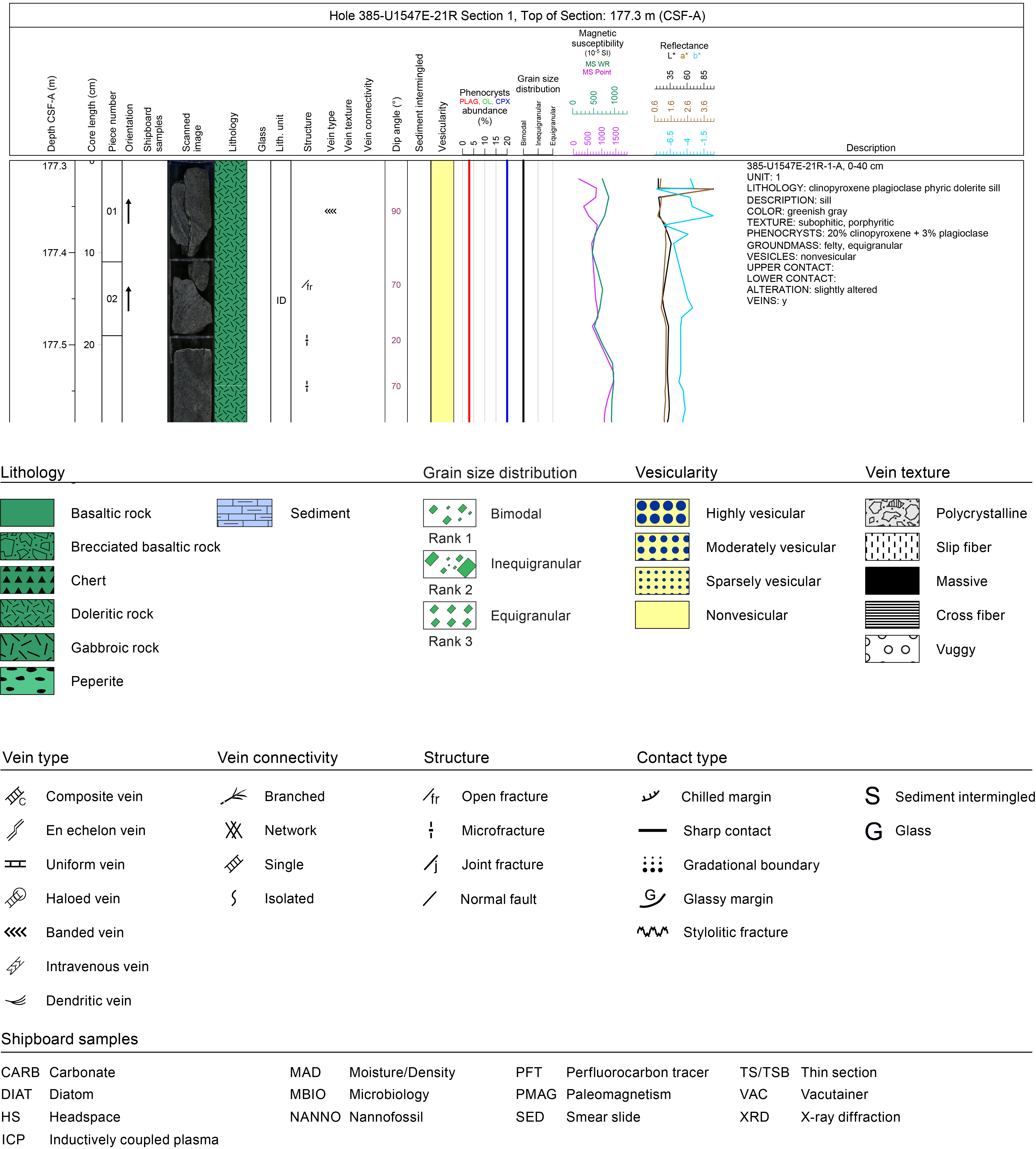
Macroscopic features observed in the cores are summarized and displayed in the VCDs. They illustrate the following entries in terms of igneous, vesicularity, alteration, structural, and physical properties features for each core section (Figure F11):

• Curated CSF-A depth scale (equivalent to mbsf);
• Core section length scale (0–150 cm);
• Number and orientation of hard rock pieces;
• Interval and type of shipboard samples;
• Scanned digital image of the archive half;
• Graphic representation of lithology;
• Symbol “G” (for igneous rocks, next to the graphic lithology), which indicates the presence of volcanic glass either in the glassy rind of chilled margins or in hyaloclastite, if encountered);
• Igneous lithologic unit number;
• Structure;
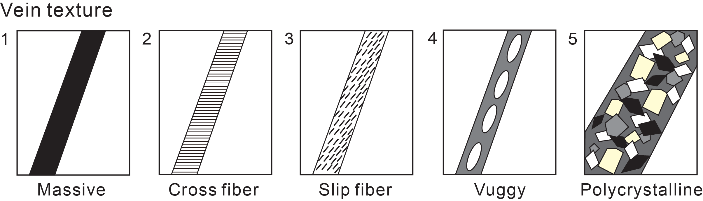
• Vein type, texture, and connectivity represented by different symbols/patterns;
• Vein dip angle (°);
• Symbol “S” if sediment intermingled with igneous rock is present;
• Column displaying variable patterns of vesicularity (in vol%);
• Stacked line chart displaying phenocryst abundance (in vol%) for plagioclase (PLAG; red line), olivine (OL; green line), and clinopyroxene (CPX; blue line) if present;
• Stacked line chart showing grain size distribution (i.e., variations in crystal size that define different types of texture);
• Stacked line chart depicting present alteration intensity;
• Diagram showing whole-round (WRMSL) and point (SHMSL) MS measurements;
• Plot displaying color reflectance, including total reflectance (L*), red (a*), and blue (b*); and
• Outline of the description of each igneous lithologic (sub)unit and possible lithologic variation within that (sub)unit identified in the corresponding section (see below for details).

The section unit summary (presented on the right side of the VCD) for each igneous lithologic unit contains the following details:

• Expedition, site, hole, core, core type (XCB or RCB), number of archive-half section, and interval (in cm);
• Igneous lithologic unit/subunit number(s);
• Lithology;
• Description of magmatic emplacement type (e.g., sill);
• Color of the bulk rock determined on dry rock surfaces using standard Munsell soil color charts (Munsell Color Company, Inc., 2000, 2009);
• Texture (microstructure) based on total percentage of (micro)phenocrysts and their textural relation;
• Phenocryst abundance (in vol%) and type based on minerals identifiable by the unaided eye, hand lens, or binocular microscope;
• Groundmass texture and/or mineralogy;
• Abundance and general shape of vesicles;
• Upper and lower unit contact relations and boundaries based on physical changes observed in retrieved core material (e.g., presence of chilled margins, sediment/igneous contact, or baked layer), including information regarding their position within the section (information provided if contact present);
• Alteration intensity and vein presence; and
• Comment (if applicable).

4.4. Identification of igneous lithologic units

The division of igneous lithologic units and subunits was guided by groundmass texture and primary modal composition. The combined color and texture of the groundmass and the major phenocryst(s) found in hand specimen were used to assign principal lithology names to igneous lithologic units. Based on the intersection of what was always interpreted as a single cooling unit in each hole where igneous rocks were recovered, we defined a single Igneous Lithologic Unit 1 with no subunits. Because all igneous rock cores recovered represent hypabyssal intrusion bodies and do not mark the top of the continuous oceanic crust, we assigned each igneous unit to the lithostratigraphic unit and subunit that hosted the intrusion (see Lithostratigraphy).

4.4.1. Magmatic rock classification

The International Union of Geological Sciences (IUGS) system (Le Maitre et al., 2005) was used to classify igneous rocks according to abundance, grain size, and texture of primary minerals.

4.4.2. Grain size classification

The categorization of Neuendorf et al. (2005) was used for grain size:

• Coarse grained (crystal diameter = 5 to ≤30 mm),
• Medium grained (crystal diameter = 1 to <5 mm), and
• Fine grained (crystal diameter = 0.2 to <1 mm).

4.4.3. Grain size distribution

Distribution of grain (crystal) sizes are described as bimodal (two dominant mineral grain sizes), inequigranular (principal minerals have different grain sizes), or equigranular (principal minerals are in the same size range).

4.4.4. Texture

Textures (microstructures) were characterized macroscopically for all igneous rock core sections and assessed microscopically for a subset of intervals sampled for thin sections. Based on Sun et al. (2018), the following textural descriptors were applied:

• Aphyric,
• Ophitic (pyroxene encloses plagioclase laths),
• Subophitic (pyroxene partially encloses plagioclase laths),
• Holocrystalline,
• Hypocrystalline (comprising both crystals [major component] and glass),
• Hypohyaline (comprising both crystals [minor component] and glass),
• Holohyaline (vitric; only glass),
• Poikilitic (larger crystals enclose smaller grains),
• Porphyritic,
• Phaneritic,
• Aphanitic,
• Trachytic,
• Flow banding,
• Perlite (rounded hydration fractures in glass),
• Glomeroporphyritic (clusters of phenocrysts),
• Chilled margin (a glassy or micro- to cryptocrystalline contact margin), and
• Layered.

4.5. Primary lithology names (hypabyssal/intrusive rocks)

Four rock categories were defined for igneous rock description based on primary matrix texture/color as well as nature of major phenocrysts and/or groundmass minerals:

• Basaltic rock: gray to dark gray, potentially phyric rock with a microcrystalline to cryptocrystalline matrix (groundmass) that contains plagioclase and pyroxene and/or olivine. Groundmass size is <0.5 mm.
• Doleritic rock: dark gray to greenish gray rock with a microcrystalline matrix that contains pyroxenes and/or feldspar and/or amphibole. Groundmass size is >0.5 mm but <2 mm.
• Gabbroic rock: dark gray to greenish gray rock with porphyritic texture that contains pyroxenes and/or feldspar and/or olivine and/or amphibole. Groundmass size is ≥2 mm.
• Peperite: genetic term attributed to a rock that contains sediment mingled with or intruded by magma that was disintegrated by the contact with the sediment; the latter is usually wet and unconsolidated or poorly consolidated (after White et al., 2000).

4.5.1. Prefixes

Prefixes were chosen to provide additional classification information where possible, such as an estimated modal composition, further specification of grain sizes, or textural information. Where appropriate, combinations of prefixes were adopted. Prefixes are as follows:

• Aphyric (<1 vol% phenocrysts),
• Phyric (1%–5 vol% phenocrysts or more),
• Plagioclase phyric (if phenocryst is plagioclase), and
• Pyroxene phyric (if phenocryst is pyroxene).

4.5.2. Suffixes

The suffix of the principal lithology name points to the nature of the hypabyssal or intrusive body. We used the following classification scheme:

• Sill intrusion: sills are defined as tabular intrusions that run parallel to horizontal or gently dipping sedimentary layers. They are generally concordant between beds of layered sediment or rock. Their thickness may vary from a few centimeters to hundreds of meters.
• Dike intrusion: unlike sills, dikes cut across horizontal or gently dipping planar structures or rock strata. They are discordant with country rock strata. They usually range from centimeters to meters or even hundreds of meters in thickness.

4.5.3. Matrix (groundmass)

The following nomenclature was applied to describe the groundmass for both macro- and microscopic characterization (MacKenzie et al., 1982; Neuendorf et al., 2005):

• Aphanitic: crystalline, but individual grains are not distinguishable with a magnifying lens.
• Phaneritic: minerals are coarse enough to be seen with the naked eye.
• Equigranular: similar crystal sizes.
• Glomeroporphyritic: containing clusters of phenocrysts.
• Felty: tightly, irregularly interwoven feldspar microlites.
• Inequigranular: different crystal sizes.
• Intergranular: plagioclase crystals surrounded by interstitial granular pyroxene, olivine, and/or oxide minerals.
• Porphyritic: significant presence of (micro)phenocrysts.
• Ophitic: large pyroxene grain encloses small random plagioclase laths.
• Subophitic: plagioclase laths are larger and only partially enclosed by the pyroxene.
• Interstitial: glassy, crypto-, or microcrystalline material between coarser grained crystals.

4.5.4. Sediment mingling

Sediment mingling was included in the igneous rock description upon encountering magma/sediment contacts or mixing demonstrated by fragmentation of igneous material or injection of sediment as veins in igneous rock. We included a yes/no column in DESClogik and used “yes” to indicate intervals where we found any igneous/sedimentary contact. Also, additional description of the nature of contact was entered in DESClogik as needed.

4.5.5. Contact types

The description of margins and contacts of hypabyssal or intrusive rocks was based on the observed features of the chilled sections that indicate a possible hiatus between two igneous rocks. A chilled contact, with or without glass, was identified by observing the terminal end of the margin for sediment that was not entrenched within the rock but rather baked or cooked onto the rock, designating a baked or chilled contact with the latter. A chilled margin was identified through a sudden change in matrix over a very short interval. In contrast to a chilled contact, establishing the nomenclature of an igneous body did not require the presence of sediment at its terminal end. Several sections were characterized as having a chilled contact (typically with glass) in direct contact with sediments with an adjoining (or grading into a) chilled margin where the matrix was described to be cryptocrystalline and graded into a microcrystalline texture further up- or downhole. Glassy margins, chilled margins, and contact boundaries were inserted individually for the top and bottom of each section where they could be determined.

The following contact types were defined:

• Baked contact: boundary to sediments overprinted (baked) by proximity of magma.
• Bottom (or top) chilled contact: chilled contact with sediments, with or without glass adjacent to sediments.
• Bottom (or top) chilled margin: chilled contact without sediments, without glass, defined by cryptocrystalline groundmass, and typically found quenched next to the chilled contact.
• Chilled contact: boundary cannot be determined to be top or bottom of a pulse that has sediment attached, such as a magma/sediment mingling or peperite.
• Chilled margin: chilled contact without sediment or obvious glass that cannot be determined to be the top or bottom of a magma pulse, or nearby obvious sediment contact is not preserved.
• Glassy margin: demarcation between two hypabyssal/intrusive pulses or presumably between magma and country sediment without displaying the latter. Potentially, igneous bodies have fused together, showing no clear indication of the boundary between the pulses as originally deposited.

4.6. Alteration

4.6.1. Alteration minerals

Procedures developed specifically to investigate hydrothermal alteration encountered during Expedition 385 are detailed in the following sections. Significant detail was incorporated into DESClogik, which enabled a comprehensive report of the predominant style of hydrothermal alteration of specific intervals of the recovered igneous rocks. Identified alteration minerals or mineral mixtures include carbonate (calcite, dolomite, or siderite), chlorite, copper sulfate, clay minerals, zeolites (e.g., natrolite), epidote, iron hydroxides, iron oxide, mica (sericite), spinel (magnetite), and sulfides (chalcopyrite or pyrite); “unknown” was used when the mineral could not be identified.

4.6.2. Alteration intensity

Low- to high-temperature and low-pressure (i.e., seafloor) mineralization, veins, and background alteration were defined as alteration. Alteration description includes secondary mineralogy, groundmass texture/color, phenocryst alteration, and infilling of vesicles and halos. Textures used to define groundmass alteration are patchy, corona, pseudomorphic, and recrystallized. Detailed description of the alteration ranks, texture of alteration, and grain size distribution are given in Tables T1, T2, and T3, respectively. Alteration rank for igneous rock is equivalent to what has been applied by the lithostratigraphy classification. Levels of background alteration were recorded as follows:

• Unaltered = <2 vol%.
• Slight = 2–10 vol%.
• Moderate = >10–50 vol%.
• High = >50–75 vol%.
• Intense = >75–95 vol%.
• Complete = >95 vol%.

4.7. Vesicularity

Vesicularity is defined by vesicle abundance:

• Nonvesicular = <1 vol% vesicles.
• Sparsely vesicular = 1–5 vol% vesicles.
• Moderately vesicular = >5–20 vol% vesicles.
• Highly vesicular = >20 vol% vesicles.

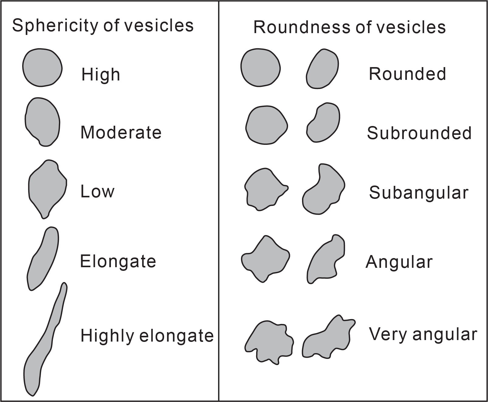
Size, shape, and roundness of vesicles were described in line with the classification charts from Integrated Ocean Drilling Program Expedition 330 and IODP Expedition 349 (Expedition 330 Scientists, 2012; Li et al., 2015), modified from Wentworth (1922) (Figure F12). An estimate of the abundance of vesicles (in vol%) is included in the VCDs.

4.7.1. Veins and halos

While we reserved the term “dike” to describe any later crosscutting feature that formed by introduction of magma, the term “vein” was deployed to refer to any later crosscutting feature formed by sediment injection or precipitation from hydrothermal fluids. The term “halo” refers to alteration zones around veins or secondary minerals identified by discoloration through change of the primary mineral assemblage. The density (i.e., the visually estimated percentage of veins within a piece or interval 10 cm in length), mineralogy, width, color, vein type (banded, composite, nonuniform, or uniform), connectivity (isolated, single, branched, or network), texture (cross-fiber, slip-fiber, massive, polycrystalline, or vuggy) (Figure F13), and contacts with host rocks (diffuse, irregular, or sharp) were described using criteria modified from ODP Leg 209 (Shipboard Scientific Party, 2004). The length, width, and orientation of representative veins in a section were measured.

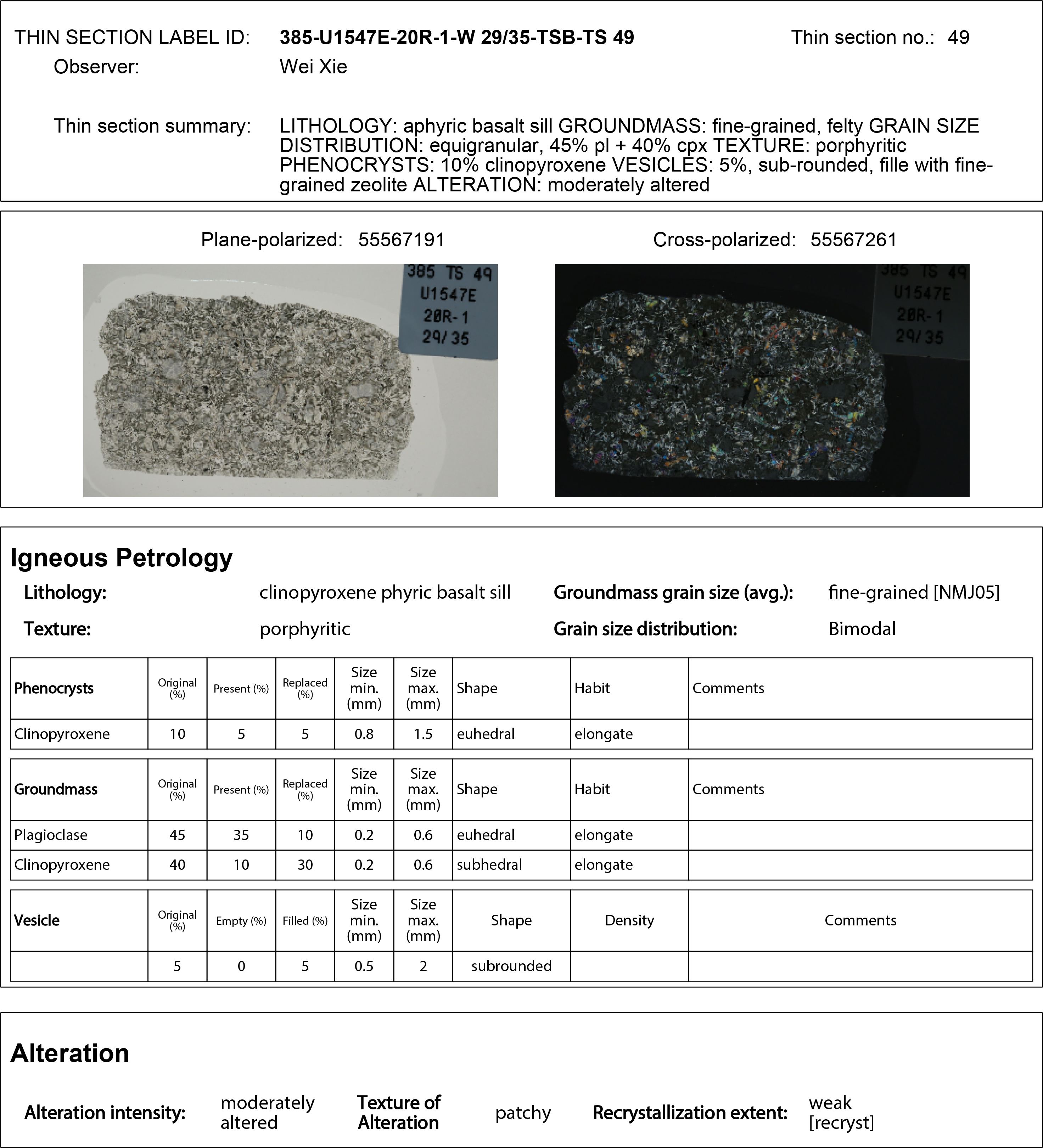
4.8. Microscopic (thin section) description

Thin section investigation was used to complement and refine macroscopic core observations for igneous rocks (Figure F14). All thin section observations were entered into the LIMS database through a special DESClogik thin section template (see DESC_WKB in Supplementary material). Thin section descriptions include both primary (igneous) rock-forming minerals (including phenocrysts, groundmass, etc.) and secondary (alteration) mineral phases (in veins, vesicles, groundmass, etc.). Their mineralogy, abundance (modal volume percentages), sizes, shapes, habits, textural relationships, inclusions, alteration color, intensity and style, veins (type and number), and vesicles (type and fillings) were determined, enabling verification of macroscopic observations. The volume percentages of the original primary mineral phases, groundmass, and vesicles are also included when entering mineral abundances in DESClogik.

Thin section descriptions include the following terms:

• Sample domain: if there is more than one domain on the slide, each domain is described separately. For example, a slide that shows a large sedimentary vein (25% of the slide) in a basaltic matrix (75% of the slide) is described as two slides (samples): the first sample domain as “vein” and the second one as “host rock.” Other possible domains include clast, glass, halo, lithology, and xenolith.
• Lithology prefix: lithology prefix for the described sample domain.
• Principal lithology: refers only to the lithology of the described sample domain, which includes basalt, brecciated basalt, breccia, and hyaloclastite.
• Average groundmass grain size modal name: grain sizes follow Neuendorf et al. (2005) using the division of glass, cryptocrystalline (<0.1 mm), microcrystalline (0.1–0.2 mm), and fine, medium, and coarse grained (see Primary lithology names (hypabyssal/intrusive rocks)).
• Maximum grain size modal name: analogous to “average groundmass grain size modal name.”
• Grain size distribution: bimodal, equigranular, granular, inequigranular, poikilitic, and seriate (see Texture).
• Texture: aphanitic, aphyric, granular, glomeroporphyritic, holocrystalline, holohyaline, hypocrystalline, hypohyaline, intergranular, intersertal, interstitial, ophitic, porphyritic, seriate, spherulitic, subophitic, trachytic, and vitrophyric (see Texture).
• Mineral phenocryst shape: the dominant (>50% of crystals) shape of the olivine, plagioclase, clinopyroxene, orthopyroxene, and spinel crystals in euhedral, subhedral, and anhedral.
• Mineral phenocryst habit: the dominant (>50% of crystals) habit of olivine, plagioclase, clinopyroxene, orthopyroxene, and spinel crystals divided into elongate, equant, subequant, and tabular habits (see definitions below).
• Plagioclase phenocryst zoning type: continuous, discontinuous, oscillatory, and patchy.
• Plagioclase phenocryst zoning extent: none, scarce, abundant, and very abundant.
• Clinopyroxene and orthopyroxene phenocryst exsolution: blebs and lamellae.
• Vesicle shape.
• Mineral groundmass shape: for olivine, plagioclase, clinopyroxene, orthopyroxene, spinel, and Fe-Ti oxides and sulfides, mineral groundmass shapes are euhedral, subhedral, and anhedral.
• Mineral groundmass habit: for olivine, plagioclase, clinopyroxene, orthopyroxene, spinel, and Fe-Ti oxides and sulfides, mineral groundmass habits are elongate, equant, subequant, and tabular.
• Additional features such as dissolution/resorption textures, sieve textures, and inclusions are noted in the comments section.

5. Structural geology

This section outlines methods for documenting structural features observed in Expedition 385 cores, such as faults, fractures, folds, bedding, laminations, paleosurface features, and veins. Structures were measured before and after the cores were split. For solid cores, we measured structures that could be seen externally on the surface of the whole-round core prior to splitting. We used the resulting measurements to split the core most evenly into archive and working halves. After a core was split and described by the sedimentologists or petrologists on shift, we documented structural features observed on the archive half using the following process:

1. Identifying structural features and classifying their structural types;
2. Determining the top and bottom locations of structural features in the core;
3. Measuring the orientation of a structural feature where applicable;
4. Determining the sense of displacement on a structural feature where applicable;
5. Determining the temporal relation between structures, especially for crosscutting structures such as shear zones; and
6. Assessing the role of fluids in deformation processes.

Our methods largely follow those used by structural geologists from Integrated Ocean Drilling Program Expedition 344 and IODP Expeditions 349 and 367/368 (Harris et al., 2013; Li et al., 2015; Sun et al., 2018). The types of structural measurements and key parameters (either observed or calculated) were recorded on spreadsheets. We made different spreadsheets for sedimentary rock observations and for igneous rock observations because the type of information needed in each case was different (Tables T4, T5, T6). These data were then entered in the LIMS database using the DESClogik software application. We were not able to correct any of the orientation measurements for rotation related to drilling using paleomagnetic declination and inclination information (see Paleomagnetism) or by comparison to observed features in the FMS log (see Azimuth correction based on Formation MicroScanner log).

5.1. Graphic symbols and terminology

A predefined set of commonly observed structural features was used in the structural description of cores. The terminology and graphic symbols used are presented in Figures F5, F11, and F15. Note that there are more graphic symbols for structures in sedimentary cores than in igneous cores. The major structural features identified include the following:

• Fractures: brittle failure with unknown displacement and no secondary infill minerals; these were further classified as microfractures, open fractures, and joint fractures. However, breaks clearly resulting from drilling were logged separately as drilling-induced fractures in the Drilling disturbance spreadsheet of DESClogik.
• Faults: brittle failure with measurable offset or juxtaposition of different lithologies.
• Veins: fractures filled with secondary minerals.
• Shear zones: strongly deformed zones surrounded by less deformed rocks.
• Sedimentary bedding: layering of sediments or lamina and sedimentary rocks.
• Folds: folded sedimentary or rock layers.
• Igneous contacts: material contacts of hypabyssal igneous rocks, including glassy margins.
• Magmatic fabrics: magmatic foliations defined by the preferred orientations of primary minerals with no evidence of crystal-plastic deformation.

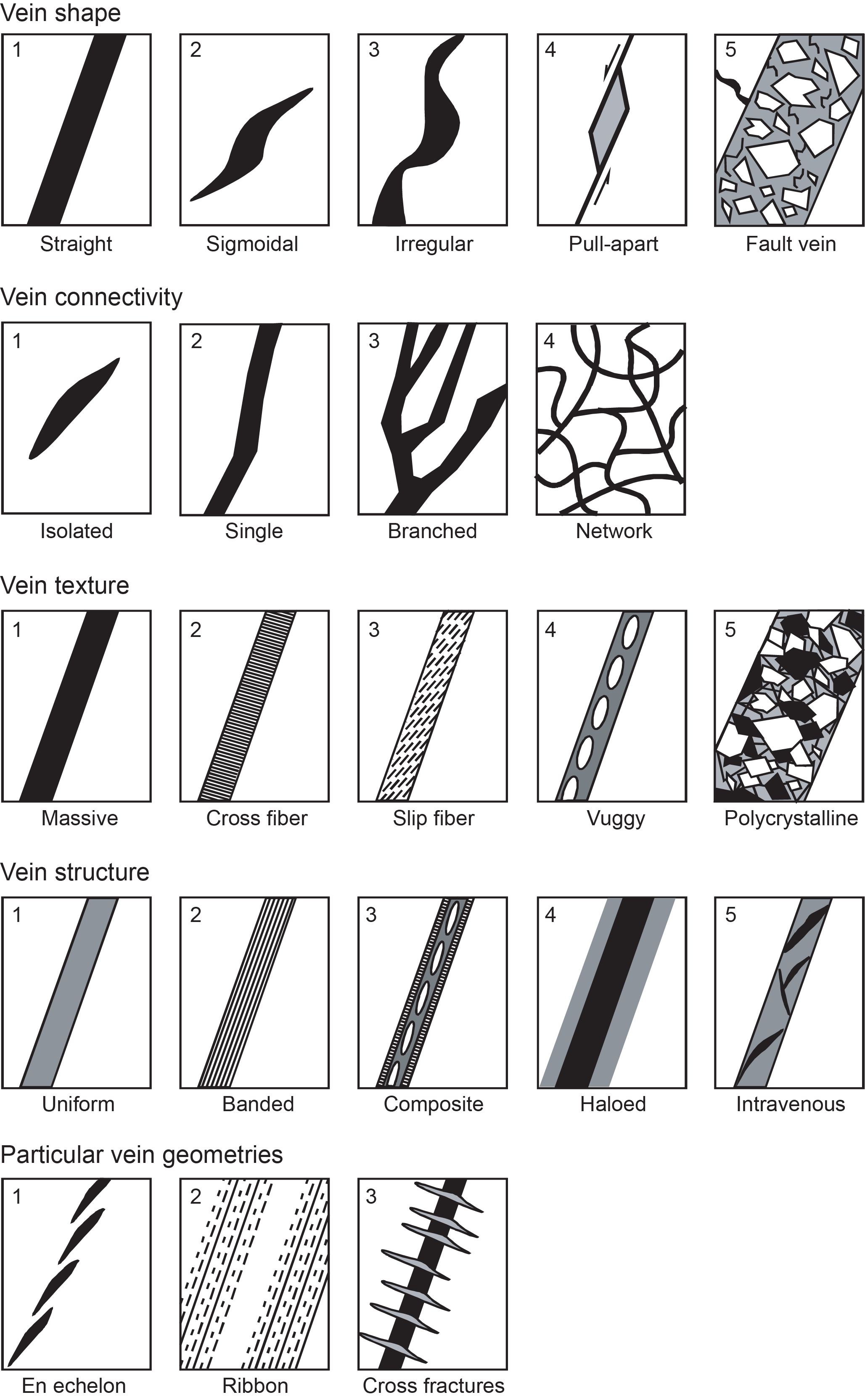
5.2. Structural observation and description

Structural features were described from top to bottom of each section of the core. For fractures and faults, we examined and measured the following parameters:

• Location: where a fracture occurs in a core, measured in centimeters from the top of the section.
• Morphology: morphological shape of a fracture (e.g., straight, curved, banded, irregular, composite, isolated, single, or branched).
• Displacement: lateral offset and/or opening of a fault measured in centimeters. A closed fracture with no lateral offset is recorded as 0 cm of displacement.
• Orientation: dip angle and dipping orientation of a fracture or fault measured in degrees if seen on the archive-half core face or X-ray image or true dip angle if measured on the outside of the whole-round core.
• Frequency: occurrence frequency of fractures per section.
• Type: type of deformation of a fracture or fault (e.g., normal, reverse, dextral, sinistral displacement, or a combination of the above).

For veins, we examined and measured several parameters:

• Location: where a vein occurs in a core, measured in centimeters from the top of the section.
• Vein type: see list of deformation structures in Lithostratigraphy and overview of vein types in Igneous petrology and alteration.
• Orientation: dip angle and dipping direction of a vein if seen on the core face or X-ray image of the archive half or true dip angle if measured on the outside of the whole-round core.
• Frequency: occurrence frequency of veins per section.
• Mineral infill and alteration: these features are recorded as described by petrologists.

For shear zones, we examined and measured the following parameters (although very few were seen):

• Location: interval where a shear zone occurs in a core, measured in centimeters from the top of the section.
• Nature (or type) of shear zone: cataclasite, gouge, or fault breccia.
• Morphology: morphological shape of the deformed zone and the clasts.
• Orientation: dip angle and dipping direction of the preferred orientation of the clasts, where applicable.
• Frequency: occurrence frequency of shear zones per section.
• Mineral and alteration: matrix and clasts are recorded as described by petrologists.

For sedimentary bedding, we described the following parameters:

• Location: where a nonsubhorizontal bedding occurs in a core (>5°), measured in centimeters from the top of the section.
• Orientation: dip angle and dipping direction of sedimentary bedding as seen on the core face or X-ray image.

For folds, we described the following parameters:

• Location: where a fold contact occurs in a core, measured in centimeters from the top of the section.
• Type: type of fold (e.g., chevron or concentric; see definitions in Fossen [2016]).
• Frequency: occurrence frequency of fold axis per section.

For igneous contacts, we described the following parameters:

• Location: where an igneous contact occurs in a core, measured in centimeters from the top of the core (usually a binned specimen).
• Type of contacts: type of igneous contact boundary.
• Orientation: dip angle and dipping direction of an igneous contact.
• Frequency: occurrence frequency of igneous contacts per section.
• Mineral assemblage and alteration: these features are recorded as described by petrologists.

For sediments and sedimentary rocks, if XRI scans were available, we further examined the X-ray images to detect and measure additional faults if they were made visible by X-ray imaging but were not seen on the split core face. Note that the location measurement of a feature in the X-ray scans could differ by 1 cm compared to the location of the same feature in the archive half of the split core (e.g., see Figure F9 in the Site U1552 chapter (Teske et al., 2021a).

Finally, we processed the SHIL color composite photos of the core to produce false-color images that more clearly highlighted the compositional difference in the sediments. This was another way to check for faults. Processing was performed in Adobe Photoshop CS6 version 13.0 × 64 on a Windows PC by choosing File > Scripts > Image Processor and then running it in batch mode on a set of files within a specified directory. A “run action” was first specified to include three processing steps:

1. Image > Adjustment > Levels,
2. Image > Adjustment > Brightness/Contrast, and
3. Layer > Flatten Image.

5.3. Orientation measurements and correction

5.3.1. Orientation measurements

We used a plastic goniometer for orientation measurements. For sealed structures in igneous rocks, we wrapped a transparent plastic protractor template around the whole-round core to determine the true dip prior to splitting the core (Figure F16). For split cores (igneous or sedimentary) the orientations of planar and linear features in the archive half were determined relative to the core reference frame (Figure F17). The vertical axis of the core reference frame is aligned with the upcore direction of the core section, whereas the double line marked on the archive half of the core liner is defined as 180° in the cross-sectional plane perpendicular to the core vertical axis.

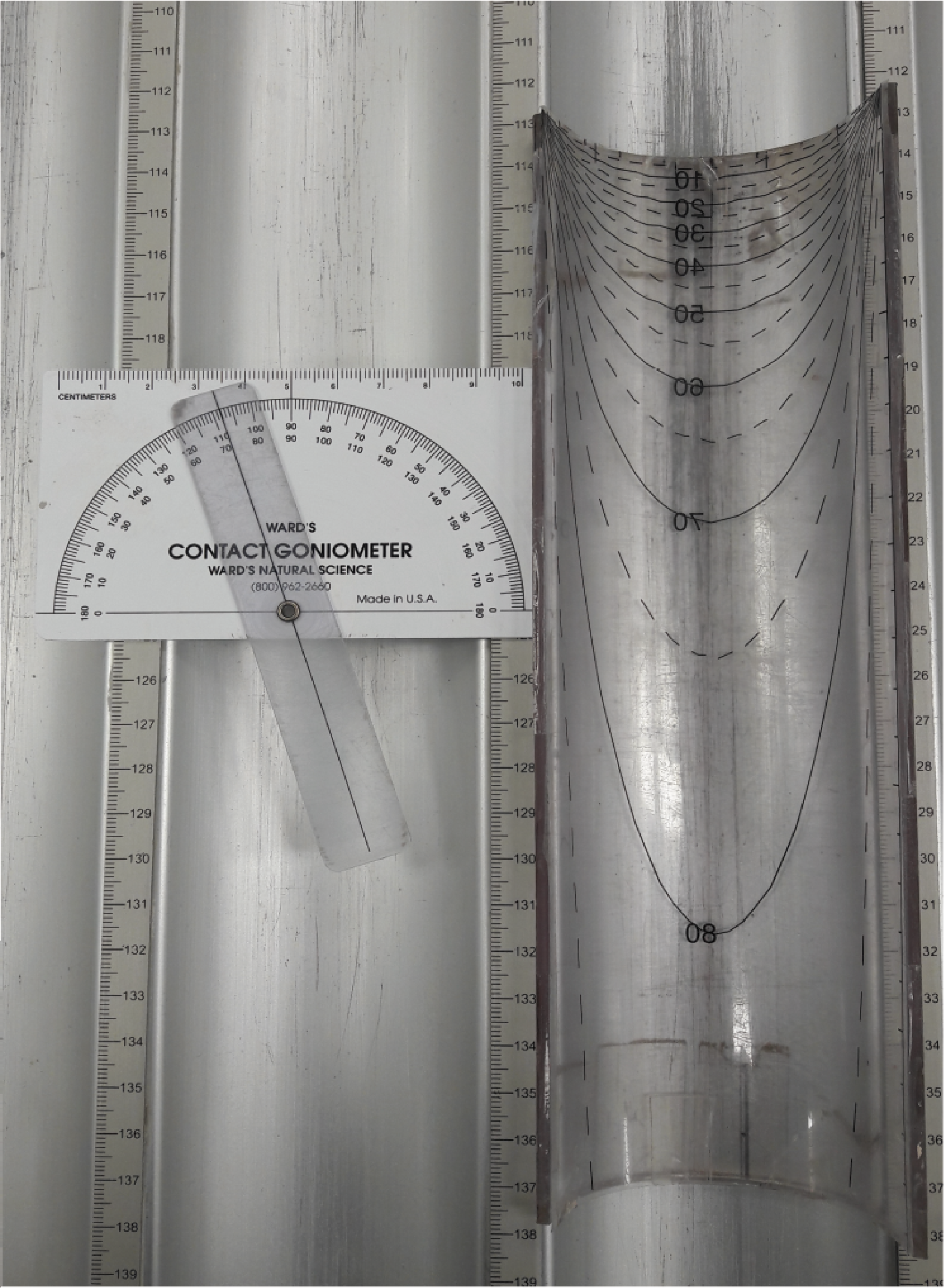
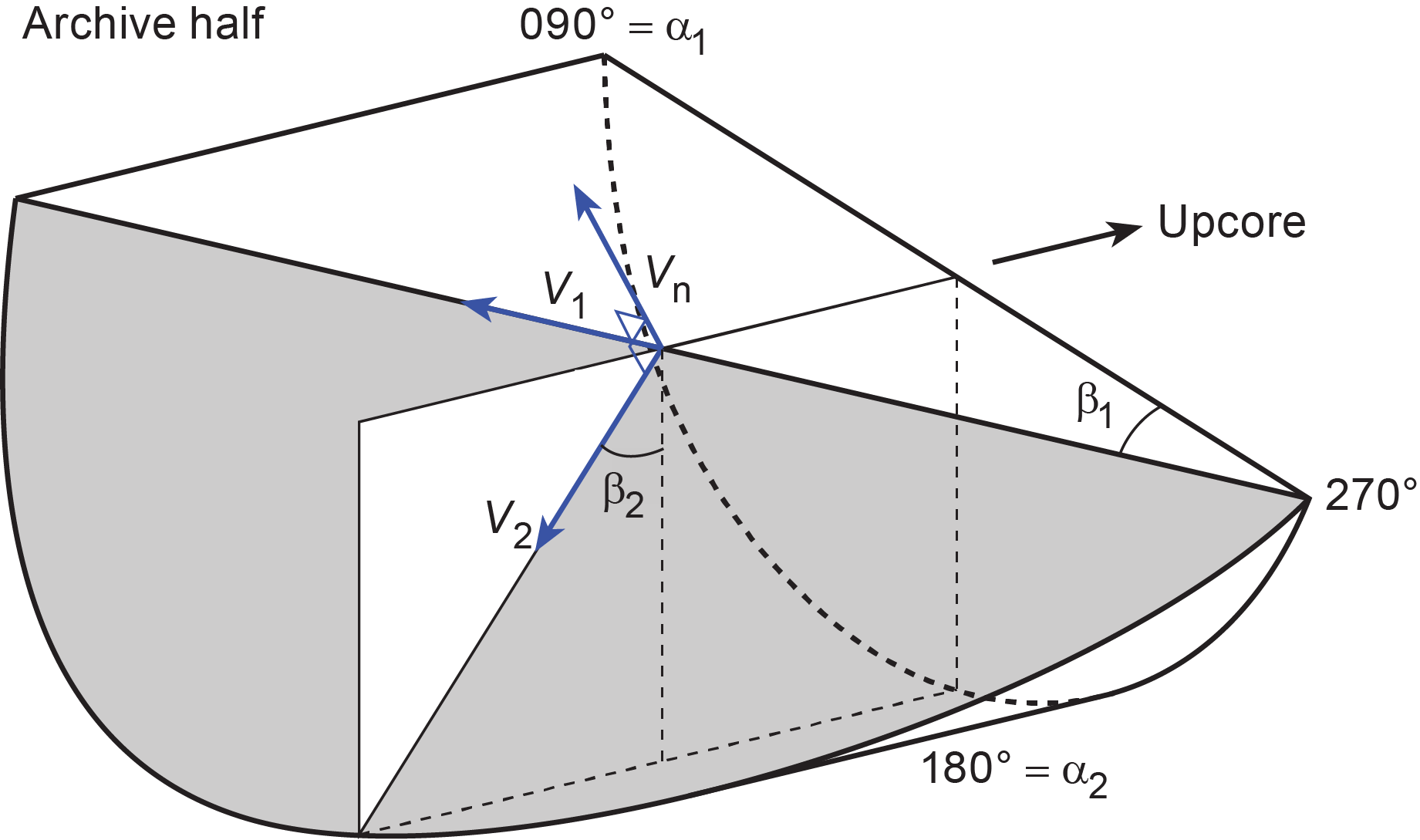
To determine the orientation of a planar structural element (shaded plane in Figure F17), two apparent dips of the element were measured in the core reference frame. The first apparent dip measures the intersection angle between the planar structural element and the split face of the core (β₁ in Figure F17); it is determined by measuring the dip direction and angle of the planar structural element in the core reference frame. A planar structural element could have a trend of 90° or 270°, with a plunge angle ranging from 0° to 90°. The second apparent dip measures the intersection angle between the central line of the planar structural element and the split face of the core (β₂ in Figure F17). In most cases, this is a plane either parallel or perpendicular to the core axis. In the former case, the apparent dip trends 0° or 180° with plunge angle ranging from 0° to 90°; in the latter case, the trend ranges from 0° to 360° with a plunge angle of 0°.

A linear feature observed on the surface of a split core is often associated with a planar structural element (e.g., a fault plane) in the core; the orientations of the planar structural element are determined by measuring either the rake (or pitch) of the associated plane or the trend and plunge of the planar element in the core reference frame. All measured data were manually written into the log sheet together with the measured depths in the core section and descriptive information (Table T4).

5.3.2. Plane orientation calculation

For a planar structural element (e.g., a bedding or fault plane), two apparent dips on two different surfaces (one being the split core surface, which is east–west vertical, and the other being the horizontal surface, or north–south vertical) were measured in the core reference frame. The two apparent dips are the azimuth (measured clockwise from north, looking down) and plunge. An x, y, z coordinate system was defined so that the positive x-, y-, and z-directions coincide with north, east, and vertical downward, respectively. If the azimuths and plunges of the two apparent dips are given as (α₁, β₁) and (α₂, β₂), respectively (as in Figure F17), the unit vectors representing these two lines, v₁ and v₂, are given by the following expressions:

ν1=l1m1n1=cos⁡α1cos⁡β1sin⁡α1cos⁡β1sin⁡β1; ν2=l2m2n2=cos⁡α2cos⁡β2sin⁡α2cos⁡β2sin⁡β2. (1)

For any plane, the direction of the normal to the plane can be found by taking the cross product of two (nonparallel) vectors that lie within the plane. Using the above equations for v₁ and v₂, therefore, the unit vector normal to plane v_n (Figure F18) is defined as follows:

νn=lnmnnn=ν1 × ν2ν1 × ν2, (2)

where

ν1 × ν2= m1m2n1n2n1n2l1l2l1l2m1m2=m1n2-m2n1n1l2-n2l1l1m2-l2m1. (3)

The azimuth α_n and plunge β_n of v_n are given by

αn=tan-1⁡mn/ln and (4)

βn=sin-1⁡nn. (5)

The dip direction α_d and dip angle β of this plane are calculated as follows:

αd=αn and β=90°+βn whenβn<0°, and (6)

αd=αn±180° andβ=90°-βn when βn≥0°. (7)

The strike of this plane α_s according to the right-hand rule is then given by α_s = α_d − 90° (Figure F18).

5.3.3. Azimuth correction based on paleomagnetic data

Provided that a core is vertical, its magnetization is primary, the core was magnetized in the Northern Hemisphere, and its bedding is horizontal, its paleomagnetic declination α_p indicates the magnetic north direction when its inclination is β_p ≥ 0° (Figure F19); in contrast, the angle α_p indicates the magnetic south direction when β_p < 0°. The dip direction (α_d*) and strike (α_s*) of a planar structural element in the geographic reference frame are therefore

αd*=αp-αd and αs*=αp-αs when βp≥0°, or (8)

αd*=180°+αp-αd and αs*=180°+αp-αs when βp<0°. (9)

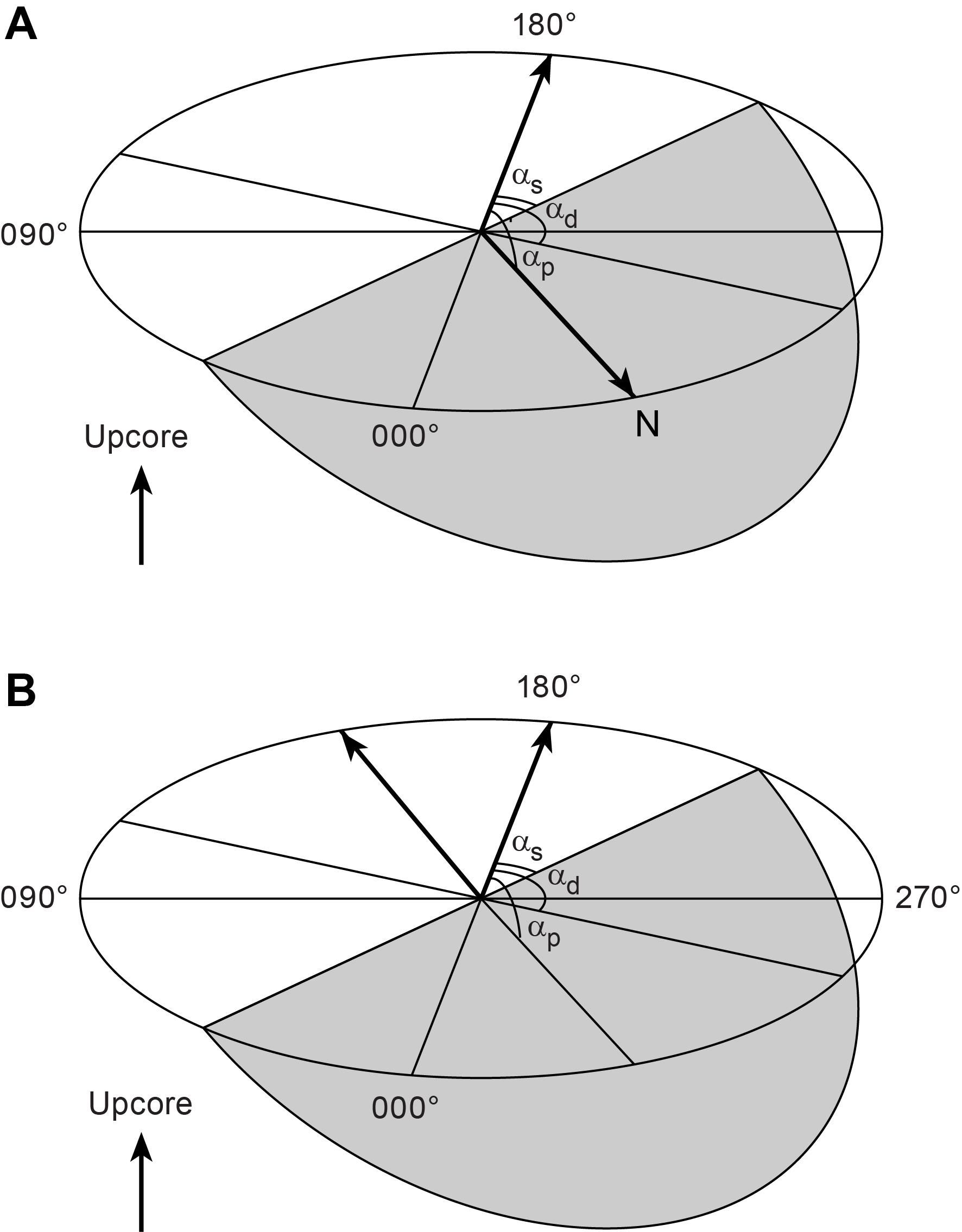
If a core section was complete and continuous, one paleomagnetism sample per section (1.5 m in length) was deemed sufficient to determine the paleomagnetic orientation of the core section. If the core was discontinuous, one paleomagnetism sample was required for each continuous subsection of the core that was deemed structurally important. Paleomagnetism samples were taken as cubic or cylindrical samples close to a planar structural element of interest (usually within 5 cm) and from a coherent core interval that included that structural element of interest. In general, we avoided core fragments that were so small that potential spinning during drilling might cause significant deviation from the core axis (e.g., fragments of brecciated segments).

5.3.4. Azimuth correction based on Formation MicroScanner log

If an FMS log is available for the section of the drill hole that contains the core, there may be distinctive features that can be correlated between the FMS log and the core, such as bedding, fractures, folds, veins, stratification, and bioturbation. In this case, the core can be oriented with respect to geographic north. However, this orientation has to be done after the FMS log is obtained and all the cores in the hole have been collected. See the discussion of the details of orienting the cores in Petrophysics.

6. Biostratigraphy

Preliminary shipboard biostratigraphy for Expedition 385 was provided by fossil marine diatoms and calcareous nannofossils. Biostratigraphic age assignments were based on analysis of core catcher samples from selected holes at all drill sites, provided that the core catcher sample was sedimentary in origin. As time permitted, additional toothpick samples were taken from core section halves (typically the archive half) as needed to refine biostratigraphic horizons (biohorizons) or where changes in lithology suggested changes in sediment deposition. Biostratigraphy focused mainly on the identification of biohorizons in the cores, generally the top (T) or base (B) of the stratigraphic range of the age-diagnostic species, including the top common (Tc) and base common (Bc) occurrences and the top acmes (Ta) and base acmes (Ba). The top and base of a species correspond to its last appearance datum (LAD) and first appearance datum (FAD), respectively. Each biohorizon was assigned an absolute age based on the geological timescale of Gradstein et al. (2012) (Figure F20).

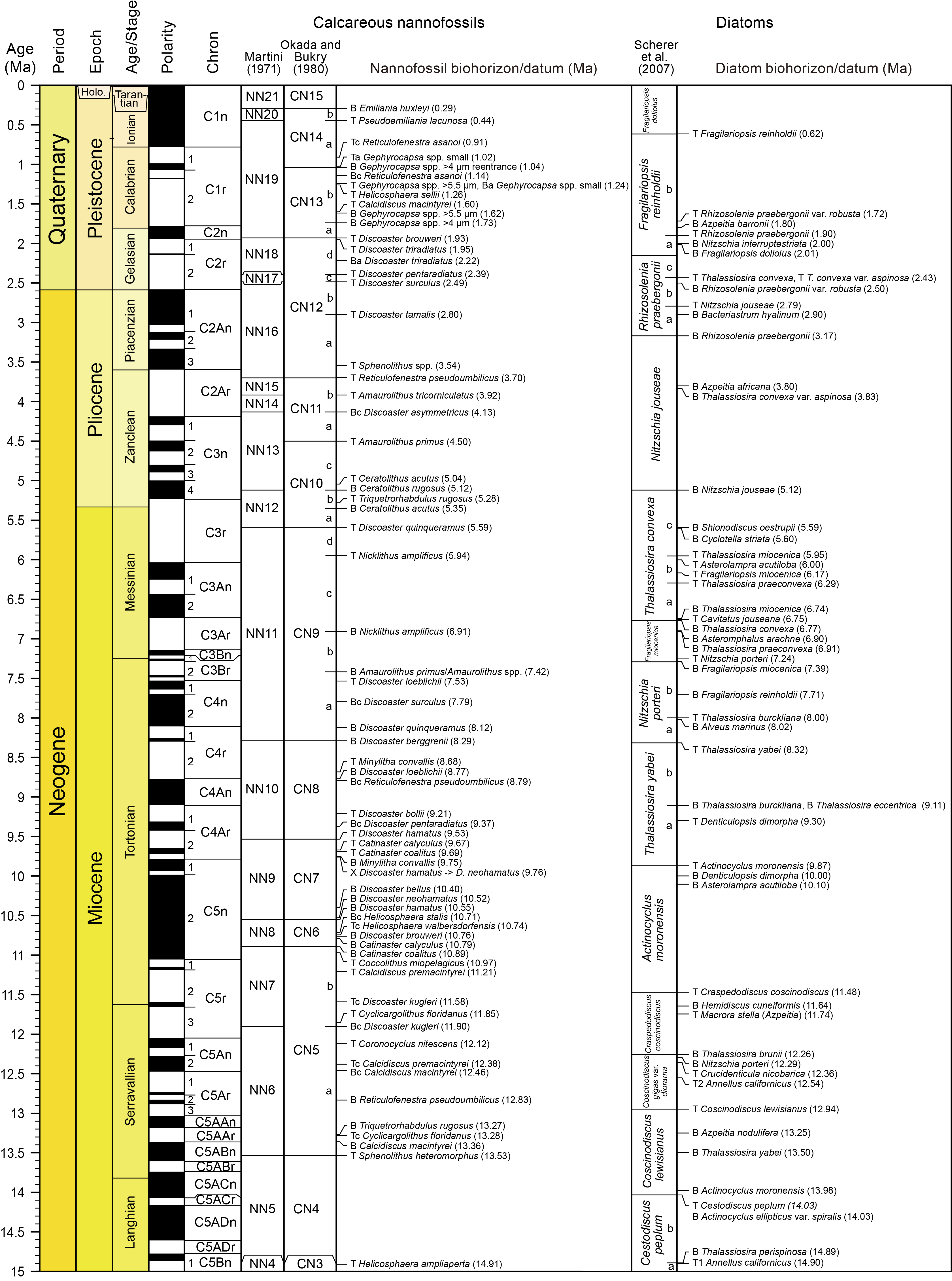
6.1. Slide preparation and microscopic examination

All micropaleontological data gathered during shipboard investigations were entered using DESClogik data entry software and are available from the LIMS database in accordance with IODP policy. Species distribution and abundance are included for every sample of each hole and each taxonomic group (calcareous nannofossils and marine diatoms) studied. These data are provisional because of time constraints for cross-checking and searching for rare species. Generally, this study focused on biostratigraphic marker species. The provisional, incomplete, and systematically biased nature of the data makes them unsuitable for further meta-analytical studies.

6.2. Calcareous nannofossils

6.2.1. Zonal scheme and taxonomy

Calcareous nannofossil zonation was based on the schemes of Okada and Bukry (1980) and Martini (1971) supplemented with Backman et al. (2012). Calibrated ages for bioevents are from Gradstein et al. (2012) (Table T7). The geological timescale of Gradstein et al. (2012) assigns the Pleistocene/Pliocene boundary an age between the Gelasian and Piacenzian stages (2.59 Ma), the Pliocene/Miocene boundary an age between the Zanclean and Messinian stages (5.33 Ma), and the late/middle Miocene boundary an age between the Serravallian and Tortonian stages (11.63 Ma). For calcareous nannofossil biostratigraphy, the Pleistocene/Pliocene boundary now falls in Zone NN16 (Martini, 1971) between the LADs of Discoaster surculus (2.49 Ma) and Discoaster tamalis (2.80 Ma). The Pliocene/Miocene boundary is marked by Zone NN12 between the LAD of Triquetrorhabdulus rugosus (5.28 Ma) and the FAD of Ceratolithus larrymayeri (5.34 Ma), the latter of which can be approximated using the FAD of Ceratolithus acutus (5.35 Ma). The late/middle Miocene boundary is placed in Zone NN7 between the LAD of common Discoaster kugleri (11.58 Ma) and the FAD of common D. kugleri (11.90 Ma). During Expedition 385, the identification of these geological time boundaries was mostly based on recognition of these nannofossil bioevents.

Nannofossil taxonomy mainly follows that of Perch-Nielsen (1985) and Bown (1998), which are included in the Nannotax3 online database (http://www.mikrotax.org/Nannotax3; last date of retrieval 9 November 2019), except for the taxa discussed below.

Several species of the genus Gephyrocapsa, which are commonly used as Pleistocene biostratigraphic markers, often show a great range of variation in sizes and other morphological features, causing problems in identification (e.g., Samtleben, 1980; Su, 1996; Bollmann, 1997). Size-defined morphological groups of this genus (Young, 1998; Maiorano and Marino, 2004; Lourens et al., 2005; Raffi et al., 2006) were used as bioevent markers during shipboard study, including small Gephyrocapsa spp. (<3.5 µm), medium Gephyrocapsa spp. (≥4 µm), and large Gephyrocapsa spp. (≥5.5 µm).

Several Reticulofenestra species with different coccolith and central opening sizes have been used as Neogene and Quaternary biostratigraphic markers; however, these characteristics show considerable intra- and intertaxon variation, making species determination difficult (e.g., Young, 1998; Su, 1996). We followed the definition of Reticulofenestra pseudoumbilicus by Young (1998) as having a maximum coccolith length >7 µm (similar to the size of its holotype), especially for specimens from its uppermost range in the early Pliocene. We distinguished Reticulofenestra asanoi from the similarly sized Pseudoemiliania lacunosa by the absence of slits on the shield (Su, 1996).

The LAD of Sphenolithus spp. (3.54 Ma) in Pliocene Zone NN16 was based on the LAD of Sphenolithus abies and Sphenolithus neoabies according to Raffi et al. (2006).

6.2.2. Abundance and preservation classification

Calcareous nannofossil samples were prepared using standard smear slide techniques. For sandy sediments, suspended aliquots of the raw sample were utilized for analysis. Slides were mounted with Norland optical adhesive Number 61 and cured under ultraviolet light for examination. Slides were analyzed by means of a Zeiss Axiophot microscope under cross-polarized and plane-polarized or phase-contrast light using oil immersion at 1000× magnification. All photomicrographs were taken using a SPOT Flex system with the IODP Image Capture and commercial SPOT software. A Hitachi TM3000 tabletop SEM was used to confirm the presence of small forms and the preservation state of calcareous nannofossils.

Total calcareous nannofossil abundance in the sediment (referred to as “group abundance” in DESClogik) was visually estimated at 500× magnification by referring to the particle abundance charts in Rothwell (1989) and reported using the following abundance categories (here applied to fossil tests):

• D = dominant (>90% of tests present).
• A = abundant (>50%−90% of tests).
• C = common (>10%−50% of tests).
• F = few (1%−10% of tests).
• R = rare (<1% of tests).
• B = barren (no nannofossil tests present in 100 fields of view [FOVs]).

The relative abundance of individual calcareous nannofossil taxa was based on the number of specimens per FOV at 1000× magnification and recorded as follows:

• D = dominant (>50%, or >100 specimens per FOV).
• A = abundant (10%−50%, or 10−100 specimens per FOV).
• C = common (1%−10%, or 1−10 specimens per FOV).
• F = few (0.1%−1%, or 1 specimen per 2−10 FOVs).
• R = rare (<0.1%, or <1 specimen per 10 FOVs).
• P = present (1 specimen per >100 FOVs).

Preservation of nannofossil tests was noted as follows:

• VG = very good (no evidence of dissolution and/or overgrowth, no alteration of primary morphological characteristics, and specimens are identifiable to the species level).
• G = good (little dissolution and/or overgrowth, primary morphological characteristics unaltered or only slightly altered, and specimens are identifiable to the species level).
• M = moderate (some etching and/or overgrowth, primary morphological characteristics somewhat altered, and most specimens are identifiable to the species level).
• P = poor (severely etched and fragmented or with overgrowth, primary morphological characteristics largely destroyed, fragmentation has occurred, and most specimens cannot be identified at the species and/or generic level).

6.3. Marine diatoms

6.3.1. Zonal scheme and taxonomy

Marine diatom biostratigraphy followed the works of Schrader (1974) from DSDP Leg 22/23, Barron (1980) from DSDP Leg 54, Barron (1985) and Barron and Gladenkov (1995) from ODP Leg 145, and Barron (2003). Although the majority of the biostratigraphy followed the work of Barron (1985, 2003), the zonal schemes were refined as needed.

Diatom ages for zones and datum events were calibrated to the Gradstein et al. (2012) geological timescale if there were changes from the astronomically tuned Neogene timescale 2004 (ATNTS2004; Lourens et al., 2005) and also compared to other microfossil datums (Table T8). The LAD and FAD defined by Yanagisawa and Akiba (1998) and modified by Gladenkov (2003) were applied as top (T) and base (B), respectively. Diatoms were identified to the species level when possible.

6.3.2. Abundance and preservation classification

Diatom observations were made on every core, being based on standard smear slides prepared from core catcher or section-half samples. Strewn slides were prepared according to McKay et al. (2019) if time allowed. Additional smear/strewn slides were made from intervals within section halves (usually the archive half) to refine particular zone assignments or for improved age control as needed. Norland optical adhesive Number 61 was placed on the coverslip, and the coverslip was then glued to the slide. The adhesive was solidified by placing it under an ultraviolet lamp for 10–15 min.

Diatom total qualitative abundance was determined at 630× magnification using phase contrast. Observations were made on the two slide transects located at the center of the slide. This slide area is where the sediment is placed before spreading; thus, it is the area with the most consistent amount of sediments between all slides. The number of transects increases if any doubt in the species or their abundance occurs.

Diatom preservation was assessed by applying the following criteria:

• G = good (majority of specimens complete with minor dissolution and/or breakage and no significant enlargement of the areolae or dissolution of the frustule rim detected; the sample generally had a high concentration of diatoms per gram).
• M = moderate (minor but common areolae enlargement and dissolution of the frustule rim with a considerable amount of breakage of specimens).
• P = poor (strong dissolution or breakage, some specimens unidentifiable, and strong dissolution of the frustule rim and areolae enlargement; the sample generally had a lower concentration of diatoms per gram).

A question mark (?) regarding preservation was used when the sample did not allow an assessment of this property.

Diatom total abundance, a qualitative measure, was based on the number of diatom valves found in one or two slide transects:

• D = dominant (>90% of valves present).
• A = abundant (50%–90% of valves).
• C = common (10%–50% of valves).
• F = few (1%–10% of valves).
• R = rare (<1% of valves).
• B = barren (no diatom valves present).

Relative abundance of individual diatom species (percentage of the total diatom valves) was based on the assemblages found in one or two slide transects and was recorded using the following categories:

• D = dominant (>30% of diatom valves in 1 or 2 slide transects).
• A = abundant (>10%–30% of diatom valves in 1 or 2 slide transects).
• C = common (>5%–10% of diatom valves in 1 or 2 slide transects).
• F = few (>1%–5% of diatom valves in 1 or 2 slide transects).
• R = rare (≤1% of diatom valves in 1 or 2 slide transects).

For the purpose of biostratigraphy and to minimize biases because of the amount of sediment placed on the smear slides, the datums are defined by the presence of at least two specimens in two slide transects. This method was chosen after considering the identification uncertainties and confidence levels discussed in Fatela and Taborda (2002) and the existence of laboratory cross contamination because of the presence of sediment derived from previous samples. Therefore, only relative diatom abundances defined as common or higher were considered for dating purposes. The number of transects was increased once any doubt had arisen regarding species identification or when only fragments of a particular species were present. The counting procedure and definition of counting units (diatom valves) followed Schrader and Gersonde (1978).

7. Paleomagnetism

7.1. Samples, instruments, and methodology

Paleomagnetic studies during Expedition 385 principally focused on measurement of the natural remanent magnetization (NRM) of archive-half sections on the superconducting cryogenic rock magnetometer (SRM) before and after alternating field (AF) demagnetization. Our aim was to produce a magnetostratigraphy to merge with paleontological datums to yield an age model for each site. Analyses of the archive halves were complemented by stepwise demagnetization and measurement of discrete cube specimens taken from the working halves; these samples were demagnetized to higher AF levels and at closer AF intervals than sections measured on the SRM (Figure F21A). Additionally, discrete samples of sills and indurated sediments were subjected to thermal demagnetization.

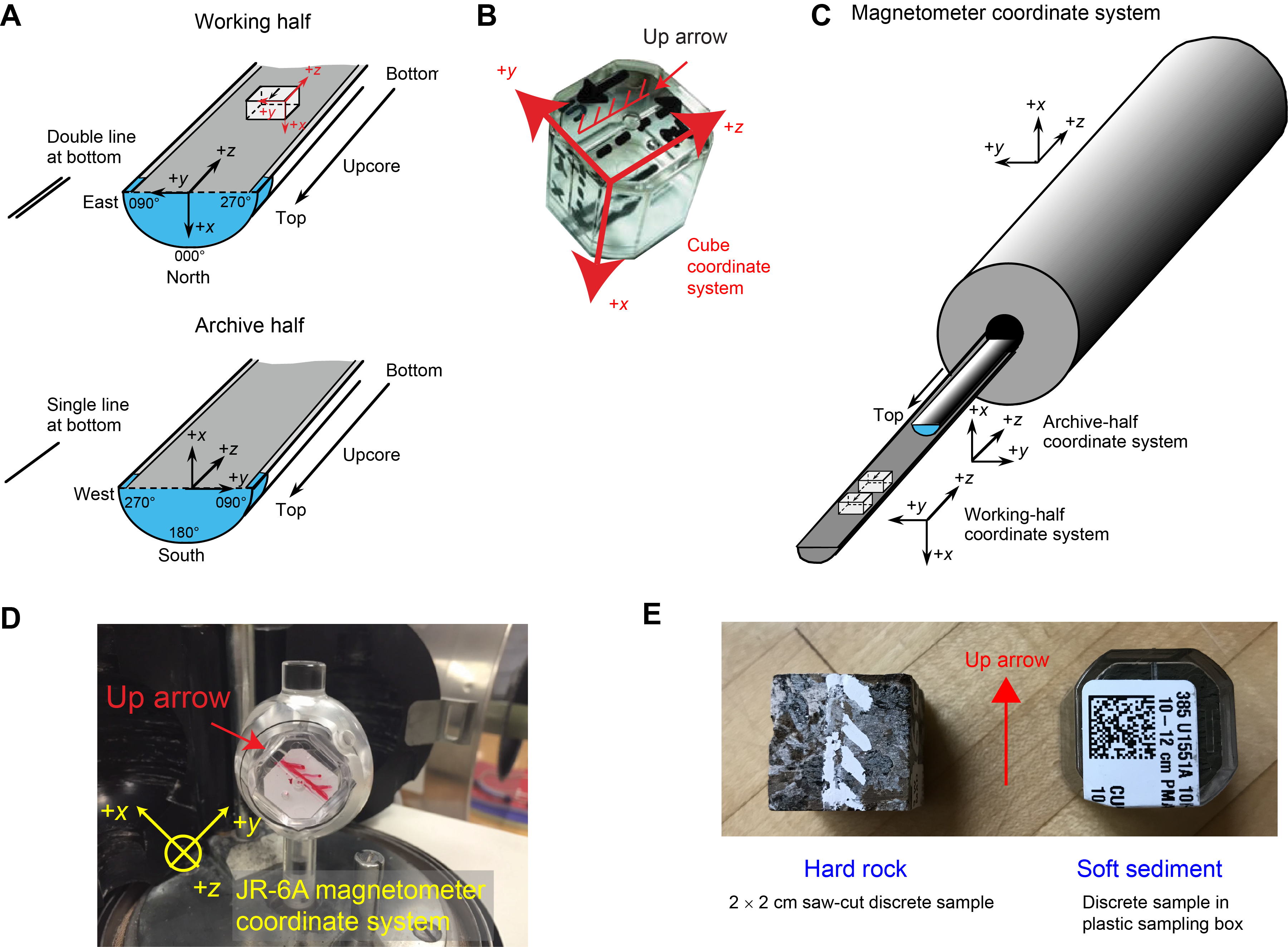
Demagnetization was conducted with the aim of removing magnetic overprints, which arise both naturally, particularly by the acquisition of viscous remanent magnetization, and as a result of drilling, coring, and sample preparation. Intense, usually steeply inclined overprint has been routinely described from ODP and IODP cores; it results from exposure of the cores to strong magnetic fields due to magnetization of the core barrel and elements of the BHA and drill string (Stokking et al., 1993; Richter et al., 2007). The use of nonmagnetic stainless steel core barrels during APC, HLAPC, and RCB coring during Expedition 385 reduced the severity of this drilling-induced overprint (Lund et al., 2003).

Discrete cube samples for paleomagnetic analysis were collected where the core sections were relatively continuous and undisturbed (usually the case in APC- and HLAPC-cored intervals) or where discontinuous recovery or core disturbance made use of continuous sections unreliable (in this case, the discrete samples became the sole basis for magnetostratigraphy). We collected one to two discrete samples per core throughout all sites. We also examined the downhole variation in paleomagnetic results to determine the extent of alteration processes caused by the sill intrusions.

7.2. Archive-half measurements

Measurements of remanence and stepwise AF demagnetization were conducted on archive halves with the SRM, driven with the IMS SRM software, version 10.3 (Figure F21C). The SRM is a 2G Enterprises Model 760R-4K equipped with direct-current superconducting quantum interference devices (DC-SQUIDs) and an in-line automated three-axis AF demagnetizer capable of reaching a peak field of 80 mT. The spatial resolution, measured by the width at half height of the response of the pickup coils, is <10 cm for all three axes, although magnetization can be sensed over a core length of as much as 30 cm. The magnetic-moment noise level of the SRM is ~2 × 10⁻¹⁰ Am². The practical noise level, however, is affected by the magnetization of the core liner and the background magnetization of the measurement tray, resulting in a lower limit of magnetization of ~2 × 10⁻⁵ A/m, which can be reliably measured.

We measured the archive halves at 5 cm intervals, and they were passed through the sensor at a speed of 10 cm/s. A 15 cm long interval of empty track was measured before the start of the section passed the center of the pickup coils of the SQUID sensors, and an equal interval of empty track was measured after the end of the section had passed through it. These are referred to as the header and trailer measurements and serve the dual functions of monitoring the background magnetic moment and enabling future deconvolution analysis. After an initial measurement of NRM, we proceeded to demagnetize the archive halves over steps of 5, 10, 15, and 20 mT to provide detailed data on potential drilling overprints. NRM after AF demagnetization was plotted for individual sample points as vector plots (Zijderveld, 1967) to assess the effectiveness of removal of overprints and to show variations with depth at individual demagnetization levels. We inspected the plots visually to judge whether the remanence after demagnetization at the highest AF demagnetization step reflected the characteristic remanent magnetization (ChRM) and geomagnetic polarity sequence.

7.3. Discrete samples

Where the sediment was sufficiently soft, we collected discrete 7 cm³ volume samples in plastic Natsuhara Giken sampling boxes (Figure F21B). In soft sediment, these boxes were pushed into the working half of the core by hand with the“up” arrow on the box pointing upsection in the core (Figure F21E). In sills and more indurated sediment, we cut cubes with orthogonal passes of a tile saw that had two parallel blades spaced 2 cm apart (Figure F21E). We simply marked an upcore orientation arrow on the split core face of the cut cube sample. These lithified samples, without a plastic container, were available for both AF and thermal demagnetization.

7.3.1. Remanence measurements

We measured the NRM of discrete samples before and after demagnetization on an AGICO JR-6A dual speed spinner magnetometer (sensitivity = ~2 × 10⁻⁶ A/m). We used the automatic sample holder for measuring the plastic sampling boxes and lithified cubes without a plastic container (Figure F21D).

For sediment, progressive AF demagnetization of the discrete samples was achieved with a DTech D-2000 AF demagnetizer in three subsequent positions at intervals of 5 mT up to 30 mT followed by steps at 40, 50, and 60 mT.

For hard rock, we thermally demagnetized a subset of the lithified cube samples, an alternative method that is more effective at demagnetizing high-coercivity materials (e.g., hematite). This method is also efficient at removing the magnetization of magnetic sulfides, particularly greigite, which thermally decomposes during heating in air at temperatures of 300°–400°C (Roberts and Turner, 1993; Musgrave et al., 1995). Difficulties in thermally demagnetizing samples in plastic boxes discouraged us from applying this method to softer samples.

We demagnetized the samples in a Schonstedt TSD-1 thermal demagnetizer, initially at temperature steps of 50° to 450°C and then at steps of 25° to 600°C, and measured demagnetized NRM after each step on the spinner magnetometer. Additional 25°C steps were later added at 175°, 225°, 275°, 325°, and 375°C to better constrain the demagnetization of multidomain magnetite. Samples were held at the specified temperature for a minimum of 30 min and then cooled to room temperature by the built-in fan. To minimize the effect of any magnetism that could be acquired in any residual magnetic field while samples cooled in the oven, samples were arranged in antipodal positions between each heating step.

Demagnetization data for archive halves and all discrete samples were displayed in vector component diagrams (Zijderveld, 1967). ChRM directions were calculated from the best fitting component by principal component analysis (Kirschvink, 1980) using the software MacPaleomag by Jeffrey Gee (Scripps Institution of Oceanography) (https://earthref.org/ERDA/2203). We analyzed the data using inclination-only statistics (Arason and Levi, 2010). In addition, the mean destructive field and median destructive temperature were calculated at the field (for AF demagnetization) and temperature (for thermal demagnetization) at which the NRM intensity is reduced to 50%, which helps to determine the magnetic mineral composition present in samples and their associated grain sizes.

7.3.2. Liquid nitrogen treatment

Multidomain magnetite, with grain sizes typically greater than ~1 µm, does not exhibit the simple relationship between acquisition and unblocking temperatures predicted by Néel (1949) for single-domain grains, which could potentially cause low-temperature or low-coercivity overprints. For this reason, when we had evidence that overprints in multidomain grains were obscuring the magnetostratigraphic signal (e.g., in igneous rocks), we instituted a program of liquid nitrogen cooling of the discrete samples in field-free space (Dunlop et al., 1997). This involved inserting the samples (after first drying them during thermal demagnetization at 110°C) into a bath of liquid nitrogen held in a Styrofoam container, which was then placed in a triple-layer mu-metal cylindrical can to provide a (near) zero-field environment. We then allowed the nitrogen to boil off and the samples to warm. Cooling the samples forces the magnetite below the Verwey transition; warming within field-free space above the transition enables remanence to recover in single-domain grains, but it randomizes remanence in multidomain grains. Once the samples were at room temperature, they were transferred to a smaller mu-metal can until measurement to avoid acquisition of a viscous remanence. Their remanence was measured, and then routine thermal demagnetization was continued.

7.3.3. Anisotropy of magnetic susceptibility

At all drill sites, we carried out magnetic fabric analysis in the form of measurements of anisotropy of magnetic susceptibility as a measure of sediment compaction. We carried this out on all discrete samples using an AGICO Kappabridge KLY 4 magnetic susceptibility meter. We calculated anisotropy as the foliation F = K₂/K₃ and the lineation L = K₁/K₂, where K₁, K₂, and K₃ are the maximum, intermediate, and minimum eigenvalues of the anisotropy tensor. We describe the shape of the anisotropy ellipsoid by the shape parameter T (Jelínek and Kropáček, 1978) where −1.0 < T < 1.0 indicate prolate/oblate fabrics, respectively. Additionally, we describe the strength of anisotropy using the corrected anisotropy degree Pj (Jelínek and Kropáček, 1978), where Pj = 1.0 indicates an isotropic fabric, and, for example, Pj = 1.05 indicates 5% anisotropy. Both the shape parameter and anisotropy degree are dependent on the relationships between the eigenvalues of the anisotropy tensor.

7.4. Sample coordinates

All magnetic data are reported relative to the IODP orientation conventions: +x is into the face of the working half, +y points toward the left side of the face of the working half, and +z points downsection. The relationship of the SRM coordinates (x-, y-, and z-axes) to the data coordinates (x-, y-, and z-directions) is as follows: for archive halves, x-direction = x-axis, y-direction = −y-axis, and z-direction = z-axis; for working halves, x-direction = −x-axis, y-direction = y-axis, and z-direction = z-axis (Figure F21A). Discrete cubes are marked with an arrow on the split face (or the corresponding face of the plastic box) in the upsection (i.e., −z) direction (Figure F21B, F21E).

7.5. Core orientation

The core orientation process determines the angular correction to apply to the archive halves’ declination values as measured by the SRM. APC and HLAPC cores were oriented by means of the Icefield MI-5 core orientation tool. The Icefield orientation tool is connected to the core barrel in such a way that the double lines on the core liner are at a fixed known angle to the sensors. The Icefield orientation tool orients cores by taking orientation measurements for a short period of time just prior to when the core is taken. The orientation tool is run on the APC BHA in a nonmagnetic core barrel. The drill string is kept steady while the tool measures and stores measurements (declination, inclination, total magnetic field, and temperature) from a triaxial magnetometer and a triaxial accelerometer. During Expedition 385, a measurement interval of 10 s was used. The Icefield orientation tool records an azimuth to magnetic north for each core. The sensors provide an azimuthal correction for the core barrel that, combined with the local magnetic declinations, enables the measured NRM declinations on archive halves to be transformed into true geographic coordinates. The data were processed using the in-house Inclin software.

The ChRMs can also provide a reference frame to orient cores. Provided that the reference magnetic pole is known, the orientation of the paleomagnetic vector is then used to restore the azimuth of the +x core axis (e.g., Fuller, 1969).

7.6. Magnetostratigraphy

Expedition 385 drill sites are located between ~27°10′N and 27°40′N, far enough from the Equator to easily identify distinct changes in inclination. By considering the mean state of the Earth’s magnetic field to be a geocentric axial dipole, it is possible to calculate the field inclination, I, as tan(I) = 2 tan(lat), where lat is the latitude. Hence, the time-averaged normal field at the present-day positions of Sites U1545–U1552 has a positive (downward) inclination of ~46°. Negative inclinations indicate reversed polarity. The shipboard data were correlated to the geomagnetic polarity timescale of Gradstein et al. (2012) with the aid of biostratigraphic datums. Magnetic excursions within the Brunhes Chron (C1n) and Matuyama Chron (C1r) are dated according to Laj and Channell (2015) and references therein (Table T9).

8. Inorganic geochemistry

8.1. Interstitial water collection

Inorganic geochemical data from IW profiles provide information on biogeochemical reactions, abiotic reactions, water-rock interactions, and fluid migration. During Expedition 385, IW samples were collected for onboard analysis and for a wide range of postexpedition analyses. The squeeze cakes, residual sediments after IW extraction, were also collected and distributed for postexpedition research. In addition, sediment subsampling and extraction of dissolved inorganic nitrogen (i.e., ammonium and nitrate) for nitrogen isotope analysis of dissolved inorganic nitrogen and mineral nitrogen were performed aboard the vessel.

IW was extracted using a titanium squeezer (Manheim and Sayles, 1974) according to the following procedure. After cutting from the core liner, the surface of each whole-round core sample was carefully scraped off with a ceramic knife to remove potential contamination from seawater, drilling disturbances, and sediment smearing that may have happened along the inside of the core liners. Holes U1545C, U1546D, U1548C–U1548E, U1551B, and U1552A–U1552C were trimmed under a nitrogen-filled glove bag to minimize the oxidation of redox-sensitive elements (S, Fe, and Mo); the other holes were processed under atmospheric conditions. For APC cores, ~0.5 cm of material from the outer diameter, top, and bottom of the whole-round sample was usually removed, whereas in XCB and RCB cores, where borehole contamination may be more substantial, ~1 cm of the outer sediment and any physically disturbed layers were removed from each whole-round core section. The cleaned sediment (~150–300 cm³) was placed into a 9 cm diameter titanium squeezer that was then placed in a Carver hydraulic laboratory press (Manheim and Sayles, 1974) and squeezed at pressures no higher than ~20,000 lb (~10 MPa) to prevent water release from clay minerals during squeezing. After each use, the squeezer was cleaned with tap water, rinsed with 18 MΩ deionized water (DI), and thoroughly dried with compressed air.

The squeezed IW was filtered through a DI-prewashed Whatman No. 1 filter placed in the squeezer cell above a titanium screen. The squeezed fluids were filtered through a 0.2 µm polyethersulfone membrane disposable filter attached to the squeezing assembly and collected in a precleaned (10% HCl) high-density polyethylene (HDPE) syringe attached to the filter. Squeeze cakes were saved for separate analyses by science party members and generally frozen at −20°C unless specified otherwise.

To better understand the processes in the shallow sediment column of Sites U1547–U1549, IW was sampled using Rhizon samplers at a higher spatial resolution. This technique was previously tested and validated during Integrated Ocean Drilling Program Expedition 302 (Dickens et al., 2007). Within 10 min after cores were recovered on the core receiving platform, core sections were transported inside and holes were drilled into the plastic liner (1–2 per section). Precleaned (10% HCl) 5 cm long Rhizon samplers were inserted into holes, connected to precleaned (10% HCl) 30 mL syringes that were pulled to generate a vacuum, and held open with a spacer.

Sample distribution was determined based on the recovered IW volume and analytical priorities as well as the objectives of the expedition. Shipboard analyses were done on all IW recovered, whereas personal sampling was mainly done on holes where microbiology sampling occurred. For personal sampling, the relative priorities of geochemistry and microbiology sample distribution, as well as sample pretreatment and storage, are summarized in Table T10.

Generally, IW samples were analyzed on board following the protocols outlined by Gieskes et al. (1991), Murray et al. (2000), and the IODP user manuals for shipboard instrumentation (http://iodp.tamu.edu/labs/documentation), which were updated during this expedition. Details for specific analyses are provided below.

8.2. Interstitial water analysis

8.2.1. Salinity, alkalinity, and pH

Salinity, alkalinity, and pH were measured immediately after squeezing following the procedures in Gieskes et al. (1991). Salinity was measured using an Index Instruments Ltd. temperature-compensated digital refractometer. International Association for the Physical Sciences of the Oceans (IAPSO) standard seawater was used for salinity calibration (salinity = 35). The pH value was measured by means of a combination glass electrode, and alkalinity was determined by Gran titration with a Metrohm 794 basic Titrino autotitrator. A 3 mL sample was titrated against 0.1 N HCl at 25°C to reach an endpoint of pH = 4.2. The IAPSO standard seawater (alkalinity = 2.325 mM; certified value) as well as laboratory-made standards (20 and 40 mM of the 0.1 M KCl + 0.7 M Na₂CO₃ mixture) were used for calibration. The IAPSO standard was analyzed at the beginning and end of a set of samples for each site and after every 10 samples. Repeated measurements of IAPSO seawater for alkalinity yielded precision better than 2.5%.

8.2.2. Chloride concentration by titration

High-precision chloride concentrations were acquired using a Metrohm 785 DMP autotitrator. A 0.1 mL aliquot of sample was diluted with 30 mL of 90 ± 2 mM HNO₃ and titrated with 0.015 N AgNO₃. The silver nitrate (AgNO₃) solutions were calibrated against repeated titrations of the IAPSO standard seawater (~559 mM chloride). The IAPSO standard was analyzed at the beginning and end of a set of samples for each site and after every 10 samples. Repeated measurements of the IAPSO standard seawater yielded precision better than 0.4%.

8.2.3. Sulfate, chloride, bromide, sodium, magnesium, potassium, and calcium

Sulfate, chloride, bromide, sodium, magnesium, potassium, and calcium concentrations were analyzed by ion chromatography (Metrohm 850 Professional IC) using aliquots of 100 µL that were diluted 1:100 with DI water. For anion (Cl⁻, SO₄²⁻, and Br⁻) analyses, a Metrosep C6 column (100 mm long; 4 mm inner diameter) was used with 3.2 mM Na₂CO₃ and 1.0 mM NaHCO₃ solutions as eluents. For cation analyses (Na⁺, K⁺, Mg²⁺, and Ca²⁺), a Metrosep A supp 7 column (150 mm long; 4 mm inner diameter) was used with 1.7 mM of HNO₃ and pyridine-2,6-dicarboxylic acid (PDCA) solutions as eluents. The standards used were based on IAPSO dilutions (1:50 to 1:350) to create a 6-point calibration curve. Reproducibility was checked based on the standard IAPSO sample dilution of 1:100 run after every 10 samples. The reproducibility of chloride, sulfate, sodium, magnesium, and calcium was better than 1.5%, whereas for bromide and potassium it was better than 3.0%.

8.2.4. Ammonium, phosphate, and sulfide

Concentrations of dissolved ammonium, phosphate, and sulfide were determined using an Agilent Technologies Cary Series 100 UV-Vis spectrophotometer with a sipper sample introduction system following Gieskes et al. (1991). The ammonium concentrations were determined by a colorimetric method that incorporates diazotization of phenol and subsequent oxidation of the diazo compound by Clorox to yield a blue color, measured spectrophotometrically at 640 nm. Samples were diluted prior to color development so that the highest ammonium concentration was always <1000 µM. The solution was kept at room temperature for ~6.5 h to develop color after adding the reagents. The reproducibility of the analysis was better than 2.0%.

Phosphate concentrations were based on the reaction of orthophosphate with Mo(VI) and Sb(III) in an acidic solution, forming an antimony-phosphomolybdate complex that is subsequently reduced by ascorbic acid to form a blue color. The absorbance was measured spectrophotometrically at 885 nm wavelength ~30 min after adding the mixed reagent solution (Gieskes et al., 1991). Samples were diluted prior to color development so that the highest concentration was always <100 µM. The reproducibility was better than 2.0%.

For sulfide analysis (ΣH₂S = S²⁻ + HS⁻ + H₂S), exposure to air must be minimized to prevent abiotic oxidation of IW sulfide. These samples were fixed with a zinc acetate solution (100 g/L: 50 µL per 1 mL of sample) that was immediately added to freshly squeezed IW. Sulfide concentrations were measured following the Cline method (Cline, 1969; Grasshoff et al., 1999) with no dilution for concentrations ranging between 1 and 60 µM and with a dilution factor of 10 for concentrations up to 600 µM. Dilutions were made with N₂-purged DI water. For each dilution factor, a calibration curve was prepared with the same zinc acetate final concentrations. The absorbance was read at 670 nm. Because most of our samples had sulfide concentrations higher than 600 µM (several millimolar), we also measured high concentrations of sulfide directly using a solution containing a known excess of triiodide (I₃⁻) (Grasshoff et al., 1999) that forms a yellow color. Sulfide reacts with triiodide to form I⁻ and S, and therefore lowers the absorbance at 400 nm. This titration is commonly used to determine the concentration of the Na₂S stock solution later used to build the standards for the Cline method.

8.2.5. Sample preparation for shore-based sulfur isotope analysis

While handling IW samples for sulfur isotopic analyses, prolonged exposure to air must be minimized to prevent abiotic oxidation of IW sulfide. Because of their oxygen sensitivity, these samples were processed immediately from freshly squeezed IW. Before IW sampling, sample vials were prepared as shown in Table T10.

8.2.6. Major, minor, and trace elements

Major and minor elements (Na⁺, Ca²⁺, Mg²⁺, K⁺, Li⁺, B, Si, Ba²⁺, Fe, Mn, and Sr²⁺) were analyzed using ICP-AES (Agilent 5110 ICP-OES instrument in ICP-AES mode with a SPS4 autosampler). The general method for shipboard ICP-AES analysis of samples is described in ODP Technical Note 29 (Murray et al., 2000) and in the user manuals for shipboard instrumentation with modifications as indicated. Samples and standards were diluted 1:10 in 2% HNO₃ and spiked with an internal standard to correct for atomic and ionic interferences. Specifically, 100 µL of spike solution containing 100 ppm Be, In, and Sc and 200 ppm Sb was added to 500 µL of IW sample and 4.4 mL of 2% HNO₃. Each batch of samples analyzed on the ICP-AES contained blanks and solutions of known concentrations. Each item aspirated into the ICP-AES was counted three times from the same dilute solution in a given sample run. Following each instrument run, the measured raw intensity values were transferred to a data file and automatically corrected for instrument drift and blank values using Agilent’s ICP Expert software (version 7.3.0.1.9507).

Standardization of major cations (Na⁺, K⁺, Mg²⁺, and Ca²⁺) was achieved by successive dilution of IAPSO standard seawater (1:1 to 1:100). Analytical reproducibility was based on repeated analyses of the 1:1 dilution standard over the 2 month expedition and had the following variability ranges: Ca²⁺ < 1.5%, Mg²⁺ < 1.6%, Na⁺ < 1.7%, and K⁺ < 1.5%.

For minor and trace element concentration analyses (Li⁺, B, Si, Ba²⁺, Fe, Mn, and Sr²⁺), the 1:10 dilution of the sample was not sufficient to prevent a matrix effect. Thus, standards were prepared in an acidified synthetic seawater with an ionic strength similar to seawater. A stock multielement standard solution was prepared from ultrapure primary standards (1000 ppm; SPEX CertiPrep reference standards) in a 2% HNO₃ solution. The stock solution was then diluted in the same 2% ultrapure HNO₃ solution (1:1 to 1:20). For consistency, the calibration standards were then diluted using the same method as the samples. The 1:1 standard was repeatedly analyzed with each batch of samples over the 2 month expedition as a check of analytical reproducibility. Analytical reproducibility based on repeated analyses of the minor and trace elements was Li⁺ < 1.6%, B < 1.6%, Si < 2.4%, Ba²⁺ < 2.6%, Fe < 2.5%, Mn < 1.7%, and Sr²⁺ < 2.2%.

8.3. Extraction experiment for shore-based nitrogen isotope analysis

Dissolved inorganic nitrogen species (i.e., ammonium and nitrate) and exchangeable ammonium within clay mineral interlayers were extracted from sediment samples (about 5 cm³ wedge samples) collected at 10–20 m depth intervals by shaking the sample in ~80 mL of 2 M KCl solution in a flask overnight. After extraction, the liquid phase was filtered with a 0.2 µm membrane filter and stored in a freezer (colder than −20°C) in plastic bottles (125 mL). The solid phase containing mineral nitrogen was washed with pure water and stored in a plastic bag and then freeze-dried. The dried samples were stored in a refrigerator at 4°C.

8.4. Igneous rock geochemistry

8.4.1. Sample preparation

Least-altered rock chips 5–10 cm³ in volume were selected from fragmented core pieces of the working-half sections of recovered sill material from Sites U1545–U1548 and U1550. Each solid rock sample was placed in a beaker containing isopropanol and agitated in an ultrasonic bath for 15 min. Upon decanting the isopropanol, the samples were then agitated twice in an ultrasonic bath in nanopure DI water (18 MΩ·cm) for 10 min. Subsequently, the clean pieces were dried for 10–12 h at 110°C. The rock samples were then crushed to <1 cm in length between two Delrin plastic disks in a hydraulic press.

Crushed rock chips were then subjected to grinding to produce a fine powder using a SPEX 8515 Shatterbox powdering system with a tungsten carbide mill. A potential contamination effect of the latter was investigated during ODP Leg 206 (Shipboard Scientific Party, 2003b). This study found contamination to be negligible for major elements and most trace elements determined aboard the vessel (Sc, V, Cr, Ni, Sr, Y, Zr, and Ba). A systematic analysis of shipboard powders from Integrated Ocean Drilling Program Expedition 304/305, however, pointed to possible Co contamination during the powdering process (Godard et al., 2009). Upon milling, the prepared powder was processed for ICP-AES measurements.

8.4.2. Loss on ignition

Upon powdering, a sample powder aliquot of 2.00 to 5.00 ± 0.05 g was weighed on a Mettler Toledo balance and ignited for 4 h at 1025°C for igneous rocks to determine weight loss on ignition (LOI) volatile budgets with an estimated precision of 0.02 g (0.4%).

8.4.3. ICP-AES

For IW measurements, the standard shipboard procedure for digestion of rocks and subsequent ICP-AES analysis is outlined in Murray et al. (2000) and the shipboard user guide for ICP-AES. Modifications as indicated in the IODP Expedition 366 methods (Fryer et al., 2018) and Expedition 369 methods (Huber et al., 2019) were applied to igneous rock analysis during Expedition 385. The analytical protocol, which is adopted from the IODP Expedition 376 methods (de Ronde et al., 2019), is summarized below.

Samples and standards were weighed on a Cahn C-29 microbalance to 100.0 ± 0.5 mg. Weighing errors are estimated to be ±0.2 mg under relatively smooth sea-surface conditions. Aliquots of ignited bulk rock powders were mixed with 400.0 ± 0.5 mg of LiBO₂ flux (preweighed on shore). An aqueous LiBr solution (10 μL of 0.172 mM) was added to the flux and rock powder mixture as a nonwetting agent prior to sample fusion to prevent the fused bead from sticking to the crucible during cooling. Samples were fused individually in Pt-Au (95:5) crucibles for ~12 min at a maximum temperature of 1050°C in an internally rotating induction furnace (Bead Sampler NT-2100).

For the subsequent digestion procedure, each bead was transferred into a 125 mL, precleaned (10% HCl) HDPE bottle and dissolved in a 50 mL solution containing 10 wt% HNO₃ (derived from Optima-grade concentrated HNO₃). To promote the dissolution, bottles with mixed beads and HNO₃ were placed in a Burrell wrist-action shaker and shaken for 1–2 h at a temperature of 7°C. After the bead was completely dissolved in HNO₃, 20 mL of each acidified sample solution was extracted and transferred through a 0.45 µm Acrodisc filter into a 60 mL Nalgene bottle to avoid any insoluble material during the ICP-AES measurement. Each filtered sample solution was then diluted by pipetting a 0.5 mL aliquot into 4.4 mL of 10 wt% HNO₃ and 0.1 mL of internal standard solution containing Be, In (100 μg/g), and Sb (200 μg/g), applying a solution-to-sample dilution factor of 4000×.

Measurements of major and trace element contents of standards and samples were performed on an Agilent 5110 ICP-OES instrument in ICP-AES mode. Analyses of certified international rock reference materials, calibration and drift solutions, and chemical procedure blanks were processed along with the unknown samples for each measurement run (Table T11). Detection limits were calculated as 3× the standard deviation of the mean for blank solution measurements (Table T12).

The ICP-AES plasma was ignited at least 20 min prior to each sample run to enable the instrument to stabilize sufficiently. All other premeasurement preparation on the ICP-AES instrument was routinely performed using the JRSO shipboard procedures to maintain consistency between different runs. The ICP-AES data presented in the Igneous petrology sections of corresponding site chapters (i.e., Sites U1545, U1546, U1547/U1548, and U1550) were acquired using Agilent’s ICP Expert software. Twenty measurements for each element define the intensity curve within the designated wavelength window. Integration of the area delineated by the baseline and the intensity curve is done by the Expert software. Each sample was analyzed three times from the same dilute solution in a given sample run. The wavelength yielding the best calibration line was identified and used to determine the concentrations for each element of unknown samples.

Estimates of accuracy of major and trace element analyses were based on analyses of seven international, certified igneous rock powder standards (Table T12). During the single ICP-AES igneous rock measurement run on Expedition 385, an international rock standard was analyzed in every fourth to fifth sample position so that each standard was measured once within the single sample run. A procedural blank solution was analyzed at the beginning and end of this run, and 35 unknown samples were analyzed. A 10% HNO₃ wash solution was run for 90 s between each sample analysis. Check standards were used to monitor and determine analytical accuracy and precision of the final data. Detection limits were obtained from blank measurements.

Data reduction consisted of initial drift correction applied to each element of all analyses, based on a linear interpolation between drift-monitoring solutions that were run every fourth analysis. Upon implementing this step and subtracting the procedural blank, a calibration line for each element was calculated through applying the results of the certified rock standards. Element contents used for the calibrations represented values compiled from the literature. They were recalculated on a volatile-free basis for those samples having LOI values >2 wt%. Total Fe oxide concentrations are reported as Fe₂O₃(t). The compiled element contents of the international rock standards are those recommended by Govindaraju (1994) and the GeoReM database (http://georem.mpch-mainz.gwdg.de; Jochum et al., 2005) (Table T11). Element abundances in the Expedition 385 igneous rock samples were then derived from the relevant calibration lines. Only those ICP-AES analyses of Expedition 385 igneous rock samples yielding a total sum of minimum 98 wt% and maximum 102 wt% (hydrous composition) were considered for data analysis and interpretation.

9. Organic geochemistry

Organic geochemical data provide essential information on the cycling of carbon and other elements in marine sediments. Downhole profiles of total organic carbon (TOC) and total nitrogen (TN) are needed to quantify the sedimentary organic matter pool and to characterize the availability of substrates for microbial communities. Profiles of dissolved organic matter (DOM) and hydrocarbon gases provide insights into the microbial utilization and thermogenic alteration of sedimentary organic matter. Quantifying dissolved inorganic carbon (DIC) and molecular hydrogen (H₂) enables assessments of free energy yields for methanogenesis and other H₂-consuming reactions. Moreover, the presence of hydrocarbon gases must be monitored to prevent safety and environmental risks during drilling.

During Expedition 385, we conducted safety gas monitoring according to the routine shipboard safety and pollution prevention protocol for every site and hole (Kvenvolden and McDonald, 1986; Pimmel and Claypool, 2001). In addition, we sampled gases, IW, and the solid phase of sediments and igneous rocks for a wide range of shipboard and shore-based chemical and isotopic analyses in the holes dedicated to microbiological and geochemical investigations (Table T13). Our sampling program was closely coordinated with inorganic geochemists, microbiologists, and physical properties specialists. Organic geochemists focused on gas sampling, which included analyses of hydrocarbon gases, H₂, and CO, whereas inorganic geochemists collected corresponding IW samples in adjacent depth intervals, including those for DIC and DOM analyses (see Inorganic geochemistry). Adjacent to gas samples, small solid-phase samples were taken for shipboard analysis of TOC, TN, total sulfur (TS), and carbonate contents (see Solid-phase analysis) as well as porosity (see Petrophysics). In cooperation with microbiologists, whole-round core sections were collected from selected depth intervals and prepared for shipboard and shore-based incubation experiments and for shore-based analysis of sedimentary organic matter and biomarkers (see Microbiology).

9.1. Gas analysis

9.1.1. Gas sampling

While recovering cores with the APC and HLAPC systems, the expansion of entrapped gases can form voids in the sediments. When such voids were observed, their length was recorded before they were sampled on the core retrieval platform. Void gas (VAC) samples were collected by piercing the core liner with a custom piercing tool that allows gas to expand into a 60 mL gas-tight syringe connected to the tool. A 10 mL split of the sample was taken for immediate shipboard analyses of hydrocarbon gases, H₂, and CO, and the remaining sample was transferred into crimp-capped headspace vials prefilled with a saturated solution of NaCl for shore-based analysis of the stable isotopic composition of hydrocarbon gases and CO₂ and for methane clumped isotopologue analysis (for sample codes, see Table T13).

For safety gas monitoring, samples for hydrocarbon gas analysis were collected from each core immediately after retrieval on the core receiving platform. Samples were taken as a headspace (HS) sample: ~5 cm³ of sediment was collected from the bottom of Section 1 using a cut-off syringe for soft to semiconsolidated sediment or a metal boring tool when the sediment became more lithified. During hard rock drilling, small rock chips from igneous rocks were used when available. Sediment samples were extruded or placed into preweighed 21.5 mL glass vials and immediately sealed with a polytetrafluoroethylene/silicone septum and metal crimp cap. The vial was incubated in an oven at 70°C for 30 min to allow dissolved hydrocarbon gases to equilibrate with the headspace prior to analysis (samples identified as “HS” in Table T13 and Figure F22) following the sampling protocol of previous expeditions (Expedition 322 Scientists, 2010; Expedition 337 Scientists, 2013; Morono et al., 2017; Sun et al., 2018).

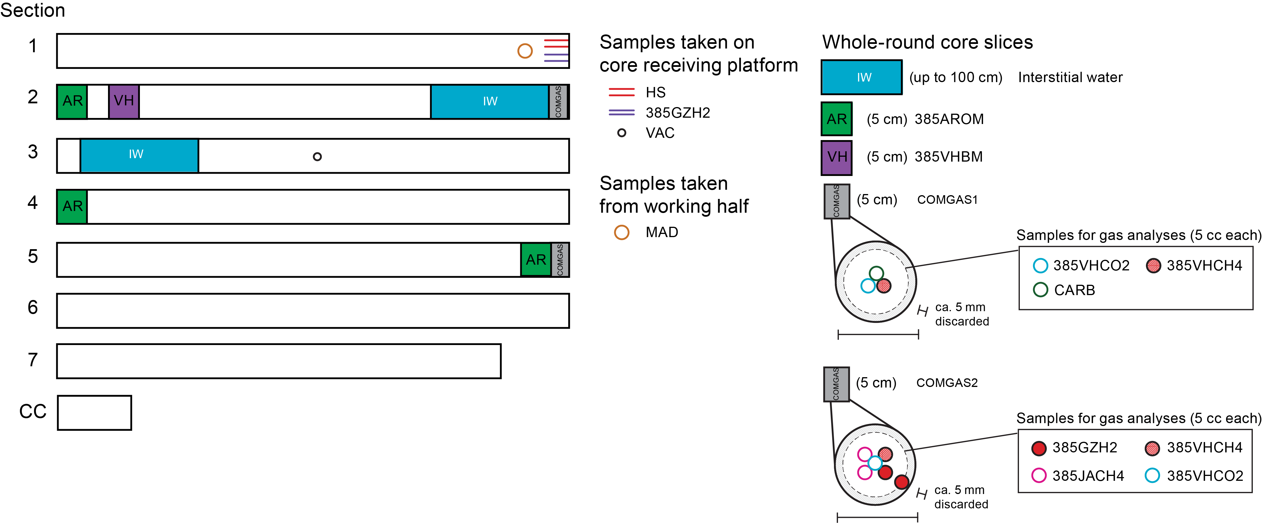
Safety gas monitoring was accompanied by shipboard analysis of H₂ and CO. Exactly 3 cm³ of sediment was collected in replicate from the bottom of Section 1 with a cut-off syringe. Sediment samples were transferred into preweighed 21.5 mL glass vials, which were subsequently filled with low-H₂ 18 MΩ water, closed with a gray butyl rubber stopper, and crimp capped. Care was taken to overfill the vials with the 18 MΩ water before closing to avoid any air contamination. Subsequently, 5 cm³ of molecular nitrogen (N₂) gas headspace was inserted into the vial using a needle with a gas-tight syringe. The N₂ gas used for the headspace injection was taken from the bypass-out outlet of the reduced gas analyzer used for the analysis of H₂ and CO. This ensures low H₂ and CO contents because this gas has gone through a catalytic converter that oxidizes H₂ and CO. To avoid overpressurization of the sample vial during the headspace injection, an equivalent amount of water was allowed to escape the vial through a separate needle. Next, the samples were vortexed and stored upside down for 20 min to allow H₂ and CO to diffuse out of the IW and equilibrate with the headspace at room temperature.

The analysis of hydrocarbon gases, H₂, and CO relies on the nearly complete extraction of the dissolved gases into a defined headspace volume and subsequent analyses of their partial pressures in headspace gas. To determine the corresponding molar concentrations of the dissolved gases, the headspace volume, the sample volume, and the sample’s water content need to be known. Therefore, in microbiology holes, a MAD sample was taken from the working half as close to the headspace sample as possible to determine sediment porosity (see Petrophysics).

During sediment sampling at sites where high-resolution sampling was desired, two 5 cm long whole-round core samples were taken as designated community gas samples referred to as COMGAS1 and COMGAS2 for shipboard and shore-based analyses (Figure F22). The samples were cut from the bottom of Sections 2 and 5 immediately after core retrieval and split into subsamples without delay. The following subsamples were taken:

• For shore-based stable carbon isotope analysis of CO₂ (δ¹³C-CO₂): ~5 cm³ of wet sediment from both COMGAS1 and COMGAS2 were placed in 20 mL glass vials (385VHCO2). Glass vials were completely filled with a saturated NaCl solution, sealed with soft gray chlorobutyl stoppers, and crimp capped. Within ~2 h after sampling, artificial headspace was introduced by replacing 5 mL of NaCl solution with pure CO₂-free N₂ gas; vials were stored upside down at 4°C (cf. Inagaki et al., 2015; Morono et al., 2017).
• For shore-based stable carbon and hydrogen isotope analysis of CH₄ (δ¹³C-CH₄ and δD-CH₄) and higher hydrocarbon gases: ~5 cm³ of wet sediment from both COMGAS1 and COMGAS2 was placed in a 20 mL glass vial containing 5 mL of 1 M NaOH solution (385VHCH4). The vial was capped with a precleaned black butyl stopper (heated to boiling with 1 M KOH for ~1 h and subsequently rinsed and left immersed with nanopure water overnight [cf. Oremland et al., 1987]) and frozen upside down at −20°C (cf. Hinrichs et al., 2006; Ertefai et al., 2010).
• For shore-based clumped isotope analysis of CH₄ (Δ¹²CH₂D₂ and Δ¹³CH₃D): two replicates of ~5 cm³ of wet sediment from COMGAS2 were placed in 20 mL glass vials containing 5 mL of 1 M NaOH solution (385JACH4). The vials were capped with a polytetrafluoroethylene/silicone septum and crimped sealed. Vials were vortexed and then stored upside down at 4°C (Andrén et al., 2015).
• Remaining material from the interior of COMGAS1 was used for shipboard total carbon/inorganic carbon (CARB) analyses of the solid phases (see Solid-phase analysis) and for sedimentological investigations (see Lithostratigraphy).
• Remaining material from the interior of COMGAS2 was subsampled for shore-based characterization of organic matter (385VHTOC) and mineral-bound nitrogen characterization (YAMA).

At other sites, COMGAS1 and COMGAS2 were combined into a single 7 cm long COMGAS whole-round core. From this whole-round core, samples were taken for 385VHCO2, 385VHCH4, 385JACH4 in replicate, CARB, 385VHTOC, and YAMA approximately once per 9.5 m advance.

During hard rock coring, a small (5–15 cm long) whole-round sample of igneous rock was placed into a trilaminated foil barrier bag and immediately sealed. These samples were incubated for at least 24 h at 70°C to stimulate degassing. Bags were then sampled by gas-tight syringe through a polytetrafluoroethylene/silicone septum to quantitatively remove gas. The volume of gas was recorded along with the weight of the rock segment. This gas was then subsampled into crimped septa vials prefilled with saturated NaCl solution for shore-based stable isotope (385VHCH4) and clumped isotope (385JACH4) analyses. Additionally, 10 mL of this gas was immediately subsampled for shipboard hydrocarbon, H₂, and CO analyses.

When the Kuster FTS was deployed to sample borehole fluids, samples of enclosed gases and fluids were taken using an incremental depressurization approach: ~5 mL of gas was released into a stainless steel tube equipped with two Swagelok valves. One valve served to open and close the connection of the tube toward the Kuster FTS and the other valve served to open and close the tube toward a gas-tight syringe connected by means of a luer lock (see Figure F23). In this manner, the gas content of the Kuster FTS was quantitatively sampled and further treated like a void gas sample. In addition, the fluid was transferred into a 20 mL headspace and sealed with a polytetrafluoroethylene/silicone septum and a metal crimp cap. A 5 mL headspace of pure nitrogen was inserted into the vial, and dissolved gases were allowed to exsolve into this headspace for 20 min prior to analysis.

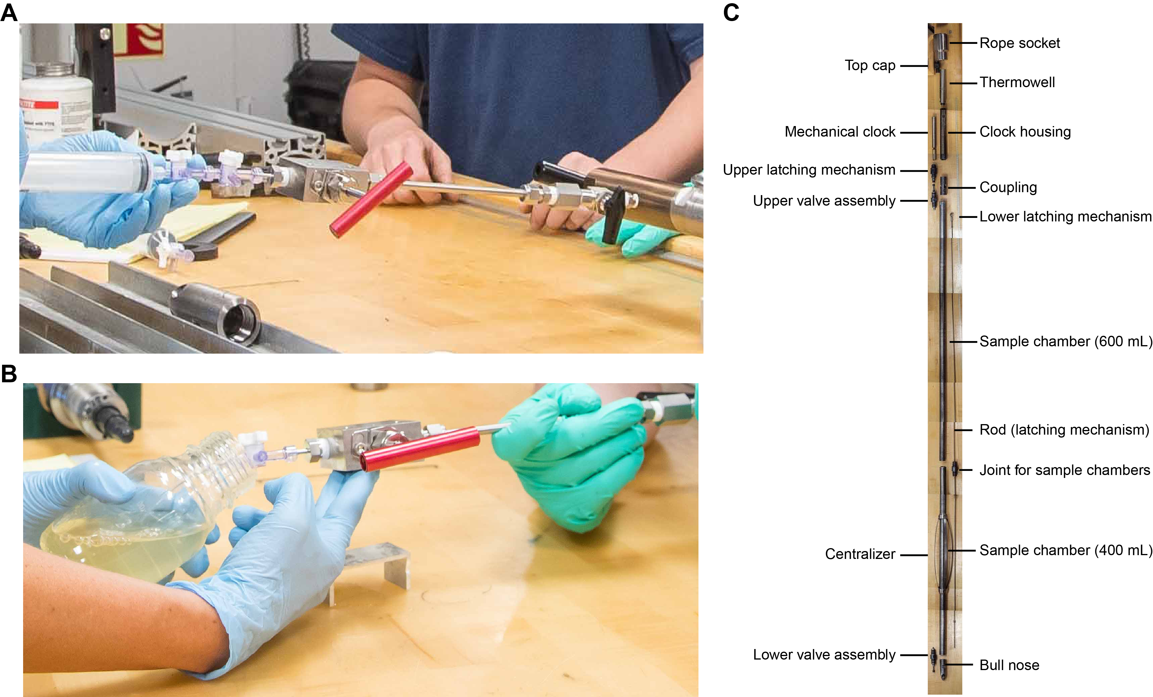
9.1.2. Hydrocarbon gases

For safety gas monitoring, the molar ratios of hydrocarbon gases, including methane (C₁ or CH₄), ethene + ethane (C₂), propene + propane (C₃), i-butane (i-C₄), n-butane (n-C₄), i-pentane (i-C₅), n-pentane (n-C₅), i-hexane (i-C₆), and n-hexane (n-C₆), were monitored following standard headspace gas sampling and analysis procedures (Kvenvolden and McDonald, 1986) and IODP pollution prevention and safety protocol (JOIDES Pollution Prevention and Safety Panel, 1992; Shipboard Scientific Party, 1994; Fritz, 1980). When present, unsaturated compounds were at low concentration. To derive molar concentrations of dissolved hydrocarbon gases, we followed the approaches of previous ocean drilling expeditions that had a strong biogeochemical focus (Shipboard Scientific Party, 2003a; Expedition 301 Scientists, 2005; Expedition 307 Scientists, 2006; Expedition 311 Scientists, 2006; Expedition 322 Scientists, 2010; Expedition 337 Scientists, 2013; Morono et al., 2017). In addition to these compounds, four additional hydrocarbons were also monitored and semiquantified: an unknown compound almost co-eluting with iso-pentane; 2,2-dimethylbutane; 2,3 dimethylbutane; and 3-methylpentane. The three latter compounds were previously described in headspace gas samples from Guaymas Basin sediments (Whelan and Hunt, 1982) and were identified based on their elution properties. Additional compounds were also observed in some samples but not monitored (Figure F24). From the volume concentration in parts per million of individual hydrocarbons, the C₁/C₂ and C₁/C₊ values were calculated. The latter ratio was calculated as follows:

C1/C+=C1/C2+C3+i-C4+n-C4+i-C5+n-C5+i-C6+n-C6. (10)

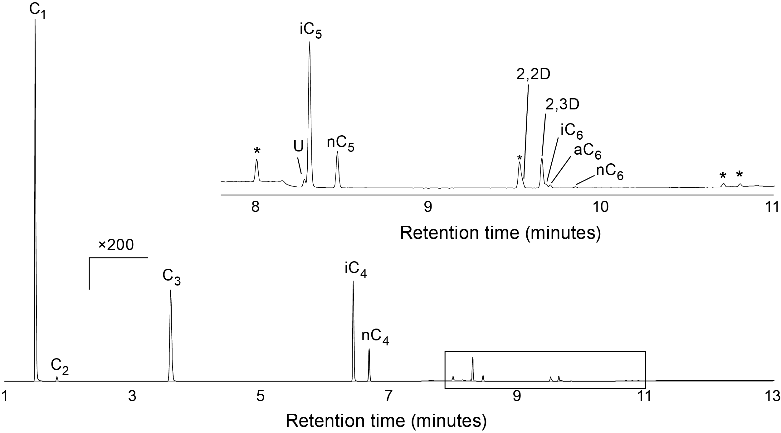
For shipboard C₁–C₆ hydrocarbon gas analysis, 5 cm³ of headspace gas was extracted from the 21.5 mL headspace vials with a gas-tight syringe and manually injected onto an Agilent 7890A gas chromatograph (GC) equipped with a split/splitless injector and a flame ionization detector (FID). The chromatogram conditions were as follows:

• Injector temperature: 300°C.
• Split ratio: 30:1.
• GC column: DB-1 precolumn (5 m × 320 µm diameter × 0 µm film thickness) coupled to an Agilent J&W PLOT Alumina/S column (25 m × 320 µm diameter × 80 µm film thickness).
• Oven temperature: hold at 35°C for 5 min, increase from 35° to 200°C at 25°C/min, and a final hold at 200°C for 5 min.

Helium was used as the carrier gas at a flow rate of 3 mL/min. Total run time per injection was 15.6 min. Data were collected and analyzed using the Agilent OpenLab CDS ChemStation software (2001–2016). The FID response was calibrated against gas standards with variable quantities of low molecular weight hydrocarbons provided by Scott Specialty Gases (Air Liquide). For quantification of the additional hydrocarbons monitored, in the absence of reference compounds, the FID response factor of the unknown compound was considered identical to that of closely eluting iso-pentane. For the branched C₆ compounds, the response factors were considered identical to that of iso-hexane. Concentrations of hydrocarbon gases are reported in parts per million by volume.

Methane concentration in IW was derived from the headspace concentration using a mass balance approach (modified from Expedition 322 Scientists, 2010):

CH4=χM×Patm×VH/R×T×Vpw, (11)

where

• χ_M = molar fraction of methane in the headspace gas (obtained from GC-FID analysis),
• P_atm = pressure in the vial headspace (assumed to be the measured atmospheric pressure when the vials were sealed),
• V_H = volume of headspace in the sample vial,
• R = universal gas constant (8.314 × 10⁻² L·bar/mol·K),
• T = temperature of the vial headspace in Kelvin, and
• V_pw = volume of pore water in the sediment sample.

The volume of IW in the sediment sample (V_pw) was determined based on the mass of the bulk wet sample (M_b), the porosity of the sediment (φ; taken from shipboard MAD measurements in adjacent samples), grain density (ρ_g), and the density of the pore water (ρ_pw):

Vpw=Mpw/ρpw=ϕ×Mb/ϕ×ρpw+1-ϕρg, (12)

where

• M_pw = mass of pore water in the sample,
• ρ_pw = 1.024 g/cm³, and
• ρ_s = 2.8 g/cm³.

The volume of headspace in the sample vial (V_H) was determined by the difference between the total volume of the vial (V_vial) and the volume of the bulk sediment sample (V_b):

VH=Vvial-Vb=Vvial-Mb/ρb, (13)

where

• V_vial = 21.5 cm³ and
• ρ_b = bulk density of the sediment (from MAD data).

After measurement of the headspace gases using GC-FID, the mass of the bulk wet sample (M_b) was determined to a precision of 0.01 g using two electronic balances and a computer averaging system that compensates for ship motion (Mettler Toledo XS204 dual analytical balance system).

The same mass balance approach was used to derive a first estimate for the molar concentrations of methane in igneous rocks that had been incubated in trilaminated foil barrier bags using the molar fraction of methane in the gas phase, the total volume of the gas phase inside the bag used for incubation, the weight of the incubated rock, and an assumed average porosity of 14% and density of 2.7 g/cm³.

9.1.3. Dissolved hydrogen and carbon monoxide

The analysis of dissolved H₂ and CO follows the approach described by Lin et al. (2012) and has been applied and modified during recent expeditions (Expedition 322 Scientists, 2010; Expedition 329 Scientists, 2011; Expedition 337 Scientists, 2013; Morono et al., 2017). The method relies on the nearly complete extraction of dissolved H₂ and CO into a defined H₂/CO-free gas volume. To this end, samples were taken and prepared as described above. Prior to measurement, the vials were vortex mixed for 3 s to ensure that the dissolved H₂ and CO were concentrated in the headspace.

The molar fraction of H₂ and CO in the headspace gas was quantified using a Peak Performer 1 (PP1) GC (Peak Laboratories LLC, USA), a third-party tool provided by the University of Georgia. The PP1 was fitted with a 100 µL sample loop and calibrated on a daily basis using a 10 ppmv H₂ gas standard and a 10 ppmv CO gas standard balanced in nitrogen. A 5-point calibration curve was obtained by diluting the 10 ppmv H₂ and CO with nitrogen gas in a gas-tight syringe (0, 1, 2.5, 5, and 10 ppmv). To perform a measurement, 1 mL of headspace gas was extracted using a gas-tight syringe with a needle and injected into the PP1. The measured H₂ and CO concentrations of the headspace were then converted to molar IW H₂ and CO concentrations using the following equations:

nH2=XH2Vheadspace/Vmolar and (14)

nCO=XCOVheadspace/Vmolar, (15)

where

• n = total number of moles (H₂ or CO) in the sample (mol),
• X = molar fraction of H₂ (or CO) in the headspace gas (ppm, obtained from GC analysis),
• V_molar = molar volume of headspace gas at laboratory temperature (L/mol), and
• V_headspace = volume of the headspace (L),

and

H2IW=nH2Vsed/ϕ and (16)

COIW=nCOVsed/ϕ, (17)

where

• [H₂]_IW = concentration of H₂ dissolved in the IW (M),
• [CO]_IW = concentration of CO dissolved in the IW (M),
• V_sed = sediment sample volume (L), and
• φ = sediment porosity.

Each sample was analyzed in duplicate. Procedural blank samples, which were headspace vials solely filled with 18 MΩ water, were prepared for each whole-round core section sampled for gas analysis. The procedural blank associated with this method averaged 23 ± 3 nM for H₂ and 43 ± 15 nM for CO. The PP1 H₂ and CO blank-corrected concentration detection limit obtained using this protocol was 40 nM for H₂ and 150 nM for CO based on 6× and 7× the standard deviation of the blank, respectively. Laboratory air H₂ and CO concentrations were monitored regularly throughout the span of the measuring campaign.

9.2. Solid-phase analysis

9.2.1. Solid-phase sampling

Samples for shipboard solid-phase analysis were taken as regular subsamples from the COMGAS samples (see Gas sampling), as well as from intervals of sedimentological interest noticed in the split cores. About 5 cm³ of sediment was transferred into sampling bags using a syringe or a ceramic knife. Samples were freeze-dried for ~12 h, ground and homogenized with an agate pestle and mortar, and then analyzed for TC, TIC, TS, and TN. In addition, solid-phase samples were taken from whole-round cores and preserved for shore-based analyses as follows (Table T13):

• Organic matter diagenesis: under nitrogen atmosphere in a glove bag, the central part (~30 cm³) of a 5 cm whole round was recovered with a spatula and transferred into a 60 mL glass jar (I-chem) with polytetrafluoroethylene-lined polypropylene caps. Samples were stored frozen at −20°C.
• Shore-based incubation experiments: 10–20 cm whole rounds were sampled as described in Microbiology.

9.2.2. Inorganic carbon content

Inorganic carbon (IC) concentrations were measured using a Coulometrics 5012 CO₂ coulometer. Approximately 10 mg of freeze-dried and powdered sediment was accurately weighed using two electronic balances and a computer averaging system that compensates for ship motion (Cahn C-31 automatic electrobalance). The sediment was then reacted with 6.5 mL of 2 M HCl in a glass vial. The liberated CO₂ was reacted with a solution containing excess monoethanolamine, forming the carbamate salt of monoethanolamine. This solution was titrated with electrochemically generated OH⁻ to a colorimetric end point, and the change in light transmittance was monitored with a photodetection cell. The weight percent of calcium carbonate was calculated from the IC content, assuming that all the evolved CO₂ was derived from the dissolution of calcium carbonate, using the following equation:

CaCO3 wt%=IC wt%×100/12. (18)

No correction was made for the presence of other carbonate minerals. A standard reference material (>99.9% CaCO₃; Fisher Scientific) was used to monitor analytical precision and accuracy (standard deviation less than ±0.4 wt%).

9.2.3. Total carbon, nitrogen, and sulfur contents

For TC, TS, and TN contents, samples were freeze-dried and powdered, and ~15 mg (±5 mg) was accurately weighed into tin cups with the Cahn C-31 automatic electrobalance. Samples were mixed with an equivalent mass of V₂O₅ catalyst, and the tin cups were carefully folded closed. Analysis was conducted using a Thermo Finnigan FlashEA 1112 CHNS elemental analyzer, in which the sample was combusted (950°C) in a stream of O₂, nitrogen oxides were reduced to N₂, and the mixture of CO₂, N₂, and SO₂ gases was separated by packed column CHNS/CNS GC (Thermo Electron) and detected using a thermal conductivity detector (TCD). A CHNS calibration standard (2.5-bis[5-tert-butyl-benzoxazol-2-yl]thiophene, BBOT; C = 72.53 wt%, N = 6.517 wt%, and S = 7.44 wt%) and two soil reference standards (NIST 2704, Buffalo River Sediments; Soil CNS Reference Material, Säntis Analytical) run every 10 samples were used to ascertain analytical precision and accuracy (standard deviation was less than ±0.04% for N, ±0.43% for C, and ±0.09% for S).

Because of analytical problems during the final elemental analysis campaign offshore, elemental analysis of the samples from Hole U1548E was duplicated onshore at the LOG laboratory (Lille University, France), using a FlashEA 1112 CHNS elemental analyzer. The analysis was performed on 1.5–2 mg of sample weighed on a MX5 Mettler Toledo microbalance in addition to ~5 mg of V₂O₅. BBOT was used as a calibration standard and was run every 10 samples to ascertain analytical precision and accuracy (standard deviation was ±0.01% for N, ±0.30% for C, and ±0.02% for S). TOC and TN data were comparable to offshore data, so only S is presented here.

TOC contents were calculated by the subtraction of IC from TC contents as determined by elemental analysis. Finally, the TOC/TN atomic ratio was determined as a source indicator of organic matter (Meyers, 1994).

TS and TOC relationships in sediments are often compared to the so-called “normal marine” trend, which has a TOC/TS ratio of 2.8. This trend is observed in fine-grained, reducing, and organic-rich (TOC < 6 wt%) platform sediments deposited under an oxygenated water column (Goldhaber and Kaplan, 1974; Berner, 1982). In such sediments, organoclastic sulfate reduction is dominant in the sediment and the quasi-absence of bioturbation leads to limited escape of generated H₂S. Reduced sulfur is thus fixed within the sediment, generally as iron sulfide, in proportion to remaining organic carbon (Goldhaber and Kaplan, 1974; Berner, 1982). TOC/TS < 2.8 can be indicative of anoxic depositional conditions (Leventhal, 1983) or of fluid circulation in the sediment (e.g., Passier et al., 1996).

9.2.4. Source rock analysis (organic matter characterization)

For selected intervals, the thermal maturity of the organic matter was evaluated by pyrolysis assay using the SRA (Weatherford Laboratories). This assay also yields quantification of the TOC and indicates the type of organic matter. The SRA parameters are the following:

• S1 peak (mg HC/g rock): free hydrocarbons (HC) already present in the samples. They were released during a first heating step at 300°C for 3 min under helium.
• S2 peak (mg HC/g rock): hydrocarbons generated by the pyrolysis of organic matter during the programmed temperature increase from 300° to 610°C at 25°C/min under helium.
• T_max: nominal temperature at which the hydrocarbon yield is maximum during the pyrolysis step.
• S3 peak (mg CO₂/g rock): CO₂ released during pyrolysis between 340° and 390°C.
• S4 peak (mg C/g rock): CO₂ produced by oxidizing the pyrolysis residue at 580°C under air.

TOC_SRA was calculated from S1, S2, and S4, assuming that S1 and S2 are 83% carbon, as follows:

TOCSRA%=0.83×S1+S2+S4/10. (19)

The hydrogen index (HI; mg HC/g TOC) and the oxygen index (OI; mg CO₂/g TOC) were calculated as follows:

HI=100×S2/TOCSRA and (20)

OI=100×S3/TOCSRA. (21)

Between 60 and 150 mg of freeze-dried, ground sediment was used. All measurements were preceded by a blank and then calibrated to a rock standard from Weatherford Laboratories (STD 533) The same standard was used for quality control every 10 samples.

Organic matter types are based on the chemical composition of the insoluble organic matter (i.e., kerogen) (Tissot and Welte, 1978). Type I kerogen is hydrogen rich and oxygen poor and prone to oil formation upon thermal maturation. It is usually derived from algal organic matter deposited in a lacustrine setting. Type II kerogen is moderately hydrogen rich and oxygen poor and is moderately prone to oil formation upon thermal maturation. It usually stems from algal organic matter deposited in anoxic marine basins. Type III kerogen is hydrogen poor and oxygen rich and prone to gas formation upon thermal maturation. It is mainly derived from terrestrial plant debris, in particular wood. It must be noted that because the chemical composition of the organic matter is susceptible to evolution during burial, the type (I, II, III, or a mixture of them) as determined from the chemical composition is not a strong indicator of the origin of the organic matter (Tissot and Welte, 1978).

10. Microbiology

During Expedition 385, microbiology sampling explored the evolutionary and functional diversity of microbes that inhabit the Guaymas Basin subsurface sediments and ultimately the limits of life in hydrothermal sediments where seismic data indicate potential magmatic intrusions of sills at various depths (Teske et al., 2014). Initial sequencing surveys of samples from shallow gravity piston coring to 5 mbsf obtained prior to Expedition 385 showed strong regional differences in bacterial and archaeal community composition and richness that reflect different settings such as organic-rich diatom ooze, strongly reducing methane-rich sediments, and hydrothermally influenced sediments above cooling sills (Teske et al., 2019; Ramírez et al., 2020). However, little is known about how tectonic processes shape subsurface habitats, transform organic matter, or impact the structure and activities of local microbial communities. Expedition 385 provides an unprecedented opportunity to explore the limits of life in these deeply buried sediments, the past and present geologic processes that occur along divergent plate margin segments at sites in the Gulf of California, and the feedbacks between microbiology, diagenesis, hydrothermal alteration, and local geology.

10.1. Sampling

Sediment samples for microbiological studies were obtained using the APC, HLAPC, and XCB coring systems. APC drilling to refusal for microbial and biogeochemical samples was extended by HLAPC coring when sediments became increasingly indurated/heavily compacted (Teske et al., 2018) (see Drilling and logging operations); these drilling techniques produce the highest quality (cleanest and least disturbed) sediments (House et al., 2003; Lever et al., 2006). The RCB and XCB coring systems were used when sills and indurated sediments were encountered. For microbiological studies, sampling occurred immediately using syringes or by taking samples as whole-round cores to avoid any alteration or contamination introduced by sample handling before and during the core splitting process. Time-sensitive samples that required rapid processing were taken as soon as possible after a core was recovered on the core receiving platform. Samples for cell counting, 3-D structural imaging, and RNA analyses were collected using sterile 2 cm³ × 3 cm³ and 15 cm³ syringe tubes from near the center of the freshly cut end of core sections (cut using sterilized tools). Sediments for cell counts and 3-D structural analysis were transferred to a 15 mL centrifuge tube or 300 mL wide-mouth jar containing fixing solution and stored in the cold room of the microbiology laboratory (~4°C). Samples for mRNA analyses were transferred to 50 mL Falcon tubes and immediately frozen by dipping them in liquid nitrogen prior to placement in a −80°C freezer. Additionally, a 10 cm whole-round core sample was collected from the middle of each sediment core recovered in boreholes drilled for microbiology sampling for immediate shipboard frozen (−80°C) storage and eventual onshore archiving at −86°C in the IODP Gulf Coast Repository at Texas A&M University (USA). Further microbiology samples were not collected on the core receiving platform but were obtained after fast-track analysis of core sections for physical properties (see Petrophysics). From these core sections, whole-round samples listed in Table T14 were collected with ethanol-wiped spatulas, capped with ethanol-wiped end caps, and immediately transferred to the microbiology laboratory. There, the samples were placed in trifoil gas-tight laminated bags, flushed with nitrogen, heat sealed, and then stored temporarily in the cold room at ~4°C until further processing, as outlined below. All further sampling procedures of whole-round samples were conducted either inside an anaerobic chamber (Coy Laboratory Products, USA) or on the bench with open clean zone system KOACH (KOKEN, Ltd.) on sterilized foil to maintain as sterile conditions as possible. Gloves were worn, and all utensils were sterilized with 70% ethanol between samples.

In addition to sediment cores, microbiological samples were also obtained from seawater injected into the drill pipe, drilling mud, and core liner fluid (when available). Drilling fluid analyses were primarily performed to monitor both the concentration of chemical tracer and any changes in microbial population size and structure.

10.2. Contamination testing

As part of the drilling process, surface seawater was injected into the borehole; injected volumes depended on the coring method. This is the major source of microbiological contamination of the cores collected. To evaluate the extent to which contaminating cells may have penetrated a sample, perfluorocarbon tracer (PFT) was continuously injected into the drilling fluid. Contamination will be further assessed postexpedition by DNA-based comparisons of microbial communities within the sediment samples and the drilling fluid at the time of coring.

Previous shipboard PFT studies have shown that the drilling and coring approach has a major impact on the degree of seawater contamination. Contamination tends to be much greater in RCB and XCB cores than in APC cores (Smith et al., 2000; House et al., 2003; Lever et al., 2006), which is related to the hydraulically actuated piston corer advancement for the latter versus advancing the hole through rotation of the drill string for RCB/XCB coring. Therefore, microbial and biogeochemical samples were recovered preferentially by APC coring to refusal, followed by using the HLAPC system when sediments became increasingly indurated or heavily compacted (Teske et al., 2018) (see Drilling and logging operations). The RCB and XCB systems were used when sills and indurated sediments were encountered (see Drilling and logging operations). Shipboard PFT studies have also consistently shown that the interiors of cores are much less contaminated (by factors of 3–300) than the core peripheries (Smith et al., 2000; House et al., 2003) and that the uppermost 1.5 m section of APC cores tends to be more contaminated than deeper sections (Lever et al., 2006). However, in all core categories, potential contamination varies considerably from sample to sample. Consequently, to avoid contamination-based distortions of microbiological results, contamination tests were conducted on each sediment core section or each sedimentary and igneous rock sample that is used for a microbiological experiment.

10.2.1. Perfluorocarbon tracer

Previous expeditions have used perfluoromethylcyclohexane (PFMC) or, more recently, perfluoromethyldecalin (PFMD) injected into drilling fluid (seawater) to quantify the percolation of drilling fluid into the interior of samples (Smith et al., 2000; Lever et al., 2006; Inagaki et al., 2015; Dick et al., 2017; Fryer et al., 2018). The less volatile PFMD tracer was used while drilling holes for microbiology until it ran out, and we switched to PFMC starting at Site U1551. As a group, PFTs are nontoxic, inert, insoluble in water, and they can be detected with sensitivity using a GC with an electron capture detector (ECD). PFTs were introduced into the drilling fluids with a high-pressure liquid chromatography pump (rate of injection = 9.77 × 10⁻³ × [stroke of mud pump, 19.54 L/stroke]; 0.55 mL/min at 50 mud pump strokes/min) to provide a final concentration of ~0.5 mg/L. PFTs are dissolved in the drilling fluid and their presence on/in sampled core material is a direct indicator of contamination by drilling fluid. Because microbial cells are larger than these molecules, they may not penetrate a sediment or rock sample in proportion to the drilling fluid, and therefore the tracer should be regarded as providing a qualitative estimate of contamination potential.

10.2.2. Contamination tracer measurements of sediment samples

Samples were collected on the core receiving platform from the ends of freshly cut core sections immediately after core recovery to assess the possible degree of contamination within sediment core material using GC measurements of PFT concentration. Contamination was assessed along the length of a core and across its diameter. Syringe samples (V = 3 cm³) were collected at the top of a core, where the highest contamination is expected, and from the central section and bottom of the core. To measure the contamination gradient within a core at each of these three locations, one ~3 cm³ syringe sample was collected perpendicular to the z-axis of the core at the interface of the sediment core and core liner, a second sample was collected at the center of the sediment core, and a third was collected in between these two. All sediment samples were placed in 20 mL GC headspace vials, closed with screw caps and fluoropolymer seals, and stored at ~4°C for later analysis.

For rock samples collected for microbiology studies, pieces of the rock interior (after removing the outside ~1 cm surface layer using sterilized metal chisels) were placed in 20 mL headspace glass vials with metal caps and fluoropolymer seals; the same was done for the exterior chips of rock that were removed from the samples.

Headspace samples were heated to volatilize any tracer present, and the gas was injected into an Agilent 6890N GC with ECD after preparing and running calibration standards using 10⁻⁴, 10⁻⁶, 10⁻⁸, and 10⁻¹⁰ dilutions of each tracer. Any tracer detected on the interior of a whole-round sample is interpreted to imply drilling fluid was able to penetrate into the sample, and thus it is likely contaminated. The PFT molecules are smaller than microbial cells, and therefore PFTs indicate the potential but not the certain presence of microbial contamination.

We interpret the measurement of PFMC tracer concentrations with more caution than the measurement of the PFMD tracer because PFMC is extremely volatile (Dick et al., 2017). Once a few samples have entered the laboratory, it can generally be detected in most samples because it remains in the air in the laboratory. The GC was calibrated for each tracer by the shipboard technicians according to their standard protocols.

10.2.3. Contamination tracer measurements of rock samples

Only the interiors of sedimentary and igneous rock samples were sampled for microbiology to avoid the contaminated surfaces that are exposed to drilling fluid. The exterior ~1 cm of sedimentary rock cores was removed with a sterile spatula or ceramic knife prior to sampling the interior. The exteriors of whole-round igneous rock samples were washed briefly with sterile distilled and deionized water inside an anaerobic chamber (Coy Laboratory Products, USA) and then dried. At least 1 cm of the contamination-exposed surface of each igneous rock sample was then removed by careful chiseling using a sterilized stainless steel plate placed inside a large sterile sample bag to contain small rock pieces. All chisels and hammers used for this process were repeatedly sterilized with 70% ethanol or RNase AWAY (Thermo Fisher Scientific). The surface rock pieces were collected separately from the interior pieces and saved for analyses in which contamination is not a critical factor, for example, high-temperature enrichments that cold-adapted seawater microbes would not survive. The interior pieces were saved for the most critical analyses where the absence of contaminations is essential.

10.2.4. DNA assessments

In addition to monitoring the presence of tracer, contamination can be assessed by analyzing the microbial composition of the drilling fluid (primarily composed of surface ocean water) postexpedition using DNA sequencing approaches. Therefore, a sample of the drilling fluid was collected at the beginning of drilling in every hole established for microbiology sampling. The drilling fluids were collected directly from the injection pipe on the rig floor in sterile bottles with screw caps and handled using sterile equipment. Replicate 250 mL aliquots were filtered onto 45 mm, 0.20 µm pore-size Millipore Durapore filters and frozen at −80°C for shore-based DNA extraction and analysis of marker genes. Aliquots were preserved for cell counts, and 50 mL volumes were frozen at −80°C for lipid biomarker and other potential analyses in home laboratories. Additionally, drilling mud, or sepiolite, which is occasionally used to flush cuttings out of the hole while drilling, was collected in two 50 mL centrifuge tubes prior to injection into the drill pipe and frozen at −80°C for shore-based DNA extraction. Results will be compared with the composition of marker genes in our samples to look for overlap. Signatures of organisms found to be present in both the drilling fluid and rock samples will be an indication of potential contamination and will not be considered subsurface residents. Any samples in which all of the organisms detected during postexpedition analyses are also detected in the drilling fluid will be excluded from further analysis. Although some species may be present both in surface seawater and the subsurface biosphere, the different physical, geochemical, and thermal conditions of the subsurface are more likely to select for different organisms, and any conclusions should be based conservatively on microorganisms known to be present in subsurface samples only.

10.3. Microbial cell detection and enumeration

10.3.1. Prokaryotic cell counts

Samples for cell detection and enumeration were taken using tip-cut plastic syringe (sediment) or hammer and chisel (rock). A 1 cm³ sediment or crushed rock sample was transferred into a sterile 15 mL centrifuge tube containing 4 mL of 3× phosphate-buffered saline (PBS) (pH = 7.5; Invitrogen 70013) with 2% (V/V) neutralized formalin as a fixative and then thoroughly mixed by vortexing to form a homogeneous suspension. The slurry sample was then subjected to either simple filtration (non-cell-extraction method) or the cell detachment and separation procedure.

The simple filtration procedure was completed as follows:

1. An aliquot of 50 µL, 1/5 diluted formalin-fixed sediment slurry was put into a 1.5 mL tube with 750 µL of 0.6 M NaCl solution. Then, 100 µL of detergent mix (100 mM ethylenediamine tetra-acetic acid [EDTA], 100 mM sodium pyrophosphate, and 1% [V/V] Tween 80 [polyethylene glycol sorbitan monooleate solution]) and 100 µL of pure methanol were added.
2. The slurry samples were sonicated at 20 W for 60 s.
3. A total of 20 µL of the slurry was passed through a 0.22 µm polycarbonate membrane filter. Cells on the membrane filter were stained with SYBR Green I staining solution (1/40 [V/V] of SYBR Green I in TE [tris-EDTA] buffer) for epifluorescence microscopy. A total of 10 photomicrographs were taken for counting the number of SYBR Green I–stained cells with ImageJ software as described in Morono et al. (2009).

The cell detachment and separation procedure was completed as follows:

1. An aliquot of as much as 500 µL, 1/5 diluted formalin-fixed sediment slurry was put into a 15 mL tube. Then, 1.9 mL of 0.6 M NaCl solution, 300 µL of detergent mix (as above), and 300 µL of pure methanol were added.
2. The samples were shaken using the vortex at maximum speed for 30 min.
3. The samples were layered onto a density layer composed of 30% Nycodenz (1.15 g/cm³), 50% Nycodenz (1.25 g/cm³), 80% Nycodenz (1.42 g/cm³), and 66% sodium polytungstate (2.00 g/cm³), which was prepared by successively overlaying the higher density solutions with the lower density solutions.
4. Cells and sediment particles were then separated by centrifugation at 4000 × g for 30 min at 25°C with swinging rotors.
5. The light density layer that might contain microbial cells was carefully collected using a 20 gauge needle syringe.
6. 50% of the supernatant was passed through a 0.22 µm polycarbonate membrane filter. Cells on the membrane filter were stained with SYBR Green I staining solution (as above). The number of SYBR Green I–stained cells was enumerated by eye on an epifluorescence microscope as described in Morono et al. (2009).

All cell separation and filtration procedures for cell detection and enumeration were performed under ultraclean air conditions created by a KOACH system (KOKEN Ltd.) and an ionizer (Winstat, Shinshido Electrostatic, Ltd.) to neutralize static electricity charged on plastic wares and floating dust.

10.4. CARD-FISH cell counts of fungi

Catalyzed reporter deposition–fluorescence in situ hybridization (CARD-FISH) cell counts of fungi were prepared as follows:

1. 10 cm³ of sediment was placed in a 50 mL Falcon tube and diluted 50:50 with sterile PBS to a sample volume of 20 mL.
2. A total of 4 mL of 20% paraformaldehyde (PFA; final concentration = 4%) was added to each sample. Two replicate tubes were prepared for cell counts from each sample.
3. Samples were fixed for 2–12 h at 4°C.
4. The fixative was exchanged twice with PBS by adding ~25 mL 1× PBS each time and centrifuging for 5 min at 10,000 × g to pellet the sediment/cells.
5. The sediment was subsequently stored in a 50:50 (V/V) PBS/ethanol mixture at −20°C.

10.5. Molecular biology

10.5.1. DNA-based molecular analysis

For DNA analyses of bacteria and Archaea, we collected one or two whole-round core samples per selected core and stored the samples at −80°C for postexpedition analyses of marker genes. In addition, we collected two 50 mL samples in Falcon tubes for analysis of 18S rRNA genes and intergenic spacer sequences for eukaryotes. Generally, individual analyses by different shipboard scientists will differ by sample and primer choice. Because the portfolio of potential sequence-based analyses far exceeds the capabilities of any individual laboratory, mutual postexpedition prioritization and coordination between different laboratories will be required, and this section is therefore limited to methodological outlines and callouts of the most important alternate primer choices for gene amplification.

For analyses of marker genes of methanogenesis/methane oxidation, extracted DNA will be amplified using polymerase chain reaction (PCR) and customized primer pairs for the methyl coenzyme M reductase/alpha subunit of euryarchaeotal methanogens and ANME-1 Archaea (Lever and Teske, 2015). This multiprimer approach is superior to older primer versions that recover a lower diversity of methanogens and are generally biased against ANME-1 Archaea (Dhillon et al., 2005).

Partial 16S rRNA genes (the v4v5 region) will be amplified using domain-specific primers for bacteria and Archaea, as established by the Josephine Bay Paul Sequencing Center at the Marine Biological Laboratory under the sponsorship of the Deep Carbon Observatory (https://vamps2.mbl.edu/resources/primers).

According to these guidelines, which are widely accepted in the subsurface research community, bacterial 16S rRNA gene amplification is carried out using forward primer 518F (5′-CCAGCAGCYGCGGTAAN-3′) in combination with three versions of reverse primer 926R (Huse et al., 2014):

• 5′-CCGTCAATTCNTTTRAGT-3′,
• 5′-CCGTCAATTTCTTTGAGT-3′, and
• 5′-CCGTCTATTCCTTTGANT-3′.

The archaeal 16S rRNA gene is targeted using a combination of five variants of forward primer 517F:

• 5′-GCCTAAAGCATCCGTAGC-3′,
• 5′-GCCTAAARCGTYCGTAGC-3′,
• 5′-GTCTAAAGGGTCYGTAGC-3′,
• 5′-GCTTAAAGNGTYCGTAGC-3′,
• 5′-GTCTAAARCGYYCGTAGC-3′,

and a single reverse primer 958R (5′-CCGGCGTTGANTCCAATT-3′) (Topçuoğlu et al., 2016).

Alternate primer combinations in wide use are the Earth Microbiome primer pair, 515F and 806R, which covers the majority of both bacteria and Archaea (Parada et al., 2016; Caporaso et al., 2011). It is important to keep in mind that, regardless of advertisement to the contrary, no single primer combination covers every microbial lineage, and many published primer combinations have “blind spots” that discriminate against certain subsurface lineages (for archaeal subsurface examples, see Teske and Sørensen, 2008). Therefore, it may prove useful to test multiple primer combinations to obtain more than one window into sequence diversity of the deep biosphere. For researchers who are particularly interested in archaeal community structure, the less frequently used archaeal primer combination A751F (5′-CGACGGTGAGRGRYGAA-3′) and A1204R (5′-TTMGGGGCATRCNKACCT-3′) (Baker et al., 2003) provides a “second opinion” that has proven useful in Guaymas Basin subsurface analyses (Ramírez et al., 2020). Finally, attempts will be made to isolate sufficient DNA for metagenomic analyses (Biddle et al., 2008), as done previously for surficial Guaymas Basin sediments collected from hydrothermally active spots covered with microbial mats (Dombrowski et al., 2017, 2018). Because of increasingly limited DNA yield downcore, DNA may have to be pooled and purified further after initial extraction from sediments.

10.6. Eukaryotic RNA analyses

Samples of core interiors were placed in sterile 50 mL Falcon tubes, labeled, and immediately frozen in liquid nitrogen on the core receiving platform and then stored at −80°C. For RNA analyses, using a 15–45 mL cutoff syringe, we collected two tubes of ~15–30 mL of sample (increasing volumes with core depth below seafloor) from the end of one dedicated whole-round sample immediately after the core had been cut on the core receiving platform. These samples will be analyzed during postexpedition research.

10.6.1. Fungal lipids

For analyses of fungal lipid biomarkers that complement the fungal intergenic spacer sequence diversity survey, ~50 mL samples were placed in sterile 50 mL Falcon tubes and frozen at −80°C for postexpedition analysis.

10.7. Microbial activity measurements

10.7.1. Single-cell stable isotope analysis using nano(SIMS)

After temporary storage (hours) under anaerobic conditions, whole-round samples were transferred to an anaerobic chamber for further processing in preparation for nanoscale secondary ion mass spectrometry (nanoSIMS) analysis to determine substrate and nutrient uptake on a cell-specific basis. The surfaces of whole-round core samples that faced the core liner were trimmed (~1 mm) using ceramic knives to remove drilling fluid contamination in cored sediments. One part sediment was mixed with two parts sterile anaerobic ammonium- and sulfate-free seawater media (Widdel and Bak, 1992). The final concentration of the media (after dilution with ²H₂O) contained 0.1× vitamin, 0.1× trace element, and 0.1× selenite-tungsten solution. A total of 35 mL of slurry was dispensed into 60 mL serum vials and sealed using black bromobutyl stoppers (Glasgerätebau Ochs, Bovenden, Germany). Serum vial headspace was flushed with argon, and the slurry was diluted with 5.8 mL of 70 atom% ²H₂O to a final isotope ratio of 10 atom% ²H (DLM-2259-70-1L). Incubations were additionally amended with Na¹⁵NH₄ (99 atom% ¹⁵N; NLM-467-1), Na₂³⁴SO₄ (90 atom% ³⁴S; Sigma Aldrich, USA), NaH¹³CO₃ (99 atom% ¹³C; CLM-441-1), Na¹³C₂H₃O₂, (99 atom% ¹³C; CLM-440-1), and/or ¹³CH₄ (99 atom% ¹³C; CLM-429-1-BS) to a final concentration of 3.3 mM, 2.0 mM, 6.1 mM, 1.7 mM, and 18.7% (V/V), respectively (all isotope compounds by Cambridge Isotope Laboratories, USA). Control stable isotope incubations using drilling fluid, drilling mud, and anaerobic artificial seawater medium were used to monitor possible contamination during coring operations and sample processing. In addition, parallel killed sediment controls were amended with zinc chloride (m/V). Incubations were overpressured to 20 psi (equivalent to 137.9 kPa) using argon, subsampled (see below), and incubated at their in situ temperatures. Incubations were subsampled on board after 0, 1, 2, and 4 weeks. At all time points, 2 × 1 mL of slurry was added to 2 × 1 mL of 4% (V/V) PFA in PBS (Electron Microscopy Sciences, USA) and incubated overnight at 4°C. Fixed cells were washed with PFA and ethanol, as previously described by Dekas and Orphan (2011), and will be analyzed onshore by nanoSIMS. Furthermore, at 0 and 4 weeks, geochemical subsamples were obtained to track activity over the course of the experiment and to choose the ideal time point for nanoSIMS. Pore water was obtained by centrifuging 2 × 2 mL of slurry for 30 s at 12,000 relative centrifugal force (rcf). Approximately 1 mL of pore water was added to N₂-filled exetainers containing 1 mL of 85% phosphoric acid (V/V). The mixture was stored at room temperature for onshore ¹³C DIC analysis. For the Cline assay, 200 µL of pore water was added to 200 µL of 0.5 M zinc acetate and stored at 4°C (Cline, 1969). Finally, for ion chromatography, 0.5–1.5 mL of pore water was frozen at −20°C.

10.7.2. Stable and radioisotope probing of carbon substrate utilization experiments

To elucidate the impact of temperature on carbon flow in the deep biosphere, whole-round core samples 10–20 cm in length were taken from selected horizons for shore-based stable isotope probing (SIP) and radio isotope probing (RIP) experiments to track microbial utilization of various substrates (DIC, acetate, glucose, and complex substrates), their transformation into metabolites and products, and their uptake into microbial membrane lipids (total lipid pool, intact polar lipids versus core lipids, and individual building blocks of lipids) as a function of temperature. Selected whole-round samples were closed with ethanol-wiped end caps, temporarily stored at ~4°C in N₂-flushed bags, and processed in an anaerobic chamber. For each sample, the core liner was removed and the outer 0.5 cm of the whole-round core was trimmed off with a sterile ceramic knife to remove drilling-induced contamination. The remaining sediment was transferred into a precombusted glass bottle (250 or 500 mL; Schott) using a fresh set of sterile spoons and knives. The bottle was closed with an autoclaved butyl rubber stopper, and the sample was stored in the dark at 4°C.

10.7.3. Stable isotope probing bioassays of hydrocarbon degradation

¹³C-labeled phenanthrene and naphthalene were used to measure incorporation rates of these hydrocarbons by heterotrophic microbes, including fungi, using RNA-SIP. Four samples (two near-surface samples and two deeper samples) from the same cores will be assessed postexpedition for their fraction of active fungi using ~90 mL of sediment to examine whether and how fungi may respond to the addition of these available carbon sources in the subsurface in time-course SIP. These two hydrocarbons were chosen based on profiles of hydrocarbon composition in sediment push cores collected in the fall of 2018 using deep-sea submersible Alvin and the R/V Atlantis (Cruise AT42-05). For each sample, 90 mL of sediment core was collected in an anaerobic chamber and mixed with 810 mL anaerobic artificial seawater or filtered bottom water in a 1 L bottle. A 50 mL aliquot of this slurry was dispensed to sixteen 100 mL Hungate bottles. Labeled and unlabeled naphthalene or phenanthrene were added to bottles to a final concentration at 20× in situ average concentration. One bottle was incubated with no addition. Volumes of 0.76 mL labeled naphthalene (76 µg) or 1.14 mL (114 µg) labeled phenanthrene (both at 0.1 mg/mL stock) were added to four bottles each. The labeled substrates were labeled on all carbon atoms. The procedure was repeated for unlabeled substrates. Bottles were sealed using butyl rubber stoppers and crimp caps and bubbled for 5 min with biogas (a mixture of 70% N₂, 25% CO₂, and 5% H₂ (V/V)). Stock solutions contained 0.1 mg/mL naphthalene in nonane or phenanthrene in ethanol. Bottles were incubated at close to in situ temperature for 24 days. At each time point (T₀, T6 days, T12 days, and T24 days), half the volume of each replicate was frozen at −80°C for lipids and half for RNA extraction.

10.7.4. Extremophile activity

The subsurface of Guaymas Basin potentially harbors novel evolutionary lineages and metabolic types of microbial life that are distinct from those found in the nonhydrothermal subsurface. To explore this unknown microbial life and the thermal and energetic limits that shape the extent and persistence of microbial life in Guaymas Basin, microbial incubation experiments are planned in high-temperature and high-pressure conditions. For this purpose, whole-round core samples 30 cm in length were stored shipboard in N₂-flushed plastic bags at ~4°C and subsampled using 20 cm³ tip-cut syringes that were flushed with N₂ in oxygen-impermeable, trifoil laminated bags and stored in pressurized (20 MPa) and unpressurized (atmospheric pressure) conditions at ~4°C. In onshore laboratories, those samples will be separately incubated at various temperatures (~80°–130°C) under pressured conditions with stable isotope–labeled substrates.

10.7.5. Rates of methane production and anaerobic methane oxidation

We used radioactive tracer (or radiotracer) approaches to measure the potential rates of methane production and anaerobic methane oxidation. Whole-round samples (~30 cm long) were collected and temporarily stored in glove bags filled with nitrogen. In an anaerobic chamber (95:5 [V/V] N₂:H₂), ~5 mL of soft sediment from the innermost part of the core was transferred into cut-end Hungate tubes with cut-end syringes, and a modified butyl rubber stopper was added from the cut end to move the sediment to the threaded end of the tube. The septum was then placed onto the sediment without headspace and tightened with the screw cap. All vials, stoppers, and septa were autoclaved before use.

At each sampling depth, triplicate live samples and one killed control (killed with 4 mL of 2 M NaOH before tracer addition) were collected for quantification of methane oxidation rates with ¹⁴C-labeled methane and methane production rates using five different ¹⁴C substrates (¹⁴C-labeled bicarbonate, formate, acetate, methanol, and methylamine). In the radiation van (aft of the microbiology laboratory), 100 µL of ¹⁴C-labeled methane (~15 kBq), bicarbonate (~850 kBq), ¹⁴C-formate (~380 kBq), ^2–14C-acetate (~330 kBq), ¹⁴C-labeled methanol (~350 kBq), or ¹⁴C-labeled methylamine (~170 kBq) were injected into triplicate and control samples. Prior to radiotracer addition, killed control samples were injected with 4 mL of 2 M NaOH and homogenized (Zhuang et al., 2019). Samples were incubated for 2–3 weeks at different temperatures, and their microbial activities were terminated by injecting and mixing 4 mL of 2 M NaOH into each sample. Fixed samples were stored at room temperature and shipped to the University of Georgia (USA) after the expedition for further processing.

10.7.6. Sulfate reduction activity

We used radiotracer approaches to track the rate of sulfate reduction in sediment samples. Whole-round samples collected on the core receiving platform were transferred to trifoil laminated gas-tight bags which were flushed with N₂ gas, heat sealed, and stored at ~4°C until further processing. Samples were prepared inside an anaerobic chamber (95:5 [V/V] N₂:H₂). All vials, stoppers, and ceramic knives were autoclaved prior to use. The outermost ~7 mm of the whole-round core and both ends were cut off with a sterile ceramic knife to remove potentially contaminated material. The uncontaminated inner part of the whole-round core was chopped into small chips with a sterile ceramic knife. Approximately 10 g of chopped sample material was put into a 20 mL crimp vial with 5 mL of sulfate-reducing (5 mM SO₄²⁻, 5 mM HCO₃⁻) medium. The medium used for sulfate reduction rate measurements was based on the medium used during IODP Expedition 370 (Morono et al., 2017; see paragraph “Preparation of WRC samples for potential metabolic activity determination with radiotracers”) and contained the following in grams per liter of deionized water:

• KH₂PO₄, 0.2;
• NH₄Cl, 0.25;
• NaCl, 25.0;
• MgCl₂·6H₂O, 0.5;
• KCl, 0.5;
• CaCl₂·2H₂O, 0.15; and
• Na₂SO₄, 1.42.

The following additions were included:

• NaHCO₃, 84 g/L, 10 mL;
• Resazurin, 0.1 mass (m)/V solution, 300 µL; and
• Na₂S·9H₂O, 12 g/L, 3 mL.

Resazurin was added to the inoculation medium before autoclaving. The media and additions were autoclaved and purged with N₂ gas. During the N₂ gas purge of the media, NaHCO₃ was added through a sterile 0.2 µm (pore size) filter. Na₂S·9H₂O was added through a sterile 0.2 µm filter after autoclaving and gassing. After adding the sampling material and sulfate reducer medium, media vials were crimp sealed with nontoxic blue chlorobutyl stoppers and aluminum crimp caps. Triplicates were prepared for each sample. For approximately every other sample, an extra kill control was prepared by stopping microbial activity of the sample with 5 mL 20% [m/V] zinc acetate immediately after injection of the radiotracer. The headspace of the vials was flushed with N₂ gas to remove surplus hydrogen. To ensure a hydrogen concentration of ~400 nM, 40 µL of N₂:H₂ (95:5 [V/V]) was injected into each vial. In addition, 100 µL of radiolabeled ³⁵SNa₂SO₄ (5 MBq) was added to the medium/sample mix.

Samples were incubated at temperatures within their approximate in situ range at 20°, 30°, 40°, 50°, or 70°C. Because of time constraints, an incubation time of 10 days was chosen, forming a compromise between the maximum length of incubation and the duration of the expedition.

After 10 days of incubation, 5 mL of 20% (m/V) zinc acetate solution was injected into each vial and shaken to trap the produced H₂S gas. The slurry was quantitatively transferred to 50 mL Falcon tubes and the 20 mL headspace vial were rinsed two times with 5 mL 20% (m/V) zinc acetate solution and then shaken to distribute the zinc acetate and frozen immediately at −20°C for 2 days to terminate any microbial activity. The Falcon tubes were stored at 4°C afterward. Before cold chromium distillation, the inactive sediment (sediment with zinc acetate) in the 50 mL Falcon tubes was centrifuged at ~4000 × g for 10 min. Per sample, 50 µL of supernatant was pipetted into a small scintillation vial with the addition of 4 mL UltimaGold solution (Perkin Elmer) for analysis of the total injected activity. Additionally, per sample, 1 mL of supernatant was stored in a 1.5 mL cryovial in case replicate counts were needed. The rest of the supernatant was discarded. Postexpedition sulfate reduction rate measurements will be carried out according to the protocol of Kallmeyer et al. (2004).

10.8. BONCAT analyses

We determined the identity of fungi, archaea, and bacteria active under close to in situ conditions using shipboard incubations and a recently developed approach of bioorthogonal noncanonical amino acid tagging (BONCAT) (Hatzenpichler et al., 2014, 2015, 2016; Pasulka et al., 2018; Samo et al., 2014; Leizeaga et al., 2017). In BONCAT experiments, samples are incubated in the presence of a synthetic amino acid analog, which is taken up by cells and incorporated into newly made proteins of biosynthetically active cells due to the substrate promiscuity of the translational machinery (Kiick et al., 2002). We used the synthetic amino acid L-homopropargylglycine (HPG), a surrogate of L-methionine (Kiick et al., 2002). After incubation with HPG, active cells can be fluorescently detected using azide-alkyne click chemistry (Hatzenpichler et al., 2014, 2015, 2016).

Because cell activity is determined by fluorescence staining, active cells can be separated from inactive ones using fluorescence activated cell sorting (BONCAT-FACS). After sorting, identities of active cells can be determined by taxonomic marker gene sequencing. Alternatively, sorted cells that have been glycerol stored can be genome amplified (Hatzenpichler et al., 2016), or activity can be directly linked with taxonomic identity using rRNA FISH.

A 50 mM stock solution of HPG was prepared in 1× PBS and aliquoted to 1 mL cryovials that were stored at 4°C. For each group of four samples analyzed by SIP (as described in Stable isotope probing bioassays of hydrocarbon degradation), 130 mL sediment of the shallow core sample or 390 mL of the deeper sample were diluted with three volumes of sterile bottom water. A total of 40 mL of each slurry was removed to a 100 mL Hungate bottle as a no-addition control for the BONCAT assay because the addition of the labeled amino acid analog that is used for molecular tagging of active microbial cells could potentially alter microbial community structure and activity, particularly in substrate-depleted subsurface sediments. To the remaining slurry, the synthetic amino acid HPG was added to a final concentration of 0.05 mM. Then, the shallow and deeper slurries were divided after mixing: the shallow slurries were divided into 12 volumes of 40 mL each and paced into 100 mL Hungate bottles, and the deeper slurries were divided into 12 volumes of 120 mL each and placed into 250 mL bottles. This scheme provided sufficient slurry volumes for triplicate samples at all four points of time considered: immediately (T₀) and after 2 days, 1 week, and 2 weeks. By performing incubations at higher volumes for deeper samples, we improved the chances that enough active cells will be available for cell sorting later on. Depending on in situ temperature, the timescales for incubation might be varied because higher temperatures necessitate shorter incubation times. By taking samples after short and long incubation times, highly active cells can be detected already after short incubation times and differentiated from less active cells that are revealed by longer incubation. Incubation bottles were placed at in situ temperatures after gassing with Biomix, a mixture of 70% N₂, 25% CO₂, and 5% H₂ (V/V). At the time of sacrifice, slurry volumes were transferred to and spun in 50 mL Falcon tubes briefly (15 min at 4500 × g), the supernatant was decanted, and the sediment was washed in PBS to remove unincorporated HPG.

For near-surface sediment slurries, time-point samples of 40 mL were divided as follows:

• 3 mL of slurry was stored in 3 separate 1 mL cryotubes at −80°C for DNA analyses.
• 27 mL of slurry for FACS cell counts was stored in glycerol-TE (GlyTE) buffer following published protocols (Rinke et al., 2014). GlyTE buffer was prepared by mixing 20 mL of 100× TE (pH 8), 60 mL Milli-Q water, and 100 mL molecular grade glycerol; the buffer was filtered through a 0.2 µm syringe filter and stored at −20°C during the expedition. GlyTE was added to slurry samples at a 9:1 (V/V) ratio of sample to GlyTE.
• 10 mL of slurry was stored for BONCAT-FISH by fixing it with 8 mL of 8% formaldehyde (in PBS; 3.6% final concentration) for 2–24 h. After spinning 5 min at max speed = 16,000 × g, the formaldehyde solution was exchanged twice with PBS and sediments were resuspended in 50:50 (V/V) PBS:ethanol and stored at −20°C.

For deeper sediment slurries, time-point samples of 120 mL were divided into 84 mL for FACS cell counts, 30 mL for BONCAT-FISH, and 6 mL for DNA extraction and preserved as above, scaling volumes accordingly.

10.9. Cultivation experiments

Cultivation-dependent studies will provide particularly useful information on physiology, potential biogeochemical function, diversity, and habitat range of subseafloor microorganisms. During Expedition 385, shipboard microbiologists initiated cultivations with a wide range of culture media, targeting various physiological types of microbes, as shown below. Generally, the inoculum slurries used for onboard cultivation experiments were individually prepared by individual shipboard scientists using subsamples taken from whole-round cores with cutoff syringes of various sizes. In addition, some sediment samples or inoculum slurries, as well as the sample-inoculated test tube cultures, were stored at 4°C or appropriate conditions for shore-based cultivation experiments.

10.9.1. Mesophilic, thermophilic, and hyperthermophilic methanogenic subsurface microorganisms

Sediments with in situ temperatures of 20°–80°C were selected to enrich mesophilic, thermophilic, and hyperthermophilic microorganisms. Thus, incubation temperatures of 50°, 60°, 70°, and 80°C were used to cover these different populations.

• For enrichment cultures, sediments from 30 cm long whole-round cores were stored in plastic bags flushed with nitrogen at 4°C or immediately transferred to an anaerobic chamber.
• Uncontaminated sediments (V = 100 cm³ per sample) from the innermost part of the whole-round core sample were collected anaerobically with cut-end syringes or sterile spatula for harder sediments, transferred to 500 or 250 mL glass bottles containing sterile, carbonate-buffered anoxic artificial seawater (of a similar volume to the sediment), and crimp sealed with butyl rubber septum stoppers and caps (Ochs Glasgerätebau, Bovenden, Germany). The carbonate-buffered artificial seawater was modified from the methanogen medium 141 of the German Collection of Microorganisms and Cell Cultures (DSMZ) (https://dsmz.de/microorganisms/medium/pdf/DSMZ_Medium141.pdf) (Vigneron et al., 2015) with the addition of 0.3 g/L of yeast extract.
• Sediment slurries were dispensed into 50 or 100 mL anaerobic glass vials. The vials were sealed with butyl rubber septum stoppers and aluminum crimp tops and then flushed with N₂ and stored at 4°C under a 200 kPa N₂/CO₂ (80/20 V/V) gas atmosphere. Resazurin (1 mg/L stock solution) was used as a oxidation-reduction (redox) indicator.
• Master sediment slurries were used to inoculate substrate-specific methanogen enrichments at 10%–20% (volumes of inoculum versus medium) for subsequent incubation.

All media and incubations were anaerobic, unless otherwise stated. To prepare separate enrichment media for CO₂-reducing, acetoclastic, methylotrophic, and alkanotrophic methanogens, media were usually supplemented individually with one of the following carbon substrates: bicarbonate, acetate (10 mM), trimethylamine (20 mM), dodecane, hexane, and hexadecane (100 µL) under an H₂/CO₂ (80/20 V/V; 200 kPa) and N₂/CO₂ (80/20 V/V; 200 kPa) gas atmosphere. Uninoculated media were used as negative controls. All cultures were statically incubated in the dark at near in situ temperature of sediment. The time-course enrichments were monitored through methane production by headspace using a GC and microscopic observations.

Toward the end of the expedition (Sites U1550–U1552), samples were prepared for time-course enrichments in home laboratories. Aliquots of sediment slurry were dispensed into 100 mL serum glass vials. The bottles and vials were flushed with argon, crimp sealed with butyl rubber septum stoppers and crimp top caps, and stored at ~4°C under a ~200 kPa argon gas atmosphere.

As a starting point for enrichment and incubation monitoring, subsamples of ~50 cm³ were frozen at −80°C within a few hours of core recovery for shore-based metagenomic and metabarcoding analyses.

10.9.2. Time-course stable isotope probing monitoring

For selected sediment samples, triplicates of 50 mL anaerobic sediments slurries were spiked with labeled (¹³C) and unlabeled (¹²C) substrates. Specifically, sediment slurries were amended independently with Na¹³C-acetate (1,2-¹³C₂, 99 atom%), NaH¹³C-CO₃ (99 atom%), trimethylamine (1,2,3-¹³C₃, 99 atom%), and ¹³C-methanol (99 atom%) to a final concentration of 10 mM (all compounds from Sigma Aldrich, USA). Vials were then statically incubated at near in situ temperatures in the dark. Controls were amended with the same volume of unlabeled ¹²C substrates. Sediment slurry samples of ~5 mL from microcosms were collected anaerobically at several time points for complex organic compound degradation, intermediates, and gas characterization and stored at −20°C for postexpedition analyses. Sediment slurry samples of 20 mL were collected anaerobically with cut-end syringes and stored in a glass vial crimp sealed at −20°C for postexpedition analyses of hydrocarbons.

Enrichment cultures were monitored during the incubation by subsampling 10 mL volumes in 50 mL centrifuge tubes using sterile 10 mL tip-cut syringes (Falcon) and freezing at −80°C for postexpedition metagenomic and metabarcoding analyses.

10.9.3. Methanogenic and sulfate-reducing microbial enrichments and DNA preservation for metagenomic analyses

Independently of previously described cultivations, further enrichments were performed with the intention of linking these with postexpedition metagenomic analyses. In order to observe the influence of local geochemistry on methanogenic and sulfate-reducing microbial communities, anaerobic methanogenic and sulfate-reducing microbial enrichments were started shipboard from the geochemically distinct Holes U1545B, U1546B, and U1547B at two in situ temperatures (20° and 50°C). Sediment was collected from the middle of a 20 cm long whole-round core using cut-end syringes. Sediment slurry was then prepared by adding 6 cm³ of sample sediment to 40 mL of preprepared anaerobic media for methanogens (Table T14) and sulfate reducers (Table T15). This slurry was aliquoted in a volume ratio of 5% into methanogenic media, in triplicate, that contained either 10 mM methanol, acetic acid, formic acid, or (80/20) H₂/CO₂ as substrate and was incubated at near in situ temperature. In the same volume ratio, the slurry was aliquoted in triplicate into sulfate reducing bacteria (SRB) media that contained a substrate mixture of acetic acid, pyruvate, and formic acid and incubated at near in situ temperature. A time-point 0 sample was taken from all enrichments for cell counts, from sulfate-reducing microorganism enrichments for sulfide concentration, and from methanogen enrichments for methane concentration.

Subsamples for shore-based DNA extraction and metagenomic analyses were taken from all whole-round cores collected from Holes U1545–U1545C, U1546B, U1546D, U1547B, U1550B, and U1551B. Subsamples were obtained from 20 cm long whole-round cores collected in Holes U1545A, U1545B, U1546B, and U1547B by cutting a 7 cm sample from the full 20 cm whole-round core, trimming the top 1 cm of the 7 cm sample, taking four 10 cm³ syringes of sediment from the remaining 6 cm, and freezing the syringe samples at −80°C in sterile Whirl-pak bags. The remainder of the 7 cm sample was stored in a sterile sample bag at ~4°C for mineralogic analysis. The remaining 13 cm of the whole-round core was sealed anaerobically in a gas-tight, trilaminated, foil barrier bag and stored at ~4°C for further shore-based enrichment experiments. From Holes U1545C, U1546D, U1550B, and U1551B, 10 cm long whole-round cores were collected and either frozen at −80°C in sterile Whirl-pak bags or stored at ~4°C in mylar bags for shore-based enrichments or DNA extractions, respectively.

Enrichments were also set up in duplicate with basaltic samples obtained from Hole U1547D for sulfate-reducing microorganisms and methanogenic Archaea. About 100 mL of chiseled/ground basaltic rock was mixed into 100 mL of medium (Parkes et al., 2010) to create a master slurry. This master slurry was then aliquoted as 10 mL into 30 mL serum bottles. The serum bottles were capped with blue butyl stoppers, crimped with aluminum caps, and pressurized to 2 bar (200 kPa) with either N₂/CO₂ (80/20 V/V) or H₂/CO₂ (80/20 V/V) gas. For methanogenic enrichments, either 10 mM acetate, 10 mM methanol, 10 mM formate, or H₂/CO₂ (80/20 V/V) served as a substrate. For sulfate-reducing microorganism enrichments, either a mixture of 10 mM formate, acetate, and pyruvate or H₂/CO₂ (80/20 V/V) served as a substrate. All enrichments were incubated at 80°C.

10.9.4. Cultivation experiments for fungi

Based on prior work on Guaymas Basin sediments, the functional groups of eukaryotic microbes include filamentous fungi and yeasts. For fungal enrichments, ~3 mL sediment was mixed 1:5 (V/V) with sterile bottom water in a 30 mL glass Hungate bottle with a rubber septum and topped up with sterile bottom water, leaving approximately a third of the bottle volume headspace that was gassed with Biomix gas (5% H₂, 75% N₂, 20% CO₂). Bottles were stored at 4°C for continuation of shore-based fungal culturing using high-throughput culturomics on diverse fungal media.

10.10. Structural imaging

10.10.1. 3-D spatial arrangement imaging

At the same frequency as cell count sampling, 5 cm³ of sediment was taken on the core receiving platform, sealed with parafilm, and temporarily stored at 4°C until further processing after several days. The syringe plug samples were capped with low–melting point agarose and fixed with 2% formaldehyde and 1% glutaraldehyde in 3× PBS. The fixed samples were shipped to a shore-based laboratory to be further stained with osmium and embedded in resin for postexpedition high-spatial resolution X-ray computed tomography analysis.

10.10.2. 3-D imaging of fungi

For the same cores and sections targeted for fungal SIP and BONCAT studies, syringe cores were collected for mapping fungal mycelia using micro–computed tomography (CT) scanning of filamentous fungal growth in those cores. We collected three 5–15 cm³ syringe plug samples from the center of each designated whole-round core section using sterile cut-off syringes. The syringe plunger was removed, and the bottom of each syringe was plugged with sterilized cellulose sponge at its top and bottom. The syringe sample was then placed into a polypropylene Covidien 20 mL Monoject syringe casing filled with 5–15 mL of 8% formalin (4% final concentration) and closed by tightening its cap. Syringe core plugs were stored in a fume hood at room temperature and percolated for 3 days. Formaldehyde was then exchanged with sterile 1× PBS twice over 4 days each, and then syringe plugs were stored in 50:50 (V/V) PBS:ethanol at 4°C in the sealed casings at −20°C for further processing and visualization in a shore-based laboratory. On shore, chitin-specific primary antibodies labeled with gold will be incubated inside the core for 1–2 days. Subsequently, most of the unbound antibodies will be flushed from the plug by incubating with sterile PBS prior to labeling with secondary antibodies. Labeled sediment cores will be visualized using micro-CT scanning.

10.11. Hydrocarbon analyses

For a detailed profile of saturated hydrocarbons, polyaromatic hydrocarbons (PAHs), and alkylated PAHs (~200 compounds) in samples targeted for studies of fungi (generally with in situ temperature of 80°C or below), 20 mL of pore water was squeezed from ~100 mL of each sample using a Carver titanium hydraulic squeezer (pressure < 10 MPa), filtered through a 0.22 µm syringe filter, and stored at 4°C in 20 mL gas-tight vials for shore-based postexpedition analysis at Alpha Analytical (USA). Sediment cakes (2 × 50 mL stored in Falcon tubes) were also analyzed. Methane concentrations were measured by other shipboard scientists (see Organic geochemistry). Selected samples will be analyzed by comprehensive 2-D GC (GC×GC) at the Woods Hole Oceanographic Institution (USA).

10.12. Nutrient analyses

To quantify nutrients in 15 mL of pore water squeezed from each sample studied for fungi, pore water samples were set aside for postexpedition analysis at the Louisiana State University (LSU) College of the Coast and Environment Laboratory. These analyses include NO₂⁻ + NO₃⁻, NH₄⁺, PO₄³⁻ (5 mL pore water required), carbon (total dissolved organic and inorganic, DIC, dissolved organic carbon), and dissolved organic nitrogen (10 mL required for C and N analyses). Samples were stored at −20°C in 2 or 5 mL aliquots in screw-cap Eppendorf tubes without headspace. TOC, TC, and TN were measured in the sediment cakes remaining for each sample and stored in two 50 mL Falcon tubes (see Organic geochemistry).

10.13. Summary of shipboard general objectives

The general sampling objectives and codes for shipboard microbiology participants are outlined in Table T16 to supplement the list of samples collected by all participants presented in LIMS.

11. Petrophysics

High-resolution physical properties measurements were taken during Expedition 385 to aid lithostratigraphic characterization and to link core observations with downhole measurements and seismic reflection profiles. In particular, physical properties data were used in hole-to-hole and site-to-site stratigraphic correlation, detection of lithologic discontinuities and heterogeneities, identification of changes in sediment composition and texture, and identification of major seismic reflectors. These physical properties include density (ρ), MS/MSP, P-wave velocity, NGR (i.e., measurements providing insights into elemental bulk composition of the cores), thermal conductivity, rheology (i.e., compressive and shear strength), and porosity. Physical properties of cores were characterized using a variety of techniques and methods on recovered whole-round core sections, section halves, and discrete samples. Finally, a variety of downhole logging tools have been used to characterize the following physical properties in situ: density, NGR, compressional (P-wave) and shear (S-wave) seismic velocities, electrical resistivity, and MS.

11.1. Core laboratory measurements

11.1.1. Standard core flow

A standard set of physical properties measurements were made on sediment cores in the core laboratory, following a standard sequence. We describe this standard sediment core flow here. Recovered whole-round sections were first stored in a rack for ~4 h for equilibration to room temperature (~20°C) and atmospheric pressure (~101 kPa). After thermal equilibration, a sequence of measurements was made on whole-round core sections. Whole-round sections were first run through the WRMSL, which measures density using the GRA system, MS, and compressional wave velocity (V_P) deploying the PWL. NGR emissions from the sections were then measured using the NGRL. The final whole-round measurement was thermal conductivity, which was made on one whole-round section per sediment core using a needle probe inserted into the section through a small hole drilled through the plastic core liner close to the middle of the section. When the sediment cores were too hard to insert the needle probe, a contact probe was used instead to measure the thermal conductivity on the section half after core splitting.

Core sections were split laterally after whole-round measurements were completed. One split-section half was designated as the archive half and the other as the working half for sampling and analysis. The archive half of the core was passed through section-half measurements starting with the SHMSL to measure MSP and color reflectance. The Section Half Measurement Gantry (SHMG) includes bidirectional P-wave velocity measurements (x- and z-axis directions) and two rheological measurements to estimate the compressive and shear strengths of the material. Finally, discrete samples were collected from the working halves (every other section) to measure wet bulk density, dry bulk density, water content, porosity, and grain density following the MAD procedure described below.

The flow and processing of hard rock cores was slightly different from that of sediment cores. Drilling through and coring cohesive sedimentary and igneous rocks was done using the RCB coring system. RCB cores have a smaller diameter than cores recovered by the APC and XCB systems. RCB cores commonly consist of numerous discrete pieces, though a number of long, continuous hard rock cores were recovered during Expedition 385. Here we describe only the differing core flow process for sedimentary and igneous rock cores relative to the standard sediment core flow described above. The discrete pieces of a given recovered hard rock section were shaken into a sterile split liner in the core-splitting room for examination by a petrologist and/or a structural geologist, who determined the splitting line for obtaining working and archive halves from each whole-round piece (see Structural geology). The pieces were then put back into a full core liner and run through the WRMSL and NGRL. P-wave velocity was not measured because the air-filled space between the core liner and the hard rock pieces would make these measurements meaningless. After physical properties measurements on whole-round cores were complete, the core sections were split into working and archive halves and all rock pieces were labeled.

The archive halves of hard rock cores were passed through the SHMSL to measure MSP and color reflectance. Thermal conductivity of igneous rock pieces was measured once per core (i.e., on a single section-half rock piece chosen from the core) using a contact probe in a seawater bath after saturation of the piece in seawater for 4 h. Paleomagnetic, MAD, and P-wave velocity measurements were made on samples taken from the working half of the core at ~1 m intervals depending on lithologic variability. All three measurements were made on each sample in most cases. The P-wave velocity measurements for these samples were made in the x-, y-, and z-directions.

A full discussion of all methodologies and calculations used aboard JOIDES Resolution in the physical properties laboratory is available in Blum (1997). Details and procedures for each physical properties measurement are described below.

11.1.2. Whole-round measurements

GRA bulk density, MS, and P-wave velocity were measured nondestructively on the WRMSL (Figure F25); NGR was measured on the NGRL (Figure F26); and thermal conductivity was measured using a TeKa TK-04 thermal conductivity meter (Figure F27).

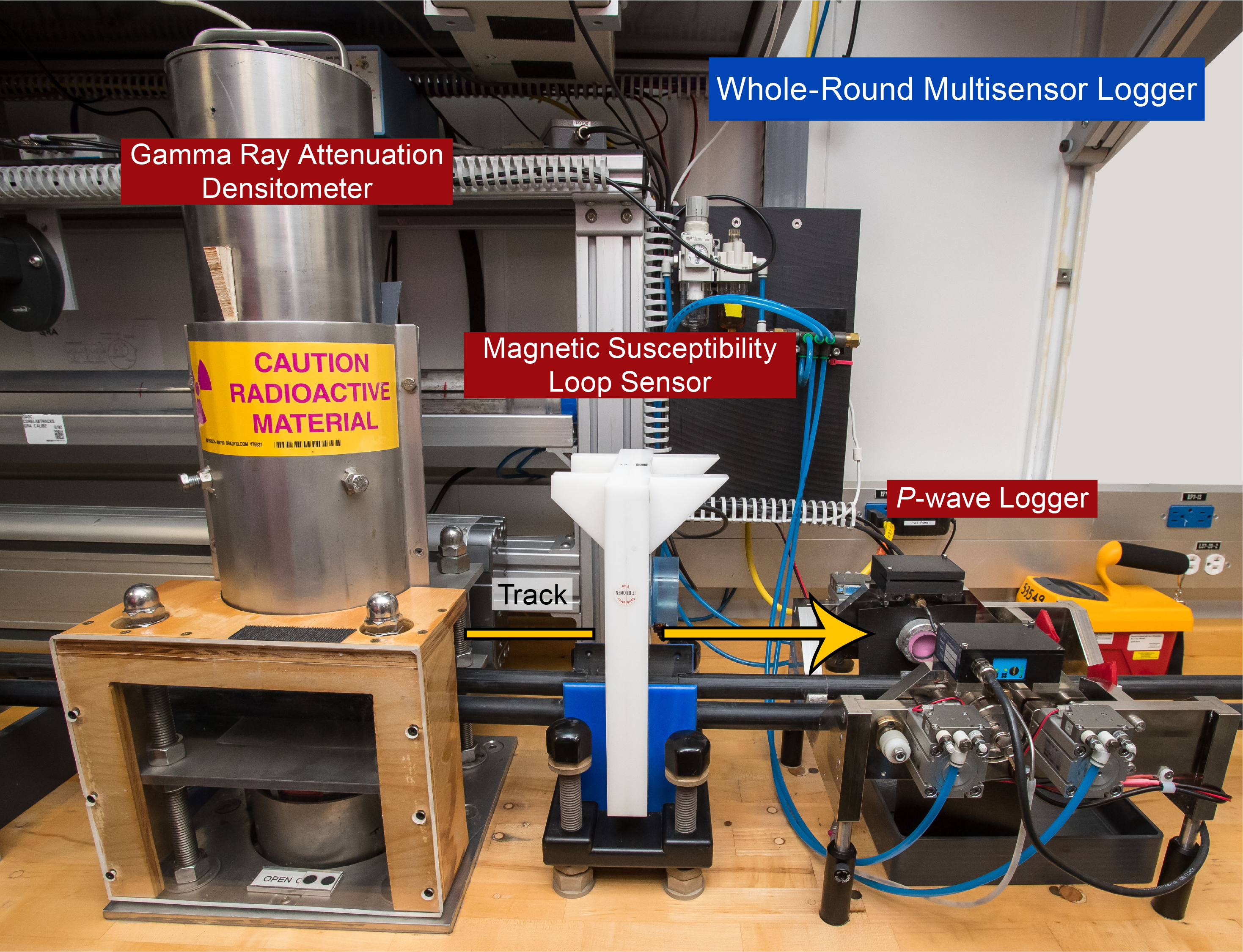
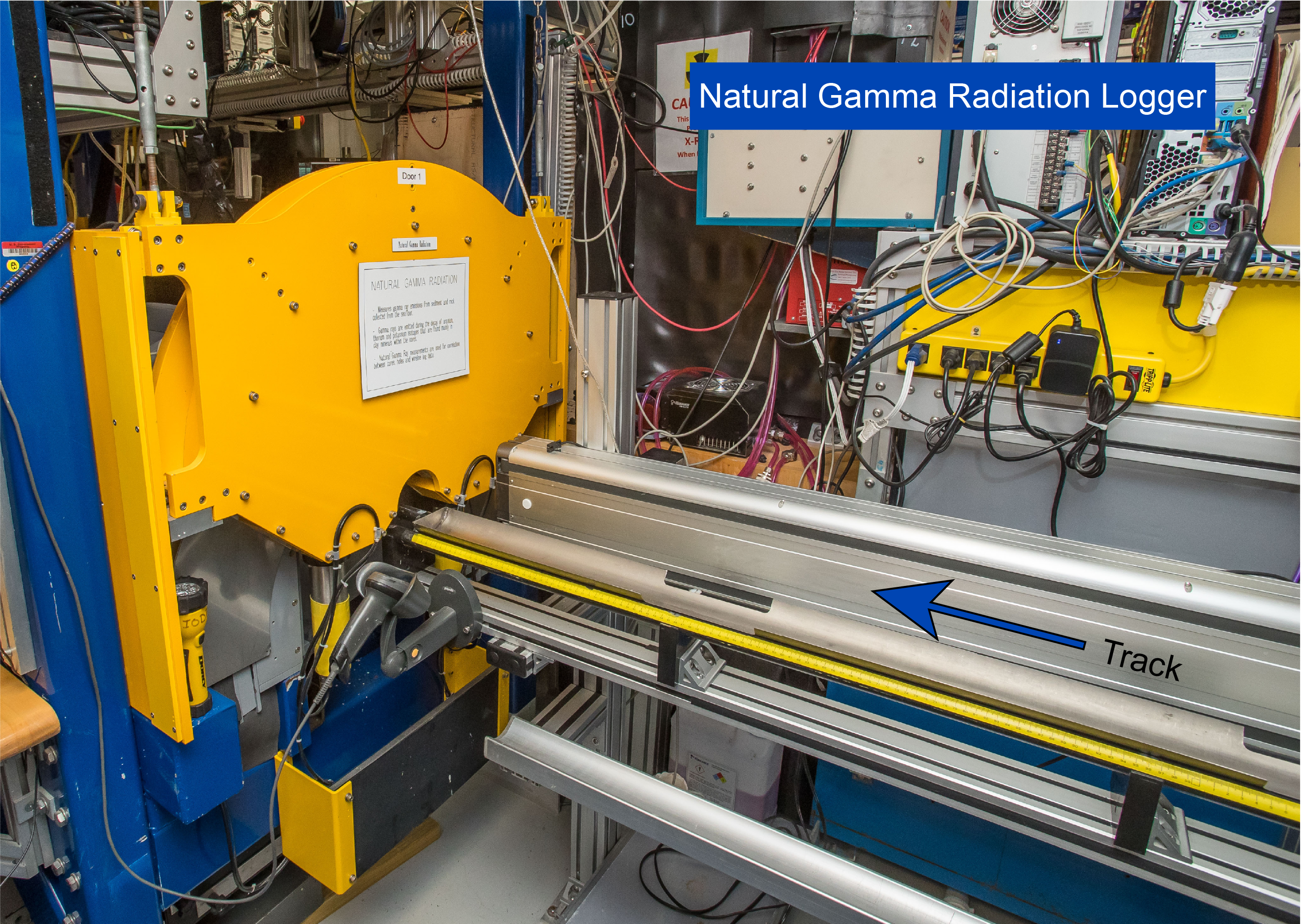
To optimize the measurement process, the same sampling intervals and measurement times were used for all sensors on each of the WRMSL instruments. These sampling intervals are common denominators of the distances between the sensors installed on the WRMSL (30–50 cm), which enables sequential and simultaneous measurements. For the WRMSL, the sampling interval was 2.0 cm with an integration time of 3 s for each measurement. A QC measurement was performed after every core by passing a single core liner filled with deionized water through the WRMSL. If deviations from expected values were observed, a recalibration procedure was performed.

11.1.2.1. Gamma ray attenuation bulk density

The bulk density of a sample can be used to estimate the pore volume of the sample and to evaluate the consolidation state of sedimentary material. GRA provides a means to estimate material bulk density based on the attenuation of a gamma ray beam. The beam is produced by a ¹³⁷Cs gamma ray source at a radiation level of 370 MBq within a lead shield with a 5 mm collimator that is vertically directed through the whole-round core (Figure F25). The gamma ray receiver consists of a 75 mm³ sodium iodine (NaI) detector located on the upper side of the core, opposite to the source, that records the gamma radiation that passes through the core. The input gamma ray peak has a principal energy of 0.662 MeV and is attenuated as it passes through the core.

The attenuation of gamma rays occurs primarily by Compton scattering, in which gamma rays are scattered by electrons in the formation, and the degree of scattering is related to the material bulk density. Therefore, for a known thickness of sample, density (ρ) is proportional to the measured intensity of the attenuated gamma rays (Harms and Choquette, 1965):

ρ=ln⁡I0/I/μd, (22)

where

• I = the measured intensity of gamma rays passing through the sample,
• I₀ = gamma ray source intensity,
• μ = Compton attenuation coefficient, and
• d = sample diameter.
• Note: μ and I₀ are treated as constants so ρ can be calculated from I.

In general, WRMSL measurements are most accurate when taken on a completely filled core liner with minimal drilling disturbance; otherwise, measurements tend to underestimate true values. By default, the instrument reports measurements using the internal diameter of the core liner (66 mm) as the assumed sample diameter. This assumption is suitable for most sediment cores obtained using the APC system. However, for sediment and/or hard rock cored using the XCB or RCB system, core diameter is usually about 58 mm or smaller. Following Jarrard and Kerneklian (2007), the density measurements of cores obtained using the XCB or RCB systems may be corrected by multiplying the density values by 66/58 = 1.138 to account for this bias. We chose not to correct the raw values, but the offset is mentioned in the description of the measurements.

The spatial resolution of the GRA densitometer is <1 cm. The gamma ray detector is calibrated with a sealed calibration core consisting of one standard core liner filled with distilled water and a telescoped aluminum bar machined into discrete diameter steps of various diameters located at the top of the core. To establish the calibration curves, gamma ray counts were taken through each of the discrete diameter steps for 60 s. Recalibration was performed whenever the deionized water QC standard deviated significantly (1.00 ± 0.02 g/cm³).

11.1.2.2. Magnetic susceptibility

MS is measured on whole-round core sections using a pass-through loop on the WRMSL (Figure F25). MS (χ) is a dimensionless measure of the degree to which a material can be magnetized by an external magnetic field:

χ=M/H, (23)

where M is the magnetization induced in the material by an external field of strength H.

MS measurements were made using a Bartington MS2C loop sensor with an 88 mm diameter (Bartington Instruments, 2011). An oscillator circuit in the sensor operating at a frequency of 0.565 kHz produces a low-intensity (250 μT), nonsaturating alternating magnetic field within the loop that has a strength proportional to the magnetic permeability within the loop. Sediment or hard rock core sections passing through the loop represent a change in permeability and thus cause a change in the induced field that can be measured as a change in oscillator frequency. Frequency information returned in pulse form to the susceptometer provides a direct estimate of the core material’s magnetic permeability, which is converted into MS. The loop sensor has a spatial resolution of 20 mm and is accurate to within 5%. MS is reported in instrument units. To convert results into dimensionless units, it is necessary to multiply the data by a correction factor that is a function of the probe type, core diameter, and loop size. The sizes of small rock pieces in incomplete cores vary, so application of a single correction factor is not justified; therefore no correction is applied to the WRMSL MS data. This conversion factor does not change the order of magnitude of the measured susceptibility values, so the results are comparable with the susceptibility measured by the paleomagnetism group with the same physical units (SI).

The along-core response curve of the MS2C coil has a full width at half maximum of ~4 cm (Blum, 1997) and is consistent with the decay in magnetic intensity with distance from a dipole. Therefore, measurements of susceptibility from core pieces <8 cm long will significantly (>10%) underestimate MS. MS data recorded on the WRMSL must therefore be interpreted with reference to breaks and variable diameters of fragmented cores; this information can be obtained from the 360° photo imaging record.

MS varies with the type and concentration of magnetic grains, such as the ferromagnetic minerals (e.g., magnetite and maghemite), making it useful for identifying compositional variations. MS responds to variations in the magnetic composition of cored materials that are commonly related to variations in mineralogic composition (e.g., terrigenous versus biogenic materials) and diagenetic overprinting. Paramagnetic materials such as clay generally have MS that is several orders of magnitude lower than ferromagnetic minerals, which are common constituents of igneous material. Diamagnetic minerals such as calcite, aragonite, and opal, as well as water and plastics (such as the core liner), have a slightly negative MS. Thus, calcareous and siliceous biogenic deposits with very small amounts of clay and iron-bearing minerals have values approaching the detection limit of the MS meters.

11.1.2.3. Sonic velocity

P-wave velocity data can be used to evaluate small-strain elastic moduli, porosity, compaction, and cementation. P-wave velocity is the rate at which a compressional seismic wave travels through a medium, expressed in meters per second. P-wave velocity is dependent on the composition, porosity, bulk density, fabric, and temperature of the material, which in turn are functions of consolidation and lithification, state of stress, and degree of fracturing. P-wave velocity (V_P) of a homogeneous, isotropic material can be defined by the time required for a compressional wave to travel a specific distance:

VP=d/tcore, (24)

where, for the case of a drill core, d is the path length of the wave across the core and t_core is the traveltime through the core.

The PWL on the WRMSL transmits a 500 kHz P-wave pulse across the core liner at a specified repetition rate (Figure F25). The pulse transmitter and receiver are mounted on a caliper-type device and are aligned to make wave propagation perpendicular to the section’s long axis. A linear variable differential transducer measures the P-wave travel distance between the pulse source and the receiver. Good coupling between transducers and the core liner is facilitated with water dripping onto the contact from a peristaltic water pump system. Signal-processing software picks the first arrival of the wave at the receiver, and the processing routine corrects for the thickness of the liner. The total observed traveltime (t_o) is composed of

• t_delay = time delay related to transducer faces and electronic circuitry,
• t_pulse = delay related to the peak detection procedure,
• t_liner = transit time through the core liner, and
• t_core = traveltime through the cored material,

with the traveltime through the core expressed as

tcore=to-tpulse-tdelay-2tliner. (25)

The system is calibrated using a core liner filled with distilled water, which provides control for t_delay, t_pulse, and t_liner. From these calibrations, V_P can be calculated for the whole-round core in liners as

Vp=dcl-2dliner/tcore, (26)

where

• d_cl = measured diameter of core and liner,
• d_liner = liner wall thickness.

This equation assumes that the core completely fills the core liner. Measurements of V_P made with the PWL when the core liner is not completely filled, and thus contains air-filled gaps, are not useful. Most cores recovered with the XCB and RCB systems do not fill the core liner and are thus not considered useful.

A series of acrylic cylinders of varying thicknesses are used to calibrate the PWL system. The regression of traveltime versus travel distance yields the P-wave velocity of the standard material, which should be 2750 ± 20 m/s. The thickness of the calibration samples, corrected for liner thickness, are divided by the traveltime to calculate P-wave velocity in meters per second. The calibration is verified by measuring a core liner filled with pure water at room temperature, and the calibration passes if the velocity is within ± 20 m/s of the expected P-wave velocity of water at room temperature and 1 atm (1485 m/s).

11.1.2.4. Natural gamma radiation

Gamma radiation is emitted from the decay series of mineral-hosted 238-uranium (²³⁸U), 232-thorium (²³²Th), and 40-potassium (⁴⁰K). The system in use (Figure F26) was designed and built at the JOIDES Resolution Science Operator (JRSO) at Texas A&M University (USA) (Vasiliev et al., 2011). When ²³⁸U, ²³²Th, and ⁴⁰K radioisotopes decay, they and their daughter isotope products emit gamma radiation at specific energy levels unique to each isotope. NGR spectroscopy measures a wide energy spectrum that can be used to estimate the abundance of each isotope based on the strength of the signal at characteristic energies. Spectral data were collected and can be used for postexpedition processing to obtain U, Th, and K abundances, but they were not processed aboard the vessel. Total counts were used on board, and high counts usually identified fine-grained deposits containing K-rich clay minerals and their absorbed U and Th isotopes. NGR data thus reveal stratigraphic details that aid in core-to-core correlations. For example, in hard rocks, NGR measurements can yield information about the alteration and heat production of rocks (Dunlea et al., 2013) that is useful when correlating core measurements with downhole measurements of NGR (e.g., Révillon et al., 2002).

The main NGR detector unit consists of 8 NaI scintillator detectors arranged along the core-measurement axis at 20 cm intervals surrounding the section. The section is measured once and then moves 10 cm and is measured again every 10 cm to provide a final measurement spacing of 10 cm. The detector array has passive (layers of lead) and active (plastic scintillators) shielding to reduce background environmental and cosmic radiation. The overlying plastic scintillators detect incoming high-energy gamma and muon cosmic radiation and cancel this signal from the total counted by the NaI detectors. The NGRL was calibrated using ¹³⁷Cs and ⁶⁰Co sources to identify peaks at 662 and 1330 keV, respectively.

Total counts are routinely summed over the range of 100–3000 keV. The quality of the measured energy spectrum depends on the concentration of radionuclides in the sample and on the counting time, with longer counting times providing better counting statistics. A live counting time of 5 min was set in each position for a total live count time of about 10 min per section. Sections were scanned only once. Sections less than 50 cm long were not measured.

11.1.2.5. Thermal conductivity

Thermal conductivity (k) is the coefficient of proportionality relating conductive heat flow to a thermal gradient. It reflects the rate at which heat is conducted through a material and is dependent on saturating fluid types, porosity, bulk density, water content, temperature, composition and texture of the mineral phases, and so on. At steady state, thermal conductivity is the coefficient of heat transfer (q) across a steady-state temperature difference (ΔT) over a distance (Δx):

q=k(ΔT/Δx). (27)

Thermal conductivity measurements were attempted on the third section, or on a neighboring section if the third was unavailable. Measurements were performed on every core recovered from each drill site using the TeKa Berlin TK04 system described by Blum (1997) (Figure F27). For whole-round soft-recovery cores, a needle probe (number V10702) (Figure F27A, F27C) in full-space configuration (Von Herzen and Maxwell, 1959) was used, and for sedimentary and igneous rock split cores, a contact probe method in half-space configuration was used (Figure F27B–F27C). The probes contain a heater wire and calibrated thermistor.

For soft-sediment cores, the full-space needle probe (VLQ) was inserted into a 2 mm diameter hole drilled along one of the lines that later guided core splitting. The location was at around 60–70 cm from the top of the section or in an interval with low disturbance based on visual inspection. To avoid interference from air flow in the laboratory, the core was placed in an enclosed box insulated with foam (Figure F27A). For sedimentary and igneous rock cores, half-space determinations of thermal conductivity were made using standard half-space needle probe (HLQ) pucks (number H11017) and mini-HLQ pucks (number H51027). These pucks are recommended to be used on planar surfaces and consist of a Plexiglas block (k = 0.184 W/[m·K]) with a half-space needle probe embedded in its base. Heat is assumed to be transferred through the sample, and the TK04 system documentation indicates that heat flow through the Plexiglas block itself is only significant for samples with thermal conductivities <1 W/(m·K). The measurement was conducted in a polystyrene box that insulated the sample from the ambient air flow (Figure F27B).

All measurements were made at room temperature and pressure with no correction for in situ conditions. This system measures thermal conductivity by transient heating of the sample with a known heating power and geometry. Changes in temperature with time during heating are recorded and used to calculate thermal conductivity. Heating power can be adjusted for each sample depending on the type of probe used; heating power can be varied from 1 to 1.6 W/m for a standard puck and from 0.5 to 1.2 W/m for a mini-puck. For most samples, a heating power of 1.2 W/m for a standard puck and 0.8 W/m for a mini-puck was used. For the full-space needle probe, a heating power of 0.5–2.0 W/m was typically used in soft-sediment cores.

The solution to the heat-conduction equation for a line source of heat was fitted to the temperature measurements to obtain the thermal conductivity. Because the probe is much more conductive than sedimentary or igneous rock, the probe is assumed to be a perfect conductor. Under this assumption, the temperature of the probe has a linear relationship with the natural logarithm of the time after the initiation of the heat. The TK04 device uses a special approximation method to calculate conductivity and to assess the fit of the heating curve. This method fits discrete windows to the theoretical function of temperature (T) with time (t) for a continuously heated line source (Kristiansen, 1982):

Tt=A1+A2 lnt+A3lnt/t+A4/t, (28)

where A1−A4 are constants that are calculated by linear regression. A1, A3, and A4 are related to the sample geometry and the material properties surrounding the needle probe, and A2 is related to its heating power and thermal conductivity. Having determined these constants (and how well they fit the data), the apparent conductivity (ka) for the fitted curve is time dependent:

kat = Q/4π+A1+A31-lnt/t - A4/t, (29)

where Q is the input heat flux. The maximum value of ka and the time (t_max) at which it occurs on the fitted curve are used to assess the validity of that time window for calculating the thermal conductivity. The best solutions are those where t_max is greatest, and these solutions are selected for use. Data are considered good if ka has a maximum value, t_max is large, and the standard deviation of the least-squares fit is low.

Three measuring cycles separated by a cooling interval of 10 min were automatically performed to calculate average conductivity. A self-test, which included a drift study, was conducted at the beginning of each measurement cycle. Once the probe temperature stabilized, the heater circuit was closed and the temperature rise in the probe was recorded. The measurement apparatus was evaluated frequently by measuring the thermal conductivity of a certified ceramic standard (k = 1.626 W/[m·K]). For measurement of the ceramic standard, the half-space standard puck or mini-puck was coated in silicone thermal contact gel and then placed on the standard; if the measured thermal conductivity was within 2% of the known value, then the puck was used for sample measurements. After the standard and prior to sample measurement, the silicone gel was thoroughly removed from the puck to avoid potential geochemical contamination of the core material. Conductivity measurements are reported in watts per meter degree Kelvin (W/[m·K]).

11.1.3. Section half logging and discrete measurements

Here we describe measurements made on split sections and discrete samples, including color reflectance spectrophotometry, MSP, rheology, seismic velocity, and MAD.

Color reflectance spectrophotometry and MSP of the archive section halves were measured with the SHMSL (Figure F28). MSP measurements were made using a Bartington Instruments MS2E point sensor (high-resolution surface-scanning sensor) (see Paleomagnetism). Measurement resolution is 1.0 SI, and each measurement integrated a volume of 10.5 mm × 3.8 mm × 4 mm, where 10.5 mm is the length perpendicular to the core axis, 3.8 mm is the width along the core axis, and 4 mm is the depth into the core. Three measurements were made at each measurement position.

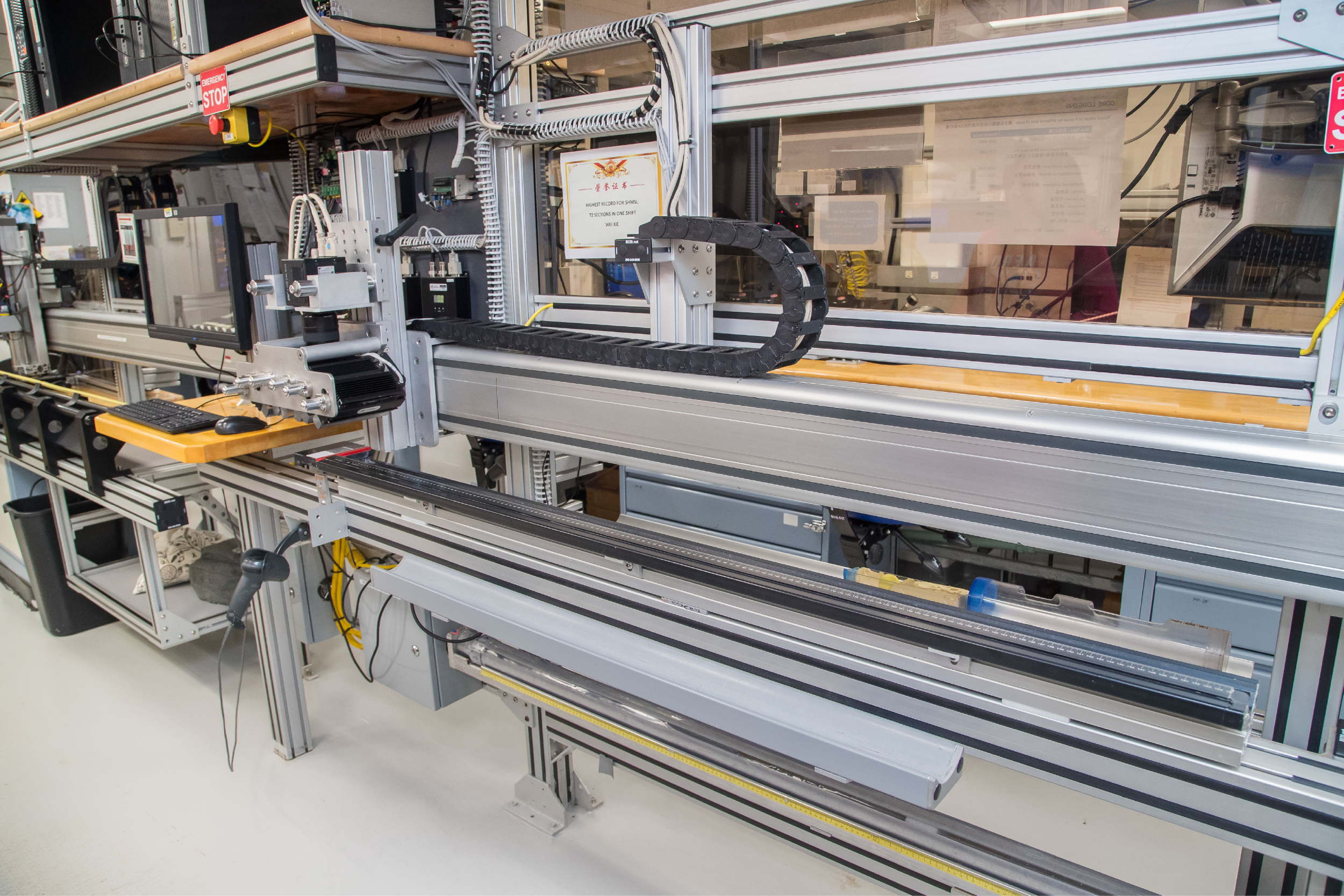
Thermal conductivity was measured once per core on hard rock pieces using a contact probe on a piece of section half in a bath of seawater for igneous rock pieces (Figure F27B–F27C). Samples from igneous rock material were shared for both paleomagnetic and MAD measurements; P-wave velocity measurements were also made on these discrete samples.

For core-section halves from Holes A and B at each site, a MAD sample was collected from the bottom of the section where a headspace analysis of hydrocarbon gases was taken previously with a syringe in the splitting room. One section half per core was then selected according to its sedimentological characteristics to perform the discrete P-wave velocity, shear strength (automated vane shear [AVS]), and compressive strength (pocket penetrometer) measurements, and other sections were used for discrete paleomagnetic measurements. Finally, all sections were processed using the SHMSL, paleomagnetism (logging), and X-ray imaging upon request from lithostratigraphy and structural groups.

11.1.3.1. Color reflectance spectrometry

Reflectance of visible light from the archive halves of sediment cores was measured using an Ocean Optics USB4000 spectrophotometer mounted on the automated SHMSL (Figure F28). Because the SHMSL demands flush contact between the MS2E point sensor and the split core, measurements were made on the archive halves of split cores, which were covered with clear plastic wrap after all visual core description, smear slide sampling, and X-ray image analyses were completed (see Lithostratigraphy). Measurements were taken at 2.5 cm spacing to provide a high-resolution stratigraphic record of color variation for visible wavelengths. Empty intervals, voids, and cracks were skipped to avoid spurious measurements. Intervals where the top of the flat surface was below the level of the core liner were lifted using foam or putty to ensure proper measurements. Each measurement was recorded in 2 nm wide spectral bands from 400 to 700 nm. Data are converted to L*, a*, and b* and X, Y, and Z color reflectance parameters for efficient archival and display. Both zero and white calibrations were conducted before measurement on each core. Additional detailed information about measurement and interpretation of spectral data can be found in Balsam et al. (1997, 1998) and Balsam and Damuth (2000). In addition to a digital color image captured by the SHIL, the VCDs include a description of sediment color and the corresponding hue, value, and chroma data as determined qualitatively using Munsell Soil Color Charts for each major and minor lithology (Munsell Color Company, 2000, 2009). Further details are described in Lithostratigraphy.

11.1.3.2. Point magnetic susceptibility

MSP is measured on the SHMSL using a Bartington MS2E contact probe with a flat 15 mm diameter sensor operating at a frequency of 0.580 kHz. The instrument takes and averages three measurements made at 1 s intervals to an accuracy of 5%. The area of response of the MS2E sensor is 3.8 mm × 10.5 mm, with a depth response of 50% at 1 mm and 10% at 3.5 mm (Bartington Instruments, Ltd., 2011). The MSP measurements made on section halves using the SHMSL therefore have a higher spatial resolution than MS measured by WRMSL on whole-round cores. The probe is zeroed in air before each measurement is made, and a background magnetic field is measured and removed from the data. Measurements are output in instrument units but reported in SI (see Magnetic susceptibility). MSP measurements were conducted at a resolution of 2.5 cm for sediment sections and 1 cm for igneous sections. Note that bulk MS data were also collected for discrete cubes taken from working section halves during analyses of anisotropic magnetic susceptibility (see Paleomagnetism).

11.1.3.3. Moisture and density measurements

MAD analyses on working halves were conducted on unconsolidated materials, ~10 cm³ samples taken with plastic syringes or spatulas for analyses. Preweighed and numbered 16 mL Wheaton glass vials were used to process and store the samples. When a lithologic variation could be observed within a single core, two MAD samples were collected. However, in most cases one sample per core for Holes A and B was collected near the sampling location for headspace analyses of hydrocarbon gases (bottom or top of a given section, see Organic geochemistry). For sedimentary and igneous rock material, the discrete cubes initially used for paleomagnetism and P-wave velocity (P-wave caliper) measurements were also used for MAD analyses whenever possible.

Mass and volume measurements were made to determine wet and dry bulk density, grain density, water content, and porosity. After measurement of wet mass, samples were dried in a convection oven for at least 24 h at 105° ± 5°C. Dried samples were then cooled in a desiccator for at least 1 h before the dry mass and volume were measured.

The procedure for igneous rocks included saturation with seawater for 12 h before the wet mass weight measurement was carried out.

Dual balance system

The weights of wet- and dry-sample masses were determined to a precision of 0.005 g using two Mettler Toledo (XS204) electronic balances and a computer averaging system to compensate for the ship’s motion (Figure F29). A standard weight, with mass comparable to the sample’s (maximum = >10% of the sample mass), was placed on a reference balance to increase accuracy. The default setting of the balances is 300 measurements. After wet mass determinations and P-wave measurements (for cube samples), samples were placed in the drying oven (24 h) and then allowed to cool in the desiccator (1 h) prior to the determination of dry masses.

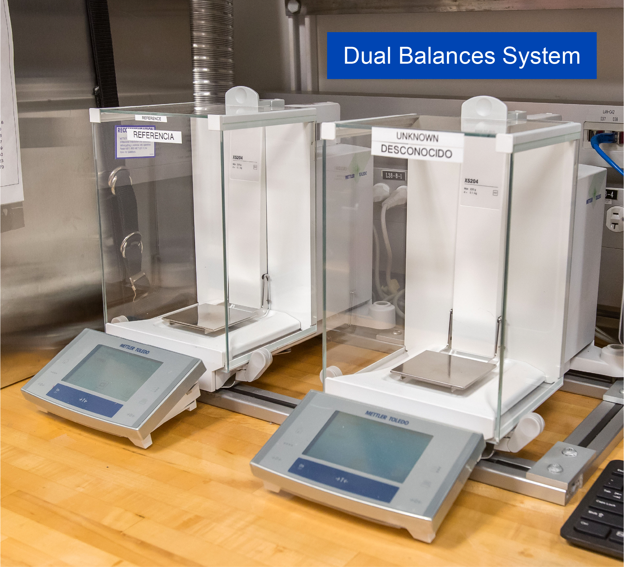
Hexapycnometer volume measurement

Dry sample volume was determined using the hexapycnometer system of a six-celled, custom-configured Micromeritics AccuPyc 1330TC helium-displacement pycnometer (Figure F30). The system measures dry sample volume using pressurized He-filled chambers; the precision of each cell is within 1% of the full-scale volume when properly calibrated and operated. Volume measurements were preceded by three purges of the sample chamber with helium. For each measurement, five unknown cells and one cell that contained two stainless steel calibration spheres (3 and 7 cm³) with a total volume of ~10 cm³ were run. Calibration spheres were cycled through the cells to identify any systematic error and/or instrument drift. Spheres are assumed known to within 1% of their total volume. The volumes occupied by the numbered Wheaton vials were calculated before the expedition by multiplying each vial’s weight against the average density of the vial glass. The procedures for the determination of these physical properties comply with the American Society for Testing and Materials (ASTM International, 1990).

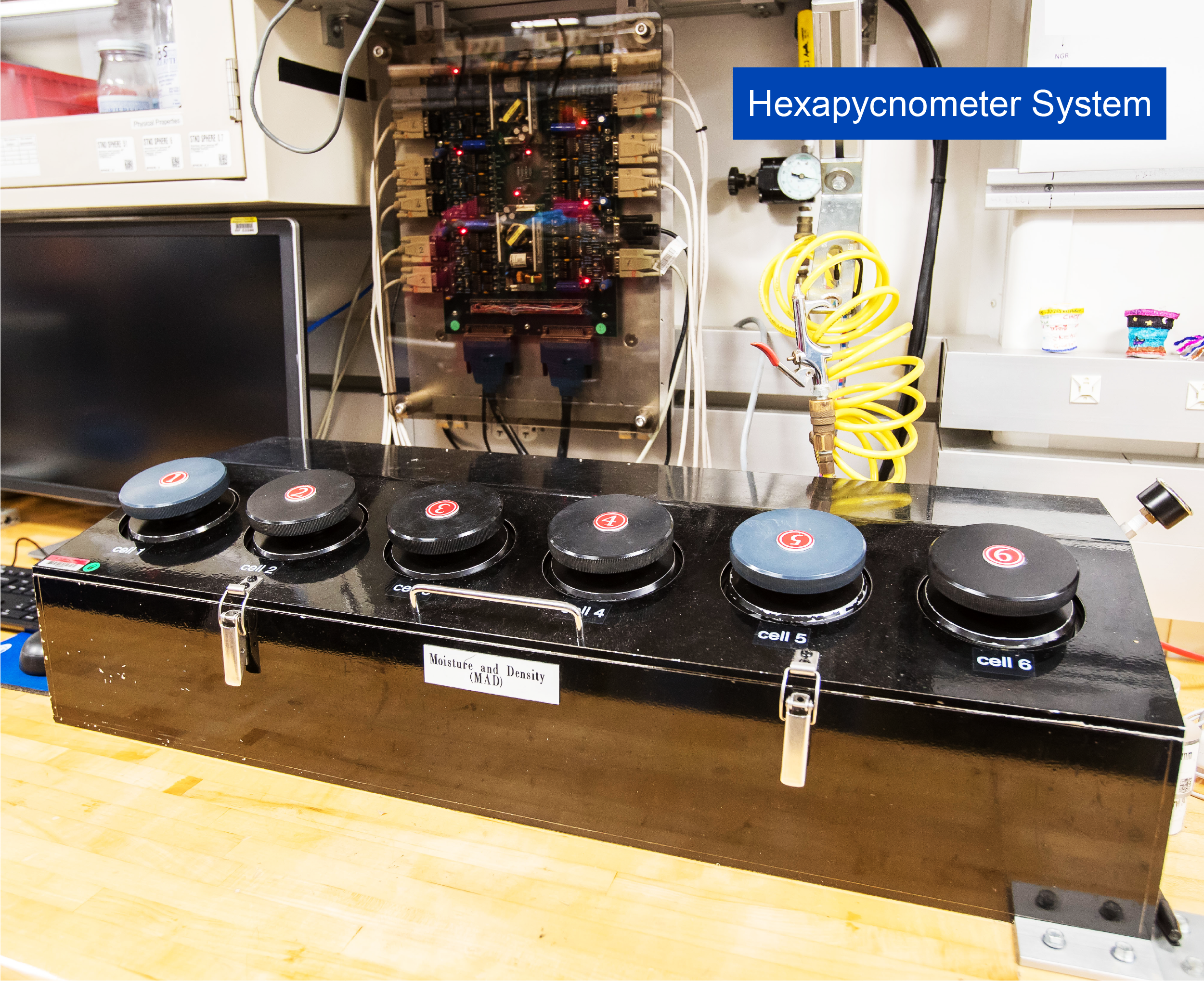
Moisture and density calculations

The calculations given below are used as an IODP standard in accordance with Blum (1997). MAD properties reported and plotted in the Physical properties section of each site chapter were calculated with the MADMax shipboard program using the method applicable to saturated, fine-grained sediments called “Method C.” Method C is based on the measurement of wet mass (M_wet), dry mass (M_dry), and dry volume (V_dry). The ratio of mass (rm) is a computational constant of 0.965 (i.e., 0.965 g of freshwater per 1 g of seawater). Salt precipitated in pores in the samples during the drying process is included in the M_dry and V_dry values. The mass of the evaporated water (M_water) and salt (M_salt) in the sample are given by

Mwater=Mwet-Mdry and (30)

Msalt=Mwaters/1-s, (31)

where s is the assumed saltwater salinity (0.035) corresponding to pore water density (ρ_pw) of 1.024 g/cm³ and a salt density (ρ_salt) of 2.22 g/cm³. The corrected mass of pore water (M_pw), volume of pore water (V_pw), mass of solids excluding salt (M_solid), volume of salt (V_salt), volume of solids excluding salt (V_solid), and wet volume (V_wet) are

Mpw=Mwet-Mdry/rm, (32)

Vpw=Mpw/ρpw, (33)

Msolid=Mwet-Mpw, (34)

Msalt=Mpw-Mwet-Mdry, (35)

Vsalt=Msalt/ρsalt, (36)

Vwet=Vdry-Vsalt+Vpw, and (37)

Vsolid=Vwet-Vpw. (38)

For all samples, water content (w) is expressed as the ratio of mass of pore water to wet sample (total) mass:

w=Mpw/Mwet. (39)

Wet bulk density (ρ_wet), dry bulk density (ρ_dry), sample grain density (ρ_solid), porosity (φ), and void ratio (V_R) are calculated as

ρwet=Mwet/Vwet, (40)

ρdry=Msolid/Vwet, (41)

ρsolid=Msolid/Vsolid, (42)

ϕ=Vpw/Vwet, and (43)

VR=Vpw/Vsolid. (44)

Precision and accuracy of MAD measurements are ~0.5%, although accuracy can vary with sediment type. The largest sources of potential error are the loss of material or change in moisture during the ~30–48 h procedure for each sample.

11.1.3.4. Rheology

Rheology measurements provide constraints on the finite-strain deformation of material under stress. The mode of deformation (e.g., viscous, plastic, or brittle) can vary considerably in sediments. The shear strength of relatively soft sedimentary materials can be characterized by two separate complementary measurements. The pocket penetrometer (PEN) is an unconfined compression strength test, and the vane shear strength (AVS) test is an undrained shear strength test. Both measurements quantify the effective shear strength of the material by applying known compressive and shear stress, respectively. The undrained condition specific to the AVS test implies that the quantified shear strength is the effective shear strength, which corresponds to the applied stress minus the intergranular pore fluid pressure:

σ′m=σm-Pf, (45)

where

σm=σ1-σ3/2. (46)

However, in practice, we observe that both tests in laboratory conditions aboard JOIDES Resolution do not really prevent the pore fluid from draining during the experiments. This is confirmed by the fact that both measurements consistently overlap whenever the measurements are reliable (see detail below). We therefore consider that both tests actually provide a measure of the shear strength (σ_m).

Note that the unconfined condition for the PEN measurement implies that loosely compacted sediments do not provide reliable values for the first drilled 50 m of sediment. However, the depth limit of the measurement capability for the PEN test is slightly greater than the AVS. AVS test measurements are not possible whenever the compressive strength is above ~250 kPa. Depending on the site, this translates to a depth of 150–300 mbsf. PEN measurements typically extend this maximum depth an additional 50 m.

Pocket penetrometer

Compressive strength was measured on every core with a pocket penetrometer (Figure F31). The yield envelope of a material can be defined as the maximum principal stress difference prior to failure (or maximum differential stress). This value is the same as the unconfined compressive strength of the material, that is, Δσ_f = (σ₁–σ₃). At prescribed stress, the shear strength of a material or yield (τ_f) is related to the compressive strength (Δσ_f) by

τf=Δσf/2. (47)

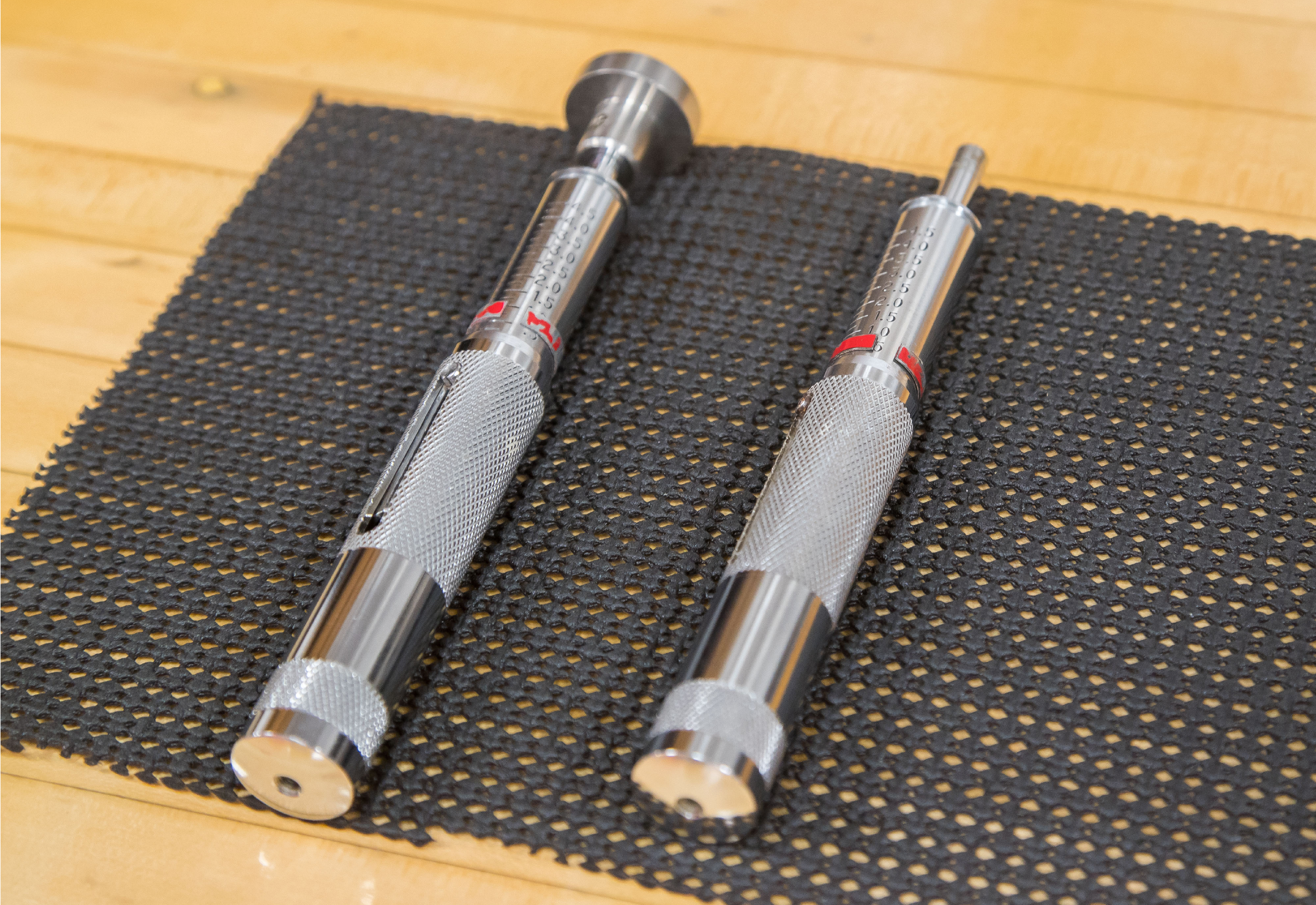
To obtain the shear strength, values read directly from the pocket penetrometer are divided by 2. The penetrometer is a flat-footed, spring-operated device (Figure F31) used to measure compressive strength by pushing a 6.4 mm (0.25 inch) diameter probe 6.4 mm (0.25 inch) deep (to the red marker) below the split-core surface. The selected probe location must be placed where surfaces are smooth. The mechanical scale is in kilograms per square centimeter, and data uploaded to the LIMS database are in these units. Conversion from kg/cm² to kPa is as follows:

2τf kPa=98.1×2τf kg/cm2. (48)

The maximum shear strength value measurable by the pocket penetrometer is 4.5 kg/cm².

A 2.54 cm (1 inch) adapter foot was available for measuring very soft sediments, providing a 16× increase in piston area. An allen wrench was used to adjust the set screw that holds the foot to the piston. When used, the reading obtained with the added foot adapter must be multiplied by ¹⁄₁₆ (0.0625).

Vane shear strength

The shear strength of a material describes the point at which the material yields (i.e., permanently deforms) in response to an applied shear stress. In contrast to the PEN experiment, the AVS theoretically provides a direct measurement of the effective shear stress at yield or shear strength (σ′_m) of the recovered sediment. The Giesa system is suited for measuring the shear strength of very soft to relatively stiff marine sediments (Figure F32). This geotechnical test is useful for determining the undrained strength of undisturbed clay- or silt-rich samples.

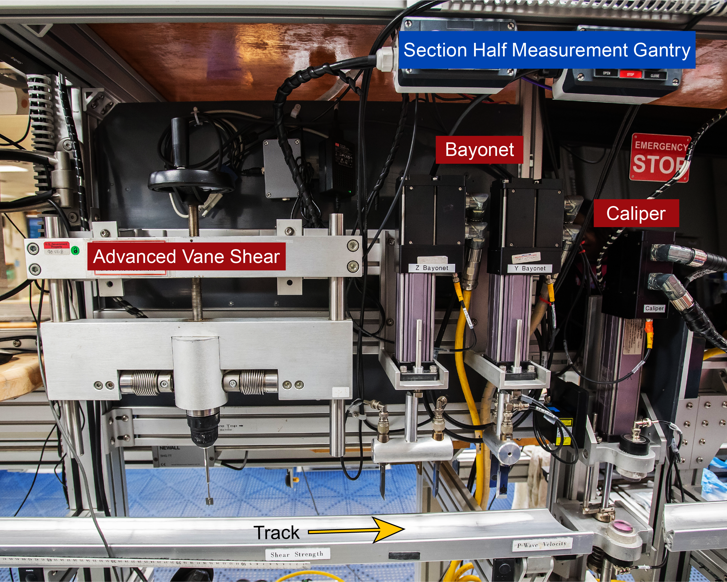
The Giesa system consists of a controller and a gantry for shear vane insertion. A four-bladed miniature vane was pushed carefully into the sediment of the working halves until the top of the vane was level with the core surface. The vane was then rotated at a constant rate of 60°/min to determine the torque required to cause the core material to shear (failure torque). All vane shear strength measurements were obtained using a 12.7 mm vane. Failure torque was determined by measuring the rotation of a torsional spring using a spring-specific relation between rotation angle and torque.

Vane shear strength (Su[V]) can be determined as follows:

SuV=T/Kv=Δ/B/Kv, (49)

where

• T = torque required to induce material failure (N·m),
• Kv = constant, depending on vane dimensions (m³),
• Δ = maximum torque angle (°) at failure, and
• B = spring constant that relates the deflection angle to the torque (°/N·m) (Blum, 1997).

We performed one measurement per core section until the recovered material became too stiff for vane insertion. Measurements were conducted in regions considered to be the most representative of the core lithology.

11.1.3.5. Discrete P-wave velocity

Discrete P-wave velocity was measured on every core using Panametrics-NDT Microscan delay line transducers transmitting at 0.5 MHz (Figure F32). The signal received through the section half or discrete sample was recorded by the Velocity Gantry 2.0.5.0 IODP software, where the peak of the first P-wave arrival is automatically or manually chosen. In case of a weak signal, manual picking of the first arrival was performed.

The distance between transducers was measured with a built-in linear voltage displacement transformer (LVDT). Calibration was performed daily with a series of acrylic cylinders of differing thicknesses and a known P-wave velocity of 2750 ± 20 m/s. The system time delay determined from calibration was subtracted from the picked arrival time to give a traveltime of the P-wave through the sample. The thickness of the sample (calculated by the LVDT, in meters) was divided by the traveltime (in seconds) to calculate P-wave velocity in meters per second. A clean first P-wave arrival can be difficult to pick depending on the material. Measurement attempts were conducted once per core.

For soft sediment cores, P-wave velocity measurements were performed on the working half before any sampling. Following standard IODP conventions, P-wave velocity measurements used the x-, y-, and z-axis of the SHMG and completed one analysis per core. Different positions with respect to lithology were chosen to generate viable data. Measurements of rock cube samples were conducted after orienting the sample (Blum, 1997) and placing it on a gantry that measures P-wave velocity in three orthogonal directions (x-, y-, and z-directions). P-wave anisotropy ratios were calculated from these multidirectional analyses.

11.1.4. Data cleaning procedure

Data acquired using automatic systems such as the WRMSL, NGR, and SHMSL (e.g., MSP) typically contained outliers that had to be removed. Most of these outliers are due to cracks or voids in core material that formed in response to volume expansion due to the change in confining pressure for recovered cores. Void formation was most dramatic when dissolved gases were exsolved due to this pressure change, which was common. Void gas volume and composition were measured at each site during this expedition and are documented in the organic geochemistry site reports. The measured value of a given physical property for any gas is typically orders of magnitude different from that property measured for any solid or fluid-saturated sediment. Cracks and voids formed through volume expansion are, by definition, not representative of in situ conditions, but aberrant measured physical property values can easily be recognized and removed by setting an expected value range for that property consistent with gas-free core material.

All the measurements conducted on instruments with automated core or section scanning may return aberrant values at the beginning and end of each section due to the proximity of the section end (i.e., void or plastic end caps of the core liners). Thus, our data-cleaning procedure removes the first two points near the beginning and end of each core section. Figure F33 shows an example of the overall application of the cleaning procedure on the measured GRA density from the WRMSL.

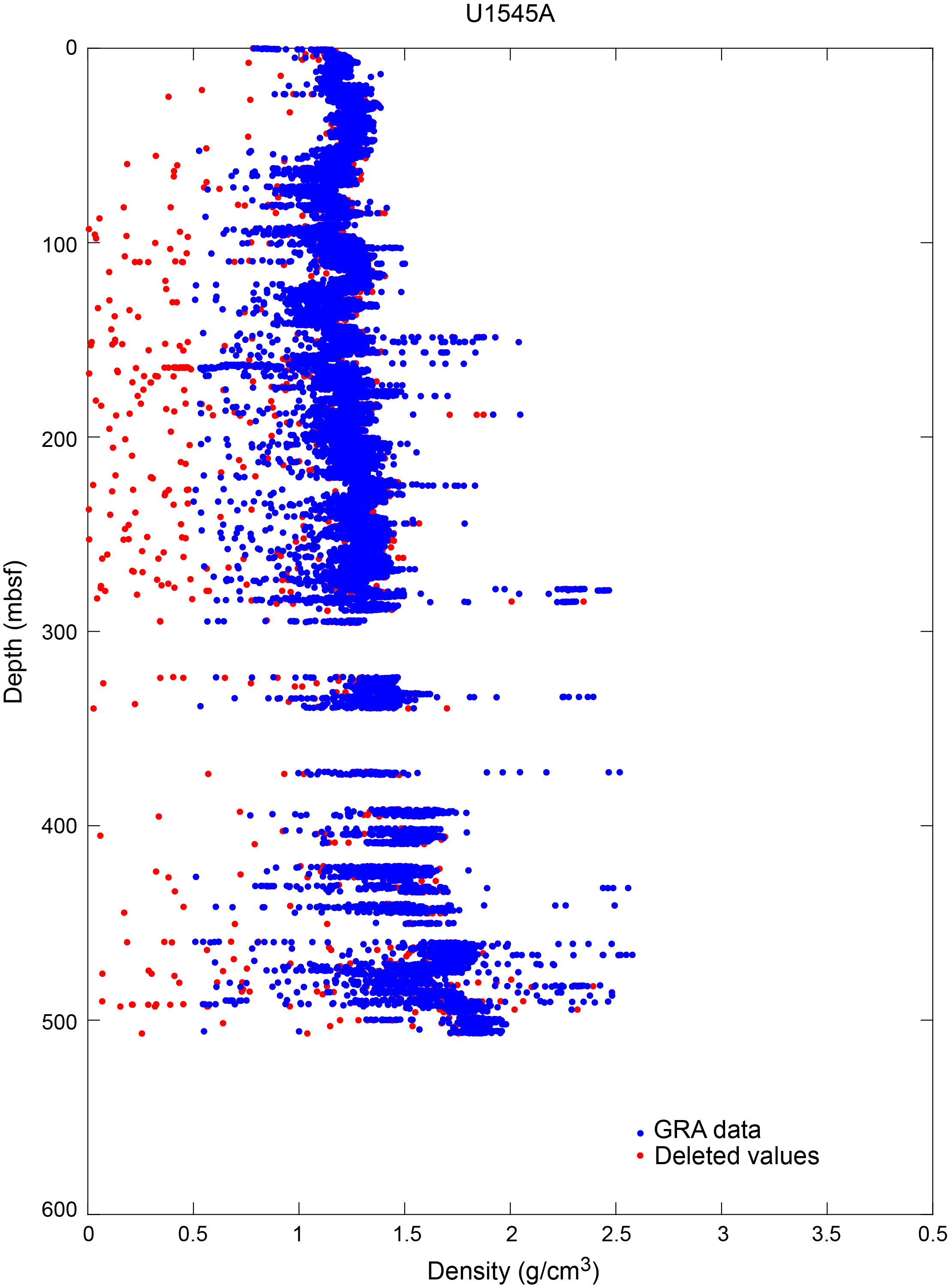
11.1.5. Core laboratory measurement summary

The WRMSL was used to measure GRA bulk density, MS, and P-wave velocity at 2 cm spacing. NGR was measured on whole-round core sections with the NGRL at 10 cm spacing (Table T17). Thermal conductivity was measured every 10 m when possible. Depending on the nature of the recovered material, we measured thermal conductivity on whole-round sections for soft sediment and on working-half sections for indurated sediment and igneous rock. MSP measurements were made every 2.5 cm for sediment sections and 1 cm for igneous sections.

MAD measurements were conducted on samples collected every 20 m on standard holes (usually Hole A) and at every 10 m in coordination with headspace samples for hydrocarbon gas analysis (usually Hole B) (see Organic geochemistry). These MAD measurements were used to calculate wet bulk density, dry bulk density, sediment grain density, porosity, and void ratio. Rheological measurements (i.e., shear and compressive strength) were measured at discrete offsets on section halves to characterize the average rheological properties of the material. These measurements were only possible on soft to moderately indurated sediments at an intended spacing of 10 m. Discrete P-wave velocity was measured with the SHMG using the caliper for measurements through the split core and bayonets inserted into the sediment for measurements along and across the core. Rock cube samples collected on igneous material, in collaboration with the Paleomagnetism group, were measured through a specific discrete measurement procedure in three orthogonal directions. These cubes went through a special MAD procedure (see Moisture and density measurements) before being passed to the Paleomagnetism group for further analyses (Table T17).

11.2. Downhole measurements

A range of in situ physical properties and state measurements, collectively referred to as downhole measurements, were made using tools either attached to the BHA during drilling or lowered into the borehole on a conducting wireline after drilling. In situ downhole temperature measurements were acquired using the APCT-3 (Figure F34) and SET2 tools (Figure F35). These temperature measurements were conducted at all sites (see Temperature measurements; Table T18).

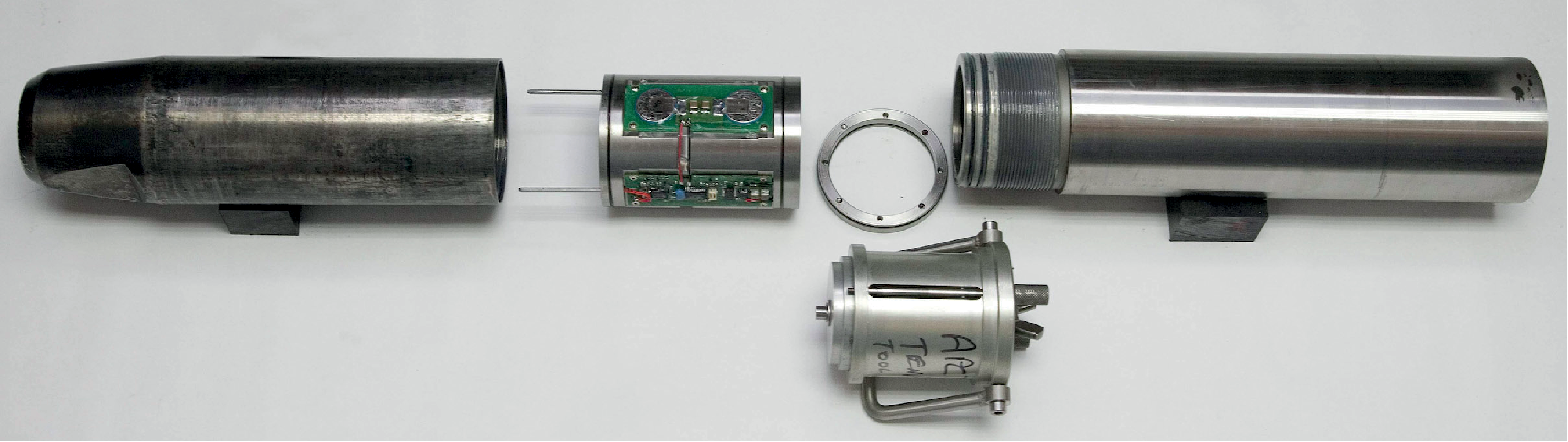
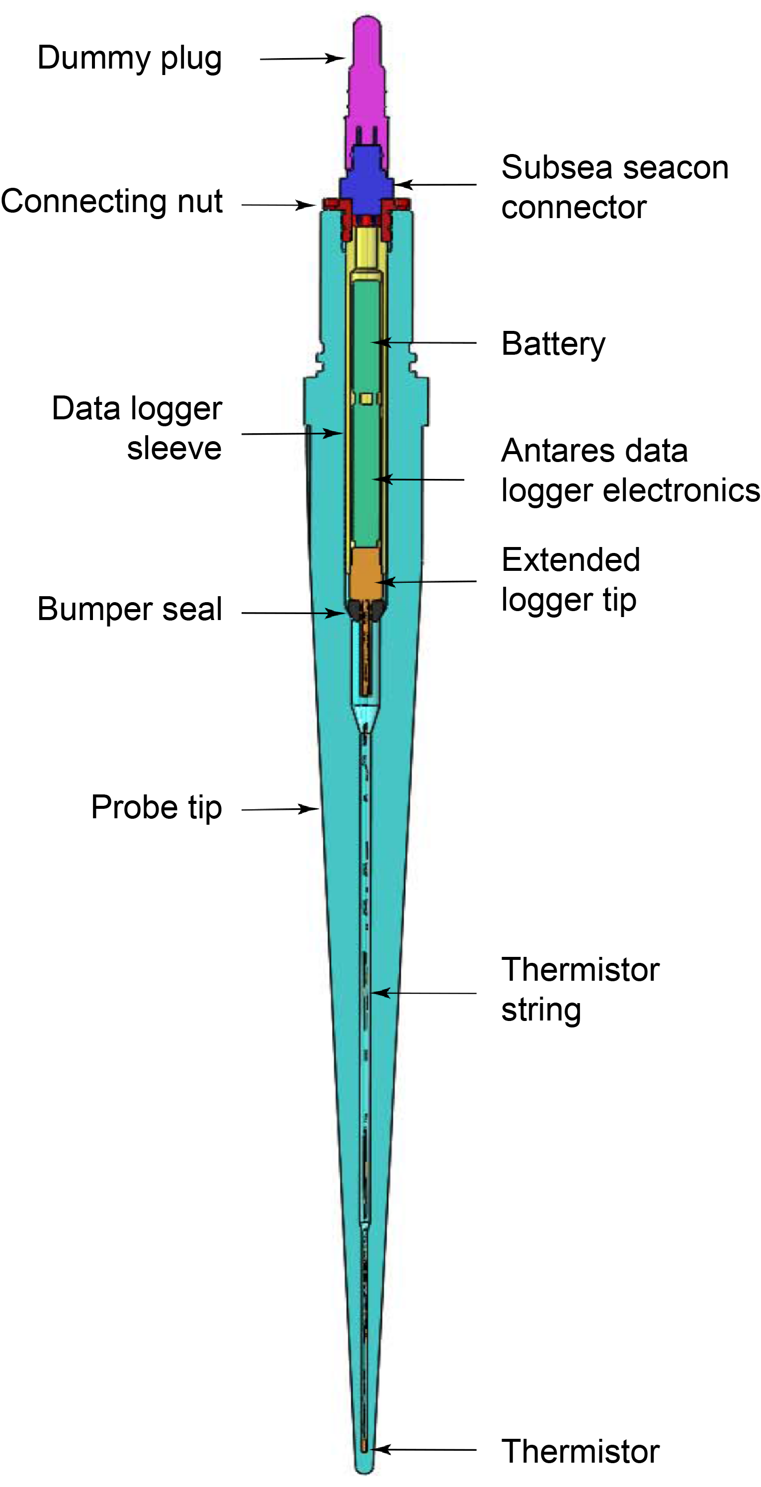
Downhole wireline logging data were collected at Sites U1545–U1547. Two Schlumberger logging tool strings were used during Expedition 385: the triple combo tool string and the FMS-sonic tool string (Figure F36). Individual logging runs with each of these tool strings were done in succession after completion of coring operations. These downhole logging instruments collect continuous measurements of in situ physical, chemical, and structural properties along the length of the penetrated formation. These continuous data provide physical properties information over depth intervals where core recovery is potentially incomplete or disturbed, and they are particularly useful for stratigraphic and lithologic correlation between sites regionally. Downhole logging measurements can be directly tied to seismic profiles, which commonly have regional extent, by the creation of synthetic seismograms based on the logging data and, where appropriate, by the time-to-depth conversion of seismic profiles. The quality of logging data compared to core laboratory measurements depends on the physical property considered and other factors, including the spatial scale of interest. Downhole logging tools measure most formation properties averaged over spatial scales on the order of a meter, whereas laboratory measurements typically have a scale length of centimeters and geophysical surveys are sensitive to properties at the scale of tens of meters.

11.2.1. Temperature measurements

In situ temperature measurements were made using both the APCT-3 tool and the SET2 tool, with the latter being designed to measure and record formation temperature in semiconsolidated sediments that are too stiff for the APCT-3 tool to be deployed. Temperature measurements are useful for many reasons, but they were particularly useful for Expedition 385 in helping to determine sampling plans for microbiological studies aimed at understanding the temperature dependence of microbial populations and processes.

11.2.1.1. Advanced piston corer temperature tool

In situ temperature measurements were made with the APCT-3 tool (Figure F34) when the APC system was deployed. The APCT-3 thermistor tool fits directly into the coring shoe of the APC coring system and can therefore be used to measure formation temperatures during regular piston coring. The tool consists of a battery pack, a data logger, and a platinum thermistor probe calibrated over a temperature range from −5° to 55°C with an accuracy of ±0.02°C. Before entering the borehole, the tool is first held at the mudline for 5 min to thermally equilibrate and to estimate the bottom water temperature. However, the lowest temperature recorded during the run was occasionally used as an estimate of the bottom water temperature instead of the average temperature at the mudline because (1) it was more repeatable and (2) the bottom water is expected to have the lowest temperature in the profile. When the APCT-3 tool is fired into the formation, there is an instantaneous temperature rise from frictional heating. This heat gradually dissipates into the surrounding sediment as the temperature within the APCT-3 tool and adjacent sediment equilibrate to the temperature of the surrounding sediment volume. After the APCT-3 tool penetrates the sediment, it is held in place for 10 min while it records the temperature of the cutting shoe every second.

11.2.1.2. Sediment temperature 2 tool

Formation temperatures are measured using a thermistor in the SET2 tool (Figure F35) that records actual in situ temperature and is located ~1 cm from the probe tip. The thermistor is calibrated for a temperature range of −2° to 50°C with an accuracy of ±0.002°C. Once the tool is retrieved, the data are downloaded and processed on the ship. The probe tip contains both the data logger and the thermistor string and is designed to enter the sediment with minimal disturbance. Features of the probe tip design include the following:

• High-strength stainless steel construction survives penetration into highly consolidated sediment and contact with igneous rock.
• The 8 mm spherical probe tip tapers upward at an included angle of 5° to minimize mechanical disturbance of the soil and the tendency to crack the formation upon penetration by the tool.

The SET2 tool is deployed by the motion-decoupled hydraulic delivery system (MDHDS). The SET2 tool may also be deployed by wireline using the colleted delivery system (CDS) (see SET2 manual for information on the CDS tool, available at https://iodp.tamu.edu/tools/logging/index.html).

We used two devices each of the APCT-3 and SET2 tools. One of the devices of each tool setup was modified by technicians to operate at up to 90°C (upper limit of the electronics inside each device), and the counterpart was used at the standard calibrated temperature range of up to 55°C (APCT-3) and 50°C (SET2). High-temperature calibration for the APCT-3 and SET2 tools was achieved by using hot and cold baths in the laboratory to generate a known range of temperatures measured by thermometer while recording changing resistance values in the APCT-3 and SET2 tools with varying bath water temperatures and fitting a linear temperature regression line to those resistance values. Using this approach, it was possible to convert resistance measured by the tool into temperature value with an accuracy of ±2°–3°C for temperatures above the standard calibration range. A total of 93 in situ temperature measurements were conducted during the expedition using all four units of equipment of the two tool setups (Table T19). For holes in unusually warm sediments, the tool temperature may continue to rise after penetration. It is not possible to leave the tool in the seafloor long enough to achieve complete equilibration. This would require 40–60 min or more of stationary time. Instead, partial equilibration is achieved under such conditions. Processing of APCT-3 and SET2 tool data to infer the in situ formation temperature requires extrapolation of a short record of thermal equilibration.

11.2.1.3. Elevated Temperature Borehole Sensor

The ETBS is a slim-hole probe run on the coring line (Figure F37) that was modified and upgraded from the Ultra High Temperature Multisensor Memory Tool (UHT-MSM) prior to IODP Expedition 376 which successfully tested this new tool (de Ronde et al., 2019). The UHT-MSM was used during ODP Legs 169 and 193 (Shipboard Scientific Party, 1998, 2002a). The tool was originally developed for the University of Miami (USA) (Geophysical Research Corporation, 1994a, 1994b, 1996). The ETBS contains internal and ultra-high external temperature measuring devices, a pressure gauge, a multisensor memory unit, and a Dewar flask that acts as an insulator to maintain a stable temperature and cool-down rate for the tool (Figure F37). The heat shield is aircraft-grade aluminum bound at both ends by brass heat sinks. The Dewar flask can maintain an internal temperature suitable for tool operation for 4–5 h at an external temperature of 400°C. Operations are possible for as long as 10 h if the average temperature does not exceed 232°C.

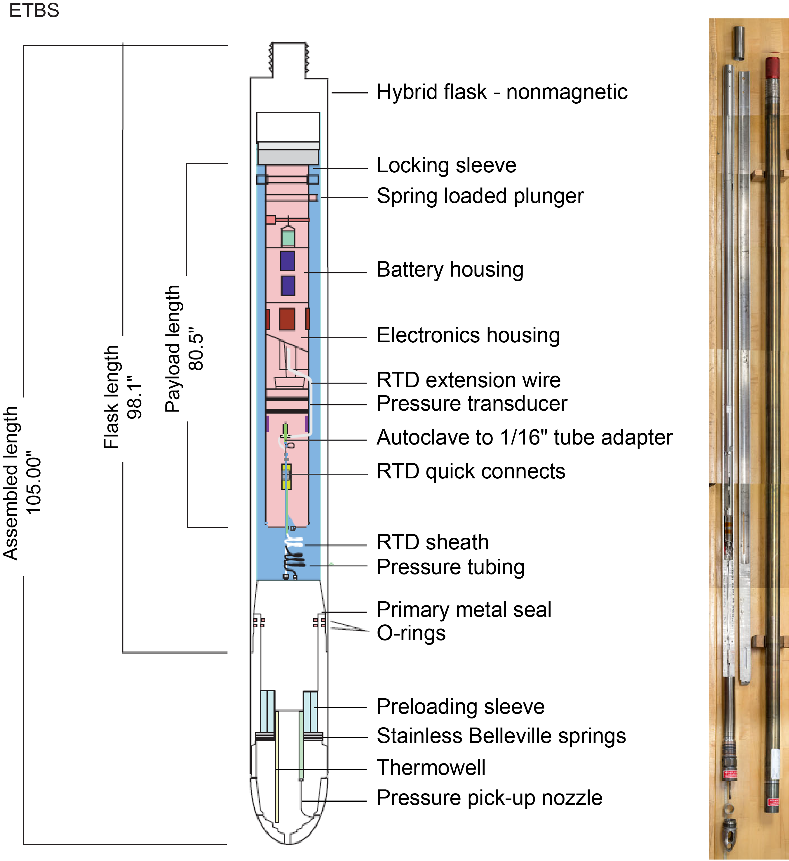
The ETBS tool was connected to the core line via a new adapter designed on board to be compatible with both the ETBS and the Kuster FTS. This attachment enables deployment through the throat of the RCB coring bit. Such an approach minimizes the time that the drill string spends without circulation of seawater in the hole, which is when risk of borehole collapse is highest. The ETBS was fitted with Chemraz seals and Kalrez O-rings.

11.2.1.4. Thermal data reduction

The equilibrium temperature of the sediment is estimated by applying a mathematical heat-conduction model to the temperature-decay record (Horai and Von Herzen, 1985).

The theoretical thermal-decay curve for the APCT-3 tool is a function of the geometry and thermal properties of the probe and the sediment (Bullard, 1954; Horai and Von Herzen, 1985). The characteristic thermal time constant of the cutting shoe assembly into which the APCT-3 tool is inserted is ~2–3 min. Where the APC does not achieve a full stroke or where ship heave pulls the APC up from full penetration, the temperature equilibration curve is disturbed and temperature determination is less accurate. The nominal accuracy of APCT-3 temperature measurements is ±0.002°C.

Data reduction for the APCT-3 tool was performed using the program TP-Fit (Heeseman et al., 2006). Generally, it is not possible to obtain a perfect match between the analytical curves and the data because (1) the probe does not reach thermal equilibrium during the penetration period; (2) contrary to ideal theory, the frictional pulse upon insertion is not instantaneous; and (3) temperature data are sampled at discrete intervals, so the exact time of penetration is uncertain. Therefore, both the effective penetration time and equilibrium temperature must be estimated by applying a fitting procedure, which involves shifting the synthetic curves in time to obtain a match with the recorded data. Heeseman et al. (2006) suggests that the best fit is obtained from the final third of the data set. A single, laboratory-measured thermal conductivity was used for calculating heat flow and also input into the TP-Fit calculation for estimating in situ temperatures. Additional laboratory measurements of core-sample thermal conductivity were not used to account for in situ conditions when fitting the APCT-3 data because the correction relative to a single, constant thermal conductivity would be small at the shallow depths over which the APCT-3 was used, owing to the high thermal gradient.

If heat transfer is by conduction and heat flow is constant, the thermal gradient will be inversely proportional to thermal conductivity, according to Fourier’s law. This relationship can be linearized by plotting temperature as a function of cumulative thermal resistance (Bullard and Schonland, 1939):

Tz=T0+q∑i = 0NΔzikzi, (50)

where

• T = temperature,
• z = depth,
• T₀ = temperature at the seafloor,
• q = heat flow,
• Σ = thermal resistance,
• k = thermal conductivity, and
• N = number of thermal conductivity measurements.

In practice, q and T₀ are estimated by plotting T(z) against cumulative thermal resistance (Bullard plot) from the slope and intercept with z = 0, respectively. The conditions for the linearity of the plot are affected by conductive conditions, steady state, and absence of internal heat source. For Expedition 385, three of these conditions may not be met: advective heat transport could be important and steady state is a poor assumption because of high sedimentation rate and the possibility of still-cooling sills, which would also be an internal heat source. Geothermal gradients were quite linear (indicative of steady-state conditions) at all sites except Ringvent (Site U1547 and Holes U1548A–U1548C).

11.2.2. Wireline logging

Downhole wireline logging was conducted using two Schlumberger tool strings: the triple combo tool string, which measures borehole (fluid) temperature, NGR, density, electrical resistivity, and MS (Figure F36), and the FMS-sonic tool string, which measures NGR and sonic velocity and captures FMS resistivity images of the borehole wall (Figure F36). Both tool strings also contain a telemetry cartridge for communicating through the wireline to the Schlumberger data acquisition system (multi-tasking acquisition and imaging system [MAXIS]) on the ship.

In preparation for logging, the boreholes were flushed of debris by circulating high-viscosity sepiolite mud. The BHA was pulled up to about 80 m WSF to cover the unstable upper part of the hole. The tool strings were then lowered downhole on a seven-conductor wireline cable before being pulled up at a constant speed of ~275 m/h to provide continuous measurements of several properties simultaneously. A wireline heave compensator (WHC) was used to minimize the effect of the ship’s heave on the tool position in the borehole, except when ship heave was minimal. During each logging run, incoming data were recorded and monitored in real time on the Schlumberger Minimum Configuration MAXIS (MCM) logging computer.

11.2.2.1. Log data quality

The main factor affecting logging data quality is the condition of the borehole wall. Where the borehole diameter varies over short intervals because of washouts (wide borehole) or ledges made of layers of harder material, the logs from tools that require good contact with the borehole wall (i.e., the FMS and density tools) may be degraded. Deep investigation measurements such as NGR, resistivity, and sonic velocity, which do not require contact with the borehole wall, are generally less sensitive to borehole conditions. Very narrow (“bridged”) sections also cause irregular log results. The quality of the borehole is improved by minimizing the circulation of seawater (drilling fluid) while drilling, flushing the borehole to remove debris prior to logging, and logging soon after drilling and hole conditioning are completed. During the expedition, circulation of drilling fluid, necessary to cool the bit and clear the hole of cuttings, washed out (widened) the corresponding borehole in places, particularly at locations with large contrasts in formation consolidation.

The quality of the wireline depth determination depends on several factors. The depth of the logging measurements is determined from the length of the cable payed out from the winch on the ship. The seafloor is identified on the NGR log by the abrupt reduction in gamma ray count at the water/seabed boundary (mudline). Discrepancies between the drilling depth and the wireline log depth occur. In the case of drilling depth, discrepancies are caused by core expansion, incomplete core recovery, or incomplete heave compensation. In the case of log depth, discrepancies between successive runs occur because of incomplete heave compensation, incomplete correction for cable stretch, and cable slip. Tidal changes in sea level affect both drilling and logging depths.

11.2.2.2. Wireline heave compensator

The WHC system is designed to compensate for the vertical motion of the ship and maintain a steady motion for the logging tools. The system uses vertical acceleration measurements made by a motion reference unit (MRU) located under the rig floor near the center of gravity of the ship to calculate the vertical motion of the ship. It then adjusts the length of the wireline by varying the distance between two sets of pulleys through which the cable passes. Real-time measurements of uphole (surface) and downhole acceleration are made simultaneously by the MRU and the Enhanced Digital Telemetry Cartridge (EDTC), respectively.

11.2.2.3. Logging data flow and log depth scales

Data for each wireline logging run were monitored in real time and recorded using the Schlumberger MAXIS 500 system. The initial logging data were referenced to the rig floor (WRF scale). After logging was completed, the data were shifted to a seafloor reference (WSF scale) based on the step in gamma radiation at the water/seabed interface. The data were transferred to the Lamont-Doherty Earth Observatory Borehole Research Group (LDEO-BRG; Columbia University, USA), where standardized data reduction took place. The main correction was depth matching to remove depth offsets between data from different logging runs, producing a new depth scale (WMSF). The second uplog became the wireline depth reference, and its WSF scale is the same as its WMSF scale. The logs are documented with an assessment of log quality, and the data were converted to ASCII. Schlumberger Geo-Quest’s Techlog software package is used for most of the wireline log data processing. Data were transferred back to the ship within a few days of logging completion, and this processed data set was made available to the science party in ASCII format.

11.2.3. Logged formation properties and tool measurement principles

The logged properties and the principles used to measure them are briefly described in this section. The logging tools are listed in Tables T20 and T21. More detailed information on individual tools and their geological applications may be found in Rider (1996), Goldberg (1997), and Ellis and Singer (2007). A complete online list of acronyms for Schlumberger tools and measurement curves is available at the Schlumberger Curve Mnemonic Dictionary (http://www.apps.slb.com/cmd/, accessed 30 September 2020).

11.2.3.1. Borehole diameter (caliper)

The borehole diameter measured by the caliper provides an indication of formation strength and its response to the artificial erosion associated with drilling operations (Figure F36). Additionally, caliper measurements can provide information on the present-day stress field inferred from the ellipticity of borehole deformation induced by downhole operations.

The method for estimating stress-field orientation uses the orthogonal borehole diameter measured by the calipers of the FMS-sonic tool string (called C1 and C2, respectively) and the caliper orientation provided by the general purpose inclination tool (GPIT) (see below). Displaying this information along depth can provide evidence of breakouts or borehole ellipticity that can be interpreted in terms of maximum and minimum plane stresses. A breakout signal typically shows an increase in diameter in one of the orthogonal calipers, whereas the other caliper remains close to the bit size. Theoretically, the greater diameter highlights the minimum plane stress.

11.2.3.2. Natural gamma radiation

The Hostile Environment Natural Gamma Ray Sonde (HNGS) was used on both the triple combo and FMS-sonic tool strings to measure and classify NGR in the formation (Figure F36). Each HNGS instrument has two bismuth germanate scintillation detectors that measure concentrations of K (in weight percent) as well as U and Th (both in parts per million) that are determined from the characteristic gamma ray energy spectra of isotopes in the ⁴⁰K, ²³²Th, and ²³⁸U radioactive decay series. An additional NGR sensor, housed in the EDTC, is run on both tool strings. Its sodium iodide scintillation detector measures the total NGR emission of the formation with no spectral information. The inclusion of an NGR sonde in every tool string improves core-log integration by enabling the use of NGR data for depth correlation between logging strings and logging-run passes. This in turn enables more confident direct comparison of downhole and core laboratory physical properties measurements.

11.2.3.3. Density and photoelectric factor

Formation density was measured with the Hostile Environment Litho-Density Sonde (HLDS) (Figure F36). The sonde contains a radioactive cesium (¹³⁷Cs) gamma ray source (622 keV) and far and near gamma ray detectors mounted on a shielded skid that is pressed against the borehole wall by a hydraulically activated decentralizing arm. Gamma radiation emitted by the source undergoes Compton scattering, in which gamma rays are scattered by electrons in the formation. The number of scattered gamma rays that reach the detectors is proportional to the density of electrons in the formation, which is in turn related to bulk density. Porosity may also be derived from this bulk density if the matrix (grain) density is known.

The HLDS also measures the photoelectric effect factor (PEF), which is a measure of the photoelectric absorption of low-energy gamma radiation. Photoelectric absorption occurs when the energy of the gamma rays falls below 150 keV as a result of being repeatedly scattered by electrons in the formation. PEF is determined by comparing the counts from the far detector in the high-energy region, where only Compton scattering occurs, to those in the low-energy region, where count rates depend on both reactions. Because PEF depends on the atomic number of the elements in the formation (heavier elements have a higher PEF), it also varies according to the chemical composition of the minerals present and can be used for the identification of the overall mineral makeup of the formation. For example, the PEF of calcite is 5.08 barn/e⁻, illite is 3.03 barn/e⁻, quartz is 1.81 barn/e⁻, and hematite is 21 barn/e⁻. Good contact between the tool and the borehole wall is essential for good HLDS logs; poor contact results in underestimation of density values. Both the density correction and caliper measurement of the hole are used to check the contact quality. In the deeper parts of the hole, the PEF log should be used with caution, especially in washouts, because barium in the logging mud swamps the signal despite correction for mud effect.

11.2.3.4. Electrical resistivity

The High-Resolution Laterolog Array (HRLA) provides six resistivity measurements with different depths of investigation, including borehole mud resistivity and five measurements of formation resistivity with increasing penetration into the formation: 0.254, 0.508, 0.762, 1.524, and 2.286 m (Figure F36). The tool sends a focused current into the formation and measures the intensity necessary to maintain a constant drop in voltage across a fixed interval, providing direct resistivity measurements. Two curves are calculated from these values: true resistivity (RT) of the hole, which is always the closest value to the deepest measurements, and resistivity of the borehole fluids (RM). Because it is least affected by the borehole fluids infiltrating the formation, the deepest depth of investigation, RLT5, is consistently used to describe variations of resistivity with depth.

The tool has one central (source) electrode and six electrodes above and below it that serve alternately as focusing and returning current electrodes. By rapidly changing the role of these electrodes, simultaneous resistivity measurement at six penetration depths is achieved. The tool is designed to ensure that all signals are measured at the same time and tool position and to reduce the sensitivity to “shoulder bed” effects when crossing beds that are thinner than the electrode spacing. HRLA needs to be run centralized in the borehole for optimal results, so bowspring centralizers were used to keep the HRLA in the center of the borehole and knuckle joints allowed the density tool to be centralized and maintain good contact with the borehole wall (Figure F36). Calcite, silica, and hydrocarbons are electrical insulators, whereas ionic solutions like IW are conductors. Electrical resistivity can therefore be used to evaluate porosity for a given salinity and resistivity of IW. Clay surface conduction also impacts formation resistivity, but at high porosities this effect is relatively minor.

11.2.3.5. Magnetic susceptibility

The Magnetic Susceptibility Sonde (MSS) is a nonstandard wireline tool designed by LDEO (Figure F36). It measures the ease with which formations are magnetized when subjected to a magnetic field. The ease of magnetization is ultimately related to the concentration and composition (size, shape, and mineralogy) of magnetic minerals (principally magnetite) in the formation. These measurements provide one of the best methods for investigating stratigraphic changes in mineralogy and lithology because the measurement is quick, repeatable, and nondestructive and because different lithologies often have strongly contrasting magnetic susceptibilities.

The MSS dual-coil sensor provides ~40 cm resolution measurements with ~20 cm depth of horizontal investigation. The MSS was run as the lowermost tool in the triple combo tool string, and a data translation cartridge was used to enable the MSS to be run in combination with the Schlumberger tools. MS data from the MSS are plotted as noncalibrated units and are affected by temperature and borehole size (higher temperatures lead to higher susceptibility measurements). For quality control and environmental correction, the MSS also measures internal tool temperature, z-axis acceleration, and low-resolution borehole conductivity.

11.2.3.6. Acoustic velocity

The Dipole Shear Sonic Imager (DSI) measures the transit times between sonic transmitters and an array of eight receivers (Figure F36). It combines replicate measurements (i.e., upward and downward propagation), thus providing a direct measurement of sound velocity through formations that is relatively free from the effects of formation damage and borehole shape (Schlumberger, 1989). Along with the monopole transmitters found on most sonic tools, it also has two crossed-dipole transmitters that allow measurement of shear wave velocity in addition to compressional wave velocity. Dipole measurements are necessary to measure formation shear velocities that are less than the compressional velocity of the borehole fluid. Such “slow formations” are commonly encountered in deep-ocean drilling.

11.2.3.7. Formation MicroScanner

The FMS provides high-resolution electrical resistivity–based images of borehole walls (Figure F36). The tool has four orthogonal arms and pads, each containing 16 button electrodes that are pressed against the borehole wall during logging. The electrodes are arranged in two diagonally offset rows of eight electrodes each. A focused current is emitted from the button electrodes into the formation, and there is a return electrode near the top of the tool. Resistivity of the formation at the button electrodes is derived from the intensity of the current passing through the button electrodes. Processing transforms the resistivity measurements into oriented high-resolution images that reveal geologic structures of the borehole wall. Features such as bedding, stratification, fracturing, slump folding, and bioturbation can be resolved (Luthi, 1990; Salimullah and Stow, 1992; Lovell et al., 1998). Because the images are oriented to magnetic north, further analysis can provide measurement of the dip and direction (azimuth) of planar features in the formation. In addition, when the corresponding planar features can be identified in the recovered core samples, individual core pieces can be reoriented with respect to true north.

Approximately 30% of a borehole with a diameter of 25 cm (9⅞ inches) is imaged during a single pass. Standard procedure is to make two full upward passes with the FMS to maximize the chance of getting full borehole coverage with the pads. The maximum extension of the caliper arms is 40.6 cm. In holes with a diameter greater than this maximum, the pad contact at the end of the caliper arms is inconsistent, and the FMS images may appear out of focus and too conductive. Irregular (rough) borehole walls will also adversely affect the images if contact with the wall is poor.

11.2.3.8. Acceleration and inclinometry

The GPIT was included in the FMS-sonic tool string to calculate tool acceleration and orientation during logging (Figure F36). Tool orientation is defined by three parameters: tool deviation, tool azimuth, and relative bearing. The GPIT utilizes a three-axis inclinometer and a three-axis fluxgate magnetometer to record the orientation of the FMS as the magnetometer records the magnetic field components (F_x, F_y, and F_z). Thus, the FMS images can be corrected for irregular tool motion, and the dip and direction (azimuth) of features in the FMS image can be determined.

11.2.4. Downhole fluid sampling

Borehole fluid sampling was accomplished using a Kuster FTS (Figure F23). The Kuster FTS is rated to 690 bar (10,000 psi) and 232.2°C, although it has been successfully run as high as 260°C (de Ronde et al., 2019). The Kuster FTS tool was fitted with a 1000 mL sample chamber. The tool was run directly after temperature logging with the ETBS. Procedures for downhole survey operation were followed in accordance with manufacturer guidelines (available from the JOIDES Resolution laboratory manuals, guides, and resources, https://wiki.iodp.tamu.edu/display/LMUG/Downhole+Logging#DownholeLogging-KusterFTS, accessed 30 September 2020).

The tool consists of a 600 mL capacity fluid sample chamber that can be connected to an additional 400 mL capacity tube with a spring-loaded valve on each end of the sample chamber. The lower end has a removable bullnose with ports to allow the fluid to enter. At the top is a rope socket for attaching the wireline. A latching mechanism connects the valves together and holds them open during deployment. A programmable mechanical clock is attached above the chamber, with either a 1 or 3 h clock for trigger times <50 and >50 min, respectively. This clock is preset at the surface to define the closing time, at which point a ball-operated tripping mechanism releases the valves, trapping the fluid in the sampler and maintaining the pressure of the sampling depth until the tool is recovered and the fluids are retrieved through a transfer head assembly (see Organic geochemistry). Operationally, 10 min was allowed to elapse following the estimated valve closure time before the Kuster FTS was recovered at an ascent rate of 70 m/min.

Between samples, the Kuster FTS was cleaned with ACS reagent grade acetone, rinsed with deionized water, and serviced following manufacturer guidelines. Likewise, it was ensured that the transfer head assembly was free of contaminants by washing with acetone and distilled water and testing that the valves would easily open or shut. After recovery of the fluid sampler tool, all valves, connections, and O-rings were checked for mechanical wear and embrittlement and replaced as necessary prior to the next run.

11.2.5. Downhole measurements summary

A combined total of 93 downhole temperature measurements with both the APCT-3 and SET2 tools were carried out during the expedition (Tables T18, T19). Logging formation tool strings were deployed at Sites U1545–U1548 (Table T18), and downhole sampling with the Kuster FTS was conducted at Sites U1545, U1547, and U1548 (Table T18).

References

Aarnes, I., Svensen, H., Connolly, J.A.D., and Podladchikov, Y.Y., 2010. How contact metamorphism can trigger global climate changes: modeling gas generation around igneous sills in sedimentary basins. Geochimica et Cosmochimica Acta, 74(24):7179–7195. https://doi.org/10.1016/j.gca.2010.09.011

Andrén, T., Jorgensen, B.B., Cotterill, C., Fehr, A., Green, S., Andren, E., Ash, J., Bauersachs, T., Cragg, B., Fanget, A.-S., Granoszewski, W., Groeneveld, J., Hardisty, D., Herrero-Bervera, E., Hyttinen, O., Jensen, J.B., Johnson, S., Kenzler, M., Kotilainen, A., Kotthoff, U., Marshall, I.P.G., Martin, E., Obrochta, S., Passchier, S., Quintana Krupinski, N., Riedinger, N., Slomp, C., Snowball, I., Stepanova, A., Strano, S., Torti, A., Warnock, J., Xiao, N., and Zhang, R., 2015. Methods. In Andrén, T., Jørgensen, B.B., Cotterill, C., Green, S., and the Expedition 347 Scientists, Proceedings of the Integrated Ocean Drilling Program, 347: College Station, TX (Integrated Ocean Drilling Program). https://doi.org/10.2204/iodp.proc.347.102.2015

Arason, P., and Levi, S., 2010. Maximum likelihood solution for inclination-only data in paleomagnetism. Geophysical Journal International, 182(2):753–771. https://doi.org/10.1111/j.1365-246X.2010.04671.x

ASTM International, 1990. Standard method for laboratory determination of water (moisture) content of soil and rock (Standard D2216–90). In Annual Book of ASTM Standards for Soil and Rock (Volume 04.08): Philadelphia (American Society for Testing Materials). [revision of D2216-63, D2216-80]

Backman, J., Raffi, I., Rio, D., Fornaciari, E., and Pälike, H., 2012. Biozonation and biochronology of Miocene through Pleistocene calcareous nannofossils from low and middle latitudes. Newsletters on Stratigraphy, 45(3):221–244. https://doi.org/10.1127/0078-0421/2012/0022

Baker, G.C., Smith, J.J., and Cowan, D.A., 2003. Review and re-analysis of domain-specific 16S primers. Journal of Microbiological Methods, 55(3):541–555. https://doi.org/10.1016/j.mimet.2003.08.009

Balsam, W.L., and Damuth, J.E., 2000. Further investigations of shipboard vs. shore-based spectral data: implications for interpreting Leg 164 sediment composition. In Paull, C.K., Matsumoto, R., Wallace, P.J., Dillon, W.P. (Eds.), Proceedings of the Ocean Drilling Program, Scientific Results, 164: College Station, TX (Ocean Drilling Program). https://doi.org/10.2973/odp.proc.sr.164.222.2000

Balsam, W.L., Damuth, J.E., and Schneider, R.R., 1997. Comparison of shipboard vs. shore-based spectral data from Amazon Fan cores: implications for interpreting sediment composition. In Flood, R.D., Piper, D.J.W., Klaus, A., and Peterson, L.C. (Eds.), Proceedings of the Ocean Drilling Program, Scientific Results, 155: College Station, TX (Ocean Drilling Program), 193–215. https://doi.org/10.2973/odp.proc.sr.155.210.1997

Balsam, W.L., Deaton, B.C., and Damuth, J.E., 1998. The effects of water content on diffuse reflectance spectrophotometry studies of deep-sea sediment cores. Marine Geology, 149(1):177–189. https://doi.org/10.1016/S0025-3227(98)00033-4

Barron, J.A., 1980. Upper Pliocene and Quaternary diatom biostratigraphy of Deep Sea Drilling Project Leg 54, tropical eastern Pacific. In Rosendahl, B.R., Hekinian, R., et al., Initial Reports of the Deep Sea Drilling Project, 54: Washington, DC (US Government Printing Office), 455–485. https://doi.org/10.2973/dsdp.proc.54.117.1980

Barron, J.A., 1985. Late Eocene to Holocene diatom biostratigraphy of the equatorial Pacific Ocean, Deep Sea Drilling Project Leg 85. In Mayer, L., Theyer, E., et al., Initial Reports of the Deep Sea Drilling Project, 85: Washington, DC (US Government Printing Office), 413–456. https://doi.org/10.2973/dsdp.proc.85.108.1985

Barron, J.A., 2003. Planktonic marine diatom record of the past 18 m.y.: appearances and extinctions in the Pacific and Southern Oceans. Diatom Research, 18(2):203–224. https://doi.org/10.1080/0269249X.2003.9705588

Barron, J.A., Bukry, D., and Dean, W.E., 2005. Paleoceanographic history of the Guaymas Basin, Gulf of California, during the past 15,000 years based on diatoms, silicoflagellates, and biogenic sediments. Marine Micropaleontology, 56(3–4):81–102. https://doi.org/10.1016/j.marmicro.2005.04.001

Barron, J.A., and Gladenkov, A.Y., 1995. Early Miocene to Pleistocene diatom stratigraphy of Leg 145. In Rea, D.K., Basov, I.A., Scholl, D.W., and Allan, J.F. (Eds.), Proceedings of the Ocean Drilling Program, Scientific Results, 145: College Station, TX (Ocean Drilling Program), 3–19. https://doi.org/10.2973/odp.proc.sr.145.101.1995

Bartington Instruments, Ltd., 2011. Operation Manual for MS2 Magnetic Susceptibility System: Oxford, UK (Bartington Instruments, Ltd.). https://gmw.com/wp-content/uploads/2019/03/MS2-OM0408.pdf

Berner, R.A., 1982. Burial of organic carbon and pyrite sulfur in the modern ocean: its geochemical and environmental significance. American Journal of Science, 282(4):451–473. https://doi.org/10.2475/ajs.282.4.451

Biddle, J.F., Fitz-Gibbon, S., Schuster, S.C., Brenchley, J.E., and House, C.H., 2008. Metagenomic signatures of the Peru margin subseafloor biosphere show a genetically distinct environment. Proceedings of the National Academy of Sciences of the United States of America, 105(30):10583–10588. https://doi.org/10.1073/pnas.0709942105

Blum, P., 1997. Physical properties handbook: a guide to the shipboard measurement of physical properties of deep-sea cores. Ocean Drilling Program Technical Note, 26. https://doi.org/10.2973/odp.tn.26.1997

Bollmann, J., 1997. Morphology and biogeography of Gephyrocapsa coccoliths in Holocene sediments. Marine Micropaleontology, 29(3):319–350. https://doi.org/10.1016/S0377-8398(96)00028-X

Bown, P.R. (Ed.), 1998. Calcareous Nannofossil Biostratigraphy: Dordrect, The Netherlands (Kluwer Academic Publishing).

Bullard, E.C., 1954. The flow of heat through the floor of the Atlantic Ocean. Proceedings of the Royal Society of London, Series A. Mathematical and Physical Sciences, 222(1150):408–429. https://doi.org/10.1098/rspa.1954.0085

Bullard, E.C., and Schonland, B.F.J., 1939. Heat flow in South Africa. Proceedings of the Royal Society of London, Series A. Mathematical and Physical Sciences, 173(955):474–502. https://doi.org/10.1098/rspa.1939.0159

Caporaso, J.G., Lauber, C.L., Walters, W.A., Berg-Lyons, D., Lozupone, C.A., Turnbaugh, P.J., Fierer, N., and Knight, R., 2011. Global patterns of 16S rRNA diversity at a depth of millions of sequences per sample. Proceedings of the National Academy of Sciences of the United States of America, 108(S1):4516–4522. https://doi.org/10.1073/pnas.1000080107

Cline, J.D., 1969. Spectrophotometric determination of hydrogen sulfide in natural waters. Limnology and Oceanography, 14(3):454–458. https://doi.org/10.4319/lo.1969.14.3.0454

de Ronde, C.E.J., Humphris, S.E., Höfig, T.W., Brandl, P.A., Lanlan, C., Yuanfeng, C., Caratori Tontini, F., Deans, J.R., Farough, A., Jamieson, J.W., Kolandaivelu, K.P., Kutovaya, A., Labonté, J.M., Martin, A.J., Massiot, C., McDermott, J.M., McIntosh, I.M., Nozaki, T., Pellizari, V.H., Reyes, A.G., Roberts, S., Rouxel, O., Schlicht, L.E.M., Seo, J.H., Straub, S.M., Strehlow, K., Takai, K., Tanner, D., Tepley, F.J., III, and Chao, Z., 2019. Expedition 376 methods. In de Ronde, C.E.J., Humphris, S.E., Höfig, T.W., and the Expedition 376 Scientists, Brothers Arc Flux. Proceedings of the International Ocean Discovery Program, 376: College Station, TX (International Ocean Discovery Program). https://doi.org/10.14379/iodp.proc.376.102.2019

Dekas, A.E., and Orphan, V.J., 2011. Identification of diazotrophic microorganisms in marine sediment via fluorescence in situ hybridization coupled to nanoscale secondary ion mass spectrometry (FISH-NanoSIMS). Methods in Enzymology, 486(281–305). https://doi.org/10.1016/b978-0-12-381294-0.00012-2

Dhillon, A., Lever, M., Lloyd, K.G., Albert, D.B., Sogin, M.L., and Teske, A., 2005. Methanogen diversity evidenced by molecular characterization of methyl coenzyme M Reductase A (mcrA) genes in hydrothermal sediments of the Guaymas Basin. Applied and Environmental Microbiology, 71(8):4592–4601. https://doi.org/10.1128/AEM.71.8.4592-4601.2005

Dick, H.J.B., MacLeod, C.J., Blum, P., Abe, N., Blackman, D.K., Bowles, J.A., Cheadle, M.J., Cho, K., Ciazela, J., Deans, J.R., Edgcomb, V.P., Ferrando, C., France, L., Ghosh, B., Ildefonse, B.M., Kendrick, M.A., Koepke, J.H., Leong, J.A.M., Chuanzhou, L., Qiang, M., Morishita, T., Morris, A., Natland, J.H., Nozaka, T., Pluemper, O., Sanfilippo, A., Sylvan, J.B., Tivey, M.A., Tribuzio, R., and Viegas, L.G.F., 2017. Expedition 360 methods. In MacLeod, C.J., Dick, H.J.B., Blum, P., and the Expedition 360 Scientists, Southwest Indian Ridge Lower Crust and Moho. Proceedings of the International Ocean Discovery Program, 360: College Station, TX (International Ocean Discovery Program). https://doi.org/10.14379/iodp.proc.360.101.2017

Dickens, G.R., Koelling, M., Smith, D.C., Schnieders, L., and the IODP Expedition 302 Scientists, 2007. Rhizon sampling of pore waters on scientific drilling expeditions: an example from the IODP Expedition 302, Arctic Coring Expedition (ACEX). Scientific Drilling, 4:22–25. https://doi.org/10.2204/iodp.sd.4.08.2007

Dombrowski, N., Seitz, K.W., Teske, A.P., and Baker, B.J., 2017. Genomic insights into potential interdependencies in microbial hydrocarbon and nutrient cycling in hydrothermal sediments. Microbiome, 5(1):106. https://doi.org/10.1186/s40168-017-0322-2

Dombrowski, N., Teske, A.P., and Baker, B.J., 2018. Expansive microbial metabolic versatility and biodiversity in dynamic Guaymas Basin hydrothermal sediments. Nature Communications, 9(1):4999. https://doi.org/10.1038/s41467-018-07418-0

Dunlea, A.G., Murray, R.W., Harris, R.N., Vasiliev, M.A., Evans, H., Spivack, A.J., and D’Hondt, S., 2013. Assessment and use of NGR instrumentation on the JOIDES Resolution to quantify U, Th, and K concentrations in marine sediment. Scientific Drilling, 15:57–63. https://doi.org/10.2204/iodp.sd.15.05.2013

Dunlop, D.J., Özdemir, Ö., and Schmidt, P.W., 1997. Paleomagnetism and paleothermometry of the Sydney Basin 2. Origin of anomalously high unblocking temperatures. Journal of Geophysical Research: Solid Earth, 102(B12):27285–27295. https://doi.org/10.1029/97JB02478

Ellis, D.V., and Singer, J.M., 2007. Well Logging for Earth Scientists (2nd edition): New York (Elsevier). https://doi.org/10.1007/978-1-4020-4602-5

Ertefai, T.F., Heuer, V.B., Prieto-Mollar, X., Vogt, C., Sylva, S.P., Seewald, J., and Hinrichs, K.-U., 2010. The biogeochemistry of sorbed methane in marine sediments. Geochimica et Cosmochimica Acta, 74(21):6033–6048. https://doi.org/10.1016/j.gca.2010.08.006

Expedition 301 Scientists, 2005. Methods. In Fisher, A.T., Urabe, T., Klaus, A., and the Expedition 301 Scientists, Proceedings of the Integrated Ocean Drilling Program, 301: College Station, TX (Integrated Ocean Drilling Program Management International, Inc.). https://doi.org/10.2204/iodp.proc.301.105.2005

Expedition 307 Scientists, 2006. Methods. In Ferdelman, T.G., Kano, A., Williams, T., Henriet, J.-P., and the Expedition 307 Scientists, Proceedings of the Integrated Ocean Drilling Program, 307: Washington, DC (Integrated Ocean Drilling Program Management International, Inc.). https://doi.org/10.2204/iodp.proc.307.102.2006

Expedition 311 Scientists, 2006. Methods. In Riedel, M., Collett, T.S., Malone, M.J., and the Expedition 311 Scientists, Proceedings of the Integrated Ocean Drilling Program, 311: Washington, DC (Integrated Ocean Drilling Program Management International, Inc.). https://doi.org/10.2204/iodp.proc.311.102.2006

Expedition 322 Scientists, 2010. Methods. In Saito, S., Underwood, M.B., Kubo, Y., and the Expedition 322 Scientists, Proceedings of the Integrated Ocean Drilling Program, 322: Tokyo (Integrated Ocean Drilling Program Management International, Inc.). https://doi.org/10.2204/iodp.proc.322.102.2010

Expedition 323 Scientists, 2011. Methods. In Takahashi, K., Ravelo, A.C., Alvarez Zarikian, C.A., and the Expedition 323 Scientists, Proceedings of the Integrated Ocean Drilling Program, 323: Tokyo (Integrated Ocean Drilling Program Management International, Inc.). https://doi.org/10.2204/iodp.proc.323.102.2011

Expedition 329 Scientists, 2011. Methods. In D’Hondt, S., Inagaki, F., Alvarez Zarikian, C.A., and the Expedition 329 Scientists, Proceedings of the Integrated Ocean Drilling Program, 332: Tokyo (Integrated Ocean Drilling Program Management International, Inc.). https://doi.org/10.2204/iodp.proc.329.102.2011

Expedition 330 Scientists, 2012. Methods. In Koppers, A.A.P., Yamazaki, T., Geldmacher, J., and the Expedition 330 Scientists, Proceedings of the Integrated Ocean Drilling Program, 330: Tokyo (Integrated Ocean Drilling Program Management International, Inc.). https://doi.org/10.2204/iodp.proc.330.102.2012

Expedition 337 Scientists, 2013. Methods. In Inagaki, F., Hinrichs, K.-U., Kubo, Y., and the Expedition 337 Scientists, Proceedings of the Integrated Ocean Drilling Program, 337: Tokyo (Integrated Ocean Drilling Program Management International, Inc.). https://doi.org/10.2204/iodp.proc.337.102.2013

Fatela, F., and Taborda, R., 2002. Confidence limits of species proportions in microfossil assemblages. Marine Micropaleontology, 45(2):169–174. https://doi.org/10.1016/S0377-8398(02)00021-X

Fisher, R.V., and Schmincke, H.-U., 1984. Pyroclastic Rocks: Berlin (Springer). https://doi.org/10.1007/978-3-642-74864-6

Folk, R.L., 1965. Some aspects of recrystallization in ancient limestones. In Pray, L.C. and Murray, R.C. (Ed.), SEPM Special Publication (Volume 13): Dolomitization and Limestone Diagenesis: Tulsa, OK (Society of Economic Paleontologists and Mineralogists). https://doi.org/10.2110/pec.65.07.0014

Fossen, H., 2016. Structural Geology (2nd edition): Cambridge, UK (Cambridge University Press).

Fritz, D., 1980. Safety and pollution prevention program, Deep Sea Drilling Project Leg 50, Sites 415 and 416. In Lancelot, Y., Winterer, E.L. (Ed.), Initial Reports of the Deep Sea Drilling Project. 50: Washington, DC (US Government Printing Office), 855–859. https://doi.org/10.2973/dsdp.proc.50.app5.1980

Fryer, P., Wheat, C.G., Williams, T., Albers, E., Bekins, B., Debret, B.P.R., Jianghong, D., Yanhui, D., Eickenbusch, P., Frery, E.A., Ichiyama, Y., Johnson, K., Johnston, R.M., Kevorkian, R.T., Kurz, W., Magalhaes, V., Mantovanelli, S.S., Menapace, W., Menzies, C.D., Michibayashi, K., Moyer, C.L., Mullane, K.K., Park, J.-W., Price, R.E., Rayan, J.G., Shervais, J.W., Suzuki, S., Sissmann, O.J., Takai, K., Walter, B., and Zhang, R., 2018. Expedition 366 methods. In Fryer, P., Wheat, C.G., Williams, T., and the Expedition 366 Scientists, Proceedings of the International Ocean Discovery Program, 366: College Station, TX (International Ocean Discovery Program). https://doi.org/10.14379/iodp.proc.366.102.2018

Fuller, M., 1969. Magnetic orientation of borehole cores. Geophysics, 34(5):772–774. https://doi.org/10.1190/1.1440047

Geophysical Research Corporation, 1994a. Multi-Sensory Memory Module Operation Manual, #006-0112-00: Tulsa, OK (Geophysical Research Corporation).

Geophysical Research Corporation, 1994b. University of Miami UHT-MSM Operations Manual, #006-0122-00: Tulsa, OK (Geophysical Research Corporation).

Geophysical Research Corporation, 1996. MSM/MIAMI Operation Software User’s Guide, #006-0128-00: Tulsa, OK (Geophysical Research Corporation).

Gieskes, J.M., Gamo, T., and Brumsack, H.J., 1991. Chemical methods for interstitial water analysis aboard JOIDES Resolution. Ocean Drilling Program Technical Note, 15. https://doi.org/10.2973/odp.tn.15.1991

Gifkins, C.C., Herrmann, W., and Large, R.R., 2005. Altered Volcanic Rocks: a Guide to Description and Interpretation: Hobart, Australia (Centre for Ore Deposit Research, University of Tasmania). https://eprints.utas.edu.au/296/

Gifkins, C.C., and Allen, R.L., 2001. Textural and chemical characteristics of diagenetic and hydrothermal alteration in glassy volcanic rocks: examples from the Mount Read volcanics, Tasmania. Economic Geology, 96(5):973–1002. https://doi.org/10.2113/gsecongeo.96.5.973

Gladenkov, A., 2003. Diatom biostratigraphy of the Neogene Milky River formation, Alaska peninsula, southwestern Alaska. Proceedings of the California Academy of Sciences, 54(3):27–64. http://researcharchive.calacademy.org/research/scipubs/pdfs/v54/proccas_v54_n03.pdf

Godard, M., Awaji, S., Hansen, H., Hellebrand, E., Brunelli, D., Johnson, K., Yamasaki, T., et al., 2009. Geochemistry of a long in-situ section of intrusive slow-spread oceanic lithosphere: results from IODP Site U1309 (Atlantis Massif, 30°N Mid-Atlantic-Ridge). Earth and Planetary Science Letters, 279(1–2):110–122. https://doi.org/10.1016/j.epsl.2008.12.034

Goldberg, D., 1997. The role of downhole measurements in marine geology and geophysics. Reviews of Geophysics, 35(3):315–342. https://doi.org/10.1029/97RG00221

Goldhaber, M.B., and Kaplan, I.R., 1974. The sulfur cycle. In Goldberg, E.D. (Ed.), The Sea (Volume 5): Marine Chemistry: New York (Wiley), 569–655.

Govindaraju, K., 1994. 1994 compilation of working values and sample description for 383 geostandards. Geostandards Newsletter, 18(S1):1–158. https://doi.org/10.1046/j.1365-2494.1998.53202081.x-i1

Graber, K.K., Pollard, E., Jonasson, B., and Schulte, E. (Eds.), 2002. Overview of Ocean Drilling Program engineering tools and hardware. Ocean Drilling Program Technical Note, 31. https://doi.org/10.2973/odp.tn.31.2002

Gradstein, F.M., Ogg, J.G., Schmitz, M.D., and Ogg, G.M. (Eds.), 2012. The Geological Time Scale 2012: Amsterdam (Elsevier). https://doi.org/10.1016/C2011-1-08249-8

Grasshoff, K., Kremling, K., and Ehrhardt, M. (Eds.), 1999. Methods of Seawater Analysis (Third edition): Hoboken, NJ (Wiley-VCH). https://doi.org/10.1002/9783527613984

Harms, J.C., and Choquette, P.W., 1965. Geologic evaluation of a gamma-ray porosity device [presented at the SPWLA 6th Annual Logging Symposium, Dallas, TX, May 1965].

Harris, R.N., Sakaguchi, A., Petronotis, K., Malinverno, A., Baxter, A.T., Berg, R., Burkett, A., Charpentier, D., Choi, J., Diz Ferreiro, P., Hamahashi, M., Hashimoto, Y., Heydolph, K., Jovane, L., Kastner, M., Kurz, W., Kutterolf, S.O., Yongxiang, L., Martin, K.M., Millan, C., Nascimento, D.B., Saito, S., Sandoval Gutierrez, M.I., Screaton, E.J., Smith-Duque, C.E., Solomon, E.A., Straub, S.M., Tanikawa, W., Torres, M.E., Uchimura, H., Vannucchi, P., Yamamoto, Y., Quanshu, Y., and Xhao, X., 2013. Methods. In Harris, R.N., Sakaguchi, A., Petronotis, K., and the Expedition 344 Scientists, Proceedings of the Integrated Ocean Drilling Program, 344: College Station, TX (Integrated Ocean Drilling Program). https://doi.org/10.2204/iodp.proc.344.102.2013

Hatzenpichler, R., Connon, S.A., Goudeau, D., Malmstrom, R.R., Woyke, T., and Orphan, V.J., 2016. Visualizing in situ translational activity for identifying and sorting slow-growing archaeal−bacterial consortia. Proceedings of the National Academy of Sciences of the United States of America, 113(28):E4069–E4078. https://doi.org/10.1073/pnas.1603757113

Hatzenpichler, R., and Orphan, V.J., 2015. Detection of protein-synthesizing microorganisms in the environment via Bioorthogonal Noncanonical Amino Acid Tagging (BONCAT). In Timmis, K. (Ed.), Hydrocarbon and Lipid Microbiology Protocols. Berlin (Springer), 145–157. https://doi.org/10.1007/8623_2015_61

Hatzenpichler, R., Scheller, S., Tavormina, P.L., Babin, B.M., Tirrell, D.A., and Orphan, V.J., 2014. In situ visualization of newly synthesized proteins in environmental microbes using amino acid tagging and click chemistry. Environmental Microbiology, 16(8):2568–2590. https://doi.org/10.1111/1462-2920.12436

Heesemann, M., Villinger, H.W., Tréhu, A.T.F.M., and White, S., 2006. Data report; testing and deployment of the new APCT-3 tool to determine in situ temperatures while piston coring. In Riedel, M., Collett, T.S., Malone, M.J., and the Expedition 311 Scientists, Proceedings of the Integrated Ocean Drilling Program, 311: Washington, DC (Integrated Ocean Drilling Program Management International, Inc.). https://doi.org/10.2204/iodp.proc.311.108.2006

Hinrichs, K.-U., Hayes, J.M., Bach, W., Spivack, A.J., Hmelo, L.R., Holm, N.G., Johnson, C.G., and Sylva, S.P., 2006. Biological formation of ethane and propane in the deep marine subsurface. Proceedings of the National Academy of Sciences of the United States of America, 103(40):14684–14689. https://doi.org/10.1073/pnas.0606535103

Horai, K., and Von Herzen, R.P., 1985. Measurement of heat flow on Leg 86 of the Deep Sea Drilling Project. In Heath, G.R., Burckle, L.H., et al., Initial Reports of the Deep Sea Drilling Project, 86: Washington, DC (US Government Printing Office), 759–777. https://doi.org/10.2973/dsdp.proc.86.135.1985

House, C.H., Cragg, B.A., Teske, A., and the Leg 201 Scientific Party, 2003. Drilling contamination tests during ODP Leg 201 using chemical and particulate tracers. In D’Hondt, S.L., Jørgensen, B.B., Miller, D.J., et al., Proceedings of the Ocean Drilling Program, Initial Reports, 201: College Station, TX (Ocean Drilling Program). https://doi.org/10.2973/odp.proc.ir.201.102.2003

Huber, B.T., Hobbs, R.W., Bogus, K.A., Batenburg, S.J., Brumsack, H.-J., Guerra, R.d.M., Edgar, K.M., Edvardsen, T., Garcia Tejada, M.L., Harry, D.L., Hasegawa, T., Haynes, S.J., Tao, J., Jones, M.M., Kuroda, J., Lee, E.Y., Yongxiang, L., MacLeod, K.G., Maritati, A., Martinez, M., O’Connor, L.K., Petrizzo, M.R., Quan, T.M., Richter, C., Riquier, L., Tagliaro, G.T., Wainman, C.C., Watkins, D.K., White, L.T., Wolfgring, E., and Zhaokai, X., 2019. Expedition 369 methods. In Hobbs, R.W., Huber, B.T., Bogus, K.A., and the Expedition 369 Scientists, Proceedings of the International Ocean Discovery Program, 369: College Station, TX (International Ocean Discovery Program). https://doi.org/10.14379/iodp.proc.369.102.2019

Huse, S.M., Young, V.B., Morrison, H.G., Antonopoulos, D.A., Kwon, J., Dalal, S., Arrieta, R., et al., 2014. Comparison of brush and biopsy sampling methods of the ileal pouch for assessment of mucosa-associated microbiota of human subjects. Microbiome, 2(1):5. https://doi.org/10.1186/2049-2618-2-5

Inagaki, F., Hinrichs, K.U., Kubo, Y., Bowles, M.W., Heuer, V.B., Hong, W.L., Hoshino, T., et al., 2015. Exploring deep microbial life in coal-bearing sediment down to ~2.5 km below the ocean floor. Science, 349(6246):420–424. https://doi.org/10.1126/science.aaa6882

Jarrard, R.D., and Kerneklian, M.J., 2007. Data report: physical properties of the upper oceanic crust of ODP Site 1256: multisensor track and moisture and density measurements. In Teagle, D.A.H., Wilson, D.S., Acton, G.D., and Vanko, D.A. (Eds.), Proceedings of the Ocean Drilling Program, Scientific Results, 206: College Station, TX (Ocean Drilling Program). https://doi.org/10.2973/odp.proc.sr.206.011.2007

Jébrak, M., 1997. Hydrothermal breccias in vein-type ore deposits: a review of mechanisms, morphology and size distribution. Ore Geology Reviews, 12(3):111–134. https://doi.org/10.1016/S0169-1368(97)00009-7

Jelínek, V., and Kropáček, V., 1978. Statistical processing of anisotropy of magnetic susceptibility measured on groups of specimens. Studia Geophysica et Geodaetica, 22(1):50–62. https://doi.org/10.1007/BF01613632

Jochum, K.P., Nohl, U., Herwig, K., Lammel, E., Stoll, B., and Hofmann, A.W., 2005. GeoReM: a new geochemical database for reference materials and isotopic standards. Geostandards and Geoanalytical Research, 29(3):333–338. https://doi.org/10.1111/j.1751-908X.2005.tb00904.x

JOIDES Pollution Prevention and Safety Panel, 1992. Ocean Drilling Program guidelines for pollution prevention and safety. JOIDES Journal, 18(7). http://www.odplegacy.org/PDF/Admin/JOIDES_Journal/JJ_1992_V18_No7.pdf

Jutzeler, M., White, J.D.L., Talling, P.J., McCanta, M., Morgan, S., Le Friant, A., and Ishizuka, O., 2014. Coring disturbances in IODP piston cores with implications for offshore record of volcanic events and the Missoula megafloods. Geochemistry, Geophysics, Geosystems, 15(9):3572–3590. https://doi.org/10.1002/2014GC005447

Kallmeyer, J., Ferdelman, T.G., Weber, A., Fossing, H., and Jørgensen, B.B., 2004. A cold chromium distillation procedure for radiolabeled sulfide applied to sulfate reduction measurements. Limnology and Oceanography: Methods, 2(6):171–180. https://doi.org/10.4319/lom.2004.2.171

Kiick, K.L., Saxon, E., Tirrell, D.A., and Bertozzi, C.R., 2002. Incorporation of azides into recombinant proteins for chemoselective modification by the Staudinger ligation. Proceedings of the National Academy of Sciences of the United States of America, 99(1):19–24. https://doi.org/10.1073/pnas.012583299

Kirschvink, J.L., 1980. The least-squares line and plane and the analysis of palaeomagnetic data. Geophysical Journal International, 62(3):699–718. https://doi.org/10.1111/j.1365-246X.1980.tb02601.x

Kristiansen, J.I., 1982. The transient cylindrical probe method for determination of thermal parameters of Earth materials [Ph.D. dissertation]. Åarhus University, Denmark. http://digitallib.oit.edu/digital/collection/geoheat/id/2103/

Kvenvolden, K.A., and McDonald, T.J., 1986. Organic geochemistry on the JOIDES Resolution—an assay. Ocean Drilling Program Technical Note, 6. https://doi.org/10.2973/odp.tn.6.1986

Laj, C., and Channell, J.E.T., 2015. Geomagnetic excursions. In Schubert, G. (Ed.), Treatise on Geophysics (Second edition): Amsterdam (Elsevier), 343–383. https://doi.org/10.1016/b978-0-444-53802-4.00104-4

Le Maitre, R.W., Steckeisen, A., Zanettin, B., Le Bas, M.J., Bonin, B., and Bateman, P. (Eds.), 2005. Igneous Rocks: A Classification and Glossary of Terms (Second edition): Cambridge, UK (Cambridge University Press).

Leizeaga, A., Estrany, M., Forn, I., and Sebastián, M., 2017. Using click-chemistry for visualizing in situ changes of translational activity in planktonic marine bacteria. Frontiers in Microbiology, 8:2360. https://doi.org/10.3389/fmicb.2017.02360

Leventhal, J.S., 1983. An interpretation of carbon and sulfur relationships in Black Sea sediments as indicators of environments of deposition. Geochimica et Cosmochimica Acta, 47(1):133–137. https://doi.org/10.1016/0016-7037(83)90097-2

Lever, M.A., Alperin, M., Engelen, B., Inagaki, F., Nakagawa, S., Steinsbu, B.O., and Teske, A., 2006. Trends in basalt and sediment core contamination during IODP Expedition 301. Geomicrobiology Journal, 23(7):517–530. https://doi.org/10.1080/01490450600897245

Lever, M.A., and Teske, A.P., 2015. Diversity of methane-cycling archaea in hydrothermal sediment investigated by general and group-specific PCR primers. Applied and Environmental Microbiology, 81(4):1426–1441. https://doi.org/10.1128/AEM.03588-14

Li, C., Lin, J., Kulhanek, D.K., Williams, T., Bao, R., Briais, A., Brown, E.A., Yifeng, C., Clift, P.D., Colwell, F.S., Dadd, K.A., Weiwei, D., Hernández Almeida, I., Xiaolong, H., Hyun, S., Tao, J., Koppers, A.A.P., Qianyu, L., Chuanlian, L., Qingsong, L., Zhifei, L., Nagai, R.H., Peleo-Alampay, A., Xin, S., Zhen, S., Tejada, M.L.G., Trinh, H.S., Yeh, Y.-C., Chuanlun, Z., Fan, Z., Guoliang, Z., and Zhao, X., 2015. Methods. In Li, C.-F., Lin, J., Kulhanek, D.K., and the Expedition 349 Scientists, Proceedings of the International Ocean Discovery Program, 349: South China Sea Tectonics: College Station, TX (International Ocean Discovery Program). https://doi.org/10.14379/iodp.proc.349.102.2015

Lin, Y.-S., Heuer, V.B., Goldhammer, T., Kellermann, M.Y., Zabel, M., and Hinrichs, K.-U., 2012. Towards constraining H₂ concentration in sub-seafloor sediment: a proposal for combined analysis by two distinct approaches. Geochimica et Cosmochimica Acta, 77:186–201. https://doi.org/10.1016/j.gca.2011.11.008

Lourens, L., Hilgen, F., Shackleton, N.J., Laskar, J., and Wilson, D., 2005. The Neogene period. In Smith, A.G., Gradstein, F.M. and Ogg, J.G. (Ed.), A Geologic Time Scale 2004: Cambridge, UK (Cambridge University Press), 409–440. https://doi.org/10.1017/CBO9780511536045.022

Lovell, M.A., Harvey, P.K., Brewer, T.S., Williams, C., Jackson, P.D., and Williamson, G., 1998. Application of FMS images in the Ocean Drilling Program: an overview. Geological Society Special Publication, 131:287–303. https://doi.org/10.1144/GSL.SP.1998.131.01.18

Lund, S.P., Stoner, J.S., Mix, A.C., Tiedemann, R., Blum, P., and the Leg 202 Shipboard Scientific Party, 2003. Appendix: observations on the effect of a nonmagnetic core barrel on shipboard paleomagnetic data; results from ODP Leg 202. In Mix, A.C., Tiedemann, R., Blum, P., et al., Proceedings of the Ocean Drilling Program, Initial Reports, 202: College Station, TX (Ocean Drilling Program). https://doi.org/10.2973/odp.proc.ir.202.114.2003

Luthi, S.M., 1990. Sedimentary structures of clastic rocks identified from electrical borehole images. In Hurst, A., Lovell, M.A., and Morton, A.C. (Ed.), Geological Applications of Wireline Logs. Geological Society Special Publication, 48:3–10. https://doi.org/10.1144/GSL.SP.1990.048.01.02

MacKenzie, W.S., Donaldson, C.H., and Guilford, C., 1982. Atlas of Igneous Rocks and Their Textures: Essex, UK (Longman Group UK Limited).

Maiorano, P., and Marino, M., 2004. Calcareous nannofossil bioevents and environmental control on temporal and spatial patterns at the early-middle Pleistocene. Marine Micropaleontology, 53(3):405–422. https://doi.org/10.1016/j.marmicro.2004.08.003

Manheim, F.T., and Sayles, F.L., 1974. Composition and origin of interstitial waters of marine sediments, based on deep sea drill cores. In Goldberg, E.D. (Ed.), The Sea (Volume 5): Marine Chemistry: The Sedimentary Cycle: New York (Wiley), 527–568. http://pubs.er.usgs.gov/publication/70207491

Martini, E., 1971. Standard Tertiary and Quaternary calcareous nannoplankton zonation. In McKee, E.D. and Weir, G.W. (Ed.), Trace Elements Investigations Report, 269: Washington, DC (US Department of the Interior). https://doi.org/10.3133/tei269

Mazzullo, J.M., Meyer, A., and Kidd, R.B., 1988. New sediment classification scheme for the Ocean Drilling Program. In Mazzullo, J., and Graham, A.G. (Eds.), Technical Note 8: Handbook for Shipboard Sedimentologists. Ocean Drilling Program, 44–67. https://doi.org/10.2973/odp.tn.8.1988

McKay, R.M., De Santis, L., Kulhanek, D.K., Ash, J.L., Beny, F., Browne, I.M., Cortese, G., Cordeiro de Sousa, I.M., Dodd, J.P., Esper, O.M., Gales, J.A., Harwood, D.M., Ishino, S., Keisling, B.A., Kim, S., Kim, S., Laberg, J.S., Leckie, R.M., Müller, J., Patterson, M.O., Romans, B.W., Romero, O.E., Sangiorgi, F., Seki, O., Shevenell, A.E., Singh, S.M., Sugisaki, S.T., van de Flierdt, T., van Peer, T.E., Xiao, W., and Xiong, Z., 2019. Expedition 374 methods. In McKay, R.M., De Santis, L., Kulhanek, D.K., and the Expedition 374 Scientists, Ross Sea West Antarctic Ice Sheet History. Proceedings of the International Ocean Discovery Program, 374: College Station, TX (International Ocean Discovery Program). https://doi.org/10.14379/iodp.proc.374.102.2019

McKee, E.D., and Weir, G.W., 1953. Terminology for stratification and cross-stratification in sedimentary rocks. GSA Bulletin, 64(4):381–390. https://doi.org/10.1130/0016-7606(1953)64[381:TFSACI]2.0.CO;2

Meyers, P.A., 1994. Preservation of elemental and isotopic source identification of sedimentary organic matter. Chemical Geology, 114(3–4):289–302. https://doi.org/10.1016/0009-2541(94)90059-0

Morono, Y. Inagaki, F., Heuer, V., Kubo, Y., Maeda, L., Bowden, S., Cramm, M., Henkel, S., Hirose, T., Homola, K., Hoshino, T., Ijiri, A., Imachi, H., Kamiya, N., Kaneko, M., Lagostina, L., Manners, H., McClelland, H.-L., Metcalfe, K., Okutsu, N., Pan, D., Raudsepp, M.J., Sauvage, J., Schubotz, F., Spivack, A., Tonai, S., Treude, T., Tsang, M.-Y., Viehweger, B., Wang, D.T., Whitaker, E., Yamamoto, Y., Yang, K., and Kinoshita, M., 2017. Expedition 370 methods. In Heuer, V.B., Inagaki, F., Morono, Y., Kubo, Y., Maeda, L., and the Expedition 370 Scientists, Proceedings of the International Ocean Discovery Program, 370: College Station, TX (International Ocean Discovery Program). https://doi.org/10.14379/iodp.proc.370.102.2017

Morono, Y., Terada, T., Masui, N., and Inagaki, F., 2009. Discriminative detection and enumeration of microbial life in marine subsurface sediments. The ISME Journal, 3(5):503–511. https://doi.org/10.1038/ismej.2009.1

Munsell Color Company, Inc., 2000. Munsell Soil Color Chart (revised edition): Newburgh, MC (Munsell Color).

Munsell Color Company, Inc., 2009. Munsell Soil Color Book (2009 edition): Revised Washable Edition: Grand Rapids, MI (GretagMacbeth).

Murray, R.W., Miller, D.J., and Kryc, K.A., 2000. Analysis of major and trace elements in rocks, sediments, and interstitial waters by inductively coupled plasma–atomic emission spectrometry (ICP-AES). Ocean Drilling Program Technical Note, 29. https://doi.org/10.2973/odp.tn.29.2000

Musgrave, R.J., Collombat, H., and Didenko, A.N., 1995. Magnetic sulfide diagenesis, thermal overprinting, and paleomagnetism of accretionary wedge and convergent margin sediments from the Chile triple junction region. In Lewis, S.D., Behrmann, J.H., Musgrave, R.J., and Cande, S.C. (Eds.), Proceedings of the Ocean Drilling Program, Scientific Results. 141: College Station, TX (Ocean Drilling Program), 59–76. https://doi.org/10.2973/odp.proc.sr.141.015.1995

Néel, L., 1949. Théorie du traînage magnétique des ferromagnétiques en grains fins avec applications aux terres cuites. Annales De Géophysique, 5:99–136.

Neuendorf, K.K.E., Mehl, J.P., Jr., and Jackson, J.A. (Eds.), 2005. Glossary of Geology (Fifth edition, revised): Alexandria, VA (American Geosciences Institute).

Okada, H., and Bukry, D., 1980. Supplementary modification and introduction of code numbers to the low-latitude coccolith biostratigraphic zonation (Bukry, 1973; 1975). Marine Micropaleontology, 5(3):321–325. https://doi.org/10.1016/0377-8398(80)90016-X

Oremland, R.S., Miller, L.G., and Whiticar, M.J., 1987. Sources and flux of natural gases from Mono Lake, California. Geochimica et Cosmochimica Acta, 51(11):2915–2929. https://doi.org/10.1016/0016-7037(87)90367-X

Parada, A.E., Needham, D.M., and Fuhrman, J.A., 2016. Every base matters: assessing small subunit rRNA primers for marine microbiomes with mock communities, time series and global field samples. Environmental Microbiology, 18(5):1403–1414. https://doi.org/10.1111/1462-2920.13023

Parkes, R.J., Sass, H., Webster, G., Watkins, A.J., Weightman, A.J., O’Sullivan, L.A., and Cragg, B.A., 2010. Methods for studying methanogens and methanogenesis in marine sediments. In Timmis, K.N. (Ed.), Handbook of Hydrocarbon and Lipid Microbiology: Berlin (Springer), 3799–3826. https://doi.org/10.1007/978-3-540-77587-4_299

Passier, H.F., Middelburg, J.J., van Os, B.J.H., and de Lange, G.J., 1996. Diagenetic pyritisation under eastern Mediterranean sapropels caused by downward sulphide diffusion. Geochimica et Cosmochimica Acta, 60(5):751–763. https://doi.org/10.1016/0016-7037(95)00419-X

Pasulka, A.L., Thamatrakoln, K., Kopf, S.H., Guan, Y., Poulos, B., Moradian, A., Sweredoski, M.J., Hess, S., Sullivan, M.B., Bidle, K.D., and Orphan, V.J., 2018. Interrogating marine virus-host interactions and elemental transfer with BONCAT and nanoSIMS-based methods. Environmental Microbiology, 20(2):671–692. https://doi.org/10.1111/1462-2920.13996

Perch-Nielsen, K., 1985. Cenozoic calcareous nannofossils. In Bolli, H.M., Saunders, J.B. and Perch-Nielsen, K. (Ed.), Plankton Stratigraphy (Volume 1): New York (Cambridge University Press), 427–554.

Pimmel, A., and Claypool, G., 2001. Introduction to shipboard organic geochemistry on the JOIDES Resolution. Ocean Drilling Program Technical Note, 30. https://doi.org/10.2973/odp.tn.30.2001

Putnis, A., 2002. Mineral replacement reactions: from macroscopic observations to microscopic mechanisms. Mineralogical Magazine, 66(5):689–708. https://doi.org/10.1180/0026461026650056

Raffi, I., Backman, J., Fornaciari, E., Palike, H., Rio, D., Lourens, L., and Hilgen, F., 2006. A review of calcareous nannofossil astrobiochronology encompassing the past 25 million years. Quaternary Science Reviews, 25(23):3113–3137. https://doi.org/10.1016/j.quascirev.2006.07.007

Ramírez, G.A., McKay, L.J., Fields, M.W., Buckley, A., Mortera, C., Hensen, C., Ravelo, A.C., and Teske, A.P., 2020. The Guaymas Basin subseafloor sedimentary archaeome reflects complex environmental histories. iScience, 23(9):101459. https://doi.org/10.1016/j.isci.2020.101459

Révillon, S., Barr, S.R., Brewer, T.S., Harvey, P.K., and Tarney, J., 2002. An alternative approach using integrated gamma-ray and geochemical data to estimate the inputs to subduction zones from ODP Leg 185, Site 801. Geochemistry, Geophysics, Geosystems, 3(12):1–22. https://doi.org/10.1029/2002GC000344

Richter, C., Acton, G., Endris, C., and Radsted, M., 2007. Handbook for shipboard paleomagnetists. Ocean Drilling Program Technical Note, 34. https://doi.org/10.2973/odp.tn.34.2007

Rider, M.H., 1996. The Geological Interpretation of Well Logs (Second edition): Houston, TX (Gulf Publishing Company).

Rinke, C., Lee, J., Nath, N., Goudeau, D., Thompson, B., Poulton, N., Dmitrieff, E., Malmstrom, R., Stepanauskas, R., and Woyke, T., 2014. Obtaining genomes from uncultivated environmental microorganisms using FACS–based single-cell genomics. Nature Protocols, 9(5):1038–1048. https://doi.org/10.1038/nprot.2014.067

Roberts, A.P., and Turner, G.M., 1993. Diagenetic formation of ferrimagnetic iron sulphide minerals in rapidly deposited marine sediments, South Island, New Zealand. Earth and Planetary Science Letters, 115(1):257–273. https://doi.org/10.1016/0012-821X(93)90226-Y

Rothwell, R.G., 1989. Minerals and Mineraloids in Marine Sediments: An Optical Identification Guide: London (Elsevier). https://doi.org/10.1007/978-94-009-1133-8

Salimullah, A.R.M., and Stow, D.A.V., 1992. Application of FMS images in poorly recovered coring intervals; examples from ODP Leg 129. Geological Society Special Publication, 65:71–86. https://doi.org/10.1144/GSL.SP.1992.065.01.06

Salvatore, M.R., Mustard, J.F., Head, J.W., Cooper, R.F., Marchant, D.R., and Wyatt, M.B., 2013. Development of alteration rinds by oxidative weathering processes in Beacon Valley, Antarctica, and implications for Mars. Geochimica et Cosmochimica Acta, 115:137–161. https://doi.org/10.1016/j.gca.2013.04.002

Samo, T.J., Smriga, S., Malfatti, F., Sherwood, B.P., and Azam, F., 2014. Broad distribution and high proportion of protein synthesis active marine bacteria revealed by click chemistry at the single cell level. Frontiers in Marine Science, 1:48. https://doi.org/10.3389/fmars.2014.00048

Samtleben, C., 1980. Die Evolution der Coccolithophoriden-Gattung Gephyrocapsa nach Befunden im Atlantik. Paläontologische Zeitschrift, 54(1):91–127. https://doi.org/10.1007/BF02985885

Schlumberger, 1989. Log Interpretation Principles/Applications, SMP-7017: Houston (Schlumberger Education Services).

Schrader, H., and Gersonde, R., 1978. Diatoms and silicoflagellates. In Zachariasse, W.J., Riedel, W.R., Sanfilippo, A., Schmidt, R.R., Brolsma, M.J., Schrader, H.J., Gersonde, R., Drooger, M.M., Broekman, J.A. (Eds.), Micropaleontological counting methods and techniques: an exercise on an eight metres section of the lower Pliocene of Capo Rossello, Sicily. Utrecht Micropaleontological Bulletin, 17:129–176.

Schrader, H.J., 1974. Cenozoic marine planktonic diatom stratigraphy of the tropical Indian Ocean. In Fisher, R.L., Bunce, E. T., et al., Initial Reports of the Deep Sea Drilling Project, 24: Washington, DC (US Government Printing Office), 887–967. https://doi.org/10.2973/dsdp.proc.24.122.1974

Shepard, F.P., 1954. Nomenclature based on sand-silt-clay ratios. Journal of Sedimentary Research, 24(3):151–158. https://doi.org/10.1306/D4269774-2B26-11D7-8648000102C1865D

Shipboard Scientific Party, 1994. Explanatory notes. In Westbrook, G.K., Carson, B., Musgrave, R.J., et al., Proceedings of the Ocean Drilling Program, Initial Reports. 146 (Part 1): College Station, TX (Ocean Drilling Program). https://doi.org/10.2973/odp.proc.ir.146-1.005.1994

Shipboard Scientific Party, 1998. Explanatory notes. In Fouquet, Y., Zierenberg, R.A., Miller, D.J. et al., Proceedings of the Ocean Drilling Program, Initial Reports, 169: College Station, TX (Ocean Drilling Program). https://doi.org/10.2973/odp.proc.ir.169.102.1998

Shipboard Scientific Party, 2002a. Explanatory notes. In Binns, R.A., Barriga, F.J.A.S., Miller, D.J., et al., Proceedings of the Ocean Drilling Program, Initial Reports. 193: College Station, TX (Ocean Drilling Program). https://doi.org/10.2973/odp.proc.ir.193.102.2002

Shipboard Scientific Party, 2002b. Site 1188. In Binns, R.A., Barriga, F.J.A.S., Miller, D.J., et al., Proceedings of the Ocean Drilling Program, Initial Reports, 193: College Station, TX (Ocean Drilling Program). https://doi.org/10.2973/odp.proc.ir.193.103.2002

Shipboard Scientific Party, 2003a. Explanatory notes. In D’Hondt, S.L., Jørgensen, B.B., Miller, D.J., et al., Proceedings of the Ocean Drilling Program, Initial Reports, 201: College Station, TX (Ocean Drilling Program). https://doi.org/10.2973/odp.proc.ir.201.105.2003

Shipboard Scientific Party, 2003b. Explanatory notes. In Wilson, D.S., Teagle, D.A.H., Acton, G.D., et al., Proceedings of the Ocean Drilling Program, Initial Reports, 206: College Station, TX (Ocean Drilling Program). https://doi.org/10.2973/odp.proc.ir.206.102.2003

Shipboard Scientific Party, 2004. Explanatory notes. In Kelemen, P.B., Kikawa, E., Miller, D.J., et al., Proceedings of the Ocean Drilling Program, Initial Reports, 209: College Station, TX (Ocean Drilling Program). https://doi.org/10.2973/odp.proc.ir.209.102.2004

Smith, D.C., Spivack, A.J., Fisk, M.R., Haveman, S.A., Staudigel, H., and the Leg 185 Shipboard Scientific Party, 2000. Methods for quantifying potential microbial contamination during deep ocean coring. Ocean Drilling Program Technical Note, 28. https://doi.org/10.2973/odp.tn.28.2000

Stokking, L., Musgrave, R., Bontempo, D., Autio, W., Rabinowitz, P.D., Baldauf, J., and Francis, T.J.G., 1993. Handbook for Shipboard Paleomagnetists. Ocean Drilling Program Technical Note, 18. https://doi.org/10.2973/odp.tn.18.1993

Su, X., 1996. Development of late Tertiary and Quaternary coccolith assemblages in the Northeast Atlantic [Ph.D. dissertation]. Christian-Albrechts-Universitä, Kiel, Germany. https://doi.org/10.3289/GEOMAR_Report_48_1996

Sun, Z., Jian, Z., Stock, J.M., Larsen, H.C., Klaus, A., Alvarez Zarikian, C.A., Boaga, J., Bowden, S.A., Briais, A., Chen, Y., Cukur, D., Dadd, K.A., Ding, W., Dorais, M.J., Ferré, E.C., Ferreira, F., Furusawa, A., Gewecke, A.J., Hinojosa, J.L., Höfig, T.W., Hsiung, K.-H., Huang, B., Huang, E., Huang, X.-L., Jiang, S., Jin, H., Johnson, B.G., Kurzawski, R.M., Lei, C., Li, B., Li, L., Li, Y., Lin, J., Liu, C., Liu, C., Liu, Z., Luna, A., Lupi, C., McCarthy, A.J., Mohn, G., Ningthoujam, L.S., Nirrengarten, M., Osono, N., Peate, D.W., Persaud, P., Qui, N., Robinson, C.M., Satolli, S., Sauermilch, I., Schindlbeck, J.C., Skinner, S.M., Straub, S.M., Su, X., Tian, L., van der Zwan, F.M., Wan, S., Wu, H., Xiang, R., Yadav, R., Yi, L., Zhang, C., Zhang, J., Zhang, Y., Zhao, N., Zhong, G., and Zhong, L., 2018. Expedition 367/368 methods. In Sun, Z., Jian, Z., Stock, J.M., Larsen, H.C., Klaus, A., Alvarez Zarikian, C.A., and the Expedition 367/368 Scientists, 2018. South China Sea Rifted Margin. Proceedings of the International Ocean Discovery Program, 367/368: College Station, TX (International Ocean Discovery Program). https://doi.org/10.14379/iodp.proc.367368.102.2018

Teske, A., Callaghan, A.V., and LaRowe, D.E., 2014. Biosphere frontiers of subsurface life in the sedimented hydrothermal system of Guaymas Basin. Frontiers in Microbiology, 5:362. https://doi.org/10.3389/fmicb.2014.00362

Teske, A., Lizarralde, D., and Höfig, T.W., 2018. Expedition 385 Scientific Prospectus: Guaymas Basin Tectonics and Biosphere: College Station, TX (International Ocean Discovery Program). https://doi.org/10.14379/iodp.sp.385.2018

Teske, A., Lizarralde, D., Höfig, T.W., Aiello, I.W., Ash, J.L., Bojanova, D.P., Buatier, M.D., Edgcomb, V.P., Galerne, C.Y., Gontharet, S., Heuer, V.B., Jiang, S., Kars, M.A.C., Khogenkumar Singh, S., Kim, J.-H., Koornneef, L.M.T., Marsaglia, K.M., Meyer, N.R., Morono, Y., Negrete-Aranda, R., Neumann, F., Pastor, L.C., Peña-Salinas, M.E., Pérez Cruz, L.L., Ran, L., Riboulleau, A., Sarao, J.A., Schubert, F., Stock, J.M., Toffin, L.M.A.A., Xie, W., Yamanaka, T., and Zhuang, G., 2021a. Site U1552. In Teske, A., Lizarralde, D., Höfig, T.W. and the Expedition 385 Scientists (Ed.), Guaymas Basin Tectonics and Biosphere. Proceedings of the International Ocean Discovery Program, 385: College Station, TX (International Ocean Discovery Program). https://doi.org/10.14379/iodp.proc.385.109.2021

Teske, A., Lizarralde, D., Höfig, T.W., and the Expedition 385 Scientists, 2021b. Supplementary material, https://doi.org/10.14379/iodp.proc.385supp.2021. Supplement to Teske, A., Lizarralde, D., Höfig, T.W., and the Expedition 385 Scientists, Guaymas Basin Tectonics and Biosphere. Proceedings of the International Ocean Discovery Program, 385: College Station, TX (International Ocean Discovery Program). https://doi.org/10.14379/iodp.proc.385.2021

Teske, A., McKay, L.J., Ravelo, A.C., Aiello, I., Mortera, C., Núñez-Useche, F., Canet, C., et al., 2019. Characteristics and evolution of sill-driven off-axis hydrothermalism in Guaymas Basin – the Ringvent site. Scientific Reports, 9(1):13847. https://doi.org/10.1038/s41598-019-50200-5

Teske, A., and Sørensen, K.B., 2008. Uncultured archaea in deep marine subsurface sediments: have we caught them all? The ISME Journal, 2(1):3–18. https://doi.org/10.1038/ismej.2007.90

Tissot, B.P., and Welte, D.H., 1978. Petroleum Formation and Occurrence: Berlin (Springer). https://doi.org/10.1007/978-3-642-96446-6

Topçuoğlu, B.D., Stewart, L.C., Morrison, H.G., Butterfield, D.A., Huber, J.A., and Holden, J.F., 2016. Hydrogen limitation and syntrophic growth among natural assemblages of thermophilic methanogens at deep-sea hydrothermal vents. Frontiers in Microbiology, 7:1240. https://doi.org/10.3389/fmicb.2016.01240

Vasiliev, M.A., Blum, P., Chubarian, G., Olsen, R., Bennight, C., Cobine, T., Fackler, D., et al., 2011. A new natural gamma radiation measurement system for marine sediment and rock analysis. Journal of Applied Geophysics, 75(3):455–463. https://doi.org/10.1016/j.jappgeo.2011.08.008

Vigneron, A., L’Haridon, S., Godfroy, A., Roussel, E.G., Cragg, B.A., Parkes, R.J., and Toffin, L., 2015. Evidence of active methanogen communities in shallow sediments of the Sonora margin cold seeps. Applied and Environmental Microbiology, 81(10):3451–3459. https://doi.org/10.1128/AEM.00147-15

Von Herzen, R., and Maxwell, A.E., 1959. The measurement of thermal conductivity of deep-sea sediments by a needle-probe method. Journal of Geophysical Research, 64(10):1557–1563. https://doi.org/10.1029/JZ064i010p01557

Wentworth, C.K., 1922. A scale of grade and class terms for clastic sediments. The Journal of Geology, 30(5):377–392. https://doi.org/10.1086/622910

Whelan, J.K., and Hunt, J.M., 1982. C₁–C₈ hydrocarbons in Leg 64 sediments, Gulf of California. In Curray, J.R., Moore, D.G., et al., Initial Reports of the Deep Sea Drilling Project. 64(Pt. 2): Washington, DC (US Government Printing Office), 763–780. https://doi.org/10.2973/dsdp.proc.64.123.1982

White, J.D.L., McPhie, J., and Skilling, I., 2000. Peperite: a useful genetic term. Bulletin of Volcanology, 62:65–66. https://doi.org/10.1007/s004450050293

Widdel, F., and Bak, F., 1992. Gram-negative mesophilic sulfate-reducing bacteria. In Balows, A., Trüper, H.G., Dworkin, M., Harder, W., and Schleifer, K. (Eds.), The Prokaryotes: New York (Springer). https://doi.org/10.1007/978-1-4757-2191-1_21

Yanagisawa, Y., and Akiba, F., 1998. Refined Neogene diatom biostratigraphy for the Northwest Pacific around Japan, with an introduction of code numbers for selected diatom biohorizons. Chishitsugaku Zasshi, 104(6):395–414. https://doi.org/10.5575/geosoc.104.395

Young, J.R., 1998. Neogene. In Bown, P.R. (Ed.), Calcareous Nannofossil Biostratigraphy. Dordrecht, The Netherlands (Kluwer Academic Publishing).

Zhuang, G.-C., Montgomery, A., and Joye, S.B., 2019. Heterotrophic metabolism of C1 and C2 low molecular weight compounds in northern Gulf of Mexico sediments: controlling factors and implications for organic carbon degradation. Geochimica et Cosmochimica Acta, 247:243–260. https://doi.org/10.1016/j.gca.2018.10.019

Zijderveld, J.D.A., 1967. AC demagnetization of rocks: analysis of results. In Runcorn, S.K.C., Creer, K.M., and Collinson, D.W. (Eds.), Methods in Palaeomagnetism: Amsterdam (Elsevier), 254–286.