Coggon, R.M., Teagle, D.A.H., Sylvan, J.B., Reece, J., Estes, E.R., Williams, T.J., Christeson, G.L., and the Expedition 390/393 Scientists
Proceedings of the International Ocean Discovery Program Volume 390/393
publications.iodp.org
https://doi.org/10.14379/iodp.proc.390393.102.2024
Expedition 390/393 methods1
![]() R.M. Coggon,
R.M. Coggon,
![]() D.A.H. Teagle,
D.A.H. Teagle,
![]() J.B. Sylvan,
J.B. Sylvan,
![]() J. Reece,
J. Reece,
![]() E.R. Estes,
E.R. Estes,
![]() T.J. Williams,
T.J. Williams,
![]() G.L. Christeson,
G.L. Christeson,
![]() M. Aizawa,
M. Aizawa,
![]() E. Albers,
E. Albers,
![]() C. Amadori,
C. Amadori,
![]() T.M. Belgrano,
T.M. Belgrano,
![]() C. Borrelli,
C. Borrelli,
![]() J.D. Bridges,
J.D. Bridges,
![]() E.J. Carter,
E.J. Carter,
![]() T. D'Angelo,
T. D'Angelo,
![]() J. Dinarès-Turell,
J. Dinarès-Turell,
![]() N. Doi,
N. Doi,
![]() J.D. Estep,
J.D. Estep,
![]() A. Evans,
A. Evans,
![]() W.P. Gilhooly III,
W.P. Gilhooly III,
![]() L.J.C. Grant,
L.J.C. Grant,
![]() G.M. Guérin,
G.M. Guérin,
![]() M. Harris,
M. Harris,
![]() V.M. Hojnacki,
V.M. Hojnacki,
![]() G. Hong,
G. Hong,
![]() X. Jin,
X. Jin,
![]() M. Jonnalagadda,
M. Jonnalagadda,
![]() M.R. Kaplan,
M.R. Kaplan,
![]() P.D. Kempton,
P.D. Kempton,
![]() D. Kuwano,
D. Kuwano,
![]() J.M. Labonte,
J.M. Labonte,
![]() A.R. Lam,
A.R. Lam,
![]() M. Latas,
M. Latas,
![]() C.M. Lowery,
C.M. Lowery,
![]() W. Lu,
W. Lu,
![]() A. McIntyre,
A. McIntyre,
![]() P. Moal-Darrigade,
P. Moal-Darrigade,
![]() S.F. Pekar,
S.F. Pekar,
![]() C. Robustelli Test,
C. Robustelli Test,
![]() C.M. Routledge,
C.M. Routledge,
![]() J.G. Ryan,
J.G. Ryan,
![]() D. Santiago Ramos,
D. Santiago Ramos,
![]() A. Shchepetkina,
A. Shchepetkina,
![]() A.L. Slagle,
A.L. Slagle,
![]() M. Takada,
M. Takada,
![]() L. Tamborrino,
L. Tamborrino,
![]() A. Villa,
A. Villa,
![]() Y. Wang,
Y. Wang,
![]() S.Y. Wee,
S.Y. Wee,
![]() S.J. Widlansky,
S.J. Widlansky,
![]() K. Yang,
K. Yang,
![]() W. Kurz,
W. Kurz,
![]() M. Prakasam,
M. Prakasam,
![]() L. Tian,
L. Tian,
![]() T. Yu, and
T. Yu, and
![]() G. Zhang2
G. Zhang2
1 Coggon, R.M., Teagle, D.A.H., Sylvan, J.B., Reece, J., Estes, E.R., Williams, T.J., Christeson, G.L., Aizawa, M., Albers, E., Amadori, C., Belgrano, T.M., Borrelli, C., Bridges, J.D., Carter, E.J., D'Angelo, T., Dinarès-Turell, J., Doi, N., Estep, J.D., Evans, A., Gilhooly, W.P., III, Grant, L.J.C., Guérin, G.M., Harris, M., Hojnacki, V.M., Hong, G., Jin, X., Jonnalagadda, M., Kaplan, M.R., Kempton, P.D., Kuwano, D., Labonte, J.M., Lam, A.R., Latas, M., Lowery, C.M., Lu, W., McIntyre, A., Moal-Darrigade, P., Pekar, S.F., Robustelli Test, C., Routledge, C.M., Ryan, J.G., Santiago Ramos, D., Shchepetkina, A., Slagle, A.L., Takada, M., Tamborrino, L., Villa, A., Wang, Y., Wee, S.Y., Widlansky, S.J., Yang, K., Kurz, W., Prakasam, M., Tian, L., Yu, T., and Zhang, G., 2024. Expedition 390/393 methods. In Coggon, R.M., Teagle, D.A.H., Sylvan, J.B., Reece, J., Estes, E.R., Williams, T.J., Christeson, G.L., and the Expedition 390/393 Scientists, South Atlantic Transect. Proceedings of the International Ocean Discovery Program, 390/393: College Station, TX (International Ocean Discovery Program). https://doi.org/10.14379/iodp.proc.390393.102.2024
2 Expedition 390/393 Scientists' affiliations.
1. Introduction
This section provides an overview of operations, depth conventions, core handling, curatorial procedures, and analyses performed on the R/V JOIDES Resolution during the International Ocean Discovery Program (IODP) South Atlantic Transect (SAT) Expeditions 390C, 395E, 390, and 393. This information applies only to shipboard work described in the Expedition reports section of the SAT Proceedings of the International Ocean Discovery Program volume. Methods used by investigators for shore-based analyses of expedition samples and data will be described in separate individual postexpedition research publications.
1.1. Site locations
GPS coordinates (WGS84 datum) from preexpedition site surveys were used to position the vessel at SAT expedition sites. A Knudsen CHIRP 3260 subbottom profiler with SounderSuite software was used to monitor seafloor depth during the approach to each site and to confirm the seafloor depth once on site. Once the vessel was positioned at a site, the thrusters were lowered and the position maintained via dynamic positioning. Dynamic positioning control of the vessel used navigational input from the GPS weighted by the estimated positional accuracy (Figure F1); no beacons were deployed. The final hole position was the mean position calculated from the GPS data collected over a significant portion of the time during which the hole was occupied.
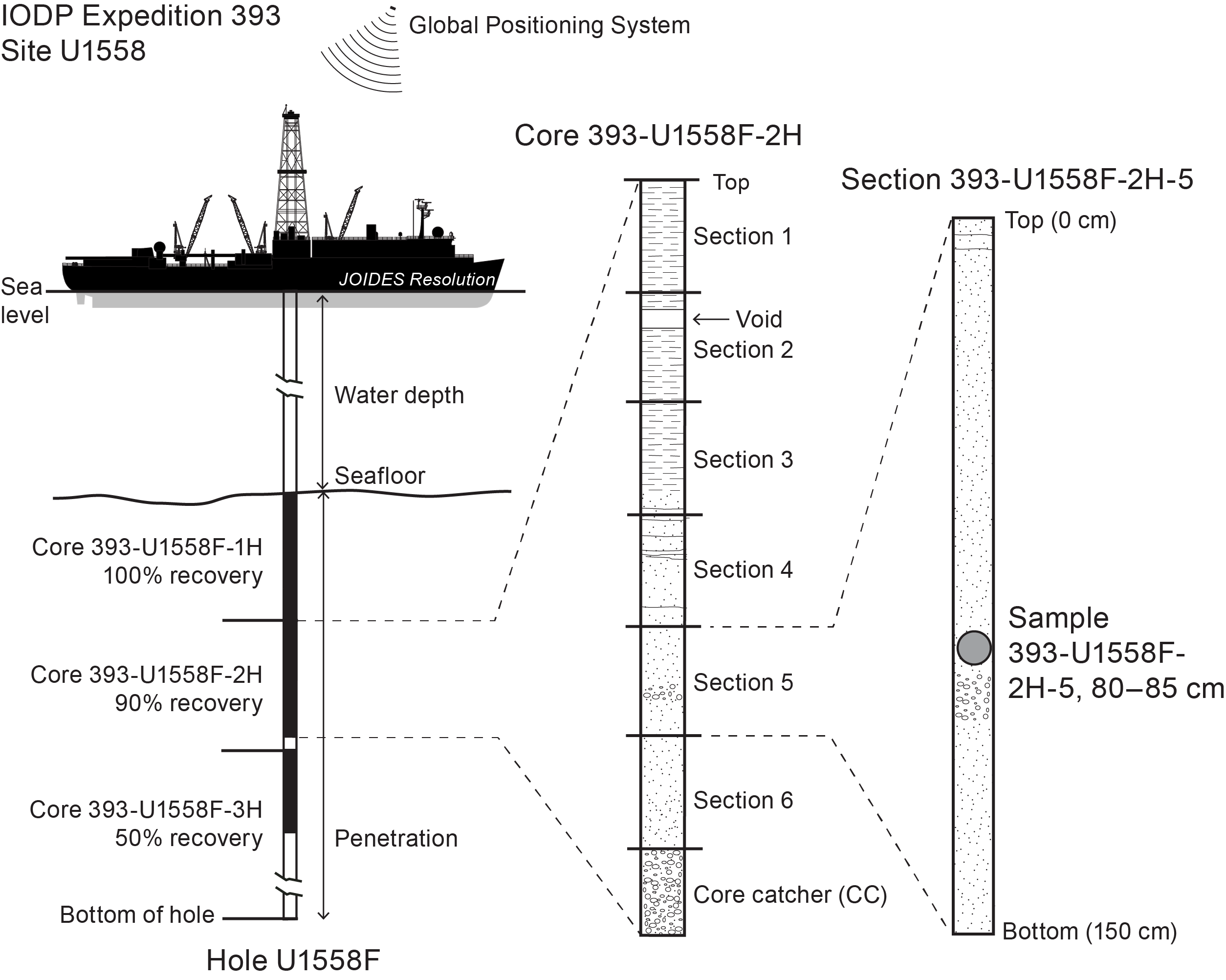
Figure F1. IODP naming convention.
1.2. Drilling and logging operations
To successfully drill both soft and indurated sediments as well as crustal material of varying age and alteration, all four standard coring tools available on JOIDES Resolution were deployed during the SAT expeditions: the advanced piston corer (APC), half-length APC (HLAPC), extended core barrel (XCB), and rotary core barrel (RCB) systems. Operations took place in international waters in water depths of ~3000–5000 m.
The APC and HLAPC systems cut soft-sediment cores with minimal coring disturbance relative to other IODP coring systems. After the APC/HLAPC core barrel is lowered through the drill pipe and lands above the bit, the drill pipe is hydraulically pressurized until the two shear pins that hold the inner barrel attached to the outer barrel fail. The inner barrel then advances into the formation and cuts the core (Figure F2). The driller can detect a successful cut, or "full stroke," by observing the pressure gauge on the rig floor because the excess pressure accumulated prior to the stroke drops rapidly.
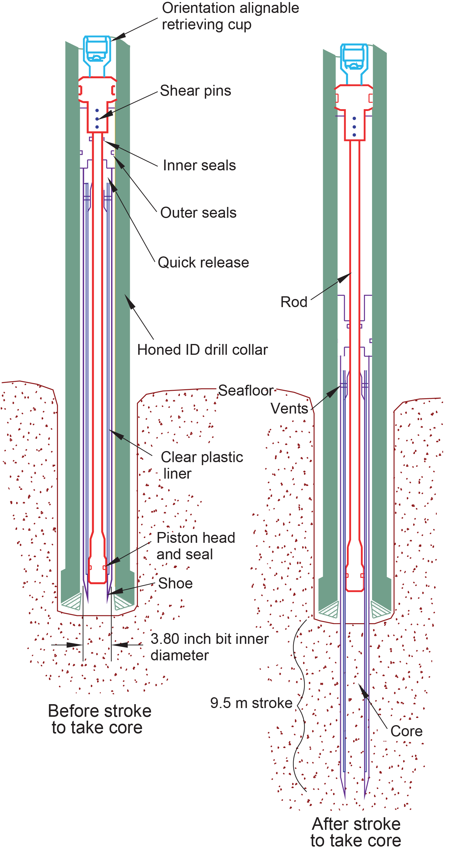
Figure F2. APC system.
APC refusal is conventionally defined in one of two ways: (1) the piston fails to achieve a complete stroke (as determined from the pump pressure and recovery reading) because the formation is too hard, or (2) excessive force (>60,000 lb) is required to pull the core barrel out of the formation. For APC cores that do not achieve a full stroke, the next core can be taken after advancing to a depth determined by the recovery of the previous core (advance by recovery) or to the depth of a full APC core (typically 9.5 m). When a full stroke is not achieved, one or more additional attempts are typically made, and each time the bit is advanced by the length of the core recovered (note that for these cores, this results in a nominal recovery of ~100%). When a full or partial stroke is achieved but excessive force is not able to retrieve the barrel, the core barrel can be “drilled over,” meaning that after the inner core barrel is successfully shot into the formation, the drill bit is advanced to total depth to free the APC barrel.
The standard APC system uses a 9.5 m long core barrel, whereas the HLAPC system uses a 4.7 m long core barrel. In most instances, the HLAPC system is deployed after the standard APC system has repeated partial strokes and/or the core liners are damaged. During use of the HLAPC system, the same criteria are applied in terms of refusal as for the APC system. Use of the HLAPC system allowed for significantly greater APC sampling depths to be attained than would have otherwise been possible. For the SAT expeditions, the HLAPC system was only deployed as time allowed.
The XCB system is a rotary system with a small cutting shoe that extends below the large rotary APC/XCB bit (Figure F3). The smaller bit can cut a semi-indurated core with less torque and fluid circulation than the main bit, potentially improving recovery. It is primarily used in sediment but can core short intervals of hard rock, such as sills, or for capturing the sediment/basement interface. The XCB system is used when the APC/HLAPC system has difficulty penetrating the formation and/or damages the core liner or core. The XCB system can also be used to either initiate holes where the seafloor is not suitable for APC coring or it can be interchanged with the APC/HLAPC system when dictated by changing formation conditions. The XCB system is used to advance the hole when HLAPC refusal occurs before the target depth is reached or when drilling conditions require it. The XCB cutting shoe typically extends ~30.5 cm ahead of the main bit in soft sediments, but a spring allows it to retract into the main bit when hard formations are encountered. Shorter XCB cutting shoes can also be used. The SAT expeditions relied on polycrystalline diamond compact (PDC) XCB cutting shoes, which improved recovery across the sediment/basement interface.
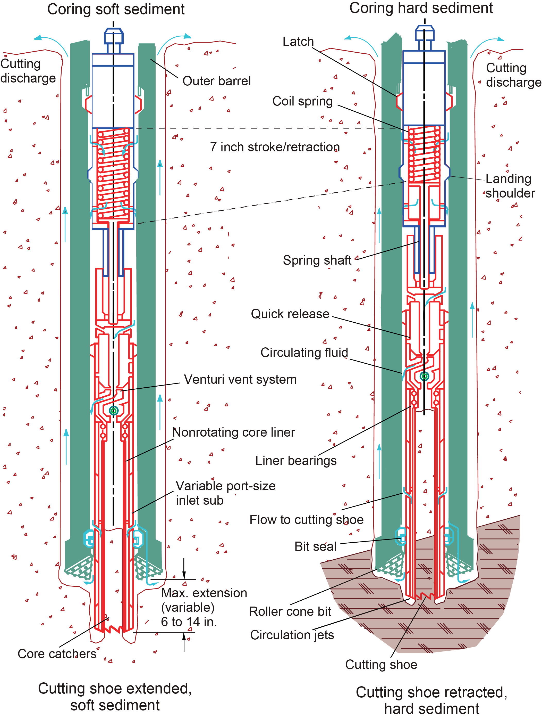
Figure F3. XCB system.
The bottom-hole assembly (BHA) used for APC and XCB coring is typically composed of an 11⁷⁄₁₆ inch (~29.05 cm) roller cone drill bit, a bit sub, a seal bore drill collar, a landing saver sub, a modified top sub, a modified head sub, 8¼ inch control length drill collars, a tapered drill collar, two stands of 5½ inch transition drill pipe, and a crossover sub to the drill pipe that extends to the surface (Figure F4).
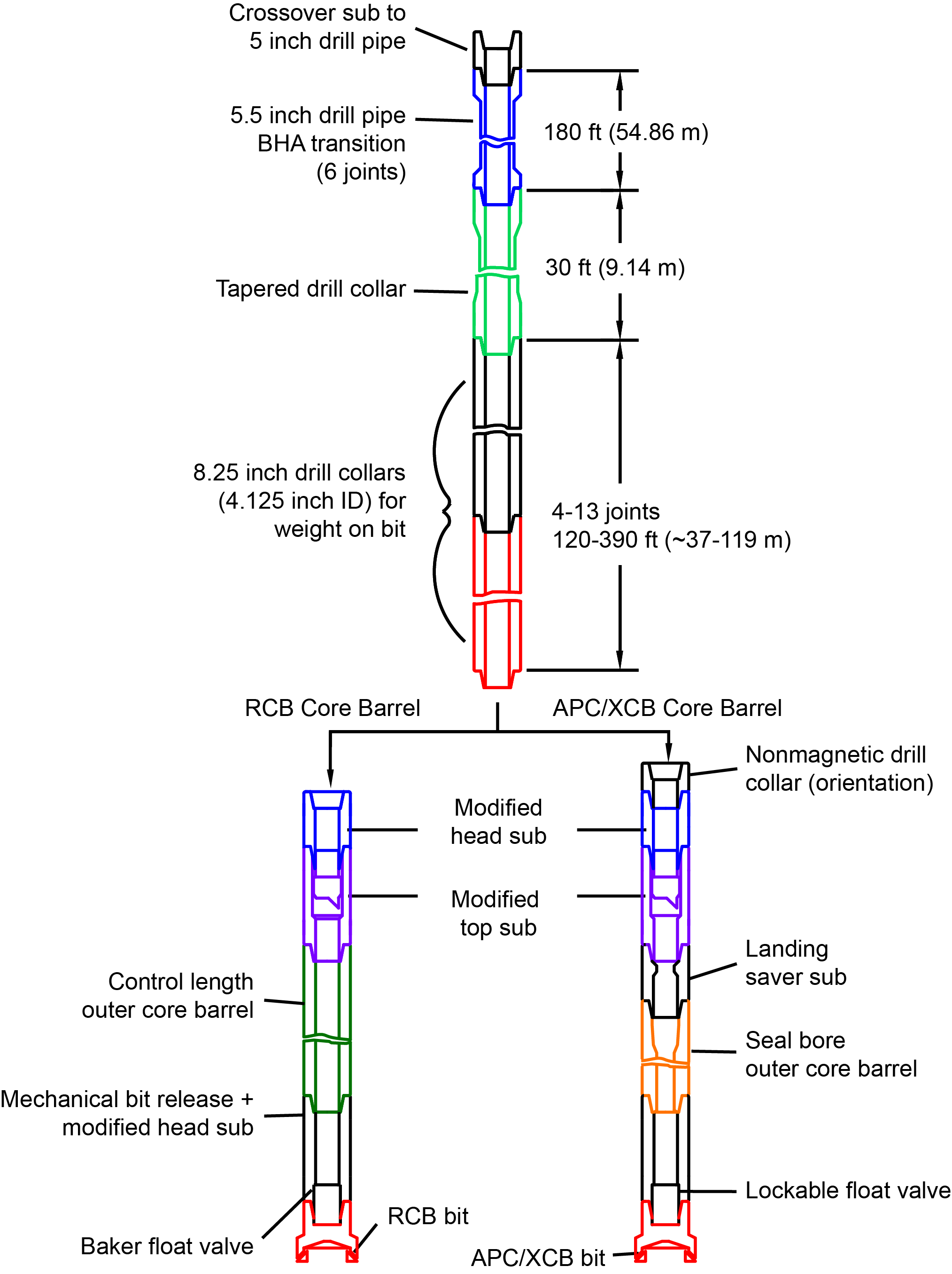
Figure F4. Typical APC/XCB and RCB BHAs.
The RCB system is a rotary system designed to recover firm to hard sediments and basement rocks. The BHA, including the bit and outer core barrel, is rotated with the drill string while bearings allow the inner core barrel to remain stationary (Figure F5).
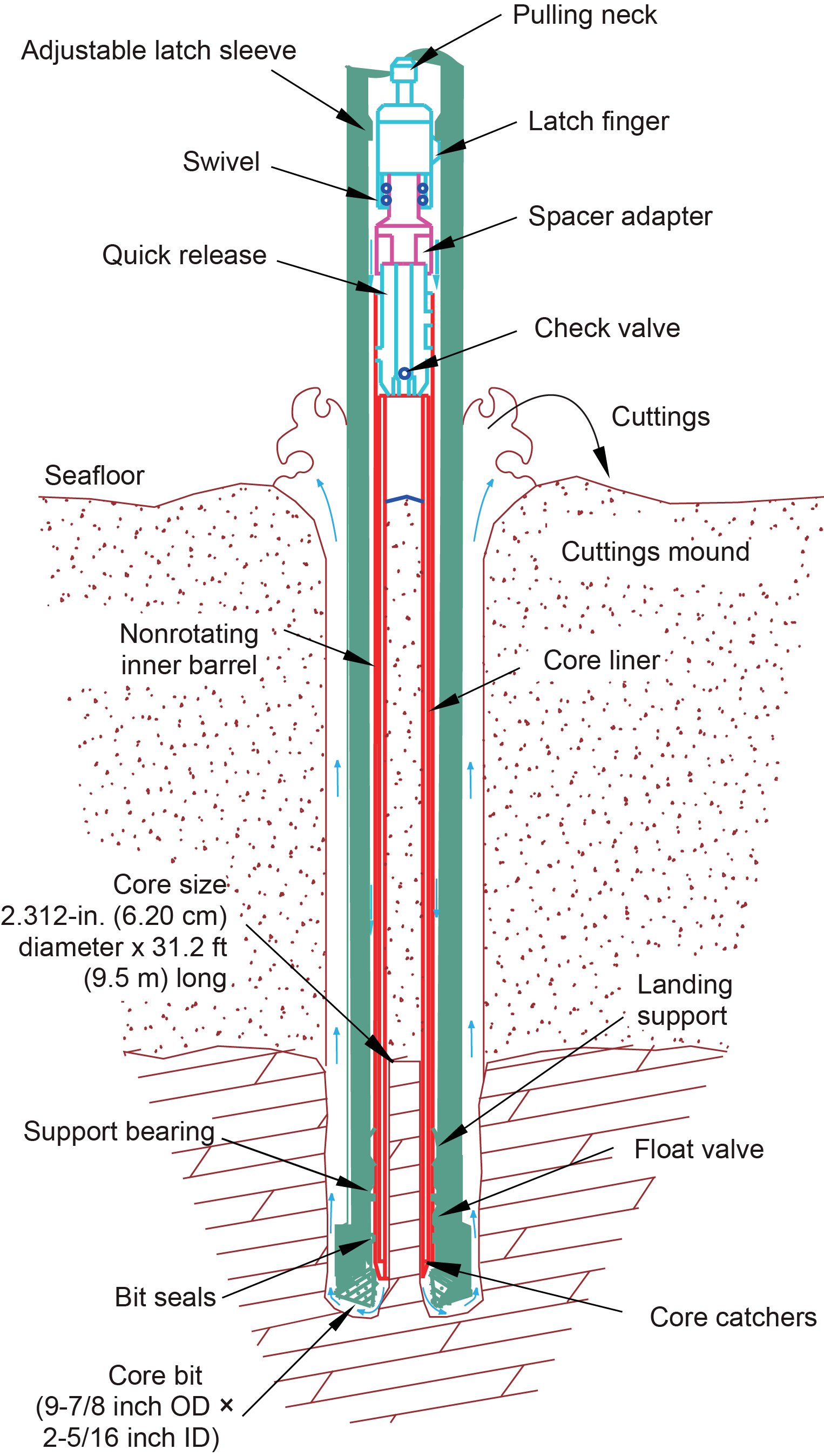
Figure F5. RCB system.
A typical RCB BHA includes a 9⅞ inch drill bit, a bit sub, an outer core barrel, a modified top sub, a modified head sub, a variable number of 8¼ inch control length drill collars, a tapered drill collar, two stands of 5½ inch drill pipe, and a crossover sub to the drill pipe that extends to the surface. Figure F4 depicts a typical BHA for each coring system.
Nonmagnetic core barrels were used for all APC, HLAPC, and RCB coring. APC cores were oriented with the Icefield MI-5 core orientation tool when coring conditions allowed. Formation temperature measurements were taken with the advanced piston corer temperature (APCT-3) tool (see In situ temperature measurements). Information on recovered cores, drilled intervals, downhole tool deployments, and related information are provided in the Operations, Paleomagnetism, and Downhole measurements sections of each site chapter.
1.3. IODP depth conventions
The primary depth scales used are defined by the length of the drill string deployed (e.g., drilling depth below rig floor [DRF] and drilling depth below seafloor [DSF]), the depth of core recovered (e.g., core depth below seafloor [CSF] and core composite depth below seafloor [CCSF]), and the length of logging wireline deployed (e.g., wireline log depth below rig floor [WRF] and wireline log depth below seafloor [WSF]) (see IODP Depth Scales Terminology for sediments at http://www.iodp.org/policies-and-guidelines/142-iodp-depth-scales-terminology-april-2011/file). In cases where multiple logging passes are made, wireline log depths are mapped to one reference pass, creating the wireline log matched depth below seafloor (WMSF) scale. All units are expressed in meters. The relationship between scales is defined either by protocol, such as the rules for computation of CSF depth from DSF depth, or by user-defined correlations, such as core-to-log correlation. The distinction in nomenclature should keep the reader aware that a nominal depth value in different depth scales usually does not refer to the exact same stratigraphic interval.
Depths of cored intervals are measured from the drill floor based on the length of drill pipe deployed beneath the rig floor (DRF scale). The depth of the cored interval is referenced to the seafloor (DSF scale; Figure F1) by subtracting the seafloor depth of the hole (i.e., water depth) from the DRF depth of the interval. Standard depths of cores in meters below seafloor (core depth below seafloor, Method A [CSF-A], scale) are determined based on the assumption that (1) the top depth of a recovered core corresponds to the top depth of its cored interval (on the DSF scale) and (2) the recovered material is a continuous section even if sediment core segments are separated by voids when recovered. Standard depths of samples and associated measurements (CSF-A scale) are calculated by adding the offset of the sample or measurement from the top of its section and the lengths of all higher sections in the core to the top depth of the core.
1.3.1. Sediment core depth scales
If a core has <100% recovery, for curation purposes all cored material is assumed to originate from the top of the drilled interval as a continuous section. In addition, voids in the core are closed by pushing core segments together, if possible, during core handling. Therefore, the true depth interval within the cored interval is unknown. This result should be considered a sampling uncertainty in age-depth analysis or in correlation of core data with downhole logging data.
When core recovery is >100% (the length of the recovered core exceeds that of the cored interval), the CSF depth of a sample or measurement taken from the bottom of a core will be deeper than that of a sample or measurement taken from the top of the subsequent core (i.e., the data associated with the two core intervals overlap on the CSF-A scale). This overlap can happen when a soft to semisoft sediment core recovered from a few hundred meters below the seafloor expands upon recovery (typically by a few percent to as much as 15%). In this case, the core depth below seafloor, Method B (CSF-B), scale can be employed, where the core is (digitally) linearly compressed to fit within the cored interval. Where core recovery is <100%, CSF-A and CSF-B depth scales are exactly equivalent. A stratigraphic interval may not have the same nominal depth on the DSF and CSF scales in the same hole.
During Expedition 390/393, both CSF-A and CSF-B depth scales were used. The CSF-A scale is the default depth scale. However, the CSF-B scale was used for some data sets (e.g., biostratigraphic depths because the core catcher micropaleontological sample should appear at the bottom of that cored interval rather than apparently expanded into the underlying core interval). Where the CSF-B scale was used, depths are labeled as such in the text, tables, and figures.
1.3.2. Basement core depth scales
Two depth scales are used in basement sections, CSF-A and meters subbasement (msb). In the basement chapter sections, meters below seafloor (mbsf) is used and is the same as the CSF-A depth scale. Meters subbasement is the depth below the sediment/basement interface; the interface depth for each hole is described in the Stratigraphic unit summary section of each site chapter. The curatorial process for hard rock (see Curatorial core procedures and sampling depth calculations) results in depths (CSF-A/mbsf) that do not reflect true depths as a result of incomplete recovery, the assumption that all material comes from the top of the cored interval, and subsequent spacing out of the recovered material to "bin" it, which adds "void" intervals.
Additionally, an "expanded" depth scale was used for plotting some basement data so that data points did not overlap with each other on plots. For basement cores with <100% recovery, the recovered length was linearly stretched to fit into the cored depth interval.
1.4. Curatorial core procedures and sampling depth calculations
Numbering of sites, holes, cores, and samples follows standard IODP procedures (Figure F1). A full curatorial identifier for a sample consists of the following information: expedition, site, hole, core number, core type, section number, section half, piece number (for cores/sections of igneous/metamorphic rocks only), and interval in centimeters measured from the top of the core section. For example, a sample identification of "390-U1556C-15H-2W, 46–48 cm" indicates a 2 cm long sample taken from the interval between 46 and 48 cm below the top of Section 2 (working half) of Core 15 ("H" designates that this core was taken with the APC system) of Hole C at Site U1556 (Figure F1). The "U" preceding the site/hole number indicates the hole was drilled by the US platform, JOIDES Resolution. The coring system used to obtain a core is designated in the sample identifiers as follows: H = APC, F = HLAPC, R = RCB, and X = XCB. Integers are used to denote the "core" type of drilled intervals (e.g., a drilled interval before Core 2R would be denoted by Core 11 [i.e., Core 1 and Type 1]).
1.5. Core handling and analysis
1.5.1. Sediment
When the core barrel reached the rig floor, the core catcher from the bottom of the core was removed and taken to the core receiving platform ("catwalk"), and a sample was extracted for paleontological (PAL) analysis. Next, the sediment core was extracted from the core barrel in its plastic liner. The liner was carried from the rig floor to the core processing area on the catwalk outside the core laboratory, where it was labeled and split into ~1.5 m sections. Blue (uphole direction) and clear (downhole direction) liner caps were glued with acetone onto the cut liner sections. In holes where oxygen measurements and Rhizon sampling for interstitial water (IW) occurred, liner caps were not glued with acetone until after sampling and analyses were completed.
Once the core was cut into sections, whole-round samples were taken for IW chemical analyses, as microbiological samples, and as geotechnical samples. When a whole-round sample was removed, a yellow end cap was used at the bottom of the remaining core section to indicate it was taken. In one hole at each site, syringe samples were taken for gas analyses according to the IODP hydrocarbon safety monitoring protocol.
The core sections were placed in a core rack in the laboratory, core information was entered into the database, and the sections were laser engraved. In holes where stratigraphic correlations were being made, sediment cores were run on the Special Task Multisensor Logger (STMSL) to measure magnetic susceptibility (MS) and gamma ray attenuation (GRA) bulk density before equilibration to room temperature. Oxygen probe measurements and Rhizon pore water samples were typically taken before core sections reached equilibrium with laboratory temperature (after ~4 h), apart from in Hole U1556C. Core sections were then run through the Whole-Round Multisensor Logger (WRMSL) for P-wave velocity (P-wave logger [PWL]), MS, and GRA bulk density measurements (see Physical properties and downhole measurements). The core sections were also run through the Natural Gamma Radiation Logger (NGRL), often prior to temperature equilibration because that does not affect the natural gamma radiation (NGR) data. Thermal conductivity measurements were taken once per core when the material was suitable, typically with the puck probe rather than the needle probe.
Core sections were then split lengthwise from bottom to top into working and archive halves. Investigators should note that older material can be transported upward on the split face of each section during splitting.
The working halves of each core section were then laid out on the sampling tables, and samples were taken for moisture and density (MAD) and paleomagnetic (PMAG) analyses and for remaining shipboard geochemical analyses such as X-ray diffraction (XRD), carbonate (CARB), and inductively coupled plasma–atomic emission spectroscopy (ICP-AES). Samples were not collected when the lithology was a high-priority interval for expedition or postexpedition research, the core material was unsuitable, or the core was severely deformed. During the expedition, samples for personal postexpedition research were taken when they concerned ephemeral properties (e.g., IW samples that require acidification).
The archive half of each core was scanned on the Section Half Imaging Logger (SHIL) to provide linescan images and then measured for point magnetic susceptibility (MSP) and reflectance spectroscopy and colorimetry (RSC) on the Section Half Multisensor Logger (SHMSL). Labeled foam pieces were used to denote removed whole-round intervals in the SHIL images. The archive halves were then described visually and by means of smear slides for sedimentology. During Expedition 393, archive-half sections were imaged on the XMAN X-ray scanner. Finally, the magnetization of archive halves and working-half discrete pieces was measured with the cryogenic magnetometer and spinner magnetometer.
When all steps were completed, cores were wrapped in plastic wrap, sealed in plastic tubes, and transferred to cold storage space aboard the ship. At the end of the expedition, the working halves of the cores were sent to the IODP Bremen Core Repository (Center for Marine Environmental Sciences [MARUM], Bremen, Germany), where samples for postexpedition research were taken in January 2023. The archive halves of the cores were first sent to the IODP Gulf Coast Repository (Texas A&M University, College Station, Texas [USA]), where a subset was scanned for X-ray fluorescence (XRF), before being forwarded to the Bremen Core Repository for long-term storage. Sediment core flow is summarized in Figure F6.
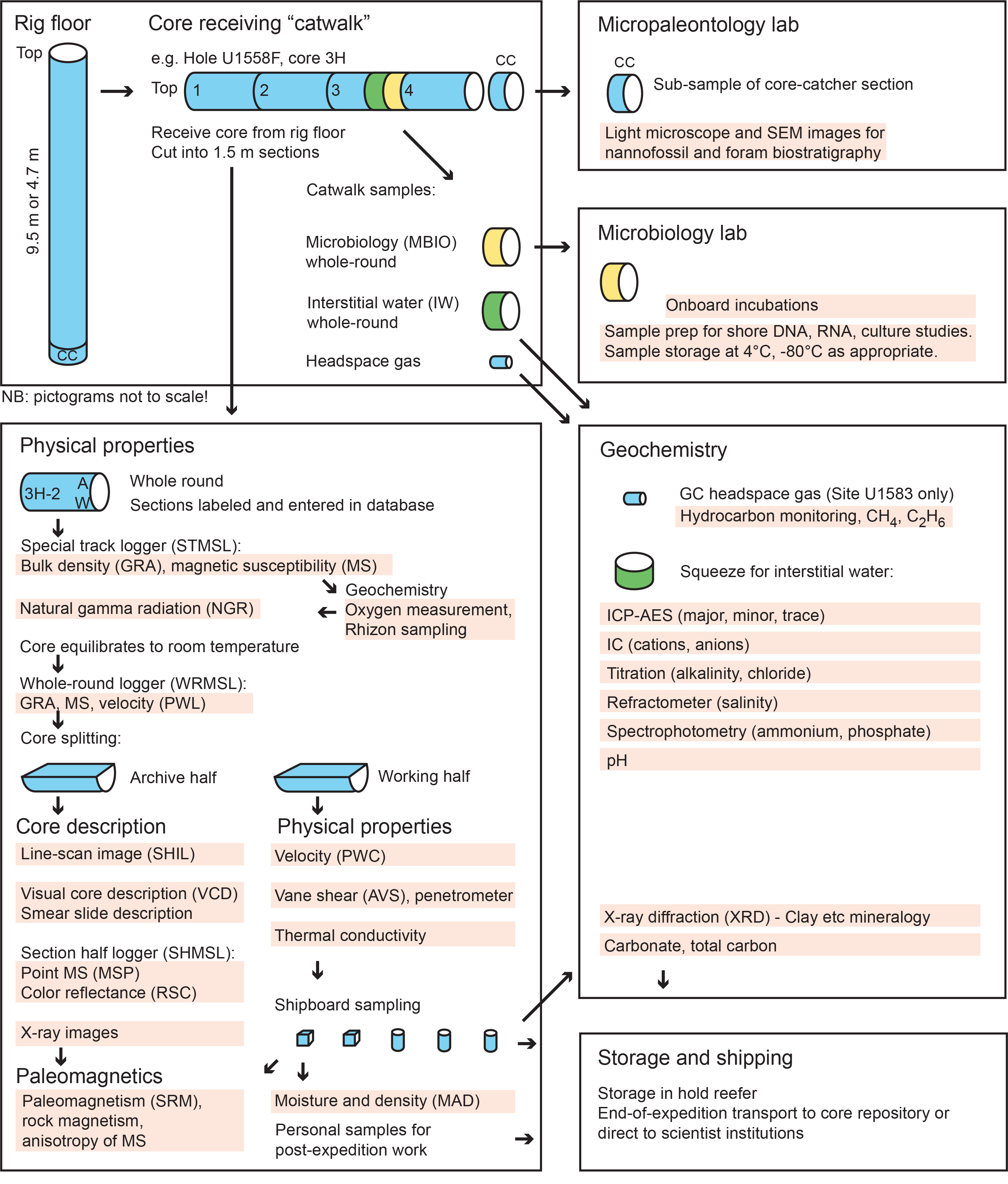
Figure F6. Sediment laboratory core flow.
1.5.2. Igneous rock
Igneous and indurated rock cores were extracted from the core barrel in its plastic liner. The liner was carried from the rig floor to the core processing area on the catwalk outside the core laboratory, where it was split into ~1.5 m sections. These sections were immediately carried into the splitting room. Pieces were extracted from the core liner in the splitting room and subsequently put into split plastic liners in consecutive order while maintaining the original orientation of pieces as much as possible. The pieces were then pushed to the bottom of the 1.5 m liner sections, and the total rock length was measured. The length was entered into the database as "recovered length" using the SampleMaster application. This number was used to calculate recovery. If a core catcher sample was present, it was taken to the core splitting room separately and added to the bottom section of the recovered core.
For microbiological sampling, the split liners were sprayed with 70% ethanol and wiped down prior to shaking pieces out. Only the necessary scientists (petrologist and microbiologists on shift), an assigned representative of the Sample Allocation Committee, and technicians were present in the core splitting room for microbiology sampling to minimize contamination. Those present wore face masks and nitrile gloves sprayed with 70% ethanol and made sure to pull hair back. The selected microbiological sample was photographed in context with the rest of the core sections overhead, and the sample/section was then immediately transferred in a sterile and sealed sample bag to the microbiology laboratory for further processing (see Microbiology).
Oriented pieces of core that could not have rotated around a horizontal axis during drilling were marked on the bottom with a blue- or red-colored wax pencil to preserve orientation. Adjacent but broken pieces that could be fit together along fractures were curated as single pieces. The petrologists confirmed piece matches, marked a split line on each piece, and denoted the working half with the letter "W," which defined how the pieces were to be cut into two equal halves. The aim was to preserve representative lithologic and mineralogical features in both archive and working halves while ensuring the availability of fresh glass and vein features in the working halves for sampling purposes. Where possible, cutting lines were drawn parallel to the dip direction of structural features to maximize the expression of dipping structures on the cut face of the core. A plastic spacer was secured with acetone to the split core liner between individual pieces or reconstructed continuous groups of subpieces. These spacers can add artificial gaps and also represent substantial intervals of no recovery. The length of each section of core, including spacers, was entered into the database as "curated length," which commonly differs by several centimeters from the length measured on the core receiving platform. Ultimately, the curated depth of each piece in the database was recalculated based on the curated length. The curatorial process can result in overestimation or underestimation of the depth from which a piece was cored.
Core pieces were imaged around the full 360° circumference using the Deutsche Montan Technologie (DMT) scanner (see Physical properties and downhole measurements). When the core sections reached equilibrium with laboratory temperature (typically after 2 h), the whole-round core sections were run through the WRMSL (GRA and MS only) and NGRL (see Physical properties and downhole measurements).
Each piece of core was split with a diamond-impregnated saw into an archive half and a working half, with the positions of plastic spacers between pieces the same in both halves. Pieces were numbered sequentially from the top of each section, beginning with 1. Separate subpieces within a single piece were assigned the same number but lettered consecutively (e.g., 1A, 1B, etc.). Labels were attached using epoxy only on the outer cylindrical surfaces of the core. If it was evident that an individual piece had not rotated around a horizontal axis during drilling, an arrow pointing to the top of the section was added to the label. The oriented character of each piece was recorded in the database using the SampleMaster application.
The archive half of each core was scanned on the SHIL (with a dry surface during Expedition 390 and with both dry and wet surfaces during Expedition 393) and measured for MSP and RSC on the SHMSL. Thermal conductivity measurements were made on selected archive-half pieces (see Physical properties and downhole measurements). After the archive-half sections of each core were fully described by the petrologist and structural geologist on shift, samples were taken from the working-half sections for shipboard analyses (billets for thin sections, chips for ICP-AES, and cube samples [~8 cm3] for paleomagnetism analyses, MAD, and discrete P-wave velocity measurements; see Igneous petrology, Alteration petrology, Geochemistry, Paleomagnetism, and Physical properties and downhole measurements). The magnetizations of archive-half sections and pieces, as well as discrete cube samples taken from the working-half sections, were measured with the cryogenic magnetometer and spinner magnetometer, respectively (see Paleomagnetism).
When all laboratory processing steps were completed, cores were wrapped in shrink wrap, sealed in plastic tubes, and transferred to cold storage space aboard the ship. At the end of the expedition, the cores were sent to the IODP Gulf Coast Repository, where personal non-ephemeral samples for postexpedition research were taken in November 2022 prior to forwarding the cores to the Bremen Core Repository for long-term storage. Basement core flow is summarized in Figure F7.
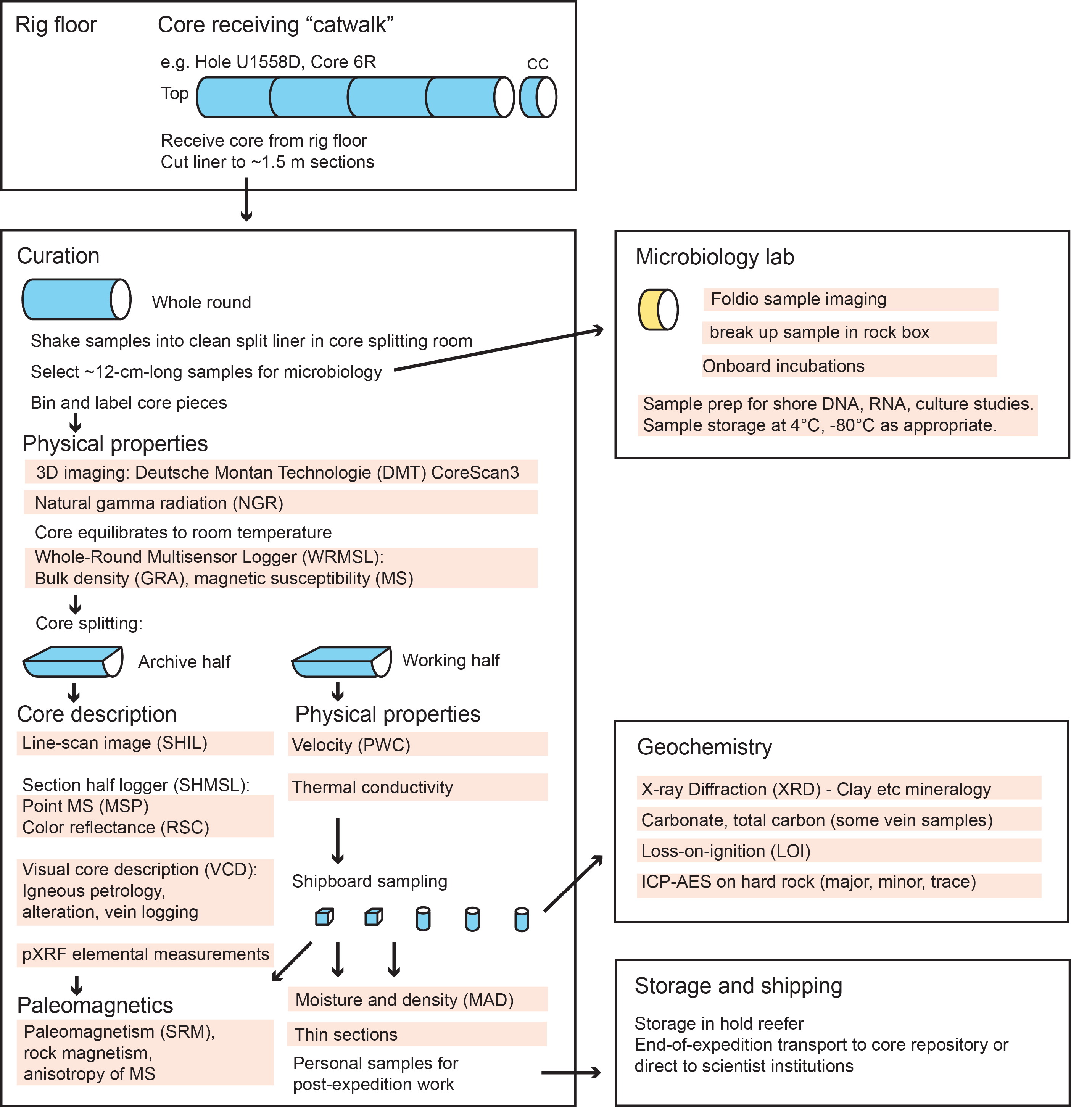
Figure F7. Hard rock laboratory core flow.
1.6. Handling of drilling and core disturbance
Cores may be significantly disturbed and contain extraneous material as a result of the coring and core handling process (Jutzeler et al., 2014). In formations with loose layers, material from intervals higher in the hole may be washed down by drilling circulation, accumulate at the bottom of the hole, and be sampled with the next core. The uppermost 10–50 cm of each core must therefore be examined critically during description for potential "fall-in" material. Common coring-induced deformation includes the concave-downward appearance of originally horizontal bedding. Piston action can result in fluidization ("flow-in") at the bottom of APC/HLAPC cores. The rotation and fluid circulation used during XCB and RCB coring can also cause cored material to fragment into discrete pieces ("biscuits") that may rotate relative to each other. A slurry of drilling fluid, seawater, and fluidized sediment can be injected between and around the biscuits, producing what is colloquially termed "biscuits and gravy." Retrieval from depth to the surface can result in elastic rebound. Gas that is in solution at depth may become free and drive apart core segments within the liner. When gas content is high, pressure must be relieved for safety reasons by drilling holes into the plastic liner before the cores are cut into segments. These holes force some sediment as well as gas out of the liner. Such observed disturbances are described in each site chapter and graphically indicated on the visual core descriptions (VCDs).
2. Sedimentology
Sediments and sedimentary rocks recovered during SAT Expeditions 390C, 395E, 390, and 393 were described macroscopically from archive-half sections by shipboard scientists during Expeditions 390 and 393. Microscopic descriptions were based on smear slides and thin sections. Digital color images of all archive-half sections were produced using the SHIL, and visual color determination followed Munsell soil color charts (Munsell Color Company, 1994). Some of the cores were obtained in November 2020 (Expedition 390C) and May 2021 (Expedition 395E) and described in April–August 2022 (during Expeditions 390 and 393) (see Background and objectives in each site chapter). Some color differences may exist between the digital color images generated with the SHIL and the visual color determinations, likely reflecting changes such as postcoring drying and/or oxidation of the sediments.
The description of sedimentary lithologies was supported by XRD analyses, scanning electron microscope (SEM) photomicrographs, carbonate content measurements (see Geochemistry), and physical properties measurements (see Physical properties and downhole measurements). Observations were recorded in separate macroscopic (drilling disturbance, lithologic description, and deformational structures) and microscopic (smear slide) DESClogik templates (Version x.16.2.0.0; see the DESClogik user guide at https://wiki.iodp.tamu.edu/
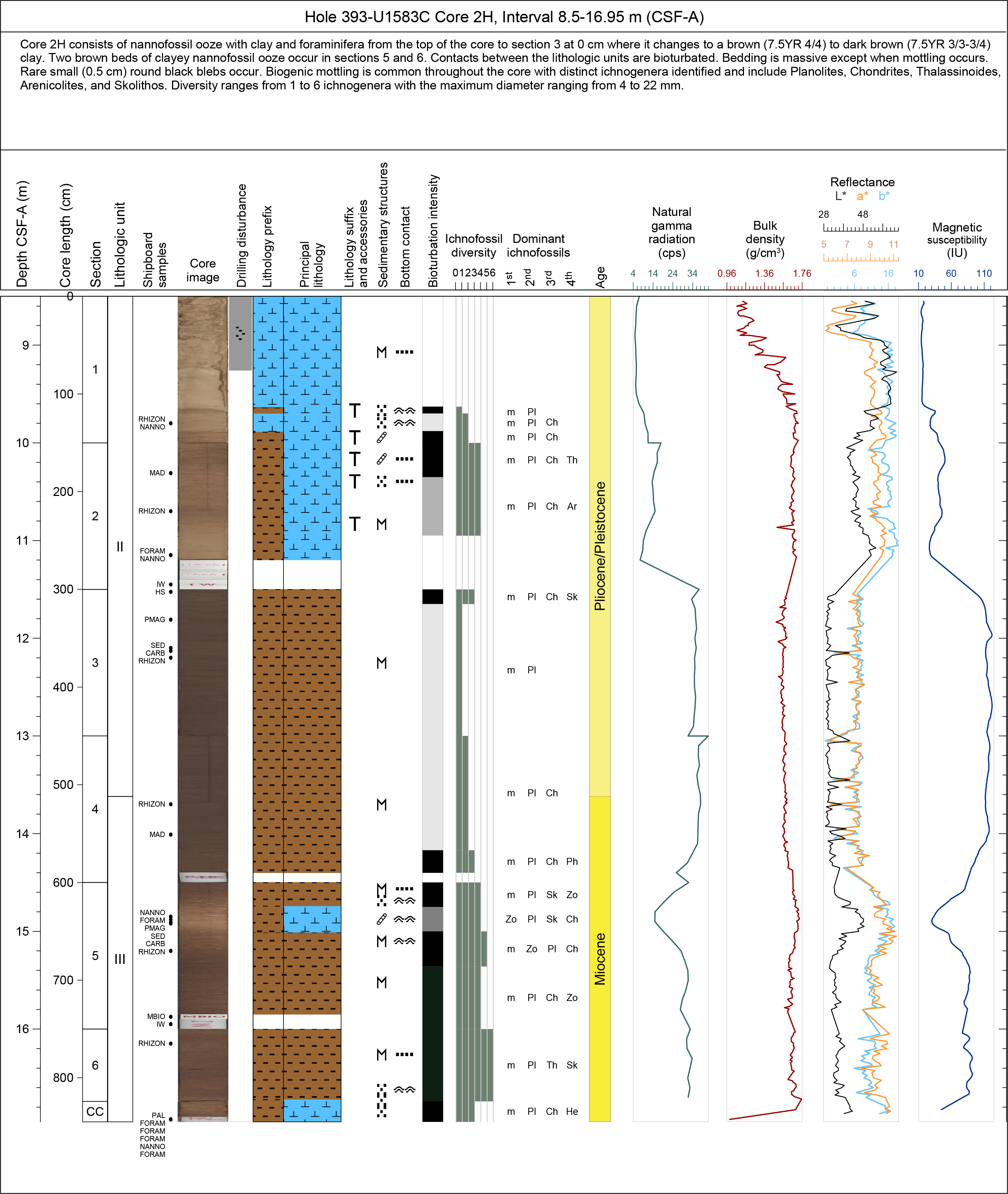
Figure F8. Example sediment VCD.
2.1. Macroscopic descriptions
2.1.1. Section half images
Standard core splitting can affect the appearance of the section half surface, obscuring fine details of lithology and sedimentary structures. Therefore, when required, the archive-half sections were scraped parallel to bedding using a stainless steel or glass scraper (from the bottom of the section to the top). For XCB cores with moderately consolidated sediments, water was used to clean the section half surface before describing. After cleaning the core surface (if necessary), the archive half was scanned with the SHIL as soon as possible to avoid color changes caused by oxidation and sediment drying. In cases of watery or soupy sediment, the surface was dried sufficiently with lint-free wipes prior to scanning to avoid reflected light photographic artifacts. Three pairs of advanced illumination, high-current, focused LED line lights with adjustable angles to the lens axis illuminated any large cracks and blocks in the core surface and sidewalls. Each of the LED pairs had a color temperature of 6,500 K and emitted 90,000 lx at 7.62 cm. Digital images were taken by a linescan camera at an interval of 10 lines/mm to create a high-resolution TIFF file. The camera height was set so that each pixel imaged a 0.1 mm2 area of the section half surface. Actual core width per pixel varied because of slight differences in the section half surface height. JPEG files were created from the high-resolution TIFF files. One set of JPEG image files includes a gray-scale reference card and offset ruler; a second set is cropped to include only the section half surface.
2.1.2. Stratification and sedimentary structures
We described the locations and types of stratification and sedimentary structures visible on the surfaces of the section halves in the following macroscopic DESClogik worksheet columns: Lithology sedimentary structure, Sedimentary structure abundance, and Bedding thickness. Observations in these columns indicate the locations and scales of interstratification and individual bedding. The following terminology (based on Stow [2005]) was used to describe the scale of lamination and bedding:
- Thin lamination = <0.3 cm thick.
- Medium lamination = 0.3–0.6 cm thick.
- Thick lamination = 0.6–1 cm thick.
- Very thin bed = 1–3 cm thick.
- Thin bed = 3–10 cm thick.
- Medium bed = 10–30 cm thick.
- Thick bed = 30–100 cm thick.
- Very thick bed = >100 cm thick.
The presence of graded beds was entered in the Grading column separately from other sedimentary structures. "Normal grading" corresponds to layers with a gradual decrease in grain size from the bottom to the top of the bed, whereas "reverse grading" corresponds to layers with a gradual increase in grain size from the bottom to the top of the bed.
2.1.3. Bioturbation
The trace fossils herein were used for interpreting environmental parameters, such as oxygen variations in pore and bottom waters, substrate consistency, sedimentation rate, organic matter availability, and hydraulic energy at the seafloor in the past geologic epochs. The bioturbation index (BI) is a semiquantitative assessment of bioturbation intensity based on the percentage grades of sediment reworked by organismal activity (cf. Reineck, 1963; Taylor and Goldring, 1993; Taylor et al., 2003). We reported seven levels of bioturbation intensity in the Bioturbation index column in DESClogik (Figure F9):
- Absent: no bioturbation (0%).
- Sparse: few discrete traces and/or escape structures (<10%).
- Low: bedding is distinct, low trace density, escape structures are often common (10%–30%).
- Moderate: bedding boundaries are sharp, traces are discrete (>30%–60%).
- High: bedding boundaries are indistinct, high trace density with overlap common (>60%–90%).
- Intense: bedding is completely disturbed, limited reworking due to repeated overprinting (>90%).
- Complete: sediment reworking due to repeated overprinting (100%).
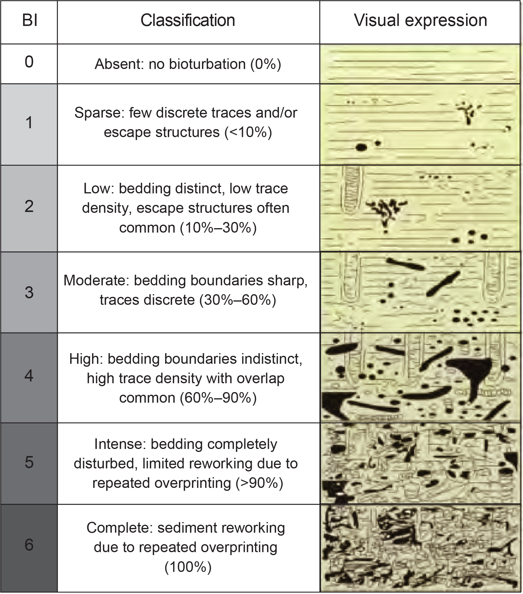
Figure F9. Bioturbation intensity.
2.1.4. Biogenic sedimentary structures
During Expedition 393, a new Bioturbation tab was added to the DESClogik template to describe in detail intervals with biogenic mottling and distinct biogenic sedimentary structures. In addition to characterizing bioturbation intensity (as described in Bioturbation above), Expedition 393 shipboard scientists specified the four most common trace fossils observed (as the 1st, 2nd, 3rd, and 4th dominant ichnofossils), defined ichnofossil diversity as the total number of identified ichnofossils, measured the maximum trace fossil diameter, and added comments in an Ichnofossil comment column for extra observations and details. The most common trace fossils, namely Zoophycos, Chondrites, Planolites, Palaeophycus, Thalassinoides, Skolithos, Nereites/Cosmorhaphe, Phycosiphon, and rarely Arenicolites, Cylindrichnus, and Spirophyton, were defined based on various atlases, books, and scientific papers devoted to ichnological analysis of cores from modern marine sediments (Bromley and Ekdale, 1984; Buatois and Mángano, 2011; Dorador et al., 2020; Ekdale and Bromley, 1984, 1991; Pemberton et al., 2009; Rodríguez-Tovar and Dorador, 2015; Wetzel et al., 2010).
2.1.5. Lithology sedimentary structures
The locations and types of sedimentary structures that are not a result of drilling disturbance observed on the surfaces of the section halves were selected in the Sedimentary structure column in DESClogik and assigned to, for example (commonly used), cross-lamination/stratification, interlamination/stratification, trends in grain size (coarsening or fining upward), ripple, lens or pods, or "trails, tracks, and burrows" for trace fossils. Additionally, the terms "mottling" or "indistinct mottling" were used where identification of individual ichnotaxa was not possible but the media had a bioturbated and mottled appearance. The abundance of the sedimentary structures is quantitatively expressed by the frequency parameters in Table T1. When mottling was present, both a sedimentary structure abundance (Table T1) and a bioturbation index were assigned in DESClogik, assuming mottling was due to bioturbation, unless otherwise noted (e.g., "sediment mottling").
2.1.6. Lithologic contacts and consolidation state
We described bottom contact geometry for every distinct lithologic interval recorded and entered in DESClogik using these terms: bioturbated, gradational, erosive, planar, irregular, and sharp. Also, the attitude of the lithologic bottom contacts was described as curved, horizontal, subhorizontal, inclined, or steeply dipping (>45°). For comparison, the lithologic contact that marks the top/bottom limit of a unit/subunit is defined as a "boundary." We reported the degree of lithification of the sediments as unconsolidated, moderately consolidated, or lithified.
2.1.7. Drilling disturbance
We recorded drilling-related sediment disturbances for each core (see Disturbance column; Figures F8, F10). The type of drilling disturbance for soft (unconsolidated) and firm (moderately consolidated) sediment were described using these terms:
- Fall-in: out of place material at the top of a core that fell downhole onto the cored surface.
- Bowed: bedding contacts slightly–moderately deformed but still subhorizontal and continuous.
- Uparching: material retains coherency; material closest to the core liner bent downward.
- Void: empty space in the cored material (e.g., caused by gas or sediment expansion during core retrieval). To the extent possible, voids were closed on the core receiving platform by pushing the recovered intervals toward the top of the core before cutting the sections. The space left at the bottom of the core below all the recovered material due to incomplete recovery was not described as a void.
- Flow-in, coring/drilling slurry, or along-core gravel/sand contamination: soft-sediment stretching and/or compressional shearing structures when severe.
- Soupy or mousse-like: water-saturated intervals that have lost all aspects of original bedding.
- Biscuit: sediment of intermediate stiffness with vertical variations in the degree of disturbance, whereas firmer intervals are relatively undisturbed.
- Cracked or fractured: firm sediment broken during drilling; not displaced or rotated significantly.
- Fragmented or pulverized: firm sediment pervasively broken by drilling; may be displaced or rotated.
- Drilling breccia: core is crushed and broken into many small and angular pieces; original orientation and stratigraphic position are affected.
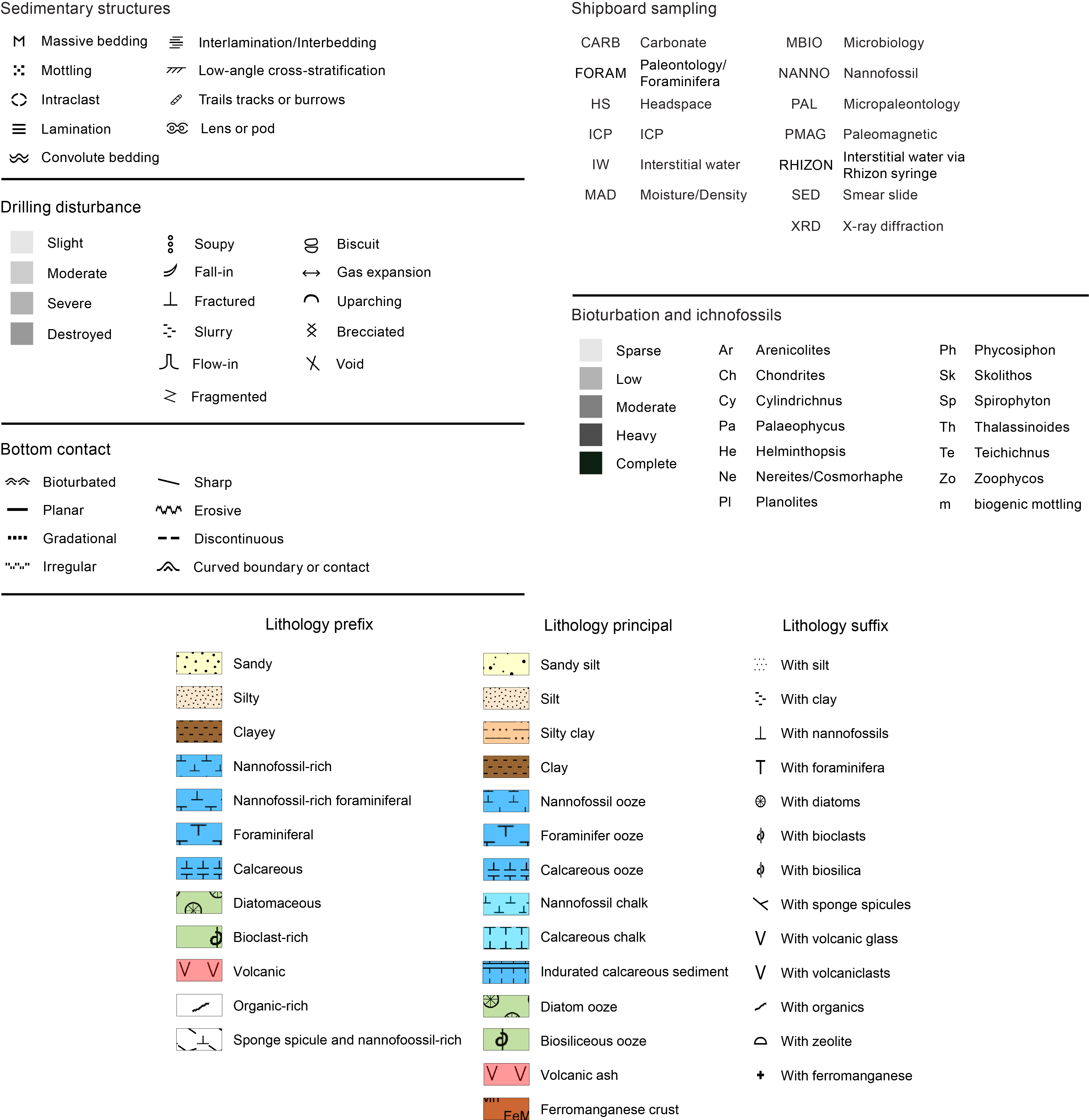
Figure F10. Symbols used for sediment VCDs.
Each instance of drilling disturbance was assigned a degree of severity:
- Slight: core material is in place but broken or otherwise disturbed.
- Moderate: core material is in place or partly displaced, but original orientation is preserved or recognizable.
- Severe: core material is probably in the correct stratigraphic sequence, but original orientation is lost.
- Destroyed: core material is in the incorrect stratigraphic sequence, and original orientation is lost. In the case of voids, core material is absent.
2.2. Microscopic descriptions
2.2.1. Smear slide descriptions
We estimated sediment constituent size, composition, and abundance microscopically using smear slides. Smear slide samples of the main lithologies were collected from the archive-half sections. Additional samples were collected from areas of interest, such as distinct intervals (e.g., organic-rich layers or diatom or foraminiferal oozes).
For each smear slide, a small amount of sediment was removed from the section half using a flat wooden toothpick and put on a 25 mm × 75 mm glass slide. A drop of deionized water was added to the sediment, and the sediment was homogenized with the toothpick and evenly spread across the glass slide. The dispersed sample was dried on a hot plate at a low setting (110°–120°C). A drop of adhesive (Norland optical adhesive Number 61) was added as a mounting medium for a glass coverslip, which was carefully placed on the dried sample to prevent air bubbles from being trapped in the adhesive. The smear slide was then fixed in a UV light box for 5–10 min to cure the adhesive.
Smear slides were examined with a transmitted-light petrographic microscope (Carl Zeiss AXIO with a HAL 100 halogen lamp) equipped with a standard eyepiece micrometer and a SPOT Insight FireWire digital camera. Biogenic and mineral components were identified following standard petrographic techniques as described in the Rothwell (1989), Marsaglia et al. (2013, 2015), Scholle and Ulmer-Scholle (2003), and Ulmer-Scholle et al. (2015) reference manuals and books. Several fields of view were examined at 10×, 20×, and 40× to assess the abundance of detrital (e.g., quartz, feldspar, clay minerals, mica, and heavy minerals), biogenic (e.g., nannofossils, other calcareous bioclasts, diatoms, foraminifera, and radiolarians), and authigenic (e.g., carbonate, iron sulfide, iron oxides, and glauconite) components. The average grain size of clay (<4 µm), silt (4–63 µm), and sand (>63 µm) was estimated for siliciclastic, carbonate, biogenic, and volcaniclastic material. The relative percent abundances of the sedimentary constituents were visually estimated using the techniques of Rothwell (1989). The texture of siliciclastic lithologies (i.e., relative abundance of sand-, silt-, and clay-sized grains) and the proportions and presence of biogenic and mineral components were recorded in the smear slide worksheet of the microscopic DESClogik template. Components observed in smear slides were categorized according to their abundance as shown in Table T1.
2.3. Sediment and sedimentary rock classification
Sediment and sedimentary rock types were entered in the lithology columns of the macroscopic DESClogik worksheet. Corresponding patterns and colors were defined on the graphic core summaries and hole summaries during the core descriptions accomplished during Expeditions 390 and 393.
2.3.1. Sedimentary lithologic classes
Following prior IODP expeditions (e.g., Röhl et al., 2022; Sutherland et al., 2019) and the Handbook for Sedimentologists (Mazzullo and Graham, 1988), three main sedimentary lithologic classes (Figure F11) were defined based on the primary origin of the sediment constituents (but not the depositional processes):
- Biogenic: >50% carbonate, chemical, undifferentiated calcareous bioclasts, and calcareous microfauna and microflora.
- Siliciclastic: >50% siliciclastic particles, <25% volcanic particles, and <50% biogenic particles; therefore, nonvolcanic siliciclastic particles dominate over chemical and biogenic particles.
- Volcaniclastic: >25% volcanic particles. In this class, volcanic sediments are defined as >75% of volcanic clasts and grains, whereas tuffaceous sediments contain 75%–25% volcanic clasts and grains mixed with nonvolcanic particles (either nonvolcanic siliciclastic, biogenic, or both). The definition of the term "tuffaceous" (25%–75% volcanic particles) was modified from Fisher and Schmincke (1984). Note that the term "volcaniclastic" was used following Fisher (1961) and therefore includes both volcanic and tuffaceous lithologies.
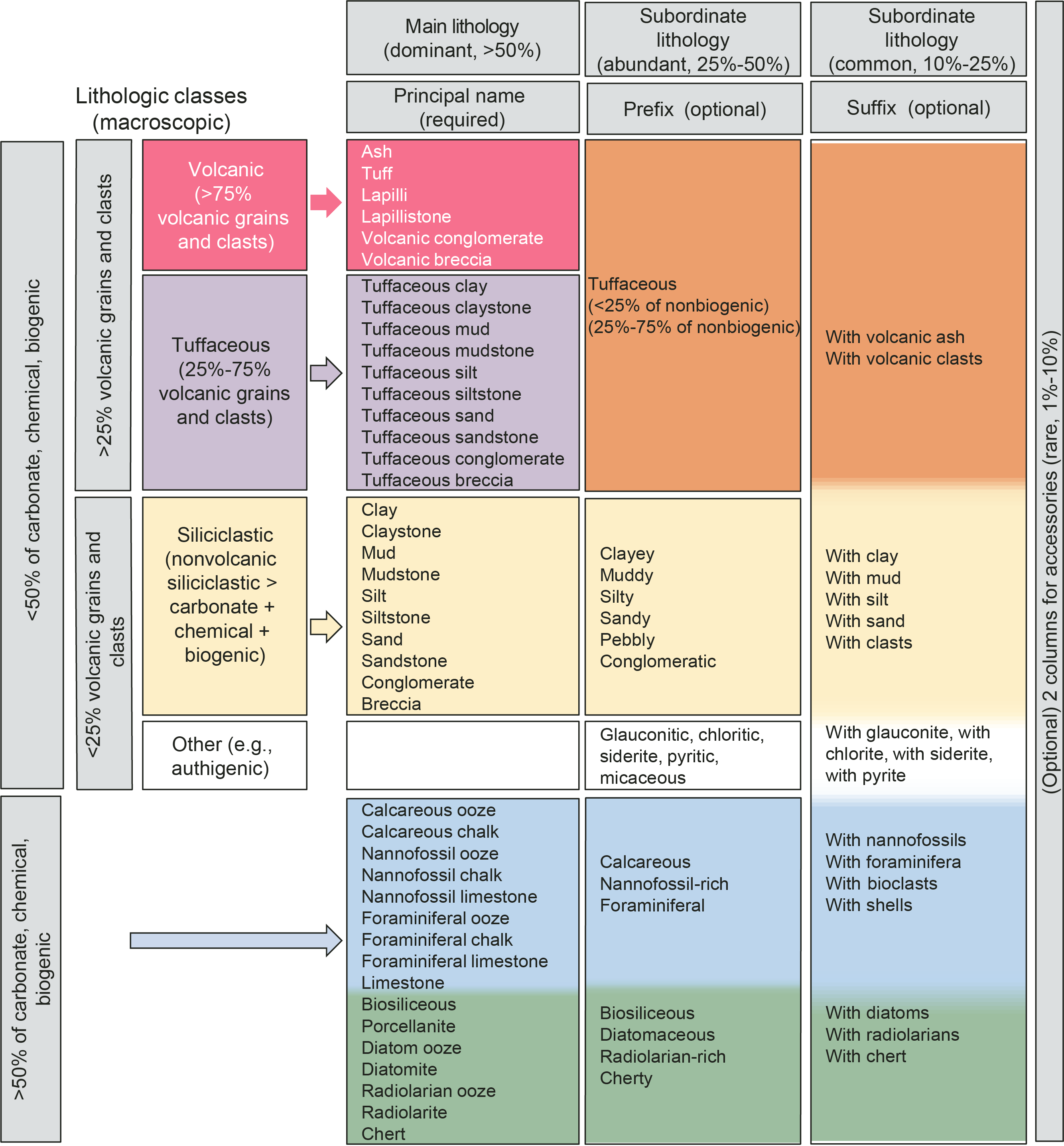
Figure F11. Sedimentary lithology naming conventions.
These three lithologic classes formed the basis of the principal name of the described sediments and sedimentary rocks, with appropriate prefixes and suffixes that could be chosen for mixed lithologies (see Principal names and modifiers below).
2.3.2. Principal names and modifiers
The principal name was based on the most abundant sediment class (Figure F11). Principal names for the siliciclastic class were adapted from the grain size classes of Wentworth (1922), whereas principal names for the volcaniclastic class were adapted from the grain size classes of Fisher and Schmincke (1984). Thus, the Wentworth (1922) and Fisher and Schmincke (1984) classifications were used to refer to particle type (siliciclastic versus volcanic, respectively) and the maximum size of the particles. For the biogenic sediment class, commonly used terms were applied (e.g., ooze and chalk) and did not have a separate size or texture notation because those aspects are inherent in the fossil groups that make up the sediment. For example, nannofossil and foraminiferal ooze imply a dominant grain size corresponding to clay and sand, respectively. For each principal name, both a lithified and a nonconsolidated term exist that are mutually exclusive (e.g., clay or claystone; ash or tuff).
For all lithologies, the principal lithologic name was modified by prefixes and/or suffixes representing secondary components as follows:
- Prefixes describe a secondary component with abundance of 25%–50% (corresponding to "abundant" in smear slide descriptions) (Table T1).
- Suffixes are secondary or tertiary components with abundances of 10%–25% (corresponding to "common" in smear slide descriptions) and are indicated by the suffix "with" (e.g., with clay or with radiolarians) in order of decreasing abundance.
For example, an unconsolidated sediment containing 45% nannofossils, 30% clay, 15% foraminifera, and 10% radiolarians is described as clayey nannofossil ooze with foraminifera and radiolarians.
The degree of lithification was expressed in the principal name using terms common in geology:
- Siliciclastic class:
- If the sediment could be deformed with a gloved finger, no lithification term was applied (e.g., clay).
- If the sediment could not be deformed with a gloved finger or scratched with a fingernail, the suffix "-stone" was added to the grain size identifier (e.g., claystone).
- Biogenic class:
- If the sediment could be deformed easily with a gloved finger, the unconsolidated term "ooze" was used in conjunction with the most abundant component (e.g., nannofossil ooze or radiolarian ooze).
- If the source of the calcareous sediment was unclear (fragments of carbonate bioclasts <4 µm) the generic term "calcareous ooze" was used.
- If the calcareous sediment could not be deformed easily with a gloved finger but could be easily scratched with a fingernail, the lithified term "chalk" was used for calcareous sediments (e.g., nannofossil chalk) and the terms "radiolarite," "diatomite," and "porcellanite" were used for siliceous sediments according to their most dominant component.
- If the sediment could not be scratched easily with a fingernail, the lithified term "limestone" was used for calcareous sediments (e.g., foraminiferal limestone).
- If siliceous sediment could not be scratched with a fingernail and displayed a glassy luster, the term "chert" was used.
- Volcaniclastic class:
- If the sediment could be deformed easily with a gloved finger, the terms "ash" and "lapilli" were applied.
- If the sediment could not be deformed easily with a gloved finger, the terms "tuff" and "lapillistone" would have been used, but these lithologies were not encountered during the SAT expeditions.
2.3.3. Lithologic accessories
Lithologic, diagenetic, and paleontological features other than those delineated above were entered in the Lithologic accessories column and depicted using symbols in the VCDs (Figures F8, F10). Accessories included macroscopic biogenic remains, such as shells, sponge spicule aggregates, worm tubes, wood fragments, and mottling (e.g., ash, sand, and pyrite) as well as clasts, concretions, nodules, alteration halos, and blebs. When possible, clasts, concretions, and nodules were described on the basis of their composition:
- Concretion: small irregularly rounded knot, mass, or lump of a mineral or mineral aggregate that has a warty or knobby surface and no internal structure and usually exhibits a contrasting composition from the sediment or rock matrix within which it is embedded.
- Nodule: regular globular structure with a contrasting composition, such as pyrite, to the surrounding sediments.
- Alteration halo: ring surrounding a grain or accessory phase where sediment has a different color or composition.
- Blebs (centimeter scale) and specks (millimeter scale): spots or smears where the material has a different color or composition than the surrounding sediment (not ring shaped like an alteration halo).
2.4. Spectrophotometry
We measured reflectance of visible light from the archive-half cores using an Ocean Optics USB4000 spectrophotometer mounted on the automated SHMSL. Freshly split sediment cores were covered with clear plastic wrap and placed on the SHMSL. Measurements were taken at 1.0 or 2.0 cm spacing to provide a high-resolution stratigraphic record of color variations for visible wavelengths. Spectral data are routinely reduced to the L*a*b* color space for output and presentation, in which L* is lightness (greater value = lighter) in the range between 0 (black) and 100 (white), a* is the red-green value (greater value = redder) in the range between −60 (green) and 60 (red), and b* is the yellow-blue value (greater value = yellower) in the range between −60 (blue) and 60 (yellow). The color reflectance spectrometer calibrates on two spectra, pure white (reference) and pure black (dark). Each measurement (~5 s) was recorded in wide spectral bands from 400 to 900 nm in 2 nm steps.
The SHMSL takes measurements in empty intervals and over intervals where the core surface is well below the level of the core liner, but it cannot recognize relatively small cracks, disturbed areas of core, or plastic section dividers. Thus, the SHMSL data may contain spurious measurements that have to be edited out of the data set by the user. Additional detailed information about measurement and interpretation of spectral data can be found in Balsam et al. (1997, 1998) and Balsam and Damuth (2000).
2.5. X-ray diffraction analysis
We prepared samples for XRD analysis for semiquantitative bulk mineral estimates. The XRD results combined with smear slide estimates, weight percent carbonate, and visual descriptions were used to assist in lithologic classification. During Expedition 390, in general, 5 cm3 samples were routinely taken for analysis from each core retrieved using the APC, XCB, and RCB systems. If XRD was required to determine the lithology, we analyzed additional samples based on visual core observations (e.g., color variability and visual changes in lithology and texture) and smear slides. In general, XRD samples were taken adjacent to MAD samples (see Physical properties and downhole measurements) or using material left over from the samples used for alternating field (AF) demagnetization (see Paleomagnetism) or from IW squeeze cake residue (see Geochemistry).
Samples for XRD analysis were freeze-dried for 24 h and either ground by hand or in an agate ball mill, depending on sediment lithification. During Expeditions 390C, 395E, and 390, the samples were top-mounted onto a sample holder and analyzed using a Bruker D4 Endeavor diffractometer mounted with a Vantec-1 detector using nickel-filtered CuKα radiation. The standard locked coupled scan was as follows:
- Voltage = 40 kV.
- Current = 40 mA.
- Goniometer angle = 4°–61.715°2θ.
- Step size = 0.01649°2θ.
- Scan speed = 0.18 s/step.
- Divergence slit = 0.6 mm.
During Expedition 393, XRD measurements were always coupled with coulometry analyses and were required to determine the lithology complementing visual core observations (e.g., color variability and visual changes in lithology and texture). Identical sample preparation to Expedition 390 was used, but samples were analyzed using a Malvern Panalytical Aeris diffractometer (Table T2). The standard locked coupled scan was as follows:
- Voltage = 40 kV.
- Current = 15 mA.
- Goniometer angle = 4°–70°2θ.
- Step size = 0.0108664°2θ.
- Scan speed = 39.525 s/step.
- Divergence slit = 0.125 mm.
Expedition 390 diffractograms of bulk samples were analyzed with the DIFFRAC.EVA software package, whereas those from Expedition 393 were analyzed with the Panalytical HighScore Plus software (Table T2). Both allowed for mineral identification and basic peak characterization (e.g., baseline removal and maximum peak intensity).
2.5.1. Semiquantitative and qualitative XRD analyses of primary phases
During Expedition 390, we carried out semiquantitative XRD analyses following the methods described during IODP Expedition 372B/375 (Underwood et al., 2020). Diagnostic net peak areas (recorded in units of counts/s × angle [in degrees 2-theta], measured above the baseline) for each mineral (or mineral group) were determined using the "create area" function in DIFFRAC.EVA; that function accommodates manual adjustment of the upper and lower limits of the peaks. Diagnostic peaks for weight percent computation are composite clay minerals (19.4°–20.4°2θ; area), quartz [101] (26.3°–27.0°2θ; area), feldspar composite (27.4°–28.2°2θ; area), and calcite [104] (29.1°–29.7°2θ; area). Polynomial regression plots (together with corresponding equations) for the weight percent and net peak area values were generated by the Bruker diffractometer on JOIDES Resolution and DIFFRAC.EVA software. Shipboard data analysis focused on determining the relative contribution of four primary phases: total clay (mineral), quartz, feldspar, and calcite. The absolute error of the computed weight percent averages less than 3 wt% (Underwood et al., 2020). The XRD data are available from the Laboratory Information Management System (LIMS) database as digital files.
During Expedition 393, we carried out qualitative XRD analyses using the Panalytical HighScore Plus software and the following method. The background of the XRD spectra was first fitted in the software using a bending factor selected by the user to preserve all measured peaks. Peak positions were then automatically located by the software, with the minimum significance defined by the user for each spectrum such that all detected peaks were recognized. First, a broad pass search of all minerals in the database identified the dominant mineral phases of sediments, which were calcite and quartz most of the time. Second, a restricted search was made on just clay family minerals including illite, kaolinite, chlorite, and smectite. Third, a restricted search was made on just feldspar family minerals. From the clay and feldspar family searches, any minerals that are known to be present in deep-sea sediments and that scored a match were added to the pattern list. This multistep pattern search was found to better locate potential matches for clay and feldspar phases recognized but not identified during smear slide examination. Rietveld fitting analysis then usually reduced this large list of possible minerals down to a best-fit set of minerals and estimated abundances that could explain all the diffraction peaks (Table T3). One way to evaluate the potential accuracy of Rietveld fitting is to compare the estimated abundance of calcite with an independent CaCO3 weight percent measurement of the same material. Because XRD analyses and CaCO3 determinations (see Geochemistry) were performed on the same samples, we could compare the values of calcite abundances estimated with the Rietveld refinement and CaCO3 weight percent from coulometry analysis. The resulting plot shows a decent correlation between both techniques; however, it also includes three outliers (excluded from the correlation) (Figure F12). We observed that three dominant calcite peaks (Samples 393-U1558F-3H-1, 70–72 cm; 4H-1, 31–33 cm; and 19H-2, 25–27 cm) were ignored during Rietveld refinement, and consequently this technique underestimated the calcite content. Therefore, we did not use the Rietveld refinement to estimate semiquantitative mineral abundances but interpreted the diffractogram peaks and matches provided by the software to identify the various minerals that may be present in the samples.
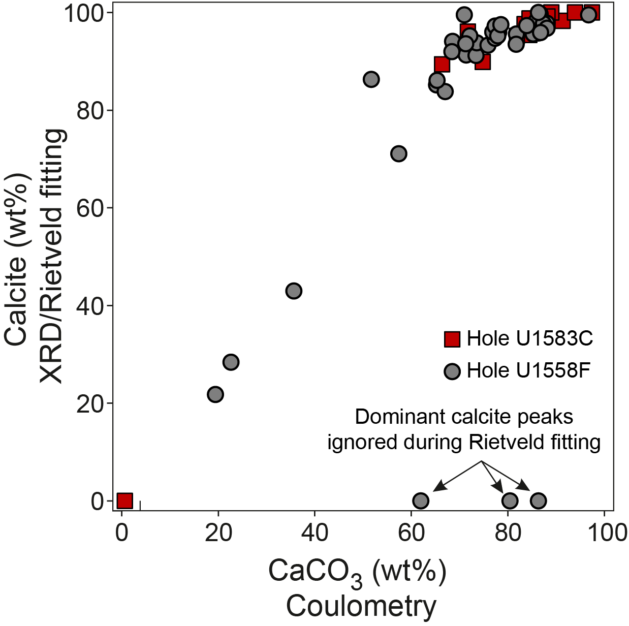
Figure F12. CaCO3 content and calcite abundance.
3. Igneous petrology
3.1. Hard rock visual core descriptions
Each section of core was examined consecutively by two teams of describers, focusing first on igneous characteristics (recorded principally in the igneous log described here) and then on alteration (recorded principally in the alteration and vein and mineral fill logs described in Alteration petrology). Each team described all sections of hard rock cores.
Hard rock VCDs summarize observations from each section of the igneous rock cores (see Core descriptions). An example VCD is given in Figure F13, and a key to the symbols used on the VCDs is given in Figure F14. From left to right on the VCDs, the following are displayed:
- Depth,
- Section length scale,
- Piece number,
- Photograph of the archive half of the core,
- Arrow indicating whether a piece is oriented,
- Indication of whether a DMT whole-round image is available,
- Location of samples selected for shipboard studies,
- Graphical representation of the rock type and emplacement style,
- Lithologic unit,
- Phenocryst abundance and mineralogy,
- Presence of glass or altered glass,
- Groundmass grain size,
- Vesicularity,
- Alteration intensity, and
- Veins.
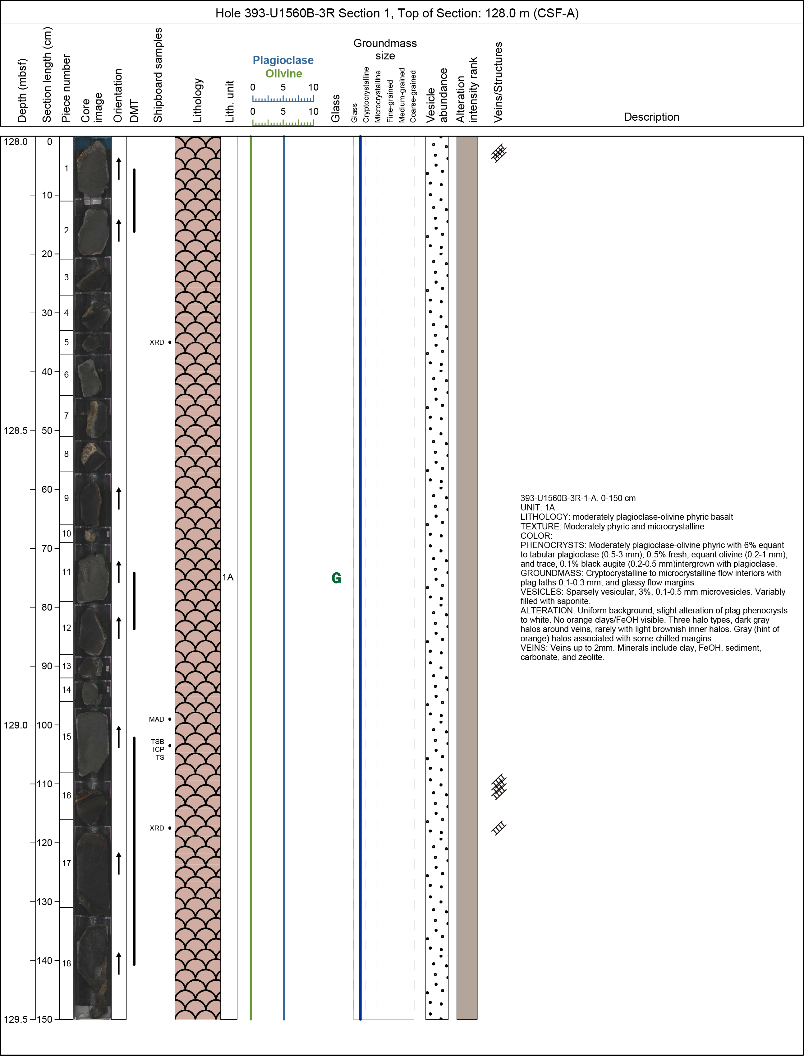
Figure F13. Example hard rock VCD.
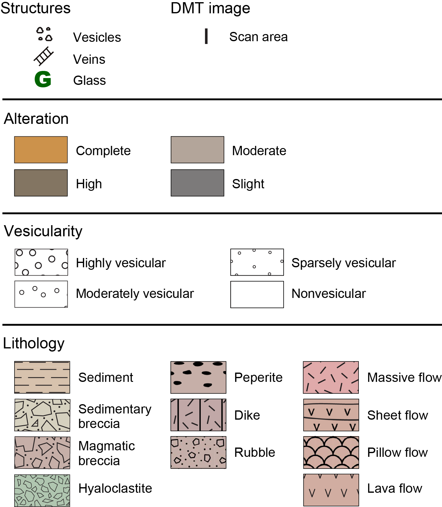
Figure F14. Symbols used for hard rock VCDs.
The locations of samples selected for shipboard studies use the following notation:
- XRD = XRD analysis.
- XRF = powder portable XRF (pXRF) analysis (same as ICP).
- pXRF = pXRF analysis of split core surface (archive half).
- ICP = ICP-AES analysis.
- TS = petrographic thin section.
- PP = physical properties analysis.
- TC = thermal conductivity.
- PM = paleomagnetic analysis.
- MB = microbiological analysis.
The Lithologic unit column displays the locations of the boundaries between units and subunits and the unit designator (e.g., 1, 2A, and 2B).
The boundaries of the lithologic units and subunits were drawn on the VCDs across columns (solid lines = unit boundaries; dotted lines = subunit boundaries). VCDs also contain a text description of each unit in each section of core that includes the following:
- Expedition, site, hole, core number, core type, and section number;
- Unit number (consecutive downhole; subunits are designated by letters after the unit number [e.g., 1, 2A, and 2B]); note that any sedimentary units within the basement were also numbered consecutively downhole but were numbered separately from igneous units and were distinguished from them with the letter "S" (e.g., S1 and S2); minor amounts of sediment incorporated into various breccias were not identified as separate units;
- Lithology;
- Summary description of the unit as it appears in the section, including a brief rock name and the interpreted emplacement of the rock (e.g., pillow basalt or sheet flow);
- Textural summary;
- Color summary;
- Phenocryst summary;
- Groundmass summary;
- Vesicle summary;
- Alteration summary;
- Vein summary; and
- Additional comments.
3.2. Describing igneous cores
3.2.1. Expedition 390
The procedures and methods for igneous rock core descriptions used during Expedition 390 were modified from those adopted during Ocean Drilling Program (ODP) Leg 187 (Shipboard Scientific Party, 2001); Integrated Ocean Drilling Program Expeditions 309/312, 329, and 335 (Expedition 309/312 Scientists, 2006; Expedition 329 Scientists, 2011; Expedition 335 Scientists, 2012a); and IODP Expedition 385 (Teske et al., 2021). Much of the discussion presented here comes from those sources. In general, written descriptions sought to include the following information:
- Lithologic unit number (numbered consecutively downhole; see Lithologic units) and rock name (see Rock classification).
- Descriptions of contact relationships with neighboring lithologic units and of contact relationships within lithologic units (see Igneous contacts). The latter may include descriptions of textural variations across chilled margins and note the presence of sediment adhering to pillow lava pieces or occurring between clasts in rubble or talus.
- List of phenocryst types visible with a hand lens or a binocular microscope: distribution, abundance, size, shape, and degree of alteration and other characteristics.
- Description of groundmass texture and grain size (see Rock classification).
- Abundance of vesicles by volume; their distribution, size, and shape; and the presence/absence of mineral linings and fillings (see Rock classification). The method used to make detailed description of minerals filling vesicles, including their abundance, is given in Alteration petrology.
- Description of color using the Munsell color chart on the dry rock surface.
- Description of the igneous structure (i.e., whether the unit is massive, pillow, sheet flow, etc.) (see Rock structure).
- Qualitative assessment of the degree of alteration (see Unit alteration). A detailed description of veins and fractures, including their abundance, width, mineral linings and fillings, and, where possible, their orientation, was carried out as part of alteration and vein logging. The corresponding methods are given in Alteration petrology.
3.2.2. Expedition 393
During Expedition 393, the same observations were made and recorded using DESClogik as those made during Expedition 390 to ensure comparability along the SAT. To improve efficiency with the different size of the core description team, the sequence of observations was slightly modified and some additional observations were also made. These changes are set out in addenda to each methods section.
Previously, volcanic glass was macroscopically logged across the Extrusive hypabyssal, Glass, and Alteration tabs in DESClogik. During Expedition 393, the observation of glass on the Extrusive hypabyssal tab was simplified to Present or not, with the more detailed observations made on the Glass and Alteration tabs. Based on the entries for Glass physical occurrence (a free text comment) in the Glass tab during Expedition 390, this was modified during Expedition 393 to a value list with the following options:
- Chilled margin clast in hyaloclastite,
- Glass fragments in hyaloclastite,
- Chilled margin at top of piece,
- Glass fragments in breccia,
- Chilled margin (unoriented),
- Chilled margin at bottom of piece,
- Internal chilled margin,
- Palagonite,
- Glass fragments,
- Chilled margin on side of piece,
- Double chilled margin,
- Discrete glass clast, and
- Thin glassy margin.
3.3. Lithologic units
The division of igneous lithologic units and subunits used the criteria of changing grain size, occurrence of contacts or chilled margins, changes in petrographic type, and phenocryst abundances. Generally, boundaries were not defined on the basis of type or degree of alteration or deformation. Lithologic units defined as rubble, breccia, or talus may consist of more than one rock type; such units were generally identified by the random mixture of lithologic types in the core, a predominance of weathered rounded surfaces, and/or cementing sediments.
Lithologically and texturally similar pieces from consecutive core sections were assigned to the same unit. To preserve important information about igneous stratigraphy without defining an unreasonable number of units within a single core, subunits were designated in cases where there were marked changes in texture without accompanying changes in mineralogy or vice versa. Where contacts deviated from horizontal within the core reference frame, their depth was logged at their midpoint.
During Expedition 393, division of igneous units was supported by pXRF analyses on the cut core surfaces and evaluated downhole during core description. The key ratios and elements that were monitored downhole were Cr/Ti to assess degree of fractionation and Zr/Ti to assess incompatible element enrichment or depletion (e.g., depleted mid-ocean-ridge basalt [D-MORB] versus enriched MORB [E-MORB]). Details of the Expedition 393 pXRF method, calibration, precision, and accuracy are given in Geochemistry.
3.4. Rock classification
Rock names were assigned initially on the basis of hand-specimen observations of groundmass texture/color as well as the nature of phenocryst phases, if present. These were later checked with representative thin sections. Rock names were assigned based on the primary phases present prior to alteration.
Porphyritic rocks are named by phenocryst type and their relative abundances as follows:
- Aphyric: phenocrysts constitute <1% of the volume of the rock.
- Sparsely phyric: phenocryst content ranges 1%–5%.
- Moderately phyric: phenocryst content ranges 5%–10%.
- Highly phyric: phenocryst content >10%.
Note that the term "phenocryst" is used for a crystal that is significantly larger than the average size of the groundmass crystals (typically ~5×) and generally euhedral in shape. The names of phenocryst phases are listed in order of decreasing abundance. Thus, a highly olivine-plagioclase-phyric basalt contains >10% (by volume) phenocrysts and the dominant phenocryst is olivine with lesser amounts of plagioclase. The minerals named include all of the phenocryst phases in the rock, as long as the total content is >1%.
The term "glass" was reserved for a homogeneous, isotropic material free of quench crystals, with <2% alteration. For ease of reference, all altered or hydrated glass was lumped under the term "palagonite" during Expedition 390, but the more generic designation of "altered glass" was used during Expedition 393, following the advice of Honnorez (1981). In chilled margins, glass containing discrete spherulitic quench growth was distinguished from clear glass free of these textures.
Phenocrysts were also characterized by their size (in millimeters) and shape, where the shape categories were defined as follows:
- Equant: aspect ratio = less than 1:2.
- Subequant: aspect ratio = 1:2 to 1:3.
- Tabular: aspect ratio = 1:3 to 1:5.
- Elongate: aspect ratio = more than 1:5.
The description of groundmass at the macro scale is on the basis of the predominant grain size, with more detailed description of texture provided through thin section observation (see Thin section descriptions). Note that particularly for intervals dominated by pillow lavas, grain sizes could vary from glassy to microcrystalline or even fine grained over distances of just a few centimeters. Average grain sizes were assigned on the basis of the predominant grain size in the rock and interval. A cryptocrystalline basalt, for example, would consist predominantly of phases that were <0.1 mm but could contain some microcrystalline plagioclase or olivine microlites. Grain size categories used were as follows:
- Glassy,
- Cryptocrystalline (<0.1 mm),
- Microcrystalline (0.1–0.2 mm),
- Fine grained (>0.2–1 mm),
- Medium grained (>1–2 mm), and
- Coarse grained (>2 mm).
Vesicles were described by their abundance, size, and shape/roundness (low, moderate, high, and highly elongate). Vesicles were noted as filled or unfilled, but the nature of filling minerals was detailed during alteration logging (see Alteration petrology). The following abundance categories were used:
- Nonvesicular (<1%),
- Sparsely vesicular (1%–5%),
- Moderately vesicular (>5%–20%), and
- Highly vesicular (>20%).
Groundmass grain size designations during Expedition 393 were typically defined by the modal grain size of groundmass plagioclase or, more rarely, olivine microlites as assessed by binocular microscope. Consequently, a basalt with abundant microcrystalline groundmass plagioclase laths but cryptocrystalline interstitial clinopyroxene was classified as microcrystalline. Where described intervals encompass one or more lava flows, the logged groundmass grain size for that interval refers to that of the flow interior, not the cryptocrystalline to glassy chilled margins, the presence of which was noted in the groundmass comments and glass columns. Primary crystals present in flow interiors but not in the glassy margins were assumed to have crystallized in situ and were considered as part of the groundmass, not as phenocrysts. However, the distinction between phenocryst and groundmass phases becomes somewhat blurred in more coarsely crystallized or seriate textures typical of massive flows greater than ~3 m thick.
3.5. Rock structure
Igneous structure was determined by whether the rock is massive, sheeted, pillowed, hyaloclastic, brecciated, scoriaceous, or tuffaceous. These terms provide a picture of the style of magmatism and the environmental setting in which they occur by identifying features that are diagnostic of specific physical processes.
- Massive basalts: distinguished by long (50–60 cm) continuous core pieces that are relatively unaffected by drilling, and by their uniform texture.
- Pillow basalts: characterized by chilled pillow margins that are mostly curved or inclined, radial fracture patterns, and V-shaped piece outlines. They are also typically cryptocrystalline to microcrystalline and associated with the presence of hyaloclastic breccias.
- Sheet flows: characterized by parallel, closely spaced (<0.5 m apart), mainly horizontal, flat glassy selvages distinct from the rounded or inclined margins for pillows.
- Dike: any sharp, well-defined, and relatively thick (>1 cm) crosscutting feature formed by injection of magma; dikes typically have 1–2 chilled margins. In the absence of distinguishing features, samples were labeled as lava flows.
- Basaltic rubble: distinguished by pieces with semirounded shapes having multiple weathered surfaces that were not cut by the drill. Usually rubble can be recognized as originating from pillow basalts, based on the criteria above.
- Chilled margins: typically composed of an outer 1–10 mm glassy rind that grades through a discrete spherulitic zone into a coalesced spherulitic zone followed by variolitic textures. The variolitic zones are usually identifiable in hand specimen because the mesostasis is altered to a light brown color, highlighting the variolitic texture. Many of the glassy rims have attached veneers or crosscutting veins of interpillow sediment that is carbonate or clay rich. Sediments may be present as fracture fill or as a cement for basaltic breccias.
In contrast to Expedition 390 but similar to previous Expedition 309/312 (Expedition 309/312 Scientists, 2006), sheet flows during Expedition 393 were recognized and defined as single lava flows <3 m thick with gradational changes in internal grain size. Consistent microcrystalline to fine grain size, planar and subhorizontal glassy margins, and coalesced vuggy vesicles were taken as supporting evidence for emplacement as sheet or massive flows.
During Expedition 393, massive flows were defined as single lava flows >3 m thick, with gradational grain size changes and fine- to medium-grained flow interiors used to establish continuity across pieces and sections (following Expedition 309/312 Scientists [2006]). Note that this contrasts with the 0.5 m threshold used during Expedition 390.
3.6. Breccias
Breccias were entered into the main igneous log but described in further detail collaboratively between the igneous and alteration petrology teams using a separate breccias sheet. They were divided principally into the following:
- Magmatic breccias: containing glass or quench textures such as pillow breccia, primary matrix minerals (or sediments);
- Hyaloclastites: as above with >30% glass;
- Hydrothermal breccias: with secondary matrix or vein minerals;
- Tectonic breccias: such as cataclasites and fault gouges in which the matrix consists of the same material as the host rock; and
- Sedimentary breccias: characterized by matrix filling composed entirely of sedimentary materials such as clays and carbonate.
Breccia characteristics such as clast lithology, volume, size, sorting, alteration, and shape, as well as matrix and cement composition were recorded.
We defined matrix as anything granular consisting of fragments of rocks or minerals and cements as anything crystalline that precipitated in situ to fill void space. Thus, a magmatic breccia might have no cement, and a hydrothermal breccia might have no matrix. The method adopted was as follows:
- Assign breccia type (see Breccia type, below) and define whether clast or matrix supported.
- Estimate clast volume proportion (percentage), clast size range (minimum/maximum, in millimeters), and sorting (see Breccia sorting).
- Record clast lithology (see Clast/matrix composition), alteration (see Clast/matrix alteration), shape (see Clast/matrix shape), grain size (see Clast/matrix internal grain size), and internal structure (see Clast internal structure).
- Estimate matrix volume proportion (percentage), identify matrix composition (same values as Clast/matrix composition) and alteration (same values as Clast/matrix alteration), and record any internal structure (same values as Clast/matrix internal grain size).
- Identify cement mineral composition, and estimate volume proportion (percentage).
- Record any further details as a comment.
Definitions for breccia descriptions noted above include the following:
- Breccia type: magmatic breccia, hyaloclastite, hydrothermal breccia, tectonic breccia, and sedimentary breccia.
- Breccia sorting: poorly, moderately, moderately well, well, very well, and bimodal.
- Clast/matrix composition: glass, basalt, dolerite, gabbro, peridotite, serpentinite, chert, mudstone, siltstone, limestone, sandstone, sediment—siliceous, sediment—calcareous, and sediment—undifferentiated.
- Clast/matrix alteration:
- Fresh/unaltered = <2% alteration.
- Slight = 2%–10% alteration.
- Moderate = >10%–50% alteration.
- High = >50%–95% alteration.
- Complete = >95%–100% alteration.
- Clast shape: angular, subangular, subrounded, rounded
- Clast/matrix internal grain size: cryptocrystalline, microcrystalline, fine grained, medium grained, coarse grained, glassy.
- Clast internal structure: none, veined, glassy, crystalline, vesicular, aphyric, sparsely phyric, moderately phyric, highly phyric.
To allow quantitative recalculation of different breccia components, during Expedition 393 the areal proportion of breccia on the cut surface of the archive half of the logged breccia interval was recorded as a percentage under Breccia comments. The percentage of different clast or matrix types were similarly recorded as areal percentages of the cut core surface under Clast comments and Matrix comments.
3.7. Intermingled and interlayered sediment
Intermingled or interlaying of thin (meta)sediment with igneous rock was included in the igneous rock description upon encountering magma/sediment contacts or mixing (e.g., from fragmentation of igneous material or injection of sediment into igneous rock). Thicker and more coherent intervals of sediment were described as part of the sedimentary section.
During Expedition 393, discrete sediment layers were generally described under their own interval, and in several cases even relatively thin (~5–10 cm) layers were split in lithologic (sub)units in order to promote assessment of changing lava compositions over these possible volcanic hiatuses. The catch-all nongenetic term "indurated calcareous sediment" was used to identify indurated intervolcanic materials, which could include materials derived from sedimentary and/or volcanic sources (e.g., volcanic glasses), some exhibiting recrystallization and/or hydrothermal alteration.
3.8. Igneous contacts
Glassy margins, chilled margins, and contact boundaries were inserted individually for the top and bottom of each interval where they could be determined. Contacts may be sharp or gradational.
The following contact types were defined:
- Baked contact: boundary to sediments overprinted (baked) by proximity of magma.
- Bottom or top chilled contact: chilled contact with sediments, with or without glass adjacent to sediments.
- Bottom or top chilled margin: chilled contact without sediments, without glass, defined by cryptocrystalline groundmass, and typically found quenched next to the chilled contact.
- Chilled contact: a magma or lava that has clearly chilled against another rock or sediment.
- Chilled margin: a rapidly chilled margin, for example with a cryptocrystalline, or incomplete variolitic to glassy selvage.
- Glassy margin: a rapidly chilled margin with preserved glass.
- Grain size: units on either side have markedly different grain sizes.
- Modal boundary or contact: units on either side have markedly different mineral proportions.
- Brecciated flow top: consists of angular, scoriaceous to vesicular fragments of basaltic rubble.
- Contact not recovered.
During Expedition 393, contacts were differentiated as "within-unit" and "upper unit" contacts using the same value lists as Expedition 390 to facilitate easy location and extraction of unit contact information.
3.9. Unit alteration
A qualitative assessment of alteration was included along with the description of the igneous petrology to record the overall extent of alteration in that igneous unit/subunit. Separate detailed alteration and vein logs were made, and the associated methods are described in Alteration petrology. Qualitative alteration categories were as follows:
- Fresh/unaltered = <2% alteration.
- Slight = 2%–10% alteration.
- Moderate = >10%–50% alteration.
- High = >50%–95% alteration.
- Complete = >95%–100% alteration.
3.10. Thin section descriptions
Thin section investigation was used to complement and refine macroscopic core observations for igneous rocks. All thin section observations were entered into the LIMS database through a DESClogik thin section template. Thin section descriptions include both primary (igneous) rock-forming minerals (including phenocrysts, groundmass, etc.) and secondary (alteration) mineral phases (in veins, vesicles, groundmass, etc.). Their mineralogy, abundance (modal volume percentages), sizes, shapes, habits, textural relationships, inclusions, alteration (color, intensity, and style), veins (type and number), and vesicles (type and fillings) were determined, enabling verification of macroscopic observations. When time permitted, the estimated volume percentages of the original primary mineral phases, groundmass, and vesicles were also included when entering mineral abundances in DESClogik.
Thin section descriptions include the following information:
- Sample domain: because thin sections are often taken from intervals that contain more than one lithologic feature, it is necessary in the thin section description log to identify which feature (i.e., domain) is being described. In this case, where there is more than one domain represented in the slide, each domain is described separately. For example, a slide that shows a large secondary vein (25% of the slide) in a basaltic matrix (75% of the slide) is given two descriptions: one being the "vein" and the other the "host rock." Other possible domains include clast, glass, halo, and xenolith.
- Lithology prefix modifier and lithology prefix for the described sample domain, following the nomenclature for rock classification described in Rock classification.
- Principal lithology: refers only to the lithology of the described sample domain and follows the nomenclature for rock classification (see Rock classification).
- Overall rock texture/crystallinity of the domain described (i.e., holohyaline, holocrystalline, hypohyaline, hypocrystalline).
- Interpretation of the rock structure/mode of emplacement: pillow lava, sheet flow, massive flow, dike, pyroclastic rock, rubble.
- Average groundmass grain size modal name following Neuendorf et al. (2005). Note that because of time constraints, groundmass grain sizes were not determined for most thin section descriptions during Expedition 390:
- Glassy,
- Cryptocrystalline (<0.1 mm),
- Microcrystalline (0.1–0.2 mm),
- Fine grained (0.2–1 mm),
- Medium grained (1–2 mm),
- Coarse grained (>2 mm).
- Maximum and minimum groundmass grain size modal name. Because of time constraints, grain sizes were not determined for most thin section descriptions during Expedition 390.
- Groundmass texture: intergranular, intersertal, granular, felty, ophitic, subophitic, trachytic, microlitic, graphic, vitrophyric, eutaxitic, skeletal, spherulitic, variolitic, dendritic, fibrous.
- Mineral phenocryst shape: the dominant (>50% of crystals) shape of the olivine, plagioclase, clinopyroxene, orthopyroxene, and spinel crystals in euhedral, subhedral, and anhedral.
- Mineral phenocryst habit: the dominant (>50% of crystals) habit of olivine, plagioclase, clinopyroxene, orthopyroxene, and spinel crystals divided into elongate, equant, subequant, tabular, acicular, dendritic, skeletal, variolitic, spherulitic, sheaf, plumose, and glomeroporphyritic.
- Plagioclase phenocryst zoning type: continuous, discontinuous, oscillatory, patchy, unzoned.
- Clinopyroxene and orthopyroxene phenocryst exsolution: blebs, lamellae.
- Vesicle size, shape, and abundance.
- Proportion of groundmass phases.
- Additional features such as dissolution/resorption textures, sieve textures, and inclusions are noted in the comments sections.
Modal data were visually estimated by reference to standard charts. Crystal sizes were measured using a micrometer scale; generally, these measurements are more precise than hand-specimen estimates.
3.10.1. Expedition 393 modifications
Two minor modifications were made for the Expedition 393 thin section igneous petrography descriptions, captured on the 393_microscopic template in DESClogik:
- Where necessary, thin sections were divided into domains based on both primary igneous and secondary alteration criteria. These domain types may coincide spatially but not necessarily. For example, a single igneous domain may be covered by multiple alteration domains, and vice versa. Igneous domains were selected from chilled margin, glassy margin, flow interior, breccia clast, and breccia matrix, and any additional information was provided as a comment.
- All thin sections were screened in reflected light for primary and secondary oxide and sulfide minerals, with particular emphasis on locating any primary sulfide blebs in glasses.
To visually calibrate micro- and macroscopic modal abundance estimates of phenocrysts and vesicles across the hard rock core description team, a digital areal abundance exercise was undertaken following approaches used during Integrated Ocean Drilling Program Expeditions 309/312 and 327 (Expedition 309/312 Scientists, 2006; Expedition 327 Scientists, 2011). A set of Expedition 390 thin sections were selected to cover different abundance ranges. Full page images of the thin sections were printed, and the phenocrysts and vesicles were traced onto an overlay using different colors. This overlay was scanned, and using the threshold function in Adobe Photoshop, each phase was separated. The area represented by each phase was then determined by using the histogram function, where the number of pixels of each color was divided by the total number of pixels in the image to calculate a percent abundance of each phase.
3.11. Expanded depths and unit thicknesses (Expedition 393)
3.11.1. Expanded depths
The incomplete recovery of basement cores remains a reality of scientific ocean drilling, and recoveries for individual basement cores ranged from 0% to >90% along the SAT. Immediately after recovery, the pieces from each core were curated into bins, each separated by 1–2 cm, starting from the top of the core. For cores with near 100% recovery, this spacing may lead to curated lengths in excess of the drill-advanced length over which that core was cut. In the far more common case of <100% recovery, the curated length of a core will be less than the drill-advanced length, but the lower pieces of the core could nevertheless have originated from the bottom of the drill-advanced length. To account for this, curated depths were recalculated to "expanded depths" for certain applications, such as plotting continuous data downhole (e.g., veins or pXRF results) and for making a best estimate of the true unit contact depths and thicknesses for visualization in the lithostratigraphic summary figure in each chapter, for eventual comparison with wireline logging data.
To make this expansion, the curated offset from the top of each core was multiplied by a factor calculated from the drill-advanced depth/curated recovery for that core and then this expanded offset was added to the top depth of each core to arrive at an expanded depth. This recalculation essentially spreads the depths of recovered pieces evenly throughout the drill-advanced interval over which the core was cut, such that the lowermost pieces will be near the bottom of the drill-advanced interval and the uppermost pieces will be near the top. In the case of a curated length greater than the drill-advanced length, which did not occur during this expedition, this expansion factor would be <1 and would similarly work to compress the pieces into the drill-advanced length.
3.11.2. Curated, expanded, and minimum unit thicknesses
The curated, expanded, and minimum unit thicknesses are reported in a table in each site chapter. The curated thickness is the difference between the curated depths (on the CSF-A depth scale) of the upper and lower unit contacts. The expanded thickness is the difference between the upper and lower contacts expanded to account for variable recovery, as described above, and represents the best estimate of the true intersected thickness of the unit, most suitable for direct comparison with wireline logs and for quantitative treatment of unit thicknesses. The minimum thickness is given by the sum of the drill-advanced lengths for any cores entirely within a unit, plus the sum of any piece lengths or recovered sections lengths within a unit for any cores that contain only part of a unit.
4. Alteration petrology
Virtually all igneous rocks recovered during Expeditions 390C, 395E, 390, and 393 have undergone alteration. This alteration manifests as replacement of groundmass and phenocrysts, hydrothermal veins and alteration halos, lining and filling of vesicles, and replacement or cementation of breccia clasts and matrix. Each of these alteration types was described and recorded and combined into a brief summary on the VCD.
4.1. Alteration logs
Altogether, three separate alteration logs were recorded: (1) an alteration log recording the background alteration and the proportions of different types of halo and patch alteration; (2) a vein (and other mineral fill) log recording the occurrence and size/area of each individual vein, vein networks, or areas of vesicles, quantifying their mineral fill and describing any associated halos; and (3) a breccia log recording the occurrence, matrix, and cement of breccias (see DESC_WKB in Supplementary material). These logs enable quantification of variations in alteration and secondary mineral abundance both downhole and between different holes (Figure F15). The logs were made at slightly different scales; the proportions of different alteration styles were assessed on a section by section basis, whereas veins and other secondary mineral fills were recorded for each vein or each interval or piece of cemented breccia or filled vesicles.
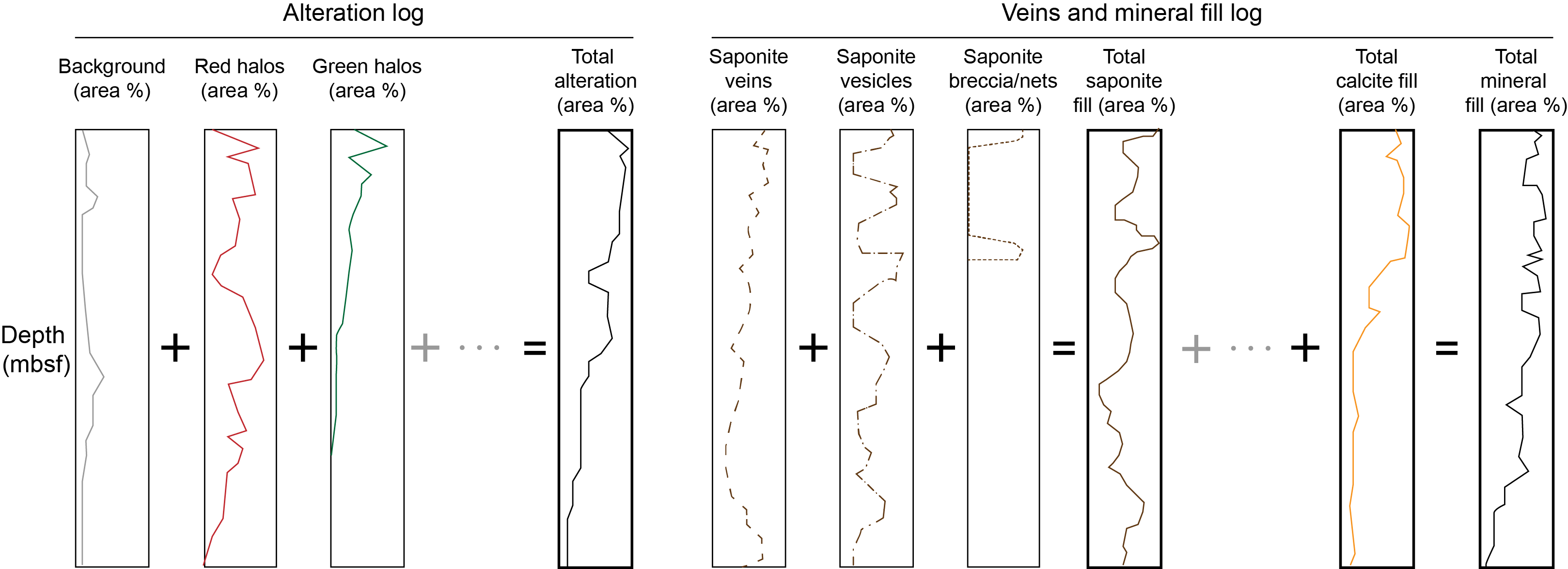
Figure F15. Alteration and mineral fill logs.
This approach to logging alteration follows closely that of Integrated Ocean Drilling Program Expeditions 301 and 327 (Expedition 301 Scientists, 2005; Expedition 327 Scientists, 2011) and the Oman Drilling Project (Kelemen et al., 2020) and incorporates elements of the approaches of ODP Leg 206 (Shipboard Scientific Party, 2003) and Expeditions 309/312 and 335 (Expedition 309/312 Scientists, 2006; Expedition 335 Scientists, 2012a).
4.1.1. Background alteration log
The overall background alteration log was made to quantify the overall area proportions of different types of background, halo, and patch alteration in the core. Sections were only divided where an igneous unit boundary, as defined in the igneous lithology log, was encountered. Alteration was logged on the basis of macroscopic color because individual background and halo mineral species could rarely be distinguished at this scale. The relative proportions of alteration styles were logged based on the recovered core (rather than the curated/binned length) and excluded mineral vein and breccia fillings that were logged separately (see below). In practice, active effort to exclude such mineral fills was only necessary in areas of extremely abundant vuggy carbonate. Where rocks clearly expressed oxidative alteration overprinted by green alteration (in Hole U1557D), this was recorded in the alteration logs as a 50:50 mixture of the two alteration types.
The procedures adopted for macroscopic observation and description of cores was as follows:
- Determine the number of igneous units in each section from the igneous log and assign each interval to a record/row in the alteration tab in DESClogik. Log each individual interval (row) following Steps 2–7.
- Estimate the proportion by area of each type and color of alteration (e.g., gray background, dark patches, green halos, and red halos).
- Estimate alteration intensity in surface area percentage of background alteration:
- Fresh/unaltered = <2% alteration.
- Slight = 2%–10% alteration.
- Moderate = >10%–50% alteration.
- High = >50%–95% alteration.
- Complete = >95%–100% alteration.
- Characterize the texture/style of background alteration:
- Assign a color and Munsell color code to each type of alteration.
- For patches of alteration, characterize patch size.
- Record additional characteristic features of each alteration group in Comments.
4.1.2. Vein and mineral fill log
Detailed logs of vein, vesicles, and breccias were produced, allowing the precise interval of their occurrence to be recorded independent of the larger scale alteration log and enabling accurate quantification and plotting of different mineral occurrences downhole.
The vein and mineral fill log records the presence, location, width, crosscutting relationships, shape, and composition percent along with color, and width of associated halos of each vein. The fill texture, connectivity, and morphology of veins was described. Structural measurements on veins were not undertaken during Expedition 390.
A detailed log was made of the relative proportions and abundance of minerals filling void spaces. This principally recorded veins but also included vein networks, vesicles, breccia cements, and secondary minerals (of indeterminate geometry) in rubble bins. This allowed easy quantification and plotting of the abundance of filling minerals downhole. Using the width and geometry of these veins, the area and subsequently volume of each vein was calculated and used to determine the volume percent of the core filled by secondary minerals in veins (e.g., see Figure F44 in the Site U1559 chapter [Coggon et al., 2024b]) normalized for core recovery.
Filling minerals (and their relative proportions) were assessed based on color, texture, and habit and confirmed by analysis of thin sections and/or XRD where necessary.
Halos surrounding veins or vesicles were described by their half-width and color. Secondary mineral assemblages were noted where distinguishable in macroscopic core.
Features were not logged across pieces to simplify normalizing the abundance of secondary minerals to recovery using the piece log. Continuous occurrences of breccia were logged piece by piece. In rare cases, a long vein crossing two pieces may have been logged as two veins. Where pieces logged for breccia cement (or in the piece log) had tapered or irregular ends, the top and bottom interval of the piece were chosen to approximate a square end piece of full width core (e.g., for a planar tapered end this would be halfway up the tapered interval).
For each secondary mineral-filled feature logged, the proportion of the area filled (as opposed to open void) was also recorded. This allowed the quantification of the open voids/macroporosity as a proportion of the total rock downhole.
Each feature was described as following:
- Filling type: vein, vein net, vesicles, cemented breccia, sediment, rubble.
- Vein section interval (in centimeters): measured upper and lower intersections with the margin of the split face of the archive half of the core or the greatest upper and lower extent of a vein (Figure F16) and mean perpendicular width. This allows the area percent of specific veins and their mineral fills to be calculated.
- Other fill type interval: measured upper and lower interval and estimate the total proportion of secondary minerals in the interval resulting in data comparable to veins.
- Vein generation: if distinguishable, via crosscutting or other relationships.
- Qualitative vein dip:
- Vertical: vein extends across <50% of core width.
- Horizontal/moderately inclined/steeply inclined: vein extends across >50% of core width.
- Vein texture (schematic illustrations of vein textures, connectivity, and morphologies described are provided in Figure F17): massive, cross-fiber (antitaxial), oblique-fiber, vuggy, polycrystalline, crack-seal (syntaxial), crack-seal (stretching), sheared, patchy, overgrowth, cemented breccia (hydrothermal, tectonic).
- Vein connectivity: Isolated, single, branched, network, en echelon, crosscutting, ribbon, parallel, anastomosing, overlapping.
- Vein morphology: planar, curved, irregular, vein tip, tension gash, cemented fault breccia.
- Fill color and Munsell color code (Expedition 390 only).
- Estimated relative abundance of each secondary mineral: including clay, carbonate, zeolite, Fe oxyhydroxides, other clay, green clay, sulfides, amorphous silica, quartz, and chlorite; for Expedition 393: unknown 1, unknown 2, and unknown 3 were used primarily for variations in sediment fill).
- XRD results, if any, for comparison.
- Orientation of major veins (Expedition 393 only; see Structures below for core reference frame [CRF]).
- Associated halo half-width: if halo is zoned, use width 1 (and color 1, etc.) for the inner zone and width 2 for the outer zone.
- Assign color and Munsell color code to halo/zones.
- Pyrite fronts associated with the halo.
- Further details as comments.
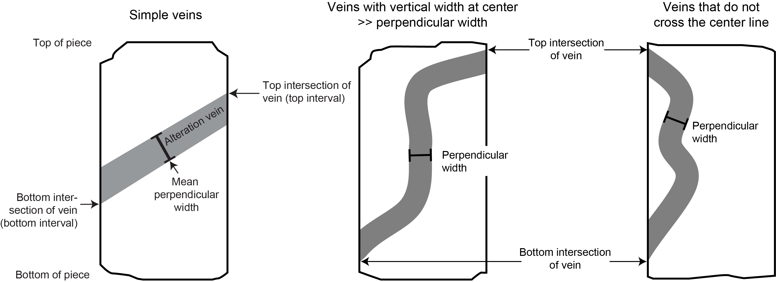
Figure F16. Intervals and width measured for veins.
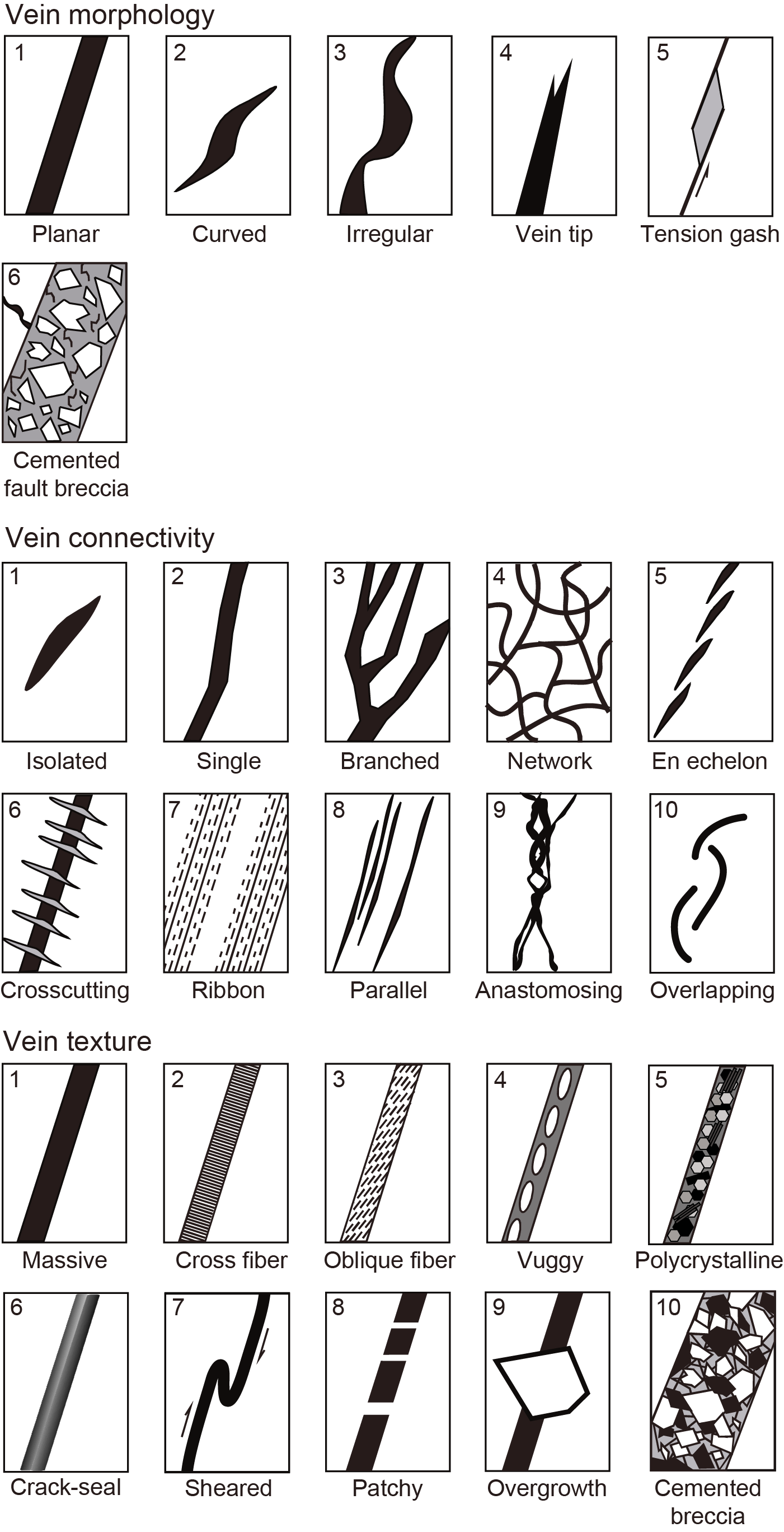
Figure F17. Vein fill textures, morphologies, and connectivities.
4.1.3. Breccia log
Breccias were recorded separately to allow, among other things, detailed characterization of each clast type, matrix, and cement. This was carried out collaboratively between the igneous and alteration petrologists, and the method is described in Igneous petrology. Where breccias were encountered, they were first logged in detail and then a piece-by-piece estimate of secondary mineral abundances in the breccia cement was made in the vein_halos_fill log. This enables downhole quantification of secondary minerals in a consistent way for veins, vesicles, and breccias, whereas the breccia log allows other relevant details to be recorded.
4.1.4. Piece log
The length and, if less than 5.7 cm, width of each recovered piece of hard rock core was logged to calculate the cut surface area of the core to normalize the results of vein and alteration logging to recovery within each section and thereby accurately quantify the volume proportion of altered rock and secondary minerals within the core (see Figure F18).
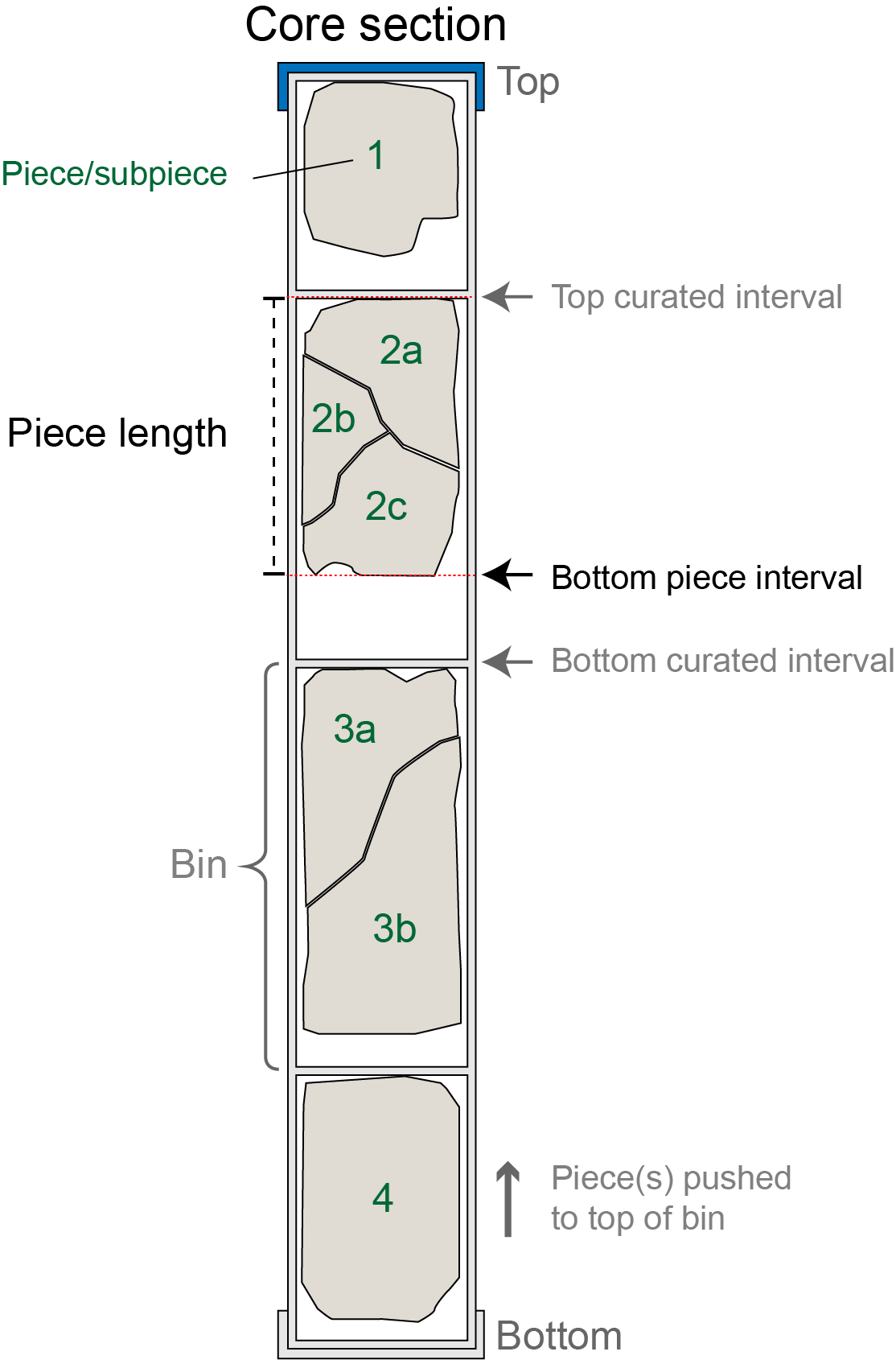
Figure F18. Hard rock sample bins and piece length measurement.
The curated length is usually slightly longer than the true piece length because there must be some room left to allow the removal and inspection of core pieces. These gaps may be up to a few centimeters, which may be significant for shorter pieces of core and when core recovery is low.
To produce the piece log, curated details of the core, including upper and lower curated bin depths in the core, were exported. Within each bin, the core piece(s) were pushed to the top of the bin and their lower interval in the core was measured. The piece length was calculated from the difference between the top bin interval and the bottom piece interval measured. The piece logs are available in ALTPET in Supplementary material.
4.2. Thin sections
To complement and refine macroscopic descriptions of the alteration and structural features of the core, thin sections of igneous rocks were studied in transmitted and reflected polarizing light microscopy. Thin section samples were selected typically once per igneous unit, often coincident with a bulk geochemistry sample, and generally positioned to include multiple features of interest.
Alteration was characterized in thin section by division of the sample into one or more alteration domains (e.g., background, vein, or halo; see Figure F19) and listing the secondary minerals identified in each, together with their estimated abundance and what features of the rock they replaced or filled. During Expedition 390 when only one alteration petrologist was able to sail, only a free-text summary description was produced and included in the thin section reports in the visual core descriptions.
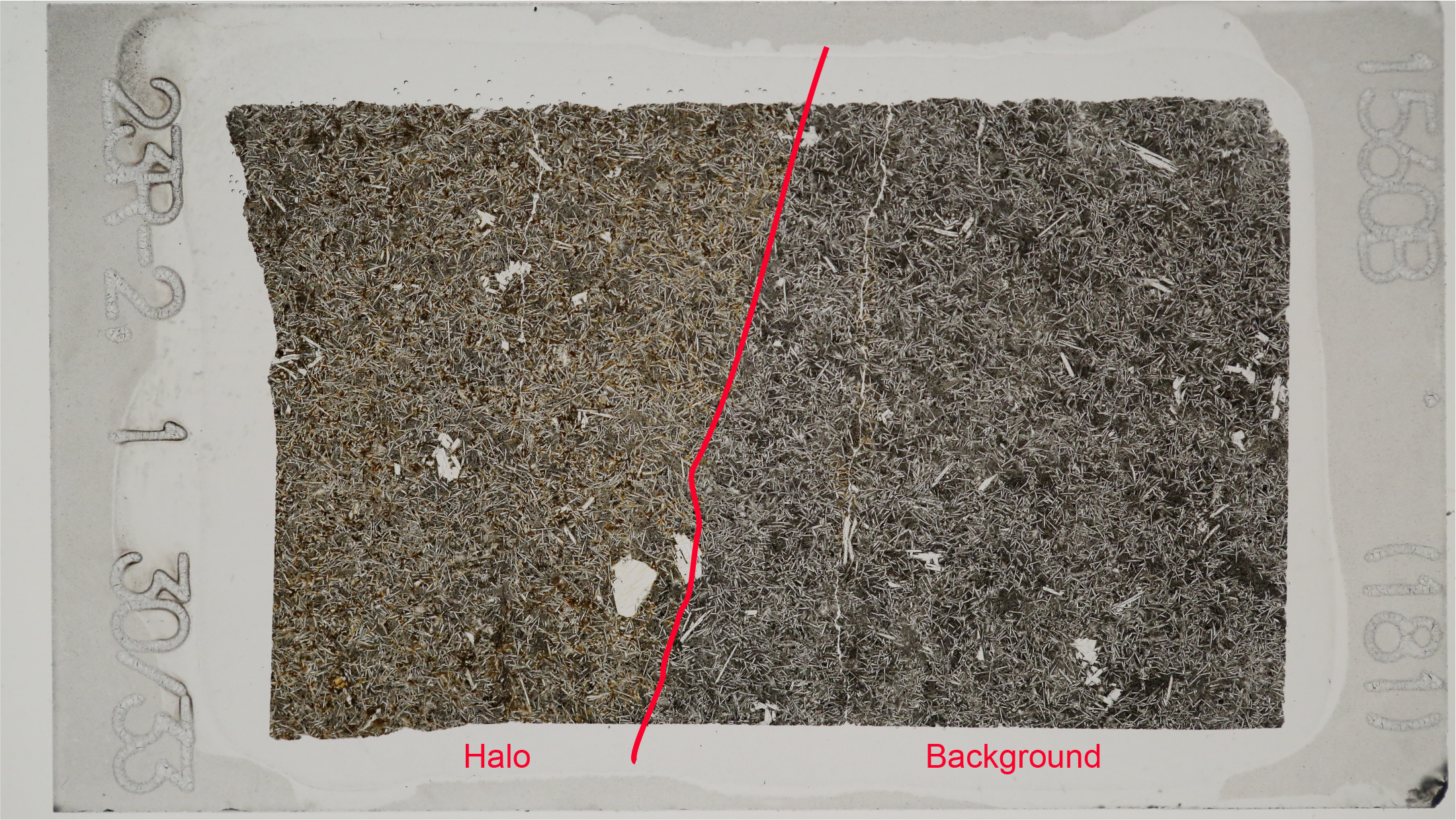
Figure F19. Approach taken to defining alteration domains.
Thin section descriptions are included in Core descriptions and are also available from the LIMS database. Digital photomicrographs were taken during the expedition to document features described in the thin sections; these can be obtained from the IODP data librarian.
4.3. Structures
This section outlines the techniques used for macroscopic and microscopic description of structural features observed in hard rock basement cores. Conventions for structural studies established during previous hard rock drilling expeditions (e.g., ODP Legs 118, 140, 147, 148, 153, 176, 206, and 209; Integrated Ocean Drilling Program Expeditions 304/305 and 335; IODP Expeditions 357 and 360; and the Oman Drilling Project) were generally followed during Expedition 393, but these descriptions were not undertaken during Expedition 390 because of a lack of personnel.
All material from both working and archive halves was examined. The most representative structural features in the cores recovered during Expeditions 390 and 393 are summarized on the VCD form (see Hard rock visual core descriptions).
4.4. X-ray diffraction analysis
To refine identification of secondary alteration minerals, selected veins, vesicles, and breccia cement minerals were analyzed by XRD. Minerals were separated from the working half of the core using a stainless steel spatula or a dremel tool to abrade or chip off small (~10–50 mg) samples with minimal damage to the core. In addition, whole-rock geochemistry powders (see Geochemistry) were also analyzed by XRD.
Samples for XRD analysis were freeze-dried for 12 h prior to being crushed and powdered using an agate mortar and pestle. Diffraction data were generated on the shipboard Bruker D4 Endeavor X-ray diffractometer, which is equipped with a Cu source and uses a generator voltage of 35 kV and current of 40 mA. Depending on the rate of core recovery and scientific objectives, the XRD operated under two different protocols. For routine analyses to aid core description and deliver essentially qualitative analyses, the operating conditions were set to step scans of 4°–75°2θ for 3750 steps at a rate of 1 s/step (the typical setting used on the ship during previous expeditions). For high-precision XRD analyses capable of quantitative analysis via Rietveld-based full-pattern fitting techniques using small amounts of sample, acquisition occurred at step scans of 4°–120°2θ for 5800 steps at a rate of 2 s/step. Diffraction results were evaluated against powder diffraction files for a large database of natural and synthetic minerals using the HighScore software package. The results of this evaluation included matched mineral species (see XRD files in ALTPET in Supplementary material).
4.5. Expedition 393 alteration petrology
During Expedition 393, the same observations were made and recorded using DESClogik as those made during Expedition 390 to allow for comparability along the SAT. The data were captured in the following DESClogik templates: 393_macroscopic and 393_microscopic. To ensure efficiency of core flow, the sequence in which observations were made was slightly modified and some additional observations made. These changes are set out below.
4.5.1. Alteration description
During Expedition 390, an alteration type designated as "mottled gray area%" was used to describe a characteristic alteration style associated with chilled margins. During Expedition 393, this was clarified in DESClogik to "Chilled margin mottled gray area%" and was counted toward the proportion of background alteration rather than as its own category of alteration. In addition to estimating the area percentage represented by different alteration types (as identified by dominant color and appearance), during Expedition 393 the intensity of alteration (expressed as percent alteration) was also estimated for each alteration type. These estimations were calibrated against thin section observations and are generally correlated with color intensity, where the more intense colors are associated with higher degrees of alteration. The inclusion of this estimation allows the total alteration percentage to be weighted by the proportion and intensity of the different alteration types. During Expedition 390, alteration intensity was estimated only for background alteration.
Modifications to the observation sequence were made in relation to the logging of veins-halos-fills. During Expedition 393, these observations were separated into veins-halos and vesicle-other fills with breccia cement fills moved to the Breccias tab. These are mechanical changes to aid the description core flow and do not reflect changes in what was observed and recorded.
4.5.2. Thin section description
The following additions and clarifications were added for the Expedition 393 thin section alteration petrography descriptions captured in the 393_microscopic template in DESClogik:
- Where necessary, thin sections were divided into domains based on both primary igneous and secondary alteration criteria. These two domain types may coincide spatially but not necessarily. For example, a single igneous domain may be covered by multiple alteration domains and vice versa. Alteration domains were selected from "background," "vein halo," and "other halo," and any additional information was provided as a description.
- Vesicle fill and veins were also described on separate tabs in the 393_microscopic template that are slightly modified from the macroscopic versions of these tabs. New to the microscopic template is the specific recording of the sequence of fills in the fill sequence column. This column has a standard format of reporting minerals from rim to center (e.g., a vein lined with brown clay and filled with carbonate would be listed as brown clay–carbonate).
- Breccia cements were described in the vesicle tab.
4.5.3. Structure description
The orientation of veins (width > 0.1 mm) were measured by the Expedition 393 hard rock core description team. These methods follow conventions for structural studies established during previous hard rock drilling projects (e.g., Legs 118, 140, 147, 148, 153, 176, 206, and 209; Expeditions 304/305, 335, 357, and 360; and the Oman Drilling Project).
4.5.3.1. Core reference frame
Measurements of vein-related structural features were undertaken on the archive-half cores in accordance to the standard IODP core reference frame (CRF) (Figure F20). The plane normal to the axis of the borehole is referred to as the horizontal plane. On this plane, a 360° net is used with a pseudosouth (180°) pointing into the archive half and a pseudonorth (0°) pointing out of the archive half and perpendicular to the cut surface of the core. The cut surface of the core, therefore, is a vertical plane striking 90°–270°. Apparent dip angles (0°–90°) and dip direction (0°–360°) of planar structures were measured on the split cores. True dip angles and dip directions were obtained from a second apparent dip angle and dip direction measurement and calculated using a macro in Microsoft Excel (Oman Drilling Project [Kelemen et al., 2020]).
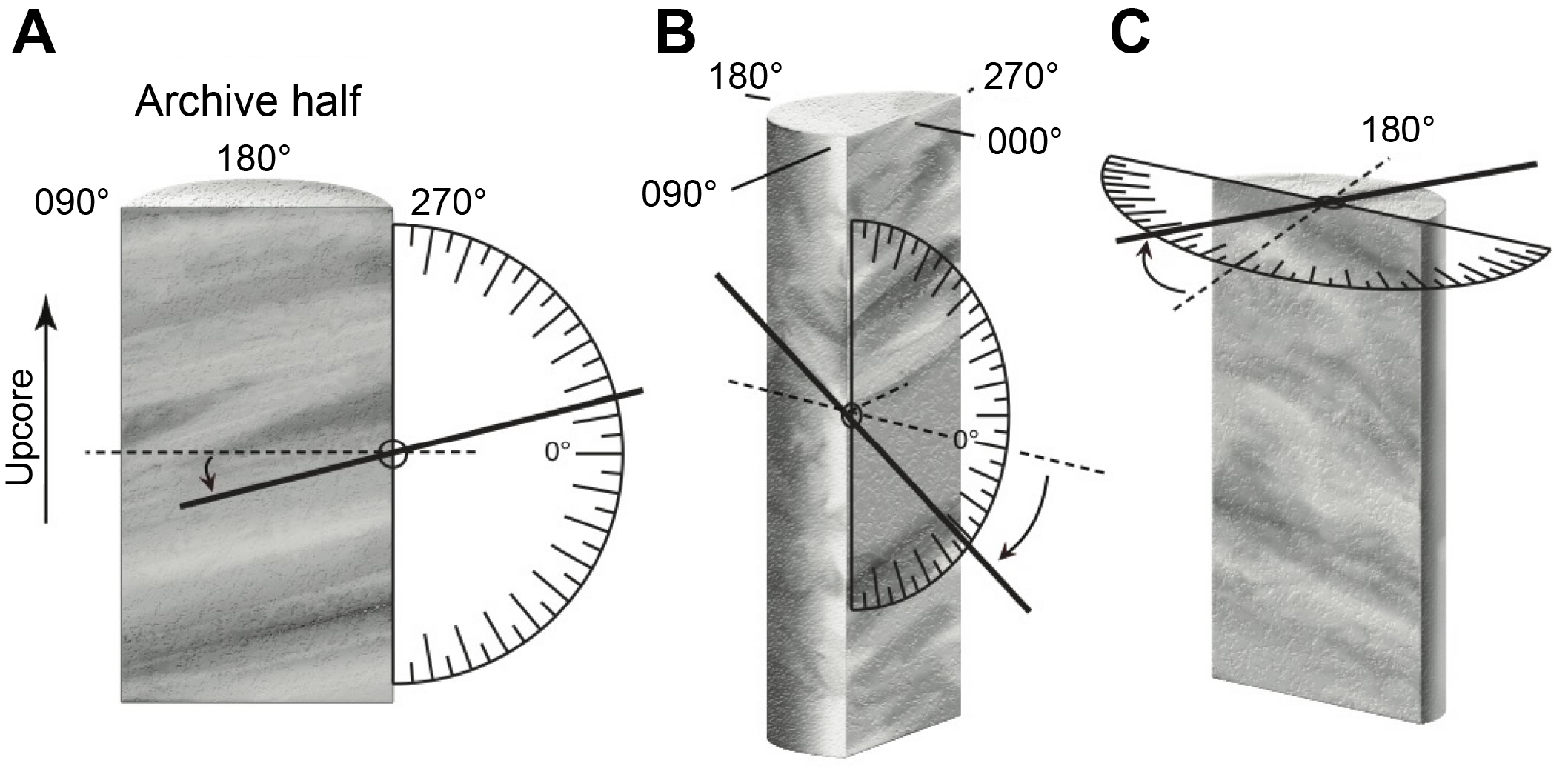
Figure F20. Reference frame and measuring orientation of planar feature.
4.5.4. X-ray diffraction
Whole-rock powders and picked mineral separates were analyzed for their mineralogical composition by powder XRD following the same analytical protocol as that detailed for Expedition 390. Mineralogical compositions were determined by semiquantitative, standardless Rietveld analysis using Panalytical HighScore Plus software and both the Panalytical Example Database and PDF-4/Axiom 2019 database.
The background of the XRD spectra was first fitted in the software using a bending factor selected by the user to preserve all measured peaks. Peak positions were then automatically located by the software, with the minimum significance defined by the user for each spectrum such that all detected peaks were recognized. Library mineral diffraction patterns that matched the measured data were then searched in three steps prior to Rietveld analysis. Firstly, a broad pass search of all minerals in the database identified the dominant mineral phases. Multiple possible patterns for different mineral solid solutions were added to the pattern list at this stage. Secondly, a restricted search was made of just clay family minerals. Thirdly, a restricted search was made of just zeolite family minerals. From the clay and zeolite family searches, any minerals that had a reasonable possibility of being present in oceanic crust and scored a match were added to the pattern list. Rietveld fitting analysis then reduced this large list of possible minerals and mineral solid solutions down to a best-fit set of minerals and estimated abundances that could explain all the diffraction peaks. This multistep pattern search was found to better locate potential matches for low-abundance secondary clay and zeolite phases recognized but not exactly identified by thin section petrography.
5. Biostratigraphy
Calcareous nannofossils (also called calcareous nannoplankton) and planktic foraminifera were examined to provide preliminary age constraints for recovered sediment, and benthic foraminifera were analyzed to provide preliminary estimates of paleodepth. Biostratigraphic and paleodepth analyses were performed on the core catcher (CC) samples, and additional samples were taken from split sections as needed to further refine the stratigraphic position of key datums.
Core catcher samples from Expeditions 390C and 395E (Holes U1556A, U1557B, U1558A, U1559A, U1560A, and U1561A) were sent to the Expedition 390/393 paleontologists for shore-based analyses at their home institutions. Only the archive halves of these cores were made available on JOIDES Resolution during Expeditions 390 and 393, so no additional section samples were available for planktic or benthic foraminiferal analyses. However, additional calcareous nannoplankton smear slide samples were taken from the archive halves to refine the age model at critical intervals. Whole-round cores spanning the sediment/basement interface from Holes U1556A, U1557B, and U1559A were split shipboard during Expedition 390, and whole-round cores spanning the sediment/basement interface from Holes U1558F, U1583C, and U1560C were split shipboard during Expedition 393. These cores were sampled for both calcareous nannoplankton and planktic foraminifera as needed (at least one sample per section) to determine the age of the sediment/basement interface. Thin section samples from indurated calcareous sediments in basement rocks were taken as needed (generally one or two samples per site) for planktic foraminiferal biostratigraphy of interflow sediments.
Biostratigraphic age assignments were based on identification of calcareous nannoplankton and planktic foraminiferal lowest occurrences (base [B]) and highest occurrences (top [T]). Biozone boundaries were placed at the midpoint between the sample containing the marker species and the sample below (for lowest occurrences) or above (for highest occurrences) without the marker species. The ages of the calcareous nannoplankton and planktic foraminiferal biozonation schemes used during Expedition 390/393 followed Gradstein et al. (2020) as modified by King et al. (2020) for Neogene planktic foraminifera. Calcareous nannoplankton and planktic foraminiferal biozone marker species and other useful biostratigraphic datums are illustrated in Figure F21.
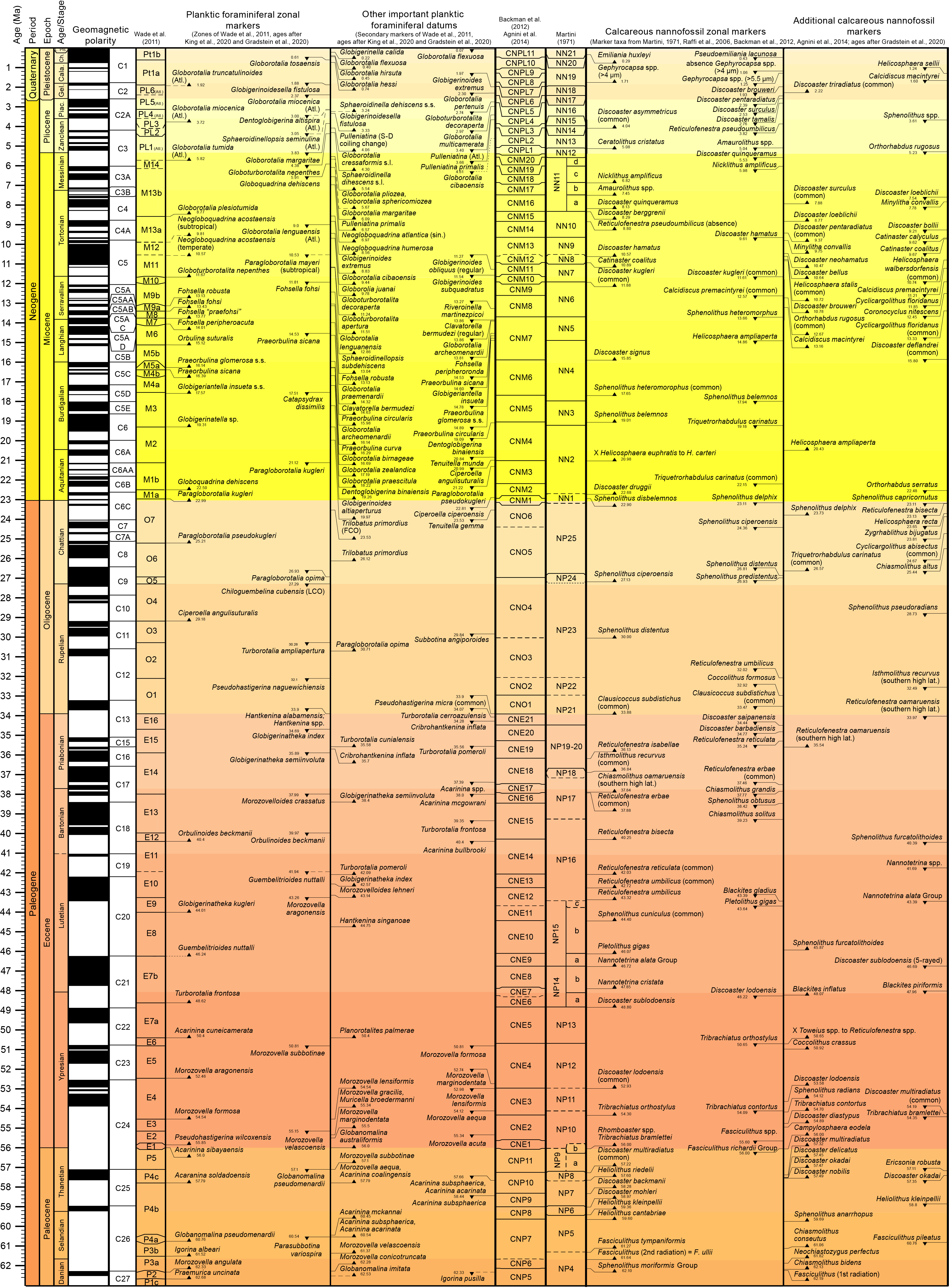
Figure F21. Microfossil datums.
Calcareous nannoplankton and foraminiferal occurrences, preservation, abundance, and zonal assignments were entered into the LIMS database using the DESClogik software package, with the exception of benthic foraminifera for Site U1557, which samples were analyzed at the end of Expedition 390/393. Biostratigraphic data are reported in tables summarizing recorded datums, distribution charts, qualitative abundance plots, and preservation summaries for each site. Both onshore analysis of Expeditions 390C and 395E core catchers and shipboard Expedition 390/393 biostratigraphic analyses largely focused on the presence of age- and depth-diagnostic species, and therefore distribution data do not represent the complete microfossil assemblage. Qualitative notes about the overall abundance and preservation state were made for calcareous nannoplankton and planktic and benthic foraminifera in each sample analyzed. Observations regarding other notable sedimentary material (e.g., fish teeth, echinoderm spines, and diatoms) were also included.
5.1. Calcareous nannofossils
5.1.1. Calcareous nannofossil taxonomy and biostratigraphy
Nannofossil taxonomy primarily follows Bown (1998, 2005) and Perch-Nielsen (1985) as compiled in the online database Nannotax3 (Young et al., 2022). The zonal scheme of Martini (1971) (zonal code numbers NP and NN) were used for Cenozoic calcareous nannofossil biostratigraphy. Additional biohorizons from the Paleogene scheme of Agnini et al. (2014) (zonal code numbers CNP, CNE, and CNO) and the Neogene/Quaternary scheme of Backman et al. (2012) (zone numbers CNM and CNPL) are also included. The compilation of Raffi et al. (2006) was also partially used to provide additional information on the reliability, definition, and timing of Quaternary bioevents. These zonations represent a general framework for the biostratigraphic classification of middle- to low-latitude nannofossil assemblages and are presented in Figure F21.
The genus Gephyrocapsa dominates Pleistocene assemblages. However, this group demonstrates a large range of variation in size and morphology, which causes problems in identification (e.g., Samtleben, 1980; Su, 1996; Bollmann, 1997). Size variations in Gephyrocapsa spp. are commonly used as biostratigraphic markers in the Pleistocene, and several studies confirm the reliability of these biometric subdivisions as biostratigraphic markers (e.g., Raffi et al., 1993, 2006; Young, 1998; Raffi, 2002; Lourens et al., 2004; Maiorano and Marino, 2004). We elected to use this biometric classification with the following divisions applied for shipboard identification of Gephyrocapsa:
- Gephyrocapsa spp. <4 µm (small): includes a number of different species (e.g., Gephyrocapsa ericsonii and Gephyrocapsa ornata, as well as small specimens of Gephyrocapsa oceanica and Gephyrocapsa caribbeanica). Zones NN21–NN19/CNPL11–CNPL8.
- Medium-sized Gephyrocapsa (4–5.5 µm) were identified to species level based on the size and morphology of the central area: G. oceanica (large central area with bridge angle <90° to the minor axis) and G. caribbeanica (small central area nearly filled by a bridge). Gephyrocapsa omega and Gephyrocapsa muellerae were included with G. oceanica. Zones NN21–NN19/CNPL11–CNPL8. This was only done during Expedition 390.
- Gephyrocapsa spp. >5.5 µm (large) includes large specimens of both G. oceanica and G. caribbeanica. Zones NN19/CNPL8.
The genus Reticulofenestra dominates most early Eocene to Neogene nannofossil assemblages. One of this taxon's distinguishing features is the central area grill or net. However, this feature is not always preserved or is not birefringent, making identification difficult. As a result, species are often differentiated based on rim shape and lith size (e.g., Backman, 1980; Su, 1996; Young, 1998). Large variations in size ranges of coccoliths exist, and whereas some species are more easily distinguishable, elliptical forms are particularly problematic, especially since different names have been applied to similar morphologies from the Paleogene and Neogene. For the SAT cores, we defined the taxonomy applied for members of this genus as follows:
Elliptical forms >3 µm with open central area:
- Reticulofenestra haqii: open central area 3–5 µm in length.
- Reticulofenestra pseudoumbilicus: Neogene sediments; divided into two size categories following the definition of Young (1998) for biostratigraphic utility:
- Reticulofenestra pseudoumbilicus (5–7 µm).
- Reticulofenestra pseudoumbilicus (>7 µm) for Miocene–early Pliocene (Zones NN15–NN1/CNPL3–CNM1).
- Reticulofenestra dictyoda: open central area 5–14 µm (Paleogene sediments).
- Reticulofenestra umbilicus: >14 µm with open central area.
Elliptical forms >3 µm with closed central area:
- Reticulofenestra producta: closed central area 3–5 µm in length.
- Reticulofenestra perplexa: closed central area 5–8 µm in length.
- Reticulofenestra bisecta: closed central area 8–10 µm in length.
- Reticulofenestra stavensis: closed central area >10 µm in length.
5.1.2. Methods of calcareous nannofossil study
Calcareous nannoplankton were examined on smear slides using standard preparation techniques (Bown and Young, 1998); at least one sample was analyzed per core. When necessary, additional smear slide samples were taken between core catcher samples to refine the stratigraphic position of biohorizons. Samples were analyzed using a Zeiss Axiophot microscope with cross-polarized, plane-transmitted, and/or phase-contrast light at 630× or 1000× magnification; abundance estimates were made at 1000× magnification. All light microscope images were taken using a Spot RTS system with the IODP Image Capture and Spot commercial software.
All light microscope images were uploaded to the LIMS database.
Total calcareous nannofossil group abundance in the sediment was recorded as follows:
- A = abundant (>50% of sediment particles).
- C = common (>10%–50% of sediment particles).
- F = few (1%–10% of sediment particles).
- R = rare (<1% of sediment particles).
- B = barren (no specimens).
Individual calcareous nannofossil taxa abundance was recorded as follows:
- A = abundant (>10–100 specimens per field of view [FOV]).
- C = common (>1–10 specimens per FOV).
- F = few (1 specimen per 1–10 FOV).
- R = rare (1 specimen per 10 FOV).
- VR = very rare (<5 specimens seen while logging slide).
- ? = questionable occurrence.
- rw = reworked occurrence.
Calcareous nannofossil preservation was recorded as follows:
- G = good (little or no evidence of dissolution or recrystallization, primary morphological characteristics only slightly altered, and specimens identifiable to the species level).
- M = moderate (specimens exhibit some etching or recrystallization, primary morphological characteristics somewhat altered, and most specimens identifiable at species level).
- P = poor (specimens were severely etched or overgrown, primary morphological characteristics largely destroyed, fragmentation had occurred, and specimens often could not be identified at the species or genus level).
5.2. Foraminifera
5.2.1. Planktic foraminifera taxonomy and biostratigraphy
Taxonomic concepts of planktic foraminifera follow Saito et al. (1981), Olsson et al. (1999), Pearson et al. (2006), Wade et al. (2018), Kennett and Srinivasan (1983), and Lam and Leckie (2020a), as well as genus-specific publications (e.g., Fabbrini et al., 2021) and references on pforams@mikrotax (Huber et al., 2016; Young et al., 2017). Identification of planktic foraminifera in thin sections followed Postuma (1971).
Planktic foraminiferal biostratigraphy follows the Cenozoic zonation scheme of Wade et al. (2011) incorporating the Neogene updates of King et al. (2020). Age estimates for planktic foraminiferal datums follow King et al. (2020) for the Neogene and Gradstein et al. (2020) elsewhere. Planktic foraminiferal range charts developed from Deep Sea Drilling Program Leg 73 and 72 sites (Poore, 1984; Berggren et al., 1983) drilled in the South Atlantic were also used to help determine age during Expedition 393 because several primary and secondary datums used in the tropical–subtropical zonation schemes of Wade et al. (2011) and King et al. (2020) were missing at some sites and diachroneity is known to occur in Pacific Ocean mid-latitude sites (Lam and Leckie, 2020b; Lam et al., 2022).
5.2.2. Benthic foraminifera taxonomy and paleodepth estimates
Benthic foraminiferal taxonomy and depth distribution follow Boersma (1984), Holbourn et al. (2013), Katz et al. (2003), Miller (1983), Tjalsma (1983), Tjalsma and Lohmann (1983), and Van Morkhoven et al. (1986). When necessary, benthic foraminifera identification was refined by using the images on https://foraminifera.eu (Hesemann, 2020).
For paleodepth estimates, the schemes by Van Morkhoven et al. (1986) and Berggren and Miller (1989) were used. Specifically, paleodepths were categorized as follows:
5.2.3. Methods of study for foraminifera
5.2.3.1. Washed residues
Samples collected during Expeditions 390C and 395E were washed on shore following established protocols. Soft-sediment samples were washed over a 63 µm sieve; indurated sediment samples were soaked in deionized water and, if necessary, in a 10% solution of hydrogen peroxide for at least 2 h and then washed with tap water over a 63 µm sieve. Sieved residues were then dried in an oven before examination. Samples collected during Expedition 390/393 were processed in the same way, although sieved residues were air-dried in a fume hood during Expedition 393. Sieves were thoroughly cleaned and visually inspected between samples to prevent contamination. During Expedition 393, sieves were also soaked in methylene blue dye between samples to flag contamination. All samples were examined using a stereomicroscope equipped with an external light source.
Identification of biostratigraphically significant planktic foraminiferal species was primarily conducted on the >150 µm size fractions. The 63–150 µm size fraction was analyzed as needed. Identification of benthic foraminiferal species for paleodepth estimates was based on the >250 and >150 µm size fractions.
The relative abundance of both planktic and benthic foraminifera (defined as group abundance on the datum tables) relative to the total sieved residue was estimated based on the following criteria:
- D = dominant (>30% of sediment particles).
- A = abundant (>20%–30% of sediment particles).
- C = common (>10%–20% of sediment particles).
- F = few (>5%–10% of sediment particles).
- R = rare (>1%–5% of sediment particles).
- P = present (<1% of sediment particles).
- B = barren.
We define sediment particles as including fragmented microfossil tests and broken planktic foraminiferal tests with more than 50% of the shell preserved. Abundance estimates were predominantly based on inspections from the >150 µm size fraction for planktic foraminifera and from the >250 and >150 µm size fractions for benthic foraminifera.
Specimens that were clearly reworked during Expedition 390 were noted in the Comments column on the distribution tables. During Expedition 393, reworked species were noted on the tables under the Species column as "rw." Questionable occurrences were marked with a question mark. Occurrences of species that do not match the sensu stricto species concept but that clearly have an affinity for that species were designated as "aff." When poor preservation made taxonomic identification ambiguous, specimens were designated as "cf." The preservation status of planktic and benthic foraminifera was estimated using the following criteria:
- E = excellent (glassy preservation).
- VG = very good (no evidence of overgrowth, dissolution, or abrasion).
- G = good (little evidence of overgrowth, dissolution, or abrasion).
- M = moderate (calcite overgrowth, dissolution, and/or abrasion are common but minor).
- P = poor (substantial overgrowth, dissolution, and/or fragmentation).
- VP = very poor (foraminifera are present but cannot be speciated).
Benthic foraminiferal preservation was assessed also considering the recent revision of preservation by Poirier et al. (2021), which is based on the identification of three main preservation states (glassy, pseudoglassy, and frosty). Thus, the above criteria were assigned to benthic foraminifera in the context of the Poirier et al. (2021) classification as follows:
- E = excellent (glassy preservation); glassy according to Poirier et al. (2021).
- VG = very good (no evidence of overgrowth, dissolution, or abrasion); glassy/pseudoglassy according to Poirier et al. (2021). The possible presence of visual whitening, particularly along the suture, was considered a diagnostic feature for VG specimens.
- G = good (little evidence of overgrowth, dissolution, or abrasion); pseudoglassy according to Poirier et al. (2021). The presence of some visual whitening, particularly along the suture, was considered a diagnostic feature for G specimens.
- M = moderate (calcite overgrowth, dissolution, and/or abrasion are common but minor); pseudoglassy/frosty according to Poirier et al. (2021). Substantial whitening throughout the test was considered a diagnostic feature for M specimens.
- P = poor (substantial overgrowth, dissolution, and/or fragmentation); frosty according to Poirier et al. (2021). Poorly preserved benthic specimens are completely opaque with the possible presence of shiny luster.
- VP = very poor; frosty according to Poirier et al. (2021). Very poorly preserved benthic specimens are completely opaque with a distinct matte luster but still identifiable.
5.2.3.2. Thin sections
Thin sections of lithified sediments from the basement were analyzed when these sediments were sufficiently thick to indicate the likely presence of microfossils. Thin sections were prepared shipboard using standard techniques (see Igneous petrology). Samples were analyzed for age-diagnostic taxa following the thin section identification guide of Postuma (1971).
5.2.3.3. Imaging
Age-diagnostic planktic foraminifera, as well as other notable specimens, were imaged using the Hitachi TM3000 Bench Top SEM on JOIDES Resolution and illustrated as part of each site chapter where appropriate. To aid in future sampling for geochemical proxies, foraminiferal preservation in representative samples from different time intervals (Neogene, Oligocene, Eocene, and Paleocene) was assessed using the SEM during Expedition 390. At least one planktic and one benthic foraminiferal species typically used for proxy analysis in each time interval were selected and imaged on the SEM without sputter coating. Specimens were then gently broken with a needle on the SEM stub and returned to the SEM for imaging of the interior wall texture and chamber infilling (when present). All SEM images were uploaded to the LIMS database.
6. Paleomagnetism
Paleomagnetic investigations carried out during Expeditions 390C, 395E, 390, and 393 examined both sediment and igneous basement cores recovered from Sites U1556–U1561 and U1583. Natural remanent magnetization (NRM) measurement of the sediment archive halves before and after AF demagnetization gave a magnetic polarity stratigraphy for each site. These records could then be correlated, with guidance from biostratigraphic constraints, to the geomagnetic polarity timescale. The remanence behavior of basement cores was studied to characterize the magnetic signatures of different volcanic units and the effects of alteration.
Stepwise full AF and thermal demagnetization of discrete samples, including both sediment and hard rock material, was used to determine the sediment geomagnetic polarity sequence and the polarity of the basement rocks. In the basement sections at each site, discrete samples were primarily located in the least-altered portion of each magmatic unit to investigate both the remanence and the dominant magnetic carrier of successive lava flows. Supplementary samples were taken from representative intervals of progressively altered basalts to investigate the effects of hydrothermal alteration across the aging ocean crust on a range of rock magnetic properties. For sediment cores collected and measured during Expeditions 390C and 395E, only the archive-half cores were available for analysis during Expeditions 390 and 393. Consequently, no discrete samples were taken from those cores, except for hitherto unsplit cores directly at the sediment/basement interface. Discrete samples were taken from sediment cores collected during Expeditions 390 and 393 to support polarity interpretations and help characterize the magnetic mineralogy.
6.1. Sample coordinates, core orientation, and drilling operations
The coordinate systems used for archive halves and discrete samples follow IODP protocol and are shown in Figure F22. Nonmagnetic stainless steel core barrels employed during APC and RCB coring reduced the drill string overprint (Lund et al., 2003). The Icefield MI-5 core orientation tool was deployed during collection of most APC cores for the purpose of core orientation. By providing an azimuthal correction, NRM declinations could be transformed into true geographic coordinates. However, there were instances where the tool was not deployed or the tool provided ambiguous results. Paleomagnetic measurements made on RCB cores were unoriented because of rotation of the outer core barrel. Because XCB coring requires rotation of both the inner and outer core barrels, XCB cores were neither oriented nor drilled with nonmagnetic core barrels, and those impacts must be accounted for during data processing.
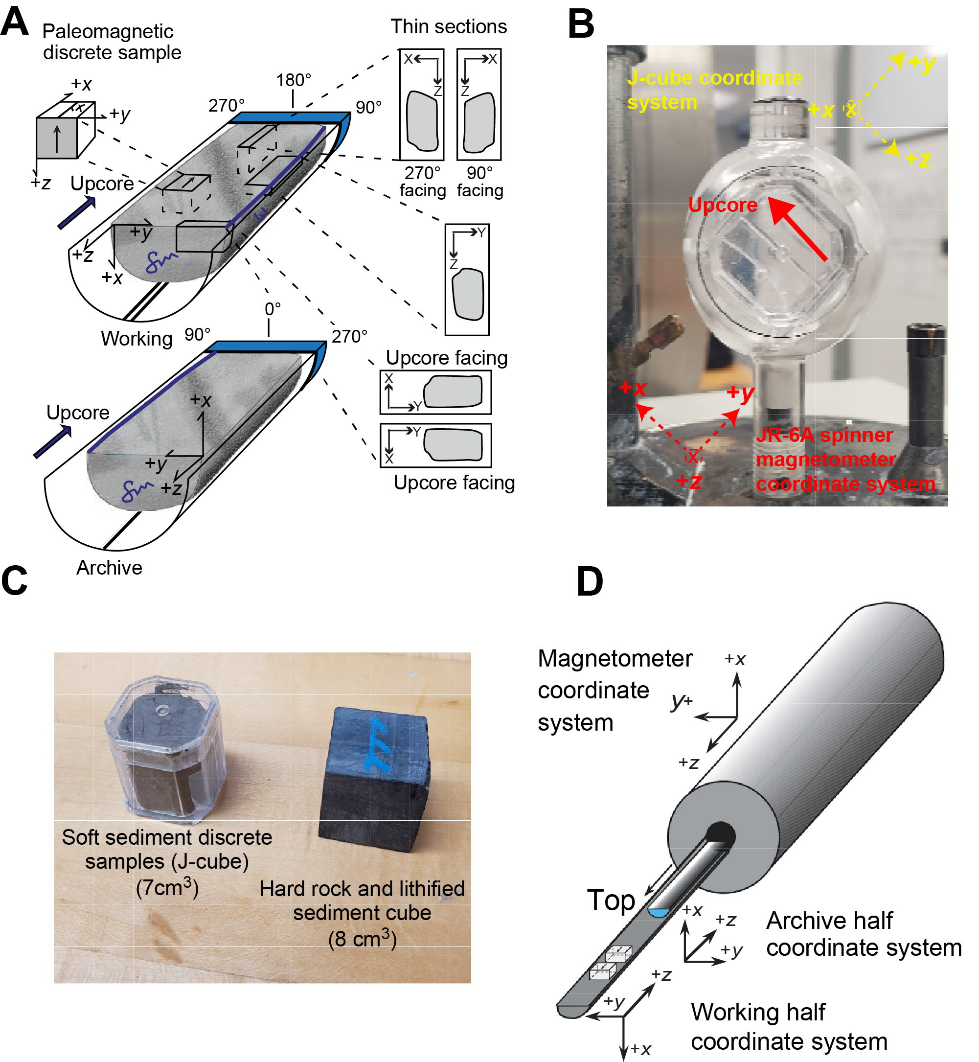
Figure F22. Coordinate system for paleomagnetic measurements.
6.2. Archive-half measurements
Measurements of NRM and partial stepwise AF demagnetization at steps of 5, 10, and 20 mT carried out on archive halves (Figure F22A) used a 2G Enterprises Model 760R-4K superconducting rock magnetometer (SRM). Noise levels of the SRM, established from empty core tray measurements during transits at the start of Expeditions 390 and 393, were ≤5 × 10⁻⁸ Am2 for the three superconducting quantum interference device (SQUID) sensors. Both the x- and z-axis were found to be the noisiest, and the y-axis was the cleanest. The SRM is driven by the Integrated Measurement System (IMS) SRM software (Version 12.0) and is equipped with direct-current SQUIDs (DC-SQUIDs) and in-line 3-axis orthogonal coils for AF demagnetization that can reach peak fields of 80 mT. The SRM SQUID sensors have a spatial resolution of ~8 cm, determined by the width at half height of the response of the pickup coils. Measurements made within ~4 cm of gaps in the core material or core section breaks will thus be affected by edge effects and were treated with caution. Sediment and hard rock archive halves were measured at 2 cm spacing.
Measurement of the igneous basement depended on recovery and signal intensity. SRM measurements on archive-half core sections were done only when recovery was good and pieces were long enough (≥9 cm) to avoid edge effects. In cases where we obtained spurious results on the SRM due to strongly magnetized materials generating residual flux counts, the measuring resolution was lowered to 5 cm. If this too gave spurious results or when recovery was poor and pieces were too short to analyze, we instead solely measured discrete samples.
To avoid potential magnetic contamination, the sample track was cleaned each day, both physically and magnetically, at an AF of 60 mT. Prior to and following measurement of each archive-half section, a portion of empty track (6 cm) was measured. These are referred to as the header and trailer measurements and serve the dual functions of monitoring the background magnetic moment and allowing for future deconvolution analysis.
6.3. Discrete samples
6.3.1. Paleomagnetic measurements
An AGICO JR-6A dual-speed spinner magnetometer (sensitivity = ~2 × 10⁻⁶ A/m) was used to measure the NRM before and after demagnetization (AF or thermal) of all discrete samples collected (Figure F22B).
In relatively undisturbed and continuous soft sediment, we collected two samples per core. For disturbed cores, sampling resolution was dependent on available material. These sediments were collected in 7 cm3 plastic Natsuraha-Giken sampling boxes (J-cubes; Figure F22C). In all cases, samples were extracted from the middle of the working half of the core with the arrow on the face of the J-cube pointing upcore (Figure F22).
Discrete sample cubes (8 cm3) of lithified sediments and hard rock material were removed with a tile saw equipped with two parallel blades. Although minicores (~12 cm3 cylinders of rock) are more commonly used in paleomagnetic laboratories, cubes are preferred here because they have a more reproducible vertical reference and facilitate sample sharing for paleomagnetic and physical properties analyses. An orientation arrow was drawn directly on the cube face (Figure F22C). These samples were used for both AF and thermal demagnetization experiments.
Similarly to the SRM analysis of hard rock core archive-half sections, discrete sampling of the hard rock working-half sections was determined by recovery and the nature of the material recovered. In cores where recovery was good, discrete samples for shipboard analysis were selected on the basis of identified flow/magmatic unit boundaries (see Igneous petrology), targeting the freshest available representative material, typically two samples per core. In a subset of the magmatic units, an additional discrete sample representative of the unit's hydrothermal alteration was taken to assess the effects of hydrothermal alteration on the magnetic properties of the rocks.
We performed progressive AF demagnetization of discrete samples using a DTech D-2000 AF demagnetizer. Following NRM measurement, we used one of two primary demagnetization schemes (Table T4). Sequence Main I used 5 mT steps up to 40 mT, 10 mT steps between 40 and 60 mT, and 20 mT steps up to 100 mT. Sequence Main II was a condensed form of Sequence Main I and consisted of 10 mT steps starting at 5 mT up to 25 mT, a single 5 mT step up to 30 mT, a single 10 mT step up to 40 mT, and 20 mT steps up to 100 mT. If a characteristic remanent magnetization (ChRM) had not yet been identified or a significant drop in intensity not observed by 100 mT, we carried out additional AF demagnetization in 30 mT steps until we achieved either result. Variations of these two sequences (i.e., skipped steps) were also used when (1) time was a factor, (2) initial demagnetization data indicated that such long sequences were not necessary (i.e., a straight line to the origin was isolated early on), or (3) results from similar rock types previously measured suggested detailed demagnetizations were not necessary.
Where possible in basement cores, paleomagnetic and physical properties analyses were conducted on shared samples to allow comparison of these properties in a given rock to provide semiquantitative assessment of the effects of alteration. This also reduced the amount of sample material required in intervals of low recovery. When samples were shared, AF and thermal demagnetization experiments (using an ASC Scientific TD-48 thermal demagnetizer) for hard rock material occurred prior to and following MAD measurements, respectively (see Physical properties and downhole measurements). MAD measurements required saturating samples with water and then drying them at 105°C for ~24 h in a magnetically unshielded environment. In these instances, NRM was measured before and after the MAD measurements. The sample was then demagnetized at 110°C to remove any viscous magnetization acquired during the MAD measurements, followed by demagnetization at 150°C. Subsequent demagnetization occurred at 50° steps up to 400°C, 25° steps up to 500°C, and 40° steps thereafter up to 580°C. Samples were heated for 30 min and then cooled to room temperature before measuring. Because of time constraints, thermal demagnetization experiments were performed only on every fifth core. Additionally, we calculated the median destructive field (MDF; from AF demagnetization) and median destructive temperature (MDT; thermal demagnetization) of our discrete samples. This is the field and temperature, respectively, where 50% of the NRM is reduced. This further aids in both mineralogical and grain size analyses.
During Expedition 393, a magnetic shield casing (Figure F23) was built for discrete hard rock samples that were being shared for MAD analyses to prevent samples from acquiring artificial viscous overprints while allowing for faster processing of the shared samples. This also reduced the overall number of samples taken from the hard rock cores. The shield casing contained three concentric layers of wood, each covered with µ-metal foil. The seams in the wood and foil of each layer were rotated to different positions to avoid leakage of magnetic fields into the shielding.
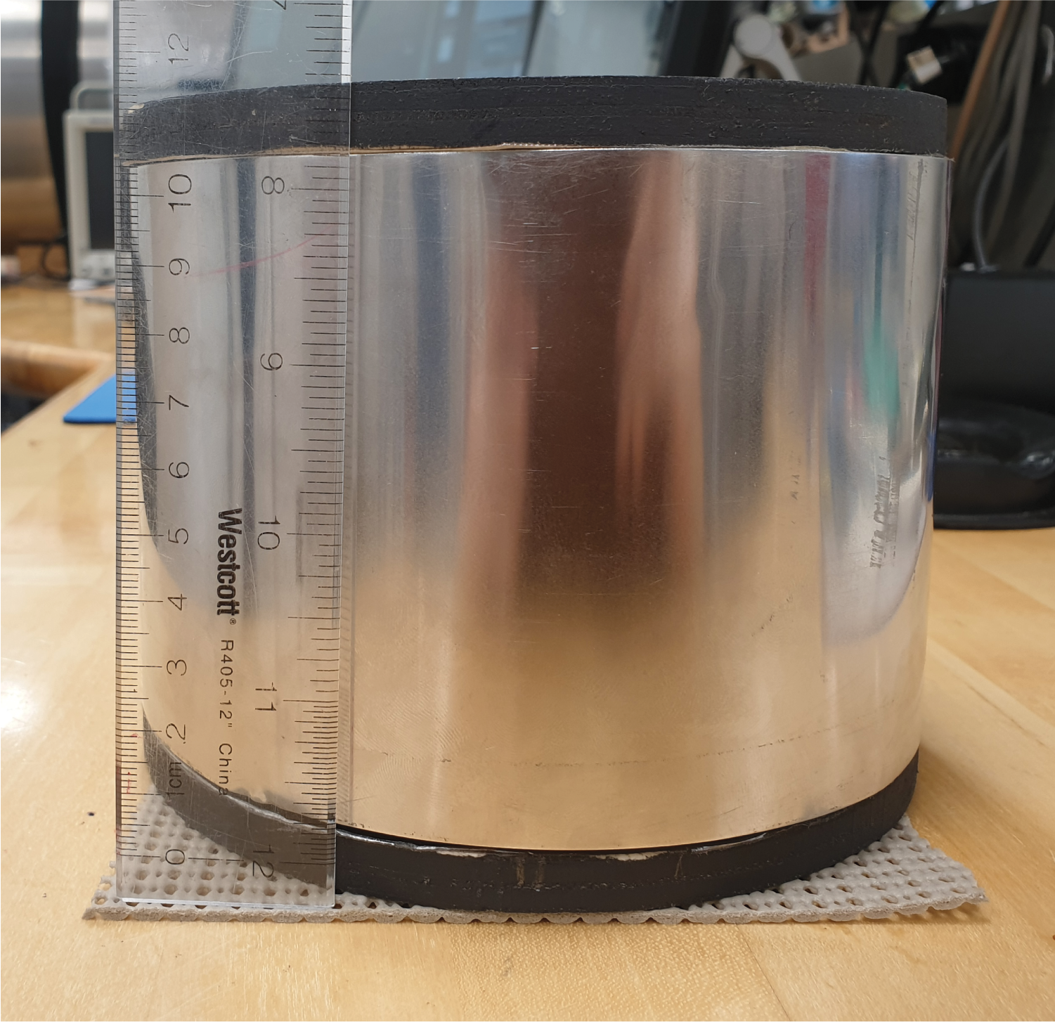
Figure F23. Magnetic shield casing.
Measurements of NRM before and after each demagnetization step were plotted as orthogonal vector plots (OVPs; Zijderveld, 1967). For representation of these demagnetization diagrams, the software package Rema6 (AGICO) was utilized. Visual inspection determined whether or not the ChRM had been isolated, and directions were calculated using the principal component analysis (PCA) approach (Kirschvink, 1980) implemented in the https://paleomagnetism.org web interface package (Koymans et al., 2016).
Isolation of the ChRM serves a variety of functions. First, it determines if any viscous magnetizations have been effectively removed. These could occur naturally or via drill string overprint acquired during core collection. A drilling overprint will present as a steeply inclined direction in OVPs and is routinely found during coring operations. Additionally, determination of the ChRM ensures that the correct geomagnetic polarity sequence has been identified.
6.3.2. Rock magnetic measurements
A subset of the representative discrete samples was subjected to isothermal remanent magnetization (IRM) experiments following AF demagnetization. We chose representative samples from each lithologic and volcanic unit to conduct a pilot study investigating any mineralogical changes occurring downcore. Impulse fields were imparted with an ASC Scientific Impulse Magnetizer (Model IM-10-30) along the positive z-axis up to the saturation IRM (SIRM) at 1200 mT. Backfields (negative z-axis) were imparted following one of the three different sequences (Table T5), depending on time. The full sequence applied on at least one sample per unit consists of equidistant field steps on a log scale between 10 and 1200 mT, including two additional steps at 100 and 300 mT. These measurements permit deconvolution of the IRM acquisition curves to examine mixed ferromagnetic assemblages (Maxbauer et al., 2016). A modified version of this sequence was employed to expedite measurements. A 3-step sequence—using only 1200 mT and two backfields (100 and 300 mT)—was also used on additional samples from cores already characterized by one of the longer sequences. Some intraparametric ratios can also be calculated from these measurements. Hard IRM (HIRM = 0.5 × [SIRM + IRM−300mT]; Thompson and Oldfield, 1986) and the S-ratio = IRM−300mT/SIRM (Bloemendal et al., 1992) are used to monitor the contribution and concentration of high-coercivity minerals (hematite + goethite). IRM−100mT/SIRM (IRM100/SIRM) is used as a proxy of low-coercivity mineral phases (e.g., [titano]magnetite and [titano]maghemite).
During Expedition 393, measurements of magnetic susceptibility at two different frequencies, low field (χlf) and high field (χhf) (χlf = 465 Hz and χhf = 4650 Hz) were performed using a Bartington MS2B magnetic susceptibility meter. The frequency-dependent magnetic susceptibility (χfd%), as χfd% = [(χlf − χhf)/χlf] × 100 (Dearing et al., 1996), was calculated to estimate the contribution of superparamagnetic particles (Thompson and Oldfield, 1986; Dearing et al., 1996).
The anisotropy of low-field magnetic susceptibility (AMS) was measured for all discrete samples to characterize the rock texture or petrofabric. AMS depicts the preferred orientations and degree of alignment of minerals (ferromagnetic, paramagnetic, and diamagnetic phases) in rocks and sediments. This permits us to investigate sediment compaction and whether paleocurrent directions were recorded. AMS is also used to determine if there is any superimposed deformation, either tectonic or sampling/drilling related. In addition, AMS can be used to evaluate flow fabrics for basement basaltic rocks, although this is often not straightforward and prone to bias data (e.g., Schöbel et al., 2013). AMS is described by a triaxial ellipsoid with principal axis lengths equal to the eigenvalues of the magnetic susceptibility tensor, Kmax ≥ Kint ≥ Kmin, that correspond to the maximum, intermediate, and minimum susceptibility axes, respectively. AMS was measured with the MFK2-FA multifunction frequency Kappabridge (AGICO) (sensitivity = 2 × 10⁻⁸ SI) using 975 Hz frequency and the 3-position protocol. The susceptibility tensor and associated eigenvalues were calculated using Anisoft (AGICO) software (v.5.1.03). Anisoft software was also used to correct the direction of the three principal AMS ellipsoid axes for samples taken from cores that had been oriented with the Icefield MI-5 core orientation tool. To describe and quantify the AMS ellipsoid, we used the following parameters:
- Magnetic lineation (L = Kmax/Kint; Balsley and Buddington, 1960),
- Magnetic foliation (F = Kint/Kmin; Stacey et al., 1960),
- Anisotropy degree (P; Jelinek, 1981), and
- Shape parameter (T; Jelinek, 1981).
6.4. Magnetostratigraphy
The SAT drill sites are located between ~30°15′S and 30°57′S. At these latitudes, the sites are sufficiently distant from the Equator that changes in inclination are discernible. Moreover, by assuming that a geocentric axial dipole characterizes the magnetic field at this Southern Hemisphere location, a field inclination of approximately −49.1° (tan[I] = 2 tan[lat], where I = inclination and lat = latitude) is predicted. Negative inclinations therefore represent normal polarity and positive inclinations represent reversed polarity. We used the geomagnetic polarity timescale of Gradstein et al. (2020) (GPTS2020) for correlation and age assignment, assisted by the biostratigraphic datums. The spliced inclination stratigraphy (see Stratigraphic correlation) was used during Expedition 393 to complete the remanence data where significant gaps were observed in the stratigraphic column. The GPTS2020 scale completes the astronomical-tuned age model for nearly all chrons, whereas earlier scales required interpolations from spreading rate models for the South Atlantic C-sequence synthetic profile of marine magnetic anomalies.
7. Age model and mass accumulation rates
7.1. Age models
The age models for sediments recovered along the SAT are based on calcareous nannoplankton and planktic foraminiferal datums and paleomagnetic reversals. Biostratigraphic datums were placed at the midpoint between samples that contain the datum and the nearest sample that does not. Likewise, paleomagnetic reversals were placed at midpoints between inflection points in the declination or inclination curves for magnetochron boundaries. The placement of datums at the midpoint between samples represents a source of uncertainty in the age-depth calculation, which is shown on age-depth plots by vertical error bars on each data point. These error bars do not incorporate uncertainty from diachroneity of first and last occurrences of microfossils between mid-latitude and tropical/subtropical sites, which is well documented (e.g., Dowsett, 1988; Lam et al., 2022) and yet difficult to quantify without an independent age model (see Biostratigraphy and Paleomagnetism for detailed explanations of biostratigraphic and paleomagnetic datums, respectively). Age determinations for both biostratigraphic datums and paleomagnetic reversals are based on Gradstein et al. (2020) (as modified by King et al., 2020, for Neogene planktic foraminifera) unless otherwise stated. Datums and ages are illustrated in Figure F21.
7.2. Linear sedimentation rates
Linear sedimentation rates (LSRs) were calculated using both magnetochronology and biostratigraphy. For Expedition 390 (Sites U1556, U1557, U1559, and U1561), these plots use the CSF-B depth scale; for Expedition 393 (Sites U1558, U1560, and U1583), the plots use the CSF-A depth scale. The LSR curve was drawn through the most robust biostratigraphic and magnetostratigraphic datums, avoiding datums that were identified based on poorly preserved specimens, have inconsistent occurrences, resulted in age inversions, have high uncertainty because of taxon rarity, and/or were highly diachronous compared to other fossil groups (e.g., planktic foraminiferal datums that lie outside of the age model compared to calcareous nannofossils).
7.3. Mass accumulation rates
Bulk sediment mass accumulation rates (MARs) were calculated based on the LSR and sediment density. Sediment density used in MAR calculations is calculated from GRA measured on the WRMSL and calibrated by discrete dry bulk density (DBD) measurements conducted shipboard (see Physical properties and downhole measurements).
To convert GRA measurements to DBD, percent porosity (POR) was calculated for each GRA data point by dividing the difference in GRA and grain density (GD) by the difference in GD and water density (WD), using 1.03 g/cm3 as the density of water and 2.71 g/cm3 as the density of sediment grains (calcite and clays have similar grain densities: 2.71 g/cm3 for calcite and ~2.75 g/cm3 for illite):
Then, DBD was calculated by multiplying the assumed GD by the calculated POR:
MAR was calculated using the following equation:
Carbonate accumulation rates (CARs) and organic carbon accumulation rates (OCARs) were calculated by multiplying the weight percent of carbonate (CaCO3) and total organic carbon (TOC), which were both acquired on carbonate samples, by the MAR calculated for the same sample:
Time steps for MAR are based on the sampling density for CaCO3 and TOC (routinely once or twice per core).
8. Physical properties and downhole measurements
Physical properties measurements were taken during the SAT expeditions to characterize the physical, chemical, and structural properties of the recovered sediment and rock cores and the formation surrounding the borehole. These core and downhole log data are also used to link the geologic observations made on the core to the regional geophysical survey data. Physical properties measured during the expeditions include bulk density, NGR, magnetic susceptibility, compressional and shear velocities, thermal conductivity, porosity, shear strength, and electrical resistivity. They were characterized using a variety of techniques and methods on core sections and samples, as well as a series of downhole measurements carried out through wireline logging of the drilled and cored boreholes, as described below.
8.1. Standard physical properties measurements and core flow
Physical properties measurements on sediment cores followed this general sample workflow:
- After core sections were curated and laser engraved, sections were analyzed on the STMSL so that the data could be used in stratigraphic correlation.
- Whole-round core sections (>50 cm long) were run on the NGRL.
- Core sections were thermally equilibrated to ambient room temperature (~20°C) for ~4 h.
- Whole-round core sections were run on the WRMSL: GRA bulk densitometer, magnetic susceptibility pass-through loop system (loop magnetic susceptibility [MSL]), and PWL.
- Whole-round core sections were passed to geochemistry and microbiology teams for dissolved O2 measurements and Rhizon sampling (see Geochemistry and Microbiology).
- Thermal conductivity (TCON) was measured once per core.
- Cores were split lengthwise into archive and working halves.
- Samples for MAD analyses were collected from the working half, generally two per core in representative lithologies, and analyzed for MAD properties.
- Discrete compressional velocity measurements were made on the working half using the Section Half Measurement Gantry (SHMG).
- Strength measurements were made on the working half using the automated vane shear (AVS) and pocket penetrometer (soft sediments only).
- The archive half of the core sections was passed through the SHIL for imaging and the SHMSL for RSC and MSP measurements.
Expedition 393 followed a slightly modified workflow for sediment cores. During this expedition, dissolved O2 measurements were made by the geochemistry and microbiology group on whole-round core sections immediately after STMSL logging. Thermal conductivity was measured on section halves after splitting. Additionally, the archive halves were run on the X-ray Imaging Logger just after splitting or after full completion of the hole, before storing the sections in the reefer.
Hard rock cores followed a slightly different sequence:
- Core sections were shaken out onto the core cutting table, and pieces were oriented where possible. At this point, discrete pieces were removed for microbiological work (see Microbiology).
- Discrete pieces of a given recovered hard rock section were shaken into a sterile split liner in the core splitting room for examination by a petrologist and/or a structural geologist, who determined the splitting line for obtaining working and archive halves from each whole-round piece. The core pieces were then put back into a full core section liner with plastic spacers between curated pieces (see Introduction).
- Core sections were thermally equilibrated to ambient room temperature (~20°C) for ~4 h.
- NGRL measurements (for sections >50 cm in length) and X-ray imaging, neither of which were sensitive to temperature, were made on whole-round sections during this equilibration time.
- After equilibration, whole-round core sections were run on the WRMSL with the GRA bulk densitometer and MSL (PWL was turned off).
- Whole-round core exteriors were imaged on a DMT digital color CoreScan3 system.
- Cores were split into archive and working halves along the previously marked splitting lines.
- The archive half of the cores was passed through the SHIL for imaging and SHMSL for RSC and MSP.
- Oriented, discrete cube samples (~8 cm3) were taken from the working-half cores for P-wave velocity and MAD analyses, generally two per core, in representative lithologies. These cubes were also used for paleomagnetic measurements (see Paleomagnetism) to minimize the material removed from the core. The samples were placed in seawater under vacuum for 4–12 h for resaturation before measurement. Discrete samples were measured for P-wave velocity in three orthogonal directions and then processed for MAD analyses.
- Selected pieces of core sections were also resaturated for 4 h under vacuum and measured for thermal conductivity. This analysis was nondestructive; pieces were returned to the core following measurement.
During Expedition 393, the whole-round sections were usually run through DMT imaging before NGRL or WRMSL, and selected sections were run on the X-ray imager after the NGRL.
A subset of the physical properties measurements were made during Expeditions 390 and 393 on cores recovered from Expeditions 390C and 395E (Estes et al., 2021; Williams et al., 2021). Only archive halves of the Expedition 390C and 395E sediment cores were available during Expeditions 390 and 393; therefore, only nondestructive SHMSL and SHIL measurements were made.
Hard rock (lithified sediment and igneous basement) core sections associated with the sediment/basement interfaces that were recovered during Expeditions 390C and 395E received the full array of hard rock core measurements listed above.
8.2. Whole-round core section measurements
Whole-round cores were used to collect measurements of NGR, MS, compressional wave velocity, thermal conductivity, and digital images.
8.2.1. Special Task Multisensor Logger
The STMSL is run during sediment coring on whole-round sections immediately after laser engraving. The recovery of a complete stratigraphic section relies on the rapid hole-to-hole stratigraphic correlation of incoming sediment cores. The STMSL was used to measure GRA and MS at a sampling interval of 10 cm (see Whole-Round Multisensor Logger below). The data were used for real-time stratigraphic correlation (see Stratigraphic correlation). Higher resolution GRA and MS data were later measured using the WRMSL after the core sections had thermally equilibrated to ambient room temperature.
8.2.2. Natural Gamma Radiation Logger
Natural gamma rays occur primarily as the result of the decay of 238U, 232Th, and 40K isotopes. Because radioactive decay and the resultant gamma ray emissions are not sensitive to temperature, the whole-round cores could be run through the NGRL before equilibrating to room temperature. The NGRL detector unit was calibrated using 137Cs and 60Co sources and identifying the peaks at 662 (137Cs) and 1330 keV (60Co).
Counts were summed over the range of 100–3000 keV during Expeditions 390 and 393 to be compatible with data collection from Expeditions 390C and 395E and for direct comparison with downhole logging data. Background gamma radiation measurements of an empty core liner counted for 21,600 s (6 h) were made prior to measuring core sections. The background signal is then automatically subtracted from the measured values of the core sections. A new background gamma radiation measurement is only necessary when the ship moves ≥2° latitude, which made quantification of background gamma radiation only necessary once during Expedition 390 and once during Expedition 393.
A single NGRL run consisted of two sets of measurements taken by eight sensors, each spaced 20 cm apart. The two sets of measurements were offset by 10 cm, which yielded a total of 16 measurements equally spaced 10 cm apart over a 150 cm long section of core. The quality of the energy spectrum measured in a core depends on the concentration of radionuclides in the sample and on the counting time, with higher times yielding more clearly defined spectra. Each set of measurements for a single NGRL run were counted for 300 s. Core sections <50 cm in length were not typically run through the NGRL because of constraints imposed by the sensor geometry.
The shipboard NGRL acquisition system outputs only the total counts. However, it also stores the whole spectrum for all element-specific energy intervals, which can be used to extract the single contribution and concentration of K, U, and Th.
During Expedition 393, an open access MATLAB algorithm designed by De Vleeschouwer et al. (2017) to extract, quantify, and correct the K, U, and Th concentrations was adapted to the most recent LIMS file nomenclature. The script provides an estimate of the K, U, and Th contents by integrating NGR counts over specific energy intervals and by comparing those counts to energy spectra of the shipboard standards that are used to calibrate the NGRL.
8.2.3. Whole-Round Multisensor Logger
Following temperature equilibration, whole-round core sections were measured on the WRMSL, which nondestructively measures GRA for bulk density, MS, and P-wave velocity on whole-round core sections. The sampling interval was set at 2.5 cm for both sediment and hard rock for each measurement. The sampling interval was chosen to collect the maximum number of quality measurements while not slowing core flow. QA/QC was monitored and maintained by running a core liner with freshwater through the WRMSL after every full core.
WRMSL measurements are most accurate on a liner completely filled with core that has experienced minimal drilling disturbance. As a result, the diameter of the core liner (66 mm) is assumed for hard rock density calculations, even though the liner is often less than 100% filled. Furthermore, hard rock material was often recovered in disaggregated pieces rather than as a continuous core, which reduces the rock volume. Therefore, GRA bulk density and MS measurements often underestimate actual values for hard rock cores but still provide useful information for stratigraphic correlation and can be compared to the discrete measurements of density, MS, and P-wave velocity. P-wave velocities measured by the WRMSL suffer the most because of poor coupling on hard rock core sections and were thus measured only on sediment core sections.
8.2.3.1. Gamma ray attenuation bulk density
The GRA densitometer on the WRMSL operates by passing gamma rays from a 137Cs source down through a whole-round core section into a 75 mm × 75 mm sodium iodide detector located directly below the core. Gamma rays with an energy peak at 662 keV are attenuated by Compton scattering as they pass through the core. The resultant gamma ray count is proportional to bulk density. Calibration of the GRA densitometer was performed using core liners filled with seawater and aluminum density standards. Recalibration was performed as needed if the value of the freshwater QA/QC standard run after every full core deviated significantly (more than a few percent) from 1 g/cm3. The spatial resolution of the GRA densitometer is <1 cm.
8.2.3.2. Magnetic susceptibility
Magnetic susceptibility (k) is a dimensionless measure of the degree to which a material can be magnetized by an external magnetic field:
where M is the magnetization induced in the material by an external field strength (H). Magnetic susceptibility responds to variations in the type and concentration of magnetic grains, making it useful for identifying compositional variations and alteration in hard rock cores. In the case of sediments, magnetic susceptibility can often be related to mineralogical composition (e.g., terrigenous versus biogenic material) and diagenetic overprinting (e.g., clays from the alteration of igneous materials have a susceptibility orders of magnitude lower than the material's original iron oxide constituents). Water and plastics (core liner) have a slightly negative magnetic susceptibility.
The WRMSL incorporates a Bartington Instruments MS2 meter coupled to an MS2C sensor coil with a diameter of 8.8 cm that operates at a frequency of 565 Hz (Bartington Instruments, Ltd., 2011). The sensor output can be set to centimeter-gram-second (cgs) units or SI units; IODP standard practice is to use the SI setting. MS is reported in instrument units. To convert results into dimensionless units, it is necessary to multiply the data by a correction factor that is a function of the probe type, core diameter, and loop size. The sizes of small rock pieces in incomplete cores vary, so application of a single correction factor is not justified; therefore, no correction is applied to the WRMSL magnetic susceptibility data. This conversion factor does not change the order of magnitude of the measured susceptibility values, so the results are comparable with the susceptibility measured by the paleomagnetism group with the same physical units (SI).
The MS2C coil was calibrated with a homogeneous mixture of magnetite and epoxy in a 40 cm long piece of core liner to an accuracy of ±5%. The resolution of the method was ±4 cm for continuous core section; therefore, magnetic susceptibility was underestimated for core material that was not continuous over an 8 cm interval.
8.2.3.3. P-wave velocity
P-wave velocity of the whole-round sediment core sections was measured through the incorporated PWL in the WRMSL. The PWL uses a 500 kHz compressional wave pulse transmitted across the core liner (orthogonal to depth) between two transducer-coupled calipers. Coupling between the calipers and the core liner was aided by water continuously dripping across the caliper surfaces. The pulse waveform was bandpass filtered between 0.4 and 1.0 MHz, stacked, summed, and ensemble-averaged to allow for automatic first arrival picking by the integrated WRMSL software. The PWL automatically corrected for the acrylic liner and was calibrated using known velocities of a freshwater-filled liner and aluminum standards. Because XCB and RCB coring in hard rock often produces cores that do not fill the core liner and air-filled voids are introduced, the PWL was only active in the WRMSL runs on the sediment cores and was not active for the hard rock whole-round cores.
8.3. Digital imaging
Imaging of hard rock core exteriors was carried out on a DMT digital color CoreScan3 system prior to splitting the cores into their working and archive halves (Figure F24A). The DMT CoreScan3 produces a full-circumference image of drill core up to 1 m long and 25–150 mm in diameter. In 360° mode, true color images are recorded at 5, 10, or 40 pixel/mm resolution by a linescan camera as the core is incrementally rotated about its cylindrical axis. This camera captures a new line of the full core length every time the circumference rotates by 1 pixel (DMT GeoTec, 1996; DMT GmbH, 2000). The advantage of obtaining such a high-resolution image data set is that it permanently records the original core's external features that are lost once it is split into two halves and sampled. Use of these images for core-log integration, as well as machine learning applications, requires them to be a consistent and accurate depiction of the original core, so a systematic approach should be taken to avoid variation in two images of the same rock type.
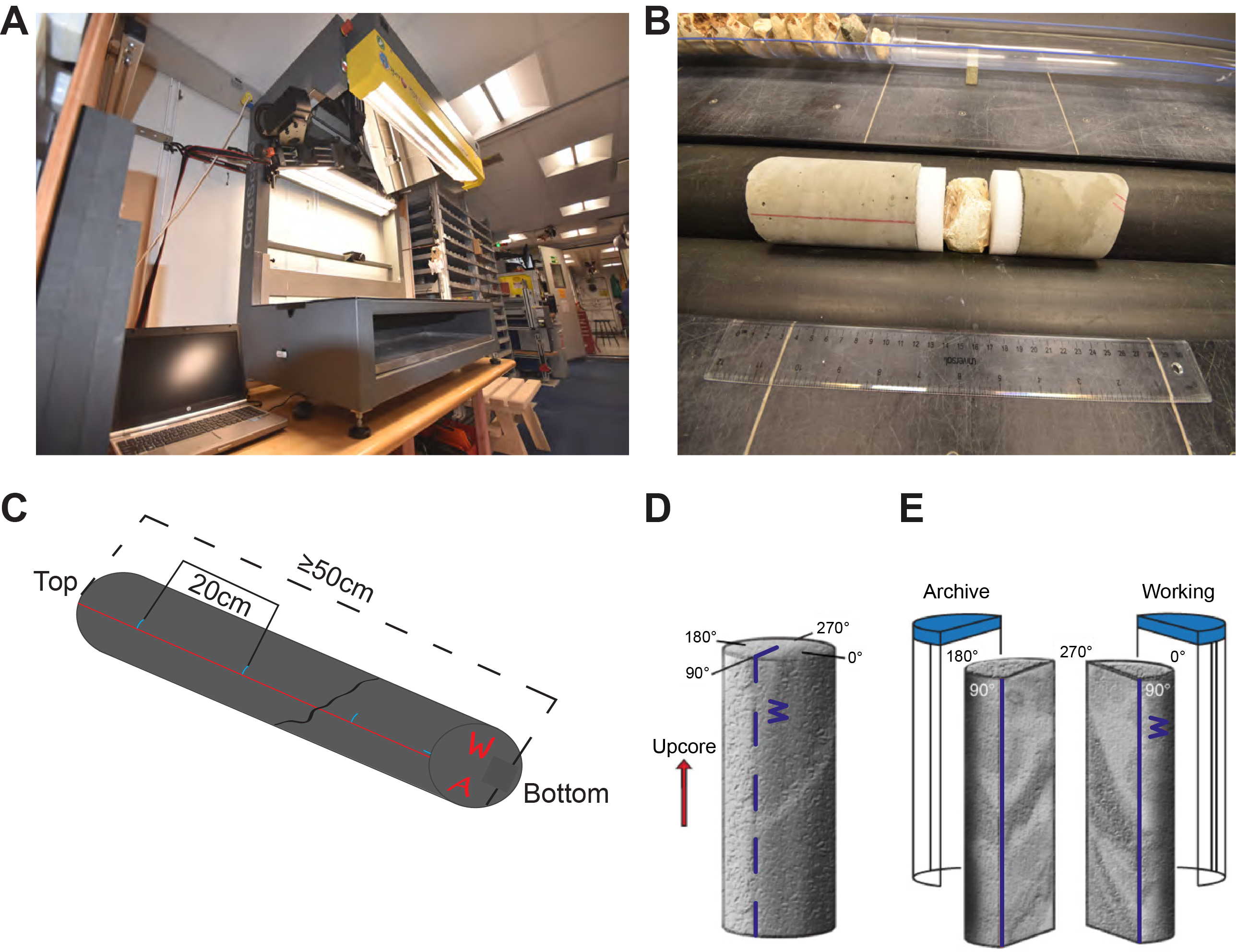
Figure F24. DMT digital color imager and geographic coordinate system for CRF.
Whole-round DMT CoreScan3 digital images are recorded in association with the IODP CRF (Figure F24D; see Alteration petrology). The red/blue cutting line drawn on the outside of the whole round core surface denotes a plane separating the working and archive halves with the coordinates of 090° in the CRF (Figure F24E). For Expedition 393, during postacquisition processing images were orientated to maintain consistency with the CRF using the software package CoreScan3.
Standard procedure during IODP expeditions is to divide each 9.5 m core recovered into 1.5 m sections; however, the DMT CoreScan3 is limited to sections ≤1 m. Fortunately, even cores with high recovery consisted of many continuous yet fractured pieces that could fit on the scanner. The IODP curatorial process involves dividing the typically fragmented/fractured hard rock core sections into core pieces, or bins (see Core handling and analysis). The bins are numbered sequentially downhole in each section, starting with 1, and their top and bottom offsets (within the section) are recorded in a piece log that is uploaded to the LIMS database after curation. Bins that contain multiple continuous fragments are given the same bin number, but the fragments, or subpieces, are lettered consecutively from top to bottom (see Core handling and analysis). Only the exterior of round pieces that were able to roll about their cylindrical axis were scanned, although some pieces that were too uneven to roll cleanly were supported using two round foam pads braced by concrete cylinders (Figure F24B). Core bins that contained fragmented and rubbly material were not scanned.
All cores were scanned in high-resolution mode (40 pixels/mm), which limits a single image frame to just 25 cm, so longer pieces were scanned in multiple 25 cm frames starting with the top 25 cm and working downcore until the whole piece was imaged. All subpieces in a single bin were considered a single piece and scanned together, and if their combined length was >25 cm they were scanned in multiple frames. Additional blue lines were marked at 20 cm intervals along the exterior of the core in this case to enable images to be cropped and reconstructed using a dedicated Python script (see Core image processing) (Figure F25). Finally, any highly fractured core that still fit together to form a cylinder was secured using rubber bands or shrink-wrapped prior to scanning, though this was a last resort because the wrapping creates interference in the image because of spurious reflectance.
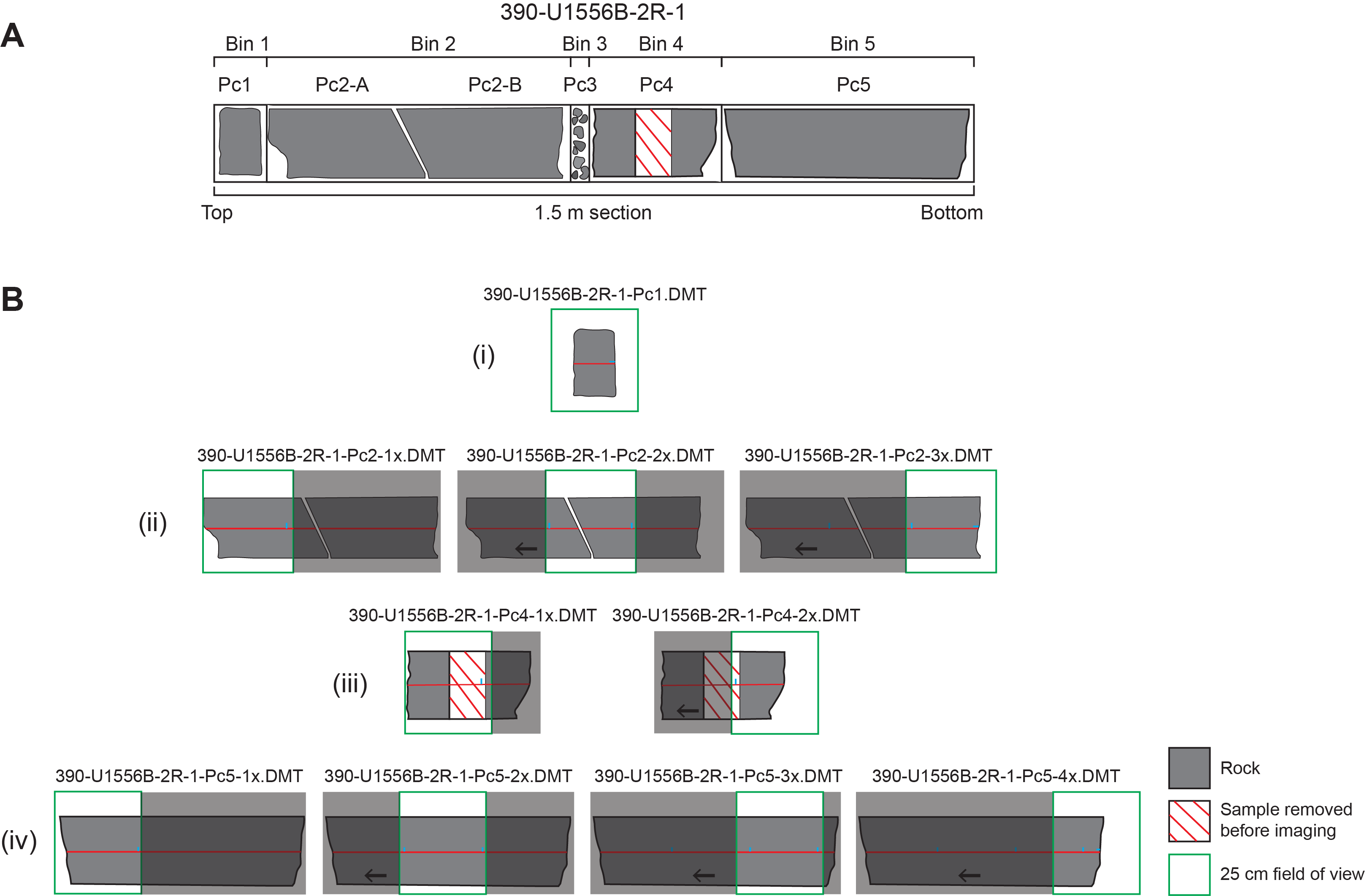
Figure F25. Examples of how to scan each bin type.
Default settings for the CoreScan3 software were customized to ensure minimal correction by the software to ensure a consistent brightness across the data set. These settings are imperative for accurate manipulation by the Python program and include the following:
- Disabling Auto-adjust exposure;
- Selecting No core detection, no selection; and
- Choosing the Slightly lighter exposure setting
During Expedition 393, an X-Rite ColorChecker balance chart was imaged every 12 h during imaging periods to standardize colors across each unwrapped core image scan.
8.3.1. Core image processing
Each core piece scanned on the DMT CoreScan3 was saved both as DMT and BMP files and named using the following convention: Expedition of core recovery-Site-Hole-Core-Section-Bin.Extension (e.g., 390C-U1556A-2R-1-Pc1.DMT). If a bin contained multiple subpieces that were scanned separately, each piece's file name was appended with a numbered identifier followed by an x (e.g., 390C-U1556A-2R-1-Pc1-1x.DMT). Similarly, if a long piece (or multiple continuous pieces) were scanned together but in separate frames, each filename is also appended with a numbered identifier followed by an x (e.g., 390C-U1556A-2R-1-Pc1-1x.DMT; 390C-U1556A-2R-1-Pc1-2x.DMT) (for examples see Figure F25).
Individual image frames were stitched together to reconstruct bins >25 cm to provide a single high-resolution image per whole-round core section. Image processing was carried out using a Python program to allow comparison between full section DMT and SHIL data sets that will be made available postexpedition.
Because the DMT's computer was not able to be connected to the ship's server, a 1 TB external solid-state hard drive was strapped to the desk to avoid knocking and all images were saved directly onto it. These images were then exported manually to another hard drive before being copied onto the backup servers aboard the ship at the end of each shift.
8.4. Thermal conductivity
TCON is the coefficient of proportionality relating conductive heat flow to a thermal gradient (Blum, 1997). Thermal conductivity was measured using the transient needle probe method in whole- or half-space geometry (Von Herzen and Maxwell, 1959), using a Teka Bolin TK04 system.
For a minority of sediment cores, thermal conductivity was measured after whole-round core sections had equilibrated to room temperature but prior to the cores being split. The needle probe method was used in full-space configuration for soft sediments (Von Herzen and Maxwell, 1959). The needle probe was inserted into the unconsolidated sediment through 2 mm holes drilled into the core liner roughly once per core, generally in locations determined using MS data gathered on the WRMSL. In general, MS is lower in carbonate-rich intervals and higher in clay-rich intervals. Both kinds of intervals were targeted in order to assess thermal conductivity in these end-member lithologies.
For the majority of sediment cores, thermal conductivity was measured with a half-space needle puck (similar to the method used for hard rock) because the needle probe method was found to result in poor data quality. The needle puck was pressed gently against a split core section of the working half to measure thermal conductivity.
For hard rock material, TCON measurements were taken from pieces that were at least 10 cm long after splitting. If the split face of the piece was significantly rough, a lap plate and grit were used to smooth the sample face for better connection to the probe. The split samples were first saturated in ambient-temperature seawater for 4 h with a vacuum pump to aid in the full saturation of pore space. A puck with the measurement probe was attached to the split face and secured with a strap or rubber band. Three steps of heating–cooling cycles were used, and the final TCON value was the mean of the three cycles, although data from each of the cycles are also recorded in the LIMS database.
8.5. Split core section-half and discrete measurements
Once cores were split, samples for discrete petrophysical measurements were taken for MAD analysis, as well as P-wave velocity in the case of hard rock. For soft rocks, discrete samples were taken for MAD analysis; however, shear strength and P-wave velocity measurements were made directly on the cut surface of the working half. Meanwhile, the archive half was used for nondestructive SHMSL measurements and half-round imaging of the split core surface on the SHIL.
8.5.1. X-ray image logger (Expedition 393)
During Expedition 393, X-ray images were recorded on the archive half of each section of sediment recovered to evaluate bioturbation intensity, drilling disturbance, or any structures or features that could produce a recognizable density signature. X-ray imaging was also attempted on selected sections of basement but produced underwhelming results. The X-ray imager is composed of a Teledyne ICM CP120B X-ray generator and a detector unit. The generator works with a maximum voltage of 120 kV and a tube current of 1 mA, and the focal spot is 0.8 mm × 0.5 mm. The generator produces a directional cone at a beam angle of 50° × 50°. The detector unit is located 65 cm from the source and consists of a Go-Scan 1510 H system composed of an array of complementary metal oxide semiconductor (CMOS) sensors arranged to offer an active area of 102 mm × 153 mm and a resolution of 99 µm. Core sections were run through the imaging area at 12 cm intervals, providing images of 15 cm onto the detector with an overlap of 3 cm.
Tests were conducted to obtain the best image resolution for determining the internal structure of the cores, beginning with a standard 80 kV voltage and 1.0 mA current, 60 ms exposure time, and stack of 20 images for all cores. Some adjustments were made during the course of the expedition to improve the image quality in different lithologies. Separate routines were developed for basement and sediment cores, where both used a 300 ms exposure time and a stack of 20 images. Basement core images were acquired using a 100 kV voltage and 0.6 mA current, whereas sediment cores were scanned using 80 kV and 0.5 mA. Image processing parameters were set to a range of 0–1 for basement cores and 0–2 for sediment cores, with a 1% mask threshold for both.
The raw images were collected as 16-bit images and were processed with the IODP in-house processing utility in the IMS software. The software applies corrections for the detector (gain and offset corrections), compensates for core shape and thickness, and adjusts the image contrast. The Savitzky-Golay finite impulse response (FIR) filter is used to smooth images. The resulting processed images include a masked background, the depth scale of the section, and the acquisition parameters. The software applies different processing to APC or rotary cores.
The X-ray imager was not run during Expedition 390 because of time and staffing limitations.
8.5.2. Section-Half Multisensor Logger
8.5.2.1. Point magnetic susceptibility
MSP was measured on archive-half sections using a Bartington Instruments MS2E point sensor at a higher spatial resolution than MS measured by the WRMSL on whole-round cores. Flush contact between the probe and the archive halves was needed; thus, the sediment section halves were covered with plastic wrap to avoid contamination. The instrument takes and averages three measurements made at 1 s intervals to an accuracy of 5%. Before each measurement, the probe was zeroed in air and a background magnetic field was measured and removed from the data. MSP measurements were conducted at a resolution of 2.5 cm for sediment and hard rock sections. A built-in laser surface analyzer aided in the recognition of irregularities in the split core surface (e.g., cracks and voids) and provided an independent check on the fidelity of SHMSL measurements (e.g., Expeditions 301, 371, and 378 [Expedition 301 Scientists, 2005; Sutherland et al., 2019; Röhl et al., 2022]).
The Bartington Instruments MS2E point sensor that is used for MSP measurements uses a higher frequency than the WRMSL (2 kHz). This could introduce small differences in values measured on the two systems if superparamagnetic grains displaying frequency-dependent magnetic susceptibility are present (Dearing et al., 1996). Further differences may also arise from averaging point measurements compared to continuous measurements. Because it is difficult to isolate these different factors, absolute differences between the two magnetic susceptibility systems should be interpreted with caution.
8.5.2.2. Reflectance spectroscopy and colorimetry
The reflectance of visible light from the archive halves of sediment cores was measured using an Ocean Optics USB4000 spectrophotometer mounted on the automated SHMSL. Measurements were taken at 2.5 cm spacing to provide a high-resolution stratigraphic record of color variation for visible wavelengths. Empty intervals, voids, and gaps were skipped to avoid spurious measurements. Intervals where the top of the flat hard rock surface was below the level of the core liner were lifted by adding support matting or foam beneath each hard rock piece to ensure good contact with the sensor. Each measurement was recorded in 2 nm wide spectral bands from 400 to 700 nm. Colorimetry and reflectance data were reported using the L*a*b* color system, in which L* is lightness, a* is redness (positive) versus greenness (negative), and b* is yellowness (positive) versus blueness (negative). The color reflectance spectrometer calibrates on two spectra, pure white (reference) and pure black (dark). Color calibration was conducted approximately once every 6 h (twice per shift).
8.5.3. Pocket penetrometer and vane shear strength
Both pocket penetrometer and vane shear strength quantify the effective shear strength (σm) of the lithology by applying a known compressive and shear stress, respectively.
The pocket penetrometer (PEN) is an unconfined compression strength test and was measured on every core. At a prescribed stress, the shear strength of a material or yield (τf) is related to the compressive strength (Δσf) by
The penetrometer uses a 6.4 mm diameter probe, which is gently pushed into the core below the split core section surface to a marked line on the probe. The selected probe location must be where core section surfaces are smooth. The mechanical scale is in kilograms per square centimeter, and the maximum value measurable by the pocket penetrometer is 4.5 kg/cm2. The data were uploaded to the LIMS database in kg/cm2 and can be converted to kPa as follows:
The vane shear strength (AVS) test is an undrained shear strength test, implying that the quantified shear strength is the effective shear strength, which corresponds to the applied stress minus the intergranular pore fluid pressure (ρf):
The Giesa AVS system is suited for measuring the shear strength of very soft to relatively stiff marine sediments and is especially useful for analyzing undisturbed clay- or silt-rich samples. The system consists of a controller and a gantry for shear vane insertion. A four-bladed miniature vane was pushed carefully into the sediment of the working halves until the top of the vane was level with the core surface. The vane was then rotated to determine the torque required to cause the core material to shear (failure torque). All vane shear strength measurements were obtained using a 12.7 mm vane. Failure torque was determined by measuring the rotation of a torsional spring using a spring-specific relation between rotation angle and torque.
Vane shear strength (Su[V]) can be determined as described by Blum (1997):
- T = torque required to induce material failure (in N·m),
- Kv = constant, depending on vane dimensions (in m3),
- Δ = maximum torque angle (in degrees) at failure, and
- B = spring constant that relates the deflection angle to the torque (in °/N·m)
We performed one measurement per sediment core section until the recovered material became too stiff for vane insertion. Measurements were conducted in regions considered to be the most representative of the core lithology. Shear and compressional strength measurements should be considered approximations of the true sediment strength, as these experiments do not account for pore pressure changes in the cores after splitting.
8.5.4. Moisture and density
Two discrete samples were taken per core from the working half (~10 cm3 samples in sediment and ~8 cm3 samples in hard rock), with additional samples taken at notable lithologic boundaries. The aim was to have at least one sample characterizing each lithologic unit. In indurated sediment and hard rock, discrete samples were extracted for MAD analyses as well as P-wave velocity measurements and paleomagnetism where possible. MAD samples were used to measure wet and dry bulk density, grain density, water content, and porosity following methods presented in Blum (1997), which are briefly outlined below. In hard rocks, MAD samples are typically taken from rock pieces appearing cohesive enough to withstand being cut into cubes, which may bias the data toward higher density values than any surrounding more heterogeneous intervals. During Expedition 393, the initial mass was also measured prior to saturation.
Preweighed and numbered 16 mL Wheaton glass vials were used to process and store the sediment samples. Following measurement of wet mass, samples were dried in a convection oven for at least 24 h at 105° ± 5°C. Dried samples were then cooled in a desiccator for at least 2 h before the dry mass and volume were measured. For hard rock, the procedure included resaturation with seawater for 4–12 h under vacuum before the wet mass measurement was conducted.
Wet and dry sample masses were measured to a precision of 0.005 g using dual-Mettler Toledo (XS204) electronic balances, with one acting as a reference. A standard with a comparable mass to each sample was placed on the reference balance and the computer averaging system compensated for the ship's motion by taking multiple measurements—typically 300 per sample.
Dry sample volumes were determined using a hexapycnometer system of a six-celled custom-configured Micrometrics AccuPyc 1330TC helium-displacement pycnometer. The system measures dry sample volume using pressurized He-filled chambers, where the precision of each cell was 1% of the full-scale volume. Volume measurements were preceded by three purges of the sample chamber with helium. For each measurement, five unknown cells and one cell that contained two stainless steel calibration spheres with a total volume of ~10 cm3 were run. Calibration spheres were sequentially cycled through the cells to identify any systematic error and/or instrument drift. The volumes occupied by the numbered Wheaton vials were calculated before the expedition by multiplying each vial's weight against the average density of the vial glass. The fundamental relation and assumptions for the calculations of all physical properties parameters, such as wet bulk density (ρwet), dry bulk density (ρdry), sample grain density (ρsolid), porosity (ϕ), and void ratio (VR) were included in the MADMax shipboard program set with the "Method C" calculation process (Blum, 1997).
8.5.5. Discrete P-wave velocity
Triaxial P-wave velocity was measured using the P-wave gantry system on discrete samples generally twice but at least once per core. When lithologies of interest were identified visually, additional measurements were taken. Velocity was measured using Panametrics-NDT Microscan delay line transducers transmitting at 0.5 MHz. The signal received through the section half or discrete sample was recorded by the Velocity Gantry 2.0.5.0 IODP software, where the peak of the first P-wave arrival is either automatically or manually chosen. In case of a weak signal, manual picking of the first arrival was performed.
The distance between transducers was measured with a built-in linear voltage displacement transformer (LVDT). Calibration was performed daily with a series of acrylic cylinders of differing thicknesses and a known P-wave velocity of 2750 ± 20 m/s. The system time delay determined from calibration was subtracted from the picked arrival time to give a traveltime of the P-wave through the sample. The thickness of the sample (calculated by the LVDT, in meters) was divided by the traveltime (in seconds) to calculate P-wave velocity in meters per second. A clean first P-wave arrival can be difficult to pick depending on the material; therefore, distilled water was applied to the contacts between sample cube and calipers to improve the coupling and resulting reading.
For soft-sediment cores, P-wave velocity measurements were performed on the working half along the x-axis. Different positions with respect to lithology were chosen to generate viable data. Discrete measurements were chosen to target intact pieces and avoid the drilling mud from XCB coring, which is significantly softer. Given the instrument uncertainties, the higher discrete P-wave value was always considered likely to be the better representation of the true P-wave velocity.
Measurements of hard rock P-wave velocity were made using the 2 cm × 2 cm × 2 cm cubes also used for MAD analysis and paleomagnetism measurements. The P-wave measurement was taken on the seawater-saturated cube (see Moisture and density) to best represent in situ conditions. The hard rock measurements were conducted after orienting the sample (Blum, 1997) and placing it on the gantry that measures P-wave velocity in three orthogonal directions (x-, y-, and z-directions). P-wave anisotropy ratios could be calculated from these multidirectional analyses.
One of the factors affecting the measurements is the less than perfect shape of the cubes, which are cut by hand using an electric double-bladed trimming saw from the working half. Despite all the care taken, they can have slightly nonparallel or irregular surfaces that will affect the velocity measurement. Considering that any such imperfection can only decrease the velocity (by introducing spaces between the pieces and the transducers), we consider the fastest measurement for each sample (regardless of its direction) to be the most representative of the formation at that depth.
8.6. Data filtering procedure
WRMSL and SHMSL data contained spurious values measured at gaps in the core section (empty intervals), cracks in core pieces, and, for bulk volumetric measurements (WRMSL), due to reduced volume of material (departure from a continuous cylindrical core) in the vicinity of the sensor. Filtering out these spurious data points provides a data set more suitable for quantitative analysis. In the case of full-diameter continuous core recovery, only a minor amount of filtering was required, for example for fall-in material at the top of some APC cores. Valid measurement intervals were identified from the SHMSL laser profile data, which detects gaps and cracks between pieces. The SHMSL and WRMSL MS data were filtered based on those data. Additional manual editing was required in specific intervals where the SHMSL laser could not detect gaps.
8.7. Comparison to ODP Hole 896A
During Expedition 393, the discrete physical properties measurements on basement (MAD, VP, and TCON) were compared to the same type of data from ODP Hole 896A (Shipboard Scientific Party, 1993; Table T6). Hole 896A is located ~1 km from the deep ocean crust reference ODP Hole 504B and was drilled 290 m into heavily sedimented basalts (~179 m of overburden) that formed at ~6.9 Ma at the intermediate-spreading Costa Rica Rift. The Hole 896A data provide a convenient benchmark to compare physical properties measurements from across the SAT. The full data set from Hole 896A was used for comparison, and encompasses the range of basalt alteration levels that were sampled from these cores. Because the sediment cover is different between the sites from Expedition 393 and Hole 896A, we compared the data as a function of basement depth rather than depth below seafloor.
8.8. Stratigraphic correlation
The paleoceanographic scientific objectives of the SAT expeditions are best addressed when there is recovery of complete stratigraphic sections for all sites. However, recovery of a continuous section from a single IODP hole is technically impossible, even with up to 100% or greater nominal recovery (e.g., Ruddiman et al., 1987; Hagelberg et al., 1995; Lisiecki and Herbert, 2007), because core recovery gaps occur between successive APC and XCB cores in a single hole. Additionally, tides, ship heave, drilling disturbance, and missing material (through whole-round sampling) generally preclude complete recovery of the sediment package in a single drilled hole. Therefore, construction of a complete stratigraphic section requires multiple holes at a given site referenced to a composite depth scale. The SAT composite depth and splice construction methodology followed previous expeditions (e.g., Integrated Ocean Drilling Program Expedition 342 and Expeditions 371 and 378 [Norris et al., 2014; Sutherland et al., 2019; Röhl et al., 2022]). By offsetting the recovery depth of cores below seafloor between each hole, it was possible to maximize the probability that adjacent holes recover most core gaps encountered in previous holes. Then, stratigraphic intervals from two or more holes cored at the same site can be combined into a splice. Where there are two holes at a site, stratigraphic gaps often remain.
The STMSL was used to provide rapid measurements of MS and GRA density for real-time correlation. Correlating the first and second holes, core by core, allows tracking of the depth of coring gaps in both holes to prevent coinciding core gaps. This required coordination with the drill floor toolpushers throughout drilling, where we either maintained the drill shot depth, pulled up the drill string, or advanced the drill string, thus altering the projected depth of the core gap in the second hole.
Subsequently, once thermal equilibration was reached and WRMSL and SHMSL measurements were completed, the raw physical properties data and core images were downloaded using the Correlation Downloader software or directly from the LIMS database. One exception was GRA density, where we filtered and removed data <1 g/cm3 (i.e., the density of water) from the data sets because these were considered spurious.
The magnetic susceptibility, GRA density, NGR, paleomagnetic inclination, and L* data were imported into the Correlator software (version 4.0) to refine the composite depth scale and splice. Core images were a useful tool to validate the position of tie points, particularly when the physical properties data indicate lithologic transitions, which naturally are sensible tie points.
8.8.1. Composite depth scale
The aim of a composite depth scale (CCSF) is to place coeval, laterally continuous stratigraphic features into a common frame of reference by shifting the depths of individual cores from the original CSF-A scale to the CCSF scale (Figure F26). In generating the composite depth scale, the rule was to shift the depths of individual cores by a constant amount (affine transformation). Core-by-core depth shifting does not permit corrections for expansion or contraction within cores. This method provides good first-order correlation between cores from different holes without adding more subjective and potentially erroneous interpretations. It preserves the actual relationship between curated core sections and the depth scale. Thus, the established CCSF scale provides a basis upon which higher order depth composite scales can be built.
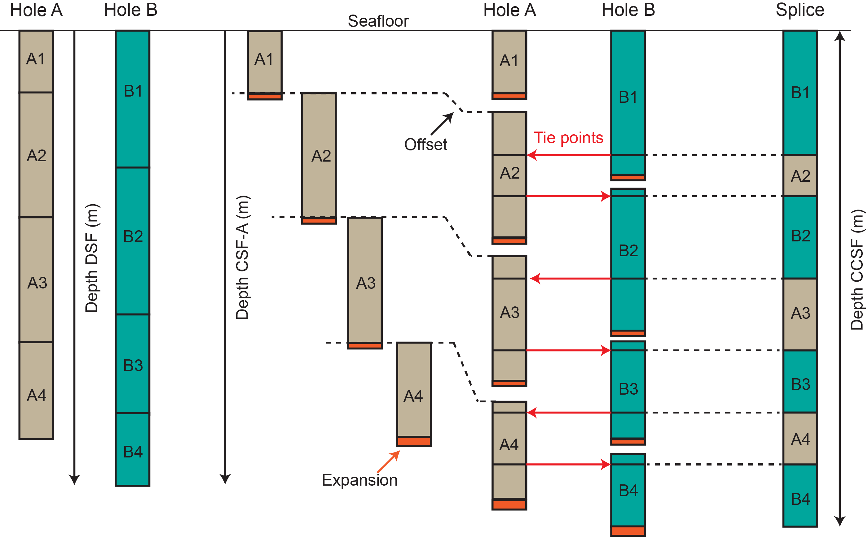
Figure F26. Generation of composite section.
The CCSF scale was built by assuming that the uppermost sediment (mudline) in the first core from a given hole is the sediment/water interface. This core becomes the anchor in the composite depth scale and was the only core in which depths are the same on both the CSF-A and CCSF scales. From this anchor, correlative features in physical properties core logging data were correlated between holes downsection. The selection of correlation tie points was highly subjective, but selections are made to optimize correlation of specific features that will later define splice intervals. It was impossible to align all correlative features of a single physical property data type or multiple data types within cores without drastic and irregular squeezing or stretching depth intervals. The appearance of apparently compressed or expanded intervals when comparing cores from different holes may reflect small-scale differences in sedimentation and/or distortion caused by the coring and archiving processes. The depth offset of every core per hole was tabulated in an affine table for every site and uploaded to the LIMS database using the SCORS uploader.
Because of core expansion, the CCSF depths of stratigraphic intervals are typically 10%–15% deeper than their CSF-A depths. CCSF depth scale construction also reveals that coring gaps on the order of 1.0–1.5 m typically occur between two subsequent cores, despite the apparent >100% recovery. During the process of constructing the composite section, the CCSF depth becomes systematically deeper than that of the CSF-A depth for equivalent horizons. This expansion has four main causes:
- Decompression of the sediment as it is brought to atmospheric pressure;
- Pore-space gases coming out of solution, warming, and expanding;
- Stretching that occurs as part of the coring process; and/or
- Recovering borehole wall sediment that fell downhole and was cored.
8.8.2. Splice
For each site a splice was generated, where core sections from adjacent holes were combined to minimize coring gaps for each site (Figure F26). The placement of splice tie points was inherently subjective, but we used the following guidelines for splice construction:
- The top and bottom 1 m of cores, where drilling disturbance was more likely, were typically avoided.
- Caution was taken during compositing and splicing within the uppermost 2 cores at every site to avoid artifacts caused by entrainment and duplication of loose sediment at the top of the hole because of imperfect alignment of the "shot" core barrels.
- We routinely attempted to avoid intervals of cores from holes where whole-round samples for IW, microbiological, and geochemistry samples were taken to maximize the possibility of still generating a spliced continuous sediment record for postexpedition sampling.
- We attempted to select portions of core that were the most representative of the stratigraphic section using all the physical properties data sets and core images at our disposal.
8.9. Downhole measurements
The downhole measurements made during the SAT expeditions included formation temperature measurements during APC coring operations at all sites, as well as downhole logging in most of the basement holes.
Downhole logs are measurements used to assess the physical, chemical, and structural properties of the formation surrounding a borehole that are made by lowering sondes with an electrical wireline in the hole after completion of drilling. The data are continuously acquired with depth (at vertical sampling intervals ranging from 2.5 mm to 15 cm) and measured in situ. Downhole logs measure formation properties on a scale that is intermediate between those obtained from laboratory measurements on core samples and those from geophysical surveys. They are useful in calibrating the interpretation of geophysical data and provide a link for the integrated understanding of physical properties on a wide range of scales.
Downhole logs can be interpreted in terms of the stratigraphy, lithology, mineralogy, magnetic characteristics, and geochemical composition of the penetrated formation. They also provide information on the condition, shape, and size of the borehole and on possible deformation induced by drilling or formation stress. In intervals where core recovery is incomplete or disturbed, log data may provide the only way to characterize the formation and can be used to determine the actual thickness of individual units or lithologies when contacts are not recovered, to pinpoint the actual depth of features in cores with incomplete recovery, or to identify and characterize intervals that were not recovered. Where core recovery is good, log and core data complement one another and may be interpreted jointly.
8.9.1. Wireline logging operations
During wireline logging operations, logs are recorded with a variety of tools combined into tool strings, which are lowered into the hole after completion of coring operations. Three primary tool strings were used during Expeditions 390 and 393 (Figure F27): the Triple combination (triple combo), which measures spectral and natural gamma radiation, porosity, density, resistivity, and magnetic susceptibility; the Formation MicroScanner (FMS)-sonic string, which provides high-resolution resistivity images of the borehole wall and sonic velocities; and the Ultrasonic Borehole Imager (UBI), which provides acoustic images of the borehole wall. Each tool string also contains a telemetry cartridge for communicating through the wireline to the Schlumberger data acquisition system on the drillship. Individual tools, measurements, and units are listed in Tables T7 and T8.
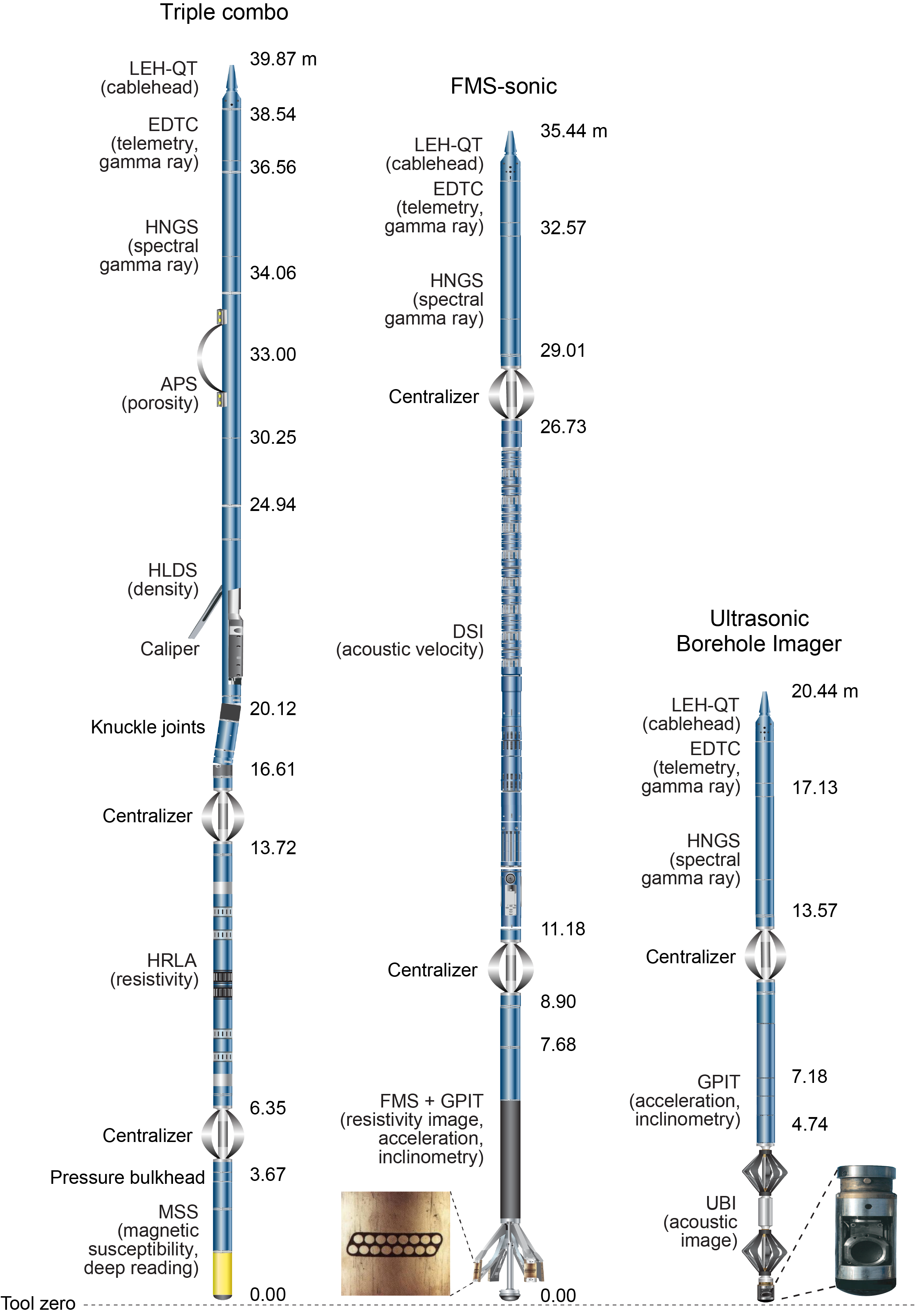
Figure F27. Wireline tool strings.
In preparation for logging, the boreholes were flushed of debris by circulating viscous drilling fluid and filled with seawater or seawater-based logging gel (sepiolite mud mixed with seawater and weighted with barite; approximate density = 10.5 lb/gal or 1.258 g/cm3) to help stabilize the borehole walls. After completion of coring, the bottom of the drill string was set high enough above the bottom of the casing for the longest tool string to fit inside the casing before entering the open hole. The tool strings were then lowered downhole on a seven-conductor wireline cable during sequential deployments. The gamma ray tool and in some cases the sonic tool are the only tools that provide meaningful data inside the drill pipe or casing (mostly qualitative). Such data are used primarily to identify the depth of seafloor and the sediment/basement boundary but can also be used for stratigraphic characterization.
Each tool string deployment is a logging run, starting with the assembly of the tool string and any necessary calibrations. The tool string is then lowered to the bottom of the hole while recording a partial set of data, and then it is pulled up at a constant speed (typically 250–500 m/h) to record the main data. During each run, tool strings can be lowered down and pulled up the hole several times for repeatability or to try to improve the data quality. Each lowering or raising of a tool string while collecting data constitutes a pass. During each pass the incoming data are recorded and monitored in real time on the surface minimum configuration multitasking acquisition and imaging system (MAXIS). A logging run is complete once a tool string has been recovered to the rig floor and disassembled. A wireline heave compensator (WHC) was employed to minimize the effect of ship's heave on the tool string's position in the borehole (see below).
8.9.2. Logged properties and tool measurement principles
The primary logging measurements recorded during Expeditions 390 and 393 are listed in Table T7. The logged properties and the principles used in the tools that measure them are briefly described below. More detailed information on individual tools and their geologic applications may be found in Serra (1984, 1986, 1989), Schlumberger (1989, 1994), Rider (1996), Goldberg (1997), Lovell et al. (1998), and Ellis and Singer (2007). A complete online list of acronyms for the Schlumberger tools and measurement curves is available at https://www.apps.slb.com/cmd.
8.9.2.1. Natural radioactivity
The Hostile Environment Natural Gamma Ray Sonde (HNGS) was used on all tool strings to measure natural radioactivity in the formation. The HNGS uses two bismuth germanate scintillation detectors and five-window spectroscopy to determine concentrations of potassium (in weight percent), thorium (in parts per million), and uranium (in parts per million) from the characteristic gamma ray energies of isotopes in the 40K, 232Th, and 238U radioactive decay series, which dominate the natural radiation spectrum. The computation of the elemental abundances uses a least-squares method of extracting U, Th, and K elemental concentrations from the spectral measurements. The HNGS filters out gamma ray energies below 500 keV, eliminating sensitivity to bentonite or KCl in the drilling mud and improving measurement accuracy. The HNGS also provides a measure of the total spectral gamma ray (HSGR) emission measured in American Petroleum Institute gamma radiation units (gAPI). The HNGS response is influenced by the borehole diameter, and therefore HNGS data are corrected for borehole diameter variations during acquisition.
The Enhanced Digital Telemetry Cartridge (EDTC; see Auxiliary logging equipment), a telemetry cartridge used primarily to communicate data to the surface, includes a sodium iodide scintillation detector that also measures the total natural gamma ray (NGR) emission. It is not a spectral tool but it provides high-resolution total gamma ray for each pass, which allows precise depth match processing between logging runs and passes.
8.9.2.2. Porosity
Formation porosity was measured with the Accelerator Porosity Sonde (APS). The sonde includes a minitron neutron generator that produces fast (14.4 MeV) neutrons and five neutron detectors (four epithermal and one thermal) positioned at different spacing from the minitron. The tool's detectors count neutrons that arrive at the detectors after being scattered and slowed by collisions with atomic nuclei in the formation.
The highest energy loss occurs when neutrons collide with hydrogen nuclei, which have practically the same mass as the neutron (the neutrons bounce off heavier elements without losing much energy). If the hydrogen (i.e., water) concentration is low, as in low-porosity formations, neutrons can travel farther before being captured and the count rates increase at the detector. The opposite effect occurs in high-porosity formations where the water content is high. The raw porosity value is often an overestimate because hydrogen bound in minerals such as clays or in hydrocarbons also contributes to the measurement.
Upon reaching thermal energies (0.025 eV), the neutrons are captured by the nuclei of Cl, Si, B, and other elements, resulting in a gamma ray emission. This neutron capture cross section (Σf) is also measured by the tool.
8.9.2.3. Density
Formation density was measured with the Hostile Environment Litho-Density Sonde (HLDS). The sonde contains a radioactive cesium (137Cs) gamma ray source (622 keV) and far- and near-gamma ray detectors mounted on a shielded skid, which is pressed against the borehole wall by a hydraulically activated decentralizing arm. Gamma rays emitted by the source undergo Compton scattering, where gamma rays are scattered by electrons in the formation. The number of scattered gamma rays that reach the detectors is proportional to the density of electrons in the formation, which is in turn related to bulk density. Porosity may also be derived from this bulk density if the matrix (grain) density is known.
The HLDS also measures the photoelectric effect (PEF), a measure of the photoelectric absorption of low-energy gamma radiation. Photoelectric absorption occurs when gamma ray energy falls below 150 keV as a result of being repeatedly scattered by electrons in the formation. Because PEF depends on the atomic number of the elements in the formation (heavier elements have higher PEF), it also varies according to the chemical composition of the minerals.
Good contact between the tool and borehole wall is essential for good HLDS logs. Poor contact results in underestimation of density values. Both the density correction and caliper measurement of the hole are used to check the contact quality.
8.9.2.4. Electrical resistivity
The High-Resolution Laterolog Array (HRLA) provides six electrical resistivity measurements with different depths of investigation (including the borehole, or mud, resistivity and five measurements of formation resistivity with increasing penetration into the formation). The sonde sends a focused current into the formation and measures the intensity necessary to maintain a constant drop in voltage across a fixed interval, providing direct resistivity measurements. The array has one central source electrode and six electrodes above and below it, which serve alternatively as focusing and returning current electrodes. By rapidly changing the role of these electrodes, a simultaneous resistivity measurement at six penetration depths is achieved. The tool is designed to ensure that all signals are measured at exactly the same time and tool position and to reduce the sensitivity to "shoulder bed" effects when crossing sharp beds thinner than the electrode spacing. The HRLA needs to be run centralized in the borehole for optimal results, so knuckle joints were used to centralize the HRLA while allowing the density and porosity tools that are often on the same tool string to maintain good contact with the borehole wall.
Typically, minerals found in sedimentary and crustal rocks are electrical insulators, whereas ionic solutions like pore water are conductors. In most rocks, electrical conduction occurs primarily by ion transport through pore fluids and is strongly dependent on the porosity, the types of pores and connectivity, the permeability, and the pore fluid.
8.9.2.5. Magnetic susceptibility
The Magnetic Susceptibility Sonde (MSS) is a nonstandard wireline tool designed by Lamont-Doherty Earth Observatory (LDEO). It measures the ease with which formations are magnetized when subjected to a magnetic field. The ease of magnetization, or susceptibility, is ultimately related to the concentration and composition (size, shape, and mineralogy) of magnetic minerals in the formation. These measurements provide one of the best methods for investigating stratigraphic changes in mineralogy and lithology because the measurement is quick, repeatable, and nondestructive and because different lithologies often have strongly contrasting susceptibilities. The data can be compared to the susceptibility measurements made on the recovered core by the WRMSL and the MSP measurements of the SHMSL (see Whole-round core section measurements).
The MSS dual-coil sensor provides ~40 cm resolution measurements with ~20 cm depth of horizontal investigation. The MSS was run as the lowermost tool in the triple combo tool string using a specially developed data translation cartridge to enable the MSS to be run in combination with the Schlumberger tools. MSS data are plotted as uncalibrated units and are affected by temperature and borehole size. For quality control and environmental correction, the MSS also measures internal tool temperature, z-axis acceleration, and low-resolution borehole conductivity.
8.9.2.6. Acoustic velocity
The Dipole Shear Sonic Imager (DSI) measures the transit times between sonic transmitters and an array of eight receivers. The waveforms are then used to calculate the sonic velocity in the formation. The omnidirectional monopole transmitter emits high frequency (5–15 kHz) pulses to extract the compressional velocity (VP) of the formation, as well as the shear velocity (VS) when it is faster than the sound velocity in the borehole fluid. It combines replicate measurements, thus providing a direct VP measurement through sediments that is relatively free from the effects of formation damage or an enlarged borehole (Schlumberger, 1989). The same transmitter can be fired in sequence at a lower frequency (0.5–1 kHz) to generate Stoneley waves that are sensitive to fractures and variations in permeability. Along with the monopole transmitters found on most sonic tools, the DSI also has two crossed-dipole transmitters that allow an additional VS measurement.
8.9.2.7. Acoustic images
Acoustic images of the borehole wall were generated from measurements taken by the UBI. The UBI features a high-resolution transducer, which emits ultrasonic pulses at a frequency of 250 and 500 kHz (low and high resolution, respectively) that are reflected by the borehole surface and then received by the same transducer recording the amplitude and traveltime of the reflected signal. Continuous rotation of the transducer combined with the upward motion of the tool result in a 360° image of the borehole wall. The amplitude of the signal depends on the reflection coefficient of the borehole fluid/borehole wall interface, the position of the UBI tool in the borehole, the shape of the borehole, and the roughness of the borehole wall. Modulation of the reflected signal is dependent on the borehole wall roughness. Therefore, fractures or other changes in the character of the drilled formation (e.g., grain size and texture) can be recognized in the amplitude image. The recorded traveltime image gives detailed information about the cross-sectional shape of the borehole, which allows calculation of one caliper value (radius) of the borehole from each traveltime measurement. These amplitude and traveltime measurements are recorded in combination with an azimuthal measurement (from the General Purpose Inclinometry Tool [GPIT]), permitting orientation of these images. The full coverage of UBI measurements make the images a useful tool for core orientation and for stress analysis (Paillet and Kim, 1987).
8.9.2.8. Microresistivity images
The FMS provides high-resolution electrical resistivity–based images of the borehole walls that can be used for detailed lithostratigraphic or structural interpretation. The tool has four orthogonally oriented arms, each with 16 button electrodes that are pressed against the borehole walls during logging. The electrodes are arranged in two diagonally offset rows of 8 electrodes each. A focused current is emitted from the button electrodes into the formation, with a return electrode near the top of the tool. Resistivity of the formation at the button electrodes is derived from the intensity of current passing through the button electrodes.
Processing transforms the resistivity measurements into oriented high-resolution images that reveal geologic structures of the borehole wall based on their conductivity. Features such as bedding, stratification, fracturing, slump folding, and bioturbation can be resolved (Luthi, 1990; Salimullah and Stow, 1992; Lovell et al., 1998). Because the images are oriented to magnetic north, further analysis can provide measurement of the dip and direction (azimuth) of planar features in the formation. In addition, when the corresponding planar features can be identified in the recovered core samples, individual core pieces can be reoriented with respect to true north.
The maximum extension of the FMS caliper arms is 40.6 cm (16 inches). In holes with a diameter greater than this maximum, the pad contact at the end of the caliper arms will be inconsistent and the FMS images may appear out of focus and too conductive. Irregular (rough) borehole walls will also adversely affect the images if contact with the wall is poor. Approximately 30% of a borehole with a diameter of 25 cm is imaged during a single pass. Standard procedure is to make two full uphole passes with the FMS to maximize the borehole coverage with the pads.
8.9.2.9. Acceleration and inclinometry
The GPIT makes three-component acceleration and magnetic field measurements. The primary purpose of this tool is to determine the acceleration and orientation of the tool string in which it is deployed. Tool orientation is defined by three parameters: tool deviation, tool azimuth, and relative bearing. The GPIT uses a three-axis inclinometer and a three-axis fluxgate magnetometer to record the orientation of the logging tool as the magnetometer records the magnetic field components (Fx, Fy, and Fz). The resulting data can be used to facilitate corrections for irregular tool motion and to provide oriented image data from the FMS and UBI tools. Corrections for cable stretching and/or ship heave using GPIT acceleration data (Ax, Ay, and Az) allow precise determinations of log depths.
8.9.2.10. Auxiliary logging equipment
The Schlumberger logging equipment head (LEH, or cablehead) measures tension at the very top of the wireline tool string, which diagnoses difficulties in running the tool string up or down the borehole or when exiting or entering the drilling string or casing.
Telemetry cartridges are used in each tool string to allow transmission of the data from the tools to the surface. The EDTC also includes a sodium iodide scintillation detector to measure the total natural gamma ray emission of the formation. This gamma ray log was used to match the depths between the different passes and runs. In addition, it includes an accelerometer, and that data can be used in real time to evaluate the efficiency of the WHC.
Because the tool strings combine tools of different generations and with various designs, they include several adapters and joints between individual tools to allow communication, provide isolation, avoid interferences (mechanical, acoustic), terminate wirings, or to position the tool properly in the borehole. The knuckle joints, in particular, were used to allow some of the tools such as the HRLA to remain centralized in the borehole, whereas the overlying HLDS was pressed against the borehole wall.
All these additions are included and contribute to the total length of the tool strings in Figure F27.
8.9.3. Log data quality
The condition of a borehole is the principal factor contributing to log data quality. The ideal conditions for logging include a consistent borehole diameter of the size of the bit with no washouts or bridges. Oversized borehole diameters can have a significant impact on measurements, especially those that require tool eccentering (e.g., HLDS) or tool centralization (e.g., FMS and UBI). The measurement principles of the eccentered tools, as well as the centralized FMS, means that direct contact with the formation is essential for the acquisition of high-quality data. The UBI is a noncontact tool, but data quality is best when the tool is actively centered in the borehole. Deep investigation measurements such as gamma radiation, resistivity, and sonic velocity, which do not require contact with the borehole wall, are generally less sensitive to borehole conditions, although data are optimized in boreholes where the tools can be centralized (up to ~20 inch diameter).
If the borehole diameter varies over short intervals because of washouts of softer material or ledges of harder material, the logs from tools that require good contact with the borehole wall (i.e., FMS, density, and porosity tools) may be degraded. Bridged sections, where the borehole diameter is significantly less than the bit size, will also cause irregular log results. The quality of the borehole can be improved by minimizing the circulation of drilling fluid while drilling, flushing the borehole to remove debris prior to logging, and logging as soon after drilling and conditioning as possible.
The quality of the wireline depth determination depends on several factors. The depth of the logging measurements is determined from the length of the cable spooled out from the winch on the ship. Uncertainties in logging depth occur because of ship heave, cable stretch, cable slip, and tidal changes. To minimize the wireline tool motion caused by ship heave, a hydraulic WHC was used to adjust the wireline depth for rig motion during wireline logging operations (see Wireline heave compensator). The seafloor is identified on the gamma ray log by the abrupt reduction in gamma ray count at the water/sediment interface (mudline), an important reference datum for matching logging depths and providing depth consistency across all logging data. Discrepancies between the drilling core depth and wireline logging depth may occur because of core expansion, incomplete core recovery, incomplete heave compensation, and drill pipe stretch. Reconciling the differences between the two data sets is possible through comparison of the common data sets acquired in situ and on core (e.g., magnetic susceptibility and NGR).
8.9.4. Wireline heave compensator
During wireline logging operations, the up-and-down motion of the ship (heave) causes a similar motion of the downhole logging tools. If the amplitude of this motion is large, depth discrepancies can be introduced into the logging data. The risk of damaging downhole instruments is also increased. A WHC system was designed to compensate for the vertical motion of the ship and maintain a steady motion of the logging tools to ensure high-quality logging data acquisition (Iturrino et al., 2013; Liu et al., 2013). The WHC uses a vertical accelerometer (motion reference unit [MRU]) positioned under the rig floor near the ship's center of gravity to calculate the vertical motion of the ship with respect to the seafloor. It then adjusts the length of the wireline by varying the distance between two sets of pulleys through which the cable passes in order to minimize downhole tool motion.
8.9.5. Logging data flow and depth scales
Data for each wireline logging run were monitored in real time and recorded using the Schlumberger surface acquisition system. Data were shortly thereafter transferred onshore to LDEO for standardized data processing, formatting for the online logging database, and archiving. Processed data were returned to the ship and made available to the shipboard scientists within a few days of logging.
The processing included several stages. First, using the gamma ray logs recorded by every tool string, a visually interactive program was used to match the depths of recognizable features across all the passes to a reference curve, commonly the gamma ray log of the longest upward pass. Image data (FMS and UBI) were also processed to correct the effects of irregular tool motion using the acceleration data from the GPIT. After depth matching, all the logging depths were shifted from the rig floor depth reference (in which they were initially recorded) to a seafloor depth reference, based on the seafloor as identified by the step in gamma radiation at the sediment/water interface. All the processed data were made available in ASCII and DLIS formats for most logs and in GIF for the images.
8.10. In situ temperature measurements
During all SAT expeditions, in situ formation temperature measurements were made at selected depths in the sediments at all sites to assess the thermal structure of the sedimentary section along the transect and measure the regional heat flow.
The APCT-3 tool fits directly into a modified coring shoe of the APC and consists of a battery pack, data logger, and a platinum resistance-temperature device calibrated over a temperature range of 0°–30°C. Before entering the borehole, the tool is stopped at the seafloor for 5–10 min to thermally equilibrate with bottom water. However, the lowest temperature recorded during the run down is preferred to the average temperature at the seafloor as an estimate of bottom water temperature because (1) this measurement is more repeatable and (2) the bottom water is expected to have the lowest temperature in the profile. After the APC penetrated the sediment, it was held in place for ~10 min as the APCT-3 tool recorded the temperature of the cutting shoe every second. When the APC was fired into the formation, there was typically an instantaneous temperature rise due to frictional heating. The heat gradually dissipated into the surrounding sediment as the temperature at the APCT-3 tool equilibrated toward the temperature of the sediment.
The equilibrium temperature of the sediment was estimated by applying a mathematical heat-conduction model to the temperature decay record (Horai and Von Herzen, 1985). The synthetic thermal decay curve for the APCT-3 tool is a function of the geometry and thermal properties of the probe and the sediment (Bullard, 1954; Horai and Von Herzen, 1985). The equilibrium temperature must be estimated by applying a fitting procedure in the TP-Fit software (Heesemann et al., 2006). However, when the APC system did not achieve a full stroke or when ship heave pulled up the APC system from full penetration, the temperature equilibration curve was disturbed and temperature determination was less accurate. The nominal accuracy of the APCT-3 tool temperature measurements is ±0.05°C.
8.11. Heat flow
A simple estimation of the vertical conductive heat flow at each site can be made by calculating a least-squares linear fit of the measured formation temperature as a function of depth. The slope of this linear fit is the temperature gradient, and the local vertical conductive heat flow is the product of this gradient with the mean thermal conductivity measured in the sediments from this site.
Another measure of the heat flow in a conductive regime can be established with a Bullard plot (Bullard, 1939). If the vertical heat flow (q) is assumed constant with depth, such as in a predominantly conductive regime, the temperature at depth z can be calculated by a simple integration:
where T0 is the temperature at the seafloor and K(z) the thermal conductivity at a depth z. The value in the integral is the thermal resistance of the interval between the seafloor and z. If the heat flow is constant with depth, as in a conductive regime, this defines a linear relationship between temperature and thermal resistance, and its slope is the conductive heat flow (Bullard, 1939).
9. Geochemistry
Shipboard geochemistry data routinely collected during the SAT expeditions (390C, 395E, 390, and 393) included headspace analysis of hydrocarbon gases, in situ pore water oxygen measurements, IW chemistry (e.g., salinity, pH, alkalinity, major cations and anions, nutrients, major and minor elements), loss on ignition (LOI), total carbon (TC) and total inorganic carbon (TIC), and elemental compositions of basement rocks using both ICP-AES and XRF using a handheld portable instrument (pXRF). During Expedition 390, sulfide concentrations in IW were also determined. All data generated during shipboard analyses have been uploaded to the LIMS database. This combination of analyses provides insight into biogeochemical processes including metabolic rates, abiotic diagenetic reactions, mineral alteration (e.g., authigenic mineral precipitation and water-rock interactions), and advective fluid migration.
9.1. Headspace analysis of hydrocarbon gases
During Expeditions 390C and 395E and at Site U1583 during Expedition 393, headspace hydrocarbon analyses were conducted as part of standard shipboard safety monitoring procedures, as described in Kvenvolden and McDonald (1986) and Pimmel and Claypool (2001), to prevent drilling into sediments that contain hydrocarbon concentrations above safety levels. One sample per sediment core was subjected to headspace hydrocarbon gas analysis.
The ~3–5 cm3 sediment sample was collected from the interior of a freshly exposed core directly after sectioning on the catwalk. This sample was placed in a 20 cm3 glass vial and sealed with a Teflon/silicon septum and a crimped aluminum cap. The headspace sample was typically taken at the top of Section 4 (below the IW sample), unless obvious core disturbance suggested that a different section should be selected. The sample was placed in the oven at 80°C for 30 min. A 5 cm3 aliquot of the evolved hydrocarbon gases was extracted from the headspace vial with a standard gas syringe and then manually injected into an Agilent 7890 Series II gas chromatograph (GC) equipped with a flame ionization detector (FID) set at 250°C. The column (2 mm inner diameter, 6.3 mm outer diameter) was packed with 80/100 mesh HayeSep T (Restek). The GC oven program was set to stay at 80°C for 8.25 min with a subsequent heat-up to 150°C at 40°C/min. The total run time was 15 min.
Results were collected using the Hewlett Packard 3365 ChemStation software. The chromatographic response was calibrated using nine different gas standard analyses and checked daily. The concentration of the analyzed hydrocarbon gases was reported as parts per million by volume (ppmv). Table T9 lists precision and detection limits for the headspace gas analyses during the SAT expeditions.
9.2. Interstitial water collection and analysis
During the SAT expeditions, IW was extracted (1) through squeezing of whole round core samples that were cut on the catwalk (all expeditions including 390C and 395E) and (2) at a higher resolution on entire sections of core using Rhizon samplers during Expeditions 390 and 393 to enable a wide range of shipboard analyses and for postexpedition research (Table T9). The residual whole-round sediments after IW extraction (squeeze cakes) were sampled for shipboard inorganic carbon and total carbon analyses as well as for postexpedition research.
9.2.1. IW sampling from sediment squeezing
Whole round samples 5–20 cm in length for IW extraction were cut on the catwalk, immediately capped, and then transferred to the chemistry laboratory for squeezing. The surfaces of each whole-round sample were carefully scraped away under ambient laboratory conditions using stainless steel knives to remove contamination due to seawater, drilling disturbances, and/or sediment smearing along the insides of the core liners. More exterior material was removed from XCB cores because XCB coring can result in more significant physical disturbance and seawater contamination in the core liner. The remaining sediments were transferred to titanium squeezers and loaded into a Carver hydraulic laboratory press (Manheim and Sayles, 1974). The sediments were squeezed to extract IW at pressures up to 25,000 lb (~24.3 MPa). A minimum of 30 min of squeezing was required for all cores; up to 2 h of squeezing was required to extract sufficient IW from some XCB cores because sediments collected with the XCB system are generally more compacted. IW extracted in the squeezers was passed through a nanopure water-precleaned Whatman Number 1 filter above a titanium screen into a 60 mL high-density polyethylene (HDPE) syringe that had been acid-cleaned with 10% HCl. For Expedition 393, two stacked Whatman Number 1 filters were used to reduce the particulates passing through to the syringe. For all expeditions, a 0.45 µm polyethersulfone membrane filter was attached to the syringe tip upon collection of IW from the squeezers. The collected fluids were then filtered through a 0.2 µm polyethersulfone membrane filter into appropriate containers and processed for shipboard and postexpedition analyses. The squeeze cake residues were then subsampled for postexpedition research and shipboard carbonate and total carbon analyses. The residual squeeze cakes were stored at 4°C. Squeezers were cleaned between samples with tap water, rinsed with 18.2 MΩ deionized water, and dried with compressed air before further sample processing.
9.2.2. Interstitial water analysis
9.2.2.1. Salinity, pH, and alkalinity
Salinity, alkalinity, and pH were measured immediately on IW extracted from squeezing following the procedures in Gieskes et al. (1991). Hole U1558D IW salinity was measured on a temperature-compensated digital refractometer (Index Instruments Ltd.) Salinity measurements for Hole U1558F were consistently offset by 1 salinity unit and were corrected to reflect this drift. The instrument began to drift to higher values and could not be recalibrated. For subsequent holes, measurements were made with a Fisher Model S66366 optical refractometer. International Association for the Physical Sciences of the Oceans (IAPSO) standard seawater (salinity = 35) and 18.2 MΩ water (salinity = 0) were used to calibrate salinity. During Expeditions 390C and 395E, salinity was also measured using a Metrohm 785 DMP chloride autotitrator; a 100 µL sample was titrated against 0.015 M silver nitrate solution. IW pH and alkalinity were determined using a Metrohm 794 Basic Titrino autotitrator with a glass pH electrode. A 3 mL sample was titrated against 0.1 M HCl at 25°C to reach an endpoint of pH = 4.2. The IAPSO standard seawater (alkalinity = 2.325 mM; certified value) and laboratory standards (5–100 mM Na2CO3 alkalinity, made by mixing different proportions of 0.7 M KCl + 0.1 M Na2CO3) were used for calibration. The IAPSO standard was analyzed at the beginning and end of the sequence and after every 10 samples. Repeated measurements of IAPSO seawater for alkalinity yielded precision better than 2.5%.
9.2.2.2. Major cations and anions
Sulfate (SO4), chloride (Cl), bromide (Br), sodium (Na), magnesium (Mg), potassium (K), and calcium (Ca) concentrations were analyzed by ion chromatography (Metrohm 850 Professional IC) using 100 µL of IW diluted by 100 times with 18.2 MΩ water. For anions (Cl, SO4, and Br), a Metrosep C6 column (100 mm long; 4 mm inner diameter) was used with 3.2 mM Na2CO3 and 1.0 mM NaHCO3 solutions as eluents, whereas a Metrosep A supp 7 column (150 mm long; 4 mm inner diameter) was used with 1.7 mM HNO3 and pyridine-2,6-dicarboxylic acid (PDCA) solutions as eluents for cations (Na, K, Mg, and Ca). The standards were IAPSO in various dilutions (ranging from 150% to 1% IAPSO) to create a 9-point calibration curve. Reproducibility was checked on the repeated measurements of standard IAPSO and IAPSO dilution of 1:10 every 10 samples. Reproducibility (defined by standard deviation/average; relative standard deviation [RSD]) of repeated IAPSO measurements (N = 16) was better than 1.5% for Cl, SO4, Na, Mg, K, and Br, whereas for Ca2+ it was 3.5% for Expedition 390 and <1.8% for Ca for Expedition 393. Recoveries of most cations and anions were within 100% ± 3% except for Ca (93%–104%). Table T9 lists precision and detection limits for our ion chromatographic measurements.
9.2.2.3. Spectrophotometric analysis of ammonium, phosphate, and sulfide
Shipboard analyses of dissolved ammonium (NH4+) and phosphate (PO43−) were performed on an Agilent Technologies Cary Series 100 UV-Vis spectrophotometer with a sipper sample introduction system, following Gieskes et al. (1991). Ammonium concentrations were determined using a colorimetric method measured at 640 nm, which incorporates diazotization of phenol and subsequent oxidation of the diazo compound by Clorox to yield a blue color. During Expedition 390, two calibration curves were used to better quantify the low-concentration range: the regular 9-point calibration curve (0, 50, 100, 150, 200, 400, 600, 800, and 1000 µM) run at both Sites U1556 and U1559 and a 6-point low-concentration calibration (10, 20, 40, 80, 120, and 160 µM) run at Site U1559. Check standards were run every 10 samples. The solution was kept at room temperature for ~6.5 h to develop color after adding the reagents. Recoveries for check standards (50 and 400 µM for Hole U1556C, 20 and 100 µM for Hole U1559D) are generally better than 90%. Because of contamination issues, the ammonium concentrations from Expedition 390C were not reported. During Expeditions 390 and 393, ammonium was also measured on a third-party Tecan Spark 10M Multimode plate reader to test the feasibility of using a microplate reader during expeditions. Samples and reagents were pipetted into 96-well polystyrene plates. Sample and reagent volumes were in the same proportions as those used for shipboard colorimetric method analysis of ammonium but were reduced by a factor of 20 to accommodate relatively smaller 350 µL well volumes of the plate. The reagent volumes were the same for both expeditions, but samples from Hole U1583A were prepared without dilution to improve analytical sensitivity for low-concentration samples. The sample-reagent mixture was kept at room temperature for ~6.5 h for full color development. Absorbance was measured at 640 nm in the plate reader, and sample concentrations were corrected to a 7-point calibration curve (0, 50, 100, 150, 200, 400, and 600 µM). The high standard bracketed the highest ammonium concentrations measured during the expeditions. Check standards were run every 10 samples.
Phosphate concentrations were measured through the reaction of orthophosphate with Mo(VI) and Sb(III) in an acidic solution to form an antimony-phosphomolybdate complex that was then reduced by ascorbic acid to form a blue color. After adding the mixed reagent solution and letting the samples react for 30 min, the absorbance was measured at 885 nm (Gieskes et al., 1991). A 9-point calibration curve (0, 5, 10, 15, 20, 40, 60, 80, and 100 µM) was used, and check standards were run every 10 samples. Recoveries for check standards (10 and 20 µM) were generally better than 90%. Because of contamination issues, the phosphate concentrations from Expedition 390C were not reported. Phosphate was also measured on the third-party Tecan Spark 10M Multimode plate reader during Expeditions 390 and 393. Sample and reagent volumes were reduced by a factor of 20 to accommodate the well volume of the polystyrene plates. The reagent volumes were the same for both expeditions, but samples from Hole U1583A were prepared without dilution to improve analytical sensitivity. The sample-reagent mixture was kept at room temperature for 30 min to allow color development. Absorbance was measured at 885 nm on the microplate reader, and sample concentrations were corrected to a calibration curve. Check standards were run approximately every 10 samples. Table T9 lists the precision and detection limits for nutrient analyses.
Total sulfides (ΣH2S = S2− + HS− + H2S) in IW samples were measured colorimetrically on the third-party Tecan Spark 10M Multimode plate reader. Zinc acetate solution (100 g/L: 50 µL per 1 mL of sample) was immediately added to freshly squeezed IW to fix sulfide. Sulfide concentrations were measured using the methylene blue method (Hach reagents 181632 and 181732) according to the proportions: 50 µL sample, 100 µL 18 MΩ water, and 50 µL of each Hach reagent. Absorbance was measured at 670 nm after waiting 5 min for color development. Dilutions were made with N2-purged 18.2 MΩ water. For each dilution factor, a 5-point calibration curve (0, 0.1, 0.2, 0.4, and 0.8 mM) was prepared with the same zinc acetate final concentrations. Precision on replicate sulfide standards was better than ±0.02 mM (1σ, n = 15).
9.2.2.4. Major, minor, and trace elements
Selected major and minor elements (Na, Ca, Mg, K, Li, B, P, Si, Ba, Fe, Mn, and Sr) were analyzed using the shipboard Agilent 5110 ICP-AES with an Agilent SPS4 autosampler. The general method for shipboard ICP-AES IW analysis is modified from ODP Technical Note 29 (Murray et al., 2000) with updates related to the specifications of the current Agilent ICP-AES instrument. Internal standards were used to correct for instrument performance variations across the spectral range of the elements of interest. A 500 µL aliquot of each IW sample was diluted to 5 mL with 100 µL of an internal standard solution containing 100 ppm Be, In, and Sc and 200 ppm Sb, and 4.4 mL of 2% HNO3. Each batch of samples analyzed on the ICP-AES included blanks and reference samples of known concentrations. Each sample was analyzed three times in a sample run. Following each instrument run, the measured raw intensity values were automatically corrected for instrument drift and blank values, and calibration curves were calculated, using Agilent's ICP Expert software (Version 7.3.0.1.9507).
Calibration curves for major cations (Na, K, Mg, and Ca) were established using a series of dilutions of IAPSO standard seawater (from 1:1 to 1:100 IAPSO:2% HNO3). For minor and trace element analyses (K, Li, B, Si, Ba, Fe, Mn, and Sr), standards are made from a stock multielement solution prepared from ultrapure primary standards (1000 ppm; SPEX CertiPrep reference standards) in 2% HNO3 with 35 ppt NaCl. This stock solution was diluted using 2% HNO3 + NaCl to produce a set of standards ranging from 1% to 100% of the stock solution elemental abundances. For consistency, calibration standards were diluted for ICP-AES measurement in the same way as the samples, which were run at a 10:1 dilution factor. The 1:1 standard was repeatedly analyzed with each batch of samples over the expedition. The ICP-AES plasma was ignited at least 30 min before the sample run to allow the instrument to stabilize. For each run, the wavelengths with calibration curves showing the highest correlation coefficient (r value) for each element were used to determine concentrations. Table T10 presents analytical precision and procedural detection limits for major and trace metals measured on IW using ICP-AES during Expeditions 390C, 395E, 390, and 393.
9.2.2.5. Comparison of Ca, K, and Na data in IW samples measured by IC and ICP-AES
As the shipboard ion chromatography (IC) and ICP-AES instruments both produce data for the metals Ca, K, and Na, questions as to the relative quality of these data and which data set is the "best" to use for each of these species are raised during nearly every IODP expedition. This question has become more pertinent with the installation of the new Agilent ICP-AES system, which is capable of simultaneously measuring and calibrating multiple optical wavelengths for these and other elements in both axial and radial modes, potentially improving analytical precision by expanding the data collected for any given element in each sample (see Bulk elemental composition of rocks below for more about these capabilities). During Expedition 393, we did a comparative analysis of the performance of the IC and ICP for the alkaline elements following the standard shipboard procedures for IW analysis, originally outlined in Murray et al. (2000), to help establish clear criteria regarding which of the alkaline metal data sets should be used for final reporting on shipboard analyses.
Although the IC and ICP-AES both produce precise (1%–2%) data on unknown samples, measures of data accuracy on the two instruments differ. IC accuracy can be inferred from element yields through the column. Na and K show 100% ± 3% yields using IC and are typically >99%, whereas Ca is more variable (93%–104%). ICP-AES accuracy is a function of the choice of standards, the quality of fit from calibration curves generated using these standards (e.g., r values ≥ 0.999X are preferred), and the spectral characteristics of the chosen optical wavelength(s) related to their linear dynamic ranges, which typically range from 10 times the elemental detection limits up to values several orders of magnitude higher before optical saturation occurs and measured intensities level off. For alkali metals, which all emit light in the red to infrared range (500–800 nm), detection limits are often very low, but the dynamic analytical ranges of these wavelengths are more limited. Optically, alkalis suffer from matrix enhancement effects, in which the light matrix produced by all the elements in solution lead to nonlinear increases in signal on alkali metal wavelengths. Thus, it is important when measuring alkali abundances on ICP-AES systems that the sample and standard compositions be similar to minimize matrix enhancement variations.
Two different sets of standard solutions are used for IW runs: the first set is made by diluting the IAPSO seawater standard with 2% HNO3 and running from 1% to 200% dilutions (i.e., twice the normal amount of IAPSO is added, producing a 5:1 IAPSO standard solution for calibration of unknowns that are uniformly diluted at 10:1); and the second is made from a synthetic seawater solution with 35 ppt NaCl that is spiked with varying amounts of lower abundance elements (B, Li, Mn, Fe, P, S, Ba, Sr, and Si). The IAPSO standards suite is used to calibrate higher abundance species (Na, K, and Ca), and the in-house synthetic seawater standard suite is used for all lower abundance species. Na is only measured using the IAPSO standards, whereas K is measured using both.
ICP-AES calibration curves generated for Na, K, and Ca on IW runs during Expedition 393 show evidence of nonlinearity for K and Na wavelengths, whereas the Ca calibration curves appear to show no such issues. Figure F28A–F28C show working curves for the three available Na analytical wavelengths. The 588.995 and 589.595 nm lines, which are the most sensitive for Na, both show concave-down shapes indicative of detector saturation for the higher concentration standards. Although the Na correlation coefficient is better than that of the other two Na lines, the 330.298 nm Na line shows a slightly concave-up shape with a large negative intercept value, which points to increased signal/concentration ratios at higher Na contents, a symptom of matrix enhancement effects related to the comparatively high (>10 mM) Na contents of these standards as prepared for IW analysis. In the case of K, Figure F28D shows that the two different sets of IW standards form different curves for the 766.491 nm line, and both of these curves are concave downward, suggesting that signal saturation effects impact the higher abundance level standards. In nearly all cases, IW samples will have seawater-like Na and K contents, and some may have higher contents (see Fryer et al. [2018] and Johnston et al. [2018] for discussions of IODP Expedition 366 IW samples with 1.5–2 times seawater values for Na and K), which places these samples as unknowns along the sections of the Na and K calibration curves where this nonlinearity is most pronounced and results are the most likely to be affected.
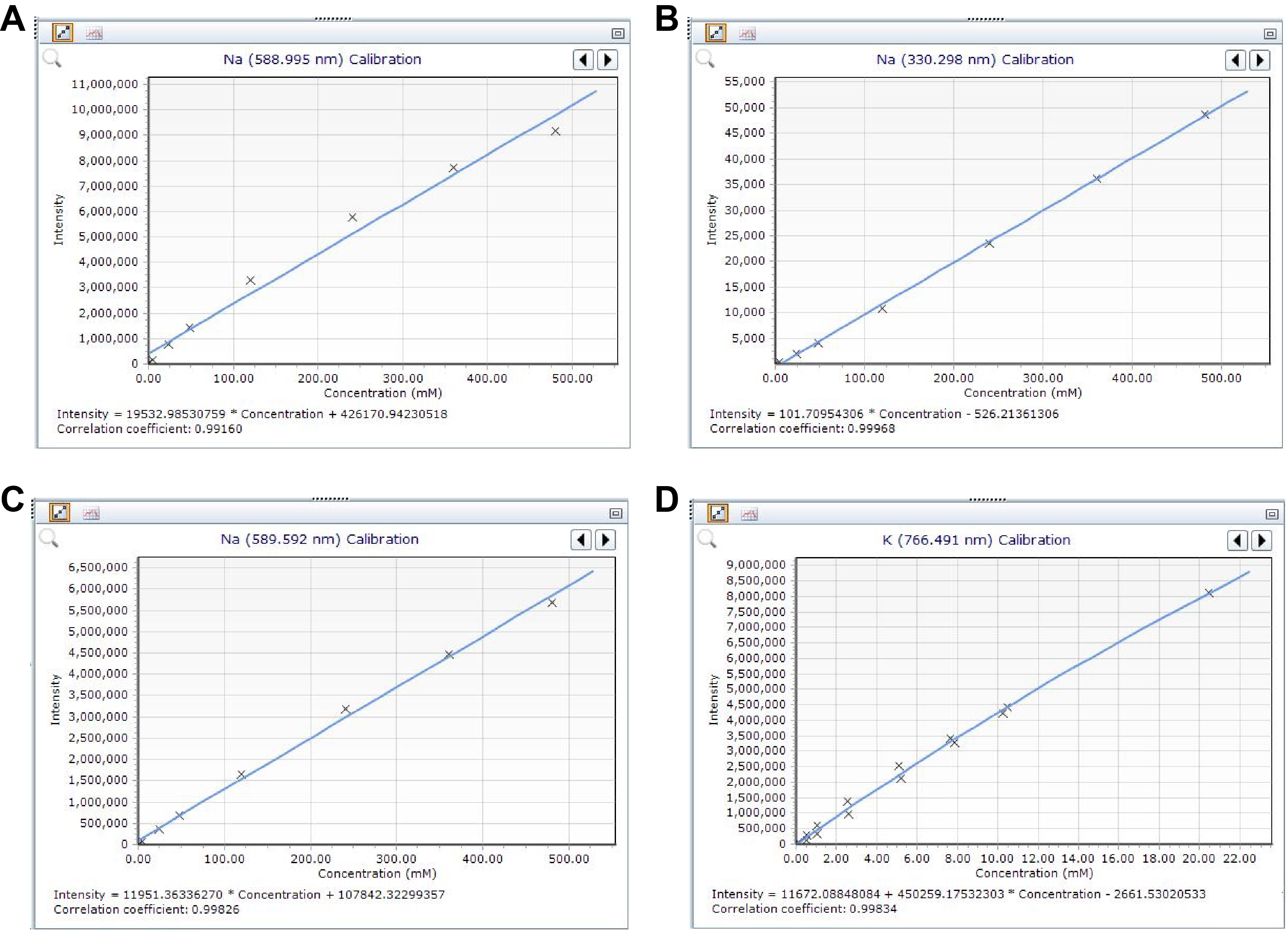
Figure F28. ICP-AES calibration curves for Na and K.
Although the Na and K calibrations on the ICP-AES are impacted by signal saturation and matrix enhancement effects at the concentrations encountered in IW samples as prepared for ICP-AES measurement, the instrument can nonetheless make highly reproducible measurements on these elements at these abundance levels, so there is often no clear evidence that these data are problematic beyond the shapes of their working curves and poor correlations with other data sources (e.g., shipboard IC results). Generating reliable Na and K data using ICP-AES, as noted above, requires attempting to generate uniform solution matrixes, which for these elements would involve a much more substantial dilution of the IW samples (from 10:1 to 100:1 or 500:1) to reduce the influence of variable sample matrixes. Given the need to measure many other, much lower abundance elements in these same samples, doing so would involve preparing a separate set of IW dilutions for Na and K ± Ca and running these elements on the ICP-AES separately. This approach may be feasible during expeditions where IW sampling and analysis are not a large component of the required work, but it may be problematic in terms of materials and technician and scientist time on many others. Given that the ion chromatography system measures both K and Na in waters with high precision and accuracy, it is clear that data for these elements should be preferred over ICP-AES results for IW samples under nearly all circumstances. Because Ca data from the ICP-AES show no like concerns, choices whether to use IC or ICP Ca data can be made based on the relative performance of the two instruments during an expedition and other related factors.
Table T9 lists precision and detection limits for analytes from IW and Table T10 for ICP-AES measurements on IW samples during the SAT expeditions.
9.3. Oxygen measurements and Rhizon IW sampling
9.3.1. Oxygen measurements
During Expeditions 390 and 393, oxygen concentrations were measured in sediments from Holes U1556C and U1556E, U1559C and U1559D, U1558F, U1560C, and U1583C to determine pore water dissolved oxygen profiles at each site. In cases where multiple sediment holes were drilled at a given site during Expeditions 390 and 393, oxygen measurements were obtained from the first hole to guide IW and microbiology sampling in subsequent sediment holes.
Oxygen concentrations were measured using Presens PM-PSt7 oxygen profiling microsensors (PreSens, Regensburg, Germany; Fischer et al., 2009), and each sensor had a unique temperature probe assigned to it. The oxygen sensors were calibrated daily using air-saturated deionized water (100% oxygen saturation) and 10 g/L sodium sulfite (Na2SO3) solutions (0% oxygen saturation). Oxygen measurements were determined using whole-core sections prior to splitting. A hole was drilled in the core liner using a power drill with a ~3 mm diameter drill bit, and the oxygen microsensor was inserted manually into sediments (~2.5 cm) through the hole. As many as 10 microsensors were used simultaneously for oxygen measurements through the multichannel oxygen meter OXY-10ST, and the signal was allowed to equilibrate to a steady value (~20–30 min, on average, but sometimes as long as 90 min). All calibration and measurement data were processed using PreSens Measurement Studio 2 software.
At Site U1556, two core flows were used for oxygen measurements. During drilling in Hole U1556C, whole cores were allowed to equilibrate to room temperature (~4–6 h) and were run through all whole-round loggers (see Physical properties and downhole measurements) before the oxygen measurements. Because the core sections were equilibrated to room temperature by the time oxygen was measured, temperature probes were placed in a room temperature water bath. This core flow sometimes resulted in more than a 12 h delay between core retrieval and oxygen measurements, which was deemed too long and resulted in scattered data downhole. For Hole U1556E, a quicker core flow was implemented. The physical properties team agreed to run core sections through the NGRL and WRMSL (see Physical properties and downhole measurements) within 3 h of core retrieval and thus prior to core equilibration to room temperature. The core was then moved to the downhole laboratory for oxygen measurements. This resulted in an average time from catwalk to oxygen measurement of ~6.75 h (range = 3.5–12.5 h). There was less sample-to-sample variation in the dissolved oxygen concentrations with this protocol. Because the core was not yet equilibrated to room temperature, an additional hole was drilled in the core liner to insert the temperature probe. Oxygen and temperature probes were drilled ~20 cm apart to avoid disturbances caused by potential cracks in the core, as insertion of the probes into compacted sediments may induce cracking.
For Hole U1559C, the core flow was further revised, and this core flow was subsequently used for all holes with oxygen measurements during Expedition 393. For this core flow, core sections were scanned on the STMSL by the physical properties team after arriving on the catwalk and then immediately given to the geochemist/microbiologist measuring oxygen. Again, temperature probes were inserted through the liner ~20 cm from the oxygen probe. This resulted in oxygen measurements starting ~30 min after arriving on the catwalk. Measurements were taken typically in Sections 1–6. We avoided the core catcher, which is disturbed, as well as the last section of a core, as these were often short and/or disturbed as well.
For Hole U1559D, the core flow used during Hole U1556C (oxygen measured 4–6 h after the core arrival on deck) was used to test if the measurement lag would significantly alter the oxygen profile. Although the general pattern is the same, the Hole U1556C approach resulted in slightly noisier data than achieved for Hole U1559D at the same depths, indicating the time lag in oxygen measurements does matter. This test was conducted using only two sections per core.
Oxygen measurements were made at a frequency of ~3 per core in Hole U1556C (1.5–5 m resolution), ~1 per section in Holes U1556E and U1559C, and 2 per core in Hole U1559D; intervals with drilling disturbance were avoided. Several 5 cm whole rounds were also taken from the catwalk for oxygen measurements from Hole U1556C (see Geochemistry in the Site U1556 chapter [Coggon et al., 2024a]). Both the oxygen and temperature probes were inserted into these whole-round samples because they were not equilibrated to room temperature. This was done only during XCB drilling to determine if removing obvious drilling disturbance was better than inserting the probe through the core liner, during which it is harder to see minor disturbance.
During Expedition 393, the Presens PM-PSt7 oxygen profiling microsensors were spent after oxygen measurements were completed at Site U1583, and only three Presens PM-PSt7 oxygen profiling microsensors remained. This number was insufficient to complete measurements at Site U1560. A Presens Microx TX3 oxygen profiling system and accompanying probes were on the ship for this. A test comparison was made between the two different oxygen measurement systems using sediment cores from Hole U1583E. Oxygen measurements in Hole U1583E were subsequently taken using the remaining Presens PM-PSt7 oxygen profiling microsensors along with Presens NTH-PSt1-L5-TF-NS40-0.8-OIW oxygen microsensors using the Presens Microx TX3 oxygen transmitter system and TX3v602 software. The oxygen microsensors used with the Microx TX3 system were calibrated in the same fashion as described above. This confirmed that both microsensor systems gave similar oxygen concentration readings. The oxygen concentration profile from Hole U1560C was subsequently measured using the Microx TX3 system.
9.3.2. Rhizon IW sampling
For the core flow used in Hole U1559C and during Expedition 393, cores were given back to the physical properties team after oxygen measurements, equilibrated to room temperature, run on the WRMSL, and then returned to the geochemist/microbiologist on duty for Rhizon sampling. This core flow was applied because Rhizon sampling affects the physical properties of the core, so sampling needs to be done after WRMSL logging is complete.
Upon completing the oxygen profile and WRMSL measurements, we extracted IW samples with Rhizon samplers prior to core splitting (Rhizosphere Research Products, Wageningen, The Netherlands), following the sampling protocol from Dickens et al. (2007). New holes were drilled at least 20 cm away from the holes of oxygen measurements. Precleaned (10% HCl) 5 cm long Rhizon samplers were inserted into holes and connected to precleaned (10% HCl) 12 mL syringes. The syringe plungers were pulled to generate a vacuum and held open with a wood spacer. Depending on the sediment porosity, as much as 11 mL of IW was collected in ~2 h. In some samples, up to 21 mL of IW was collected, although high volumes derived from XCB cores may be the result of drill fluid contamination. After collection, Rhizon IW samples were filtered through 0.2 µm polyethersulfone (PES) filters and stored in appropriate containers for postexpedition research.
During Expedition 393, Rhizon-collected samples were run for major cations (Na, Mg, K, and Ca) and anions (Cl, Br, and SO4) by IC. Concentration data agreement between Rhizon-collected and squeezed IW was overall excellent in Holes U1558F and U1560C, with the exception of Ca, which had persistently lower concentrations in Rhizon samples compared to squeezed IW. In Hole U1583C, the offset in measured concentrations between Rhizon and squeezed IW samples was larger than analytical uncertainties for Mg, K, Ca, Cl, and SO4.
9.4. Sediment collection and bulk geochemistry
9.4.1. Sediment collection
Approximately 10 cm3 of bulk sediment was collected for geochemical analyses taken from squeeze cake residue, directly subsampled by the sedimentologists, or a combination of both. Samples were freeze-dried for a minimum of 12 h and ground to a fine powder using an agate pestle and mortar. Splits were taken from the ground sample for carbon, nitrogen, sulfur, and XRD analysis. Remaining sample was stored in a glass vial and archived. XRD methodology is reported in Sedimentology.
9.4.2. Inorganic and organic carbon
TIC was measured by quantifying the carbon dioxide evolved from an acidification process on an UIC Coulometrics 5017 CO2 coulometer. During Expedition 390, ~10 mg of bulk powdered sediment was weighed using two electronic balances and a computer averaging system that corrects for ship motion (Cahn C-31 automated electrobalance). During Expedition 393, an average of 12 mg was weighed. The sediment was transferred to a clean sample vial, where it was reacted with 5.0 mL of 2 M HCl on a hot plate set at 50°C. This reaction converts any present carbonate to CO2. The sample gas was then transferred with an N2 carrier gas to a coulometer cell that was filled with a monoethanolamine solution and a colorimetric pH indicator. As the gas passed through the cell, CO2 was quantitatively absorbed and reacted with the monoethanolamine to form a titratable acid. The increased acidity causes the color indicator to change, and the spectrophotometer tracked the change in light transmittance.
Weight percent calcium carbonate was calculated from the TIC content, assuming all CO2 was derived from calcium carbonate: CaCO3 (wt%) = TIC (wt%) × 10/12. No correction was made for the presence of other carbonate minerals. A standard reference material (>99.9%, CaCO3, Fisher Scientific) was used to determine analytical precision (0.5% and 0.6%, TIC and CaCO3, respectively). Weight percent TOC was calculated by subtracting TIC from TC (see next section).
9.4.3. Total carbon, nitrogen, and sulfur content
The concentrations of TC, total nitrogen (TN), and total sulfur (TS; with the exclusion of Expedition 393) in sediments and selected indurated ("cooked") sediments in contact with basalts were determined by flash combustion on a ThermoScientific FlashSmart carbon-hydrogen-nitrogen-sulfur (CHNS) elemental analyzer. Approximately 15 mg of powdered sample was weighed into tin capsules on the Cahn C-31 electrobalance system. To ensure complete combustion of sulfur, an equivalent mass of V2O5 catalyst was mixed with the sample before sealing the tin capsule during Expedition 390. Samples were combusted in the elemental analyzer at 1020°C in a stream of helium, nitrogen oxides were reduced to N2 in the presence of reduced copper (650°C), and the CO2, N2, and SO2 produced from the sample were separated on a GC column (packed PTFE, 2 m, 6 mm × 5 mm, CE Elantech, 260082-15). Sample gas intensities were detected by a thermal conductivity detector (TCD) and normalized to a CNS calibration standard (2.5-bis[5-tert-butyl-benzoxazol-2-yl]thiophene [BBOT]; C = 72.53 wt%, N = 6.517 wt%, and S = 7.44 wt%). Buffalo River Sediment (NIST 2704; C = 3.35 wt%, N = 0.18 wt%, and S = 0.40 wt%) was run every 10 samples to monitor for analytical drift and determine analytical precision (0.9% and 8.6% relative standard deviation [RSD] for C and N, respectively).
The extent to which the TN contains inorganic nitrogen such as ammonium within the clay matrix was assessed by regression of TN vs. TOC, where a positive relationship with a near-zero y-intercept indicates the nitrogen is predominantly from organic matter (Schubert and Calvert, 2001).
Table T9 lists precision and detection limits for the sediment geochemistry analyses during the SAT expeditions.
9.5. Bulk elemental compositions of rocks
9.5.1. Sample preparation
Representative samples of basement rocks were taken from the working halves of cores recovered during Expeditions 390 and 393 for major and minor/trace element analyses by ICP-AES supplemented with additional samples from cores recovered during Expeditions 390C and 395E, where available (i.e., only cores from the sediment/basement interface because only the archive halves of shallower sediment cores were onboard).
Within the basement sections of the SAT sites, representative samples were taken from the macroscopically freshest portions of each igneous unit to obtain a downhole record of the primary magmatic conditions, following the approaches described for Expeditions 301, 336, 352, and 385 (Expedition 301 Scientists, 2005; Expedition 336 Scientists, 2012; Reagan et al., 2015; Teske et al., 2021). More intensely altered rocks were generally avoided, with the exception of a few paired samples that displayed different styles or extents of alteration within different portions of the same lava or a single basaltic clast in a breccia to investigate alteration effects on the bulk rock compositions. These paired samples are referred to as alteration pairs. During Expeditions 390 and 393, geochemistry samples and a thin section billet were both taken from the same core piece, across the width of the piece, where possible.
All outer surfaces of selected rock samples were ground with a diamond wheel to remove surface contamination by saw marks and any altered rinds from drilling. Each rock sample was then ultrasonicated in trace-metal-grade 70% isopropyl alcohol for 15 min. The samples were then sonicated in deionized water for 10 min and in 18.2 MΩ·cm deionized water for another 10 min. The cleaned pieces were dried for 12 h at 110°C. The cleaned, dried rock samples were crushed to <1 cm chips between two disks of Delrin plastic in a hydraulic press. The chips were powdered using a SPEX Shatterbox with a tungsten carbide grinding canister. As documented by the Expedition 304/305 Scientists (2006), contamination from the tungsten carbide mill is negligible for most of the elements analyzed during shipboard chemical analyses, although Co contamination during the powdering process is possible (Godard et al., 2009).
This sample powder was used to determine LOI and make glass beads for ICP-AES analysis (5 g). Sample powders were also used to make powder mounts for pXRF measurements and semiquantitative mineralogy by XRD. All remaining materials were saved for postexpedition research.
9.5.2. Loss on ignition
A sample of 5.00 ± 0.05 g of each powder was weighed into a quartz crucible using a Mettler Toledo balance and then ignited to determine the weight LOI. During Expedition 390, samples were heated for 4 h at 1025°C. During Expedition 393, failure of heating elements in the muffle furnace led to a modified procedure aimed at extending furnace life, in which samples were heated at 950°C for 30–45 min. This change in procedure led to no differences in sample measurements by ICP-AES (e.g., major element totals approximated 100%), indicating our samples were fully devolatilized despite the lower temperature and shorter duration. Estimated precision is ±0.02 g (±0.4%).
9.5.3. Bulk major and trace element concentrations (ICP-AES) for hard rock
Ignited sample powder (100 ± 0.5 mg) was weighed and mixed with 400.0 ± 0.5 mg of LiBO2 flux. An aqueous LiBr solution (10 µL of 0.172 mM) was added to the flux and powder mixture as a nonwetting agent to prevent the fused bead from sticking to the crucible during cooling. Standard reference samples (Expedition 390: USGS BHVO-2, GSJ JB-1b, NIST-2702, BCR-2, BIR-1, and JB-2; Expedition 393 basalts: BHVO-2, BCR-2, DNC-1, BIR-1, W-2, JB-3, JB-2a, JGB-1, NBS 688, and BAS 140 [in-house standard from Hole 504B]; Expedition 393 sediments: SCO-1, SDC-1, SDO-1, AGV-1, JA-1, and NIST-1C) and full procedural blanks were prepared as stock solutions and included with unknowns in each ICP-AES run. Standard stock solutions prepared at the final dilution factor for ICP analysis (5000:1) can last several weeks without deterioration. During Expedition 393, new standard digestions were prepared and new stock solutions were made approximately every 3 weeks. Reference materials were measured as check standards during each run, and during Expedition 393 reference Sample JB-1b and later W-2 were run as monitors for instrument drift.
Samples were fused in Pt-Au (95:5) crucibles for ~12 min at 1250°C in an internally rotating induction furnace (Bead Sampler NT-2100). After cooling, beads were transferred to 125 mL HDPE bottles and dissolved in 50 mL 10% HNO3, aided by shaking with a Burrell wrist-action bottle shaker for 1 h. An aliquot of 0.5 mL of each solution was diluted with 4.4 mL of 10 wt% trace metal grade HNO3 and 0.1 mL of an internal standard solution containing Be, In (100 µg/g), and Sb (200 µg/g). The final dilution factor for the samples is ~5000:1. Major (Si, Ti, Al, Fe, Mn, Mg, Ca, Na, K, and P) and trace (Ba, Sr, Zr, Y, V, Sc, Cu, Zn, Cr, Ni, and Y) element concentrations were determined using the shipboard Agilent 5110 ICP-AES. During a given run, each analysis involves three ICP measurements, and samples are each measured at least twice, whereas check standards and drift and blank samples are measured 4–5 times throughout the course of the runs. The optical wavelengths that produced the best calibration curves, as defined by their r values, were used to calculate solution concentrations. In the case of all the major elements except K, multiple wavelengths per element had r values of 0.999X and were 10× above instrument detection limits in their linear dynamic ranges. Results from all such wavelengths, in many cases both axially and radially measured by the instrument, were used to calculate solution concentrations.
Analytical reproducibility on the ICP-AES for rock analysis is a function of both the measurement precision of the chosen wavelengths (1%–2% uncertainties are typical) and the number of wavelengths calibrated for each element, as each measured wavelength is an independent abundance determination. Table T11 lists the detection limits and measurement precision for each analyzed element, based on duplicate measurements of sample unknowns. For the higher abundance major elements (Si, Al, Fe, Mg, and Ca), all of which are measured axially and/or radially on multiple wavelengths, precision lies between ±0.6% and ±1.1%, whereas the lower abundance major species (Na, K, Ti, and Mn) range 0.7%–1.9%. Major element totals, which can be treated as a secondary net measurement of overall instrument precision, were 98%–101.5%.
9.5.4. Rock and sample powder analysis using pXRF spectrometer
Expeditions 390 and 393 made extensive use of the shipboard handheld pXRF spectrometers to expand geochemical capabilities and to provide near-real-time data on compositional changes in recovered hard rock cores. During Expedition 390, the shipboard pXRF was the Olympus Delta Premium 6000 portable XRF analyzer, whereas during Expedition 393, a new Bruker Tracer 5g handheld XRF was available. These instruments are self-contained energy-dispersive XRF survey tools that include data correction packages tailored to a variety of applications (metals, plastics, soils and minerals, consumer goods). Instrumental data correction methods combine Compton normalization strategies (specific to lower Z elements) and "fundamental parameters" (FP) methodologies, which solve a series of nonlinear equations for each analyzed element. The parameters used in the FP equations comprise metrics for the X-ray source, fluorescence intensities, absorption coefficients, and absorption edge effects for each wavelength analyzed, together with parameters for sample geometry (e.g., van Sprang, 2000).
Both the Olympus and Bruker pXRF instruments include geologic materials correction protocols: the "Geochem" analysis protocol on the Olympus instrument, and the "GeoExploration" protocol on the Bruker instrument. These protocols, which include both FP and Compton normalization correction, optimize analysis for many higher atomic number species, as well as a number of key lower Z elements. As a practical matter, many of the elements determined using pXRF on rocks, sediments, and related geologic materials (Cd, Sb, As, Hg, W, Mo, Bi, Ag, Sn, Se, Pb, Th, and U) largely occur at levels below the in-rock detection limits for these instruments, and a few (in particular Sc and Ba) suffer from spectral interference problems that preclude reliable analysis at the levels likely to be encountered in common igneous rocks or marine sediments. Elements with low atomic numbers (Na, Mg, Si, and Al) are poor at generating X-rays and produce only low-energy, readily absorbed X-rays. Consequently, even though these species are high in abundance in rocks, their X-ray yields are poor and nonlinear as related to concentration. As such, pXRF is analytically useful for a subset of elements whose abundances are high enough for detection and that produce X-rays sufficiently energetic for quantifiable analysis. This list of elements varies somewhat with rock type but commonly includes K, Ca, Ti, V, Cr, Mn, Fe, Ni, Zn, Cu, Rb, Sr, Y, and Zr. S and P are also quantitatively accessible at higher concentrations, as may be encountered in sulfate-, sulfide-, or phosphate-rich lithologies.
Prior expeditions, including Integrated Ocean Drilling Program Expeditions 330, 335, and 345 and IODP Expeditions 352, 366, and 376, used the pXRF and evaluated its efficacy (e.g., Expedition 330 Scientists, 2012; Expedition 335 Scientists, 2012b; Gillis et al., 2014; Reagan et al., 2015; Fryer et al., 2018; Ryan et al., 2017; Johnston et al., 2018; de Ronde et al., 2019). Earlier expeditions found the available pXRF instrument (an earlier generation Fisher Niton GOLDDxlt pXRF) to be of limited use (Expedition 330 Scientists, 2012; Expedition 335 Scientists. 2012b; Gillis et al., 2014). However, during Expedition 352 the Fisher Niton pXRF was used extensively in characterization of recovered forearc basalts and boninites from the Izu-Bonin forearc and was deemed critical to resolving flow and unit boundaries in the cores as well as in recognizing features indicative of open-system processes (mixing and magma mingling fabrics; Reagan et al., 2015, 2017; Ryan et al., 2017; Shervais et al., 2019, 2021). During Expedition 352, pXRF output was calibrated externally for the elements listed above using working curves developed through analysis of pertinent geologic reference materials, and tests were conducted documenting that instrument results on rock powders and sample surfaces were analytically indistinguishable (Ryan et al. 2017).
The Olympus pXRF instrument was used successfully during a number of expeditions, including Expeditions 366 (see Johnston et al., 2018) and 376. During Expedition 390, scientists attempted to use the Olympus pXRF to examine samples that had been powdered for XRD and ICP-AES analysis as well as for sample surface measurements. Unfortunately, only the most sensitive elements (K, Sr, Ti, and Zr) gave reliable results. The issues related largely to the quality of the data produced by the instrument, which may have been an issue of age (the Olympus instrument was put into service in 2016), but may have also related to the inherent challenges of analyzing solid rock material that is heterogeneous and/or highly altered. However, Expedition 390 was able to document good correlations for shipboard samples analyzed by both ICP-AES and pXRF that supported their use of these elements in surveys of the solid core materials. For Expedition 393, the Olympus instrument was replaced with the new Bruker Tracer 5g pXRF, which included both updated X-ray generation and detector hardware and updated data correction protocols. The cores recovered during Expedition 390 were subsequently characterized using a Bruker Tracer 5g instrument in College Station, Texas (USA), during the Expedition 390/393 hard rock sampling party.
9.5.4.1. pXRF analytical protocols
For shipboard XRF analysis, samples were either loaded into the sample holder systems provided with the Bruker or Olympus instruments or placed in the specially made shielded sample analysis assembly available on the ship. In all cases, it was important that the geometry of the sample was consistent, with its surface parallel to and in very close proximity to the face of the analyzer. This is required to minimize atmospheric absorption effects and geometry-related intensity losses. The protocols for instrument analyses were outlined in instructions for instrument provided by the JOIDES Resolution Science Operator (JRSO). For the Olympus instrument, the Geochem analysis mode was used with counting times of 30 s for both Beam 1 and Beam 2. For the Bruker instrument the GeoExploration application was used, with the Oxide 3 Phase Method. For analysis of archive-half core samples, sample names were either entered automatically using the barcode scanner on the D-tube cap labels (expedition number, site, hole, core, and section), or it was typed manually into the instrument application on the PC. The locations of analyses within a core section (in centimeters) was input manually. Depending on the homogeneity of the sample material, purpose of the analysis, and time available, one or more measurements were made for each sample. Where multiple measurements were taken, these were averaged to provide a single sample analysis. One powdered standard reference material (BHVO-2) was analyzed with each set of unknowns to track daily instrument performance, consistent with past practice (e.g., Ryan et al. 2017) (Tables T12, T13).
Examples of the daily variations for Zr, Ti, Sr, and K for the Olympus pXRF are shown in Figure F29. The diagrams show that the pXRF results are relatively reproducible but tend to be highly inaccurate (i.e., they do not reproduce the preferred values for the standard). As an example, K yields average values that are less than one-third of the accepted value for the standard, BHVO-2 (Figure F29). Similar differences were seen with the Bruker instrument, but these were much smaller: as examples, TiO2 reported from the instrument was generally within 10% of accepted values, whereas K2O and Sr contents were often identical within error. Day-to-day variations for calibrated elements using the Bruker instrument were commonly within the uncertainties of their analyses. Although the Bruker instrument reports SiO2, MgO, and Al2O3 values, these data are unreliable absent a controlled atmosphere: generally they are low relative to accepted values and can vary considerably from day to day. External calibration curves were necessary to generate accurate data with both of these instruments, as had been noted previously (e.g., Johnston et al. 2018).
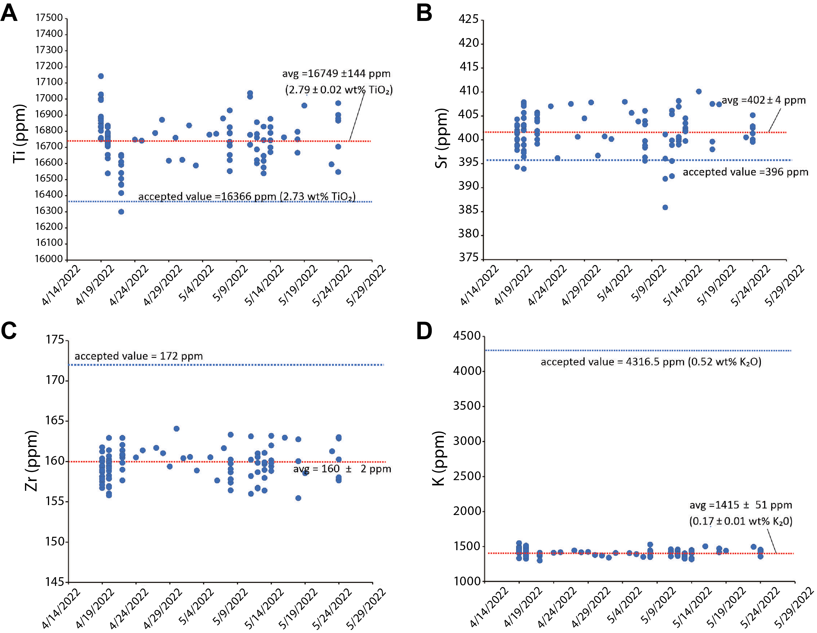
Figure F29. Raw elemental concentration data, BHVO-2.
9.5.4.2. Rock surface analyses
During the SAT expeditions, the primary use of the pXRF was to conduct geochemical assessments of volcanic rocks in the core through direct measurements on cut rock surfaces.
pXRF measurements were predominantly made on the archive halves of the cores. The sample holder systems were used to position smaller samples, and during Expedition 390 a specially made, shielded XRF holder and mounting system was used for longer core segments and larger rock samples. Both sample holder systems provided optimal geometry for quantitative use of the system in ideal conditions. Analyses of larger core segments may suffer from greater uncertainties because of difficulties in precisely positioning the pXRF in the inverted position over the area of interest and/or the potential for the gun to shift or wobble during analysis because of ship movement because it is not tightly secured when used in this position.
9.5.4.3. Analyses of sample powders
The pXRF systems were also used to assess elemental abundances in rock powders produced for ICP-AES analysis from samples taken from the working half of the core. Samples were prepared for pXRF analysis using plastic powder mount assemblies. A short length of thin transparent film for XRF applications (Ultralene or an equivalent product) was stretched across one end of the mount base and held in place using a plastic ring-cap, producing a smooth, transparent surface for sample loading. Sample powder was loaded inside the mount base on the transparent film to a depth of 2–10 mm. A small circle of filter paper (Whatman 24 mm circles, grade 540) was placed on top of the sample, and a round 24 mm plastic foam spacer (similar to those used to fill gaps in sediment core left by sampling) was packed behind the filter paper to hold the sample powder in place, followed by a snap-on plastic sealing cap. The transparent surface of the mount was placed face-up in the XRF sample holder to permit analysis of the powder.
To generate accurate abundances using the pXRF during Expedition 390, measurements were conducted on ICP-AES sample powders from Sites U1556, U1557, U1559, and U1561. ICP-AES and pXRF data for the same sample powders were plotted and data distributions evaluated using the regression functions available in Microsoft Excel. Correlations for Ti, Zr, K, and Sr are shown in Figure F30. The Olympus data initially produced linear regressions for all four elements, and this approach works well for Zr, K, and Sr, with all three elements yielding correlation coefficients (R2) of 0.99 or greater (Figure F30B–F30D). The linear function for fitting the Ti data yielded a low correlation coefficient (R2 = 0.75) (Figure F30A). A second-order polynomial produces a much better fit for the Ti data (R2 = 0.94). The [y] intercept values for all four elements indicate significant offset from the origin (Figure F30), particularly for K and Zr, which reflects the inaccuracy of the raw Olympus pXRF data discussed above (Figure F29).
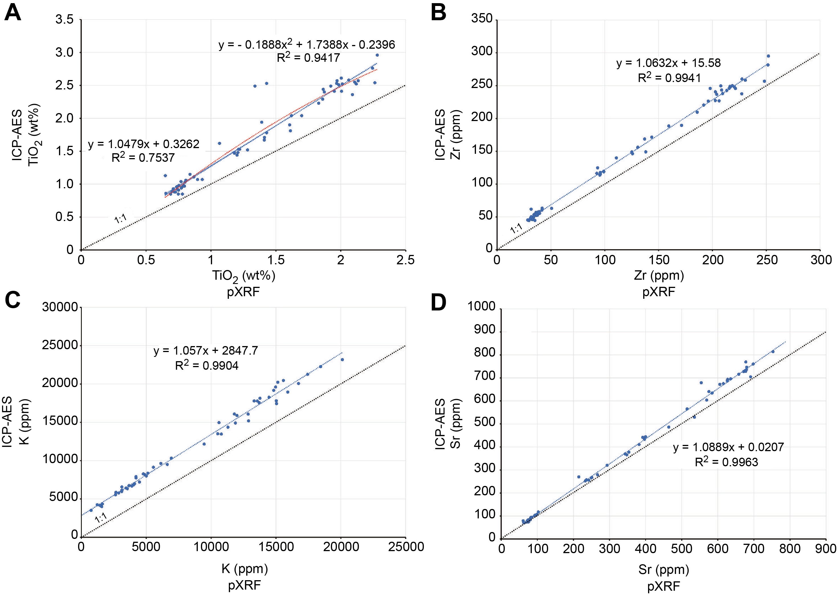
Figure F30. Raw pXRF concentrations vs. ICP-AES data.
Measurements of the solid core surface of the archive half that corresponded to the sample locations taken for ICP-AES analysis show reasonable agreement. Figure F31 shows this comparison graphically in a plot of [Ti/Zr]N values for data determined by ICP-AES versus [Ti/Zr]N calculated from the corrected concentrations determined by pXRF for the solid core samples. Even though there is the potential for uncertainty in this analysis, as the powders and rock surface materials are not identical the data show a remarkably good correlation, with most plotting close to the 1:1 correlation line (Figure F31). The correction is best for samples with [Zr/Ti]N ratios <1 or >1.6. The discrepancy is greatest for rocks with [Zr/Ti]N of 1.3–1.6. In this interval, the ratios determined by pXRF are 5%–10% too low because the shape of the second-order polynomial used to fit the Olympus pXRF Ti data passes directly through the data above 1.75 wt% and below 1 wt% but is offset in the middle region due to scatter (see Figure F30A).
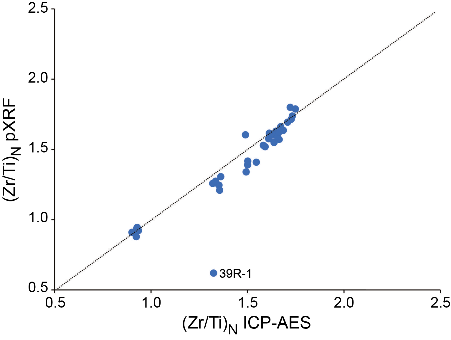
Figure F31. [Zr/Ti]N for solid core surface vs. ICP-AES from working-half samples.
9.5.4.4. Analyses using the Bruker Tracer 5g pXRF system
Using the Bruker pXRF during Expedition 393, we followed the pXRF calibration protocols outlined in Ryan et al. (2017) and Johnston et al. (2018). The standards chosen for establishing our working curves were drawn from those listed in Johnston et al. (2018), adjusted by element to be more appropriate to the basaltic compositions of our sample unknowns. Depending on the element, between 10 and 15 reference materials were used to establish calibration curves. Figure F32 includes working curve plots, slopes, and intercepts for all of the elements analyzed.
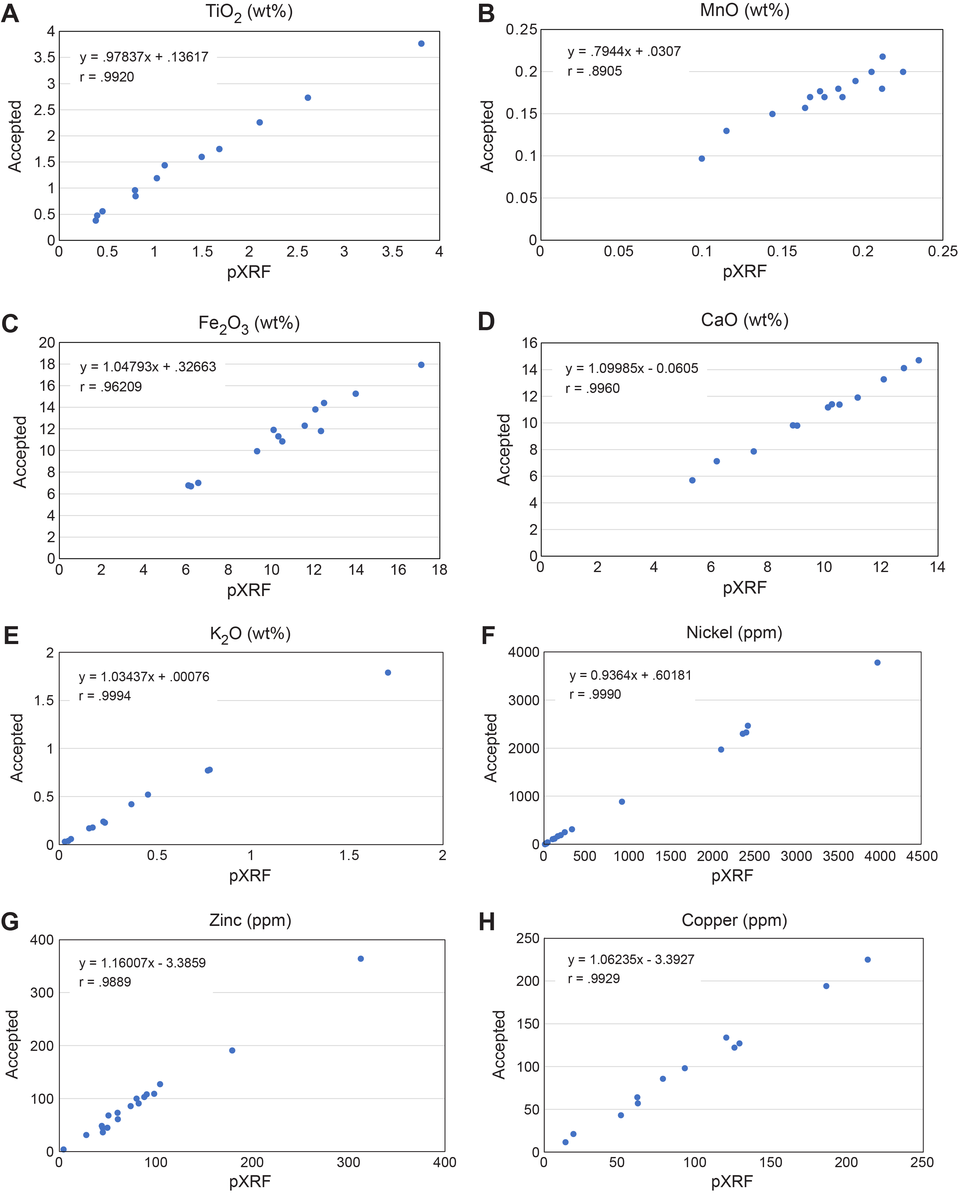
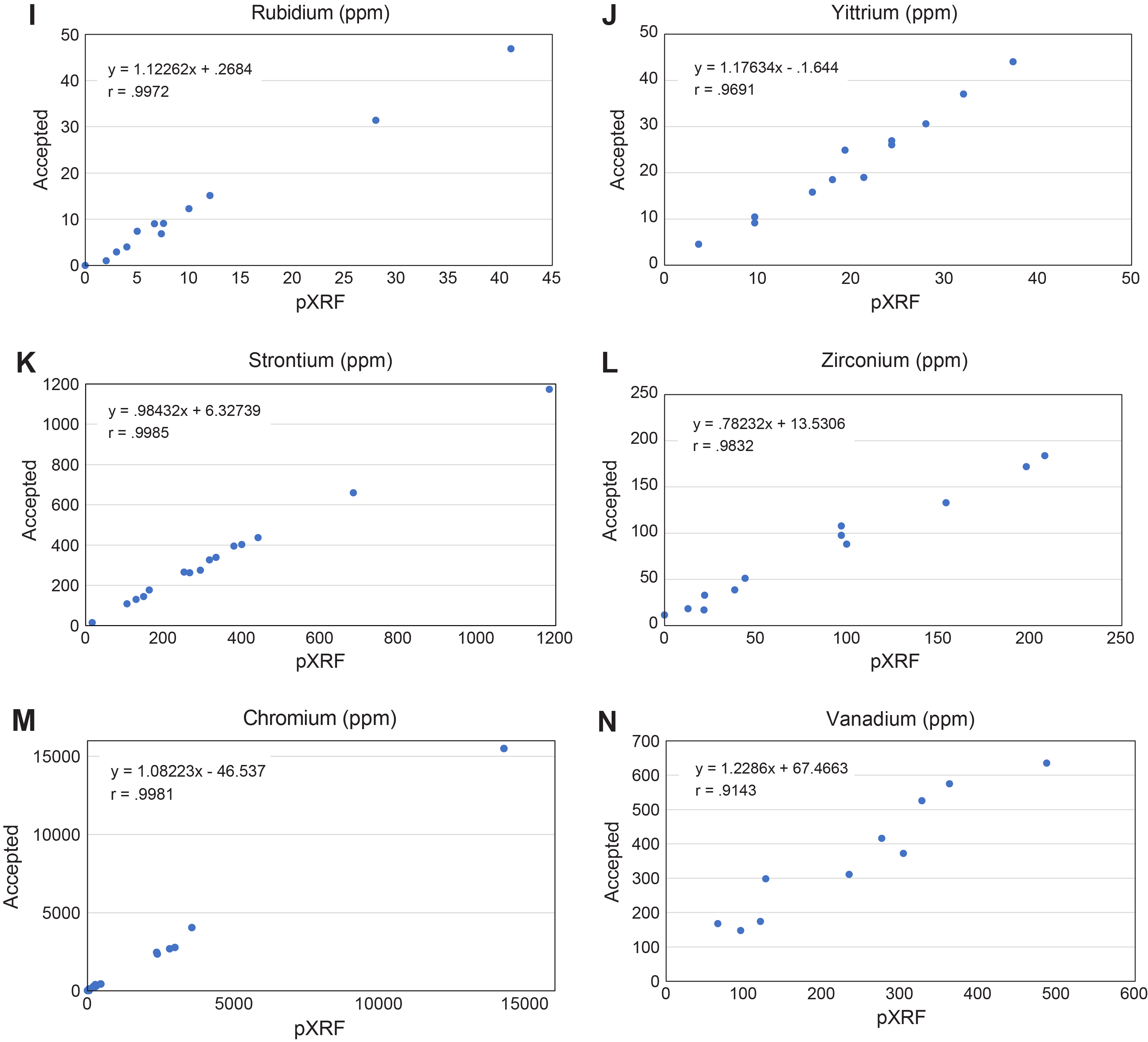
Figure F32. Calibration curves for reliable elements.
Generally speaking, those elements deemed to be reliable for analysis by pXRF have clearly linear working curves (r = 0.95 or better) and near-zero intercept values, though in detail there are exceptions to these criteria. MnO yields reliable data despite an r = 0.89, which relates more to the limited variability in Mn and data quality for Mn in reference samples than to any issues with instrument performance. The Cr working curve has a high r value but also a large intercept, yet Cr measurements are reproducible over time. V is an important element for tectonic discrimination, so it is useful chemostratigraphically even if its correlation parameters are marginal. To better maintain instrument accuracy, working curves were rerun every several weeks and two Hole U1559B samples (5R-1, 106–112 cm, and 11R-1, 6–13 cm) and BHVO-2 were run as check standards with each set of unknowns (see below). Table T14 documents the performance of the Bruker instrument through time. Similar to what was observed by Ryan et al. (2017) and Johnston et al. (2018), the Bruker pXRF working curves are robust, requiring only limited updating over periods of a month.
More elements were accessible using the Bruker pXRF relative to the Olympus, a number of which are potentially useful in examining the sourcing of recovered basalts (Ti, Zr, Y, V, Zn, and Cu) and the extent of hydrothermal alteration (K, Ca, Sr, and Rb). The calibration spreadsheet for use with pXRF data is designed such that one can input CSV text files generated by the instrument software directly into the sheet, which then calculates corrected concentrations (see PXRF in Supplementary material for an example calibration workbook). Powdered rock samples run for full quantitative analysis by pXRF were measured three times each. Chemostratigraphic surveys of core rock surfaces in the archive halves of cores may only measure any given spot once but also include transects across key boundaries (basalt/sediment interfaces at the seafloor and also within cores).
9.5.4.5. Assessment of pXRF rock surface precision and accuracy
To assess the precision, accuracy, and reproducibility of the Bruker instrument as applied to split core surfaces (rock surfaces), two cut surfaces of basalt samples recovered from Hole U1559B were measured repeatedly over the course of Expedition 393 (Samples 393-U1559B-5R-1, 106–112 cm, and 11R-1, 6–13 cm, referred to herein as rock standards). Rock standard 5R-1, 106–112 cm, is an aphyric crypto- to microcrystalline basalt from Volcanic Subunit 2B of Hole U1559B (Figure F33B). Rock standard 11R-1, 6–13 cm, is an aphyric microcrystalline basalt from Subunit 3B of Hole U1559B (Figure F33B). These standards were selected for their fresh, homogeneous, and aphyric texture at the scale of the ~1 cm × 1 cm surface analyzed by pXRF. The back of the sample was cut and powdered for comparative whole-rock analysis by both ICP-AES and pXRF (as a powder mount).
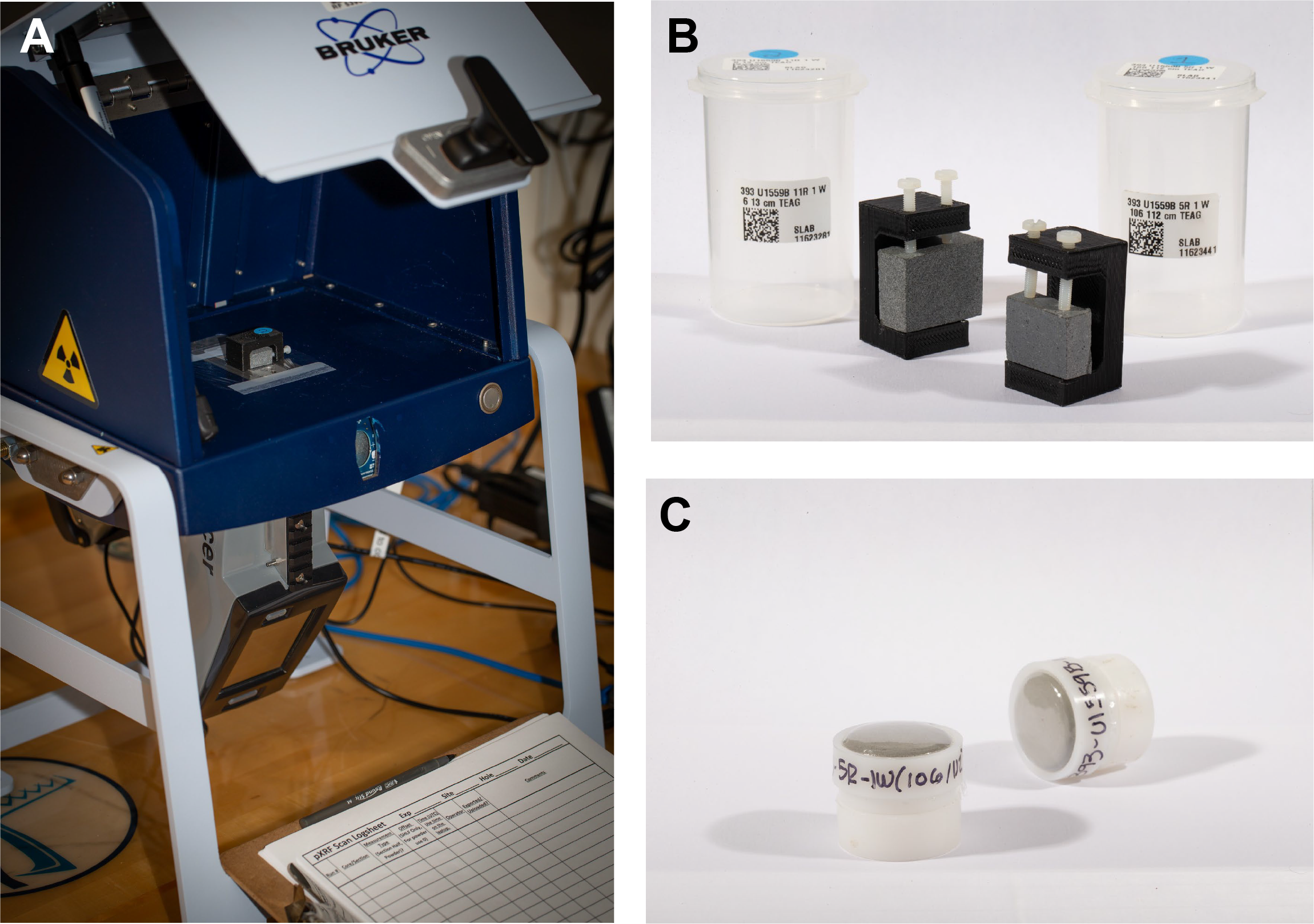
Figure F33. pXRF setup and rock surface standards.
The two rock standards were measured repeatedly alongside the split core surfaces over the course of Expedition 393 (n = 40). The results are summarized in Table T14, and key elements are plotted in Figures F34 and F35. Whole-rock powders cut from the same piece, and these powders were analyzed by pXRF (Figure F33C) and by ICP-AES, and are presented alongside the rock surface results for comparison (Figures F34, F35).
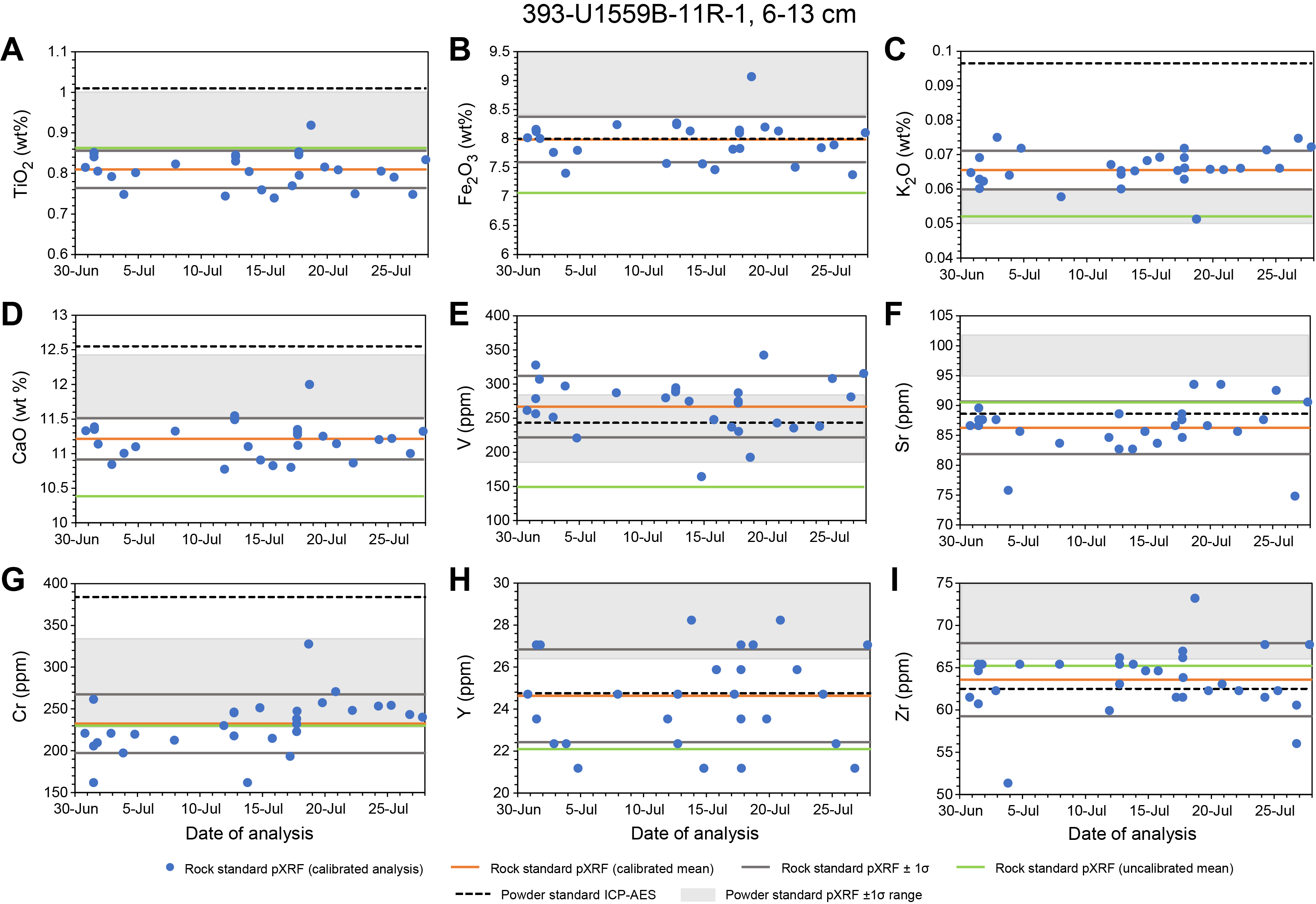
Figure F34. pXRF analyses of microcrystalline rock surface standard.
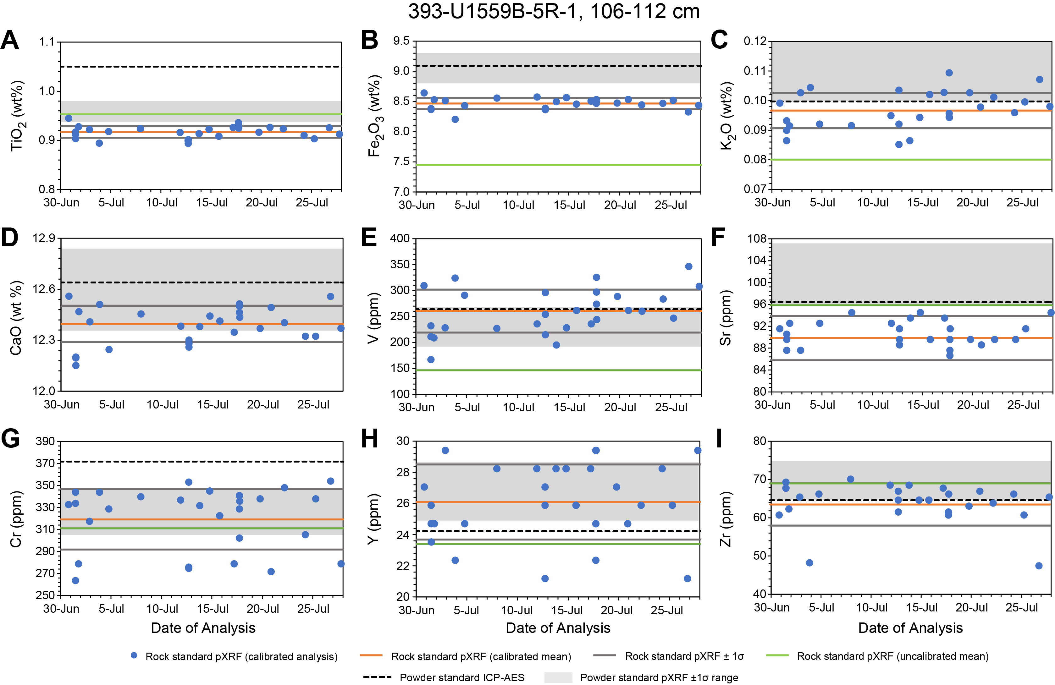
Figure F35. pXRF analyses of ctrypto- to microcrystalline rock surface standard.
Considering the precision based on 40 repeat analyses, major element oxide relative standard deviations (RSDs) are as follows: TiO2, Fe2O3, and CaO RSD = 0.9%–5.7%; K2O and MnO RSD = 6.2%–9.3%. Trace element precision is as follows: Ni, Zn, Sr, Y, and Zr RSD < 10%, and Cr, V, Cu, and Rb RSD < 20%.
In terms of accuracy, the 1σ range of our mean calibrated pXRF rock surface measurements overlaps with the concentrations determined by ICP-AES for V, Y, and Zr. For Fe2O3, K2O, and Sr, only one of the two standards has a 1σ range in rock surface pXRF results that overlaps with the ICP-AES result. For CaO, TiO2, and Cr, the rock surface pXRF 1σ range is lower than the ICP-AES result.
Precisions of <15% RSD for all the key major and trace elements utilized for shipboard study of magmatic and hydrothermal processes are encouraging and may reflect the natural limits of heterogeneity for the rock standard surfaces. The discrepancies in mean pXRF rock surface values between the rock surface and ICP-AES results suggest that some elements may benefit from recalibration or normalization to the standards measured throughout the expedition, if the ICP-AES results for the rock standard powders are shown to be accurate by repeat onshore analyses.
10. Microbiology
10.1. Sample selection
For microbiological studies of both sediment and hard rocks, whole-round core samples are required to allow removal of the core exterior, which may have been contaminated during drilling and subsequent sample handling. Microbiology whole-round core samples are selected before the core splitting process because this process introduces substantial contamination. All scientists and technicians involved in sampling wore gloves sprayed with ethanol and face masks to limit possible contamination of the samples from human contact. Whole-round core samples recovered from sediment using APC and XCB coring were selected and cut with sterile spatulas on the catwalk before being taken to the microbiology laboratory. Whole-round samples from hard rock cores collected using RCB coring were sampled in the splitting room immediately after the core was brought in from the catwalk. Technicians shook the hard rock core into a clean split core liner that had been sprayed with ethanol. A microbiologist then selected a whole-round section for sampling in consultation with a Co-Chief Scientist and a member of the petrology team. An ideal sample had some indication of permeability (such as visible veins) but had not split apart during the coring process. The whole-round rock sample chosen for dedicated microbiology investigation was photographed from overhead in context with the remainder of the core and then transferred into a sterile bag, sealed, and brought to the microbiology laboratory for processing.
10.2. Sampling protocols for sediment and hard rock
For SAT Expeditions 390 and 393, all hard rock samples were initially processed on the laboratory bench between two KOACH units (Figure F36A). Each KOACH unit contains a fan to push air through HEPA filters so that when two units are placed facing each other, the air in the space between is clean and has positive pressure, preventing contamination from particles in the air. In addition to the clean air environment, a deionization bar placed behind the KOACH units (closest to wall) and a Ptec air ionizer placed atop one of the KOACH units were used to prevent particles from sticking to samples. Masks, gloves, and laboratory coats were worn by those handling the sample during whole-round cleaning and all subsequent steps. At all stages of this process, samples were handled as little as possible and with gloved hands only.
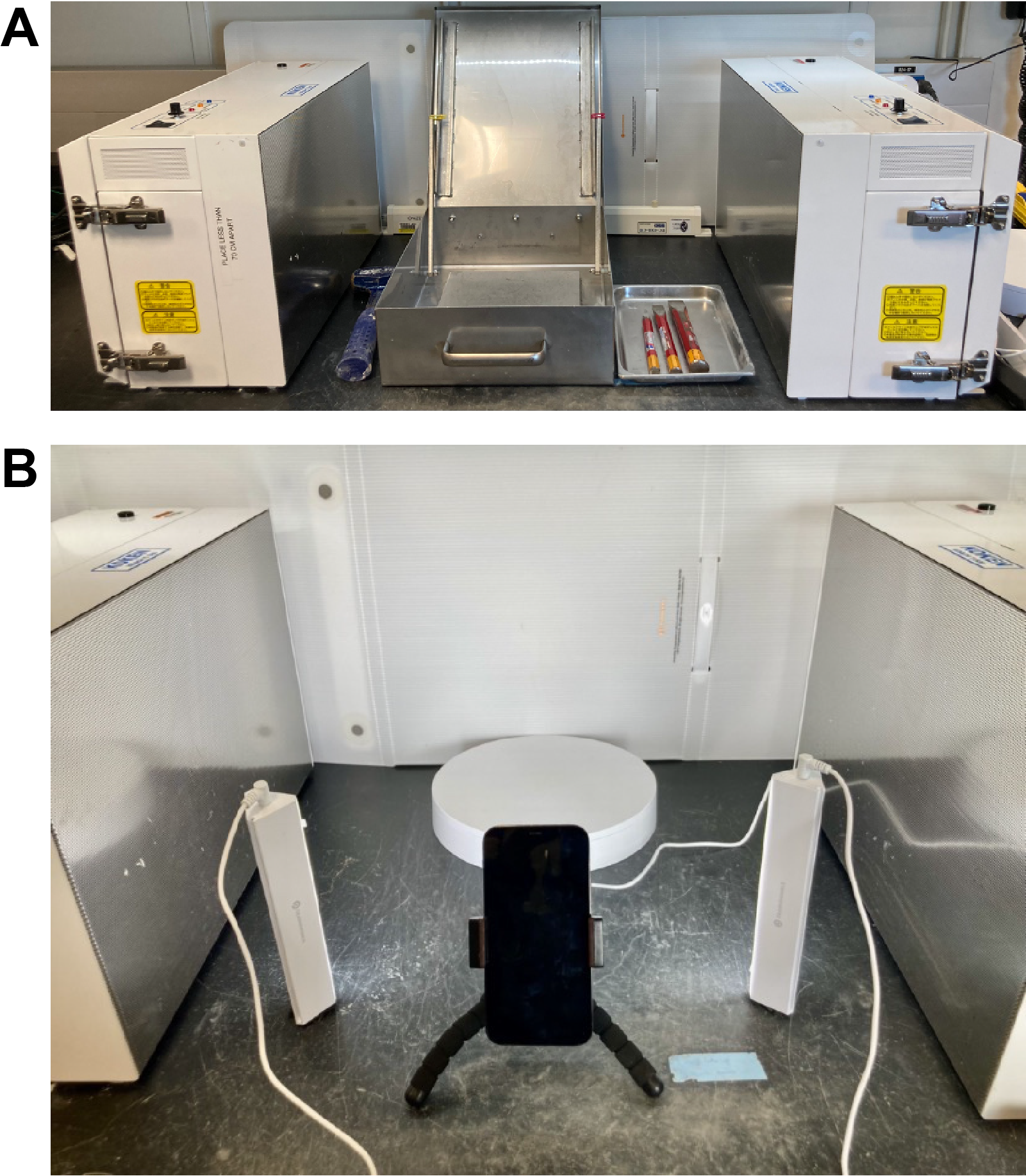
Figure F36. Microbiology sampling and Foldio imaging setup.
Hard rock samples were handled in an ethanol-washed stainless steel rock box. Whole-round samples of hard rock material were rinsed four times in sterile autoclaved 3.5% NaCl water in a sterile sample bag (changing the bag once after the second rinse) to reduce contamination from drilling fluids and then transferred to the rock box, where the outside of the core was sprayed with 70% ethanol. The whole round was then placed on the Foldio light box imaging turntable (Figure F36B), photographed once with a color-correction card and the curatorial identifiers of the rock including directionality, if known, and then imaged using the Foldio device (see below). After imaging, the whole-round sample was sprayed with 70% ethanol once more and placed in the presterilized rock box. The outside of the whole round, which had been in contact with drilling fluids, seawater, and air, was labeled with a wax pencil and removed. The rock was broken using either a sterile hammer and chisel or the SPEX X-Press rock crusher if the pieces were too hard to break manually. To maintain the sample in a clean environment, the inside of the X-Press machine was sprayed with 70% ethanol before each use, and the sample was placed into two sterile sample bags. The interior pristine rock pieces were further broken down into smaller pieces using a sterile hammer and chisel to fulfill the microbiologists' postexpedition research requirements, as described below.
Whole-round samples from sediments were processed differently depending on the subsampling required. Samples to be used for analyses measuring microbial activity and/or anaerobic microbial processes (sulfate reduction assays, stable isotope incubations, anaerobic culturing, or viral production) were placed in the anaerobic chamber in the walk-in cold room until processing could occur. Whole-round samples selected for postexpedition cell counts, nucleic acid analysis, ammonium enrichment incubations, or lipid analysis were placed in the cold room or a 4°C refrigerator until processing in aerobic conditions between the two KOACH units to mitigate contamination. This dual setup (processing samples in both the anaerobic chamber and KOACH unit) allowed more rapid sample processing of sediment sections. Note that during initial sediment sampling in Hole U1556B, all sediment was handled in the anaerobic chamber for the first several cores. It was subsequently decided that the pace of subsampling and sample processing was too slow, resulting in the microbiology team being several cores behind, so the sample work flow described above was implemented.
10.2.1. Digital imaging of microbiological hard rock samples
A Foldio light box and Foldio turntable connected to the Foldio360 application on an iPhone 12 was used to image all microbiological hard rock samples prior to processing (Figure F36B). Only the turntable was placed inside the KOACH bench to allow ease of use and to prevent the air from the KOACH bench being blocked by the walls of the light box. However, the light box was folded down (as it is designed to do) and placed behind the turntable to provide a white background for contrast when photographing. Cleaned microbiological samples were placed on a piece of aluminum foil on the turntable after the foil was wiped down with 70% ethanol. The Foldio360 application pairs via Bluetooth to the turntable and can be programmed to generate a series of photos capturing all sides of the sample. We used 36 photos, but this number is adjustable. Medium turning speed and brightest lights (both adjustable in the Foldio360 app) were used. Velcro was placed on the bottom of the standing column lights, and the bottom of the Velcro was taped to the laboratory bench for consistent placement of the lights. Additionally, the turntable light, also at brightest setting, was turned "backward," facing the rear of the setup toward the backdrop so that it provided reflected backlight off the white surface of the backdrop. During Expedition 390, samples were imaged oriented vertically with the top-side up and then imaged vertically top-side down. Samples were imaged occasionally in a horizontal orientation if the whole round could not be propped to remain upright while photographing. During Expedition 393, samples were always imaged in a horizontal orientation. The generated image folders were named with the sample identifiers, the direction the sample was facing, and the timestamp, which was automatically used by Foldio360 as the name initially (e.g., U1557D_5R5_down-20220513114258). A log sheet was kept for these images. Logging the time is important for keeping track of folders. When renaming files later with the sample name, the timestamp helped the scientist match the log to the files. The images generated were stitched into a movie of the whole round rotating by the Foldio360 application. This documentation/imaging is valuable for understanding the physical context of the microbiology samples (how many veins, how large, etc.), integration with the petrologic visual core descriptions, and postexpedition core-log integration.
10.3. Contamination testing of drilling fluids
As part of the drilling process, a large amount of surface seawater is injected into the borehole. This fluid is the main potential source of microbial contamination during coring. To check for fluid intrusion and contamination, the microbial composition of drilling fluid will be assessed postexpedition using DNA sequencing approaches. Organisms found to be present in both the drilling fluid and rock samples will be considered contaminants (Sheik et al., 2018; Li et al., 2020).
Drilling fluid samples were collected during drilling at each site during Expeditions 390 and 393 (Figure F37). Sterile gloves were worn throughout these procedures. Samples were accessed directly from the injection pipe on the rig floor and collected in sterile bottles with screw caps. In each instance, drilling fluid was collected and then two samples were taken for cell counts (treated as indicated below), one sample was taken for perfluoromethyldecalin (PFMD) analysis (Expedition 393 only), and the rest was filtered onto one or two 47 mm diameter, 0.20 µm pore-size Millipore Express Plus polycarbonate filters and frozen at −80°C for shored-based DNA extraction and analysis. Additionally, samples of the sepiolite drilling mud used during RCB coring were collected for microbiological contamination monitoring prior to injection of the mud into the drill pipe using two 50 mL centrifuge tubes; these samples were frozen at −80°C for shore-based DNA extraction. During Expedition 393 only, samples of sepiolite were also preserved for cell counts.
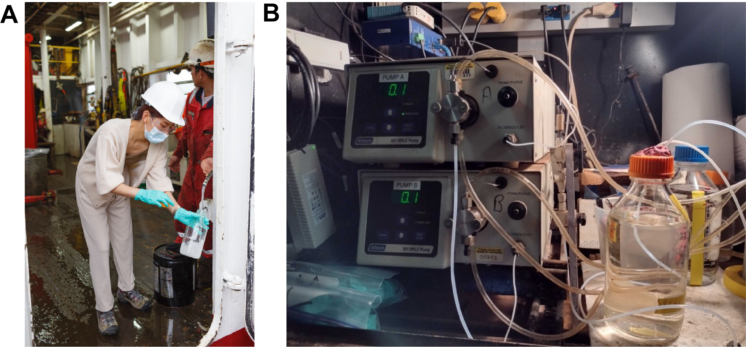
Figure F37. Collecting drilling fluid.
We used the contamination tracer PFMD for the SAT expeditions (Li et al., 2020; Sylvan et al., 2021) (Figure F37), following the methodology used during Expedition 360 (MacLeod et al., 2017). PFMD was continuously pumped with the drilling fluid at an average rate of ~0.5 mL/min; the pump rate was set to vary with drill fluid pump rate. The tracer was used during RCB coring in Hole U1556B and APC/XCB coring in Holes U1559C and U1556D during Expedition 390 and in Holes U1559B, U1558D, and U1583F (through Core 393-U1583F-12R) during Expedition 393. Prohibitive costs of PFMD prevented purchase of enough tracer to run in every hole; therefore, pumping during basement drilling in the full range of lithologies encountered was prioritized.
For sediment samples, a 2 cm3 scraping from the exterior of the whole-round sample was transferred to a 20 mL headspace glass vial and sealed for later analysis of PFMD. A 2 cm3 sample from the interior of the whole round was taken using an autoclaved 3 mL syringe with the tip cut off and likewise transferred to a 20 mL headspace vial. For hard rock samples, a fragment of the exterior of each core was selected from pebbles in the core liner in the splitting room instead of sampling directly from the microbiology whole round. This method ensured that we could detect delivery of the PFMD to the exterior of the sample. During sampling of Hole U1559B and if no pebbles were available in the core liner, rock chips from the whole-round exterior were used instead. It should be noted that sampling the outer part of the core typically happens after rinsing and cleaning of the core, which can cause the sample to be diluted with interior unexposed material, which would result in PFMD tracer concentrations too low to provide conclusive results. Therefore, "outside" samples taken from basement whole-round samples should be viewed as minimum values. An interior sample was taken after breaking apart the hard rock sample in the rock box. For all samples, vials were preweighed and then weighed again after sample addition so that concentrations can be mass-normalized. Drilling fluid samples were also collected during Expedition 393 to serve as controls, as was core liner fluid remaining after pouring out hard rock cores. Similarly, in the few instances during Expedition 393 when whole-round samples of hard rock had to be cut in the splitting room using a MK-101 tile saw to either preserve sample ends for petrologic observations or to shorten long, intact whole-round pieces to the desired length of 10–12 cm, samples of the saw fluid were taken as a control and frozen for further analyses.
Detection of the tracer was measured after heating at 70°C for 10 min in an oven to evaporate and release the tracer. Headspace samples were injected into an Agilent Technologies 6890N GC for measurement after preparing and running calibration standards using 10−4, 10−6, 10−8, and 10−10 dilutions of the tracer.
10.4. Standard microbiology sampling
For every whole-round sample, subsamples were collected for cell counts and nucleic acid–based postexpedition analysis. For many samples, additional subsamples were collected for a range of postexpedition microbiological analyses. Methods for all sampling approaches are described below.
10.4.1. Cell and viral counts
Samples were taken in duplicate for rock samples and triplicate for sediment samples to be able to cross-calibrate cell counts among different laboratories. A total of 4 mL of 5% Epredia Formal-Fixx in 3X phosphate buffered solution (Expedition 390) or paraformaldehyde (4% solution in 100 mM phosphate-buffered saline [PBS]) was added to autoclaved 7 mL plastic tubes, and 1 cm3 of sediment or powdered rock material was added to each tube, bringing the total volume to 5 mL. During Expedition 390, rocks were crushed into smaller pieces using a clean (autoclaved or ethanol washed and dried) Fisher Scientific CerCo Diamonite mortar and pestle. During Expedition 393, small rock chips were selected because the inside of the whole round was broken into smaller pieces. Preserved samples were stored at 4°C for onshore analysis using a density gradient separation of cells from rocks and sediments followed by epifluorescence microscopy counts. The protocol used was adapted from Morono et al. (2013) and Li et al. (2020) for microbial cells and Pan et al. (2019) for viruses.
10.4.2. Nucleic acid analyses
For DNA- and RNA-based analyses, we collected duplicate 10 or 100 cm3 samples of sediment in sterile cut-tip syringes for microbial and viral analyses, respectively, and up to 50 cm3 of material from hard rock samples. All samples were placed in sterile plastic centrifuge tubes and then immediately frozen at −80°C. These samples were collected for postexpedition research.
10.5. Nonstandard microbiology sampling
10.5.1. Stable isotope incubations
Stable isotope probing (SIP) experiments were started during Expedition 390 to determine preferred carbon (C) and nitrogen (N) sources used by metabolically active microorganisms in subseafloor sediments and basement rock. Similar methods were used during Expedition 329 to reveal the presence of active microorganisms in sediments of the South Pacific Gyre as old as 101.5 Ma (Morono et al., 2020). Samples for SIP incubations were initially handled in the anaerobic chamber in the microbiology cold room. A total of 15 cm3 of sediment was collected with a sterile cut-tip 20 mL syringe, avoiding the outer edges of the whole-round core, and put into a 50 cm3 sterile glass vial (Figure F38). Each vial was sealed with a sterile rubber stopper and a screw cap and then taken outside the anaerobic chamber and flushed with 0.2 µm filter-sterilized nitrogen gas. From here, the vials were transferred to the radioisotope laboratory, where a labeled substrate (13C-labeled sodium bicarbonate, 13C-labeled amino acid mix, and 15N-labeled ammonium) was injected onto each sample using a syringe and needle. Four conditions were tested:
- No added nutrients (control),
- 100 mM 13C-labeled amino acid mix + 10 mM 15N-labeled NH4Cl,
- 100 mM 13C-labeled NaHCO3 + 10 mM 15N-labeled NH4Cl, and
- 10 mM 15N-labeled NH4Cl.
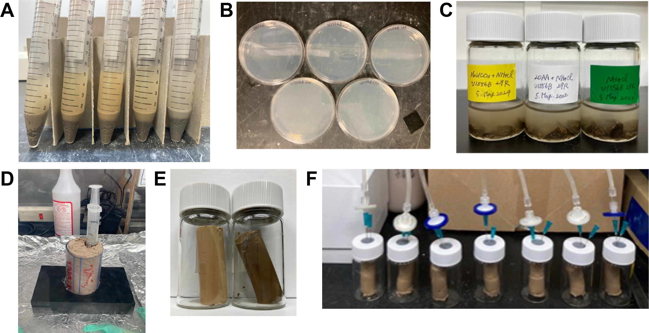
Figure F38. Enrichment and SIP experiments.
Half of the samples were kept anaerobic for the duration of the experiment. For the other half, 7 cm3 of filter-sterilized air was added to compose the microaerobic environment (3.3% O2). All samples were incubated at 4°C in the radioisotope laboratory. The first time point of individual experimental vials was fixed by adding 15 mL of 4% paraformaldehyde in PBS solution after 10 days. The remaining three time points will be fixed after the expedition at 30 days, 2 months, and 6 months. The fixed incubations were frozen at −80°C until further processing.
SIP incubation setup for basement samples was conducted in the KOACH bench under aerobic conditions. Crushed basalt pieces and sterilized artificial seawater were put in a 50 cm3 sterile glass vial to make a 1:4 slurry (Table T15; Figure F38) with a total volume of 20 mL. The slurry was purged, the headspace was replaced with N2, and then 10 mL of filtered air was injected into the vial to create a microaerobic environment (5% O2). The combinations of substrates were the same as those for SIP experiments with sediment. Samples were incubated at 10°C until shipment to shore at the end of Expedition 390. Individual experimental vials will be fixed at four time points (2, 3, 6, and 12 months) prior to analysis.
All experimental tools used for the SIP experiments were sterilized by autoclaving at 121°C for 20 min. Reagents and gas components, including air used for sample preparation, were filtered through 0.2 µm syringe top filters.
10.5.2. Enrichment experiments
To enrich and isolate new microbial species during Expedition 390, sediment and hard rock samples were selected for microbial enrichments on agar plates. When recovered material and/or time was sufficient for sampling, 1 cm3 of sediment or rock was suspended in 4 mL of sterile artificial seawater (Table T15). A small amount of the slurry (100 µL) was spread on 1/10 Zobell Marine Agar 2216 medium (Difco). The Petri dishes were left at 9.5°C with the top facing down and then shipped to shore for postexpedition research.
Samples were also collected for high-throughput culturing (Mullis et al., 2021). Sediment was sampled with a 3 cm3 syringe, parafilm was wrapped around the top of the syringe, and then the syringe was placed in a sterile sample bag at 4°C. These samples were shipped to shore refrigerated for postexpedition research.
For anaerobic sediments, 30–70 cm3 was placed into anaerobic bottles in the anaerobic chamber with an N2 headspace. The bottles were then placed in wine bags with an Anaeropack to remove oxygen and sealed under a vacuum. Incubations were shipped to shore for initiation of long-term enrichments targeted at growing uncultured Archaea.
10.5.3. Single-cell genomics and fluorescence-based activity assays
For single-cell genomics and to determine which microorganisms are metabolically active in situ and their relative amounts of activity, RedoxSensor Green (RSG; Invitrogen) was used in incubations with samples. Sediment and hard rock samples were processed slightly differently. For sediment samples, 1 cm3 of sample was placed in a 15 mL Falcon tube with 1:1 (volume:volume) cold, oxic 1× PBS buffer containing a 1× concentration of RSG. The sediment and solution were shaken briefly with a vortex mixer. The sample was incubated in a 4°C refrigerator in the dark for 20 min, and then 8 mL of glycerol-tris-ethylenediamine tetra-acetic acid (EDTA) buffer was added to the sample and vortexed to mix. The sample was then flash frozen with liquid N2 and stored at −80°C until shore-based analysis. An RSG-free sample was also prepared by mixing 1 cm3 of sediment with 9 mL of glycerol-tris-EDTA, vortexing to mix, flash freezing in liquid N2, and storing at −80°C until shore-based analysis. Samples collected from oxygen-free sediment were processed in the anaerobic chamber prior to flash freezing and storage.
For hard rock samples, a sterile mortar and pestle were used to homogenize approximately 5 cm3 of material to a greater extent than was done with the hammers and chisels in the rock box. For activity-based cell sorting using RSG, 1 cm3 of this homogenized rock was added to a 15 mL Falcon tube with 1:1 (volume:volume) cold, oxic 1× PBS buffer containing a 1× concentration of RSG. An RSG-free sample was also prepared in the same way as that for the sediment. These samples were processed as described for the sediment samples. The remaining 3 cm3 was archived for future shore-based analyses by adding 7 mL of glycerol-tris-EDTA, flash freezing with liquid N2, and storing at −80°C.
10.5.4. Metagenomics in sediment and hard rock
Metagenomic analysis of microbial community DNA provides information regarding the functional potential of a community. Samples were collected during Expeditions 390 and 393 for shore-based analysis of both microbial and viral metagenomics. For sediments, a 10 cm long (200 cm3) whole-round sample was collected and stored at −80°C for shore-based analysis of microbial prokaryotic metagenomics. For basement samples, at least 50 cm3 was collected into sterile centrifuge tubes and then frozen at −80°C. Samples were shipped frozen to shore for postexpedition research. For viral metagenomics in sediment, 5 cm long (~100 cm3) whole-round core samples were collected at 20 m intervals to 100 m depth, and then two samples were collected per major lithology in deeper sections. Viral metagenomics samples were frozen at −80°C and shipped to shore frozen for postexpedition research.
10.5.5. Lipid sampling in hard rock
Lipid biomarkers inform analysis of microbial communities and are complementary to DNA- and RNA-based studies (Li et al., 2020). Samples collected for lipid analysis were wrapped in aluminum foil and then put in bags and vacuum-sealed. These samples were kept at −20°C until they were shipped to shore for postexpedition research.
10.5.6. Sulfate reduction activity
During Expedition 390, radiolabeled (35S) sulfate was used to characterize the rate of sulfate reduction in sediment samples. Whole-round samples were transferred to gas-tight bags, flushed with N2 gas, heat sealed, and stored at ~4°C until they were prepared for radiotracer additions. All vials, caps, bottles, plastic syringes, stoppers, and ceramic knives were autoclaved prior to use, and solutions were either autoclaved or filtered through sterile syringe filters (0.2 µm). As described below, the potentially contaminated exteriors were removed from whole-round cores, and then subsamples were placed in a vial and amended with sulfate-reducing medium, injected with radiotracer, and incubated for 10 days at approximately in situ temperatures before termination of the experiment. The sulfate-reducing medium was prepared according to procedures used during IODP Expeditions 370 and 385 (Morono et al., 2017; Teske et al., 2021; Beulig et al., 2022).
Resazurin was used to indicate the presence of oxygen in incubation and media bottles. It was added to the medium, and the bottle was capped loosely before autoclaving. After autoclaving, the cap was replaced with a sterile butyl stopper and screw cap. The medium was purged with N2 gas while still warm (>60°C) by placing a long syringe needle between the stopper and the wall of the bottle. After purging, the bottle was sealed with the butyl stopper and cap. Sterile filtered sodium bicarbonate (NaHCO3) was injected through the stopper. The pH of the medium was adjusted to 7.5 by injection of sterile filtered 6.5% HCl or NaOH. Sterile filtered Na2S·9H2O was then injected through the stopper to reduce the medium. Reduction was confirmed by color loss (pink to clear) of the resazurin in solution.
Samples were prepared inside an anaerobic chamber (95:5 [v/v] N2:H2). The outermost layer of the whole-round core and both ends were cut off with a sterile ceramic knife to remove potentially contaminated material. A cut-off syringe was used to take 5 cm3 of mud from the center of each whole round. The sediment plug was transferred to a 20 mL crimp-top vial, 5 mL of sulfate-reducing medium was added, and the vial was sealed with a nontoxic blue butyl stopper and aluminum crimp cap. The vial headspace was then flushed with N2 gas to remove surplus hydrogen. Each sample was prepared in triplicate. In the radioisotope laboratory, the vials were injected with 10 µL of 35S radiolabeled Na2SO4 (3.7 MBq) and then vigorously shaken with a vortex mixer. Samples were incubated at the in situ temperature of 4°C, as determined by APCT-3 tool measurements. After 10 days of incubation, 5 mL of 20% (w/v) zinc acetate solution was injected into each vial to trap H2S gas produced during sulfate reduction. Vials were then thoroughly shaken with a vortex mixer. The vials were opened, and the sediment slurries were quantitatively transferred to 50 mL centrifuge tubes with three rinses of 5 mL 20% zinc acetate solution. The centrifuge tubes were shaken with a vortex mixer and then frozen immediately at −20°C to stop microbial activity. The samples were shipped to a shore-based laboratory for extraction and analysis following Kallmeyer et al. (2004). Kill controls, sediment controls, medium controls, and drilling fluid controls were taken to test for contamination or abiogenic turnover of sulfur. A kill control was prepared for approximately every other sample by injecting 5 mL of 20% zinc acetate immediately after injection of the radiotracer to stop microbial activity. Sediment controls were incubated without radiotracer. The radiotracer was added after microbial activity was stopped to check for reactions postincubation. Medium controls (5 mL of sterile medium, no sediment) and drilling fluid controls (5 mL of drilling fluid, no sediment) were prepared and incubated with radiotracer added to check for reactions in the medium and in contaminating drilling fluids. Drilling fluid was also collected after core retrieval from the gap between the core and liner, and additional samples were taken directly from the drilling fluid tank.
10.5.7. Ammonium enrichment
Ammonium enrichment incubation experiments were set up during Expedition 393. About 35–40 cm3 of rocks from the interior of the whole-round core sample were crushed using a sterile Fisher Scientific CerCo Diamonite mortar and pestle. One basement sample and one sediment sample were collected from as close as possible to the sediment/basement interface. Serum vials (50 mL) were used for this experiment, with aerobic sterile filtered seawater (SW) as the basal media for all enrichments (MacLeod et al., 2017). To initiate enrichments, ~9–12 g of crushed rock chips were transferred to serum vials and submerged in SW to a level equivalent to 40 mL total volume (rocks plus media). These ammonium nutrient addition experiments were coupled with bio-orthogonal noncanonical amino acid tagging (BONCAT). For these enrichments, L-homopropargylglycine (HPG) was added to the vial at a final concentration of 50 µM. After adding NH4Cl to a final concentration of 0.4 mM, the vials were sealed with butyl stoppers and allowed to incubate for ~6 months at 4°C. Five treatments were prepared for each selected sample:
- Crushed rocks in SW and 1.5 mM NH4Cl (no HPG);
- Crushed rocks in SW, 1.5 mM NH4Cl, and HPG;
- Crushed rocks in SW, 0.5 mM NH4Cl, and HPG;
- Crushed rocks in SW and HPG (no NH4Cl); and
- Crushed rocks in SW only.
For each sample and each of these treatments, a killed control was set up using autoclaved rocks from the outer core. Once the incubation period is completed, further analysis will be performed in the shore-based laboratory at Texas A&M University. This involves Cu(i)-catalyzed click chemistry to be applied to the BONCAT samples following methods outlined by Hatzenpichler and colleagues (Hatzenpichler et al., 2014, 2016; Hatzenpichler and Orphan, 2015). After click-staining, the stained cells will be sorted using fluorescence-activated cell sorting (Reichart et al., 2020) and the sorted cells will be prepared for sequencing.
10.5.8. Virus-induced microbial mortality and viral production experiments
For Expedition 393, we used the dilution technique developed for surface sediments (Dell'Anno et al., 2009) to set up experiments with the goal of determining virus-induced microbial mortality and viral production rates from lytic viruses. To compare anaerobic and aerobic conditions, one set of experiments (Site U1558) was performed in a Coy anaerobic chamber installed on the tween deck flushed with N2. The other experiments were performed in the KOACH bench under sterile aerobic conditions. Sediment samples (10 cm3) were subsampled with a cut-off syringe and then diluted with autoclaved seawater. Seawater used for sample dilution was collected either from surface water, using a field-rinsed bucket attached to a rope, or near the seafloor using the Niskin bottle attached to the subsea camera system frame. Experiments were set up in duplicate in 50 mL centrifuge tubes. Samples were incubated anaerobically inside the chamber (room temperature of ~20°C). In duplicate, 1 mL samples were taken at t = 0, 6, 12, 24, and 48 h and 7 and 14 days in sterile cryotubes. Each sample was fixed with paraformaldehyde (final concentration 2%), incubated 10 min at 4°C, and frozen at −80°C to be further processed in the shore-based laboratory (Texas A&M University at Galveston [USA]). Cell and viral counts will be performed using epifluorescence microscopy following Pan et al. (2019). The remaining material from the incubations was shipped to the shore-based laboratory for total DNA extraction and metagenomic sequencing.
10.5.9. Prophage induction
For Expedition 393, we induced prophages to determine the extent of lysogeny in sediment. To compare anaerobic and aerobic conditions, one set of experiments (Site U1558) was performed in a Coy anaerobic chamber installed on the tween deck flushed with N2. The other experiments were performed in the KOACH bench under sterile aerobic conditions. Samples (10 cm3) were diluted 1:1 (v/v) in autoclaved seawater supplemented with Mitomycin C (1 µg/mL final concentration in 0.02 µm prefiltered seawater). Experiments were set up in duplicate in 50 mL Falcon tubes. In duplicate, 1 mL samples were taken at t = 0, 6, 12, 24, and 48 h and 7 and 14 days in sterile cryotubes. Each sample was fixed with paraformaldehyde (final concentration 2%), incubated 10 min at 4°C, and frozen at −80°C to be further processed in the shore-based laboratory (Texas A&M University at Galveston). Cell and viral counts will be performed using epifluorescence microscopy following Pan et al. (2019). The remaining material from the incubations were shipped to the shore laboratory for total DNA extraction and metagenomic sequencing.
References
Agnini, C., Fornaciari, E., Raffi, I., Catanzariti, R., Pälike, H., Backman, J., and Rio, D., 2014. Biozonation and biochronology of Paleogene calcareous nannofossils from low and middle latitudes. Newsletters on Stratigraphy, 47(2):131–181. https://doi.org/10.1127/0078-0421/2014/0042
Backman, J., 1980. Miocene-Pliocene nannofossils and sedimentation rates in the Hatton-Rockall Basin, NE Atlantic Ocean. Stockholm Contributions in Geology, 36:1–91.
Backman, J., Raffi, I., Rio, D., Fornaciari, E., and Pälike, H., 2012. Biozonation and biochronology of Miocene through Pleistocene calcareous nannofossils from low and middle latitudes. Newsletters on Stratigraphy, 45(3):221–244. https://doi.org/10.1127/0078-0421/2012/0022
Balsam, W.L., and Damuth, J.E., 2000. Further investigations of shipboard vs. shore-based spectral data: implications for interpreting Leg 164 sediment composition. In Paull, C.K., Matsumoto, R., Wallace, P.J., Dillon, W.P., Proceedings of the Ocean Drilling Program, Scientific Results. 164: College Station, TX (Ocean Drilling Program), 314–324. https://doi.org/10.2973/odp.proc.sr.164.222.2000
Balsam, W.L., Damuth, J.E., and Schneider, R.R., 1997. Comparison of shipboard vs. shore-based spectral data from Amazon Fan cores: implications for interpreting sediment composition. In Flood, R.D., Piper, D.J.W., Klaus, A., and Peterson, L.C., Proceedings of the Ocean Drilling Program, Scientific Results. 155: College Station, TX (Ocean Drilling Program), 193–215. https://doi.org/10.2973/odp.proc.sr.155.210.1997
Balsam, W.L., Deaton, B.C., and Damuth, J.E., 1998. The effects of water content on diffuse reflectance spectrophotometry studies of deep-sea sediment cores. Marine Geology, 149(1):177–189. https://doi.org/10.1016/S0025-3227(98)00033-4
Balsley, J.R., and Buddington, A.F., 1960. Magnetic susceptibility anisotropy and fabric of some Adirondack granites and orthogneisses. American Journal of Science, 258-A:6–20.
Bartington Instruments, Ltd., 2011. Operation Manual for MS2 Magnetic Susceptibility System: Oxford, UK (Bartington Instruments, Ltd.). https://gmw.com/wp-content/uploads/2019/03/MS2-OM0408.pdf
Berggren, W.A., Aubry, M.P., and Hamilton, N., 1983. Neogene magnetobiostratigraphy of Deep Sea Drilling Project Site 516 (Rio Grande Rise, South Atlantic). In Barker, P.F., Carlson, R. L., Johnson, D. A., et al., Initial Reports of the Deep Sea Drilling Project. 72: Washington, DC (US Government Printing Office), 675–713. https://doi.org/10.2973/dsdp.proc.72.130.1983
Berggren, W.A., and Miller, K.G., 1989. Cenozoic bathyal and abyssal calcareous benthic foraminiferal zonation. Micropaleontology, 35(4):308–320. https://doi.org/10.2307/1485674
Beulig, F., Schubert, F., Adhikari, R.R., Glombitza, C., Heuer, V.B., Hinrichs, K.U., Homola, K.L., Inagaki, F., Jørgensen, B.B., Kallmeyer, J., Krause, S.J.E., Morono, Y., Sauvage, J., Spivack, A.J., and Treude, T., 2022. Rapid metabolism fosters microbial survival in the deep, hot subseafloor biosphere. Nature Communications, 13(1):312. https://doi.org/10.1038/s41467-021-27802-7
Bloemendal, J., King, J.W., Hall, F.R., and Doh, S.J., 1992. Rock magnetism of late Neogene and Pleistocene deep-sea sediments: relationship to sediment source, diagenetic processes, and sediment lithology. Journal of Geophysical Research: Solid Earth, 97(B4):4361–4375. https://doi.org/10.1029/91JB03068
Blum, P., 1997. Physical properties handbook: a guide to the shipboard measurement of physical properties of deep-sea cores. Ocean Drilling Program Technical Note, 26. https://doi.org/10.2973/odp.tn.26.1997
Boersma, A., 1984. Handbook of Common Tertiary Uvigerina: Stony Point, NY (Microclimates Press).
Bollmann, J., 1997. Morphology and biogeography of Gephyrocapsa coccoliths in Holocene sediments. Marine Micropaleontology, 29(3–4):319–350. https://doi.org/10.1016/S0377-8398(96)00028-X
Bown, P.R., 1998. Calcareous Nannofossil Biostratigraphy: Dordrect, Netherlands (Kluwer Academic Publishing).
Bown, P.R., 2005. Palaeogene calcareous microfossils from the Kilwa and Lindi areas of coastal Tanzania (Tanzania Drilling Project 2003–4). Journal of Nannoplankton Research, 27:21–95.
Bown, P.R., and Young, J.R., 1998. Techniques. In Bown, P.R., Calcareous Nannofossil Biostratigraphy. Dordrect, Netherlands (Kluwer Academic Publishing), 16–28.
Bromley, R.G., and Ekdale, A.A., 1984. Chondrites: a trace fossil indicator of anoxia in sediments. Science, 224(4651):872–874. https://doi.org/10.1126/science.224.4651.872
Buatois, L.A., and Mángano, M.G., 2011. Ichnology: Organism-Substrate Interactions in Space and Time: Cambridge, UK (Cambridge University Press).
Bullard, E.C., 1939. Heat flow in South Africa. Proceedings of the Royal Society of London, A: Mathematical and Physical Sciences, 173(955):474–502. https://doi.org/10.1098/rspa.1939.0159
Bullard, E.C., 1954. The flow of heat through the floor of the Atlantic Ocean. Proceedings of the Royal Society of London, A: Mathematical and Physical Sciences, 222(1150):408–429. https://doi.org/10.1098/rspa.1954.0085
Coggon, R.M., Sylvan, J.B., Estes, E.R., Teagle, D.A.H., Reece, J., Williams, T.J., Christeson, G.L., Aizawa, M., Borrelli, C., Bridges, J.D., Carter, E.J., Dinarès-Turell, J., Estep, J.D., Gilhooly, W.P., III, Grant, L.J.C., Kaplan, M.R., Kempton, P.D., Lowery, C.M., McIntyre, A., Routledge, C.M., Slagle, A.L., Takada, M., Tamborrino, L., Wang, Y., Yang, K., Albers, E., Amadori, C., Belgrano, T.M., D'Angelo, T., Doi, N., Evans, A., Guérin, G.M., Harris, M., Hojnacki, V.M., Hong, G., Jin, X., Jonnalagadda, M., Kuwano, D., Labonte, J.M., Lam, A.R., Latas, M., Lu, W., Moal-Darrigade, P., Pekar, S.F., Robustelli Test, C., Ryan, J.G., Santiago Ramos, D., Shchepetkina, A., Villa, A., Wee, S.Y., Widlansky, S.J., Kurz, W., Prakasam, M., Tian, L., Yu, T., and Zhang, G., 2024a. Site U1556. In Coggon, R.M., Teagle, D.A.H., Sylvan, J.B., Reece, J., Estes, E.R., Williams, T.J., Christeson, G.L., and the Expedition 390/393 Scientists, South Atlantic Transect. Proceedings of the International Ocean Discovery Program, 390/393: College Station, TX (International Ocean Discovery Program). https://doi.org/10.14379/iodp.proc.390393.103.2024
Coggon, R.M., Teagle, D.A.H., Sylvan, J.B., Reece, J., Estes, E.R., Williams, T.J., Christeson, G.L., Aizawa, M., Albers, E., Amadori, C., Belgrano, T.M., Borrelli, C., Bridges, J.D., Carter, E.J., D'Angelo, T., Dinarès-Turell, J., Doi, N., Estep, J.D., Evans, A., Gilhooly, W.P., III, Grant, L.J.C., Guérin, G.M., Harris, M., Hojnacki, V.M., Hong, G., Jin, X., Jonnalagadda, M., Kaplan, M.R., Kempton, P.D., Kuwano, D., Labonte, J.M., Lam, A.R., Latas, M., Lowery, C.M., Lu, W., McIntyre, A., Moal-Darrigade, P., Pekar, S.F., Robustelli Test, C., Routledge, C.M., Ryan, J.G., Santiago Ramos, D., Shchepetkina, A., Slagle, A.L., Takada, M., Tamborrino, L., Villa, A., Wang, Y., Wee, S.Y., Widlansky, S.J., Yang, K., Kurz, W., Prakasam, M., Tian, L., Yu, T., and Zhang, G., 2024b. Site U1559. In Coggon, R.M., Teagle, D.A.H., Sylvan, J.B., Reece, J., Estes, E.R., Williams, T.J., Christeson, G.L., and the Expedition 390/393 Scientists, South Atlantic Transect. Proceedings of the International Ocean Discovery Program, 390/393: College Station, TX (International Ocean Discovery Program). https://doi.org/10.14379/iodp.proc.390393.109.2024
Coggon, R.M., Teagle, D.A.H., Sylvan, J.B., Reece, J., Estes, E.R., Williams, T.J., Christeson, G.L., and the Expedition 390/393 Scientists, 2024c. Supplementary material, https://doi.org/10.14379/iodp.proc.390393supp.2024. In Coggon, R.M., Teagle, D.A.H., Sylvan, J.B., Reece, J., Estes, E.R., Williams, T.J., Christeson, G.L., and the Expedition 390/393 Scientists, South Atlantic Transect. Proceedings of the International Ocean Discovery Program, 390/393: College Station, TX (International Ocean Discovery Program).
de Ronde, C.E.J., Humphris, S.E., Höfig, T.W., Brandl, P.A., Cai, L., Cai, Y., Caratori Tontini, F., Deans, J.R., Farough, A., Jamieson, J.W., Kolandaivelu, K.P., Kutovaya, A., Labonté, J.M., Martin, A.J., Massiot, C., McDermott, J.M., McIntosh, I.M., Nozaki, T., Pellizari, V.H., Reyes, A.G., Roberts, S., Rouxel, O., Schlicht, L.E.M., Seo, J.H., Straub, S.M., Strehlow, K., Takai, K., Tanner, D., Tepley III, F.J., and Zhang, C., 2019. Expedition 376 methods. In de Ronde, C.E.J., Humphris, S.E., Höfig, T.W., and the Expedition 376 Scientists, Brothers Arc Flux. Proceedings of the International Ocean Discovery Program, 376: College Station, TX (International Ocean Discovery Program). https://doi.org/10.14379/iodp.proc.376.102.2019
de Vleeschouwer, D., Dunlea, A.G., Auer, G., Anderson, C.H., Brumsack, H., de Loach, A., Gurnis, M.C., Huh, Y., Ishiwa, T., Jang, K., Kominz, M.A., März, C., Schnetger, B., Murray, R.W., Pälike, H., and Expedition 356 Shipboard Scientists, 2017. Quantifying K, U, and Th contents of marine sediments using shipboard natural gamma radiation spectra measured on DV JOIDES Resolution. Geochemistry, Geophysics, Geosystems, 18(3):1053–1064. https://doi.org/10.1002/2016GC006715
Dearing, J.A., Dann, R.J.L., Hay, K., Lees, J.A., Loveland, P.J., Maher, B.A., and O'Grady, K., 1996. Frequency-dependent susceptibility measurements of environmental materials. Geophysical Journal International, 124(1):228–240. https://doi.org/10.1111/j.1365-246X.1996.tb06366.x
Dell'Anno, A., Corinaldesi, C., Magagnini, M., and Danovaro, R., 2009. Determination of viral production in aquatic sediments using the dilution-based approach. Nature Protocols, 4(7):1013-1022. https://doi.org/10.1038/nprot.2009.82
Dickens, G.R., Koelling, M., Smith, D.C., Schnieders, L., and the, I.E.S., 2007. Rhizon sampling of pore waters on scientific drilling expeditions: an example from the IODP Expedition 302, Arctic Coring Expedition (ACEX). Scientific Drilling, 4:22–25. https://doi.org/10.2204/iodp.sd.4.08.2007
DMT GeoTec, 1996. DMT CoreScan Color User's Manual: Acquisition and Evaluation Software: Essen, Germany (Deutsche Montan Technologie GmbH).
DMT GmbH, 2000. DMT CoreScan Color Acquisition Software Digicore and Hardware Information: Essen, Germany (Deutsche Montan Technologie GmbH).
Dorador, J., Rodríguez-Tovar, F.J., and Titschack, J., 2020. Exploring computed tomography in ichnological analysis of cores from modern marine sediments. Scientific Reports, 10(1):201. https://doi.org/10.1038/s41598-019-57028-z
Dowsett, H.J., 1988. Diachrony of late Neogene microfossils in the Southwest Pacific Ocean: application of the graphic correlation method. Paleoceanography, 3(2):209–222. https://doi.org/10.1029/PA003i002p00209
Ekdale, A.A., and Bromley, R.G., 1984. Comparative ichnology of shelf-sea and deep-sea chalk. Journal of Paleontology, 58(2):322–332. https://www.jstor.org/stable/pdf/1304787.pdf
Ekdale, A.A., and Bromley, R.G., 1991. Analysis of composite ichnofabrics; an example in Uppermost Cretaceous chalk of Denmark. Palaios, 6(3):232–249. https://doi.org/10.2307/3514904
Ellis, D.V., and Singer, J.M., 2007. Well Logging for Earth Scientists (2nd edition): New York (Elsevier). https://doi.org/10.1007/978-1-4020-4602-5
Estes, E.R., Williams, T., Midgley, S., Coggon, R.M., Sylvan, J.B.,Christeson, G.L., Teagle, D.A.H., and the Expedition 390C Scientists, 2021. Expedition 390C Preliminary Report: South Atlantic Transect Reentry Systems. International Ocean Discovery Program. https://doi.org/10.14379/iodp.pr.390C.2021
Expedition 301 Scientists, 2005. Methods. In Fisher, A.T., Urabe, T., Klaus, A., and the Expedition 301 Scientists, Proceedings of the Integrated Ocean Drilling Program. 301: College Station, TX (Integrated Ocean Drilling Program Management International, Inc.). https://doi.org/10.2204/iodp.proc.301.105.2005
Expedition 304/305 Scientists, 2006. Methods. In Blackman, D.K., Ildefonse, B., John, B.E., Ohara, Y., Miller, D.J., MacLeod, C.J., and the Expedition 304/305 Scientists, Proceedings of the Integrated Ocean Drilling Program. 304/305: College Station, TX (Integrated Ocean Drilling Program Management International, Inc.). https://doi.org/10.2204/iodp.proc.304305.102.2006
Expedition 309/312 Scientists, 2006. Methods. In Teagle, D.A.H., Alt, J.C., Umino, S., Miyashita, S., Banerjee, N.R., Wilson, D.S., and the Expedition 309/312 Scientists, Proceedings of the Integrated Ocean Drilling Program. 309/312: Washington, DC (Integrated Ocean Drilling Program Management International, Inc.). https://doi.org/10.2204/iodp.proc.309312.102.2006
Expedition 327 Scientists, 2011. Methods. In Fisher, A.T., Tsuji, T., Petronotis, K., and the Expedition 327 Scientists, Proceedings of the Integrated Ocean Drilling Program. 327: Tokyo (Integrated Ocean Drilling Program Management International, Inc.). https://doi.org/10.2204/iodp.proc.327.102.2011
Expedition 329 Scientists, 2011. Methods. In D'Hondt, S., Inagaki, F., Alvarez Zarikian, C.A., and the Expedition 329 Scientists, Proceedings of the Integrated Ocean Drilling Program. 329: Tokyo (Integrated Ocean Drilling Program Management International, Inc.). https://doi.org/10.2204/iodp.proc.329.102.2011
Expedition 330 Scientists, 2012. Supplemental materials: evaluation of handheld XRF by Expedition 330 geochemists. In Koppers, A.A.P., Yamazaki, T., Geldmacher, J., and the Expedition 330 Scientists, Proceedings of the Integrated Ocean Drilling Program. 330: Tokyo (Integrated Ocean Drilling Program Management International, Inc.).
Expedition 335 Scientists, 2012a. Methods. In Teagle, D.A.H., Ildefonse, B., Blum, P., and the Expedition 335 Scientists, Proceedings of the Integrated Ocean Drilling Program. 335: Tokyo (Integrated Ocean Drilling Program Management International, Inc.). https://doi.org/10.2204/iodp.proc.335.102.2012
Expedition 335 Scientists, 2012b. Supplemental materials: evaluation of the Niton XL3 X-ray fluorescence analyzer. In Teagle, D.A.H., Ildefonse, B., Blum, P., and the Expedition 335 Scientists, Proceedings of the Integrated Ocean Drilling Program. 335: Tokyo (Integrated Ocean Drilling Program Management International, Inc.).
Expedition 336 Scientists, 2012. Methods. In Edwards, K.J., Bach, W., Klaus, A., and the Expedition 336 Scientists, Proceedings of the Integrated Ocean Drilling Program. 336: Tokyo (Integrated Ocean Drilling Program International, Inc.). https://doi.org/10.2204/iodp.proc.336.102.2012
Fabbrini, A., Zaminga, I., Ezard, T.H.G., and Wade, B.S., 2021. Systematic taxonomy of middle Miocene Sphaeroidinellopsis (planktonic foraminifera). Journal of Systematic Palaeontology, 19(13):953–968. https://doi.org/10.1080/14772019.2021.1991500
Fischer, J.P., Ferdelman, T.G., D'Hondt, S., Røy, H., and Wenzhöfer, F., 2009. Oxygen penetration deep into the sediment of the South Pacific gyre. Biogeosciences, 6(8):1467–1478. https://doi.org/10.5194/bg-6-1467-2009
Fisher, R.V., 1961. Proposed classification of volcaniclastic ssediments and rocks. Geological Society of America Bulletin, 72(9):1409–1414. https://doi.org/10.1130/0016-7606(1961)72[1409:PCOVSA]2.0.CO;2
Fisher, R.V., and Schmincke, H.-U., 1984. Pyroclastic Rocks: Berlin (Springer). https://doi.org/10.1007/978-3-642-74864-6
Fryer, P., Wheat, C.G., Williams, T., Albers, E., Bekins, B., Debret, B.P.R., Jianghong, D., Yanhui, D., Eickenbusch, P., Frery, E.A., Ichiyama, Y., Johnson, K., Johnston, R.M., Kevorkian, R.T., Kurz, W., Magalhaes, V., Mantovanelli, S.S., Menapace, W., Menzies, C.D., Michibayashi, K., Moyer, C.L., Mullane, K.K., Park, J.-W., Price, R.E., Rayan, J.G., Shervais, J.W., Suzuki, S., Sissmann, O.J., Takai, K., Walter, B., and Zhang, R., 2018. Expedition 366 methods. In Fryer, P., Wheat, C.G., Williams, T., and the Expedition 366 Scientists, Mariana Convergent Margin and South Chamorro Seamount. Proceedings of the International Ocean Discovery Program, 366: College Station, TX (International Ocean Discovery Program). https://doi.org/10.14379/iodp.proc.366.102.2018
Gieskes, J.M., Gamo, T., and Brumsack, H.J., 1991. Chemical methods for interstitial water analysis aboard JOIDES Resolution. Ocean Drilling Program Technical Note, 15. https://doi.org/10.2973/odp.tn.15.1991
Gillis, K.M., Snow, J.E., Klaus, A., Guerin, G., Abe, N., Akizawa, N., Ceuleneer, G., Cheadle, M.J., Adrião, Á., Faak, K., Falloon, T.J., Friedman, S.A., Godard, M.M., Harigane, Y., Horst, A.J., Hoshide, T., Ildefonse, B., Jean, M.M., John, B.E., Koepke, J.H., Machi, S., Maeda, J., Marks, N.E., McCaig, A.M., Meyer, R., Morris, A., Nozaka, T., Python, M., Saha, A., and Wintsch, R.P., 2014. Methods. In Gillis, K.M., Snow, J.E., Klaus, A., and the Expedition 345 Scientists, Proceedings of the Integrated Ocean Drilling Program. 345: College Station, TX (Integrated Ocean Drilling Program). https://doi.org/10.2204/iodp.proc.345.102.2014
Godard, M., Awaji, S., Hansen, H., Hellebrand, E., Brunelli, D., Johnson, K., Yamasaki, T., Maeda, J., Abratis, M., Christie, D., Kato, Y., Mariet, C., and Rosner, M., 2009. Geochemistry of a long in-situ section of intrusive slow-spread oceanic lithosphere: results from IODP Site U1309 (Atlantis Massif, 30°N Mid-Atlantic-Ridge). Earth and Planetary Science Letters, 279(1–2):110–122. https://doi.org/10.1016/j.epsl.2008.12.034
Goldberg, D., 1997. The role of downhole measurements in marine geology and geophysics. Reviews of Geophysics, 35(3):315–342. https://doi.org/10.1029/97RG00221
Graber, K.K., Pollard, E., Jonasson, B., and Schulte, E. (Eds.), 2002. Overview of Ocean Drilling Program engineering tools and hardware. Ocean Drilling Program Technical Note, 31. https://doi.org/10.2973/odp.tn.31.2002
Gradstein, F.M., Ogg, J.G., Schmitz, M.D., and Ogg, G.M. (Eds.), 2020. The Geologic Time Scale 2020: Amsterdam (Elsevier BV). https://doi.org/10.1016/C2020-1-02369-3
Hagelberg, T.K., Pisias, N.G., Shackleton, N.J., Mix, A.C., and Harris, S., 1995. Refinement of a high-resolution, continuous sedimentary section for studying equatorial Pacific Ocean paleoceanography, Leg 138. In Pisias, N.G., Mayer, L.A., Janecek, T.R., Palmer-Julson, A., and van Andel, T.H. (Eds.), Proceedings of the Ocean Drilling Program, Scientific Results. 138: College Station, TX (Ocean Drilling Program). https://doi.org/10.2973/odp.proc.sr.138.103.1995
Hatzenpichler, R., Connon, S.A., Goudeau, D., Malmstrom, R.R., Woyke, T., and Orphan, V.J., 2016. Visualizing in situ translational activity for identifying and sorting slow-growing archaeal−bacterial consortia. Proceedings of the National Academy of Sciences of the United States of America, 113(28):E4069–E4078. https://doi.org/10.1073/pnas.1603757113
Hatzenpichler, R., and Orphan, V.J., 2015. Detection of protein-synthesizing microorganisms in the environment via Bioorthogonal Noncanonical Amino Acid Tagging (BONCAT). In Timmis, K.E., Hydrocarbon and Lipid Microbiology Protocols. Berlin (Springer), 145–157. https://doi.org/10.1007/8623_2015_61
Hatzenpichler, R., Scheller, S., Tavormina, P.L., Babin, B.M., Tirrell, D.A., and Orphan, V.J., 2014. In situ visualization of newly synthesized proteins in environmental microbes using amino acid tagging and click chemistry. Environmental Microbiology, 16(8):2568–2590. https://doi.org/10.1111/1462-2920.12436
Heesemann, M., Villinger, H.W., Tréhu, A.T.F.M., and White, S., 2006. Data report: testing and deployment of the new APCT-3 tool to determine in situ temperatures while piston coring. In Riedel, M., Collett, T.S., Malone, M.J., and the Expedition 311 Scientists, Proceedings of the Integrated Ocean Drilling Program. 311: Washington, DC (Integrated Ocean Drilling Program Management International, Inc.). https://doi.org/10.2204/iodp.proc.311.108.2006
Hesemann, M., 2020. Foraminifera.eu webpage. Foraminifera.eu Lab. www.foraminifera.eu
Holbourn, A., Henderson, A.S., and MacLeod, N., 2013. Atlas of Benthic Foraminifera: United Kingdom (John Wiley & Sons, Ltd.). https://doi.org/10.1002/9781118452493
Honnorez, J., 1981. The aging of the oceanic crust at low temperature. In Emiliani, C., The oceanic lithosphere. The Sea: Ideas and Observations on Progress in the Study of the Seas: 525–588.
Horai, K., and Von Herzen, R.P., 1985. Measurement of heat flow on Leg 86 of the Deep Sea Drilling Project. In Heath, G.R., Burckle, L. H., et al., Initial Reports of the Deep Sea Drilling Project. 86: Washington, DC (US Government Printing Office), 759–777. https://doi.org/10.2973/dsdp.proc.86.135.1985
Huber, B.T., Petrizzo, M.R., Young, J.R., Falzoni, F., Gilardoni, S.E., Bown, P.R., and Wade, B.S., 2016. Pforams@microtax: a new online taxonomic database for planktonic foraminifera. Micropaleontology, 62(6):429–438. https://www.jstor.org/stable/26645533
Iturrino, G., Liu, T., Goldberg, D., Anderson, L., Evans, H., Fehr, A., Guerin, G., Inwood, J., Lofi, J., Malinverno, A., Morgan, S., Mrozewski, S., Slagle, A., and Williams, T., 2013. Performance of the wireline heave compensation system onboard D/V JOIDES Resolution. Scientific Drilling, 15:46–50. https://doi.org/10.2204/iodp.sd.15.08.2013
Jelinek, V., 1981. Characterization of the magnetic fabric of rocks. Tectonophysics, 79(3–4):T63–T67. https://doi.org/10.1016/0040-1951(81)90110-4
Johnston, R.M., Ryan, J.G., Fryer, P., Wheat, C.G., Williams, T., Albers, E., Bekins, B.A., Debret, B.P.R., Jianghong, D., Yanhui, D., Eickenbusch, P., Frery, E.A., Ichiyama, Y., Johnson, K., Kevorkian, R.T., Kurz, W., Magalhaes, V., Mantovanelli, S.S., Menapace, W., Menzies, C.D., Michibayashi, K., Moyer, C.L., Mullane, K.K., Park, J.-W., Price, R.E., Shervais, J.W., Suzuki, S., Sissmann, O.J., Takai, K., Walter, B., and Rui, Z., 2018. pXRF and ICP-AES characterization of shipboard rocks and sediments; protocols and strategies. In Mariana Convergent Margin and South Chamorro Seamount. Proceedings of the International Ocean Discovery Program, 366: (Proceedings of the International Ocean Discovery Program). https://doi.org/10.14379/iodp.proc.366.110.2018
Jutzeler, M., White, J.D.L., Talling, P.J., McCanta, M., Morgan, S., Le Friant, A., and Ishizuka, O., 2014. Coring disturbances in IODP piston cores with implications for offshore record of volcanic events and the Missoula megafloods. Geochemistry, Geophysics, Geosystems, 15(9):3572–3590. https://doi.org/10.1002/2014GC005447
Kallmeyer, J., Ferdelman, T.G., Weber, A., Fossing, H., and Jørgensen, B.B., 2004. A cold chromium distillation procedure for radiolabeled sulfide applied to sulfate reduction measurements. Limnology and Oceanography: Methods, 2(6):171–180. https://doi.org/10.4319/lom.2004.2.171
Katz, M.E., Tjalsma, R.C., and Miller, K.G., 2003. Oligocene bathyal to abyssal benthic foraminifera of the Atlantic Ocean. Micropaleontology, 49:1–45. https://www.jstor.org/stable/3648457
Kelemen, P.B., Matter, J.M., Teagle, D.A.H., Coggon, J.A., and the Oman Drilling Project Science Team, 2020. Methods and explanatory notes. In Kelemen, P.B., Matter, J.M., Teagle, D.A.H., Coggon, J.A., et al, Proceedings of the Oman Drilling Project. College Station, TX (International Ocean Discovery Program). https://doi.org/OmanDP.proc.2020
Kennett, J.P., and Srinivasan, M.S., 1983. Neogene Planktonic Foraminifera: A Phylogenetic Atlas: London (Hutchinson Ross).
King, D.J., Wade, B.S., Liska, R.D., and Miller, C.G., 2020. A review of the importance of the Caribbean region in Oligo-Miocene low latitude planktonic foraminiferal biostratigraphy and the implications for modern biogeochronological schemes. Earth-Science Reviews, 202:102968. https://doi.org/10.1016/j.earscirev.2019.102968
Kirschvink, J.L., 1980. The least-squares line and plane and the analysis of palaeomagnetic data. Geophysical Journal International, 62(3):699–718. https://doi.org/10.1111/j.1365-246X.1980.tb02601.x
Koymans, M.R., Langereis, C.G., Pastor-Galán, D., and van Hinsbergen, D.J.J., 2016. Paleomagnetism.org: an online multi-platform open source environment for paleomagnetic data analysis. Computers & Geosciences, 93:127–137. https://doi.org/10.1016/j.cageo.2016.05.007
Kvenvolden, K.A., and McDonald, T.J., 1986. Organic geochemistry on the JOIDES Resolution—an assay. Ocean Drilling Program Technical Note, 6. https://doi.org/10.2973/odp.tn.6.1986
Lam, A.R., Crundwell, M.P., Leckie, R.M., Albanese, J., and Uzel, J.P., 2022. Diachroneity rules the mid-latitudes: a test case using Late Neogene planktic foraminifera across the Western Pacific. Geosciences, 12(5):190. https://doi.org/10.3390/geosciences12050190
Lam, A.R., and Leckie, R.M., 2020a. Late Neogene and Quaternary diversity and taxonomy of subtropical to temperate planktic foraminifera across the Kuroshio Current Extension, northwest Pacific Ocean. Micropaleontology, 66(3):177–268. https://www.micropress.org/microaccess/micropaleontology/issue-359/article-2177
Lam, A.R., and Leckie, R.M., 2020b. Subtropical to temperate late Neogene to Quaternary planktic foraminiferal biostratigraphy across the Kuroshio Current Extension, Shatsky Rise, northwest Pacific Ocean. PloS One, 15(7):e0234351. https://doi.org/10.1371/journal.pone.0234351
Li, J., Mara, P., Schubotz, F., Sylvan, J.B., Burgaud, G., Klein, F., Beaudoin, D., Wee, S.Y., Dick, H.J.B., Lott, S., Cox, R., Meyer, L.A.E., Quémener, M., Blackman, D.K., and Edgcomb, V.P., 2020. Recycling and metabolic flexibility dictate life in the lower oceanic crust. Nature, 579(7798):250–255. https://doi.org/10.1038/s41586-020-2075-5
Lisiecki, L.E., and Herbert, T.D., 2007. Automated composite depth scale construction and estimates of sediment core extension. Paleoceanography and Paleoclimatology, 22(4):PA4213. https://doi.org/10.1029/2006PA001401
Liu, T., Iturrino, G., Goldberg, D., Meissner, E., Swain, K., Furman, C., Fitzgerald, P., Frisbee, N., Chlimoun, J., Van Hyfte, J., and Beyer, R., 2013. Performance evaluation of active wireline heave compensation systems in marine well logging environments. Geo-Marine Letters, 33(1):83–93. https://doi.org/10.1007/s00367-012-0309-8
Lourens, L., Hilgen, F., Shackleton, N.J., Laskar, J., and Wilson, D., 2004. The Neogene period. In Smith, A.G., Gradstein, F.M. and Ogg, J.G., A Geologic Time Scale 2004. Cambridge, UK (Cambridge University Press), 409–440. https://doi.org/10.1017/CBO9780511536045.022
Lovell, M.A., Harvey, P.K., Brewer, T.S., Williams, C., Jackson, P.D., and Williamson, G., 1998. Application of FMS images in the Ocean Drilling Program: an overview. Geological Society Special Publication, 131:287–303. https://doi.org/10.1144/GSL.SP.1998.131.01.18
Lund, S.P., Stoner, J.S., Mix, A.C., Tiedemann, R., Blum, P., and the Leg 202 Shipboard Scientific Party, 2003. Appendix: observations on the effect of a nonmagnetic core barrel on shipboard paleomagnetic data; results from ODP Leg 202. In Mix, A.C., Tiedemann, R., Blum, P., et al., Proceedings of the Ocean Drilling Program, Initial Reports. 202: College Station, TX (Ocean Drilling Program). https://doi.org/10.2973/odp.proc.ir.202.114.2003
Luthi, S.M., 1990. Sedimentary structures of clastic rocks identified from electrical borehole images. In Hurst, A., Lovell, M.A., and Morton, A.C., Geological Applications of Wireline Logs. Geological Society Special Publication, 48: 3–10. https://doi.org/10.1144/GSL.SP.1990.048.01.02
MacLeod, C.J., Dick, H.J.B., Blum, P., Abe, N., Blackman, D.K., Bowles, J.A., Cheadle, M.J., Cho, K., Ciazela, J., Deans, J.R., Edgcomb, V.P., Ferrando, C., France, L., Ghosh, B., Ildefonse, B.M., Kendrick, M.A., Koepke, J.H., Leong, J.A.M., Chuanzhou, L., Qiang, M., Morishita, T., Morris, A., Natland, J.H., Nozaka, T., Pluemper, O., Sanfilippo, A., Sylvan, J.B., Tivey, M.A., Tribuzio, R., and Viegas, L.G.F., 2017. Expedition 360 methods. In MacLeod, C.J., Dick, H.J.B., Blum, P., and the Expedition 360 Scientists, Southwest Indian Ridge Lower Crust and Moho. Proceedings of the International Ocean Discovery Program, 360: College Station, TX (International Ocean Discovery Program). https://doi.org/10.14379/iodp.proc.360.102.2017
Maiorano, P., and Marino, M., 2004. Calcareous nannofossil bioevents and environmental control on temporal and spatial patterns at the early-middle Pleistocene. Marine Micropaleontology, 53(3):405–422. https://doi.org/10.1016/j.marmicro.2004.08.003
Manheim, F.T., and Sayles, F.L., 1974. Composition and origin of interstitial waters of marine sediments, based on deep sea drill cores. In Goldberg, E.D., The Sea (Volume 5): Marine Chemistry: The Sedimentary Cycle. New York (Wiley), 527–568. http://pubs.er.usgs.gov/publication/70207491
Marsaglia, K., Milliken, K., and Doran, L., 2013. IODP digital reference for smear slide analysis of marine mud, Part 1: Methodology and atlas of siliciclastic and volcanogenic components. Integrated Ocean Drilling Program Technical Note, 1. https://doi.org/10.2204/iodp.tn.1.2013
Marsaglia, K., Milliken, K., Leckie, R., Tentori, D., and Doran, L., 2015. IODP smear slide digital reference for sediment analysis of marine mud, Part 2: Methodology and atlas of biogenic components. Integrated Ocean Drilling Program Technical Note, 2. https://doi.org/10.2204/iodp.tn.2.2015
Martini, E., 1971. Standard Tertiary and Quaternary calcareous nannoplankton zonation. Proceedings of the Second Planktonic Conference, Roma, 1970:739–785.
Maxbauer, D.P., Feinberg, J.M., and Fox, D.L., 2016. MAX UnMix: a web application for unmixing magnetic coercivity distributions. Computers & Geosciences, 95:140–145. https://doi.org/10.1016/j.cageo.2016.07.009
Mazzullo, J., and Graham, A., 1988. Handbook for shipboard sedimentologists. Ocean Drilling Program Technical Note, 8. https://doi.org/10.2973/odp.tn.8.1988
Miller, K.G., 1983. Eocene-Oligocene paleoceanography of the deep Bay of Biscay: benthic foraminiferal evidence. Marine Micropaleontology, 7(5):403–440. https://doi.org/10.1016/0377-8398(83)90018-X
Morono, Y., Inagaki, F., Heuer, V.B., Kubo, Y., Maeda, L., Bowden, S., Cramm, M., Henkel, S., Hirose, T., Homola, K., Hoshino, T., Ijiri, A., Imachi, H., Kamiya, N., Kaneko, M., Lagostina, L., Manners, H., McClelland, H.-L., Metcalfe, K., Okutsu, N., Pan, D., Raudsepp, M.J., Sauvage, J., Schubotz, F., Spivack, A., Tonai, S., Treude, T., Tsang, M.-Y., Viehweger, B., Wang, D.T., Whitaker, E., Yamamoto, Y., and Yang, K., 2017. Expedition 370 methods. In Heuer, V.B., Inagaki, F., Morono, Y., Kubo, Y., Maeda, L., and the Expedition 370 Scientists, Temperature Limit of the Deep Biosphere off Muroto. Proceedings of the International Ocean Discovery Program, 370: College Station, TX (International Ocean Discovery Program). https://doi.org/10.14379/iodp.proc.370.102.2017
Morono, Y., Ito, M., Hoshino, T., Terada, T., Hori, T., Ikehara, M., D'Hondt, S., and Inagaki, F., 2020. Aerobic microbial life persists in oxic marine sediment as old as 101.5 million years. Nature Communications, 11(1):3626. https://doi.org/10.1038/s41467-020-17330-1
Morono, Y., Terada, T., Kallmeyer, J., and Inagaki, F., 2013. An improved cell separation technique for marine subsurface sediments: applications for high-throughput analysis using flow cytometry and cell sorting. Environmental Microbiology, 15(10):2841–2879. https://doi.org/10.1111/1462-2920.12153
Mullis, M.M., Weisend, R.E., and Reese, B.K., 2021. Draft genome sequences of Idiomarina abyssalis Strain KJE, Marinobacter salarius Strain NP2017, and Marinobacter salarius Strain AT3901, isolated from deep-sea sediment near the western flank of the Mid-Atlantic Ridge. Microbiology Resource Announcements, 10(3):e01295-01220. https://doi.org/10.1128/MRA.01295-20
Munsell Color Company, 1994. Munsell Soil Color Charts (revised edition): Baltimore, MD (Munsell Color).
Murray, R.W., Miller, D.J., and Kryc, K.A., 2000. Analysis of major and trace elements in rocks, sediments, and interstitial waters by inductively coupled plasma–atomic emission spectrometry (ICP-AES). Ocean Drilling Program Technical Note, 29. https://doi.org/10.2973/odp.tn.29.2000
Neuendorf, K.K.E., Mehl, J.P., Jr., and Jackson, J.A. (Eds.), 2005. Glossary of Geology (Fifth edition, revised): Alexandria, VA (American Geosciences Institute).
Norris, R.D., Wilson, P.A., Blum, P., Fehr, A., Agnini, C., Bornemann, A., Boulila, S., Bown, P.R., Cournede, C., Friedrich, O., Ghosh, A.K., Hollis, C.J., Hull, P.M., Jo, K., Junium, C.K., Kaneko, M., Liebrand, D., Lippert, P.C., Li, Z., Matsui, H., Moriya, K., Nishi, H., Opdyke, B.N., Penman, D., Romans, B., Scher, H.D., Sexton, P., Takagi, H., Turner, S.K., Whiteside, J.H., Yamaguchi, T., and Yamamoto, Y., 2014. Methods. In Norris, R.D., Wilson, P.A., Blum, P., and the Expedition 342 Scientists, Proceedings of the Integrated Ocean Drilling Program. 342: College Station, TX (Integrated Ocean Drilling Program). https://doi.org/10.2204/iodp.proc.342.102.2014
Olsson, R.K., Berggren, W.A., Hemleben, C., and Huber, B.T., 1999. Atlas of Paleocene Planktonic Foraminifera: Washington, DC (Smithsonian Institution Press). https://doi.org/10.5479/si.00810266.85.1
Paillet, F.L., and Kim, K., 1987. Character and distribution of borehole breakouts and their relationship to in situ stresses in deep Columbia River basalts. Journal of Geophysical Research: Solid Earth, 92(B7):6223–6234. https://doi.org/10.1029/JB092iB07p06223
Pan, D., Morono, Y., Inagaki, F., and Takai, K., 2019. An improved method for extracting viruses from sediment: detection of far more viruses in the subseafloor than previously reported. Frontiers in Microbiology, 10:878. https://doi.org/10.3389/fmicb.2019.00878
Pearson, P.N., Olsson, R.K., Huber, B.T., Hemleben, C., and Berggren, W.A., 2006. Atlas of Eocene planktonic foraminifera. Special Publication - Cushman Foundation for Foraminiferal Research, 41.
Pemberton, G., MacEachern, J.A., and Gingras, M., 2009. Atlas of Trace Fossils: Amsterdam (Elsevier Science).
Perch-Nielsen, K., 1985. Cenozoic calcareous nannofossils. In Bolli, H.M., Saunders, J.B., and Perch-Nielsen, K. (Eds.), Plankton Stratigraphy (Volume 1). Cambridge, UK (Cambridge University Press), 427–554.
Pimmel, A., and Claypool, G., 2001. Introduction to shipboard organic geochemistry on the JOIDES Resolution. Ocean Drilling Program Technical Note, 30. https://doi.org/10.2973/odp.tn.30.2001
Poirier, R.K., Gaetano, M.Q., Acevedo, K., Schaller, M.F., Raymo, M.E., and Kozdon, R., 2021. Quantifying diagenesis, contributing factors, and resulting isotopic bias in benthic foraminifera using the foraminiferal preservation index: implications for geochemical proxy records. Paleoceanography and Paleoclimatology, 36(5):e2020PA004110. https://doi.org/10.1029/2020PA004110
Poore, R.Z., 1984. Middle Eocene through Quaternary planktonic foraminifers from the southern Angola Basin: Deep Sea Drilling Project Leg 73. In Hsü, K.J., LaBrecque, J. L., et al., Initial Reports of the Deep Sea Drilling Project. 73: Washington, DC (US Government Printing Office), 429–448. https://doi.org/10.2973/dsdp.proc.73.111.1984
Postuma, J.A., 1971. Manual of Planktonic Foraminifera: Amsterdam (Elsevier).
Raffi, I., 2002. Revision of the Early-Middle Pleistocene calcareous nannofossil biochronology (1.75–0.85 Ma). Marine Micropaleontology, 45(1):25–55. https://doi.org/10.1016/S0377-8398(01)00044-5
Raffi, I., Backman, J., Fornaciari, E., Pälike, H., Rio, D., Lourens, L., and Hilgen, F., 2006. A review of calcareous nannofossil astrobiochronology encompassing the past 25 million years. Quaternary Science Reviews, 25(23):3113–3137. https://doi.org/10.1016/j.quascirev.2006.07.007
Raffi, I., Backman, J., Rio, D., and Shackleton, N.J., 1993. Plio-Pleistocene nannofossil biostratigraphy and calibration to oxygen isotope stratigraphies from Deep Sea Drilling Project Site 607 and Ocean Drilling Program Site 677. Paleoceanography and Paleoclimatology, 8(3):387–408. https://doi.org/10.1029/93PA00755
Reagan, M.K., Pearce, J.A., Petronotis, K., Almeev, R., Avery, A.A., Carvallo, C., Chapman, T., Christeson, G.L., Ferré, E.C., Godard, M., Heaton, D.E., Kirchenbaur, M., Kurz, W., Kutterolf, S., Li, H.Y., Li, Y., Michibayashi, K., Morgan, S., Nelson, W.R., Prytulak, J., Python, M., Robertson, A.H.F., Ryan, J.G., Sager, W.W., Sakuyama, T., Shervais, J.W., Shimizu, K., and Whattam, S.A., 2015. Expedition 352 methods. In Reagan, M.K., Pearce, J.A., Petronotis, K., and the Expedition 352 Scientists, Izu-Bonin-Mariana Fore Arc. Proceedings of the International Ocean Discovery Program, 352: College Station, TX (International Ocean Discovery Program). https://doi.org/10.14379/iodp.proc.352.102.2015
Reagan, M.K., Pearce, J.A., Petronotis, K., Almeev, R.R., Avery, A.J., Carvallo, C., Chapman, T., Christeson, G.L., Ferré, E.C., Godard, M., Heaton, D.E., Kirchenbaur, M., Kurz, W., Kutterolf, S., Li, H., Li, Y., Michibayashi, K., Morgan, S., Nelson, W.R., Prytulak, J., Python, M., Robertson, A.H.F., Ryan, J.G., Sager, W.W., Sakuyama, T., Shervais, J.W., Shimizu, K., and Whattam, S.A., 2017. Subduction initiation and ophiolite crust: new insights from IODP drilling. International Geology Review, 59(11):1439–1450. https://doi.org/10.1080/00206814.2016.1276482
Reichart, N.J., Jay, Z.J., Krukenberg, V., Parker, A.E., Spietz, R.L., and Hatzenpichler, R., 2020. Activity-based cell sorting reveals responses of uncultured archaea and bacteria to substrate amendment. The ISME Journal, 14(11):2851–2861. https://doi.org/10.1038/s41396-020-00749-1
Reineck, H.E., 1963. Sedimentgefüge im Bereich der südlichen Nordsee. Abhandlungen der Senckenbergischen Naturforschenden Gesellschaft, 505.
Rider, M.H., 1996. The Geological Interpretation of Well Logs (Second edition): Houston, TX (Gulf Publishing Company).
Rodríguez-Tovar, F.J., and Dorador, J., 2015. Ichnofabric characterization in cores: a method of digital image treatment. Annales Societatis Geologorum Poloniae 85(3):465–471. https://doi.org/10.14241/asgp.2015.010
Röhl, U., Thomas, D.J., Childress, L.B., Anagnostou, E., Ausín, B., Borba Dias, B., Boscolo-Galazzo, F., Brzelinski, S., Dunlea, A.G., George, S.C., Haynes, L.L., Hendy, I.L., Jones, H.L., Khanolkar, S.S., Kitch, G.D., Lee, H., Raffi, I., Reis, A.J., Sheward, R.M., Sibert, E., Tanaka, E., Wilkens, R., Yasukawa, K., Yuan, W., Zhang, Q., Zhang, Y., Drury, A.J., Crouch, E.M., and Hollis, C.J., 2022. Expedition 378 methods. In Röhl, U., Thomas, D.J., Childress, L.B., and the Expedition 378 Scientists, South Pacific Paleogene Climate. Proceedings of the International Ocean Discovery Program, 378: College Station, TX (International Ocean Discovery Program). https://doi.org/10.14379/iodp.proc.378.102.2022
Rothwell, R.G., 1989. Minerals and Mineraloids in Marine Sediments: An Optical Identification Guide: London (Elsevier). https://doi.org/10.1007/978-94-009-1133-8
Ruddiman, W.F., Cameron, D., and Clement, B.M., 1987. Sediment disturbance and correlation of offset holes drilled with the hydraulic piston corer - Leg 94. In Ruddiman, W.F., Kidd, R. B., Thomas, E., et al., Initial Reports of the Deep Sea Drilling Project. 94: Washington, DC (US Government Printing Office), 615–634. https://doi.org/10.2973/dsdp.proc.94.111.1987
Ryan, J.G., Shervais, J.W., Li, Y., Reagan, M.K., Li, H.Y., Heaton, D., Godard, M., Kirchenbaur, M., Whattam, S.A., Pearce, J.A., Chapman, T., Nelson, W., Prytulak, J., Shimizu, K., and Petronotis, K., 2017. Application of a handheld X-ray fluorescence spectrometer for real-time, high-density quantitative analysis of drilled igneous rocks and sediments during IODP Expedition 352. Chemical Geology, 451:55–66. https://doi.org/10.1016/j.chemgeo.2017.01.007
Saito, T., Thompson, P.R., and Breger, D., 1981. Systematic index of Recent and Pleistocene planktonic foraminifera. . Geological Magazine, 119(6):636–637. https://doi.org/10.1017/S0016756800027175
Salimullah, A.R.M., and Stow, D.A.V., 1992. Application of FMS images in poorly recovered coring intervals; examples from ODP Leg 129. In Hurst, A., Griffiths, C.M., and Worthington, P.F. (Eds.), Geological Applications of Wireline Logs II. Geological Society Special Publication, 65: 71–86. https://doi.org/10.1144/GSL.SP.1992.065.01.06
Samtleben, C., 1980. Die Evolution der Coccolithophoriden-Gattung Gephyrocapsa nach Befunden im Atlantik. Paläontologische Zeitschrift, 54(1):91–127. https://doi.org/10.1007/BF02985885
Schlumberger, 1989. Log Interpretation Principles/Applications, SMP-7017: Houston (Schlumberger Education Services).
Schlumberger, 1994. IPL Integrated Porosity Lithology, SMP-9270: Houston (Schlumberger Education Services).
Schöbel, S., Wall, H.d., and Rolf, C., 2013. AMS in basalts: is there a need for prior demagnetization? Geophysical Journal International, 195(3):1509–1518. https://doi.org/10.1093/gji/ggt325
Scholle, P.A., and Ulmer-Scholle, D.S., 2003. A Color Guide to the Petrography of Carbonate Rocks: Grains, Textures, Porosity, Diagenesis. AAPG Memoir, 77. https://doi.org/10.1306/M77973
Schubert, C., and Calvert, S., 2001. Nitrogen and carbon isotopic composition of marine and terrestrial organic matter in Arctic Ocean sediments. Deep Sea Research, Part I: Oceanographic Research Papers, 48:789–810. https://doi.org/10.1016/S0967-0637(00)00069-8
Serra, O., 1984. Fundamentals of Well-log Interpretation: The acquisition of logging data: (Elsevier).
Serra, O., 1986. Fundamentals of Well-Log Interpretation (Volume 2): The Interpretation of Logging Data: Amsterdam (Elsevier).
Serra, O., 1989. Formation MicroScanner Image Interpretation, SMP-7028: Houston (Schlumberger Education Services).
Sheik, C.S., Reese, B.K., Twing, K.I., Sylvan, J.B., Grim, S.L., Schrenk, M.O., Sogin, M.L., and Colwell, F.S., 2018. Identification and removal of contaminant sequences from ribosomal gene databases: lessons from the census of deep life. Frontiers in Microbiology, 9:840. https://doi.org/10.3389/fmicb.2018.00840
Shervais, J.W., Reagan, M., Haugen, E., Almeev, R.R., Pearce, J.A., Prytulak, J., Ryan, J.G., Whattam, S.A., Godard, M., Chapman, T., Hongyan, L., Kurz, W., Nelson, W.R., Heaton, D., Kirchenbaur, M., Shimizu, K., Sakuyama, T., Yibing, L., and Vetter, S.K., 2019. Magmatic response to subduction initiation: Part I. Fore-arc basalts of the Izu-Bonin Arc from IODP Expedition 352. Geochemistry, Geophysics, Geosystems, 20(1):314–338. https://doi.org/10.1029/2018GC007731
Shervais, J.W., Reagan, M.K., Godard, M., Prytulak, J., Ryan, J.G., Pearce, J.A., Almeev, R.R., Li, H., Haugen, E., Chapman, T., Kurz, W., Nelson, W.R., Heaton, D.E., Kirchenbaur, M., Shimizu, K., Sakuyama, T., Vetter, S.K., Li, Y., and Whattam, S., 2021. Magmatic response to subduction initiation, Part II: Boninites and related rocks of the Izu-Bonin arc from IOPD Expedition 352. Geochemistry, Geophysics, Geosystems, 22(1):e2020GC009093. https://doi.org/10.1029/2020GC009093
Shipboard Scientific Party, 1993. Site 896. In Alt, J.C., Kinoshita, H., Stokking, L.B., et al., Proceedings of the Ocean Drilling Program, Initial Reports, 148. College Station, TX (Ocean Drilling Program), 123–192. https://doi.org/10.2973/odp.proc.ir.148.103.1993
Shipboard Scientific Party, 2001. Explanatory notes. In Christie, D.M., Pedersen, R.B., Miller, D.J., et al., Proceedings of the Ocean Drilling Program, Initial Reports. 187: College Station, TX (Ocean Drilling Program). https://doi.org/10.2973/odp.proc.ir.187.102.2001
Shipboard Scientific Party, 2003. Explanatory notes. In Wilson, D.S., Teagle, D.A.H., Acton, G.D., et al., Proceedings of the Ocean Drilling Program, Initial Reports. 206: College Station, TX (Ocean Drilling Program). https://doi.org/10.2973/odp.proc.ir.206.102.2003
Stacey, F.D., Joplin, G., and Lindsay, J., 1960. Magnetic anisotropy and fabric of some foliated rocks from S.E. Australia. Geofisica pura e applicata, 47(1):30–40. https://doi.org/10.1007/BF01992481
Stow, D.A.V., 2005. Sedimentary Rocks in the Field: A Colour Guide: London (Manson Publishing).
Su, X., 1996. Development of late Tertiary and Quaternary coccolith assemblages in the northeast [PhD dissertation]. Christian-Albrechts-Universität, Kiel, Germany. https://doi.org/10.3289/GEOMAR_Report_48_1996
Sutherland, R., Dickens, G.R., Blum, P., Agnini, C., Alegret, L., Asatryan, G., Bhattacharya, J., Bordenave, A., Chang, L., Collot, J., Cramwinckel, M.J., Dallanave, E., Drake, M.K., Etienne, S.J.G., Giorgioni, M., Gurnis, M., Harper, D.T., Huang, H.-H.M., Keller, A.L., Lam, A.R., Li, H., Matsui, H., Morgans, H.E.G., Newsam, C., Park, Y.-H., Pascher, K.M., Pekar, S.F., Penman, D.E., Saito, S., Stratford, W.R., Westerhold, T., and Zhou, X., 2019. Expedition 371 methods. In Sutherland, R., Dickens, G.R., Blum, P., and the Expedition 371 Scientists, Tasman Frontier Subduction Initiation and Paleogene Climate. Proceedings of the International Ocean Discovery Program, 371: (International Ocean Discovery Program). https://doi.org/10.14379/iodp.proc.371.102.2019
Sylvan, J.B., Estes, E.R., Bogus, K., Colwell, F.S., Orcutt, B.N., and Smith, D.C, 2021. Technical Note 4: Recommendations for microbiological sampling and contamination tracer use aboard the JOIDES Resolution following 20 years of IODP deep biosphere research. International Ocean Discovery Program. https://doi.org/10.14379/iodp.tn.4.2021
Taylor, A., Goldring, R., and Gowland, S., 2003. Analysis and application of ichnofabrics. Earth-Science Reviews, 60(3):227–259. https://doi.org/10.1016/S0012-8252(02)00105-8
Taylor, A.M., and Goldring, R., 1993. Description and analysis of bioturbation and ichnofabric. Journal of the Geological Society (London, UK), 150(1):141–148. https://doi.org/10.1144/gsjgs.150.1.0141
Teske, A., Lizarralde, D., Höfig, T.W., Aiello, I.W., Ash, J.L., Bojanova, D.P., Buatier, M.D., Edgcomb, V.P., Galerne, C.Y., Gontharet, S., Heuer, V.B., Jiang, S., Kars, M.A.C., Kim, J.-H., Koornneef, L.M.T., Marsaglia, K.M., Meyer, N.R., Morono, Y., Neumann, F., Negrete-Aranda, R., Pastor, L.C., Peña-Salinas, M.E., Pérez Cruz, L.L., Ran, L., Riboulleau, A., Sarao, J.A., Schubert, F., Khogenkumar Singh, S., Stock, J.M., Toffin, L.M.A.A., Xie, W., Yamanaka, T., and Zhuang, G., 2021. Expedition 385 methods. In Teske, A., Lizarralde, D., Höfig, T.W. and the Expedition 385 Scientists, Guaymas Basin Tectonics and Biosphere. Proceedings of the International Ocean Discovery Program, 385: College Station, TX (International Ocean Discovery Program). https://doi.org/10.14379/iodp.proc.385.102.2021
Thompson, R., and Oldfield, F., 1986. Environmental Magnetism: Dordrecht (Springer). https://doi.org/10.1007/978-94-011-8036-8
Tjalsma, L.R.C., 1983. Eocene to Miocene benthic foraminifers from DSDP Site 516, Rio Grande Rise, South Atlantic. In Barker, P.F., Carlson, R. L., Johnson, D. A., et al., Initial Reports of the Deep Sea Drilling Project 72: Washington, DC (US Government Printing Office), 731–755. https://doi.org/10.2973/dsdp.proc.72.133.1983
Tjalsma, R.C., and Lohmann, G.P., 1983. Paleocene-Eocene Bathyal and Abyssal Benthic Foraminifera from the Atlantic Ocean. Micropaleontology, Special Publication, 4.
Ulmer-Scholle, D.S., Scholle, P.A., Schieber, J., and Raine, R.J., 2015. A Color Guide to the Petrography of Sandstones, Siltstones, Shales and Associated Rocks: Tulsa, OK (American Association of Petroleum Geologists). https://doi.org/10.1306/M1091304
Underwood, M.B., Lawler, N., and McNamara, K., 2020. Data report: standard mineral mixtures, normalization factors, and determination of error for quantitative X-ray diffraction analyses of bulk powders and clay-sized mineral assemblages. In Wallace, L.M., Saffer, D.M., Barnes, P.M., Pecher, I.A., Petronotis, K.E., LeVay, L.J., and the Expedition 372/375 Scientists, Hikurangi Subduction Margin Coring, Logging, and Observatories. Proceedings of the International Ocean Discovery Program, 372B/375: College Station, TX (International Ocean Discovery Program). https://doi.org/10.14379/iodp.proc.372B375.201.2020
Van Morkhoven, F.M., Berggren, W.A., and Edwards, A.S., 1986. Cenozoic cosmopolitan deep-water benthic foraminifera. Bulletin des centres de Recherches exploration-production elf-aquitaine, 11.
van Sprang, H.A., 2000. Fundamental parameters methods in XRF spectroscopy. In Blanton, T., Brehm, L., and Schmeling, M. (Eds.), JCPDS-International Centre for Diffraction Data 2000. Advances in X-ray Analysis, 42.
Von Herzen, R., and Maxwell, A.E., 1959. The measurement of thermal conductivity of deep-sea sediments by a needle-probe method. Journal of Geophysical Research 64(10):1557–1563. https://doi.org/10.1029/JZ064i010p01557
Wade, B.S., Olsson, R.K., Pearson, P.N., Huber, B.T., and Berggren, W.A., 2018. Atlas of Oligocene Planktonic Foraminifera. Special Publication - Cushman Foundation for Foraminiferal Research, 46.
Wade, B.S., Pearson, P.N., Berggren, W.A., and Pälike, H., 2011. Review and revision of Cenozoic tropical planktonic foraminiferal biostratigraphy and calibration to the geomagnetic polarity and astronomical time scale. Earth-Science Reviews, 104(1–3):111–142. https://doi.org/10.1016/j.earscirev.2010.09.003
Wentworth, C.K., 1922. A scale of grade and class terms for clastic sediments. The Journal of Geology, 30(5):377–392. https://doi.org/10.1086/622910
Wetzel, A., Tjallingii, R. and Stattegger, K., 2010. Gyrolithes in Holocene estuarine incised-valley fill deposits, offshore southern Vietnam. Palaios, 25(4):239–246. https://doi.org/10.2110/palo.2009.p09-131r
Williams, T., Estes, E.R., Rhinehart, B., Coggon, R.M., Sylvan, J.B., Christeson, G.L., and Teagle, D.A.H., 2021. Expedition 395E Preliminary Report: Complete South Atlantic Transect Reentry Systems. International Ocean Discovery Program. https://doi.org/10.14379/iodp.pr.395E.2021
Young, J.R., 1998. Neogene. In Bown, P.R., Calcareous Nannofossil Biostratigraphy. Dordrecht, Netherlands (Kluwer Academic Publishing), 225–265.
Young, J.R., Bown, P.R., and Lees, J.A., 2022. Nannotax3 website. International Nannoplankton Association. https://www.mikrotax.org/Nannotax3
Young, J.R., Wade, B.S., and Huber B.T. (Eds) 2017. pforams@mikrotax website. http://www.mikrotax.org/pforams
Zijderveld, J.D.A., 1967. AC demagnetization of rocks: analysis of results. In Runcorn, S.K.C., Creer, K.M., and Collinson, D.W. (Eds.), Methods in Palaeomagnetism. Developments in Solid Earth Geophysics, 3: 254–286. https://doi.org/10.1016/B978-1-4832-2894-5.50049-5