Site U1556

Coggon, Rosalind M.; Sylvan, Jason B.; Estes, Emily R.; Teagle, Damon A.H.; Reece, Julia; Williams, Trevor J.; Christeson, Gail L.; Aizawa, Masataka; Borrelli, Chiara; Bridges, Joshua D.; Carter, Elliott J.; Dinarès-Turell, Jaume; Estep, Justin D.; Gilhooly III, William P.; Grant, Lewis J.C.; Kaplan, Michael R.; Kempton, Pamela D.; Lowery, Christopher M.; McIntyre, Andrew; Routledge, Claire M.; Slagle, Angela L.; Takada, Mako; Tamborrino, Leonardo; Wang, Yi; Yang, Kiho; Albers, Elmar; Amadori, Chiara; Belgrano, Thomas M.; D'Angelo, Timothy; Doi, Nobuhiro; Evans, Aled; Guérin, Gilles M.; Harris, Michelle; Hojnacki, Victoria M.; Hong, Gilbert; Jin, Xiaobo; Jonnalagadda, Mallika; Kuwano, Daisuke; Labonte, Jessica M.; Lam, Adriane R.; Latas, Marcin; Lu, Wanyi; Moal-Darrigade, Paul; Pekar, Stephen F.; Robustelli Test, Claudio; Ryan, Jeffrey G.; Santiago Ramos, Danielle; Shchepetkina, Alina; Villa, Alexandra; Wee, Shu Ying; Widlansky, Sarah J.; Kurz, Walter; Prakasam, Muthusamy; Tian, Liyan; Yu, Tiantian; Zhang, Guoliang

doi:10.14379/iodp.proc.390393.103.2024

Site U1556

Figure F1. Bathymetric map.

Figure F2. Seismic reflection profiles.

Figure F3. Backscatter reflections.

Figure F4. Reentry system, casing, and BHA.

Figure F5. Map of holes drilled.

Figure F6. Stratigraphic unit summary.

Figure F7. Lithologic summary, Hole U1556A.

Figure F8. Lithologic summary, Hole U1556C.

Figure F9. Lithologic summary, Holes U1556D and U1556E.

Figure F10. Main sedimentary components.

Figure F11. X-ray diffractograms, Holes U1556A and U1556C.

Figure F12. Changes in mineralogy, Holes U1556A and U1556C.

Figure F13. Core sections.

Figure F14. MSP and L*, Holes U1556A and U1556C.

Figure F15. Color reflectance data, Holes U1556A and U1556C.

Figure F16. Stratigraphic summary of volcanic sequences.

Figure F17. Sedimentary breccia, Lithologic Unit 1.

Figure F18. Orange spotty basalt and pinkish brown titanaugite crystals.

Figure F19. Breccias, Unit 3.

Figure F20. Arcuate pillow margins.

Figure F21. Hydrothermal fracturing of chilled pillow margins.

Figure F22. Cr-spinel inclusions in olivine.

Figure F23. Fresh glass in hyaloclastite.

Figure F24. Calcite-cemented breccia.

Figure F25. Chilled margins.

Figure F26. Olivine.

Figure F27. Comparison of breccias, Unit 7.

Figure F28. Arcuate chilled pillow margin.

Figure F29. Variations in alteration, Unit 8.

Figure F30. Orange spotty basalt with hyaloclastite.

Figure F31. Texture and mineralogy of groundmass.

Figure F32. Contact between orange spotty and old red basalt.

Figure F33. Variation between orange spotty and old red basalt.

Figure F34. Old red basalt.

Figure F35. Green hyaloclastite.

Figure F36. Paired chilled margins.

Figure F37. Massive interval.

Figure F38. Chilled margins in H-POPP basalts.

Figure F39. Macrocrysts in H-POPP basalts.

Figure F40. Olivine pseudomorphs in H-POPP basalts.

Figure F41. Exterior core faces.

Figure F42. Pelagic sediment in chilled margin, H-POPP basalt.

Figure F43. Pelagic sediment.

Figure F44. H-POPP basalt showing thin chilled margin.

Figure F45. Hyaloclastites.

Figure F46. Long, continuous piece of H-POPP basalt.

Figure F47. Folded chilled margins.

Figure F48. Textural sequence, pillow chilled margin.

Figure F49. Plagioclase microlite at core of brown spherulites.

Figure F50. Patchy/selective alteration.

Figure F51. Alteration of olivine spherulitic overgrowths.

Figure F52. Skeletal olivine forming pseudobladed structures.

Figure F53. Textural sequence, H-POPP basalt lava flows.

Figure F54. [Zr/Ti]_N for basalts.

Figure F55. Common alteration types.

Figure F56. Orange speckled background.

Figure F57. Olivine in background alteration and orange halos.

Figure F58. Variety of orange halos in basalt.

Figure F59. Dark gray background alteration.

Figure F60. Dark gray background altered basalt.

Figure F61. Green clay minerals in halos.

Figure F62. Mottled gray altered margins.

Figure F63. Banding features.

Figure F64. Bright yellow clay replacing groundmass.

Figure F65. Mineralogy of an orange halo.

Figure F66. Green clay–filled vein.

Figure F67. Well-developed orange halos.

Figure F68. Orange spotty and old red basalts.

Figure F69. Dark brown halo around thin carbonate vein.

Figure F70. Breccia and breccia cement/matrixes.

Figure F71. Zeolite + clay-cemented hyaloclastite.

Figure F72. Alteration of volcanic glass.

Figure F73. Delamination of glass.

Figure F74. Green/black hyaloclastite.

Figure F75. Green and orange breccias.

Figure F76. Carbonate veins.

Figure F77. Gravity settling features.

Figure F78. Massive brown sediment-derived vein.

Figure F79. Mineralogy of hybrid zeolite-carbonate vein.

Figure F80. Hybrid zeolite-carbonate vein.

Figure F81. Pale green clay-filled veins, H-POPP basalts.

Figure F82. Sharp reaction/oxidation front.

Figure F83. Breccia cements.

Figure F84. Thin zeolite + clay lining.

Figure F85. Alteration types.

Figure F86. SHMSL spectral reflectance.

Figure F87. Spectral reflectance and alteration logging.

Figure F88. Vein density.

Figure F89. Vein widths.

Figure F90. Secondary minerals and porosity in breccia cements.

Figure F91. Secondary minerals and porosity in vesicles.

Figure F92. Nannofossil and foraminifera biostratigraphic zones.

Figure F93. Abundance and preservation of nannofossils and foraminifera.

Figure F94. Foraminifera in pelagic limestone.

Figure F95. Important and notable calcareous nannofossil taxa.

Figure F96. Neogene planktic foraminifera.

Figure F97. Oligocene planktic foraminifera.

Figure F98. Paleocene–Eocene planktic foraminifera.

Figure F99. Abundance estimates in sieved residues.

Figure F100. Preservation of selected specimens.

Figure F101. Diatom ooze.

Figure F102. MSP and SRM, Hole U1556A.

Figure F103. MSP and SRM, Hole U1556C.

Figure F104. MSP and SRM, Hole U1556D.

Figure F105. MSP and SRM, Hole U1556E.

Figure F106. SRM inclination after 20 mT AF.

Figure F107. OVPs and stereonets of sediments.

Figure F108. AMS and MS, Hole U1556C.

Figure F109. AMS, Hole U1556C.

Figure F110. MSP and inclination.

Figure F111. Inclination.

Figure F112. MSP, NRM, and inclination, Hole U1556B.

Figure F113. Inclination, Hole U1556B.

Figure F114. NRM demagnetization, Hole U1556B.

Figure F115. Overprint and ChRM, Hole U1556B.

Figure F116. Normalized and backfield IRM, Hole U1556B.

Figure F117. Rock magnetic parameters, Hole U1556B.

Figure F118. AMS, Hole U1556B.

Figure F119. Age-depth model.

Figure F120. MAR, CAR, and OCAR.

Figure F121. Core physical properties data, Hole U1556C.

Figure F122. Physical properties, Subunits IA and IB.

Figure F123. Thermal properties and conductive heat flow.

Figure F124. 0–100 m CCSF composite depth scale and splice.

Figure F125. 100–200 m CCSF composite depth scale and splice.

Figure F126. 200–340 m CCSF composite depth scale and splice.

Figure F127. APCT-3 temperature.

Figure F128. NGR logs recorded in casing.

Figure F129. MAD sediment analyses, Hole U1556C.

Figure F130. Core physical properties, Hole U1556B.

Figure F131. Physical properties, Unit 12/13 boundary.

Figure F132. Thermal conductivity in basalts and hyaloclastites.

Figure F133. DMT composite section image.

Figure F134. Triple combo logging data.

Figure F135. Spectral gamma ray logs.

Figure F136. UBI logging data.

Figure F137. FMS-sonic logging data.

Figure F138. Porosity and P-wave velocity.

Figure F139. P-wave velocity vs. porosity.

Figure F140. Alteration classes.

Figure F141. Variation in alteration classes.

Figure F142. IW Na, Cl, Br, and K.

Figure F143. IW pH, alkalinity, Ca, Sr, and Mg.

Figure F144. IW B, Li, and Si.

Figure F145. Sulfate, Mn, ammonium, phosphate, and oxygen.

Figure F146. Sediment calcium carbonate, TIC, and TOC.

Figure F147. Major element concentrations and LOI.

Figure F148. Trace element concentrations, basalts.

Figure F149. Paired Hole U1556B basalt samples.

Figure F150. TAS.

Figure F151. Mean MORB–normalized trace element data.

Figure F152. SSI vs. Ba, K₂O, and Sr.

Figure F153. Mean MORB–normalized multielement data.

Figure F154. Zr/TiO₂ ratios.

Figure F155. Mean MORB–normalized data compared to Rio Grande Rise data.

Figure F156. Samples for microbiology research.

Figure F157. PFMD data.

Table T1. Core summary.

Table T2. Sedimentary units, contacts, and thicknesses.

Table T3. XRD results.

Table T4. Stratigraphic and lithologic units.

Table T5. [Zr/Ti]_N.

Table T6. XRD.

Table T7. XRD of ICP-AES powders.

Table T8. Calcareous nannofossils.

Table T9. Nannofossil and foraminifera datums.

Table T10. Calcareous nannofossils, Hole U1556A.

Table T11. Calcareous nannofossils, Hole U1556B.

Table T12. Calcareous nannofossils, Hole U1556C.

Table T13. Planktic foraminifera, Hole U1556A.

Table T14. Planktic foraminifera, Hole U1556B.

Table T15. Planktic foraminifera, Hole U1556C.

Table T16. Notable benthic foraminifera.

Table T17. Directional data, Hole U1556C.

Table T18. Polarity chrons, Site U1556.

Table T19. Polarity chrons, Holes U1556A, U1556C, U1556E, and U1556D.

Table T20. Directional and mineralogical data, Hole U1556B.

Table T21. Biostratigraphic datums.

Table T22. Affine table.

Table T23. Splice table.

Table T24. Formation temperature.

Table T25. Derived temperature gradient and heat flow.

Table T26. Thermal conductivity.

Table T27. Physical properties and alteration class.

Table T28. IW elemental concentrations.

Table T29. Oxygen concentrations.

Table T30. Geochemical analyses of sediments.

Table T31. Elemental compositions and LOI.

Table T32. Microbiology whole-round samples, Holes U1556C and U1556E.

Table T33. Microbiology whole-round samples, Hole U1556B.

Table T34. PFMD tracer concentrations.

References (RIS)

Acton, G.D., Okada, M., Clement, B.M., Lund, S.P., and Williams, T., 2002. Paleomagnetic overprints in ocean sediment cores and their relationship to shear deformation caused by piston coring. Journal of Geophysical Research: Solid Earth, 107:2067–2081. https://doi.org/10.1029/2001JB000518

Agnini, C., Fornaciari, E., Raffi, I., Catanzariti, R., Pälike, H., Backman, J., and Rio, D., 2014. Biozonation and biochronology of Paleogene calcareous nannofossils from low and middle latitudes. Newsletters on Stratigraphy, 47(2):131–181. https://doi.org/10.1127/0078-0421/2014/0042

Allen, D.E., and Seyfried, W.E., 2003. Compositional controls on vent fluids from ultramafic-hosted hydrothermal systems at mid-ocean ridges: an experimental study at 400°C, 500 bars. Geochimica et Cosmochimica Acta, 67(8):1531–1542. https://doi.org/10.1016/S0016-7037(02)01173-0

Alt, J.C., 1995. Subseafloor processes in mid-ocean ridge hydrothermal systems. In Humphris, S.E., Zierenberg, R.A., Mullineaux, L.S., and Thomson, R.E. (Eds.), Seafloor Hydrothermal Systems: Physical, Chemical, Biological, and Geological Interactions. Geophysical Monograph, 91: 85–114. https://doi.org/10.1029/GM091p0085

Alt, J.C., 2004. Alteration of the upper oceanic crust: mineralogy, chemistry, and processes. In Davis, E., and Elderfield, H. (Eds.), Hydrogeology of the Oceanic Lithosphere. Cambridge, England (Cambridge University Press), 456–488.

Alt, J.C., Honnorez, J., Laverne, C., and Emmermann, R., 1986. Hydrothermal alteration of a 1 km section through the upper oceanic crust, Deep Sea Drilling Project Hole 504B: mineralogy, chemistry and evolution of seawater-basalt interactions. Journal of Geophysical Research: Solid Earth, 91(B10):10309–10335. https://doi.org/10.1029/JB091iB10p10309

Backman, J., Raffi, I., Rio, D., Fornaciari, E., and Pälike, H., 2012. Biozonation and biochronology of Miocene through Pleistocene calcareous nannofossils from low and middle latitudes. Newsletters on Stratigraphy, 45(3):221–244. https://doi.org/10.1127/0078-0421/2012/0022

Baker, P.A., Gieskes, J.M., and Elderfield, H., 1982. Diagenesis of carbonates in deep-sea sediments; evidence from Sr/Ca ratios and interstitial dissolved Sr²⁺ data. Journal of Sedimentary Research, 52(1):71–82. https://doi.org/10.1306/212F7EE1-2B24-11D7-8648000102C1865D

Bartetzko, A., Pezard, P., Goldberg, D., Sun, Y.-F., and Becker, K., 2001. Volcanic stratigraphy of DSDP/ODP Hole 395A: An interpretation using well-logging data. Marine Geophysical Researches, 22(2):111–127. https://doi.org/10.1023/A:1010359128574

Berger, W.H., and Winterer, E.L., 1975. Plate Stratigraphy and the Fluctuating Carbonate Line. In Pelagic Sediments: On Land and under the Sea. 11–48. https://doi.org/10.1002/9781444304855.ch2

Boyer, T.P., García, H.E., Locarnini, R.A., Zweng, M.M., Mishonov, A.V., Reagan, J.R., Weathers, K.A., Baranova, O.K., Paver, C.R., Seidov, D., and Smolyar, I.V., 2018. World Ocean Atlas 2018. NOAA National Centers for Environmental Information. https://www.ncei.noaa.gov/archive/accession/NCEI-WOA18

Butler, R.F., 1992. Paleomagnetism: Magnetic Domains to Geologic Terranes: Boston (Blackwell Science Publishing). https://www.geo.arizona.edu/Paleomag/

Carlson, R.L., 2014. The effects of alteration and porosity on seismic velocities in oceanic basalts and diabases. Geochemistry, Geophysics, Geosystems, 15(12):4589–4598. https://doi.org/10.1002/2014GC005537

Christeson, G., and Reece, R., 2020. Bathymetric site survey gridded data in support of IODP Expeditions 390 and 393, South Atlantic Transect (MGL1601, CREST). Interdisciplinary Earth Data Alliance (IEDA). https://doi.org/10.26022/IEDA/327528

Christeson, G.L., Goff, J.A., and Reece, R.S., 2019. Synthesis of Oceanic Crustal Structure From Two-Dimensional Seismic Profiles. Reviews of Geophysics, 57(2):504–529. https://doi.org/10.1029/2019RG000641

Christeson, G.L., Reece, R.S., Kardell, D.A., Estep, J.D., Fedotova, A., and Goff, J.A., 2020. South Atlantic transect: variations in oceanic crustal structure at 31°S. Geochemistry, Geophysics, Geosystems, 21(7):e2020GC009017. https://doi.org/10.1029/2020GC009017

Coggon, R.M., Sylvan, J.B., Estes, E.R., Teagle, D.A.H., Reece, J., Williams, T.J., Christeson, G.L., Aizawa, M., Borrelli, C., Bridges, J.D., Carter, E.J., Dinarès-Turell, J., Estep, J.D., Gilhooly, W.P., III, Grant, L.J.C., Kaplan, M.R., Kempton, P.D., Lowery, C.M., McIntyre, A., Routledge, C.M., Slagle, A.L., Takada, M., Tamborrino, L., Wang, Y., Yang, K., Albers, E., Amadori, C., Belgrano, T.M., D'Angelo, T., Doi, N., Evans, A., Guérin, G.M., Harris, M., Hojnacki, V.M., Hong, G., Jin, X., Jonnalagadda, M., Kuwano, D., Labonte, J.M., Lam, A.R., Latas, M., Lu, W., Moal-Darrigade, P., Pekar, S.F., Robustelli Test, C., Ryan, J.G., Santiago Ramos, D., Shchepetkina, A., Villa, A., Wee, S.Y., Widlansky, S.J., Kurz, W., Prakasam, M., Tian, L., Yu, T., and Zhang, G., 2024a. Site U1557. In Coggon, R.M., Teagle, D.A.H., Sylvan, J.B., Reece, J., Estes, E.R., Williams, T.J., Christeson, G.L., and the Expedition 390/393 Scientists, South Atlantic Transect. Proceedings of the International Ocean Discovery Program, 390/393: College Station, TX (International Ocean Discovery Program). https://doi.org/10.14379/iodp.proc.390393.105.2024

Coggon, R.M., Sylvan, J.B., Estes, E.R., Teagle, D.A.H., Reece, J., Williams, T.J., Christeson, G.L., Aizawa, M., Borrelli, C., Bridges, J.D., Carter, E.J., Dinarès-Turell, J., Estep, J.D., Gilhooly, W.P., III, Grant, L.J.C., Kaplan, M.R., Kempton, P.D., Lowery, C.M., McIntyre, A., Routledge, C.M., Slagle, A.L., Takada, M., Tamborrino, L., Wang, Y., Yang, K., Albers, E., Amadori, C., Belgrano, T.M., D'Angelo, T., Doi, N., Evans, A., Guérin, G.M., Harris, M., Hojnacki, V.M., Hong, G., Jin, X., Jonnalagadda, M., Kuwano, D., Labonte, J.M., Lam, A.R., Latas, M., Lu, W., Moal-Darrigade, P., Pekar, S.F., Robustelli Test, C., Ryan, J.G., Santiago Ramos, D., Shchepetkina, A., Villa, A., Wee, S.Y., Widlansky, S.J., Kurz, W., Prakasam, M., Tian, L., Yu, T., and Zhang, G., 2024b. Site U1561. In Coggon, R.M., Teagle, D.A.H., Sylvan, J.B., Reece, J., Estes, E.R., Williams, T.J., Christeson, G.L., and the Expedition 390/393 Scientists, South Atlantic Transect. Proceedings of the International Ocean Discovery Program, 390/393: College Station, TX (International Ocean Discovery Program). https://doi.org/10.14379/iodp.proc.390393.104.2024

Coggon, R.M., Teagle, D.A.H., Sylvan, J.B., Reece, J., Estes, E.R., Williams, T.J., Christeson, G.L., Aizawa, M., Albers, E., Amadori, C., Belgrano, T.M., Borrelli, C., Bridges, J.D., Carter, E.J., D'Angelo, T., Dinarès-Turell, J., Doi, N., Estep, J.D., Evans, A., Gilhooly, W.P., III, Grant, L.J.C., Guérin, G.M., Harris, M., Hojnacki, V.M., Hong, G., Jin, X., Jonnalagadda, M., Kaplan, M.R., Kempton, P.D., Kuwano, D., Labonte, J.M., Lam, A.R., Latas, M., Lowery, C.M., Lu, W., McIntyre, A., Moal-Darrigade, P., Pekar, S.F., Robustelli Test, C., Routledge, C.M., Ryan, J.G., Santiago Ramos, D., Shchepetkina, A., Slagle, A.L., Takada, M., Tamborrino, L., Villa, A., Wang, Y., Wee, S.Y., Widlansky, S.J., Yang, K., Kurz, W., Prakasam, M., Tian, L., Yu, T., and Zhang, G., 2024c. Expedition 390/393 methods. In Coggon, R.M., Teagle, D.A.H., Sylvan, J.B., Reece, J., Estes, E.R., Williams, T.J., Christeson, G.L., and the Expedition 390/393 Scientists, South Atlantic Transect. Proceedings of the International Ocean Discovery Program, 390/393: College Station, TX (International Ocean Discovery Program). https://doi.org/10.14379/iodp.proc.390393.102.2024

Coggon, R.M., Teagle, D.A.H., Sylvan, J.B., Reece, J., Estes, E.R., Williams, T.J., Christeson, G.L., Aizawa, M., Albers, E., Amadori, C., Belgrano, T.M., Borrelli, C., Bridges, J.D., Carter, E.J., D'Angelo, T., Dinarès-Turell, J., Doi, N., Estep, J.D., Evans, A., Gilhooly, W.P., III, Grant, L.J.C., Guérin, G.M., Harris, M., Hojnacki, V.M., Hong, G., Jin, X., Jonnalagadda, M., Kaplan, M.R., Kempton, P.D., Kuwano, D., Labonte, J.M., Lam, A.R., Latas, M., Lowery, C.M., Lu, W., McIntyre, A., Moal-Darrigade, P., Pekar, S.F., Robustelli Test, C., Routledge, C.M., Ryan, J.G., Santiago Ramos, D., Shchepetkina, A., Slagle, A.L., Takada, M., Tamborrino, L., Villa, A., Wang, Y., Wee, S.Y., Widlansky, S.J., Yang, K., Kurz, W., Prakasam, M., Tian, L., Yu, T., and Zhang, G., 2024d. Expedition 390/393 summary. In Coggon, R.M., Teagle, D.A.H., Sylvan, J.B., Reece, J., Estes, E.R., Williams, T.J., Christeson, G.L., and the Expedition 390/393 Scientists, South Atlantic Transect. Proceedings of the International Ocean Discovery Program, 390/393: College Station, TX (International Ocean Discovery Program). https://doi.org/10.14379/iodp.proc.390393.101.2024

Coggon, R.M., Teagle, D.A.H., Sylvan, J.B., Reece, J., Estes, E.R., Williams, T.J., Christeson, G.L., Aizawa, M., Albers, E., Amadori, C., Belgrano, T.M., Borrelli, C., Bridges, J.D., Carter, E.J., D'Angelo, T., Dinarès-Turell, J., Doi, N., Estep, J.D., Evans, A., Gilhooly, W.P., III, Grant, L.J.C., Guérin, G.M., Harris, M., Hojnacki, V.M., Hong, G., Jin, X., Jonnalagadda, M., Kaplan, M.R., Kempton, P.D., Kuwano, D., Labonte, J.M., Lam, A.R., Latas, M., Lowery, C.M., Lu, W., McIntyre, A., Moal-Darrigade, P., Pekar, S.F., Robustelli Test, C., Routledge, C.M., Ryan, J.G., Santiago Ramos, D., Shchepetkina, A., Slagle, A.L., Takada, M., Tamborrino, L., Villa, A., Wang, Y., Wee, S.Y., Widlansky, S.J., Yang, K., Kurz, W., Prakasam, M., Tian, L., Yu, T., and Zhang, G., 2024e. Site U1559. In Coggon, R.M., Teagle, D.A.H., Sylvan, J.B., Reece, J., Estes, E.R., Williams, T.J., Christeson, G.L., and the Expedition 390/393 Scientists, South Atlantic Transect. Proceedings of the International Ocean Discovery Program, 390/393: College Station, TX (International Ocean Discovery Program). https://doi.org/10.14379/iodp.proc.390393.109.2024

Coggon, R.M., Teagle, D.A.H., Sylvan, J.B., Reece, J., Estes, E.R., Williams, T.J., Christeson, G.L., and the Expedition 390/393 Scientists, 2024f. Supplementary material, https://doi.org/10.14379/iodp.proc.390393supp.2024. In Coggon, R.M., Teagle, D.A.H., Sylvan, J.B., Reece, J., Estes, E.R., Williams, T.J., Christeson, G.L., and the Expedition 390/393 Scientists, South Atlantic Transect. Proceedings of the International Ocean Discovery Program, 390/393: College Station, TX (International Ocean Discovery Program).

Copons, R., Parés, J.M., Dinarès-Turell, J., and Bordonau, J., 1997. Sampling induced AMS in soft sediments: A case study in Holocene (glaciolacustrine rhythmites from Lake Barrancs (central Pyrenees, Spain). Physics and Chemistry of the Earth, 22(1):137–141. https://doi.org/10.1016/S0079-1946(97)00091-8

Corliss, B.H., 1979. Recent deep-sea benthonic for aminiferal distributions in the southeast Indian Ocean: Inferred bottom-water routes and ecological implications. Marine Geology, 31(1):115–138. https://doi.org/10.1016/0025-3227(79)90059-8

Dunlea, A.G., Murray, R.W., Harris, R.N., Vasiliev, M.A., Evans, H., Spivack, A.J., and D'Hondt, S., 2013. Assessment and use of NGR instrumentation on the JOIDES Resolution to quantify U, Th, and K concentrations in marine sediment. Scientific Drilling, 15:57–63. https://doi.org/10.2204/iodp.sd.15.05.2013

Estep, J., Reece, R., Kardell, D.A., Christeson, G.L., and Carlson, R.L., 2019. Seismic Layer 2A: evolution and thickness from 0- to 70-Ma crust in the slow-intermediate spreading South Atlantic. Journal of Geophysical Research: Solid Earth, 124(8):7633–7651. https://doi.org/10.1029/2019JB017302

Estes, E.R., Williams, T., Midgley, S., Coggon, R.M., Sylvan, J.B., Christeson, G.L., Teagle, D.A.H., and the Expedition 390C Scientists, 2021. Expedition 390C Preliminary Report: South Atlantic Transect Reentry Systems. International Ocean Discovery Program. https://doi.org/10.14379/iodp.pr.390C.2021

Expedition 301 Scientists, 2005. Site U1301. In Fisher, A.T., Urabe, T., Klaus, A., and the Expedition 301 Scientists, Proceedings of the Integrated Ocean Drilling Program. 301: College Station, TX (Integrated Ocean Drilling Program Management International, Inc.). https://doi.org/10.2204/iodp.proc.301.106.2005

Expedition 336 Scientists, 2012. Site U1383. In Edwards, K.J., Bach, W., Klaus, A., and the Expedition 336 Scientists, Proceedings of the Integrated Ocean Drilling Program. 336: Tokyo (Integrated Ocean Drilling Program Management International, Inc.). https://doi.org/10.2204/iodp.proc.336.105.2012

Gale, A., Dalton, C.A., Langmuir, C.H., Su, Y., and Schilling, J.-G., 2013. The mean composition of ocean ridge basalts. Geochemistry, Geophysics, Geosystems, 14(3):489–518. https://doi.org/10.1029/2012GC004334

Gill, R., and Fitton, G., 2022. Igneous Rocks and Processes: A Practical Guide, 2nd Edition: Chichester, UK (John Wiley & Sons, Ltd).

Gradstein, F.M., Ogg, J.G., Schmitz, M.D., and Ogg, G.M. (Eds.), 2020. The Geologic Time Scale 2020: Amsterdam (Elsevier BV). https://doi.org/10.1016/C2020-1-02369-3

Hellevang, B., and Pedersen, R.B., 2008. Magma Ascent and Crustal Accretion at Ultraslow-Spreading Ridges: Constraints from Plagioclase Ultraphyric Basalts from the Arctic Mid-Ocean Ridge. Journal of Petrology, 49(2):267–294. https://doi.org/10.1093/petrology/egm081

Hodych, J.P., and Matzka, J., 2004. Saturation magnetostriction and its low-temperature variation inferred for natural titanomaghemites: implications for internal stress control of coercivity in oceanic basalts. Geophysical Journal International, 157(3):1017–1026. https://doi.org/10.1111/j.1365-246X.2004.02231.x

Hoyer, P.A., Haase, K.M., Regelous, M., O'Connor, J.M., Homrighausen, S., Geissler, W.H., and Jokat, W., 2022. Mantle plume and rift-related volcanism during the evolution of the Rio Grande Rise. Communications Earth & Environment, 3(1):18. https://doi.org/10.1038/s43247-022-00349-1

Ijiri, A., Tomioka, N., Wakaki, S., Masuda, H., Shozugawa, K., Kim, S., Khim, B.-K., Murayama, M., Matsuo, M., and Inagaki, F., 2018. Low-temperature clay mineral dehydration contributes to porewater dilution in Bering Sea slope subseafloor. Frontiers in Earth Science, 6(36). https://doi.org/10.3389/feart.2018.00036

Kardell, D.A., Christeson, G.L., Estep, J.D., Reece, R.S., and Carlson, R.L., 2019. Long-lasting evolution of Layer 2A in the western South Atlantic: evidence for low-temperature hydrothermal circulation in old oceanic crust. Journal of Geophysical Research: Solid Earth, 124(3):2252–2273. https://doi.org/10.1029/2018JB016925

Kempton, P.D., 1985. An interpretation of contrasting nucleation and growth histories from the petrographic analysis of pillow and dike chilled margins, Hole 504B, Deep Sea Drilling Project, Leg 83. In Anderson, R.N., Honnorez, J., Becker, K., et al., Initial Reports of the Deep Sea Drilling Project. 83: Washington, DC (US Government Printing Office), 165–181. https://doi.org/10.2973/dsdp.proc.83.105.1985

Kirschvink, J.L., 1980. The least-squares line and plane and the analysis of palaeomagnetic data. Geophysical Journal International, 62(3):699–718. https://doi.org/10.1111/j.1365-246X.1980.tb02601.x

Korenaga, T., and Korenaga, J., 2008. Subsidence of normal oceanic lithosphere, apparent thermal expansivity, and seafloor flattening. Earth and Planetary Science Letters, 268(1):41–51. https://doi.org/10.1016/j.epsl.2007.12.022

Lange, A.E., Nielsen, R.L., Tepley, F.J., III, and Kent, A.J.R., 2013. The petrogenesis of plagioclase-phyric basalts at mid-ocean ridges. Geochemistry, Geophysics, Geosystems, 14(8):3282–3296. https://doi.org/10.1002/ggge.20207

Langmuir, C.H., Bézos, A., Escrig, S., and Parman, S.W., 2006. Chemical systematics and hydrous melting of the mantle in back-arc basins. In Christie, D.M., Fisher, C.R., Lee, S.-M., and Givens, S. (Eds.), Back‐Arc Spreading Systems: Geological, Biological, Chemical, and Physical Interactions. Geophysical Monograph, 166: 87–146. https://doi.org/10.1029/166GM07

Le Maitre, R.W., Steckeisen, A., Zanettin, B., Le Bas, M.J., Bonin, B., and Bateman, P. (Eds.), 2002. Igneous Rocks: A Classification and Glossary of Terms (Second edition): Cambridge, UK (Cambridge University Press). https://doi.org/10.1017/CBO9780511535581

Li, J., Mara, P., Schubotz, F., Sylvan, J.B., Burgaud, G., Klein, F., Beaudoin, D., Wee, S.Y., Dick, H.J.B., Lott, S., Cox, R., Meyer, L.A.E., Quémener, M., Blackman, D.K., and Edgcomb, V.P., 2020. Recycling and metabolic flexibility dictate life in the lower oceanic crust. Nature, 579(7798):250–255. https://doi.org/10.1038/s41586-020-2075-5

Li, Z.-X.A., and Lee, C.-T.A., 2004. The constancy of upper mantle fO₂ through time inferred from V/Sc ratios in basalts. Earth and Planetary Science Letters, 228(3):483–493. https://doi.org/10.1016/j.epsl.2004.10.006

Mackensen, A., Schmiedl, G., Harloff, J., and Giese, M., 1995. Deep-Sea Foraminifera in the South Atlantic Ocean: Ecology and Assemblage Generation. Micropaleontology, 41(4):342–358. https://doi.org/10.2307/1485808

Mallmann, G., and O'Neill, H.S.C., 2009. The Crystal/Melt Partitioning of V during Mantle Melting as a Function of Oxygen Fugacity Compared with some other Elements (Al, P, Ca, Sc, Ti, Cr, Fe, Ga, Y, Zr and Nb). Journal of Petrology, 50(9):1765–1794. https://doi.org/10.1093/petrology/egp053

Martini, E., 1971. Standard Tertiary and Quaternary calcareous nannoplankton zonation. In McKee, E.D., and Weir, G.W. (Eds.), Trace Elements Investigations Report. 269: Washington, DC (US Department of the Interior). https://doi.org/10.3133/tei269

Marty, J.C., and Cazenave, A., 1989. Regional variations in subsidence rate of oceanic plates: a global analysis. Earth and Planetary Science Letters, 94(3):301–315. https://doi.org/10.1016/0012-821X(89)90148-9

McLennan, S.M., 1989. Rare earth elements in sedimentary rocks: influence of provenance and sedimentary processes. Reviews in Mineralogy and Geochemistry, 21:169–200.

Miyashiro, A., 1978. Nature of alkalic volcanic rock series. Contributions to Mineralogy and Petrology, 66(1):91–104. https://doi.org/10.1007/BF00376089

Morono, Y., Ito, M., Hoshino, T., Terada, T., Hori, T., Ikehara, M., D'Hondt, S., and Inagaki, F., 2020. Aerobic microbial life persists in oxic marine sediment as old as 101.5 million years. Nature Communications, 11(1):3626. https://doi.org/10.1038/s41467-020-17330-1

Olson, P., Reynolds, E., Hinnov, L., and Goswami, A., 2016. Variation of ocean sediment thickness with crustal age. Geochemistry, Geophysics, Geosystems, 17(4):1349–1369. https://doi.org/10.1002/2015GC006143

Parsons, B., and Sclater, J.G., 1977. An analysis of the variation of ocean floor bathymetry and heat flow with age. Journal of Geophysical Research (1896-1977), 82(5):803–827. https://doi.org/10.1029/JB082i005p00803

Pribnow, D.F.C., Kinoshita, M., and Stein, C.A., 2000. Thermal data collection and heat flow recalculations for ODP Legs 101-180: Hannover, Germany (Institute for Joint Geoscientific Research, GGA). http://www-odp.tamu.edu/publications/heatflow/

Reece, R., and Estep, J., 2019. Processed MCS (PSTM) data from the Mid-Atlantic Ridge (MAR) to the Rio Grande Rise, South Atlantic Ocean, acquired by the R/V Marcus G. Langseth in 2016 (MGL1601). https://doi.org/10.1594/IEDA/500255

Ríos, A.F., Resplandy, L., García-Ibáñez, M.I., Fajar, N.M., Velo, A., Padin, X.A., Wanninkhof, R., Steinfeldt, R., Rosón, G., and Pérez, F.F., 2015. Decadal acidification in the water masses of the Atlantic Ocean. Proceedings of the National Academy of Sciences, 112(32):9950–9955. https://doi.org/10.1073/pnas.1504613112

Shau, Y.-H., Torii, M., Horng, C.-S., and Liang, W.-T., 2004. Magnetic properties of mid-ocean-ridge basalts from Ocean Drilling Program Leg 187. In Pedersen, R.B., Christie, D.M., and Miller, D.J. (Eds.), Proceedings of the Ocean Drilling Program, Scientific Results. 187: College Station, TX (Ocean Drilling Program). https://doi.org/10.2973/odp.proc.sr.187.204.2004

Shipboard Scientific Party, 2003. Site 1256. In Wilson, D.S., Teagle, D.A.H., Acton, G.D., et al., Proceedings of the Ocean Drilling Program, Initial Reports. 206: College Station, TX (Ocean Drilling Program). https://doi.org/10.2973/odp.proc.ir.206.103.2003

Smith, K.L., Milnes, A.R., and Eggleton, R.A., 1987. Weathering of Basalt: Formation of Iddingsite. Clays and Clay Minerals, 35(6):418–428. https://doi.org/10.1346/CCMN.1987.0350602

Spinelli, G.A., Giambalvo, E.R., and Fisher, A.T., 2004. Sediment permeability, distribution, and influence on fluxes in oceanic basement. In Davis, E.E., and Elderfield, H. (Eds.), Hydrogeology of the Oceanic Lithosphere. Cambridge, UK (Cambridge University Press), 151–188.

Stein, C.A., and Stein, S., 1994. Constraints on hydrothermal heat flux through the oceanic lithosphere from global heat flow. Journal of Geophysical Research: Solid Earth, 99(B2):3081–3095. https://doi.org/10.1029/93JB02222

Straume, E.O., Gaina, C., Medvedev, S., Hochmuth, K., Gohl, K., Whittaker, J.M., Abdul Fattah, R., Doornenbal, J.C., and Hopper, J.R., 2019. GlobSed: updated total sediment thickness in the world's oceans. Geochemistry, Geophysics, Geosystems, 20(4):1756–1772. https://doi.org/10.1029/2018GC008115

Sun, S., and McDonough, W.F., 1989. Chemical and isotopic systematics of oceanic basalts: implications for mantle composition and processes. In Saunders, A.D., and Norry, M.J. (Eds.), Magmatism in the Ocean Basins. Geological Society Special Publication, 42: 313–345. https://doi.org/10.1144/GSL.SP.1989.042.01.19

Tarling, D.H., and Hrouda, F., 1993. The Magnetic Anisotropy of Rocks: London (Chapman and Hall).

Teagle, D.A.H., Alt, J.C., Bach, W., Halliday, A.N., and Erzinger, J., 1996. Alteration of upper ocean crust in a ridge-flank hydrothermal upflow zone; mineral, chemical, and isotopic constraints from Hole 896A. In Alt, J.C., Kinoshita, H., Stokking, L.B., and Michael, P.J. (Eds.), Proceedings of the Ocean Drilling Program, Scientific Results. 148: College Station, TX (Ocean Drilling Program). http://doi.org/10.2973/odp.proc.sr.148.113.1996

Tjalsma, R.C., and Lohmann, G.P., 1983. Paleocene-Eocene Bathyal and Abyssal Benthic Foraminifera from the Atlantic Ocean. Micropaleontology, Special Publication, 4.

van Morkhoven, F.M., Berggren, W.A., and Edwards, A.S., 1986. Cenozoic cosmopolitan deep-water benthic foraminifera. Bulletin des centres de Recherches exploration-production elf-aquitaine, 11.

Wade, B.S., Olsson, R.K., Pearson, P.N., Huber, B.T., and Berggren, W.A., 2018. Atlas of Oligocene Planktonic Foraminifera. Special Publication - Cushman Foundation for Foraminiferal Research, 46.

Wade, B.S., Pearson, P.N., Berggren, W.A., and Pälike, H., 2011. Review and revision of Cenozoic tropical planktonic foraminiferal biostratigraphy and calibration to the geomagnetic polarity and astronomical time scale. Earth-Science Reviews, 104(1–3):111–142. https://doi.org/10.1016/j.earscirev.2010.09.003

Williams, T., Estes, E.R., Rhinehart, B., Coggon, R.M., Sylvan, J.B., Christeson, G.L., and Teagle, D.A.H., 2021. Expedition 395E Preliminary Report: Complete South Atlantic Transect Reentry Systems. International Ocean Discovery Program. https://doi.org/10.14379/iodp.pr.395E.2021

Young, J.R., Bown, P.R., and Lees, J.A., 2022. Nannotax3 website. International Nannoplankton Association. https://www.mikrotax.org/Nannotax3

Zijderveld, J.D.A., 1967. AC demagnetization of rocks: analysis of results. In Runcorn, S.K.C., Creer, K.M., and Collinson, D.W. (Eds.), Methods in Palaeomagnetism. Developments in Solid Earth Geophysics, 3: 254–286. https://doi.org/10.1016/B978-1-4832-2894-5.50049-5

PDF

Figures

Tables

Volume 390/393 front matter

Volume 390/393 expedition-related bibliography

Core descriptions

Supplementary material

Zenodo datasets

https://doi.org/10.14379/iodp.proc.390393.103.2024

ISSN: World Wide Web: 2377-3189

ISBN: 978-1-954252-83-7

Cited by

MS 390393-103

Published 23 January 2024

Funded by NSF OCE1326927

Keywords

International Ocean Discovery Program, IODP, JOIDES Resolution, Expedition 390, Expedition 393, Expedition 390C, Expedition 395E, South Atlantic Transect, Biosphere Frontiers, Earth Connections, Mid-Atlantic Ridge, Site U1556

Coggon, R.M., Teagle, D.A.H., Sylvan, J.B., Reece, J., Estes, E.R., Williams, T.J., Christeson, G.L., and the Expedition 390/393 Scientists
Proceedings of the International Ocean Discovery Program Volume 390/393
publications.iodp.org

https://doi.org/10.14379/iodp.proc.390393.103.2024

Site U1556¹

R.M. Coggon, J.B. Sylvan, E.R. Estes, D.A.H. Teagle, J. Reece, T.J. Williams, G.L. Christeson, M. Aizawa, C. Borrelli, J.D. Bridges, E.J. Carter, J. Dinarès-Turell, J.D. Estep, W.P. Gilhooly III, L.J.C. Grant, M.R. Kaplan, P.D. Kempton, C.M. Lowery, A. McIntyre, C.M. Routledge, A.L. Slagle, M. Takada, L. Tamborrino, Y. Wang, K. Yang, E. Albers, C. Amadori, T.M. Belgrano, T. D'Angelo, N. Doi, A. Evans, G.M. Guérin, M. Harris, V.M. Hojnacki, G. Hong, X. Jin, M. Jonnalagadda, D. Kuwano, J.M. Labonte, A.R. Lam, M. Latas, W. Lu, P. Moal-Darrigade, S.F. Pekar, C. Robustelli Test, J.G. Ryan, D. Santiago Ramos, A. Shchepetkina, A. Villa, S.Y. Wee, S.J. Widlansky, W. Kurz, M. Prakasam, L. Tian, T. Yu, and G. Zhang²

¹Coggon, R.M., Sylvan, J.B., Estes, E.R., Teagle, D.A.H., Reece, J., Williams, T.J., Christeson, G.L., Aizawa, M., Borrelli, C., Bridges, J.D., Carter, E.J., Dinarès-Turell, J., Estep, J.D., Gilhooly, W.P., III, Grant, L.J.C., Kaplan, M.R., Kempton, P.D., Lowery, C.M., McIntyre, A., Routledge, C.M., Slagle, A.L., Takada, M., Tamborrino, L., Wang, Y., Yang, K., Albers, E., Amadori, C., Belgrano, T.M., D'Angelo, T., Doi, N., Evans, A., Guérin, G.M., Harris, M., Hojnacki, V.M., Hong, G., Jin, X., Jonnalagadda, M., Kuwano, D., Labonte, J.M., Lam, A.R., Latas, M., Lu, W., Moal-Darrigade, P., Pekar, S.F., Robustelli Test, C., Ryan, J.G., Santiago Ramos, D., Shchepetkina, A., Villa, A., Wee, S.Y., Widlansky, S.J., Kurz, W., Prakasam, M., Tian, L., Yu, T., and Zhang, G., 2024. Site U1556. In Coggon, R.M., Teagle, D.A.H., Sylvan, J.B., Reece, J., Estes, E.R., Williams, T.J., Christeson, G.L., and the Expedition 390/393 Scientists, South Atlantic Transect. Proceedings of the International Ocean Discovery Program, 390/393: College Station, TX (International Ocean Discovery Program). https://doi.org/10.14379/iodp.proc.390393.103.2024

²Expedition 390/393 Scientists' affiliations.

1. Background and objectives

Site U1556 (30°56.5244′S, 26°41.9472′W; proposed Site SATL-53B) is in the central South Atlantic Ocean at a water depth of 5002 meters below sea level (mbsl) ~1250 km west of the Mid-Atlantic Ridge (see Figure F1 and Tables T1, T2, all in the Expedition 390/393 summary chapter [Coggon et al., 2024d]) on crust that formed at a slow half spreading rate of ~13.5 mm/y, which is the slowest spreading rate in the study region (Kardell et al., 2019; Christeson et al., 2020) (see Figure F7 in the Expedition 390/393 summary chapter [Coggon et al., 2024d]). With an estimated age of 61.2 Ma, Site U1556 is the oldest location of the South Atlantic Transect (SAT) campaign (International Ocean Discovery Program [IODP] Expeditions 390C, 395E, 390, and 393). Site U1556 is less heavily sedimented than Site U1557, which is located 6.5 km east of Site U1556 on 60.7 Ma ocean crust. Together, both sites allow for investigation of the effect of sediment thickness on crustal evolution.

1.1. Geologic setting

Site U1556 is located on the approximately east-west–trending (094) Crustal Reflectivity Experiment Southern Transect (CREST) Seismic Line 1A/1B at Common Depth Point 3410 about 1 km west of the north-south–trending (358.5) CREST crossing Line 05 (Figures F1, F2) (Reece et al., 2016; Reece and Estep, 2019). Interpretation of multichannel seismic and ocean-bottom seismograph data in this region suggests that the ocean crust is anomalously thin at the site (~3.6 km; Christeson et al., 2020) compared to normal ocean crust (~6.15 ± 0.93 km; Christeson et al., 2019). Reasons for the thin crust could be the proximity to the plume-derived Rio Grande Rise (see Figure F1 in the Expedition 390/393 summary chapter [Coggon et al., 2024d]) and a potentially reduced magma supply. At a water depth of 5002 m, Site U1556 falls within the depth range predicted by simple lithospheric cooling models (see Figure F4 in the Expedition 390/393 summary chapter [Coggon et al., 2024d]) (e.g., Parsons and Slater, 1977; Korenaga and Korenaga, 2008; Marty and Cazenave, 1989). In contrast, the basement at nearby Sites U1557 and U1561 is significantly deeper and slightly shallower, respectively, than predicted because of their locations in a deep basin and on an elevated feature superimposed upon the rugged faulted terrain, respectively.

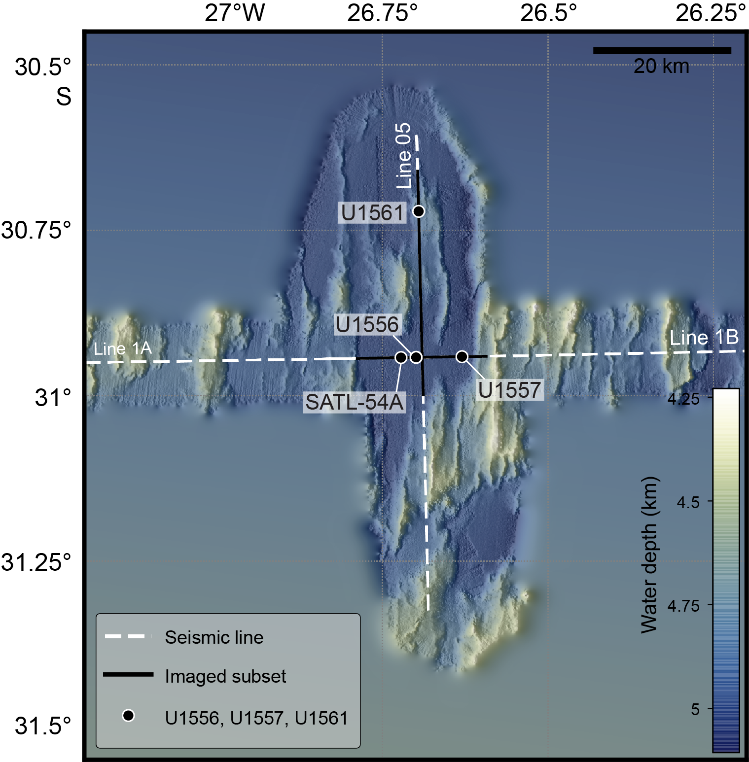
Figure F1. Bathymetric map.

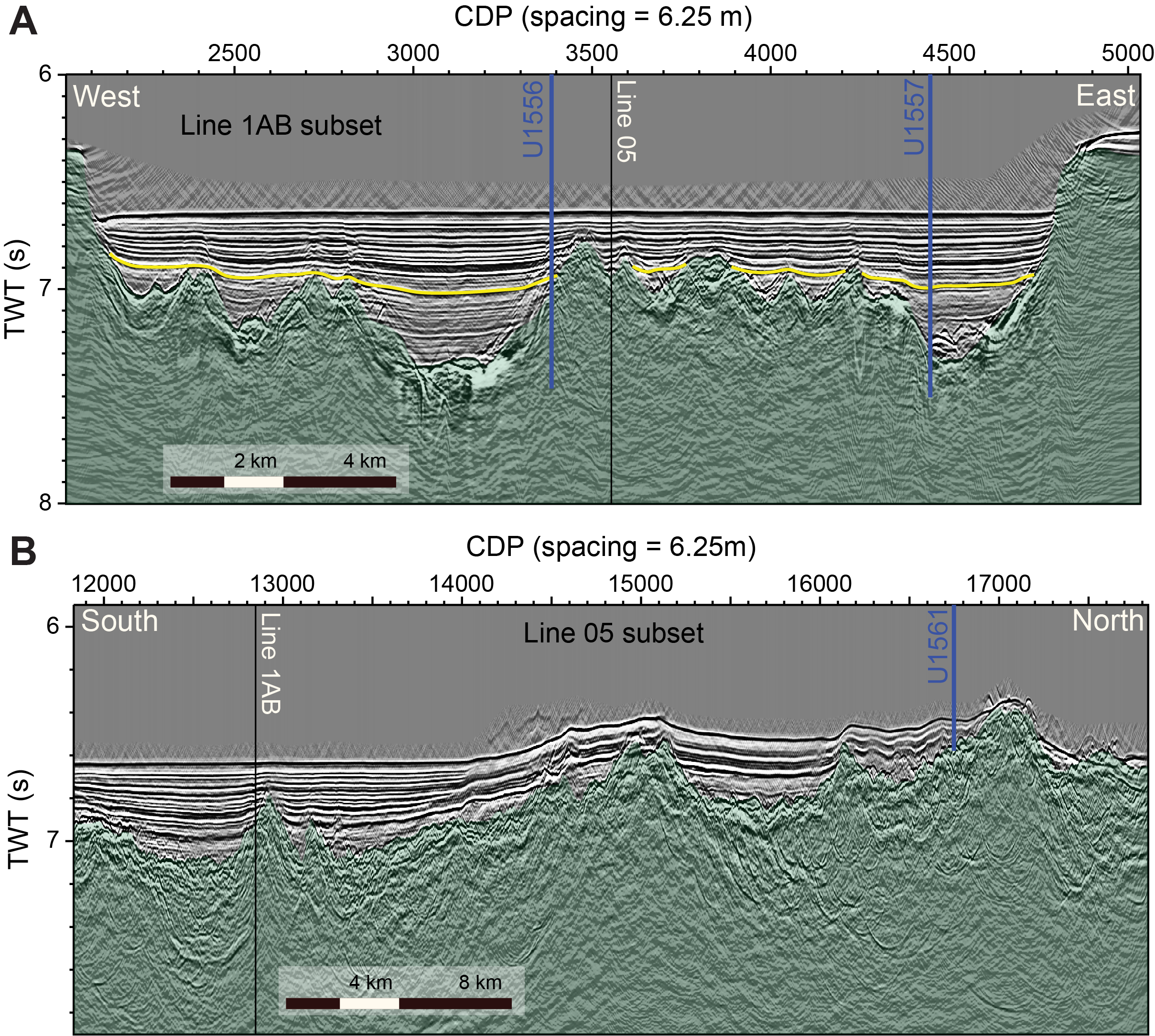
Figure F2. Seismic reflection profiles.

Site U1556 is located in the middle of a ~17.5 km wide basin that is filled with sediments to a uniform bathymetric level of ~5000 mbsl (Figure F1). The basin sits between two near north-south–trending, strongly faulted basement ridges that have steep flanks and very thin or no sediment cover (Figures F1, F2). Basement topography changes significantly within this basin resulting in large differences in sedimentary cover. Site U1556 is located on the western flank of a basement highpoint that has ~450 m relief above the deepest point of the basin (~565 m) (Figure F2A). This basement feature emerges to the north and particularly the south of Site U1556 as one of the many parallel north-south–trending ridges, as can be seen in the shallower bathymetric levels (Figure F1) and higher normalized reflectivities (Figure F3). The north–south crossing line does not pass over Site U1556 directly, but the site appears to be located at the lowest elevation of the north-south–trending basement ridge, which steadily shallows to the south and north, where it emerges with very little sediment cover just north of Site U1561 (Figure F2B).

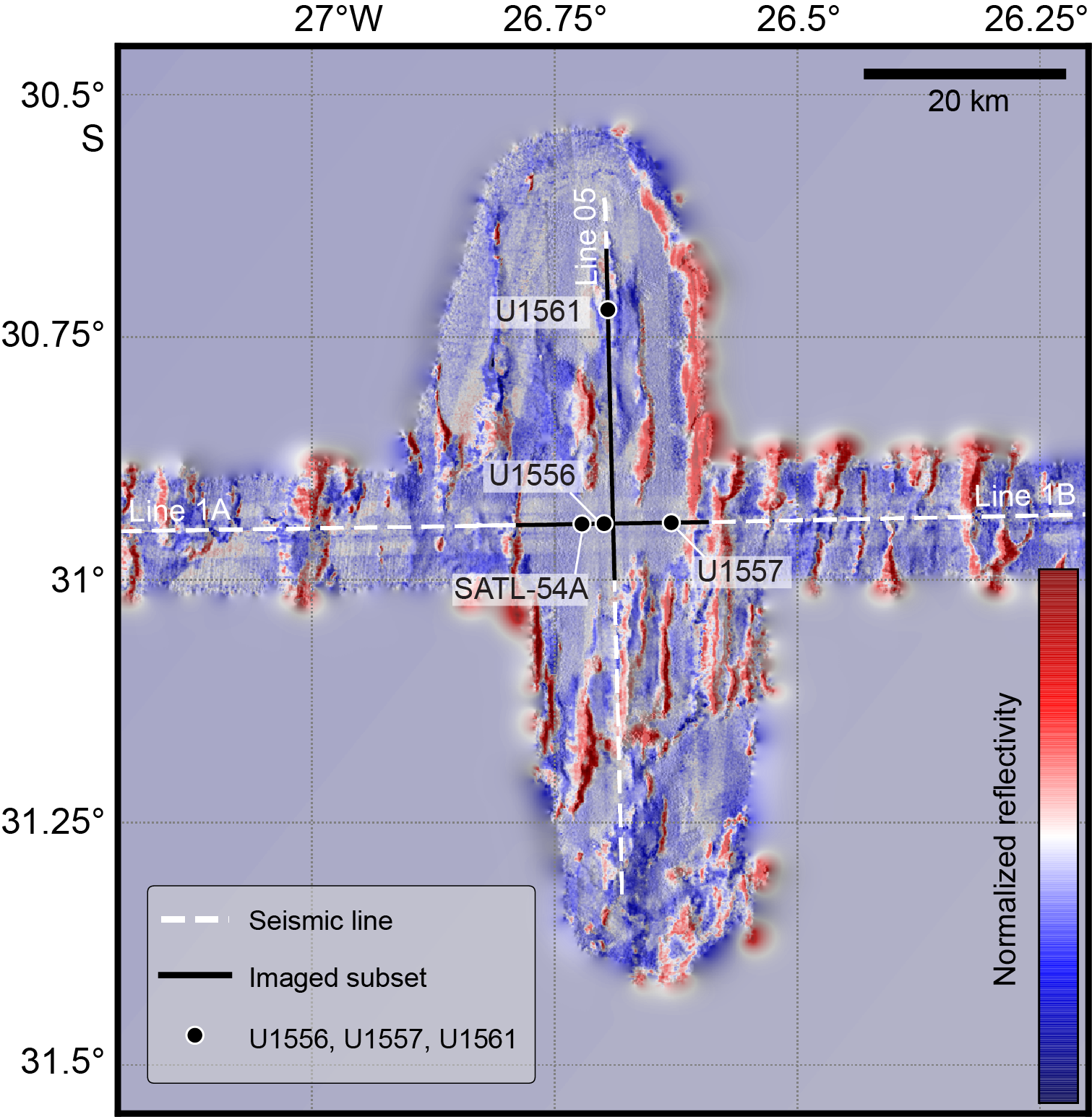
Figure F3. Backscatter reflections.

The ocean crust at Site U1556 has a sediment cover of 278 m, which is thicker than the global average overburden thickness for basement of this age (~200 m; Spinelli et al., 2004; see Figure F3 in the Expedition 390/393 summary chapter [Coggon et al., 2024d]). Sediment cover is also thicker than the reported mean sediment thickness encountered along CREST Seismic Lines 1B (48–63 Ma) and 1A (63–70 Ma) of 132 and 223 m, respectively (Estep et al., 2019). A recent sedimentation thickness global synthesis suggests though that ~60 Ma ocean crust should host around 460 m of sediment (cf. Olson et al., 2016), although there are very large ranges in global and regional estimates of sediment thickness with crustal age (e.g., ~560 m; Straume et al., 2019). Although the seafloor appears very flat near Site U1556, the basin-infilling sediments deeper in the subsurface, closer to the basement, are not draped flat across but instead follow the topography of the basement (Figure F2).

Backscatter reflections from multibeam profiles (Figure F3) reveal that a significant proportion of the seafloor in this basin near Site U1556 boasts continuous sediment cover, which is in contrast to other sites along the SAT. Therefore, ventilation of the volcanic rocks of the upper ocean crust through the ingress of seawater and egress of seawater-derived low-temperature hydrothermal fluids may be reduced compared to other sites. However, the relatively steep flanks of the faulted basement ridges and sometimes also crests of the Site U1556 region are unsedimented, as can be seen by the high normalized reflectivity (Figure F3) and may influence the local fluid flow system with consequent impacts on heat flow, sediment pore waters, basement hydrothermal alteration, and microbial communities in both the marine sediments and underlying basalts. Basement at Site U1556 was predicted to be ~61.2 Ma based on CREST site survey magnetic data (Kardell et al., 2019) and preliminary biostratigraphy analyses from Hole U1556A sampled during Expedition 390C.

Site U1556 was first occupied during engineering Expeditions 390C and 395E. Hole U1556A was cored using the advanced piston corer (APC) and extended core barrel (XCB) systems to a total depth of 283.8 meters below seafloor (mbsf), penetrating the entire sediment succession and ~5.8 m into basement (Figure F5; Table T1; see Table T2 in the Expedition 390/393 summary chapter [Coggon et al., 2024d]; Estes et al., 2021).

1.2. Objectives

The operational objectives at Site U1556 during Expedition 390 were to (1) core the entire sediment section and a few meters into basement with the APC/XCB system in Hole U1556C to collect material that addresses the paleoceanographic, paleoclimate, and microbiological objectives of the SAT expeditions; (2) core 250 m into basement with the rotary core barrel (RCB) system in Hole U1556B to collect material that addresses the petrologic, geochemical, and microbiological objectives of the SAT expeditions; and (3) collect a comprehensive suite of wireline geophysical logging data through the basement section.

2. Operations

Site U1556 was visited during engineering Expeditions 390C and 395E, as well as Expedition 390. Holes U1556A (Expedition 390C) and U1556C (Expedition 390) completed APC/XCB coring through the sediment cover to the basement interface. Hole U1556D was a missed mudline, and Hole U1556E recovered the top ~40 m of the sediment section using APC coring to improve microbiological and geochemical sampling. In Hole U1556B, a reentry system and casing installed during Expedition 395E allowed for reentry during Expedition 390 and a 342.2 m advance through basement to 633.2 mbsf. Unfortunately, subsidence of the reentry cone meant it was partly obscured by sediment, and this made reentries difficult. Therefore, Hole U1556B will not be a good legacy hole, so the decision was made to drop the second RCB drill bit deployed during coring in the bottom of the hole prior to logging to avoid the need for another reentry.

2.1. Expedition 390C Hole U1556A

Site U1556 was first visited during Expedition 390C, an engineering leg with the goal of coring a single hole with the APC and XCB systems to basement for gas safety monitoring and installing a reentry system with casing through sediment to ~5 m into basement in a second hole. Hole U1556A was cored to a total depth of 283.3 mbsf, and 243.78 m of sediment was recovered as well as the sediment/basement interface at 278.0 mbsf (86% recovery overall) (Table T1; Estes et al., 2021). The intention during Expedition 390C was to core to basement at adjacent Site U1557 and then return to Site U1556 to install a Dril-Quip reentry system and casing; however, failure of the subsea camera system prevented installation of the reentry system at Site U1556 during Expedition 390C. During subsequent Expedition 390C operations at Site U1558, we determined that the Dril-Quip reentry systems cannot be used to install casing and a reentry system into basement in a single step because the release mechanism on the running tool will not work with the casing shoe directly in basement at the hole bottom. Either a hydraulic release tool (HRT) reentry system must be used, or the hole must be first fully drilled out beyond the depth of the intended casing such that the Dril-Quip release mechanism will work. Dril-Quip systems are, in principle, advantageous because they allow future extensions of the casing, whereas the HRT is designed for only a single casing string.

2.2. Expedition 395E Hole U1556B

Engineering Expedition 395E returned to Site U1556 and installed an HRT reentry system with 284.2 m of 10¾ inch casing in Hole U1556B (Figure F4; Williams et al., 2021). The weight of the casing was lifted off the drill string at an apparent depth of 282.3 mbsf, indicating that the reentry cone base had landed on the seafloor at a shallower depth than expected. The subsea camera system observed the top of the reentry cone to be level with the seafloor, making the water depth 5001.8 mbsl and total hole depth 286.2 mbsf, extending 2 m beyond the casing shoe. Casing did not extend into basement in Hole U1556B because of thicker sediment resulting from either a shallower seafloor and/or deeper basement. The hole was reentered with a cementing bottom-hole assembly (BHA), but a circulation test determined that the formation had sealed around the casing and cementing was unnecessary.

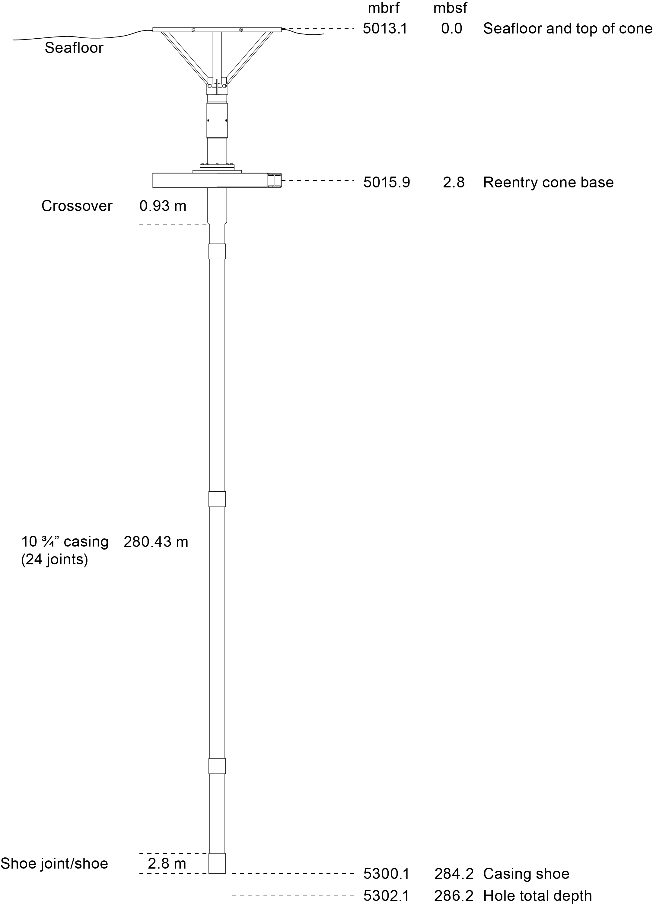
Figure F4. Reentry system, casing, and BHA.

2.3. Expedition 390 port call

Expedition 390 began in Repair Quay 3 in Cape Town, South Africa, at 1154 h on 7 April 2022. Because of the Coronavirus Disease 2019 (COVID-19) quarantine period in the hotel (7 days), the JOIDES Resolution Science Operator (JRSO) technical staff, crew, and scientists did not board the ship until 9 April. During the quarantine, Expedition 390 scientists received a virtual orientation to the ship and IODP procedures, including an operations overview, publication obligations, curation, laboratory safety, shipboard outreach, shipboard computing and software, and life at sea. Scientists gave presentations of their individual research objectives, began organizing research collaborations, and worked within their laboratory groups to develop shipboard sampling plans and begin writing drafts of their methods for the expedition.

Polymerase chain reaction (PCR) COVID-19 tests for boarding personnel were conducted on Days 4 and 6 of the hotel quarantine period. All members of the science party and staff tested negative and were cleared to board the vessel, except for four staff members whose quarantine was either delayed or prolonged. On 9 April, the outgoing staff and crew disembarked and the 40 oncoming scientists and staff boarded the vessel. The remaining staff boarded on 10 or 11 April. All personnel took a final PCR COVID-19 test on 10 April as well as a rapid antigen test on 11 April. All tests were negative.

Between 10 and 11 April, scientists received training in shipboard software including SampleMaster and DESClogik as well as a core flow tour. Training sessions were conducted in groups of 5 or 6 as part of the COVID-19 mitigation protocols. Laboratory group–specific training sessions and safety overviews occurred between 12 and 16 April, including physical properties instrumentation, microscopes, and use of the portable X-ray fluorescence (pXRF) scanner.

On the morning of 12 April, the pilot boarded at 0812 h, two harbor tugs arrived, and the mooring lines were released, with the last line released at 0836 h. The pilot departed the vessel at 0857 h at the pilot station, but three contractors remained on board to conduct testing and maintenance. Two of the contractors observed the function of the ship's uninterruptible power supply (UPS) system while under way. The other contractor inspected and adjusted the ship's magnetic compass. The contractors completed their work and disembarked at 1135 h. The vessel began sea passage at 1136 h.

2.4. Expedition 390 Hole U1556B

The research vessel (R/V) JOIDES Resolution completed its 2296 nmi voyage from Cape Town, South Africa, to Site U1556 on 20 April 2022, arriving at 2330 h. Overall, the vessel averaged 11.1 kt and took 8.6 days to complete the transit. After the vessel transitioned from cruise to dynamic positioning (DP) mode and lowered the thrusters, rig floor preparations for drilling began. The RCB BHA was made up with a C-4 bit for drilling in Hole U1556B. Pipe was tripped to 5011 meters below rig floor (mbrf), stopping twice to fill stands with seawater and the perfluorocarbon microbial contamination tracer (see Microbiology in the Expedition 390/393 methods chapter [Coggon et al., 2024c]), which was pumped continually with drilling fluid throughout coring in Hole U1556B. At 1930 h on 21 April, we deployed the subsea camera system to observe reentry into Hole U1556B. The reentry cone for Hole U1556B was spotted immediately, but the first reentry attempt stirred up sediment and obscured the cone's location. Repeated attempts were made, but the combination of stirred up sediment and weather conditions near the operational limit made reentry challenging. The cone appeared to be flush with the seafloor and was partially buried by resuspended sediment. Reentry was finally made at 0405 h on 22 April, and the subsea camera system was recovered at 0640 h. Pipe was tripped down the cased hole to 267.0 mbsf, the top drive was picked up and drilling knobbies put in, and the hole was washed down to 291.0 mbsf where the bit contacted a hard layer. This depth is deeper than the 286.2 mbsf hole bottom observed during Expedition 395E; whether this discrepancy is due to subsidence of the reentry system, tidal variation in water depth, or another factor remains undetermined.

The drilled interval from the seafloor to 291.0 mbsf was designated drilled interval 390C-U1556B-11. A nonmagnetic core barrel and liner was pumped down, and RCB coring began at 1052 h. Core 2R advanced 9.3 m to 300.3 mbsf and recovered 1.64 m (18%). The decision was made to drill half-length cores to improve recovery and reduce the time on bit per core. The ship was experiencing heave that made drilling difficult, and the rate of penetration was slow (<3 m/h for Cores 2R and 3R); both factors limited our ability to drill and achieve good recovery of full-length cores. Coring continued smoothly through Core 28R, achieving a penetration depth of 475.6 mbsf. At this point, the RCB bit had 61.0 h of drill time on it and the decision was made to pull out of the hole, change the bit, and reenter. After tripping pipe with the BHA and RCB bit back to the surface, a new C-4 bit with a mechanical bit release (MBR) was installed on the outer core barrel and all parts were inspected. Pipe was tripped to 4952 mbrf, stopping twice to fill stands with seawater and microbial contamination tracer. The subsea camera system was deployed to guide reentry into Hole U1556B. We achieved reentry at 0625 h on 28 April and recovered the subsea camera system through the moonpool.

Coring resumed in Hole U1556B with the recovery of Core 29R, which advanced 8.6 m and recovered 5.61 m (65%). Because of low penetration rates (<3 m/h), the decision was made to take half-length cores through Core 33R. Core 34R advanced a full 9.7 m after penetration rates increased and recovered 6.82 m of material (70%). However, the core catchers were missing teeth, and there were gaps in the core liner. During coring of Core 35R, we experienced high pump pressures (>2400 pounds per square inch [psi]); therefore, the core barrel was retrieved so that we could attempt to restore circulation. The deplugger tool was deployed, and several mud sweeps were run, which successfully returned circulating pressure to normal coring values. The decision was made to only make half-length advances for the rest of the hole to both improve recovery and prevent further damage to the RCB system. Mud sweeps were conducted following every core. During initial drilling of Core 51R, we again experienced high pump pressures (>2000 psi) and recovered the core barrel. Circulating pressure returned to normal after additional mud sweeps and running the deplugger tool. Core 59R was the last core for the hole, and it arrived on deck at 1505 h on 4 May. Given the subsidence of the reentry cone below the seafloor, there were concerns both that a further reentry to conduct wireline logging would be challenging and regarding the viability of Hole U1556B as a legacy hole. Consequently, the RCB bit, having completed 78 h of drill time without failure, was dropped at the bottom of the hole using the MBR system. We then began pulling out of the hole, setting pipe depth to 41 mbsf to prepare for logging operations.

To assist with logging, the hole was cleaned by pumping twice the hole's volume of seawater. The triple combo logging tool string, including tools for measuring formation density, resistivity, and magnetic susceptibility, was lowered until it tagged the hole bottom. The calipers were opened, and the first upward pass started. Tool string telemetry failed after only a few meters of logging, and the string was pulled back to the surface and recovered at 0815 h on 5 May. The Hostile Environment Natural Gamma Ray Sonde (HNGS) was identified as the issue, and a spare tool was substituted into the string. The second attempt at logging was successful, with two passes of the triple combo string completed before pulling it back to surface. The second tool string run contained the Ultrasonic Borehole Imager (UBI) and Accelerator Porosity Sonde (APS). The tool string was lowered to 622 mbsf, with the UBI sensor manually rotated to the "measurement" position, facing outward toward the formation, to avoid possibly fouling and jamming the sensor closed in the open hole. The upward pass generated high-quality data. The tool string was recovered at 0605 h on 6 May, and the final logging tool string, the Formation MicroScanner (FMS), was lowered until it tagged the hole bottom. The string logged two upward passes and reached the surface for recovery at 1710 h. The rig floor was cleared of logging equipment, and pipe was tripped back toward the surface. The seafloor was cleared at 1830 h. With the drill string at 2200 mbrf, the ship was repositioned 30 m south of Hole U1556B to prepare for drilling Hole U1556C.

Hole U1556B officially ended when the BHA and MBR were recovered on the rig floor at 0405 h on 7 May. RCB drilling in Hole U1556B advanced 342.2 m to 633.2 mbsf and recovered 191.87 m of basement material (56%). A total of 16.2 days of operational time was used for Hole U1556B.

2.5. Expedition 390 Hole U1556C

For sediment coring in Hole U1556C, the ship moved 30 m south of Hole U1556B (Figure F5) and the drill string with an APC/XCB BHA was tripped toward the seafloor and then spaced out to a shot depth of 5012.5 mbrf. For the first core in Hole U1556C, a target shot depth 5 m above the predicted seafloor depth was selected to attempt to recover material across core breaks and core gaps present in Hole U1556A. Core 390-U1556C-1H recovered 7.61 m of sediment as well as the mudline. The core was received on deck at 2315 h on 7 May 2022. It was significantly disturbed, so seafloor depth was assumed to be 5005.7 mbsl, offset from Hole U1556A instead of calculated from recovery. Following Core 5H, the decision was made to pull back 3 m before the next core to improve the splice for Site U1556 (see Physical properties and downhole measurements). This pullback resulted in several meters of heavily disturbed fall-in deposits in the upper 2.8 m of Core 6H (see Sedimentology) and failed to increase the offset to the desired amount. A second, successful attempt to increase the offset was made by pulling the bit back 4 m when shooting Core 9H, resulting in a short 5 m advance, again overlain by 2.7 m of fall-in debris. Coring continued smoothly through Core 11H. Cores 12H–15H were partial strokes but had full or nearly full recoveries. Cores 13H–16H required overpull forces of 10,000–20,000 lb; we switched to XCB coring following Core 16H. Core 30X penetrated to 276.3 mbsf and recovered basalt fragments in the core catcher. Two additional 2 m advances were made to capture the sediment/basement interface (Cores 31X and 32X) using the XCB system with a polycrystalline diamond compact (PDC) cutting shoe. The PDC cutting shoe was shown during Expedition 390C to provide high-recovery cores across the sediment/basement interface.

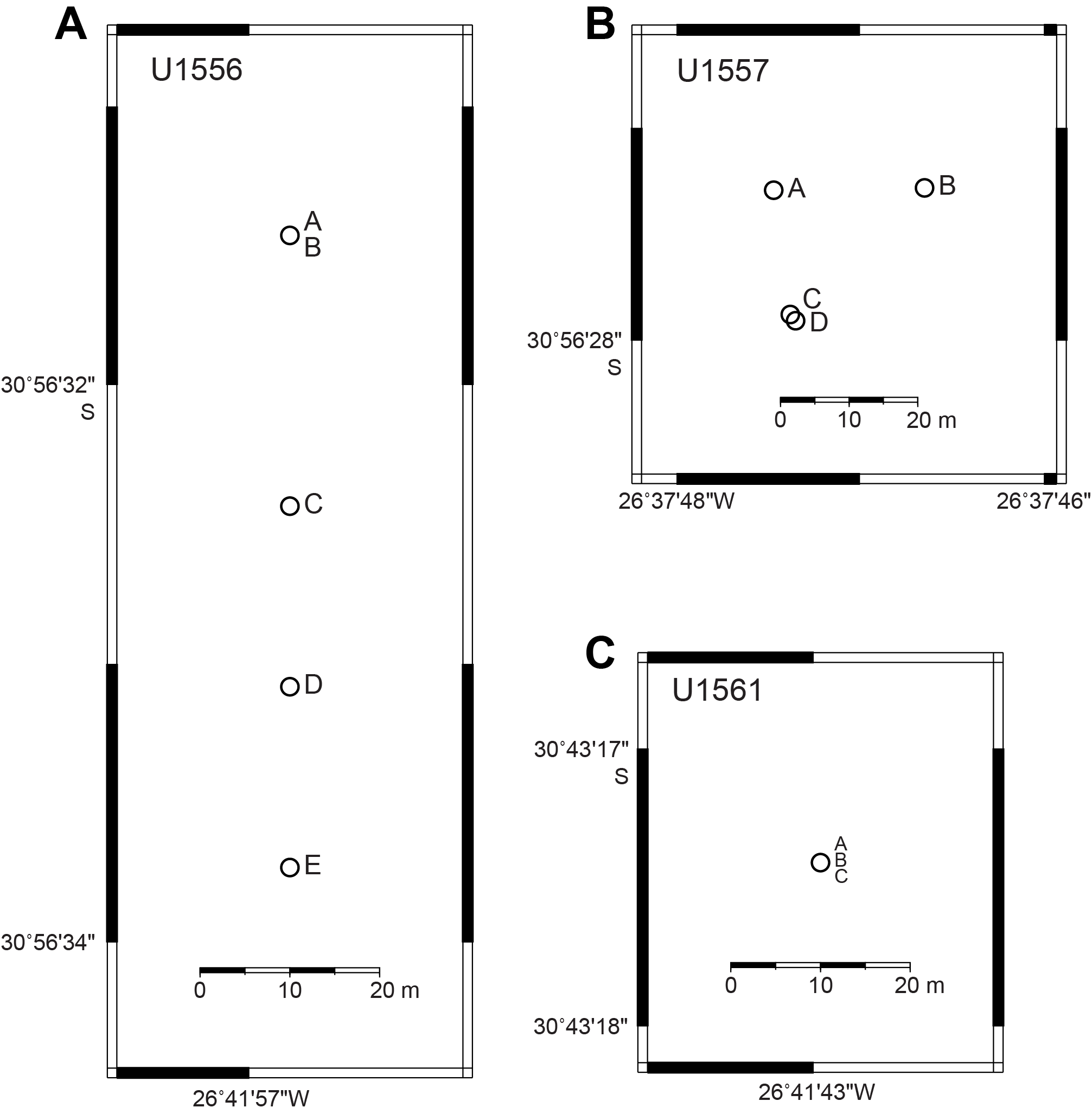
Figure F5. Map of holes drilled.

APC cores (390-U1556C-1H through 16H) were collected using nonmagnetic core barrels and oriented for paleomagnetic research using the Icefield MI-5 core orientation tools. Advanced piston corer temperature (APCT-3) tool temperature measurements were made on Cores 4H, 7H, 10H, and 13H. Overall, Cores 1H–30X penetrated to 276.3 mbsf and recovered 281.74 m of sediment (102%). Cores 31X and 32X advanced another 4 m to 280.3 mbsf, recovering 2.07 m (52%). Core 32X had 77% recovery. Hole U1556C officially ended at 1920 h on 10 May when the bit cleared the seafloor; it took 3.6 days of operational time.

2.6. Expedition 390 Hole U1556D

Coring Hole U1556D was motivated by the severe disturbance observed in the upper cores collected from Hole U1556C. Because microbiology and geochemistry are primary expedition objectives, capturing undisturbed cores across a chemically important zone—the sediment/water interface—was considered to be critical. Additional coring also contributed to the paleoceanographic splice. For Hole U1556D, the vessel moved another 20 m south (Figure F5) and the bit was spaced out to a shot depth of 5015.0 mbrf. The hole was spudded at 2120 h on 10 May 2022 and returned a core barrel with 9.67 m of sediment and no definitive mudline. The decision was made to terminate the hole. Hole U1556D took 0.1 day of operational time.

2.7. Expedition 390 Hole U1556E

Hole U1556E is located 20 m south of Hole U1556D (Figure F5). The hole was spudded at 2300 h on 10 May 2022 from a shot depth of 5010.0 mbrf; Core 390-U1556E-1H recovered 5.12 m of sediment and the mudline, establishing a water depth of 5003.1 mbsl. Coring in Hole U1556E continued through Core 5H, achieving a final hole depth of 43.1 mbsf and recovering 43.33 m (100.5%). Cores from Hole U1556E were not oriented, and no temperature measurements were made. The bit cleared the seafloor following completion of Hole U1556E at 0610 h on 11 May. We began tripping drill pipe toward the surface while moving the vessel in DP mode to Site U1557 at a speed of 0.5 kt. Hole U1556E used 0.8 day of operational time.

3. Stratigraphic unit summary

The cores recovered at Site U1556 comprise 2 sedimentary units overlying 13 basement units identified on the basis of macro- and microscopic visual observations combined with mineralogical analyses by X-ray diffraction (XRD), spectral color analyses, and magnetic susceptibility (MS) data. The units are numbered from the top of the hole, with units in the sedimentary section designated by Roman numerals (e.g., I and II) and basement units designated by Arabic numerals (e.g., 1 and 2); subunits are designated with letters (e.g., IA, IIB, 2a, and 2b).

3.1. Sedimentary units

A mixture of biogenic and siliciclastic sediments were recovered from the five holes cored at Site U1556. Biogenic sediments consist primarily of calcareous nannofossil ooze that is lithified to chalk in the lower portion of the sediment section. Variable but minor amounts of foraminifera are present throughout. Intervals with siliciclastic sediments consist of silty clays with variable carbonate content. Two lithologic units (I and II) are defined (Figure F6; Table T2). Unit I is composed of >235 m of upper Oligocene to Pleistocene sediments that are mainly silty clay and calcareous nannofossil ooze. Unit I is divided into five subunits (IA–IE; see Sedimentology). Unit II is composed of ~42 m of Paleocene or Eocene sediments that are predominantly nannofossil-rich calcareous chalk or calcareous nannofossil chalk.

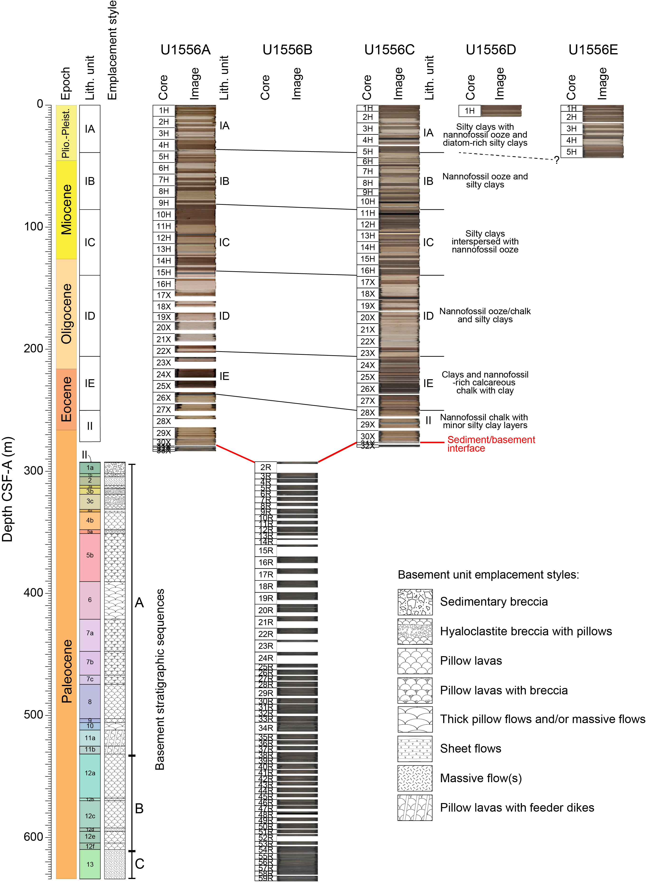
Figure F6. Stratigraphic unit summary.

3.2. Basement units

Hole U1556B penetrated the sediment/basement interface at 291 mbsf, below which 342.3 m of volcanic rock was cored. The volcanic sequence consists predominantly of pillow lavas with thin intervals of either more massive lava flows or larger pillows, all punctuated by periodic occurrences of breccias. The volcanic sequence was divided into 13 lithologic units based on changes in petrographic type and phenocryst assemblage (Table T4). The lithologic units were grouped into three overarching stratigraphic sequences (A–C) based on differences in magma composition inferred from petrographic observations and subsequently confirmed by geochemical analyses, the geometry of lava flows, and their intrusive relationships (see Igneous petrology and Geochemistry).

The uppermost volcanic basement and the top of Stratigraphic Sequence A comprise sedimentary breccia (Lithologic Unit 1) that likely represents talus deposits of volcaniclastic debris transported downslope. Beneath this is a series of sparsely to moderately olivine phyric basalt pillow lava flows intercalated with volcanic breccias in Units 2–11. The breccias contain clasts of chilled pillow margins and altered glass. The proportions of sedimentary matrix and carbonate cement vary significantly between breccia units. Unit 11 records intrusive relationships between the lavas of Stratigraphic Sequences A and B. Unit 12 (Stratigraphic Sequence B) consists of a series of aphyric to very sparsely olivine (micro)phyric basalts that are highly altered; this unit is divided into six subunits. Unit 13 (Stratigraphic Sequence C) is a highly plagioclase-olivine-clinopyroxene phyric (H-POPP) basalt that contains cognate inclusions interpreted to be cumulates formed in a magma chamber.

3.3. Sediment/basement interface

The sediment/basement interface was recovered in Holes U1556A–U1556C. In all three holes, the interface comprises basalt cobbles in unlithified sediment at the top of transitional Unit 1, which is sedimentary breccia with volcaniclastic clasts in an indurated calcareous sediment matrix. The indurated calcareous sediment likely formed from foraminifera-bearing nannofossil chalk lithified through circulation of hydrothermal fluids combined with burial diagenesis. In Holes U1556B and U1556C, sediments overlying and intercalated with the uppermost volcanic rocks (i.e., from the base of Unit II and the top of Unit 1) contain a middle Paleocene assemblage of calcareous nannoplankton and planktic foraminifera.

3.3.1. Sediment/basement interface depth

In each hole, we defined the sediment/basement interface as the curated depth of the top of the shallowest occurrence of basalt. The depth of the sediment/basement interface varies by ~16 m between Holes U1556A, U1556B, and U1556C, in which it occurs at 278.32, 291.29, and 275.74 mbsf, respectively. These differences in the basement depth are not just an artifact of the curatorial process in intervals of incomplete recovery, by which recovered material is assigned to the top of a cored interval (see Curatorial core procedures and sampling depth calculations in the Expedition 390/393 methods chapter [Coggon et al., 2024c]). Its shallowest occurrence at Site U1556 is in the core catcher of Core 390-U1556C-32X, which had 100% recovery. Hence, its depth in Hole U1556C is well constrained. In contrast, the cores in which the interface was recovered in Holes U1556A and U1556B had incomplete recovery, and the curated depths of the top of the shallowest occurrence of basalt in these cores provide minimum estimates of the depth of the sediment/basement interface in these holes. For Hole U1556B, however, the estimate is in good agreement with the depth of the sediment/basement interface based on downhole logging data (~292 wireline log matched depth below seafloor [WMSF]) (see Physical properties and downhole measurements) and drilling parameters (see Operations).

Differences in basement depth are likely attributable to basement topography and hence different sediment thicknesses, but they may also be due to differences in seafloor topography. For stratigraphic correlation between SAT sites and with other sections of upper ocean crust recovered by scientific ocean drilling, we have defined a site basement/sediment interface depth for each of the SAT sites. For consistency, this is taken as the curated depth of the top of the shallowest occurrence of basalt in the hole with the greatest basement penetration at each site. The Site U1556 sediment/basement interface depth is therefore defined as 291.29 mbsf based on the first occurrence of basalt in Hole U1556B.

4. Sedimentology

Five holes were cored at Site U1556: two were cored to basement (Holes U1556A and U1556C; ~275 m), two recovered only the uppermost sediments (Holes U1556D [~10 m] and U1556E [~43 m]), and one collected the lowermost sediments (Hole U1556B; ~30 cm) above the sediment/basement interface (Lithologic Unit 1; see Igneous petrology). The sedimentary lithologies recovered at Site U1556 are a mix of biogenic (mainly calcareous nannofossils with a variable abundance of foraminifera) and siliciclastic sediments (mainly silty clays) (Figures F7, F8, F9). The sediment color primarily reflects its lithologic characteristics; sediments composed mainly of nannofossil and calcareous ooze are generally pinkish white, whereas silty clays range from brown/dark brown where carbonate is absent to reddish brown where carbonate content is higher (Figure F13). Hole U1556A was cored during Expedition 390C, but it was described during Expedition 390 (see Background and objectives). We observed some differences between colors on the digital color images (obtained using the Section Half Imaging Logger during Expedition 390C; see Physical properties and downhole measurements in the Expedition 390/393 methods chapter [Coggon et al., 2024c]) and in visual core descriptions (see Core descriptions) during Expedition 390, likely reflecting changes such as postcoring drying and/or oxidation of the sediments.

Smear slides (Figure F10) and XRD (Figures F11, F12; Table T3) were used to confirm lithologic composition. In general, the alternations between nannofossil ooze/chalk and silty clays are well correlated with MS and the luminosity (L*) color reflectance parameter, as well as with natural gamma radiation (NGR) (see Physical properties and downhole measurements; Figure F7). The bioturbation index varies from absent to heavy in the Site U1556 cores, but it is typically sparse throughout the site, most commonly observed at lithologic contacts (see Sedimentology in the Expedition 390/393 methods chapter [Coggon et al., 2024c]).

Two main sedimentary lithologic units (I and II) and five subunits (all in Unit I) were defined at Site U1556 based on a combination of visual observations of sedimentologic characteristics (color, sedimentary structures, bioturbation, and general appearance), microscopic examination of smear slides, and bulk mineralogical analysis using XRD (see Sedimentology in the Expedition 390/393 methods chapter [Coggon et al., 2024c]) integrated with MS and color spectral observations (see Physical properties and downhole measurements in the Expedition 390/393 methods chapter [Coggon et al., 2024c]). Ages were assigned to each subunit based on biostratigraphic datums (see Age model and mass accumulation rates). In the following unit descriptions, the interval describes the core interval in which the unit was observed, depth is the curated depths (on the core depth below seafloor, Method B [CSF-B], scale) of the top and bottom boundaries of the unit/subunit, and thickness is the distance between these boundaries in each hole.

4.1. Unit descriptions

4.1.1. Unit I

Intervals: 390C-U1556A-1H-1, 0 cm, to 26X-2, 6 cm; 390-U1556C-1H-1, 0 cm, to 28X-2, 143.5 cm; 390-U1556D-1H-1, 0 cm, to 1H-CC, 5 cm; 390-U1556E-1H-1, 0 cm, to 5H-CC, 13 cm
Depths: Hole U1556A = 0–236.76 m CSF-B; Hole U1556C = 0–250.12 m CSF-B; Hole U1556D = 0–9.62 m CSF-B (unit bottom boundary not reached); Hole U1556E = 0–43.38 m CSF-B (unit bottom boundary not reached)
Thickness: Hole U1556A = 236.76 m; Hole U1556C = 250.12 m (244.76 m excluding intervals of major drilling disturbance); Hole U1556D = 9.62 m; Hole U1556E = 43.68 m
Age: early Eocene to recent
Lithology: silty clay, calcareous nannofossil ooze

Unit I is composed of >235 m of lower Eocene to Pleistocene silty clay and calcareous nannofossil ooze (Figures F7, F8, F9). The unit is divided into five subunits based on alternations between biogenic carbonates (mostly nannofossil ooze) and siliciclastic sediments (silty clays). In detail, the top of Unit I comprises ~37 m of Pliocene–Pleistocene brown silty clays with pinkish white nannofossil ooze intervals and distinct diatom-rich layers (Subunit IA). Distinct diatom-rich intervals within pale yellow clay were observed exclusively in this subunit (Cores 390C-U1556A-1H and 390-U1556C-1H). Core 390-U1556C-2H has a relatively high abundance of foraminifera (Figure F10) compared to the rest of Subunit IA. Below Subunit IA, nannofossil oozes are more common but have a different color (light gray), defining Subunit IB (~37–83 m CSF-B; Late Miocene–Pliocene). Two relatively thick intervals (>10 m) composed of dark brown clays that bookend a sequence of alternating pinkish gray nannofossil ooze and brown silty clays characterize most of the Miocene sediments (Subunit IC; ~83–137 m CSF-B). Below Subunit IC, a thick (~65 m) sequence of pinkish white nannofossil ooze interrupted by rare reddish brown silty clay intervals (1–2 m thick) represents most of the Oligocene and late Eocene (Subunit ID; ~137–200 m CSF-B). The color (see Core descriptions) and mineralogy of Subunit ID (Figures F11, F12) suggest a marly composition of the two major lithologies described in Unit I. Dark brown to black silty clays and brown clayey nannofossil ooze occur at the bottom of Unit I (Subunit IE; ~200–240 m CSF-B).

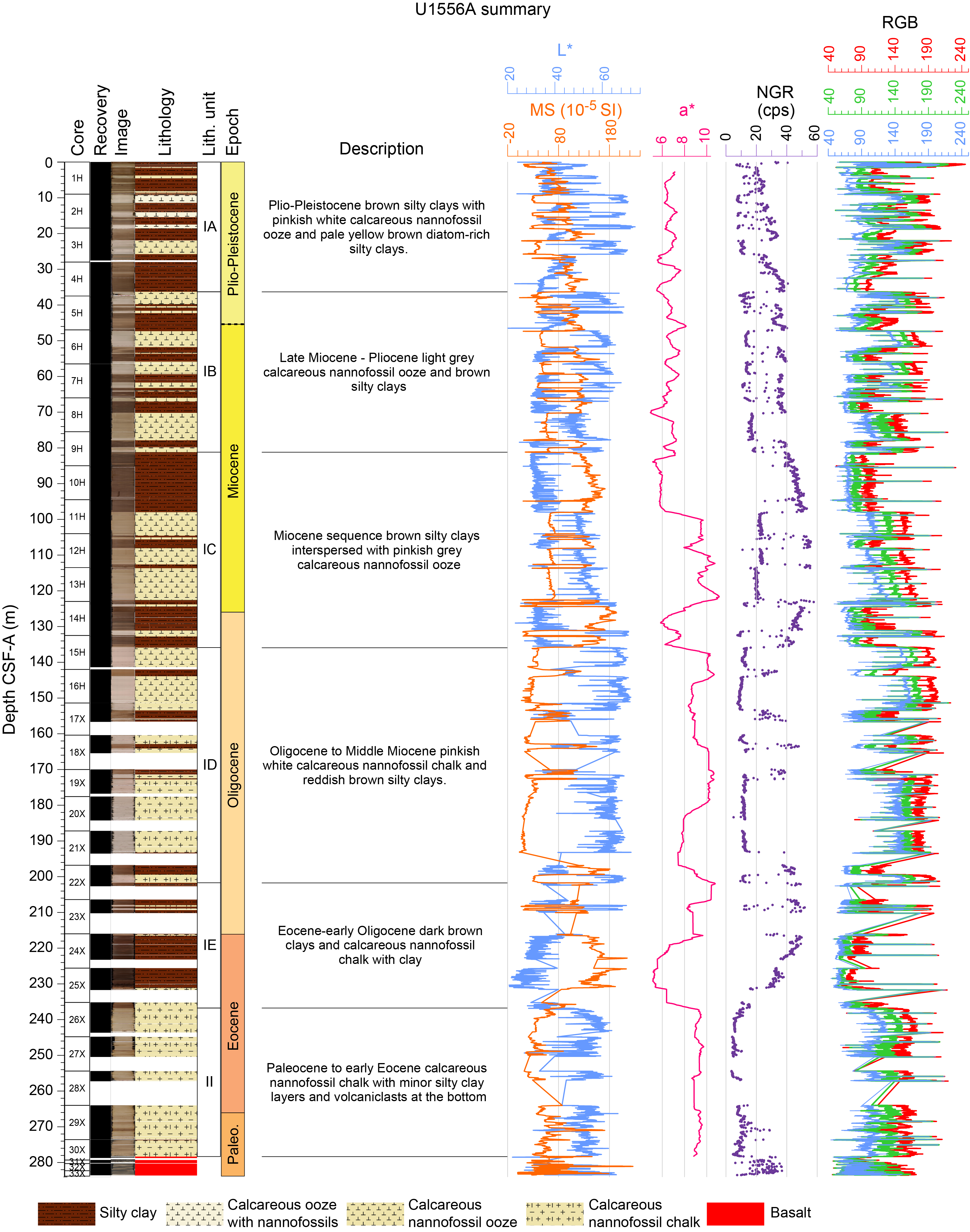
Figure F7. Lithologic summary, Hole U1556A.

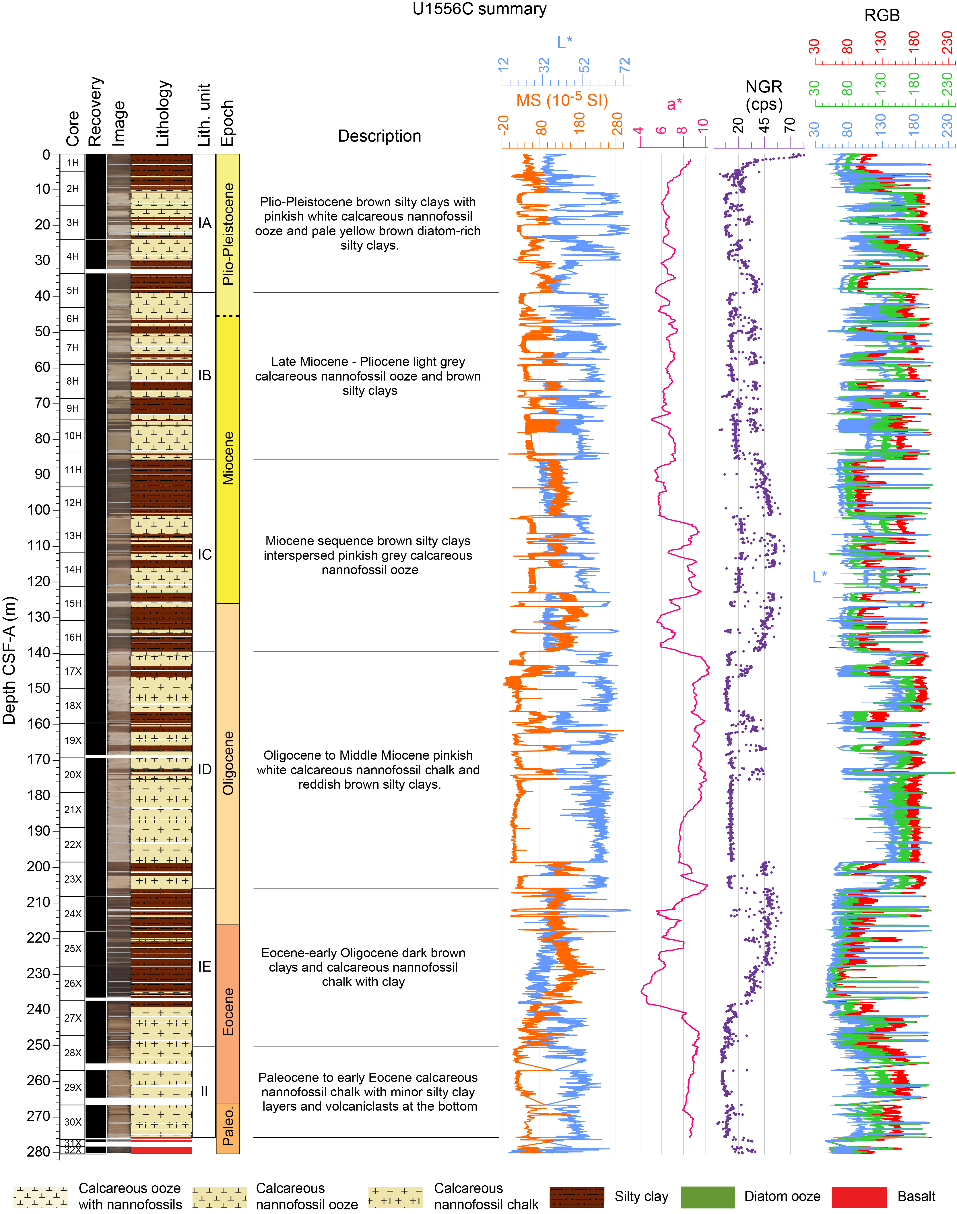
Figure F8. Lithologic summary, Hole U1556C.

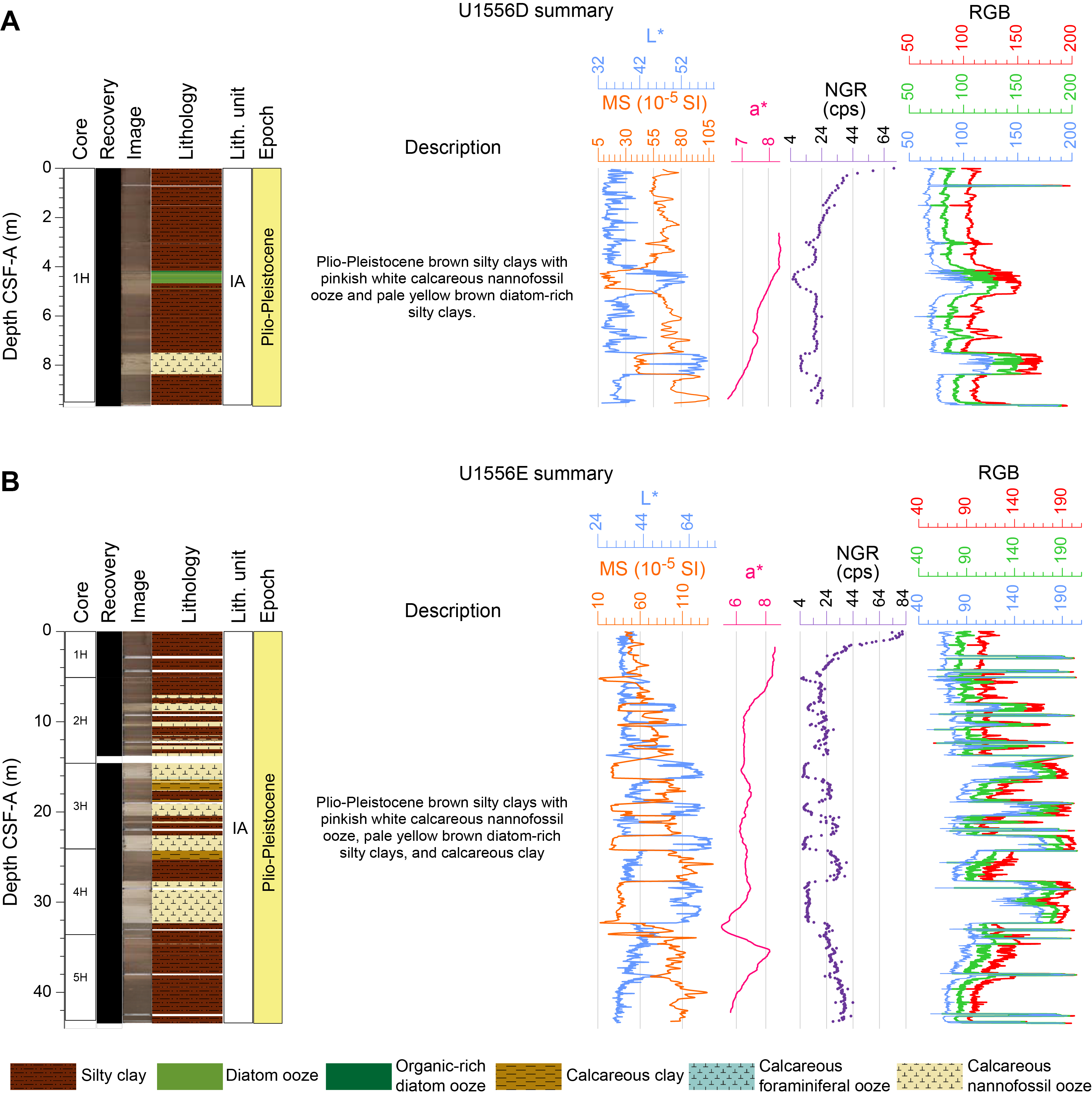
Figure F9. Lithologic summary, Holes U1556D and U1556E.

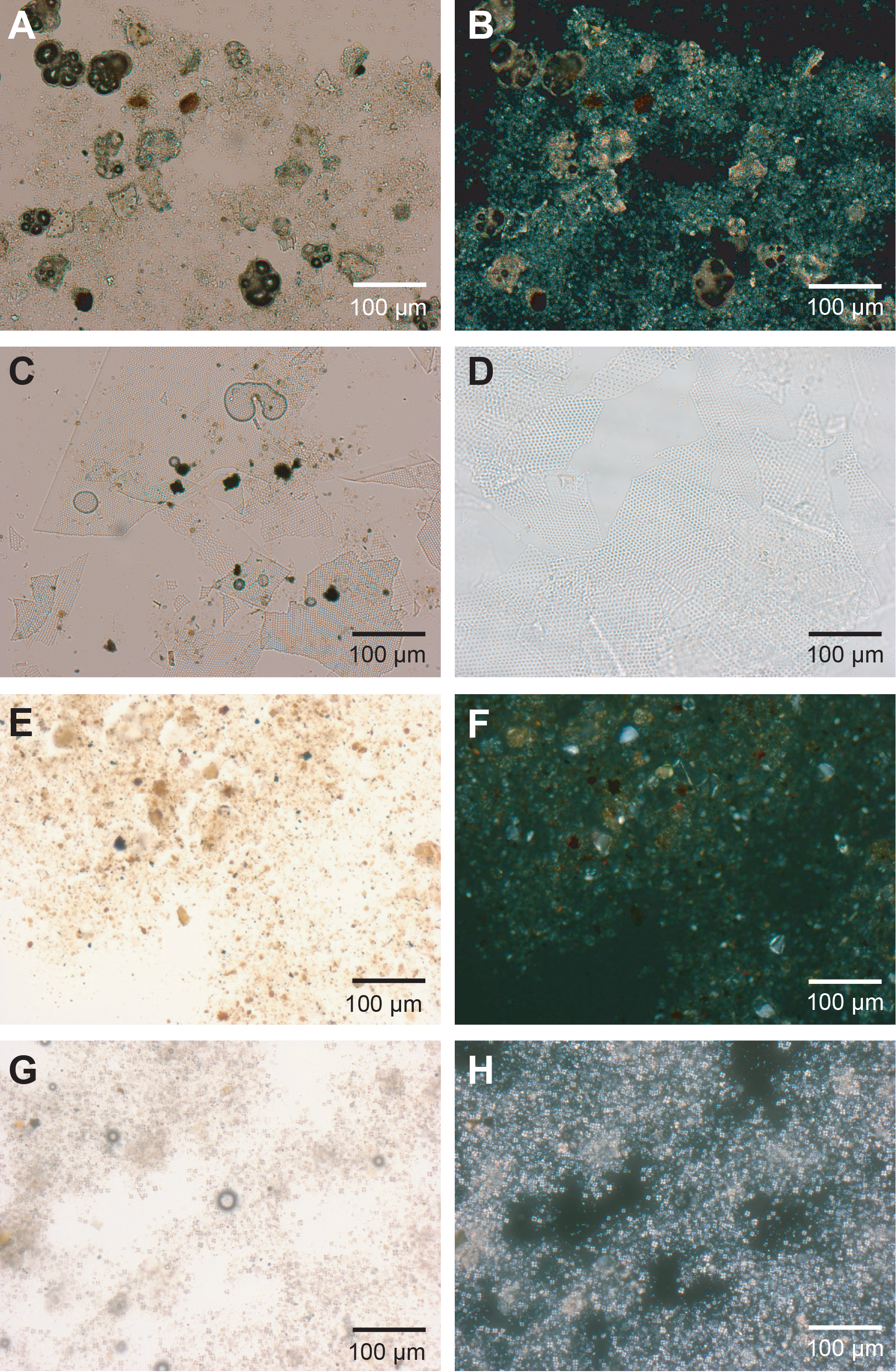
Figure F10. Main sedimentary components.

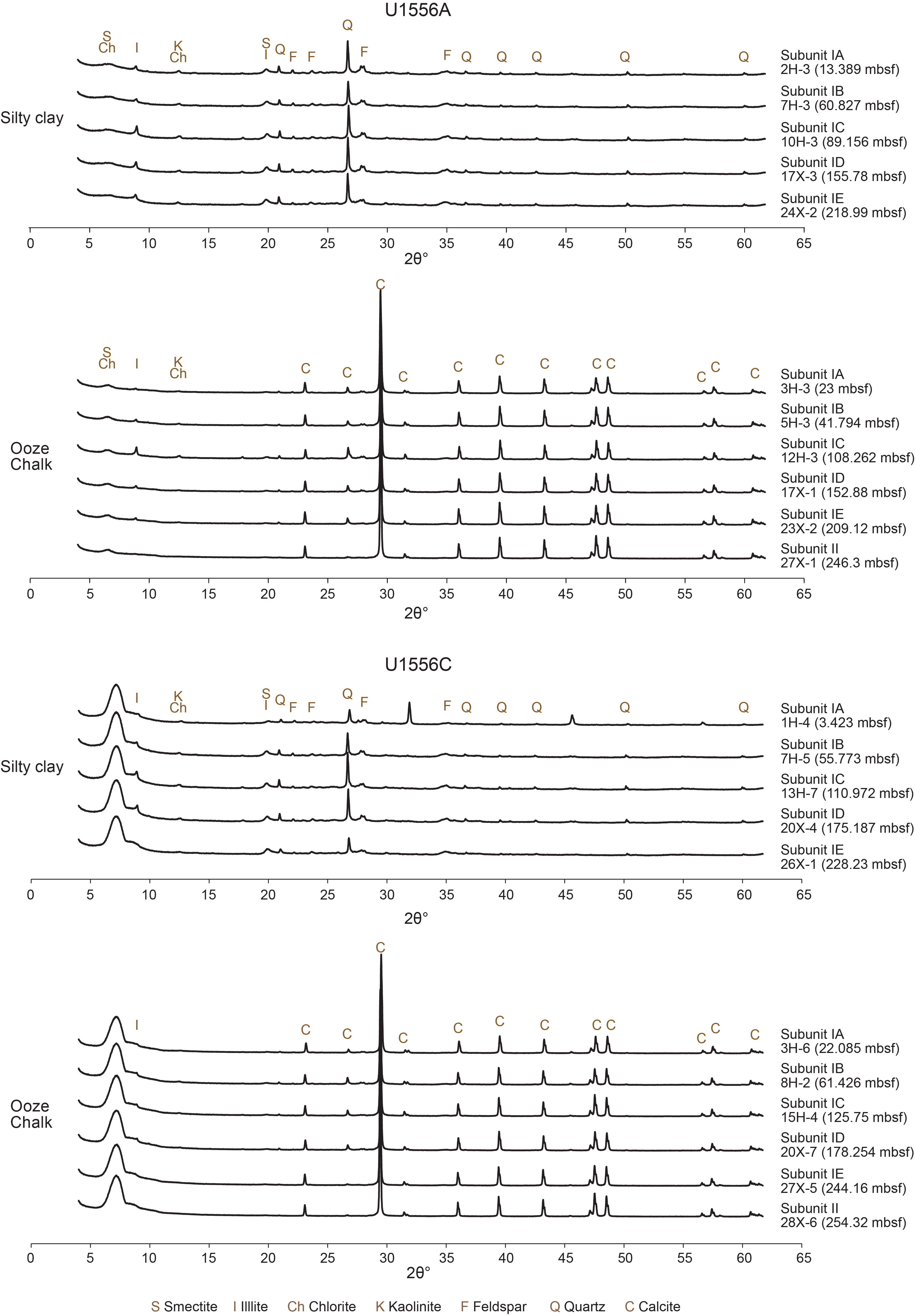
Figure F11. X-ray diffractograms, Holes U1556A and U1556C.

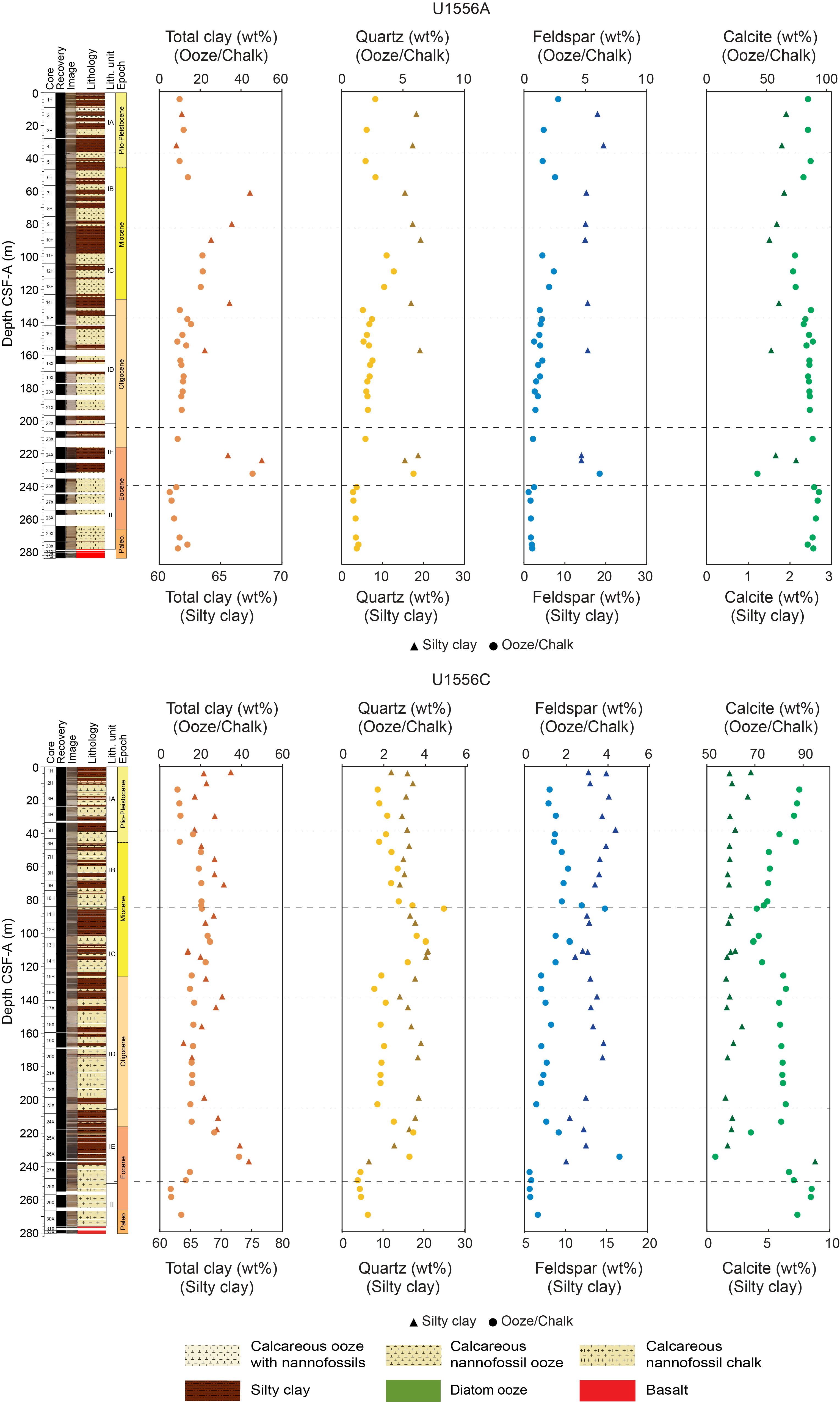
Figure F12. Changes in mineralogy, Holes U1556A and U1556C.

4.1.1.1. Subunit IA

Intervals: 390C-U1556A-1H-1, 0 cm, to 4H-6, 88 cm; 390-U1556C-1H-1, 0 cm, to 5H-4, 87 cm; 390-U1556D-1H-1, 0 cm, to 1H-CC, 5 cm; 390-U1556E-1H-1, 0 cm, to 5H-CC, 13 cm
Depths: Hole U1556A = 0–36.31 m CSF-B; Hole U1556C = 0–38.85 m CSF-B; Hole U1556D = 0–9.62 m CSF-B; Hole U1556E = 0–43.38 m CSF-B
Thickness: Hole U1556A = 36.31 m; Hole U1556C = 38.85 m; Hole U1556D = 9.62 m; Hole U1556E = 43.38 m
Age: Pliocene–Pleistocene
Lithology: silty clays, nannofossil calcareous ooze, diatom-rich silty clays

Subunit IA is mostly composed of brown silty clay interrupted by minor pinkish white calcareous nannofossil ooze intervals (~1 m average thickness). Organic-rich clays and light greenish gray diatom ooze layers within pale yellow brown clays occur in Cores 390C-U1556A-1H and 390-U1556C-1H (Figure F13). Smear slides (Figure F10) show that organic matter is associated with broken diatom frustules. The bioturbation index is absent to moderate in Subunit IA. Most of the lithologic contacts in Subunit IA are gradational or bioturbated.

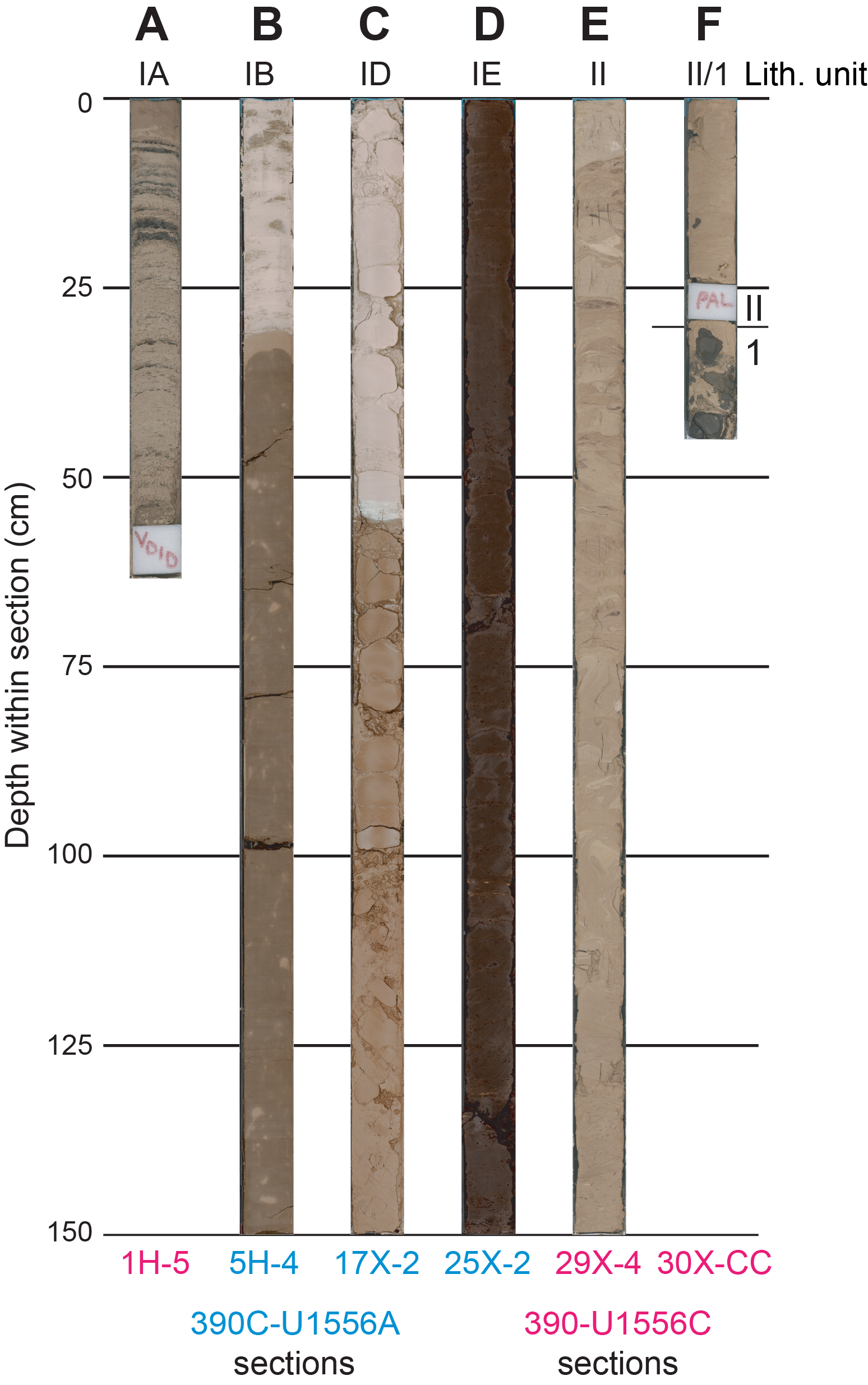
Figure F13. Core sections.

The Subunit IA/IB boundary is located at Sections 390C-U1556A-4H-6, 88 cm (36.31 m CSF-B), and 390-U1556C-5H-4, 87 cm (38.85 m CSF-B). The boundary is defined by a sharp transition between a ~10 m thick interval of brown silty clay (above) and light gray calcareous nannofossil ooze (below), distinct from the pinkish white calcareous nannofossil ooze observed in Cores 390C-U1556A-1H through 4H and 390-U1556C-1H through 5H. Holes U1556D and U1556E did not penetrate deeply enough to recover the Subunit IA/IB boundary.

4.1.1.2. Subunit IB

Intervals: 390C-U1556A-4H-6, 88 cm, to 9H-4, 135.5 cm; 390-U1556C-5H-4, 87 cm, to 11H-2, 23 cm
Depths: Hole U1556A = 36.31–81.19 m CSF-B; Hole U1556C = 38.85–85.53 m CSF-B
Thickness: Hole U1556A = 44.88 m; Hole U1556C = 46.68 m (41.32 m excluding intervals of major drilling disturbance in Cores 6H and 9H)
Age: Late Miocene–Pliocene
Lithology: calcareous nannofossil ooze, silty clay

Subunit IB is mostly composed of light gray/pinkish white calcareous nannofossil ooze alternating with brown silty clay intervals (Figure F13). Occasional thin organic-rich laminations occur throughout Subunit IB (Cores 390C-U1556A-5H and 390-U1556C-6H). Two foraminiferal ooze layers (<2 cm) were observed in this subunit (55.57–55.59 and 63.13–63.14 m CSF-B) in Hole U1556C. Bioturbation is generally sparse throughout Subunit IB. The lithologic contacts are mostly planar or gradational. In Hole U1556C, two intervals of severe drilling disturbance (fall-in) (~43 to ~46 and ~71 to ~99 m CSF-B) were recovered, resulting from pullback operations necessary to cover stratigraphic gaps in Hole U1556A (see Operations; see Stratigraphic correlation in the Expedition 390/393 methods chapter [Coggon et al., 2024c]).

The Subunit IB/IC boundary is located at Sections 390C-U1556A-9H-4, 135.5 cm (81.19 m CSF-B), and 390-U1556C-11H-2, 23 cm (85.53 m CSF-B). The boundary is defined by a sharp transition between calcareous nannofossil ooze (above) and a long interval (>10 m) of brown silty clay (below).

4.1.1.3. Subunit IC

Intervals: 390C-U1556A-9H-4, 135.5 cm, to 15H-3, 40 cm; 390-U1556C-11H-2, 23 cm, to 16H-6, 105 cm
Depths: Hole U1556A = 81.19–135.90 m CSF-B; Hole U1556C = 85.53–139.39 m CSF-B
Thickness: Hole U1556A = 54.71 m; Hole U1556C = 53.86 m
Age: Early to Late Miocene
Lithology: silty clays, calcareous nannofossil ooze

Subunit IC is composed of two relatively thick layers (>10 m) of mostly brown silty clays that bookend an alternating sequence of pinkish gray calcareous nannofossil ooze with silty clay intervals (~1–2 m average thickness). The bioturbation index is sparse to low in Subunit IC. Planar and bioturbated lithologic contacts are observed between sediment layers in Subunit IC.

The Subunit IC/ID boundary is located at Sections 390C-U1556A-15H-3, 40 cm (135.90 m CSF-B), and 390-U1556C-16H-6, 105 cm (139.39 m CSF-B), where there is a sharp transition between brown silty clay at the base of Subunit IC and pink calcareous nannofossil chalk at the top of Subunit ID. Subunits IC and ID have different colored calcareous nannofossil ooze (Subunit IC is pinkish gray; Subunit ID is pink) and silty clays (Subunit IC is brown; Subunit ID is reddish brown), as well as different consolidation states (e.g., Subunit IC is ooze; Subunit ID is chalk).

4.1.1.4. Subunit ID

Intervals: 390C-U1556A-15H-3, 40 cm, to 22X-4, 41 cm; 390-U1556C-16H-6, 105 cm, to 23X-5, 142.5 cm
Depths: Hole U1556A = 135.90–201.72 m CSF-B; Hole U1556C = 139.39–205.84 m CSF-B
Thickness: Hole U1556A = 65.82 m; Hole U1556C = 66.45 m
Age: middle Eocene to Middle Miocene
Lithology: calcareous nannofossil chalk, silty clays

Subunit ID is composed of pink calcareous nannofossil ooze with reddish brown silty clay intervals. A long (>20 m) uninterrupted interval of calcareous nannofossil ooze represents most of the lower portion of Subunit ID (Hole U1556A = 172.75–193.21 m CSF-B; Hole U1556C = 175.43–198.57 m CSF-B). Light greenish gray foraminifera-rich intervals (<5 cm) commonly occur, typically observed at the contacts between nannofossil ooze and silty clays (Figure F13). The bioturbation index is generally absent or sparse in Subunit ID. Planar, sharp, and bioturbated lithologic contacts are observed in Subunit ID. Drilling fluids/grease drops on the split surface of the cores were found in Sections 390-U1556C-17X-1 through 17X-3 immediately below the change from the APC system to the XCB system.

The Subunit ID/IE boundary is located at Sections 390C-U1556A-22X-4, 41 cm (201.72 m CSF-B), and 390-U1556C-23X-5, 142.5 cm (205.85 m CSF-B). The boundary is defined by a sharp transition between pink nannofossils ooze (above) and brown/very dark brown silty clay (below).

4.1.1.5. Subunit IE

Intervals: 390C-U1556A-22X-4, 41 cm, to 26X-2, 6 cm; 390-U1556C-23X-5, 142.5 cm, to 28X-2, 143.5 cm
Depths: Hole U1556A = 201.72–236.76 m CSF-B; Hole U1556C = 205.84–250.12 m CSF-B
Thickness: Hole U1556A = 35.04 m; Hole U1556C = 44.28 m
Age: early to middle Eocene
Lithology: silty clay, nannofossil-rich calcareous chalk with clay

The upper portion of Subunit IE predominantly comprises dark brown silty clay or clay (Figure F13) (Hole U1556A = 201.72–231.12 m CSF-B; Hole U1556C = 205.84–238.90 m CSF-B). Black organic-rich silty clay dots (<2 mm average diameter) are common throughout the upper portion of Subunit IE. Two small calcareous nannofossil chalk intervals (<0.5 m) interrupt the dark brown silty clay sequence in Core 390-U1556C-24X. Nannofossil-rich calcareous chalk with clay characterizes the lower portion of Subunit IE (Hole U1556A = 236.12–236.76 m CSF-B; Hole U1556C = 238.90–250.12 m CSF-B). The bioturbation index is absent to moderate in Subunit IE. Lithologic contacts in Subunit IE are generally planar, irregular, or bioturbated.

Lithologic contacts between the upper and lower portion of Subunit IE sediments, as well the Subunit IE/Unit II boundary, are sharp/linear in Hole U1556A and gradational in Hole U1556C. The Subunit IE/Unit II boundary is located at Sections 390C-U1556A-26X-2, 6 cm (236.76 m CSF-B), and 390-U1556C-28X-2, 143.5 cm (250.12 m CSF-B), where the siliciclastic component is drastically reduced in favor of light brown/very pale brown nannofossil-rich calcareous ooze (Unit II). Subunit IE is transitional between Units I and II (and corresponds to the Eocene–Oligocene transition), with the latter characterized by the almost complete absence of siliciclastic lithologies.

4.1.2. Unit II

Intervals: 390C-U1556A-26X-2, 6 cm, to 30X-4, 72.5 cm; 390-U1556B-2R-1, 0–29.5 cm; 390-U1556C-28X-2, 143.5 cm, to 30X-CC, 31 cm
Depths: Hole U1556A = 236.76–278.32 m CSF-B; Hole U1556B = 291–291.29 m CSF-B (unit top boundary not cored); Hole U1556C = 250.12–275.74 m CSF-B
Thickness: Hole U1556A = 41.56 m; Hole U1556B = 0.29 m; Hole U1556C = 25.62 m
Age: Paleocene to early Eocene
Lithology: calcareous nannofossil chalk, nannofossil-rich calcareous chalk

The recovered sediments in Unit II are composed of 41.56 m (Hole U1556A), 0.29 m (Hole U1556B), and 25.62 m (Hole U1556C) of Paleocene to early Eocene deposits, predominantly nannofossil-rich calcareous chalk or calcareous nannofossil chalk (Figures F7, F8). The difference in the thickness of Unit II between Holes U1556A and U1556C likely reflects variability of the underlying topography and accommodation space.

In Hole U1556A, Unit II (236.76–278.32 m CSF-B) is composed almost entirely of calcareous nannofossil chalk. In Hole U1556B, Unit II is composed of calcareous nannofossil chalk with clay (291–291.15 m CSF-B) and calcareous nannofossil chalk with foraminifera (291.15–291.30 m CSF-B). In Hole U1556C, Unit II is composed almost entirely of nannofossil-rich calcareous chalk except for Sections 390-U1556C-29X-3 through 29X-CC (260.83–264.47 m CSF-B), where calcareous nannofossil chalk dominates the lithology. Nannofossil-rich calcareous chalk with clay occurs in Sections 28X-4 and 28X-5 (251.69–253.49 m CSF-B), and nannofossil-rich calcareous chalk with minor foraminifera exists in Section 29X-3 (259.90–260.59 m CSF-B) and Core 30X (268.18–268.19, 268.33–268.34, 269.26–269.41, and 272.44–272.46 m CSF-B). Volcanic glass and basalt clasts (<1.5 cm diameter) were found in Sections 30X-7 and 30X-CC (274.91–275.77 m CSF-B) above the top of Unit 1 (Figure F13).

Convolute bedding exists in Holes U1556A and U1556C in Unit II. For example, in interval 390C-U1556A-26X-2, 6–54 cm (236.76–237.24 m CSF-B), laminations and lithologic contacts are convoluted and crosscut each other. In places, blocks of lighter brown calcareous chalk (up to ~1–2 cm) appear interspersed with darker brown silty clays. In Hole U1556C, convoluted bedding is observed (Figure F13) in interval 390-U1556C-29X-4, 8.5–132 cm (261.50–262.73 m CSF-B), including synsedimentary deformational features such as folded or inclined thin and medium laminations and very thin and thin beds, creating swirly features several centimeters in length and crosscutting each other. In the rest of Unit II (i.e., outside the convoluted bedding interval), additional inclined thin laminations occur in Core 390C-U1556A-27X at 244.19–244.80, ~246.5, and 247.80–248.67 m CSF-B. In interval 390-U1556C-30X-1, 50–76 cm, inclined laminations also occur (~267.2 to ~267.4 m CSF-B).

Horizontal and subhorizontal thin or medium laminae occur in Unit II (e.g., in Sections 390C-U1556A-27X-1 and 27X-2 [244.80–247.15 m CSF-B], 27X-3 [247.80–248.67 m CSF-B], and 30X-3 [276.60–277.56 m CSF-B] and in Sections 390-U1556C-28X-3 [250.48–250.88 m CSF-B] and 30X-1 [266.70–267.42 m CSF-B]). Dark (gray-black) pod-like features <0.5 cm in size occur in Sections 390-U1556C-29X-4 and 29X-5 (262.73–263.71 m CSF-B).

The nature of the lithologic contacts in Unit II varies and includes planar, sharp, irregular, gradational, and bioturbated; none of these boundary types appears predominant. Notably, inclined lithologic contacts occur relatively close to the convoluted sections discussed above, specifically in Sections 390C-U1556A-27X-1 and 27X-2 (244.80–247.80 m CSF-B) and 390-U1556C-29X-3 (260.59–260.83 m CSF-B).

The bioturbation index in Unit II is variable, ranging from absent to high. Drilling disturbance in Unit II includes typically slight uparching or biscuits. In addition, in Cores 390-U1556C-28X (~247.2 to ~247.3 m CSF-B), 29X (~256.9–257.02 m CSF-B), and 30X (~266.6–266.70 m CSF-B), fall-in occurs in the top ~10 cm of each core.

The lithologic Unit II/Unit 1 boundary (see Igneous petrology) is located in Sections 390C-U1556A-30X-4 (278.32 m CSF-B), 390-U1556B-2R-1 (291.29 m CSF-B), and 390-U1556C-30X-CC (275.74 m CSF-B). The boundary is a transition from chalk at the base of Unit II to the shallowest occurrence of igneous basement lithologies (the first basalt cobble) at the top of Unit 1 (Figure F13).

4.1.3. Unit 1 (sediment/basement interface)

Intervals: 390C-U1556A-30X-5 through 33X-1; 390-U1556B-2R-2 to 3R-2, 130 cm; 390-U1556C-30X-CC through 32X-2
Depths: Hole U1556A = 278.32–283.57 m CSF-B; Hole U1556B = 291.29–303.70 m CSF-B; Hole U1556C = 275.74–280.15 m CSF-B
Thickness: Hole U1556A = 5.25 m; Hole U1556B = 12.41 m; Hole U1556C = 4.41 m
Age: late Paleocene
Sedimentary lithology: indurated calcareous sediment
Basement lithology: basalt, hyaloclastite, breccia

The uppermost basement unit in Holes U1556A–U1556C is a transitional unit that comprises both sedimentary material and volcanic clasts (see Igneous petrology). Note that the depth of the sediment/basement interface for Site U1556 holes collectively is defined as the shallowest occurrence of basalt material cored in Hole U1556B (291.4 mbsf; see Stratigraphic unit summary).

In Unit 1, the sediment is mostly composed of indurated calcareous sediment that likely formed as a result of nannofossil chalk being lithified by hydrothermal fluids combined with burial diagenetic processes. Observed colors are pale brown, dark brown, and reddish yellow, probably indicative of different degrees of hydrothermal/contact fluids circulation. Sparse submillimeter-sized dark particles (altered sediment particles, foraminifera, and/or igneous clasts) are embedded in the indurated calcareous sediment. Sedimentary textures are mostly absent or limited.

In Subunit 1a, sediment occurs as the matrix of the sedimentary breccia among basalt blocks >10 cm in diameter at the top of the sediment/basement transition unit in all holes (Hole U1556A = 278.32–283.57 m CSF-B; Hole U1556B = 291.29–303.70 m CSF-B; Hole U1556C = 276.3–280.15 m CSF-B). In Subunit 1b (Hole U1556C = 276.97–280.15 m CSF-B), the lithified sediment forms the reddish brown matrix of the breccia (with glass/basalt clasts <2 cm) among the basalt blocks/cobbles.

4.2. X-ray diffraction

Bulk powder XRD analyses results are summarized in Figure F11 and Table T3. Powder samples from Hole U1556A cores were obtained from every interstitial water (IW) whole-round sample squeeze cake residue during Expedition 390C (see Geochemistry in the Expedition 390/393 methods chapter [Coggon et al., 2024c]). Most of the samples were collected from homogeneous intervals (silty clay or ooze/chalk). The differences in mineral assemblages in silty clay intervals and ooze/chalk intervals with increasing burial depth are small (Figure F12).

Calcite composition in the nannofossil ooze intervals of Unit I is 81.5% in Hole U1556A, 78.5% in Hole U1556C, and 86.3% in Hole U1556E. The nannofossil chalk intervals of Unit II host the same calcite composition (average = 89.9%), which decreases toward the boundary with the basement (Figure F12). The amount of calcite in the silty clay intervals drops to ~2%, except in Hole U1556E where it is 7.6%.

In Hole U1556A, the average content of clay minerals in the silty clay intervals of Unit I is 64.9%, slightly lower than the average in Hole U1556C, which is 67.8%. Similar trends in the quantity of total clays were recorded throughout both holes, with significantly higher values in Subunits IB and IE (Figure F12). The average amount of total clay in the nannofossil ooze/chalk of Hole U1556C is higher than in Holes U1556A and U1556E (Table T3).

In the silty clay of Unit I, quartz and feldspar showed average contents of 17.6% and 15.8%, respectively, in Hole U1556A and 16.7% and 13.4%, respectively, in Hole U1556C, exhibiting similar variations throughout the unit (Figure F12). Quartz and feldspar in the nannofossil ooze of Unit I have average contents of 2.6% and 1.7%, respectively, in Hole U1556A and 2.5% and 1.5%, respectively, in Hole U1556C. These values showed similar downhole trends with the total clay content (Figure F12). In the nannofossil chalk of Unit II, the average contents of quartz and feldspar were 1.1% and 0.6%, respectively, in Hole U1556A and 1.3% and 1.0%, respectively, in Hole U1556C. The total clay, quartz, and feldspar all showed the same change composition trend (Figure F12).

Overall, the mineral composition of Holes U1556A and U1556C shows similar trends. In these two holes (Figure F12), there is lower total clay content and higher calcite in the silty clay of Subunit IC (light brown color) compared with the silty clay of Subunit IE (dark brown color). This likely suggests correlation between the color and the mineral composition as observed by XRD analyses.

4.3. Spectrophotometry and point source magnetic susceptibility

Comparisons of spectral data, specifically reflectance and color space (L* a* b*) (see Sedimentology in the Expedition 390/393 methods chapter [Coggon et al., 2024c]), and point magnetic susceptibility (MSP) measured on the Section Half Multisensor Logger (SHMSL; see Physical properties and downhole measurements in the Expedition 390/393 methods chapter [Coggon et al., 2024c]) confirm that the subunits exhibit different physical properties (Figures F14, F15). Essentially, the silty clays, which occur in Unit I and not in Unit II, have less reflectance and higher MSP than the carbonate oozes/chalks. For example, for Subunits IA–ID, which consist of alternating silty clays and nannofossil ooze/chalk (Figures F10, F12, F13), reflectance and MSP values are concentrated in distinct clusters (Figure F14). In Figure F14, Unit I subunits overlap with Unit II, whereas ooze/chalk dominates in the former. In Holes U1556A and U1556C, Subunit ID (mainly Eocene–Miocene chalks) consistently has the highest reflectance and lowest MSP measured. The pinkish white or white ooze/chalk in Subunits IA–IC and IE overlap with characteristics of Subunit ID. Subunit IE, which exhibits low reflectance and chromaticity and has the highest MSP of all Site U1556 sediments (Figures F14, F15), is dominated by dark brown silty clay. Unit II, which is chalk with a high proportion of calcite (Figure F12), only exhibits high reflectance and high a*/b* ratios (e.g., less yellowish or more reddish; Figure F15).

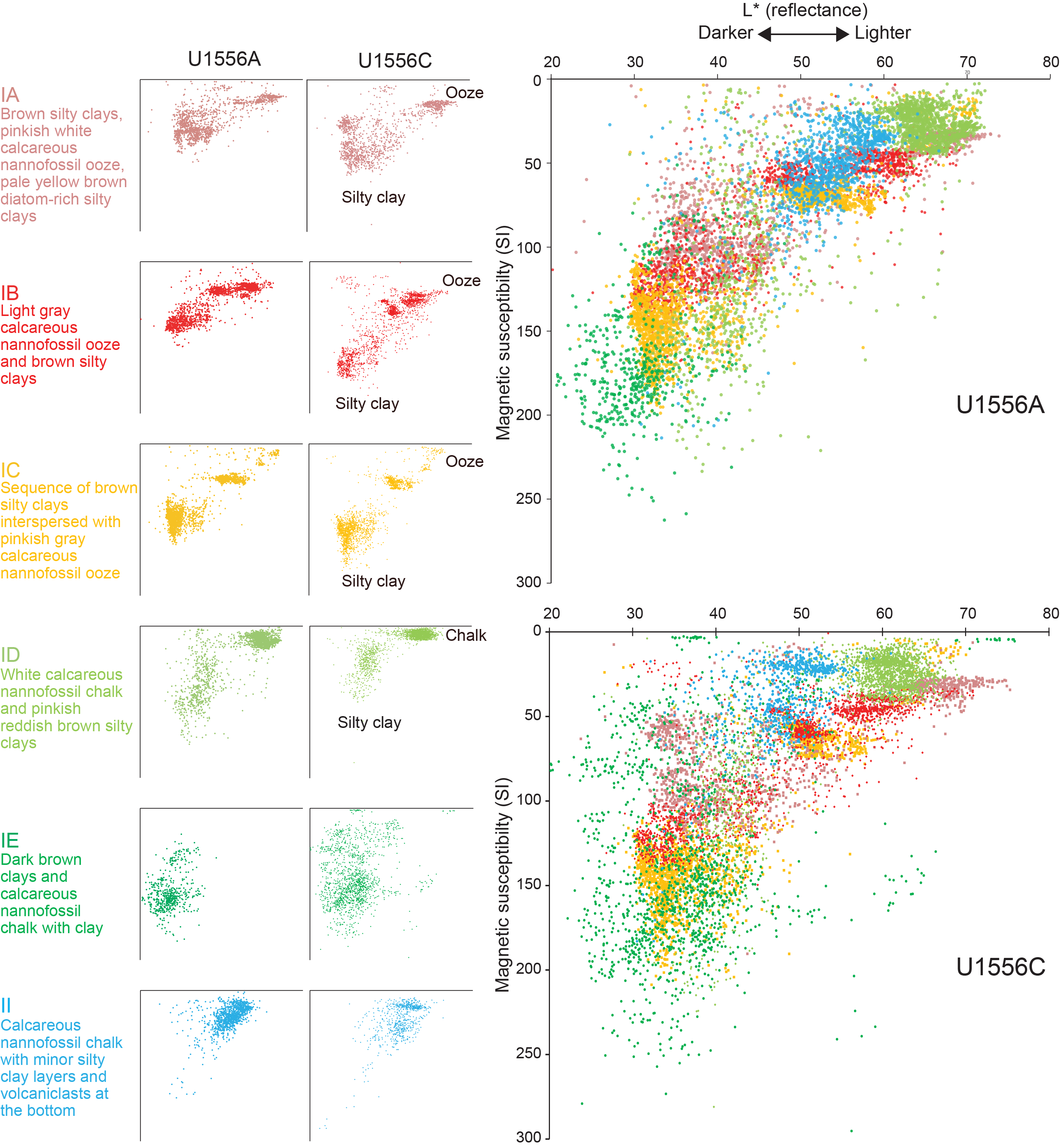
Figure F14. MSP and L*, Holes U1556A and U1556C.

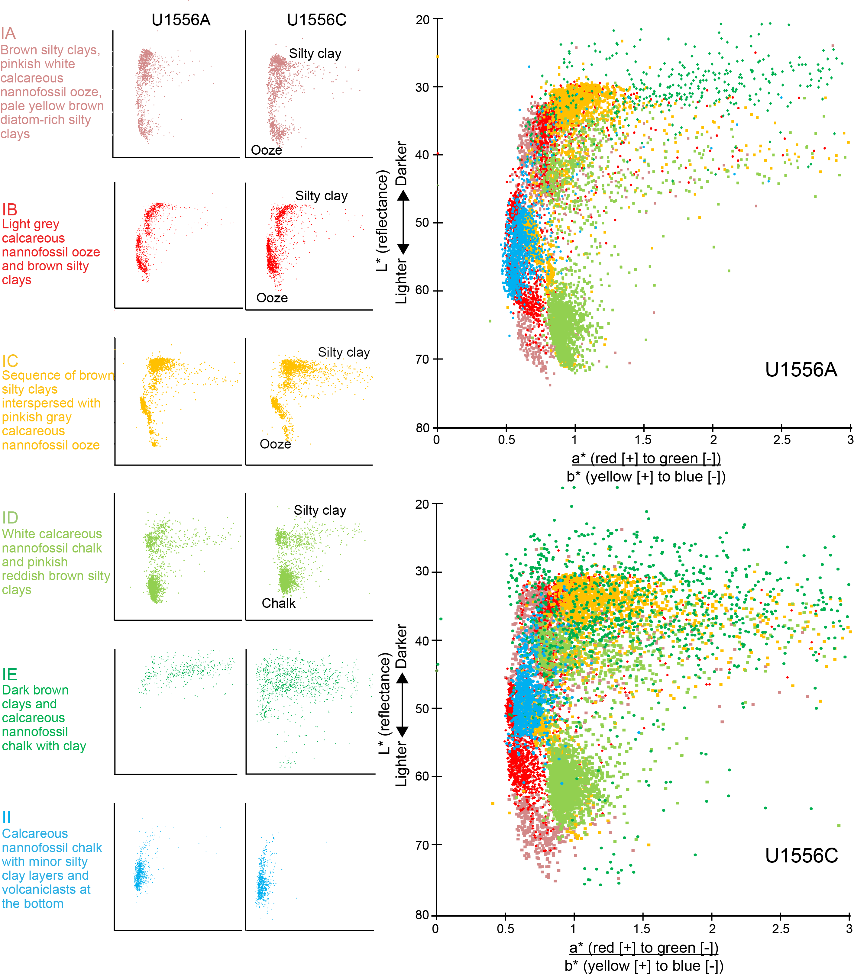
Figure F15. Color reflectance data, Holes U1556A and U1556C.

5. Igneous petrology

In Hole U1556B, 342.3 m (curated length) of volcanic rock, including breccias, was cored after the igneous basement was reached at 291.4 mbsf. The hole was advanced to 609 mbsf, and 185.44 m of core was recovered for a mean recovery of 54.2%. The volcanic rock succession consists predominantly of pillow lavas with thin intervals of either more massive lava flows or larger pillows, all punctuated by episodic occurrences of breccias. The igneous sequence was divided into 13 lithologic units based on changes in petrographic type, phenocryst assemblage, and/or inferred eruptive style (e.g., pillow lavas versus massive flows). Units defined as breccia or hyaloclastite typically consist of more than one rock type and were generally identified by the random mixture of lithologic types in the core and/or variations in cementing material (see Igneous petrology in the Expedition 390/393 methods chapter [Coggon et al., 2024c]) (Table T4). The lithologic units were grouped into three overarching stratigraphic sequences based on differences in magma composition inferred from petrographic observations and subsequently confirmed by geochemical analyses (see Geochemistry), the geometry of lava flows, and their intrusive relationships (Stratigraphic Sequence A: Sections 390-U1556B-2R-2 through 38R-2; Stratigraphic Sequence B: Sections 38R-3 to 54R-3, 130 cm; Stratigraphic Sequence C: Sections 54R-3, 130 cm, through 59R-4) (Figure F16). The uppermost 5.1 and 4.7 m of the volcanic sequence at Site U1556 were also recovered in Holes U1556A and U1556C, respectively.

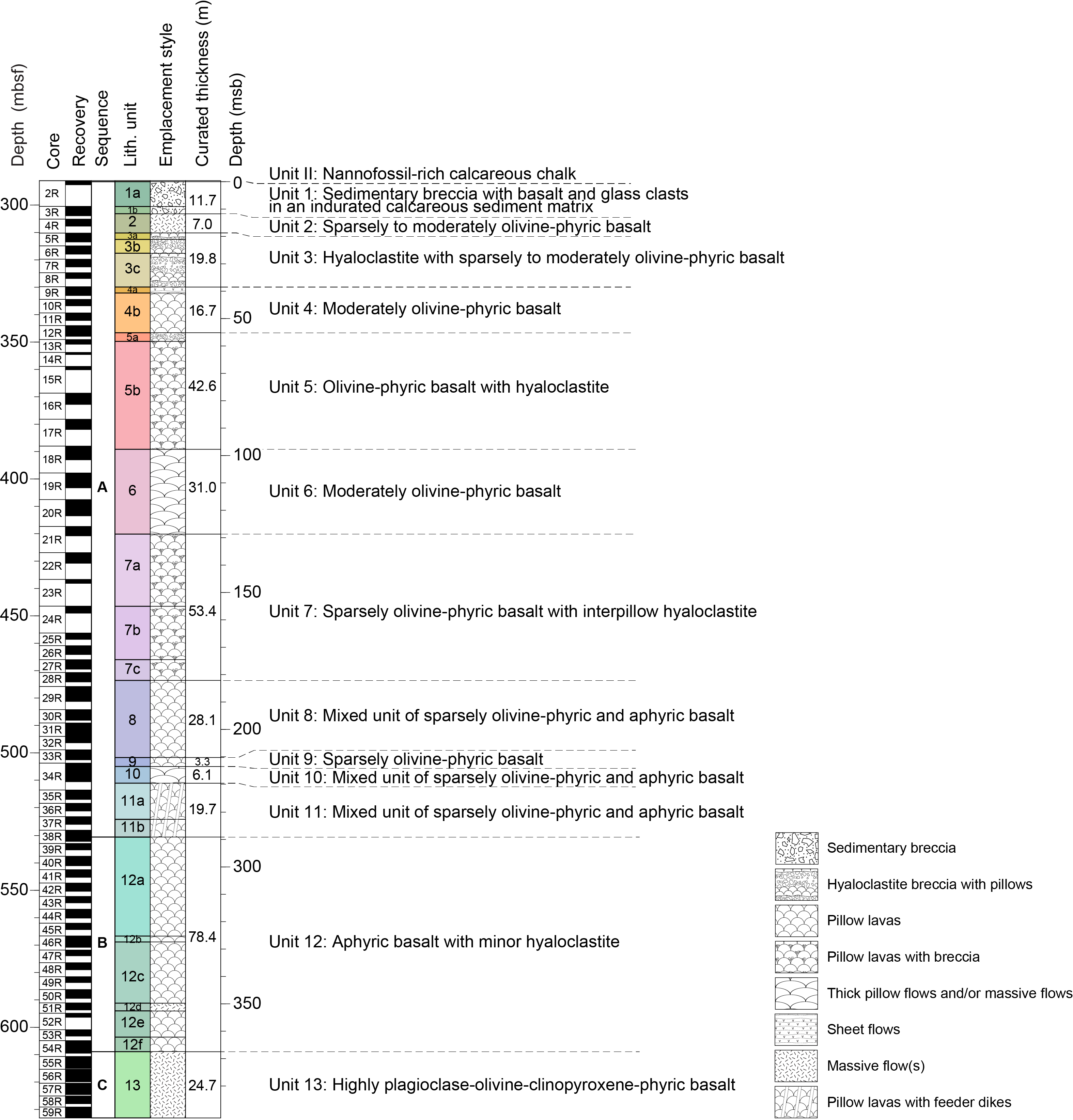
Figure F16. Stratigraphic summary of volcanic sequences.

The uppermost igneous basement, and the top of Stratigraphic Sequence A, comprises an 11.7 m thick sedimentary breccia (Lithologic Unit 1) that probably represents talus deposits of volcaniclastic debris transported downslope through mechanical erosion. Beneath this breccia is a series of sparsely to moderately olivine phyric basalt pillow lava flows interspersed with volcanic breccias in Units 2–11. The breccias contain clasts of chilled pillow margins and altered glass, but the proportions of sedimentary matrix and carbonate cement vary significantly between breccia units. Unit 12, which has six subunits, corresponds to Stratigraphic Sequence B. It consists of a series of aphyric to very sparsely olivine (micro)phyric basalts that are highly altered. Lithologic Unit 11 is noteworthy in that it records intrusive relationships between the lavas of Stratigraphic Sequences A and B. Lithologic Unit 13 (Stratigraphic Sequence C) is highly plagioclase-olivine-clinopyroxene phyric (H-POPP) basalt that contains cognate inclusions interpreted to be cumulates formed in a magma chamber. In this section, we describe each igneous unit and our preliminary interpretation of the entire igneous succession. The unit thicknesses discussed below are the curated thicknesses of the units; minimum thicknesses based on actual lengths of the recovered pieces are given in Table T4.

5.1. Lithologic and stratigraphic igneous units

5.1.1. Stratigraphic Sequence A

5.1.1.1. Lithologic Unit 1

Intervals: 390C-U1556A-30X-5 through 33X-1; 390-U1556B-2R-2 to 3R-2, 130 cm; 390-U1556C-30X-CC through 32X-2
Depth: 291.4–300.5 mbsf
Lithology: sedimentary breccia

Unit 1 is a sedimentary breccia that ranges from clast to matrix supported (Figure F17); it comprises the sediment–basement transition at Site U1556, which was penetrated in Holes U1556A–U1556C. Clast sizes are highly variable and range up to 23 cm in maximum dimension. The unit consists of two subunits defined by a change in the breccia matrix composition. In Subunit 1a, the matrix consists of light gray (10YR 7/2) indurated calcareous sediment (Figure F17A). Some original sedimentary structures, such as bioturbation (burrows), are partially preserved, confirming a near-seafloor origin. In Subunit 1b, the matrix is more variable and hosts a range of millimeter- to centimeter-sized altered glass clasts as well as submillimeter dark particles (altered volcaniclastic material) (Figure F17C, F17D). Matrix color changes in response to the variable clast load from reddish yellow (7.5YR 7/6), where altered glass clasts are abundant, to more light brown (7.5YR 6/4) to brown (7.5YR 4/3), where basalt clasts dominate (Figure F17). In Hole U1556C, the different colors of sediment also seem to record remobilization or rebrecciation of previous deposits because angular sediment clasts of one color are observed floating in another (Figure F17B) and basalt clasts retain rims of sediment that are different in color from the bulk of the sediment in which they now occur (Figure F17C).

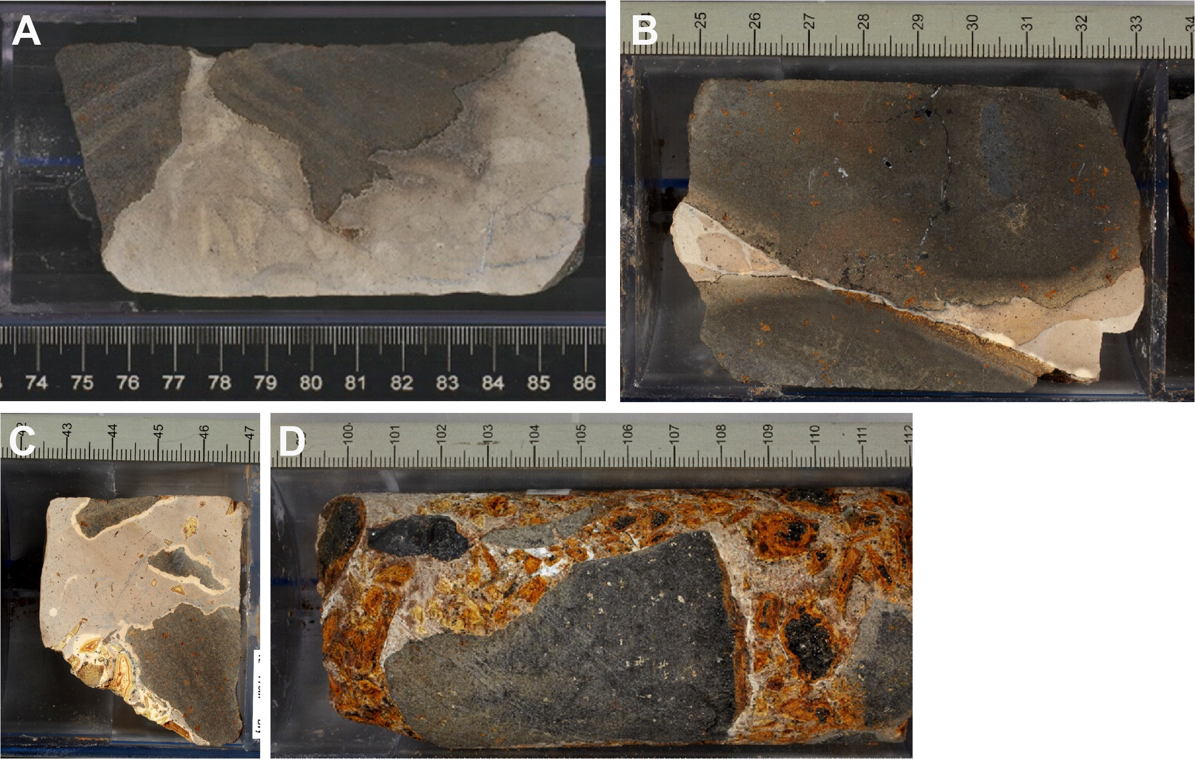
Figure F17. Sedimentary breccia, Lithologic Unit 1.

Throughout Subunits 1a and 1b, the clasts consist of moderately olivine phyric basalts in which the olivine is highly to completely altered to a distinctive orange-brown, creating a speckled appearance in hand sample (Figure F18A). This rock type is present throughout Stratigraphic Sequence A, and for convenience we refer to it in the remainder of this report as "orange spotty" basalt. Basaltic clasts show no indication of having chilled against the sedimentary matrix. Similarly, the sediment shows no signs of having been baked adjacent to the basalt, suggesting that the basalts did not intrude into cold sediments as per peperite formation. Instead, the breccias record the accumulation of talus deposits as volcaniclastic debris was transported downslope because of gravitational instability.

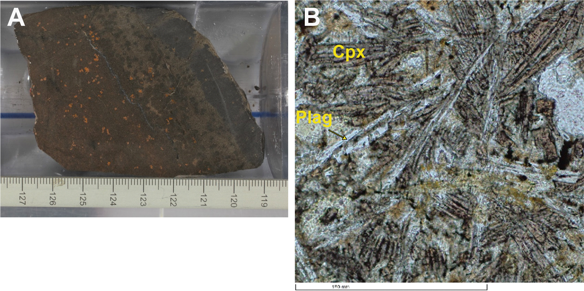
Figure F18. Orange spotty basalt and pinkish brown titanaugite crystals.

5.1.1.2. Lithologic Unit 2

Interval: 390-U1556B-3R-2, 130 cm, through 4R-3
Depth: 303.1–310.1 mbsf
Lithology: sparsely to moderately olivine phyric basalt

Unit 2 is a 7 m thick interval consisting of sparsely olivine phyric basalt pillow lavas and sheet flows (orange spotty). Chilled margins on larger cored pieces are common with many exhibiting arcuate shapes and radial fractures typical of pillow lavas. Chilled margins on both the top and bottom of continuous pieces are also common, indicating pillow lobes at least 35 cm in size. The basalts are typically sparsely vesicular with small (<0.75 mm) round vesicles homogeneously distributed throughout. Larger (3–4 mm) vesicles that are irregular in shape and heterogeneously distributed are less abundant. Both vesicle types are filled with secondary minerals, predominantly calcite (see Alteration petrology). The larger vesicles probably formed through coalescence of much smaller vesicles.

In thin section, olivine phenocrysts are euhedral and equant, forming crystals up to 1 mm in size. Both phenocryst and groundmass olivines are completely replaced by iddingsite ± Fe oxyhydroxides, which produces the characteristic orange spotty appearance of this basalt type (see Alteration petrology). The groundmass is dominated by dendritic and skeletal textures, affirming the rapid rate of crystallization. Groundmass clinopyroxenes that are large enough to examine microscopically are pinkish brown, which is typical of titanaugite (e.g., Sample 390-U1556B-4R-1, 46–50 cm; Figure F18B). This observation suggests a magma composition that is more Ti rich and alkalic than is typical of mid-ocean-ridge basalts (MORBs), which is confirmed by the geochemistry of these rocks (see Geochemistry).

5.1.1.3. Lithologic Unit 3

Interval: 390-U1556B-5R-1 through 9R-1
Depth: 310.1–329.9 mbsf
Lithology: hyaloclastite breccia with sparsely to moderately olivine phyric basalt

Unit 3 is a 19.8 m thick interval characterized by relatively small pillow lobes (~15–30 cm) associated with hyaloclastite. The hyaloclastite occurs attached to external surfaces of cored basalt but also forms discrete pieces in the core, the longest interval of which is ~12 cm (Sample 390-U1556B-9R-1 [Piece 1]) (Figure F19A). The unit has three subunits (3a–3c) that are defined based on variations in breccia lithology, particularly matrix composition and the proportion of calcite cement.

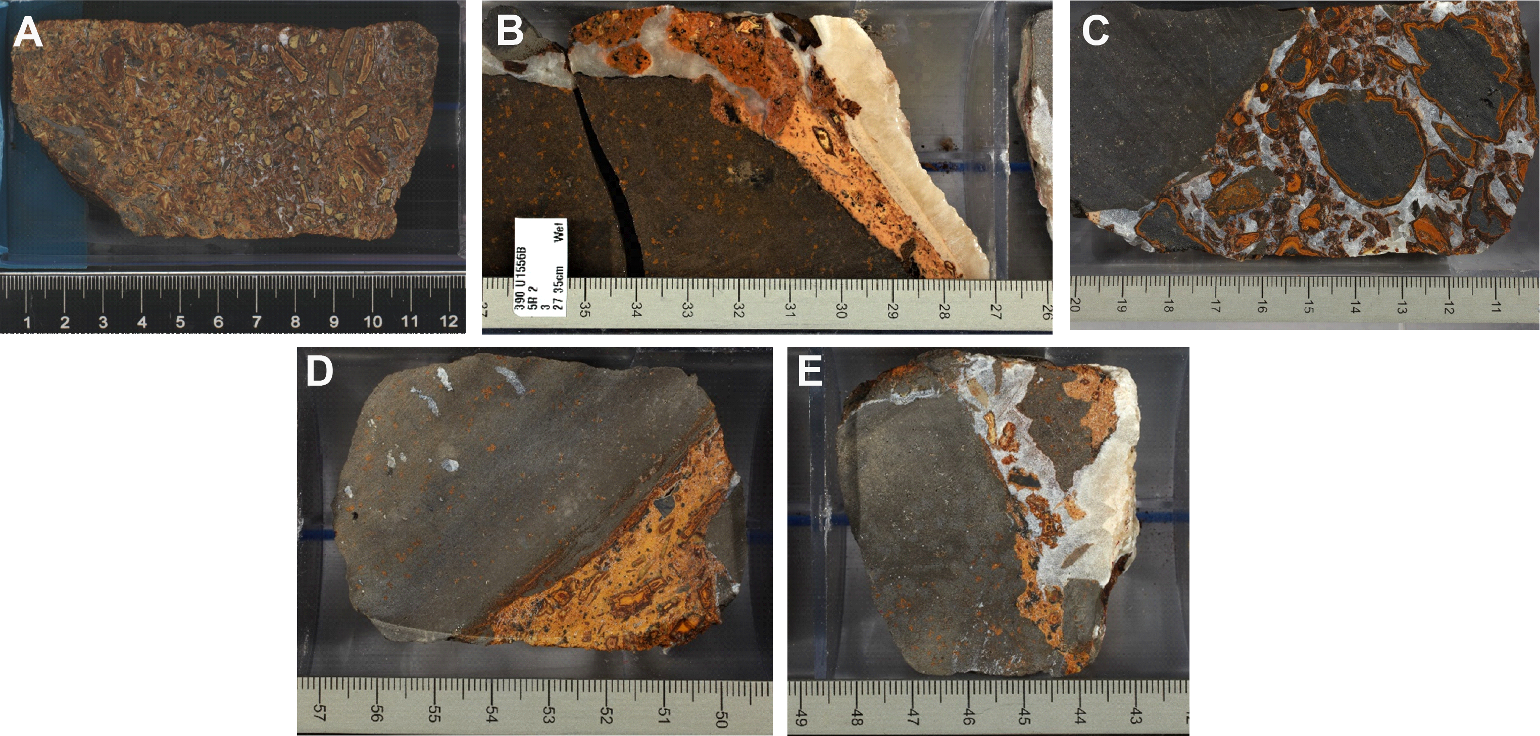
Figure F19. Breccias, Unit 3.

Subunit 3a (Sections 390-U1556B-5R-1 to 5R-2, 86 cm) is clast-supported breccia with clasts up to ~15 cm. Compositionally, the clasts are all moderately olivine phyric basalt (orange spotty), but they are highly rather than moderately altered. Some pieces preserve textures typical of rapidly cooled pillow lavas (see Chilled margin petrography for summary of textures observed and interpreted to be evidence for pillow chilled margin origin), and these chilled pillow margins are commonly less altered than clasts from more coarsely crystalline pillow interiors. The breccia matrix, which forms 15%–25% of the rock, is now indurated calcareous sediment that contains highly to completely altered basaltic glass fragments (Figure F19B). Most of these altered glass clasts are <5 mm, but some are as large as 2.5 cm. Calcite cement is present throughout, typically representing <10% of the rock.

Subunit 3b (Sections 390-U1556B-5R-2, 86 cm, to 6R-2, 123 cm) is similar to Subunit 3a, but the breccias include little to no pelagic sediment matrix. Instead, they are cemented by coarse sparry calcite (Figure F19C). Subunit 3c (Sections 6R-2, 123 cm, to 9R-1, 25 cm) is also similar to Subunit 3a. However, although the breccias in this interval again contain sedimentary matrix (Figure F19D), they can be highly disrupted by sparry calcite cement that dominates the rock (Figure F19E).

5.1.1.4. Lithologic Unit 4

Interval: 390-U1556B-9R-1, 26 cm, through 12R-2
Depth: 329.9–346.5 mbsf
Lithology: moderately olivine phyric basalt

Unit 4 is a 16.9 m thick interval of moderately olivine phyric basalt (orange spotty). It consists of two subunits defined on the basis of inferred eruptive style. Subunit 4a is interpreted to be a series of sheet flows based on recovery of subhorizontal chilled margins in several intervals, including paired horizontal chilled margins (i.e., at the top and bottom) on more than one continuous core piece (e.g., Samples 390-U1556B-9R-1 [Piece 5] and 9R-2 [Piece 1]).

The basalts in Subunit 4b were emplaced as pillow lavas. Recovery of arcuate chilled margins (e.g., Sample 390-U1556B-12R-1 [Piece 6]) (Figure F20A), chilled margins that run along the sides of core pieces, and wedge-shaped core pieces are common, as well as paired chilled margins (commonly in an individual piece) that are oriented at steep angles to the core vertical (e.g., Sample 10R-1 [Piece 10]) (Figure F20B).

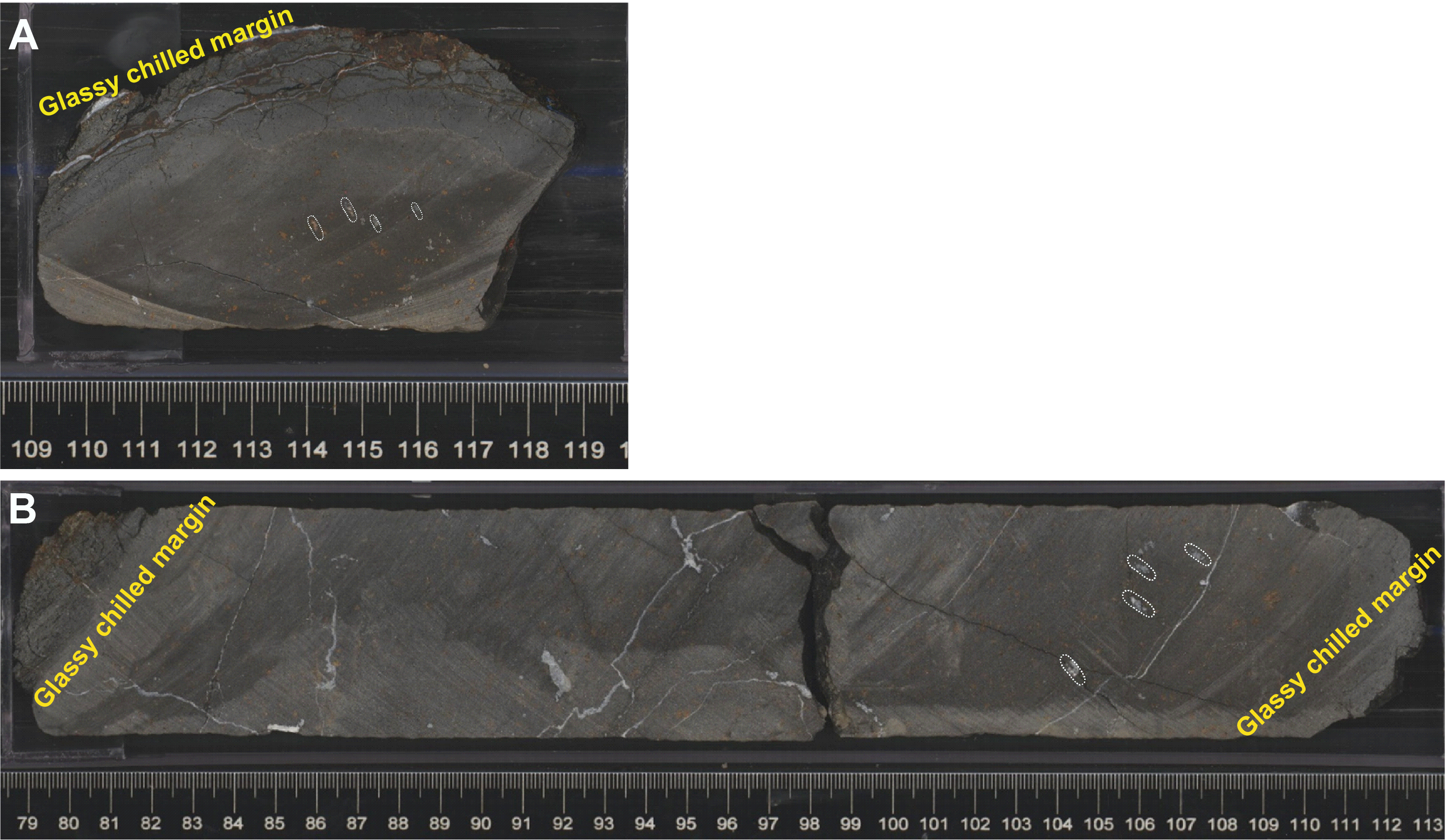
Figure F20. Arcuate pillow margins.

Lithologically, the basalts throughout Unit 4 are typically orange spotty, as described for Units 2 and 3. They contain euhedral equant olivine phenocrysts up to 1 mm that are completely replaced by iddingsite ± Fe oxyhydroxides ± clay minerals. They are typically sparsely vesicular with small (<0.25 mm) round vesicles homogeneously distributed throughout but with heterogeneously distributed much larger (up to 8 mm) vug-like irregularly shaped vesicles that are filled predominantly with calcite (see Alteration petrology). In Sample 390-U1556B-12R-1 (Piece 6), these larger vesicles are elongate perpendicular to the chilled margin, suggesting they represent coalescence of smaller vesicles that attempted to form escape routes to the pillow margin but were trapped by the crystallization front (Figure F20A). Calcite veins disrupt the glassy portions of pillow chilled margins, some of which delaminate to form hyaloclastite (Figure F21). This in situ cementation process may be the source of many of the elongate/tabular clasts present in the core that are described as sediment-free hyaloclastites.

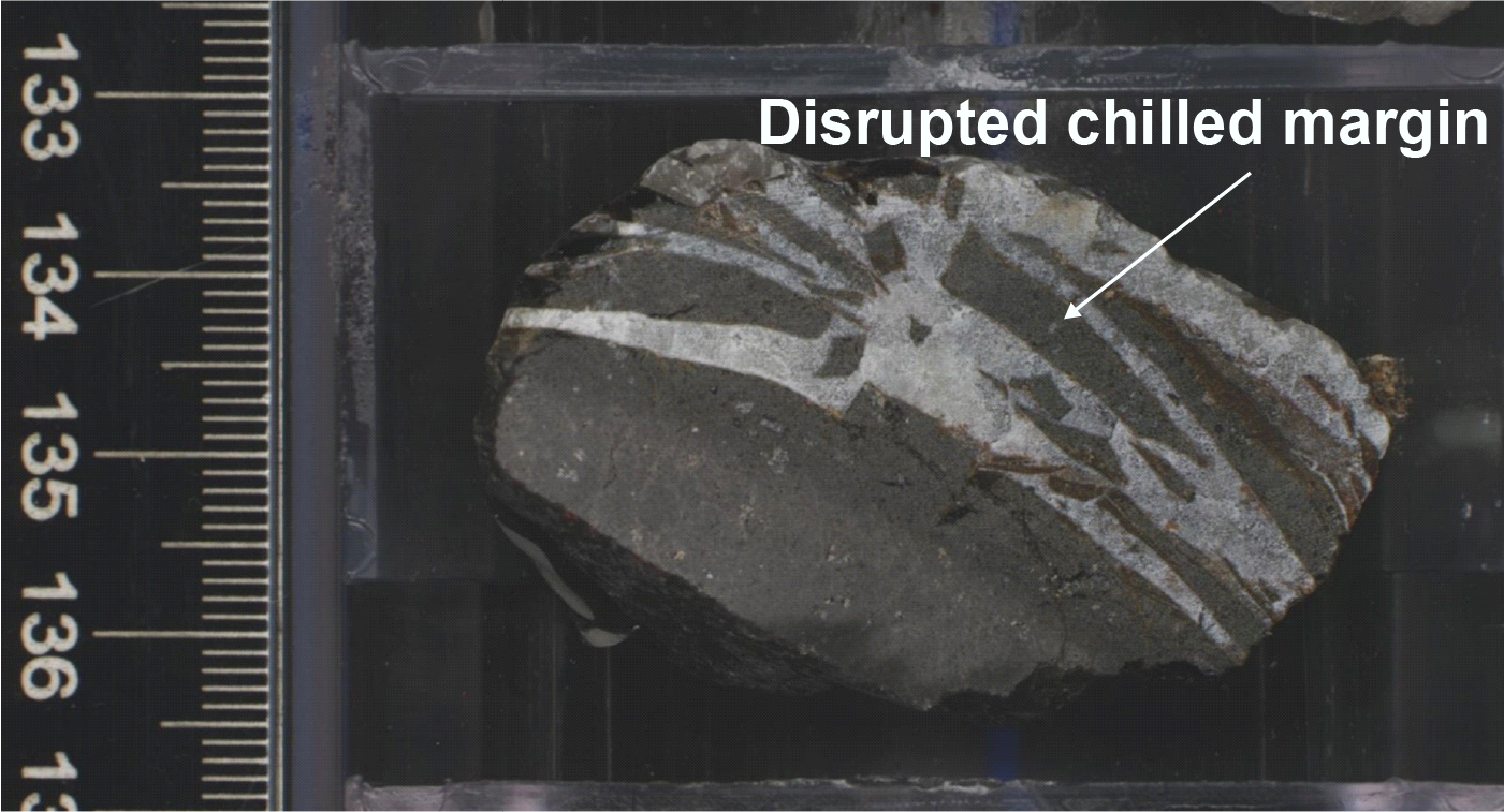
Figure F21. Hydrothermal fracturing of chilled pillow margins.

In thin section, olivine phenocrysts are observed to contain equant crystals of chromium (Cr) spinel (Figure F22). Groundmass textures are typically dominated by acicular to tabular plagioclase intergrown with elongate crystals of clinopyroxene to form radiating fabrics. The clinopyroxene is pinkish brown, indicative of titanaugite. This observation suggests the parental magma is alkaline rather than tholeiitic, consistent with the geochemistry of these samples (see Geochemistry).

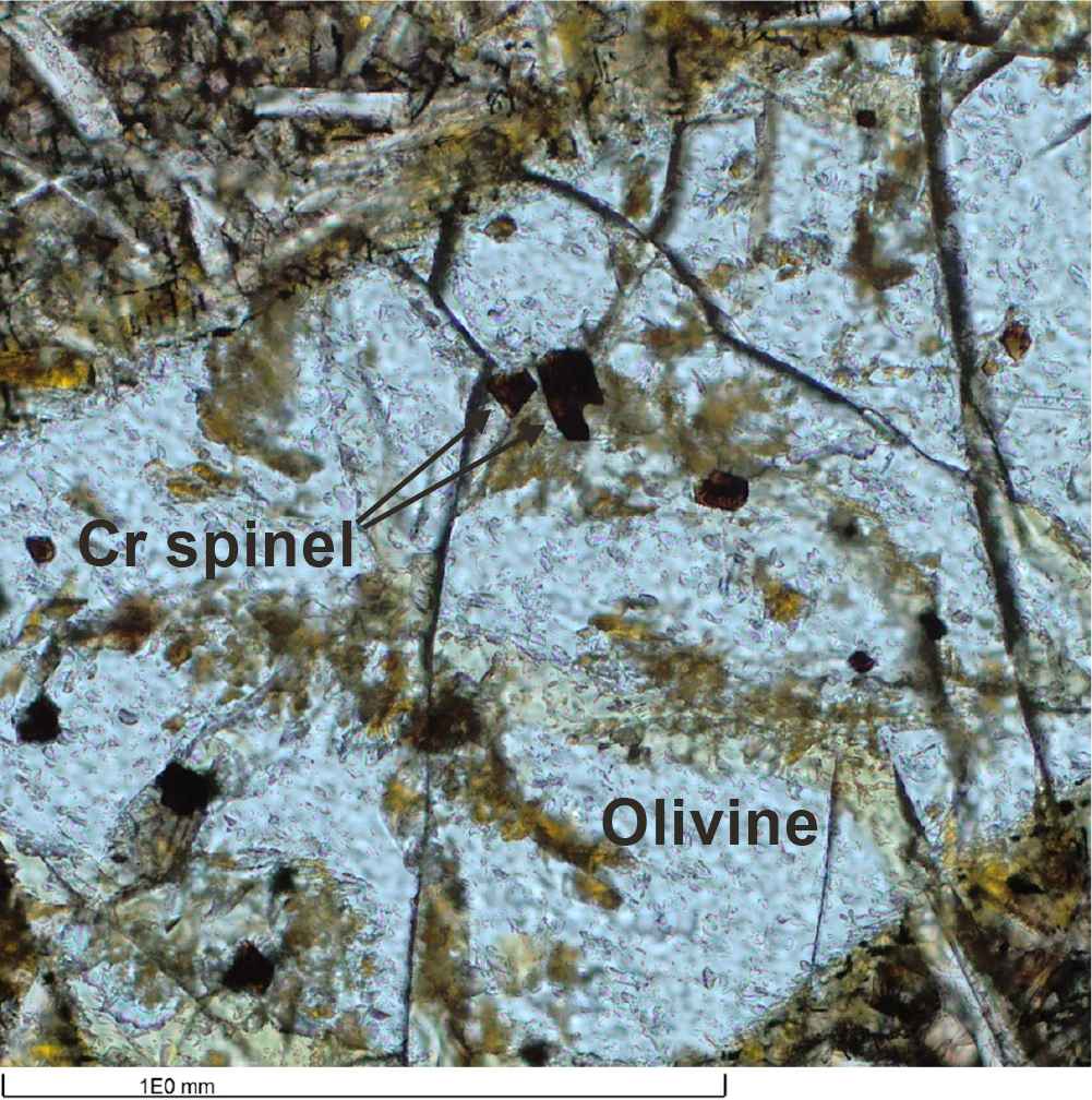
Figure F22. Cr-spinel inclusions in olivine.

5.1.1.5. Lithologic Unit 5

Interval: 390-U1556B-12R-2, 107 cm, to 18R-1, 109 cm
Depth: 346.5–389.1 mbsf
Lithology: moderately olivine phyric basalt with interpillow hyaloclastite

Unit 5 is a 42.6 m thick interval of moderately olivine phyric basalt (orange spotty) with thick intervals (up to ~2.7 m) of hyaloclastite. The unit is divided into two subunits based on the proportion of basalt to breccia in the core. Subunit 5a is dominated by hyaloclastite and extends from Section 390-U1556B-12R-2, 107 cm, to Section 13R-1, 70 cm. Subunit 5b, which extends from Section 13R-1, 70 cm, to Section 18R-1, 108 cm, is predominantly basalt with minor hyaloclastite occurring as small (<1–2 cm thick) masses attached to cored basalt pieces, mostly on chilled margins.

The breccias of Unit 5 are similar to those of Subunits 3b and 3c in that many contain little to no sediment but significant amounts of calcite cement, whereas others contain small amounts (<15%) of matrix as well as calcite cement. The breccia clasts are large (up to 8 cm) and consist predominantly of fragments of chilled pillow margins, including both glass and the adjacent zones of cryptocrystalline quench crystal growth. Larger clasts are mostly unaltered in their interiors, and some fresh glass is present (e.g., Sample 390-U1556B-12R-3 [Piece 19]; Figure F23). In addition, the breccia in this interval is characterized by the presence of void spaces that make up as much as ~10% of the rock (Figure F24). Subunit 5b is predominantly basalt with relatively small amounts of hyaloclastite, but that small amount is persistent throughout the subunit. The hyaloclastites of Subunit 5b are also finer grained than those of Subunit 5a, with most glass completely altered.

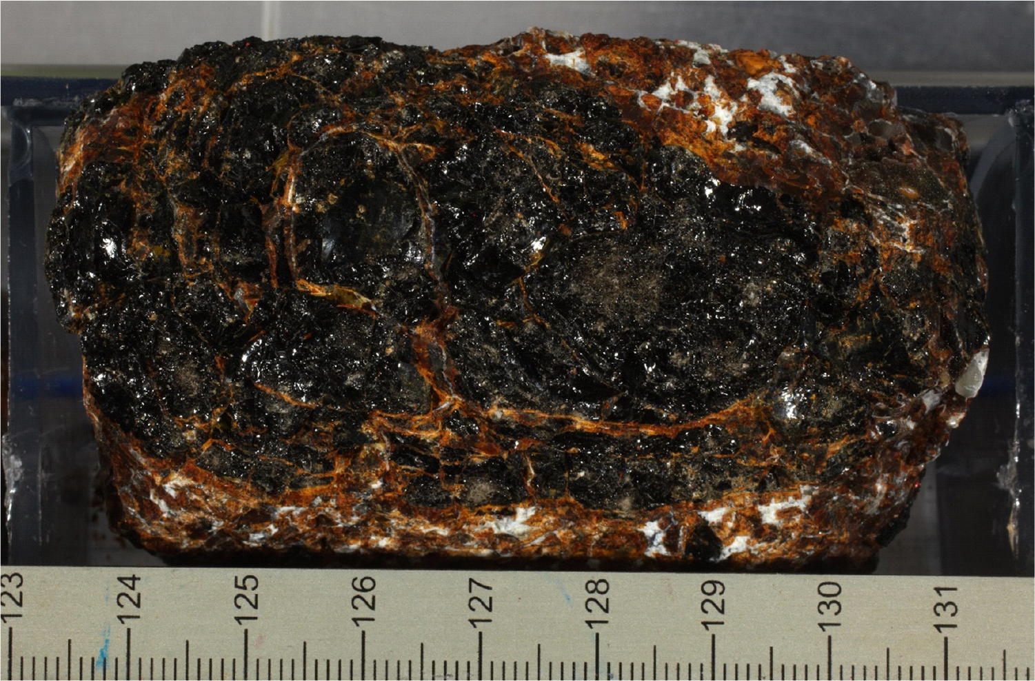
Figure F23. Fresh glass in hyaloclastite.

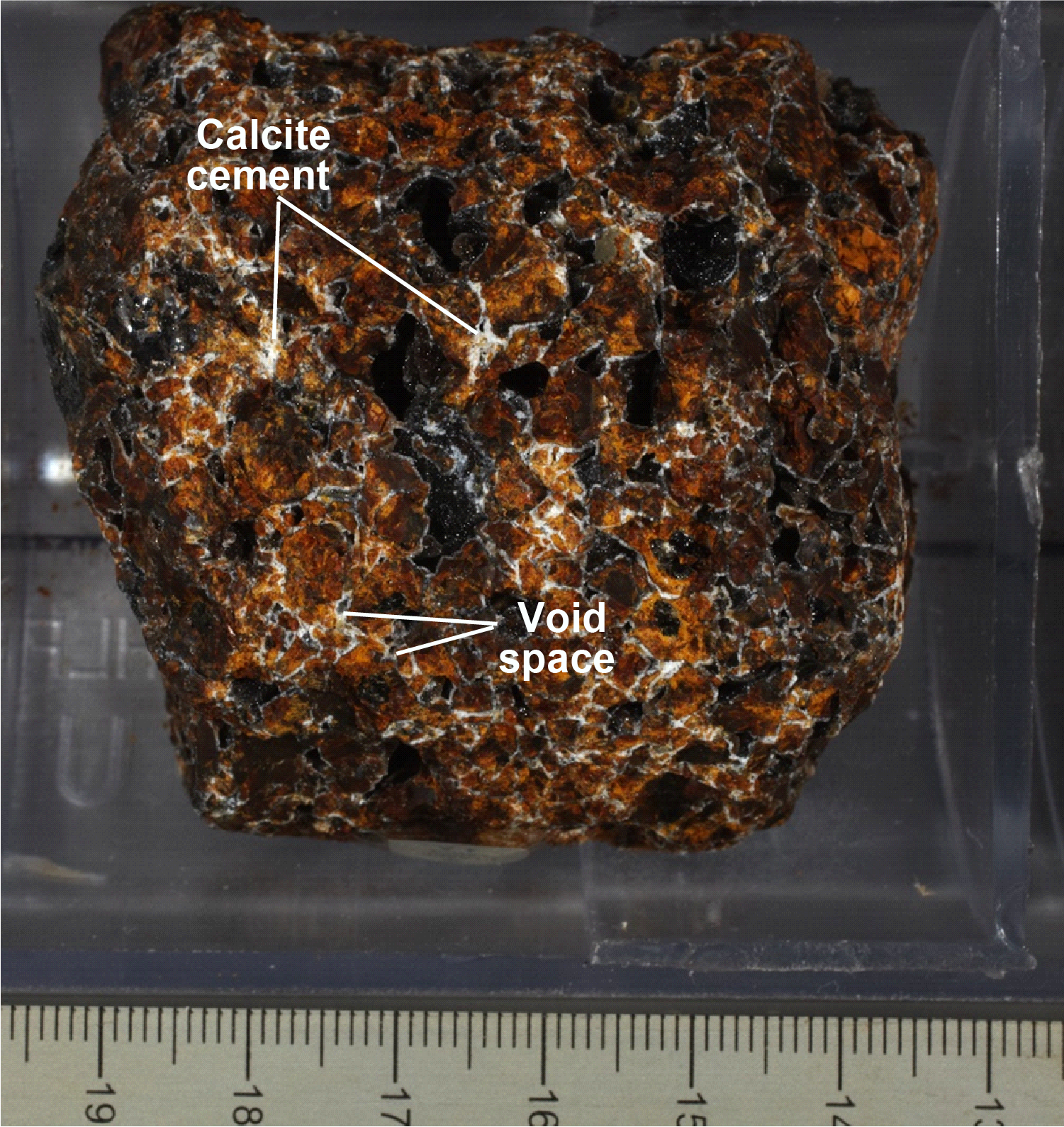
Figure F24. Calcite-cemented breccia.

The basalts in Subunit 5b contain euhedral, equant olivine phenocrysts totally replaced by secondary minerals, giving them the typical orange spotty character of Stratigraphic Sequence A lavas (see Alteration petrology). Recovery of chilled margins that exhibit quench crystallization textures and paired chilled margins typical of pillow lavas are common (e.g., Sections 390-U1556B-16R-2, 16R-3, 16R-4, and 17R-1). The lengths of pieces with paired chilled margins indicate pillow lobes that are at least 40–75 cm in size.

5.1.1.6. Lithologic Unit 6

Interval: 390-U1556B-18R-1, 109 cm, through 21R-2
Depth: 389.1–420.0 mbsf
Lithology: moderately olivine phyric basalt

Unit 6 consists of 31 m of moderately olivine phyric basalt emplaced as thick pillow and massive flows. Paired chilled margins are very common in this unit; some show chilled margins with steep dips (e.g., Sample 390-U1556B-20R-6 [Piece 1]) (Figure F25A), whereas others are subhorizontal (e.g., Sample 20R-1 [Piece 3]) (Figure F25B). The longest continuous piece, which has a steeply dipping chilled margin at the top, occurs in interval 20R-4, 0–107 cm (i.e., piece length > 1 m). These observations suggest an interval of thick pillow lobes and/or flows that are at least 35–65 cm, and >1 m in some cases. Toward the bottom of this unit, the maximum observed pillow size decreases to less than ~30 cm. The high proportion of paired chilled margins recovered made it possible to observe that the large, irregularly shaped vesicles tend to occur in bands about 4–6 cm away from a chilled margin (e.g., Sample 20R-6 [Piece 1]) (Figure F25A). Moreover, when the split surface of the core is oriented in a plane sufficiently perpendicular to the chilled margin, it is clear that many of these vesicles are elongate perpendicular to the chilled margin surface. When cut through at other angles, these vesicles look roughly circular or oval in outline, indicating that they are tubular.

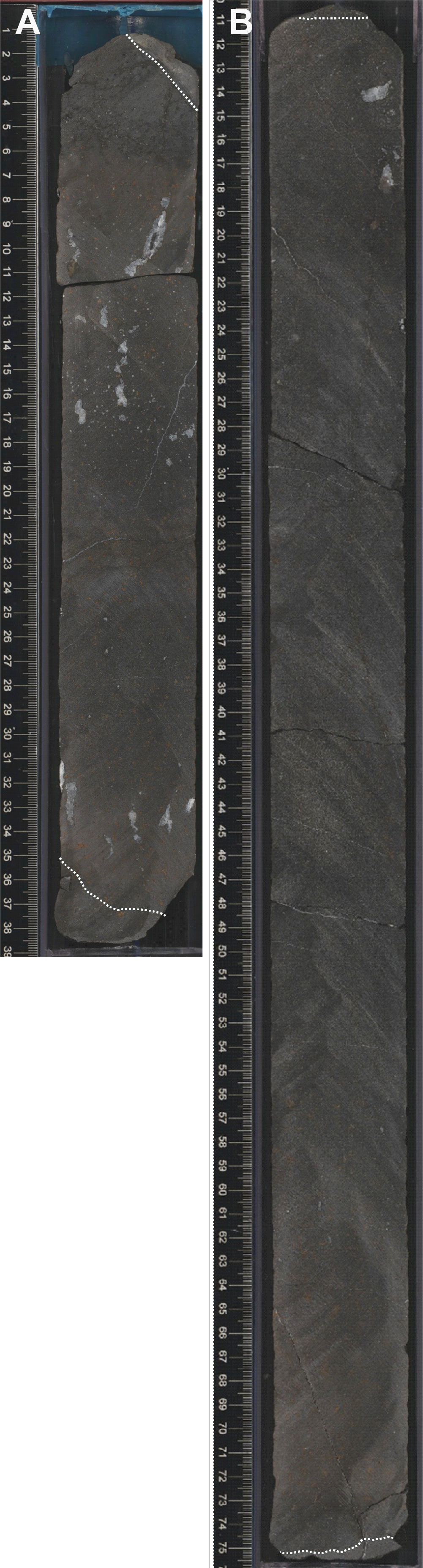
Figure F25. Chilled margins.

Lithologically, the basalts are typical of the altered olivine phyric (orange spotty) variety described for all overlying units. Coarser grained intervals, such as pillow interiors, are moderately phyric, whereas chilled margins tend to be sparsely phyric even within the same pillow. Moreover, olivine phenocrysts in pillow interiors are completely replaced by iddingsite ± Fe oxyhydroxides and clay minerals (see Alteration petrology), whereas those occurring in the chilled margins can be remarkably unaltered (Figure F26).

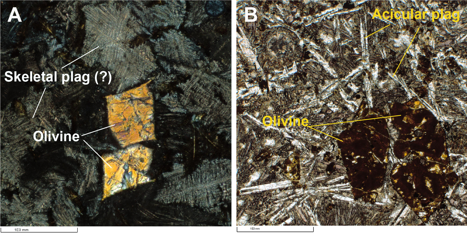
Figure F26. Olivine.

5.1.1.7. Lithologic Unit 7

Interval: 390-U1556B-21R-3 through 28R-2
Depth: 420.0–473.5 mbsf
Lithology: sparsely olivine phyric basalt with interpillow hyaloclastite

Unit 7 is a 53.4 m thick interval of aphyric to sparsely olivine phyric basalt intercalated with hyaloclastite. The unit is divided into three subunits based on variations in breccia lithology and proportion of basalt to breccia. Piece lengths are smaller in this unit relative to Unit 6, and fewer paired chilled margins are recovered on continuous core pieces. This limits assessment of maximum pillow size or flow thickness. The basalts are all of the orange spotty olivine phyric variety. However, the lower modal proportion of phenocryst phases reported reflects a relatively higher recovery of pillow chilled margins, particularly in the breccias. As noted in earlier unit descriptions, the modal proportion of phenocrysts is much lower in the chilled margins relative to pillow interiors, so the lower modal phenocryst abundances reported from macroscopic description do not (necessarily) reflect a change in the magma type. Rather, they reflect the lower average crystallinity of the material recovered. In all other aspects, there are no distinguishing features in the basalts of Unit 7 relative to those in previous units.

Subunit 7a extends from Section 390-U1556B-21R-3 through 23R-2. It consists predominantly of small pieces of basalt (most less than ~10 cm) with hyaloclastite either attached to the basalt or occurring as small (less than ~5 cm), discrete, unoriented pieces in the core (Figure F27A). The breccias are clast supported with a low proportion of sedimentary matrix (typically less than a few percent). The clasts are dominated by angular to subrounded pillow chilled margin fragments, 2–9 cm, that can be remarkably unaltered (see Alteration petrology). The matrix between the clasts appears to be dominated by disaggregated altered glass clasts, which gives it an orange-brown color. Calcite cement typically constitutes ~20%–25% of the rock.

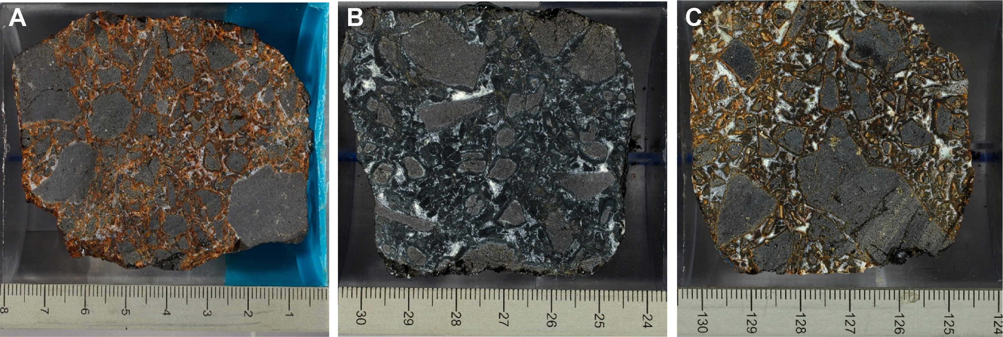
Figure F27. Comparison of breccias, Unit 7.

Subunit 7b, which extends from Section 390-U1556B-24R-1 through Section 26R-3, is notable for the distinct green color of the breccia compared to the orange-brown breccias in the overlying units (Figure F27B), reflecting the occurrence of minerals indicative of a less oxidizing environment (see Alteration petrology). Breccia dominates the unit; indeed, all of Section 25R-1 is green hyaloclastite breccia. It is clast supported, and the clasts are dominated by basaltic glass that is only slightly altered. The matrix is dark green to black and there is little cement, so the breccia is friable and easily disaggregates.

In Subunit 7c (Sections 390-U1556B-27R-1 through 28R-2), the breccia is also clast supported and glass dominated; however, the extent of alteration is greater than in Subunit 7b and there is apparent overprinting of the green minerals in Subunit 7b by more oxidative alteration. A higher proportion of calcite cement in Subunit 7c means that these breccias are more consolidated than those in Subunit 7b (Figure F27C).

5.1.1.8. Lithologic Unit 8

Interval: 390-U1556B-28R-3 through 33R-2
Depth: 473.5–501.6 mbsf
Lithology: aphyric to sparsely olivine phyric basalt with interpillow hyaloclastite

Unit 8 consists of 28.1 m of aphyric to sparsely olivine phyric basalt emplaced as small (<30 cm) to large (up to 70 cm) pillows or massive flows. There are numerous examples of chilled margins, most of which are steeply dipping. Paired chilled margins are also common, with margins ranging from subhorizontal (e.g., Sample 390-U1556B-30R-2 [Piece 3]) to arcuate shapes (e.g., Sample 29R-4 [Piece 4]; Figure F28). The longest continuous core piece occurs in interval 30R-2, 71–144 cm, indicating flow thicknesses in this unit can reach up to ~70 cm. As observed in Unit 6, irregularly shaped vesicles tend to occur in bands about 4–6 cm away from chilled margins and may be elongate perpendicular to the chilled margin surface (e.g., Sample 29R-4 [Piece 4]; Figure F28).

Figure F28. Arcuate chilled pillow margin.

The basalts in this unit are more sparsely phyric than is typical of the orange spotty variety observed in units higher in the hole, with some intervals being classified as aphyric. In addition, the extent of alteration varies considerably throughout the unit from moderate to very high, even from one piece to the next within a section (e.g., Section 33R-2; Figure F29) (see Alteration petrology). Although not recognized during macroscopic core description, subsequent analysis of representative samples from this unit by pXRF suggests that there may be more than one basalt type present, distinguished by high-field-strength element (HFSE) systematics (see Corroboration of stratigraphic units: pXRF analysis). One basalt type is petrographically similar to the olivine phyric orange spotty variety that occurs in all overlying units. The other appears to be aphyric and more highly altered. In Unit 11, we observe intrusive relationships between two basalt types that are petrographically similar to the two basalt types recovered in Unit 8. Intrusive contacts were not observed in Unit 8, so detailed shore-based research will be required to confirm the details of the stratigraphic distributions of these two magma types and their relationship to one another.

Figure F29. Variations in alteration, Unit 8.

5.1.1.9. Lithologic Unit 9

Interval: 390-U1556B-33R-3 through 34R-1
Depth: 501.6–504.9 mbsf
Lithology: sparsely olivine phyric basalt with interpillow hyaloclastite

Unit 9 is a 3.3 m thick interval of sparsely olivine phyric basalt with low abundances of hyaloclastite. There are three small (<5 cm) unoriented hyaloclastite rollers at the top of Section 390-U1556B-33R-3. Otherwise, the unit is characterized by thin remnants of hyaloclastite attached to the chilled margins of basalt (Figure F30). The breccia is clast supported, with clasts of basalt and altered glass in a yellowish white matrix. However, it is unclear whether this material represents cement (i.e., authigenic) or fine particles of disaggregated altered glass (i.e., detrital). Although chilled margins are common, most recovered pieces of basalt are short (<10 cm); the longest continuous piece (Sample 33R-3 [Piece 5]) is only 40 cm long. This observation indicates an interval of relatively small pillow lavas.

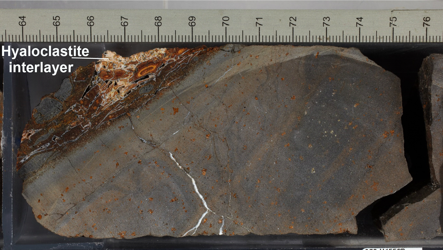
Figure F30. Orange spotty basalt with hyaloclastite.

Like Unit 8, the basalts in Unit 9 range from aphyric to sparsely phyric and exhibit significant differences in alteration style from one piece to another (with color varying from reddish brown [5YR 5/4] to dark gray [7.5YR 4/1] to very dark gray [GLEY 1 3/N]). Samples from Unit 9 were not analyzed using pXRF or shipboard inductively coupled plasma–atomic emission spectroscopy (ICP-AES), so shore-based research will be required to confirm whether there is more than one basalt type in this unit.

5.1.1.10. Lithologic Unit 10

Interval: 390-U1556B-34R-2 to 34R-7, 86 cm
Depth: 504.9–511.0 mbsf
Lithology: moderately olivine phyric basalt with interpillow hyaloclastite

Unit 10 is a 6.1 m thick interval of pillow lavas and massive flows. A single continuous piece 1.8 m in length spans two sections (390-U1556B-34R-4 and 34R-5), indicating a massive flow (i.e., long continuous core pieces [50–60 cm] with uniform texture and relatively unaffected by drilling; see Igneous petrology in the Expedition 390/393 methods chapter [Coggon et al., 2024c]). Section 34R-6 recovered another continuous piece 91 cm long. Moreover, veins in Sample 34R-6 (Piece 2) align with those in Sample 34R-7 (Piece 1), suggesting that the basalts from Sections 34R-6 and 34R-7 could be part of the same piece. Although all the pieces in Sections 34R-4, 34R-5, and 34R-6 cannot be definitively established as a single cooling unit, they are petrologically similar, suggesting they are part of a similar eruptive phase.

Most of the basalts in Unit 10 are petrographically similar to the olivine phyric orange spotty variety from Units 1–9, containing euhedral, equant olivine phenocrysts and pinkish brown groundmass clinopyroxene (Figure F31). However, Sample 390-U1556B-34R-2 (Piece 2) records an intrusive relationship between two different basalt types in interval 34R-2, 85–105 cm. Close-up images of the contact (Figure F32) show that the orange spotty basalt has intruded an older aphyric pillow lava that is highly altered to a distinctive reddish brown color. The images show that the margin of the older, intruded pillow lava is brittle and fractured, and fragments of its chilled margin have been incorporated into the intruding orange spotty basalt, establishing the sequence of events. Moreover, pXRF data confirm that the two basalt types are compositionally distinct, with the orange spotty rocks having higher Zr/Ti ratios than the older, more altered pillows (see Corroboration of stratigraphic units: pXRF analysis). For ease of reference, we refer to these older basaltic rocks as "old red."

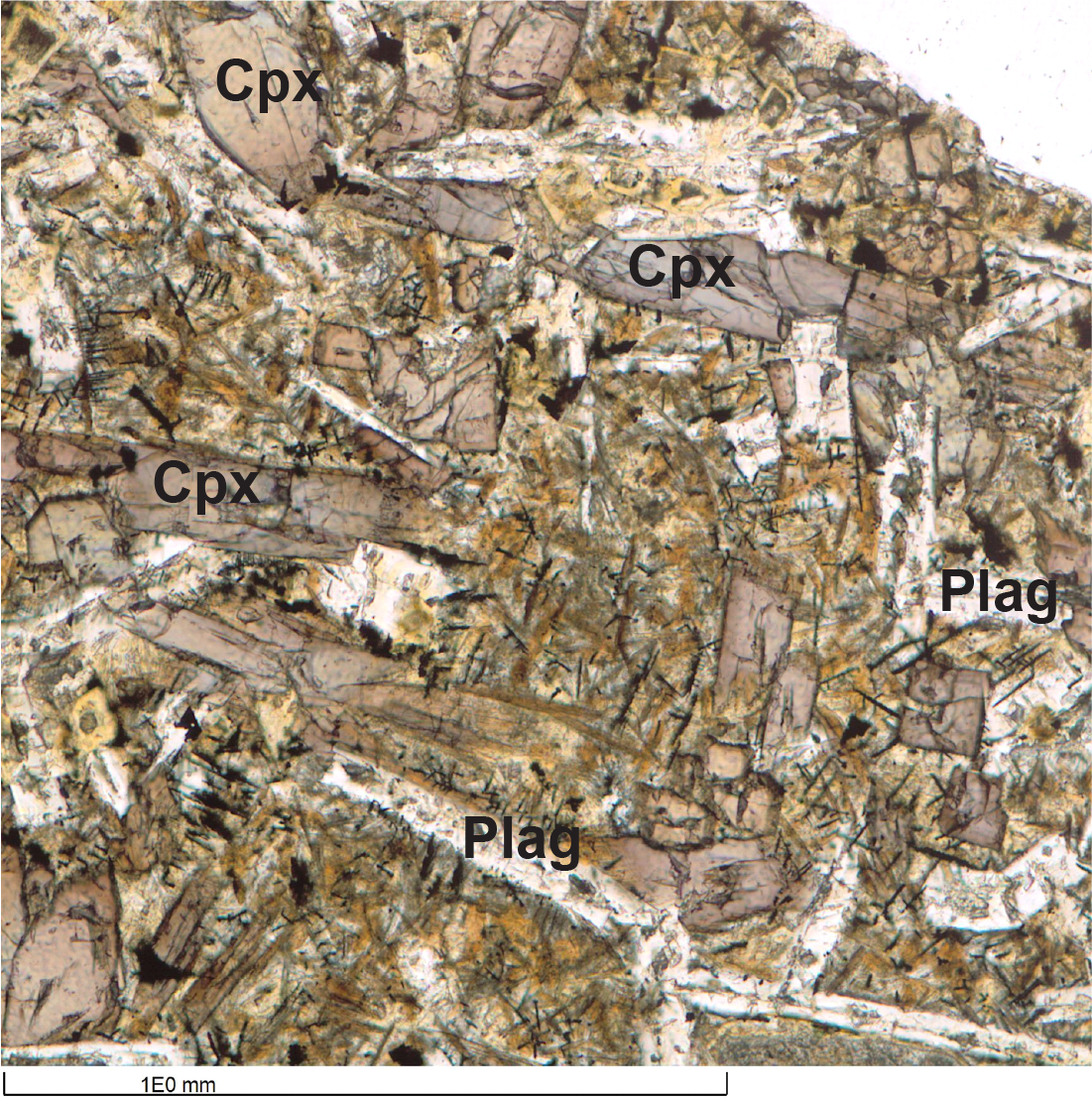
Figure F31. Texture and mineralogy of groundmass.

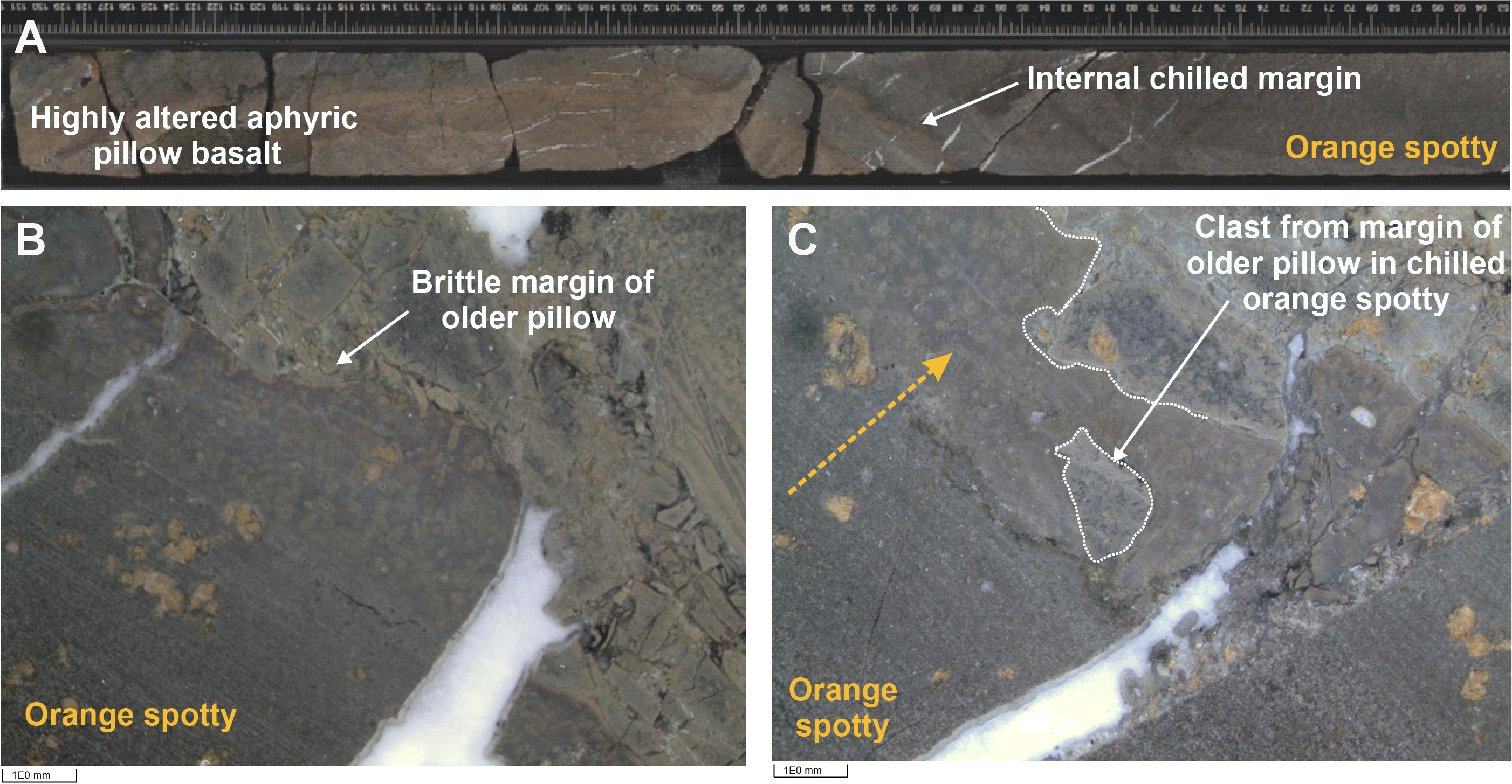
Figure F32. Contact between orange spotty and old red basalt.

5.1.1.11. Lithologic Unit 11

Interval: 390-U1556B-34R-7, 86 cm, through 38R-2
Depth: 511.0–530.7 mbsf
Lithology: aphyric to moderately olivine phyric basalt with interpillow hyaloclastite

Unit 11 is a 19.7 m thick interval of aphyric to moderately olivine phyric basalt intercalated with hyaloclastite. As in Units 9 and 10, the basalts recovered show significant variation in degree of alteration from piece to piece, particularly in Sections 390-U1556B-35R-1 through 36R-3, ranging from the typical olivine phyric orange spotty appearance to highly altered old red. At the time of macroscopic core description, it was assumed that these variations were solely a function of differing alteration histories. However, revised petrographic analysis combined with pXRF data (see Corroboration of stratigraphic units: pXRF analysis) shows that these two basalts also represent different magma types. Indeed, Unit 11 records several intrusive relationships between the two groups, allowing us to examine their order of emplacement. Superimposed on that variation is a change in the abundance of hyaloclastite over the interval such that the unit is divided into two subunits: Subunit 11a (Sections 34R-7, 86 cm, through 37R-1), which contains hyaloclastite, and Subunit 11b (Sections 37R-2 through 38R-2), which does not.

Although hyaloclastite recurs throughout Subunit 11a, it is present in relatively low abundance (i.e., one or two small [less than a few centimeters thick] pieces per section and/or thin layers adhering to the basalts). The hyaloclastite consists of glass and basalt clasts that are 100% altered; it is cemented primarily by zeolites and clay minerals of various colors rather than calcite (see Alteration petrology). In Section 390-U1556B-35R-1, the hyaloclastite is cemented by a pinkish gray (7.5YR 7/1) matrix/cement, whereas in Section 35R-2 the matrix/cement is light greenish gray (GLEY 1 7/10Y). In Section 37R-1, the matrix/cement is yellowish red (5YR 5/8) with calcite in low abundance. Note that in many cases it is difficult to distinguish between matrix (i.e., detrital) and cement (i.e., authigenic) in these rocks solely using macroscopic observation.

Petrographically, the orange spotty basalt in this interval is similar to that described for overlying units (i.e., sparsely to moderately olivine phyric, moderately altered, with bimodal vesicularity). The older pillow lavas (old red) display the same range of pillow margin crystallization sequences seen in orange spotty (i.e., quenched glass to dispersed varioles to coalesced varioles to cryptocrystalline and/or microcrystalline pillow interiors [see Chilled margin petrography]). However, the old red lavas are distinct from the orange spotty basalt by being aphyric to sparsely olivine (micro)phyric. They are also more altered than the orange spotty basalt to various shades of brown to reddish orange, which contrasts markedly with the overall gray (speckled) appearance of the orange spotty basalts (see Alteration petrology).

Intrusive relationships between the orange spotty and old red basalts are present in Sections 390-U1556B-36R-1, 36R-2, 37R-3, 38R-1, and 38R-2. The textural relationships produced are variable and complex (Figure F33). Interval 36R-1, 45–58 cm, for example, shows a piece of old red basalt with banding produced by alteration that is truncated against the chilled margin of orange spotty basalt. This indicates that old red basalts are older than orange spotty basalts because the banded alteration pattern must have occurred prior to the chilled margin; otherwise, the basalts would share the same or similar patterns of alteration (Figure F33A). Intervals 38R-1, 87–95 cm, and 38R-2, 87–95 cm, show old red basalts with variably planar to convoluted margins that subsequently have orange spotty basalt chilled against them but with no chilled margin in the old red basalt against the orange spotty (Figure F33D, F33E). The contacts between old red and orange spotty basalts are even more complicated in intervals 37R-3, 28–37 cm, and 36R-1, 58–70 cm, because they have subsequently been used as conduits for fluid flow and are now partially brecciated and hydrothermally altered (Figure F33C, F33F).

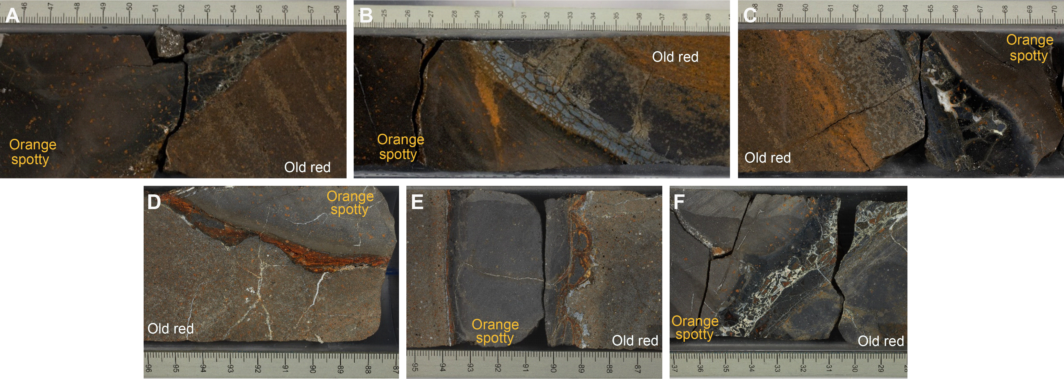
Figure F33. Variation between orange spotty and old red basalt.

We interpret these relationships to be evidence that an older sequence of pillow lavas (old red) was intruded by orange spotty basalts in this interval and possibly in overlying Units 8–10. As such, they may represent part of the feeder dike network for the moderately olivine phyric basalts higher in the sequence. We note that two thicker intervals of orange spotty basalt occur in between the intervals of pillow basalts in Sections 390-U1556B-37R-1 and 37R-2. The latter includes a single continuous core piece that is 89 cm long (Sample 37R-2 [Piece 1]). Chilled margins were not recovered for this piece, so its emplacement mechanism is indeterminate, but such a long piece would be compatible with a feeder dike emplacement origin, as inferred for other orange spotty basalts in this unit.

5.1.2. Stratigraphic Sequence B

5.1.2.1. Lithologic Unit 12

Interval: 390-U1556B-38R-3, 86 cm, through 54R-3
Depth: 530.7–609.0 mbsf
Lithology: aphyric to sparsely olivine phyric basalt with interpillow hyaloclastite

Unit 12 is a 78.5 m thick interval of aphyric to sparsely olivine (micro)phyric old red basalt. It is divided into six subunits based on the presence or absence of hyaloclastite and inferred changes in eruptive style. Petrographically, the old red basalt retains a similar appearance throughout most of Unit 12. As described for Unit 11, it is a highly altered, aphyric to sparsely (micro)phyric olivine basalt (Figure F34) (see Alteration petrology). Its color can vary on the scale of a single piece from brown to very dark gray, with the darker colors corresponding to chilled margins. In thin section, the olivine is typically replaced completely by iddingsite, Fe oxyhydroxides, and/or clay minerals, and groundmass is highly altered to smectite and Fe oxyhydroxides, which collectively gives the rocks their distinctive orange-red color (Figure F34B, F34C). In chilled margins, it is not uncommon for unaltered olivine microphenocrysts to persist even when the rest of the rock is highly to completely altered (e.g., Sample 390-U1556B-45R-2 [Piece 2, 26–28 cm]) (Figure F34D, F34E).

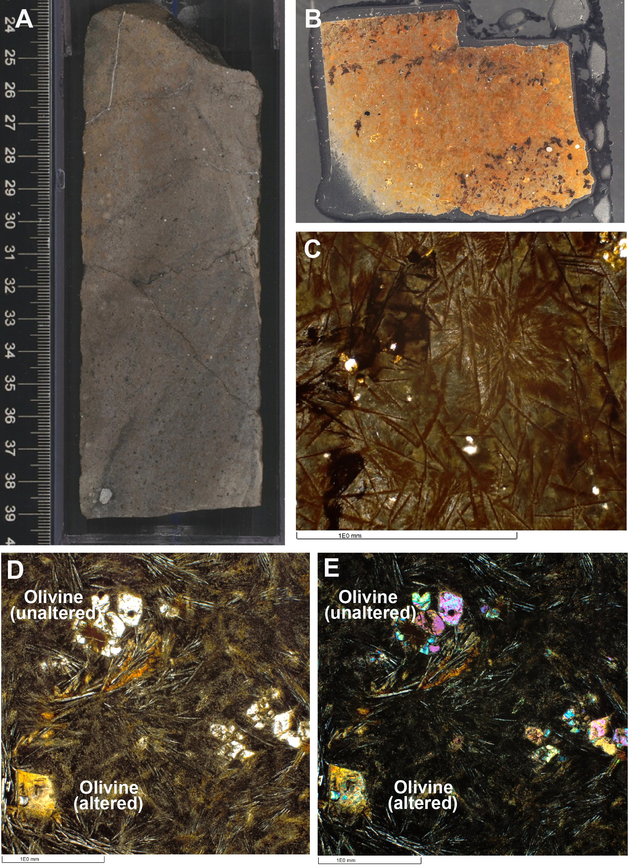
Figure F34. Old red basalt.

Subunits 12a (Sections 390-U1556B-38R-3 through 45R-3), 12c (Sections 46R-2 through 50R-3), and 12e (Sections 51R-3 through 53R-2) are defined by their relatively low abundance of hyaloclastite. In these subunits, hyaloclastite predominantly occurs as thin layers or small masses (<2–3 cm thick) on external core surfaces, with few discrete cored pieces of hyaloclastite (<4 cm). The hyaloclastites are clast supported and up to 80% of the rock consists of basalt and glass fragments that are highly to completely altered. Sorting is effectively bimodal: altered glass clasts are most commonly less than a few millimeters, whereas basalt clasts reach sizes of up to 4 cm, although most are less than ~2 cm. Moreover, many of the altered clasts have disaggregated into submillimeter-sized particles such that they are part of the matrix. Clasts are partially cemented by a grayish white to pale brown clay/silty material and/or calcite (see Alteration petrology). It is unclear what proportion of this material is sediment (i.e., detrital) versus cement (i.e., authigenic). Subunit 12f is also an interval of old red basalt associated with hyaloclastite, but here the glass fragments appear to have altered to a very dark greenish gray mineral (Figure F35) rather than the more commonly observed golden yellow (see Alteration petrology). Basalt clasts in Subunit 12f range up to 6 cm in size, although most are less than ~2 cm, and are cemented by calcite.

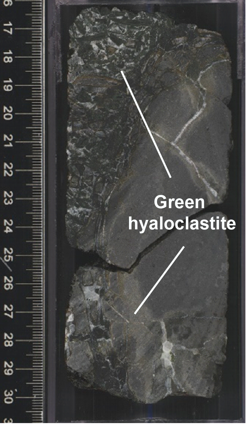
Figure F35. Green hyaloclastite.

Paired chilled margins are common throughout Subunits 12a, 12c, and 12e; excellent examples can be seen in Sections 390-U1556B-40R-1, 40R-3, and 44R-2 (Figure F36). Most indicate pillow lobes that are less than ~30 cm thick. In contrast, Subunits 12b and 12d are characterized by thicker pillows or massive flows (Figure F37). Section 51R-1, for example, is dominated by a large, continuous piece 82 cm long. The basalt in this interval is distinct from most old red basalts in that it is gray rather than reddish brown, suggesting a lower degree of oxidative alteration. It is also microcrystalline, as opposed to cryptocrystalline, and tends to fracture into sharp, angular pieces (Figure F37). Chemical analysis, however, indicates that it is compositionally indistinguishable from other basalts in Unit 12 in terms of Zr/Ti ratios (see Corroboration of stratigraphic units: pXRF analysis).

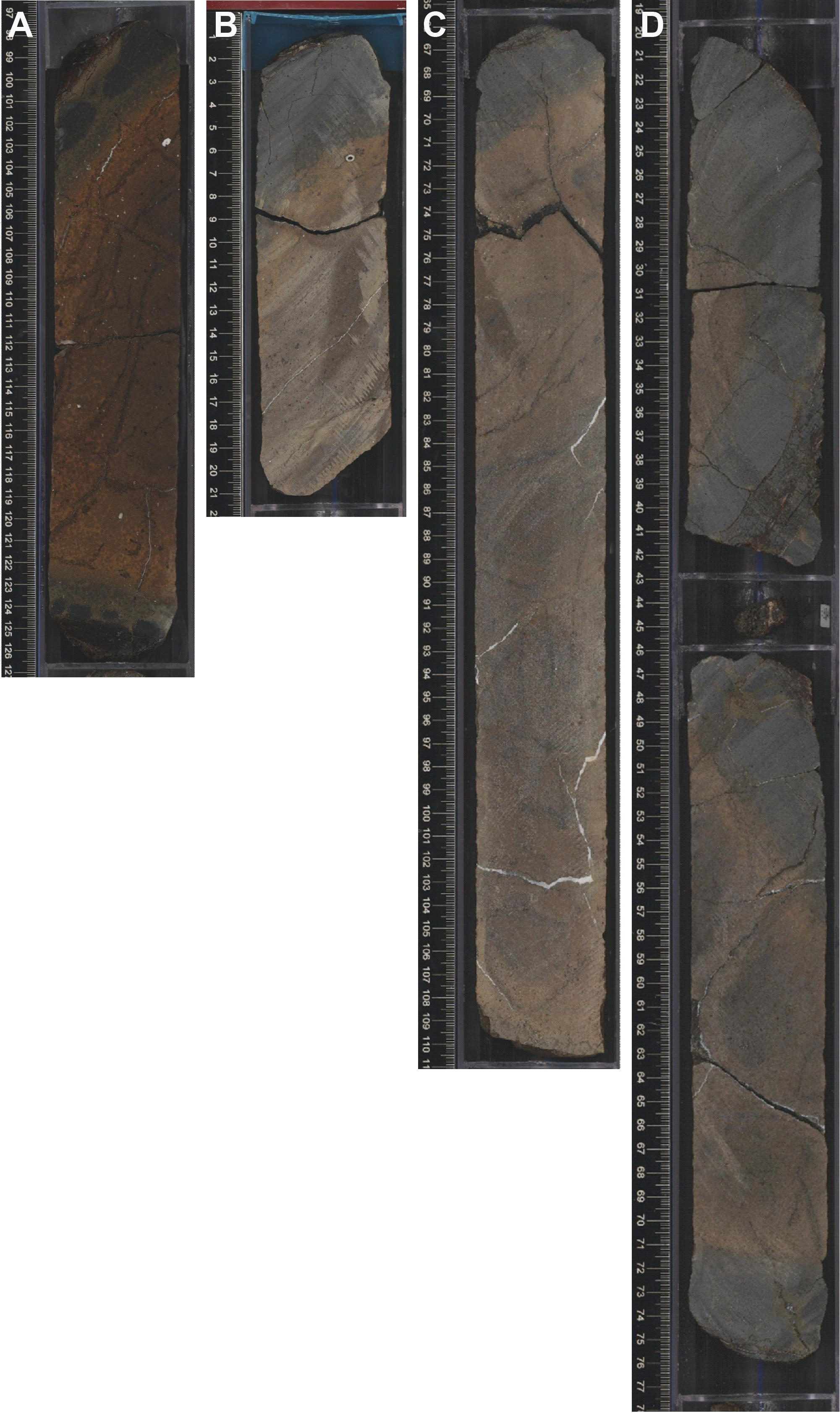
Figure F36. Paired chilled margins.

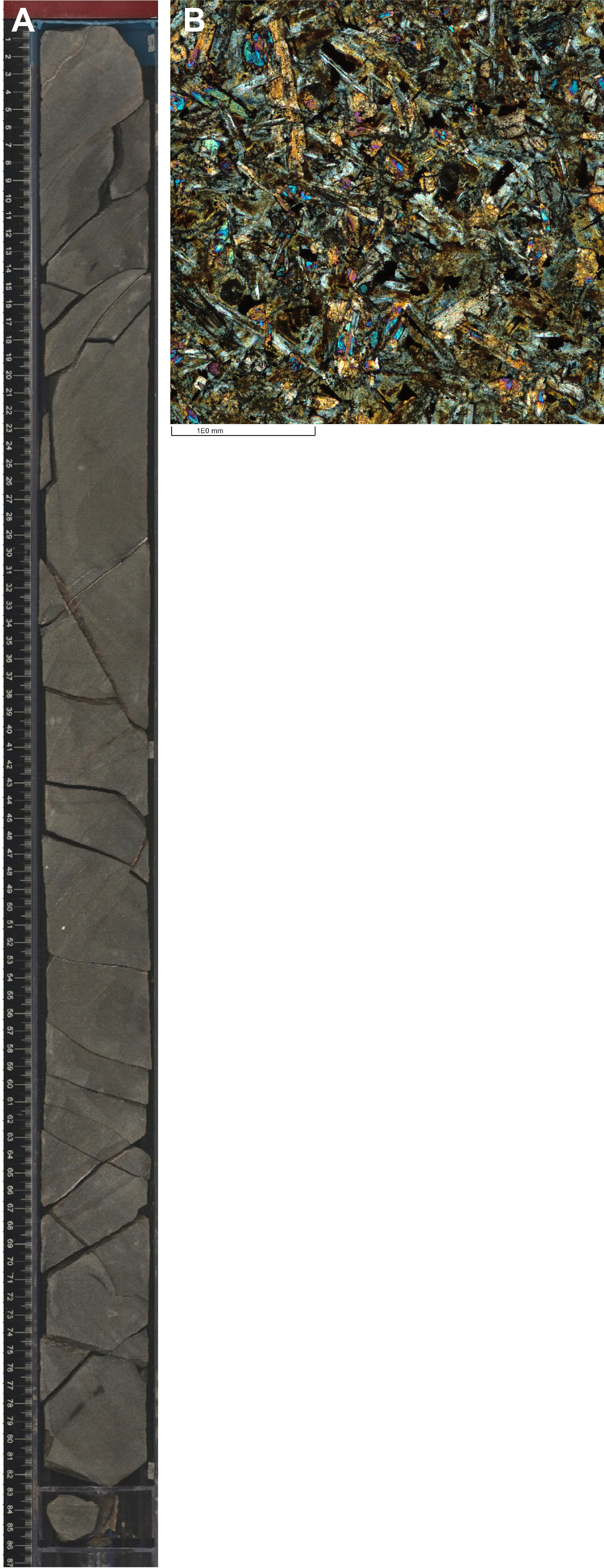
Figure F37. Massive interval.

5.1.3. Stratigraphic Sequence C

5.1.3.1. Lithologic Unit 13

Interval: 390-U1556B-54R-3 through 59R-4
Depth: 609.0–633.7 mbsf
Lithology: highly plagioclase-olivine-clinopyroxene phyric basalt

Unit 13 is a 24.7 m thick interval of H-POPP basalt. The rocks are gray and only moderately altered (see Alteration petrology). They are sparsely vesicular with small (<1 mm) round vesicles now filled with secondary clay minerals. The total phenocryst content is high (~20%) throughout the unit, even in glassy chilled margins (Figure F38). Plagioclase is the most abundant phenocryst/macrocryst phase. It ranges from unzoned subhedral tabular crystals to larger (up to 8 mm) anhedral to subhedral equant crystals that show subtle oscillatory zoning on their rims (Figure F39). These larger crystals may also contain melt inclusions and/or show signs of significant partial resorption (Figure F39), but they are typically unaltered.

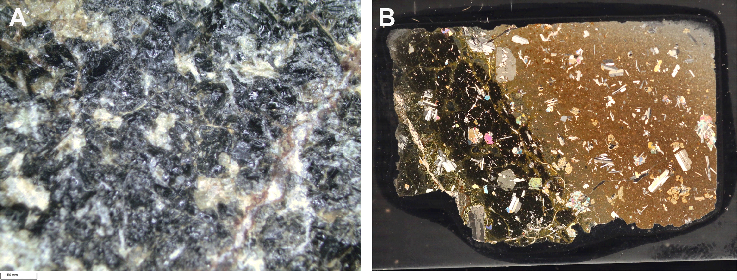
Figure F38. Chilled margins in H-POPP basalts.

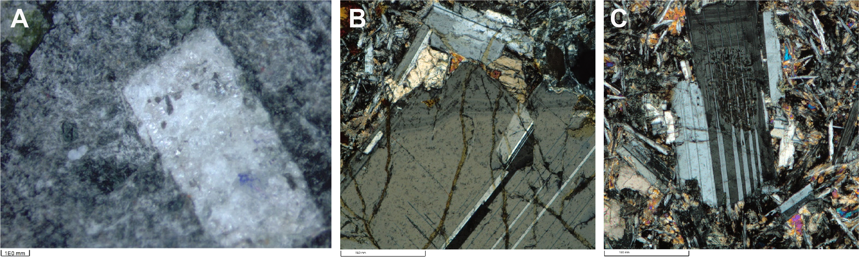
Figure F39. Macrocrysts in H-POPP basalts.

Olivine is the second most abundant phenocryst/macrocryst phase (up to 1.5 mm). It occurs as equant euhedral crystals that are completely altered to clay minerals ± Fe oxyhydroxides (Figure F40), although the composition of the clay minerals (based on color) varies throughout the unit (see Alteration petrology). Some larger olivine phenocrysts contain inclusions of dark red-brown Cr spinel (Figure F40B).

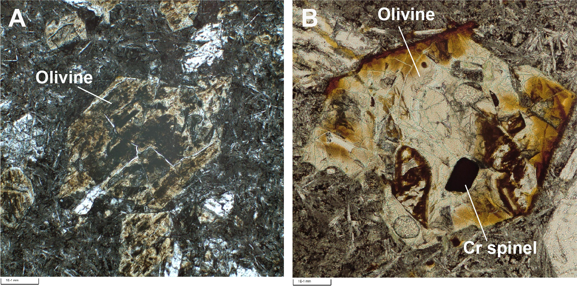
Figure F40. Olivine pseudomorphs in H-POPP basalts.

Clinopyroxene was not recognized as modally significant during macroscopic core description, although rare emerald green crystals (Figure F41A, F41B), inferred to be Cr diopside xenocrysts/macrocrysts, were identified on external core surfaces in a few sections. However, examination of the rocks in thin section shows that clinopyroxene is present throughout the unit. It occurs as large anhedral to euhedral crystals (Figure F41E), although only in association with plagioclase in microgabbroic crystal clots (Figure F41C). Clinopyroxene and plagioclase show ophitic to subophitic relationships in these assemblages (Figure F41C, F41E). More rarely, the crystal clots include olivine (pseudomorphs) (Figure F41D); in most cases, olivine (pseudomorphs) occurs as solitary crystals or in glomerocrystic clusters of olivine alone. Clinopyroxene is typically unaltered, although there are rare examples of partial resorption (Figure F41F). Based on the textural and compositional characteristics, these crystal clots are interpreted to be cognate inclusions (autoliths).

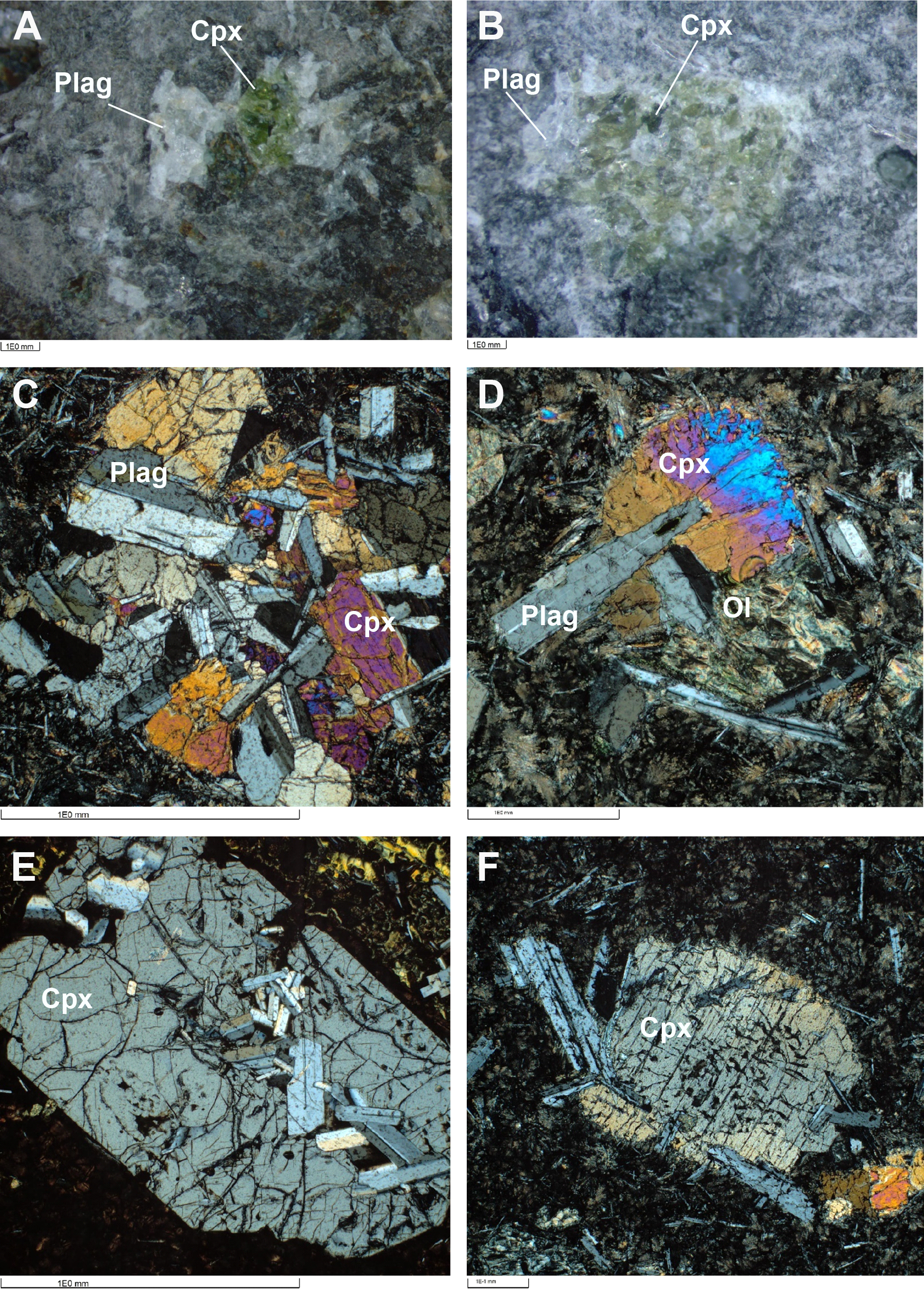
Figure F41. Exterior core faces.

Long, continuous core pieces (up to 65 cm) are common in Unit 13 (e.g., Sections 390-U1556B-58R-1, 58R-2, 59R-1, 59R-2, and 59R-3), and many have subhorizontal chilled margins, although chilled margins with high angles to the core vertical are also observed. For example, Sample 56R-1 (Piece 1) is a single continuous piece 110 cm long, suggesting it is a massive flow. Together, this suggests that Unit 13 was emplaced as a series of relatively large (0.5–1 m) pillow and massive lava flows.

Indurated calcareous sediment ± hyaloclastite occurs throughout the unit. In most cases, it is present as thin layers or small masses a few centimeters thick attached to basalt pieces, particularly in association with glassy chilled margins (Figure F42A), but there are also several thicker sedimentary intervals (e.g., intervals 390-U1556B-55R-1, 42–50 cm; 55R-3, 10–15 cm; 56R-4, 58–64 cm; 57R-1, 34–43 cm; and 59R-4, 22–36 cm) between flows (Figure F42B). In the absence of significant quantities of glass or basaltic glass, the sediment (micritic limestone) tends to be pale brown (2.5Y 8/1) or light gray (10YR 7/2). The sediment matrix of the hyaloclastites, however, exhibits a wide range of colors, including not only pale brown (2.5Y 8/1) and light gray (10YR 7/2) but also dark grayish brown (2.5Y 4/2), brown (7.5YR 5/3), light reddish brown (5YR 6/4), dusky red (5R 3/3), pink (7.5YR 7/3), pinkish gray (10YR 6/2), olive-brown (2.5Y 4/3), and reddish brown (2.5YR 5/6) (Figure F42B). Thin section analysis of the sediments confirms that they include a significant pelagic component because they contain abundant microfossils (Figure F43) (see Biostratigraphy).

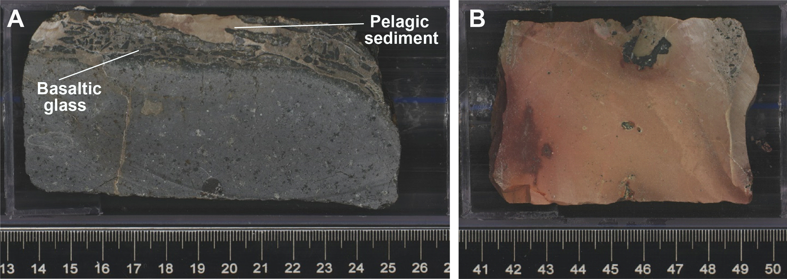
Figure F42. Pelagic sediment in chilled margin, H-POPP basalt.

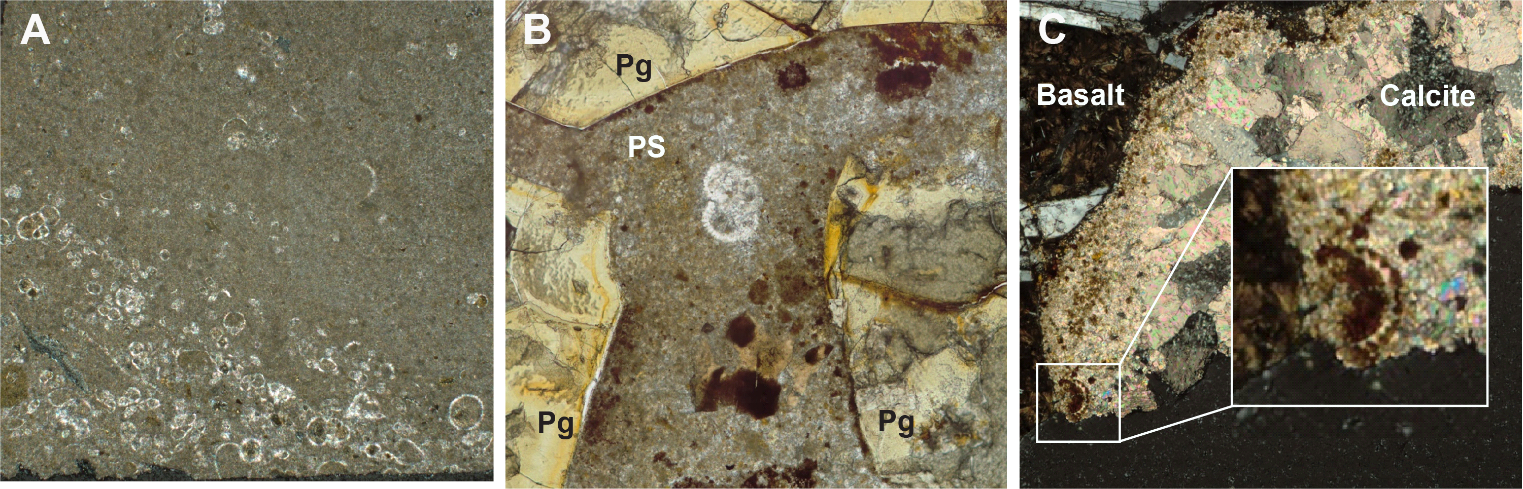
Figure F43. Pelagic sediment.

The chilled margins of the H-POPP basalts are texturally distinct from those of pillow lavas encountered higher in the hole (see Chilled margin petrography), and this contributes to the character of the hyaloclastites recovered in Unit 13. In particular, the glassy zone is remarkably consistent in thickness between 1 and 1.5 cm, and the adjacent spherulitic inner zone is very thin (i.e., <0.5 cm; Figure F44). These thick, glassy chilled margins commonly detach in slabs 2–4 cm long and become incorporated into sequences of sediment-supported hyaloclastite (e.g., Samples 390-U1556B-55R-4 [Piece 1] and 56R-2 [Piece 2]; Figure F45). When they are part of a continuous core piece, the sediments are typically less than ~10 cm thick, but where there are intervals that span several core pieces, they can reach apparent thicknesses of up to 36 cm (e.g., intervals 390-U1556B-56R-2, 2–38 cm, and 58R-1, 46–82 cm).

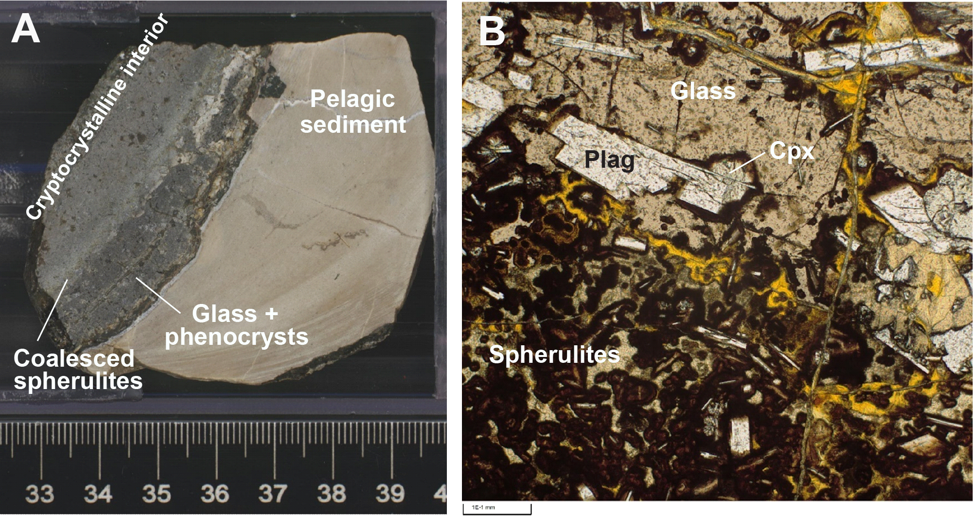
Figure F44. H-POPP basalt showing thin chilled margin.

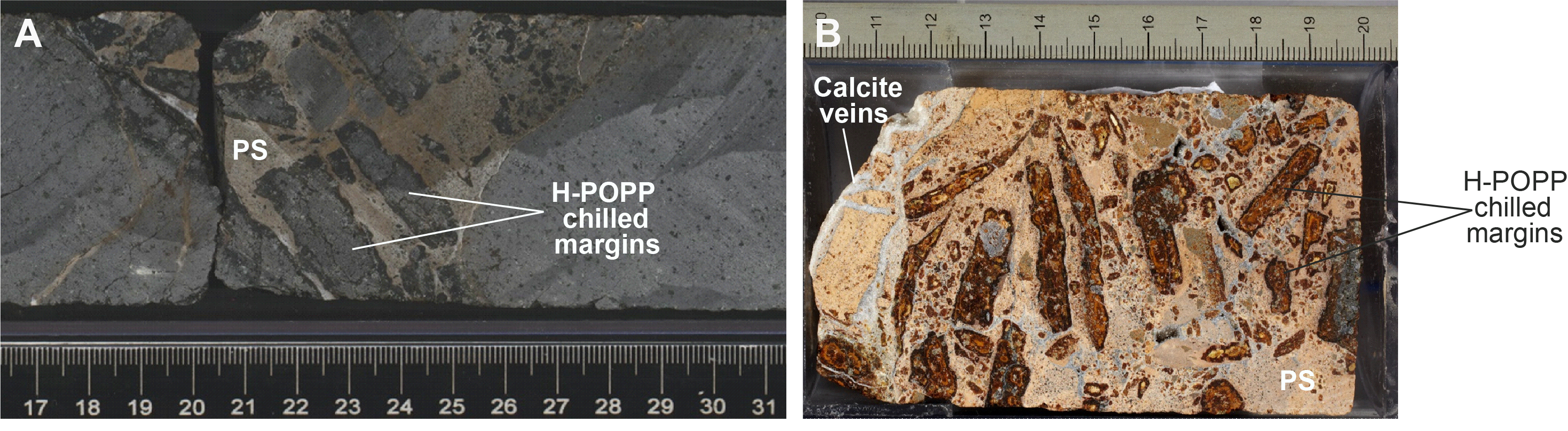
Figure F45. Hyaloclastites.

The chilled intervals observed in the H-POPP basalts also exhibit complex structural relationships as well as distinct crystallization textures; in particular, many chilled intervals occur internal to core pieces rather than at their margins. They are commonly associated with pelagic sediment and/or hyaloclastites that are sediment matrix rich. In Sample 390-U1556B-55R-2 (Piece 3), chilled margins occur at the top and bottom but also in the middle—all in one continuous piece (Figure F46). The chilled margin captured in the middle of the piece has thin spherulitic zones on both sides, meaning it is essentially a normal H-POPP-type chilled margin that has been completely folded over. In some intervals, this folding process is only partial and trapped pelagic sediment between the two limbs of the fold (Figure F47).

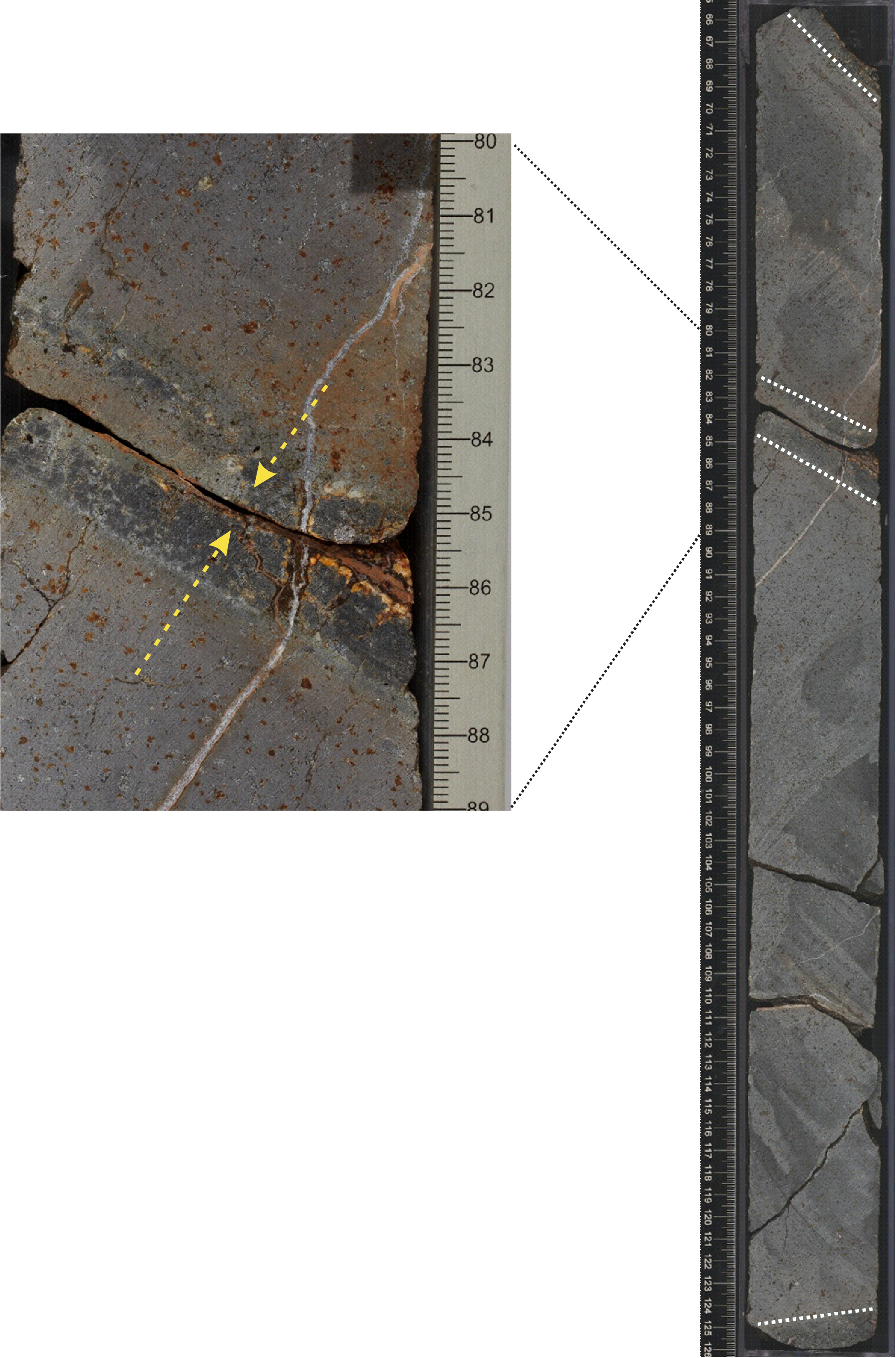
Figure F46. Long, continuous piece of H-POPP basalt.

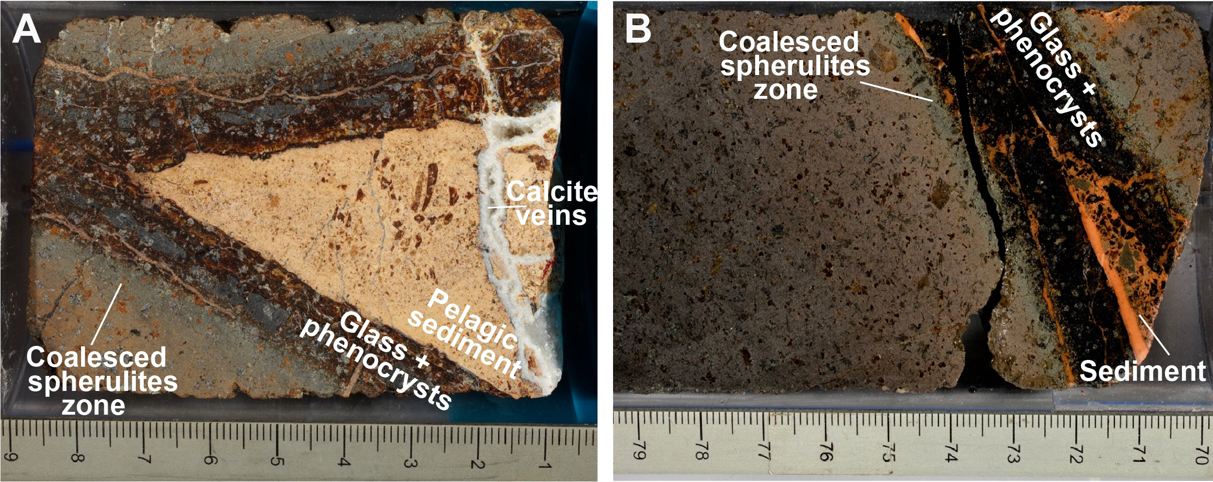
Figure F47. Folded chilled margins.

We interpret these textures to be evidence that the H-POPP magmas erupted onto pelagic sediment. As the lavas attempted to flow, the chilled outer surface folded over, entrapping sediment.

5.2. Chilled margin petrography

As shown by Kempton (1985), the petrographic fabrics observed in pillow basalts are the product of significant deviations from equilibrium crystallization temperatures and a progressive decrease in cooling rate from the margin toward the interior. The resulting textures are distinctive and can aid in identification of this mode of lava emplacement when other criteria (e.g., radial fractures, wedge-shaped pieces, and complete arcuate glassy margins) are lacking. This approach was used throughout the description of the basalts from Site U1556. Moreover, these textural variations respond differently to alteration (see Alteration petrology). In this section, we review the sequence of textures commonly observed in chilled margins to put the background alteration of Site U1556 basement rocks into context.

Figure F48 summarizes the textures commonly observed in pillow basalts from Site U1556, using Sample 390-U1556B-9R-2, 59–62 cm, as an example. In general, four distinct textural zones are observed. From the glassy margin inward, these zones are as follows:

Zone A = glass (± alteration).
Zone B = glass (± alteration) with isolated spherulites.
Zone C = coalesced spherulites.
Zone D = plumose and dendritic quench growth.

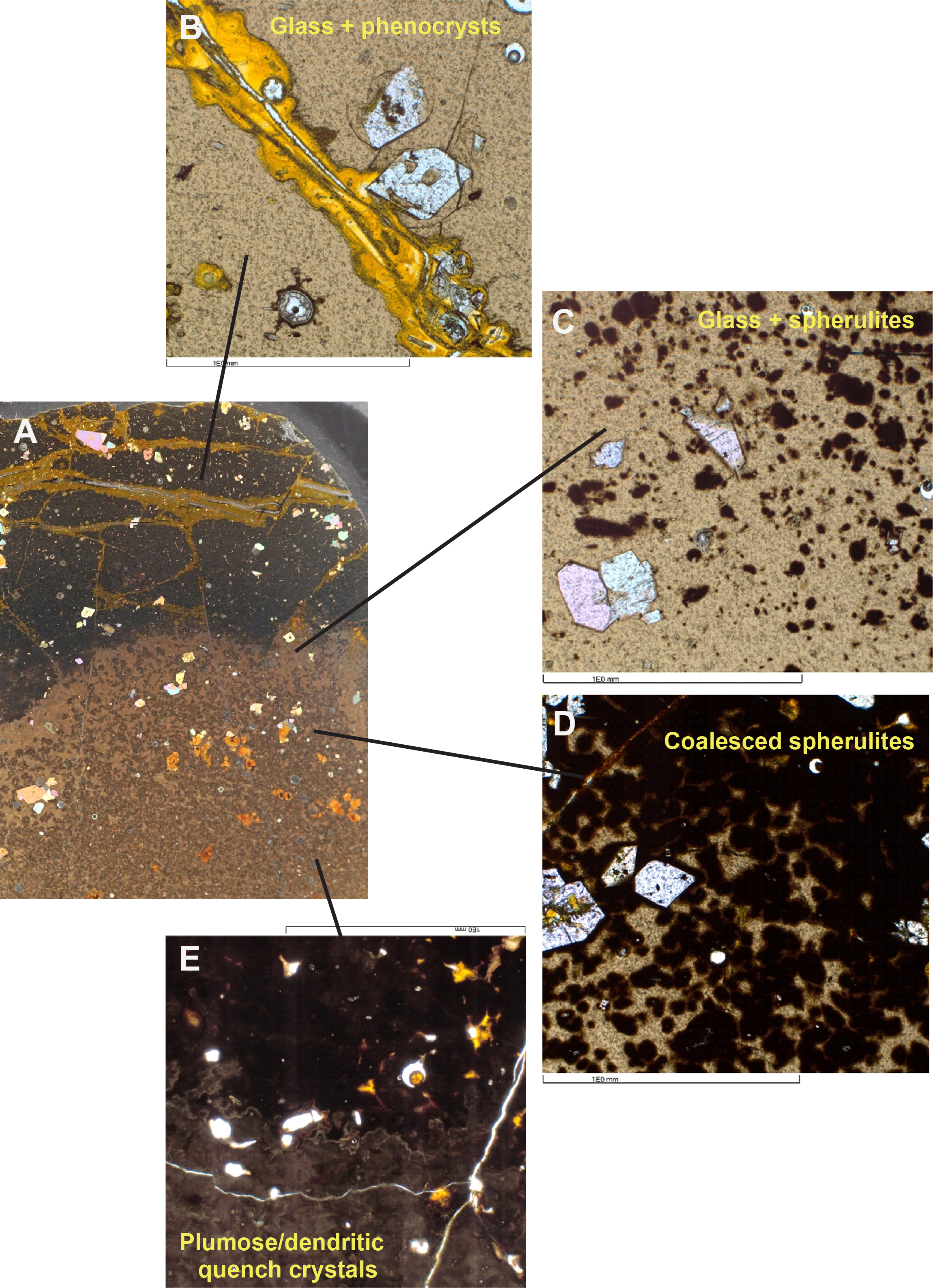
Figure F48. Textural sequence, pillow chilled margin.

In Zone D, the plumose textures are typically produced by clinopyroxene and the dendritic and skeletal textures tend to be produced by plagioclase and olivine. Phenocrysts may be present in any or all of these zones depending on the composition of the magma.

In Zone A (Figure F48B), the glass is commonly brecciated or fractured into triangular or polygonal shapes and altered along those fractured edges. Inward from the glassy margin (in Zone B), spherulites appear in isolation in glass (Figure F48C). The spherulites form small circular or oval shapes and are typically dark brown. Plagioclase microlites may occupy the centers of some spherulites (Figure F49); however, as shown by Kempton (1985) using backscatter electron imaging, the highly skeletal structures surrounding the plagioclase are usually not produced by the plagioclase microlite. Instead, they are produced by olivine or clinopyroxene that has nucleated on the plagioclase.

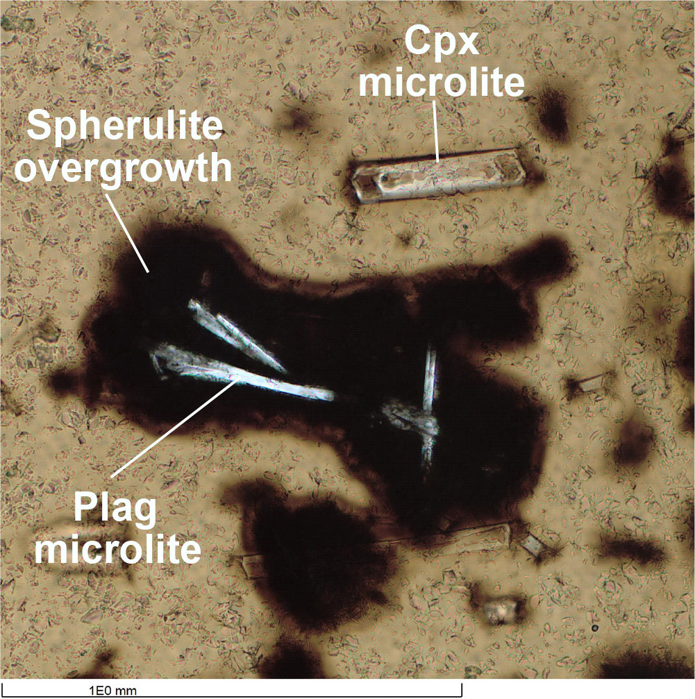
Figure F49. Plagioclase microlite at core of brown spherulites.

The zone of isolated spherulites is followed by coalescence and slight enlargement of the spherulites in Zone C (Figure F48D). This zone may appear dark gray to black in hand specimen and may appear relatively fresh compared to the interior portions of the pillow lavas, but it should be recognized that this material is not glass even if it may appear glassy. The zone of coalesced spherulites is followed inward by the abrupt loss of dark brown spherulites (inferred to be olivine spherulites) and the rise and predominance of lighter brown plumose quench growth (Figure F48E). Although detailed shore-based research will be required to confirm the nature of this transition and the mineralogy of the various spherulites, based on the rocks studied from Deep Sea Drilling Project Hole 504B (Kempton, 1985) this color transition corresponds to a decrease in the spherulitic growth of olivine (dark brown) and an increase in the plumose quench growth of clinopyroxene (lighter brown). Fe-Ti oxides commonly occur as equant crystals lining the boundaries of coalesced plumose clinopyroxene in Zone D, so this zone effectively marks the first appearance of an Fe-Ti oxide during crystallization.

These textural variations have an impact on the alteration of the basalts. We have observed, for example, that if the zones of glass and isolated spherulites survive early alteration, they can remain unaltered even when the background alteration is high (e.g., as exemplified by the abundance of fresh glass in many chilled margins and breccias). The zones of coalesced spherulites, however, appear to be relatively susceptible to alteration, and they may produce a light gray zone adjacent to relatively unaltered glass (see Alteration petrology). Another feature present is patchy (variolitic) alteration of some samples in zones that do not correspond to the primary spherulitic texture of Zones B and C (Figure F50). These may represent selective alteration of dendritic olivine intergrown with plagioclase, whereas plumose clinopyroxene growth remains largely unaltered (Figure F51). This sequence would be consistent with the alteration observed at coarser grain sizes (see Alteration petrology) (i.e., the selective complete replacement of olivine when clinopyroxene remains largely unaltered).

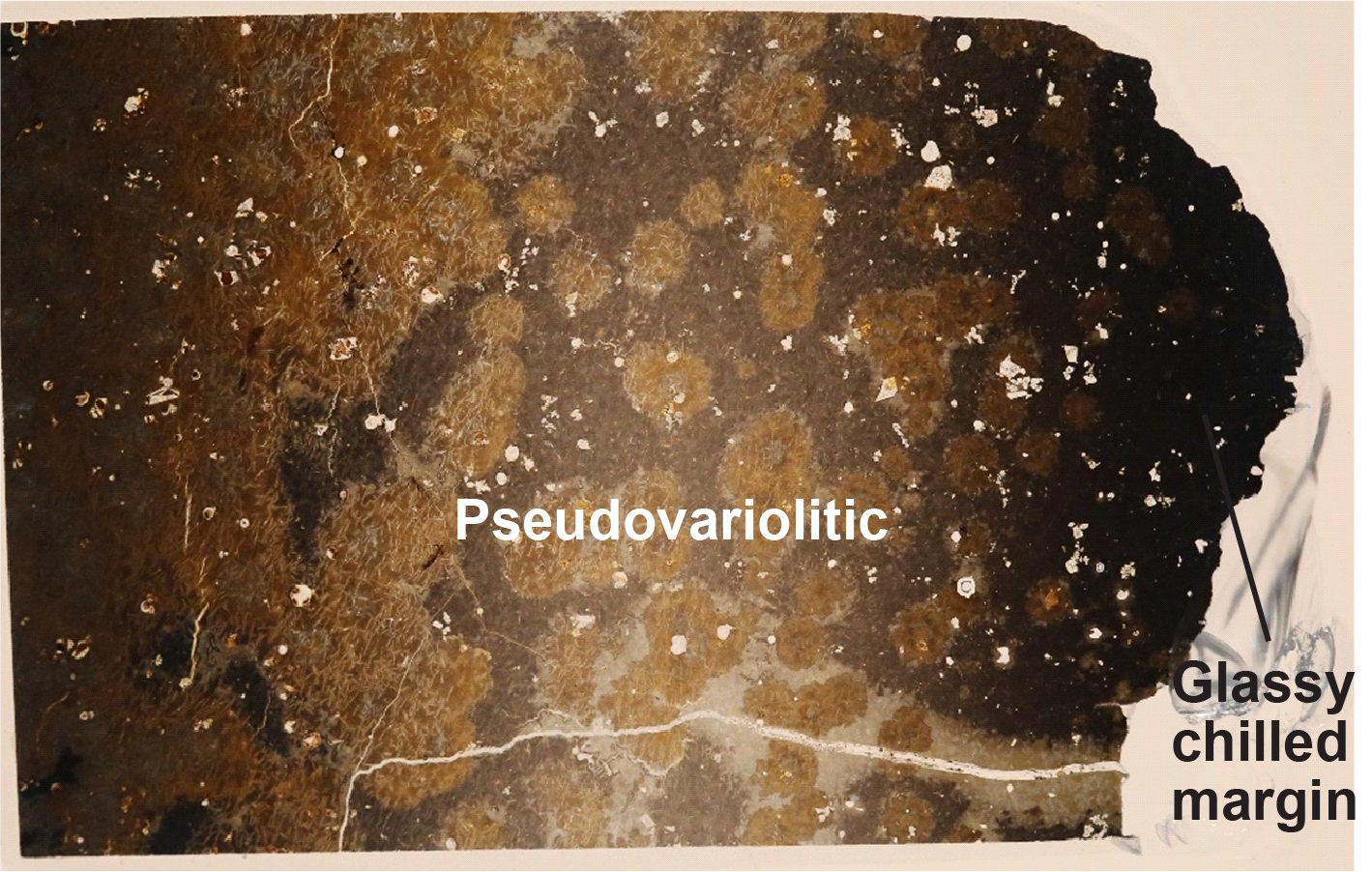
Figure F50. Patchy/selective alteration.

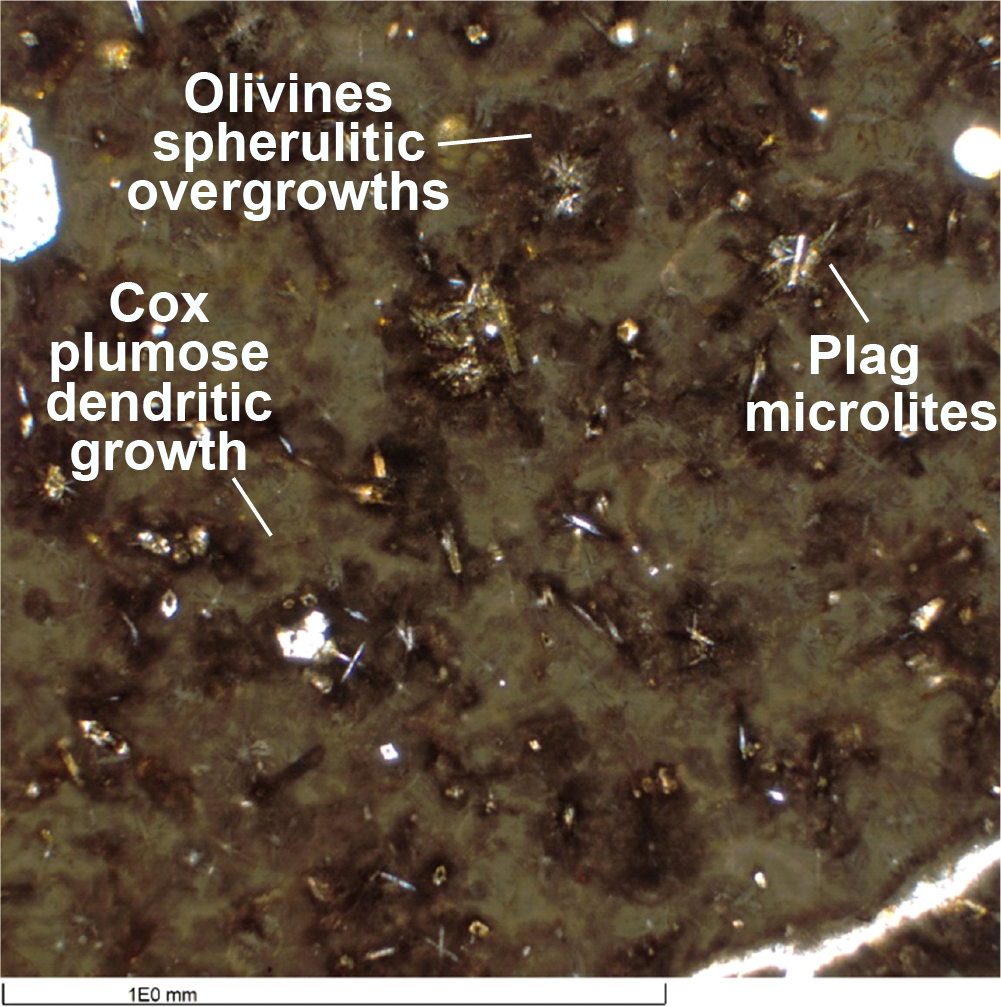
Figure F51. Alteration of olivine spherulitic overgrowths.

The skeletal growth morphology of olivine in the microcrystalline interior portions of pillow basalts in Hole U1556B exhibits some distinctive aspects relative to the habits observed in Hole 504B. In particular, rather than equant skeletal lantern or hopper crystal shapes, the olivines in Hole U1556B samples form pseudobladed structures that consist of chains of equant skeletal crystals reminiscent of spinifex textures (Figure F52). This morphology is restricted to pillow basalts from Units 1–11 and may be related to the more alkaline composition of the rocks in the middle and upper parts of Hole U1556B (see Geochemistry).

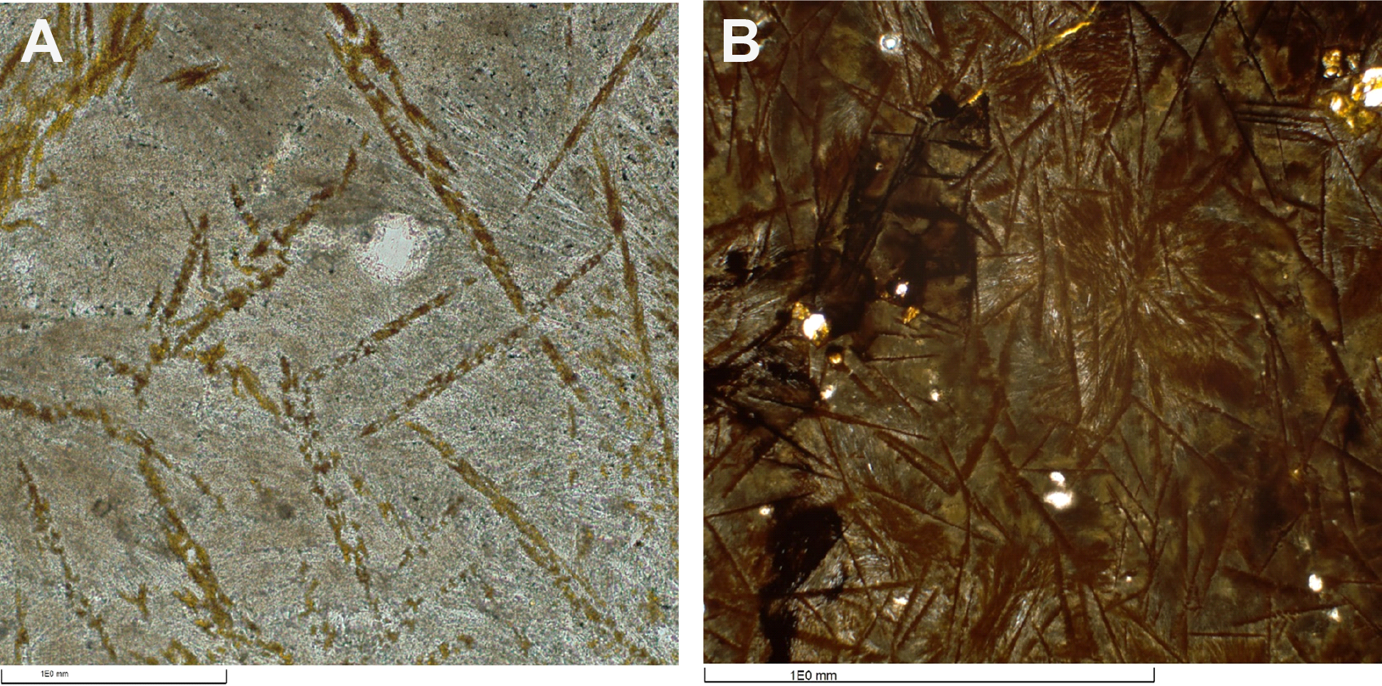
Figure F52. Skeletal olivine forming pseudobladed structures.

The textural sequence described above for chilled pillow margins dominates the basalts recovered in Units 1–11 at Site U1556 (i.e., orange spotty and old red basalts), indicating that these units are predominantly a series of pillow lavas. However, the H-POPP basalts of Unit 13 exhibit a much more abbreviated sequence of textures. These are summarized in Figure F53 using Sample 390-U1556B-55R-3, 99–102 cm, as an example. The figure shows that the sequence of textures is similar to that for pillow basalt Sample 9R-2, 59–62 cm, but the transition from glass to coalesced spherulites occurs over a much shorter length scale. Shore-based research will be required to fully understand the reason for this variation, but the highly phyric nature of the H-POPP basalts and the fact that they are multiply saturated in plagioclase, olivine, and clinopyroxene could mean that nucleation is easier and therefore more nuclei per volume survive to produce quench growths.

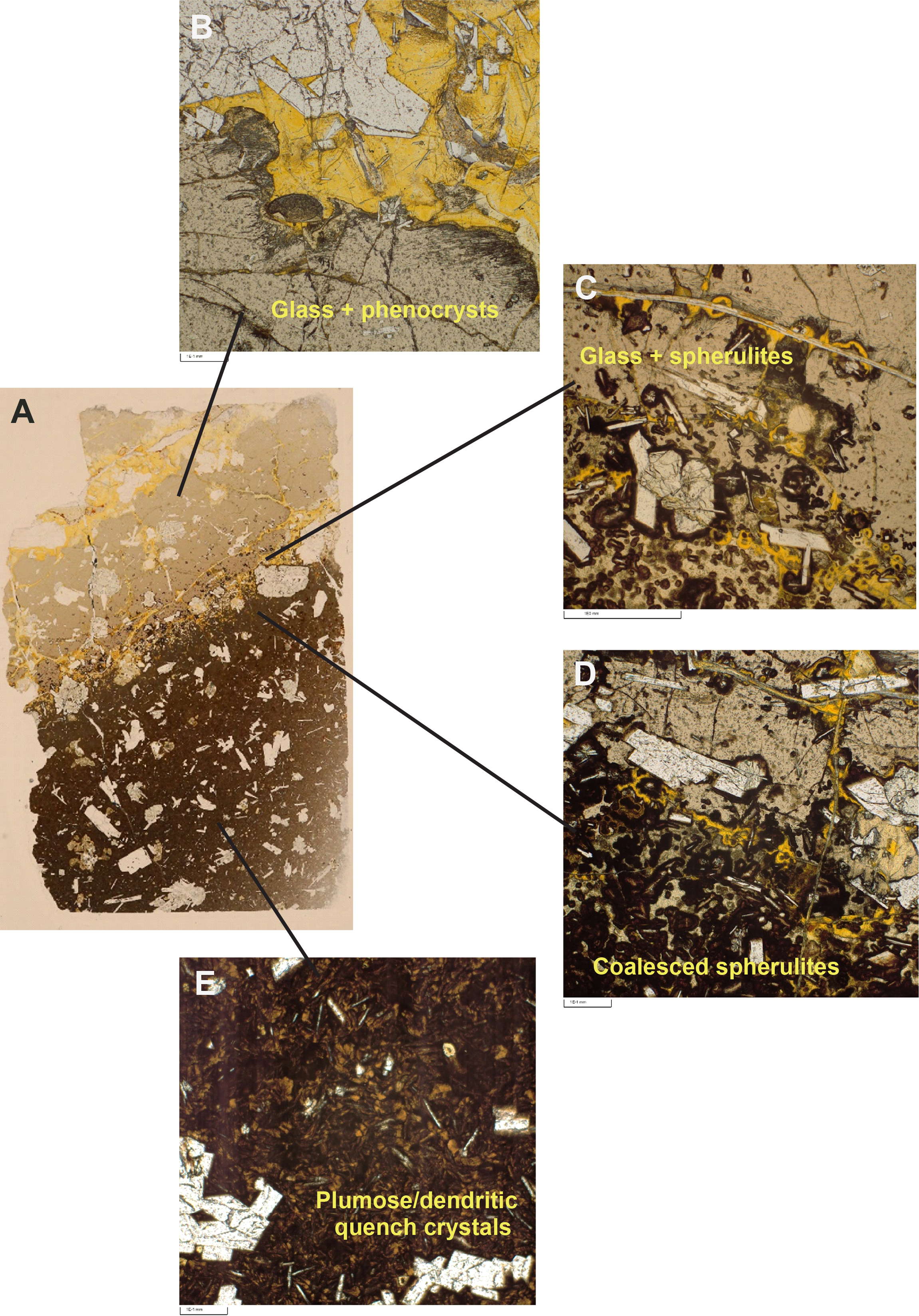
Figure F53. Textural sequence, H-POPP basalt lava flows.

5.3. Corroboration of stratigraphic units: pXRF analysis

Petrologic interpretations made from macroscopic core description were corroborated using pXRF analyses of samples from the archive half of the core (see Geochemistry in the Expedition 390/393 methods chapter [Coggon et al., 2024c]). The pXRF was particularly helpful because the rapid analysis time meant we could do the analyses in real time. In addition, the nondestructive nature of the technique allowed us to analyze a greater number of samples than was possible using shipboard ICP-AES because we could analyze smaller and/or more unique samples (e.g., glass clasts) that were potentially less altered than the material available for analysis of whole-rock powders.

However, in our usage of pXRF, we found that the results for most elements were insufficiently precise and/or accurate to be useful (see Geochemistry in the Expedition 390/393 methods chapter [Coggon et al., 2024c]). Exceptions to this are the elements Ti and Zr, both of which have analytical reproducibility of around 1% based on repeat analyses of the BHVO-2 basalt powder reference material. Titanium and Zr are also both HFSEs, which are known to be relatively insensitive to the effects of alteration. As such, these elements are useful geochemical tools for discriminating magma types where alteration may be high, such as at Site U1556 (see Alteration petrology). However, despite being among the most reproducible elements measured using the pXRF (i.e., the most precise), inaccuracy of the analyses turned out to be a significant problem. Even after correcting our measured values to the certified values for BHVO-2, when we compared the pXRF analyses of powdered samples with the data measured using ICP-AES, the results showed significant discrepancies (up to 60%), particularly for Zr. Moreover, we found that the correction needed to bring the two data sets into alignment was dependent on composition. We have, therefore, used the data determined by ICP-AES to apply a compositional correction so that the analyses of solid core samples can be compared robustly. Using this approach, we believe the pXRF data can be viewed as internally consistent and sufficiently comparable to the ICP-AES analyses for the purposes of documenting downhole variations in Zr/Ti in Hole U1556B (see Geochemistry).

For Site U1556, we produced 235 analyses of 99 samples (solid core pieces) from the archive half of the core and 42 analyses of powders prepared for ICP-AES analysis from samples taken from the working half of the core (see Geochemistry). Our analyses cover all 13 lithologic units (25 subunits), except Unit 9 (Table T5).

Figure F54 summarizes the data, as a function of depth in a plot of Zr/Ti normalized to the Zr/Ti ratio for normal MORBs (N-MORBs) (Sun and McDonough, 1989), which we represent as [Zr/Ti]_N. Collectively, basalts from Site U1556 show a wide range of values (0.62–1.83). Even considering the analytical difficulties described above, this range is much larger than expected. N-MORBs should have [Zr/Ti]_N values near 1, and enriched MORBs (E-MORBs) should have slightly higher values of ~1.2 (Sun and McDonough, 1989). By comparison, ocean-island basalts (OIBs) have [Zr/Ti]_N values of ~1.6 (Sun and McDonough, 1989).

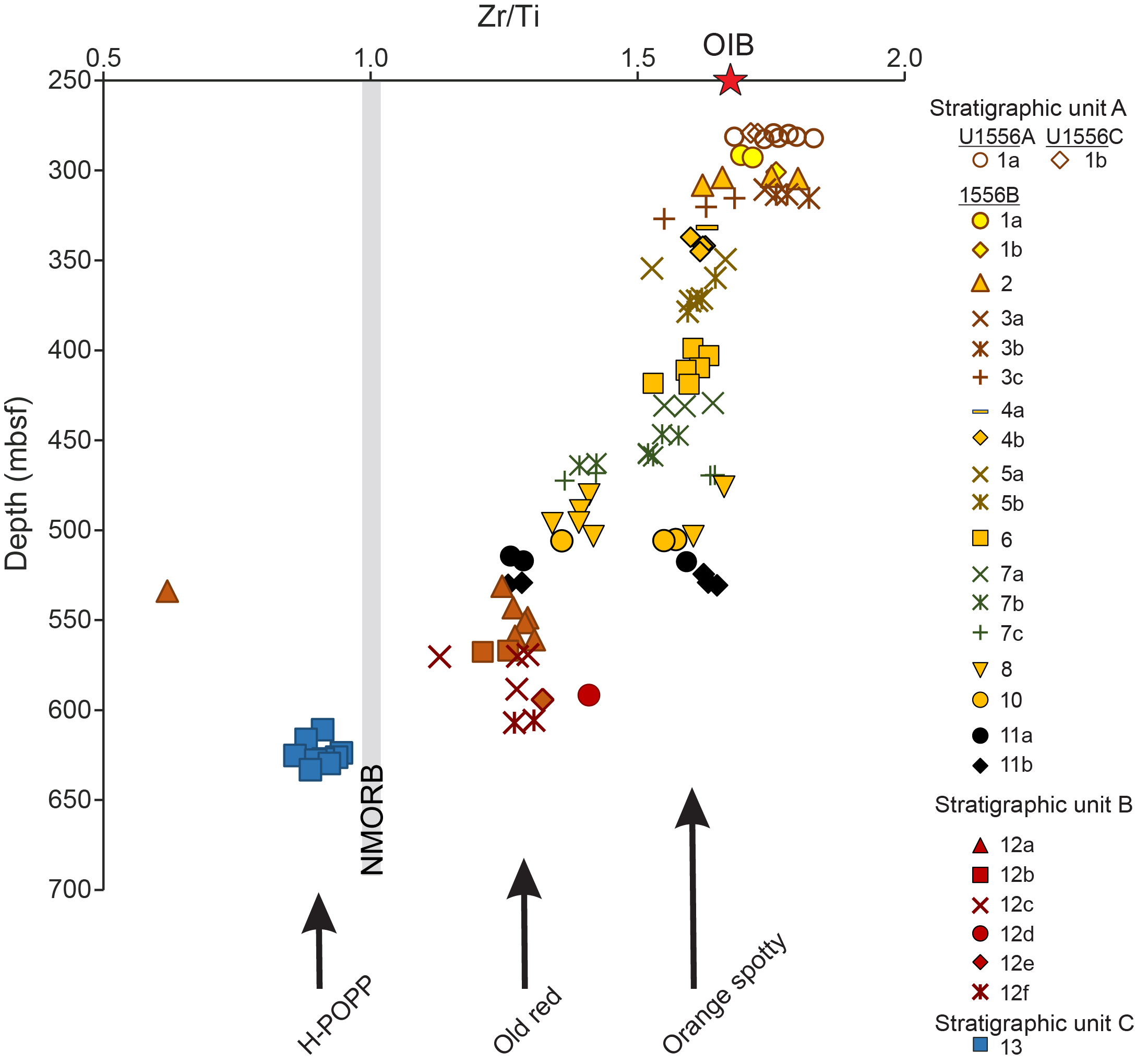
Figure F54. [Zr/Ti]_N for basalts.

Site U1556 basalts thus range from values slightly less than N-MORBs to compositions typical of OIBs. However, the data clearly cluster into three groups. Basalts from Units 1–10 (Stratigraphic Sequence A; i.e., orange spotty) have [Zr/Ti]_N values ranging 1.34–1.83 (average = 1.6 ± 0.1; 1σ). Basalts from Unit 12 (Stratigraphic Sequence B; i.e., old red) range 0.62–1.41, although the low end of this range is a single analysis we consider to be an outlier (see Geochemistry in the Expedition 390/393 methods chapter [Coggon et al., 2024c]). If that sample is discounted, the range for Unit 12 is 1.13–1.41 (average = 1.24 ± 0.06; 1σ). Basalts from Unit 13 (Stratigraphic Sequence C; i.e., H-POPP) show quite a limited range of 0.86–0.95 (average = 0.91 ± 0.03; 1σ). Therefore, based on pXRF data, the three groups of basalts map precisely onto the three petrologic groups identified by macroscopic and microscopic core description, corroborating the division of the volcanic sequence at Site U1556 into the three Stratigraphic Sequences A–C.

Note that we intentionally omitted Unit 11 from the averages reported for the three groups because we know this unit includes intrusive relationships between two different magma types. Based on petrographic observations, we interpreted those two magma types to be orange spotty and old red (Stratigraphic Sequences A and B, respectively). The pXRF data confirm that macroscopic observation, showing a spread of values from 1.26 to 1.65 for Unit 11, with the low values similar to those of Stratigraphic Sequence B basalts and the high values similar to those of Stratigraphic Sequence A.

These data suggest that most of the basalts recovered from Site U1556, (i.e., orange spotty and old red) are more alkaline than MORBs, a result that is consistent with petrographic observations (e.g., the presence of titanaugite) as well as the ICP-AES major element data (see Geochemistry). The H-POPP basalts (Stratigraphic Sequence C) are the most MORB-like, both petrographically and geochemically, although [Zr/Ti]_N values are slightly lower than average MORBs (Figure F54). The highly phyric nature of H-POPP basalts—and the presence of abundant microgabbros/autoliths—may contribute to the lower ratios, or it could simply be an analytical artifact of the pXRF data correction applied. Shore-based research, particularly high-precision isotope data, will be required to fully understand the petrogenesis of these rocks.

5.4. Summary

In summary, basalts from Site U1556 can be grouped into 13 lithologic units, defined by changes in petrographic type, phenocryst assemblage, inferred eruptive style (e.g., pillow lavas versus massive flows), and/or the appearance or disappearance of breccias/hyaloclastites. These 13 lithologic units can be further grouped into three major stratigraphic sequences:

Stratigraphic Sequence A: sparsely to moderately olivine phyric pillow basalts (i.e., orange spotty).
Stratigraphic Sequence B: aphyric to sparsely olivine (micro)phyric pillow basalts (i.e., old red).
Stratigraphic Sequence C: highly plagioclase-olivine-clinopyroxene phyric basalt (massive flows) (i.e., H-POPP).

The oldest rocks among these stratigraphic sequences (i.e., H-POPP) are the most MORB-like. They are highly phyric (~20%) and multiply saturated with plagioclase, olivine, and clinopyroxene. They also contain microgabbros/autoliths. The origin of such crystal accumulations remains debated, with some authors suggesting that they require accumulation in a shallow magma chamber prior to eruption (Hellevang and Pedersen, 2008), whereas others argue for derivation from crustal or mantle mush zones (Lange et al., 2013). The H-POPP basalts erupted as relatively thick pillow and massive lava flows and incorporated layers of pelagic sediment into folds in their chilled margins. This suggests that the magmatism occurred after a period of magmatic quiescence, during which the sediments accumulated.

In contrast, the aphyric old red basalts erupted predominantly as pillow lavas. They are compositionally distinct from H-POPP basalts, with [Zr/Ti]_N values that are not only higher than those of H-POPP basalts but also higher than N-MORB. This suggests a change of source composition from that giving rise to H-POPP basalts to one that is more incompatible element enriched. That source is unlikely to be an OIB-type source, however, because concentrations of Ti and Zr are significantly lower than those of most OIBs (see Geochemistry). Instead, they are more similar to MORBs. This suggests that the source of old red basalts may be more akin to that of some E-MORBs. The intense weathering and alteration of the old red basalts suggest a significant period of exposure at the seafloor, although the apparent absence of thick accumulations of sediment presumably places limits on that time span.

The youngest rocks in the stratigraphic succession are the olivine phyric orange spotty basalts that compose Stratigraphic Sequence A. They formed as pillow lavas, most of which are moderately olivine phyric. Petrographic characteristics, such as the presence of titanaugite as well as their high [Zr/Ti]_N values (Figure F54), are typical of OIBs. Such enriched alkalic compositions raise the question as to whether there is a role for the Tristan-Gough mantle plume system and/or the Rio Grande Rise plateau in the petrogenesis of basalts from Site U1556. Further work will be required to assess the similarities and differences between these older plume-related rocks and those from Site U1556.

6. Alteration petrology

All the basement rocks recovered from Site U1556 have experienced some degree of alteration. This alteration manifests in a wide range of styles, with secondary minerals (1) replacing interstitial mesostasis and glass, (2) replacing groundmass, (3) filling fractures to form veins, and (4) lining or filling vesicles and cavities. The extent of alteration is highly variable, with most pieces exhibiting slight to moderate background alteration but some pieces displaying almost complete oxidation and replacement of both the groundmass and phenocrysts. The pattern of this alteration is strongly spatially controlled at the scale of individual core sections and pieces and is primarily related to the proximity of veins (i.e., filled fractures) and the chilled margins of igneous flows/pillows that provided fluid flow pathways and surfaces for interaction with fluids (Figure F55). Here, we provide an overview of the different alteration features that were described in Site U1556 basement cores, principally using macroscopic (hand specimen) observations of cores from Hole U1556B (see Alteration petrology in the Expedition 390/393 methods chapter [Coggon et al., 2024c]), and their distributions throughout the uppermost basement recovered at Site U1556. Macroscopic observations of secondary mineralogy were refined using thin section observations and XRD analyses of vein filling minerals and breccia cements (52 mineral samples + 42 whole-rock powder samples (Tables T6, T7).

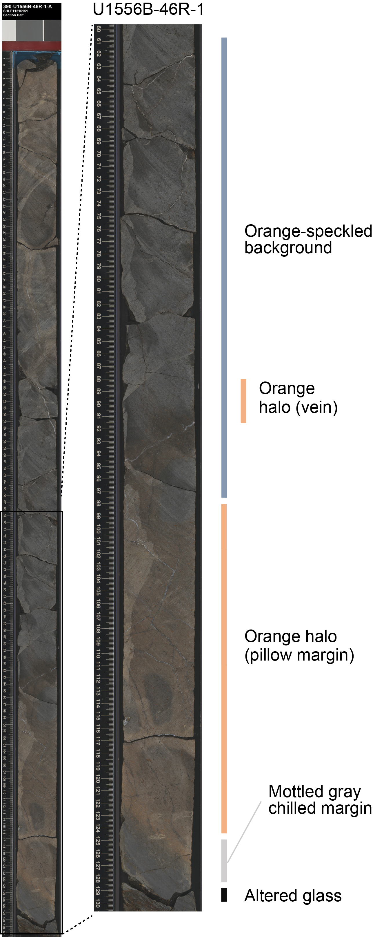
Figure F55. Common alteration types.

6.1. Background alteration

The basement rocks throughout Hole U1556B exhibit variable background alteration, in which secondary minerals replace mesostasis, partially to completely replace phenocryst phases, and fill vesicles/pore space. The different styles of background alteration, described in the basement rocks of Site U1556 on the basis of the color in hand specimen, are described here.

6.1.1. Orange speckled alteration

Much of the background alteration throughout Hole U1556B is characterized by a relatively dark gray or brown groundmass (typically very dark gray [10YR 3/1] to dark gray [7.5YR 4/1]) speckled by orange to red completely altered olivine phenocrysts (Figure F56). It should be noted that orange speckled background alteration, although typical of the orange spotty rock type in Stratigraphic Sequence A (Sections 390-U1556B-2R-2 through 38R-2) (see Igneous petrology), is a distinct and generic designation related only to the style of alteration. As such, it applies to other stratigraphic units and to rocks from other sites.

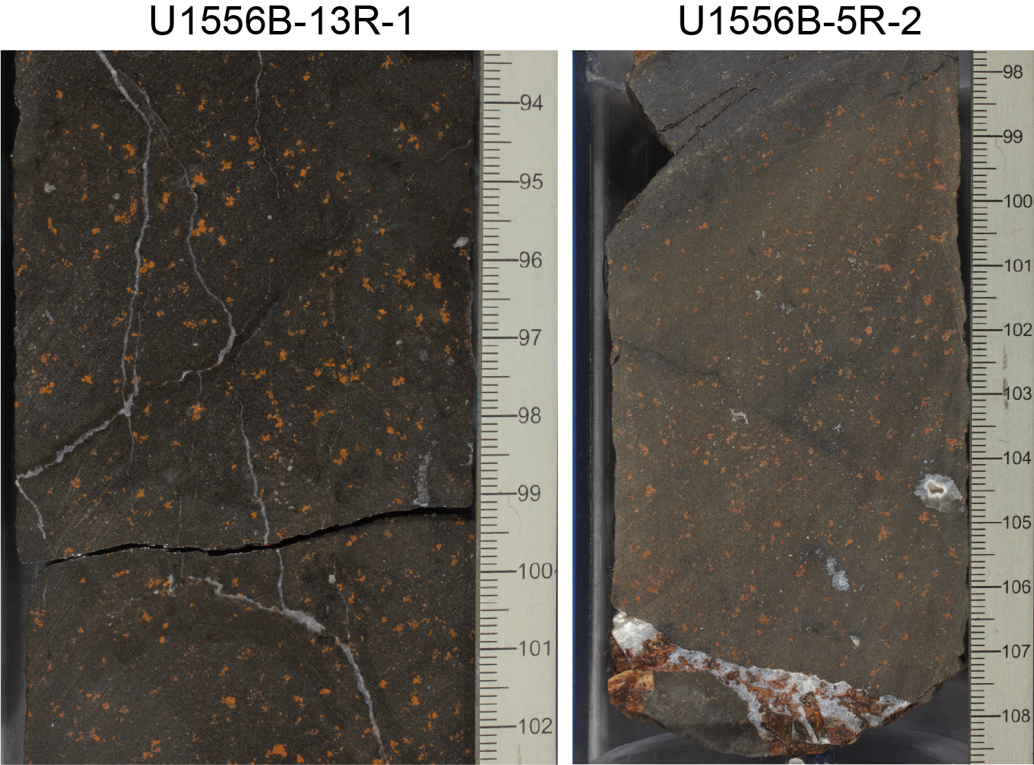
Figure F56. Orange speckled background.

In thin section, olivine is pseudomorphically replaced by iddingsite and subordinate carbonate. The groundmass is variably reddened (ranging from dark gray to dark brown) and never totally fresh, but groundmass color is always less intense than the altered phenocrysts themselves (in contrast to orange halos; see Orange halos). Groundmass is typically patchily replaced by carbonate or clay + Fe oxyhydroxides that range in color from yellow to red-brown. Pale brown or greenish brown clays interpreted to be saponite in fresher samples (see Dark gray background) occur but are relatively rare and most common in transitional samples that span from dark gray to orange speckled background alteration (e.g., Sample 390-U1556B-28R-2, 33–35 cm, TS31). Compared to orange halos, orange speckled background alteration is distinguished in thin section by less pervasive replacement of groundmass by red Fe oxyhydroxides and/or bright yellow clays.

The apparent intensity of orange speckled background alteration does not always reflect genuine variation in the intensity of alteration. Its appearance can vary with the abundance and size of olivine phenocrysts and/or the phyric/aphyric nature of the primary igneous lithology. At the scale of a single continuous piece of core (typically 10–50 cm), orange speckled alteration is fairly homogeneous. That said, in some intervals, most commonly toward the center of larger pillows/flows, orange speckling appears to have developed only as broad halos to veins with reddening of phenocrysts (and groundmass) less pronounced or absent away from fluid pathways. For example, in Sample 390-U1556B-4R-1, 46–50 cm (TS12), olivine, otherwise altered to dull brown clays and carbonate, is partially altered to iddingsite within an orange halo, although the order of alteration is not clear (Figure F57). This and similar observations suggest that all the orange speckled background alteration initially forms as a halo related to fluid/rock interfaces (vein fractures and pillow/flow margins) but that the time and length scales involved mean that in much of the recovered lava sequence alteration is ultimately pervasive at the scale of 10–50 cm. This alteration type is therefore described here as background alteration.

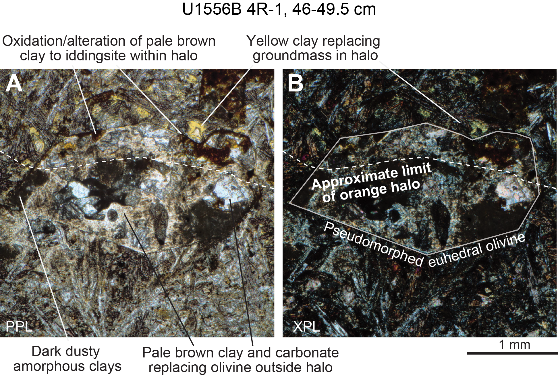
Figure F57. Olivine in background alteration and orange halos.

This speckled orange style of background alteration is similarly expressed in the H-POPP (see Igneous petrology) basalts recovered from the lowermost part of the hole, in which there is red pseudomorphic replacement of olivine and variable reddening of the groundmass. Overall, the color of orange speckled H-POPP basalts (Stratigraphic Sequence C) is significantly lighter than rocks altered in a similar fashion in the olivine phyric (Stratigraphic Sequence A [orange spotty]) and aphyric (Stratigraphic Sequence B [old red]) lithologies that overlie them (gray [GLEY 1 5/N]; cf. dark gray [7.5YR 4/1]; Figure F58C). This is likely due to the greater abundance of plagioclase rather than a major difference in alteration style or extent.

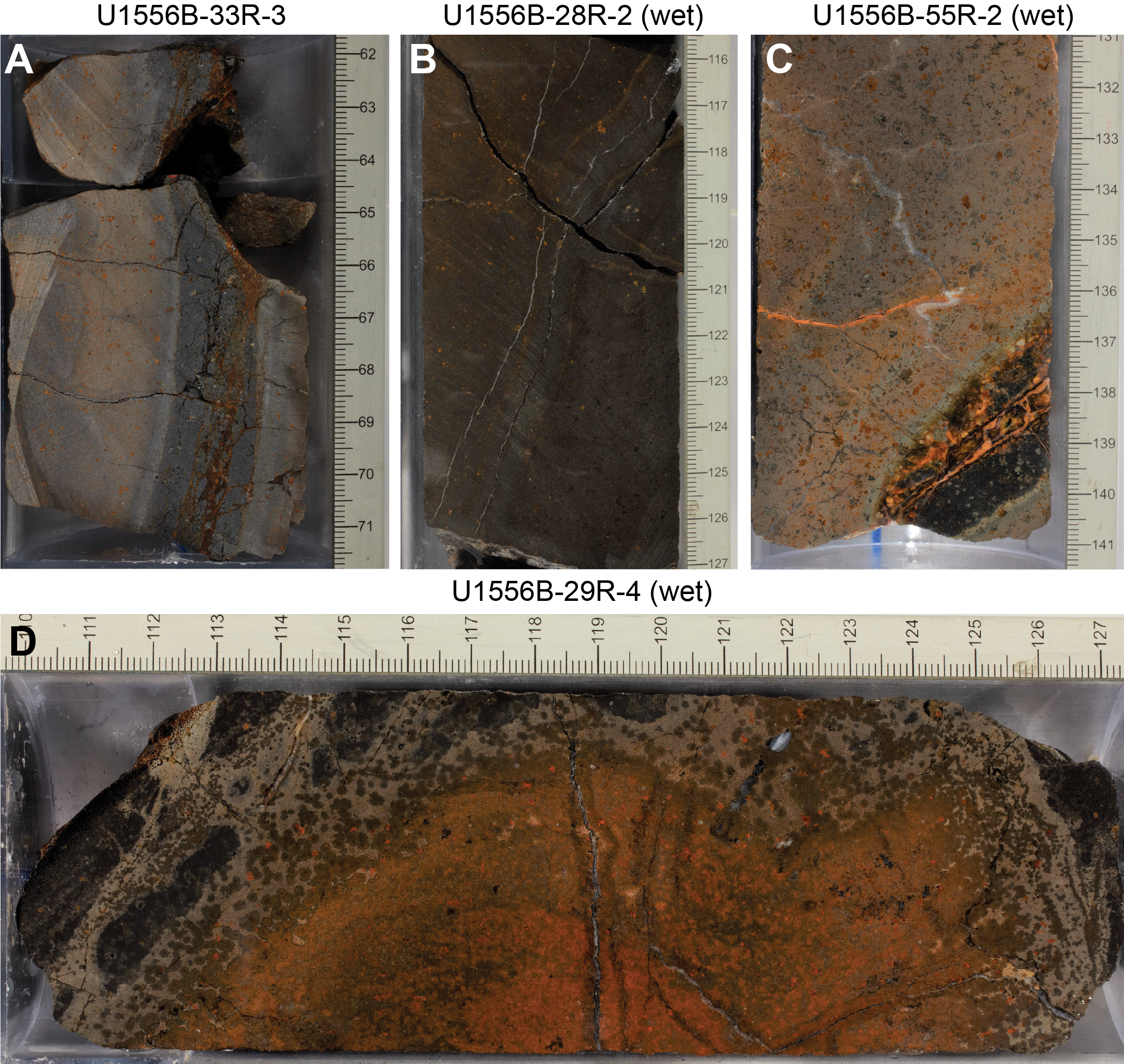
Figure F58. Variety of orange halos in basalt.

6.1.2. Dark gray background

Dark gray background alteration of basalts is a very dark gray color in hand specimen (very dark gray [GLEY 1 3/N]) and most distinctively lacks the ubiquitous orange speckling of altered olivine phenocrysts that typifies most of the background alteration in the hole (Figure F59). It most commonly occurs in quite small (<20 cm), relatively unaltered interiors of larger pillows or massive flows. These intervals show diffusive gradients with other styles of alteration, which are predominantly more oxidative (e.g., orange speckled background).

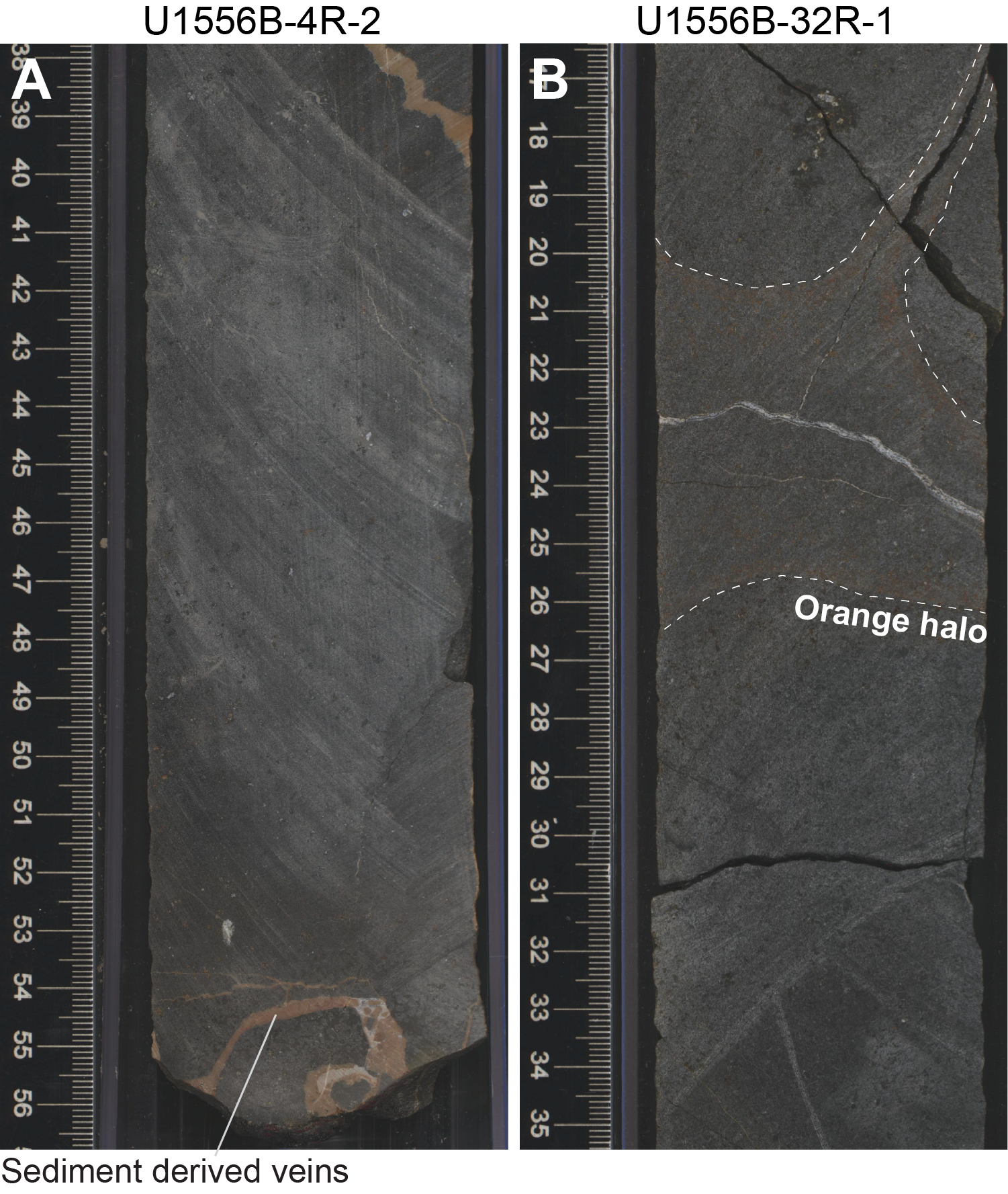
Figure F59. Dark gray background alteration.

In thin section, examples of dark gray background are not completely fresh and are typified by abundant replacement of groundmass and olivine and the filling of vesicles with clays (Figure F60). These are generally a light dull brown to very pale greenish brown in plane-polarized light (PPL), and based on their mode of occurrence and appearance, they likely correspond to compositions nearer to saponite (Ca<_0.25[Mg,Fe]₃[(Si, Al)₄O₁₀][OH]₂·n[H₂O]; e.g., Teagle et al., 1996) than the red and yellow clay–Fe oxyhydroxide mixtures common in orange speckled background. Compared to alteration of basalts described as dark gray background in other locations (e.g., in 15 Ma superfast spreading rate crust from Ocean Drilling Program Hole 1256D in the eastern Pacific; Shipboard Scientific Party, 2003), secondary sulfides such as pyrite and marcasite are absent in the gray background at Site U1556.

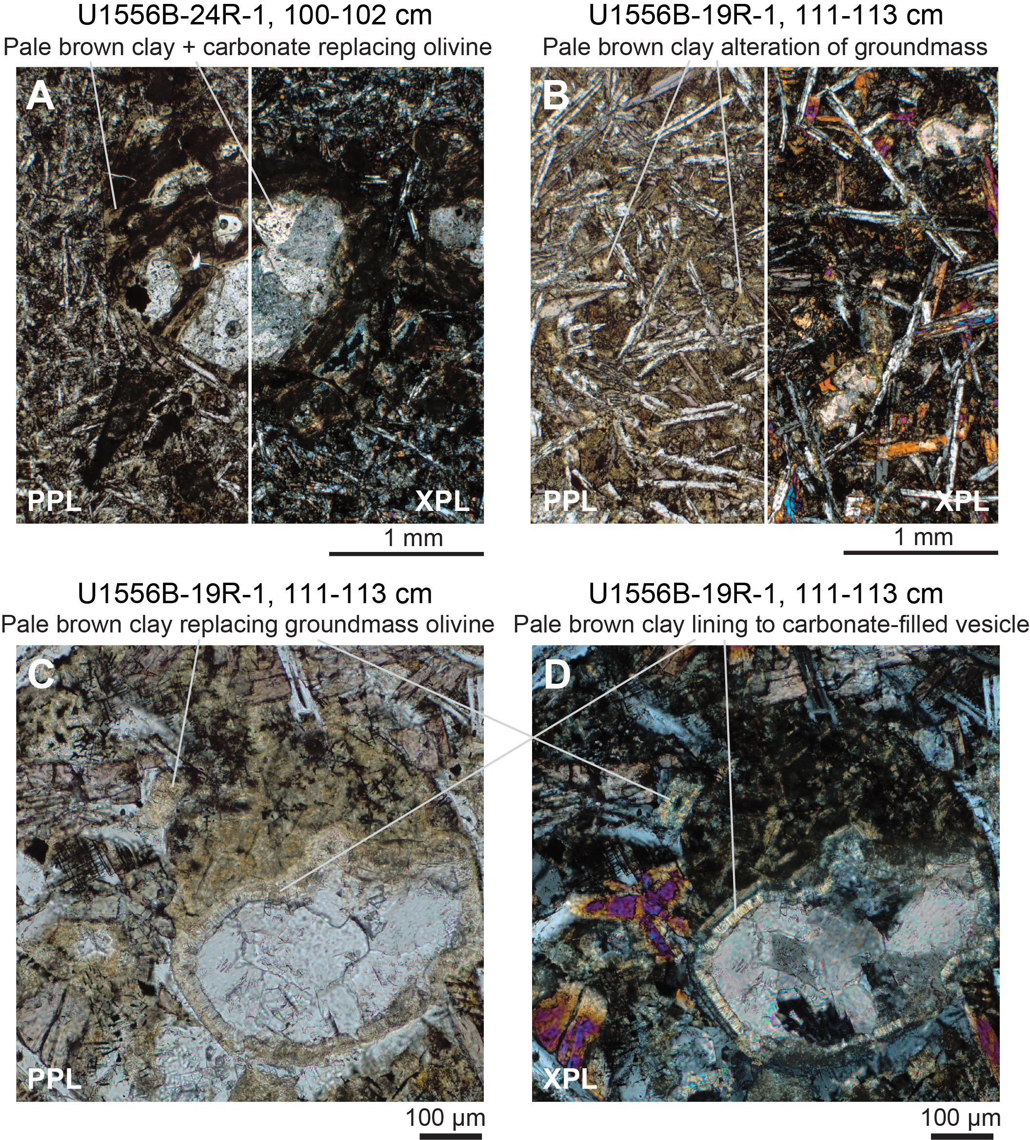
Figure F60. Dark gray background altered basalt.

6.1.3. Dark green background

Two ~15 m intervals of core (approximately Sections 390-U1556B-24R-1 through 26R-1 and 55R-4 through 59R-4) are characterized by dark gray and green alteration, which is otherwise absent in the rest of the hole. In the olivine phyric lavas of the upper parts of the hole (Sections 24R-1 through 26R-1), this manifests as very dark gray (GLEY 1 3/N) to black (GLEY 1 2.5/N) background alteration of the olivine phyric basalts with pseudomorphic replacement of olivine by a mineral that appears black in hand specimen. In H-POPP basalts of the lowermost part of the hole (Sections 55R-4 through 59R-4), a similar style of background alteration, characterized by saponite replacement of olivine and groundmass in thin section, is expressed macroscopically as dark greenish gray alteration colors (typically dark gray [GLEY 4/N]) and pseudomorphic replacement of olivine by green to black clays. As with orange speckled background, the macroscopic colors seen in the H-POPP basalts are paler than those in overlying Stratigraphic Sequences A and B despite very similar alteration mineralogy, likely due to the higher modal abundance of plagioclase.

Wherever dark green background alteration is seen, it is accompanied by very dark green or black alteration of glass (see Green altered glass) and in one interval (Sections 390-U1556B-24R-1 through 26R-1) by pale green to white noncarbonate hyaloclastite cements, tentatively identified through XRD as consisting mainly of phillipsite and smectite clays, possibly nontronite and saponite (Table T6).

Where it has been recovered, the transition between dark green background and other background alteration styles occurs as either gradients or sharp fronts of iron oxidation leading into more orange-red rocks.

In thin sections of samples displaying dark green background alteration, green clays generally but not exclusively occur in discrete halos around veins (Figure F61). The main alteration mineral outside these halos is pale dull brown clay, likely saponite. Also seen is an amorphous, dusty looking and slightly opaque clay that replaces olivine and is likely responsible for the macroscopic black appearance of some grains (e.g., Sample 390-U1556B-24R-1, 100–102 cm, TS26). In some cases, this clay appears to be transitional in composition with the pale brown saponite. The groundmass is generally gray to very dark gray in thin section, the latter commonly having lost some of its microtextural definition and suggestive of replacement by clays, although it is not possible to identify the specific secondary minerals present.

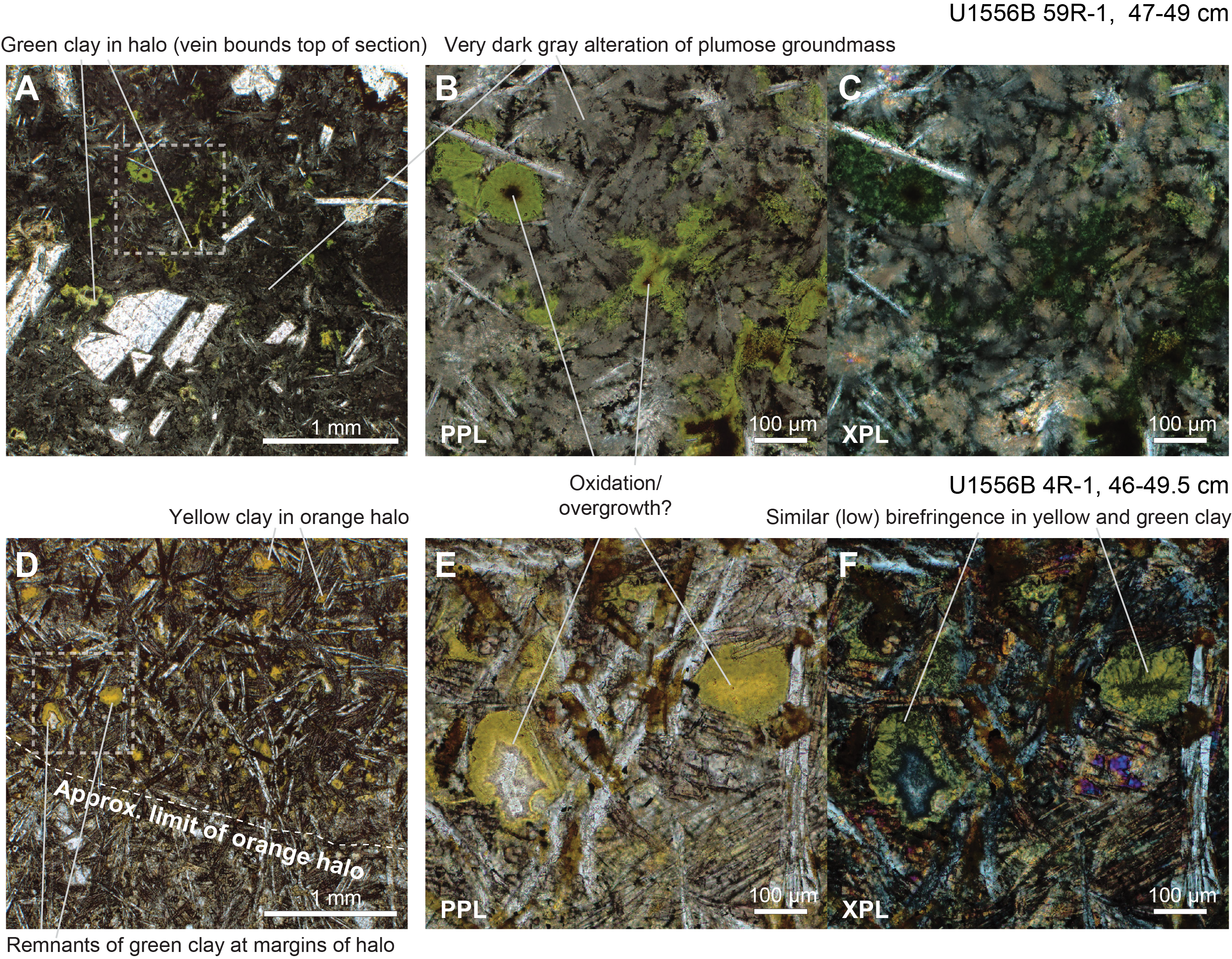
Figure F61. Green clay minerals in halos.

In general, it appears that the difference between dark gray and dark green alteration may be more apparent macroscopically than in thin section. What manifests as a noticeable difference in macroscopic color may amount to a very slight difference in the color of clays in thin section, possibly reflecting some minor difference in chemistry or oxidation. Conversely, strongly green colored minerals in thin section (e.g., green clays and green altered glass) manifest as black macroscopically, similar to black celadonitic halos recorded in young upper oceanic crust (Alt, 2004).

Consequently, it remains unclear the extent to which dark green background alteration differs from dark gray background or if it simply represents an end-member case with very limited red/orange oxidative alteration (whether preceding or overprinting green clays and/or saponitic alteration). In support of the latter are traces of green minerals in thin section at the edge of an orange halo from the upper part of the core (Sample 390-U1556B-4R-1, 46–50 cm, TS12), with most of the green clays having been apparently altered to yellow clay (Figure F61D–F61F). This suggests that alteration by green, possibly ferric clays was initially widespread but has been ubiquitously overprinted by more oxidative alteration though much of the hole. This is consistent with observations of celadonite overprinted by Fe oxyhydroxides in halos in many basalts from upper oceanic crust (e.g., Alt et al., 1986; Alt, 2004). Postexpedition studies, including in situ characterization of secondary mineral chemistries by electron microprobe combined with XRD, will be required to determine the mineralogy and composition of the different secondary minerals associated with the various macroscopic styles of background alteration.

6.2. Vein and pillow/flow margin related alteration

Alteration at fluid/rock interfaces is very common in the recovered rocks. This includes halos of distinct alteration of the groundmass and/or phenocrysts in the wall-rock flanking veins (secondary mineral-filled fractures that were previously fluid conduits). Even more volumetrically important are one-sided halos formed along the interior of pillow/flow chilled margins and also along the fractured outer surfaces of basalt clasts in breccias. These are typically wider than vein-related halos and result in more pervasive alteration, potentially encompassing entire pillows or flows.

6.2.1. Mottled gray alteration of chilled margins

Chilled margins in the olivine phyric and aphyric units show a distinct alteration style. This results from differential alteration of the sequence of grain sizes and textures arising from a gradient of cooling rates across the chilled margin. From the pillow/flow edge inward, the sequence comprises concentric layers of glassy cryptocrystalline and variolitic groundmass subparallel to the outermost surface and typically ~1–4 cm thick (see Igneous petrology).

This sequence of igneous textures is picked out by alteration (Figure F62). The outermost cryptocrystalline material is generally very dark gray in hand specimen and appears both macro- and microscopically to be the least altered. This layer commonly preserves fresh olivine. The alteration color of slightly coarser (still cryptocrystalline) material inward from this layer is typically a paler gray. Superimposed on this pale gray layer is the appearance of spherulitic quench crystals that display darker alteration colors and coalesce across the transition to the dark gray/gray-brown background-altered microcrystalline groundmass of the basalt. We compare the appearance of this variegated alteration of cryptocrystalline and variolitic basalt to trout skin (Figures F62, F58D). Very similar textures in altered chilled margins were encountered at Integrated Ocean Drilling Program Site U1383 at North Pond in the North Atlantic and were termed "blotchy alteration texture" (Expedition 336 Scientists, 2012). During quantitative alteration logging of the recovered core, the entire profile across altered chilled margins—encompassing both (relatively fresh) dark and (more altered) light variegation—was logged together as mottled gray alteration, distinct from visibly reddened and oxidized orange speckled background or orange halos.

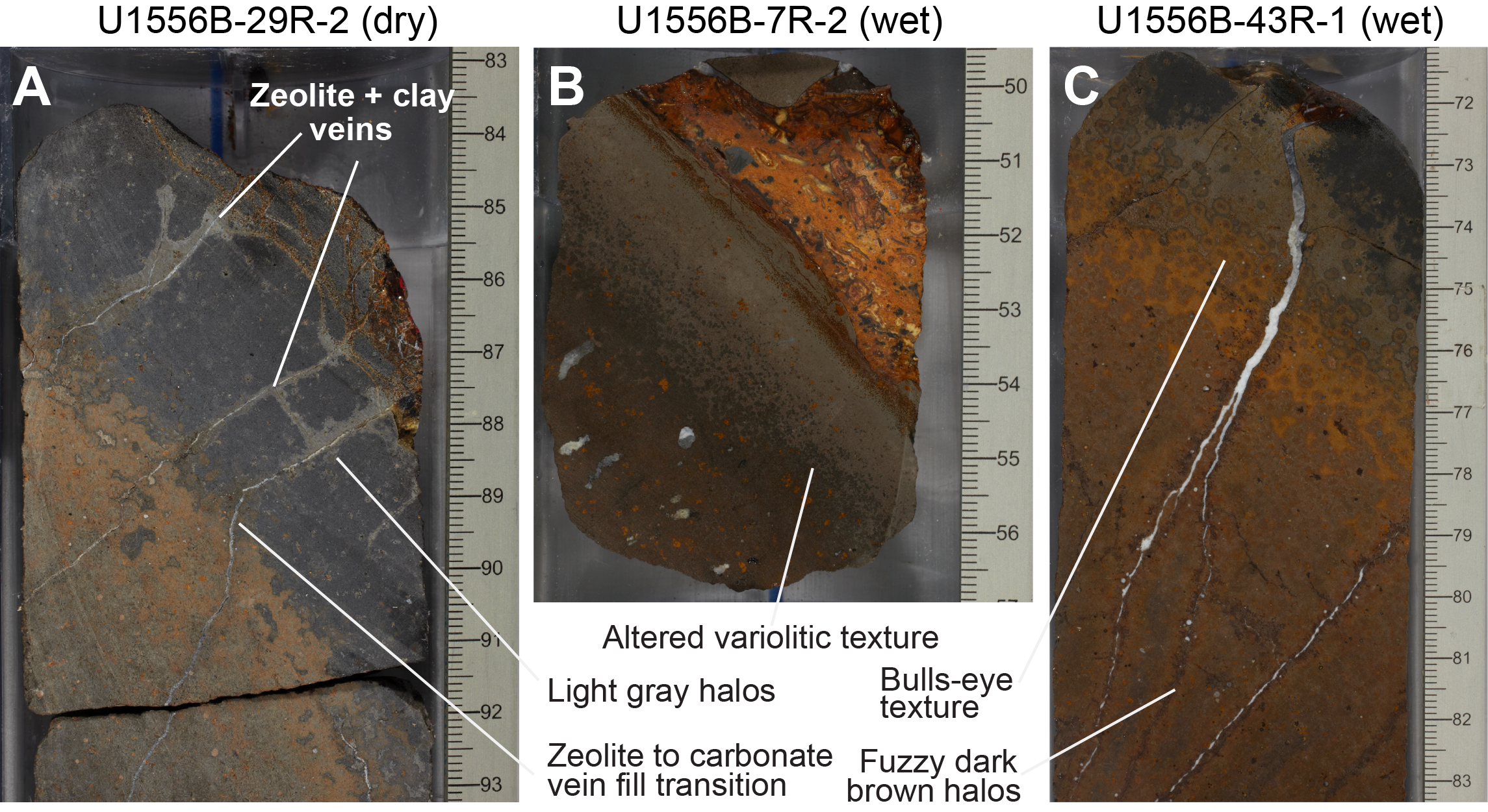
Figure F62. Mottled gray altered margins.

In areas of more intense orange halo alteration, these sequences may be partially overprinted or may overlap with orange oxidation profiles (Figure F62A, F62C). This is most commonly expressed as a reddened variant of the altered variolitic pattern consisting of light gray altered cryptocrystalline material dotted by circular red patches with a concentric bull's-eye–like variation in color. These patches are commonly carbonate bearing at their centers, locally effervescing when tested with a solution of dilute HCl, whereas the enclosing light gray rock is not.

In rare examples, mostly in upper parts of the core (e.g., interval 390-U1556B-2R-2, 80–82 cm), bands of macroscopically light and dark basalt occur, similar to the variegated altered variolitic texture (Figure F63). The banding appears igneous in origin, arising from differential nucleation of plagioclase and olivine quench crystals, with the former giving rise to slightly coarser grained domains with abundant radiating clusters of crystals. These may have acted as nucleation sites for alteration minerals, fluid pathways, or both. More typically, similar features that have radial geometry are seen in the mottled gray margins with heterogeneities, including radial clusters of quench crystals, vesicles, or phenocrysts acting as the starting point of spherical zones of alteration around them. These latter pick out the variolitic pattern commonly seen at the transition between orange halos and gray chilled margins (Figure F62A, F62C).

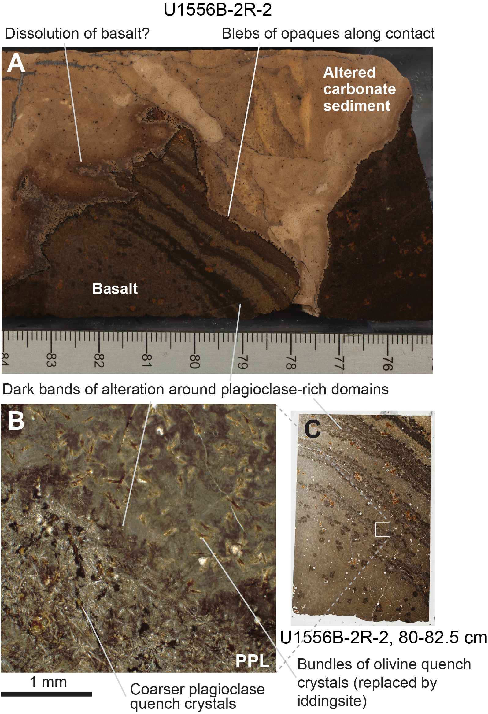
Figure F63. Banding features.

6.2.2. Orange halos

Orange halos, consisting of orange-red to red-brown areas of alteration around veins and along pillow/flow margins (Figure F58), are the most abundant halo type in the core by area and flank approximately 8% of logged veins (496 veins). The halos reflect relatively intense oxidative alteration that resulted in formation of red Fe oxyhydroxides and mixtures with clay and manifest as a range of red-brown to orange colors (typically brown [7.5YR 4/2] to brown [7.5YR 5/3]). These appear to be similar to the orange-red Fe oxyhydroxide–rich halos recorded in previously drilled upper oceanic crust (e.g., Hole 504B; Alt et al., 1986) and may be equivalent to the brown halos present, albeit rarely, in Hole 1256D (Shipboard Scientific Party, 2003).

Fine-grained groundmass within orange halos is typically pervasively altered to orange-red to red-brown clays and Fe oxyhydroxides with individual phases difficult to identify. The halos are commonly demarked in thin section by the presence of markedly clear and bright looking yellow clays of similar appearance to altered glass (Figure F64). These phases are brightly colored in PPL with low birefringence; the strong color of the mineral makes assessing the exact interference colors difficult, but these are generally no higher than first-order white or yellow. Another bright yellow mineral of very similar appearance and mode of occurrence differs in being isotropic. This may be limonite (i.e., a mixed layer mixture of goethite and clay).

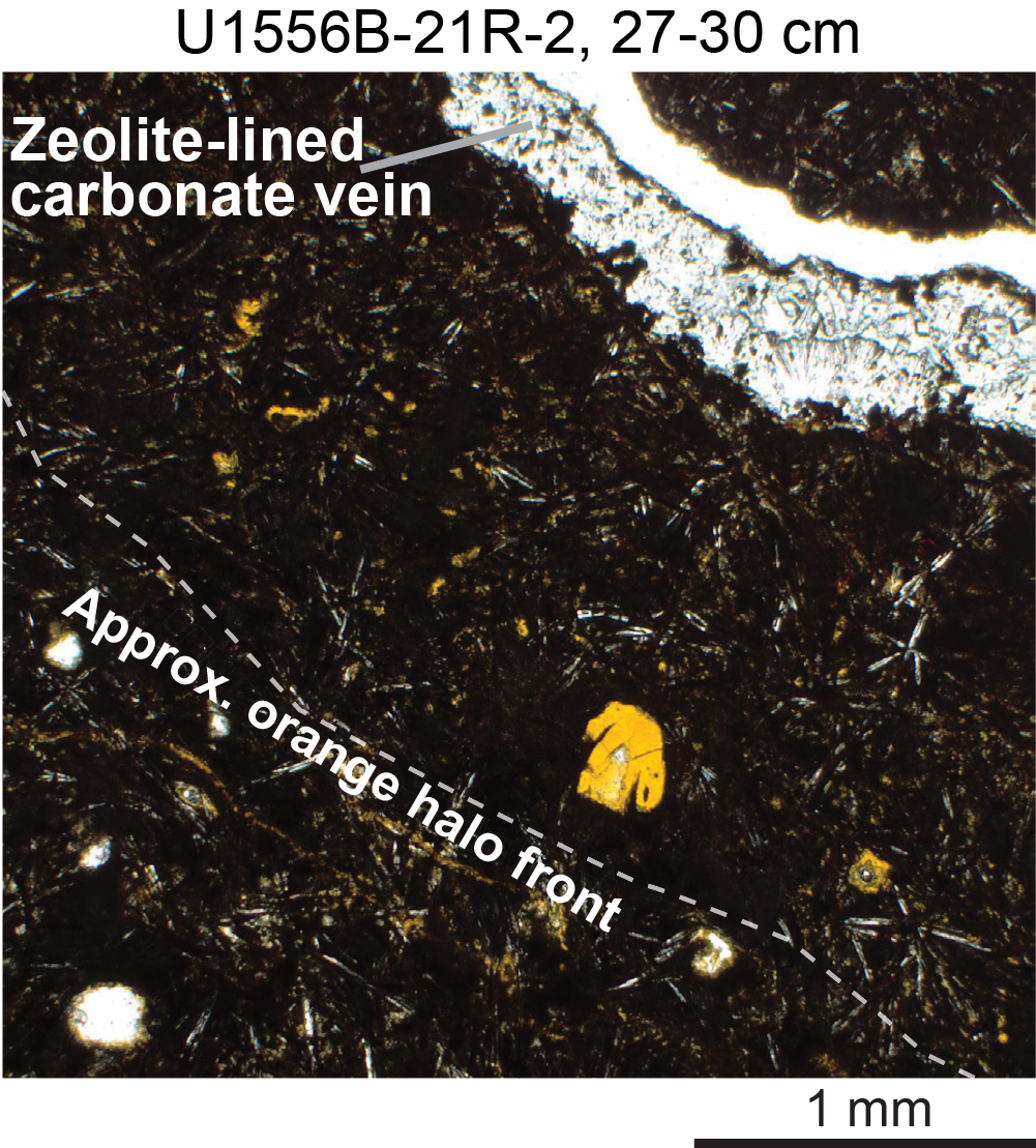
Figure F64. Bright yellow clay replacing groundmass.

The bright yellow clays principally occur replacing groundmass and lining or filling vesicles. They commonly form a well-defined rim to the halo and in some cases are progressively more strongly red-brown closer to the veins. In some cases, there is a color gradient from yellow to orange-red across a single filled vesicle, incongruent with the microtexture of the clay. This implies that the variation in color is a result of further alteration rather than spatial variation in the composition of secondary mineral composition at the time of formation (Figure F65). Where green clays occur in halos, they are commonly partially altered to yellow or orange clays but otherwise have markedly similar optical properties, suggesting a similar process of further oxidation/alteration may be common (Figure F66). Given the similarity of appearance and apparently continuous range of compositions between bright yellow and red clay/Fe oxyhydroxide mixtures, it seems likely these yellow minerals represent variable smectite–Fe oxyhydroxide mixtures of the sort that form iddingsite. A similar range of compositions, with pure Fe oxyhydroxide as the most altered end-member, has been described for progressive oxidative alteration of olivine to iddingsite (Smith et al., 1987).

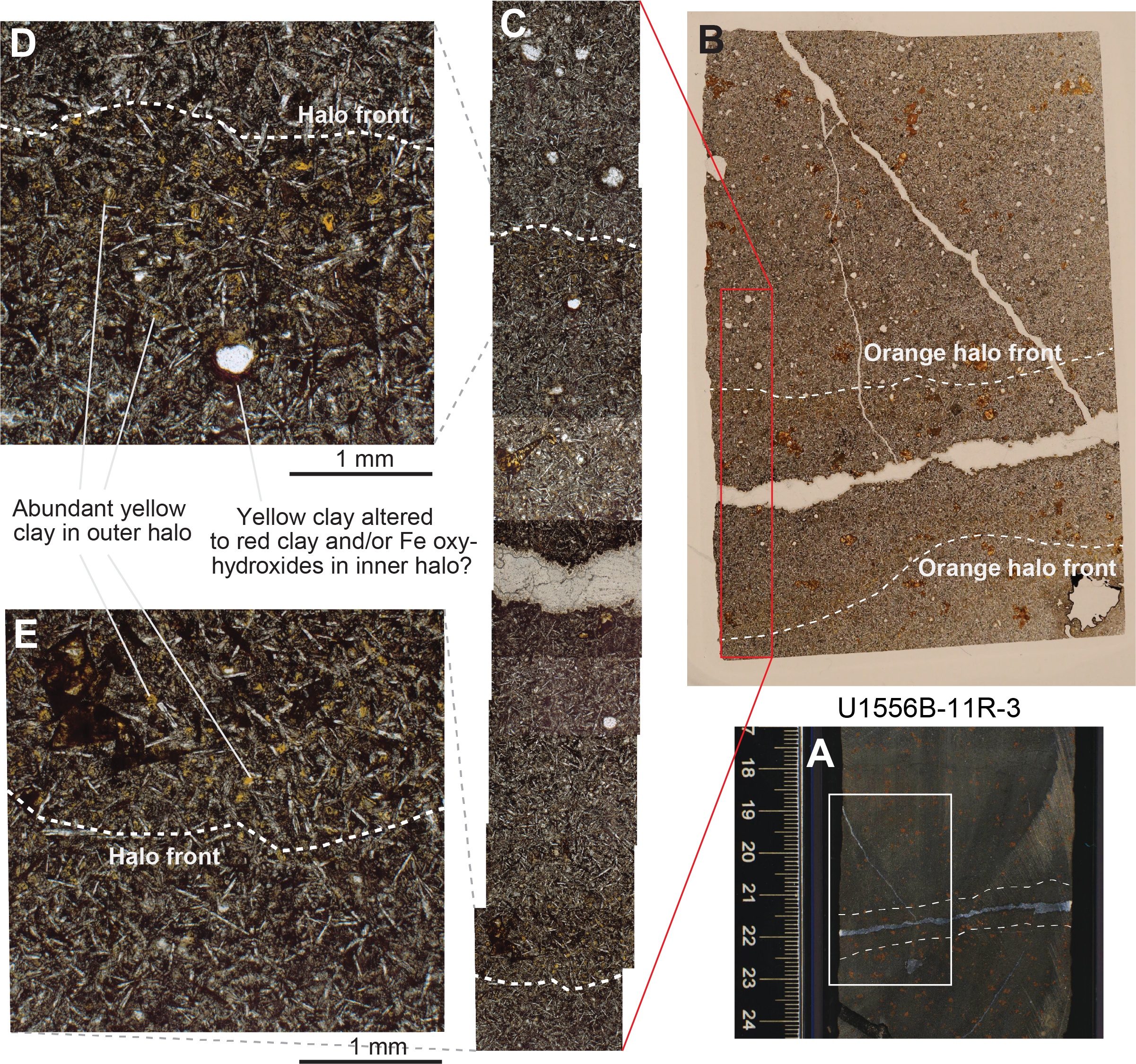
Figure F65. Mineralogy of an orange halo.

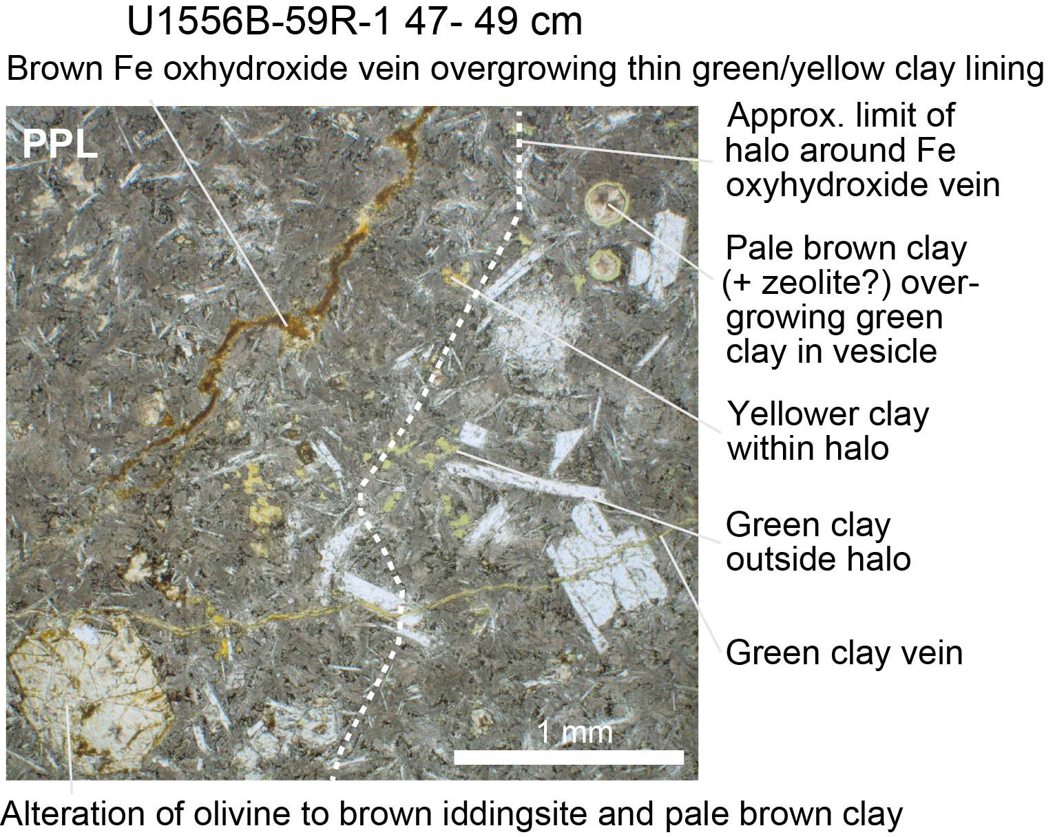
Figure F66. Green clay–filled vein.

The orange halos typically have diffuse edges and range in half width from 1 mm to >10 cm. They have narrower widths where they flank veins compared to along chilled margins, although diffuse orange halos do occur in pillow interiors commonly associated with vein networks and are difficult to associate with one particular vein. Rarely, orange halos have a sharp orange front (Figure F58B); such fronts could be a result of oxidation of a pyrite front like those observed between alteration halos and background altered basalt elsewhere (Teagle et al., 1996; Shipboard Scientific Party, 2003; Expedition 301 Scientists, 2005), although no pyrite was observed during the description of Hole U1556B cores. More commonly, orange halos have a compound structure with both orange and dark brown portions (see Multihalos).

In intervals with particularly intense alteration and/or relatively small pillow sizes, orange halos can constitute nearly the entirety of individual core pieces. However, slight contrasts in color along veins or with the background color of adjacent fresher pieces tend to mark these out as halos rather than a different type of background alteration (Figure F67), although the distinction is at some level arbitrary. In numerous examples, broad orange halos around the edge of large basalt pillows extend inward toward the fresher pillow interiors along veins, suggesting that halos along veins and flow/pillow margins are generally equivalent and formed penecontemporaneously. As a result, orange halos around veins and pillow/flow margins (the only halo type that occurs in both settings) were described and logged together to avoid introducing an arbitrary distinction that would be difficult to apply consistently.

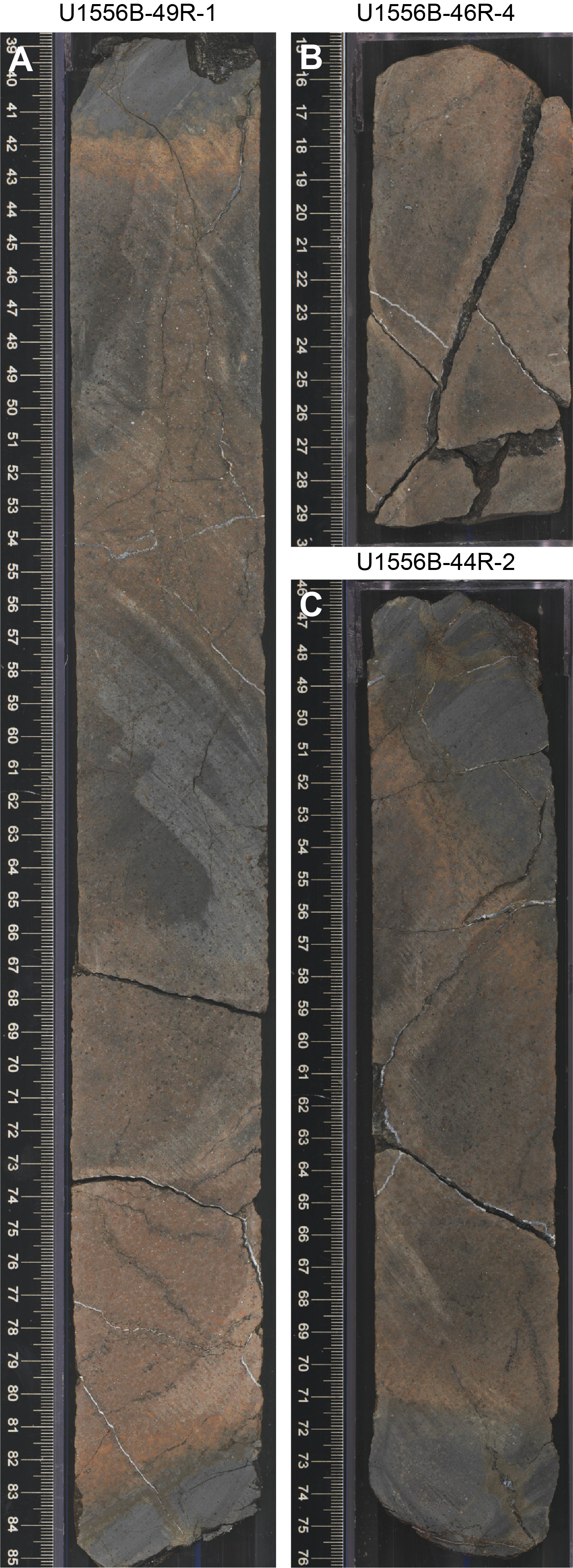
Figure F67. Well-developed orange halos.

In the transitional units where geochemical data, petrology, and crosscutting relationships indicate that olivine phyric Stratigraphic Sequence A (orange spotty) basalts have intruded into largely aphyric Stratigraphic Sequence B (old red) basalts (see Igneous petrology), there are indications that the Stratigraphic Sequence B rocks were altered to intense orange halos prior to intrusion by Stratigraphic Sequence A. This is evidenced by major differences in the degree of alteration across sharp intrusive contacts that indicate the (similar) rocks on either side cannot share a common alteration history (Figure F68). Although the time interval between eruption of Stratigraphic Sequences A and B is not known, the entire igneous succession in Hole U1556B is constrained to have erupted within 220 ky (within middle Paleocene foraminifera Zone P4a) by micropaleontology of samples from the sediment/basement interface and intercalated sediments from the lowermost Stratigraphic Sequence C (H-POPP) basalts (see Biostratigraphy). This would tend to suggest that the formation of orange halos may have been similarly rapid and largely complete within a few hundred thousand years of eruption in at least some of the basalts. However, such intense orange alteration halos are typically absent in young oceanic crust, including 7 Ma basalts sampled at Site U1559 (see Alteration petrology in the Site U1559 chapter [Coggon et al., 2024e]). This would imply that the differential alteration seen either arises because of grain size variation (i.e., that the intense orange color of altered pillow margins is more related to their grain size than the proximity of the basalt/fluid interface) or that early stages of alteration of the outer portions of pillows modify the mineralogy or microstructure of the rocks such that later oxidative alteration is promoted.

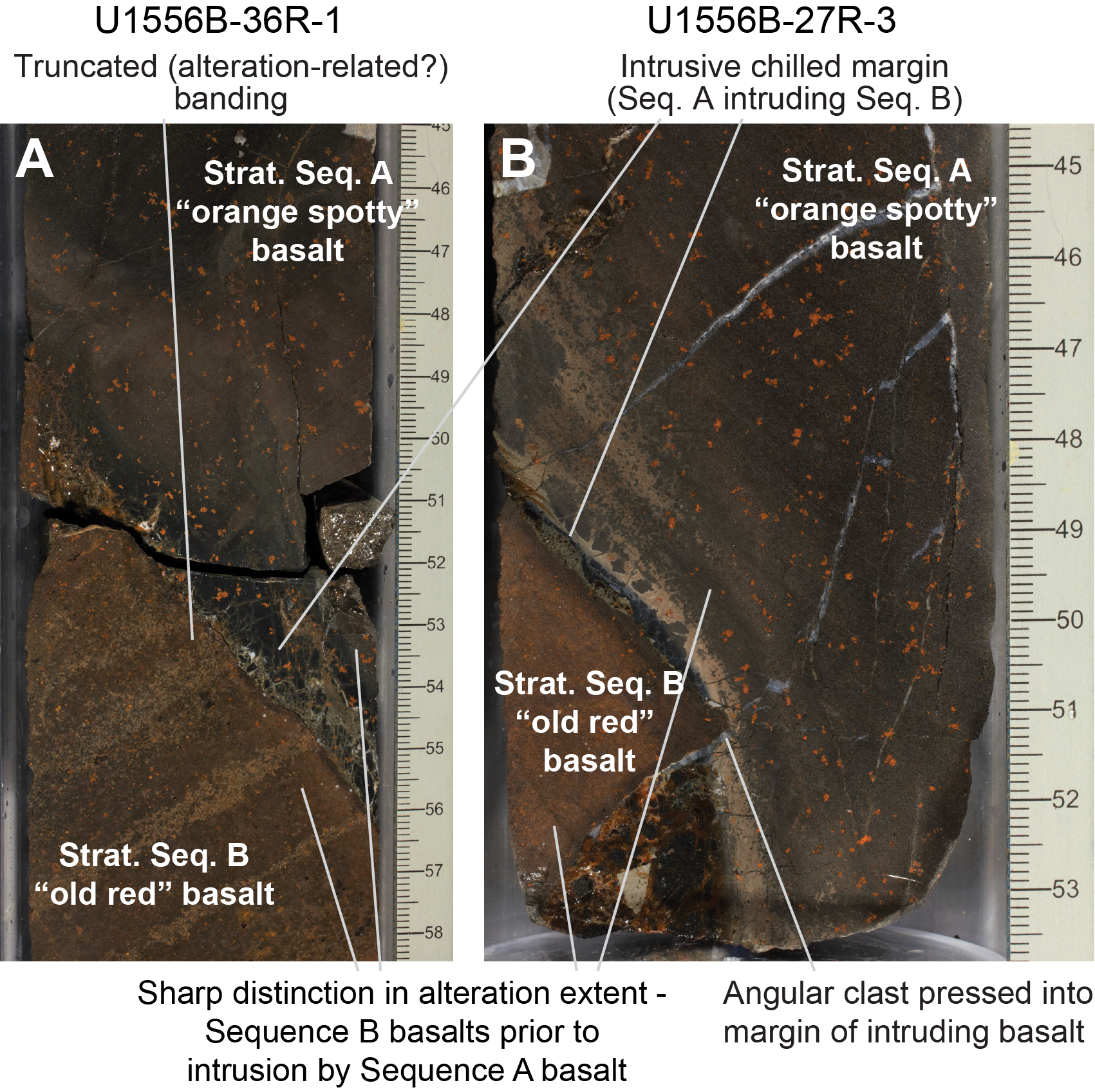
Figure F68. Orange spotty and old red basalts.

6.2.3. Yellow halos

Yellow halos are restricted to the H-POPP basalts in the lowermost cores of the hole (Sections 390-U1556B-54R-3 through 59R-4) (see Igneous petrology). They occur as relatively wide (<3 cm) zones of yellowish alteration (dark gray [2.5Y 4/1]), principally around massive textured orange to buff-colored sediment-derived veins. Because of the similarities in mineralogy and occurrence with orange halos seen elsewhere in the hole (and given also the differences in the manifestation of other alteration styles between the H-POPP basalts and the overlying basalt lithologies; see Orange speckled alteration), these were logged together with orange halos to be consistent throughout the hole.

6.2.4. Dark brown halos

Although less volumetrically significant than orange halos, dark brown halos are the most abundant type, occurring along around 11% of veins (652 veins) (see DESC_WKB in Supplementary material). The vast majority are 1 mm in half width or thinner. The morphology of these halos varies between simple areas of dark brown alteration (dark gray [GLEY 1 4/N] to very dark gray [2.5Y 3/1]) paralleling veins (Figure F56) and concentrations of dark fuzzy blebs or dendritic growths into the wall-rock adjacent to a vein (Figures F62C, F58D). In thin section, the latter appear to be concentrations of opaque clays + Fe oxyhydroxides/iron oxides (Figure F69), typically growing along and replacing red-brown iddingsite pseudomorphs after elongate quench crystals. These fuzzy variants of halos mostly occur along thin dark clay ± Fe oxyhydroxide veins in areas of intense orange halo development, particularly in the highly altered aphyric pillow basalts (old red; see Igneous petrology) in the lower part of the hole.

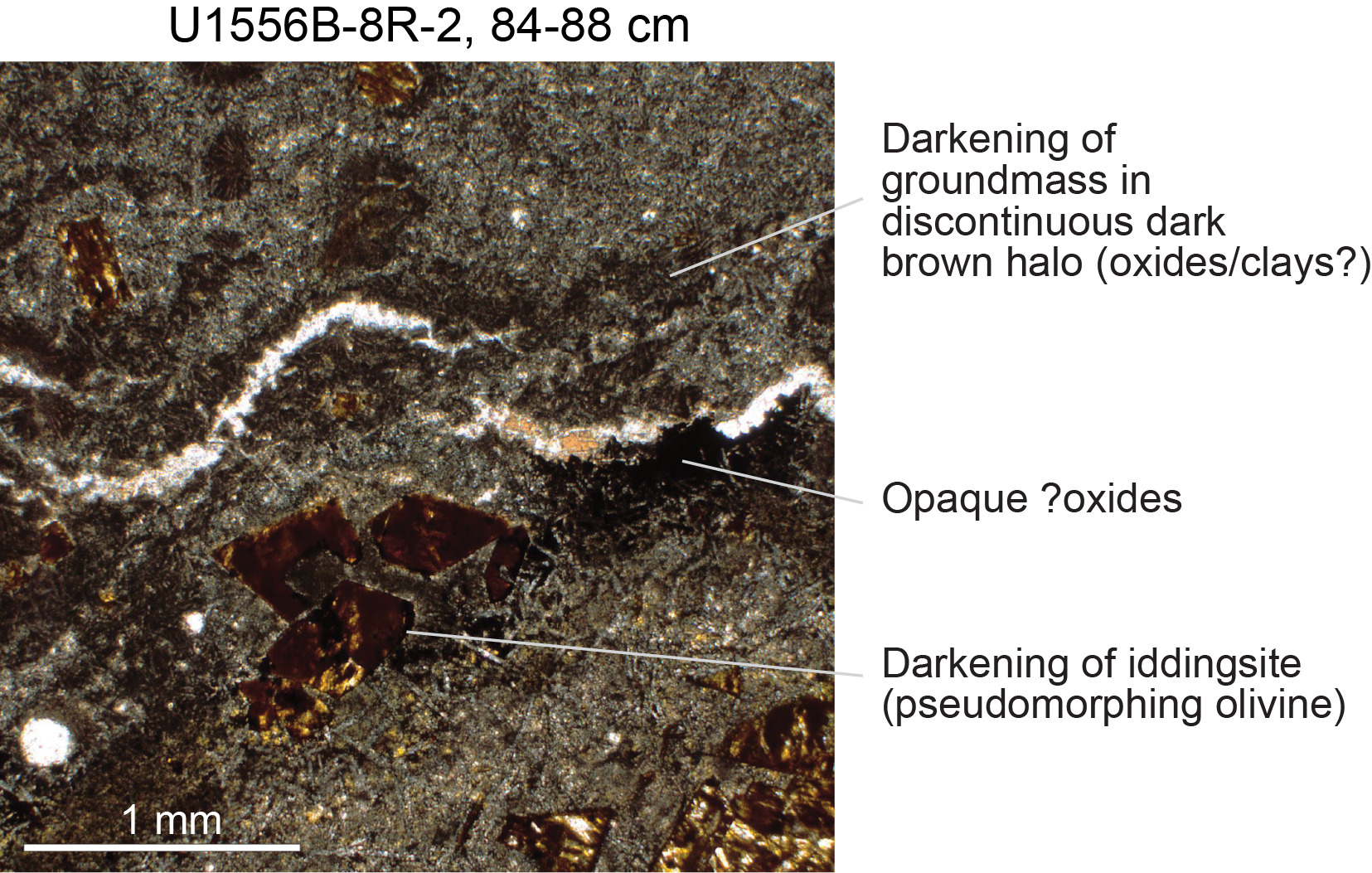
Figure F69. Dark brown halo around thin carbonate vein.

6.2.5. Multihalos

Approximately 10% of veins flanked by halos are flanked by multihalos with subparallel/concentric bands of multiple colors. The majority of these comprise orange halos with a dark brown outer rim that is generally thinner than the orange halo. Less commonly, orange halos may have a thin inner dark brown halo. In thin section, the outer, darker part of some of these halos corresponds to a front of abundant yellow clay. In some cases inward of this front toward the vein these clays transition to deeper red-brown (Figure F65). Given their mode of occurrence, these may be remnants of dark gray halos (such as those seen in basalts at Site U1559) that have been largely overprinted by later orange alteration halos.

6.2.6. Light brown halos

Light brown halos are restricted in occurrence to sedimentary breccias in the upper part of the hole (Cores 390-U1556B-2R through 3R) where they form in the basalt clasts along their contacts with the host carbonate sediment matrix. They are typically thin (<3 cm) zones subparallel to the basalt/sediment interface and characterized by a light brownish gray color (brown [10YR 5/3]). Abundant blebs of black opaque minerals, likely manganese oxides, visible in both thin section and hand specimen, typically form in the sediment along these interfaces (e.g., Sample 390-U1556B-2R-2, 38–40 cm [TS9], and Figure F63A).

6.3. Alteration of glass

6.3.1. Orange/brown altered glass

Volcanic glass is abundant throughout much of Hole U1556B (see Igneous petrology) and is variably altered, with the degree of alteration depending at least in part on the degree of brecciation and the resulting surface area for reaction with fluids. Most altered glass in the hole is altered to dark brown to bright orange clays and Fe oxyhydroxide minerals (black [7.5YR 2.5/1] to yellowish red [5YR 5/6]) (Figure F70).

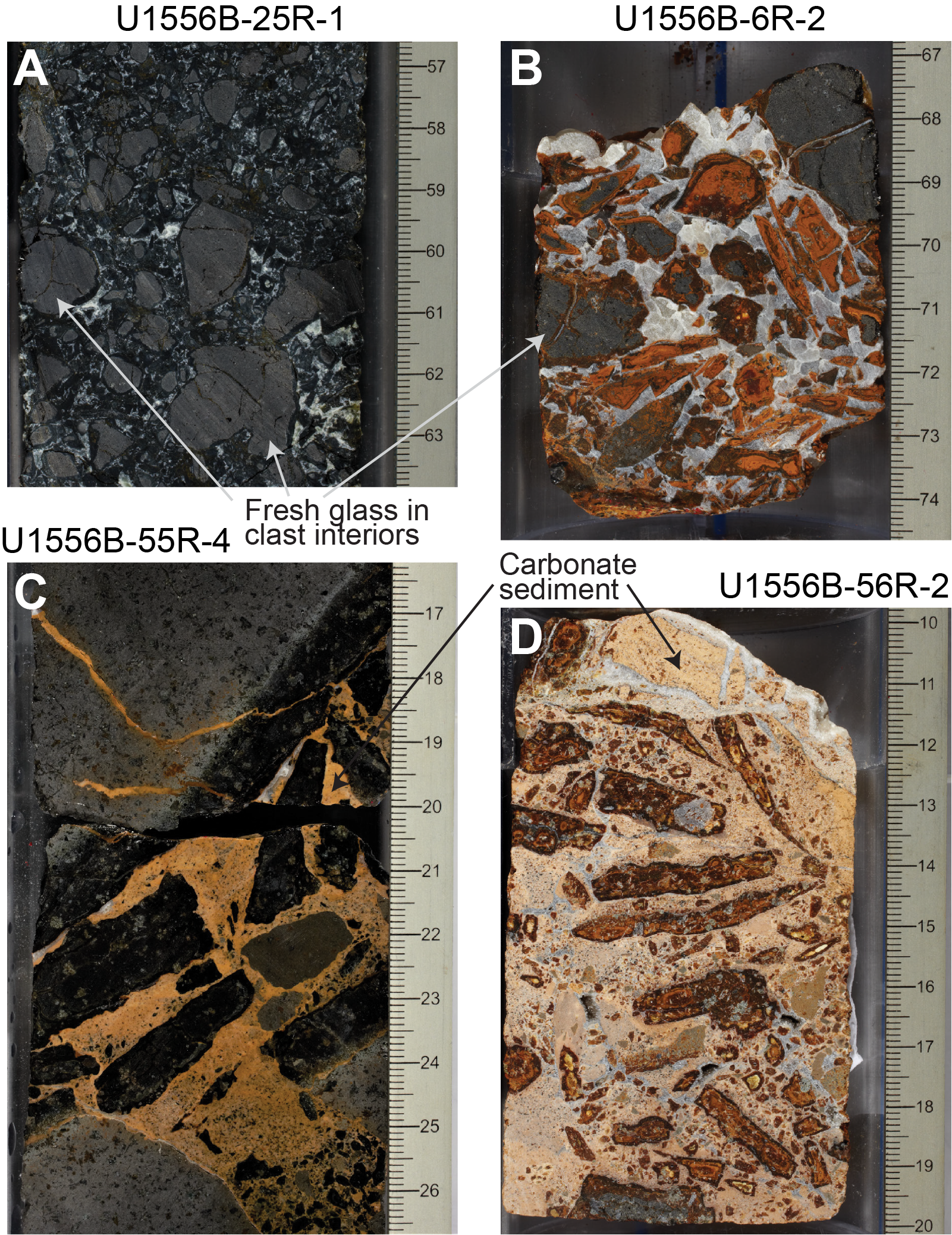
Figure F70. Breccia and breccia cement/matrixes.

In thin section, these are distinctively bright yellow with low first-order interference colors (Figure F71). XRD patterns suggest they are predominantly formed of amorphous material and smectite clays (Table T6). The altered glass consists of a series of finely spaced concentric laminations and typically shows spherulitic growth from a series of nucleation sites along the rim of the original glass and around vesicles, fractures, phenocrysts, and other heterogeneities, indicating alteration predominantly proceeding from the exterior surfaces of the glass inward (Figure F72). Olivine phenocrysts within glass are typically the freshest olivine found in any of the rocks in Hole U1556B and in some cases are completely unaltered. This suggests very limited pathways for fluid ingress, consistent with the textural evidence for alteration initiating on exterior surfaces of glass fragments (Figure F72).

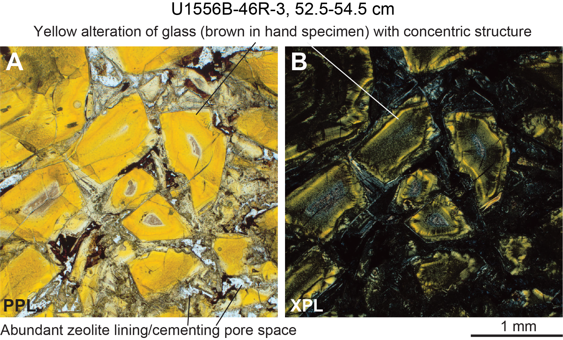
Figure F71. Zeolite + clay-cemented hyaloclastite.

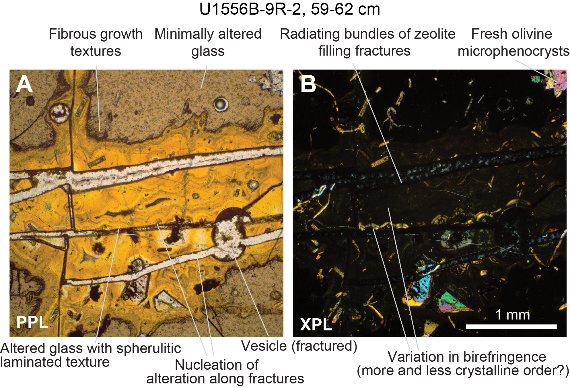
Figure F72. Alteration of volcanic glass.

Where it is found in situ, comprising the outer portion of a chilled margin still attached to a piece of basalt, glass is commonly partially delaminated (Figure F73) with veins preferentially oriented along cracks parallel to the margin. This behavior may explain the preponderance of elongate/tabular clasts of glass in many hyaloclastic horizons (see Igneous petrology; Figure F21).

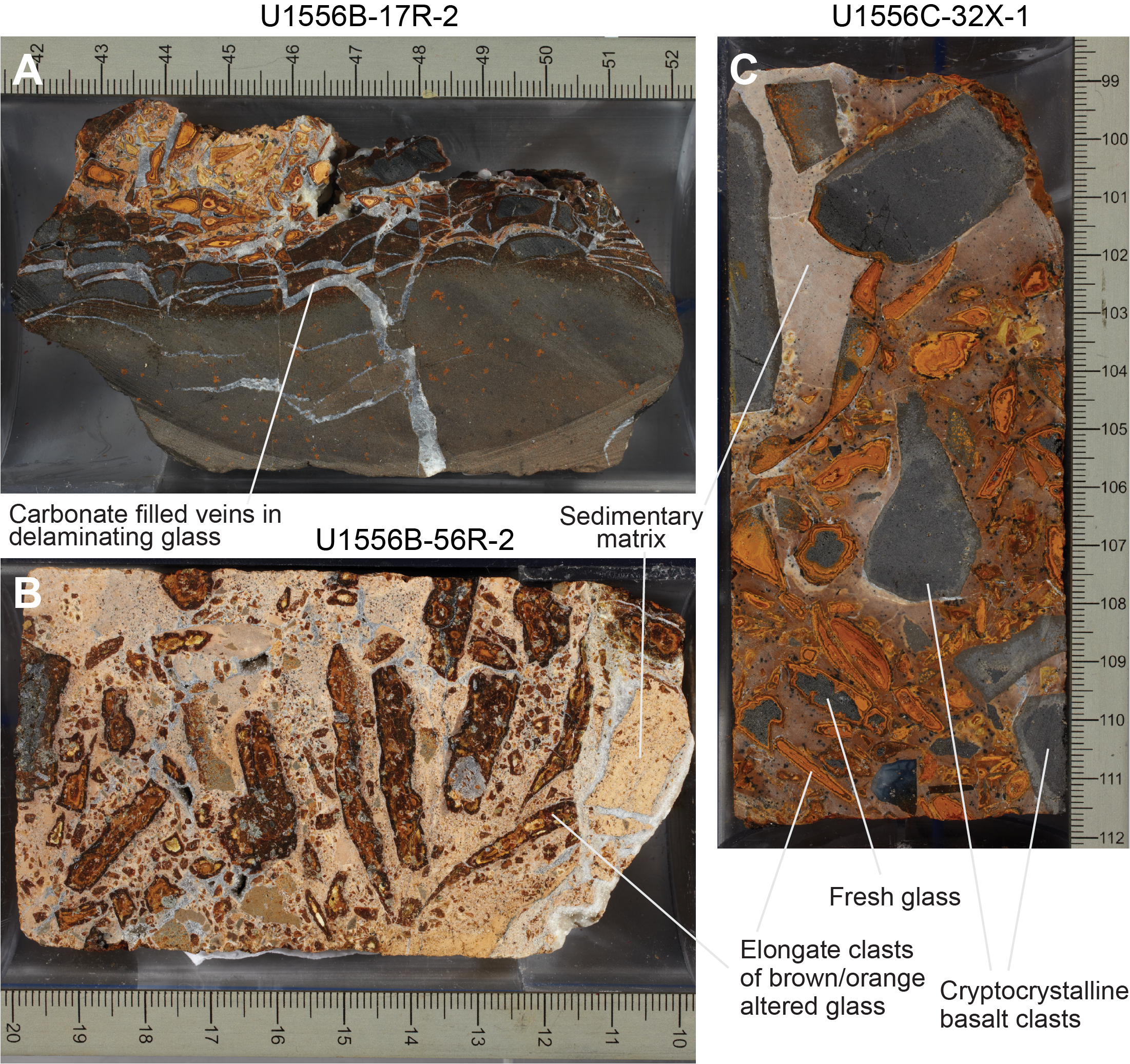
Figure F73. Delamination of glass.

6.3.2. Concentric alteration of glass

Fragments or clasts of altered glass typically have a concentric structure with two or more sequential shells of distinct alteration minerals. In the simplest (and most common) case, these comprise continuous variation in the color of altered glass and commonly its birefringence too, with colors ranging from pale yellow through orange to brown in PPL. Other examples have cores composed of clay, zeolite, or carbonate (or mixtures of one or more of these minerals). Clay-bearing cores appear to be particularly common in fragments of green altered glass (e.g., Sample 390-U1556B-25R-1, 13–15 cm). More complex sequences are seen in some intervals, including successive altered glass, Fe oxyhydroxide, and zeolite layers (Sample 26R-1, 120–122 cm) or altered glass, clay, and carbonate (Sample 56R-2, 33–36 cm). In most occurrences, some or even all glass clasts have a rim of altered glass and preserve fresh or only moderately altered glass at their centers (Figure F71).

6.3.2.1. Green altered glass

In two intervals characterized by dark green background alteration (Subunit 7b, Sections 390-U1556B-24R-1 through 26R-3, and the lower part of Unit 13, Sections 55R-4 through 59R-4), altered glass is macroscopically dark green or black (approximately GLEY 1 2.5/N; Figure F70). In thin section, the green altered glass typically has low birefringence and a similar appearance in PPL to green clays that occur as groundmass alteration products (Figure F74). As with yellow altered glass, there is commonly variation between more and less birefringent zones, indicating variation in the degree of crystalline order of the secondary clays. Olivine is markedly fresh in the green hyaloclastites, even within the altered glass. Where such glass is set in a sedimentary matrix, the sediments also show green coloration. In most occurrences, green altered glass appears to have undergone some oxidation, resulting in yellow to brown rims to the green material (Figures F74A, F75).

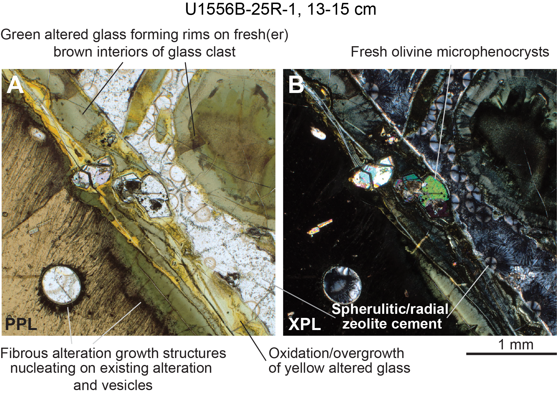
Figure F74. Green/black hyaloclastite.

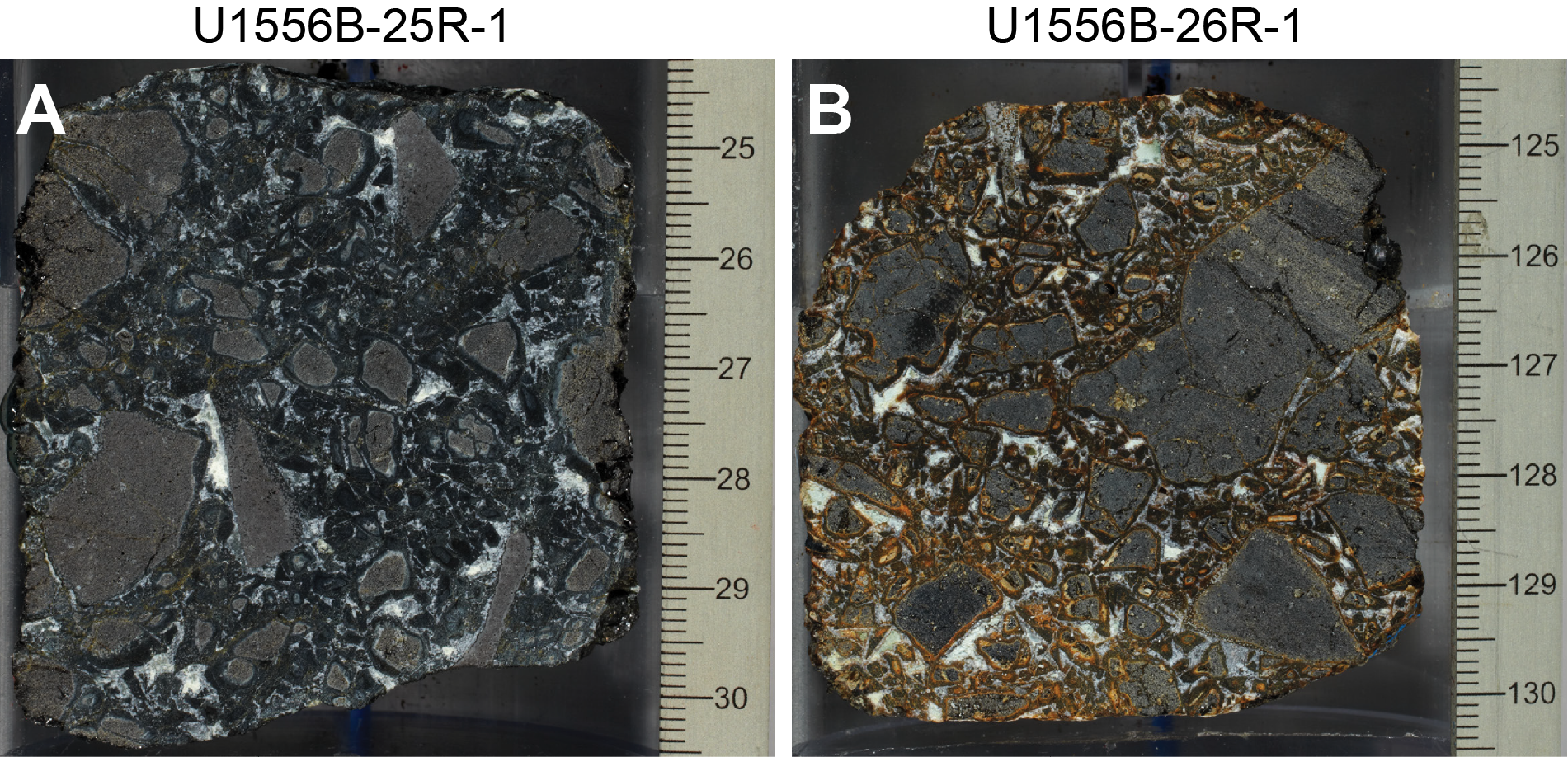
Figure F75. Green and orange breccias.

6.4. Veins

A total of 5029 veins and vein networks were documented in cores recovered from Hole U1556B. In addition, 549 occurrences of breccia cement, 321 occurrences of secondary mineral–filled vesicles, and 55 occurrences of secondary minerals in rubble of indeterminate geometry were recorded (see DESC_WKB in Supplementary material). Among veins and vein networks, smectite clays were the most commonly occurring mineral fill; 4268 veins were recorded as smectite bearing, 3716 veins were recorded as carbonate bearing, 1146 veins were recorded as Fe oxyhydroxide bearing, 989 veins were recorded as zeolite bearing, 206 veins were recorded as green clay bearing, and 124 veins were recorded as bearing other clays. Examples of typical carbonate-, smectite-, and Fe oxyhydroxide–bearing veins are illustrated in Figure F76.

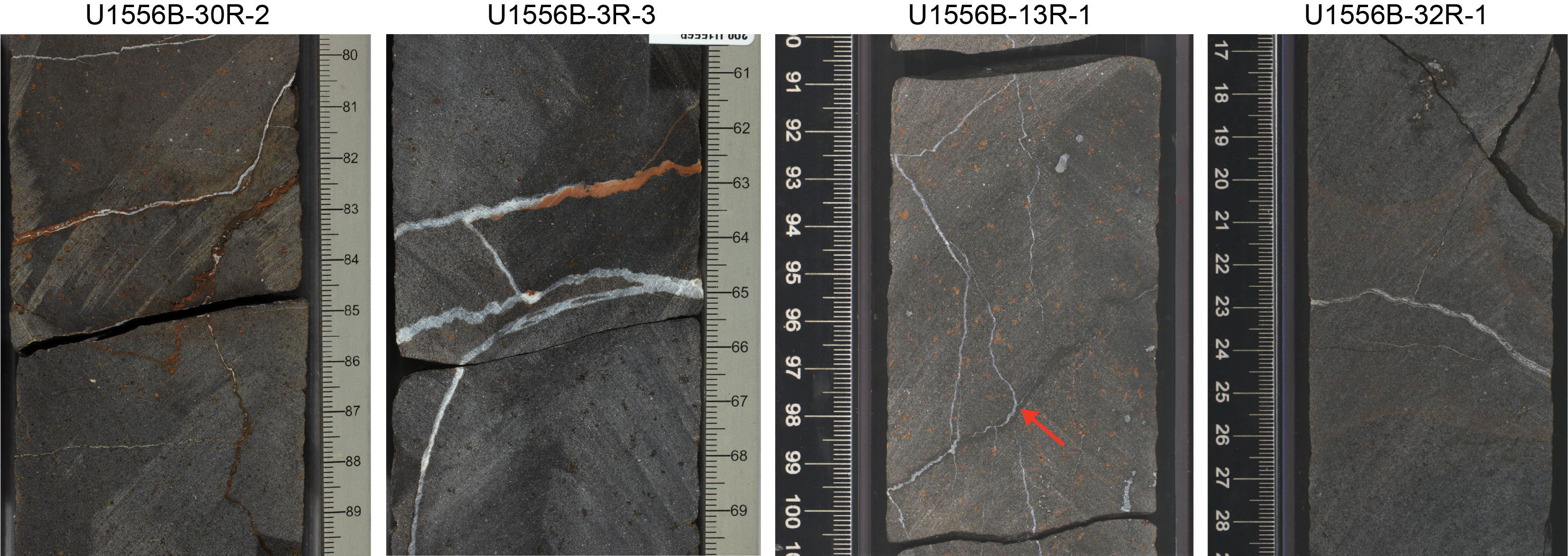
Figure F76. Carbonate veins.

6.4.1. Comparison of macroscopic and thin section observations of veins

Thin section observations broadly support the macroscopic vein descriptions and confirm that carbonate, clays, Fe oxyhydroxides, and zeolites are the predominant vein-filling minerals. The abundance of zeolite is most probably underestimated because it commonly occurs as a lining to carbonate veins, where its presence is mostly masked macroscopically by the similar color of the two minerals, with the latter more readily identifiable because it effervesces on contact with a 10% HCl solution.

6.4.2. Sediment-derived veins

In the uppermost and lowermost 25 m of the hole (particularly Cores 390-U1556B-2R, 3R, 5R, and 55R–59R), sediment is common, constituting ~5%–30% of the rock by volume, interspersed between basalt pillows or flows and as a matrix in breccia. The sediment is pale yellow to pinkish orange indurated calcareous sediment, typically with abundant foraminifera. It is strongly lithified compared to sediments overlying basement, implying that lithification is related to proximity to the basalts, occurring via thermal recrystallization and/or circulating fluids.

Wherever sediments are abundant, so too are basalt-hosted veins ranging <0.1 to >3 mm in thickness and filled with massive, amorphous yellow, orange, or brown calcareous material (Figure F77). This vein fill is very similar in color and texture to the local sedimentary matrix (Figures F67, F77). Some of the thicker examples of these veins are of indisputable sedimentary origin, containing fragments of brown altered basaltic glass and even foraminifera (Figure F78). Also seen are gravity settling features in mixed-fill veins, in which orange-brown material of sedimentary origin filled the lower half of vugs or veins and the upper parts were subsequently cemented by crystalline carbonate (Figure F77).

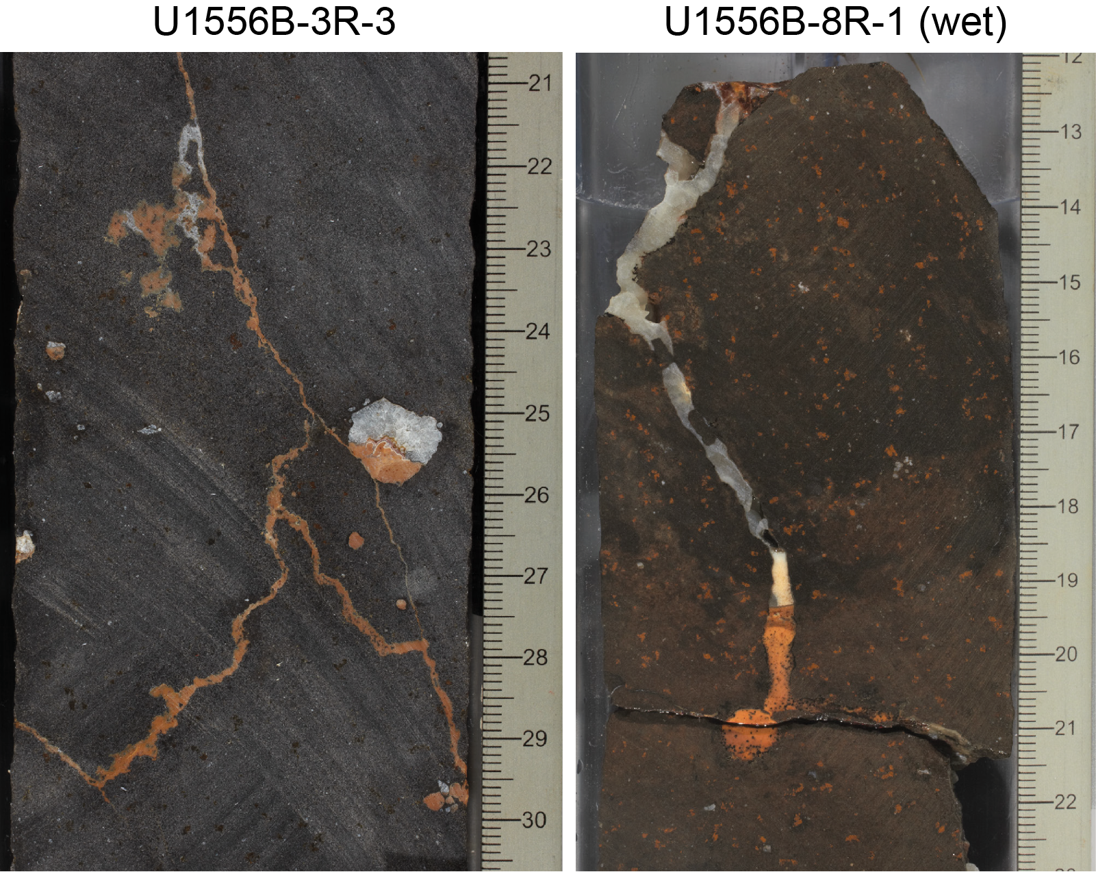
Figure F77. Gravity settling features.

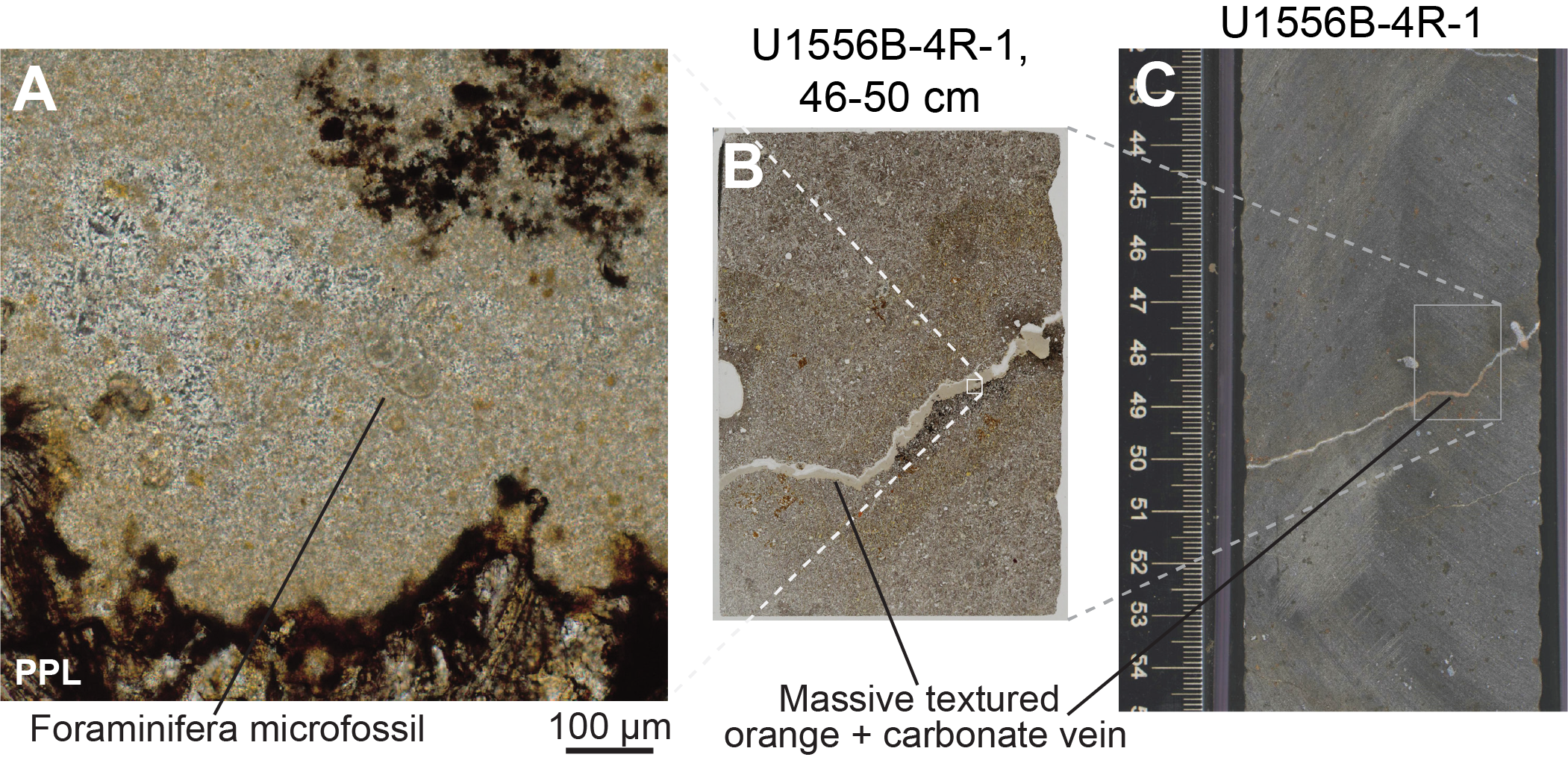
Figure F78. Massive brown sediment-derived vein.

Other veins whose fill is ostensibly the same material (though lacking hyaloclastite and microfossils) include very thin veins and veins deep in the interiors of pillows/flows. Transport of pelagic ooze into such structures may have involved winnowing from bottom currents and injection via fluidization rather than simple gravitational settling. Orange halos are common around such veins. Below Core 390-U1556B-54R, yellow halos are also common. These features suggest that an element of partial dissolution, recrystallization, and redistribution of sediments might also play a role in the formation of these veins. This is supported by the lithified nature of the sediments themselves, which implies recrystallization may have taken place (although not thoroughly enough to completely destroy foraminifera; see Biostratigraphy). The proximity of these veins to interflow sediments and their absence elsewhere in the core suggest that these processes may have been possible only over quite short length scales (e.g., <1 m).

6.4.3. Hybrid zeolite to carbonate veins

A feature of the mottled gray alteration of chilled margins is a general paucity of carbonate veins. This is in marked contrast to the abundance of carbonate veins in the interiors of pillow lavas and massive flows. Veins that cut through the mottled gray altered margins are typically filled with zeolites and smectite and are commonly flanked by light gray halos (Figure F62A). At or very close to the transition from the light or mottled gray altered chilled margin to the coarser grained (typically reddened) interior of the pillow/flow, these veins abruptly transition from zeolite to carbonate filled (Figures F79, F80). This indicates that stabilization of zeolite is likely to be closely related to the leaching of elements such as Si and Al during alteration of the glass, suggesting that formation of zeolite and glass alteration are coupled, both temporally and spatially.

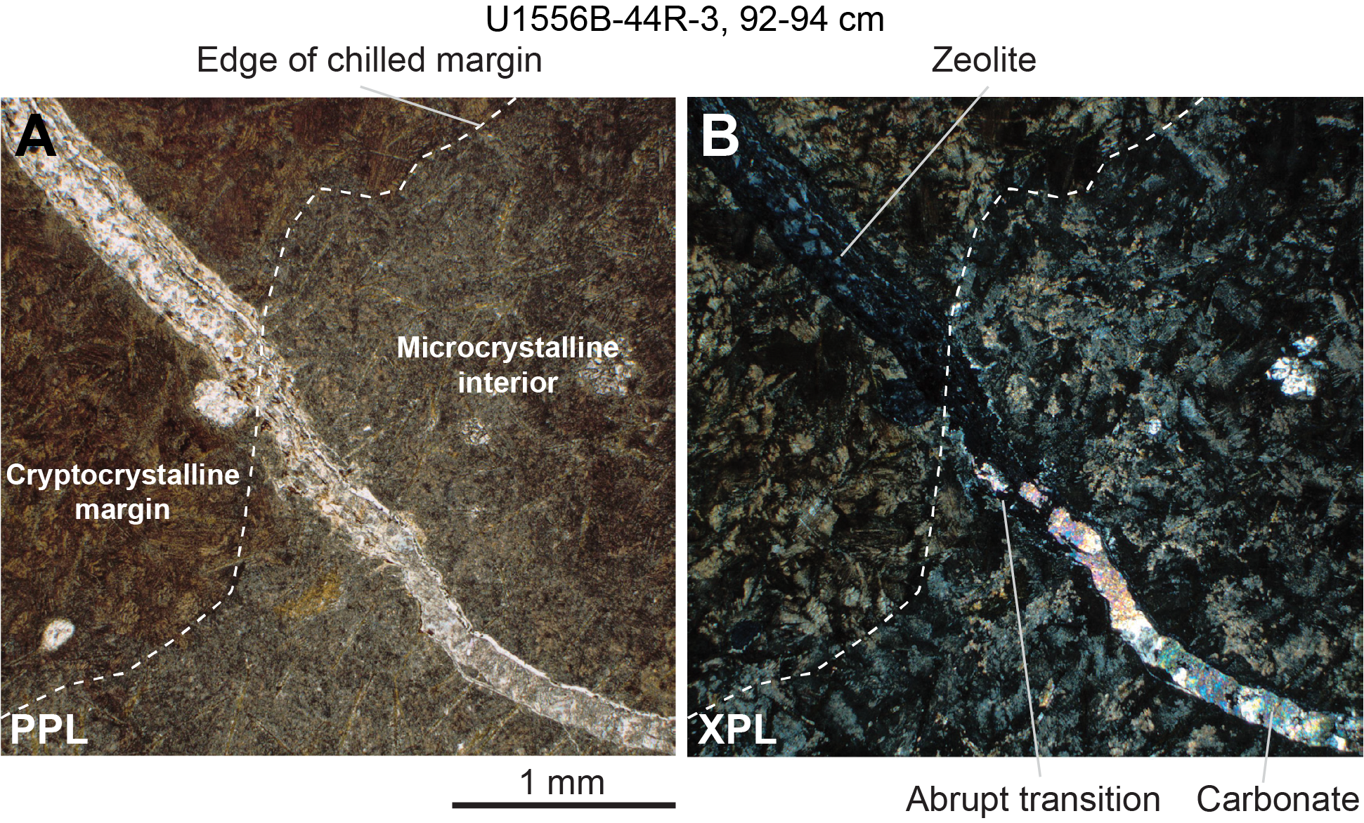
Figure F79. Mineralogy of hybrid zeolite-carbonate vein.

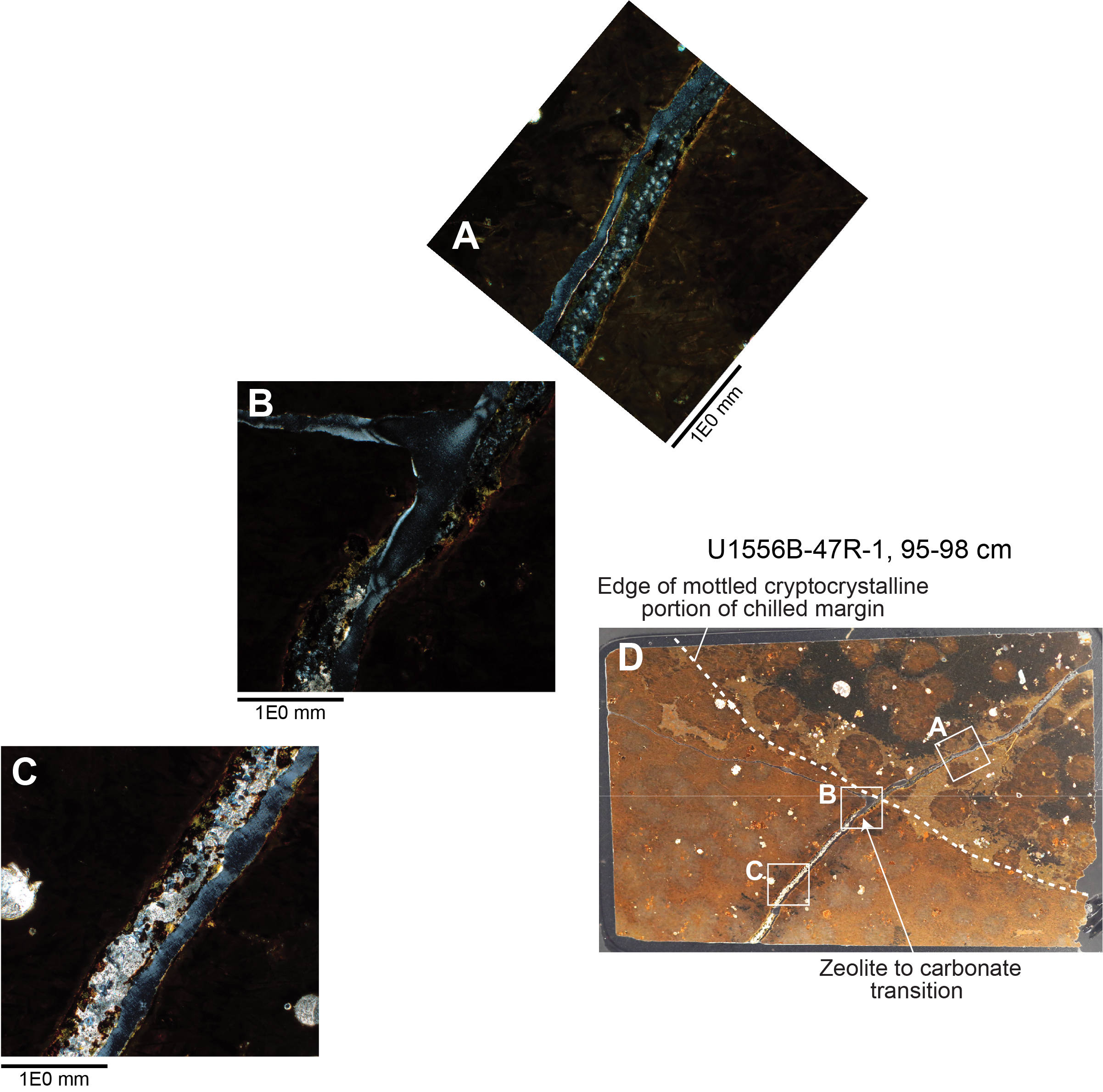
Figure F80. Hybrid zeolite-carbonate vein.

6.4.4. Green vein mineral(s)

Green vein-filling minerals are only abundant in the H-POPP basalts in Lithologic Unit 13 at the base of Hole U1556B. Most common is a macroscopically pale green, dusty textured, swelling clay that coats but does not cement vein surfaces, causing veins to fracture along these coated surfaces where they occur (Figure F81). Pale green–stained carbonate in association with dark saponite in Unit 13 may represent a mixture of carbonate with the same green clay. A similar mineral fills vesicles throughout this interval and was observed to swell out of the cut rock surface when wetted during visual core description (see Alteration petrology in the Expedition 390/393 methods chapter [Coggon et al., 2024c]).

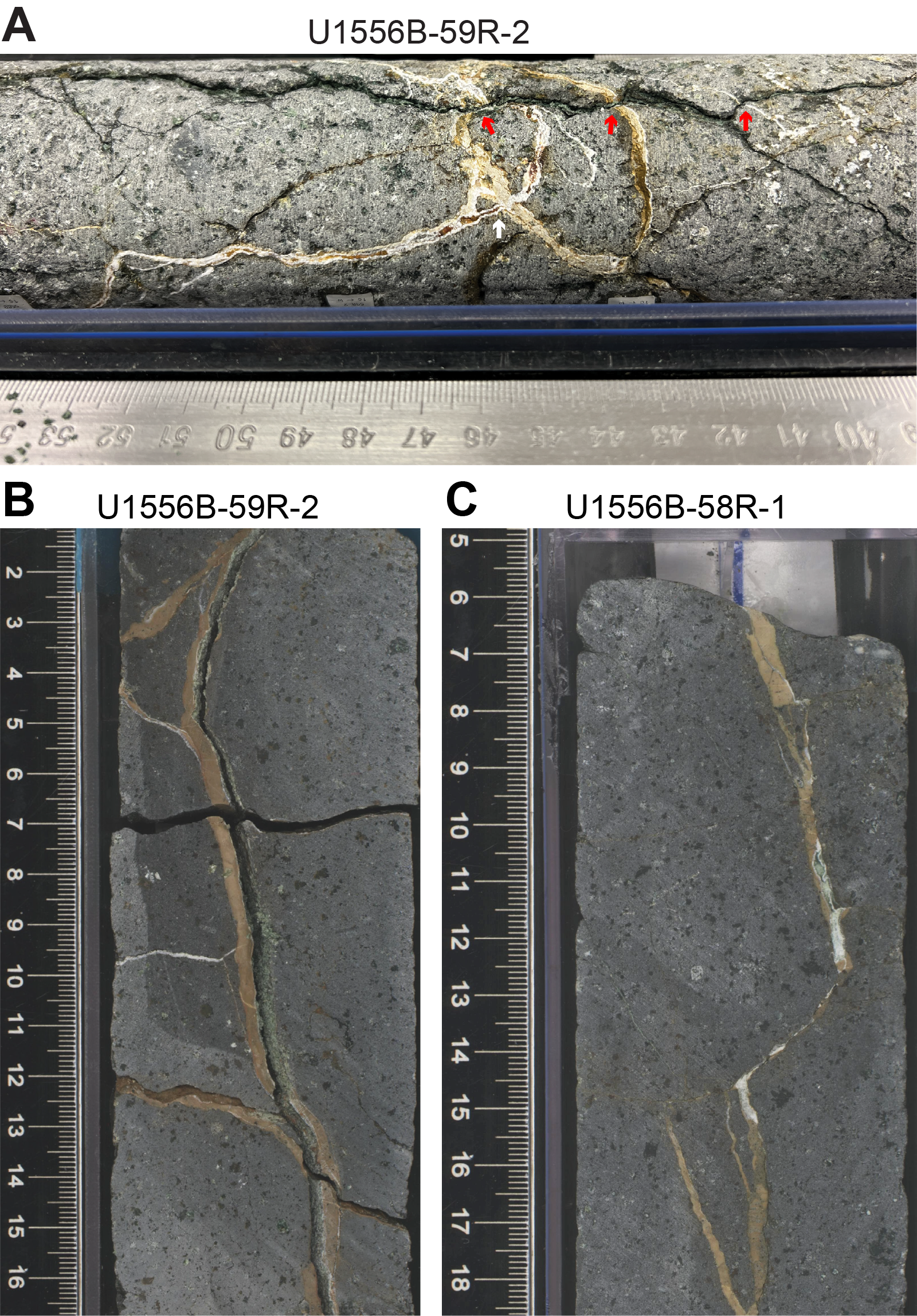
Figure F81. Pale green clay-filled veins, H-POPP basalts.

Shipboard thin section examination and XRD analyses were inconclusive regarding the identity of this mineral. It lacks the micaceous parting, pleochroism, and anomalous interference colors typical of chlorite. Shipboard XRD often did not yield precise classifications for clay minerals, which typically require further analyses (e.g., glycolation experiments) to unambiguously identify them. However, analyses of green vein and breccia cement separates indicate the presence of montmorillonite/smectite + zeolite ± nontronite. Notably, the spectra lack a clear illite peak, suggesting any celadonite component is minor. It appears most likely that the majority of green minerals in the core represent a mixture of clays, including some proportion of saponite, nontronite, and possibly celadonite. That said, the presence of a slightly higher temperature phase such as chlorite-smectite cannot be ruled out on the basis of the available evidence.

6.4.5. Aragonite veins

Four veins from Cores 390-U1556B-31R through 38R were analyzed using XRD and found to contain aragonite (Table T6). The mineralogy of these veins variously consists of dark smectite, carbonate, and greenish or brownish clays, typically intergrown or layered with dark clays along the medial line. Some aragonite formed as rosettes of radiating needles (only visible on broken vein surfaces). Another example contained both calcite and aragonite, which could either represent inversion of a metastable phase or possibly co-precipitation of both phases.

6.5. Crosscutting relationships

Unambiguous crosscutting relationships are rare in the Hole U1556B basement cores. That said, some important crosscutting relationships are revealed in the lowermost lithologic unit (13). In this unit, four distinct alteration phases are present. The earliest is the formation of brown to yellow to buff sediment-derived veins common throughout Unit 13 (Sections 390-U1556B-54R-1 through 59R-4). These are crosscut by white carbonate veins in multiple examples. Carbonate and buff veins are both crosscut by green swelling clay-bearing veins (e.g., interval 59R-2, 40–53 cm) (Figure F81). These crosscutting relationships are cryptic throughout much of the core; carbonate and green veins commonly run along the edges or through the middle of the buff sediment-derived veins. However, both carbonate and green veins almost never occur on both sides of a buff vein and in some places change sides of (i.e., crosscut) the central buff vein, indicating that they are not early linings later filled with buff sediment-derived material. The final event in the sequence is oxidation of the green veins. This is clearly demonstrated by a sharp oxidation front between green clay and rusty Fe oxyhydroxides running horizontally across the internal surface of a vein in the lowermost 30 cm of Hole U1556B (interval 59R-4, 90–97 cm) (Figure F82). This front and the transition from greenish to orange oxidative alteration are present through the entire rock, not just the vein surface. Oxidative overprints also affect green hyaloclastite breccias in the upper green alteration zone (Cores 24R–26R) (Figure F75) and are observed in thin section (Figures F61, F74).

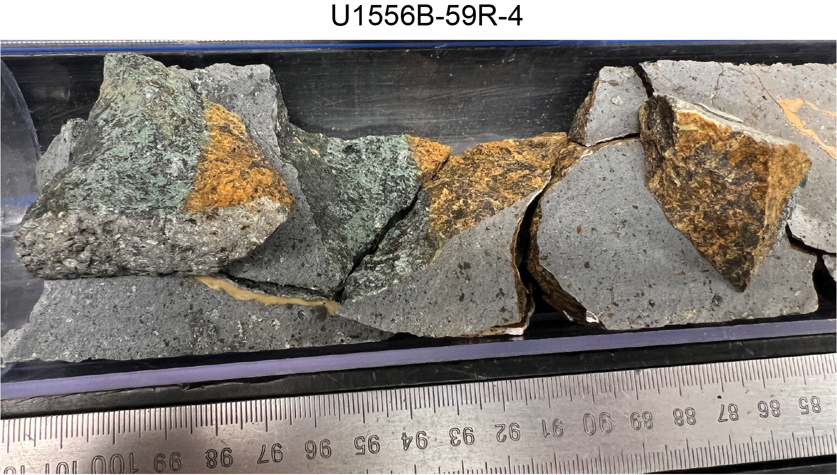
Figure F82. Sharp reaction/oxidation front.

A slight puzzle arising from these observations is that the macroscopic crosscutting relationships observed appear to be inconsistent with the general sequence of alteration apparent in thin sections, in which bright green clays represent the earliest forming minerals and carbonate typically represent the latest (see Secondary mineralogy and sequence of alteration). A likely possibility is that the green clays observed in thin section and hand specimen do not correspond to the same phase of alteration and may even be mineralogically dissimilar (e.g., a green montmorillonite versus celadonite). Regardless, this dichotomy suggests that there are complexities in the sequence of alteration that remain to be understood and will require further characterization of the compositions of secondary phases and their textural relationships to one another.

6.6. Breccia cements

Breccias, predominantly hyaloclastites, occur throughout the basement section cored in Hole U1556B (see Igneous petrology). The volume proportion of breccia cement and its mineralogy were quantitatively logged through Hole U1556B (see DESC_WKB in Supplementary material). The logged breccia cements include 390 occurrences of carbonate, 374 occurrences of smectite, 288 occurrences of zeolite, 56 occurrences of Fe oxyhydroxide, and 56 occurrences of green clay. These figures belie the fact that volumetrically, breccia cements predominantly consist of either voluminous crystalline carbonate or zeolite + smectite forming as thin overgrowths to clasts (Figure F83). The extent to which cements fill the void space of breccia varies spatially and by cementing mineralogy. Carbonate cementation is variable. In some examples, carbonate completely fills the void space. In others, significant porosity remains with centimeter-scale voids in many cores (<50 vol% at the scale of individual core pieces). The morphology of carbonate cements undergoes a transition over the upper eight cores of the hole from sparry dogtooth forms (Figure F83A) to more conical forms similar to piped meringue (Figure F83B).

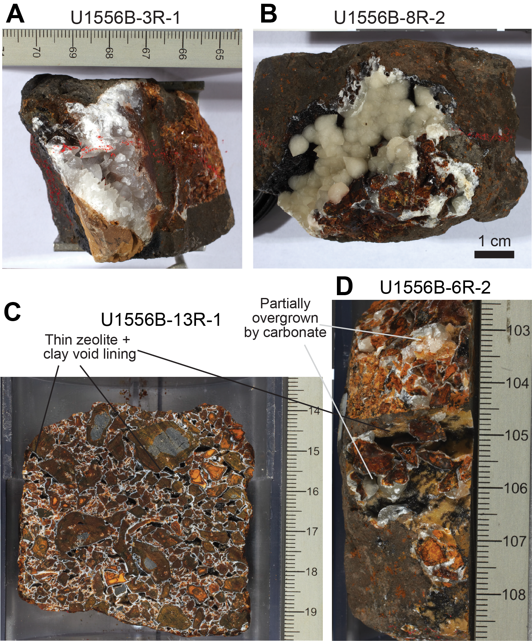
Figure F83. Breccia cements.

Zeolite-bearing cements are typically much less voluminous than carbonate and in most cases preserve significant porosity (Figure F83C). A further qualitative observation is that zeolite-cemented breccias tend to have smaller clast and pore sizes than carbonate-cemented counterparts. Where carbonate cements with significant void space are present, they most commonly overgrow a thin zeolite + smectite cement. Thin section observations also confirm that thin layers of radiating zeolite crystals typically comprise the initial lining of the void space, with the zeolite subsequently overgrown by carbonate (if present) in hyaloclastite and basalt breccias (Figure F84).

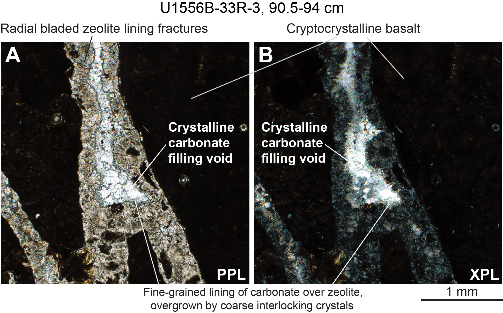
Figure F84. Thin zeolite + clay lining.

6.7. Downhole variations in alteration

Downhole variations in the proportion of alteration types are plotted as a proportion of recovered rock (calculated on a section basis using the piece log (see U1556_PieceLog.xlsx in ALTPET in Supplementary material) in Figure F85. In the upper part of the hole, orange speckled background is the predominant alteration type. There is a transition in alteration throughout the middle and lower parts of the hole, with intense orange halos constituting the majority of the alteration from about 230 to 310 meters subbasement (msb). This corresponds to a major stratigraphic shift from Stratigraphic Sequence A olivine phyric basalts (orange spotty) to Stratigraphic Sequence B aphyric basalts (old red) (see Igneous petrology).

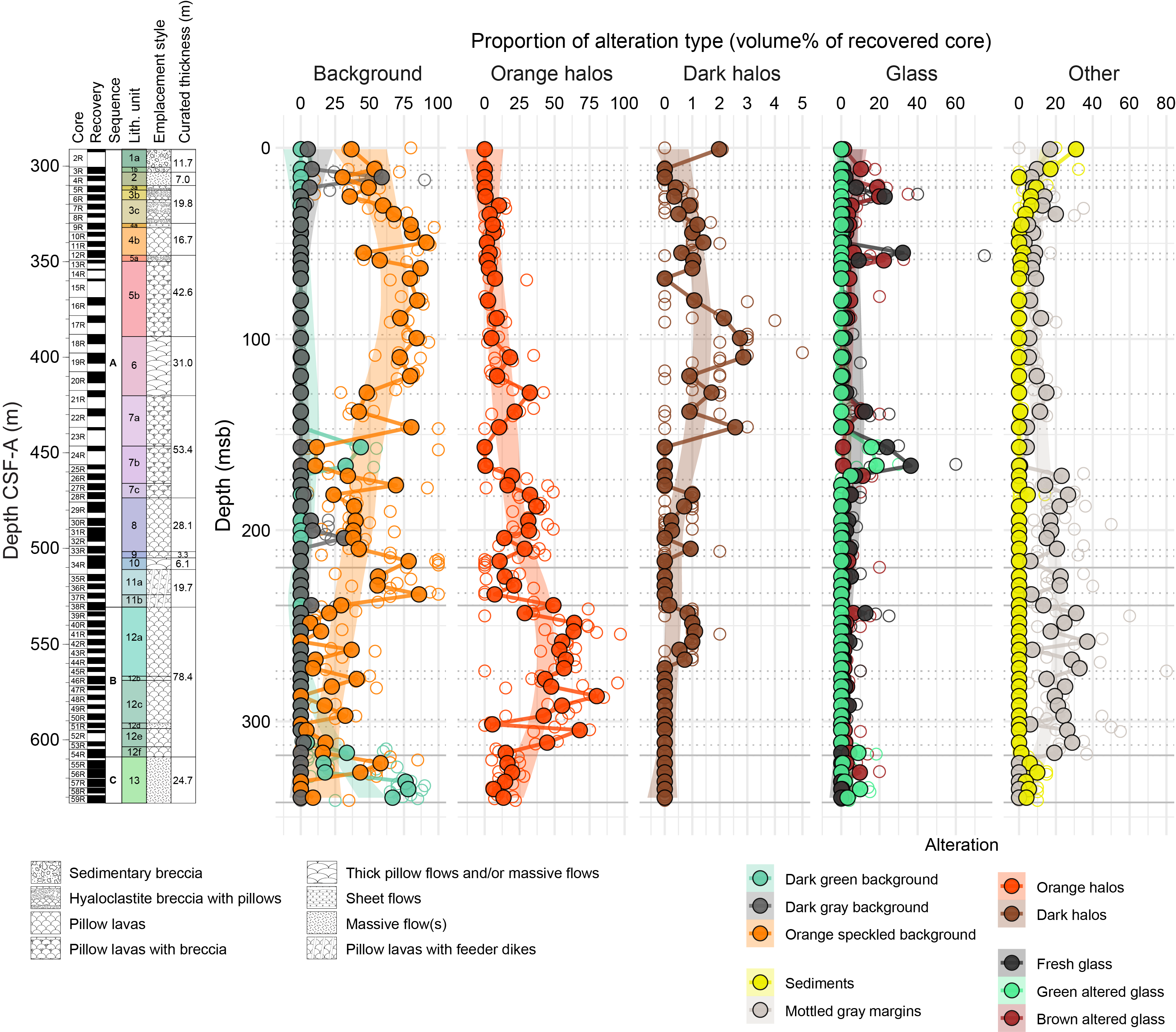
Figure F85. Alteration types.

This broad stratigraphy of alteration can be mapped to color variations measured on each core using the SHMSL (see Physical properties and downhole measurements in the Expedition 390/393 methods chapter [Coggon et al., 2024c]) (Figure F86). When plotted downhole, a* and b* reflectance values (corresponding to green–red and blue–yellow variation, respectively) show higher maximum and mean values in the same interval as the intense orange halo weathering of the pillows from 230 to 310 msb. Plotted against mean a* and b* values for each section, the proportion of orange halos shows a strong positive correlation above ~20% orange halo abundance (Figure F87A–F87C). Sections with a low proportion of orange halos may nonetheless have moderate a* and b* values and correspond to intervals of abundant orange speckled background (Figure F87D). Sections with abundant dark gray and dark green background show low values of both color parameters, reflecting dominantly green-blue hues (Figure F87E).

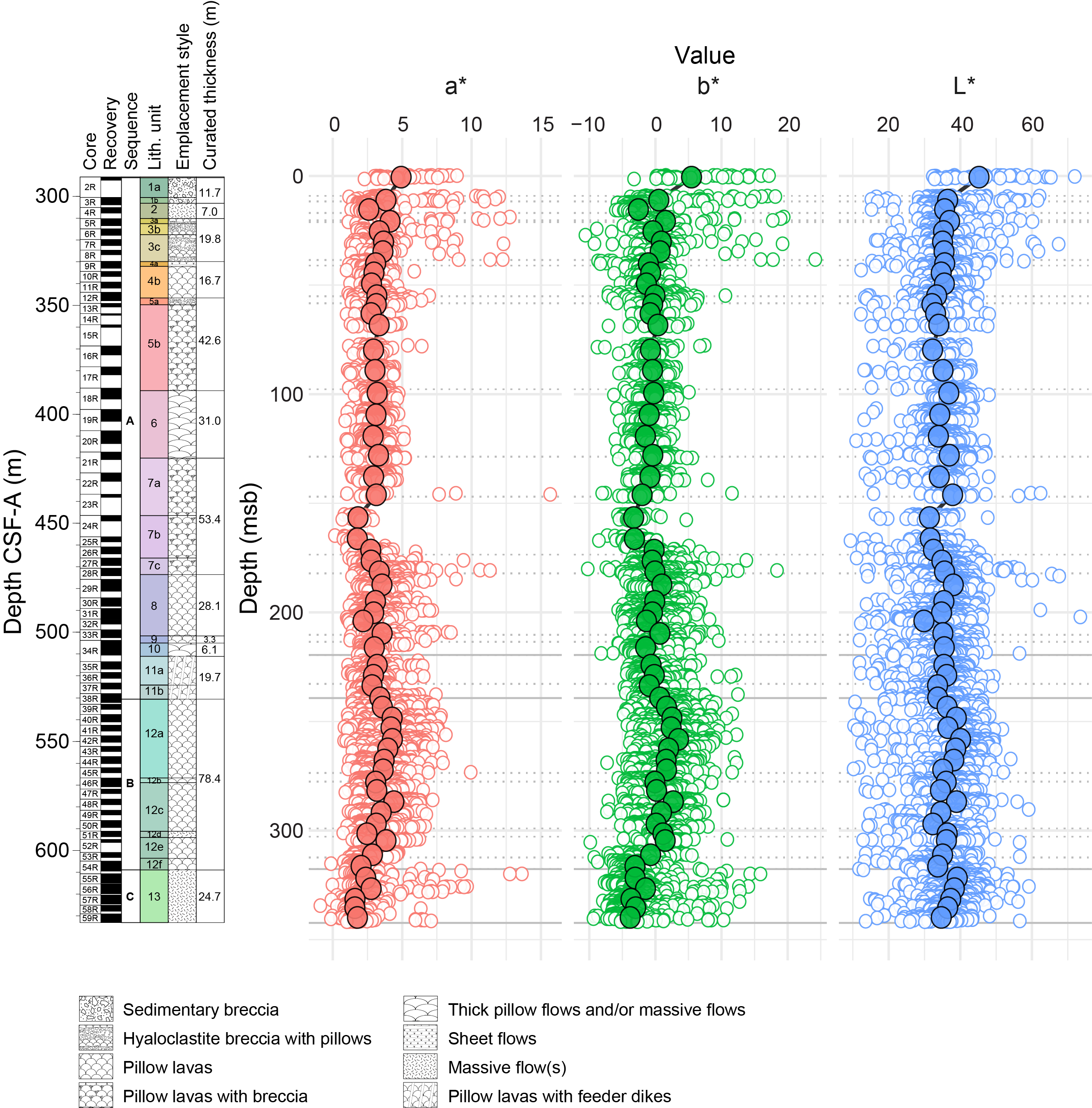
Figure F86. SHMSL spectral reflectance.

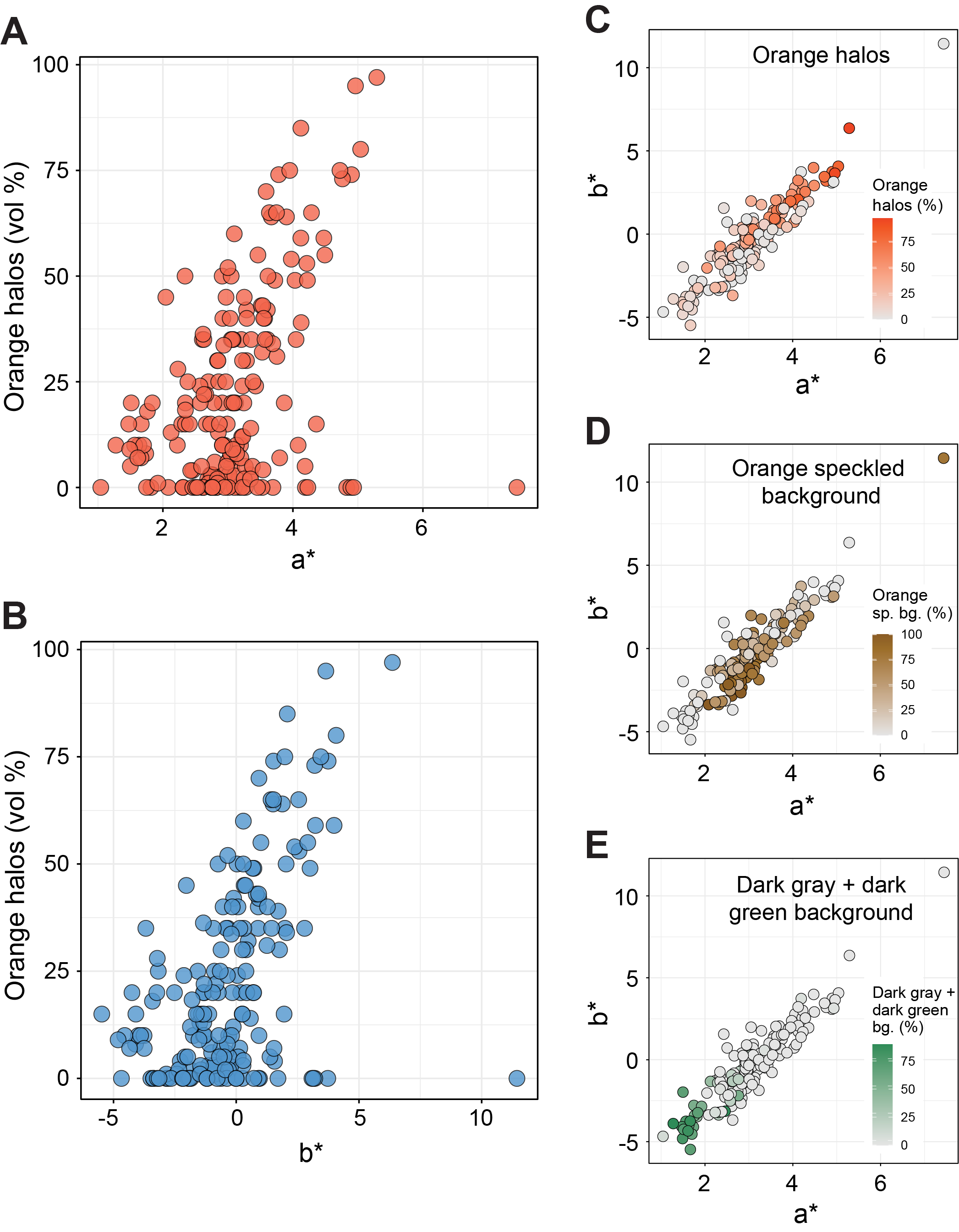
Figure F87. Spectral reflectance and alteration logging.

There is a broad correlation (R² = 0.44), too, between the proportion of mottled gray chilled margins and orange halos (Figure F85), consistent with the formation of a large proportion of the orange halos along pillow margins. Sediments are relatively abundant in the upper parts of the core, rapidly decreasing downhole in the uppermost 50 msb, and then reappearing below 320 msb in the H-POPP basalts. This finding suggests that the bulk of basalts recovered in the hole erupted relatively rapidly, without sufficient time for sediment accumulation, but that there might have been some hiatus or period of relatively reduced volcanic activity following the eruption of the H-POPP basalts.

The densities of veins (in number of occurrences per meter curated core) are plotted for each core downhole in Figure F88, and the median, mean, and maximum width of veins are plotted in Figure F89. There are noteworthy variations in the density of veins downhole. In particular, intervals of relatively denser veining (~20–30/m) are commonly associated with correspondingly high proportions of speckled orange background and particularly orange halos (e.g., Units 4–6 at 39–129 msb, Unit 8 at 182–210 msb, and Unit 12 at 239–318 msb). Conversely, minima of vein density correspond in several intervals with relatively high proportions of dark and green background alteration or fresh glass (e.g., Subunit 7b at 155–175 msb). It should be noted, however, that some of this is an effect of brecciated intervals having typically low vein densities. This is presumably because any veins or fractures initially present in the rock have become fractures along which brecciation occurred and because further veining is inhibited by the open porosity, which tends to localize both stress and fluid flow between clasts.

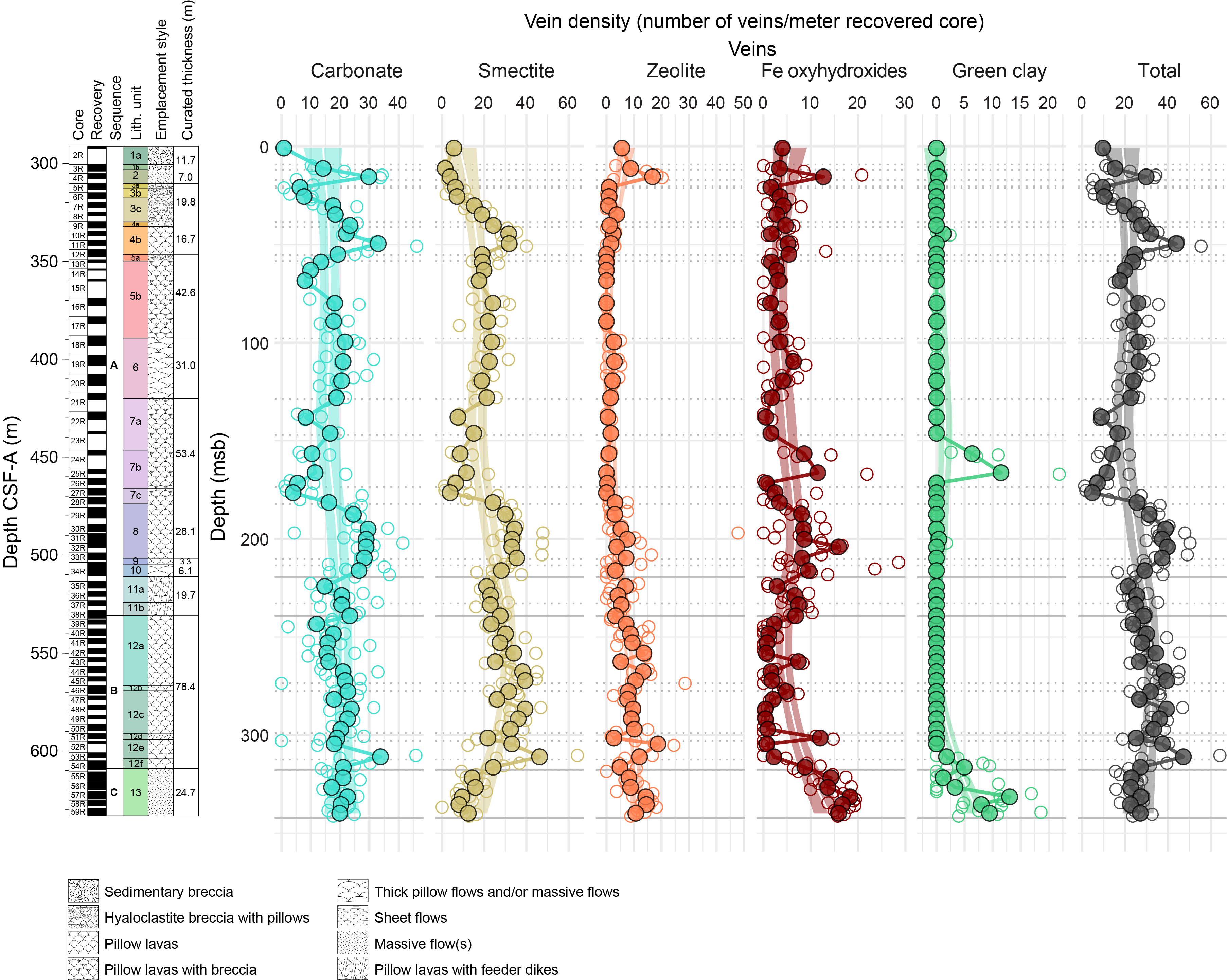
Figure F88. Vein density.

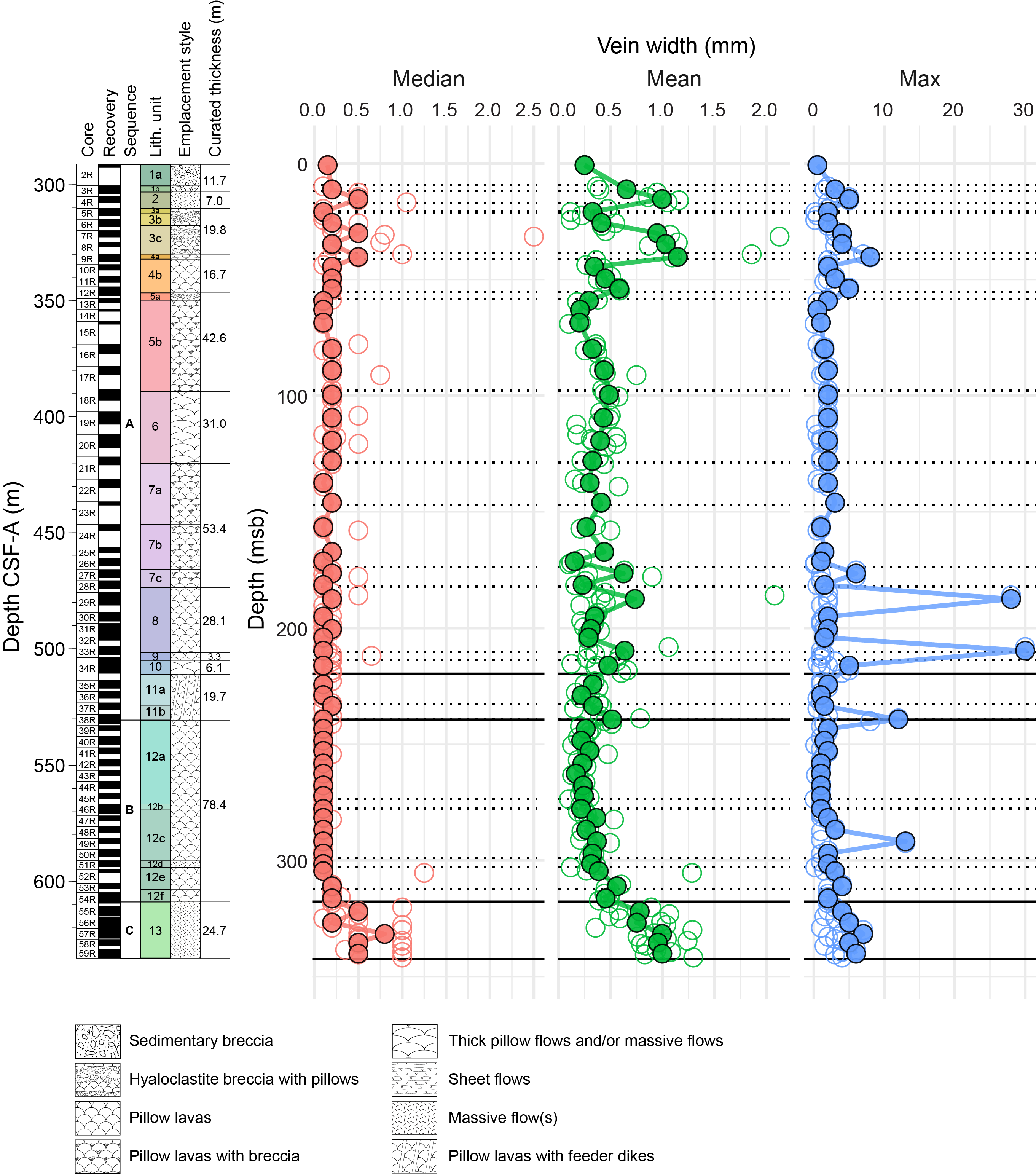
Figure F89. Vein widths.

The volume proportions of selected secondary minerals in breccia cements and vesicle fills are plotted downhole in Figures F90 and F91, respectively. The volume proportion of carbonate breccia cements decreases markedly downhole in the uppermost 50 m of the basement (Figure F90). A similar trend is seen in the proportion of carbonate-filled vesicles (Figure F90). Another interval of abundant breccia occurs between about 120 and 200 msb but shows a clear difference in the composition of the cement, with zeolites and minor smectite clays far more common than in the upper parts of the hole. Nonetheless, the total volume of zeolite cements logged in the hole is relatively low, averaging only 0.13% across the entire volume of recovered core, partly owing to the high porosity of zeolite-cemented breccias. Vein widths vary downhole. High mean and median values in the uppermost and lowermost sections correspond to abundant, typically thick (1+ mm) sediment-derived veins, a proportion of which are likely sediment-filled cracks. In the middle of the hole from about 170 to 230 msb, carbonate veins as thick as 30 mm (and vug fills not recorded as veins) are relatively common and sufficiently large to affect the median and mean vein widths of the entire core. Exactly what the causes for this interval of intense, thick veining and void-filling carbonate precipitation are remains to be seen. Conversely, the highly orange halo altered aphyric basalts (old red) show generally thin vein widths by all three metrics, albeit with overall high vein densities.

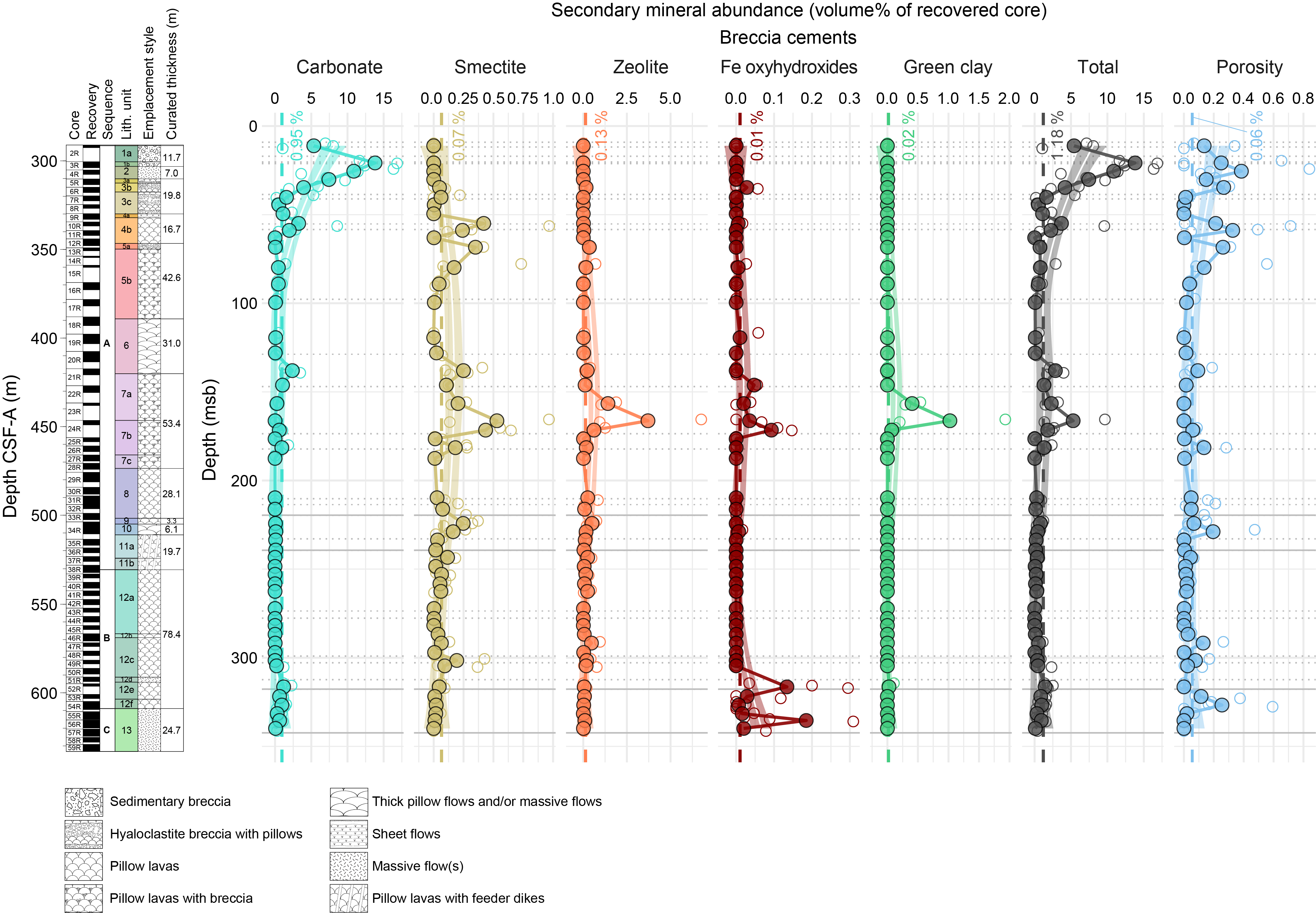
Figure F90. Secondary minerals and porosity in breccia cements.

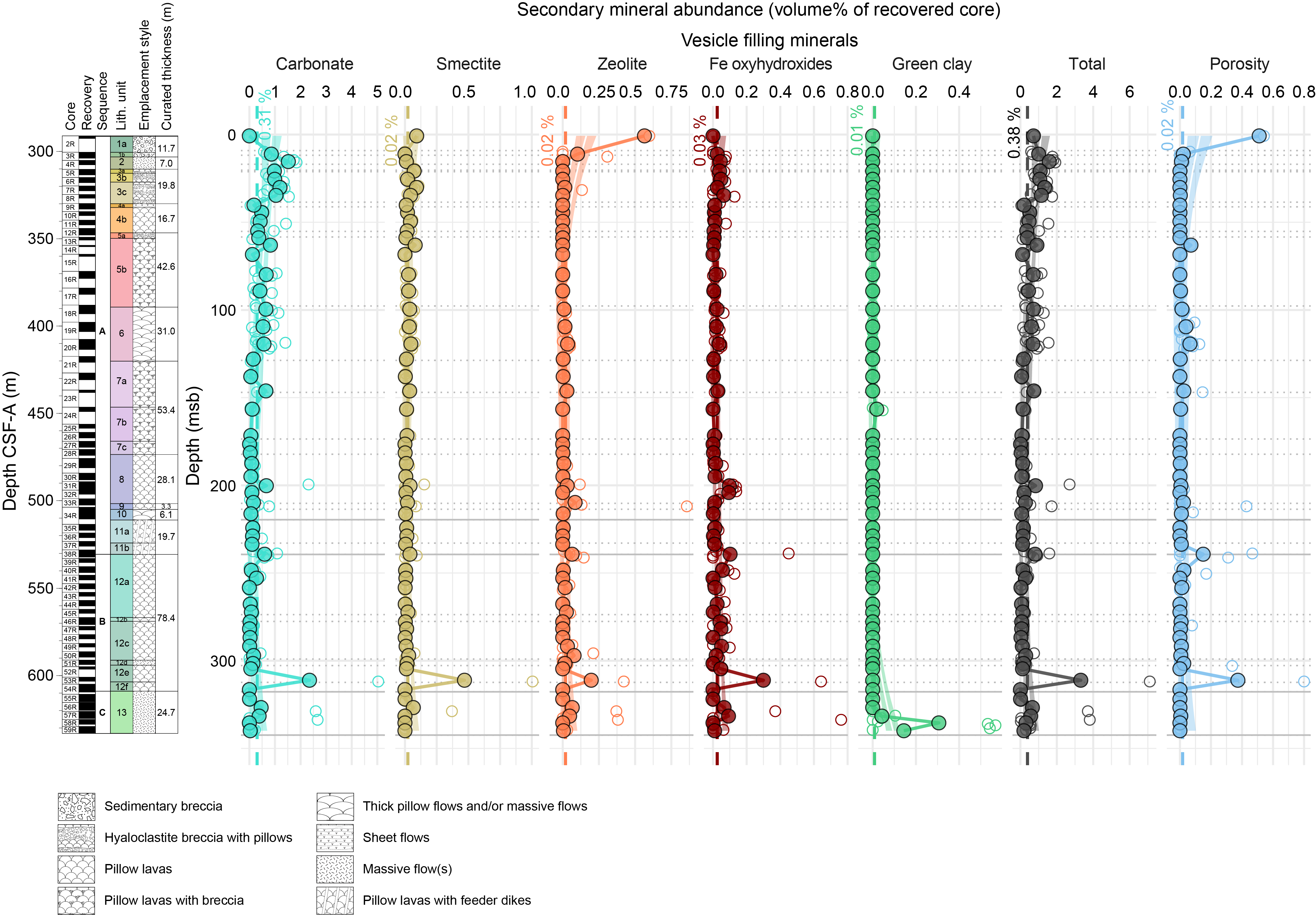
Figure F91. Secondary minerals and porosity in vesicles.

6.8. Secondary mineralogy and sequence of alteration

Secondary minerals occur throughout the basement interval cored at Site U1556, replacing groundmass, glass, and pseudomorphing primary igneous minerals as well as filling veins, vesicles, and open pore space in breccias. Specific secondary minerals are not generally distinguished beyond broad mineral groups (e.g., clays, carbonates, and zeolites) in the vein and alteration logs (see DESC_WKB in Supplementary material). The principal secondary minerals encountered in basalts and associated breccias are clays, Fe oxyhydroxides, carbonate, and zeolites.

In thin section under PPL, pale brown to very pale green clay is ubiquitous away from veins in less altered/dark background altered samples and is tentatively identified as saponite (Figure F60). It occurs principally as a replacement phase of olivine and as a lining in vesicles, commonly in association with carbonate. In the halos of veins, it most commonly occurs in association with iddingsite and/or bright yellow (or green) clays, both of which it commonly overgrows where a clear sequence is apparent (most commonly in vesicles; e.g., Figure F66).

The most abundant class of secondary minerals observed in thin section is a spectrum of clay + Fe oxyhydroxides mixtures that range from bright yellow to deep red-brown (Figures F64, F65, F57). These include the red-brown olivine alteration product termed iddingsite (nominally a mixture of smectite clays and goethite; Smith et al., 1987) and extend to bright yellow colors taken to likely represent more clay-rich compositions. Iddingsite is common in a large proportion of samples studied in thin section and pseudomorphically replaces olivine and fine-grained quench groundmass.

Bright yellow and orange clays are more typically observed within halos of oxidative alteration and commonly occur as a front to the halo (Figure F57).

Green clay, showing bright apple green to blue-green absorption colors in thin section, is common in parts of the hole, mostly from the intervals of abundant green glass and dark gray or green background alteration from Cores 390-U1556B-24R through 26R and in the lowermost cores of the hole (Cores 54R–59R). It occurs mainly in halos around veins or less commonly in restricted patches (Figures F61, F66). The green clays have a similar mode of occurrence and optical properties to the yellow clays, with low interference colors and radial/feathery to cryptocrystalline habit.

In several thin sections that contain green clay, yellow clays appear to overgrow (or form from) the green clay, generally in the outer rim of halos (Figure F61). This observation is taken as evidence that much of the yellow clay may have originated as halos of green clay that have been largely overprinted by later oxidative halos in most parts of the rock. Where iddingsite or brown Fe oxyhydroxides and green clays coexist, the brown iddingsite consistently overgrows the green clays and is typically itself overgrown by pale brown saponite (Figures F61, F66). Similar sequences of alteration minerals have been reported in the other drilled sections of upper oceanic crust (Alt et al., 1986; Alt, 2004).

XRD analyses of numerous examples of green vein minerals support the identification of this (or these) green mineral(s) as clay (Table T6). It may represent celadonite, but XRD patterns are not conclusive and generally indicate the presence of smectite over illite (Table T7). There is no evidence for the presence of chlorite, although small proportions of chlorite in a mixed layer chlorite-smectite cannot be ruled out. Given that nontronite and some montmorillonites may also show green colors and that what has been identified as celadonite in the oceanic crust typically contains some proportion of nontronite and montmorillonites (Alt, 2004), we refer to this simply as green clay pending further investigation.

Zeolites are common throughout the basement succession at Site U1556. They occur as radiating masses of spherulitic to bladed crystals with very low birefringence (Figure F64) and are almost always associated with altered glass, hyaloclastites, or cryptocrystalline margins of flows/pillows. They occur as vesicles and vein fills and most abundantly as linings on glass in hyaloclastites, where they may constitute a large proportion of the cement (Figure F74). Phillipsite is the main zeolite present, and its identity has been confirmed in numerous XRD analyses throughout Hole U1556B (Table T6). Where zeolites occur with other alteration phases, they are typically a late forming mineral and only overgrown by carbonate.

Carbonates are common throughout the succession, filling veins and vesicles and cementing breccias. They are typically a late-forming phase and are seen to overgrow both saponite (typically in vesicles; Figure F60) and zeolite (typically cemented in the central portion of breccia pore space; Figure F84). Carbonate also commonly fills vesicles without any other minerals present, implying that those vesicles remained unfilled until comparatively late in the alteration sequence.

XRD analyses of splits of whole-rock powders from basalts sampled for geochemical analyses (see Geochemistry) yield monotonous identifications (Table T7). They almost universally indicate the presence of typical basaltic igneous minerals clinopyroxene (augite or diopside) and anorthite, together with smectite clays and illite clays. The ubiquitous presence of primary igneous minerals is notable because it implies that even in the most pervasively altered samples there are some remnant primary phases. It should, however, be noted that the geochemistry samples typically aimed to sample fresher portions of rock in a given core rather than the most altered (see Geochemistry in the Expedition 390/393 methods chapter [Coggon et al., 2024c]).

The XRD patterns tend to show a distinct illite peak that is mostly absent in the analyses of discrete green (and other) veins. This might be evidence of cryptic celadonite alteration in the groundmass of these samples, but it could also be explained by sericitization of plagioclase or by the presence of a number of other illite clay or phyllosilicate species. Another intriguing feature of the whole-rock XRD analyses is the apparent presence of amphibole in several samples (Table T7). This observation has not been confirmed in thin section, and these identifications should be treated with caution and require further postexpedition research. If present, the amphiboles are likely to be fine grained. The XRD peaks detected do not appear to be particularly sensitive to the chemistry of the amphibole, so they cannot enlighten us any further about the potential paragenesis. The apparently amphibole-bearing samples are broadly from the upper part of the hole in Cores 390-U1556B-2R through 28R.

6.9. Summary

The alteration at Site U1556 shows a wide range of alteration styles attesting to multiple phases of mutually overprinting alteration. Much of the apparent sequence of alteration, from the early formation of green clay-bearing halos and oxidative overprinting, followed by a transition to apparently more reducing, possibly saponitic, alteration and in turn late carbonate formation in veins, is consistent with what is seen at other sites drilled in upper oceanic crust (e.g., Alt, 2004). However, certain features including evidence for late (postcarbonate) formation of green clays and the presence of aragonite veins in old crust suggests a potentially protracted alteration history. Equally notable is the relatively high abundance of carbonate veins and breccia cement downhole. Further research, including more thorough characterization of the exact mineralogy and chemistry of alteration phases, will be required to better understand the sequence and significance of successive alteration events in the rocks.

7. Biostratigraphy

The 278.35–291.29 m thick sedimentary succession at Site U1556 contains a Holocene to Paleocene sequence of pelagic ooze, chalk, and clay (see Sedimentology). Calcareous nannoplankton are present in the oozes and chalks but are mostly absent from the clays; planktic and benthic foraminifera are also mostly absent from the clays and have variable abundances in the nannofossil oozes of Unit I, in which they often comprise a depauperate assemblage of mostly very small specimens. Biostratigraphic zonation is based on analysis of core catcher samples from Holes U1556A (collected during Expedition 390C and examined on shore; see Background and objectives) and U1556C (collected and examined during Expedition 390), which had significantly better recovery, particularly during XCB coring (see Operations). Additional calcareous nannofossil samples were taken from carbonate-rich intervals of the archive halves of Hole U1556A, and both calcareous nannofossil and planktic foraminifera samples were taken together from the working halves of Hole U1556C to refine the biostratigraphic zonation.

The mudline sample from Core 390-U1556C-1H contains a recent assemblage of planktic foraminifera, and sedimentation appears to be relatively continuous through the early Oligocene. A 44.28 m thick condensed interval or unconformity composed of dark brown pelagic clay and spanning the early Oligocene to early Eocene occurs in Sections 390C-U1556A-22X-4 through 26X-2 (202.42–238.20 m CSF-B) and 390-U1556C-23X-5 through 28X-2 (204.42–250.19 m CSF-B). Below this interval, the Eocene extends through to 266.10 m CSF-B in Hole U1556C. Eocene assemblages contain a substantial proportion of reworked Paleocene calcareous nannofossils and foraminiferal taxa that appear to be principally or entirely sourced from the middle Paleocene planktic foraminiferal Zone P4a and calcareous nannoplankton Zones CNP8–CNP7. A similar phenomenon was observed in the same interval at Site U1557 (see Biostratigraphy in the Site U1557 chapter [Coggon et al., 2024a]), but at that site obviously reworked Paleocene material is typically rare compared to the overall Eocene assemblage. At Site U1556, the reverse is true; the assemblage initially appears to be Paleocene, but further examination reveals rare taxa that are restricted to the Eocene. This interval showed limited coring disturbance, and foraminiferal and nannofossil samples taken from the working halves of cores from Hole U1556C were carefully selected to avoid disturbed intervals: samples were taken from the middle of biscuits using 10 cm³ cylinders and toothpicks, thus avoiding sampling downhole contamination. Instead, this reworking appears to reflect extensive downslope reworking during the Paleocene–Eocene. Increasing microfossil reworking downhole makes precise age determinations difficult, but the middle Eocene (likely below planktic foraminiferal Zone E5 and calcareous nannofossil Zone CNE3) unconformably overlies the middle Paleocene in the lowermost part of the sediment section, representing an interval of missing time spanning at least 5 My and as long as 10 My. Samples below the Paleocene–Eocene unconformity are middle Paleocene in age and are assigned to planktic foraminiferal Zone P4a and calcareous nannofossil Zones CNP8–CNP7. An integrated calcareous nannofossil and planktic foraminiferal biozonation for Site U1556 is presented in Figure F92 and Tables T8 and T9. An age-depth plot of biostratigraphic datums and paleomagnetic reversals can be found in Figure F119, and datums are provided in Table T21.

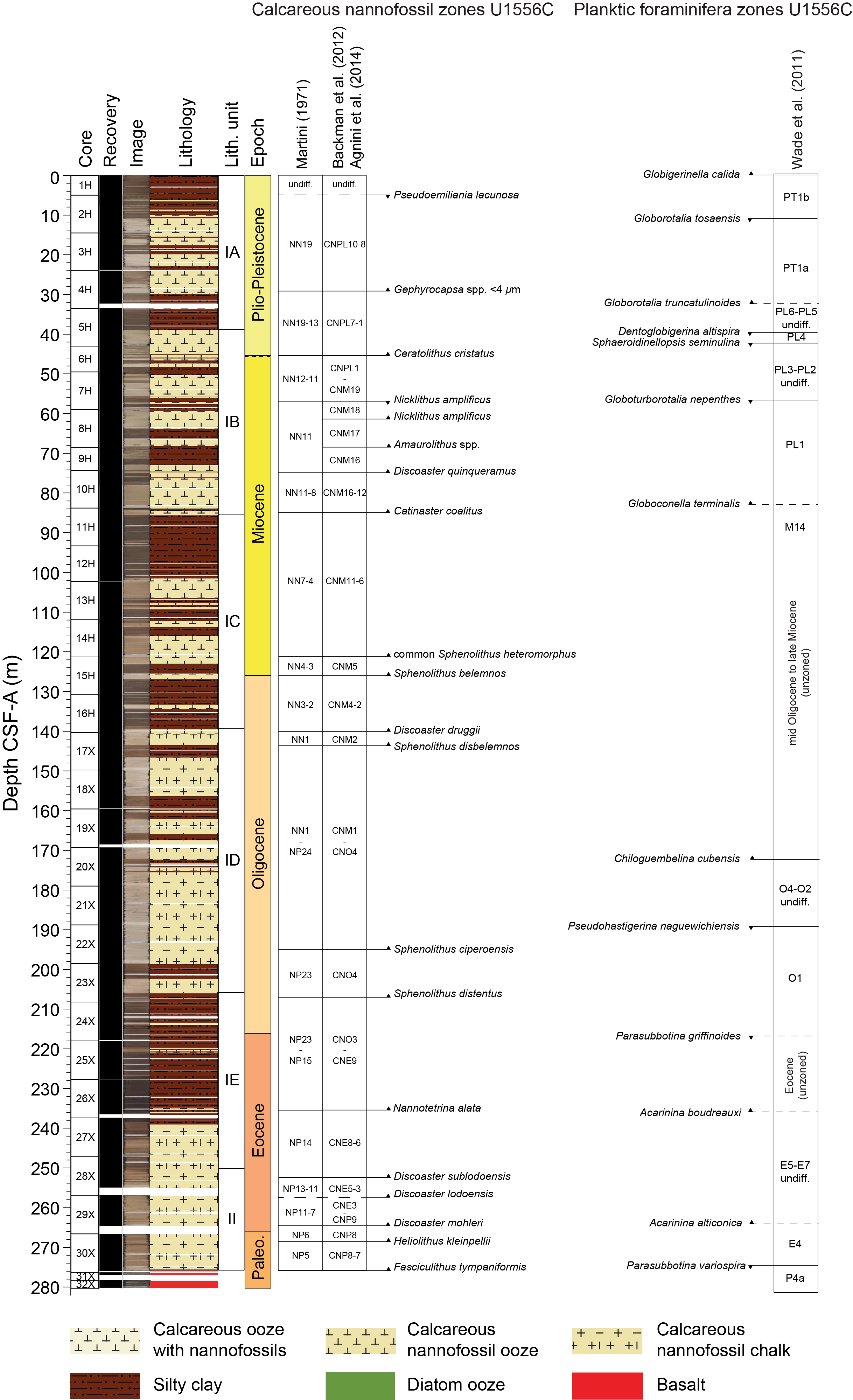
Figure F92. Nannofossil and foraminifera biostratigraphic zones.

Paleodepth estimates are based on onshore analysis of benthic foraminifera from core catcher samples from Hole U1556A. In Hole U1556A, benthic foraminifera are generally present in Pleistocene Sample 390C-U1556A-1H-CC, 12–17 cm, and then again in middle Eocene samples from Lithologic Subunit IE and Unit II (Samples 25X-CC, 10–15 cm, to 29X-CC, 15–20 cm). In Hole U1556C, benthic foraminifera are rare throughout the section but are more abundant in Lithologic Unit II and dominate the foraminiferal assemblage in some samples from Core 390-U1556C-30X, possibly indicating the position of the unconformity. Benthic foraminiferal assemblages indicate upper abyssal depths (~2000–3000 m) in the Paleogene and lower abyssal depths (>3000 m) in the Pleistocene.

A summary of microfossil preservation and abundance is shown in Figure F93.

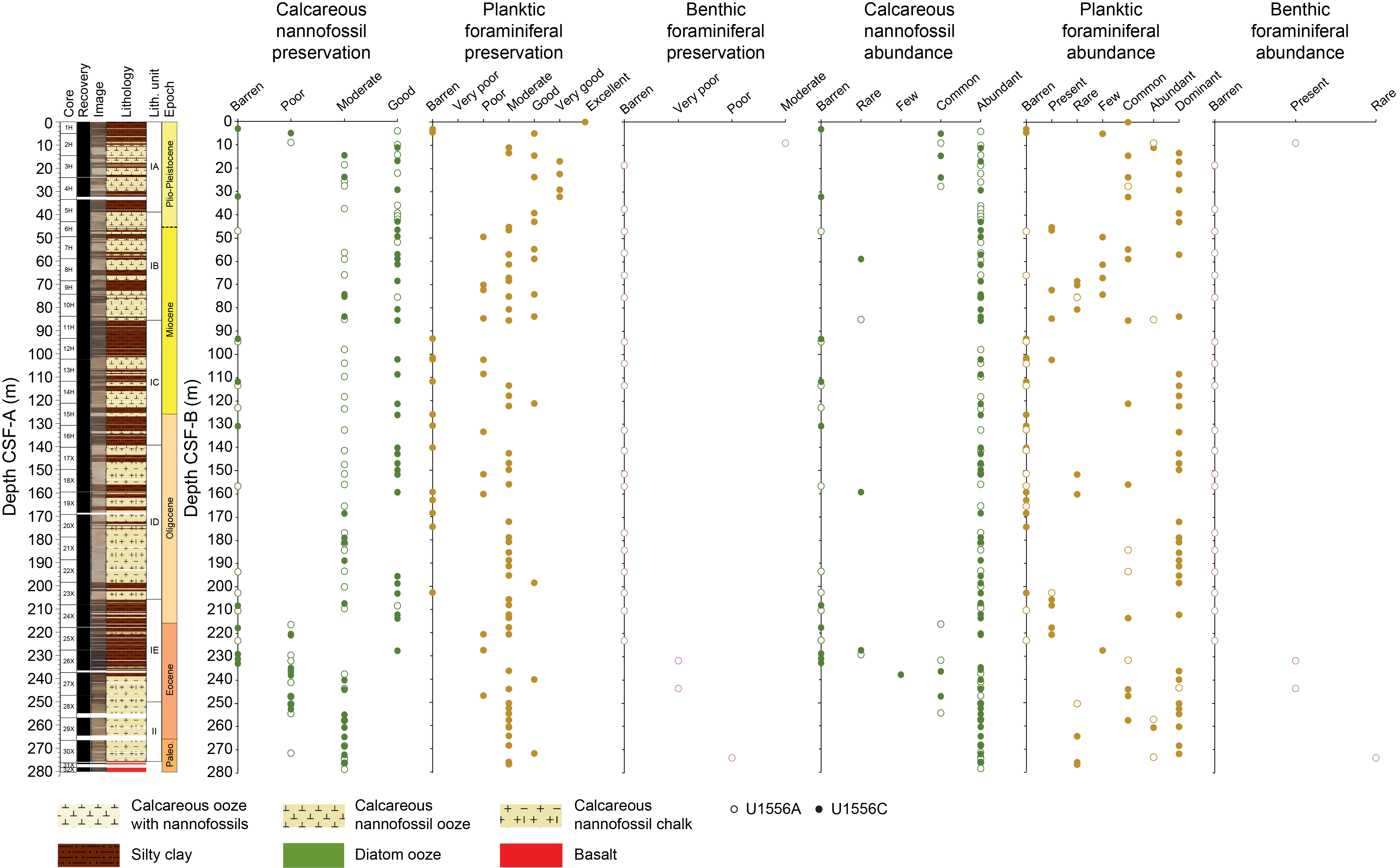
Figure F93. Abundance and preservation of nannofossils and foraminifera.

7.1. Age of basement

To constrain the age of basement at Site U1556, samples were analyzed as close to the sediment/basement interface as possible in all three holes (Samples 390C-U1556A-30X-4, 65–67 cm [278.25 m CSF-B]; 390-U1556B-2R-1, 17–19 cm [291.18 m CSF-B]; and 390-U1556C-31X-2, 14–16 cm [276.70 m CSF-B]), all of which contain the same middle Paleocene assemblage of planktic foraminifera (Zone P4a, based on the co-occurrence of Globanomalina pseudomenardii and Parasubbotina variospira) and calcareous nannoplankton (Zones CNP8–CNP7, based on the presence of Fasciculithus tympaniformis and absence of Heliolithus kleinpellii). This is equivalent in age to the oldest assemblage observed at Sites U1557 and U1561 (see Biostratigraphy in the Site U1557 chapter and Biostratigraphy in the Site U1561 chapter [Coggon et al., 2024a, 2024b]) and the 61 Ma projected age of basement (see Background and objectives).

In Hole U1556B basement, small (centimeter scale) sediment lenses between basalt flows represent brief intervals of pelagic sedimentation between eruptions. We examined a thin section of a sediment lens from the deepest core (Sample 390-U1556B-59R-4, 26–29 cm; 632.71 m CSF-B) and found a relatively diverse, abundant, and moderately well preserved assemblage of planktic foraminifera. This assemblage is similar to that recorded at the top of the lava pile and includes Globanomalina chapmani (Figure F94), which evolved within Zone P4a. Because the sediments at the top of the basement and at the bottom of the basement were deposited within the same planktic foraminiferal zone (P4a), the entire 341 m sequence of basalt cored at Site U1556 must have erupted within 220 ky, between 60.54 and 60.76 Ma (based on the global calibration for the duration of Zone P4a by Gradstein et al. [2020]).

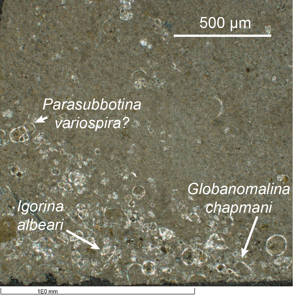
Figure F94. Foraminifera in pelagic limestone.

7.2. Calcareous nannofossils

All core catcher samples from Holes U1556A and U1556C were examined to establish a calcareous nannofossil biostratigraphy; additional samples were taken from the split-core sections of both holes to better constrain biohorizons. Hole U1556A samples were taken from the archive half, whereas Hole U1556C samples were often paired with planktic foraminiferal samples taken from the working half. Biostratigraphic datums used for the age-depth model are listed in Table T21 and illustrated in Figure F119, and calcareous nannofossil occurrence data are shown in Tables T10, T11, and T12. Note that the distribution chart is biased toward age-diagnostic and other notable taxa; a plate of photomicrographs, including many of these taxa, is shown in Figure F95.

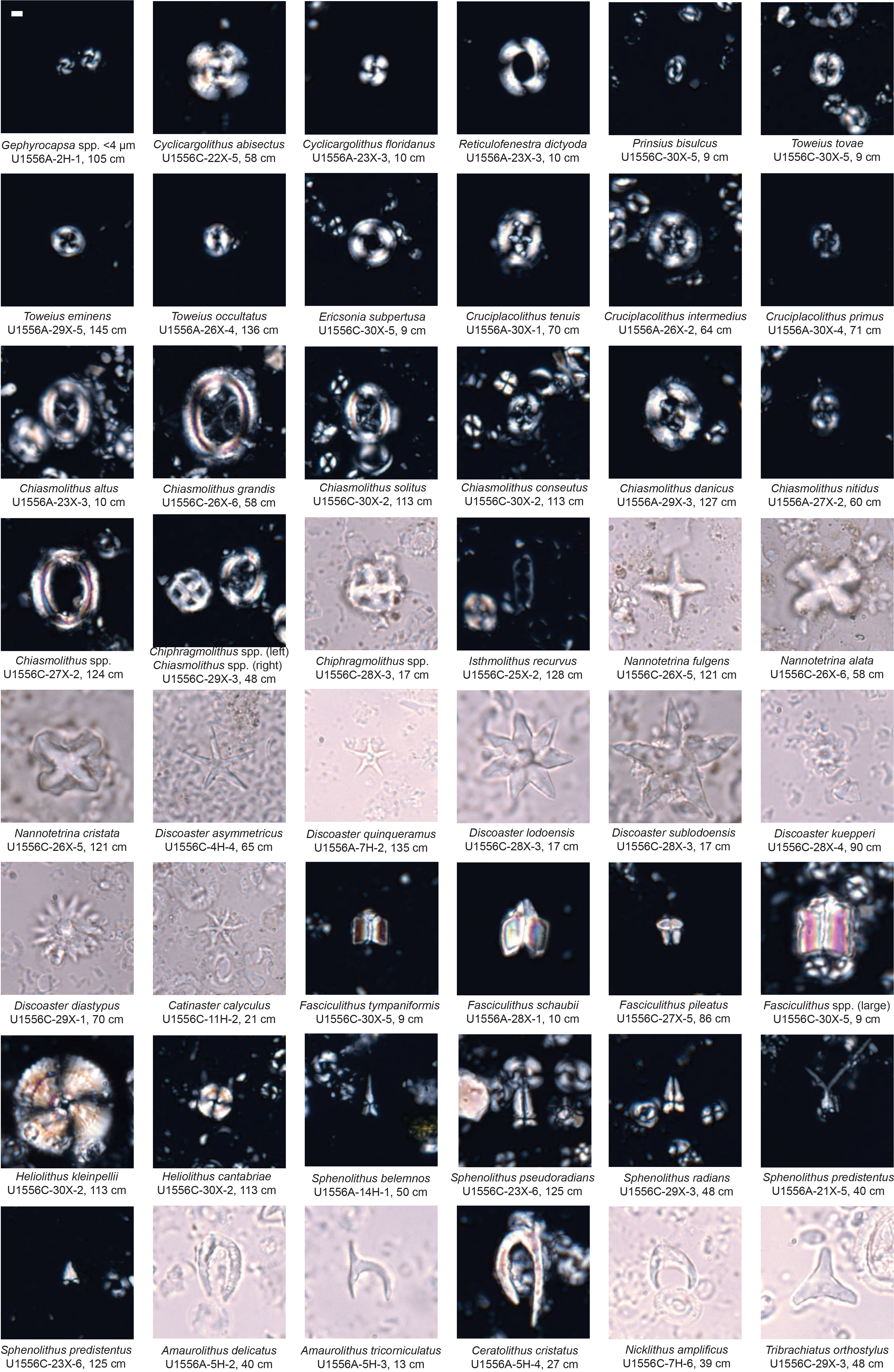
Figure F95. Important and notable calcareous nannofossil taxa.

Calcareous nannofossils vary in abundance and preservation in samples from Site U1556 depending on lithology (see Sedimentology); pelagic clays are often barren of nannofossils or contain rare to common abundances and poor to moderate preservation. In carbonate-rich samples, nannofossils are generally abundant and moderately to well preserved (Figure F93). Reworking is common in Paleogene and Neogene forms throughout Lithologic Unit I and Paleogene forms throughout Unit II. Reworked Cretaceous taxa were also identified and occur consistently but in low abundance throughout the Site U1556 sedimentary succession.

The absence of the relatively cosmopolitan modern taxon Emiliania huxleyi in Cores 390C-U1556A-1H and 390-U1556C-1H suggests that the site (5006.4 mbsl) currently lies below the carbonate compensation depth (CCD), which is 4500–5000 m in the South Atlantic Ocean (Berger and Winterer, 1975). The youngest nannofossil-bearing sediments preserved at Site U1556 represent Pleistocene Zones CNPL10–CNPL7, identified by the co-occurrence of Pseudoemiliania lacunosa and Gephyrocapsa spp. <4 µm in Samples 390C-U1556A-1H-3, 107 cm, to 2H-4, 75 cm (4.06–14.12 m CSF-B), and 390-U1556C-1H-CC, 12–17 cm, to 4H-4, 65–67 cm (4.97–29.17 m CSF-B). The nannofossil assemblages in these uppermost samples clearly reflect the alternating clay and carbonate lithologies and contain common reworking of Late Pliocene to Early Pleistocene forms, most noticeably several species of Discoaster.

The intervals between Samples 390C-U1556A-2H-CC, 12–17 cm, and 5H-4, 27 cm (18.45–42.05 m CSF-B), and between Samples 390-U1556C-4H-CC, 26–31 cm, and 6H-4, 63–65 cm (32.22–46.58 m CSF-B), represent the Early Pleistocene–Pliocene (Zones CNPL7–CNPL1) from the base of Gephyrocapsa spp. <4 µm to the base of Ceratolithus cristatus. The top of Amaurolithus spp. is identified within this interval in Hole U1556A (4H-6, 100 cm; 36.03 m CSF-B) and marks the boundary between the Early and Late Pliocene (top of Zone NN14 and within Zone CNPL3).

The relatively short ranging Late Miocene taxon Nicklithus amplificus is observed at Site U1556, representing Zone CNM18. In Hole U1556A, the top and base of this species are recorded in the same sample (390C-U1556A-7H-2, 135 cm; 59.24 m CSF-B), whereas in Hole U1556C, N. amplificus occurs in Samples 390-U1556C-7H-6, 39–41 cm, through 8H-2, 94–96 cm (57.03–61.36 m CSF-B). The top of Zone CNM6 is marked by the base of Amaurolithus spp. in Samples 390C-U1556A-7H-CC, 18–23 cm, and 390-U1556C-8H-CC, 11–16 cm (65.95 and 68.45 m CSF-B), and within Zone CNM16 the base of Discoaster quinqueramus is identified in Sample 390-U1556C-10H-1, 89–91 cm (75.16 m CSF-B).

A sequence of bioevents represents the early Middle Miocene (Zones CNM16–CNM1) in Samples 390C-U1556A-8H-CC, 6–11 cm, to 16H-4, 80 cm (75.45–147.30 m CSF-B), and 390-U1556C-10H-5, 56–58 cm, through 17X-2, 95–97 cm (80.68–142.71 m CSF-B). The youngest of these bioevents is the base of Catinaster coalitus (top of Zone CNM11), identified in Sample 390-U1556C-11H-2, 21–23 cm (85.46 m CSF-B). Nannofossil zonation schemes for the Oligocene and Lower Miocene rely heavily on sphenolith origination and extinction events. Although this group is common and well preserved at Site U1556, we observe pervasive reworking of sphenoliths throughout this interval. This reworking made it difficult to accurately identify extinction events (tops), so we have chosen to exclude sphenolith extinctions from our zonation scheme. The base common of Sphenolithus heteromorphus (top of Zone CNM5) is identified in Samples 390C-U1556A-12H-4, 148 cm, and 390-U1556C-14H-CC, 6–11 cm (109.66 and 121.25 m CSF-B). The base of the distinctive nannofossil Sphenolithus belemnos (within Zone CNM5) occurs in Samples 390C-U1556A-14H-1, 50 cm (123.48 m CSF-B), and 390-U1556C-15H-4, 50–52 cm (125.99 m CSF-B), and base of Discoaster druggii (within Zone CNM2) is only identified in Hole U1556C in Sample 16H-CC, 21–26 cm (140.25 m CSF-B). The earliest Miocene bioevent identified at Site U1556 is the base of Sphenolithus disbelemnos, marking the top of Zone CNM1 and recorded in Samples 390C-U1556A-16H-4, 80 cm, and 390-U1556C-17X-2, 95–97 cm (147.30 and 142.71 m CSF-B).

The short-ranging and distinctive Oligocene/Miocene boundary marker species Sphenolithus delphix is not identified at Site U1556, likely due to sampling resolution. In Hole U1556A, the only Oligocene markers identified are base Sphenolithus ciperoensis (within Zone CNO4) and base Sphenolithus distentus (top of Zone CNO3); both are recorded in Sample 390C-U1556A-23X-2, 20 cm (208.11 m CSF-B). Because core catchers from Cores 21X–24X are barren of nannofossils and cores comprise extensive clay intervals interrupted by short carbonate-rich intervals (see Sedimentology), additional nannofossil samples were specifically taken in the carbonate intervals to provide some age constraints within this interval. The bases of S. ciperoensis and S. distentus occur in the first of two short carbonate-rich intervals in Hole U1556A (23X-2, 7–44 cm; 207.98–208.35 m CSF-B). The second carbonate-rich interval does not contain either sphenolith (23X-2, 97–111 cm, to 23X-3, 0–21 cm; 208.88–209.02 through 209.12–209.33 m CSF-B). As a result, we use the youngest bioevent (base of S. ciperoensis) to construct the age model; however, this provides a large error of 2.87 My, which is the difference in age between the two datums (Gradstein et al., 2020) (Table T21; Figure F119). In Hole U1556C, the base of S. ciperoensis is identified in Sample 390-U1556C-22X-5, 58–60 cm, and the base of S. distentus is recorded in Sample 23X-6, 125 cm (195.31 and 207.18 m CSF-B).

The Eocene/Oligocene boundary (EOB) is poorly constrained at Site U1556 due in part to the absence of key marker taxa, lithology, and sampling resolution. This interval falls within the dark brown clay–silty clay interval described as Lithologic Subunit IE (see Sedimentology; also recorded at Site U1557). Core catchers through this interval (390C-U1556A-22X through 25X and 390-U1556C-23X through 27X) are all either barren of nannofossils or have low abundance and poor preservation; thus, assemblages are not representative. To better constrain the EOB, we took an additional 15 samples from section halves of these cores from both holes, preferentially from intervals that appeared lighter in color, indicating higher carbonate content. Sample 390-U1556C-26X-6, 58 cm (235.78 m CSF-B), contains several species of the middle Eocene genus Nannotetrina, including Nannotetrina alata (a marker for the top of Zone CNE8), as well as Nannotetrina cristata and Nannotetrina fulgens. This suggests that we have an unconformity spanning the middle–late Eocene through the EOB, ~16 My in duration (based on the calibration of Gradstein et al. [2020]). Shipboard samples from Hole U1556A did not tighten the bounds of the unconformity because no species of Nannotetrina were identified. This genus was also not observed at Site U1557, although there the unconformity spans only ~15 My because of a better constrained earliest Oligocene interval (see Biostratigraphy in the Site U1557 chapter [Coggon et al., 2024a]).

The first bioevent in Lithologic Unit II, the base of Discoaster sublodoensis, recorded in Sample 390-U1556C-28X-4, 90–92 cm (252.59 m CSF-B), represents the top of the early Eocene Zone CNE5. This event is not recorded in Hole U1556A, although Sample 390C-U1556A-25X-CC, 10–15 cm (231.67 m CSF-B), contains the first Eocene markers, Discoaster lodoensis and Sphenolithus radians co-occurring, suggesting the sample occurs somewhere within Zones CNE5–CNE3.

Many Eocene samples at Site U1556 contain extensive reworking of Paleocene forms; this reworking is observed across all calcareous microfossil groups and is on a larger scale than that seen at Site U1557. Contrary to Site U1557, where Paleocene nannofossils are present in a predominantly Eocene assemblage, at Site U1556 Paleocene forms often dominate and the scarcity of Eocene markers makes it difficult to determine what is actually in situ. This finding is particularly evident in Sample 390-U1556C-27X-2, 124–126 cm (240.14 m CSF-B), where F. tympaniformis and H. kleinpellii (both Paleocene species that do not range above Zones CNE1 and CNP9, respectively; Gradstein et al., 2020) are recorded in the same sample as S. radians, which only evolves in Zone CNE3. However, Sample 390-U1556C-27X-5, 86–88 cm (244.26 m CSF-B), and samples from interval 390C-U1556A-26X-2, 64 cm, through 27X-2, 60 cm (237.34–246.90 m CSF-B), contain no Eocene marker taxa and are instead entirely a mixture of Paleocene forms including F. tympaniformis, Fasciculithus involutus (restricted to Zone CNE1; Gradstein et al., 2020), species of Tectulithus (restricted to Zone CNP8; Gradstein et al., 2020), Toweius tovae, Prinsius bisulcus, and Prinsius martinii (restricted to Zone CNP11; Young et al., 2022). These intervals of predominantly Paleocene nannofossils are sandwiched between samples that are assigned to early Eocene Zones CNE7–CNE3 and appear to be located within and proximal to intervals of sedimentary deformation. Visible slumping in the cores is described in Lithologic Unit II (see Sedimentology for detailed description of deformation). More extensive reworking and slumping is recorded at Site U1556 compared with that at Site U1557 and could be related to the former's location on a bathymetric high (see Background and objectives), which is more exposed to bottom water currents.

The early Eocene base of D. lodoensis (within Zone CNE3) is recorded in Sample 390-U1556C-29X-1, 70–72 cm (257.60 m CSF-B). The base of S. radians (base of Zone CNE3) is observed in Samples 390C-U1556A-28X-1, 10 cm (254.50 m CSF-B), and 390-U1556C-29X-3, 48–50 cm (260.38 m CSF-B); however, this sample is located proximal to another interval of deformation observed in Sections 29X-3 through 29X-4 (see Sedimentology). This co-occurrence is therefore likely an artifact of the slumping and does not represent a true base, and for that reason we have not included this bioevent in the age model.

Biostratigraphic evidence suggests an unconformity that spans ~5 My across the Paleocene/Eocene boundary, with the lowermost sediment samples at Site U1556 representing nannofossil Zones CNP8–CNP7 within the Selandian epoch of the Paleocene. The unconformity lies between the oldest Paleocene markers, the base of Discoaster mohleri dated to 58.97 Ma (Gradstein et al., 2020) (Sample 390-U1556C-29X-CC, 13–18 cm; 264.47 m CSF-B) and the base of H. kleinpellii dated to 59.36 Ma (Gradstein et al., 2020) (Samples 390C-U1556A-29X-5, 145 cm, and 390-U1556C-30X-2, 113 cm; 271.45 and 268.55 m CSF-B), and the youngest Eocene markers, the base of S. radians (54.12 Ma; Gradstein et al., 2020) and base of D. lodoensis, dated to 53.58 Ma (Gradstein et al., 2020). This unconformity is also recognized in the planktic foraminiferal biostratigraphy, which indicates the duration could be as long as ~10 My. Below this unconformity, Samples 390C-U1556A-29X-5, 145 cm, through 30X-4, 71 cm (271.45–278.31 m CSF-B), and 390-U1556C-29X-CC, 13–18 cm, to 30X-CC, 25–30 cm (264.47–275.68 m CSF-B), are identified from the base of D. mohleri, base of H. kleinpellii, and base of F. tympaniformis (Samples 390C-U1556A-30X-4, 71 cm, and 390-U1556C-30X-CC, 25–30 cm; 278.31 and 275.68 m CSF-B). These zones correlate well to the planktic foraminiferal zones and the estimated crustal age for Site U1556 of ~61 Ma (see Stratigraphic unit summary).

7.3. Planktic foraminifera

Core catcher samples were examined for planktic foraminifera from Hole U1556A following Expedition 390C, but many of the samples were taken from pelagic clay facies and were barren. During Expedition 390, core catcher samples from Hole U1556C were supplemented with additional samples from the working half (up to two per core) to improve the age model. Planktic foraminiferal occurrences are summarized in Tables T13, T14, and T15. Key species are illustrated in Figures F96, F97, and F98. Qualitative abundance estimates of other biogenic and authigenic material observed in the sieved residue are presented in Table T15, and a few notable categories (fish debris and manganese oxides) are plotted by depth in Figure F99.

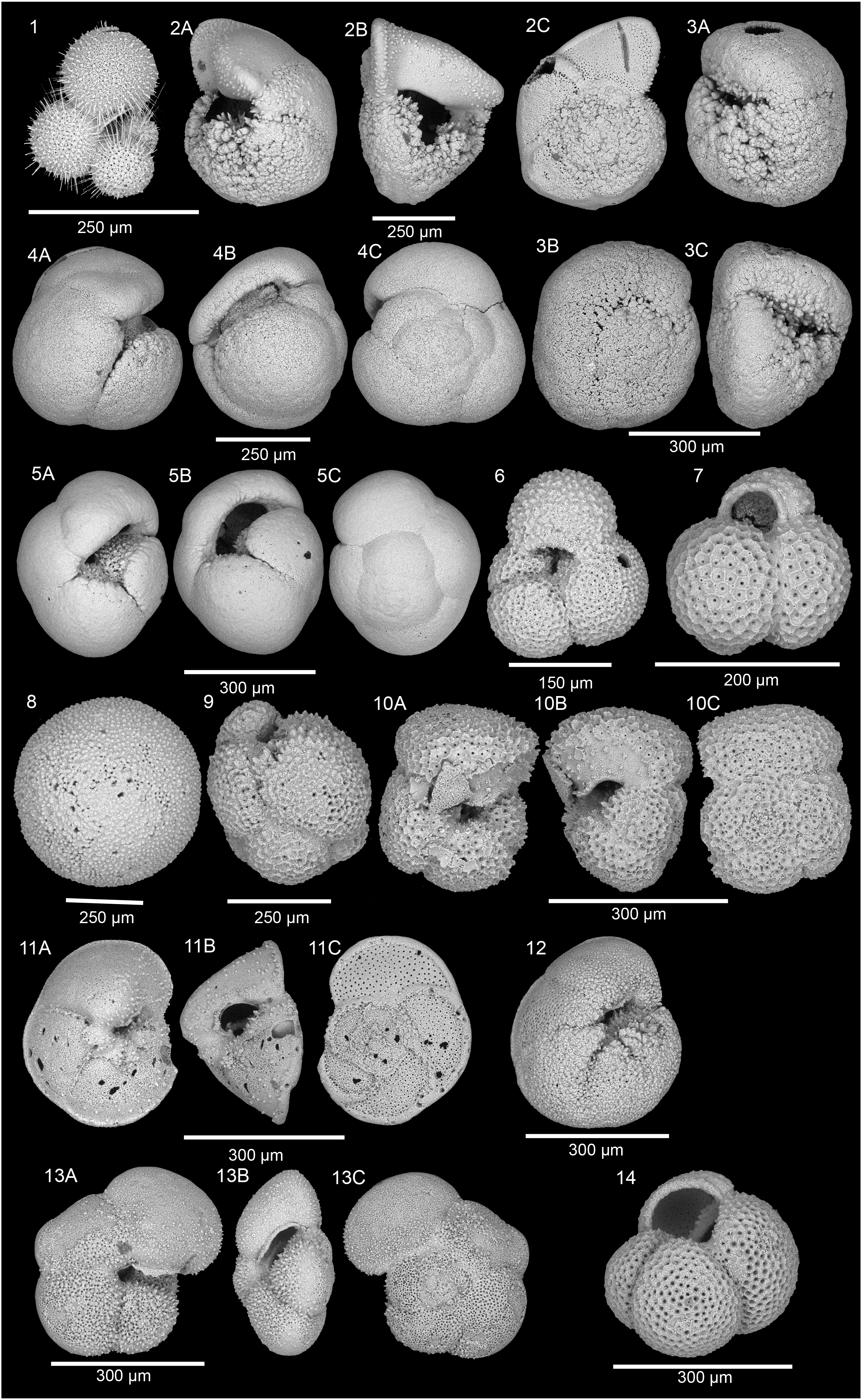
Figure F96. Neogene planktic foraminifera.

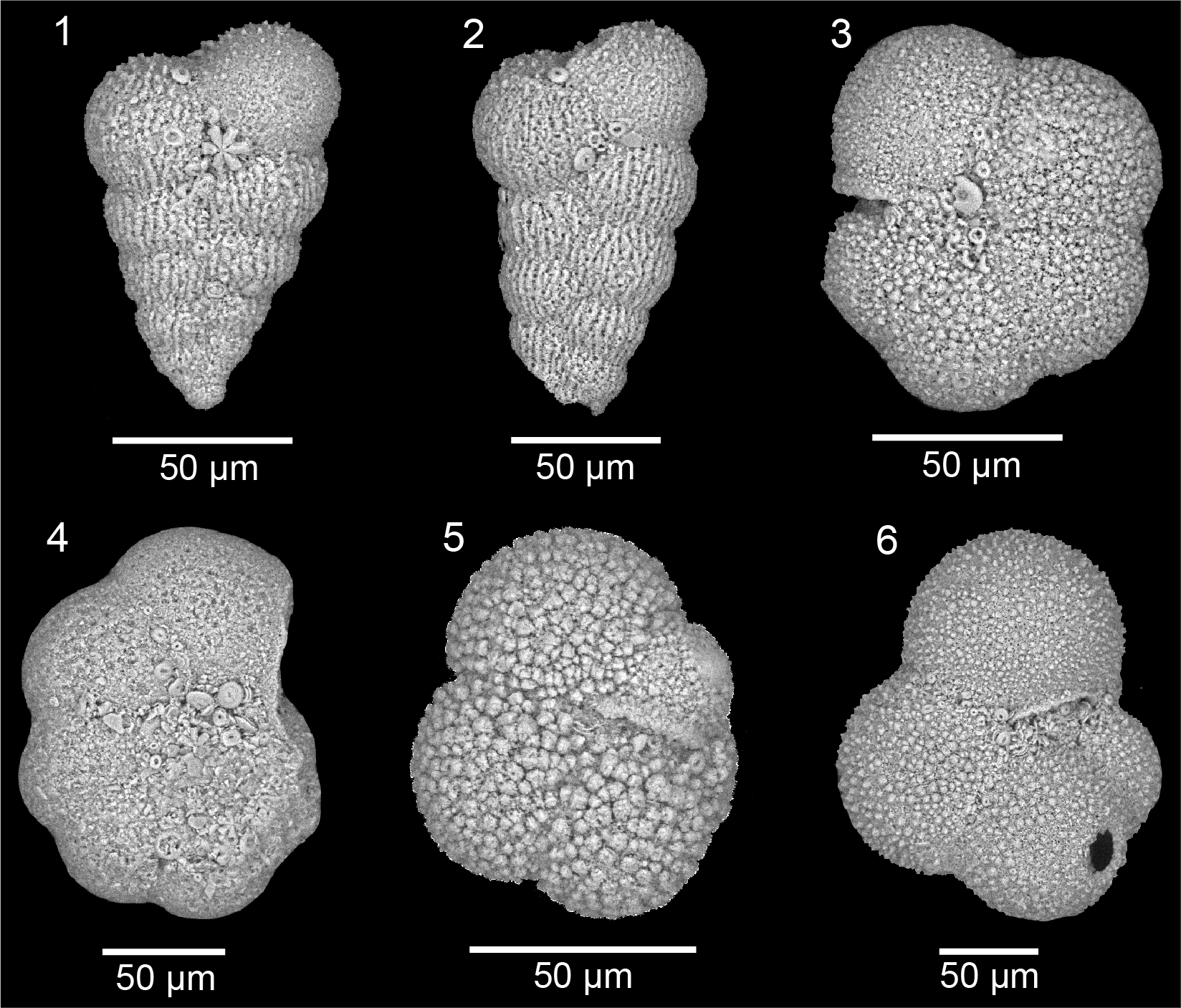
Figure F97. Oligocene planktic foraminifera.

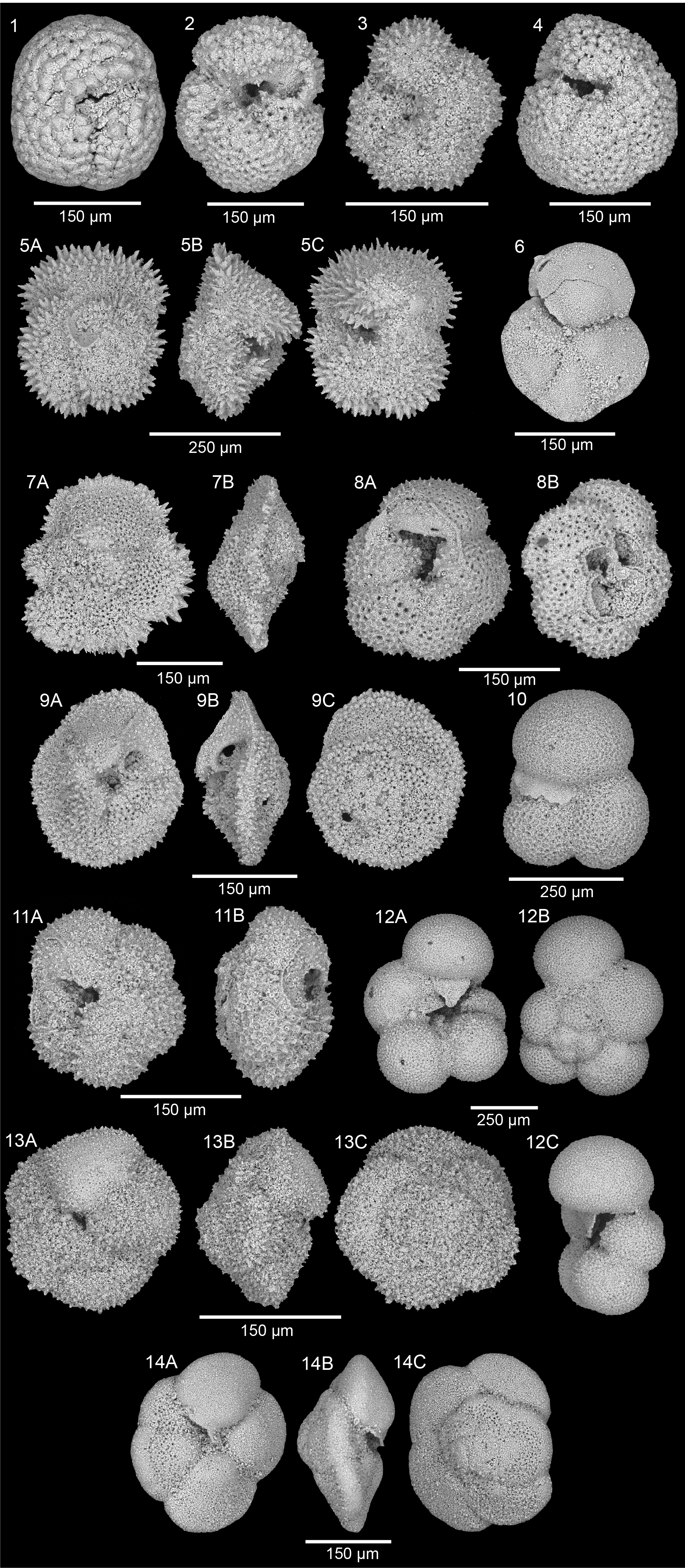
Figure F98. Paleocene–Eocene planktic foraminifera.

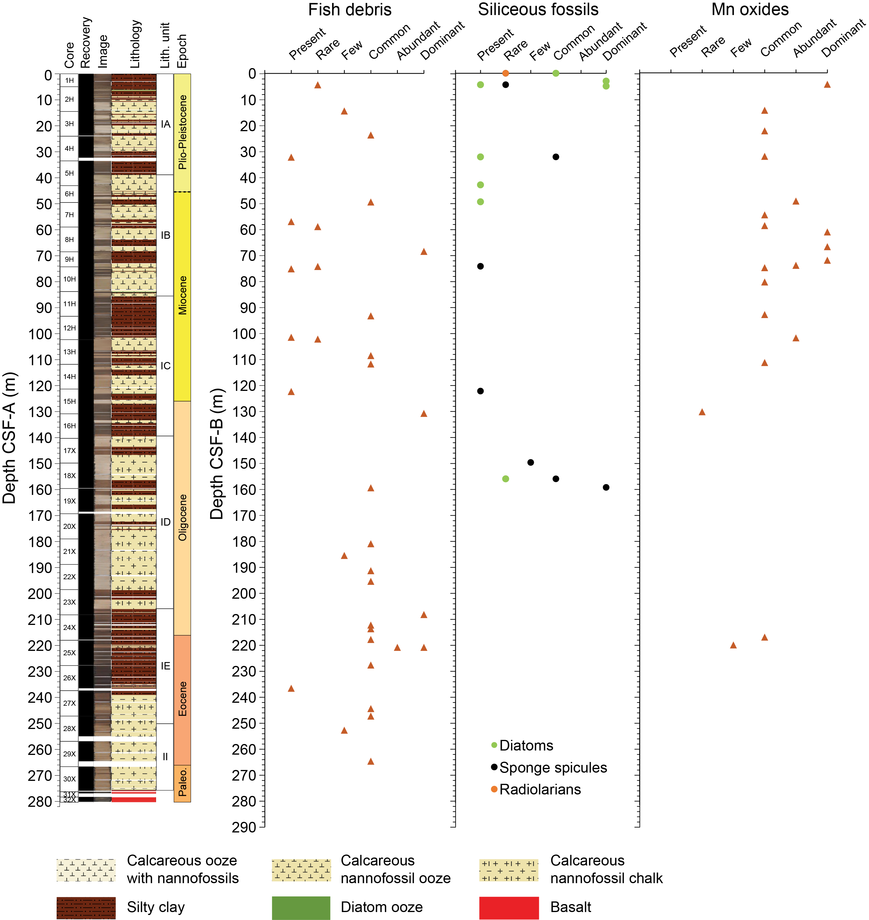
Figure F99. Abundance estimates in sieved residues.

The mudline sample for Core 390C-U1556A-1H does not contain any microfossils, but the mudline in Core 390-U1556C-1H contains a diverse and abundant assemblage of planktic and benthic foraminifera. Siliceous microfossils (diatoms, radiolarians, and sponge spicules) are also common. Although the seafloor at Site U1556 (~5000 m water depth) is composed of pelagic clay and is well below the depth of the modern CCD in the South Atlantic (4500–5000 m; Berger and Winterer, 1975), the occurrence of Globigerinella calida (Figure F96), which has a lowest occurrence of 220 ka, indicates that the seafloor is Late Pleistocene to recent in age.

Pleistocene through Oligocene sediments at Site U1556 contain typically small and depauperate assemblages of planktic foraminifera. Pelagic clay samples are often barren (washed residues are usually dominated by fish teeth, otoliths, bone fragments, and other phosphatic debris) (Figure F97). In the nannofossil oozes, large planktic foraminifera are typically absent or very rare. Globoconella inflata, an extant species that evolved in the Late Pliocene, is often the only species that appears in the >125 µm sieved fraction, and the rest of the assemblage is composed of small individuals and juveniles. Diatoms and radiolarians are common in samples from Core 390-U1556C-1H, present in some samples from Cores 4H–6H, and then absent for the rest of Hole U1556C. Sponge spicules are intermittently present throughout the same interval and then are very abundant in samples from Cores 17X and 18X. Authigenic deposits of manganese oxide were found in the foraminiferal-sized fraction in numerous samples from Cores 1H–15H and then again in the dark brown clays in Cores 25X and 26X.

Contrary to Hole U1556A, very few samples in the Pliocene–Pleistocene in Hole U1556C were barren, and we were able to identify a number of datums in this interval. This is the result of both the lack of barren samples due to intentional sampling of carbonate lithology and more importantly the (mostly) consistent presence of large specimens that belong to biostratigraphically significant groups. The top of Globorotalia tosaensis, which marks the top of Zone PT1a, was observed in both Samples 390C-U1556A-1H-CC, 12–17 cm (8.95 m CSF-B), and 390-U1556C-2H-5, 21–23 cm (11.01 m CSF-B). The lowest occurrence of Globorotalia truncatulinoides (top of Zone PL6) occurs in Sample 390-U1556C-4H-CC, 26–31 cm (32.22 m CSF-B), which is the rare sample that contains a relatively abundant and diverse assemblage of large foraminifera; in addition to G. truncatulinoides, it contains large specimens of Orbulina universa, Globigerinoides ruber, G. inflata, Globorotalia scitula, and Globoturborotalita decoraperta. The sample below this (390C-U1556A-5H-4, 124–126 cm; 39.18 m CSF-B) contains Dentoglobigerina altispira, marking the top of Zone PL4. If these two adjacent datums are both plotted at the midpoint between the sample containing the datum species and the adjacent sample in which that species is absent (as described in Biostratigraphy in the Expedition 390/393 methods chapter [Coggon et al., 2024c]), they appear to plot on top of each other; however, the species do not actually co-occur, and there does not appear to be any missing time. The top of Sphaeroidinellopsis seminulina (top of Zone PL3) occurs in Sample 390-U1556C-6H-3, 24–26 cm (45.26 m CSF-B). The deepest marker we observed in the Pliocene is the top of Globoturborotalita nepenthes (top of Zone PL1), which occurs in Sample 7H-6, 39–41 cm (57.03 m CSF-B).

Although the consistent presence of large specimens allowed for confident identification of many zonal markers in the Pliocene–Pleistocene, the general absence of large specimens precluded the recognition of all but a few markers in the Oligocene and Miocene. The Miocene/Pliocene boundary occurs somewhere between Cores 390-U1556C-7H and 10H (~50–80 m CSF-B). Sample 10H-CC, 26–31 cm (83.75 m CSF-B), contains the lowest occurrence of Globoconella terminalis, which occurs in Zone M14. This is the only planktic foraminiferal event identified in the Miocene at Site U1556. Many samples in this interval (Cores 390C-U1556A-10H through 18X [94.53–165.41 m CSF-B] and 390-U1556C-11H through 20X [93.25–178.95 m CSF-B]) are barren, and those that are not contain only very small foraminifera (mostly globigerinids and globorotalids), many of which are juveniles and cannot be confidently identified for biostratigraphic purposes.

This trend of very small planktic foraminifera continues through the Oligocene, but the overall reduced size of the planktic foraminifera during the so-called "Ugly ocene" (Wade et al., 2018) actually works in our favor here, as a few key marker taxa are easily identifiable from the small size fraction. The first Oligocene datum encountered is the top of Zone O4, the highest common occurrence of Chiloguembelina cubensis, in Sample 390-U1556C-20X-2, 138–140 cm (172.13 m CSF-B). The top of Pseudohastigerina naguewichiensis, which defines the top of lowest Oligocene Zone O1, occurs in Sample 21X-CC, 31–36 cm (188.75 m CSF-B).

The precise location of the EOB is difficult to determine because of the presence of a thick (44.28 m) dark brown clay (Lithologic Subunit IE; see Sedimentology) similar to that observed at Site U1557. Unlike at Site U1557 (and perhaps because of the increased sampling frequency at Site U1556), we found planktic foraminifera throughout much of Subunit IE, but unfortunately these are the same small, undiagnostic assemblage as the one observed in Subunit ID, which is entirely Oligocene in age. The first sample with a clear Eocene assemblage is 390-U1556C-24X-CC, 17–22 cm (217.69 m CSF-B), which contains Paragloborotalia griffinoides, a species that has the somewhat unhelpful range of Zones E1–E16 (i.e., the entire Eocene).

Dating of the Eocene is complicated by the extensive reworking of Paleocene material into the Eocene section. Most of the reworked material appears to be from the middle Paleocene assemblage observed on top of basement and described below (notably G. pseudomenardii, G. chapmani, Morozovella acutispira, Igorina albeari, Igorina tadjikistanensis, P. variospira, and Parasubbotina varianta), but there are also taxa with ranges from the late Paleocene or early Eocene to middle Eocene. A slump in Core 390-U1556C-29X (~260–262 m CSF-B) contains an assemblage identical to that found in interval 30X-CC, 25–30 cm. The rest of the samples taken from Cores 25X–29X contain a few incontrovertibly Eocene taxa, including Acarinina cuneicamerata, Acarinina pseudotopilensis, Acarinina pseudosubsphaerica, Acarinina pentacamerata, Dentoglobigerina galavisi, Morozovella crater, Morozovella gracilis, Pearsonites broedermanni, and Subbotina senni. The base of Acarinina boudreauxi, which occurs in planktic foraminiferal Zone E7a, was observed in Sample 390-U1556C-27X-CC, 24–29 cm (247.13 m CSF-B), whereas the base of Acarinina alticonica, which occurs in Zone E4, was observed in Sample 29X-1, 70–72 cm (257.60 m CSF-B). An unconformity spanning at least 5 My separates the Paleocene and Eocene at Site U1556. Based on planktic foraminifera, this unconformity appears to occur somewhere in Core 390-U1556C-30X (between ~265 and 275 m CSF-B). Sample 30X-CC, 25–30 cm (275.69 m CSF-B), contains an abundant, diverse, and well-preserved assemblage of middle Paleocene planktic foraminifera assigned to Zone P4a based on the co-occurrence of G. pseudomenardii and P. variospira, but other samples from Core 30X (Samples 30X-2, 113–115 cm, and 30X-5, 9–11 cm; 268.55 and 272.01 m CSF-B) contain a less abundant assemblage with a much higher degree of fragmentation, fewer large individuals, and common to abundant benthic foraminifera. This may represent an interval of erosion or reduced deposition and may be the stratigraphic expression of the hiatus between the Eocene and middle Paleocene.

Preservation of planktic and benthic foraminifera is generally moderate in samples that are not barren (Figure F93). Scanning electron microscope images showing example poor to moderate preservation states for a Neogene and an Eocene benthic foraminifera are presented in Figure F100. These are the only intervals in which isotope analysis of these respective groups might be feasible based on specimen availability at Site U1556; no benthic foraminifera occur in the Neogene or Oligocene, and the Eocene is characterized by dissolution-resistant assemblages of planktic foraminifera and then extensive Paleocene reworking.

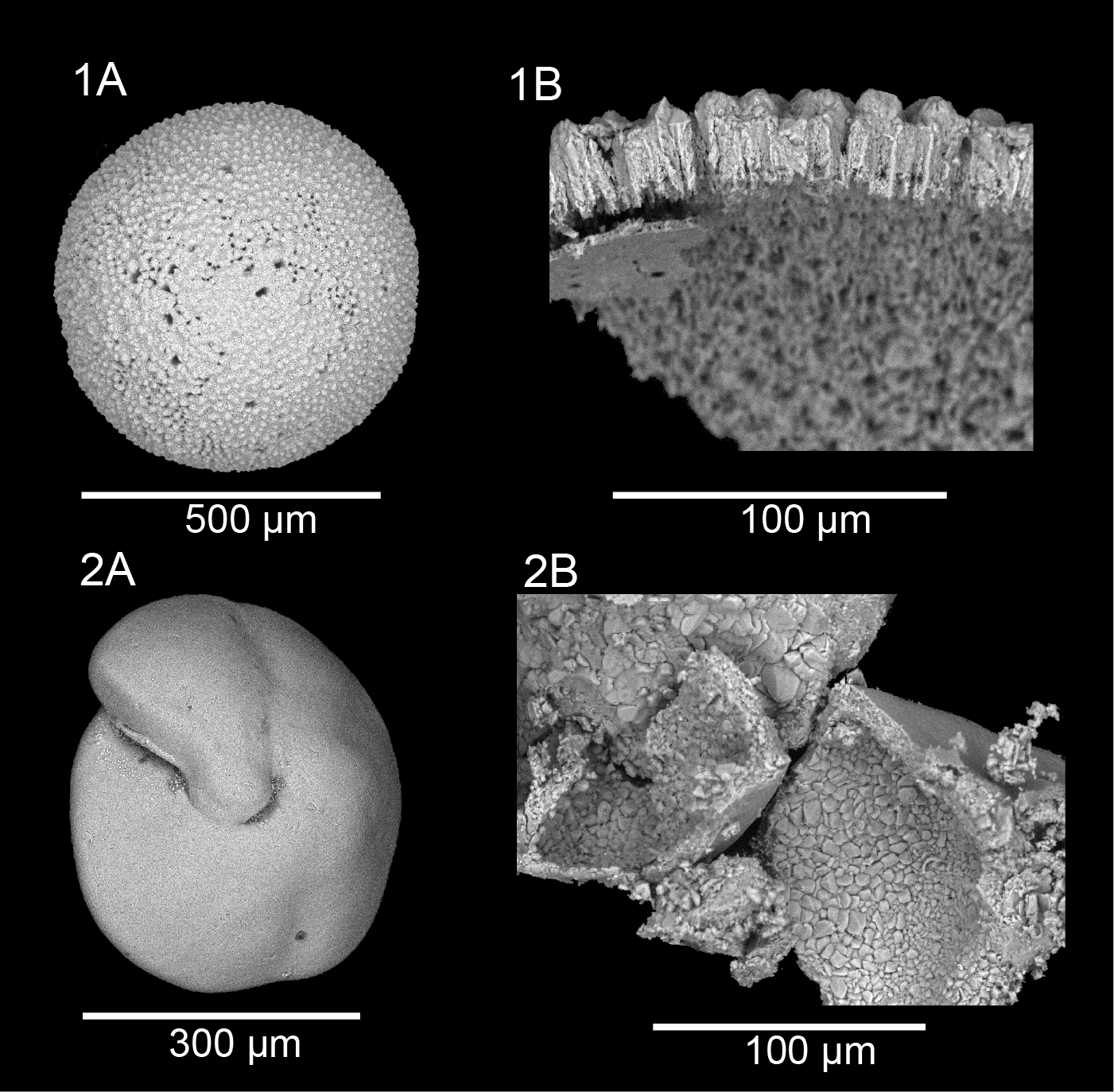
Figure F100. Preservation of selected specimens.

7.4. Benthic foraminifera

Onshore analysis of benthic foraminifera was conducted on core catcher samples from Hole U1556A following Expedition 390C. Qualitative estimates of benthic foraminiferal preservation and abundance, as well as assemblage composition, are biased toward depth-diagnostic calcareous species and other notable calcareous taxa. Agglutinated species are reported if identified. Overall, the benthic foraminiferal species identified in the samples analyzed suggest that Site U1556 lay at upper abyssal depths (~2000–3000 m) from the Paleocene to the middle Eocene. By the Pleistocene, Site U1556 was located at lower abyssal depths (>3000 m). Unfortunately, the absence of benthic foraminifera in core catcher samples from Cores 390C-U1556A-2H through 24X (18.45–223.17 m CSF-B) prevents us from reconstructing the timing of the gradual seafloor deepening at Site U1556.

Benthic foraminifera are present in Sample 390C-U1556A-1H-CC, 12–17 cm (8.95 m CSF-B), and samples from interval 25X-CC, 10–15 cm, to 29X-CC, 15–20 cm (231.67–273.49 m CSF-B). Overall, core catcher samples from Cores 2H–24X (18.452–223.17 m CSF-B), which span nearly all of Lithologic Unit I (see Sedimentology), are barren of benthic foraminifera. Preservation ranges from very good to very poor in the shallowest sample analyzed (Sample 1H-CC, 12–17 cm) but declines to moderate to very poor in deeper cores (Cores 25X–29X). Benthic foraminiferal preservation and abundance are summarized in Figure F93. The occurrence of important benthic foraminiferal species is reported in Table T16.

The benthic foraminiferal assemblage found in Sample 390C-U1556A-1H-CC, 12–17 cm (8.95 m CSF-B), is dominated by Cibicidoides wuellerstorfi, Nuttallides umbonifera, and Oridorsalis umbonatus. Other observed taxa include Melonis sphaeroides, Parafissurina cf. curvitubulosa, Pullenia aff. quinqueloba, and Pullenia bulloides. This assemblage indicates deposition at lower abyssal depths (>3000 m), in particular because of the abundance of N. umbonifera, a species considered indicative of Antarctic Bottom Water (Corliss, 1979; Mackensen et al., 1995).

Eocene species are present in Sample 390C-U1556A-25X-CC, 10–15 cm (231.67 m CSF-B): Cibicidoides cf. subspiratus, Cibicidoides cf. ungerianus, and Nuttallides truempyi. C. cf. subspiratus and N. truempyi have a wide bathymetric range, but C. cf. ungerianus suggests an upper abyssal depth of this site ~45 Ma (Tjalsma and Lohmann, 1983; van Morkhoven et al., 1986).

A mix of Paleocene and Eocene benthic foraminiferal species characterizes Sample 390C-U1556A-26X-CC, 12–17 cm (243.60 m CSF-B). This observation is in line with the mixed Paleocene/Eocene assemblages that were also observed in the calcareous nannoplankton and planktic foraminiferal assemblages. Paleocene benthic foraminiferal species (i.e., species that are extinct by the early Eocene, planktic foraminiferal Zones P5–P6a) (Tjalsma and Lohmann, 1983; van Morkhoven et al., 1986) present include Anomalina praeacuta, Aragonia ouezzanensis, Cibicidoides hyphalus, Coryphostoma cf. midwayensis, Gavelinella beccariiformis, Lenticulina whitei, Neoeponides cf. lunata, Neoflabellina cf. semireticulata, and Pullenia coryelli. Typically (although not necessarily exclusively), Eocene species in this sample include Bulimina trinitatensis, Buliminella beaumonti, Lenticulina excisa, Nonion havanense, N. truempyi, O. umbonatus, and Osangularia mexicana. Several Cibicidoides species are present in the sample including C. cf. subspiratus, Cibicidoides cf. haitiensis, and C. ungerianus. The age model (see Age model and mass accumulation rates) indicates that Sample 26X-CC, 12–17 cm, is of late early Eocene age (Figure F119); paleodepth estimates therefore utilize typical Eocene species. Several of these species have a wide bathymetric range; however, the presence of many buliminids, as well as lenticulinids and Gyroidinoides spp. suggest deposition at upper abyssal depths (~2000–3000 m) (based on Tjalsma and Lohmann, 1983).

The benthic foraminiferal assemblage observed in the lowermost sample (390C-U1556A-29X-CC, 15–20 cm; 273.49 m CSF-B) indicates a late Paleocene age (based on Tjalsma and Lohmann, 1983), in agreement with constraints from other microfossil groups. The assemblage is dominated by A. praeacuta, A. ouezzanensis, G. beccariiformis, and N. truempyi. Other species include Aragonia sp., Bulimina midwayensis, B. beaumonti, Gyroidinoides cf. quadratus, N. havanense, O. umbonatus, Osangularia velascoensis, and P. coryelli. This assemblage suggests an upper abyssal depositional environment (~2000-3000 m; Tjalsma and Lohmann, 1983).

7.5. Siliceous microfossils

Many samples from Lithologic Subunits IA–ID in Hole U1556C contain varying abundances of siliceous microfossils in the sieved residue used for foraminiferal analysis (Figure F99). Discrete diatom layers observed in Core 1H in all sediment holes at Site U1556 contain a nearly monospecific assemblage of large broken diatom tests (Figure F101). Sponge spicules and smaller unbroken diatoms and radiolarians occur in the pelagic clays and nannofossil oozes, particularly in the Pliocene–Pleistocene (Cores 390-U1556C-1H through 5H) and the late Oligocene (Cores 17X and 18X), intervals in which dissolved silica is also high (see Sediment in Geochemistry). Qualitative abundance of these siliceous groups is plotted in Figure F99. Although they are not siliceous, it should also be noted that calcareous dinoflagellates were observed (mostly as broken tests) sporadically throughout Hole U1556C and are particularly abundant in Cores 10H and 11H (~75–93 m CSF-B).

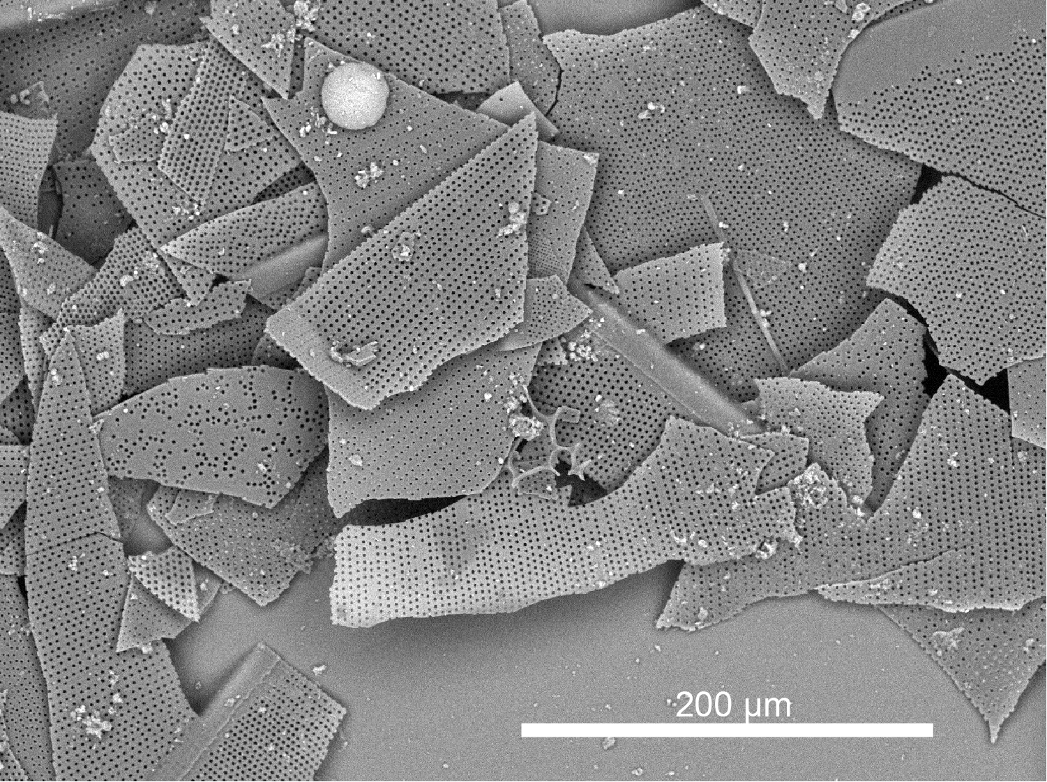
Figure F101. Diatom ooze.

8. Paleomagnetism

8.1. Sediment

Hole U1556A was cored during engineering Expedition 390C, and remanence measurements were made at three alternating field (AF) steps (5, 10, and 20 mT) (Estes et al., 2021). During Expedition 390, cores from Hole U1556A were remeasured. Holes U1556C, U1556D, and U1556E were cored and measured for the first time during Expedition 390. Remanence measurements were made using the superconducting rock magnetometer (SRM) (see Paleomagnetism in the Expedition 390/393 methods chapter [Coggon et al., 2024c]). The natural remanent magnetization (NRM) of core sections was measured at 2 cm spacing. Three AF steps (5, 10, and 20 mT) were applied and the remanence measured after each step for Hole U1556A cores and to Core 390-U1556C-28X. To expedite measurements, the 10 mT step was skipped for the remainder of Hole U1556C and all of Holes U1556D and U1556E.

Discrete samples were collected from Hole U1556C, but no discrete samples were collected from Hole U1556A because the working half was not on board, nor from Holes U1556D and U1556E because SRM measurements from these holes had already provided clear magnetic polarity sequences and typically discrete samples are collected only from one hole at a site.

Paleomagnetic investigation of Site U1556 sediments therefore comprised remanence analysis of Cores 390C-U1556A-1H through 30X, 390-U1556C-1H through 30X-7, 390-U1556D-1H, and 390-U1556E-1H through 5H and 59 discrete sediment samples. Here, we use these data to primarily establish a magnetic polarity stratigraphy for the sediment package at Site U1556 and date this stratigraphy by correlation to known magnetochrons in the geomagnetic polarity timescale (Gradstein et al., 2020) to create a magnetostratigraphy for this site. We present a preliminary magnetostratigraphy; this interpretation will be refined with additional analyses postexpedition.

Rock magnetic studies were also carried out. Anisotropy of magnetic susceptibility (AMS) was measured on all 59 discrete samples to characterize the magnetic fabric of the sediments. Acquisition of isothermal remanent magnetization (IRM) and backfield IRM experiments were performed on a subset of the discrete samples to characterize the magnetic mineral assemblage. Data from all measurements, including AMS and IRM acquisition experiments, are available through the Laboratory Information Management System (LIMS) database.

8.1.1. Results

Measurements of NRM and in-line AF demagnetization of APC (Cores 390-U1556C-1H through 16H, 390-U1556D-1H, and 390-U1556E-1H through 5H) and XCB (Core 390-U1556C-17X through Section 30X-7) cores on the SRM were carried out to establish a magnetic polarity sequence for the entire sediment package at Site U1556. Hereafter, the intensity/inclination after demagnetization at 20 mT is referred to as the 20 mT intensity/inclination. All three holes displayed clear polarity reversals that can be tied to the existing results from Hole U1556A for a more complete polarity stratigraphy (see Magnetostratigraphy and Age model and mass accumulation rates) (Figures F102, F103, F104, F105).

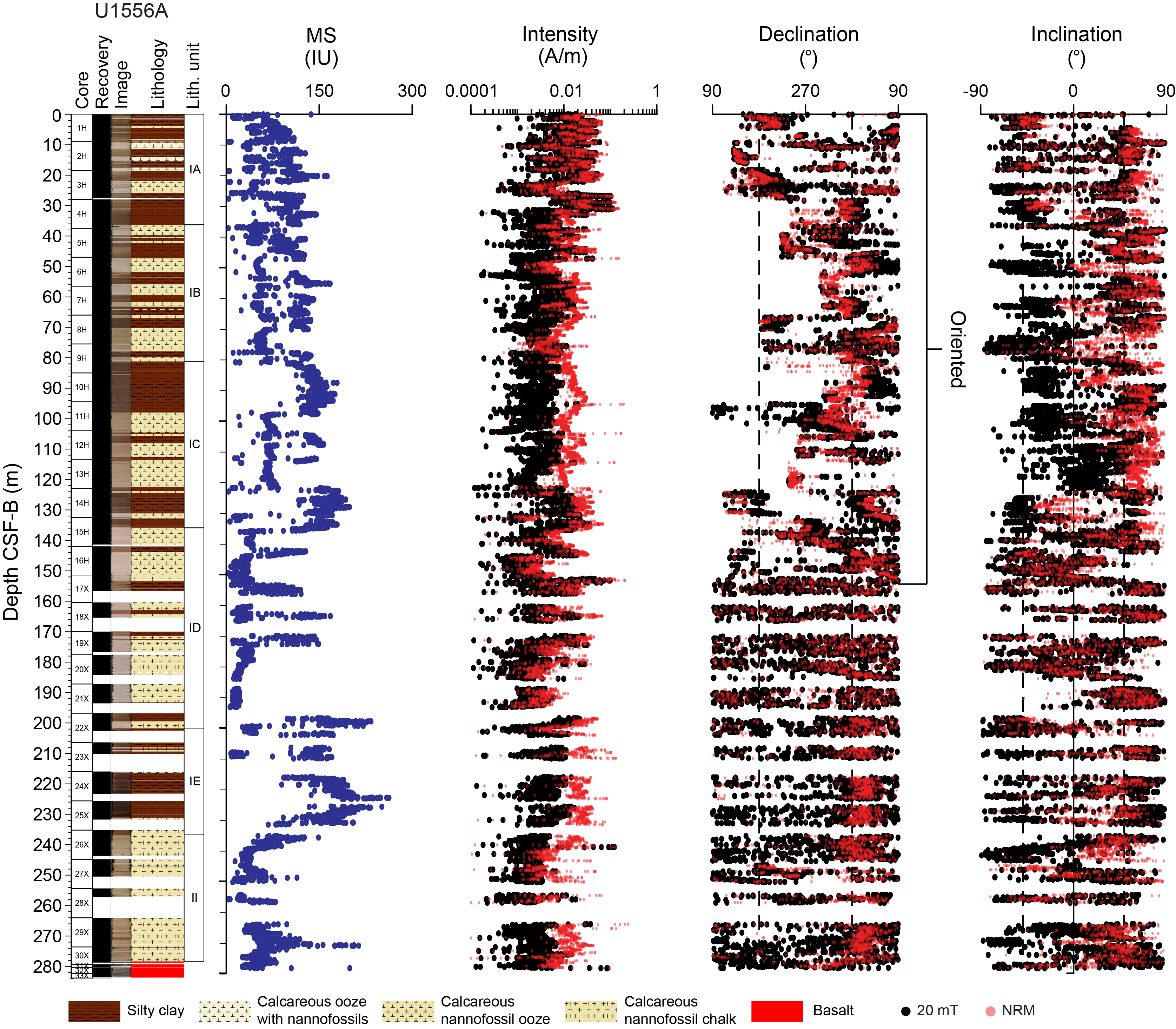
Figure F102. MSP and SRM, Hole U1556A.

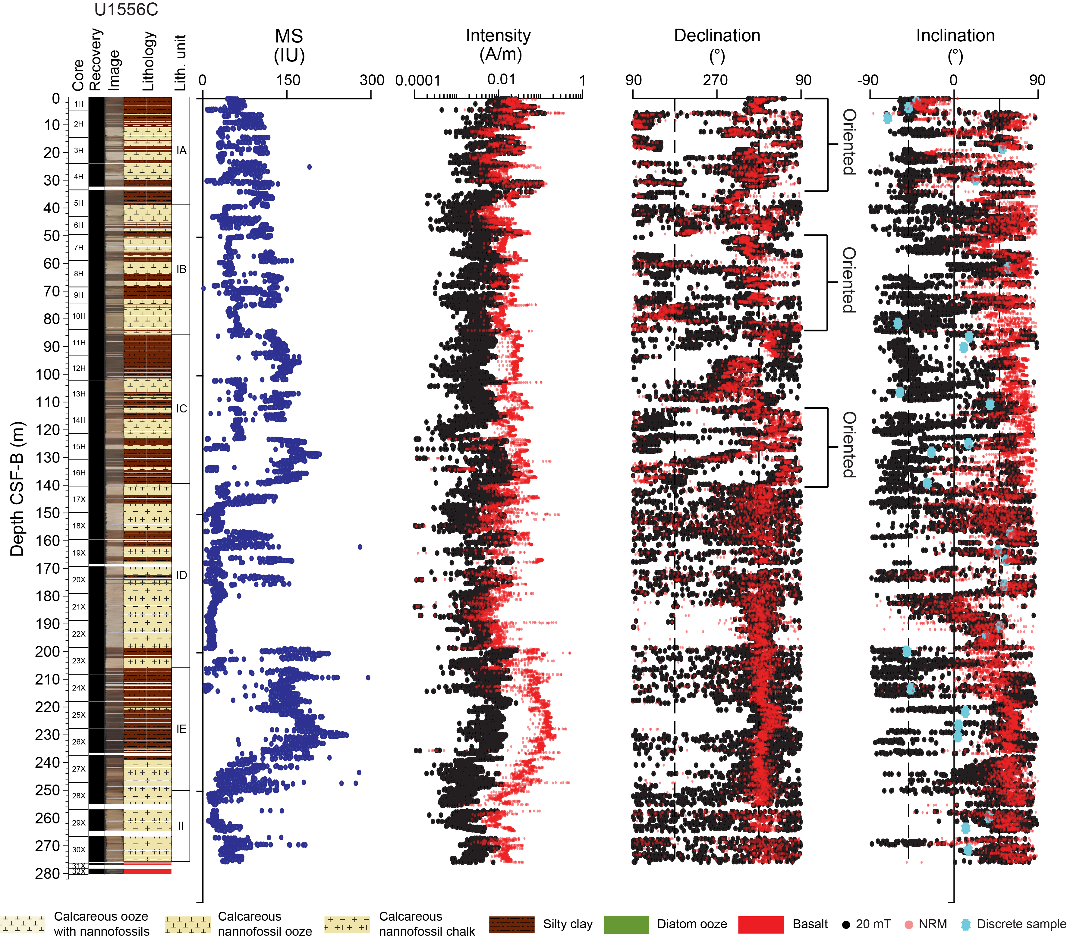
Figure F103. MSP and SRM, Hole U1556C.

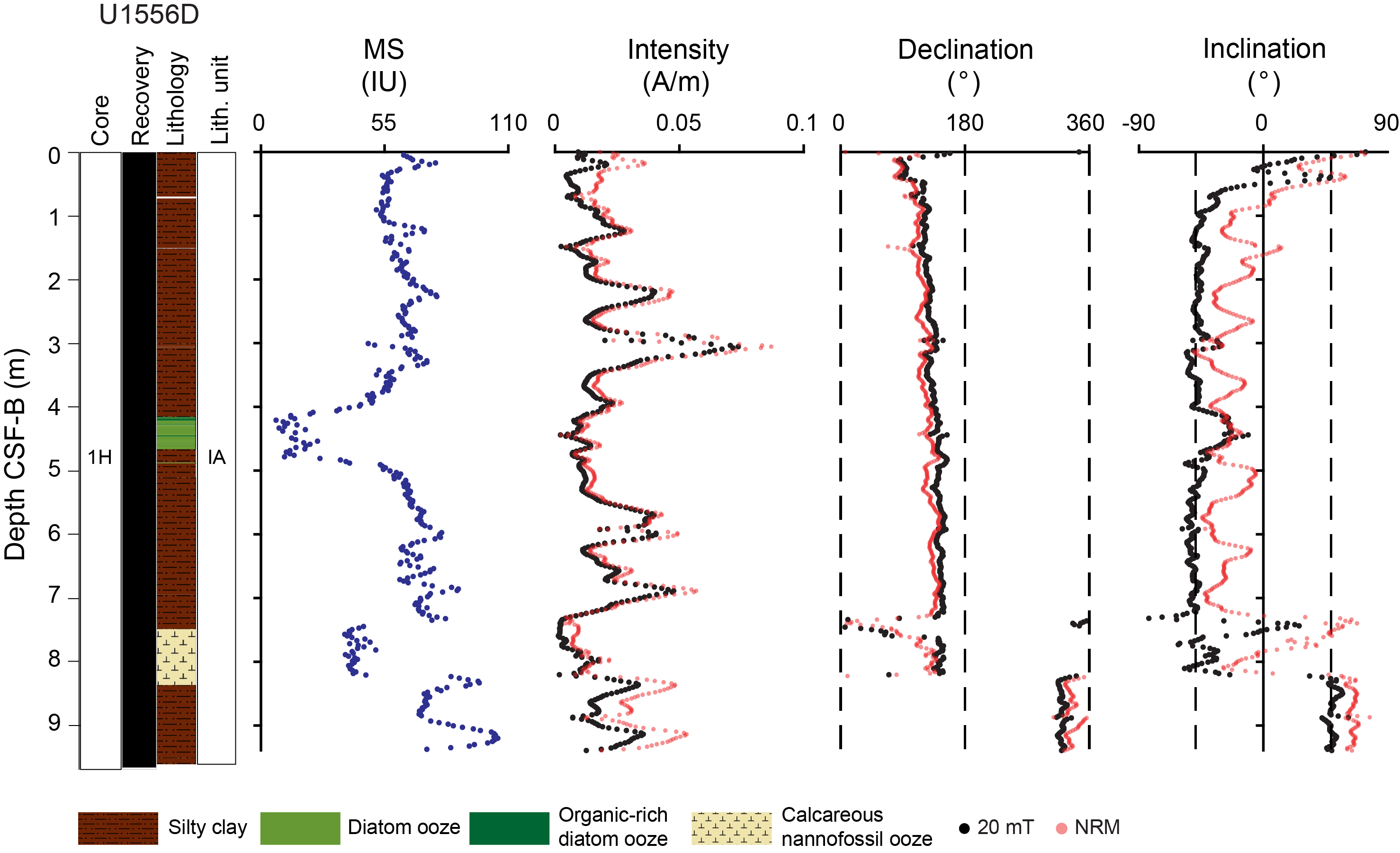
Figure F104. MSP and SRM, Hole U1556D.

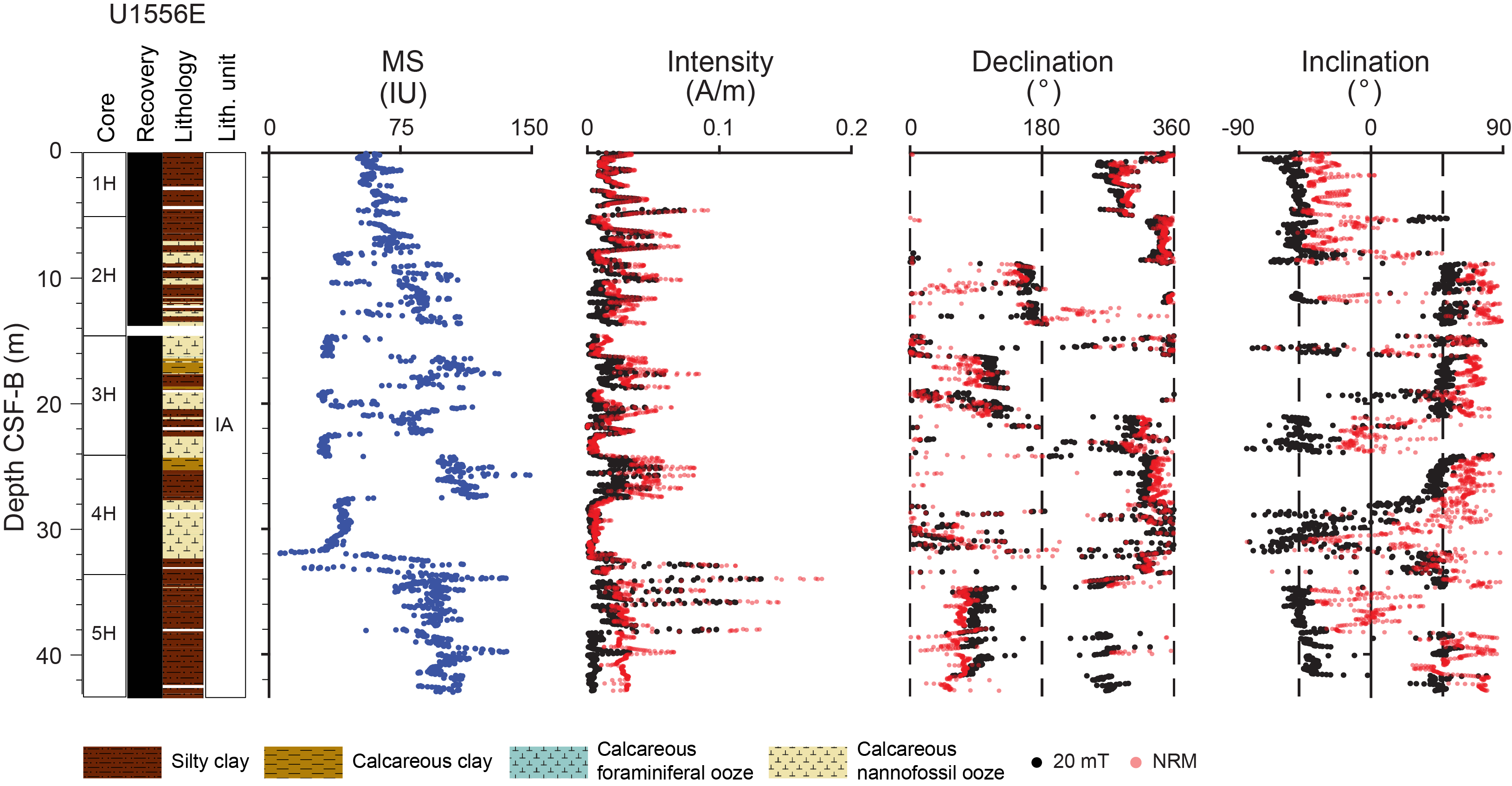
Figure F105. MSP and SRM, Hole U1556E.

AF demagnetization by 5–10 mT removes a minor viscous overprint for most samples. This viscous overprint is, in most cases, an unavoidable drilling overprint, even when nonmagnetic core barrels are employed (i.e., during APC and RCB coring). A drilling overprint would bias inclinations toward more positive values; it manifests as a near-vertical component on an orthogonal vector plot (OVP) (Acton et al., 2002). The 20 mT inclinations measured in Holes U1556A, U1556C, U1556D, and U1556E are all bimodal (Figure F106). These inclinations, with the exception of the positive modal inclination in Hole U1556C, are close to what is expected for this latitude (±49.1° at 30°S) from a geocentric axial dipole (GAD) (Figure F106). The slightly greater inclination of Hole U1556C sediments (with a positive modal inclination of 60°) is likely the result of a stronger viscous overprint of cores from this hole, which is observed for most of the XCB inclination data and portions of the APC inclination data (Figure F103).

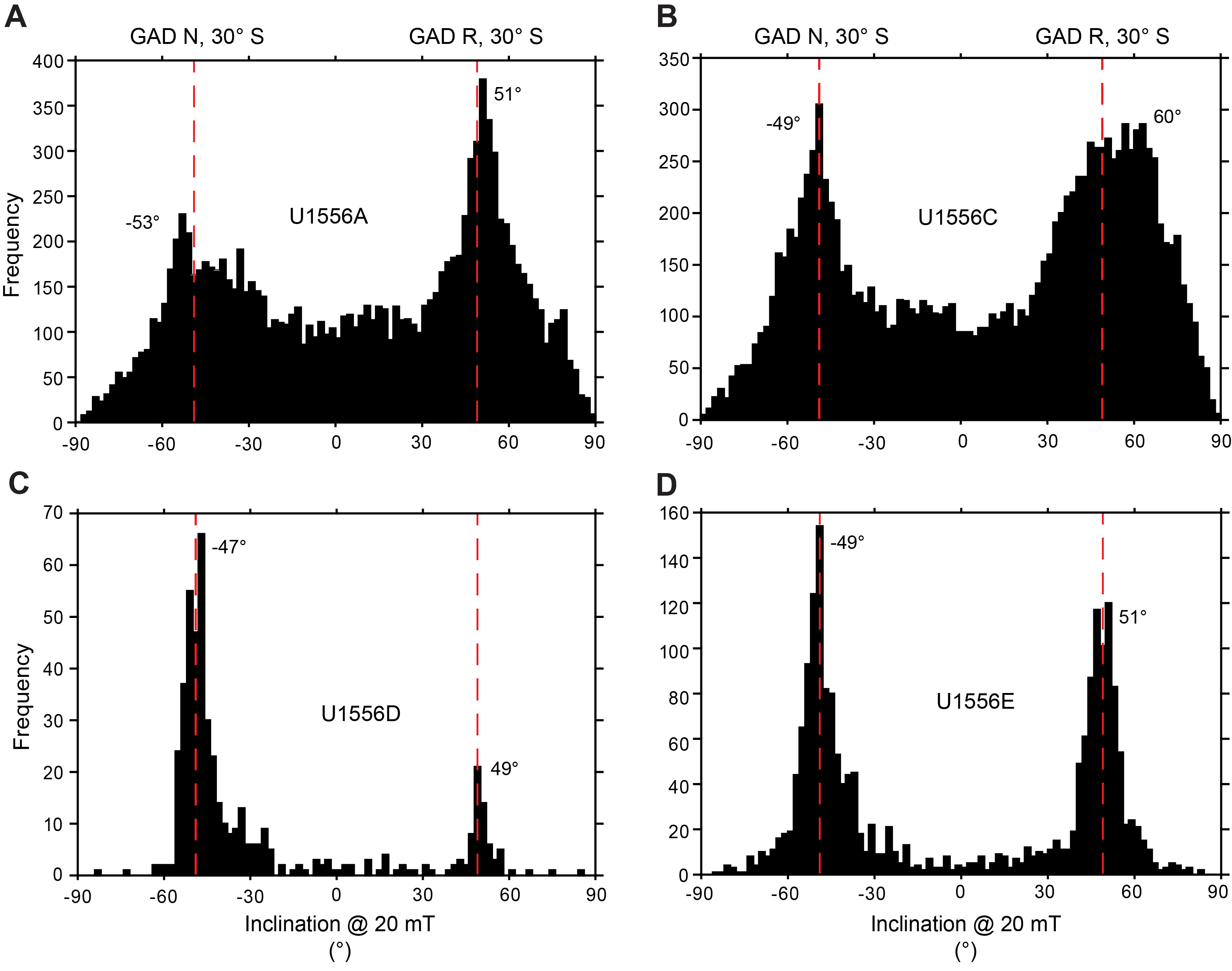
Figure F106. SRM inclination after 20 mT AF.

The remanence intensities for the sediment packages at Site U1556 are relatively strong for pelagic material. Averages are on the order of 10⁻² A/m for the NRM and 10⁻² to 10⁻³ A/m for 20 mT intensity. Maximum values are also on the order of 10⁻² A/m, with the notable exception of the interval 200–250 m CSF-B in Hole U1556C. Measurement of interval 390-U1556C-19X-2, 69–73 cm, revealed a spike in intensity with a value of 11.78 A/m. Further investigation revealed the presence of a broken shear pin embedded in the sediments. Thus, data for Section 19X-2 were removed (Figure F103).

Magnetic susceptibility (MS) (see Physical properties and downhole measurements) and intensity correlate well with lithologic variations (see Sedimentology); high values correspond to silty clays, whereas lower values correspond to biogenic carbonates. The 20 mT intensities are highest in both Holes U1556A (average = 1.5 × 10⁻² A/m; Figure F102) and U1556C (average = 1.3 × 10⁻² A/m; Figure F103) in Subunit IA, which is predominantly composed of silty clays (see Sedimentology). A broad peak is also noted in both the NRM and 20 mT intensities from the dark brown silty clays of Subunit IE (interval 390-U1556C-23X-5, 142.5 cm, to 28X-2, 143.5 cm; see Sedimentology). Throughout Hole U1556C, NRM and 20 mT average intensities in Unit I are more than double what their values are in Unit II. The NRM intensity in Unit I is 3.3 × 10⁻² A/m, whereas the Unit II value is 1.4 × 10⁻² A/m. Likewise, the 20 mT intensity averages 6.3 × 10⁻³ A/m for Unit I and 2.4 × 10⁻³ A/m for Unit II. NRM and 20 mT intensities from Unit I in Hole U1556A are also higher than their Unit II counterparts, but only the 20 mT intensity shows doubling of the intensity value. Holes U1556D (Figure F104) and U1556E (Figure F105) did not extend through the base of Subunit IA. Despite the difference in cored sediment package thickness between these two holes, average 20 mT intensities are similar in magnitude: 1.89 × 10⁻² A/m for Hole U1556D versus 1.64 × 10⁻² A/m for Hole U1556E.

8.1.1.1. Discrete samples

We collected approximately two discrete sediment cubes per core from Hole U1556C (59 sediment discrete samples total). All cubes were AF demagnetized, in some instances up to 190 mT. By demagnetizing the samples in a stepwise fashion, we determined the characteristic remanent magnetization (ChRM) of the samples, which reflects the magnetic field direction at or soon after sediment deposition and aids in magnetostratigraphic interpretation. Several of the discrete sediment samples displayed noisy OVPs; of the 59 sediment samples, 49 sample had OVPs clean enough to define the ChRM.

Only 28 of those clean samples gave maximum angular deviation angles <15°, typically considered the uppermost cutoff for well-defined magnetic field directions (Table T17) (Butler, 1992). Lithology appeared to have a negligible effect on the quality of magnetic data. Both the silty clays and biogenic carbonates produced clean OVPs (Figure F107A, F107B), and shallow inclinations or noisy data were not confined to one particular lithology (Figure F107C, F107D). Additionally, more than half the discrete sediment samples regardless of composition still had at least 20% of the remanence remaining after demagnetization was complete. A subset (9 total) of the 59 sediment cubes representative of the cored lithologies indicate that samples acquire more than 80% of the saturation IRM (SIRM) between 100 and 300 mT and are completely saturated by 900 mT with the exception of 1 sample that was close to saturation. Both the AF demagnetization and IRM experiments suggest the presence of low-coercivity minerals (e.g., magnetites/maghemites) as the main remanence carriers and local occurrence of high-coercivity minerals such as hematite in the studied sediments.

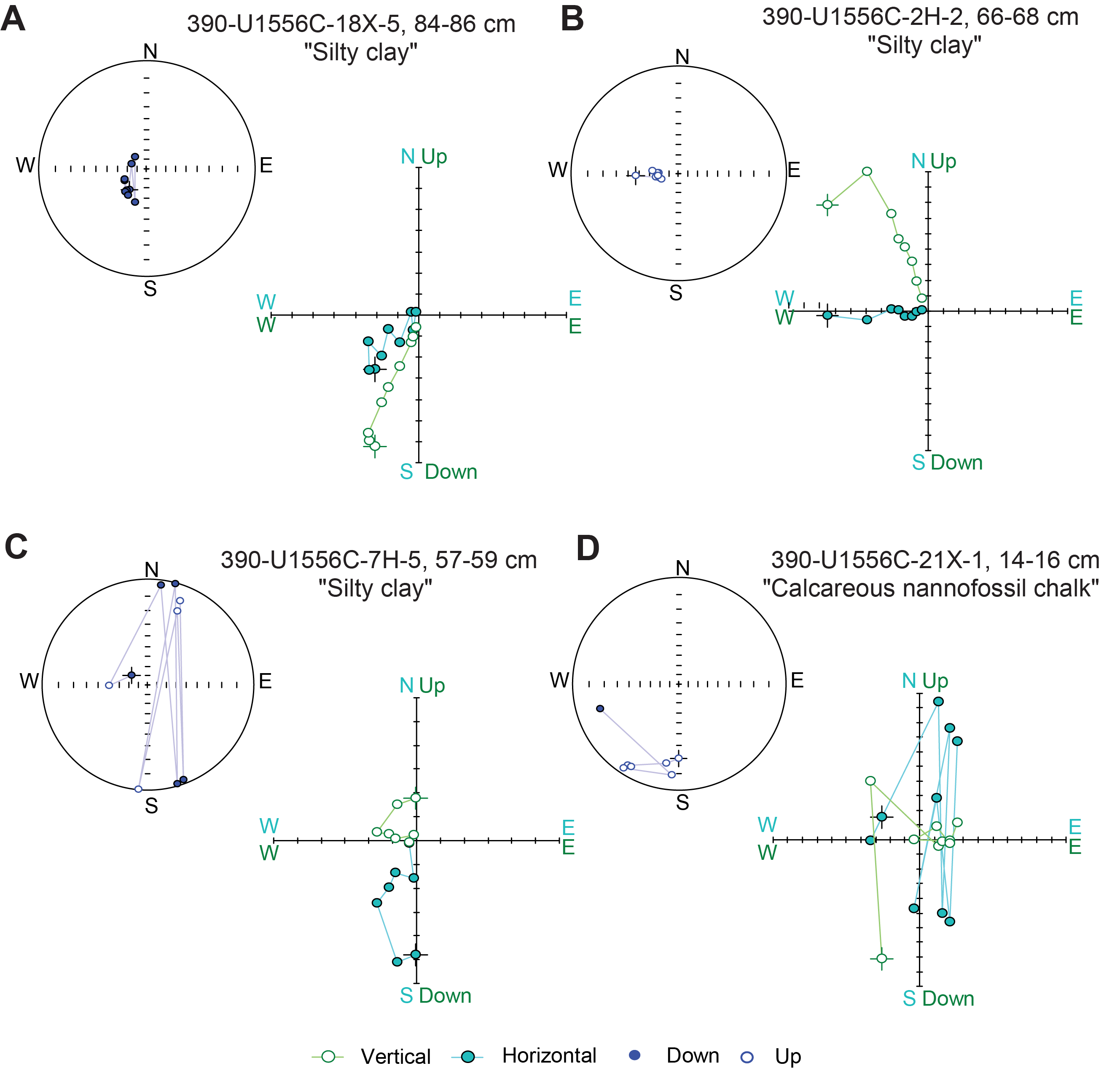
Figure F107. OVPs and stereonets of sediments.

AMS measurements were carried out on all discrete sediment samples from Hole U1556C. The mean bulk magnetic susceptibility (K_m) for the carbonate-rich lithologies (calcareous chalks and nannofossils ooze) is 0.34 × 10⁻³ SI, whereas the silty clays have a mean value of 1.16 × 10⁻³ SI (Figure F108B). A scatter plot of K_m versus NRM intensity for the two lithology groups shows no within-group significant correlation (low correlation coefficient [R] values), which indicates that magnetic susceptibility in the studied sediments is not controlled by the ferromagnetic mineral phases but principally by the paramagnetic phases (mostly clays). Therefore, variations in K_m values with depth through the sedimentary package (Figure F109) correspond to variations in core lithology (see Sedimentology) in a manner similar to the magnetic susceptibility measured in the whole-round pass-through and point sensor instruments (see Physical properties and downhole measurements). The magnetic fabric (Figure F108A) shows subvertical K_min axes for most samples and K_max axes randomly distributed in the horizontal plane, suggesting primary depositional fabrics (Tarling and Hrouda, 1993). The high values of the shape parameter (T) (Figure F108D) close to 1 denote a strong compaction fabric that is independent of lithology. Likewise, the anisotropy degree (P) is also independent of lithology (Figure F108C). However, the trend of increasing P and foliation (F) values with depth throughout the sedimentary succession from the uppermost samples at ~35 m CSF-B to about 250 m CSF-B (Figure F109) may reflect porosity loss due to increased compaction at greater sediment overburdens (see Physical properties and downhole measurements). The orientation of this fabric, with K_max axes roughly distributed parallel to the split core surface or orthogonal to the direction the sample extraction tool is pushed into cores to take the discrete cubic samples, suggests the processes of core splitting and sample extraction may have slightly interfered with an original sedimentary oblate (planar) fabric that could have, in turn, been only partially overprinted by the drilling process. These types of drilling/splitting/pushing interferences have been previously documented in cores in deep-sea sediments and elsewhere (Copons et al., 1997).

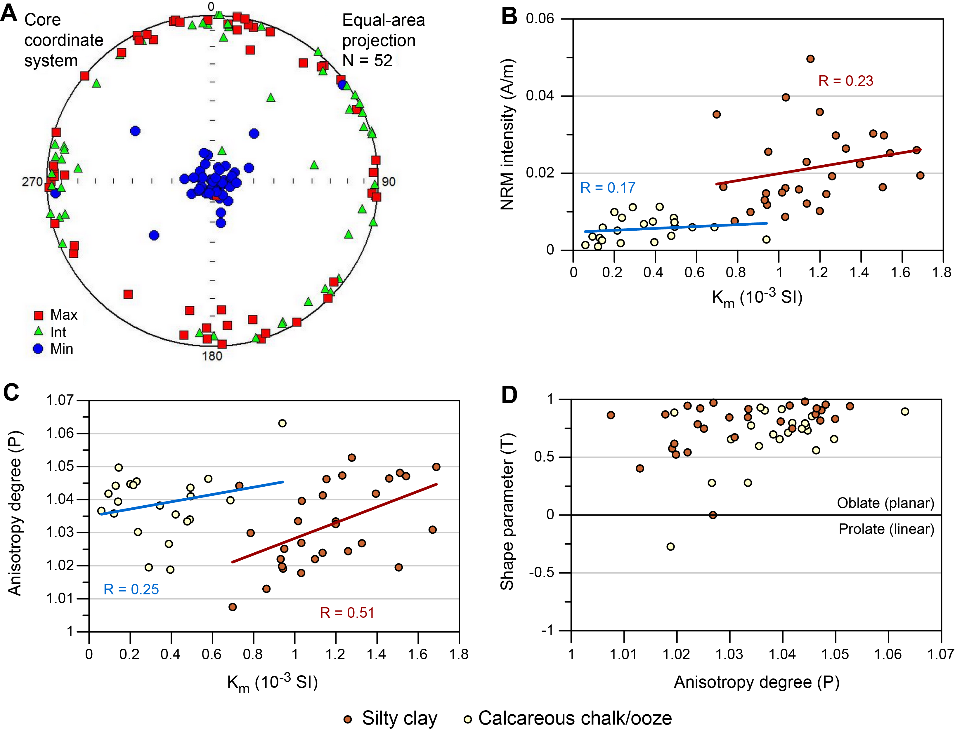
Figure F108. AMS and MS, Hole U1556C.

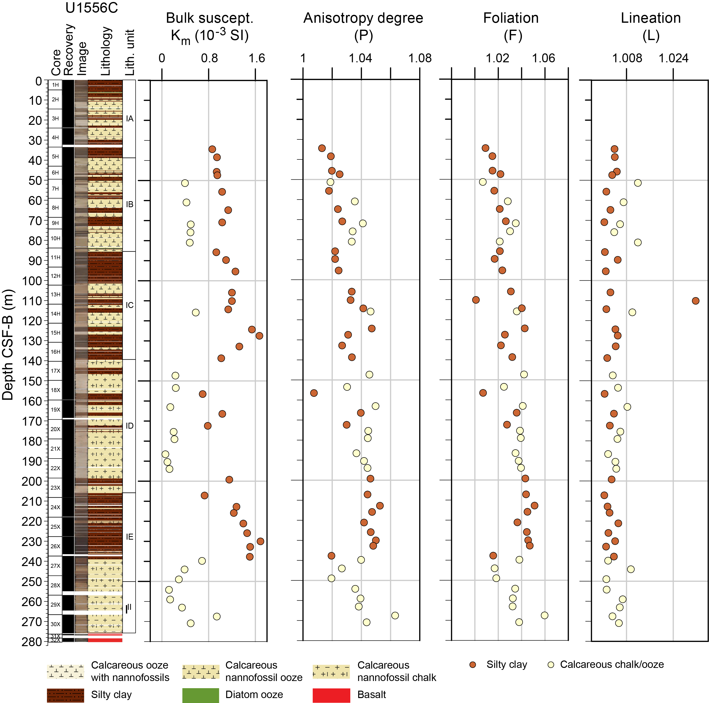
Figure F109. AMS, Hole U1556C.

8.1.2. Magnetostratigraphy

SRM measurements of the archive halves of Holes U1556A, U1556C, U1556D, and U1556E after AF demagnetization at 20 mT were used to construct a polarity sequence for the Site U1556 sediment package. The interpreted polarity sequence is primarily based on the inclination sign (after the 20 mT demagnetization step) supplemented with the corrected declination measurements of the oriented (APC) cores. Inclinations from the calculated discrete sample ChRM directions using principal component analysis (PCA) (Kirschvink, 1980) verify the inclinations measured from the SRM and support the polarity interpretations (light blue points in Figure F103). Correlation of the MSP measurements made with the SHMSL (see Physical properties and downhole measurements; see Figure F110) and close inspection of images of the archive-half sections also aided in the correlation of the polarity stratigraphies between holes at Site U1556.

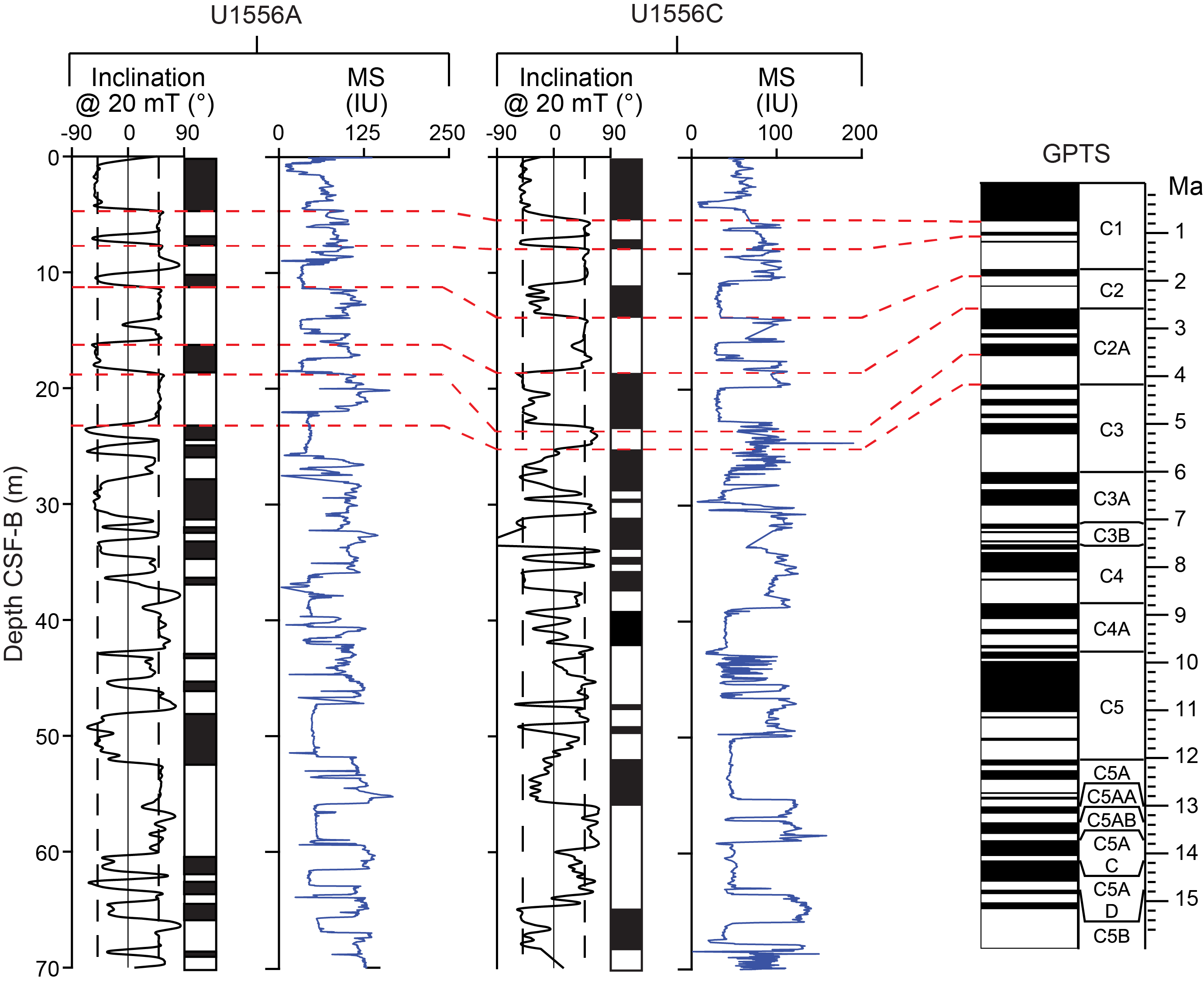
Figure F110. MSP and inclination.

Holes U1556A and U1556C display polarity reversals that can be unambiguously correlated to each other to ~70 m CSF-B (Figure F111). Holes U1556D and U1556E can be correlated to these two holes to ~10 and 45 m, respectively. This reversal sequence can be tentatively correlated to the Brunhes, Jaramillo, Olduvai, Gauss, and Gilbert Chrons (Tables T18, T19). The depths associated with the base of the Brunhes Chron in Hole U1556C are tentative because of a recovery gap that misses stratigraphy between Cores 390-U1556C-1H and 2H. It was difficult to unambiguously assign polarity chrons at Site U1556 to the 2020 geologic timescale (Gradstein et al., 2020), but it should be possible in postexpedition work when a refined biostratigraphy becomes available. Large coring gaps occur throughout Hole U1556A, whereas only a handful of coring gaps are present throughout Hole U1556C. Drilling disturbance is common throughout the XCB portions of both holes (below 151.4 m CSF-B in Hole U1556A and 140.3 m CSF-B in Hole U1556C) to ~245 m CSF-B (see Sedimentology), although it is generally less intense in Hole U1556C cores. The interval between ~210 and 250 m CSF-B contains hiatuses in biostratigraphic markers spanning several tens of meters in both Holes U1556A and U1556C, suggesting a possible unconformity, and there is evidence of reworked sediments due to slumping, limiting magnetostratigraphy.

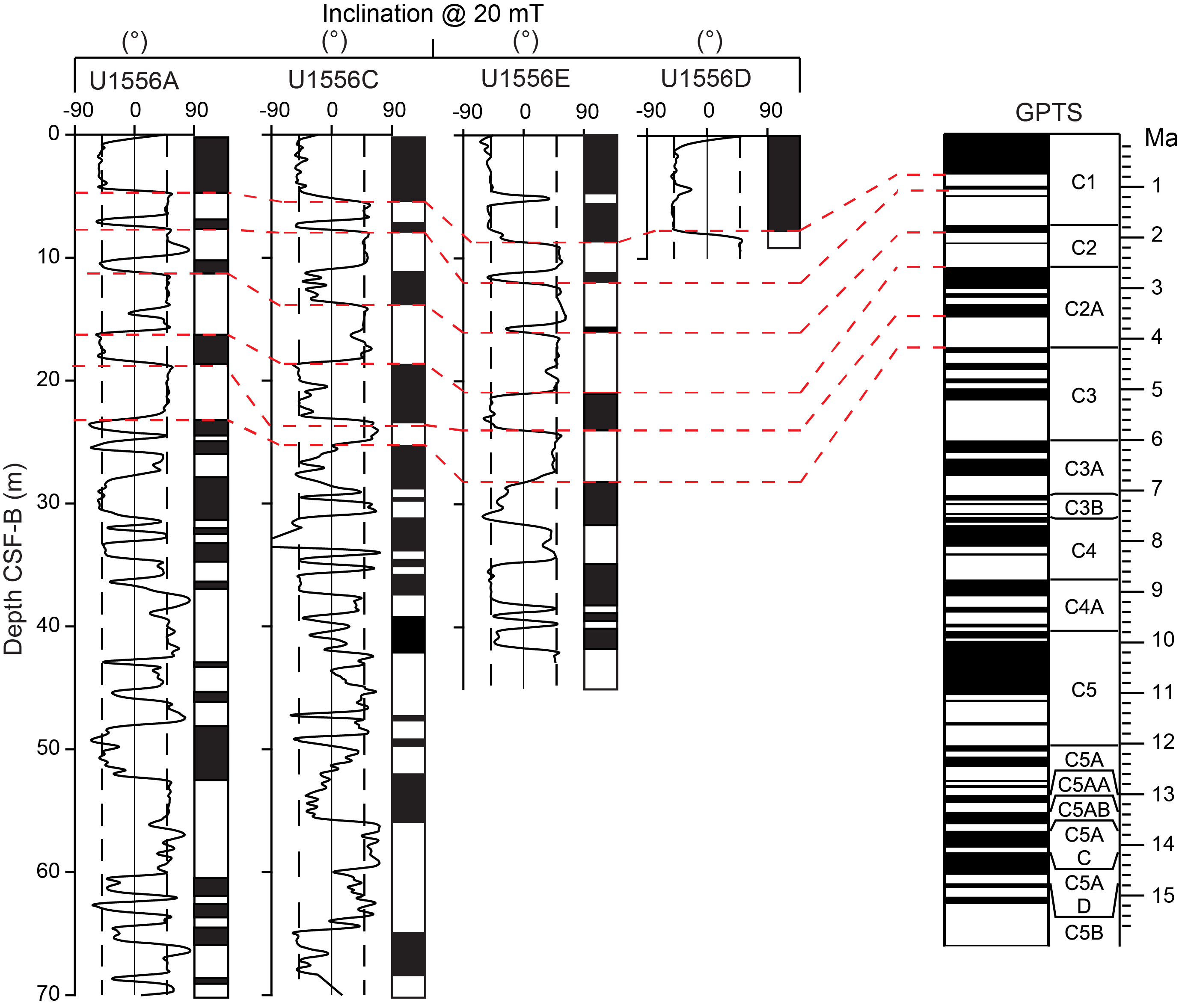
Figure F111. Inclination.

8.2. Basement

The primary goals of paleomagnetic studies of igneous cores from Site U1556 were twofold: (1) to use SRM and discrete sample analyses to confirm the age of upper basement at Site U1556 (~61.2 Ma; calculated from magnetic data acquired during the CREST cruise [Kardell et al., 2019]), which lies in the middle of reversed Chron C26r, and (2) to investigate the effects of ridge flank alteration on the magnetic properties of the upper basement using discrete samples representative of the recovered lithologies (lithified sediment, pillow lavas, massive flows, hyaloclastite, and breccias) and their variable styles of alteration (see Igneous petrology; see Alteration petrology).

Measurements of the NRM and in-line AF demagnetization of basement in Hole U1556B (291–633 mbsf) focused on archive-half core pieces ≥9 cm in length. Recovery averaged 56% in Hole U1556B, and most cores contained few pieces long enough to measure with the SRM. Hereafter, the intensity/inclination after demagnetization at 20 mT is referred to as the 20 mT intensity/inclination. To complement SRM data, paleomagnetic investigation concentrated on discrete samples taken from the working halves of these cores. Remanence demagnetization measurements were made on 45 cube samples (8 cm³ volume) and a single 7 cm³ sediment sample collected at the sediment/basement interface (Sample 390-U1556B-2R-1, 20–22 cm). Stepwise AF demagnetization up to 190 mT was applied to 36 of the discrete samples, and a subset of these were further subjected to IRM acquisition experiments. Nine additional cube samples were subjected to thermal demagnetization up to 580°C. AMS measurements were performed from all discrete samples prior to stepwise demagnetization (see Paleomagnetism in the Expedition 390/393 methods chapter [Coggon et al., 2024c]).

In addition, paleomagnetic investigation includes two discrete samples taken from the uppermost basement of Hole U1556A, a few pieces longer than 9 cm, and a single discrete sample from Cores 390-U1556C-30X through 33X. Data collected on the discrete samples can be found in Table T20.

8.2.1. Results

The NRM and 20 mT intensities of the igneous rocks average ~4.2 and 3.1 A/m, respectively, throughout Hole U1556B. The highest NRM and 20 mT intensities occur in Subunit 12f (Figure F112), which comprises highly altered pillow lavas (see Igneous petrology), with values of 7.3 and 6.2 A/m, respectively. Additionally, Unit 13, which comprises H-POPP basalts (see Igneous petrology), has high intensities (7.5 and 5.3 A/m for NRM and 20 mT, respectively) and also the highest MS values, suggesting either a higher concentration of ferromagnetic minerals and/or the presence of finer grained titanomagnetite. In-line AF demagnetization with the SRM has a negligible effect on the NRM intensity (Figure F112). Positive (downward) inclination values dominate throughout Hole U1556B, although short intervals of negative inclinations, particularly in the uppermost 40 m, are observed. However, the modal inclination (Figure F113) is somewhat shallower (33°) than the expected inclination for a GAD at this latitude (±49.1° at 30°S). The origin of this shallower inclination could be the result of a viscous/drilling overprint that in most cases is unavoidable even when nonmagnetic core barrels are employed (i.e., during APC coring), though this is not always the case. It could also be due to the presence of magnetic minerals with slightly overlapping coercivities that were not fully demagnetized by 20 mT.

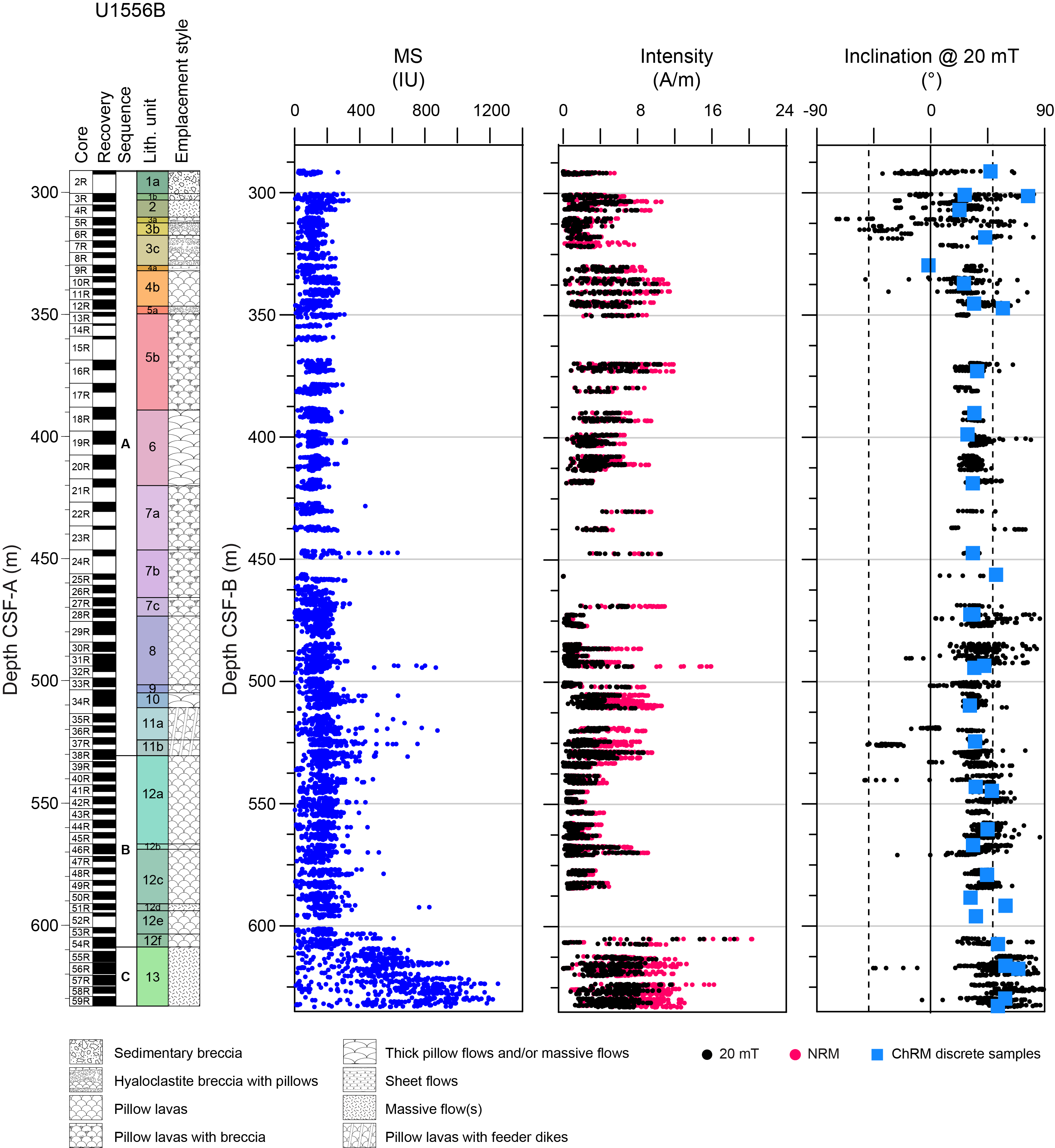
Figure F112. MSP, NRM, and inclination, Hole U1556B.

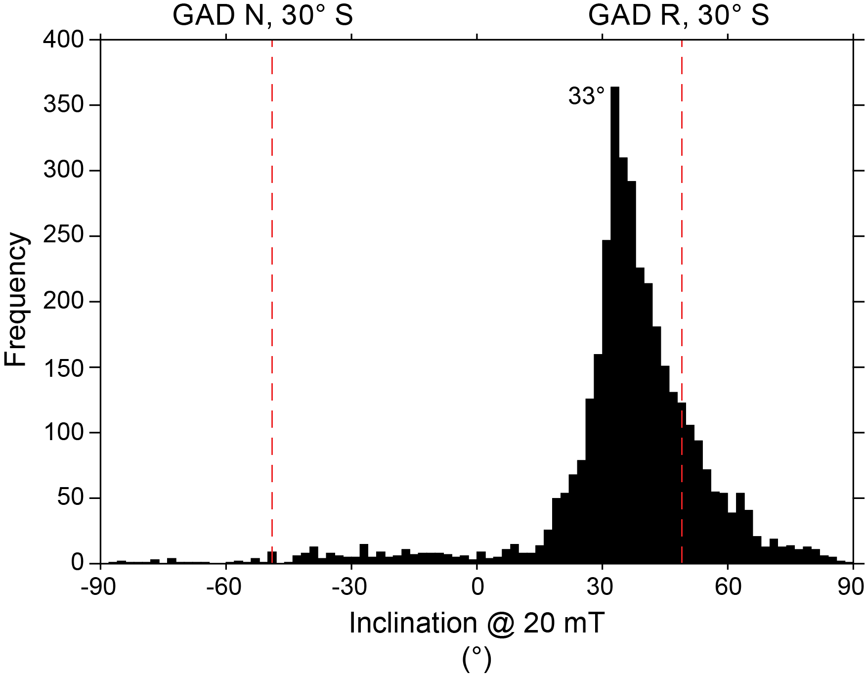
Figure F113. Inclination, Hole U1556B.

8.2.1.1. Discrete samples

We collected ~1 discrete cube per core from Hole U1556B for a total of 46 basement samples. To investigate what effects lithology and alteration have on the magnetic signature, representative discrete samples were subjected to stepwise full AF demagnetization up to 190 mT (Figure F114). IRM experiments contribute additional information regarding the magnetic minerals present (e.g., their coercivity) using qualitative relationships between intensities at various field values. AMS and bulk susceptibility were measured on all discrete cubes to determine the preferred alignment of the magnetic mineral assemblage.

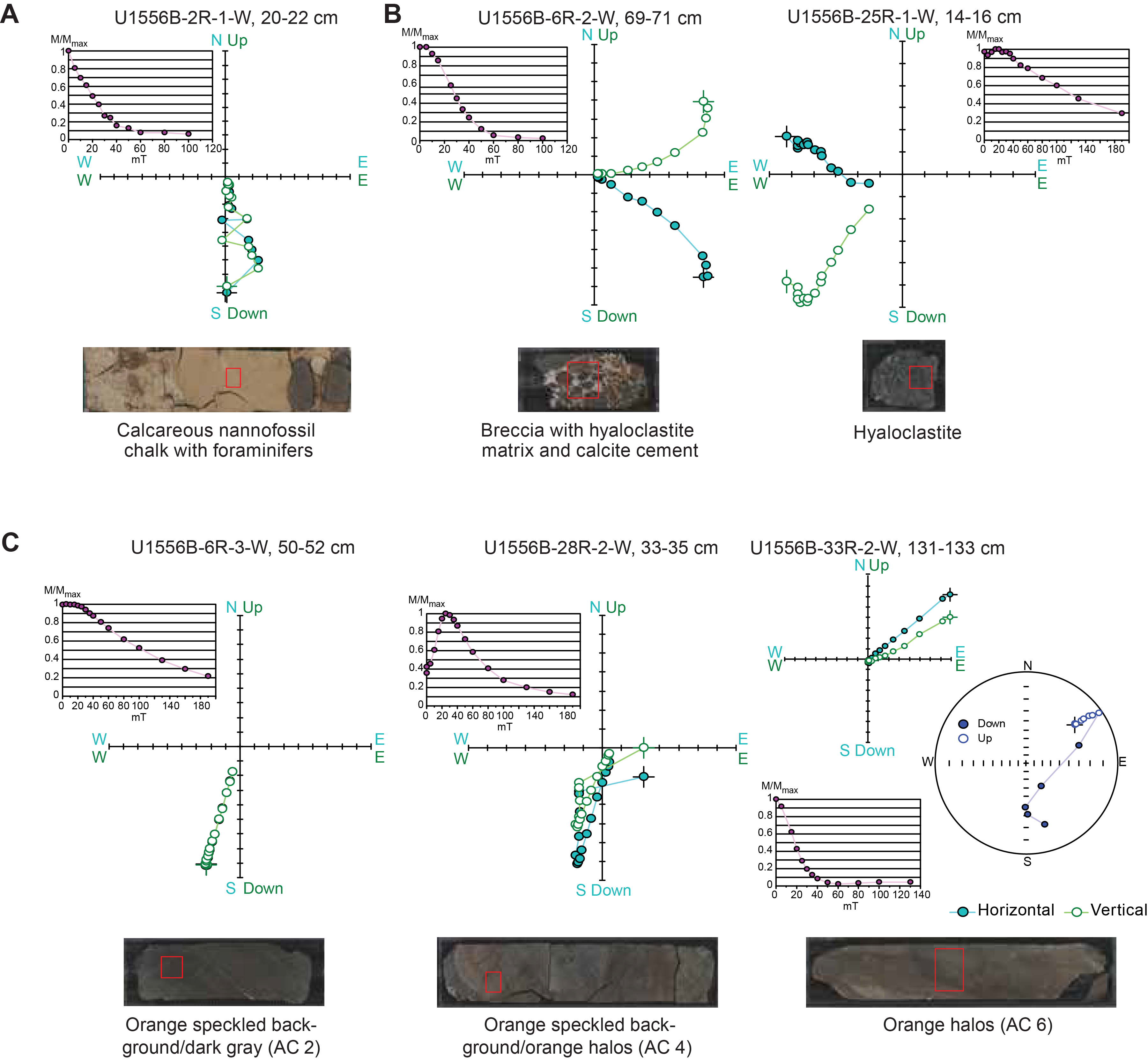
Figure F114. NRM demagnetization, Hole U1556B.

ChRM directions calculated using PCA (Kirschvink, 1980) of the discrete samples from both AF demagnetization and thermal demagnetization support the inclinations measured in the archive-half sections using the SRM. The sole sediment sample analyzed exhibits noisier remanence directions through stepwise demagnetization, as illustrated in its OVP (Zijderveld, 1967) (Figure F114A) compared to breccia and altered basalt samples (Figure F114B, F114C). The ChRM indicates a positive (downward) reversed polarity isolated by 35 mT (shown as inset in Figure F114A). The inclination (47.2°) is close to that expected for a GAD at this latitude (±49.1°), and <10% of the remanence remains by 60 mT. Breccia Sample 390-U1556B-6R-2, 69–71 cm, from Subunit 3b (see Igneous petrology) has a weak secondary component, and the ChRM is isolated by 25 mT (Figure F114B). The ChRM indicates a negative upward inclination and, thus, a normal polarity opposite to that expected given the Site U1556 crustal age (~61 Ma) (Kardell et al., 2019) in the Paleocene reversed Chron C26r (59.237–62.278 Ma; Gradstein et al., 2020), which probably results from clast rotation after remanence was acquired. A second breccia sample, a hyaloclastite (Sample 25R-1, 14–16 cm) (Figure F114B), also contains a secondary component. Because the overprint has opposite polarity to the ChRM primary direction, it manifests as an initial increase in the intensity. The ChRM for this sample is not isolated until 35 mT, and ~30% of the remanence remains after demagnetization up to 190 mT, suggesting the presence of high-coercivity minerals.

Sample 390-U1556B-6R-3, 50–52 cm, is a relatively fresh (Alteration Class 1; see Physical properties and downhole measurements) basalt with orange speckled/dark gray background from Subunit 3c (see Alteration petrology) with an OVP that displays a clean, straight line to the origin (Figure F114C). The demagnetization curve shows just a little more than 20% remanence remaining and the OVP does not reach the origin, suggesting the presence of a still harder magnetic component. The ChRM inclination (43°) is close to but shallower than expected for a GAD. Sample 28R-2, 33–35 cm, is a basalt with orange speckled background/orange halo alteration (Alteration Class 4; see Physical properties and downhole measurements) from Subunit 7c (see Alteration petrology) that displays a significantly harder overprint, which is revealed by a steady increase in intensity with demagnetization up to 30 mT followed by a decrease in intensity with additional demagnetization steps up to 190 mT. Once isolated, the ChRM component trends just off origin, and its inclination (33.7°) is shallower than expected. Approximately 10% of the remanence remains, which suggests a higher coercivity component remains unaffected at 190 mT. Sample 33R-2, 131–133 cm, which is a basalt with orange halos (Alteration Class 6; see Physical properties and downhole measurements) from Unit 8 (see Igneous petrology), also displays a straight line to the origin on its OVP, and only less than 10% of its remanence remains after 40 mT (Figure F114C). However, the OVP indicates that this sample is fully overprinted, given the ChRM component is completely defined by a negative upward (and thus normal polarity) inclination. Given that the normal polarity of this overprint, which is observed across alteration classes (see Physical properties and downhole measurements) and lithologies (e.g., both breccia and altered basalt), is opposite to that expected for 61 Ma lavas, we speculate that it postdates the original magnetic signal acquired during crystallization of these lavas. Such an overprint was only determined in about 5% of the samples studied.

For all discrete samples that displayed an overprint (Table T20), we calculated the direction of the overprint component in addition to the ChRM direction (Figure F115). Overprint directions have negative inclinations (denoted by open symbols in Figure F115A) indicating a normal polarity overprint. All discrete breccia samples analyzed contain this overprint, and the sample from Unit 8, which has distinct green alteration (see Alteration petrology), is completely overprinted. Breccias and relatively fresh basalt samples tend to have steeper overprinted inclinations, whereas the more altered basalt samples display shallower overprint inclinations. ChRM inclinations—for those samples where the maximum angular deviation is ≤15°—are also on average shallower than expected (~38°). Despite this, all computed ChRM directions represent positive downward inclinations indicative of reversed polarity, which is consistent with the identification of Chron C26r (59.237–62.278 Ma; Gradstein et al., 2020) at the sediment/basement interface (291 m CSF-B) and the estimated age of the basement (61.2 Ma; Kardell et al., 2019). The cause of the observed overprint (Figure F115A) and trend to shallower inclinations in our ChRM directions is uncertain, but possible explanations include a drilling overprint, the acquisition of a viscous component, and/or magnetic directions acquired as a result of alteration processes during a normal polarity interval following crustal accretion.

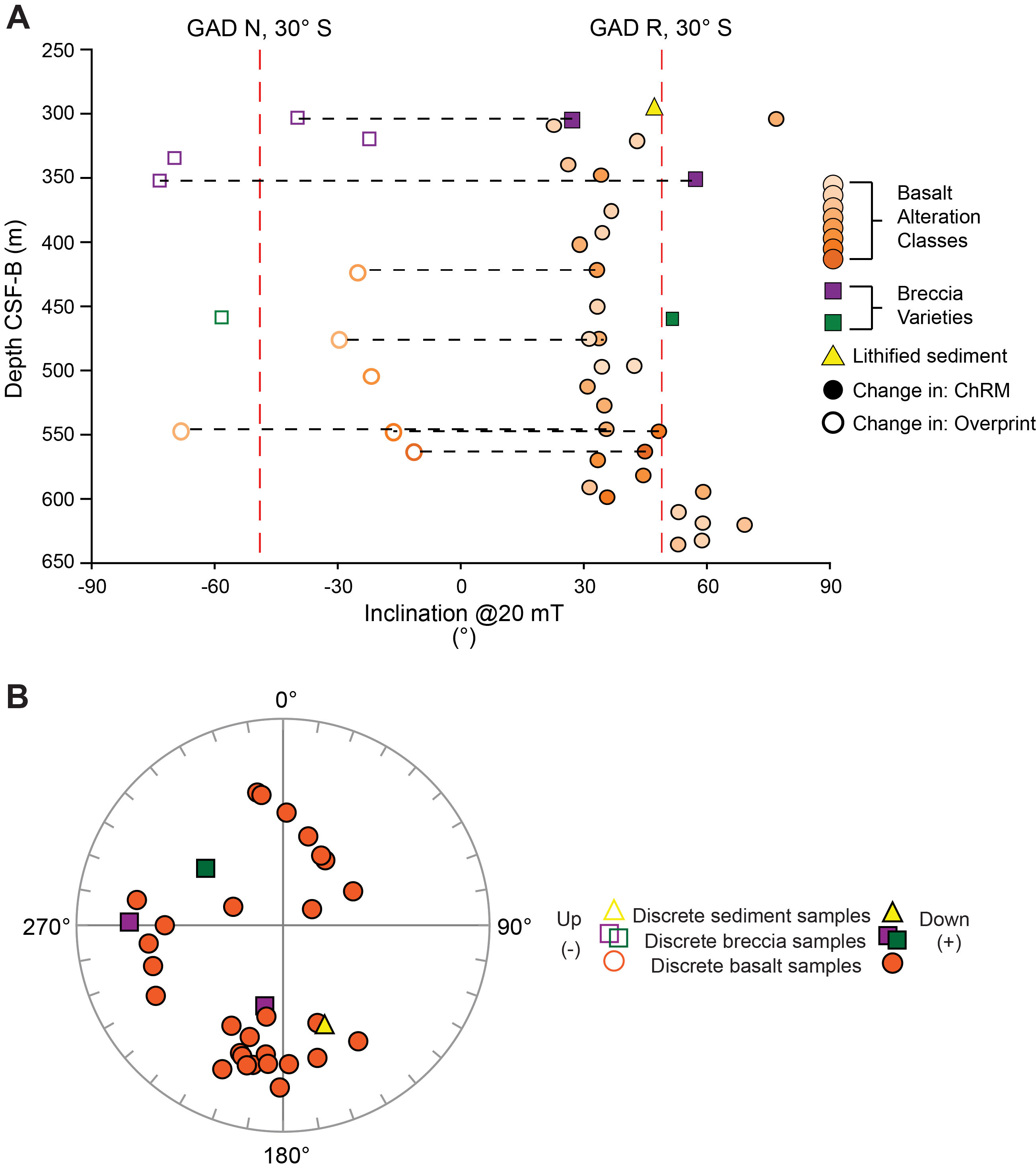
Figure F115. Overprint and ChRM, Hole U1556B.

IRM and backfield IRM experiments were performed on 24 discrete samples (Table T20) to help decipher the ferromagnetic phases present from their characteristic coercivities (see Paleomagnetism in the Expedition 390/393 methods chapter [Coggon et al., 2024c]). Most samples attain saturation by 200–400 mT and more than 80% of the IRM is acquired at ~100 mT, indicating that no high-coercivity phases like hematite are present (Figure F116A). However, the backfield IRM curves display a coercivity of remanence (B_cr) range of 10–130 mT (Figure F116A), which indicates that a variety of ferromagnetic minerals with relatively low to intermediate coercivity dominate the magnetic assemblage of all rocks analyzed. S ratios are close to 1 (Figure F117), confirming the dominance of low-coercivity phases with little variation throughout the volcanic section. Additionally, unblocking temperatures from the thermal demagnetization treatments are in the range of 550°–580°C, indicative of the presence of magnetite-like magnetic carriers. The SIRM intensity is variable with depth in Hole U1556B (Figure F117), with the highest values occurring in the lowermost Unit 13 (see Igneous petrology), suggesting a higher abundance of ferrimagnetic minerals. In contrast, there is no clear pattern in either B_cr or IRM₁₀₀/SIRM with depth (Figure F117). However, samples that were not fully demagnetized at the highest fields applied appear to correspond to higher B_cr values. This is best demonstrated by Sample 390-U1556B-6R-3, 50–52 cm, which has a B_cr value of 126 mT (Figures F113, F116A).

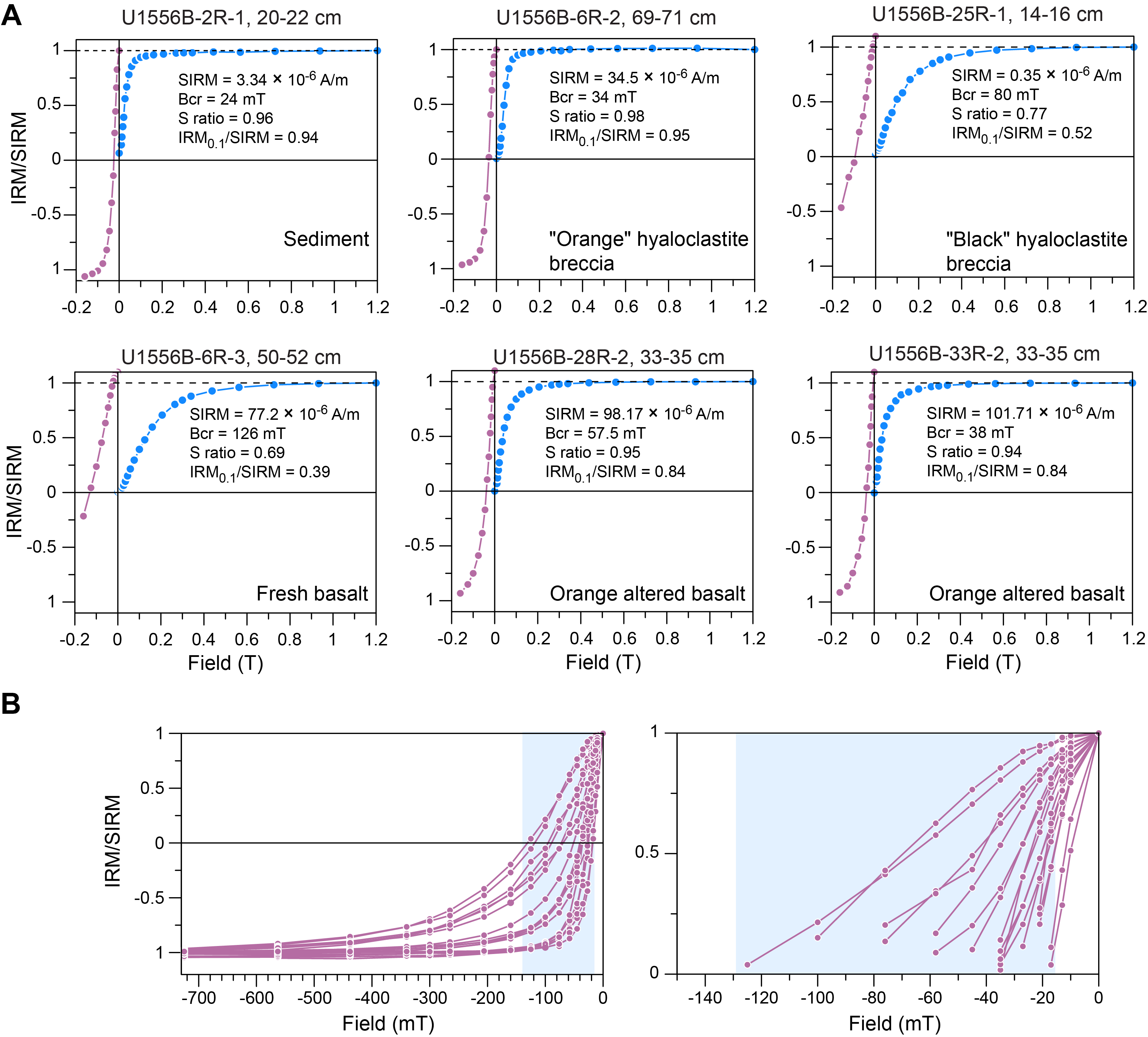
Figure F116. Normalized and backfield IRM, Hole U1556B.

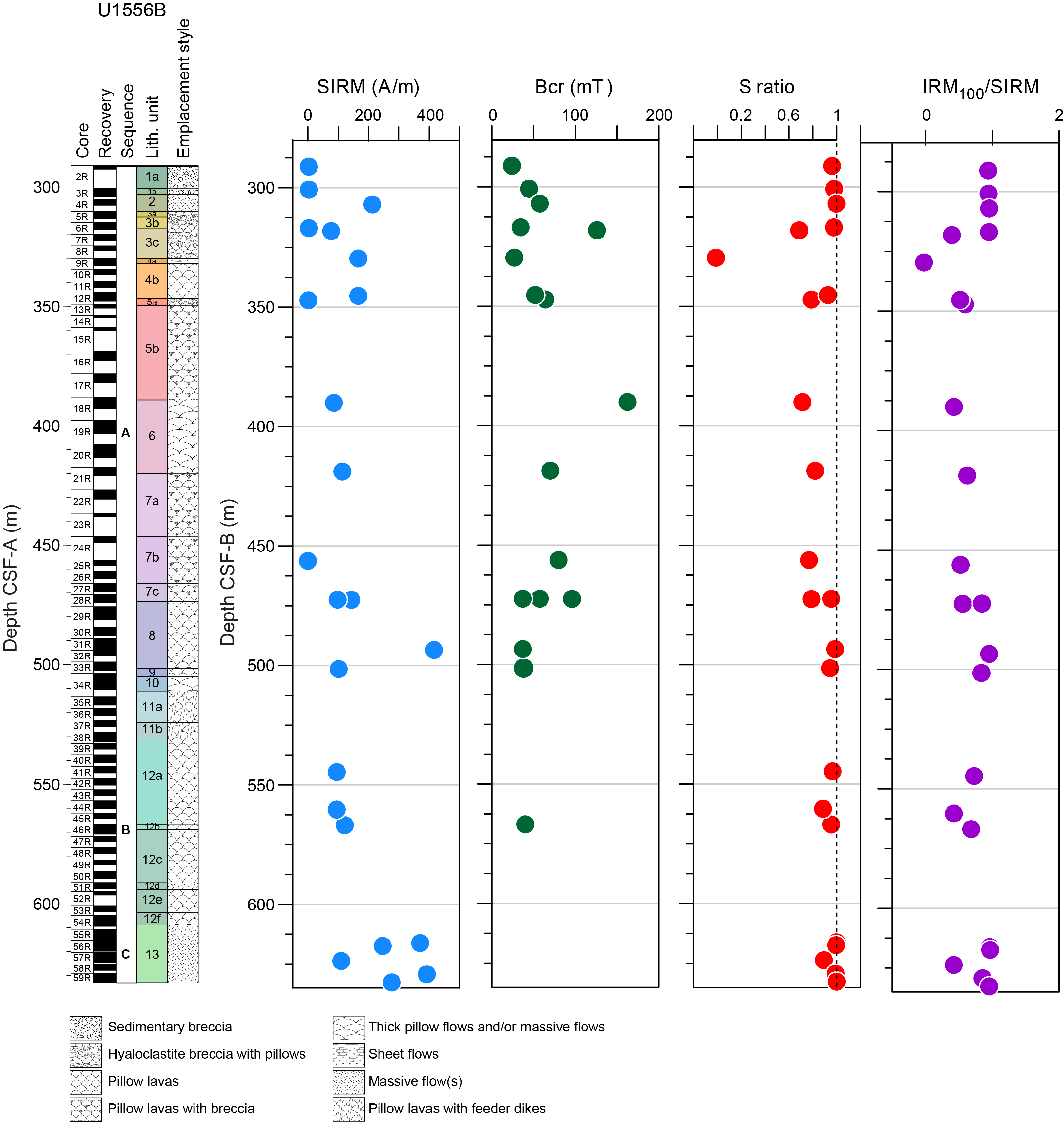
Figure F117. Rock magnetic parameters, Hole U1556B.

Highly oxidized titanomaghemite dominates the magnetic mineralogy of oceanic basalts older than ~10 My and is likely the main carrier of the remanence responsible for most oceanic magnetic anomalies (Hodych and Matzka, 2004, and references therein). Other studies of MORBs indicate this dominant presence of titanomaghemite, which presumably forms via low-temperature oxidation (maghemitization) of primary titanomagnetite (Shau et al., 2004). Massive basalt samples contained minimally oxidized titanomagnetite, indicating that the permeability of the lavas is a primary controlling factor of maghemitization (Shau et al., 2004). In this scenario, pillow lavas, which are typically more fractured than massive lavas, are potentially prone to the maghemitization favored by their higher permeability. This idea broadly fits with the observations made here regarding the presence of secondary overprint magnetic directions in some altered basalt and altered hyaloclastite breccias in Hole U1556B. However, further shore-based research is required to better characterize the ferromagnetic assemblage present in the basement recovered in Hole U1556B.

The mean bulk susceptibility of the discrete samples ranges 3.45 × 10⁻⁴ to 8.15 × 10⁻³ SI. The highest values occur in lowermost Unit 13 (Figure F118A), which is consistent with the MSP data (Figure F112). Bulk susceptibility and NRM intensity show a significant linear correlation (R = 0.74) (Figure F118B), which indicates that magnetic properties are chiefly controlled by the content of ferrimagnetic phases. There is no systematic variation of magnetic lineation and foliation throughout Hole U1556B or with lithology (Figure F118A). The anisotropy degrees values average 1.021 and are relatively low. The values of the shape parameter (T) indicate that both oblate and prolate ellipsoids occur, but there is no clear pattern with depth downhole. Overall, prolate fabrics (−1 < T < 0) apparently dominate in the interval 400–470 m CSF-B, corresponding to the sparsely olivine phyric basalt with interpillow hyaloclastite in Lithologic Subunits 7a and 7b (see Igneous petrology). In contrast, in Unit 12 and 13 oblate fabric becomes dominant with no clear correlation with emplacement style.

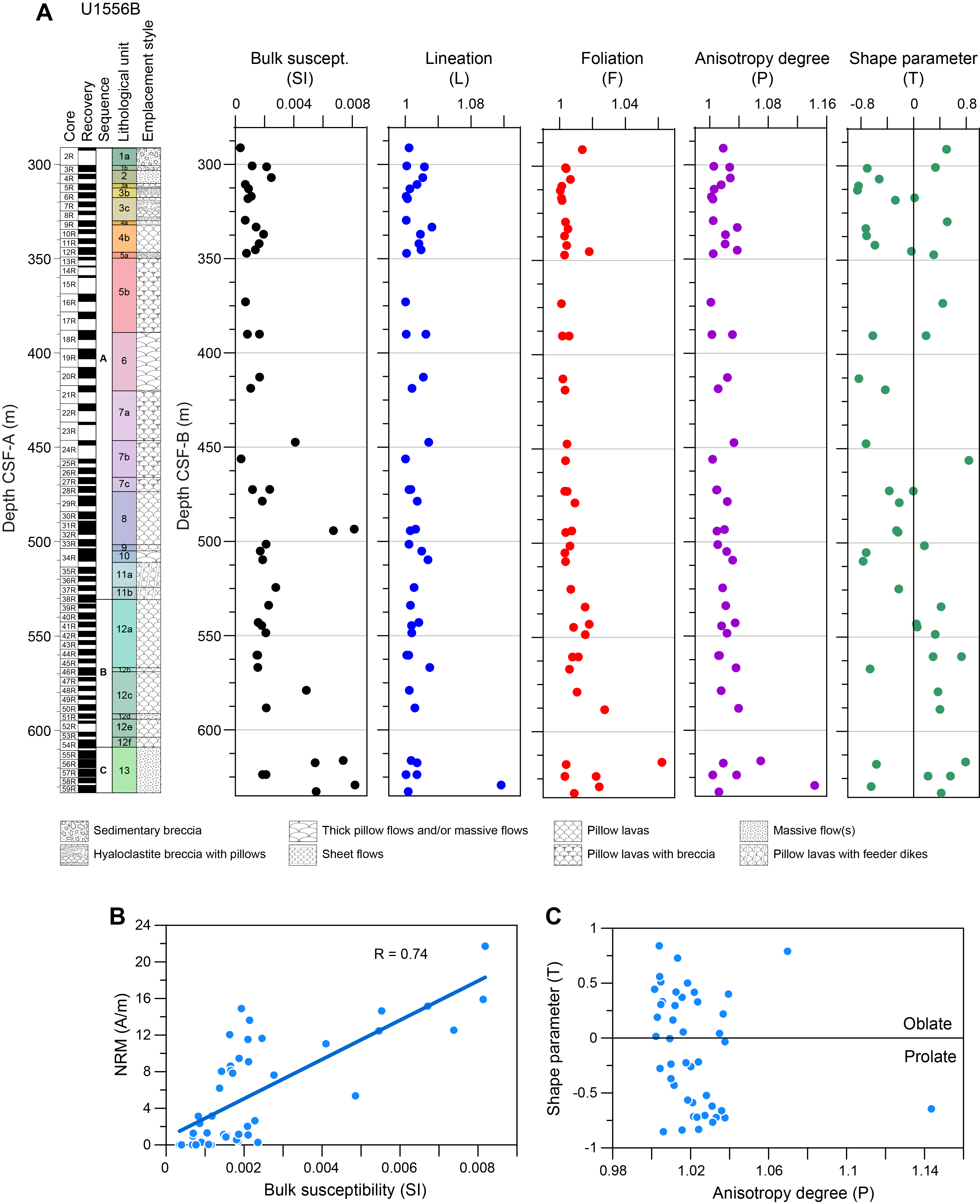
Figure F118. AMS, Hole U1556B.

9. Age model and mass accumulation rates

9.1. Age model and linear sedimentation rates

The age model for Site U1556 is based on calcareous nannoplankton and planktic foraminiferal lowest (base) and highest (top) occurrence datums from Hole U1556C, which has the best sediment recovery of the five sediment holes at Site U1556 and is the one most densely sampled for biostratigraphy (Figure F119; Table T21). The paleomagnetic reversal stratigraphy was not calibrated with biostratigraphic markers, so it was not used to construct the age model.

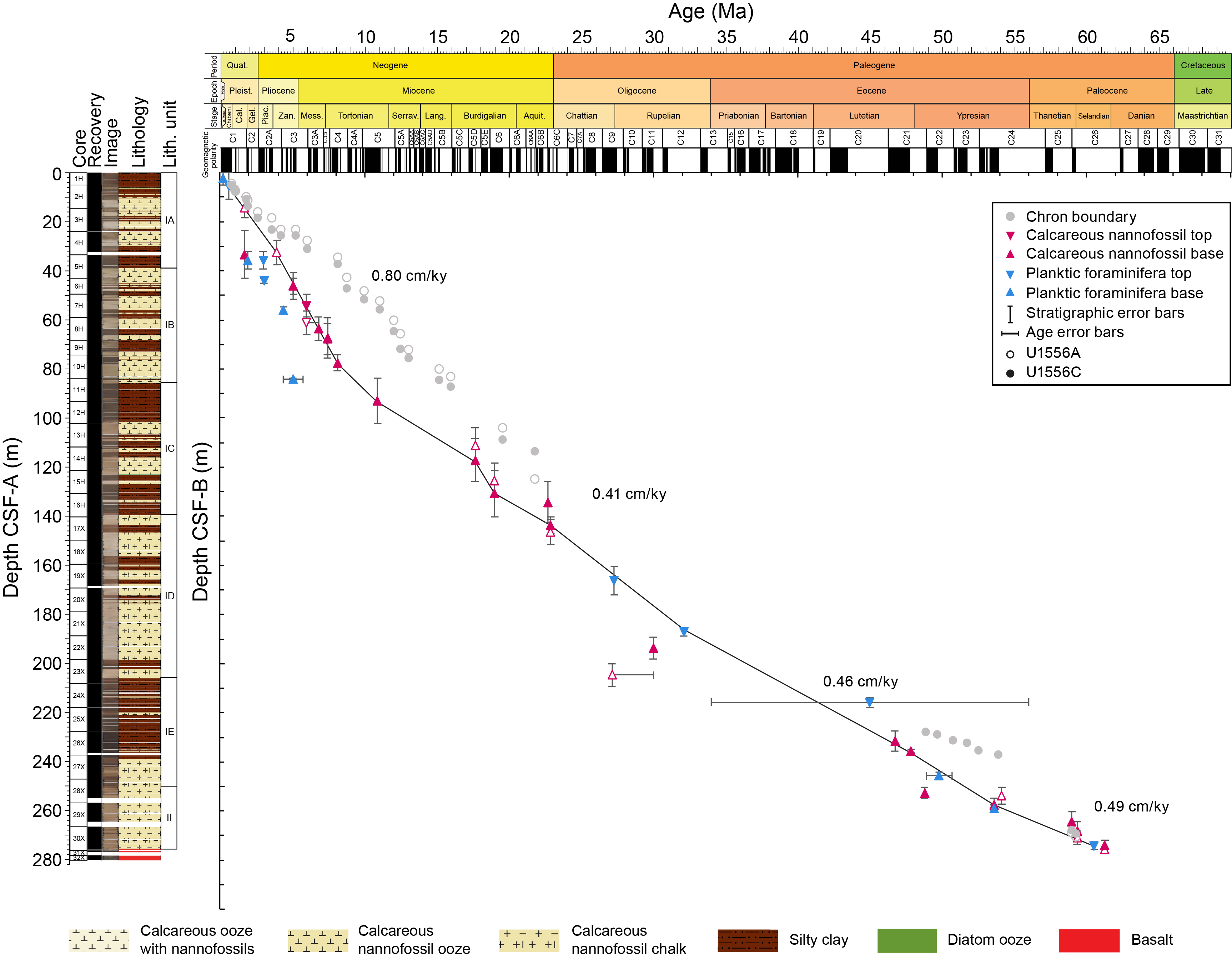
Figure F119. Age-depth model.

Planktic foraminifera and calcareous nannoplankton range throughout the cored interval but tend to be absent or rare and poorly preserved in the pelagic clays that characterize large intervals of Lithologic Unit I (see Sedimentology and Biostratigraphy). Although the nannofossil oozes that make up the dominant carbonate lithology of Unit I are rich in nannoplankton, they tend to contain a depauperate and poorly preserved planktic foraminiferal assemblage composed almost entirely of juveniles or otherwise very small specimens that are not age diagnostic. Preservation and abundance of foraminifera improve and increase in Unit II. Overall, we identified 13 planktic foraminifera and 19 calcareous nannoplankton bioevents. Except for a few datums in the Pliocene–Pleistocene and Oligocene, which mostly occur in intervals of poor preservation, these two fossil group bioevents agree very well with each other (Figure F119).

A total of 29 paleomagnetic reversal datums were identified at Site U1556 and were correlated to the global magnetic polarity timescale based on pattern matching. Nearly all magnetic reversal datums were identified in the uppermost 100 m of the sediments cored at Site U1556. The switch to XCB coring (from Core 390-U1556C-17X) and the associated increase in coring disturbance and reduction in recovery made the recognition of reversal datums below this level (100 m) difficult. Six Eocene datums were identified in the interval of reworking and slumping of Subunit IIA, and two Paleocene reversals were identified directly above the basement.

With the exception of the very top and very bottom of Hole U1556C, there is little agreement between biostratigraphic and paleomagnetic reversal datums, with plankton consistently trending younger (Figure F119). There is as much as a 5 My offset, with Miocene chron boundaries identified in intervals containing plankton that evolved in the Pliocene. However, there are other potential correlations of paleomagnetic reversals in Hole U1556C to paleomagnetic reversal datums in the geologic timescale that would result in magnetostratigraphic ages closer to the biostratigraphic ages. For the purposes of this chapter, we built the age model with biostratigraphic datums, based on the assumption that species occurrences from two separate microfossil groups are unlikely to be consistently millions of years younger than they've been described elsewhere. Below the Eocene/Oligocene unconformity, we rely on microfossils throughout the slumped interval but note that both microfossil groups and magnetic reversal datums are in good agreement with respect to the age of the oldest sediments overlying the basement.

Linear sedimentation rates are low at the top of the hole and decline downhole. Sedimentation rates are highest in the Late Miocene and Pliocene–Pleistocene, averaging 0.80 cm/ky. Overall sedimentation rates average about 0.63 cm/ky in the Neogene and 0.41 cm/ky in the Oligocene. Sedimentation rates remain fairly consistent in the Eocene (0.46 cm/ky) (Subunit IE), and the average slightly increases again to 0.49 cm/ky in the Paleocene (Unit II), although given the large Paleocene/Eocene unconformity and the extensive reworking recognized in this unit (see Biostratigraphy), it is likely that the original pelagic sedimentation rate was much different.

Compared with the adjacent Site U1557 (located ~6.5 km to the east; see Background and objectives; see also Age model and mass accumulation rates in the Site U1557 chapter [Coggon et al., 2024a]), sedimentation rates in the Neogene (0.68 cm/ky) to recent (Unit I) are broadly similar at Site U1556. However, in the Oligocene, Site U1556 has less than half of the sedimentation rate (0.41 cm/ky) of that at Site U1557 (0.87 cm/ky). The difference in sedimentation rates between the two sites increases with age; the Paleocene–Eocene Unit II is very expanded at Site U1557, which has a maximum sedimentation rate of 9.62 cm/ky, nearly two orders of magnitude greater than the 0.49 cm/ky observed in Hole U1556C. This is almost certainly the result of differences in accommodation between the two sites because Site U1557 sits within a fault-bounded basement basin and Site U1556 sits near the top of an adjacent basement high (see Background and objectives).

9.2. Mass accumulation rates

Mass accumulation rates (MARs) for Hole U1556C were calculated using bulk density calculated from gamma ray attenuation (GRA) whole-round core scans (see AGEMODEL in Supplementary material; see also Age model and mass accumulation rates in the Expedition 390/393 methods chapter [Coggon et al., 2024c]). Discrete dry bulk density samples are in good agreement with GRA data (see Physical properties and downhole measurements), but the latter have a much higher resolution. Data presented in Figure F120 are binned at 1 My intervals.

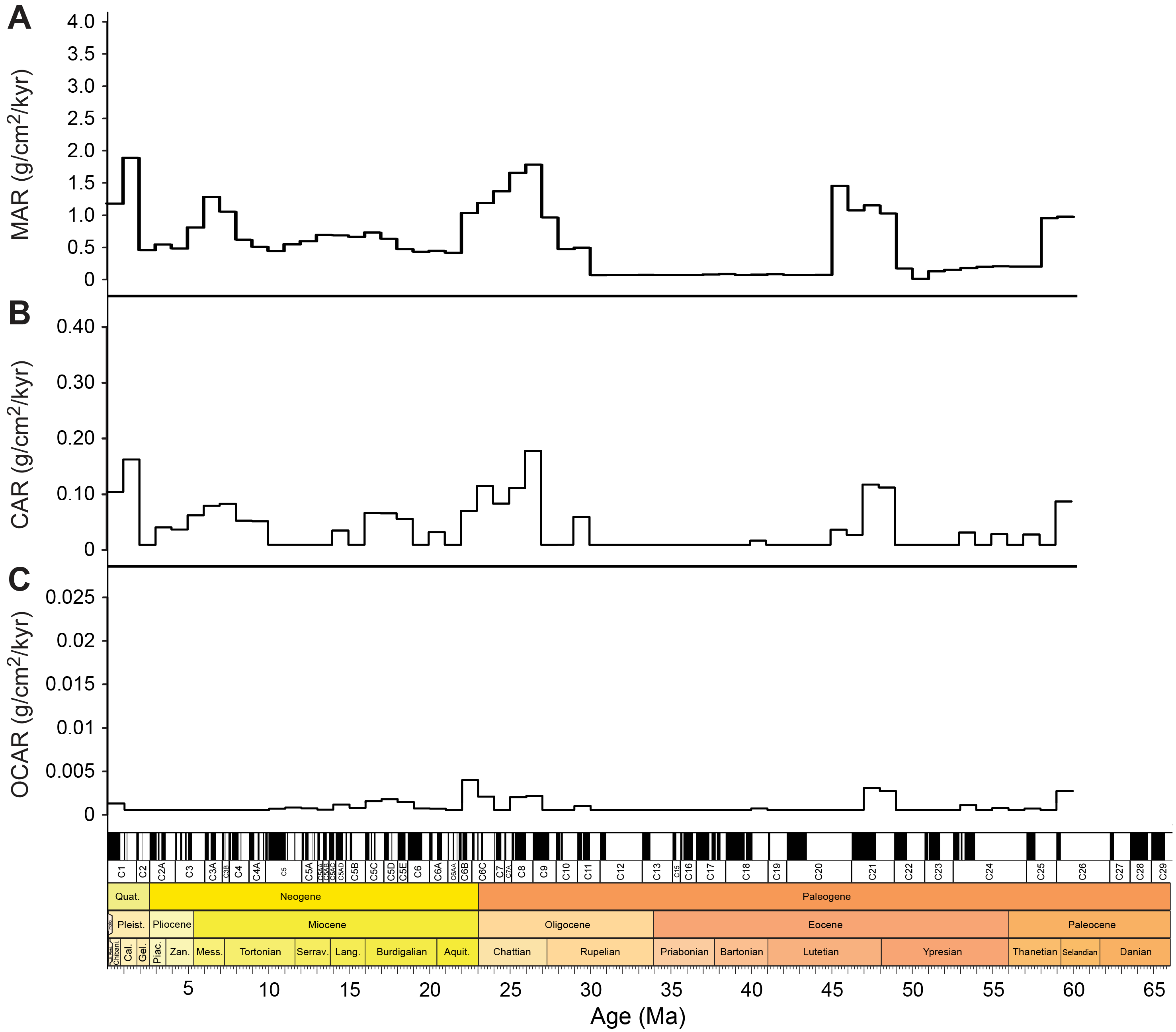
Figure F120. MAR, CAR, and OCAR.

The MAR at Site U1556 is generally highest in the Pleistocene through Oligocene, with peaks in the Pleistocene (1.9 g/cm²/ky), Late Miocene (1.3 g/cm²/ky), and around the Oligocene/Miocene boundary (1.8 g/cm²/ky). Across the condensed interval in the mid- to late Eocene, MAR values are around 0.06 g/cm²/ky. Below the condensed interval, MAR values are more elevated (~1.4 g/cm²/ky) from 45 to 49 Ma, low (0.2 g/cm²/ky) from 49 to 58 Ma, and then relatively elevated again above the top of basement (0.9 g/cm²/ky). Paleocene–Eocene MAR values are all notably lower at Site U1556 than at adjacent Site U1557, reflecting the difference in accommodation between the two sites. MARs during the Paleocene and Eocene at Site U1556 should be viewed cautiously because of the two large unconformities bracketing the Eocene and the extensive reworking and slumped material observed in the middle of this time interval (see Biostratigraphy). Thus, MARs are more reflective of penecontemporaneous downslope reworking than of original pelagic sedimentation.

9.3. Carbonate and organic carbon accumulation rates

Carbonate accumulation rates (CARs) and organic carbon accumulation rates (OCARs) are calculated by multiplying the MAR by the weight percent of carbonate and total organic carbon (TOC), respectively (see AGEMODEL in Supplementary material; see also Age model and mass accumulation rates in the Expedition 390/393 methods chapter [Coggon et al., 2024c]). Carbonate chemistry samples from Hole U1556C were taken from IW squeeze cakes after they were squeezed. To ensure sampling of variable lithologies, at least one additional carbonate chemistry sample was taken from the working half of each core from a different lithology than that sampled in the IW whole-round sample. Bulk density was calculated from GRA measurements collected during Whole-Round Multisensor Logger (WRMSL) scans conducted after the IW whole-round sample was taken from the core. Thus, we do not have carbon and bulk density data from the same interval. Fortunately, every IW sample was taken from the bottom of one of the middle sections of each core, so MAR was interpolated from the adjacent GRA measurements above and below. These measurements were just a few centimeters away from the IW sample (at that scale at Site U1556, bulk density can vary by a few tenths of a gram per centimeter cubed). Measurements with calculated dry bulk density values that were negative (likely the result of measuring a crack or void space) were deleted. The CAR and OCAR data reported are binned at 1 My intervals and are presented in Figure F120.

9.3.1. Carbonate accumulation rates

On a first-order basis, CARs mirror MARs at Site U1556. In Unit I (Oligocene–recent), the CAR varies on several-million-year timescales, matching lithologic changes from pelagic carbonate to pelagic clay. The highest CAR values occur in the Pleistocene (0.09–0.15 g/cm²/ky) and across the Oligocene/Miocene boundary (0.07–0.19 g/cm²/ky), with lower values through the Pliocene (0.03–0.05 g/cm²/ky) and Miocene (0.00003–0.10 g/cm²/ky). The CAR is extremely low in the Eocene–Oligocene condensed interval, which is composed almost entirely of clay, and in the Paleocene/Eocene unconformity.

9.3.2. Organic carbon accumulation rates

The OCAR is extremely low throughout Hole U1556C, despite TOC values that average 0.12 wt%. OCAR values are extremely low in the Neogene, with peak values in the Miocene at 0.003 g/cm²/ky. Oligocene OCAR values are similarly low, with values reaching a maximum of 0.0016 g/cm²/ky. Values reach a maximum off 0.0024 g/cm²/ky in the early Eocene. It is interesting to compare this value with the high OCAR observed at Site U1557, which has a peak near 0.01 g/cm²/ky in this same time interval. Given the differences in sediment thickness between the two sites, the orders of magnitude higher value of OCAR at the thicker Site U1557 may simply be the result of overall sediment accumulation rates. On the other hand, the Site U1557 sediments were buried more quickly than those at Site U1556, which may suggest that preservation potential of organic carbon may play an important role in organic carbon content in this area. Disentangling the respective roles of organic matter production and preservation and sedimentary processes related to erosion and redeposition in controlling organic matter accumulation rates in the South Atlantic Gyre will require detailed postexpedition work.

10. Physical properties and downhole measurements

10.1. Sediment

10.1.1. Physical properties

Physical properties characterization of the sediment sequence at Site U1556 was primarily based on cores from Holes U1556C (Expedition 390) and U1556A (cored during Expedition 390C; Estes et al., 2021) and downhole logging measurements from Hole U1556B (Expedition 390). Physical properties profiles for all three holes extended through the sediment column to basement. The precision and accuracy of physical properties in the uppermost sedimentary section is enhanced by physical properties data from Holes U1556D (1 core) and U1556E (5 cores). Whole-round core section measurements included NGR, GRA bulk density, MS, and compressional wave (P-wave) velocity. Split-core section measurements included discrete sampling of MSP, P-wave velocity, moisture and density (MAD), thermal conductivity (TCON), and shear and compressional strength. Because Hole U1556C had higher core recovery than Hole U1556A and because data from Hole U1556A have very similar characteristics, the Site U1556 sediment data are summarized here with reference to Hole U1556C (Figure F121).

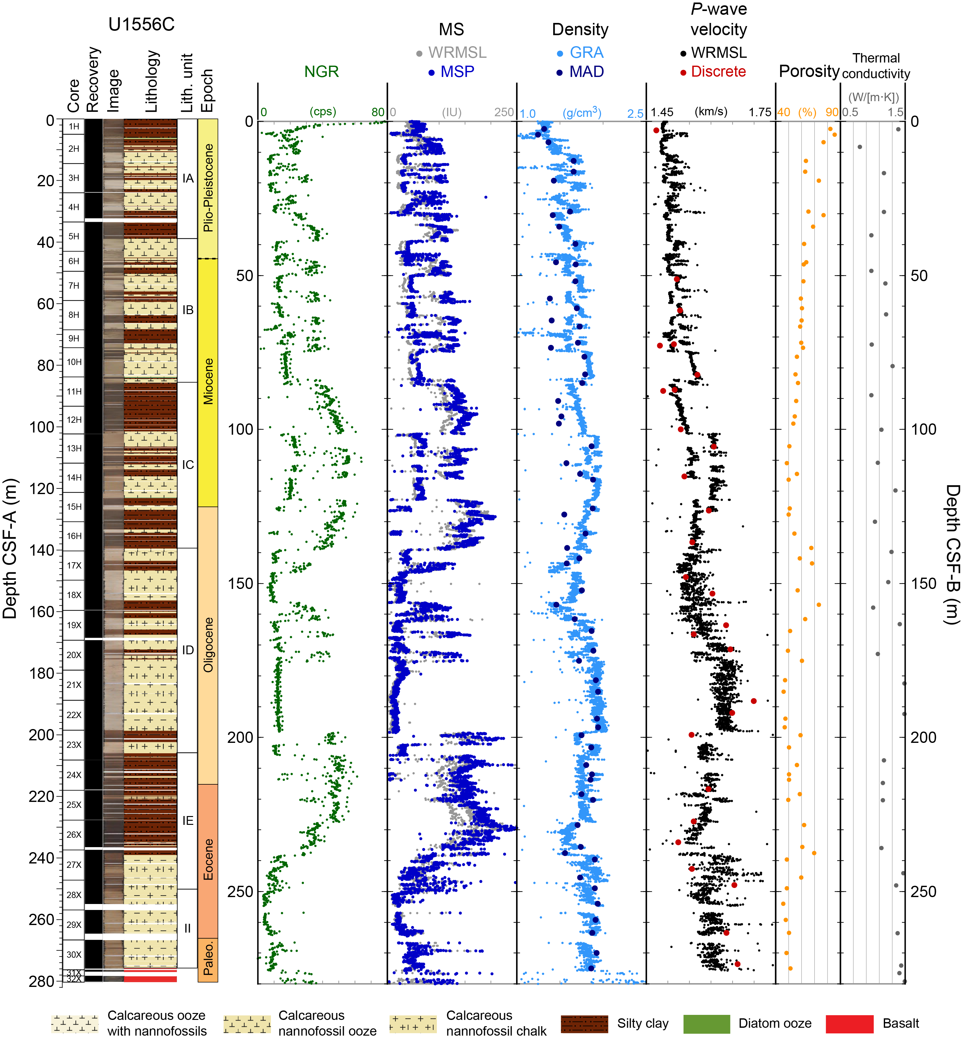
Figure F121. Core physical properties data, Hole U1556C.

10.1.1.1. Natural gamma radiation

NGR was measured at 10 cm intervals on all whole-round core sections that exceeded 50 cm in length; the minimum section length that could be measured was limited by the response function of the sodium iodide detectors (see Physical properties and downhole measurements in the Expedition 390/393 methods chapter [Coggon et al., 2024c]). Each measurement reflects the integration of two separate 5 min counts (i.e., 10 min of counting per section, consisting of 5 min at each of two positions separated by 10 cm). NGR is a proxy for the concentration of radioactive elements (⁴⁰K, ²³⁸U, and ²³²Th) in the cored sediment. NGR data from marine sediments are especially useful in distinguishing clay-rich intervals from clay-poor carbonate ooze intervals (Dunlea et al., 2013).

NGR ranges 0–60 counts/s through the sedimentary section at Site U1556 (Figure F121). The upper ~200 m CSF-B displays an alternating pattern between relatively low (~5–15 counts/s) and high NGR (~35–55 counts/s), which is typical of alternating clay and ooze layers and corresponds to Lithologic Subunits IA–ID described at this site (see Sedimentology) (Figure F122). Between ~200 and 240 m CSF-B, NGR does not alternate consistently but remains more uniformly high at ~50 counts/s, which is typical for the silty clay of Subunit IE. This interval also contains an unconformity or condensed interval of the same duration as that observed in the Hole U1557B sedimentary cores at a similar depth (see Sedimentology and Biostratigraphy, both in the Site U1557 chapter [Coggon et al., 2024a]). Below ~250 m CSF-B to basement (~280 m CSF-B), NGR is more uniformly low, ~10–15 counts/s, which is typical of carbonate ooze.

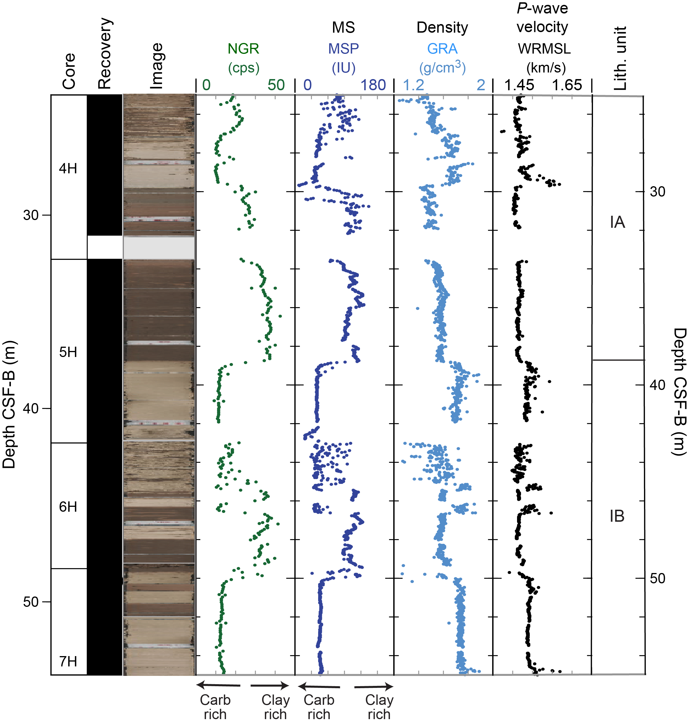
Figure F122. Physical properties, Subunits IA and IB.

10.1.1.2. Gamma ray attenuation bulk density

GRA is defined as the fraction of gamma rays that are not absorbed by a material, and this can be used as an approximation for bulk density. Variations in bulk density can reflect changes in mineralogy, composition, and porosity in the sedimentary section. However, drilling disturbance, expansion cracks, incomplete filling of the core liner, or any other disturbance of the cored sediment can produce spurious values not realistic of marine sediment, which is typically about 1–2 g/cm³, depending on lithology and compaction. No data filtering to remove spurious values was done shipboard. Because spurious GRA data are typically lower than true values, a useful method to reduce the potential influence of spurious data is to consider the upper envelope of the GRA data as a first-order estimate of bulk density and to discount unrealistically low values.

Bulk density from the sedimentary section at Site U1556 (Figure F121) subtly increases from the seafloor to the basement, which is likely a reflection of compaction due to the increasing load of overlying sediments with depth. Because carbonate ooze is denser than silty clay, many of the small-scale variations in bulk density reflect alternations and transitions between silty clay and carbonate layers (Figure F122).

10.1.1.3. Magnetic susceptibility

MS is an indicator of the tendency of minerals to become magnetized upon application of a magnetic field and can be considered an approximation of the concentration of magnetic minerals in the sediment. Similar to NGR, MS from marine sediments is primarily affected by the proportion of clay minerals in the cored material. Higher MS is generally an indication of clay-rich intervals, and lower MS is generally an indication of clay-poor carbonate ooze intervals. MS of cored sediments at Site U1556 was measured using the WRMSL, and MSP was measured on the SHMSL.

Measured MS of the sedimentary section at Site U1556 from both the WRMSL and SHMSL exhibits similar characteristics and variations downhole (Figure F121). Variations in these data can be described using the same depth intervals used to describe variations in NGR, which is intuitive, given both MS and NGR are sensitive to clay content. The upper ~200 m displays an alternating pattern between low values near 0 instrument units (IU) and high values of ~100–150 IU, reflecting the alternations between silty clay and carbonate layers throughout Subunits IA–ID (Figure F122). From ~200 to ~250 m CSF-B, which corresponds to Subunit IE, MS generally increases from 100 to 200 IU and then decreases to ~50 IU. Although some peaks exist, the MS from ~250 m CSF-B to basement is typically low, ~50 IU, characteristic of carbonate ooze.

10.1.1.4. P-wave velocity

P-wave velocity is a measure of the velocity with which a compressional body wave (P-wave) propagates through a sample. P-wave velocity is directly related to the bulk density, compressibility, and shearability of the material. P-wave velocity is indirectly related to the porosity, mineralogy, fabric, or lithology of the material. Shipboard P-wave velocity measurements of the core are especially useful in correlating different scales of data, from regional seismic imaging (at the scale of tens to hundreds of meters) to downhole logs (at the centimeter to meter scale) to core-based data (at the millimeter to centimeter scale).

P-wave velocity measurements made on the split-core sections using the Section Half Measurement Gantry (SHMG) (see Physical properties and downhole measurements in the Expedition 390/393 methods chapter [Coggon et al., 2024c]) are generally more accurate because a measurement location that is not disturbed can be selected. P-wave velocity measurements made on whole-round sections using the WRMSL are more reliable in sediments than in basement, but spurious values still occur. Similar to the GRA measurement, P-wave velocity is adversely affected by drilling disturbance, expansion cracks, incomplete filling of the core liner, or any other disturbance of the cored sediment and produces spurious values not realistic of marine sediment, which should typically be 1.48 to ~1.80 km/s, depending on compaction and lithology. However, spurious P-wave velocities from the WRMSL are typically both higher and lower, and the best approximation of true velocity is to use the clustering of values and disregard any outliers.

Site U1556 sediment P-wave velocities generally increase downhole from ~1.49 km/s at the seafloor to ~1.60 km/s near the basement (Figure F121), which is likely a reflection of compaction due to the increasing load of overlying sediments with depth. Where coring was done using the APC system (Cores 390-U1556C-1H through 16H; <140 m CSF-B), velocity data are less noisy and likely more accurate because APC disturbs the core less than XCB coring. Velocity measurements become noisier below ~140 m CSF-B, where the XCB system was utilized. However, discrete P-wave velocity measurements taken approximately once per core on the SHMG are in close agreement with the general trend of the corresponding WRMSL track data (Figure F121).

10.1.1.5. Thermal conductivity

Thermal conductivity is a measure of the potential for conductive heat flow through a material. Thermal conductivity in sediment and basement is affected by the mineralogy, porosity, density, and fabric of the lithology being measured. Measurements of thermal conductivity help develop an understanding of thermal insulation and heat dissipation processes from the underlying igneous crust through the sediment to the ocean. The thermal conductivity of sediment is an essential parameter required to calculate conductive heat flow through marine sediments from in situ temperature measurements. Representative samples were chosen to reflect the general properties of each core through Holes U1556A and U1556C. A total of 32 discrete measurements were conducted on samples from Hole U1556C and 33 measurements were conducted on samples from Hole U1556A; at least three individual measurements were used to calculate the average thermal conductivity for each sample. The needle probe method of measurement was attempted with whole-round sections of the first uppermost cores of Hole U1556C, but it produced poor and inconsistent results. That method was abandoned in favor of using the puck probe on the working half of the split cores (see Physical properties and downhole measurements in the Expedition 390/393 methods chapter [Coggon et al., 2024c]). Thermal conductivity of the sediment at Site U1556 ranges between 0.8 and 1.5 W/(m·K) and generally increases with depth, from an average of ~1.1 W/(m·K) at the seafloor to ~1.4 W/(m·K) at the bottom of the hole (Figures F121, F123A).

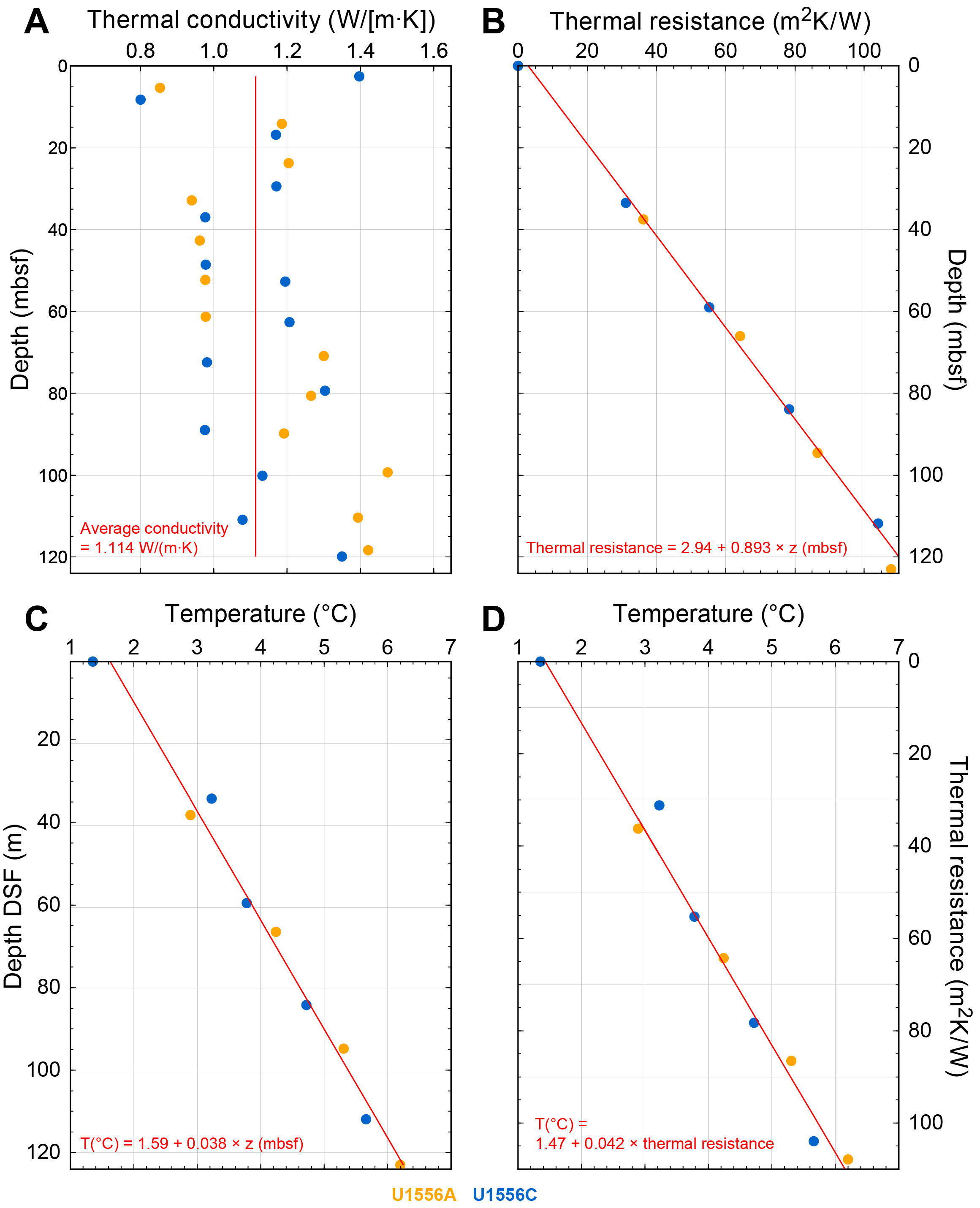
Figure F123. Thermal properties and conductive heat flow.

10.1.1.6. Moisture and density

MAD procedures allow the high-precision, high-accuracy measurement of discrete sample mass and volume that are used to calculate bulk density, grain density, and porosity. Porosity is especially useful for determining the volume of water that can be stored in the interval or lithology represented by the discrete sample. Bulk density is useful for MAR calculations and, in part, controls seismic wave velocity. Grain density is the density of the dry material only (pore space and water content are not considered) and is related to the mineralogy of the sample. A total of 63 discrete samples were taken for MAD analysis, sampled at a typical frequency of two per core and selected to be both generally representative of each core and of the sedimentary lithologies throughout the hole. Broadly, the MAD samples consisted of either silty clay or carbonate ooze, which were the two primary sedimentary lithologies recovered at Site U1556.

Porosity of the sedimentary section at Site U1556 decreases downhole from ~85% at the seafloor to ~50% at 100 m CSF-B, below which porosity remains ~45%–50% to the sediment/basement interface at ~275 m CSF-B (Figure F121). Local variations at ~150 and 230 m CSF-B are likely a product of XCB drilling disturbance. When selecting the specific core intervals to sample for MAD measurements, care was taken to sample the less disturbed biscuit and not the "gravy" (see Sedimentology) in XCB cores, but it is still possible that the XCB coring method artificially introduced water into the samples, thus resulting in slightly higher porosity values. Bulk density measurements of discrete MAD samples generally compare well with the WRMSL GRA data.

10.1.1.7. Sediment strength

Measurements of both shear strength and compressional strength provide estimates of the consolidation, deformability, and stability of marine sediments. The measurements are useful for geotechnical studies of abyssal sediments that may be subject to stress. The shear strength of the sediment, measured at a frequency of one per core from Cores 390-U1556C-2H through 15H, increases from 11.9 kN/m² at 9.90 m CSF-B to 95.3 kN/m² at 129.90 m CSF-B. The sediments became too compact for the automatic vane shear tool below Core 15H, so measurements were not taken at greater depths. The compressional strength of the sediment, measured at a frequency of one per core from Cores 2H–17X, increases from 0.1 kg/cm² at 9.89 m CSF-B to 4.4 kg/cm² at 142.96 m CSF-B. Drilling disturbance in XCB cores made compressional strength measurements far less accurate, so measurements were not taken below Core 17X.

10.1.2. Stratigraphic correlation

Although recovery of sediments during ocean drilling is generally high, gaps in recovery between individual cores are inevitable. To compensate for this loss, multiple sediment holes were cored at Site U1556. Hole U1556A was cored during preliminary engineering Expedition 390C (Estes et al., 2021) (see Background and objectives), whereas three holes were cored during Expedition 390: Holes U1556C, U1556D, and U1556E.

Hole U1556A consists of 33 cores, including 3 cores of the uppermost basement, for a total depth of 283.8 m drilling depth below seafloor (DSF), with recovery of 86%. Hole U1556C consists of 32 cores collected to a total depth of 280.3 m DSF, with recovery of 101%, including the recovery of the sediment/basement interface at 275.7 m DSF. The additional Holes U1556D and U1556E were drilled to allow further geochemical and microbiological analyses because the uppermost cores from Hole U1556C experienced severe drilling disturbance (see Operations). Hole U1556D failed to recover the mudline; Hole U1556E consisted of 5 cores for a total depth of 43.1 m DSF.

For the first core in Hole U1556C, the bit was positioned at 5 m above the predicted seafloor to attempt to recover material across core breaks and cover gaps present in Hole U1556A (see Operations). Coring operations for Hole U1556C were guided by comparing MS and GRA bulk density track data, acquired using the Special Task Multisensor Logger (STMSL) on thermally unequilibrated cores from Hole U1556C, with the same data set from Hole U1556A (see Physical properties and downhole measurements in the Expedition 390/393 methods chapter [Coggon et al., 2024c]). This preliminary correlation allowed us to advise drillers on subsequent drill bit advancement, which was useful to close the core gaps between holes.

For a given core (n) from Hole U1556C tied to a core (y) in Hole U1556A, a broad y = n − 1 correlation was established, with an offset of ~1 m sufficient to cover core gaps in Hole U1556A until 53.2 mbsf (Figure F124). Afterward, a decision was made to pull back 3 m before the next core. This pullback resulted in several meters of heavily disturbed fall-in deposits in the upper 2.8 m of Core 390-U1556C-6H (see Sedimentology) and failed to increase the offset to the desired amount. A second, successful attempt to increase the offset was made by pulling the bit back 4 m when shooting Core 390-U1556C-9H, resulting in a short 5 m advance, again overlain by 2.7 m of fall-in debris. This offset, combined with the high recovery in Hole U1556C, resulted in covering all core gaps in Hole U1556A until Core 390-U1556C-18X. The XCB coring system does not allow adjustment of the drill bit advance, so breaks in recovery remain below Core 390-U1556C-18X, particularly in intervals where recovery is low, as is the case in Hole U1556A. XCB coring of sediment in Hole U1556C had a notably higher recovery (95%) compared to the 66% recovery for XCB coring of sediment in Hole U1556A. This improved recovery resulted in coverage across previous gaps through the lower portion of the sediment succession that could not be cored with the APC system.

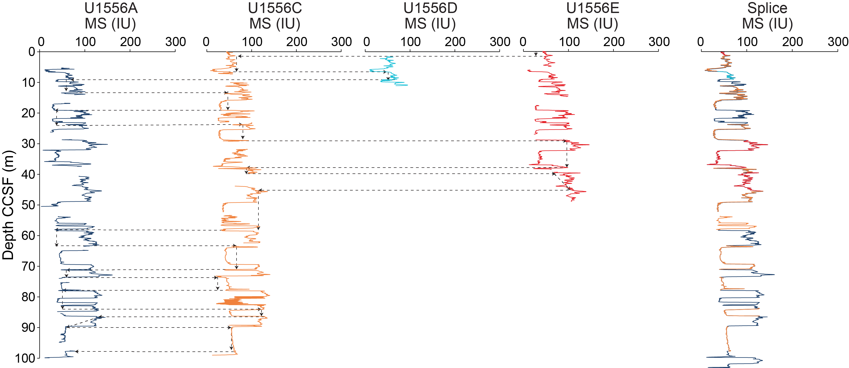
Figure F124. 0–100 m CCSF composite depth scale and splice.

10.1.2.1. Correlation and splice

Physical properties data from Holes U1556A, U1556C, U1556D, and U1556E were correlated to establish a core composite depth scale below seafloor (CCSF) at Site U1556 (see Table T22). Physical properties data correlated well between Holes U1556A and U1556C throughout the interval cored using the APC system and in the upper two XCB cores in Hole U1556C (Cores 390-U1556C-17X and 18X). This resulted in a near-continuous spliced record to 195.6 m CCSF (Figures F124, F125). Although Hole U1556D did not recover a definitive mudline, the recovered sediments in Core 390C-U1556D-1H show log trends similar to those in Core 390C-U1556A-1H (Figure F124). Furthermore, Core 390-U1556E-1H recorded the same stratigraphy as the upper part of Core 390-U1556C-1H, and subsequent cores in Hole U1556E correlated well with those from both Holes U1556A and U1556C. Hole U1556E recorded a unique stratigraphy spanning the coincident core gaps in Holes U1556A and U1556C at ~40 m CCSF, filling a previous gap in an earlier iteration of the shipboard splice for Site U1556. As a whole, the four holes correlate in the upper ~50 m (Figure F124; Table T23), improving upon initial correlations made using only Holes U1556A and U1556C.

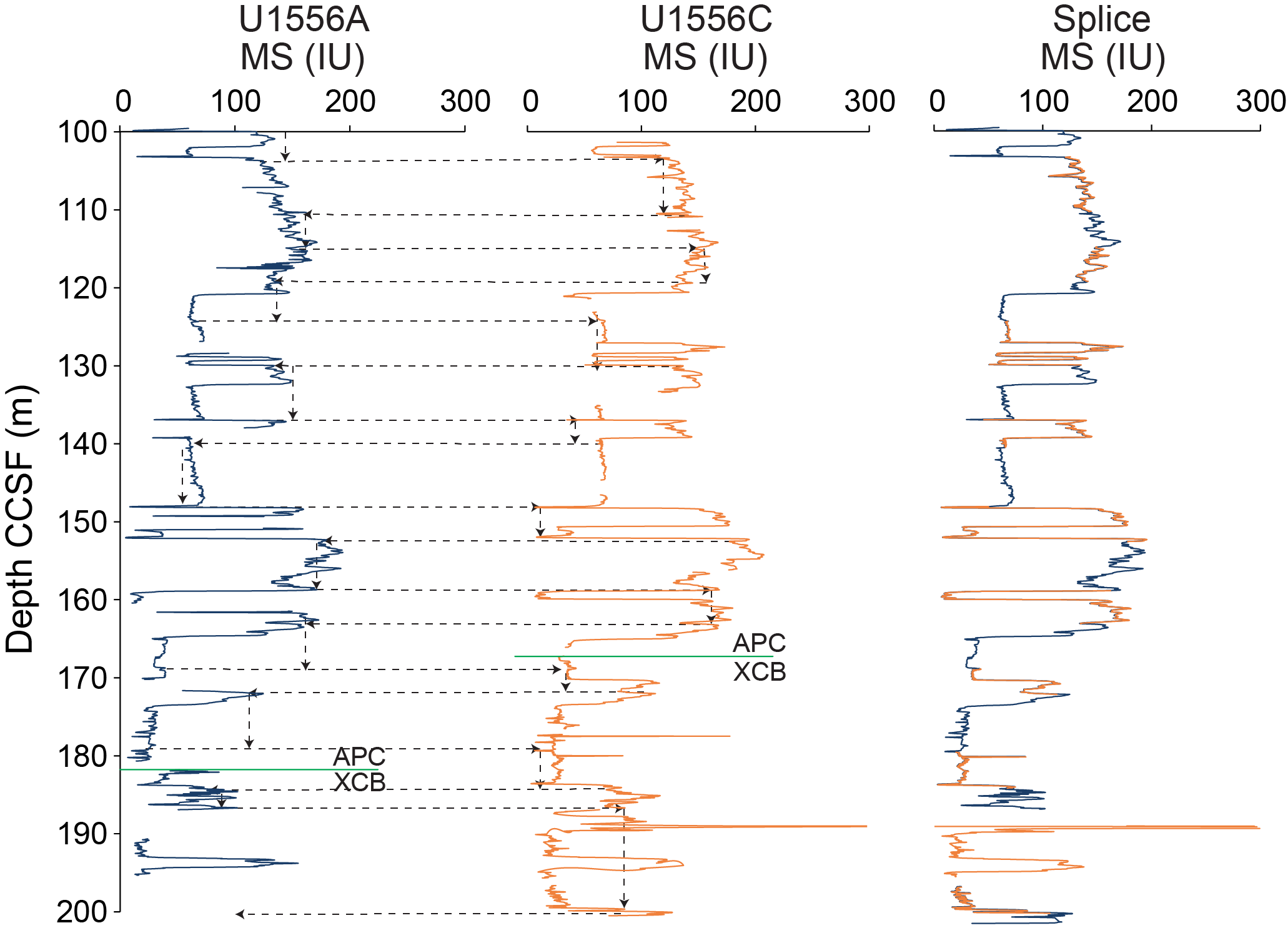
Figure F125. 100–200 m CCSF composite depth scale and splice.

Below ~50 m CCSF (i.e., deeper than the bottom of Hole U1556E), the splice consists only of cores from Holes U1556A and U1556C (Figures F124, F125, F126). Small gaps (up to 0.5 m) exist in the shipboard splice until the switch from APC to XCB in Hole U1556A at ~180 m CCSF. Below ~195.6 m CCSF, larger (up to 10 m) core gaps between Holes U1556A and U1556C routinely coincide as a consequence of the lower recovery associated with the XCB system compared to the APC system, especially in Hole U1556A. Cores 390C-U1556A-20X and 21X were difficult to correlate with any confidence to Hole U1556C because of low variability in physical properties data through this relatively homogeneous carbonate interval in Subunit ID (see Sedimentology). Below this interval, stratigraphies are well correlated until the tie point correlating Core 390C-U1556A-25X to Core 390-U1556C-27X (~266 m CCSF). Below 275.5 m CCSF, the correspondence between the physical properties of the material recovered from the two holes declines and it is difficult to confidently correlate them, except for the correlative stratigraphy of Sections 390C-U1556A-29X-5 and 390-U1556C-30X-3, just above basement (Figure F126).

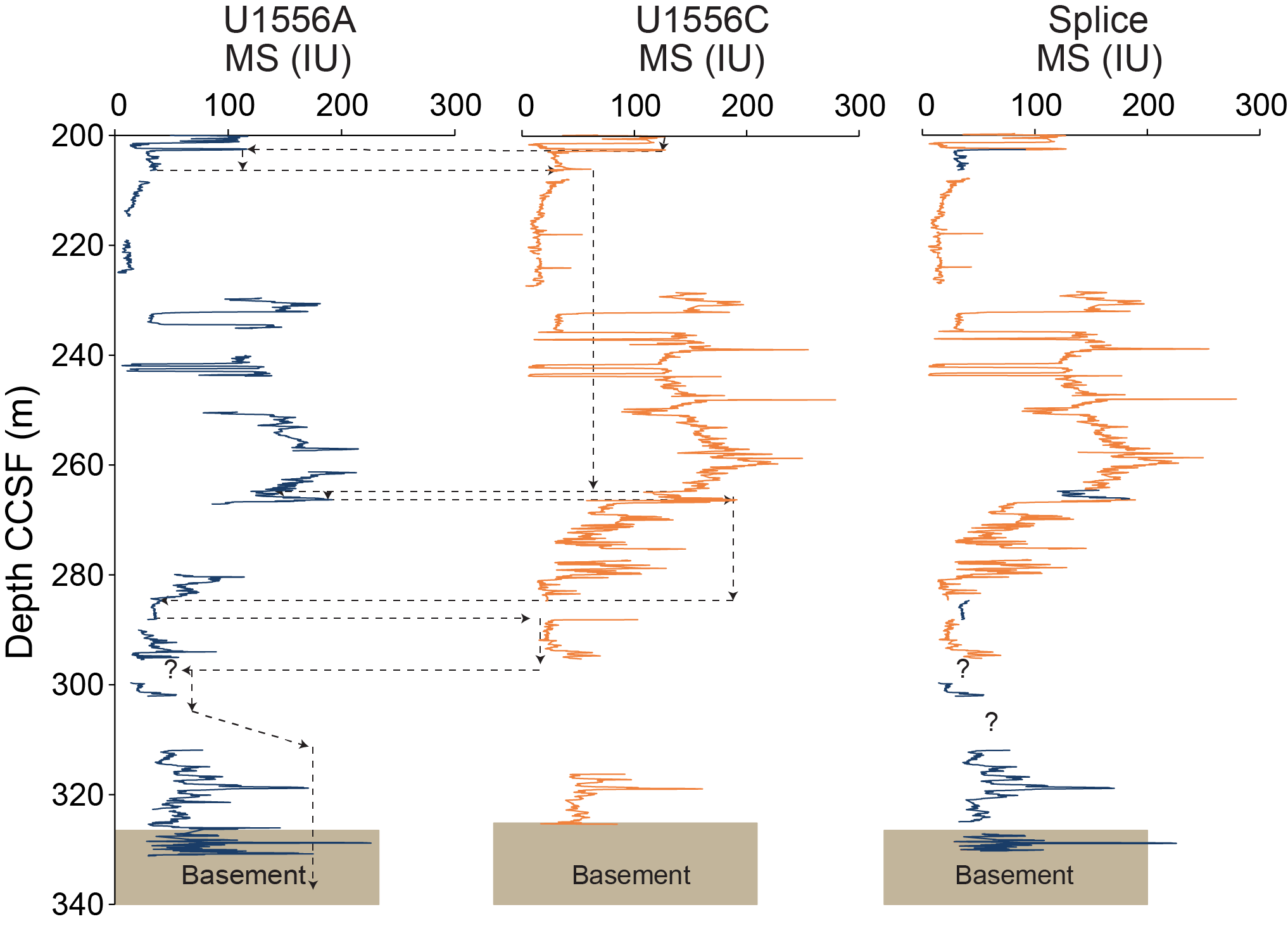
Figure F126. 200–340 m CCSF composite depth scale and splice.

10.1.3. Wireline logging and downhole measurements

10.1.3.1. Downhole temperature

During APC coring in both Holes U1556A (during Expedition 390C) and U1556C (Expedition 390), an APCT-3 tool was used to measure in situ formation temperature at selected depths downhole, typically ~30 m apart. Before the first APCT-3 measurement in each hole, the probe was suspended several meters above the seafloor for 5 min to equilibrate the sensor to ambient bottom water conditions, allowing an estimation of the seafloor (or mudline) temperature. Downhole measurements were then taken with Cores 4H, 7H, 10H, and 13H by shooting the core barrel and waiting 10–15 min for the sensor to record the formation temperature before the core was retrieved. Temperature measurements were taken at similar depths in both holes (Table T24; Figure F127). The records show that the probe remained steady during most deployments in Hole U1556A, whereas most records in Hole U1556C indicate some disruption. However, all deployments included long enough stable intervals of thermal recovery to derive robust fits to theoretical models and derive reliable formation temperature data. Data from the two holes, along with an estimated mudline temperature (1.35°C), suggest a geothermal gradient of 38°C/km for Site U1556 (Figure F123C).

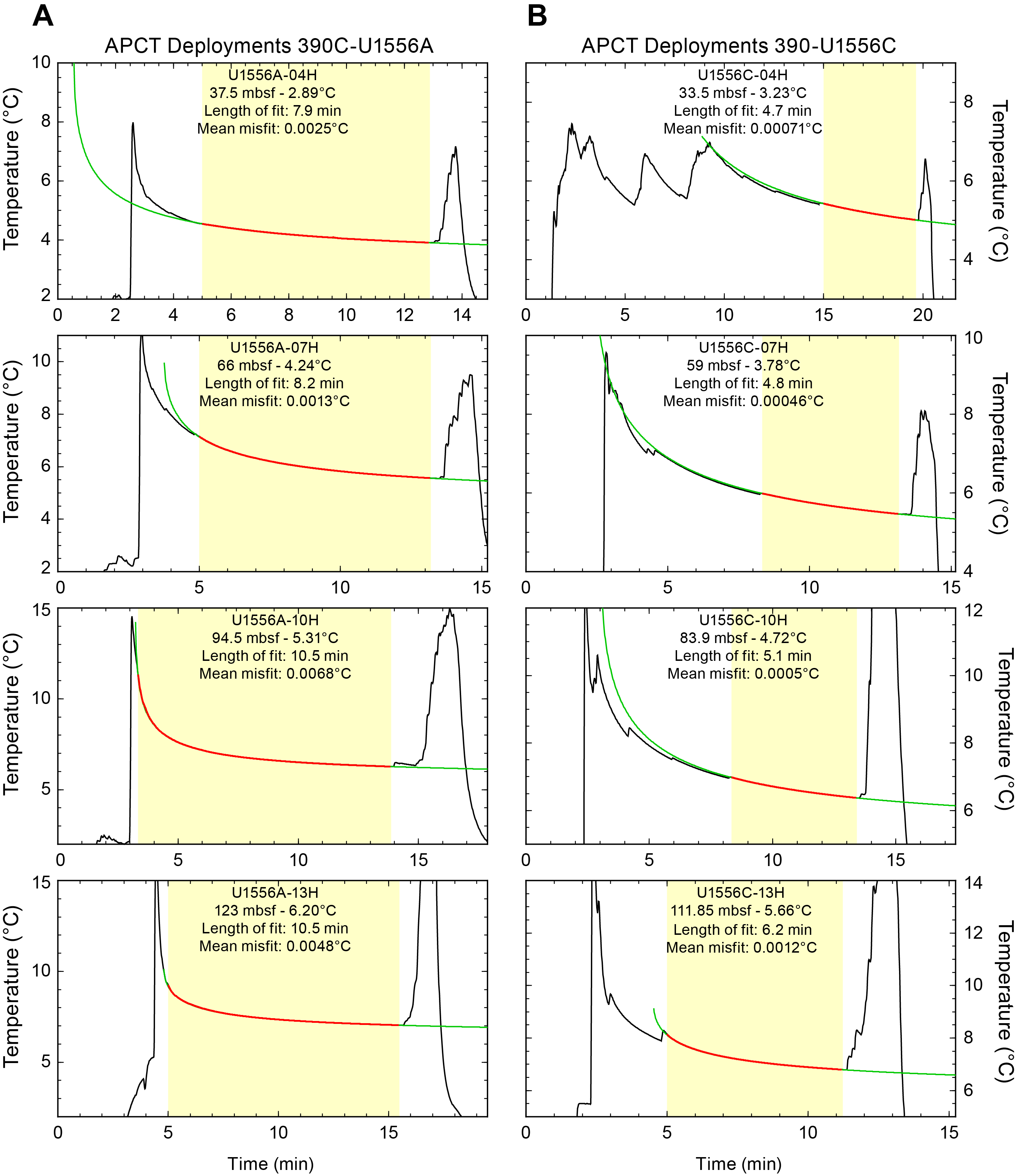
Figure F127. APCT-3 temperature.

10.1.3.2. Heat flow

A simple estimate of the vertical conductive heat flow (42 mW/m²; Table T25) can be made by the product of the geothermal gradient of 38°C/km for Site U1556 with the mean thermal conductivity (1.11 W/[m·K]; Figure F123) measured on the cores recovered through this interval.

Another method of calculating conductive heat flow for Site U1556 can be established using thermal conductivity measurements to calculate the thermal resistance and plotting this versus depth for each hole (Figure F123A, F123B). This allows thermal resistance to be calculated at depths coincident with the temperature measurements made during APC coring (see Physical properties and downhole measurements in the Expedition 390/393 methods chapter [Coggon et al., 2024c]). The intercept (T₀) of a linear trend on a plot of temperature versus thermal resistance, known as a Bullard plot (Pribnow et al., 2000) (Figure F123D), is the temperature at depth 0 m in the sediment succession (i.e., at the seafloor). The heat flow estimate, defined by the slope of the least-squares linear fit to the temperature data as a function of thermal resistance, is 42 mW/m² for Site U1556, the same as the simple estimate above. Tables T24 and T25 summarize these data and calculated results.

10.1.3.3. Logging operations

Logging operations for Site U1556 began after the completion of RCB coring in Hole U1556B to 633.2 m DSF on 4 May 2022. In preparation for logging, a heavy mud sweep was circulated through the hole, the RCB bit was released at the bottom of the hole, and the hole was filled with seawater (see Operations). The drill pipe was raised to 41 m DSF for logging. Sea condition was high, with average heave of ~3 m; the wireline heave compensator was used for the entirety of the logging operations.

In Hole U1556B, the sedimentary section was cased during Expedition 395E to ~5 m above basement (Williams et al., 2021) (see Background and objectives). The primary target of wireline logging during Expedition 390 was the open hole below 293 mbsf, predominantly in the Site U1556 basement. However, the gamma ray wireline logging tool received adequate signal through casing below the depth of the pipe during logging operations to record spectral gamma ray data from the sedimentary formation. Gamma ray data from wireline logging operations in Hole U1556B provide information on the nature of the sediments that can be correlated with properties of the sediment cores from Hole U1556C. However, logs recorded through casing were used primarily qualitatively because of the attenuation of the incoming signal. Full detail on wireline logging operations and basement results are provided in the basement section for Site U1556 (see Wireline logging in Basement).

10.1.3.4. Logging data through casing

Gamma ray logs recorded the contributions from U, K, and Th to the total gamma ray signal through the cased interval of sediments in Hole U1556B. These logs reflect changes in sediment properties including the distinct alternations in lithology between silty clay and nannofossil ooze/chalk that is likely the primary sedimentary characteristic affecting both in situ and core physical properties data at Site U1556. Silty clay layers have higher NGR relative to the carbonate-rich intervals (Figure F128). The pattern of alternating higher and lower gamma ray from downhole logging is also seen in physical properties measurements of cores from Holes U1556A (Estes et al., 2021) and U1556C (Figure F121). This similarity enables the downhole gamma ray logs from Hole U1556B to be correlated to the core data from Hole U1556C after adding a slight depth offset on the order of a few meters (Figure F128). Discrepancies between the drilling core depth and wireline logging depth may occur because of core expansion, incomplete core recovery, incomplete heave compensation, wireline stretch, drill pipe stretch, and tidal changes.

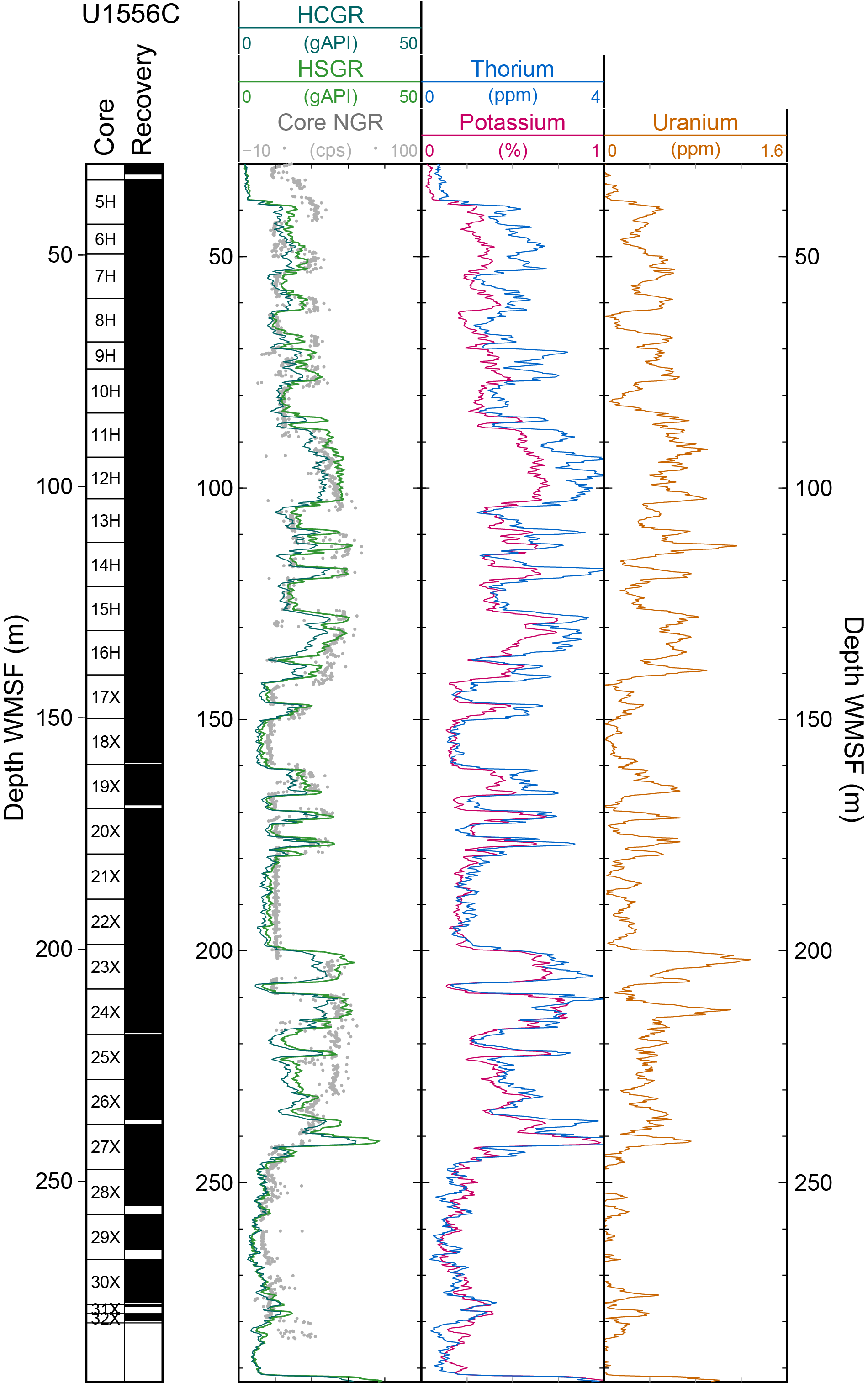
Figure F128. NGR logs recorded in casing.

The lithologic unit and subunit boundaries that generally correspond to significant changes in core physical properties data are also clearly evident in the gamma ray log data. There is strong agreement between core and logging gamma ray data recorded within the cased interval, below the depth at which the drill pipe was set (39–216 m WMSF). Below this depth, the gamma ray log also shows clearly defined intervals of higher and lower gamma ray, consistent with the presence of alternating silty clay and ooze/chalk, respectively (see Sedimentology), to 245 m WMSF, whereas the core data are somewhat noisier in this interval (Figure F128). Below 245 m WMSF, gamma ray decreases significantly, consistent with the carbonate-dominated interval described in cores. Several local peaks in gamma ray logging data at 277–279 m WMSF may correspond to the first appearances of basalt in Hole U1556B. These local peaks in Hole U1556B occur at a similar depth as and are consistent with the elevated gamma ray measured in cores that recovered the first basalt intervals in Hole U1556C (Cores 390-U1556C-31X and 32X; see Figure F121). The return to lower gamma ray below 280 m WMSF at the base of the cased interval suggests an additional interval of carbonate-rich sediment before the appearance of significant basement intervals, which is further described in Basement.

Spectral data from the gamma ray logging tool show variations in the relative contributions of the radioactive isotopes of U, K, and Th to the total gamma ray signal (Figure F128). At Site U1556, the total gamma ray signal comes mostly from the radioactive isotopes of potassium, with additional contributions from thorium throughout the logged sedimentary section. Thorium is a trace element typically associated with clays and heavy minerals, and spectral gamma ray data show relatively higher contributions from thorium in the more clay-rich intervals of the sedimentary section (see Sedimentology). There is also a contribution from uranium in the higher gamma ray intervals, which may be associated with higher organic carbon in silty clay layers.

10.1.4. Data integration

10.1.4.1. Lithologic unit correlations

The physical properties data show distinct changes and character at Site U1556 that correspond closely to the lithologic units defined based on visual core descriptions (see Sedimentology). Similar lithologic units were observed in the upper half of the more thickly sedimented Site U1557 (see Sedimentology in the Site U1557 chapter [Coggon et al., 2024a]), located ~6.5 km east of Site U1556 on similar age crust (see Background and objectives). Consequently, the Site U1556 sediment physical properties between 0 and ~250 m CSF-B are similar to the physical properties of the upper portion (above ~290 m CSF-B) of the sediment section cored at Site U1557.

10.1.4.2. Density and porosity versus lithology

Because of the alternating carbonate and silty clay layers at Site U1556, the discrete MAD samples taken at a frequency of two per core from representative lithologies often resulted in one MAD sample from a carbonate ooze and one MAD sample from a silty clay for each core. Shipboard analyses of bulk density versus porosity and bulk density versus grain density reveal distinct trends within the overall data set (Figure F129). Comparing bulk density to porosity shows the expected anticorrelation of higher porosity with lower bulk density (Figure F129A). However, two populations are present that display different trends toward the 100% porosity/1.0 g/cm³ density origin of pure water. The difference is likely not related to variable drilling disturbance from different coring methods given that cores sampled using the less disruptive APC system are present in both populations (Figure F129B). Furthermore, comparing bulk density to grain density also shows two or possibly three distinct populations that have different bulk density versus grain density relationships (Figure F129C, F129D). The difference in populations is a product of different grain densities in the MAD samples of silty clay, which suggests multiple, different silty clay compositions are present at Site U1556.

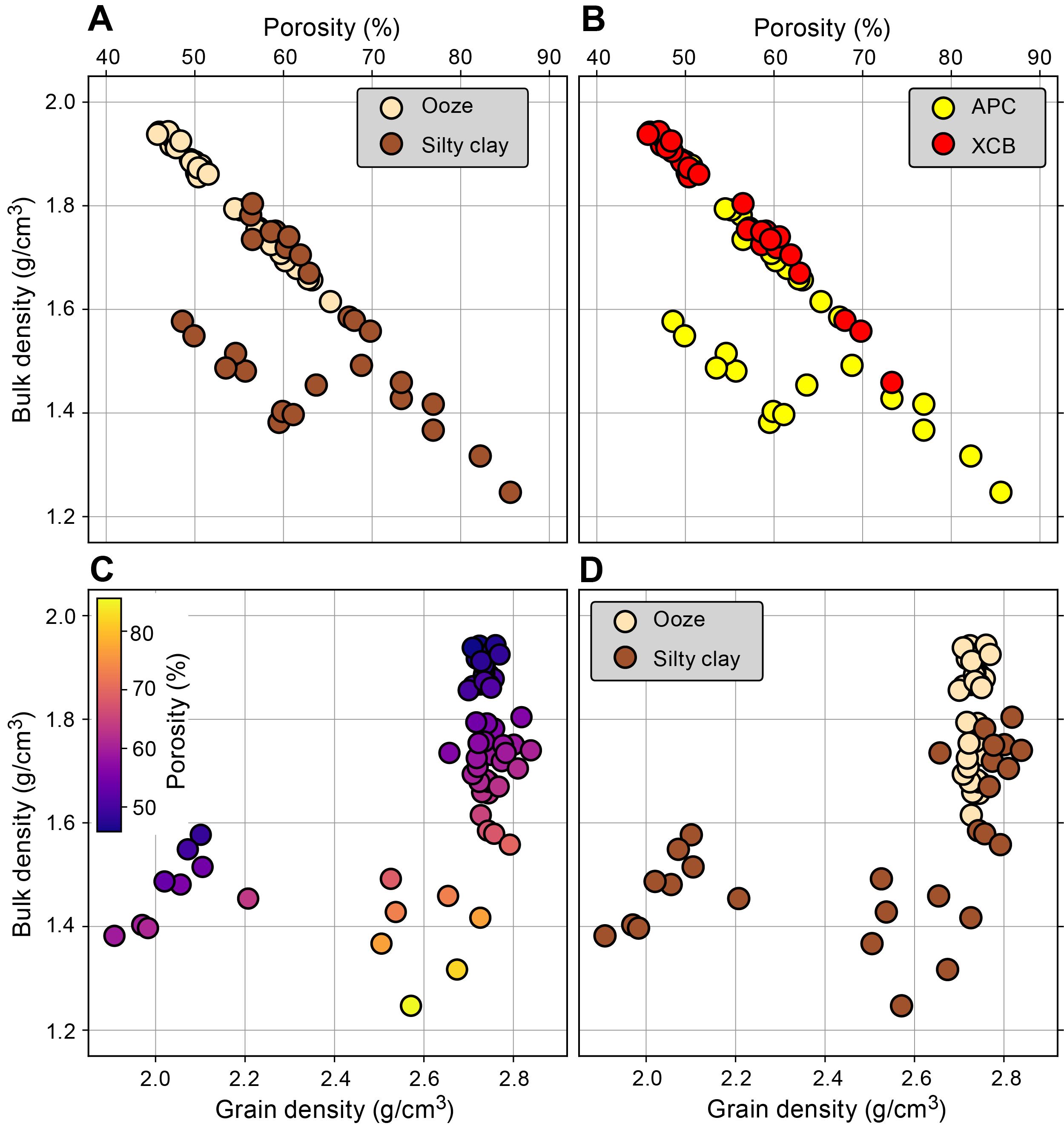
Figure F129. MAD sediment analyses, Hole U1556C.

10.1.4.3. Heat flow and hydrothermal circulation

Based on the relationship between predicted average global conductive heat flow through the ocean crust as a function of its age from cooling plate models (e.g., Stein and Stein, 1994), oceanic crust formed at ~60 Ma would be expected to have a conductive heat flow of ~80 mW/m². For crust younger than 64 Ma, the measured conductive heat flow is typically lower than that predicted using the cooling plate model, which assumes all heat loss from the aging crust is lost through conduction. The discrepancy between these values is ascribed to the advective removal of heat via hydrothermal circulation (Stein and Stein, 1994; Alt, 1995). The basement at Site U1556 formed at ~61.2 Ma (see Background and objectives), so its age is near the sealing age when the global average measured conductive heat flow and modeled heat flow become equal (see Background and objectives). The heat flow of 42 mW/m² is at least ~35 mW/m² lower than would be expected from crust of this age.

10.2. Basement

10.2.1. Physical properties

Physical properties characterization in the basement section at Site U1556 was based primarily on cores from Hole U1556B drilled during Expedition 390. Whole-round core section measurements included NGR, GRA bulk density, and MS. Full-circumference, true color images of whole-round core exteriors were recorded with the DMT CoreScan3 system prior to splitting. Archive halves of all split core sections were also measured for MSP and color reflectance (see Sedimentology). A total of 77 discrete rock cubes were cut for P-wave velocity and MAD measurements. Most of these discrete samples were also used for paleomagnetic measurements (see Paleomagnetism). Nondestructive thermal conductivity measurements were made on representative samples (individual pieces) from split cores. Generally, all physical properties data consistently reflect macroscopic lithologic variations in the igneous stratigraphic units defined for Site U1556 (Figure F130; see Igneous petrology).

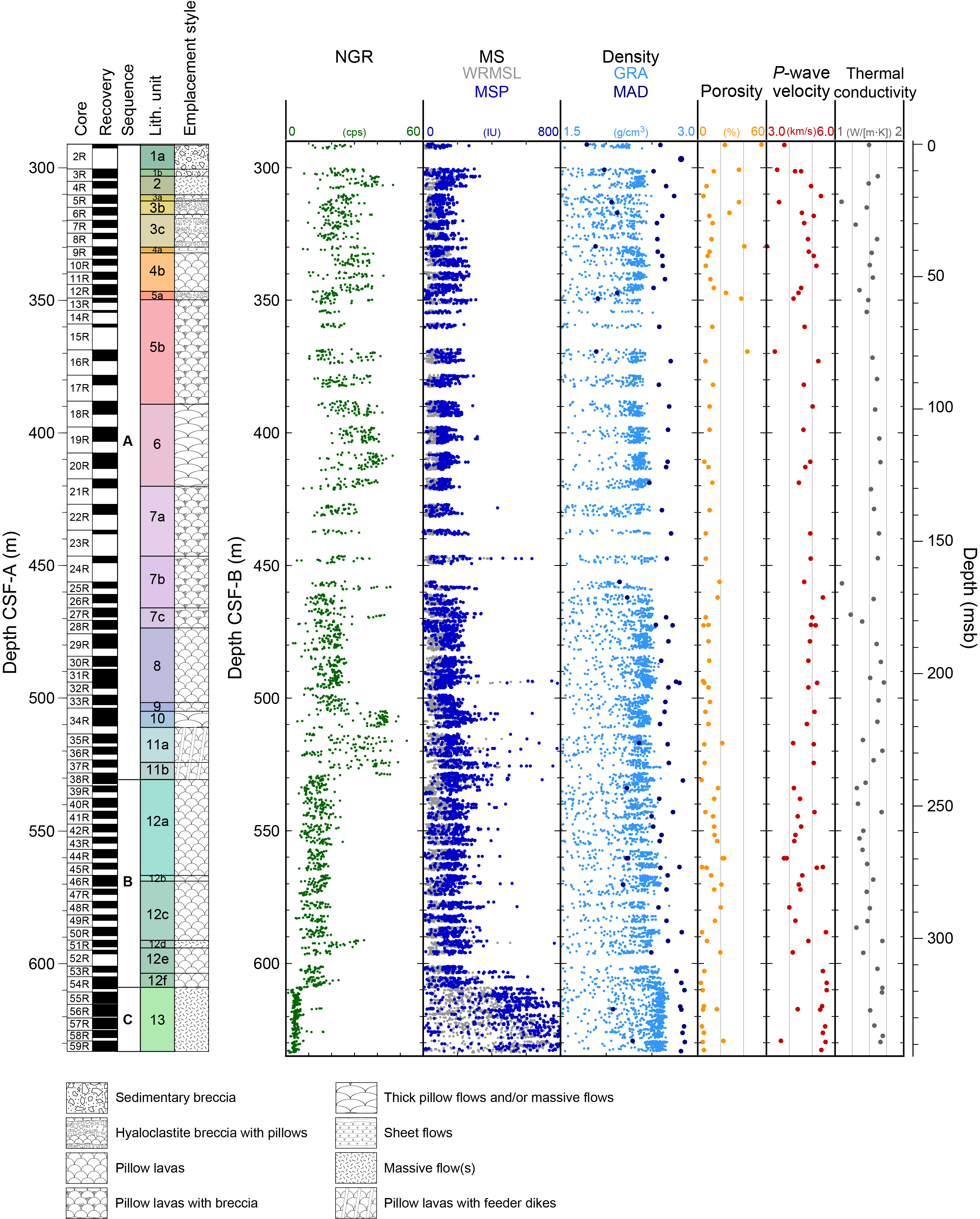
Figure F130. Core physical properties, Hole U1556B.

10.2.1.1. Natural gamma radiation

NGR serves as an estimate of the variability in concentration of radioactive elements (⁴⁰K, ²³⁸U, and ²³²Th). Because radioactive element concentrations are generally low in the upper oceanic crust, potassium added via secondary mineral precipitation is likely to be the main component in the NGR variability (Alt, 1995). Assuming that is the case, NGR can serve as a proxy for alteration of the oceanic crust (Bartetzko et al., 2001). NGR was measured at 10 cm intervals on all whole-round core sections that exceeded 50 cm in length; the minimum section length that could be measured was limited by the response function of the sodium iodide detectors (see Physical properties and downhole measurements in the Expedition 390/393 methods chapter [Coggon et al., 2024c]).

NGR ranges 0–53 counts/s in Hole U1556B (Figure F130) and shows high-frequency variability above 472 m CSF-B (181 msb). NGR data are limited by incomplete core recovery throughout this interval, and low values are most likely associated with breaks between core pieces and/or individual pieces with diameters significantly smaller than the interior core liner, which suggests the interval may be best represented by the high values. Despite these possible data limitations, the interval of high variability corresponds well to the uppermost igneous basement stratigraphic sequence at the site, an olivine phyric pillow basalt unit with interpillow hyaloclastite layers (Stratigraphic Sequence A [orange spotty]; see Igneous petrology). Olivine phenocrysts in these basalts have been highly to completely altered and replaced by iddingsite, carbonate, and to a lesser extent saponite (see Alteration petrology) that are likely the source of higher NGR throughout this unit. Between 472 and 504 m CSF-B (181–213 msb), the range of values narrows and the maximum value decreases to <30 counts/s. A sharp increase in the maximum values occurs at 504 m CSF-B (213 msb); between 504 and 530 m CSF-B (213–239 msb), the data span the full range of variability seen in Hole U1556B. At 530 m CSF-B (239 msb), mean NGR abruptly decreases and the range of values narrows (to 7–25 counts/s). This NGR character extends to 608 m CSF-B (317 msb) throughout an interval that coincides with the presence of the aphyric to sparsely olivine phyric old red basalt (Stratigraphic Sequence B; see Igneous petrology). The olivine phenocrysts in this highly altered unit have been replaced by secondary minerals including iddingsite and clays such as saponite, and the groundmass of the basalts has altered to clays and Fe oxyhydroxides (see Alteration petrology). From 608 m CSF-B (317 msb) to the base of the drilled section, NGR decreases sharply (0–16 counts/s). This interval of low NGR corresponds to the appearance of the H-POPP basalts that comprise the lowermost igneous stratigraphic unit at Site U1556 (Lithologic Unit 13/Stratigraphic Sequence C; see Igneous petrology). Although these H-POPP basalts are moderately altered and contain small vesicles filled with secondary clay minerals, the NGR response is distinctly low, suggesting that radioactive element–bearing clay minerals are a small fraction of the total material.

10.2.1.2. Gamma ray attenuation bulk density

Variations in bulk density can reflect changes in mineralogy, composition, and porosity within basement units. A caveat to the GRA bulk density is that missing pieces, edge effects of binned pieces, incomplete filling of the core liner, or any other interruption of cored basement can produce spurious values not representative of oceanic crust, which should typically be between ~2.0 and ~3.3 g/cm³, depending on mineralogy and porosity. No data filtering to remove spurious values was done shipboard. Because spurious GRA data points are typically lower than true values, a useful method to reduce the potential influence of spurious data is to consider the upper envelope of the GRA data as a first-order estimate of bulk density and to discount low values (see Physical properties and downhole measurements in the Expedition 390/393 methods chapter [Coggon et al., 2024c]).

Bulk density measurements from the WRMSL range from 1.0 to ~2.7 g/cm³ in the basement material cored in Hole U1556B (Figure F130). Values <1.0 g/cm³ were considered erroneous because they were lower than seawater density (1.03 g/cm³). Between 0 and ~317 msb, most of the bulk density measurements cluster between 2.2 and 2.4 g/cm³; the high variability in the data masks any more detailed downhole trends. Below 317 msb, bulk density subtly increases to 2.3–2.7 g/cm³. This increase in bulk density is coincident with and likely reflective of the petrologic change to the Unit 13 H-POPP basalts (Stratigraphic Sequence C; see Igneous petrology) (Figure F131).

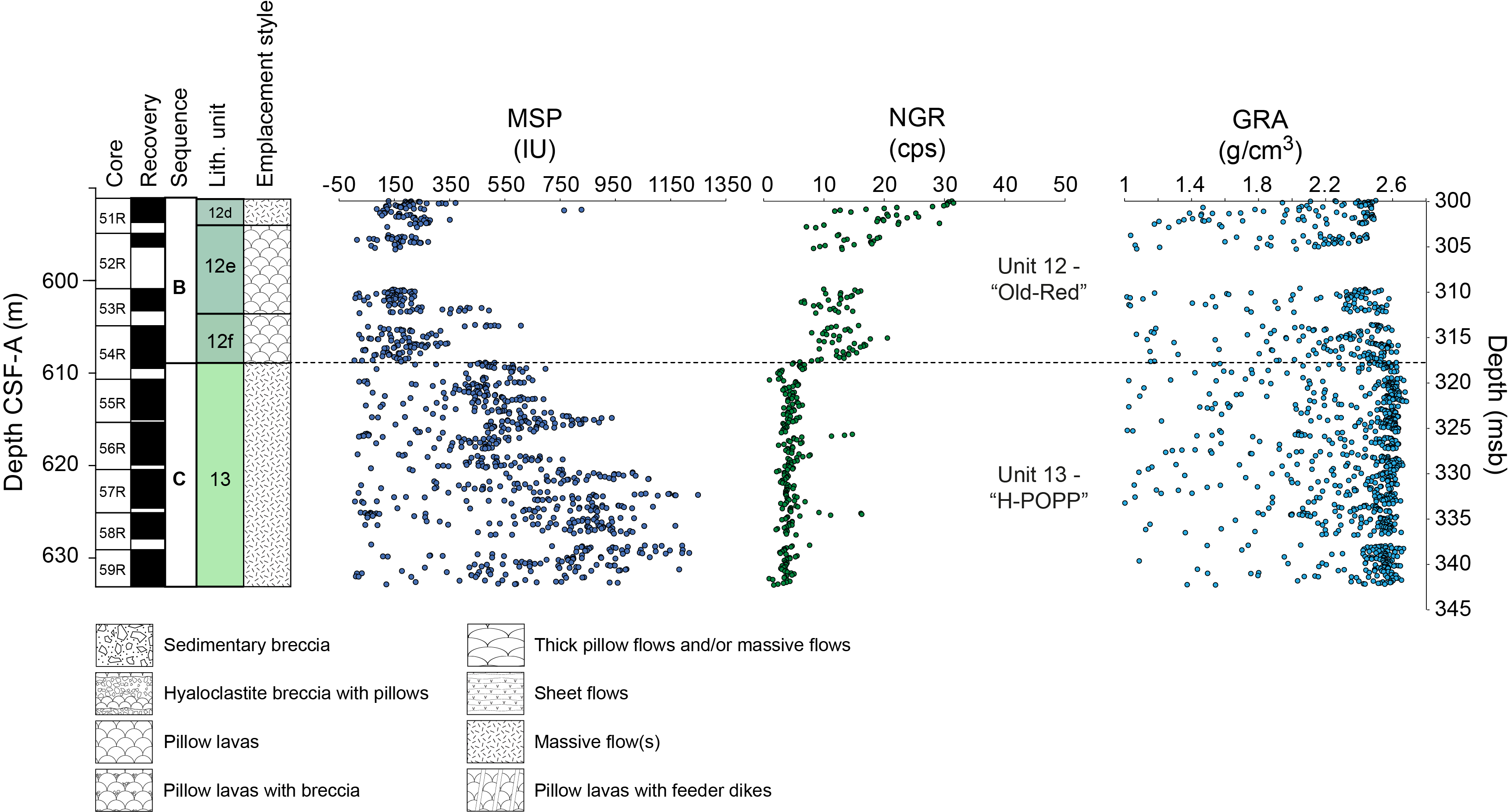
Figure F131. Physical properties, Unit 12/13 boundary.

10.2.1.3. Magnetic susceptibility

MS is an indicator of the tendency of minerals to become magnetized upon application of a magnetic field; it can therefore be considered an approximation of the concentration of magnetic minerals within the rock. The WRMSL-derived MS of cores from Hole U1556B ranges ~0–250 IU between 0 and ~317 msb. A similar range (50–350 IU) for MSP from the SHMSL is observed. MS is likely more accurately measured using the SHMSL because there is direct contact between the rock and the Bartington MS2E point sensor (see Physical properties and downhole measurements in the Expedition 390/393 methods chapter [Coggon et al., 2024c]), whereas the WRMSL-derived MS data are measured through the core liner. Therefore, MSP data are preferentially presented in Figure F130, and only MSP data are shown in Figure F131.

Below ~317 msb, a sharp increase in MS (Figure F131) is coincident with the Lithologic Unit 12/13 boundary (which corresponds to the Stratigraphic Sequence B [old red]/C [H-POPP] boundary; see Igneous petrology). The average MS values for Lithologic Unit 13 are 377 and 592 IU for WRMSL and MSP measurements, respectively, whereas throughout Lithologic Units 1–12, the averages are 90 and 153 IU, respectively. The higher MS values in Unit 13 may be an indicator of a higher abundance of Fe-rich magnetic minerals or a difference in the extent of alteration of magnetic minerals in the basement rocks.

10.2.1.4. Thermal conductivity

Thermal conductivity measurements offer a means of calculating the potential for conductive heat flow through a material and can help develop an understanding of thermal insulation and heat dissipation processes from the underlying igneous crust through the sediment to the ocean. Thermal conductivity is controlled by properties such as chemical composition, porosity, density, and fabric of the basement rocks.

A total of 57 discrete samples (approximately one per core) representing the range of rock types and alteration styles recovered from Hole U1556B were analyzed. Three measurements were taken to calculate an average thermal conductivity per sample (the sample mean thermal conductivity) (see Physical properties and downhole measurements in the Expedition 390/393 methods chapter [Coggon et al., 2024c]). The sample mean thermal conductivity ranges 1.10–1.71 W/(m·K) through Hole U1556B (average = 1.50 W/[m·K]) with no discernible downhole trend (Table T26; Figure F132). The three breccia (hyaloclastite) samples analyzed have substantially lower thermal conductivities than basalt samples, suggesting hyaloclastites are poorer conductors of heat relative to the altered basalts, probably reflecting the more porous nature of the breccia/hyaloclastites.

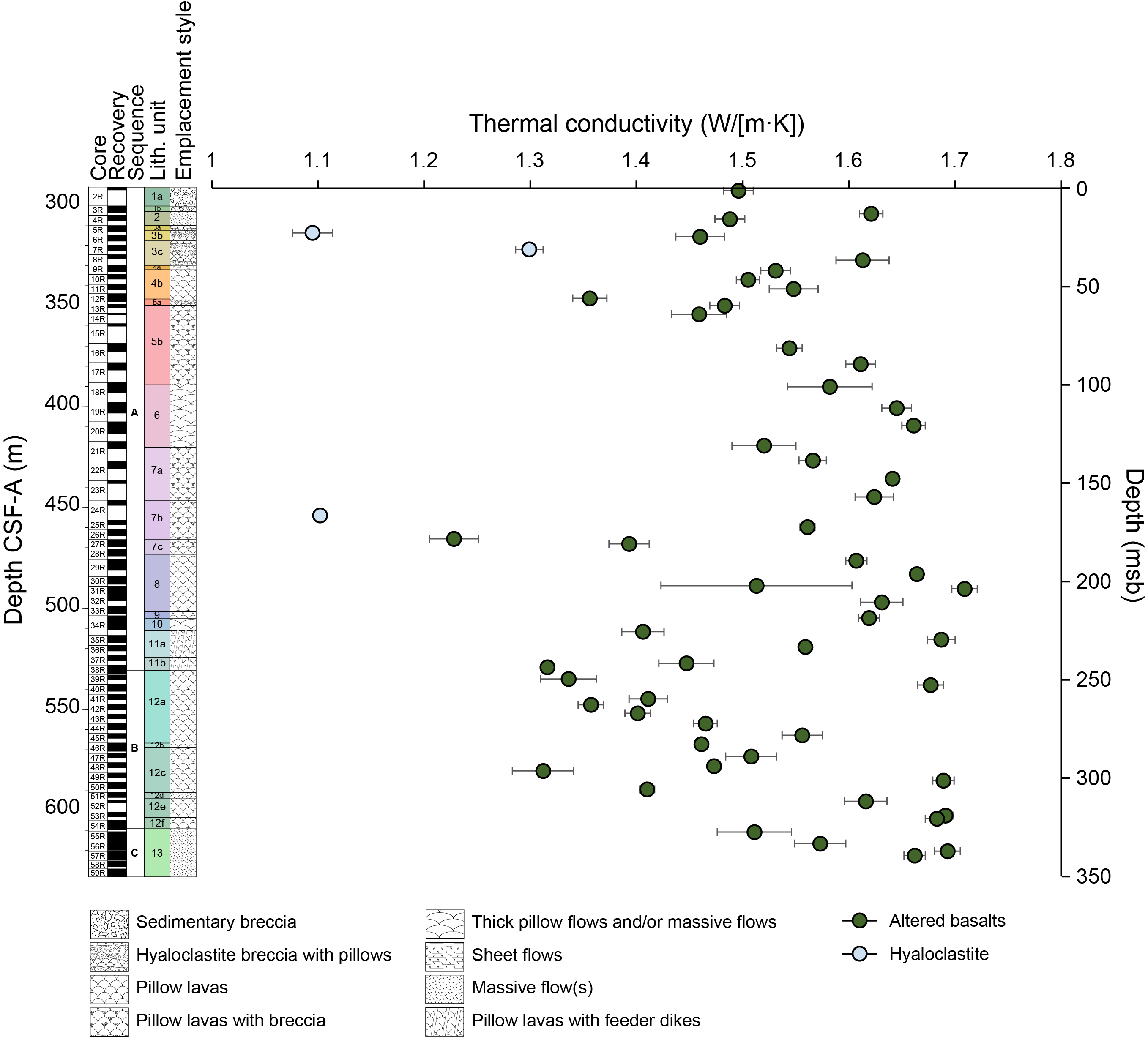
Figure F132. Thermal conductivity in basalts and hyaloclastites.

10.2.1.5. Moisture and density

MAD procedures include high-precision, high-accuracy measurements of discrete sample mass and volume from which bulk density, grain density, and porosity can be calculated. Porosity is especially useful for determining the volume of water that can be stored in the interval or lithology represented by the discrete sample. Bulk density, in part, controls seismic wave velocity, and grain density is related to the mineralogy of the sample and is useful for mineralogical and alteration analyses.

Discrete samples for MAD analysis were generally taken twice per core and were selected to be representative of the recovered core and to characterize end-member rock types and styles of alteration observed in the cores. Broadly, the samples analyzed consist of either basalt or hyaloclastite, the main lithologies recovered.

The measured porosity of the discrete samples ranges between 3.4% and 43.2% (mean = 12.9% ± 9.1%). The samples with the highest porosity are predominantly hyaloclastites, which have a mean porosity of 28.6%, whereas the mean porosity of the basalt samples is 10.0%. Bulk density of the discrete samples ranges 1.89–2.86 g/cm³ (mean = 2.55 ± 0.25 g/cm³). Basalt samples have higher bulk density (mean = 2.64 g/cm³). The hyaloclastite samples have lower bulk density (mean = 2.09 g/cm³). Grain density ranges 2.29–3.07 g/cm³ (mean = 2.77 ± 0.15 g/cm³). Basalt samples have a mean grain density of 2.82 g/cm³, whereas hyaloclastite samples have a mean of 2.51 g/cm³.

10.2.1.6. P-wave velocity

P-wave velocity is a measure of the velocity with which a compressional body wave (P-wave) propagates through a sample. P-wave velocity is directly controlled by the bulk density, compressibility, and shearability of the material sampled and is indirectly related to the porosity, mineralogy, and fabric of the interval or lithology represented by that material. P-wave velocity was measured on the discrete samples used for MAD analyses, allowing direct comparison of porosity and density with velocity. The P-wave velocity of discrete samples can also be used to correlate downhole logging velocities and regional seismic imaging to the core measurements.

P-wave velocity was measured along the x-, y-, and z- axes of each discrete sample cube. There was no significant difference between measured triaxial (x, y, and z) velocities for any given sample and thus no evidence to suggest systematic anisotropy in the basement cored at Site U1556. Therefore, the mean three-axis velocity was considered a reasonable estimate of velocity for each of the discrete samples. The range of P-wave velocity measured from discrete samples is 3.03–5.68 km/s (mean = 4.74 ± 0.58 km/s). Like MAD measurements, a distinct difference was observed between the hyaloclastite and basalt samples; basalt samples have a mean of 4.49 ± 0.46 km/s, and hyaloclastite samples have a mean of 4.03 ± 0.59 km/s.

10.2.2. Digital imaging

Imaging core exteriors before they are split provides a useful data set for core-log integration because planar veins and cracks appear as sinusoids in both downhole logging images of the borehole wall and rolled-out 360° images of whole-round cores. At Site U1556B, 191.87 m of basement core was recovered from the 342.2 m cored interval. Of this recovered core, ~170 m was consolidated and cylindrical enough to be scanned on the DMT CoreScan3, accounting for 89% of the recovered material. Using techniques developed during Expedition 390 (see Physical properties and downhole measurements in the Expedition 390/393 methods chapter [Coggon et al., 2024c]), even angular and fractured pieces of core could be imaged, although uneven surfaces on these cores may appear blurred. Poorer image quality was common for fractured rocks, whereas well-cemented hyaloclastites and robust basalt pieces were easily scanned and produced high-quality images.

Scanning individual pieces longer than 25 cm in multiple frames proved an excellent means of preserving fine-scale features on the core surface because the high-resolution setting on the DMT could be used throughout the hole. It is, however, important to reassemble all images collected in each core section to see the pieces in their original position within the section (Figure F133). Reassembly of individual sections was done by stitching images together using a dedicated Python program (see Curatorial core procedures and sampling depth calculations in the Expedition 390/393 methods chapter [Coggon et al., 2024c]).

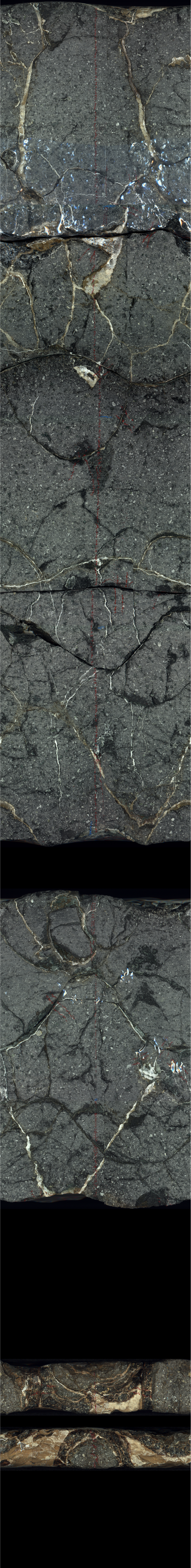
Figure F133. DMT composite section image.

Because Site U1556 was the first site visited during Expedition 390 and the DMT did not have a tried and tested methodology for scanning igneous cores on board JOIDES Resolution, some issues encountered were resolved toward the end of coring activities at Site U1556. Notably, the DMT CoreScan3 software included with the scanner applied autoexposure correction and also attempted to autoselect where it thought the core was; brightness differences existed between images of adjacent portions of the same rock. This resulted in recognizable but artificial color differences within a core that will be resolved by adjusting the gain and offset for images postexpedition. This discrepancy was not identified until images were stitched together following Hole U1556B operations but was resolved for the remaining holes drilled during Expedition 390/393 (see Physical properties and downhole measurements in the Expedition 390/393 methods chapter [Coggon et al., 2024c]).

10.2.3. Wireline logging

Three logging runs were planned to follow basement coring in Hole U1556B. The triple combo tool string would be run first, recording an initial set of measurements (gamma ray spectroscopy, density, electrical resistivity, and MS) to characterize the drilled formation and evaluate the hole conditions. If borehole conditions (hole size) and sea state were suitable for further logging, the FMS-sonic tool string (sonic velocity and microresistivity images of the borehole wall), and the UBI tool string with the APS (acoustic images of the borehole wall and neutron porosity) would be run. The sea state was moderate to high, and all three tool strings were deployed successfully, providing good quality data over multiple passes of the basement interval with each tool string.

10.2.3.1. Operations

Logging operations for Site U1556 began after the completion of RCB coring in Hole U1556B to a total depth of 633.2 m DSF on 4 May 2022. In preparation for logging, a high-viscosity mud sweep was circulated through the hole to clear it of cuttings. The initial operations plan had included time for an extra pipe trip to release the RCB bit on the seafloor prior to logging and preserve Hole U1556B as a legacy hole for future scientific ocean drilling operations. However, given the subsidence of the reentry cone below the seafloor that presented challenges for hole reentry, the decision was made to drop the bit at the bottom of the hole and make up some of the time lost to slow RCB drilling rates and circulation issues (see Operations) and preserve operational time for later operations in the expedition. The bit was released at the bottom of the hole with the MBR, the hole was filled with seawater, and the drill pipe was raised to a depth of 41 m DSF for logging. Sea condition was high, with average heave of ~3 m total, and the wireline heave compensator was used for the entirety of the logging operations.

The triple combo was rigged up and run into the hole at 0020 h (local time [UTC + 2 h]) on 5 May. A downlog was recorded starting at 5005 mbrf, from just above the seafloor (identified by a step in the gamma ray log) to the bottom of the hole at 5650 mbrf. The first attempted upward pass was halted ~10 m above total depth (TD) because of power fluctuations and apparent loss of communications with the tool string. The attempted uplog was stopped and the tool string was pulled out of the hole without recording logging data to troubleshoot the issue. The tool string was recovered on the rig floor at 0815 h and tested to identify the source of the electronics problem. The HNGS was found to be faulty and was replaced with the back-up sonde. The tool string was run back into the hole at 0920 h, recording a second downlog from just above the seafloor to the bottom of the hole. The main pass started at 1310 h, recording a full set of data from 5642 mbrf, and stopped when the tool string was fully back into the casing at 5296 mbrf. The tool string was run back into the open hole, recording another downlog. The bottom of the hole was reached without incident and a second uplog was recorded starting at 1430 h. The second pass continued until the entire tool string was above the seafloor (observed in the gamma ray log at 5009 mbrf). The tools were back at the surface at 1910 h.

The caliper log established the borehole was in gauge and in good condition for the imaging tools (FMS and UBI). The sea state was moderate but within the limit for the UBI. The UBI tool string was rigged up and run into the hole at 2030 h. A downlog, with only the gamma ray tools active, was recorded from above the seafloor to 5635 mbrf, stopping ~10 m above TD to keep the UBI from tagging bottom and stirring up sediment that would cloud the optical sensor. The APS was turned on and a short (~100 m) verification pass was recorded starting at 0115 h on 6 May. The tool string was run back into the hole, stopping once again ~10 m above TD. The main pass started at 0140 h from 5635 mbrf and completed at 0320 h when the tool string passed above the seafloor. The upward passes were recorded at standard resolution; it was determined that the high-resolution setting was unlikely to provide good quality images, given the marginal sea state. The UBI tool string was pulled up to the surface and rigged down by 0635 h.

The FMS-sonic tool string was rigged up and run into the hole at 0715 h. A downlog was recorded from 4998 mbrf, just above the seafloor, to the bottom of the hole at 5647 mbrf. The first upward pass started at 1130 h and was completed at 1225 h as the FMS calipers were closed for the tool string to enter the casing (at 5300 mbrf). The tool string was run back to the bottom of the hole, and a second pass began at 1300 h from 5648 mbrf. FMS data were recorded to the base of casing, then the FMS calipers were closed for the rest of the upward pass. Gamma ray tools and the Dipole Sonic Imager (DSI) were active up through the casing. The second pass was concluded at 1430 h, when the tool string passed above the seafloor, and the tool string was returned to the surface. All tools were rigged down by 1740 h, and the drill floor was returned to drilling operations at 1755 h on 6 May.

10.2.3.2. Data overview

A summary of the main data recorded from the triple combo run is shown in Figures F134 and F135. The quality of downhole logging data is typically affected by hole diameter. Gamma ray and resistivity logs are generally reasonable even in larger diameter boreholes, whereas density and porosity measurements require that the logging tools have good contact with the borehole wall. The caliper log in Figure F134 shows that the borehole was in good condition with a diameter close to bit size and a few slightly enlarged intervals. A larger diameter interval from 350 to 400 m WMSF coincides with an interval of poor core recovery, suggesting that the nature of the formation may be influencing hole size at this depth. The density log shows realistic values through this interval, but the porosity log in this interval appears to be anomalously elevated and should be interpreted with caution.

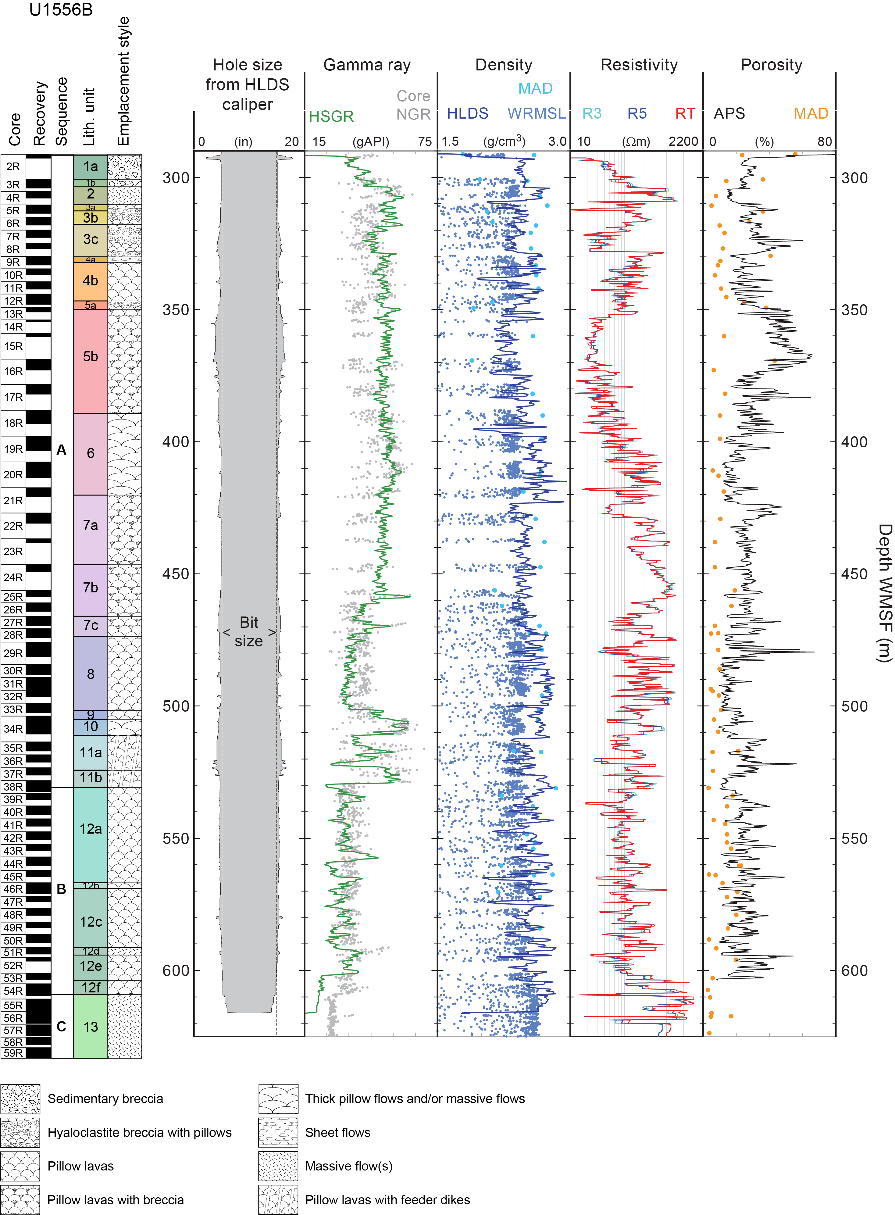
Figure F134. Triple combo logging data.

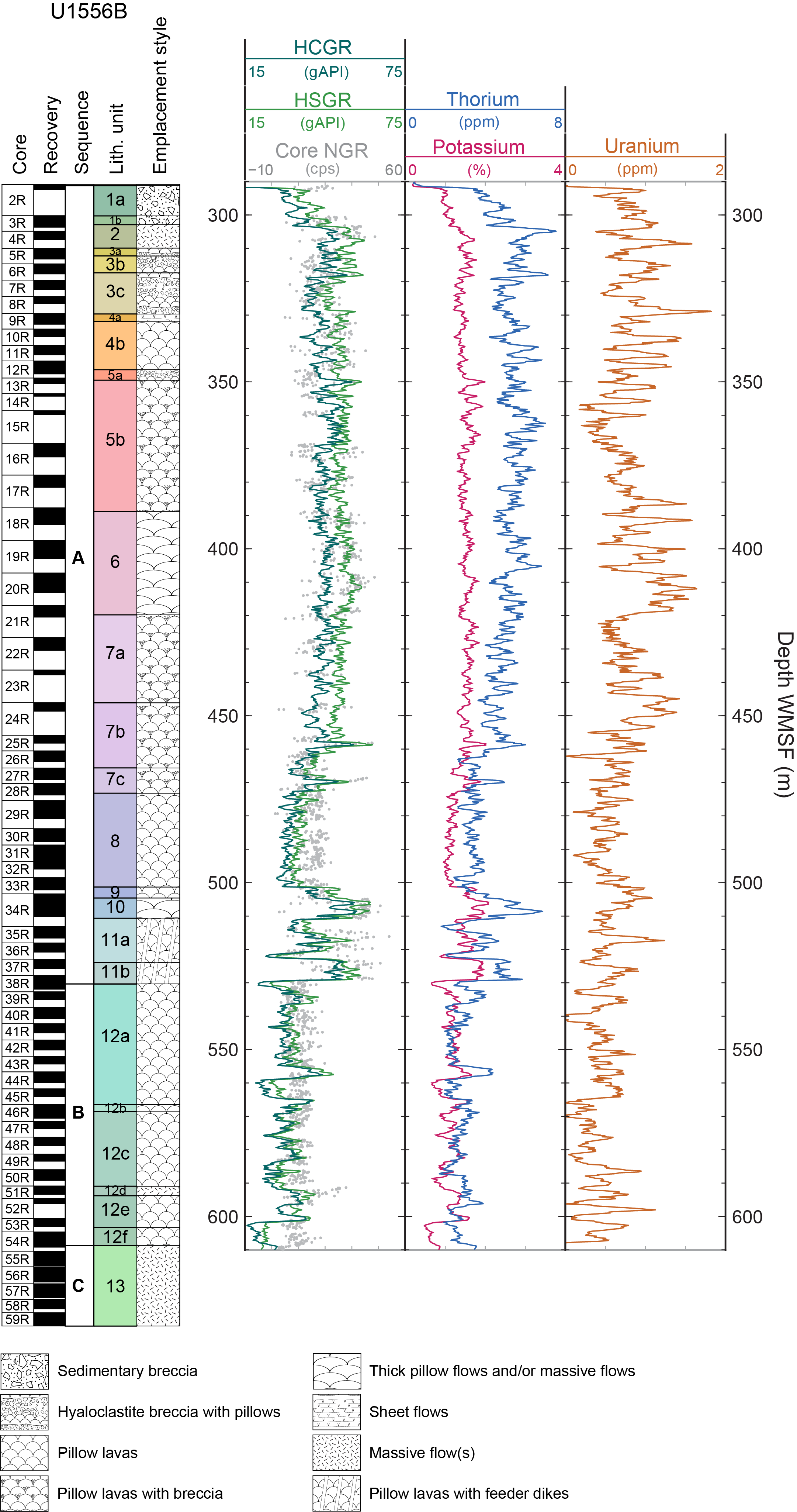
Figure F135. Spectral gamma ray logs.

The quality of downhole logs can also be assessed by comparison with measurements made on cores from the same hole. Total natural gamma ray from the triple combo shows good agreement with NGR data from cores, with a slight depth offset of a few meters (Figure F134). Discrepancies between the drilling core depth and wireline logging depth may occur because of core expansion, incomplete core recovery, incomplete heave compensation, wireline stretch, drill pipe stretch, and tidal changes. In the upper basement section (290–470 m WMSF), the density log shows generally higher values than GRA track measurements, which are affected by variable core recovery and incomplete filling of the core liner (see Physical properties above), and lower values than measurements made on MAD samples, which are biased toward recovered lithologies. Below 470 m WMSF, the density log generally follows the upper envelope of GRA track data and agrees very well with MAD sample measurements. The porosity log values are generally higher than porosity from MAD sample measurements, likely an overestimate of true formation porosity, though there is less discrepancy between these two data types from 490 m WMSF to the bottom of the logged interval.

Gamma ray and resistivity logs display trends that coincide with some of the lithologic units identified in cores (see Igneous petrology). The gamma ray log shows very good agreement with NGR data from cores, resolving the same corresponding changes with igneous basement sequences (Stratigraphic Sequence A [orange spotty], the transition interval between Stratigraphic Sequences A [orange spotty] and B [old red], and the Stratigraphic Sequence B/C boundary between old red and H-POPP) described in detail in Physical properties above. Resistivity is relatively variable between the top of basement and ~460 m WMSF in Hole U1556B, within Stratigraphic Sequence A (Lithologic Units 1–7; see Igneous petrology). Resistivity has relatively uniform character between 460 and 600 m WMSF, corresponding to the lower units of Stratigraphic Sequence A and nearly all of Stratigraphic Sequence B. Resistivity increases deeper than ~600 m WMSF within Stratigraphic Sequence C. Core recovery is variable through this hole, so it is difficult to correlate resistivity directly with lithology. However, lower resistivity intervals appear to correspond to lithologic units with significant hyaloclastite, whereas higher resistivity intervals are associated with basalt-dominated units.

The Magnetic Susceptibility Sonde (MSS) was run in the triple combo tool string to record in situ MS, but shore-based data processing and comparison with core-based MS from the same hole indicated that the MS log data were not valid.

Figure F136 is a summary of the data collected by the UBI tool string, the second logging deployment in Hole U1556B. The rotating ultrasonic transponder creates a radius image of the borehole; the hole size is calculated from its average on each rotation. These data provide a more detailed representation of the hole conditions than the mechanical Hostile Environment Litho-Density Sonde (HLDS) and FMS calipers (Figures F134, F137) from the first and third logging runs, but both radius and amplitude images identify the same intervals of borehole enlargement.

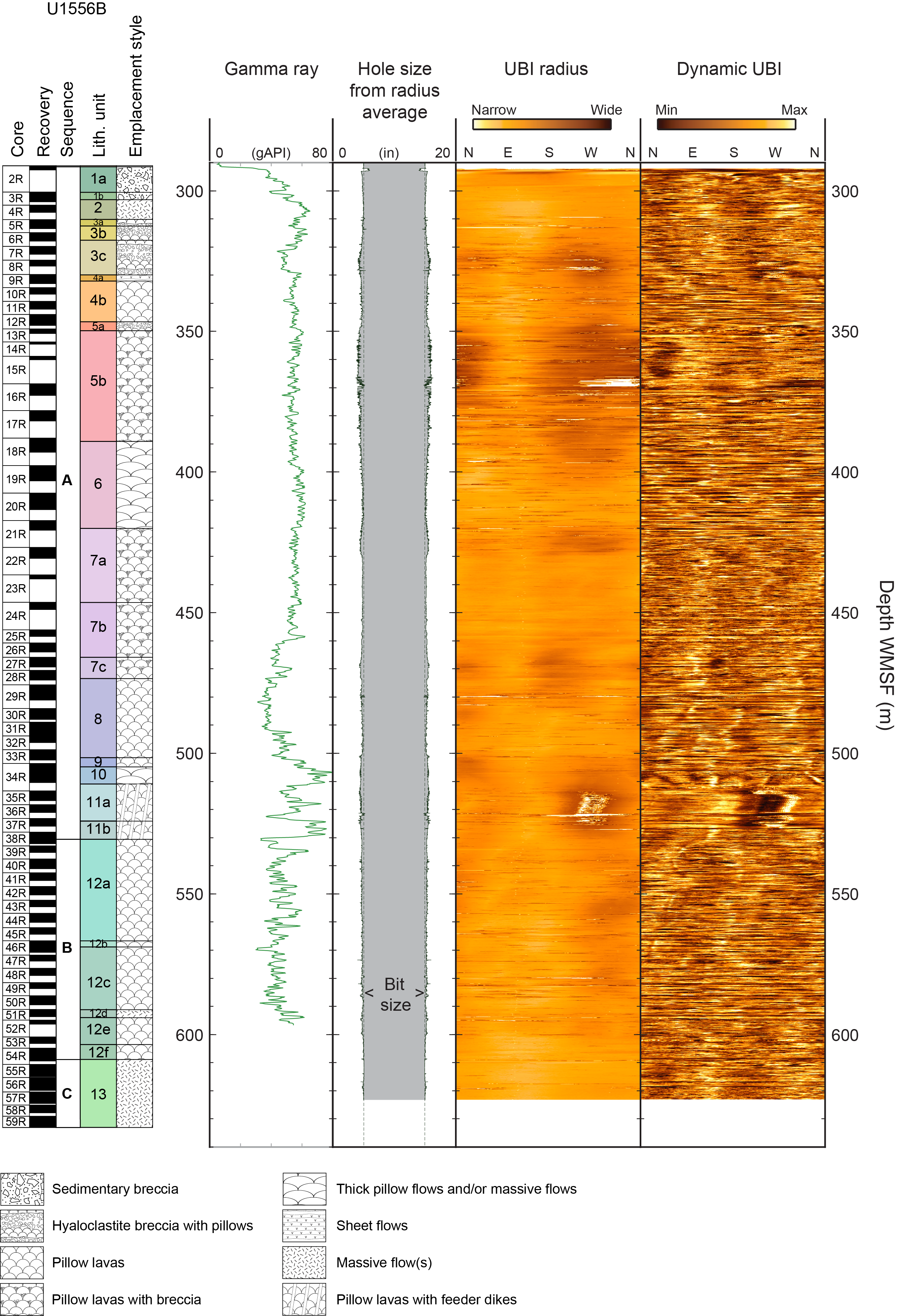
Figure F136. UBI logging data.

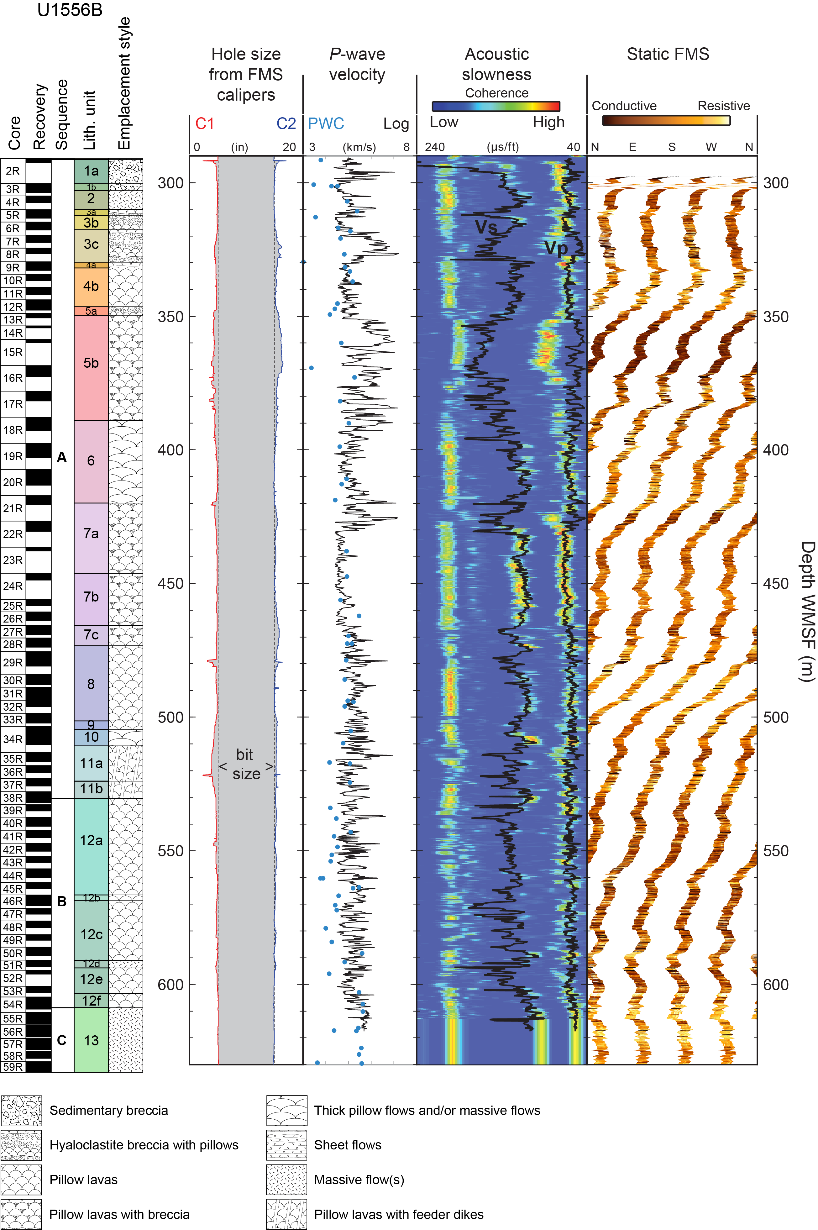
Figure F137. FMS-sonic logging data.

Figure F137 is a summary of data collected by the FMS-sonic tool string, the third and final logging deployment in Hole U1556B. P-wave velocities in the basement section of Hole U1556B range from ~4 to 7 km/s, with more high-frequency variability from the top of the logged interval to ~430 m WMSF, through Stratigraphic Sequence A (see Igneous petrology). P-wave velocity is relatively uniform from ~430 to 465 m WMSF, corresponding to Lithologic Unit 7. From 465 m WMSF to the base of the logged interval in Hole U1556B, P-wave velocity is moderately variable. The velocity and resistivity logs show similar characteristics, as both measurements are responsive to porosity and density of the formation (Figures F134, F137). There are several regions of weak coherence (Acoustic slowness column on Figure F137), but P-wave velocity is reasonable throughout the logged interval and shows agreement with discrete velocity measurements on core samples. There are several intervals where the shipboard acquisition algorithm failed to identify the highest coherence regions (e.g., 350–400 m WMSF); velocities through those intervals may be refined with additional postexpedition processing.

10.2.4. Data integration

10.2.4.1. Discrete sample comparison to stratigraphy and alteration

Trends in both porosity and P-wave velocity correspond well with the described stratigraphic sequences (see Igneous petrology). In the depth interval that corresponds to orange spotty, Lithologic Units 1–11 from 0 to 239 msb (Stratigraphic Sequence A; see Igneous petrology), the mean porosity and P-wave velocity of the discrete samples of basalt are 9.3% and 4.92 km/s, respectively (orange lines on Figure F138). Between 239 and 317 msb, coincident with Lithologic Unit 12 (Stratigraphic Sequence B [old red]; see Igneous petrology), the mean porosity and P-wave velocity are 12.7% and 4.65 km/s, respectively (red lines on the same figure). The decrease in average P-wave velocity is likely indicative of the higher degree of alteration of old red compared to orange spotty basalts (see Igneous petrology and Alteration petrology). Below 317 msb, coincident with Lithologic Unit 13, H-POPP (Stratigraphic Sequence C, see Igneous petrology), the mean porosity decreases and the mean P-wave velocity increases to 4.7% and 5.53 km/s, respectively (cyan lines on the same figure). The low porosity and high velocity are likely reflections of the less altered material in H-POPP basalts.

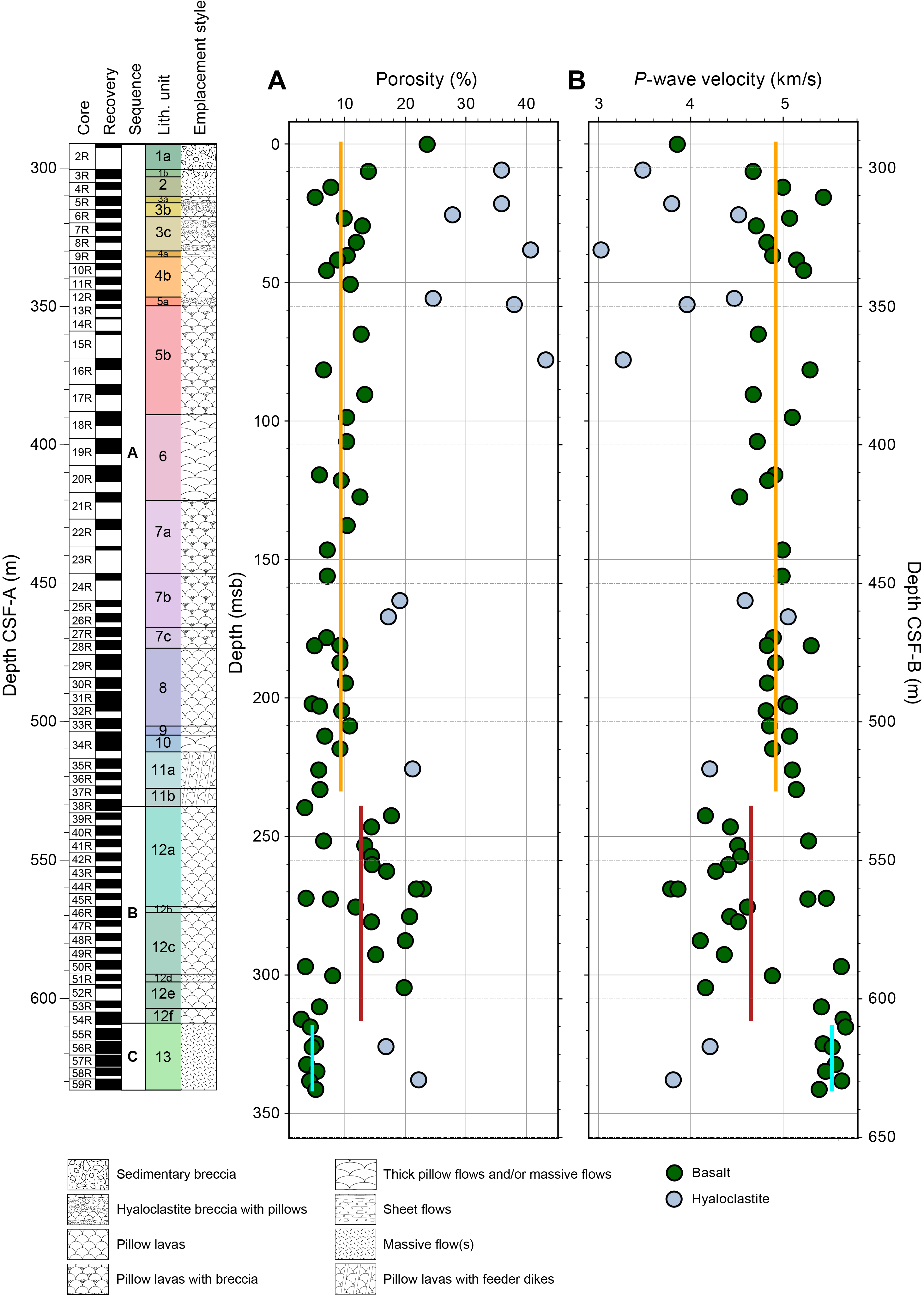
Figure F138. Porosity and P-wave velocity.

The velocity and porosity measurements made on discrete samples from Hole U1556B are negatively correlated (Figure F139). Because velocity is sensitive to bulk density, compressibility, and shearability of the material sampled, it is also sensitive to porosity. The high coefficient of determination (R² = 0.9) of a linear regression for the basalt samples alone suggests porosity is the primary control on P-wave velocity in the basalt of the upper oceanic crust, which is similar to the finding of Carlson (2014). To determine whether the extent of alteration influences this trend, 64 basalt samples taken for MAD and velocity analysis were divided into eight classes of alteration, ranging from the least altered, Class 1 (dark gray) to the most altered, Class 8 (very intense orange halos) (Table T27; Figure F140). Variations in discrete sample alteration class (Figure F141) are consistent with trends in alteration styles described in detail in Alteration petrology. The color mask applied to the data shown in Figure F139B indicates that as alteration extent increases, the measured porosity of the rock increases, with correspondingly slower P-wave velocities. This observation is counterintuitive because we would expect porosity to decrease as secondary (alteration) minerals fill available pore space, which raises the question of what is actually being measured as porosity following the MAD method (see Physical properties and downhole measurements in the Expedition 390/393 methods chapter [Coggon et al., 2024c]).

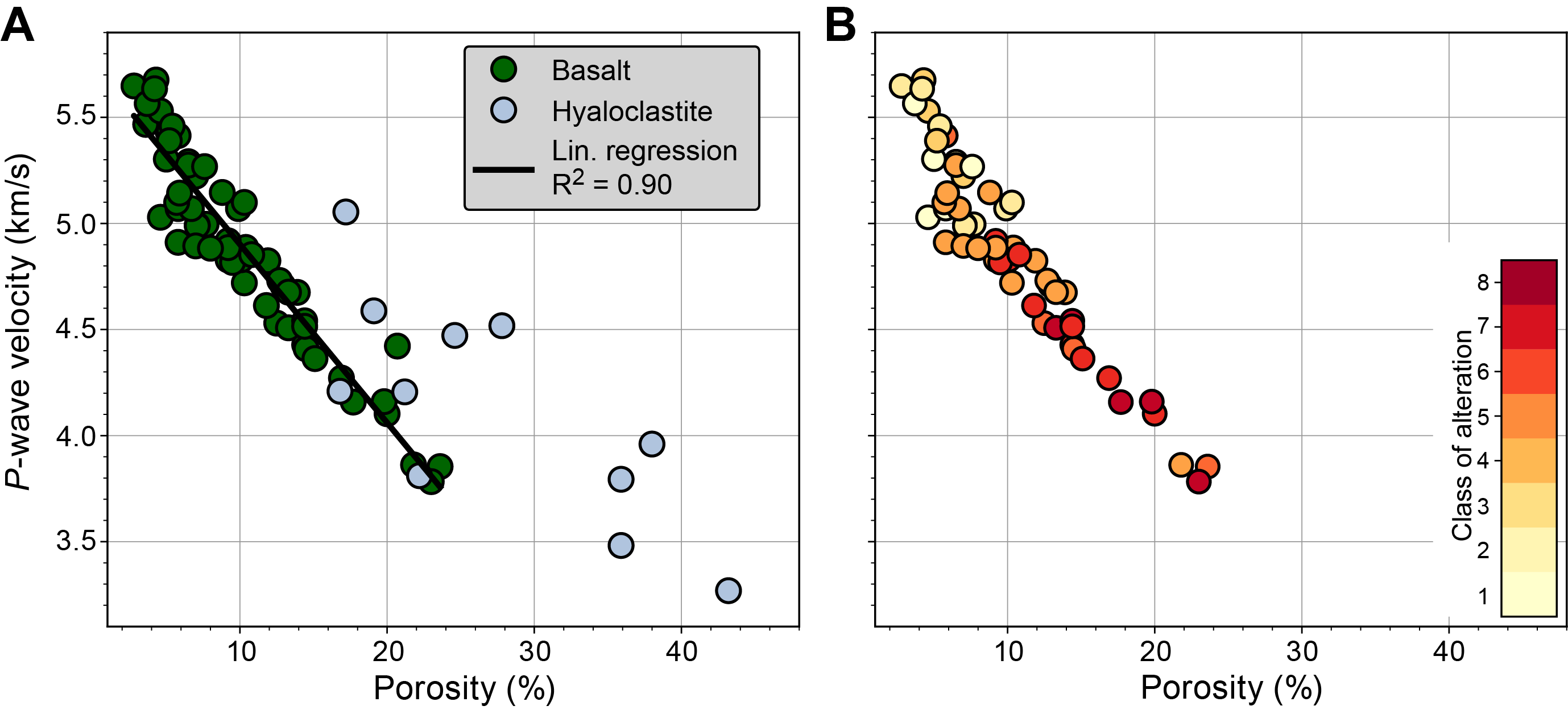
Figure F139. P-wave velocity vs. porosity.

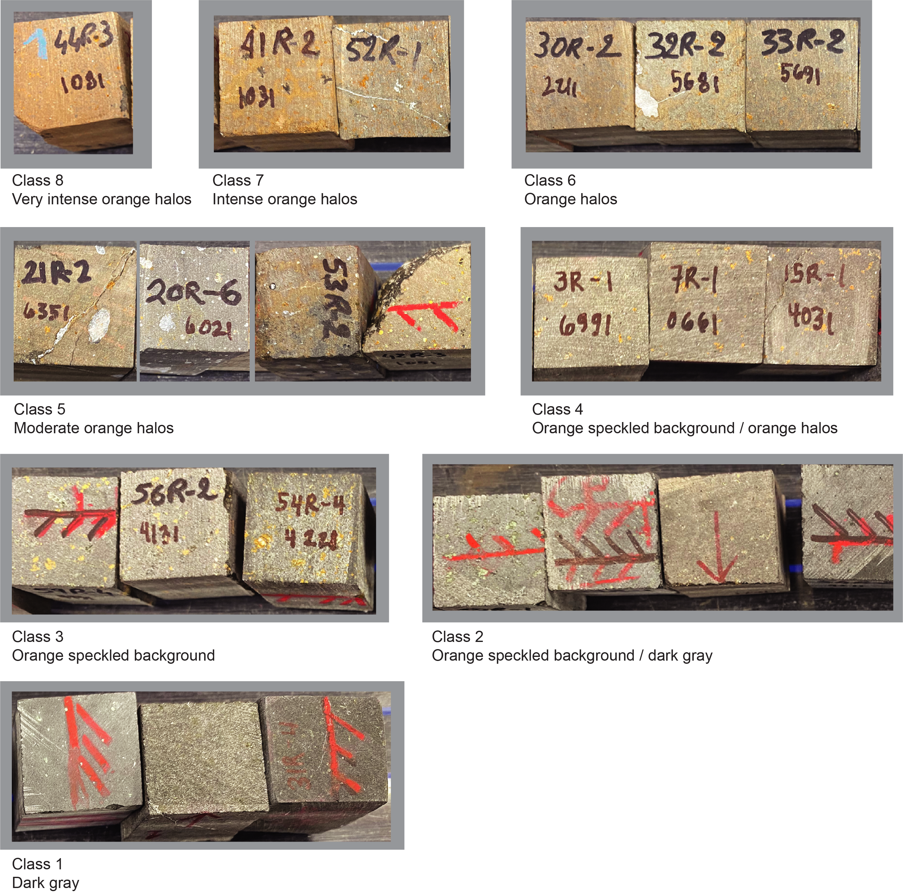
Figure F140. Alteration classes.

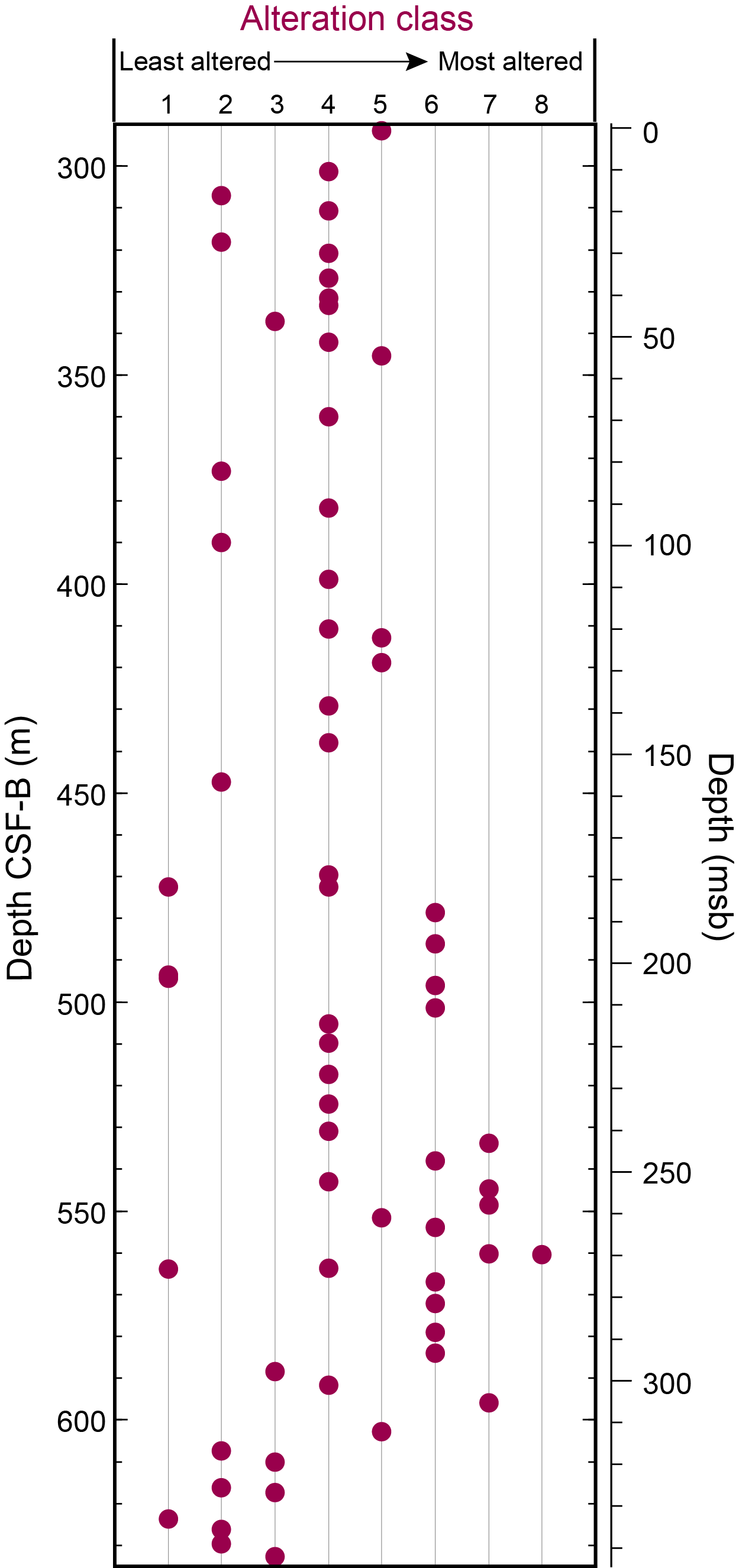
Figure F141. Variation in alteration classes.

11. Geochemistry

11.1. Sediment

11.1.1. Interstitial water sampling

During sediment coring in Holes U1556A, U1556C, and U1556E, mudline water samples were collected and IW was extracted by squeezing under laboratory atmosphere (see Geochemistry in the Expedition 390/393 methods chapter [Coggon et al., 2024c]). During engineering Expedition 390C, squeezed IW was collected once per core from Cores 390C-U1556A-1H through 12H, twice per core from Cores 13H–20X, once per core from Cores 21X–23X, 25X, 27X, 28X, and 30X, and twice per core from Cores 26X and 29X. During Expedition 390, squeezed IW samples were taken at a frequency of two per core from intervals cored with the APC system (Cores 390-U1556C-1H through 16H and 390-U1556E-1H through 5H). One IW sample was collected per core during XCB coring for Cores 390-U1556C-17X through 26X, and then sampling frequency increased to twice per core ~40 m above the basement in Cores 27X–30X. Mudline samples were also collected from Cores 390C-U1556A-1H and 390-U1556C-1H for geochemical analysis. A total of 41, 50, and 10 IW samples were taken from Holes U1556A, U1556C, and U1556E, respectively. Rhizon IW samples for postexpedition research were additionally collected from cores from Holes U1556C and U1556E prior to core splitting (see Geochemistry in the Expedition 390/393 methods chapter [Coggon et al., 2024c]). Shipboard analyses of the squeezed IW from Holes U1556A and U1556C include pH, salinity, alkalinity, major cations and anions (sodium, calcium, magnesium, potassium, chloride, and sulfate) using ion chromatography (IC), major and minor elements using ICP-AES, and nutrients (phosphate and ammonium) and sulfide using a spectrophotometer (see Geochemistry in the Expedition 390/393 methods chapter [Coggon et al., 2024c]). Carbonate and TOC measurements were conducted on the solid sample residues (squeeze cakes) and additional samples selected from the working half. The remaining squeezed IW and squeeze cake splits were distributed to scientists for postexpedition research. Dissolved oxygen in the pore waters was also measured in cores from Holes U1556C and U1556E using the PreSens optical oxygen sensors (optodes) at a resolution of ~1–5 m in Hole U1556C and ~1.5 m in Hole U1556E (see Geochemistry in the Expedition 390/393 methods chapter [Coggon et al., 2024c]). Sediment cores were initially allowed to equilibrate to room temperature before the oxygen measurements; measurements on Hole U1556E cores were made prior to equilibration but after the physical properties whole-round logger measurements were conducted, 4–6 h after the core first arrived on the catwalk. For Hole U1556E, the temperature probe was inserted into the core through a hole in the core liner (see Geochemistry in the Expedition 390/393 methods chapter [Coggon et al., 2024c]). Intervals selected for measurements did not include those clearly exhibiting drilling disturbance. Whole-round samples (5 cm) were also taken from the catwalk for oxygen measurements for Cores 390-U1556C-22X through 24X. Oxygen and temperature probes were both inserted into these whole-round samples because they were not yet equilibrated to room temperature (see Geochemistry in the Expedition 390/393 methods chapter [Coggon et al., 2024c]).

All data from shipboard analyses of the squeezed IW, sedimentary carbonate, and total carbon (TC) for Site U1556 sedimentary sections are shown in Table T28, and depth profiles for selected elements in the pore waters and total inorganic carbon (TIC) and TOC of the sediments are plotted in Figures F142, F143, F144, F145, and F146. Major cations (Na, K, Ca, and Mg) and anions (sulfate) were measured by both ICP-AES and IC. The analytical method that resulted in mudline values closest to International Association for the Physical Sciences of the Oceans (IAPSO) standard seawater was used for plotting data here. For minor elements, Br concentrations were measured only in Hole U1556C, and Ba concentrations are reported only for Hole U1556C because Hole U1556A concentrations were all below the detection limit. The following profiles, unless otherwise noted, describe trends observed in both Holes U1556A and U1556C.

11.1.2. Measurement results of interstitial water

11.1.2.1. Salinity, chloride, bromine, sodium, and potassium

Salinity varies between 34 and 35 throughout Holes U1556A and U1556C (Table T28). Sodium (Na) concentrations range 437–473 and 463–487 mM for Holes U1556A and U1556C, respectively (Figure F142A). Our decision to use ICP-AES data for Hole U1556A and IC data for Hole U1556C because of data quality issues (see above) could explain the lower Na concentrations in Hole U1556A. This offset likely results from the more highly concentrated matrix used for ICP-AES during Expedition 390C, which was selected to allow measurement of both major and minor elements in one run. Chloride (Cl) concentrations range 535–587 mM (Figure F142B). The linear correlation between Na and Cl (R² = 0.9552 and 0.8111 for Holes U1556A and U1556C, respectively) indicates that there is no measurable addition of fluids with a Na/Cl ratio distinct to that of seawater. Bromide is also conservative, as suggested by relatively uniform concentrations (0.83–0.87 mM) through the sedimentary section (Figure F142C) and a constant seawater Br/Cl ratio of ~1.5 × 10⁻³ (Br and Cl are linearly correlated; R² = 0.90 in Hole U1556C).

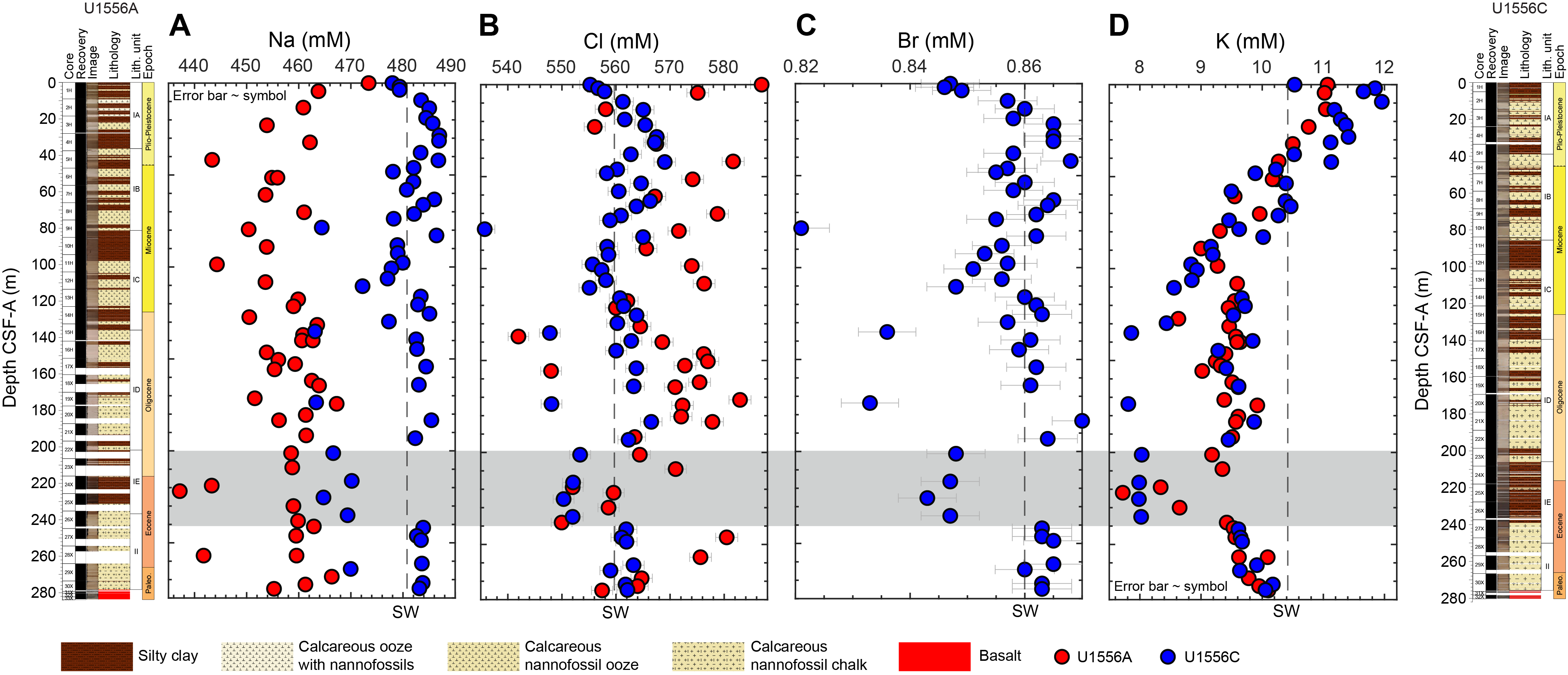
Figure F142. IW Na, Cl, Br, and K.

Potassium (K) concentrations are similar through Holes U1556A and U1556C, decreasing from ~11 mM near the seafloor to ~8 mM at 135 m core depth below seafloor, Method A (CSF-A) (near the base of Lithologic Subunit IC), in Hole U1556C (Figure F142D), which may be associated with the transformation of smectite into illite. Bulk sediment XRD (see Figure F11) shows a subtle increase in illite downhole, but further investigation is needed to confirm whether this trend represents the smectite–illite transition or another factor, such as temporal changes in the clay source. A similar K decline caused by smectite–illite transition at low temperatures was observed in the Bering Sea, associated with microbial Fe reduction (Ijiri et al., 2018). Below Subunit IC, K concentrations increase slightly to a maximum of 10.17 mM at ~275 m CSF-A above the basement. Potassium concentrations are lower in Subunit IE (~8 mM), consistent with low Na, Cl, Br, K, and salinity values in the same interval, which may indicate conservative mixing of low-salinity water. Potassium concentrations increase toward the basement through Unit II.

11.1.2.2. pH, alkalinity, magnesium, calcium, and strontium

Pore fluid pH decreases from the mudline sample (pH = 7.8 in Hole U1556A; pH = 7.7 in Hole U1556C) through the uppermost 80 m of Holes U1556A and U1556C, below which it ranges 7.5–7.7 (Figure F143A). Overall, alkalinity ranges between 2 and ~3 mM in samples from Site U1556 (Figure F143B). Concentrations decrease from ~3 mM in Subunit IA to ~2 mM toward the bottom of Subunit IB at ~80 m CSF-A. In both holes, alkalinity has a broad hump approaching ~3.2 mM in the interval ~120–190 m CSF-A, coinciding with the maximum concentrations of calcium (Ca) and strontium (Sr) through the sedimentary section (Figure F143C, F143D). Below this interval, alkalinity increases to ~2.5 mM in Subunit IE and decreases to 2 mM through Unit II.

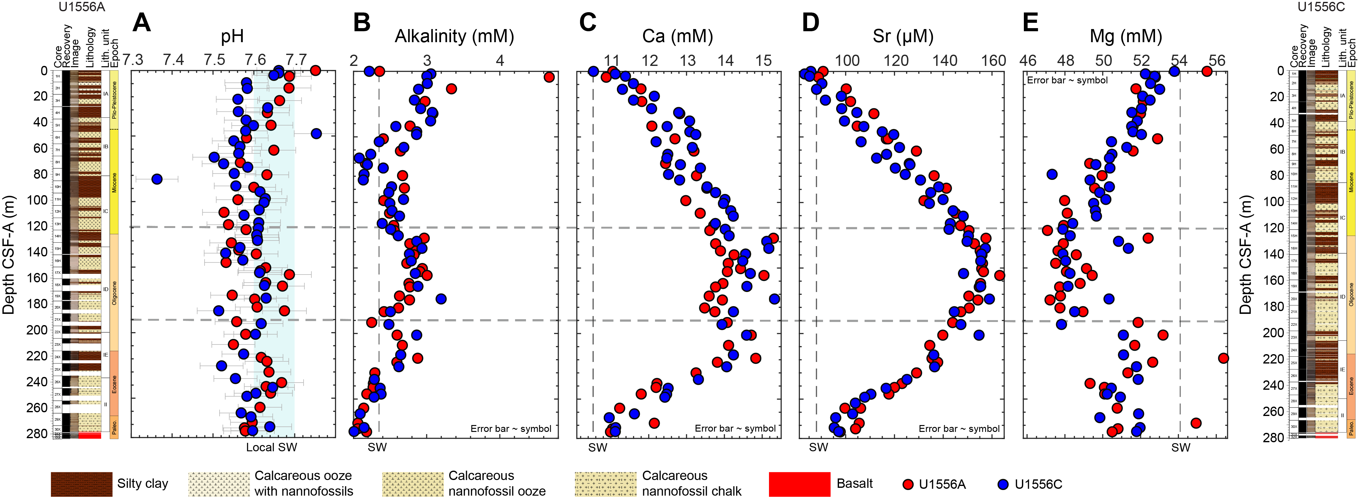
Figure F143. IW pH, alkalinity, Ca, Sr, and Mg.

Ca and Sr concentrations have very similar profiles in both Holes U1556A and U1556C. The concentrations of Ca (~10 mM) and Sr (~80 µM) at the seafloor increase with depth to ~15 mM and ~160 µM, respectively, at ~150 m CSF-A in the calcareous nannofossil ooze (in Hole U1556A) and calcareous nannofossil chalk (in Hole U1556C) of Subunit ID, which contains more than ~80 wt% calcium carbonate (Figure F146A). These increases may be caused by biogenic carbonate dissolution and inorganic calcite recrystallization, as evidenced from higher Sr/Ca in the pore waters relative to the mudline value (Baker et al., 1982) (Table T28). Pore water Ca and Sr concentrations are highest in Subunits IC and ID, whereas pore waters from this interval have the lowest magnesium (Mg) concentrations of the entire sedimentary succession (~48 mM). Ca and Sr concentrations decrease from these maxima to ~11 mM and ~100 µM, respectively, through Unit II.

In both Holes U1556A and U1556C, the Mg concentration of pore waters decreases through Subunits IA–IC, from seawater concentrations (~54–55 mM) near the seafloor to ~48 mM at ~120 m CSF-A (Figure F143E); this is the same interval through which pore water K concentrations also decrease (Figure F142D). Magnesium concentrations display constant values at ~120–190 m CSF-A near the Subunit ID/IE boundary. Below this, they increase in a stepwise fashion to ~50–53 mM in both holes.

11.1.2.3. Boron, lithium, and silica

Boron (B) concentrations in Holes U1556A and U1556C pore waters increase from 420 µM near the seawater interface to ~700 µM at ~90 m CSF-A but decrease back to ~420 µM at ~150 m CSF-A (Figure F144A). Another peak in B concentration (~700 µM) is observed in Subunit IE at ~220 m CSF-A. Below this depth, B concentrations decrease to ~500 µM at the Subunit IE/Unit II boundary and remain the same through the rest of the underlying sediment package. Lithium (Li) concentrations display a profile shape that is broadly consistent with B, albeit with more noise in the data (Figure F144B). Li concentrations increase from the sediment surface to a peak value of ~32 µM at ~50–80 m CSF-A. Li then decreases to ~27 µM at ~154 m CSF-A and increases to ~32 µM in Subunit IE, below which it decreases toward the bottom of the hole (Figure F144B). Based on XRD analyses of samples from Hole U1556A (Figure F12), pore waters from whole rounds with higher clay contents have some of the highest concentrations of Li and B (Figure F144).

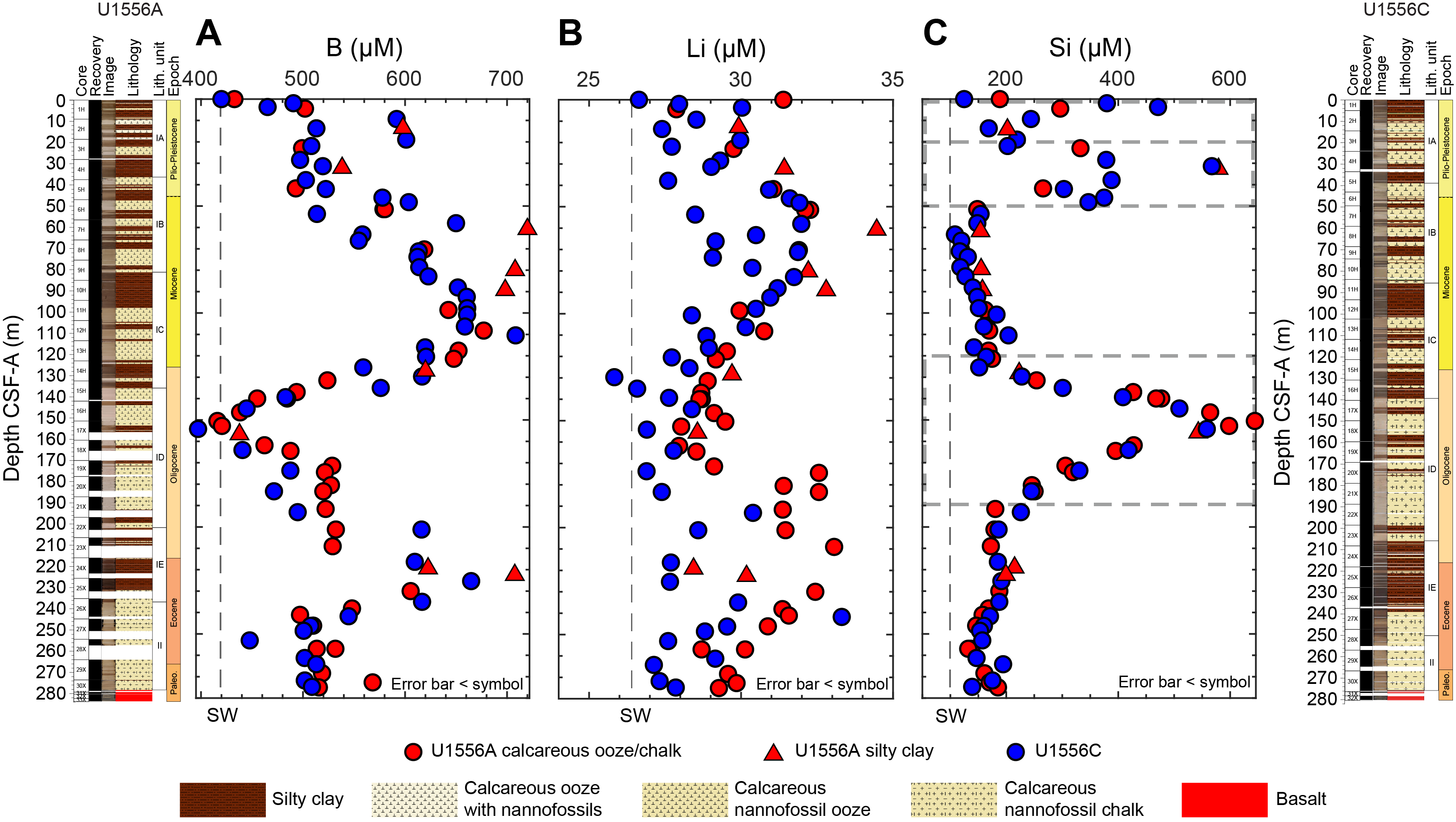
Figure F144. IW B, Li, and Si.

Dissolved silica (Si) concentration exhibits several peaks that indicate extensive silica dissolution at ~8, ~35, and ~150 m CSF-A (Figure F144C). The peaks at ~8 and ~35 m CSF-A are likely due to dissolution of biogenic silica based on the high abundances of diatoms and sponge spicules at these depths (see Figure F99). The broad Si peak at ~150 m CSF-A is coincident with Ca and Sr maxima (Figure F143) as well.

11.1.2.4. Sulfate, manganese, ammonium, and phosphate

Sulfate (SO₄²⁻) decreases from seawater concentration (~28 mM) in the mudline sample to ~25 mM at ~120 m CSF-A in both Holes U1556A and U1556C (Figure F145A). Concentrations then range 24–25 mM to ~230 m CSF-A, below which they increase to ~27 mM downhole. The observed increase in dissolved manganese (Mn), with a peak of ~130 µM at ~25 m CSF-A, coincides with a decrease in sulfate concentrations over the same interval (Figure F145B). This decrease in sulfate combined with Mn release suggests reduction of Mn(IV) oxides and sulfate by organic carbon respiration in reducing IW. Relatively smaller peaks in Mn concentration occur at ~135 and ~200 m CSF-A. Below 225 m CSF-A, dissolved Mn remains <5 µM. Ammonium (NH₄⁺) concentrations in Hole U1556C increase from ~10 µM near the surface to ~50 µM at ~70 CSF-A in Hole U1556C (Figure F145C), indicative of release from organic carbon decay. Concentrations remain almost constant until ~120 m CSF-A, below which they decrease to ~10 µM at the bottom of Hole U1556C. Phosphate (PO₄³⁻) concentrations vary between ~0 and 3 µM, with considerable scatter throughout the sediment package (Figure F145D).

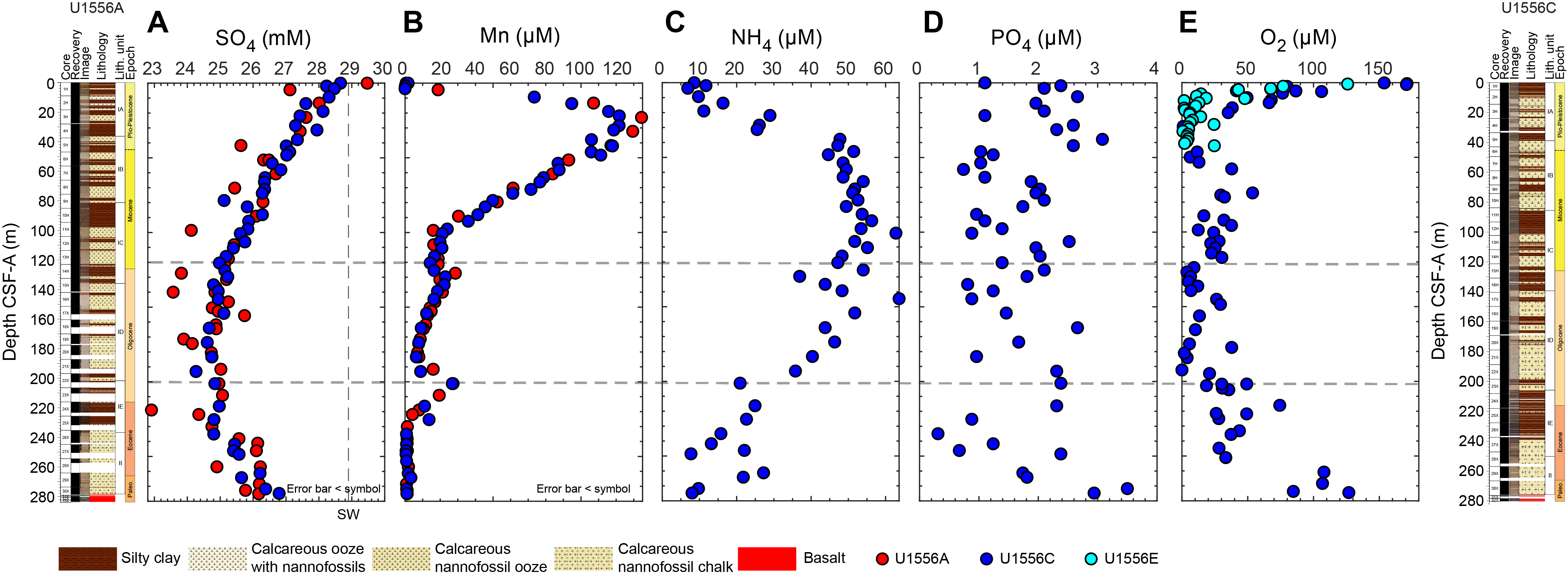
Figure F145. Sulfate, Mn, ammonium, phosphate, and oxygen.

11.1.2.5. Oxygen

Oxygen is the pore water constituent measured with the highest reduction potential and is the first molecule reduced during microbial degradation of organic matter. Its profile provides insight into subseafloor biogeochemical and microbial processes. In Hole U1556C, oxygen was measured after the Physical Properties team had run the cores through all the whole-round loggers (see Physical properties and downhole measurements in the Expedition 390/393 methods chapter [Coggon et al., 2024c]). This core logging resulted in wait times as long as 15 h after the core was received on the catwalk. In addition, methodology was altered slightly after Core 390-U1556C-6H (see Geochemistry in the Expedition 390/393 methods chapter [Coggon et al., 2024c]). The generated oxygen data are noisy but do indicate reduction from the seafloor to ~50 m CSF-A, below which O₂ values vary between 0 and ~60 µM until ~200 m CSF-A, and then O₂ increases toward basement (Table T29; Figure F145E). During analysis of cores from Hole U1556E, oxygen was measured approximately once per core section and wait time was shorter because O₂ was measured immediately after the STMSL. Additionally, for these measurements, the temperature probe was placed in the core itself through a hole in the core liner (see Geochemistry in the Expedition 390/393 methods chapter [Coggon et al., 2024c]). Oxygen concentrations from Hole U1556E decrease toward anoxic conditions faster than Hole U1556C, indicating that the majority of sediments at Site U1556 are anoxic below 50 µM CSF-A until they begin to increase below 200 m CSF-A.

11.1.3. Sediment bulk geochemistry

11.1.3.1. Calcium carbonate

Calcium carbonate (CaCO₃) concentrations in Hole U1556A sediments were measured in IW squeeze cakes at a frequency of once per core for Cores 390C-U1556A-1H through 12H, twice per core for Cores 13H–20X, and once or twice per core for Cores 21X–33X for a total of 42 analyses (Table T30). One sample was selected from sedimentary breccia in Core 390C-U1556B-2R at the sediment/basement interface (Table T30). Carbonate concentrations of Hole U1556C sediments were measured in the IW squeeze cakes at a frequency of twice per core for Cores 1H–16H, once per core for Cores 17X–26X, and twice per core for Cores 27X–30X for a total of 50 analyses (Figure F146A). To ensure representative lithologies were collected, an additional 5 cm³ discrete sediment sample was collected from every core from 390-U1556C-1H through 30X, for a total of 30 samples. A total of 16 sediment samples from Hole U1556E were sampled at least twice per core for Cores 390-U1556E-1H through 5H. The average carbonate content in all holes (38.0 ± 35.4 wt%, ±1 standard deviation [σ], n = 71) was highly variable in upper Lithologic Subunits IA–IC (above 120 m CSF-A), composed of alternating silty clay and calcareous nannofossil ooze (minimum = 0.02 wt%; maximum = 85.32 wt%). Overall, carbonate content is higher from Subunit ID to the bottom of the sedimentary package (63.2 ± 31.4 wt%, ±1σ, n = 68; maximum = 94.0 wt%). The sediment sample from the sediment/basement interface (Basement Unit 1) (see Igneous petrology) contains 84.1 wt% calcium carbonate.

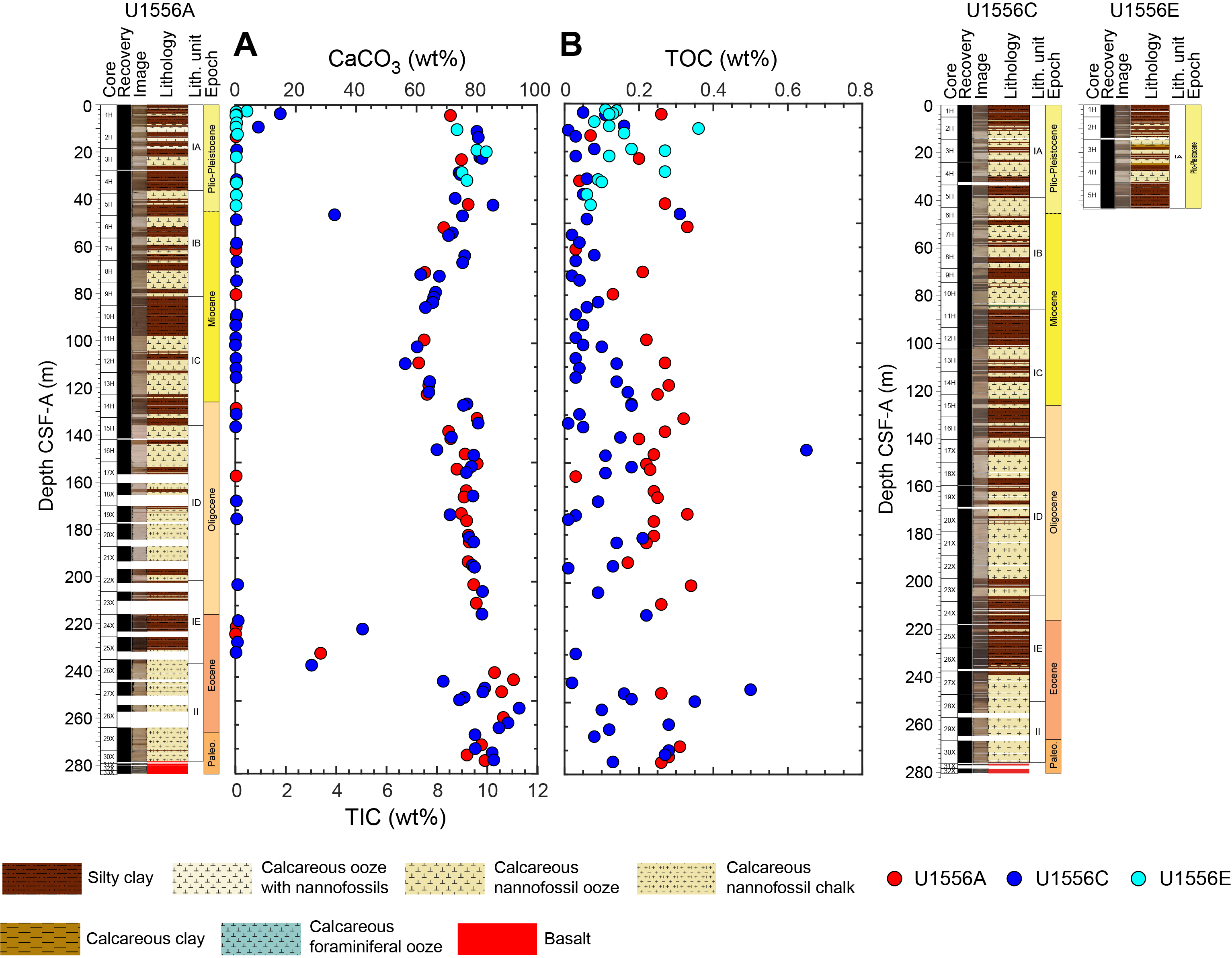
Figure F146. Sediment calcium carbonate, TIC, and TOC.

11.1.3.2. Total organic carbon

TOC was calculated for all samples measured for CaCO₃ as the difference between TC and TIC (see Geochemistry in the Expedition 390/393 methods chapter [Coggon et al., 2024c]). TOC concentrations are highly variable and overall low throughout all holes at Site U1556 (0.15 ± 0.11 wt%, ±1σ, n = 111; maximum = 0.65 wt%) (Figure F146B). Most of the total nitrogen (TN) and total sulfur (TS) concentrations were close to zero or below detection and are not reported here.

11.1.4. Sediment gas sampling

Routine safety hydrocarbon measurements were made in Hole U1556A during Expedition 390C (Estes et al., 2021) at a sampling resolution of two analyses per core from Cores 390C-U1556A-1H through 30X (Table T30). No gas was detected in any of the samples.

11.2. Basement

11.2.1. Sampling strategy and sample classification

A 342.3 m basement succession was cored in Hole U1556B during Expedition 390. Representative samples were taken from the freshest portions of each lithologic unit/subunit (see Igneous petrology) for bulk rock elemental analyses to obtain a downhole record of the primary magmatic compositions. These were supplemented with samples of basalt that exhibited different styles of alteration (see Alteration petrology) and were homogeneous at the scale of sampling to investigate the effects of hydrothermal exchange on bulk rock composition. In addition to the variably altered basalt samples, the sample suite also included lithified sediments. These sediments were sampled from the matrix of sedimentary breccia and original calcareous pelagic sediment mixed with volcanic glass and potentially other components and referred to as indurated calcareous sediments (see Sedimentology; also see Igneous petrology in the Expedition 390/393 methods chapter [Coggon et al., 2024c]). A total of 45 samples were taken for bulk rock geochemical analysis from Hole U1556B cores using ICP-AES.

Because the sampled basalts experienced variable degrees of alteration, they were categorized as follows for simplicity in this chapter (see Alteration petrology):

Slightly altered basalt: basalt with minimal phenocryst and groundmass alteration (i.e., typically <10% of the rock is secondary minerals).
Moderately altered basalt: basalt with macroscopic phenocryst and groundmass alteration (i.e., typically 10%–50% of the rock).
Highly altered basalt: basalt with significant macroscopic phenocryst and groundmass alteration (i.e., typically >50% of the rock) and the color of the groundmass in hand specimen indicates significant replacement by secondary minerals.

Following this classification scheme, the samples selected include 2 indurated calcareous sediments, 12 highly altered basalts, 15 moderately altered basalts, and 16 slightly altered basalts (Table T31). To investigate the effects of alteration on the bulk rock composition, three paired basalt samples were included that sampled different portions of a single lava flow exhibiting different styles or extents of alteration (Samples 390-U1556B-28R-2, 33–35 and 42–44 cm; 33R-2, 125–127 and 131–133 cm; and 46R-1, 7–9 and 80–81.5 cm). Rocks with thin fresh glassy margins that preserve primary magma compositions and samples of distinct alteration domains will be analyzed postexpedition.

11.2.2. Basement geochemistry

Loss on ignition (LOI) was first determined by ignition at 1025°C for 4 h, and concentrations of major (SiO₂, TiO₂, Al₂O₃, Fe₂O₃, MnO, MgO, CaO, Na₂O, K₂O, and P₂O₅) and minor/trace (Ba, Co, Cr, Cu, Ni, Sc, Sr, V, Zn, and Zr) elements were then measured on the ignited samples using ICP-AES (see Geochemistry in the Expedition 390/393 methods chapter [Coggon et al., 2024c]). Results are reported on a volatile-free basis as weight percent for major element oxides and LOI and as parts per million for minor/trace elements (Table T31).

11.2.2.1. Indurated calcareous sediments

Indurated calcareous sediments were sampled from both the top and bottom of the basement section cored in Hole U1556B (from Cores 2R and 59R, respectively). These lithified sediments, which commonly form the matrix or interstitial material of sedimentary breccias, hyaloclastites, and pillow lavas in these cores (see Igneous petrology), contain 80.1–86.4 wt% CaO, 8.9–10.7 wt% SiO₂, and 1.7–2.4 wt% Al₂O₃. These compositions confirm that the matrix of these breccias is dominated by carbonate material (e.g., calcite) with a small contribution from silicate minerals, consistent with visual core descriptions (see Sedimentology and Igneous petrology).

11.2.2.2. Lava

11.2.2.2.1. Variations with depth

Figure F147 summarizes the major element variations for the rocks from Site U1556 as a function of depth. The data are predominantly from Hole U1556B, but one sample was analyzed from Hole U1556A. This sample is included for completeness, plotting at the top of each graph. For simplicity, when discussing the data we will refer to a single hole (i.e., Hole U1556B), but the sample from Hole U1556A is included throughout unless otherwise stipulated. For comparison, the compositional range for N-MORBs, depleted MORB (D-MORB), E-MORB, and mean MORB from Gale et al. (2013) is shown as a gray bar. Note that this means the gray bar is of variable width, reflecting the compositional variation that is observed among these different MORB groups. The compositional variation tends to be small for SiO₂, CaO, and Na₂O (i.e., the bar is narrow) because N-MORB, D-MORB, E-MORB, and mean MORB have similar concentrations of these elements. In contrast, the variation is greater for Al₂O_3, FeO, MgO, K₂O, and P₂O₅ (i.e., the bar is wider), reflecting possible differences in source composition, depth or degree of melting, and/or magma chamber processes that have contributed to generation of these different MORB groups. The gray bar shown for LOI represents the estimated H₂O content (and does not account for CO₂, following the recommendation of Langmuir et al. [2006]: H₂O_est = 1.5 × K₂O). Also shown for comparison is the average composition for OIB from Sun and McDonough (1989); these authors reported predominantly average trace element data, so an average OIB composition is not shown for most major elements.

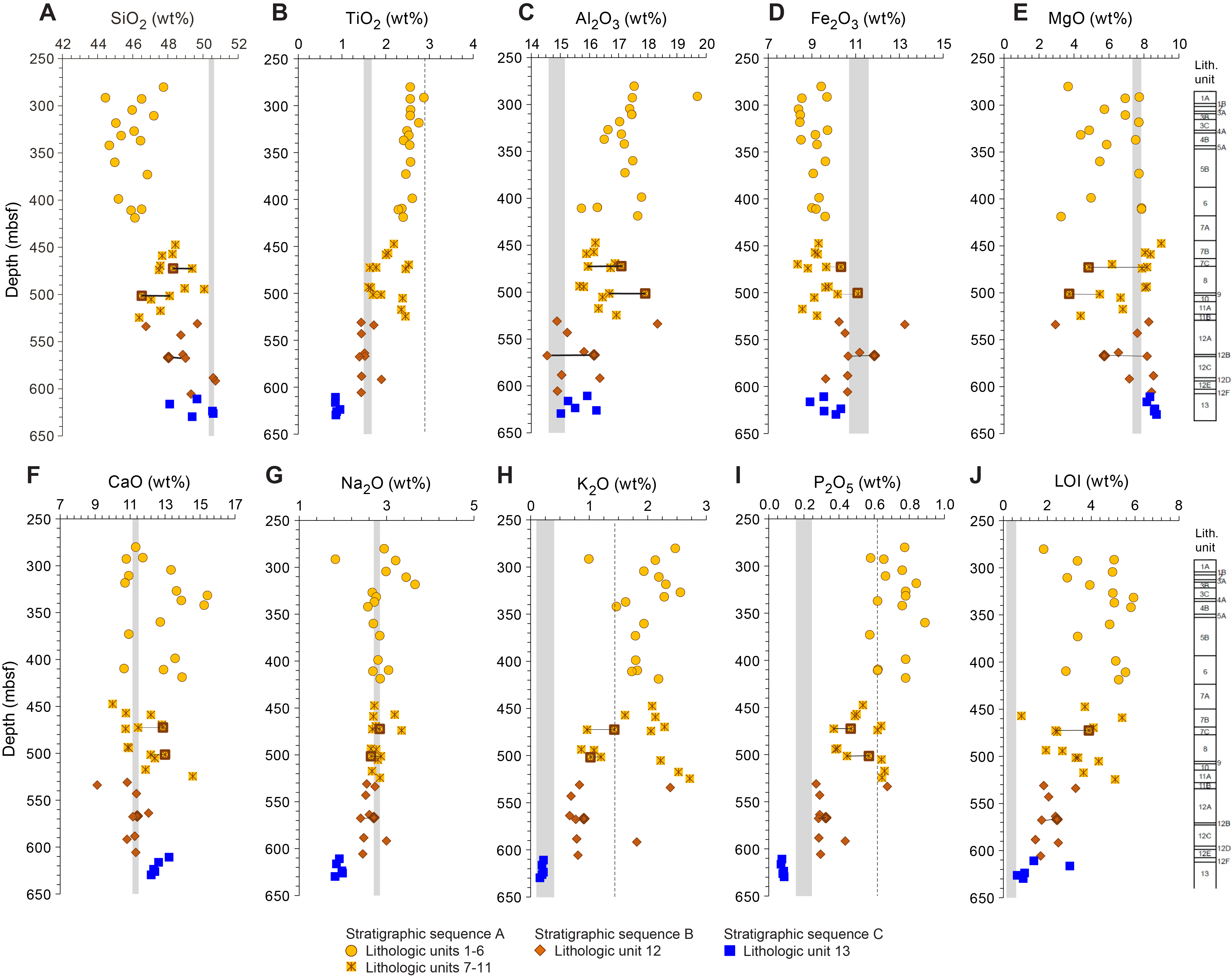
Figure F147. Major element concentrations and LOI.

Figure F147 shows the significant major element variation from the top to the bottom of Hole U1556B. The data are plotted using different symbols for the different stratigraphic sequences identified petrographically (i.e., Stratigraphic Sequences A [orange spotty], B [old red], and C [H-POPP]; see Igneous petrology for definitions of the appellative names used for the three stratigraphic sequences).

Petrographic observations indicate the presence of more than one lithologic type in cores toward the bottom of Stratigraphic Sequence A (see Igneous petrology). Indeed, intrusive relationships between basalts recognized as orange spotty and old red are observed in Unit 11, and ratios of HFSEs determined by pXRF, such as Zr and Ti (which are relatively resistant to alteration), suggest the interval of mixed lithology may have extended much higher in the hole, including Lithologic Units 7–10 (see Figures F16, F54). The higher precision ICP-AES data shown here allow us to confirm that the interval from Units 7 to 11 (Sections 390-U1556B-21R-3 to 38R-3, 85 cm) indeed represents intercalation of lavas from both Stratigraphic Sequences A and B (see below). Therefore, in these geochemical results we have divided the rocks from Stratigraphic Sequence A into two subgroups: Lithologic Units 1–6 and Units 7–11.

In general, Lithologic Units 1–6, which we view as the best representation of the orange spotty lava composition, have the lowest SiO₂ and highest TiO₂, Al₂O₃, K₂O, and P₂O₅ (Figure F147) of the rocks recovered at Site U1556. The concentrations of these elements are significantly lower and higher, respectively, than any of the average MORB compositions reported by Gale et al. (2013). Although average major element compositions for OIB from Sun and McDonough (1989) are limited to TiO₂, K₂O, and P₂O₅, based on these data orange spotty rocks are clearly more akin to OIB than MORB.

In contrast, Stratigraphic Sequence C (H-POPP), which was recovered below 609 mbsf (i.e., from Section 390-U1556B-54R-3 to the bottom of Hole U1556B), plots closer to the range of average MORB. However, in most cases their compositions do not overlap the range for D-MORB, N-MORB, E-MORB, or mean MORB. Instead, they are depleted in incompatible elements such as TiO₂, Na₂O, and P₂O₅(i.e., lower than average MORBs) and enriched in Al₂O₃, MgO, and CaO (i.e., higher than average MORBs). Stratigraphic Sequence B (old red) and Lithologic Units 7–11 of Stratigraphic Sequence A form an array that spreads between these two extremes; old red tends to plot closer to the range of average MORBs. Lithologic Units 7–11 show the most compositional scatter, with some individual samples clearly overlapping the composition of orange spotty (Lithologic Units 1–6) and others more akin to old red, consistent with the observation of intercalation of these two lithologic types within this interval (see Igneous petrology).

Trace elements show similar variations with depth to those shown by major elements (Figure F148). Rocks from Lithologic Units 1–6 (Stratigraphic Sequence A) overlap the composition of average OIB for incompatible elements such as Sr and Zr, although they are significantly enriched in Ba (i.e., concentrations up to 750 ppm compared to 350 ppm for average OIB; Sun and McDonough, 1989). In common with the variations in Na₂O and TiO₂, concentrations of these incompatible trace elements decrease with depth in the hole, with H-POPP basalts showing the lowest Sr, Zr, Ba, and Y contents measured for Hole U1556B lavas. Of particular note is that all these incompatible trace elements have concentrations that are lower even than average D-MORB (i.e., the lower bound of each gray bar in Figure F148). The rocks from Stratigraphic Sequence B (old red) and Lithologic Units 7–11 from Stratigraphic Sequence A plot between these two compositional extremes.

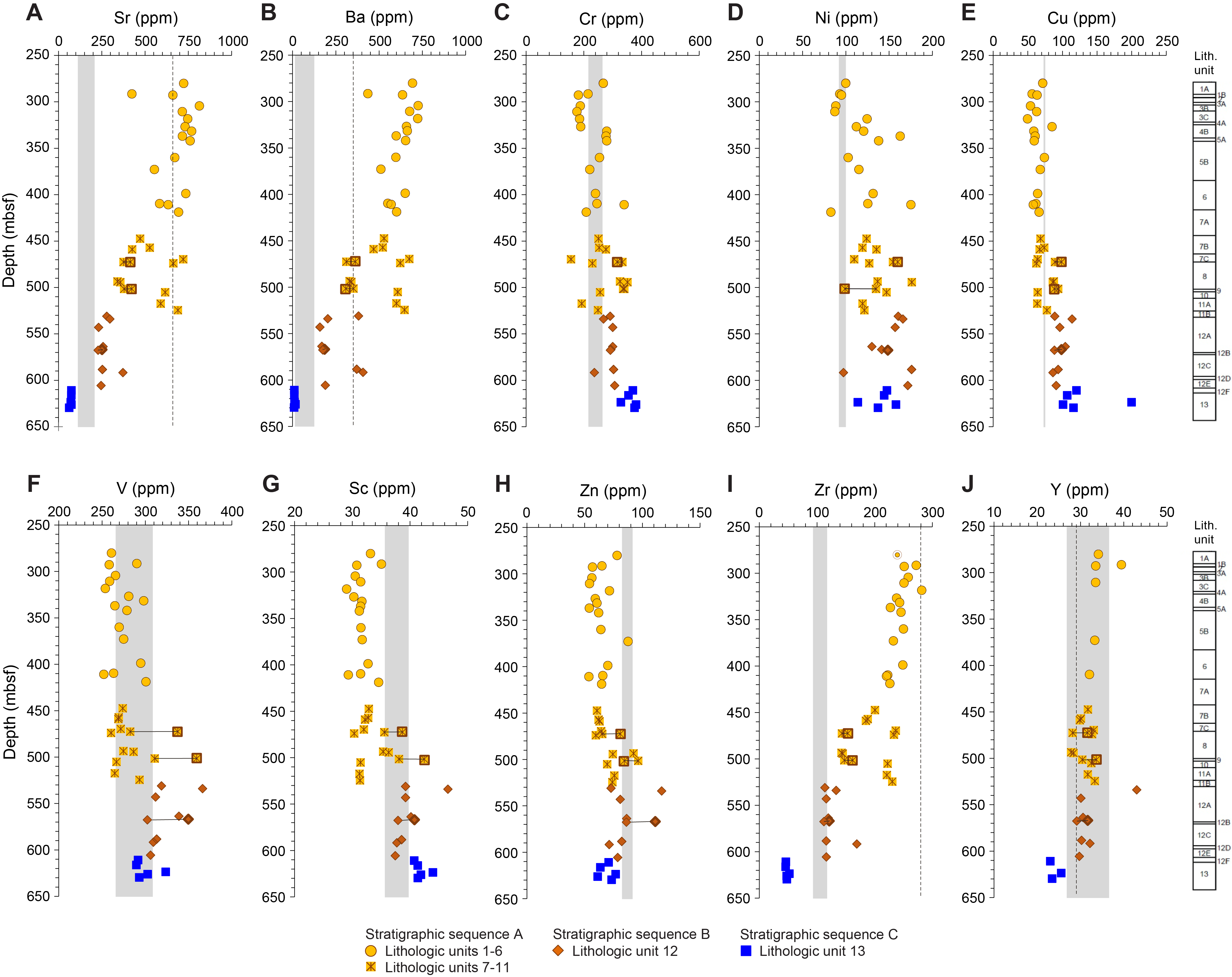
Figure F148. Trace element concentrations, basalts.

Compatible elements Cr and Ni and transition metals Cu and Sc show the opposite trend: lowest in the upper part of Stratigraphic Sequence A and highest in Stratigraphic Sequence C. Zinc and to a lesser extent V show no or limited systematic variation in concentration with depth. The high concentrations of Cr and Ni in H-POPP basalts (i.e., 369 and 140 ppm on average, respectively) relative to the range of average MORB compositions are particularly notable, given that they are even higher than average D-MORB (i.e., 269 and 140 ppm, respectively; Gale et al., 2013). In contrast, the transition metals Cu, V, Sc, and Zn show variable behavior; Cu and Sc are significantly higher than average MORBs and Zn is lower. V is the only transition metal that significantly overlaps the compositional range of average MORBs, and like Zn, it shows limited systematic variation with depth despite the significant difference in major element composition from top to bottom of the hole (Figure F148).

11.2.2.2.2. Comparison of paired basalt samples

Three paired basalt samples that sampled different portions of a single lava flow were analyzed to highlight the effects on bulk rock composition of differing styles or extents of alteration. The paired samples include the following:

Intervals 390-U1556B-28R-2, 33–35 and 42–44 cm, from Lithologic Unit 7;
Intervals 390-U1556B-33R-2, 125–127 and 131–133 cm, from Lithologic Unit 8; and
Intervals 390-U1556B-46R-1, 7–9 and 80–82 cm, from Lithologic Unit 12 (old red).

Core photographs of each pair are shown in Figure F149. Based on this macroscopic observation, Samples 390-U1556B-28R-2, 33–35 cm; 33R-2, 125–127 cm; and 46R-1, 7–9 cm, are from orange halo areas (see Alteration petrology) and are inferred to be more altered than Samples 28R-2, 42–44 cm; 33R-2, 131–133 cm; and 46R-1, 80–82 cm. Where sufficient variation is present between the pairs and discernible on Figures F147 and F148, the paired samples are linked by a tie line. The figures show that for most elements the compositional differences between paired samples from the same flow are relatively small, regardless of alteration, and within the size of the symbols used. Nonetheless, there are some consistent variations (see Table T31). In general, SiO₂ and MgO are noticeably lower in the more altered portions of the lava flows, whereas Al₂O₃, Fe₂O₃, Sr, and LOI are higher. CaO and TiO₂ show small but discernible increases in the more altered portions as well. Transition metals (V, Sc, Cu, and Zn) and HFSEs (Zr and Y) also show small but significant increases in the more altered portions of each pair. It is unclear whether these small differences/increases reflect actual addition of these elements as part of hydrothermal exchange or simply an increase due to the relative mass loss from significant removal of SiO₂ and MgO. Detailed shore-based study, possibly involving isotope analysis, will be needed to confirm the nature of some element mobility. Surprisingly, behavior of the alkali elements, Na₂O and K₂O, is variable; the (apparently) more altered portions of each pair have higher concentrations of these elements in Samples 28R-2, 33–35 cm, and 46R-1, 7–9 cm, but lower in Sample 33R-2, 125–127 cm. Mobility of the alkali elements may, therefore, require a more sophisticated assessment of alteration style and extent if we are to understand the drivers and mineralogical reactions involved.

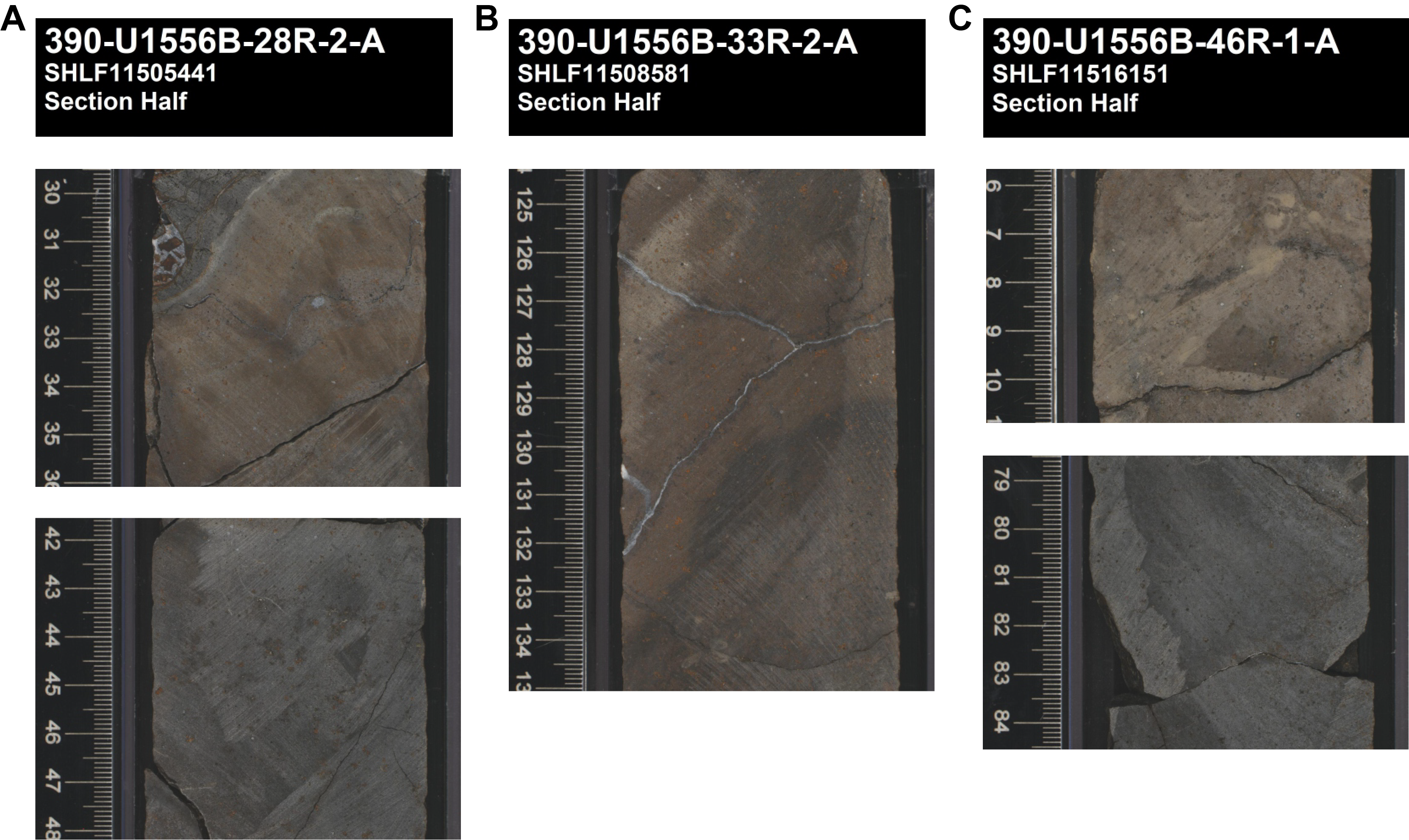
Figure F149. Paired Hole U1556B basalt samples.

Collectively, the geochemical data for paired samples suggest that, as a result of hydrothermal alteration, basalt samples from Hole U1556B may, in general, appear more evolved (lower MgO and higher Fe₂O₃), more alkaline (lower SiO₂ and generally higher K₂O), and possibly more enriched in some trace elements than their original compositions, necessitating care when interpreting primary petrology.

11.2.2.2.3. Classification

Consistent with analysis of Figures F147 and F148, which suggests compositions that range from OIB-like to MORB-like in Hole U1556B, a plot of total alkalis versus silica (TAS) (Figure F150A) suggests that the rocks range from alkaline to subalkaline. In this diagram, the different stratigraphic sequences are shown as different symbols to facilitate comparison with Figures F147 and F148. Rocks from Stratigraphic Sequence A (orange spotty) are predominantly alkaline, with relatively low SiO₂ concentrations (44.5–47.8 wt%) and high total alkali contents (up to 6 wt%), such that they plot above the alkaline/subalkaline dividing line of Miyashiro (1978). Individual samples range from alkali basalt to basanite to trachybasalt, with one sample (390-U1556B-2R-2, 11–13 cm) plotting in the picrobasalt field. The latter, Sample 2R-2, 11–13 cm, which is a highly altered basalt clast encased in the indurated calcareous matrix of the sedimentary breccia at the top of Hole U1556B (see Igneous petrology), has LOI > 5 wt%, among the highest observed in Hole U1556B. The sample almost certainly plots in the picrobasalt field because of significant loss of SiO₂ during alteration, as observed above for the paired samples (see Table T31). A thin section of this exact sample is not available, but other basalts from the same core show complete replacement of olivine by Fe oxyhydroxides and extensive replacement of groundmass feldspar and pyroxene by clay minerals and possibly zeolites. Because these minerals tend to have lower SiO₂ contents than the original minerals they replace, these replacements result in a lower SiO₂ content for the residual whole rock. Therefore, the fact that this sample plots in the picrobasalt field is not petrologically significant (i.e., it is not evidence for picritic basalts at Site U1556).

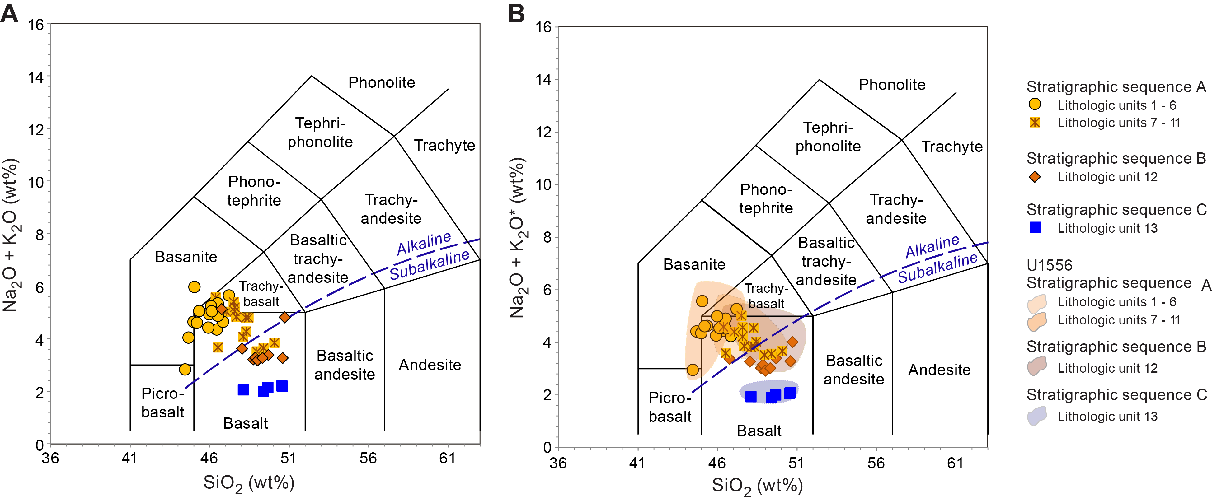
Figure F150. TAS.

Although Lithologic Units 1–11 are all from the same stratigraphic sequence, lavas from Units 1–6 are all alkaline, whereas those from Units 7–11 range from alkaline to subalkaline, consistent with the mixed nature of this interval (see Igneous petrology). In contrast, rocks from Stratigraphic Sequence B (old red) have higher SiO₂ (46.8–50.7 wt%) and lower total alkalis, with most samples plotting within the subalkaline field. However, two samples plot on or close to the alkaline/subalkaline boundary and one sample plots within the alkaline trachybasalt field, suggesting there may be a range of alkalinity in the primary magmas for old red. H-POPP basalts are all subalkaline, with significantly lower total alkalis than both Stratigraphic Sequences A and B (<2.2 wt%) but overlapping the range of SiO₂ concentrations for Stratigraphic Sequence B.

Although most samples were selected because they appeared to be the least altered material available (based on macroscopic observation), LOI values are high throughout, ranging 0.63–5.93 wt%. Only four samples have LOI values <1 wt% (Table T31). Such high LOI values suggest significant degrees of alteration, particularly for subalkaline basalts. Gale et al. (2013) estimate that mean MORB has an H₂O content of only about 0.24 wt%, which is significantly lower than any samples analyzed from Site U1556. Given that the alkali elements, particularly K, can be significantly affected by such high degrees of alteration (see Igneous petrology; also see Figure F38 in the Site U1557 chapter [Coggon et al., 2024a]), sample classification based on TAS may be suspect. Indeed, an incompatible trace element plot, normalized to average N-MORB, emphasizes the extent of secondary enrichment of K₂O relative to adjacent large-ion lithophile (LIL) elements, particularly for rocks with the lowest initial K₂O concentrations (i.e., H-POPP basalts) (Figure F151). If we assume that the average trace element patterns for MORB and OIB should follow relatively smooth patterns across the diagram (Gill and Fitton, 2022) (e.g., red dotted lines in Figure F151), the concentration of K₂O in H-POPP basalts is enriched by more than a factor of 5 and by nearly a factor of 2 in old red.

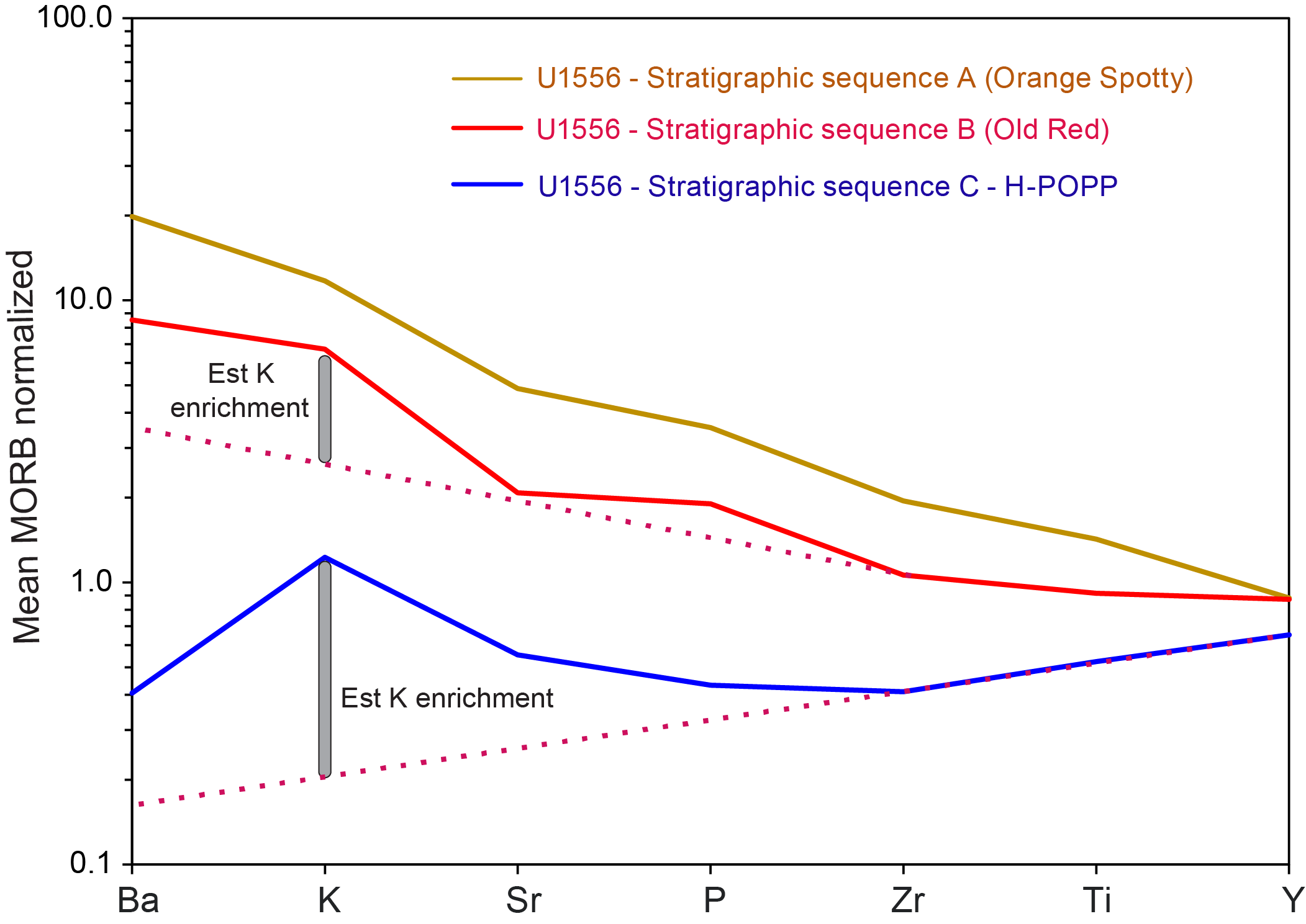
Figure F151. Mean MORB–normalized trace element data.

We can use these data to apply at least a minimum correction to the K₂O concentrations by extrapolating between adjacent elements on the multielement diagram, following the process commonly used to calculate Eu anomalies by McLennan (1989). Clearly, this approach rests on the assumption that adjacent elements (Ba and Sr) are not affected by alteration. Although probably not strictly true, plots of element concentration versus silica saturation index (SSI) suggest that much of the variation in both Ba and Sr can be attributed to magmatic processes (Figure F152). SSI, which is defined as

$100 \times [Si - (Al + {Fe}^{2 +} + Mg + 3 Ca + 11 Na + 11 K + Mn - {Fe}^{3 +} - Cr - Ti - 10 P) / 2],$

is predominantly a function of degree of partial melting; as the degree of partial melting decreases (for the same source composition), the SSI decreases (Gill and Fitton, 2022). Rocks with SSI < 0 are alkaline, whereas those with SSI > 0 are subalkaline. Because the calculation of SSI includes the complete major element analysis, it is less sensitive to perturbations of a single element, such as K, although it will obviously be impacted where alteration and loss of SiO₂ are most extensive.

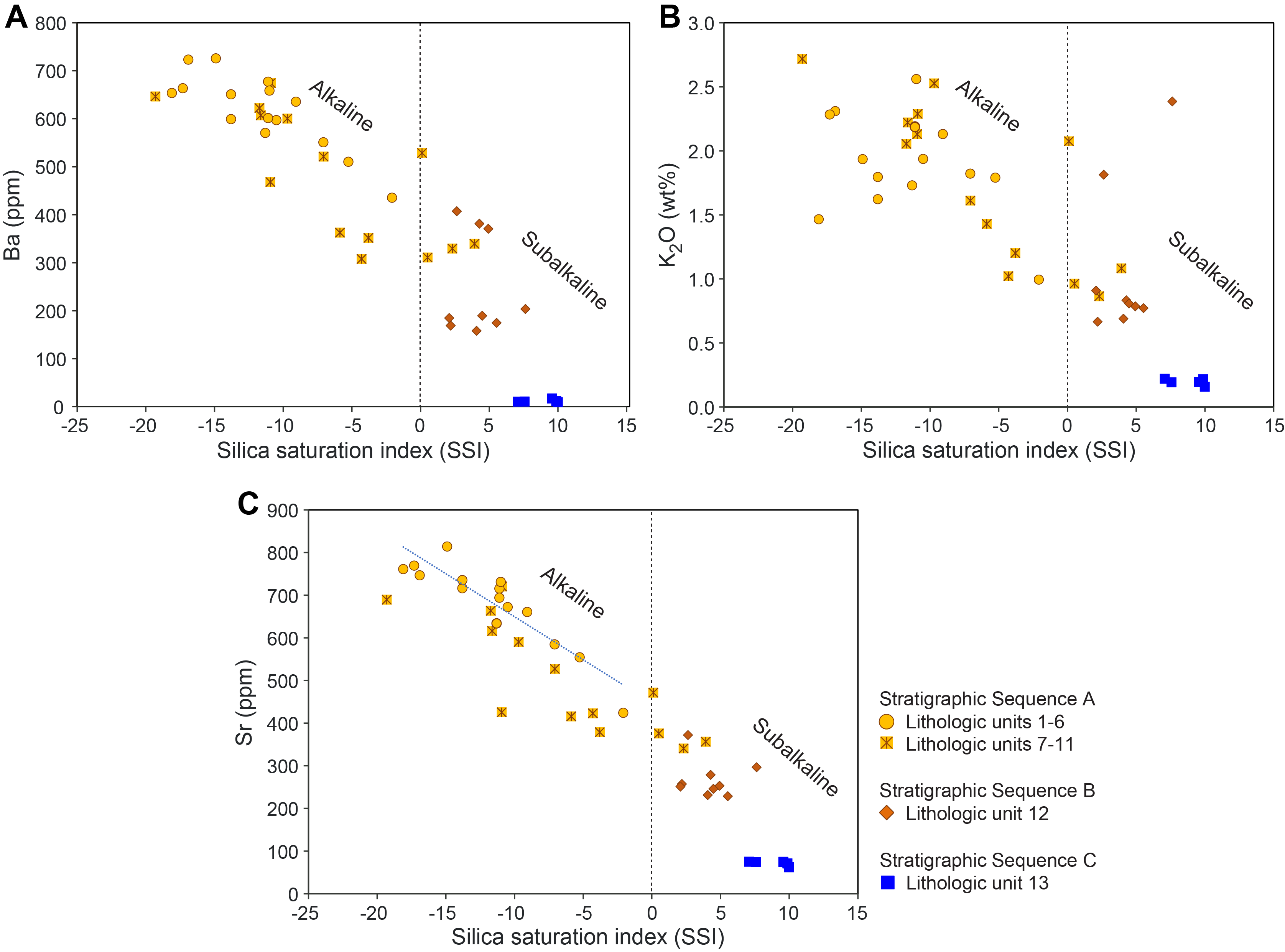
Figure F152. SSI vs. Ba, K₂O, and Sr.

Figure F152A and F152C shows broad negative correlations between SSI and the concentrations of Ba and Sr in which orange spotty rocks (Lithologic Units 1–6) form the low-SSI (alkaline; SSI < 0)–high Sr and Ba end of the array, whereas H-POPP forms the high-SSI (subalkaline; SSI > 0)–low Sr and Ba end. Lithologic Units 7–11 range from alkaline to subalkaline (SSI = −19 to 4), and old red rocks are all subalkaline (SSI > 0). Although there is clearly some scatter in the arrays shown by Ba and Sr versus SSI (Figure F152A, F152C), it is far less than the scatter in the K₂O versus SSI plot (Figure F152B), consistent with greater perturbation of K₂O by hydrothermal alteration (Figure F151). This suggests that the main control on Ba and Sr concentrations is a primary magmatic one such as source composition or degree of partial melting. We can, therefore, use these concentrations to correct for at least some of the K₂O addition apparent in Figure F151.

Figure F150B shows the distribution of data in the TAS diagram using the corrected K₂O contents compared to the field for uncorrected data from Figure F150A. The changes to the total alkalis contents of rocks from Stratigraphic Sequence A, Lithologic Units 1–6, are relatively small, although the correction does move most samples into the alkali basalt field; few samples now plot in the adjacent trachybasalt and basanite fields. Lithologic Units 7–11 still range from alkaline to subalkaline, but all alkaline samples now plot as alkali basalts and none are trachybasalts. Given that the correction applied is almost certainly a minimum, this suggests that orange spotty lavas are alkali basalts, as opposed to more alkaline rock types, such as basanite or trachybasalt.

Although the size of the correction is largest for the H-POPP basalts, the impact on classification is small because the rocks are already correctly identified as subalkaline basalts. In contrast, the reclassification of old red lavas is petrologically significant. Prior to correction of the K₂O values, classification implied that the lavas of this unit ranged from alkaline to subalkaline, which has significant implications for understanding source composition and degree of partial melting. After K₂O correction, all but one sample plots within the subalkaline field. Although a thin section is not available for the one sample that still plots within the alkaline field (i.e., Sample 390-U1556B-33R-2, 125–127 cm), it is one of the paired basalt samples discussed above. Macroscopic observation shows that it is highly altered, and the less altered sample from the same pillow lava (i.e., Sample 33R-2, 131–133 cm) has similar corrected total alkalis but higher SiO₂ and, hence, plots within the subalkaline field. Therefore, the corrected data indicate that old red basalts are subalkaline (tholeiitic) in character. Note that this is consistent with the observation that all old red basalts have SSI values >0, even those that plot in the TAS diagram near or within the alkaline field, providing strong evidence that old red basalts are entirely tholeiitic in character.

11.2.2.2.4. Comparison of the three principal magmatic units

Figure F153 summarizes average compositions for the three stratigraphic sequences on an extended multielement plot, normalized to average N-MORB of Sun and McDonough (1989). A first-order observation from this diagram is that H-POPP basalts show N-MORB-like compositions for most elements to the right of Na (i.e., concentrations plot near a N-MORB normalized value of 1), with some variation in the transition metals (Zn, Cu, Mn, and Fe) and elevated concentrations for the compatible elements Cr and Ni. However, the most incompatible elements (Ba to Y) show distinct depletion in relation to N-MORB, except for potassium. The latter shows a strong positive anomaly relative to adjacent LIL elements due to hydrothermal alteration, as discussed above. Collectively, the data for H-POPP basalts suggest they were derived from a mantle source that was significantly more depleted than that of N-MORB, indeed, more depleted even than D-MORB (see Figures F147, F148), but they have been secondarily enriched in (some) LIL elements, particularly K, by hydrothermal alteration. The ratio of V/Sc, often cited as a sensitive recorder of the oxygen fugacity of MORB-source mantle, averages ~7 for H-POPP basalts, which is within the range for average MORB (6.74 ± 1.11; Li and Lee, 2004) that was derived by melting in the spinel lherzolite stability field at slightly below quartz-fayalite-magnetite (QFM) (Mallmann and O'Neill, 2009). However, other transition metals (i.e., Zn and Cu) show unusual negative and positive anomalies, respectively. These variations are interesting because the differences among D-MORB, N-MORB, and mean MORB averages (Gale et al., 2013) are <3 ppm for both elements, whereas H-POPP basalts are up to 14 ppm lower and 130 ppm higher in Zn and Cu, respectively, relative to mean MORB. This suggests the variations observed in H-POPP basalts are due to something other than typical MORB-source melting or magma chamber processes. Whether this is due to secondary alteration processes, unusual source conditions, or possibly analytical uncertainty in the shipboard data will require detailed shore-based research.

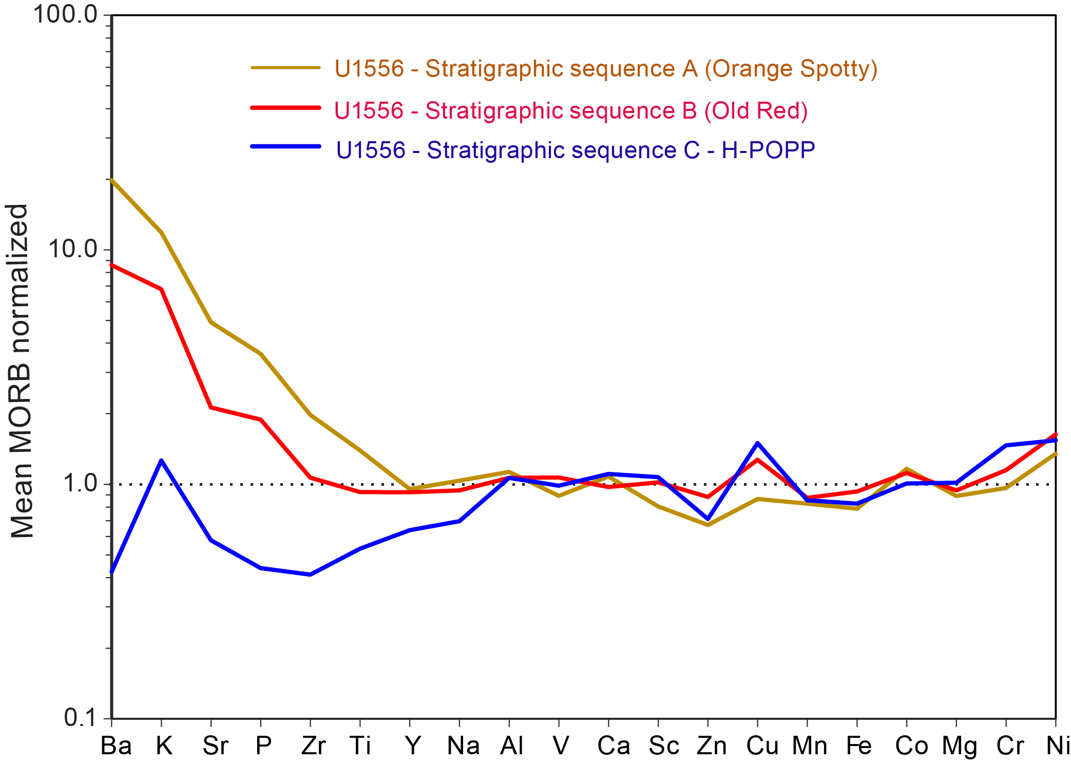
Figure F153. Mean MORB–normalized multielement data.

In contrast, Stratigraphic Sequences A and B show significant enrichments in the most incompatible trace elements (i.e., those on the left side of Figure F153; Ba to Ti); Stratigraphic Sequence A (orange spotty) is more enriched than Stratigraphic Sequence B (old red). Note that the average composition for orange spotty excludes Lithologic Units 7–11 because of the intercalation of at least two different magma types in this interval.

The incompatible trace element enrichment observed in Stratigraphic Sequence A (orange spotty) basalts is consistent with their low SSI values (Figure F152) and alkali basalt compositions (Figure F150B). V/Sc ratios range 8.3–9.4, which is within the range for OIBs reported by Mallmann and O'Neill (2009) (8–14) and consistent with derivation of orange spotty from a mantle source that is slightly more oxidizing than that for H-POPP or that partial melting of the same source composition took place at greater depths within the garnet rather than spinel stability field. The latter scenario seems unlikely, given the significant depletion of H-POPP basalts and, by implication, the H-POPP source. In addition, partial melting in the garnet stability field would produce lower Y contents rather than higher (see Figure F153) because Y is compatible in garnet. Small relative depletions and enrichments in Zn and Cu, respectively, are noted in orange spotty basalts, but average compositions in OIBs for these two elements have not been established.

In contrast to orange spotty basalts, the incompatible trace element enrichment observed in Stratigraphic Sequence B (old red) occurs in rocks that are tholeiitic in composition (i.e., SSI > 0), and the shape of the normalized multielement pattern for elements to the right of Na is more akin to H-POPP than to orange spotty basalts. The enrichment in incompatible trace elements (i.e., Ba to Y; Figure F153) is greater than that for average E-MORB, ranging 5%–100%, but less than average OIB enrichment, ranging 25%–50%, except for Y, which is slightly higher. This raises the question of whether old red basalts represent a less enriched OIB or a more enriched MORB. V/Sc ratios (7.9–8.6) are unhelpfully intermediate between reported ranges for MORB (<7) and OIB (>8) (Mallmann and O'Neill, 2009), and the sizes of Zn and Cu anomalies are intermediate between those for orange spotty and H-POPP.

Given that all Hole U1556B samples are hydrothermally altered to some extent, as suggested by their high LOI contents, ratios of HFSEs such as Zr/Nb, Nb/Y, and Zr/TiO₂ can be among the most useful tools for studying magmatic compositional variations because the HFSE ratios generally are not strongly affected by fractional crystallization or alteration (e.g., Gill and Fitton, 2022). Similar Zr/TiO₂ ratios (parts per million/weight percent) for paired basalt samples in Hole U1556B (Table T31), regardless of the degree of alteration, indicate this ratio records primary magmatic compositions with high fidelity.

The ratios of Zr/TiO₂ are summarized graphically in Figure F154. Lithologic Units 1–6 have Zr/TiO₂ ratios that are relatively high (96 ± 2 ppm/wt% on average), close to the composition of average OIB (~98 ppm/wt%; Sun and McDonough, 1989). In contrast, lower ratios (54 ± 0.6 ppm/wt% on average) in Stratigraphic Sequence C (H-POPP) indicate MORB-like magma compositions (~58 ppm/wt%; Sun and McDonough, 1989). Samples from Units 7–11 have intermediate Zr/TiO₂ ratios (85–95 ppm/wt%) with a bimodal distribution, whereas the Zr/TiO₂ ratios are relatively uniform through Stratigraphic Sequence B (old red) with an average composition (80 ± 3 ppm/wt%) that is intermediate between typical OIB and N-MORB compositions. However, Zr/TiO₂ ratios for old red are within the propagated uncertainties reported on the average compositions for TiO₂ and Zr for average E-MORB in Gale et al. (2013).

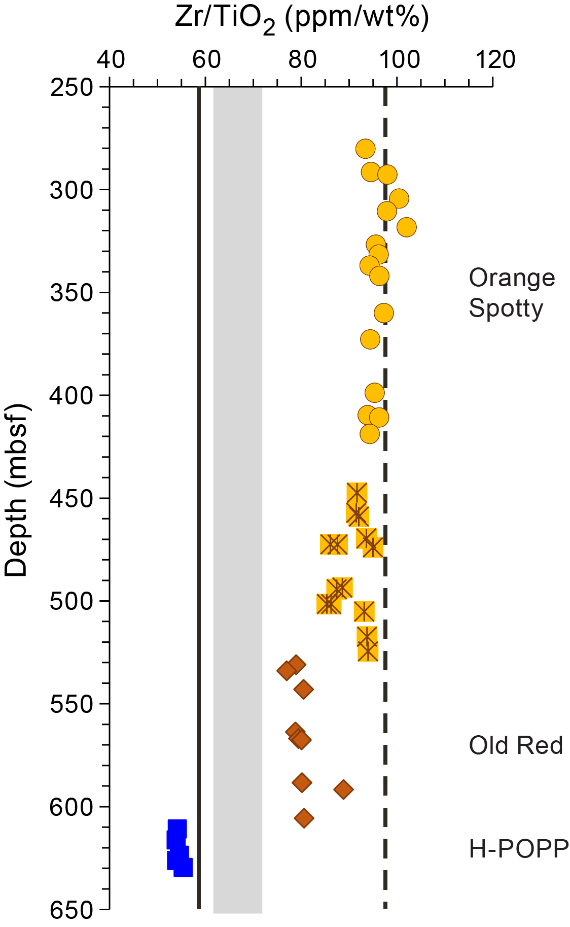
Figure F154. Zr/TiO₂ ratios.

It is tempting to equate the OIB-like compositions of Stratigraphic Sequence A (orange spotty) and possibly Stratigraphic Sequence B (old red) to plume magmatism associated with formation of the Rio Grande Rise, which is located west of Site U1556. However, much of the Rio Grande Rise is significantly older (>80 Ma) than the basalts from Site U1556. It is believed to have formed when the Tristan plume was centered beneath the ocean ridge (Hoyer et al., 2022). However, between 80 and 60 Ma, southward propagation of the ridge separated the western Rio Grande Rise from the Walvis Ridge and created the north-south–oriented eastern Rio Grande Rise, which overlaps in age with the 60 Ma basalts from Site U1556.

Figure F155 compares the basalts from Site U1556 with average compositions for the western and eastern Rio Grande Rise from Hoyer et al. (2022). The data show that none of the rocks from the Rio Grande Rise are compositionally similar to the tholeiitic H-POPP basalts at the bottom of Hole U1556B. Conversely, alkaline rocks from the western Rio Grande Rise are strongly enriched in incompatible trace elements (Hoyer et al., 2022) and clearly distinct from even the most enriched rocks from Site U1556 (i.e., orange spotty). In particular, (1) concentrations of the most incompatible elements are higher; (2) Y concentrations are lower; (3) V and Sc are lower, but the V/Sc ratio is significantly higher (~13); and (4) the anomalies for Zn and Cu are of the reverse sense (i.e., the Zn anomaly is positive, whereas the Cu anomaly is negative).

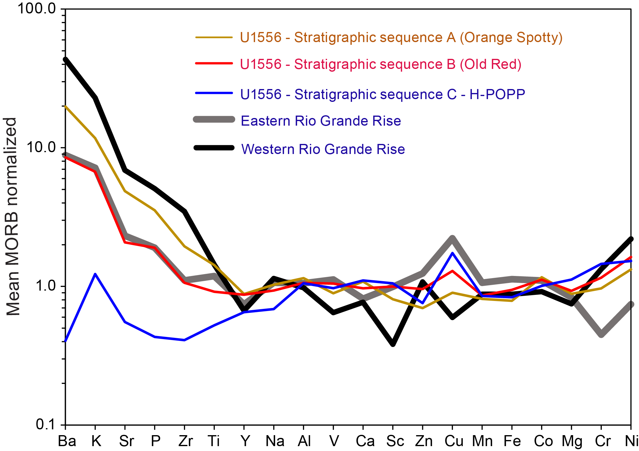
Figure F155. Mean MORB–normalized data compared to Rio Grande Rise data.

However, there are some intriguing similarities between the rocks from the eastern Rio Grande Rise and Stratigraphic Sequence B (old red) from Site U1556. Both are tholeiitic and there is significant overlap in the degree of incompatible element enrichment for the two groups of rocks (Figure F155). However, Y concentrations are higher, Ti concentrations are lower, and V/Sc is higher in the eastern Rio Grande Rise relative to old red basalts. Lower Mg, Cr, and Ni concentrations for eastern Rio Grande Rise rocks indicate they are more evolved than old red, but this should not significantly affect the ratios of the HFSE (e.g., Zr/Y and Ti/Y). Nonetheless, the eastern Rio Grande Rise is only ~200 km west of Site U1556, and given the overlaps in age and composition, links to formation of the eastern Rio Grande Rise seem likely for old red basalts. The lack of similarities for H-POPP and orange spotty basalts with either the eastern or western Rio Grande Rise makes their origins even more enigmatic. Shore-based research, including isotopic analysis, will be required to understand the petrogenesis of the basalts from Site U1556.

12. Microbiology

12.1. Sediment

Microbiology sampling in sediment from Site U1556 during Expedition 390 focused on exploring evidence for life in the sediments and the sediment/basement interface using culture-based and culture-independent approaches. From Holes U1556C and U1556E, 118 whole-round sediment samples (5–20 cm long) were collected for microbiological standard (38 samples) and personal (80 samples) analyses. At least two whole-round core samples were collected from each 9.5 m advance and processed and subsampled for different analyses. In addition, Sample 390-U1556C-32X-1, 70.5–82 cm, was taken from the sediment/basement interface (Table T32).

12.1.1. Microbiological sample processing and experiments

12.1.1.1. Cell and viral counts

A total of 36 samples were processed for cell and virus enumeration. Performing shipboard cell counts samples is difficult and time consuming; therefore, shipboard cell counts were not attempted during the SAT expeditions. Instead, samples were preserved for postexpedition analysis in a 20% vol/vol slurry in 5 mL total of sediment and 5% Epredia Formal-Fixx in 3× phosphate-buffered solution, respectively. Duplicate subsamples were taken for cross-calibration of cell counts in different laboratories, and a third subsample was taken for viral counts.

12.1.1.2. Microbial community structure

A total of 39 samples were processed for postexpedition DNA (PCR amplicon-based) and/or RNA (PCR amplicon-based) analysis, 34 samples for single-cell genomics, 14 samples for viral metagenomics, 11 samples for sediment metagenomics, 13 samples for anaerobic enrichments, and 11 samples for high-throughput culturing (Table T32). Material for these analyses of microbial community composition was collected and preserved following the procedures described in Microbiology in the Expedition 390/393 methods chapter (Coggon et al., 2024c). Whole-round samples to be subsampled for anaerobic enrichments were brought from the core receiving platform to the anaerobic chamber in the walk-in cold room in the microbiology laboratory and subsampled in the anaerobic hood to prevent exposure to oxygen. These samples were selected from depths assumed to be anaerobic based on the Mn and sulfate profiles of Hole U1556A (see Geochemistry).

12.1.1.3. Microbial incubation experiments

To attempt to isolate new microbial species, enrichment experiments using 1/10 ZoBell Marine Agar Petri dishes were initiated during Expedition 390. This media selects for heterotrophic marine microorganisms and is commonly used to isolate new microorganisms from marine environments. These culturing experiments were initiated as described in Microbiology in the Expedition 390/393 methods chapter (Coggon et al., 2024c). After inoculation, Petri dishes were incubated for the duration of Expedition 390 at 9.5°C with the tops facing down and then shipped to shore for postexpedition research.

Stable isotope probing experiments were initiated to determine preferred carbon (C) and nitrogen (N) sources used by metabolically active microorganisms in subseafloor sediments (Table T32). Similar methods were used during Integrated Ocean Drilling Program Expedition 329 to reveal the presence of active microorganisms in South Pacific Gyre sediments as old as 101.5 Ma (Morono et al., 2020). Our aim is to determine whether the host sediment age and/or oxygen concentration influences C and N substrate utilization. These experiments were conducted according to the procedure outlined in Microbiology in the Expedition 390/393 methods chapter (Coggon et al., 2024c). Samples were incubated at 4°C, comparable to in situ sediment temperatures measured during Expedition 390C, until shipment to shore at the end of Expedition 390. The first time point of individual experimental vials were killed and fixed by adding 15 mL of 4% paraformaldehyde in phosphate-buffered saline solution after 10 days. The remaining three time points will be killed during shore-based research at 30 days, 2 months, and 6 months.

The rate of microbially mediated sulfate reduction was determined by the addition of radiolabeled (³⁵S) sulfate to a subset of 25 sediment samples at a sampling resolution of approximately one sample every 10 m of core (Table T32). Samples with visual evidence of drilling disturbance were not chosen for sulfate-reduction incubations. For these experiments, whole-round samples were brought from the core receiving platform to the anaerobic chamber in the walk-in cold room in the microbiology laboratory and subsampled in the anaerobic hood to prevent exposure to oxygen, which would inhibit sulfate reduction. Once the whole-round sample was inside the anaerobic chamber, the outer centimeter of the core was removed using autoclaved ceramic knives, and the remaining core was transferred to gas-tight bags, flushed with N₂ gas, heat sealed, and stored at ~4°C until prepared for radiotracer additions. Sulfate-reduction experiments were conducted as indicated in Microbiology in the Expedition 390/393 methods chapter (Coggon et al., 2024c).

12.1.2. Microbiological contamination monitoring

To determine the number of microorganisms present in drilling fluid and also generate a database of potential contaminants, we collected drilling fluid from a pipe on the rig floor two times during coring operations in Hole U1556C: during the coring of Core 390-U1556C-24X (~218 mbsf) and during the coring of Core 27X (~240 mbsf). Subsamples were collected for cell counts, and 500 mL of drill fluid was filtered onto two separate 0.20 µm pore size, 47 mm diameter filters and frozen at −80°C for shore-based molecular biology analysis.

12.2. Basement

Microbiology sampling in basement at Site U1556 during Expedition 390 focused on exploring evidence for life using culture-based and culture-independent approaches. For Hole U1556B, sampling efforts focused on collecting a single whole-round core sample from each 9.5 m advance that would be processed and subsampled for different analyses. The aim was to generate a suite of samples that were representative of the different rock and alteration types that comprise the volcanic basement stratigraphy of the site (see Igneous petrology and Alteration petrology). Preference was given to core pieces with evidence of alteration or fracturing because the presence of these features indicates potential fluid flow, which is a prerequisite for delivery of microorganisms to subseafloor basement. In total, 41 whole-round samples (4–21.5 cm long) were collected for microbiological analysis (Figure F156). The lithologies of the samples collected were sedimentary breccia (1 sample), breccia with hyaloclastite (3 samples), olivine basalt (11 samples), hyaloclastite breccia (1 sample), olivine phyric basalt with interpillow hyaloclastite (9 samples), basalt (7 samples), hyaloclastite (3 samples), basalt with hyaloclastite (3 samples), plagioclase olivine-phyric basalt with hyaloclastite (1 sample), plagioclase olivine phyric basalt with sediment (1 sample), and plagioclase olivine basalt with micritic limestone (1 sample) (Figure F156).

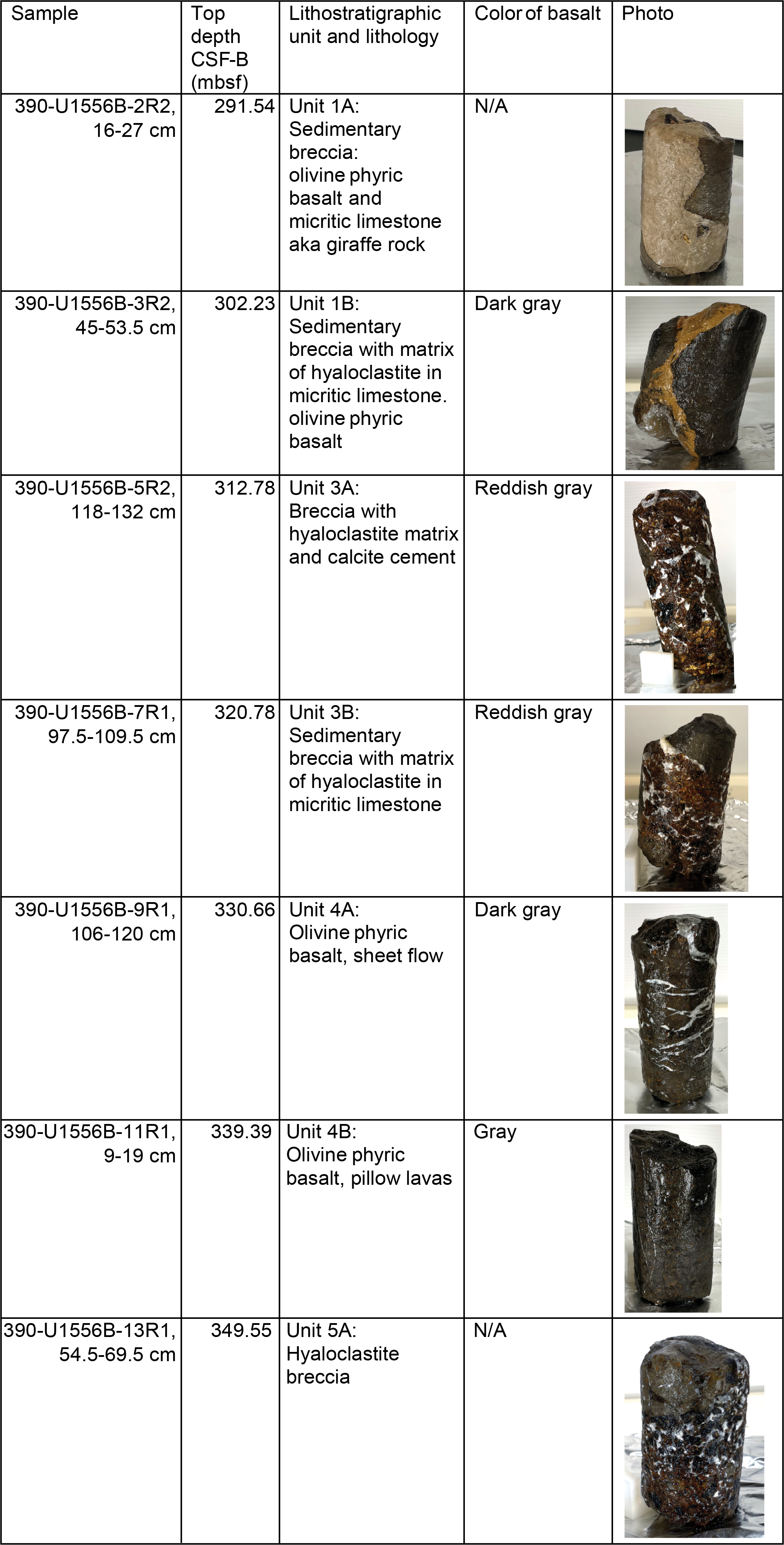
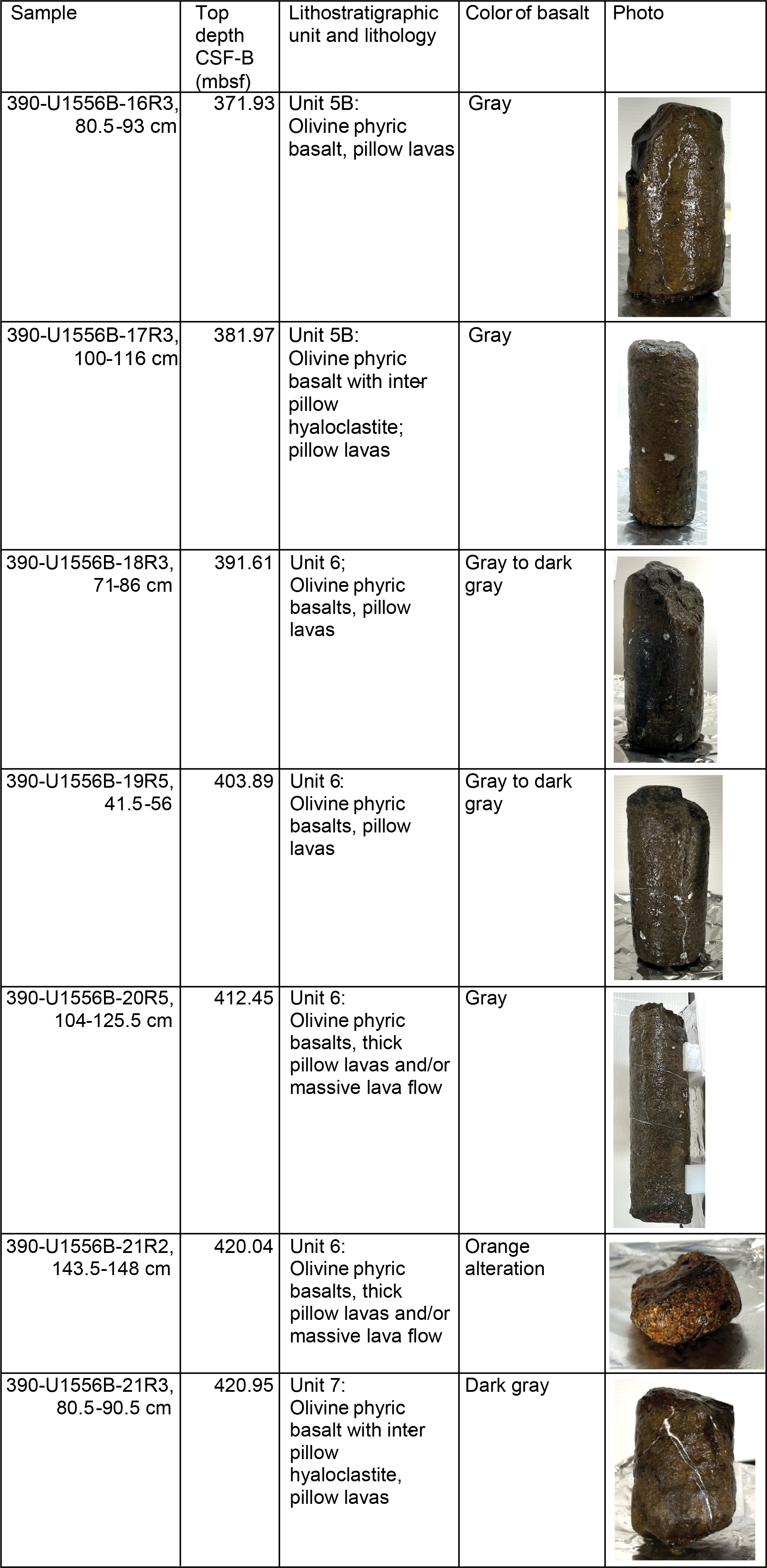
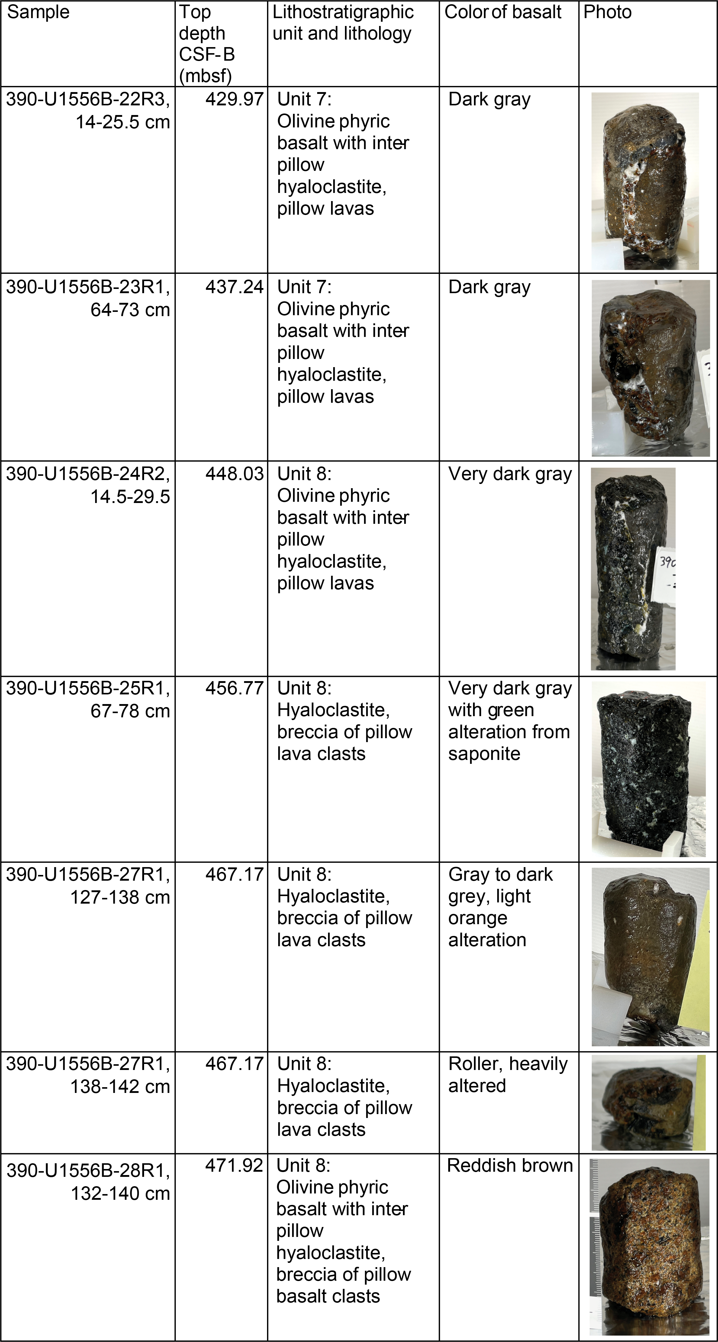
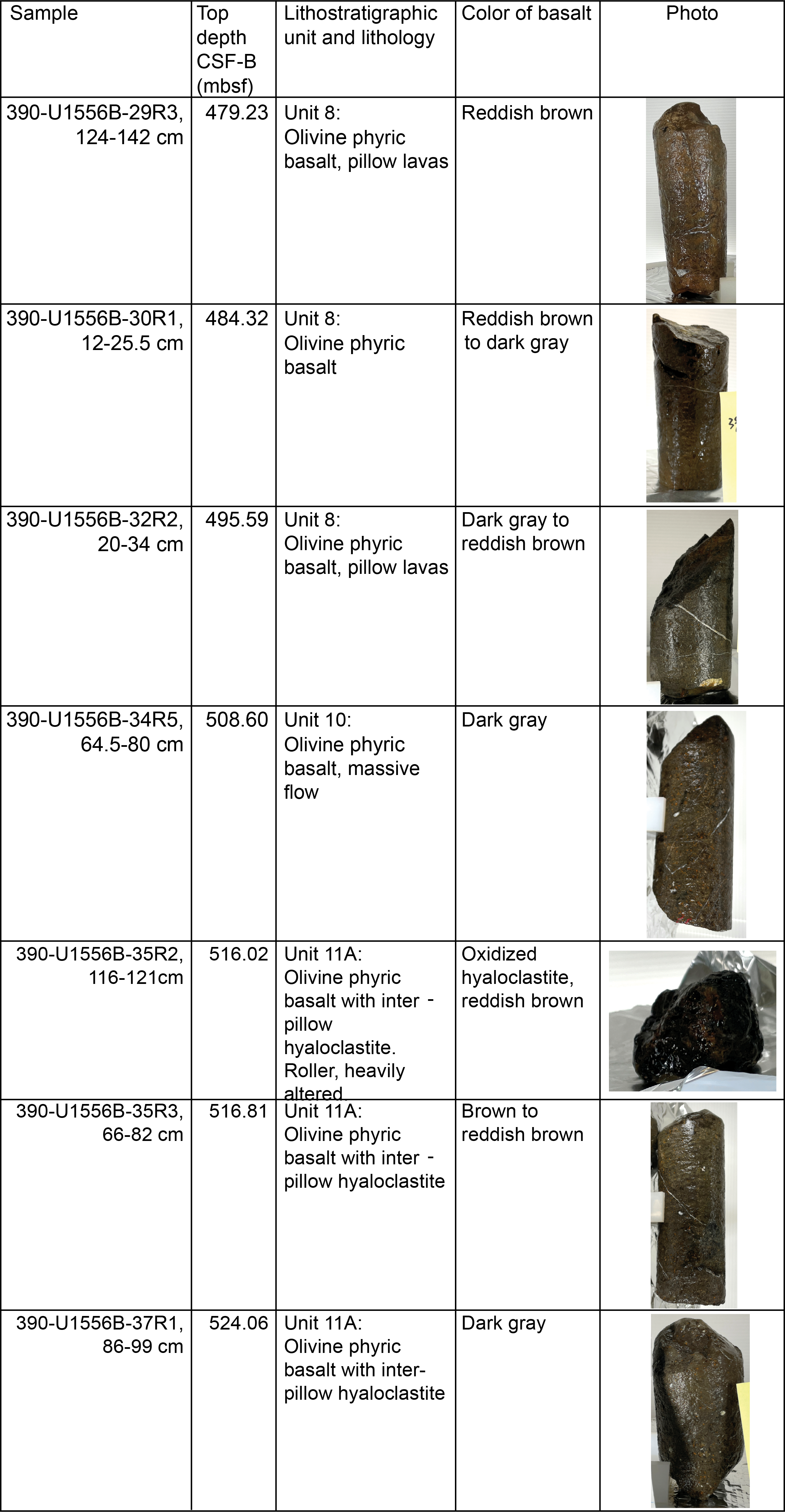
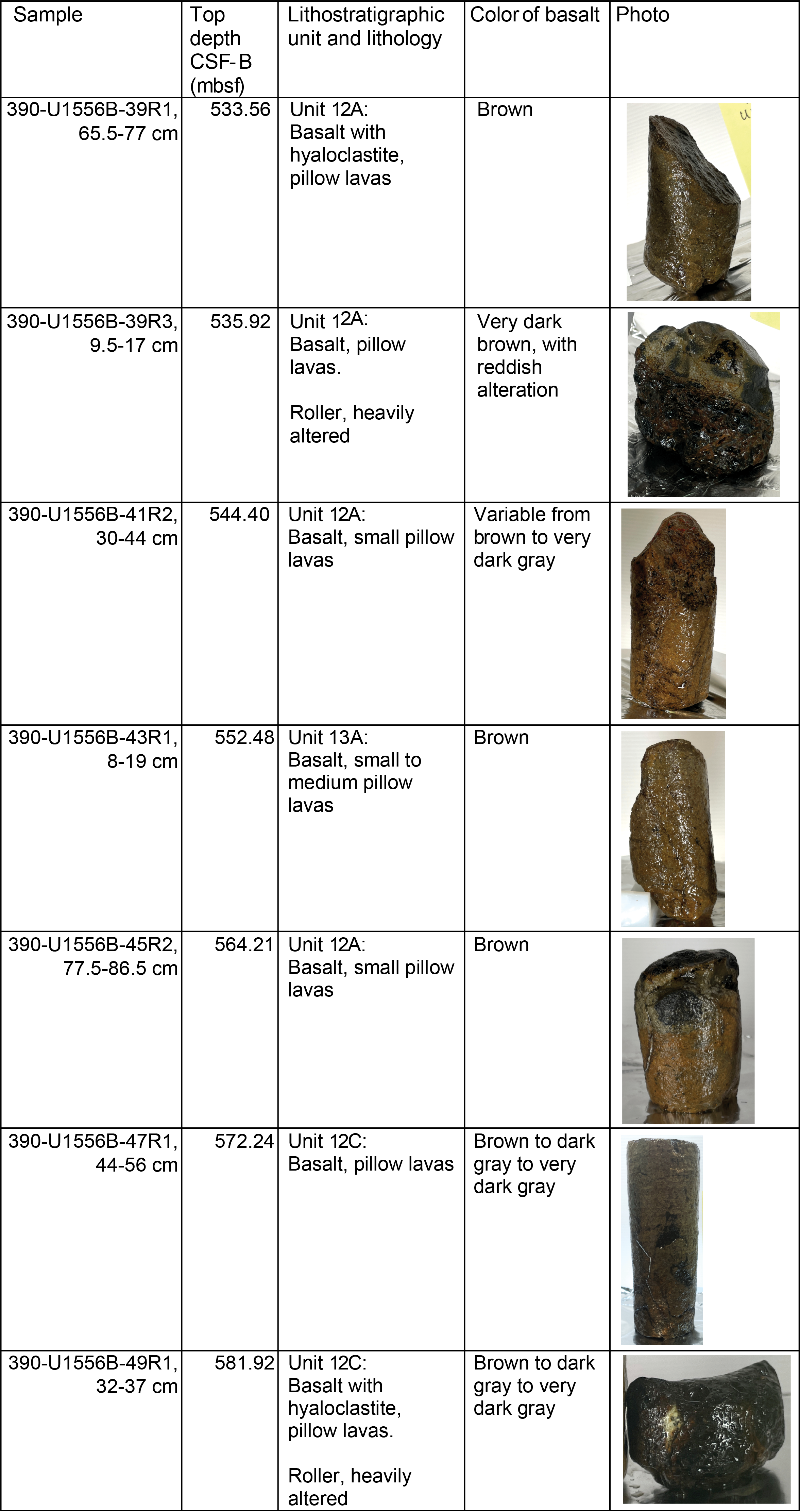
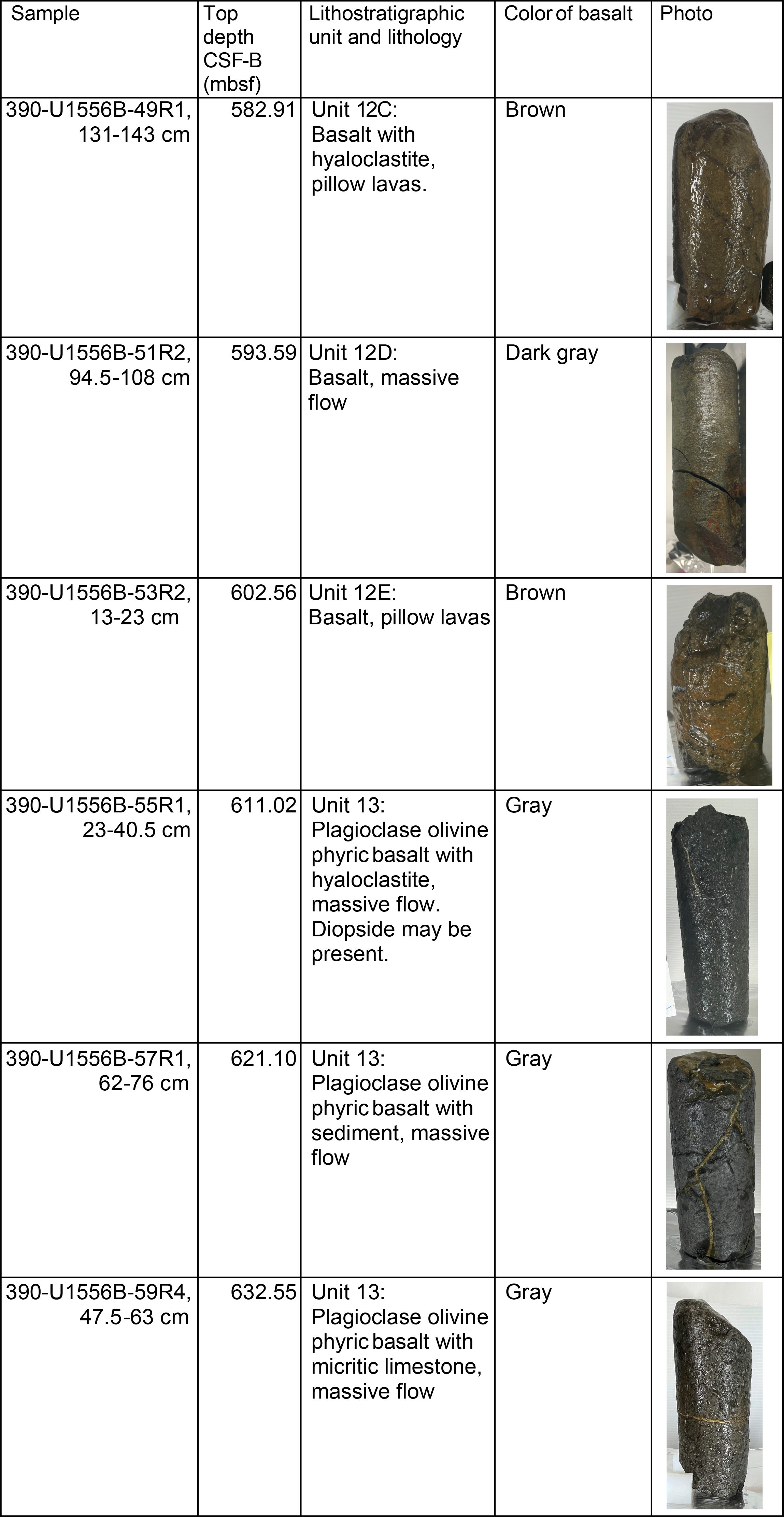
Figure F156. Samples for microbiology research.

After the exteriors of whole-round pieces were removed to avoid material contaminated during coring in microbiology samples (see Microbiology in the Expedition 390/393 methods chapter [Coggon et al., 2024c]), the remaining material was split into subsamples that were prepared for different microbiology analyses. The number of subsamples that could be processed for each analysis type depended on the amount of material available from each parent sample (Table T33).

12.2.1. Microbiological sample processing and experiments

12.2.1.1. Cell counts

A total of 40 samples were processed for cell counts. Performing shipboard cell counts on rock samples is difficult and time consuming; therefore, shipboard cell enumeration was not attempted during the SAT expeditions. Samples were instead broken into small chips and/or powder and preserved for postexpedition analysis in a 20% vol/vol slurry of rock and 5% Epredia Formal-Fixx in 3× phosphate-buffered solution, respectively.

12.2.1.2. Microbial community structure

A total of 41 samples were preserved for DNA (PCR amplicon-based and metagenomes) and/or RNA (PCR amplicon-based and/or metatranscriptomes) analysis, 39 samples were preserved for single-cell genomics, and 36 samples were collected for lipid analysis (Table T33). Material for DNA, RNA, and lipid-based postexpedition analyses of microbial community composition was collected and preserved following the procedures described in Microbiology in the Expedition 390/393 methods chapter (Coggon et al., 2024c).

12.2.1.3. Microbial incubation experiments

To attempt to isolate new microbial species, an isolation experiment using enrichment media in Petri dishes with 1/10 ZoBell Marine Agar media was conducted. This media selects for heterotrophic marine microorganisms and is commonly used to isolate previously uncultured species. Enrichment experiments were initiated for Samples 390-U1556B-18R-3, 71–86 cm; 29R-3, 124–142 cm; 34R-2, 20–34 cm; 51R-2, 94.5–108 cm; and 59R-4, 47.5–63 cm (Table T33), using methods described in Microbiology in the Expedition 390/393 methods chapter (Coggon et al., 2024c). The Petri dishes were incubated at 9.5°C with the top facing down for the duration of the expedition. Samples were checked for microbial colony growth periodically throughout Expedition 390 and then shipped to shore for postexpedition research.

To detect whether metabolically active microbes are present in basaltic basement at Site U1556 and, if so, determine their identity, Samples 390-U1556B-29R-3, 124–142 cm; 34R-2, 20–34 cm; 51R-2, 94.5–108 cm; and 59R-4, 47.5–63 cm, were used to initiate stable isotope probing (SIP) experiments (Table T33). Similar methods were used during Expedition 329 to reveal the presence of active microorganisms in sediments as old as 101.5 Ma beneath the South Pacific Gyre (Morono et al., 2020). The aim is to determine whether microbial cells are active in the basement at Site U1556, calculate their growth rate, and quantify how many cells take up C and N substrates. For each SIP experiment, ~4 cm³ of rock chips and powder were placed in vials with thick rubber stoppers to prevent oxygen exchange. Artificial seawater was used to make a 1:4 slurry (total volume = 20 mL), and then labeled substrates (¹³C-labeled sodium bicarbonate, ¹³C-labeled amino acid mix, and ¹⁵N-labeled ammonium) were injected into each sample according to the procedure outlined in Microbiology in the Expedition 390/393 methods chapter (Coggon et al., 2024c). The slurries were purged and the headspace was replaced with N₂, and then 10 mL of filtered air was injected into the vial to create a microaerobic environment comparable to predicted in situ conditions (5% O₂). Samples were incubated at 10°C until shipment to shore at the end of Expedition 390. Individual experimental vials will be killed at three time points (2, 3, and 6 months) prior to analysis.

12.2.2. Microbiological contamination monitoring

Drilling fluid and mud circulated during the coring process are potential sources of contamination for cores collected for microbiology analysis. To determine the extent of contamination of the microbiology samples, the perfluorocarbon tracer perfluoromethyldecalin (PFMD) was injected into drilling fluids during circulation in Hole U1556B. Samples from both the exterior and interior of core intervals selected for microbiology analysis were collected to quantify the presence of PFMD. Ideally, PFMD is detected on the core exterior, indicating successful delivery down the drill string to the core exterior, but not in the interior portions of whole rounds (i.e., the portion from which microbiological samples are taken); detection of PFMD in the whole-round interior would indicate intrusion of drilling fluid and hence potential microbial contamination.

Five of the collected samples were rollers (<5 cm long) or <10 cm long: 390-U1556B-21R-2, 143.5–148 cm; 27R-1, 138–142 cm; 35R-2, 116–121 cm; 39R-3, 9.5–17 cm; and 49R-1, 32–37 cm (Figure F156). Microbiologists aimed to collect whole-round pieces >10 cm in length because these pieces have enough material to allow removal of the core exterior and sample the interior. However, the roller samples originated from highly altered hyaloclastite intervals that were identified as potential regions of fluid flow in the basement and were therefore deemed of high importance for microbiological investigation, despite the risks of contamination. They were collected as a pilot study to determine whether these types of samples from regions of both high microbiological interest and high potential for contamination can be used to generate meaningful results.

Exterior samples for PFMD analysis were collected from rubble (core fragments <2 cm) in every core interval from which a microbiology sample was collected (37 samples; Table T34). These samples were chosen after the core was laid out in the splitting room, targeting rubble or small rollers that were most likely in contact with drilling fluid and/or mud but were not of high interest for further scientific analysis because of their small size. For every microbiology sample larger than a roller, an interior piece was also collected for PFMD analysis to determine if tracer infiltrated the interior of the core. PFMD was pumped for the entirety of drilling operations in Hole U1556B. PFMD was routinely detected in the exterior samples with a mean concentration of 24.7 ng PFMD/g core and a median concentration of 1.13 ng PFMD/g rock (Figure F157). For the whole-round interior samples, the mean PFMD concentration was 1.02 ng PFMD/g rock and the median concentration was 0. The PFMD concentration was 0 g PFMD/g rock for 25 of 39 microbiology samples analyzed and was <0.10 g PFMD/g rock for 8 of 14 samples where it was detected. Contamination tracing with PFMD during Expedition 360 RCB coring operations found 11–4595 ng PFMD on core exteriors in gabbroic basement samples and did not detect PFMD on interiors (Li et al., 2020). These values compare well with those measured here (range 0–2341 ng PFMD on exteriors).

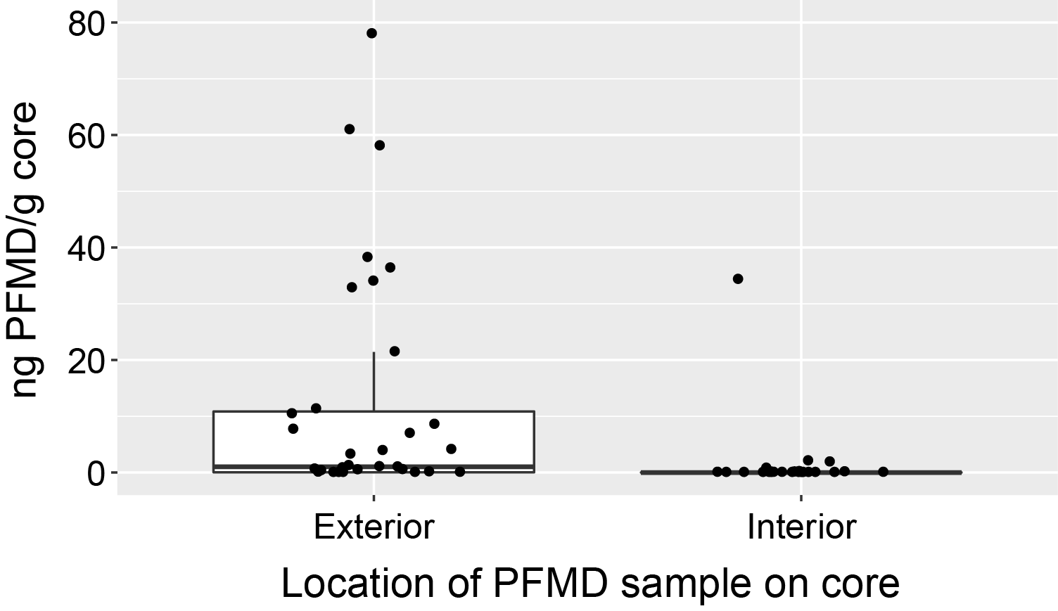
Figure F157. PFMD data.

To determine the number of microorganisms present in drill fluid and generate a database of potential contaminants, we collected drilling fluid from a pipe on the rig floor three times during coring operations in Hole U1556B: during coring of Core 390-U1556B-16R when the drill bit was 377 mbsf, during coring of Core 39R when the bit was 539 mbsf, and during coring of Core 55R when the drill bit was 612 mbsf. Samples were collected for cell counts, and 500 mL of drilling fluid was filtered onto two separate 0.20 µm pore size, 47 mm diameter filters and frozen at −80°C for shore-based molecular biology analysis.

References