McCaig, A.M., Lang, S.Q., Blum, P., and the Expedition 399 Scientists
Proceedings of the International Ocean Discovery Program Volume 399
publications.iodp.org
https://doi.org/10.14379/iodp.proc.399.102.2025
Expedition 399 methods1
![]() S.Q. Lang,
S.Q. Lang,
![]() A.M. McCaig,
A.M. McCaig,
![]() P. Blum,
P. Blum,
![]() N. Abe,
N. Abe,
![]() W. Brazelton,
W. Brazelton,
![]() R. Coltat,
R. Coltat,
![]() J.R. Deans,
J.R. Deans,
![]() K.L. Dickerson,
K.L. Dickerson,
![]() M. Godard,
M. Godard,
![]() B.E. John,
B.E. John,
![]() F. Klein,
F. Klein,
![]() R. Kuehn,
R. Kuehn,
![]() K.-Y. Lin,
K.-Y. Lin,
![]() C.J. Lissenberg,
C.J. Lissenberg,
![]() H. Liu,
H. Liu,
![]() E.L. Lopes,
E.L. Lopes,
![]() T. Nozaka,
T. Nozaka,
![]() A.J. Parsons,
A.J. Parsons,
![]() V. Pathak,
V. Pathak,
![]() M.K. Reagan,
M.K. Reagan,
![]() J.A. Robare,
J.A. Robare,
![]() I.P. Savov,
I.P. Savov,
![]() E. Schwarzenbach,
E. Schwarzenbach,
![]() O.J. Sissmann,
O.J. Sissmann,
![]() G. Southam,
G. Southam,
![]() F. Wang, and
F. Wang, and
![]() C.G. Wheat2
C.G. Wheat2
1 Lang, S.Q., McCaig, A.M, Blum, P., Abe, N., Brazelton, W., Coltat, R., Deans, J.R., Dickerson, K.L., Godard, M., John, B.E., Klein, F., Kuehn, R., Lin, K.-Y., Lissenberg, C.J., Liu, H., Lopes, E.L., Nozaka, T., Parsons, A.J., Pathak, V., Reagan, M.K., Robare, J.A., Savov, I.P., Schwarzenbach, E., Sissmann, O.J., Southam, G., Wang, F., and Wheat, C.G., 2025. Expedition 399 methods. In McCaig, A.M., Lang, S.Q., Blum, P., and the Expedition 399 Scientists, Building Blocks of Life, Atlantis Massif. Proceedings of the International Ocean Discovery Program, 399: College Station, TX (International Ocean Discovery Program). https://doi.org/10.14379/iodp.proc.399.102.2025
2 Expedition 399 Scientists’ affiliations.
1. Introduction
This chapter outlines the procedures and methods employed for coring and drilling operations and in the various shipboard laboratories of the R/V JOIDES Resolution during International Ocean Discovery Program (IODP) Expedition 399. The laboratory information applies only to shipboard work described in the Expedition reports section of the Expedition 399 Proceedings of the International Ocean Discovery Program volume that used the shipboard sample registry, imaging and analytical instruments, core description tools, and Laboratory Information Management System (LIMS) database. Methods used by investigators for shore-based analyses of Expedition 399 data will be documented in separate publications.
All shipboard scientists contributed in various ways to this volume with the following primary responsibilities (authors are listed in alphabetical order; see Expedition 399 scientists for contact information):
Summary chapter: Expedition 399 Scientists
Methods and site chapters:
- Background and objectives: A. McCaig and S. Lang
- Operations: P. Blum and B. Rhinehart
- Igneous petrology: K.-Y. Lin, J. Lissenberg, H. Liu, and M. Reagan
- Alteration petrology: R. Coltat, F. Klein, T. Nozaka, E. Schwarzenbach, O. Sissmann, and I. Savov
- Structural geology: B. John, R. Kuehn, and A. Parsons
- Geochemistry: M. Godard and G. Wheat
- Microbiology: W. Brazelton, J. Robare, G. Southam, and F. Wang
- Petrophysics: N. Abe, J. Deans, and K. Dickerson
- Paleomagnetism: E. Lopes and V. Pathak
2. Operations
2.1. Sites and holes
Coordinates from previous IODP drill sites as well as site surveys were used to position the vessel at the Expedition 399 sites. A SyQwest Bathy 2010 CHIRP subbottom profiler was used to monitor the seafloor depth during the approach to the site to reconfirm the depth profiles from precruise surveys. Once the vessel was positioned at the new Site U1601, a camera survey was conducted to confirm suitable flat bedrock for spudding the hole. A positioning beacon was ready to be deployed in case we needed it to backup GPS navigation. While on site, ship location over the hole was maintained using the Neutronics 5002 dynamic positioning (DP) system on JOIDES Resolution. DP control of the vessel used navigational input from the GPS, and the final hole position was the mean position calculated from the GPS data collected over a significant portion of the time the hole was occupied.
The drilling site was numbered according to the series that began with the first site drilled by the Glomar Challenger in 1968. Starting with Integrated Ocean Drilling Program Expedition 301, the prefix “U” designates sites occupied by JOIDES Resolution. For all IODP drill sites, a letter suffix distinguishes each hole drilled at the same site. The first hole drilled is assigned the site number modified by the suffix “A,” the second hole takes the site number and the suffix “B,” and so forth. During Expedition 399, we reoccupied Hole U1309D and drilled the new Holes U1601A, U1601B, and U1601C.
2.2. Drilling and coring operations
We used the rotary core barrel (RCB) system exclusively for all coring operations during Expedition 399, with standard 9⅞ inch coring bits. In addition, we used a stinger bottom-hole assembly (BHA), including a mud motor, underreamer, and 12¼ inch drilling bit, to attempt a drill-in casing in Hole U1601B and a drilling system with a 14¾ inch tricone bit to drill a ~22 m deep casing hole in Hole U1601C.
The RCB is the most conventional rotary coring system and is suitable for lithified rock material. It cuts a core up to 9.5 m long with nominal diameter of 5.87 cm. During Expedition 399, we cored 4.8 or 4.9 m intervals as a general rule to optimize core recovery. All cores were drilled with core liners.
The BHA is the lowermost part of the drill string, configured to provide appropriate strength and tension in the drill string. A typical RCB BHA consists of a drill bit, a bit sub, an outer core barrel, a top sub, a head sub, eight joints of 8¼ inch drill collars, a tapered drill collar, two joints of standard 5½ inch drill pipe, and a crossover sub to the regular 5 inch drill pipe.
The length of the recovered core varies based on a number of factors. In igneous rock, the length of the recovered core is typically less than the cored interval. A common cause of poor recovery is core jamming in the bit or in the throat of the core barrel, which prevents core from entering the core barrel. Cored intervals may not be contiguous if separated by intervals drilled but not cored. Holes thus consist of a sequence of cored and drilled intervals, or advancements. These advancements are numbered sequentially from the top of the hole downward. Numbers assigned to physical cores recovered correspond to advancements and may not be consecutive.
The recovery rate for each core was calculated based on the total length of a core recovered divided by the length of the cored interval. In rocks, recovery rates are typically <100%. However, recovery rates of >100% do occur, and because the rocks do not expand (significantly) upon recovery, the following two possibilities must be considered:
- The cored interval is underestimated, perhaps because it was largely drilled during a rising tide (maximum ~2 m). Monitoring tides using tide tables for the area could provide evidence.
- Part of the previous core was left behind as a stub or piston and recovered in the top of the subsequent core barrel. One supporting (but not conclusive) indication for this phenomenon would be a lower recovery in the previous core by at least the excessive amount in the next core. In addition, when a stub is re-cored it tends to have a smaller diameter than a freshly cut core.
2.3. Tracer delivery for microbiological contamination testing
Perfluorocarbon tracer (PFT) was continuously added to the drill fluid to assess drilling contamination on the exterior of microbiology samples. A pure perfluorodecalin fluid (Oakwood Products P/N 003283; lot #003283R19X) was injected without dilution using a high-pressure liquid chromatography pump at a variable rate over the course of the expedition. While drilling Hole U1601A, the rate of injection was initially set at 0.3 mL/min for a mud pump rate of 60 strokes/min (stroke of the mud pump = 19.54 L/stroke) and designed to automatically increase with higher mud pump rates. The delivery of PFT to the cores at this rate was sufficient for detection of the tracer on the exterior of cores but too low to reliably detect after the core pieces were washed.
In Hole U1309D, the tracer pump rate was increased to 0.4 mL/min. At the start of drilling, a software malfunction caused the rate to increase to 7.7 mL/min for 1 h before being manually returned to 0.4 mL/min. Excess tracer remained detectable at elevated levels in cores recovered from Hole U1309D throughout the remainder of drilling operations.
In Hole U1601C, the tracer pump was initially set at a nonvariable rate of 0.4 mL/min and then manually increased to 0.5 mL/min after the first four cores were recovered. It remained at 0.5 mL/min through Core 399-U1601C-128R, at which point the variable rate program was again implemented to adjust tracer pump speeds to mud pump rates. Brief malfunctions delivered significantly higher PFT to the core while drilling Cores 118R, 124R, 184R, 190R, and 217R and sporadically thereafter. At the start of drilling Core 241R, the tracer pump was set to nonvariable mode again at a rate of 0.5 mL/min.
2.4. Fluid sampling
Fluid sampling was an important objective of Expedition 399, and more than 1000 subsamples were collected for analysis. Four methods were employed to recover fluids.
Water column seawater samples were collected at both Sites U1309 and U1601 using two Niskin water sampling bottles attached to the subsea camera frame and triggered from the ship using a transponder release mechanism not used otherwise. These samples were collected to document the extent of reaction with rocks and debris within the borehole, determine hydrologic pathways, and assess microbial processes and populations. The camera was deployed for seafloor surveys (Site U1601) and each time the hole was reentered. Niskin bottles were deployed 11 times during Expedition 399, resulting in 220 fluid subsamples for analysis.
Two Kuster Flow-Through Samplers (KFTSs) were deployed in tandem a total of nine times in Holes U1309D and U1601C, collecting 16 in situ borehole fluid samples, resulting in 377 fluid subsamples for analysis. The KFTS uses a mechanical clock to trigger sample chamber closure that must be set in accordance with target depths and expected tool traveltimes.
The novel in situ Multi-Temperature Fluid Sampler (MTFS) was deployed for the first time ever in Hole U1309D. It uses shape memory alloy triggers on up to 12 titanium syringe-style fluid sample chambers. The tool targets temperatures, and the sample depths must be estimated based on temperature profiles. The MTFS is therefore run with the Elevated Temperature Borehole Sensor (ETBS). The MTFS-ETBS assembly was run once in Hole U1309D and collected 11 samples, resulting in 160 subsamples for analysis.
A total of 243 core liner fluid samples (all but 2 from Hole U1601C) were collected on the rig floor by tilting the core barrel so that fluid could drain into sample vials.
The Niskin bottle, KFTS, MTFS, and ETBS tools are described in more detail in Petrophysics, and their deployments are summarized in the operations sections of the site chapters.
2.5. Depth measurements and computations
The depths below seafloor are computed for all samples and shipboard measurements by the LIMS database routines, following the principles summarized in IODP Depth Scales Terminology (https://www.iodp.org/policies-and-guidelines/142-iodp-depth-scales-terminology-april-2011/file) (Figure F1). The relevant depth scale types and the terminology used in the JOIDES Resolution Science Operator (JRSO) LIMS database, the Columbia University logging database, and this volume, if different, are summarized here.
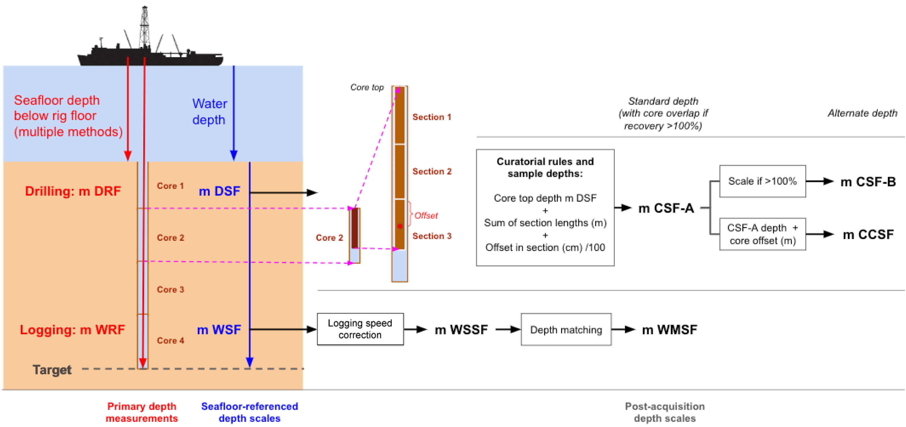
Figure F1. Depth scale types.
2.5.1. Holes and cores
Drilling depth below rig floor (DRF):
- Definition: the sum of lengths of all drill string components deployed beneath the rig floor; includes length of all components and the portions thereof below the rig floor.
- Terminology in this volume: meters below rig floor (mbrf).
Drilling depth below seafloor (DSF):
- Definition: the length of all drill string components between seafloor and target.
- Terminology in this volume: meters below seafloor (mbsf).
Core depth below seafloor, Method A (CSF-A):
- Definition: distance from seafloor to target within recovered core. Combines DSF to top of cored interval with curated section length to target within cored material. This method allows overlap at cored interval boundaries.
- Terminology in this volume: mbsf.
Core depth below seafloor, Method B (CSF-B):
- Definition: distance from seafloor to target within recovered core. Combines DSF to top of cored interval with curated length to target within cored material. This method applies a compression algorithm (i.e., scaling) if recovery is above 100%.
- Not used in this volume but provided by default as a second depth column in all LIMS database reports.
The bit depths in a hole during deployment of a reentry system and during drilling and coring are based on the length of drill pipe added at and deployed beneath the rig floor, measured to the nearest 0.1 m (DRF scale). When applicable, these depths are converted to the DSF scale by subtracting the seafloor depth determined by tagging the seafloor (or some other method) from the current bit depths (both on the DRF scale). The bit depths (DSF scale) at which a coring advance begins and ends define the cored interval.
Core curatorial procedures create the CSF-A scale for core samples by adding the lengths of core sections to the top depth of a core on the DSF scale. The bottom depth of the core on the CSF-A scale is typically less than the bottom of the cored interval on the DSF scale but can also be greater (often so in soft sediment), resulting in a core recovery rate of >100%. Depths of samples and associated measurements on the CSF-A scale are calculated by adding the offset of the sample or measurement from the top of its section and the lengths of all higher sections in the core to the top depth of the cored interval. This standard procedure places all recovered material at the top of the cored interval for convenience. The lower the recovery, the greater the uncertainty of the actual depth a sample came from. If recovery is >100%, cored intervals overlap on the CSF-A depth scale. For this reason, the LIMS database routinely presents the CSF-B depths, which are scaled to remove the overlap for data visualization purposes.
If cores must be depth shifted to create a modified depth scale that better represents the stratigraphy at a site or simply to remove artificial overlaps between cores related to natural, drilling, or curatorial processes, a core composite depth below seafloor (CCSF) is constructed. A single depth offset is defined for each core, and the transform from the CSF-A scale to the CCSF scale for all cores in a hole is given by the affine table. CCSF (or alternate depth) database tools were primarily designed to meet the needs of paleoceanographic projects where cores from multiple adjacent holes are depth shifted to correlate stratigraphic features and create stratigraphic splices. However, previous igneous rock expeditions, including IODP Expedition 360, used the alternate depth database tools to remove artificial core overlaps of many cores. Out of 286 cores recovered during Expedition 399, 20 cores have a recovery rate of 101%–115%, mostly as a result of the curatorial procedure of binning core pieces. A CCSF scale was not developed.
2.5.2. Wireline logging data
Wireline log depth below rig floor (WRF):
- Definition: length of wireline and sensor offset between the rig floor and the target.
- WRF terminology is used in some logging database files.
- Terminology used in Schlumberger files (original, processed, and field log plots): meters or meters measured depth (MD).
- Terminology used in some files (vertical seismic profile [VSP]): mbrf.
- Terminology in this volume: not used, superseded by corrected depth scales.
Wireline log depth below seafloor (WSF):
- Definition: WRF depth with seafloor depth below the rig floor subtracted.
- Terminology used in some logging database files (depth match files).
- Terminology in this volume: mbsf.
Wireline log speed-corrected depth below seafloor (WSSF):
Wireline log matched depth below seafloor (WMSF):
- Definition: depth derived by correlation between reference run and another run to make a set of WSF runs internally consistent.
- WMSF scale type name is used in most logging database files.
- Terminology in this volume and in some logging database files (log plots): mbsf.
2.6. Core curatorial procedures, sampling, and measurements
2.6.1. Changes to shipboard processing of Hole U1601C cores on recognition of chrysotile
During coring operations at Site U1601, core describers identified and reported the presence of chrysotile veins in the recovered serpentinized peridotite cores.
Chrysotile (one of three polymorphs of serpentine) has long been recognized as a common alteration mineral in serpentinized mantle rock, and in most cases it occurs in low concentrations. Chrysotile is a type of asbestos, and asbestos is an acknowledged health hazard in asbestos mining and asbestos abatement jobs at industrial concentrations. Regulations for exposure to airborne asbestos emphasize the danger of longtime exposure to significant asbestos dust (defined by most regulations as 0.1 fiber/cm3 as an 8 h time-weighted average in a specific microscopic size range). During Expedition 399, the occurrence of white vein material of >1 mm thickness, in a few cases large enough that fibers could be seen with the naked eye, led to concerns by the JRSO technical support staff handling cores that their health might be at risk. These concerns were communicated to shore management and Texas A&M University Environmental Health and Safety (TAMU EHS) officials. Consequently, throughout May 2023 core handling, including splitting and sampling, as well as imaging, description, and other core analyses were altered in an abundance of caution to decrease the potential for exposure. Precautionary procedures for core handling were implemented, but continued concerns and slow communications between ship and shore led to stop-and-go core processing. Shipboard scientific data analysis was significantly compromised to different extents throughout these periods.
After a conversation with shore management on 6 May, shipboard processing of cores at various stages was suspended for several days before modified procedures were adopted. On 24 May, JRSO management received the detailed review and advice from TAMU EHS and forwarded it to the ship. The document stated “…widespread or significant contamination aboard the vessel is unlikely at this time…” and recommended that “If any ongoing assessment of workspaces positively identifies asbestos contamination, associated activities should cease immediately until additional review can determine the likely cause, potential for exposure, and the feasibility of resuming work….” On 25 and 26 May, more than 50 swab samples of laboratory surfaces and floors were collected by JRSO staff, and images of putative chrysotile fibers were sent to shore. Because cleaning of many parts of the laboratories had been suspended as a precaution, it is not clear whether these fibers accumulated before or after the precautionary core handling protocols were put in place. This led to the halt of all core handling, including splitting, description, and sampling, so that procedures could be reassessed. On 29 May, per instruction from shore, all core splitting and sampling stopped. The expedition was shortened by 4 days to allow professional cleaning of parts of the ship in Ponta Delgada (Portugal). The cleaning company analyzed 24 air and tape samples taken from the ventilation system and various surfaces in the core splitting room; core, downhole, and chemistry laboratories; and elevator before and after cleaning. Their report concluded that “The investigations show no sign of asbestos fibres [sic].”
A major postcruise effort at the Gulf Coast Repository (GCR) in College Station, Texas (USA), was required to complete core curation, proper imaging of section halves, core description, and typical shipboard sampling. In August 2023, a double-wide trailer was acquired and installed next to the GCR facilities. In September, the trailer was equipped with special air handling, tables, rock saws, and other equipment, while 66 whole-round sections were split in an improvised open-air laboratory adjacent to the GCR building. Throughout October, JRSO staff recurated 606 section halves by inserting plastic dividers to secure the rock pieces. All archive and section halves were also imaged by staff members.
During the October recuration and preliminary sampling effort in the trailer, an environmental consulting service carried out asbestos air monitoring tests for 5 days. Three staff members working on the cores in Tyvek suits and full face masks were equipped with a personal monitor and sampling device. The samples were analyzed by phase contrast microscopy (PCM) and transmission electron microscopy (TEM). The 27 October 2023 report stated that “All air sample results were found to be in compliance with Occupational Safety and Health Administration (OSHA) 8 hour permissible exposure limits of 0.1 f/cm3 and 1.0 f/cm3 (30 min excursion limit). Ambient air samples were in compliance with Texas DSHS and EPA NESHAP ‘clean air standard’ of 0.01 f/cm3.”
In December, 11 scientists attended a 2 week workshop to redescribe all archive halves, with focus on the recurated sections and selected “shipboard samples.” No personal protective equipment (PPE) was required for core description and sampling. However, another set of tests was commissioned, focusing on the separate trailer compartment where samples were being cut. Staff members cutting the samples were again in Tyvek suits and full-face breathing masks. The 5 January 2024 report concluded that “All nine (9) PCM personnel air samples were found to be in compliance with OSHA 8 hour permissible exposure limits of 0.1 f/cm3 and 1.0 f/cm3 (30 min excursion limit). All six (6) PCM ambient area air samples exceeded Texas DSHS and EPA NESHAP ‘clean air standard’ of 0.01 f/cm3. All three (3) TEM samples collected in front of the negative air exhaust were found to be overloaded with both asbestos and nonasbestos particulates. Due to this, Moody Labs was only able to perform and report presence/absence. The analysis found all three (3) TEM samples to have ‘abundant chrysotile asbestos present.’”
Here we document the core handling and general measurement steps as carried out on the ship under regular and special procedures and months later on shore. The regular procedures apply to Holes U1309D and U1601A and partly to Hole U1601C, and the special procedures apply to Hole U1601C. The impact of the disruptions and special procedures is summarized in Table T1.
2.6.2. Whole-round section handling
2.6.2.1. Regular procedures
To minimize contamination of the core with platinum group elements and gold, all personnel handling and describing the cores or other sample material removed jewelry from their hands and wrists before handling. Because all cores were assessed for microbiological samples and most were sampled, all personnel handling the cores wore nitrile gloves and masks to reduce contamination.
Cores were recovered in core liners and extracted from the core barrel by rig personnel and carried to the catwalk by JRSO technicians. Technicians cut the liner and the core if necessary into ~1.4 m long sections. The sections were temporarily secured with blue and colorless liner end caps to denote top and bottom, respectively, a convention that was used throughout the curation process. The total length of all rock material in each section was measured and entered in the sample registry as recovered length. The sum of all sections’ recovered lengths in a core was used to compute core recovery as a percentage of the cored interval.
The sections were then transferred to the core splitting room for further processing. One microbiologist, one petrologist, and the JRSO Curator, equipped with face masks and nitrile gloves, assessed the core and selected a whole-round piece for microbiological processing, which was immediately transferred to the microbiology laboratory (see Microbiology for information on microbiology sample handling and preparation). Next, JRSO personnel washed the whole-round pieces next to the splitting saw one piece at a time and allowed them to dry. They marked the bottom of all oriented pieces (pieces with greater length than diameter) with a blue wax pencil. The core catcher sample was added to the bottom of the last section. Plastic dividers were inserted between core pieces to keep them in place for curation. The spacers may represent substantial intervals of no recovery, which in some cases results in a curated core that is longer than the cored interval (>100% recovery). Adjacent core pieces that could be fitted together along fractures were curated as single pieces. Core pieces that appeared susceptible to crumbling were encased in shrink wrap. A designated scientist was then called to the splitting room to check and approve the binning and reconstruction of fractured pieces. The scientist marked a splitting line on each piece with a blue wax pencil, ideally maximizing the expression of dipping structures on the cut face of the core while maintaining representative features in both archive and working halves. To ensure a consistent protocol, the splitting line was drawn so that the working half was on the right side of the line with the core upright. The working half of each piece was marked with a “W” to the right of the splitting line. Where magmatic fabrics or crystal-plastic fabrics (CPFs) were present, cores were marked for splitting with the fabric dipping to the east (090°) in the IODP core reference frame (CRF) (Figure F2). This protocol was sometimes overridden by the presence of specific features (e.g., mineralized patches or dike margins) that were divided between the archive and working halves to ensure preservation and/or allow shipboard or postcruise sampling.
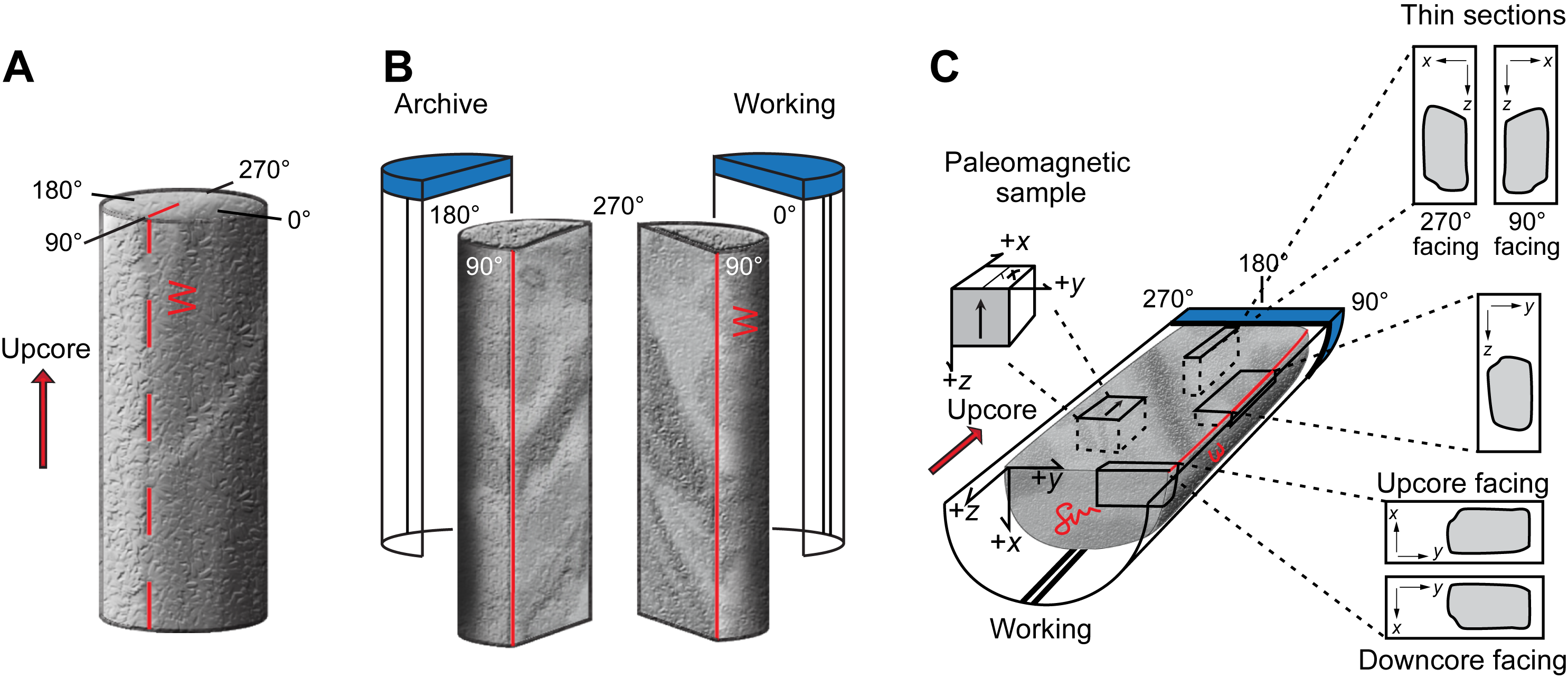
Figure F2. Core reference frame.
After the split line was drawn, JRSO technical personnel secured the plastic spacers permanently with acetone between individual pieces into matching working and archive half split core liners. Spacers were mounted into the liners with the angle brace facing uphole. This ensured that the top of each piece had the same depth as the top of the curated interval for each bin. The top and bottom offsets of each bin were entered into the sample registry. Based on the calculated bin lengths, the cumulative length of all bins, including spacers, was computed as the curated length of the section. The empty split liner with spacers glued in was then placed over the split liner containing the pieces, and the two halves were taped together in a few places for temporary storage until core pieces were dry and equilibrated to laboratory conditions (usually <1 h from arrival from the catwalk).
2.6.2.2. Special procedures
Starting with Core 399-U1601C-19R, sections cut on the catwalk were not transferred immediately to the splitting room. Instead, the following steps were carried out on the catwalk. Core liners were emptied by tilting, shaking, and knocking them as needed, and the pieces were placed in the order they were recovered in 1.5 m long presplit core liners. The microbiologist, petrologist, and JRSO Curator, equipped with face masks and nitrile gloves, assessed the core and selected a whole-round piece on the catwalk for microbiological processing. In a few cases where the Curator decided to quarantine a core (not to split it because of the presence of conspicuous white veins), a petrology whole round was also removed at that stage for shipboard description. Pieces were washed and not dried before bottom marks and connecting hashes were applied with a blue wax pencil, making them easier to be wiped away by accident. The pieces were then moved in their prepared split liners. Starting with Core 155R, dividers were only glued into the liners to separate intervals of rubble and where whole-round samples were removed; these sections therefore had to be recurated on shore. The petrologist marked the splitting line on each wet piece such that it aligned with the edge of the underlying split liner, in preparation for the special splitting method (see below). The covering split liner was added, and the two section halves were taped together. The section was racked in the laboratory and was ready for whole-round measurements.
2.6.2.3. Follow-up procedures at the GCR
Recuration of 304 sections at the GCR resulted in the elimination of 4 sections registered incorrectly on JOIDES Resolution (Sections 399-U1601C-147R-3, 147R-CC, 156R-CC, and 162R-CC). A total of 21 new sections were created and registered as a result of the recuration (Sections 146R-4, 172R-3, 174R-4, 177R-3, 179R-3, 180R-3, 182R-4, 185R-4, 186R-4, 187R-4, 199R-4, 201R-4, 202R-4, 211R-3, 213R-3, 215R-4, 218R-4, 223R-3, 233R-3, 245R-2, and 254R-3).
2.6.3. Whole-round section measurements
2.6.3.1. Regular procedures
After the core sections were deemed thermally equilibrated, the following whole-round measurements were taken (see Petrophysics for details on the procedures):
- Whole-round surface imaging (i.e., four surface quarter-image scans orthogonal to angles of 0°, 90°, 180°, and 270° relative to the CRF) using the Section Half Imaging Logger (SHIL) configured for whole-round sections,
- Core logging using the Whole-Round Multisensor Logger (WRMSL) with the loop magnetic susceptibility (MSL) sensor and gamma ray attenuation (GRA) detector, and
- Core logging using the Natural Gamma Radiation Logger (NGRL).
2.6.3.2. Special procedures
Whole-round surface imaging was canceled after Core 399-U1601C-36R to reduce core handling. These measurements could not be completed on Cores 37R–259R because (most of) the sections were subsequently split and the equipment was not available on shore.
WRMSL and NGRL measurements were carried out on all sections. However, because the sections of Cores 399-U1601C-146R, 147R, and 155R–249R had to be recurated on shore, the precuration measurement positions are offset relative to the recurated core piece positions that were measured. Correcting these offsets will only be possible with a major effort of comparing images before and after recuration.
2.6.4. Section half preparation
2.6.4.1. Regular procedures
After the completion of whole-round measurements, the sections were placed on the table in the splitting room. Each piece of core was split into archive and working halves, with the positions of the plastic spacers between pieces maintained in both halves. Piece halves were labeled sequentially from the top of each section, beginning with Number 1. Pieces were labeled on the outer cylindrical surfaces of the core.
2.6.4.2. Special procedures
After a conversation with shore management on 6 May 2023, core splitting was suspended. On 9 May, after a pause of almost 5 days, splitting of core sections resumed under special safety protocols approved by TAMU EHS, including utilization of special PPE. Concerns about asbestos contamination were addressed in three ways: (1) the saw was encased with a heavy-duty plastic cover that prevented splashes exiting, (2) sections were split in two to four batches of eight in one or two daily sessions, and (3) the core splitting operators wore Tyvek single-use polyester coveralls and full-face masks with a positive pressure air supply. Scientists and operations personnel participated in the splitting to catch up with the backlog and allow people who remained concerned about exposure to not carry out these tasks.
Starting with Core 399-U1601C-19R, pieces were not cut individually anymore. Instead, the entire section was split in the plane defined by the two split liners containing the pieces. Sections that had numerous smaller pieces were adversely affected by this process. The operators first verified that the split lines marked on the pieces collectively aligned reasonably well with the gap between the split liners. The sections were placed in the saw enclosure and split along the gap between the split liners. The split sections were removed from the enclosure, the split pieces and liners were washed, and the liners were drained of excess water as possible. The section halves were moved into the core laboratory after each splitting batch, and the sections were kept moist during further processing. Concerns were raised about piece halves resting in puddles of water in their split liners for too long. A handful of selected dry samples were taken to test the effect of excess water exposure in postcruise experiments.
A few sections were split by cutting through the core pieces and the liner at the same time.
Starting with Core 399-U1601C-155R, no further binning was done. This created the need to set up a major core curation operation on shore after the expedition.
After 29 May, when all core processing was stopped per instruction from shore, starting with Core 399-U1601C-235R, sections were no longer split. The whole-round sections were cut and sampled for microbiology on the catwalk, capped, processed through the WRMSL and NGRL, described through the core liners, and then boxed. These protocols were applied to all cores, including those consisting entirely of gabbro.
2.6.4.3. Follow-up procedures at the GCR
Sections 399-U1601C-235R-1 through 259R-2 were split in September 2023 in an open-air custom cutting area next to the GCR building. The water used with the saws was collected and filtered, and the filtrate was discarded as hazardous material. These sections were properly binned during the process.
Section halves of Cores 399-U1601C-155R through 234R were recurated in October in the specially leased and equipped double-wide trailer next to the GCR building. In addition, the pieces of most of the shallower section halves had to be labeled. The hole-core-section-offset identities of shipboard samples taken from the recurated section halves, including thin section billets (TSBs), resulting thin sections, and close-up photographs, were updated accordingly. Depths were recalculated based on the updated identities. Note that hole-core-section-offset identities and depths reported in the Expedition 399 Preliminary Report were not updated and should not be used or referenced in any future work.
2.6.5. Archive section half measurements
2.6.5.1. Regular procedures
The following measurements and observations were carried out on the archive section halves:
- Imaging of the dry faces of the section halves using the SHIL. A core composite image was created automatically whereby all sections of a core are displayed next to each other in a 1 page layout.
- Core logging using the Section Half Multisensor Logger (SHMSL) with reflectance spectroscopy and colorimetry (RSC) and point magnetic susceptibility (MSP) contact probe (see Petrophysics).
- Macroscopic core description using the GEODESC Data Capture program (see Igneous petrology, Alteration petrology, and Structural geology).
- Remanent magnetization logging using the superconducting rock magnetometer (SRM) (see Paleomagnetism).
- Close-up images of selected intervals and features for illustration in this volume, as requested by individual scientists.
2.6.5.2. Special procedures
Starting with Core 399-U1601C-16R, imaging of section half surfaces had to be done while the surfaces were wet, which compromised the usability of the images. Serpentinized harzburgite is so dark in color that the wet surface images do not reveal details in as high a resolution as dry surface images do.
On 10 May 2023, starting with Core 399-U1601C-37R, rapid core description methods were established to manage the confluence of backlog resulting from the pause in section splitting and continued rapid core recovery. This resulted in less detailed descriptions than planned under the regular procedures. SHMSL measurements were limited to gabbroic intervals for Cores 16R–37R and discontinued altogether starting with Core 38R to alleviate the core laboratory pressure created by the new conditions.
By 15 May, core splitting had caught up with core recovery, and rapid core description had caught up with splitting the next day. This allowed us to discuss, both on the ship and with shore management, strategies for reestablishing sampling. At this stage, all section halves were immediately shrink wrapped after splitting, often resulting in excessive moisture being enclosed with the cores. On 16 May, starting with Core 399-U1601C-131R, the working halves were imaged and described instead of the archive halves. This allowed for the identification of shipboard samples and sampling after shrink wrapping but before storage in the hold, without excessive core handling.
The archive section halves were shrink wrapped immediately after splitting and racked for paleomagnetic measurements, which could be done without removing the shrink wrapping. The working section halves were kept damp while being described over the ~24 h after splitting.
2.6.5.3. Follow-up procedures at the GCR
In October 2023, after recuration of all Hole U1601C section halves, JRSO technicians imaged all archive section halves in the special trailer laboratory at the GCR. Both the wet and dry surfaces were imaged (1580 section scans).
In December 2023, 11 expedition project scientists, supported by a team of JRSO technicians, (re)described all archive section halves from Hole U1601C during a 2 week workshop held in the special trailer laboratory at the GCR. Additional portable X-ray fluorescence spectrometer (pXRF) measurements were also taken while the cores were being redescribed.
2.6.6. Working section half sampling and measurements
2.6.6.1. Regular procedures
The following working section half samples and measurements were taken:
- TSBs were sampled to prepare thin sections and collect microscopic observations on thin sections (see Igneous petrology, Alteration petrology, and Structural geology).
- Cube samples (~8 cm3) were taken for moisture and density (MAD) tests and for P-wave velocity measurements using the P-wave caliper (PWC) mounted on the Section Half Measurement Gantry (see Petrophysics).
- Cube samples (~8 cm3) were taken for paleomagnetic and rock magnetism tests (PMAG) (see Paleomagnetism).
- Wedges or chips were taken and powdered for inductively coupled plasma–atomic emission spectroscopy (ICP-AES) and X-ray diffraction (XRD) analysis (see Geochemistry).
2.6.6.2. Special procedures
Starting on 6 May 2023 with Core 399-U1601C-8R, sampling was restricted in various ways based on changing core processing protocols and type of lithology. Discrete samples were changed from cubes to microbiology (MBIO) off cuts between Cores 38R and 131R (see Petrophysics for more details).
Starting on 19 May with Core 131R, sampling of section halves for shipboard analysis resumed using special procedures. The working section halves were shrink wrapped after rapid core descriptions and made available for sampling for another ~24 h. The scientists selected ~30 samples from no more than 16 sections each day based on the core descriptions and entered them in a shared spreadsheet. After review and approval, the half-round pieces containing the marked samples were extracted daily in a ~1 h operation, and the sections were subsequently taped shut as necessary and moved to storage. Some of the samples were cut (mainly those of gabbroic rocks), whereas other (serpentinized harzburgite) half-round pieces were packed up and shipped to shore for cutting the samples. This procedure was effective under the circumstances, yielding a limited set of shipboard samples. Unfortunately, it was discontinued after only 6 days when core handling became further restricted.
A limited number of TSBs of serpentinized peridotite were cut for processing on shore instead of being prepared shipboard. Likewise, a small number of samples, mostly gabbroic, were processed for ICP-AES and XRD. Therefore, the material of greatest scientific interest that constituted the vast majority of the recovered section could not be fully characterized shipboard. This in turn prevented the science party from completing the initial scientific reports for this volume.
2.6.6.3. Follow-up procedures at the GCR
During the core description workshop in December 2023, the participating scientists selected ~112 TSB samples, which were cut and sent to a commercial petrographic service company in early January 2024 for thin section preparation. Upon receipt at the GCR, the thin sections were distributed to the Expedition 399 scientists for description. The workshop scientists also selected 24 additional samples for ICP-AES and XRD analysis. These samples were shipped to JOIDES Resolution for processing. All follow-up data were received in time to be incorporated in this volume at the April 2024 editorial postcruise meeting.
2.6.7. Samples for shore-based research
The plan was to take all samples for individual investigators on JOIDES Resolution during the voyage. However, personal sampling for scientists was restricted to residues of microbiology samples that had been processed in a controlled environment and a handful of other samples. Furthermore, the compromised and incomplete core descriptions and initial geochemical data set were insufficient to select samples for personal research. A sampling meeting was therefore organized to take place after the additional core description and “shipboard” sample data were available, in conjunction with the editorial postcruise meeting in April 2024.
2.6.8. Final sample storage
Based on IODP policies, Atlantic cores are stored at the Bremen Core Repository (BCR). Because of all the work that was left incomplete during the voyage and needed to be done on shore, all samples were instead shipped from JOIDES Resolution to the GCR in June 2023. Following recuration and reimaging in October, redescription and sampling in December, and the editorial meeting and personal sampling meeting in April–May 2024, all materials were shipped to the BCR.
2.6.9. Sample naming
All Expedition 399 samples and analytical data were stored in the JRSO LIMS database. Samples were registered using the Sample Master application, starting with the driller entering information about the hole and the cores retrieved, followed by JRSO personnel and in some cases expedition scientists entering sections, pieces, and any other samples taken from these.
Investigators using shipboard data or receiving samples may encounter three types of sample names used in the LIMS database: text ID, label ID, and printed labels.
2.6.9.1. Text ID
The text ID (e.g., SHLF12268391) is the unique identifier generated by the LIMS database when a sample is created. It is the concatenation of the sample type (e.g., SHLF for section half) and a unique sequential number. The text ID is useful for computer programs and troubleshooting but is not very practical for most users.
2.6.9.2. Label ID
For a more process-oriented human-readable sample name, the label ID concatenates a number of parameters according to specific rules. It is made up of two parts: the primary sample identifier and the sample name. The label IDs are not forcibly unique.
The primary sample identifier is a concatenation of the following conventional scientific drilling parameters to the level they apply:
- Expedition during which the core was taken (e.g., 399),
- Site at which one or more holes were drilled (e.g., U1601),
- The hole drilled at the site (e.g., A, B, or C),
- Core number (e.g., 35),
- Core type based on the tool used to cut it (e.g., R = RCB),
- Section number cut from the core (e.g., 1, 2, or 3),
- Type of section half after splitting, (A = archive half or W = working half), and
- Offset top and offset bottom in section (e.g., 35/37 or 35–37 cm).
The sample name component is a free text parameter for subsamples taken from a primary sample or from subsamples thereof. It is always added to the primary sample identifier following a hyphen (-NAME) and populated from one of the following prioritized user entries:
- Sample type (-TYPE), which is the same as used in the text ID. By default, -NAME = -TYPE (e.g., SHLF, CUBE, or LIQ).
- Test code (-TEST) replaces the sample type (i.e., -NAME = -TEST). The test code (e.g., TSB, ICP, PMAG, MAD, or XRD) indicates what the purpose of taking the sample was, which does not guarantee that the test was actually completed.
- Requester code (-REQ) replaces -TYPE or -TEST (i.e., -NAME = -REQ). The requester code represents the name of the requester of the sample who will conduct postcruise analysis (e.g., BRAZ, LANG, or WANG).
- Any free text (-TEXT) replaces -TYPE, -TEST or -REQ (i.e., -NAME = -TEXT). This is typically used for samples taken directly from the hole, standard subsamples of subsamples such as thin sections or aliquots taken from a fluid sample, piece numbers, etc.
These rules resulted in sample names like the ones listed here:
- 399-U1601C-2R-2-W 68/71-TSB (-TYPE),
- 399-U1601C-2R-1-W 55/57-MAD (-TEST),
- 399-U1601C-132R-1-W 112/113-REAG (-REQ),
- 399-U1601C-NB-#7 (5L)-NBLIUKLI (-TEXT, water subsample from “hole”),
- 399-U1601C-132R-2-MBIO(0-15)-WANG4 (-TEXT, subsample of microbiology whole-round), and
- 399-U1601C-2R-2-W 68/71-TSB-TS 123 (-TEXT, subsample of subsample of section).
2.6.9.3. Printed labels
Printed labels typically include the text ID, its barcode, and the Label ID. However, if space is too tight, a shorter variation of the label ID may be used.
2.7. Core reference frame for sample orientation
Each core piece that has a length exceeding that of the core liner diameter is considered oriented within the CRF (Figure F2). The core axis defines the z-direction, where positive is downcore. The horizontal orientations are based on the plane defined by the axis-parallel splitting line marked by a scientist on the whole-round surface of the piece and the core axis. The cut line was defined to maximize the dip angle of planar features on the split surface, which facilitates accurate structural measurements. The x-axis of the CRF is defined orthogonally to the cut plane, positive (pseudonorth; 0°) into the working half and negative (pseudosouth; 180°) into the archive half. The y-axis is orthogonal to the x-z plane and, using the right-hand cork-screw rule, is positive (pseudoeast; 090°) to the right and negative (pseudowest; 270°) to the left when looking upcore onto the working half (see Structural geology).
Cube samples taken from oriented samples in the working half were marked with an arrow in the −z-direction (upcore) on the working half surface (y-z plane), which defines the cube’s orientation unequivocally within the CRF. TSBs and thin sections made from billets were also marked with an upcore arrow in the most common case where the thin section was cut from the y-z (or x-z) plane of the working half sample.
2.8. Section graphic summary
For each core section, the most pertinent instrument measurement parameters and core description observables were plotted on a section graphic summary (also traditionally referred to as visual core description [VCD]). An existing template was reviewed by the science party, and JRSO personnel implemented modifications as needed during the course of the expedition and the follow-up December 2023 workshop at the GCR to arrive at the final template. JRSO personnel plotted all graphic summaries using the final template and data retrieved from the LIMS database, using the commercial plotting program Strater. All section summary plots are included in this volume.
Thin section reports were created to summarize the most significant information for each thin section, extracted with a program from the GEODESC description data files. JRSO personnel created the report definition in the report Builder custom tool, updated the definition with input from scientists after the expedition, and generated batches of PDF reports using the report writer tool.
3. Igneous petrology
In this section, we describe the procedures used for the description of igneous features of the core recovered during Expedition 399. These procedures were used in full during the first part of the expedition (descriptions of Holes U1309D and U1601A and Cores 399-U1601C-1R through 18R). Cores 399-U1601C-19R through 259R were described using a slightly trimmed down version of these methods to account for the unusual volume of core flow at that time; any properties that were not recorded for these cores are designated in the text below with an asterisk (*).
Rock description procedures during Expedition 399 closely followed those used during Integrated Ocean Drilling Program Expeditions 335 and 345 and IODP Expeditions 357 and 360 (Expedition 335 Scientists, 2011; Expedition 345 Scientists, 2014; Früh-Green et al., 2016; Dick et al., 2016). These, in turn, were based on Ocean Drilling Program (ODP) Leg 209 and earlier “gabbro” ODP legs (118, 147, 153, and 176 and Integrated Ocean Drilling Program Expedition 304/305; e.g., Expedition 304/305 Scientists, 2006) to maintain a relatively high degree of uniformity. As during these earlier expeditions, core descriptions were performed by the entire igneous petrology team working together. In contrast to many earlier expeditions, all aspects of the descriptions (including igneous units, contacts, textures, mineral modes, and habits) were generally agreed by the entire team.
Recovered cores were described macroscopically with a subset described microscopically. All descriptions were entered into the LIMS database through the GEODESC software. Templates were developed in GEODESC during the expedition for this purpose. Key information was entered into the Section-Unit summary tab in GEODESC for the production of graphic summary reports.
3.1. Igneous units and contact logs
The first step in describing core was the identification of unit boundaries on the basis of the presence of contacts, chilled margins, changes in primary mineralogy, color, grain size, and structural or textural variations.
3.1.1. Units, subunits, and domains
We define a lithologic unit as an entity of recovered rocks in a given interval that share similarities in igneous features, which may include different combinations of mineral proportions, grain sizes, grain size distributions, and textures. Accordingly, if neighboring pieces were homogeneous with respect to igneous features, they were combined into one lithologic unit. Similarly, lithologically and texturally similar pieces from consecutive core sections were curated as belonging to the same unit. If within a given piece or between consecutive pieces a contact (e.g., chilled margin, change in primary mineralogy, color, grain size, and structural or textural variation) was recognized, a new lithologic unit was defined and described.
Mantle peridotite in Hole U1601C formed an exception to the general unit designation procedure described above. There, we have assumed that the peridotite represents a long section of mantle rocks, which we have designated as a single unit, with subunits for different peridotite lithologies and/or textures.
To preserve important information about igneous stratigraphy without defining an unreasonable number of units within a single core, subunits and domains were designated. Subunits were defined where there were marked changes in texture without accompanying changes in mineralogy or vice versa. Frequently, these variations were gradual and/or irregular, implying an overall genetic link. Subunits were designated by letters (e.g., Unit 1 might have Subunits 1A and 1B). Further, heterogeneities within a given interval that cannot be attributed to a new unit were described as different domains. Domains were identified when patches or areas with a variation in grain size, modal composition, or texture were recognized within an interval. The volume percentage of each domain was estimated, and the nature of contacts were noted.
Magmatic veins, which we define as relatively thin crosscutting features formed by injection of magma with generally high-temperature (e.g., sutured) contacts, were designated units, subunits, or domains, depending on their occurrence. Where they are prominent and crosscutting the core, thus defining an interval, they are generally designated as units. Examples include sharp and relatively thick gabbro veins or pyroxenite veins in peridotite. Where veins are present as minor constituents throughout a section or they do not crosscut the core (and hence do not define an interval), they are designated as domains. Dikes, which are sharp, well-defined, generally cryptocrystalline to fine-grained, and relatively thick crosscutting features formed by injection of magma, are designated as separate units.
Where contacts deviated from horizontal within the CRF, their depth was logged at their midpoint. Graphic summary reports were produced for each section in each hole (see Core descriptions). Igneous units in Hole U1309D were numbered continuously from the end of Expedition 305, starting with Unit U1309D-771.
3.1.2. Contacts
3.1.2.1. Upper/lower boundary description
For contacts between units, the type, definition, shape, and interpretation were described, and where the contact was not recovered this was noted. The entries used are listed below.
- Grain size: units on either side have markedly different grain sizes.
- Modal: units on either side have markedly different mineral proportions.
- Magmatic contact: contact of a magmatic unit against its host rock.
- Magmatic vein contact: contact of a magmatic vein with its host rock.
- Dike contact: contact of a dike with its host rock.
- Sheared: an interval with deformation fabric is in contact with an undeformed interval.
- Foliated: both intervals have deformation fabrics.
- Faulted: the contact appears to be the result of faulting.
If contacts were characterized by combinations of the above parameters, the terms were combined (e.g., “grain size and modal contact”).
Contact definition describes how well defined a contact is, using the terms sharp, gradational, and sutured. “Sutured” refers to contacts where individual mineral grains interlock across the contact.
Following description, contacts are interpreted as follows:
- Intrusive: one unit was interpreted to crosscut another unit.
- Extrusive: contact was interpreted to separate two extrusive packages.
- Igneous: units on either side of the contact were interpreted to form part of the same igneous package (e.g., modal contact between cumulate layers or a grain size contact in a graded sequence).
- Reaction: a contact along which a reaction rim is interpreted to have formed.
3.2. Macroscopic core description
3.2.1. Plutonic rocks
Macroscopic descriptions on plutonic rocks includes the following categories.
3.2.1.1. Lithology with prefix
Plutonic rocks were given a principal lithologic name on the basis of abundances of their primary minerals (as inferred prior to alteration), based on the International Union of Geological Sciences (IUGS) system (Le Maitre, 1989; Le Maitre et al., 2002; Streckeisen, 1974). The mineral abundances were estimated visually with the aid of a hand lens. Where required and grain size was sufficiently large, pXRF was used to aid mineral identification (see Geochemistry for details on pXRF procedures). This was particularly used to confirm the presence of orthopyroxene in gabbroic rocks, which was difficult to estimate macroscopically because the clinopyroxene in the gabbroic rocks was frequently brown. Thin section observations generally aligned well with macroscopically estimated mineral abundances but identified orthopyroxene in a number of units initially described as gabbro during macroscopic description. These macroscopic descriptions were subsequently modified to reflect the microscopic estimates of orthopyroxene. Olivine proportions in ultramafic rocks were obtained by estimating the proportions of other phases (orthopyroxene, clinopyroxene, and Cr-spinel) and subtracting those from 100%.
The IUGS classification defines the following rocks (Figures F3, F4):
- Harzburgite: >95% olivine + orthopyroxene and 40% < olivine < 90%.
- Lherzolite: ultramafic rock with 40% < olivine < 90% with both orthopyroxene and clinopyroxene >5%.
- Websterite: ultramafic rock with <5% olivine and both clinopyroxene and orthopyroxene >10%.
- Wehrlite: >95% olivine + clinopyroxene and 40% < olivine < 90%.
- Pyroxenite:
- Dunite: olivine >90%.
- Troctolite: olivine + plagioclase >95%, with both olivine and plagioclase >10%.
- Olivine gabbro: olivine + plagioclase + clinopyroxene, none of which is <5%.
- Gabbro or diorite: plagioclase + clinopyroxene >95%, plagioclase >10%, clinopyroxene >10%, and quartz <5%.
- Gabbronorite: plagioclase + clinopyroxene + orthopyroxene, none of which is <5%.
- Quartz diorite: quartz 5%–20% of quartz + alkali feldspar + plagioclase (QAP), with alkali feldspar <10% of QAP.
- Tonalite: quartz 20%–60% of QAP, with alkali feldspar <10% of QAP.
- Trondhjemite: tonalite with total mafic mineral content <10%.
- Anorthosite: plagioclase >95%.
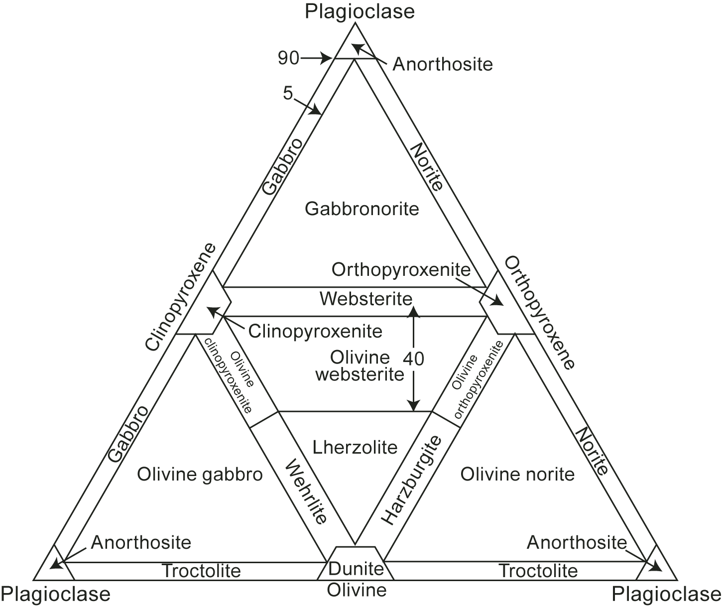
Figure F3. Classification, mafic–ultramafic plutonic igneous rocks.
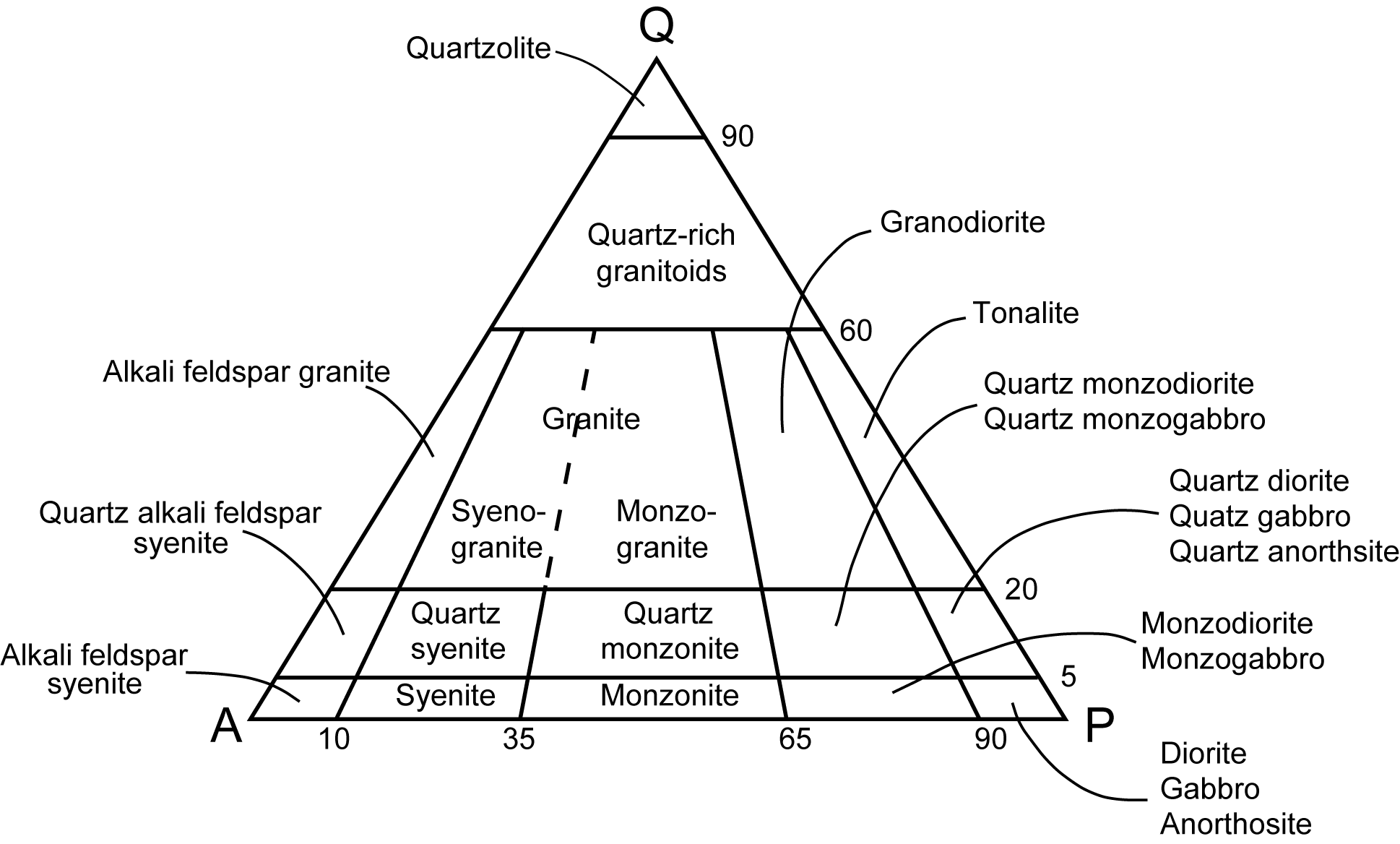
Figure F4. QAP scheme.
In the IUGS classification, diorite is distinguished from gabbro by the anorthite (An) content of plagioclase, with diorites having <50 mol% An. Because this cannot be established during macroscopic description, we used the following convention: if a gabbroic rock contained quartz or primary amphibole, indicating a relatively high degree of fractionation, the rock was classified as diorite; if no quartz or primary amphibole was observed, the rock was classified as gabbro.
Minor modifications to the IUGS system were made to subdivide the rock types more accurately on the basis of significant differences rather than arbitrary cutoffs based on the abundance of a single mineral. We have attempted to follow as closely as possible the lithologic subdivisions from previous expeditions at Atlantis Massif (Expeditions 304/305 and 357 [Expedition 304/305 Scientists, 2006; Früh-Green et al., 2016]), as well as earlier gabbro legs (Expeditions 335, 345, and 360 [Expedition 335 Scientists, 2011; Expedition 345 Scientists, 2014; Dick et al., 2016]) to facilitate both continuity of descriptions of Hole U1309D and intersite comparisons.
For peridotites, the prefix orthopyroxene-bearing is added to dunites with orthopyroxene abundances from 1% to 10%. For gabbroic rocks, the following prefixes based on modal content of minerals are used:
- Disseminated oxide = Fe-Ti oxide 1%–2%.
- Oxide-bearing = Fe-Ti oxide 2%–5%.
- Oxide = Fe-Ti oxide >5%.
- Olivine-bearing = olivine 1%–5%.
- Orthopyroxene-bearing = orthopyroxene 1%–5%.
- Troctolitic = clinopyroxene 5%–15%; olivine >20%.
- Olivine-rich = >70% olivine.
- Anorthositic = >80% plagioclase.
Additional descriptive modifiers are defined as follows:
- Leucocratic = light colored; high proportions of plagioclase.
- Melanocratic = dark colored; high proportions of pyroxene and/or amphibole.
- Micro = very fine grain size.
3.2.1.2. Mineral description
In ultramafic rocks, the minerals orthopyroxene, clinopyroxene, and Cr-spinel were described in terms of modal abundance and average grain size (in millimeters). For olivine, serpentinization obscured grain size determination and only proportions were estimated. In gabbroic rocks, the minerals olivine, plagioclase, clinopyroxene, orthopyroxene, amphibole, and Fe-Ti oxide were described for the following:
- Modal abundance (percent).
- Size: average, maximum*, and minimum* in millimeters. In plutonic rocks, Fe-Ti oxides commonly occur as aggregates, and for grain size determination an aggregate is counted as a single grain.
- Shape*: euhedral, subhedral, or anhedral. Where oxides and sulfides form aggregates, they are divided into angular aggregates, amoeboid aggregates, and interstitial aggregates.
- Habit*:
The first four habit terms apply predominantly to subhedral or euhedral grains, the latter two generally to anhedral grains. Descriptions of any further features (e.g., reaction coronas or symplectites) are made in the comment for each mineral*.
Where a mineral occurs in trace quantities (i.e., too low to assign a meaningful percentage), 0.1% is recorded without further description. For sulfides, only the abundance was described (in percent). Accessory phases were also noted where observed.
3.2.1.3. Average grain size and grain size distribution
The average grain size for gabbroic rocks was described using the following terms:
- Glassy,
- Cryptocrystalline (<0.1 mm),
- Microcrystalline (0.1–0.2 mm),
- Fine grained (0.2–1 mm),
- Medium grained (1–5 mm),
- Coarse grained (5–30 mm), and
- Pegmatitic (>30 mm).
The grain size distribution of the gabbroic domain is described using the following terminology:
- Equigranular: all minerals are of similar size.
- Seriate: a continuous range of crystal sizes.
- Varitextured: domains with contrasting grain size.
- Porphyritic: grains show a bimodal distribution in grain size with a fine-grained matrix and coarse-grained crystals.
- Bimodal: grain size falls into two distinct clusters.
3.2.1.4. Texture
The following terms were used to describe the textural relationships between different silicate grains in gabbroic rocks (Figure F5):
- Granular: aggregation of grains of approximately equal size.
- Intergranular: coarser grains (typically plagioclase) form a touching framework of the rock with interstices filled by crystalline material.
- Intersertal: coarser touching grains form a framework of the rock with interstices filled by glass.
- Subophitic: partial inclusion of plagioclase in clinopyroxene.
- Ophitic: total inclusion of plagioclase in clinopyroxene.
- Poikilitic: large oikocrysts containing numerous chadacrysts of any type.
- Porphyritic: texture containing large grains within a finer grained matrix.
- Comb structure: comb-like arrangement of crystals growing inward from a contact.
- Skeletal: either hopper crystals or crystals with hourglass shape.
- Dendritic: branching arrangement of elongate crystals.
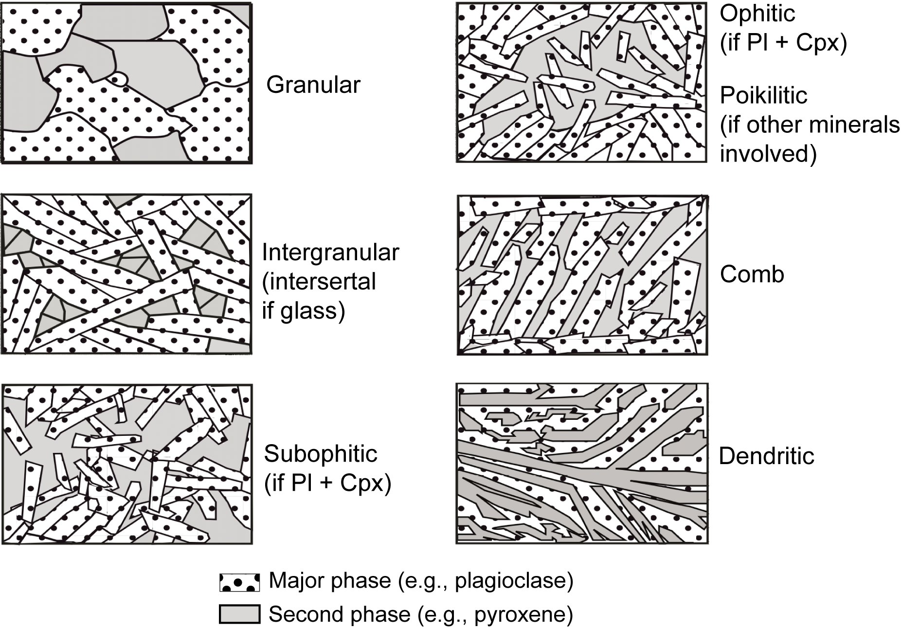
Figure F5. Textural classification, igneous rocks.
3.2.1.5. Body of rock interpretation
Finally, an overall interpretative description of the unit is made.
3.2.2. Volcanic rocks
3.2.2.1. Nomenclature
For volcanic and hypabyssal rocks, we used the following definitions for primary lithology:
- Basalt: all igneous rocks of basaltic composition that are not clearly intrusive, in the size range glassy to fine grained.
- Diabase: holocrystalline, aphanitic to medium-grained intrusive rock of basaltic composition often with well-developed subophitic or ophitic textures. This rock type is referred to as dolerite in European nomenclature and for Expedition 357. Expedition 357 further used the term “metadolerite” for altered equivalents; we did not use that term during Expedition 399.
Prefixes were added according to phenocryst content, using the following convention:
- Aphyric = <1% phenocrysts.
- Sparsely phyric = 1%–5% phenocrysts.
- Moderately phyric = 5%–10% phenocrysts.
- Highly phyric = >10% phenocrysts.
If present and >1%, phenocryst phases were put as modifiers in front of the rock name. If less than 1% phenocrysts are present, the rock was given the modifier “aphyric.”
3.2.2.2. Phenocryst abundance, mineralogy, grain size, and grain size distribution
Similar to plutonic rock description, phenocrysts in volcanic rocks were described in terms of their mineralogy, percent volume, size (in millimeters), shape, habit, and average grain size following the same conventions and definitions as for plutonic rocks.
3.2.2.3. Groundmass volume, mineralogy, grain size, and grain size distribution
Groundmass of a volcanic/hypabyssal rock is described for their volume (percent), average grain size, and grain size distribution. Grain size was described as glassy, cryptocrystalline, microcrystalline, fine grained, and medium grained using the same conventions as for plutonic rocks.
3.2.2.4. Vesicles
Vesicle descriptions include their abundance (in percent), size (minimum, maximum, and average size in millimeters), and sphericity (spherical, elliptical, or irregular). If vesicles are elongate, the direction is noted.
3.3. Thin section descriptions
All thin sections were described to determine original igneous mineral modes, grain sizes, and textures at the mineral and rock scale. These descriptions were used, when necessary, to refine and revise hand specimen descriptions. Each thin section was photographed in both plane-polarized light (PPL) and cross-polarized light (XPL), with thumbnail versions printed on the thin section form reports. In addition, photomicrographs were taken of particularly interesting features in many thin sections. All images are available from the LIMS database.
Thin section descriptions closely follow the procedures and nomenclature used for macroscopic core description. Where a thin section contained more than one domain in terms of the parameters below, the different domains were described separately, with their relative volumes noted. The following data were recorded and entered into the LIMS database through GEODESC.
3.3.1. Lithology and texture
- Number of igneous domains within the thin section;
- Nature of igneous domains, if any (e.g., contact between two units; mix of two lithologies in one section; presence of texturally different regions within one thin section);
- Igneous domain relative abundance (in percent);
- Igneous domain lithology name, using the same definitions as those for macroscopic descriptions; if only one domain is present, this is identical to the rock name;
- Igneous domain grain size name (glassy, cryptocrystalline, microcrystalline, fine grained, medium grained, coarse grained, and pegmatitic; see Average grain size and grain size distribution for definitions);
- Igneous domain grain size distribution (equigranular, seriate, varitextured, porphyritic, and poikilitic); and
- Igneous domain texture (granular, subophitic, ophitic, porphyritic, intergranular, intersertal, skeletal, and dendritic).
3.3.2. Mineral descriptors
Features described include: abundance (in percent) of primary minerals preserved; estimated abundance (in percent) of primary minerals prior to alteration; minimum size, maximum size, average size, shape, and habit of primary minerals, using the same conventions as during macroscopic description; exsolution in pyroxenes; and individual comments for primary minerals. Accessory minerals were noted where present. For fine-grained diabase and basalt samples, groundmasses and crystal cargoes were discussed separately.
In estimating the original abundance of primary minerals prior to alteration, we have assumed that there has been no changes in relative abundance of the main silicates due to the volume change associated with alteration.
For plagioclase, zoning was recorded in terms of extent and type, using the following convention.
- Rank 0: None (Rank 0),
- Rank 1: Zoning is rare and weakly developed,
- Rank 2: Abundant zoning that can range from weak to strong, and
- Rank 3: Nearly ubiquitous, generally strong zoning.
The type of zoning in plagioclase was also documented:
- Continuous: zoning is optically continuous from core to rim.
- Discontinuous: zoning occurs from core to rim but with distinct break(s).
- Patchy: zoning occurs in patches randomly throughout the grain. This type was generally the result of deformation.
- Oscillatory.
- Sector.
Finally, a “Body of rock interpretation” was completed that discussed noteworthy features and their potential origins.
4. Alteration petrology
4.1. General work organization
The characteristics of metasomatism (hydrothermal alteration) of rocks recovered from Holes U1601A, U1601C, and U1309D were observed with the naked eye through a magnifying lens or stereo microscope and in thin sections using petrographic microscopes (note that the terms “alteration” and “metamorphism” in this report are used interchangeably without implication as to spatial scale or open- versus closed-system processes). The macroscopic identification of minerals was complemented by hardness tests, acid tests, and where possible microscopic observations of thin sections, XRD, scanning electron microscope (SEM), and X-ray fluorescence (XRF) analyses.
For serpentinized peridotites, bulk density and magnetic susceptibility (MS) measurements with the WRMSL (see Petrophysics) were used to improve the estimates of the total alteration extent. MS measured on the SHMSL was also used for cores from Holes U1309D and U1601A and from Hole U1601C as deep as Core 399-U1601C-37R (see Operations). Shipboard macroscopic and microscopic observations were recorded using the GEODESC applications and uploaded to the LIMS database. The data were then used for the production of graphic section summaries that report a petrographic description of each section and present downhole variation of alteration characteristics along with other observations and measurements. Microscopic observations captured using GEODESC were summarized in thin section form reports. The terminology and mineral abbreviations used for alteration descriptions are summarized in Tables T2 and T3 (Expedition 304/305 Scientists, 2006; Whitney and Evans, 2010; MacLeod et al., 2017). Core descriptions were completed in a collaborative fashion in which each member of the alteration petrology team was responsible for one or more aspects of observation and description.
Two distinct methods, described in detail below, were used in the core descriptions. Method 1 was used to describe cores from Holes U1309D and U1601A. Because operational procedures were changed for Hole U1601C and to handle the unexpected volume of core, a new set of streamlined methods (Method 2) had to be established. This was done to ensure that all cores could be described in the given time frame. Method 2 was applied to cores from Hole U1601C (excluding Cores 2R–18R, 22R, 25R, 35R, and 36R).
4.2. Macroscopic core description
4.2.1. Alteration log Method 1
All macroscopic descriptions using Method 1 (including descriptions of veins and halos; see Vein and halo log Method 1) were carried out on the archive section halves of the cores and logged as description intervals. The first step of description was the estimation of intervals with different characteristics of alteration. Hydrothermal alteration was categorized into three groups: (1) pervasive background alteration, (2) halo alteration in proximity to veins or fractures, and (3) localized patchy alteration without apparent relationship to veining. Where a primary phase was partially or completely altered to pseudomorphic minerals, it was categorized as background alteration. The approximate proportions of each group of static alteration style were estimated in each descriptive interval.
The extent of hydrothermal alteration of rocks and individual igneous and mantle minerals was recorded in the GEODESC worksheets. For the estimation of the alteration extent, a rank scale was used as follows:
- 1 = fresh (<3%).
- 2 = slight alteration (3%–20%).
- 3 = moderate alteration (21%–50%).
- 4 = high alteration (51%–99%).
- 5 = complete alteration (100%).
Hardness tests were performed in small areas of selected samples under a binocular microscope to aid with the identification of minerals and better constrain the extent of alteration. Although more precise than assigning a rank scale, the estimation of alteration extent of each primary mineral in rocks is subject to uncertainties. The main causes are the small grain size, inhomogeneous distribution, and complicated microscopic- or submicroscopic-scale textures of alteration minerals. Alteration minerals replacing each igneous mineral, where observable, were logged in separate columns of worksheets in order of relative abundance. The variation of alteration intensity plotted on the graphic section summaries corresponds to background alteration intensity. The graphic section summaries also contain a summary statement of the alteration characteristics for each core section.
The sections from Holes U1309D and U1601A and Cores 399-U1601C-2R through 18R, 22R, 25R, 35R, and 36R were described on the basis of alteration intervals, which were defined on the basis of major changes in alteration mineralogy and/or intensity usually reflecting the variations of igneous lithology and intensity of hydrothermal activity and deformation. Because lithologic variations (e.g., mafic intrusions in peridotite) may occur at a very local scale (e.g., centimeter), no minimum size was assigned to an interval. The intervals that were sampled for microbiological analyses were incorporated into our descriptions when residues were present, which allowed confirmation of a similar nature to the surrounding rocks, or if the notes made during the selection and description of microbiology samples indicated that the sample was continuous with neighboring rocks. Otherwise, those intervals were omitted from our descriptions.
The procedures adopted for macroscopic observations and descriptions of cores using the alteration worksheets in GEODESC are summarized as follows:
- Determine the number and type of different alteration intervals in each section and assign each interval to a row in the GEODESC worksheet.
- Estimate the proportion by area of the three categories of hydrothermal alteration (i.e., background, halo, and patchy).
- Estimate the alteration extent and assign a percentage of replacement to each primary mineral (i.e., olivine, orthopyroxene, clinopyroxene [or just “pyroxene” if macroscopic identification between orthopyroxene and clinopyroxene was not possible], amphibole, plagioclase, oxide [including spinel], and opaque phases [including sulfide] for mantle rocks, gabbroic rocks, diorite, and diabase).
- Identify the secondary minerals that replace each primary mineral and list them by decreasing abundance.
- Estimate the total hydrothermal alteration extent and assign a rank scale to each alteration interval. A weighted average of alteration intensity of each primary mineral, if its volume proportion is estimated, gives the total alteration intensity of the interval.
- Record characteristic features of alteration in the interval as “alteration comments.”
- Create a section summary description, which appears near the top of the graphic section summaries. Use the classification terms for alteration intensity.
A list of minerals that were identified in altered rocks and veins based on the XRD analyses is provided in Table T7 in the Site U1309 chapter (McCaig et al., 2025a) and Table T5 in the Site U1601 chapter (Lang et al., 2025).
4.2.2. Alteration log Method 2
Because operational procedures were changed several times while logging Hole U1601C, all sections of Hole U1601C were macroscopically redescribed for consistency on shore at the GCR (see Operations). Method 2 largely followed Method 1, but in addition, all sections were tested for carbonate abundance using HCl. An overall alteration rank was assigned to entire sections that may include several alteration intervals. Colors of sections were described and logged in order of decreasing abundance. Percentages of background, halo, and patchy alteration were estimated. Alteration mineral assemblages that form at the expense of distinct primary minerals were identified. Any other relevant macroscopic observations were logged in a section comment.
4.2.3. Vein and halo log Method 1
Veins and halos were logged using Method 1, described here, in cores from Holes U1309D and U1601A and parts of Hole U1601C. Veins were defined as cracks partially or completely filled by secondary minerals. Fractures were defined as cracks with no mineral fill. The term halo was used to describe alteration in the original rock adjacent to veins and fractures.
Veins and halos were described collaboratively by representatives from the structural geology, igneous petrology, and alteration petrology teams and collected in a GEODESC tab named “Veins-and-halos.” The alteration petrology team recorded vein color and vein fillings with respect to the phases.
Certain minerals could not be identified with confidence but could be attributed to a mineral group, such as clay minerals, carbonates, sulfides, and oxides. Unidentifiable minerals were categorized as “other minerals.” The identification of minerals or mineral groups allowed grouping them into distinct vein types. Alteration halos, representing zones of increased alteration adjacent to veins, were described, including their width, (assemblages of) secondary minerals, and general comments in the veins-and-halos worksheet. Other vein data, such as abundance, width, orientation, texture, connectivity, and other structural features, were described by the structural geology and alteration petrology teams in the veins-and-halos worksheet. Vein shape, connectivity, texture and structure were described following the classification reported in the methods of Expedition 360 (MacLeod et al., 2017) (Figure F6). A vein generation was attributed to each vein or group of veins where apparent crosscutting relationships were observed. If two or more vein types did not show crosscutting relationships, the same vein generation was attributed to each vein type. The rest of the structural features regarding veins and the related methods are described in Structural geology.
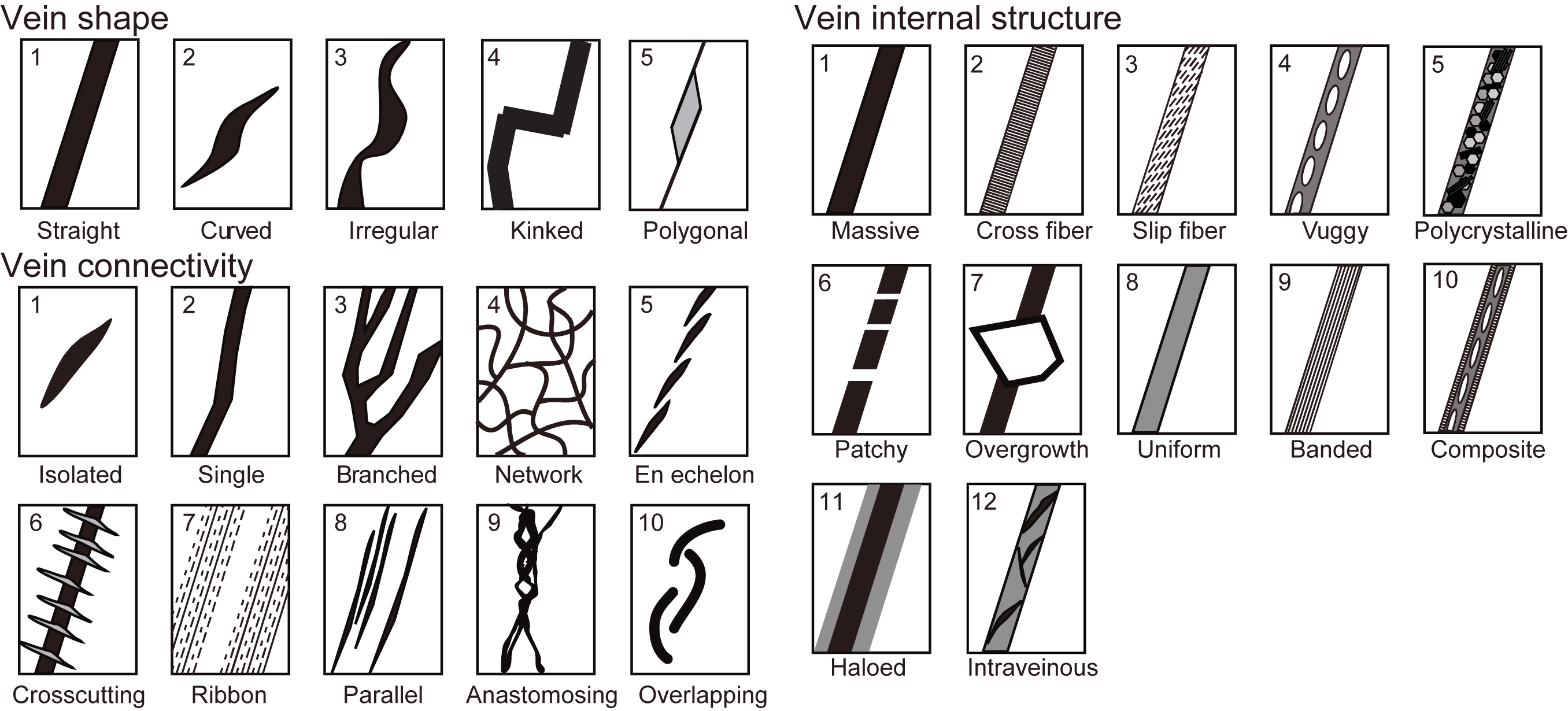
Figure F6. Characteristics of veins.
Data were recorded for each piece containing one or more veins. In pieces with more than one vein, (groups of) veins were numbered sequentially from the top of the piece. All three description teams used the same vein numbering scheme. Veins were measured on the archive half unless otherwise noted. The classification used for vein geometry, texture, and connectivity is shown in Figure F11 (see Structural geology). The orientations of veins in oriented core pieces were systematically measured by the structural geology team in close liaison with the alteration petrology group to ensure consistency of vein classification.
For the magmatic veins of Hole U1601A and U1309D, magmatic and alteration features were logged by the igneous and alteration petrology teams, respectively. Details of the particular methods of the igneous petrology team are described in the corresponding sections in this chapter. Observations for the following magmatic vein features were entered in the veins-and-halos worksheet: texture, texture comment, modal grain size, grain size comment, proportions (percent) of minerals, and rock name. The alteration petrology team reported the percentage of secondary minerals within the magmatic veins.
4.2.4. Vein log Method 2
Because operational procedures changed in Hole U1601C, the alteration vein and halo log of Method 1 was simplified to vein comment, vein color, vein frequency, and maximum vein width in Method 2. The vein comment of Method 2 includes mineral identity where identification was possible or a generic description of mineral features where identification was not possible or uncertain. Vein frequency either refers to a number where veins were enumerable, a “set” when veins were not enumerable and without connectivity, or a “network” when veins were abundant and connected. A brief description of additional vein specific features was included where possible. A summary of findings was entered into the section summary worksheet.
Observations for the following magmatic vein features were entered in the veins-and-halos worksheet: texture, texture comment, modal grain size, grain size comment, proportions (percent) of minerals, and rock name. Small magmatic intrusions were referred to as veins, and thicker centimeter- to decimeter-sized intrusions were referred to as dikes.
Note that all the Hole U1601C cores were redescribed and updated postcruise at the GCR using Method 2 (see above).
4.3. Thin section description
Thin sections of rocks were examined to further evaluate macroscopic identifications of secondary minerals on a microscopic scale and to establish their abundances, distribution, and relative timing of formation (ts-alteration template in GEODESC). Whole images of each thin section in PPL and XPL were taken and uploaded to the LIMS database by technical support personnel. Photomicrographs at variable magnifications were taken by core describers and uploaded to the LIMS database when notable occurrences of alteration minerals and textures were observed. When a thin section contained distinguishable areas with different alteration intensity, mineralogy, texture, deformation style, and/or igneous lithology, a different domain number was assigned to each area (e.g., Domain 1 or Domain 2). The different domains were described separately, and the relative abundance of each domain was noted.
For consistency, the mineral nomenclature used for microscopic descriptions is the same as that for macroscopic descriptions. In addition, different amphiboles were distinguished on the basis of their color, pleochroism, and extinction angle. In some cases (e.g., in late-stage magmatic intrusions and veins), amphibole can be of igneous or hydrothermal origin, and it is not always possible to unequivocally distinguish these processes based on petrographic observations. Consequently, amphibole was not counted as an alteration product where it shows a mode of occurrence suggestive of magmatic origin such as discrete euhedral crystals coexisting with plagioclase. In rocks subjected to ductile deformation, the recrystallized neoblasts of anhydrous minerals (e.g., olivine, pyroxene, and plagioclase) were not counted as alteration products for consistency with macroscopic descriptions. We reported the different types of veins present in the thin section, their mineralogy given in order of abundance, and if crosscutting relationships were observed, their chronological order (“Vein 1,” “Vein 2,” etc.). We also recorded primary and secondary fluid inclusions in primary minerals that formed during crystal growth or healing of fluid-filled fractures where fluid inclusions were abundant. Because the fluid inclusion contents vary depending on their mineral hosts, a column was added to the template to indicate the identity of the host mineral. Another column was added to indicate the abundance of fluid inclusions. The latter used the following rank system:
Finally, two columns were added to report the presence of secondary lamellae in distinct minerals (e.g., clinopyroxene in olivine) and their abundance. The procedures adopted for microscopic observation and description of each thin section were as follows:
- Determine the number of different alteration domains and their relative abundance and assign each domain to a row in the spreadsheet.
- For each alteration domain (row), enter observations in the appropriate columns. Observations include estimation of alteration extent of primary minerals (percent) and the determination of secondary minerals replacing them. Describe the textural relationships between the secondary and primary minerals. Where primary minerals are not visible or absent, determine the hydrothermal mineral and their abundance.
- Determine the number of veins of different mineralogy, assign each vein type to a column (i.e., Vein 1, Vein 2, and Vein 3 in chronological order, if possible), and describe constituent minerals of each vein.
- Provide a short summary giving the main alteration features, a qualitative estimation of the total alteration, the main mineralogical characteristics of the vein(s), and their chronological relationships. This is recorded in the summary alteration comments column. Also included in these columns were characteristic textures (e.g., corona, mesh texture, and halos).
- Create a brief summary description worksheet for the alteration characteristics in the thin section summary template. The summary appears in the thin section form report along with summaries from the igneous petrology and structural geology teams.
4.3.1. Characterization of serpentine minerals and replacement textures
The main serpentine group minerals include lizardite, chrysotile, and antigorite. All three serpentine minerals have been detected in oceanic serpentinite (Beard et al., 2009; Klein et al., 2017; Rouméjon et al., 2019; Früh-Green et al., 1996). Except for chrysotile, which can form macroscopic fibers, a positive identification of serpentine minerals by macroscopic means (naked eye, hand lens, or binocular microscope) is not possible. The identification of distinct serpentine minerals using optical microscopy in thin sections is possible in relatively coarse-grained domains but is problematic or impossible in fine-grained domains. During Expedition 399, established methods were attempted to assess the identity of serpentine minerals and texture in thin sections (Wicks and Whittaker, 1977; O’Hanley, 1996). Serpentine textures in thin sections consist of fibers or apparent fibers in countless orientations. Except for asbestiform chrysotile, which occurs as late-stage fracture fills in veins, lizardite and antigorite are not actually fibrous; they rather represent cross sections of platy grains and are referred to as apparent fibers (or pseudofibers). In thin sections, Wicks and Whittaker (1977) characterize (apparent) fibers of serpentine minerals based on their optical sign of elongation. However, a routine analysis of fine-grained serpentine intergrown with other minerals, such as brucite, chlorite, or talc was not possible. In thin sections, serpentine, especially antigorite, is almost always elongated parallel to its basal plane (001). Antigorite polished well in thin sections, chrysotile polished less well, and lizardite polished the least well (O’Hanley, 1996). In reflected light, the presence of antigorite is indicated by arrowhead-shaped crystals, and chrysotile is indicated by irregularly shaped strings. Although these characteristics are indicative of antigorite and chrysotile, the absence of these features does not indicate that neither antigorite nor chrysotile are present because these characteristics are only recognizable if the crystals are relatively coarse grained, which is usually not the case in serpentinite. Accordingly, the identification of antigorite in thin sections of samples from Holes U1601A and U1601C should be considered preliminary until the presence of antigorite can be confirmed by other analytical means.
4.4. X-ray diffraction
Vein materials and when necessary powders of whole rocks, vein halos, or patches were analyzed for mineral identification using XRD. For the first group of samples, XRD analyses were carried out shipboard using a Aeris diffractometer with Vantec-1 detector and nickel-filtered CuKα radiation from Malvern Panalytical. Small amounts of powder (usually ~20 mg) were prepared for XRD analysis by freeze-drying, crushing, and either mounting as smear slides or pressing onto depressions in sample holders. Mineral identification based on multiple peak matches was carried out using the interactive software package HighScore Plus and its associated powder diffraction file database. Instrument conditions were as follows:
- Voltage = 40 kV.
- Current = 15 mA.
- Goniometer scan (bulk samples) 2θ = 4°–70°2θ.
- Step size = 0.0108664°2θ.
- Scan speed = 39.525 s/step.
- Divergence slit = 0.125 mm.
The second group of XRD analyses was carried out at the University of Fribourg (Fribourg, Switzerland) on a Powder XRD Rigaku Ultima IV with a D/TEX Ultra 2 detector and using CuKα radiation. Samples with distinct domains, such as those with hydrothermally altered magmatic veins in a surrounding serpentinite host rock, were subsectioned by cutting. Rock powders were then prepared by crushing in a steel mortar and pestle and subsequently milled in an agate mill. Small amounts of sample material were then put onto glass slides. The following instrument conditions were used for analyses:
- Voltage = 40 kV.
- Current = 40 mA.
- Goniometer scan (bulk samples) 2θ = 5°–70°2θ.
- Step size: 0.002°2θ.
- Scan speed = 1°/min.
- Divergence slit: open.
Peak evaluation was carried out using the PDXL2 software together with the ICDD2024 database. In addition, Rietveld refinement was carried out to estimate mineral abundances. However, because most samples contain a large number of minerals, peak overlap leads to relatively high uncertainties.
5. Structural geology
Sites drilled during Expedition 399 at Atlantis Massif are part of a young oceanic core complex that exposes gabbroic and mantle rocks in the footwall of an oceanic detachment fault system. These rocks commonly show a variety of magmatic and solid-state deformation features associated with magmatic accretion, alteration, and deformation during plate spreading, denudation, and cooling, often superposed. The continuum of superposed events span the transitions from hypersolidus to subsolidus and from ductile to brittle, decreasing in temperature with time. Ultramafic rocks can include original mantle fabrics, and/or lower temperature overprints due to tectonic and hydrothermal processes during denudation to the seafloor.
Conventions for structural studies established during previous “hard rock” drilling projects (e.g., ODP Legs 118, 131, 140, 147, 153, 176, 179, 206, and 209; Integrated Ocean Drilling Program Expeditions 304/305, 309/312, 335, and 345; and Expeditions 357 and 360 [Shipboard Scientific Party 1989, 1991, 1992a, 1992b, 1992c, 1993a, 1993b, 1995, 1999, 2003, 2004; Expedition 304/305 Scientists, 2006; Expedition 309/312 Scientists, 2006; Expedition 335 Scientists, 2012; Gillis et al., 2014; Früh-Green et al., 2017; MacLeod et al., 2017]) were generally followed during Expedition 399. Definitions of structural measurements and descriptive parameters were refined from Leg 209 and Expeditions 345, 357, and 360 to configure the core description software application GEODESC for hard rock descriptions. GEODESC is used to enter and upload the information into the JRSO LIMS database (see Introduction). Macroscopic core description and terminology used to describe cores recovered from Holes U1309D and U1601A are presented as Methods 1; those used for cores from Hole U1601C, modified for more rapid description because of delays in access to the cores, unprecedented recovery in hard rock drilling, and postcruise redescription, are presented as Methods 2.
5.1. Structural orientations
5.1.1. Measurements
Structural features categorized as magmatic, crystal plastic, mantle crystal plastic, schistose, serpentinite foliation, and brittle, together with alteration and magmatic veins and igneous contacts, were logged by interval in centimeters from the top of each section. Depth intervals of structures were recorded as the offset from the top of the section to the top and bottom of the feature, where the feature intersects the center of the section half surface or core edge (veins) (Figure F7). Structures were measured relative to the standard IODP CRF (Figure F8). The plane normal to the axis of the borehole is referred to as the horizontal plane. On this plane, a 360° net is used with pseudosouth (180°; −x-direction) perpendicular to the cut surface pointing into the archive half and pseudonorth (000°; x-direction) perpendicular to the cut surface pointing out of the archive half (and into the working half). The cut surface of the section half, therefore, is a vertical plane striking 090°–270°.
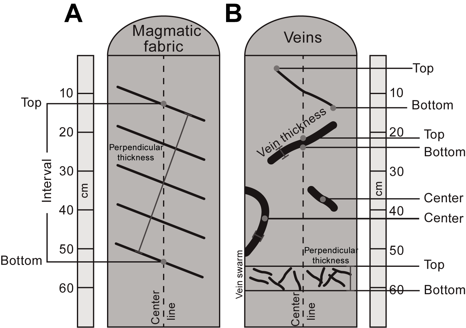
Figure F7. Structure logging.
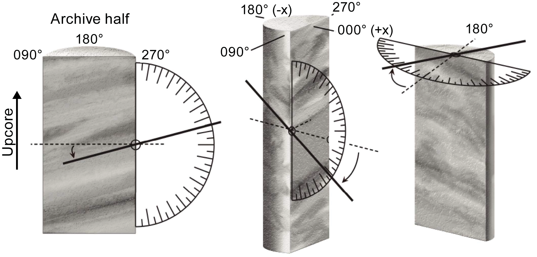
Figure F8. Reference frame and method of measuring orientation.
Dip and dip directions were measured directly relative to the CRF using a contact goniometer. Where linear structural elements were observed (such as slickenlines on a fault or sheared vein), the trend and plunge of the lineation was measured directly using a contact goniometer relative to the CRF. The sense of shear on fault surfaces and/or veins is determined by structures such as slickenfibers, groove marks, or steps in the slickensides. Sense of shear for magmatic fabrics and CPFs are determined using the asymmetry of rotated crystals, porphyroclast-tails, or the morphology of foliation deflection (Passchier and Trouw, 2005).
Where unoriented pieces have a clear up-down direction, measured dips were recorded without an accompanying dip direction. To aid rapid core description in Hole U1601C (Methods 2), dip and dip directions were measured to an accuracy of 5°.
5.1.2. Statistical analysis of true-dip vein and fracture data
Statistical analysis of the true dip of discrete planar features with short intervals compared to the width of the borehole, including veins and fractures, is affected by a borehole bias effect (Martel, 1999), which leads to preferential sampling of gently dipping planar structures compared to more steeply dipping structures (Figure F9). Histograms of dip angles are plotted to determine whether measured distributions reflect random or systematic populations. A length scale effect proposed in Shipboard Scientific Party (1992c), which would predict that sampling of a uniform distribution of dips if combined with the borehole bias effect would peak at a dip of 45°, is not supported by the methodology or data in Martel (1999) (S. Martel, pers. comm., 2024) and is not used here.
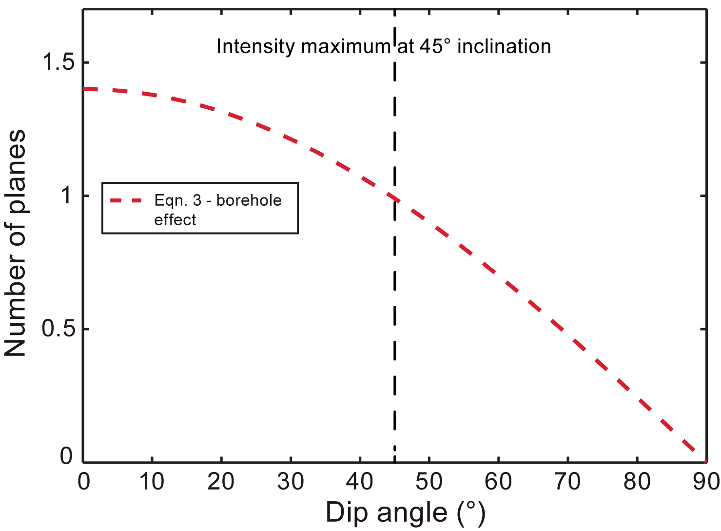
Figure F9. Predicted distribution of set of planar features.
5.2. Macroscopic core description and terminology
5.2.1. Workflow organization
Whole-round pieces were oriented by a designated scientist during each shift for splitting (when possible) prior to curation. Cores were marked and split to maximize the dip of planar structures so that the dominant structure dips toward 090° in the CRF (Figure F8). Where no obvious structures were present, cores were marked to maximize contiguity and/or to ensure that representative material is present in both working and archive halves of the core. This convention was adopted primarily for ease of structural feature measurement and allows some impression to be gained as to the relative orientation of other structural features (e.g., veins and CPFs).
The structural geology team worked together during Expedition 399 and during the follow-up description at the GCR and described core collectively, sharing expertise. Each core section was described and logged with detailed structural information. During core description, data were entered directly into templates (spreadsheets) made using the GEODESC online database system. During Expedition 399, the unexpected increase in the rate of core recovery from Hole U1601C required us to modify our methods for macroscopic core descriptions midway through the expedition. Consequently, two different methods of core description were used during Expedition 399, defined separately below, each with their own set of templates used for data entry. Methods 1 were used to describe cores from Holes U1309D and U1601A. Methods 2 were used to describe Cores from Hole U1601C. Thin section description methods did not change during the expedition and are outlined following the macroscopic description methods.
5.2.2. Methods 1
Methods 1 applies to Holes U1309D and U1601A.
Methods 1 used six GEODESC data entry templates to capture a range of macroscopic structural parameters summarized as follows, detailed below (see GEODESC in Supplementary material):
- Igneous petrology template: magmatic contact characterization in conjunction with the igneous petrology team, including contact nature (e.g., intrusive, fault, and grain size), geometry, and orientation (template filename: 399_macroscopic_igneous_igneous-petrology).
- Magmatic fabric template: compositional or grain size layering and/or shape preferred orientation (SPO) of dominant minerals, as well as orientation (template filename: 399_macroscopic_structure_Magmatic-Fabric).
- CPF template: solid-state foliation geometry, CPF intensity, and asymmetry/shear sense for CPF, including a separate distinction of mantle fabrics, schistosity displayed by alteration products, serpentine foliation, and orientations (template filename: 399_macroscopic_igneous_cp-fabric).
- Brittle deformation template: fault rock type and intensity, apparent fault offset, fracture morphology, fracture network, and striae (e.g., slickenfibers) (template filename: 399_macroscopic_igneous_brittle-deformation).
- Vein template: alteration and magmatic vein data in conjunction with the metamorphic and igneous petrology teams; includes vein type, morphology, connectivity, texture, structure, vein-wall relationship, and vein crosscutting relationships with other veins and other structural elements (template filename: 399_macroscopic_igneous_veins-and-halos).
- Vein and fracture density template: measuring the number of veins or fractures every 10 cm (template filename: 399_macroscopic_igneous_vein-fracture-density).
5.2.2.1. Magmatic fabrics and veins
Intrusive and structural contacts were measured and described in accordance with the igneous petrology worksheet (see Igneous petrology). Descriptions include the following:
Magmatic vein contacts were reported by the igneous petrology team, defined as distinct intervals. The structure team measured orientations of individual magmatic veins in the veins-and-halos template where previously defined as an interval by the alteration petrology team.
Magmatic layering and foliation, where present, were measured and described in the magmatic fabric worksheet. Descriptions include the following:
- Magmatic fabric type: modal layering, grain size layering, SPO, and isotropic; when none of these terms describes the observations well, the nature of layering is described in the comments.
- Magmatic fabric intensity accompanied by intensity rank (Figure F10):
- Magmatic fabric boundary definition: sharp or diffuse.
- Upper contact type of magmatic contacts: grain size layering, modal layering, or intrusive.
- Orientation of the upper contact (dip and dip azimuth in CRF).
- Upper contact dip attitude: horizontal (0° dip), subhorizontal (1°–10° dip), shallow (10°–30° dip), moderate (30°–60° dip), steep (60°–80° dip), subvertical (80°–89° dip), or vertical (90° dip).
- Magmatic fabric layering geometry (if present): planar, curved, or irregular.
- Magmatic fabric SPO geometry (if present): planar, linear, or planar-linear.
- Magmatic phase(s) defining the SPO: olivine (ol), plagioclase (pl), clinopyroxene (cpx), orthopyroxene (opx), or oxides (ox).
- Orientation of the magmatic fabric (dip and dip azimuth of magmatic fabrics, as well as trend and plunge of any lineation in the layering, where measured, in the CRF).
- Magmatic fabric dip attitude: horizontal (0° dip), subhorizontal (1°–10° dip), shallow (10°–30° dip), moderate (30°–60° dip), steep (60°–80° dip), subvertical (80°–89° dip), or vertical (90° dip).
- Magmatic fabric comment.
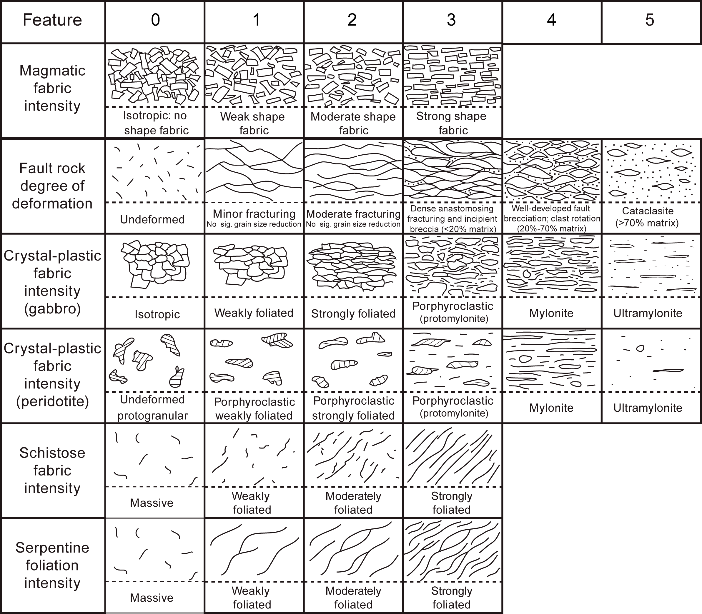
Figure F10. Intensity ranks.
5.2.2.2. Crystal-plastic fabrics, mantle fabrics, schistosity, and serpentine foliation
CPFs include planar or linear fabrics defined by crystals exhibiting crystal-plastic deformation. CPFs associated with mantle deformation in peridotite (mantle fabrics) were classified separately from CPFs produced by discrete shear zones (Figure F10). Schistosity was reported from zones of alteration, where fabrics are controlled by secondary minerals including talc, chlorite, and amphibole (Figure F10). Serpentine foliations were reported from serpentinized peridotite where mesh textures displayed a preferred orientation, which may pseudomorph a preexisting mantle fabric (Figure F10).
Abyssal peridotites represent a special problem for grading crystal-plastic deformation because they have usually been emplaced from the Earth’s deep interior by high-temperature crystal-plastic creep processes and therefore lack any primary igneous texture. They generally have either protogranular or porphyroclastic textures when unmodified by relatively shallow deformation processes associated with unroofing and exposure to the seafloor. We therefore use a separate textural criterion for mantle fabrics in abyssal peridotites (Figure F10) based on the methodology used during Leg 209 and Expedition 357 (Shipboard Scientific Party, 2004; Früh-Green et al., 2017).
Protogranular textures are generally the earliest fabric formed and are characterized by smoothly curved grain boundaries with complex cusps and lobes. However, alteration has largely obscured olivine grain size and shape entirely in hand specimen of abyssal peridotite; the visual core description is almost entirely based on textures in pyroxene and spinel. Rocks with a purely protogranular texture are graded 0 because this is the earliest formed texture and may or may not have a preferred crystallographic mineral fabric or a shape fabric. Porphyroclastic textures are generally superimposed on protogranular textures, and usually elements of both are present. Rocks with porphyroclastic texture are graded 1 (weak foliation) if there is only a weak pyroxene shape fabric developed. When pyroxenes exhibit a significant shape fabric, the sample is graded 2 (strong foliation) under the crystal-plastic field, noting that at this grade only a few protogranular textural elements are present. These samples are still referred to as porphyroclastic. When the shape fabric is strong and a foliation developed, with significant grain size reduction, the texture is referred to as protomylonitic and graded 3 under crystal-plastic deformation. At this grade, there are generally no protogranular textural elements left. With significant grain size reduction in peridotite forming a fine-grained mass of olivine (or serpentine) with embedded pyroxene porphyroclasts and a prominent foliation, the rock is graded 4 and listed as a mylonite. If there is no visible foliation because of extreme grain size reduction, the rock is listed as an ultramylonite and graded 5. This deformation scale closely parallels that used for crystal-plastic deformation of gabbro and other crustal rocks here and during previous expeditions and represents very similar or the same intensities of deformation at each grade (Figure F10).
Schistose fabrics defined by the preferred orientation of alteration mineral assemblages are classified separately (Figure F10). Based on observations from Expedition 357, we anticipated recovery of a range of variably deformed serpentinite and talc-tremolite-chlorite schist formed during alteration. Typically, we anticipate these fabrics in sheared alteration veins. The compositional features of these schists are reported by the alteration team, whereas the type, intensity (ranked from 0 to 3), and orientation of schistose fabrics within these rock types are reported here as part of the structural geology section (Figure F10).
Serpentine foliation produced by background alteration of mantle peridotite are reported as a distinct fabric (Figure F10). Strong planar fabrics may form during serpentinization by development of closely spaced subparallel veins termed “ribbon texture” (O’Hanley, 1996). The texture is characterized by anastomosing, often cross-fiber, replacement serpentine veins. In general, the veins wrap around relict or pseudomorphed pyroxene grains with little evidence of shear offset. These create a strongly foliated serpentinite that is actually a variant of hourglass serpentine texture and largely represents in situ replacement of the primary olivine (O’Hanley, 1996). This texture may parallel preexisting crystal-plastic foliation, and its intensity may reflect stress state or the presence of a preexisting fabric in the rock. The strength of serpentine foliation is rated on a scale from 0 (no foliation) to 3 (strongly foliated) (Figure F10).
Descriptions for CPFs, mantle fabric, schistosity, and serpentine foliation were captured in the CPF template and include the following:
- CPF intensity and rank (Figure F10); the final characterization of the structure was performed after petrographic inspection, when possible:
- 0 = undeformed.
- 1 = weakly foliated/lineated.
- 2 = strongly foliated/lineated.
- 3 = protomylonitic.
- 4 = mylonitic.
- 5 = ultramylonitc.
- CPF boundary definition: sharp or diffuse.
- CPF perpendicular thickness (in centimeters).
- CPF sense of shear: normal (n), reversed (r), dextral (d), sinistral (s), a combination of these (nd, ns, rd, or rs), or unknown (u).
- CPF shear sense confidence: low, medium, or high.
- Comments on deformation fabric.
- Type of deformation fabric: linear (L), planar (S), or planar-linear (L-S).
- Mantle fabric intensity and rank (Figure F10); the final characterization of the structure was performed after petrographic inspection, when possible:
- 0 = protogranular.
- 1 = porphyroclastic-weakly foliated.
- 2 = porphyroclastic-strongly foliated.
- 3 = porphyroclastic/protomylonitic.
- 4 = mylonitic.
- 5 = ultramylonitic.
- Mantle fabric comments.
- Upper contact type of different mantle rock types: modal contact or grain size contact.
- Orientation of the upper contact (dip and dip azimuth in CRF).
- Upper contact dip attitude: horizontal (0° dip), subhorizontal (1°–10° dip), shallow (10°–30° dip), moderate (30°–60° dip), steep (60°–80° dip), subvertical (81°–89° dip), or vertical (90° dip).
- Schistose fabric intensity (Figure F10):
- Serpentine foliation intensity (Figure F10):
- Schistose/serpentine fabric type: planar (S), anastomosing, S-C fabric, or mesh texture.
- Schistose/serpentine fabric comment.
- Lineation mineral.
- Lineation intensity: weak or strong.
- Orientation of the lineation: trend and plunge, where measured in the CRF.
- Fabric attitude: horizontal (0° dip), subhorizontal (1°–10° dip), shallow (10°–30° dip), moderately inclined (30°–60° dip), steeply inclined (60°–80° dip), subvertical (81°–89° dip), or vertical (90° dip).
- Orientation of fabric and the measured fabric type: dip and dip azimuth in the CRF; in practice almost exclusively foliation planes.
5.2.2.3. Brittle deformation
Brittle fabrics described during Expedition 399 include breccias, faults, and fractures (Figures F10, F11). Descriptions are captured in the brittle deformation worksheet of the macroscopic template and include the following:
- Fault rock type: microfault, fault gouge, fault breccia, cataclasite, ultracataclasite, pseudotachylite, fault, or piece-end fault surface.
- Fault rock degree of deformation, based on the percentage of matrix present in each fault rock (Figure F10); thin section descriptions, wherever available, aided this classification:
- 0 = no fracturing.
- 1 = minor fracturing.
- 2 = moderate fracturing.
- 3 = dense anastomosing fracturing.
- 4 = well-developed fault brecciation.
- 5= cataclastic.
- Fault rock cohesion: incohesive or cohesive.
- Fault sense of shear: normal (n), reversed (r), dextral (d), sinistral (s), a combination of these (nd, ns, rd, or rs), or unknown (u).
- Apparent fault offset (in millimeters), where measurable.
- Clast content in fault rock (in percent).
- Average size of clast in fault rock (in millimeters).
- Fracture morphology (if present) (Figure F11): planar, curved, irregular, stepped, or fracture tip.
- Fracture network: stepped, splayed, anastomosing, isolated, single, branched, en echelon, crosscutting, parallel, or overlapping (Figure F11).
- Fracture perpendicular thickness (in centimeters).
- Brittle deformation comments.
- Striae comments (e.g., slickensides/slickenlines/slickenfibers).
- Orientation (dip and dip azimuth) of fracture and trend and plunge of associated striae (e.g., slickensides/slickenlines/slickenfibers) including striae in veins.
- General fabric attitude of the brittle feature: horizontal (0° dip), subhorizontal (1°–10° dip), shallow (10°–30° dip), moderate (30°–60° dip), steep (60°–80° dip), subvertical (80°–89° dip), or vertical (90° dip).
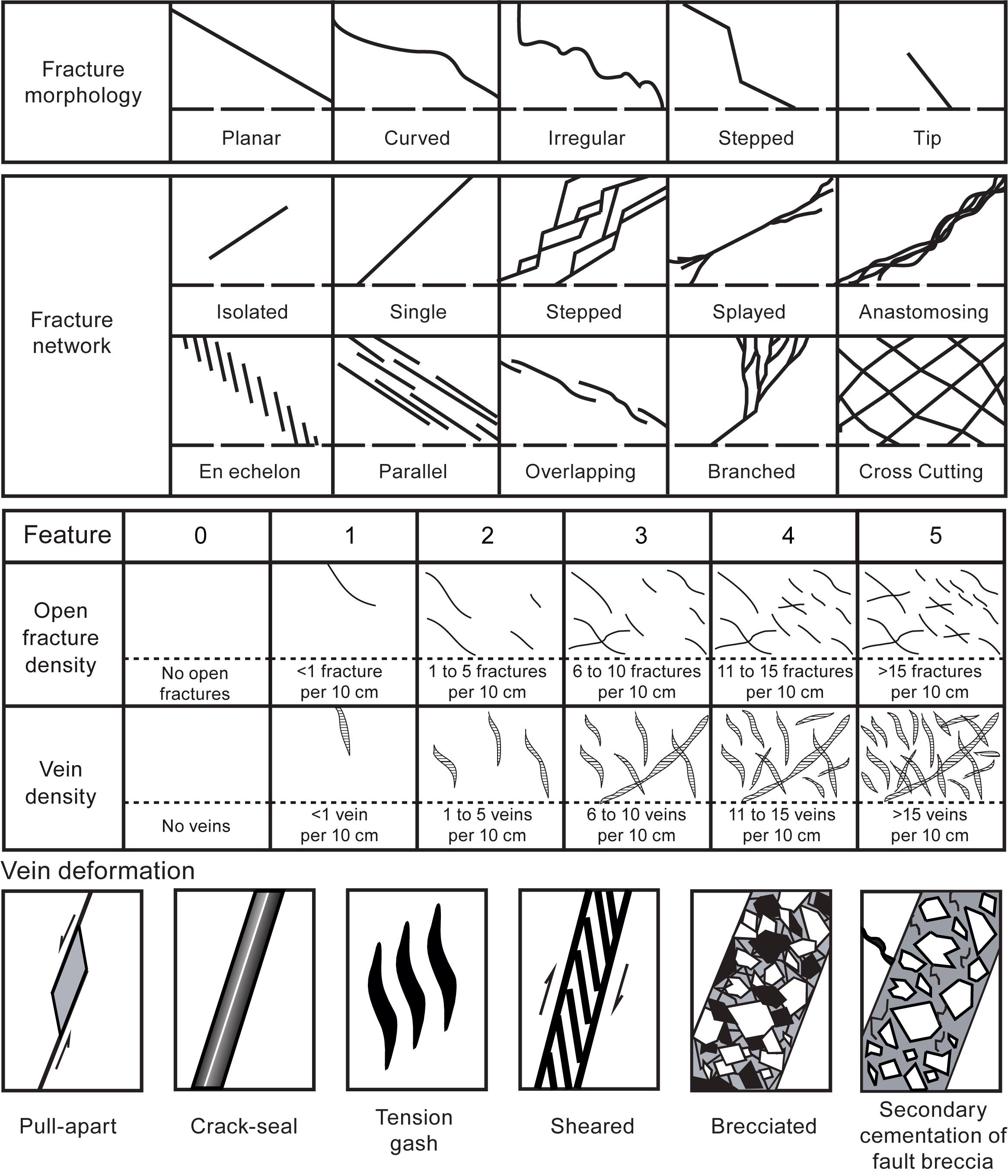
Figure F11. Macroscopic classification, fractures and veins.
Density of fractures and drilling-induced fractures, as well as veins, were recorded in the vein_fracture_density template:
- Vein density (Figure F11):
- 0 = no open veins.
- 1 = <1 vein/10 cm.
- 2 = 1–5 veins/10 cm.
- 3 = 6–10 veins/10 cm.
- 4 = 11–15 veins/10 cm.
- 5 = >15 veins/10 cm.
- Fracture density (Figure F11):
5.2.2.4. Alteration veins
Alteration vein description during Expedition 399 was captured in the veins-and-halos template. Petrologic descriptions of alteration veins, as well as descriptions of vein shape, vein boundary, vein connectivity and vein internal structure were reported by the alteration team, whereas structural descriptions of the deformation displayed by those veins were reported by the structural team (Figure F11). Structural descriptions of veins include the following:
- Vein deformation (Figure F11): pull-apart, brecciated, crack-seal, sheared, tension gash, or secondary cementation of fault breccia.
- Sense of shear: normal (n), reversed (r), dextral (d), sinistral (s), a combination of these (nd, ns, rd, or rs), or unknown.
- Comments on vein structure, including relation to other veins or vein orientations including crosscutting relationships, sets of parallel veins, or conjugate vein sets and opening directions if macroscopically observable.
- Orientation of the vein given by dip and dip azimuth in the CRF.
5.2.3. Methods 2
Methods 2 applies to Hole U1601C.
Core description Methods 2 used a single GEODESC template (speedy structures template) for data entry. It combines the essential structural parameters of Methods 1 templates, including the description of magmatic contacts and fabrics, mantle fabrics and contacts, serpentinite fabrics, crystal-plastic deformation fabrics, brittle deformation fabrics, and vein orientations. The details of the parameters are described as follows. Definitions used can be found in the detailed descriptions and figures in Methods 1.
5.2.3.1. Contacts
Recovered intervals with measurable contacts were described and measured, including those between different mantle rock types (harzburgite, dunite, and websterite), different gabbroic rock types, and mantle and gabbroic lithologies. Strongly altered magmatic veins (e.g., rodingite) are reported as veins; magmatic veins with a clear gabbroic composition were measured as distinct lithologic intervals with defined upper and lower contacts. Contacts were described as upper and lower unit contacts using the following parameters:
- Description of the upper/lower contact type and possible deformation and
- Orientation of the upper/lower contact (dip and dip azimuth in CRF).
5.2.3.2. Magmatic fabric
Magmatic fabric was described following the detailed explanations given in Methods 1:
- Magmatic fabric type (with multiple selections possible):
- Orientation of the magmatic fabric (dip and dip azimuth in CRF).
5.2.3.3. Mantle fabric
The description of mantle fabrics follows the detailed explanations given in Methods 1. To acknowledge the presence of serpentinized mantle in sections where the fabric was highly obscured (e.g., by intensive veining or very small pieces), we used the term “undetermined.” In sections where alteration veins strongly influenced the rock structure, the term “Serpentinite, no mantle fabric” was recorded.
- Mantle fabric intensity and rank:
- 0 = protogranular.
- 1 = porphyroclastic-weakly foliated.
- 2 = porphyroclastic-strongly foliated.
- 3 = porphyroclastic/protomylonitic.
- 4 = mylonite.
- 5 = ultramylonite.
- 6 = undetermined.
- 7 = serpentinite, no mantle fabric.
- Orientation of the mantle fabric (dip and dip azimuth in CRF).
5.2.3.4. Serpentinite fabric
Description of the serpentinite fabrics followed the detailed explanations given in Methods 1. For early serpentine mesh in variably altered serpentinized peridotite lacking a pervasive mesh structure, the term “incipient mesh” was used. In sections where the serpentinite foliation could not be clearly observed because of too small pieces or obscured fabrics due to veining or fracturing, the term “undetermined” was used. The introduction of these new terms led to a reordering in ranking for classification as follows:
- Serpentine foliation intensity and rank:
- 0 = no mesh.
- 1 = incipient mesh.
- 2 = regular mesh.
- 3 = weakly foliated mesh.
- 4 = moderately foliated mesh.
- 5 = strongly foliated mesh.
- 6 = undetermined.
- Orientation of the serpentinite mesh fabric (dip and dip azimuth in CRF).
5.2.3.5. Crystal-plastic fabric
Description of the CPF intensity and orientation follows the detailed explanations given in Methods 1. Shear sense, where determined, is included in the Comments on deformation section. Note that crystal-plastic protomylonitic/mylonitic/ultramylonitic fabrics differ from mantle fabrics of the same name, in that the former occurred during or after exhumation to crustal conditions, whereas the latter occurred at mantle conditions prior to exhumation-related deformation. Where distinction between these two scenarios is not possible, we classify protomylonitic/mylonitic/ultramylonitic fabrics as CPFs.
5.2.3.6. Brittle features
Description of the brittle features and fabrics follows the detailed explanations in Methods 1, with additions. Ranking of brittle deformation intensity rank is expanded to include the terms “microfault” (faults/fractures with millimeter or less offset), “fault” (single slip planes with larger offset), and “piece-end fault surface” (faults found at piece ends, with documented striae). The new ranks are listed below. Fault striae are reported and measured. Shear sense determined from faults are mentioned in Summary of structural features (see below).
- Brittle deformation features:
- 1 = fractured.
- 2 = microfault.
- 3 = fault.
- 3 = piece-end fault surface.
- 3 = fault gouge.
- 3 = fault breccia.
- 4 = cataclasite.
- 5 = ultracataclasite.
- 6 = pseudotachylite.
- Orientation of brittle features (dip and dip azimuth in CRF).
- Description of striae (e.g., slickenfibers, slickenlines, or slickensides).
- Orientation of striae (trend and plunge in CRF).
Summary of structural features could refer to any observed deformation feature and was used to record observed sense of shear, overprinting relationships, indicators of pressure and temperature conditions of deformation, or a more detailed description of deformation features.
5.2.3.7. Veins
Veins were observed by the structure team directly and described using the observed mineral content or, if undetermined, vein color. Vein intervals were measured between the top and bottom intersections of the vein with the edges of the cut surface of the core section (Figure F7). If multiple veins of the same type and orientation were observed, they were reported as a single interval from the structurally highest vein to the structurally lowest vein in the section. Strongly altered magmatic veins (e.g., rodingite) and magmatic veins <2 cm were recorded under the Veins column rather than described as distinct (e.g., gabbroic) intervals. Crosscutting relations, in addition to any vein deformation, were documented:
- Description of the vein type, color, and crosscutting relationships;
- Description of vein deformation; and
- Orientation of veins (dip and dip azimuth in CRF).
5.3. Thin section descriptions
5.3.1. Workflow organization
To better characterize deformation in the sections recovered during Expedition 399, microstructural descriptions of structures of interesting and/or prominent mesoscopic structures were completed on all shipboard thin sections. Members of the structure team (extended to include a range of scientists during shore-based thin section description) assessed the following and entered details into the GEODESC template with filename 399-microscopic_igneous_ts-microstructures:
- Describe characteristics of the sample microstructure,
- Confirm macroscopic descriptions of structures,
- Document crystal plastic and brittle overprinting of primary textures,
- Provide information on the kinematics of deformation,
- Identify crosscutting relationships between magmatic and crystal-plastic deformation and alteration processes, and
- Document downhole variations in strain.
Shipboard thin sections were oriented relative to the CRF (barring sampled in unoriented pieces), and marked on each thin section (Figure F2). Thin sections from Holes U1601A and U1309D and Cores 399-U1601C-2R through 35R were scribed with an arrow indicating up in the CRF. For Cores 131R–240R, thin section were scribed with a dot if the one edge of the thin section was parallel to the section half edge; thin sections from Cores 131R–240R were scribed with an arrow if one edge of the thin section was perpendicular to the section half edge.
Macroscopic observations were refined by the microscopic description. Digital photomicrographs were taken to document microstructures that best illustrate different deformation styles, crosscutting relationships, and intensity recorded in the LIMS database. Microstructural notes were entered into the ts-microstructures template in GEODESC.
5.3.2. Microstructure terminology
Structures described from thin sections closely followed the scheme used for macroscale core descriptions. Magmatic fabrics, CPFs, mantle fabrics, brittle deformation, schistosity, serpentine foliations, fractures, and alteration veins are reported as distinct structures (Figures F10, F11). Where identified, these structures are reported separately for each mineral, with a rank given for the highest intensity observed for each fabric type. We followed the terminology used during Legs 153, 176, and 209 and Expeditions 304/305, 345, 357, and 360 (Expedition 304/305 Scientists, 2006; Gillis et al., 2014; Früh-Green et al., 2017; MacLeod et al., 2017), which broadly follows that of Passchier and Trouw (2005). Mineral abbreviations are based on Whitney and Evans (2010). In the ts-microstructures template, we described the following microscopic features for each thin section:
- Recrystallized grain phase.
- Recrystallized average grain size:
- Recrystallized grain shape: equant, elongate, irregular, or prismatic.
- Recrystallized grain boundaries: straight, serrate, or curved.
- Intracrystalline deformation features: fractures, undulous extinction, deformation twins, subgrains, kinked, or bent specifying the deformed mineral.
- Intensity of static recrystallization.
- Magmatic fabric intensity: listed for each individual phase using the same descriptors as above.
- Maximum magmatic fabric intensity and rank (independent of phase):
- 0 = isotropic.
- 1 = weak.
- 2 = moderate.
- 3 = strong.
- CPF intensity: listed for each individual phase using the same descriptors as above.
- Maximum CPF intensity and rank (independent of phase):
- 0 = undeformed.
- 1 = weakly foliated/lineated.
- 2 = strongly foliated/lineated.
- 3 = porphyroclastic/protomylonitic.
- 4 = mylonitic.
- 5 = ultramylonitic.
- Mantle fabric intensity and rank (independent of phase):
- 0 = protogranular.
- 1 = porphyroclastic-weakly foliated.
- 2 = porphyroclastic-strongly foliated.
- 3 = porphyroclastic/protomylonitic.
- 4 = mylonitic.
- 5 = ultramylonitc.
- CPF sense of shear: normal (n), reversed (r), dextral (d), sinistral (s), a combination of these (nd, ns, rd, or rs), or unknown (u).
- Maximum lineation intensity (independent of phase): weak or strong.
- Lineation intensity: listed for each individual phase using the same descriptors as above.
- Fault rock intensity: describing the brittle deformation of the fault rock.
- Maximum fault rock intensity and rank (independent of phase):
- 0 = no fracturing.
- 1 = minor fracturing.
- 2 = moderate fracturing.
- 3 = dense anastomosing fracturing.
- 4 = well-developed fault breccia.
- 5 = cataclastic.
- Fault rock clast phase.
- Percentage of clasts in fault rock (percent).
- Size of clasts in fault rock (millimeters).
- Fault sense of shear: normal (n), reversed (r), dextral (d), sinistral (s), a combination of these (nd, ns, rd, or rs), or unknown (u).
- Fracture abundance:
- 0 = no fracture.
- 1 = rare fractures.
- 2 = few fractures.
- 3 = common fractures.
- 4 = abundant fractures.
- Vein abundance:
- Serpentine foliation intensity:
- Maximum schistosity intensity (independent of phase):
- Schistose/serpentine fabric type, listed for each mineral: planar (s), anastomosing, S-C fabric, or mesh texture.
- Schistose sense of shear: normal (n), reversed (r), dextral (d), sinistral (s), a combination of these (nd, ns, rd, or rs), or unknown (u).
- General microstructure comments: includes all features that were not kept within the above mentioned categories (e.g., crosscutting relationships or the shear sense indicator[s] used to determine the shear sense in deformed rocks).
In addition, a microstructure summary description was entered in the GEODESC template with the file name 399_microscopic_general_ts-summaries, where the igneous petrology and alteration teams entered their summaries as well for a complete summary assessment of each thin section.
5.4. Data presentation
The most representative and/or prominent structural features in the cores recovered during Expedition 399 at the macroscopic scale are plotted on the section graphic summaries along with section half images and MS data (see Core descriptions). Each graphic summary page displays the data of one section, with a summary description in the header and selected observable data as column depth plots. Selected structural features include intensity of magmatic and CPF fabric; brittle deformation intensity (fault rock intensity and fracture density); and precise locations of observed prominent structures, including igneous contacts, magmatic layering and magmatic veins/dikes, alteration veins and vein networks, fault rocks, fractures, crosscutting relationships, and/or folds, where recognized (Figures F10, F11). In addition, the dip of magmatic contacts, magmatic fabrics, CPFs, veins, and fractures are plotted on the summary graphic.
Thin section data collected in GEODESC were presented in thin section reports (1 or 2 page forms for each section). The reports include a structure summary in the header, along with summaries for igneous petrology and alteration; two whole-thin section images in PPL and XPL, respectively; and selected data in nested table layouts.
6. Geochemistry
Shipboard geochemical analyses were performed on fluids and rocks recovered during Expedition 399. Most deep seawater and borehole fluids from Holes U1309D and U1601C were analyzed for pH, alkalinity, volatile content, and inorganic chemical composition. Rocks sampled for geochemistry and microbiology were analyzed for major and trace element concentrations, inorganic carbon content, and total carbon and hydrogen contents on a subset of samples. Our analytical procedures follow those described by Expedition 345 and IODP Expeditions 352, 366, 369, 376, and 390/393 (Gillis et al., 2014; Reagan et al., 2015; Fryer et al., 2018; Huber et al., 2019; de Ronde et al., 2019; Coggon et al., 2024).
6.1. Fluid geochemistry
6.1.1. Sampling
Bottom seawater samples were collected near (about 10 m off) the seafloor before drilling at Sites U1601 and U1309 using two Niskin bottles attached to the vibration isolated television (VIT) frame. Water samples were also collected while drilling operations were ongoing to characterize volatile concentrations in the water column that may have been liberated from the borehole. Before drilling in Hole U1309D, borehole waters were collected using fluid sampling tools attached to the core line: the temperature activated MTFS and the mechanical clock activated KFTS. After the majority of drilling operations was complete, borehole fluids were collected from both Holes U1309D and U1601C with multiple deployments of the KFTS. The design and preparation of the MTFS and KFTS are detailed in Petrophysics, and the deployments are described in Operations in the Site U1309 chapter (McCaig et al., 2025a) and Operations in the Site U1601 chapter (Lang et al., 2025).
6.1.2. Shipboard sampling
Bottom seawater and borehole fluids were extracted from the fluid sampling tools according to the following protocols.
For the Niskin bottle, samples that required collection without exposure to air were collected into syringes using acid-cleaned tubing and included aliquots for pH, alkalinity, shipboard geochemistry, volatiles, and culturing experiments. The tubing was removed for the remainder of sampling, during which water from the Niskin bottle flowed directly into the sample bottle.
For the MTFS water sampling tool, the spring was released, and the inlet nut was removed and replaced with a ⅜ inch national pipe taper (NPT)-threaded titanium tube. Flexible tubing and a Kynar ball valve that had been cleaned with alcohol, rinsed three times with Milli-Q water, and dried were connected to the titanium tube to allow samples to be transferred without exposure to the atmosphere. The piston was pushed to extract water through the flexible tubing; however, the presence of particles around the piston’s O-ring resulted in water leaking from the sample reservoir. For half of the samplers, gravity was used instead of applying pressure to the piston.
For the KFTS tool, the transfer head assembly was outfitted with a 25 MPa (250 bar) pressure gauge (de Ronde et al., 2019), which verified the lack of pressure in the water sample. Samples were collected by gravity and by pulling fluid into syringes.
Small volumes of fluids were also collected from the core catcher of some core barrels. When the core catcher was removed, the fluids that leaked from the barrel were collected into a 10 mL glass vial and stored frozen for geochemical analysis. The fluids that pooled at the bottom lip of the core catcher were collected into a 30 mL BD syringe for H2 analysis. On a few occasions, the core liner returned with several hundred milliliters of water as the result of an obstruction. In these instances, the fluids were aliquoted as described below.
Samples were aliquoted for multiple analyses depending on total volume and sample availability as follows:
- A 60 mL aliquot was sampled using an all high-density polyethylene (HDPE) acid-washed syringe with a 0.45 µm filter for routine shipboard analyses: salinity, pH, alkalinity, and chlorinity measurements and spectrophotometric, ion chromatography (IC), and ICP-AES analyses. The remaining was aliquoted for shore-based analysis of trace metals (acid-washed HDPE; 4°C) and nutrients (acid-washed HDPE; −20°C), thiol and alcohol concentrations (combusted 2 mL glass vials; −20°C), the isotopes of water (sealed glass ampules; room temperature), boron isotopes (acid-washed HDPE; 4°C), and chlorine isotopes (evacuated 2 mL Exetainer; room temperature);
- Three 20 mL aliquots were sampled into separate 30 mL BD syringes for H2, CH4, and H2S (ΣH2S = H2S + HS− + S2−) concentrations;
- Multiple 60 mL aliquots were sampled into individual BD syringes for enumeration of microbial cells and viral-like particles, SEM imaging, enrichment cultivations, stable isotope tracer incubations, and single-cell sorting and processed as described below;
- Aliquots for organic acids, amino acids, and major ion isotopes were collected in acid-soaked HDPE 60 mL bottles and stored at −20°C; and
- Any remaining fluids were transferred to large glass bottles that had been rinsed with 0.2 µm filtered Milli-Q water and autoclaved for DNA sequencing. The filtrate was used for either radium isotopes or K and Li isotopes.
Shipboard fluid samples were processed immediately upon recovery of the fluids. The amount of water for each subsample collected during the MTFS deployment and KFTS Deployments 1–4 are listed in Table T4.
6.1.3. Shipboard analyses and further processing
The fluid samples were analyzed on board following the protocols of Gieskes et al. (1991), Murray et al. (2000), and for newer shipboard instrumentation those reported in the IODP user manuals. Precision and accuracy were tested using International Association for the Physical Sciences of the Oceans (IAPSO) standard seawater with the following composition: 2.35 mM alkalinity, 10.53 mM Ca, 54.11 mM Mg, 10.46 mM K, 90.62 µM Sr, 28.93 mM SO4, 559.8 mM Cl, 478.7 mM Na, and 426.0 µM B.
The 0.45 µm filtered fluid aliquots were split for the following analyses: (1) ~50 µL for salinity measurement with a refractometer; (2) 3 mL for pH and alkalinity; (3) 100 µL for chloride titration; (4) 100 µL for IC analysis of major anions and cations; (5) 200 µL for ammonium analysis; (6) 600 µL for phosphate analysis by spectrophotometry; and (7) 500 µL for analysis of major, minor, and trace elements by ICP-AES.
6.1.3.1. Salinity, alkalinity, and pH
Salinity, alkalinity, and pH were determined following the procedures in Gieskes et al. (1991).
Salinity was measured using a Fisher temperature-compensated handheld refractometer (Fisher Model S66366). A transfer pipette was used to transfer two drops of fluid onto the salinity refractometer, and the corresponding salinity value, expressed in per mil, was manually registered in the corresponding log book.
Fluid pH was measured with a combination glass electrode standardized with pH 4, 7, and 10 buffers (±0.02 at 25°C; National Institute of Standards and Technology [NIST] traceable).
Alkalinity was determined by Gran titration with an autotitrator (Metrohm 794 basic Titrino) using 0.1 N HCl at 25°C. The IAPSO standard seawater was used as check standard and analyzed at the beginning and end of the sample set for each site and after every 10 samples. Repeated measurements of IAPSO standard seawater alkalinity yielded a precision ~1.6%, based on the analysis of five bottom seawater samples.
6.1.3.2. Chloride by titration
Chlorinities were measured through titration using a Metrohm 785 DMP autotitrator and silver nitrate (AgNO3) solution, which was calibrated against repeated titrations of an IAPSO standard. A 100 µL sample aliquot was diluted with 30 mL of nitric acid (0.1 N HNO3) solution and titrated with 0.015 N AgNO3. IAPSO standard solutions interspersed with the unknowns yielded a precision 0.4%, based on the analysis of five bottom seawater samples.
6.1.3.3. Ion chromatography
Anion (chloride, sulfate, and bromide) and cation (sodium, magnesium, potassium, and calcium) elemental abundances were analyzed on a Metrohm 850 Professional ion chromatograph equipped with a Metrohm 858 Professional sample processor, an MSM, a CO2 suppressor, and two conductivity detectors. For anion (Cl−, SO42−, and Br−) analyses, a Metrosep A supp 7 column (150 mm length and 4 mm inside diameter [ID]) was used, with a 3.2 mM Na2CO3 and 1.0 mM NaHCO3 solution as eluent. For cation (Na+, Mg2+, K+, and Ca2+) analyses, a Metrosep C6 column (100 mm length and 4 mm ID) was used, with a 1.7 mM HNO3 and 1.7 mM pyridine-2,6-dicarboxylic acid (PDCA; CAS# 499-83-2) solution as eluent.
The calibration curve was established by diluting the IAPSO standard. 100 µL sample aliquots were 1:100 diluted with deionized water for IC analyses. For every 10 samples, an IAPSO standard with a specific dilution was run as a check standard to ensure accuracy. Reproducibility (expressed as the percent of 1 relative standard deviation [RSD]) for 100× IAPSO analyses interspersed with the unknowns were 0.7% Br, 0.5% Cl, 0.7% ΣSO4 (ΣSO4 = SO42− + HSO4− + H2SO4), 2.6% Ca, 1.3% Mg, 0.6% K, and 0.5% Na.
6.1.3.4. Ammonium and phosphate
Concentrations of ammonium and phosphate were determined on an Agilent Technologies Cary Series 100 UV-Vis spectrophotometer equipped with a sipper sample introduction system, following the protocol in Gieskes et al. (1991).
The determination of ammonium in 100 µL of water was based on diazotization of phenol and subsequent oxidation of the diazo compound by Clorox to yield a blue color, measured spectrophotometrically at 640 nm.
The determination of phosphate concentration was based on the reaction of orthophosphate with Mo(VI) and Sb(III) in an acidic solution that forms an antimony-phosphomolybdate complex that is subsequently reduced by ascorbic acid to form a blue color. The absorbance is measured spectrophotometrically at 885 nm (Gieskes et al., 1991). For phosphate analysis, 300 µL of water was diluted prior to color development so that the highest concentration was <1000 µM.
6.1.3.5. Inductively coupled plasma–atomic emission spectroscopy
Major and minor elements were analyzed on borehole fluids with an Agilent 5110 ICP-AES spectrometer. The general method for shipboard ICP-AES analysis of samples is described in ODP Technical Note 29 (Murray et al., 2000) and the shipboard user guide for ICP-AES, with modifications as indicated in the Expedition 369 methods chapter (Huber et al., 2019). The procedure for elemental measurement and data acquisition was typically as follows.
The ICP-AES data were acquired using Agilent’s ICP Expert software. The analyzed elements and the wavelengths used for sample analysis are provided in Table T5. The intensity curve for each element was defined by 20 measurements within the designated wavelength window. The Expert software integrates the area delineated by the baseline and the intensity curve. Each sample was analyzed three times from the same dilute solution in a given sample run. For several elements, measurements were made at two or more wavelengths in axial/radial mode. For each run, the wavelength yielding the best calibration line was identified and used to determine concentrations. A batch of samples run on the ICP-AES typically included blanks and calibration solutions (i.e., standard solutions of known concentrations). Following each instrument run, the measured raw intensity values were corrected for instrument drift, and then blank concentrations were calculated by Agilent’s ICP Expert software. Detection limits were calculated as three times the standard deviation of the mean for blank solution measurements.
Fluid samples and standards were diluted 1:50 using 2 wt% HNO3 for metals, trace element, and major cation analyses. Calibration of major cations was achieved by successive dilution of IAPSO. Because of the high concentration of matrix salts in the fluid samples at 1:50 dilution, matrix matching the calibration standards for minor elements was necessary to achieve accurate results by ICP-AES. A matrix solution that approximated seawater Na and Cl concentrations was prepared by adding trace metal clean NaCl to a stock standard solution prepared from ultrapure primary standards (SPEX CertiPrep) in a 2% HNO3 solution. The stock solution was then serially diluted in the same 2 wt% HNO3 solution. To monitor drift, all fluid samples and standards were spiked just prior to analysis with the same internal standard suite to a final concentration of 100 µg/L Be, In, and Sc and 200 µg/L Sb. Replicate analyses of 1:40 diluted IAPSO were run as unknowns every 10 analyses to yield estimates for precision and accuracy. Reproducibility was between 1% and 3%. For calibrated trace elements, the reproducibility of duplicate measurements was between 1% and 3%.
6.1.3.6. Dissolved gases
Hydrogen and methane concentrations were determined by equilibrating the fluid with a headspace of helium. For hydrogen, the headspace gas was injected into an Agilent G1530A gas chromatograph equipped with a Restek Molesieve packed (13 × 80/100, 6 feet, and 2 mm ID) column and a helium ionization detector at a constant temperature of 60°C. For methane, the headspace gas was injected into an Agilent 7890 HP-Molesieve column (30 m × 0.53 mm × 50 µm) at an initial temperature of 35°C. After holding for 4 min, the oven was ramped at 25°C/min to 200°C and held for 5 min.
6.1.3.7. Dissolved sulfide
Concentrations of dissolved ∑H2S (∑H2S = H2S + HS− + S2−) were determined in the fluids using a Unisense µSensor Instruments H2S-NPLR probe. It was calibrated according to the manufacturer’s recommendation using standard solutions.
6.1.3.8. Enumeration of microbial cells and viral-like particles
Samples were preserved for cell counting by mixing 5 mL of fluid with 5 mL of paraformaldehyde (PFA), allowing the sample to stand at room temperature for 1 h, then stored at 4°C. For virus counting, 5 mL water samples were filtered through 0.2 µm polyethersulfone syringe filters, mixed with an equal volume of PFA in 12 mL falcon tubes, flash-frozen in liquid nitrogen for 10 min, and stored at −80°C.
6.1.3.9. Stable isotope incubations
Two suites of stable isotope experiments were carried out on fluids collected from MTFS Bottle 4 (trigger temperature of 128°C). The first set were prepared by aliquoting 2 mL of the water sample into 12 mL glass Exetainer vials containing 0.5 mM final concentration of one of the following compounds: NaH13CO3 (sodium bicarbonate), NaH13COO (sodium formate), CH313COONa (C1-labeled sodium acetate), 13CH3COONa (C2-labeled sodium acetate), 13CH3OH, 13CH315NH2, H215NCH213COOH (C1-labeled glycine), H215N13CH2COOH (C2-labeled glycine), or 15NH4Cl (ammonium chloride). Vials were incubated at 65°–70°C and killed after 3 weeks by adding 0.2 mL of concentrated phosphoric acid.
The second set of stable isotope tracer incubations were prepared by transferring and sealing 30 mL of the sample into 40 mL serum bottles within the Coy anaerobic chamber. Then the serum bottles were brought to the isotope van to add the stable isotope-labeled substrates. One isotope-labeled substrate was added into the vials using needles and syringes at final concentrations of 0.5 mM: NaH13CO3 (sodium bicarbonate), NaH13COO (sodium formate), CH313COONa (C1-labeled sodium acetate), 13CH3COONa (C2-labeled sodium acetate), dodecane, hexane, hexadecane, and 15NH4Cl (ammonium chloride). The vials were incubated at room temperature in the dark and will be halted at different incubation times (e.g., 3, 6, and 12 months) before further analyses (e.g., omic, lipid, and Raman analyses).
6.1.3.10. Single cell sorting
Subsamples intended for sorting of single cells from fluid samples were prepared by mixing 5 mL of the water sample with 5 µL of BacLight RedoxSensor Green (RSG) reagent in a sterile plastic centrifuge tube. After an incubation of 60 min in the dark at room temperature, 500 µL of 10× GlyTE (glycerol diluted into tris-ethylenediamine tetra-acetic acid [EDTA] buffer) was added to each tube. A control without RSG reagent was conducted concurrently. After the incubation, 1 mL aliquots were distributed into separate cryovials, flash-frozen in liquid nitrogen, and stored at −80°C. After the expedition, the cells will be sorted using flow cytometry into metabolically active (i.e., those that incorporated the RSG fluorescent dye) and inactive populations and prepared for whole-genome sequencing of individual cells.
6.1.3.11. DNA sequencing
Water samples were prepared for DNA sequencing by filtration through a 0.2 µm Sterivex filtration cartridge. The Sterivex filter cartridge was then stored at −80°C. When water availability was low, the filtrate was used for Ra analysis or K and Li isotope analysis.
6.1.3.12. SEM imaging
Water samples ranging 3–10 mL were added to 10 mL serum bottles and fixed using 100 µL of 25% glutaraldehyde. Fixed samples were transferred to a 10 mL syringe and filtered (0.2 µm; 13 mm) using a 13 mm stainless steel filter holder, dehydrated through an ethanol gradient, and critical point dried. Dried samples were stuck to a carbon tab on an Al-SEM sample holder, coated in 5 nm iridium, and examined at 1 keV using secondary electron SEM to count cells along a transect to calculate cells per milliliter of original sample and to observe exopolymer and/or secondary minerals.
6.1.3.13. High-pressure cultivation (variable pressure)
Triplicate Hungate tubes were filled with ~15 mL of fluid, capped without headspace, and placed inside a single high-pressure chamber. The pressure of the chamber was raised to then the pressure that corresponded to the depth of sample collection.
6.1.3.14. Enrichment cultures
Aliquots (0.25 mL) of select samples were inoculated into 10 mL of Marine Broth (Difco) in a 10 mL serum bottle and sealed using a butyl rubber stopper and an Al-crimp seal. Cultures were stored at room temperature.
6.1.3.15. Dissolved radium isotopes
The Ra isotope content of fluids was determined with a Durridge RAD7 instrument that circulates air in a closed system through solutions in a 250 mL bottle. The air from the sample is sent through a Drierite-filled column to remove moisture before it circulates into the RAD7. Three Ra isotopes potentially can be analyzed: 223Ra (11.4 day half-life), 224Ra (3.6 day half-life), and 226Ra (1600 y half-life). The circulating air removes the daughter Rn isotopes for the parent Ra isotopes (219Rn, 220Rn, and 222Rn, respectively). The Rn, in turn, decays to various short-lived Po daughters depending on isotope. It is the decay of the Po isotopes that is measured through monitoring their alpha emissions distinguished by energy. The alpha energies overlap somewhat, so multiple analyses are needed to determine initial Ra isotope abundances. The first analysis ideally occurs as soon after sample collection as possible, before extensive 223Ra decay. The solution is analyzed at least once more after ~20 days to allow ingrowth of 222Rn by the decay of 226Ra. Background seawater was transferred directly from the Niskin container for analysis. Because of limited availability, the filtrate that had been previously passed over a Sterivex filter for DNA analysis was analyzed from the MTFS and KFTS borehole fluids. To prevent any solution from leaving the bottle as air is bubbled through, only 225 mL of solution was used.
6.2. Igneous and metamorphic rock geochemistry
Shipboard chemical analyses were performed on igneous and metamorphic rocks sampled for geochemical and microbiological studies at Sites U1309 and U1601. The geochemistry samples were selected as representative of the rocks recovered during Expedition 399 by the shipboard science party when shipboard sampling was permitted. A thin section or an XRD sample was located next to each geochemistry rock sample to precisely determine its modal composition and degree of alteration (see Igneous petrology and Alteration in each site chapter for the characterization of the lithologic units). In addition, a ~5–10 g aliquot of all microbiology samples was set aside for mineralogical characterization using XRD (all lithologies from Holes U1309D and U1601A and gabbros from Hole U1601C) and geochemical analyses. All rock samples were analyzed for major and trace element concentrations using ICP-AES and for inorganic carbon using coulometry. A subset of samples was also analyzed for CO2 and H2O using a carbon-hydrogen-nitrogen-sulfur (CHNS) analyzer. A total of 27 of the samples recovered from Hole U1601C were prepared and analyzed for major and trace element concentrations using ICP-AES and for CO2 and H2O after Expedition 399 on JOIDES Resolution. During Expedition 399 and the on-shore core description event at the GCR, pXRF measurements were conducted on rock surfaces and a subset of rock powders to facilitate fast material identification during core description activities (see Igneous petrology and Alteration in each site chapter for the analytical results).
6.2.1. Sample preparation
Samples were prepared from 30 to 150 cm3 of rock cut from cores using a diamond-blade rock saw. Their outer surfaces were ground on a diamond-impregnated grinding wheel to remove saw marks, as well as altered rinds resulting from drilling. Each cleaned solid rock sample was placed in a beaker containing isopropanol and put in an ultrasonic bath for 15 min. The isopropanol was decanted, and the samples were then put twice in an ultrasonic bath with nanopure deionized water (18 MΩ·cm) for 10 min. The cleaned pieces were then dried for 10–12 h at 110°C for geochemistry samples. The microbiology aliquots were freeze-dried for 12 h for samples from Holes U1309D and U1601A and a subset of gabbros from Hole U1601C. All other samples from Hole U1601C were dried for 48 h at 65°C. After drying, the rock samples were crushed to <1 cm between two Delrin plastic disks in a hydraulic press. When the collected geochemistry sample was large enough, the coarse crush was split in two: one portion was stored for on-shore crushing and analyses as part of a communal sampling strategy for geochemical analyses, and the other portion was processed for shipboard analyses.
The crushed chips of rock were ground to a fine powder using a SPEX 8515 Shatterbox powdering system with a tungsten carbide mill. A check on grinding contamination contributed by the tungsten carbide mills was performed during Leg 206 (Shipboard Scientific Party, 2003), and contamination was found to be negligible for major elements and most of the trace elements measured on board (Sc, V, Cr, Ni, Zn, Cu, Sr, Y, Zr, and Ba). A systematic analysis of the shipboard powders from Expedition 304/305 indicated a possible Co contamination during powdering (Godard et al., 2009). For most regular geochemistry samples, the prepared powder was divided into two parts: one portion was processed for XRD analysis, and the other portion was processed for ICP-AES and volatile measurements. For samples from the microbiology aliquots, powders were analyzed shipboard only for ICP-AES and volatile measurements.
After powdering, a 5.00 ± 0.05 g aliquot of the sample powder was weighed on a Mettler Toledo balance. It was ignited for 4 h at 1025°C to determine weight loss on ignition (LOI) with an estimated precision of 0.02 g (0.4%). LOI was determined only on the geochemistry rock samples.
6.2.2. Volatile measurements
Volatile concentrations of rock samples were measured on nonignited powder splits of ICP-AES samples.
6.2.2.1. Total CO2 and H2O contents
Total H2O and CO2 concentrations were measured by gas chromatographic separation on a ThermoScientific FlashSmart elemental analyzer (EA) equipped with a Thermo Electron packed CHNS/nitrogen-carbon-sulfur (NCS) column and a thermal conductivity detector (TCD).
Rock powders were dried for 12 h at 110°C to ensure evaporation of possible adsorbed moisture and kept in a desiccator prior to measurements. Approximately 20–30 mg of bulk powder was weighed into a tin capsule on a Cahn Microbalance Model 31 (estimated weighing error ± 0.2 mg), packed into tin containers (Universal Tin Container “light”; Thermo Electron P/N 240-06400). A revolving autosampler with 31 spaces dropped the sample capsules into a 950°C resistance furnace, where they were combusted in a reactor. Tin from the capsule creates a flash combustion within an oxygen-enriched atmosphere. The liberated oxidized volatiles were carried by a constant helium gas flow through a commercial glass column (Costech P/N 061110) packed with an oxidation catalyst of tungsten trioxide (WO3) and a copper reducer. The liberated gases were transported by the helium carrier flow and separated by a 2 m packed gas chromatography (GC) column (Costech P/N 0581080). During the measuring time (600 s), the millivoltage at the detector was continuously recorded. The carbon and hydrogen peaks separated by the GC column arrived at the TCD at ~85 s (CO2) and ~190 s (H2O).
The routine calibration method for quantitative geochemical analyses of sedimentary rocks involves the preparation of a series of standard solutions (e.g., 80 mM L-(+)-cysteine hydrochloride). Because of the low volatile concentrations and different mineralogy of ultramafic and mafic rocks, a new calibration strategy was devised based on the methods used during Expeditions 345 and 360 (Gillis et al., 2014; MacLeod et al., 2017) to increase the standard coverage at lower concentrations. A certified rock standard, slate OU-6, was used to calibrate the low levels concentrations of hydrogen and carbon and combined with sulfanilamide (41.84 wt% C, 16.27 wt% N, 18.62 wt% S, and 4.68 wt% H) for the higher concentration end of the calibration. Peak areas of the measured volatiles from the geostandard chromatographs were integrated and weight corrected. They were then plotted as a function of their reference concentrations, which were obtained from the GeoReM database for slate OU-6 (Tables T6, T7). Background blanks were determined by measuring by-pass flow. Blanks and standard checks were measured after 10 samples during each EA run that typically included 32 unknown samples and 3 reference material analyses measured as unknowns; this approach allowed the frequent restandardization required for high accuracy. After weight correction, H2O and CO2 abundances were calculated by using the function resulting from the linear or polygonal functions of the calibration lines.
In-house serpentinite 147-895D-10W and certified rock standards serpentinite UB-N, gabbro MRG-1, and slate OU-6 (measured as unknown) were used to monitor analytical accuracy and reproducibility. Based on 24 runs of UB-N and MRG-1, the reproducibility for CO2 was better than 5% and 1.5% when concentrations were higher than 0.5 and 1 wt%, respectively, and for H2O, it was better than 8% and 3% when concentrations were higher than 1 and 10 wt%, respectively (Table T6), during Expedition 399. The limit of detection for each analyte was determined from 3× standard deviation of replicate analyses of MRG-1 measured as unknown. The obtained concentrations for these reference materials were in agreement with recommended values.
It is important to bear in mind when comparing the measured volatile contents to the LOI results that during ignition of the sample in an atmospheric oxygen fugacity, Fe2+ changes into Fe3+. This can result in a weight gain of as much as 11.1% of the proportion of ferrous Fe within the sample (e.g., a sample with 10% Fe2+ could increase in weight by more than 1% weight). Also, ignition at or above 1000°C can result in the loss of K and Na, as these elements have vapor points below 1000°C (759°C for K and 883°C for Na) (Lide, 2000). These issues lead to discrepancies between LOI analyses and volatile concentrations determined using the CHNS EA.
6.2.2.2. Total inorganic carbon
The carbonate-associated carbon content, also referred to as total inorganic carbon (TIC), was determined by acidifying approximately 100 mg of powder with 5 mL 2 M HCl at 50°C and measuring the amount of CO2 generated on a UIC 5017 CO2 coulometer. CO2 was adsorbed by the proprietary cathode solution containing monoethanolamine and a colorimetric pH indicator. This reaction formed a titratable acid. The end point of the titration was determined by a photodetector where the change in light transmittance is proportional to the inorganic carbon content of the sample. All CO2 was assumed to derive from dissolution of CaCO3. No corrections were made for other carbonate minerals. Standards (listed by decreasing weight percent carbon) 147-895D-10W, UB-N, OU-6, JB-1a, JB-3, and JR-2 were used to determine the detection limit of the coulometer. All standards except JR-2 were able to be measured with reproducibility at 100 mg (Table T7). Alternating measurements of 10–12 mg CaCO3 or 100 mg OU-6 were taken every 10 sample measurements to verify consistency.
To determine the lower limit of quantification for samples run at 100 mg on the coulometer, reference standards with known weight percent carbon were tested in triplicate at 100 mg. Measured values were reproducible as low as 0.002 weight percent carbon, corresponding to standard JB-3. However, all standards measured significantly lower than values reported by elemental analysis. A dilution experiment was done to determine whether this was an artifact of the method or if the standards potentially have carbon other than that in CaCO3 (Figure F12; Table T8). Pure CaCO3 was diluted with combusted Ottawa sand over a range of weight percent carbon. A total of 50 mg of each dilution were tested three times using coulometry and compared to expected values. Concentrated dilutions measured near calculated values, but less concentrated dilutions deviated around 0.1% carbon and lower. While mixing each dilution using a vortex, it was noticed that the white CaCO3 powder seemed to stick to the glass vials more easily than the powdered sand. To avoid this, a second set of dilutions were made. This time, powdered sand was vortexed in the vial before adding CaCO3 or the parent dilution so that sand would coat the glass and prevent sticking of CaCO3. During the second run, 100 mg of each dilution was tested. There was a slight improvement in measuring values close to expected values. Below 0.01% carbon, the dilution measurement was dramatically lower than the expected value. Standard JB-3, with a known value of 0.012% carbon, consistently measured 0.002% carbon. Accuracy at these low concentrations is uncertain because we were unable to produce and measure such a low dilution of CaCO3. To be conservative, we established a quantification limit of 0.01 weight percent carbon or 100 parts per million (ppm). Further tests are needed to establish the accuracy of lower data points.
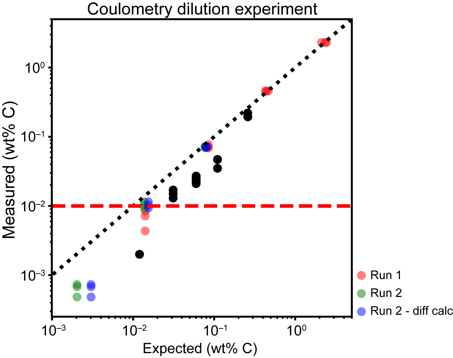
Figure F12. Coulometry dilution experiment.
The weight percent of carbonate was calculated from TIC by
Total organic carbon was calculated by subtracting the weight percent of inorganic carbon from total C obtained with the CHNS analyzer.
6.2.3. Inductively coupled plasma–atomic emission spectroscopy
The major and trace element concentrations of rock samples were measured using ICP-AES on splits of ignited powders, except for the microbiology rock samples that were measured on nonignited powders. The standard shipboard procedure for digestion of rocks and subsequent ICP-AES analysis is described in Murray et al. (2000), with modifications as indicated in the Expedition 369 methods chapter (Huber et al., 2019). The following protocol is a synopsis of this procedure with minor changes and additions.
6.2.3.1. Digestion procedure and preparation of solutions
Each rock sample was weighed on a Cahn C-31 microbalance to 100.0 ± 0.2 mg splits; weighing errors were estimated to be ±0.05 mg under relatively calm sea conditions. Splits of whole-rock powders were mixed with 400.0 ± 0.5 mg of LiBO2 flux (preweighed on shore). Aqueous LiBr solution (100 µL of 0.172 mM) was added to the flux and rock powder mixture as a nonwetting agent prior to sample fusion to prevent the fused bead from sticking to the crucible during cooling. Samples were fused individually in Pt-Au (95:5) crucibles for ~12 min at a maximum temperature of 1050°C in an internally rotating induction furnace (Bead Sampler NT-2100).
The beads were transferred into 125 mL HDPE bottles and dissolved in a 50 mL solution containing 10% HNO3 (prepared from trace metal-grade concentrated HNO3). The solution bottle was placed in a Burrell wrist-action shaker for 1–2 h to aid dissolution. Next, 20 mL increments of the solution were passed through a 0.45 µm filter into a clean 60 mL wide-mouth high-density polypropylene bottle.
The solution analyzed for major and trace elements was prepared from the filtered solution, with a final solution-to-sample dilution factor of 5000×.
Unknown samples were prepared according to the following protocol: 0.5 mL was pipetted into a polyethylene centrifuge tube and diluted with 4.4 mL of 10 wt% HNO3 and 0.1 mL of an internal standard solution containing Be, In, and Sb (final concentration of 100 µg/L Be and In and 200 µg/L Sb).
The Expedition 393 science party showed that solutions prepared at the final dilution factor for ICP analysis (5000:1) can last several weeks without deterioration if refrigerated. A new preparation protocol was developed whereby calibration, drift, and quality check standard solutions were prepared in larger volumes to be used for several ICP-AES runs (Coggon et al., 2024). This procedure was adapted for the ICP-AES analyses of the rocks recovered during Expedition 399. Calibration and drift standard solutions were prepared by pipetting 10 mL into a polyethylene bottle then diluted with 88 mL of 10 wt% HNO3 and 2 mL of internal standard solution containing Be, In, and Sb (final concentrations of 100 µg/L Be and In and 200 µg/L Sb). Quality check standard solutions were prepared for each sample run similar to the unknown samples.
6.2.3.2. Analysis
Major and trace element concentrations of standards and samples were determined using an Agilent 5110 ICP-AES instrument. The instrument setup and the procedure for elemental measurement and data acquisition spectrometer were overall the same as those implemented for fluid analyses (see Inductively coupled plasma–atomic emission spectroscopy in Fluid geochemistry), with minor differences described thereafter. The analyzed elements and the wavelengths used for rock analysis are provided in Table T5.
Typically, 22 unknown samples were analyzed during a single run. A 10% HNO3 rinse solution was run for 90 s between each sample analysis. Procedural blank solutions were run at the beginning and end of each run. Certified international rock reference materials run as calibration, drift, and quality check standard solutions were included with the unknown samples for each sample run. Basalt BHVO-2 was used as a drift-monitoring solution to check internal drift corrections; it was analyzed in approximately every eighth sample position and at the beginning and end of each run. Certified international rock reference materials for calibration standard solutions were chosen for their wide range of compositions to bracket the expected range of compositions of unknown samples. During Expedition 399, they comprised a set of nine certified rock standards analyzed at the start and, for a subset of standards, also at the end of the sequence to check repeatability: peridotites JP-1 and DTS-1, basalts BIR-1 and BCR-2, gabbros MRG-1 and JGb-1, andesite AGV-1, granite JG-2, and carbonate NBS-1C (Table T9).
Two to four certified international rock reference materials were chosen for their compositional similarity to that of the analyzed material and run as unknowns to check the precision and accuracy of major and trace analyses.
6.2.3.3. Data reduction and data quality assessment
After drift correction using internal standards (Be, In, and Sb) and subtraction of the procedural blank, a calibration line for each element was calculated using the results for the certified rock standards by Agilent’s ICP Expert software. Concentrations used for the calibrations were compiled values from Govindaraju et al. (1994) and the GeoReM website (http://georem.mpch-mainz.gwdg.de, 28 April 2023; Jochum et al., 2005) (Table T9). Total Fe oxide concentrations were reported as T-Fe2O3.
Estimates of accuracy and precision of major and trace element analyses were based on replicate analyses of check standards compared to published values. During Expedition 399, run-to-run RSD by ICP-AES was generally ±1% for major elements and ±5%–10% for trace elements (Table T10).
6.2.4. Portable X-ray fluorescence spectrometry
During previous expeditions, pXRFs have been demonstrated to be a valuable tool for initial assessments of the composition of igneous rock and hydrothermal alteration products (e.g., Expeditions 352, 366, and 393 [Ryan et al., 2017; Johnston et al., 2018; Coggon et al., 2024]), and the pXRF was regularly employed during Expedition 399. Measurements were conducted on 272 samples from all sites during Expedition 399. Most of these analyses were done on cut core surfaces to aid in material identification during core description activities.
A Bruker Tracer 5 pXRF was used during Expedition 399. This instrument employs a rhodium X-ray source that allows for a broad range of excitation conditions. Runs used the Geoexploration mode, which analyzes for elements in three phases at energies between 15 and 50 kV and currents from 13 to 27 µA. Each phase analyzed for 30 s, for a total analytical period of 90 s. The pXRF instrument is internally calibrated, which ensures comparable raw data output in percent for all elements measured. This was confirmed early during the expedition by multiple analyses of two internal standards consisting of TSBs taken from intervals 399-U1601A-2R-1, 45–52 cm, and 5R-1, 57–86 cm, as well as powder mounts of international standards JP-1, UB-N, and BHVO-2 (Tables T11, T12). Reproducibility based in these analyses was (expressed as a percent of 1 RSD) 1%–5% for most of the elements whose concentrations were reasonably above detection limits. V (15%–18%) and P2O5 (11%–23%) displayed more variability but were nevertheless precise enough to assist with basic characterization of solid materials encountered in the cores.
7. Microbiology
Rock samples for microbiology were collected to explore the abundance, diversity, and metabolic activity of microbes that inhabit the subsurface of the Atlantis Massif and characterize trace levels of organic compounds. The overall workflow was designed to reveal pristine, uncontaminated interior zones of the core material for microbiological analyses while enabling direct links with geologic and geochemical analyses (Figure F13). Sampling methods were largely adapted from recent recommendations by Sylvan et al. (2021). Some modifications were employed to accommodate simultaneous trace-level organic geochemical analyses, as described below.
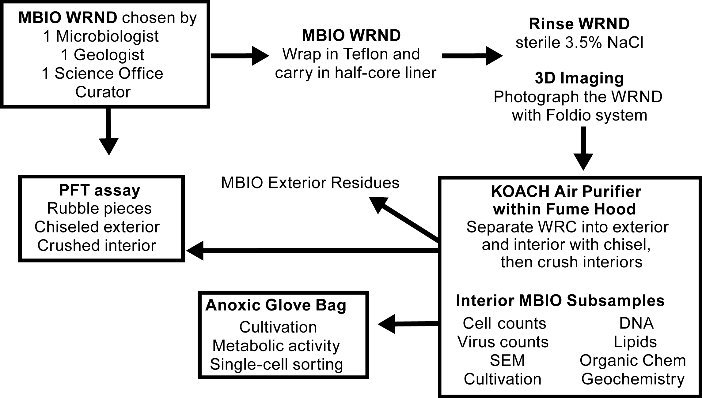
Figure F13. Workflow for microbiology whole-round samples.
7.1. Sampling from cores
Upon recovery, cores were shaken out into split core liners that had been cleaned and sterilized with isopropanol. A small group wearing gloves and masks inspected the core and identified an appropriate whole-round sample ~10–15 cm long, ideally containing indications of fluid flow (e.g., veins) that would be conducive to microbial habitation and did not appear to contain features that were geologically unique to the section. The selected microbiology whole round was photographed before being removed from the core, wrapped in a sheet of Teflon that had been washed with 10% hydrochloric acid, and carried to the microbiology laboratory for processing. A Styrofoam insert was placed in the core where the whole round was removed. When available, small pieces of rubble were sampled from the core into a 20 mL headspace vial for PFT analysis.
All handling, crushing, and subsampling of the microbiology section was conducted within a KOACH clean air system (Koken Ltd.) placed in front of an air Static Eliminator ELIMINOSTAT (Shishido Electrostatic Ltd.). For Hole U1601C samples, the KOACH system and ELIMINOSTAT were placed inside a chemical fume hood lined with clean sheets of Teflon. Each microbiology sample was rinsed with a 3.5% sodium chloride solution (NaCl that had been combusted at 500°C for 5 h and then dissolved in filter-sterilized Milli-Q water), labeled with its sample ID and orientation, and photographed with a Foldio 360 system (Orangemonkey) with a sheet of acid-washed Teflon on top of the rotating turntable. The Foldio system captured a still image after each 15° rotation of the turntable (Coggon et al., 2022).
7.2. Chiseling, crushing, and subsampling
The microbiology whole-round sample was placed in a clean and methanol-wiped metal rock box for chiseling, crushing, and subsampling. All tools were washed with soap and water, rinsed three times with Milli-Q water, and wiped with methanol before use. Tools were not autoclaved because of concerns with potential contamination of organic molecules from the autoclave.
The exterior of each microbiology whole-round sample was removed with a hammer and chisel, including the top, bottom, and sides of the cylindrical rock segment. These exterior portions, sometimes >1 cm thick, were placed into bags and returned to the section half core liner from which the whole-round sample was taken for potential description and sampling. An alternative technique for removing exterior material from the whole-round sample using an electric Dremel tool was explored with a few samples, but this technique was deemed unfavorable because of the production of dust, likely contribution of organic molecule contamination, and lack of external material available to be returned to the section half core liner. After the exterior zones were removed, the interior rock section was transferred to a clean rock box within the KOACH system. The interior zones were then crushed with a hammer and chisel along grain boundaries into approximately millimeter-sized grains, which were subsampled for the analyses listed below. An impact mortar was used to facilitate crushing for the first few samples, but most samples, including all Hole U1601C samples, were crushed only with the clean, methanol-wiped hammer within the rock box.
7.3. Perfluorocarbon tracer
In addition to the small pieces of rubble collected from the core in the splitting room, material from the interior and exterior of the whole-round sample was collected for PFT analysis in the microbiology laboratory. Approximately 4 cm3 of the liberated exterior and 4 cm3 of the crushed interior were collected into 20 mL glass headspace vials and immediately sealed.
Headspace vials were heated at 70°C in a shaking oven to release the tracer, and then an aliquot of the vial headspace was injected into a HP 6890 gas chromatograph equipped with a microelectron capture detector (GC-µECD). The compounds were separated on a megabore column (Rt-Alumina BOND/KCl, 50 m, 0.53 mm ID, 10 µm Agilent column). Headspace concentrations of the PFT, perfluorodecalin, were determined by calibration with a 7 point standard curve.
7.4. Geochemical analysis of the microbiology section
Approximately 1–5 g of the crushed interior core sample was aliquoted for shipboard XRD and ICP-AES to aid in correlating the sampled microbiology section to the larger core and guide the development of culture medium. Analyses were carried out as described in Geochemistry, with the exception that the powders were not ignited to remove volatiles prior to analysis.
7.5. Imaging and culturing for geobiology
A piece of the microbiology sample (~5 cm3) was selected prior to crushing and placed in a Kapak bag, sealed, and stored at room temperature in the dark for synchrotron-XRF microscopy (XFM). Approximately ~5 cm3 of crushed material was placed into each of three 10 cm3 serum bottles for the following applications:
- DNA: Lifeguard was added until the crushed rock was submerged, sealed with a butyl rubber stopper and an Al-crimp seal, and stored at −20°C.
- Cultures: For lithotrophs, serum bottles were filled with sterile anaerobic artificial seawater (AASW) and sealed. For heterotrophs, water samples collected with the KFTS were inoculated into 10 mL serum bottles containing 9 mL Difco Marine Broth 2216.
- SEM: Serum bottles were filled with AASW containing 2.5% glutaraldehyde and sealed.
Cultures and SEM samples were stored in the dark at room temperature.
7.6. Enumeration of microbial cells and viral particles
Approximately 12 cm3 of crushed material from each microbiology sample was collected for enumeration of microbial cells and viral-like particles. Triplicate aliquots (~2 cm3) were transferred to sterile plastic centrifuge tubes with 4% paraformaldehyde in phosphate-buffered saline (PBS) buffer for cell counts. For viral-like particles, triplicate aliquots (~2 cm3) were transferred to sterile plastic centrifuge tubes, flash frozen in liquid nitrogen for 10 min, and then stored at −80°C.
7.7. Single-cell activity and sorting
Crushed material was subsampled from each microbiology sample and preserved for sorting of single cells. Approximately 1–2 cm3 of crushed core material was transferred in triplicate to sterile plastic centrifuge tubes containing RSG reagent diluted with filter-sterilized artificial seawater (Hole U1309D and U1601A samples) or filter-sterilized deep seawater collected with a Niskin bottle (Hole U1601C samples). The same amount of core was also added in triplicate to sterile plastic centrifuge tubes containing only filter-sterilized seawater as a no-RSG control. Samples were incubated for 20 min at room temperature in the dark, and then 8 mL of GlyTE was added to each tube. The tubes were gently but thoroughly shaken by hand, flash-frozen in liquid nitrogen, and stored at −80°C (Hole U1309D and Hole U1601A samples) or placed directly in the −80°C freezer without flash freezing (Hole U1601C samples).
An anoxic variation of the procedure was conducted in which the crushed material was prepared in an anoxic serum bottle and incubated with RSG that had been prepared in a serum bottle flushed with the ship’s N2 supply to test for metabolic activity under more anoxic conditions. The ship’s N2 supply consistently contained ~30 ppm O2. For samples collected from Hole U1601C, another variation was conducted inside the Coy anaerobic chamber, containing 2%–4% H2 and <20 ppm O2, in which the samples were incubated in anoxic, filtered seawater (collected with a Niskin bottle near Hole U1601C) for 24 h before adding the RSG reagent followed by another incubation of 24 h.
Finally, a killed control was included in each experiment by transferring 1–2 cm3 of crushed material into a 10 cm3 serum bottle and autoclaving it twice, 24 h apart, to allow potential spores to form prior to the second autoclaving. The autoclaved material was mixed with RSG diluted into artificial seawater as above. After the expedition, the cells will be sorted using flow cytometry into metabolically active (i.e., those that incorporated the RSG fluorescent dye) and inactive populations and prepared for whole-genome sequencing of individual cells.
7.8. Preparation of samples for DNA sequencing
Subsamples of each microbiology sample were collected for future DNA analyses, including sequencing of 16S rRNA amplicons and metagenomes. Approximately 20–40 cm3 of crushed material from each sample was stored in sterile plastic centrifuge tubes at −80°C. Subsamples of crushed material from some samples were also cross-linked with formaldehyde in preparation for future generation of metagenome libraries with proximity ligation, which will link DNA sequences that were in close physical proximity at the time of sampling. Future sequencing of these metagenome libraries will identify DNA sequences that were physically associated with each other at the time of sampling, potentially revealing which sequences were present as extracellular fragments or inside genomes, as well as virus-host interactions. To prepare these samples for proximity ligation, an additional 20 cm3 of crushed material was fixed with 25 mL of filter-sterilized 4% paraformaldehyde in PBS buffer for 1 h at room temperature with continuous mixing, followed by quenching with 2.5 M glycine in filter-sterilized artificial seawater for 20 min. For samples from Hole U1601C, filter-sterilized bottom water collected near the hole with a Niskin bottle was substituted for artificial seawater. The tubes were centrifuged briefly at 1800 relative centrifugal field, the supernatant was discarded, and the pellets were washed with 10 mL of filter-sterilized seawater. The tubes were centrifuged again, the supernatant was discarded, and the pellets were stored at −80°C.
7.9. Preparation of samples for analyses of organic chemistry
Approximately 20–40 cm3 of crushed core material was collected either in aluminum foil that had been combusted at 450°C for 6 h and then vacuum sealed and stored at −80°C for shore-based lipid analysis or in glass vials that had been combusted at 500°C for 5 h with acid-washed, Teflon-lined caps and stored at −20°C for additional organic geochemical analyses.
7.10. Stable isotope tracer incubations
For select microbiology samples, crushed core material was aliquoted into vials containing compounds labeled with stable isotopes for metabolic activity assays. Multiple compounds and several different experiments under varying conditions were conducted. In one experiment, 2–4 cm3 of crushed core material was added to a 12 mL glass Exetainer vial containing 4 mL filter-sterilized artificial seawater or deep seawater collected near Hole U1601C with a Niskin bottle. The vials were equilibrated with the atmosphere of a Coy anoxic chamber for ~20 min with continuous flushing of the chamber with N2 gas containing 20–30 ppm O2. For samples from Hole U1601C, samples were aliquoted into vials inside the Coy anoxic chamber containing 2–4% H2 and <20 ppm O2. The vials were then sealed and brought to the isotope van where 0.2 mL of one of the following compounds (each at 20 mM for a final concentration of 0.5 mM inside the Exetainer vial) was added to each vial with a syringe and needle: NaH13CO3 (sodium bicarbonate), Na13COOH (sodium formate), CH313COONa (C1-labeled sodium acetate), 13CH3COONa (C2-labeled sodium acetate), 13CH315NH2 (methylamine), H215NCH213COOH (C1-labeled glycine), H215N13CH2COOH (C2-labeled glycine), or 15NH4Cl (ammonium chloride). Vials were incubated in the isotope van (~18°C) and killed after 4 weeks (Hole U1601A samples) or 2–3 weeks (Hole U1601C samples) by adding 0.2 mL of concentrated phosphoric acid.
In a second experiment, ~15 cm3 of each sample of crushed rock was added to a 40 mL serum bottle in the Coy anaerobic chamber and filled with 30 mL AASW or filter-sterilized deep seawater. The bottles were sealed within the chamber and brought to the isotope van to add the stable isotope-labeled substrates. One of the following isotope-labeled substrates was added to the vials using needles and syringes at final concentrations of 0.5 mM: NaH13CO3 (sodium bicarbonate), NaH13COO (sodium formate), CH313COONa (C1-labeled sodium acetate), 13CH3COONa (C2-labeled sodium acetate), dodecane, hexane, hexadecane, or 15NH4Cl (ammonium chloride). At the final incubation time (e.g., 6, 12, and 18 months), the incubations will be halted and the contents analyzed for metagenomic, lipid, and Raman analyses.
7.11. High-pressure cultivation (70 MPa)
Approximately 10 cm3 of crushed rock was added into individual high-pressure tubes (Shanghai, China) (Figure F14) within the Coy anaerobic glove chamber and filled with 20 mL AASW. The tubes were then closed tightly within the Coy chamber, removed, and pressurized to 70 MPa by hand, using a high-pressure pump (Figure F15). The tubes were incubated at room temperature in the dark and will be opened and sampled at different times (e.g., 6, 12, and 18 months) for further analyses (e.g., omics, lipids, and Raman analyses) and for the isolation of pure strains present in the enrichment.
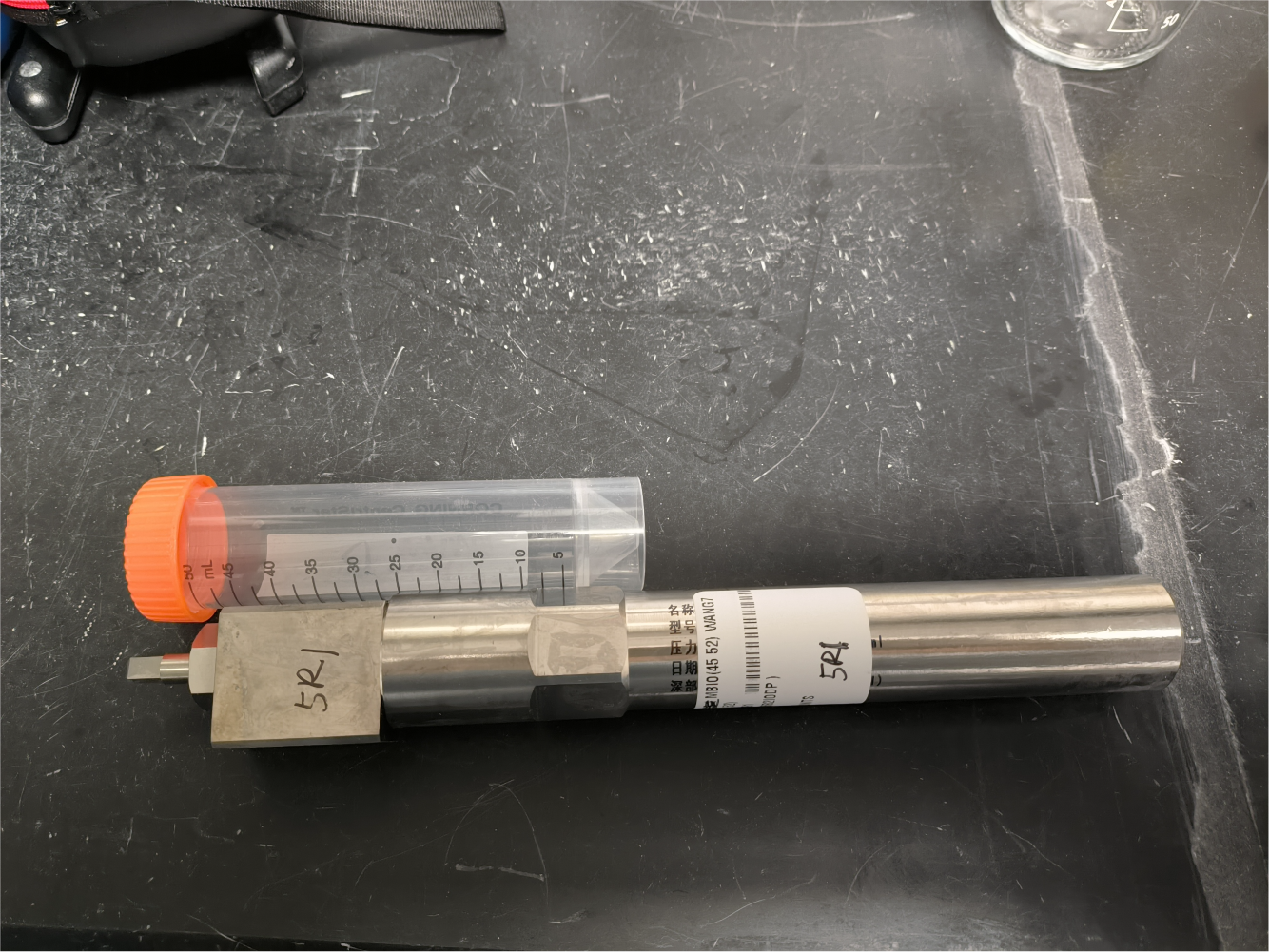
Figure F14. Steel high-pressure tubes.
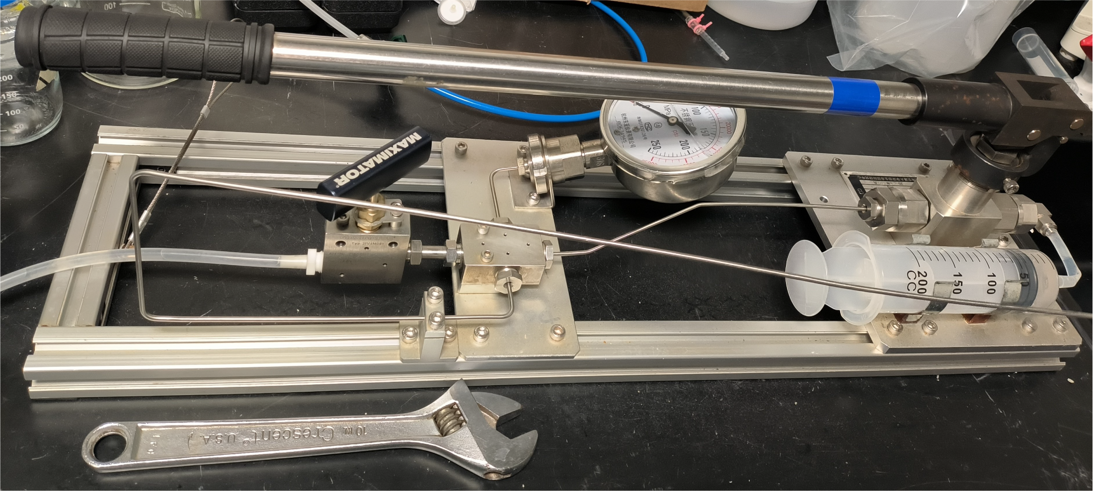
Figure F15. Hand-operated, high-pressure pump system.
High-pressure experiments that utilized stable isotope tracers were conducted in the isotope van. ~10 cm3 of crushed rock samples were added into the high-pressure tubes in the anaerobic bag in the isotope van and filled with 20 mL AASW. The same suite of stable isotope-labeled substrates listed for the 15 cm3 experiments in Stable isotope tracer incubations were added to a final concentration of 0.5 mM. The tubes were then closed tightly within an anoxic glove bag, removed, and pressurized to 70 MPa by the hand-operated high-pressure pump. The tubes were incubated at room temperature. At the final incubation time (e.g., 6, 12, and 18 months), the incubations will be halted and the contents analyzed for metagenomic, lipid, and Raman analyses.
7.12. High-pressure cultivation (variable pressures)
A separate suite of high-pressure experiments was carried out at variable pressures. Triplicate Hungate tubes were filled with an aliquot of crushed core material (~15 cm3) and Niskin-collected deep seawater that had been filtered through a 0.2 µm Sterivex filter for sterilization and purged with N2 to create anoxic conditions. The three tubes were then capped without headspace and placed inside a single high-pressure chamber. The pressure of each chamber was set to roughly correspond to the depth of sample collection: 150 bar for Section 399-U1601A-10R-2, 260–300 bar for Hole U1309D MTFS #2 and Section 399-U1309D-298R-2, and 300 bar for Core 399-U1601C-244R.
7.13. Fluids
The processing of fluids from deep seawater, Hole U1309D, and Hole U1601C was closely integrated with geochemical sampling. Details are reported in Geochemistry.
8. Petrophysics
This section describes the petrophysical measurements and tools employed during Expedition 399. We include the descriptions of downhole sampling tools even if the sampling objectives were geochemical and microbiological in nature. Petrophysical measurements include those carried out on whole-round sections and section halves, discrete core samples, downhole temperature measurements, and a suite of downhole wireline measurements.
Methods and results were compared to previous hard rock legs and expeditions that drilled serpentinized peridotite and gabbroic rocks (Legs 153 and 209 [Shipboard Scientific Party, 1995, 2004]), previous expeditions to Atlantis Massif (Expeditions 304/305 and 357 [Expedition 304/305 Scientists, 2006; Früh-Green et al., 2016]), and more recent hard rock expeditions (360 and 376 [MacLeod et al., 2017; de Ronde et al., 2019]).
During Expedition 399, all raw data were uploaded to the LIMS database. A comprehensive discussion of most methodologies and calculations used aboard JOIDES Resolution in the physical properties laboratory can be found in Blum (1997).
General procedures and a description of each petrophysical property investigated during Expedition 399 are provided for core logging, discrete sample measurements, downhole temperature and fluid sampling, and downhole wireline logging. The overall workflow in the core laboratory is described in Operations. Cores in Hole U1601C were processed in different ways depending on the health risk and need for expediency because of high coring rates; see below for specific methods depending on how the core was processed. Cores 399-U1601C-235R through 240R were not split until after the expedition, so they were only measured on whole-round tracks. Note that core logging data were not corrected for the recuration of most sections from Hole U1601C after the expedition. As a result of the recuration, hundreds of pieces were moved downhole a few centimeters to a few tens of centimeters, a few sections were eliminated, and several new sections were created (see Operations). The core logging data point locations in the LIMS database therefore do not exactly match the new identities and depths of the pieces measured in many intervals. The identities (and therefore the depths) of discrete samples taken from sections and section halves were adjusted for the recuration, and the measurements taken on these samples therefore match their curated location.
8.1. Core whole-round and section half measurements
8.1.1. General procedures
After the whole-round pieces in the core sections were curated by the technical staff, which included binning as necessary in a split half liner, and the sections had equilibrated for at least 2 h to near room temperature, the sections were run through the following whole-round core loggers:
- WRMSL, which includes a GRA bulk densitometer and a MS pass-through loop (MSL) system;
- NGRL, which was only used when the length of an individual core section was >50 cm; and
- Whole-round 360° linescan imaging (see below for exceptions).
After the technical staff split the whole-round pieces and curated them as piece halves in the archive and working half split liners, the archive section halves were measured with the following section half loggers:
Most working section halves and some archive section halves were also scanned with the X-ray imager (X-Ray Linescan Logger [XSCAN]).
8.1.2. Filtering of core section data
WRMSL and SHMSL data contain spurious values measured because of gaps in the core section (empty intervals and microbiology samples) and cracks in core pieces and for measurements that are affected by volume (i.e., WRMSL; departure from a continuous cylindrical core that fills the core liner, therefore requiring a volume correction). The SHMSL includes a platform moving along a track above the section half that first records the sample height using a laser sensor. The laser profile establishes the location of the end of the core section and the distribution of core pieces by locating gaps and cracks between pieces based on a laser distance exceeding a set value; 25 mm was used for this instrument parameter during Expedition 399. The SHMSL laser profiler initially detects almost all the gaps between pieces; however, given the 25 mm measuring interval, some gaps and core liner spacers are measured as a sample. Filtering out these data provides a data set more suitable for analysis. In the case of full diameter, continuous core recovery, only a minor amount of filtering is required. A MATLAB-based graphical user interface (GUI) (see clipWRdata.mlapp in PETROPHYS in Supplementary material) was used to identify valid measurement intervals based on SHMSL laser profile data for Holes U1309D and U1601A (Figure F16). Data filtering was not completed on whole-round measurements in Hole U1601C because of record core recovery and the lack of SHMSL data for the majority of the hole.
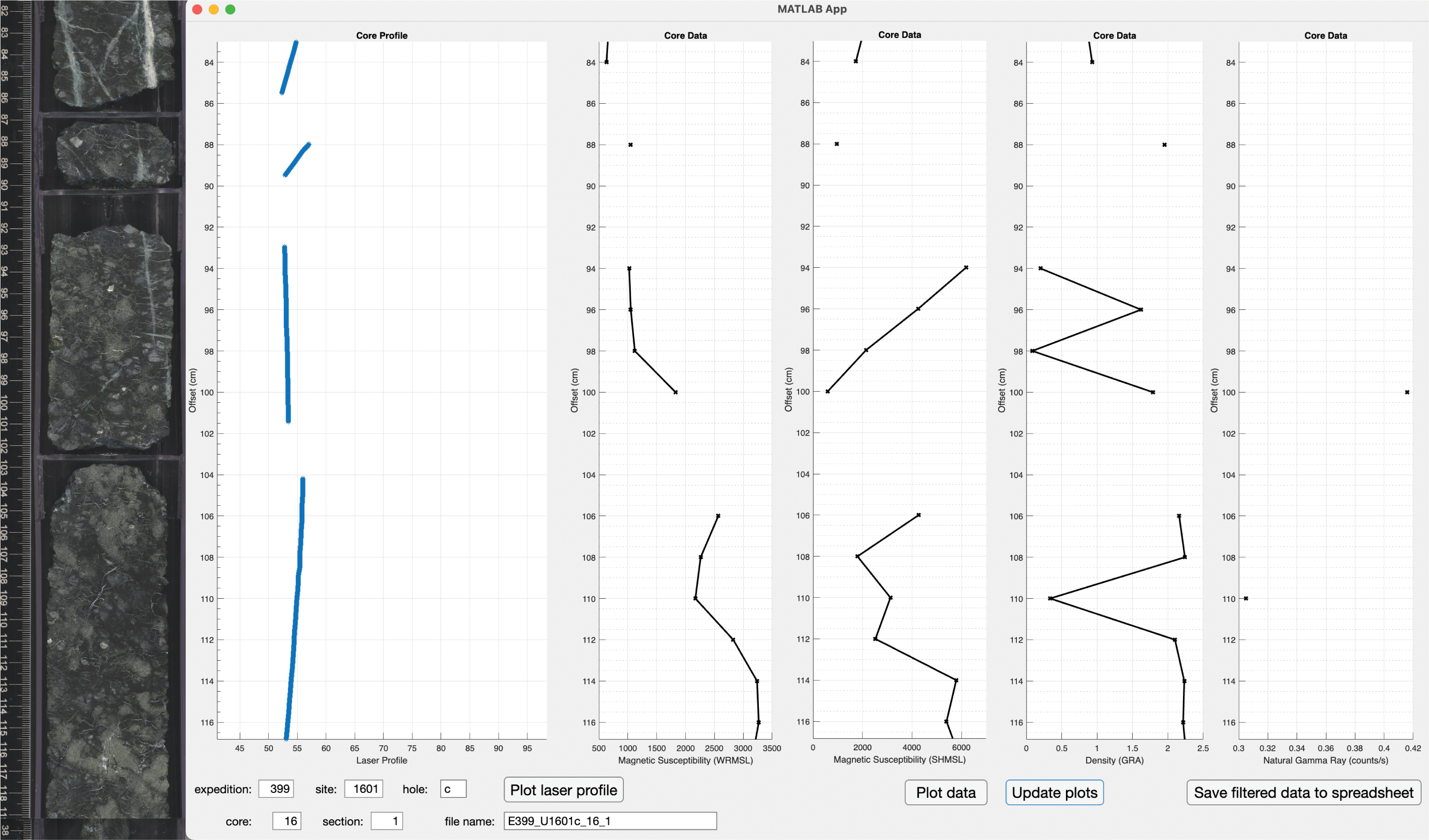
Figure F16. Filtering process for whole and section half core.
The filtering MATLAB-based GUI includes plots for each section showing the laser profile and MS recorded on the SHMSL, bulk density and MS recorded on the WRMSL, and natural gamma radiation (NGR) concentration recorded on the NGRL (Figure F16). The section half images from the SHIL are also aligned with the data plots using the shipboard curation (Figure F16). The user can remove invalid data due to gaps, breaks, and edge effects of rock pieces using the GUI’s brush tool. Only data with reasonable values (e.g., >2.25 g/cm3) were kept in the data set following manual filtering, most often data from longer pieces (>10 cm). Data from each section were filtered separately and saved to individual Excel spreadsheets that were later compiled for each hole. Raw data are available in the LIMS database; filtered data are available in PETROPHYS in Supplementary material.
8.1.3. Core logging sensors
8.1.3.1. Whole-round magnetic susceptibility
MS (κ) is a volume-specific measurement of the degree to which a material can be magnetized by an external magnetic field, calculated using the equation
where M is the magnetization induced in the material by an external field with strength (H), very low field, ≤0.5 mT. MS varies in response to the type and abundance of magnetic minerals.
WRMSL MS was measured using a Bartington Instruments MS2 meter coupled to a MS2C sensor coil with a diameter of 90 mm. This instrument has an operating frequency of 0.513 kHz. The instrument was set to record with an integration period of ~1 s to give a sensitivity of 1 × 10⁻⁵ instrument units (IU). The core diameter is smaller than the sensor coil aperture. MS measured by this method (κMEAS) depends on the diameter of the core (d) passing through the coil diameter (D), so a correction factor (κREL) is necessary to convert instrument output to true volume susceptibility (in SI), where κREL = 3.45(d/D)3 (Bartington Instruments Ltd., 2019, 2011). κREL is ~1 for d = 59.6 mm and D = 90 mm; d is typically 59 mm ± 1 mm for well-cut RCB hard rock cores; however, the size of small pieces and rollers varies in an unpredictable manner. A single correction factor was therefore not justified; hence, no correction was applied to WRMSL MS measurements. Raw data are reported in instrument units, which may be multiplied by κREL × 10−5 to obtain SI units where sufficiently long (>15 cm) full diameter (~59 mm) core intervals were measured.
MS data were obtained on whole-round core sections every 2 cm. The along-core response curve of the MS2C coil has a full width at half maximum of ~4 cm (Blum, 1997) and is consistent with the decay in magnetic intensity with distance from a dipole (Figure F17). Therefore, susceptibility measurements from core pieces <8 cm long will underestimate MS by more than 10%. Data from these pieces are filtered out prior to data analysis (filtered data are available in PETROPHYS in Supplementary material).
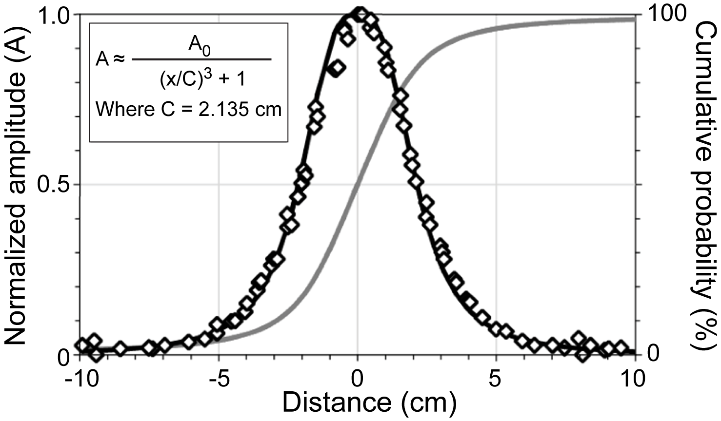
Figure F17. Normalized response curve of MS2C on WRMSL.
8.1.3.2. Point magnetic susceptibility
MSP was measured using a Bartington MS2E contact probe with a flat 15 mm diameter sensor operating at a frequency of 0.580 kHz mounted on the SHMSL. The area of response of the MS2E sensor is 3.8 mm × 10.5 mm, with a depth response of 50% at 1 mm and 10% at 3.5 mm, providing higher resolution measurements than the whole-round MS instrument on the WRMSL (Bartington Instruments, 2011). Measurements are reported in instrument units. The MSP meter was calibrated by the manufacturer before installation on the ship. The probe is zeroed in air before each measurement point, and a background magnetic field is measured and removed from the data before being output. MSP measurements were taken at 2 cm intervals.
During Expedition 399, the MSP measurement was carried out in all cores from Holes U1309D and U1601A and in Cores 399-U1601C-2R through 16R, 22R, 25R, 35R, 36R, and 37R.
8.1.3.3. Natural gamma radiation
Gamma rays are emitted from rocks primarily as a result of the radioactive decay of 40K and the decay of isotopes in the decay series of 238U and 232Th. NGR measurements from the core provide an indication of the concentration of these elements and can also be used to correlate core with the wireline natural gamma ray logs (e.g., Révillon et al., 2002).
The NGRL installed on JOIDES Resolution was designed and built at the Integrated Ocean Drilling Program U.S. Implementing Organization at Texas A&M University in College Station, Texas (Vasiliev et al., 2011). The main NGR detector unit consists of 8 sodium iodide (NaI) scintillator detectors (~500 in3 each), 7 plastic scintillation detectors, 22 photomultipliers, and passive lead shielding. The eight NaI detectors are spaced every 20 cm in the detector (Figure F18); the detectors themselves form a semicylindrical annuli around the lower half of the core (each crystal is ~13 cm wide along the core). The detectors are shielded by lead to reduce external gamma radiation, and the NGRL also employs seven plastic scintillation detectors that detect and actively suppress the effect of high-energy gamma and muon components of cosmic radiation. The NGRL was calibrated using 137Cs and 60Co sources to identify peaks at 662 keV for 137Cs and 1173 and 1330 keV for 60Co.
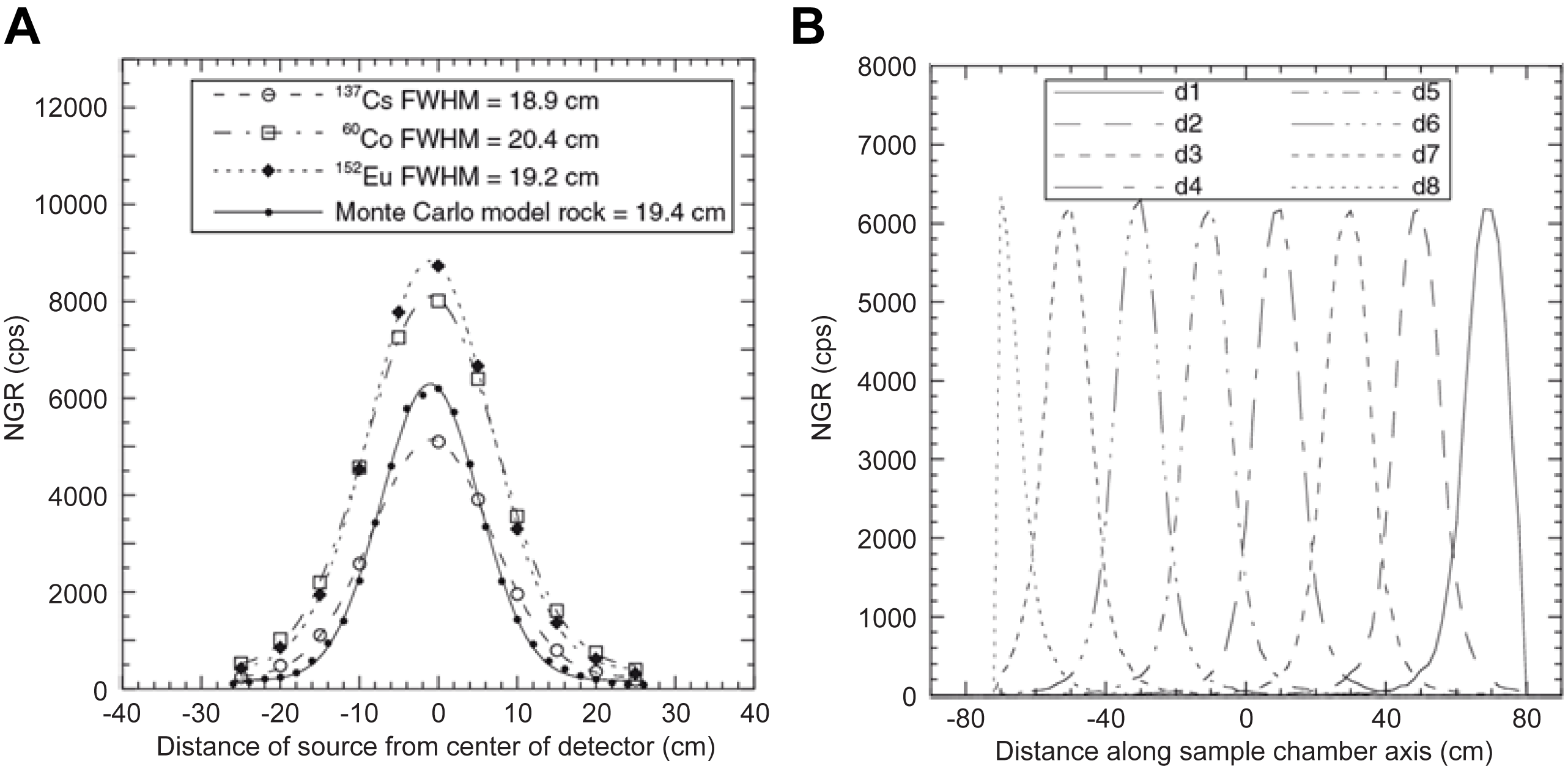
Figure F18. NGRL detector space resolution and position.
A single measurement run with the NGRL provides a total of 16 measurements at 10 cm intervals over a 150 cm section of core. To achieve a 10 cm interval using the NGRL’s eight sensors spaced every 20 cm (Figure F18), the NGRL records two sets of measurements offset by 10 cm. Total counts are routinely summed over the range of 100–3000 keV and depend on the concentration of radionuclides in the sample and the counting time, with longer counting times providing better counting statistics. A live counting time of 900 s (15 min) was set in each position (total live count time of 30 min per section). Because of a backlog of core from very high recovery, some cores were measured for 450 s per position, 15 min total measuring time, specifically Cores 399-U1601C-66R through 240R (334–1181 mbsf).
We attempted to calculate the concentration of 40K, 238U, and 232Th using a MATLAB routine developed by de Vleeschouwer et al. (2017) and Uenzelmann-Neben et al. (2023) for sediments and sedimentary rocks. The routine extracts the NGR spectra data and then evaluates each spectrum for the associated energy levels of 40K, 238U, and 232Th and related isotopes including 208Tl for Th and 214Bi for U. The peaks for each energy level are then compared to the expected energy peaks in the standard and a correction for the bulk density is applied. Bulk density of the sample, measured on the WRMSL, is averaged over 20 cm centered on the NGR data points. The concentration of each isotope is then calculated using the following proportion:
where ρ is density. Concentration for 40K is given in weight percent and 238U and 232Th concentration is given in parts per million. Given that the bulk density from the WRMSL is a minimum (see below), the concentrations calculated by this method are also minimums and better represent changes in concentration downhole, not necessarily absolute concentration.
8.1.3.4. Reflectance spectroscopy and colorimetry
An Ocean Optics Inc. system for UV through visible to near-infrared light (171–1100 nm wavelength at 2 nm increments) mounted on the SHMSL was used to measure spectral reflectance. Spectral data are routinely reduced to the L*a*b* (CIELAB) color space for output and presentation, in which L* is luminescence, a* is the red–green value, and b* is the blue–yellow value. The color reflectance spectrometer calibrates on two spectra: pure white (reference) and pure black (dark). Each measurement takes 1 s with the final value representing a stacked average of 3 measurements.
During Expedition 399, the RSC measurement was carried out in all cores from Holes U1309D and U1601A and in Cores 399-U1601C-2R through 16R, 22R, 25R, 35R, 36R, and 37R.
8.1.3.5. Gamma ray attenuation density
The GRA densitometer on the WRMSL operates by passing gamma rays from a 137Cs source through a whole-round core into a 75 mm × 75 mm sodium iodide detector located directly below the core and liner. The input gamma ray peak has a principal energy of 0.662 MeV and is attenuated as it passes through the core. Attenuation of gamma rays, mainly by Compton scattering, is related to electron density, which is related to material bulk density (Blum, 1997).
For the majority of elements and for rock-forming minerals, the mass attenuation coefficient is ~1, whereas for hydrogen it is 1.9841. Therefore, for a known thickness of sample and a simple two-phase system consisting of minerals and water, the gamma ray count is proportional to bulk density. Calibration of the GRA densitometer was performed using a core liner filled with freshwater after each core measurement. Recalibration was performed with a freshwater and aluminum density standard if the measured density of the seawater standard was not 1.00 ± 0.02 g/cm3. The spatial resolution of the GRA densitometer is <1 cm. Data were filtered to remove biased measurements near piece edges using the MATLAB routine and GUI (clipWRdata.mlapp) (see Filtering of core section data).
GRA bulk density was measured nondestructively with the WRMSL at 2 cm intervals with an integration time of 3 s for each data point. GRA data were obtained at the same points that whole-round MS was measured, and the measurement spacing was set to the same value for the SHMSL and the SRM. The nominal accuracy of the GRA calibrated instrument is 1%–2% assuming a perfectly cylindrical core. Core pieces do not fill the core liner and can be of variable diameter, meaning that the bulk density is in general underestimated.
8.1.3.6. Whole-round visible light imaging
The SHIL was used to image 360° composite images of whole-round sections. Only oriented pieces were transferred from the core liner to a custom whole-round scanning tray. An image is taken at the 0°, 90°, 180°, and 270° orientations starting from the splitting line at 0° and rotating 90° after each image is taken. Each image was cropped, saved, and then uploaded to the LIMS database. The Imaging Specialist stitched the four images together using Adobe Photoshop to create the 360° composite images. The resolution of the images is 200 pixels/cm. For a 150 cm section, this results in 1317 pixels × 29964 pixels.
In Hole U1601C, whole-round images were only taken of Cores 2R–25R and 35R–36R because of safety concerns and for expediency.
8.1.3.7. Archive section half visible light imaging
During Expedition 399, most section halves were imaged using the SHIL. The Hole U1601C core handling issues described in Operations led to numerous compromises. For some intervals, imaging was done on the working halves rather than the archive halves. Some section halves were imaged dry and others were imaged wet. For the sections not split on the ship, no imaging was possible at all. Therefore, after recurating all sections from Hole U1601C, all archive sections were (re-)images in wet and dry conditions, generating a complete data set now available from the LIMS database.
The SHIL produces a high-resolution RGB file that measures red, green, and blue values for each line of pixels down the length of the core. This method produces ~30,000 lines of data for a 150 cm long section, or a resolution of 0.05 mm.
8.1.3.8. XSCAN imager
The XSCAN imager is an imaging system capable of collecting linescan X-radiographs on whole-round and section half cores. The source and detector can be rotated around the core material for linescans with different view angles for a pseudo–computed tomography (CT) scan. These scans allow for structures and objects such as faults, fractures, and materials with distinct densities (e.g., alteration zones, oxides, and sulfides) that aid in core observation logging and interpretation.
The XSCAN imager is an X-ray scanner with a 210 W, 160 kV, 1.3 mA constant potential X-ray source and linescan detector. The source is a Spellman XRBD 160PN210 Monoblock X-ray generator with a 0.5 mm focal spot. The beam angle is 90° × 12°, and it is spaced ~36 cm from the source. The detector is a Hamamatsu C12300-321, composed of a charge-coupled device sensor with a ~22 cm field of view utilizing time-delayed integration and a resolution of 48 µm per pixel.
Initial set up and configuration were always performed by the technical staff. Whole-round images were attempted; however, the rocks from this expedition were too dense given the energy of the X-ray source, so only section halves were measured. Some experimentation was required to find the best results, with the maximum settings for energy providing the best results: a voltage of 110 kV and a current of 1.9 mA. The exposure time was 7.7 µs, and the track speed was set to 5 cm/s. All scans were done as a single measurement at 0°, meaning 2D images were generated that cannot be resolved in 3D.
Imaging acquisition and processing was completed within the IMS system (v. 14). Processing of the images during the expedition was limited and only included a black and white correction. Early in the expedition, processing was attempted for a few core sections, but the image quality was not greatly improved. All images were uploaded to the LIMS database.
During Expedition 399, plastic wrapped half core sections were imaged from Hole U1601A (Cores 2R-1, 4R–6R, 8R, and 10R); Hole U1601C (Cores 2R–18R, 22R, 25R, 35R–36R, 55R–145R, 148R–155R, 157R–226R, and 228R–234R); and Hole U1309D (Core 313R).
8.2. Core discrete sample measurements
8.2.1. General procedure
Four types of discrete samples were taken for physical properties measurements:
- Representative archive half pieces ≥7.5 cm long for thermal conductivity (TC) measurements.
- Cube samples (8 cm3) from the working section halves of representative materials for both MAD and compressional wave (P-wave) velocity measurements. These samples were also used by the paleomagnetism team for bulk susceptibility, anisotropy of magnetic susceptibility (AMS), alternating field (AF) demagnetization, and isothermal remanent magnetization (IRM) measurements if the cubes were oriented (see Paleomagnetism).
- In Hole U1601C, microbiology off cuts with irregular shapes (~4.0–10.0 cm3) were used for MAD measurements starting with Core 19R.
- In Hole U1601C, cubes were not always sampled; therefore, section half core pieces were selected for P-wave velocity measurements starting with Core 19R.
All sample types were saturated in seawater under vacuum conditions for ~24 h at ambient temperature to remove air from pore spaces. Thermal conductivity, P-wave, and initial MAD measurements (wet mass) were conducted on the saturated samples. Samples used for P-wave velocity and thermal conductivity in Hole U1601C, starting at Core 19R, were only saturated for ~12 h because of the need for expediency with high core recovery. In that hole, there are measurement gaps for discrete samples between Cores 6R–19R and 25R–32R and a cube measurement gap between Cores 38R and 131R (202–635 mbsf).
Cube samples were preferentially located close to where shipboard geochemistry and thin section samples were taken whenever possible. A comprehensive discussion of the MAD and P-wave velocity methodologies and calculations used in the JOIDES Resolution physical properties laboratory is presented in Blum (1997).
8.2.2. Moisture and density
Mass and volume measurements on discrete samples were made to determine bulk, dry, and grain densities and porosity. IODP shipboard Method C was used in the MAD facility for hard rock samples, which consists of a vacuum water saturator, a dual balance system, and a custom built Helium hexapycnometer.
After saturating the cube samples with seawater, the wet mass was measured. The samples were subsequently dried in a 105°C oven for 24 h and then cooled to room temperature in a desiccator for 3 h, after which their dry mass was obtained for MAD measurements. The volume of the dry cube samples was then obtained using helium pycnometry. Bulk density, dry density, grain density, and porosity were calculated from wet mass, dry mass, and dry volume measurements using IODP Method C (see below; Blum, 1997).
8.2.2.1. Vacuum water saturator
A vacuum pump system was used to ensure seawater saturation of discrete samples. The system consists of a plastic chamber filled with seawater. The vacuum pump removes air from the chamber, essentially sucking air from connected pore spaces and replaced by seawater. Samples were typically kept under vacuum for at least 24 h. During this time, pressure in the chamber is monitored periodically using a gauge attached to the vacuum pump to ensure a stable vacuum. After removal from the saturator, cubes were stored in sample containers filled with seawater to maintain saturation. On many samples, cutting mud was present after washing, so seawater was changed regularly.
8.2.2.2. Dual balance system
A dual balance system was used to measure both wet and dry masses. Two analytical balances (Mettler-Toledo XS204) compensate for ship motion; one acts as a reference, and the other measures the unknown sample. The discrete samples were placed in aluminum trays, which were used to for the reference and unknown masses. A standard mass of similar mass to that of the sample was placed on the reference balance to increase accuracy. By using a reference mass within ~10% of the sample mass, an accuracy of 0.005 g is readily attainable. After wet mass determinations and P-wave velocity measurements (see P-wave velocity) and prior to the determination of dry mass and volume, samples were placed in an oven at 105° ± 5°C for 24 h and then allowed to cool in a desiccator for a minimum of 3 h.
8.2.2.3. Hexapycnometer system
The hexapycnometer is an IODP custom-built system that uses six Micromeritics cell units, custom electronics, and custom control programs. The system measures dry sample volume using pressurized helium-filled chambers with a precision of 0.02 cm3. At the start of the expedition, and whenever the helium gas tank was changed, shipboard technicians performed a calibration using stainless steel spheres of known volume. For each measurement series, five cells contained unknowns and one cell contained two stainless steel calibration spheres (3 and 7 cm3) with a total volume of ~10 cm3. Calibration spheres were cycled through each cell to identify any systematic error and/or instrument drift. The standard spheres are assumed to be known to within 1% of their total volume. Three helium purge cycles were carried out for each sample for increased accuracy.
8.2.2.4. Moisture and density calculations
For density calculations, both mass and volume are first corrected for the salt content of the pore fluid:
- Ms = mass of salt,
- S = pore water salinity (seawater with salinity 35 psu or 0.035 g/cm3),
- Mw = wet mass of the sample, and
- Md = dry mass of the sample.
Grain density (ρg) is determined from the dry mass (Md) and dry volume (Vd) measurements:
where ρs is the density of salt (2.20 g/cm3; Blum, 1997).
The salt-corrected mass of pore water (Mpw) is calculated as
Then, the volume of pore water (Vpw) is
where we assume the density of the pore fluid (ρpw) = 1.024 g/cm3 (seawater with salinity of 35 g/L; Blum, 1997).
To calculate sample bulk density (ρb), bulk volume (Vb) is first computed:
Porosity (ϕ) is calculated from the two volume parameters obtained from the MAD measurements and resulting bulk and pore water volume calculations:
8.2.3. P-wave velocity
P-wave velocity measurements were performed on the same discrete cube samples that were used for MAD determinations in all samples from Holes U1309D and U1601A and some samples from Hole U1601C (see above). In cases where cubes were not available, section half pieces were used. Measurements were taken on seawater-saturated samples immediately before wet mass determinations were made. The P-wave velocity gantry has caliper contact transducers, and the delay line transducers are a Panametrics-NDT Microscan, which transmit at 0.5 MHz. The distance between the stainless steel capped transducers was measured with a built-in linear voltage displacement transformer, and pressure was maintained constant using the SlowClose option. Deionized water was placed on the lower transducer and the upper part of the sample to increase contact and reduce noise. The peak of the first arrival is identified automatically by the IODP software (Seismic Velocity Gantry, Version 14) and is checked and can be adjusted manually. Measurement signals were stacked to increase the signal-to-noise ratio with a typical value of 100 measurements, but up to 1000 measurements were stacked for noisier samples, especially on section half pieces. A voltage threshold was used to help the system pick the first arrival, with a typical value of 10 mV, but a threshold upward of 1000 mV was used on noisier samples. The waveform is stored with the data. Visual checks confirmed that the automatic picks were satisfactory, and the picks were adjusted if necessary. System calibration runs with standards were conducted weekly using a series of acrylic cylinders (VP = 2750 ± 20 m/s) of different thicknesses so that system and transducer delay time settings were updated.
The measurement protocol included eight successive measurements in each of the three directions for each cube sample (x, y, and z in the CRF; Figure F2) with four measurements done parallel to each axis with the cube faced up then flipped for four more measurements with the cube faced down. The transducers were opened and closed between each measurement. Variability between individual measurements was sufficiently high that documenting the average and associated standard deviation was warranted. These average values are available in PETROPHYS in Supplementary material; they are not stored in the LIMS database. The eight-part series averages typically provided low standard deviations, ≤1% of the determined acoustic velocity.
The apparent anisotropy was calculated from the three averaged measurements along the x, y, and z directions as
where VPmax and VPmin were the highest and lowest velocity, respectively, measured in one of the x, y, or z sample directions.
In Hole U1601C when core pieces were used (Cores 19R–226R; 107–1111 mbsf), saturation in seawater was for ~12 h and only the P-wave velocity along the x-axis was measured. Each core piece was wrapped in plastic film, and deionized water was added to the bottom transducer and on the top of the plastic film. A series of four measurements was made without moving or flipping the piece. The transducers were opened and closed between measurements. P-wave velocity averages and associated standard deviations were reported, but apparent anisotropy could not be calculated for these samples.
8.2.4. Thermal conductivity
Thermal conductivity (k, in watts per meter degree Kelvin) is a measure of the rate at which heat is transported through a material. At steady state, it is the coefficient of heat transfer (q) across a steady-state temperature (T) difference over a distance (x):
Thermal conductivity of rock depends on many factors, including temperature; pressure, porosity; type of saturating fluid; and the composition, distribution, and alignment of mineral phases.
Thermal conductivity was measured on split core pieces under ambient conditions using the TeKa TK04 system described in Blum (1997). All measurements were made at room temperature and pressure and were not corrected for in situ conditions. This system measures thermal conductivity by transient heating of the sample with a known heating power and geometry (Carslaw and Jaeger, 1959). The system uses a single-needle probe heated continuously in half-space configuration for hard rock samples (Vacquier, 1985). Three different heating probes consisting of a Plexiglass block and an embedded superconductive needle in the bottom of the block were used (H11060, H11080, and H11090). Changes in temperature with time during heating are recorded and used to calculate thermal conductivity. The temperature of the superconductive needle probe has a quasilinear relationship with the natural logarithm of the time after the initiation of heating (Blum, 1997). The TeKa TK04 device uses a special approximation method to calculate conductivity and assess the fit of the heating curve. This method fits discrete windows of the heating curve to the theoretical temperature (T) with time (t) function:
where A1–A4 are constants that are calculated by linear regression. A1 is the initial temperature, whereas A2, A3, and A4 are related to geometry and material properties surrounding the needle probe. Having defined these constants (and how well they fit the data), the apparent conductivity (ka) for the fitted curve is time dependent and given by
where q is the input heat flux. The maximum value of ka and the time (tmax) at which it occurs on the fitted curve are used to assess the validity of that time window for calculating the thermal conductivity. The best solutions are those where tmax is greatest, and these solutions are selected for output. Fits are considered good if ka has a maximum value, tmax is large, and the standard deviation of the least-squares fit is low. For each heating cycle, several output values can be used to assess the quality of the data, including natural logarithm of extreme time (LET) tmax, which should be large; the number of solutions (N), which should also be large; and the contact value, which assesses contact resistance between the probe and the sample and should be small and uniform for repeated measurements. The quality of measurements done with the large needle probe was assessed using LET and N.
Half-space determinations of thermal conductivity were made with heating probes that have a thermal conductivity of 0.184 W/(m·K) (Vacquier, 1985). Heat is assumed to be transferred through the sample, and heat flow through the Plexiglas block itself is only significant for sample thermal conductivities <1 W/(m·K). Good thermal contact with the heating needle is required, so the split face of the samples was polished with 240 gauge silicon carbide powder. Gabbroic samples from Hole U1309D were more irregular, so a polishing disk in the thin section laboratory was used to improve smoothness and therefore contact with the probe. Samples from Hole U1601C, including both gabbro and serpentinized harzburgite, were not polished.
Heating power was typically set at 2 W/m, but higher values were also attempted to test different settings (2–4 W/m). The measurement protocol for Holes U1309D and U1601A was a series of six measurements. The measurement protocol for Hole U1601C was a series of four measurements for expediency. The measurement time for each step was 80 s with a 10 min rest between measurements. Both measurement protocols provided consistent analyses within an analytical error <2%. Core pieces were left to equilibrate to room temperature in a seawater vacuum saturator for ≥12 h, and then the piece and sensor needle were kept equilibrated at room temperature in an isolated seawater bath (k = ~0.6 W/[m·K]) for at least 15 min prior to measurement. The sample and needle were placed in parallel with the needle affixed to the core by either a rubber band, a Velcro compression band, and/or a 3D printed vice. Seawater was used to improve the needle/sample contact with the piece being fully submerged in regularly changed seawater and the probe only partially submerged keeping the electrical connections dry. Silicone thermal contact gel was avoided in light of potential contamination of the core. Isolation of the sample and sensor needle in an insulated box eliminated the effect of small but rapid temperature changes introduced by air currents in the laboratory. The instrument internally measures temperature drift and does not begin a heating run until sufficient thermal equilibrium is attained.
Archive section half pieces were measured at irregular intervals downhole depending on the availability of homogeneous and relatively vein/crack free pieces long enough to be measured without edge effects (pieces >7.5 cm long; i.e., longer than the heat probe needle). The probe was regularly checked using the MACOR ceramic standard and the heating probe was changed if the thermal conductivity of the standards were not within a given range. All results were uploaded to the LIMS database.
8.3. Downhole fluid sampling with associated temperature and salinity
8.3.1. General procedures
Temperature logs and fluid sampling were a critical part of the measurement and sampling objectives of Expedition 399. The tool descriptions and operation principles of the tools employed are summarized here:
- Two Niskin water bottles were mounted on the VIT frame and deployed on the VIT line, sliding up and down along the drill string.
- The MTFS was deployed in an open hole for the first time ever during this expedition.
- The KFTSs were two sample bottles deployed in series on the coring line inside the drill pipe and in the open borehole.
- The ETBS was deployed at the bottom of both the MTFS and the KFTS.
- The Conductivity-Temperature-Depth (CTD) tool was deployed at the top of the KFTS assemblage.
8.3.2. Niskin bottles
A pair of 1.7 and 5 L Niskin bottles (General Oceanics) was deployed with nearly all subsea camera deployments on the VIT frame Figure F19). The bottles were attached in a series to the release mechanism of a deepwater positioning beacon (Falmouth Scientific Inc.) that was also mounted on the VIT frame. As the VIT descended along the drill string, a transducer was lowered into the moonpool and connected to a beacon’s Table Acoustic Command unit in the Subsea Control Room. When the sampling time and depth were reached near the seafloor, a series of four signals with 1–2 min intervals was transmitted to a receiving transducer on the VIT. Each signal pulse caused the release mechanism gear to rotate once and spool in the cord attached to the Niskin bottles trigger mechanism. When a bottle closed, a weight dropped into the field of view of the subsea cameras, visually confirming that a sample was successfully collected. The period that the acoustic signals were sent was noted, and the corresponding sampling depth and in situ temperature and salinity were extracted from the CTD (Minos-X; AML Oceanographic), also attached to the VIT.
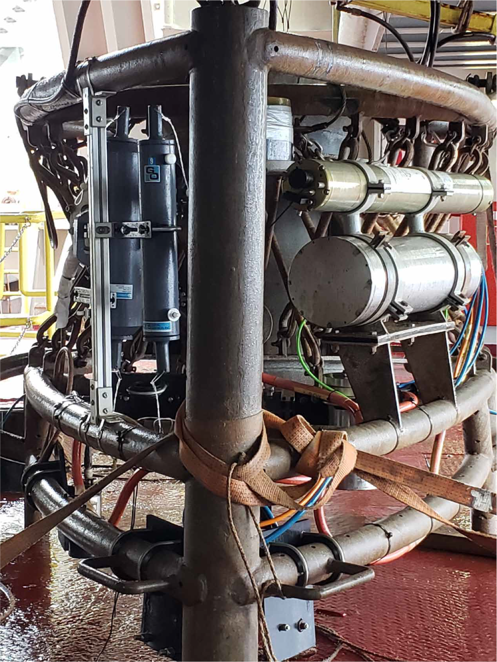
Figure F19. Niskin bottles deployed on VIT.
8.3.3. Multi-Temperature Fluid Sampler
The MTFS is a wireline borehole tool that can collect up to twelve 1 L water samples during a single wireline run (Wheat et al., 2020) (Figure F20). Each sample unit is independent of the others and contains a shape memory alloy (SMA) trigger designed to activate a syringe-style sampler at a specified temperature. The activation temperature depends on the SMA style (tube or spring), SMA diameter and composition, and pin breaking strength. The sample tube and all surfaces that the sample contacts are made of titanium except for two silicone Food and Drug Administration (FDA) O-rings (food-grade high temperature silicone) and a gasket and silicone O-ring in the check valve near the intake. The titanium sample tube extends the length of the sample reservoir and the trigger mechanism, and both ends are designed to connect with another sample tube to allow multiple samplers to be deployed on a single lowering. Two slots were milled in the sample tube to guide the piston and keep it centered. Another hole in the sample tube allows the trigger to be activated. A fourth penetration of the sample tube allows water to exchange near the sample intake. The spring and trigger components are made of stainless steel and other metals but do not contact the water sample. Triggers were chosen to activate at temperatures between 38° and 142°C.
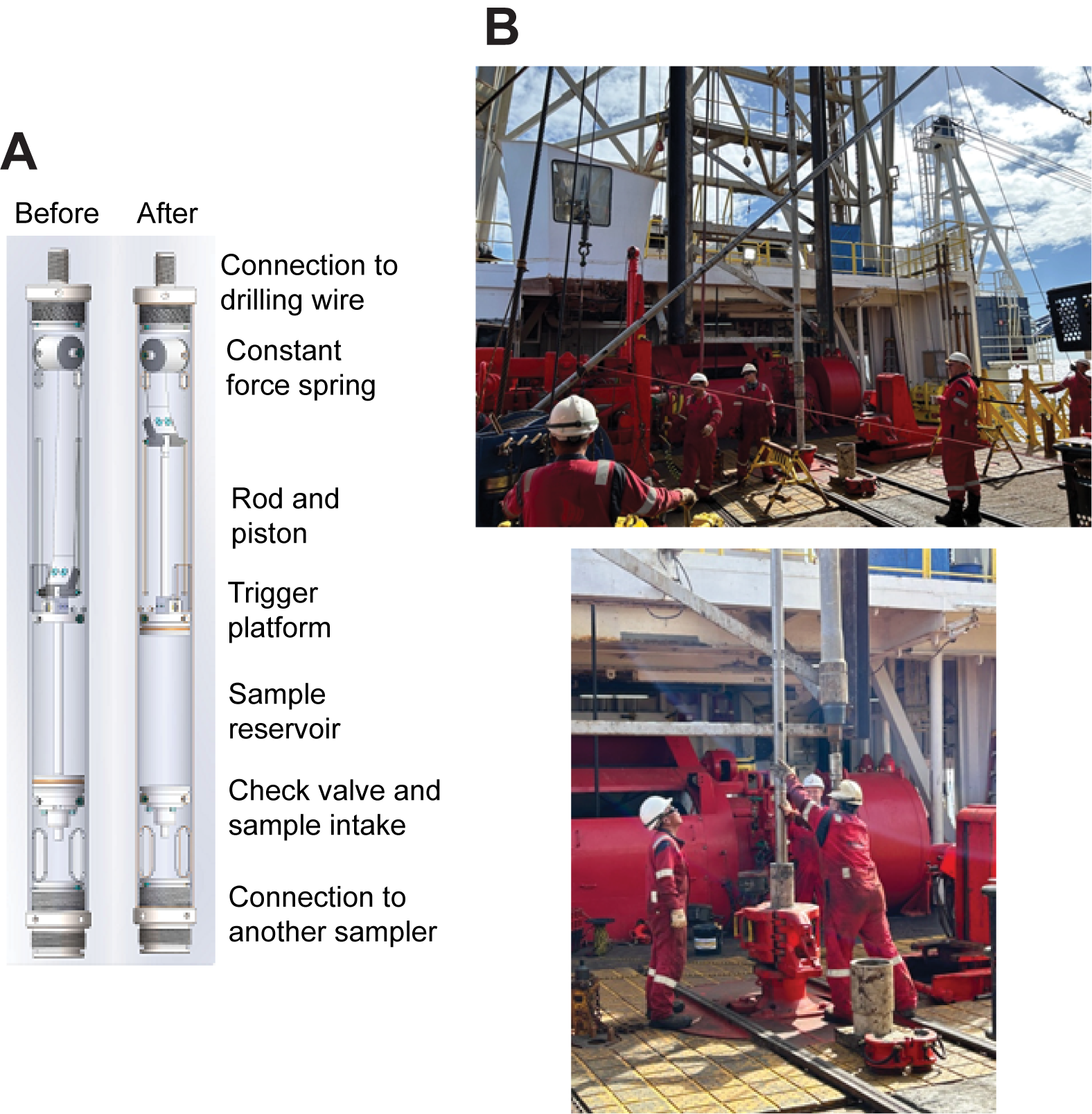
Figure F20. MTFS.
8.3.3.1. Tool preparation
The interior and exterior of the MTFS tubes were cleaned with a pressure washer, soap (Simple Green), and a plastic brush and then pressure-washed again. The interior of the titanium tubes were then wiped with lint-free wipes soaked with methanol to remove organics along the section that would be exposed to samples. Based on the cleanliness of the lint-free wipes after multiple rounds of cleaning, the titanium tubes were rated outstanding, clean, or dirty.
The intake component was assembled without grease. Silicon grease (DOW Corning 111 valve lubricant and sealant) was then applied to the O-ring, the metal surface that contacts the titanium tube, and the threads of the titanium tube prior to inserting the intake component into the titanium tube. The intake assembly was positioned by hand so that the outflow was at a 30° angle to the right of the trigger window. Seals were tested by filling the sample volume with water prior to and after tightening the bolts in place. Because the titanium tubes were extruded, their inner diameters are not exact and may differ. Thus, one intake assembly required an extra layer of Teflon tape (half of the width of a standard roll of Teflon tape) in the O-ring groove to prevent leakage. Two others required the intake assembly to be rotated 90° to achieve a good seal. A dab of liquid Teflon (Loctite 5113 thread sealant with polytetrafluoroethylene) was applied to each bolt in the assembly and the bolts that hold the assembly in place.
Triggers were assembled by first measuring the length of tube-shaped SMAs and then subjecting them to a torque of 60 lb·inch for about 10 s with a precision torque wrench. This resulted in an average deformation of 91.2% (0.3°). A notched stainless steel (0.065 inch) or titanium (0.055 inch) pin was chosen to achieve a specific temperature. The bolt was placed inside of the SMA and through the holder and attached with a nut. This nut was tightened to 4 lb·inch with a precision torque wrench and held for about 10 s. A spacer tube was placed in the well to prevent the SMA from being lost after activation, and then the assembly was bolted to the trigger platform with a dab of liquid Teflon at the ends of the bolts.
The plunger, trigger platform, and spring assembly with a 28 lb constant force spring were installed after fluorolube (a high-temperature grease) was applied to the plunger O-ring and associated metal surface. Prior to inserting the spring, a precision tool was attached. This tool retracts the spring so that the spring rod can be bolted in place.
Each assembled unit was cleaned by pulling solutions through the sample intake and expelling them from outflow. The intake was connected to a plastic tube, and the outflow was connected to a threaded titanium tube, a Kynar ball valve, and acid-washed polyurethane tubing. Water was drawn into the sampler to test for leaks around the piston’s O-ring. Like the O-ring in the intake assembly, leaks around the piston O-ring seal resulted from imperfections in the inner diameter of the titanium tube. To eliminate leaks, we added either 1.5 or 3 wraps of Teflon tape in the O-ring groove.
Final cleaning of the system consisted of drawing in a 5% HCl solution and exposing each surface prior to expelling the solution, followed by a 1% Clorox solution and three rinses with Milli-Q water. Finally, a tracer solution (1 mL of Er 1000 mg/L solution diluted in 1 L of Milli-Q water) was added (about 5 mL). For tube-style SMA, the trigger was set by pulling the spring in place and tightening with a wrench 2–3 nuts on the pin, secured further with Loctite (Loctite 242 threadlocker, red). With the trigger in place, the sampler was placed upside down and about 5 mL of tracer solution was dispensed in the sample container prior to securing the intake nut, which had been soaked in methanol and rinsed with Milli-Q water.
Two spring-shaped SMAs that targeted lower temperatures were deployed. After cleaning, the samplers were set aside with aluminum foil around the intakes until the spring assembly was inserted. The spring assemblies were difficult to position and set. First, a spring guide was attached and the unit was placed in a wood jig. This jig allows the spring to be stretched to extend the piston such that the groove in the piston could be engaged with the arms of the spring assembly. Retracting and securing the spring arms was difficult because of a lack of space through the window of the titanium tubing. One spring-shaped assembly was deployed as designed. The second was deployed without the two bolts meant to secure the base because of these alignment issues. Prior to deployment, the tracer solution was poured into the sampler intakes and the intake nuts were fastened.
After sample removal, the internal MTFS sampler pieces were cleaned with WD-40 to remove grease and grit. Isopropanol was insufficient for this task. The titanium tubes were pressure washed, sprayed with isopropanol, and wiped with a rag, inside and out. More intensive cleaning was not warranted because the tool was not redeployed during this expedition and the threads will need to be adjusted prior to future deployments.
8.3.4. Kuster Flow-Through Sampler
Two KFTSs joined with the ETBS (see below) were used to collect fluid samples from the boreholes. The KFTS has a 600 mL sample chamber and is rated to 10,000 psi (690 bar) and 232.2°C.
The lower end of the tool has a removable bullnose with ports to allow the fluid to enter. At the top is a rope socket for attaching the wireline. A latching mechanism connects the valves together and holds them open during deployment (Figure F21). A programmable mechanical clock is attached above the chamber capable of a maximum of 140 min at 5 min intervals. This clock is preset at the surface to define the closing time, at which point a ball-operated tripping mechanism releases the valves, trapping the fluid in the sampler and maintaining the pressure of the sampling depth until the tool is recovered and the fluids are retrieved through a transfer head assembly (see Geochemistry). Given the uncertainty in the exact deployment time at the target depth, the clock-triggered closing mechanism was given a 10 min buffer from the expected time to reach the target depth of sampling.
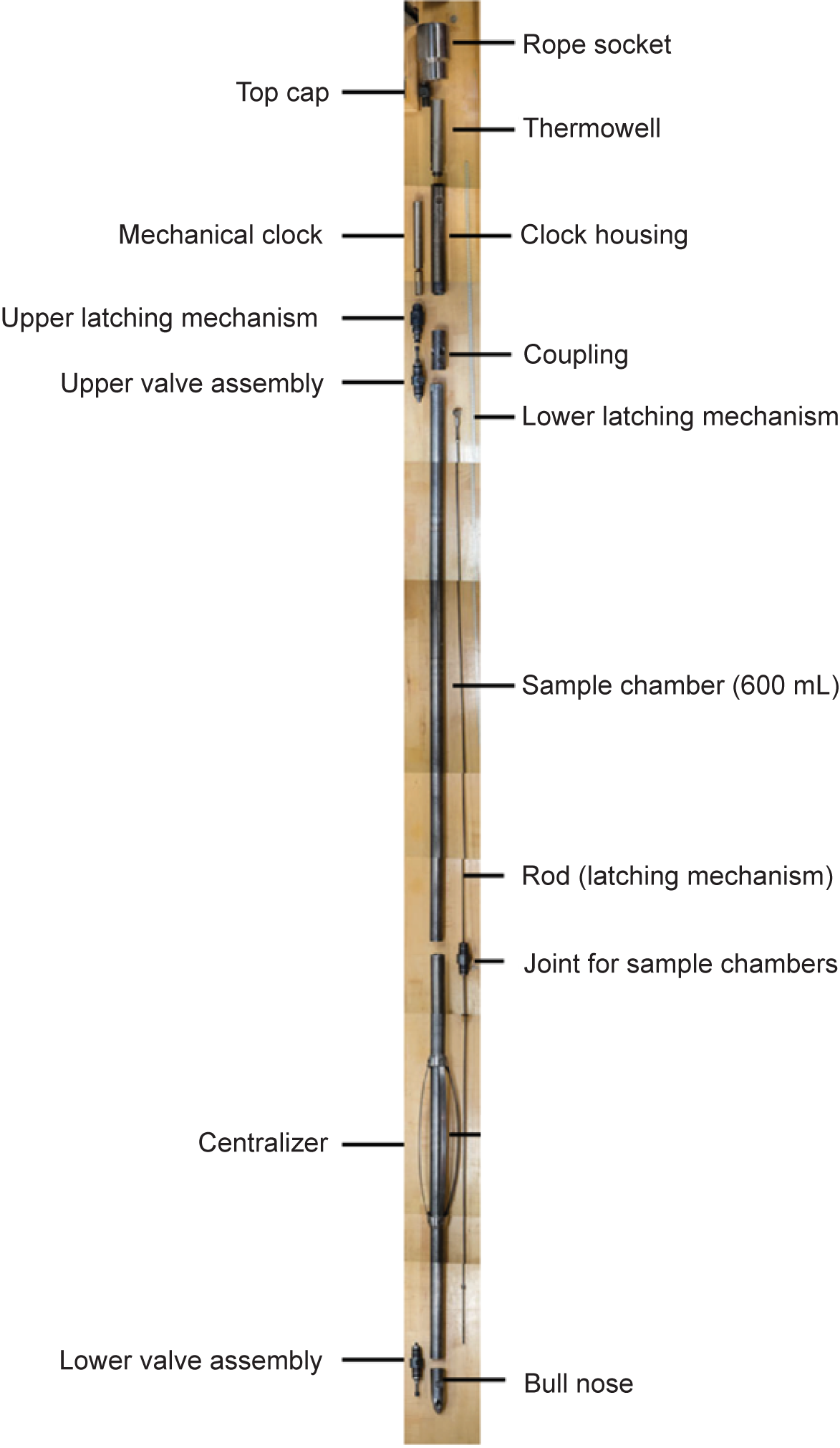
Figure F21. KFTS.
Before the first deployment, the KFTS was cleaned with ACS reagent grade acetone, rinsed with deionized water, and serviced following manufacturer guidelines (MB Century, unpubl. data). Likewise, it was ensured that the transfer head assembly was free of contaminants by washing with acetone and distilled water and testing that the valves would easily open or shut. After the first series of deployments in Hole U1309D, the interior was further cleaned with isopropanol and then scrubbed with a brush and Simple Green soap, followed by a Milli-Q rinse. The interiors were subsequently wiped with lint-free wipes soaked in dichloromethane, then soaked in methanol, and lastly dried. The interiors were then rinsed with a 5% HCl solution followed by three rinses with Milli-Q water. After recovery of the sampler, the valves, the O-rings, and any stuck particles on the O-rings were checked for mechanical wear and embrittlement and replaced as necessary prior to the next run.
8.3.5. Elevated Temperature Borehole Sensor
The ETBS is a slim-hole probe run on the coring line that was modified and upgraded from the ultra high temperature multisensor memory (UHT-MSM) tool used during ODP Legs 169 and 193 (Shipboard Scientific Party, 1998, 2000) (Figure F22). The tool was originally developed for the University of Miami (USA) by Geophysical Research Corporation (1994a, 1994b, 1996). The ETBS contains internal and ultrahigh external temperature measuring devices, a pressure gauge, a multisensor memory unit, and a dewar flask that acts as an insulator to maintain a stable temperature and cooldown rate for the tool. The heat shield is aircraft-grade aluminum bound at both ends by brass heat sinks. The dewar flask can maintain an internal temperature suitable for tool operation for 4–5 h at an external temperature of 400°C. Operations are possible for as long as 10 h if the average temperature does not exceed 232°C.
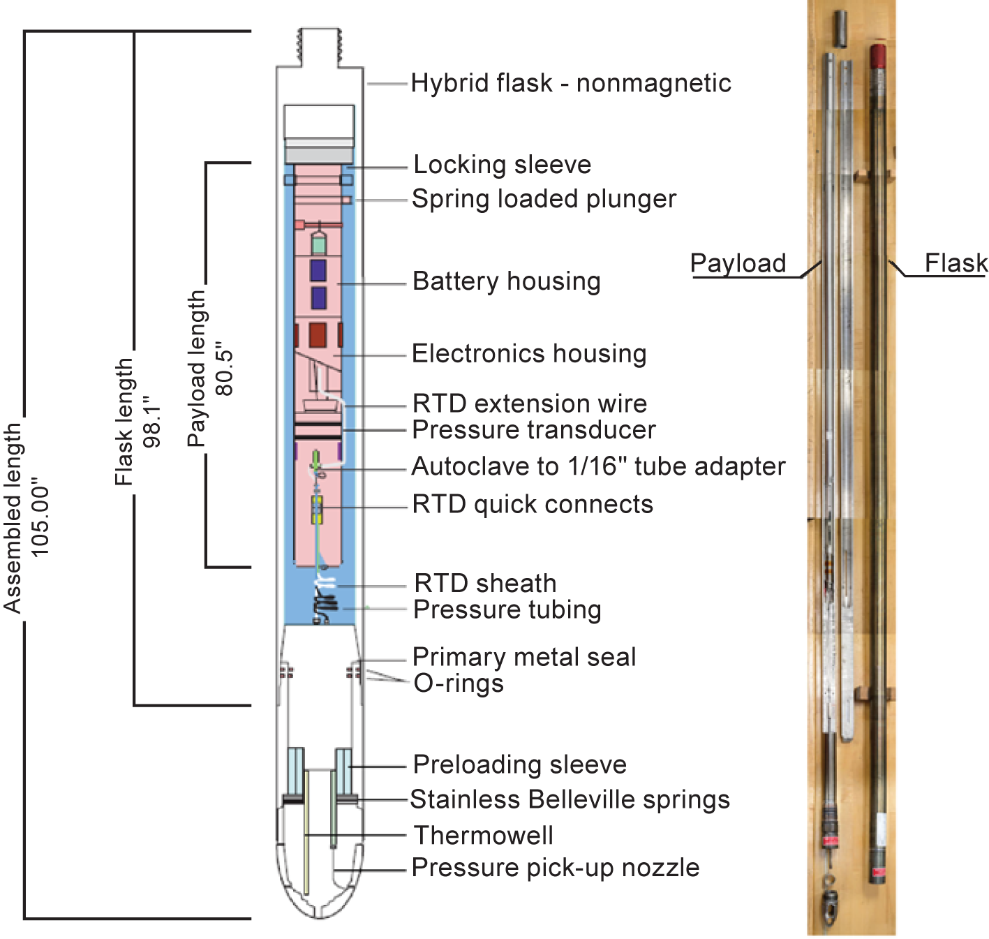
Figure F22. ETBS.
The ETBS was connected to the bottom of the KFTS and the MTFS. The ETBS was fitted with Chemraz seals and Kalrez O-rings.
The ETBS has a longer response time than the logging equipment head-mud temperature (LEH-MT) tool on the Schlumberger tool strings (see Downhole wireline logging). The ETBS also reaches higher speeds of acquisition compared with the LEH-MT (8–10 m/min), indicating that the ETBS underestimates temperatures in zones of rapidly increasing temperature with depth and the converse. To assess the magnitude of the lag, lowering and raising of the tool in conjunction with the MTFS (see above) was paused for 3 min every 100 m in Hole U1309D and paused for 5 min every 100 m in Hole U1601C.
8.3.6. Conductivity-Temperature-Depth tool
A self-recording conductivity, temperature, and pressure (CTD) instrument was placed within the protective titanium housing that was used as the outer shell of a single MTFS sampler. The near perfect length and ideal inner diameter allowed the CTD to slide down the titanium tube to the region where the intake would normally be found, exposing the sensors to the open portion of the titanium tube. Spacers were added to keep the CTD instrument from moving within the tube. The MTFS connectors were emplaced after the CTD was programed and prior to deployment. The CTD was deployed once in each borehole (Holes U1309D and U1601C), each time with two KFTS water samplers and the ETBS temperature sensor attached below. The fast response capabilities of the CTD provided data not affected by hysteresis, in contrast to data collected using the ETBS; however, it has a limited range of deployment temperature and so was only deployed to 350 mbsf.
8.4. Downhole wireline logging
8.4.1. General procedure
Wireline logging data can be obtained after drilling to characterize the physical, chemical, and structural properties of the in situ formation surrounding a borehole. For the intervals that were logged successfully, geologic observations made on the core can be correlated to the borehole and put in a regional context using geophysical survey results. Wireline log data are continuous with depth, with measurement or computed intervals ranging from 2.5 mm to 15 cm. The logs also provide information on the status and size of the borehole and on possible deformations induced by drilling or formation stress. When core recovery is incomplete or disturbed, log data may provide the only way to characterize the formation or determine the actual thickness of individual units or lithologies when contacts are not recovered. In complex settings such as Atlantis Massif, imaging logs may provide a link for understanding the structure surrounding the borehole as well as being crucial for determining orientation of the core. Wireline logging was only conducted in Hole U1601C.
Each tool string deployment is a logging run, starting with assembly of the tool string and the necessary calibrations. The tool string was sent to the bottom of the hole while recording a partial set of data and was then pulled up at a constant speed (typically 250–500 m/h) to acquire the main run data. Each lowering or hauling-up of the tool string while collecting data constitutes a pass. During each pass, the incoming data are recorded and monitored in real time using the Schlumberger MAXIS 500 system.
The Schlumberger logging equipment head (or cablehead) measured tension at the very top of the wireline tool string, which detects and can diagnose difficulties in running the tool string up or down the borehole or when exiting or entering the drill string or casing. Corrections are made for changes in the velocity of the tool string.
Telemetry cartridges were used in each tool string to transmit the data in real time from the tools to the surface using the Enhanced Digital Telemetry Cartridge (EDTC). The EDTC includes an accelerometer whose data are used to evaluate the efficiency of the wireline heave compensator (WHC) (see below). The EDTC also includes a scintillation gamma ray detector, which aids detection of when the tool passes the seafloor (see Log data processing and quality); used to correlate different log runs. A clearer indication of the seafloor is provided by the Hostile Environment Natural Gamma Ray Sonde (HNGS), which was included on the Formation MicroScanner (FMS)-sonic and Ultrasonic Borehole Imager (UBI) runs as well as the triple combo tool string.
Because the tool strings combined tools of different generations and with various designs, they included several adapters and joints between individual tools to allow communication, provide isolation, avoid interference (mechanical or acoustic), terminate wirings, or position the tool properly in the borehole. Knuckle joints in particular were used to allow some of the tools, such as the High-Resolution Laterolog Array (HRLA) resistivity tool, to remain centralized in the borehole, in contrast to the Hostile Environment Litho-Density Sonde (HLDS), which was pressed against the borehole wall. All these additions are included and contribute to the total length of the tool strings (Figure F23).
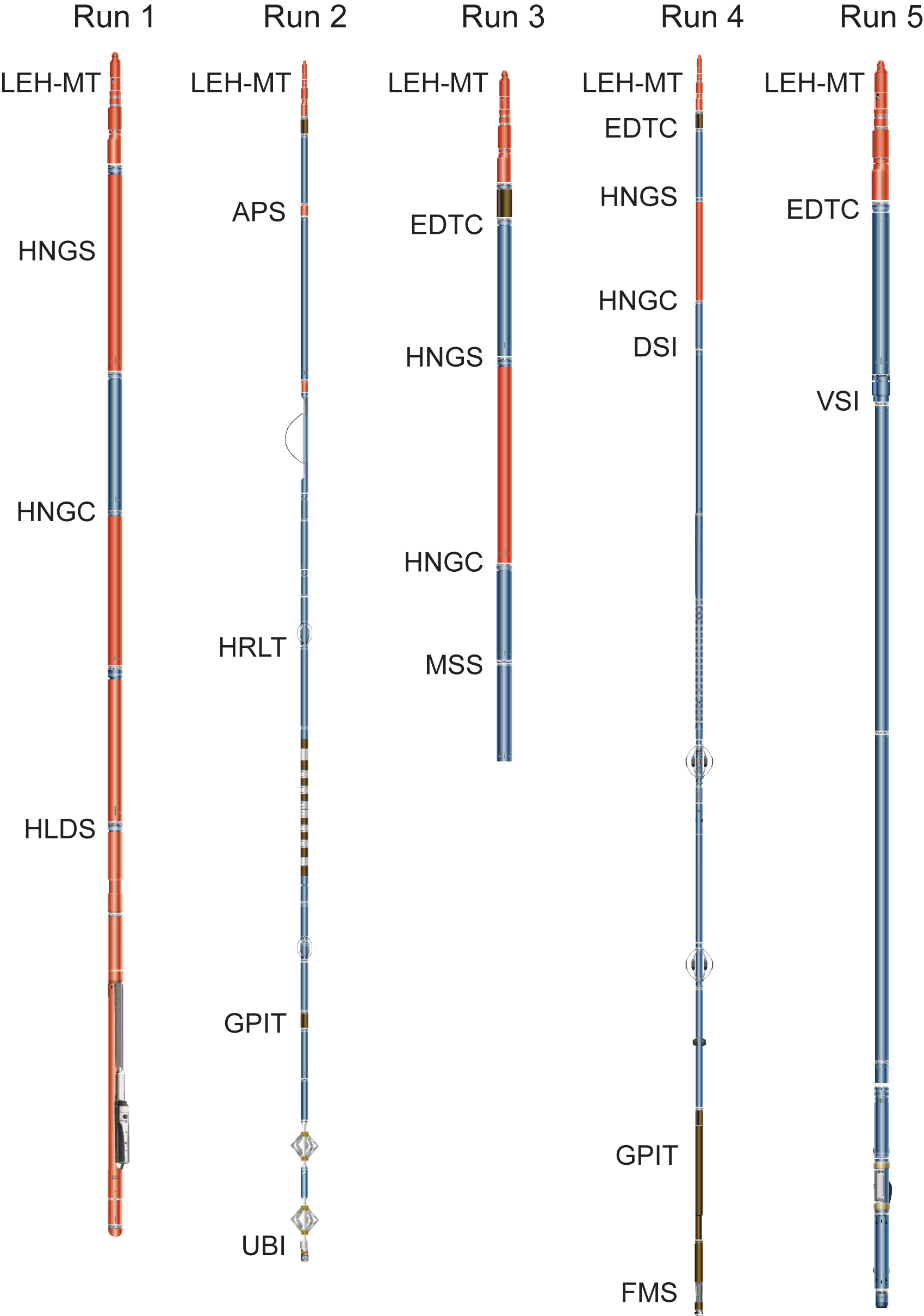
Figure F23. Petrophysical logging tools.
The WHC, first used during Integrated Ocean Drilling Program Expedition 320T in 2009, is designed to compensate for the ship’s vertical motion to help maintain the steady movement of the logging tools in the borehole (Iturrino et al., 2013). It uses vertical acceleration measurements made by a motion reference unit (MRU), located under the rig floor near the ship’s center of gravity, to calculate the vertical motion of the ship. The WHC then adjusts the length of the wireline by varying the distance between two sets of pulleys through which the cable passes. Real-time measurements of uphole (surface) and downhole acceleration are made simultaneously by the MRU and the EDTC tool, respectively.
8.4.2. Log data processing and quality
Initially, the logging data were referenced to the rig floor. After completion of logging operations, the data were shifted to a seafloor reference using the step in the natural gamma ray data (acquired in all logging runs) at the seafloor.
Downhole logging data were transferred onshore to Lamont-Doherty Earth Observatory for standard data processing. Processing primarily involves depth matching to provide consistency in the depth scale between the different logging runs. Similar to the depth shift to the seafloor datum, this depth matching was undertaken primarily by utilizing the natural gamma ray data. In addition, corrections were made to certain tools and logs (e.g., speed and voltage corrections to microresistivity images), documentation for the logs was prepared (including an assessment of log data quality), and the data were converted to ASCII format for the conventional logs and GIF for the images. The data were transferred back to the ship within a few days of logging and were made available in ASCII and DLIS formats through the shipboard IODP logging database.
The principal factor that influences log data quality is the condition of the borehole wall. If the borehole diameter varies over short intervals because of washouts or ledges, logs from tools that require good contact with the borehole wall may be degraded. Very narrow (bridged) sections will also cause irregular results. The quality of the borehole can be improved by minimizing the circulation of drilling fluid, flushing the borehole to remove debris prior to logging, performing a full wiper trip, and starting logging as soon as possible after drilling and hole conditioning. Hole U1601C was flushed, and logging was initiated right after drilling. Drilling was continued after wireline logging was completed.
The ideal conditions for logging include a consistent borehole diameter of the size of the bit. Oversized borehole diameters can have a significant impact on measurements, especially those that require tool eccentering (e.g., HLDS) or tool centralization (e.g., FMS). The measurement principles of the eccentered tools and the centralized FMS mean that direct contact with the formation is essential for acquisition of high-quality data sets. Borehole wall contact is lost beyond a 20 inch (~50 cm) borehole diameter for the HLDS and a 15 inch (~38 cm) borehole diameter for the FMS. High temperatures can also limit data quality because of the faster pass speeds required for tool preservation. The borehole diameter in Hole U1601C is almost constant, with the largest deviation being ~150 and 165 mbsf.
The length of wireline cable payed out is used to determine the depth of logging measurements. The quality of this logging depth determination is dependent on a number of factors, including the ship’s heave, cable stretch, cable slip, and tidal changes. To minimize the effect of the ship’s heave on logging depth, a hydraulic WHC is used to adjust the wireline length for rig motion during logging operations (see above). An important reference datum in wireline logging is the seafloor/mudline, which is determined from the natural gamma ray logs acquired from each logging run. Discrepancies between the drilling core depth and the wireline logging depth occur because of incomplete core recovery, core expansion, incomplete heave compensation, and drill pipe stretch. Reconciling the differences between the two data sets is possible through comparison of the common data sets acquired in situ and on the core (e.g., NGR) as well as matching obvious structures that are observable in image logs and in the core (e.g., thicker veins, textural changes, and contacts).
8.4.3. Wireline logging tools used during Expedition 399
Detailed information on the physical properties measured by individual logging tools and their geologic applications may be found in Ellis and Singer (2007), Goldberg (1997), Lovell et al. (1998), Rider (1996), Schlumberger (1989), and Serra (1984, 1986, 1989). A complete list of acronyms for Schlumberger tools and logs is available at http://www.apps.slb.com/cmd/index.aspx.
8.4.3.1. Formation density
In situ formation density was measured with the HLDS. The sonde contains a radioactive cesium (137Cs) gamma ray source and far and near gamma ray detectors mounted on a shielded skid, which is pressed against the borehole wall by an eccentralizing arm. Gamma rays emitted by the source undergo Compton scattering, by which gamma rays are scattered by electrons in the formation. The number of scattered gamma rays that reach the detectors is proportional to the density of electrons in the formation, which is in turn related to bulk density. Porosity may be derived from this bulk density if the matrix (grain) density is known.
The HLDS also measures photoelectric absorption as the photoelectric effect (PEF). Photoelectric absorption of gamma rays occurs when their energy is reduced below 150 keV after being repeatedly scattered by electrons in the formation. Because PEF depends on the atomic number of the elements encountered, it varies with the chemical composition of the minerals present and can be used for the identification of some minerals such as sulfides (e.g., Bartetzko et al., 2003) or some specific lithologic intervals such as diabase or oxide gabbro (e.g., Expedition 304/305 Scientists, 2006).
8.4.3.2. Formation radiation
The HNGS measures natural radioactivity in the borehole wall using two bismuth germanate scintillation detectors. Concentrations of K, Th, and U, whose radioactive isotopes dominate the natural radiation spectrum, were computed by Schlumberger’s proprietary spectroscopy method. The inclusion of HNGS in all tool strings allows the use of gamma ray data for depth correlation between consecutive tool string runs and individual tool string passes (up and down).
8.4.3.3. Formation magnetic susceptibility
The Magnetic Susceptibility Sonde (MSS) measures formation MS in the borehole. These measurements provide a means to investigate downhole changes in mineralogy and lithology, which are most sensitive to magnetic minerals. The sensor used during Expedition 399 was a dual-coil sensor providing deep-reading measurements, with a vertical resolution of ~36 cm.
8.4.3.4. Formation seismic velocity sonic log
The Dipole Shear Sonic Imager (DSI) generates acoustic pulses from various sonic transmitters and records the waveforms with an array of eight receivers. The waveforms are then used to calculate velocity in the formation. The omnidirectional monopole transmitter emits high-frequency (5–15 kHz) pulses to extract the compressional velocity (VP) of the formation, as well as the shear velocity (VS) when it is faster than the sound velocity in the borehole fluid. The same transmitter can be fired in sequence at a lower frequency (0.5–1 kHz) to generate Stoneley waves, which are sensitive to fractures and variations in permeability. The DSI also has two crossed-dipole transmitters, which allow an additional measurement of shear wave velocity in slow formations, where VS is slower than the velocity in the borehole fluid. However, in igneous formations, VS is primarily measured from the monopole waveforms that produce sharper shear arrival. The waveforms produced by the two orthogonal dipole transducers can be used to identify the degree and orientation of seismic anisotropy in the formation.
The DSI measures the transit times between sonic transmitters and an array of eight receiver groups with 15 cm spacing along the tool. During acquisition, VP and VS are determined from the recorded waveforms using a slowness/time coherence processing algorithm (Kimball and Marzetta, 1984). In the process, a semblance function is calculated for a fixed time window across the receiver array, varying travel times, and velocity within a predefined range to identify peaks in semblance corresponding to individual mode arrivals. The average repeatability of the seismic velocity measurements is 2%, 3%, 5%, and 3% for compressional, shear, dipole shear, and Stoneley waves, respectively.
8.4.3.5. Electrical resistivity
The HRLA tool provides six resistivity measurements at different depths of investigation into the formation (including the borehole fluid, or mud resistivity, and five measurements of formation resistivity with increasing penetration into the formation). The sonde sends a focused current beam into the formation and measures the intensity necessary to maintain a constant drop in voltage across a fixed interval, providing direct resistivity measurement. The array has one central source electrode and six electrodes above and below it, which serve alternately as focusing and returning current electrodes. By rapidly changing the role of these electrodes, a simultaneous resistivity measurement is achieved at six penetration depths.
Typically, igneous, silicate minerals are electrical insulators, whereas sulfide, phyllosilicate, and oxide minerals, as well as ionic solutions like pore water, are conductors. In most rocks, electrical conduction occurs primarily by ion transport through pore fluids and thus is strongly dependent on porosity and conductive minerals (Bartetzko et al., 2003). Electrical resistivity can hence be used to estimate porosity, alteration, and fluid salinity. In gabbroic and serpentinized rocks such as those encountered at Atlantis Massif, electrical resistivity will be sensitive most of all to fractured formations and to a lesser extent to oxide-rich lithologies (e.g., Haggas et al., 2005; Tominaga et al., 2009).
8.4.3.6. Tool orientation
The General Purpose Inclinometry Tool (GPIT) incorporates a three-component accelerometer and a three-component magnetometer, deployed in all logging runs. The primary purpose of this tool is to determine the acceleration and geographic orientation of the tool string. This allows orientation-sensitive logs like the FMS and UBI to be corrected for irregular tool motion, and the dip and dip direction (azimuth) of planar structures can be determined. GPIT data are also used to provide real-time evaluation of the WHC (see above).
8.4.3.7. Formation MicroScanner
The FMS provides high-resolution electrical resistivity images of borehole walls (Bourke et al., 1989). The tool has four orthogonal arms and pads, each containing 16 button electrodes that are pressed against the borehole wall during each upward pass. The electrodes are arranged in two diagonally offset rows of eight electrodes each. A focused current is emitted from the button electrodes into the formation, with a return electrode near the top of the tool. Resistivity of the formation at each pad is derived from the intensity of current passing through the button electrodes. Processing transforms these measurements into oriented high-resolution (millimeter to centimeter scale) images that reveal the structures in the borehole wall. Features such as fracturing, folding, and alteration may be resolved. The images are oriented with respect to magnetic north so that the dip and dip direction (azimuth) of planar features in the formation can be measured. The FMS microresistivity images do not provide full coverage of the borehole wall with a single pass (~37% coverage in an 8½ inch hole). To increase this coverage, it is standard practice to undertake two passes of the borehole in the hope that the tool will be oriented differently on the second pass.
8.4.3.8. Ultrasonic Borehole Imager
The UBI features a high-resolution transducer that provides acoustic images of the borehole wall. The transducer emits ultrasonic pulses at a frequency of 250 or 500 kHz (low and high resolution, respectively), which are reflected at the borehole wall and then received by the same transducer. The amplitude and traveltime of the reflected signal are determined. Continuous rotation of the transducer and the upward motion of the tool produce a complete map of the borehole wall. The amplitude depends on the reflection coefficient of the borehole fluid/rock interface, the position of the UBI tool in the borehole, the shape of the borehole, and the roughness of the borehole wall. Changes in the borehole wall roughness (e.g., at fractures intersecting the borehole) modulate the reflected signal; therefore, fractures or other variations in the character of the drilled rocks can be recognized in the amplitude image. The recorded traveltime image gives detailed information about the shape of the borehole, which allows calculation of one caliper value of the borehole from each recorded traveltime. Amplitude and traveltime are recorded together with a reference to magnetic north by means of a magnetometer (GPIT), permitting the orientation of images.
8.4.3.9. Versatile Seismic Imager
The Versatile Seismic Imager (VSI) is deployed on a wireline and allows for the acquisition of seismic waves in the borehole generated by an active source (Figure F24). The purpose of these measurements is to provide a direct measurement of the time necessary for seismic waves to travel from the surface to a given depth and to tie the seismic log measurements recorded in depth to the reflections observed in seismic survey data recorded in travel time. Analysis of the full waveforms can be used to characterize seismic reflectivity beyond the borehole (Expedition 340T Scientists, 2012).
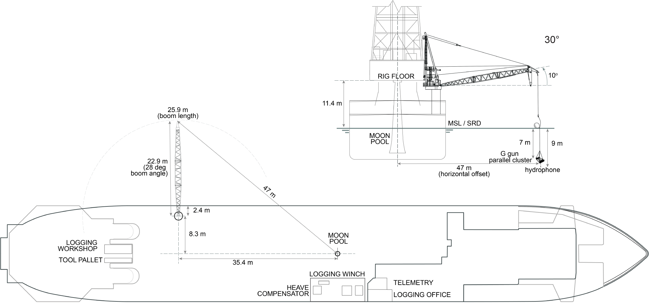
Figure F24. VSI source and ship geometry.
The VSI employs three-axis single sensor seismic hardware and software and advanced telemetry for efficient transmission of the data from the borehole to the surface. It consists of three parts (a power cartridge, a control cartridge, and the measurement sonde) and takes its measurements by means of a three-axis gimbaled accelerometer package in the sonde. Each sensor package delivers high-quality wavefields by using three-axis geophone omnitilt accelerometers, which are acoustically isolated from the main body of the tool and provide a flat response from 3 to 200 Hz. The configuration of the tool (number of sensor packages, sensor spacing, and type of connection [stiff or flexible]) varies to provide the maximum versatility of the array.
The tool is used to collect seismic data by anchoring in the hole at the desired depth using a caliper arm. When anchored, the accelerometer package is pressed firmly against the formation while remaining decoupled acoustically from the body of the shuttle. Air guns deployed from the ship by crane then provide the necessary source pulse, and the resulting acoustic wave is recorded downhole on all three axes. The guns are held in one location relative to the borehole while the VSI tool is moved to each of the desired depth stations within the hole. The anchoring, size, and acoustic isolation of the sensors allow for suppression of the tool harmonic noise and removal of tube waves from the borehole-seismic band. Furthermore, digitization close to the sensor package helps reduce signal distortion.
9. Paleomagnetism
Routine shipboard paleomagnetic experiments were carried out using both archive section halves and discrete cube samples (~8 cm3) taken from working half sections. Magnetic anisotropy and rock magnetism analyses were also conducted on the discrete samples. The criteria for discrete sample selection for shipboard analysis was based on physical properties, lithologic variation, and visible alteration. Sampling intervals were core recovery dependent; however, sampling of different lithologic units was prioritized. On average, one discrete sample was selected from most working half sections for every ~4.5 m cored interval, except in Hole U1601C where sampling was limited (see Operations).
As inherent in all drilling cores, the azimuths of the recovered core samples were unknown; therefore, relative magnetic directions were conducted within the CRF (Figure F2). In this reference frame, +x points into the working section half (i.e., toward the double line), +z is downcore, and +y is orthogonal to x and z in a right-hand sense.
Shipboard magnetization directions of most discrete samples were determined using the PmagPy software package version 4.2.72 (Tauxe et al., 2016), which uses principal component analysis (Kirschvink, 1980), makes orthogonal vector plots (Zijderveld, 1967), and can use inclination-only statistics (McFadden and Reid, 1982). The PmagPy software suite offers a comprehensive graphical user interface that facilitates the analysis of magnetic directions in geologic samples or specimens. Users can specify the fitting method—either a line or a plane—depending on the nature of the data. The software allows for the selection of specific samples for analysis and computes the principal component of demagnetization vectors, providing the best-fit line or plane through the demagnetization data points. This computation is based on user-input starting and ending points for the demagnetization steps. PmagPy displays the calculated magnetic component directions, including declination and inclination, along with statistical parameters such as the maximum angular deviation and the degree of angle. Additionally, these results can be visualized using equal area projections and Zijderveld plots, enhancing the user’s ability to interpret the magnetic data effectively.
Outcomes of the proposed work were compared to similar work carried out previously in this area (i.e., Expeditions 304/305 and 357 [Expedition 304/305 Scientists, 2006; Früh-Green et al., 2016]). Sample subsections were subjected to a variety of paleomagnetic tests to evaluate their magnetic fidelity and highlight samples of interest for future shore-based studies.
9.1. Archive section analysis
Archive half remanence measurements were collected using a pass-through 2G Enterprises Model-760R-4K SRM interfaced with the Integrated Measurement System SRM software (version 13.0). The magnetometer contains direct-current superconducting quantum interference devices (DC-SQUIDs) as well as an integrated in-line AF demagnetizer capable of applying peak fields of 80 mT. The SQUID sensors within the SRM have fixed response functions of 8 cm (Parker and Gee, 2002), placing a lower bound on the length of samples that could accurately be measured. Any pieces shorter than 8 cm were removed before demagnetization and then returned in their respective original positions postmeasurement. Further details concerning the SQUID response functions can be found in the Expedition 360 methods chapter (MacLeod et al., 2017).
Baseline drift and empty tray calibrations, both AF demagnetized at 80 mT, were conducted approximately every 24 h. Archive halves were measured at an interval of 2 cm and at a measuring frequency of 1 Hz. These measurement parameters were consistent with other expedition reports and physical properties measurements (e.g., SHMSL and SHIL; see Petrophysics), thus enabling more direct comparisons between different shipboard data sets. Initial magnetizations were progressively demagnetized using the following steps: 5, 10, 15, 20, 30, 40, and 50 mT. However, several archive section halves with particularly variable inclinations and/or stable magnetization intensities were treated to the additional steps of 60, 70, and 80 mT. Whole-round measurements of 2 mT increments up to 16 mT were only performed for whole-round cores that were not split on the ship. This was to characterize the low coercivity components that could be remagnetized during the transport of the whole rounds.
Recuration was completed after the expedition, but archive section analysis was not corrected, causing an offset of some samples between measurements made on the ship and the current interval or newly made core sections.
9.2. Discrete samples
All discrete samples from the working half had their intensities and remnant magnetization directions measured using an AGICO JR-6A spinner magnetometer. Measurements were taken after daily calibrations of the instrument. Calibrations consisted of using both a 7.99 A/m cube standard and an empty holder for corrections. AGICO’s Rema6 software stored the measurements and converted the inclination and declination values measured in the specimen coordinate system to the CRF. The Remasoft30 was used for initial analytical assessments. It is worth noting that the practical noise limit for this system is 1 × 10⁻⁵ A/m.
To reduce drilling overprints and other unreliable signatures, most of the discrete paleomagnetism samples were dunked twice into liquid nitrogen baths (T ≈ 77 K) as part of a low-temperature pretreatment (Merrill, 1970; Dunlop, 2003; Morris et al., 2009). This pretreatment cools samples below magnetite’s characteristic crystallographic transition—the Verwey transition (Dunlop, 2003). Consequently, multidomain magnetite grains lose their remanence upon returning to room temperature conditions. After each dunk, samples were nested in six cylindrical mu-metal shields to ensure gradual thermal recovery over a period of approximately 6 h. The magnetization directions and intensities of the samples were measured following each dunk to assess changes.
9.2.1. Paleomagnetic analysis
Discrete samples were subjected to demagnetization tests. Stepwise AF demagnetizations were performed to approximately a third of the paleomagnetism samples using the Model D-200 DTech AF demagnetizer, which has a peak field of 200 mT. Samples were demagnetized using the following AF field steps: 5, 10, 15, 20, 30, 40, 50, 60, 80, 90, 100, 125, 150, 175, and 200 mT. Additionally, the physical properties team granted permission for their samples to be subjected to AF demagnetization, greatly expanding the paleomagnetism data set. Although all physical properties samples were brought to 105°C prior to paleomagnetic measurements, this temperature was considered low enough to avoid unblocking most magnetic grains that contribute to the characteristic remanent magnetization. Consequently, the potential influence of these low unblocking temperatures on the characteristic magnetization directions of the samples is minimal.
Thermal demagnetizations of all discrete paleomagnetism samples were performed using an ASC Scientific thermal demagnetizer (model TD-48 SC), which is capable of demagnetizing samples up to 700°C. A significant subset of the paleomagnetism samples was part of a hybrid experiment consisting of both thermal and AF demagnetizations. After observing that AF demagnetizations of 200 mT did not fully demagnetize the samples, post-AF thermal demagnetizations could allow for a more nuanced characterization of the most coercive components, possibly including contributions from iron sulfides within the samples. Heating steps for the thermal demagnetizations varied by site due to time constraints; however, all samples remained within their respective heating steps for 0.5 h to thermally equilibrate.
Even though the oven was shielded in mu-metal, fluxgate magnetometer measurements reveal that the shielding for particular regions of the oven were rather weak (Figure F25). Discrete samples were therefore placed 5–20 cm away from the innermost edge of the tray where the shielding was strongest. Samples were loaded along the +z-axis for even numbered thermal steps and along the −z-axis for odd numbered thermal steps. This procedure’s intent was to cancel out the inducing effects of residual ambient magnetic fields. Additionally, bulk MS measurements were taken with a Bartington dual frequency sensor (MS2B) after every thermal demagnetization step. These measurements were used to monitor oxidizing alterations in magnetic carrier composition, as high temperature measurements were conducted in atmospheric conditions.
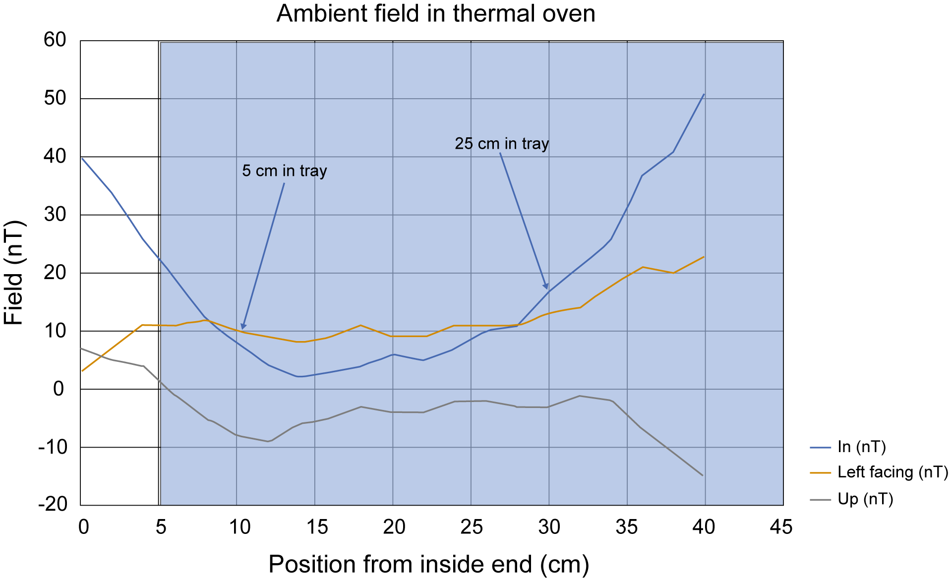
Figure F25. Ambient magnetic field profile inside thermal demagnetizer.
9.2.2. Magnetic anisotropy and rock magnetism analyses
Standard paleomagnetic measurements were supplemented by anisotropy of low-field magnetic susceptibility (AMS) and IRM measurements. AMS measurements were determined for all discrete samples (including physical properties samples). Measurements were taken and analyzed using AGICO’s Safyr7 and Anisoft5 software, which use equations from Hext (1963). The magnetic fabric evolutions, variations in degree of anisotropy, shape parameter, types of shape ellipsoid, and magnetic foliation and lineation were studied to determine directional and deformational signatures with depth.
Additional rock magnetic investigations were conducted onboard to get a baseline understanding of sample hysteretic properties. IRMs were imparted twice per step along the +z-axis of the samples using an ASC Scientific Model IM-10 impulse magnetizer. IRM acquisition and backfield steps varied based on the individual sample saturation levels. IRM acquisition at higher fields is more sensitive to the occurrence of coarse-grained (>0.1 µm) multidomain magnetite (King et al., 1982; Frederichs et al., 1999). The contributions of high-coercivity minerals, like hematite, can be investigated by looking at the differences between the saturating IRMs and the backfield IRMs. By identifying the remanences, one can track the relative contributions of each mineral to the overall remanence (e.g., Liu et al., 2013; Roberts et al., 2019). Identification of different magnetic carrier populations was conducted using the program MaxUnmix, which effectively decomposes magnetization curves to isolate and analyze specific magnetic mineral components from the overall signal (Maxbauer et al., 2016).
References
Bartetzko, A., Paulick, H., Iturrino, G., and Arnold, J., 2003. Facies reconstruction of a hydrothermally altered dacite extrusive sequence; evidence from geophysical downhole logging data (ODP Leg 193). Geochemistry, Geophysics, Geosystems, 4(10):1087. https://doi.org/10.1029/2003GC000575
Bartington Instruments, L., 2011. Operation Manual for MS2 Magnetic Susceptibility System: Oxford, UK (Bartington Instruments, Ltd.). https://gmw.com/wp-content/uploads/2019/03/MS2-OM0408.pdf
Bartington Instruments, L., 2019. MS2/MS3 Magnetic Susceptibility Systems: Oxford, United Kingdom (Bartington Instruments, Ltd.). http://www.bartington.com/Literaturepdf/Datasheets/MS2_MS3_DS0020.pdf
Beard, J.S., Frost, B.R., Fryer, P., McCaig, A., Searle, R., Ildefonse, B., Zinin, P., and Sharma, S.K., 2009. Onset and progression of serpentinization and magnetite formation in olivine-rich troctolite from IODP Hole U1309D. Journal of Petrology, 50(3):387–403. https://doi.org/10.1093/petrology/egp004
Blackman, D.K., Ildefonse, B., John, B.E., Ohara, Y., Miller, D.J., MacLeod, C.J., and the Expedition 304/305 Scientists, 2006. Proceedings of the Integrated Ocean Drilling Program, 304/305: College Station, TX (Integrated Ocean Drilling Program Management International, Inc.). https://doi.org/10.2204/iodp.proc.304305.2006
Blum, P., 1997. Physical properties handbook: a guide to the shipboard measurement of physical properties of deep-sea cores. Ocean Drilling Program Technical Note, 26. https://doi.org/10.2973/odp.tn.26.1997
Bourke, L., Delfiner, P., Trouiller, J.-C., Fett, T., Grace, M., Luthi, S., Serra, O., and Standen, E., 1989. Using Formation MicroScanner images. The Technical Review, 17:16–40. https://www.slb.com/-/media/files/oilfield-review/2-microscanner
Carslaw, H.S., and Jaeger, J.C., 1959. Conduction of Heat in Solids (2nd edition): Oxford, United Kingdom (Clarendon Press).
Coggon, R.M., Sylvan, J.B., Teagle, D.A.H., Reece J., Christeson, G.L., Estes, E.R., Williams, T.J., and the Expedition 390 Scientists, 2022. Expedition 390 Preliminary Report: South Atlantic Transect 1. International Ocean Discovery Program. https://doi.org/10.14379/iodp.pr.390.2022
Coggon, R.M., Teagle, D.A.H., Sylvan, J.B., Reece, J., Estes, E.R., Williams, T.J., Christeson, G.L., Aizawa, M., Albers, E., Amadori, C., Belgrano, T.M., Borrelli, C., Bridges, J.D., Carter, E.J., D’Angelo, T., Dinarès-Turell, J., Doi, N., Estep, J.D., Evans, A., Gilhooly, W.P., III, Grant, L.C.J., Guérin, G.M., Harris, M., Hojnacki, V.M., Hong, G., Jin, X., Jonnalagadda, M., Kaplan, M.R., Kempton, P.D., Kuwano, D., Labonte, J.M., Lam, A.R., Latas, M., Lowery, C.M., Lu, W., McIntyre, A., Moal-Darrigade, P., Pekar, S.F., Robustelli Test, C., Routledge, C.M., Ryan, J.G., Santiago Ramos, D., Shchepetkina, A., Slagle, A.L., Takada, M., Tamborrino, L., Villa, A., Wang, Y., Wee, S.Y., Widlansky, S.J., Yang, K., Kurz, W., Prakasam, M., Tian, L., Yu, T., and Zhang, G., 2024. Expedition 390/393 summary. In Coggon, R.M., Teagle, D.A.H., Sylvan, J.B., Reece, J., Estes, E.R., Williams, T.J., Christeson, G.L., and the Expedition 390/393 Scientists, South Atlantic Transect. Proceedings of the International Ocean Discovery Program, 390/393: College Station, TX (International Ocean Discovery Program). https://doi.org/10.14379/iodp.proc.390393.101.2024
Cordier, C., Clément, J. P., Caroff, M., Hémond, C., Blais, S., Cotten, J., Bollinger, C., Launeau, P., and Guille, J., 2005. Petrogenesis of coarse-grained intrusives from Tahiti Nui and Raiatea (Society Islands, French Polynesia). Journal of Petrology, 46(11):2281–2312. https://doi.org/10.1093/petrology/egi055
de Ronde, C.E.J., Humphris, S.E., Höfig, T.W., Brandl, P.A., Cai, L., Cai, Y., Caratori Tontini, F., Deans, J.R., Farough, A., Jamieson, J.W., Kolandaivelu, K.P., Kutovaya, A., Labonté, J.M., Martin, A.J., Massiot, C., McDermott, J.M., McIntosh, I.M., Nozaki, T., Pellizari, V.H., Reyes, A.G., Roberts, S., Rouxel, O., Schlicht, L.E.M., Seo, J.H., Straub, S.M., Strehlow, K., Takai, K., Tanner, D., Tepley III, F.J., and Zhang, C., 2019. Expedition 376 methods. In de Ronde, C.E.J., Humphris, S.E., Höfig, T.W., and the Expedition 376 Scientists, Brothers Arc Flux. Proceedings of the International Ocean Discovery Program, 376: College Station, TX (International Ocean Discovery Program). https://doi.org/10.14379/iodp.proc.376.102.2019
De Vleeschouwer, D., Dunlea, A.G., Auer, G., Anderson, C.H., Brumsack, H., de Loach, A., Gurnis, M.C., Huh, Y., Ishiwa, T., Jang, K., Kominz, M.A., März, C., Schnetger, B., Murray, R.W., Pälike, H., and Expedition 356 Shipboard Scientists, 2017. Quantifying K, U, and Th contents of marine sediments using shipboard natural gamma radiation spectra measured on DV JOIDES Resolution. Geochemistry, Geophysics, Geosystems, 18(3):1053–1064. https://doi.org/10.1002/2016GC006715
Dick, H.J.B., MacLeod, C.J., Blum, P., and the Expedition 360 Scientists, 2016. Expedition 360 Preliminary Report: Southwest Indian Ridge Lower Crust and Moho. International Ocean Discovery Program. https://doi.org/10.14379/iodp.pr.360.2016
Dunlop, D.J., 2003. Stepwise and continuous low-temperature demagnetization. Geophysical Research Letters, 30(11):1582. https://doi.org/10.1029/2003GL017268
Ellis, D.V., and Singer, J.M., 2007. Well Logging for Earth Scientists (2nd edition): New York (Elsevier). https://doi.org/10.1007/978-1-4020-4602-5
Expedition 304/305 Scientists, 2006. Methods. In Blackman, D.K., Ildefonse, B., John, B.E., Ohara, Y., Miller, D.J., MacLeod, C.J., and the Expedition 304/305 Scientists, Proceedings of the Integrated Ocean Drilling Program, 304/305: College Station, TX (Integrated Ocean Drilling Program Management International, Inc.). https://doi.org/10.2204/iodp.proc.304305.102.2006
Expedition 309/312 Scientists, 2006. Methods. In Teagle, D.A.H., Alt, J.C., Umino, S., Miyashita, S., Banerjee, N.R., Wilson, D.S., and the Expedition 309/312 Scientists, Proceedings of the Integrated Ocean Drilling Program, 309/312: Washington, DC (Integrated Ocean Drilling Program Management International, Inc.). https://doi.org/10.2204/iodp.proc.309312.102.2006
Expedition 335 Scientists, 2011. Superfast spreading rate crust 4: drilling gabbro in intact ocean crust formed at a superfast spreading rate. International Ocean Discovery Program Preliminary Report, 335. https://doi.org/10.2204/iodp.pr.335.2011
Expedition 335 Scientists, 2012. Methods. In Teagle, D.A.H., Ildefonse, B., Blum, P., and the Expedition 335 Scientists, Proceedings of the Integrated Ocean Drilling Program, 335: Tokyo (Integrated Ocean Drilling Program Management International, Inc.). https://doi.org/10.2204/iodp.proc.335.102.2012
Expedition 340T Scientists, 2012. Atlantis Massif Oceanic Core Complex: velocity, porosity, and impedance contrasts within the domal core of Atlantis Massif: faults and hydration of lithosphere during core complex evolution. Integrated Ocean Drilling Program Preliminary Report, 340T. https://doi.org/10.2204/iodp.pr.340T.2012
Expedition 345 Scientists, 2014. Hess Deep plutonic crust: exploring the plutonic crust at a fast-spreading ridge: new drilling at Hess Deep. Integrated Ocean Drilling Program Preliminary Report, 345. https://doi.org/10.2204/iodp.pr.345.2014
Frederichs, T., Bleil, U., Däumler, K., Von Dobeneck, T., and Schmidt, A.M., 1999. The magnetic view on the marine paleoenvironment: parameters, techniques and potentials of rock magnetic studies as a key to paleoclimatic and paleoceanographic changes. In Fischer, G. and Wefer, G., Use of Proxies in Paleoceanography: Examples from the South Atlantic. Berlin (Springer-Verlag), 575–599. https://doi.org/10.1007/978-3-642-58646-0_24
Früh-Green, G.L., Orcutt, B.N., Green, S., Cotterill, C., and the Expedition 357 Scientists, 2016. Expedition 357 Preliminary Report: Atlantis Massif Serpentinization and Life. International Ocean Discovery Program. https://doi.org/10.14379/iodp.pr.357.2016
Früh-Green, G.L., Orcutt, B.N., Green, S.L., Cotterill, C., Morgan, S., Akizawa, N., Bayrakci, G., Behrmann, J.-H., Boschi, C., Brazelton, W.J., Cannat, M., Dunkel, K.G., Escartin, J., Harris, M., Herrero-Bervera, E., Hesse, K., John, B.E., Lang, S.Q., Lilley, M.D., Liu, H.-Q., Mayhew, L.E., McCaig, A.M., Menez, B., Morono, Y., Quéméneur, M., Rouméjon, S., Sandaruwan Ratnayake, A., Schrenk, M.O., Schwarzenbach, E.M., Twing, K.I., Weis, D., Whattam, S.A., Williams, M., and Zhao, R., 2017. Expedition 357 methods. In Früh-Green, G.L., Orcutt, B.N., Green, S.L., Cotterill, C., and the Expedition 357 Scientists, Atlantis Massif Serpentinization and Life. Proceedings of the International Ocean Discovery Program, 357: College Station, TX (International Ocean Discovery Program). https://doi.org/10.14379/iodp.proc.357.102.2017
Früh-Green, G.L., Plas, A., and Lécuyer, C.M., 1996. Petrologic and stable isotope constraints on hydrothermal alteration and serpentinization of the EPR shallow mantle at Hess Deep (Site 895). In Mével, C., Gillis, K.M., Allan, J.F., and Meyer, P.S. (Eds.), Proceedings of the Ocean Drilling Program, Scientific Results, 147: College Station, TX (Ocean Drilling Program), 147:255–291. https://doi.org/10.2973/odp.proc.sr.147.016.1996
Fryer, P., Wheat, C.G., Williams, T., Albers, E., Bekins, B., Debret, B.P.R., Jianghong, D., Yanhui, D., Eickenbusch, P., Frery, E.A., Ichiyama, Y., Johnson, K., Johnston, R.M., Kevorkian, R.T., Kurz, W., Magalhaes, V., Mantovanelli, S.S., Menapace, W., Menzies, C.D., Michibayashi, K., Moyer, C.L., Mullane, K.K., Park, J.-W., Price, R.E., Rayan, J.G., Shervais, J.W., Suzuki, S., Sissmann, O.J., Takai, K., Walter, B., and Zhang, R., 2018. Expedition 366 methods. In Fryer, P., Wheat, C.G., Williams, T., and the Expedition 366 Scientists, Mariana Convergent Margin and South Chamorro Seamount. Proceedings of the International Ocean Discovery Program, 366: College Station, TX (International Ocean Discovery Program). https://doi.org/10.14379/iodp.proc.366.102.2018
Geophysical Research Corporation, 1994a. Multi-Sensory Memory Module Operation Manual, #006-0112-00: Tulsa, OK (Geophysical Research Corporation).
Geophysical Research Corporation, 1994b. University of Miami UHT-MSM Operations Manual, #006-0122-00: Tulsa, OK (Geophysical Research Corporation).
Geophysical Research Corporation, 1996. MSM/MIAMI Operation Software User’s Guide, #006-0128-00: Tulsa, OK (Geophysical Research Corporation).
Gieskes, J.M., Gamo, T., and Brumsack, H.J., 1991. Chemical methods for interstitial water analysis aboard JOIDES Resolution. Ocean Drilling Program Technical Note, 15. https://doi.org/10.2973/odp.tn.15.1991
Gillis, K.M., Snow, J.E., Klaus, A., Guerin, G., Abe, N., Akizawa, N., Ceuleneer, G., Cheadle, M.J., Adrião, Á., Faak, K., Falloon, T.J., Friedman, S.A., Godard, M.M., Harigane, Y., Horst, A.J., Hoshide, T., Ildefonse, B., Jean, M.M., John, B.E., Koepke, J.H., Machi, S., Maeda, J., Marks, N.E., McCaig, A.M., Meyer, R., Morris, A., Nozaka, T., Python, M., Saha, A., and Wintsch, R.P., 2014. Methods. In Gillis, K.M., Snow, J.E., Klaus, A., and the Expedition 345 Scientists, Proceedings of the Integrated Ocean Drilling Program, 345: College Station, TX (Integrated Ocean Drilling Program). https://doi.org/10.2204/iodp.proc.345.102.2014
Godard, M., Awaji, S., Hansen, H., Hellebrand, E., Brunelli, D., Johnson, K., Yamasaki, T., Maeda, J., Abratis, M., Christie, D., Kato, Y., Mariet, C., and Rosner, M., 2009. Geochemistry of a long in-situ section of intrusive slow-spread oceanic lithosphere: results from IODP Site U1309 (Atlantis Massif, 30°N Mid-Atlantic-Ridge). Earth and Planetary Science Letters, 279(1–2):110–122. https://doi.org/10.1016/j.epsl.2008.12.034
Goldberg, D., 1997. The role of downhole measurements in marine geology and geophysics. Reviews of Geophysics, 35(3):315–342. https://doi.org/10.1029/97RG00221
Govindaraju, K., Rubeska, I., and Paukert, T., 1994. 1994 Report on Zinnwaldite ZW-C analysed by ninety-two GIT-IWG member-laboratories. Geostandards Newsletter, 18(1):1–42. https://doi.org/10.1111/j.1751-908X.1994.tb00502.x
Haggas, S.L., Brewer, T.S., Harvey, P.K., and Macleod, C.J., 2005. Integration of electrical and optical images for structural analysis: a case study from ODP Hole 1105A. In Harvey, P.K., Brewer, T.S., Pezard, P.A., and Petrov, V.A. (Eds.), Petrophysical Properties of Crystalline Rocks. Geological Society Special Publication, 240: 165–177. https://doi.org/10.1144/GSL.SP.2005.240.01.13
Hext, G.R., 1963. The estimation of second-order tensors, with related tests and designs. Biometrika, 50(3–4):353–373. https://doi.org/10.1093/biomet/50.3-4.353
Huber, B.T., Hobbs, R.W., Bogus, K.A., Batenburg, S.J., Brumsack, H.-J., do Monte Guerra, R., Edgar, K.M., Edvardsen, T., Garcia Tejada, M.L., Harry, D.L., Hasegawa, T., Haynes, S.J., Jiang, T., Jones, M.M., Kuroda, J., Lee, E.Y., Li, Y.-X., MacLeod, K.G., Maritati, A., Martinez, M., O’Connor, L.K., Petrizzo, M.R., Quan, T.M., Richter, C., Riquier, L., Tagliaro, G.T., Wainman, C.C., Watkins, D.K., White, L.T., Wolfgring, E., and Xu, Z., 2019. Expedition 369 methods. In Hobbs, R.W., Huber, B.T., Bogus, K.A., and the Expedition 369 Scientists, Australia Cretaceous climate and tectonics. Proceedings of the International Ocean Discovery Program, 369: College Station, TX (International Ocean Discovery Program). https://doi.org/10.14379/iodp.proc.369.102.2019
Iturrino, G., Liu, T., Goldberg, D., Anderson, L., Evans, H., Fehr, A., Guerin, G., Inwood, J., Lofi, J., Malinverno, A., Morgan, S., Mrozewski, S., Slagle, A., and Williams, T., 2013. Performance of the wireline heave compensation system onboard D/V JOIDES Resolution. Scientific Drilling, 15:46–50. https://doi.org/10.2204/iodp.sd.15.08.2013
Jochum, K.P., Nohl, U., Herwig, K., Lammel, E., Stoll, B., and Hofmann, A.W., 2005. GeoReM: a new geochemical database for reference materials and isotopic standards. Geostandards and Geoanalytical Research, 29(3):333–338. https://doi.org/10.1111/j.1751-908X.2005.tb00904.x
Johnston, R., Ryan, J.G. and the Expedition 366 Scientists, 2018. pXRF and ICP-AES characterization of shipboard rocks and sediments; protocols and strategies. In Fryer, P., Wheat, C.G., Williams, T., and the Expedition 366 Scientists, Proceedings of the International Ocean Discovery Program. 366: College Station, TX (International Ocean Discovery Program). https://doi.org/10.14379/iodp.proc.366.110.2018
Kimball, C.V., and Marzetta, T.L., 1984. Semblance processing of borehole acoustic array data. Geophysics, 49(3):274–281. https://doi.org/10.1190/1.1441659
King, J., Banerjee, S.K., Marvin, J., and Özdemir, Ö., 1982. A comparison of different magnetic methods for determining the relative grain size of magnetite in natural materials: Some results from lake sediments. Earth and Planetary Science Letters, 59(2):404–419. https://doi.org/10.1016/0012-821X(82)90142-X
Kirschvink, J.L., 1980. The least-squares line and plane and the analysis of palaeomagnetic data. Geophysical Journal International, 62(3):699–718. https://doi.org/10.1111/j.1365-246X.1980.tb02601.x
Klein, F., Marschall, H.R., Bowring, S.A., Humphris, S.E., and Horning, G., 2017. Mid-ocean ridge serpentinite in the Puerto Rico Trench: from seafloor spreading to subduction. Journal of Petrology, 58(9):1729–1754. https://doi.org/10.1093/petrology/egx071
Lang, S.Q., McCaig, A.M, Blum, P., Abe, N., Brazelton, W., Coltat, R., Deans, J.R., Dickerson, K.L., Godard, M., John, B.E., Klein, F., Kuehn, R., Lin, K.-Y., Lissenberg, C.J., Liu, H., Lopes, E.L., Nozaka, T., Parsons, A.J., Pathak, V., Reagan, M.K., Robare, J.A., Savov, I.P., Schwarzenbach, E., Sissmann, O.J., Southam, G., Wang, F., and Wheat, C.G., 2025. Site U1601. In McCaig, A.M., Lang, S.Q., Blum, P., and the Expedition 399 Scientists, Building Blocks of Life, Atlantis Massif. Proceedings of the International Ocean Discovery Program, 399: College Station, TX (International Ocean Discovery Program). https://doi.org/10.14379/iodp.proc.399.104.2025
Le Maitre, R.W., 1989. A Classification of Igneous Rocks and Glossary of Terms: Boston (Blackwell).
Le Maitre, R.W., Steckeisen, A., Zanettin, B., Le Bas, M.J., Bonin, B., and Bateman, P. (Eds.), 2002. Igneous Rocks: A Classification and Glossary of Terms (Second edition): Cambridge, UK (Cambridge University Press). https://doi.org/10.1017/CBO9780511535581
Lide, D.R. (Ed.), 2000. CRC Handbook of Chemistry and Physics, 81st edition: Boca Raton, FL (CRC Press).
Liu, T., Iturrino, G., Goldberg, D., Meissner, E., Swain, K., Furman, C., Fitzgerald, P., Frisbee, N., Chlimoun, J., Van Hyfte, J., and Beyer, R., 2013. Performance evaluation of active wireline heave compensation systems in marine well logging environments. Geo-Marine Letters, 33(1):83–93. https://doi.org/10.1007/s00367-012-0309-8
Lovell, M.A., Harvey, P.K., Brewer, T.S., Williams, C., Jackson, P.D., and Williamson, G., 1998. Application of FMS images in the Ocean Drilling Program: an overview. In Cramp, A., MacLeod, C.J., Lee, S.V., and Jones, E.J.W. (Eds.), Geological Evolution of Ocean Basins: Results from the Ocean Drilling Program. Geological Society, London, Special Publication, 131: 287–303. https://doi.org/10.1144/GSL.SP.1998.131.01.18
MacLeod, C.J., Dick, H.J.B., Blum, P., Abe, N., Blackman, D.K., Bowles, J.A., Cheadle, M.J., Cho, K., Ciazela, J., Deans, J.R., Edgcomb, V.P., Ferrando, C., France, L., Ghosh, B., Ildefonse, B.M., Kendrick, M.A., Koepke, J.H., Leong, J.A.M., Chuanzhou, L., Qiang, M., Morishita, T., Morris, A., Natland, J.H., Nozaka, T., Pluemper, O., Sanfilippo, A., Sylvan, J.B., Tivey, M.A., Tribuzio, R., and Viegas, L.G.F., 2017. Expedition 360 methods. In MacLeod, C.J., Dick, H.J.B., Blum, P., and the Expedition 360 Scientists, Southwest Indian Ridge Lower Crust and Moho. Proceedings of the International Ocean Discovery Program, 360: College Station, TX (International Ocean Discovery Program). https://doi.org/10.14379/iodp.proc.360.102.2017
Martel, S.J., 1999. Analysis of fracture orientation data from boreholes. Environmental and Engineering Geoscience, V(2):213–233. https://doi.org/10.2113/gseegeosci.V.2.213
Maxbauer, D.P., Feinberg, J.M., and Fox, D.L., 2016. MAX UnMix: a web application for unmixing magnetic coercivity distributions. Computers & Geosciences, 95:140–145. https://doi.org/10.1016/j.cageo.2016.07.009
McCaig, A.M., Lang, S.Q., Blum, P., Abe, N., Brazelton, W., Coltat, R., Deans, J.R., Dickerson, K.L., Godard, M., John, B.E., Klein, F., Kuehn, R., Lin, K.-Y., Lissenberg, C.J., Liu, H., Lopes, E.L., Nozaka, T., Parsons, A.J., Pathak, V., Reagan, M.K., Robare, J.A., Savov, I.P., Schwarzenbach, E., Sissmann, O.J., Southam, G., Wang, F., and Wheat, C.G., 2025a. Site U1309. In McCaig, A.M., Lang, S.Q., Blum, P., and the Expedition 399 Scientists, Building Blocks of Life, Atlantis Massif. Proceedings of the International Ocean Discovery Program, 399: College Station, TX (International Ocean Discovery Program). https://doi.org/10.14379/iodp.proc.399.103.2025
McCaig, A.M., Lang, S.Q., Blum, P., and the Expedition 399 Scientists, 2025b. Supplementary material, https://doi.org/10.14379/iodp.proc.399supp.2025. In McCaig, A.M., Lang, S.Q., Blum, P., and the Expedition 399 Scientists, Building Blocks of Life, Atlantis Massif. Proceedings of the International Ocean Discovery Program, 399: College Station, TX (International Ocean Discovery Program).
McFadden, P.L., and Reid, A.B., 1982. Analysis of palaeomagnetic inclination data. Geophysical Journal International, 69(2):307–319. https://doi.org/10.1111/j.1365-246X.1982.tb04950.x
Merrill, R.T., 1970. Low-temperature treatments of magnetite and magnetite-bearing rocks. Journal of Geophysical Research: Solid Earth, 75(17):3343–3349. https://doi.org/10.1029/JB075i017p03343
Morris, A., Gee, J.S., Pressling, N., John, B.E., MacLeod, C.J., Grimes, C.B., and Searle, R.C., 2009. Footwall rotation in an oceanic core complex quantified using reoriented Integrated Ocean Drilling Program core samples. Earth and Planetary Science Letters, 287(1–2):217–228. https://doi.org/10.1016/j.epsl.2009.08.007
Murray, R.W., Miller, D.J., and Kryc, K.A., 2000. Analysis of major and trace elements in rocks, sediments, and interstitial waters by inductively coupled plasma–atomic emission spectrometry (ICP-AES). Ocean Drilling Program Technical Note, 29. https://doi.org/10.2973/odp.tn.29.2000
O’Hanley, D.S., 1996. Serpentinites: Records of Tectonic and Petrological History: Oxford, UK (Oxford University Press).
Parker, R.L., and Gee, J.S., 2002. Calibration of the pass-through magnetometer—II. Application. Geophysical Journal International, 150(1):140–152. https://doi.org/10.1046/j.1365-246X.2002.01692.x
Passchier, C.W., and Trouw, R.A., 2005. Microtectonics: Dordrecht, Netherlands (Springer Science & Business Media).
Reagan, M.K., Pearce, J.A., Petronotis, K., Almeev, R., Avery, A.A., Carvallo, C., Chapman, T., Christeson, G.L., Ferré, E.C., Godard, M., Heaton, D.E., Kirchenbaur, M., Kurz, W., Kutterolf, S., Li, H.Y., Li, Y., Michibayashi, K., Morgan, S., Nelson, W.R., Prytulak, J., Python, M., Robertson, A.H.F., Ryan, J.G., Sager, W.W., Sakuyama, T., Shervais, J.W., Shimizu, K., and Whattam, S.A., 2015. Expedition 352 methods. In Reagan, M.K., Pearce, J.A., Petronotis, K., and the Expedition 352 Scientists, Izu-Bonin-Mariana Fore Arc. Proceedings of the International Ocean Discovery Program, 352: College Station, TX (International Ocean Discovery Program). https://doi.org/10.14379/iodp.proc.352.102.2015
Révillon, S., Barr, S.R., Brewer, T.S., Harvey, P.K., and Tarney, J., 2002. An alternative approach using integrated gamma-ray and geochemical data to estimate the inputs to subduction zones from ODP Leg 185, Site 801. Geochemistry, Geophysics, Geosystems, 3(12):1–22. https://doi.org/10.1029/2002GC000344
Rider, M.H., 1996. The Geological Interpretation of Well Logs (Second edition): Houston, TX (Gulf Publishing Company).
Roberts, A.P., Hu, P., Harrison, R.J., Heslop, D., Muxworthy, A.R., Oda, H., Sato, T., Tauxe, L., and Zhao, X., 2019. Domain state diagnosis in rock magnetism: evaluation of potential alternatives to the day diagram. Journal of Geophysical Research: Solid Earth, 124(6):5286–5314. https://doi.org/10.1029/2018JB017049
Rouméjon, S., Andreani, M., and Früh-Green, G.L., 2019. Antigorite crystallization during oceanic retrograde serpentinization of abyssal peridotites. Contributions to Mineralogy and Petrology, 174(7):60. https://doi.org/10.1007/s00410-019-1595-1
Ryan, J.G., Shervais, J.W., Li, Y., Reagan, M.K., Li, H.Y., Heaton, D., Godard, M., Kirchenbaur, M., Whattam, S.A., Pearce, J.A., Chapman, T., Nelson, W., Prytulak, J., Shimizu, K., and Petronotis, K., 2017. Application of a handheld X-ray fluorescence spectrometer for real-time, high-density quantitative analysis of drilled igneous rocks and sediments during IODP Expedition 352. Chemical Geology, 451:55–66. https://doi.org/10.1016/j.chemgeo.2017.01.007
Schlumberger, 1989. Log Interpretation Principles/Applications, SMP-7017: Houston (Schlumberger Education Services).
Serra, O., 1984. Fundamentals of Well-log Interpretation (Volume 1): The Acquisition of Logging Data: Amsterdam (Elsevier).
Serra, O., 1986. Fundamentals of Well-Log Interpretation (Volume 2): The Interpretation of Logging Data: Amsterdam (Elsevier).
Serra, O., 1989. Formation MicroScanner Image Interpretation, SMP-7028: Houston (Schlumberger Education Services).
Shipboard Scientific Party, 1989. Introduction and explanatory notes. In Robinson, P.T., Von Herzen, R., et al., Proceedings of the Ocean Drilling Program, Initial Reports, 118. College Station, TX (Ocean Drilling Program), 3–23. https://doi.org/10.2973/odp.proc.ir.118.101.1989
Shipboard Scientific Party, 1991. Explanatory notes. In Taira, A., Hill, I., Firth, J.V., et al., Proceedings of the Ocean Drilling Program, Initial Reports, 131. College Station, TX (Ocean Drilling Program), 25–60. https://doi.org/10.2973/odp.proc.ir.131.104.1991
Shipboard Scientific Party, 1992a. Explanatory notes. In Dick, H.J.B., Erzinger, J., Stokking, L.B., et al., Proceedings of the Ocean Drilling Program, Initial Reports, 140. College Station, TX (Ocean Drilling Program), 5–33. https://doi.org/10.2973/odp.proc.ir.140.101.1992
Shipboard Scientific Party, 1992b. Explanatory notes. In Parson, L., Hawkins, J., Allan, J., et al., Proceedings of the Ocean Drilling Program, Initial Reports, 135. College Station, TX (Ocean Drilling Program), 49–79. https://doi.org/10.2973/odp.proc.ir.135.102.1992
Shipboard Scientific Party, 1992c. Site 504. In Dick, H.J.B., Erzinger, J., Stokking, L.B., et al., Proceedings of the Ocean Drilling Program, Initial Reports, 140. College Station, TX (Ocean Drilling Program), 37–200. https://doi.org/10.2973/odp.proc.ir.140.102.1992
Shipboard Scientific Party, 1993a. Explanatory notes. In Alt, J.C., Kinoshita, H., Stokking, L.B., et al., Proceedings of the Ocean Drilling Program, Initial Reports. 148: College Station, TX (Ocean Drilling Program). https://doi.org/10.2973/odp.proc.ir.148.101.1993
Shipboard Scientific Party, 1993b. Explanatory notes. In Gillis, K., Mével, C, Allan, J., et al., Proceedings of the Ocean Drilling Program, Initial Reports, 147. College Station, TX (Ocean Drilling Program), 15–42. https://doi.org/10.2973/odp.proc.ir.147.102.1993
Shipboard Scientific Party, 1995. Explanatory notes. In Cannat, M., Karson, J.A., Miller, D.J., et al., Proceedings of the Ocean Drilling Program, Initial Reports, 153. College Station, TX (Ocean Drilling Program), 15–42. https://doi.org/10.2973/odp.proc.ir.153.10X.1995
Shipboard Scientific Party, 1998. Explanatory Notes. In Fouquet, Y., Zierenberg, R.A., Miller, D.J., et al., Proceedings of the Ocean Drilling Program, Initial Reports. 169: College Station, TX (Ocean Drilling Program). https://doi.org/10.2973/odp.proc.ir.169.102.1998
Shipboard Scientific Party, 1999. Explanatory notes. In Dick, H.J.B., Natland, J.H., Miller, D.J., et al., Proceedings of the Ocean Drilling Program, Initial Reports, 176. College Station, TX (Ocean Drilling Program), 1–42. https://doi.org/10.2973/odp.proc.ir.176.102.1999
Shipboard Scientific Party, 2000. Explanatory notes. In Binns, R.A., Barriga, F.J.A.S., Miller, D.J., et al., Proceedings of the Ocean Drilling Program, Initial Reports. 193: College Station, TX (Ocean Drilling Program). https://doi.org/10.2973/odp.proc.ir.193.102.2002
Shipboard Scientific Party, 2003. Explanatory notes. In Wilson, D.S., Teagle, D.A.H., Acton, G.D., et al., Proceedings of the Ocean Drilling Program, Initial Reports. 206: College Station, TX (Ocean Drilling Program). https://doi.org/10.2973/odp.proc.ir.206.102.2003
Shipboard Scientific Party, 2004. Explanatory notes. In Kelemen, P.B., Kikawa, E., Miller, D.J., et al., Proceedings of the Ocean Drilling Program, Initial Reports. 209: College Station, TX (Ocean Drilling Program). https://doi.org/10.2973/odp.proc.ir.209.102.2004
Streckeisen, A., 1974. Classification and nomenclature of plutonic rocks recommendations of the IUGS subcommission on the systematics of Igneous Rocks. Geologische Rundschau, 63(2):773–786. https://doi.org/10.1007/BF01820841
Sylvan, J.B., Estes, E.R., Bogus, K., Colwell, F.S., Orcutt, B.N., and Smith, D.C, 2021. Technical Note 4: Recommendations for microbiological sampling and contamination tracer use aboard the JOIDES Resolution following 20 years of IODP deep biosphere research. International Ocean Discovery Program Technical Note. https://doi.org/10.14379/iodp.tn.4.2021
Tauxe, L., Shaar, R., Jonestrask, L., Swanson-Hysell, N.L., Minnett, R., Koppers, A.A.P., Constable, C.G., Jarboe, N., Gaastra, K., and Fairchild, L., 2016. PmagPy: software package for paleomagnetic data analysis and a bridge to the Magnetics Information Consortium (MagIC) Database. Geochemistry, Geophysics, Geosystems, 17(6):2450–2463. https://doi.org/10.1002/2016GC006307
Tominaga, M., Teagle, D.A.H., Alt, J.C., and Umino, S., 2009. Determination of the volcanostratigraphy of oceanic crust formed at superfast spreading ridge; electrofacies analyses of ODP/IODP Hole 1256D. Geochemistry, Geophysics, Geosystems, 10(1):Q01003. https://doi.org/10.1029/2008GC002143
Uenzelmann-Neben, G., Bohaty, S.M., Childress, L.B., and the Expedition 392 Scientists, 2023. Agulhas Plateau Cretaceous Climate. Proceedings of the International Ocean Discovery Program, 392: College Station, TX (International Ocean Discovery Program). https://doi.org/10.14379/iodp.proc.392.2023
Vacquier, V., 1985. The measurement of thermal conductivity of solids with a transient linear heat source on the plane surface of a poorly conducting body. Earth and Planetary Science Letters, 74(2–3):275–279. https://doi.org/10.1016/0012-821X(85)90027-5
Vasiliev, M.A., Blum, P., Chubarian, G., Olsen, R., Bennight, C., Cobine, T., Fackler, D., Hastedt, M., Houpt, D., Mateo, Z., and Vasilieva, Y.B., 2011. A new natural gamma radiation measurement system for marine sediment and rock analysis. Journal of Applied Geophysics, 75(3):455–463. https://doi.org/10.1016/j.jappgeo.2011.08.008
Wheat, C.G., Kitts, C., Webb, C., Stolzman, R., McGuire, A., Fournier, T., Pettigrew, T., and Jannasch, H., 2020. A new high-temperature borehole fluid sampler: the Multi-Temperature Fluid Sampler. Scientific Drilling, 28:43–48. https://doi.org/10.5194/sd-28-43-2020
Whitney, D.L., and Evans, B.W., 2010. Abbreviations for names of rock-forming minerals. American Mineralogist, 95(1):185–187. https://doi.org/10.2138/am.2010.3371
Wicks, F.J., and Whittaker, E.J.W., 1977. Serpentine textures and serpentinization. The Canadian Mineralogist, 15(4):459–488. https://pubs.geoscienceworld.org/canmin/article/15/4/459/11203/Serpentine-textures-and-serpentinization
Zijderveld, J.D.A., 1967. AC demagnetization of rocks: analysis of results. In Runcorn, S.K.C., Creer, K.M., and Collinson, D.W. (Eds.), Methods in Palaeomagnetism. Developments in Solid Earth Geophysics. J.R. Balsley (Series Ed.), 3:254–286. https://doi.org/10.1016/B978-1-4832-2894-5.50049-5