Sun, Z., Jian, Z., Stock, J.M., Larsen, H.C., Klaus, A., Alvarez Zarikian, C.A., and the Expedition 367/368 Scientists
Proceedings of the International Ocean Discovery Program Volume 367/368
publications.iodp.org
https://doi.org/10.14379/iodp.proc.367368.103.2018

Site U14991
Zhen Sun, Joann M. Stock, Adam Klaus, Hans Christian Larsen, Zhimin Jian, Carlos A. Alvarez Zarikian, Jacopo Boaga, Stephen A. Bowden, Anne Briais, Yifeng Chen, Deniz Cukur, Kelsie A. Dadd, Weiwei Ding, Michael J. Dorais, Eric C. Ferré, Fabricio Ferreira, Akira Furusawa, Aaron J. Gewecke, Jessica L. Hinojosa, Tobias W. Höfig, Kan-Hsi Hsiung, Baoqi Huang, Enqing Huang, Xiao-Long Huang, Shijun Jiang, Haiyan Jin, Benjamin G. Johnson, Robert M. Kurzawski, Chao Lei, Baohua Li, Li Li, Yanping Li, Jian Lin, Chang Liu, Chuanlian Liu, Zhifei Liu, Antonio Luna, Claudia Lupi, Anders J. McCarthy, Geoffroy Mohn, Lachit Singh Ningthoujam, Michael Nirrengarten, Nobuaki Osono, David W. Peate, Patricia Persaud, Ning Qiu, Caroline M. Robinson, Sara Satolli, Isabel Sauermilch, Julie C. Schindlbeck, Steven M. Skinner, Susanne M. Straub, Xiang Su, Liyan Tian, Froukje M. van der Zwan, Shiming Wan, Huaichun Wu, Rong Xiang, Rajeev Yadav, Liang Yi, Cuimei Zhang, Jinchang Zhang, Yang Zhang, Ning Zhao, Guangfa Zhong, and Lifeng Zhong2
Keywords: International Ocean Discovery Program, IODP, JOIDES Resolution, Expedition 367, Expedition 368, Site U1499, northern South China Sea, continent–ocean transition zone, Ridge A, hyperextension, continental breakup, lithosphere thinning, rifting, gravel, Cenozoic, red clay, manganese nodules, turbidite
MS 367368-103: Published 28 September 2018
Site summary
International Ocean Discovery (IODP) Expedition 367 Site U1499 (proposed Site SCSII-14A; Sun et al., 2016) is located on basement Ridge A within the South China Sea (SCS) continent–ocean transition (COT) zone ~60 km seaward and southeast of the outer margin high. The goal of drilling here was to core through the sediment to sample the basement rocks and thus determine basement age and lithology, which would provide a test of different possible models for the processes and rheology controlling the extension and ultimate breakup of the continent. Ridge A was expected to have basement of either upper continental crust, lower continental crust, or exhumed mantle rocks. Coring and drilling also constrain the postrift history by determining the age, water depth, and subsidence rates of the overlying sedimentary packages.
We conducted operations in two holes at Site U1499. Hole U1499A is located at 18°24.5698′N, 115°51.5881′E in a water depth of 3760.2 m. In Hole U1499A, advance piston corer/extended core barrel (APC/XCB) coring penetrated from the seafloor to 659.2 m and recovered 417.05 m (63%). Hole U1499B is located at 18°24.5705′N, 115°51.5990 ′E in a water depth of 3758.1 m. We installed casing in Hole U1499B to 651 m followed by rotary core barrel (RCB) coring that penetrated from 655.0 to 1081.8 m and recovered 150.64 m (35%). Coring terminated in gravel before deteriorating drilling conditions prevented further penetration; no crystalline basement was encountered. Despite challenging conditions in the lowermost part of Hole U1499B, two successful wireline logging runs were conducted from 652 to 1020 m.
Lithostratigraphy
The cored sediment at Site U1499 is divided into nine lithostratigraphic units (Figure F8). Lithostratigraphic Unit I is a 48.85 m thick middle−upper Pleistocene sequence of dark greenish gray bioclast-rich clay with thin clayey silt and sand interbeds. Fining-upward silt and fine sand intervals are abundant and interpreted as turbidite sequences. Four thin (2–7 cm) ash layers were identified in Unit I; none were observed in the deeper units. Unit II (48.85−100.04 m) is a 51.19 m thick middle–upper Pleistocene sequence of interbedded greenish gray clay-rich calcareous ooze and dark greenish gray nannofossil-rich clay. Synsedimentary deformational structures such as folds, microfaults, and inclined beds are well developed in the sediment of this unit, which is interpreted as a slump deposit. This unit is underlain by Unit III (Pliocene−middle Pleistocene), which is divided into Subunits IIIA (100.04−181.80 m) and IIIB (181.80−333.65 m). The 233.61 m of Unit III is dominated by dark greenish gray clay with thick to very thick clayey silt and calcareous sand interlaminations. Subunit IIIA contains clayey silt layers that are thick laminations (<1 cm), whereas Subunit IIIB has abundant thin beds (2−5 cm) of clayey silt and an overall increase in nannofossil and foraminifer content. Unit IV (333.65−404.90 m) is a 71.25 m thick sequence of upper Miocene–Pliocene dark greenish gray silty sand with clay interbeds. Recovery is very low throughout this unit, but the recovered intervals and physical property data suggest that the sections with no recovery may contain unconsolidated to weakly consolidated sand.
Unit V (404.90−469.45 m) is a 64.55 m thick sequence of upper Miocene dark greenish gray clay with mostly thin (<5 cm) clayey silt and foraminifer sand interbeds. Drilling disturbance in the form of biscuiting increases significantly in this unit. Similar to Unit IV, recovery in Unit VI (469.45−618.30 m) is very low. The recovered intervals in this unit include upper Miocene dark greenish gray silty sand with clay interbeds. Unit VII (618.30−761.70 m) is mainly composed of upper Miocene dark greenish gray to dark gray sandstone and claystone with siltstone interbeds. Lithification increases sharply downhole from the top of this unit, although sections with no recovery are inferred to be nonlithified sand. Unit VIII (761.70−929.02 m) comprises a 167.32 m thick interval of upper Oligocene−Miocene reddish brown to reddish gray claystone and clay-rich chalk. Based on the abundance of calcareous material, this unit is divided into two subunits. Subunit VIIIA (761.70−892.10 m) contains lower–upper Miocene dark reddish brown claystone with siltstone and foraminifer sandstone interbeds, whereas Subunit VIIIB (892.10−929.02 m) is composed of upper Oligocene−lower Miocene reddish brown to reddish gray clay-rich nannofossil chalk and clay-rich chalk. In the lowest part of Subunit VIIIB, abundant brownish black iron-manganese nodules occur within reddish brown nannofossil-rich claystone.
Unit IX (929.02−1081.80 m) is readily distinguished from the overlying units by containing Oligocene (and pre-Oligocene?) sandstone, claystone, matrix-supported breccia, and gravel. This unit is 152.78 m thick and comprises three subunits. Subunit IXA (929.02−933.28 m) is defined by dark brown and greenish gray sandstone and breccia. Subunit IXB (933.28−933.35 m) is defined by dark gray matrix-supported breccia in Core 367-U1499B-30R. Subunit IXC (933.35−1081.80 m) contains gray to dark gray gravel with silty sand intervals. The cores in Subunit IXC are completely fragmented and were recovered as pebbles and cobbles. In general, the pebbles and cobbles are recycled sedimentary rocks (such as sandstone) that contain a variety of individual lithic components including igneous, sedimentary, and metamorphic clasts. Although the matrix that likely surrounded these cobbles and pebbles was not recovered, we infer that the matrix is poorly consolidated and washed away by the drilling process. Based on this description, Subunit IXC may represent synrift or prerift sediments.
Structural geology
The tilting of sedimentary beds and deformation structures observed at Site U1499 are limited to lithostratigraphic Units II, VII, VIII, and IX. The folds, faults, and tilted beds observed in Unit II are related to two slump events that reworked older sediment between younger Units I and III. Tilted beds and faults with slickensides were observed in Units VII and VIII. These faults are linked to compaction processes of the clays, and the tilted beds are associated with sandy layers. Unit IX is divided into three subunits. In Subunit IXA, tilted beds and a downhole increase in clast size, angularity, and proportion of clasts were observed. The matrix-supported breccia of Subunit IXB exhibits no clear deformation structure or tilted sedimentary bedding. Some of the sandstone and breccia clasts in Subunit IXC exhibit veins and fractures. These clasts were transported before sedimentation; therefore, their veins and fractures must have originated in a previous tectonic event.
Biostratigraphy
All core catcher samples at Site U1499 were analyzed for calcareous nannofossil and foraminiferal content, and additional samples were taken from the split-core sections when necessary to refine the ages. Preservation of microfossils varies from poor to very good, and total abundance varies from barren to abundant. Although samples exhibit some degree of reworking, 28 biostratigraphic datums are recognized, revealing that we recovered an apparently continuous succession of the Oligocene to the Pleistocene spanning nannofossil Zones NP25–NN21 and foraminifer Zones M4/M3 to Subzone PT1b. The Pleistocene/Pliocene boundary is located between Cores 367-U1499A-20X and 27X, the Pliocene/Miocene boundary is located between Cores 31X and 43X, and the Miocene/Oligocene boundary is in Section 367-U1499A-30R-2. Sedimentation rates varied from ~80 mm/ky in the late Miocene–early Pliocene and ~50 mm/ky in the early Pliocene–early Pleistocene to ~130 mm/ky in the middle–late Pleistocene. Extremely low sedimentation rates (~8 mm/ky) occurred in the early–middle Miocene during deposition of Unit VIII. Subunit IXA contains early–late Oligocene microfossils (calcareous nannofossils and foraminifers) with different preservation and abundance, probably influenced by transported and reworked materials.
Paleomagnetism
Paleomagnetic analysis was conducted on both archive-half sections and discrete samples from the working half. The archive-half sections were measured with the pass-through superconducting rock magnetometer (SRM) with demagnetization steps at 5, 15, and 25 mT. The discrete samples were subjected to alternating field (AF) and thermal demagnetization, and remanence was measured on the spinner magnetometer. We adopted a combination of stepwise AF and thermal demagnetization steps to fully demagnetize the discrete samples and obtain the characteristic remanent magnetization (ChRM).
Variations in natural remanent magnetization (NRM) intensity are well correlated to observable changes in lithology and magnetic susceptibility; for example, the low NRM intensity at ~60 m (Core 367-U1499A-7H) agrees with the carbonate-rich slump in which magnetic susceptibility values are also low. Drilling-induced remanence was identified and removed in most core sections at AF treatments of 15 mT. In addition, magnetic mineral variations were observed from the demagnetization behavior. From Core 367-U1499B-12R downhole, the drilling overprint becomes stronger and hard to remove with the relatively low AF steps used on the archive-half sections, whereas AF treatments up to 200 mT and temperatures up to 675°C could not fully demagnetize the discrete samples. These characteristics confirm the presence of higher coercivity magnetic minerals, such as hematite, compared with the predominant magnetite and/or titanomagnetite. But further rock magnetic property measurements should be conducted in a shore-based lab in order to better understand the compositions.
We constructed the magnetostratigraphy of Holes U1499A and U1499B based on the interpretation of the raw paleomagnetic data that show stable and clear demagnetization behaviors. Declinations from 0 to 162 m have been corrected by the Icefield MI-5 core orientation tool and therefore could help accurately define magnetic reversals. Otherwise, only inclinations are used for polarity interpretations. After correlating the magnetostratigraphy to the standard geomagnetic timescale, we confidently identified the boundary between the Brunhes and Matuyama Chrons at ~110 m. We thus conclude that the middle/early Pleistocene boundary (0.78 Ma) is at ~110 m, the early Pleistocene/late Pliocene boundary is at ~220 m, the late/early Pliocene (3.6 Ma) boundary is at ~260 m, and early Pliocene/late Miocene boundary (5.33 Ma) is at ~370 m.
Geochemistry
Geochemical analyses were conducted for headspace gas safety monitoring; quantification of sediment CaCO3, organic carbon, and nitrogen content; and interstitial water characterization. Calcium carbonate contents vary between 0.4 and 82 wt%, with higher values of >20 wt% corresponding to intervals of nannofossil/foraminifer ooze or chalk. Total organic carbon (TOC) contents mostly range from ~0 to ~ 1.0 wt%. TOC decreases gradually downhole from 1.0 to 0.3 wt% in the uppermost 110 m corresponding to the base of the sulfate reduction zone, reflecting active degradation of sedimentary organic matter. The TOC to total nitrogen molar ratio (TOC/TN) is mostly <8, indicating that TOC is derived dominantly from a marine source.
Hydrocarbon monitoring shows headspace gas consistently approaching zero throughout the site. Relatively higher methane contents of approximately tens to 6000 ppmv occur across the ~100–250 m interval, just below the sulfate reduction zone. The overall low methane content indicates limited microbial methanogenesis likely caused by low TOC contents (<0.3 wt%) deeper than 110 m.
We obtained 58 interstitial water samples from Hole U1499A. The inorganic geochemistry of interstitial water is controlled by the remineralization of organic matter and carbonate and clay diagenesis. The sediment rapidly becomes suboxic, as indicated by a Mn peak of ~120 μM at ~6 m. Sulfate reduction coupled with sedimentary organic matter degradation occurs to ~110 m, with near-complete depletion to 257 m before increasing slowly to 16.9 mM at the bottom of Hole U1499A. The interval of near-complete sulfate consumption is also marked by pronounced high Ba concentrations >50 µM, suggesting the dissolution of barite (BaSO4). The peak alkalinity and steady increase in NH4+ and Br– in the upper 110 m are consistent with progressive remineralization of sedimentary organic matter. The gradual decrease in Ca2+ shallower than 80 m suggests active authigenic carbonate precipitation triggered by sulfate reduction. A subsequent downhole increase in Ca2+ and Sr2+ is likely caused by biogenic carbonate dissolution and recrystallization. Nearly parallel downhole decreases in Mg2+ and K+ are mostly driven by clay mineral cation exchange and/or clay mineral authigenesis. The lower Cl– and Na+ concentrations compared to those of seawater at the bottom of Hole U1499A are mostly driven by the smectite–illite transformation. Elevated Si concentrations of 700–820 μM from the seafloor to 45 m suggest active dissolution of biogenic silica.
Petrophysics
At Site U1499, measurements of P-wave velocity, bulk density, magnetic susceptibility, and natural gamma radiation (NGR) were made on whole-round cores, and additional measurements were made on split cores and discrete samples, including thermal conductivity; caliper P-wave velocity on the P-wave caliper (PWC); porosity; and bulk, dry, and grain density. In general, bulk density, P-wave velocity, and thermal conductivity increase with depth, whereas porosity decreases with depth as a result of compaction and lithification. However, some properties, such as NGR or magnetic susceptibility, show local variations related to the specific lithology. The soft sediment in the upper 100 m shows rapid compaction with depth, marked by a decrease in porosity and increase in bulk density and thermal conductivity. Four thin volcanic ash layers in the uppermost 50 m are marked by peaks in magnetic susceptibility. The mass transport deposit (48.85−100.04 m) displays low magnetic susceptibility and low NGR counts, reflecting the high carbonate content of the calcareous ooze. Below these layers downhole to ~890 m, physical properties show small variations; bulk density, P-wave velocity, and thermal conductivity gradually increase, whereas porosity decreases with depth. The NGR and magnetic susceptibility data in this interval do not show much variation. From 830 to 930 m, we observed a general decrease in magnetic susceptibility values and NGR counts where densities increase slightly and P-wave velocities increase significantly from 2200 to 2900 m/s. These variations are associated with a significant increase in the carbonate content in the Subunit VIIIB chalks. The cobbles and pebbles in the deepest part (930–1080 m) show large variations in NGR, bulk density, and P-wave velocity and very low magnetic susceptibility.
Downhole measurements
Two downhole logging tool strings were run in Hole U1499B, a modified triple combo (sonic velocity, NGR, bulk density, resistivity, and caliper) tool string and the Formation MicroScanner (FMS)-sonic tool string (FMS resistivity images and calipers, as well as NGR). We added the velocity tool to the first tool string because sonic velocities were needed for an accurate prediction of basement depth for the subsequent Site U1500 and to better constrain core-log-seismic correlation. We also did not know if hole conditions would allow a second logging run. Although stable borehole conditions in Hole U1499B allowed the second FMS logging run, we did not attempt a check shot due to time constraints and concerns about hole stability. Borehole conditions from the bottom of the casing at ~651 m to the bottom of Hole U1499B at ~1020 m were generally good, with measured diameters from ~10 to 16 inches. Washout zones were observed from 670 to 710 m, which corresponds to an interval of very low core recovery, as well as from 830 to 920 m, affecting quality of the log data in these intervals. Log and core data are generally in good agreement. Downhole logging provided information in zones of poor core recovery in Hole U1499B. The log data from 726 to 739 m exhibits high NGR values and low bulk densities and P-wave velocities, whereas the data from 820 to 840 m is characterized by a sharp increase in bulk densities, a slight increase in P-wave velocities, and an abrupt decrease in NGR values compared to average values above and below these depths. The Subunit VIIIB chalks (~890–930 m) display a sharp decrease in NGR and an increase in bulk density and P-wave velocity with depth, as well as only small variations in resistivity. Deeper than 930 m, bulk densities, P-wave velocities, and resistivities show large variability, in part because of the presence of cobbles and pebbles. The quality of the acquired FMS images is strongly influenced by variations in hole diameter; they generally show alternating smooth and patchy textures with contrasting resistivity values marking horizontal to slightly tilted bedding downhole to 930 m. The deepest layers of sandstones, breccias, and gravels show highly variable and oblique textures on the FMS images, possibly reflecting the varied orientation of the gravel clasts or the presence of faults and fractures in the gravel or the matrix. In general, the velocities measured with the sonic velocity logging tool match the PWC measurements taken with the caliper on the split cores. Six in situ formation temperature measurements were made in Hole U1499A and give a geothermal gradient of 93°C/km. The estimated heat flow is 110 mW/m2, a value in agreement with the general heat flow of the area.
Correlation to seismic data
We used downhole log data and physical property measurements on cores and samples as well as other available data to correlate Site U1499 data with the available seismic reflection profiles. We also used the Site U1499 density and sonic velocity data to create synthetic seismograms that provided additional constraints on the correlation. Log sonic velocities and PWC velocities are in very good agreement, except for the deepest breccias and gravels (deeper than ~930 m) where measurement on individual pebbles leads to an overestimate of the velocity in the formation. For seismic correlation, we use the PWC and density values from moisture and density (MAD) and gamma ray attenuation (GRA) measurements from Hole U1499A (0–655 m), whereas below that depth we used the downhole logging velocity and density data. We used a constant velocity of 2100 m/s in the low-recovery zones (333–406 and 531–561 m), interpreted to be sandy layers, based on the downhole logging velocity values measured at greater depth. The comparison of the time-depth relationship (TDR) obtained for Site U1499 to those for Ocean Drilling Program (ODP) Site 1148 and IODP Sites U1431 and U1433 shows substantial agreement, except for the Site 1148 TDR, which shows higher velocities in the deeper layers. The comparison among the seismic reflectors and the variations in physical properties and lithology characteristics using the computed Site U1499 TDR shows a good correlation between the main upper reflectors and the poor-recovery sandy intervals. However, the main physical property changes related to the top of the deep gravel layer do not correlate to the reflector observed at ~5.9 s in the seismic profile.
Background and objectives
Site U1499 (Figures F1, F2) is located on a basement high (Ridge A) clearly visible in the map of two-way traveltime (TWT) to basement (Figure F3) and is well imaged on seismic Line 15ecLW3 (Figure F4). This site is a high priority for Objectives 1–4 as listed in Expedition objectives in the Expedition 367/368 summary chapter (Larsen et al., 2018). Seismic Unconformity T30 (inferred to correlate to the Miocene/Pliocene boundary [Reflector Tmp]) (Li et al., 2015a) is seen at ~5.5 s TWT within the sedimentary sequence that overlies the basement target location. Seismic Unconformities T32, T40, and T60 pinch out against the basement high. Site U1499 was originally an alternate for primary proposed Site SCSII-1A. Site SCSII-1A would have penetrated these deeper reflectors but could not be used due to an undersea cable that had recently been installed close to the site’s coordinates. Although Site U1499 could not sample these deeper reflectors, we did reach the interpreted top of acoustic basement (Reflector Tg) at a shallower depth.
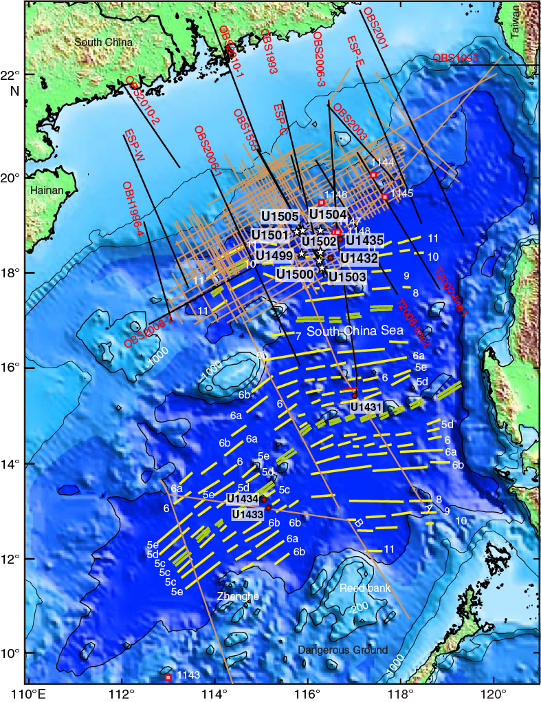
Figure F1. Seismic data coverage and magnetic anomalies.
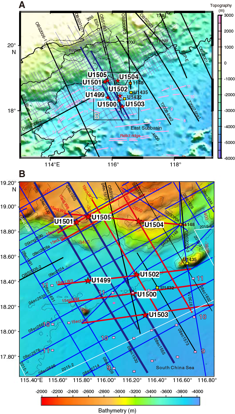
Figure F2. North SCS margin with seismic coverage.

Figure F3. TWT to basement Tg unconformity and Reflector T60.

Figure F4. Original and interpreted seismic profiles.
The primary objective at Site U1499 was to sample basement in a region of the COT where the basement composition is not known so that rifting models could be constrained. Basement at Site U1499 could have been upper or lower continental crust, exhumed mantle (serpentinized or not), or, less likely, igneous oceanic rock (e.g., basalt and gabbro). The model in Figure F5 shows the basement at Site U1499 as possibly corresponding to serpentinized lithospheric mantle, but it could also be lower continental crust or upper continental crust, depending on the rheological differences among these various units during the rifting process. Figure F6 shows that there is a broad spectrum of possible magma-poor rifted-margin structures that may form, depending on the initial rheologic structure of the extending lithosphere.
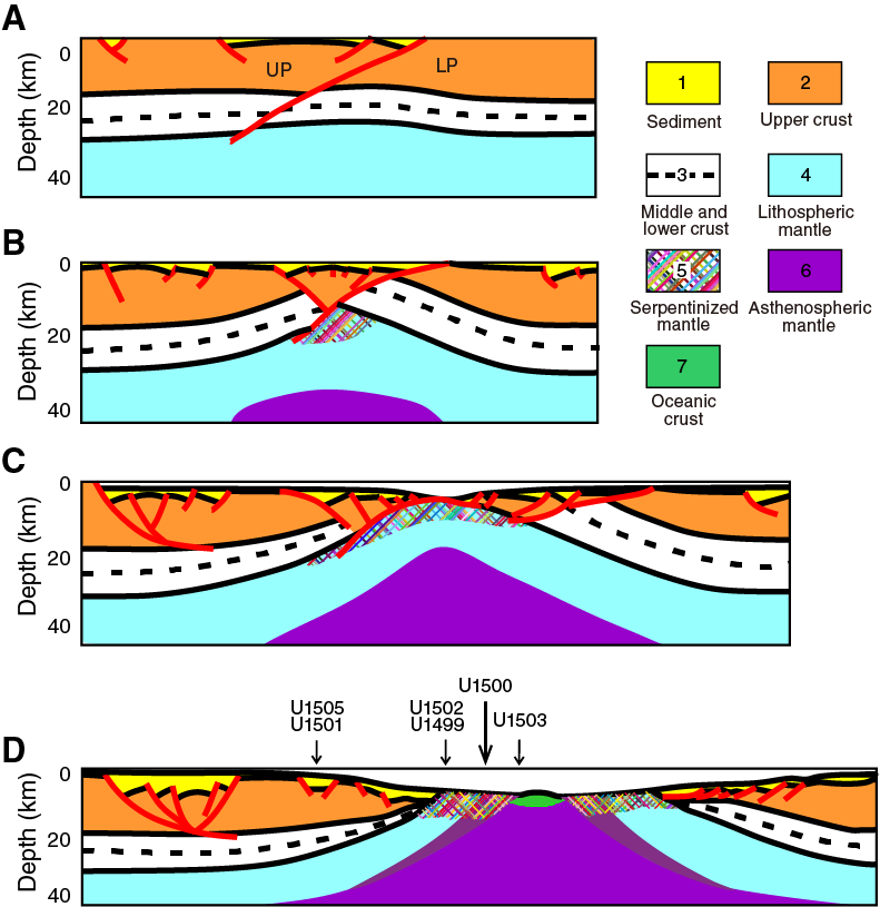
Figure F5. Schematic development of continental breakup.

Figure F6. Spectrum of possible magma-poor rifted margin models.
We expected the upper sedimentary section shallower than Unconformity T30 to be deep-marine clay, silt, or fine-grained sand based on Site 1148 data (e.g., Shipboard Scientific Party, 2000; Clift et al., 2001) and seismic stratigraphic correlation. Sediments below Unconformity T30 and above the basement reflection appear to have more sandy layers or thin interlayered sand and clay (Figure F4). On the seismic cross Line 04ec1530, some channel-like reflections are associated with the inferred sandy layers. However, the nature of the lower sedimentary section, including Paleogene synrift and possible prerift strata, is poorly constrained and may be shallow- to deep-marine rocks. Recovery of core from the lower synrift sedimentary section is important here because this constrains the timing and depositional environment of final breakup as well as the subsidence history.
Operations
We conducted operations in two holes at Site U1499. We APC/XCB cored in Hole U1499A (18°24.5698′N, 115°51.5881′E; 3760.2 m water depth) from the seafloor to 659.2 m and recovered 417.05 m of core (63%). We installed 651 m of casing in Hole U1499B (18°24.5705′N, 115°51.5990′E; 3758.1 m water depth) (Figure F7), RCB cored from 655.0 to 1081.8 m (recovering 150.64 m, or 35%), and conducted two wireline logging runs from ~65 m above the base of the hole upward to the casing. Coring summaries of Holes U1499A and U1499B are in Table T1. In this section we also document the first part of the expedition leading up to Site U1499.
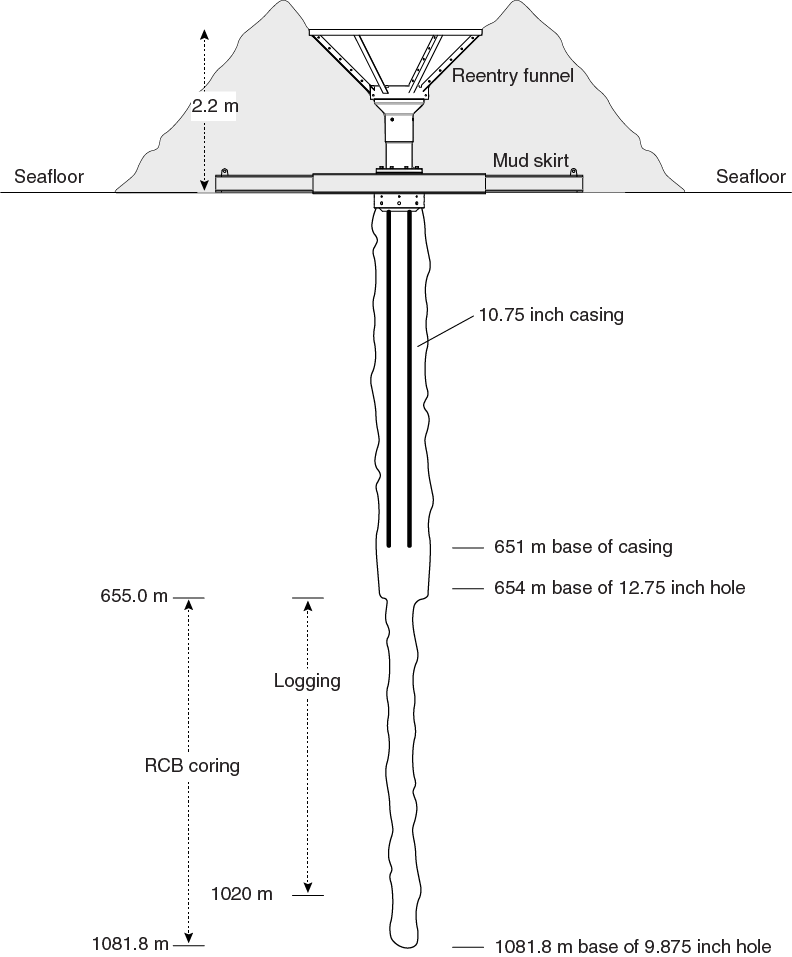
Figure F7. Reentry system and casing.
Table T1. Site U1499 core summary. View table in PDF format. Download table in CSV format.
Hong Kong port call
Expedition 367, South China Sea Rifted Margin, started at 0812 h (all times are UTC + 8 h) on 7 February 2017 with the first line ashore at the China Merchants Wharf in Hong Kong. The Co-Chief Scientists and IODP staff moved onto the ship and started crossover with their Expedition 366 counterparts. Initial loading of incoming shipments began. The Expedition 367 scientists boarded the ship on the morning of 8 February. After they got settled in their rooms, the scientists were introduced to life on board the R/V JOIDES Resolution and participated in an initial laboratory and ship safety tour. The scientists were then introduced to the information technology on board the ship and started to connect their computers to the shipboard network, and half of the science party went on a core-flow tour. Transfer of incoming and outgoing shipments continued throughout the day. Arriving sea freight was partially loaded, along with fresh and refrigerated food products and 300 metric tons of potable water. All departing freight was moved to the pier. On 9 February, the day began with introductions of the Expedition 367 scientists and JOIDES Resolution Science Operator (JRSO) shipboard staff followed by a presentation of the expedition scientific objectives by the Co-Chief Scientists. The rest of the day’s science meetings were postponed until the next day so that seven scientists could address issues with their travel documents. Major port call activities on 9 February included loading of 40 short tons of drilling mud, 987.3 metric tons of marine gas oil, sea freight, and frozen food, as well as offloading frozen shipments from the previous expedition. Because of a missed boat transfer in Shanghai, China, a shipment of essential hardware (reentry cones, casing, and mud motors) was delayed until 10 February. Because of the time required to load this essential hardware, our departure was delayed by 1 day to 13 February.
On 10 February, scientists were introduced to shipboard deliverables, met in laboratory groups with their JRSO technical staff team members, and underwent the Captain’s introduction and safety orientation. The other half of the science party went on a core-flow tour. A Texas A&M University System film crew spent the day filming some promotional videos and was escorted around the ship. In addition to routine loading/offloading, the trucks with our delayed shipment of essential hardware started arriving in the late afternoon on 10 February. After carefully calculating the remaining work, arrangements were made with the agent and immigration authorities for a departure at 1200 h on 13 February.
On 11 February, the scientists were introduced to drilling/coring/logging operations, our shipboard Educator and Journalist gave an overview of their plans for the expedition, and the Captain held the first fire and boat safety drill. In the afternoon, the scientists shared their individual research interests for the expedition with each other. Loading of essential hardware continued throughout the day, and by the end of the day all casing had been secured in the riser hold. All that remained of port call activities was to load five flats of drill pipe and final securing of cargo prior to departure.
We finished loading all remaining operations hardware on 12 February, including 288 joints of drill pipe. We also spooled new coring line onto the forward coring winch, offloaded trash prior to sailing, secured all cargo and equipment for heading out to sea, and made necessary arrangements with port authorities for departing the next day.
At 1000 h on 13 February, immigration authorities boarded the ship and cleared the vessel for departure. The harbor pilot arrived on board just before noon, and the last line was released at 1215 h on 13 February. We proceeded to the pilot station, and after a 7 nmi transit the pilot disembarked at 1248 h. Our 277 nmi transit to Site U1499 took 28.0 h with an average speed of 9.8 kt.
Hole U1499A
After arriving at Site U1499 at 1615 h on 14 February 2017, we lowered the thrusters, deployed a seafloor beacon, assembled two extra stands for RCB coring later in the expedition, put together the APC/XCB bottom-hole assembly (BHA), and lowered it to 3749.4 m below rig floor (mbrf) in preparation for coring. As each piece of the drill string was assembled, its length was measured and its interior was verified to be unobstructed. The top drive was picked up, the entire string was spaced out to place in preparation for starting coring, and a wiper pig was pumped through the drill string to clean rust and debris from the inside of the drill string. The calculated precision depth recorder (PDR) depth for the seafloor at Hole U1499A was 3774.4 mbrf; we chose to place the bit at 3769 mbrf to take the first core. An APC core barrel was lowered to the bit, and coring in Hole U1499A started at 0930 h on 15 February. Based on a mudline core recovery of 7.5 m, we calculated the seafloor to be at 3771.0 mbrf (3760.2 m below sea level [mbsl]). APC Cores 367-U1499A-1H through 18H penetrated to 162.4 m and recovered 167.51 m (103%). All APC cores used nonmagnetic core barrels and were orientated. Formation temperature measurements with the advanced piston corer temperature tool (APCT-3) were made while taking Cores 4H, 6H, 8H, 10H, 12H, and 14H.
APC Cores 12H through 18H (102.5–162.4 m) encountered increasingly firm formation, and the core barrel did not fully penetrate the formation for many of them. Because of our primary expedition objectives, we switched to XCB coring instead of first using the half-length APC (HLAPC) system, which would have taken twice as long to penetrate the formation.
XCB Cores 19X through 57X penetrated from 162.4 to 540.7 m and recovered 227.37 m (60%). XCB core recovery was highly bimodal. We had quite high core recovery in the fine-grained intervals (Cores 19X through 36X from 162.4 to 337.0 m with 158.99 m recovered [91%] and Cores 44X through 50X from 404.9 to 472.8 m with 65.19 m recovered [96%]). We had very fast penetration rates and extremely low recovery in unconsolidated sands (Cores 37X through 43X from 337.0 to 404.9 m with 1.37 m recovered [2%] and Cores 51X through 57X from 472.8 to 540.7 m with 1.82 m recovered [3%]). One exception was Core 25X, which came back with only 2 cm of core, but the core liner appeared to have had sediment in it, so we inferred that the sediment was fine grained and that it fell out of the core barrel while it was being retrieved.
Once we encountered unconsolidated sand, we started circulating mud sweeps (30 bbl at 337.0, 346.7, 375.8, 404.9, 443.7, 472.8, 492.2, 511.6, and 531.0 m). While making a connection at 492.2 m, the drill string became stuck and could not be rotated. We circulated an additional 50 bbl of mud, were able to regain rotation, and resumed XCB coring in Hole U1499A. Cores 58X through 67X penetrated from 540.7 to 637.7 m (20.37 m recovered; 21%). For the first eight cores (58X through 65X), the bit penetrated very quickly through 77.6 m and recovered only 4.16 m (5%), so we inferred that the sediment is predominantly unconsolidated sand. Core 66X had slower penetration and 100% recovery in the finer grained formation. However, the penetration rate increased again in Core 67X, indicating that we had encountered sand again. The last core on 19 February (Core 68X) also cut very quickly and had almost arrived back on the rig floor (~100 mbrf) when the low-clutch diaphragm in the drawworks failed at 2245 h; we could not raise the drill string. We secured the drill string and circulated, rotated, and pumped a mud sweep every hour to keep the drill string from getting stuck while repairing the ruptured diaphragm. After the 24.5 h it took to repair the drawworks, we were finally able to open the drill string and get Core 68X out of it at 2320 h on 20 February. We had suspected it would be empty because it cored very quickly through inferred sand, but it also had been sitting in the drill string for a full day. Although coring recovery was quite variable, we were very close to XCB coring refusal, and the finer grained formation we did recover was getting quite hard, we wanted to penetrate a few more cores to verify an appropriate formation to set the base of the casing to be deployed in our next hole (firm formation, not sand).
Cores 69X through 71X penetrated quite slowly from 647.4 to 659.2 m and recovered 1.8 m of hard sedimentary rock; we decided this was an appropriate interval for the base of the casing. The driller then circulated the entire hole with mud to minimize risks of hole problems as we pulled the drill string out of the hole. We started pulling the drill string out of Hole U1499A at 0815 h on 21 February. We kept the top drive installed until the bit was at 299 m, above the uppermost interval of unconsolidated sand. The bit cleared the seafloor at 1230 h on 21 February and arrived on the rig floor at 2015 h, ending Hole U1499A. APC/XCB coring in Hole U1499A penetrated 659.2 m. As mentioned above, core recovery was highly variable (formation dependent), and core recovery totaled 417.05 m (63%). We suspect that unconsolidated sand accounted for the poor recovery. The overall drilling, coring, and formation information from Hole U1499A was used for planning the casing installation for the second hole to achieve our deep-coring and logging objectives.
Hole U1499B
We offset the ship 20 m east of Hole U1499A and conducted required routine rig servicing (drill line slip and cut). At 2345 h on 21 February 2017, we started preparing the rig floor for assembling the reentry cone and 651 m long casing to be drilled into the seafloor in Hole U1499B.
We spent all of 22 February and the first part of 23 February assembling the 10.75 inch casing and the drill string we would use to drill it into the seafloor. This included
- Moving the mud skirt over the moonpool;
- Assembling 651 m of 10.75 inch casing, lowering it through, and latching it into the mud skirt; and
- Assembling a 9.875 inch tricone bit, underreamer set to 12.75 inches, and mud motor and lowering them through the casing hung off in the moonpool.
At 0430 h on 23 February, we finished putting together the final parts of the drilling assembly. This included attaching the upper part of the casing running tool (which contains the hydraulic release tool [HRT]) and attaching the reentry funnel. We started lowering the entire 651 m long casing string and drilling assembly to the seafloor and deployed the camera system at 1115 h on 23 February to monitor the reentry funnel while the casing was being drilled into the seafloor. When the pilot bit that extends 2.71 m below the casing shoe was just above the seafloor, the drillers measured the pressures at various pump rates to get information to compare to measurements when we would start penetrating the formation. Drilling in Hole U1499B started at 1535 h on 23 February. While drilling the casing into the seafloor, we circulated 25 bbl mud sweeps at 152.6, 327.8, 356.98, 493.1, and 619.8 m. We continued to drill the casing into the seafloor until the mud skirt landed on the seafloor.
We deployed the go-devil to activate the casing running tool, which released the casing at 2300 h on 24 February. We retrieved the entire drilling assembly, with the bit clearing the seafloor at 0230 h on 25 February, and the bit arrived back on the rig floor at 1230 h on 25 February. After taking apart the drilling assembly and flushing the mud motor, underreamer, and bit with freshwater, we began preparing the rig floor for RCB coring. We started assembling the RCB BHA at 1430 h on 25 February, and the rest of the day was spent lowering it to the seafloor. At 2230 h on 25 February, the subsea camera was deployed. Once the RCB bit and camera reached the seafloor, we started searching for the Hole U1499B reentry funnel at 0215 h on 26 February. After we were unable to find it relatively quickly (as is usual), we initiated an expanding 5 m grid search. After just over 6 h, we eventually found the reentry funnel cone. It was clearly visible inside a small crater of sediment located about half-way (~10 m) back toward and a little south of Hole U1499A to the west. Also, the top of the reentry funnel appeared to be close to level with the top of the cuttings pile. After only 10 min of maneuvering, we reentered Hole U1499B at 0825 h on 26 February, started lowering the RCB bit down through the casing, and recovered the camera system. As the bit was being lowered, it encountered sediment inside the casing at 571 m, 80 m above the casing shoe. This sediment was assumed to be sand that entered the casing as the drilling stinger assembly (with pilot bit, underreamer, and mud motor), used to drill the casing in, was withdrawn from the casing. We picked up the top drive, deployed a core barrel at 1230 h, and washed back to the bottom of the hole at 655 m (4 m below the base of the casing). We circulated 30 bbl of mud, retrieved the core barrel (empty), and started RCB coring in Hole U1499B at 2230 h on 26 February.
On 27 February, RCB coring in Hole U1499B penetrated from 655.0 to 790.8 m with an overall recovery of 41.44 m (Cores 367-U1499B-2R through 15R; 31%). However, recovery continued to be highly variable and formation dependent. In fine-grained intervals, we had higher recovery (53%) and steady, relatively slow penetration rates (Cores 2R through 3R from 655.0 to 674.4 m, Cores 9R through 10R from 722.9 to 742.3 m, and Cores 13R through 15R from 752.0 to 790.8 m). In other intervals, inferred to consist of loosely consolidated coarse-grained sand, we had very low recovery (0.7%) and very quick penetration rates. The drillers noted these intervals at 672.9–727.6 and 739.3–759.7 m, which correspond mostly with Cores 4R through 8R (674.4–722.0 m) and 11R (742.3–752.0 m). We circulated 30 bbl mud sweeps at 684.1, 713.2, 742.3, 761.7, and 781.1 m. At first light on 27 February, a boat (M/V Taikoo) with critical spares for the drawworks clutch arrived on site, and the transfer was completed.
We continued RCB coring from 790.8 to 897.5 m (Cores 16R through 26R; 72.33 m recovered; 68%) and circulated 30 bbl mud sweeps at 810.2, 839.3, and 878.1 m. Each of these cores (16R through 26R) took from 20 to 60 min to cut. Another fast-drilling zone from 825.0 to 834.0 m was also noted by the drillers. After Core 26R, however, we encountered a substantial formation when Core 27R took over 2 h (205 min) to cut. RCB Cores 27R through 29R continued in very hard formation. These cores took 120–205 min to cut, penetrated 29.1 m from 897.5 to 926.6 m, and recovered 16.43 m (56%). However, Core 30R took only 45 min to cut (as opposed to 205, 130, and 120 min for the cores just above). In addition, when the bit was being raised off bottom to recover the core, the drill string became stuck momentarily, so we circulated 30 bbl of mud, and hole conditions improved. The penetration time for Core 31R went back up (130 min), but the drill string became temporarily stuck again. This time we circulated 90 bbl of mud and were able to continue coring.
RCB Cores 31R through 38R penetrated 77.6 m from 936.3 to 1013.9 m and recovered 8.66 m (11%). It took from 2 to >3 h to cut each core. The drill string became stuck momentarily while cutting Core 33R. We circulated 30 bbl of mud after cutting Cores 32R and 35R through 37R.
Because we decided to stop coring to change the RCB bit to core deeper and the bit had accumulated 40.6 rotating hours, we circulated the cuttings out of the hole with 70 bbl of mud after Core 38R. Before pulling the bit up into the casing and out of the hole, we first raised the bit up to 780 m, circulated the hole with 35 bbl of mud, and then filled the uncased (open) part of the hole with 235 bbl of heavy mud (11.0 lb/gal; barite). This process was intended to help stabilize the hole while we changed the bit and to reduce the amount of fill we might encounter when we reentered the hole to resume RCB coring. It was also expected to give us some indication of the hole conditions we might encounter for planned downhole logging after coring had finished. Because we had some challenges locating the hole the first time we reentered, we lowered the subsea camera system to observe the reentry funnel as we pulled the bit out of the hole. While we were still in the hole, we could see the drill pipe clearly in the center of the crater created by the cuttings mound. Although the reentry funnel’s concentric black and white stripes were not visible, we didn’t anticipate problems finding and reentering the hole. The bit was pulled out of the hole at 1655 h on 3 March, and we spent the rest of the day recovering the drill string (except for a 0.5 h repair of the pipe racker).
We finished recovering the drill string at 0215 h on 4 March, attached a new RCB bit (C-7), lowered it to the seafloor, and then deployed the subsea camera system at 0915 h. We paused rig floor operations from 0915 to 1045 h to conduct required routine rig servicing (drill line slip and cut) before we resumed lowering the drill bit to the seafloor. At 1345 h on 4 March, the bit and camera were in position, and we were able to immediately see the reentry funnel in the center of the cuttings pile caldera. It took us 22 min to position the bit over the funnel and reenter Hole U1499B at 1407 h on 4 March. We retrieved the camera and lowered the bit down through the 651 m of casing to 848.1 m in the open hole. We installed the top drive and circulated/rotated to 987 m, only ~27 m from the bottom of the hole, before the bit encountered any resistance. This resistance was easily penetrated, and we only encountered 1 m of fill on the bottom of the hole. At the end of the day, we pumped 40 bbl of mud to clear cuttings from the hole and retrieved the core barrel that was in place while getting back to the bottom of the hole. We resumed RCB coring from 1013.9 m at 0115 h on 5 March. Cores 39R through 43R penetrated from 1013.9 to 1062.4 m and recovered 4.1 m (4%). We pumped 30 bbl of mud after each of these cores.
At 0100 h on 6 March, Core 44R arrived on the rig floor (1062.4–1072.1 m; 0.45 m recovered; 5%), and we dropped the next core barrel to start cutting Core 45R. While this core was being cut, there were periods of erratic torque and high pump pressure, as well as some short times when the drill string could not be rotated. The driller raised and lowered the drill string and was able to keep coring. Just after we put the core line into the drill string to retrieve Core 45R, the pipe became stuck. For ~45 min, we worked the drill string until it was freed at 0615 h on 6 March. We then removed the core line from the drill string. We raised the bit back up to 994 m and worked to clean out the hole. Eventually at 1045 h, conditions had improved enough that we retrieved Core 45R at 1150 h (1072.1–1081.8 m; 0.09 m recovered; 0.9%). We spent the next 9 h attempting to wash, ream, drill, and circulate our way back to bottom. However, we never were able to get below ~1053 m (~30 m above the bottom of the hole) without the drill string getting stuck. At 2045 h on 6 March, we decided that further attempts to get back to the bottom of the hole and core deeper were not reasonable, so we started to prepare the hole for wireline logging. We circulated 50 bbl of mud to clean cuttings out of the hole, retrieved the core (wash) barrel that was in place during the hole remediation efforts, and lowered the rotary shifting tool on the coring line to release the bit in the hole.
After the bit was released in the bottom of the hole at 0000 h on 7 March, we raised the end of the pipe from 1052.7 to 877.3 m and shifted the mechanical bit release sleeve back into the circulating position. We then raised the end of the pipe to 780 m and pumped 235 bbl of heavy mud into the hole to help maintain good hole conditions for logging. By 1030 h on 7 March, we had raised the end of pipe back inside the casing to 85.1 m and started to prepare the rig floor for logging. Our first logging tool string consisted of the resistivity, velocity, density, and NGR tools. We started lowering it at 1345 h on 7 March. The tool string was able to reach 1020 m, and we successfully logged from that depth up to the base of the casing at 651 m. Log data were also collected up the casing and drill pipe to the seafloor. The tool string arrived back at the rig floor at 2215 h on 7 March. Based on the first logging run results, we decided to conduct a second logging run with the FMS and NGR tools.
We assembled the FMS and NGR tools and started lowering them at 0130 h on 8 March. The tool string was able to reach 1010 m, and we were able to make two passes of the open hole up to the base of the casing at 651 m. Initial results showed that we collected some excellent data in intervals with good borehole diameter. The tool string arrived back on the rig floor at 0925 h, and all of the logging equipment was off the rig floor at 1030 h on 8 March. We pulled the end of the drill string out of Hole U1499B at 1120 h, recovered the seafloor beacon, and started the transit to Site U1500 in dynamic positioning mode just before 1300 h on 8 March. While in transit, we continued to recover the drill string (arrived back on the rig floor at 1830 h on 8 March) and assembled a new RCB bit and started lowering it to the seafloor. We spent a total of 22.1 days at Site U1499.
Lithostratigraphy
We defined nine lithostratigraphic units at Site U1499 based on visual core description, smear slide and thin section inspection, physical property measurements (e.g., magnetic susceptibility and color spectra), geochemistry data, and X-ray diffraction (XRD) (see Lithostratigraphy and Physical properties in the Expedition 367/368 methods chapter [Sun et al., 2018]). We constructed a composite lithostratigraphy by combining data from Holes U1499A and U1499B (Figure F8). The lithostratigraphy for all of Site U1499 is divided into three dominant lithologic sections. The dominant lithologies in the upper part of the stratigraphy (Units I−VII) are composed of clay, clayey silt, silty sand, claystone, sandstone, and calcareous ooze with minor intervals of volcanic ash. The second dominant lithologic section consists of dark brown to reddish brown claystone in Unit VIII. The lower part of the stratigraphy (Unit IX) marks the third main lithologic section and contains gravelly sandstone, matrix supported breccia, and gravel. The transition from Unit VIII to Unit IX (the lowermost unit) is marked by a stark change from manganese nodule–bearing reddish brown chalk to matrix-supported breccia and gravel.
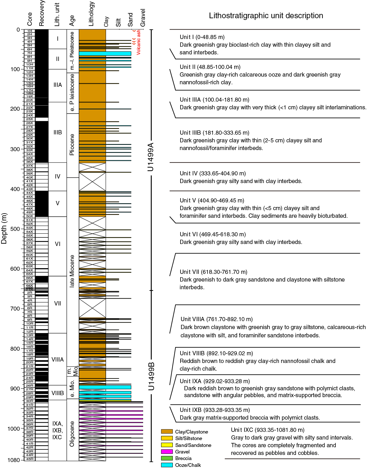
Figure F8. Lithostratigraphic summary.
Unit I is composed of dark greenish gray bioclast-rich clay with thin clayey silt and sand interbeds. Unit II contains interbedded greenish gray clay-rich calcareous ooze and dark greenish gray nannofossil-rich clay. Unit III contains dark greenish gray clay with very thick (<1 cm) clayey silt interlaminations in the upper part (Subunit IIIA) and thin (2−5 cm) clayey silt and nannofossil/foraminifer interbeds in the lower part (Subunit IIIB). Unit IV is dominated by dark greenish gray silty sand with clay interbeds. Recovery was very low in this unit, but limited recovery in core catcher samples, fast drilling penetration rates, and seismic reflection data suggest that the unrecovered sections are primarily composed of loose sand. Unit V is composed of dark greenish gray clay with thin (<5 cm) clayey silt and foraminifer sand interbeds. Unit VI contains dark greenish gray silty sand with clay interbeds but has limited recovery. Similar to Unit IV, we infer that the low-recovery sections in Unit VI are composed of loose sand. Unit VII is composed mainly of dark greenish gray to dark gray sandstone and claystone with siltstone interbeds. Lithification increases sharply downhole from the top of this unit, although sections with very low recovery are assumed to be primarily composed of nonlithified sand.
Unit VIII comprises two subunits. Subunit VIIIA contains dark brown claystone with greenish gray to gray siltstone, calcareous-rich claystone with silt, and foraminifer sandstone interbeds in the upper part. Subunit VIIIB contains reddish brown to reddish gray clay-rich nannofossil chalk. Unit IX comprises three subunits, predominately composed of polymict breccia and gravel. Subunit IXA is defined by dark reddish brown to greenish gray sandstone and breccia and Subunit IXB is defined by dark gray matrix-supported breccia in Core 367-U1499B-30R. Subunit IXC contains gray to dark gray gravel with silty sand intervals. The cores in Subunit IXC are completely fragmented and recovered as pebbles and cobbles. Unit boundaries are also recognized in magnetic susceptibility, color reflectance spectroscopy, and bulk mineralogy compositions (Figures F9, F10).
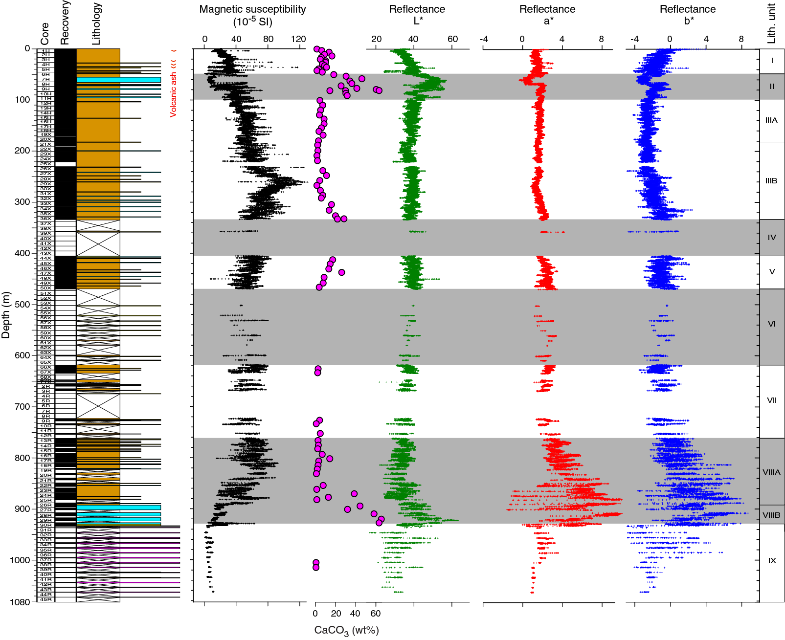
Figure F9. Correlation of lithostratigraphic units.
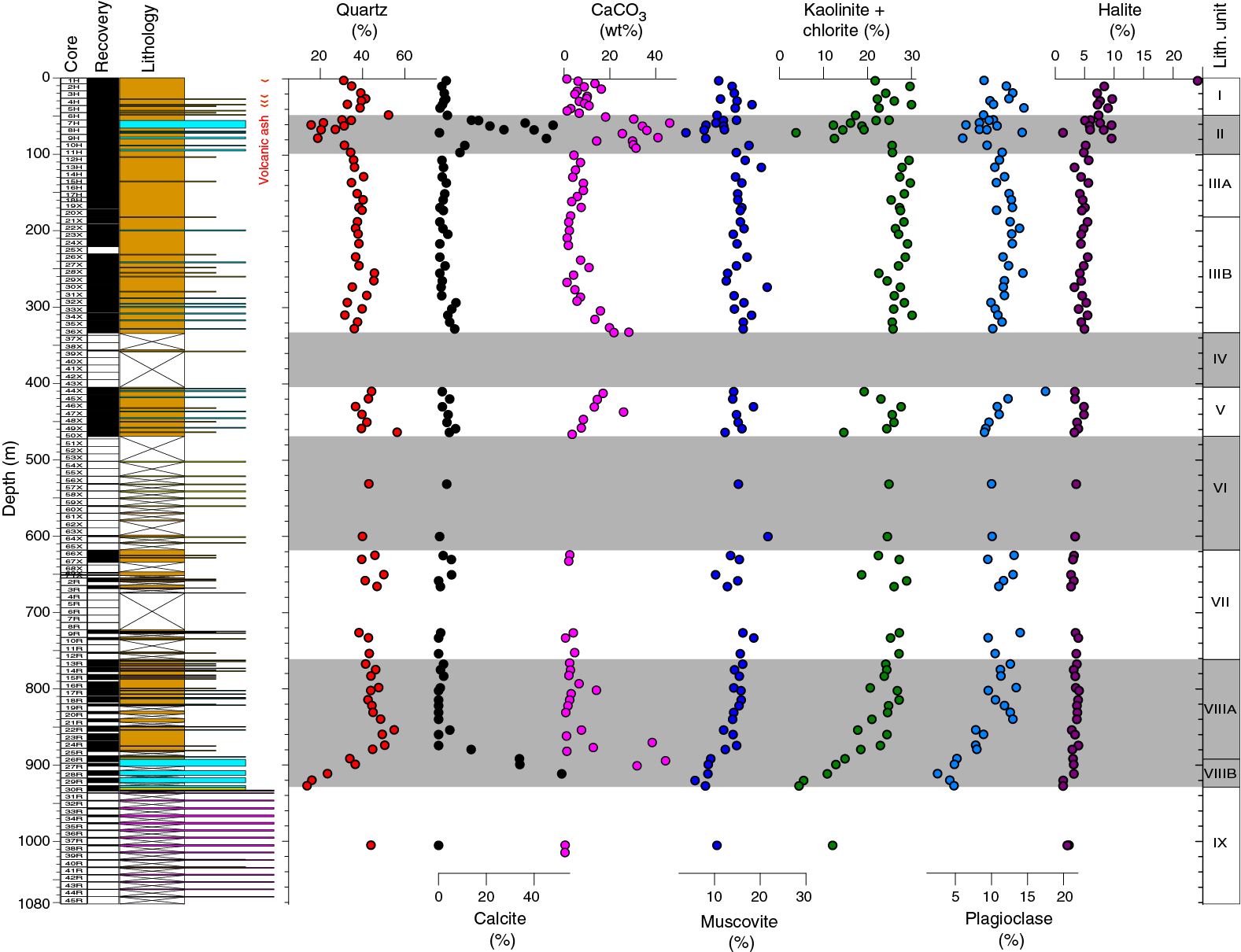
Figure F10. Bulk mineralogy by XRD.
Unit descriptions
Unit I
Unit I spans the uppermost 48.85 m and is dominated by a sequence comprising dark greenish gray bioclast-rich clay with thin clayey silt and sand interbeds. The clay is generally massive and homogeneous, sometimes marked by faint color banding of more intense green against the background of greenish gray. Most of the clay intervals have heavy bioturbation. Some light-colored intervals have higher biogenic content, mostly including foraminifer, nannofossil, diatom, and radiolarian particles (Figure F11). A distinct oxidized layer (dark yellowish brown) occurs in the top of this unit. The silt and fine sand layers, varying from 2−5 to 15−20 cm in thickness, occur as dark greenish gray interbeds within a finer grained primary lithology. We interpret these graded, fining-upward cycles as distal turbidite sequences. At the base of each coarse-grained bed is a sharp erosive contact between the overlying silty and fine sand layer and the underlying clay layer. Fine to medium sand layers can be occasionally as thick as 50−70 cm in Cores 4H, 5H, and 6H. The erosive base of a medium-grained sand interval in Section 6H-7 marks the boundary between Units I and II.

Figure F11. Dark greenish gray bioclast-rich clay.
Unit I has four thin volcanic ash layers (2−6 cm thick) that are not present in any other unit. They occur in Cores 1H, 3H, 4H, and 5H. The ash layers are pale brown and comprise unaltered pumice and ash shards (Figure F12B). This unit is characterized by relatively low magnetic susceptibility (<40 × 10−5 SI) but with several abrupt peaks (>100 × 10−5 SI) that correspond to the ash layers (Figures F9, F12A). However, the magnetic susceptibility data are not density-normalized, which can cause artificially low values in shallower intervals because of low degrees of sediment compaction. Bulk light reflectance (L*) slightly increases downhole, whereas b* (blue) slightly decreases, suggesting gradually decreasing sediment oxidation. The bulk mineralogy of this unit, measured by XRD, consists mainly of quartz (31%–52%), plagioclase (9%−15%), muscovite (11%−18%), kaolinite + chlorite (17%−30%), and halite (7%−24%) (Figure F10). Mineralogy does not vary strongly with depth, except in the uppermost sample, which has the highest halite concentration (24%) as a result of high seawater content (Table T2).
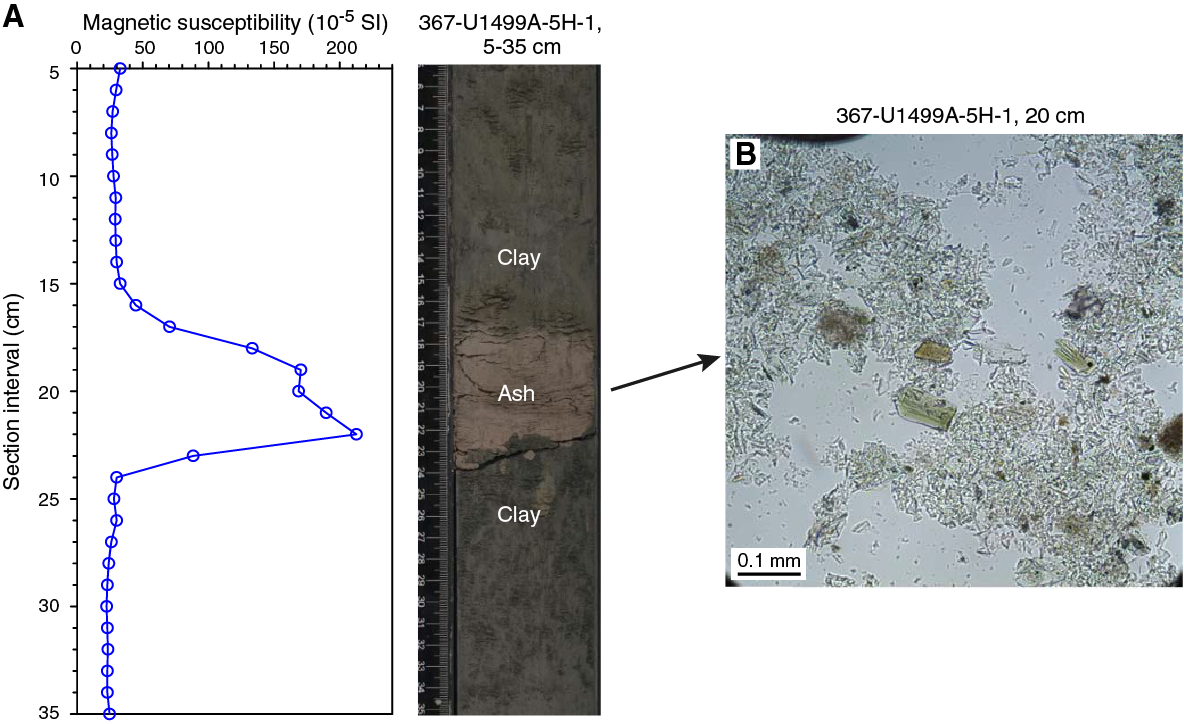
Figure F12. Pale brownish volcanic ash layer.
Table T2. Mineral percentages. View table in PDF format. Download table in CSV format.
Unit II
- Interval: 367-U1499A-6H-3, 35 cm, to 11H-5, 104 cm
- Depth: 48.85−100.04 m
- Age: early−middle Pleistocene
Unit II is composed of alternating greenish gray clay-rich calcareous ooze and dark greenish gray nannofossil-rich clay. The two colors usually form alternating bands with gradational contacts. Sand-sized foraminifers and clay-sized nannofossils are common in both calcareous ooze and clay intervals (Figure F13). Foraminifer grains are observable on the core surface and are usually more abundant in light greenish gray intervals. Very thin beds (<3 cm thick) of dark gray sandy silt occur occasionally in the nannofossil-rich clay layers.
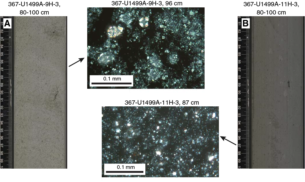
Figure F13. Greenish gray clay-rich calcareous ooze.
This unit has erosive upper and lower contacts (Figure F31A). The dark greenish gray medium-grained sand of Unit I in Core 6H overlies Unit II, and the dark greenish gray clay of Unit III in Core 11H underlies it. Intervals in Unit II, especially in Cores 6H, 8H, 10H, and 11H, exhibit synsedimentary deformation with distinct folds, faults, and inclined bedding (Figures F14, F15). Based on the erosive contacts and deformation structures, we interpret this unit as a slump deposit. The age of foraminifers and nannofossils preserved in the ooze and clay layers are mainly Pliocene (see Biostratigraphy), which is older than the underlying Pleistocene sediments of Unit III, further supporting the slump deposit interpretation.
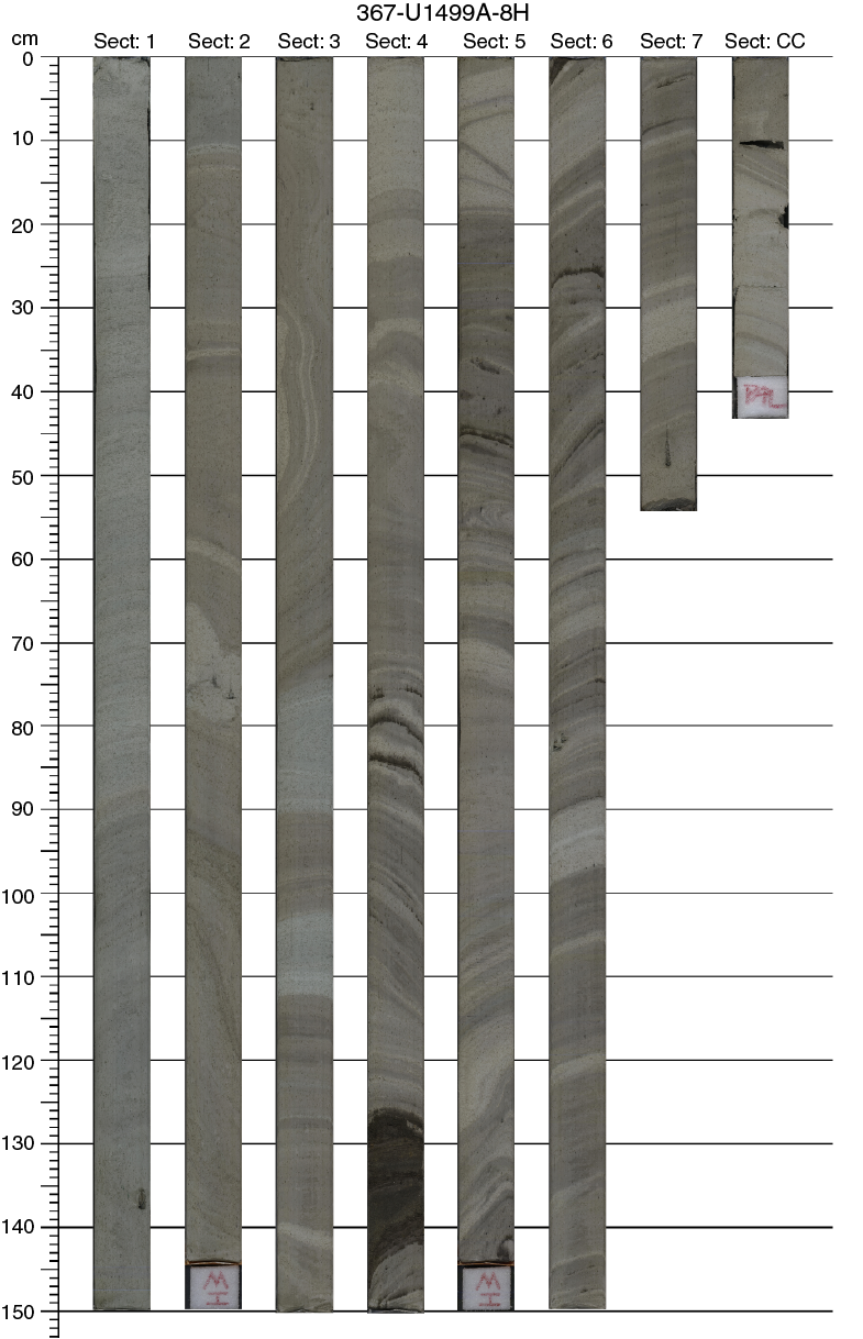
Figure F14. Synsedimentary deformation.
Figure F15. Representative section of clay with silt interbeds.
Greenish gray clay-rich calcareous ooze layers (mainly in Core 7H) in Unit II exhibit very low magnetic susceptibility (~10 × 10−5 SI), high bulk reflectance, and low a* (red) (Figure F9). These layers correlate to high carbonate content (30−45 wt%) and calcite abundance (20%−48%) (Figure F10). Accordingly, quartz (15%−35%), plagioclase (7%−11%), muscovite (8%−12%), and kaolinite + chlorite (14%−22%) concentrations largely decrease through dilution by high calcite content.
Unit III
- Interval: 367-U1499A-11H-5, 104 cm, to 36X-CC, 30 cm
- Depth: 100.04−333.65 m
- Age: middle Pleistocene−Pliocene
Unit III contains dark greenish gray clay with thick laminations, very thin beds of clayey silt, and calcareous-rich intervals. This unit is divided into two subunits based on relative thickness and recurrence of silt interbeds and abundance of calcareous-rich intervals. Subunit IIIA contains thick laminations of clayey silt (<1 cm), whereas Subunit IIIB has abundant thin beds (2−5 cm) of clayey silt and increased occurrence of nannofossil- or foraminifer-rich intervals.
Subunit IIIA
- Interval: 367-U1499A-11H-5, 104 cm, to 21X-1, 0 cm
- Depth: 100.04−181.80 m
- Age: early−middle Pleistocene
The dominant lithology of Subunit IIIA is greenish gray and dark gray clay, with thick (<1 cm) clayey silt interlaminations. The silt interlaminations generally occur every 20−50 cm and have erosive bases (Figure F15). We interpret the recurring silt interbeds fining upward into clays as distal turbidites. At one interval in the subunit (15H-3, 141−145 cm), the coarser interbed contains foraminiferal silty sand, but presence of other biogenic material is low in the rest of the subunit. Correspondingly, no distinct bioturbation was observed.
Color reflectance, magnetic susceptibility, and mineralogy remain fairly constant throughout Subunit IIIA (Figures F9, F10). The dominant mineralogical components are quartz (35%−40%) and kaolinite + chlorite (25%−30%), whereas calcite content is low (<8 wt%).
In Subunit IIIA, we transitioned from APC to XCB coring (at 162.4 m), which led to increased drilling disturbance starting at Core 19X. Presence of drilling biscuits increased at Core 21X.
Subunit IIIB
- Interval: 367-U1499A-21X-1, 0 cm, to 36X-CC, 30 cm
- Depth: 181.80−333.65 m
- Age: early Pleistocene−Pliocene
Subunit IIIB is a thick interval of primarily dark greenish gray clay with thin (2−5 cm) clayey silt and nannofossil/foraminifer-rich interbeds. Although clay is the dominant grain size in both subunits, Subunit IIIB contains more calcareous bioclasts and bioturbation than Subunit IIIA (Figure F16). Similar to Subunit IIIA, the coarser grained interbeds have erosive bases and fining-upward sequences, implying deposition by turbidity currents.
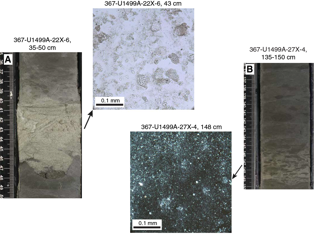
Figure F16. Increased carbonate content and bioturbation.
Magnetic susceptibility increases downhole from values near 45−50 × 10−5 SI at the top of the subunit to a peak interval of 120 × 10−5 SI in Section 28X-6 (Figure F9). Values then decrease back to the 40−50 × 10−5 SI range at the bottom of the subunit. Carbonate content also varies downhole, with concentration increasing from <2 wt% in Section 21X-4 to 28 wt% in Section 36X-4. The steepest increase of carbonate content occurs in Cores 30X through 36X. Despite this change in composition, color reflectance data remain mostly invariant throughout Subunit IIIB. XRD analysis of Subunit IIIB shows similar mineralogy to Subunit IIIA (Figure F10). The dominant components of the clays are quartz (32%–46%) and kaolinite + chlorite (23%–30%), both of which decrease slightly as carbonate increases.
Unit IV
- Interval: 367-U1499A-36X-CC, 30 cm, to 44X-1, 0 cm
- Depth: 333.65−404.90 m
- Age: early Pliocene−late Miocene
Recovery in Unit IV is very low (2%). Most lithostratigraphic information comes from Core 39X, which had 12% recovery of dark greenish gray clay and silty sand. Because of poor recovery, fast drilling penetration rates, and seismic reflection data, we infer most of this unit to contain unconsolidated sand similar to that found in the Section 39X-CC. Because of low recovery, we have no measurements of sediment composition from this unit (XRD and carbonate) and limited magnetic susceptibility and color reflectance data (Figure F9).
Unit V
Higher recovery resumed in Core 44X, and the primary lithologies of Unit V are similar to those of Subunit IIIB. The dominant component is dark greenish gray clay with mostly thin (<5 cm) clayey silt and foraminifer sand interbeds. However, some coarser foraminifer sand intervals are much thicker (e.g., interval 48X-5, 18−54 cm; Figure F17). Clay sediments are heavily bioturbated. Drilling disturbance, in the form of biscuiting, increases significantly in this unit.
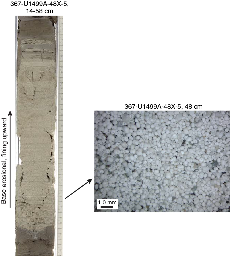
Figure F17. Thick interval of well-sorted foraminiferal sand.
Carbonate content and magnetic susceptibility both decrease downhole, whereas color reflectance data stay within a narrow range (Figure F9). XRD analysis shows concentrations of quartz from 37% to 56% with kaolinite + chlorite between 15% and 28% (Figure F10). Plagioclase contents decrease downhole from 18% to 9%.
Unit VI
Recovery in Unit VI was very low (0%–20%). Similar to Unit IV, the fast rates of drilling penetration, seismic reflection data, and recovered sand intervals in the core catchers of Cores 57X, 60X, and 64X imply that this unit predominantly consists of unconsolidated sand. The recovered intervals include dark greenish gray fine- to medium-grained sand (Figure F18) interbedded with clay and foraminifer-rich intervals.

Figure F18. Unconsolidated medium-grained sands.
Limited measurements of magnetic susceptibility and color reflectance do not show distinct differences from the previous unit (Figure F9). The major minerals include quartz (average = 41%), kaolinite + chlorite (25%), muscovite (18%), and plagioclase (10%) (Figure F10).
Unit VII
- Intervals: 367-U1499A-66X-1, 0 cm, to 71X-CC, 26 cm; 367-U1499B-2R-1, 0 cm, to 13R-1, 0 cm
- Depths: Hole U1499A = 618.30−659.20 m; Hole U1499B = 655.00−761.70 m
- Age: late Miocene
Unit VII comprises dark greenish gray to dark gray sandstone and claystone with siltstone and foraminifer sandstone interbeds. This unit was recovered in the lower part of Hole U1499A and the upper part of Hole U1499B (Figure F8). Lithification increases sharply downhole, although sections with very low recovery are assumed to be primarily composed of nonlithified sand. The recovered siltstone and sandstone layers are generally 3−10 cm thick, have erosive bases, contain parallel laminations, and fine upward into fine-grained claystone intervals (Figure F19). Thus, we interpret these intervals as turbidite sequences. Dark greenish gray sandstone intervals usually contain abundant biogenic carbonate clasts and blue-green material that we infer to be a result of alteration from sulfide-rich fluids based on the increased presence of authigenic pyrite near these zones. The claystone is mostly heavily bioturbated with distinctive trace fossils (e.g., Zoophycos and Planolites).
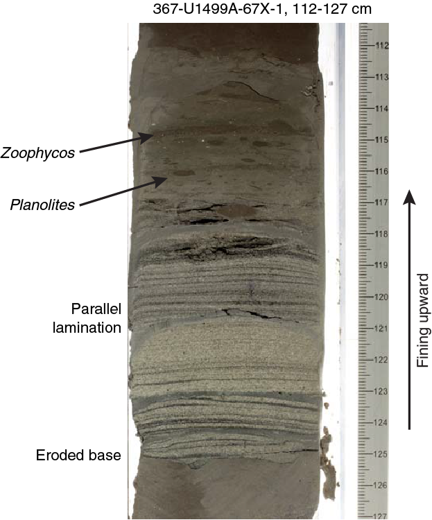
Figure F19. Foraminifer siltstone layer.
Measurements of magnetic susceptibility, color reflectance, and bulk mineralogy are fairly consistent downhole (Figures F9, F10). Quartz (38%−46%), kaolinite + chlorite (18%−27%), muscovite (10%−19%), and plagioclase (10%−14%) dominate the mineralogy.
Unit VIII
In Unit VIII, the sediments become lithified, although the transition between well-consolidated and fully lithified sediments is not clear. The unit primarily includes dark brown claystone and reddish brown to reddish gray clay-rich nannofossil chalk. Based on the abundance of calcareous material, we divided this unit into two subunits. Subunit VIIIA contains dark brown claystone with siltstone and foraminifer sandstone interbeds, whereas Subunit VIIIB comprises reddish brown to reddish gray clay-rich nannofossil chalk and clay-rich chalk.
Subunit VIIIA
Subunit VIIIA is characterized by dark brown claystone with greenish gray to gray siltstone, calcareous-rich claystone with silt, and foraminifer sandstone interbeds. The top of the subunit, in Section 13R-1, marks the first occurrence of dark brown claystone. The color gradually becomes lighter from dark brown to reddish brown downhole, and the siltstone interbeds occur less frequently (Figure F20). The color and minor lithology transition happens in Cores 20R and 21R. Gray, thin (<10 cm) interbeds of foraminifer silty sandstone occur frequently in the upper part of this subunit and usually have an erosive base, parallel laminations, and fining-upward bed forms. The reddish brown claystone is usually massive with moderate bioturbation, and abundant calcareous grains are observable in smear slides. Some thin to medium-thick green intervals occur in the sections of reddish brown claystone in the lower part of this subunit, and green alteration halos around foraminifer tests are common in the reddish brown clay intervals. The green intervals and alteration halos are interpreted as a diagenetic response of formation of glauconite or other secondary minerals.
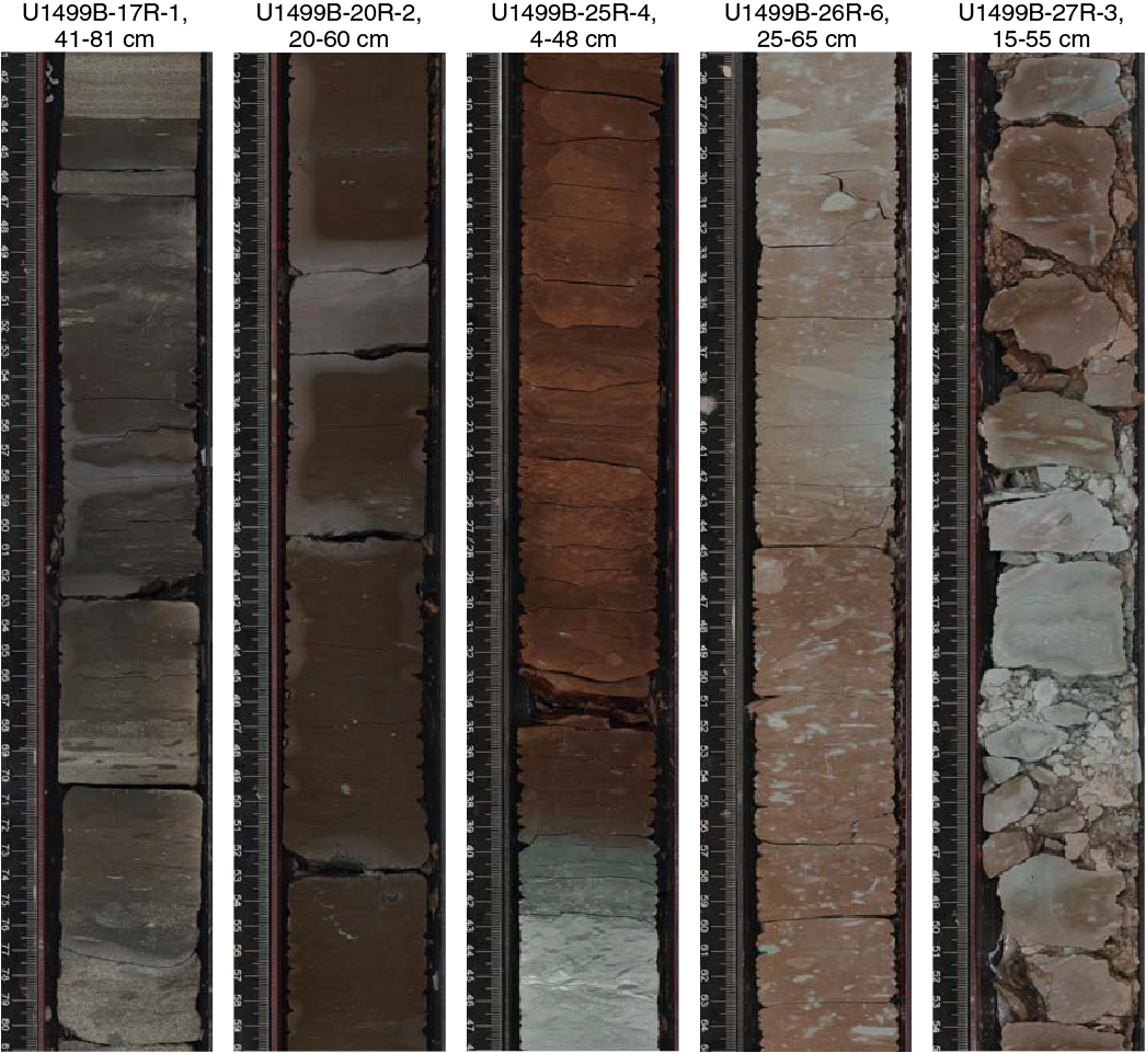
Figure F20. Lithology and color change.
Magnetic susceptibility values are relatively high (60 × 10−5 SI) in the upper part of this subunit and rapidly decrease along with the minor lithology change in Cores 20R and 21R (Figure F9). Reflectance parameters a* and b* generally increase toward the lower portion of the subunit. Accordingly, the majority of mineralogical components also change downhole in this subunit, showing a decrease in plagioclase, kaolinite + chlorite, and muscovite and an increase in quartz (Figure F10).
Subunit VIIIB
Subunit VIIIB features pelagic reddish brown to reddish gray clay-rich nannofossil chalk and clay-rich chalk. The transition from overlying dark brown claystone (Subunit VIIIA) to underlying reddish clay-rich chalk (Subunit VIIIB) is gradual and occurs in the middle of Core 26R. The reddish brown nannofossil chalk is massive with moderate bioturbation. Greenish gray alteration or diagenesis occurs within discrete intervals or as small halos around individual bioclasts (foraminifer tests), fractures, and bioturbated lenses (Figure F21).
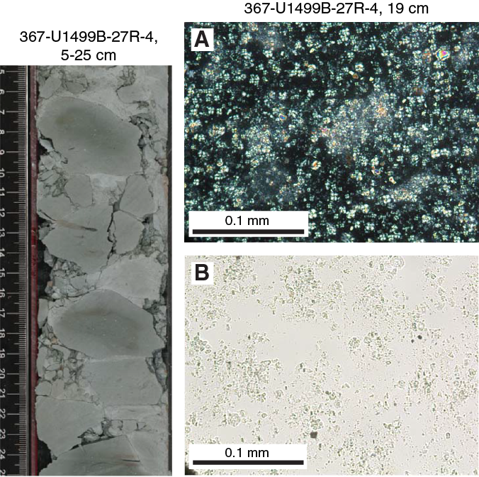
Figure F21. Greenish gray claystone interbedded in brown claystone.
Abundant brownish black iron-manganese nodules occur in the lowest part of Subunit VIIIB (interval 30R-2, 39–103 cm) within a reddish brown nannofossil-rich claystone matrix (Figure F22). The composition of these nodules was later confirmed with postexpedition XRF analysis. The round, concentric nodules are 2–5 cm in diameter. Small to medium, angular to subrounded pebbles form the core of each nodule, providing a nucleation site. The boundary between this nodule-bearing claystone and the underlying sandstone of Unit IX is gradational (Figures F22, F23).
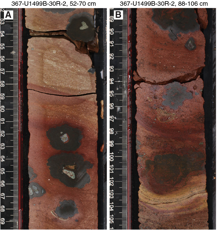
Figure F22. Black-brownish iron-manganese nodules.
Figure F23. Contacts between subunits.
Because the majority of Subunit VIIIB is pelagic nannofossil chalk, it has very low magnetic susceptibility (~10 × 10−5 SI) and the highest reflectance values (L*, a*, and b*) at Site U1499 (Figure F9). The deviations in a* and b* to negative values occur within the green alteration zones. The major lithology change is also reflected in bulk mineralogical compositions, with increased calcite (34%−68%) and decreased quartz (13%−37%), kaolinite + chlorite (4%−13%), plagioclase (3%−5%), and muscovite (6%−9%) (Figure F10).
Unit IX
- Interval: 367-U1499B-30R-2, 103 cm, to 45R-1, 9 cm
- Depth: 929.02−1081.80 m
- Age: Oligocene (and pre-Oligocene?)
Unit IX contains sandstone, claystone, matrix-supported breccia, and gravel. The unit is broken into three subunits (Figure F23) based on the presence or absence of recovered matrix, matrix composition, and the size and shape of clasts embedded in the matrix material.
Subunit IXA
Subunit IXA is a short but important interval entirely contained within Sections 30R-2 through 30R-6. The contact between the clay-rich chalk of Subunit VIIIB and the gravelly sandstone of Subunit IXA is inclined and gradational. Below the contact is 3.8 m of greenish gray and reddish brown sandstone and claystone with gravel, some of which shows inclined bedding (see Structural geology for more details). The bottom of the subunit comprises 45 cm of matrix-supported breccia. Sorting of the subunit decreases from moderate to very poor downhole. Also downhole, the maximum clast size increases from granule to pebble. Throughout the subunit, clasts are angular and of variable lithologic composition (Figures F23, F24), with angularity increasing downhole. The large clasts were identified as claystone, siltstone, sandstone, and conglomerate.
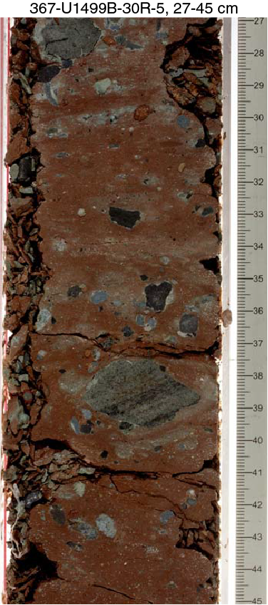
Figure F24. Poorly sorted angular clasts of sedimentary rocks.
Magnetic susceptibility in Subunit IXA ranges from 10 × 10−5 to 50 × 10−5 SI and is much lower than the overlying, nodule-bearing portion of Subunit VIIIB (Figure F9). Reflectance L* and a* shift to more negative values as a result of darker and greener core material. Because of the limited material in this section, no samples were taken for XRD or carbonate analysis.
Subunit IXB
- Interval: 367-U1499B-30R-6, 55 cm, to 30R-6, 62 cm
- Depth: 933.28−933.35 m
- Age: Oligocene (and pre-Oligocene?)
Subunit IXB is 7 cm thick with textural properties similar to the matrix-supported breccia at the base of Subunit IXA (Figure F25). The subunit is entirely composed of dark gray matrix-supported breccia that includes pebble- and granule-sized polymict clasts of sandstone, siltstone, and claystone. Subunit IXB is distinguished from Subunit IXA because (1) its fine-grained matrix is barren of nannofossils; (2) the matrix changes from greenish gray in Subunit IXA to dark gray in Subunit IXB; (3) the pebble-sized clasts of Subunit IXB are subangular to rounded, which is in contrast to the angular to subrounded pebbles at the base of Subunit IXA; and (4) sand-sized pyrite clasts are common in Subunit IXB. The contact between Subunits IXA and IXB may be obscured by drilling disturbances; however, it has an irregular geometry and could be erosive.
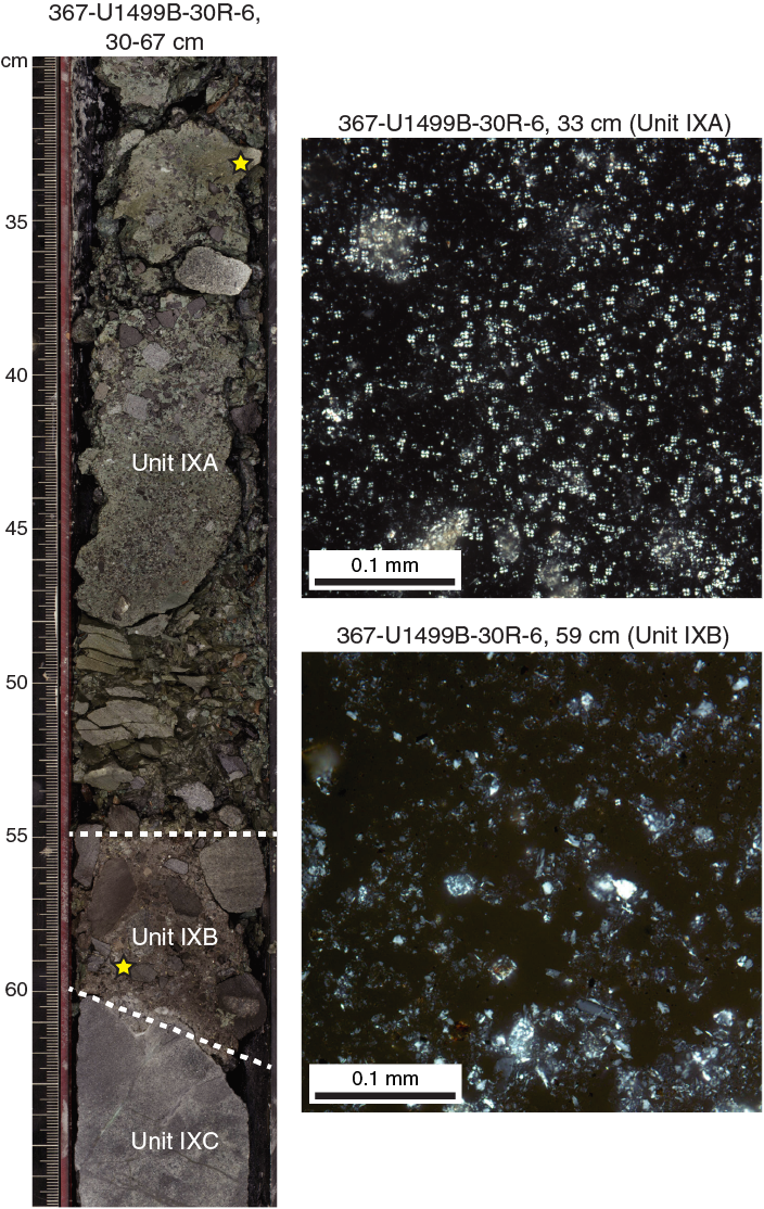
Figure F25. Breccia intervals.
Subunit IXC
- Interval: 367-U1499B-30R-6, 62 cm, to 45R-1, 9 cm
- Depth: 933.35−1081.80 m
- Age: Oligocene (and pre-Oligocene)
Subunit IXC comprises mostly gravel with some intervals of nonlithified clayey silt or silty sand. The gravel was recovered as pebbles and cobbles without matrix, which we infer was lost during the RCB drilling process. The overall recovery was very low for the subunit (~9%), indicating the difficulty in coring this formation. Thus, our information on the lithology and mineralogy of this subunit is biased toward the clasts we recovered, with little information about remaining constituents of this interval (such as the matrix).
Based on visual identification and thin section analysis, gravels as pebbles or cobbles consist of various kinds of grayish fine- to coarse-grained sandstone. The sandstone is well lithified, poorly to well sorted, and grain supported (Figure F26). See Discussion for more details on this classification.
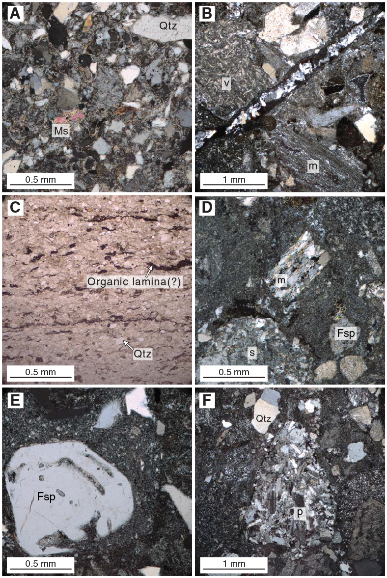
Figure F26. Sandstone cobbles.
We measured magnetic susceptibility on cobble-sized clasts, which were determined to be sedimentary rocks. Values were very low (<30 × 10−5 SI) regardless of clast lithology (Figure F9). The color reflectance data show large amounts of scatter, except for a*, which remains slightly positive but low. These values may be a result of very low levels of green/red hues in the clasts, which are mostly gray, black, and bluish gray.
Carbonate content remains low throughout Subunit IXC, although only four samples were taken. All samples contained <0.5 wt% carbonate (Figure F9). However, one sample did have a relatively high organic carbon content of 4.9 wt% (Sample 38R-1, 74–77 cm; see Geochemistry). XRD analysis of a clast from Core 38R shows dominant quartz (44%) and plagioclase (21%) (Figure F10), although that is not representative of all clasts in the subunit.
Discussion
The lithostratigraphic units observed at Site U1499 characterize deposition in a deep-marine setting. However, lithologic and stratigraphic differences between units likely reflect changes in transport mechanisms, sediment sources, and/or rates of sedimentation. The depositional changes recorded in the stratigraphy at Site U1499 provide important information about the regional climatic and tectonic evolution of the SCS.
Modern day deposition in the SCS consists of several types of sediment, including sand, calcareous silt and clay, and clay progressing in that order as distance from the coast and water depth increase (Wang et al., 1995). Site U1499 sits close to the boundary between deposition of calcareous silt and clay and deep-sea clay, meaning the site will be particularly sensitive to changes in sea level and energy of sediment transport from more proximal environments.
Characteristic fining-upward sequence types
Sequences that have erosive bases and fining-upward transitions from sand to clay are pervasive throughout the cores, but they are more frequent in Units I, III, and V–VII. The coarse-grained basal beds are often >5 cm thick. Sometimes these beds are composed of siliciclastic material, whereas other intervals contain calcareous bioclasts, especially foraminifers (Figure F27). In almost all cases, grains are moderately sorted and subrounded to subangular. As the sequences fine upward, they move into clay-sized particles, which are the dominant size fraction throughout all units. The overlying clay varies in content. Siliciclastic material is almost always the dominant component, but the relative amount of biocalcareous material, particularly nannofossils, changes. Often, the overlying clay intervals are heavily bioturbated.
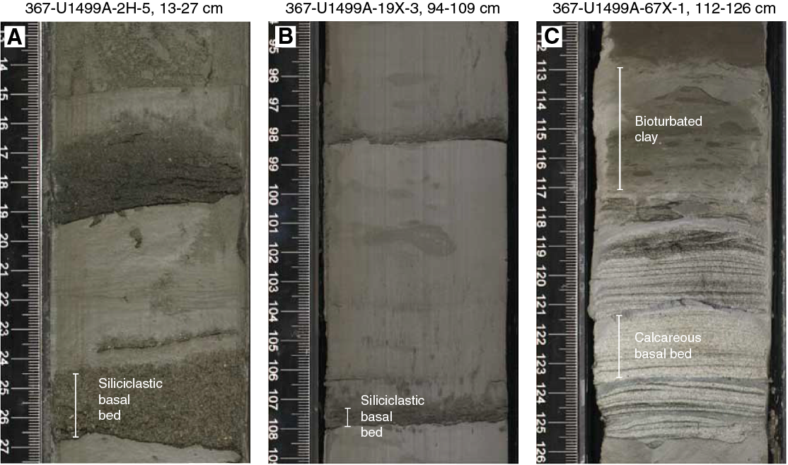
Figure F27. Fining-upward sequences.
In Subunits IIIA and IIIB, fining-upward sequences are also present. However, the coarsest material present is generally silt-sized (Figure F27), and silt layers are mostly <2 cm thick. The transition between the deposition of fining-upward silt interbeds and overlying background sediment could not be resolved, has important implications for accumulation rates at Site U1499. If the series of interpreted distal turbidites stack on top of one another, each represents a relatively short event in geologic time. However, if the deposit fines into clay and then background clay sedimentation occurs, potentially at rates as low as 1 cm/ky (see Biostratigraphy; Li et al., 2015b), then the 20–30 cm between recurring thin silt beds could represent 20–30 ky.
Mechanisms of mass transport
Tectonics
The South China Sea Basin formed as a result of continental breakup and rifting, followed by seafloor spreading through the middle Miocene (Briais et al., 1993; Sibuet et al., 2016; Yan et al., 2006). The depositional setting of the sediment at Site U1499 was not strongly influenced by regional tectonics because most of the sediments (middle of Subunit VIIIA and above) were deposited during the late Miocene or later. However, later Neogene and Quaternary tectonic activity, including the collision of the Luzon Arc with Eurasia, subduction in the eastern SCS, and/or the uplift of Taiwan (Li et al., 2015a) could have influenced sediment transport to Site U1499 through the early to middle Miocene (Subunits VIIIB and VIIIA).
Climate
The East Asian monsoon system and its temporal variability is another potential cause of episodic sediment delivery to the SCS. The summer monsoon is characterized by strong rainfall and warm winds from the southwest, whereas the winter monsoon brings strong, dry winds from the north/northeast (Jian et al., 2009). Although the East Asian monsoon was established by the early Miocene (Jia et al., 2003), predating most of the sediments at Site U1499, the intensity of the monsoon system is thought to have increased during the Pliocene–Pleistocene as a response to growing Northern Hemisphere ice sheets and higher amplitude glacial cycles (Clemens et al., 1996; Zachos et al., 2001). Thus, changes in the monsoon system through the Neogene and Quaternary could influence the amount of sediment being delivered to Site U1499, particularly as increased precipitation and glaciation increase continental weathering (Liu et al., 2007).
Slope instability
Because Site U1499 is located on the outer slope, close to the abyssal plain, it is likely to receive sediments transported from upslope. These sediments could be terrigenous in origin or derived from a higher location on the shelf/slope. For example, Unit II contains apparent slump deposits containing high amounts (up to ~50%) of biogenic carbonate (Figure F9), indicating shallow water production and transport downslope. Other fining-upward sequences also include biogenic carbonate that was most likely produced higher on the shelf and transported downslope. A potential trigger for this movement could be overloading of weak sediments (Pickering et al., 1989b).
Lateral transport
Site U1499 is susceptible to lateral transport of sediment due to the South China Sea Contour Current, which is a deep-water cyclonic current that may transport sediments sourced from Taiwan and/or the Red River outflow as well as other southern sources (Figure F28) to Site U1499 (Liu et al., 2016). Importantly, deposition through this mechanism may lead to the preservation of contourite deposits in the sedimentary record, which can have similar characteristics to turbidites (e.g., fining upward) but a different depositional mechanism (Pickering et al., 1989a). Although the majority of sediment transported downslope is from episodic mass transport, the lateral redistribution of this material is an important and often underappreciated influence on the ultimate burial and preservation of sedimentary sequences.
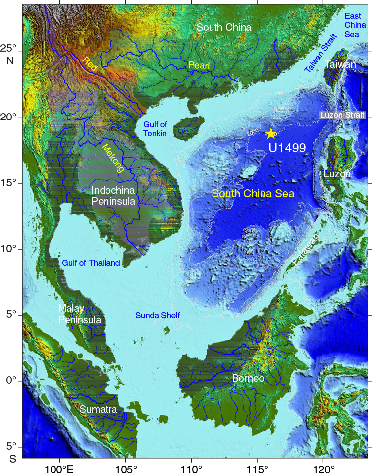
Figure F28. SCS and surrounding region.
Ash layers
Four thin ash layers, 2–7 cm thick each, were identified in Cores 367-U1499A-1H through 5H of lithostratigraphic Unit I; no ash layers were observed in any of the underlying units. These ash layers are defined by bioturbated and gradational upper contacts as well as sharp to irregular basal contacts (Figure F12A). They show an intermediate to felsic composition with an increasing content of mafic minerals (rare to abundant) downhole from the uppermost to the lowermost layer. The major mafic constituent is amphibole and subordinate accessory clinopyroxene. Amphibole is euhedral to subhedral and appears brown-green in plane-polarized light (Figure F12B). Overall, the well-sorted ash layers contain up to ~75% fresh colorless glass shards that range in size from silt to fine sand (0.01–1 mm). Opaque inclusions (presumably oxides) are present in glass shards. Tabular plagioclase crystals as large as 0.1 mm occur throughout the ashes in rare to common abundances.
Red claystone
In Unit VIII, red coloration increases in the claystone and chalk that makes up the dominant lithologies. The transition from gray/brown to reddish brown clay is gradual and can be seen in both core images and color reflectance data. In particular, a* represents psychometric red–green values, where more positive values indicate increasing red content and more negative values indicate greener colors. The shift to more positive values as depth increases in Unit VIII can be seen in Figure F9. Based on the interpretation of similar pelagic red clays in the Pacific Ocean, we interpret the increased red content to be a result of deposition in a pelagic environment where accumulation rates are low and bottom waters are oxygenated (Bryant and Bennett, 1988).
Biostratigraphic evidence supports a decrease in sedimentation rates (see Biostratigraphy) during deposition of Unit VIII. These environmental conditions allow for oxidation of Fe-bearing siliciclastic minerals from land, producing Fe oxides that have a characteristic red color. Smear slides from Unit VIII confirm the presence of abundant Fe oxides (Figure F29). Although the overall trend in a* is toward more positive values, there is also increased scatter in Unit VIII. The shifts to more negative a* values correspond to greenish layers within the red clay, which we interpret to be related to diagenesis from reducing fluids flowing through fractures in the clays.
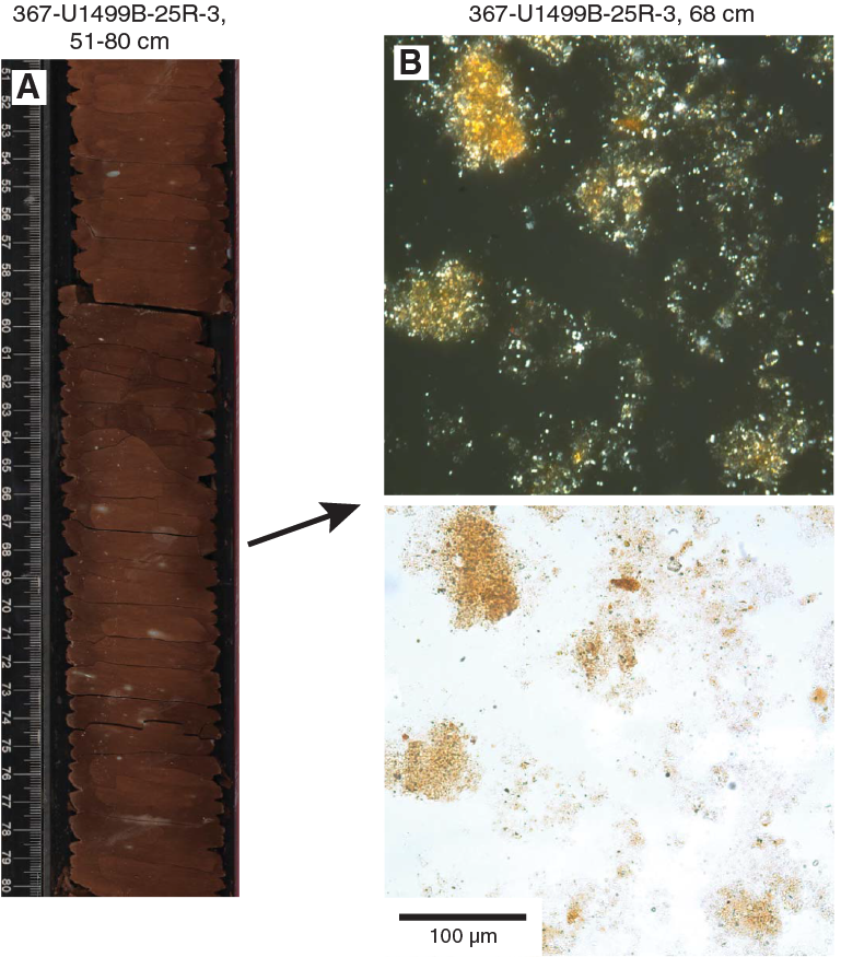
Figure F29. Red claystone.
In Subunit VIIIA, carbonate content is very low (Figure F9). Three possible scenarios could lead to this. First, there may have been production of biogenic carbonate in the water column that fell below the carbonate compensation depth (CCD), leading to dissolution of carbonate. Slow sedimentation rates would aid in this process because sediments sit at or near the sediment–water interface for longer periods of time, allowing for more dissolution. A second scenario involves reduced primary productivity, leading to no or little biogenic carbonate production during the deposition of Subunit VIIIA.
A third scenario involves the geographic location of the site. Site U1499 is positioned on top of a structural high bounded by two sedimentary basins. Sediments coming from the continent could have been trapped in the continent-side basin, causing a reduced and finer sedimentary input at the site location and reducing siliciclastic sedimentation rates on the structural high, allowing for higher carbonate deposition (shown in the abundance of calcareous sediment in Subunit VIIIB). When the basin was filled, the site would no longer be isolated, and siliciclastic sedimentation would dilute the carbonate deposition.
Regardless of which scenario actually occurred, Subunits VIIIA and VIIIB are markedly different. In Subunit VIIIB (starting at Section 367-U1499B-26R-4), carbonate content drastically increases to a maximum of 65%. The dominant components of these cores are nannofossils, suggesting high primary productivity and/or conditions favorable to preservation. The reddish color remains in the minor clays associated with the chalks, indicative of an oxygenated environment similar to Subunit VIIIA. However, it is possible that this site was above the CCD during deposition of Subunit VIIIB, leading to enhanced preservation of carbonate.
Interpretation of Unit IX
The gravel and breccia intervals of Unit IX (Section 367-U1499B-30R-2 through Core 45R) are divided into three subunits based on the compositional changes in the fine-grained supporting matrix and changes in clast shape and size (Figures F24, F25). However, the clasts have similar lithologies throughout Unit IX.
Subunit IXA
Subunit IXA is composed of sandstone and claystone clasts in a pelagic matrix. Clast concentration and clast size increase downsection. The clasts are angular. Oblique bedding was observed in the upper part of the subunit, whereas the lower part is more chaotic. Identifiable bioclasts in Core 367-U1499B-30R suggest reworking (see Biostratigraphy), and the base of Subunit IXA is irregular and could be erosive (Figure F25). The massive structure, poor sorting, and matrix-supported character of this unit suggest deposition by gravity-flow processes.
Subunit IXB
Subunit IXB was defined based on (1) increased rounding of pebble-sized clasts compared to the angular to subrounded clasts of Subunit IXA, (2) change in color of the matrix, (3) poor sorting, (4) presence of detrital pyrite grains in the matrix, (5) lack of nannofossils in the matrix, and (6) irregular and potentially erosive contact with Subunit IXA (Figure F25).
The base of Subunit IXB is inclined above a large sandstone cobble of Subunit IXC. Four scenarios are proposed for this subunit:
- It was formed in the same environment as Subunit IXA.
- It corresponds to the matrix of Subunit IXC, which was washed out during drilling.
- It has a distinct primary origin different than that of Subunits IXA and IXC.
- The matrix is distinct from Subunits IXA and IXC because of contamination by drilling slurry.
Subunit IXC
The depositional setting and source of the gravel of Subunit IXC is unknown, but the angularity and size of many of the clasts suggest that transport distances likely were short. The clasts are composed of sedimentary rock, mostly sandstone similar to the clasts of Subunits IXA and IXB. The composition and stratigraphic architecture of the Subunit IXC matrix is also uncertain because recovery was low (<10%) and drilling disturbance was high in the cored intervals (Cores 367-U1499B-30R through 45R). P-wave velocity values from measurements of individual cobbles from Subunit IXC range from 2.7 to 5.5 km/s, whereas downhole logging sonic velocity measurements range from 2.3 to 4.1 km/s (see Downhole measurements). The reduced velocity measurements from the downhole logging imply that the cobbles of Subunit IXC are supported by a finer grained, lower velocity matrix.
Although Subunit IXC cores are heavily fragmented and were recovered only as cobbles due to drilling disturbances, the gravel fragments can be studied to further understand provenance and transport mechanisms. Thin sections of the cobbles were made and analyzed for each major cobble lithology type (Figure F26). Five major cobble lithology types were identified for Subunit IXC, as well as several other minor lithologies. The major lithologies include gray fine-grained sandstone, gray medium-grained gravelly sandstone, very dark gray fine-grained sandy siltstone, layered gray/very dark gray medium-grained sandstone, and gray medium-grained (low-grade) metasandstone.
A variety of framework grains were identified and photographed for each thin section in this subunit (Figure F26). The framework grains include abundant mono- and polycrystalline quartz, feldspar, muscovite, and lithic grains of igneous, metamorphic, and sedimentary origin. Small inclusions of apatite and zircon were also identified within some of these grains (as shown in the feldspar grain in Figure F26E). Thin sections made of the gray medium-grained gravelly sandstone included volcanic grains with plagioclase-phyric texture, plutonic grains, metamorphic grains with gneissic texture, and sandstone fragments containing quartz and feldspar (Figure F26B, F26D, F26F). Thin sections made of the other main cobble lithologies have similar compositions with varying grain size. The thin section made of the fine-grained very dark gray sandy siltstone, shown in Figure F26C, contains abundant silt- to fine sand–sized quartz and mica grains, along with common lithic and chert fragments. It also contains strands of opaque sediment inferred to be organic or sulfide-rich lamina. The pervasive fine-grained mica in the clay matrix of the sandstone cobbles could have formed in response to low-grade metamorphism that occurred prior to deposition of the gravel of Subunit IXC.
The pervasive presence of lithic grains in most of the sandstone cobbles highlight a complex sedimentological history that occurred before the transport and deposition of the gravel (Figure F26). The lithic grains that compose the cobbles were sourced from a variety of sedimentary, metamorphic, and igneous rocks. Their presence also indicates multiple sedimentary cycles. Qualitatively applying the provenance fields of Dickinson et al. (1983), we infer that the sediments within the cobbles were sourced from a magmatic arc or recycled orogen. The angularity and coarseness of some of the grains within the cobbles implies that the sediments accumulated in proximity to their source and were not transported over long distances.
Well-lithified cobbles represent most of the recovery in Subunit IXC. However, moderately consolidated dark clayey silt to sandy gravel was also recovered in some intervals (e.g., Cores 367-U1499B-38R, 39R, 41R, 42R, and 43R). This material could potentially correspond to the matrix of Subunit IXC, which was mostly unrecovered. This moderately consolidated lithology is barren of microfossils. The high organic carbon content of 4.9 wt% in some black, fissile clasts (interval 38R-1, 74–77 cm) could mark an important terrigenous component in the sedimentation of Subunit IXC.
Structural geology
Site U1499 is located on the northwestern flank of Ridge A at the COT of the northern SCS margin. Drilling at Site U1499 penetrated a sedimentary sequence reaching Oligocene deposits followed by polymict gravels of unknown age and undetermined thickness. The tilting of sedimentary bedding (Figure F30) and deformation structures observed at Site U1499 are limited to lithostratigraphic Units II and VII–IX.
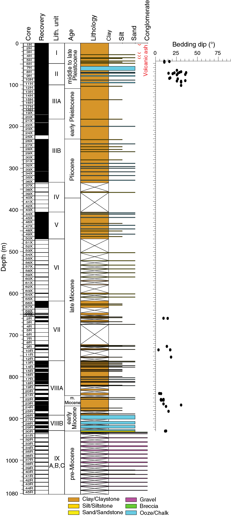
Figure F30. Lithostratigraphic summary.
Unit II
Unit II is bounded by two erosive contacts (Figure F31) and is composed of greenish gray clay-rich calcareous ooze and dark greenish gray nannofossil-rich clay beginning at Section 367-U1499A-6H-3, 35 cm. The color variations of Unit II highlight the deformation structures. The top of Unit II is slightly deformed with few inclined beds. In Sections 6H-5, 100 cm, to 8H-1, 90 cm, the bedding is flat, and no deformation structures were observed. Variations of the bedding dip and centimeter-scale synsedimentary folds (Figure F32) were observed in Sections 8H-1, 90 cm, to 8H-4, 126 cm, where a 17 cm thick dark clayey silt layer (Figure F31) occurs. Below this layer, the cores present several bedding-dip variations and synsedimentary folds downhole to the base of Unit II (Section 11H-5, 104 cm). However, we note that the deformation intensity is not homogeneous throughout Unit II. Additionally, one subvertical normal fault was observed (Figure F32).
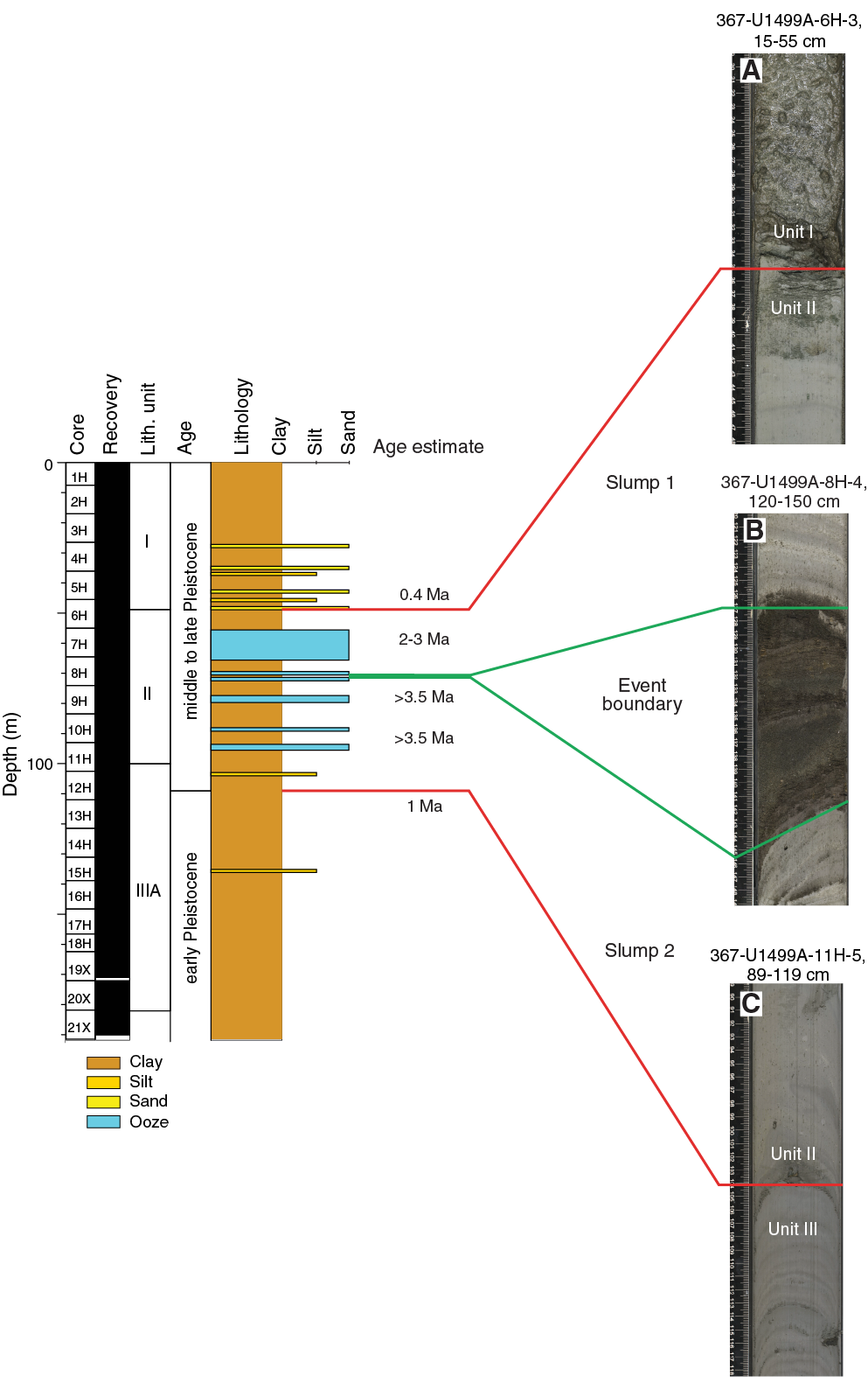
Figure F31. Correlated lithostratigraphic summary..

Figure F32. Unit II structures.
Interpretation
The deformation structures observed in Unit II indicate slump activity. Paleontological correlations show that Unit II contains older microfossils than Unit III, but within Unit II the ages of the species are still increasing with depth (Figure F31). This observation suggests that slumping moved the strata from upslope into the sedimentary basins with limited internal deformation or sediment reworking. Unit II may correspond to two slump events separated by the 17 cm thick dark clayey silt layer.
Units VII and VIII
Units VII and VIII are mainly composed of claystones and sandstones. Tilted bedding observed in Cores 367-U1499B-2R through 25R has an average dip of 11° with a standard deviation of 6°. Only six normal, one strike slip, and eight undetermined faults were observed in Cores 12R through 30R. The mean dip of these faults is 48° with a standard deviation of 24°. Some of these faults have slickenside surfaces (Figure F32); however, the offset can rarely be determined and never exceeds 2 cm. Reorientation to the geographical reference frame using paleomagnetic measurements was attempted, but the shipboard demagnetization process was not effective deeper than Unit VI due to the presence of hematite. Lithification in Units VII and VIII is more developed than in shallower units; therefore, these faults likely may be related to compaction and lithification of the claystones (Figure F33). Tilted bedding is often related to contacts with sandy layers or associated with layers containing a significant proportion of coarser sand-sized material. Veins 1–2 mm thick filled by magnetite or other Fe oxide showing single vein connectivity appear in Unit VIII. Interval 14R-3, 31–49 cm, revealed a subrounded triangular sandy structure occupying one side of the core (Figure F32). The surrounding claystone is deformed, in particular above the sandy formation, which suggests that the deformation took place in soft sediments below the seafloor.
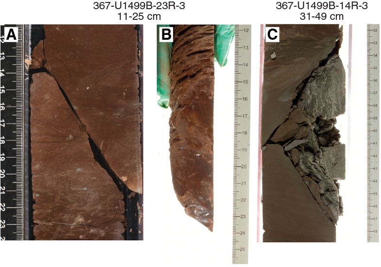
Figure F33. Subunit VIIIA structures.
Unit IX
Unit IX is composed of three subunits (IXA, IXB, and IXC). Subunit IXA consists of matrix-supported breccia and sandstone with polymict clasts. Subunit IXB is nannofossil-barren dark gray matrix-supported breccia. Subunit IXC is formed by polymict gravel (Figure F24). A bedding dip of 11° was observed in the upper part of Subunit IXA (Sections 367-U1499B-30R-2, 105 cm, to 30R-3, 110 cm). The subunit’s lower part contains pebble-sized clasts. The alignment of some of these clasts may reflect sedimentary bedding, but the overall organization is chaotic. Clast proportion and angularity generally increase downhole. The paleontological record of Subunit IXA indicates reworking of foraminifers and nannofossils; however, older species were observed at the bottom of this subunit (Figure F37). Although the biostratigraphy of this section is not clear, the time gap between the older and younger species is ~5 My in only 4.3 m (see Biostratigraphy), which may suggest that the deposition was discontinuous. Subunit IXA is interpreted as a gravity flow deposit accumulated on a slope showing a succession of several deposition events. Subunit IXA may show an erosive basal contact boundary (Figure F24). Subunit IXB does not exhibit any clear structures or sedimentary bedding. Subunit IXB was distinguished from the two other subunits, but it could also belong to Subunit IXA, be the washed matrix of Subunit IXC, be a different subunit, or be induced by drilling. The gravel of Subunit IXC comprises pebble- to boulder-sized sandstones, siltstones, and breccias, but no matrix was recovered. Several types of sandstone have sedimentary bedding, and some contain vein networks principally filled by quartz, pyrite, and/or Fe oxides (in altered parts). In addition, fractures were observed in the gravel clasts. However, their orientations cannot be related to a tectonic event because the age of the first deposition, the lithification, and the age of resedimentation of the pebble- to cobble-sized clasts remain unknown. Paleomagnetic inclination data from these clasts show a large scatter, which also suggests that these cobbles were not formed in situ but were transported (see Paleomagnetism). In addition, only a weak (low-grade) metamorphic imprint is found in a few clasts of Subunit IXC.
Comparison and interpretation
The determination of pre-, syn-, and postrift sequences and their relative ages is key for characterizing the tectonic evolution of the SCS margin. At Site U1499, the significance of Unit IX is not clear due to the lack of a complete stratigraphy, clear structural information, and unequivocal biostratigraphic data. However, the major sedimentological differences between Subunits IXA and IXC may suggest a drastic change in the depositional environment from potentially more continental to pelagic environment; this change may be consistent with a sedimentation hiatus.
Interestingly, the ODP Iberia margin Site 1069 shows sedimentation patterns (Shipboard Scientific Party, 1998) that are strikingly similar to Unit IX at Site U1499. At Site 1069, the 2.3 m thick Unit IV, which contains slump deposits that rework clasts of deeper units into hemipelagic material, lies between hemipelagic sediments and a deeper Unit V (Shipboard Scientific Party, 1998). This deeper Unit V has very low recovery (<3%) and is characterized by an extremely fragmented Subunit VA that contains limestone clasts and an Upper Jurassic (Tithonian) fossil assemblage. In contrast, the lower Subunit VB is composed of fossil-barren, polymict conglomerates with rounded pebble- to boulder-sized gravel of igneous, sedimentary (sandstones), and metamorphic (gneiss) origin. Because the Upper Jurassic age corresponds to the initiation of rifting on the Iberia margin, Subunit VB was interpreted as prerift (Shipboard Scientific Party, 1998). Based on such analogy with Site 1069, Subunit IXA might correspond to syn- to early postrift sedimentation, whereas Subunit IXC may represent prerift sediments containing pebbles and boulders of an older eroded sedimentary basin. Following this interpretation, the presence of prerift sedimentary rock would imply that the targeted high is a tectonic block composed of upper continental crust. However, due to the lack of age and deformation constraints at Site U1499, such interpretation remains speculative. Another interpretation is that the detrital facies of Subunit IXC corresponds to a synrift sequence related to tectonic activity during the rifting of the SCS.
Biostratigraphy
All core catcher samples from Holes U1499A and U1499B were analyzed for calcareous nannofossil and foraminiferal content. Additional samples were taken from the split-core sections when necessary to refine the ages between core catcher samples. Preservation of microfossils varies from poor to very good. Overgrown and abundant broken fragments are common in the sediment sequences. The total abundance varies from barren to abundant, but most samples exhibit some reworking.
Twenty-eight biostratigraphic datums were recognized from Holes U1499A and U1499B, revealing an apparently continuous succession of Oligocene to Pleistocene age at Site U1499 (Table T3; Figures F34, F35). No nannofossils or foraminifers were found in Sample 367-U1499B-30R-CC through Section 38R-1 (933.66 m to the bottom of the Hole U1499B). An age-depth plot based on the biostratigraphic and paleomagnetic data (see Paleomagnetism) allows a direct comparison of the data (Figure F35).
Table T3. Biostratigraphic events. Download table in CSV format.
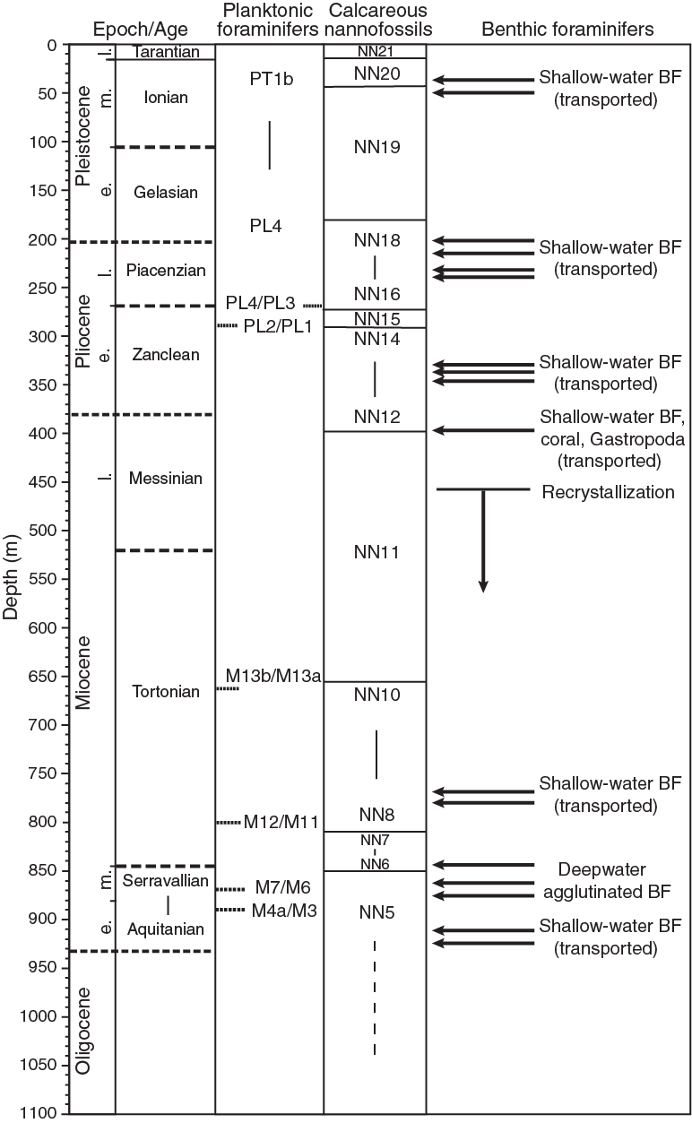
Figure F34. Biostratigraphic and paleoenvironmental summary.
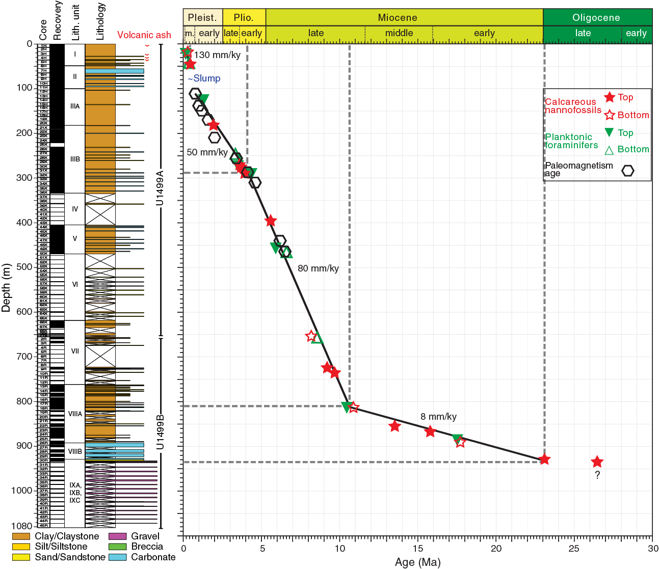
Figure F35. Age-depth model.
Cores 367-U1499A-1H through 5H (0 to ~45 m) represent the middle–late Pleistocene sequence. Preservation of calcareous nannofossils is moderate, but planktonic foraminifers are poorly preserved. The estimated sedimentation rate is ~130 mm/ky.
Cores 367-U1499A-6H through 11H (45 to ~112 m) correspond to lithostratigraphic Unit II and are defined as the slump deposit. Preservation is very good for all calcareous microfossils. The reworked microfossil assemblages are dominated by the Pliocene–early Pleistocene species.
Cores 367-U1499A-11H through 31X (112 to ~288 m) represent the Pliocene–early Pleistocene sequence with a sedimentation rate of ~50 mm/ky. Fossil preservation is moderate to good. Several events could be placed with a high degree of certainty to define the boundaries. The last appearance datum (LAD) of Discoaster brouweri (1.93 Ma) and the first appearance datum (FAD) of Globorotalia tosaensis (3.35 Ma) indicate the Pleistocene/Pliocene boundary (2.58 Ma) lies between Samples 20X-CC and 27X-CC. The FAD of Sphaeroidinellopsis seminulina (3.59 Ma) indicates the late/early Pliocene boundary is in Sample 29X-CC (269.15 m).
Cores 367-U1499A-31X through 367-U1499B-18R (288 to ~812 m) correspond to the late Miocene–early Pliocene sequence and have a sedimentation rate of ~80 mm/ky. The microfossils are generally sparse and poorly to moderately preserved throughout the succession. Five nannofossil and four foraminiferal datum events are identified in this interval. The Pliocene/Miocene boundary (5.33 Ma) is close to the LAD of Discoaster quinqueramus (5.59 Ma) in Sample 367-U1499A-43X-CC (395.15 m).
Cores 367-U1499B-18R through 30R (812 to ~928 m) correspond to lithostratigraphic Unit VIII and were assigned to the early–middle Miocene. Microfossils are moderately abundant and preserved in this interval. Eight biostratigraphic events constrain this interval well, and calibrated biohorizons allow us to estimate extremely low sedimentation rates (~8 mm/ky) during the early to late Miocene.
Based on the LADs of Reticulofenestra bisecta (>10 µm; 23.13 Ma) and Globigerina ciperoensis (22.9 Ma) in Sample 367-U1499B-30R-2, 35–37 cm (928.34 m), the Miocene/Oligocene boundary is tentatively placed within Section 30R-2. This placement is also supported by the regional correlation of the early to middle Miocene red claystone in this site with Sites U1500 and U1502.
Sections 367-U1499B-30R-3 through 30R-6 (~928 to ~933 m) were studied by analyzing 12 additional samples for nannofossil and foraminiferal biostratigraphy (Figure F36). This succession comprises microfossils from the early Oligocene to the late Oligocene. Compared to the generally moderate preservation at Site U1499, the well-preserved and abundant calcareous nannofossils in Sections 30R-3 through 30R-6 indicate that they are probably transported and reworked, a theory that is also supported by the sorted foraminifers at this succession. This theory makes the age determination less reliable, and only one nannofossil event is given. Hence, it is difficult to calculate the sedimentation rate. The resolution of the age discrepancy between foraminiferal and nannofossil bioevents given for this interval (question mark in Figure F35) awaits further postcruise studies.
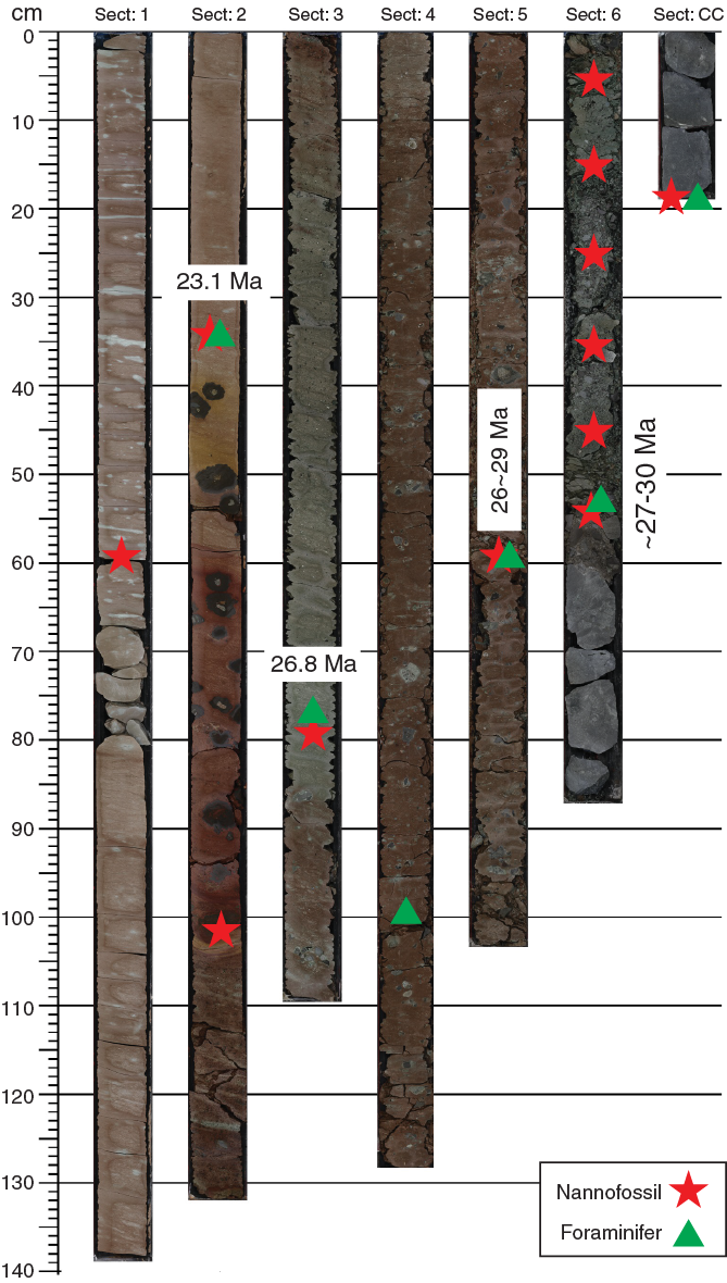
Figure F36. Additional samples.
Calcareous nannofossils
Calcareous nannofossil biostratigraphy at Site U1499 is based on the analyses of all core catcher samples and additional split-core samples from Holes U1499A and U1499B (Tables T4, T5). Calcareous nannofossil zonation is based on the scheme of Martini (1971), and calibrated ages for bioevents are from Gradstein et al. (2012). Calcareous nannofossil abundances vary in the succession; they are more abundant in the upper portion within bioclastic- and nannofossil-rich clay beds and rare or absent in the more lithified units below Core 367-U1499B-30R (~933 m). Various overgrowths on nannofossils, reworked specimens, and abundant broken fragments, especially among discoasters, are common in the whole sediment sequences.
Table T4. Calcareous nannofossils, Hole U1499A. View table in PDF format. Download table in CSV format.
Table T5. Calcareous nannofossils, Hole U1499B. View table in PDF format. Download table in CSV format.
In general, the calcareous nannofossil assemblages and preservation at Site U1499 are variably affected by carbonate dissolution and turbidites. Sixteen nannofossil biostratigraphic datums were recognized in the Oligocene to Pleistocene sediment sequence (Table T3). The oldest nannofossil event identified, the LAD of Sphenolithus distentus, occurs at 930.1 m, indicating an age <26.84 Ma for most of the sedimentary sequence at Site U1499.
Pleistocene
The top of Hole U1499A is dated as the middle–late Pleistocene (<0.29 Ma) based on the presence of Emiliania huxleyi (marker species for Zone NN21) in Samples 1H-CC through 2H-CC. Recognition of the FAD of E. huxleyi (0.29 Ma) in Sample 2H-CC defines the base of Zone NN21. Samples 3H-CC and 4H-CC were assigned to Zone NN20 based on the absence of both E. huxleyi and Pseudoemiliania lacunosa. The LAD of P. lacunosa (0.44 Ma) in Sample 5H-CC (45.68 m) defines the top of Zone NN19. The interval from Cores 6H through 11H (48.85–100.04 m) consists of calcareous ooze and nannofossil-rich clay. Nannofossils are exceptionally well preserved, and the assemblage is mostly represented by P. lacunosa, Calcidiscus macintyrei, D. brouweri, Discoaster pentaradiatus, Discoaster tamalis, and Sphenolithus abies. Based on the occurrence of these species, this interval could be assigned to the Pliocene–early Pleistocene.
In Samples 11H-CC through 19X-CC (103.09–170.93 m), however, the nannofossil assemblage is dominated by typical middle–early Pleistocene taxa such as Gephyrocapsa spp. and P. lacunosa. For this reason, the interval between Cores 6H and 11H is considered as reworked and related to the occurrence of a slumping deposit (see Lithostratigraphy), and Samples 11X-CC through 19X-CC are assigned to Zone NN19. Because of the poor preservation, many specimens of Gephyrocapsa spp. are lacking in clear bridges, which makes their identification difficult; moreover, specimens of large Gephyrocapsa spp. (>5.5 µm), C. macintyrei, and Reticulofenestra asanoi are very rare and occur discontinuously, preventing the recognition of the subsidiary events that divided Zone NN19.
Zone NN18 is marked by the LAD of D. brouweri (1.93 Ma) in Sample 20X-CC (181.70 m). However, because of the poor preservation of Samples 20X-CC through 26X-CC (181.70–240.14 m), these events could not be identified until Sample 27X-2, 75 cm (242.25 m), making it difficult to recognize the true depths of Zone NN17. Some subsidiary events such as the LADs of Discoaster triradiatus (1.95 Ma) and D. tamalis (2.80 Ma) could add information to distinguish the Zone NN18–NN16 interval, but these species are too rare and occur too discontinuously in the sample to allow clear identification of their last occurrences.
Pliocene
The bottom of Zone NN16 is defined by the LAD of Sphenolithus spp. (3.54 Ma) in Sample 367-U1499A-29X-CC (269.10 m). The Zone NN16/NN15 boundary was assigned in Sample 30X-5, 72 cm (275.8 m), based on the LAD of Reticulofenestra pseudoumbilicus (3.70 Ma). The LAD of Amaurolithus tricorniculatus (3.92 Ma) in Sample 31X-CC (288.54 m) marks the top of Zone NN14. The interval between Cores 36X and 43X (327.64–395.20 m) is predominantly a long sequence of assemblages with very similar nannofossil composition. Poor preservation and rare occurrence of large coccoliths/nannoliths such as Ceratolithus, Amaurolithus, and Triquetrorhabdulus make it difficult to identify the boundaries from Zones NN15 to NN12.
Miocene
Eight events occur in the Miocene strata of Holes U1499A and U1499B (Table T3). The LAD of D. quinqueramus (5.59 Ma) marks the top of Zone NN11 in Sample 367-U1499A-43X-CC (395.20 m), which corresponds to the top of the upper Miocene (Pliocene/Miocene boundary at 5.33 Ma). D. quinqueramus occurs continually until Sample 367-U1499B-2R-1, 128 cm (656.28 m), which is the uppermost core taken in Hole U1499B, allowing reliable biostratigraphic correlation between the deep part of Hole U1499A and the uppermost section of Hole U1499B (Tables T4, T5). The FAD of D. quinqueramus (8.12 Ma) in Sample 367-U1499B-2R-1, 128 cm, defines the bottom of Zone NN11. Zones NN11–NN9 could not be reliably identified in samples from Cores 2R through 17R (656.76–808.97 m) due to the poor preservation, the absence of nannofossils in several core catchers, or very low recovery.
The LAD of Discoaster bollii (9.21 Ma) within Zone NN10 occurs in Sample 9R-2, 12 cm (724.42 m). The LAD of Catinaster coalitus (9.69 Ma) within Zone NN9 occurs in Sample 10R-CC (735.62 m). The FAD of C. coalitus (10.89 Ma) defines the top of Zone NN7 in Sample 18R-2, 94 cm (812.64 m). Low abundance and barren samples between Cores 19R and 21R prevented identification of the boundary between Zones NN7 and NN6 and make the last common appearance (LCA) of Cyclicargolithus floridanus event (13.28 Ma) less reliable at Site U1499. The LAD of Sphenolithus heteromorphus (13.53 Ma), which defines the top of Zone NN5, occurs in Sample 22R-5, 98 cm (855.24 m).
The boundaries between Zones NN5 and NN2 could not be identified; however, the LAD of Discoaster deflandrei group (15.80 Ma) and the FAD of S. heteromorphus (17.81 Ma) within Zone NN4 occur in Samples 23R-CC (867.41 m) and 26R-2, 89 cm (890.09 m), respectively. The middle/early Miocene boundary falls between the last aforementioned datums.
Oligocene
The LAD of R. bisecta (>10 µm; 23.13 Ma), which corresponds to the Zone NN1/NP25 boundary, occurs in Sample 367-U1499B-30R-2, 34 cm (928.33 m). The Miocene/Oligocene boundary should thus be placed between Samples 30R-1, 59 cm, and 30R-2, 34 cm. Throughout Sections 30R-3 through 30R-6, an early late Oligocene assemblage composed of Sphenolithus ciperoensis, Sphenolithus predistentus, S. distentus, and R. bisecta was found from the brownish to greenish matrix-supported breccia. The LAD of S. distentus (26.84 Ma) is found in Sample 30R-3, 79 cm (930.10 m). The nannofossil preservation in this interval is much better than in the upper parts. Considering the features of the sediments, the occurrence of these species in these sections could be attributed to reworking; therefore, they are not taken into account for stratigraphic purposes (Figure F35). Samples from the bottom of the sequence recovered in Hole U1499B (Cores 30R through 45R; 933.6–1081.8 m) are gray gravel with silty sand intervals that were recovered as pebbles and cobbles. No nannofossils were observed in this section, so no age could be assigned to the lowermost section at Site U1499.
Planktonic foraminifers
Planktonic foraminiferal biostratigraphy was constructed by analyzing planktonic foraminifers in all core catcher samples from Holes U1499 and samples from selected core sections in Hole U1499B, especially within Core 30R (Table T6). Planktonic foraminifers were additionally checked in the fine fraction >63 µm for samples from Core 30R.
Table T6. Planktonic foraminifers. View table in PDF format. Download table in CSV format.
The preservation of planktonic foraminifers varies from poor to very good. Based on the evaluation of the percentage of planktonic foraminiferal fragmentation and the distinct microstructure of foraminiferal shells, there is evident foraminiferal dissolution (e.g., Globigerinoides) and recrystallization in the lower part of Hole U1499A (cores below Core 50X). In general, most core catcher samples from Holes U1499A and U1499B show poor to moderate preservation of foraminifers, except for Samples 367-U1499A-6H-CC through 10H-CC, where they are well preserved and the planktonic foraminiferal assemblage indicates a mixture of late Pliocene and early Pleistocene components. In addition, some shallow-water species of ostracods were found in Section 5H. Therefore, the interval between Samples 5H-CC and 10H-CC is considered to be a turbidite or slump deposit. In some deeper cores, planktonic foraminifers are rare to common with moderate to good preservation; however, most of them are reworked and possibly transported from the shallow water as indicated by common occurrence of shallow-water benthic foraminifers and coral debris (e.g., Samples 43X-CC and 54X-CC). In samples from Hole U1499B, preservation of planktonic foraminifers varies from poor to good, and reworking and recrystallization are common.
The Site U1499 planktonic foraminiferal biostratigraphy was established by the planktonic foraminiferal evolution events and assemblages. Because most foraminifers are reworked, we distinguished in situ bioevents from reworked occurrences by relying more heavily on FADs than LADs.
The sediment sequence recovered in Hole U1499A is continuous and spans the upper Miocene (Zone M13) through the Pleistocene (Subzone Pt1b) based on eight planktonic foraminiferal bioevents (Table T3). Within Subzone PT1b, the FAD (0.12 Ma) of pink Globigerinoides ruber and LAD (0.40 Ma) of pink Globigerinoides ruber acme provide two biostratigraphic control points that are present in Samples 367-U1499A-2H-CC (17.33 m) and 5H-CC (45.68 m), respectively. The LAD of Globigerinoides obliquus (1.3 Ma) in Sample 13H-CC (121.33 m) indicates Subzone PT1a. The Pleistocene/Pliocene boundary could not be determined due to the absence of the zonal marker species. Through comparison with nearby Site 1148 (Wang et al., 2000), we observed the FAD of Globorotalia inflata in Sample 22H-CC (201.11 m), which is near the Pleistocene/Pliocene boundary.
For Zone PL5, the FAD of G. tosaensis (3.35 Ma) was found in Sample 27X-CC (249.82 m). The FAD of S. seminulina (3.59 Ma) appears in Sample 29X-CC (269.15 m) and was used as a marker for the bottom of Zone PL4. The LAD of Globoturborotalia nepenthes (4.36 Ma) was assigned in Sample 31X-CC (288.59 m), which marks the bottom of Zone PL2. The LAD of Globoquadrina dehiscens (5.92 Ma) was observed in Sample 48X-CC (453.66 m), marking Zone M14. The FAD of Pulleniatina primalis (6.6 Ma) occurs in Sample 50X-CC (469.37 m) and indicates Zone M13b. The lowermost part of Hole U1499A is still in the late Miocene.
Five planktonic foraminiferal bioevents (Table T3) were discerned in Hole U1499B. The FAD of Globoratalia plesiotumida (8.58 Ma) in Sample 2R-CC (659.76 m) marks the boundary of Subzones M13b and M13a. The LAD of Paragloborotalia mayeri (10.46 Ma) in Sample 17R-CC (808.97 m) constrains the boundary of Zones M12 and M11. Fohsella peripheroacuta is present in Sample 24R-CC, but because it was only found in this sample, we did not use it as the FAD of F. peripheroacuta (14.24 Ma). However, the LAD of Catapsydrax dissimilis (17.54 Ma) in Sample 25R-CC (882.13 m) marks the boundary of Subzone M4a and Zone M3. Therefore, the middle/early Miocene boundary occurs between Samples 24R-CC and 25R-CC.
Foraminifers were only observed above Core 30R. Five additional samples were analyzed from Sections 30R-2 through 30R-6, and the LAD of Globigerina ciperoensis (22.9 Ma) in Sample 30R-2, 35–37 cm (928.34 m) indicates the possible Miocene/Oligocene boundary. Foraminifers from Sections 30R-3 and 30R-4 are deformed and sorted distinctly, which implies that foraminifers were transported. The early–late Oligocene assemblage of planktonic foraminifers (such as Globigerina euapertura, Tenuitella gemma, Chiloguembelina cubensis, and Globigerina angulisuturalis) is present in Sections 30R-5 and 30R-6; however, any accurate age or age boundary cannot be provided due to the poor preservation and low abundance (almost barren) of foraminifers.
Benthic foraminifers
Shallow-water (shelf) benthic foraminifers (e.g., Ammonia and Florius) and upper slope benthic foraminifers (e.g., Bulimina and Globocassidulina) are present in some of the core catchers of Hole U1499A. They are especially common in turbidite and slump deposits (e.g., from Core 367-U1499A-5H and Samples 37X-CC through 43X-CC and 54X-CC), suggesting that downslope transportation/reworked foraminifers from the shallow shelf to slope is a common phenomenon at this site. In the red clay deposit (lithostratigraphic Unit VIII) in Hole U1499B, deep-water agglutinated foraminifers (e.g., Glomospira and Ammodiscus; Figure F37) were observed and are abundant in Samples CC, 23R-CC, 24R-CC, and 26R-CC), suggesting a deep-water environment.

Figure F37. Deepwater agglutinated benthic foraminifers.
Paleomagnetism
Shipboard measurements
Shipboard paleomagnetic studies consisted of two complementary approaches (see Paleomagnetism in the Expedition 367/368 methods chapter [Sun et al., 2018]): (1) measurement and in-line AF demagnetization of archive-half sections on the pass-through 2G Enterprises SRM and (2) measurement and AF and thermal demagnetization of oriented discrete samples on the spinner magnetometer (Agico JR-6A). Representative discrete samples were collected from every core section (1.5 m), except those that were severely disturbed or contained unique sediments or structures deemed important for other research.
We used the remanent magnetization of archive-half sections, measured after the maximum AF treatment, to determine the polarity along the core (Figure F38). Discrete samples were analyzed using Zijderveld diagrams (Zijderveld, 1967), and ChRM direction were calculated by principal component analysis (PCA) (Kirschvink, 1980) using PuffinPlot (version 1.03, 23 April 2015) (Lurcock and Wilson, 2012).

Figure F38. Remanent magnetization data.
Demagnetization behavior
The drilling-induced remanence was removed in most core sections with an AF treatment of 15 mT. Changes in magnetic remanence with depth can be correlated to observable changes in lithology. Low values of NRM near ~60 m (Core 367-U1499A-7H) correlate with a carbonate-rich layer that also has low magnetic susceptibility values (Figure F48). A decrease in the moment of the NRM and in our ability to effectively demagnetize the archive-half cores deeper than ~800 m (Core 367-U1499B-17R and below) correlates with an increase in the red color of the sediments and the presence of hematite.
The maximum field strength of in-line AF demagnetization used on the archive-half sections is limited because of the destructive nature of the treatments and our limited ability to measure weak magnetizations in the magnetically noisy shipboard environment. As a consequence, the maximum AF treatment used on the long-core sections is usually not sufficient to isolate a stable ChRM vector. When we did not have enough data to quantitatively solve for the ChRM but the demagnetization path suggests normal or reversed polarity, we then used the term potential normal or potential reversed. A typical example of potential normal from the archive-half section of Hole U1499A is illustrated in Figure F39A.
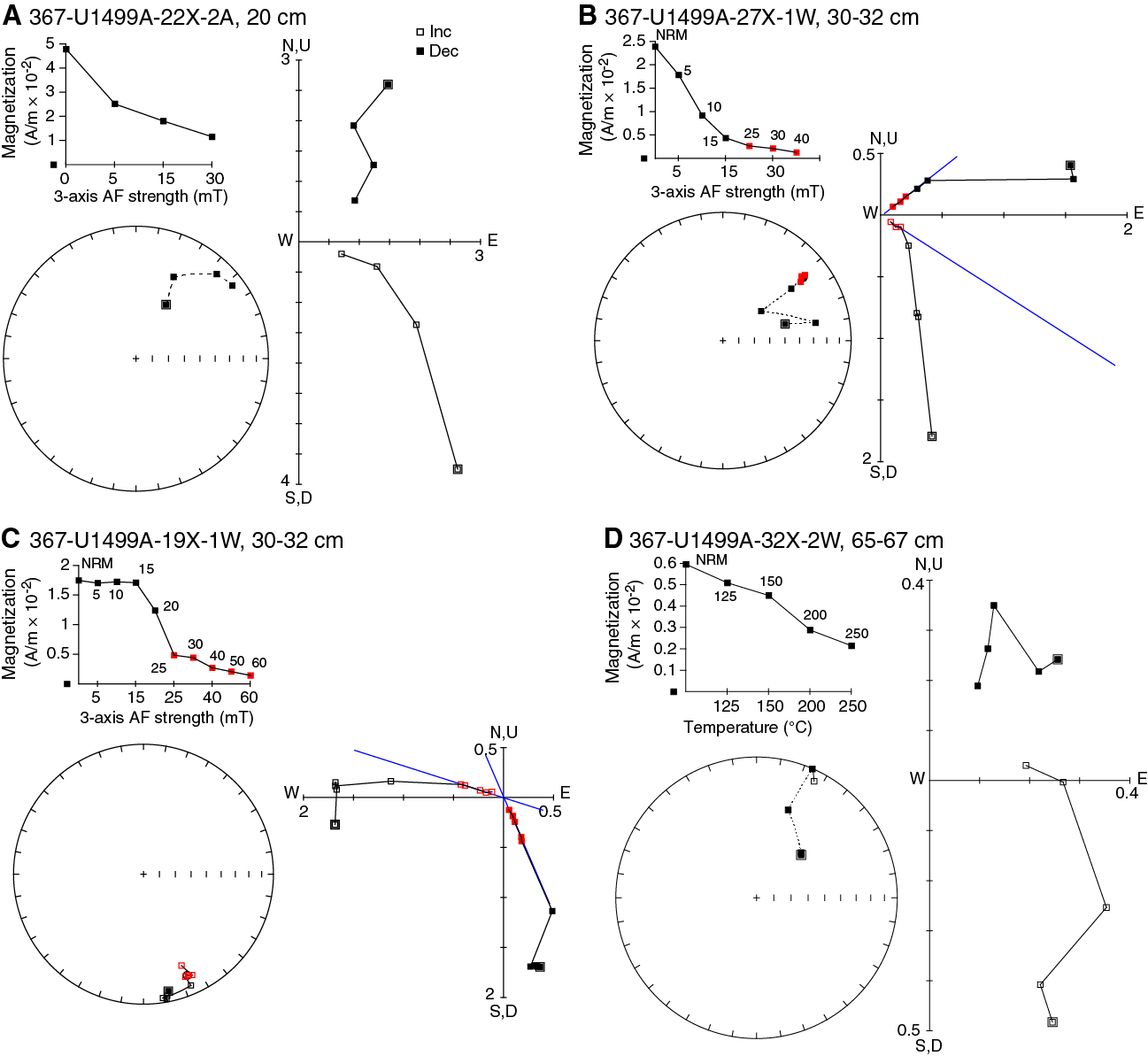
Figure F39. Demagnetization data, Hole U1499A.
The typical behavior of discrete samples from Hole U1499A are shown in Figure F39. AF demagnetization of these samples produces demagnetization paths that are easier to interpret than the results of samples subjected to thermal demagnetization. Both treatments show removal of a steep low-temperature/low-coercivity component that represents the drilling overprint. Thermal demagnetization at higher temperatures becomes noisy and thus not reliable, possibly due to the remagnetization of weak samples in the magnetically unshielded environment. The magnetization level of some samples subjected to thermal demagnetization decreased below what we could reliably resolve on the ship. Further thermal demagnetization will take place on shore. Many of the AF demagnetized discrete samples reveal robust trends showing clear normal or reversed polarity. During AF demagnetization, many samples show an anomalous increase in magnetization at fields greater than 60 mT, which indicates the existence of greigite (e.g., Roberts et al., 2011).
We have very low (0%–30%) recovery in Cores 367-U1499B-2R through 11R. From Core 12R downhole, color changes from greenish gray to dark brownish with relatively higher magnetic susceptibility (Figure F48). Deeper than Core 27R, magnetic susceptibility decreases by an order of magnitude, whereas the drilling overprint becomes stronger and drilling disturbance intensifies. All of these factors hampered a reliable identification of possible magnetic reversals in Hole U1499B. The number of discrete samples was also reduced and limited only to the most intact pieces. The change in AF and thermal demagnetization behaviors indicates the presence of high-coercivity and high–blocking temperature hematite rather than the previous dominating low-coercivity and low–blocking temperature components (e.g., titanomagnetite) that could be easily demagnetized (Figure F40C, F40D).
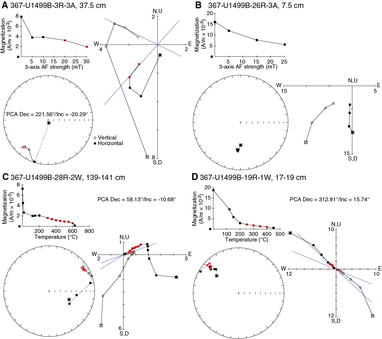
Figure F40. Demagnetization data, Hole U1499B.
Magnetostratigraphy
We constructed the magnetostratigraphy of Site U1499 (Figures F41, F42) based on the polarity assigned to the archive-half cores where they exhibit stable demagnetization paths (e.g., Figures F38, F39A, F40A, F40B). We do not use the paleomagnetic data from ~50 to 100 m where sediments are interpreted as slumps. Declinations from the archive-half sections from the seafloor to 162 m (APC Cores 367-U1499A-1H through 18H) were corrected using the Icefield MI-5 core orientation tool. Our interpretation of polarity deeper than 162 m is based only on the inclination data because the XCB and RCB coring processes disturb the geographic core orientation. Our interpretations of inclination are based on directions derived from the raw moments measured on the SRM.
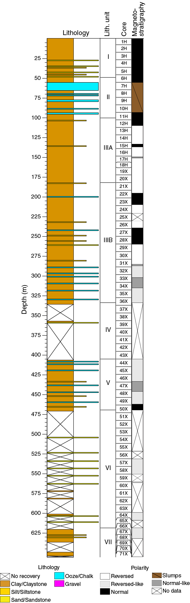
Figure F41. Magnetostratigraphy, Hole U1499A.
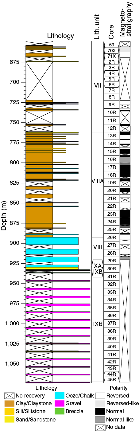
Figure F42. Magnetostratigraphy, Hole U1499B.
The first reversal for the interval shallower than 162 m, where we have constraints based on both inclination and declination, is at ~110 m and interpreted to be the boundary between the Brunhes and Matuyama Chrons. For intervals of poor recovery or poor data quality, the polarity is difficult to determine and thus denoted by question marks (Figure F43). The recovery in Hole U1499B is poor (35%), making it challenging to correlate the polarity patterns to the standard geomagnetic polarity timescale.
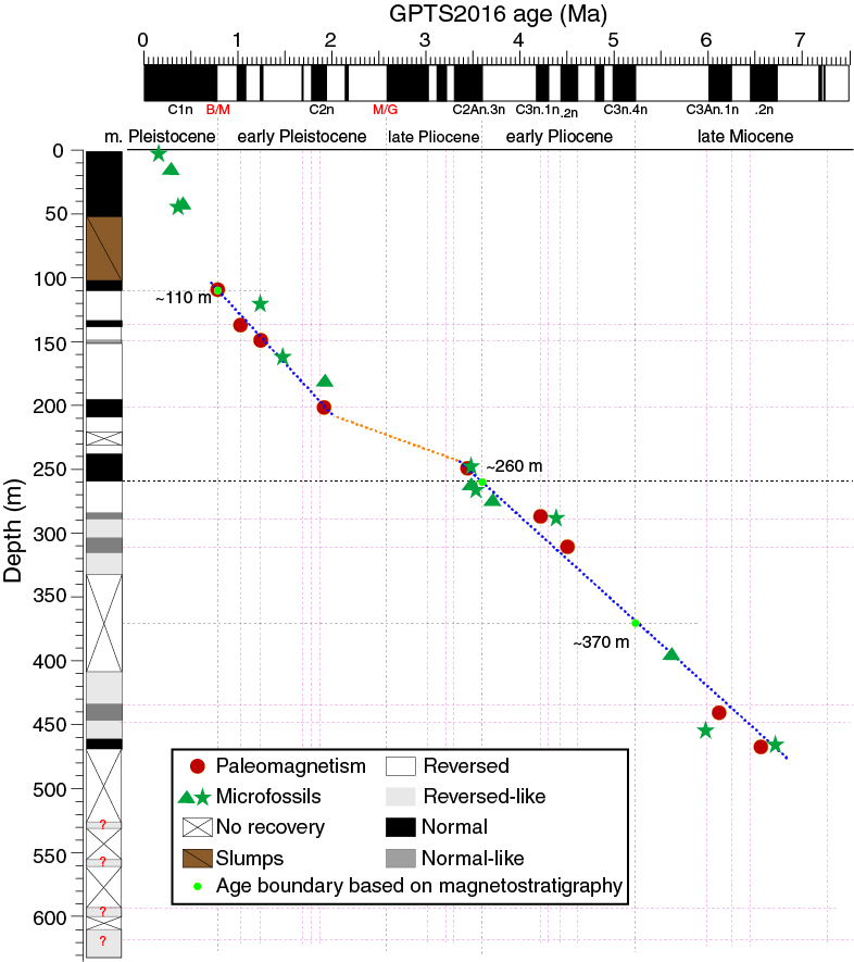
Figure F43. Age-depth model.
We correlate the magnetostratigraphy of Hole U1499A to the standard timescale (Ogg et al., 2016) and plot it along with tie points from the microfossil ages from the shipboard paleontologists (Figure F43). The paleomagnetic and paleontological age constraints match well over most of the section.
Based on our shipboard paleomagnetic age model (Figure F43; Table T7), the middle/early Pleistocene boundary (0.78 Ma) is at ~110 m, the late/early Pliocene (3.6 Ma) boundary is at ~260 m, and the early Pliocene/late Miocene boundary (5.33 Ma) is at ~370 m. Considering only the paleomagnetic data, the early Pleistocene/late Pliocene boundary might be at ~220 m.
Table T7. Magnetostratigraphy. Download table in CSV format.
Geochemistry
At Site U1499, measurements of headspace gas, organic and inorganic carbon, nitrogen, and interstitial water were made in Hole U1499A, and the same measurements, except for interstitial water, were made in Hole U1499B. The headspace gas consistently approaches zero throughout the site, with approximately tens to 6000 ppmv of methane across ~100–250 m, indicating limited microbial methanogenesis because of low TOC content <0.3 wt%. Bulk sediment geochemistry is controlled by lithology. Calcium carbonate contents are predominantly the result of biogenic carbonate abundance. TOC decreases downhole, reflecting the mineralization of sedimentary organic matter. The interstitial water concentration-depth profiles show typical redox zones in marine sediments: oxic seawater, manganese reduction, iron reduction, and sulfate reduction. The interstitial water chemistry also reflects various diagenetic processes: organic matter degradation, carbonate diagenesis, and clay diagenesis occurring in sediments.
Headspace gas
Headspace gas samples (99 samples) were taken at a frequency of one sample per core in Holes U1499A and U1499B for routine safety monitoring (Table T8). Methane concentrations were extremely low (<4 ppmv) in the upper 81 m in Hole U1499A. They increased to 1819 ppmv at 100 m, reached a maximum of ~4000–6000 ppmv from 110 to 180 m, and then reduced to 96 ppmv at 257 m. Below this depth, methane concentrations are quite low (<200 ppmv) to the base of Holes U1499A (651 m) and U1499B (1062 m). The distinct higher methane between ~100 and 250 m (Figure F44) correlates with the reduction of sulfate concentrations in the upper 100 m in the interstitial water profile (Figure F45), suggesting a transition from sulfate reduction to methanogenesis. Ethane, ethene, propane, and propene were below the detection limits in the majority of the samples investigated with concentrations <12 ppmv in only a few samples (12 samples).
Table T8. Headspace gas data. View table in PDF format. Download table in CSV format.
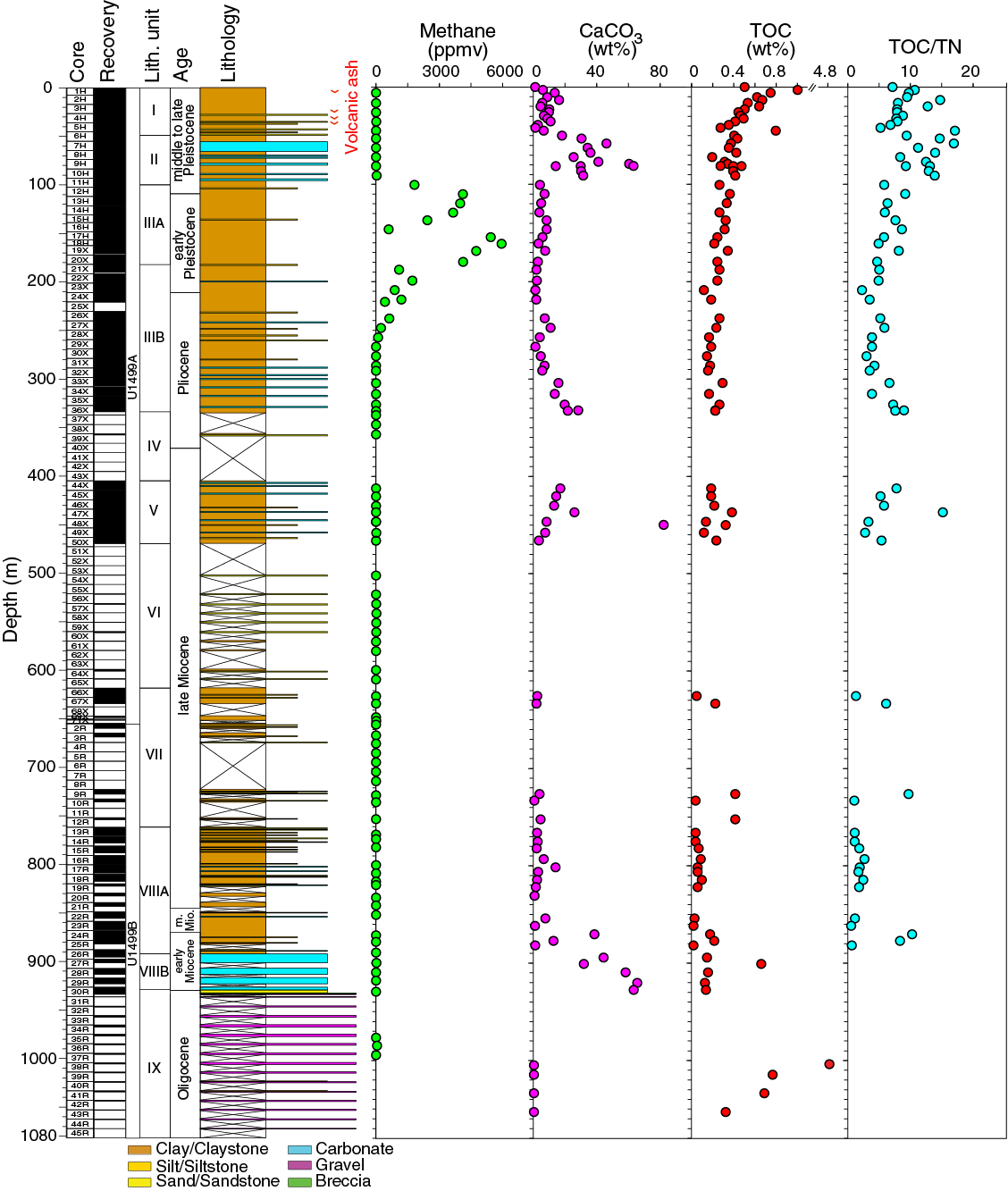
Figure F44. Lithology, carbon, and TOC/TN profiles.
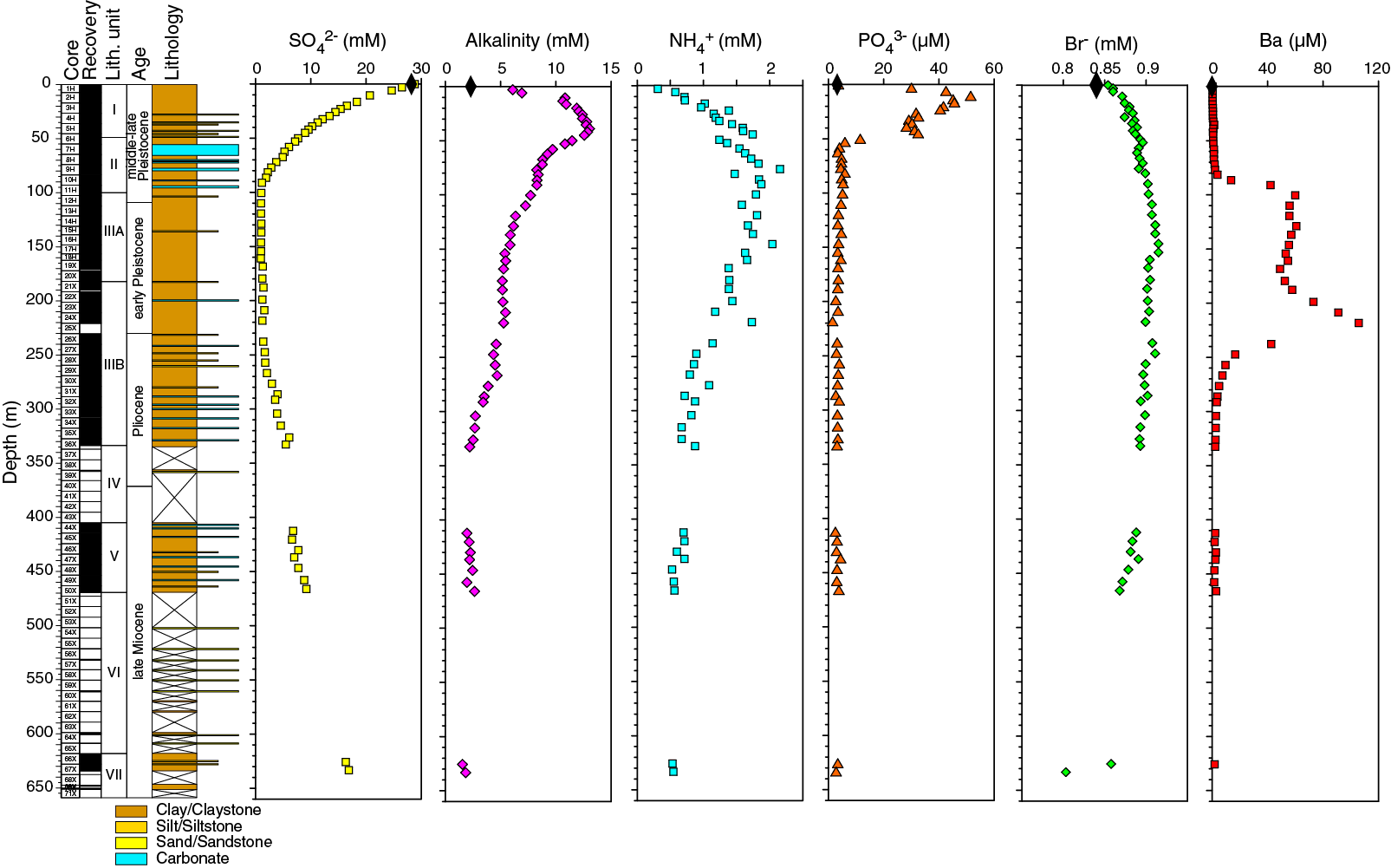
Figure F45. Interstitial water sulfate, alkalinity, ammonium, phosphate, bromide, and barium.
Bulk sediment geochemistry
Total carbon, total inorganic carbon (TIC), calcium carbonate, TOC, and TN were determined on 89 sediment samples from interstitial water squeeze cakes (58 samples from Hole U1499A) and discrete samples selected by scientists describing the cores (5 samples from Hole U1499A and 26 samples from Hole U1499B; Table T9; Figure F44). The downhole profile of carbonate content was also indicated by the reflectance L* and calcite contents as measured by XRD (Figures F45, F46).
Table T9. Carbon and nitrogen. View table in PDF format. Download table in CSV format.
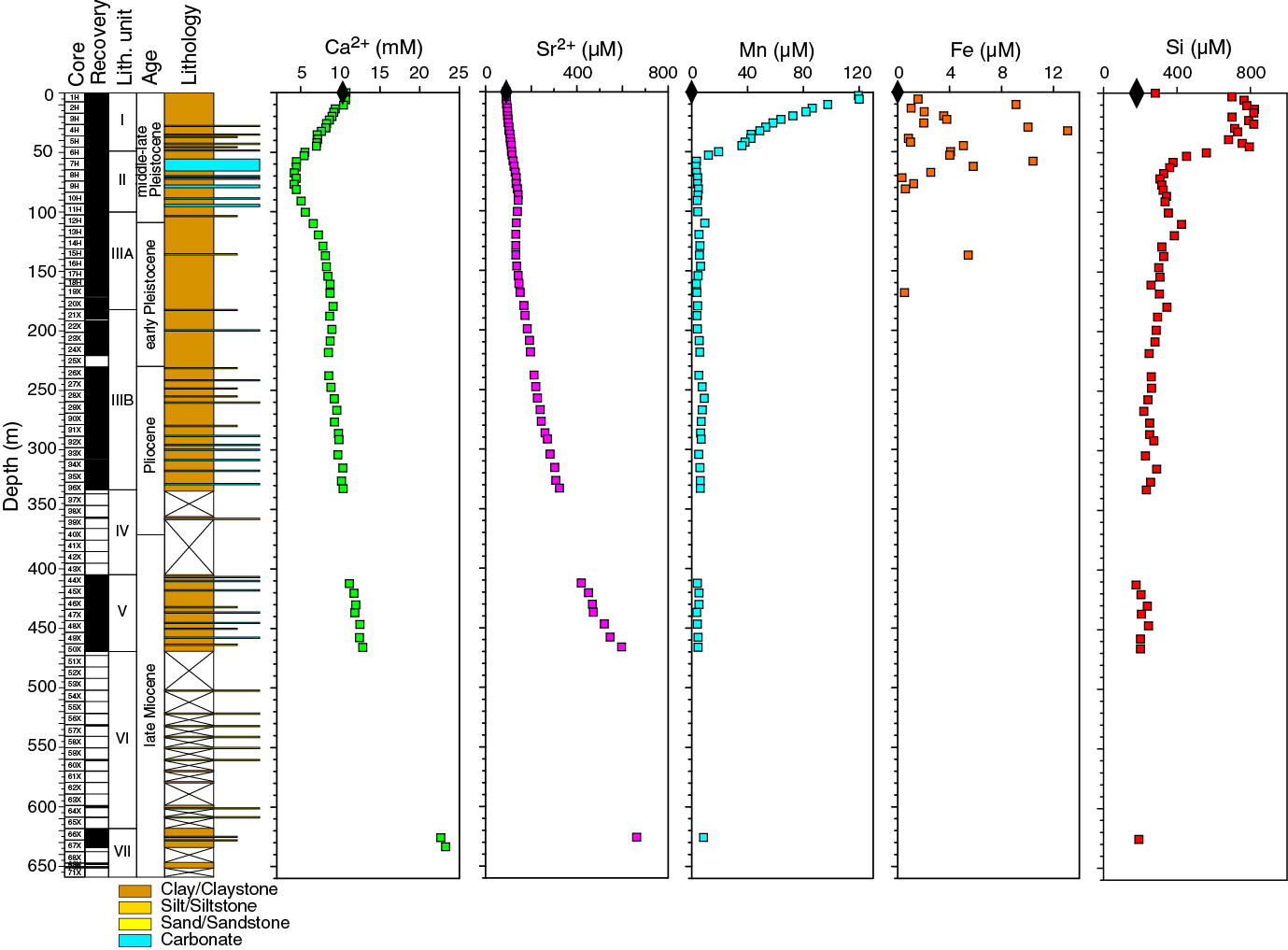
Figure F46. Interstitial water calcium, strontium, manganese, iron, and silica.
TIC content ranges from <0.1 to 9.9 wt% (average = 1.8 wt%). TIC is expressed as weight percent CaCO3, assuming inorganic carbon is exclusively present as CaCO3, and varies between 0.4 and 82 wt% (average = 14.8 wt%). Carbonate content varies from 1 to 18 wt% in the upper 50 m in Hole U1499A, reaching the highest values (25–63 wt%) between 50 and 91 m and then decreasing to <10 wt% to 291 m. Below this depth, carbonate content slightly increases to 13–28 wt% at 300–436 m and then increases to 2 wt% at the bottom of the hole. Low carbonate content continues (<10 wt%) in the upper part of Hole U1499B (726–861 m), and then carbonate increases to 65 wt% from 870 to 927 m before finally decreasing to extremely low values in the gravels of lithostratigraphic Subunit IXB.
The two intervals with the highest carbonate content (50–91 and 870–927 m) correspond well to lithostratigraphic Unit II and the lower part of Unit VIII, which are characterized by abundant nannofossil oozes and clay-rich chalk, respectively. An interval between has relatively high carbonate content (300–436 m) and contains clay, clayey silt, and sand with nannofossil/foraminifer interbeds; this interval also had very poor core recovery. One sample (367-U1499A-48X-5, 33–34 cm; 450 m) is characterized by very high carbonate content, reaching 82 wt% (Table T9). This sample was taken from a foraminifer sand layer.
Total carbon concentrations vary between 0.1 and 10.2 wt% (Table T9). TOC, calculated as the difference between total carbon and TIC, decreases gradually in the upper 100 m from 1 to 0.2 wt%, possibly because of the early postdepositional degradation of organic matter. TOC generally varies between 0 and 0.3 wt% with increasing depth (Figure F44). One sample in Hole U1499B (38R-1, 74–77 cm; 1005 m) exhibited extremely high TOC content (4.8 wt%). The high TOC in this sample from the gravel of lithostratigraphic Subunit IXC may not be representative of the unit as a whole because it was selected due to its dark color, which is scarce in this unit.
TOC/TN is generally used as a preliminary estimate for the source of organic material with high values (TOC/TN > 12) typically attributed to a predominantly terrestrial source, whereas lower values (TOC/TN < 8) are indicative of dominant marine contributions (Müller and Mathesius, 1999). TOC/TN values range from 1 to 17 in Hole U1499A (Table T9; Figure F44), indicating mixed marine/terrestrial organic input in this site. The higher values in the upper 100 m (Figure F44) imply relatively high contributions from terrestrial sources during this time interval compared to the following deeper sections where marine sources appear to dominate.
Interstitial water chemistry
A total of 58 whole-round core sections were collected from Hole U1499A for interstitial water analyses, including 32 samples from near the seafloor to ~160.9 m that were taken from APC cores and 26 samples from 168.3 to ~633.4 m taken from XCB cores. A mudline bottom seawater sample was also taken from Hole U1499A. No interstitial water samples were available from Hole U1499B.
Sulfate, alkalinity, ammonium, phosphate, bromide, and barium
Sulfate concentration decreases gradually from the seawater-like value of 28.8 mM at the mudline to ~1 mM at ~110 m. Sulfate maintains near-complete depletion values of <2 mM to 257 m and thereafter increases slowly to 16.9 mM at ~633 m, near the bottom of Hole U1499A (Table T10; Figure F45). The curvature of sulfate profile shallower than ~110 m suggests that sulfate reduction is predominantly mediated by sedimentary organic matter degradation (Chen et al., 2010) with a net simplified equation:
Table 10. Interstitial water chemistry data. View table in PDF format. Download table in CSV format.
As shown in the equation, sulfate reduction coupled with organic matter oxidation produces bicarbonates and increases the alkalinity of interstitial water in the sulfate reduction zone. Consequently, alkalinity increases from a seawater-like value of 2.38 mM at the mudline to a maximum of 13.1 mM at ~39 m before decreasing steadily with depth to a minimum of 1.5 mM at ~625 m (Figure F45). The last two samples near the bottom of the hole have alkalinity values <2.0 mM, lower than a typical seawater value of 2.3 mM. These values are likely caused by the pure water released during the smectite-illite transformation (see Chloride, sodium, and salinity).
During sedimentary organic matter degradation, ammonium, phosphate, and bromide are released into the pore fluids. Dissolved NH4+ increases from the mudline to a peak of 2.16 mM at ~77 m and then decreases gradually to 0.55 mM at 633.4 m approaching the bottom of Hole U1499A (Figure F45). The decrease in NH4+ below the sulfate reduction zone reflects diffusion and/or clay mineral ion exchange. The dissolved PO43− concentration increases sharply from 3.7 μM at the mudline to a maximum of 51.5 μM at ~10 m and then declines quickly to a local background value of 3.4 μM at ~62 m. Phosphate increases slightly to concentrations between 3.7 and 6.0 μM between ~67 and 146 m before staying fairly stable at ~3.0 μM to the bottom of the hole. The slight increase in PO43− in the short interval from ~67 to 146 m is likely controlled by the geochemistry of slump deposits there (see Lithostratigraphy). The overall downhole decrease in PO43− is likely the result of its adsorption onto Fe/Mn oxyhydroxides.
Bromide concentrations increase from 0.85 mM at the mudline to a maximum of 0.92 mM at ~154 m and then remain constant at ~0.90 mM to ~304 m before declining downhole to a minimum of 0.80 mM near the bottom of the hole. The minimal concentrations in bromide near the bottom of the hole are mostly caused by dilution from pure water released from the smectite-illite transformation (see Chloride, sodium, and salinity).
Barium concentrations remain consistently low (<2 µM) shallower than ~72 m and then sharply increase from 2.3 to 60.0 µM from ~77 to 100 m. Ba varies from 55 to 61 µM in the ~109–146 m interval and thereafter quickly increases from 53.2 to 105.8 µM from 154 to 218 m, followed by a sharp decrease from 42.7 µM at ~238 m to 1.8 µM at 633 m near the bottom of the hole. The interval of high Ba concentrations >50 µM corresponds to the interval of near-complete consumption of SO42−, suggesting the dissolution of barite (BaSO4), a mineral that precipitates in highly productive surface ocean water (Dymond et al., 1992). The two Ba concentration peaks possibly mark two barite fronts existing in sediments.
Calcium and strontium
Calcium concentrations decrease from 10.7 mM at the mudline to a minimum of 4.2 mM at ~77 m and then increase gradually to 12.5 mM at ~466 m before increasing sharply to >22 mM in the 626–633 m interval near the bottom of the hole (Figure F46). The minimum calcium concentration occurring at ~77 m correlates with the sulfate reduction zone (Figure F45), indicating that authigenic carbonate precipitation driven by active sulfate reduction coupled with sedimentary organic matter decomposition is actively ongoing (2HCO3− + Ca2+ ↔ CaCO3 = ↓ H2O + CO2). It also suggests that the calcium profile shallower than 77 m is mainly controlled by authigenic carbonate precipitation with minor calcareous microfossil dissolution (see Biostratigraphy); this suggestion is further supported by the Sr data. The downhole increase in calcium is likely caused by biogenic carbonate dissolution and recrystallization, which is evidenced by the poorer downhole preservation of calcareous microfossils and clear overgrowth of calcareous fossils deeper than 450 m (see Biostratigraphy).
Strontium concentrations monotonically increase downhole from a seawater-like value of 90.7 μM at the mudline to 662.3 μM at ~633 m near the bottom of the hole. Biogenic calcite dissolution and recrystallization release Sr into fluids, leading to an overall Sr increase with depth. Therefore, the Sr profile suggests that biogenic carbonate has experienced dissolution throughout the hole, particularly through lithostratigraphic Units V–VII (see Lithostratigraphy) since the late Miocene. This suggestion is supported by the variability in preservation of calcareous microfossils (see Biostratigraphy). Less dissolution of biogenic carbonate in the sulfate reduction zone suggests that the high alkalinity produced by sulfate reduction and organic matter oxidation might help preserve calcareous microfossils.
Chloride, sodium, and salinity
Chloride concentrations increase from 555.5 mM at the mudline to a maximum value of 565.7 mM at 35.5 m and then decrease gradually to an average downhole value of ~558.5 mM at 81.3 m (Figure F47). Thereafter, chloride concentrations are consistent, with an average value of 558.3 ± 2.9 mM to ~466 m. However, near the bottom of Hole U1499A, chloride concentrations sharply decrease to 542.7 mM at ~626 m and 533.6 mM at ~633.4 m. The maximum chloride concentration at 35.5 m was possibly caused either by the imprint of bottom seawater chloride of the Last Glacial Maximum and/or by water uptake during the alteration of kaolinite to smectite or illite in sediments. Pure water released from the smectite-illite transformation may be responsible for the lower chloride concentrations near the bottom of the hole. The transformation is mostly caused by the relatively high temperature of ~60°C in sediments at ~630 m because the optimal temperature for the smectite-illite transformation is between 50° and 120°C (Kastner and Rudnicki, 2004). Sediment temperature was calculated based on a bottom seawater temperature of 2.5°C and the geothermal gradient (91°C/km) found in Hole U1499A (see Physical properties and Downhole measurements).
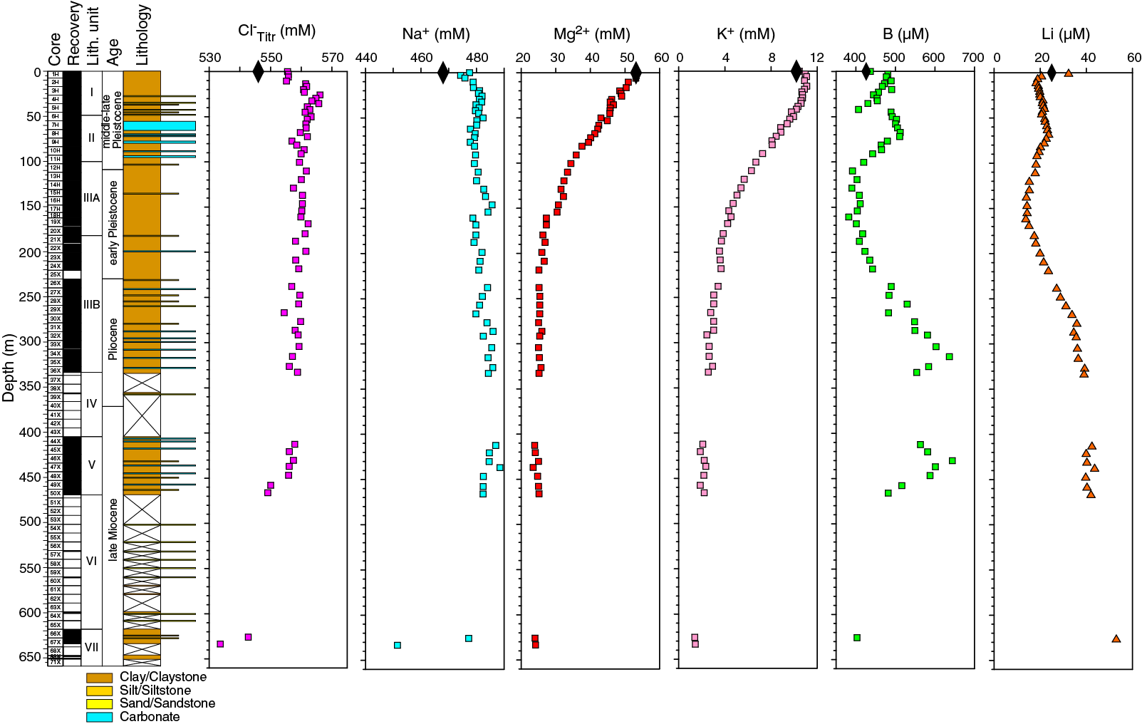
Figure F47. Interstitial water chloride, sodium, magnesium, potassium, boron, and lithium.
Sodium concentrations are nearly constant with a seawater-like value of 481 ± 2.8 mM shallower than 466 m before sharply decreasing to 452 mM at ~633 m near the bottom of the hole. The lower sodium concentrate at the bottom of the hole is mostly driven by the smectite-illite transformation (see Chloride, sodium, and salinity).
Salinity decreases from 36.5 at the mudline to 35 at 62.4 m and then varies between 34 and 33 to the bottom of Hole U1499A. Decreasing salinity is likely driven by the downhole decreases in calcium, magnesium, potassium, and sulfate.
Silica
Dissolved silica concentrations increase sharply from ~282 μM at the mudline to >700 μM with a maximum of 822 μM between ~3 and 45 m. Deeper than this, Si decreases from 560 μM at ~50 m to 192 μM at 626 m near the bottom of the hole. Elevated Si concentrations (>700 μM) in the uppermost 45 m suggest active dissolution of biogenic silica in these sediments, consistent with the presence of siliceous microfossils such as diatoms and radiolarians in the uppermost 19 m. Below this depth, the sediments are barren of siliceous microfossils (see Biostratigraphy).
Manganese and iron
Downhole distributions of manganese and iron in interstitial waters are shown in Figure F46, and concentrations of both elements are given in Table T10. Manganese concentrations increase sharply from below the detection limit of ~0.8 μM at the mudline to a maximum of ~120 μM at ~6 m and then decline gradually to a minimum value of ~3 μM at ~62 m. Thereafter, manganese varies between 3 and 10 μM to the bottom of Hole U1499A. This trend reflects the transition from oxic bottom seawater to suboxic sediments at a shallow depth, which is consistent with the relatively high organic carbon contents (~0.6–1.0 wt%) at shallow depths (see Bulk sediment geochemistry). Iron concentrations increase from the mudline to a peak of 13.1 μM at ~33 m and quickly decrease to ~1.0 μM at 42 m. Concentrations then increase to a high value of 10.43 μM at ~58 m before decreasing to a background value of ~0.59 μM at ~81 m. The second peak of iron concentration (10.43 μM) at ~58 m is within the slump deposit between 36.0 and 103.1 m (see Lithostratigraphy), which must have carried more iron rich sediments. Iron concentrations are mostly below the detection limit of 0.3 μM, particularly from ~90 m to the bottom of Hole U1499A, suggesting a limited supply of available iron in sediments and/or efficient removal of ferrous iron by hydrogen sulfide produced by sulfate reduction to form pyrite (Fe2+ + S2− → FeS2↓).
Magnesium and potassium
Magnesium concentrations gradually decrease from a seawater-like value of 53.4 mM at the mudline to ~23.9 mM at ~412 m (Figure F47) and remain fairly constant at ~24.0 mM to the bottom of the hole. Potassium concentrations are nearly constant at a seawater-like value of 10.8 ± 0.2 mM in the uppermost ~35 m and then decrease steadily downhole to ~1.4 mM at 626–633 m near the bottom of the hole. The nearly identical Mg2+ and K+ profiles indicate that a common process influenced their concentrations, such as clay mineral cation exchange and/or clay mineral authigenesis as kaolinite is transformed to smectite/illite with Mg2+ and/or K+ being incorporated into newly formed clay minerals.
Boron and lithium
Boron concentrations exhibit considerable variation with depth (Figure F47). B first decreases from 481 to 407 μM in the 3‒42 m interval and then increases from 489 to 511 μM through the 45‒72 m interval. Thereafter, B decreases from 480 to 390 μM from 77 to 129 m followed by a gradual increase from 409 μM at 137 m to a maximum of 636 μM at 315 m. Finally, B concentrations decrease from 584 μM at 326 m to 482 μM at 466 m before sharply decreasing to 403 μM at ~633 m near the bottom of the hole. This erratic B profile is likely driven by clay mineral cation exchange, its adsorption onto clay minerals, and desorption from clay minerals.
The lithium profile mimics that of boron because of the similar behavior of these two ions. Li concentrations are 19 ± 3 μM, less than the modern seawater value of 25 μM shallower than 218 m, likely because of adsorption of Li onto clay minerals such as kaolinite and smectite and/or onto other terrigenous sediments. Thereafter, Li concentrations increase gradually from 27 μM at 238 m to 53 μM at 626 m toward the bottom of the hole, possibly a result of diagenetic release of Li from clay minerals and/or diffusion from Li-enriched deep fluid.
In general, interstitial water chemistry at Site U1499 is controlled by sediment input and organic matter degradation, sulfate reduction, carbonate diagenesis, and clay diagenesis.
Physical properties
We measured physical properties on whole-round cores and working-half sections from Holes U1499A and U1499B for lithostratigraphic characterization and correlation between core description, borehole data, and seismic profiles. These measurements included GRA bulk density, magnetic susceptibility, NGR, P-wave velocity, MAD porosity, and thermal conductivity. We used the Whole-Round Multisensor Logger (WRMSL) to measure GRA bulk density, magnetic susceptibility, and P-wave velocity. NGR was measured on whole-round cores with the Natural Gamma Radiation Logger (NGRL). After the cores were split into section halves, P-wave velocity was measured with the Section Half Measurement Gantry (SHMG) using the caliper for measurements through the split core and bayonets inserted into the sediment for measurements along and across the core. Discrete samples were taken for MAD measurements, including mass measurement with dual balances and volume measurement with a pycnometer. Resulting values were used to calculate bulk properties (wet bulk density, dry bulk density, sediment grain density, porosity, and void ratio).
We measured P-wave velocities using the WRMSL for Hole U1499A cores collected with the APC system (367-U1499A-1H through 18H; 0–162 m). Cores recovered with the XCB or the RCB systems are slightly smaller in diameter than those cored with the APC system. As a result, sections cored with the XCB or RCB systems typically have gaps between the liner and the core, so we did not measure P-wave velocity with the WRMSL on these cores (i.e., from Core 19X to the bottom of Hole U1499A and all RCB cores from Hole U1499B). Velocity measurements with the X-caliper on the SHMG were performed on section halves for all cores from Holes U1499A and U1499B (usually 3 per core). Y- and Z-bayonet velocity measurements on the SHMG were stopped after Section 367-U1499A-9H-6 (~82 m) because the sediment was too hard for the bayonets to penetrate without disrupting and introducing cracks.
In Hole U1499B, we performed whole-round measurements of magnetic susceptibility, GRA bulk density, and NGR along with P-wave measurements on half cores using the PWC on Cores 2R through 38R and MAD measurements on discrete samples downhole to Core 30R. As the sediment in the cores became harder in Hole U1499B, we changed the sampling method and either cut small pieces or drilled minicores from the working-half sections for MAD measurements. For Cores 30R through 38R, P-wave measurements were made with the PWC on individual core pieces without the core liner.
For cores containing soft material in Hole U1499A (lithostratigraphic Units I–VI; to ~530 m), thermal conductivity was measured with the TK-04 (Teka Bolin) system with a needle probe inserted into whole-round cores. Because of the increased compaction, thermal conductivity on cores from deeper formations (Cores 367-U1499A-60X through 71X and all RCB cores from Hole U1499B) was measured on split section halves with a puck probe. For each core, three measurements were conducted in the middle section (usually Section 3). The puck probe measurements showed unstable results, presenting notable differences between the three measurements. The contact probe values likely overestimate the average in situ thermal conductivity.
In addition, downhole formation temperature measurements were made in Hole U1499A, and wireline log data were acquired from the bottom of the casing (651 m) to ~1020 m in Hole U1499B (see Downhole measurements).
Data cleaning and depth correction
Data measured using automatic systems such as the WRMSL, NGRL, and Section Half Multisensor Logger (SHMSL; point magnetic susceptibility) can contain data outliers (e.g., data from voids in core, unrealistic high values, etc.) that must be removed. This cleaning is required before the integration of these data into the models (e.g., computation of synthetic scenario seismograms).
We defined values exceeding μ ± Nσ (with N = 2), where μ is the mean and σ is the standard deviation of the entire data set (Table T11), as outliers and removed them from the data set. We also smoothed the data when used for modeling computation by applying a moving average filter. SHMG data were usually considered to be reliable because the operator checks the result as it is acquired. For MAD data, we observed very few outliers with values exceeding μ ± 2σ.
Table T11. Mean and SD for physical property measurements. Download table in CSV format.
We tested the accuracy of the PWC measurements by performing several measurements in the same sample. Table T12 presents the results of one test on Core 367-U1499B-14H. Error in the PWC measurements is <3%. For computation of synthetic seismograms to be compared to the real seismic data (e.g., with Petrel software), we chose to use the downhole logging velocity data (available deeper than 650 m) and the PWC data (in the uppermost 650 m) because the quality of the latter is manually checked at each measurement. Choosing the highest quality data is important because they can change the estimation of the reflectivity of the layers and thus have major impact on the computation.
Table T12. SHMG velocity caliper accuracy test. Download table in CSV format.
To insure the homogeneity of the descriptions and the comparisons of our measurements with other core characteristics collected in other laboratories, we used sample depths below seafloor calculated by the CSF-A method (see http://www.iodp.org/policies-and-guidelines/142-iodp-depth-scales-terminology-april-2011/file). It is important to note that depths calculated this way do not account for core expansion, including cores that have >100% recovery.
Density
GRA bulk density was measured automatically every 2 cm by the WRMSL. In addition, bulk density was measured on discrete core samples with the MAD system (~10 cm3 volume each; usually three samples per core according to recovery). Both types of density measurements show similar variations (Figure F48). A clear shift can be observed in the GRA bulk density from ~1.90 to ~1.75 g/cm3 at ~160 m. This shift coincides with the change from the APC to XCB. The reduced diameter of the XCB cores does not completely fill the core liner and causes lower density values during WRMSL measurements. No data were collected for the sandy layers within lithostratigraphic Units IV and VI and the lower part of Unit VII because of the poor core recovery in these intervals. No MAD samples were collected from Core 367-U1499B-31R to the bottom of Hole U1499B because the cores contained mostly small pieces of hard sandstone similar to the sample collected from Core 30R, which likely were not individually representative of the properties of the section penetrated.
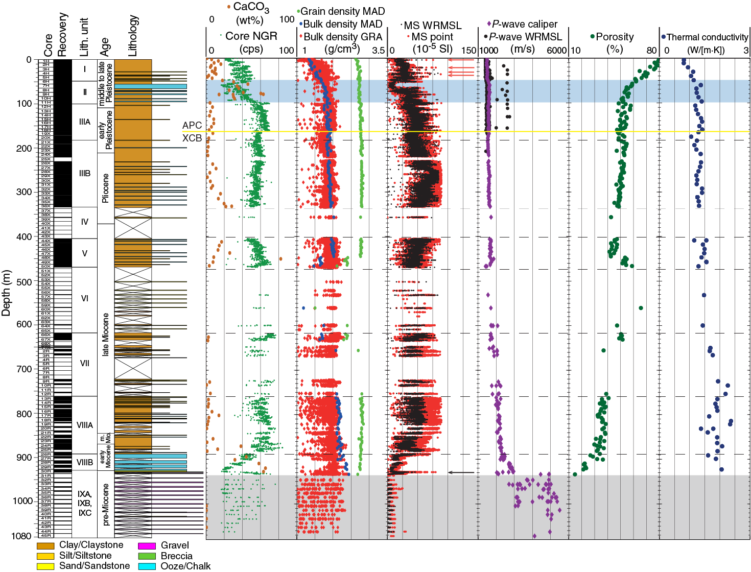
Figure F48. Petrophysics data summary.
Bulk densities increase quickly with depth from 1.4 g/cm3 to nearly 2 g/cm3 in the uppermost 100 m in Units I and II. Bulk densities then exhibit a slower increase from 2.0 g/cm3 near 100 m to 2.3 g/cm3 near the bottom of Hole U1499B. GRA bulk density data show high scatter in the indurated sediment deeper than ~650 m due to the fact that some of the measurements are made on partly empty liners when the recovered rocks are relatively small. The only discrete MAD sample taken from this unit was in the core catcher of Core 367-U1499B-30R and has a bulk density of 2.4 g/cm3 (higher than the ~2.3 g/cm3 average of lithostratigraphic Subunit VIIIB above) and a porosity of 15% (lower than the ~22% average of the unit above). Grain densities are almost constant (2.7 g/cm3) to ~450 m (Units I–V). Below that depth, grain densities are lower (~2.4 g/cm3), which can be related to the sandy layer of Unit VI.
Porosities sharply decrease from 80% at the seafloor to ~50% at 100 m in Hole U1499A and are relatively constant (53%) through Subunit IIIA and the upper part of Subunit IIIB. Porosities then slowly decrease to 45% at 470 m (base of Unit V). The sand in Units VI and VII between 450 and 650 m has a higher porosity (50%–55%). Porosities decrease again slowly from ~40% to 30% between 760 and 890 m. The deepest sample measured for MAD in Hole U1499B is a piece of sandstone from Subunit IXA (Core 367-U1499B-30R) with a porosity of only 15%.
Magnetic susceptibility
Magnetic susceptibility was measured on the WRMSL and the SHMSL (point magnetic susceptibility). Magnetic susceptibility is sensitive to magnetic mineral content and the mineralogy of the formation. After Clark and Emerson (1991), magnetic susceptibility varies between 0 and 2000 × 10−5 SI for sandstone and between 20 and 200 × 10−5 SI for clay material. Magnetic susceptibility data were collected every 2 cm, whereas point magnetic susceptibility data were collected every 1 cm through Section 367-U1499A-11H-4 (~95 m) and every 2 cm downsection to the bottom of Hole U1499A and throughout Hole U1499B. Magnetic susceptibility and point magnetic susceptibility values are in very good agreement along the entire profile of Site U1499.
Magnetic susceptibility displays four distinct peaks in Cores 1H through 5H (~30–50 m) that correspond with volcanic ash layers containing an increased amount of magnetic minerals. An abrupt decrease from ~30 × 10−5 to ~5 × 10⁻⁵ SI was observed in Cores 6H and 7H (~50 to ~70 m) and corresponds to a mass transport deposit composed of calcareous ooze and nannofossil-rich clay in Unit II. A local increase in magnetic susceptibility values from ~60 × 10−5 to 80 × 10−5 SI was observed from ~240 to 290 m (Cores 27H through 31H). This increase is associated with a slight decrease in reflectance a* values (Figure F9) and likely reflects higher Fe-rich mineral content. Between 300 and 830 m, magnetic susceptibility values are relatively constant around 50 × 10−5 SI and then significantly decrease with depth to 0–20 × 10−5 SI at 930 m. In Core 30R near the base of Subunit VIIIB (~930 m), a unique layer of reddish brown claystone with Fe-Mn nodules has high magnetic susceptibility values and NGR counts. Deeper than ~933 m, magnetic susceptibility values are very low in the gravel and sandstone of Subunit IXC.
P-wave velocity
P-wave velocities for the uppermost sediment are close to the seawater velocity, ~1500 m/s, for the uppermost 50 m, reflecting the high porosity of the sediment near the surface. WRMSL P-wave velocity values are slightly lower than the SHMG caliper values, probably because the WRMSL has a looser contact between measuring sensors and core material being measured. Some WRMSL P-wave velocity values, however, are much larger than the caliper measurements (2700 versus 1500 m/s, respectively; Figure F48). This might be related either to material in the core not measured with the caliper or to other unidentified factors. The caliper values were considered more accurate for the computation of synthetic seismograms (see Correlation to seismic data). P-wave velocity gradually increases with depth from 1500 m/s near 50 m to values around 2300 m/s at ~930 m. Some slightly higher P-wave velocity values (2000 m/s compared to 1800 m/s in the layers above) were observed in the partially recovered cores of Units IV and V around 350 and 450 m, corresponding to coarser sands. Deeper than 930 m, the gravels of Subunit IXC measured individually yielded relatively high velocities (~5500 m/s), whereas the silty sand interbeds give lower values (~3060 m/s).
Natural gamma radiation
NGR counts vary with lithology, with higher values in sediments rich in clay, silt, and mud (40–70 counts/s; Russell, 1944) and lower values in sand or sandstone (0–25 counts/s; Russell, 1944). NGR values in Hole U1499A present an increase in counts for the uppermost 60 m (Figures F48, F49). Below this depth, values decrease abruptly to ~20 counts/s near 60 m and then increase again to ~60 counts/s at ~100 m. This anomaly coincides with the drop in magnetic susceptibility and is correlated with the lithology in the slump deposits in lithostratigraphic Unit II. A clear decrease can be observed in NGR counts at ~160 m from ~65 to ~55 counts/s when coring switched from the APC system to the XCB system, resulting in a reduced volume of material being measured in the core liner. Between 100 and 830 m, NGR values only show small variations between 50 and 70 counts/s. From ~830 to 920 m, a sharp decrease in NGR from 70 to 20 counts/s is associated with a decrease in magnetic susceptibility values and an increase in carbonate content. This change corresponds to the chalks of lithostratigraphic Subunit VIIIB (Cores 367-U1499B-26R through 29R). In Core 30R, a sharp increase in NGR values corresponds to the clay with Fe-Mn nodules; this increase continues into the breccia of Subunits IXB and IXC.
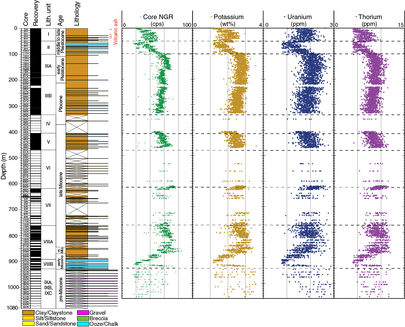
Figure F49. Core NGR measurements.
We estimated concentrations of K, U, and Th using NGR and bulk density measurements (Figure F49) based on a study from De Vleeschouwer et al. (2017). The general trend of each element concentration is similar to the total count values.
Thermal conductivity
Thermal conductivity presents an almost linear increase from the seafloor, with values from 0.8 to ~2 W/(m·K) at ~900 m. The trend of increasing thermal conductivity with depth is used to calculate a heat flow of 110 mW/m2 (see Downhole measurements). This relatively high value is consistent with previous estimates in the area.
Data interpretation and lithology correlation
Correlation with lithology
The variations of magnetic susceptibility and NGR data show some interesting and variable correlations with lithology. For example, low NGR values are associated with the high carbonate content of lithostratigraphic Unit II and Subunit VIIIA, whereas clay/silt has relatively low NGR but high magnetic susceptibility from 260 to 350 m, and an opposite correlation occurs at 420–480 m. The content of magnetic mineral and its mineralogy is reflected in magnetic susceptibility measurements of the formation of clay/silt/sand. Meanwhile, NGR values vary not only with lithology but also within the same sediment type.
Sediment compaction
The compaction of the sediments is reflected by the variation with depth of most of the physical properties in the uppermost 100 m. Density, P-wave velocity, NGR, magnetic susceptibility, and thermal conductivity increase gradually, whereas porosity drops from ~80% to ~50%. For the lower part of Hole U1499A (>170 m) and in Hole U1499B downsection to 930 m (top of the gravel layer in Subunit IXC), density, P-wave velocity, and thermal conductivity keep increasing with depth but to a lower extent, whereas NGR and magnetic susceptibility show undulations with opposite variations, reflecting other controlling factors such as the carbonate content.
Ash layers
In Hole U1499A, several peaks in magnetic susceptibility values in the uppermost cores (~5, 20, and 40 m) appear to be associated with ash layers observed in the lithology. Ash layers are characterized by relatively high magnetic susceptibility values in WRMSL and SHMSL measurements. However, although additional ash layers were not identified during core description, others may be present but too thin or dispersed to be observed within the resolution of magnetic susceptibility measurements.
Mass transport deposit in Unit II
The mass transport deposit observed in Sections 367-U1499A-6H-3 through 11H-5 (48.85–100.04 m; 51.19 m thick) coincides with a prominent decrease in magnetic susceptibility and NGR values. The very low values of magnetic susceptibility are likely due to the high concentration of carbonate (see Lithostratigraphy and Geochemistry). The deposit is also well detected by the decrease in NGR values (Figure F48).
Carbonate layer in Subunit VIIIB
From 830 to 930 m (Cores 367-U1499B-26R through 29R), magnetic susceptibility values and NGR counts generally decrease where density increases slightly and P-wave velocity increases significantly from 2200 to 2900 m/s. These variations are associated with a significant increase in the carbonate content from ~1 to ~65 wt% in the lowermost part of Subunit VIIIA and in the chalks of Subunit VIIIB.
Gravel layer in Subunit IXC
Section 367-U1499B-30R-6 through Core 45R recovered predominantly pebbles and cobbles with a few limited intervals of clayey silt or silty sand. The P-wave velocity of the pebbles/cobbles ranges from ~3000 to ~5500 m/s. The pebbles with the lowest P-wave velocity values are mainly the rocks showing fractures or weathering. Because of the low recovery in Subunit IXC, we are not able to determine a trend in velocity.
Downhole measurements
Wireline downhole logging
Logging operations and tools
Downhole log data was acquired after RCB coring in Hole U1499B penetrated to 1081.8 m. Hole conditions in the lowermost part of the hole significantly deteriorated after cutting the last core. The drillers were able to free the stuck drill string, pumped 100 bbl of mud, and raised the bit to 994 m but were never able to get the bit back deeper than ~1053 m. After circulating another 50 bbl of mud to clean cuttings out of the hole, the core (wash) barrel was recovered, and the bit was released in the hole. The end of the pipe was then raised to 877.3 m, where the mechanical bit release sleeve was shifted back into the circulating position. The end of the pipe was raised again to 780 m, and 235 bbl of heavy mud (11 lb/gal barite weighted) were pumped into the borehole to stabilize the hole for the downhole measurements. Finally, the end of the pipe was raised back inside the casing to 85.1 m, and the rig floor was prepared for the logging.
Borehole conditions from end of casing at 651 m to bottom of hole that could be logged at 1020 m were sufficiently good to run two different logging tool strings (Figure F50).
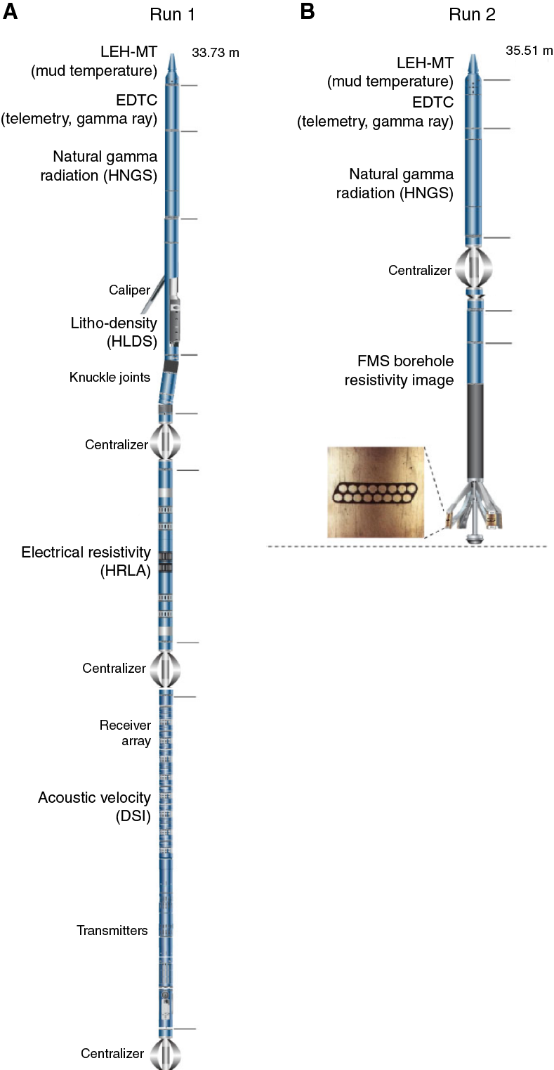
Figure F50. Downhole logging tool strings.
The first tool string, a modified triple combo tool string, included the following tools:
- Dipole Sonic Imager (DSI) for acoustic velocity,
- High-Resolution Laterolog Array (HRLA)/Phasor Dual Induction-Spherically Focused Resistivity Tool (DIT) for electrical resistivity,
- Hostile Environment Litho-Density Sonde (HLDS) for bulk density, and
- Hostile Environment Natural Gamma Ray Sonde (HNGS)/Enhanced Digital Telemetry Cartridge (EDTC-B) for NGR.
The first tool run was conducted downward (downlog), collecting data with all the string tools (DSI, HRLA, DIT, HLDS, HNGS, and EDTC-B) with the HLDS caliper closed. An uplog run (“repeat”) was then collected with the same recording tools but with the caliper open to ensure the HLDS tool was against the borehole wall and for borehole diameter measurements. Finally, the upward (uplog) main pass collected data with all the string tools (DSI, HRLA, DIT, HLDS, HNGS, and EDTC-B) and with the caliper open as before.
The second tool string was set up with a FMS to collect borehole resistivity images and the HNGS and EDTC-B for correlating with the previous logging runs. The FMS provides geographically orientated images and caliper measurements for both sets of arms. During the first pass, HNGS data were collected while lowering the tools into the borehole (downlog) without collecting FMS data and with the calipers closed (Figure F51). We collected FMS and HNGS data during two complete (uplog) runs over the entire open borehole.
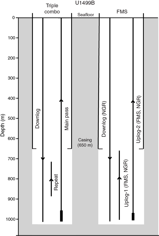
Figure F51. Logging operations summary.
The focus of our data analysis is primarily on the uplog main pass measurements. However, in general, measurements during down- and uplogging match well for all data types. Average heave conditions were ~0.5 m just prior to logging. The heave compensator was utilized whenever the tools were in open hole.
Log data processing
After we collected downhole logging information, the raw data were sent to Lamont-Doherty Earth Observatory for processing. Depth corrections were made to the data to account for the offset between rig floor and seafloor and for depth matching between each logging pass. For each logging run, the NGR information was used to define the water–sediment transition (water-casing; seafloor). The original logs were first shifted to the seafloor determined by the step in NGR values at 3770 m wireline log depth below rig floor (WRF) on the FMS/General Purpose Inclinometry Tool (GPIT)/EDTC-B/HNGS main pass. This differs by 1 m from the seafloor depth given by the drillers. Afterward, depth offsets between measurements taken during different logging runs were adjusted. The HLDS and HRLA data were corrected for hole size, and the HNGS data were corrected for hole size and mud weight during the recording. Sonic data were a high priority, and the Schlumberger engineer reprocessed the labeling for both compressional and shear data to improve the data quality. FMS images were processed to convert the electrical signals recorded by the FMS sensors to color-scaled images with both static and dynamic normalization. After this shore-based processing, the resulting data were sent back to the ship a few days later in a variety of formats (ASCII for conventional logs, GIF for FMS images, binary for acoustic waveforms, and SEGY for velocity data).
The collected log data are shown in DOWNHOLE in Supplementary material.
Log data quality
The borehole was generally in good condition, with measured diameters from ~10 inches at 664.15 m to >16 inches in the washout areas (Figure F52). Log data quality can be affected by the large borehole diameter in the washout zones. These zones were observed from 670 to 710 m, which corresponds to an interval of very low core recovery, and from 830 to 920 m, which spans a variety of lithologies in the lower half of lithostratigraphic Subunit VIIIA and relatively well recovered claystones and chalks in Subunit VIIIB. The borehole diameter decreases to 8 inches in the lowermost formation of the borehole (sandstones, breccias, and gravels of Unit IX) and in some intervals between 705 and 830 m. The FMS resistivity images are generally of good quality, except where large borehole diameters do not allow good contact of the FMS sensors to the borehole wall, resulting in dark (conductive) images. The two FMS passes followed nearly the same track over most parts of the borehole. The sonic velocities are very consistent with the shipboard laboratory measurements on the recovered cores, suggesting a general good quality of the DSI measurements.

Figure F52. Hole U1499B diameter.
Logging units
Downhole logging data for Hole U1499B are summarized in Figures F52 and F53. The logged interval is divided into 10 logging units, which are described below and are shown in Figure F53.

Figure F53. Downhole logs.
Logging Unit 1
Logging Unit 1 spans from 651 m (end of casing) to 726 m and is characterized by small-scale variations in NGR, bulk density, P-wave velocity, and borehole size. Within the uppermost part of the unit (~651–697 m), NGR gradually increases from ~60 to ~80 gAPI and then gradually decreases with depth from ~80 to ~55 gAPI within the underlying part (~697–726 m). Consequently, Th, K, and U concentrations follow this trend. However, bulk density, P-wave velocity, and resistivity are relatively homogeneous within logging Unit 1. FMS images show many interlayers with high resistivity and nearly horizontal bedding (e.g., 675, 685, 690, and 720 m; see DOWNHOLE in Supplementary material).
Logging Unit 2
Logging Unit 2 spans from 726 to 739 m and is characterized by high NGR values and relatively low bulk density and P-wave velocity. Resistivity is relatively homogeneous. Around 730 m, a high NGR peak coincides with a low in bulk density and P-wave velocity (~2.0 g/cm3 and 2.2 km/s, respectively). In the FMS images, horizontal bedding continues in this unit. Notably, a relatively thick interlayer with low resistivity was observed from ~734 to 735 m.
Logging Unit 3
Logging Unit 3 spans from 740 to 760 m and is characterized by relatively high NGR values and P-wave velocity, whereas density and resistivity are in the same range as Unit 1. The FMS images show a slightly scattered pattern within the unit.
Logging Unit 4
Logging Unit 4 spans from 760 to 820 m and presents a constant character and trend of most of the log values (e.g., density, resistivity, and P-wave velocity). Caliper measurements indicate that the borehole is relatively narrow in this zone (Figure F52). The FMS data show continuous, horizontal layering within this unit, even though the lower part (~788–813 m) presents poor quality in logging imagery.
Logging Unit 5
Logging Unit 5 spans from 820 to 840 m and is characterized by a sharp increase in bulk density, a slight increase in P-wave velocity, and an abrupt decrease in NGR values. This unit, especially at ~823–833 m, is characterized by scattered pattern in the FMS images, except for the lowermost part (~833–840 m), which shows horizontal bedding.
Logging Unit 6
Logging Unit 6 spans from 840 to 890 m and is characterized by relatively constant values of NGR, P-wave velocity, and bulk density. The FMS data are of poor quality; the variation in bedding, however, increases with depth throughout this unit.
Logging Unit 7
Logging Unit 7 spans from 890 to 925 m and is characterized by increasing values in density, P-wave velocity, and resistivity combined with NGR values decreasing from ~ 62 to ~30 gAPI with depth. The FMS images show many short-interval variations resulting in thin, horizontal layering in the upper part (~890–905 m), whereas scattered patterns were observed in the lower part (~905–925 m).
Logging Unit 8
Logging Unit 8 spans from 925 to 950 m and shows a change in the character and trend of most of the log curves. In general, NGR, density, P-wave velocity, and resistivity show very scattered values. P-wave velocity, NGR, and resistivity with generally increase with depth, and bulk density decreases. The FMS data are poor quality and show thicker beds than the unit above.
Logging Unit 9
The data set in logging Unit 9 shows very scattered values. This deeper unit (950–990 m) presents a NGR mean value of 63 gAPI and a relatively high resistivity value (mean value = 12 Ωm). P-wave velocity is highly variable, ranging from 2.1 to 4.0 km/s (mean value = 3.4 km/s). The FMS images show highly variable and oblique textures (Figure F54).
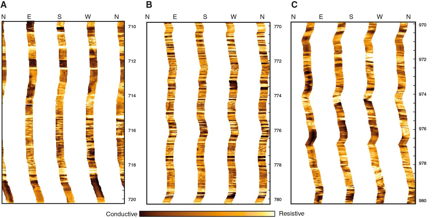
Figure F54. FMS images.
Logging Unit 10
In the bottom part of the hole (990 m to bottom of hole) in logging Unit 10, we observed scattered data with relatively high values of P-wave velocity and resistivity. As in logging Unit 9, the FMS images present variable and oblique textures.
Downhole logs and lithology
Downhole logs and FMS images provide important constraints on the lithology at Site U1499. Lithostratigraphic Subunit VIIIA is ~130 m of claystones and siltstones with variable amounts of carbonate, as well as interbeds of silt and foraminifer-rich sandstone. In this zone, the log data show relatively constant values of NGR, density, and P-wave velocity. The only observable change is in logging Unit 5, in an interval from which there was no recovery in lithostratigraphic Subunit VIIIA. Low NGR values and high density values in this no-recovery zone can be tentatively ascribed to a richer carbonate content.
Within the chalks of lithostratigraphic Subunit VIIIB, NGR values clearly decrease and density and velocity increase with depth, which likely reflects the increase of carbonate content with depth, as confirmed by geochemical analyses. The transition from carbonate to sandstone, breccia, and gravel at the boundary between lithostratigraphic Units VIII and IX corresponds to an increase in NGR and velocity and a notable decrease in density. All the log values in lithostratigraphic Unit IX are very scattered, confirming the heterogeneity of this deepest unit cored and logged in Hole U1499B.
NGR measurements from downhole logging generally agree with laboratory NGR measurements. A decrease to ~50 gAPI was observed in the formation of lithostratigraphic Subunit VIIIB (high carbonate) between 870 and 925 m.
Resistivity measurements from downhole logging show relatively constant values throughout logging Units 1–7 (downhole to 925 m). Resistivity increases sharply and exhibits more variability in the sandstones, breccias, and gravels of lithostratigraphic Unit IX.
The acquired FMS images provide constraints on the formation characteristics in addition to contributing to constraining the nature of the formation in zones where core recovery was poor (Figure F53), but they are strongly influenced by the hole diameter variations. The FMS images from the low-recovery zones in the lower part of lithostratigraphic Unit VII (~660–665, ~669–723, and ~727–761 m) generally show alternating smooth and patchy textures (Figure F54). Images from the no-recovery zone within lithostratigraphic Subunit VIIIA (~823–849 m) are similar. The sandstones, breccias, and gravels of lithostratigraphic Unit IX (logging Units 9 and 10) show highly variable and oblique textures on the FMS images (Figure F54), possibly reflecting the scattered orientation of the gravel clasts or the presence of faults and fractures in the gravel or the matrix (see DOWNHOLE in Supplementary material).
Comparison of sonic velocity and PWC measurements
In general, the velocities measured with the Versatile Seismic Imager (VSI) tool match the PWC measurements taken with the x-axis caliper on the SHMSL on the split cores. In the lowermost lithostratigraphic Unit IX, PWC velocities are higher than those measured in situ downhole with the DSI. In this unit, core recovery was very low, and the PWC velocity could only be measured on the cobbles and pebbles recovered. Thus, the PWC velocities are clearly higher than and not representative of the overall formation velocity.
Downhole temperature measurement and heat flow calculation
Six in situ formation temperature measurements were conducted using the APCT-3 (Figure F55). Extrapolated formation temperature values range from 5.46°C at 36 m (Core 367-U1499A-4H) to 14.42°C at 131 m (Core 14H) (Table T13). These values, with a seafloor temperature of 2.5°C, indicate a linear increase of the temperature with depth and give a geothermal gradient of 93°C/km (Figure F56). Thermal resistance was calculated in the upper 131 m using the “linear approach” (Pribnow et al., 2000; see Downhole measurements in the Expedition 367/368 methods chapter [Sun et al., 2018]). The slope of the linear fit between temperature and thermal resistance indicates a heat flow estimation of 110 mW/m2. This value is in agreement with the general high heat flow of the area (Figure F57).
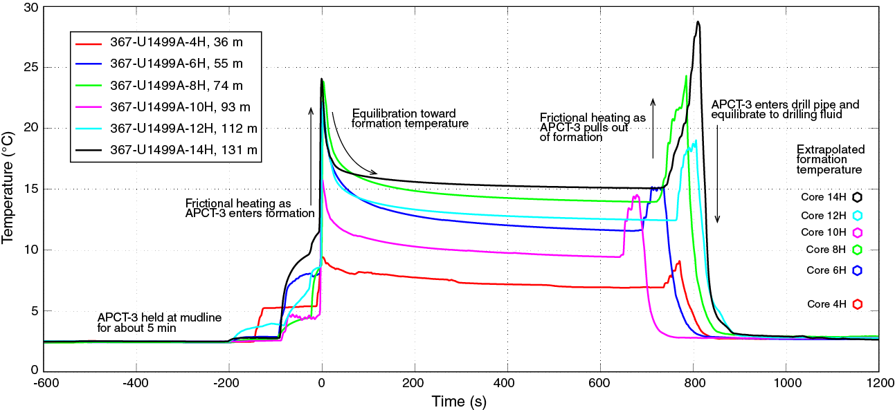
Figure F55. APCT-3 temperature-time series.
Table T13. APCT-3 measurements. Download table in CSV format.
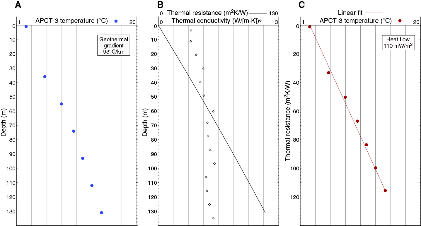
Figure F56. Heat flow calculations.
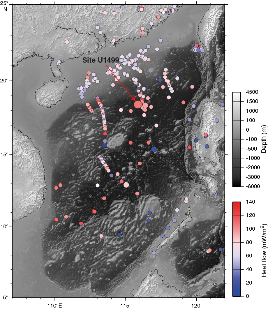
Figure F57. SCS seafloor heat flow values.
Correlation to seismic data
We used downhole log data, physical property measurements on cores and samples, and other available data to correlate Site U1499 data to the available seismic reflection profiles. We also used the Site U1499 density and sonic velocity data to create synthetic seismograms that provided additional constraints on the correlation. All correlations of the seismic reflection data with the Site U1499 core and log data, as well as the synthetic seismogram tests, were performed onboard using the Petrel software.
Velocity and density data
Velocity and density data were acquired in the laboratory (whole-round core sections [P-wave logger; PWL] and split-core sections [PWC]) in Holes U1499A and U1499B and from downhole logging between 655 and ~1020 m in Hole U1499B (see Physical properties and Downhole measurements).
The PWL data were measured only for whole-round APC core sections from the upper part of Hole U1499A (0–162 m). PWL data, once cleaned of the outliers resulting from automatic WRMSL data acquisition (see Physical properties in the Expedition 367/368 methods chapter [Sun et al., 2018]), are in substantial agreement with the PWC velocity data acquired from split-core sections.
Downhole log velocity data were collected using the DSI tool, and downhole density data were collected using the HDSL. Log-sonic velocities and PWC velocities are in very good agreement except for the deepest breccias and gravels of lithostratigraphic Subunit IXC. In Subunit IXC, PWC overestimates the velocities; they could only be measured on the cobbles and pebbles of the matrix-supported formation. In addition, core recovery in this unit was very poor. DSI log-velocity is considered to be more representative of the true formation velocity in this section. For seismic correlation, we used PWC values and density values from MAD and GRA from Hole U1499A (0–655 m), whereas below we used the downhole logging velocity and density data (Table T14).
Table T14. Velocity and density information used for TDR computation. Download table in CSV format.
Time-depth relations from the velocity data
TDRs are generally assumed to be quadratic polynomial functions from the interpolation of depth-velocity data. From the depth-velocity data, we computed the incremental TWT (Tin) as
Tin = [(dn − dn − 1)/Vn] × 2 × 1000,
where dn is the depth of the nth layer and Vn is the relative velocity. The incremental Ti is multiplied by 2000 for conversion into TWT expressed in milliseconds.
From Tin we derived the cumulative TWT (Tcn) expressed as
and finally the TWT adjusted from the seafloor (Ta) as
where Ta is the TWT at the seafloor expressed in milliseconds.
If the TDR is referred to the seafloor, the intercept of the interpolated quadratic polynomial functions is set to 0.
Figure F58 shows the velocity and density values collected with the PWC and the downhole measurements at Site U1499. TDR is computed relative to the seafloor and assuming a constant velocity of 2.1 km/s for the poor-recovery intervals that are inferred to be predominantly loosely consolidated sands/silts and for which no downhole log data were acquired (Table T14). We considered these poor-recovery zones as our seismic upper reflectors. Because we had no meaningful core recovery to make PWC velocity measurements on cores and no log data in these intervals, we assumed a velocity of 2.1 km/s based on velocity values measured with the DSI in the deeper poor-recovery sandy part (670–720 m; see Downhole measurements and Inderbitzen, 1974).
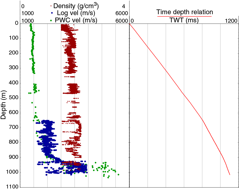
Figure F58. HLDS density, DSI and PWC velocity, and TDR.
The resulting quadratic polynomial function is
where d is the depth in meters and t the TWT in milliseconds.
Comparison of time-depth relations
We compared our Site U1499 TDR with others collected during previous expeditions in the SCS (Wang et al. 2000; Li et al. 2008, 2015c). Figure F59 shows the comparison of the Site U1499 TDR to those for Sites 1148, U1431, and U1433. The TDRs are in substantial agreement, except for the Site 1148 TDR, which shows higher velocities in the deeper layers.
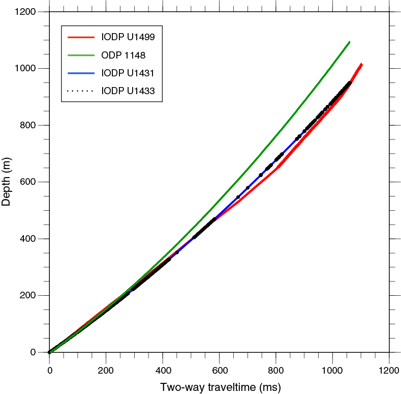
Figure F59. Site U1499 TDR curve.
Data correlations with Petrel
We correlated the site survey seismic reflection data with the data collected from whole-round cores (GRA density), split cores (MAD and PWC velocity), and log data (HDSL density and SVEL-DSI velocity). We also considered other data collected on board such as NGR, magnetic susceptibility, lithostratigraphic unit descriptions, and carbonate content. All of these properties were plotted over the seismic section with Petrel (Figure F60).
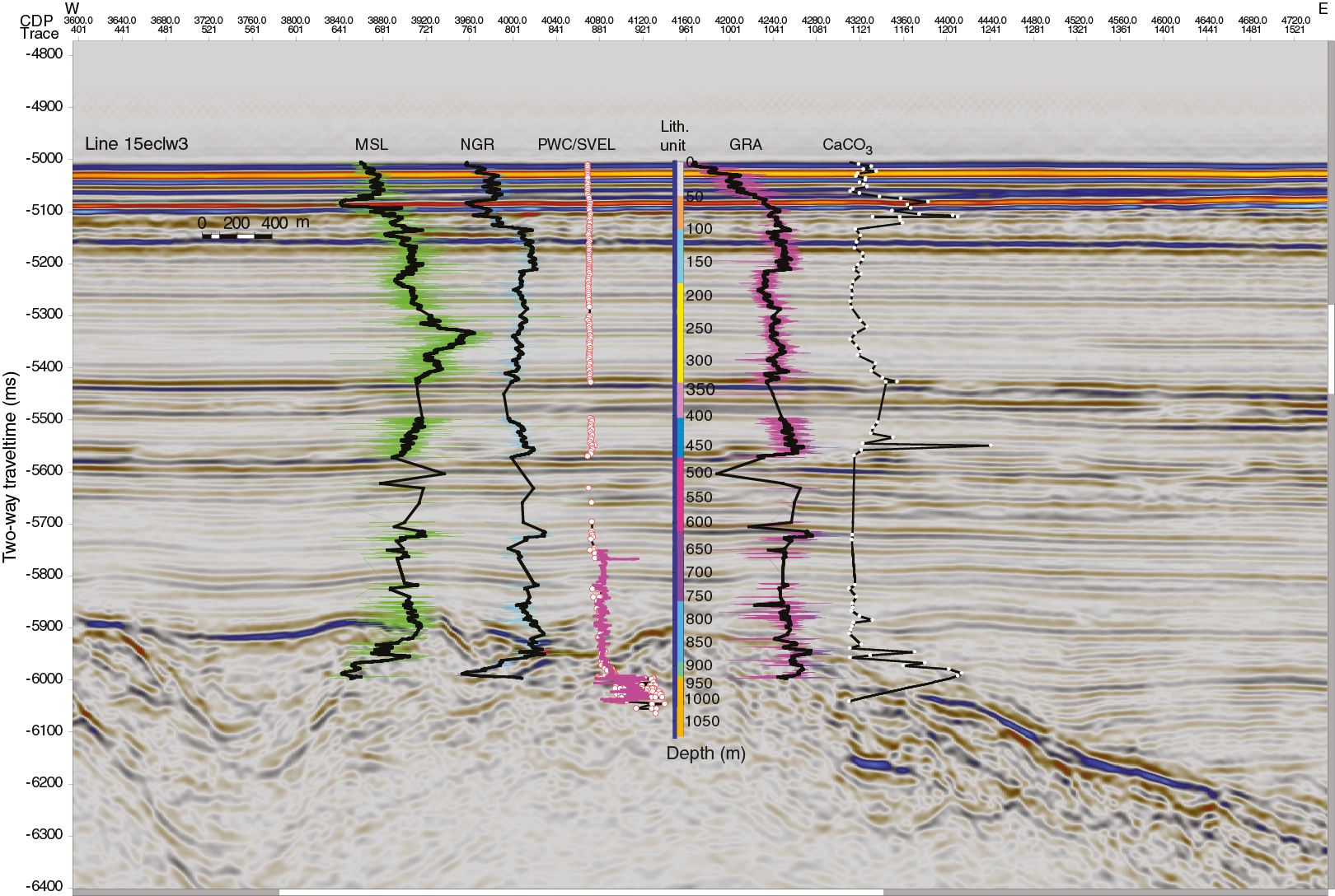
Figure F60. Seismic section.
The following import flow process was used:
- The coordinate system of the project was set (for Expedition 367: WGS1984_UTM50N),
- A new seismic folder and a new survey were created,
- SEGY data were imported with presettings (after the check of the Trace Header Information with the SeiSee software),
- The “Well” was created,
- The TDR file was imported (the file must have the depth-TWT adjusted with respect to the seafloor; we first chose the raw caliper and PWL VP curve to generate it), and
- Well logs (ASCII files) for all the properties of interest were imported (the file must be tab delimited and can be directly imported from the LIMS database; we chose to import CSF-B depths and values of interest).
We cleaned the data to remove the outliers before importing the values in Petrel (see Physical properties). An additional moving smoothing filter was also applied for GRA density. For the velocity data, more cleaning was applied; we manually checked the differences that might be created by manual or automatic picking of the first break for the caliper data.
The physical properties were displayed over the seismic data to allow a direct comparison between the reflectors and the property trends. The data shown in Figure F60 use the computed Site U1499 TDR (Figure F58) and show a good correlation between the main upper reflectors and the poor-recovery sandy intervals. In contrast, the main sedimentological and physical property changes related to the boundary between lithostratigraphic Units VIII and IX do not correlate to the reflector observed at ~5.9 s if the latter is interpreted to be the acoustic basement Tg reflector. The Tg reflector in this region is a distinct unconformity onto which seismic Unconformities T60 and T40 onlap, and younger strata above these show undisturbed and parallel bedding. Below the Tg reflector, seismic data indicate the presence of discontinuous and partly dipping reflectors strongly suggesting the presence of tectonically disturbed beds. Within the cored section, the boundary between undisrupted sedimentary layers (top) and syntectonic sediments (below) form the boundary between lithostratigraphic Units VIII and IX within Core 367-U1499B-30R at ~930 m, which contains an extremely large age span of supposedly early Oligocene to lowermost early Miocene.
Locally on the seismic profile, the acoustic basement is less clear than on other sections of the profiles, and the reflector at 5.9 s TWT has a relatively low amplitude (Figure F61). Moreover, although the correlation between the Tg reflector at ~ 5.9 s TWT and the boundary between lithostratigraphic Units VIII and IX would be intuitively obvious, this interpretation is difficult to reconcile with the observed physical properties and logging data. The only way for the top of lithostratigraphic Unit IX (~930 m) to fit with both the ~5.9 s Tg reflector and the ~5.42 s reflector (upper sandy layers; ~330 m) would be to apply a 30% velocity increase in the deeper part of the TDR from 300 to 930 m (Figure F62). This velocity increase seems unrealistic and led to much discussion on how to resolve the apparent discrepancy (see discussion on alternate TDR, below).
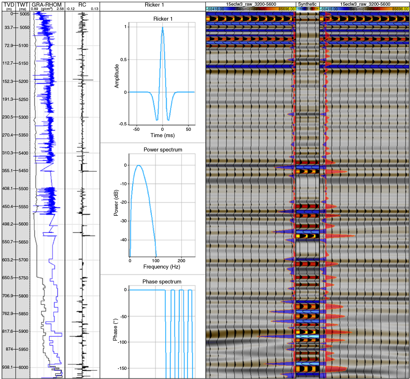
Figure F61. Synthetic seismogram.

Figure F62. Preferred and modified TDR.
Evaluation of alternative time-depth relations
We performed tests of alternative velocity assumptions. Two of them help characterize the effects of the TDR on the fit with the available seismic data.
The first test included the use of PWC velocity and downhole measurements data without imposing a constant velocity for the sandy poor-recovery zones (333–406 and 531–561 m). In this case, the TDR equation is
where d is the depth in meters and t is the TWT in milliseconds.
The resulting seismic correlation with this equation is shown in Figure F63. In this case, the velocity in the poor-recovery zone at 333–406 m is likely underestimated; there is a misfit between the relatively strong reflectors near 5.55–5.70 s TWT and the poor-recovery zones.
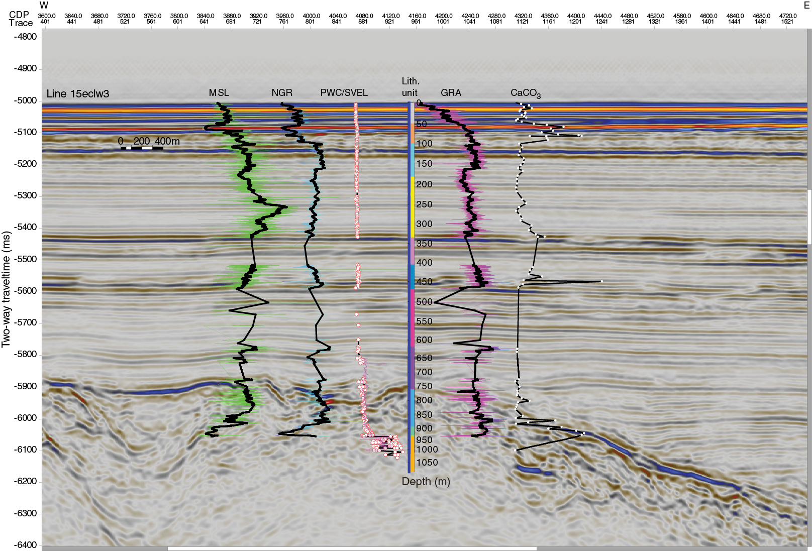
Figure F63. Seismic section using alternative TDRs without constant velocity.
The second test was aimed to fit the top of lithostratigraphic Unit IX (~930 m) with the ~5.9 s TWT Tg reflector and to fit the upper sandy layers (~330 m) with the ~5.42 s TWT. To reach these constraints, we needed to compute an alternative TDR with a 30% increase in velocity in the deeper part from 300 to 930 m with respect to the original TDR (Figure F62). The resulting polynomial interpolation is
The resulting seismic correlation with this equation is shown in Figure F64. Despite the intervals of low recovery, the data quality and the good match between laboratory and downhole data seems to exclude such overall velocity values as being too far from the observations. So although the correlation with lithologic variations could be made to match the Tg reflector at ~5.9 s TWT, this model conflicts with both caliper and log velocity data in the deeper parts of the section. In contrast, the model in Figure F60 honors the velocity data from core and logging and includes reasonable assumptions about the velocities in sandy layers of low recovery. Postcruise research, including the analysis of FMS images from Site U1499, detailed interpretations of seismic profiles close to Site U1499, and comparisons with TDR profiles from nearby Sites U1501, U1502, and U1505, will all be necessary to further address this issue and could possibly result in a unique model.
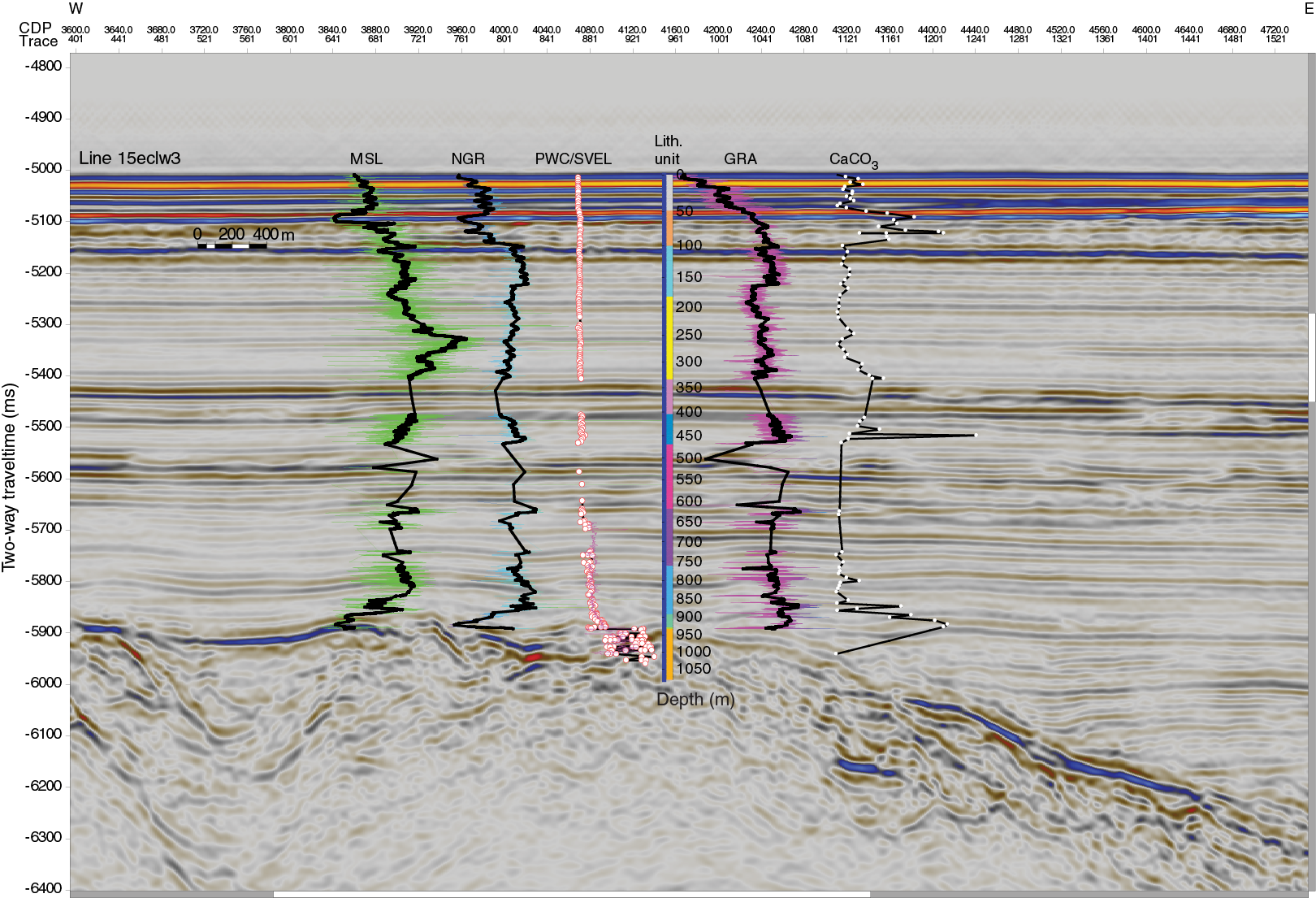
Figure F64. Seismic section using alternative TDRs with an increase in velocity.
Synthetic seismograms with Petrel
We used the Seismic interpretation module in Petrel to compute synthetic seismograms to further constrain the TDR. The parameters that need to be defined to compute synthetic seismograms are the seismic source signature, density curve, and velocity curve.
We performed several trials comparing the synthetic seismograms with the seismic reflection data. Petrel allows the choice of single frequency–centered sources. We chose Ricker wavelets centered at the mean values of the frequency content in our seismograms. For Hole U1499A (from the seafloor to 655 m), we used the density data derived from the MAD and GRA density data, whereas deeper than that (Hole U1499B) we used the HDSL density log data (Table T14). Similarly, we used the PWC velocity data from 0 to 655 m and the DSI logging velocity data below that. We conducted several trials with binning density and velocity data over different depth intervals. Our best fit was obtained with a 5 m binning for both density and velocity, which did not decimate the data. The resulting synthetic seismogram is shown in Figure F61.
References
Briais, A., Patriat, P., and Tapponnier, P., 1993. Updated interpretation of magnetic anomalies and seafloor spreading stages in the South China Sea: implications for the Tertiary tectonics of Southeast Asia. Journal of Geophysical Research: Solid Earth, 98(B4):6299–6328. http://dx.doi.org/10.1029/92JB02280
Bryant, W.R., and Bennett, R.H., 1988. Origin, physical, and mineralogical nature of red clays: the Pacific Ocean Basin as a model. Geo-Marine Letters, 8(4):189–249. http://dx.doi.org/10.1007/BF02281640
Chen, Y., Ussler, W., III, Haflidason, H., Lepland, A., Leif, R., Hovland, M., and Hjelstuen, B.O., 2010. Sources of methane inferred from pore water δ13C of dissolved inorganic carbon in Pockmark G11, offshore Mid-Norway. Chemical Geology, 275(3–4):127–138. https://doi.org/10.1016/j.chemgeo.2010.04.013
Clark, D.A., and Emerson, D.W., 1991. Notes on rock magnetization characteristics in applied geophysical studies. Exploration Geophysics, 22(3):547–555. http://dx.doi.org/10.1071/EG991547
Clemens, S.C., Murray, D.W., and Prell, W.L., 1996. Nonstationary phase of the Plio-Pleistocene Asian monsoon. Science, 274(5289):943–948. http://dx.doi.org/10.1126/science.274.5289.943
Clift, P.D., Lin, J., and ODP Leg 184 Scientific Party, 2001. Patterns of extension and magmatism along the continent-ocean boundary, South China margin. In Wilson, R.C.L., Beslier, M.-O., Whitmarsh, R.B., Froitzheim, N., and Taylor, B. (Eds.), Non-Volcanic Rifting of Continental Margins: A Comparison of Evidence from Land and Sea. Geological Society Special Publication, 187:489–510. http://dx.doi.org/10.1144/GSL.SP.2001.187.01.24
De Vleeschouwer, D., Dunlea, A.G., Auer, G., Anderson, C.H., Brumsack, H., de Loach, A., Gurnis, M., et al., 2017. Quantifying K, U, and Th contents of marine sediments using shipboard natural gamma radiation spectra measured on DV JOIDES Resolution. Geochemistry, Geophysics, Geosystems, 18(3):1053–1064. https://doi.org/10.1002/2016GC006715
Dickinson, W.R., Beard, L.S., Brakenridge, G.R., Erjavec, J.L., Ferguson, R.C., Inman, K.F., Knepp, R.A., Lindberg, F.A., and Ryberg, P.T., 1983. Provenance of North American Phanerozoic sandstones in relation to tectonic setting. Geological Society of America Bulletin, 94(2):222–235. http://dx.doi.org/10.1130/0016-7606(1983)94<222:PONAPS>2.0.CO;2
Dymond, J., Suess, E., and Lyle, M., 1992. Barium in deep-sea sediment: a geochemical proxy for paleoproductivity. Paleoceanography, 7(2):163–181. https://doi.org/10.1029/92PA00181
Gradstein, F.M., Ogg, J.G., Schmitz, M.D., and Ogg, G.M. (Eds.), 2012. The Geological Time Scale 2012: Amsterdam (Elsevier).
Huismans, R., and Beaumont, C., 2011. Depth-dependent extension, two-stage breakup and cratonic underplating at rifted margins. Nature, 473(7345):74–78. https://dx.doi.org/10.1038/nature09988
Inderbitzen, A. (Ed.), 1974. Marine Science (Volume 2): Deep-Sea Sediments: Physical and Mechanical Properties: New York (Springer US). https:/doi.org/10.1007/978-1-4684-2754-7
Jia, G., Peng, P., Zhao, Q., and Jian, Z., 2003. Changes in terrestrial ecosystem since 30 Ma in East Asia: stable isotope evidence from black carbon in the South China Sea. Geology, 31(12):1093–1096. http://dx.doi.org/10.1130/G19992.1
Jian, Z., Tian, J., and Sun, X., 2009. Upper water structure and paleo-monsoon. In Wang, P., and Li, Q. (Eds.), Developments in Paleoenvironmental Research (Volume 13): The South China Sea. Smol, J.P. (Series Ed.): Dordrecht, Netherlands (Springer), 297–394. https://doi.org/10.1007/978-1-4020-9745-4_5
Kastner, M., and Rudnicki, M.D., 2004. Ridge flank sediment-fluid interactions. In Davis, E., and Elderfield, H. (Eds.), Hydrogeology of the Oceanic Lithosphere: Cambridge, UK (Cambridge University Press), 534–571.
Kirschvink, J.L., 1980. The least-squares line and plane and the analysis of palaeomagnetic data. Geophysical Journal of the Royal Astronomical Society, 62(3):699–718. https://doi.org/10.1111/j.1365-246X.1980.tb02601.x
Larsen, H.C., Sun, Z., Stock, J.M., Jian, Z., Alvarez Zarikian, C.A., Klaus, A., Boaga, J., Bowden, S.A., Briais, A., Chen, Y., Cukur, D., Dadd, K.A., Ding, W., Dorais, M.J., Ferré, E.C., Ferreira, F., Furusawa, A., Gewecke, A.J., Hinojosa, J.L., Höfig, T.W., Hsiung, K.-H., Huang, B., Huang, E., Huang, X.-L., Jiang, S., Jin, H., Johnson, B.G., Kurzawski, R.M., Lei, C., Li, B., Li, L., Li, Y., Lin, J., Liu, C., Liu, C., Liu, Z., Luna, A., Lupi, C., McCarthy, A.J., Mohn, G., Ningthoujam, L.S., Nirrengarten, M., Osono, N., Peate, D.W., Persaud, P., Qui, N., Robinson, C.M., Satolli, S., Sauermilch, I., Schindlbeck, J.C., Skinner, S.M., Straub, S.M., Su, X., Tian, L., van der Zwan, F.M., Wan, S., Wu, H., Xiang, R., Yadav, R., Yi, L., Zhang, C., Zhang, J., Zhang, Y., Zhao, N., Zhong, G., and Zhong, L., 2018. Expedition 367/368 summary. In Sun, Z., Jian, Z., Stock, J.M., Larsen, H.C., Klaus, A., Alvarez Zarikian, C.A., and the Expedition 367/368 Scientists, South China Sea Rifted Margin. Proceedings of the International Ocean Discovery Program, 367/368: College Station, TX (International Ocean Discovery Program). https://doi.org/10.14379/iodp.proc.367368.101.2018
Li, C.-F., Li, J., Ding, W., Franke, D., Yao, Y., Shi, H., Pang, X., et al., 2015a. Seismic stratigraphy of the central South China Sea basin and implications for neotectonics. Journal of Geophysical Research: Solid Earth, 120(3):1377–1399. https://doi.org/10.1002/2014JB011686
Li, C.-F., Lin, J., Kulhanek, D.K., Williams, T., Bao, R., Briais, A., Brown, E.A., Chen, Y., Clift, P.D., Colwell, F.S., Dadd, K.A., Ding, W., Hernández-Almeida, I., Huang, X.-L., Hyun, S., Jiang, T., Koppers, A.A.P., Li, Q., Liu, C., Liu, Q., Liu, Z., Nagai, R.H., Peleo-Alampay, A., Su, X., Sun, Z., Tejada, M.L.G., Trinh, H.S., Yeh, Y.-C., Zhang, C., Zhang, F., Zhang, G.-L., and Zhao, X., 2015b. Expedition 349 summary. In Li, C.-F., Lin, J., Kulhanek, D.K., and the Expedition 349 Scientists, South China Sea Tectonics. Proceedings of the International Ocean Discovery Program, 349: College Station, TX (International Ocean Discovery Program). https://doi.org/10.14379/iodp.proc.349.101.2015
Li, C.-F., Lin, J., Kulhanek, D.K., Williams, T., Bao, R., Briais, A., Brown, E.A., Chen, Y., Clift, P.D., Colwell, F.S., Dadd, K.A., Ding, W., Hernández-Almeida, I., Huang, X.-L., Hyun, S., Jiang, T., Koppers, A.A.P., Li, Q., Liu, C., Liu, Q., Liu, Z., Nagai, R.H., Peleo-Alampay, A., Su, X., Sun, Z., Tejada, M.L.G., Trinh, H.S., Yeh, Y.-C., Zhang, C., Zhang, F., Zhang, G.-L., and Zhao, X., 2015c. Site U1435. In Li, C.-F., Lin, J., Kulhanek, D.K., and the Expedition 349 Scientists, South China Sea Tectonics. Proceedings of the International Ocean Discovery Program, 349: College Station, TX (International Ocean Discovery Program). http://dx.doi.org/10.14379/iodp.proc.349.107.2015
Li, C.-F., Shi, X., Zhou, Z., Li, J., Geng, J., and Chen, B., 2010. Depths to the magnetic layer bottom in the South China Sea area and their tectonic implications. Geophysical Journal International, 182(3):1229–1247. https://doi.org/10.1111/j.1365-246X.2010.04702.x
Li, C.-F., Zhou, Z., Li, J., Chen, B., and Geng, J., 2008. Magnetic zoning and seismic structure of the South China Sea ocean basin. Marine Geophysical Research, 29(4):223–238. https://doi.org/10.1007/s11001-008-9059-4
Liu, Z., Colin, C., Huang, W., Le, K.P., Tong, S., Chen, Z., and Trentesaux, A., 2007. Climatic and tectonic controls on weathering in south China and Indochina Peninsula: clay mineralogical and geochemical investigations from the Pearl, Red, and Mekong drainage basins. Geochemistry, Geophysics, Geosystems, 8(5):Q05005. https://doi.org/10.1029/2006GC001490
Liu, Z., Zhao, Y., Colin, C., Stattegger, K., Wiesner, M.G., Huh, C.-A., Zhang, Y., et al., 2016. Source-to-sink transport processes of fluvial sediments in the South China Sea. Earth-Science Reviews, 153:238–273. https://doi.org/10.1016/j.earscirev.2015.08.005
Lurcock, P.C., and Wilson, G.S., 2012. PuffinPlot: a versatile, user-friendly program for paleomagnetic analysis. Geochemistry, Geophysics, Geosystems, 13(6):Q06Z45. https://doi.org/10.1029/2012GC004098
Makris, J., Papoulia, J., McPherson, S., and Warner, L., 2012. Mapping of sediments and crust offshore Kenya, East Africa: a wide aperture refraction/reflection Survey. In SEG Technical Program Expanded Abstracts 2012: Tulsa, OK (Society of Exploration Geophysicists). https://doi.org/10.1190/segam2012-0426.1
Martini, E., 1971. Standard Tertiary and Quaternary calcareous nannoplankton zonation. In Farinacci, A. (Ed.), Proceedings of the Second Planktonic Conference, Roma 1970: Rome (Edizioni Tecnoscienza), 2:739–785.
Müller, A., and Mathesius, U., 1999. The palaeoenvironments of coastal lagoons in the southern Baltic Sea, I. The application of sedimentary Corg/N ratios as source indicators of organic matter. Palaeogeography, Palaeoclimatology, Palaeoecology, 145(1–3):1–16. https://doi.org/10.1016/S0031-0182(98)00094-7
Ogg, J.G., Ogg, G., and Gradstein, F.M., 2016. A Concise Geologic Time Scale 2016: Boston (Elsevier).
Pickering, K.T., Hiscott, R.N., and Hein, F.J., 1989a. Contourite drifts. In Pickering, K.T., Hiscott, R.N., and Hein, F.J., (Eds.), Deep-Marine Environments: Clastic Sedimentation and Tectonics: London (Unwin Hyman), 219–245.
Pickering, K.T., Hiscott, R.N., and Hein, F.J., 1989b. Facies, processes, sequences and controls. In Pickering, K.T., Hiscott, R.N., and Hein, F.J., (Eds.), Deep-Marine Environments: Clastic Sedimentation and Tectonics: London (Unwin Hyman), 13–40.
Pribnow, D., Kinoshita, M., and Stein, C., 2000. Thermal Data Collection and Heat Flow Recalculations for Ocean Drilling Program Legs 101–180: Hanover, Germany (Institute for Joint Geoscientific Research, Institut für Geowissenschaftliche Gemeinschaftsaufgaben [GGA]). http://www-odp.tamu.edu/publications/heatflow/ODPReprt.pdf
Roberts, A.P., Chang, L., Rowan, C.J., Horng, C.-S., and Florindo, F., 2011. Magnetic properties of sedimentary greigite (Fe3S4): an update. Reviews of Geophysics, 49(1):RG1002. https://doi.org/10.1029/2010RG000336
Russell, W.L., 1944. The total gamma ray activity of sedimentary rocks as indicated by Geiger counter determinations. Geophysics, 9(2):180–216. https://doi.org/10.1190/1.1445076
Shipboard Scientific Party, 1998. Site 1069. In Whitmarsh, R.B., Beslier, M.-O., Wallace, P.J., et al., Proceedings of the Ocean Drilling Program, Initial Reports, 173: College Station, TX (Ocean Drilling Program), 219–263. http://doi.org/10.2973/odp.proc.ir.173.107.1998
Shipboard Scientific Party, 2000. Site 1148. In Wang, P., Prell, W.L., Blum, P., et al., Proceedings of the Ocean Drilling Program, Initial Reports, 184: College Station, TX (Ocean Drilling Program), 1–122. https://doi.org/10.2973/odp.proc.ir.184.109.2000
Sibuet, J.-C., and Tucholke, B.E., 2012. The geodynamic province of transitional lithosphere adjacent to magma-poor continental margins. Geological Society Special Publication, 369:429–452. https://doi.org/10.1144/SP369.15
Sibuet, J.-C., Yeh, Y.-C., and Lee, C.-S., 2016. Geodynamics of the South China Sea. Tectonophysics, 692(B):87–119. https://doi.org/10.1016/j.tecto.2016.02.022
Sun, Z., Jian, Z., Stock, J.M., Larsen, H.C., Klaus, A., Alvarez Zarikian, C.A., Boaga, J., Bowden, S.A., Briais, A., Chen, Y., Cukur, D., Dadd, K.A., Ding, W., Dorais, M.J., Ferré, E.C., Ferreira, F., Furusawa, A., Gewecke, A.J., Hinojosa, J.L., Höfig, T.W., Hsiung, K.-H., Huang, B., Huang, E., Huang, X.-L., Jiang, S., Jin, H., Johnson, B.G., Kurzawski, R.M., Lei, C., Li, B., Li, L., Li, Y., Lin, J., Liu, C., Liu, C., Liu, Z., Luna, A., Lupi, C., McCarthy, A.J., Mohn, G., Ningthoujam, L.S., Nirrengarten, M., Osono, N., Peate, D.W., Persaud, P., Qui, N., Robinson, C.M., Satolli, S., Sauermilch, I., Schindlbeck, J.C., Skinner, S.M., Straub, S.M., Su, X., Tian, L., van der Zwan, F.M., Wan, S., Wu, H., Xiang, R., Yadav, R., Yi, L., Zhang, C., Zhang, J., Zhang, Y., Zhao, N., Zhong, G., and Zhong, L., 2018. Expedition 367/368 methods. In Sun, Z., Jian, Z., Stock, J.M., Larsen, H.C., Klaus, A., Alvarez Zarikian, C.A., and the Expedition 367/368 Scientists, South China Sea Rifted Margin. Proceedings of the International Ocean Discovery Program, 367/368: College Station, TX (International Ocean Discovery Program). https://doi.org/10.14379/iodp.proc.367368.102.2018
Sun, Z., Stock, J., Jian, Z., McIntosh, K., Alvarez Zarikian, C.A., and Klaus, A., 2016. Expedition 367/368 Scientific Prospectus: South China Sea Rifted Margin. International Ocean Discovery Program. https://doi.org/10.14379/iodp.sp.367368.2016
Wang, P., Prell, W.L., Blum, P., et al., 2000. Proceedings of the Ocean Drilling Program, Initial Reports, 184: College Station, TX (Ocean Drilling Program). https://doi.org/10.2973/odp.proc.ir.184.2000
Wang, P., Wang, L., Bian, Y., and Jian, Z., 1995. Late Quaternary paleoceanography of the South China Sea: surface circulation and carbonate cycles. In Tokuyama, H., Taira, A., and Kuramoto, S. (Eds.), Asian Marine Geology. Marine Geology, 127(1–4):145–165. https://doi.org/10.1016/0025-3227(95)00008-M
Yan, P., Deng, H., Liu, H., Zhang, Z., and Jiang, Y., 2006. The temporal and spatial distribution of volcanism in the South China Sea region. Journal of Asian Earth Sciences, 27(5):647–659. https://doi.org/10.1016/j.jseaes.2005.06.005
Zachos, J., Pagani, M., Sloan, L., Thomas, E., and Billups, K., 2001. Trends, rhythms, and aberrations in global climate 65 Ma to present. Science, 292(5517):686–693. https://doi.org/10.1126/science.1059412
Zijderveld, J.D.A., 1967. AC demagnetization of rocks: analysis of results. In Collinson, D.W., Creer, K.M., and Runcorn, S.K. (Eds.), Methods in Palaeomagnetism: Amsterdam (Elsevier), 254–286.
1 Sun, Z., Stock, J.M., Klaus, A., Larsen, H.C., Jian, Z., Alvarez Zarikian, C.A., Boaga, J., Bowden, S.A., Briais, A., Chen, Y., Cukur, D., Dadd, K.A., Ding, W., Dorais, M.J., Ferré, E.C., Ferreira, F., Furusawa, A., Gewecke, A.J., Hinojosa, J.L., Höfig, T.W., Hsiung, K.-H., Huang, B., Huang, E., Huang, X.-L., Jiang, S., Jin, H., Johnson, B.G., Kurzawski, R.M., Lei, C., Li, B., Li, L., Li, Y., Lin, J., Liu, C., Liu, C., Liu, Z., Luna, A., Lupi, C., McCarthy, A.J., Mohn, G., Ningthoujam, L.S., Nirrengarten, M., Osono, N., Peate, D.W., Persaud, P., Qui, N., Robinson, C.M., Satolli, S., Sauermilch, I., Schindlbeck, J.C., Skinner, S.M., Straub, S.M., Su, X., Tian, L., van der Zwan, F.M., Wan, S., Wu, H., Xiang, R., Yadav, R., Yi, L., Zhang, C., Zhang, J., Zhang, Y., Zhao, N., Zhong, G., and Zhong, L., 2018. Site U1499. In Sun, Z., Jian, Z., Stock, J.M., Larsen, H.C., Klaus, A., Alvarez Zarikian, C.A., and the Expedition 367/368 Scientists, South China Sea Rifted Margin. Proceedings of the International Ocean Discovery Program, 367/368: College Station, TX (International Ocean Discovery Program). https://doi.org/10.14379/iodp.proc.367368.103.2018
2 Expedition 367/368 Scientists’ addresses.
This work is distributed under the Creative Commons Attribution 4.0 International (CC BY 4.0) license. 
- F1. Seismic data coverage and magnetic anomalies.
- F2. North SCS margin with seismic coverage.
- F3. TWT to basement Tg unconformity and Reflector T60.
- F4. Original and interpreted seismic profiles.
- F5. Schematic development of continental breakup.
- F6. Spectrum of possible magma-poor rifted margin models.
- F7. Reentry system and casing.
- F8. Lithostratigraphic summary.
- F9. Correlation of lithostratigraphic units.
- F10. Bulk mineralogy by XRD.
- F11. Dark greenish gray bioclast-rich clay.
- F12. Pale brownish volcanic ash layer.
- F13. Greenish gray clay-rich calcareous ooze.
- F14. Synsedimentary deformation.
- F15. Representative section of clay with silt interbeds.
- F16. Increased carbonate content and bioturbation.
- F17. Thick interval of well-sorted foraminiferal sand.
- F18. Unconsolidated medium-grained sands.
- F19. Foraminifer siltstone layer.
- F20. Lithology and color change.
- F21. Greenish gray claystone interbedded in brown claystone.
- F22. Black-brownish iron-manganese nodules.
- F23. Contacts between subunits.
- F24. Poorly sorted angular clasts of sedimentary rocks.
- F25. Breccia intervals.
- F26. Sandstone cobbles.
- F27. Fining-upward sequences.
- F28. SCS and surrounding region.
- F29. Red claystone.
- F30. Lithostratigraphic summary.
- F31. Correlated lithostratigraphic summary.
- F32. Unit II structures.
- F33. Subunit VIIIA structures.
- F34. Biostratigraphic and paleoenvironmental summary.
- F35. Age-depth model.
- F36. Additional samples.
- F37. Deepwater agglutinated benthic foraminifers.
- F38. Remanent magnetization data.
- F39. Demagnetization data, Hole U1499A.
- F40. Demagnetization data, Hole U1499B.
- F41. Magnetostratigraphy, Hole U1499A.
- F42. Magnetostratigraphy, Hole U1499B.
- F43. Age-depth model.
- F44. Lithology, carbon, and TOC/TN profiles.
- F45. Interstitial water sulfate, alkalinity, ammonium, phosphate, bromide, and barium.
- F46. Interstitial water calcium, strontium, manganese, iron, and silica.
- F47. Interstitial water chloride, sodium, magnesium, potassium, boron, and lithium.
- F48. Petrophysics data summary.
- F49. Core NGR measurements.
- F50. Downhole logging tool strings.
- F51. Logging operations summary.
- F52. Hole U1499B diameter.
- F53. Downhole logs.
- F54. FMS images.
- F55. APCT-3 temperature-time series.
- F56. Heat flow calculations.
- F57. SCS seafloor heat flow values.
- F58. HLDS density, DSI and PWC velocity, and TDR.
- F59. Site U1499 TDR curve.
- F60. Seismic section.
- F61. Synthetic seismogram.
- F62. Preferred and modified TDR.
- F63. Seismic section using alternative TDRs without constant velocity.
- F64. Seismic section using alternative TDRs with an increase in velocity.
- T1. Site U1499 core summary.
- T2. Mineral percentages.
- T3. Biostratigraphic events.
- T4. Calcareous nannofossils, Hole U1499A.
- T5. Calcareous nannofossils, Hole U1499B.
- T6. Planktonic foraminifers.
- T7. Magnetostratigraphy.
- T8. Headspace gas data.
- T9. Carbon and nitrogen.
- T10. Interstitial water chemistry data.
- T11. Mean and SD for physical property measurements.
- T12. SHMG velocity caliper accuracy test.
- T13. APCT-3 measurements.
- T14. Velocity and density information used for TDR computation.