Wallace, L.M., Saffer, D.M., Barnes, P.M., Pecher, I.A., Petronotis, K.E., LeVay, L.J., and the Expedition 372/375 Scientists
Proceedings of the International Ocean Discovery Program Volume 372B/375
publications.iodp.org

https://doi.org/10.14379/iodp.proc.372B375.105.2019
Site U15201
P.M. Barnes, L.M. Wallace, D.M. Saffer, I.A. Pecher, K.E. Petronotis, L.J. LeVay, R.E. Bell, M.P. Crundwell, C.H. Engelmann de Oliveira, A. Fagereng, P.M. Fulton, A. Greve, R.N. Harris, Y. Hashimoto, A. Hüpers, M.J. Ikari, Y. Ito, H. Kitajima, S. Kutterolf, H. Lee, X. Li, M. Luo, P.R. Malie, F. Meneghini, J.K. Morgan, A. Noda, H.S. Rabinowitz, H.M. Savage, C.L. Shepherd, S. Shreedharan, E.A. Solomon, M.B. Underwood, M. Wang, A.D. Woodhouse, S.M. Bourlange, M.M.Y. Brunet, S. Cardona, M.B. Clennell, A.E. Cook, B. Dugan, J. Elger, D. Gamboa, A. Georgiopoulou, S. Han, K.U. Heeschen, G. Hu, G.Y. Kim, H. Koge, K.S. Machado, D.D. McNamara, G.F. Moore, J.J. Mountjoy, M.A. Nole, S. Owari, M. Paganoni, P.S. Rose, E.J. Screaton, U. Shankar, M.E. Torres, X. Wang, and H.-Y. Wu2
Keywords: International Ocean Discovery Program, IODP, JOIDES Resolution, Expedition 372, Expedition 375, Site U1520, Hikurangi margin, slow slip events, subduction inputs, Hikurangi Plateau
MS 372B375-105: Published 5 May 2019
Background and objectives
The primary objective at Site U1520 (proposed Site HSM-05A) was to log and sample the sedimentary sequence on the subducting Pacific plate to characterize the lithologies and initial conditions for material transported downdip along the subduction interface and into the slow slip event (SSE) source area. Site U1520 is located on the floor of the Hikurangi Trough between the deformation front and Tūranganui Knoll (see Figures F2 and F3, both in the Expedition 372B/375 summary chapter [Saffer et al., 2019a]). The site lies approximately 95 km from shore and 16 km east of the deformation front in ~3520 m water depth (Figure F1). The seafloor at this location is a flat turbidite plain underlain by about 1 km of oceanic sediment overlying volcaniclastic deposits, sedimentary rocks, and volcanic rocks of the Hikurangi Plateau. This sequence of sedimentary and volcanic rocks collectively represents the “inputs” to the subduction zone. At the deformation front west of Site U1520, most of the ~1 km thick sedimentary cover sequence is accreting along the plate boundary décollement located close to the base of the sequence. The site was chosen at a location adjacent to Tūranganui Knoll, where the uppermost turbiditic section is relatively condensed and the lowermost part of the section is more accessible than the area farther to the west and closer to the deformation front.
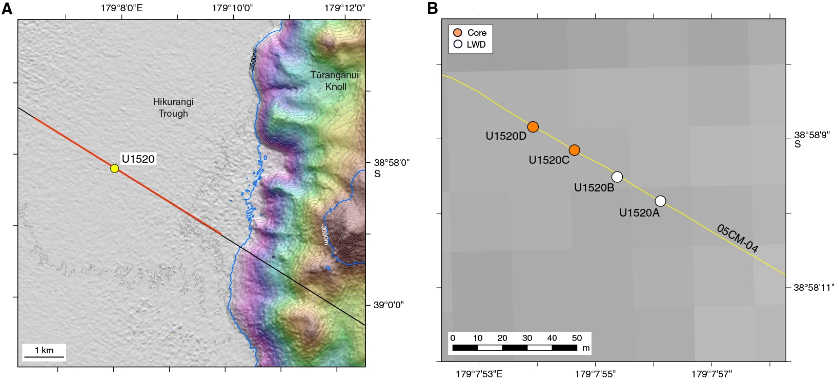
Figure F1. Bathymetry and location.
Site U1520 was expected to encounter sediments and rocks of late Quaternary to Cretaceous age. Based on predrilling interpretation of seismic data at the site (Figure F2) (Saffer et al., 2017), which considered regional Hikurangi Plateau seismic stratigraphy and previous Ocean Drilling Program drilling at Site 1124 (Leg 181) on the eastern side of the plateau (Davy et al., 2008), and interpretations of the subduction inputs seismic stratigraphy further south (Barnes et al., 2010; Plaza-Faverola et al., 2012; Ghisetti et al., 2016), we expected the sequence at Site U1520 to include the following (from top to bottom):
- An upper interval of ~610–640 m of clastic sediments including turbidites, mass transport deposits (MTDs), hemipelagic sediments, and volcanic ash, all likely to be Pliocene–Quaternary in age. This sequence includes the Ruatoria MTD (Lewis et al., 1998; Collot et al., 2001).
- About 210–230 m of predominantly pelagic sediment of possibly Late Cretaceous to Miocene age thought to include nannofossil chalk, mudstone, and tephra, with several possible unconformities.
- Basalts and volcaniclastic rocks of the Hikurangi Plateau, including possible chert and/or limestone deeper than 840 meters below seafloor (mbsf).
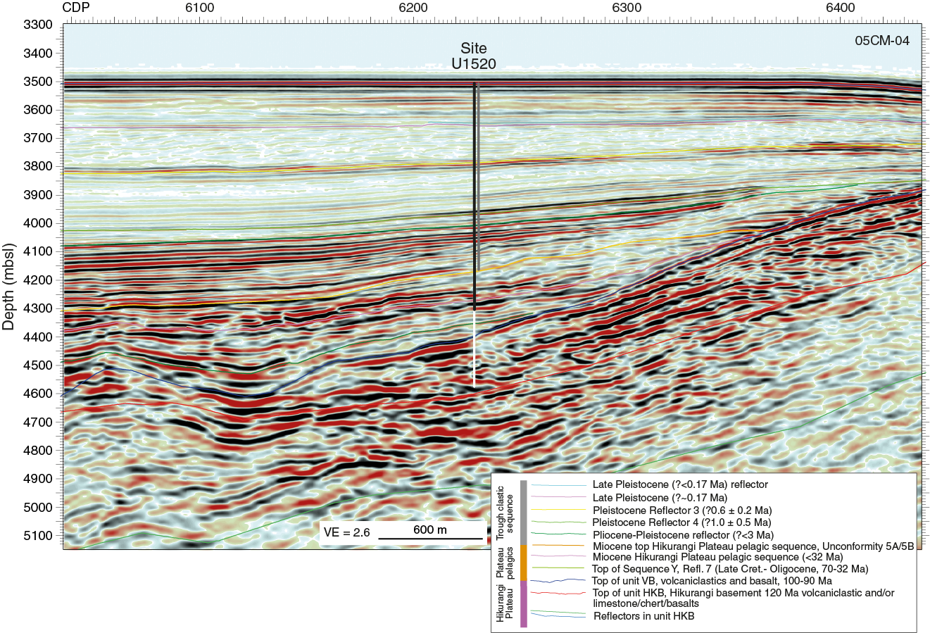
Figure F2. Seismic reflection image, Profile 05CM-04.
The aim of logging (logging while drilling [LWD] and wireline) and coring at Site U1520 was to sample the entire sedimentary section on the Pacific plate with the highest priority of logging and sampling the succession below ~600 mbsf that represents the protolith for material transported into the SSE source region. To maximize our ability to core the deep portion of the section, the drilling plan for International Ocean Discovery Program (IODP) Expedition 375 included installing a reentry system with casing to ~600–650 mbsf and then rotary core barrel (RCB) coring below the casing to a total depth (TD) of ~1200 mbsf. If time allowed, operations would then include drilling a second hole with the advanced piston corer (APC)/extended core barrel (XCB) systems to sample the upper ~600 m of the sedimentary section. Wireline logging was considered a possibility if hole conditions and time allowed.
The scientific objectives of logging and coring at Site U1520 were to evaluate the lithologic, structural, thermal, and physical properties of the Hikurangi Trough inputs sequence prior to subduction to provide insight into the rock properties and physical conditions expected in the shallow SSE source region. Coring and logging data will also be used for core-log-seismic integration (CLSI) across the Hikurangi Trough and will enable in situ rock properties and conditions to be estimated away from the boreholes over a broader region of 2-D and 3-D seismic data. Priorities for post-expedition analysis of cores include, but are not limited to, measurement of the mechanical, elastic, frictional, and hydrological properties of the incoming sediment and basement and detailed analyses of composition and alteration.
Holes U1520A and U1520B were drilled with LWD during IODP Expedition 372; Hole U1520A was abandoned at 97.9 mbsf because of weather, and Hole U1520B was drilled to 750 mbsf. During Expedition 375, Hole U1520C was cored with the RCB system from 646 to 1054.1 mbsf and wireline logging was conducted from 642 to 947 mbsf. After completing observatory and coring operations at Site U1519 and coring at Site U1526, we returned to Site U1520 to conduct APC/half-length APC (HLAPC)/XCB coring in Hole U1520D from 0 to 642 mbsf.
Operations
Expedition 372
Site U1520 consisted of two LWD holes during Expedition 372 (Table T1). The time spent at Site U1520 during Expedition 372 was 2.9 days, with 45.75 h of that time waiting on weather.
Hole U1520A
The vessel arrived at Site U1520 at 1302 h (UTC + 13 h) on 26 December 2017. The LWD bottom-hole assembly (BHA) was made up with the geoVISION, NeoScope, StethoScope, TeleScope, SonicScope, and proVISION tools behind an 8½ inch drill bit. The BHA was deployed to 390 meters below sea level (mbsl) and flow tested to determine the appropriate flow rates. The proVISION tool was not sending real-time data, and the BHA was pulled up so that the spare proVISION tool could be deployed. The tools and drill string were set at 390 mbsl for a second LWD tool test. Again, the proVISION tool failed to send real-time information. Because pulling the tool back up to the rig floor had a low chance of fixing the activation issue, the BHA was deployed to the seafloor (3527.4 mbsl), and Hole U1520A (38°58.1641ʹS, 179°7.9357ʹE; 3521.3 mbsl; Table T1) was spudded at 0845 h on 27 December. The seafloor depth was 3521.3 mbsl based on the LWD data. The proVISION began sending real-time data once the tool was turned on above the seafloor. The weather and sea conditions began to deteriorate, and the BHA was pulled out of the hole after reaching 97.9 mbsf. Hole U1520A ended when the bit cleared the seafloor at 1410 h on 27 December.
Hole U1520B
The vessel waited on the weather to clear for 45.75 h (1.91 days). During this time, the ship was offset 20 m northwest of Hole U1520A at a bearing of 300° with the BHA in the water column. Hole U1520B (38°58.1587ʹS, 179°7.9233ʹE; 3520.1 mbsl; Table T1) was spudded at 1245 h on 29 December 2017. LWD measurements were collected from the seafloor to 750 mbsf. After reaching a TD of 750 mbsf at 0430 h on 31 December, the hole was cleaned with a 30 bbl mud sweep and the drill string was pulled out of the hole. The bit cleared the seafloor at 0715 h and the rotary table at 1930 h. The LWD tools were broken down, and the vessel began the 32 nmi transit to Site U1517 at 1954 h (Barnes et al., 2019a).
Safety monitoring
Continuous safety monitoring (see Logging while drilling in the Expedition 372B/375 methods chapter [Wallace et al., 2019a]) was completed during LWD operations at Site U1520 to monitor for the presence of abnormal pressure or free gas and to ensure safe drilling conditions. Real-time monitoring in Hole U1520A started at 40 mbsf and continued to 97.5 mbsf. Real-time monitoring in Hole U1520B started at 15 mbsf and continued to 750 mbsf. Observed annular pressure was high (as high as 0.345 MPa [50 psi]) at the shallowest depths because of the high cuttings load in the annulus. Pressures decreased and then eventually increased slowly with depth as drilling continued. A maximum pressure of 1.055 MPa above hydrostatic (153 psi) occurred at the bottom of Hole U1520B. One pressure kick was observed in Hole U1520B, but pressure quickly recovered; it was likely an issue with localized cuttings load in the annulus or minor pack-off. With the exception of the shallowest measurements, all pressures were less than the pressure that could have been supplied using 10.5 lb/gal mud. No mud circulation was required at this site.
Expedition 375
We first occupied Site U1520 during Expedition 375 while waiting for the R/V Tangaroa to deliver replacement seals needed for the observatory installation at Site U1518. Site U1520 consisted of two coring holes during Expedition 375 (Table T1). The time spent at Site U1520 during Expedition 375 was 18.26 days. The total time spent at Site U1520 during both expeditions was 21.16 days.
Hole U1520C
Upon arrival at 0257 h (UTC + 12 h) on 28 March 2018, the thrusters were lowered, the dynamic positioning (DP) system was engaged, and an acoustic positioning beacon was deployed. We started the installation of a reentry system (Figure F3) by fabricating the base of the reentry cone, which was moved to the moonpool at 0630 h. Then we assembled the hydraulic release tool (HRT) needed to deploy the reentry system and set it in the derrick at 0900 h. Finally, we completed the casing string by assembling and welding 54 joints of 10¾ inch casing and a casing shoe and secured it in the moonpool at 0130 h on 29 March.

Figure F3. Reentry system installation.
Next, we put together a drilling assembly to drill in the reentry system. The drilling assembly was composed of a 9⅞ inch drill bit, an underreamer with its arms set to 14¾ inches, and a mud motor to rotate the bit and underreamer in isolation from the casing. The underreamer arms were tested, and the drilling assembly was completed and landed inside the casing by 0500 h on 29 March.
The drilling assembly and HRT were connected to the casing and mud skirt by 0730 h, and the reentry cone was assembled and welded by 1030 h. The moonpool doors were opened, and the reentry system was lowered to the seafloor until the bit reached 3499 m below rig floor (mbrf) at 1730 h. While the reentry system was being lowered to the seafloor, the Tangaroa arrived at 1615 h to deliver the replacement seals needed for the CORK-II installation at Site U1518 (see Operations in the Site U1518 chapter [Saffer et al., 2019b]).
The subsea camera was deployed to monitor the reentry cone and base during drilling. Hole U1520C (38°58.1532ʹS, 179°7.9112ʹE; 3522.1 mbsl; Table T1) was spudded at 1940 h, and it took ~27 h for the bit to reach a TD of 646 mbsf with the casing shoe at 642 mbsf. Once the drilling assembly was released from the reentry system at 2230 h on 30 March, we recovered the subsea camera and then the drill string at 1120 h. With the reentry system installed, we departed for Site U1518 at 1310 h on 31 March to complete the observatory installation there (see Operations in the Site U1518 chapter [Saffer et al., 2019b]).
We returned to Site U1520 on 2 April following a ~10 h deviation to the Gisborne Pilot Station for a personnel transfer. We arrived at the coordinates for Hole U1520C at 1848 h on 2 April. We assembled an RCB coring assembly and reentered Hole U1520C at 0525 h on 3 April. The next several hours were spent cleaning cuttings out of the inside of the 642 m deep casing. RCB coring started at 1200 h on 3 April. Cores 375-U1520C-2R through 44R penetrated from 646.0 to 1054.1 mbsf and recovered 235.40 m (58% recovery). Nonmagnetic core barrels were used for all cores. Coring was terminated so that Hole U1520C could be logged before the weather deteriorated.
To prepare the hole for logging, we circulated cuttings out of the hole with a 50 bbl mud sweep, filled it with heavy mud, and recovered the RCB BHA. The subsea camera was deployed to check the reentry cone, which seemed to have sediment inside, and the cone was flushed with seawater. Once the drill string was recovered, we made up a logging BHA and lowered it to the seafloor. Hole U1520C was reentered at 0250 h on 9 April, and the drill pipe was set at 599 mbsf for logging, 42 m above the casing shoe. We deployed a modified triple combo tool string with the following tools from the bottom up: Dipole Shear Sonic Imager (DSI; sonic velocity), High-Resolution Laterolog Array (HRLA; resistivity), Hostile Environment Litho-Density Sonde (HLDS; caliper only, without the density source), and Enhanced Digital Telemetry Cartridge (EDTC; gamma ray and telemetry). We made two logging passes from 642 to 947 mbsf, where we encountered an obstruction 107 m from the bottom of the hole. The tools were back on the rig floor at 1505 h on 9 April, and the drill string was recovered at 0010 h on 10 April, ending operations in Hole U1520C. The time spent in Hole U1520C was 10.7 days.
Based on weather forecasts predicting 7–10 m swells in the vicinity of our drill sites, we headed north to the Bay of Plenty to seek shelter. We started the 204 nmi transit at 0118 h on 10 April and completed it at 1054 h on 11 April at an average speed of 6.1 kt because of the strong winds and high sea state. We waited on weather for 36.75 h. We started the 172 nmi transit back to our area of operations at 0018 h on 13 April and arrived at Site U1519 at 1810 h.
Hole U1520D
After a ~6 h transit in DP mode from Site U1526, we arrived at the specified coordinates for Hole U1520D at 2305 h on 24 April 2018. Our objective for Hole U1520D was to core the uppermost sediment (above ~650 mbsf) that was not cored in Hole U1520C. We assembled an APC/XCB BHA, and Hole U1520D (38°58.1475ʹS, 179°7.8991ʹE; 3520.3 mbsl; Table T1) was spudded at 0850 h on 25 April. Cores 375-U1520D-1H through 67X advanced from 0 to 642.3 mbsf and recovered 318.38 m (62% recovery). In this interval, we drilled without coring from 189.3 to 220.0 mbsf and from 270.8 to 366.6 mbsf. Coring was suspended from 1600 h on 29 April until 1315 h on 30 April while we waited on weather. Nonmagnetic core barrels were used with all APC cores. Formation temperature measurements were taken with the advanced piston corer temperature tool (APCT-3) for Cores 4H, 7H, 10H, 13H, 16H, 19F, 23F, and 27F. The time spent in Hole U1520D was 7.56 days.
Lithostratigraphy
We defined six lithostratigraphic units based on cores recovered from Holes U1520C and U1520D (Figure F4; Table T2). Figure F4 compares the lithostratigraphic units with the 11 logging units that were defined using LWD data in the upper 750 m (Holes U1520A and U1520B) (see Logging while drilling) and wireline logs obtained to ~920 mbsf in Hole U1520C (see Downhole measurements and Core-log-seismic integration). Correlations between the logging and lithostratigraphic units are valid at the scale of facies, but not at the scale of individual beds. Overall, the sediments and sedimentary rocks range in age from early Late Cretaceous to Holocene. Sediment composition and texture change markedly downhole from a depositional system dominated by terrigenous clastic gravity flow processes to a pelagic carbonate system to a volcaniclastic gravity flow system.
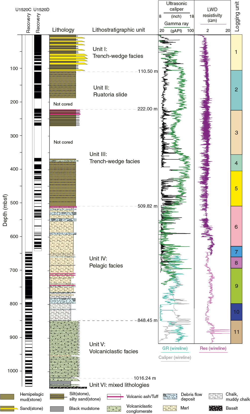
Figure F4. Lithostratigraphic summary.
The criteria for distinguishing among lithostratigraphic units (Table T2) are based mostly on primary attributes that provide evidence of depositional processes and the overall environmental setting. These descriptive features include the texture, fabric, and thickness of coarser grained event beds (with most inferred to be turbidites and other types of gravity flow deposits); internal sedimentary structures and bioturbation; zones of soft-sediment deformation (inferred MTDs); and calcium carbonate contents (inferred to originate mostly from biocalcareous pelagic debris) (Figure F5). We gave secondary consideration to changes in compaction, lithification, and diagenesis (e.g., replacement of detrital grains by clay minerals and cementation by calcite and zeolites).
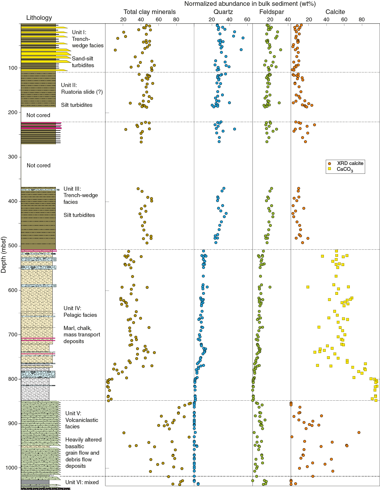
Figure F5. Lithostratigraphic summary, carbonate, and XRD abundance.
Unit I
- Interval: 375-U1520D-1H-1, 0 cm, to 13H-1, 0 cm
- Thickness: 110.50 m
- Depth: 0–110.50 mbsf
- Age: Holocene to Late to Middle Pleistocene
- Lithology: silty clay to clayey silt with abundant interbeds of silt and sand
Lithostratigraphic Unit I extends from the seafloor to 110.5 mbsf (Section 375-U1520D-13H-1, 0 cm) (Figure F6). Cores over this range contain a pervasive background of greenish gray mud (silty clay to clayey silt), which we regard as typical hemipelagic deposits from suspension fallout. Seven thin (5–14 cm) grayish to pinkish ash beds occur in the upper 37 m of Unit I (Figure F7). The defining feature of Unit I is the widespread dominance of dark gray silt and sand interbeds with sharp bases and normal size grading (Figure F8). These beds are as thick as 6.89 m (Figure F7). Thicker and coarser beds have lost their internal sedimentary structures because the cohesionless sand was disturbed during coring and core handling (Figure F8). We interpret these coarser deposits to be products of deposition by turbidity currents on the floor of the Hikurangi Trough.

Figure F6. Lithostratigraphic summary, Hole U1520D.
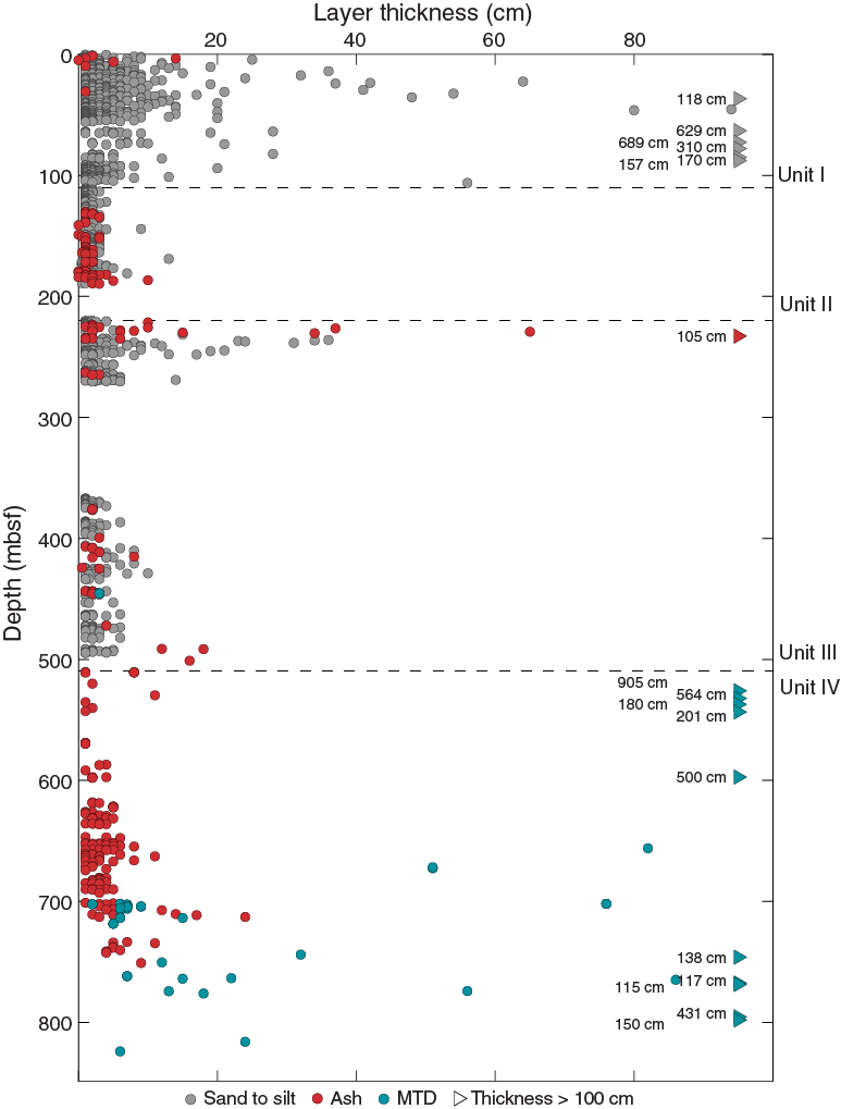
Figure F7. Event bed thickness.
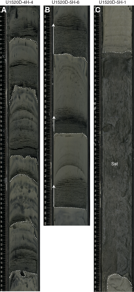
Figure F8. Typical Unit I lithologies, Hole U1520D.
The total number of recovered turbidites in Unit I is 563, and the average frequency is 13.6 event beds per meter of sediment (Figure F9). The thicker examples of sand perturb these statistics to lower frequency values over the associated depth intervals, but the volumetric proportion assigned to turbidity currents increases. Turbidite distribution can also be evaluated as a function of thickness. In this unit, a single power law distribution with the exponent of β = 0.96 can be fit to the number of turbidite beds thicker than T (Figure F10). Fitting the single power law distribution indicates that the turbidity currents responsible for Unit I deposits were largely unconfined and that the effects of erosion and amalgamation are minimal (Rothman et al., 1994; Carlson and Grotzinger, 2001). Flat-floored environments without channel-levee complexes are generic examples of such systems.
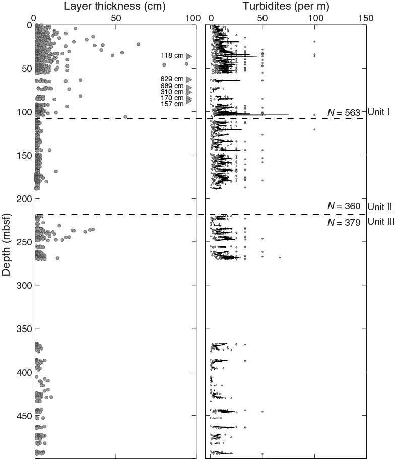
Figure F9. Turbidite emplacement frequency, Units I–III.
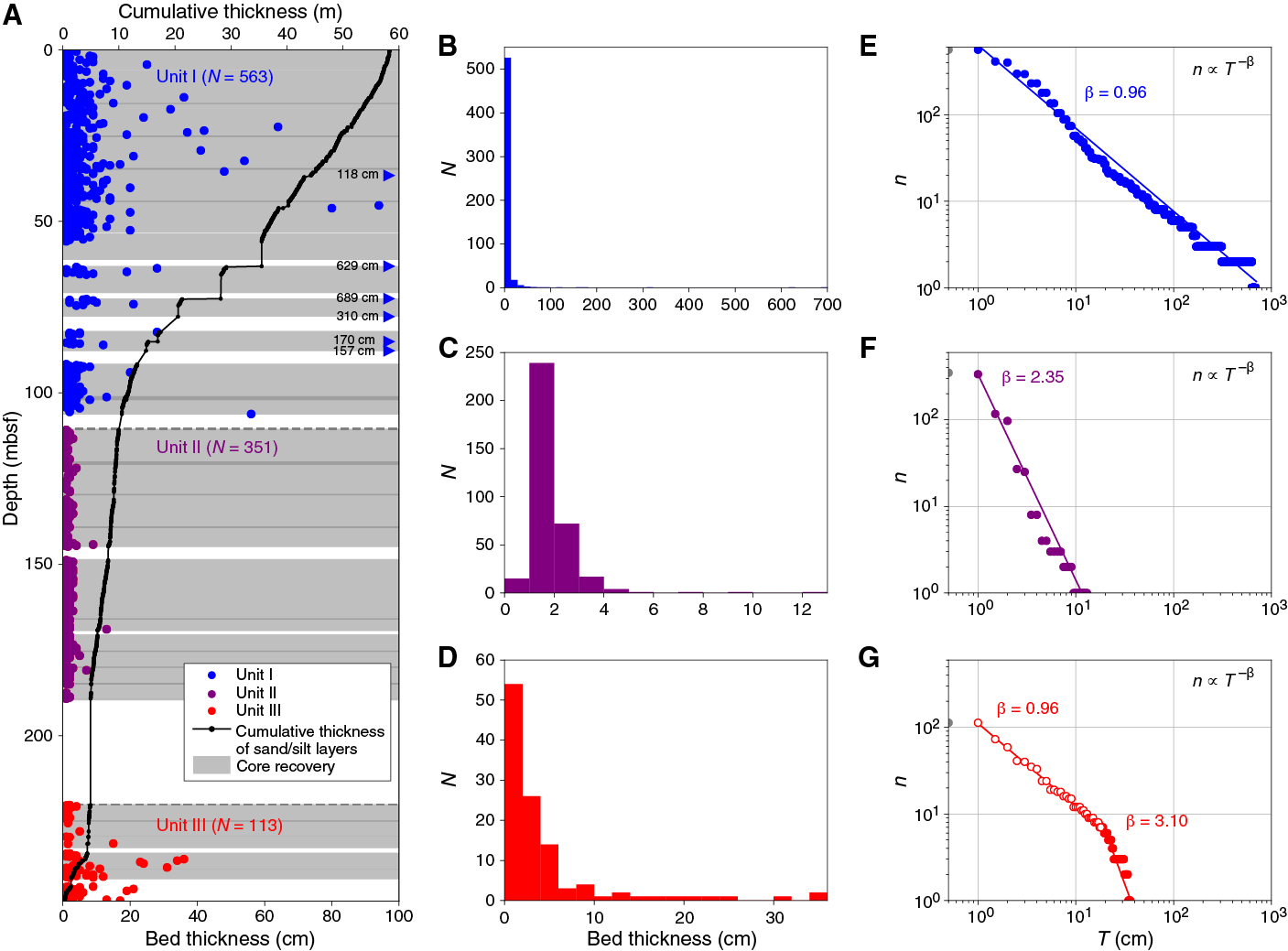
Figure F10. Sand and silt layer thickness, Units I–III.
A ubiquitous fine-grained black stain appeared on split-core surfaces from this unit (Figure F8). This staining can be seen in core images and became more pronounced in coarser interbeds of silt and fine sand. Smear slides show that the stain covered silt and sand grains of quartz, feldspar, and other detrital minerals. The black mineral that created the stain is metastable, however, and the stain faded quickly after exposure to the atmosphere. We believe that the mineral was probably mackinawite, an amorphous to poorly crystalline form of iron sulfide (Vaughan and Craig, 1978). Direct confirmation of its identity (e.g., using X-ray diffraction [XRD]) was not possible on board because of the extremely fine grain size and rapid oxidation.
Smear slides also show that the detrital grain assemblage in the background hemipelagic mud lithology is dominated by clay minerals and has significant amounts of calcareous nannofossils, quartz, feldspar, and sedimentary lithic and volcaniclastic grains. The sand and silt beds are within the compositional range of mixed clastic with common occurrences of sedimentary lithic grains, volcaniclasts, quartz, and feldspar. Carbonate content in mud specimens ranges from 2.1 to 8.7 wt% with an average value of 5.5 wt% (Table T3). Normalized mineral abundances from bulk powder XRD are shown in Figure F5 and Table T3. Proportions of total clay minerals (smectite + illite + chlorite + kaolinite) range from 11.1 to 55.0 wt% (mean = 41.3 wt%). Quartz values range from 23.4 to 52.8 wt% (mean = 32.6 wt%). Feldspar (plagioclase + K-feldspar) abundance ranges from 13.5 to 31.4 wt% (mean = 19.9 wt%), and calcite abundance ranges from 1.4 to 11.6 wt% (mean = 6.2 wt%). Representative X-ray diffractograms are shown in Figure F11. The XRD data display considerable scatter in Unit I. Relative abundances of total clay minerals are inversely related to those for quartz and feldspar. This effect is probably due to grain size (i.e., more quartz and feldspar in silt-rich specimens).
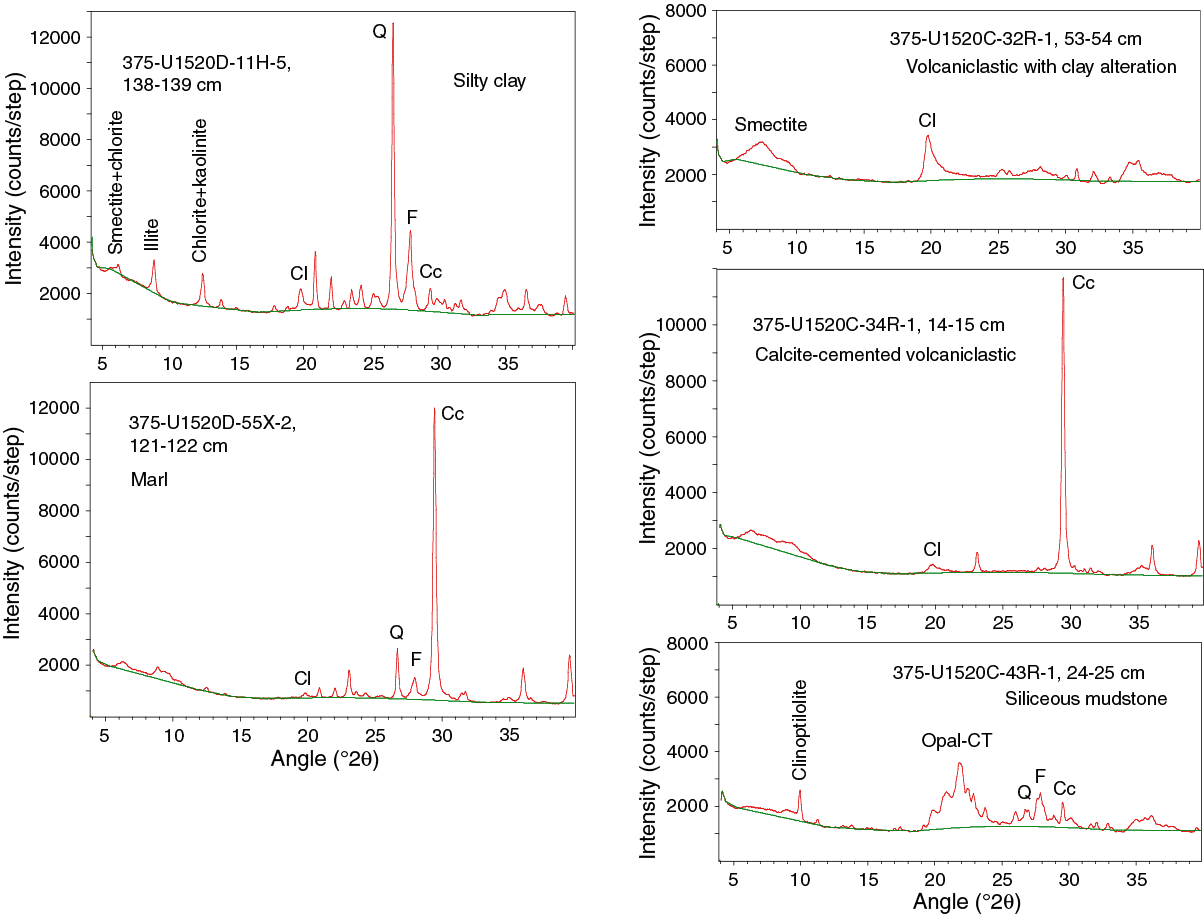
Figure F11. X-ray diffractograms spanning common lithologies.
Unit II
- Interval: 375-U1520D-13H-1, 0 cm, to 25F-1, 0 cm
- Thickness: 109.50 m
- Depth: 110.50–220.00 mbsf
- Age: Quaternary
- Lithology: silty clay to clayey silt with thin interbeds of silt
The upper boundary of Unit II is subjective due to considerable overlap of lithologies above and below. We placed the Unit I/II boundary at the top of Section 375-U1520D-13H-1, 0 cm, based on a reduction in the number and thickness of sand and silt interbeds (Figures F6, F9, F10). A small decrease in magnetic susceptibility also occurs over this interval (see Physical properties; Figure F55), probably in response to reduction in sand- and silt-sized particles. The dominant lithology in Unit II is greenish gray to dark gray silt with rhythmic spacing interbedded with mud (silty clay to clayey silt). Most of the thin silt beds are normally graded, and some include erosional basal contacts and mud intraclasts.
We observed 360 silt beds in Unit II and interpret them to be turbidites with a frequency of 11.1 beds per meter of sediment. These deposits are generally finer grained and consistently thinner than those recovered from Unit I (Figures F7, F12) and have a maximum thickness of 13 cm (Figure F9). The layer thicknesses can be fit with a single power law distribution with β = 2.35 (Figure F10). In previous studies, β values >1 have been attributed to flow striping or channel overspill of turbidity currents (Sinclair and Cowie, 2003). The lower proportion of thicker beds (compared with Unit I) is indicative of a lower energy environment and/or isolation from a major conduit of turbidity currents.
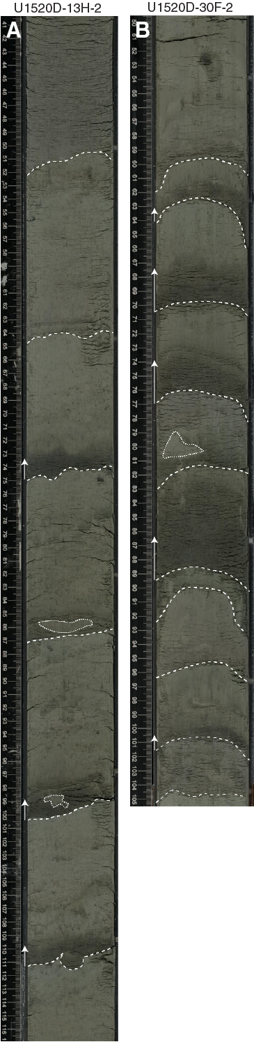
Figure F12. Typical Unit II lithologies, Hole U1520D.
Based on interpretations of seismic reflection data (see Core-log-seismic integration), this coring interval represents part of the distal edges of the Ruatoria debris avalanche (a very large MTD), which resulted from failure of the landward trench slope to the northeast (Lewis et al., 1998; Collot et al., 2001). Mesoscopic evidence from cores at Site U1520 is lacking, however, for soft-sediment gravity-driven deformation of the beds (e.g., truncated and rotated laminae, irregular bedding dips, fragmentation of cohesive mud clasts, clasts in matrix fabrics, and flow banding). Although the 30.7 m interval from 189.3 to 220.0 mbsf was not cored and the base of the inferred MTD was not identified, no evidence was found for an inversion in age across the Unit I/II boundary (see Biostratigraphy). On the other hand, the bed thickness statistics described above for Unit II point to an original (preavalanche) depositional environment for the turbidites that is unlike the settings for Units I and III. These observations are consistent with the suggestion that Unit II might represent an intact block in the regional-scale MTD. It is worth noting that cores from inferred submarine slides at Sites U1517 and U1519 are similarly lacking in mesoscale indicators of remobilization (Barnes et al, 2019a; see Lithostratigraphy in the Site U1519 chapter [Barnes et al., 2019b]).
Smear slides show that the detrital grain assemblage in the Unit II background mud lithology is dominated by clay minerals and includes significant amounts of quartz, feldspar, sedimentary lithic and volcaniclastic grains, and nannofossils. Carbonate contents in mud specimens range from 2.2 to 17.1 wt% with an average value of 7.9 wt% (Table T3). Normalized mineral abundances from bulk powder XRD are shown in Figure F5 and Table T3. Proportions of total clay minerals (smectite + illite + chlorite + kaolinite) range from 28.0 to 53.3 wt% (mean = 45.0 wt%). Quartz values range from 20.2 to 39.6 wt% (mean = 27.4 wt%). Feldspar (plagioclase + K-feldspar) abundance ranges from 12.8 to 29.8 wt% (mean = 17.5 wt%), and calcite abundance ranges from 2.2 to 23.4 wt% (mean = 10.1 wt%). These compositions are very similar to the bulk mud compositions in Unit I but have slightly lower abundances of quartz and feldspar.
Unit III
- Interval: 375-U1520D-25F-1, 0 cm, to 50X-CC, 0 cm
- Thickness: 289.82 m
- Depth: 220.00–509.82 mbsf
- Age: Quaternary
- Lithology: silty clay to clayey silt with common interbeds of silt and minor volcanic ash
Unit III is similar to the facies character of Unit I but without thick sand beds (Figures F6, F9). The Unit II/III boundary is subtle to arbitrary if based on the presence or absence of silt beds; turbidites occur throughout both units. Positioning this boundary accurately is important, however, if it represents the base of a regional-scale MTD. The top of the correlative logging unit (3) is placed at 225.0 mbsf (Figure F4). We set the Lithostratigraphic Unit II/III boundary at 220.0 mbsf (Section 375-U1520D-25F-1, 0 cm), which is immediately below an interval that was not cored (Figure F6). In addition, several prominent beds of light gray volcanic ash are clustered just below the boundary in Cores 25F, 26F, and 27F (Figures F7, F13). These silicic tephra deposits provide the most definitive contrast with the lithologies in Unit II, although their occurrences as air fall deposits are not unique to either depositional environment (i.e., trench floor versus landward trench slope). A thin interval of stratal disruption with mudstone clasts in a mud matrix occurs in Sections 35X-7 and 35X-CC.
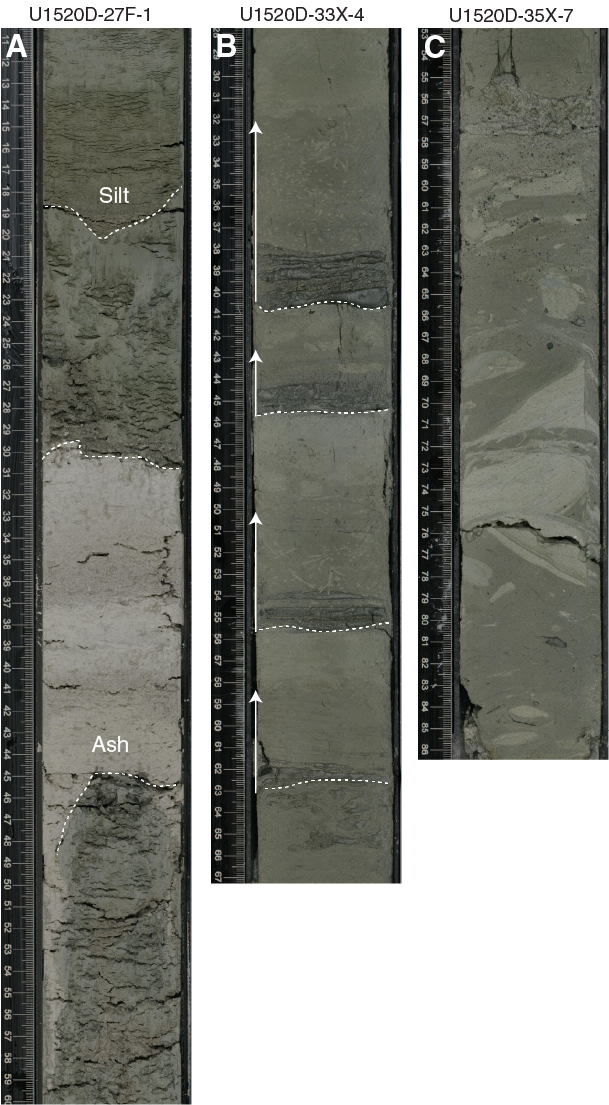
Figure F13. Typical Unit III lithologies, Hole U1520D.
Turbidites in Unit III are characterized by thin alternations of dark greenish gray mud (silty clay to clayey silt) and normally graded fine sand to silt; internal sedimentary structures include planar and cross-lamination (Figure F13). The total number of turbidites in Unit III is 379, and the frequency is 10.8 event beds per meter of sediment (Figure F9). The maximum layer thickness is 36 cm. Unlike the statistics for the units above, the layer thicknesses for Unit III fit best with a segmented power law distribution (Figure F10). A similar segmented distribution is evident in data from Unit I at Site U1518. Segmented power law distributions have been observed in other systems in which the depositional area is more confined (Rothman et al., 1994; Malinverno, 1997) or the rheological properties of the flows range from low- to high-density turbidity currents (Felletti and Bersezio, 2010). When considered as a whole, we conclude that the depositional environment for Unit III was in the Hikurangi Trough trench-wedge setting during a time period in which turbidity currents were less frequent, more dilute, and finer in grain size than those during depositional periods for Unit I.
Smear slides show that the detrital grain assemblage in the background silty clay (mudstone) lithology is dominated by clay minerals and contains significant amounts of quartz, feldspar, sedimentary lithic and volcaniclastic grains, and nannofossils. Carbonate contents in mud and mudstone specimens range from 2.5 to 18.4 wt% with an average value of 6.7 wt% (Table T3). Normalized mineral abundances from bulk powder XRD are shown in Figure F5 and Table T3. Proportions of total clay minerals (smectite + illite + chlorite + kaolinite) range from 22.9 to 52.0 wt% (mean = 45.4 wt%). Quartz values range from 23.4 to 45.4 wt% (mean = 28.3 wt%). Feldspar (plagioclase + K-feldspar) abundance ranges from 14.4 to 26.8 wt% (mean = 18.2 wt%), and calcite abundance ranges from 2.1 to 18.9 wt% (mean = 8.1 wt%). The upper part of Unit III is compositionally similar to Unit II. Data from the lower part of the unit show gradual decreases in both quartz and feldspar that are probably due to finer textures.
Unit IV
- Interval: 375-U1520D-50X-CC, 0 cm, and 375-U1520C-2R-1, 0 cm, to 375-U1520C-23R-5, 39 cm
- Thickness: Holes U1520C and U1520D = 338.63 m
- Depth: Holes U1520C and U1520D = 509.82–848.45 mbsf
- Age: middle to early Paleocene to middle to early Pleistocene
- Lithology: marl, calcareous mudstone, and chalk with debris flow deposits and volcanic ash/tuff
Placing the Unit III/IV boundary was problematic. We set its depth in Hole U1520D at 509.82 mbsf (Section 50X-CC, 0 cm), and the base of Unit IV was set at 848.45 mbsf in Hole U1520C (Section 23R-5, 39 cm) (Figures F6, F14; Table T2). Coring in Hole U1520C began at 646 mbsf (Core 2R), well below the upper unit boundary (Figure F4). The upper boundary itself was not recovered in Hole U1520D. The in situ position of the boundary was inferred to occur between the bottom of Core 375-U1520D-49X and Section 50X-CC. The lithologies change markedly over that depth interval from greenish gray mudstone with sparse interbeds of siltstone to light greenish gray marl with interbeds of volcanic ash (Figure F15). Core 50X, however, was limited to only 0.48 m of sediment in the core catcher. Our assumption was that the core catcher material originated at the bottom of the drilled interval of Core 50X, so we raised the unit boundary to 0.48 m above the top of Core 51X (509.82 mbsf) rather than at the archived depth at the bottom of Core 50X (501.18 mbsf).
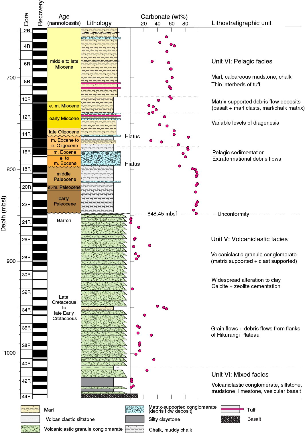
Figure F14. Lithostratigraphic summary, Hole U1520C.
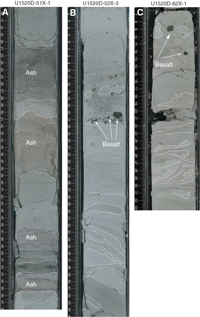
Figure F15. Unit IV lithologies, Hole U1520D.
The age distribution in Unit IV is also challenging to determine because of extensive microfossil reworking and discrepancies between nannofossil datums and foraminifer datums (see Biostratigraphy). The youngest nannofossil age is Middle to early Pleistocene (1.62 Ma). Microfossils from Section 375-U1520C-2R-CC indicate an age range of 8.96–11.21 Ma. Nannofossil datums indicate that two unconformities occur in Hole U1520C (see Biostratigraphy). The oldest nannofossil age from the pelagic carbonate facies is early Paleocene (64.81 Ma); that datum was recognized in chalks forming the deepest ~50 m of Unit IV (Figure F14).
The pelagic carbonate facies is composed mostly of marl (including calcareous mudstone) and chalk. Variations in color and carbonate content provide the keys to distinguishing among these carbonate lithologies (Figures F5, F14, F16). We refer to intervals with demonstrably higher concentrations of clay minerals as calcareous mudstone (a subset of marl). Secondary constituents in the facies include matrix-supported gravity flow deposits, thin layers of volcaniclastic siltstone, and tuff. Except for features diagnostic of debris flows (see below), we did not observe any textural changes, internal sedimentary structures, or bedding geometries indicative of dilute sediment gravity flows (e.g., turbidity currents). Two of the debris flow deposits in Hole U1520C coincide with hiatuses recognized from nannofossil datums (Figure F14). We interpret the remaining carbonate deposits to have resulted from slow pelagic settling.
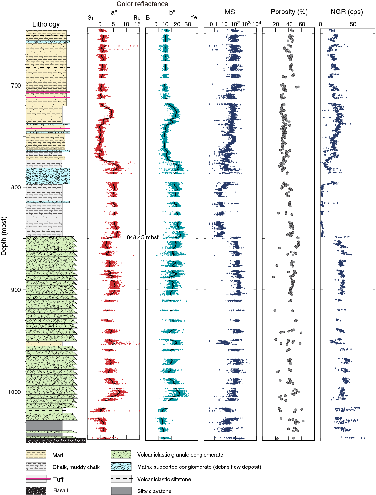
Figure F16. RSC a* and b*, MS, porosity, and NGR, Hole U1520C.
The marl in Unit IV is moderately to strongly lithified, typically light greenish gray in color (Figure F17), and composed of highly variable mixtures of microcrystalline carbonate (26.9–63.7 wt%) and clay minerals (17.3–55.0 wt%) (Figure F5). Recrystallization of very fine biocalcareous debris (e.g., nannofossils) to microcrystalline carbonate (micrite) is more pervasive below ~600 mbsf, but smear slides show that some bioclasts, including mollusks and foraminifers, are preserved. Spherical clasts of micrite are enigmatic; they show a bimodal size distribution but are structureless internally, perhaps due to pervasive micritization. Some of what appear to be spheres in thin section are probably axial slices of bioclasts. Detrital grains in the marl include quartz, feldspar, sedimentary lithic fragments, volcaniclasts, and a variety of heavy minerals (olivine, pyroxene, amphibole, apatite, and zircon). Most of the lithic grains are altered. Decreases in natural gamma radiation (NGR) (Figure F16) indicate a progressive increase in the ratio of carbonate to clay minerals.
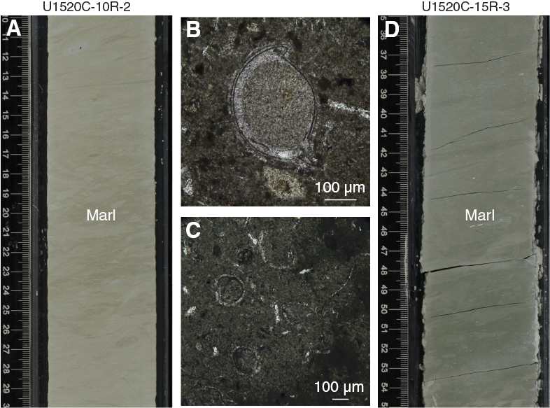
Figure F17. Bioclasts and other characteristics of marl, Unit IV.
Light brownish gray calcareous mudstone is the dominant lithology from 720.93 to 738.68 mbsf (interval 375-U1520C-10R-2, 113 cm, to 12R-1, 108 cm). This lithology is distinguished in split cores largely by its color, seen as an increase in a* and b* values (Figure F16). Nannofossil preservation improves in this lithology relative to the typical marl, but carbonate concentration decreases to an average of ~40 wt% (Figure F14). This lithology sometimes expanded in the core liners after split cores were exposed to freshwater, which is consistent with higher clay mineral contents (Figure F5).
Chalk (lithified nannofossil ooze) is the dominant lithology from 776.09 to 848.45 mbsf (interval 375-U1520C-16R-1, 19 cm, to 23R-5, 39 cm). These deposits are characterized by high carbonate concentration (>75 wt%) and a pale brown color. NGR values in this lithology drop nearly to zero (Figure F16). Foraminifers and nannofossils are present to dominant, and the fossils are better preserved than in the overlying marl layers (Figure F18). Mineral grains are diverse and include quartz, feldspar, volcaniclasts, and apatite. Most of the volcaniclasts are altered. Opaque grains, which include pyrite and Fe oxides, are trace to rare in abundance. Pressure solution and stylolitic seams are concentrated in this lithology (see Structural geology).
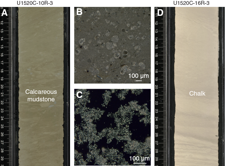
Figure F18. Carbonate-rich lithologies from Unit IV, Hole U1520C.
Discrete layers of matrix-supported carbonate conglomerates with “floating” extraformational clasts are scattered through Unit IV (Figure F19). We interpret these zones to be debris flow deposits. They are composed of contorted to fragmented marl and chalk together with angular to subrounded clasts of volcaniclastic sandstone and vesicular (amygdaloidal) basalt. The debris flow deposits are intercalated with intact, bioturbated marl and, to a lesser extent, chalk. Most examples occur between Cores 375-U1520C-3R and 20R. Their thicknesses range from a few centimeters to more than a meter, and the clast-matrix organization is variable. Cores 3R–8R contain contorted marl layers, flow banding, and a few scattered clasts of basalt and lithified volcaniclastic sandstone (Figure F20). Cores 14R and 15R, in contrast, contain rounded, cobble-sized clasts of muddy chalk and marl along with higher concentrations of basalt and volcaniclastic pebbles, all supported by a marl matrix (Figure F21). Other varieties of clast-matrix mixtures include a closely packed, clast-supported mixture (e.g., interval 15R-1, 50–100 cm); flow-banded marl with only chalk and marl clasts (Figure F22); and muddy chalk matrix with only volcanic clasts (Figure F23).
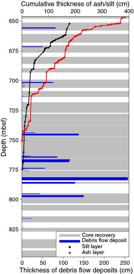
Figure F19. Bed thickness of debris flow deposits.
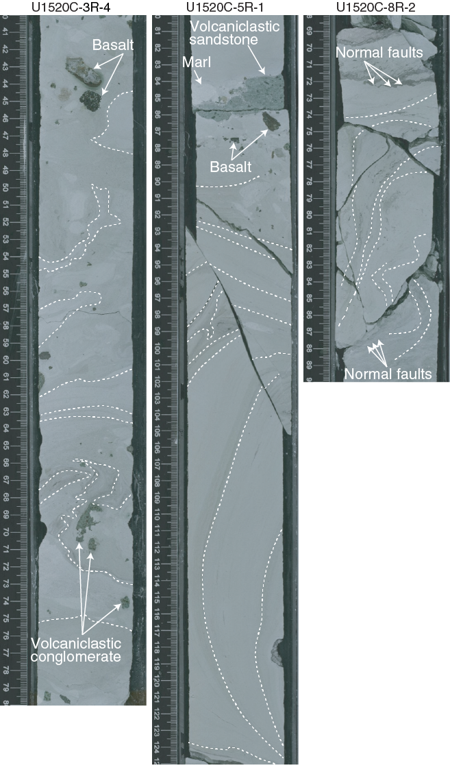
Figure F20. Debris flow deposits in Unit IV, Hole U1520C.
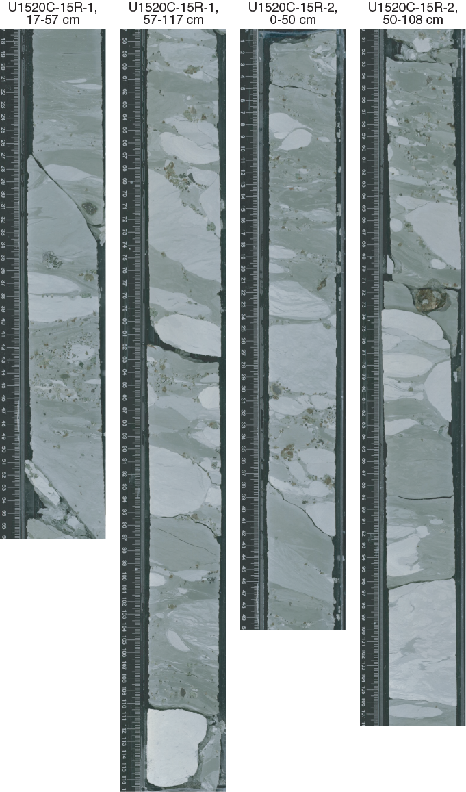
Figure F21. Debris flow deposit, Hole U1520C.
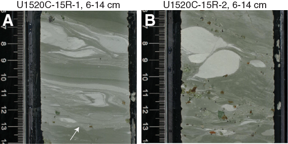
Figure F22. Debris flow deposit in Unit IV, Hole U1520C.
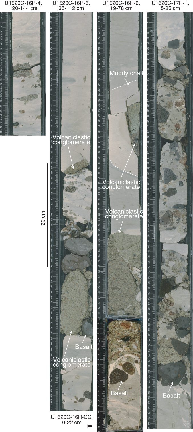
Figure F23. Debris flow deposits, Hole U1520C.
Incorporation of the rounded to subrounded clasts of vesicular basalt into inferred debris flows (Figure F23) obviously required exposure of a volcanic edifice in an erosional environment outside of a pelagic setting. One likely source of the clasts of basalt and volcaniclastic sand grains is the western flank of the Tūranganui Knoll, one of several seamounts constructed at the top of the Hikurangi Plateau (e.g., Wood and Davy, 1994). The parent rocks of reworked volcaniclastic sandstone clasts may not have been thoroughly cemented, and some of the larger clasts may have disaggregated further during transport. The styles of soft-sediment deformation displayed by the carbonate matrix and the rounded shape of carbonate clasts indicate that the indigenous carbonate sediment was poorly lithified but cohesive when remobilized. The prevalence of reworked foraminifers in Unit IV (see Biostratigraphy) is also consistent with extensive remobilization of the pelagic sediment.
The carbonates in Unit IV also exhibit a wide range of bioturbation in terms of both intensity (absent to strong) and type. The sediments display ubiquitous fine-scale mottling. Burrows are preserved locally. We also recognized several specific trace fossils, including Zoophycos, Nereites, and Chondrites, throughout the unit. Additionally, we identified many occurrences of Ophiomorpha in the chalk lithology. These forms commonly occur as composite burrows and include donut-shaped features with different colors comprising the initial and superimposed burrows (Figure F24). Thin section observations showed that bioturbated zones are rich in Fe oxides and opaque grains. Smear slides from bioturbated zones typically reveal heavy minerals in spherical aggregates of micrite.
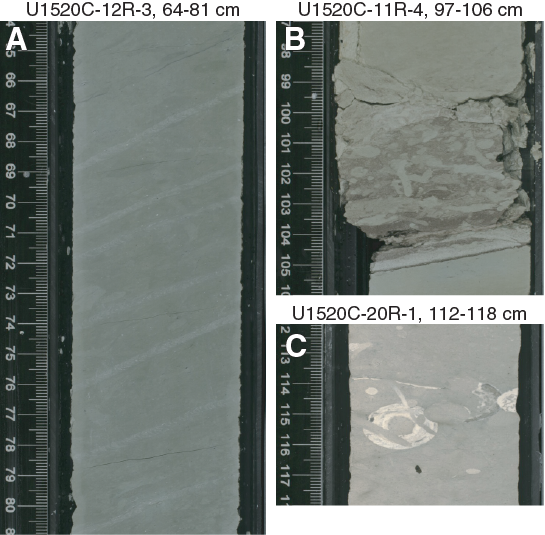
Figure F24. Examples of bioturbation, Hole U1520C.
Unit V
- Interval: 375-U1520C-23R-5, 39 cm, to 41R-1, 54 cm
- Thickness: 167.79 m
- Depth: 848.45–1016.24 mbsf
- Age: Late Cretaceous
- Lithology: granule-sized volcaniclastic conglomerate
Unit V extends from 848.45 to 1016.24 mbsf (interval 375-U1520C-23R-5, 39 cm, to 41R-1, 54 cm). Its defining lithology is volcaniclastic conglomerate with granule-sized clasts. We discerned a crude upward-thinning and fining-upward trend over the entire unit. The Unit IV/V boundary is sharp (Figure F25), and the facies change is dramatic in terms of the respective depositional processes (slow pelagic settling versus high-density gravity flow). We interpret the contact to be an unconformity, even though the duration of the age gap between these two units could not be determined (see Biostratigraphy). The only significant change in lithology in Unit V occurs between 949.76 and 953.65 mbsf (interval 375-U1520C-34R-2, 29 cm, to 34R-CC, 20 cm) where an interval of marl is sandwiched between volcaniclastic beds. This marl has a carbonate concentration of ~50 wt% and contains distributed millimeter-scale clasts of altered volcaniclastic fragments. Eight zones of red laminae are evident in the marl (Figure F26D). Microfossils from the marl range from 66.0 to 84.0 Ma in age (see Biostratigraphy). Foraminifers in Core 41R near the lower boundary of Unit V are indicative of early Late Cretaceous ages.
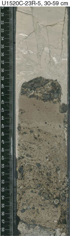
Figure F25. Contact between Units IV and V, Hole U1520C.
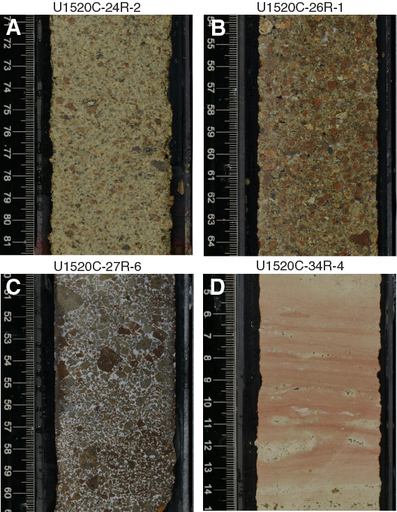
Figure F26. Unit V lithologies, Hole U1520C.
The coarse volcaniclastic deposits in Unit V are characterized by a marked increase in magnetic susceptibility compared with the overlying carbonates (Figure F16). The constituents are mostly subangular clasts of altered basalt that range in size from a few millimeters to 6 cm. Bedding is cryptic with only a few interbeds of finer grained volcanic sandstone. The textures and colors of the conglomerate are quite variable. In Cores 375-U1520C-24R and 25R, the fabric is matrix supported and the poorly sorted clasts are highly altered and brown in color; the surrounding matrix is pale green (Figure F26A). In Core 26R and below, the deposits are clast supported with sparse clay matrix; this variety of clast-matrix organization is associated with a general increase in the average clast size. The clasts are tightly packed and commonly bounded by pore-filling cements (Figure F26B, F26C). Pervasive cementation contributes to strong lithification of the deposits.
At the microscale, the vast majority of clasts in the volcaniclastic conglomerate are highly altered basalt (Figure F27). Thin sections show that the preservation of feldspar laths and needles is rare. Abundant vesicles (now amygdules) are filled by palagonite and/or spherulitic calcite. Most of the clasts are coated with palagonite. Only a few clasts of microcrystalline basalt retain their original textures. Siderite and hydroxides, as well as chlorite and epidote, are pervasive alteration products seen in thin section. Widespread replacement by clay minerals is also evident, although we could not identify the specific mineral optically (e.g., chlorite or smectite group, possibly saponite). XRD analysis of similar rocks recovered by dredging along scarps on the Hikurangi Plateau suggests that smectite makes up as much as 90% of the altered rock mass (Mortimer and Parkinson, 1996). Our subsequent XRD results yielded similar concentrations of total clay minerals (Figure F28) and confirm the dominance of smectite as the main replacement product (Figure F11).
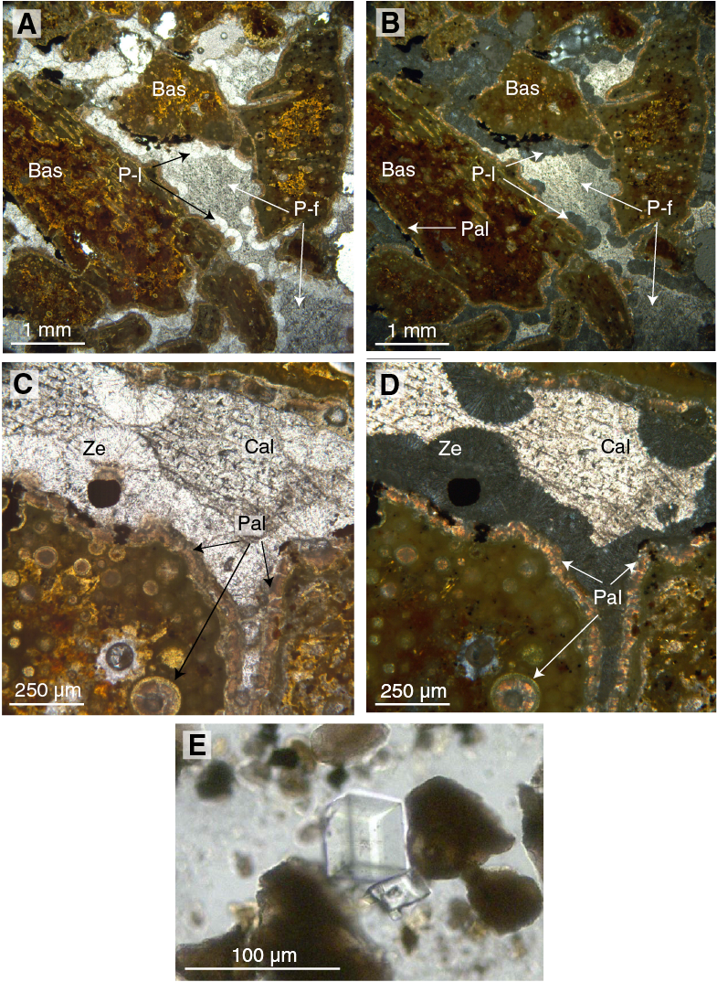
Figure F27. Variability of volcaniclastic facies, Hole U1520C.
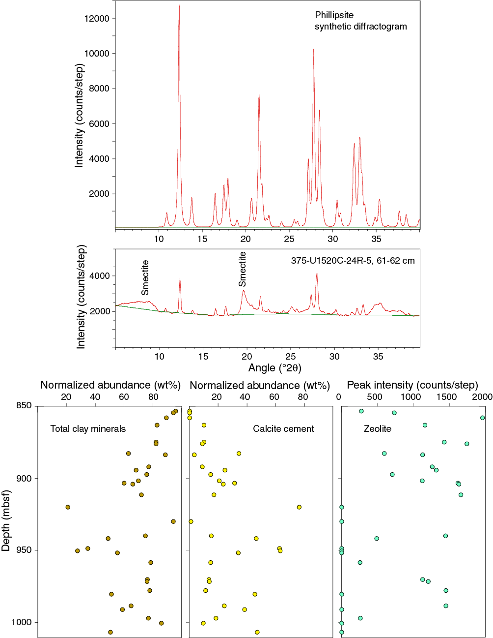
Figure F28. XRD results, Unit V.
The cement between clasts in the conglomerate is dark gray zeolite to milky white calcite (Figure F27). XRD shows that the zeolite is phillipsite (Figure F28). Several generations of cement are visible in thin section, which is suggestive of a complex and spatially inconsistent paragenetic sequence. Additional work will be needed post-expedition to establish the chronological sequence of diagenetic events. Pore-lining cement is visible around the palagonite-coated clasts and is composed of either calcite or zeolite. Zeolite typically displays radial patterns, especially where filling larger voids. Some cement zones show signs of recrystallization.
Subhorizontal and scattered steeper veins, generally filled with calcite, are also common. They occur both as diffuse veins and as fractures filled by zeolite and/or calcite (see Structural geology). Some of these cemented intervals contain dark basalt clasts completely surrounded by milky white cement. Thin section observations show no significant difference in the degree of basalt alteration in intervals with green versus white cement. The white cement appears to be dominated by calcite, whereas the green cement is largely zeolite and associated with more palagonite rims.
Beginning at 1006.33 mbsf (Section 375-U1520C-40R-1, 13 cm), the volcaniclastic conglomerate exhibits some dark bluish greenish gray coloration that becomes pervasive at 1015.7 mbsf (Section 41R-1, 0 cm) (Figure F29). Despite this obvious color change, the morphology of the volcaniclastic conglomerate appears to be unchanged. We were unable to identify compositional differences between the brown and dark greenish gray conglomerates from smear slides and thin sections.

Figure F29. Dark bluish gray to greenish gray conglomerate.
Judging from the combination of clast- and matrix-supported varieties of conglomerate, the absence of well-developed bedding, the absence of preferred clast orientation, the absence of size grading at the scale of individual beds, and the poor sorting of clasts, we interpret these deposits to be products of two physical mechanisms: grain flow and debris flow. Larger clasts in the debris flows were supported during transport by the finite yield strength of the matrix (clay plus seawater) and buoyancy. Clasts in the grain flows were supported during transport by dispersive pressure (i.e., grain collision). Because grain flows require steep slopes to sustain motion (i.e., at or above the angle of repose for gravel), seamount flanks or scarp walls are logical possibilities for staging areas prior to resedimentation. The extent of vesicularity in basalt fragments may be indicative of eruptions and degassing in shallow water. Some fragmentation and alteration of the basalt clasts probably occurred prior to resedimentation. We see evidence for only one period of cessation of the gravity flows, when deposition of the marl interval occurred (interval 375-U1520C-34R-2, 29 cm, to 34R-CC, 20 cm). Based on distributions of similar deposits recovered by dredging along scarps on the Hikurangi Plateau and assessments of flat-topped (guyot-like) geometries of associated seamounts, others have suggested that some seamounts on the plateau were exposed to erosion close to or above sea level (Mortimer and Parkinson, 1996; Hoernle et al., 2010). The total thickness of Unit V requires large volumes of fragmented basaltic material in the staging area and largely uninterrupted transport into deeper water.
Unit VI
- Interval: 375-U1520C-41R-1, 54 cm to 44R-1, 125 cm
- Thickness: 29.51 m
- Depth: 1016.24–1045.75 mbsf
- Age: early Late Cretaceous
- Lithology: granule-sized volcaniclastic conglomerate, siliceous mudstone, siltstone, black mudstone, limestone, and basalt
Unit VI extends from 1016.24 to 1045.75 mbsf (interval 375-U1520C-41R-1, 54 cm, to 44R-1, 125 cm) and is early Late Cretaceous in age (see Biostratigraphy). This unit comprises a blend of lithologies whose stratigraphic organization and thicknesses are unresolvable because of poor recovery, coring disturbance, and biscuiting. A distinctive, dark bluish green color is widespread among most of the rock fragments.
Most of Unit VI (1016.24–1044.5 mbsf; interval 375-U1520C-41R-1, 54 cm, to 44R-1, 0 cm) is made up of alternating volcaniclastic conglomerate similar to the overlying examples in Unit V and dark gray clayey siltstone or siliceous mudstone (Figure F30). The volcaniclastic conglomerate exhibits the same distinctive, dark bluish gray to dark greenish gray color seen at the bottom of Unit V (interval 40R-1, 13 cm, to 41R-1, 54 cm). We were unable to isolate a compositional cause of the color change through petrographic analysis. The conglomerate clasts consist of altered basalt with many amygdules.
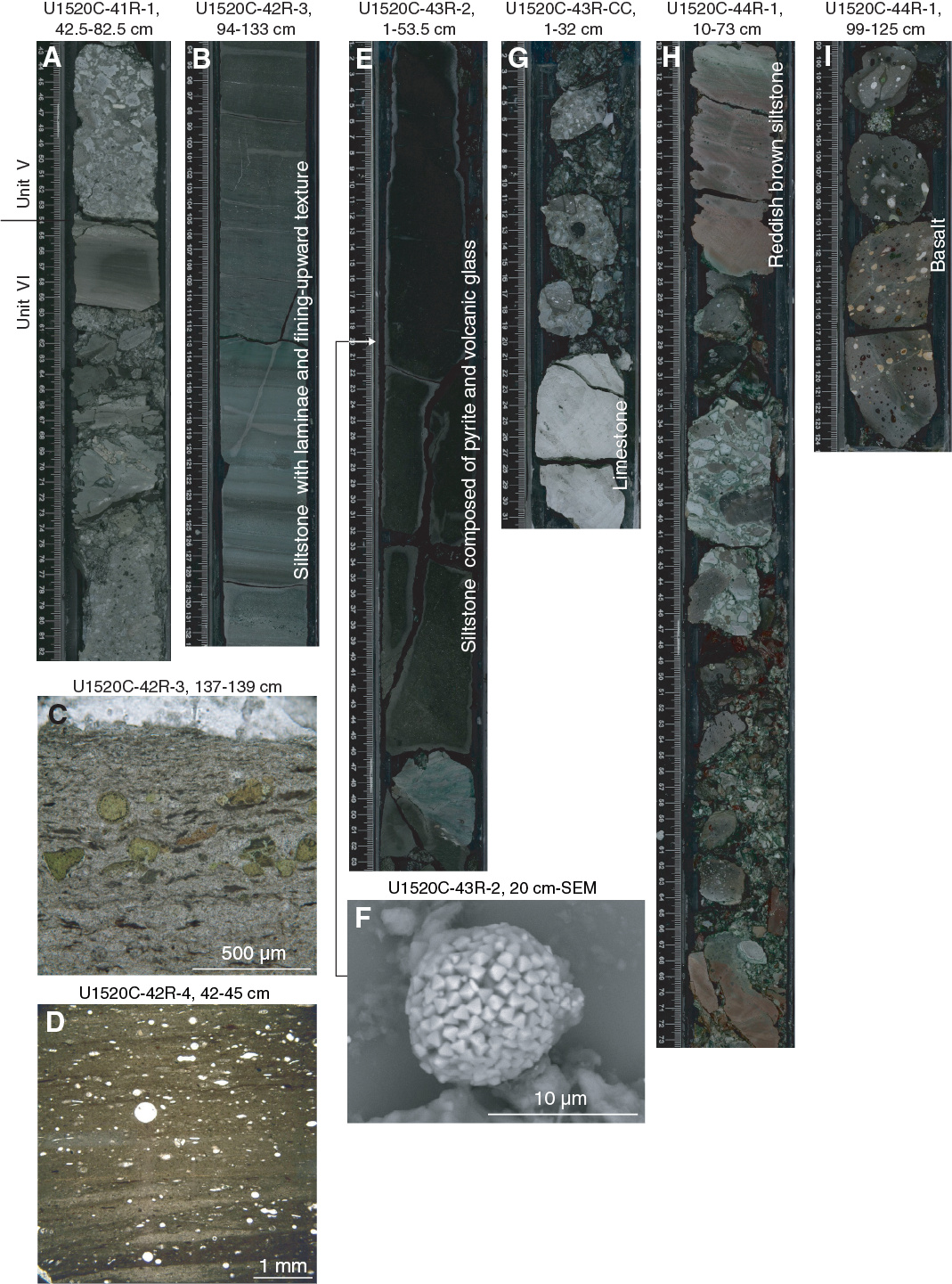
Figure F30. Disjointed blend of lithologies in Unit VI, Hole U1520C.
Mudstone and siltstone beds, where intact, are characterized by coarser silty bases with normal grading and well-developed planar lamination with only slight bioturbation (Figure F30B–F30D). Their composition is dominantly volcaniclastic and includes altered glass, feldspar, quartz, microfossils (radiolarians and foraminifers), and sand-sized greenish spheres in a clay matrix. The spheres are probably amygdules liberated from vesicular basalt (Figure F30B). XRD shows significant amounts of silica in the mudstone in the form of opal-CT (Figure F11). Between 1036.37 and 1036.97 mbsf (Section 375-U1520C-43R-2), another distinctive siltstone occurs that is darker gray to black in color and composed of pyrite and clear volcanic glass (Figure F30E). A single clast of pyrite (~1 cm) was found in this layer (Section 43R-2, 60 cm) (Figure F30F). This siltstone yielded high total organic carbon (TOC) values as high as 14.6 wt% (see Geochemistry). Deposition in an anoxic environment is likely.
From 1038.8 to 1045.75 mbsf (interval 375-U1520C-43R-CC, 21 cm, to 44R-1, 125 cm), Unit VI exhibits even more variability in lithologies. At the bottom of Section 43R-CC, we found biscuited chunks of white limestone unlike any lithologies recovered from cores above (Figure F30G). Interval 44R-1, 0–79 cm, is composed of alternating thin layers of reddish brown siltstone and dark greenish gray volcaniclastic conglomerate (Figure F30H). The conglomerate is composed of centimeter-scale angular-shaped clasts of microcrystalline plagioclase basalt (Figures F30H, F31). The texture of the basalt is trachytic or interstitial. The matrix appears to be glass that was extensively altered to clay minerals. Below this interval, we recovered several pieces of vesicular basalt (Figure F30I) composed of fine-grained euhedral plagioclase phenocrysts showing interstitial and/or trachytic texture (Figure F31D, F31F). Some vesicles are filled with aggregates of spherulitic calcite. Interstitial glass is altered to clay minerals (smectite) or replaced by calcite.
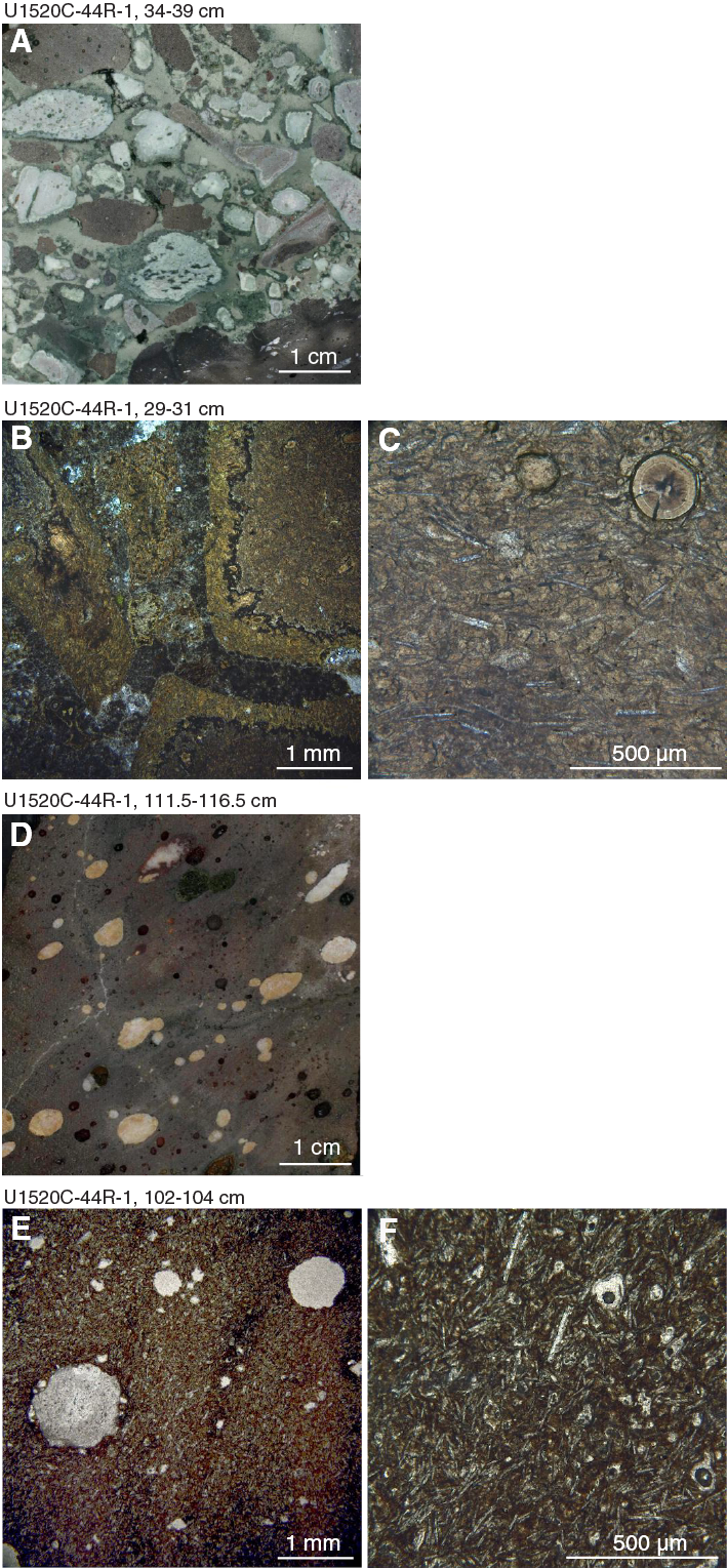
Figure F31. Variable textures of basalt, Unit VI.
Pyroclastic deposits
A total of 224 ash layers and ash pod layers were observed in Site U1520 cores. In Unit I (Cores 375-U1520D-1H through 13H), five thin to medium beds (≤14 cm) of brownish to gray ash layers with normal grading occur in the uppermost 30 m (Figure F32).
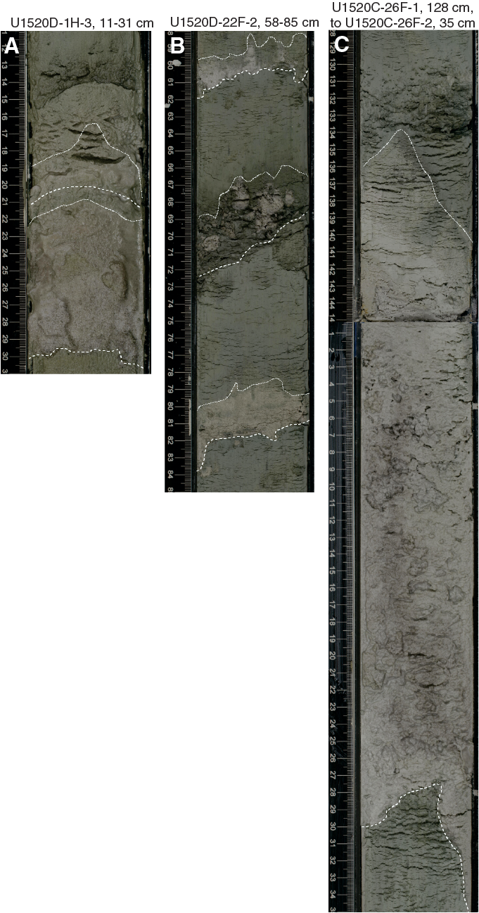
Figure F32. Examples of tephra layers, Units I–III.
In Unit II, normally graded ash layers appear in Core 375-U1520D-15H and below. In total, Unit II contains 37 ash layers and ash pod layers with a maximum thickness of 4 cm (Figure F32). Unit III includes 44 ash layers as thick as 1 m, and many show normal grading. Half of them are concentrated between 220 and 232.77 mbsf. We recorded an increase in thickness across the transition from Unit III to Unit IV (Cores 46X–53X), where ash layers are as thick as 18 cm.
Smear slides show that the ash layers from Units I–III are dominated by colorless glass with common abundances of plagioclase; variable abundances of hornblende, biotite, and pyroxene; and traces of quartz, zircon, and allanite. We also found common to trace amounts of nannofossils and foraminifers along with sedimentary lithic and volcanic lithic fragments, depending on how the tephras mixed with the background sediment.
The tephras in Units I–III differ in terms of relative abundances of glass textures and vesicles (Figure F32). Samples from Units I and II and the upper part of Unit III have glass shard textures that are a mixture of tubular and elongated pumiceous and dense-blocky and cuspate varieties. In Core 375-U1520D-28F and below, blocky to cuspate dense shard types dominate and highly vesicular pumiceous clasts are rare. In the lowermost part of Unit III, highly vesicular pumiceous clasts are dominant (e.g., Sample 49X-CC, 31 cm).
In Unit IV (Section 375-U1520D-50X-CC, 0 cm), the ash layers are more lithified. In Hole U1520C, 138 thin intercalations of felsic and mafic silt-sized tuff were identified, mostly between 509.82 and 750.89 mbsf. These layers range in color from grayish to pinkish to whitish brown, dark gray, and black. One additional tuff occurs at 849.45 mbsf at the top of Unit V. The layers are as thick as 24 cm but are weakly to strongly bioturbated or disturbed by drilling. This dissemination obscures the primary structure of the bed or the coarser basal contact (Figure F32). When complete, these layers are normally graded and in some cases finely laminated (Figure F33).
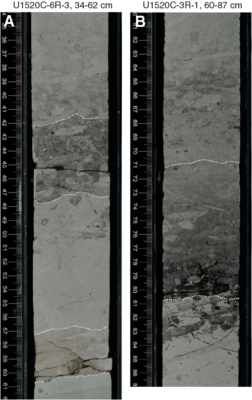
Figure F33. Examples of bioturbated tephra layers, Unit IV.
A subset of the tuff layers in Unit IV was also sampled for more detailed smear slide analyses. The tuff layers are dominated by colorless glass with present to rare but persistent occurrences of feldspar and variable occurrences of quartz, hornblende, pyroxene, and traces of biotite. Exceptions are some strongly bioturbated mafic examples between 586.96 and 750.89 mbsf (intervals 375-U1520D-60X-1, 12–14 cm, and 375-U1520C-13R-3, 70–79 cm) that are characterized by a mixture of dark brownish to transparent glass shards and rare to present feldspar, pyroxene, apatite, and opaque crystals (Figure F34A, F34B).

Figure F34. Examples of tephra layers, Unit IV.
All of the examples examined in smear slides also contain rare to common altered glass, clay minerals, and sedimentary lithic fragments as well as biogenic constituents including calcareous nannofossils and occasional foraminifer fragments. These constituents were probably introduced by bioturbation. Smear slides also reveal a change from normal glass-rich tuffs to devitrified tuffs between Sections 375-U1520C-9R-3, 5 cm, and 9R-4, 49 cm (Figure F35A, F35D).
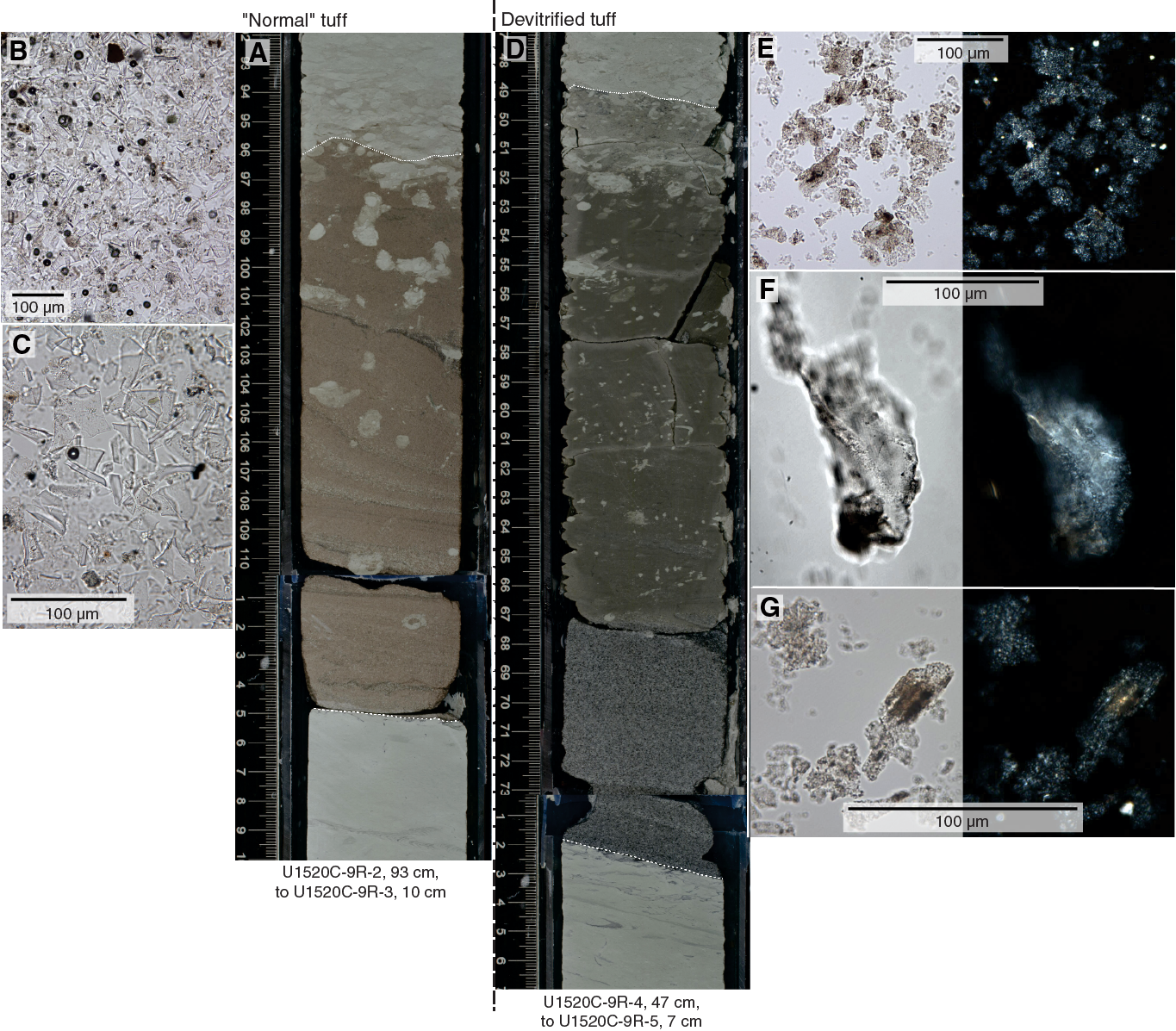
Figure F35. Unaltered “normal” tuff and devitrified tuff.
We recognized four compositional groups of tephra in Unit IV based on detailed investigation of the texture of the glass shards and the shape of the vesicles. Vesicular pyroclasts are more common toward the top of the unit. The first category consists predominantly of highly vesicular, tubular, and elongate bubble-bearing pumiceous clasts along with less abundant dense-blocky and cuspate glass shards (e.g., Samples 375-U1520C-2R-2, 33 cm; 4R-2, 66 cm; 4R-5, 53 cm; and 4R-CC, 19 cm) (Figure F34D, F34E). A second group, also containing vesicular erupted pyroclasts, is made up of a mixture of dominant cuspate-shaped glass shards and common to abundant dense-blocky glass shards along with highly vesicular pumiceous grains that are rich in elongate vesicles (Samples 2R-1, 104 cm; and 4R-1, 1 cm). Cuspate-shaped glass shards are interpreted to be the remnants of bubble walls of larger, highly vesicular pumiceous clasts (see scanning electron microscope [SEM] images in Figure F14 in the Site U1518 chapter [Saffer et al., 2019b]). The third category is predominantly made up of dense-blocky and cuspate glass shards (Figures F34G, F34H, F35B, F35C). This group has a moderate abundance of rounded to elongate bubbles but only a minor amount of highly vesicular, tubular pumiceous clasts (e.g., Samples 3R-1, 32 cm; 4R-1, 55 cm; 7R-1, 40 cm; 9R-2, 16 cm; and 9R-2, 106 cm). The fourth category is a transitional group with abundant pumiceous clasts rich in elongate and elliptical vesicles as well as abundant cuspate and blocky-shaped, predominantly dense glass shards (e.g., Samples 2R-1, 80 cm; 3R-2, 119 cm; 5R-2, 121 cm; and 8R-5, 23 cm). This group includes the more mafic tuffs; however, varieties exhibit round and elliptical vesicles dominating the pumiceous grains (e.g., Sample 4R-5, 109 cm) (Figure F34B).
The devitrified tuffs below 712.59 mbsf (Sample 375-U1520C-9R-4, 49 cm) commonly have pumiceous textures, although most of the glass has been recrystallized (Figure F35D–F35G) (Samples 9R-4, 62 cm; 9R-4, 70 cm; 11R-5, 63 cm; 13R-3, 76 cm; 23R-5, 79 cm; 23R-5, 99 cm; and 23R-6, 12 cm). Some of these layers have the same mineral assemblages as the vitrified tuffs above.
Glass textures and vesicles provide important hints regarding eruption processes and conditions. The category with predominating fine-grained blocky and dense glass shards, for instance, may be derived from eruptions that caused extensive fragmentation due to interaction with external water (e.g., Zimanowski et al., 2015). In contrast, highly vesicular pyroclasts are typical of extensively degassed magmas often seen in subaerial eruptions with large explosions (e.g., Kutterolf et al., 2008, 2018).
We interpret the majority of the deposits to be air fall derived, although this conclusion remains speculative for some of the heavily disturbed layers. Supporting evidence includes the normal grading and a lack of sedimentary structures indicative of pyroclastic flow processes and the inferred distance to likely source volcanic centers on mainland New Zealand. Nevertheless, some tuffs show parallel laminae indicative of beds emplaced by mass flows (turbidity currents) or local reworking by bottom currents (e.g., Kutterolf et al., 2018). Irregular ash pod layers are possible products of bioturbation and/or locally confined gravitational creeping and subsequent dissemination shortly after initial emplacement by air fall or flow (e.g., Kutterolf et al., 2008).
Comparison of Hole U1520C–U1520D core data and Hole U1520A–U1520C log data
In general, facies-level comparisons (i.e., packets of beds at a ≥10 m scale) can be made between the lithostratigraphy defined from core descriptions (Figure F4) and the provisional log-based stratigraphy defined in Holes U1520A–U1520C (see Logging while drilling). The two data sets are complementary, especially when lithologic and petrophysical attributes are grouped at the facies scale. Finer scale observations of sedimentary structures and microscopic verification of grain size distributions and mineralogy help guide interpretations of the logging data (e.g., discriminating between beds of sand versus silt, ratios of carbonate to clay, etc.), whereas continuous logging records help fill gaps in the lithostratigraphy caused by incomplete core recovery.
Comparisons among lithostratigraphic units and logging units
Lithostratigraphic Unit I correlates with Logging Unit 1 (Figure F4). Coring confirmed the presence of numerous sand and silt beds in a turbidite succession that accumulated on the floor of the Hikurangi Trough. Some sand beds reach thicknesses >1 m, which helps explain the spiky gamma ray response and washouts recorded by the ultrasonic caliper.
Lithostratigraphic Unit II correlates with Logging Unit 2. The respective picks for the top of the Ruatoria MTD are within about 4 m of one another, and coring confirmed that the remobilized sediment is dominated by fine-grained hemipelagic mud with thin interbeds of silt. The overall character of this facies is consistent with deposition on the landward trench slope prior to slope failure. However, the cores do not display any mesoscopic evidence of internal deformation in the inferred slide mass, and the steep bedding dips interpreted from geoVISION (GVR) images are not evident in the cores (see Structural geology). After drilling without coring to 222 mbsf, we failed to recover the base of the slide, which was interpreted to occur at 225 mbsf based on the LWD data. One explanation for this discrepancy is erosional relief along the base of the debris avalanche. A 3–5 m shift in depth to the base of the slide, measured over the 40 m of horizontal separation between Holes U1520B and U1520D, seems reasonable given the dimensions of the debris avalanche.
Lithostratigraphic Unit III correlates with the succession of Logging Units 3–5. Coring confirmed that the sediments below the Ruatoria deposit are silty trench-floor turbidites, and their typical grain sizes are finer than those in Unit I. The gradual downsection decreases in turbidite frequency, interbed thickness, and grain size, however, are opposite to the expectation for a decreasing gamma ray response (i.e., more clay should equate with higher gamma ray).
The upper part of Lithostratigraphic Unit IV correlates with Logging Unit 6. Core recovery was poor in this interval, but the lithologies consist of marl and carbonate-rich MTDs. The fundamental transition is from turbidite sedimentation above to carbonate-dominated pelagic sedimentation below. We see no significant changes in lithology or lithification, however, over the depth intervals of Logging Units 7 and 8. Conversely, the distinctive deposits of calcareous mudstone (~720–740 mbsf), which show substantial reductions in carbonate (weight percent) and commensurate increases in total clay minerals, occur in the middle of Logging Unit 9 without differentiation (Figure F4). The transition into Logging Unit 10 is in close agreement with core observations; the large decrease in gamma ray response is consistent with the occurrence of chalk.
Logging Unit 11 coincides with the upper part of the volcaniclastic conglomerate facies (Lithostratigraphic Unit V). Both unit boundary types are sharp. The dramatic increase in gamma ray response relative to the overlying chalk (Unit 10) is consistent with extensive amounts of alteration and replacement of basaltic protoliths by clay minerals. The spikes in resistivity and bimodal clustering of attributes on crossplots are also consistent with variable amounts of cementation in the heavily altered conglomerate.
Biostratigraphy
Planktonic foraminifers and calcareous nannofossils from core catcher samples and additional split-core samples from Holes U1520C and U1520D were examined to develop a shipboard biostratigraphic framework for Site U1520. Additionally, benthic foraminifers provided data on paleowater depths, downslope reworking, and dissolution of foraminiferal shells.
At Site U1520, we drilled the Hikurangi Trough sedimentary sequence and upper portion of the Hikurangi Plateau basement adjacent to Tūranganui Knoll and recovered a 1045 m thick, discontinuous Holocene to Late Cretaceous succession comprising several hiatus-bound sedimentary packages. Calcareous nannofossil and planktonic foraminifer ages are generally in agreement, but the details of some biostratigraphic boundaries differ (see below). The ages provided by benthic foraminifers were sometimes inconsistent with those of planktonic foraminifers and calcareous nannofossils and consequently were only used when no other age data were available. Biostratigraphic datums recognized at Site U1520 are given in Table T4, and age versus depth is shown in Figure F36.
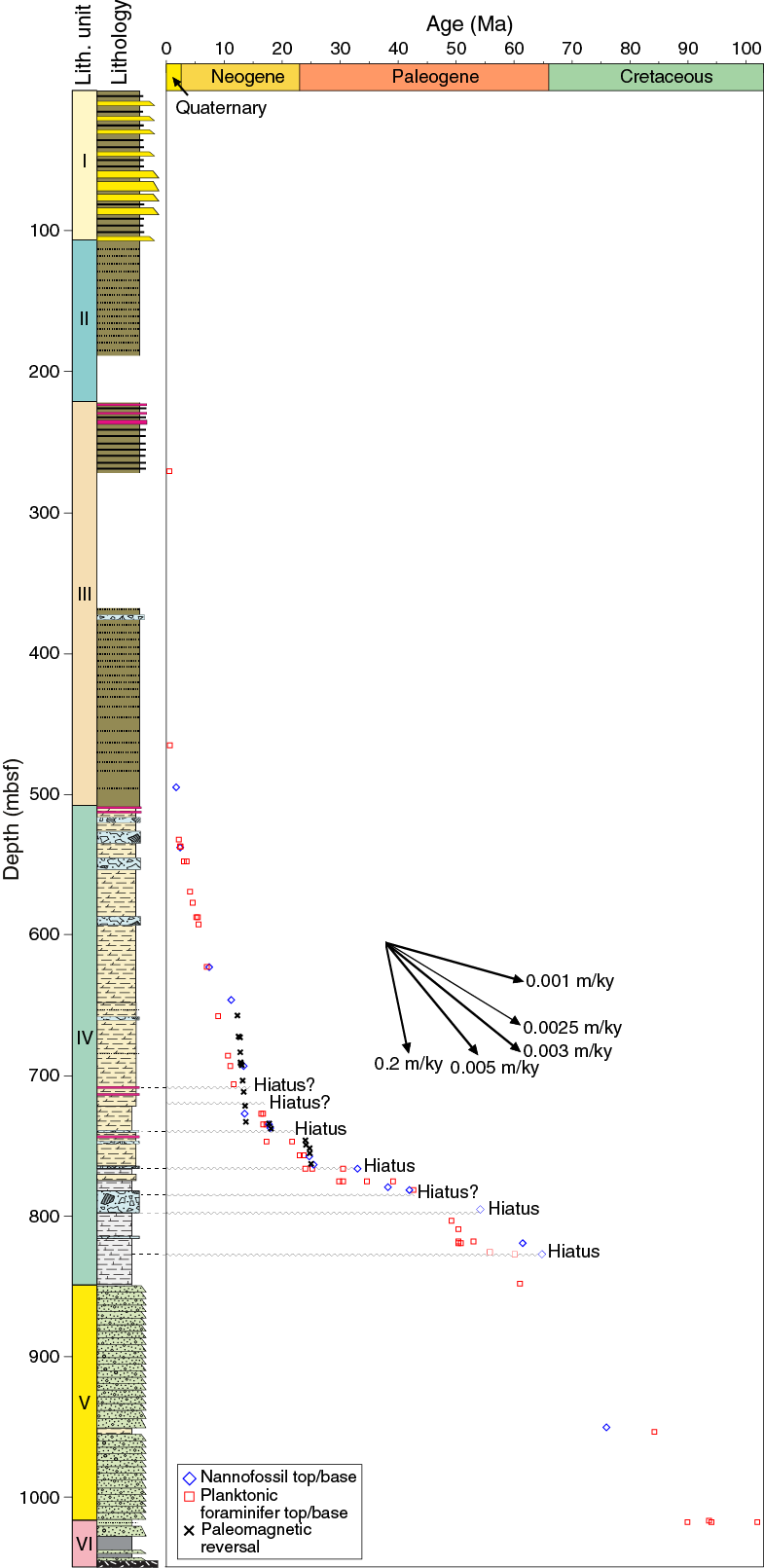
Figure F36. Biostratigraphic and paleomagnetic age-depth plot.
Calcareous nannofossils are common to abundant through the Pleistocene–Paleocene interval but are rare to common in Cretaceous samples. Preservation varies from moderate to poor throughout the sequence, and older material is significantly reworked in most of the Pleistocene samples. Minor reworking of planktonic foraminifers was evident throughout the cored sedimentary succession but was most notable in Sample 375-U1520D-51X-CC, 30–35 cm (511.84 mbsf), where common, very well preserved middle to early Eocene, Miocene, and Pliocene taxa occur in a Pleistocene fauna, and Sample 60X-CC, 0–10 cm (587.74 mbsf), where late Miocene (8.96–9.63 Ma) taxa dominate a Miocene/Pliocene boundary fauna.
Calcareous nannofossils
Calcareous nannofossil biostratigraphy in Holes U1520C and U1520D was established through the analysis of core catcher samples, and additional split-core samples were analyzed to better constrain biostratigraphic events. Nannofossils are common to abundant in samples from the Pleistocene–Paleocene sequence (24.91–848.01 mbsf) but are rare to common in Cretaceous samples (849.96–1037.58 mbsf). Preservation is moderate to poor throughout the sequence, and older material is significantly reworked in most of the Pleistocene samples. A total of 18 nannofossil biostratigraphic datums are recognized at Site U1520, representing a discontinuous Pleistocene to Late Cretaceous sedimentary sequence. The sampling resolution through Hole U1520D was lower than through Hole U1520C because of time constraints; only every other core catcher sample was examined. Post-expedition analysis of additional core catcher samples will help constrain datums through the Pleistocene interval. Distribution of calcareous nannofossil taxa is shown in Table T5, and biostratigraphic datums are given in Table T4.
Pleistocene
The presence of Emiliania huxleyi in Samples 375-U1520D-3H-CC, 7–17 cm, through 9H-CC, 6–16 cm (24.90–77.7 mbsf), indicates a Middle Pleistocene to Holocene age (0.29 Ma or younger) in Zone NN21 of Martini (1971). Below 77.7 mbsf, the recognition of key datums is problematic because of significant reworking of Pliocene–Eocene taxa throughout the Pleistocene sequence. The last appearance datum (LAD) of Pseudoemiliania lacunosa defines the Zone NN19/NN20 boundary. The last consistent appearance of P. lacunosa in Hole U1520D occurs in Sample 35X-CC, 20–30 cm (376.10 mbsf). Rare occurrences of this taxa occur in the younger interval of the Pleistocene sequence (Sample 13H-CC, 40–50 cm [119.90 mbsf]); however, this occurrence is likely reworked given that it falls in the Ruatoria submarine slide unit (see Lithostratigraphy). Therefore, the interval between Samples 11H-CC, 7–17 cm, and 33X-CC, 9–19 cm (100.75–270.32 mbsf), is tentatively assigned to Zone NN20. The first appearance datum (FAD) of large Gephyrocapsa spp. (>5.55 µm) in Sample 49X-CC, 33–43 cm (494.80 mbsf), indicates lower Zone NN19 (1.62 Ma). Consequently, Samples 37X-CC, 21–31 cm, through 49X-CC, 33–43 cm (395.20–494.80 mbsf), are assigned an early Pleistocene age. The LAD of Discoaster pentaradiatus (2.39 Ma) in Sample 54X-CC, 7–17 cm (537.11 mbsf), defines the Zone NN18/NN17 boundary.
Miocene
The FAD of Amaurolithus spp. (7.42 Ma) in Sample 375-U1520D-65X-CC, 17–22 cm (622.95 mbsf), indicates lower Zone NN11 (late Miocene). The LAD of Calcidiscus premacintyrei in Sample 375-U1520C-2R-CC, 0–5 cm (647.70 mbsf), indicates an earliest late Miocene age (11.21 Ma) in Zone NN7 of Martini (1971). The FAD of Calcidiscus macintyrei (13.36 Ma) in Sample 7R-CC, 18–23 cm (693.05 mbsf), indicates lower Zone NN6 (middle Miocene). The LAD of Sphenolithus heteromorphus (13.53 Ma) in Sample 10R-CC, 0–5 cm (726.98 mbsf), defines the Zone NN6/NN5 boundary. The FAD of S. heteromorphus (17.71 Ma) in Sample 11R-5, 66 cm (734.61 mbsf), which occurs in lower Zone NN4, indicates an early Miocene age. Sample 11R-CC, 16–21 cm (737.38 mbsf), yields the LAD of Sphenolithus belemnos (17.95 Ma), which defines the Zone NN4/NN3 boundary. No nannofossil bioevents were identified in Samples 12R-CC, 0–7 cm, through 13R-CC, 0–5 cm (746.82–756.62 mbsf), and this interval is tentatively assigned to a combined Zone NN1–NN2 (early Miocene) based on the absences of latest Oligocene taxa (e.g., Reticulofenestra bisecta and common Cyclicargolithus abisectus) and S. belemnos, whose FAD marks the base of Zone NN3.
Oligocene
The last common occurrence of C. abisectus (24.67 Ma) in Sample 375-U1520C-14R-1, 74 cm (757.44 mbsf), which falls in Zone NP25, indicates a late Oligocene age. The last appearance of Chiasmolithus occurs in Sample 14R-5, 92 cm (763.34 mbsf), and despite being unable to identify specimens to species level because of poor preservation, this occurrence likely corresponds to the LAD of Chiasmolithus altus (25.44 Ma) in Zone NP25, which represents the extinction of the genus. The LAD of Isthmolithus recurvus (32.49 Ma) occurs in Sample 14R-CC, 0–5 cm (766.15 mbsf), indicating Zone NP22 (early Oligocene) or older. A hiatus is inferred between Samples 14R-7, 6 cm, and 14R-CC, 0–5 cm (765.34–766.15 mbsf) because sediments of late early to early late Oligocene age are missing.
Eocene
The FAD of R. bisecta (>10 µm = Reticulofenestra stavensis in distribution chart; 38.25 Ma), which falls in lower Zone NP17 (middle Eocene), occurs in Sample 375-U1520C-16R-3, 52 cm (779.33 mbsf). Sample 16R-4, 146–150 cm (781.36 mbsf), yields the FAD of Reticulofenestra umbilicus (>14 µm), which indicates lower Zone NP16 (middle Eocene). The first appearance of Reticulofenestra occurs in Sample 17R-CC, 20–25 cm (786.64 mbsf). The first appearance of this genus is dated to 50.50 Ma in Zone NP12 (Gradstein et al., 2012); however, Reticulofenestra is known to have an earlier first appearance in the New Zealand region, so its presence indicates Zone NP11 or younger (early to middle Eocene) (Shepherd and Kulhanek, 2016). It is possible that a hiatus occurs between Samples 16R-4, 146–150 cm, and 17R-CC, 20–25 cm (781.36–786.64 mbsf); however, further work is needed to constrain this interval. The FAD of Sphenolithus radians (54.17 Ma), which is used as a secondary marker for the base of Zone NP11 (Backman, 1986; Hollis et al., 2015; Shepherd and Kulhanek, 2016), occurs in Sample 18R-1, 69 cm (795.69 mbsf).
Paleocene
A distinct change in the nannofossil assemblage occurs in Sample 375-U1520C-18R-6, 15 cm (802.37 mbsf), with a shift to a middle Paleocene assemblage that includes Cruciplacolithus frequens, Cruciplacolithus intermedius, Cruciplacolithus tenuis, Ericsonia aliquanta, Ericsonia subpertusa, Ericsonia robusta, Fasciculithus involutus, Fasciculithus tympaniformis, Hornibrookina teuriensis, Lithoptychius pileatus, Prinsius bisulcus, Prinsius dimorphosus, Prinsius martini, and Zeugrhabdotus sigmoides. Consequently, a hiatus is inferred between this sample and Sample 18R-1, 69 cm (795.69 mbsf). The FAD of F. tympaniformis (61.51 Ma), which defines the Zone NP4/NP5 boundary, occurs in Sample 20R-CC, 16–21 cm (819.17 mbsf). The first appearance of Toweius eminens is documented to occur in Zone NP5 (Monechi et al., 2013); however, Faris and Farouk (2012) place the first occurrence of this taxon in Zone NP4. T. eminens occurs in Sample 21R-1, 97 cm (824.87 mbsf). Below this interval, identification of nannofossils to species level is problematic because fine-grained sediment infills and obscures the central area of specimens. However, the first appearance of Chiasmolithus danicus (64.81 Ma), which defines the NP3/NP2 boundary, occurs in Sample 23R-4, 152–157 cm (848.01 mbsf).
Cretaceous
An abrupt lithologic change at the Lithostratigraphic Unit IV/V boundary between Samples 375-U1520C-23R-4, 152–157 cm, and 23R-CC, 0–5 cm (848.01–849.96 mbsf), likely represents a significant unconformity (see Lithostratigraphy). Nannofossils are not present in samples examined from the upper portion of the volcaniclastic conglomerate sequence of Unit V (Samples 23R-CC, 0–5 cm, through 24R-CC, 0–5 cm [849.96–859.71 mbsf]). Consequently, Samples 25R-CC to 33R-CC (866.30–942.24 mbsf) from similar volcaniclastic sediments were not examined for nannofossil content. Samples 34R-2, 75–80 cm, through 34R-CC, 0–5 cm (950.22–953.50 mbsf), comprise a layer of marl (see Lithostratigraphy), and this interval yields a Cretaceous assemblage dominated by Seribiscutum primitivum with less common Cyclagelosphaera margerelii, Cyclagelosphaera reinhardtii, Placozygus fibuliformis, and Tranolithus orionatus. The interval between Samples 41R-1, 54 cm, and 44R-1, 39 cm (1016.24–1044.89 mbsf), lies in Lithostratigraphic Unit VI and comprises a mixture of lithologies (see Lithostratigraphy). Two intervals in this sequence contain Cretaceous assemblages of similar composition to the upper interval: Samples 41R-1, 58 cm, to 41R-2, 64 cm (1016.28–1017.83 mbsf), and Samples 42R-3, 117 cm, to 43R-2, 121 cm (1029.13–1037.58 mbsf).
Foraminifers
Planktonic and benthic foraminifers were examined from core catcher and split-core samples from Holes U1520C and U1520D (Figure F37). Absolute ages assigned to biostratigraphic datums follow those listed in Table T4 in the Expedition 372B/375 methods chapter (Wallace et al., 2019a). Planktonic and benthic foraminifer datums are given in Table T4, the distribution of important planktonic and benthic foraminifer taxa is given in Table T6, and planktonic foraminifer abundances and indications of oceanicity (qualitative measure of the extent to which the paleoenvironment recorded by the faunal assemblage represents open ocean conditions relative to a nearshore-influenced environment), paleowater depths, and downslope reworking are given in Table T7.
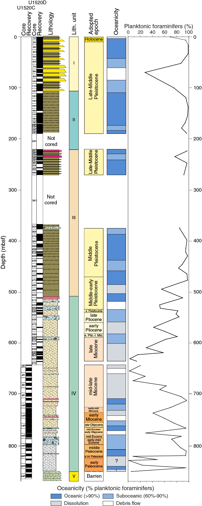
Figure F37. Lithostratigraphy, planktonic foraminifer abundance, and oceanicity.
Moderately to poorly preserved foraminifers are common in the Neogene section through the upper part of Lithostratigraphic Unit IV (see Lithostratigraphy), where faunas have been modified by the selective dissolution of foraminifer shells. Foraminifer abundance and preservation is better in the upper part of the Paleogene and generally improves to the lower part of Unit IV. Echinoid spines, fish teeth, and radiolarians are also present in some samples, but they are relatively rare compared with foraminifers. In the Cretaceous section, foraminifers with moderate to poor preservation are present in pelagic sediments interbedded with barren volcaniclastic sediments in Lithostratigraphic Units V and VI (see Lithostratigraphy). Foraminifer abundances are generally low, and specimens are largely confined to the <150 µm sediment-sized fraction of washed microfossil residues. Additionally, bivalve and inoceramid shell fragments as well as rare fish teeth and echinoid spines are present in some samples. Abundant poorly preserved radiolarians and common fragments of siliceous, branched, tube-like fossils of unknown affinity are also present in fine-grained, organic-rich sediments in Unit VI (see Geochemistry). Encrusting coralline algae were also observed in split cores and thin sections.
Quaternary
Common to abundant Holocene and Pleistocene age planktonic foraminifers were recovered from Samples 375-U1520D-1H-1, 0 cm, through 54X-CC, 7–17 cm (0–537.11 mbsf), which span Lithostratigraphic Units I–III and the upper part of Unit IV. Assemblages are generally well preserved and abundances are relatively high, indicating deposition under suboceanic to oceanic conditions with occasional fluctuations to extraneritic and outer neritic values (e.g., Sample 8H-CC, 0–10 cm [70.82 mbsf]). Benthic foraminifers in Lithostratigraphic Units I and II and the upper part of Unit III suggest deposition was in midbathyal or deeper water depths >600 m (Table T7) and involved some downslope reworking of inner to midshelf taxa (e.g., Sample 11H-CC, 7–17 cm [100.75 mbsf]). Water depths in the lower part of Lithostratigraphic Unit III and the uppermost part of Unit IV generally record deeper lower bathyal water depths >1000 m. Minor reworking of Pliocene and Miocene taxa is also noted through the Quaternary. More extensive reworking is also evident in Sample 51X-CC, 30–35 cm (511.84 mbsf), from the top of Lithostratigraphic Unit IV, where well-preserved Pliocene, Miocene, and middle to early Eocene taxa occur in a Pleistocene age fauna. The faunal association in this sample is possibly related to an MTD. The Quaternary succession is biostratigraphically divided into two units: Holocene to early Pleistocene (Haweran to late Nukumaruan; 0–2.17 Ma) in Samples 1H-1, 0 cm, through 53X-CC, 6–16 cm (0–532.17 mbsf), and early Pleistocene (2.37–2.40 Ma) in Sample 54X-CC, 7–17 cm (537.11 mbsf).
Holocene to Pleistocene
The base of the Holocene, located between Samples 375-U1520D-1H-CC, 15–20 cm, and 2H-CC, 17–27 cm (5.88–15.40 mbsf), is marked by the base of the Hirsutella hirsuta Marine Isotope Stage 1 subzone. A change from sinistral to dextral coiled populations of Truncorotalia truncatulinoides between Samples 33X-CC, 9–19 cm, and 35X-CC, 20–30 cm (270.32–376.10 mbsf), suggests the base of the sinistral Tr. truncatulinoides zone (0.53 Ma) is likely to occur in the drilled interval (270.80–366.60 mbsf) where no core was recovered. The underlying interval (Samples 35X-CC, 20–30 cm, through 46X-CC, 27–37 cm [376.10–464.95 mbsf]) is Middle Pleistocene (Castlecliffian; 0.53–0.62 Ma) based on the abundance of Tr. truncatulinoides and the presence of mostly dextral coiled populations of Tr. truncatulinoides. The interval from Sample 47X-CC, 18–28 cm, through Sample 53X-CC, 6–16 cm (477.23–532.17 mbsf), between the first common occurrence of Tr. truncatulinoides (0.62 Ma) and the FAD of Tr. truncatulinoides (2.17 Ma), respectively, is Middle to early Pleistocene (Castlecliffian to late Nukumaruan). The base of the Pleistocene is marked by the FAD of Truncorotalia crassula (2.40 Ma) in Sample 54X-CC, 7–17 cm (537.11 mbsf). The presence of a dextral coiled population of Truncorotalia crassaformis in the same sample indicates an early Pleistocene age (Nukumaruan; 2.37–2.40 Ma). A hiatus is inferred between the FAD of Tr. crassula (2.40 Ma) and the LAD of Truncorotalia crassaconica s.s. (2.98 Ma) in the underlying core catcher sample (see below).
Quaternary water depths and oceanicity
Quaternary planktonic foraminifer abundances are generally high and range from 98% to 28%, open oceanic to neritic values (Figure F37). Mid- to lower bathyal markers including Sigmoilopsis schlumbergeri, Eggerella bradyi, and Planulina wuellerstorfi are common in samples with higher planktonic abundances, and samples with lower planktonic abundances have variable numbers of inner to midshelf taxa, typical of the Notorotalia, Elphidium, and Zeaflorilus biofacies. The deep-water taxa are typical of lower bathyal and deeper environments (>1000 m), and they suggest the shelf taxa that occur in some samples have been transported downslope in mass flow deposits.
Neogene
Pliocene and Miocene/Pliocene boundary planktonic foraminifer assemblages from marl and calcareous mudstone in the upper part of Lithostratigraphic Unit IV are well preserved compared with those of the Miocene, where faunas have been affected to some degree by dissolution. Rare reworking of older Neogene taxa is noted throughout the Neogene but is most notable in Sample 375-U1520D-60X-CC, 0–10 cm (587.74 mbsf), where the Miocene/Pliocene boundary fauna (see below) is largely composed of late Miocene (8.96–9.63 Ma) taxa that are clearly associated with an MTD.
Pliocene
A late Pliocene (Mangapanian to Waipipian) age is assigned to Samples 375-U1520D-55X-CC, 22–32 cm, through 56X-CC, 0–10 cm (543.45–548.88 cm), based on the presence of dextral coiled specimens of Tr. crassaconica s.s. (2.98–3.53 Ma) in both samples. Globorotalia tumida also occurs in the lower sample, indicating that the age of the upper sample is 2.98–3.03 Ma and that of the lower sample is 3.03–3.53 Ma. No sediment was recovered from Core 57X (558.1–567.7 mbsf), and this interval is included in the late Pliocene. Encrusted populations of Globoconella pseudospinosa in Samples 58X-CC, 31–36 cm, through 59X-CC, 12–15 cm (569.75–577.32 mbsf), indicate an early Pliocene age (Opoitian; 4.10–4.57 Ma).
Early Pliocene to late Miocene boundary fauna
Planktonic foraminifer assemblages from Samples 375-U1520D-60X-CC, 0–10 cm, through 61X-CC, 0–10 cm (587.74–592.94 mbsf), have Miocene/Pliocene boundary faunas with Globoconella sphericomiozea s.s. (5.15–5.58 Ma), Globoconella conomiozea s.l., Globoconella puncticuloides, Globoconella pliozea (4.41–5.44 Ma), and early specimens of Tr. crassaformis (FAD; 5.45 Ma), all of which are typical of the late Kapitean Gc. sphericomiozea zone (5.15–5.58 Ma).
Late Miocene
A late Miocene (early Kapitean) age is assigned to Samples 375-U1520D-63X-CC, 14–25 cm, through 65X-CC, 17–22 cm (609.71–622.95 mbsf), based on the presence of Gc. conomiozea s.s. (5.58–6.96 Ma). This age is supported by the presence of Globoconella mons (FAD; 5.78 Ma) in Sample 63X-CC, 14–25 cm, which indicates that the upper part of this interval is dated 5.58–5.78 Ma and the lower part (Samples 64X-CC, 28–38 cm, through 65X-CC, 17–22 cm [619.44–622.95 mbsf]) is dated 5.78–6.96 Ma.
Early late Miocene faunas from Samples 375-U1520D-66X-CC, 33–38 cm, through 375-U1520C-8R-CC, 0–5 cm (631.48–706.02 mbsf), are severely affected by dissolution, as indicated by highly variable planktonic abundances that range from 2% to 97% (Figure F37), the relatively high proportion of fragmented foraminifer shells, and the dominance of heavily encrusted dissolution-resistant species like Zeaglobigerina nepenthes and Zeaglobigerina druryi that would normally be much less abundant in strata of this age. Foraminifers and bolboformids are, however, sufficiently common to reliably date the sediments from this interval.
Samples 375-U1520C-2R-CC, 0–5 cm, through 8R-CC, 0–5 cm (647.70–706.02 mbsf), are dated early late Miocene (early Tongaporutuan) based on the presence of Globoquadrina dehiscens (LAD; 8.96 Ma) and Zg. nepenthes (FAD; 11.63 Ma) as well as Bolboforma subfragoris s.l. (10.58–11.67 Ma) in the lowermost sample. Populations of Globoconella miotumida with significant representations of dextrally coiled specimens (>20%) in Samples 6R-CC, 17–22 cm (685.85 mbsf), and 7R-CC, 18–23 cm (693.05 mbsf), are indicative of either the Mapiri coiling zone or Kaiti coiling zone (Crundwell and Nelson, 2007). The interval spanning these zones occurs near the base of the early Tongaporutuan and is dated 10.66–11.04 Ma. A hiatus is inferred between the FAD of Zg. nepenthes (11.63 Ma) and the LAD of Menardella praemenardii (12.9 Ma) in the underlying core catcher sample (see below).
Washed microfossil residues from early Tongaporutuan sediments are dominated by tephra that are possibly age correlative with marine tephra beds that outcrop near Table Cape, Mahia Peninsula (New Zealand) (Shane et al., 1998; Crundwell, 2004).
Middle Miocene
Sample 375-U1520C-9R-CC, 0–5 cm (713.69 mbsf), is dated middle Miocene based on the presence of Mn. praemenardii (LAD; 12.9 Ma) and Orbulina suturalis (FAD; 15.10 Ma). A Lillburnian age (12.98–15.10 Ma) is supported by the presence of typical late middle Miocene taxa including Globoconella cf. amuria, sinistrally coiled specimens of Hirsutella cf. panda, and common Paragloborotalia cf. continuosa. A hiatus is inferred between the FAD of Or. suturalis (15.10 Ma) and the LAD of Globoconella zealandica (16.39 Ma) in the underlying core catcher sample (see below), where the middle Miocene (Lillburnian) overlies the early Miocene (late Altonian).
Early Miocene
An early Miocene (late to middle Altonian) age is assigned to Samples 375-U1520C-10R-CC, 0–5 cm (726.98 mbsf), and 11R-CC, 16–21 cm (737.38 mbsf), based on the presence of Gc. zealandica, which has an age range of 16.39–17.26 Ma. The presence of the FAD of Globoconella miozea (16.70 Ma) with Gc. zealandica in the upper sample indicates an early late Altonian age (16.39–16.70 Ma). The LAD of Globoconella praescitula occurs with Gc. zealandica in the lower sample and indicates a middle Altonian age (16.70–17.26 Ma). A hiatus is recognized in the early Miocene between the FAD of Gc. zealandica (17.26 Ma) and a cluster of bioevents that includes the LADs of Zeaglobigerina brazieri (21.7 Ma), Zeaglobigerina connecta (17.4 Ma), and Catapsydrax dissimilis (17.54 Ma) in the underlying core catcher sample.
The top of the early Miocene (Otaian to late Waitakian) section is marked by the occurrence of Zg. brazieri (LAD; 21.7 Ma) in Sample 375-U1520C-12R-CC, 0–7 cm (746.82 mbsf), and the base of the early Miocene is placed immediately above the LAD of Zeaglobigerina euapertura (23.03 Ma) in the underlying core catcher sample (see below). An early Miocene age is supported by the LADs of Cs. dissimilis (17.54 Ma) and Zg. connecta (17.4 Ma) in the same sample. Based on the examination of core catcher samples, no evidence was seen of a hiatus between the early Miocene and late Oligocene.
Neogene water depths and oceanicity
Deep-water benthic taxa including Cibicides kullenbergi and P. wuellerstorfi, which are indicative of lower bathyal water depths (>1000 m), are present throughout the Neogene sedimentary succession. Rare agglutinated taxa indicative of deep lower bathyal water depths (>1500 m) are also present in some samples. The presence of these taxa combined with the evidence for the dissolution of foraminiferal shells suggests water depths were very deep and probably below the foraminiferal lysocline in the early late Miocene, where the abundance of planktonic foraminifers is very low (2%–28%) (Figure F37). Planktonic abundances are much higher in the upper part of the Neogene section (30%–84%) and are consistent with extraneritic to suboceanic conditions.
Paleogene
Planktonic foraminifers recovered from Samples 375-U1520C-13R-CC, 0–5 cm, through 23R-4, 152–157 cm (756.62–848.01 mbsf), are indicative of a discontinuous Paleogene (Oligocene to Paleocene) succession, wherein planktonic abundances vary from 1% to 96% of the total foraminifer population and exhibit moderate to good preservation. Additionally, echinoid spines, fish teeth, ostracods, otoliths, and radiolarians are present in some samples.
Late Oligocene
The late Oligocene (Waitakian) is recognized based on the LAD of Zg. euapertura (23.03 Ma) in Sample 375-U1520C-13R-CC, 0–5 cm (756.62 mbsf), and the FAD of Gq. dehiscens (25.2 Ma) in Sample 14R-CC, 0–5 cm (766.15 mbsf). The presence of the LAD of Globorotaloides testarugosa (24.0 Ma) in the deeper sample is consistent with the assigned Waitakian age. A hiatus is indicated between the FAD of Gq. dehiscens (25.2 Ma) and a cluster of bioevents that includes the LAD of Acarinina primitiva (39.12 Ma; see below) in the underlying core catcher sample, where the late Oligocene (Waitakian) overlies the middle Eocene (Bortonian to Porangan).
Middle Eocene
The top of the middle Eocene (Bortonian to Porangan) section is marked by the LADs of Ar. primitiva (39.12 Ma) and Globigerinatheka index (34.61 Ma) in Sample 375-U1520C-15R-7, 95–99 cm (775.17 mbsf), and extends to the FAD of Ar. primitiva (45.7 Ma) in Sample 17R-CC, 20–25 cm (786.64 mbsf). A hiatus is inferred between the FAD of Ar. primitiva and the LAD of Acarinina pentacamerata (49.2 Ma) in the underlying core catcher sample (see below), where the middle Eocene (Bortonian to Porangan) overlies the early Eocene (Mangaorapan to Waipawan).
Early Eocene
The top of the early Eocene (Mangaorapan to late Waipawan) section is identified based on the presence of the LAD of Ar. pentacamerata (49.2 Ma) in Sample 375-U1520C-18R-CC, 25–30 cm (803.21 mbsf), and extends to the FAD of Globanomalina australiformis (~55.0 Ma) in Sample 21R-2, 6–12 cm (825.47 mbsf). The early Eocene age is consistent with the occurrence of Acarinina collactea (FAD: 52.8 Ma), Acarinina esnehensis (50.4–53.0 Ma), and Morozovella lensiformis (~47–54.5 Ma) and the presence of Subbotina triloculinoides, Subbotina triangularis, Catapsydrax unicavus, Acarinina subsphaerica, and Igorina broedermanni. Additionally, the occurrence of the FAD of Ar. collactea in Sample 20R-CC, 16–21 cm (819.17 mbsf), indicates the upper part of the section is Waipawan (49.2–50.4 Ma), and the presence of radially compressed forms of Ga. australiformis (44.1–55 Ma) in the basal sample indicates a late Waipawan age (53.0–55 Ma). Minor Paleocene reworking was observed in the form of rare Globanomalina compressa. A hiatus is inferred between the FAD of Ga. australiformis (~55.0 Ma) and the LAD of Parasubbotina pseudobulloides (60.1 Ma) in the underlying core catcher sample (see below), where the early Eocene (late Waipawan) overlies the middle Paleocene (Teurian).
Middle to early Paleocene
Middle to early Paleocene (Teurian) planktonic foraminifer assemblages were recovered from the lower part of the chalk sequence in Lithostratigraphic Unit IV between Samples 375-U1520C-21R-CC, 12–17 cm (827.04 mbsf), and 23R-4, 152–157 cm (848.01 mbsf). The presence of Sb. triloculinoides (46.5–65.7 Ma) and Ps. pseudobulloides (60.1–65.7 Ma) in all samples indicates an age in Zones P1b–P3b (Wade et al., 2011). Planktonic foraminifer abundance is highly variable, constituting 1%–96% of the total foraminiferal faunal component, and preservation is moderate to good. This age assignment is supported by the occurrence of Sb. triangularis, Subbotina cancellata, Acarinina strabocella, Ga. compressa, Globanomalina ehrenbergi, Igorina spp., Parasubbotina varianta, Parasubbotina variospira, and Parvularugoglobigerina alabamensis. Rare reworking is present from the early Paleocene in the form of poorly preserved specimens of Eoglobigerina edita, Guembelitria cretacea, and Praemurica taurica and from the Cretaceous in the form of Marginotruncana cf. sigali, Globigerinelloides cf. blowi, Pseudoguembelina cf. costata, and Heterohelix spp.
Paleogene water depths and oceanicity
Paleogene planktonic foraminifer abundances are generally higher than those observed in the Neogene, fluctuating primarily between suboceanic to oceanic values (Figure F37). Paleocene planktonic foraminifer abundances in the chalk interval in the lower part of Lithostratigraphic Unit IV are highly variable, however, and abundances are very low (<5%) in some samples.
Cretaceous
Late Maastrichtian
Samples 375-U1520C-23R-CC, 17–22 cm, through 33R-CC, 17–22 cm (849.96–942.41 mbsf), from the upper part of Lithostratigraphic Unit V contain volcaniclastic debris and are barren of microfossil remains.
Planktonic foraminifer assemblages from Samples 375-U1520C-34R-2, 75–80 cm, through 34R-CC, 0–5 cm (950.22–953.45 mbsf), consist of rare, moderately to poorly preserved Late Cretaceous taxa exhibiting variable levels of recrystallization. The fauna consists primarily of early Late Cretaceous (Albian–Cenomanian) reworking, with in situ Late Cretaceous taxa, in the form of Gu. cretacea (~65.9–84 Ma) exhibiting good preservation in Sample 34R-CC, 0–5 cm (953.45 mbsf). Other planktonic foraminifers in this sample include poorly to moderately preserved populations of Helvetoglobotruncana helvetica, Microhedbergella rischi, Microhedbergella pseudoplanispira, Muricohedbergella delrioensis, Muricohedbergella planispira, and Whiteinella cf. aprica. Additionally, common, large specimens of the benthic foraminifer Gyroidinoides globosa that are typical of the Late Cretaceous (Haumurian; ~66.0–83.6 Ma) are present in all samples. The lack of Paleocene planktonic markers and supplementary nannofossil assemblage data also supports a Late Cretaceous age.
The lower part of Unit V (Samples 375-U1520C-35R-CC, through 40R-CC [959.54–1008.02 mbsf]) recovered volcaniclastic debris and is barren of microfossil remains.
Albian–Turonian
Foraminifer assemblages were recovered from Lithostratigraphic Unit VI in Samples 375-U1520C-41R-1, 99–104 cm (1016.69 mbsf), and 41R-2, 61–63 cm (1017.80 mbsf), with moderately to poorly preserved Late Cretaceous taxa exhibiting variable levels of recrystallization. The planktonic fauna consists primarily of small (212–63 µm) Aptian to Santonian taxa. The presence of Guembelitria cenomana in the upper sample indicates a late Albian to early Turonian age (~93.52–101.92 Ma). Typical Albian–Turonian taxa such as Mu. planispira and Mu. delrioensis are also present. Additionally, specimens of the benthic foraminifer Neobulimina canadaensis, which is reported by Hornibrook et al. (1981) to be restricted to the Ngaterian (95.2–99.5 Ma), were also recovered from both samples.
The interval from Sample 375-U1520C-41R-CC, 19–24 cm (1019.85 mbsf), to the base of the cored section of Unit VI has volcaniclastic debris and generally yielded no microfossil remains. Samples 43R-2, 20–24 cm (1036.57 mbsf), and 43R-2, 80–84 cm (1037.17 mbsf), however, have rare benthic foraminifers, abundant poorly preserved radiolarians, common silicified branching tubular structures of indeterminate affinity, and rare fragments of fish teeth. The age of these samples is indeterminate.
Paleomagnetism
Paleomagnetic analysis at Site U1520 included natural remanent magnetization (NRM) measurement of archive halves prior to and following stepwise alternating field (AF) demagnetization. Measurements were made on a superconducting rock magnetometer (SRM; 2G Enterprises, model 760R-4K) with a spacing of 2.5 cm. Demagnetization intervals were modified on multiple occasions to adjust for the magnetic coercivity of the remanence carriers in the differing lithologies while meeting the time constraints set by the core flow. In general, we demagnetized in 10 mT steps up to a peak field of 30 or 40 mT. However, in some intervals that were dominated by low-coercivity mineral phases, we decreased the step size to as little as 3–5 mT. APC cores had moderate core disturbance or sections affected by significant bed drag, flow texture, or other disturbance, and some core catcher samples were not measured. Biscuiting affected all core material recovered using the RCB and XCB systems. RCB core sections from Hole U1520C were commonly segmented into several 5–25 cm long subhorizontal biscuits that can be traced in declination records and core photographs. Biscuiting was significantly more severe in XCB cores from Hole U1520D, where biscuits were usually 1 cm or less in length.
In Lithostratigraphic Unit IV, strongly magnetized mafic clasts from volcaniclastic deposits resulted in significant flux jumps. When possible and if loosely located in the archive halves, these clasts were removed from the archive halves prior to measurement and the relevant intervals were excluded. To augment our analysis, we subjected two samples per core from Unit IV (Cores 375-U1520C-2R through 23R) to more detailed thermal or AF demagnetization. Fewer samples were analyzed from Units I–III in Hole U1520D and Units V–VI in Hole U1520C, and they are not discussed further. In some cases, when sample material was too unconsolidated to be measured prior to heating, we first dried these samples at 100°C in the thermal demagnetizer.
Although AF demagnetization was usually conducted using ASC Scientific’s DTECH demagnetizer and measured using an AGICO JR6A spinner magnetometer (see Paleomagnetism in the Expedition 372B/375 methods chapter [Wallace et al., 2019a]), 13 samples were demagnetized and measured using the SRM. Anisotropy of magnetic susceptibility (AMS) was measured on all discrete samples from Hole U1520C prior to demagnetization to monitor potential compaction-related inclination shallowing.
Archive-half measurements
Figures F38 and F39 display magnetic inclination, declination, and NRM intensity records from archive-half measurements at 0 and 20 mT demagnetization levels along with the best-fit characteristic remanent magnetization (ChRM) directions from discrete samples for Holes U1520D and U1520C, respectively, and the corresponding magnetic susceptibility logs (see Physical properties). To avoid erroneous data interpretation caused by the instrument response, we excluded the top and bottom 5 cm of each core section in our analysis.
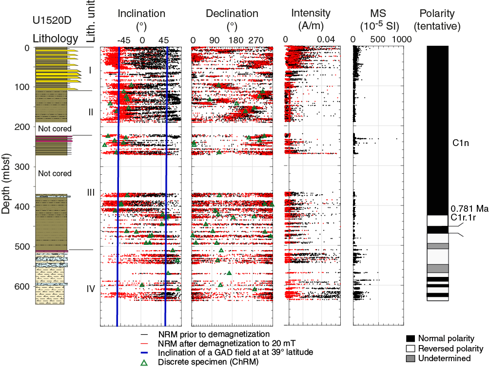
Figure F38. Magnetic inclination, declination, intensity, and MS, Hole U1520D.

Figure F39. Magnetic inclination, declination, intensity, and MS, Hole U1520C.
Hole U1520D (0–642.3 mbsf) was drilled using the APC/HLAPC (Cores 375-U1520D-1H through 30F) and XCB (Cores 31X–67X) systems, whereas all Hole U1520C cores were recovered using the RCB system. We noted that the differences in drilling methodologies affected core recovery, drilling disturbance, and the drilling overprints, requiring differing data treatment.
Hole U1520D
The NRM of APC cores recovered between 0 and 248.2 mbsf shows a pervasive drilling-induced overprint that manifests in steep positive inclinations. This overprint was usually successfully removed following partial demagnetization to 10 mT, after which the remanence vector decays linearly toward the origin. Declination records are usually offset from core to core. Further demagnetization up to 30 or 40 mT was conducted to verify the data sets. Remanence intensity values prior to demagnetization range from ~5 × 10⁻³ to 1 A/m, whereas peak intensity values usually correspond to sand or tephra layers. Following demagnetization, all data from APC cores yield negative inclinations that scatter around the direction of a geocentric axial dipole (GAD) field at 39°S. Significant variations from this mean direction usually coincide with susceptibility peaks and the presence of turbidite deposits, which are unlikely to carry a reliable depositional remanence. The pelagic calcareous mudstones yield significantly lower median destructive fields than the overlying mud and turbidite layers of Lithostratigraphic Units I–III. XCB coring resulted in significant magnetic overprinting and increased scatter in both NRM declination and inclination records and lower quality demagnetization trajectories. The declination values prior to and following demagnetization predominantly cluster around 270° and 90°, and a systematic offset from core to core is not visible. In undamaged core, this result may be an indicator of drilling overprints. We note, however, that the millimeter- to centimeter-scale biscuiting in the XCB cores lies below the resolution of the SRM and the declination records are not representative. Inclinations describe a relatively well defined pattern, and both negative (normal polarity) and positive (reversed polarity) inclinations were encountered. Transitional intervals however, were only measured in Cores 375-U1520D-64X and 66X. In all other cases, polarity transitions are suspected to fall in coring gaps.
Hole U1520C
The rock magnetic and paleomagnetic properties of the pelagic sediments in Lithostratigraphic Unit IV (650–850 mbsf) differ significantly from those in the volcaniclastic deposits in Units V and VI (850–1054 mbsf).
NRM intensity values prior to demagnetization in Unit IV range from ~1 × 10⁻³ to 1.2 A/m, and the highest values coincide with intervals that contain mafic clasts. NRM intensity and magnetic susceptibility values in Lithostratigraphic Unit V are significantly higher and peak at 1.96 A/m. The magnetic declinations at the 0 and 20 mT demagnetization levels usually show a systematic offset from core to core and across biscuit boundaries. We therefore suggest that drilling-induced overprints at the 0 mT demagnetization level are small and are adequately removed after demagnetization to 20 mT (or less). An exception is between 800 and 850 mbsf, where the magnetic inclinations and declinations calculated from the NRM direction prior to and following demagnetization are similar. Assuming that secondary overprints acquired during drilling are not aligned parallel or antiparallel to the NRM direction, they provide further evidence that in most units such overprints are primarily viscous.
Between 650 and 710 mbsf, the records show a well-defined pattern with alternating intervals of negative and positive inclination. To support our analyses, we visually inspected the demagnetization trajectories in vector component diagrams (Figure F40). Measurements from negative inclination intervals show single-component remanences that demagnetize across a broad coercivity range between 10 and 40 mT. In contrast, measurements that yield a net remanence direction with positive inclination usually have a significant magnetic overprint in the unblocking range 0–15 mT. In many cases, principal component analysis shows that the low-field overprint is roughly antipodal to the high coercivity component.
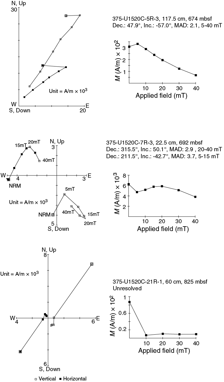
Figure F40. Vector components and NRM intensity, SRM.
Between 720 and 735 mbsf (Sections 375-U1520C-10R-2 through 11R-4) and between 775 and 785 mbsf (Sections 15R-7 through 17R-1), the inclination records are more poorly defined and the NRM direction frequently switches from steep negative to shallow positive inclinations. NRMs measured between 795 and 848 mbsf (Sections 18R-1 through 24R-4) have negative inclination prior to and positive inclination following demagnetization to 10 mT or more. NRM intensity versus demagnetization level diagrams show that the lithologies in this interval exhibit median destructive fields smaller than 10 mT and the inclination records represent a magnetic mineral fraction that retains 10% or less of the NRM intensity following demagnetization to 20 mT (Figure F40). In all three affected intervals, the lithologies are calcareous with lithologic descriptions ranging from calcareous mudstones to chalk with tuffaceous interbeds (see Lithostratigraphy). The volcaniclastic sediments recovered below 850 mbsf carry exclusively normal polarity directions, and individual measurements largely show single component demagnetization through the origin.
Discrete samples
We identified two major behavior types during AF and thermal demagnetization of discrete samples that are similar to those identified during archive-half measurements (Figures F40, F41). Samples that have NRM directions with net negative inclination demagnetize linearly toward the origin. In contrast, samples from reversed polarity intervals demagnetize in two major intervals. During thermal demagnetization up to 200°C, a component that is antiparallel to the NRM direction is removed. Upon demagnetization to a higher temperature, the magnetic vector demagnetizes linearly toward the origin with a reversed ChRM direction. This observation is consistent with low-field overprints (coercivity ≤ 15 mT) identified during AF demagnetization. We interpret the low blocking temperature (TB) and coercivity components to be viscous remanent magnetization or chemical remanent magnetization acquired in a normal polarity (probably present-day) magnetic field and only calculate ChRM directions from the high-temperature, high-field components. Samples extracted from lithologies high in carbonate content (chalk or muddy chalk) demagnetize rapidly in the temperature range 0°–200°C, which compares well with the low median destructive fields identified on samples and/or measurement locations in this unit during AF demagnetization experiments. On these samples, ChRM directions were usually calculated from the high-temperature or high-field component. Data from the few samples that did not demagnetize toward the origin were rejected. Overall, the ChRM directions calculated for discrete samples compare well with the declination and inclination records obtained from archive-half measurements (Figure F39).
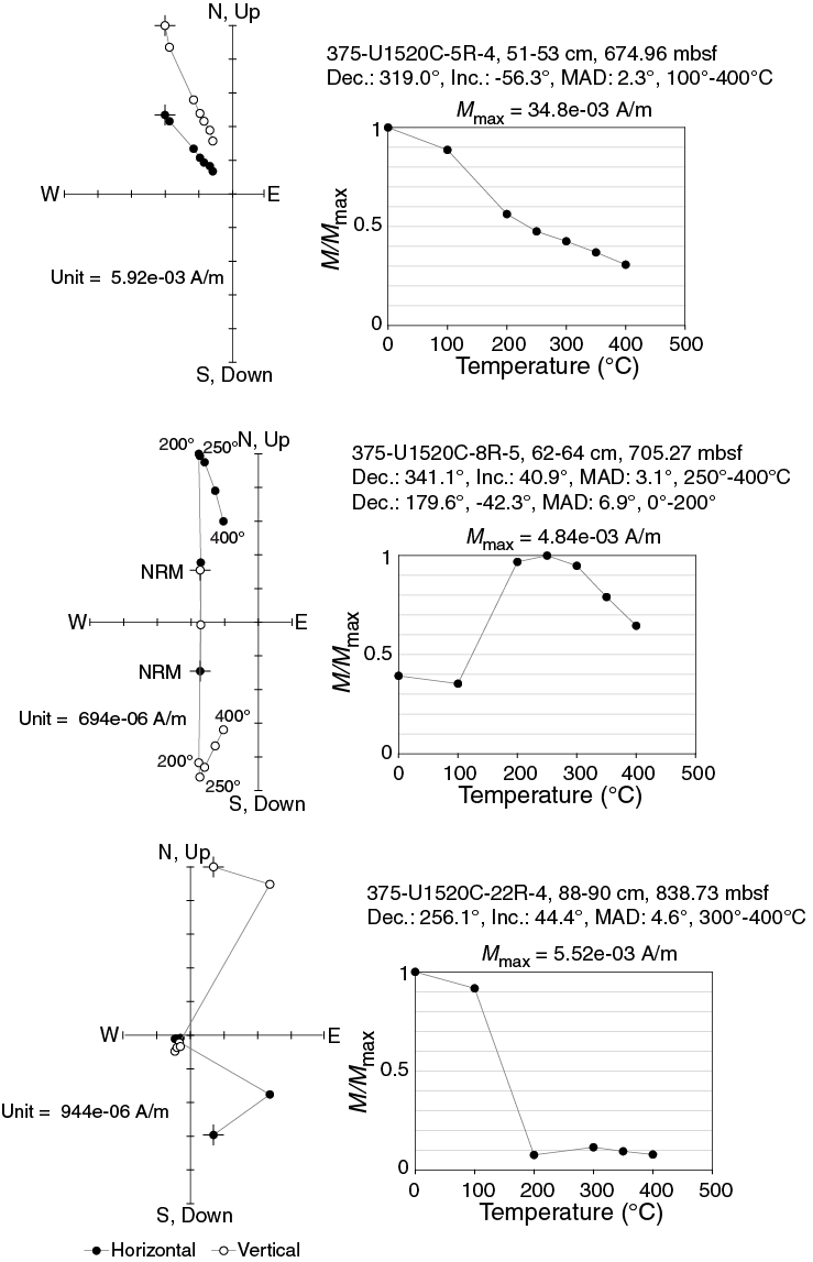
Figure F41. Vector components and NRM intensity, thermal demagnetization.
AMS measurements reveal that all samples are dominated by an oblate foliation texture with background F ratios that generally range from 1.0 to 1.05 (Figures F42, F43). Between 710 and 760 mbsf, we recorded higher F values ranging from 1.07 to 1.1, indicating vertical shortening. Throughout the section, the principal axis of magnetic susceptibility (χ1) is predominantly aligned with ±z, which is characteristic for deformation fabrics developed in response to lithostatic loading and compaction.

Figure F42. Flinn diagram showing shape of AMS.
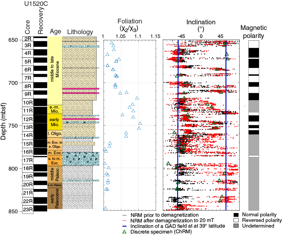
Figure F43. Magnetic foliation, inclination, and polarity, Unit IV.
Magnetostratigraphy
We base our interpretation on the identification of magnetic polarity horizons defined by the inclination calculated from the NRM direction at the 20 mT demagnetization level, which is generally consistent with the ChRM directions calculated from discrete samples (Figure F43). Tables T8 and T9 summarize the individual polarity transitions we identified. In Hole U1520C, to pick individual polarity transitions we visually inspected both inclination and declination records alongside core photographs. In ideal cases, chron boundaries are characterized by a transition from negative to positive inclinations together with a ~180° shift in declination (e.g., Section 375-U1520C-13R-6). In some cases, however, polarity transitions coincided with biscuit boundaries, section ends, or sections with incomplete core recovery. In such cases, we selected the midpoint between the last and first point where each horizon was identified. Where preserved, polarity transitions are sharp and span an interval no larger than 20 cm.
The declination records from Hole U1520D are inconclusive because of extensive biscuiting, and polarity transitions were thus selected only on the basis of inclinations. Furthermore, low recovery rates and coring gaps in Hole U1520D resulted in the loss of a large proportion of the paleomagnetic information, and in many cases, the location of polarity transitions can only be inferred. A number of intervals in which the polarity determination was ambiguous were further classified as “undefined,” including the following:
- All lithologies below 850 mbsf because we suspect the volcaniclastic materials deposited in Units V and VI are completely remagnetized, and
- Carbonate-rich units encountered at 720–735, 775–785, and 795–848 mbsf because of magnetic overprinting and/or the magnetically soft remanence carriers encountered.
Our preliminary shipboard investigations suggest the presence of 30 polarity horizons (Table T8), although with some horizons spanning a section or less, further verification based on more detailed analyses of discrete samples is required. Assignment of individual chrons based on the geomagnetic polarity timescale (GPTS) of Gradstein et al. (2012) (Table T9) is based on biostratigraphic data. Above ~413 mbsf, the NRM has a negative inclination consistent with biostratigraphic datums that place the record in the Brunhes Normal Chron (C1n). We place the Brunhes–Matuyama transition in a coring gap between Cores 375-U1520D-39X and 40X (413 mbsf), which is roughly consistent with the biostratigraphic interpretations. Further assignment of polarity chrons is tentative and requires refinement of the paleomagnetic and biostratigraphic results during post-expedition research.
Structural geology
The lithologies encountered at Site U1520 are generally undeformed. Bedding dips are gentle (<30°) over the entire depth range of coring (Figure F44) except for folded strata in debris flow deposits. geoVISION (GVR) image logs document some intervals of steeper dips that are not recognized in the core (Figure F44). These image logs are relatively low quality, however, and further post-expedition work is required to interpret them (see Logging while drilling). Distinct structural domains are mostly correlated with lithostratigraphy. Structural Domain 1 (0–596.4 mbsf; Cores 375-U1520D-1H through 61X) is defined by subhorizontal to gently dipping beds with rare discrete deformation features. Below 596.4 mbsf (top of Core 375-U1520D-62X), faults and dissolution features are present throughout Domain 2, which coincides with calcareous, clay-rich sediments in Lithostratigraphic Unit IV. Domain 3 is defined by common zeolite and carbonate veins and coincides with volcaniclastic Lithostratigraphic Unit V. Domain 4 is near the bottom of the hole and coincides with Lithostratigraphic Unit VI, which is characterized by heterogeneous lithologies, including highly altered volcaniclastics in which deformation is dominated by minor faults.
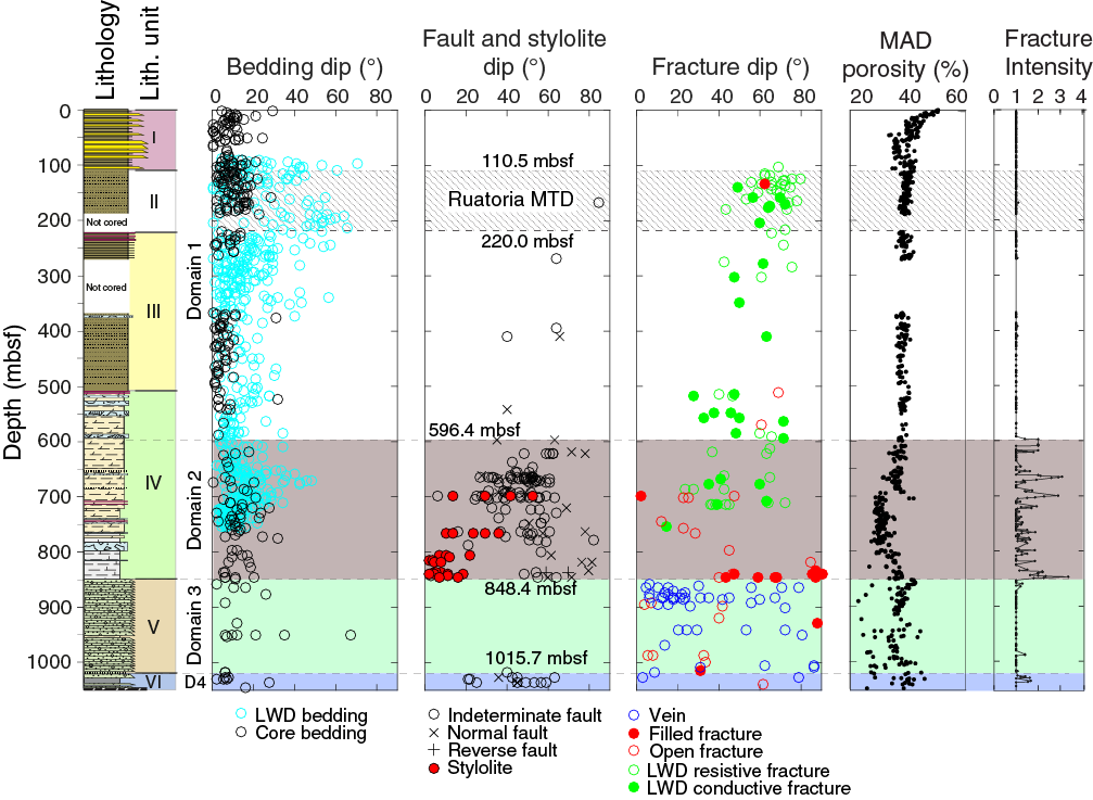
Figure F44. Structure dips.
Types of structures observed
The main structures observed at Site U1520 are small faults, fractures, veins, and dissolution seams (i.e., stylolites). Fractures include all opening-mode discontinuities that show little to no evidence of shear displacement. At this site, these fractures are predominantly open fractures, although the bottom of Domain 2 contains some subvertical filled fractures. We define sets of fractures, faults, veins, and stylolites based on consistency in orientation between multiple features, and the relative timing of these sets was determined using crosscutting relationships where possible. Disruption caused by debris flows and soft-sediment deformation is prevalent in some intervals, resulting in folded bedding and locally sheared zones, but they were not considered to be tectonic structures and are not described further here (see Lithostratigraphy for more detail).
Small faults occur predominantly in marl and clay-rich sediments (Figure F44; see Lithostratigraphy) and commonly display shiny, striated surfaces on which slip direction could be measured (Figure F45B). If apparent offset was visible in the core, sense of motion was determined. In some cases, sense of motion was inferred from the roughness direction defined by steps on striated fault surfaces. Stylolites predominantly occur in muddy chalks and are most prevalent toward the bottom of Domain 2. In some places, stylolites occur as anastomosing features in layers as thick as a few centimeters (Figure F46E), but they also occur in spaced sets. Veins occur in the volcaniclastic sequence from ~830 to 1030 mbsf (Figure F44) and can be divided into types based on orientation, composition, and morphology (Figure F47). Some veins appear similar to filled opening-mode fractures, with distinct, sharp edges. Others have more diffuse boundaries and occur over thicker (centimeter scale) intervals (Figure F47A). In this case, the term “vein” is used to describe a tabular zone that differs texturally and compositionally from the surrounding rock and is inferred to postdate sediment deposition, but it does not necessarily imply that this feature required an open fracture to have formed.
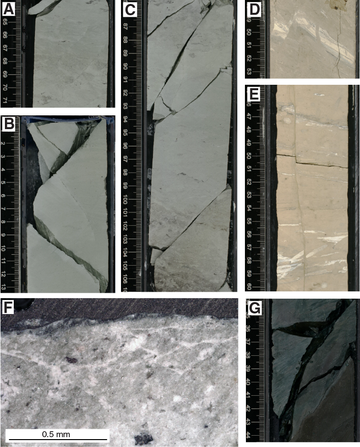
Figure F45. Faults and fractures.
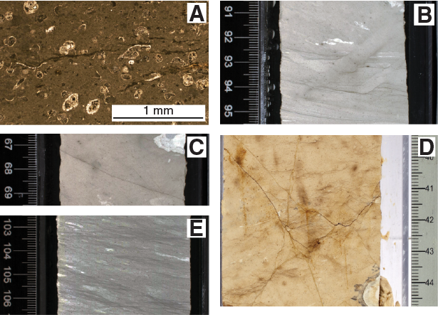
Figure F46. Stylolites.
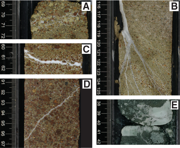
Figure F47. Veins.
Domain 1: undeformed, subhorizontal beds
The top of Hole U1520D from 0.0 to 596.4 mbsf (Cores 375-U1520D-1H through 61X) comprises gently dipping mud-silt sequences and sandier intervals that contain no observed discrete deformation features. The GVR resistivity image log shows some steeper beds in the interpreted Ruatoria MTD, but bedding dip angles greater than 30° were not measured in the core (Figure F44) and image log picks were reported with low confidence (see Logging while drilling). Two intervals were drilled without coring: 375-U1520D-241 (189.3–220.0 mbsf) and 341 (270.8–366.6 mbsf). No change in structure was observed across these intervals, nor is any significant change noted in GVR image log data.
Domain 2: faults and stylolites in marl and mudstones
Domain 2 is defined by intervals of faulting and zones of stylolites that generally occur in the more calcareous lithologies. The top of the domain coincides with the onset of multiple, well-defined faults observed in the cores, as shown by the shallowest qualitative fracture intensity > 1 (Figure F44). The domain includes the lower ~40 m of Hole U1520D (596.4–636.27 mbsf; Sections 375-U1520D-62X-1 through 67X-1) and the upper ~200 m of Hole U1520C (646–848.4 mbsf; Sections 375-U1520C-2R-1 through 23R-5). The rocks in Domain 2 consist of interbedded calcareous mudstones, muddy chalks, and occasional debris flow deposits (see Lithostratigraphy). Except where disrupted by debris flow deposits, beds are gently dipping. These gentle dips are seen in both the core and the bedding orientations derived from the GVR image logs, although some steeper dips measured from the image logs are not identified in the core (Figure F44).
Faults occur in marl and muddy chalks (Figures F44, F45B, F45C). Some striated fault surfaces have a shiny appearance (Figure F45B) that may be a result of calcite crystallization (Figure F45F) or realignment of clay minerals along the fault. Where sense of slip could be determined, faults appear to have normal offsets (Figure F45D). Fault dips generally become steeper with increasing depth from ~700 to ~850 mbsf (Figure F44). Preliminary paleomagnetic data were used to orient many of the normal faults in the shallower portion of Domain 2, revealing south to southwest dips in Cores 375-U1520C-4R and 5R.
Toward the base of Domain 2 (Cores 375-U1520C-22R through 23R; ~830–850 mbsf), subvertical fractures tens of centimeters long are observed (Figure F44). Some of these fractures exhibit small apparent normal offsets (e.g., Figure F45D, F45E). Several of the fractures are recrystallized but are evident because of their discoloration (e.g., in interval 18R-3, 22–82 cm, and Sections 23R-3 and 23R-4). Just above the base of the domain (interval 23R-5, 17–39 cm), an array of subvertical open fractures and breccias was observed in a more friable lithology, which could represent preexisting filled fractures that were reactivated during drilling. Both resistive and conductive fractures were reported in the GVR image logs but could not be clearly correlated with fractures seen in the core (Figure F44). However, both the resistive and conductive fractures are found at depths where faults with similar dips are observed.
Stylolites are most common in muddy chalks between 760 and 780 mbsf and between 805 and 845 mbsf, and they occur in a variety of forms (Figure F46). Dissolution of fossils along pressure solution seams documents submillimeter shortening perpendicular to the stylolites (Figure F46A). End-member types of stylolite occurrences are (1) isolated, typically submillimeter amplitude, wavy black seams (e.g., interval 375-U1520C-19R-1, 67–69 cm; Figure F46C) and (2) zones of closely spaced, anastomosing seams (e.g., intervals 14R-6, 103–110 cm; and 23R-2, 31–36 cm; Figure F46E). Stylolites are deflected along compositional boundaries, most notably adjacent to homogenized burrow fill, and examples of stylolites both crosscutting and abutting burrows occur (e.g., interval 19R-1, 91–95 cm; Figure F46B). Typically, the stylolites are subhorizontal even where bedding is inclined (e.g., interval 14R-6, 103–110 cm; Figure F46E). In several examples (including interval 14R-6, 103–110 cm), however, the stylolites occur in two dominant orientations, subhorizontal and subparallel to gently inclined bedding.
Faults, fractures, and stylolites occur in the same structural domain (Figure F44); however, individual beds tend to have deformed either through faulting or pressure solution but rarely both. In zones where both fractures and stylolites occur, fractures predominantly crosscut stylolites, although locally stylolites also continue across fractures without being offset (interval 375-U1520C-22R-5, 38–45 cm; Figure F46D).
Domain 3: veins in volcaniclastic sediments and mudstones
The sharp boundary between the calcareous sediments and coarser grained volcaniclastics in Hole U1520C (Lithostratigraphic Units IV and V) coincides with a change in structural characteristics from Domain 2 to Domain 3 (848.4–1015.7 mbsf; Sections 375-U1520C-23R-5 through 40R-2). Veins become more common in Domain 3 compared with other structures (Figure F44). The first clear onset of cementation and veining occurs in Section 24R-6, 137 cm (859.58 mbsf), which is characterized by thin, anastomosing vein strands cutting across the cemented matrix. This cemented interval occurs below a zone of poorly lithified volcaniclastic sediments with elevated porosity. In general, the volcaniclastic unit shows variations in grain size but few clear bedding horizons (see Lithostratigraphy). Grain size variations, however, are common and appear to influence the nature of matrix or cement and the occurrence of veins and vein-like features described below.
Cemented intervals occur throughout Unit V. These cements appear to fill pore spaces but are compositionally varied. The fill is carbonate (calcite), typically in a very fine grained or fibrous form (Figure F48A–F48C, F48E, F48G), and zeolites (phillipsite) that are typically fibrous and distinguished by their low birefringence (Figure F48B, F48D, F48E). Filled pore spaces are commonly bounded by moderately birefringent bands of phyllosilicates that rim volcanic clasts. Some coarser grained beds appear to contain more cement between grains, whereas most finer grained beds have little or no visible cement.

Figure F48. Veins and cements, Domain 3.
Two types of vein-like features occur, distinguished as diffuse veins and fracture veins (Figure F47A, F47C, F47D). Fracture veins have sharply defined boundaries with the wall rocks and occur in a range of orientations that locally intersect. Fracture veins can be divided into thin veins that are typically wavy and/or anastomosing (Figure F47D) and thicker veins with a blocky to elongate blocky morphology (Figures F47C, F48F). Diffuse veins occur as zones defined by interstitial cement that occur in subhorizontal bands, typically in coarser grained material (Figure F47A). The diffuse veins are locally parallel to bedding defined by gradual but subtle grain size or grain shape variations. The cement is not concentrated along discrete fractures but rather forms an interconnected fill within pore spaces; thus, the boundaries are irregular and diffuse and controlled by the texture of the host rock.
Vein thickness ranges from submillimeter to ~1 cm with a general, qualitative trend of increasing thickness with depth. Vein orientations show no clear depth-dependent trends (Figures F44, F49). The diffuse veins are generally gently dipping (<40°), whereas the fracture veins range from subhorizontal to nearly vertical (Figure F49). Although overlaps in orientation occur among the fracture veins, the blocky veins are typically gentler dipping than the wavy and anastomosing veins.
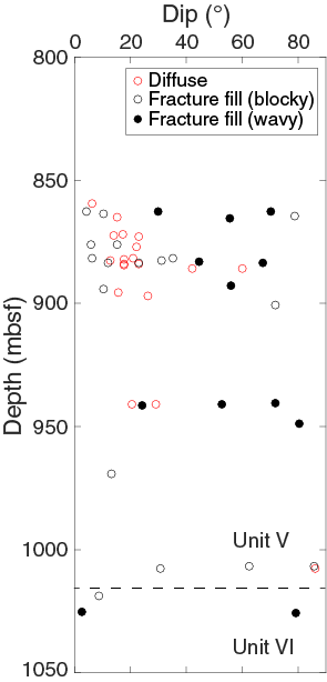
Figure F49. Vein dip angles, Units V and VI.
The diffuse veins are typically filled by calcite and are commonly crosscut by the fracture veins filled with both carbonate and zeolite (e.g., Figure F48F). Calcite is the dominant fill in the fracture veins and occurs most abundantly as medium to coarse crystals of sparry calcite near the centers of the veins (Figure F48F, F48G). The vein margins consist variously of micritic and/or botryoidal calcite or botryoidal zeolite, sometimes in alternating zones (Figure F48E). Smaller subparallel vein sets also occur, and they are typically banded and locally crosscut by later veins that are thicker and typically have a blocky morphology (Figure F48A, F48F, F48G). Some sparry calcite shows an elongate blocky morphology with crystal long axes oriented at a high angle to vein margins (Figure F48F).
Several features that have a similar appearance to veins (Sections 375-U1520C-34R-4 through 34R-6 and Section 42R-4, 42–43 cm) consist of uniform, planar bodies of prismatic calcite oriented subparallel to bedding horizons, with blocky calcite overgrowths (Figure F48H). These features are interpreted to be fossil shell material, specifically inoceramids (see Biostratigraphy), that accumulated detritally along bedding planes and served as nucleation zones for later calcite precipitation.
Domain 4: deformation in highly altered claystones and volcaniclastic sandstones
Below 1015.7 mbsf in Hole U1520C (Sections 375-U1520C-41R-1 through 43R-2), we observed highly altered volcaniclastics alternating with clay-rich units (see Lithostratigraphy). Several small veins occur in both the volcaniclastic and clay lithologies, but striated faults are more common in this zone than in the overlying volcaniclastic rocks (Figure F45G). Most of the faults occur in clayey siltstone beds. Where determined, the sense of slip on these faults is normal. The clay units are heterogeneous and marked by sharp color boundaries and irregular banding suggestive of sediment flow presumably incurred during deposition.
A “crack-seal” vein found in interval 375-U1520C-41R-3, 41–45 cm (Figure F48I), is characterized by fibrous calcite crystals that are elongated perpendicular to the vein walls and separated by margin-parallel elongate wall rock fragments. This vein is the only occurrence of such a feature in the cores recovered at this site and occurs relatively deep (1018.87 mbsf) in the section.
Drilling disturbance
Drilling disturbance in Hole U1520D includes upward-arching beds in APC and HLAPC Cores 1H–30F. This upward arching is minor, allowing measurement of some bedding orientations in most cores. Sandy intervals are typically soupy with no recognizable structures. Near the base of APC cores, the upward arching is more severe, and any recognizable bedding has been rotated to be parallel to the core axis. The tops of most cores are brecciated, precluding any structural measurements. In XCB Core 31X through Section 67X-1, biscuiting is common.
Drilling disturbance in cores is minimal throughout most of Hole U1520C and predominantly includes biscuiting and brecciation. Core expansion occurred after splitting some cores and was likely caused by swelling of hydrous clays (see Lithostratigraphy). Biscuiting and brecciation are most severe in the highly altered volcaniclastics and basalt in Domain 4. Differential biscuit rotation affected our ability to reorient measured deformation structures. Post-expedition analysis of magnetic declinations may allow us to reorient structures at the biscuit scale.
Summary
Deformation features at Site U1520 are typically small scale and localized. Subhorizontal stylolites locally crosscut gently inclined bedding and indicate a subvertical principal compressive stress at the time of their formation. Normal faults dip >45° and are also consistent with vertical shortening. Subvertical fractures are localized near the Domain 2/3 boundary, possibly suggesting some interaction between these two zones.
The variation in structures among the different units highlights an apparent lithologic control on deformation style. The carbonate-rich chalks in Hole U1520C deform through both faulting and pressure solution, whereas the mud and clay-rich sections deform primarily through faulting. Fractures occur in both lithologies. Veins are the predominant deformation feature in the volcaniclastics.
Geochemistry
Inorganic geochemistry
The main objective of the inorganic geochemistry program at Site U1520 was to document and characterize variations in pore water chemical and isotopic compositions that can be used to elucidate fluid flow and fluid–rock reactions that affect the physical, hydrological, and mechanical properties of the subducting sediment. A total of 89 whole-round (WR) samples were selected and squeezed for pore water. WRs from Units I–III, V, and VI were chosen and cut directly on the catwalk. In contrast, at the base of Unit IV, core sections were cut, capped, and taped on the catwalk and then immediately scanned on the Whole-Round Multisensor Logger (WRMSL) to identify intervals of lower density and higher porosity that would yield greater volumes of interstitial water (see Physical properties in the Expedition 327B/375 methods chapter [Wallace et al., 2019a]). WR selection for pore water chemistry was based on the real-time gamma ray attenuation (GRA) density log. Despite the high bulk density and cemented nature of some sediments recovered in Hole U1520C, pore water was recovered in all lithostratigraphic units.
WR samples were thoroughly cleaned in an effort to remove drilling fluid contamination. The cleaned samples were placed in titanium squeezers and pressed at gauge forces to a maximum of 30,000 lb. The volume of pore water recovered varied with lithology and bulk density and ranged from 2 to 60 mL. The pore water data were not corrected for drilling water contamination at this site because sulfate concentrations from the sulfate–methane transition zone (SMTZ) to the bottom of Unit III are low, mostly below 0.4 mM, indicating <2% drilling water contamination, and in the pelagic and volcaniclastic sediments (Units IV–VI), sulfate is naturally present at all depths. Although we cannot quantitatively assess the degree of drilling water contamination using sulfate as a tracer in these lower units, the smooth nature of the solute profiles and the large difference between the drilling water composition and that of the pore water with respect to other elements (e.g., Sr, Li, Mg, Ca, and K) suggests that contamination is minimal. The major and minor element concentrations are listed in Tables T10 and T11, respectively. Major and minor element concentration profiles are shown in Figures F50, F51, and F52.
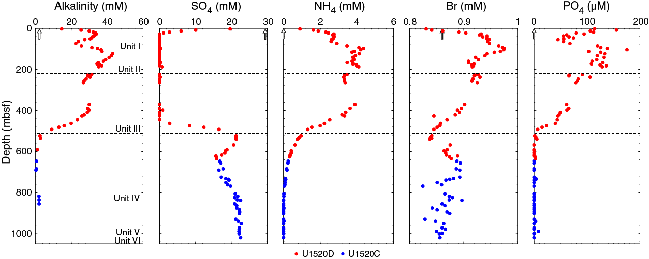
Figure F50. Alkalinity, sulfate, ammonium, bromide, and phosphate.

Figure F51. Chloride, sodium, potassium, calcium, magnesium, and silica.
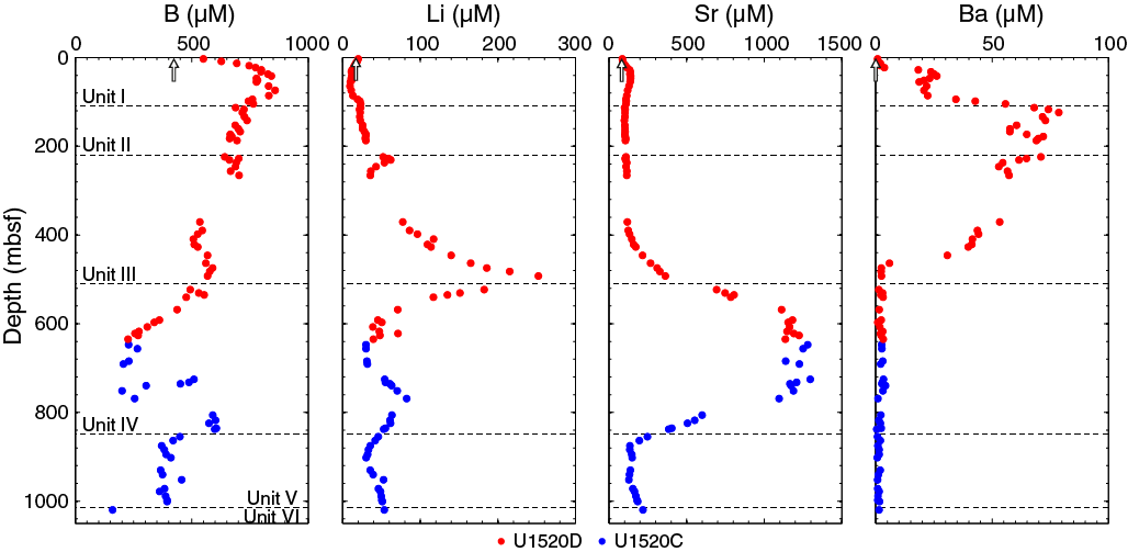
Figure F52. Boron, lithium, strontium, and barium.
The geochemical profiles at Site U1520 reflect the combined effects of organic matter diagenesis, nonsteady-state sedimentation, volcanic ash/silicate mineral diagenesis, carbonate mineral diagenesis, solute diffusion, and potential lateral fluid flow in the volcaniclastic sediments of Lithostratigraphic Unit V. Below, we provide a general description of the pore water chemical profiles and the evidence for fluid–rock reactions, the impact of nonsteady-state sedimentation on the pore water profiles, and fluid flow.
Organic matter diagenesis
The pore water profiles of sulfate, alkalinity, ammonium, bromide, and phosphate in Lithostratigraphic Unit I show characteristic changes with depth related to organic matter degradation. Sulfate concentrations rapidly decrease from 19.7 mM at 3.0 mbsf to depletion by 27.8 mbsf, marking the SMTZ. Sulfate concentrations remain depleted to 464 mbsf and then increase linearly to the Unit III/IV boundary (discussed below). Alkalinity initially increases in concentration from 14.7 mM at 3.0 mbsf to a maximum of 34 mM at the SMTZ; however, in contrast to the sulfate data that remain depleted to 464 mbsf, alkalinity reaches a second maximum of 43 mM at 124 mbsf (Figure F50). Ammonium concentrations also increase from the seafloor to the SMTZ in a pattern similar to the alkalinity data, whereas phosphate concentrations reach a concentration maximum at 8.6 mbsf, decrease with depth to a minimum at 55 mbsf, and increase toward the base of Unit I.
Alkalinity, ammonium, phosphate, and bromide increase sharply across the Unit I/II boundary and reach peak concentrations that are greater in Unit II than in Unit I. These high concentrations likely reflect higher particulate organic carbon burial rates when the unit was at the seafloor and the greater time since burial. The “Z” shape in the alkalinity and ammonium profiles in the upper 150 mbsf is accompanied by “S”-shaped calcium and potassium profiles (Figure F51). We relate these nonsteady-state concentration profiles to rapid burial of an older early diagenetic sequence in Unit II (the Ruatoria MTD) characterized by enhanced organic matter diagenesis and continued microbial methanogenesis, which is followed by the modern resetting of the early diagenetic sequence to Unit I. Not enough time has elapsed since the burial of Unit II for diffusion to erase the strong gradients produced through organic matter degradation when Unit II was near the seafloor, producing two distinct but separate intervals of elevated alkalinity, ammonium, and phosphate, which is consistent with the high average sedimentation rates (~1 m/ky) of the trench wedge facies at this site (see Lithostratigraphy and Biostratigraphy).
Geochemical profiles across the Unit III/IV boundary
Alkalinity concentrations decrease linearly from 29 mM at 409 mbsf to 2.6 mM at 523 mbsf just below the Unit III/IV boundary. Likewise, ammonium concentrations decrease from 3.4 mM at 409 mbsf to 0.94 mM at 523 mbsf. The phosphate profile is similar to ammonium; concentrations decrease at the base of Unit III to values ranging between 1.2 and 5.3 µM at the top of Unit IV. Sulfate concentrations, however, increase sharply from 0 mM at 446 mbsf to 21 mM at 523 mbsf. Sulfate then remains constant to 540 mbsf before decreasing to a minimum at 647 mbsf. Sulfate concentrations then increase steadily and approximately linearly to the top of Unit V. The sharp decrease in barium concentrations at ~464 mbsf is the result of barite precipitation driven by the increase in sulfate concentrations (Figure F52).
The sharp gradient in sulfate concentrations between Units III and IV (Figure F50) is enigmatic and difficult to reconcile solely using shipboard data. If the gradient is from sulfate reduction driven by particulate organic carbon oxidation (POCSR) or anaerobic oxidation of methane, then a peak in alkalinity and ammonium (for POCSR) should occur at the depth of sulfate depletion, which was not observed. Rather, the ammonium and alkalinity profiles are linear through the SO4 depletion zone and reach maximum values 40 m higher in the sediment section. Furthermore, we would expect a diffusional gradient toward the depth where sulfate is depleted in Unit III, at least if this process was operating since the emplacement of Units I–III. Transient lateral flow (introduction) of an externally sourced SO4-rich fluid at the top of Unit IV would help create a steep sulfate gradient, but the profiles of most other solutes, except for lithium, are smooth through this zone and are most consistent with diffusional communication between Units III and IV. Post-expedition modeling and isotopic studies may further shed light on the controls on the sulfate profile in this interval.
A dramatic increase in Li concentrations occurs from 30 µM at 173 mbsf to a peak concentration of 252 µM at 492 mbsf at the Unit III/IV boundary. Deeper than 492 mbsf, Li concentrations decrease steadily in Unit IV to 30 µM at 660 mbsf. The Li peak at the Unit III/IV boundary, like the sulfate gradient, is also enigmatic in that no similar change occurs in the other pore water solutes analyzed shipboard. The peak in Li corresponds to the depth interval of highest silica concentrations (~1000 µM) and several volcanic ash layers (see Lithostratigraphy) at the Unit III/IV boundary; thus, it may be associated with ongoing alteration of volcanic ash.
Evidence for ongoing carbonate recrystallization
Contemporary carbonate mineral recrystallization is indicated by elevated Sr concentrations ranging from 1096 to 1297 µM in Unit IV between 600 and 769 mbsf. Deeper than 769 mbsf, Sr concentrations decrease monotonically to near constant values ranging from 134 to 164 µM in Unit V (Figure F51). The linear decrease in Sr concentrations at the base of Unit IV suggests that carbonate recrystallization is minor (i.e., rates of recrystallization are lower than rates of diffusion in this interval) and that present-day carbonate mineral diagenesis is mainly occurring between 600 and 769 mbsf.
In approximately the same depth interval, dissolved Mg concentrations are low, ranging from 13.8 to 25.9 mM (52%–74% less than modern seawater value), and dissolved Ca concentrations are elevated, ranging from 24.5 to 27.8 mM (more than twice modern seawater value). Deeper than ~700 mbsf, Mg concentrations increase linearly with depth to the top of Unit V. A sharp kink in the Mg concentration profile occurs at the top of Unit V, below which Mg concentrations remain relatively constant downhole (Figure F51). Ca concentrations decrease from the zone of carbonate recrystallization to the top of Unit V, reaching a minimum value of 15.1 mM at 875 mbsf, and then increase steadily to the base of the hole.
Collectively, these results suggest ongoing carbonate recrystallization to a higher Mg calcite between 647 and 769 mbsf in Unit IV. Deeper than 769 mbsf, dissolved Sr, Mg, and Ca concentration profiles reflect diffusional exchange with the underlying volcaniclastic unit (Unit V), with little evidence of ongoing carbonate recrystallization in this zone.
Evidence for potential lateral fluid flow in Unit V
The average organic carbon concentrations in Units IV and V are 0.17 and 0.1 wt%, respectively (Figure F53). As a result of the very low organic carbon concentrations in the pelagic sediments, sulfate reduction through organic matter degradation does not fully deplete Unit IV of dissolved sulfate. The small-scale variability in sulfate concentrations likely reflects variable but small amounts of drilling water contamination (Figure F50). Sulfate concentrations increase linearly from 16.7 mM at 647.3 mbsf to ~21 mM at the bottom of Unit IV. A kink in the SO4 concentration profile occurs at the top of Unit V, and then SO4 concentrations remain relatively constant downhole. The kink in the SO4 profile between Units IV and V is similar to the observed change in the Sr and Mg profiles discussed above.
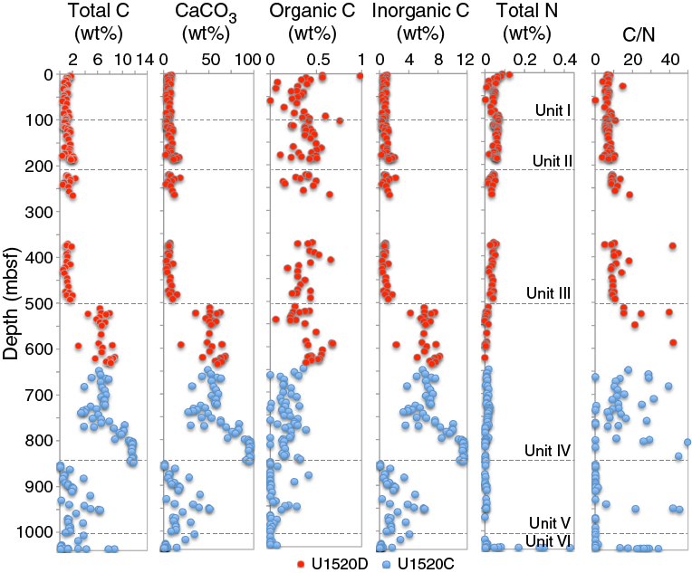
Figure F53. TC, CaCO3, TOC, inorganic carbon, TN, and C/N.
To maintain the mature (nearly linear) diffusional gradient in Unit IV and the kink in the sulfate profile observed at the top of Unit V requires lateral flow of a fluid with sulfate concentrations of ~21–22 mM in the volcaniclastic sediments. Without introduction of sulfate-rich fluids via lateral fluid flow in Unit V, maintaining the diffusional gradient observed in the overlying Unit IV would require sulfate concentrations to continue to increase below the unit boundary, which is not observed, suggesting that a flow system in Unit V maintains the sulfate gradient in a manner similar to off-axis hydrothermal flow systems in the igneous crust (i.e., Baker et al., 1991; Fisher and Wheat, 2010; Solomon and Kastner, 2012; Expedition 334 Scientists, 2012); however, the fluid flow system is hosted by volcaniclastic sediments in Hole U1520C.
Lateral fluid flow in Unit V is also consistent with the Sr and Mg concentration profiles, which are characterized by constant values in Unit V and steep diffusional gradients at the base of Unit IV to the zone of carbonate recrystallization in Unit IV. Collectively, these results suggest that although variably cemented, at least some of the volcaniclastic sediment layers are sufficiently permeable to host fluid flow and that this fluid has a composition that is only moderately altered with respect to seawater. The nature and driving forces of this inferred flow system remain unresolved and will be addressed via post-expedition studies.
Evidence for volcanic ash alteration and silicate mineral diagenesis
Chloride concentrations increase linearly from 554 mM at 3.0 mbsf to a peak concentration of 574 mM (2.7% greater than modern seawater value) at 51.3 mbsf (Figure F51). Deeper than 51.3 mbsf, Cl concentrations decrease to 559 mM at 142 mbsf and remain relatively constant to the base of Lithostratigraphic Unit III. In the depth interval where Cl concentrations increase, potassium concentrations decrease to a minimum of 9.7 mM and then increase to the top of Unit II. Boron and sodium concentrations also increase in this depth interval. Collectively, these profiles suggest a zone of localized volcanic ash alteration or silicate mineral diagenesis and the precipitation of hydrous aluminosilicate minerals.
Dissolved silica concentrations increase progressively from the seafloor to values averaging 900 µM and as high as 1091 µM at the base of Unit III (Figure F51). A steady increase in Na concentrations and a decrease in Mg, K, and B concentrations also occur in the same depth interval, likely reflecting volcanic ash alteration or silicate mineral weathering and the production of authigenic silicate minerals.
In Hole U1520C, pore water profiles provide evidence for four additional zones where the pore water composition is impacted by ongoing silicate mineral diagenesis: Zone 1 = ~740–770 mbsf (Unit IV), Zone 2 = ~863–880 mbsf (Unit V), Zone 3 = ~930 mbsf (Unit V), and Zone 4, which is characterized by diffusional gradients to a reaction zone either in or below Unit VI. The upper three zones exhibit abrupt depletions in Cl concentrations from modern seawater value (Figure F51). The Cl concentration anomalies are 5.5%, 6%, and 6% less than modern seawater value at 769, 875, and 930 mbsf, respectively. Between these anomalies, Cl concentrations remain near seawater value and exhibit little variability. The Cl anomalies are not related to drilling water contamination because the drilling water Cl concentration was 565 mM (Table T10), and they are not the result of analytical error. Each sample was analyzed for Cl concentration via titration in triplicate and by ion chromatography, and Cl values are consistent between methods. Sodium concentrations were measured by ion chromatography and inductively coupled plasma–atomic emission spectrometry (ICP-AES), and the profile also shows sharp decreases in concentration in these zones that are 4.5%, 6%, and 6% less than modern seawater value at 769, 875, and 930 mbsf, respectively. The other major element concentration profiles (e.g., Ca and K) also show minima at these depths, but a dilution of only ~6% produces a small change in their concentration (i.e., a 6% dilution of seawater Ca would only cause a concentration decrease of 0.6 mM). Based on these trends, we suggest that the anomalies in the Cl and Na concentration profiles result from local, relatively recent mineral dehydration reactions that release fresh (bound) water. The in situ temperature in these units, however, is estimated to be ~40°C (see Downhole measurements), considerably lower than the temperature range where most clay minerals begin to dehydrate.
In Zone 1, potassium concentrations also decrease abruptly from a background concentration of ~10 mM to values between 5.9 and 6.9 mM. Deeper than 770 mbsf, K concentrations increase sharply back to a value of ~9.5 mM (Figure F51). Concomitant with the sharp decrease in K is a drop in dissolved silica concentrations from 600 to 152 µM and an increase in Li concentrations from 30 to 83 µM. The decrease in Cl concentrations in Zones 2 and 3 in Unit V, although similar in magnitude to that observed in Zone 1, is not accompanied by large decreases in K and Si concentrations. Dissolved silica concentrations, however, remain low throughout Unit V, ranging between 100 and 300 µM. The Cl anomalies in Zones 2 and 3 are also not accompanied by an increase in Li concentrations like that observed in Zone 1.
Zone 4 is characterized by a slight decrease in Cl concentrations, a linear decrease in K, strong depletion of dissolved Si to 100 µM, and a linear increase in Ca and Li concentrations. These trends likely reflect a diffusional signal to/from a reaction zone below the base of the hole and may result from fluid–basalt interaction in Unit VI at depth.
In all cases, the rates of fluid–rock reactions in these zones are likely faster than the rates of solute diffusion or advection to explain the observed sharp concentration anomalies. These zones are characterized by the consumption of K and Si, no significant change in Mg and B concentrations, and addition of H2O (in Zones 1–3), Li, and Ca (in Zone 4). Ongoing silicate diagenesis in the lower three of these zones overprints the potential lateral flow system in Unit V discussed above. The release of bound water is somewhat enigmatic because the estimated in situ temperature in these units is below the temperature window for the onset of many clay dehydration reactions. Similarly, water addition is not compatible with opal dehydration because dissolved Si concentrations are never in equilibrium with these phases and are less than 300 µM. It is likely that several co-occurring reactions are operating in these diagenetic zones, and understanding these reactions will be a focus of post-expedition research.
Organic geochemistry
Bulk sediment analysis
A total of 93 samples were measured in Hole U1520C. Samples were collected at a higher resolution in Lithostratigraphic Unit VI (Core 375-U1520C-43R between 1036 and 1037 mbsf) from a black siltstone (see Lithostratigraphy), and 108 samples were measured in Hole U1520D to determine inorganic carbon, calcium carbonate, total carbon (TC), hydrogen, and nitrogen content and organic carbon concentrations. The results from Site U1520 are listed in Table T12 and shown in Figure F53.
In Lithostratigraphic Units I–III, calcium carbonate (CaCO3) varies from 2.06 to 18.4 wt%. In Units IV–VI, CaCO3 varies from 0.35 to 96.9 wt%, reflecting variations in lithology. The CaCO3 profile mimics the depth profiles of TC, which ranges from 0.04 to 14.72 wt%, and inorganic carbon, which ranges from 0.07 to 11.63 wt%, with similar trends in all lithostratigraphic units. From 640 to 722 mbsf in Unit IV, CaCO3 concentrations increase slightly to 57.1 wt% at 721 mbsf (Figure F53), and then they decrease rapidly to 32.35 wt% at 739 mbsf. From 743 to 796 mbsf, CaCO3 concentrations increase with depth but exhibit a large degree of scatter between 83.9 wt% at 765 mbsf and 30.0 wt% at 769 mbsf. In the deepest part of Unit IV, CaCO3 values are consistently high and range from 90.0 wt% at 799.0 mbsf to 91.4 wt% at 844 mbsf. This high carbonate content reflects the contribution of pelagic carbonate (see Lithostratigraphy). In Unit V, CaCO3 content ranges from 0.54 wt% at 858 mbsf to 51.18 wt% at 952 mbsf (average = 17.19 wt%). High values (e.g., interval 375-U1520C-31R-1, 31–33 cm) reflect several localized zones of calcite cementation (see Lithostratigraphy and Physical properties), except for 950–954 mbsf (interval 34R-2, 29 cm, to 34R-CC, 20 cm), where an interval of marl in the volcaniclastic succession is associated with an increase (as high as 50 wt%) in carbonate content.
Organic C values, calculated from the difference between TC and inorganic carbon content (see Geochemistry in the Expedition 372B/375 methods chapter [Wallace et al., 2019a]), are low (<1.19 wt%) in Lithostratigraphic Units I–V but range from 0 to 14.62 wt% in Unit VI (Core 375-U1520C-43R) (Figure F53). This peak value occurs in a black siltstone layer (see Lithostratigraphy).
Total nitrogen (TN) values range from <0.01 to 0.12 wt% in Lithostratigraphic Units I–V but exceed 0.17 wt% in the black siltstone in Unit VI (1036–1037 mbsf). TOC/TN (C/N) ratios range from 0 to 166. In Units I and II, C/N ratios range from 5 to 8 and reflect the influence of marine organic matter. In Unit VI between 1036 and 1037 mbsf, C/N ratios are >13.3 and reflect an influence of terrestrial organic matter.
Four samples of black siltstone taken from Core 375-U1520C-43R (between 1036 and 1037 mbsf) were also analyzed using the source rock analyzer (Table T13). TOC values range between 3.77 and 11.25 wt% and primarily reflect a mixture of marine and terrestrial organic matter (Type II to Type III kerogen). Sulfur is often associated with Type II organic matter or occurs as pyrite (Vandenbroucke, 2003), which is consistent with some observations of framboidal pyrite in this layer between 1036 and 1037 mbsf (interval 43R-2, 0–60 cm; see Lithostratigraphy). The depositional environment associated with Type II kerogen corresponds to a moderately deep marine environment with planktonic input as the primary source, whereas Type III kerogen corresponds to a shallow marine environment sourced by continental deltaic input. Type III kerogen is frequently found in deltaic settings and derives from plant debris, often reworked and associated with clastic sedimentation (Tissot and Vandenbroucke, 1983; Vandenbroucke, 2003). The temperature at the maximum of the S2 peak (defined as Tmax) is an indicator of rock maturity. Tmax values suggest thermal immaturity (Tmax < 435°C).
Gas analyses
Headspace gas samples were taken from each sediment core to monitor for the abundance of C1–C3 hydrocarbons as part of the standard safety protocol (Pimmel and Claypool, 2001). These samples were generally taken from sediments next to the pore water WR samples. A few additional void gas samples were also taken. A total of 111 headspace and 6 void gas samples were taken at Site U1520 (Table T14). Methane was not detected between 0 and 27 mbsf. At 28 mbsf, which coincides with the base of the SMTZ, concentrations increase rapidly to 5 parts per million by volume (ppmv) (Figure F54), indicating ongoing methanogenesis. Between 32 and 464 mbsf, methane concentrations in headspace samples remain between 23.3 and 11,416 ppmv. Ethane was not detected shallower than 103 mbsf but was consistently measured at low concentrations (1–12 ppmv) between 220 and 250 mbsf. The absence of ethane or high C1/C2 ratios throughout most of the cores suggests a microbial source for the hydrocarbons (Claypool and Kvenvolden, 1983). Very small and intermittent occurrences of ethane, ethene, or propane peaks in gas chromatograms were interpreted to be erroneous measurements.
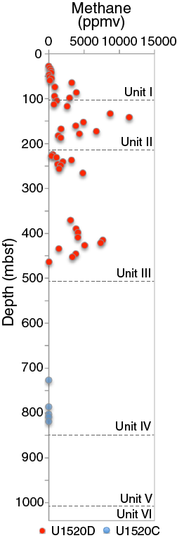
Figure F54. Methane.
Physical properties
Density and porosity
GRA bulk density was measured on WR cores, and moisture and density (MAD) bulk density, grain density, and porosity were determined on discrete samples from working halves (see Physical properties in the Expedition 372B/375 methods chapter [Wallace et al., 2019a]).
GRA bulk density measured with the WRMSL increases from 1.4–1.6 g/cm3 at the seafloor to ~1.8–2.0 g/cm3 at 12 mbsf, decreases to 1.6–1.8 g/cm3 at 80 mbsf, and then increases to 1.8–2.0 g/cm3 at 110 mbsf (Figure F55). It remains relatively constant at 1.8–2.0 g/cm3 from 110 to 500 mbsf. GRA bulk density shifts to a lower value of ~1.5 g/cm3 at 500 mbsf near the Unit III/IV boundary (see Lithostratigraphy) and gradually increases with depth to 1.8–2.0 g/cm3 at ~650 mbsf, followed by a decrease to 1.6–1.8 g/cm3 at 690 mbsf. At 690 mbsf, GRA bulk density shifts abruptly to a higher value of ~2.0 g/cm3, and it remains unchanged to 800 mbsf. From 800 to 860 mbsf, it decreases slightly to 1.8 g/cm3. Deeper than 860 mbsf, GRA bulk density ranges from 1.6 g/cm3 to as high as 2.4 g/cm3 with considerable scatter.
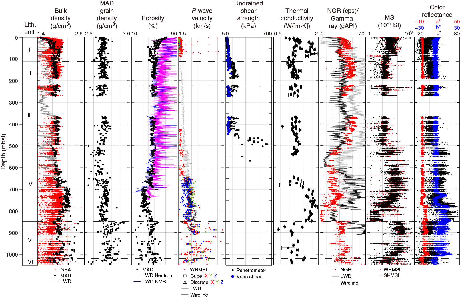
Figure F55. Physical properties.
MAD bulk density follows the same trends as GRA density values (Figure F55). MAD bulk density increases rapidly from 1.5 g/cm3 at the seafloor to ~1.8 g/cm3 at ~20 mbsf. From 20 to 500 mbsf, bulk density generally increases with depth to 1.9–2.0 g/cm3 at 500 mbsf. Locally higher bulk density values of 1.9–2.0 g/cm3 observed between 53 and 118 mbsf correspond to sand layers (see Lithostratigraphy). At 500 mbsf, bulk density shifts to a lower value of ~1.8 g/cm3 and increases gradually with depth to 1.9–2.0 g/cm3 at ~660 mbsf, followed by a decrease to 1.8 g/cm3 at 700 mbsf. From ~700 to 800 mbsf, bulk density shifts abruptly to higher values of ~2.0–2.2 g/cm3. From 800 to 860 mbsf, bulk density decreases from 2.1 to ~1.8 g/cm3. Bulk density values generally increase with depth from ~860 to ~920 mbsf. From 920 mbsf to the bottom of Hole U1520C, MAD bulk density is characterized by a general decrease with depth, albeit with a large scatter that varies between 1.6 and 2.4 g/cm3. The instances of locally high bulk density (>2.2 g/cm3) appear primarily in Lithostratigraphic Units V and VI deeper than 860 mbsf.
GRA, MAD, and LWD bulk density show similar trends (Figure F55). Deeper than ~650 mbsf, GRA bulk density values are consistently lower than MAD bulk density values, likely due to underestimated GRA bulk density associated with the small diameter of RCB cores. GRA bulk density values corrected for RCB core diameter (based on archive-half section photographs; see Physical properties in the Expedition 372B/375 methods chapter [Wallace et al., 2019a]) are similar to MAD bulk density (Figure F56). LWD bulk density values are lower than both GRA and MAD bulk density values at depths shallower than ~250 mbsf.

Figure F56. Core diameter and GRA and MAD bulk density.
MAD grain density is generally constant at ~2.7 g/cm3 from the seafloor to 270 mbsf (Figure F55) except for some values as low as ~2.3 g/cm3 at ~230 mbsf that correspond to ash layers (see Lithostratigraphy). Grain density decreases slightly from ~2.7 g/cm3 at 367 mbsf to 2.6 g/cm3 at ~550 mbsf. From 550 to 690 mbsf, grain density values are scattered, ranging from 2.55 to 2.8 g/cm3. From 690 to 848 mbsf, grain density is mostly constant, ranging from 2.7 to 2.75 g/cm3. From 848 to ~1010 mbsf (Lithostratigraphic Unit V), grain density shows increased scatter and ranges from 2.7 to 2.9 g/cm3. Deeper than 1010 mbsf (Unit VI), grain density decreases slightly with depth to values as low as 2.4 g/cm3 at ~1035 mbsf.
MAD porosity decreases from 72% at the seafloor to 50%–55% at 20 mbsf (Figure F55). From 20 to 500 mbsf, the majority of the data show a trend of decreasing porosity with depth, and porosity reaches 45% at ~500 mbsf. From 40 to 106 mbsf, porosity values shift to lower values ranging from 40% to 55% and the greater scatter corresponds to sand layers with relatively lower values (see Lithostratigraphy). From 500 at 600 mbsf, porosity increases slightly with depth, ranging from 46% to 52%, and then decreases with depth to values as low as 38% at ~660 mbsf. Deeper than 660 mbsf, porosity increases with depth to reach 50% at ~700 mbsf before shifting to lower values of 28%–38% (average = 33%) and remaining constant to 800 mbsf. Deeper than 800 mbsf, porosity values increase with depth to values as high as 56% at 855 mbsf. Porosity then generally decreases from 855 mbsf to 40% at ~920 mbsf before gradually increasing with depth to reach ~50% at the bottom of the hole. From 826 mbsf to the bottom of the hole and primarily deeper than 848 mbsf in the volcaniclastic units, porosity exhibits greater scatter with excursions to values ~20%–25% lower than the overall trend defined by the adjacent data. These lower porosity values correspond to zones of enhanced cementation within the volcaniclastic sediments.
Visual inspection of selected samples used for MAD measurements with an optical microscope provides further evidence for the cause of these porosity variations (Figure F57). We compare two samples, 375-U1520C-16R-4, 112 cm (781.0 mbsf), and 23R-1, 51 cm (843.5 mbsf), from the chalk in Lithostratigraphic Unit IV (773.26–848.45 mbsf) (see Lithostratigraphy) where porosity increases with depth (Figures F55, F57). Sample 23R-1, 51 cm, has a porosity of 47% and a greater abundance of pores, many of which are small in scale, compared with Sample 16R-4, 112 cm, which has a porosity of 34%. This textural difference likely explains the general increase in porosity in the lower portion of Unit IV, especially between ~780 and 850 mbsf.
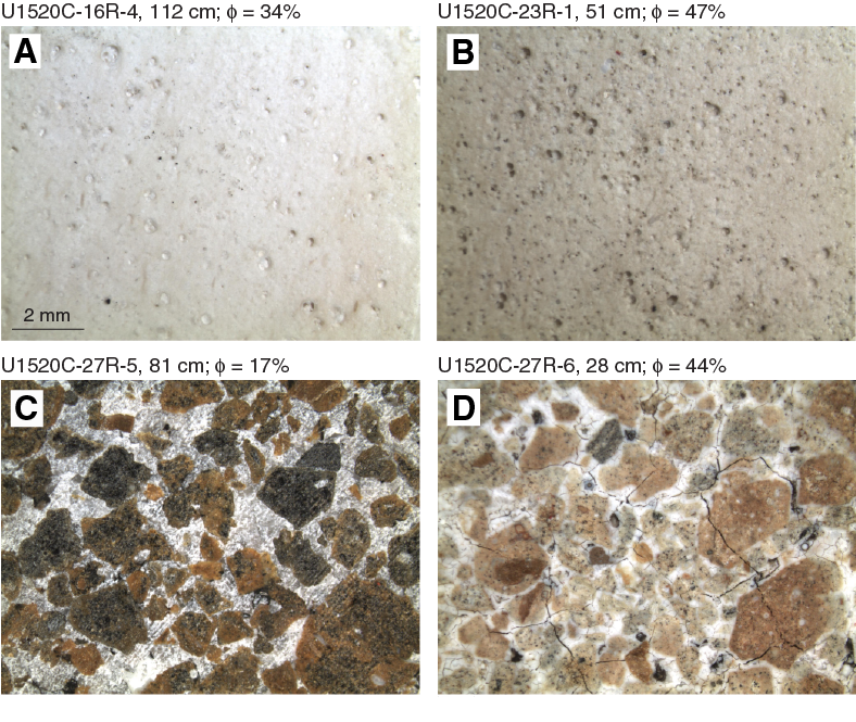
Figure F57. Selected MAD samples.
From ~850 mbsf to the bottom of Hole U1520C, where volcaniclastic material is predominant, several samples exhibit porosity values that are substantially lower than the overall trend. We compare optical microscope images of two MAD samples from Unit V: Samples 375-U1520C-27R-5, 81 cm (887.75 mbsf), and 27R-6, 28 cm (888.16 mbsf) (Figure F57). Sample 27R-6, 28 cm, has a porosity of 44% and exhibits pervasive cracking, including in clasts, whereas Sample 27R-5, 81 cm, has a porosity of 17% and no cracking. Much of the cracking in Sample 27R-6, 28 cm, appears to be concentrated in the intergranular cement, whereas the cement in Sample 27R-5, 81 cm, appears to be solid. Although cracking in Sample 27R-6, 28 cm, was likely exacerbated during oven drying at 105°C for 24 h, the porosity measurement should not have been affected because water was not added into the cracks. Rather, the cracks likely represent inherited areas of locally higher porosity and weak cementation by hydrous minerals (e.g., zeolite).
A possible explanation for the porosity difference in the volcaniclastic material lies in the character of the cement. Geochemical data show a wide scatter in CaCO3 content, which ranges from <1 to 51 wt% from 850 mbsf to the bottom of Hole U1520C (Figure F53). The presence of elevated CaCO3 content indicates that calcite could be one of the primary cementing phases. In Lithostratigraphic Unit V at 850–1010 mbsf, porosity exhibits a strong inverse correlation with CaCO3 content (Figure F58), suggesting that low porosity is the result of carbonate cementation. We also observed no correlation between porosity and CaCO3 content shallower than 850 mbsf in Unit IV. This observation highlights the difference between granular carbonate sediment (i.e., the marl/calcareous mudstone/chalk in Unit IV) and the carbonate cement in Unit V.
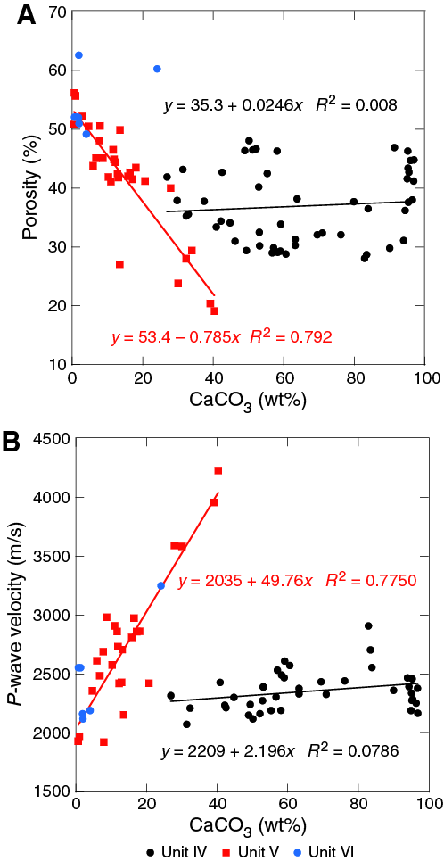
Figure F58. MAD porosity, P-wave velocity, and carbonate.
P-wave velocity
Compressional wave (P-wave) velocity was measured on WR cores, working halves, and discrete cubes. The discrete cubes were shared for either MAD or paleomagnetism (PMAG) measurements. The physical dimensions of discrete cubes are different for MAD (1 cm × 1 cm × 2 cm) and PMAG (2 cm × 2 cm × 2 cm) samples.
P-wave velocity measured with the WRMSL ranges from 1450 to 1700 m/s between the seafloor and 88 mbsf, which is consistent with the values of 1470–1800 m/s between the seafloor and 87 mbsf measured on working halves (Figure F55). Between 90 and 420 mbsf, P-wave velocity measurements on WR cores and working halves were mostly unsuccessful because of the gap between cores and liners and as a result of expansion of existing cracks. From 424 to 636 mbsf in Hole U1520D, P-wave velocity measured along the x-axis on the working halves increases slightly with depth, ranging from 1500 to 1900 m/s.
For RCB cores in Hole U1520C, P-wave velocity was measured on working halves and discrete cubes. P-wave velocity increases gradually with depth from 2000 to 2500 m/s from 646 to 720 mbsf, where the major lithology is marl (Figure F55). From 720 to 740 mbsf, where the major lithology is calcareous mudstone, P-wave velocity decreases slightly with depth to 2200 m/s. P-wave velocity increases again to ~2770 m/s at ~767 mbsf and then slightly decreases with depth to 2200 m/s at ~845 mbsf. Intervals of higher and lower velocity correspond to major lithologies of marl and chalk, respectively. Deeper than 845 mbsf, P-wave velocity values exhibit significant scatter as a result of varying degrees of cementation in Lithostratigraphic Units V and VI. P-wave velocity is as high as ~5000 m/s on highly cemented samples and as low as <1800 m/s on poorly cemented samples. P-wave velocity in Unit V exhibits a positive linear correlation with CaCO3 content, whereas P-wave velocity is independent of CaCO3 content in Unit IV (Figure F58).
Anisotropy in P-wave velocity was calculated only for PMAG cubes (2 cm × 2 cm × 2 cm) because the geometry and sample faces of MAD cubes (1 cm × 1 cm × 2 cm) did not allow these measurements. Although no data are available from Unit V, horizontal anisotropy in Units IV and VI ranges between −0.1 and 0.1 with a mean near zero, and vertical anisotropy is mostly positive, ranging from 0 to 0.12 (Figure F59; Table T15). The positive values of vertical anisotropy (higher horizontal velocity than vertical velocity) are likely attributed to the opening of microcracks by relieving in situ stress during core recovery. Microcracks can open perpendicular to the maximum principal stress or along bedding planes, which are observed to be subhorizontal (see Structural geology).
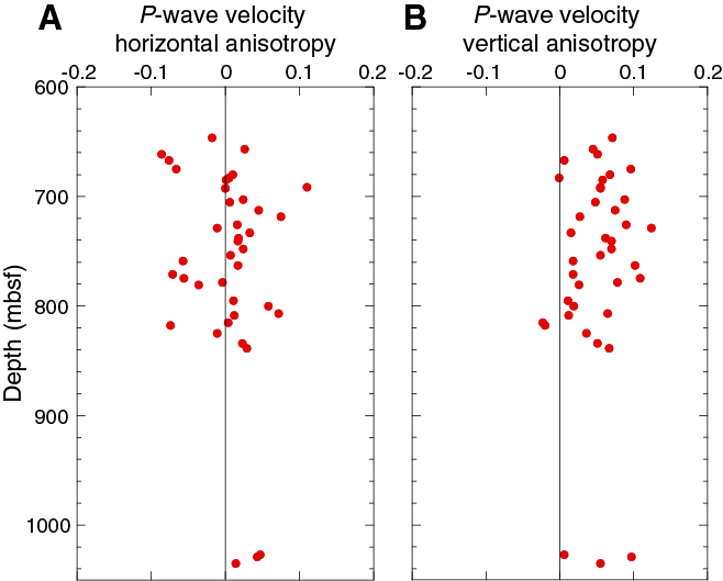
Figure F59. Horizontal and vertical anisotropy.
P-wave velocity measured on cores is generally consistent with LWD data from Hole U1520B and wireline logging data in the lower portion of Hole U1520C except from 420 to ~650 mbsf, where P-wave velocity measured on cores is consistently lower than LWD values, likely due to cracking in the cores (Figure F55). From 795 to 845 mbsf, both core measurements and logging data show a trend of decreasing P-wave velocity with depth. However, P-wave velocity values on cores in this interval are lower than those from wireline logging data.
Relationships between P-wave velocity and porosity show a clear difference between lithostratigraphic units (Figure F60). The evolution of both porosity and P-wave velocity can be controlled by many factors (e.g., overburden stress, lithology, alteration, or cementation). Carbonate cement is likely the main factor that controls changes in porosity and P-wave velocity in Units V and VI but not in Unit IV (Figure F58).
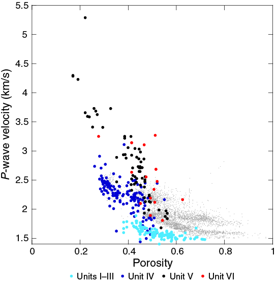
Figure F60. P-wave velocity vs. porosity.
Undrained shear strength
Undrained shear strength measurements were conducted on the working halves of sediment cores using the Giesa automated vane shear (AVS) and a pocket penetrometer (Figure F55). From 0 to 60 mbsf, undrained shear strength measured using the AVS increases linearly with depth with a gradient of ~0.9 kPa/m. From 60 to 160 mbsf, shear strength increases more rapidly with a gradient of 1.7 kPa/m. Undrained shear strength remains approximately constant from 160 to 450 mbsf with a mean value of ~40 kPa. Deeper than 450 mbsf, the sediment was too stiff to conduct AVS measurements.
Undrained shear strength values determined using the penetrometer increase linearly with depth from 0 to 60 mbsf with a gradient of 0.4 kPa/m. The strength gradient increases to 1.25 kPa/m in Lithostratigraphic Unit II between 100 and 200 mbsf. Deeper than 200 mbsf, strength values exhibit significant scatter, and no clear depth dependence is discernible. Between 210 and 280 mbsf, the average undrained shear strength is ~87 kPa with minimum and maximum values of 25 and 182 kPa, respectively. Between 350 and 460 mbsf, the mean undrained shear strength increases to 105 kPa with minimum and maximum values of 25 and 196 kPa, respectively. Deeper than 460 mbsf, the average undrained shear strength is 415 kPa with a minimum value of 196 kPa and a maximum of 638 kPa. Deeper than 570 mbsf, the sediment was sufficiently indurated that the pocket penetrometer could no longer be used to determine undrained shear strength.
Thermal conductivity
Thermal conductivity measurements were conducted on WR cores using the needle probe in Hole U1520D and on working halves using the half-space probe in Hole U1520C (see Physical properties in the Expedition 372B/375 methods chapter [Wallace et al., 2019a]). In most cases, three or more measurements were attempted, but some measurements failed to converge on a solution. This failure was likely due to uneven core surfaces or cracks causing poor contact between the half-space measurement puck and the sample. Additionally, some solutions yielded unrealistic values less than the thermal conductivity of water (0.6 W/[m·K]); these values were excluded from the analysis. Other values yielded unreasonably large departures from mean values for specific samples, and these values were also excluded.
Thermal conductivity varies between 0.9 and 1.9 W/(m·K). Thermal conductivity increases from 1.0 W/(m·K) at the seafloor to 1.3 W/(m·K) at ~20 mbsf and remains nearly constant to ~550 mbsf. Some higher thermal conductivity values of 1.6–1.9 W/(m·K) are observed between 23 and 87 mbsf, corresponding to sand layers. No measurements were made between 550 and 646 mbsf because the sediments were too indurated for a needle probe and too fragile and disturbed by coring for a half-space probe. Thermal conductivity increases from about 1.2 W/(m·K) at 648 mbsf to 1.8 W/(m·K) at 700 mbsf and then remains relatively constant between 700 and ~850 mbsf. The mean thermal conductivity in Lithostratigraphic Unit IV is 1.64 W/(m·K). Thermal conductivity throughout Units V and VI is relatively constant at 1.2 W/(m·K).
Thermal conductivity of rock matrix depends on mineralogy, grain size, and shape. Mineralogy has the biggest influence, and thus thermal conductivity for the constituents at Site U1520 likely depends on the relative proportions of intermediate-conductivity components (such as carbonate) and low-conductivity components (such as basalt and clay). A second factor influencing thermal conductivity is porosity. Figure F61 shows thermal conductivity plotted as a function of porosity for Units I–VI. These data can be fit using an empirical relationship:
- λ = bulk thermal conductivity of each sample,
- λm = grain thermal conductivity,
- λw = thermal conductivity of seawater (0.6 W/[m·K]), and
- ϕ = fractional porosity.
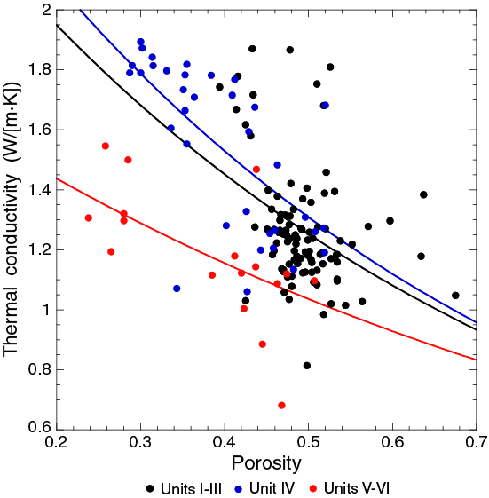
Figure F61. Thermal conductivity vs. porosity.
On the basis of these fits, estimated grain thermal conductivity values in Units I–III (siliciclastic sediments), IV (pelagic facies), and V–VI (volcaniclastics) are 2.9, 1.8, and 2.6 W/(m·K), respectively.
Natural gamma radiation
At Site U1520, NGR values range from approximately 0 to 75 counts/s. Mean values are between 30 and 50 counts/s for all lithostratigraphic units (see Lithostratigraphy) except Unit IV (pelagic facies), where the mean NGR value is lower with values of ~20 counts/s (Figure F55). In Unit I, NGR values generally increase from 20 counts/s at the seafloor to about 40 counts/s at 45 mbsf and then vary between about 30 and 50 counts/s through the rest of the unit. Variability in Unit I is likely due to the interbedded nature of the hemipelagic mudstone and sandstone (see Lithostratigraphy). NGR values through Units II and III vary between approximately 35 and 55 counts/s and likely reflect the silty nature of these units (see Lithostratigraphy). NGR values throughout Unit IV are generally low and vary between approximately 0 and 35 counts/s. NGR values throughout Unit V range from approximately 20 to 40 counts/s with some variations that likely reflect heterogeneity in clay content in the volcaniclastics that make up this unit. NGR values in Unit VI show a positive trend with depth and increase from 30 counts/s at the top of the unit to 60 counts/s at the bottom of the hole. NGR data on cores and logging gamma ray data are consistent with each other and show similar trends (see Core-log-seismic integration).
The NGR spectra were used to estimate 40K, 232Th, and 238U concentrations using the algorithm presented by De Vleeschouwer et al. (2017) (Figure F62). K, Th, and U concentrations generally mimic NGR trends and have mean values of 1.7 wt%, 4.4 ppm, and 1.2 ppm, respectively.
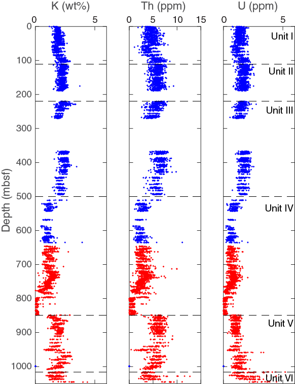
Figure F62. K, Th, and U.
Magnetic susceptibility
Magnetic susceptibility ranges from 0 to 2064 × 10−5 SI with average values of 40 × 10−5 for Lithostratigraphic Unit I, 21 × 10−5 for Unit II, 16 × 10−5 for Unit III, 50 × 10−5 for Unit IV, 150 × 10−5 for Unit V, and 42 × 10−5 SI for Unit VI (Figure F55). Between 0 and 80 mbsf, magnetic susceptibility is nearly constant with an average value of 30 × 10−5 SI. From 80 to 110 mbsf, magnetic susceptibility shifts to lower values of 10 × 10−5 to 15 × 10−5 SI, and then it remains constant at 10 × 10−5 SI to 500 mbsf. At 500 mbsf, corresponding to the Unit III/IV boundary, magnetic susceptibility shifts abruptly to higher values of ~40 × 10−5 before increasing with depth to reach ~90 × 10−5 SI at ~600 mbsf. Between 600 and 710 mbsf, magnetic susceptibility is nearly constant with an average of ~100 × 10−5 SI, followed by a decrease with depth to ~4 × 10⁻⁵ SI at 800 mbsf. Values then remain constant at ~3 × 10⁻⁵ SI between 800 and ~849 mbsf. At the top of Unit V at ~849 mbsf, magnetic susceptibility shifts abruptly to a higher value of ~100 × 10−5 SI, and then it increases gradually with depth to 300 × 10−5 SI at ~900 mbsf before gradually decreasing to 10 × 10−5 SI at ~1020 mbsf. A value of approximately 15 × 10−5 SI observed between 950 and 955 mbsf corresponds to a marl interval (see Lithostratigraphy). Between ~1020 and 1040 mbsf, magnetic susceptibility is nearly constant at ~20 × 10−5 SI, but it shows some scatter with peaks >100 × 10−5 SI. At 1045 mbsf, magnetic susceptibility rapidly increases to ~300 × 10−5 SI.
Reflectance spectroscopy and colorimetry
Color reflectance data are measured on archive halves and reported as L*, a*, and b* values (Figure F55). The color parameters a* and b* remain relatively constant between 0 and 500 mbsf with values of 0 and −2, respectively. L* remains constant with an average value of 35 between 0 and 110 mbsf and then increases to a slightly higher value of 41 and remains constant between 110 and 500 mbsf. L* shifts to a higher value of ~55 at 500 mbsf and decreases gradually with depth to reach 50 at 770 mbsf. Between 500 and 770 mbsf, a* and b* are nearly constant at 0 and −2, except for between 720 and 740 mbsf where a* and b* increase to 4 and 9, respectively, at 728 mbsf before they decrease to 0 and −2, respectively, at ~770 mbsf. At 773 mbsf, L*, a*, and b* increase rapidly to average values of 63, 5, and 11, respectively, and then they remain relatively constant to ~848 mbsf. At 848 mbsf, L*, a*, and b* shift to lower values of 45, 2, and 8, respectively. They stay nearly constant with average values of 39, 4, and 5, respectively, to 985 mbsf, except for a slight increase in L* and b* to 56 and 10, respectively, between 949 and 954 mbsf. Deeper than 980 mbsf, L*, a*, and b* increase with depth to reach peak values of 45, 8, and 12, respectively, at ~1000 mbsf, decrease with depth to 35, 0, and −5, respectively, at 1020 mbsf, and then remain constant to 1046 mbsf.
Downhole measurements
Formation temperature
The APCT-3 was deployed eight times in Hole U1520D (Table T16) and yielded five reliable measurements of in situ formation temperature. APCT-3 1858005C was used for the first three deployments. During the third deployment, the coring shoe lost integrity and the instrument was flooded. APCT-3 1858002C was used for the last five measurements. The first four and the last temperature measurements, associated with Cores 375-U1520D-4H, 7H, 13H, 16H, and 27F, show a clear frictional heating spike upon insertion, indicating that the tool penetrated the sediment (Figure F63). The measurement associated with Core 19F did not result in a useful formation temperature value. Of the five viable temperature estimates, most show a smooth decay of temperature between penetration and pull out. The deepest two measurements (Cores 23F and 27F) are degraded by temperature spikes during the temperature decay, likely caused by tool movement.
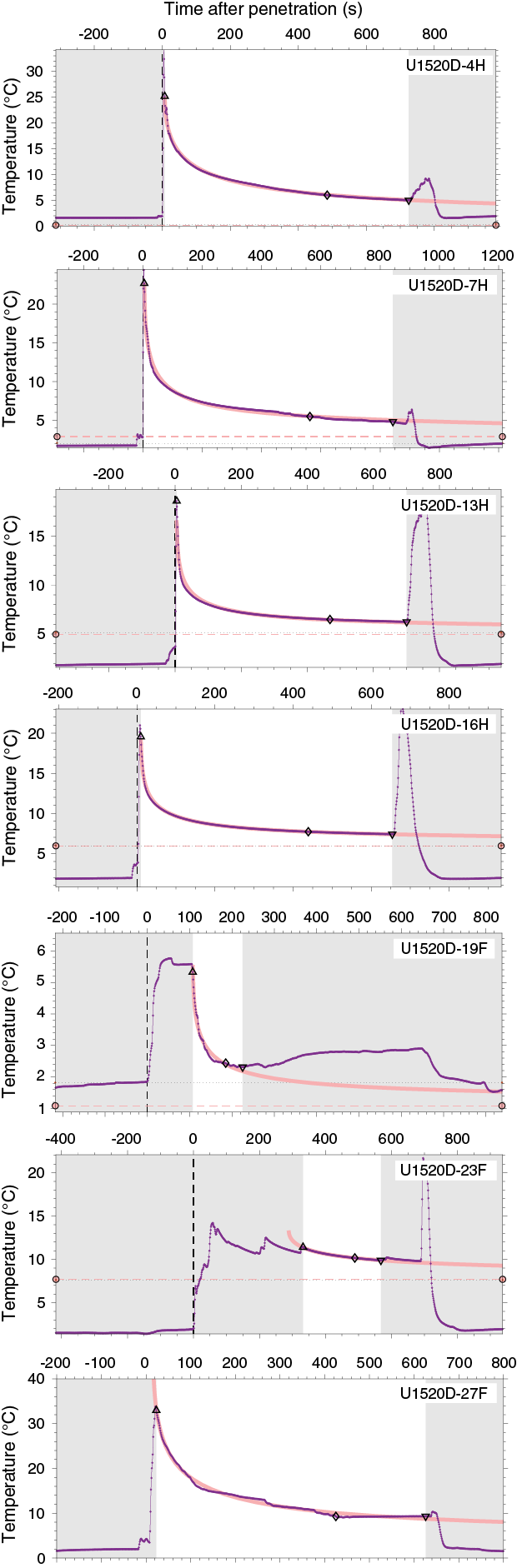
Figure F63. APCT-3 temperature-time series.
Estimated equilibrium temperatures are plotted as a function of measurement depth (Figure F64A). The best-fit linear trend to these data yields a thermal gradient of 38°C/km and a bottom water temperature of 0.4°C. In determining this trend, temperature estimates associated with Cores 375-U1520D-4H and 27F (black dots) were not used. Both of these temperature estimates show large departures from the best-fitting linear trend, and including these measurements yields an unrealistically low bottom water temperature of −0.8°C. We speculate that the low temperature value associated with Core 4H may be due to cracking of the formation during tool insertion, leading to the infiltration of bottom water. The low-quality temperature estimate associated with Core 27F is likely associated with poor penetration of the tool and subsequent disturbance, as indicated by the unsteady temperature decay curve (Figure F63).
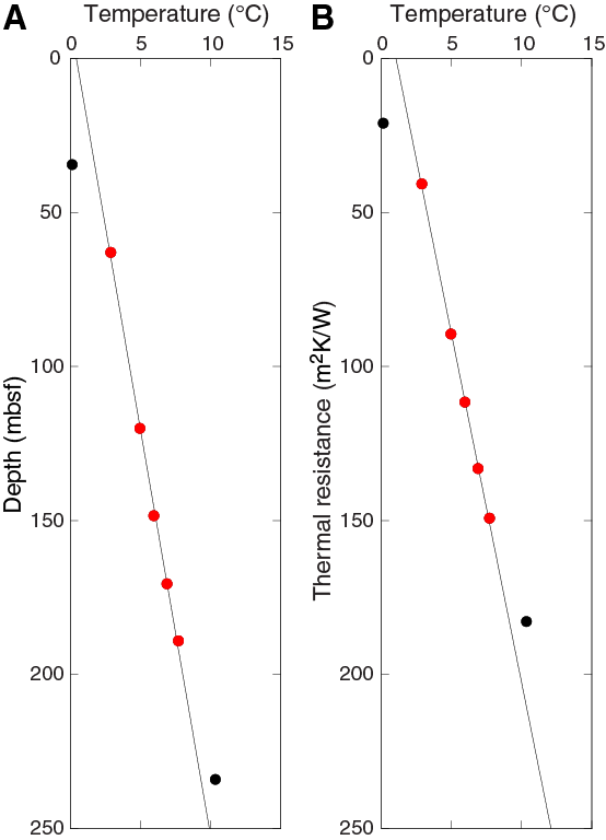
Figure F64. Estimated equilibrium temperatures.
Because of significant variations in thermal conductivity at Site U1520 (see Physical properties), we estimate the vertical conductive heat flow (q) using the thermal resistance method developed by Bullard (1939):
where k(z)i is the individual thermal conductivity value and Δzi is the distance between adjoining thermal conductivity measurements.
In practice, q and T0 can be estimated by plotting T(z) against thermal resistance between the seafloor and the depth of the temperature measurement (Figure F64B). The thermal resistance of the sediment overlying each APCT-3 measurement is given in Table T16. The heat flow estimate defined by the slope of the least-squares linear fit is 44 mW/m2 (Figure F64B) and is consistent with 3.5 m deep probe measurements of heat flow made during R/V Roger Revelle Cruise RR1508 in the same location (Antriasian et al., 2018). The estimated bottom water temperature using this technique is 1.0°C and is marginally cooler than bottom water temperatures measured with the heat flow probe in this area (Antriasian et al., 2018).
Wireline logging operations
Hole U1520C was prepared for logging with a 50 bbl mud sweep to circulate cuttings out of the hole and was filled with heavy mud. The drill string was recovered, and the logging BHA was lowered to the seafloor. The logging bit was set at 599 mbsf, 42 m above the casing shoe. We made two logging passes from 642 to 947 mbsf, where we encountered an obstruction 107 m from the bottom of the hole. A repeat pass was made from ~850 to 910 mbsf (see Operations).
Data and log quality
Hole U1520C was logged using a modified triple combo tool string (see Downhole measurements in the Expedition 372B/375 methods chapter [Wallace et al., 2019a]). The data set includes borehole diameter from a mechanical caliper (HLDS), gamma ray (EDTC-B), resistivity (HRLA), and velocity (DSI) (Figure F65). The Hostile Environment Natural Gamma Ray Sonde (HNGS) was not used, nor was the nuclear source mounted on the HLDS; therefore, only caliper data and total gamma measurements were acquired by the HLDS. The gamma ray data from the EDTC-B were recorded at sampling intervals of 5.08 and 15.24 cm. Resistivity was also acquired every 5.08 cm but was resampled at 15.24 cm for ease of comparison with the other logs. All of the tools (apart from the caliper) were operational during the down pass through the hole, including the upper 640 m cased in Hole U1520C. Gamma ray variations from 0 to 640 mbsf are useful for correlation purposes, but the magnitude of the signal is significantly lower than LWD data because of the shielding effect of the casing and pipe. All tools, including the caliper, were operational from 642 to 947 mbsf, providing new logging information for the depth interval 750–947 mbsf, which was not drilled with LWD during Expedition 372. The target depth of 1050 mbsf for wireline logging was not reached because of an obstruction 107 m from the bottom of the hole. Raw wireline data were sent onshore for processing and calibration.
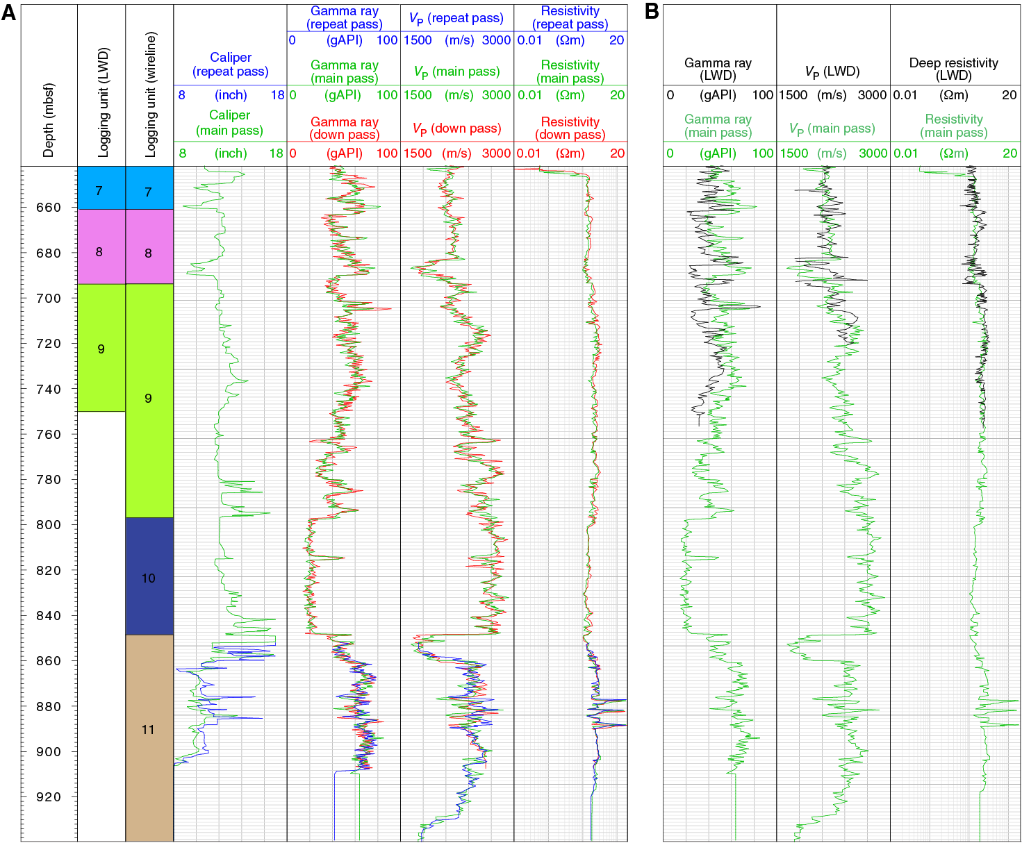
Figure F65. Logging units and wireline logs, Hole U1520C.
Figure F65 shows the full suite of wireline logs acquired during the downward pass, main pass, and repeat pass, and a comparison with LWD data (see Logging while drilling). The three passes for all wireline logs are very similar; we focus on the main pass logs in the following discussion and use them for comparison with LWD data.
The RCB system drills a 9⅞ inch diameter hole. The caliper shows that the hole ranges in size from 8 inches (likely due to collapse or swelling of clays) to 17 inches, which is the full range of the calipers. The hole is irregular and has many washouts below 780 mbsf.
Although overall patterns are similar, some differences are evident between the LWD and wireline logs (see Core-log-seismic integration). For example, from 685 to 691 mbsf the wireline gamma log indicates relatively high gamma ray values of 70 gAPI, whereas the LWD gamma ray log shows only 23 gAPI. We note that the caliper in this interval during wireline logging was only 9 inches, which is narrower than the original borehole width and could indicate borehole collapse in this interval compared with LWD Hole U1520B.
Despite fine-scale differences between the LWD and wireline logs, the depths of major lithostratigraphic boundaries identified in the wireline logs are consistent with those observed in the LWD data (see Core-log-seismic integration) and depth shifting of the wireline logs relative to the LWD logs is not needed.
Log characterization and lithologic interpretation
Logging Units 1–9 were identified during Expedition 372 based on LWD data. The wireline logging data overlap the LWD data for Units 7–9 and sample an additional 190 m of deeper formation (Figure F65). Based on wireline log properties, we suggest that Logging Unit 9 extends to 848 mbsf, where a major change in physical properties occurs.
In the open hole section of Hole U1520C, gamma ray values vary between about 20 and 80 gAPI, P-wave velocity varies between about 1600 and 2900 m/s, and resistivity is relatively constant at about 2 Ωm with the exception of strong peaks between 870 and 890 mbsf (discussed below). In general, gamma ray and P-wave velocity are inversely correlated between 640 and 848 mbsf and positively correlated below 848 mbsf.
Logging Units 7–9 are characterized by large changes in gamma ray values that indicate significant variability in clay content. Conspicuous peaks in gamma ray values with amplitudes of about 60–90 gAPI occur at 703, 705, 767, and 785 mbsf. P-wave velocity through Logging Units 7 and 8 is relatively constant at about 2100 m/s. One notable departure occurs between approximately 682 and 696 mbsf where P-wave velocity decreases to ~1800 m/s. Here, gamma ray values are relatively high and the caliper shows a narrowing of the hole, suggesting the presence of clay. P-wave velocity through Logging Unit 9 exhibits a slight positive trend and increases from 2250 to 2550 m/s.
In Logging Unit 10, gamma ray values are relatively low and constant at 20 gAPI and P-wave velocity values are relatively high and constant at ~2700 m/s. Variations in resistivity are particularly muted. This logging unit corresponds to chalk/muddy chalk in the lower portion of Lithostratigraphic Unit IV (see Lithostratigraphy) and is characterized by low and high values of gamma ray and P-wave velocity, respectively.
The Logging Unit 10/11 boundary marks a notable change in the character of the gamma ray and P-wave velocity logs. The transition is marked by an increase in gamma ray and a notable decrease in P-wave velocity. Just below the Logging Unit 10/11 boundary, the caliper log indicates a washout, and part of the change in these properties could be attributed to the larger borehole diameter (see Core-log-seismic integration). Logging Unit 11 shows a generally positive correlation between gamma ray and P-wave velocity values. Throughout Logging Unit 11, the gamma ray, P-wave, and resistivity wireline logs show significant variability over length scales of a few meters or less. The variations in P-wave velocity in Logging Unit 11 are less extreme than those observed on discrete core samples (see Physical properties), likely a result of smoothing inherent to the larger measurement interval of 1.07 m for the wireline data relative to the centimeter-scale resolution of the core measurements (see Downhole measurements in the Expedition 372B/375 methods chapter [Wallace et al., 2019a]). In Logging Unit 11, three conspicuous peaks in resistivity occur at 876, 882, and 888 mbsf. The resistivity peaks (~14–24 Ωm, relative to a background of ~4 Ωm) at 876 and 882 mbsf correspond to local peaks in P-wave velocity (~2400–2800 m/s against a background of ~2300 m/s).
Logging while drilling
LWD data for Site U1520 were collected in two holes: Hole U1520A from a seafloor depth of 3522.3 mbsl and Hole U1520B from a seafloor depth of 3520.9 mbsl. The LWD BHA for this site is composed of six LWD tools attached behind the bit (from bottom to top): geoVISION, NeoScope, StethoScope, TeleScope, SonicScope, and proVISION. These tools provide a wide array of measurements including gamma ray (geoVISION and NeoScope), resistivity (geoVISION and NeoScope), porosity (NeoScope and proVISION), and compressional (P-wave) and shear (S-wave) wave velocity (SonicScope), as described in Logging while drilling in the Expedition 372B/375 methods chapter (Wallace et al., 2019a).
Drilling parameters
In the composite plot of drilling parameters for Hole U1520A (Figure F66), data are sorted according to the LWD operations period starting on 26 December 2017 at 1956 h local time and terminating on 27 December at 0025 h. The rate of penetration (ROP) was faster on average than other Expedition 372 boreholes and highly variable (ranging from 0 to 100 m/h) because of unconsolidated sandy turbidites and spudding in with inclement weather approaching. The drilling pipe rotation rate steadily increased with depth. Weight on bit (WOB) ranged between −10 and 10 klb; negative values indicate little weight was placed on the bit. Annular pressure increased progressively with depth. The equivalent circulating density (ECD) started at 2.4 g/cm3 at the top of the hole and slowly decreased to 1.8 g/cm3. From the seafloor to total depth, the annular temperature was ~2°C.
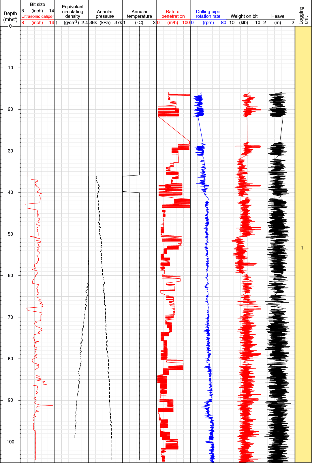
Figure F66. Drilling parameters, Hole U1520A.
For Hole U1520B (Figure F67), the data are sorted according to the LWD operations period starting on 29 December at 0042 h local time and terminating on 30 December at 1542 h. Weather conditions remained poor throughout, with typical total heave of ~4 m. The ROP was over 100 m/h in the first 90 mbsf, where the hole overlapped with Hole U1520A, and then slowed to ~40–20 m/h to acquire higher quality LWD data deeper in the borehole. The drilling pipe rotation rate was maintained close to 50 rpm. WOB ranged between negative values and 20 klb. Annular pressure increased progressively with depth. The ECD was 2.4 g/cm3 at the top of the borehole and decreased gradually to 1.5 g/cm3 at the bottom of the borehole. During drilling, the measured annular temperature slowly increased from 2°C at the top of the borehole to a maximum of 7°C at the bottom of the borehole at 750 mbsf.

Figure F67. Drilling parameters, Hole U1520B.
Data quality
Both Holes U1520A and U1520B were drilled during heavy sea conditions that deteriorated logging data quality. The ROP in both boreholes, especially the first 100 m of Hole U1520B, was faster than recommended for LWD data collection, which contributed to poor data quality at these depths. Additionally, the proVISION (nuclear magnetic resonance [NMR]) tool failed repeated water column pump tests before entry into Hole U1520A; the tool was switched to an alternate proVISION that also failed the water column pump test. Ultimately, proVISION data were collected in both boreholes; however, data quality may be negatively affected.
In general, the highest quality logging measurements are collected when the borehole is close to bit size. Thus, borehole conditions were assessed by the ultrasonic caliper measurement of borehole diameter to define zones of borehole enlargement, or washouts (Figures F68, F69). The ultrasonic caliper, however, can incorrectly identify intervals with extreme borehole enlargement (>5 cm) and instead report values near bit size (8½ inch); therefore, porosity and resistivity measurements were also used to identify enlarged borehole intervals. These zones are characterized by anomalously low resistivity (~0.3–0.9 Ωm) and unrealistically high porosity (~0.7–1.0), both of which imply that measurements are affected by an increased volume of seawater between the tool and borehole wall. Degraded borehole conditions are more likely in intervals with less cohesive sediment such as sand and silt with little clay. In finer grained (typically clay-rich) intervals, the borehole is likely to be closer to bit size. Enlarged borehole and poor log quality were encountered in most of Hole U1520A and in specific depth intervals in Hole U1520B (0–90, 230–240, and 500–513 mbsf).
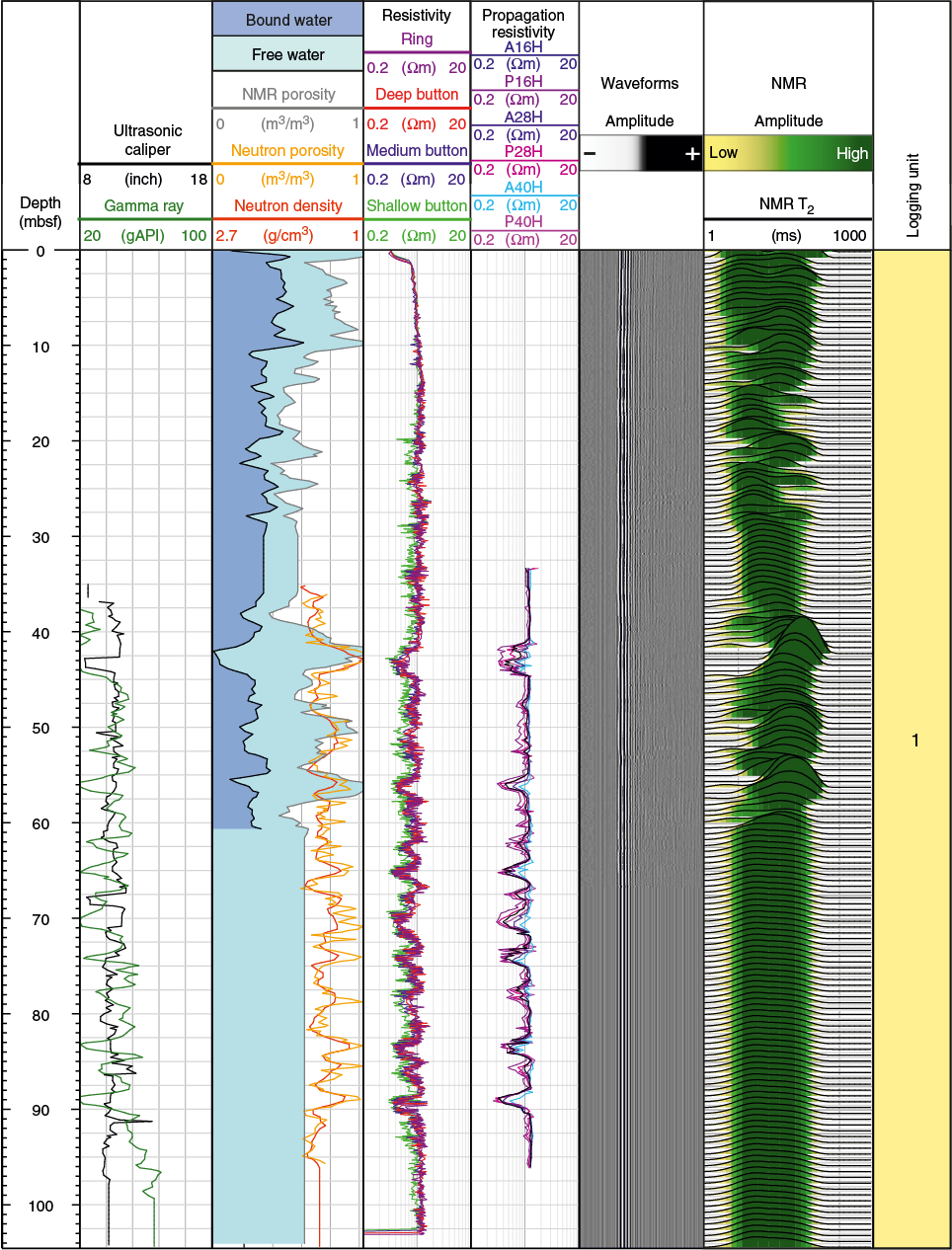
Figure F68. LWD measurements, Hole U1520A.
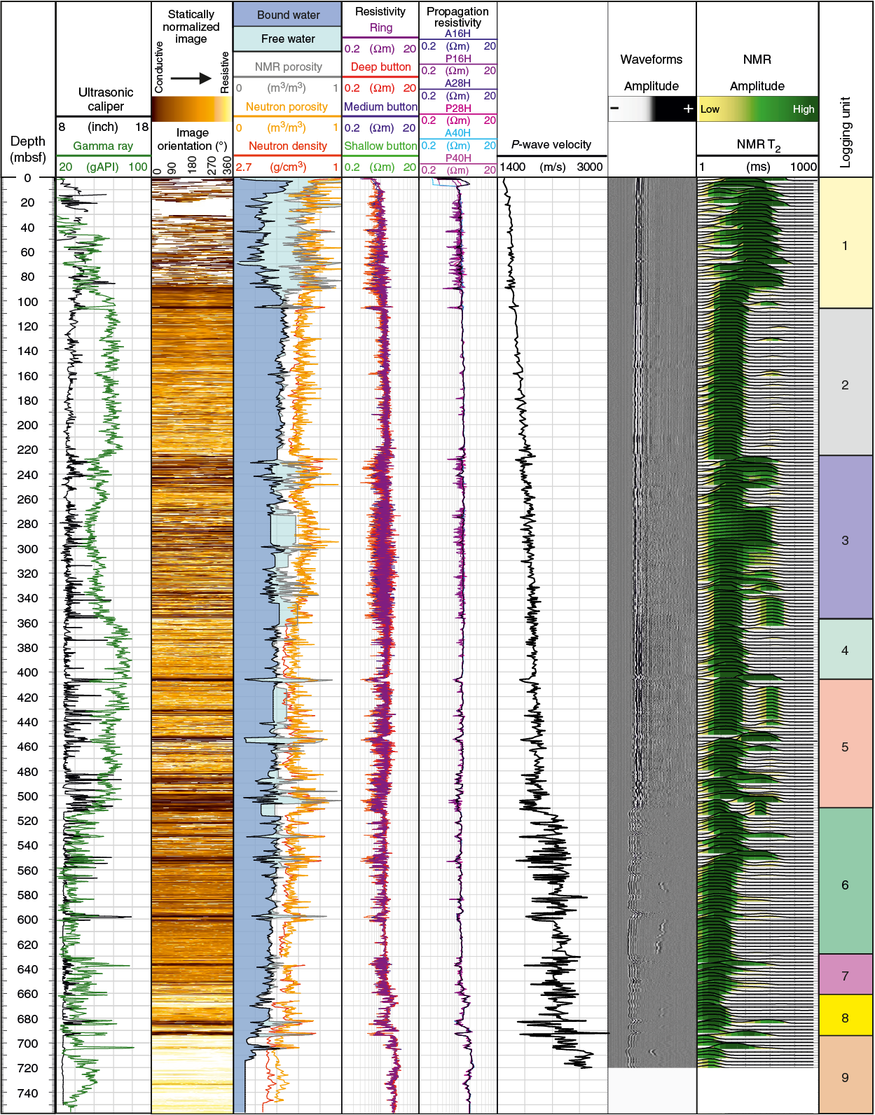
Figure F69. LWD measurements, Hole U1520B.
A GVR resistivity image log was acquired from 0 to 103 mbsf in Hole U1520A (Figure F70). The image quality is poor throughout because of the high ROP and heave. From 0 to 36 mbsf, data loss is high. Stretching image log artifacts are noted throughout the entire imaged interval and are likely related to heave during data acquisition. Horizontal image log artifacts are also common throughout the imaged interval and are likely related to stick and slide as the resistivity buttons rotate around the borehole.
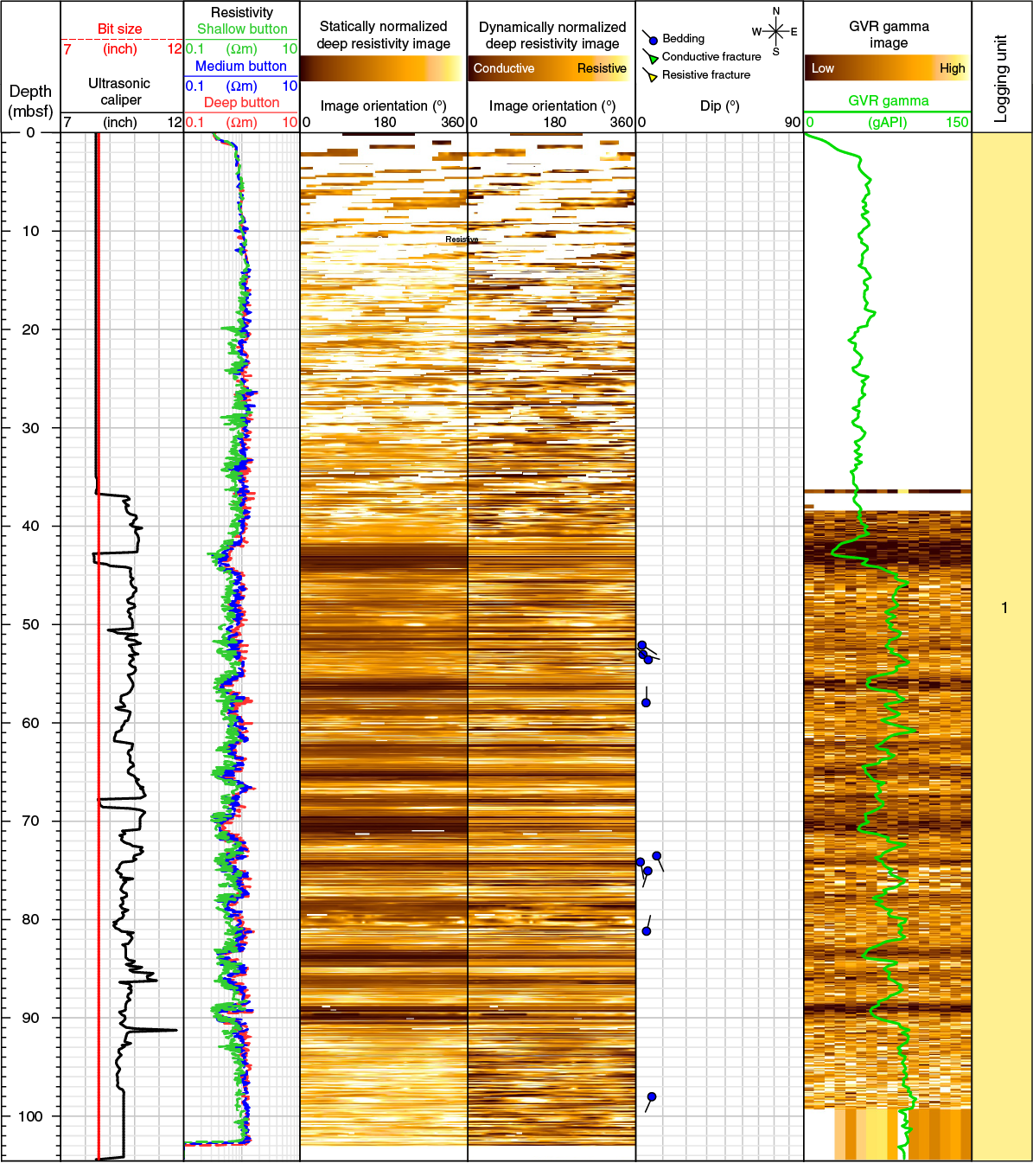
Figure F70. Resistivity image log data, Hole U1520A.
In Hole U1520B, a resistivity image log was collected from 0 to 757.38 mbsf. The image quality is variable, but for the majority of the borehole it is poor. At 0–87, 222–223, and 370–505 mbsf, the image quality is too low to identify more than a few geological features with confidence. As was the case for Hole U1520A, the low quality of this image log is a result of the high ROP used to drill the majority of this borehole and significant heave. Numerous stretching image log artifacts are noted (e.g., 240, 408, 432, 453, 480–513, 550, and 600 mbsf), which obscure geological features and also in places misrepresent bedding because the artifacts are of similar width to the thin beds. At 570–580 and 602–630 mbsf, a weak spiral-hole artifact reduces image log quality, but geological features can still be observed. As for Hole U1520A, horizontal image log artifacts are again common throughout the imaged interval. The best image quality in this interval can be found across Logging Units 6–9 where pelagic carbonates dominate.
The NMR data are of variable quality because of long gaps in the data at 265–290, 333–364, 411–440, and 505–513 mbsf. Even in areas where full NMR data were collected, the transverse relaxation time (T2) distribution is truncated to values between 1 and 1000 ms. Therefore, not all of the clay-bound water (which typically ranges from 0.3 to 3 ms) is recorded. Additionally, the largest pores in coarse sediments and any open pore space or washouts are recorded as a long T2 peak between 50 and 500 ms rather than the longer T2 of 3000 s for bulk water.
Logging units
The combination of different LWD measurements allowed us to define nine logging units (Figures F68, F69). Logging Units 1–6 broadly correspond to Seismic Units 1–6 (see Core-log-seismic integration and Lithostratigraphy). Logging Units 1 and 2 broadly correspond to Lithostratigraphic Units I and II, respectively. Logging Units 3–5 correspond to Lithostratigraphic Unit III, and Logging Units 6–9 correspond to Lithostratigraphic Unit IV. Because Holes U1520A and U1520B were drilled in close proximity (~20 m) and Hole U1520A only covered a short depth interval compared with Hole U1520B, the logging unit definitions are combined into a single description here.
Logging Unit 1 (0–106.4 mbsf)
Logging Unit 1 is defined by low gamma ray (commonly <30 gAPI) that increases to 60 gAPI at the base of the logging unit. The unit also has variable resistivity ranging from 0.4 to 1.6 Ωm and a P-wave velocity increase from ~1500 to ~1650 m/s with depth. The ultrasonic caliper in Hole U1520B indicates the borehole is significantly enlarged through most of this logging unit. The long NMR T2 relaxation time indicates dominantly coarser grained sediments. The high ROP caused poor image quality in both boreholes, resulting in few confidently identified bedding planes (Figures F70, F71). Logging Unit 1 is interpreted to be thinly bedded (alternating resistive and conductive beds), with bedding orientations dominantly gently dipping (<30°) with no consistent dip azimuth.
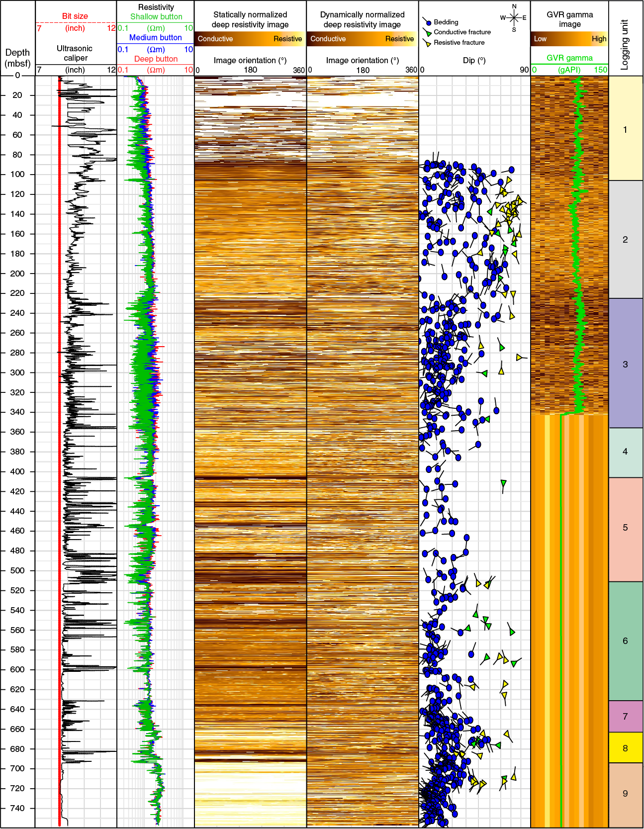
Figure F71. Resistivity image log data, Hole U1520B.
Logging Unit 2 (106.4–225.0 mbsf)
Logging Unit 2 is defined by a change to improved borehole conditions, higher gamma ray (~70 gAPI), and unimodal short NMR T2 distributions that indicate dominantly bound water in the formation from which we infer the presence of fine-grained sediments. Average resistivity increases slightly with depth from ~1.3 to 1.5 Ωm throughout the logging unit. Porosity decreases slightly and gradually with depth: neutron porosity decreases from 0.63 to 0.55, and NMR porosity decreases from 0.50 to 0.44. P-wave velocity continues to increase with depth in this logging unit from ~1650 to ~1800 m/s. Scarce and uncertain bedding orientations from the resistivity image logs have variable dip angles of as much as 70° and no consistent dip azimuth. Logging Unit 2 is more fractured than most other logging units at Site U1520 and contains a mix of conductive and resistive fractures that mostly dip >60° in a range of azimuths. The image logs for this unit have poor quality, however, and further post-expedition analysis is required to improve the confidence of bed and fracture identification.
Logging Unit 3 (225.0–357.0 mbsf)
Logging Unit 3 log responses are variable and influenced by the washout of what are assumed to be coarse-grained sediment layers. The uniformly lower gamma ray (~40 gAPI) suggests that sediment between 254 and 267 mbsf contains less clay than sediment in Logging Unit 2. The resistivity measurements are more variable than in Logging Unit 2 because of washout, but average resistivity is similar (~1.4 Ωm). Porosity is variable in Logging Unit 3 and marked by the presence of higher porosity, coarser sediments relative to Logging Unit 2. P-wave velocity increases slightly with depth from ~1800 to ~1875 m/s. Bedding dips are mostly <40° with variable azimuths. Only a few conductive and resistive fractures are identified, and they do not exhibit consistent orientations. As in Unit 2, image quality is poor, and additional analysis is required to increase confidence in bedding and fracture measurements. Logging Unit 3 is interpreted to contain mainly thick, coarse-grained sediment layers with a few thin layers of finer sediments.
Logging Unit 4 (357.0–406.0 mbsf)
Logging Unit 4 is marked by a return to unimodal, short T2 distribution indicating a uniformly fine grained sediment. This logging unit is thinly bedded, as observed from GVR resistivity image logs. Bedding is gently dipping (<20°) with no dominant dip azimuth. Resistivity is mostly uniform at ~1.3 Ωm and decreases slightly downhole. Neutron porosity (~0.51) and NMR porosity (~0.40) are consistent throughout this unit. The sonic waveforms in this unit have a uniform response. P-wave velocity is consistently ~1875 m/s.
Logging Unit 5 (406.0–510.4 mbsf)
Logging Unit 5 exhibits resistivity, density, porosity, and P-wave velocity responses similar to those in Logging Unit 4; however, gamma ray, density, and resistivity values decrease slightly with depth. NMR T2 distributions are variable in this unit, with short unimodal, elongated unimodal, and bimodal responses. Enlarged borehole sizes, higher porosity, and decreases in resistivity indicate the presence of thin, coarser grained layers in this logging unit, which could represent the coarsest grained intervals of turbidite beds (see Lithostratigraphy). Bedding dominantly dips <30° with no consistent dip direction.
Logging Unit 6 (510.4–629.3 mbsf)
The top of Logging Unit 6 marks an abrupt change in logging measurements that coincides with the change from clastic to calcareous lithology in the core from Hole U1520C (see Lithostratigraphy). Gamma ray decreases to 25–40 gAPI at the top of Logging Unit 6, suggesting a decrease in clay content. P-wave velocity increases to 2100 m/s at the Logging Unit 5/6 boundary and then increases gradually to 2250 m/s to the base of Logging Unit 6 but with excursions to values as low as 1800 m/s. The upper portion of Unit 6 (510.4–540 mbsf) has a variable NMR T2 signature indicative of a range of pore sizes. From 540 mbsf to the base of this unit, short NMR T2 values average ≤10 ms, indicating uniformly small pores. Moreover, short T2 peaks are centered on smaller modal values in Unit 6 than in overlying logging units. Neutron porosity decreases from ~0.54 at the top of Logging Unit 6 to ~0.50 at the base with local variations throughout. Bedding in this unit dips <40° with no dominant dip direction. Fracture intensity is higher in Logging Unit 6 than overlying Unit 5, with a combination of conductive and resistive fractures throughout and with a dominant northwest–southeast strike orientation.
Logging Unit 7 (629.3–661.0 mbsf)
Logging Unit 7 is defined by a sharp increase in gamma ray to as high as ~40 gAPI, an increase in porosity and resistivity, and a small decrease in compressional wave velocity (from 2200 to ~2100 m/s). NMR T2 distributions continue to decrease downhole in this unit, which is likely a result of calcareous lithofacies (see Lithostratigraphy). Bedding orientations are varied to ~647 mbsf, below which bedding dips <20° consistently west to northwest. Fracture intensity is low in this unit.
Logging Unit 8 (661.0–693.8 mbsf)
In Logging Unit 8, log responses exhibit large variations and nonuniform properties. Gamma ray has low and high spikes over meter-scale intervals. Over similarly short length scales, P-wave velocity varies with peak values as high as 2700 m/s and local minima of ~1900 m/s. Resistivity exhibits similar variation and ranges from >0.8 to <2.3 Ωm. Porosity is also variable; NMR porosity ranges from 0.15 to 0.71, and neutron porosity ranges from 0.33 to 0.75. Bedding dips <30° to the west to southwest from 610 to 668 mbsf, 20°–60° toward the east and southeast from 668 to 675 mbsf, and <50° to the west from 675 to 693.8 mbsf. Fracture intensity is higher in this logging unit than above.
Logging Unit 9 (693.8–750 mbsf)
Logging Unit 9 is defined by high resistivity (2.0 to 2.4 Ωm) and the lowest neutron porosity (0.37–0.43) measured in the borehole. Similarly, neutron density is the highest in the borehole at ~2.2 g/cm3. P-wave velocity is generally ~2600 m/s, although a drop to only ~1700 m/s occurs at the top of the unit and we note significant variability both in the velocity and in the nature of the recorded waveforms. Gamma ray is 25 gAPI at the top and base of the logged interval but increases to 50 gAPI at 720–730 mbsf before decreasing again toward the base. Bedding dips <30° to the west and northwest. A cluster of resistive fractures occurs between 711 and 715 mbsf, which may correlate with filled fault structures reported in core from Hole U1520C (see Structural geology).
Core-log-seismic integration
A key objective was to integrate core-based observations from Expedition 375 with in situ physical properties measurements from LWD data collected during Expedition 372 (see Logging while drilling), wireline log data collected during Expedition 375 (see Downhole measurements), and seismic reflection profiles. In this section, we discuss correlations across these different data sets that detect variations in physical properties, lithology, and structure at a range of scales.
Depth scale
During Expedition 372, LWD data were acquired in Holes U1520A and U1520B. The seafloor depth was determined from LWD to be 3521.3 mbsl in Hole U1520A and 3520.1 mbsl in Hole U1520B. Coring was undertaken in Holes U1520C and U1520D, and the seafloor was tagged at 3522.1 and 3520.3 mbsl, respectively. Holes U1520B and U1520C are located 20 m from each other, and all boreholes at Site U1520 lie on Seismic Line 05CM-04. Because of the minor differences in seafloor depth, close proximity of the LWD and coring sites, and relatively simple geological structure, it is possible to conduct a correlation of the core, log, and seismic data with no depth shifting required.
LWD operations in Hole U1520B collected logging data to a TD of 750 mbsf. After installation of a reentry system to 642 mbsf in Hole U1520C, RCB coring took place from 646.0 to 1054.1 mbsf, providing as much as 104 m of overlap between LWD logs and cores. These data were supplemented by wireline logging data collected during Expedition 375 (see Downhole measurements), including gamma ray, compressional and shear velocity, caliper, and resistivity logs from 643.8 to 944 mbsf. In Hole U1520D, core was collected at 0–189.3, 220.0–270.8, and 366.6–642.3 mbsf.
Seismic-well ties
A seismic-well tie is needed to correlate physical properties changes in the logging data, lithostratigraphic units and structural domains in cores, and seismic reflections and seismic facies units to extrapolate results from drilling using regional seismic data. Hole U1520B intersects Seismic Line 05CM-04 at common depth point (CDP) 6227, Hole U1520C is located at CDP 6226, and Hole U1520D is located at CDP 6224. To correlate seismic data (recorded in time) and log/core data (recorded in depth), it is necessary to develop an accurate time-depth relationship. P-wave velocity data were acquired by the SonicScope LWD tool in both Holes U1520A and U1520B, providing velocity information from 0 to 721 mbsf (see Logging while drilling). Wireline logging sonic data collected during Expedition 375 from 643.8 to 944 mbsf were integrated with the LWD data to produce a continuous sonic log from 0 to 944 mbsf. Density data were not collected while wireline logging during Expedition 375, so a density log for 750–944 mbsf was constructed from whole-round track and discrete sample bulk density data from cores (see Physical properties).
The LWD and wireline P-wave velocity logs were compared with seismic velocity estimates produced for the depth migration of Seismic Line 05CM-04 and a full waveform inversion (FWI) (see Core-log-seismic integration in the Expedition 372B/375 methods chapter [Wallace et al., 2019a]). LWD sonic–derived interval velocity values in the upper 250 m are generally higher than the FWI velocity model (provided by R. Bell and Imperial College London, United Kingdom) and lower than the prestack depth migration (PSDM) models (Barker et al., 2018) (Figure F72A). Between 250 and 700 mbsf, both models match the sonic velocity well. The FWI model matches the wireline log velocity values well to 850 mbsf but fails to identify the low velocity zone below this depth.
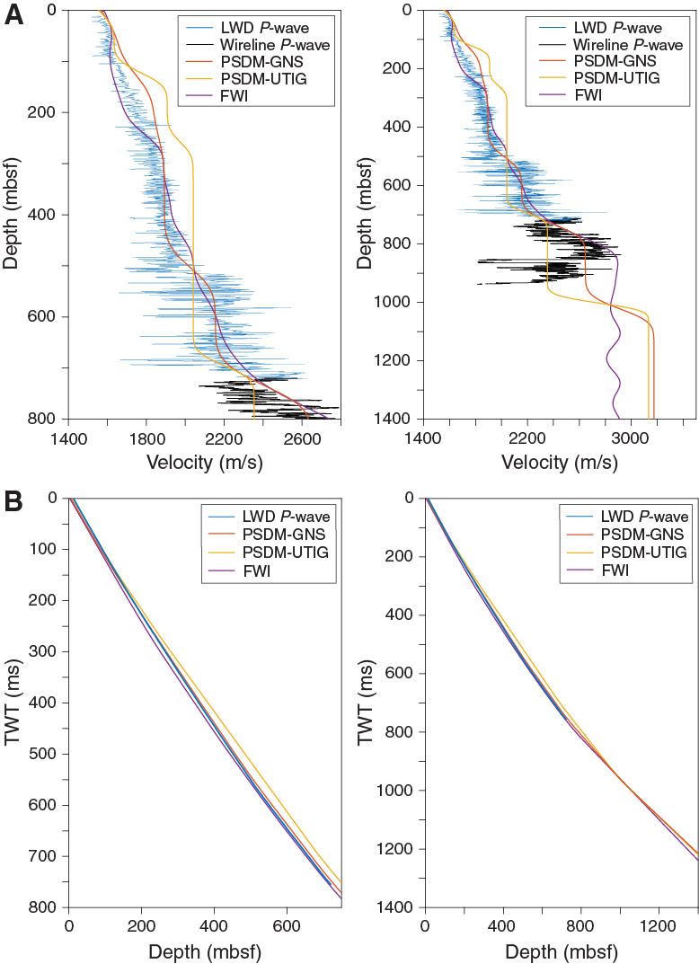
Figure F72. LWD, wireline, PSDM, and FWI P-wave velocity profiles.
Construction of velocity and density logs for 0–940 mbsf
The LWD and wireline logs provide a direct measurement of P-wave velocity at Site U1520, so a combined LWD and wireline P-wave velocity log was used to perform the depth-time conversion in the production of a synthetic seismic trace (Figure F73A). Comparison of the LWD and wireline logging P-wave velocity in the 643–720 mbsf interval reveals a good correlation between the data sets (see Downhole measurements). The wireline logging data from 720 mbsf were spliced directly with the LWD P-wave velocity data. The complete P-wave velocity log was smoothed over 20 samples (sampling interval of 15 cm) to produce a profile relevant for the vertical resolution of the seismic data.
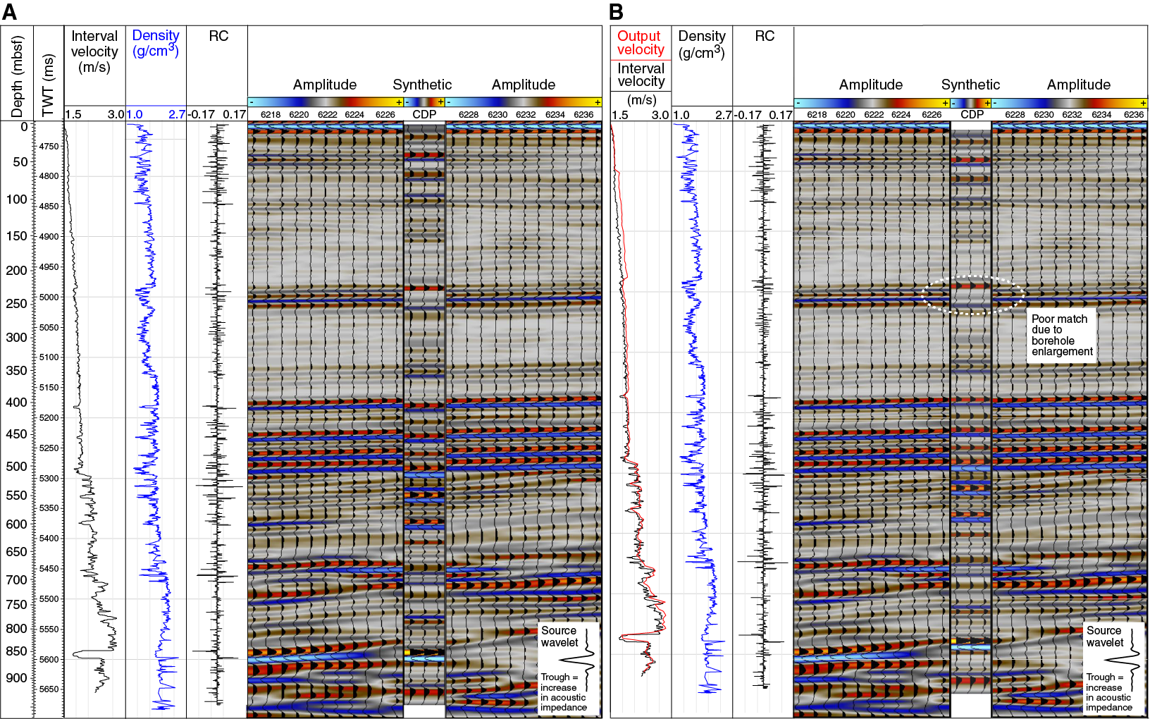
Figure F73. Synthetic seismic-well tie.
LWD sourceless neutron-gamma density logs from Hole U1520B were used in the construction of the synthetic seismic-well tie from 0 to 750 mbsf. Whole-round track density measurements are systematically lower than LWD density, whereas discrete MAD measurements on core samples from Hole U1520C provide a good match to the LWD data where they overlap (see Physical properties). For this reason, MAD density values were spliced to the bottom of the LWD density log to produce a complete log from 0 to 940 mbsf. The combined density log was also smoothed over 20 samples (sampling interval of 15 cm) (Figure F73A).
Construction of the synthetic seismic trace
Following testing using analytical, statistical, and deterministic wavelet extractions, a preferred wavelet was selected from Seismic Profile 05CM-04 by stacking 10 adjacent seismic traces from a flat region of the seafloor around the intersection with Hole U1520B between CDPs 6220 and 6230 to yield a high signal-to-noise ratio (Figure F73). This wavelet was convolved with the reflection coefficient log measured in two-way traveltime (TWT) to produce a synthetic seismic trace that can be compared with Seismic Line 05CM-04 in the vicinity of CDP 6227 near Site U1520.
The resulting synthetic seismic trace in the time domain is shown in Figure F73A, together with the seismic data (Line 05CM-04, CDPs 6217–6237), with no depth shifts applied. The synthetic predicts high-amplitude reflections around 400–500 mbsf and low-amplitude reflections between 250 and 400 mbsf, where high- and low-amplitude reflections are observed in the real seismic data. Minor changes to the velocity log (red line, Figure F73B) bring the synthetic trace and real seismic reflections into close alignment. The discrepancies between the velocity required by the seismic-well tie and the real velocity logs could be the result of reduced quality P-wave velocity logging data because of borehole washouts. The only region where a significant velocity change would be required to match reflections is around 220–250 mbsf where the caliper data reveal the presence of a significant borehole enlargement (Figure F74) (see Logging while drilling). The close match between the synthetic trace and Line 05CM-04 provides high confidence in the correlation between LWD, wireline logging, core, and seismic reflection data.
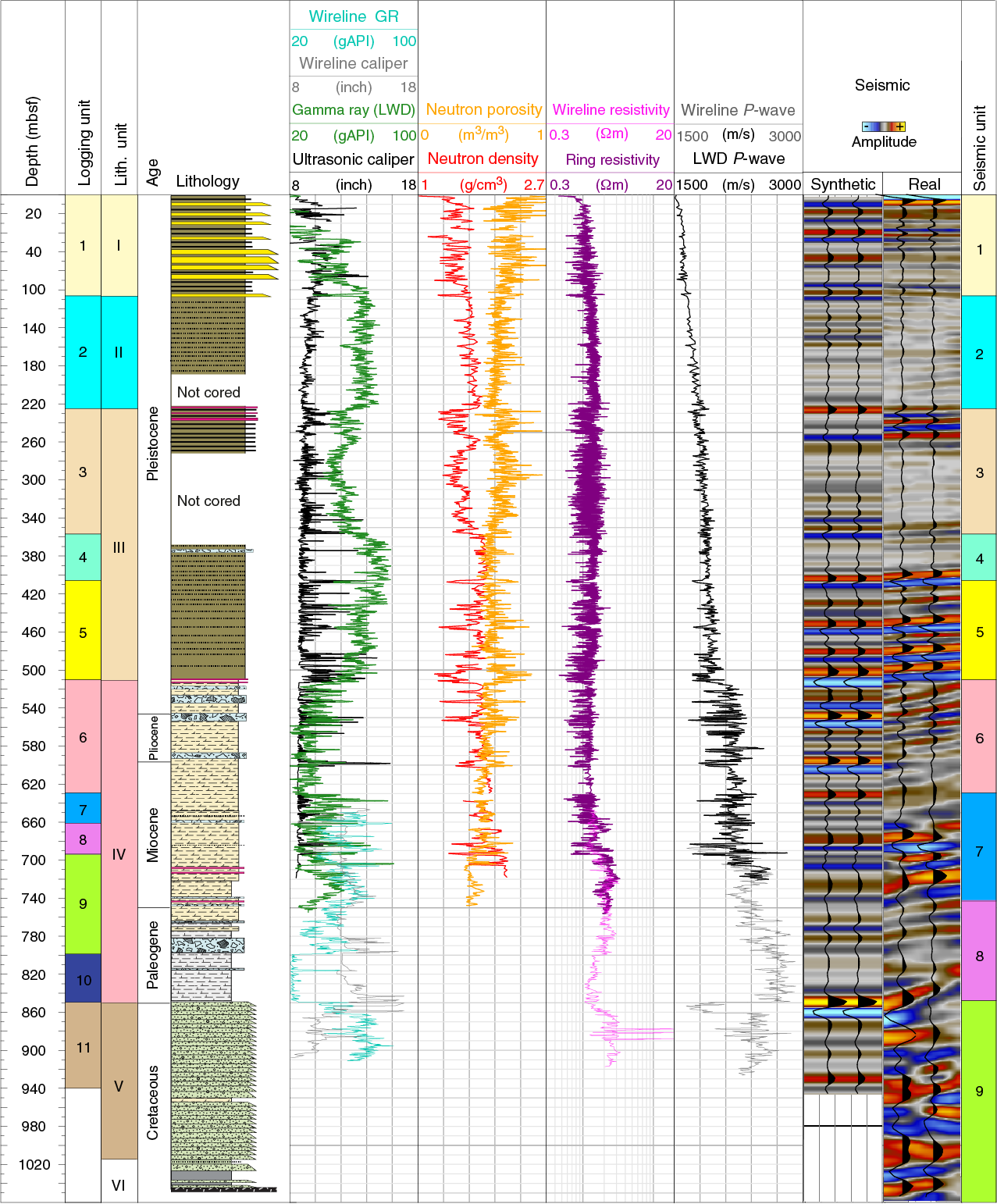
Figure F74. Lithologic, LWD, wireline log, and seismic data.
Seismic stratigraphy, seismic units, and comparison with log and core data
Nine seismic units are defined at Site U1520. The seismic units are shown in meters below seafloor converted from time using the seismic-well tie (Figure F73; Table T17) in Figure F74 where they are compared with the logging units defined by LWD and wireline logging (see Logging while drilling and Downhole measurements). In Figure F75, the broad seismic stratigraphic architecture of the seismic units is highlighted and compared with pre-expedition interpretations of seismic stratigraphy (P. Barnes, unpubl. data).

Figure F75. Seismic units, Line 05CM-04.
At Site U1520, the upper 406 mbsf is characterized by an overall low-amplitude reflection sequence that includes Seismic Units 1–4 (Figures F74, F75). This interval is underlain by a section that is more strongly reflective and extends to 848 mbsf, which includes Seismic Units 5–8. Between 848 and 1040 mbsf, Seismic Unit 9 is characterized by high-amplitude, lower frequency, and less continuous seismic reflections than the overlying seismic units. The seismic units generally correlate with both logging and lithostratigraphic units defined for this site.
Nine logging units are identified between 0 and 750 mbsf based on shifts in the LWD trends (see Logging while drilling) (e.g., Figures F74, F76). Two additional logging units are identified between 750 and 940 mbsf from wireline logging data (see Downhole measurements).
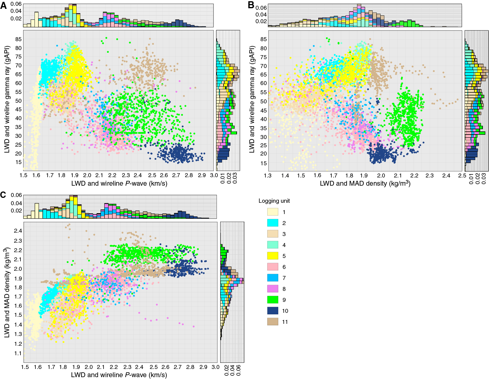
Figure F76. Gamma ray, P-wave velocity, and density, Holes U1520B and U1520C.
Using a combination of correlation panels, crossplots, and the seismic-well tie, we describe the reflection and logging characteristics of each seismic unit and discuss the in situ physical properties that likely lead to the observed reflection characteristics. We also tie lithologic, biostratigraphic, and core-based physical properties to the seismic data at Site U1520 to enable interpretation away from the drill site (see Lithostratigraphy, Physical properties, and Biostratigraphy).
Seismic Unit 1 (0–106 mbsf)
Seismic Unit 1 is 106 m thick at Site U1520 and is characterized by moderate- to low-amplitude, laterally continuous reflections (Figure F75). At a regional scale, this seismic unit has a generally tabular geometry, but it thins to the east and onlaps the Tūranganui Knoll seamount. The top of the seismic unit is the seafloor, which is a flat plain (Figure F1). Seismic Unit 1 directly correlates with Logging Unit 1. Logging Unit 1 exhibits variable logging signatures from 40 to 90 mbsf. From 90 to 106 mbsf, the resistivity, gamma ray, and density curves show increasing trends (Figure F74).
Seismic Unit 1 was cored in Hole U1520D and correlates approximately with Lithostratigraphic Unit I (see Lithostratigraphy) (Figure F77). The lithofacies is composed mostly of mud, silt, and fine-grained sand deposited as turbidites and hemipelagic beds (see Lithostratigraphy). The base of Lithostratigraphic Unit I was identified in the core data at 110.5 mbsf, similar to the base of Seismic Unit 1 and Logging Unit 1 at 106 mbsf. Biostratigraphy indicates that Seismic Unit 1 is Late Pleistocene to Holocene (see Biostratigraphy).
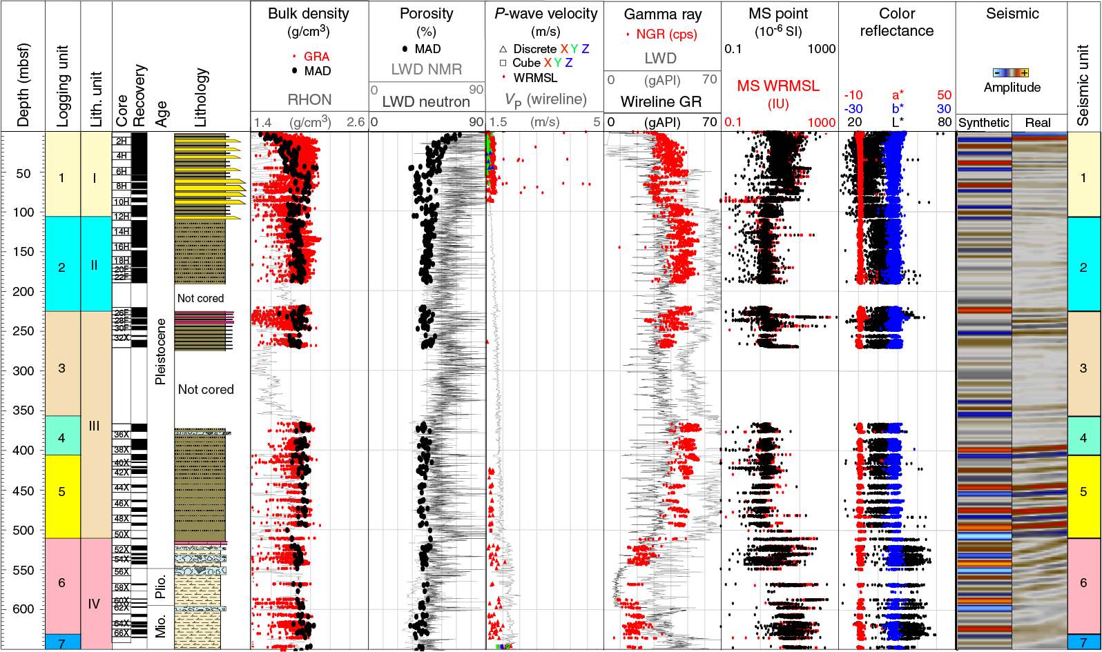
Figure F77. LWD, wireline, Hole U1520D physical properties, and seismic data.
Seismic Unit 2 (106–225 mbsf)
Seismic Unit 2 (106–225 mbsf) is 119 m thick and is characterized regionally by moderate- to low-amplitude, semicontinuous, and chaotic reflections. At Site U1520, the reflections are more continuous (Figures F75, F78). The seismic unit increases in thickness as much as 150 m approximately 7 km west of Site U1520, thins eastward, and onlaps the Tūranganui Knoll. The upper surface of the seismic unit is irregular, and subtle, mounded, steep reflection geometries occur in it, providing evidence of internal deformation. This seismic unit can be traced widely in regional seismic data and is interpreted to be a thick MTD associated with the Ruatoria debris avalanche (Lewis et al., 1998; Collot et al., 2001). Seismic Unit 2 correlates directly with Logging Unit 2 where gamma ray values are higher (60–75 gAPI) and resistivity is more uniform than in Logging Unit 1. Logging Unit 2 is interpreted to represent a change to finer grained sediments based on improved borehole conditions, slightly higher density, higher gamma ray, and a unimodal, short NMR T2 distribution (see Logging while drilling). On crossplots of gamma ray to P-wave velocity, gamma ray to density, and density to P-wave velocity (Figure F76), Logging Unit 2 (and Seismic Unit 2) is located in a tight cluster that separates it from other logging units. Density and P-wave velocity slightly increase throughout Seismic Unit 2 and decrease abruptly at the base (Figure F74). The base of the seismic unit is defined by a high-amplitude, reversed polarity reflection that indicates a decrease in acoustic impedance caused by a drop in density and a small decrease in P-wave velocity.

Figure F78. LWD, physical properties, and structural interpretations.
Seismic Unit 2 was cored in Hole U1520D and correlates approximately with Lithostratigraphic Unit II (see Lithostratigraphy) (Figure F77). The lithofacies is composed mostly of hemipelagic mud interbedded with thin-bedded silty turbidites with local mud intraclasts and erosional bases. No evidence was seen in the cores for mass transport of the sediments (such as chaotic disturbance), and laboratory-measured physical properties do not show as significant a change at the Lithostratigraphic Unit I/II boundary as those observed in the LWD data (Figure F77) (see Lithostratigraphy and Physical properties). Measurements made on cores reveal that bedding remains gently dipping in both Units II and III; however, GVR resistivity image logs suggest significantly higher and more variable dip directions in Unit II compared with Unit III (Figure F78) (see Logging while drilling and Structural geology), although these are noted to be low confidence interpreted features because of poor image quality and require further study. In detail, we note that reflections in Hole U1520B that are slightly more deformed than in Hole U1520D, which is 40 m away (Figure F78). However, the deformation in Hole U1520B observed in seismic data still appears to be low. Biostratigraphy indicates that Seismic Unit 2 is Late to Middle Pleistocene (see Biostratigraphy).
Seismic Unit 3 (225–357 mbsf)
Seismic Unit 3 (225–357 mbsf) is 132 m thick and is characterized by an overall weakly reflective interval that includes laterally continuous reflections that can be traced widely along and across the Hikurangi Trough (Figure F75). The seismic unit thickens to >200 m 8 km west of Site U1520, where it covers a field of sedimentary waves and onlaps an older sequence draping a volcanic high. To the east, the seismic unit onlaps the Tūranganui Knoll. Reflection amplitudes are highest in the upper 40 m of the seismic unit and decrease toward the middle of the interval (Figure F74), where weak, irregular, and mottled reflections are slightly inclined (Figure F75). Reflection coherence, continuity, and amplitude generally increase toward the base of Seismic Unit 3.
Seismic Unit 3 corresponds directly to Logging Unit 3. The top of Logging Unit 3 is marked by a sharp decrease in gamma ray, density, P-wave velocity, and resistivity, an increase in porosity, and high-amplitude resistivity changes and spikes in caliper associated with bad borehole conditions in the upper 20–30 m (Figures F74, F76). The synthetic seismic trace provides the poorest match to the seismic data in this zone (Figure F73). From here to the base of Logging Unit 3, both density and P-wave velocity show increasing trends. On crossplots of gamma ray to P-wave velocity, gamma ray to density, and density to P-wave velocity, Logging Unit 3 exhibits more spread than the overlying and underlying logging units (Figure F76). Based on the LWD data, Logging Unit 3 is interpreted to be a lithologically mixed package of sediments that is relatively coarser grained than Logging Unit 2 (and Seismic Unit 2) and has likely intervals of fine-grained sediments (see Logging while drilling).
Seismic Unit 3 was partially cored in Hole U1520D from 225 to 270.8 mbsf and approximately correlates with the upper part of Lithostratigraphic Unit III (see Lithostratigraphy) (Figure F77). The lithofacies is composed of hemipelagic mud interbedded with normally graded silty turbidites and thick volcanic ash layers near the top of this lithostratigraphic unit (see Lithostratigraphy). Biostratigraphy indicates that Seismic Unit 3 is Late to Middle Pleistocene (see Biostratigraphy).
Seismic Unit 4 (357–406 mbsf)
Seismic Unit 4 (357–406 mbsf) consists of generally low to moderate amplitude reflections that increase in amplitude locally toward the flank of Tūranganui Knoll where the seismic unit thins (Figure F75). This seismic unit is 49 m thick at Site U1520, and it thickens westward to about 60 m approximately 5 km west of the site. The base of the seismic unit is defined by a high-amplitude tuned reflection caused by a 5 m thick interval of reduced density and velocity (Figure F73). Seismic Unit 4 correlates directly with Logging Unit 4. The gamma ray values are the highest observed in Hole U1520B and increase with depth in this seismic unit. Density and P-wave velocity also increase slightly with depth, whereas resistivity shows a steady decrease punctuated by negative spikes (Figure F74). On crossplots of gamma ray to P-wave velocity, gamma ray to density, and density to P-wave velocity, Logging Unit 4 forms a cluster that separates it from Logging Unit 3 and overlaps with Logging Unit 5 (Figure F76). The base of Seismic Unit 4 and Logging Unit 4 is marked by an abrupt drop in density, resistivity, and gamma ray. This interval is interpreted to be uniformly fine grained sediments based on a unimodal NMR T2 distribution and a thin-bedded appearance in LWD resistivity logs (see Logging while drilling).
Seismic Unit 4 was partially cored in Hole U1520D from 366.6 to 406 mbsf and correlates with the middle part of Lithostratigraphic Unit III (see Lithostratigraphy) (Figure F77). The lithofacies is composed mostly of hemipelagic mud interbedded with thin-bedded silty turbidites and rare, thin MTDs. Turbidite frequency decreases with depth (see Lithostratigraphy). Biostratigraphy indicates that Seismic Unit 4 is Middle Pleistocene (see Biostratigraphy).
Seismic Unit 5 (406–511 mbsf)
Seismic Unit 5 (406–511 mbsf) is 105 m thick and is characterized by moderate- to low-amplitude, semicontinuous reflections grading to high-amplitude, continuous reflections toward its base (Figures F74, F75). Regionally, this seismic unit shows a marked lateral change in its seismic character. West of Site U1520, the seismic character changes to well-defined, high-amplitude reflections with high lateral coherence (Figure F75). About 6 km west of Site U1520, the upper part of the seismic unit drapes a field of sediment waves that include reflections in the lower part of Seismic Unit 5. To the east, this seismic unit onlaps the irregular upper surface of Seismic Unit 6. The base of Seismic Unit 5 is defined by a normal polarity reflection caused by an increase in both density and P-wave velocity.
Seismic Unit 5 correlates directly with Logging Unit 5. Density and resistivity curves show a general decrease with negative spikes coincident with high caliper log values that indicate localized intervals of increased washout and poor borehole conditions (see Logging while drilling). A noticeable decrease in gamma ray, density, P-wave velocity, and resistivity occurs over the basal 30 m of the seismic unit (Figure F74). Crossplots in Figure F76 reveal that overall Logging Unit 5 plots in the same domain as Logging Units 1–4 but is more variable in its gamma ray, density, and velocity, which suggests that Seismic Unit 5 is likely composed of a wider mix of lithologies with different physical properties than the overlying seismic units.
Seismic Unit 5 was cored in Hole U1520D and correlates with the lower part of Lithostratigraphic Unit III (see Lithostratigraphy) (Figure F77). The lithofacies is composed mostly of hemipelagic mud and silt deposited as thin-bedded turbidites. The frequency of turbidites decreases downsection (see Lithostratigraphy). Biostratigraphy indicates that Seismic Unit 5 is Middle to early Pleistocene (see Biostratigraphy).
Seismic Unit 6 (511–631 mbsf)
Seismic Unit 6 (511–631 mbsf) is 120 m thick and has a more irregular geometry than the more tabular Seismic Units 1–5 (Figure F75). Reflections in Seismic Unit 6 at Site U1520 have higher dips and are less well organized than the overlying reflections in Seismic Unit 5 and those farther west in Seismic Unit 6. In addition, reflections in Seismic Unit 6 are moderate to low amplitude and locally are offset by small normal faults. The disrupted nature of the reflections could be interpreted to be one or more debris flows originating from the flanks of Tūranganui Knoll. Immediately west of Site U1520, the reflections transition to higher amplitudes and are more continuous. These reflections grade into and form the lower part of the well-developed sediment waves 6–7 km west of Site U1520. The top of Seismic Unit 6 appears to be an unconformity at Site U1520. The base of Seismic Unit 6 is defined by a decrease in density and velocity (Figure F74).
Seismic Unit 6 correlates directly with Logging Unit 6, which is marked by a significant drop in gamma ray relative to overlying seismic and logging units that indicates a likely decrease in clay content (Figures F74, F76). In this seismic unit, gamma ray and porosity decrease slightly with depth. The caliper log is uniform apart from two spikes, indicating good borehole conditions. Resistivity is generally lower than Logging Unit 5, whereas P-wave velocity, and to a lesser extent density, are higher and increase with depth (Figure F74). The gamma ray, P-wave velocity, and density data for Seismic Unit 6 and Logging Unit 6 plot in a very different domain of the crossplots in Figure F76 when compared with Logging Units 1–5.
Seismic Unit 6 was cored in Hole U1520D and correlates with the upper part of Lithostratigraphic Unit IV. The lithofacies is composed mostly of light greenish gray calcareous mudstone and marl with minor beds of volcanic tuff and convoluted, matrix-supported debris flow deposits near the top of this seismic unit. The latter include pebble-sized clasts of basalt and marl. The depositional setting is pelagic with extraformational debris flows derived from the flank of Tūranganui Knoll and intraformational submarine slides (see Lithostratigraphy). Biostratigraphy indicates that Seismic Unit 6 is late Miocene to early Pleistocene (see Biostratigraphy).
Seismic Unit 7 (631–745 mbsf)
Seismic Unit 7 (631–745 mbsf) is 114 m thick and is characterized by highly variable, low- to very high amplitude, discontinuous reflections (Figure F75). The upper boundary of the seismic unit is irregular and may coincide with an unconformity. In the upper 20 m of Seismic Unit 7, the seismic character has low amplitude and is poorly defined by weak, irregular reflections that may correspond to debris derived from the flank of Tūranganui Knoll. From 693 mbsf to the bottom of Seismic Unit 7, reflections are very high amplitude and highly discontinuous. Locally small normal faults offset the reflections (e.g., Figure F75). The base of the seismic unit is marked by a relatively continuous, reversed polarity reflection, coinciding with a small decrease in density and P-wave velocity (Figures F74, F79).
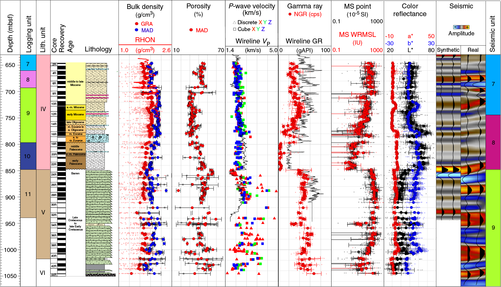
Figure F79. LWD, wireline, Hole U1520C physical properties, and seismic data.
Seismic Unit 7 correlates with Logging Units 7 and 8 and part of Logging Unit 9 (Figure F74). Logging Unit 7 is characterized by an increase in gamma ray and porosity and irregular resistivity relative to Seismic Unit 6 and Logging Unit 6 (see Logging while drilling). In Logging Unit 7, P-wave velocity ranges from ~2000 to 2400 m/s. Logging Unit 8 is characterized by a relative reduction in resistivity and a significantly greater spread of porosity, density, and P-wave velocity. P-wave velocity in Logging Unit 8 ranges from <1700 m/s (associated with highly conductive intervals) to 2800 m/s at the base of the logging unit (Figures F74, F75). At 694 mbsf (top of Logging Unit 9), resistivity and density markedly increase and then gradually increase toward the bottom of Hole U1520B at 750 mbsf. Logging Units 7 and 8 plot in a similar location to Logging Unit 6 in the crossplots in Figure F76, consistent with them having similar lithology (see Lithostratigraphy). From resistivity image logs, bedding is dominantly dipping west throughout Seismic Unit 7.
Seismic Unit 7 was cored in the lower part of Hole U1520D and below 646 mbsf in Hole U1520C. This seismic unit correlates with the middle part of Lithostratigraphic Unit IV (see Lithostratigraphy) (Figure F79). The lithofacies is composed mostly of marl and calcareous mudstone with rare, thin intervals of matrix-supported debris flow deposits, volcanic tuff, and thin volcaniclastic siltstone (see Lithostratigraphy). A brown, more clay-rich lithology in Lithostratigraphic Unit IV between 720 and 735 mbsf has reduced density and velocity; those properties result in a high-amplitude peak and trough doublet reflection caused by constructive interference of a reversed polarity reflection from the top of the clay-rich interval and a normal polarity reflection from the base (Figure F73). The high-amplitude trough of this doublet reflection correlates with the base of Seismic Unit 7 (Figure F79). Other high-amplitude reflections between 640 and 745 mbsf may be related to variations in the amount of microcrystalline calcite in the recrystallized calcareous mudstone and marl (see Lithostratigraphy). Biostratigraphy indicates that Seismic Unit 7 is early to late Miocene (see Biostratigraphy).
Seismic Unit 8 (745–848 mbsf)
Seismic Unit 8 (745–848 mbsf) is 103 m thick and is composed of moderate-amplitude, continuous reflections (Figure F75). West of the site, the reflections are higher amplitude, irregular, and semicontinuous, and to the east, they onlap against a very high amplitude reflection that has a wide peak-trough-peak wavelet at the base of the seismic unit. About 10 km west of Site U1520 on Seismic Line 05CM-04 (Figure F2), the seismic unit onlaps buried volcanic highs beneath the Hikurangi Trough, and it is more difficult to correlate the reflections further west with certainty. Seismic Unit 8 correlates with the lower part of Logging Units 9 and 10 (Figure F79).
Wireline logs reveal a reduction in gamma ray with depth in Seismic Unit 8 and through the lower part of Logging Units 9 and 10 and an abrupt change across the Logging Unit 9/10 boundary (Figures F74, F76). Logging Unit 10 has the lowest gamma ray values (~20 gAPI) and highest velocity values of any of the logging units at Site U1520. P-wave velocity gradually increases through the logging unit from ~2600 m/s at its top and reaches a maximum of 2800 m/s at its base (Figures F74, F79). Resistivity decreases with depth to values of only 1.2 Ωm at the base of Logging Unit 9 (Figure F74). Density and P-wave velocity in Logging Unit 9 are considerably greater than in any of the overlying logging units (Figure F76).
Seismic Unit 8 corresponds to the lower part of Lithostratigraphic Unit IV. Between 745 and 848 mbsf, Lithostratigraphic Unit IV is composed predominantly of marl, calcareous mudstone, and chalk with carbonate debris flow deposits characterized by poor core recovery (Figure F79). These debris flow deposits can be correlated as localized spikes of higher gamma ray in the wireline logs (Figure F74). The overall low gamma ray values and relatively high P-wave velocity observed in Logging Unit 10 are related to the presence of chalk (see Lithostratigraphy). Biostratigraphy indicates that Seismic Unit 8 is late Paleocene to early Miocene (see Biostratigraphy).
Seismic Unit 9 (848–1040 mbsf)
Seismic Unit 9 consists of high-amplitude reflections that have longer wavelengths than reflections in the seismic units above (on the order of 50 m compared with less than 30 m above Seismic Unit 9). Some of the reflections exhibit double peaks and troughs, which suggests that they may be the result of interference of reflections from the top and bottom of thin layers having acoustic impedance contrasts (Figures F74, F79). These high-amplitude reflections at Site U1520 are semicontinuous to discontinuous and have an overall progradational geometry, building outward into the basin away from the flank of Tūranganui Knoll and forming a wedge-shaped body that distinctively pinches out 1.3 km west of Site U1520 (Figure F75). Reflections beneath Seismic Unit 9 at Site U1520 have a similar high-amplitude, low-frequency, discontinuous character and similarly show evidence of westward progradation. Farther east, however, beneath the buried slope of the seamount, younger units analogous to Seismic Unit 9 are observed to be stacked into an upslope-migrating complex of wedge-shaped bodies.
Seismic Unit 9 corresponds to Logging Unit 11, which exhibits a dramatic change in physical properties from the overlying Logging Unit 10. This change is characterized by a decrease in P-wave velocity from 2700 to 1700 m/s, an abrupt increase in gamma ray from 20 gAPI to as high as 70 gAPI, an abrupt increase in magnetic susceptibility, and a subtle decrease in bulk density in the upper ~10 m of the seismic unit (Figures F76, F79). Log attributes in Logging Unit 11 appear widely scattered; some parts of the logging unit plot with extremely low P-wave velocity (~1700 m/s) and others have P-wave velocity values comparable to Logging Unit 9. The seismic unit also exhibits bimodal density values; some parts of the seismic unit have density values of ~1.85 g/cm3 and others have values ~2 g/cm3. The parts of the seismic unit with higher velocity and density also have higher gamma ray values.
Seismic Unit 9 corresponds to Lithostratigraphic Units V and VI. Unit V is composed predominantly of heavily altered volcaniclastic conglomerate and a thin interval of calcareous mudstone or marl. Unit VI is composed of mixed volcaniclastic, siliciclastic, carbonate, and basaltic lithologies (see Lithostratigraphy). The volcaniclastics are cemented to variable degrees, and replacement of primary minerals and volcanic glass by clay minerals is pervasive. The uneven distribution of diagenesis may explain some of the observed variations in physical properties (see below). P-wave velocity measured on cores is significantly more variable than LWD measured P-wave velocity, and values as high as 5000 m/s locally (see Physical properties) suggest that the variation in velocity occurs over thin intervals (<1 m) such that they are below the resolution of the LWD SonicScope tool. Biostratigraphy indicates that Seismic Unit 9 is early Late Cretaceous (see Biostratigraphy).
Synthesis of physical properties, lithology, structure, and seismic architecture of the subduction inputs section
Based on the CLSI, the subduction inputs section at Site U1520 was divided into three distinctive stratigraphic packages. Package 1 consists of Seismic Units 1–5, Package 2 consists of Seismic Units 6–8, and Package 3 consists of Seismic Unit 9. Seismic Units 1–5 and Logging Units 1–5 define a package composed primarily of terrigenous clastic sediments. At Site U1520, this sequence is 511 m thick. These sediments are composed of sandy–silty turbidites, hemipelagic background sediment, and MTDs (e.g., Lewis et al., 1998; Orpin, 2004; Pouderoux et al., 2012; Mountjoy et al., 2018) (Figure F80) (see Lithostratigraphy and Logging while drilling). Sediment waves in Seismic Unit 5 (and 6) appear similar to modern sediment waves resulting from turbidity currents associated with the present Hikurangi Channel to the south (Lewis et al., 1998; Lewis and Pantin, 2001).

Figure F80. Seismic Line 05CM-04 around Hole U1520D.
Although the seismic reflection character of Seismic Unit 6 appears similar to that of Seismic Unit 5 farther west of Site U1520, Seismic Unit 6 has abnormally low gamma ray values and its velocity and density character are more similar to Seismic Units 7 and 8 than Seismic Units 1–4 (Figure F76). We note that Seismic Unit 6 at the location of Site U1520 contains lower amplitude and more chaotic reflections than in Seismic Unit 6 farther west (Figure F75), possibly reflecting debris flows from the western flank of Tūranganui Knoll. Coring confirms that the lithology of Seismic Unit 6 is pelagic carbonate with mass flow deposits, similar to the lithology of Seismic Unit 7 (Figure F80). Seismic Units 7–8 define a sequence of variable amplitude with semicontinuous to discontinuous reflectivity. These reflections have a lower frequency than those in Seismic Units 1–5, and synthetic seismograms suggest that reflections in this seismic unit are related to the presence of thin layer tuning (Figure F73). Some of these reflections are likely related to debris flows containing volcaniclastic material observed in cores from Hole U1520C, whereas other reflections may correspond to differences in clay content or state of microcrystalline cementation (Figure F79).
Seismic Unit 9 is defined by its wedge-like prograding morphology and high-amplitude, low-frequency reflections. This unit is largely composed of volcaniclastic grain flow and debris flow deposits (see Lithostratigraphy) (Figure F81) with high-amplitude reflections related to large P-wave velocity and density contrasts, potentially with amplitudes enhanced by tuning in layers thinner than vertical seismic resolution (Figure F79). Additional higher amplitude, low-frequency reflections occur east of Site U1520, which suggests lateral variation in physical properties.
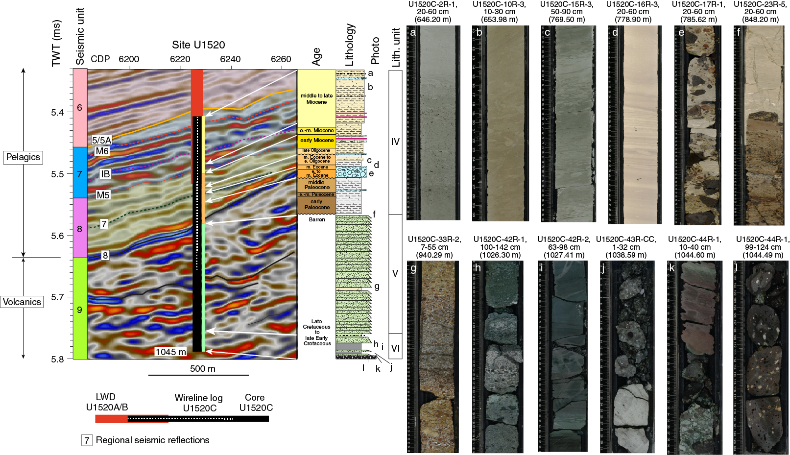
Figure F81. Seismic Line 05CM-04 around Hole U1520C.
The source of the volcaniclastic sediments in Seismic Unit 9, which comprises Lithostratigraphic Units V and VI, is inferred to be the western slope of Tūranganui Knoll. Multibeam bathymetry data show a series of present-day erosional gullies along the upper western flank of the seamount (Figures F1, F82). We infer that the seamount slope geomorphology may be largely relict and that former mass wasting and sediment transport from the gullies supplied a series of coalescing volcaniclastic fans that developed on the now-buried former lower slope region (Figure F75).
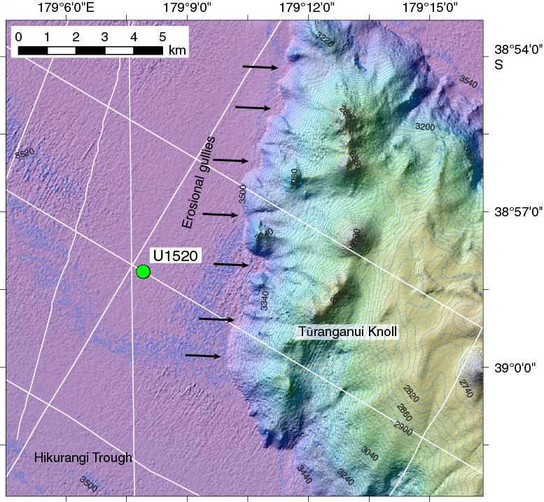
Figure F82. Bathymetry map, western flank of Tūranganui Knoll.
References
Antriasian, A., Harris, R.N., Tréhu, A.M., Henrys, S.A., Phrampus, B.J., Lauer, R., Gorman, A.R., Pecher, I.A., and Barker, D., 2018. Thermal regime of the northern Hikurangi margin, New Zealand. Geophysical Journal International, 216(2):1177–1190. https://doi.org/10.1093/gji/ggy450
Backman, J., 1986. Late Paleocene to middle Eocene calcareous nannofossil biochronology from the Shatsky Rise, Walvis Ridge and Italy. Palaeogeography, Palaeoclimatology, Palaeoecology, 57(1):43–59. https://doi.org/10.1016/0031-0182(86)90005-2
Baker, P.A., Stout, P.M., Kastner, M., and Elderfield, H., 1991. Large-scale lateral advection of seawater through oceanic crust in the central equatorial Pacific. Earth and Planetary Science Letters, 105(4):522–533. https://doi.org/10.1016/0012-821X(91)90189-O
Barker, D.H.N., Henrys, S., Caratori Tontini, F., Barnes, P. M., Bassett, D., Todd, E., and Wallace, L., 2018. Geophysical constraints on the relationship between seamount subduction, slow slip and tremor at the north Hikurangi subduction zone, New Zealand. Geophysical Research Letters, 45(23):12804-12813. https://doi.org/10.1029/2018GL080259
Barnes, P.M., Lamarche, G., Bialas, J., Henrys, S., Pecher, I., Netzeband, G.L., Greinert, J., Mountjoy, J.J., Pedley, K., and Crutchley, G., 2010. Tectonic and geological framework for gas hydrates and cold seeps on the Hikurangi subduction margin, New Zealand. Marine Geology, 272(1–4):26–48. https://doi.org/10.1016/j.margeo.2009.03.012
Barnes, P.M., Pecher, I.A., LeVay, L.J., Bourlange, S.M., Brunet, M.M.Y., Cardona, S., Clennell, M.B., Cook, A.E., Crundwell, M.P., Dugan, B., Elger, J., Gamboa, D., Georgiopoulou, A., Greve, A., Han, S., Heeschen, K.U., Hu, G., Kim, G.Y., Kitajima, H., Koge, H., Li, X., Machado, K.S., McNamara, D.D., Moore, G.F., Mountjoy, J.J., Nole, M.A., Owari, S., Paganoni, M., Petronotis, K.E., Rose, P.S., Screaton, E.J., Shankar, U., Shepherd, C.L., Torres, M.E., Underwood, M.B., Wang, X., Woodhouse, A.D., and Wu, H.-Y., 2019a. Site U1517. In Pecher, I.A., Barnes, P.M., LeVay, L.J., and the Expedition 372 Scientists, Creeping Gas Hydrate Slides. Proceedings of the International Ocean Discovery Program, 372A: College Station, TX (International Ocean Discovery Program). https://doi.org/10.14379/iodp.proc.372A.103.2019
Barnes, P.M., Wallace, L.M., Saffer, D.M., Pecher, I.A., Petronotis, K.E., LeVay, L.J., Bell, R.E., Crundwell, M.P., Engelmann de Oliveira, C.H., Fagereng, A., Fulton, P.M., Greve, A., Harris, R.N., Hashimoto, Y., Hüpers, A., Ikari, M.J., Ito, Y., Kitajima, H., Kutterolf, S., Lee, H., Li, X., Luo, M., Malie, P.R., Meneghini, F., Morgan, J.K., Noda, A., Rabinowitz, H.S., Savage, H.M., Shepherd, C.L., Shreedharan, S., Solomon, E.A., Underwood, M.B., Wang, M., Woodhouse, A.D., Bourlange, S.M., Brunet, M.M.Y., Cardona, S., Clennell, M.B., Cook, A.E., Dugan, B., Elger, J., Gamboa, D., Georgiopoulou, A., Han, S., Heeschen, K.U., Hu, G., Kim, G.Y., Koge, H., Machado, K.S., McNamara, D.D., Moore, G.F., Mountjoy, J.J., Nole, M.A., Owari, S., Paganoni, M., Rose, P.S., Screaton, E.J., Shankar, U., Torres, M.E., Wang, X., and Wu, H.-Y., 2019b. Site U1519. In Wallace, L.M., Saffer, D.M., Barnes, P.M., Pecher, I.A., Petronotis, K.E., LeVay, L.J., and the Expedition 372/375 Scientists, Hikurangi Subduction Margin Coring, Logging, and Observatories. Proceedings of the International Ocean Discovery Program, 372B/375: College Station, TX (International Ocean Discovery Program). https://doi.org/10.14379/iodp.proc.372B375.104.2019
Bullard, E.C., 1939. Heat flow in South Africa. Proceedings of the Royal Society of London, Series A, 173(955):474–502. https://doi.org/10.1098/rspa.1939.0159
Carlson, J., and Grotzinger, J.P., 2001. Submarine fan environment inferred from turbidite thickness distributions. Sedimentology, 48(6):1331–1351. https://doi.org/10.1046/j.1365-3091.2001.00426.x
Claypool, G.E., and Kvenvolden, K.A., 1983. Methane and other hydrocarbon gases in marine sediment. Annual Review of Earth and Planetary Sciences, 11(1):299–327. https://doi.org/10.1146/annurev.ea.11.050183.001503
Collot, J.-Y., Lewis, K., Lamarache, G., and Lallemand, S., 2001. The giant Ruatoria debris avalanche on the northern Hikurangi margin, New Zealand; result of oblique seamount subduction. Journal of Geophysical Research: Solid Earth, 106(B9):19271–19297. https://doi.org/10.1029/2001JB900004
Crundwell, M.P., 2004. New Zealand late Miocene biostratigraphy and biochronology: studies of planktic foraminifers and bolboforms at oceanic Sites 593 and 1123 and selected onland sections [Ph.D. thesis]. University of Waikato, New Zealand. http://odp.georef.org/vufind/Record/2009082475/Details
Crundwell, M.P., and Nelson, C.S., 2007. A magnetostratigraphically constrained chronology for late Miocene bolboformids and planktic foraminifers in the temperate Southwest Pacific. Stratigraphy, 4(1):1–34. http://www.micropress.org/microaccess/check/1502
Davy, B., Hoernle, K., and Werner, R., 2008. Hikurangi Plateau: crustal structure, rifted formation, and Gondwana subduction history. Geochemistry, Geophysics, Geosystems, 9(7):Q07004. https://doi.org/10.1029/2007GC001855
De Vleeschouwer, D., Dunlea, A.G., Auer, G., Anderson, C.H., Brumsack, H., de Loach, A., Gurnis, M., et al., 2017. Quantifying K, U, and Th contents of marine sediments using shipboard natural gamma radiation spectra measured on DV JOIDES Resolution. Geochemistry, Geophysics, Geosystems, 18(3):1053–1064. https://doi.org/10.1002/2016GC006715
Expedition 334 Scientists, 2012. Expedition 334 summary. In Vannucchi, P., Ujiie, K., Stroncik, N., Malinverno, A., and the Expedition 334 Scientists, Proceedings of the Integrated Ocean Drilling Program, 334: Tokyo (Integrated Ocean Drilling Program Management International, Inc.). https://doi.org/10.2204/iodp.proc.334.101.2012
Faris, M., and Farouk, S., 2012. Integrated biostratigraphy of two upper Maastrichtian–Paleocene successions in north-central Sinai, Egypt. Geologica Croatica, 65(2):139–160. https://doi.org/10.4154/GC.2012.10
Felletti, F., and Bersezio, R., 2010. Quantification of the degree of confinement of a turbidite-filled basin: a statistical approach based on bed thickness distribution. Marine and Petroleum Geology, 27(2):515–532. https://doi.org/10.1016/j.marpetgeo.2009.11.003
Fisher, A.T., and Wheat, C.G., 2010. Seamounts as conduits for massive fluid, heat, and solute fluxes on ridge flanks. Oceanography, 23(1):74–87. https://doi.org/10.5670/oceanog.2010.63
Ghisetti, F.C., Barnes, P.M., Ellis, S., Plaza-Faverola, A.A., and Barker, D.H.N., 2016. The last 2 Myr of accretionary wedge construction in the central Hikurangi margin (North Island, New Zealand): insights from structural modeling. Geochemistry, Geophysics, Geosystems, 17(7):2661–2686. https://doi.org/10.1002/2016GC006341
Gradstein, F.M., Ogg, J.G., Schmitz, M.D., and Ogg, G.M. (Eds.), 2012. The Geological Time Scale 2012: Amsterdam (Elsevier). https://doi.org/10.1016/C2011-1-08249-8
Hoernle, K., Hauff, F., van den Bogaard, P., Werner, R., Mortimer, N., Geldmacher, J., Garbe-Schönberg, D., and Davy, B., 2010. Age and geochemistry of volcanic rocks from the Hikurangi and Manihiki oceanic plateaus. Geochimica et Cosmochimica Acta, 74(24):7196–7219. https://doi.org/10.1016/j.gca.2010.09.030
Hollis, C.J., Hines, B.R., Littler, K., Villasante-Marcos, V., Kulhanek, D.K., Strong, C.P., Zachos, J.C., et al., 2015. The Paleocene–Eocene Thermal Maximum at DSDP Site 277, Campbell Plateau, southern Pacific Ocean. Climates of the Past, 11:1009–1025. https://doi.org/10.5194/cp-11-1009-2015
Hornibrook, N.d.B., Brazier, R.C., and Strong, C.P., 1989. Manual of New Zealand Permian to Pleistocene foraminiferal biostratigraphy. New Zealand Geological Survey Paleontological Bulletin, 56.
Kutterolf, S., Freundt, A., Peréz, W., Mörz, T., Schacht, U., Wehrmann, H., and Schmincke, H.-U., 2008. Pacific offshore record of plinian arc volcanism in Central America: 1. Along-arc correlations. Geochemistry, Geophysics, Geosystems, 9(2):Q02S01. https://doi.org/10.1029/2007GC001631
Kutterolf, S., Schindlbeck, J., Robertson, A.H.F., Avery, A., Baxter, A., Petronotis, K., and Wang, K.-L., 2018. Tephrostratigraphy and provenance from IODP Expedition 352, Izu-Bonin arc: tracing tephra sources and volumes from the Oligocene to the Recent. Geochemistry, Geophysics, Geosystems, 19(1):150–174. https://doi.org/10.1002/2017GC007100
Lewis, K.B., Collot, J.-Y., and Lallemand, S.E., 1998. The dammed Hikurangi Trough: a channel-fed trench blocked by subducting seamounts and their wake avalanches (New Zealand–France GeodyNZ Project). Basin Research, 10(4):441–468. https://doi.org/10.1046/j.1365-2117.1998.00080.x
Lewis, K.B., and Pantin, H.M., 2001. Channel-axis, overbank and drift sediment waves in the southern Hikurangi Trough, New Zealand. Marine Geology, 192(1–3):123–151. https://doi.org/10.1016/S0025-3227(02)00552-2
Malinverno, A., 1997. On the power law size distribution of turbidite beds. Basin Research, 9(4):263–274. https://doi.org/10.1046/j.1365-2117.1997.00044.x
Martini, E., 1971. Standard Tertiary and Quaternary calcareous nannoplankton zonation. In Farinacci, A. (Ed.), Proceedings of the Second Planktonic Conference, Roma 1970: Rome (Edizioni Tecnoscienza), 2:739–785.
Monechi, S., Reale, V., Bernaola, G., and Balestra, B., 2013. The Danian/Selandian boundary at Site 1262 (South Atlantic) and in the Tethyan region: biomagnetostratigraphy, evolutionary trends in fasciculiths and environmental effects of the Latest Danian Event. Marine Micropaleontology, 98:28–40. https://doi.org/10.1016/j.marmicro.2012.11.002
Mortimer, N., and Parkinson, D., 1996. Hikurangi Plateau: a Cretaceous large igneous province in the southwest Pacific Ocean. Journal of Geophysical Research: Solid Earth, 101(B1):687–696. https://doi.org/10.1029/95JB03037
Mountjoy, J.J., Howarth, J.D., Orpin, A.R., Barnes, P.M., Bowden, D.A., Rowden, A.A., Schimel, A.C.G., et al., 2018. Earthquakes drive large-scale submarine canyon development and sediment supply to deep-ocean basins. Science Advances, 4(3):eaar3748. https://doi.org/10.1126/sciadv.aar3748
Orpin, A.R., 2004. Holocene sediment deposition on the Poverty-slope margin by the muddy Waipaoa River, East Coast New Zealand. Marine Geology, 209(1–4):69–90. https://doi.org/10.1016/j.margeo.2004.06.001
Pimmel, A., and Claypool, G., 2001. Technical Note 30: Introduction to Shipboard Organic Geochemistry on the JOIDES Resolution. Ocean Drilling Program. https://doi.org/10.2973/odp.tn.30.2001
Plaza-Faverola, A., Klaeschen, D., Barnes, P., Pecher, I., Henrys, S., and Mountjoy, J., 2012. Evolution of fluid expulsion and concentrated hydrate zones across the southern Hikurangi subduction margin, New Zealand: an analysis from depth migrated seismic data. Geochemistry, Geophysics, Geosystems, 13(8):Q08019. https://doi.org/10.1029/2012GC004228
Pouderoux, H., Proust, J.-N., Lamarche, G., Orpin, A., and Neil, H., 2012. Postglacial (after 18 ka) deep-sea sedimentation along the Hikurangi subduction margin (New Zealand): characterisation, timing and origin of turbidites. Marine Geology, 295–298:51–76. https://doi.org/10.1016/j.margeo.2011.11.002
Rothman, D.H., Grotzinger, J.P., and Flemings, P.B., 1994. Scaling in turbidite deposition. Journal of Sedimentary Research, 64(1A):59–67. https://doi.org/10.1306/D4267D07-2B26-11D7-8648000102C1865D
Saffer, D., Wallace, L., and Petronotis, K., 2017. Expedition 375 Scientific Prospectus: Hikurangi Subduction Margin Coring and Observatories. International Ocean Discovery Program. https://doi.org/10.14379/iodp.sp.375.2017
Saffer, D.M., Wallace, L.M., Barnes, P.M., Pecher, I.A., Petronotis, K.E., LeVay, L.J., Bell, R.E., Crundwell, M.P., Engelmann de Oliveira, C.H., Fagereng, A., Fulton, P.M., Greve, A., Harris, R.N., Hashimoto, Y., Hüpers, A., Ikari, M.J., Ito, Y., Kitajima, H., Kutterolf, S., Lee, H., Li, X., Luo, M., Malie, P.R., Meneghini, F., Morgan, J.K., Noda, A., Rabinowitz, H.S., Savage, H.M., Shepherd, C.L., Shreedharan, S., Solomon, E.A., Underwood, M.B., Wang, M., Woodhouse, A.D., Bourlange, S.M., Brunet, M.M.Y., Cardona, S., Clennell, M.B., Cook, A.E., Dugan, B., Elger, J., Gamboa, D., Georgiopoulou, A., Han, S., Heeschen, K.U., Hu, G., Kim, G.Y., Koge, H., Machado, K.S., McNamara, D.D., Moore, G.F., Mountjoy, J.J., Nole, M.A., Owari, S., Paganoni, M., Rose, P.S., Screaton, E.J., Shankar, U., Torres, M.E., Wang, X., and Wu, H.-Y., 2019a. Expedition 372B/375 summary. In Wallace, L.M., Saffer, D.M., Barnes, P.M., Pecher, I.A., Petronotis, K.E., LeVay, L.J., and the Expedition 372/375 Scientists, Hikurangi Subduction Margin Coring, Logging, and Observatories. Proceedings of the International Ocean Discovery Program, 372B/375: College Station, TX (International Ocean Discovery Program). https://doi.org/10.14379/iodp.proc.372B375.101.2019
Saffer, D.M., Wallace, L.M., Barnes, P.M., Pecher, I.A., Petronotis, K.E., LeVay, L.J., Bell, R.E., Crundwell, M.P., Engelmann de Oliveira, C.H., Fagereng, A., Fulton, P.M., Greve, A., Harris, R.N., Hashimoto, Y., Hüpers, A., Ikari, M.J., Ito, Y., Kitajima, H., Kutterolf, S., Lee, H., Li, X., Luo, M., Malie, P.R., Meneghini, F., Morgan, J.K., Noda, A., Rabinowitz, H.S., Savage, H.M., Shepherd, C.L., Shreedharan, S., Solomon, E.A., Underwood, M.B., Wang, M., Woodhouse, A.D., Bourlange, S.M., Brunet, M.M.Y., Cardona, S., Clennell, M.B., Cook, A.E., Dugan, B., Elger, J., Gamboa, D., Georgiopoulou, A., Han, S., Heeschen, K.U., Hu, G., Kim, G.Y., Koge, H., Machado, K.S., McNamara, D.D., Moore, G.F., Mountjoy, J.J., Nole, M.A., Owari, S., Paganoni, M., Rose, P.S., Screaton, E.J., Shankar, U., Torres, M.E., Wang, X., and Wu, H.-Y., 2019b. Site U1518. In Wallace, L.M., Saffer, D.M., Barnes, P.M., Pecher, I.A., Petronotis, K.E., LeVay, L.J., and the Expedition 372/375 Scientists, Hikurangi Subduction Margin Coring, Logging, and Observatories. Proceedings of the International Ocean Discovery Program, 372B/375: College Station, TX (International Ocean Discovery Program). https://doi.org/10.14379/iodp.proc.372B375.103.2019
Shane, P., Black, T., Eggins, S., and Westgate, J., 1998. Late Miocene marine tephra beds: recorders of rhyolitic volcanism in North Island, New Zealand. New Zealand Journal of Geology and Geophysics, 41(2):165–178. https://doi.org/10.1080/00288306.1998.9514801
Shepherd, C.L., and Kulhanek, D.K., 2016. Eocene nannofossil biostratigraphy of the mid-Waipara River section, Canterbury Basin, New Zealand. Journal of Nannoplankton Research, 36(1):33–59. http://ina.tmsoc.org/JNR/online/36/Shepherd_JNR36-1_2016.pdf
Sinclair, H.D., and Cowie, P.A., 2003. Basin-floor topography and the scaling of turbidites. Journal of Geology, 111(3):277–299. https://doi.org/10.1086/373969
Solomon, E.A., and Kastner, M., 2012. Progressive barite dissolution in the Costa Rica forearc—implications for global fluxes of Ba to the volcanic arc and mantle. Geochimica et Cosmochimica Acta, 83:110–124. https://doi.org/10.1016/j.gca.2011.12.021
Tissot, B., and Vandenbroucke, M., 1983. Geochemistry and pyrolysis of oil shales. In Miknis, F.P., and McKay, J.F. (Eds.), Geochemistry and Chemistry of Oil Shales. ACS Symposium Series, 230:1–11. https://doi.org/10.1021/bk-1983-0230.ch001
Vandenbroucke, M., 2003. Kerogen: from types to model of chemical structure. Oil and Gas Science and Technology, 58(2):243–269. https://ogst.ifpenergiesnouvelles.fr/articles/ogst/pdf/2003/02/vandenbroucke_v58n2.pdf
Vaughn, D.J., and Craig, J.R., 1978. Marine Chemistry of Metal Sulfides: Cambridge, United Kingdom (Cambridge University Press).
Wade, B.S., Pearson, P.N., Berggren, W.A., and Pälike, H., 2011. Review and revision of Cenozoic tropical planktonic foraminiferal biostratigraphy and calibration to the geomagnetic polarity and astronomical time scale. Earth-Science Reviews, 104(1–3):111–142. https://doi.org/10.1016/j.earscirev.2010.09.003
Wallace, L.M., Saffer, D.M., Barnes, P.M., Pecher, I.A., Petronotis, K.E., LeVay, L.J., Bell, R.E., Crundwell, M.P., Engelmann de Oliveira, C.H., Fagereng, A., Fulton, P.M., Greve, A., Harris, R.N., Hashimoto, Y., Hüpers, A., Ikari, M.J., Ito, Y., Kitajima, H., Kutterolf, S., Lee, H., Li, X., Luo, M., Malie, P.R., Meneghini, F., Morgan, J.K., Noda, A., Rabinowitz, H.S., Savage, H.M., Shepherd, C.L., Shreedharan, S., Solomon, E.A., Underwood, M.B., Wang, M., Woodhouse, A.D., Bourlange, S.M., Brunet, M.M.Y., Cardona, S., Clennell, M.B., Cook, A.E., Dugan, B., Elger, J., Gamboa, D., Georgiopoulou, A., Han, S., Heeschen, K.U., Hu, G., Kim, G.Y., Koge, H., Machado, K.S., McNamara, D.D., Moore, G.F., Mountjoy, J.J., Nole, M.A., Owari, S., Paganoni, M., Rose, P.S., Screaton, E.J., Shankar, U., Torres, M.E., Wang, X., and Wu, H.-Y., 2019a. Expedition 372B/375 methods. In Wallace, L.M., Saffer, D.M., Barnes, P.M., Pecher, I.A., Petronotis, K.E., LeVay, L.J., and the Expedition 372/375 Scientists, Hikurangi Subduction Margin Coring, Logging, and Observatories. Proceedings of the International Ocean Discovery Program, 372B/375: College Station, TX (International Ocean Discovery Program). https://doi.org/10.14379/iodp.proc.372B375.102.2019
Wallace, L.M., Saffer, D.M., Barnes, P.M., Pecher, I.A., Petronotis, K.E., LeVay, L.J., and the Expedition 372/375 Scientists, 2019b. Supplementary material, https://doi.org/10.14379/iodp.proc.372B375supp.2019. Supplement to Wallace, L.M., Saffer, D.M., Barnes, P.M., Pecher, I.A., Petronotis, K.E., LeVay, L.J., and the Expedition 372/375 Scientists, 2019. Hikurangi Subduction Margin Coring, Logging, and Observatories. International Ocean Discovery Program, 372B/375: College Station, TX (International Ocean Discovery Program). https://doi.org/10.14379/iodp.proc.372B375.2019
Wood, R., and Davy, B., 1994. The Hikurangi Plateau. Marine Geology, 118(1–2):153–173. https://doi.org/10.1016/0025-3227(94)90118-X
Zimanowski, B., Büttner, R., Dellino, P., White, J.D.L., and Wohletz, K.H., 2015. Magma–water interaction and phreatomagmatic fragmentation. In Sigurdsson, H., Houghton, B., McNutt, S.R., Rymer, H., and Stix, J. (Eds.), The Encyclopedia of Volcanoes (2nd edition): Amsterdam (Elsevier), 473–484. https://doi.org/10.1016/B978-0-12-385938-9.00026-2
1 Barnes, P.M., Wallace, L.M., Saffer, D.M., Pecher, I.A., Petronotis, K.E., LeVay, L.J., Bell, R.E., Crundwell, M.P., Engelmann de Oliveira, C.H., Fagereng, A., Fulton, P.M., Greve, A., Harris, R.N., Hashimoto, Y., Hüpers, A., Ikari, M.J., Ito, Y., Kitajima, H., Kutterolf, S., Lee, H., Li, X., Luo, M., Malie, P.R., Meneghini, F., Morgan, J.K., Noda, A., Rabinowitz, H.S., Savage, H.M., Shepherd, C.L., Shreedharan, S., Solomon, E.A., Underwood, M.B., Wang, M., Woodhouse, A.D., Bourlange, S.M., Brunet, M.M.Y., Cardona, S., Clennell, M.B., Cook, A.E., Dugan, B., Elger, J., Gamboa, D., Georgiopoulou, A., Han, S., Heeschen, K.U., Hu, G., Kim, G.Y., Koge, H., Machado, K.S., McNamara, D.D., Moore, G.F., Mountjoy, J.J., Nole, M.A., Owari, S., Paganoni, M., Rose, P.S., Screaton, E.J., Shankar, U., Torres, M.E., Wang, X., and Wu, H.-Y., 2019. Site U1520. In Wallace, L.M., Saffer, D.M., Barnes, P.M., Pecher, I.A., Petronotis, K.E., LeVay, L.J., and the Expedition 372/375 Scientists, Hikurangi Subduction Margin Coring, Logging, and Observatories. Proceedings of the International Ocean Discovery Program, 372B/375: College Station, TX (International Ocean Discovery Program). https://doi.org/10.14379/iodp.proc.372B375.105.2019
2 Expedition 372B/375 Scientists’ affiliations.
This work is distributed under the Creative Commons Attribution 4.0 International (CC BY 4.0) license. 