Previous   |    Next

doi:10.2204/iodp.proc.314315316.132.2009

Physical properties

Physical property measurements provide fundamental information required to characterize lithologic units and allow for the correlation of coring results with downhole logging data. A variety of techniques and methods were used to characterize Expedition 316 core samples. Prior to sampling and interpretation, X-ray CT images were captured for all cores. After the CT scans were completed, GRA density, magnetic susceptibility, natural gamma radiation, P-wave velocity, and electrical resistivity were measured using the MSCL-W after thermal equilibriation at room temperature (~20°C). Moisture and density were determined for discrete samples collected from working halves, using a custom built BAL-2 motion-compensated shipboard balance system and a Quantachrome penta-pycnometer. The shear strength of sediments in the working halves was measured using a Wykeham Farrance WF23500 vane shear device and a Geotest E-284b penetrometer. For cores with unlithified sediments, thermal conductivity measurements were carried out on whole-round core sections using a Teka (Berlin, Germany) thermal conductivity meter with the VLQ full-space needle probe following MSCL measurements. However, if the sediments were lithified such that a needle probe could not be inserted or good contact between the core material and the needle probe could not be made, thermal conductivity measurements were made on split working halves using the Teka thermal conductivity meter in half-space mode. At Site C0004, a Kyoto Electronics QTM-500 thermal conductivity meter was used for half-space measurements. Digital image scanning and color spectrophotometry were carried out on the cut surfaces of archive halves using the photo image capture logger (MSCL-I) and color spectrophotometer (MSCL-C), respectively. Details about each physical property measurement are described below.

MSCL-W

Gamma ray attenuation density

The gamma ray detector comprises a scintillator and an integral photomultiplier tube. A gamma ray beam produced by a ¹³⁷Cs gamma ray source at a radiation level of 370 MBq within a lead shield with a 5 mm collimator is directed through whole-round cores. Bulk density, ρ, determined with this method can be expressed as follows:

where

• µ = Compton attenuation coefficient,
• d = sample diameter,
• I₀ = gamma ray source intensity, and
• I = measured intensity of gamma rays passing through the sample.

Because µ and I₀ are treated as constants, ρ can be calculated from I. The gamma ray detector is calibrated with a set of aligned aluminum cylinders of various diameters, surrounded by distilled water in a sealed core liner used for drilling. Gamma ray counts through each cylinder are determined for a period of 60 s, and the resulting intensities are plotted as ln(I) versus µd. Here ρ of each aluminum cylinder was 2.7 g/cm³, and d was 1, 2, 3, 4, 5, or 6 cm. The relationship between I and µd can be expressed as follows:

where A, B, and C are coefficients determined during calibration. These coefficients fluctuated slightly during the time period over which the measurements were made, as indicated by repeat calibrations over time. The MSCL provided the values of I and µ, and ρ was calculated with Equation 26. Density measurements on the core samples were conducted every 4 cm for 4 s. The spatial resolution was 5 mm, so each data point reflects the properties of the nearest 5 mm interval.

Magnetic susceptibility

Magnetic susceptibility is the degree to which a material can be magnetized by an external magnetic field. A Bartington loop sensor (MS2C) with an 8 cm loop diameter was used to measure magnetic susceptibility. An oscillator circuit in the sensor produces a low-intensity (~80 A/m RMS), nonsaturating, alternating magnetic field (0.565 kHz). Any material near the sensor that has a magnetic susceptibility causes a change in the oscillator frequency. This pulse frequency is then converted into magnetic susceptibility values. The spatial resolution of the loop sensor is 23–27 mm, and it is accurate to within 2%. Like the GRA density data, magnetic susceptibility data were obtained at 4 cm intervals with a 4 s acquisition time.

Natural gamma ray

Natural gamma ray (NGR) emissions were recorded from all core sections to determine variations in the radioactive counts of the samples and for correlation with downhole NGR measurements. A lead-shielded counter, optically coupled to a photomultiplier tube and connected to a bias base that supplied the high-voltage power and a signal preamplifier, is used. Two horizontal and two vertical sensors are mounted in a lead cube-shaped housing. The NGR system records radioactive decays of ⁴⁰K, ²³²Th, and ²³⁸U, which are three long-period isotopes that decay at an essentially constant rate within measurable timescales. Spatial resolution for Expedition 316 samples was 120–170 mm, and NGR was measured every 20 cm for 30 s. Background radiation noise was 38 cps, measured by inserting a blank filled with quartz powder into the instrument.

P-wave velocity

The basic relationship for sonic velocity, V, is

where

• d = path length of the wave across the core diameter, and
• t = traveltime through the core.

P-wave velocity transducers are mounted on the MSCL system and t is measured horizontally across the whole core diameter. Total traveltime between the transducers includes three components:

• t_delay = time delay related to transducer faces and electronic circuitry,
• t_pulse = delay related to the peak detection procedure, and
• t_liner = transit time through the core liner.

The system is calibrated using a core liner filled with pure water. For routine measurements on whole-round cores in core liners, the corrected core velocity, V_core , can be expressed by

where

• d′_core = measured diameter of core and liner,
• d_liner = liner wall thickness, and
• t₀ = measured total traveltime.

Electrical resistivity

The bulk electrical resistivity, Φ_b, of a core of length, L, and cross section area, S, at constant temperature can be expressed as

where R is electrical resistance. The effect of pore fluid on bulk resistivity depends critically on whether the fluid-filled pores are connected in a through-going network or are isolated. The bulk electrical resistivity of a fluid-filled sediment relative to that of the pore fluid is described by an apparent formation factor, F_a (Archie, 1947),

where Φ_w is the resistivity of the pore fluid. Values of F_a include the effect of grain-surface conductivity and thus do not represent the true formation factor, F = τ²/ϕ_c, where τ is the true tortuosity of the fluid flow path and ϕ_c is the connected porosity.

The noncontact resistivity sensor on the MSCL system operates by inducing a high-frequency magnetic field in the core with a transmitter coil. This induces an electrical current in the core that is inversely proportional to its resistivity. The secondary magnetic field generated by this induced electrical current is measured by a receiver coil. To measure this smaller magnetic field accurately, a differencing technique has been developed that compares readings from the sample core to readings from an identical set of coils operating in air. Electrical resistivity data were obtained at 4 cm intervals.

Moisture and density measurements

Index properties (bulk density, grain density, water content, porosity, and dry density) of core samples were calculated from measurements of wet and dry weights and dry volumes on discrete samples from the working half of the split core. Approximately 10 cm³ of material was sampled from two intervals (conventionally at 24 and 100 cm) for each working-half section. In addition, MAD samples were routinely taken from the “cluster” slices adjacent to whole-round samples. If the whole-round sampling location overlapped the regular MAD sampling intervals, no additional sample was taken.

Wet and dry masses were measured using a paired electronic balance system, which is designed to compensate for the ship’s heave. The sample mass was counterbalanced with a precisely known mass (usually 10 g) that was within 5 g of the sample mass. The sample mass was determined to a precision of ±0.01 g. The balance system was calibrated at each drill site.

Immediately after the samples were collected, wet sediment mass (M_wet) was measured. Care was taken to sample undisturbed parts of the core and to avoid drilling mud. Dry sediment mass (M_dry) and volume (V_dry) were measured after drying the samples in a convection oven for >24 h at 105° ± 5°C. Dried samples were then cooled in a desiccator for >1 h before the dry mass was measured. Dry volume was measured using a helium-displacement pycnometer with a nominal precision of ±0.04 cm³. Each reported value consists of an average of three measurements. A reference volume (calibrated sphere) was run with each group of four samples, and the sphere was rotated between cells to check for systematic error.

For calculation of bulk density, dry density, grain density, porosity, and void ratio, the traditional ODP method is used (“Method C;” Blum, 1997). Water content, porosity, and void ratio are defined by the mass or volume of extracted water before and after removal of interstitial pore water through the drying process. Standard seawater density (1.024 g/cm³) was assumed for the density of pore water.

Water content

Water content, W_c, was determined following the methods of the American Society for Testing and Materials (ASTM) designation D2216 (ASTM, 1990). Corrections are required for salt when measuring the water content of marine samples. In addition to the recommended water content calculation in ASTM D2216 (i.e., the ratio of pore fluid mass to dry sediment mass [percent dry weight]), we also calculated the ratio of pore fluid mass to total sample mass (percent wet weight). The equations for water content are:

and

where

• M_t = total mass of the saturated sample,
• M_d = mass of the dried sample, and
• r = permil salinity.

Bulk density

Bulk density, ρ, is the density of the saturated samples with ρ = M_t/V_t. Mass, M_t, was measured using the balance, and V_t was determined from the pycnometer measurements of grain volume and the calculated volume of the pore fluid (V_t = V_pore + V_d).

Porosity

Porosity, ϕ, was calculated using

where

• ρ = measured bulk density,
• ρ_w = density of the pore fluid, and
• W_c = water content expressed as a decimal ratio of percent dry weight.

Grain density

Grain density, ρ_grain, was determined from measurements of dry mass and dry volume made in the balance and in the pycnometer, respectively. Mass and volume were corrected for salt using

where

• s = salt content (in grams) and
• ρ_salt = density of salt (2.257 g/cm³).

Shear strength measurements

The shear strength of sediments in the working half of the core was measured using an analog semiautomated laboratory vane shear device (Wykeham Farrance, model WF23544) and a pocket penetrometer (Geotest Instrument Co., model E-284B). Measurements were made at discrete locations on the working halves at a frequency of approximately three per core and, where possible, adjacent to MAD sampling horizons. Care was taken to conduct tests within undisturbed and homogeneous parts of the core. To minimize disturbance effects resulting from the measurement itself, vane shear tests were generally conducted first, followed by penetrometer tests, and then MAD sampling. Measurements were made with the vane rotation axis and the penetrometer penetration direction perpendicular to the flat face of the split core.

Vane shear strength, S_u(v), can be expressed as

where

• T = torque in N·m required to cause failure in the material, and
• K_v = constant with units of volume with magnitude dependent on the dimensions of the vane (Blum, 1997).

All measurements were obtained using a vane with a height of 12.7 mm and a blade length of 6.35 mm. Failure torque was determined by measuring the rotation of one of four torsional springs and applying linear calibration equations (manufacturer specified) relating rotation angle to torque for each spring. Selection of the appropriate spring was based on the anticipated shear strength of the material. Vane shear strength results were generally considered reliable for shear strength values less than ~150–200 kPa, above which excessive cracking and separation of the core material occurred.

The pocket penetrometer provides a measure of unconfined compressive strength (q_u) in units of kilograms per square centimeter. Compressive strength is calculated from the penetration resistance generated by pushing a cylindrical probe 6.4 mm into the split core surface (Blum, 1997). Penetrometer-based shear strength (S_u(p)) is calculated as measured compressive strength converted to units of kilopascals and divided by two. Reported shear strength values were calculated from the average of three penetration tests conducted at adjacent points on the core. The typical spatial separation between tests was ~1 cm. All measurements were obtained using a flat surface probe with a nominal diameter of 6.4 mm.

Anisotropy of electrical conductivity and P-wave velocity

Electrical conductivity and P-wave velocity measurements were performed on ~20 mm × 20 mm × 20 mm samples cut from RCB cores with a diamond blade saw. This sample preparation enables first order measurement of both electrical conductivity and P-wave velocity anisotropies. All cubes were cut with faces 1, 2, and 3 orthogonal to the x-, y-, and z-axes of the core reference, respectively. Orientation of the axes was the same as the convention for paleomagnetism, with z pointing down along the core axis, x pointing into the working half, and y perpendicular to z within the core face.

To measure electrical conductivity, the sample was held between two stainless steel electrodes covered with filters soaked in seawater. The complex impedance (R + jX) was measured at 10 kHz between opposite cube faces with an Agilent 4263B component analyzer. Three such measurements were performed along directions x, y, and z. The conductance tensor component (e.g., σ_x) along a given direction (e.g., x) was computed from the impedance measured along this direction and sample dimensions according to the formula

,

(37)

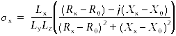
where L is the length and R₀ and X₀ refer to the measured impedance of the filter. Conductance tensor components σ_y and σ_z were obtained by substitution in this formula.

To measure P-wave velocity along a given direction, the sample was held with a force of 49 N (corresponding to a pressure of 120 kPa) between two transducers (large-bandwidth transducers with a central working frequency at 500 MHz) covered with rubber spacers. The transmitter was connected to a pulse generator (Physical Acoustics C-101-HV), and the receiver was connected to an oscilloscope synchronized with the pulse generator. The oscilloscope signal was transferred to a computer, and the arrival time was picked and logged automatically. This configuration had a characteristic delay of 2.10 µs, which was subtracted from the arrival time to obtain the traveltime. The velocity along a given direction is simply given by the path length divided by the traveltime.

When only three measurements are made, the orientation of the tensor cannot be determined. However, some simplifications may be expected if the sample is almost transversely isotropic around the core axis. The apparent anisotropy in the horizontal plane is

.

(38)

Apparent transverse anisotropy is

.

(39)

For a truly transversely anisotropic medium in the core reference frame (x, y, and z), the anisotropy ratio α = a_I/a_T is a function of the dip of the foliation in the sample. Plotting the anisotropy ratio as a function of dip for a collection of samples within the same interval can resolve the ambiguity between a dipping transversely anisotropic medium and a fully anisotropic one.

At Site C0006, measurements in more directions that the three orthogonal ones described above were made by cutting off the eight corners of the cube at a bisecting angle to x, y, and z, providing a total of seven measurements. From these values, a best fitting ellipsoidal function (which requires a minimum of six measurements in different directions) was calculated following the method of Louis et al. (2004). Such an analysis can provide both anisotropy values and 3-D principal directions of the dominant microstructural feature (preferential alignment of matrix components, crack network, solution cleavage surfaces, etc.).

Apart from an instrumental uncertainty on the order of 1%, an important issue prior to interpreting electrical conductivity and P-wave velocity data is the effect of decreasing sample saturation prior to measurement. Electrical conductivity is strongly sensitive to the saturation of the pore network, and P-wave velocity is sensitive to water content through changes in the incompressibility modulus (K). The effects of decreasing saturation on electrical conductivity were not analyzed because this measurement was typically performed immediately after sawing the sample into a cube. However, in order to compensate for the effect of partial drying of the sample during the measurement, the first impedance value obtained across the sample was remeasured after impedances in the other two orientations were recorded.

P-wave velocity values are more likely to be affected by partial drying because of the time needed to cut the cubes into polyhedrons. We investigated the effect of drying on a cubic sample left at ambient laboratory conditions (average over the test of 20.4°C and 32.5% relative humidity). Traveltimes were measured along the three directions every 30 min until a stable level was reached (Fig. F28). The evolution of P-wave velocity with time is clearly nonlinear and indicates a considerable decrease of >20% over the first 2 h. This effect has the potential to exert a strong bias on the final velocity-depth profile and tensor. Moreover, further testing showed that, at least for some of the samples measured at Site C0006, this decrease in P-wave velocity could not be recovered through resaturation with seawater. After the tested sample had been immersed for <2 min in a beaker filled with seawater, we observed an increase of 10% in P-wave traveltime. This effect could be due to a loss of overall material cohesion associated with clay swelling or to dissolution of newly crystallized sodium chloride near the sample surface or within pore throats. We estimated the uncertainty associated with the drying process as a function of the typical time between the cutting operation and P-wave velocity measurement. Figure F28 suggests that an uncertainty of –0.2 km/s appears appropriate for a duration of up to 1 h for the full measurement process.

Thermal conductivity

Thermal conductivity was measured on unconsolidated sediment and rock samples using either the full-space needle probe (Von Herzen and Maxwell, 1959) or the half-space line source (Vacquier, 1985), depending on the consolidation state of the material being measured. Both the full- and half-space methods approximate the heating element as an infinite line source (Blum, 1997). These measurements produce a scalar value in a plane perpendicular to the orientation of the probe. All measurements were made after the cores had equilibrated to ambient laboratory temperature. At the beginning of each measurement, temperature in the samples was monitored to ensure that the background thermal drift was <0.04°C/min. After the background thermal drift was determined to be stable, the heater circuit was closed and the increase in the probe temperature was recorded. In most cases the reported thermal conductivity value for full-space needle probe measurements is the average of at least three repeated measurements. For half-space line source thermal conductivity, values typically represent the average of between five and ten repeated measurements. Based on repeated measurements, individual measurements are usually within 1% of the mean for both full- and half-space measurements. Both of these values are within the stated uncertainty of 5% (Blum, 1997). All data are corrected to in situ pressure and temperature, assuming a hydrostatic pressure gradient and a background temperature gradient based on advanced piston coring temperature tool (APCT3) and Davis-Villinger Temperature Probe (DVTP) or sediment temperature (SET) tool measurements. The pressure correction is +1% for each 1800 mbsf (Ratcliffe, 1960). In porous rocks, temperature influences thermal conductivity in two competing ways. The thermal conductivity of rock matrix is inversely related to temperature (Zoth and Haenel, 1988), whereas the thermal conductivity of water increases with temperature (Keenan et al., 1978). We applied a temperature correction of +1% for each +20°C change in temperature between laboratory and in situ conditions, a value intermediate between +5% suggested by Ratcliffe (1960) for a high-porosity water-saturated sediment and mean value of –3% derived from data reported by Clark (1966) for several hard rocks. Both uncorrected and corrected values of thermal conductivity are reported.

Unfortunately, many sites had sections of core where neither the full-space nor half-space method was appropriate. These sections are typified by consolidated material that was either loose or cracked when the needle probe was inserted such that good contact between core material and the needle probe was not possible or the material was so consolidated that the needle probe could not be inserted. Although these sections were consolidated, they also lacked pieces large enough for the half-space method. Divided bar measurements are planned postcruise to fill in these intervals. Importantly though, these intervals were below the depths of temperature measurements so that the lack of thermal conductivity measurements does not affect the determination of heat flow. They do, however, affect the confidence with which temperature can be extrapolated to depth.

Soft-sediment full-space measurements

A full-space single-needle probe TeKa TK04 unit (Blum, 1997) was utilized to measure thermal conductivity of HPCS whole cores. To insert this probe, a 2 mm hole was made in the core liner at a position based on visual inspection of the core supplemented in some cases with CT scans. Needle probes consist of a heater wire and a thermistor. At the beginning of each measurement, temperature in the sediment was monitored to ensure that a thermal drift of no more than 0.4 mK/min was present. This step normally took 1–2 min. After the temperature field was determined to be near equilibrium, a calibrated heat source was applied and the rise in temperature was recorded for ~80 s. Values of thermal conductivity were based on the observed rise in temperature for a given quantity of heat. In most cases, repeated measurements were made at the same location and the needle probe was left in place to reequilibrate for 10 min prior to the next measurement. Thus, most of the measurement time consisted of waiting for the sample to reequilibrate.

Between holes or when time permitted, the needle probe was calibrated using three standards with thermal conductivities of 0.517 (rubber), 1.237 (glass), and 1.623 W/(m·K) (Fig. F29A). These measurements were plotted against true values, and the slope of the linear regression gave constants that were used to calibrate the needle probe (Table T13).

With increasing depths, sediments became more consolidated such that it was not possible to simply insert the needle probe into the core without damaging the probe. In these cases, a half-space line source was used to measure thermal conductivity.

Lithified sediment and hard rock half-space measurements

Increased consolidation of core sediments with depth required thermal conductivity measurements to be conducted on split core halves instead of on whole-round samples. At Site C0004, a Kyoto Electronics QTM-500 quick thermal conductivity meter was utilized for thermal conductivity measurements on lithified samples, and for later sites, the TK04 device was used in half-space mode. Selected samples taken from split-core working halves were relatively intact and at least 8 cm long. Samples were placed in a seawater bath for at least 15 min. For the QTM-500 device, samples were placed in plastic wrap to protect the line source. Care was taken to remove any visible air bubbles between the plastic wrap and the sample surface. The heating element/​temperature probe was then placed on a flat surface of the sample, and heating and temperature measurements were conducted by the instrument. Between measurements, the sample was allowed to cool for at least 10 min. For measurements made with the QTM-500, each reported value consists of an average of three measurements, whereas measurements made with the TeKa device report values consisting of 5–10 measurements. Calibration procedures for this half-space heating technique are similar to those for the needle probe technique used on whole-round samples. For the TeKa device, calibrations were made using four standards with thermal conductivities of 0.517 (rubber), 1.237 (glass), 1.414, and 1.623 W/(m·K) (Fig. F29B), whereas for the QTM-500 only three standards were used (Fig. F29C). These measurements are plotted against the true values and calibrations constants determined through a least-squares inversion (Table T13).

In situ temperature measurements

In situ temperature measurements were made using the APCT3, DVTP, and SET tool. The APCT3 is the third-generation tool of its kind and is used with the HPCS. The APCT3 consists of three components: electronics, coring hardware, and computer software. The SET tool was developed by IODP, based on the DVTP design used during ODP and early IODP expeditions. Improved electronics and packaging provides high-resolution temperature measurements. The SET tool was used to take temperature measurements in stiffer formations during Expedition 316. During Expedition 316, in situ temperature measurements were made for approximately every third core during HPCS coring. The temperature sensors were calibrated for a working range of 0°–45°C.

Prior to entering the hole, each instrument was held at the approximate mudline for ~5 min to equilibrate with bottom water temperature. However, the core winch depth meter was not calibrated, and site variability in measured bottom water temperature is likely due to uncertainties in depth. After bottom water temperature equilibration, the tools were lowered down the hole and penetrated the formation. The penetration of each tool into the formation causes a rise in temperature because of frictional heating. Following the initial rise in temperature, temperature decreases along a decay curve to near equilibrium. During this decay phase, it is important that the temperature tool is not disturbed. A second rise in temperature is due to frictional heating as the tool is pulled out of the formation. Temperature was measured as a time series sampled every 1 s and logged onto a microprocessor within the downhole tool; when the tool was retrieved, data were downloaded to the computer. The formation equilibrium temperature is determined based on fitting the temperature decay curve using the program TP-Fit, which runs on Matlab (M. Heeseman, pers. comm., 2007).

Determination of heat flow

If heat transfer is by conduction and heat flow is constant, the thermal gradient will be inversely proportional to thermal conductivity, according to Fourier’s law. This relationship can be linearized by plotting temperature as a function of summed thermal resistance (Bullard, 1939):

(40)

where

• T = temperature,
• z = depth,
• T_o = bottom water temperature,
• = thermal resistance, and
• N = number of thermal conductivity measurments.

In practice, q and T_o are estimated by plotting T(z) against summed thermal resistance.

MSCL-I: photo image logger

The MSCL-I scans the surface of archive-half cores and creates a digital image. The line-scan camera is equipped with three charge-coupled devices; each charge-coupled device has 1024 arrays. Light reflection from the sample surface passes through the lens and is split into three paths (red, green, and blue) by a beam splitter inside the line-scan camera. Then, each reflection is detected by the corresponding charge-coupled device. Finally, the signals are combined and the digital image is reproduced. Optical distortion downcore is avoided by precise movement of the camera. Spatial resolution is 100 pixels/cm.

MSCL-C: color spectroscopy logger

The MSCL-C system is equipped with a color spectrophotometer (Konica-Minolta, CM-2600d). The aluminum frame of the instrument allows operators to load up to seven core sections, and the sensor unit (including the spectrophotometer and small distance laser measuring system) translates along each section and moves down at each measurement point to measure the split archive core surface.

Light reflected from the sample surface is collected in the color spectrophotometer’s integration sphere. The instrument’s structure allows for the specular component to be included (SCI setting) or excluded (SCE setting). The SCE setting is the recommended mode of operation, especially for sediments, to exclude glare. The light is divided into wavelengths at a 10 nm pitch (400–700 nm), and the spectral sensors in the sphere convert the light to electrical currents proportional to the intensity of the light. Next, the color spectrum from the sample is normalized by the source light of the reflectance. The obtained spectrum is calibrated with the measurement of a pure white standard, which has a high reflectance true value at visible wavelengths and is measured by the vendor and with a black box (zero calibration). Measurements can be calculated based on the 2° or 10° standard observer and any of 11 illuminants.

Color reflectance is categorized as an IODP standard measurement, and the measured color spectrum is normally converted to L*, a*, and b* parameters. L*, a*, and b* provide relative changes in the composition of the bulk material and are widely used to correlate sections from core to core or hole to hole and to analyze the characteristic and cyclicity of lithologic changes.

Core-log-seismic integration

There was no downhole logging during Expedition 316. The integration of logging-while-drilling (LWD) data with seismic reflection data for Sites C0004 and C0006 was conducted during IODP Expedition 314. The reference seismic profiles are prestack depth-migrated lines from the CDEX and IFREE 3-D surveys (see Moore et al.). At Site C0004, seismic depth-migrated reflections were fit to the LWD check shot data by the Expedition 314 shipboard science party. However, at Site C0006, reflection depths had not yet been check shot–corrected at the time of Expedition 316.

The integration of cores with seismic data relies primarily on the presence of key boundaries, including unconformities, lithologic changes, and faults. Hole locations and MSCL-W data (e.g., NGR) are referenced to 3-D seismic data so that they can be accurately correlated to seismic data. Stratum and fault reflections in the 3-D seismic data are illuminated for the interpretation of lithology, structural patterns, and the integration between core and LWD data. Some of these reflections become key boundaries.

The integration of core data with LWD data relies primarily on correlations between lithologic boundaries and P-wave velocity and NGR from MSCL data. NGR data are especially useful for correlation between cores and logs. The LWD geoVISION resistivity tool was used at Sites C0004 and C0006 and comprises NGR measurements, resistivity measurements, and resistivity-at-the-bit (RAB) borehole images. Sonic log data are available from the sonicVISION tool and can also be compared with P-wave velocity from MSCL measurements on HPCS cores or with measurements on discrete samples (MAD and P-wave velocity measurements).

MSCL-W gamma emission data are reported in counts per second, and the only calibration is an ambient noise measurement (~40 cps for MSCL-W). Values below 15 cps (or 55 cps before noise correction) were discarded because they often correspond to voids. The LWD gamma ray tool records natural gamma rays in the formations adjacent to the borehole. This nuclear measurement indicates the radioactive content of the formations. Its unit is American Petroleum Institute gamma ray unit (gAPI).

LWD depth below seafloor (LSF) is used as the depth reference for LWD logs. There are two definitions of core depth. In the standard definition of core depth below seafloor (CSF), the core depth is added to the depth of the drill bit at the beginning of coring. This definition leads to overlaps between expanded HPCS cores and, in some cases, between RCB cores when drilling fluid and/or cuttings enter the core barrel. The core depth below seafloor (CSF-B) depth is also given by J-CORES and corrects the discrepancy between the length of expanded cores and the advance of the drill bit by applying an arbitrary linear correction over the whole length of core. The correlation between core depth below seafloor and LWD depth below seafloor is based on the CSF-B depth in the intervals with expanded cores. Depth transfer functions are defined by linear regression between correlated peaks. In general, cores with <50% recovery do not provide useful constraints. In intervals with better recovery, several peak-to-peak correlations within a single RCB core indicate that the core log may be condensed by 5%–30% with respect to LWD data. This is interpreted that partial recovery can be spread over most of the cored interval.

Top of page   |    Previous   |    Next