Betzler, C., Eberli, G.P., Alvarez Zarikian, C.A., and the Expedition 359 Scientists
Proceedings of the International Ocean Discovery Program Volume 359
publications.iodp.org
doi:10.14379/iodp.proc.359.102.2017

Expedition 359 methods1
C. Betzler, G.P. Eberli, C.A. Alvarez Zarikian, M. Alonso-García, O.M. Bialik, C.L. Blättler, J.A. Guo, S. Haffen, S. Horozal, M. Inoue, L. Jovane, D. Kroon, L. Lanci, J.C. Laya, A. Ling Hui Mee, T. Lüdmann, M. Nakakuni, B.N. Nath, K. Niino, L.M. Petruny, S.D. Pratiwi, J.J.G. Reijmer, J. Reolid, A.L. Slagle, C.R. Sloss, X. Su, P.K. Swart, J.D. Wright, Z. Yao, and J.R. Young2
Keywords: International Ocean Discovery Program, IODP, JOIDES Resolution, Expedition 359, Site U1465, Site U1466, Site U1467, Site U1468, Site U1469, Site U1470, Site U1471, Site U1472, Maldives, Kardiva Channel, Goidhoo atoll, Indian Ocean paleoceanography, Oligocene, Miocene, Pliocene, Pleistocene, carbonate platform, carbonate platform drowning, celestine, dolomite, drift deposits, large benthic foraminifers, monsoon, sea level, sequence stratigraphy
MS 359-102: Published 4 May 2017
Introduction, background, and operations
This chapter documents the procedures and methods employed in the various shipboard laboratories on the research vessel (R/V) JOIDES Resolution during International Ocean Discovery Program (IODP) Expedition 359. This information applies only to shipboard work described in the expedition reports section of the Expedition 359 Proceedings of the International Ocean Discovery Program volume. Methods used by investigators for shore-based analyses of Expedition 359 data will be described in separate individual publications. This introductory section provides an overview of operations, curatorial conventions, depth scale terminology, and general core handling and analyses.
Site locations
GPS coordinates from pre-expedition site surveys were used to position the vessel at all Expedition 359 sites. A SyQuest Bathy 2010 compressed high-intensity radar pulse (CHIRP) subbottom profiler was used to monitor seafloor depth on the approach to each site to confirm the depth profiles from pre-expedition surveys. Once the vessel was positioned over a site’s coordinates, the thrusters were lowered and a positioning beacon was dropped to the seafloor. Dynamic positioning control of the vessel used navigational input from the GPS system and triangulation to the seafloor beacon, weighted by the estimated positional accuracy. The final hole position was the mean position calculated from GPS data collected over a significant time interval.
Coring and drilling operations
All three standard coring systems, the advanced piston corer (APC), extended core barrel (XCB), and rotary core barrel (RCB) systems, were used during Expedition 359. The APC was used in the upper portion of each hole (except at Site U1469 where only the RCB system was used [see Operations in the Site U1469 chapter (Betzler et al., 2017d)]) to obtain higher quality core. The APC cuts soft-sediment cores with minimal coring disturbance relative to other IODP coring systems. After the APC core barrel is lowered through the drill pipe and lands near the bit, the drill pipe is pressured up until the two shear pins that hold the inner barrel attached to the outer barrel fail. The inner barrel then advances into the formation and cuts the core. The driller can detect a successful cut, or “full stroke,” from the pressure gauge on the rig floor.
APC refusal is conventionally defined in two ways: (1) the piston fails to achieve a complete stroke (as determined from the pump pressure reading) because the formation is too hard, or (2) excessive force (>60,000 lb; ~267 kN) is required to pull the core barrel out of the formation. When a full stroke cannot be achieved, additional attempts are typically made, and after each attempt, the bit is advanced by the length of core recovered. The number of additional attempts is generally dictated by the length of recovery of the partial stroke core and the time available to advance the hole by piston coring. This results in a nominal recovery of ~100% based on the assumption that the barrel penetrates the formation by the equivalent of the length of core recovered. When a full or partial stroke is achieved but excessive force cannot retrieve the barrel, the core barrel is sometimes “drilled over,” meaning after the inner core barrel is successfully shot into the formation, the drill bit is advanced to total depth to free the APC barrel.
The standard APC coring system contains a 9.5 m long core barrel. Expedition 359 also used the half-length APC (HLAPC) coring system, which uses a 4.7 m long core barrel. In most instances, the HLAPC system was deployed after APC refusal. During use of the HLAPC system, the same criteria for refusal were applied as for the APC system. Use of this new technology allowed for significantly greater continuous APC sampling depths to be attained than would have otherwise been possible.
Nonmagnetic core barrels were used during all APC deployments to a pull force of ~40,000 lb. APC cores were oriented using the FlexIT tool (see Paleomagnetism). Formation temperature measurements were made with the advanced piston corer temperature tool (APCT-3). The APCT-3 was used to obtain temperature gradients and heat flow estimates (see Downhole measurements) for APC holes. A newly designed Motion Decoupled Hydraulic Delivery System (MDHDS) used to deploy the Sediment Temperature Tool (SET2) was tested at Sites U1467 and U1471. The MDHDS is designed to decouple the SET2 from the ship heave and thereby give more accurate readings because of reduced movement in sediment (see Operations in the Site U1467 and Site U1471 chapters [Betzler et al., 2017c, 2017e]).
The XCB coring system was used to advance the hole when APC refusal occurred before the target depth was reached or when either the formation became too stiff for APC coring or hard substrate was encountered. The XCB system is a rotary system with a small cutting shoe (bit) that extends below the large APC/XCB bit. The smaller bit can cut a semi-indurated core with less torque and fluid circulation than the main bit, optimizing recovery. The XCB cutting shoe extends ~30.5 cm ahead of the main bit in soft sediment but retracts into the main bit when hard formations are encountered. XCB core barrels are 9.5 m long.
The bottom-hole assembly (BHA) is the lowermost part of the drill string. The exact configuration of the BHA is reported in the Operations section of each site chapter. A typical APC/XCB BHA consisted of a drill bit (outer diameter = 11⁷⁄₁₆ inch), a bit sub, a seal bore drill collar, a landing saver sub, a modified top sub, a modified head sub, a nonmagnetic drill collar (for APC/XCB), a number of 8 inch (~20.32 cm) drill collars, a tapered drill collar, six joints (two stands) of 5½ inch (~13.97 cm) drill pipe, and one crossover sub. A lockable float valve was used when downhole logging was planned so that downhole logs could be collected through the bit.
The RCB coring system was deployed when the formation became too hard for XCB coring. The RCB system is the most conventional rotary drilling system and was used during Expedition 359 to drill and core into lithified carbonate rocks. The RCB system requires a dedicated RCB BHA and a dedicated RCB drilling bit. The BHA used for RCB coring included a 9⅞ inch RCB drill bit, a mechanical bit release (if logging was considered), a modified head sub, an outer core barrel, a modified top sub, a modified head sub, and seven to ten control-length drill collars followed by a tapered drill collar to the two stands of 5½ inch drill pipe. Most cored intervals are ~9.7 m long, which is the length of a standard rotary core and approximately the length of a joint of drill pipe. In some cases, the drill string is drilled or “washed” ahead without recovering sediment to advance the drill bit to a target depth to resume core recovery. Such intervals are typically drilled using a center bit installed within the RCB bit. During RCB coring, half cores were sometimes collected to improve recovery.
Core handling and analysis
Cores recovered during Expedition 359 were extracted from the core barrel in 67 mm diameter plastic liners. These liners were carried from the rig floor to the core processing area on the catwalk outside the core laboratory, where they were split into ~1.5 m sections. The exact section length was noted and later entered into the database as “created length” using the SampleMaster application. This number was used to calculate recovery. Headspace samples were taken from selected section ends (at least one per core) using a syringe for immediate hydrocarbon analysis as part of the shipboard safety and pollution prevention program. Similarly, whole-round samples for interstitial water (IW) were cut on the catwalk at the same sampling resolution. Core catcher samples were taken for biostratigraphic analysis. When catwalk sampling was complete, liner caps (blue = top; colorless = bottom; yellow = bottom; whole-round cut) were glued with acetone onto liner sections, and the sections were placed in core racks in the laboratory for analysis. Rhizon IW samples were taken from selected intervals in addition to whole rounds after the whole-round core sections were measured for physical properties (see Geochemistry).
Indurated rock core pieces were slid out of the liners and placed in order in new, clean sections of core liner that were already split in half. Pieces having a vertical length greater than the internal (horizontal) diameter of the core liner are considered oriented pieces because they could have rotated only around their vertical axes. Those pieces were immediately marked on the bottom with a red wax pencil to preserve their vertical (upward) orientations. Pieces that were too small to be oriented with certainty were left unmarked. Adjacent but broken core pieces that could be fit together along fractures were curated as single pieces. The carbonate sedimentologist on shift confirmed the piece matches and corrected any errors.
Core sections were then placed in core racks in the laboratory. When the cores reached equilibrium with laboratory temperature (typically after ~4 h), whole-round core sections were run through the Whole-Round Multisensor Logger (WRMSL; measuring P-wave velocity, density, and magnetic susceptibility) and the Natural Gamma Radiation Logger (NGRL). Thermal conductivity measurements were typically taken at a rate of one per core (see Physical properties). Core sections were then split lengthwise from bottom to top into working and archive halves. This process may transport older material upward on the split face of each section during splitting. For hard rock sections, each piece of core was split with a diamond-impregnated saw into archive and working halves.
The working half of each core was sampled for shipboard biostratigraphic, physical properties, carbonate, paleomagnetic, and inductively coupled plasma–atomic emission spectroscopy (ICP-AES) analyses. Archive halves of all cores were scanned on the Section Half Imaging Logger (SHIL) with a line scan camera at 20 pixels/mm and measured for color reflectance and magnetic susceptibility on the Section Half Multisensor Logger (SHMSL). At the same time, archive halves were described visually and by means of smear slides and thin sections. All observations were recorded in the Laboratory Information Management System (LIMS) database using DESClogik, a descriptive data capture application. After visual description, archive halves were run through the cryogenic magnetometer. Finally, digital color close-up images were taken of particular features of the archive or working halves, as requested by individual scientists. For hard sedimentary rock cores, routine sampling meetings were held to select key sampling intervals for shipboard and limited shore-based analyses. Discrete samples were taken from working halves for physical properties, paleomagnetism, thin section, and ICP-AES analyses. After these shipboard samples were taken, limited sampling for personal postexpedition research was conducted on the working halves. The IODP curator kept records of all samples taken.
Both halves of the core were put into labeled plastic tubes (D-tubes) that were sealed and transferred to cold storage space aboard the ship. At the end of the expedition, the cores were transported to cold storage at the Gulf Coast Repository at Texas A&M University (USA) for inventory and preparation for the postexpedition sampling party. After the sampling party was completed, all Expedition 359 cores were shipped to permanent cold storage at the Kochi Core Center (Japan), which houses cores collected from the western Pacific Ocean, Indian Ocean, Kerguelen Plateau, and Bering Sea.
Drilling disturbance
Cores may be significantly disturbed as a result of the drilling process and may contain extraneous material as a result of the coring and core handling processes. In formations with loose sand layers, sand from intervals higher in the hole may be washed down by drilling circulation, accumulate at the bottom of the hole, and be sampled with the next core. The uppermost 10–50 cm of each core must therefore be examined critically during description for potential “fall-in.” Common coring-induced deformation includes the concave-downward appearance of originally horizontal bedding. Piston action may result in fluidization (“flow-in”) at the bottom of APC cores. Retrieval from depth to the surface may result in elastic rebound. Gas that is in solution at depth may become free and drive core segments within the liner apart. Both elastic rebound and gas pressure can result in a total length for each core that is longer than the interval that was cored and thus a calculated recovery of >100%. If gas expansion or other coring disturbance results in a void in any particular core section, the void can be closed by either moving material to the very large void, stabilized by a foam insert if moderately large, or left as is. These disturbances are described in the Lithostratigraphy sections of each site chapter and are graphically indicated on the core summary graphic reports (digital visual core descriptions [VCDs]). Core disturbance by gas was minimal during Expedition 359. The few core sections so affected are marked by a yellow label with the word “disturbed,” and the nature of the disturbance is noted in the coring log.
Curatorial procedures
Numbering of sites, holes, cores, and samples follows standard IODP procedure. Drilling sites are numbered consecutively from the first site drilled by the drilling vessel (D/V) Glomar Challenger in 1968. Integrated Ocean Drilling Program Expedition 301 began using the prefix “U” to designate sites occupied by the United States Implementing Organization (USIO) platform, the JOIDES Resolution. This practice is continued today by IODP and the JOIDES Resolution Science Operator (JRSO). For all IODP drill sites, a letter suffix distinguishes each hole drilled at the same site. The first hole drilled is assigned the site number modified by the suffix “A,” the second hole the site number and the suffix “B,” and so on.
Cores taken from a hole are numbered sequentially from the top of the hole downward. When an interval is drilled down, this interval is also numbered sequentially, and the drill down is designated by a “1” instead of a letter that designates the coring method used (e.g., 359-U1465A-11). Cores taken with the APC system are designated with “H” (APC cores) or “F” (HLAPC cores), “X” designates XCB cores, and “R” designates RCB cores. “G” designates “ghost” cores that are collected while washing down through a previously drilled portion of a hole with a core barrel in place. The core barrel is then retrieved prior to coring the next interval. Core numbers and their associated cored intervals are unique in a given hole. Generally, maximum recovery for a single core is 9.5 m of sediment (APC) or 9.7 m of rock or sediment (XCB/RCB) contained in a plastic liner (6.6 cm internal diameter) plus an additional ~0.2 m in the core catcher, which is a device at the bottom of the core barrel that prevents the core from sliding out when the barrel is retrieved from the hole. In certain situations, recovery may exceed the 9.5 or 9.7 m maximum. In soft sediment, this is normally caused by core expansion resulting from depressurization. In hard rock cores, this typically occurs when a pedestal of rock fails to break off and is grabbed by the core barrel of the subsequent core. High heave, tidal changes, and overdrilling can also result in an advance that differs from the planned 9.5/9.7 m.
Recovered cores are divided into 1.5 m sections that are numbered serially from the top downcore. When full recovery is obtained, the sections are numbered 1–7, with the last section usually being <1.5 m. Rarely, an unusually long core may require more than seven sections. When the recovered core is shorter than the cored interval, by convention the top of the core is deemed to be located at the top of the cored interval for the purpose of calculating (consistent) depths. When coring hard rock, all pieces recovered are placed immediately adjacent to each other in the core tray. Samples and descriptions of cores are designated by distance, measured in centimeters, from the top of the section to the top and bottom of each sample or interval. By convention, hard rock material recovered from the core catcher is placed below the last section. In sedimentary cores, the core catcher section is treated as a separate section (“CC”). When the only recovered material is in the core catcher, it is placed at the top of the cored interval.
A full curatorial sample identifier consists of the following information: expedition, site, hole, core number, core type, section number, and interval in centimeters measured from the top of the core section. For example, a sample identification of “359-U1469C-2H-5, 80–85 cm,” represents a sample taken from the interval between 80 and 85 cm below the top of Section 5 of Core 2 (collected using the APC system) of Hole C of Site U1469 during Expedition 359.
Sample depth calculations
The primary depth scale types are based on the measurement of the drill string length deployed beneath the rig floor (drilling depth below rig floor [DRF] and drilling depth below seafloor [DSF]), the length of each core recovered (core depth below seafloor [CSF] and core composite depth below seafloor [CCSF]), and the length of the logging wireline deployed (wireline log depth below rig floor [WRF], wireline log depth below seafloor [WSF], and wireline log matched depth below seafloor [WMSF]). All units are in meters. Depths of samples and measurements are calculated at the applicable depth scale either by fixed protocol (e.g., CSF) or by combinations of protocols with user-defined correlations (e.g., CCSF). The definition of these depth scale types and the distinction in nomenclature should keep the user aware that a nominal depth value at two different depth scale types usually does not refer to exactly the same stratigraphic interval in a hole.
Depths of cored intervals are measured from the drill floor based on the length of drill pipe deployed beneath the rig floor (DRF scale). The depth of the cored interval is referenced to the seafloor (DSF scale) by subtracting the seafloor depth at the time of the first hole from the DRF depth of the interval. In most cases, the seafloor depth is the length of pipe deployed minus the length of the mudline core recovered. However, some seafloor depths were determined by offset from a previous known measurement of depth or by tagging the seafloor with the camera system in place.
Standard depths of cores in meters below the seafloor (CSF-A scale) are determined based on the assumptions that (1) the top depth of a recovered core corresponds to the top depth of its cored interval (DSF scale) and (2) the recovered material is a contiguous section even if core segments are separated by voids when recovered. Voids in the core are closed by pushing core segments together, if possible, during core handling. This convention is also applied if a core has incomplete recovery, in which case the true position of the core within the cored interval is unknown and should be considered a sample depth uncertainty, up to the length of the core barrel used, when analyzing data associated with the core material. Standard depths of samples and associated measurements (CSF-A scale) are calculated by adding the offset of the sample or measurement from the top of its section and the lengths of all higher sections in the core to the top depth of the cored interval.
A soft to semisoft sediment core from less than a few hundred meters below seafloor expands upon recovery (typically a few percent to as much as 15%), so the length of the recovered core exceeds that of the cored interval. Therefore, a stratigraphic interval may not have the same nominal depth at the DSF and CSF scales in the same hole. When core recovery (the ratio of recovered core to cored interval times 100%) is >100%, the CSF depth of a sample taken from the bottom of a core will be deeper than that of a sample from the top of the subsequent core (i.e., the data associated with the two core intervals overlap at the CSF-A scale).
Core composite depth scales (CCSF) are constructed to mitigate the CSF-A core overlap or coring gap problems and to create as continuous a stratigraphic record as possible. Using shipboard track-based physical properties data verified with core photos, core depths in adjacent holes at a site are vertically shifted to correlate between cores recovered in adjacent holes. This process produces the CCSF-A depth scale. The correlation process results in affine tables, indicating the vertical shift of cores at the CCSF scale relative to the CSF-A scale. Once the CCSF scale is constructed, a splice can be defined that best represents the stratigraphy of a site by utilizing and splicing the best portions of individual sections and cores from each hole at a site. This process produces the CCSF-D depth scale, which is strictly correct only along the splice. Because of core expansion, the CCSF-A/D depths of stratigraphic intervals are typically 10%–15% deeper than their CSF-A depths. CCSF-A construction also reveals that coring gaps on the order of 1–1.5 m may occur between two subsequent cores, despite the apparent >100% recovery.
Cored intervals are defined by the core top depth on the DSF scale and the distance the driller advanced the bit and/or core barrel in meters. The length of the core is defined by the sum of the lengths of core sections. The CSF depth of a sample is calculated by adding the offset of the sample below the section top and the lengths of all higher sections in the core to the core top depth measured with the drill string (DSF). During Expedition 359, all core depths below seafloor were calculated according to CSF Method A (CSF-A) depth scale (see IODP Depth Scales Terminology, v.2, at http://www.iodp.org/policies-and-guidelines). To more easily communicate shipboard results, CSF-A depths are reported in this volume in text, tables, and figures as meters below seafloor (mbsf) unless otherwise noted.
Authorship of site chapters
The separate sections of the site chapters and Methods chapter were written by the following shipboard scientists (authors are listed in alphabetical order; no seniority is implied):
- Background and objectives: C. Betzler, G.P. Eberli
- Operations: C.A. Alvarez Zarikian, M. Storms
- Lithostratigraphy: O. Bialik, J.C. Laya, A. Ling Hui Mee, B.N. Nath, J.J.G. Reijmer, J. Reolid, C. Sloss, Z. Yao
- Biostratigraphy: M. Alonso-Garcia, C.A. Alvarez Zarikian, D. Kroon, K. Niino, L.M. Petruny, S.D. Pratiwi, X. Su, J. Young
- Geochemistry: C.L. Blättler, M. Inoue, M. Nakakuni, P.K. Swart
- Paleomagnetism: L. Jovane, L. Lanci
- Physical properties: J. Guo, S. Haffen, S. Horozal
- Downhole measurements: T. Lüdmann, A.L. Slagle
- Stratigraphic correlation and sedimentation rates: J.D. Wright
- Seismic stratigraphy: C. Betzler, G.P. Eberli, T. Lüdmann.
Lithostratigraphy and sedimentology
The primary procedures used for lithostratigraphic analysis during Expedition 359 included visual core description, sediment classification, digital color imaging, and smear slide and thin section description. These analyses are complemented by color spectrophotometry and point source magnetic susceptibility data acquired prior to core description, which are described in detail in Physical properties. Carbonate, organic matter (carbon-hydrogen-nitrogen-sulfur [CHNS] analysis), X-ray diffraction (XRD), and geochemical measurements are described in detail in Geochemistry.
Core preparation
The standard method of splitting cores into working and archive halves (using either piano wire or a saw) can affect the appearance of the split-core surface and obscure fine details of lithology and sedimentary structure. When necessary, the archive halves of cores were gently scraped using a stainless steel or glass scraper to prepare the surface for sedimentologic examination and digital imaging. Scraping parallel to bedding with a freshly cleaned tool prevented contamination. Cleaned sections were then photographed using the SHIL and measured for magnetic susceptibility using the SHMSL (see Physical properties).
Sediment and rock classification
Sediments were described using a modified classification scheme derived from those of Ocean Drilling Program (ODP) Legs 166 and 194 (Shipboard Scientific Party, 1997a, 2002) and Integrated Ocean Drilling Program Expedition 346 (Tada et al., 2015a). For consistency and uniformity, the Dunham (1962) textural classification was applied in conjunction with the depositional textures described by Embry and Klovan (1972) (Figure F1). Following Dunham (1962), carbonate crystals or fragments smaller than 30 µm (not visible/determinable with a hand lens) are considered as matrix or microcrystalline carbonates known as micrite or mud. Constituents >30 µm are called grains. We used the following definitions:
- Mudstone = mud-supported fabric with <10% grains.
- Wackestone = mud-supported fabric with >10% grains.
- Packstone = grain-supported fabric with intergranular mud, >50% grains.
- Grainstone = mud-free grain-supported fabric.
- Floatstone = matrix-supported fabric grains, at least 10% of which are >2 mm in size.
- Rudstone = grain-supported fabric grains, at least 10% of which are >2 mm in size.
- Boundstone = components organically bound during deposition.
The boundstone group includes the following:
- Bafflestone = formed by organisms that act as baffles.
- Bindstone = formed by organisms that encrust or bind.
- Framestone = formed by organisms that build a rigid framework.
Figure F1. Textural classification scheme.
Nomenclature
Lithologic names assigned to sediments consist of a principal name and modifiers based on composition, texture, and degree of lithification, as well as texture as determined from visual core description. Additional detail to visual descriptions was derived from smear slide observations.
If possible, the major modifiers “skeletal” and “nonskeletal” were used to indicate the occurrence of bioclastic fragments and nonbioclastic allochems, respectively, within the carbonate sediments. The lack of such a modifier implies that components were not identified or that the sediments include an even proportion of skeletal and nonskeletal allochems. If nonskeletal components exceed 25%, then the lithology was determined to be nonskeletal.
Whenever dolomite or dolomitic texture was recognized (>25%) in carbonate sediments, the term “dolomitic” was used as a major modifier (e.g., dolomitic mudstone). When a lithology appeared to contain more than ~75% dolomite, it was called “dolostone” or, if skeletal components were recognized, “skeletal dolostone.”
Sediment core description
The following strategy was adopted before writing comments on the VCD template used for each core section (Figure F2):
- Digital photographs of every core section, including core catcher fraction and voids, were taken using the methodology described in Digital color imaging.
- Descriptive logging sheets and VCD forms with core photographs were printed and used for macroscopic core description.
- Cores were examined to identify boundaries, determine lithologies, identify key features, and identify samples to be collected (i.e., smear slide, thin section, and/or close-up photograph sites). Observations were recorded on the VCDs.
- Cores were described in detail on the VCDs following the procedure outlined in Visual core description.
- The archive halves of soft-sediment cores were analyzed with the contact core logger (SHMSL) to obtain spectral color reflectance data and point magnetic susceptibility (the latter is described in Physical properties).
- Information recorded on the VCDs was entered in the LIMS database using the data entry software DESClogik to store the data and produce the final digital VCDs (see Core descriptions). Entry parameters were customized according to the objectives of Expedition 359 and based on the above classification scheme.
- Ultimately, VCD data from different holes at a site were compiled into one figure and one table, visualizing an overview of lithostratigraphic units.
Figure F2. VCD form.
Visual core description
VCD sheets provide a summary of data collected during shipboard analysis of each core (Figure F2). Detailed observations of each section were initially recorded by hand on paper, adjacent to the printed scanned image of that section. Copies of these original descriptions were scanned and converted to PDF files and are included in SHIL in Supplementary material. The recorded data were subsequently entered with the DESClogik software into the LIMS database, which provides data that can be used in Strater to generate a simplified, annotated graphical description (VCD) for each core.
Site, hole, and depth (in meters CSF-A, or mbsf) are given at the top of the VCD sheets, with the corresponding depths of core sections along the right margin of the core photograph (depth acronyms follow the IODP Depth Scale Terminology at http://www.iodp.org/policies-and-guidelines). Columns on the VCD sheets include Lithologic unit, Core image, Shipboard samples, Coring disturbance (type and intensity), Graphic lithology, Texture classification (Dunham, 1962), Average grain size, Lithologic accessories (Components), Sedimentary structures, Lithification, Bioturbation intensity, Age, and Color. Profiles of magnetic susceptibility, natural gamma radiation (NGR), and reflectance (L*, a*, and b*) are also included. These columns are discussed in more detail below.
IODP conventions used for compiling hand-drawn and digital VCDs and the modifications to these procedures adopted during Expedition 359 are described below. The order of the following headers reflects the order from left to right of the columns on the hand-drawn section VCDs.
Photolog
The SHIL provided a detailed photo image of the section. A cropped image was produced and inserted into the VCD (see Digital color imaging).
Centimeter scale
This column lists the offset from the top of the section in centimeters.
Samples
Sample material for shipboard sedimentological and chemical analyses consisted of IW whole rounds, micropaleontology samples, smear slides, thin sections, and XRD samples for bulk analysis and was routinely taken from the core catcher of each core adjacent to the micropaleontological sample and at other levels of lithologic interest. Carbonate analyses were routinely taken from IW squeeze cakes at the rate of two per core and at additional levels where requested. The following abbreviations were used on the digital VCDs for samples: S = smear slide, TS = thin section, PAL = micropaleontology, CP = close-up photo, XRD = X-ray diffraction, and IW = interstitial water. All samples taken were noted in the Shipboard samples column with the following abbreviations: S = smear slide, C = carbonate, IW = interstitial water, P = micropaleontology, X = X-ray diffraction, T = thin section, and H = headspace.
Drilling disturbance
Because core disturbance from the drilling process can impact the integrity of the stratigraphic sequence, drilling disturbances, if any, are documented for both soft and firm sediment using the following classification scheme:
- Slightly disturbed: bedding contacts are slightly bent or bowed in a concave-downward appearance.
- Moderately disturbed: bedding is moderately deformed but probably still in the correct stratigraphic sequence.
- Heavily disturbed: sediment is completely deformed and may show no traces of original bedding or structure.
In addition to this first-order assessment of disturbance, a number of other terms (Figure F3) may appear on the VCDs to characterize drilling disturbance. Some of the more common types observed include the following:
- Flow-in: soupy, displaced sediment was pulled into the core liner during APC coring.
- Fall-in: downhole contamination resulting from loose material falling from the drill hole walls into the top of the core. The uppermost 10–15 cm of each core was inspected during description for potential fall-in.
- Bowed: bedding contacts are slightly to moderately deformed but still subhorizontal and continuous.
- Soupy/mousse-like (“soupy”): intervals are water saturated and have lost all aspects of original bedding.
- Biscuit: sediment of intermediate stiffness shows vertical variations in the degree of disturbance. Softer intervals are washed and/or soupy, whereas firmer intervals are relatively undisturbed.
- Cracked or fractured: firm sediment is broken but not displaced or rotated significantly.
- Fragmented or brecciated: firm sediment is pervasively broken and may be displaced or rotated.
Figure F3. Lithologic patterns.
Lithology
General terminology defining the type of rock/sediment. IODP generally uses standard lithologic descriptors (e.g., ooze for nonlithified sediments or limestone for hard calcareous rock made of aragonite, calcite, or Mg-calcite) to produce the standard lithologic column. However, during Expedition 359, the Dunham (1962) textural classification was applied in conjunction with the depositional textures described by Embry and Klovan (1972) to classify all carbonate sediments. Hard rock composed of dolomite was classified as dolostone.
Texture
Sedimentary textures in all levels of lithification and with no separation for environments and components were systematically classified using the Dunham (1962) textural classification with modification by Embry and Klovan (1972).
Color
Color was determined qualitatively using Munsell Soil Color Charts (Munsell Color Company, Inc., 1994) and described immediately after cores were split to avoid color changes associated with drying and redox reactions. When portions of the split core surface required cleaning with a stainless steel or glass scraper, they were cleaned prior to determining the color. Munsell color names and the corresponding hue and chroma values are provided in the Color column on the VCDs.
Grain size
Four major grain size classes were used: <63, 63–250, 250–2000, and >2000 µm (scale from Wentworth, 1922). Relative abundances of a sample were estimated based on sieving small samples taken from the working half. Alternatively, if sieving was not possible, the dominant grain size of the components is listed; grains were measured under a magnifying glass with respect to length scale.
Special notes for modality and matrix grain size are made in the Comments column.
Components
A preliminary list (prior to smear slides and thin sections) of components is given in Figure F3.
Sedimentary structures
This column includes sedimentary structures not related to bioturbation, syn- and postdepositional (e.g., grain sorting, cross-bedding, and erosional boundaries). The locations and types of stratification and sedimentary structures visible on the prepared surfaces of the split cores are shown on the hand-drawn section VCD. Symbols on the digital core VCD indicate the locations and scales of stratification and the locations of individual bedding features and any other sedimentary features, such as scours, ripple laminations, and fining-upward, coarsening-upward, or bigradational bedded intervals.
Lithification
Firmness of recovered materials was defined as in Gealy et al. (1971). Three levels of firmness were used to describe sediments and rocks, indicating the degree of lithification:
- Unlithified: soft sediments that have little strength and are readily deformed under the pressure of a fingernail or the broad blade of a spatula. Corresponds to the term “ooze” for pelagic calcareous sediments.
- Partially lithified: firm but friable sediments that can be scratched with a fingernail or the edge of a spatula blade.
- Lithified: hard, nonfriable cemented rock, difficult or impossible to scratch with a fingernail or the edge of a spatula.
Bioturbation
Five levels of bioturbation intensity were recognized using a scheme similar to that of Droser and Bottjer (1986). These levels are illustrated with a numeric scale in the Bioturbation intensity column.
- 1 = no bioturbation.
- 2 = slight bioturbation (<10%–30%).
- 3 = moderate bioturbation (>30%–60%).
- 4 = heavy bioturbation (>60%–90%).
- 5 = complete bioturbation (>90%).
Any identifiable trace fossils (ichnofossils) are identified in the bioturbation comments.
Layering
Layers and bedding thickness were further described and classified following terminology based on Stow (2005) and described in the comments column:
- Thin lamination = <3 mm thick.
- Medium lamination = 0.3–0.6 cm thick.
- Thick lamination = >0.6–1 cm thick.
- Very thin bed = >1–3 cm thick.
- Thin bed = >3–10 cm thick.
- Medium bed = >10–30 cm thick.
- Thick bed = >30–100 cm thick.
- Very thick bed = >100 cm thick.
Descriptive terms for bed boundaries, such as sharp, erosive, gradual, irregular, and bioturbated, are noted.
Comments
This section of the VCD contains a written summary of the lithologies graphically presented. Dominant and supporting skeletal components are listed in order of importance, as well as other distinctive observations that are not indicated graphically. Key features such as exposure surfaces, changes in mineralogy, sudden porosity changes, and so on, are noted for emphasis where they are critical to identifying lithologic unit boundaries. In some cases, informal interpretation of the depositional environment is additionally provided.
Other lithostratigraphy and sedimentology analyses
Smear slides
Smear slide samples were taken from archive halves during core description to determine the matrix of the sediments at locations with a major lithologic change. A small amount of sediment was removed with a wooden toothpick, dispersed evenly in deionized water on a 25 mm × 75 mm glass slide, and dried on a hot plate at a low setting. A drop of mounting medium (Norland Optical) and a 22 mm × 30 mm cover glass were added, and the slide was placed in an UV light box for ~15 min. Once fixed, each slide was scanned at ×100 to ×200 with a transmitted light petrographic microscope using an eyepiece micrometer to assess grain size distributions in clay (<4 µm), silt (4–63 µm), and sand (>63 µm) fractions. An eyepiece micrometer was calibrated once for each magnification and combination of ocular and objective using an inscribed stage micrometer.
Relative abundance (percent) of each grain size and type was estimated by microscopic examination. Smear slide analyses tend to underestimate the abundance of sand-sized and larger grains (e.g., foraminifers, radiolarians, and siliciclastic/volcaniclastic sand) because these are difficult to incorporate into the smear. After scanning for grain size distribution, several fields were examined at ×200 to ×500 for mineralogical and microfossil identification.
Standard petrographic techniques were employed to identify minerals and skeletal components, as well as important accessory minerals and microfossils. The smear slide analysis data worksheet used during these analyses is shown in Figure F4. The data generated are included in the core descriptions. These tables provide information about the sample location, a description of where the smear slide was taken, the estimated abundances of texture (i.e., sand, silt, and clay), and the relative composition of individual components in the sediment (i.e., detrital carbonate, biogenic carbonate, and biogenic silica).
Figure F4. Smear slide analysis data worksheet.
Relative abundances of identified components such as mineral grains, microfossils, and biogenic fragments were assigned on a semiquantitative basis using the following abbreviations:
- A = abundant (>20% of field of view).
- C = common (>5%–20% of field of view).
- F = few (1%–5% of field of view).
- R = rare (<1% of field of view).
- P = present (1 per 1–10 fields of view).
- B = barren (none in field of view).
Thin sections
Thin sections were described using dedicated forms for listing texture and skeletal and nonskeletal components and registering cement content and morphology; these forms include a hand drawing showing significant features (Figure F5). In addition, pore types were identified and percentage of visual porosity was estimated during this process.

Figure F5. Thin section analysis data worksheet.
Digital color imaging
The archive half of each core was placed in the SHIL, which captures continuous high-resolution images of the archive-half surface for analysis and description. Images were collected shortly after core splitting and surface scraping in an effort to avoid color changes resulting from excessive sediment drying and oxidation of the surface. The shipboard system uses a commercial line-scan camera lens (AF Micro Nikon; 60 mm; 1:2.8 D), with illumination provided by a custom assembly of three pairs of LED strip lights that provide constant illumination over a range of surface elevations. Each LED pair has a color temperature of 6,500 K and emits 90,000 lux at 3 inches. The resolution of the line-scan camera was set at 20 pixels/mm. Available files include the original high-resolution TIFF image with a gray scale and ruler and reduced JPEG images cropped to show only section-half surfaces. High-resolution color data (red, green, and blue) were acquired by digital color imaging. A manually cropped JPEG image was generated to assist in visual core description. Postprocessing of data included color balance (performed by the Imaging Specialist) and construction of a composite JPEG of each core.
Grain size distribution
Either small samples taken from the working halves or cleaning residue from the archive halves were used for grain size analysis. Samples were wet sieved and dry sieved using the following grain size classes: <63 µm, 63–250 µm, 250 µm to 2 mm, and >2 mm. Results were noted on the sieve sample analysis form (Figure F6).

Figure F6. Sieve grain size analysis worksheet.
Biostratigraphy
Calcareous nannofossils, radiolarians, ostracods, and foraminifers in core catcher samples were studied at all sites. Samples from core sections were also examined when a more refined age determination was necessary and when time permitted. Biostratigraphic events, mainly the first occurrence (FO or base) and last occurrence (LO or top) of diagnostic species, are tied to the geomagnetic polarity timescale of Gradstein et al. (2012). Because we mainly studied core catchers, the depth of an event was calculated as the midpoint between the two core catchers that enclose the event. Correlation of the zonation and events for the different groups is presented in Figure F7.
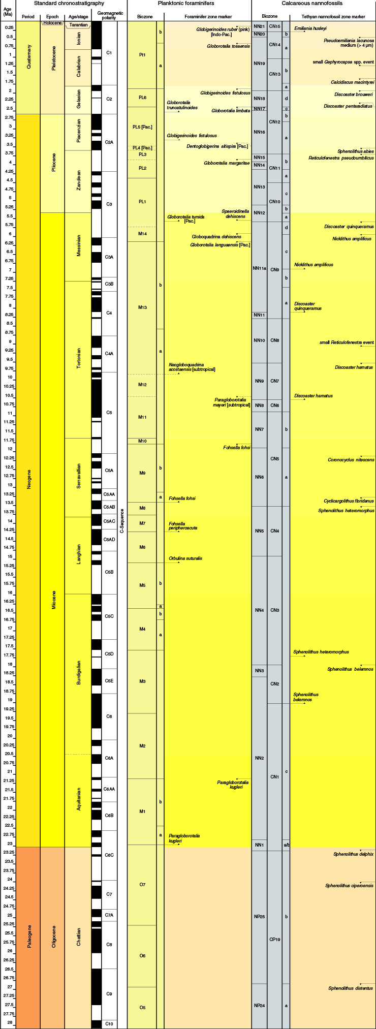
Figure F7. Zonation and events for planktonic foraminifers and calcareous nannofossil datums. This figure is available in an oversized format.
Calcareous nannofossils
Calcareous nannofossils were examined in smear slides using standard light microscope techniques under crossed polarizers, transmitted light, and phase contrast at 1000× magnification. Nannofossil taxonomy follows Young (1998), Hine and Weaver (1998), and Young et al. (2003) as synthesized on the Nannotax website (http://ina.tmsoc.org/Nannotax3). Bioevent ages were assigned based on the occurrence of calcareous nannofossils (dominant, present, or absent) in core catcher samples and in additional split-core sections when necessary. Calibration of the identified events was derived mainly from Gradstein et al. (2012) as synthesized in TimeScaleCreator v6.3. The principal events recognized are summarized in Table T1. The standard zonal scheme of Martini (1971) was adopted as a general frame of reference. However, for age models and intersite calibration, individual events were used according to their reliability and ease of recognition irrespective of whether they formed part of the standard zonation. The compilations of Backman et al. (2012) and Raffi et al. (2006) were used to provide additional information on the reliability, definition, and timing of events.
T1. Principal biostratigraphic events. Download table in .csv format.
Preparation techniques
Samples were primarily prepared following the rippled smear slide technique (Bown and Young, 1998) and mounted with Norland Optical Adhesive-NOA61. Coarse sands encountered at some sites were not easily prepared using smear slides, and in these levels suspension slides were used: a few millimeters cubed of crushed sediment was suspended in water in a 5 mL microcentrifuge tube and allowed to settle for approximately 30 s, and then a few drops of the overlying suspension were pipetted onto a slide. In addition, “mudline” samples were analyzed for core-top calcareous nannofossils. These samples were collected from the suspended sediment in the seawater recovered from above the sediment/seawater interface in the first core of each site. Approximately 20 mL of suspension was collected in a centrifuge tube and centrifuged at 3000 rpm for 1 min to separate the seawater, and the pellet was resuspended in a buffered solution. Selected samples were also examined using the shipboard scanning electron microscope (SEM) (Hitachi TM3000).
Data recording
To facilitate consistent data recording between the three nannofossil specialists, a common assemblage record sheet was produced (Figure F8). This sheet provided a list of all significant taxa we anticipated finding in the target interval (Holocene to the base of the Miocene) with, where relevant, brief indications of taxonomic concepts used. This sheet was transcribed into the DESClogik system and is available in the LIMS database (http://iodp.tamu.edu/tasapps).
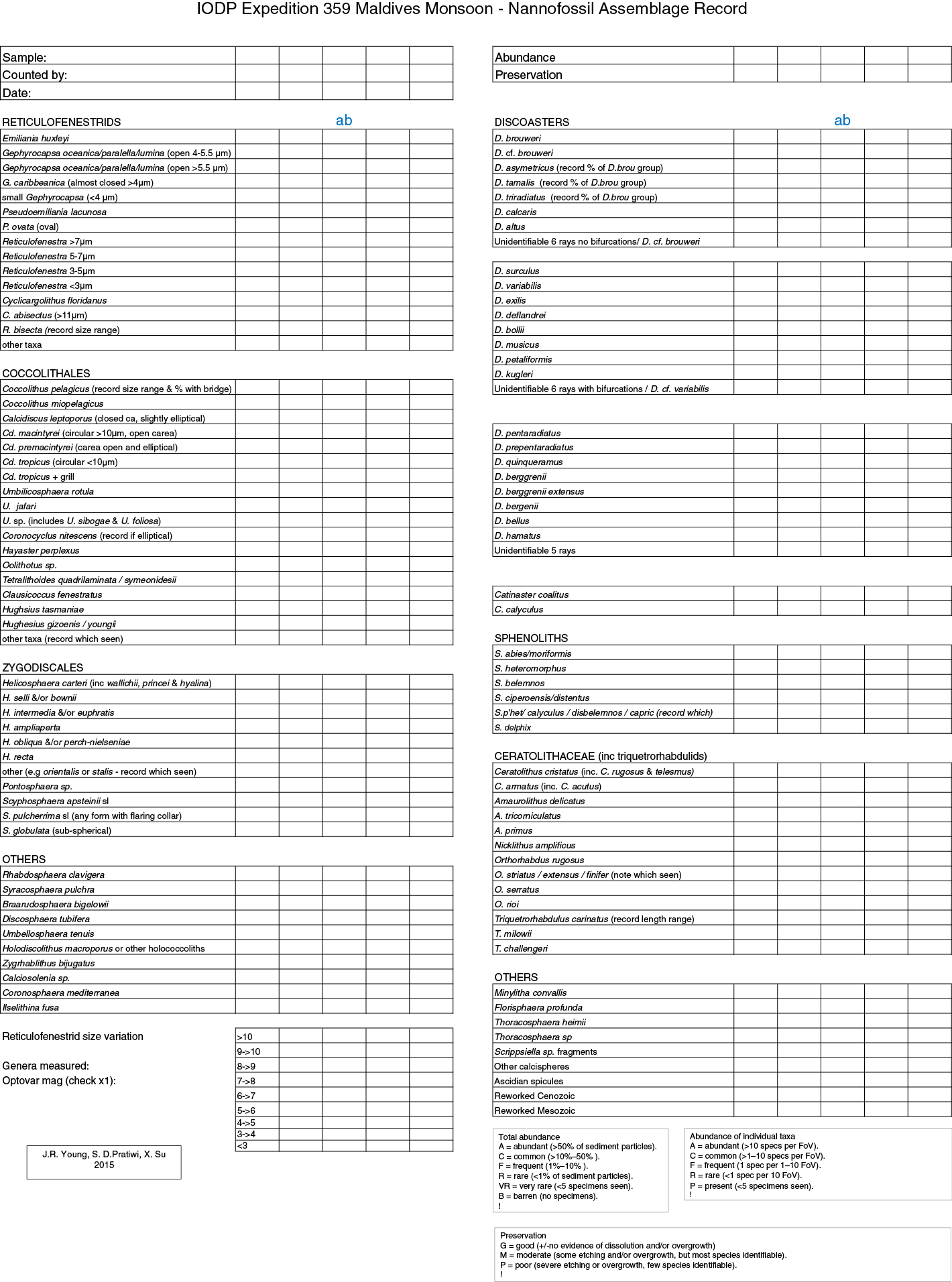
Figure F8. Calcareous nannofossils assemblage record sheet.
Total calcareous nannofossil abundance within the sediment was recorded as follows:
- A = abundant (>50% of sediment particles).
- C = common (>10%–50% of sediment particles).
- F = few (1%–10% of sediment particles).
- R = rare (<1% of sediment particles).
- B = barren (no specimens).
Abundance of individual calcareous nannofossil taxa was recorded as follows:
- A = abundant (>10 specimens per field of view).
- C = common (>1–10 specimens per field of view).
- F = few (1 specimen per 1–10 fields of view).
- R = rare (<1 specimen per 10 fields of view).
Preservation of calcareous nannofossils was recorded as follows:
- G = good (little or no evidence of dissolution and/or recrystallization, primary morphological characteristics only slightly altered, and specimens identifiable to the species level).
- M = moderate (specimens exhibit some etching and/or recrystallization and primary morphological characteristics somewhat altered; however, most specimens identifiable to the species level).
- P = poor (specimens severely etched or overgrown, primary morphological characteristics largely destroyed, fragmentation has occurred, and specimens often unidentifiable at the species and/or generic level).
These are standard categories; in practice, overgrowth and recrystallization were far more common than etching at all sites.
Foraminifers
Planktonic foraminifers
The planktonic foraminiferal biostratigraphic zonation schemes of Blow (1969, 1979) and Berggren et al. (1995) as modified by Wade et al. (2011) were used in this study. Calibrated ages for bioevents used during this expedition are from Gradstein et al. (2012) and are summarized in Table T1. We included the LO of Globigerinoides ruber (pink) (0.12 Ma; Thompson et al., 1979) as a biostratigraphic indicator. Taxonomic concepts for Neogene and Paleogene taxa mainly follow those of Kennett and Srinivasan (1983) and Bolli and Saunders (1985).
Benthic foraminifers
Taxonomic assignments follow Tjalsma and Lohmann (1983), van Morkhoven et al. (1986), Miller and Katz (1987), Thomas (1990), Van Marle (1991), Katz and Miller (1991), Kato (1992), Jones (1994), Nomura (1995), Hanagata (2003), Hanagata and Hiramatsu (2005), Kaminski and Gradstein (2005), and Holbourn et al. (2013). The generic classification of Loeblich and Tappan (1988) was used and updated in some instances, particularly for uniserial taxa (Hayward, 2002).
Paleodepth estimates were based on selected benthic foraminiferal taxa noted and described by van Morkhoven et al. (1986) using the following categories:
- Neritic = <200 m.
- Bathyal = 200–2000 m.
- Upper bathyal = 200–600 m.
- Middle bathyal = 600–1000 m.
- Lower bathyal = 1000–2000 m.
- Abyssal = >2000 m.
- Upper abyssal = 2000–3000 m.
- Lower abyssal = >3000 m.
Preparation and examination techniques
Sample preparation for foraminifer identification uses the same techniques as for planktonic and benthic foraminifers. Core catcher samples were soaked in distilled water and washed over a 63 µm mesh sieve. Lithified material was crushed to ~0.5 cm pieces, occasionally heated in a Calgon/hydrogen peroxide solution, and then sieved as above. All samples were dried on a <60°C hot plate. Dried samples were sieved over a 150 µm sieve, retaining the <150 µm size fraction for additional observation when necessary. When lithified sediments occurred, samples were also sieved using a 500 µm mesh to facilitate foraminifer picking and identification. The >150 µm size-fraction specimens were examined under a Zeiss Discovery V8 microscope. In addition, mudline samples were taken from at least one hole from each site and analyzed for planktonic and benthic foraminifers and ostracods. Mudline samples were collected by emptying the sediment/water material that sometimes spills out from the top of the core liner of the mudline core (Core 1H in each hole) when laid horizontally in the core receiving platform into a bucket and then washing it with tap water over a 63 µm wire mesh sieve. Tests using Rose Bengal (1 g/L) were performed to confirm the presence of living ostracods and planktonic and benthic foraminifers in the mudline sample. For this, a portion of the sample was incubated for 12 h with Rose Bengal stain before being washed on a 63 µm sieve. All samples were then dried in a low-temperature oven at ~50°C and subsequently examined under a light microscope. Selected samples and microfossil specimens were also examined and imaged using the shipboard SEM.
The total abundance of foraminifers was defined as follows, for both planktonic and benthic foraminifers:
- A = abundant (>30% foraminifer specimens in total residue).
- C = common (10%−30% foraminifer specimens in total residue).
- R = rare (1%−10% foraminifer specimens in total residue).
- P = present (<1% foraminifer specimens in total residue).
- B = barren (no foraminifer specimens in total residue).
Individual species of foraminifers were recorded in qualitative terms based on an assessment of forms observed in a random sample from the >150 µm size fraction. For planktonic foraminifers, we mainly focused on the key species to date the sequences. For benthic foraminifers, we focused on the species that provide age control as well as paleobathymetry. Relative abundances were reported using the following categories:
Preservation of foraminifer assemblages was recorded as follows:
- VG = very good (no evidence of breakage or dissolution).
- G = good (>80% of specimens unbroken with only minor evidence of diagenetic alteration).
- M = moderate (30%−80% of the specimens unbroken).
- P = poor (strongly recrystallized or dominated by fragments and broken or corroded specimens).
- VP = very poor (strong recrystallization, only a few specimens can be identified)
The information included in the tables generated for each site was transferred to DESClogik to be stored in the IODP data sets and is also included in each site report.
Ostracods
Sample preparation for ostracod examination and illustration followed the same techniques as for planktonic and benthic foraminifers. Representative ostracod taxa were imaged using the shipboard SEM. Ostracod taxonomic assignments follow Hartmann (1978), Jellinek (1993), and Mostafawi et al. (2005).
Abundance of ostracods was noted as follows:
- A = abundant (>30 specimens per sample).
- C = common (10–30 specimens per sample).
- R = rare (<10 specimens per sample).
- B = barren.
The preservation status of ostracods was estimated as follows:
- VG = very good (valves translucent; no evidence of overgrowth, dissolution, or abrasion).
- G = good (valves semitranslucent; little evidence of overgrowth, dissolution, or abrasion).
- M = moderate (common but minor calcite overgrowth, dissolution, or abrasion).
- P = poor (substantial overgrowth, dissolution, or fragmentation of the valves).
In addition, the presence of pteropods, fish teeth, sponge spicules, and other bioclasts in the >150 µm size fractions of the core catcher samples was noted as follows:
Radiolarians
Radiolarian biostratigraphy was mainly based on the zonation of Sanfilippo and Nigrini (1998), which uses the FOs and LOs of key species. These datums are correlated to the timescale of Gradstein et al. (2012) and given in Table T1. For Pleistocene sections, we used the more specific radiolarian zonation for the South China Sea defined by Wang and Abelmann (2002). Taxonomic concepts for radiolarian species are mainly based on Moore (1995), Chen and Tan (1996), Sanfilippo and Nigrini (1998), Nigrini and Sanfilippo (2001), and Takahashi (1991).
Gradstein et al. (2012) ages were assigned to all tropical radiolarian datums. All other datums were converted to Gradstein et al. (2012) from previous geologic timescales.
Methods
Sample preparation for light microscopy observation was conducted as follows:
- Core catcher sediment was sieved and rinsed using a 45 μm mesh sieve.
- When needed, samples were processed with 10% hydrogen peroxide (H2O2) and 15% hydrochloric acid (HCl) to remove calcium carbonate and clay infillings and sieved over a 45 μm mesh sieve.
- Residues were pipetted on a glass slide and then dried and mounted with Norland optical adhesive and a cover glass.
- The adhesive was solidified by placing the slide under UV light for ~15 min.
- Slides were partially examined at 50× to 400× magnification for stratigraphic markers and other common taxa using a Zeiss Axioskop microscope.
Abundance estimates of the radiolarian assemblage are qualitative estimates of the concentration of radiolarians in individual sediment samples, using the following categories. The size of each sample is constant throughout this expedition.
- A = abundant (>100 specimens in a sample).
- C = common (51–100 specimens in a sample).
- F = few (11–50 specimens in a sample).
- R = rare (1–10 specimens in a sample).
- B = barren (0 specimens in a sample).
- A = abundant (>16% of the radiolarian assemblage).
- C= common (4%–16% of the radiolarian assemblage).
- F = few (1%–4% of the radiolarian assemblage).
- R = rare (0.2%–1% of the radiolarian assemblage).
- P = present (<0.2% of the radiolarian assemblage).
Abundance of individual radiolarian species was recorded as follows:
Preservation of the radiolarian assemblage was recorded as follows:
- G = good (majority of specimens complete with no or minor dissolution, recrystallization, and/or breakage).
- M = moderate (minor but common dissolution with a small amount of breakage of specimens).
- P = poor (strong dissolution, recrystallization, or breakage; many specimens unidentifiable).
Geochemistry
The shipboard geochemistry program for Expedition 359 included measurements for
- Headspace gas content;
- IW composition;
- Sedimentary geochemistry including total inorganic carbon (TIC), total carbon, total nitrogen, and major and minor element contents; and
- XRD composition.
These analyses were carried out to satisfy routine shipboard safety and pollution prevention requirements, characterize IW and sediment geochemistry for shipboard interpretation, and provide a basis for sampling for shore-based research. Future shore-based research will include the interpretation of (1) carbonate diagenesis in a setting in which a majority of sediments are derived from shallow-water platforms and are therefore composed of aragonite and high-Mg calcite (HMC), rather than low-Mg calcite (LMC), and (2) the geochemical history of organic and inorganic proxies. The data will therefore supplement materials collected from previous ODP expeditions that studied similar processes at other carbonate platforms including the Maldives (Shipboard Scientific Party, 1988), the Bahamas (Palmer, Austin, and Schlager, 1986; Shipboard Scientific Party, 1997b), the Great Barrier Reef (Shipboard Scientific Party, 1991), and the Great Australian Bight (Shipboard Scientific Party, 2000).
Interstitial water chemistry
During Expedition 359, the standard IODP analytical protocols were employed for major and trace element analyses in the pore fluids. In this context, major elements are Na, Cl, Ca, K, S, and Mg, and trace elements are the remainder of elements measured (Sr, Ba, B, Li, Si, Mn, P, N, V, and Fe). In most cases, elements exist mainly as their free ionic form; for example, the calcium concentration is referred to as Ca2+ concentration. In some instances where the valence state of an element or the nature of its complex is uncertain, however, the element is referred to without a charge balance. For example, iron is referred to as Fe rather than Fe2+ or Fe3+. Sulfur exists mainly as SO42–, B as B(OH)4–, Si as Si(OH)40, and P as PO43–.
Sample collection
Routine IW samples were obtained by squeezing whole-round sections cut from cores. Standard whole-round samples were 5 cm long, but as water content decreased downhole, the size of the whole-round samples increased to 15 cm to enable extraction of the ~30 mL of water needed for shipboard and shore-based analyses. Whole-round samples were cut and capped as quickly as possible after the core arrived on deck and immediately moved to the chemistry laboratory for squeezing. Whole-round samples were typically collected at a frequency of one sample per core for the top ~200 m, and then one sample for every three cores to the maximum drilling depth or until IW extraction required a >15 cm whole-round section to preserve core for visual core description and other sampling. The exterior of the whole-round sample was carefully cleaned with a spatula to remove potential contamination from drilling fluid. For XCB cores, the intruded drilling mud between biscuits was also removed to eliminate contamination. The cleaned sediment was placed into a 9 cm diameter titanium squeezer that was then placed in a Carver hydraulic press (Manheim and Sayles, 1974) and squeezed at pressures up to 35,000 lb (~17 MPa). The squeezed IW was collected into an HCl- and water-washed (18 MΩ∙cm) high-density polyethylene (HDPE) syringe attached to the squeezing assembly and subsequently filtered through a 0.45 µm polyethersulfone membrane filter into various sample containers. For Sites U1466 and U1467, IW was collected both by squeezing whole-round samples and Rhizon samplers (Tada et al., 2015b). Whole-round samples were taken once per core, with one to two Rhizon samples per section to obtain high-resolution IW depth profiles for the upper 40 m of sediment. Rhizon sampling for IW lasted for ~2–4 h to obtain ~20 mL water samples for shore-based analyses.
Sample allocation was determined based on the pore fluid volume obtained and analytical priorities based on expedition objectives. Aliquots for analysis by ICP-AES were acidified by adding ~10 µL of trace metal–grade concentrated HNO3 and placed in 4 mL cryovials. Aliquots for titration and ion chromatography (IC) analyses were put in 10 mL HDPE vials. Aliquots for dissolved inorganic carbon (DIC) and its δ13C were treated with 10 µL of saturated HgCl2 solution and placed in glass ampules that were subsequently sealed with a torch. Aliquots for other isotopic analyses (e.g., oxygen isotopes) were also placed into 2 mL sealed glass ampules. Aliquots for total H2S were placed in 2 mL septum screw-lid glass vials with 0.5 mL of 20% zinc acetate solution. Samples were stored at 4°C after collection.
After IW extraction was complete, sediment squeeze cakes were divided and sealed in plastic bags for shipboard and shore-based analyses. Squeeze cake samples were refrigerated at 4°C.
Shipboard analysis
IW samples were analyzed on board following the protocols in Gieskes et al. (1991), Murray et al. (2000), and the IODP user manuals for shipboard instrumentation.
Salinity, alkalinity, and pH
Salinity, alkalinity, and pH were measured immediately after squeezing, following the procedures in Gieskes et al. (1991). Salinity was measured using a Fisher temperature-compensated handheld refractometer. Alkalinity was determined by Gran titration with an autotitrator (Metrohm 794 basic Titrino) on 3 cm3 of sample using 0.1 M HCl at 25°C, and pH was measured with a combination glass electrode. International Association for the Physical Sciences of the Oceans (IAPSO) standard seawater was used for calibration and was analyzed at the beginning and end of a set of samples for each site and after every ~10 samples. Alkalinity titrations had a precision better than 2% based on repeated analysis of IAPSO standard seawater. For sample volumes ≤15 mL, alkalinity and pH were not measured.
Salinity, alkalinity, and pH were analyzed immediately after the IW sample was obtained. For the first three sites (U1465–U1467), the default settings for pH measurement were used. In essence, the pH-meter program waited for the pH reading to stabilize, and if it did not do so to the parameters set by the software, it took the reading after an interval of 10 min and proceed with titration. As samples are retrieved from depth they are initially under higher pressure and contain higher concentrations of dissolved CO2. At the surface, CO2 degases from the sample, causing pH to change continually. Eventually, given sufficient time, pH will reflect equilibrium with laboratory CO2 levels. Over the 10 min the alkalinity program waits for pH to stabilize, during which the sample is continually agitated, pH continually rises from low values representative of those in situ to higher values. We considered 10 min to be too long and reduced it to 120 s for samples collected from Sites U1468–U1472. This time is somewhat arbitrary, but we feel that it provides more meaningful data than the 10 min default.
Chloride by titration
High-precision analyses of chloride concentrations were carried out on 0.5 cm3 of sample diluted with 30 mL of an 80 mM HNO3 solution by titration with a 0.1 M silver nitrate (AgNO3) solution using a Metrohm 785 DMP autotitrator and calibrated against repeated titrations of an IAPSO standard. Repeated analyses of an IAPSO standard yielded a precision better than 0.05%; however, chloride concentrations yielded by titration include not only dissolved chloride but also all of the other halide elements and bisulfide. In addition, chloride was determined by IC (Metrohm 850 Profession IC).
Sulfate, chloride, bromide, calcium, magnesium, and sodium
Concentrations of sulfate (SO42–), chloride (Cl–), bromide (Br–), calcium (Ca2+), magnesium (Mg2+), and sodium (Na+) were analyzed by IC (Metrohm 850 Professional IC) using aliquots of 100 µL diluted 1:100 with deionized water (18 MΩ·cm). At the beginning and end of each run, different dilutions of IAPSO standard seawater were analyzed for quality control and to determine accuracy and precision.
Ammonium and phosphate
Concentrations of ammonium (NH4+) and phosphate (PO43–) were determined using an Agilent Technologies Cary Series 100 UV-Vis spectrophotometer with a sipper sample introduction system following the protocol in Gieskes et al. (1991). For analysis of NH4+ concentrations, a 0.1 mL sample aliquot was diluted with 1 mL of deionized water, to which 0.5 mL phenol ethanol, 0.5 mL sodium nitroprusside, and 1 mL oxidizing solution (trisodium citrate and sodium hydroxide) were added in a 5 mL capped glass vial. The solution was kept at room temperature for ~6.5 h to allow the color to develop. Intensities were determined at an absorbance of 640 nm. Precision and accuracy of the NH4+ analyses were within 2.5% and 3%, respectively.
For the analysis of PO43–, a 0.3 mL sample was diluted with 1 mL deionized water (18 MΩ·cm) in a 4 mL glass vial. Then 2 mL of mixed reagent (ammonium molybdate, sulfuric acid, ascorbic acid, and potassium antimony tartrate) was added to the vial, which was capped and kept at room temperature for at least several minutes to develop color. Concentrations of PO43– were determined at an absorbance of 885 nm ~30 min after adding the mixed reagent solution. Precision and accuracy of PO43– analyses were better than 2% and 2%, respectively.
Major and minor elements
Dissolved major and minor elements were determined using a Leeman ICP-AES. For major cation (Na+, K+, Ca2+, and Mg2+) analyses, dilutions of IAPSO standard seawater were used as calibration standards. Standards and acidified samples were diluted 1:100 (v/v) with a 2% HNO3 (by volume) solution (matrix) with Y at 10 ppm as an internal standard. Calibration for minor elements (Mn2+, Fe2+, B, Si, Sr2+, Ba2+, and Li+) was done with dilutions of a multielement synthetic standard solution composed of mixed single-element standards. Acidified samples measured for minor elements on the ICP-AES were diluted 1:20 (v/v) with the same matrix used for major element analysis. Drift correction was made for both major and minor elements using the factor from a drift monitor solution (100% IAPSO for majors and 100% stock solution for minors) that was analyzed every eight samples. The ICP-AES autosampler and analysis chamber were rinsed with a 3% (by volume) HNO3 solution between samples. Major cations (Mg2+, Ca2+, K+, and Na+) were also determined by IC at 1:100 dilution.
Headspace gas geochemistry
One sediment sample (~5 cm3) from each core, collected immediately after core retrieval, was placed in a 20 cm3 glass vial and sealed with a crimped metal cap with a septum. When consolidated or lithified samples were encountered, chips of material were placed in the vial and sealed. If an IW sample was obtained, the headspace sample was taken from the top of the section immediately next to the IW sample whenever possible. The vial was labeled with the core, section, and interval from which the sample was taken and placed in an oven at 70°C for 30 min. A 5 cm3 volume of gas extracted through the septum was then injected with a gas-tight glass syringe into a gas chromatograph.
The gas chromatograph (Agilent 6890 equipped electronic pressure control and a flame ionization detector) was set at 250°C and used to accurately and rapidly measure concentrations of methane (C1), ethane (C2), ethylene (C2=), propane (C3), and propylene (C3=). A 2.4 m × 2.0 mm stainless steel column packed with 80/100 mesh HayeSep “R” is installed in the oven. The injector consists of a ¹⁄₁₆ inch Valco union with a 7 µm screen connected to a Valco-to-Luerlock syringe adaptor. This injector connects to a 10-port Valco valve that was switched pneumatically by a digital valve interface. The injector temperature was set at 120°C. Samples were introduced into the gas chromatograph through a 0.25 cm3 sample loop connected to the Valco valve. The valve can be switched automatically to backflush the column. The oven temperature was programmed to start at 80°C for 8.25 min and then increase to 150°C for 5 min at a rate of 40°C/min. Helium was used as the carrier gas. Initial helium flow in the column was 30 mL/min. Flow was ramped to 60 mL/min after 8.25 min to accelerate elution of C3 and C3=. Run time was 15 min.
Sediment geochemistry
Sedimentary inorganic and organic carbon content
Sediment samples were collected from IW squeeze cakes, with additional samples taken from intervals of distinct lithology. Samples were freeze-dried for ~24 h, crushed using an agate pestle and mortar, and then analyzed for total carbon, TIC, and total nitrogen.
Total carbon and total nitrogen of sediment samples were determined with a Thermo Electron Corporation Flash EA 1112 CHNS elemental analyzer equipped with a Thermo Electron packed column CHNS/NCS gas chromatograph and a thermal conductivity detector. Approximately 10–15 mg of sediment was weighed into a tin cup and then combusted at 950°C in a stream of oxygen. The reaction gases were passed through a reduction chamber to reduce nitrogen oxides to nitrogen and were then separated by the gas chromatograph before detection by thermal conductivity detector. All measurements were calibrated to a standard (Soil Reference Material NC [PN 33840025]) run every 10 samples. Peak areas from the thermal conductivity detector were calculated to determine the total carbon and total nitrogen of the samples.
TIC was determined using a Coulometrics 5015 CO2 coulometer. Approximately 10 mg of sediment was weighed into a glass vial and acidified with 2 M HCl. The liberated CO2 was titrated, and the corresponding change in light transmittance in the coulometric cell was monitored using a photodetection cell. The weight percent of calcium carbonate was calculated from the inorganic carbon content using the following equation:
CaCO3 (wt%) = TIC (wt%) × 100/12.
This equation assumes that all carbonate is present as calcium carbonate, which can result in overestimates of carbonate content when dolomite is present. Where significant amounts (>10%) of dolomite were identified using XRD data, carbonate content was scaled appropriately to reflect this contribution.
A weighed amount of standard calcium carbonate (standard reference material) was used to confirm accuracy. Total organic carbon content was calculated by subtraction of inorganic carbon from total carbon.
Elemental analysis of bulk sediment/sedimentary rock by ICP-AES
Major, minor, and trace element analyses were performed on all squeeze cake samples. Because the types of sediment were expected to contain greater than 90% carbonate, we dissolved approximately 10 mg of sample in 5 cm3 of 4% acetic acid solution and 5 cm3 of 4% nitric acid and assumed that all major and trace elements were derived from the dissolution of calcium carbonate. After digestion, the samples were centrifuged, and the supernatant was pipetted into a sample vial prior to being analyzed using a Leeman ICP-AES.
Standardization and data reduction
Standardization was achieved using a matrix-matched approach in which standard solutions that spanned concentrations expected in the carbonate samples were prepared. Additional standard solutions were prepared with high magnesium content to permit calibration of samples containing dolomite. A blank solution was also prepared that consisted of equal volume amounts of 2% acetic and 2% nitric acid. Concentrations of elements in the solutions were calculated by developing equations between intensity and concentrations from the standards. Because concentrations of Ca, Sr, and Mg were significantly above background values, intensity values for the blank solutions were not incorporated into the relationship between intensity and concentration. For the other elements analyzed (Al, Ba, Co, Cr, Fe, K, Mn, Na, P, and V), the background value of the blank solution was used to calculate the calibration line. Changes in intensity as a function of instrument drift were corrected by the analysis of a standard carbonate material every 10 samples. Corrections for the actual amount of carbonate in the samples were derived from percent carbonate data, and trace and minor elemental data are reported as molar ratios relative to calcium.
X-ray diffraction
Samples were prepared for XRD analysis to make qualitative to semiquantitative bulk mineral estimates. XRD results combined with smear slide estimates and visual descriptions were used to assist in lithologic classification. In general, one 2.5 cm3 sample was routinely taken from the squeeze cake IW sample. Additional limited samples were taken and analyzed based on visual core descriptions (e.g., color variability and visual changes in lithology and texture) and smear slides. Samples analyzed for bulk mineralogy were freeze-dried and ground by hand (soft sediment) or in an agate ball mill (rock) as necessary. Prepared samples were top-mounted onto a sample holder and analyzed using a Bruker D-4 Endeavor diffractometer mounted with a Vantec-1 detector using nickel-filtered CuKα radiation. The standard locked coupled scan was as follows:
- Voltage = 40 kV.
- Current = 40 mA.
- Goniometer scan = 20°–40°2θ.
- Step size = 0.0087°2θ.
- Scan speed = 0.2 s/step.
- Divergence slit = 0.3 mm.
Diffractograms of bulk samples were evaluated with the aid of the EVA software package, which allowed for mineral identification and basic peak characterization (e.g., baseline removal and maximum peak intensity). Files were created that contained d-spacing values, diffraction angles, and peak intensities with background removed. The peak areas of the appropriate major peaks for aragonite (1,1,1), quartz (1,0,1), LMC (1,0,4), HMC (1,0,4), and dolomite (1,0,4) were determined, and the percentage of the minerals was calculated using the approach of Swart et al. (2002). In this method, it is assumed that the entire sample is composed only of these five minerals and the ratios of the peak areas aragonite, quartz, dolomite, and HMC relative to the areas of HMC and LMC are plotted relative to the same ratios in weighed standards. From these relationships, the ratios of the unknown minerals are calculated and their percentage determined in the sample. The relative percentage error on this method is approximately ±10%. Because these standards were not available during the time the samples were measured aboard the JOIDES Resolution, the relationships calculated using the X-ray diffractometer at the University of Miami (USA; Panalytical X-pert Pro) were used. Shore-based analysis of Site U1466 samples showed that the Miami instrument provided concentrations similar to those provided by the shipboard instrument. In some samples, the mineral celestine was also identified, but no attempt was made to quantify its abundance using XRD. Digital files with diffraction patterns are available from the LIMS database (http://iodp.tamu.edu/tasapps).
Rationale for geochemical analyses
Fluids
The rationale for studying any of these species in the pore fluids is that their concentrations provide information about diagenetic processes currently taking place in the sedimentary system (Swart, 2015). Major, minor, and trace elements can be fundamentally separated into two classes: conservative and nonconservative species. Conservative species include Br–, Cl–, Na+, B(OH)4–, and K+; they generally do not participate in reactions involving precipitation of carbonate minerals or oxidation of organic matter. Most other elements are nonconservative. Calcium is nonconservative because as calcium carbonate is dissolved, the concentration of Ca2+ in the pore fluids increases, and when it is precipitated, its concentration decreases. Because the salinity of the pore fluids might change as a result of diffusion of fluids with differing salinities, concentration of Ca2+ can be altered without involving the precipitation or dissolution of carbonate. It is therefore convenient to normalize concentrations of Ca2+ and other elements that are involved in carbonate reactions, such as Mg2+ and Sr2+, to a conservative ion such as Cl– and report changes relative to Cl– (i.e., Ca2+/Cl–, Mg2+/Cl–, and Sr2+/Cl– ratios). In addition, because the distribution coefficients (DSr or DMg) of minor elements such as Sr2+ and Mg2+ are typically different for the formation of diagenetic minerals such as calcite and dolomite, it is useful to calculate changes in Sr2+/Ca2+, Mg2+/Ca2+, and Li+/Ca2+ ratios in pore waters. Increases in the Sr2+/Ca2+ ratio, for example, indicate the formation of minerals such as LMC and dolomite, which have lower DSr values than the precursor minerals:
DSr = (Sr/Cacarbonate)/(Sr2+/Ca2+fluid).
Changes in concentrations of redox-sensitive elements (Mn and Fe) reflect changes in oxidation state and their subsequent incorporation in diagenetic carbonates. For example, both Mn and Fe normally exist in seawater as oxidized forms and as such are present in seawater in very low concentrations. Fe and Mn exist predominantly as insoluble Fe and Mn oxides. During slight reductions in Eh, Fe3+ and Mn4+ are reduced to Fe2+ and Mn2+, increasing the concentrations of Fe2+ and Mn2+ dissolved within the pore fluids. These divalent forms are more readily incorporated in diagenetic carbonate, thus rapidly reducing their concentrations in the pore fluids as carbonates are precipitated and sediment is buried.
Barium is often considered to be a nutrient-type element tracking changes in upwelling (Lea et al., 1989). It is easily incorporated into carbonate because it is similar in ionic radius to Sr2+.
The oxidation of organic material can be tracked by examining changes in alkalinity, pH, and SO42– concentrations in the pore fluids. Sediments high in organic material and with relatively low permeability will undergo bacterial sulfate reduction, using up available SO42– and producing alkalinity. At the same time, concentrations of species such as NH4+ and PO43– will increase, related to the degradation of organic material.
Sediments
Although pore fluids are powerful indicators of the diagenetic reactions taking place, they only provide an indication of what is presently taking place in the pore fluids or what took place in the recent past. Many assume that the present measured pore water profile might have been similar throughout the history of a particular site and have used gradients in various elements and isotopes to calculate rates of neomorphism and recrystallization (Baker et al., 1982; Richter and DePaolo, 1987). Such an assumption can only be considered valid if the pore water profiles have not changed, an assumption which is unlikely in sediments deposited adjacent to shallow-water carbonate systems, which are subjected to sea level changes, hiatuses in deposition, and erosion. Sediments lock in changes related to diagenesis, which occurred at the time of alteration, and therefore bulk chemistry reflects a combination of the original sediment and some diagenetic contribution. It is therefore valuable to examine the same elements that were measured in the pore fluids and assess changes in light of what has been learned over several decades of pore water studies during the Deep Sea Drilling Project (DSDP), ODP, and the Integrated Ocean Drilling Program by numerous investigators (Baker, 1986; Gieskes, 1973; Kastner and Gieskes, 1976; Kramer et al., 2000; Lawrence et al., 1975; McDuff, 1981; Presley and Kaplan, 1971; Swart and Burns, 1990). These studies characterize the behavior of minor and trace elements under numerous hydrologic scenarios, some of which can be applied to data from Expedition 359. Assessment of elemental changes in the sediment can therefore provide information on the timing and environments of sediment diagenesis.
In sediments mainly composed of calcium, carbon, and oxygen (carbonates), these elements are considered major elements. The minor elements are Sr, Mg, and Na, and the remainder are considered trace elements. During Expedition 359, we measured Al, K, Ba, B, Li, Mn, Si, Co, Cr, V, and Fe in addition to minor and major elements. Elements are reported relative to Ca as molar ratios (e.g., Sr/Ca and Mg/Ca).
An example of how Sr might be expected to behave in carbonates is as follows. Normal calcitic and aragonitic sediments have relatively high Sr concentrations. Coccoliths and many foraminifers are LMC, with Sr contents of ~1000 to 1200 ppm, whereas aragonitic sediments typically have values above 7000 ppm. In contrast, diagenetic LMC has much lower concentrations of Sr, and therefore as these Sr-rich allochems dissolve and LMC or dolomite forms, Sr is rejected and accumulates in the pore fluids. Typically this process is reflected by increased Sr2+/Ca2+ ratios in the pore fluids. Consequently, diagenetic carbonates formed from this fluid will have higher Sr/Ca ratios than those formed from normal seawater. Similar principles hold with other elements, but if the distribution coefficient of an element is greater than unity, then the concentration of the elements will decrease as recrystallization or neomorphism progresses. This is the case for elements such as Mn and Fe. Examination of such patterns helps to ascertain the nature of the past diagenetic regime.
Paleomagnetism
We conducted paleomagnetic studies primarily to determine directions of remanence components. Routine measurements were completed on all archive halves with stepwise alternating field (AF) demagnetization. Discrete cube samples were taken from selected working halves and were measured with stepwise AF demagnetization. We also performed isothermal remanent magnetization (IRM) acquisition experiments on selected samples to define the magnetic carrier. These data were used to support magnetostratigraphic dating and define rock magnetic properties. The low-field mass normalized magnetic susceptibility and anisotropy of magnetic susceptibility (AMS) was also measured on discrete cubes to gather information on possible sedimentation flattening (namely compaction due to the weight of overlying sediments) and paleocurrent direction and strength.
Magnetic measurements
Remanent magnetization was measured using a superconducting rock magnetometer (SRM) (2G Enterprises model 760R) equipped with direct-current superconducting quantum interference devices (SQUIDs) and an in-line automated AF demagnetizer capable of reaching a peak field of 80 mT. Ocean drilling cores generally carry secondary remanence components (overprints), including natural viscous remanence and a steep downward-pointing component attributed to the drill string. To separate the overprints from the characteristic remanent magnetization (ChRM), stepwise demagnetization experiments were performed as described below.
Archive-half sections
Measurements of archive halves were conducted using the SRM software for every section (version 1.0) with a nominal sample-area parameter of 15.59 cm2. The measurement interval varied between 5 and 15 cm depending on core flow, with speed of 10 cm/s. The response functions of the pick-up coils of the SQUID sensors have a full width of 7–8 cm at half height (Parker and Gee, 2002); therefore, except for the 5 cm interval, each measurement is independent from the adjacent ones. Data collected within ~4 cm of piece boundaries (or voids) are significantly affected by edge effects. Consequently, all data points within 4.5 cm of piece boundaries (as documented in the curatorial record) were filtered out prior to further processing. It should be noted that edge effects may also occur in a contiguous core piece if substantial heterogeneity in intensity is present in the piece. These heterogeneities can sometimes be detected examining a plot of natural remanent magnetization (NRM) intensity.
We performed progressive AF demagnetization using the in-line AF demagnetizer of the SRM (2G Enterprises model 2G600) on all archive sections. The in-line AF demagnetizer applies a field to the x-, y-, and z-axes of the SRM in this fixed order. Previous reports suggest that higher AF demagnetization fields produce significant anhysteretic remanent magnetization along the z-axis of the SRM. With this limitation, we performed steps from NRM to 40 mT demagnetization. If needed, AF demagnetization results were plotted individually as vector plots (Zijderveld, 1967). We analyzed the stepwise demagnetization data by principal component analyses (PCA) to define ChRM (Kirschvink, 1980). More often, paleomagnetic data were interpreted using blanket demagnetization at 30 mT. We inspected plots visually to judge whether the remanence after demagnetization at the highest AF step reflects the ChRM and geomagnetic polarity sequence.
Discrete samples
Discrete samples representative of lithology were collected from working-half sections. In soft sediment, discrete samples were taken in plastic “Japanese” Natsuhara-Giken sampling cubes (7 cm3 sample volume). Cubes were pushed by hand into the working half of the core with the “up” arrow on the cube pointing upsection. For indurated intervals, cubes were cut with a table saw or cylinders were drilled from the working halves. The NRM of discrete samples was measured using a spinner magnetometer (AGICO model JR-6A).
In discrete samples, we performed stepwise AF demagnetization using the DTech AF demagnetizer (model D-2000) up to 90 mT and measured them using the spinner measurements. We also performed a few acquisitions of IRM up to 1 T using the ASC-Scientific Model IM-10 impulse magnetizer to investigate the magnetic mineralogy of the sediments to decipher which magnetic mineral carries the magnetization. Section-half and discrete data collected on the pass-through SRM were uploaded to the LIMS database. We also analyzed the stepwise demagnetization data by PCA to define ChRM (Kirschvink, 1980).
Low-field magnetic susceptibility of both whole rounds and split sections (see Lithostratigraphy and sedimentology and Physical properties) was routinely measured to roughly indicate the presence of paramagnetic and ferromagnetic minerals. Low-field mass normalized magnetic susceptibility and AMS measurements were made on an AGICO KLY 4S Kappabridge instrument using the Sufar (AGICO) software. The KLY 4S Kappabridge measures AMS by rotating the sample along three axes, stacking the data, and calculating the best-fit second-order tensor. It also measures the volume-normalized, calibrated bulk susceptibility (χ).
Coordinates
All magnetic data are reported relative to IODP orientation conventions (Figure F9): +x is into the face of the working half, +y points toward the left side of the face of the working half, and +z points downsection. The relationship between the SRM coordinates (X, Y, and Z) and the data coordinates (x, y, and z) is x = X, y = –Y, and z = Z for archive halves and x = –X, y = Y, and z = Z for working halves. The coordinate systems for the spinner magnetometer and Natsuhara-Giken sampling cubes are indicated in Figure F10.
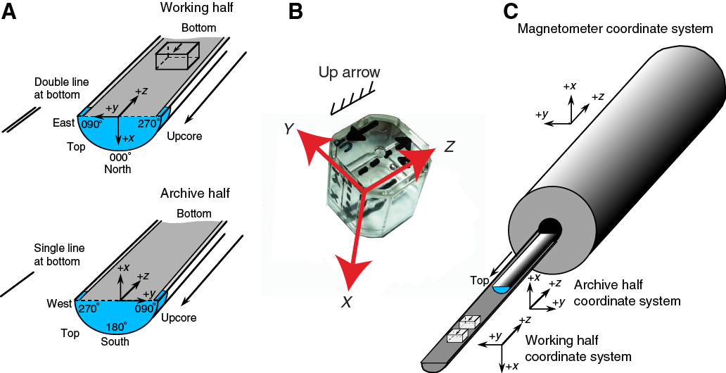
Figure F9. Coordinates for SRM and reported data and Natsuhara-Giken sampling cubes.
Figure F10. Positioning of discrete samples in the automatic holder of the JR-6A magnetometer.
Core orientation
When possible, APC core orientation was measured with an orientation tool (Icefield MI-5) mounted on the core barrel. The tool consists of three mutually perpendicular fluxgate magnetic sensors and two perpendicular gravity sensors. The information from both sets of sensors allows the azimuth and dip of the hole to be measured, as well as the azimuth of the APC core orientation. Orientation information was fundamental for paleomagnetic polarity determinations and magnetostratigraphic interpretations at low-latitude sites such as the cores from the Maldives (4°40′–4°50′N); however, we noticed that the orientation data collected were not very reliable.
Magnetostratigraphy
Magnetostratigraphy for each site was constructed by correlating observed polarity sequences with the geomagnetic polarity timescale in combination with biostratigraphic datums. We adopted the geomagnetic polarity timescale of Gradstein et al. (2012), in which boundary ages for Chrons C1n–C13n and C24n.1n–C34n are orbitally tuned and those for Chrons C13r–C23r are spline fitted.
For azimuthally unoriented samples from sedimentary rock deposited at low latitudes, determining the polarity of sedimentary units can be challenging. Polarity ambiguity arises when samples are azimuthally unoriented and the inclination is shallow in subequatorial sites (the angular distance between reversed and normal polarity inclinations is small) (Figure F11). Very often, the large dispersion around the mean inclination value observed in these sediment cores introduced large uncertainty in the determination of magnetic polarity (e.g., McFadden and Reid, 1982; Cox and Gordon, 1984); therefore, the results should be used with caution as a definitive estimate of magnetic polarity. Additional problems can arise from inclination anomalies due to nondipole fields, which bias the inclinations at low latitudes (e.g., Schneider and Kent, 1998).
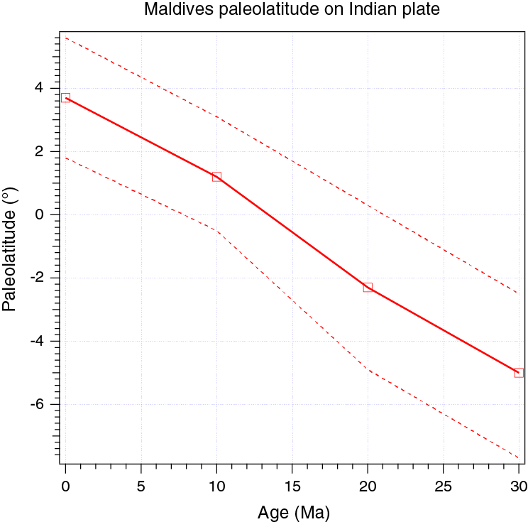
Figure F11. Paleolatitude reconstruction for the Maldives sites.
Whenever possible, we offer an interpretation of the magnetic polarity following the naming convention of correlative anomaly numbers prefaced by the letter C (Tauxe et al., 1984). Normal polarity subchrons are referred to by adding suffixes (n1, n2, etc.) that increase with age. For the younger part of the timescale (Pliocene–Pleistocene), we use traditional names to refer to the various chrons and subchrons (e.g., Brunhes, Jaramillo, Olduvai, etc.). In general, polarity reversals occurring at core section ends have been treated with extreme caution.
Physical properties
High-resolution physical property measurements were made to petrophysically characterize sediments and rocks recovered during Expedition 359. These data also complement lithostratigraphic descriptions and help tie sediment/rock properties to downhole logging data and seismic profiles. In particular, physical property data play a major role in hole-to-hole and site-to-site stratigraphic correlation, discontinuity/inhomogeneity detection, compositional and textural differences, major seismic reflection identification, and construction of synthetic seismic profiles. A variety of petrophysical techniques and methods were used to characterize whole-rounds, split cores, and discrete samples. Procedures for measuring sediment or hard rock cores differ slightly. The sampling plan for the Expedition 359 is summarized in Table T2.
T2. Sampling plan. Download table in .csv format.
Sedimentary cores
Recovered whole-round core sections are traditionally allowed to equilibrate to ambient room temperature (~20°C) and pressure for ~4 h in the ship’s Core Laboratory. However, because water bottom temperatures at the relatively shallow water sites cored during Expedition 359 were close to 15°C, it was determined that an equilibration period was unnecessary. Therefore, core sections were measured for physical properties soon after recovery. First, core sections were run through the WRMSL to measure density by gamma ray attenuation (GRA), magnetic susceptibility, and compressional wave velocity on the P-wave logger (PWL). Cores recovered with the XCB or RCB systems are slightly smaller in diameter than those cored with the APC system, producing gaps between the liner and the core. As a result, P-wave velocity was measured with the WRMSL on sections cored with the APC system but not always measured on sections cored with the XCB or RCB systems. Sections were then measured with the spectral NGRL. Thermal conductivity was the final measurement made on whole-round sections prior to splitting them into working and archive halves.
Archive halves were passed through the SHMSL to measure point magnetic susceptibility and color reflectance. Discrete samples were collected from the working halves (one per section) to measure wet bulk density, dry bulk density, water content, porosity, and grain density using moisture and density (MAD) procedures. P-wave velocity measurements were made on working halves that had been sampled for MAD, employing a transducer oriented in the x-axis direction.
Rock cores
Recovered core sections were run through the WRMSL and NGRL. Afterward, core sections were split into working and archive halves and all rock pieces were labeled. Archive halves were passed through the SHMSL to measure point magnetic susceptibility and color reflectance. Thermal conductivity was measured once per core using a contact probe on a piece of the section half in a seawater bath. P-wave velocity measurements were made on discrete samples. Two samples were taken in each section of the working half at offsets of 25 and 125 cm. Some of these samples (one per section) were shared for MAD measurements.
A full discussion of all methodologies and calculations used aboard the JOIDES Resolution in the Physical Properties Laboratory is available in Blum (1997). Details and procedures for each physical property measurement are described below.
Whole-Round Multisensor Logger measurements
GRA-derived bulk density, P-wave velocity, and magnetic susceptibility were measured nondestructively with the WRMSL. To optimize the measurement process, sampling intervals and measurement integration times were the same for all sensors. Sampling intervals were set at 5 cm with an integration time of 2.5 s for each measurement. These sampling intervals are common denominators of the distances between the sensors installed on the WRMSL (30–50 cm), which allows sequential and simultaneous measurements. Following the last section in each core, quality assurance/quality control (QA/QC) was conducted by passing a single core liner filled with deionized water through the WRMSL.
Gamma ray attenuation bulk density
Bulk density can be used to estimate pore volume and evaluate the consolidation state of sediment. GRA density is an estimate of bulk density based on the attenuation of a gamma ray beam. The beam is produced by a 137Cs gamma ray source at a radiation level of 370 MBq within a lead shield with a 5 mm collimator and is directed through the whole-round core. The gamma ray detector on the opposite side of the core from the source includes a scintillator and an integral photomultiplier tube to record the gamma radiation that passes through the core. The attenuation of gamma rays occurs primarily by Compton scattering, in which gamma rays are scattered by electrons in the formation; the degree of scattering is related to the material bulk density. Therefore, for a known thickness of sample, the density (ρ) is proportional to the intensity of the attenuated gamma rays and can be expressed as
- I = measured intensity of gamma rays passing through the sample,
- I0 = gamma ray source intensity,
- μ = Compton attenuation coefficient, and
- d = sample diameter.
To calculate ρ from I, μ and I0 are treated as constants.
In general, WRMSL measurements are the most accurate when taken on a completely filled core liner with minimal drilling disturbance; otherwise, measurements tend to underestimate true values. By default, the instrument reports measurements using the internal diameter of the core liner (66 mm) as the assumed sample diameter. This assumption is suitable for most sediment cores obtained with the APC system; however, for sediment and/or hard rock cored by the XCB or RCB systems, core diameter is usually about 58 mm or less. Following Jarrard and Kerneklian (2007), density measurements of XCB and RCB cores were corrected by multiplying the density values by 66/58 = 1.138 to account for this bias. The spatial resolution of the GRA densitometer is less than ±1 cm. The gamma ray detector is calibrated with sealed calibration cores (one standard core liner filled with distilled water and PVC cylinders of various diameters). To establish the calibration curves, gamma ray counts were taken through each water/PVC cylinder for 60 s. Each water/PVC cylinder has a density of 2.7 g/cm3, and d is 1, 2, 3, 4, 5, or 6 cm. The relationship between I and µd is
where A, B, and C are coefficients determined from the calibration.
Recalibration was performed as needed when the deionized water QA/QC standard deviated significantly (more than a few percent) from 1 g/cm3.
Magnetic susceptibility
Low-field magnetic susceptibility (χ) is a dimensionless measure of the degree to which a material can be magnetized by an external magnetic field:
where M is the magnetization induced in the material by an external field of strength H. Magnetic susceptibility is primarily sensitive to the concentration of ferromagnetic and ferrimagnetic minerals (e.g., magnetite, hematite, and maghemite), which is significant for understanding the provenance of the sediment and processes that occurred soon after deposition. When ferromagnetic/ferrimagnetic minerals are scarce, magnetic susceptibility may also be sensitive to paramagnetic and diamagnetic minerals, which can be related to the origin of the materials and their subsequent diagenesis.
Measurements were made using a Bartington MS2C loop sensor with a 9 cm diameter. An oscillator circuit in the sensor, operating at a frequency of 0.565 kHz and an AF of ~140 A/m, produces a low-intensity, nonsaturating alternating magnetic field. Sediment or hard rock core sections going through the influence of this field cause a change in its oscillator frequency. Frequency information returned in pulse to the susceptometer is converted into magnetic susceptibility. The loop sensor has a spatial resolution of 23–27 mm and is accurate to within 2%.
P-wave velocity
P-wave velocity data can be used to evaluate small-strain moduli to correlate downhole logging and core data. P-wave velocity (VP) is defined by the time required for a compressional wave to travel a specific distance:
where d is the path length of the wave across the core and tcore is the traveltime through the core.
The PWL measures the traveltime of 500 kHz ultrasonic waves horizontally through the core at 5 cm intervals while the core remains in the core liner. Waves are transmitted to the core by plastic transducer contacts connected to linear actuators. Pressure is applied to the actuators to ensure good coupling between the transducers and the core liner. P-wave velocity transducers measure the total traveltime of the compressional wave between transducers. The wave travels horizontally through the whole core and core liner. The total observed traveltime tcore is composed of
- tdelay = time delay related to transducer faces and electronic circuitry,
- tpulse = delay related to the peak detection procedure,
- tliner = transit time through the core liner, and
- tcore = traveltime through the sediment.
The system is calibrated using a core liner filled with distilled water, which provides control for tdelay, tpulse, and tliner. From these calibrations, VP can be calculated for whole-round specimens in core liners:
VP = (dcl – 2dliner)/(to – tpulse – tdelay – 2tliner),
- dcl = measured diameter of core and liner,
- dliner = liner wall thickness, and
- to = measured total traveltime.
This equation assumes that the core completely fills the core liner. The WRMSL PWL was turned off for XCB and RCB cores, which often do not fill the core liner.
Natural Gamma Radiation Logger measurements
Gamma radiation is emitted from the decay of mineral-hosted 238-uranium (238U), 232-thorium (232Th), and 40-potassium (40K). The NGRL measures this natural emission on whole-round cores using a system designed and built at the USIO (Texas A&M University, USA) (Vasiliev et al., 2011; Dunlea et al., 2013). When 238U, 232Th, and 40K radioisotopes decay, they and their daughter products emit gamma radiation at specific energy levels unique to each isotope. NGR spectroscopy measures a wide energy spectrum that can be used to estimate the abundance of each isotope based on the strength of the signal at characteristic energies (Blum et al., 1997; Gilmore, 2008). Spectral data were collected and can be used for postcruise processing for U, Th, and K abundance but were not processed during the expedition. Total counts were used for shipboard reporting of NGR, with high counts usually identifying either fine-grained deposits containing K-rich clay minerals and their absorbed U and Th isotopes or organic-rich intervals with increased U content. NGR data thus reveal stratigraphic details that aid in core-to-core correlations. The main NGR detector unit consists of eight sodium iodide (NaI) detectors arranged along the core measurement axis at 20 cm intervals surrounding the lower half of the section. The detector array has passive (layers of lead) and active (plastic scintillators) shielding to reduce background environmental and cosmic radiation. The overlying plastic scintillators detect incoming high-energy gamma and muon cosmic radiation and cancel this signal from the total counted by the NaI detectors.
A measurement run consisted of two sample positions 10 cm apart for a total of 16 measurements per 150 cm section. The quality of the energy spectrum measured in a core depends on the concentration of radionuclides in the sample and on the counting time, with higher times yielding better spectra. Counting times were 5 min per position, or ~10 min per core, yielding statistically significant energy spectra (Vasiliev et al., 2011).
Thermal conductivity measurements
After NGR measurements were completed, thermal conductivity was measured with the TK04 (Teka Bolin) system using a needle probe method in full-space configuration for whole-round sediment cores (Von Herzen and Maxwell, 1959) or a contact probe method in half-space configuration on split cores for hard rock. The probes contain a heater wire and a calibrated thermistor.
For soft sediment, the needle probe was inserted into a 2 mm diameter hole drilled through the liner (typically in Section 3) along one of the lines that later guided core splitting. To avoid interference from air flow in the laboratory, the core was placed into an enclosed box insulated with foam.
For hard rock cores, samples were selected from the working half and returned unaltered to the core liner upon completion of the tests. The contact probe embedded in the surface of an epoxy block with a low thermal conductivity (Vacquier, 1985) was maintained in contact with the sample, and both were equilibrated together in a seawater bath at room temperature in a cooler insulated with extruded polystyrene foam. The calibrated heat source of the probe was then turned on, and the increase in temperature was recorded over 80 s. A heating power of 1.7 W/m was typically used in soft sediment, and 1.9 W/m was used for indurated material. The solution to the heat conduction equation with a line source of heat was then fit to the temperature measurements to obtain the thermal conductivity. Because the probe is much more conductive than sediment or hard rock, the probe is assumed to be a perfect conductor. Under this assumption, the temperature of the superconductive probe has a linear relationship with the natural logarithm of the time after the initiation of the heat:
- T = temperature (K),
- q = heat input per unit length per unit time (J/m/s),
- k = thermal conductivity (W/[m·K]),
- t = time after the initiation of the heat (in seconds), and
- C = instrumental constant.
Three measuring cycles were automatically performed to calculate average conductivity. A self-test, which included a drift study, was conducted at the beginning of each measurement cycle. Once the probe temperature stabilized, the heater circuit was closed and the temperature rise in the probe was recorded. Thermal conductivity was calculated from the rate of temperature rise while the heater current was flowing. Temperatures measured during the first 80 s of the heating cycle were fitted to an approximate solution of a constantly heated line source (for details, see Kristiansen, 1982; Blum, 1997). Measurement errors were 5%–10%. Thermal conductivity measurements were routinely taken in one section per core (middle interval of Section 3). Some XCB cores yielded no results for thermal conductivity because cracks in the hard sediment caused poor coupling of the needle probe to the sediment.
Section Half Multisensor Logger measurements
Color reflectance and magnetic susceptibility were measured on archive halves using the SHMSL. The archive half was placed on the core logger, above which an electronic platform moves along a track, recording the height of the split-core surface with a laser sensor. The laser establishes the location of the bottom of the section, and then the platform reverses the direction of movement, moving from bottom to top making measurements of point magnetic susceptibility and color reflectance. All foam inserts were removed from the section-half cores before measurement so that the measured range of values represented the core material only. Point magnetic susceptibility and color reflectance data were collected at constant 5 cm intervals for most cores but were collected at 1 and 2.5 cm for some cores, depending on the available processing time. The measurements collected at 5 cm have sufficient resolution for comparison with the results obtained from the magnetic susceptibility loop of the WRMSL.
Color reflectance spectrometry
The color reflectance spectrometer uses an Ocean Optics 30 mm integrating sphere and both halogen and LED light sources, which cover wavelengths from ultraviolet through visible to near infrared. Measurements were taken from 380 to 900 nm wavelengths at 2 nm intervals. The approximate 3 s data acquisition offset was applied for the entire scan of the archive half. Data are reported using the L*a*b* color system, in which L* is lightness, a* is redness (positive) versus greenness (negative), and b* is yellowness (positive) versus blueness (negative). The color reflectance spectrometer calibrates on two spectra, pure white (reference) and pure black (dark). Color calibration was conducted approximately every 6 h (twice per shift).
Point magnetic susceptibility
Point magnetic susceptibility was measured with a Bartington MS2 meter and an MS2K contact probe with a flat 15 mm diameter round sensor with a 25 mm field of influence and an operation frequency of 930 Hz. The instrument averages three measurements from the sensor for each offset, leading to an accuracy of ~5%. The spatial resolution of the point magnetic susceptibility instrument is ~3.8 mm, higher than that of whole-round magnetic susceptibility for sections containing broken pieces <4 cm in length (the spatial resolution of whole-round magnetic susceptibility). As with whole-round measurements, the output displayed by the point magnetic susceptibility sensor must be converted to dimensionless SI units by multiplying by 10–5. The probe is zeroed in air before each measurement to avoid influence from the metal track. The point magnetic susceptibility meter was calibrated by the manufacturer before installation on the ship and was quality checked every ~6 h at the same time as color reflectance sensor calibration.
Section Half Measurement Gantry measurements
For soft-sediment cores, P-wave velocity and shear strength measurements were performed on the working halves of split cores before any samples were taken. P-wave velocity measurements used the x-axis caliper on the Section Half Measurement Gantry (SHMG), with two analyses per section. Measurements were usually taken at 25 and 125 cm in each section; however, if this interval provided no good sediment/transducer coupling (e.g., caused by high amounts of sand or cracks), different positions were chosen to generate reliable data. XCB cores generally did not provide usable data because of bad sediment/liner contact and disturbed sediment. For hard rock cores, P-wave velocity was measured on the discrete samples chosen for both physical property and paleomagnetic measurements.
P-wave velocity
The P-wave velocity system uses Panametrics-NDT Microscan delay line transducers, which transmit at 0.5 MHz. The signal received through the section half or the discrete sample was recorded by the computer attached to the system with the peak (P-wave arrival) usually chosen by autopicking software. In the case of a weak signal, the first arrival was manually picked at the very base of the first arrival peak, leaving out the automatically picked points that usually fell along the ascending curve. The distance between transducers was measured with a built-in linear voltage displacement transformer. Calibration was performed with a series of acrylic cylinders of differing thicknesses and a known P-wave velocity of 2750 ± 20 m/s. The system time delay determined from calibration was subtracted from the picked arrival time to give a traveltime of the P-wave through the sample. The thickness of the sample (calculated by the linear voltage displacement transformer, in meters) was divided by the traveltime (in seconds) to calculate P-wave velocity in meters per second.
Shear strength
Shear strength is the resistance of a material to failure in shear. Shear stress in unconsolidated materials is resisted only by the network of solid particles. Shear strength (τf) is expressed as a function of the effective normal stress at failure (σ′), the effective cohesion (c′), and friction angle (φ′),
where c′ and φ′ are the shear strength parameters that define a linear relationship between τf and φ′, according to the Mohr-Coulomb failure criterion.
Shear strength parameters were determined by means of multiple laboratory tests. Values of c′ and φ′ are relevant in situations where field drainage conditions correspond to test conditions. The shear strength of a soil under undrained conditions (IW drainage does not occur during failure) is different from that under drained conditions (IW drainage occurs).
Undrained shear strength (Su) is expressed in terms of total stress in the case of fully saturated materials of low permeability (e.g., clays). The most common strength tests in shipboard laboratories are vane shear and penetrometer tests, which provide measurement of undrained shear strength (Blum, 1997).
Su was measured in undisturbed fine-grained sediment using the handheld Torvane shear device on working halves. Undrained shear strength was determined by inserting an eight-bladed vane into the split core and putting it under shear stress to cause a cylindrical surface to be sheared by the vane. This procedure provides a measurement of peak shear strength expressed in units of kilograms per square centimeter. Measurements were made with the vane rotation axis perpendicular to the split surface. Shear strength was measured once in each core when sediments were within the instrument range.
Discrete sample measurements of moisture and density
Discrete samples were collected from the working halves to determine wet and dry bulk density, grain density, water content, and porosity. In soft sediment, ~10 cm3 samples were collected with a plastic syringe, the diameter of which fit that of shipboard glass vials. An attempt was made to sample every section. In indurated sediment and hard rock, minicores were extracted from the working halves for physical property measurements, with some also shared for paleomagnetic measurements.
Sample preparation
Soft-sediment samples were placed in numbered, preweighed ~16 mL Wheaton glass vials for wet and dry sediment weighing, drying, and dry volume measurements. Determination of an accurate wet mass of the minicore samples of indurated sediment and hard rock first required that the pore space of the samples be completely saturated with seawater. As soon as the core was split, therefore, samples were taken and the wet mass was immediately determined using the dual balance system. Then the samples were dried in a convection oven for at least 24 h at 105° ± 5°C. Dried samples were then cooled in a desiccator for at least 60 min before dry mass and volume were measured.
Dual balance mass measurement
The weights of wet and dry sample masses were determined to a precision of 0.005 g using two Mettler Toledo electronic balances, with one acting as a reference. A standard weight of similar value to the sample was placed upon the reference balance to increase accuracy. A computer averaging system was used to compensate for the ship’s motion. The default setting of the balances is 300 measurements (taking ~1.5 min).
Pycnometer volume measurement
Dry sample volume was determined using a hexapycnometer system of a six-celled, custom-configured Micrometrics AccuPyc 1330TC helium-displacement pycnometer. The precision of each cell is 1% of the full-scale volume. Volume measurement was preceded by three purges of the sample chamber with helium warmed to ~28°C. Three measurement cycles were run for each sample. A reference volume (set of two calibration spheres) was placed sequentially in one of the chambers to check for instrument drift and systematic error. The volumes occupied by the numbered Wheaton vials were calculated before the expedition by multiplying each vial’s weight by the average density of the vial glass. Dry mass and volume were measured after samples were heated in an oven at 105° ± 5°C for 24 h and allowed to cool in a desiccator. Procedures for determining these physical properties comply with the American Society for Testing and Materials (ASTM) designation (D) 2216 (ASTM International, 1990). The fundamental relation and assumptions for the calculations of all physical property parameters are discussed by Blum (1997) and summarized below.
Mass and volume calculation
We measured wet mass (Mwet), dry mass (Mdry), and dry volume (Vdry). The ratio of mass (rm) is a computational constant of 0.965 (i.e., 0.965 g of freshwater per 1 g of seawater). Salt precipitated in sediment pores during the drying process is included in the Mdry and Vdry values. The mass of the evaporated water (Mwater) and salt (Msalt) in the sample are given by
where s is the assumed saltwater salinity (0.035%) corresponding to a pore water density (ρpw) of 1.024 g/cm3 and a salt density (ρsalt) of 2.22 g/cm3. The corrected mass of pore water (Mpw), volume of pore water (Vpw), mass of solids excluding salt (Msolid), volume of salt (Vsalt), volume of solids excluding salt (Vsolid), and wet volume (Vwet) are
Calculation of bulk properties
For all sediment samples, water content (w) is expressed as the ratio of mass of pore water to wet sediment (total) mass:
Wet bulk density (ρwet), dry bulk density (ρdry), sediment grain density (ρsolid), porosity (φ), and void ratio (VR) are calculated as
MAD properties reported and plotted in the Physical properties sections of the site chapters were calculated with the MADMax shipboard program set with the “method C” calculation process.
Downhole measurements
Downhole logs record measurements of physical, chemical, and structural properties of the formation surrounding a borehole that are made after completion of drilling. Data are rapidly collected, continuous with depth (at vertical sampling intervals ranging from 2.5 mm to 15 cm), and measured in situ. Downhole logs record formation properties on a scale that is intermediate between those obtained from laboratory measurements on core samples and those from geophysical surveys. As such, they are useful in calibrating the interpretation of geophysical data and provide a critical link for the integrated understanding of physical properties on all scales.
Downhole logs can be interpreted in terms of the stratigraphy, lithology, mineralogy, magnetic characteristics, and geochemical composition of the penetrated formation. They also provide information on the condition, shape, and size of the borehole and on possible deformation induced by drilling or formation stress. Where core recovery is incomplete or disturbed, log data may provide the only way to characterize the borehole section and fill in between sampled intervals. Where core recovery is good, log and core data complement one another and may be interpreted jointly.
During Expedition 359, downhole logging measurements were recorded in Holes U1466B, U1467C, U1467E, U1468B, and U1471E. An attempt was made in Hole U1470B, but the first tool string was not able pass more than ~50 m below the base of pipe; limited downhole logging data were recorded over a few tens of meters. In addition, downhole temperature measurements were acquired using the APCT-3 in Holes U1465A, U1466A, U1467B, and U1471C.
Wireline logging operations
During wireline logging operations, logs are recorded with a variety of logging tools combined into tool strings that are lowered into the hole after completion of coring operations. Three primary tool strings were used during Expedition 359 (Figure F12):
- The triple combination (triple combo) tool string, which measures spectral and NGR, porosity, density, resistivity, and magnetic susceptibility;
- The Formation MicroScanner (FMS)-sonic tool string, which provides high-resolution resistivity images of the borehole wall and sonic velocities; and
- The Versatile Seismic Imager (VSI) tool string for vertical seismic profiles (VSPs).

Figure F12. Wireline tool strings planned for deployment.
These tool strings were modified in response to expected borehole conditions or tool performance during the expedition (see Figure F13 for modified tool strings). Each tool string also contains a telemetry cartridge for communicating through the wireline to the Schlumberger data acquisition system (multitasking acquisition and imaging system [MAXIS] unit) on the ship. Individual tools are listed in Table T3.
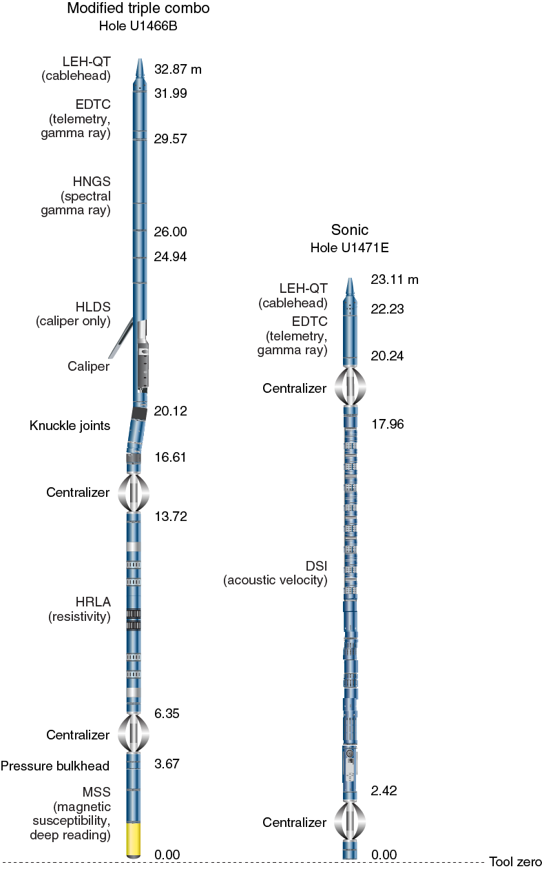
Figure F13. Additional wireline tool strings.
T3. Downhole measurements made by wireline tool strings. Download table in .csv format.
In preparation for logging, boreholes were flushed of debris by circulating viscous drilling fluid and filled with seawater or seawater-based logging gel (sepiolite mud mixed with seawater and weighted with barite; approximate density = 10.5 lb/gal or 1.258 g/cm3) to help stabilize the borehole walls. The BHA was pulled up to 90–150 mbsf, depending on the stability of the hole. Tool strings were then lowered downhole on a seven-conductor wireline cable during sequential deployments. Each tool string deployment is a logging “run,” starting with the assembly of the tool string and any necessary calibrations. The tool string is then lowered to the bottom of the hole while recording a partial set of data and, except for the VSI, is pulled up at a constant speed (typically 250–500 m/h) to record the main data. The VSI is held stationary at regularly spaced depths while shooting the seismic source and then pulled up between stations. During each run, tool strings can be lowered down and pulled up the hole several times for repeatability or to try to improve the data quality. Each lowering or hauling-up of a tool string while collecting data constitutes a “pass.” During each pass, incoming data are recorded and monitored in real time on the surface minimum configuration MAXIS. A logging run is complete when a tool string has been recovered to the rig floor and disassembled. A wireline heave compensator (WHC) can be employed to minimize the effect of ship’s heave on the tool string’s position in the borehole (see Wireline heave compensator). The sea state was calm during all Expedition 359 logging operations, so the WHC was not needed.
Logged sediment properties and tool measurement principles
The primary logging measurements recorded during Expedition 359 are listed in Table T4. The logged properties and the principles used in the tools that measure them are briefly described below. More detailed information on individual tools and their geological applications may be found in Serra (1984, 1986, 1989), Schlumberger (1989, 1994), Rider (1996), Goldberg (1997), Lovell et al. (1998), and Ellis and Singer (2007). More information about IODP downhole logging tools and measurements can be found at http://iodp.tamu.edu/tools/logging/index.html. A complete online list of acronyms for Schlumberger tools and measurement curves is available at http://www.apps.slb.com/cmd.
T4. Acronyms and units used for downhole wireline tools and measurements. Download table in .csv format.
Natural gamma radiation
The Hostile Environment Natural Gamma Ray Sonde (HNGS) was used on both the triple combo and FMS-sonic tool strings to measure natural gamma radioactivity in the formation. The HNGS uses two bismuth germanate scintillation detectors and five-window spectroscopy to determine concentrations of potassium (in weight percent), thorium (in parts per million), and uranium (in parts per million) from the characteristic gamma ray energies of isotopes in the 40K, 232Th, and 238U radioactive decay series, which dominate the natural radiation spectrum. Computation of elemental abundances uses a least-squares method of extracting U, Th, and K elemental concentrations from the spectral measurements. The HNGS filters out gamma ray energies below 500 keV, eliminating sensitivity to bentonite or KCl in the drilling mud and improving measurement accuracy. The HNGS also measures total gamma ray (HSGR) emission and uranium-free or computed gamma ray (HCGR) emission in American Petroleum Institute units (gAPI). The HNGS response is influenced by the borehole diameter, and therefore HNGS data are corrected for borehole diameter variations during acquisition.
The Enhanced Digital Telemetry Cartridge (EDTC; see Auxiliary logging equipment), which is used primarily to communicate data to the surface, includes a sodium iodide scintillation detector that also measures total natural gamma ray emission. It is not a spectral tool, but it provides high-resolution total gamma ray measurements for each pass, which allows precise depth-match processing between logging runs and passes.
The inclusion of a gamma ray sonde in every tool string provides gamma ray data for precise depth correlation between logging strings and passes.
Porosity
Formation porosity was measured with the Accelerator Porosity Sonde (APS), which includes a minitron neutron generator that produces fast (14.4 MeV) neutrons and five neutron detectors (four epithermal and one thermal) positioned at different spacing from the minitron. The tool’s detectors count neutrons that arrive at the detectors after being scattered and slowed by collisions with atomic nuclei in the formation.
The highest energy loss occurs when neutrons collide with hydrogen nuclei, which have practically the same mass as the neutron (the neutrons bounce off heavier elements without losing much energy). If the hydrogen (i.e., water) concentration is low, as in low-porosity formations, neutrons can travel farther before being captured, and the count rates increase at the detector. The opposite effect occurs in high-porosity formations where the water content is high. The raw porosity value is often an overestimate because hydrogen bound in minerals such as clays or in hydrocarbons also contributes to the measurement.
Upon reaching thermal energies (0.025 eV), the neutrons are captured by the nuclei of Cl, Si, B, and other elements, resulting in a gamma ray emission. This neutron capture cross section (Σf) is also measured by the tool.
Density and photoelectric factor
Formation density was measured with the Hostile Environment Litho-Density Sonde (HLDS). The sonde contains a radioactive cesium (137Cs) gamma ray source (622 keV) and far and near gamma ray detectors mounted on a shielded skid, which is pressed against the borehole wall by a hydraulically activated decentralizing arm. Gamma rays emitted by the source undergo Compton scattering, where gamma rays are scattered by electrons in the formation. The number of scattered gamma rays that reach the detectors is proportional to the density of electrons in the formation, which is in turn related to bulk density. Porosity may also be derived from this bulk density if the matrix (grain) density is known.
The HLDS also measures the photoelectric effect factor (PEF), a measure of the photoelectric absorption of low-energy gamma radiation. Photoelectric absorption occurs when gamma ray energy falls below 150 keV as a result of being repeatedly scattered by electrons in the formation. PEF is determined by comparing counts from the far detector in the high-energy region, where only Compton scattering occurs, with those in the low-energy region, where count rates depend on both reactions. The far detector is used because it has a greater depth of investigation (approximately tens of centimeters). The response of the short-spaced detector, most influenced by mudcake (not typically present in IODP-drilled boreholes because seawater-based drilling mud is used) and borehole rugosity, is used to correct the density measurement for these effects. Because PEF depends on the atomic number of the elements in the formation (heavier elements have higher PEFs), it also varies according to the chemical composition of the minerals present and can be used for the identification of some minerals. For example, the PEF of calcite is 5.08 barns per electron (b/e–), celestine is 55.13 b/e–, and quartz is 1.81 b/e–.
Good contact between the tool and borehole wall is essential for good HLDS logs. Poor contact results in underestimation of density values. Both the density correction and caliper measurement of the hole are used to check the contact quality.
Electrical resistivity
The High-Resolution Laterolog Array (HRLA) provides six electrical resistivity measurements with different depths of investigation (including the borehole, or mud, resistivity and five measurements of formation resistivity with increasing penetration into the formation). The sonde sends a focused current into the formation and measures the intensity necessary to maintain a constant drop in voltage across a fixed interval, providing direct resistivity measurements. The array has one central (source) electrode and six electrodes above and below it, which serve alternatively as focusing and returning current electrodes. By rapidly changing the role of these electrodes, a simultaneous resistivity measurement at six penetration depths is achieved. The tool is designed to ensure that all signals are measured at exactly the same time and tool position, and to reduce the sensitivity to “shoulder bed” effects when crossing sharp beds thinner than the electrode spacing. The design of the HRLA, which eliminates the need for a surface reference electrode, improves formation resistivity evaluation compared to traditional dual induction and allows the full range of resistivity to be measured, from low (e.g., in high-porosity sediments) to high (e.g., in basalt). The HRLA needs to be run centralized in the borehole for optimal results, so knuckle joints were used to centralize the HRLA while allowing the density and porosity tools that are on the same tool string to maintain good contact with the borehole wall.
Calcite, silica, and hydrocarbons are electrical insulators, whereas ionic solutions like IW are conductors. Electrical resistivity, therefore, can be used to evaluate porosity for a given salinity and resistivity of the IW. Clay surface conduction also contributes to the resistivity values, but at high porosities, this is a relatively minor effect.
Magnetic Susceptibility
The Magnetic Susceptibility Sonde (MSS) is a nonstandard wireline tool designed by Lamont-Doherty Earth Observatory (LDEO). It measures the ease with which formations are magnetized when subjected to a magnetic field. The ease of magnetization, or susceptibility, is ultimately related to the concentration and composition (size, shape, and mineralogy) of magnetic minerals in the formation. These measurements provide one of the best methods for investigating stratigraphic changes in mineralogy and lithology because the measurement is quick, repeatable, and nondestructive and because different lithologies often have strongly contrasting susceptibilities.
The MSS dual-coil sensor provides ~40 cm resolution measurements with ~20 cm depth of horizontal investigation. The MSS was run as the lowermost tool in the triple combo tool string, using a specially developed data translation cartridge to enable the MSS to be run in combination with Schlumberger tools. The MSS also has an optional single-coil sensor to provide higher resolution measurements, but this was not used during Expedition 359.
Magnetic susceptibility data are plotted as uncalibrated units. MSS responses are affected by temperature (higher temperatures lead to higher susceptibility readings) and borehole size; preliminary processing can be performed to remove the temperature drift by calculating a least-squares polynomial fit to the data and subtracting the calculated trend from the data set. When the magnetic susceptibility signal in sediment is very low, the detection limits of the tool may be reached. For quality control and environmental correction, the MSS also measures internal tool temperature, z-axis acceleration, and low-resolution borehole conductivity.
Acoustic velocity
The Dipole Shear Sonic Imager (DSI) measures transit times between sonic transmitters and an array of eight receivers. The waveforms are then used to calculate the sonic velocity in the formation. The omnidirectional monopole transmitter emits high-frequency (5–15 kHz) pulses to extract the compressional velocity (VP) of the formation, as well as the shear velocity (VS) when it is faster than the sound velocity in the borehole fluid. It combines replicate measurements, thus providing a direct measurement of compressional velocity through sediments that is relatively free from the effects of formation damage and an enlarged borehole (Schlumberger, 1989). The same transmitter can be fired in sequence at a lower frequency (0.5–1 kHz) to generate Stoneley waves that are sensitive to fractures and variations in permeability. Along with the monopole transmitters found on most sonic tools, the DSI also has two crossed-dipole transmitters that allow an additional measurement of shear wave velocity. Dipole measurements are necessary to measure shear velocities in “slow” formations in which shear velocity is slower than the borehole fluid velocity. Such slow formations are typically encountered in deep ocean drilling. The two shear velocities measured from the two orthogonal dipole transmitters can be used to identify sonic anisotropy that can be associated with the local stress regime.
Resistivity images
The FMS provides high-resolution electrical resistivity–based images of the borehole walls that can be used for detailed lithostratigraphic or structural interpretation. The tool has four orthogonally oriented arms, each with 16 button electrodes that are pressed against the borehole walls during logging. The electrodes are arranged in two diagonally offset rows of eight electrodes each. A focused current is emitted from the button electrodes into the formation, with a return electrode near the top of the tool. Resistivity of the formation at the button electrodes is derived from the intensity of current passing through the button electrodes.
Processing transforms the resistivity measurements into oriented high-resolution images that reveal geologic structures of the borehole wall based on their conductivity. Features such as bedding, stratification, fracturing, slump folding, and bioturbation can be resolved (Luthi, 1990; Salimullah and Stow, 1992; Lovell et al., 1998). Because the images are oriented to magnetic north, further analysis can provide measurement of the dip and direction (azimuth) of planar features in the formation. In addition, when the corresponding planar features can be identified in the recovered core samples, individual core pieces can be reoriented with respect to true north.
The maximum extension of the FMS caliper arms is 40.6 cm (16 inches). In holes with a diameter greater than this maximum, the pad contact at the end of the caliper arms will be inconsistent and the FMS images may appear out of focus and too conductive. Irregular (rough) borehole walls will also adversely affect the images if contact with the wall is poor. Approximately 30% of a borehole with a diameter of 25 cm is imaged during a single pass. Standard procedure is to make two full uphole passes with the FMS to maximize the borehole coverage with the pads.
Acceleration and inclinometry
The General Purpose Inclinometry Tool (GPIT) was included in the FMS-sonic tool string to measure tool acceleration and orientation during logging. Tool orientation is defined by three parameters: tool deviation, tool azimuth, and relative bearing. The GPIT utilizes a three-axis inclinometer and a three-axis fluxgate magnetometer to record the orientation of the FMS as the magnetometer records the magnetic field components (Fx, Fy, and Fz). Thus, the FMS images can be corrected for irregular tool motion, and the dip and direction (azimuth) of features in FMS images can be determined. Corrections for cable stretching and/or ship heave using GPIT acceleration data (Ax, Ay, and Az) allow precise determination of log depths.
Vertical seismic profile
In a VSP experiment, a borehole seismic tool (VSI) is anchored against the borehole wall at regularly spaced intervals (or where borehole conditions permit) and records the full waveform of elastic waves generated by a seismic source positioned just below the sea surface. The main purpose of this experiment is to provide a direct measurement of the time needed for seismic waves to travel from the surface to a given depth and thus to tie observations in the borehole, recorded as a function of depth, to reflections in the seismic survey data, recorded as a function of time.
The VSI used for the VSP experiment is a three-axis geophone accelerometer that is anchored to the borehole wall by a caliper arm prior to recording. The orientation of the horizontal components, X and Y, vary because of sensor rotation during logging, but tool orientation is recorded. During Expedition 359, the VSI was anchored against the borehole wall at approximately 50 m station intervals and 5–10 air gun shots were typically taken at each station. The recorded waveforms were stacked, and a one-way traveltime was determined from the median of the first breaks for each station. The seismic source on the JOIDES Resolution was a Sercel G. Gun Parallel Cluster composed of two 250 in3 air guns separated by 1 m; however, only a single gun was used during the VSP experiments for Expedition 359, for a total source volume of 250 in3. The source was positioned off the port side of the JOIDES Resolution at a total horizontal offset from the top of the wellhead of 34 m and maintained at a water depth of 3 meters below sea level (mbsl).
In accordance with the requirements of the National Environmental Policy Act and the Endangered Species Act, all seismic activities were conducted during daytime, and Protected Species Observers kept watch for protected species for the duration of the VSP experiment. Any sight of protected species within the exclusion zone of 900 m, used for a 250 in3 source in intermediate water depths (100–1000 m), would interrupt the survey for 60 min after the last sighting or until the protected species were seen leaving the exclusion zone. Protected Species Observers began observations 1 h prior to the use of the seismic source, which started with a 30 min ramp-up procedure, gradually increasing the operational pressure and firing rate to provide time for undetected protected species to vacate the area. The same ramp-up procedure would be used when resuming activity after any interruption due to the sighting of protected species or whenever the gun was not fired for more than 30 min.
Auxiliary logging equipment
The Schlumberger logging equipment head (LEH or cable head) measures tension at the very top of the wireline tool string, which diagnoses difficulties in running the tool string up or down the borehole or when exiting or entering the drilling string or casing.
Telemetry cartridges are used in each tool string to transmit data from the tools to the surface. The EDTC also includes a sodium iodide scintillation detector to measure the total natural gamma ray emission of the formation. This gamma ray log was used to match the depths between the different passes and runs. In addition, it includes an accelerometer, whose data can be used in real time to evaluate the efficiency of the WHC.
Because the tool strings combine tools of different generations and with various designs, they include several adapters and joints between individual tools to allow communication, provide isolation, avoid interferences (mechanical and acoustic), terminate wirings, or to position the tool properly in the borehole. The knuckle joints in particular were used to allow tools such as the HRLA to remain centralized in the borehole while the overlying HLDS was pressed against the borehole wall.
All of these additions are included and contribute to the total length of the tool strings as shown in Figures F12 and F13.
Log data quality
The main influence on log data quality is the condition of the borehole wall. Where borehole diameter varies over short intervals because of washouts of softer material or ledges of harder material, the logs from tools that require good contact with the borehole wall (i.e., FMS, density, and porosity tools) may be degraded. Deep investigation measurements such as gamma radiation, resistivity, and sonic velocity, which do not require contact with the borehole wall, are generally less sensitive to borehole conditions. “Bridged” sections, where borehole diameter is significantly less than the bit size, will also cause irregular log results. The quality of the borehole is improved by minimizing the circulation of drilling fluid while drilling, flushing the borehole to remove debris, and logging as soon as possible after drilling and conditioning are completed.
The quality of the wireline depth determination depends on several factors. The depth of the logging measurements is determined from the length of the cable payed out from the winch on the ship. The seafloor is identified on the natural gamma ray log by the abrupt reduction in gamma ray count at the water/sediment interface (mudline). Discrepancies between the drilling depth (DSF), core depth (CSF-A), and wireline log depth may occur because of core expansion, incomplete core recovery, or incomplete heave compensation for the drilling depth. In the case of log depth, discrepancies between successive runs may occur because of incomplete heave compensation, incomplete correction for cable stretch, and cable slip. In the case of very fine sediments in suspension, the mudline can be an elusive datum. Tidal changes in sea level may also affect both drilling and logging depths. To minimize the wireline tool motion caused by ship heave, a hydraulic WHC can be used to adjust the wireline depth for rig motion during wireline logging operations.
Wireline heave compensator
During wireline logging operations, the up-and-down motion of the ship (heave) causes a similar motion in the downhole logging tools. If the amplitude of this motion is large, depth discrepancies can be introduced into the logging data. The risk of damaging downhole instruments is also increased. A WHC system was thus designed to compensate for the vertical motion of the ship and maintain a steady motion of the logging tools to ensure high-quality logging data acquisition (Liu et al., 2013; Iturrino et al., 2013). The WHC uses a vertical accelerometer (motion reference unit [MRU]) positioned under the rig floor near the ship’s center of gravity to calculate the vertical motion of the ship with respect to the seafloor. It then adjusts the length of the wireline by varying the distance between two sets of pulleys through which the cable passes in order to minimize downhole tool motion. Real-time measurements of uphole (surface) and downhole acceleration are made simultaneously by the MRU and the EDTC, respectively. The sea state was calm during all Expedition 359 logging operations, and the ship’s heave was minimal, so the WHC was not used.
Logging data flow and log depth scales
Data for each wireline logging run were monitored in real time and recorded using the Schlumberger MAXIS 500 system. Initial logging data were referenced to the rig floor (WRF). After logging was completed, data were shifted to a seafloor reference (WSF) based on the step in gamma radiation at the sediment/water interface.
Data were transferred onshore to LDEO, where standardized data processing took place using Schlumberger Geo-Quest’s GeoFrame software package. The main part of the processing is depth matching to remove depth offsets between logs from different logging runs, which results in a new WMSF depth scale. Also, corrections are made to certain tools and logs (e.g., FMS imagery is corrected for tool acceleration, including “stick and slip”), documentation for the logs (with an assessment of log quality) is prepared, and data are converted to ASCII for the conventional logs and GIF for the FMS images. Data were transferred back to the ship within a few days of logging, and this processed data set was made available to the science party (in ASCII and digital log information standard [DLIS] formats) through shipboard servers.
In situ temperature measurements
During Expedition 359, in situ temperature measurements were made using the APCT-3 temperature tool in one hole at Sites U1465, U1466, U1467, and U1471 when the APC system was deployed. The APCT-3 fits directly into the coring shoe of the APC system and consists of a battery pack, data logger, and platinum resistance-temperature device calibrated over a temperature range of 0°–30°C. Before entering the borehole, the tool is first stopped at the seafloor for 5–10 min to thermally equilibrate with bottom water. However, the lowest temperature recorded during the run down is preferred to the average temperature at the seafloor as an estimate of bottom water temperature because (1) this measurement is more repeatable and (2) the bottom water is expected to have the lowest temperature in the profile. After the APC penetrated the sediment, it was held in place for 5–10 min while the APCT-3 instrument recorded the temperature of the cutting shoe every second. When the APC was fired into the formation, there was typically an instantaneous temperature rise due to frictional heating (although this was not observed during any APCT-3 deployments at Site U1467). The heat gradually dissipated into the surrounding sediment as the temperature at the APCT-3 equilibrated to the temperature of the sediment.
The equilibrium temperature of the sediment was estimated by applying a mathematical heat-conduction model to the temperature decay record (Horai and Von Herzen, 1985). The synthetic thermal decay curve for the APCT-3 tool is a function of the geometry and thermal properties of the probe and the sediment (Bullard, 1954; Horai and Von Herzen, 1985). The equilibrium temperature must be estimated by applying a fitting procedure in the TP-Fit software designed by Heesemann. However, when the APC does not achieve a full stroke or when ship heave pulls up the APC from full penetration, the temperature equilibration curve is disturbed and temperature determination is less accurate. The nominal accuracy of the APCT-3 temperature measurements is ±0.05°C.
When a reasonable number of data points are measured, APCT-3 temperature data may be combined with measurements of thermal conductivity (see Physical properties) obtained from whole-round core sections to obtain heat flow values. Heat flow may be calculated according to the Bullard method, to be consistent with the synthesis of ODP heat flow data by Pribnow et al. (2000).
Stratigraphic correlation and sedimentation rates
Meeting the scientific objectives of Expedition 359 required recovery of complete stratigraphic sections at some of the coring sites. Such sections cannot be constructed from a single borehole because core-recovery gaps on the order of 20 to 50 cm occur between successive cores despite 100% or more nominal recovery at these sites (e.g., Ruddiman et al., 1987; Hagelberg et al., 1995; Acton et al., 2001). The construction of a complete stratigraphic section, referred to as a splice, requires combining stratigraphic intervals from two or more offset holes cored at the same site.
Meters below seafloor scale
Expedition 359 uses the scale terminology of meters below seafloor (mbsf) to designate positions of recovered core relative to the seafloor instead of the CSF-A scale adopted by some IODP expeditions. The depth to the top of each core is based on the DSF scale, which is determined by the length of drill string below the rig floor to the top of the cored interval minus the length of drill string from the rig floor to the mudline (assumed to be the seafloor). The depth to a position within a given core is determined by adding to the core top depth the distance the position occurs from the top of the core, which is measured onboard by a curator and includes growth due to relief of overburden as well as gas expansion. Therefore, the mbsf depth scale used during Expedition 359 is exactly the same as that used in the historical DSDP, ODP, and Integrated Ocean Drilling Program expeditions. Error in the mbsf scale includes pipe and BHA stretch and compression, tides, uncompensated heave, and incomplete recovery and core expansion. Tidal influence on this depth measurement was first predicted during ODP Leg 138 (Hagelberg et al., 1995) and demonstrated during ODP Leg 202 (Mix, Tiedemann, Blum, et al., 2003). During Expedition 359, tidal range was low (<1 m) and was not considered in the mbsf scale.
Core composite depth below seafloor scale
The goal of constructing a composite depth scale is to place coeval, laterally continuous stratigraphic features into a common frame of reference by depth-shifting individual cores (starting on the mbsf scale) to maximize correlation between holes. The resulting CCSF-A scale is equivalent to the historical ODP and Integrated Ocean Drilling Program meters composite depth (mcd) scale. In constructing the CCSF-A scale from the mbsf scale, individual core depths are shifted by a constant amount (no stretching or squeezing within an individual core). Ultimately, this provides good first-order correlation between cores from different holes, estimates of the length of coring gaps, and a basis on which higher order composite depth scales are constructed. Rather than being tied to a drill string measurement, the CCSF-A scale is built by correlating features downhole from the sedimentological mudline. Here, the mudline is not merely taken as the top of the first core in a given hole but is the top of the first core at the site with the best-preserved sediment/water interface. This establishes the top of the stratigraphic section and anchors the entire composite depth scale for all cores from all holes at a site. The mudline (or anchor) core is typically the only core in which the depths are the same for both the mbsf and CCSF-A scales. Each core downhole is tied to the composite section by adding or subtracting a depth offset (a constant) that best aligns an observed lithologic feature among adjacent cores from different holes. Because of the differing effects of coring-induced stretching and squeezing among cores, as well as hole-to-hole sedimentological differences, this approach very rarely aligns all features (Figure F14).
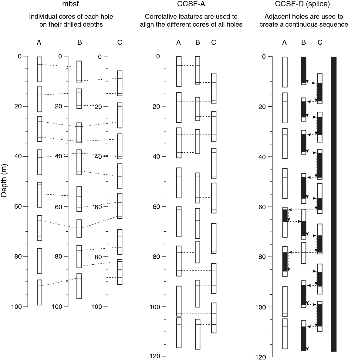
Figure F14. Cored material and depth scales.
The depth offset of every core is tabulated in an affine table. Provided between-core gaps never come into alignment among all holes at a site and recovery is sufficiently high, it should be possible to correlate (“tie”) each successive core in one hole to a core from an adjacent hole all the way to the bottom of a drilled section. Aligned coring gaps across all holes cored at a site may still occur, in which case cores below the gaps are no longer tied to the mudline core but can often still be tied to one another.
In the process of constructing the composite section, the total CCSF-A depth is usually larger than that of the mbsf scale. This expansion, typically ~5% to 15%, is mostly caused by decompression of the cores as they are brought to the surface, gas expansion, stretching that occurs as part of the coring process, and/or curation practice, in which material that has fallen downhole or gas expansion voids are curated as part of the core (e.g., Hagelberg et al., 1995; Acton et al., 2001).
Core composite depth below seafloor scale
Once the CCSF-A scale is developed and the between-core gaps are identified, a complete stratigraphic section (splice) is constructed by combining selected intervals from among holes and avoiding the gaps, overlaps, and disturbed sections. The depth scale for the splice is the CCSF-D scale (Figure F14). Although the CCSF-D scale is merely a subset of the CCSF-A scale, the “-D” designation applies only to intervals included in the splice. Intervals not included in the primary splice, including any alternate splice(s), are assigned a CCSF-A scale only. Should coring gaps happen to align across all holes drilled at a site, the spliced sections below are “appended” to those above and referred to as floating splice sections (i.e., not tied to the mudline). In this case, the amount of missing material between floating splices can be measured using downhole logs. Where no logs are available, the mbsf scale provides a reasonably accurate estimate of the length of the missing section, especially when coring in calm seas.
Age models and sedimentation rates
Preliminary age models and sedimentation rates were generated for each site considering all available datums generated by the Biostratigraphy, Paleomagnetism, and Lithostratigraphy (tephra) groups. These shipboard age models provide the context for variations in physical properties (e.g., GRA, NGR, and L*) generated on either whole- or half-round sections that can be used to identify sedimentary cycles with a periodic forcing. Preliminary “astrochronologies” provide refinement of the biostratigraphic age models.
Seismic stratigraphy
Seismic stratigraphy relies on high-resolution reflection seismic lines acquired during NEOMA Cruise M74/4 with the R/V METEOR in 2007 and Cruise SO236 with the R/V SONNE in 2014 by the University of Hamburg (Betzler et al., 2013; Lüdman et al., 2013). In addition, published low- to medium-resolution industrial reflection seismic lines shot for Elf in 1973–1974 (Purdy and Bertram, 1993; Aubert and Droxler, 1996) and for Shell in 1989–1990 (Belopolsky and Droxler, 2004) were used for regional context and initial sequence analysis. The Shell seismic data set covers the Inner Sea and the interatoll passages. The Elf seismic grid also transects most of the Maldivian atolls and offers good penetration depths across the atolls and their drowned parts.
The high-resolution seismic data set consists of approximately 1715 km (Cruise M74/4) and 1400 km (Cruise SO236) of reflection seismic profiles. During both cruises, seismic signals were generated by a 2-gun cluster of a standard and mini generator injector (GI) guns. Both fired in true GI modus with a total volume of 195 in3 (150 + 45 in³). A digital 144-channel streamer array with an active length of 600 m and a group interval of 4.167 m was used. The data were digitized with seven SeaMUX 24-channel 24-bit digitizing modules configured in six multiple arrays totaling 144 channels. The shotpoint distance during the entire cruise was 12.5 m. The dominant frequencies center around 100–200 Hz. Processing of reflection seismic data was done using the software package ProMAX 2-D (Halliburton-Landmark). Data were processed to zero phase, filtered in time and f-k domains, and corrected for dip moveout. In basinal areas, a suppression of multiple reflections was achieved by predictive deconvolution of prestacked data. Amplitude losses were compensated by a power function.
The vertical resolution of the newly acquired data is approximately 4–6 m, depending on depth. In comparison, the Shell seismic data had a resolution of only 10–25 m (Belopolsky and Droxler, 2004), and the vertical resolution of the Elf seismic data is even lower.
Interpretation and visualization was performed on time-migrated data in time domain using the software package Petrel (Schlumberger). All seismic data were tied to the seafloor topography computed from the multibeam data acquired during the presite surveys (see Figure F5 in the Expedition 359 summary chapter [Betzler et al., 2017a]). A preliminary time model was established via correlation of the mapped seismic units to published data of exploration Wells NMA-1 and ARI-1 (Aubert and Droxler, 1996; Belopolsky and Droxler, 2004) and ODP Site 716 (Backman, Duncan, et al., 1988). A velocity model for the basin and platform sequences was deduced from interval velocities obtained from Well ARI-1 (basin) and a comparable platform setting (ODP Leg 166; Great Bahama Bank; Eberli, Swart, Malone, et al., 1997), respectively. Mapping seismic units is based on the principles of sequence stratigraphy established by Mitchum and Vail (1977), who define a sequence as a relatively conformable succession of genetically related strata bounded by unconformities or their correlative conformities. Sequence and system tract boundaries are identified by their termination pattern: onlap, toplap, downlap, or truncation. Their external (sheet, wedge, clinoform, mound, etc.) and internal (reflector pattern: parallel, shingled, chaotic, etc.) configuration as well as seismic facies (reflection amplitude, continuity, frequency, and interval velocity) are interpreted in terms of depositional environment.
The sequences in the Inner Sea are deposited in two main depositional environments, prograding carbonate platform and drift deposits (see Figures F7 and F8 in the Expedition 359 summary chapter [Betzler et al., 2017a]). The environments are reflected in the names, which are platform sequences (PS) and drift sequences (DS). The basal sequence boundary is numbered from old to young; 11 sequences in the platform environment are thus labeled PS1–PS11 and the overlying drift sequences are labeled DS1–DS10 (see Figure F30 in the Site U1465 chapter [Betzler et al., 2017b]).
Seismic-core-log correlation
The work flow for correlation between seismic profiles, cores, and logs comprises a number of different steps:
- Fine tuning the preliminary velocity models by newly acquired VSI velocity data (see Downhole measurements),
- Tying sequence boundaries to core chronostratigraphy (see Biostratigraphy),
- Correlating WRMSL logs (density, magnetic susceptibility, and P-wave velocity) with sequence boundaries (see Physical properties),
- Correlating core lithology with seismic facies (see Lithostratigraphy and sedimentology),
- Using downhole logs to fill core gaps and identify spatial and temporal depositional trends along the platform to basin transects (see Downhole measurements),
- Correlating lithostratigraphic and log units to the seismic sequence, and
- Importing age information from age-depth plots to determine ages of seismic sequence boundaries (see Biostratigraphy).
Seismic-core-log correlation was carried out with the interpretation software package Petrel 2014 (Schlumberger) provided by IODP.
References
Acton, G.D., Borton, C.J., and the Leg 178 Shipboard Scientific Party, 2001. Palmer Deep composite depth scales for Leg 178 Sites 1098 and 1099. In Barker, P.F., Camerlenghi, A., Acton, G.D., and Ramsay, A.T.S. (Eds.), Proceedings of the Ocean Drilling Program, Scientific Results, 178: College Station, TX (Ocean Drilling Program), 1–35. http://dx.doi.org/10.2973/odp.proc.sr.178.202.2001
ASTM International, 1990. Standard method for laboratory determination of water (moisture) content of soil and rock (Standard D2216–90). In Annual Book of ASTM Standards for Soil and Rock (Volume 04.08): Philadelphia (American Society for Testing Materials). [revision of D2216-63, D2216-80]
Aubert, O., and Droxler, A.W., 1996. Seismic stratigraphy and depositional signatures of the Maldive carbonate system (Indian Ocean). Marine and Petroleum Geology, 13(5):503–536. http://dx.doi.org/10.1016/0264-8172(96)00008-6
Backman, J., Duncan, R.A., et al., 1988. Proceedings of the Ocean Drilling Program, Initial Reports, 115: College Station, TX (Ocean Drilling Program). http://dx.doi.org/10.2973/odp.proc.ir.115.1988
Backman, J., Raffi, I., Rio, D., Fornaciari, E., and Pälike, H., 2012. Biozonation and biochronology of Miocene through Pleistocene calcareous nannofossils from low and middle latitudes. Newsletters on Stratigraphy, 45(3):221–244. http://dx.doi.org/10.1127/0078-0421/2012/0022
Baker, P.A., 1986. Pore-water chemistry of carbonate-rich sediments, Lord Howe Rise, Southwest Pacific Ocean. In Kennett, J.P., von der Borch, C.C., et al., Initial Reports of the Deep Sea Drilling Project, 90: Washington, DC (U.S. Government Printing Office), 1249–1256. http://dx.doi.org/10.2973/dsdp.proc.90.132.1986
Baker, P.A., Gieskes, J.M., and Elderfield, H., 1982. Diagenesis of carbonates in deep-sea sediments: evidence from Sr/Ca ratios and interstitial dissolved Sr2+ data. Journal of Sedimentary Research, 52(1):71–82. http://dx.doi.org/10.1306/212F7EE1-2B24-11D7-8648000102C1865D
Belopolsky, A.V., and Droxler, A.W., 2004. Seismic expressions and interpretation of carbonate sequences: the Maldives platform, equatorial Indian Ocean. AAPG Studies in Geology, 49. http://archives.datapages.com/data/specpubs/study49/images/st49.pdf
Berggren, W.A., Kent, D.V., Swisher, C.C., III, and Aubry, M.-P., 1995. A revised Cenozoic geochronology and chronostratigraphy. In Berggren, W.A., Kent, D.V., Aubry, M.-P., and Hardenbol, J. (Eds.), Geochronology, Time Scales and Global Stratigraphic Correlation. Special Publication - SEPM (Society for Sedimentary Geology), 54:129–212. http://dx.doi.org/10.2110/pec.95.04.0129
Betzler, C., Eberli, G.P., Alvarez Zarikian, C.A., Alonso-García, M., Bialik, O.M., Blättler, C.L., Guo, J.A., Haffen, S., Horozal, S., Inoue, M., Jovane, L., Kroon, D., Lanci, L., Laya, J.C., Ling Hui Mee, A., Lüdmann, T., Nakakuni, M., Nath, B.N., Niino, K., Petruny, L.M., Pratiwi, S.D., Reijmer, J., Reolid, J., Slagle, A.L., Sloss, C.R., Su, X., Swart, P.K., Wright, J.D., Yao, Z., and Young, J.R., 2017a. Expedition 359 summary. In Betzler, C., Eberli, G.P., Alvarez Zarikian, C.A., and the Expedition 359 Scientists, Maldives Monsoon and Sea Level. Proceedings of the International Ocean Discovery Program, 359: College Station, TX (International Ocean Discovery Program). http://dx.doi.org/10.14379/iodp.proc.359.101.2017
Betzler, C., Eberli, G.P., Alvarez Zarikian, C.A., Alonso-García, M., Bialik, O.M., Blättler, C.L., Guo, J.A., Haffen, S., Horozal, S., Inoue, M., Jovane, L., Kroon, D., Lanci, L., Laya, J.C., Ling Hui Mee, A., Lüdmann, T., Nakakuni, M., Nath, B.N., Niino, K., Petruny, L.M., Pratiwi, S.D., Reijmer, J.J.G., Reolid, J., Slagle, A.L., Sloss, C.R., Su, X., Swart, P.K., Wright, J.D., Yao, Z., and Young, J.R., 2017b. Site U1465. In Betzler, C., Eberli, G.P., Alvarez Zarikian, C.A., and the Expedition 359 Scientists, Maldives Monsoon and Sea Level. Proceedings of the International Ocean Discovery Program, 359: College Station, TX (International Ocean Discovery Program). http://dx.doi.org/10.14379/iodp.proc.359.103.2017
Betzler, C., Eberli, G.P., Alvarez Zarikian, C.A., Alonso-García, M., Bialik, O.M., Blättler, C.L., Guo, J.A., Haffen, S., Horozal, S., Inoue, M., Jovane, L., Kroon, D., Lanci, L., Laya, J.C., Ling Hui Mee, A., Lüdmann, T., Nakakuni, M., Nath, B.N., Niino, K., Petruny, L.M., Pratiwi, S.D., Reijmer, J.J.G., Reolid, J., Slagle, A.L., Sloss, C.R., Su, X., Swart, P.K., Wright, J.D., Yao, Z., and Young, J.R., 2017c. Site U1467. In Betzler, C., Eberli, G.P., Alvarez Zarikian, C.A., and the Expedition 359 Scientists, Maldives Monsoon and Sea Level. Proceedings of the International Ocean Discovery Program, 359: College Station, TX (International Ocean Discovery Program). http://dx.doi.org/10.14379/iodp.proc.359.105.2017
Betzler, C., Eberli, G.P., Alvarez Zarikian, C.A., Alonso-García, M., Bialik, O.M., Blättler, C.L., Guo, J.A., Haffen, S., Horozal, S., Inoue, M., Jovane, L., Kroon, D., Lanci, L., Laya, J.C., Ling Hui Mee, A., Lüdmann, T., Nakakuni, M., Nath, B.N., Niino, K., Petruny, L.M., Pratiwi, S.D., Reijmer, J.J.G., Reolid, J., Slagle, A.L., Sloss, C.R., Su, X., Swart, P.K., Wright, J.D., Yao, Z., and Young, J.R., 2017d. Site U1469. In Betzler, C., Eberli, G.P., Alvarez Zarikian, C.A., and the Expedition 359 Scientists, Maldives Monsoon and Sea Level. Proceedings of the International Ocean Discovery Program, 359: College Station, TX (International Ocean Discovery Program). http://dx.doi.org/10.14379/iodp.proc.359.107.2017
Betzler, C., Eberli, G.P., Alvarez Zarikian, C.A., Alonso-García, M., Bialik, O.M., Blättler, C.L., Guo, J.A., Haffen, S., Horozal, S., Inoue, M., Jovane, L., Kroon, D., Lanci, L., Laya, J.C., Ling Hui Mee, A., Lüdmann, T., Nakakuni, M., Nath, B.N., Niino, K., Petruny, L.M., Pratiwi, S.D., Reijmer, J.J.G., Reolid, J., Slagle, A.L., Sloss, C.R., Su, X., Swart, P.K., Wright, J.D., Yao, Z., and Young, J.R., 2017e. Site U1471. In Betzler, C., Eberli, G.P., Alvarez Zarikian, C.A., and the Expedition 359 Scientists, Maldives Monsoon and Sea Level. Proceedings of the International Ocean Discovery Program, 359: College Station, TX (International Ocean Discovery Program). http://dx.doi.org/10.14379/iodp.proc.359.109.2017
Betzler, C., Fürstenau, J., Lüdmann, T., Hübscher, C., Lindhorst, S., Paul, A., Reijmer, J.J.G., and Droxler, A.W., 2013. Sea-level and ocean-current control on carbonate-platform growth, Maldives, Indian Ocean. Basin Research, 25(2):172–196. http://dx.doi.org/10.1111/j.1365-2117.2012.00554.x
Blow, W.H., 1969. Late middle Eocene to recent planktonic foraminiferal biostratigraphy. Proceedings of the International Conference on Planktonic Microfossils, 1:199–422.
Blow, W.H., 1979. The Cainozoic Foraminifera (Volumes 1−3): Leiden, The Netherlands (E.J. Brill).
Blum, P., 1997. Technical Note 26: Physical Properties Handbook—A Guide to the Shipboard Measurement of Physical Properties of Deep-Sea Cores. Ocean Drilling Program. http://dx.doi.org/10.2973/odp.tn.26.1997
Bolli, H.M., and Saunders, J.B., 1985. Oligocene to Holocene low latitude planktic foraminifera. In Bolli, H.M., Saunders, J.B., and Perch-Nielsen, K. (Eds.), Plankton Stratigraphy (Volume 1): Planktic Foraminifera, Calcareous Nannofossils and Calpionellids: Cambridge, United Kingdom (Cambridge University Press), 155–262.
Bown, P.R., and Young, J.R., 1998. Techniques. In Bown, P.R. (Ed.), Calcareous Nannofossil Biostratigraphy: Dordrecht, The Netherlands (Kluwer Academic Publishing), 16–28.
Bullard, E.C., 1954. The flow of heat through the floor of the Atlantic Ocean. Proceedings of the Royal Society of London, Series A: Mathematical, Physical and Engineering Sciences, 222(1150):408–429. http://dx.doi.org/10.1098/rspa.1954.0085
Chen, M.H., and Tan, Z.Y., 1996. Radiolaria from Surface Sediments of the Central and Northern South China Sea: Beijing (Science Press). (in Chinese with English summary)
Cox, A., and Gordon, R.G., 1984. Paleolatitudes determined from paleomagnetic data from vertical cores. Reviews of Geophysics and Space Physics, 22(1):47–71. http://dx.doi.org/10.1029/RG022i001p00047
Droser, M.L., and Bottjer, D.J., 1986. A semiquantitative field classification of ichnofabric. Journal of Sedimentary Research, 56(4):558–559. http://dx.doi.org/10.1306/212F89C2-2B24-11D7-8648000102C1865D
Dunham, R.J., 1962. Classification of carbonate rocks according to depositional texture. In Ham, W.E. (Ed.), Classification of Carbonate Rocks. AAPG Memoir, 1:108–121. http://archives.datapages.com/data/specpubs/carbona2/data/a038/a038/0001/0100/0108.htm
Dunlea, A.G., Murray, R.W., Harris, R.N., Vasiliev, M.A., Evans, H., Spivack, A.J., and D’Hondt, S., 2013. Assessment and use of NGR instrumentation on the JOIDES Resolution to quantify U, Th, and K concentrations in marine sediment. Scientific Drilling, 15:57–63. http://dx.doi.org/10.2204/iodp.sd.15.05.2013
Eberli, G.P., Swart, P.K., Malone, M.J., et al., 1997. Proceedings of the Ocean Drilling Program, Initial Reports, 166: College Station, TX (Ocean Drilling Program). http://dx.doi.org/10.2973/odp.proc.ir.166.1997
Ellis, D.V., and Singer, J.M., 2007. Well Logging for Earth Scientists (2nd edition): New York (Elsevier).
Embry, A.F., III, and Klovan, J.E., 1972. Absolute water depth limits of late Devonian ecological zones. Geologische Rundschau, 61(2):672–686. http://dx.doi.org/10.1007/BF01896340
Gealy, E.L., Winterer, E.L., and Moberly, R., Jr., 1971. Methods, conventions, and general observations. In Winterer, E.L., Riedel, W.R., et al., Initial Reports of the Deep Sea Drilling Project, 7: Washington, DC (U.S. Government Printing Office), 9–26. http://dx.doi.org/10.2973/dsdp.proc.7.102.1971
Gieskes, J.M., 1973. Interstitial water studies, Leg 15: alkalinity, pH, Mg, Ca, Si, PO4, and NH4. In Heezen, B.C., MacGregor, I.D., et al., Initial Reports of the Deep Sea Drilling Project, 20: Washington, DC (U.S. Government Printing Office), 813–829. http://dx.doi.org/10.2973/dsdp.proc.20.210.1973
Gieskes, J.M., Gamo, T., and Brumsack, H., 1991. Technical Note 15: Chemical Methods for Interstitial Water Analysis Aboard JOIDES Resolution. Ocean Drilling Program. http://dx.doi.org/10.2973/odp.tn.15.1991
Gilmore, G.R., 2008. Practical Gamma-ray Spectrometry (2nd edition): Hoboken, NJ (John Wiley & Sons). http://dx.doi.org/10.1002/9780470861981
Goldberg, D., 1997. The role of downhole measurements in marine geology and geophysics. Reviews of Geophysics, 35(3):315–342. http://dx.doi.org/10.1029/97RG00221
Gradstein, F.M., Ogg, J.G., Schmitz, M.D., and Ogg, G.M. (Eds.), 2012. The Geological Time Scale 2012: Amsterdam (Elsevier).
Hagelberg, T.K., Pisias, N.G., Shackleton, N.J., Mix, A.C., and Harris, S., 1995. Refinement of a high-resolution, continuous sedimentary section for studying equatorial Pacific Ocean paleoceanography, Leg 138. In Pisias, N.G., Mayer, L.A., Janecek, T.R., Palmer-Julson, A., and van Andel, T.H. (Eds.), Proceedings of the Ocean Drilling Program, Scientific Results, 138: College Station, TX (Ocean Drilling Program), 31–46. http://dx.doi.org/10.2973/odp.proc.sr.138.103.1995
Hanagata, S., 2003. Reconsideration of the geohistory of the Eocene Poronai and the Oligocene Momijiyama formations from foraminiferal data. Journal of the Japanese Association for Petroleum Technology, 68(4):259–270. (in Japanese with English abstract) http://dx.doi.org/10.3720/japt.68.259
Hanagata, S., and Hiramatsu, C., 2005. Miocene–Pliocene foraminifera from the subsurface sections in the Yufutsu oil and gas field, Hokkaido. Paleontological Research, 9(4):273–298. http://dx.doi.org/10.2517/prpsj.9.273
Hartmann, G., 1978. Die Ostracoden der Ordnung Podocopida G.W. Müller, 1894 der tropisch-subtropischen Westküste Australiens (zwischen Derby im Norden und Perth im Süden). In Hartmann, G., and Hartmann-Schröder, G. (Eds.), Zur Kenntnis des Eulitorals der australischen Küsten unter besonderer Berücksichtigung der Polychaeten und Ostracoden, Teil 1. Mitteilungen aus dem Hamburgischen Zoologischen Museum und Institut, 76:63–219.
Hayward, B.W., 2002. Late Pliocene to Middle Pleistocene extinctions of deep-sea benthic foraminifera (“Stilostomella extinction”) in the southwest Pacific. Journal of Foraminiferal Research, 32(3):274–307. http://dx.doi.org/10.2113/32.3.274
Hine, N., and Weaver, P.P.E., 1998. Quaternary. In Bown P.R. (Ed.), Calcareous Nannofossil Biostratigraphy: Dordrecht, The Netherlands (Kluwer Academic Publishing), 266–283.
Holbourn, A., Henderson, A.S., and MacLeod, N., 2013. Atlas of Benthic Foraminifera: Chichester, United Kingdom (John Wiley & Sons, Ltd.). http://dx.doi.org/10.1002/9781118452493
Horai, K., and Von Herzen, R.P., 1985. Measurement of heat flow on Leg 86 of the Deep Sea Drilling Project. In Heath, G.R., Burckle, L.H., et al., Initial Reports of the Deep Sea Drilling Project, 86: Washington, DC (U.S. Government Printing Office), 759–777. http://dx.doi.org/10.2973/dsdp.proc.86.135.1985
Iturrino, G., Liu, T., Goldberg, D., Anderson, L., Evans, H., Fehr, A., Guerin, G., Inwood, J., Lofi, J., Malinverno, A., Morgan, S., Mrozewski, S., Slagle, A., and Williams, T., 2013. Performance of the wireline heave compensation system onboard D/V JOIDES Resolution. Scientific Drilling, 15:46–50. http://dx.doi.org/10.2204/iodp.sd.15.08.2013
Jarrard, R.D., and Kerneklian, M.J., 2007. Data report: physical properties of the upper oceanic crust of ODP Site 1256: multisensor track and moisture and density measurements. In Teagle, D.A.H., Wilson, D.S., Acton, G.D., and Vanko, D.A. (Eds.), Proceedings of the Ocean Drilling Program, Scientific Results, 206: College Station, TX (Ocean Drilling Program), 1–11. http://dx.doi.org/10.2973/odp.proc.sr.206.011.2007
Jellinek, T., 1993. Zur Ökologie und Systematik rezenter Ostracoden aus dem Bereich des kenianischen Barriere-Riffs. Senckenbergiana Lethaea, 73(1):83–225.
Jones, R.W., 1994. The Challenger Foraminifera: New York (Oxford University Press USA).
Kaminski, M.A., and Gradstein, F.M., 2005. Atlas of Paleogene cosmopolitan deep-water agglutinated foraminifera. Grzybowski Foundation Special Publication, 10. http://www.foraminifera.eu/atlas.html
Kastner, M., and Gieskes, J.M., 1976. Interstitial water profiles and sites of diagenetic reactions, Leg 35, DSDP, Bellingshausen Abyssal Plain. Earth and Planetary Science Letters, 33(1):11–20. http://dx.doi.org/10.1016/0012-821X(76)90152-7
Kato, M., 1992. Benthic foraminifers from the Japan Sea: Leg 128. In Pisciotto, K.A., Ingle, J.C., Jr., von Breymann, M.T., Barron, J., et al., Proceedings of the Ocean Drilling Program, Scientific Results, 127/128 (Part 1): College Station, TX (Ocean Drilling Program), 365–392. http://dx.doi.org/10.2973/odp.proc.sr.127128-1.142.1992
Katz, M.E., and Miller, K.G., 1991. Early Paleogene benthic foraminiferal assemblages and stable isotopes in the Southern Ocean. In Ciesielski, P.F., Kristoffersen, Y., et al., Proceedings of the Ocean Drilling Program, Scientific Results, 114: College Station, TX (Ocean Drilling Program), 481–512. http://dx.doi.org/10.2973/odp.proc.sr.114.147.1991
Kennett, J.P., and Srinivasan, M.S., 1983. Neogene Planktonic Foraminifera: A Phylogenetic Atlas: Stroudsburg, PA (Hutchinson Ross).
Kirschvink, J.L., 1980. The least-squares line and plane and the analysis of palaeomagnetic data. Geophysical Journal of the Royal Astronomical Society, 62(3):699–718. http://dx.doi.org/10.1111/j.1365-246X.1980.tb02601.x
Kramer, P.A., Swart, P.K., De Carlo, E.H., and Schovsbo, N.H., 2000. Overview of interstitial fluid and sediment geochemistry, Sites 1003–1007 (Bahamas transect). In Swart, P.K., Eberli, G.P., Malone, M.J., and Sarg, J.F. (Eds.), Proceedings of the Ocean Drilling Program, Scientific Results, 166: College Station, TX (Ocean Drilling Program), 179–195. http://dx.doi.org/10.2973/odp.proc.sr.166.117.2000
Kristiansen, J.I., 1982. The transient cylindrical probe method for determination of thermal parameters of earth materials [Ph.D. dissertation]. Åarhus University, Åarhus, Denmark.
Lawrence, J.R., Gieskes, J.M., and Broecker, W.S., 1975. Oxygen isotope and cation composition of DSDP pore waters and the alteration of Layer II basalts. Earth and Planetary Science Letters, 27(1):1–10. http://dx.doi.org/10.1016/0012-821X(75)90154-5
Lea, D.W., Shen, G.T., and Boyle, E.A., 1989. Coralline barium records temporal variability in equatorial Pacific upwelling. Nature, 340(6232):373–376. http://dx.doi.org/10.1038/340373a0
Liu, T., Iturrino, G., Goldberg, D., Meissner, E., Swain, K., Furman, C., Fitzgerald, P., Frisbee, N., Chlimoun, J., Van Hyfte, J., and Beyer, R., 2013. Performance evaluation of active wireline heave compensation systems in marine well logging environments. Geo-Marine Letters, 33(1):83–93. http://dx.doi.org/10.1007/s00367-012-0309-8
Loeblich, A.R., Jr., and Tappan, H., 1988. Foraminiferal Genera and Their Classification: New York (Van Nostrand Reinhold).
Lovell, M.A., Harvey, P.K., Brewer, T.S., Williams, C., Jackson, P.D., and Williamson, G., 1998. Application of FMS images in the Ocean Drilling Program: an overview. In Cramp, A., MacLeod, C.J., Lee, S.V., and Jones, E.J.W. (Eds.), Geological Evolution of Ocean Basins: Results from the Ocean Drilling Program. Geological Society Special Publication, 131(1):287–303. http://dx.doi.org/10.1144/GSL.SP.1998.131.01.18
Lüdmann, T., Kalvelage, C., Betzler, C., Fürstenau, J., and Hübscher, C., 2013. The Maldives, a giant isolated carbonate platform dominated by bottom currents. Marine and Petroleum Geology, 43:326–340. http://dx.doi.org/10.1016/j.marpetgeo.2013.01.004
Luthi, S.M., 1990. Sedimentary structures of clastic rocks identified from electrical borehole images. In Hurst, A., Lovell, M.A., and Morton, A.C. (Eds.), Geological Applications of Wireline Logs. Geological Society Special Publication, 48:3–10. http://dx.doi.org/10.1144/GSL.SP.1990.048.01.02
Manheim, F.T., and Sayles, F.L., 1974. Composition and origin of interstitial waters of marine sediments, based on deep sea drill cores. In Goldberg, E.D. (Ed.), The Sea (Volume 5): Marine Chemistry: The Sedimentary Cycle: New York (Wiley), 527–568.
Martini, E., 1971. Standard Tertiary and Quaternary calcareous nannoplankton zonation. In Farinacci, A. (Ed.), Proceedings of the Second Planktonic Conference, Roma 1970: Rome (Edizioni Tecnoscienza), 2:739–785.
McDuff, R.E., 1981. Major cation gradients in DSDP interstitial waters: the role of diffusive exchange between seawater and upper oceanic crust. Geochimica et Cosmochimica Acta, 45(10):1705–1713. http://dx.doi.org/10.1016/0016-7037(81)90005-3
McFadden, P.L., and Reid, A.B., 1982. Analysis of paleomagnetic inclination data. Geophysical Journal of the Royal Astronomical Society, 69(2):307–319. http://dx.doi.org/10.1111/j.1365-246X.1982.tb04950.x
Miller, K.G., and Katz, M.E., 1987. Eocene benthic foraminiferal biofacies of the New Jersey Transect. In Poag, C.W., Watts, A.B., et al., Initial Reports of the Deep Sea Drilling Project, 95: Washington, DC (U.S. Government Printing Office), 267–298. http://dx.doi.org/10.2973/dsdp.proc.95.107.1987
Mitchum, R.M., and Vail, P.R., 1977. Seismic stratigraphy interpretation procedure. In Payton, C.E. (Ed.), Seismic Stratigraphy: Applications to Hydrocarbon Exploration. AAPG Memoir, 26:135–143.
Mix, A.C., Tiedemann, R., Blum, P., et al., 2003. Proceedings of the Ocean Drilling Program, Initial Reports, 202: College Station, TX (Ocean Drilling Program). http://dx.doi.org/10.2973/odp.proc.ir.202.2003
Moore, T.C., Jr., 1995. Radiolarian stratigraphy, Leg 138. In Pisias, N.G., Mayer, L.A., Janecek, T.R., Palmer-Julson, A., and van Andel, T.H. (Eds.), Proceedings of the Ocean Drilling Program, Scientific Results, 138: College Station, TX (Ocean Drilling Program), 191–232. http://dx.doi.org/10.2973/odp.proc.sr.138.111.1995
Mostafawi, N., Colin, J.-P., and Babinot, J.-F., 2005. An account on the taxonomy of ostracodes from recent reefal flat deposits in Bali, Indonesia. Revue de Micropaléontologie, 48(2):123–140. http://dx.doi.org/10.1016/j.revmic.2004.12.001
Munsell Color Company, Inc., 1994. Munsell Soil Color Chart (revised edition): Newburgh, MD (Munsell Color).
Murray, R.W., Miller, D.J., and Kryc, K.A., 2000. Technical Note 29: Analysis of Major and Trace Elements in Rocks, Sediments, and Interstitial Waters by Inductively Coupled Plasma–Atomic Emission Spectrometry (ICP-AES). Ocean Drilling Program. http://dx.doi.org/10.2973/odp.tn.29.2000
Nigrini, C., and Sanfilippo, A., 2001. Technical Note 27: Cenozoic Radiolarian Stratigraphy for Low and Middle Latitudes with Descriptions of Biomarkers and Stratigraphically Useful Species. Ocean Drilling Program. http://dx.doi.org/10.2973/odp.tn.27.2001
Nomura, R., 1995. Paleogene to Neogene deep-sea paleoceanography in the eastern Indian Ocean: benthic foraminifera from ODP Sites 747, 757 and 758. Micropaleontology, 41(3):251–290. http://dx.doi.org/10.2307/1485862
Palmer, A.A., Austin, J.A., Jr., and Schlager, W., 1986. Introduction and explanatory notes. In Austin, J.A., Jr., Schlager, W., Palmer, A.A., et al., Proceedings of the Ocean Drilling Program, Initial Reports, 101: College Station, TX (Ocean Drilling Program), 5–23. http://dx.doi.org/10.2973/odp.proc.ir.101.101.1986
Parker, R.L., and Gee, J.S., 2002. Calibration of the pass-through magnetometer—II. Application. Geophysical Journal International, 150:140–152. http://dx.doi.org/10.1046/j.1365-246X.2002.01692.x
Presley, B.J., and Kaplan, I.R., 1971. Interstitial water chemistry: Deep Sea Drilling Project, Leg 8. In Tracey, J.I. (Ed.), Initial Reports of the Deep Sea Drilling Project, 8: Washington, DC (U.S. Government Printing Office), 853–856. http://dx.doi.org/10.2973/dsdp.proc.8.120.1971
Pribnow, D., Kinoshita, M., and Stein, C., 2000. Thermal Data Collection and Heat Flow Recalculations for Ocean Drilling Program Legs 101–180: Hanover, Germany (Institute for Joint Geoscientific Research, Institut für Geowissenschaftliche Gemeinschaftsaufgaben [GGA]). http://www-odp.tamu.edu/publications/heatflow/ODPReprt.pdf
Purdy, E.G., and Bertram, G.T., 1993. Carbonate Concepts from the Maldives, Indian Ocean. AAPG Studies in Geology, 34. http://archives.datapages.com/data/specpubs/carbona1/data/a047/a047/0001/0000/0007.htm
Raffi, I., Backman, J., Fornaciari, E., Pälike, H., Rio, D., Lourens, L., and Hilgen, F., 2006. A review of calcareous nannofossil astrobiochronology encompassing the past 25 million years. Quaternary Science Reviews, 25(23–24):3113–3137. http://dx.doi.org/10.1016/j.quascirev.2006.07.007
Richter, C., Acton, G., Endris, C., and Radsted, M., 2007. Technical Note 34: Handbook for Shipboard Paleomagnetists. Ocean Drilling Program. http://dx.doi.org/10.2973/odp.tn.34.2007
Richter, F.M., and DePaolo, D.J., 1987. Numerical models for diagenesis and the Neogene Sr isotopic evolution of seawater from DSDP Site 590B. Earth and Planetary Science Letters, 83(1–4):27–38. http://dx.doi.org/10.1016/0012-821X(87)90048-3
Rider, M.H., 1996. The Geological Interpretation of Well Logs (2nd edition): Caithness, Scotland (Whittles Publishing).
Ruddiman, W.F., Kidd, R.B., Thomas, E., et al., 1987. Initial Reports of the Deep Sea Drilling Project, 94: Washington, DC (U.S. Government Printing Office). http://dx.doi.org/10.2973/dsdp.proc.94.1987
Salimullah, A.R.M., and Stow, D.A.V., 1992. Application of FMS images in poorly recovered coring intervals: examples from ODP Leg 129. In Hurst, A., Griffiths, C.M., and Worthington, P.F. (Eds.), Geological Application of Wireline Logs II. Geological Society Special Publication, 65(1):71–86. http://dx.doi.org/10.1144/GSL.SP.1992.065.01.06
Sanfilippo, A., and Nigrini, C., 1998. Code numbers for Cenozoic low latitude radiolarian biostratigraphic zones and GPTS conversion tables. Marine Micropaleontology, 33(1–2):109–117, 121–156. http://dx.doi.org/10.1016/S0377-8398(97)00030-3
Schlumberger, 1989. Log Interpretation Principles/Applications: Houston (Schlumberger Education Services), SMP–7017.
Schlumberger, 1994. IPL Integrated Porosity Lithology: Houston (Schlumberger Education Services), SMP-9270.
Schneider, D.A., and Kent, D.V., 1988. Inclination anomalies from Indian Ocean sediments and the possibility of a standing nondipole field. Journal of Geophysical Research: Solid Earth, 93(B10):11621–11630. http://dx.doi.org/10.1029/JB093iB10p11621
Serra, O., 1984. Fundamentals of Well-Log Interpretation (Volume 1): The Acquisition of Logging Data: Amsterdam (Elsevier).
Serra, O., 1986. Fundamentals of Well-Log Interpretation (Volume 2): The Interpretation of Logging Data: Amsterdam (Elsevier).
Serra, O., 1989. Formation MicroScanner Image Interpretation: Houston (Schlumberger Education Services), SMP-7028.
Shipboard Scientific Party, 1988. Introduction. In Backman, J., Duncan, R.A., et al., Proceedings of the Ocean Drilling Program, Initial Reports, 115: College Station, TX (Ocean Drilling Program), 5–15. http://dx.doi.org/10.2973/odp.proc.ir.115.102.1988
Shipboard Scientific Party, 1991. Introduction. In Davies, P.J., McKenzie, J.A., Palmer-Julson, A., et al., Proceedings of the Ocean Drilling Program, Initial Reports, 133: College Station, TX (Ocean Drilling Program), 5–30. http://dx.doi.org/10.2973/odp.proc.ir.133.101.1991
Shipboard Scientific Party, 1997a. Explanatory notes. In Eberli, G.P., Swart, P.K., Malone, M.J., et al., Proceedings of the Ocean Drilling Program, Initial Reports, 166: College Station, TX (Ocean Drilling Program), 43–65. http://dx.doi.org/10.2973/odp.proc.ir.166.104.1997
Shipboard Scientific Party, 1997b. Introduction. In Eberli, G.P., Swart, P.K., Malone, M.J., et al., Proceedings of the Ocean Drilling Program, Initial Reports, 166: College Station, TX (Ocean Drilling Program), 5–12. http://dx.doi.org/10.2973/odp.proc.ir.166.101.1997
Shipboard Scientific Party, 2000. Leg 182 summary: Great Australian Bight—Cenozoic cool-water carbonates. In Feary, D.A., Hine, A.C., Malone, M.J., et al., Proceedings of the Ocean Drilling Program, Initial Reports, 182: College Station, TX (Ocean Drilling Program), 1–58. http://dx.doi.org/10.2973/odp.proc.ir.182.101.2000
Shipboard Scientific Party, 2002. Leg 194 summary. In Isern, A.R., Anselmetti, F.S., Blum, P., et al., Proceedings of the Ocean Drilling Program, Initial Reports, 194: College Station, TX (Ocean Drilling Program), 1–88. http://dx.doi.org/10.2973/odp.proc.ir.194.101.2002
Stow, D.A.V., 2005. Sedimentary Rocks in the Field: A Colour Guide: London (Manson Publishing)
Swart, P.K., 2015. The geochemistry of carbonate diagenesis: the past, present and future. Sedimentology, 62(5):1233–1304. http://dx.doi.org/10.1111/sed.12205
Swart, P.K., and Burns, S.J., 1990. Pore-water chemistry and carbonate diagenesis in sediments from Leg 115: Indian Ocean. In Duncan, R.A., Backman, J., Peterson, L.C., et al., Proceedings of the Ocean Drilling Program, Scientific Results, 115: College Station, TX (Ocean Drilling Program), 629–645. http://dx.doi.org/10.2973/odp.proc.sr.115.187.1990
Swart, P.K., James, N.P., Mallinson, D., Malone, M.J., Matsuda, H., and Simo, T., 2002. Data report: carbonate mineralogy of sites drilled during Leg 182. In Hine, A.C., Feary, D.A., and Malone, M.J. (Eds.), Proceedings of the Ocean Drilling Program, Scientific Results, 182: College Station, TX (Ocean Drilling Program), 1–14. http://dx.doi.org/10.2973/odp.proc.sr.182.010.2002
Tada, R., Murray, R.W., Alvarez Zarikian, C.A., Anderson, W.T., Jr., Bassetti, M.-A., Brace, B.J., Clemens, S.C., da Costa Gurgel, M.H., Dickens, G.R., Dunlea, A.G., Gallagher, S.J., Giosan, L., Henderson, A.C.G., Holbourn, A.E., Ikehara, K., Irino, T., Itaki, T., Karasuda, A., Kinsley, C.W., Kubota, Y., Lee, G.S., Lee, K.E., Lofi, J., Lopes, C.I.C.D., Peterson, L.C., Saavedra-Pellitero, M., Sagawa, T., Singh, R.K., Sugisaki, S., Toucanne, S., Wan, S., Xuan, C., Zheng, H., and Ziegler, M., 2015a. Expedition 346 summary. In Tada, R., Murray, R.W., Alvarez Zarikian, C.A., and the Expedition 346 Scientists, Proceedings of the Integrated Ocean Drilling Program, 346: College Station, TX (Integrated Ocean Drilling Program). http://dx.doi.org/10.2204/iodp.proc.346.101.2015
Tada, R., Murray, R.W., Alvarez Zarikian, C.A., Anderson, W.T., Jr., Bassetti, M.-A., Brace, B.J., Clemens, S.C., da Costa Gurgel, M.H., Dickens, G.R., Dunlea, A.G., Gallagher, S.J., Giosan, L., Henderson, A.C.G., Holbourn, A.E., Ikehara, K., Irino, T., Itaki, T., Karasuda, A., Kinsley, C.W., Kubota, Y., Lee, G.S., Lee, K.E., Lofi, J., Lopes, C.I.C.D., Peterson, L.C., Saavedra-Pellitero, M., Sagawa, T., Singh, R.K., Sugisaki, S., Toucanne, S., Wan, S., Xuan, C., Zheng, H., and Ziegler, M., 2015b. Methods. In Tada, R., Murray, R.W., Alvarez Zarikian, C.A., and the Expedition 346 Scientists, Proceedings of the Integrated Ocean Drilling Program, 346: College Station, TX (Integrated Ocean Drilling Program). http://dx.doi.org/10.2204/iodp.proc.346.102.2015
Takahashi, K., 1991. Radiolaria: Flux, Ecology, and Taxonomy in the Pacific and Atlantic. Ocean Biocoenosis Series, 3. http://hdl.handle.net/1912/408
Tauxe, L., Tucker, P., Peterson, N.P., and LaBrecque, J.L., 1984. Magnetostratigraphy of Leg 73 sediments. In Hsü, K.J., LaBrecque, J.L., et al., Initial Reports of the Deep Sea Drilling Project, 73: Washington, DC (U.S. Government Printing Office), 609–621. http://dx.doi.org/10.2973/dsdp.proc.73.123.1984
Thomas, E., 1990. Late Cretaceous through Neogene deep-sea benthic foraminifers (Maud Rise, Weddell Sea, Antarctica). In Barker, P.F., Kennett, J.P., et al., Proceedings of the Ocean Drilling Program, Scientific Results, 113: College Station, TX (Integrated Ocean Drilling Program), 571–594. http://dx.doi.org/10.2973/odp.proc.sr.113.123.1990
Thompson, P.R., Bé, A.W.H., Duplessy, J.-C., and Shackleton, N.J., 1979. Disappearance of pink-pigmented Globigerinoides ruber at 120,000 yr BP in the Indian and Pacific Oceans. Nature, 280(5723):554–558. http://dx.doi.org/10.1038/280554a0
Tjalsma, R.C., and Lohmann, G.P., 1983. Paleocene–Eocene bathyal and abyssal benthic foraminifera from the Atlantic Ocean. Micropaleontology, Special Publication, 4.
Torsvik T.H., Van der Voo, R., Preeden, U., Mac Niocaill, C., Steinberger, B., Doubrovine, P.V., van Hinsbergen, D.J.J., Domeier, M., Gaina, C., Tohver, E., Meert, J.G., McCausland, P.J.A., and Cocks, L.R.M., 2012. Phanerozoic polar wander, palaeogeography and dynamics. Earth-Science Reviews, 114(3–4):325–368. http://dx.doi.org/10.1016/j.earscirev.2012.06.007
Vacquier, V., 1985. The measurement of thermal conductivity of solids with a transient linear heat source on the plane surface of a poorly conducting body. Earth and Planetary Science Letters, 74(2–3):275–279. http://dx.doi.org/10.1016/0012-821X(85)90027-5
Van Marle, L.J., 1991. Eastern Indonesian late Cenozoic smaller benthic foraminifera. Verhandelingen - Koninklijke Nederlandse Akademie van Wetenschappen, Afdeling Natuurkunde, Eerste Reeks, 34.
van Morkhoven, F.P.C.M., Berggren, W.A., Edwards, A.S.,and Oertli, H.J., 1986. Cenozoic cosmopolitan deep-water benthic foraminifera. Bulletin des Centres de Recherches Exploration-Production Elf-Aquitaine, 11.
Vasiliev, M.A., Blum, P., Chubarian, G., Olsen, R., Bennight, C., Cobine, T., Fackler, D., Hastedt, M., Houpt, D., Mateo, Z., and Vasilieva, Y.B., 2011. A new natural gamma radiation measurement system for marine sediment and rock analysis. Journal of Applied Geophysics, 75:455–463. http://dx.doi.org/10.1016/j.jappgeo.2011.08.008
Von Herzen, R., and Maxwell, A.E., 1959. The measurement of thermal conductivity of deep-sea sediments by a needle-probe method. Journal of Geophysical Research, 64(10):1557–1563. http://dx.doi.org/10.1029/JZ064i010p01557
Wade, B.S., Pearson, P.N., Berggren, W.A., and Pälike, H., 2011. Review and revision of Cenozoic tropical planktonic foraminiferal biostratigraphy and calibration to the geomagnetic polarity and astronomical time scale. Earth-Science Reviews, 104(1–3):111–142. http://dx.doi.org/10.1016/j.earscirev.2010.09.003
Wang, R., and Abelman, A., 2002. Radiolarian responses to paleoceanographic events of the southern South China Sea during the Pleistocene. Marine Micropaleontology, 46(1–2):25–44. http://dx.doi.org/10.1016/S0377-8398(02)00048-8
Wentworth, C.K., 1922. A scale of grade and class terms for clastic sediments. Journal of Geology, 30(5):377–392. http://dx.doi.org/10.1086/622910
Young, J.R., 1998. Neogene. In Bown, P.R. (Ed.), Calcareous Nannofossil Biostratigraphy: Dordrecht, The Netherlands (Kluwer Academic Publishing), 225–265.
Young, J.R., Geisen, M., Gros, L., Kleyne, A., Sprengel, C., Probert, I., and Ostergard, J., 2003. A guide to extant coccolithosphose taxonomy. Journal of Nannoplankton Research, 1:1–125.
Zijderveld, J.D.A., 1967. AC demagnetization of rocks: analysis of results. In Collinson, D.W., Creer, K.M., and Runcorn, S.K. (Eds.), Methods in Palaeomagnetism: Amsterdam (Elsevier), 254–286.
1 Betzler, C., Eberli, G.P., Alvarez Zarikian, C.A., Alonso-García, M., Bialik, O.M., Blättler, C.L., Guo, J.A., Haffen, S., Horozal, S., Inoue, M., Jovane, L., Kroon, D., Lanci, L., Laya, J.C., Ling Hui Mee, A., Lüdmann, T., Nakakuni, M., Nath, B.N., Niino, K., Petruny, L.M., Pratiwi, S.D., Reijmer, J.J.G., Reolid, J., Slagle, A.L., Sloss, C.R., Su, X., Swart, P.K., Wright, J.D., Yao, Z., and Young, J.R., 2017. Expedition 359 methods. In Betzler, C., Eberli, G.P., Alvarez Zarikian, C.A., and the Expedition 359 Scientists, Maldives Monsoon and Sea Level. Proceedings of the International Ocean Discovery Program, 359: College Station, TX (International Ocean Discovery Program). http://dx.doi.org/10.14379/iodp.proc.359.102.2017
2 Expedition 359 Scientists’ addresses.
This work is distributed under the Creative Commons Attribution 4.0 International (CC BY 4.0) license. 
- F1. Textural classification scheme.
- F2. VCD form.
- F3. Lithologic patterns.
- F4. Smear slide analysis data worksheet.
- F5. Thin section analysis data worksheet.
- F6. Sieve grain size analysis worksheet.
- F7. Zonation and events for planktonic foraminifers and calcareous nannofossil datums. This figure is available in an oversized format.
- F8. Calcareous nannofossils assemblage record sheet.
- F9. Coordinates for SRM and reported data and Natsuhara-Giken sampling cubes.
- F10. Positioning of discrete samples in the automatic holder of the JR-6A magnetometer.
- F11. Paleolatitude reconstruction for the Maldives sites.
- F12. Wireline tool strings planned for deployment.
- F13. Additional wireline tool strings.
- F14. Cored material and depth scales.