| IODP Proceedings Volume contents Search | |||||||||||||

|
|||||||||||||
| Expedition reports Research results Supplementary material Drilling maps Expedition bibliography | |||||||||||||
|
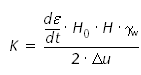
doi:10.2204/iodp.proc.308.204.2008 Laboratory testing methodologySample handling and preparationThe coring techniques include the advanced piston corer (APC) and extended core barrel (XCB) systems (Table T1). These standard coring systems and their characteristics are summarized in Technical Note 31 of the Ocean Drilling Program (Graber et al., 2002). The sample was not extruded from the core liner on board the drilling ship. Whole-core samples were capped and sealed in wax to maintain natural saturation during refrigerated storage prior to the experiments. For the experiments, each sample was removed from the wax-sealed liner and subsampled with a sharp cutting shoe (at Pennsylvania State University [PSU]) or a trimming jig (at Massachusetts Institute of Technology [MIT] and Rice University [Rice]). Sample descriptionsTable T1 illustrates all of the samples tested in this study including sample depth, type of coring used to acquire the sample, what analyses were done, and where the analyses were done. Most of the PSU and MIT samples were X-rayed at MIT’s radiography facility in order to select undisturbed portions of the core for experiments and to assess the presence of inclusions and variation in fabric. The Rice samples were X-rayed by Fugro in order to select undisturbed portions for experiments and to identify layering or inhomogeneities. Core X-ray data can be found in H. Nelson et al. (unpubl. data). All samples were taken from whole core, not core catchers. Sample locations are illustrated in Table T1. Quality of samples generally decreases with depth and many samples had significant deformation caused by the coring process. Table T1 indicates which samples were recovered by the APC and XCB systems. During APC coring, two different cutting shoes were used: the “Fugro” cutting shoe and the “IODP-APC” cutting shoe. The Fugro cutting shoe has a thinner kerf than the IODP-APC cutting shoe; therefore, less deformation during coring was expected. Grain size analysis documents that all tested samples are silty clays containing 50%–70% clay-sized grains (<2 μm), except samples from Section 308-U1324C-7H-1 (405 meters below seafloor [mbsf]), which are clayey silt with 30% clay-sized grains (Sawyer et al., this volume). The mineralogic composition of the silty clay samples is similar. Quantitative X-ray mineralogy shows that illite and smectite are the dominant minerals and together comprise 37%–60% of the bulk rock weight. Analysis of the clay-sized fraction (<2 μm) by subjective analysis of oriented mounts shows that 80%–90% of the mixed-layer interlayers are composed of smectite. Index propertiesTwo water contents were measured in the consolidation test: wc and wn. wc is the water content measured on the leftover trimmings during sample preparation. wn is the water content measured on the test specimen itself. We measured the water content by oven-drying the samples. Water content is calculated by taking the difference in the weight of the sample before and after oven-drying and dividing this difference by the oven-dried weight. In the laboratory, water content was measured on the trimmings from the specimens and on the specimens themselves. The water content of the trimmings were generally lower (~3%) than the water content of the samples. We compared the water content measured on the specimens with the shipboard measurements of moisture and density (MAD). This comparison is difficult because the sampling frequency and quality of the MAD data are variable. We find that at 15 locations the difference between the laboratory-derived water content and the MAD measurements are within 5 units in water content. There is no systematic difference. Constant rate of strain consolidation testingCRSC tests were conducted at three laboratories (MIT, PSU, and Rice) in general accordance with American Society for Testing and Materials (ASTM) D4186 guidelines (ASTM International, 2006). As the name implies, during CRSC tests the sample is deformed at a constant strain rate. This has several advantages relative to traditional step-loading tests. It provides continuous loading data, which provide a much more detailed view of compression behavior. In contrast with incremental loading, data points are obtained by doubling stress levels: behavior must be inferred between these points. In addition, continuous measurements of the flow properties are obtained (both the hydraulic conductivity [K] and the coefficient of consolidation [cv]). Finally, K is calculated directly (Equation 2), as opposed to the incremental consolidation test where it is indirectly calculated from the coefficient of consolidation (cv) and the frame compressibility (mv). The dimensions of the specimen are slightly different between the three laboratories. MIT specimens were 5.95–6.35 cm in diameter with an initial height of 2.35 cm. PSU specimens were 5 cm in diameter with an initial height of 2.0 cm. Rice specimens were 5.09 cm in diameter with an initial height of 2.41 cm. Specimens were laterally confined with a steel ring. Prior to testing, specimens were saturated with de-aired distilled water and back-pressured to 300–425 kPa for 24 h to drive any gases present into solution. We applied a constant rate of strain using a computer-controlled load frame, with the sample base undrained and sample top open to the backpressure. We continuously monitored sample height (H, in millimeters), applied vertical stress (σv, in kPa), and basal pore pressure (u, in kPa). At PSU, an axial load of 50 kN could be applied by a mechanical load frame and 5 cm diameter samples were run; therefore, the maximum vertical stress was 25.5 MPa. Backpressure was 0.3 MPa; therefore, the maximum effective stress that could be achieved was ~25.2 MPa. The MIT and Rice apparatuses were capable of lower total effective stresses. Most MIT experiments were run to ~2 MPa. Most Rice experiments were completed at effective stresses near 4 MPa. For this reason, the MIT and Rice apparatuses were used on the shallower samples. The vertical effective stress (σ′v), hydraulic conductivity (K), compressibility (mv), coefficient of consolidation (cv), and strain energy density (SED) were calculated using the following equations (ASTM, 2006; Tan et al., 2006):
Variables are defined in Table T2. |
|||||||||||||

 ,
, , and
, and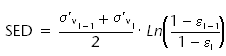 .
.