Previous   |   Next

doi:10.2204/iodp.proc.317.102.2011

Heat flow

Heat flow reflects the tectonic evolution of oceanic and continental plates, which may be accompanied by volcanism or hotspot activity. In addition to plate evolution, sedimentary processes associated with fluid circulation can also influence heat flow. Determination of heat flow requires measurement of thermal conductivity and geothermal gradient. Thermal conductivity is an intrinsic physical property of material and is dependent on pressure and temperature. It commonly varies with depth in accordance with the variation of other index properties such as porosity and bulk density. The Bullard method (Bullard, 1939) uses a linear relationship of thermal resistance versus temperature to determine heat flow over a depth interval with an established geothermal gradient. Thermal conductivity is routinely measured during IODP expeditions as part of the physical properties suite of measurements. Geothermal gradient can be calculated if successful temperature measurements are taken at several depths.

Geothermal gradient

In situ temperature data were obtained using two types of downhole tools: (1) the APCT-3, for use in soft-sediment formations, and (2) the Sediment Temperature (SET) tool, for use in more indurated sediment formations. The APCT-3 is deployed in the APC cutting shoe, and the temperature measurement is taken shortly after the core barrel is fired into pristine sediment. The results are associated with the bottom of the cored interval for that APC deployment. The SET tool is deployed in a separate wireline run, during which the ~1 m long probe is pushed into the bottom of the hole ahead of the bit. The results are associated with the interval 1 m below the top of the next advancement (cored or drilled interval). Both tools record time–temperature data in their onboard data loggers. After tool retrieval, the data are downloaded to a computer and the asymptotic temperature is estimated using the TFIT software (version 1.0). The tools are capable of measuring temperature in the range of –20° to 100°C with an accuracy of ±0.02°C.

Thermal conductivity

Thermal conductivity measurements were conducted on whole-round sections after the cores had passed through the WRMSL and the NGRL. Prior to measurements, the sections were equilibrated to ambient laboratory temperature (19°C) for at least 4 h to ensure thermal homogeneity.

Thermal conductivity was measured with the TK04 (Teka Berlin) system using the needle probe method (Von Herzen and Maxwell, 1959) in two configurations: (1) the full-space needle probe (VLQ) for soft sediments and (2) the half-space needle probe (HLQ) for rocks ("puck probe"). The needle probe contains a heater wire and a calibrated thermistor. The probe is assumed to be a perfect conductor because it is much more conductive than sediment. Under this assumption, the temperature of the superconductive probe has a linear relationship to the natural logarithm of time after initiation of heating:

where

• T = temperature (K),

• q = heat input per unit length per unit time (J/m/s),

• k = thermal conductivity (W/[m·K]),

• t = time after initiation of heating (s), and

• C = a constant.

One measuring cycle consists of three steps: (1) temperature drift self-test, (2) thermal conductivity measurement, and (3) 10 min break. Several measuring cycles can be performed automatically at each sampling location and used to calculate average conductivity. A self-test, which included a drift study, was conducted at the beginning of each measurement cycle. Once the samples were equilibrated, the heater circuit was closed and the temperature rise in the probes was recorded. Thermal conductivities were calculated from the rate of temperature rise while the heater current was flowing. Temperatures measured during the first 80 s of the heating cycle were fit to an approximate solution of a constantly heated line source (for details, see Blum, 1997).

Thermal conductivity measurements were taken once per section (~7 per full core), and one measuring cycle was performed for each measurement in soft sediments into which the TK04 needle could be inserted without risk of damage. When core material was too hard to use the full-space needle probe, the puck probe method was used instead. The puck probe method uses the same theory as the full-space needle probe method except that a flat circular puck is used as the probe and the working half of the split core is used instead of the whole-round core. Due to the limited time available, hard rock measurements were limited to one measurement with five measuring cycles per core because puck probe data showed large scatter. Heating power was adjusted to keep the power control value within a range of 2–3 W, as suggested by the TK04 manual. Drift control was set at 40 s for quick measurement. Based on repeated tests, this setting does not greatly affect the accuracy of measured values.

When the full-space needle probe method was used, the needle was inserted into unconsolidated sediment through a small 2 mm hole drilled into the core liner perpendicular to what would become the spilt-core surface. Thermal transfer compound was used during previous expeditions to improve the coupling between the needle and the sediment. However, it was not used during Expedition 317 to eliminate the possibility that the compound would contaminate the split-core surface and affect core description. Additionally, testing of the thermal transfer compound using sediments that were provided as test samples prior to drilling revealed no improvement in thermal coupling.

When the puck probe method was used, the probe was attached to the split-core surface with rubber rings in a seawater tube. Although at least 5 bar of pressure is recommended by the manufacturer to connect the puck probe thermally to the split-core surface, we used several rubber rings because our rock samples were too weak to bear the ~300 kg weight (corresponding to 5 bar) over the probe. Results obtained using the rubber rings with the puck probe are similar to those obtained with the full-space needle probe inserted into a drilled hole within hard rock. A Styrofoam box filled with seawater was used to achieve thermal coupling between the puck probe and the core and to minimize thermal disturbance. The water depth in the box was high enough to cover the contact surface between the puck probe and the core. Accordingly, it was important to get rid of air bubbles at the contact surface before taking measurements.

Thermal conductivity data were discarded when (1) contact between the probe and sediment was poor, as evidenced by a logarithm of extreme time (LET) of <50 s and/or <100 solutions in the software; (2) thermal conductivity was close to that of water (0.6 W/[m·K]), resulting from dilution of sediments during coring; and (3) measurements were taken in caved-in layers such as shell hash. In most cases, the first two criteria are controlling parameters for monitoring measurement quality. Measurement error was considered to be 5%–10% (Blum, 1997).

At sites where in situ temperatures were measured, thermal conductivity was corrected for in situ temperature and pressure prior to the calculation of heat flow. Laboratory values were corrected to in situ conditions following Hyndman et al. (1974):

,

where

• λ_{in situ}(z) = in situ thermal conductivity at depth z (m),

• λ_lab = laboratory-measured thermal conductivity,

• z_w = water depth (m),

• ρ_sed = bulk density of sediment (g/cm³),

• T(z) = in situ temperature at depth z (m), and

• T_lab = laboratory temperature.

CSF-A was the standard depth scale used for temperature and thermal conductivity measurements. The correction process typically adjusted thermal conductivity by up to ±5% for 2000 m CSF-A and 500 m water depth.

Thermal conductivity values are commonly averaged across a depth interval using a geometric mean because heat is assumed to flow vertically through the sediment layers. Averaged thermal conductivity (λ_avg) is calculated as follows:

,

where

• λ_i = thermal conductivity at the ith layer with thickness z_i and

• Z = total thickness of all layers,

that is,

.

In practice, z_i is the measurement frequency interval used (e.g., section or core). The length of the core catcher and/or of unrecovered sections that were not measured is added to the closest measured section.

Heat flow calculation

To estimate heat flow we use the Bullard method (Bullard, 1939), which is useful when thermal conductivity varies over a depth interval where geothermal gradient is established (e.g., Pribnow et al., 2000). It assumes a linear relationship between temperature and thermal resistance of the sediment:

where

• z = depth (m CSF-A),

• T₀ = temperature at z = 0, and

• q = heat flow.

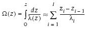
Thermal resistance (Ω[z]) is defined as

,

where

• z_i = bottom depth of the ith horizontal layer,

• z_{i – 1} = top depth of the ith horizontal layer,

• λ_i  = thermal conductivity, and

• I = the number of horizontal layers between the seafloor (z = 0) and depth z.

A plot of temperature versus thermal resistance (a Bullard plot) allows estimation of (1) surface temperature (T₀) from the intercept with z = 0 and (2) heat flow from the slope of a line fitted to the data. Data in a Bullard plot fall in a line when conditions between the seafloor and depth z include (1) conductive cooling, (2) steady state, and (3) no heat source/sink.

If thermal conductivity increases linearly with depth, thermal conductivity is represented as

where

• λ₀ = estimated surface thermal conductivity and

• Γ = the slope.

When establishing the fitting line, we used thermal conductivity corrected to in situ pressure and temperature conditions as described above.

Then, thermal resistance is solved as

where Ω_i is the thermal resistance of the ith horizontal layer.

Top of page   |   Previous   |   Next