Previous   |   Next

doi:10.2204/iodp.proc.322.102.2010

Structural geology

Our methods for documenting the structural geology of Expedition 322 cores largely followed those given by the Expeditions 315, 316, and 319 structural geologists (see "Structural geology" in Expedition 315 Scientists [2009], Expedition 316 Scientists [2009], and Expedition 319 Scientists [2010]). We documented the deformation observed in the split cores by classifying structures, determining the depth extent, measuring orientation data, and recording kinematic information. The data were hand-logged onto a printed form at the core table and then typed into both a spreadsheet and J-CORES. Where possible, the orientation data were also corrected for rotation related to drilling on the basis of paleomagnetic declination and inclination information.

Core description and orientation data collection

Each structure was recorded manually on a structural description sheet modified from that used during Expedition 316 (Fig. F6). We found that this modified sheet is particularly useful to record orientation data for linear structures (e.g., striation on the fault plane). Core measurements followed Expeditions 315 and 316, which in turn were based on previous ODP procedures developed at the Nankai accretionary margin (i.e., ODP Legs 131 and 190). We used a plastic protractor for orientation measurements (Fig. F7). During Expedition 322, we downloaded the X-ray CT images of unsplit cores to identify structures and recognize 3-D geometry and distribution of structures. Using the working half of the split core provided greater flexibility in removing (and cutting, if necessary) pieces of the core for more careful observation and measurement.

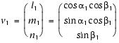
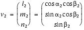
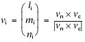
Orientations of planar and linear features in cored sediments were determined in the framework of the core coordinate system, which consists of x-axis to the "double line" marked on the working half, z-axis parallel to the core longitudinal axis to the bottom, and accordingly determined y-axis with the right-handed system (Fig. F8). To determine the orientation of a plane, two apparent dips of the planar feature were measured in the core coordinate system and converted to a plane represented by either a strike and dip or a dip and dip direction. This conversion was accomplished using a spreadsheet (Fig. F9). This approach had the advantage of increasing the data processing efficiency and reducing errors in transferring and retyping data (e.g., by using both R. Allmendinger's Stereonet program [www.geo.cornell.edu/geology/
faculty/RWA/programs.html] and a spreadsheet). One apparent dip was typically represented by the intersection of the planar feature with the split face of the core and was quantified by measuring the dip direction and angle in the core coordinate system. Typical apparent dip measurements had a trend of 090° or 270° and ranged in plunge from 0° to 90°. The second apparent dip was usually represented by the intersection of the planar feature and a cut or fractured surface at a high angle to the split face of the core axis. In many cases, this was a surface either parallel or perpendicular to the core axis. In the former cases, the apparent dip lineation would trend 000° or 180° and plunge from 0° to 90°; in the latter cases, the trend would range from 000° to 360° and plunge 0°. Linear features observed in the cores were always associated with planar structures (typically faults or shear zones), and their orientations were determined by measuring either the trend and plunge in the core coordinate system or the rake (or pitch) on the associated plane. All data were recorded on the log sheet with appropriate depths and descriptive information.

Paleomagnetic data were used during NanTroSEIZE to correct drilling-induced rotation of cored sediments. Rotation was induced during RCB coring at Holes C0011B and C0012A, as is common in ocean drilling. However, the long-core cyrogenic magnetometer on the Chikyu was malfunctioning because of liquid helium leaking and was out of use during the entire Expedition 322. The paleomagnetic data on board were therefore limited (mostly two discrete shipboard samples per section), and most magnetic corrections could not be performed.

Orientation data analysis based on the spreadsheet

During Expedition 322, we adopted the Expedition 315/316 spreadsheet template for orientation data calculation in the core coordinate system, as well as in the geographic coordinate system from those data measured on cores (e.g., Fig. F9). A minor error in the spreadsheet was corrected by an Expedition 315 scientist just before Expedition 322 started, and we made small modifications such as adding a "depth (mbsf)" column and changing the order of columns for better handling.

Calculation of plane orientation

For planar structures (e.g., bedding or faults), two apparent dips on two different surfaces (e.g., one being the split core surface and the other being the horizontal surface) were measured in the core coordinate system as azimuths (measured clockwise around the z-axis from the x-axis, looking down) and plunges (Fig. F10). If the azimuths and plunges of the two apparent dips are given as (α₁, β₁) and (α₂, β₂), respectively, as in Figure F10, then the unit vectors representing these two lines, v₁ and v₂, are

(3)

and

,

(4)

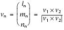
where l, m, and n represent the x-, y-, and z-components of the vectors.

The unit vector normal to this plane (v_n) (Fig. F10) is then defined as follows:

,

(5)

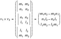
where

.

(6)

The azimuth (α_n) and plunge (β_n) of v_n are given by

.

(7)

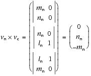
The dip direction (α_d) and dip angle (β) of this plane are α_n and 90° + β_n, respectively, when β_n is <0° (Fig. F11A). They are α_n ± 180° and 90° – β_n, respectively, when β_n is ≥0° (Fig. F11B). The right-hand rule strike of this plane (α_s) is then given by α_d – 90° (Fig. F11).

Calculation of slickenline rake

For a fault with slickenlines, the apparent rake angle of the slickenline (ϕ_a) was measured on the fault surface from either the 090° or 270° direction of the split-core surface trace (Fig. F12). Fault orientation was measured as described above. Provided that v_n and v_c are unit vectors normal to the fault and split core surfaces, respectively, the unit vector of this intersection line (v_i) is perpendicular to both v_n and v_c (Fig. F12) and is therefore defined as follows:

,

(8)

where

,

(9)

and

.

(10)

Knowing the right-hand rule strike of the fault plane (α_s), the unit vector (v_s) toward this direction is then

.

(11)

The rake angle of the intersection line (ϕ_i) measured from the strike direction is given by

because

.

(13)

The rake angle of the slickenline (ϕ) from the strike direction is ϕ_i ± ϕ_a, depending on which direction the apparent rake was measured from and which direction the fault plane dips toward. ϕ_a should be subtracted from ϕ_i when the fault plane dips toward the west and ϕ_a was measured from either the top or 090° direction (Fig. F13A) or when the fault plane dips toward the east and ϕ_a was measured from either the bottom or 090° direction (Fig. F13B). However, ϕ_a should be added to ϕ_i when the fault plane dips toward the east and ϕ_a was measured from either the top or 270° direction (Fig. F13C) or when the fault plane dips toward the west and ϕ_a was measured from either the bottom or 270° direction (Fig. F13D).

Azimuth correction using paleomagnetic data

Provided that a core is vertical, its magnetization is primary, and its bedding is horizontal, its paleomagnetic declination (α_p) indicates magnetic north where the inclination (β_p) is ≥0° (Fig. F14A), whereas it indicates magnetic south where β_p is <0° (Fig. F14B). The dip direction and strike of a plane in the geographic coordinate system (α_d* and α_s*) are therefore

and

where

and are

and

where

J-CORES structural database

J-CORES database has a VCD program to store a visual (macroscopic and/or microscopic) description of core structures at a given section index and a record of planar structures in the core coordinate system. The orientations of such features are saved as commentary notes but do not appear on the plots of Composite Log Viewer. During Expedition 322, only the locations of structural features are entered in J-CORES by sedimentologists, and orientation data management and planar fabric analysis are done with an Excel spreadsheet as mentioned above.

Description and classification of structures

In general, we described and classified the structures observed using the terminology of J-CORES and Expedition 315/316, which in turn is based on the J-DESC VCD scheme and ODP Legs 131 (Taira, Hill, Firth, et al., 1991), 156 (Shipley, Ogawa, Blum, et al., 1995), 170 (Kimura, Silver, Blum, et al., 1997), and 190 (Moore, Taira, Klaus, et al., 2001). For clarity, however, we define the terminology used to describe fault-related rocks, as well as the basis for differentiating natural and drilling-induced features. The key to the symbols used in J-CORES is given in Figure F3.

It may be difficult to distinguish natural faults from drilling-induced faults. Helicoidal striated surfaces or polished surfaces showing striations that diverge outward most likely indicate drilling-induced fracturing resulting from the torque exerted by the bit on sediments. In contrast, faults that display more planar geometries, parallel lineations, and orientations compatible with preferred orientations displayed by multiple faults nearby are likely natural features. Lastly, when multiple orientation measurements are plotted in stereographic projection, natural minor faults are expected to display preferred orientations that may define coherent strain axes, whereas drilling-induced faults are expected to yield random orientation distribution.

Top of page   |   Previous   |   Next