Previous   |   Next

doi:10.2204/iodp.proc.322.102.2010

Physical properties

Physical property measurements provide valuable constraints on bulk physical character to augment lithologic unit characterization and to facilitate correlation of downhole logging data with discrete core measurements and core descriptions. Thus, these data provide information necessary for reliable core-log-seismic integration. Expedition 322 employed multiple approaches and methods to characterize the physical properties of cores. Prior to core physical property measurements, X-ray CT images were collected for all cores, and cores were equilibrated with room temperature (~20°C). After temperature equilibration, whole-round core sections were processed in the MSCL-W to measure GRA density, magnetic susceptibility, natural gamma radiation, P-wave (compressional) velocity, and electrical resistivity. For cores with soft, unconsolidated sediments, thermal conductivity was measured using a TeKa thermal conductivity meter with the VLQ full-space needle probe inserted in whole-round cores after MSCL-W measurements. Cores were then split into archive and working halves. For cores with lithified sediments, where a needle probe could not be inserted, thermal conductivity measurements were made on working halves using the TeKa thermal conductivity meter in half-space mode. Discrete samples were collected from the working halves for MAD measurements. Specimen mass was taken with a BAL-2 motion-compensated shipboard balance system. The volume of solids was measured with a Quantachrome penta-pycnometer. For soft sediments, undrained shear strength at discrete intervals from the working halves was determined from vane shear measurements made with a Wykeham Farrance WF23544 vane apparatus and penetrometer measurements made with a Geotest E-284B penetrometer. P-wave velocity and electrical resistivity were measured on discrete core samples in the x-, y-, and z-directions (Fig. F17) to evaluate anisotropy of velocity and resistivity. Archive halves were scanned for image and color measurements. Details and procedures for each physical property measurement are described below.

MSCL-W

GRA density

Bulk density can be used to evaluate pore volume in sediment, which is used to evaluate the consolidation state of sediment. GRA density is based on the detection of a gamma ray beam produced by a cesium source. The beam, produced by a ¹³⁷Cs gamma ray source at a radiation level of 370 MBq within a lead shield with a 5 mm collimator, is directed through whole-round cores. The gamma ray detector includes a scintillator and an integral photomultiplier tube to record the gamma rays that pass through the whole-round core. GRA bulk density (ρ_b) is defined by:

where

• I₀ = gamma ray source intensity,

• I = measured intensity of gamma rays passing through the sample,

• µ = Compton attenuation coefficient, and

• d = sample diameter.

The Compton attenuation coefficient (µ) and source intensity (I₀) are treated as constants, so ρ_b can be calculated from I. The gamma ray detector is calibrated with a sealed calibration core (a standard core liner filled with distilled water and aluminum cylinders of various diameters). To establish the calibration curves, gamma ray counts were taken through each aluminum cylinder for 60 s. Each aluminum cylinder has a density of 2.7 g/cm³, and d is 1, 2, 3, 4, 5, or 6 cm. The relationship between I and µd is:

where A, B, and C are coefficients determined from the calibration experiment. GRA density measurements on core samples were conducted every 4 cm for 4 s. The spatial resolution was 5 mm.

Magnetic susceptibility

Magnetic susceptibility is the degree to which a material can be magnetized by an external magnetic field. Therefore, magnetic susceptibility provides information on sediment composition. A Bartington loop sensor with an 8 cm diameter was used to measure magnetic susceptibility. An oscillator circuit in the sensor produces a low-intensity (~80 A/m RMS), nonsaturating, alternating magnetic field (0.565 kHz). This pulse frequency is converted into magnetic susceptibility. The spatial resolution of the loop sensor is 23–27 mm, and it is accurate to within 2%. Magnetic susceptibility data were collected every 4 cm along the core.

Natural gamma radiation

Natural gamma radiation measurements provide insights into sediment composition and thus can be used to identify lithology. Whole-round cores were monitored for natural gamma ray (NGR) emissions to obtain spatial variability in radioactivity and establish gamma ray logs of cores for correlation to downhole gamma ray logs. A lead-shielded counter, optically coupled to a photomultiplier tube and connected to a bias base that supplied high-voltage power and a signal preamplifier, is used. Two horizontal and two vertical sensors are mounted in a lead, cube-shaped housing. The NGR system records radioactive decay of long-period isotopes ⁴⁰K, ²³²Th, and ²³⁸U. NGR has a resolution of 120–170 mm and was measured every 16 cm with a count time of 30 s. Background radiation noise was determined by taking measurements on a water-filled calibration core.

P-wave velocity

P-wave data can be used to evaluate small-strain moduli, to correlate between log and core data, and to evaluate pore structure and cementation. P-wave (compressional) velocity (V_P) is defined by the time required for a compressional wave to travel a set distance:

where

• d = path length of the wave across the core and

• t_core = traveltime through the core.

P-wave velocity transducers on the MSCL-W system measure total traveltime of the compressional wave between transducers. The wave travels horizontally across the whole core and core liner. The total traveltime observed is composed of

• t_delay = time delay related to transducer faces and electronic circuitry,

• t_pulse = delay related to the peak detection procedure,

• t_liner = transit time through the core liner, and

• t_core = traveltime through the sediment or rock.

The system is calibrated using a core liner filled with distilled water, which provides control for t_delay, t_pulse, and t_liner. With these calibrations, core velocity (V_P) can be calculated on whole-round specimens in core liners:

where

• d_cl = measured diameter of core and liner,

• d_liner = liner wall thickness, and

• t_o = measured total traveltime.

Equation 23 assumes that the core completely fills the core liner.

Electrical resistivity

Within limits, electrical resistivity may be useful for estimating other sediment physical properties, including porosity, tortuosity, permeability, and thermal conductivity. Bulk electrical resistivity is controlled by solid grain resistivity, interstitial water resistivity, pore space distribution, and pore connectivity. Electrical resistivity (ρ) is defined by the electrical resistance and geometry of the core measured:

where

• R = electrical resistance,

• L = length of measurement, and

• A = cross-sectional area of the core.

The noncontact resistivity sensor on the MSCL-W system induces a high-frequency magnetic field in the core with a transmitter coil. This generates an electrical current in the bulk sediment that is inversely proportional to its resistivity. The secondary magnetic field generated by this induced electrical current is measured by a receiver coil. To measure this smaller magnetic field accurately, a differencing technique has been developed that compares readings from the sample core to readings from an identical set of coils operating in air. Electrical resistivity data were obtained at 4 cm intervals on the MSCL-W.

MSCL-I: photo image logger

The photo image logger (MSCL-I) scans the surface of archive-half cores and creates a digital image. The line-scan camera equips three charge-coupled devices; each charge-coupled device has 1024 arrays. Light reflection from the sample surface passes through the lens and is split into three paths (red, green, and blue) by a beam splitter inside the line-scan camera. Then, each reflection is detected by the corresponding charge-coupled device. Finally, the signals are combined and the digital image is reproduced. Optical distortion downcore is avoided by precise movement of the camera. Spatial resolution is 100 pixels/cm.

For publication, a modified image was used in VCD tables. Image lightness was modified so that the values of the gray standard attached to the bottom of a section is somewhere near 100/100/100. This processing was done by using the image data of Core 322-C0011B-1R-1, then the same adjustments were automatically applied to all other sections through Expedition 322.

MSCL-C: color spectroscopy logger

A color spectrophotometer (Konica-Minolta, CM-2600d) is included on the color spectroscopy logger (MSCL-C) system. The xyz-type aluminum frame allows operators to set a maximum of seven core sections on the tray, and the sensor unit (including the spectrophotometer and small distance measuring system using a laser sensor) moves over each section and down at each measurement point to measure the split archive core surface.

Light reflected from the sample surface is collected in the color spectrophotometer's integration sphere. The instrument's structure allows for the specular component to be included (SCI setting) or excluded (SCE setting). The SCE setting is the recommended mode of operation, especially for sediments, to exclude glare. The light is then divided into wavelengths at a 10 nm pitch (400–700 nm), and the spectral sensors in the sphere convert the light to electrical currents proportional to the intensity of the light. Next, the color spectrum from the sample is normalized by the source light of the reflectance. The obtained spectrum is calibrated with the measurement of a pure white standard, which has a high reflectance true value at visible wavelengths and is measured by the vendor, and a black box (zero calibration). Measurements can be calculated based on the 2° or 10° standard observer and any of 11 illuminants.

Color reflectance is categorized as an IODP standard measurement, and the measured color spectrum is normally converted to L*, a*, and b* parameters. L*, a*, and b* provide relative changes in the composition of the bulk material and are widely used to correlate sections from core to core or hole to hole and to analyze the characteristics and cyclicity of lithologic changes.

Moisture and density measurements

Discrete samples from working-half cores are used for determination of index properties (e.g., bulk density, grain density, dry density, water content, porosity, and void ratio). Index properties are determined from phase relations, mass measurements on wet and dry specimens, volume measurements on dry specimens, and corrections for salinity. In general, two discrete samples of homogeneous lithology for index properties were collected from each core section. Where whole-round samples were taken (e.g., interstitial water sample, community whole round, or individual sample requests) a MAD sample was taken adjacent to the whole-round sample as part of a cluster sample. Sample intervals and frequency were occasionally shifted to select minimally disturbed, homogeneous samples. Lithology was noted as sand for discrete samples that contained mostly sand grains judging from visual inspection. All other samples were noted as mud. Each discrete MAD sample was ~5 cm³.

Wet and dry masses were measured using a paired electronic balance system, which is designed to compensate for the ship's heave. The sample mass was counterbalanced with a precisely known mass (10 g) that was within 5 g of the sample mass. The sample mass was determined to a precision of ±0.01 g. The balance system was calibrated ~8 times each day (~3 h interval).

To minimize desiccation, MAD sample collection was followed immediately by measurement of wet sediment mass (M_wet). After M_wet measurements, samples were dried in a convection oven at 105° ± 5°C for 24 h. Dry samples were placed in a desiccator for at least 1 h to equilibrate to room temperature (~20°C), and then dry sediment mass (M_dry) and volume (V_dry) were measured. A five-chamber Quantachrome penta-pycnometer was used to measure V_dry with a helium-displacement technique providing a precision of ±0.04 cm³. The five-chamber system allowed the measurement of four sample volumes and one calibration sphere. Each measured volume (V_dry) is the average of five volume measurements. The calibration sphere was rotated between all measurement chambers to monitor for errors in each chamber. The pycnometer was calibrated at least once per 24 h. In cases where pycnometer-derived grain density was deemed unreliable (<2.0 g/cm³ or >3.0 g/cm³), the sample grain density was recalculated after dry mass and dry volume were remeasured.

Standard ODP/IODP practices were used to determine interstitial water mass and volume, salt mass and volume, and solid grain mass and volume (Blum, 1997). From these data, bulk density, dry density, grain density, porosity, and void ratio were calculated (Blum, 1997). Standard seawater density (1.024 g/cm³), salinity (35‰), and constant salt density (2.22 g/cm³) were assumed for all calculations.

Water content

Water content (W_c) was determined following the American Society for Testing and Materials (ASTM) standard D2216 (ASTM International, 1990). Corrections are required for salt when measuring the water content of marine samples. In addition to the water content calculation in ASTM D2216 (i.e., the ratio of interstitial water mass to dry sediment mass) (W_c[dry]) we also calculated the ratio of interstitial water mass to total sample mass (W_c[wet]). The equations for water content are

and

where

• M_wet = total mass of the discrete sample,

• M_dry = mass of the dry sample, and,

• s = salinity (assumed constant at 0.035).

Bulk density

Bulk density is the density of the discrete core sample (ρ_b = M_wet/V_t). Total wet sample mass (M_wet) was measured immediately after collecting each discrete sample using the dual-balance system. Total sample volume assuming 100% saturation (V_t = V_g + V_IW) was determined from the pycnometer measurement of grain volume (V_g) and calculated volume of interstitial water (V_IW). Solid grain and interstitial water volume are determined as

and

where

• V_dry = dry volume,

• ρ_salt = salt density (assumed constant at 2.22 g/cm³), and

• ρ_IW = standard seawater density (1.024 g/cm³).

Porosity and void ratio

Porosity (ϕ) relates the volume of the pores to the total sample volume; void ratio (e) relates the pore volume to the volume of the solid grains. They are calculated as

and

Grain density

Grain density (ρ_g) was determined from measurements of dry mass and dry volume made with the dual-balance system and the pycnometer, respectively. Mass and volume were corrected for salt, yielding

,

(31)

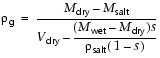
where

• M_salt = mass of salt.

Shear strength measurements

The undrained shear strength of soft sediments in the working half of the core was measured using an analog vane shear device (Wykeham Farrance, model WF23544) and a pocket penetrometer (Geotest E-284B). Measurements were made at discrete locations on the working halves above the depth where sediments behaved in a brittle manner; this corresponded to measureable shear strength <125 kPa. Where possible, the measurements were made near MAD samples. Care was taken to conduct tests within minimally disturbed, homogeneous sediments. Measurements were made on the working half of split cores with vane rotation axis and penetrometer penetration direction perpendicular to the y-z plane of the core (Fig. F17).

Vane shear strength (S_u[v]) can be determined by the torque required to cause failure (T) and a vane constant (K_v):

All vane shear strength measurements were obtained using a vane with a height of 12.7 mm and a blade length of 6.35 mm. Failure torque was determined by measuring the rotation of a torsional spring using a spring-specific relation between rotation angle and torque. Vane shear strength results were only reliable for samples with vane shear strength <125 kPa. When cracking or core separation occurred, measurements were discarded. Below the depth where strength exceeded 125 kPa, no measurements were made.

The pocket penetrometer provides a measure of unconfined compressive strength (q_u), which can be related to undrained shear strength (S_u[penet]):

where

• g = acceleration due to gravity, and

• q_u = mass per area.

Unconfined compressive strength is calculated from the penetration resistance generated by pushing a cylindrical probe 6.4 mm into the y-z plane of the core. The average of three adjacent penetrometer tests in intact, homogeneous sediment is the recorded unconfined compressive strength. Measurements were obtained using a flat surface probe with a diameter of 6.4 mm. After shear strength exceeded ~125 kPa, no penetrometer measurements were made.

Anisotropy of P-wave velocity and electrical resistivity

P-wave velocity and electrical resistivity measurements were performed on cubic samples cut from RCB cores with a diamond blade saw. Samples for P-wave velocity measurements were ~20 mm × 20 mm × 20 mm; samples for electrical resistivity measurements were ~10 mm × 10 mm × 10 mm. All cubes were cut with faces orthogonal to the x-, y-, and z-axes of the core reference (Fig. F17). Hard rock/basement cubes were saturated in a 3.5% NaCl solution for 24 h prior to P-wave analysis. All cubes used for electrical resistivity analysis were saturated in a 3.5% NaCl solution for 6 h prior to measurement. This sample preparation and three-component measurement plan enable first-order measurement of both P-wave velocity and electrical resistivity anisotropies.

To measure P-wave velocity in a given direction, a P-wave logger for discrete samples (PWL-D) was used. The PWL-D has two 230 kHz transducers, one used as a transmitter and one as a receiver, and a laser distance sensor. A sample was placed between the transducers and held in place with a vertical mass of 2.5 kg. The transmitter was connected to a pulse generator, and the receiver was connected to an oscilloscope synchronized with the pulse generator. The oscilloscope signal was digitally displayed; P-wave total traveltime (t) for the first arrival was picked and recorded. The laser distance sensor provided the sample length (L). The velocity in any direction (e.g., V_Px) was defined by the sample length (e.g., L_x), total traveltime (t_x), and system-calibrated delay time (t_delay):

Calibration of the traveltime delay and laser distance sensor was conducted daily. Traveltime delay was determined by placing the transmitter and receiver in direct contact and measuring traveltime. The laser distance sensor was calibrated by placing the transmitter and the receiver in direct contact and then spacing them using a 2.5 cm long reference specimen. Routine quality control measurements were made by measuring velocity on glass and acrylic standards with known lengths and velocities.

An Agilent 4294A component analyzer was used to measure electrical resistivity. The bridge method was used, and a two-terminal circuit was connected for measurement. Each specimen cube was placed between two stainless steel electrodes covered with seawater-saturated filter papers. The magnitude (|Z|) and phase (θ) of the complex impedance were measured at 25 kHz between opposite cube faces. The cube was rotated to measure impedance in the x-, y-, and z-directions (Fig. F17). Electrical resistivity for each direction (e.g., ρ_x) was computed from the complex impedance measured in each direction (e.g., x) and sample dimensions defined by face length (L):

With P-wave velocity and electrical resistivity measured in the x-, y-, and z-directions, the anisotropy is calculated following the approach of Carlson and Christensen (1977). Some sources for anisotropy include: (1) alignment of pores during consolidation, (2) fabric development, and (3) microstructures such as microfractures and microcracks. The anisotropy calculation compares the horizontal (x, y) and vertical (z) components of P-wave velocity and electrical resistivity expressed as a percentage of the mean (e.g., Shipboard Scientific Party, 2001a):

and

Thermal conductivity

Thermal conductivity was measured on sediment and rock samples using either the full-space needle probe (Von Herzen and Maxwell, 1959) or the half-space line source (Vacquier, 1985), which approximates an infinite line source. In soft sediments where a probe could be inserted into the core without fracturing the sediment, the full-space probe was inserted into whole-core sections through a hole drilled in the working-half side of the core liner. When sediment strength precluded use of the full-space probe or good contact between the probe and sediment was not possible, the half-space probe was used on the working half of the split core. For uncemented samples, the half-space probe was placed directly on the split core with seawater used to provide good contact. Lithified samples were placed in a seawater bath for at least 15 min before measurement with the half-space probe. Both full- and half-space measurements produce a scalar thermal conductivity value in the plane perpendicular to the orientation of the probe.

All measurements of thermal conductivity were made after the cores had equilibrated to room temperature. At the beginning of each measurement, temperature in the sediment was monitored to ensure that thermal drift was <0.4 mK/min (typically within 1–2 min). After it was established that the temperature was near equilibrium, a calibrated heat source was applied and the rise in temperature was recorded for ~80 s. Values of thermal conductivity were based on the observed rise in temperature for a given quantity of heat.

The full-space needle probe was calibrated at least once every 24 h. The calibration was performed on one of two Macor samples of known thermal conductivity (1.611 ± 2% W/[m·K], 1.623 ± 2% W/[m·K]). Calibration procedures for the half-space system are similar to those for the full-space needle probe. Half-space calibrations were made on a Macor sample of known thermal conductivity (1.652 ± 2% W/[m·K]).

Top of page   |   Previous   |   Next